Unit-IV

Difference between spatial domain and frequency domain

In spatial domain, we deal with images as it is.

In frequency domain, we deal with the rate at which the pixel values are changing in spatial domain.

Input imageProcessingOutput image matrix

Spatial domain transformation

Input imageFrequency distributionprocessingInverse transformationoutput image

Frequency domain transformation

Transformation: It is the process of converting signal from time/space domain to frequency domain.

Kinds of transformations:

1. Fourier series2. Fourier transformation

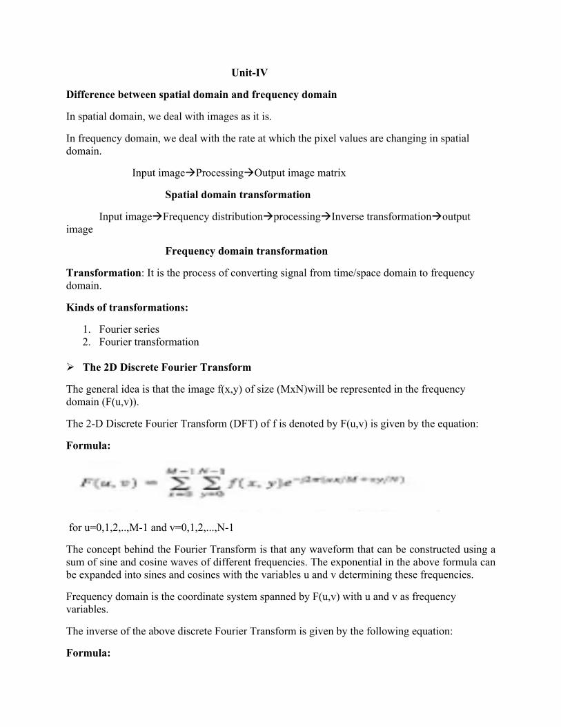
The 2D Discrete Fourier Transform

The general idea is that the image f(x,y) of size (MxN)will be represented in the frequency domain (F(u,v)).

The 2-D Discrete Fourier Transform (DFT) of f is denoted by F(u,v) is given by the equation:

Formula:

for u=0,1,2,..,M-1 and v=0,1,2,...,N-1

The concept behind the Fourier Transform is that any waveform that can be constructed using a sum of sine and cosine waves of different frequencies. The exponential in the above formula can be expanded into sines and cosines with the variables u and v determining these frequencies.

Frequency domain is the coordinate system spanned by F(u,v) with u and v as frequency variables.

The inverse of the above discrete Fourier Transform is given by the following equation:

Formula:

Thus, if we have F(u,v),we can obtain the corresponding image (f(x,y)) using the inverse ,DFT:

g(x,y)=h(x,y)*f(x,y)

MATLAB provides the functions fft and ifft to compute the Discrete Fourier transform and its inverse respectively.

Computing and visualizing the 2-D DFT in MATLAB

The DFT and its inverse are obtained using a Fast Fourier Transform (FFT) algorithm.

fft2(): Computes 2-D Fast Fourier Transform

The FFT of an MxN image array f is obtained using fft2()( in MATLAB.

Syntax:

F=fft2(f)

It will return a fourier transform that is also of size MxN. In this output, the origin of the data at the top left and with four quarter periods meeting at the center of the frequency rectangle.

It is necessary to pad the input image with zeros when the Fourier Transform is used for filtering .In this case, the syntax becomes:

F=fft2(f,P,Q)

It will pad the input with the required number of zeros so that the resulting function is of size PxQ.

The Fourier spectrum is obtained by using function abs():

S=abs(F)

It computes the magnitude (square root of the sum of the real and imaginary parts of each element of the array.

Example:

1. Create an image with a white rectangle and black background

» f=zeros(30,300);

» f(5:24,13:17)=1;

» imshow(f)

2)

» f=imread('tire.tif');

» F=fft2(f);

» imshow(F)

» 3) Calculate the DFT

>>F=fft2(f);

» F2=abs(F);

» imshow(F2,[])

It shows the four bright spots in the corners of the image.

Filtering in frequency domain

a)Fundamental concepts

The foundation for liner filtering in both the spatial and frequency domain is the convolution theorem which may be written as:

f(x,y)*h(x,y)H(u,v)F(u,v)

The convolution theorem says that convolution on one domain (e.g. spatial) is equivalent to the point by point multiplication on the other domain (or frequency) and vice versa.

Diagram:

H(u,v)

h(x,y)

f(x,y)

F(u,v)

Here, the symbol ‘*’ indicates convolution of the two functions. The above expression indicates the convolution of the two spatial functions can be obtained by computing the inverse Fourier transform of the product of the Fourier transforms of the spatial filter.

Here, H(u,v) is referred to as the filter transfer function. Basically the idea in frequency domain filtering is to select a filter transfer function that modifies F(u,v) in a specified manner.

b) Basic steps in DFT filtering

FFTMULT IFFT

FFT

g(x,y)

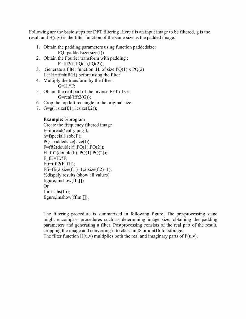
Following are the basic steps for DFT filtering .Here f is an input image to be filtered, g is the result and H(u,v) is the filter function of the same size as the padded image:

1. Obtain the padding parameters using function paddedsize:PQ=paddedsize(size(f))

2. Obtain the Fourier transform with padding :F=fft2(f, PQ(1),PQ(2));

3. Generate a filter function ,H, of size PQ(1) x PQ(2)Let H=fftshift(H) before using the filter

4. Multiply the transform by the filter :G=H.*F;

5. Obtain the real part of the inverse FFT of G:G=real(ifft2(G));

6. Crop the top left rectangle to the original size.7. G=g(1:size(f,1),1:size(f,2));

Example: %programCreate the frequency filtered imageF=imread(‘entry.png’);h=fspecial(‘sobel’);PQ=paddedsize(size(f));F=fft2(double(f),PQ(1),PQ(2));H=fft2(double(h), PQ(1),PQ(2));F_fH=H.*F;Ffi=ifft2(F_fH);Ffi=ffi(2:size(f,1)+1,2:size(f,2)+1);%dispaly results (show all values)figure,imshow(ffi,[])Or ffim=abs(ffi);figure,imshow(ffim,[]);

The filtering procedure is summarized in following figure. The pre-processing stage might encompass procedures such as determining image size, obtaining the padding parameters and generating a filter. Postprocessing consists of the real part of the result, cropping the image and converting it to class uint8 or uint16 for storage.The filter function H(u,v) multiplies both the real and imaginary parts of F(u,v).

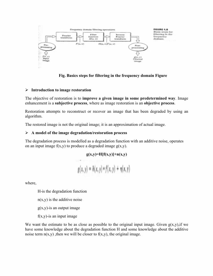
Fig. Basics steps for filtering in the frequency domain Figure

Introduction to image restoration

The objective of restoration is to improve a given image in some predetermined way. Image enhancement is a subjective process, where as image restoration is an objective process.

Restoration attempts to reconstruct or recover an image that has been degraded by using an algorithm.

The restored image is not the original image; it is an approximation of actual image.

A model of the image degradation/restoration process

The degradation process is modelled as a degradation function with an additive noise, operates on an input image f(x,y) to produce a degraded image g(x,y).

g(x,y)=H[f(x,y)]+n(x,y)

where,

H-is the degradation function

n(x,y) is the additive noise

g(x,y)-is an output image

f(x,y)-is an input image

We want the estimate to be as close as possible to the original input image. Given g(x,y),if we have some knowledge about the degradation function H and some knowledge about the additive noise term n(x,y) ,then we will be closer to f(x,y), the original image.

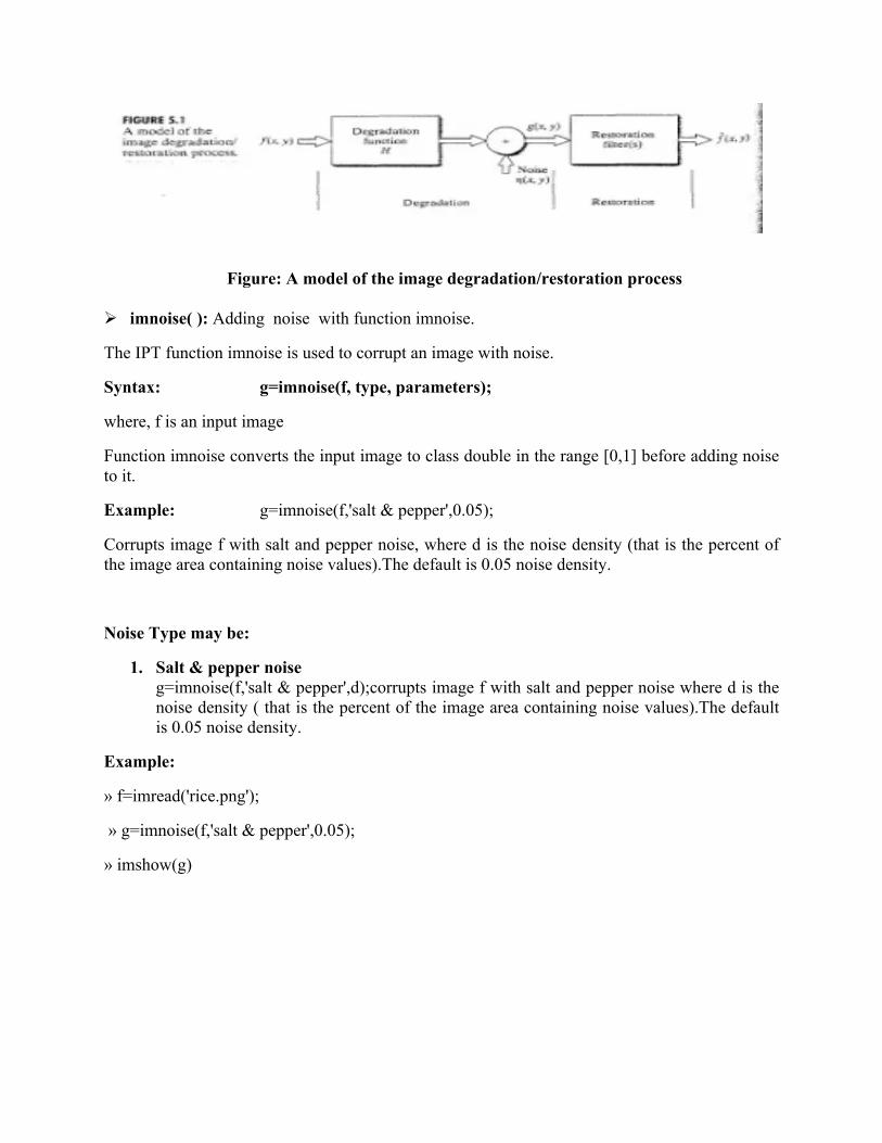
Figure: A model of the image degradation/restoration process

imnoise( ): Adding noise with function imnoise.

The IPT function imnoise is used to corrupt an image with noise.

Syntax: g=imnoise(f, type, parameters);

where, f is an input image

Function imnoise converts the input image to class double in the range [0,1] before adding noise to it.

Example: g=imnoise(f,'salt & pepper',0.05);

Corrupts image f with salt and pepper noise, where d is the noise density (that is the percent of the image area containing noise values).The default is 0.05 noise density.

Noise Type may be:

1. Salt & pepper noiseg=imnoise(f,'salt & pepper',d);corrupts image f with salt and pepper noise where d is the noise density ( that is the percent of the image area containing noise values).The default is 0.05 noise density.

Example:

» f=imread('rice.png');

» g=imnoise(f,'salt & pepper',0.05);

» imshow(g)

2. Gaussian noise

g=imnoise(f,’gaussian’,m,var) adds Gaussian noise of mean m and variance v to image f, where v is an array of same size as f containing the desired variance values at each other. The default value for mean is zero and 0.01 for variance.

Example:

» f=imread('rice.png');

» g1=imnoise(f,'gaussian',0,0.01);

» imshow(g1)

3. Speckle noise

g=imnoise(f,’speckle’,var) adds multiplicative noise to image f, using the equation g=f+n*f where n is uniformly distributed random noise with mean 0 nad variance var. The default value of var is 0.04.

Example:

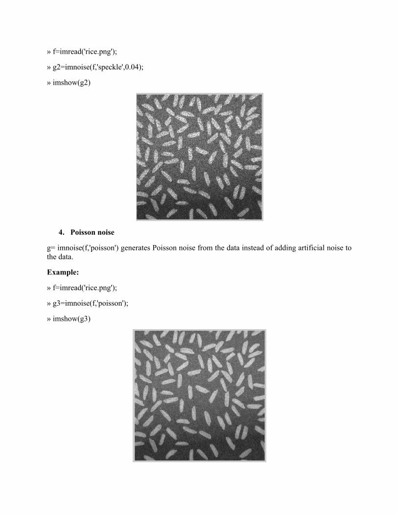
» f=imread('rice.png');

» g2=imnoise(f,'speckle',0.04);

» imshow(g2)

4. Poisson noise

g= imnoise(f,'poisson') generates Poisson noise from the data instead of adding artificial noise to the data.

Example:

» f=imread('rice.png');

» g3=imnoise(f,'poisson');

» imshow(g3)

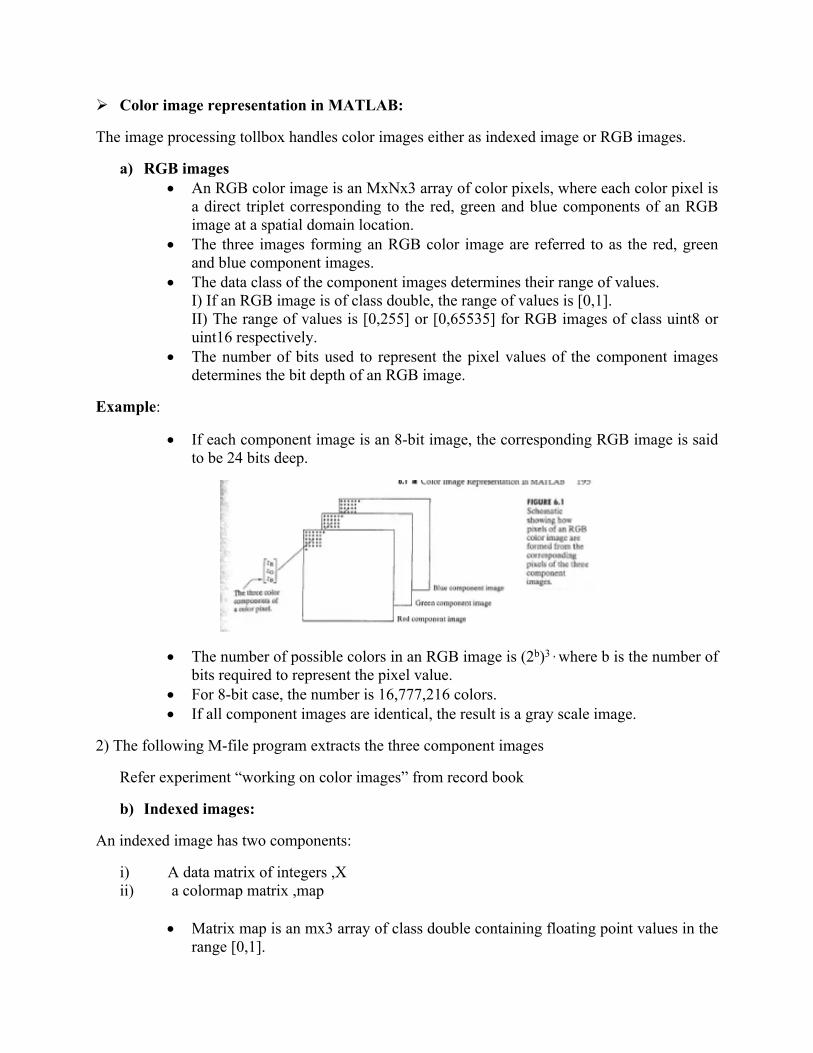
Color image representation in MATLAB:

The image processing tollbox handles color images either as indexed image or RGB images.

a) RGB images An RGB color image is an MxNx3 array of color pixels, where each color pixel is

a direct triplet corresponding to the red, green and blue components of an RGB image at a spatial domain location.

The three images forming an RGB color image are referred to as the red, green and blue component images.

The data class of the component images determines their range of values.I) If an RGB image is of class double, the range of values is [0,1].II) The range of values is [0,255] or [0,65535] for RGB images of class uint8 or uint16 respectively.

The number of bits used to represent the pixel values of the component images determines the bit depth of an RGB image.

Example:

If each component image is an 8-bit image, the corresponding RGB image is said to be 24 bits deep.

The number of possible colors in an RGB image is (2b)3 , where b is the number of bits required to represent the pixel value.

For 8-bit case, the number is 16,777,216 colors. If all component images are identical, the result is a gray scale image.

2) The following M-file program extracts the three component images

Refer experiment “working on color images” from record book

b) Indexed images:

An indexed image has two components:

i) A data matrix of integers ,Xii) a colormap matrix ,map

Matrix map is an mx3 array of class double containing floating point values in the range [0,1].

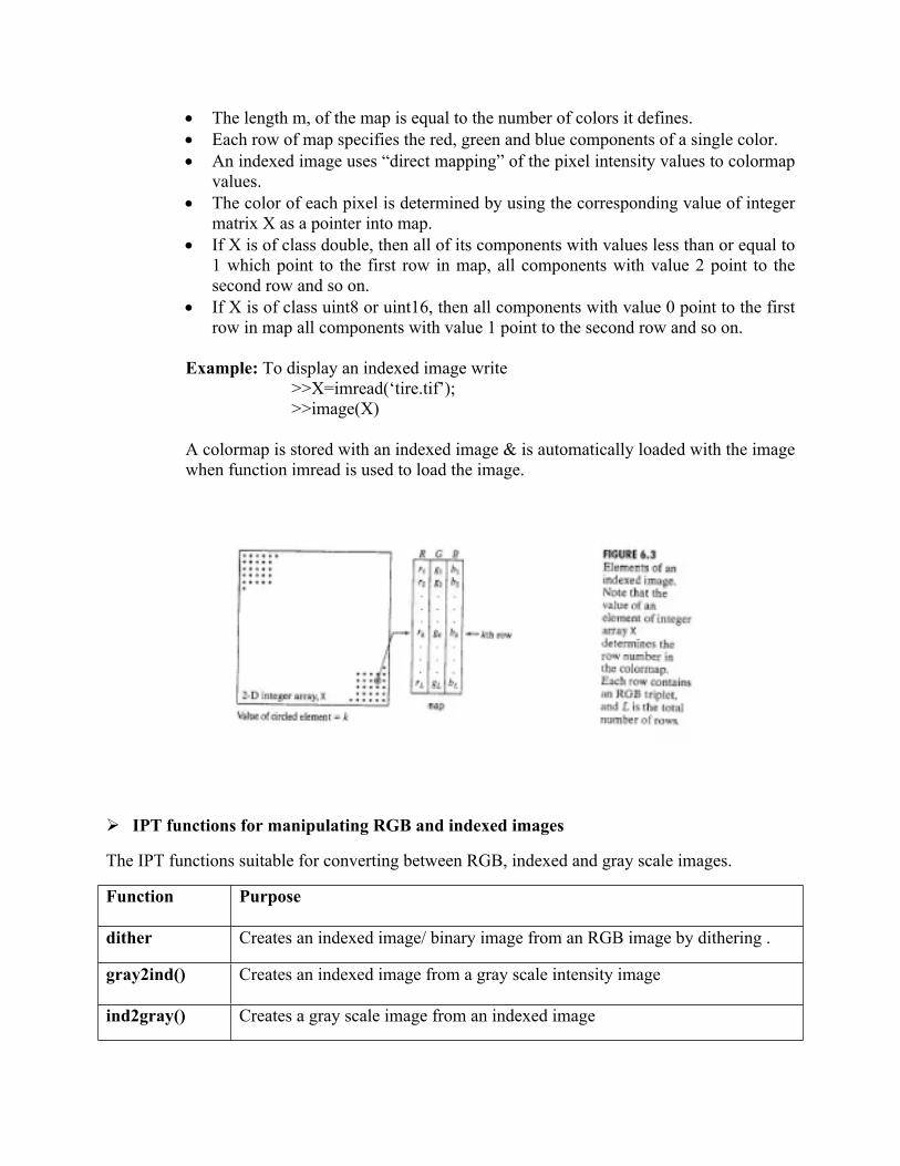
The length m, of the map is equal to the number of colors it defines. Each row of map specifies the red, green and blue components of a single color. An indexed image uses “direct mapping” of the pixel intensity values to colormap

values. The color of each pixel is determined by using the corresponding value of integer

matrix X as a pointer into map. If X is of class double, then all of its components with values less than or equal to

1 which point to the first row in map, all components with value 2 point to the second row and so on.

If X is of class uint8 or uint16, then all components with value 0 point to the first row in map all components with value 1 point to the second row and so on.

Example: To display an indexed image write >>X=imread(‘tire.tif’); >>image(X)

A colormap is stored with an indexed image & is automatically loaded with the image when function imread is used to load the image.

IPT functions for manipulating RGB and indexed images

The IPT functions suitable for converting between RGB, indexed and gray scale images.

Function Purpose

dither Creates an indexed image/ binary image from an RGB image by dithering .

gray2ind() Creates an indexed image from a gray scale intensity image

ind2gray() Creates a gray scale image from an indexed image

rgb2ind() Creates an indexed image from an RGB image

ind2rgb() Creates an RGB image from an indexed image

rgb2gray() Creates a gray scale image from an RGB image

Table: IPT functions for converting between RGB, Indexed and grayscale intensity images

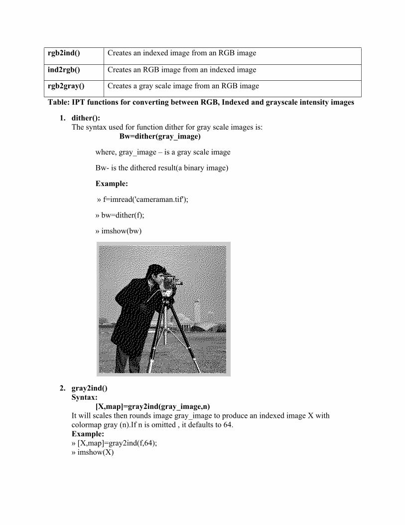
1. dither():The syntax used for function dither for gray scale images is:

Bw=dither(gray_image)

where, gray_image – is a gray scale image

Bw- is the dithered result(a binary image)

Example:

» f=imread('cameraman.tif');

» bw=dither(f);

» imshow(bw)

2. gray2ind()Syntax:

[X,map]=gray2ind(gray_image,n)It will scales then rounds image gray_image to produce an indexed image X with colormap gray (n).If n is omitted , it defaults to 64.Example:» [X,map]=gray2ind(f,64);» imshow(X)

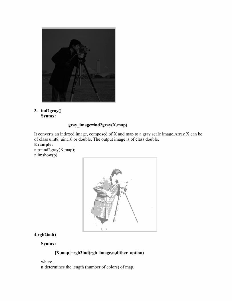
3. ind2gray()Syntax:

gray_image=ind2gray(X,map)

It converts an indexed image, composed of X and map to a gray scale image.Array X can be of class uint8, uint16 or double. The output image is of class double.Example:» p=ind2gray(X,map);» imshow(p)

4.rgb2ind()

Syntax:

[X,map]=rgb2ind(rgb_image,n,dither_option)

where , n determines the length (number of colors) of map.

dither_option-can have one of the two values:’dither’(the default) or ‘nodither’. The dither value achieves better color resolution at the spatial resolution(default). nodither value maps each color in the original image to the closest color in the new map.Example:

» g=imread('peppers.png');» [X,map]=rgb2ind(g,128);» imshow(X)

5. ind2rgb()Syntax: rgb_image=ind2rgb(X,map)

It converts the matrix X & corresponding colormap map to RGB format. X can be of class uint8, uint16 or double. The output RGB image is an M*N*3 array of class double.Example:

» g=imread('peppers.png');» g1=ind2rgb(X,map);» imshow(g1)

6. rgb2gray()

Syntax: gray_image=rgb2gray(rgb_image)

It converts an RGB image to a gray scale image .The input RGB image can be of class uint8, uint16 or double. The output image is of the same class as the input.

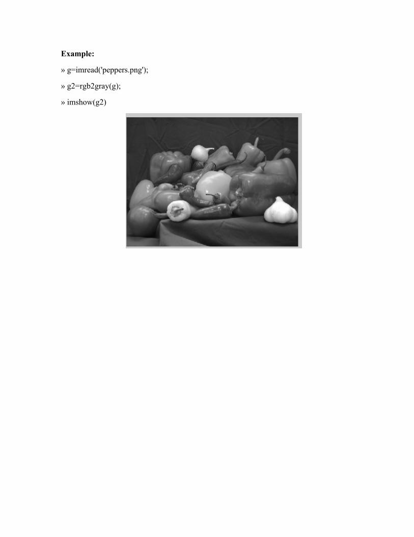
Example:

» g=imread('peppers.png');

» g2=rgb2gray(g);

» imshow(g2)