Modeling and Optimization of Reach and Exposure in TV · Modeling and Optimization of Reach and ... i 2G has attributes, ... Modeling and Optimization of Reach and Exposure in TV

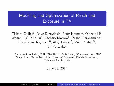
Modeling and Optimization of Reach andExposure in TV

Tishara Collins1, Dave Drzewicki2, Peter Kramer2, Qingxia Li3,Weifan Liu4, Yun Lu5, Zachary Morrow6, Pushpi Paranamana7,

Christopher Raymond8, Abiy Tasissa2, Mehdi Vahab9,Yuri Yatsenko10

1Delaware State Univ., 2RPI, 3Fisk Univ., 4Duke Univ., 5Kutztown Univ., 6NCState Univ., 7Texas Tech Univ., 8Univ. of Delaware, 9Florida State Univ.,

10Houston Baptist Univ.

June 23, 2017

MPI 2017, Clypd Inc. 1 of 23 Optimization of Exposure in TV Advertisements

Outline

Introduction

Problem Statement

Quadratic Objective Function

Clustering Algorithm

Greedy Algorithm: Pairwise Collisions

Future Work


Introduction

TV advertisements play an important role in raising awarenessof goods and services in the marketplace.

Advertisement not meeting the intended audience is an issueas it wastes the resources of the company and disenchants theaudience.

Find optimal advertisement schedule.


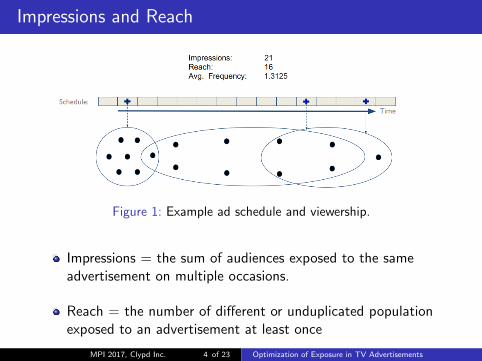
Impressions and Reach

Figure 1: Example ad schedule and viewership.

Impressions = the sum of audiences exposed to the sameadvertisement on multiple occasions.

Reach = the number of different or unduplicated populationexposed to an advertisement at least once


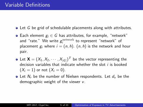
Variable Definitions

Let G be grid of schedulable placements along with attributes.

Each element gi ∈ G has attributes, for example, “network”and “rate.” We write gnetwork

i to represent “network” ofplacement gi where i = (n, h). (n, h) is the network and hourpair.

Let X = (X1,X2, · · · ,X|G |)T be the vector representing thedecision variables that indicate whether the slot i is booked(Xi = 1) or not (Xi = 0).

Let Nr be the number of Nielsen respondents. Let dv be thedemographic weight of the viewer v .


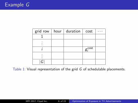
Example G

grid row hour duration cost · · ·1...

i g costi

...

|G |

Table 1: Visual representation of the grid G of schedulable placements.


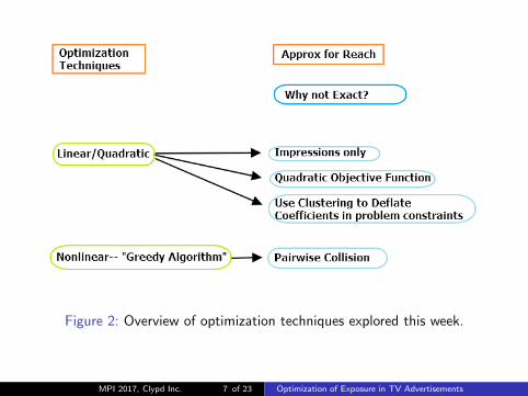
Figure 2: Overview of optimization techniques explored this week.


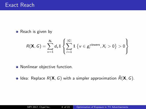
Exact Reach

Reach is given by

R(X,G ) =Nr∑v=1

dv1

|G |∑i=1

1{v ∈ g viewers

i ,Xi > 0}> 0

Nonlinear objective function.

Idea: Replace R(X,G ) with a simpler approximation R(X,G ).


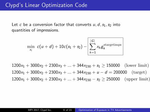
Clypd’s Linear Optimization Code

Let c be a conversion factor that converts u, d , s1, s2 intoquantities of impressions.

minxi

c(u + d) + 10c(s1 + s2)−|G |∑k=1

xkgstargetimpsk

1200x1 + 3000x2 + 2300x3 + ...+ 344x230 + s1 ≥ 150000 (lower limit)

1200x1 + 3000x2 + 2300x3 + ...+ 344x230 + u − d = 200000 (target)

1200x1 + 3000x2 + 2300x3 + ...+ 344x230 − s2 ≥ 250000 (upper limit)


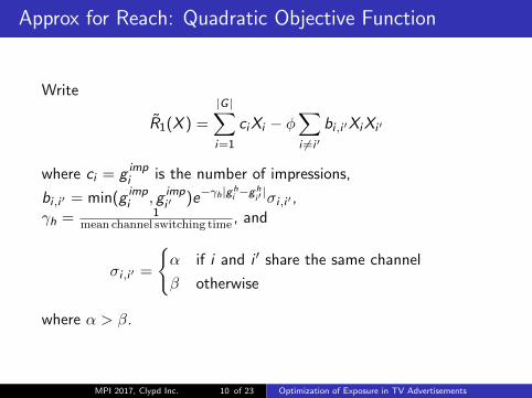
Approx for Reach: Quadratic Objective Function

Write

R1(X ) =

|G |∑i=1

ciXi − φ∑i 6=i ′

bi ,i ′XiXi ′

where ci = g impi is the number of impressions,

bi ,i ′ = min(g impi , g imp

i ′ )e−γh|ghi −g

hi′ |σi ,i ′ ,

γh = 1mean channel switching time , and

σi ,i ′ =

{α if i and i ′ share the same channel

β otherwise

where α > β.


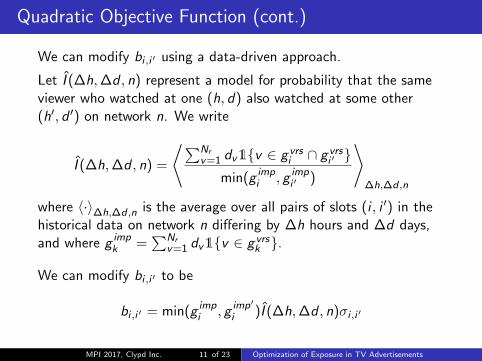
Quadratic Objective Function (cont.)

We can modify bi ,i ′ using a data-driven approach.

Let I (∆h,∆d , n) represent a model for probability that the sameviewer who watched at one (h, d) also watched at some other(h′, d ′) on network n. We write

I (∆h,∆d , n) =

⟨∑Nrv=1 dv1{v ∈ g vrs

i ∩ g vrsi ′ }

min(g impi , g imp

i ′ )

⟩∆h,∆d ,n

where 〈·〉∆h,∆d ,n is the average over all pairs of slots (i , i ′) in thehistorical data on network n differing by ∆h hours and ∆d days,and where g imp

k =∑Nr

v=1 dv1{v ∈ g vrsk }.

We can modify bi ,i ′ to be

bi ,i ′ = min(g impi , g imp′

i )I (∆h,∆d , n)σi ,i ′


Clustering: Motivation

Loss of reach happens due to repeat viewers.

Clustering viewers is hard. However, there is freedom tochoose where to place the ad slots.

Assumption: People watch shows that are “similar” to eachother.

Find a way to group similar shows together, and distribute adsamongst the various categories.


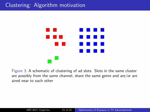
Clustering: Algorithm motivation

Figure 3: A schematic of clustering of ad slots. Slots in the same clusterare possibly from the same channel, share the same genre and are/or areaired near to each other


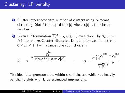
Clustering: LP penalty

1 Cluster into appropriate number of clusters using K-meansclustering. Slot i is mapped to c[i ] where c[i ] is the clusternumber.

2 Given LP formulation∑n

i=1 αixi ≥ C , multiply αi by βi , βi =f (Cluster size,Cluster diameter,Distance between clusters),0 ≤ βi ≤ 1. For instance, one such choice is

βk = e−γk

g impk

|size of cluster c[k]| ; γk =

maxi∈c[k]

g impi − g imp

k

maxi∈c[k]

g impi

The idea is to promote slots within small clusters while not heavilypenalizing slots with large estimated impressions.


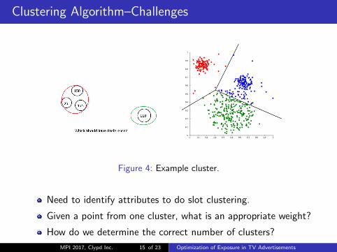
Clustering Algorithm–Challenges

Figure 4: Example cluster.

Need to identify attributes to do slot clustering.

Given a point from one cluster, what is an appropriate weight?

How do we determine the correct number of clusters?


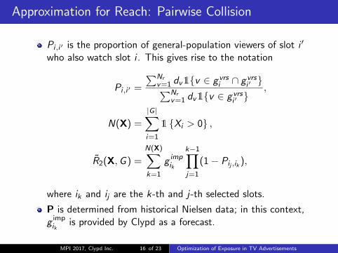
Approximation for Reach: Pairwise Collision

Pi ,i ′ is the proportion of general-population viewers of slot i ′

who also watch slot i . This gives rise to the notation

Pi ,i ′ =

∑Nrv=1 dv1{v ∈ g vrs

i ∩ g vrsi ′ }∑Nr

v=1 dv1{v ∈ g vrsi ′ }

,

N(X) =

|G |∑i=1

1 {Xi > 0} ,

R2(X,G ) =

N(X)∑k=1

g impik

k−1∏j=1

(1− Pij ,ik ),

where ik and ij are the k-th and j-th selected slots.

P is determined from historical Nielsen data; in this context,g impik

is provided by Clypd as a forecast.


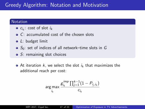
Greedy Algorithm: Notation and Motivation

Notation

cik : cost of slot ik

C : accumulated cost of the chosen slots

L: budget limit

S0: set of indices of all network–time slots in G

S : remaining slot choices

At iteration k, we select the slot ik that maximizes theadditional reach per cost:

arg maxik

g impik

∏k−1j=1 (1− Pij ,ik )

cik


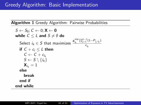
Greedy Algorithm: Basic Implementation

Algorithm 1 Greedy Algorithm: Pairwise Probabilities

S ← S0;C ← 0;X← 0while C ≤ L and S 6= ∅ do

Select ik ∈ S that maximizesg impik

∏k−1j=1 (1−Pij ,ik

)

cikif C + ci ≤ L thenC ← C + cikS ← S \ {ik}Xik = 1

elsebreak

end ifend while


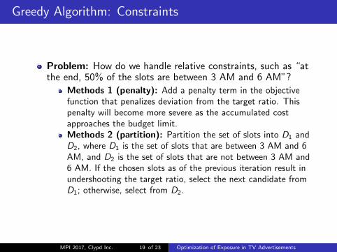
Greedy Algorithm: Constraints

Problem: How do we handle relative constraints, such as “atthe end, 50% of the slots are between 3 AM and 6 AM”?

Methods 1 (penalty): Add a penalty term in the objectivefunction that penalizes deviation from the target ratio. Thispenalty will become more severe as the accumulated costapproaches the budget limit.Methods 2 (partition): Partition the set of slots into D1 andD2, where D1 is the set of slots that are between 3 AM and 6AM, and D2 is the set of slots that are not between 3 AM and6 AM. If the chosen slots as of the previous iteration result inundershooting the target ratio, select the next candidate fromD1; otherwise, select from D2.


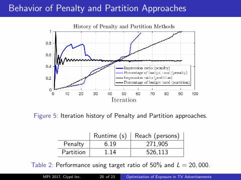
Behavior of Penalty and Partition Approaches

Figure 5: Iteration history of Penalty and Partition approaches.

Runtime (s) Reach (persons)Penalty 6.19 271,905

Partition 1.14 526,113

Table 2: Performance using target ratio of 50% and L = 20, 000.


Future Work

Is there a time δ after which the majority of the impressionsare new?

Optimize more general aspects of the exposure distributionother than raw reach

Extend to multiple objectives (e.g., reaching 18-34 year oldfemales AND nurses)


Acknowledgements

NJIT

Clypd

NSF

ROFLHF


References

Bhatt, G., Burhoe, S., Caps, G. et al. (2015). Prediction andMaximum Scheduling of Advertisements in Linear Televisions(Clypd Problem) MPI 2015 Report.

Hartigan, J. A., Wong, M. A. (1979). Algorithm AS 136: Ak-means clustering algorithm. Journal of the Royal StatisticalSociety. Series C (Applied Statistics), 28(1), 100-108.

Khuller, S., Moss, A., Naor, J. S. (1999). The budgetedmaximum coverage problem. Information Processing Letters,70(1), 39-45.


Documents

Modeling and Optimization of Reach and Exposure in TV · Modeling and Optimization of Reach and ... i 2G has attributes, ... Modeling and Optimization of Reach and Exposure in TV