Tools for Modeling Optimization ProblemsA Short Course

Algebraic Modeling Systems

Dr. Ted Ralphs

Algebraic Modeling Systems 1

The Modeling Process

• Generally speaking, we follow a four-step process in modeling.

– Develop an abstract model.– Populate the model with data.– Solve the model.– Analyze the results.

• These four steps generally involve different pieces of software working inconcert.

• For mathematical programs, the modeling is often done with an algebraicmodeling system.

• Data can be obtained from a wide range of sources, includingspreadsheets.

• Solution of the model is usually relegated to specialized software,depending on the type of model.

1

Algebraic Modeling Systems 2

Modeling Software

• Commercial Systems

– GAMS– MPL– AMPL– AIMMS– SAS (OPT MODEL)

• Python-based Open Source Modeling Languages and Interfaces

– Pyomo– PuLP/Dippy– CyLP (provides API-level interface)– yaposib

2

Algebraic Modeling Systems 3

Modeling Software (cont’d)

• Other Front Ends (mostly open source)

– FLOPC++ (algebraic modeling in C++)– CMPL– MathProg.jl (modeling language built in Julia)– GMPL (open-source AMPL clone)– ZMPL (stand-alone parser)– SolverStudio (spreadsheet plug-in: www.OpenSolver.org)– R (RSymphony Plug-in)– Matlab (OPTI)

3

Algebraic Modeling Systems 4

Solver Software: Linear Optimization

• Commercial solvers

– CPLEX– Gurobi– XPRESS-MP– MOSEK– LINDO– Excel SOLVER

• Open source solvers

– CLP– DYLP– GLPK– lp solve– SOPLEX (free for academic use only)

4

Algebraic Modeling Systems 5

Computational Infrastructure for Operations Research(COIN-OR)

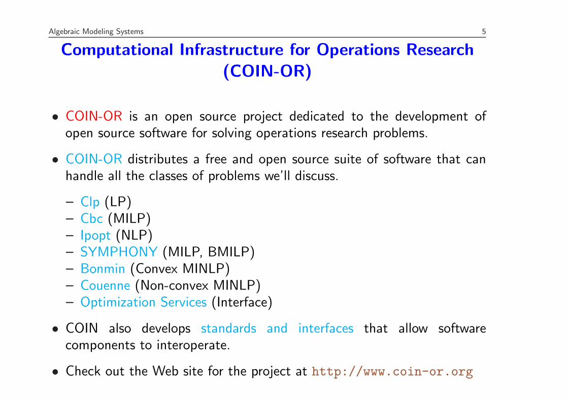
• COIN-OR is an open source project dedicated to the development ofopen source software for solving operations research problems.

• COIN-OR distributes a free and open source suite of software that canhandle all the classes of problems we’ll discuss.

– Clp (LP)– Cbc (MILP)– Ipopt (NLP)– SYMPHONY (MILP, BMILP)– Bonmin (Convex MINLP)– Couenne (Non-convex MINLP)– Optimization Services (Interface)

• COIN also develops standards and interfaces that allow softwarecomponents to interoperate.

• Check out the Web site for the project at http://www.coin-or.org

5

Algebraic Modeling Systems 6

AMPL

• AMPL is one of the most commonly used modeling languages, but manyother languages, including GAMS, are similar in concept.

• AMPL has many of the features of a programming language, includingloops and conditionals.

• Most available solvers will work with AMPL.

• GMPL and ZIMPL are open source languages that implement subsets ofAMPL.

• The Python-based languages to be introduced later have similarfunctionality, but a more powerful programming environment.

• AMPL will work with all of the solvers we’ve discussed so far.

• You can also submit AMPL models to the NEOS server.

• Student versions can be downloaded from www.ampl.com.

6

Algebraic Modeling Systems 7

How They Interface

• Although not required, it’s useful to know something about how modelinglanguages interface with solvers.

• In many cases, modeling languages interface with solvers by writing outan intermediate file that the solver then reads in.

• It is also possible to generate these intermediate files directly from acustom-developed code.

• Common file formats

– MPS format: The original standard developed by IBM in the days ofFortran, not easily human-readable and only supports (integer) linearmodeling.

– LP format: Developed by CPLEX as a human-readable alternative toMPS.

– .nl format: AMPL’s intermediate format that also supports non-linearmodeling.

– OSIL: an open, XML-based format used by the Optimization Servicesframework of COIN-OR.

7

Algebraic Modeling Systems 8

Example: Simple Bond Portfolio Model(bonds simple.mod)

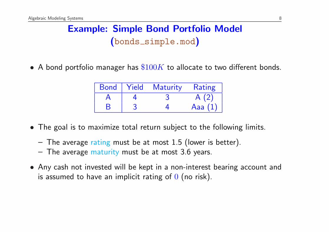
• A bond portfolio manager has $100K to allocate to two different bonds.

Bond Yield Maturity RatingA 4 3 A (2)B 3 4 Aaa (1)

• The goal is to maximize total return subject to the following limits.

– The average rating must be at most 1.5 (lower is better).– The average maturity must be at most 3.6 years.

• Any cash not invested will be kept in a non-interest bearing account andis assumed to have an implicit rating of 0 (no risk).

8

Algebraic Modeling Systems 9

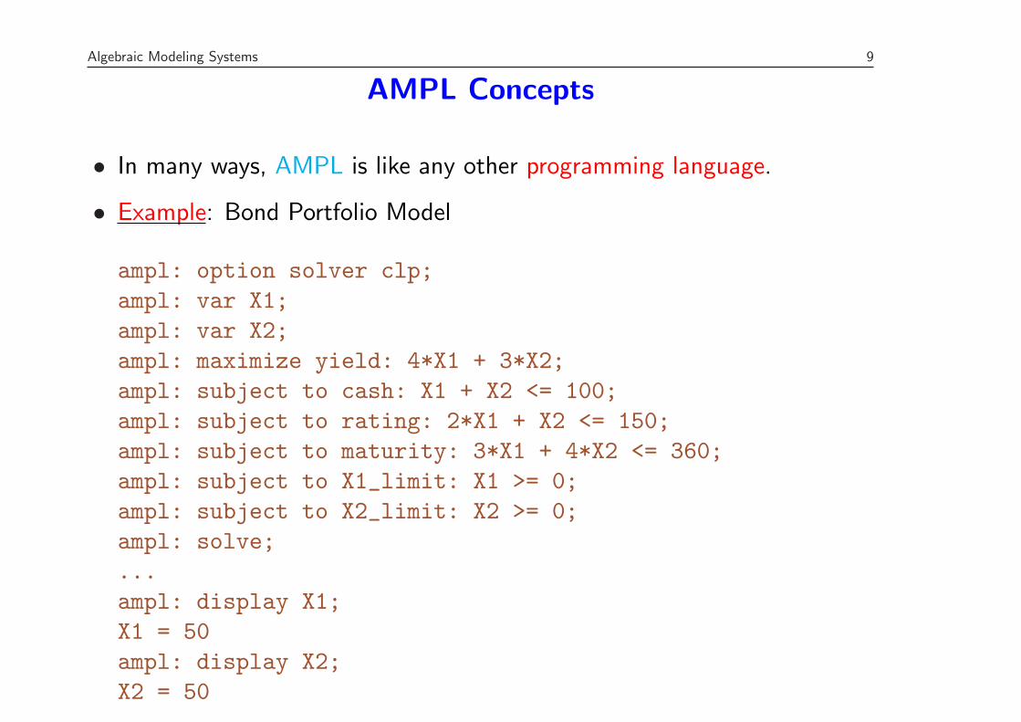
AMPL Concepts

• In many ways, AMPL is like any other programming language.

• Example: Bond Portfolio Model

ampl: option solver clp;ampl: var X1;ampl: var X2;ampl: maximize yield: 4*X1 + 3*X2;ampl: subject to cash: X1 + X2 <= 100;ampl: subject to rating: 2*X1 + X2 <= 150;ampl: subject to maturity: 3*X1 + 4*X2 <= 360;ampl: subject to X1_limit: X1 >= 0;ampl: subject to X2_limit: X2 >= 0;ampl: solve;...ampl: display X1;X1 = 50ampl: display X2;X2 = 50

9

Algebraic Modeling Systems 10

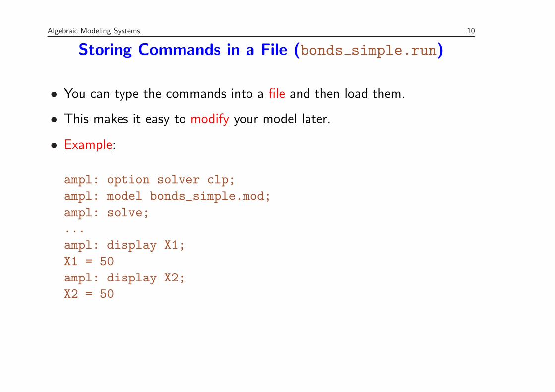
Storing Commands in a File (bonds simple.run)

• You can type the commands into a file and then load them.

• This makes it easy to modify your model later.

• Example:

ampl: option solver clp;ampl: model bonds_simple.mod;ampl: solve;...ampl: display X1;X1 = 50ampl: display X2;X2 = 50

10

Algebraic Modeling Systems 11

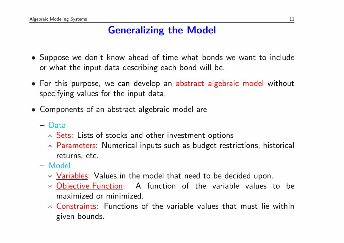
Generalizing the Model

• Suppose we don’t know ahead of time what bonds we want to includeor what the input data describing each bond will be.

• For this purpose, we can develop an abstract algebraic model withoutspecifying values for the input data.

• Components of an abstract algebraic model are

– Data∗ Sets: Lists of stocks and other investment options∗ Parameters: Numerical inputs such as budget restrictions, historical

returns, etc.– Model∗ Variables: Values in the model that need to be decided upon.∗ Objective Function: A function of the variable values to be

maximized or minimized.∗ Constraints: Functions of the variable values that must lie within

given bounds.

11

Algebraic Modeling Systems 12

Example: General Bond Portfolio Model (bonds.mod)

set bonds; # bonds available

param yield {bonds}; # yieldsparam rating {bonds}; # ratingsparam maturity {bonds}; # maturitiesparam max_rating; # Maximum average rating allowedparam max_maturity; # Maximum maturity allowedparam max_cash; # Maximum available to invest

var buy {bonds} >= 0; # amount to invest in bond i

maximize total_yield : sum {i in bonds} yield[i] * buy[i];

subject to cash_limit : sum {i in bonds} buy[i] <= max_cash;subject to rating_limit :

sum {i in bonds} rating[i]*buy[i] <= max_cash*max_rating;subject to maturity_limit :

sum {i in bonds} maturity[i]*buy[i] <= max_cash*max_maturity;

12

Algebraic Modeling Systems 13

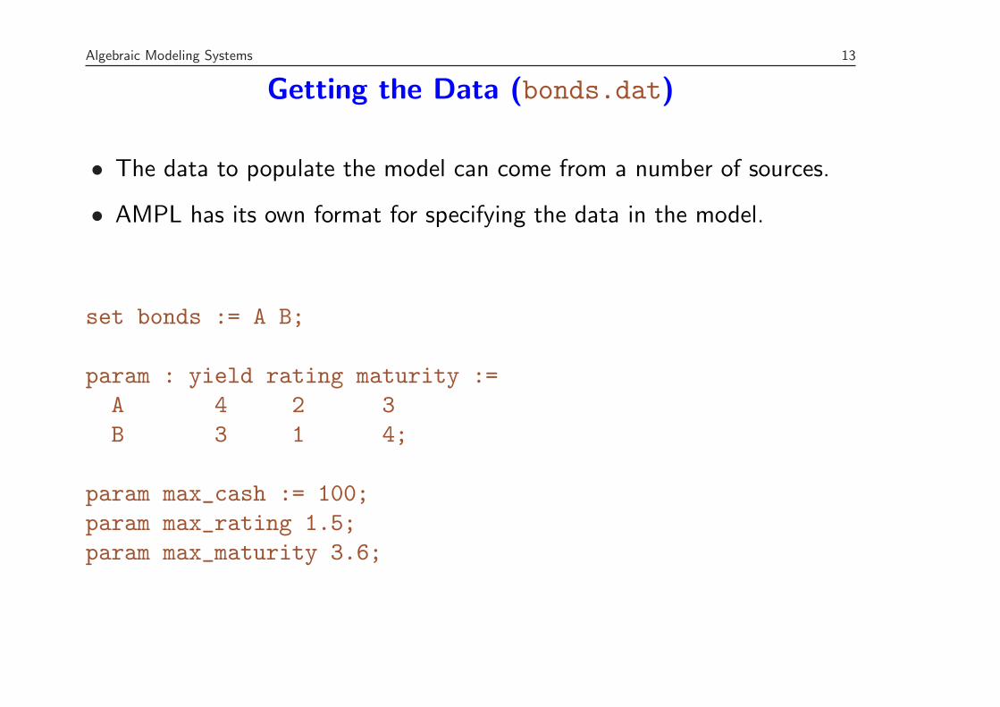
Getting the Data (bonds.dat)

• The data to populate the model can come from a number of sources.

• AMPL has its own format for specifying the data in the model.

set bonds := A B;

param : yield rating maturity :=A 4 2 3B 3 1 4;

param max_cash := 100;param max_rating 1.5;param max_maturity 3.6;

13

Algebraic Modeling Systems 14

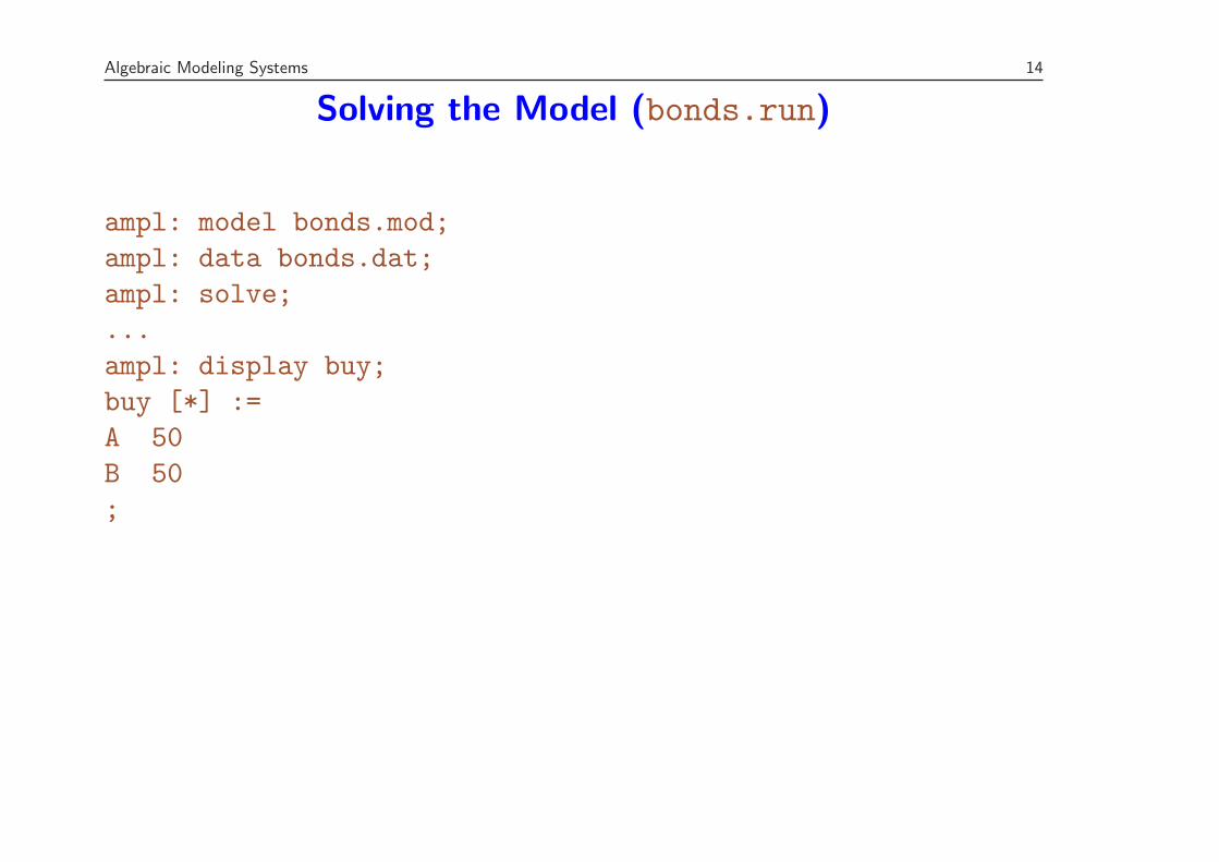
Solving the Model (bonds.run)

ampl: model bonds.mod;ampl: data bonds.dat;ampl: solve;...ampl: display buy;buy [*] :=A 50B 50;

14

Algebraic Modeling Systems 15

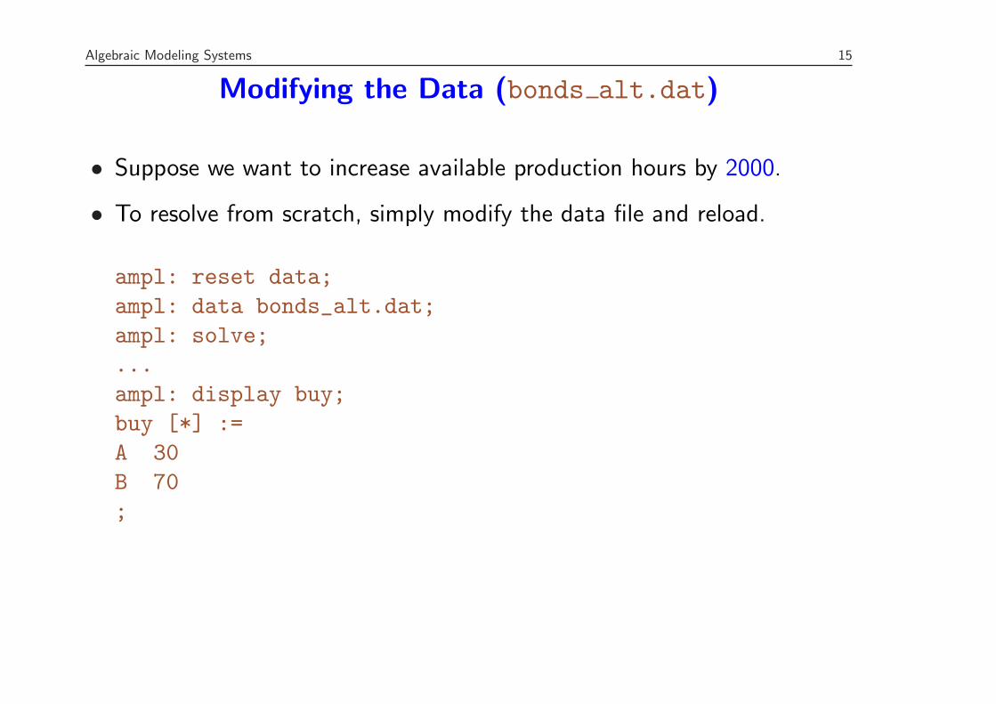
Modifying the Data (bonds alt.dat)

• Suppose we want to increase available production hours by 2000.

• To resolve from scratch, simply modify the data file and reload.

ampl: reset data;ampl: data bonds_alt.dat;ampl: solve;...ampl: display buy;buy [*] :=A 30B 70;

15

Algebraic Modeling Systems 16

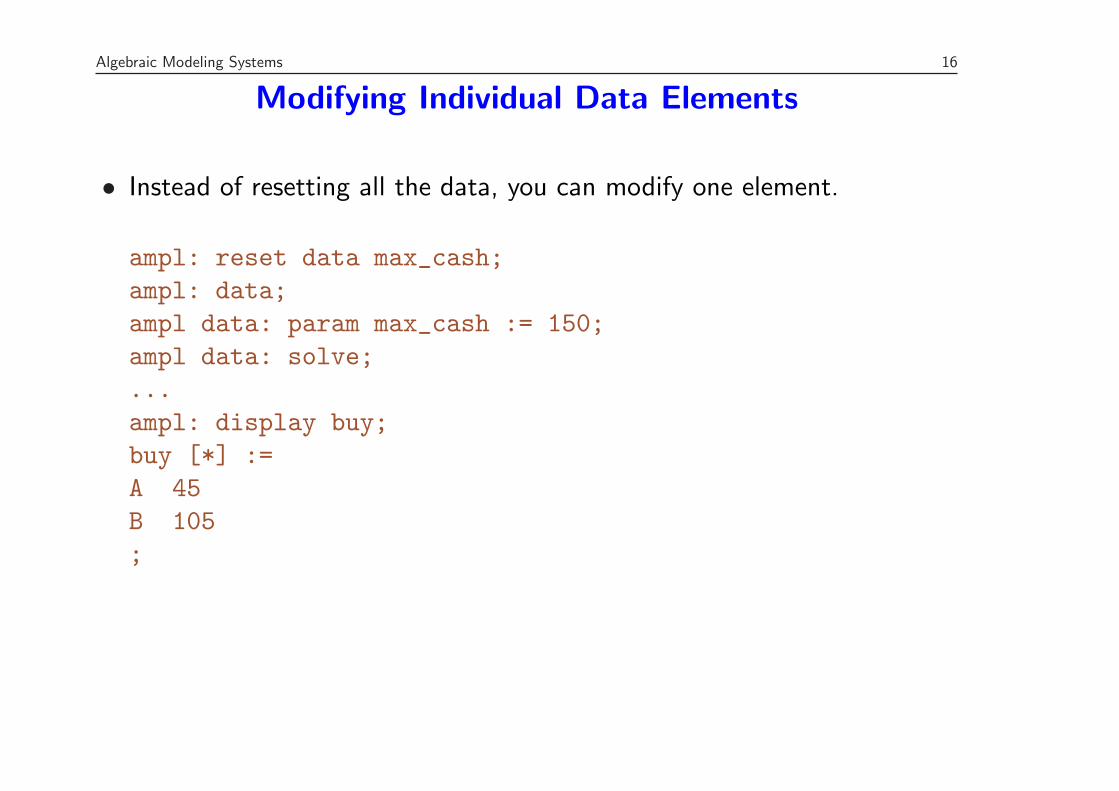
Modifying Individual Data Elements

• Instead of resetting all the data, you can modify one element.

ampl: reset data max_cash;ampl: data;ampl data: param max_cash := 150;ampl data: solve;...ampl: display buy;buy [*] :=A 45B 105;

16

Algebraic Modeling Systems 17

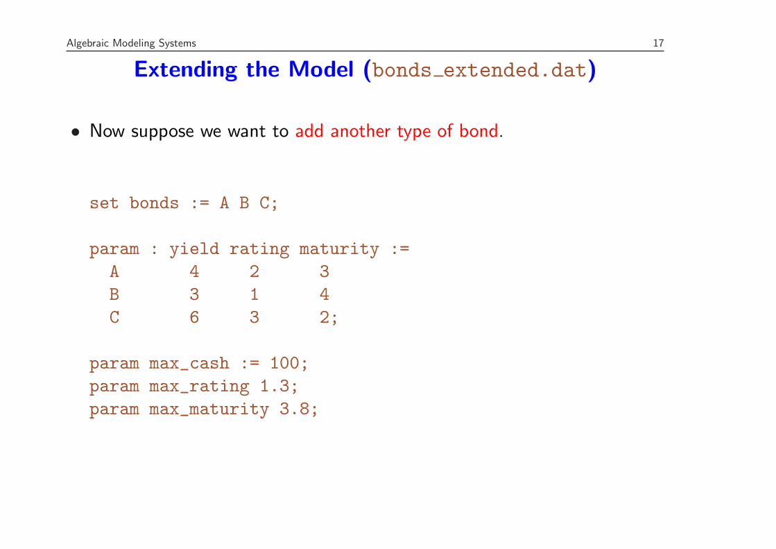
Extending the Model (bonds extended.dat)

• Now suppose we want to add another type of bond.

set bonds := A B C;

param : yield rating maturity :=A 4 2 3B 3 1 4C 6 3 2;

param max_cash := 100;param max_rating 1.3;param max_maturity 3.8;

17

Algebraic Modeling Systems 18

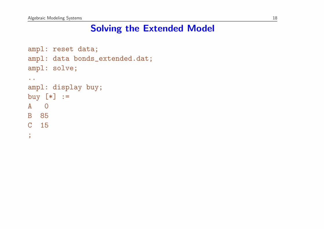
Solving the Extended Model

ampl: reset data;ampl: data bonds_extended.dat;ampl: solve;..ampl: display buy;buy [*] :=A 0B 85C 15;

18

Algebraic Modeling Systems 19

Getting Data from a Spreadsheet(FinancialModels.xlsx:Bonds1-AMPL)

• Another obvious source of data is a spreadsheet, such as Excel.

• AMPL has commands for accessing data from a spreadsheet directlyfrom the language.

• An alternative is to use SolverStudio.

• SolverStudio allows the model to be composed within Excel and importsthe data from an associated sheet.

• Results can be printed to a window or output to the sheet for furtheranalysis.

19

Algebraic Modeling Systems 20

Further Generalization(FinancialModels.xlsx:Bonds2-AMPL)

• Note that in our AMPL model, we essentially had three “features” of abond that we wanted to take into account.

– Maturity– Rating– Yield

• We constrained the level of two of these and then optimized the thirdone.

• The constraints for the features all have the same basic form.

• What if we wanted to add another feature?

• We can make the list of features a set and use the concept of atwo-dimensional parameter to create a table of bond data.

20