Modeling and Simulation of High PressureWater Mist Systems

Topi Sikanen*, Jukka Vaari, Simo Hostikka and Antti Paajanen,Fire Research, VTT Technical Research Centre of Finland, Kemistintie 3,P.O. Box 1000, 02044 Espoo, Finland

Received: 16 March 2012/Accepted: 15 March 2013

Abstract. This paper describes work done to improve and validate the capability of

fire dynamics simulator (FDS) to predict the dynamics of water mist sprays. Threesingle orifice and five multi-orifice spray heads are modeled with FDS based on infor-mation on the flow-rate, spray angle, operating pressure and experimentally deter-

mined particle size distribution. The capability of FDS to predict the drop size,velocity, mist flux and number concentration profiles within the spray cone is asses-sed. The effects of turbulence modeling on the predictions of the spray dynamics isinvestigated. The capability of FDS to predict the air entrainment by high-speed

water sprays is validated using experiments in rectangular channels with open ends.

Keywords: CFD, Water mist, High pressure, Spray dynamics, Turbulence, Three-way coupling

1. Introduction

Water mist systems are widely used to protect people and property from fires andare increasingly being used for projects that are significantly larger than the scaleof experimental test. Despite the large body of experimental work, no generaldesign and installation rules have emerged. The demonstration of the effectivenessof large scale water mist systems then calls for large scale experiments. These largescale experiments require considerable amounts of time and money. It is howeverexpected that the demands for both can be substantially reduced by the use ofnumerical simulations as part of the R&D process.

Water mist systems suppress fires by three main mechanisms: Removal of heatfrom the gases, displacement of oxygen by water vapor and the attenuation ofradiation by droplets Grant et al. [4]. The relative importance of these mecha-nisms depends on the water mist system in question as well as the application. Inorder to use the numerical simulation to examine the effectiveness of water mistsystems, it is critical that we can predict these effects with sufficient accuracy.

The key to water mist system performance is the droplet size: water mist ismade of very fine droplets. The increased surface area of the spray means that thedroplets vaporize quickly and often do not reach the burning surfaces. However,the large surface area to volume ratio of fine droplets leads to high cooling capac-ity in the gas phase. The small size of the droplets indicates a high degree of

* Correspondence should be addressed to: Topi Sikanen, E-mail: topi.sikanen@vtt.fi

Fire Technology

� 2013 Springer Science+Business Media New York. Manufactured in The United States

DOI: 10.1007/s10694-013-0335-8

12

coupling between the gas phase and the water mist. This makes modeling of watermist systems challenging.

Another and sometimes overlooked key, especially for high pressure water mistsystems, is spray dynamics. Due to aerodynamic drag, individual fine water drop-lets will decelerate quickly in the surrounding air even if their initial velocity ishigh. To effectively distribute water mist, high pressure water mist nozzles oftenconsist of a number of micro-nozzles, each discharging a relatively narrow jet.When the jet entrains surrounding air, the fine droplets in the core of the jet willnot experience significant drag, and can therefore be transported far away fromthe discharge orifice. Depending on the nozzle design, individual jets may or maynot interact with each other. In the former case, relatively narrow spray patternsare produced with a good penetration far into the protected space. In the lattercase, wider patterns are produced allowing larger nozzle spacing and good spraycoverage in shallow spaces. Understanding spray dynamics is crucially importantin the design of water mist systems, and being able to accurately model spraydynamics is therefore needed whenever it is desired that the design of water mistsystems could be aided with simulations. The focus in this paper is the near-fielddynamics of high-pressure water mist sprays.

A number of studies have utilized computational fluid dynamics (CFD) modelsfor water mist systems. Prasad et al. [15, 16] and Shimizu et al. [18] studied extin-guishment of small scale fires by water mist using two-fluid models. Two-fluidmodels were also used by Prasad et al. and Nmira et al. [12] to study extinguish-ment by water mist in large enclosures and tunnels, respectively.

Kim and Ryou [8, 9] used the fire dynamics simulator (FDS) version 3.0 formodeling fire suppression of pool fires by water mist in steel enclosure. They mod-ified the FDS-droplet model to include secondary breakup but did not report onthe effects of this modification. Hart [5] used Fluent and a Lagrangian spraymodel to study fire suppression by water mists. An extensive study of water mistmodeling by CFD was done by Husted [6] in his PHD Thesis. He used FDS ver-sion 4.0 and compared predictions to experimental measurements. In the presentwork a development version of FDS is used. The goal is to validate the FDS par-ticle model for use in modeling water mist systems based on a series of validationexperiments. Both single orifice nozzles and multi orifice spray heads are consid-ered.

2. Description of the Validation Experiments

Here we give only a brief description of the validation experiments. More com-plete descriptions can be found in the report [19].

The experimental data used to validate the simulation results comes from to dif-ferent experimental campaigns. In one set of experiments, single water mist nozzleorifice were characterized. The data was obtained by the Direct Imaging (Shadow-graphy] technique, and it consisted of size distribution, velocity, mist flux and par-ticle concentration at several locations across the spray cone. The measurementlocations were those defined in the NFPA 750 standard and an additional

Fire Technology 2013

measurements point on the center line of the cone. The center line measurementpoint was added because otherwise the dense core of the sprays would have beenmissed. All the measurements were made at 70 bar operating pressure.

In the second set of experiments mist nozzles were placed in a rectangular chan-nel and the induced gas velocities in the channel were measured. Both single andmulti-orifice spray heads were used. A smaller channel was used for single orificenozzles and a larger channel for multi-orifice nozzles

For single orifice nozzles, the channel was 1.5 m long and had a cross section of0.15 m by 0.15 m. The nozzles were installed 0.6 m from the downwind end of thechannel and they were spraying along the channel axis. The air velocity in thedirection of the channel axis was measured with a hot-wire anemometer. Measure-ments were taken 0.45 m upwind of the nozzle on the channel axis.

For multi-orifice spray heads, the channel was 2.0 m long and had a cross sectionof 0.6 m by 0.6 m. The spray heads were installed at the midpoint of the channel andthey were spraying along the channel axis. Air velocity measurements were taken 0.5m upwind the nozzle on the channel axis and 0.06 m from the channel wall.

3. Model Description

The FDS (svn revision 10155) is used in this study. The governing equations andsolution methods for the gas phase are described in the FDS Technical ReferenceManual [10] and will not be repeated here. FDS uses Large Eddy Simulation todescribe the turbulent motion of the gas phase and Lagrangian description of thedispersed phase. The sprays in this paper are evaporating. The evaporation modelused is described in the FDS Technical Reference Manual [10]. However evapora-tion is not expected to be important since we are simulating cold sprays. Further-more, the residence times of the particles in the simulations are very short.Secondary breakup was not considered in this study.

For this paper, modifications were made to the FDS source code. A model foraerodynamic interactions between droplets was added and a new shape functionwas implemented for the spray boundary condition. These modifications aredescribed in detail below.

3.1. Lagrangian Particle Model

Ignoring buoyancy, lift and forces arising from fluid acceleration, the motion of asingle spherical droplet is governed by the equation of motion

dmpvp

dt¼ mpgþ qgCDpr2p vp � vg

� �vp � vg

�� �� ð1Þ

Here on the left hand side mp is the mass of the droplet and vp is the velocity ofthe droplet. On the right hand side, g is the gravitational acceleration, qg is thedensity of the surrounding gas, vg is the velocity of the surrounding gas, rp is theradius of the droplet, and CD is the drag coefficient. The drag coefficient is givenby McGrattan et al. [10]

High Pressure Water Mist Systems

CD ¼Re=24 Re< 1Re24 1þ 0:15Re0:683� �

1<Re< 10000:44 Re> 1000

8<

:ð2Þ

where Re ¼ 2 tp � tg

�� ��rp=m is the droplet Reynolds number and m is the kinematicviscosity of air. Due to the large number of droplets in a real spray, only a frac-tion of these droplets is tracked. Each droplet in the simulation represents a parcelof droplets with the same properties.

To ensure that the momentum lost by the droplets is distributed correctly in thegas, an additional CFL-like condition can be placed on the global time step. Theglobal time-step of the numerical solver is adjusted according to

Dt � Cminvx

Dx;

vy

Dy;

vz

Dz

� �; ð3Þ

where C is a user defined constant between 1 and 0, and vx, vy, and vz are thethree components of the particle velocity vp:

3.2. Three-way Coupling Between Droplets and Gas

Typically Lagrangian particle models only consider two-way coupling of the gasphase and the dispersed phase. This means that each particle interacts with thecarrier fluid individually. Momentum lost from a particle is added to the fluid andvice versa.

If the spray is dense enough, the individual droplets start to influence eachother through aerodynamic interactions. These effects cannot be captured by thecurrent Eulerian–Lagrangian model for two reasons: First, the Lagrangian parti-cles have no volume in the Eulerian space, preventing the model from seeingeffects that take place in the length scale of the droplet diameter. Secondly, theeffects of this length scale would be sub-grid scale in most practical simulations.These aerodynamic interactions may start to have an effect when the averagedroplet spacing is <10 [13, 14] droplet diameters. This corresponds approximatelyto a droplet volume fraction a = 0.01. Volume fractions as high as this can some-times be achieved inside water mist sprays. If the spray was even more dense, par-ticle-particle collisions or four-way coupling would need to be considered. Thesprays considered in this paper are relatively dilute, so only the possibility ofthree-way coupling effects is considered.

In a configuration where two particles with the same diameter are directly inline, the reduction of the hydrodynamic forces to the second (trailing) sphere dueto the wake effect was studied in [17]. They developed the following analytical for-mula for the hydrodynamic force to the second sphere. In our work, this formulais used to compute a reduction factor for drag coefficient

CD ¼ CD0

FF0

ð4Þ

Fire Technology 2013

where CD0 is the single droplet drag coefficient and F/F0 is the hydrodynamicforce ratio of trailing droplet to single droplet:

FF0¼ W 1þRe

16

1

L=d � 1=2ð Þ2exp �Re

16

1

L=d � 1=2ð Þ

� �" #

ð5Þ

where Re is the single droplet-Reynolds number, L is the distance between thedroplets and W is the non-dimensional, non-disturbed wake velocity at the centerof the trailing droplet

W ¼ 1� CD0

21� exp �Re

16

1

L=d � 1=2ð Þ

� �� �ð6Þ

This model assumes that the spheres are traveling directly in-line with each other.As such, this provides an upper bound for the strength of the aerodynamic inter-actions between two particles of the same size. The separation distance L/dbetween droplet centers is calculated from the local droplet volume fraction andlocal average droplet diameter �d

L=d ¼ �d p=6að Þ13 ð7Þ

Here local quantities are taken as average over a single computational cell.In reality, the spray is of course not monodisperse and the separation distance

between the interacting particles varies. However seeking for each the closest par-ticle to interact with would be very time consuming. In the simulations, the dragreduction factor in Equation 4 is only used, when the local droplet volume frac-tion exceeds 10-5. This drag reduction model is turned on by default.

An alternative data on drag reduction was provided by Prahl et al. [13] whostudied the interaction between two solid spheres in steady or pulsating flow bydetailed numerical simulations. According to their study, the above correlationunderestimates the drag reduction significantly at small drop-to-drop distances.The inflow pulsations were found to reduce the effect of the drag reduction. Atlarge distances the two results are similar, the Ramırez-Munoz correlation show-ing more drag reduction. This is not surprising since the velocity profile of a fullydeveloped axisymmetric wake behind a axisymmetric body is used in developingthe drag reduction correction in Eqs. 5 and 6. At short distances, the wake is notfully developed and the assumption does not hold. The sprays considered in thispaper are relatively dilute and hence these short separation distances are notexpected to be important.

3.3. Spray Boundary Condition

In this work, no attempt is made to model the primary or secondary atomizationprocesses of the spray. Instead the spray is described as a droplet inlet boundarycondition. The droplets are injected to the simulation on a section of a spherical

High Pressure Water Mist Systems

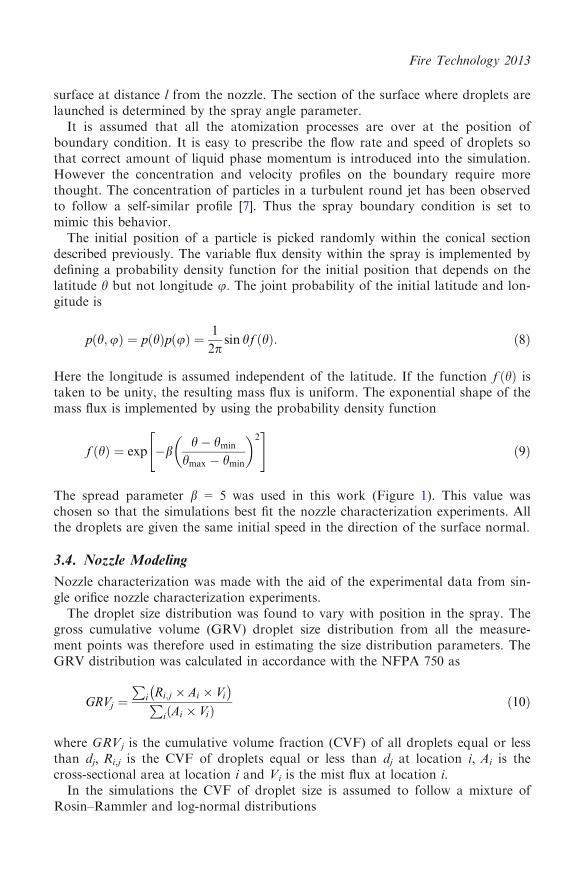
surface at distance l from the nozzle. The section of the surface where droplets arelaunched is determined by the spray angle parameter.

It is assumed that all the atomization processes are over at the position ofboundary condition. It is easy to prescribe the flow rate and speed of droplets sothat correct amount of liquid phase momentum is introduced into the simulation.However the concentration and velocity profiles on the boundary require morethought. The concentration of particles in a turbulent round jet has been observedto follow a self-similar profile [7]. Thus the spray boundary condition is set tomimic this behavior.

The initial position of a particle is picked randomly within the conical sectiondescribed previously. The variable flux density within the spray is implemented bydefining a probability density function for the initial position that depends on thelatitude h but not longitude u: The joint probability of the initial latitude and lon-gitude is

p h;uð Þ ¼ p hð Þp uð Þ ¼ 1

2psin hf hð Þ: ð8Þ

Here the longitude is assumed independent of the latitude. If the function f hð Þ istaken to be unity, the resulting mass flux is uniform. The exponential shape of themass flux is implemented by using the probability density function

f hð Þ ¼ exp �bh� hmin

hmax � hmin

� �2" #

ð9Þ

The spread parameter b = 5 was used in this work (Figure 1). This value waschosen so that the simulations best fit the nozzle characterization experiments. Allthe droplets are given the same initial speed in the direction of the surface normal.

3.4. Nozzle Modeling

Nozzle characterization was made with the aid of the experimental data from sin-gle orifice nozzle characterization experiments.

The droplet size distribution was found to vary with position in the spray. Thegross cumulative volume (GRV) droplet size distribution from all the measure-ment points was therefore used in estimating the size distribution parameters. TheGRV distribution was calculated in accordance with the NFPA 750 as

GRVj ¼P

i Ri;j � Ai � Vi� �P

i Ai � Við Þ ð10Þ

where GRVj is the cumulative volume fraction (CVF) of all droplets equal or lessthan dj, Ri,j is the CVF of droplets equal or less than dj at location i, Ai is thecross-sectional area at location i and Vi is the mist flux at location i.

In the simulations the CVF of droplet size is assumed to follow a mixture ofRosin–Rammler and log-normal distributions

Fire Technology 2013

F dð Þ ¼1ffiffiffiffi2ppR d0

1rd 0 exp �

ln d 0=dmð Þ½ �22r2

h idd0 d � dm

1� exp �0:693 ddm

�ch id � dm

8<

:ð11Þ

Here dm is the volumetric median diameter, while r and c are width parameters.The width parameters are related by r = 1.15/c to ensure continuity at dm. In thesimulations the droplet diameter is picked according to the cumulative numberfraction (CNF) defined as

f dð Þ ¼R d0 F 0ðd 0Þd 0�3dd0R10 F 0ðd 0Þd 0�3dd0

; F 0 ¼ dF ðdÞdd

ð12Þ

The distribution parameters were found by least squares fit of Equation 12 to theexperimentally determined cumulative number distribution. The difference betweenusing Eqs. 11 and 12 for parameter estimation is that the former places moreweight on large droplets while the latter emphasizes the smaller drop sizes. Thispoint was discussed extensively in [2]. Since in the numerical algorithm the dropletsizes are picked from the CNF, it was also used in the parameter estimation. Inthe simulations, the particle size is bounded from below by the parameterdmin = 1 lm. Droplets with diameters smaller than this are assumed to vaporizeinstantly. Figure 2 shows a comparison of the fitted CVF and experimental GRV.For nozzles B and C, the amount of very large droplets is underestimated. For allnozzles the amount of very small droplets is also underestimated.

θR

f(θ)

Rsin(θ)

Figure 1. Illustration of the spray boundary condition.

High Pressure Water Mist Systems

The median droplet size is known to depend on the operating pressure used.Since the experimental droplet size distributions were determined at certain pres-sure (70 bar) but the simulations were also performed at other pressures, this vari-ation in droplet size is taken into account by scaling the median droplet size asdm � p-1/3.

The spray angle h for each orifice were determined from spray photographs.This method is quite crude and furthermore depends somewhat on the choice ofthe offset parameter. The estimated parameters for the three single-orifice nozzlesare summarized in Table 1.

The tabulated flow constants (K-factors) for the high pressure nozzles are basedon the flow measurements performed for multi-orifice spray heads involving a sin-gle orifice type. The flow constant K is defined as

K ¼ Qffiffiffipp ; ð13Þ

where Q is the flow rate of water, and p is the water pressure measured at thespray head. Strictly, the flow constant is not a constant, but depends slightly onpressure. However, for practical purposes, it is sufficient to determine the flowconstant for a single pressure representative of the working pressure range of thespray head.

In all the simulations initial droplet velocities were calculated from

v0 ¼ 0:95

ffiffiffiffiffi2pql

s

; ð14Þ

0 100 200 300 400 500 6000

20

40

60

80

100

Diameter (µm)

Cum

ulat

ive

Vol

ume

Frac

tion

(%)

A B C

ExperimentFit

Figure 2. Experimentally observed droplet CVF distributions versusfitted distributions.

Fire Technology 2013

where p is the operating pressure of the nozzle and ql is the density of the liquid.Factor 0.95 was used to account for the friction losses in the nozzle. This value isthe authors estimate.

Table 2 gives the descriptions of the multiorifice nozzles considered here. Themultiorifice nozzles were modeled by positioning several single orifice models withdifferent orientations at one point in the computational domain. Each individualorifice on the nozzle was modeled with the parameters given in Table 1. The cen-ter nozzle points in the axial direction and the perimeter nozzles are equallyspaced and at the same angle in relation to the center nozzle. The smaller theperimeter angle, the more parallel are the orifices in the spray head.

4. Modeling and Simulation of Validation Experiments

Grid sensitivity studies and studies concerning the effects of three-way couplingand turbulence modeling on the sprays is done via comparisons with nozzle char-acterization tests. Air entrainment predictions are validated against induced flowvelocity data from several entrainment tests conducted for nozzles and multi-ori-fice spray heads.

4.1. Nozzle Characterization Experiments

The experimental measurements and the calculation of GRV distribution were inaccordance with the NFPA750 standard except that one measurement point wasadded in the center of the spray, since the measured nozzles (A, B and C) wereproducing a relatively narrow cone with a dense core. The NFPA750 is moreintended for sprinklers with deflector plates where the spray is wide and the centerof the spray is unoccupied with droplets. If the center point was not included, asignificant amount of the mist flux would be ignored.

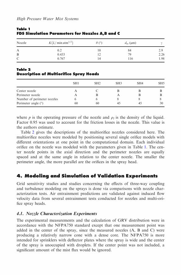
Table 1FDS Simulation Parameters for Nozzles A,B and C

Nozzle K L=min atm1=2� �

h (�) dm (lm) c

A 0.2 10 84 2.9

B 0.433 12 79 2.26

C 0.767 14 116 1.98

Table 2Description of Multiorifice Spray Heads

SH1 SH2 SH3 SH4 SH5

Center nozzle A C B B B

Perimeter nozzle A B A B B

Number of perimeter nozzles 6 6 8 8 8

Perimeter angle (�) 60 60 45 45 30

High Pressure Water Mist Systems

The experiments were modeled using a rectangular computational area 1.5 mhigh, 0.5 m wide and 0.5 m deep. The computational area was open to flow on allsides. The nozzles were placed 0.1 m from the top of the computational domainand the measurements were taken 1 m below the nozzle. Figure 3 shows the com-putational model and placement of the measurement points. The simulationresults correspond to droplet properties averaged over a sphere with 1 cm radiuscent red at the measurement location. After a sensitivity study described in section5.2, 2 cm grid was selected. The same 2 cm grid was used for the air entrainmentsimulations also. Simulation time was 5 s and the droplet statistics were collectedfor the last 3 s of the simulations. The first 2 s were ignored to ensure that thesimulation had reached steady state.

Figure 3. Pictures of the nozzle characterization simulations for noz-zle A. On the left, the measurement locations with green dots. On theright time averaged average velocity slice (Color figure online).

Fire Technology 2013

4.2. Air Entrainment

Induced air velocity data was used to validate the air entrainment predictions. Thedata was from experiments where single- and multiorifice nozzles were placed in arectangular channel.

The single nozzle experiment was modeled simply as a rectangular computa-tional domain, with dimensions of the experimental channel. On the channelwalls, inert solid wall boundary conditions were applied and open pressure bound-aries were used for the ends of the channel. In the multi-orifice spray head experi-ments, a wooden block near the inlet end of the channel affected the airflow andto capture this effect, the computational domain was extended outside the channelas shown in Figure 4. Discretization interval was 2 cm in both channels.

The offset parameter was found to have a significant effect on the simulationresults, especially for the multi-orifice spray heads. Offset value of 0.04 m wasused here instead of the 0.1 m used for the simulation of the nozzle characteriza-tion tests. Using a too small offset value was found to give unphysical results,where the flow on the channel axis behind (upwind) the sprinkler was in the nega-tive x-direction, while the sprinkler was oriented in the positive x-direction. It wasconcluded that the correct offset value depends on the numerical grid used: Theoffset should be large enough, so that the incoming droplets are distributedamong large enough number of computational cells. This effect is related to thetransfer of momentum from dispersed phase to the gas phase. By distributing thedroplets in a sufficient number of cells, we ensure that the momentum source termin the gas phase equations is better approximated. Naturally, the grid also needsto be fine enough to resolve the important flow features near the nozzle. In thecase of multi-orifice spray heads this means that it is important to ensure that the

Figure 4. Picture of the large channel computational model.

High Pressure Water Mist Systems

grid is fine enough that each of the spray jets is resolved. This becomes a problemwhen the orifices in the spray have orientations that are almost parallel.

5. Results and Discussion

The simulations were run on a computer cluster with 2.92 GHz, 8-core Intel Xeonprocessors and 2 GB of memory per core. Simulations were ran as serial jobs,with one processor handling a single simulation. The nozzle characterization simu-lations took between 7 h and 22 h for 5 s of simulation time. The entrainmentsimulations run from few hours for the small channel to 25 h for the large chan-nel simulations.

5.1. Turbulence Modeling

By default FDS version 5 uses a constant Smagorinsky coefficient model of turbu-lent viscosity. However for the current simulations the dynamic Smagorinskymodel [11, 3] was used. In newer versions of FDS the constant Smagorinsky coef-ficient model is no longer the default. Instead several alternatives are given. Fig-ure 5 shows a comparison of results between four different turbulent viscositymodels. The models considered are those available in the development version ofFDS used: Deardorff [1], Vreman [20] the constant Smagorinsky and the dynamicSmagorinsky coefficients.

There is almost 50% difference in the predicted velocities and mist fluxes on thespray axis. However, the velocity and mist flux profiles are extremely sensitive tothe spray boundary condition. Since there is considerable uncertainty in definingthe shape function and spray angle for the spray boundary condition, these resultsalone cannot be used to determine which turbulence model is more suited for thisapplication. The diameter profile on the other hand was found to be very insensi-tive to the boundary condition. The correct flat shape of the diameter profile isonly reproduced with the dynamic Smagorinsky model. Furthermore, the dynamicSmagorinsky model produces overall better fit of velocity and mist flux profilesthan the other models. The results are also sensitive to grid size. These simulationswere run on a 2 cm grid but on finer grids Deardorff, Vreman and dynamic Sma-gorinsky models tend to converge on the same result.

This result suggests that the turbulent mixing of the particles is important atthese distances. Near the nozzle, the entrained air will tend to pull dropletstowards the middle of the spray. Smaller droplets have shorter response times andthus are entrained more easily. This process should result in a diameter profilethat shows mores small droplets at the center of the spray and larger droplets onthe spray boundaries. However the droplet size in these simulations is very smalland their relative velocities are relatively small at 1 m distance from the spraynozzle, where the measurements are made. At this point the particles tend to dis-perse towards the edges of the spray. The smallest particles are influenced moreby the turbulent dispersion than heavier particles which might still have significantrelative velocity. The sum of these effects is that the differences in average particlesize are diminished.

Fire Technology 2013

It is not immediately clear how important this mixing is for predicting the effi-ciency of water mist systems. However, within the dense spray core where most ofthe water in the spray is located, the droplet size predictions are similar for bothturbulence models tested.

5.2. Sensitivity Study

Sensitivity of the single orifice models to model parameters and numerical param-eters was studied. The model parameters considered were the spray angle h andinitial velocity v0. The numerical parameters included discretization interval Dx;effect of the CFL parameter in Eg. 3, effect of offset parameter R and the dropletinsertion rate. The parameters for the base case are given in Table 3. The grid res-olution and DPS-parameters were arrived at through a sensitivity study. The off-set parameter and CFL-condition limit were set at their default values for the basecase. Table 4 presents the full experimental design for sensitivity study and theerror in each simulation. The error in the simulations is quantified as

e ¼ maxi Ei �maxi Si

maxi Ei; ð15Þ

0 5 10 15 200

10

20

30

40

Radial position (cm)

Vel

ocity

(m

/s)

ExpCSmagDSmagDeardorffVreman

(a)

0 5 10 15 200

5

10

15

20

Radial position (cm)

Mis

t flu

x (k

g/m

2 s)

ExpCSmagDSmagDeardorffVreman

(b)

0 5 10 15

40

60

80

100

120

140

160

Radial position (cm)

d 10 (

µm)

ExpCSmagDSmagDeardorffVreman

(c)

Figure 5. Effect of turbulence model on average droplet velocity,mist flux and diameter profiles. Results shown for nozzle B.

High Pressure Water Mist Systems

where Ei and Si are the experimental measurements at measurement point numberi and simulation results respectively.

The grid sensitivity study was conducted using a uniform Cartesian grid withdiscretization intervals 1 cm, 2 cm and 4 cm. The results of the grid sensitivitystudy were similar for all the single orifice nozzles. Figure 6 shows the results fornozzle B. In general, coarser grids produced flatter velocity and concentration dis-tributions. However, the diameter distribution retained its shape. It can be seenfrom Table 4 that going from 2 cm grid to 1 cm grid did not improve the enoughto warrant the increased computational cost. Increasing the number of Lagrangianparticles inserted to the spray from 2 � 105 to 4 � 105 s-1 tended to yield largervelocities on the spray center line but did not otherwise affect the results. Thenumber of Lagrangian particles in the simulation at any given time was �17000for the base case. The effect of the time step was studied by using values 0.1, 0.5and 1 for the parameter C in Equation 3. For the base case, the time step wasapproximately 10 ms for the steady state phase of the simulation. Overall thetime-step had very little effect on the results.

Offset values from 5 cm to 15 cm were tested with little effect on the results inthe nozzle characterization test. However it should be stressed that it was discov-ered later that the offset parameter was important in modeling multi orifice noz-zles. Varying the initial velocity by ±6 m/s changed the results only by a fewpercent. The spray angle parameter h had the largest effect on the results withnarrowing the angle by 5� increasing the error by as much as 120% points.Choosing a smaller spray angle increased error more than choosing a larger angle.

The minimum diameter dmin was set to 1 lm in most simulations. No dropletssmaller than this diameter are added to the simulation. Also, droplets smaller thanthis are assumed to vaporize instantly. This parameter was sometimes increased toalleviate problems with numerical stability. Sensitivity analysis showed that thisparameter did not have a noticeable effect on the results.

5.3. Three-way Coupling

The importance of three-way coupling effects on water mist properties was investi-gated by running the nozzle characterization tests, with the aerodynamic interaction

Table 3Parameters for the Base Case in Sensitivity Study

Parameter Value Description

Dx 0.02 m Discretization interval

DPS 2 � 105 How many droplets per second are inserted to the

simulation

3-way coupling On Use the three-way coupling model from Section 3.2

v0 112 m/s Initial velocity of droplets

CFL 1 Coefficient C in Equation 3

R 0.1 m Offset parameter for the spray boundary condition

h - See Table 1

Fire Technology 2013

model turned on and turned off. Figure 7 shows the effects of the drag reductionmodel on the simulation results for nozzle C. Nozzle C has the highest flow rateand densest spray, being thus the best candidate for a spray where aerodynamicinteractions are important. Results for other nozzles were very similar and areomitted for brevity The drag reduction by aerodynamic interactions had a verymodest effect on the results. The most noticeable effect was the slight flattening ofthe droplet diameter profile. The droplet volume fractions in the densest parts ofthe spray are just slightly over a > 0.01 for all nozzles. These results indicate thatdroplet-droplet aerodynamic interactions are not important in modeling the cur-rent water mist systems. The three-way coupling model was used in all simulationsof this paper.

5.4. Nozzle Characterization Experiments

Here we give an overview of the results for the simulation of the nozzle character-ization tests. Note that the nozzle characterization experiments were also used inselecting the employed turbulence model and the shape function for the sprayboundary condition.

The numerical parameters used in these simulations are listen in Table 3. Theseparameters were selected after the sensitivity study described in Sect. 5.2 and sameset of numerical parameters is used for all nozzles. One important result of thesensitivity study was that, reducing the grid size and increasing the number of

Table 4Sensitivity Analysis Table with Global Errors (%) for Each ParameterCombination

Test

Nozzle

A B C

Vel. Diam. Flux. Vel Diam Flux Vel Diam Flux

Dx ¼ 0:01 m 10.3 7.20 52.93 1.99 50.42 9.73 29.51 11.57 12.84

Dx ¼ 0:02 m 9.72 7.90 52.53 13.43 2.71 28.14 11.09 11.72 1.21

Dx ¼ 0:04 m 24.67 13.81 79.06 34.89 8.33 63.68 14.3 6.73 42.63

3-way Off 13.3 13.93 46.99 10.4 4.76 18.38 13.76 9.59 16.43

DPS = 4 � 105 8.37 8.99 54.21 12.06 2.17 23.46 11.91 13.21 0.01

v0 = 106 m/s 6.05 8.68 52.9 7.83 1.22 13.31 5.63 12.14 1.01

v0 = 118 m/s 11.83 6.86 54.39 3.34 6.86 13.22 14.4 12.69 4.21

CFL = 0.1 7.05 16.91 57.14 12.48 24.62 27.86 10.4 13.36 1.43

CFL = 0.5 9.45 7.57 53.09 9.78 1.36 25.17 13.88 7.81 4.15

R = 0.05 m 15.92 6.84 47.58 7.83 0.69 16.84 17.67 20.02 12.43

R = 0.08 m 9.72 7.9 52.53 13.43 2.71 28.14 11.81 5.28 4.98

R = 0.12 m 3.92 9.2 55.88 13.93 1.93 27.88 9.45 13.83 3

R = 0.15 m 0.8 9.46 61.63 16.9 5.26 32.23 8.44 10.23 7.12

h - 5� 77.87 5.51 104.85 33.3 40.48 165.16 40.44 9.77 134.7

h + 5� 13.53 4.35 77.36 25.5 2.27 59.57 0.92 15.89 32.93

Base case is Dx ¼ 0:02 m

High Pressure Water Mist Systems

particles used to describe the spray doesn’t always lead to better results. Better fitsthan those shown in Figure 8 could be found if the numerical and model parame-ters were selected in tandem. Where possible, we chose to find the model parame-ters from experimental data and without consideration of the numericalparameters.

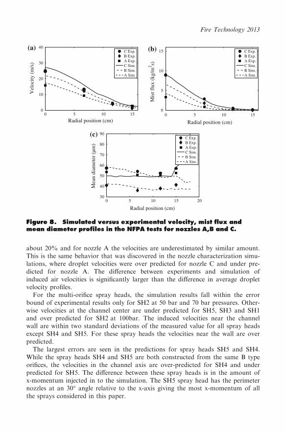
The comparison of the predicted and experimentally observed velocity, mist fluxand diameter profiles are shown in Figure 8. Velocity on the spray axis is underpredicted for nozzle B and over predicted for nozzle A. For nozzle C the velocitiesare over predicted throughout the spray.

The mist flux profiles in Figure 8 are over predicted for nozzle A, significantlyunder predicted for nozzle B and well matched for nozzle C. Further away fromthe spray center line, the discrepancy between the simulation and experimentdiminishes. It should be noted, however, that there is considerable measurementuncertainty associated with the experimental mist flux values.

Qualitatively the mist flux profiles are correct: There is a relatively thin densecore with a less dense outer spray as observed during experiments. On the sprayaxis, the mist flux is best predicted for nozzle C with only 1.2% error. For nozzlesA and B the errors are 52% and 28% respectively, with local mist fluxes over pre-dicted for nozzle A and under predicted for nozzle B.

The experimental data available was for the number median diameter, whileonly number mean was calculated from the simulations. The experimental data on

0 5 10 15 200

5

10

15

20

25

30

Radial position (cm)

Vel

ocity

(m

/s)

ExperimentΔ x = 1Δ x =2Δ x ≈ 4

(a)

0 5 10 15 200

2

4

6

8

10

Radial position (cm)

Mis

t flu

x (k

g/m

2 s)

ExperimentΔ x = 1Δ x =2Δ x ≈ 4

(b)

0 5 10 15

40

50

60

70

80

90

100

110

Radial position (cm)

d 10 (

µm)

ExperimentΔ x = 1Δ x =2Δ x ≈ 4

(c)

Figure 6. Nozzle B grid sensitivity.

Fire Technology 2013

diameter in Figure 8 is derived from the measured droplet CNFs at these points.The almost flat shape of the droplet size profiles is predicted for all the nozzles.For nozzles A and B, the mean diameter predictions are within 10% of the experi-mental value and within 11% for nozzle C.

5.5. Air Entrainment

Figure 9 shows snapshot of particle trajectories and the average velocity field atthe center of the channel. From the particle trajectories we can see that a consid-erable amount of the spray hits the walls of the channel. The average velocity fieldshows the effect of the block at the channel entrance on the flow as the flow is notsymmetrical at the channel entrance.

Comparisons of the air entrainment simulations to the experimental results areshown in Figure 10. The error bars correspond to two standard deviations of themeasured values. They do not account for the possible systematical errors in themeasurement.

Velocities on the center line of the channel are shown in Figure 10a for the multi-orifice spray head cases and in Figure 10c for the single orifice spray heads. Veloci-ties near the channel wall (for multi-orifice spray heads) are shown in Figure 10b.

Of the single-orifice nozzles, the entrainment for B nozzle is closest to the exper-imental value. For nozzle C the velocities in the channel are overestimated by

0 5 10 15 200

5

10

15

20

25

30

Radial position (cm)

Vel

ocity

(m

/s)

ExperimentBaseDrag reduction

(a)

0 5 10 15 200

2

4

6

8

10

12

Radial position (cm)

Mis

t flu

x (k

g/m

2 s)

ExperimentBaseDrag reduction

(b)

(c)

0 5 10 1540

50

60

70

80

90

Radial position (cm)

d 10 (

µm)

ExperimentBaseDrag reduction

Figure 7. Effect of three-way coupling on nozzle characterizationsimulations. Results for nozzle C.

High Pressure Water Mist Systems

about 20% and for nozzle A the velocities are underestimated by similar amount.This is the same behavior that was discovered in the nozzle characterization simu-lations, where droplet velocities were over predicted for nozzle C and under pre-dicted for nozzle A. The difference between experiments and simulation ofinduced air velocities is significantly larger than the difference in average dropletvelocity profiles.

For the multi-orifice spray heads, the simulation results fall within the errorbound of experimental results only for SH2 at 50 bar and 70 bar pressures. Other-wise velocities at the channel center are under predicted for SH5, SH3 and SH1and over predicted for SH2 at 100bar. The induced velocities near the channelwall are within two standard deviations of the measured value for all spray headsexcept SH4 and SH5. For these spray heads the velocities near the wall are overpredicted.

The largest errors are seen in the predictions for spray heads SH5 and SH4.While the spray heads SH4 and SH5 are both constructed from the same B typeorifices, the velocities in the channel axis are over-predicted for SH4 and underpredicted for SH5. The difference between these spray heads is in the amount ofx-momentum injected in to the simulation. The SH5 spray head has the perimeternozzles at an 30� angle relative to the x-axis giving the most x-momentum of allthe sprays considered in this paper.

0 5 10 150

10

20

30

40

Radial position (cm)

Vel

ocity

(m

/s)

C Exp.B Exp.A Exp.C Sim.B Sim.A Sim.

(a)

(c)

0 5 10 150

5

10

15

Radial position (cm)

Mis

t flu

x (k

g/m

2 s)

C Exp.B Exp.A Exp.C Sim.B Sim.A Sim.

(b)

0 5 10 15 2030

40

50

60

70

80

90

Radial position (cm)

Mea

n di

amet

er (

µm)

C Exp.B Exp.A Exp.C Sim.B Sim.A Sim.

Figure 8. Simulated versus experimental velocity, mist flux andmean diameter profiles in the NFPA tests for nozzles A,B and C.

Fire Technology 2013

Differences in the results for different spray heads may have to do with interac-tions of the spray jets. Parallel jets will be entrained in to a single jet after a dis-tance that depends on the jet boundary conditions. For spray heads SH1 and SH2the perimeter nozzles are at an 60� angle with the center nozzle. Therefore theinteraction between the perimeter jets and the central jet is weaker than for theother cases. Furthermore, for these two spray heads, a large portion of the sprayhits the channel walls. With lower perimeter nozzle angles, the spacing betweenthe jets diminishes and the interactions grow stronger. For spray head SH5 theinteraction of the spray jets is the strongest. The results for SH3, SH4 and SH5might be explained by wrong prediction of the aerodynamic interaction dynamicsof the individual spray-jets from the perimeter and center nozzles. However withthe available data, this hypothesis cannot be confirmed.

Resolving the individual spray jets was already found to be important whenconducting a sensitivity study for the large channel simulation cases. If a toosmall offset parameter was used, the spray jets would fuse into one jet andmomentum was lost from the simulation. This would also lead to some numericalartifacts like unphysical flow. Using fine enough grid to accurately describe, andmore importantly, discriminate between the individual jets is not enough to getthe entrainment predictions correct. This remains a topic that requires furtherexperimental and theoretical work.

Figure 9. Snapshots from the large channel simulations for sprayhead SH1. Picture on the top shows particle trajectories in the simula-tion. Also shown are the two gas velocity measurement points behindthe spray head. The picture on the bottom shows average gas velocityat the center of the channel.

High Pressure Water Mist Systems

6. Conclusions

Three single orifice and five multi-orifice spray heads were modeled with the FDSbased on flow-rate, spray angle, operating pressure and experimentally determined

50 60 70 80 90 100 110 120 1304

6

8

10

12

14

16

Pressure (bar)

Vel

ocity

(m

/s)

SH1 Sim.SH1 Exp.SH3 Sim.SH3 Exp.SH4 Sim.SH4 Exp.

(a)

50 60 70 80 90 100 110 120 1304

6

8

10

12

14

16

Pressure (bar)

Vel

ocity

(m

/s)

SH2 Sim.SH2 Exp.SH5 Sim.SH5 Exp.

(b)

50 60 70 80 90 100 110 120 1302

3

4

5

6

7

8

9

10

11

Pressure (bar)

Vel

ocity

(m

/s)

SH1 Sim.SH1 Exp.SH3 Sim.SH3 Exp.SH4 Sim.SH4 Exp.

(c)

50 60 70 80 90 100 110 120 1302

3

4

5

6

7

8

9

10

11

Pressure (bar)

Vel

ocity

(m

/s)

SH2 Sim.SH2 Exp.SH5 Sim.SH5 Exp.

(d)

40 50 60 70 80 90 100 1104

6

8

10

12

14

16

18

Pressure (bar)

Vel

ocity

(m

/s)

A SimA ExpB SimB ExpC SimC Exp

(e)

Figure 10. Average induced velocities in the air entrainment tests.a, b Results on the center line and c, d at the wall of the large chan-nel, respectively. e The results for the small channel tests. The pres-sures are exactly 50 bar, 70 bar or 100 bar in all cases.

Fire Technology 2013

particle size distribution. The observed flat droplet diameter distribution wasreproduced when the Dynamic Smagorinsky turbulence model was used. How-ever, the importance of the turbulent mixing of droplets on the effectiveness ofwater mist systems could not be determined. Three-way coupling effects werefound to be small. This suggests that droplet densities in individual water mistsprays under investigation are not high enough for droplet-droplet aerodynamicinteractions to be important.

The predictions of spray induced gas velocities inside the rectangular channelswere found to be within 30% of the experimental values. This indicates the accu-racy that can be expected from the simulations where the capability of the watermist to penetrate to the vicinity of fire and to mix the gas space are important.The dynamics of the spray were insensitive to the actual droplet size distributionor the number of particles used to describe the spray.

It was found that the numerical grid had a large effect on the simulation results.For multi-orifice spray heads it is important that each of the individual orificesdischarges within a different computational cell. This implies that the offsetparameter and grid resolution need to be selected so that there are separate sprayjets for each orifice. This is challenging to achieve if the perimeter angle of thespray nozzles is small. In addition, the number of Lagrangian particles used todescribe the spray needs to be sufficiently high. Larger the number particles usedto describe the spray, the smoother the predicted droplet density field is.

The numerical resolutions of the simulations in this paper can be unattainablein typical fire safety engineering applications. Further model development is nee-ded to facilitate simulation of large scale water mist systems. It should be notedhowever that the fine grids and high fidelity simulation is mostly needed in thenear field of nozzles. Further away from the nozzles, perhaps coarser grids wouldsuffice. The small scale validation tests considered here do not address this ques-tion.

7. Acknowledgments

The authors would like to thank Maria Putkiranta, Riina Rajala and Pentti Saa-renrinne from Tampere University of Technology for conducting the direct imag-ing experiments. Technical assistance was provided by Mr. Peter Gronberg, Mr.Ville Heikura, Mr. Toni Neitola and Mr. Veli-Pekka Vaari of VTT. The workwas sponsored by the Finnish Funding Agency for Technology and Innovation,Marioff Corporation Oy, Rautaruukki Oyj, YIT Kiinteistotekniikka Oy andInsinooritoimisto Markku Kauriala Ltd.

References

1. Deardorff JW (1972) Numerical investigation of neutral and unstable planetary bound-ary layers. J Atmos Sci 29:91–115. doi:10.1175/1520-0469(1972)029<0091:NIO-

NAU>2.0.CO;2

High Pressure Water Mist Systems

2. Ditch B, Yu HZ (2008) Water mist spray characterization and its proper applicationfor numerical simulations. Fire Saf Sci 9:541–552. doi:10.3801/IAFSS.FSS.9-541

3. Germano M, Piomelli U, Moin P, Cabot WH (1991) A dynamic subgrid-scale eddy vis-

cosity model. Phys Fluids A 3(7):1760–1765. doi:10.1063/1.8579554. Grant G, Brenton J, Drysdale D (2000) Fire suppression by water sprays. Prog Energy

Combust Sci 26(2):79–130. doi:10.1016/S0360-1285(99)00012-X5. Hart R (2006) Numerical modelling of tunnel fires and water mist suppression. PhD

thesis, University of Nottingham. http://etheses.nottingham.ac.uk/185/1/thesis.pdf6. Husted B (2007) Experimental measurements of water mist systems and implications

for modelling in CFD. PhD thesis, Lund University

7. Kennedy IM, Moody MH (1998) Particle dispersion in a turbulent round jet. Exp Ther-mal Fluid Sci 18(1):11–26. doi:10.1016/S0894-1777(98)10009-2

8. Kim SC, Ryou HS (2003) An experimental and numerical study on fire suppression

using a water mist in an enclosure. Build Environ 38(11):1309–1316. doi:10.1016/S0360-1323(03)00134-3

9. Kim SC, Ryou HS (2004) The effect of water mist on burning rates of pool fire. J FireSci 22(4):305–323. doi:10.1177/0734904104041796

10. McGrattan KB, Hostikka S, Floyd JE, Mell WE, McDermott R (2007) Fire dynamicssimulator, technical reference guide, vol 1: Mathematical model. NIST Special Publica-tion 1018, National Institute of Standards and Technology, Gaithersburg

11. Moin P, Squires K, Cabot W, Lee S (1991) A dynamic subgrid-scale model for com-pressible turbulence and scalar transport. Phys Fluids A 3(11):2746–2757. doi:10.1063/1.858164

12. Nmira F, Consalvi J, Kaiss A, Fernandezpello A, Porterie B (2009) A numerical studyof water mist mitigation of tunnel fires. Fire Saf J 44(2):198–211. doi:10.1016/j.firesaf.2008.06.002

13. Prahl L, Holzer A, Arlov D, Revstedt J, Sommerfeld M, Fuchs L (2007) On the inter-

action between two fixed spherical particles. Int J Multiph Flow 33(7):707–725. doi:10.1016/j.ijmultiphaseflow.2007.02.001

14. Prahl L, Jadoon A, Revstedt J (2009) Interaction between two spheres placed in tandem

arrangement in steady and pulsating flow. Int J Multiph Flow 35(10):963–969.doi:10.1016/j.ijmultiphaseflow.2009.05.001

15. Prasad K, Li C, Kailasanath K (1999) Simulation of water mist suppression of small

scale methanol liquid pool fires. Fire Saf J 33(3):185–212. doi:10.1016/S0379-7112(99)00028-4

16. Prasad K, Patnaik G, Kailasanath K (2002) A numerical study of water–mist suppres-sion of large scale compartment fires. Fire Saf J 37(6):569–589. doi:10.1016/S0379-

7112(02)00004-817. Ramırez-Munoz J, Soria A, Salinas-Rodrıguez E (2007) Hydrodynamic force on inter-

active spherical particles due to the wake effect. Int J Multiph Flow 33(7):802–807.

doi:10.1016/j.ijmultiphaseflow.2006.12.00918. Shimizu H, Tsuzuki M, Yamazaki Y, Koichi Hayashi A (2001) Experiments and

numerical simulation on methane flame quenching by water mist. J Loss Prev Process

Ind 14(6):603–608. doi:10.1016/S0950-4230(01)00055-919. Vaari J, Hostikka S, Sikanen T and Paajanen A (2012) Numerical simulations on the

performance of water-based fire suppression systems VTT TECHNOLOGY 54,http://www.vtt.fi/inf/pdf/technology/2012/T54.pdf. Accessed 12 Jan 2013

20. Vreman AW (2004) An Eddy-viscosity subgrid-scale model for turbulent shear flow:algebraic theory and applications. Physics of fluids, 16:3670. doi:10.1063/1.1785131

Fire Technology 2013