Embed Size (px)
Citation preview
Modeling Cations in a Contaminant Plume in Saturated Zone
A Thesis Presented
by
Qi Liu
to
The Graduate School
in Partial Fulfillment of the Requirements
for the Degree of
Master of Science
in
Earth and Space Sciences
State University of New York
at Stony Brook
August, 2005
i
State University of New York
At Stony Brook
The Graduate School
Qi Liu
We, the thesis committee for the above candidate for the Master of Science degree,
hereby recommend acceptance of this thesis.
_____________________________________ Dr. Gilbert N. Hanson, Advisor, Professor
Department of Geosciences
_____________________________________ Dr. Henry J. Bokuniewicz, Professor
Department of Marine Science
_____________________________________ Dr. Bruce J. Brownawell, Associate professor
Department of Marine Science
This thesis is accepted by the Graduate School
Dean of the Graduate School
ii
Abstract of the Thesis
Modeling Cations in a Contaminant Plume in Saturated Zone
by
Qi Liu
Master of Science
In
Earth and Space Sciences
State University of New York
At Stony Brook
2005
Contaminant plumes from different sources have different cation compositions
and corresponding concentrations. The cations in a plume are strongly sorbed on
sediments in saturated zone which will influence the rate of their transport dependent on
their valence states and atomic structure. We developed a multi-component interactive
model to simulate the sorption and transport of cations in a contaminant plume in
subsurface groundwater area using the MATLAB computer program.
High concentrations of nitrate in groundwater become more and more a concern
for geologists in Suffolk County and wastewater from septic tank-cesspool system and
turfgrass fertilizer are the two major sources of nitrate in this area. We applied our model
to predict the fate of cations accompany nitrate in contaminant plumes from wastewater
and turfgrass leachate. The results show that the cation chemistry of groundwater in
monitoring wells which are sampling close to the source of contamination is more
reliable in characterizing the source than the groundwater from public wells.
iii
Table of Contents
Abstract……………………………………….……………………………iii
List of Symbols…………………………………………………….……....vi
List of Figures…………………………………………………………….viii
List of Tables…………………………………………………………….....x
Chapter I: Introduction…………………………………………………....1
Chapter II: Theory………………………………………………………....4
2.1 Chemical Background…………..……………………………4
2.1.1 Cation exchange capacity------CEC…………………..5
2.1.2 Selectivity coefficients……………………….………...9
2.1.3 Rate of exchange reaction……………………………..9
2.1.4 Cation compositions and concentrations in
groundwater, on sediments and in contaminant plumes....10
2.2 Cations of Interest……….………….……………………….11
2.3 Chemical Equations…….………….………………..………11
Chapter III: Model………………………………………………………..15
3.1 Methodology………………………………………..………..15
3.2 Parameter Estimation………………………………………16
3.3 Results………………………………………..………………20
3.3.1 Major Cations……………………………….………...20
iv
3.3.2 NH4+……………………..……………………….…….21
3.3.3 Sr2+………………….……………………….….……...22
3.3.4 Discussions……………………….……………………25
3.4 Test…………………………………………………………..28
Chapter VI: Application to determination of nitrate sources…………32
Chapter V: Summary…………………………………………………….41
References………………………………………………………………....42
Appendix MATLAB program…………………………………………47
v
List of Symbols
1/i, 1/j, coefficients of components in chemical reaction;
[], symbol to show the concentration of the element or compound inside;
aI effective diameter of the ion
a, b, c convertible factor between KdNa and Kd
I according to the relation of KNa\I
A,B,C,D,E,F,G parameters in polynomial
AEC anion exchange capacity
C0I total concentration of element i in system;
CLI concentration of element I in liquid;
CSI concentration of element I on solid;
ΣCL0I, total concentration of cations in liquid at the initial state;
ΣCLeI, total concentration of cations in liquid at the equilibrated state;
ΣCS0I total concentration of cation sorbed on sediment at the initial
state;
ΣCSeI total concentration of cation sorbed on sediment at the
equilibrated stage
CEC cation exchange capacity
F, fraction of the liquid;
I ionic strength
Ii+ cation I in i+ valence state;
(mI/nI)f,0 initial isotope compositions of element I of the fluid
(mI/nI)s,0 initial isotope compositions of element I of the solid.
I-Xi, exchanger site hold by cation I, -Xi is surface function group with negative charge i;
KI/J, equilibrium coefficient for exchange reaction between Ii+and Jj+, also known as exchange coefficient for cation pairs I/J;
KdS/L, distribution coefficient for one element between solid and water;
M, N temperature dependent constants for Debye-Huckle equation
P porosity in volume fraction;
Ρ density in mass of cation per unit pore volume;
ρS density of solid ;
vi
ρL density of liquid;
pHPZC value of pH at the point of zero charge
RI retardation coefficient
S-OH surface Hydroxyl
S- OH2+ positively charge surface complex;
S-O- negatively charge surface complex;
subscripts L concentrations of component I in liquid
subscripts S concentrations of component I sorbed on the solid grains
zI charge of I ion
α activity
γ activity coefficient
vii
List of Figures
Figure 1: Ternary diagrams of the major cations and anions in groundwater
according to land use…………………………………………………….2
Figure 2. Transport and sorption of cations in a wastewater plume…………….6
Figure 3. Relationship between pH and pHPZC and their effects on CEC and
AEC……………………………………………………………………….8
Figure 4. Interface of my model…………………………………………………..17
Figure 5. CEC values of a core from Cathedral Pine County Park, Long
Island…………………………………………………………………….18
Figure 6. Cation chromatography of fluid after the introduction of a wastewater
plume……………………………………………………….20
Figure 7. NH42+ in turfgrass leachate and wastewater………………………..…23
Figure 8. Sr2+ in turfgrass leachate and wastewater……………….……………24
Figure 9. Sr2+ in the simulations of wastewater plume functioned as major
cation or as trace cation………………………………………………...25
Figure 10. The variation of major cations, Sr and isotopic ratio of 87Sr/86Sr in the
same wastewater plume.…………………………………..……………27
Figure 11. Comparison between experimental data and our modeling result….30
Figure 12. Simulation results based on different numbers of cells………………31
Figure 13. How contaminant sources influence drinking water in supply well...33
Figure 14. Water samples from different nitrate sources………………………..34
Figure 15. Mixing field of contaminant plumes and rainwater………………….35
Figure 16. The groundwater samples from monitoring wells…………..……….36
viii
Figure 17. The groundwater samples from public supply wells…………………37
Figure 18. The nitrate concentrations of groundwater samples from monitoring
wells……………………………………………………………………...39
Figure 19. The nitrate concentrations of groundwater samples from public
wells……………………………………………………………………...40
ix
List of Tables
Table 1. Published cation exchange capacity of different types of material…...6
Table 2. pHPZC of clay minerals and common soil matter………………………8
Table 3. Selectivity coefficients for K+, Mg2+ and Ca2+ based on the exchange
with Na+…………………………………………………………………..9
Table 4. Parameters for the Debye-Huckel equation…………………………..14
Table 5. Chemical concentrations of turfgrass leachate, wastewater and
rainwater………………………………………………………………...19
Table 6. Parameters in simulation of a contaminant plume…………………...19
Table 7. Properties of the soil column in cation transport experiment……….29
Table 8. Design of transport experiment-sequences of feed solutions………...29
x
Chapter I: INTRODUCTION
Groundwater is the only source for drinking water on Long Island outside of New
York City. So water quality control is one of the major concerns. Along with
development in Suffolk County, almost 70 percent of public water supply wells were
rated as high, or very high for susceptibility to nitrates. By the standard of Environmental
Protection Agency (EPA), if nitrogen as nitrate concentration is higher than 10 ppm, it
may induce the occurrence of blue baby syndrome, a disease causing infants deprived of
oxygen in blood.
The two main sources of nitrate in developed areas of Suffolk County are
wastewater from septic tank-cesspool system and turgrass fertilizer (Bleifuss, 1998;
Boguslavsky, 2000; Hanson & Schoonen, 2001). Our original purpose for this study is to
find a way to determine whether wastewater or turfgrass fertilizer is the major contributor
to the high nitrate level in Suffolk County groundwater.
A previous study on Long Island (Bleifuss, 1998) suggested that the major ion
chemistry of groundwater is affected by the land use of the recharge zone (Figure 1).
Groundwater recharged in residential and agricultural areas was found to have
distinct fields. Agricultural area produced a calcium-enriched water while residential area
produced water contained more sodium.
These results suggested that both cation chemistry and anion chemistry may be
used to distinguish the land use type of their source areas. I doubted the validity of this
conclusion because, as we know, anions are good tracers of groundwater, especially for
Cl, because they are conservative in saturated zone while cations are always useless due
1
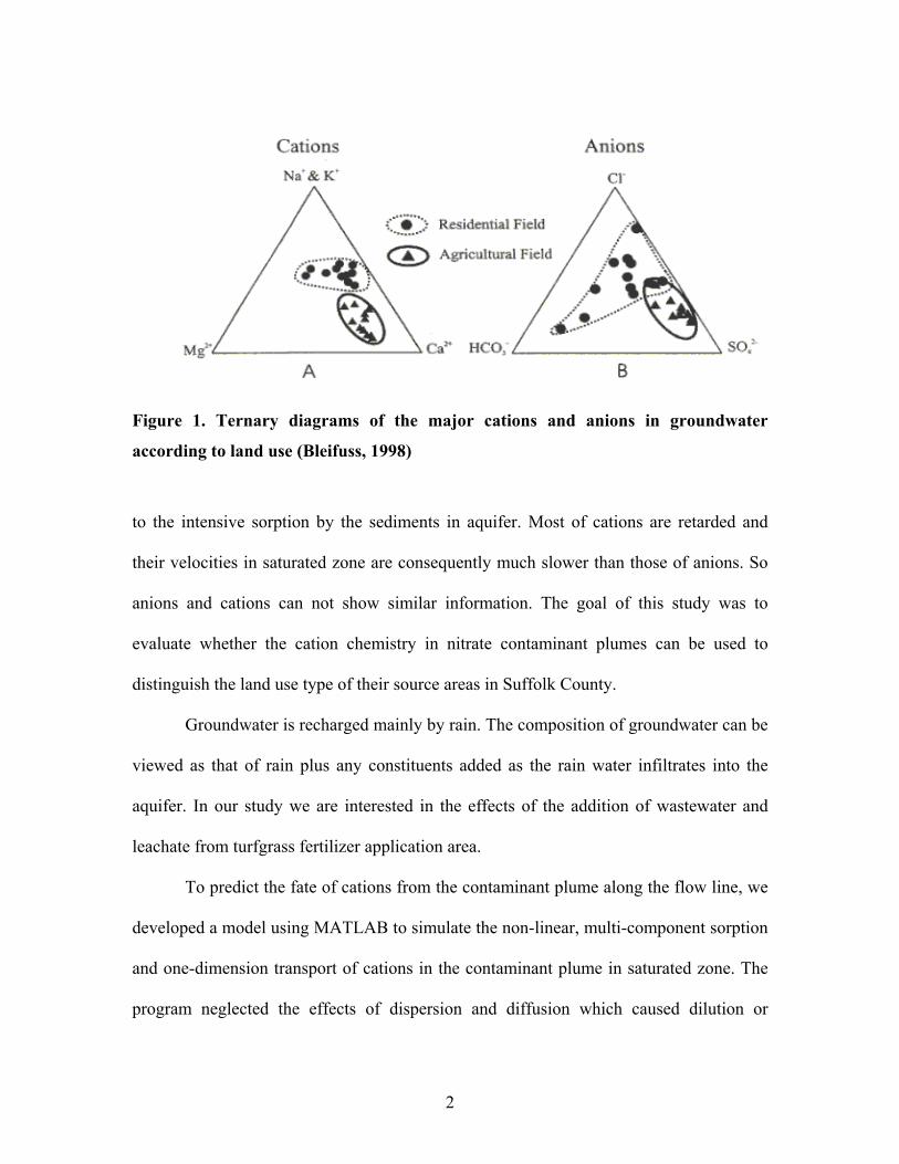
Figure 1. Ternary diagrams of the major cations and anions in groundwater
according to land use (Bleifuss, 1998)
to the intensive sorption by the sediments in aquifer. Most of cations are retarded and
their velocities in saturated zone are consequently much slower than those of anions. So
anions and cations can not show similar information. The goal of this study was to
evaluate whether the cation chemistry in nitrate contaminant plumes can be used to
distinguish the land use type of their source areas in Suffolk County.
Groundwater is recharged mainly by rain. The composition of groundwater can be
viewed as that of rain plus any constituents added as the rain water infiltrates into the
aquifer. In our study we are interested in the effects of the addition of wastewater and
leachate from turfgrass fertilizer application area.
To predict the fate of cations from the contaminant plume along the flow line, we
developed a model using MATLAB to simulate the non-linear, multi-component sorption
and one-dimension transport of cations in the contaminant plume in saturated zone. The
program neglected the effects of dispersion and diffusion which caused dilution or
2
mixing between rainwater and any contaminant plume, because groundwater collected
from the public supply well is a product of mixing between modified rainwater and the
contaminant plumes. The contaminant flow model is evaluated by comparison with
previous results from some soil column experiments (Voegelin, et al. 2000).
Before I created my own model, I considered popular software used in hydrology
to see if I could have used these existed tools, for instance, MODFLOW, MT3D and
RT3D. I found that none of them could simulate competitive sorption for multicomponent
with transport of the plume simultaneously.
3
Chapter II: THEORY
2.1 Chemical Background
During the movement of cations in a contaminant plume in saturated zone, the
plume will go with the groundwater in the same direction at the same speed. However,
owing to sorption effects, most cations in the plume are not transported at the same speed
as groundwater, which is called as retardation.
Sorption influences the transport of cations in the saturated zone. It involves mass
exchange between the plume and the sediment. There are two separate types of sorption:
if the cation is held primarily at the sediment surface, it is known as adsorption; or if the
cation is incorporated into the mineral structure, it is known as absorption. The process
in which a cation in solution replaces a sorbed cation is known as cation exchange.
In a groundwater system that has been stable for a significant period of time, the
cations in groundwater and those sorbed on sediments are in equilibrium. When the
contaminant plume enters the groundwater (figure 2), the plume displaces the
groundwater and the cations in the plume exchange with those sorbed on the sediments
(figure 3). In our model the flow line of the plume is assumed to be made up of multiple
sequential cells and the fluid volume filled in the vacancies of the whole flow line is
supposed to be one pore volume. The cells had the same unitless configuration. When the
solution enters a cell, cation exchange occurred between the contaminant plume and the
sediment. After reaction, the fluid from the first cell with a new composition will move
into the next cell and the cation exchange process is repeated until the fluid pass through
the whole pore volume. The plume and cells have no linear dimension, volume, or time
scale except those parameter described by pore volume, porosity, cation exchange
4
capacity and the composition of the cations sorbed on the sediments and in the modified
contaminant plume. When the water along the flow line all gains the composition of the
initial contaminant, the plume and sediments are in equilibrium and their compositions
will be stable.
To simulate the sorption process of multi-cations in a contaminant plume with
equilibrated sediments in groundwater, the following factors must be known:
a. Cation exchange capacity------CEC
b. Selectivity coefficients
c. Rate of exchange reaction
d. Cation composition and concentration of cations in groundwater, on sediments
and in contaminant plume
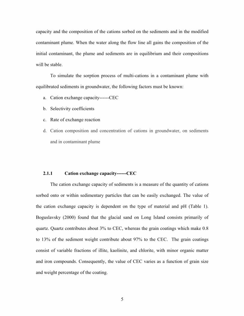
2.1.1 Cation exchange capacity------CEC
The cation exchange capacity of sediments is a measure of the quantity of cations
sorbed onto or within sedimentary particles that can be easily exchanged. The value of
the cation exchange capacity is dependent on the type of material and pH (Table 1).
Boguslavsky (2000) found that the glacial sand on Long Island consists primarily of
quartz. Quartz contributes about 3% to CEC, whereas the grain coatings which make 0.8
to 13% of the sediment weight contribute about 97% to the CEC. The grain coatings
consist of variable fractions of illite, kaolinite, and chlorite, with minor organic matter
and iron compounds. Consequently, the value of CEC varies as a function of grain size
and weight percentage of the coating.
5
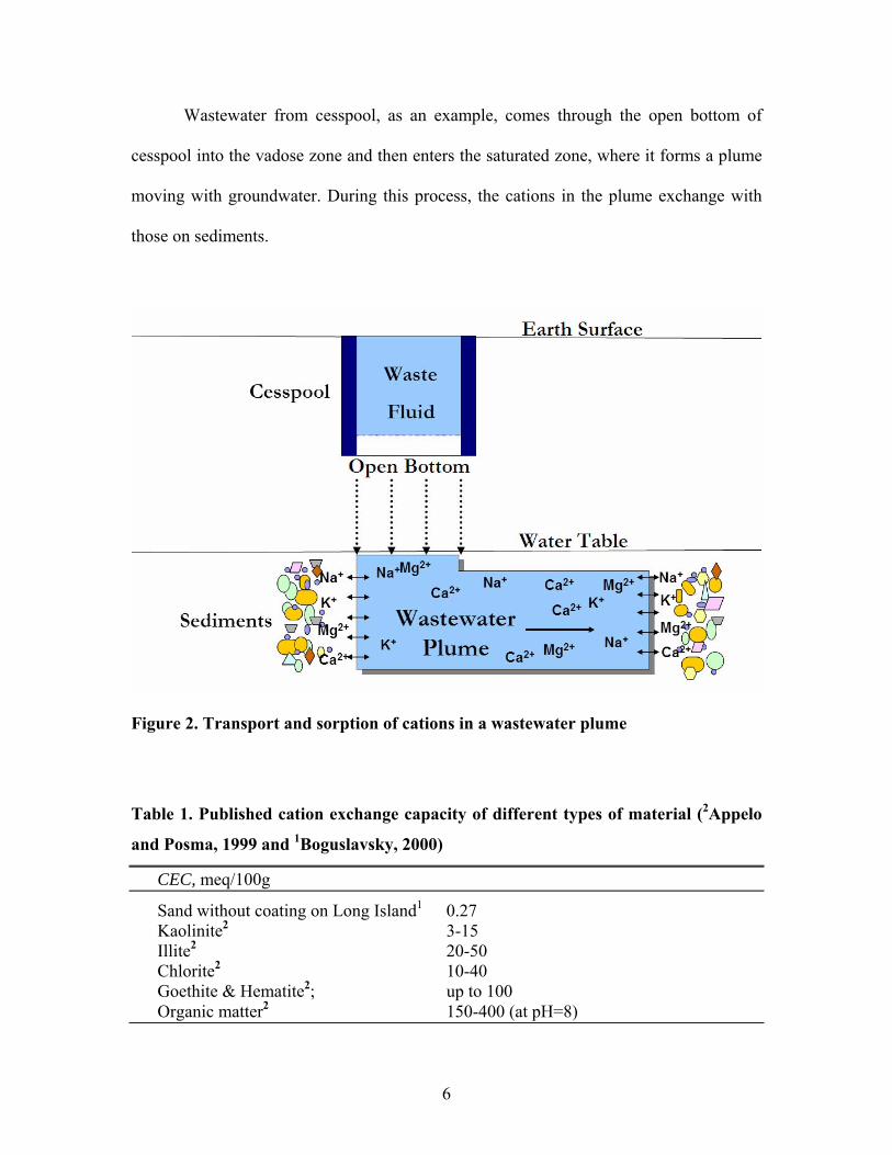
Wastewater from cesspool, as an example, comes through the open bottom of
cesspool into the vadose zone and then enters the saturated zone, where it forms a plume
moving with groundwater. During this process, the cations in the plume exchange with
those on sediments.
Figure 2. Transport and sorption of cations in a wastewater plume
Table 1. Published cation exchange capacity of different types of material (2Appelo
and Posma, 1999 and 1Boguslavsky, 2000)
CEC, meq/100g
Sand without coating on Long Island1 0.27 Kaolinite2 3-15 Illite2 20-50 Chlorite2 10-40 Goethite & Hematite2; up to 100 Organic matter2 150-400 (at pH=8)
6
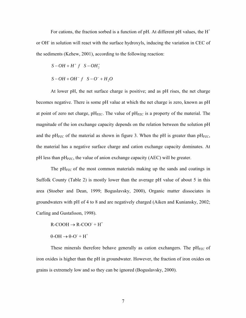
For cations, the fraction sorbed is a function of pH. At different pH values, the H+
or OH- in solution will react with the surface hydroxyls, inducing the variation in CEC of
the sediments (Kehew, 2001), according to the following reaction:
2S OH H S OH+ +− + −ƒ
2S OH OH S O H O− −− + − +ƒ
At lower pH, the net surface charge is positive; and as pH rises, the net charge
becomes negative. There is some pH value at which the net charge is zero, known as pH
at point of zero net charge, pHPZC. The value of pHPZC is a property of the material. The
magnitude of the ion exchange capacity depends on the relation between the solution pH
and the pHPZC of the material as shown in figure 3. When the pH is greater than pHPZC,
the material has a negative surface charge and cation exchange capacity dominates. At
pH less than pHPZC, the value of anion exchange capacity (AEC) will be greater.
The pHPZC of the most common materials making up the sands and coatings in
Suffolk County (Table 2) is mostly lower than the average pH value of about 5 in this
area (Stoeber and Dean, 1999; Boguslavsky, 2000), Organic matter dissociates in
groundwaters with pH of 4 to 8 and are negatively charged (Aiken and Kuniansky, 2002;
Carling and Gustafsson, 1998).
R-COOH → R-COO- + H+
θ-OH → θ-O- + H+
These minerals therefore behave generally as cation exchangers. The pHPZC of
iron oxides is higher than the pH in groundwater. However, the fraction of iron oxides on
grains is extremely low and so they can be ignored (Boguslavsky, 2000).
7
-1 .2
-0 .7
-0 .2
0 .3
0 .8
7 9 11 13 15 1 7 1 9 21 23
ion
exch
ange
cap
acity AEC
CEC
More Basic
More acidic pHPZC
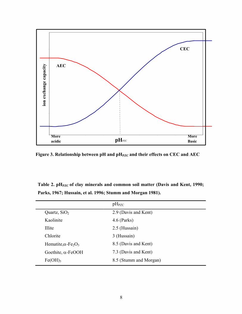
Figure 3. Relationship between pH and pHPZC and their effects on CEC and AEC
Table 2. pHPZC of clay minerals and common soil matter (Davis and Kent, 1990;
Parks, 1967; Hussain, et al. 1996; Stumm and Morgan 1981).
pHPZC
Quartz, SiO2 2.9 (Davis and Kent)
Kaolinite 4.6 (Parks)
Illite 2.5 (Hussain)
Chlorite 3 (Hussain)
Hematite,α-Fe2O3 8.5 (Davis and Kent)
Goethite, α-FeOOH 7.3 (Davis and Kent)
Fe(OH)3 8.5 (Stumm and Morgan)
8
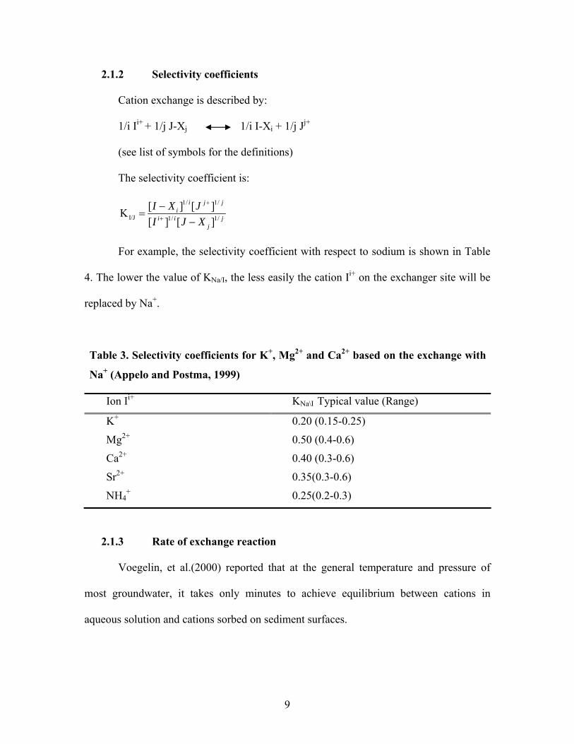
2.1.2 Selectivity coefficients
Cation exchange is described by:
1/i Ii+ + 1/j J-Xj 1/i I-Xi + 1/j Jj+
(see list of symbols for the definitions)
The selectivity coefficient is:
1/ 1/
I/J 1/ 1/
[ ] [ ]K[ ] [ ]
i j ji
i i jj
I X JI J X
+
+
−=
−
For example, the selectivity coefficient with respect to sodium is shown in Table
4. The lower the value of KNa/I, the less easily the cation Ii+ on the exchanger site will be
replaced by Na+.
Table 3. Selectivity coefficients for K+, Mg2+ and Ca2+ based on the exchange with
Na+ (Appelo and Postma, 1999)
Ion Ii+ KNa\I Typical value (Range)
K+ 0.20 (0.15-0.25)
Mg2+ 0.50 (0.4-0.6)
Ca2+ 0.40 (0.3-0.6)
Sr2+ 0.35(0.3-0.6)
NH4+ 0.25(0.2-0.3)
2.1.3 Rate of exchange reaction
Voegelin, et al.(2000) reported that at the general temperature and pressure of
most groundwater, it takes only minutes to achieve equilibrium between cations in
aqueous solution and cations sorbed on sediment surfaces.
9
2.1.4 Cation compositions and concentrations in groundwater, on sediments
and in contaminant plume
During the passage of the contaminant plume through the aquifer, I assumed that
the CEC value of sediment did not change either with time or along the flow line. The
proportion of CEC, however, was allowed to vary both in time and space for each cation.
In a plume containing a variety of inorganic metal cations, interactive competition was
allowed between them for the available charged sites on sediments. Ionic potential, i.e.
the charge of a cation over its ionic radius was one of the most significant factors that
determined the affinity of a particular cation to the soil surface. The relative ionic
potentials of major cations in a contaminant plume is Na+ < NH4+< K+ < Mg2+ <
Ca2+<Sr2+, reflecting preferential sorption sequence.
The cations in a contaminant plume changed along the flow line due to sorption.
Before the contaminant plume enters the aquifer, the cations it carries exchange with
those on sediments and eventually come to equilibrium. So in fact, the composition of
cations in groundwater determines the proportion of CEC for the cations on the sediment.
When the contaminant plume enters the aquifer, the composition of cations in plume is
different from that in groundwater, so the former equilibrium is destroyed and the
charged sites on sediment will be redistributed. After new equilibrium is established, the
proportion of CEC for the cations on the sediment will reflect the composition of cations
in the plume this time. However, because the number of charged sites on given sediments
is fixed, the total equivalent concentration of cations sorbed on the sediment and those in
the plume will not change.
10
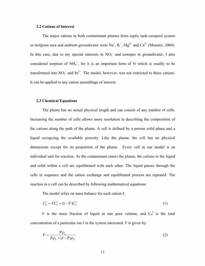
2.2 Cations of Interest
The major cations in both contaminant plumes from septic tank-cesspool system
or turfgrass area and ambient groundwater were Na+, K+, Mg2+ and Ca2+ (Munster, 2004).
In this case, due to my special interests in NO3- and isotopes in groundwater, I also
considered sorption of NH4+, for it is an important form of N which is readily to be
transformed into NO3- and Sr2+. The model, however, was not restricted to these cations.
It can be applied to any cation assemblage of interest.
2.3 Chemical Equations
The plume has no actual physical length and can consist of any number of cells.
Increasing the number of cells allows more resolution in describing the composition of
the cations along the path of the plume. A cell is defined by a porous solid phase and a
liquid occupying the available porosity. Like the plume, the cell has no physical
dimensions except for its proportion of the plume. Every cell in our model is an
individual unit for reaction. As the contaminant enters the plume, the cations in the liquid
and solid within a cell are equilibrated with each other. The liquid passes through the
cells in sequence and the cation exchange and equilibrated process are repeated. The
reaction in a cell can be described by following mathematical equations:
The model relies on mass balance for each cation I;
0 (1 )I I IL SC FC F C= + − (1)
F is the mass fraction of liquid in one pore volume, and C0I is the total
concentration of a particular ion I in the system interested. F is given by:
(1 )L
L S
PFP P
ρρ ρ
=+ −
(2)
11
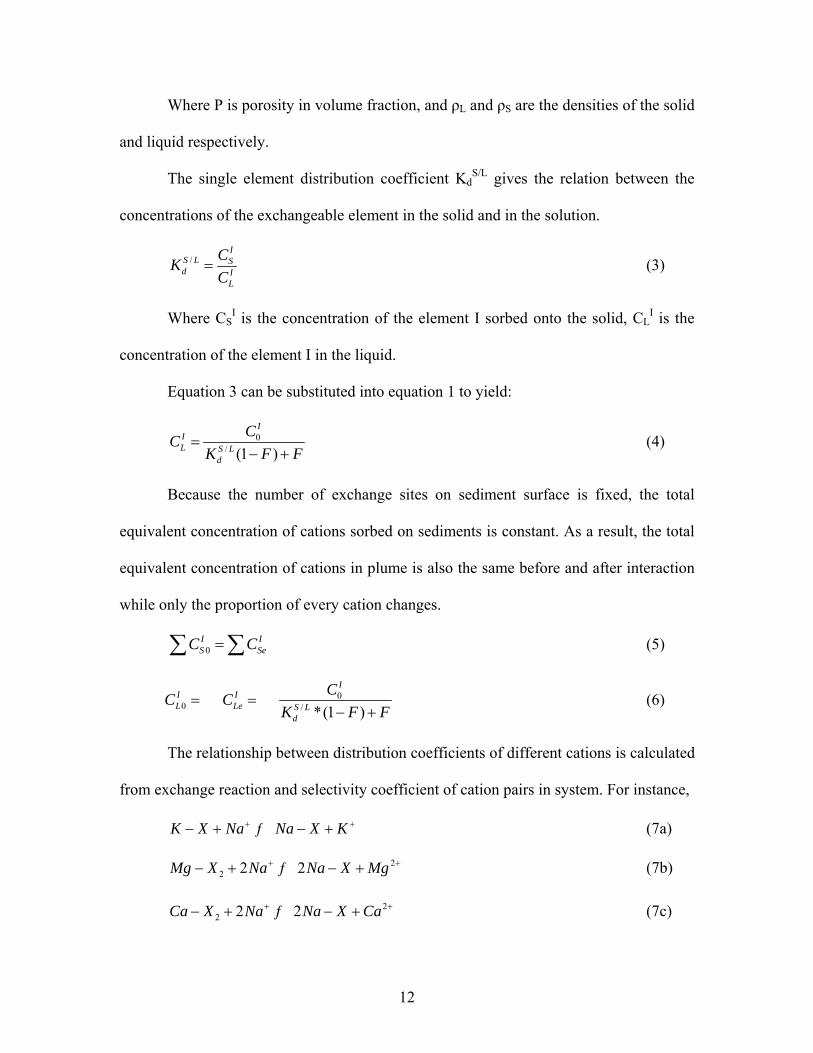
Where P is porosity in volume fraction, and ρL and ρS are the densities of the solid
and liquid respectively.
The single element distribution coefficient KdS/L gives the relation between the
concentrations of the exchangeable element in the solid and in the solution.
/I
S L Sd I
L
CKC
= (3)
Where CSI is the concentration of the element I sorbed onto the solid, CL
I is the
concentration of the element I in the liquid.
Equation 3 can be substituted into equation 1 to yield:
0/ (1 )
IIL S L
d
CCK F
=− + F
ISeC
(4)
Because the number of exchange sites on sediment surface is fixed, the total
equivalent concentration of cations sorbed on sediments is constant. As a result, the total
equivalent concentration of cations in plume is also the same before and after interaction
while only the proportion of every cation changes.
0ISC =∑ ∑ (5)
00 / *(1 )
II IL Le S L
d
CC CK F
= =F− +
(6)
The relationship between distribution coefficients of different cations is calculated
from exchange reaction and selectivity coefficient of cation pairs in system. For instance,
K X Na Na X K+− + − +ƒ + (7a)
22 2 2Mg X Na Na X Mg+− + − +ƒ +
+
(7b)
22 2 2Ca X Na Na X Ca+− + − +ƒ (7c)
12
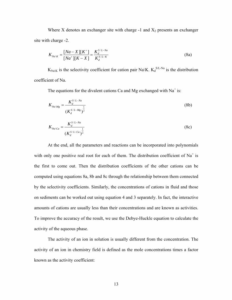
Where X denotes an exchanger site with charge -1 and X2 presents an exchanger
site with charge -2.
/
\ /
[ ][ ][ ][ ]
S L Nad
Na K S L Kd
KNa X KKNa K X K
−+
+
−= =
− − (8a)
KNa\K is the selectivity coefficient for cation pair Na\K. KdS/L-Na is the distribution
coefficient of Na.
The equations for the divalent cations Ca and Mg exchanged with Na+ is:
/
\ 1/ 2( )
S L Nad
Na MgS L Mgd
KKK
−
−
= (8b)
/
\ 1/ 2( )
S L Nad
Na CaS L Cad
KKK
−
−
= (8c)
At the end, all the parameters and reactions can be incorporated into polynomials
with only one positive real root for each of them. The distribution coefficient of Na+ is
the first to come out. Then the distribution coefficients of the other cations can be
computed using equations 8a, 8b and 8c through the relationship between them connected
by the selectivity coefficients. Similarly, the concentrations of cations in fluid and those
on sediments can be worked out using equation 4 and 3 separately. In fact, the interactive
amounts of cations are usually less than their concentrations and are known as activities.
To improve the accuracy of the result, we use the Debye-Huckle equation to calculate the
activity of the aqueous phase.
The activity of an ion in solution is usually different from the concentration. The
activity of an ion in chemistry field is defined as the mole concentrations times a factor
known as the activity coefficient:
13
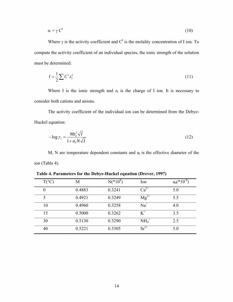
α = γ CI (10)
Where γ is the activity coefficient and CI is the molality concentration of I ion. To
compute the activity coefficient of an individual species, the ionic strength of the solution
must be determined:
212
III C z= ∑ (11)
Where I is the ionic strength and zI is the charge of I ion. It is necessary to
consider both cations and anions.
The activity coefficient of the individual ion can be determined from the Debye-
Huckel equation:
2
log1
II
I
Mz Ia N I
γ− =+
(12)
M, N are temperature dependent constants and aI is the effective diameter of the
ion (Table 4).
Table 4. Parameters for the Debye-Huckel equation (Drever, 1997)
T(°C) M N(*108) Ion a0(*10-8)
0 0.4883 0.3241 Ca2+ 5.0
5 0.4921 0.3249 Mg2+ 5.5
10 0.4960 0.3258 Na+ 4.0
15 0.5000 0.3262 K+ 3.5
30 0.5130 0.3290 NH4+ 2.5
40 0.5221 0.3305 Sr2+ 5.0
14
Chapter III: MODEL
3.1 Methodology
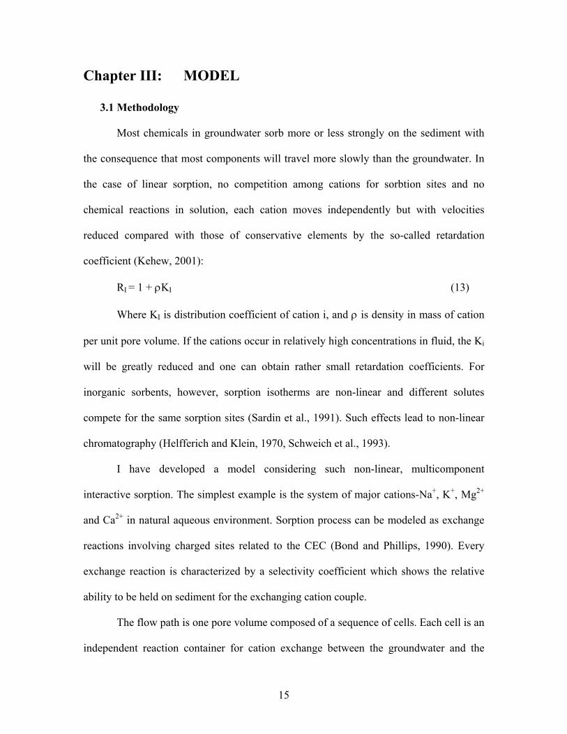
Most chemicals in groundwater sorb more or less strongly on the sediment with
the consequence that most components will travel more slowly than the groundwater. In
the case of linear sorption, no competition among cations for sorbtion sites and no
chemical reactions in solution, each cation moves independently but with velocities
reduced compared with those of conservative elements by the so-called retardation
coefficient (Kehew, 2001):
RI = 1 + ρKI (13)
Where KI is distribution coefficient of cation i, and ρ is density in mass of cation
per unit pore volume. If the cations occur in relatively high concentrations in fluid, the Ki
will be greatly reduced and one can obtain rather small retardation coefficients. For
inorganic sorbents, however, sorption isotherms are non-linear and different solutes
compete for the same sorption sites (Sardin et al., 1991). Such effects lead to non-linear
chromatography (Helfferich and Klein, 1970, Schweich et al., 1993).
I have developed a model considering such non-linear, multicomponent
interactive sorption. The simplest example is the system of major cations-Na+, K+, Mg2+
and Ca2+ in natural aqueous environment. Sorption process can be modeled as exchange
reactions involving charged sites related to the CEC (Bond and Phillips, 1990). Every
exchange reaction is characterized by a selectivity coefficient which shows the relative
ability to be held on sediment for the exchanging cation couple.
The flow path is one pore volume composed of a sequence of cells. Each cell is an
independent reaction container for cation exchange between the groundwater and the
15
sediments inside the cell. Every time fluid enters the cell and fills the pore space, the
cations in the fluid react with those on sediment. They equilibrate with each other and the
cation composition on the sediment and in the solution change but the total equivalent
cation concentration on soil (CEC) or that in the solution remain the same. Subsequently,
the packets of fluid with new cation composition continuously enter, equilibrate and exit
each cell sequentially until they come to the end of the flow path. The flow is continuous.
The volume of fluid that has passed through the whole flow line is considered as one pore
volume. Eventually the fluid that reaches the end of the flow path will have the
composition of the original contaminant fluid and the sediment throughout the column
will be in equilibrium with the original contaminant fluid. The number of pore volumes
required to reach this equilibrium will be a function of the concentration and composition
of the cations in the contaminated plumes, the CEC and the porosity of the sediment.
The computational model was developed using MATLAB (Appendix 1). The
interface of the program is presented in figure 4.
3.2 Parameter Estimation
Cation exchange capacity, selectivity coefficient and concentrations in
contaminant plumes and groundwater for Suffolk County need to be specified.
CEC of the sediments in Suffolk County is from Boguslavsky (2000) (figure 5).
The CEC data in figure 5 are in fact the values for vadose zone well below the soil
horizon. The soil horizon itself has a much higher CEC and contains high proportion of
aluminum, but it is assumed that the CEC will be similar to that of the sediments in
saturated zone. I selected a median value for CEC of 1 meq/100g.
16
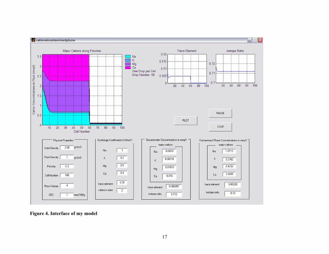
Figure 4. Interface of my model
17
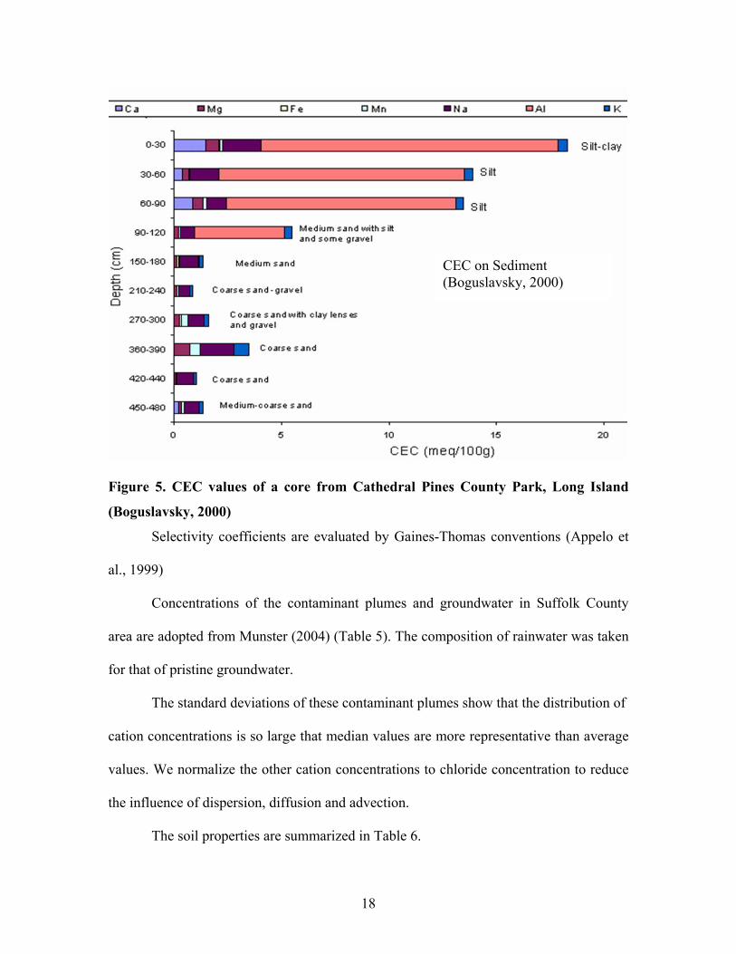
CEC on Sediment (Boguslavsky, 2000)
Figure 5. CEC values of a core from Cathedral Pines County Park, Long Island
(Boguslavsky, 2000)
Selectivity coefficients are evaluated by Gaines-Thomas conventions (Appelo et
al., 1999)
Concentrations of the contaminant plumes and groundwater in Suffolk County
area are adopted from Munster (2004) (Table 5). The composition of rainwater was taken
for that of pristine groundwater.
The standard deviations of these contaminant plumes show that the distribution of
cation concentrations is so large that median values are more representative than average
values. We normalize the other cation concentrations to chloride concentration to reduce
the influence of dispersion, diffusion and advection.
The soil properties are summarized in Table 6.
18
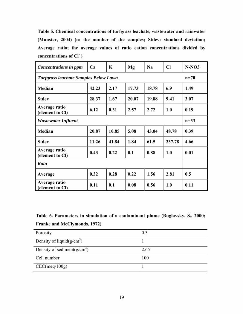
Table 5. Chemical concentrations of turfgrass leachate, wastewater and rainwater
(Munster, 2004) (n: the number of the samples; Stdev: standard deviation;
Average ratio; the average values of ratio cation concentrations divided by
concentrations of Cl- )
Concentrations in ppm Ca K Mg Na Cl N-NO3
Turfgrass leachate Samples Below Lawn n=70
Median 42.23 2.17 17.73 18.78 6.9 1.49
Stdev 28.37 1.67 20.07 19.88 9.41 3.07
Average ratio (element to Cl) 6.12 0.31 2.57 2.72 1.0 0.19
Wastewater Influent n=33
Median 20.87 10.85 5.08 43.04 48.78 0.39
Stdev 11.26 41.84 1.84 61.5 237.78 4.66
Average ratio (element to Cl) 0.43 0.22 0.1 0.88 1.0 0.01
Rain
Average 0.32 0.28 0.22 1.56 2.81 0.5
Average ratio (element to Cl) 0.11 0.1 0.08 0.56 1.0 0.11
Table 6. Parameters in simulation of a contaminant plume (Buglavsky, S., 2000;
Franke and McClymonds, 1972)
Porosity 0.3
Density of liquid(g/cm3) 1
Density of sediment(g/cm3) 2.65
Cell number 100
CEC(meq/100g) 1
19
3.3 Results
3.3.1 Major Cations
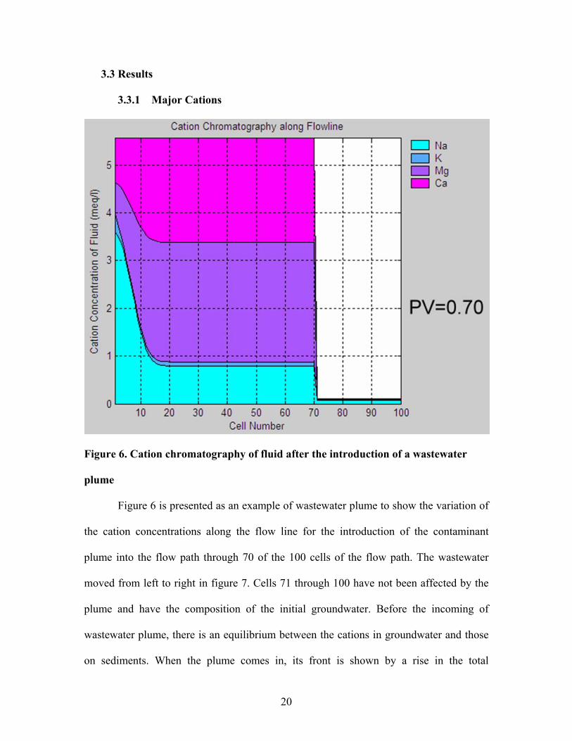
Figure 6. Cation chromatography of fluid after the introduction of a wastewater
plume
Figure 6 is presented as an example of wastewater plume to show the variation of
the cation concentrations along the flow line for the introduction of the contaminant
plume into the flow path through 70 of the 100 cells of the flow path. The wastewater
moved from left to right in figure 7. Cells 71 through 100 have not been affected by the
plume and have the composition of the initial groundwater. Before the incoming of
wastewater plume, there is an equilibrium between the cations in groundwater and those
on sediments. When the plume comes in, its front is shown by a rise in the total
20
equivalent concentration of cations to the same as that of the plume. However, the
proportion of the cations at this stage was determined by sediments instead of
wastewater. This is because sediments have a large reservoir of cations. As a result, the
fractions of cations on sediments do not change for a while but the distribution
coefficients vary correspondingly. Higher the CEC value is, larger the reservoir is.
Eventually the cations in the contaminant plume will equilibrate with the
sediments and the cation concentrations and compositions in the plume will be the same
as the initial contaminant. In this simulation, the wastewater plume needed about 130
pore volumes to come to equilibrium and the turfgrass leachate plume requires about 70
pore volumes.
Based on the number of pore volumes needed to achieve equilibrium and the rate
of groundwater flow, we can estimate the travel time of the contaminant plume. For
example, if the distance between a contaminant source and a supply well is 100 meters in
average, which is supposed as the length of the flow line, and the rate of the groundwater
flow is 30 centimeters per day. The contaminant plume will pass through 1.1 pore volume
per year. Then it will take 143 years for wastewater and 66 years for turfgrass leachate
reaching the supply well to have the composition of the original contaminant plume.
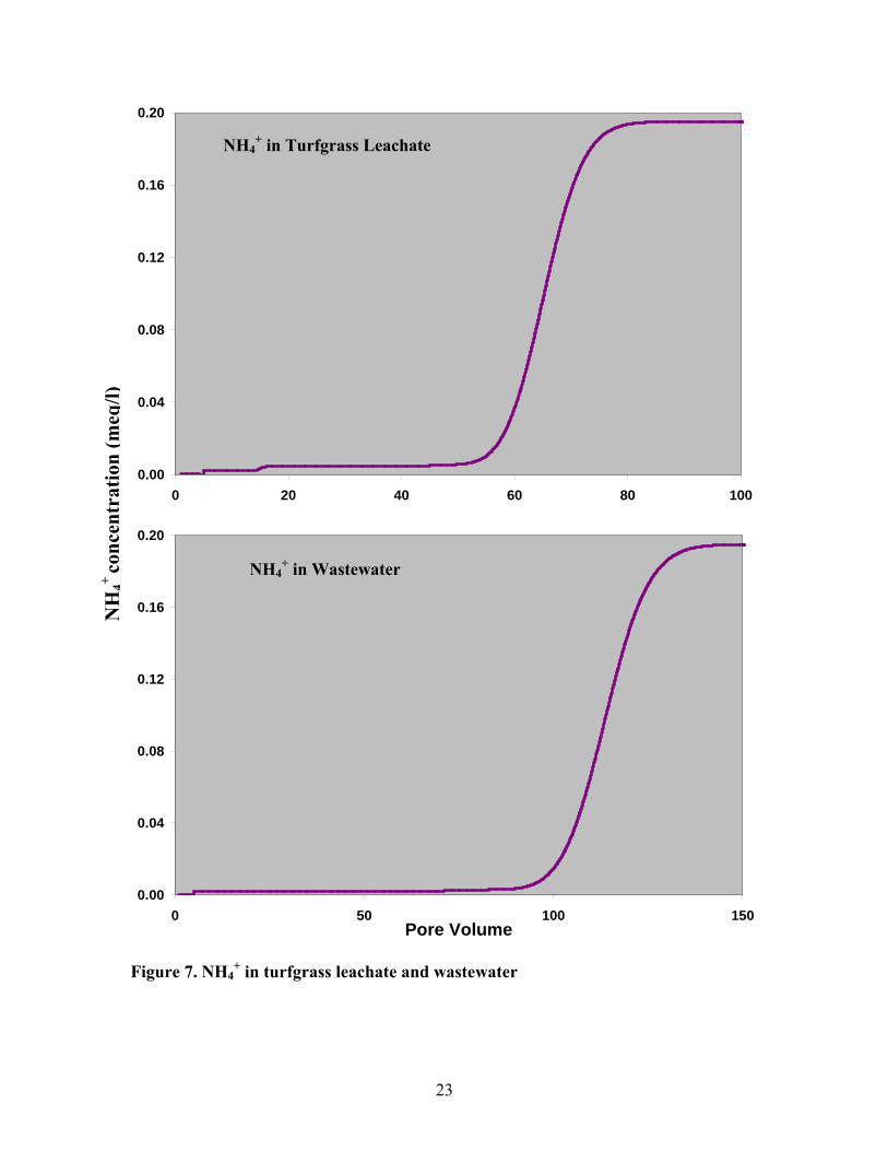
3.3.2 Ammonium – NH4+
We should not concern ourselves only with NO3+, but also with ammonium which
also accompanies a contaminant plume. Because ammonium is not only an important
component of fertilizer used in Long Island (Perlmutter and Koch, 1972), but also a
cation that is strongly sorbed on the sediment and can be converted into NO3- under
21
aerobic conditions. The variation of NH4+ in contaminant plumes of wastewater and
turfgrass leachate were presented in figure 7. The only difference between the two curves
was their equilibrated number of pore volumes.
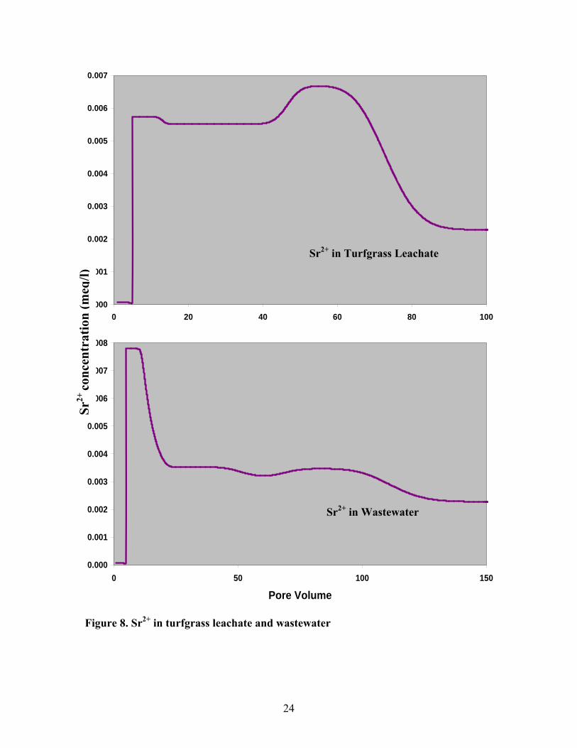
3.3.3 Strontium - Sr
Sr isotopes are commonly used in hydrogeology to distinguish different sources
(Wickman et al., 1987; Aberg et al., 1987) and quantifying the input and distribution of
Sr by using Sr isotopic composition as a tracer (Aberg et al., 1989; Graustein, 1989; Geng,
1993).
The Sr2+ in contaminant plumes of wastewater and turfgrass leachate are
presented in figure 8.
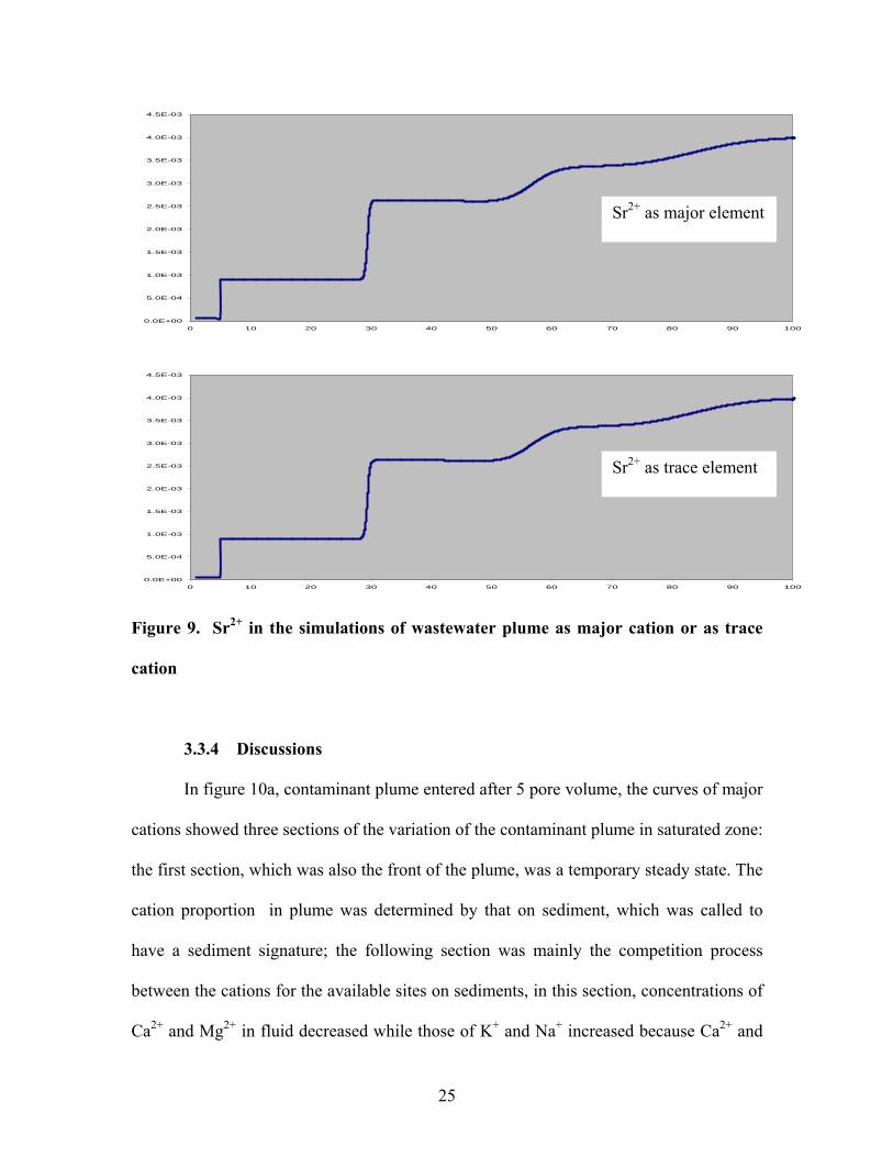
The concentrations of Strontium are 100 ppb in contaminant plumes and 5 ppb in
groundwater (Geng, 1993). Strontium should be a trace element on Long Island. As a
result, it is possible to model it independently of other major elements because its
abundance is too low to affect the concentration of the other cations either on sediments
or in fluid (Hanson & Langmuir, 1978). To test whether Sr can be treated as a trace
element, I modeled Sr2+ as a major element allowing it to exchange with the other major
cations together, and also as a trace element which varies independent of the abundance
of the other cations. The chromatography curves for the two approaches show the same
results (figure 9).
22
0.00
0.04
0.08
0.12
0.16
0.20
0 20 40 60 80
NH4+ in Turfgrass Leachate
NH
4+ co
ncen
trat
ion
(meq
/l)
100
0.00
0.04
0.08
0.12
0.16
0.20
0 50 100 150Pore Volume
NH4+ in Wastewater
Figure 7. NH4+ in turfgrass leachate and wastewater
23
0
0
.000
.001
0.002
0.003
0.004
0.005
0.006
0.007
0 20 40 60 80 100
Sr2+ in Turfgrass Leachate
0.000
0.001
0.002
0.003
0.004
0.005
0.006
0.007
0.008
0 50 100 150
Pore Volume
Sr2+
conc
entr
atio
n (m
eq/l)
Sr2+ in Wastewater
Figure 8. Sr2+ in turfgrass leachate and wastewater
24
0.0E+00
5.0E-04
1.0E-03
1.5E-03
2.0E-03
2.5E-03
3.0E-03
3.5E-03
4.0E-03
4.5E-03
0 10 20 30 40 50 60 70 80 90 10
Sr2+ as major element
0
0.0E+00
5.0E-04
1.0E-03
1.5E-03
2.0E-03
2.5E-03
3.0E-03
3.5E-03
4.0E-03
4.5E-03
0 10 20 30 40 50 60 70 80 90 10
Sr2+ as trace element
0
Figure 9. Sr2+ in the simulations of wastewater plume as major cation or as trace
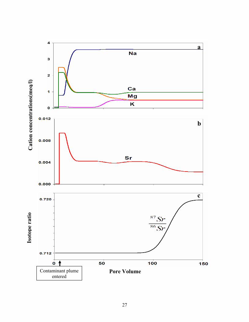
cation
3.3.4 Discussions
In figure 10a, contaminant plume entered after 5 pore volume, the curves of major
cations showed three sections of the variation of the contaminant plume in saturated zone:
the first section, which was also the front of the plume, was a temporary steady state. The
cation proportion in plume was determined by that on sediment, which was called to
have a sediment signature; the following section was mainly the competition process
between the cations for the available sites on sediments, in this section, concentrations of
Ca2+ and Mg2+ in fluid decreased while those of K+ and Na+ increased because Ca2+ and
25
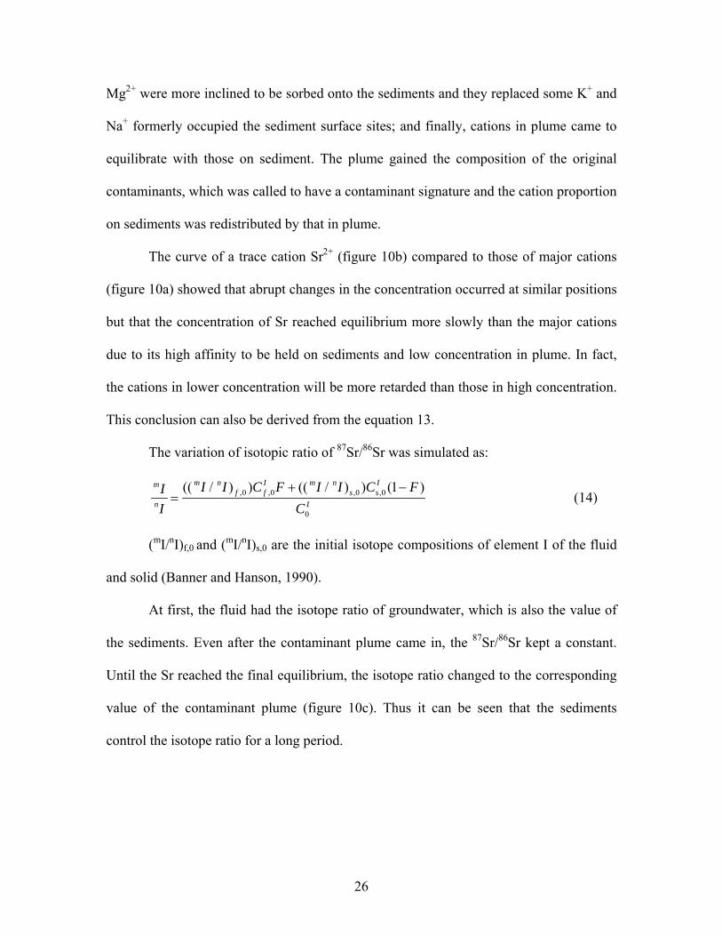
Mg2+ were more inclined to be sorbed onto the sediments and they replaced some K+ and
Na+ formerly occupied the sediment surface sites; and finally, cations in plume came to
equilibrate with those on sediment. The plume gained the composition of the original
contaminants, which was called to have a contaminant signature and the cation proportion
on sediments was redistributed by that in plume.
The curve of a trace cation Sr2+ (figure 10b) compared to those of major cations
(figure 10a) showed that abrupt changes in the concentration occurred at similar positions
but that the concentration of Sr reached equilibrium more slowly than the major cations
due to its high affinity to be held on sediments and low concentration in plume. In fact,
the cations in lower concentration will be more retarded than those in high concentration.
This conclusion can also be derived from the equation 13.
The variation of isotopic ratio of 87Sr/86Sr was simulated as:
,0 ,0 ,0 ,0
0
(( / ) ) (( / ) ) (1 )m n I m n Imf f s s
n I
I I C F I I C FII C
+ −= (14)
(mI/nI)f,0 and (mI/nI)s,0 are the initial isotope compositions of element I of the fluid
and solid (Banner and Hanson, 1990).
At first, the fluid had the isotope ratio of groundwater, which is also the value of
the sediments. Even after the contaminant plume came in, the 87Sr/86Sr kept a constant.
Until the Sr reached the final equilibrium, the isotope ratio changed to the corresponding
value of the contaminant plume (figure 10c). Thus it can be seen that the sediments
control the isotope ratio for a long period.
26
a
Cat
ion
conc
entr
atio
ns(m
eq/l)
b
c
Isot
ope
ratio
Contaminant plume
entered Pore Volume
27
Figure 10. The variation of major cations, Sr and isotopic ratio of 87Sr/86Sr in the
same wastewater plume: a. major cations; b. Sr; c. 87Sr/86Sr
3.4 Test
To testify my model, I applied it to experimental data involving cation exchange
and transport processes (Voegelin, et al., 2000). The experiments had been conducted
with a ternary cation system (Ca-Mg-Na) using a packed soil column (Table 7). The
column packed with dry soil was connected to a HPLC pump and pre-conditioned by
leaching with several hundred pore volumes of 0.5M CaCl2 solution adjusted to pH 4.6.
The HPLC pump was used to control the influent velocity. Different influent solutions
were passed through the column until each had come to equilibrium with the soil particles.
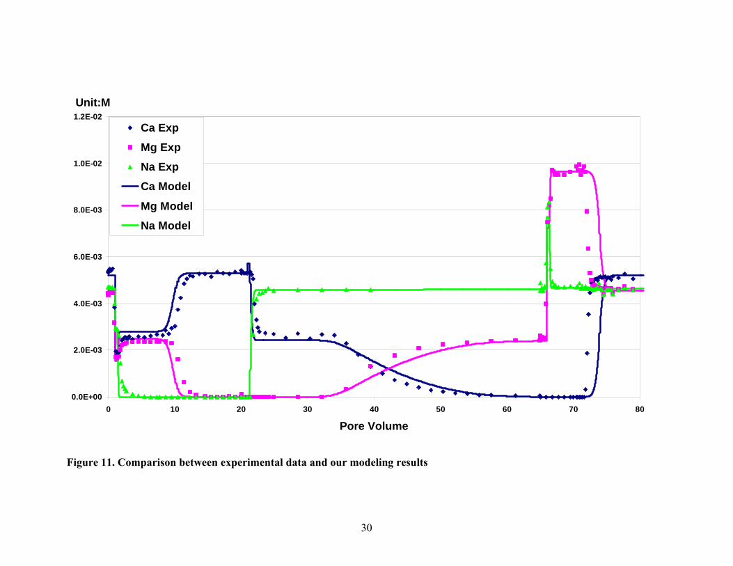
The sequence of influent solutions was given in Table 8. The comparison between
modeling result and experimental data was presented in figure 11. The points represented
the experimental data. The lines were the results of our simulation. The modeling results
showed good approximation to the experimental points.
For Na+, there was a perfect match between modeling and the experimental results
because the activity coefficient was always near one. But for divalent catoins Ca2+ and
Mg2+, the difference between model and experimental data is noticeable because the
activity coefficients were much less than one and varied according to the cation
concentrations and their interactive reactions and they probably cannot be approximated
as well as that for Na+. Whatever, the maximum difference was still within two pore
volume.
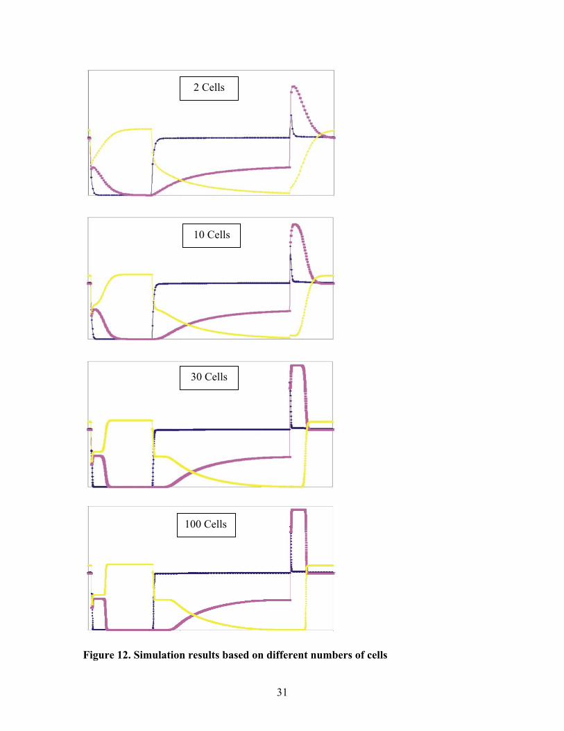
The numbers of cells describing a plume determined the resolution. Simulations
of the experimental study for 2, 5, 30 and 100 cells were shown in figure 12. To a first
approximation, the results were similar. When the cell number was small, the shapes
28
were rounded because the reduction of sharp fraction was poor. However, once the cell
number exceeded about 30 cells, the shapes and positions of the curves showed little or
no visible difference with an increase in the number of cells.
Table 7. Properties of the soil column in cation transport experiment
Diameter(cm) 0.66
Length(cm) 19.1
Volume(ml) 6.53
Mass of soil(g) 7.47
Pore volume(ml) 3.87
Bulk density(g/cm3) 1.93
Porosity(%) 59
Grain size(μm) 63-400
CEC(meq/l) 6.1
Table 8. Design of transport experiment-sequences of feed solutions
Influent(pore volume) CaCl2(mM) MgCl2(mM) NaCl(mM)
<0 5.2 4.55 4.65
0 5.3 - -
20 - 2.4 4.6
65 5.2 4.55 4.65
29
0.0E+00
2.0E-03
4.0E-03
6.0E-03
8.0E-03
1.0E-02
1.2E-02
0 10 20 30 40 50 60 70 80
Pore Volume
Ca Exp
Mg Exp
Na Exp
Ca Model
Mg Model
Na Model
Unit:M
Figure 11. Comparison between experimental data and our modeling results
30
31
Figure 12. Simulation results based on different numbers of cells
100 Cells
30 Cells
2 Cells
10 Cells
Chapter VI: APPLICATION OF MODEL
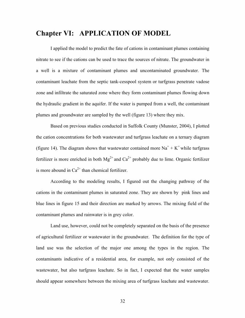
I applied the model to predict the fate of cations in contaminant plumes containing
nitrate to see if the cations can be used to trace the sources of nitrate. The groundwater in
a well is a mixture of contaminant plumes and uncontaminated groundwater. The
contaminant leachate from the septic tank-cesspool system or turfgrass penetrate vadose
zone and infiltrate the saturated zone where they form contaminant plumes flowing down
the hydraulic gradient in the aquifer. If the water is pumped from a well, the contaminant
plumes and groundwater are sampled by the well (figure 13) where they mix.
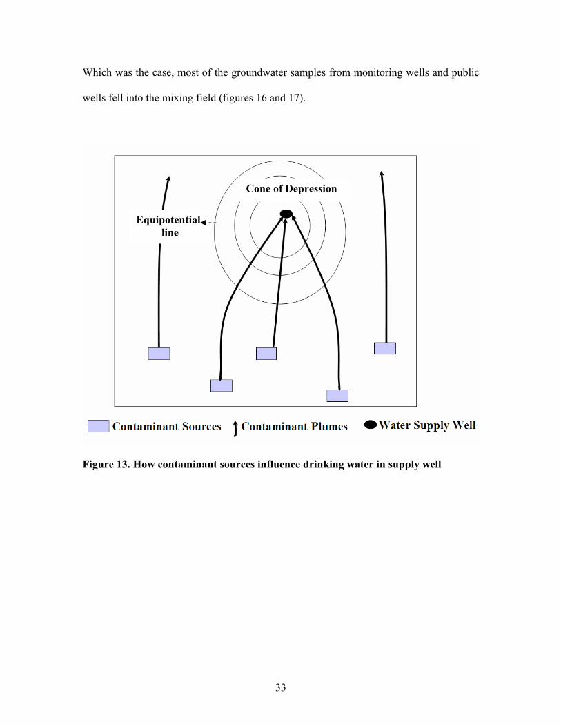
Based on previous studies conducted in Suffolk County (Munster, 2004), I plotted
the cation concentrations for both wastewater and turfgrass leachate on a ternary diagram
(figure 14). The diagram shows that wastewater contained more Na+ + K+ while turfgrass
fertilizer is more enriched in both Mg2+ and Ca2+ probably due to lime. Organic fertilizer
is more abound in Ca2+ than chemical fertilizer.
According to the modeling results, I figured out the changing pathway of the
cations in the contaminant plumes in saturated zone. They are shown by pink lines and
blue lines in figure 15 and their direction are marked by arrows. The mixing field of the
contaminant plumes and rainwater is in grey color.
Land use, however, could not be completely separated on the basis of the presence
of agricultural fertilizer or wastewater in the groundwater. The definition for the type of
land use was the selection of the major one among the types in the region. The
contaminants indicative of a residential area, for example, not only consisted of the
wastewater, but also turfgrass leachate. So in fact, I expected that the water samples
should appear somewhere between the mixing area of turfgrass leachate and wastewater.
32
Which was the case, most of the groundwater samples from monitoring wells and public
wells fell into the mixing field (figures 16 and 17).
Cone of Depression
Equipotential line
Figure 13. How contaminant sources influence drinking water in supply well
33
Figure 14. Water samples from different nitrate sources. (CP: cesspool)
34
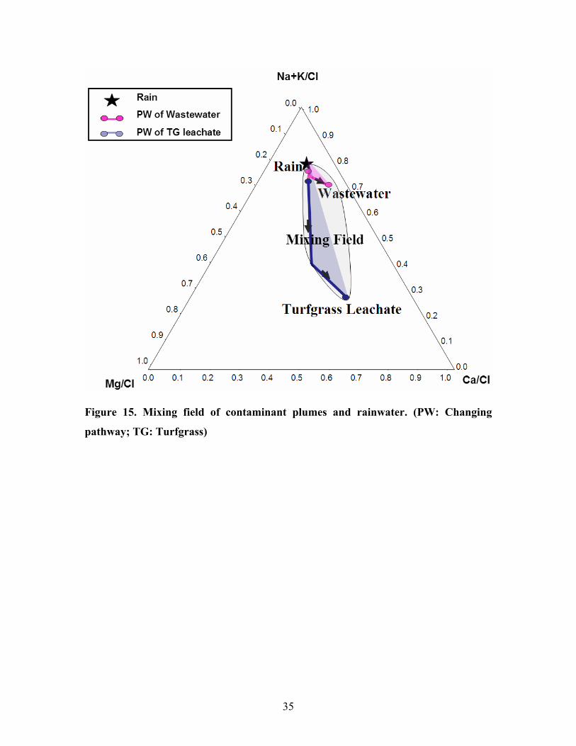
Figure 15. Mixing field of contaminant plumes and rainwater. (PW: Changing
pathway; TG: Turfgrass)
35
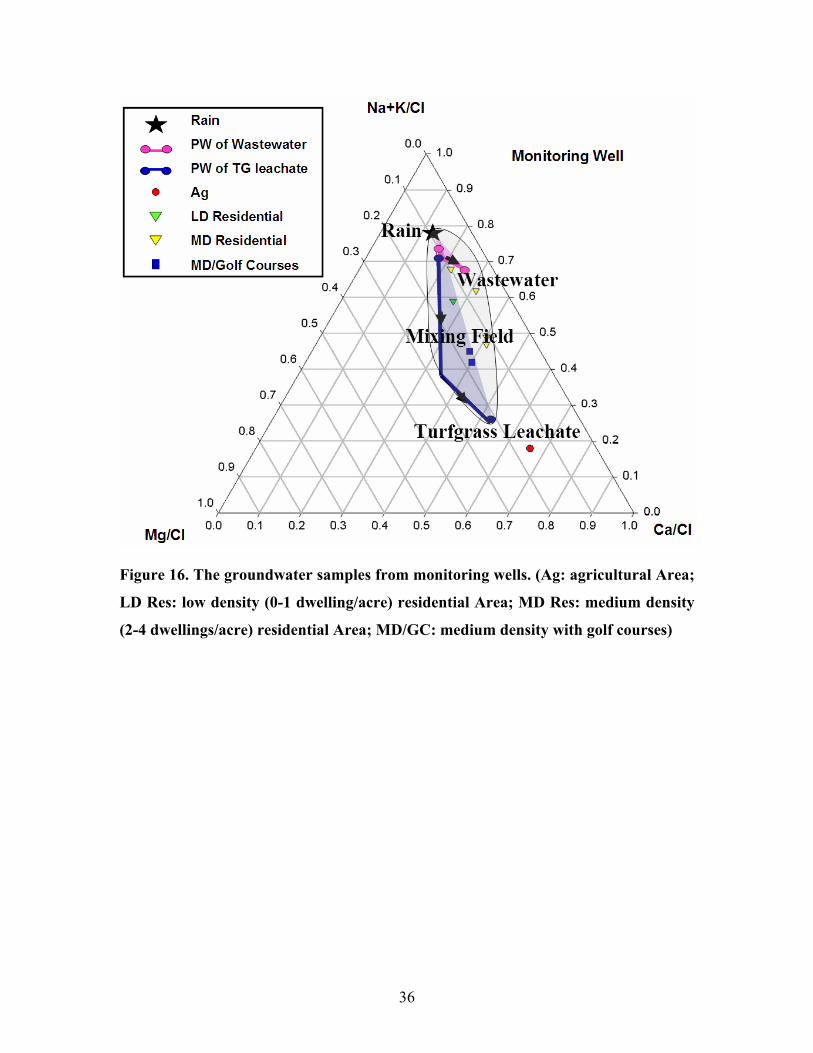
Figure 16. The groundwater samples from monitoring wells. (Ag: agricultural Area;
LD Res: low density (0-1 dwelling/acre) residential Area; MD Res: medium density
(2-4 dwellings/acre) residential Area; MD/GC: medium density with golf courses)
36
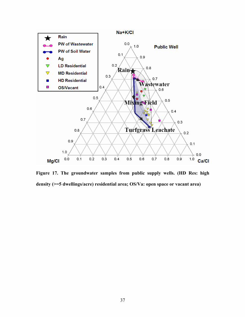
Figure 17. The groundwater samples from public supply wells. (HD Res: high
density (>=5 dwellings/acre) residential area; OS/Va: open space or vacant area)
37
In figure 16, all the samples from monitoring well displayed cation compositions
indicative of their land use. Samples from low or medium density residential area had
cation composition approaching the wastewater field. Those from medium density
residential area with golf courses have been affected by the turfgrass fertilizer. The
sample from agriculture area was near the composition of turfgrass leachate which shows
the strong influence of agricultural fertilizer.
The cation compositions of samples from public wells, however, were ambiguous
(figure 17). The compositions of the samples from agricultural area, for example, were
closer to that of wastewater than were the samples from medium density or high density
residential area. Also, with the increase of the density in residential area, the sample
composition approached the turfgrass leachate field. But Bleifuss’ study (1998) reported
a reverse tendency. Besides, the samples from open space or vacant area, which should
have a composition similar to pristine rainwater, appeared somewhere between the
wastewater and turfgrass leachate fields. Most likely, samples from public water supply
well contained water transported from a long distance. The cations in the water might be
from older land use. More details about the hydrogeology of sampling sites and their
neighboring areas would be needed to explain them. Because water samples from
monitoring wells contained water younger than those from public wells, they provided
cation signatures more indicative of the current land use.
In figure 18 and 19, the water samples from monitoring wells all exhibited nitrate
concentration exceeding 3 ppm while some of those from public wells yielded nitrate
concentration lower than 3ppm. This is because the public wells pumped the water at
38
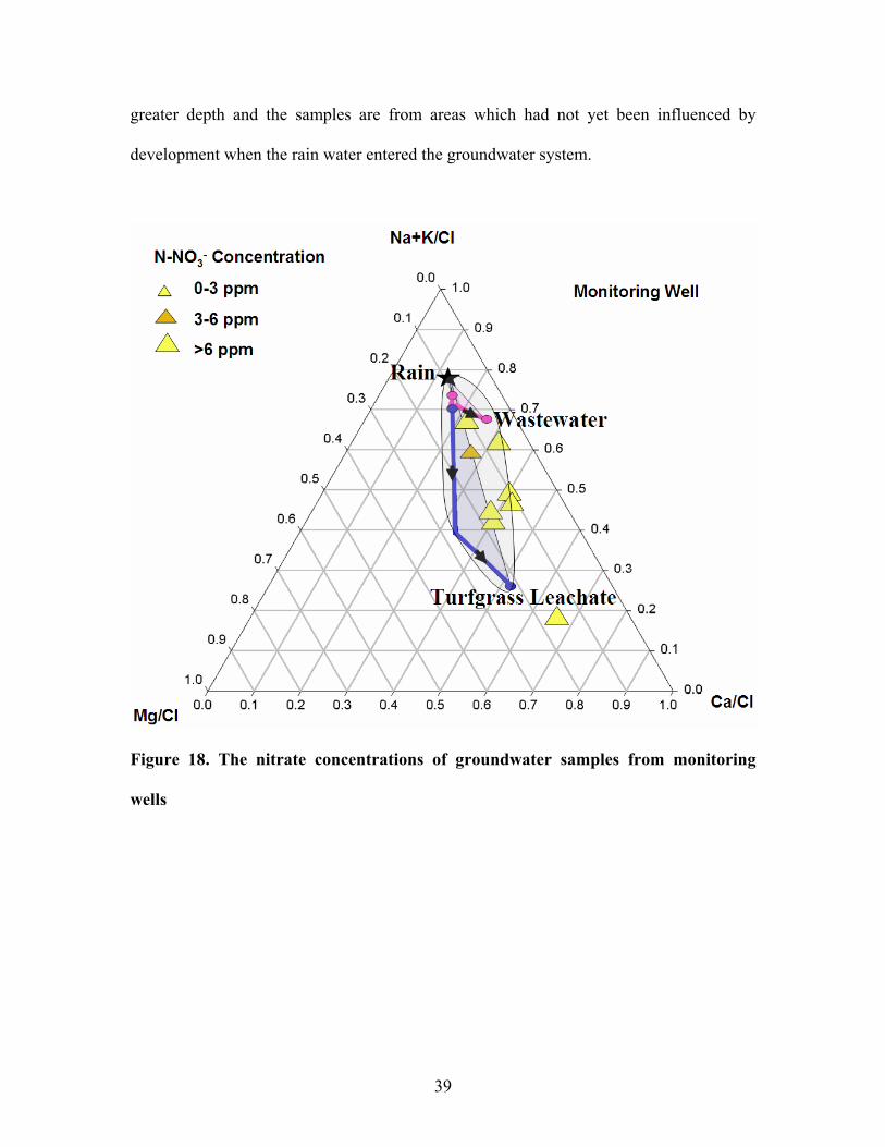
greater depth and the samples are from areas which had not yet been influenced by
development when the rain water entered the groundwater system.
Figure 18. The nitrate concentrations of groundwater samples from monitoring
wells
39
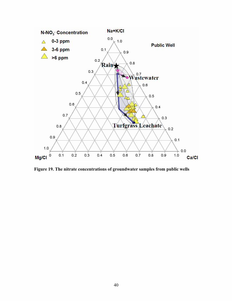
Figure 19. The nitrate concentrations of groundwater samples from public wells
40

Chapter V: SUMMARY:
Modeling reactive transport in porous media becomes an increasingly important
tool for quantitative predictions of contaminant fate in groundwater. My study
investigated the simplest multicomponent transport of four major cations, Na+, K+, Mg2+
and Ca2+ accounting for only sorption and retardation. This program can be the
foundation for the more complicated cases.
In summary:
1. The cation exchange model developed here is independent of length and
the volume of the plume, the flow velocity and dimensions of the cell. The
number of cells determines the resolution of the balancing curve.
2. My model effectively predicts the fate of cations in a contaminant plume
in saturated zone as shown by the agreement with experimental data.
3. My model can be used to estimate the travel time of the cations in a
contaminant plume given hydrologic parameters.
4. The cation chemistry of groundwater from monitoring well is more
reliable for identifying current land use than that from public well.
5. The source of cations in Suffolk County public wells is dominantly from
fertilizer.
More major cations and trace cations can be incorporated into the program. The
complexity of the mathematics will be increased with the number of the component,
especially for the heterovalent cations assemblage. As an example, we provide a program
based on four major cations Na+, K+, Mg2+, Ca2+ and a trace cation Sr2+ with its isotope
ratio.
41
Reference:
Aberg, G., Jacks, G., and Hamilton, P.J., 1989. Weathering rates and 87Sr/86Sr ratios: an isotopic
approach. Journal of Hydrology, 109: 65-78
Aberg, G., and Wickman, F.E., 1987. Variations of 87Sr/86Sr in water from streams discharging
into the Bothnian Bay, Baltic sea. Nordic Hydrology, 18: 33-42
Aiken, G.R., 2002, Organic matter in ground water, in Aiken, G.R., and Kuniansky, E.L., eds.,
U.S. Geological Survey Artificial Recharge Workshop Proceedings, Sacramento, California. U.S.
Geological Survey Open-File Report 02-89, 21-23.
Appelo, C.A.J. and Posma, D. 1999. Geochemistry, groundwater and pollution. A.A.Balkema
Publisher,VT, 160
Bleifuss, P., 1998. Tracing sources of nitrate in the Long Island aquifer system, Thesis of MS,
State University of New York at Stony Brook, NY.
Boguslavsky, S., 2000. Organic Sorption and Cation Exchange Capacity of Glacial Sand, Long
Island. Thesis of MS, State University of New York at Stony Brook, NY.
Bond, W.J. and Phillips, I.R., 1990. Cation exchange isotherms obtained with batch and misible-
displacement techniques. Soil Sci. Soc. Am. J., 54: 722-728
Bond, W.J., 1995. On the Rothmund-Kornfeld description of cation exchange. Soil science
society of America journal, 59: 436-443
Carling A.L. and Gustafsson K., 1998. Artificial recharge of groundwater-testing different spodic
B-horizon materials for the removal of dissovled organic matter,
http://www.lwr.kth.se/forskargrupper/Egc/CarlingGustafsson.pdf
42
Davis, J.A. and Kent, D.B., 1990. Surface Complexation modeling in aqueous geochemistry. In
M.F.Hochella, Jr. and A.F.White (eds), Mineral-water interface geochemisstry. Reviews in
Mineralogy 23, Mineral. Soc.Am.
Drever, J.I. 1997. The Geochemistry of Natural Waters, 3d ed. Upper Saddle River, NJ: Prentice-
Hall, Inc.,436
Flynn, J.M., Padar, F.V., Guererra, A., Andres, B., and Graner, W., 1969. The Long Island
ground water pollution study, State of New York Department of Health, 10: 4
Franke, O.L. and McClymonds, N.E., 1972. Summary of the hydrologic situation on Long Island,
N.Y. as a guide to water-management alternatives. U.S.G.S. Professional Paper. 627-F: 59
Graustein, W.C., 1989. 87Sr/86Sr ratios measure the sources and flow of strontium in terrestrial
ecosystems. Stable isotopes in ecological research, Ecological Studie. 68: 491-512
Hanson, G.N. and Langmuir, C.H., 1978. Modeling of major elements in mantle melt systems
using trace element approaches. Geochim. Cosmochim. Acta, 42: 725-741
Hanson, G.N. and Schoonen, M., 2001. A geochemical Study of the fffects of land use on nitrate
contamination in the Long Island aquifer system. Final report to Suffolk County Water Authority,
Helfferich, F. and Klein, G., 1970. Multicomponent chromatography. Dekker, New York, NY.
Hussain, S.A., Demirci S. and Özbayoğlu, G., 1996. Zeta Potential Measurements On Three
Clays from Turkey and Effects of Clays on Coal Flotation. Journal of Colloid and Interface
Science, 184: 535-541
43
Kehew, A.E., 2001. Applied Chemical hydrogeology. Prentice Hall, Upper Saddle River, NJ
07458, 110
Koppelman, L., 1978. The Long Island comprehensive waste treatment management plan:
Hauppauge. Long Island Regional Planning Board, 2: 345
Munster, J., 2004. Evaluating Nitrate sources in Suffolk County groundwater, Long Island, New
York. Thesis of MS, State University of New York at Stony Brook, NY.
Parks,G.A., 1967. Surface chemistry of oxides in aqueous systems. In Stumm, W. (ed.),
Equilibrium concepts in aqueous systems. Adv.Chem. Ser. 67, Am.Chem. Soc. Washington. 121-
160
Perlmutter, N.M., and Koch, E., 1972. Preliminary hydrogeologic appraisal of nitrate in ground
water and streams, southern Nassau County, Long Island, New York. U.S. Geol. Survey Prof.
Paper, 800-B: 225-235.
Ragone, S.E., Katz, B.G., Lindner, J.B., and Flipse, W.J., 1976. Chemical quality of ground water
in Nassau and Suffolk Counties, Long Island, New York, 1952 through 1976. U. S. Geol. Survey
Open File Report, 76-845: 93
Sardin, M., Schweich, D., Leij, F.J. and Van Genuchten, M.Th., 1991. Modeling the
nonequilibrium transport of linearly interacting solutes in porous media: a review. Water Resour.
Res., 27: 2287-2307
Schweich, D., Sardin, M. and Jauzein, M., 1993. Properties of concentration waves in presence of
nonlinear sorption, precipitation/dissolution, and homogeneous reactions, I. Fundamentals. Water
Resour. Res., 29:723-733
44
Stoeber, M. and Dean, T., 1999. Do different Long Island soils affect the pH of a body of water?
Project report for GEO 121 in State University of New York at Stony Brook.
Stumm, W. and Morgan, J.J., 1981. Aquatic chemistry. 2nd ed. Wiley & Sons, Inc.,New York, 780
Wickman, F.E., and Aberg, G., 1987. Variation in the 87Sr/86Sr ratios in lake waters from central
Sweden. Nordic Hydrology, 18: 21-32
Voegelin, A., Vulava, V.M., Kuhnen, F., and Kretzschmar R., 2000, Multicomponent transport of
major cations predicted from binary adsorption experiments. Journal of Contaminant Hydrology,
46: 319-338
Geng, X., 1993. Strontium isotope study of the peconic river watershed, Long Island, New York.
Thesis of MS, State University of New York at Stony Brook, NY.
45