A PCE groundwater plume discharging to a river: … Organic Chemicals...A PCE groundwater plume discharging to a river: influence of the streambed and near-river zone on contaminant

www.elsevier.com/locate/jconhyd

Journal of Contaminant Hydrology 73 (2004) 249–279

A PCE groundwater plume discharging to a river:

influence of the streambed and near-river zone on

contaminant distributions

Brewster Conant Jr.*, John A. Cherry, Robert W. Gillham

Department of Earth Sciences, University of Waterloo, 200 University Avenue West, Waterloo,

Ontario Canada N2L3G1

Received 6 November 2003; received in revised form 1 April 2004; accepted 1 April 2004

Abstract

An investigation of a tetrachloroethene (PCE) groundwater plume originating at a dry cleaning

facility on a sand aquifer and discharging to a river showed that the near-river zone strongly modified

the distribution, concentration, and composition of the plume prior to discharging into the surface

water. The plume, streambed concentration, and hydrogeology were extensively characterized using

the Waterloo profiler, mini-profiler, conventional and driveable multilevel samplers (MLS), Ground

Penetrating Radar (GPR) surveys, streambed temperature mapping (to identify discharge zones),

drivepoint piezometers, and soil coring and testing. The plume observed in the shallow streambed

deposits was significantly different from what would have been predicted based on the characteristics

of the upgradient plume. Spatial and temporal variations in the plume entering the near-river zone

contributed to the complex contaminant distribution observed in the streambed where concentrations

varied by factors of 100 to 5000 over lateral distances of less than 1 to 3.5 m. Low hydraulic

conductivity semi-confining deposits and geological heterogeneities at depth below the streambed

controlled the pattern of groundwater discharge through the streambed and influenced where the

plume discharged into the river (even causing the plume to spread out over the full width of the

streambed at some locations). The most important effect of the near-river zone on the plume was the

extensive anaerobic biodegradation that occurred in the top 2.5 m of the streambed, even though

essentially no biodegradation of the PCE plume was observed in the upgradient aquifer.

Approximately 54% of the area of the plume in the streambed consisted solely of PCE

transformation products, primarily cis-1,2-dichloroethene (cDCE) and vinyl chloride (VC). High

concentrations in the interstitial water of the streambed did not correspond to high groundwater-

discharge zones, but instead occurred in low discharge zones and are likely sorbed or retarded

remnants of past high-concentration plume discharges. The high-concentration areas (up to 5529 Ag/

0169-7722/$ - see front matter D 2004 Elsevier B.V. All rights reserved.

doi:10.1016/j.jconhyd.2004.04.001

* Corresponding author. Fax: +1-519-746-7484.

E-mail address: [email protected] (B. Conant).

B. Conant Jr. et al. / Journal of Contaminant Hydrology 73 (2004) 249–279250

l of total volatile organics) in the streambed are of ecological concern and represent potential adverse

exposure locations for benthic and hyporheic zone aquatic life, but the effect of these exposures on

the overall health of the river has yet to be determined. Even if the upgradient source of PCE is

remediated and additional PCE is prevented from reaching the streambed, the high-concentration

deposits in the streambed will likely take decades to hundreds of years to flush completely clean

under natural conditions because these areas have low vertical groundwater flow velocities and high

retardation factors. Despite high concentrations of contaminants in the streambed, PCE was detected

in the surface water only rarely due to rapid dilution in the river and no cDCE or VC was detected.

Neither the sampling of surface water nor the sampling of the groundwater from the aquifer

immediately adjacent to the river gave an accurate indication of the high concentrations of PCE

biodegradation products present in the streambed. Sampling of the interstitial water of the shallow

streambed deposits is necessary to accurately characterize the nature of plumes discharging to rivers.

D 2004 Elsevier B.V. All rights reserved.

Keywords: Groundwater; Surface water; Contaminant plumes; Chlorinated hydrocarbons; Biodegradation;

Sediments

1. Introduction

A National Priorities List characterization study for the United States estimates that

51% of 1218 hazardous waste sites impact surface water (USEPA, 1991) and at many of

these sites chlorinated volatile organic compounds (VOCs) are migrating by groundwater

flow to streams and rivers. Despite this relatively common occurrence, few published

studies have characterized VOC plumes in detail to examine the processes that control

how they discharge to a river. Some studies (Norman et al., 1986; Avery, 1994; Hess et

al., 1989) examined VOC groundwater plumes discharging to rivers using seepage

meters and piezometers and others have mapped plan-view distributions of VOCs in

streambeds using diffusion samplers (Vroblesky et al., 1991, 1996; Savoie et al., 1999;

Lyford et al., 1999; Church et al., 2002). These studies contain relatively little

information concerning the hydrological and geological controls on plume characteristics

and do not present the fine-scale vertical concentration data needed to evaluate how the

plume has been changed by the near-river zone. Advection, biodegradation, and

adsorption processes affecting a VOC plume discharging to a creek in a freshwater

tidal wetland were investigated by Lorah et al. (1997) and Lorah and Olsen (1999), but

only a portion of the plume was examined in vertical cross section and the studies did

not examine the resulting streambed contamination in plan view. In this study, we

attempt to provide a more holistic field study of a plume discharging to a river than

appears to be available in the literature.

It is not clear to what extent conditions within the streambed will modify a

contaminant plume prior to its discharge to the surface water. The area beneath and

adjacent to a river or stream is potentially a very complex geological, hydrological, and

biochemical zone (Huggenberger et al., 1998; Brunke and Gonser, 1997; USEPA, 2000;

Conant, 2001, 2004; Woessner, 2000). Studies of uncontaminated sites show that

conditions in the streambed may be spatially and temporally variable and subject to

large hydraulic and geochemical gradients (Brunke and Gonser, 1997; Dahm et al.,

B. Conant Jr. et al. / Journal of Contaminant Hydrology 73 (2004) 249–279 251

1998; Hendricks and White, 1991, 1995). As the plume passes through this zone, it is

hypothesized that the geometry and chemical composition of the plume should change

and that these changes would affect how the plume contaminates the streambed and

surface water. One purpose of the current study was to investigate the geology near the

river to determine if preferential flow paths or restrictions to flow existed that would

control how and where the PCE groundwater plume discharged to the river. The

concentration distribution in the streambed is relevant because ecologists view the

streambed and near-stream groundwater/surface-water transition zone (which includes

the hyporheic zone), as a unique habitat that plays an important role in the aquatic food-

web and that provides other ecological functions related to the health of a stream

(Hynes, 1970; Gibert et al., 1994; Boulton et al., 1998; Ward et al., 1998; USEPA,

2000). This study provides the first comprehensive assessment of a chlorinated solvent

groundwater plume discharging into a river and shows that the near-stream zone

substantially modifies the distribution, concentration, and composition of the plume

prior to its reaching the surface water. The results of this study have important

implications for the design of monitoring programs, evaluation of the ecological impacts

of plumes, and the remediation of these discharges.

Fig. 1. (a) Site map showing outline of PCE groundwater plume, line of geologic cross section, soil coring

locations, and Waterloo Profiler locations. (b) Geological cross section from the dry cleaner to the Pine River with

stratigraphic layers numbered in accordance with Writt (1996).


2. Description of study site and river

The study site is located in Angus, Ontario, Canada, approximately 75 km north–

northwest of Toronto and near Canadian Forces Base Borden. A 60-m-wide dissolved-phase

PCE groundwater plume extends 195 m downgradient to the Pine River from a dense

nonaqueous phase liquid (DNAPL) source of PCE beneath a dry-cleaning facility (Fig. 1a).

The groundwater at the site has likely been contaminated since at least the 1970s. The

stratigraphy of the top 15 m of the deposits at the site is divided into five sand layers that

consist primarily of fine to very fine sands and one 1- to 1.5-m-thick silty-clay aquitard layer

at a depth of about 5 m (Writt, 1996) (Fig. 1b). Because the aquitard is absent near the dry

cleaner, the DNAPL spilled there was able to reach and accumulate in the deeper sands. A

high concentration (up to 43,318 Ag/l) dissolved-phase PCE plume travels toward the river

in the confined aquifer beneath the aquitard. Although several researchers had characterized

the groundwater plume (Pitkin, 1994; Pitkin et al., 1994; Beneteau, 1996; Writt, 1996;

Beneteau et al., 1999; Guilbeault et al., in press), the extent to which the aquitard, aquifer, or

plume extended beneath or beyond the river was not determined. The only information

regarding water quality beneath the river was from six shallow mini-piezometers installed in

the streambed at about a 15-m spacing along the eastern edge of a 75 m reach of river

downstream of the King Street bridge. Contamination was only detected at one of the six

locations (AMP3) approximately 29m north of the King Street bridge (see Fig. 2) where 221

Ag/l of PCE and 9.9 Ag/l of trichloroethene (TCE) were found (Pitkin, 1994).

Fig. 2. Data location map for installations in and near the river.


The Pine River drains a basin that is about 348 km2 in area and summer base flows at

the study site are about 1 to 2 m3/s (Beebe, 1997; Burkard, 1990). The river is moderately-

to-highly sinuous and has a channel with a low width-to-depth ratio, a high entrenchment

ratio, and a slope of 0.0007 m/m (Beebe, 1997). At the study site, the river is relatively

straight and the stream banks are about 1.2 to 2.5 m high and consist of silt, clay and peat

deposits. The river is 11 to 14 m wide and in summer has an average depth of 0.5 m and

maximum depth of about 1.1 m. The river is a high-quality cold-water habitat that supports

a wide diversity of aquatic life and benthic taxa such as Glossosoma and Leuctra (Jones,

1999), trout and salmon.

3. Field methods

3.1. Characterization of geology and streambed sediments

The techniques used to characterize geology and streambed sediment at the site

included: coring, Ground Penetrating Radar (GPR), and visual mapping of sediments.

Seven cores of unconsolidated deposits were collected on land to a maximum depth of

12.2 m below ground surface (bgs) at locations SC7 to SC13 (Fig. 1a) using the piston-

core-barrel method (Starr and Ingelton, 1992). Twelve cores were collected in the

streambed at locations RC1 to RC12 (Fig. 2) by hand driving 0.051 m ID aluminum

core tubes to a maximum depth of 1.8 m. Cored materials were logged and sediments

classified. Hydraulic conductivities were determined for 178 subsamples of the streambed

cores and 48 subsamples from aquifer materials at SC12 using a falling-head permeameter

test method (Sudicky, 1986). The porosity and bulk density of each subsample was

determined by using weight-to-volume calculations. Fraction of organic carbon ( foc)

analyses were performed on 52 samples from cores SC12, SC13, RC1, RC2, RC4, and

RC11. Samples were analyzed using either the method of Tabatabi and Bremner (1970) or

Churcher and Dickout (1987) which had detection limits of 0.05% and 0.008%,

respectively.

The GPR survey was performed in October 1998 using a pulseEKKO IV GPR system

(Sensors and Software, Mississauga, Ontario, Canada) with a pair of 200 MHz unshielded

slab-antennae mounted in the bottom of a small inflatable boat. The GPR survey consisted

of 16 transects across the Pine River (Fig. 3a). Visual mapping of the surficial geology of

the streambed between transects � 4 to � 4W and 56–56W was done in July 1997,

August 1998, and February 1999. Transect locations are used to identify locations in the

streambed. For example, location 8–8W 4.5 m indicates that the transect is approximately

8 m downstream (north) of the King Street bridge (shown in Fig. 2) and the point is 4.5 m

west of stake 8 (on the east bank) toward stake 8W (on the west bank).

3.2. Water level monitoring and stream gauging

To obtain a better understanding of groundwater/surface-water interactions, ground-

water flow directions, and river stage/discharge relationships, several drivepoint piezom-

eters, mini-piezometers, dataloggers and staff gauges were installed at the site. A total of

Fig. 3. (a) Map of surficial geology of the streambed and (b) map of vertical water fluxes through the streambed

for February 1999.


41 drivepoint piezometers were installed at 20 locations (DP1 to DP20) on land to depths

of between 2.5 and 8.0 m bgs. Monthly water-level measurements were made in all land-

based piezometers for a period of 13 months starting in July 1998. In July 1998, a

drivepoint well AW1 was installed in the confined aquifer 27 m north of the bridge and 3.8

m east of the river and the water levels were monitored to within 0.005 m on a 15-min

interval until November 1999, using a Solinst Model 3001, M5 Leveloggerk (Solinst

Limited Canada, Georgetown, Ontario).

Piezometers were also installed at 40 locations in the streambed. Three pairs of mini-

piezometers were installed in the streambed at locations between 55 and 72 m downstream

of the bridge in June 1996 using the method of Lee and Cherry (1978). Thirty-four


drivepoint piezometers made of 0.021 m OD PVC pipe were also installed (Fig. 2) to

depths of 0.65 to 0.70 m in the streambed. Slug testing of the drivepoint piezometers was

performed in November and December 1998, and hydraulic conductivity was determined

using the Hvorslev (1951) variable-head method. Prior to each slug test, the hydraulic-

head difference between the river and the piezometer was measured to within 0.001 m

using a potentiomanometer similar to that described by Winter et al. (1988).

Manual measurements of stream stages began in 1996 and stages were eventually

recorded on a 15-min interval between March 1998 and June 1999, using a Solinst, Model

3001, M5 Leveloggerk placed in a stilling well in the river at PRP1 (Fig. 2). Discharge

was measured eight times at the site using a Swoffer Model 2100-STDX flowmeter. A

stage/discharge relationship was developed for the site using this data.

3.3. Plume delineation

Sampling devices used to characterize and delineate the subsurface water quality at the

site were: the Waterloo Profiler, mini-profiler, bundle multilevel samplers, and ‘‘drive-

able’’ multilevel samplers. Early in the study (June and November 1996), a few drivepoint

piezometers and mini-piezometers were also used for sampling. Table 1 summarizes the

Table 1

Summary of sampling of groundwater and streambed interstitial water

Sampling device Sample location

names

Number of

locations

Number

of GW

samples

Maximum

depth of

sampling

(m)

Vertical

sampling

interval

(m)

Date of

sampling

Drivepoints and

mini-piezometers

DP1 to DP6, SP1,

SP2, SP3

12 25a 8 NA 6/96

Drivepoints and

mini-piezometers

DP1, DP2, DP8,

DP9, SP1

5 13a 7.6 NA 11/96

Waterloo Profiler AP40 to AP52 13b 175 11.5 0.25 or 0.50 7/96 to 8/96

Waterloo profiler AP96-1 to AP96-10 10 81 12 0.3 to 1.0 6/96 to 8/96

Waterloo profiler AP53 to AP55 3 21 12.2 0.6 to 1.5 11/97 to 12/97

Waterloo profiler PRP1 to PRP8 8 106 8.5 0.1 to 0.5 8/96 to 11/96

Mini-profiler PRP7R, PRP8R,

PRP9R, PRP10

to PRP17

11 104 2.1 0.15 to 0.6 8/97 or 10/97c

Mini-profiler Plan-view mapping 80 80 0.3 NA 8/98

Driveable

multilevels

MLS3, MLS4,

MLS7, MLS8,

MLS17, MLS18

6 41 4.5 0.15 or 0.3 11/98

Driveable

multilevels

MLS1 to MLS20 10 139 5.4 0.15 or 0.3 3/99

Bundle multilevel

samplers

BML1 to BML12 12 106 9.5 0.5 3/99

NA—not applicable, only sampled at one depth.a Includes multiple piezometers sampled at a location (e.g., shallow, intermediate and deep levels).b Location AP40 profiled in two parts AP40 and AP40B but counted as one location.c PRP17 was sampled in 8/98.


characteristics of these devices and a description of their sampling and construction can be

found in Conant (2001).

The Waterloo Profiler method of obtaining vertical profiles of water quality (Pitkin et

al., 1999) was used at 34 locations to collect approximately 383 groundwater samples.

Thirteen of these profile locations (AP40 to AP52) were along profiler transects 5 and 6,

which were within 4 m of the east and west sides of the Pine River, respectively (most

locations are shown in Fig. 2). Another 10 locations in the upgradient confined aquifer

were profiled to further characterize high-concentration areas and delineate the lateral

edges of the PCE plume along previously profiled transects by Pitkin (1994) and Writt

(1996). Three locations were profiled along transect 4 near AP27 (see Fig. 1a) and next to

previously profiled locations by Writt (1996) to reassess a high-concentration plume area

29 to 37 m east of the river. Eight locations (PRP1 to PRP8) were also profiled in the

streambed (Fig. 2) and the holes sealed with bentonite.

A ‘‘mini-profiler’’ was used to obtain vertical profiles and determine the plan-view

distribution of groundwater quality in the streambed. The mini-profiler was a soil vapor

probe (Hughes et al., 1992) that was modified to collect water and was a 0.0064 m OD,

0.003 m ID stainless-steel tube, 2.6 m in length, having a 0.01-m-long screen. The mini-

profiler was used for vertical profiling at PRP7R, PRP8R, PRP9R, and PRP10 to PRP17

(Fig. 2). In August 1998, a 1.8-m-long mini-profiler was used at 80 locations to map the

horizontal extent of the plume at a depth of 0.3 m below the streambed. Samples were

collected on approximately a 2 by 4 m grid starting at transect � 4 to � 4W (beneath the

King Street bridge) and ending at transect 44–44W, with two additional samples collected

on transect 52–52W.

Twelve bundle multilevel samplers, designated BML1 to BML12, were installed along

the banks of the river (Fig. 2). BML1 to BML10 were installed in a row on the east side of

the river and roughly parallel to profiler transect 5 to assess possible changes in the

location and position of the plume. The BMLs were constructed in a similar manner to

those used by Mackay et al. (1986) and described by Bianchi-Mosquera and Mackay

(1992). Each BML sampler consisted of a 10-m-long center stalk with 8 to 11 sampling

points at the bottom having a vertical spacing of 0.5 m.

Because of the large upward hydraulic gradient between the confined aquifer and the

river, there was concern that the installation of multilevel samplers deep in the streambed

could pierce the semi-confining deposits and result in vertical water flow along the

installations and preferential pathways for the aquifer contamination to reach the river.

Therefore, two new types of driveable multilevel samplers (MLS) were developed for use

in the streambed that eliminated the need for a larger diameter temporary casing to install

samplers and thereby minimized the possibility of vertical water flow along the

installation. The MLS sampling ports were flush with the outside of a stainless steel or

PVC pipe that was driven directly into the streambed using an electric jack hammer.

Therefore, the hole that was created to install the multilevel sampler was exactly the same

size as the device and so there was no annular space that needed to be sealed to prevent

vertical flow up the borehole. The 0.034 m OD stainless-steel type was a modified version

of the multilevel sampling device used by de Oliveira (1997) and had nine sampling ports

spaced 0.3 m apart and were driven down to a maximum depth of 5.6 m. The 0.042 m OD

PVC type of driveable multilevels were 1.52 m in length and had 10 sampling ports spaced


0.15 m vertically along their length. The stainless steel and PVC type driveable multilevel

samplers (MLS1 to MLS20) were permanently installed in pairs at 10 locations along

transects 6–6W and 16–16W (Fig. 2).

Water samples collected from these devices were analyzed at the University of

Waterloo for VOCs [i.e., PCE and its seven anaerobic degradation products: TCE, 1,1-

dichloroethene (11DCE), 1,2-trans-dichloroethene (tDCE), 1,2-cis-dichloroethene

(cDCE), vinyl chloride (VC), ethene, and ethane]. Analyses for PCE and TCE were

performed using a Hewlett Packard 5890 Series II gas chromatograph equipped with an

Ni63 electron capture detector (ECD). Minimum detection limits for PCE and TCE were

0.7 and 0.9 Ag/l, respectively. Analyses for cDCE, tDCE, 11DCE, and VC were performed

using a Hewlett Packard 5890 Series II gas chromatograph equipped with an HNU

photoionization detector (PID). Minimum detection limits were as follows: for cDCE (1.0

Ag/l), tDCE (1.4 Ag/l), 11DCE (1.4 Ag/l) and VC (0.7 Ag/l). Analyses for ethene and

ethane were performed using a Hewlett Packard 5790A gas chromatograph equipped with

a flame ionization detector (FID). Minimum detection limits for ethene and ethane were

0.5 Ag/l.

3.4. Surface-water sampling

Between June 1996 and March 1999, 71 surface-water samples were collected from

various locations within the study reach and analyzed for VOCs. The majority of water

samples were collected by hand in 40 or 25 ml glass vials as grab samples from 0.02 to

0.05 m above the streambed. Other samples were collected during profiling of the

streambed by placing the Waterloo Profiler or a mini-profiler tip just above the streambed

and using a peristaltic pump and sampling manifold.

3.5. Sediment quality sampling

Total PCE and TCE concentrations in soils and sediments were determined for samples

collected during coring activities. Forty-one samples were obtained from cores SC11 and

SC12 by cutting them open in the field and immediately subsampling them with a

stainless-steel mini-corer and extruding the samples into vials containing methanol.

Samples of the methanol from each vial were extracted with pentane and analyzed for

PCE and TCE using the ECD method previously described. The minimum detection limits

for the method were 0.23 micrograms of PCE per gram of dry sediment (Ag/g) and 0.22

Ag/g for TCE. Twenty-five samples from RC1 to RC4 were subjected to a new core

sampling technique to simultaneously determine both the interstitial pore water and total

contaminant concentrations from which the sorbed concentration could be determined

(Conant, 2001). Aluminum core tubes containing sediments were immediately capped and

holes were drilled though the aluminum walls on a 0.15 m vertical spacing for sampling. A

glass syringe was used to extract water from the sediment at each drilled hole and then a

mini-corer was used to collect a sediment sample at the same location. A total of 25

sediment samples were analyzed for PCE, TCE, and cDCE using a new method where the

methanol used to preserve and extract the sample was directly injected into the gas

chromatograph with the ECD instead of extracting the methanol with pentane. The method


improved the minimum detection limits to 0.006, 0.002, and 0.11 Ag/g for PCE, TCE, and

cDCE, respectively, and did not foul the column or result in carry-over. Water samples

could be collected from only 11 of the 25 locations because some deposits were too fine

grained to obtain water using the syringe. Water samples from the sediments were

analyzed for VOCs using the same methods used for previous water samples.

4. Results and discussion

4.1. Geology

Geological investigations were designed to answer specific questions including: (1)

does the aquitard found to the east of the river extend under the river; (2) if the aquitard

extends under the river, has the river eroded down through it; (3) do the shallow fluvial

deposits emplaced by the river affect near stream groundwater flow and result in

preferential discharge locations or restrictions to flow; and (4) is the discharge through

the streambed controlled by the deeper deposits?

Soil cores showed that the silty-clay aquitard found to the east of the river was not

present beneath or near the river. Near the river, ‘‘semi-confining deposits’’ were

present instead of the aquitard. The lower sands of the confined aquifer extend beneath

these semi-confining deposits and beyond the river (see Fig. 1b). The semi-confining

deposits found in SC7 to SC12 consisted of about a 5-m-thick sequence of finely

bedded silts, peat, and clay that contain woody fragments and infrequent sand stringers.

The semi-confining deposits under the river found in cores RC1, RC2, RC7, RC9,

RC11, and RC12 ranged from a gray to darker gray silt with a small amount of clay to

a gray to olive-gray clay or silty clay. Table 2 summarizes the results of the

permeameter tests on sediment samples and includes hydraulic conductivity data,

anisotropic ratios, average porosities, and average bulk densities for the semi-confining

deposits and other deposits at the site. Results of falling head permeameter tests

indicated that the semi-confining deposits have hydraulic conductivities equal to or

lower than those reported by Writt (1996) for the silty (i.e., less clayey) upper portion

of the adjacent aquitard. Slug testing of five piezometers screened in the semi-confining

deposits in the streambed also had low vertical hydraulic conductivities (Kv) that ranged

from 9.34� 10� 4 to 4.44� 10� 6 cm/s with a mean value of 6.90� 10� 6 cm/s.

Because the semi-confining deposits are more heterogeneous and include some higher

hydraulic conductivity materials than the clay aquitard, they allow more water to pass

through them than the aquitard.

The GPR survey indicated that the semi-confining deposits were absent in some areas

and that preferential pathways (e.g., geological windows with relatively high-hydraulic-

conductivities) existed between the underlying aquifer sands and the river. Semi-

confining deposits extended from the east bank to about a third of the way across the

river (approximately 4.0 to 4.5 m) along transects 14–14W through 24–22W. GPR and

coring showed that less than 0.8 m of sandy materials overlies the semi-confining

deposits in those areas. These sandy deposits become considerably thicker (i.e., 2.5 to

over 3.1 m thick) in the center of the river. The cross-sectional areas of these sandy

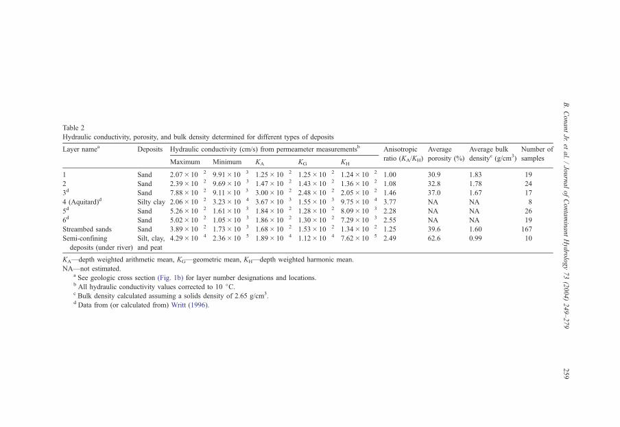
Table 2

Hydraulic conductivity, porosity, and bulk density determined for different types of deposits

Layer namea Deposits Hydraulic conductivity (cm/s) from permeameter measurementsb Anisotropic Average Average bulk Number of

Maximum Minimum KA KG KHratio (KA/KH) porosity (%) densityc (g/cm3) samples

1 Sand 2.07� 10� 2 9.91�10� 3 1.25� 10� 2 1.25� 10� 2 1.24� 10� 2 1.00 30.9 1.83 19

2 Sand 2.39� 10� 2 9.69� 10� 3 1.47� 10� 2 1.43� 10� 2 1.36� 10� 2 1.08 32.8 1.78 24

3d Sand 7.88� 10� 2 9.11�10� 3 3.00� 10� 2 2.48� 10� 2 2.05� 10� 2 1.46 37.0 1.67 17

4 (Aquitard)d Silty clay 2.06� 10� 2 3.23� 10� 4 3.67� 10� 3 1.55� 10� 3 9.75� 10� 4 3.77 NA NA 8

5d Sand 5.26� 10� 2 1.61�10� 3 1.84� 10� 2 1.28� 10� 2 8.09� 10� 3 2.28 NA NA 26

6d Sand 5.02� 10� 2 1.05� 10� 3 1.86� 10� 2 1.30� 10� 2 7.29� 10� 3 2.55 NA NA 19

Streambed sands Sand 3.89� 10� 2 1.73� 10� 3 1.68� 10� 2 1.53� 10� 2 1.34� 10� 2 1.25 39.6 1.60 167

Semi-confining

deposits (under river)

Silt, clay,

and peat

4.29� 10� 4 2.36� 10� 5 1.89� 10� 4 1.12� 10� 4 7.62� 10� 5 2.49 62.6 0.99 10

KA—depth weighted arithmetic mean, KG—geometric mean, KH—depth weighted harmonic mean.

NA—not estimated.a See geologic cross section (Fig. 1b) for layer number designations and locations.b All hydraulic conductivity values corrected to 10 jC.c Bulk density calculated assuming a solids density of 2.65 g/cm3.d Data from (or calculated from) Writt (1996).

B.ConantJr.

etal./JournalofContaminantHydrology73(2004)249–279

259


deposits are somewhat ‘‘u-shaped’’ and are consistent with the infilling of an older and

deeper river channel that can be seen along several GPR transects including 16–16W

(Fig. 4a). Fig. 4b shows a small preferential groundwater flow path in a sandy zone

through the semi-confining deposits between MLS8 and MLS10. In cores where the

contact between sandy materials and the semi-confining deposits was encountered, the

sands had hydraulic conductivities 32 to 382 times greater than the underlying semi-

confined deposits. The streambed sand deposits had a geometric mean hydraulic

conductivity (KG) of 1.53� 10� 2 cm/s which is similar to the value obtained for the

sands of the confined aquifer (Table 2). In the southern GPR transects near the bridge

(4–4W to 10–10W), nearly the entire width of the river appears to be sandy at depth

and these fluvial deposits serve as a preferential flow zone for groundwater discharge

(Fig. 4c and d).

The surficial geology of the streambed was visually mapped in July 1997, August 1998,

and February 1999. Erosion and deposition of sediments over time can change the

geomorphology, topography, and composition of streambeds, yet the map of the surficial

geology for February 1999 (Fig. 3a) was remarkably similar to the previous mappings.

Between the King Street bridge and transect 30–30W, 56.3% of the area of the streambed

consisted of fine to very fine sand and 13.7% consisted of sand and gravel with or without

cobbles and boulders. Downstream of transect 30–30 W, in an area of a gentle riffle, the

streambed material was even coarser. Fluvially deposited silty materials were primarily

found along the edges of the river during each mapping. Although erosion and deposition

cause the topography to vary by as much as 0.45 m at some locations, the semi-confining

deposits typically were not visible at the streambed surface and only outcropped as very

small areas along the stream banks.

4.2. Groundwater flow and discharge through the streambed

Fig. 5a shows the potentiometric surface for drivepoints screened in the confined

aquifer for November 1998, which corresponds to the lowest monthly water-level

conditions observed between July 1998 and August 1999. During those 13 months,

the pattern of groundwater flow was very similar and water levels in individual

piezometers changed less than 0.4 m. The section of river extending 40 m downstream

of the bridge appears to be an area of groundwater discharge and so the plume should

not flow past the river except possibly to reach the area near DP9. Deep piezometer

DP9-3 (which was confirmed to be installed and operating properly) consistently had the

lowest hydraulic head observed in the confined aquifer (hence the concentric contours

around it) and appears to be near an area of discharge from the confined aquifer up into

the overlying unconfined system. A geologic window through the semi-confining

deposits at or near DP9-3 is likely the cause of the low hydraulic head at DP9-3, since

hydraulic heads in the unconfined deposits were lower than the hydraulic heads in the

confined aquifer.

Water levels measured in piezometers screened in the confined aquifer near the river

were artesian and were 0.5 to 1.5 m higher than those in the river. Between July 1998 and

June 1999, the vertical hydraulic gradient between the confined aquifer at AW1 and the

river at PRP1 was always upward at between 0.29 and 0.42 m/m and indicated

Fig. 4. (a) GPR transect and (b) geologic cross section along river transect 16–16W. (c) GPR transect and (d)

geologic cross section along river transect 6–6W. GPR survey performed in October 1998. Note: two way travel

times based on a single radar velocity of 0.055 meters per nanosecond (m/ns) and a topography correction has

been applied to compensate for the water velocity of 0.033 m/ns.


Fig. 5. (a) Potentiometric contour map for the confined aquifer November 1998. (b) Contour map of maximum

PCE concentrations in groundwater at each vertical profile location. Concentration data from this study and from

Pitkin (1994), Writt (1996), and Guilbeault et al. (in press).


groundwater discharges to the river even during storm runoff events and the modest spring

runoff. During this time, the flow in the Pine River was between 1.4 and 6.9 m3/s and the

river stage varied by 0.84 m. The lack of gradient reversals during flooding events

indicates that uncontaminated surface water does not flow down into the underlying sand

aquifer and so cannot displace contaminated groundwater there, except possibly during

more extreme flooding situations than were observed during this period of time.

Flow in the shallow streambed deposits was spatially variable and complex. Darcy’s

law calculations using water-level measurements and slug-testing results from 34

streambed piezometers showed that the vertical flux ( qv) ranged from 0.029 to 446 liters

per square meter of streambed per day (l/m2 day) to perhaps as much as 7060 l/m2 day at

one location. This variability was primarily a function of the wide range in hydraulic

conductivity of materials in which the piezometers were screened. Water levels measured

in streambed piezometers at low river flow conditions in November and December 1998

all showed upward flow of water with head differences between the screens and the river

of between 0.002 and 0.233 m with a median value of 0.01 m. Streambed temperature

mapping combined with qv values obtained from piezometer data allowed a very detailed

plan-view map of the discharge to be created at this site (Conant, 2004). The pattern of

discharge is shown for February 1999 (Fig. 3b) and was very similar in pattern to that for

July 1998 (not shown). The mapping identified three high-discharge zones referred to as

the west-central, eastern-shore, and south-central discharge areas where vertical fluxes are

near or exceeded 200 l/m2 day. A low-flow band ( < 50 l/m2 day) was also identified that

separated the eastern-shore discharge area from the other two high-discharge areas. A

substantial area of recharge was also identified in the riffle downstream of transect 30–


30W. Springs, low-to-moderate discharge zones, and no-discharge zones were also

observed at the site.

The streambed discharge in Fig. 3b showed no direct correlation with the streambed

surficial geology in Fig. 3a. However, GPR, soil core data, and slug testing data show that

the south-central and west-central discharge areas are consistent with the geology at depth.

The geological windows through the semi-confining deposits appear to control the pattern

of discharge in the streambed. The plan-view mapping of water levels and flow lines

drawn for the confined aquifer (Fig. 5a) was also consistent with having discharge

occurring in the streambed at the three high-discharge locations and not at the riffle area to

the north.

4.3. The upgradient groundwater plume

Characterization of the upgradient land-based plume traveling toward the river

provided information on the nature of the contamination that might be found beneath

the river. Maximum PCE concentrations encountered in vertical profiles at each

Waterloo Profiler location were used to create a plan-view map for the plume (Fig.

5b). The plume shown in Fig. 5b is also based on information from an additional 49

profile points (not shown) that are just east of the area shown (locations are shown in

Fig. 1a). Within the plume are two narrow (5 to 10 m wide) high-concentration (>10,000

Ag/l) ‘‘cores’’ (terminology from Cherry, 1996) that extend from the DNAPL source area

to the river and are within a 60-m-wide lower concentration ‘‘fringe’’ that is generally

less than 1000 Ag/l. Profiling along transect 6 in July 1996 showed that the entire plume

discharges to the river prior to reaching its western shore except near DP9 where 2.5 Ag/l of PCE was detected at AP47. The presence of PCE in that area was confirmed by

sampling drivepoint piezometers DP9-2 and DP9-3 in November 1996 that detected 5.1

and 26.3 Ag/l of PCE, respectively, and when 2.1 Ag/l of PCE was detected at BML11 in

March 1999. The location of the plume near DP9 and in the upgradient aquifer was

consistent with the groundwater flow paths shown in Fig. 5a.

To determine the PCE concentration distribution about to reach the river, the plume

in the confined aquifer was characterized in cross section beneath the eastern river

bank immediately adjacent to the Pine River. PCE concentrations for transect 5

performed in 1996 and the BML1 to BML10 transect sampled in 1999 are shown

at a 1:1 scale in Fig. 6b and c, respectively, and the transect locations are shown in

Fig. 6a. In both transects, plume concentrations varied vertically by factors of 100 to

1000 over distances of less than 1 to 2 m. The PCE groundwater plume along transect

5 was generally 5 to 7 m thick and approximately 45 m wide but was only about 4 to

5 m thick in the BML transect. The plume was found only in the confined aquifer and

was not observed in the semi-confining deposits except for low concentrations ( < 10

Ag/l) found in AP45 and AP46 (Fig. 6b). In transect 5, the peak concentrations in the

plume (>1000 Ag/l) were found in a continuous band that was 1.0 to 1.5 m thick along

nearly the full width of the plume. The two plume cores (>10,000 Ag/l) shown in Fig.

5b were either not intersected by the sampling array or were not present. However, the

two highest concentrations for transect 5 were 8707 Ag/l at AP40 and 6643 Ag/l at

AP43 which were located where the plume cores should have been. When the BML

Fig. 6. (a) Plan-view of total VOCs concentrations expressed as equivalent PCE in streambed at a depth of 0.3 m

in August 1998. (b) Cross section view of PCE concentrations along transect 5 sampled with Waterloo Profiler in

July–August 1996. (c) Cross-sectional view of PCE concentrations along BML transect sampled in March 1999.

All figures are at same 1:1 scale.



transect was sampled in 1999, the area with greater than 1000 Ag/l of PCE was

discontinuous, and the peak PCE concentration for the entire cross section was only

2699 Ag/l detected at BML6. Using the contaminant distributions shown across the

entire transects in Fig. 6b and c, it was estimated that approximately 19.7 grams of

PCE per day (g/day) was flowing toward the river in 1996 but only 7.7 g/day of PCE

was traveling toward the river in 1999. These PCE mass discharges are both less than

the 58.5 to 146.2 g/day estimated for transect 4 in 1995 based on data from Writt

(1996). These differences in the plume over time could be an artifact of: how the

sampling array intersected the plume; seasonal changes in the dissolution of the

DNAPL source; depletion of the DNAPL source over time; or possibly changes in the

flow field caused by profiler holes through the aquitard along transects 1 to 4 that

were not sealed during previous studies. This decline in concentration (and mass

discharge) over time was also observed at the three profiler locations along transect 4

(near AP27) which had peak PCE concentrations of 109 to 7305 Ag/l in 1997 and

were considerably lower than the 6096 to 13064 Ag/l observed by Writt (1996) at the

same locations in 1995. Concentrations observed along the BML transect (BML1 to

BML9) in 2001 (Hunkeler et al., in press) were also consistent with this overall trend

of declining concentrations and had only two samples with PCE concentrations

exceeding 1000 Ag/l.The plume in the confined aquifer upgradient of the river was composed almost

entirely of PCE with only minor detections of PCE transformation products; therefore,

observed declines in PCE concentrations over time are not thought to be caused by

anaerobic biodegradation, particularly since the aquifer is not very reducing (anaerobic

to possibly nitrate reducing). Analyses of samples of dissolved-phase PCE from the

confined aquifer for ratios of 37Cl and 13C isotopes (Beneteau et al., 1999; Hunkeler et

al., in press) confirmed that biodegradation of PCE was not a significant process. Some

small amounts of degradation products were detected in the plume near the top of the

confined aquifer, in the organic rich materials of the semi-confining deposits, and along

the northern edge of the plume near the river. For example, along the BML transect low

concentrations of cDCE ( < 14.5 Ag/l) and TCE ( < 9.5 Ag/l) were detected in the top 2 to

4 sampling points in the aquifer at BML7, BML9, and BML10 and 26.8 Ag/l of TCEwas found at the top most point in the aquifer at BML1. Low levels of PCE degradation

products (but no PCE) were also detected in drivepoint piezometers and one streambed

piezometer in the area north and west of BML10 which is an area where the PCE plume

would have traveled through had it not curved southward to meet the river (Fig. 5a and

b). These concentrations are perhaps remnants from a time when the plume had traveled

through that area.

4.4. Contamination of interstitial water in the streambed

Fig. 6a shows in plan-view the equivalent PCE concentrations for interstitial water

samples collected from the shallow streambed using the mini-profiler in August 1998.

The figure shows that the size, configuration, concentration, and composition of the

plume found at a depth of 0.3 m in the streambed deposits were significantly different

than the PCE concentrations in the upgradient plume shown in cross sections at the


same 1:1 scale along transect 5 and the BML transect (Fig. 6b and c). The major

difference was the change in composition caused by anaerobic transformation of PCE to

TCE, cDCE, tDCE, 11DCE, VC, ethene and ethane. To directly compare the contam-

inated area of the streambed to the PCE concentrations found in the confined aquifer,

total VOCs detected in the streambed (i.e., PCE and its anaerobic degradation products)

were converted to equivalent PCE concentrations.

The plan-view area of contamination in the streambed delineated by the 1 Ag/lequivalent PCE contour in Fig. 6a is 469 m2 or about 2.3 to 3.2 times larger than in

the two cross sections (Fig. 6b and c) and the area enclosed by the 10 Ag/l contour isabout 2.9 to 3.8 times larger. The plume has a similar north–south dimension in both

the streambed and aquifer, but is much wider in the streambed than its vertical

thickness in the aquifer. This widening is not consistent with the narrowing of flow

lines and focusing of flow at the shoreline normally encountered when groundwater

discharges to surface water or when flowing through localized areas of preferred

discharge (e.g., the eastern-shore discharge area). At some locations, the plume

discharges over the full width of the river even though the river is receiving

uncontaminated groundwater discharge from the west at some locations. Although

plumes normally do not discharge over the full width of the river, that pattern of

contamination has been observed where other VOC plumes discharge to rivers

(Norman et al., 1986; Savoie et al., 1999; Lyford et al., 1999). The ability of the

plume to pass beyond the center of the river may also be a result of higher overall

groundwater discharge from the east compared to that from the west. This inequity in

flow causes groundwater from the west to discharge primarily along the 50 to 100

l/m2 day areas along the western edge of the river (Fig. 3b). The overall widening of

the plume is primarily a result of the plume traveling up through low hydraulic

conductivity semi-confining deposits at depth (see Fig. 7a and b), which requires

larger areas (and/or higher gradients) to transmit equal quantities of water through

them. Low hydraulic-conductivity layers and anisotropy of geological deposits have

been shown to cause similar widening of groundwater discharge areas for flow to a

lake (Guyonnet, 1991). Preferential discharge of water from the confined aquifer up

into the unconfined deposits near DP9 also caused the plume to spread and reach the

western shore while preventing groundwater flow from the west from reaching the

river’s edge at this location. Although three main areas of preferred groundwater

discharge exist in the streambed, these areas have not caused the plume to split up

into separate isolated sections and the plume is currently one contiguous area of

contamination. It is possible that when the plume initially reached the river decades

ago, it might have split up and discharge preferentially through these three separate

areas but since then sufficient time has elapsed to allow it to penetrate the intervening

lower hydraulic conductivity deposits. However, hyporheic mixing and recharge of

surface water into the streambed did occasionally result in small uncontaminated areas

being observed within the footprint of the plume in the streambed (e.g., at MLS9 in

Fig. 7b).

The internal distribution of concentrations in the plume in plan-view in the

streambed had distinct differences when compared to concentrations observed in cross

section along transect 5 and the BML transect. The pattern of equivalent PCE

Fig. 7. Total VOCs expressed as equivalent PCE concentrations for MLS and BML points sampled in March 1999

along (a) transect 6–6W and (b) transect 16–16W.


concentrations in the streambed was complex and changed by a factor of 100 to

10,000 over lateral distances of less than 1 to 3.5 m. The areas of the streambed

enclosed by the 100 and 1000 Ag/l contours (Fig. 6a) did not closely resemble the

distributions seen in cross section in the aquifer (Fig. 6b and c). Of the two cross


sections, the BML results obtained from the 1999 sampling are a better match to the

streambed concentration distribution, except that high concentrations at BML8 (2097

Ag/l) to the north are not found in the shallow streambed (concentrations in the

streambed were < 100 Ag/l in that area). Deeper sampling in the streambed at PRP5,

PRP6, PRP12, and PRP13 detected maximum concentrations of PCE that were only

2794, 7.3, 841, and 214 Ag/l, respectively, and also failed to locate the discharge

location of the northern plume core seen in Fig. 5b or the 8707 Ag/l of PCE observed

at AP40. The size of the northern core likely was too small to be detected by the

sampling array and/or discharged through a small preferential pathway. The relatively

small amount of PCE biodegradation products in the area suggests the core did not

disappear as a result of biodegradation. The highest equivalent PCE concentration

found during the plan-view mapping occurred at 16–16W 7.0 m where 10,323 Ag/l wasdetected and consisted of 5529 Ag/l of degradation products (no PCE) of which 83.5%

was cDCE. This high-concentration area may be where the southern high-concentration

plume core is discharging to the river but it is more likely a retarded remnant of when

the core discharge to that area in the past. Because the southern core was not detected

when sampling transect 5 or the BML transect, the core may no longer be present in

that area.

The greatest change in the plume was caused by biodegradation that was restricted

to the sub-streambed zone. After traveling about 195 m to reach the river with

essentially no biodegradation of PCE occurring, the plume is suddenly transformed as

it travels through the top 2.5 m of the streambed. Fig. 8a–c shows the distribution of

PCE, cDCE, and VC at a depth of 0.3 m in the streambed in August 1998. Peak

concentrations of PCE, TCE, cDCE, VC, ethene, and ethane observed in the streambed

were 1433, 82, 4619, 823, 100.7, and 76.8 Ag/l, respectively. At approximately 54% of

the locations detecting VOCs in the streambed, PCE had been completely transformed

to degradation products. The area of the plume still containing PCE was also 54%

(coincidentally) of the total VOC plume area and was limited to three separate and

distinct areas corresponding to the three high-discharge areas in the streambed. PCE

appears to have been primarily transformed to cDCE (Fig. 8b) with little or no

accumulation of TCE (i.e., only five locations had TCE concentrations exceeding 7.8

Ag/l) and only rare detections of 11DCE or tDCE. This pattern of degradation products

is indicative of anaerobic biodegradation processes (Wiedemeier et al., 1999). Further

biodegradation of cDCE to VC, ethene, and ethane appears to be limited to areas

having the highest equivalent PCE concentrations in Fig. 6a. Large changes in

concentrations of degradation products occur on a scale of meters to centimeters both

vertically and horizontally. For example, 3639 Ag/l of PCE with about 557 Ag/l of

degradation products were found at PRP8R at a depth of 1.2 m, but at a depth of 1.05

m the PCE concentration was only 125.6 Ag/l and degradation products, of which 90%

was cDCE, totaled about 3377 Ag/l (Fig. 9b). Clearly the streambed has reduced the

amount of PCE discharging to the river while increasing the mass of transformation

products that is discharging. The overall amount of contamination reaching the river

might even be further reduced by other biodegradation processes that mineralize cDCE

and VC but have gone undetected because the by-products are carbon dioxide and

water (Bradley and Chapelle, 1998).

Fig. 8. Plan-views of contaminant concentrations in the interstitial water of the streambed at a depth of 0.3 m in

August 1998 for (a) PCE, (b) cDCE, and (c) VC. (d) Surface-water PCE concentrations measured just above

streambed (composite of all sampling dates). Note: some locations in (d) were sampled multiple dates and some

downstream locations are not shown.


Fig. 9. Vertical profiles of VOC concentrations in interstitial water beneath and in the streambed at (a) PRP15 in

October 1997, (b) PRP8R in August 1997, (c) MLS17 and MLS18 in November 1998, and (d) PRP7 in

November 1996. Note: results for all eight VOCs were plotted in each figure but some lines overlap such as the

PCE and total VOCs lines in (d).


4.5. Interstitial water concentrations in the streambed versus groundwater discharge

An examination of streambed concentrations (Fig. 6a) versus groundwater discharge

locations (Fig. 3b) and preferred flow pathways showed that the highest VOC

concentrations did not occur where groundwater discharges were highest, but instead

occurred where discharge was rather low. High-concentration (>1000 Ag/l) portions of

the plume in cross section (Fig. 7a and b) were not found along preferential groundwater

flow pathways (geologic windows) but instead are present in low hydraulic-conductivity

semi-confining deposits. Results of sediment analyses from cores RC1 and RC2 (Fig.

10a) confirmed that high concentrations of PCE, TCE, and cDCE were present within

the low hydraulic-conductivity deposits. These high concentrations are likely highly

retarded or slowly advecting remnants from an earlier time when overall plume

concentrations were much higher (n.b., the time required for groundwater to travel

from the dry cleaner to the river is about 1.1 to 3.9 years). Since the 1970s, the semi-

confining deposits in the streambed were likely exposed to relatively high concentrations

of PCE (>10,000 Ag/l) that had ample time to penetrate the deposits and expand the


Fig. 10. Vertical profiles of sediment VOC concentrations at (a) RC2 and (c) RC4. Vertical profiles of fraction of

organic carbon ( foc) as a percentage at (b) RC2 and (d) RC4.


volume of contaminated deposits beyond the top of the confined aquifer and past the

edges of the geological windows (shown in Fig. 7a and b). A slow release of

contaminants from these deposits could explain why an equivalent PCE concentration

of 10,323 Ag/l was detected at 16–16W 7.0 m but equally high concentrations were not

detected in the upgradient sand aquifer beneath the riverbank during this study (Figs.

6b,c and 7b). An alternate explanation for why the high-concentrations areas in the

streambed do not correlate with high groundwater-discharge locations is that the two

types of locations simply do not line up (i.e., do not fall along the same groundwater

flow paths). The high-concentration plume cores represent a very small portion of the

total groundwater flow traveling from the east and so do not necessarily have to connect

directly with the geological windows and high-discharge areas in the streambed.

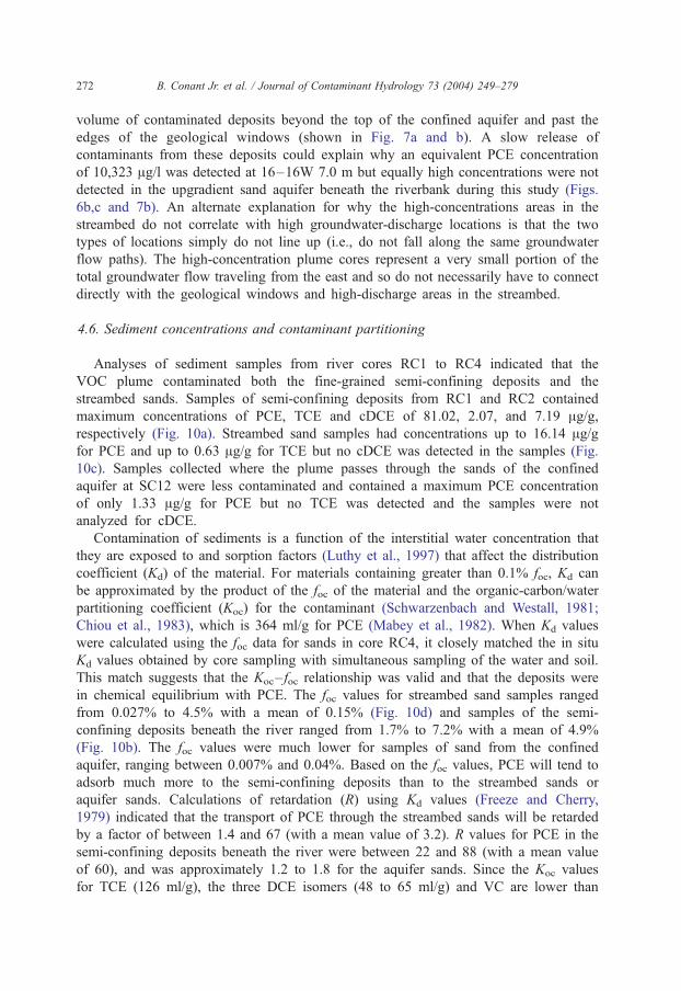
4.6. Sediment concentrations and contaminant partitioning

Analyses of sediment samples from river cores RC1 to RC4 indicated that the

VOC plume contaminated both the fine-grained semi-confining deposits and the

streambed sands. Samples of semi-confining deposits from RC1 and RC2 contained

maximum concentrations of PCE, TCE and cDCE of 81.02, 2.07, and 7.19 Ag/g,respectively (Fig. 10a). Streambed sand samples had concentrations up to 16.14 Ag/gfor PCE and up to 0.63 Ag/g for TCE but no cDCE was detected in the samples (Fig.

10c). Samples collected where the plume passes through the sands of the confined

aquifer at SC12 were less contaminated and contained a maximum PCE concentration

of only 1.33 Ag/g for PCE but no TCE was detected and the samples were not

analyzed for cDCE.

Contamination of sediments is a function of the interstitial water concentration that

they are exposed to and sorption factors (Luthy et al., 1997) that affect the distribution

coefficient (Kd) of the material. For materials containing greater than 0.1% foc, Kd can

be approximated by the product of the foc of the material and the organic-carbon/water

partitioning coefficient (Koc) for the contaminant (Schwarzenbach and Westall, 1981;

Chiou et al., 1983), which is 364 ml/g for PCE (Mabey et al., 1982). When Kd values

were calculated using the foc data for sands in core RC4, it closely matched the in situ

Kd values obtained by core sampling with simultaneous sampling of the water and soil.

This match suggests that the Koc– foc relationship was valid and that the deposits were

in chemical equilibrium with PCE. The foc values for streambed sand samples ranged

from 0.027% to 4.5% with a mean of 0.15% (Fig. 10d) and samples of the semi-

confining deposits beneath the river ranged from 1.7% to 7.2% with a mean of 4.9%

(Fig. 10b). The foc values were much lower for samples of sand from the confined

aquifer, ranging between 0.007% and 0.04%. Based on the foc values, PCE will tend to

adsorb much more to the semi-confining deposits than to the streambed sands or

aquifer sands. Calculations of retardation (R) using Kd values (Freeze and Cherry,

1979) indicated that the transport of PCE through the streambed sands will be retarded

by a factor of between 1.4 and 67 (with a mean value of 3.2). R values for PCE in the

semi-confining deposits beneath the river were between 22 and 88 (with a mean value

of 60), and was approximately 1.2 to 1.8 for the aquifer sands. Since the Koc values

for TCE (126 ml/g), the three DCE isomers (48 to 65 ml/g) and VC are lower than


that for PCE, Kd and R values for the other VOCs were also smaller. In general, the

plume would move relatively quickly and unretarded through the confined aquifer but

then move quite slowly beneath the streambed where large amounts of sorption would

occur.

Since the plume has been migrating to the river for decades, the semi-confining

deposits have likely accumulated (adsorbed) many kilograms of VOC contamination.

Even if the upgradient source of PCE at the dry cleaner is remediated, the low vertical

groundwater flow velocities (0.016 to 5.1�10� 5 m/day) and high R factors in the semi-

confining deposits could cause the plume to take decades to hundreds of years to flush

completely clean under natural conditions. Travel time calculations indicate that, on

average, it would take about 4.7 years for PCE to travel through 2 m of silty sand deposits

and about 390 years to travel through 2 m of silty clay deposits of the semi-confining

deposits. Another concern is that this mass of contaminated sediment can be eroded and

carried downstream. While sediments are being transported, they may not have sufficient

time to desorb their contaminants prior to being redeposited and buried (Cheng et al.,

1995; Rathbun, 1998) and may be detectable further downstream. Even if contaminated

sediments are eroded away and transported downstream, the clean materials that are

redeposited in their place will be subsequently contaminated by the continued discharge of

the groundwater plume.

4.7. Surface-water concentrations

The first two surface-water sampling events in June and October 1996 (consisting of 23

samples) resulted in non-detectable levels for all VOCs except for three samples

containing less than 1.6 Ag/l PCE. Additional sampling over the next few years confirmed

these findings with only 5 of 48 samples containing PCE and 5 containing TCE. The

highest PCE concentration was 23.2 Ag/l observed at PRP12, which was immediately

downstream of an underwater spring that was discharging groundwater containing up to

806 Ag/l of PCE and 3.8 Ag/l of TCE. The other surface-water samples that detected PCE

and TCE had concentrations that were less than 3.1 and 3.2 Ag/l, respectively. However,the TCE is likely an artifact of incomplete decontamination of the mini-profiler used for

those five samples. None of the 71 surface-water analyses detected 11DCE, cDCE, tDCE,

VC, ethene or ethane. The lack of cDCE in the surface water is somewhat surprising since

the cDCE plume was larger and had higher concentrations than the PCE plume (Fig. 8a

and b, respectively). Possible explanations are that either the cDCE plume mass fluxes are

low even though the streambed concentrations are high or that the cDCE aerobically

biodegrades (Bradley and Chapelle, 1998) in the top 0.3 m of the streambed prior to

reaching the surface water.

Fig. 8d shows that the PCE detected in surface water is generally found either within or

downstream of the places where PCE is discharging through the streambed (Fig. 8a). PCE

contamination in the streambed seems to coincide with or is down gradient of high

groundwater-discharge zones (Fig. 3b), which likely explains why the discharging PCE is

detectable in the surface water and has not been diluted to non-detectable levels at those

locations. A simple dilution calculation indicated the average surface-water concentration

would be 0.16 Ag/l and thus below detection limits even in this worse case scenario where


the entire mass of PCE migrating toward the river along transect 5 is instantaneously

mixed with river water under low flow conditions (1.39 m3/s).

4.8. Potential adverse ecological effects of the discharging plume

In this study, potential adverse ecological effects on aquatic life were inferred by

comparing observed water and sediment concentrations to published criteria and guide-

lines for protecting aquatic life. In the surface water, all the PCE and TCE concen-

trations detected were considerably lower than established freshwater aquatic life

guidelines and would likely not trigger further regulatory actions. USEPA ambient

water quality criteria for PCE in freshwater is set at 5280 Ag/l for acute toxicity and 840

Ag/l for chronic toxicity (USEPA, 1986) and the values for TCE are even higher. The

interim Canadian water quality guidelines for the protection and maintenance of

freshwater aquatic life (which are long-term no-effect levels) issued by the CCME

(Canadian Council of Ministers of the Environment, 1993) are 110 and 20 Ag/l for PCEand TCE, respectively. However, surface water guidelines are also used to assess

interstitial water quality of the streambed because the organisms there are believed to

be equally sensitive to contaminants as those in the water column, even though there

may be unique benthic and hyporheic-zone aquatic organisms in the streambed that have

different sensitivities. Using this guideline approach, it appears the plume may be

causing adverse ecological effects in the streambed; 9 out of 53 locations that detected

VOC contamination during the 1998 mapping of the streambed contained PCE

concentrations higher than CCME guidelines and the USEPA chronic toxicity guideline

was exceeded at one of those locations. Three locations had TCE concentrations that

exceeded the CCME guidelines. Assessing the potential impacts of the cDCE, tDCE,

11DCE, and VC found in the streambed is problematic since USEPA chronic toxicity

and CCME guidance levels have not been established for them. Furthermore, the

published criteria do not take into account the potentially synergistic effects of exposing

aquatic life to multiple contaminants simultaneously.

Adverse ecological effects might also occur as a result of aquatic life coming into

contact or ingesting contaminated streambed sediments. Even though VOCs are much

more volatile and have far lower bioconcentration factors than more recalcitrant

contaminants like PCB and polyaromatic hydrocarbons, chronic exposures to VOCs

are still possible in the streambed because the dissolved-phase groundwater plume

emanates from a relatively long-lived and continuous DNAPL source. Nonetheless,

neither the USEPA or CCME have established freshwater guidelines for PCE or it’s

degradation products in sediments. Furthermore, the set of screening quick reference

tables (SquiRTs) for contaminants in water, soil, and sediments compiled from several

sources by the National Oceanic and Atmospheric Administration (Buchman, 1998)

indicate there were no freshwater sediment guidelines for any of the 32 volatile

aromatic and halogenated compounds they listed. However, the concentrations of some

sediment samples were higher than ecological toxicity screening criteria (USEPA,

1996) and/or the U.S. Department of Energy (USDOE) preliminary remediation goals

(Efroymson et al., 1997), and so would likely trigger further investigations (if these

guidelines were applied). Given the complex nature of the exposures in the streambed,


direct in situ toxicity methods (Chappie and Burton, 2000; Greenberg et al., 2002)

would likely be a more successful approach to accurately assess the adverse effects of

this plume at discharge areas. There is a need for more ecotoxicological research to

establish toxicity criteria for volatile organic compounds in freshwater environments

and also to evaluate how the areas contaminated by groundwater plumes affect the

overall health of the river.

5. Implications for monitoring the streambed and river

The results of this study clearly illustrate that monitoring and characterizing a

discharging plume is a challenge because of the fine-scale heterogeneous nature of the

plume, geology, and groundwater discharge. For example, the four vertical concentration

profiles shown in Fig. 9 illustrate the high spatial variability in the plume vertically and

laterally and begs the question of how many samples and at what depth should samples be

collected to adequately characterize the site (n.b., profiles were done at different times but

PRP15 and MLS17 are only 0.4 m apart while PRP7 and PRP8R are 2 m apart). Spatial

variability in sediment concentrations were also seen (Fig. 10) and again raises the

question of what depth should sampling be done to obtain ‘‘representative’’ samples. Even

the selection of surface-water monitoring locations must be done with care, otherwise one

may choose sampling locations that never detect contamination even when there are

distinct areas where contamination of surface water continuously occurs. Although this

plume is very well characterized, one could still argue that even more investigations would

be necessary to resolve some unanswered questions such as what happened to the northern

high-concentration plume core? Many VOC plumes at hazardous waste sites are much

larger than the Angus plume and discharge to even larger rivers, so the idea of having to

monitor a plume on an equally fine scale over a much larger area is daunting. However, if

too few monitoring points are used, one may miss high-concentration ‘‘hot spots’’, high-

discharge, or high-biodegradation areas and potentially draw erroneous conclusions

regarding the potential impact of the plume. To determine how much monitoring is

enough one must first clearly define the questions that need answering and overall goals of

the investigation. Hydrogeologists and ecologists need to coordinate their efforts (USEPA,

2000) to develop more effective monitoring strategies for ecological risk assessments. The

key is to find quick and low cost ways to characterize the heterogeneity of both the

hydrogeological systems (e.g., Conant, 2004; Vroblesky et al., 1996) and ecological

systems and then target a subset of representative (or critical) problem areas for further in-

depth studies. Since the variability of the hydrogeologic and ecological systems may be

quite different, monitoring should be done on a fine enough scale to assure that significant

areas of adverse ecological impacts are not missed.

6. Conclusions

This study provides the first comprehensive assessment of a PCE groundwater plume

discharging into a river and shows that the near-stream zone substantially modifies the


distribution, concentration, and composition of the plume prior to its reaching the

surface water. The complex concentration distribution observed in the streambed was

caused by: (1) temporal and spatial variations in the dissolved phase contaminant plume

that is emanating from a DNAPL source and is entering the near-stream zone; (2) low-

hydraulic conductivity silty-clay semi-confining deposits beneath the river that affect

groundwater discharge into the river; (3) extensive biodegradation within the top 2.5 m

of the streambed that changes the composition of the plume; and (4) sorption of

contaminants to high foc streambed deposits. Locating the plume in the aquifer

upgradient of the river was useful in predicting the section of river where the plume

would discharge and the potential range of concentrations headed toward the stream

(e.g., plume cores with >10,000 Ag/l of PCE); however, it did not provide an accurate

image of what the concentration distribution or composition of the plume would be in

the streambed. Of the various factors affecting the plume, biodegradation occurring in

the shallow streambed deposits had the greatest effect because it altered the composition

and potentially changed the overall toxicity of the plume by producing cDCE and VC

and, to a lesser extent, TCE, 11DCE, tDCE, ethene, and ethane. The degree of

biodegradation in the streambed was not uniform and approximately 54% of the

plan-view area of the VOC plume consisted solely of PCE degradation products.

High-concentration areas in the streambed did not coincide with the groundwater

discharge areas but were associated with low groundwater discharge areas and may

represent adsorbed or retarded high-concentration remnants of the plume that have yet

to travel all the way through the high foc semi-confining deposits. Despite the relatively

large area of VOCs discharging through the streambed, rapid dilution by clean river

water caused the VOCs to be rarely detected in surface water. The low concentrations

of PCE that were detected (usually less than 3.2 Ag/l but once as high as 23.2 Ag/l)were generally found at or downstream of high groundwater-discharge locations.

Surface-water concentrations were well below Canadian ‘‘no-adverse-effect’’ levels

and USEPA chronic toxicity guidelines for freshwater aquatic life; however, at several

locations the high-VOC concentrations within the streambed were higher than those

levels and so may represent a hazard to benthic and hyporheic aquatic life. In this study,

testing of surface water samples gave no indication of the large amounts of cDCE or

VC and other VOCs present in the streambed and; therefore, this study clearly

demonstrates that to characterize the nature of a discharging plume one cannot rely

on surface-water sampling and that one must investigate the interstitial water quality of

the streambed.

Acknowledgements

Several individuals assisted in the collection of field data and performing laboratory

analysis and those that deserve particular thanks include M. Bogaart, T. Praamsma, J. Roy,

B. Gunn, J. and B. Ingelton, P. Johnson, D. Thomson, S. Chapman, R. Gibson, T. Jung, J.

Levenick, S. Sale, D. Redman, W. Nobel, G. Friday, H. Groenevelt, M. Gorecka, and S.

O’Hannesin. We are grateful to Mr. Murray McMaster and his family for allowing access

to the field site. We also wish to thank the reviewers D. Vroblesky and P. Adriaens.


Funding for this research was provided by the University Consortium Solvents-In-

Groundwater Research Program, the Natural Science and Engineering Research Council,

and an Ontario Graduate Scholarship in Science and Technology.

References

Avery, C., 1994. Interaction of ground water with the Rock River near Byron, Illinois. U.S. Geological Survey

Water-Resources Investigations Report 94-4034.

Beebe, J.T., 1997. Fluid patterns, sediment pathways and woody obstructions in the Pine River, Angus, Ontario.

PhD dissertation, Department of Geography and Environmental Studies, Wilfrid Laurier University.

Beneteau, K.M., 1996. Chlorinated solvent fingerprinting using 13C and 37Cl isotopes. MSc dissertation, De-

partment of Earth Sciences, University of Waterloo.

Beneteau, K.M., Aravena, R., Frape, S.K., 1999. Isotopic characterization of chlorinated solvents—laboratory

and field results. Org. Geochem. 30, 739–753.

Bianchi-Mosquera, G.C., Mackay, D.M., 1992. Comparison of stainless steel vs. PTFE miniwells for monitoring

halogenated organic solute transport. Ground Water Monit. Rev. 12 (4), 126–131.

Boulton, A.J., Findlay, S., Marmonier, P., Stanley, E.H., Valett, H.M., 1998. The functional significance of the

hyporheic zone in streams and rivers. Ann. Rev. Ecolog. Syst. 29, 59–81.

Bradley, P.M., Chapelle, F.H., 1998. Effect of contaminant concentration on aerobic microbial mineralization of

DCE and VC in stream-bed sediments. Environ. Sci. Technol. 32 (5), 553–557.

Brunke, M., Gonser, T., 1997. The ecological significance of exchange processes between rivers and ground-

water. Freshw. Biol. 37 (1), 1–33.

Buchman, M.F., 1998. NOAA screening quick reference tables, NOAA HAZMAT Report 97-2, Seattle WA,

Hazardous Materials Response and Assessment Division, National Oceanic and Atmospheric Administration.

Burkard, M.B., 1990. Bed load measurements: Nottawasaga River and selected tributaries, Ontario, Canada.

M.A. Dissertation, Department of Geography and Environmental Studies, Wilfrid Laurier University.

Canadian Council of Ministers of the Environment, 1993. Canadian water quality guidelines, Task Force on

Water Quality Guidelines.

Chappie, D.J., Burton Jr., G.A., 2000. Applications of aquatic and sediment toxicity testing in situ. J. Soil

Sediment. Contam. 9 (3), 219–246.

Cheng, C.-Y., Atkinson, J.F., DePinto, J.V., 1995. Desorption during resuspension events: kinetic v. equilibrium

model. Mar. Freshw. Res. 46 (1), 251–256.

Cherry, J.A., 1996. Conceptual models for chlorinated solvent plumes and their relevance to intrinsic reme-

diation. Symposium on Natural Attenuation of Chlorinated Organics in Ground Water, Dallas, Texas,

September 11–13, 1996. U.S. Environmental Protection Agency, Office of Research and Development,

Washington, DC, pp. 29–30. EPA/540/R-96/509.

Chiou, C.T., Porter, P.E., Schmedding, D.W., 1983. Partition equilibria of nonionic organic compounds between

soil organic matter and water. Environ. Sci. Technol. 17, 227–231.

Church, P.E., Vroblesky, D.A., Lyford, F.P., Willey, R.E., 2002. Guidance on use of passive-vapor-diffusion

samplers to detect volatile organic compounds in ground-water discharge areas, and example applications in

New England. U.S. Geological Survey Water-Resources Investigations Report 02-4186.

Churcher, P.L., Dickout, R.D., 1987. Analysis of ancient sediments for total organic carbon—some new ideas.

Journal of Geochemical Exploration 29, 235–246.

Conant Jr., B., 2001. A PCE plume discharging to a river: investigations of flux, geochemistry, and biodegra-

dation in the streambed. PhD dissertation, Department of Earth Sciences, University of Waterloo.

Conant Jr., B., 2004. Delineating and quantifying ground-water discharge using streambed temperatures. Ground

Water 42 (2), 243–257.

Dahm, C.N., Grimm, N.B., Marmonier, P., Valett, H.M., Vervier, P., 1998. Nutrient dynamics at the interface

between surface waters and groundwaters. Freshw. Biol. 40 (3), 427–451.

de Oliveira, E., 1997. Ethanol flushing of gasoline residuals—microscale and field scale experiments. PhD

dissertation, Department of Earth Sciences, University of Waterloo.


Efroymson, R.A., Suter II, G.W., Sample, B.E., Jones, D.S. 1997. Preliminary remediation goals for eco-

logical endpoints, U.S. Department of Energy, Office of Environmental Management. USDOE Report

ES/ER/TM-162/R2.

Freeze, R.A., Cherry, J.A., 1979. Groundwater. Prentice-Hall, Englewood Cliffs, NJ.

Gibert, J., Danielopol, D.L., Stanford, J.A. (Eds.), 1994. Groundwater Ecology. Academic Press, San Diego, CA.

Greenberg, M.S., Burton Jr., G.A., Rowland, C.D., 2002. Optimizing interpretation of in situ effects of riverine

pollutants: impact of upwelling and downwelling. Environ. Toxicol. Chem. 21 (2), 289–297.

Guilbeault, M.A., Parker, B.L., Cherry, J.A., in press. Mass and flux distributions from DNAPL zones in sandy

aquifers. Ground Water.

Guyonnet, D.A., 1991. Numerical modeling of effects of small-scale sedimentary variations on groundwater

discharge into lakes. Limnol. Oceanogr. 36 (4), 787–796.

Hendricks, S.P., White, D.S., 1991. Physicochemical patterns within a hyporheic zone of a northern Michigan

river, with comments on surface water patterns. Can. J. Fish. Aquat. Sci. 48 (9), 1645–1654.

Hendricks, S.P., White, D.S., 1995. Seasonal biogeochemical patterns in surface water, subsurface hyporheic, and

riparian ground water in a temperate stream ecosystem. Arch. Hydrobiol. 134 (4), 459–490.

Hess, E.C., Parks, J.H., Cook, J.K., 1989. The application of seepage meter technology to the monitoring of

hazardous waste sites. In: Erickson, L.E. (Ed.), Proceedings of the Conference on Hazardous Waste

Research, Manhattan, Kansas, May 23–24, 1989. Engineering Extension Kansas State University, Man-

hattan, KS, pp. 358–367.

Huggenberger, P., Hoehn, E., Beschta, R., Woessner, W., 1998. Abiotic aspects of channels and floodplains in

riparian ecology. Freshw. Biol. 40 (3), 407–425.

Hughes, B.M., McClellan, R.D., Gillham, R.W., 1992. Application of soil –gas sampling technology to studies

of trichloroethylene vapor transport in the unsaturated zone. In: Lesage, S., Jackson, R.E. (Eds.), Ground-

water Contamination and Analysis at Hazardous Waste Sites. Marcel Dekker, New York, pp. 121–146.

Chap. 5.

Hunkeler, D., Chollet, N., Pittet, X., Aravena, R., Cherry, J.A., Parker, B.L., in press. Effect of source variability

and transport processes on carbon isotope ratios of TCE and PCE in two sandy aquifers. Journal of Con-

taminant Hydrology.

Hvorslev, M.J., 1951. Time lag and soil permeability in ground-water observations Bulletin 36: U.S. Army Corps

of Engineers, Waterways Experiment Station, Vicksburg Mississippi.

Hynes, H.B.N., 1970. Ecology of Running Waters. University of Toronto Press, Toronto, Ontario.

Jones, C., 1999. 1998 Watershed Health Monitoring Summary. Nottawasaga Valley Conservation Authority,

Angus, Ontario.

Lee, D.R., Cherry, J.A., 1978. A field exercise on groundwater flow using seepage meters and mini-piezometers.

J. Geol. Educ. 27, 6–10.

Lorah, M.M., Olsen, D.L., 1999. Natural attenuation of chlorinated volatile organic compounds in a freshwater

tidal wetland: field evidence of anaerobic biodegradation. Water Resour. Res. 35 (12), 3811–3827.

Lorah, M.M., Olsen, L.D., Smith, B.L., Johnson, M.A., Fleck, W.B., 1997. Natural attenuation of chlorinated

volatile organic compounds in a freshwater tidal wetland, Aberdeen Proving Ground, Maryland. U.S. Geo-

logical Survey Water-Resources Investigations Report 97-4171.

Luthy, R.G., Aiken, G.R., Brusseau, M.L., Cunningham, S.D., Gschwend, P.M., Pignatello, J.J., Reinhard, M.,

Traina, S.J., Weber Jr., W.J., Westall, J.C., 1997. Sequestration of hydrophobic organic contaminants by

geosorbents. Environ. Sci. Technol. 31 (12), 3341–3347.

Lyford, F.P., Flight, L.E., Stone, J.R., Clifford, S., 1999. Distribution of trichloroethylene and geological controls

on contaminant pathways near the Royal River, McKin Superfund site area, Gray, Maine. U.S. Geological

Survey Water-Resources Investigations Report 99-4125.

Mabey, W.R., Smith, J.R., Podoll, R.T., Johnson, H.L., Mill, T., Chou, T.-W., Gates, J., Vandenberg, D., 1982.

Aquatic Fate Processes Data for Organic Priority Pollutants U.S. Environmental Protection Agency, Wash-

ington, DC EPA 440/4-81-014.

Mackay, D.M., Freyberg, D.L., Roberts, P.V., Cherry, J.A., 1986. A natural gradient experiment on solute

transport in a sand aquifer: 1. Approach and overview of plume movement. Water Resour. Res. 22 (13),

2017–2029.

Norman, W.R., Ostrye, D.P., Hobin, J.S., 1986. Use of seepage meters to quantify groundwater discharge and


contaminant flux into surface water at the Baird and McGuire site (NPL No. 14). Proceedings of the Third

Annual Eastern Regional Ground Water Conference, Springfield, Massachusetts, July 28–30, 1986. National

Water Well Association, Dublin, OH, pp. 472–493.

Pitkin, S.E., 1994. A point sample profiling approach to the investigation of groundwater contamination. MSc

dissertation, Department of Earth Sciences, University of Waterloo.

Pitkin, S.E., Ingelton, R.A., Cherry, J.A., 1994. Use of a drive point sampling device for detailed characterization

of a PCE plume in a sand aquifer at a dry cleaning facility. Proceedings of the Eight National Outdoor Action

Conference and Exposition, Aquifer Remediation/Ground Water Monitoring/Geophysical Methods, Minne-

apolis, Minnesota, May 23–25, 1994. National Ground Water Association, Columbus, OH, pp. 1–18.

Pitkin, S.E., Cherry, J.A., Ingelton, R.A., Broholm, M., 1999. Field demonstrations using the Waterloo ground

water profiler. Ground Water Monit. Remediat. 19 (2), 122–131.

Rathbun, R.E., 1998. Transport, behavior, and fate of volatile organic compounds in streams. U.S. Geological

Survey Professional Paper 1589.

Savoie, J.G., Lyford, F.P., Clifford, S., 1999. Potential for advection of volatile organic compounds in ground-

water to the Cochato River, Baird and McGuire Superfund site, Holbrook, Massachusetts, March and April

1998. U.S. Geological Survey Water-Resources Investigations Report 98-4257.

Schwarzenbach, R.P., Westall, J., 1981. Transport of nonpolar organic compounds from surface water to ground-

water. Laboratory sorption studies. Environ. Sci. Technol. 15 (11), 1360–1367.

Starr, R.C., Ingelton, R.A., 1992. A new method for collecting core samples without a drilling rig. Ground Water

Monit. Rev. 12 (1), 91–95.

Sudicky, E.A., 1986. A natural gradient experiment on solute transport in a sand aquifer: spatial variability of

hydraulic conductivity and its role in the dispersion process. Water Resour. Res. 22 (13), 2069–2082.

Tabatabi, M.A., Bremner, J.M., 1970. Use of the Leco automatic 70-second carbon analyzer for total carbon

analysis of soils. Soil Sci. Soc. Am. Proc. 34, 608–610.

USEPA, 1986. Quality criteria for water 1986. U.S. Environmental Protection Agency, Office of Water Regu-

lations and Standards. EPA 440/5-86-001.

USEPA, 1991. Superfund NPL Characterization Project: National Results. U.S. Environmental Protection Agen-

cy, Office of Emergency and Remedial Response. EPA/540/8-91/069.

USEPA, 1996. EcoTox Thresholds (computer program) Version dated June 10, 1996. Based on Eco update:

Ecotox thresholds. U.S. Environmental Protection Agency, Office of Solid Waste and Emergency Response.

EPA 540/F-95/083.

USEPA, 2000. Proceedings of the ground-water/surface-water interactions workshop. Environmental Protection

Agency, Office of Solid waste and Emergency Response. EPA/542/R-00/007.

Vroblesky, D.A., Lorah, M.M., Trimble, S.P., 1991. Mapping zones of contaminated ground-water discharge

using creek-bottom-sediment vapor samplers, Aberdeen Proving Ground Maryland. Ground Water 29 (1),

7–12.

Vroblesky, D.A., Rhodes, L.C., Robertson, J.F., Harrigan, J.A., 1996. Locating VOC contamination in a frac-

tured-rock aquifer at the ground-water/surface-water interface using passive vapor collectors. Ground Water

34 (2), 223–230.

Ward, J.V., Bretschko, G., Brunke, M., Danielopol, D., Gibert, J., Gonser, T., Hildrew, A.G., 1998. The bound-

aries of river systems: the metazoan perspective. Freshw. Biol. 40 (3), 531–569.

Wiedemeier, T.H., Rifai, H.S., Newell, C.J., Wilson, J.T., 1999. Natural Attenuation of Fuel and Chlorinated

Solvents in the Subsurface. John Wiley & Sons, New York.

Winter, T.C., LaBaugh, J.W., Rosenberry, D.O., 1988. The design and use of a hydraulic potentiomanometer for

direct measurement of differences in hydraulic head between groundwater and surface water. Limnol. Ocean-

ogr. 33 (5), 1209–1214.

Woessner, W.W., 2000. Stream and fluvial plain ground water interactions: rescaling hydrogeologic thought.

Ground Water 38 (3), 423–429.

Writt, R.J., 1996. The Angus PCE plume—Aquifer sedimentology and plume anatomy. MSc Project Report.

Department of Earth Sciences, University of Waterloo.

Documents

A PCE groundwater plume discharging to a river: … Organic Chemicals...A PCE groundwater plume discharging to a river: influence of the streambed and near-river zone on contaminant