Embed Size (px)
Citation preview

University of Central Florida University of Central Florida
STARS STARS
HIM 1990-2015
2014
Modeling Financial Markets Using Concepts From Mechanical Modeling Financial Markets Using Concepts From Mechanical
Vibrations and Mass-Spring Systems Vibrations and Mass-Spring Systems
Michael Gandia University of Central Florida
Part of the Mechanical Engineering Commons
Find similar works at: https://stars.library.ucf.edu/honorstheses1990-2015
University of Central Florida Libraries http://library.ucf.edu
This Open Access is brought to you for free and open access by STARS. It has been accepted for inclusion in HIM
1990-2015 by an authorized administrator of STARS. For more information, please contact [email protected].
Recommended Citation Recommended Citation Gandia, Michael, "Modeling Financial Markets Using Concepts From Mechanical Vibrations and Mass-Spring Systems" (2014). HIM 1990-2015. 1638. https://stars.library.ucf.edu/honorstheses1990-2015/1638

MODELING FINANCIAL MARKETS USING CONCEPTS
FROM MECHANICAL VIBRATIONS
AND MASS-SPRING SYSTEMS
by
MICHAEL XAVIER GANDIA
A thesis submitted in partial fulfillment of the requirements
for the Honors in the Major Program in Mechanical Engineering
in the College of Engineering and Computer Science
and in the Burnett Honors College
at the University of Central Florida
Orlando, Florida
Summer Term 2014
Thesis Chair: Dr. Tuhin Das

ii
ABSTRACT
This thesis describes a method of modeling financial markets by utilizing concepts from
mechanical vibration. The models developed represent multi-degree of freedom, mass-spring
systems. The economic principles that drive the design are supply and demand, which act as
springs, and shareholders, which act as masses. The primary assumption of this research is that
events cannot be predicted but the responses to those events can be. In other words, economic
stimuli create responses to a stock’s price that is predictable, repeatable and scientific. The
approach to determining the behavior of various financial markets encompassed techniques such
as Fast Fourier Transform and discretized wavelet analysis. The researched developed in three
stages; first an appropriate model of causation in the stock market was established. Second, a
model of steady state properties was determined. Third, experiments were conducted to
determine the most effective model and to test its predictive capabilities on ten stocks. The
experiments were evaluated based on the model’s hypothetical return on investment. The
results showed a positive gain on capital for nine out of the ten stocks and supported the claim
that stocks behave in accordance to the natural laws of vibration. As scientific approaches to
modeling the stock market are beginning to develop, engineering principles are proving to be the
most relevant and reliable means of financial market prediction.

iii
ACKNOWLEDGEMENTS
I would like to thank my Thesis Chair, Tuhin Das, for helping me develop my research and my
professor, Dr. Avelino Gonzalez, for his guidance in writing this thesis. I would also like to thank
my committee members, Dr. Kassab and Dr. Ford.

iv
TABLE OF CONTENTS CHAPTER ONE: INTRODUCTION ...................................................................................................... iv
1.1 Introduction...................................................................................................................... 1
1.2 Historical Background ...................................................................................................... 3
1.2.1 Stock Prediction before Numerical Methods ........................................................... 3
1.2.2 Computational Analysis & the Development of Algorithmic Trading ...................... 5
1.2.3 Methods of Algorithmic Trading ............................................................................... 6
1.2.4 The Effects of Algorithmic Trading ......................................................................... 10
1.2.5 The Future of Financial Market Prediction ............................................................. 13
1.3 Summary of Chapter One ............................................................................................... 16
CHAPTER TWO: STATE OF THE ART REVIEW ................................................................................. 18
2. 1 The Specific Problem ...................................................................................................... 18
2.1.1 Prediction & Principles ............................................................................................ 18
2.1.2 Laws of Vibration & the Stock Market ......................................................................... 19
2.2 The State of the Art ........................................................................................................ 22
2.2.1 Early Attempts of Vibration Analysis in the Stock Market ........................................... 22
2.2.2 Modern Day Research of Cycles and Stocks ........................................................... 24
2.2.3 Factors to Consider ................................................................................................. 29
2.3 Summary of Chapter Two ................................................................................................... 31
CHAPTER THREE: PROBLEM DEFINITION ...................................................................................... 33
3.1 The Technical Area ......................................................................................................... 33
3.2 The General Problem ..................................................................................................... 33
3.3 The Specific Problem ...................................................................................................... 34
3.4 The Hypothesis ............................................................................................................... 34
3.5 The Major and Minor Contribution ................................................................................ 35
3.6 Novelty, Significance and Usefulness ............................................................................. 35
CHAPTER FOUR: APPROACH ......................................................................................................... 37
4.1 Causation of Change ...................................................................................................... 37
4.1.1 Forced Versus Free Vibration.................................................................................. 37
4.1.2 Boundary Conditions............................................................................................... 39
4.1.3 Impulsive Forces ..................................................................................................... 40
4.2 Steady State Vibration ......................................................................................................... 41
4.3 Transient Responses............................................................................................................ 42
4.4 Error Calculations ................................................................................................................ 42

v
4.5 Phase Finding ...................................................................................................................... 43
4.6 Frequency Refinement ........................................................................................................ 43
CHAPTER FIVE: TESTING AND EVALUATION ................................................................................. 46
5.1 Unit Testing .................................................................................................................... 46
5.1.1 Causation Tests ....................................................................................................... 46
5.1.2 Steady State Tests ................................................................................................... 46
5.2 System Tests ................................................................................................................... 47
5.2.1 Ideology of Trading and Evaluation ........................................................................ 47
5.2.2 Method ................................................................................................................... 48
5.2.3 Evaluation ............................................................................................................... 48
CHAPTER SIX: EXPERIMENT & RESULTS ........................................................................................ 50
6.1 Experiment #1: Determining the Most Effective Model ..................................................... 50
6.2 Experiment #2: Evaluation of Financial Model ................................................................... 51
6.2.1 Experimental Set Up ..................................................................................................... 51
6.2.2 Procedure ..................................................................................................................... 51
6.2.3 Stocks 1-5 Results ......................................................................................................... 55
6.2.4 Stocks 6-10 Results ....................................................................................................... 61
6.2.5 Conclusion of Results .................................................................................................... 72
CHAPTER SEVEN: CONCLUSION .................................................................................................... 73
7.1 Overall Conclusion of Research ........................................................................................... 73
7.2 Research Improvements ..................................................................................................... 74
7.3 Future Work ........................................................................................................................ 75
APPENDIX ...................................................................................................................................... 76
LIST OF REFERENCES ..................................................................................................................... 82

vi
LIST OF TABLES Table 1: Example of Order Book ..................................................................................................... 6
Table 2: Results from All Six Stocks ............................................................................................... 26
Table 3: Stock #1 FALC Results ...................................................................................................... 55
Table 4: Stock #2 MENT Results .................................................................................................... 57
Table 5: Stock #3 SINA Results ...................................................................................................... 58
Table 6: Stock #4 RNWK ................................................................................................................ 59
Table 7: Stock #5 ABMD Results ................................................................................................... 60
Table 8: Stock #6 DOW Results ..................................................................................................... 62
Table 9: Stock #7 GOOG Results ................................................................................................... 63
Table 10: Stock #8 PFE Results ...................................................................................................... 64
Table 11: Stock #9 TM Results ...................................................................................................... 67
Table 12: Stock #10 Results .......................................................................................................... 68
Table 13: Observation TSLA .......................................................................................................... 70
Table 14: Summary of Experiment #2 Results .............................................................................. 72
vii
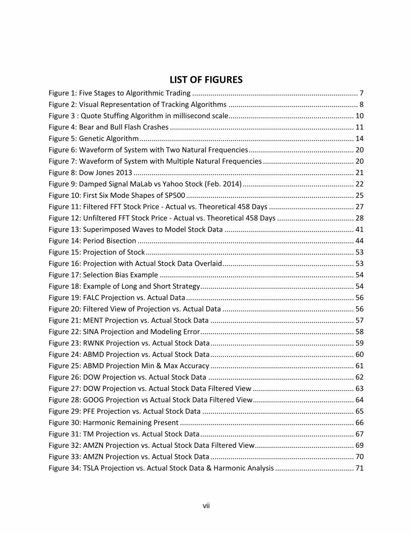
LIST OF FIGURES Figure 1: Five Stages to Algorithmic Trading .................................................................................. 7
Figure 2: Visual Representation of Tracking Algorithms ................................................................ 8
Figure 3 : Quote Stuffing Algorithm in millisecond scale.............................................................. 10
Figure 4: Bear and Bull Flash Crashes ........................................................................................... 11
Figure 5: Genetic Algorithm .......................................................................................................... 14
Figure 6: Waveform of System with Two Natural Frequencies .................................................... 20
Figure 7: Waveform of System with Multiple Natural Frequencies ............................................. 20
Figure 8: Dow Jones 2013 ............................................................................................................. 21
Figure 9: Damped Signal MaLab vs Yahoo Stock (Feb. 2014) ....................................................... 22
Figure 10: First Six Mode Shapes of SP500 ................................................................................... 25
Figure 11: Filtered FFT Stock Price - Actual vs. Theoretical 458 Days .......................................... 27
Figure 12: Unfiltered FFT Stock Price - Actual vs. Theoretical 458 Days ...................................... 28
Figure 13: Superimposed Waves to Model Stock Data ................................................................ 41
Figure 14: Period Bisection ........................................................................................................... 44
Figure 15: Projection of Stock ....................................................................................................... 53
Figure 16: Projection with Actual Stock Data Overlaid ................................................................. 53
Figure 17: Selection Bias Example ................................................................................................ 54
Figure 18: Example of Long and Short Strategy ............................................................................ 54
Figure 19: FALC Projection vs. Actual Data ................................................................................... 56
Figure 20: Filtered View of Projection vs. Actual Data ................................................................. 56
Figure 21: MENT Projection vs. Actual Stock Data ....................................................................... 57
Figure 22: SINA Projection and Modeling Error ............................................................................ 58
Figure 23: RWNK Projection vs. Actual Stock Data ....................................................................... 59
Figure 24: ABMD Projection vs. Actual Stock Data ....................................................................... 60
Figure 25: ABMD Projection Min & Max Accuracy ....................................................................... 61
Figure 26: DOW Projection vs. Actual Stock Data ........................................................................ 62
Figure 27: DOW Projection vs. Actual Stock Data Filtered View .................................................. 63
Figure 28: GOOG Projection vs Actual Stock Data Filtered View.................................................. 64
Figure 29: PFE Projection vs. Actual Stock Data ........................................................................... 65
Figure 30: Harmonic Remaining Present ...................................................................................... 66
Figure 31: TM Projection vs. Actual Stock Data ............................................................................ 67
Figure 32: AMZN Projection vs. Actual Stock Data Filtered View ................................................. 69
Figure 33: AMZN Projection vs. Actual Stock Data ....................................................................... 70
Figure 34: TSLA Projection vs. Actual Stock Data & Harmonic Analysis ....................................... 71

1
CHAPTER ONE: INTRODUCTION
1.1 Introduction
The concept of predicting and modeling the stock market has always been an exciting yet eluding
topic of research. Businessmen, academics, scientists and the ordinary man have been on a
ceaseless pursuit to understand its behavior for decades. Researchers have developed an array
of techniques that range from statistical analysis to dynamic millisecond algorithms. As
computational analysis is only becoming more prevalent today, the presence of algorithms and
their effects are continuing to grow in the market. Algorithmic trading operates at ultra-high
frequencies allowing millions of trades to be made every second. This type of trading is beginning
to consume the daily trading patterns of the financial market and this can lead to instability. The
majority of methods and the philosophies in modern day financial market prediction essentially
revolves around short term stochastic trends in data that are used to estimate when stock prices
will change. However, this approach may be flawed.
It may be impossible to predict events. On the other hand, it is not impossible to analyze
a system, determine its properties and predict the way a particular system will respond to a
specific stimuli. When an excitation force is applied to a cantilever beam, it is possible to
determine its deflection and deformation with respect to time. This model generally takes the
shape of a sinusoid with varying amplitudes. In fact, according to the laws of vibration, this beam
would actually vibrate at multiple natural frequencies in a predictable and repeatable way. The
natural frequency of this beam could be calculated given initial conditions with respect to time.

2
Then, other properties of the beam like its stiffness and mass could be determined. If a damper
was applied to this beam then some dissipation in energy would occur and its amplitude would
decrease with time until another force was applied. This could be how the stock market behaves
and could be modeled. For example, mass is essentially used to store kinetic energy. This could
be analogous to the way shareholders of stock store the energy of the market until a force acts
on them to buy or sell. This force could be analogous to a spring force which creates the
oscillations in the marketplace. Lastly, like all natural systems, friction or dissipation of energy is
always present to some degree. This can be seem in periods of stock inactivity, during times when
a stock is being accumulated or distributed until an excitation force acts on the stock yet again.
This excitation force could be analogous to a product launch or a sudden increase of demand for
a particular product.
By simply applying the laws of vibration and natural frequencies, it may be possible to get
a meaningful representation of a financial market. The current methods used to model the stock
market are operating on an inhuman nanosecond scale. There are some benefits to this, but there
are several disadvantages and potentially harmful effects as well. Perhaps a better approach to
modeling the market would utilize concepts from physics and engineering in a hope to determine
the characteristics of the system. This could result in a higher degree of understanding and
perhaps a more stable marketplace.

3
1.2 Historical Background
The following sections describe the history and development of mathematical models attempting
to predict financial markets. The history covers the transformation from analytical to numerical
methods as well as the effects of modern day trading techniques.
1.2.1 Stock Prediction before Numerical Methods
Financial markets and their behaviors are the drivers of the modern day economy. Today, the
markets are monitored closely in real time and computers programs are responsible for the large
majority of trading. However, decades ago this was not the case. In the early stages of market
prediction, before the days of computers and algorithms, economists would attempt to
determine trends in the market by using a variety of analytical methods. The first of these
methods were based on the rational expectation theory. The Rational Expectation Hypothesis
(REH) was developed in the 1960’s and the premise of this theory was that the market behaved
in an ideal fashion with no systematic error. The problem with these models was that the market
does not behave in an ideal way. There is always a large amount of uncertainty in any financial
prediction. Another problem was that these theories did not incorporate market psychology and
the human elements of trading [1].
Later in the 1960’s, another technique was developed called the Efficient Market
Hypothesis (EMH). The main assumption of the EMH is that by researching and evaluating the
existing assets of a stock and by understanding all additional useful information of that stock, it
is possible to predict the value of those assets in the future. The main problem with this method
4
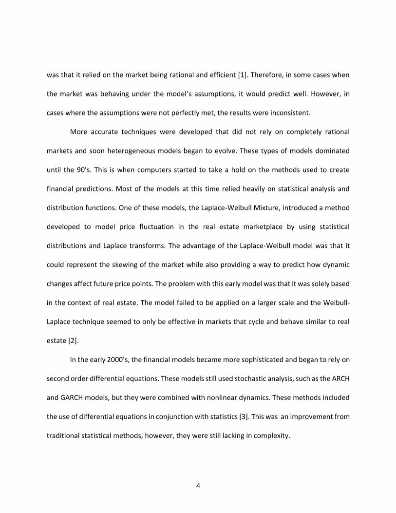
was that it relied on the market being rational and efficient [1]. Therefore, in some cases when
the market was behaving under the model’s assumptions, it would predict well. However, in
cases where the assumptions were not perfectly met, the results were inconsistent.
More accurate techniques were developed that did not rely on completely rational
markets and soon heterogeneous models began to evolve. These types of models dominated
until the 90’s. This is when computers started to take a hold on the methods used to create
financial predictions. Most of the models at this time relied heavily on statistical analysis and
distribution functions. One of these models, the Laplace-Weibull Mixture, introduced a method
developed to model price fluctuation in the real estate marketplace by using statistical
distributions and Laplace transforms. The advantage of the Laplace-Weibull model was that it
could represent the skewing of the market while also providing a way to predict how dynamic
changes affect future price points. The problem with this early model was that it was solely based
in the context of real estate. The model failed to be applied on a larger scale and the Weibull-
Laplace technique seemed to only be effective in markets that cycle and behave similar to real
estate [2].
In the early 2000’s, the financial models became more sophisticated and began to rely on
second order differential equations. These models still used stochastic analysis, such as the ARCH
and GARCH models, but they were combined with nonlinear dynamics. These methods included
the use of differential equations in conjunction with statistics [3]. This was an improvement from
traditional statistical methods, however, they were still lacking in complexity.

5
1.2.2 Computational Analysis & the Development of Algorithmic Trading
As computers continued to get faster and more available, there was an emerging wave of
financial models that would soon completely take control of the way stocks were traded. This
field was called Algorithmic Trading. This new form of trading could capture all the complexities
of the marketplace.
“Algorithmic trading (AT) refers to any form of trading using sophisticated algorithms
(programmed systems) to automate all or some part of the trade cycle. AT usually involves
learning, dynamic planning, reasoning, and decision taking. AT is growing rapidly across all types
of financial instruments, accounting for over 73% of U.S. equity volumes in 2011” [4, pp. 77].
Algorithmic trading is truly transforming the way trading takes place in the market. The
traditional view of Wall Street being overrun with commotion and hectic traders is no longer a
reality. The modern Wall Street looks more like a quiet library with several large servers running
in the background.
There are several different kinds of algorithms and techniques used in AT. “High-
frequency trading (HFT) is a more specific area, where the execution of computerized trading
strategies is characterized by extremely short position-holding periods in excess of a few seconds
or milliseconds” [4, pp.78]. Ultra high-frequency trading is another sub set of AT that operates at
even higher frequencies, literally creating an entire new world for algorithms to exist and
interact. Ultra high frequency trading takes place on the nanosecond scale and the algorithms
must account for the lag time associated with sending and receiving signals. In that respect, these
codes are computing at such a rate that they are only hindered by the speed of light. In order to

6
compensate for this, many traders use a technique called co-location. This is when traders
purposefully locate their servers as close as possible to the physical site of the transaction in
order to increase the speed of their algorithms by a few nanoseconds. Table 1 below illustrates
a simplified example of how trades are executed in only a few seconds time using algorithmic
trading.
Table 1: Example of Order Book
As seen in Table 1 above, profit is made using AT by taking advantage of the slight volatility of
the market in very short time intervals. Hundreds of thousands of dollars can be made this way.
However, not all algorithms make money. The fastest algorithms, the ones that are slightly ahead
of the others by just a few nanoseconds have a much higher chance of being profitable. That is
why techniques like co-location are so important.
1.2.3 Methods of Algorithmic Trading
Besides speed, the methods employed by the algorithm are important. There are five main stages
that make up the trading process. The first step is to obtain all relevant and necessary financial
and economic data available. However, it is also important to gather press, news, and social
media content. The next step is pre-trade analysis. Some of the most efficient AT are
characterized by their ability to read text from news sites or social media sites like Twitter and

7
Facebook. These AT then infer what the text means and makes a buying or selling decision. In
fact, these AT are so fast that they can identify, evaluate, and trade faster than a human can read
a single sentence [5]. During the pre-trade analysis stage, the AT will also look at the past events
and price ranges of the stock in order to determine probabilities and worst cases.
Step three is trade signal generation. This step is simply to infer from the pre-trade analysis which
stocks to trade and at what time. The fourth step is trade execution which is the command to
buy or sell. The fifth step is post-trade analysis. In this stage, the algorithm examines the effect
of the trade. It evaluates how the stock price reacted. An illustration of these five steps can be
seen below in Figure 1.
Figure 1: Five Stages to Algorithmic Trading
(From Ref. [4] used without permission)
8
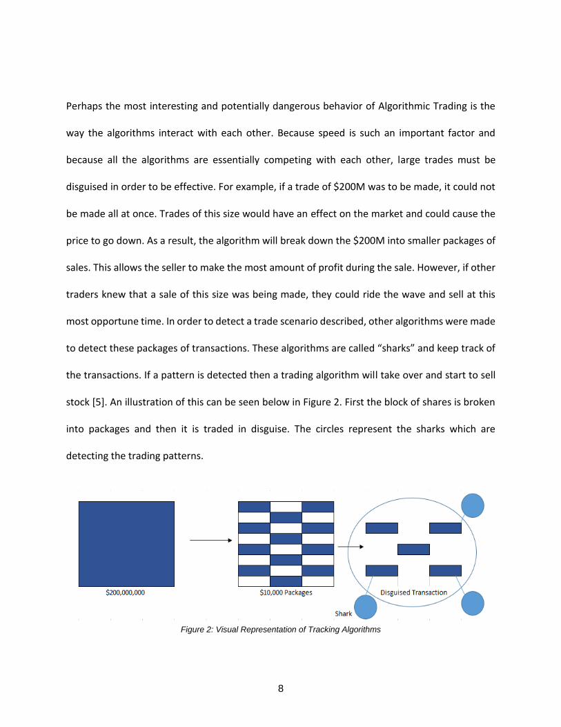
Perhaps the most interesting and potentially dangerous behavior of Algorithmic Trading is the
way the algorithms interact with each other. Because speed is such an important factor and
because all the algorithms are essentially competing with each other, large trades must be
disguised in order to be effective. For example, if a trade of $200M was to be made, it could not
be made all at once. Trades of this size would have an effect on the market and could cause the
price to go down. As a result, the algorithm will break down the $200M into smaller packages of
sales. This allows the seller to make the most amount of profit during the sale. However, if other
traders knew that a sale of this size was being made, they could ride the wave and sell at this
most opportune time. In order to detect a trade scenario described, other algorithms were made
to detect these packages of transactions. These algorithms are called “sharks” and keep track of
the transactions. If a pattern is detected then a trading algorithm will take over and start to sell
stock [5]. An illustration of this can be seen below in Figure 2. First the block of shares is broken
into packages and then it is traded in disguise. The circles represent the sharks which are
detecting the trading patterns.
Figure 2: Visual Representation of Tracking Algorithms

9
Another method that AT utilizes is divergence recognition. In this method, an algorithm will track
a stock and it will look for correlations with other stocks in the industry. If Stock A is increased in
proportion with Stock B for example, the relationship will be tracked by the algorithm. If Stock A
continues to increase and Stock B begins to decrease, the delta between them will be recorded.
When the delta increases past a certain threshold then the algorithm will initiate a buying or
selling decision. If the algorithm is fast enough, it will notice the divergence quickly and make
profit. However, if the algorithm is too slow and other codes recognize the pattern first, the slow
algorithm will lose profit. Again, this shows the importance of speed in the world of AT.
Besides using tactics like co-location, some algorithms gain a competitive speed
advantage by performing techniques to slow other algorithms down. These codes are technically
allowed but are borderline illegal in some cases because they purposefully disrupt the data in the
marketplace. An example of this is a technique called quote stuffing. Quote stuffing is a technique
used to fool the shark algorithms. This is done by making several large buying and selling
transactions in a matter of milliseconds. By making several transactions quickly, miniature spikes
and drops are developed in the price of the stock. This technique also disrupts the data related
to volumes of trades being made. The result of this is noise generation and the sharks begin to
pick up a pattern and start to analyze a substantial amount of data [5].
In reality, the sharks are spending precious time analyzing noise representing nothing
meaningful. This allows the quote stuffing algorithm to gain a few nanoseconds of computational
time on the competition. As mentioned earlier, in the world of AT where the speed of light is
considered a factor that slows performance, these few nanoseconds can make all the difference

10
between a successful algorithm and a losing one. An example of quote stuffing is shown below
in Figure 3.
(From Ref. [5] used without permission)
In Figure 3, approximately ten trend changes have taken place in about nine hundred
milliseconds. In actuality, the quote stuffing algorithm is simply selling shares and buying them
back repeatedly creating the noise shown. This is how the algorithms compete. Each code is
trying to gain a speed advantage, deceive the other, and survive.
1.2.4 The Effects of Algorithmic Trading
In this respect, these algorithms make up a micro-ecosystem. These codes behave in a way similar
to microorganisms and they are constantly evolving and competing. This process is a beautiful
example of a natural phenomenon taking place in an artificially created world. Natural selection,
survival, and adaptation are the drivers in the nanosecond environment of AT. The most
important lessons from the world of AT is that physical and natural laws are always apparent,
even in man-made systems. However, there is a downside to AT. These codes can act with a mind
Figure 3 : Quote Stuffing Algorithm in millisecond scale

11
of their own. Their behavior is not always predictable and this can lead to massive instability in
the marketplace. This instability manifests itself when algorithms create flash crashes. Figure 4
below shows two examples of recent flash crashes.
(From Ref. [5] used without permission)
As seen in A of Figure 4, in the matter of a few seconds the market can decrease by fifty
percent or more. In Figure 4 B, the market increased by more than seventy percent in less than
two seconds. This is a result of a chain reaction of multiple algorithms responding to each other.
The codes get caught in mini feedback loops that result in massive price fluctuations. There have
been approximately 18,520 flash crashes from 2006 to 2011 [5]. These events do serve as a threat
to the stability of financial markets and if not regulated may only increase in coming years. “The
speed of trade execution shrunk by a factor of ten in the last five years (2003-2008), strongly
indicating that trading very quickly over short periods of time is at the heart of modern trading”
[6].
In fact, new codes are being developed to make it possible for almost anyone to
participate in AT. Algorithmic trading is difficult for regular PC computers. “Because of the large
number of elements in the volatility matrix, such a naive estimator often behaves poorly. The
Figure 4: Bear and Bull Flash Crashes

12
estimators such as sample covariance matrix and usual realized covolatility estimators are
inconsistent in the sense that the eigenvalues and eigenvectors of the matrix estimators are far
from the true targets” [7]. However, new techniques combine low and high frequencies allowing
for a reduction in the variables needed for prediction while increasing the accuracy of results.
Perhaps even more importantly, this reduction allows for AT to be performed on normal PC
computers. AT is only becoming more popular and in order to secure the stability of the market,
regulatory action may be necessary.
The disadvantages of algorithmic trading are clear; decreased stability, decreased
innovation, decreased transparency and decreased effectiveness of risk management processes.
Via Murphy’s Law, “Whatever can go wrong will go wrong faster and bigger when computers are
involved” [8]. However, there are some benefits as well, one of which is the improvement of
liquidity in the market. In other words, AT can improve a stocks ability to sell rapidly without a
decrease in its price. Some regulatory actions that have been proposed suggest four solutions
which are described as systems-engineered, safeguard-heavy, transparency-rich and platform-
neutral regulations [8]. Essentially, these types of regulations would make it harder or illegal to
allow algorithms to implore methods such as quote stuffing and generating meaningless noise in
the market. They would also make it easy to see when AT is taking place and how it is affecting
the stock market. Additionally, it would aid investors by improving risk management. The only
problem with these proposed regulations is that they will not necessarily mitigate the probability
or reduce the effects of flash crashes.

13
One of the reasons why these flash crashes can occur in the first place is the fact that all
the algorithms behave in a similar way. For example, if a biological species only relied on one
source of food or one method to obtain that food and if that method or food source was suddenly
eliminated, then the entire species would die out. The problem with the algorithms is that they
are all competing in the same niche in the financial ecosystem. Every code is trying to be faster
than the other. They are all optimizing the same variable. This means if one code misbehaves,
the other codes are vulnerable to following the same trend [5].
One potential solution to this problem is biodiversity. If there are multiple species in a
habitat and each has its respective niche, the chances of a stable ecosystem are much higher.
The same concept can be applied to the financial market. Natural laws will always be prevalent
even in artificial systems. Therefore, natural solutions which are derived from science may be
useful to solve the problem of stability in the marketplace.
1.2.5 The Future of Financial Market Prediction
Algorithmic trading is a promising field but perhaps it is not the end all be all. Perhaps there are
other methods, techniques or concepts that should be considered. The market seems to operate
on a completely random basis. It seems as though there are fluctuations that cannot be predicted
and that statistical analysis is the only way to place a well-educated bet. However, scientific laws
would say otherwise. Every action must have an equal and opposite reaction. There is never an
effect without a cause. Natural law governs all things, the tangible and the intangible. This is why
using scientific methods to analyze the stock market is becoming more popular in the economic

14
and academic literature. If concepts of evolution are showing up in AT then it is reasonable to
believe that genetics, biology, physics and concepts from engineering may be applicable as well.
Scientists have begun to experiment with these kinds of ideas by attempting to reverse
engineer financial markets using algorithms completely designed from the theory of genetics.
This is done by gathering a sample of financial data and then applying concepts from evolution,
selection, and procreation to determine the new sample and any associated mutations [9].
Figure 5: Genetic Algorithm
(From Ref. [9] used without permission)
As seen in Figure 5 above, the data is acquired and goes through a process of evolution. Next, the
fitness is calculated and natural selection is executed. Then, new generations with high degrees
of fitness or accuracy are created along with some random mutations applied to the offspring.
This code is run until a best match is determined.
Scientific methods have been appearing more frequently in the literature of stock market
prediction. Research has been conducted on creating models based on second order differential
equations similar to those used in mechanical vibration analysis. “We observe that the model,
although not used in empirical finance and in applied economics in general, is common in
engineering. For instance, it is usual for engineers to model mechanical vibrations” [10, pp. 4].
The models created using engineering applications are limited in scope and only scratch the

15
surface of what is possible. However, the path is being paved for more serious research to take
place.
It is clear that concepts from evolution and genetics could be applied to the stock market.
It is also possible to apply concepts from physics to the market. There is a third factor that must
be considered and that is psychology or social dynamics. The connection between evolution and
principles from physics or vibration and psychology must be considered. Research has been
conducted that demonstrates the connection between evolution, natural selection and vibration.
The primary example examined in the research was the game of Rock-Paper-Scissors and how
the winner over a long period of time oscillated via natural frequencies of a three degree of
freedom, coupled system [11]. The creation of a model to represent the evolution of any system
as a function of frequency and time, be it mechanical, biological or social is an important
discovery. It demonstrates exactly how mathematical models are tied to social dynamics and how
vibration can be applied to social psychology and perception.
Understanding the relationship between social perception and the financial market is
essential for accurate prediction to occur. As a result, research has been done to analyze and
understand these connections in a controllable way. There are three primary factors in acquiring
data to create a reliable model; empirical, computational, and experimental [12]. The problem is
that the marketplace is nearly impossible to model without having control of the variables at
hand. Therefore, in order to understand the way the market operates, an experiment was
designed to simulate the stock market and observe the effects that trading has on the volatility
and stability of the system [12]. This research is helping to bridge the gap in a significant aspect

16
of financial modeling which is the human component. The marketplace is ultimately a
representation of how humans behave and perceive value.
1.3 Summary of Chapter One
The field of financial modeling is certainly an exciting and growing field. As the use of computers
and algorithmic trading only becomes prevalent, newer and more sophisticated models are being
produced. There are several different approaches that have developed throughout the past
several decades. Originally, low frequency statistical methods were the only means of prediction
but over time as computers became faster, more calculation intensive models were created.
Now, the field is evolving to incorporate scientific principles into the algorithms.
Initially, most researchers would rely primarily on statistical methods. Such techniques
would include Weibull and Gaussian distributions. However, these methods were not entirely
accurate and could only be applied to specified markets. As the state of the art evolved,
researchers began the use of more complex statistical algorithms such as ARCH, and GARCH with
the aid of computers.
The next phase of evolution for financial modeling was created when high frequency
algorithmic trading began to develop. In other words, researchers took their previous models and
applied them on a millisecond basis. This new form of trading was significantly more complex
than ever before. Now, several variables had to be calculated at high frequencies and data from
social media, press releases, and news articles could all be incorporated. This new form of trading
did have an effect on the market. Algorithmic trading actually improved the liquidity of the

17
marketplace. However, some argue that there are negative effects of algorithmic trading such as
lack of innovation and more risk for investors that should be regulated.
The newer trading models are beginning to take an emphasis on incorporating stochastic
differential equations and drawing on concepts from science. Some models are even integrating
concepts from biology by modeling the marketplace with genetic algorithms. However, in order
to accurately portray the financial market, it is important to first understand the drivers of
change. In essence, human perception and behavior is at the core of stock volatility. As a result,
research is being conducted to understand how oscillatory behavior relates to social dynamics.
Other research is being done to understand how the human aspect of trading is affecting the
market itself. This is possible by creating controlled simulations with observable participant
behavior.
Principles from science are slowly becoming integrated into the academic literature of
modeling the stock market. This research is significant as it is shining light on new methods of
modeling that could be potentially more accurate as well as less harmful to the ecosystem of the
stock market. As mentioned earlier, biodiversity allows for a stable habitat. Similarly, diverse
codes and different approaches to optimize different variables will lead to a more stable stock
market. Perhaps there is more to the stock market than random fluctuations. “In the range of
biological and social applications, seemingly stochastic fluctuations in strategy abundances need
not necessarily arise from a stochastic process” [11]. Perhaps the markets are systems that have
a scientifically predictable behavior.

18
CHAPTER TWO: STATE OF THE ART REVIEW
2. 1 The Specific Problem
The following sections discuss the primary problem with scientific approaches to modeling
financial markets. Then a brief introduction of vibration theory is discussed along with its
connection to the stock market.
2.1.1 Prediction & Principles
There have been many attempts to create a model that can accurately predict the fluctuations
of prices in the stock market. As described in the previous section, these models are becoming
more intelligent and incorporating scientific methods employed in biology, genetics, evolution,
physics and psychology. Although many of these models are promising, it has yet to be decided
on which law is the most fundamental and prevalent in the dynamics of the marketplace.
Research has been conducted to suggest that the laws of vibration are the most dominant
principles with application in the stock market. However, many of the existing models that use
frequency analysis to predict financial markets are mostly incomplete. Many of the models
determine cycle frequency but do not determine the characteristics of the stock itself. By using
the principles from vibrations, it may be possible to determine the natural frequency, stiffness
and inertial properties of a stock. This would allow for accurate prediction of responses to stimuli
in the market place. This research will attempt to solve the problem of predicting price
fluctuations of a financial market using principles from vibrations and by characterizing the
properties of a given stock in the context of vibrations.

19
2.1.2 Laws of Vibration & the Stock Market
In order to understand how the stock market and vibrations are connected, a brief introduction
of vibration theory is explained.
Every object has certain vibrational properties. The primary properties that govern how
an object will vibrate are natural frequency, mass and stiffness. The most obvious example of
vibration is by examining a spring and mass system. When a force is applied to the mass, the
spring will oscillate. The period of oscillation will be determined by how strong the spring is and
how large the mass is. The more intriguing characteristic of vibrating systems is that no matter
how large a force that is applied to the system, it will always vibrate at the same frequency.
However, if a sinusoidal force is applied to an object at its exact natural frequency, it can cause
the object to be damaged or fail regardless of how large that sinusoidal force is [13]. This is how
it is possible to break a wine glass by singing. If the frequency of the singer’s voice is the same as
the natural frequency of the object, the amplitude of vibration will grow and the glass will shatter.
Another component of vibrating systems is a damper, which is analogous to friction. The damper
is a way to dissipate energy of a system.
Even more interesting is that any object has an infinite number of natural frequencies.
However, in most cases, only a few of them are active during vibration. In order to numerically
calculate the vibration of a system, only the most active natural frequencies will be used. For
example, a system could be truncated to be represented with two natural frequencies. The
waveform that would be produced by a system like this would have a large wave and a smaller
wave superimposed inside of it. Figure 6 below illustrates this example.

20
Figure 6: Waveform of System with Two Natural Frequencies
From Figure 6, two waves are noticeable. There is a large wave and a smaller wave that acts inside
of it. If a system has more natural frequencies, it will vibrate with more waveforms embedded in
its signal. An example can be seen in Figure 7 below.
Figure 7: Waveform of System with Multiple Natural Frequencies
Figure 7 above, illustrates a waveform with four natural frequencies. As seen in the image, a
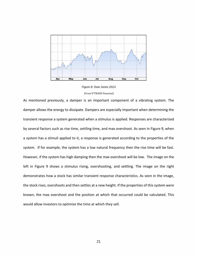
system of this type closely resembles the activities of a stock. Figure 8 below shows an actual
waveform of the Dow Jones Global Index. Upon close inspection, it is obvious to the viewer that
there seems to be similar laws governing the movement of the waveform.
21
Figure 8: Dow Jones 2013
(From E*TRADE Financial)
As mentioned previously, a damper is an important component of a vibrating system. The
damper allows the energy to dissipate. Dampers are especially important when determining the
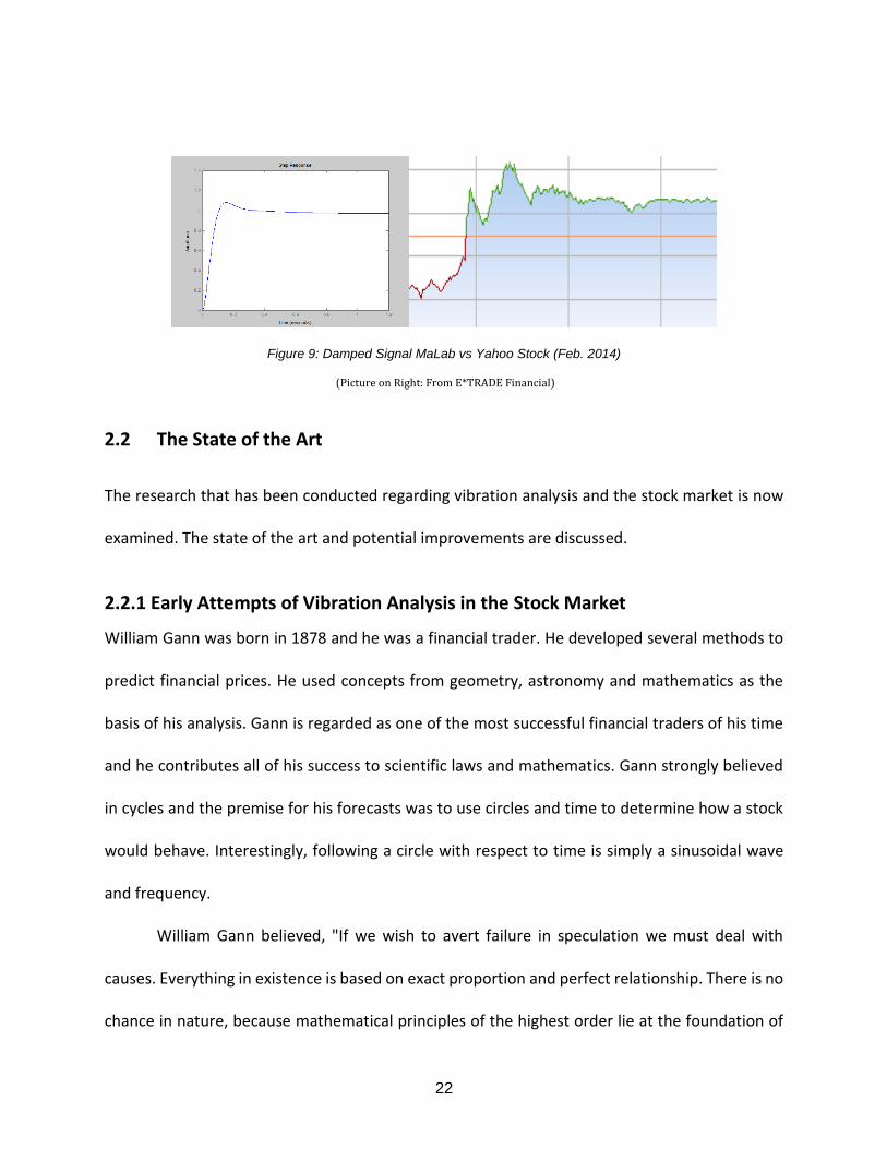
transient response a system generated when a stimulus is applied. Responses are characterized
by several factors such as rise time, settling time, and max overshoot. As seen in Figure 9, when
a system has a stimuli applied to it, a response is generated according to the properties of the
system. If for example, the system has a low natural frequency then the rise time will be fast.
However, if the system has high damping then the max overshoot will be low. The image on the
left in Figure 9 shows a stimulus rising, overshooting, and settling. The image on the right
demonstrates how a stock has similar transient response characteristics. As seen in the image,
the stock rises, overshoots and then settles at a new height. If the properties of this system were
known, the max overshoot and the position at which that occurred could be calculated. This
would allow investors to optimize the time at which they sell.
22
Figure 9: Damped Signal MaLab vs Yahoo Stock (Feb. 2014)
(Picture on Right: From E*TRADE Financial)
2.2 The State of the Art
The research that has been conducted regarding vibration analysis and the stock market is now
examined. The state of the art and potential improvements are discussed.
2.2.1 Early Attempts of Vibration Analysis in the Stock Market
William Gann was born in 1878 and he was a financial trader. He developed several methods to
predict financial prices. He used concepts from geometry, astronomy and mathematics as the
basis of his analysis. Gann is regarded as one of the most successful financial traders of his time
and he contributes all of his success to scientific laws and mathematics. Gann strongly believed
in cycles and the premise for his forecasts was to use circles and time to determine how a stock
would behave. Interestingly, following a circle with respect to time is simply a sinusoidal wave
and frequency.
William Gann believed, "If we wish to avert failure in speculation we must deal with
causes. Everything in existence is based on exact proportion and perfect relationship. There is no
chance in nature, because mathematical principles of the highest order lie at the foundation of

23
all things. Faraday said: `There is nothing in the Universe but mathematical points of force.” He
also said, “Through the Law of Vibration every stock in the market moves in its own distinctive
sphere of activities, as to intensity, volume and direction; all the essential qualities of its evolution
are characterized in its own rate of vibration. To speculate scientifically it is absolutely necessary
to follow natural law” [14].
It is clear that Gann believed in the cycles of stocks and he proved to be highly successful
in his time. The problem is that all of this work took place in a time before computers. There is
no code to document his models and it is unclear exactly how he produced his results. He used
several methods in his analysis, some of which relied heavily on astrology and the orbit of planets.
Each planet completes one full rotation around the sun in different amounts of time. Therefore,
each planet has its own frequency. By compiling data from several planets and their frequencies,
perhaps Gann was using the knowledge of planetary movement to track multiple frequencies. It
seems as though he was analyzing the way multiple frequencies interacted with each other or
were superimposed upon each other to create complex cycles. Perhaps Gann used this
knowledge of complex, interconnected cycles and applied it directly to predicting the stock
market.
Gann’s method uses geometry and angles when evaluating the frequencies of planets and
relating them to time and price. Each frequency is associated with a certain angle. These angles
which are similar to derivatives of the lines of a stock are then used to determine the trend of
prices. If a line is at a forty five degree angle, it has a time to price ratio of one to one. This would
imply that as the time increased the price would increase proportionally. This slope would
24
indicate that the supply and demand are at equilibrium. If the angle of a stock is rising at seventy
five degrees, then this would indicate a time to price of one to four. This slope would indicate the
demand far exceeds the supply. Gann would use these angles as a way to evaluate the rate of
increase or decrease of a stock. This would help him determine when a cycle is ending or
beginning.
The slope of the stock and the amount of supply or demand are all related in an interesting
way. This relationship could be analogous to potential and kinetic energy. If a mass is displaced
by some arbitrary distance, then it would have a potential energy. This would be the point at
which there was either high supply or high demand because at both those points there is much
potential for the stock price to move. However, at these points the stock would have the smallest
derivative or a one to zero time to price. Then, as the price began to change it would accelerate
fast at first. This could be represented by a one to four time to price ratio. As the supply and
demand meet equilibrium, the price would have the greatest kinetic energy. As the price began
to meet the limits of its supply or demand it would slow down, losing kinetic energy and it would
gain potential energy. This would be indicated by a time to price ratio of four to one for example.
This is a sign that the trend is beginning to change. Just as a spring acts on a mass which causes
displacement in an oscillating system, supply and demand act on shareholders which cause
change of price.
2.2.2 Modern Day Research of Cycles and Stocks
After Gann passed in the early 1900s, no known economists could reproduce his work. He was
not an academic and did not leave behind a significant body of work that could be reverse

25
engineered. The study of the law of vibration and how it is connected to the stock market had
died until recently. However, the majority of the studies done today only touch on what is
possible and there is still an immense amount of research to be done.
Recently, a study has been conducted that shows the cycles of several stocks. The
primary methods used in this research were Empirical Mode Decomposition (EMD) and
techniques like Fast Fourier Transform (FFT). The researchers retrieved the data for six stocks
from a time range of 1982 to 2004 [15]. Then they decomposed each stock into several
frequencies. In Figure 10 below, the first six mode shapes for six hundred sample points are
shown for the SP500.
(From Ref. [15] used without permission)
As seen in the figure, the very bottom image shows the sixth mode. This wavelength of
this curve is approximately ninety days. In the second to bottom image, the wavelength
decreased to be approximately thirty days. The first image in the figure illustrates the first mode
shape which has a wavelength of about two to three days. Using this method, all the frequencies
are decomposed and this is an excellent basis to start modeling the system.
Figure 10: First Six Mode Shapes of SP500
26
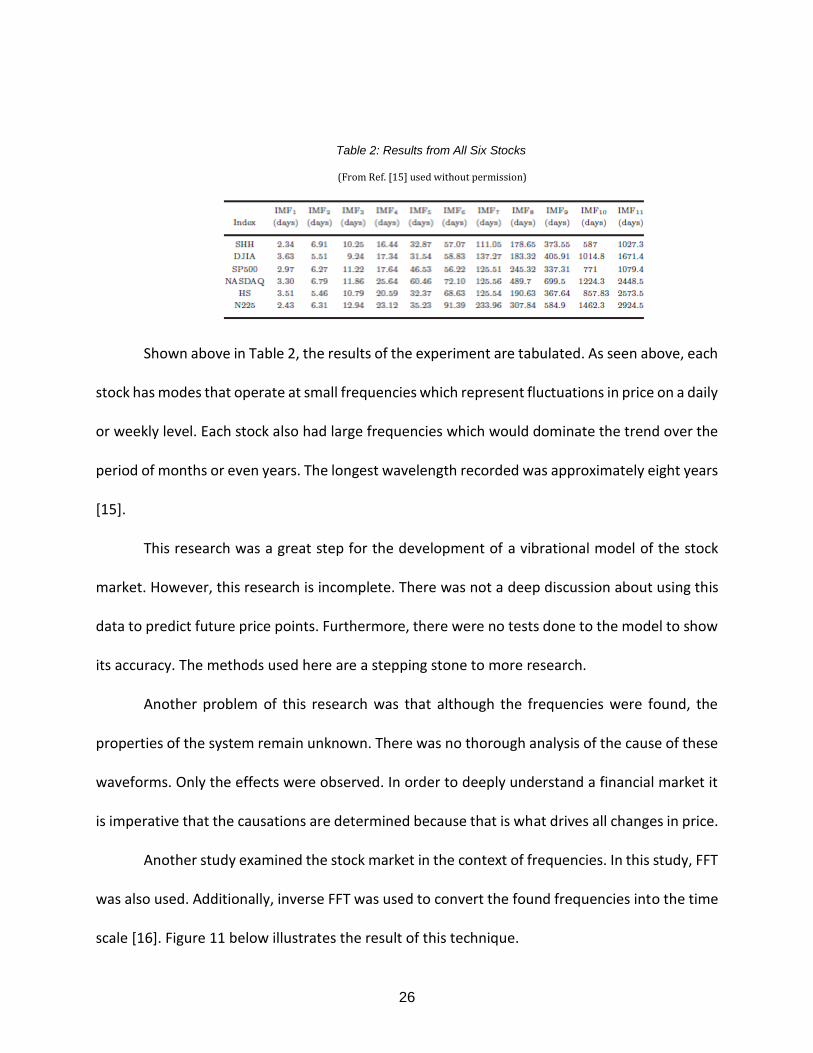
Table 2: Results from All Six Stocks
(From Ref. [15] used without permission)
Shown above in Table 2, the results of the experiment are tabulated. As seen above, each
stock has modes that operate at small frequencies which represent fluctuations in price on a daily
or weekly level. Each stock also had large frequencies which would dominate the trend over the
period of months or even years. The longest wavelength recorded was approximately eight years
[15].
This research was a great step for the development of a vibrational model of the stock
market. However, this research is incomplete. There was not a deep discussion about using this
data to predict future price points. Furthermore, there were no tests done to the model to show
its accuracy. The methods used here are a stepping stone to more research.
Another problem of this research was that although the frequencies were found, the
properties of the system remain unknown. There was no thorough analysis of the cause of these
waveforms. Only the effects were observed. In order to deeply understand a financial market it
is imperative that the causations are determined because that is what drives all changes in price.
Another study examined the stock market in the context of frequencies. In this study, FFT
was also used. Additionally, inverse FFT was used to convert the found frequencies into the time
scale [16]. Figure 11 below illustrates the result of this technique.

27
Figure 11: Filtered FFT Stock Price - Actual vs. Theoretical 458 Days
(From Ref. [16] used without permission)
In the test of the model, the actual stock price and the predicted stock price were compared. In
Figure 11, the green represents the actual price and the red represents the theoretical. The
comparison starts after 365 days and continues until day 458 [16]. As shown in the image, the
stock price was not accurately predicted. However, the approach used was a plausible technique
and certainly added to the state of the art.
The primary problem with this approach was that when the FFT was computed, it was not
clear how many data points to take in order to calculate accurate results. In Figure 11, five
percent of the total data points were taken. In Figure 12 below, the entire set of data points were
taken to compute the FFT.

28
Figure 12: Unfiltered FFT Stock Price - Actual vs. Theoretical 458 Days
(From Ref. [16] used without permission)
As seen in Figure 12, the results are unfiltered and the predicted results here are significantly
different than the red line or predicted results shown in Figure 11. This would suggest that the
way in which the data is filtered would make a substantial impact on the results. This leads to
problems in accurately calculating price fluctuations. It may be possible that different number of
data points for each sample and complex filtering techniques would have to be considered. This
adds a new level of complexity to modeling the price ranges and it may not be an optimal
approach.
Another problem that may have led to inaccurate results is not properly considering the
phase of each frequency. In other words, if the frequencies are found using the FFT method, all
that is known is the wavelength of each mode. However, what is not known is the phase or
position that wavelength is at given a particular day in its life cycle. This is a factor that needs to
be carefully considered. Each mode has to be added and superimposed properly at the exact time
of its life cycle or else the results will be inaccurate. Additionally, the amplitude of each of the
frequencies is not going to constantly resonate at the same value for each cycle. Therefore,

29
constant amplitudes cannot be used as an assumption.
Last, one of the issues with performing an analysis of this type is that it makes a general
assumption that there is no dissipation of energy or in other words that there is no damper.
When in reality, the amplitudes will die out until another force acts on them. Additionally,
assuming that the stock market is perfectly periodical is an assumption that will lead to inaccurate
results. The events in the stock market may in fact be random. It may not be as simple as finding
the frequencies of the waveform and extrapolating them into the future. The cause of each
subsequent wave must be considered in order to obtain accurate results.
The studies being conducted today certainly are advancing the state of the art of vibration
and cyclic analysis of the stock market. However, there is still much research to be done. The
breakthroughs have been the development of models that use techniques like Empirical Mode
Decomposition and techniques like Fast Fourier Transform. These models are steps forward but
they are incomplete. There are more factors that need to be considered. Most of the research
today is focused on representing the effects and not on the causes themselves. They do not
considered the forces that are acting to create the sinusoidal patterns.
2.2.3 Factors to Consider
The primary factor that is missing from the current research is the understanding of what force
causes change in the first place. Additionally, there needs to be a paradigm shift from simply
determining superficial properties to understanding the internal workings of the stock market as
a system. For example, instead of simply using frequencies to predict price fluctuations, research
should be done to go one or two steps deeper and discover the characteristics that make up
30
those frequencies.
In a vibrating system, the natural frequencies are a function of its stiffness and mass. This
is the approach that should be taken. Using EDM and FFT, the natural frequencies can be found.
Next, it would be possible to determine the stiffness and mass matrix for the system. Then, with
further analysis of the natural frequencies and amplitudes, the damping coefficients could be
determined as well. This would be a breakthrough. However, perhaps the most important aspect
of all would be determining the value and behavior of a force that acts on the system.
Determining the force is actually the most important aspect of modeling a financial
system because the force is the cause. The force is a product of supply and demand and can be
determined by using the displacement and stiffness values. The most difficult part of determining
the force would be considering whether the force was an excitation force, impulsive force, or a
combination of the two.
One potential model of the market could be analogous to a cantilever beam. The beam’s
properties would be a reflection of the company’s size and scale during the initial public offering.
When a company becomes public, this is analogous to initial conditions being set. Now, the beam
will start to resonate at a natural frequencies which is derived from supply and demand of that
product or service. However, because the economy is constantly changing, more than just spring
forces and initial conditions have to be considered. There are short impulsive forces that act on
a company throughout its life. New products and services are created constantly as well as press
releases and news articles. These impulsive forces will disrupt the beam, causing it to amplify if
the force is in phase with the beam’s displacement or decrease if it is out of phase with the

31
beam’s displacement. These forces are what creates the seemingly randomness of the stock
market and understanding these forces and how they can be modeled is what is currently lacking
from the state of the art. However, if the stiffness and mass matrix is already determined, then
modeling these forces will not be difficult. The displacement with respect to an arbitrary time
step can be observed and the stiffness can be applied to determine the impulsive force. However,
the natural supply and demand forces would have to be considered in this equation as well. When
an impulsive force is applied, it is similar to as if new initial conditions were set on the system.
The force would simply add or dissipate energy of the beam. This would result in the changes to
the stock price.
2.3 Summary of Chapter Two
There is a significant amount of work that needs to be researched and examined carefully in this
growing field. As science is becoming more adopted in financial prediction, engineering analysis
in particular is beginning to look promising. Although there hasn’t been a tremendous amount of
work done on this topic, economist William Gann proved the merit of these methods almost a
century ago. Now, scientists and researchers are using methods to examine the cyclic motion of
stocks. However, additional research needs to be done to determine the cause of those cycles.
The law of vibration and its application was developed in the early 1900s. William D. Gann
proved that by using mathematics and science, wildly accurate financial prediction was possible.
Unfortunately, he did not leave behind an academic method. His books give insight into some of
the techniques he utilized such as Gann Angles and time to price ratios. However, many of his

32
methods are still a mystery.
Recent research has been conducted on frequency analysis of the stock market. These
methods prove that analyzing certain properties of financial stocks is certainly possible. However,
the accuracy of these methods alone as a means of prediction is poor. There are still several
factors that are missing from the analysis. Some of the problems that contribute to the inaccuracy
of current methods are improper superimposition of waveforms by not considering phases.
Another issue is assuming that the market behaves in a perfectly periodic fashion without
considering impulsive forces. The techniques currently used are focused solely on the effects of
change rather than the cause of it. This is a paradigm shift that needs to occur in order to make
accurate prediction a reality.
Future methods will integrate that paradigm by focusing on system properties. This will
be done by deconstructing the system and by understanding the drivers of change. These drivers
will have to be determined and their behavior, whether excitation or impulsive must also be
evaluated.

33
CHAPTER THREE: PROBLEM DEFINITION
3.1 The Technical Area
The technical area that this thesis covers is mathematical modeling and analyzing data. The
models that will be developed will use mathematical methods such as Gauss Elimination, Linear
Regression, and extrapolation along with several other numerical method techniques. Large
volumes of data will be gathered that covers several thousand data points.
3.2 The General Problem
The general problem that this thesis addresses is to understand the behavior of financial
markets and to create a model that represents and predicts such behavior. Modeling financial
markets has been a complex and elusive topic of research for decades. Under an array of
techniques, many researchers have tried and failed to develop reliable, repeatable methods to
predict the rise and fall of stock prices. Economists have tried several techniques such as
statistical methods, advanced differential equations and even models that can receive
information, interpret that information and make a buy or sell decision in less than a few
milliseconds. Although some of these techniques have merit, there has yet to be a conclusive
model of how and why the stock market behaves the way it does. New research shows that using
scientific methods may be the most applicable method to understanding this behavior. For this
reason, this thesis will focus on solving this general problem by utilizing concepts from science
and engineering.

34
3.3 The Specific Problem
The specific problem that this thesis will attempt to solve is to determine whether a vibration
model composed of spring-mass-damper system can be used to accurately predict the behavior
of a stock market. The behavior is defined as the highs and lows with respect to time. The model
developed in this thesis will reflect that of a mechanical system vibrating at multiple natural
frequencies. Therefore, the stocks examined in this thesis will be represented as a multiple
degree of freedom, spring-mass system.
Researchers have tried to model the stock market using concepts from microbiology,
genetics and evolution such as breeding, survival, mutation and natural selection. This research
had merit and proved that specific scientific methods used to model the stock market could
produce accurate results. For this reason, this thesis will expand the state of the art of modeling
financial systems using scientific models based on engineering concepts.
3.4 The Hypothesis
A model can be developed by using vibration analysis and the laws of multiple degree of
freedom, spring-mass systems, that when given a particular economic stimuli, the behavior or
response of a financial stock can be accurately predicted.
35
3.5 The Major and Minor Contribution
The goal of this research is to further the state of the art by providing a meaningful scientific
model of financial markets using mechanical vibration analysis. The hope is that this research will
spark interest in solving the problem of modeling the stock market by using engineering concepts.
The major and minor contributions are listed below:
● Model of the causation of change of price in the stock market
● Model of oscillation of stocks using multiple degrees of freedom, mass-spring
systems under steady state conditions
● Results indicating model prediction accuracy on ten stocks
3.6 Novelty, Significance and Usefulness
This thesis addresses the problem of modeling financial markets from a unique perspective. The
stock market has been studied and analyzed in terms of frequency. However, there has not been
any significant data or models demonstrating the cause of changes in the first place. Additionally,
there has not been a model that has attempted to capture the market as a mass-spring and
damper multi-degree of freedom system. In other words, research has been done to model the
patterns of the market but attempting to understand the drivers and underlying properties in a
non-periodic manner has yet to be documented. This thesis will show how a stock progresses
throughout its life and it will attempt to determine the causes of change in price and in the
properties of the system itself.
In order to solve this problem, there are several obstacles. This problem is significant and

36
difficult to solve. The most difficult aspect of this problem is the fact that in order to create an
accurate model, the general causation must first be determined. In other words, it is clear that
the market’s behavior is not perfectly periodic. There are changes in the frequencies in which it
oscillates on a macro and micro scale. Why does the period of oscillation change? How could the
natural frequencies change over time? Could this be a result of varying excitation frequencies
that are correlated to the supply of the particular product or service that the company is offering
at that time or could it be a natural evolution of shareholder value? In other words, do the
properties of the system change over time? Several tests and a large amount of research must
be done to simply determine the behavior of change in the first place. Only then can a model
using a spring and mass system be created. Creating that model will not be easy as there are
several variables and unknowns.
The models developed throughout this research will be useful in the sense that they will
provide not only a model of how a single stock behaves but rather a representation of how all
stocks behave. Using the models developed in this research, an investor would be able to
determine the appropriate time to buy or sell a stock on annual, monthly and weekly time scales.
This research could also be used as a risk management tool allowing shareholders to understand
the effects of impulsive shocks to market prices and adeptly determine the effects that global or
economic events have on a stock’s price.

37
CHAPTER FOUR: APPROACH
The approach to solving this problem will proceed in three parts. First, the behavior of the
marketplace will be determined. Second, the steady state properties of stock will be found. Last,
transient properties will be determined in order to consider how impulsive forces cause a stock
to reset into a new amplitude or phase of vibration.
4.1 Causation of Change
This section will describe the processes needed to determine the causation of price changes in
the stock market.
4.1.1 Forced Versus Free Vibration
The preliminary phase will be to determine how the market should be modeled. In this sense,
multiple models will be created in this research and this initial understanding of the behavior sets
the foundation for the proceeding models.
The first step is to determine if the problem should be modeled as a forced vibration or a
free vibration. The difference between the two is that one has an active excitation force applied
to it. This results in a frequency of vibration that is a function of the forced vibration. The other
option is that perhaps the system should be modeled as a free vibration. Under this assumption,
initial conditions must be set on the system and the oscillation would take place as a function of
the natural frequencies. In order to determine this data, Fast Fourier Transform and discrete
wavelet analysis will take place.

38
Initially, data will be gathered from a selected active stock. Data for five or more years
will be needed in order to conduct the analysis. The data will be filtered on a yearly, monthly,
weekly and daily scale. This will be accomplished through the use of a low pass filter. The period
of the most recent three months will first be selected and a Fast Fourier Transform (FFT) will be
applied. This will convert the data from time domain into frequency domain showing the primary
and most recent monthly frequencies. As a result, the natural frequencies on that time scale will
be determined.
Next, another three month segment will be taken and the FFT computed. This process of
cutting and computing the FFT for each three month segment will be repeated for the previous
five years. The natural frequencies for each of these three month segments will then be
compared. The purpose of this analysis is to see exactly how the natural frequencies varied over
time. In this respect, it may be possible to determine a function of the rate of change of the
natural frequencies of a given stock. This analysis will be computed again but the initial position
will be phase shifted over by one month. Another analysis will be computed with a two month
phase shift. As a result, the effects of phase shifting will be determined.
Next, this procedure will be reproduced on a six month scale. The discretized cuts will be
applied to the waveform, and again, the natural frequencies and function for its change will be
computed. The phase shift procedure will then be repeated. This method will be run once more
on a yearly time scale.
This entire process will be reproduced on four more active stocks. The goal of this section
of the experiment is to establish whether the cause of change should be modeled as a forced or

39
free vibration. If the data shows the frequencies changing in a non-linear manner, particularly
around the time of product or service launches or significant company events, then it may be
more accurate to model the system using forced vibration. However, if the system changes in a
gradual manner, then it will be appropriate to model the system as a free vibration with changing
properties.
4.1.2 Boundary Conditions
Modeling the stock market as a spring and mass system has one inherent flaw: vibrating
systems oscillate between a range of values always returning to their previous position. In the
stock market, however, the price of a stock can fluctuate, but in actuality, it can be on a long term
trend upwards or downwards. Therefore, there needs to be a way to represent the displacement
of a stock price while allowing for long term trends. There are two potential solutions to this
problem.
First, if the stock is on a long term trend upwards then it can be modeled as an extremely
low frequency that is in the positive direction. This may be accurate and, for all intents and
purposes, this model will be called the Cantilever Beam Model (CBM). Under the assumption of
the CBM, the stock is considered to be a beam attached to a wall. The beam is discretized into
several masses and the masses furthest away from the base are the most receptive to impulsive
forces while the masses closest to the base receive the propagated effect of these forces. For
example, imagine a beam discretized into three masses: The first mass closest to the base would
be considered the heaviest. This may be analogous to owners of a company, or executives. They
do not make trades very often, but when they do it affects the stock price significantly. Next, in
40
the middle of the beam there are investors. These shareholders may have an intermediate effect
on the stock when they make a trade. Toward the far end of the beam are common traders. This
part of the beam fluctuates the most, but it cannot cause the beam to have a large overall change
in displacement.
The next model of interest is the Unconstrained Model (UCM). Under this model, the
stock system is considered as masses that are connected to one another with neither side
constrained. Thus, these masses are free to move and oscillate upwards until an excitation force
acts on them. This model solves the problem of perpetual upward motion as the system is simply
defined as unconstrained vibrating masses that are being struck by a force. If a positive force
strikes the system, it moves upward, and if a negative force strikes it, it oscillates its way
downward.
In order to determine which model, the CBM or the UCM, is more appropriate, several
tests will be performed. These tests will be associated with the transient properties of the system
and how impulsive forces create changes.
4.1.3 Impulsive Forces
Impulsive forces will be defined as any event that has an unnatural effect on the stock price. For
example, the stock will be oscillating in a certain manner, then when a new product is released
or if an event takes place where there is bad publicity of a company, the stock price will suddenly
change. This will be considered an impulsive force. The method to determine if the CBM or UCM
is the best match for modeling a financial market will be by evaluating how impulsive forces
change the properties of the system. This can be done by examining the previous data obtained

41
in the forcing and free vibration analyses using FFT.
4.2 Steady State Vibration
The next phase of the experiment will be to determine the steady state response of the system
and its associated characteristics. The first step in this process will be to gather the data of a
selected active stock and execute the previous procedure involving the discretized waveforms
and FFT analysis. Once this is complete, the number of natural frequencies and their rate of
oscillation will be known. Next, an equation that consists of multiple waveforms will be modeled.
The superimposition of all the generated waves will then be plotted as a multiple degree of
freedom system. An example of this is shown below in Figure 13.
Figure 13: Superimposed Waves to Model Stock Data

42
4.3 Transient Responses
The last phase of experimentation will be to determine the transient response of the system. This
will be found by observing the locations where there is a large impulsive force.
In order to determine how the transient response affects the system, the first step will be
to look at where impulsive forces occur in the chosen stock. This will be possible by looking for
news and large events that have impacted the company. For example, if Tesla Motors was the
stock of choice, then events that clearly impacted the price of the stock positively might be when
the company announced that it had the highest safety rating in its class or when it won an award
from consumer reports. Alternatively, an example of a negative event may be when the battery
pack on one of the vehicles caught fire. These events create large spikes in the stock price. The
event occurs and the stock will rise up to a maximum, come back down, and eventually settle
around a new price where it oscillates until a new event occurs.
Once the locations of these events are identified, it will be possible to compute a steady
state model of the stock and analyze how that model varies from one which includes the transient
response. In other words, it will be possible to observe the effects of an event on a stock and
determine how it may change or affect some properties of the system.
4.4 Error Calculations
Two methods for calculating the error of the computed model relative to actual stock data will
be employed. The first will use Least Squared Error; however, because this error relies primarily
on proximity, another approach to calculate the error will be created. The other approach will be
43
called Max Min Error, which will use the maximums and minimums of the model and compare
them to the stock data. This is significant because it allows the algorithm to disregard amplitude,
reducing the complexity of the problem. This method of calculating the error will optimize the
pattern of the stock and not the proximity.
4.5 Phase Finding
One of the most substantial parts of the model will be the method used to compute the phases
of each waveform found through FFT analysis. In order to do this, an algorithm will be created
that sets all the wave’s phases to zero initially allowing for the error of the actual data and the
model to be computed. Then, the phase of one of the waves will be iterated by a small resolution
and the error will again be computed. This will continue until all the wave’s phases have been
iterated from zero to two pi. The phases that return the smallest error will be recorded and initial
conditions will be set to those values. The computation will run once more and the final phases
will be documented.
4.6 Frequency Refinement
The discretized wavelet FFT will have inherit flaws. For example, a large number of samples will
be needed in order to get accurate results. Also, if there are forces acting on the stock, it will be
difficult to determine which frequency is dominant and which to ignore. Therefore, an algorithm
will be used that will not only determine the error from the different phases but also manipulate
the frequencies being used in the analysis. Essentially, this algorithm will use the FFT data as an

44
initial guess then it will stretch and shrink the periods used in the computation. The periods
returning least error will be recorded.
Another form of period refinement will be created that uses a bisection approach. In this
algorithm, instead of modulating the periods, bisection will be used to converge on the answer
with the least error. First, the FFT will find the initial guesses. Then, an upper bound and lower
bound for each period will be determined and the error will be computed for each bound on
every period. The losing bound will become the mean of the two initial bounds and this process
will continue until all the bounds are within a selected tolerance. An example of how this works
is shown below in Figure 14.
Figure 14: Period Bisection
As seen in the image above, the periods of 222, 167, and 84 days were hypothetically
found in the FFT analysis. The upper and lower bounds are then found for each period. Every
combination of each period is then used and the phases are computed. Then, a model is then
created and compared to the actual stock data using the selected method of error calculation. At

45
the end of the calculation, the number in the array of the smallest error is returned. The equation
used to determine which bound for each period is most accurate is outlined below.
o n = number of periods or waves being used
o x = position of best answer in array
o if 𝑥−1
2𝑛−1≥ 1 use upper bound; else use lower bound
o Decrement n by one and repeat process for next set of periods
o x = remainder
o Losing value becomes the mean of the pair
o Continue until the different between the pair is less than 𝛿
This approach is significant because it allows the algorithm to converge using seven waves in
approximately 650 iterations. If this code is not run using bisection it takes approximately
8,437,500,000 iterations to determine the appropriate parameters.

46
CHAPTER FIVE: TESTING AND EVALUATION
This chapter outlines all the methods and criteria used to determine the accuracy of the model
and the success of the experiment.
5.1 Unit Testing
The testing for this experiment will follow a similar structure to how mechanical designs are
generally tested. First, each component will be tested on its own. After all the unit tests are
complete and prove successful, the model will be integrated and a series of system tests will be
performed. The first step for the testing will be to choose ten stocks for which to compare
theoretical and actual results. These stocks will be selected among a wide variety of companies
including technological companies, automotive companies, new companies, and old companies.
5.1.1 Causation Tests
The first unit test will be to see under what conditions the FFT and discretized wavelet analysis
produce the most consistent results. This will be done by taking created waveforms with known
solutions and computing the wavelet on each. This will determine the optimal time interval for
each FFT and will show under which conditions the results prove most accurate.
5.1.2 Steady State Tests
Next, a similar process will proceed for the steady state testing. First, data will be gathered from
a random stock. The data will be analyzed via the wavelet analysis and the natural frequencies
will be found. Next, an equation will be generated that includes the found waveforms and the

47
behavior of a stock will be predicted using this model. In other words, a projection will be made
past the date from the data used to generate the equation. The accuracy of these predictions will
be recorded and the conditions that produce the most accurate results will be documented.
5.2 System Tests
The following tests will describe a holistic approach to evaluating the model. The previous unit
tests were designed to determine the individual weaknesses and strengths of the model, but the
following evaluation techniques will put the integrated system to the test.
5.2.1 Ideology of Trading and Evaluation
When a trader invests in a stock, it is not essential that the trader is one hundred percent accurate
of the correct time to buy and to sell. In reality, only the trend needs to be determined and profit
can be made. Because of this, the models developed will be judged on the applicability or
usefulness for an investor and on exactness.
Applicability will be evaluated based on how much percent increase or decrease in capital
that would have been made on a series of investments. The idea is relative correctness. How
much profit or losses were incurred and in how much time did it take? The exactness will be
measured from magnitude and time. What were the predicted peaks and troughs and when were
they predicted to occur?

48
5.2.2 Method
The system test will be a combination of all the previous tests combined. The first step will be to
select ten new stocks. The procedure will be the same and again the data will be selected from
2000-2012. Throughout the testing process, there will be certain buy and sell points. The model
will determine when to buy and when to sell by evaluating the highs and lows of the stock price
and at what time these are predicted to occur.
The model will then generate a plot of the stock and the evaluation will go as follows: The
theoretical model will have to predict the absolute maxima and minima within a given time
interval. It will have to determine the dates at which to buy and at which to sell. The actual data
and the theoretical will be compared and the percent error will be recorded. Questions for
evaluation to consider will be, how many days offset was the model’s peak from the actual stock
price’s peak? What is the difference in those prices? The total profit or loss from the buy and sell
points will be documented.
5.2.3 Evaluation
It is difficult to determine exactly how to define the experiment as a success. However, it is
important to remember that there are several variables and complexities that are not being
modeled; therefore, there will be room for uncertainty in the results.
There will be ten stocks to consider and the average percent return will be used as the
success criterion. An average of 25% return on capital in less than a two year period will be
considered a success. However, it may be possible that some stocks in particular industries or at
certain stages in their life cycle are much more suitable for this particular type of modeling. In

49
that case, this will be considered and correlations between the most predictable stocks will be
analyzed.

50
CHAPTER SIX: EXPERIMENT & RESULTS
The following chapter will outline the main experiments performed during the course of the
research. The first describes the experiments taken on different models in order to determine
which returned the most accurate results. The second describes the final experiment used to
determine the effectiveness of the model created and to support the original hypothesis.
6.1 Experiment #1: Determining the Most Effective Model
This first experiment was quite simple. Several stocks were analyzed using twelve different
approaches. Each approach was a combination of the following three criteria:
o Type of period refinement: None or Stretch-Shrink or Bisection
o Method of error calculation: Least Squared Error (LSE) or Max Min Error (MME)
o Data Filtering: No Filter or Low Pass Filter
Example:
o No period refinement, LSE, Low Pass Filter
The results from this experiment showed that the period refinement techniques did not always
produce the most accurate projection. The Max Min Error worked well with highly filtered data
but returned poor results with non-filtered data. The Least Squared Error with no period
refinement returned the best results with filtered data and slightly less accurate but still quality
results with non-filtered data.
The primary conclusion from this experiment was that the no period refinement was
necessary if the wavelet FFT analysis was done properly and the LSE with filtered data was the

51
best option to use for modeling.
6.2 Experiment #2: Evaluation of Financial Model
The following section will outline the experimental set up and will evaluate the predictive
capability of the model created in this research.
6.2.1 Experimental Set Up
The projections in this experiment were created using the LSE approach without period
refinement with filtered data. Ten stocks were analyzed in this experiment. Five of them were
selected at random and five were chosen. The first five stocks were selected using an online stock
analysis game (www.nonrandomwalk.com) which randomly selects stocks and dates from 2000-
2012. The last five stocks were selected based on familiarity (i.e. Google, Amazon, Toyota).
6.2.2 Procedure
The procedure for this experiment goes as follows. The stock and date was selected. Data up until
that date was retrieved from Yahoo Finance. The analysis was run to create a model of the stock’s
behavior up until the date of the retrieved data. The projection was then produced which extends
past the date of the data. The model and projection consist of four waveforms found from the
wavelet FFT analysis. The time for the projection was based on the largest period used in the
model. Next, the dates of the future maximums and minimums according to the projection were
documented, and a buy and sell execution was hypothetically ordered to occur on those dates.
The actual stock data was then overlaid on the projection and the prices for each documented

52
date from the projection was observed. The total percent gain or loss was then calculated.
Additionally, there were two immutable rules during the experiment.
1. No data can be used past the selected date.
2. The projection can only be run once. All predictions are final.
For example, if Apple and July 1, 2005 was selected then only data on and before that date can
be used for analysis. The code will then predict how the stock will behave from July 2005, to July
2006. The dates of the maximums and minimums that will occur between July, 2005 and July,
2006 according to the projection are documented. The actual stock data from July, 2005 to July,
2006 will then be observed. The predictions of the maximums and minimums are then compared
to the actual maximums and minimums. The code has one attempt at the projection. Once a
prediction is made, no parameters can be changed and the results must be recorded.
Figures 15 and 16 below illustrate the process. The black vertical line shows the end of
the data used to create the model. The blue line shows the future projection which was created
solely from an equation and not from any data.

53
Figure 15: Projection of Stock
Figure 16: Projection with Actual Stock Data Overlaid
It is important to note that there was one form of selection bias. If a stock that was presented
appeared to be chaotic, under several forces and non-harmonic, the experimenter was allowed
to discard that stock for another stock. However, this must occur before any analysis was done.
In other words, any decision to use a stock was final. During this experiment, only two stocks

54
were discarded as a result of the selection bias. An example of a stock that was discarded can be
seen below in Figure 17. The figure shows a stock that was moving up and to the right with no
distinguishable pattern or harmonics visible. Therefore, this stock was discarded pre-analysis.
Figure 17: Selection Bias Example
The investment strategy used to determine the percent return on investment proceeds as
follows. For each stock, buying long and covering a short sale occurred at every minimum of the
projection, and selling a long position and initiating a short sale occurred at every maximum.
Figure 18: Example of Long and Short Strategy

55
Figure 18 above illustrates the investment strategy. The first arrow (red) is where the algorithm
initiates a short sale which allows the investor to gain profit when the stock price falls. The second
arrow (black) is where the algorithm covers its short and initiates a buy which allows the investor
to gain profit when the stock price rises. The last arrow (green) is where the algorithm sells its
long position and then again initiates a short sale. This continues to occur at every maximum and
minimum for the length of the projection.
6.2.3 Stocks 1-5 Results
The unadulterated projection graphs of all the stocks can be seen directly in the appendix in
Figures A1-A10. The majority of the graphs will be shown in the following two sections but some
may be modified to emphasize specific points.
The first stock was FALC which had a +24.81% return. Below, in Figures 19 & 20, the
projection along with the filtered view are shown. The thick vertical black line shows where the
projection begins. The thin blue line is the projection.
Table 3: Stock #1 FALC Results
Stock #1
Stock Name Falconstor Software
Stock Symbol FALC
Year 2005
Selection Type Random
Investment Time (days) 90
Return on Investment (%) +24.81

56
Figure 19: FALC Projection vs. Actual Stock Data
Figure 20: Filtered View of Projection vs. Actual Stock Data

57
The second stock’s data is shown below in Table 4 and the projection is shown below in
Figure 21.
Table 4: Stock #2 MENT Results
Figure 21: MENT Projection vs. Actual Stock Data
Stock #2
Stock Name Mentor Graphics
Stock Symbol MENT
Year 2005
Selection Type Random
Investment Time (days) 200
Return on Investment (%) +48.29

58
The third stock is shown below in Table 5.
Table 5: Stock #3 SINA Results
Stock #3
Stock Name SINA Corporation
Stock Symbol SINA
Year 2006
Selection Type Random
Investment Time (days) 115
Return on Investment (%) +14.22
Figure 22: SINA Projection and Modeling Error
Figure 22 shows the filtered view of the model and projection for SINA. The blue circle in the
figure emphasizes a mistake in the model. As seen above, the model (black) has three peaks
within the blue circle, whereas the actual data (red) has only two. This is a sign that the model is
not using the correct periods and that the projection should not be run until the periods are
redefined. The experimenter did not see this error before the projection was run and as a result

59
SINA returns a lower percent gain on profit relative to the previous two stocks.
Table 6: Stock #4 RNWK
Stock #4
Stock Name Real Networks
Stock Symbol RNWK
Year 2004
Selection Type Random
Investment Time (days) 100
Return on Investment (%) +57.15
The fourth stock is outlined in Table 6 above and the graph is shown in Figure 23 below. RNWK
has a return of +57.15%.
Figure 23: RWNK Projection vs. Actual Stock Data
The fifth stock is outlined in Table 7 below. Figure 24 shows the graph of the ABMD projection.
Figure 25 shows a close up view of the graph emphasizing the accuracy of the projected maximum
and minimum.

60
Table 7: Stock #5 ABMD Results
Stock #5
Stock Name ABIOMED
Stock Symbol ABMD
Year 2007
Selection Type Random
Investment Time (days) 150
Return on Investment (%) +37.12
Figure 24: ABMD Projection vs. Actual Stock Data

61
Figure 25: ABMD Projection Min & Max Accuracy
As seen in Figure 25 above, the projection begins around day 3010. At day 3092, the projection
predicts there will be a minimum. The red line of the actual data shows a minimum at day 3093.
The prediction was off by a single day after approximately 80 days. Later, the projection
predicts a maximum at day 3124. According to the actual data, there was a maximum at exactly
day 3124. Approximately 110 days into the projection, the exact maximum was predicted.
6.2.4 Stocks 6-10 Results
The next stock was DOW which returned a positive 33.82% gain on capital. The non-filtered and
filtered view of the data are presented in Figures 26 and 27 and the results are outlined in
Table 8 below.

62
Table 8: Stock #6 DOW Results
Stock #6
Stock Name DOW Chemical
Stock Symbol DOW
Year 2012
Selection Type Chosen
Investment Time (days) 200
Return on Investment (%) +33.82
Figure 26: DOW Projection vs. Actual Stock Data
As seen in the figure above, the DOW projection was fairly accurate. It is important to note that
the price fluctuation from the start to the end of the projection is relatively small ranging from
approximately $27 to $32 at most. This is significant because it would be difficult for an investor
to return +33.82% on their capital with such small fluctuations in less than a year’s time.
However, the projection was capable of doing just that.

63
Figure 27: DOW Projection vs. Actual Stock Data Filtered View
The filtered view in the figure above shows that the model matched the actual data well and this
was an indication that the projection would also match well.
The next stock was GOOG which has a -18.59% return on capital. Table 9 outlines the
results and Figure 28 shows the filtered view of the projection graph.
Table 9: Stock #7 GOOG Results
Stock #7
Stock Name Google
Stock Symbol GOOG
Year 2011
Selection Type Chosen
Investment Time (days) 100
Return on Investment (%) -18.59

64
Figure 28: GOOG Projection vs Actual Stock Data Filtered View
In the figure above, the blue circle highlights an error in the model. Clearly, the model did not
have the correct periods because it did not match the actual data well. More FFT analysis should
have been done before the projection was run. As a result, GOOG returned a loss on capital.
The next stock was PFE and had a +17.62% return on capital. Table 10 outlines the data
and Figure 29 shows the PFE projection graph below.
Table 10: Stock #8 PFE Results
Stock #8
Stock Name Pfizer
Stock Symbol PFE
Year 2001
Selection Type Chosen
Investment Time (days) 200
Return on Investment (%) +17.62

65
Figure 29: PFE Projection vs. Actual Stock Data
The figure above illustrates an important point. Stocks can behave as a mass-spring system and
in particular this adds evidence that the Unconstrained Model would be the most appropriate.
As seen above, the stock was following a certain harmonic pattern, then was suddenly
interrupted by this downward impulsive force. The most fascinating aspect of the figure above is
what happened after the force occurred. The stock began to rally upwards to the projected
maximum. This illustrates that the harmonics remain present even if forces are acting on the
system.
Figure 30, below, shows a filtered view of the data and the projection was extended by
approximately 150 days. This extension is not recorded as part of the return on capital; it is only
to emphasize the behavior of this stock. The impulsive force can been seen below in the filtered
view and the effect it has on the stock is visible. First, the force or event occurs. This creates a

66
ripple in the stock’s price and it undergoes a period of transience. Then the stock begins to
oscillate at its normal harmonics once more, only there is a slight difference in its amplitude and
phase. As seen below, the projection, which has no knowledge that a force had occurred because
the force happened past the date of the data used to create the model and equation, creates an
“h” like shape and then it begins to move upward toward the end. The actual stock data creates
the exact same shape and then begins to move upward and continues on. The only difference
between the two is that the actual data is now slightly ahead of the projection, as if its phase has
been shifted.
This is a substantial observation because it demonstrates how events or forces that act
on a stock may cause a reset of initial conditions, such as phase and amplitude, but the original
harmonics remain present.
Figure 30: Harmonic Remaining Present

67
The ninth stock was TM and it has a positive return of 48.09%. Table 11 outlines the results and
Figure 31 shows the projection graph below.
Table 11: Stock #9 TM Results
Stock #9
Stock Name Toyota Motors
Stock Symbol TM
Year 2007
Selection Type Chosen
Investment Time (days) 210
Return on Investment (%) +48.09
Figure 31: TM Projection vs. Actual Stock Data
It is curious that the projection was able to return a positive result on the TM stock above. It is
obvious that the projection would make a gain on profit by betting that the stock would increase
its price, however, the algorithm also sells short. This means that the algorithm also bets that the
stock will go down at some points. The reason the algorithm was able to make a large gain and

68
not have large losses every time it sold short was because the stock staggered upwards. With
visual inspection it can be seen that there was a large force acting on this stock at the time which
caused a large rise in the price. However, when the stock price was naturally supposed to be
going downward, the price would stagger for a short period. This is another example of how the
harmonics remain present even when a force is acting on a stock. Because of this, the short sales
did not take large losses as they were predicted accurately in the staggering intervals and the
long buys made large profits as they were predicted accurately in the rising intervals.
The last stock was AMZN with a positive gain of 45.27%. The results are outlined in Table
12 and the filtered view of the projection is shown in Figure 32 below.
Table 12: Stock #10 Results
Stock #10
Stock Name Amazon
Stock Symbol AMZN
Year 2006
Selection Type Chosen
Investment Time (days) 125
Return on Investment (%) +45.27

69
Figure 32: AMZN Projection vs. Actual Stock Data Filtered View
The projection was extended to 300 days to observe the pattern over a longer period of time.
This extension was not included in the results. The extended projection can be seen below in
Figure 33. Around day 2260 and 2290, the projection predicts a minimum and a maximum almost
exactly. This is approximately 200 days after the start of the projection. As a result of this long
term accuracy, the projection returns +114.04% over a 300 day projection. This is not included in
the results of the experiment as this was just an observation and the projection extended past
the allotted time according to the experimental procedures.

70
Figure 33: AMZN Projection vs. Actual Stock Data
The next stock was not included in the experiment as it was originally discarded. Nonetheless,
analysis was computed for observational purposes. Table 13 outlines the results and Figure 34
illustrates the projection and the harmonics of the stock.
Table 13: Observation TSLA
Stock #11 (Not Included in Experiment Results)
Stock Name Tesla Motors
Stock Symbol TSLA
Year 2013
Selection Type Chosen
Investment Time (days) 50
Return on Investment (%) +40.11

71
Figure 34: TSLA Projection vs. Actual Stock Data & Harmonic Analysis
As seen in the figure above, the projection is accurate as it predicts the maximum at day 899
exactly. Next, there is a force or event that is applied to the stock. This force is a positive upward
force, however, the stock naturally wants to oscillate downward at that time. The net result is a
slight positive gain. Almost exactly as the natural force begins to come to a halt and the projection
predicts a minimum, the stock price rises aggressively. This is because, according to the
projection, the natural response would now be in the positive direction. This natural rise along
with the forced rise create a large net upward swing of the price. This illustrates how the
harmonics remain present even when forces or events are acting on a stock.

72
6.2.5 Conclusion of Results
The summary of the results of Experiment #2 are outlined below in Table 14.
Table 14: Summary of Experiment #2 Results
Summary of Results Stocks 1-10
Positive Predictions 9/10
Lowest Return on Investment GOOG 2011 -18.59%
Highest Return on Investment RNWK 2004 +57.15%
Approx. Average Investment Time (Days) 150
Average Return on Investment (%) +30.78%
Total Percent Change on Capital +307.80%
Nine out of the ten trials returned a positive gain on capital. The mean percent gain on capital
was approximately 31% over an average of roughly 150 days. These results support the claim that
stocks do follow a pattern of vibration and that prediction of financial markets may be possible.

73
CHAPTER SEVEN: CONCLUSION
The following sections will cover a conclusion of the experiments and the research conducted
as well as improvements and potential future work.
7.1 Overall Conclusion of Research
Over the course of this research several algorithms were created that were used to analyze,
model and predict the behavior of a financial stock. The models created used concepts from
mechanical vibrations and mass-spring systems. The primary premise of this research was that
stocks behave in an ordered fashion in accordance to the laws of vibration and the laws of
stimulus-response systems.
The algorithms created performed discretized wavelet analysis, frequency refinement
using a Stretch-Shrink and a Bisection approach, measured error from a generated model using
Least Squared Error and Max Min Error and generated a projection of how a financial stock will
behave.
Each approach was tested and documented in Experiment #1 of this thesis and the results
of this experiment showed that the Least Squared Error approach using filtered data and no
period refinement achieved the best results. However, it was imperative that the discretized
wavelet analysis was done accurately for this approach to return quality results.
Experiment #2 of this thesis documented the results of predictions made on ten stocks.
The results showed that nine out of the ten predictions returned a positive gain on capital and

74
that the average gain was +30.78%. Most importantly, these results support three predominant
observations.
1) Stocks vibrate with multiple degrees of freedom in a predictable manner.
2) Forces are applied to stocks which cause transient responses but their natural frequencies
still remain present.
3) Forces can cause stocks to reset their initial conditions but not necessarily change their
innate properties.
Claim number one is supported by the results of the experiment as the model was generated
from a vibrating, multiple degree of freedom system. Claim number two is supported by stock
number eight, nine and eleven, which illustrate the harmonics remaining present during or after
a force is applied to a financial stock. Claim number three is supported by stock number eight
which shows the exact shape generated by the projection occurring in the actual stock data even
after an impulsive force was applied to the stock after the start of the projection.
The experiments and research conducted support the original hypothesis, that it is
possible to predict the behavior of a financial stock by creating a model which uses concepts from
multiple degree of freedom mass-spring systems.
7.2 Research Improvements
If this research was conducted over again, it would be wise to analyze using real time data. If a
model and projection of a current stock could have been generated and tracked during the
research, it would have aided in determining the effectiveness of this approach in real time. One

75
of the problems with the approach presented in this research is that it did not take into account
the noise. In other words, only four dominant frequencies were being modeled and perhaps more
accurate results could have been obtained with a larger degree of freedom system. Also, the
algorithm’s usefulness for an investor is questionable as even though the model was able to
predict the behavior quite accurately, there were times when the noise was great and it would
be difficult for an investor to trust the algorithm through such noise. As mentioned above, adding
degrees of freedom might help combat this problem.
7.3 Future Work
This research is still in preliminary stages. Several improvements to the algorithm can be made.
First, one of the largest problems is selecting the proper frequencies from the wavelet FFT
analysis. Additional algorithms could be made to select these frequencies more effectively.
Second, supplementary algorithms could be made that identify stocks that are in the most
promising position. This could help investors know which stock to choose at any given time.
Third, significant research could be done to identify, measure and categorize the input
forces that act on the stocks. This could allow an algorithm to potentially model the system so
that the effects of any given force could be predicted or simulated. Last, research has to be
conducted with the algorithms in real time so that a proper evaluation of its effectiveness and
applicability can be measured.

76
APPENDIX PROJECTION VS. STOCK DATA

77
Figure A1: FALC Projection vs. Actual Stock Data
Figure A2: MENT Projection vs. Actual Stock Data

78
Figure A3: SINA Projection vs. Actual Stock Data
Figure A4: RNWK Projection vs. Actual Stock Data

79
Figure A5: ABMD Projection vs. Actual Stock Data
Figure A6: DOW Projection vs. Actual Stock Data

80
Figure A7: GOOG Projection vs. Actual Stock Data
Figure A8: PFE Projection vs. Actual Stock Data

81
Figure A9: TM Projection vs. Actual Stock Data
Figure A10: AMZN Projection vs. Actual Stock Data

82
LIST OF REFERENCES
[1] A. Setzu, “A Framework for Financial Markets Modeling and Simulation,” Exchange
Organizational Behavior Teaching Journal. 2007
[2] S. T. Rachev, A. SenGupta, “Laplace-Weibull Mixtures for Modeling Price Changes,”
Management Science. Vol. 39, Issue 8, p1029-1038, Aug. 1993.
[3] S. C. Nicolis and D. J. T. Sumpter, “A Dynamical Approach to Stock Market Fluctuations,”
International Journal of Bifurcation and Chaos, Vol. 21, No. 12, Pp. 3557–3564, Jan. 2011
[4] P. Treleaven, M. Galas, and V. Lalchand. "Algorithmic Trading Review." Communications
Of The ACM, Vol. 56, Issue 11, Pp. 76-85, 2011.
[5] S. Gourley, “High Frequency Trading and the New Algorithmic Ecosystem,”
TedxNewWallStreet, New York, NY, 2011.
[6] A. Cartea, “Modeling Asset Prices for Algorithmic and High Frequency Trading,” Applied
Mathematical Finance, Univ. of London, Dec. 2008.
[7] M. Tao, Y. Wang, Q. Yao and J. Zou, “Large Volatility Matrix Inference via
Combining Low-Frequency and High-Frequency Approaches.” Journal of the American
Statistical Association, Vol. 106, issue 495, pp. 1025-1040, 2011.
[8] A. A. Kirilenko and A. W. Lo, “Moore’s Law versus Murphy’s Law: Algorithmic Trading and
Its Discontents,” The Journal of Economic Perspectives, Volume 27, Number 2, Pp. 51-72,
Spring 2013.
83
[9] J. Wiesinger, D. Sornette, J. Satinover, “Reverse Engineering Financial Markets with
Majority and Minority Games using Genetic Algorithms,” Computational Economics, Vol.
41, Issue 4, pp. 475-492, April 2013.
[10] Nicolau, “Modeling financial time series through second-order stochastic differential
equations,” Statistics and Probability Letters, Vol. 78, issue 16, p2700, 5 p., March 2008.
[11] Ruelas, Rocio E., David G. Rand, and Richard H. Rand. "Parametric Excitation and
Evolutionary Dynamics," Journal of Applied Mechanics, Vol. 80, issue 5, May 2013.
[12] K. An, X. Li, G. Yang, and J. Huang, “A controllable laboratory stock market for modeling
real stock markets,” European Physical Journal B, Vol. 86, Issue 10, April 2013.
[13] W. Thomson, “Transient Vibration, Theory of Vibrations with Applications, 5th ed., NJ,
Prentice-Hall, 1981, ch. 4, pp. 92-134.
[14] P. Tony, The Law of Vibration: The Revelation of William D. Gann, UK, Harriman House,
2013.
[15] C. Yang, H Wu, and Y. Zhang. “Periodic Components and Characteristic Time Scales in the
Financial Market,” Modern Physics Letters B, Vol. 22, No. 26, pp. 2571-2578, 2008
[16] A. Wojtak, “Attempt to Predict the Stock Market,” B.S Thesis, Dept. Mechanical Eng.,
Worcester Polytechnic Institute, Worchester, MA, 2007.