University of South CarolinaScholar Commons

Theses and Dissertations

6-30-2016

Modeling Human-Structure Interaction Using AController SystemAlbert Ricardo Ortiz LasprillaUniversity of South Carolina

Follow this and additional works at: https://scholarcommons.sc.edu/etd

Part of the Civil Engineering Commons

This Open Access Dissertation is brought to you by Scholar Commons. It has been accepted for inclusion in Theses and Dissertations by an authorizedadministrator of Scholar Commons. For more information, please contact dillarda@mailbox.sc.edu.

Recommended CitationLasprilla, A. O.(2016). Modeling Human-Structure Interaction Using A Controller System. (Doctoral dissertation). Retrieved fromhttps://scholarcommons.sc.edu/etd/3484

Modeling Human-Structure Interaction Using a Controller System

by

Albert Ricardo Ortiz Lasprilla

Bachelor of ScienceUniversidad del Valle 2008 and 2011

Master of ScienceUniversidad del Valle 2011

Submitted in Partial Fulfillment of the Requirements

for the Degree of Doctor of Philosophy in

Civil Engineering

College of Engineering and Computing

University of South Carolina

2016

Accepted by:

Juan M. Caicedo, Major Professor

Robert L. Mullen, Committee Member

Dimitris Rizos, Committee Member

Gabriel Terejanu, Committee Member

Lacy Ford, Senior Vice Provost and Dean of Graduate Studies

© Copyright by Albert Ricardo Ortiz Lasprilla, 2016All Rights Reserved.

ii

Dedication

This work would not have been possible without the help of my loving wife Tayrin.

This is nothing compared to what you have done for me. I am eternally grateful.

I love you.

iii

Acknowledgments

I am deeply grateful to my supervisor Dr. Juan M. Caicedo for opening the doors

of the Structural Dynamics and Intelligent Infrastructure laboratory (SDII) at the

University of South Carolina. My experience at SDII was exciting. The expectations

related to my PhD were fulfilled. I also thank Dr. Caicedo for his motivation, positive

feedback, and personal advice. He has my admiration and gratitude for the guidance

and support throughout this research.

I am thankful to professors Dr. Robert L. Mullen, Dr. Gabriel Terejanu, and Dr.

Dimitris Rizos for their time, comments, and suggestions for the realization of this

work.

I would like to thank the institutions who financially contributed to this work:

the University of South Carolina and the Foundation for the Future of Colombia

(Colfuturo).

Many thanks to all students and staff of the structures laboratory who collab-

orated with tests. Special thanks to Ramin, Benjamin, Yohanna, Mus, Diego and

Gustavo for the feedback and the endless discussions about the research and the

methodology we used.

My deepest gratitude is to my parents, Carlos and Mary, and my brothers Carlos

Eduardo and Daniel. I am happy to be member of this wonderful family.

To my wife, Tayrin and my son, Alejandro. I cannot thank you enough for making

me happy every day of my life.

iv

Abstract

The effects of human loads on structures are difficult to predict because they depend

on the type of activity people are performing. However, models for typical activities

such as standing, sitting and jumping have been proposed in the literature. Tra-

ditional models represent the human body as a system of lumped masses, dampers

and springs arranged in a system with multiple degrees of freedom. Arguably, these

models might not fully represent the human body because lumped masses, dampers

and springs cannot add energy to the overall system. Furthermore, people could react

differently to different levels of excitation and other environmental conditions.

Controller systems have been widely used in electrical, seismic and other fields of

engineering for systems in which setting a specific response is important. Given that

the human acts like a controller system, where the feedback affects the response of

the system, and the specific use of controllers is becoming common in structural engi-

neering, this research developed a controller model to reproduce the phenomenon of

Human-Structure Interaction (HSI). The methodology consisted in updating the pa-

rameters of the controller using experimental data from tests involving humans over a

previously characterized structure. The controller system was the widely known Pro-

portional, Integrative and Derivative (PID) controller and its derivations, PD and PI.

Parameters of the controller were updated using a Bayesian probabilistic approach.

Models were developed based on transfer functions obtained from experimental tests.

A comparison of controller models and traditional Mass-Spring-Damper (MSD) mod-

els is performed at the end for validation purposes.

v

Table of Contents

Dedication . . . . . . . . . . . . . . . . . . . . . . . . . . . . . . . . . . iii

Acknowledgments . . . . . . . . . . . . . . . . . . . . . . . . . . . . . iv

Abstract . . . . . . . . . . . . . . . . . . . . . . . . . . . . . . . . . . . v

List of Tables . . . . . . . . . . . . . . . . . . . . . . . . . . . . . . . . viii

List of Figures . . . . . . . . . . . . . . . . . . . . . . . . . . . . . . . x

Chapter 1 Introduction . . . . . . . . . . . . . . . . . . . . . . . . . 1

1.1 Traditional models used in HSI . . . . . . . . . . . . . . . . . . . . . 4

1.2 The human as a control system . . . . . . . . . . . . . . . . . . . . . 7

Chapter 2 Methodology . . . . . . . . . . . . . . . . . . . . . . . . . 9

2.1 Human-structure Interaction as a closed-loop control system . . . . . 9

2.2 Bayesian Model Updating . . . . . . . . . . . . . . . . . . . . . . . . 15

2.3 Probabilistic Model Selection . . . . . . . . . . . . . . . . . . . . . . 20

Chapter 3 Experimental testing and updating of empty structure 22

3.1 Lab structure . . . . . . . . . . . . . . . . . . . . . . . . . . . . . . . 22

3.2 Instrumentation and tests . . . . . . . . . . . . . . . . . . . . . . . . 23

3.3 Parameters of the structure . . . . . . . . . . . . . . . . . . . . . . . 26

vi

3.4 Conclusion remarks . . . . . . . . . . . . . . . . . . . . . . . . . . . . 35

Chapter 4 Results . . . . . . . . . . . . . . . . . . . . . . . . . . . . 36

4.1 Parameter updating of the models . . . . . . . . . . . . . . . . . . . . 36

4.2 Model selection . . . . . . . . . . . . . . . . . . . . . . . . . . . . . . 53

4.3 Controller models for groups of people . . . . . . . . . . . . . . . . . 55

Chapter 5 Conclusions and future work . . . . . . . . . . . . . . 59

5.1 Conclusions . . . . . . . . . . . . . . . . . . . . . . . . . . . . . . . . 59

5.2 Future Work . . . . . . . . . . . . . . . . . . . . . . . . . . . . . . . . 60

Bibliography . . . . . . . . . . . . . . . . . . . . . . . . . . . . . . . . 62

Appendix A Stability Conditions . . . . . . . . . . . . . . . . . . . . 69

A.1 PID controller . . . . . . . . . . . . . . . . . . . . . . . . . . . . . . . 69

A.2 PI controller . . . . . . . . . . . . . . . . . . . . . . . . . . . . . . . . 70

A.3 PD controller . . . . . . . . . . . . . . . . . . . . . . . . . . . . . . . 70

Appendix B Convergence . . . . . . . . . . . . . . . . . . . . . . . . . 71

B.1 Models of the structure . . . . . . . . . . . . . . . . . . . . . . . . . . 71

B.2 Models of human-structure interaction . . . . . . . . . . . . . . . . . 77

vii

List of Tables

Table 1.1 Influence of human occupation or a mass on the natural fre-quency and damping ratio of a slab . . . . . . . . . . . . . . . . . 3

Table 1.2 Characteristics of SDOF and MDOF models of a standing hu-man occupant . . . . . . . . . . . . . . . . . . . . . . . . . . . . . 7

Table 2.1 Models of the structure . . . . . . . . . . . . . . . . . . . . . . . . 19

Table 2.2 Models of the human . . . . . . . . . . . . . . . . . . . . . . . . . 19

Table 2.3 Models to be updated . . . . . . . . . . . . . . . . . . . . . . . . . 19

Table 2.4 Kass and Raftery scale for Bayes factor . . . . . . . . . . . . . . . 21

Table 3.1 Prior PDFs used for updating the parameters . . . . . . . . . . . . 28

Table 3.2 Prior PDFs used for updating the parameters . . . . . . . . . . . . 31

Table 4.1 Models to be updated . . . . . . . . . . . . . . . . . . . . . . . . . 37

Table 4.2 Prior PDFs of the structure’s parameters . . . . . . . . . . . . . . 38

Table 4.3 Prior definition for parameters of the PID, PI, and PD controller . 38

Table 4.4 Number of samples used and page location of convergence plots . . 38

Table 4.5 Moments of variables describing the parameters of models 1, 2and 3 . . . . . . . . . . . . . . . . . . . . . . . . . . . . . . . . . . 40

Table 4.6 Prior definition for parameters of the SDOF model of the human . 45

Table 4.7 Moments of random variables describing the parameters of themodel 4 . . . . . . . . . . . . . . . . . . . . . . . . . . . . . . . . . 45

Table 4.8 Prior definition for parameters of the 2DOF model of the human . 48

viii

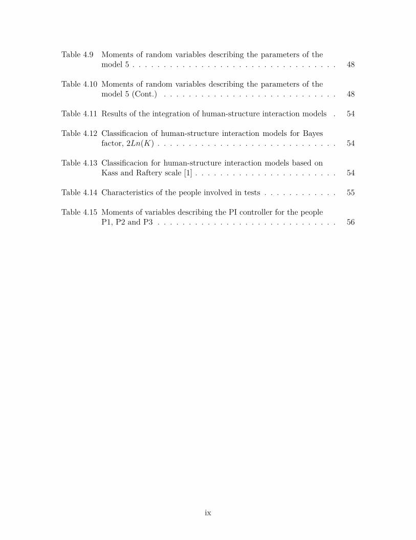
Table 4.9 Moments of random variables describing the parameters of themodel 5 . . . . . . . . . . . . . . . . . . . . . . . . . . . . . . . . . 48

Table 4.10 Moments of random variables describing the parameters of themodel 5 (Cont.) . . . . . . . . . . . . . . . . . . . . . . . . . . . . 48

Table 4.11 Results of the integration of human-structure interaction models . 54

Table 4.12 Classificacion of human-structure interaction models for Bayesfactor, 2Ln(K) . . . . . . . . . . . . . . . . . . . . . . . . . . . . . 54

Table 4.13 Classificacion for human-structure interaction models based onKass and Raftery scale [1] . . . . . . . . . . . . . . . . . . . . . . . 54

Table 4.14 Characteristics of the people involved in tests . . . . . . . . . . . . 55

Table 4.15 Moments of variables describing the PI controller for the peopleP1, P2 and P3 . . . . . . . . . . . . . . . . . . . . . . . . . . . . . 56

ix

List of Figures

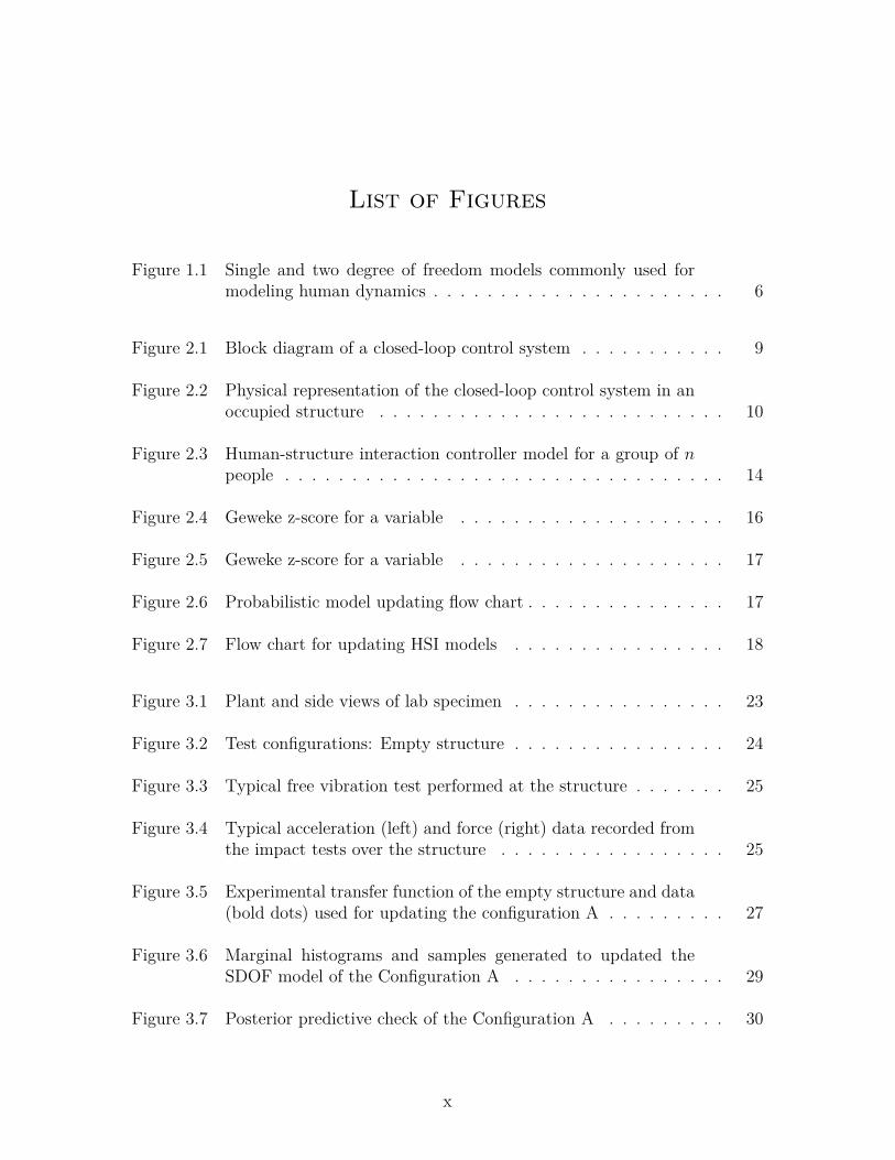
Figure 1.1 Single and two degree of freedom models commonly used formodeling human dynamics . . . . . . . . . . . . . . . . . . . . . . 6

Figure 2.1 Block diagram of a closed-loop control system . . . . . . . . . . . 9

Figure 2.2 Physical representation of the closed-loop control system in anoccupied structure . . . . . . . . . . . . . . . . . . . . . . . . . . 10

Figure 2.3 Human-structure interaction controller model for a group of npeople . . . . . . . . . . . . . . . . . . . . . . . . . . . . . . . . . 14

Figure 2.4 Geweke z-score for a variable . . . . . . . . . . . . . . . . . . . . 16

Figure 2.5 Geweke z-score for a variable . . . . . . . . . . . . . . . . . . . . 17

Figure 2.6 Probabilistic model updating flow chart . . . . . . . . . . . . . . . 17

Figure 2.7 Flow chart for updating HSI models . . . . . . . . . . . . . . . . 18

Figure 3.1 Plant and side views of lab specimen . . . . . . . . . . . . . . . . 23

Figure 3.2 Test configurations: Empty structure . . . . . . . . . . . . . . . . 24

Figure 3.3 Typical free vibration test performed at the structure . . . . . . . 25

Figure 3.4 Typical acceleration (left) and force (right) data recorded fromthe impact tests over the structure . . . . . . . . . . . . . . . . . 25

Figure 3.5 Experimental transfer function of the empty structure and data(bold dots) used for updating the configuration A . . . . . . . . . 27

Figure 3.6 Marginal histograms and samples generated to updated theSDOF model of the Configuration A . . . . . . . . . . . . . . . . 29

Figure 3.7 Posterior predictive check of the Configuration A . . . . . . . . . 30

x

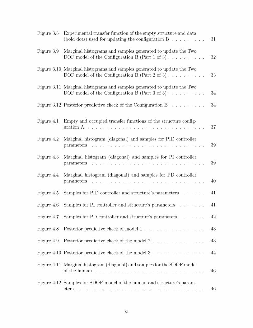
Figure 3.8 Experimental transfer function of the empty structure and data(bold dots) used for updating the configuration B . . . . . . . . . 31

Figure 3.9 Marginal histograms and samples generated to update the TwoDOF model of the Configuration B (Part 1 of 3) . . . . . . . . . . 32

Figure 3.10 Marginal histograms and samples generated to update the TwoDOF model of the Configuration B (Part 2 of 3) . . . . . . . . . . 33

Figure 3.11 Marginal histograms and samples generated to update the TwoDOF model of the Configuration B (Part 3 of 3) . . . . . . . . . . 34

Figure 3.12 Posterior predictive check of the Configuration B . . . . . . . . . 34

Figure 4.1 Empty and occupied transfer functions of the structure config-uration A . . . . . . . . . . . . . . . . . . . . . . . . . . . . . . . 37

Figure 4.2 Marginal histogram (diagonal) and samples for PID controllerparameters . . . . . . . . . . . . . . . . . . . . . . . . . . . . . . 39

Figure 4.3 Marginal histogram (diagonal) and samples for PI controllerparameters . . . . . . . . . . . . . . . . . . . . . . . . . . . . . . 39

Figure 4.4 Marginal histogram (diagonal) and samples for PD controllerparameters . . . . . . . . . . . . . . . . . . . . . . . . . . . . . . 40

Figure 4.5 Samples for PID controller and structure’s parameters . . . . . . 41

Figure 4.6 Samples for PI controller and structure’s parameters . . . . . . . 41

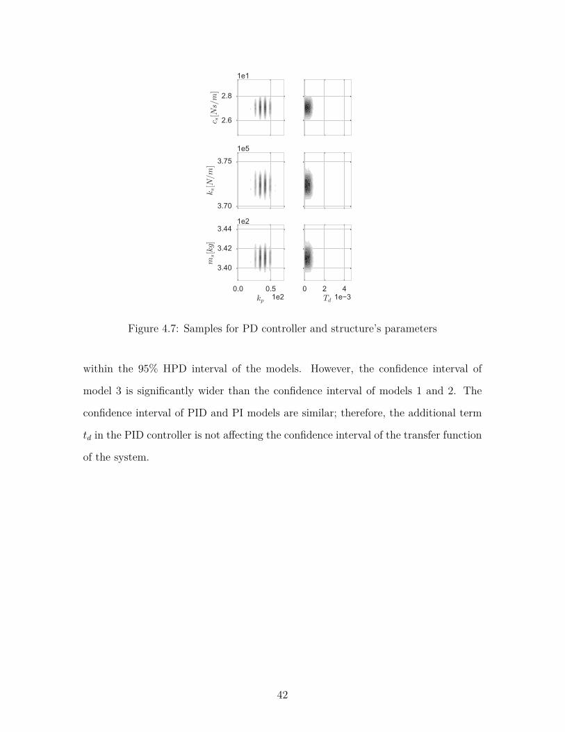
Figure 4.7 Samples for PD controller and structure’s parameters . . . . . . 42

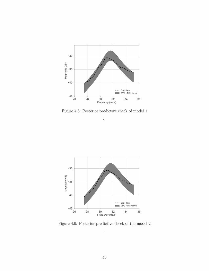
Figure 4.8 Posterior predictive check of model 1 . . . . . . . . . . . . . . . . 43

Figure 4.9 Posterior predictive check of the model 2 . . . . . . . . . . . . . . 43

Figure 4.10 Posterior predictive check of the model 3 . . . . . . . . . . . . . . 44

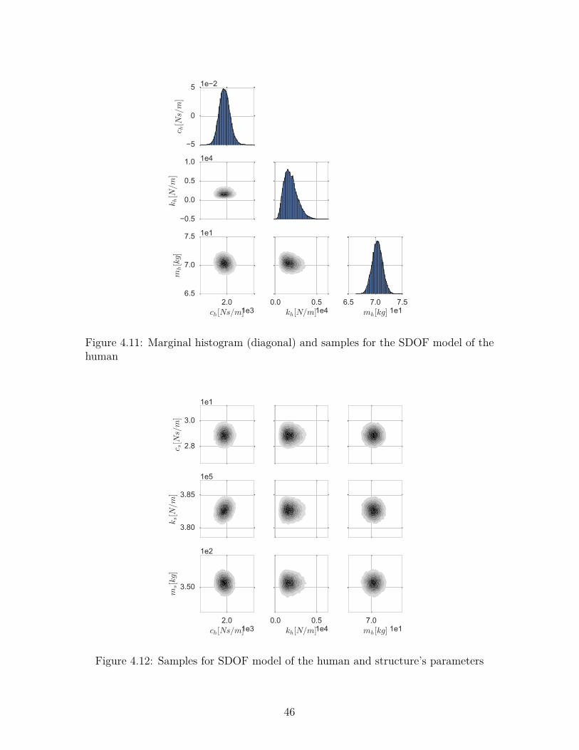
Figure 4.11 Marginal histogram (diagonal) and samples for the SDOFmodelof the human . . . . . . . . . . . . . . . . . . . . . . . . . . . . . 46

Figure 4.12 Samples for SDOF model of the human and structure’s param-eters . . . . . . . . . . . . . . . . . . . . . . . . . . . . . . . . . . 46

xi

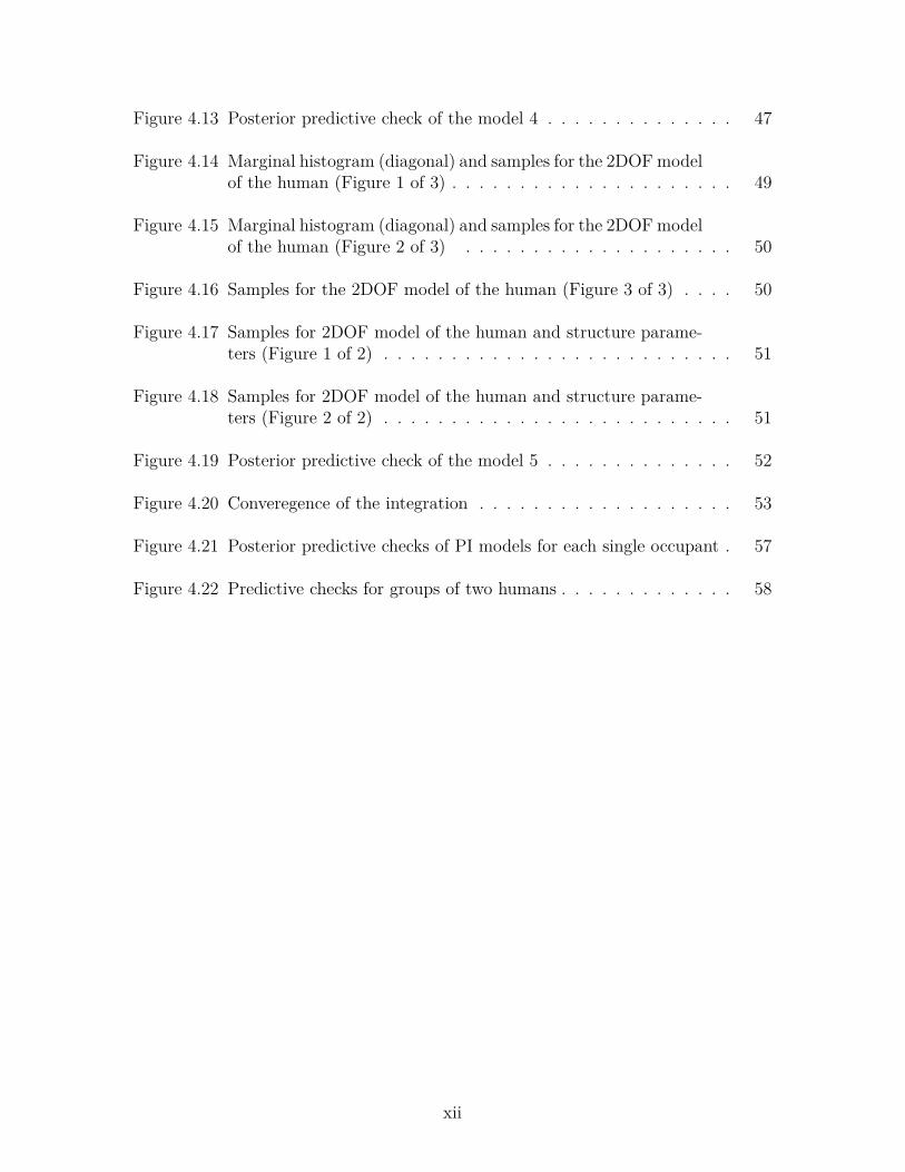
Figure 4.13 Posterior predictive check of the model 4 . . . . . . . . . . . . . . 47

Figure 4.14 Marginal histogram (diagonal) and samples for the 2DOFmodelof the human (Figure 1 of 3) . . . . . . . . . . . . . . . . . . . . . 49

Figure 4.15 Marginal histogram (diagonal) and samples for the 2DOFmodelof the human (Figure 2 of 3) . . . . . . . . . . . . . . . . . . . . 50

Figure 4.16 Samples for the 2DOF model of the human (Figure 3 of 3) . . . . 50

Figure 4.17 Samples for 2DOF model of the human and structure parame-ters (Figure 1 of 2) . . . . . . . . . . . . . . . . . . . . . . . . . . 51

Figure 4.18 Samples for 2DOF model of the human and structure parame-ters (Figure 2 of 2) . . . . . . . . . . . . . . . . . . . . . . . . . . 51

Figure 4.19 Posterior predictive check of the model 5 . . . . . . . . . . . . . . 52

Figure 4.20 Converegence of the integration . . . . . . . . . . . . . . . . . . . 53

Figure 4.21 Posterior predictive checks of PI models for each single occupant . 57

Figure 4.22 Predictive checks for groups of two humans . . . . . . . . . . . . . 58

xii

Chapter 1

Introduction

In the last century, structural engineers focused their attention on the design of

structures able to withstand large loads induced by natural and humans hazards,

such as earthquakes, high winds caused by tornadoes or hurricanes, flooding, and

explosions. The strengthening of the structural engineering field on the design of

structures against these hazards was outstanding. While a century ago many of these

hazards were not well understood and empirical methods were used in order to prevent

the collapse of many structures, today’s infrastructure is a lot more resilient due

to, in part, the design methodologies and new knowledge about hazards, materials,

construction methods, etc.

In the way that new materials were developed, new structural concepts of struc-

tures’ designs were also implemented by architects. The parallel and dependent evo-

lution of both fields led to unimaginable structures where open spaces play a key role.

This conception has been applied not only in the design of residential houses, but

also in the construction of huge structures such as stadiums, dance floors, gyms, or

lobby hotels; where the new materials, characterized as slender and lightweight, can

be used. However, as new materials decrease concerns related to strength, excessive

vibrations appear as one of the biggest challenges that the field of structural engi-

neering is facing. Therefore, serviceability problems are indisputably a side effect of

the new design tendencies.

In the study of serviceability conditions, the structures occupied by humans are

of special interest, mainly because human comfort is the main target in the design,

1

and their satisfaction could not be secured if vibration problems occur. In this way,

problems related to the vibrations induced and felt by humans have attracted the

attention as a current research topic in structural engineering.

The best example of vibrations induced by humans can be found in the UK.

During its opening in 2000, the Millennium footbridge, a structure that cost £18.7M,

showed excessive vibrations. The bridge was closed two days after opening. Repairs

left the bridge closed until 2002 when, after a retrofit and investment from ARUP

Inc. of £5M, the bridge was in-service again. Studies reported by Dallard et. al.

[2] and Fitzpatrick et. al. [3] found that the vibrations were produced because of a

feedback phenomenon that is rarely studied. This sketch of the problem has not been

developed further. Some studies suggest, though, that the problem is because there

is a coupling between the lateral frequency of the bridge and the lateral frequency

induced by humans while walking, a typical resonance phenomenon. However, the

case of resonance does not explain how the movement of the bridge induced people

to change their step frequency and the load they applied. This problem is considered

the formal starting point of human-structure interaction studies. More structural

problems caused by humans have been reported in Morris [4], Dallard et. al. [2],

Fitzpatrick et. al. [3], Bodare et. al. [5], and Macdonald [6].

Another effect of the human-structure interaction is observed when people are

in a passive condition like sitting or standing over the structure. Ortiz et. al. [7]

found that the properties of the structure change significantly when a structure is

occupied by humans. In their tests, they found that a mass produced by bags of sand

could not represent the phenomena. Falati et. al. [8] performed similar tests, but

on a simple supported slab. They found interesting changes in the frequency, but

especially in the damping ratio. Table 1.1 shows the change in the damping ratio and

the frequency for the slab’s main mode of vibration. Values reported in Table 1.1

are all deterministic. The probability distribution and the correlation of the model’s

2

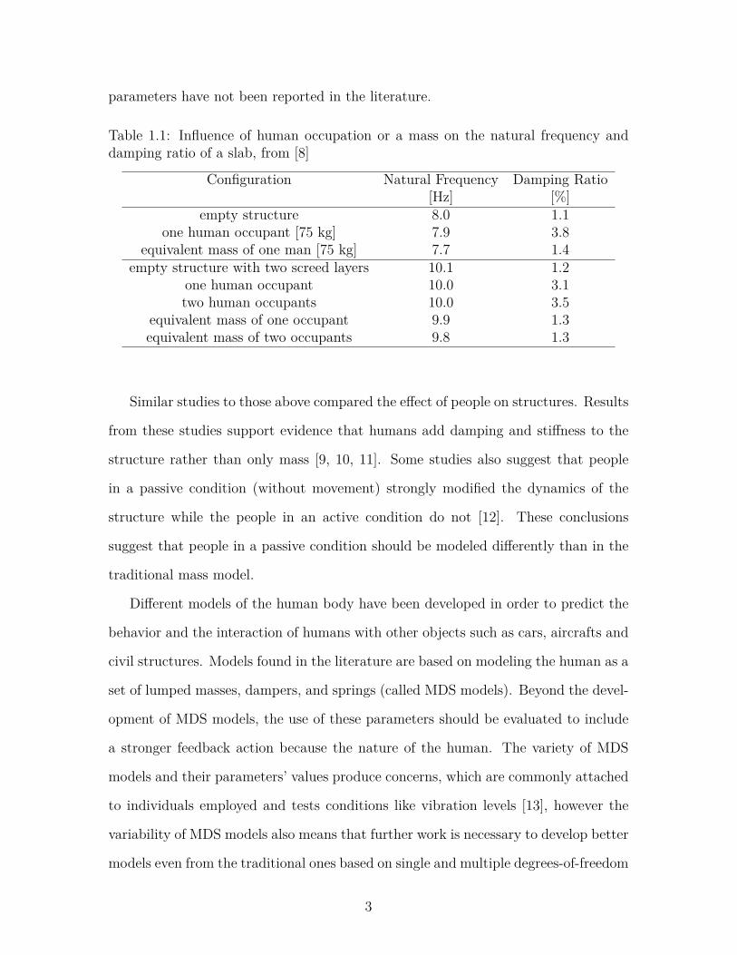
parameters have not been reported in the literature.

Table 1.1: Influence of human occupation or a mass on the natural frequency anddamping ratio of a slab, from [8]

Configuration Natural Frequency Damping Ratio[Hz] [%]

empty structure 8.0 1.1one human occupant [75 kg] 7.9 3.8

equivalent mass of one man [75 kg] 7.7 1.4empty structure with two screed layers 10.1 1.2

one human occupant 10.0 3.1two human occupants 10.0 3.5

equivalent mass of one occupant 9.9 1.3equivalent mass of two occupants 9.8 1.3

Similar studies to those above compared the effect of people on structures. Results

from these studies support evidence that humans add damping and stiffness to the

structure rather than only mass [9, 10, 11]. Some studies also suggest that people

in a passive condition (without movement) strongly modified the dynamics of the

structure while the people in an active condition do not [12]. These conclusions

suggest that people in a passive condition should be modeled differently than in the

traditional mass model.

Different models of the human body have been developed in order to predict the

behavior and the interaction of humans with other objects such as cars, aircrafts and

civil structures. Models found in the literature are based on modeling the human as a

set of lumped masses, dampers, and springs (called MDS models). Beyond the devel-

opment of MDS models, the use of these parameters should be evaluated to include

a stronger feedback action because the nature of the human. The variety of MDS

models and their parameters’ values produce concerns, which are commonly attached

to individuals employed and tests conditions like vibration levels [13], however the

variability of MDS models also means that further work is necessary to develop better

models even from the traditional ones based on single and multiple degrees-of-freedom

3

systems (SDOF and MDOF).

1.1 Traditional models used in HSI

A literature review published by Zivanovic, Pavic, and Reynolds [14] indicates that

there are two different types of models for the human body. The first and more

general is called the mass model [15]. This type of model only uses the humans’ mass

and does not model any HSI. This model is commonly used in building codes such

as the International Building Code (IBC) [16] and the guidelines proposed by the

American Society of Civil Engineers (ASCE) [15, 17]. The second type of model is

based on modeling the human as a mechanical system composed of lumped masses,

dampers, and springs (MDS) systems, which are likely used in problems related to

human-structure interaction. Many MDS models have been developed, ranging from

single to multiple degrees of freedom, in order to represent the dynamics of the human

body [8, 18, 19, 20, 21, 22].

Mass models for humans

Current design codes specify the application of live loads for structures occupied by

people [15, 16]. For example, the ASCE 7-05 code [15] specifies a load for residential

use of 30psf (1.44kN/m2), however the load is 3.3 times higher when the structure

is a gymnasium, dance hall, or a stadium, when the minimum design load is specified

as 100psf (4.49kN/m2).

A higher load is justified because of the high density of people and the possible

amplification that dynamic forces induced by humans may induce over the structure.

However, this consideration does not take into account additional changes over the

structure, such as different damping ratios, or stiffness changes, which may result in

a modification of the natural frequency of the structure, as seen before in Table 1.1.

4

Current design methodologies involve the application of Load Resistance and De-

sign Factors, (LRFD) methodology, which means that the load is amplified by a load

factor, which is usually around 1.6 for live load. The high magnitude of the live

load clearly states the importance of this type of load, but this does not consider the

human-structure interaction, causing over-design in some cases and excessive vibra-

tion in others.

The serviceability limit state is the second condition limit set in guidelines. This

focuses the attention in the human perception and their comfort, in order to avoid

the panic, or feeling of discomfort related to the dynamic response of the structure.

Serviceability conditions are based on structural accelerations. Limits are found in

different guidelines as a function of the type of structure and natural frequency of the

floor. [23, 24]

MDS Models For Humans

Mass-damper-spring models are used in HSI problems for modeling the human body

[13]. These models allow the interaction between dynamic properties of the human

body and the structure through inducing an action-reaction force. Researchers find

these models useful because they can reproduce a dynamic force induced by humans

as a function of the mass, damping, and stiffness of the body. The Joint Working

Group, from the Institution of Structural Engineers in the UK, is the only institution

which has formally proposed MDS models for guidelines [25]. This guide, "Dynamic

performance requirements for permanent grandstands subject to crowd action", rec-

ommended values for modeling passive people in grandstands in its latest edition.

The proposed models take into account the stiffness and damping beyond the mass

of the spectators.

The mathematical formulation of MDS models follows the theory of structural

dynamics. Independent of the number of degrees of freedom, the dynamic properties

5

of the model can be easily represented as deterministic values. Many researchers have

proposed values for the MDS parameters for HSI problems. Additional background of

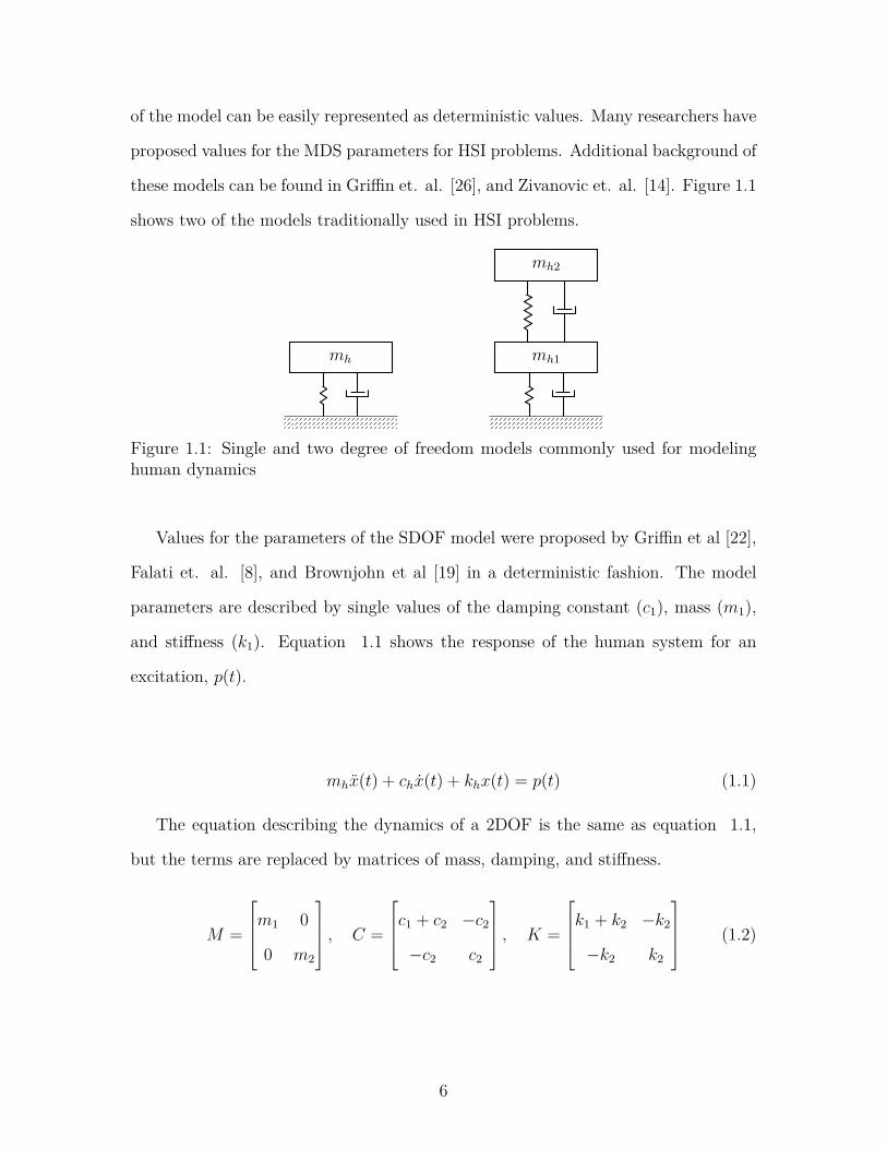
these models can be found in Griffin et. al. [26], and Zivanovic et. al. [14]. Figure 1.1

shows two of the models traditionally used in HSI problems.

mh mh1

mh2

Figure 1.1: Single and two degree of freedom models commonly used for modelinghuman dynamics

Values for the parameters of the SDOF model were proposed by Griffin et al [22],

Falati et. al. [8], and Brownjohn et al [19] in a deterministic fashion. The model

parameters are described by single values of the damping constant (c1), mass (m1),

and stiffness (k1). Equation 1.1 shows the response of the human system for an

excitation, p(t).

mhx(t) + chx(t) + khx(t) = p(t) (1.1)

The equation describing the dynamics of a 2DOF is the same as equation 1.1,

but the terms are replaced by matrices of mass, damping, and stiffness.

M =

m1 0

0 m2

, C =

c1 + c2 −c2

−c2 c2

, K =

k1 + k2 −k2

−k2 k2

(1.2)

6

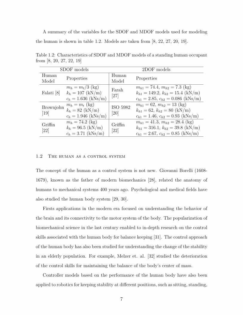
A summary of the variables for the SDOF and MDOF models used for modeling

the human is shown in table 1.2. Models are taken from [8, 22, 27, 20, 19].

Table 1.2: Characteristics of SDOF and MDOF models of a standing human occupantfrom [8, 20, 27, 22, 19]

SDOF models 2DOF modelsHumanModel Properties Human

Model Properties

Falati [8]mh = mt/3 (kg) Farah

[27]

mh1 = 74.4, mh2 = 7.3 (kg)kh = 107 (kN/m) kh1 = 149.2, kh2 = 15.4 (kN/m)ch = 1.636 (kNs/m) ch1 = 2.85, ch2 = 0.086 (kNs/m)

Brownjohn[19]

mh = mt (kg) ISO 5982[20]

mh1 = 62, mh2 = 13 (kg)kh = 82 (kN/m) kh1 = 62, kh2 = 80 (kN/m)ch = 1.946 (kNs/m) ch1 = 1.46, ch2 = 0.93 (kNs/m)

Griffin[22]

mh = 74.2 (kg) Griffin[22]

mh1 = 41.3, mh2 = 28.4 (kg)kh = 96.5 (kN/m) kh1 = 316.1, kh2 = 39.8 (kN/m)ch = 3.71 (kNs/m) ch1 = 2.67, ch2 = 0.85 (kNs/m)

1.2 The human as a control system

The concept of the human as a control system is not new. Giovanni Borelli (1608-

1679), known as the father of modern biomechanics [28], related the anatomy of

humans to mechanical systems 400 years ago. Psychological and medical fields have

also studied the human body system [29, 30].

Firsts applications in the modern era focused on understanding the behavior of

the brain and its connectivity to the motor system of the body. The popularization of

biomechanical science in the last century enabled to in-depth research on the control

skills associated with the human body for balance keeping [31]. The control approach

of the human body has also been studied for understanding the change of the stability

in an elderly population. For example, Melzer et. al. [32] studied the deterioration

of the control skills for maintaining the balance of the body’s center of mass.

Controller models based on the performance of the human body have also been

applied to robotics for keeping stability at different positions, such as sitting, standing,

7

walking and jumping [33, 34]. However, the short time response of the body to

external loads is a challenge and has not been totally achieved, therefore, optimization

techniques and faster controllers for modeling the body mechanics and body control

loops actions are still under development.

The most common biomechanical model of the human body is the inverted pen-

dulum system [35]. Controller models have been applied to this model in order to

recreate the control loop between the input sensors (vestibular, visual, and proprio-

ceptive) and the motor output. In their work, Hidenura and Jiang, develop a PID

model for human balance keeping [36]. The closed-loop model was updated from a

deterministic point of view, in the time domain. Results of their investigation sug-

gested that the derivative factor (KD) of the PID controller plays a key role in the

balance and the stability of the body.

Recent research developed by Bocian et. al. [37] used the inverted pendulum

model for modeling the force induced by pedestrians over a vertically oscillating

structure. The changes in damping induced by pedestrians over the structure, such

as the changes seen in the Millenium bridge, could be addressed through this model.

However, improvements to the model are suggested, specially focusing on the human

system, which could lead to introduce the control action.

Even though considerable work has been done to model specific tasks done by

humans using control theory, the application of controller for HSI is still at its fancy.

The use of control theory in HSI introduces an alternative way for understanding

the behavior of the human body, and its influence in the structure properties. This

research will provide probabilistic information about the controllers that could be

used for modeling the phenomenon. The traditional single and multiple degree of

freedom models will be updated, and then compared with controller models.

8

Chapter 2

Methodology

2.1 Human-structure Interaction as a closed-loop control system

The idea of using control theory for modeling human-structure interaction comes

from the fact that the feedback provided by MDS models is not adequate to correctly

model the human-structure interaction. MDS models provide forces proportional to

the relative velocity and displacement between the structure and the mass of the

human. Closed-loop control systems provide more flexibility. The term closed-loop

control implies the use of feedback in order to reduce system error [38]. Figure 2.1

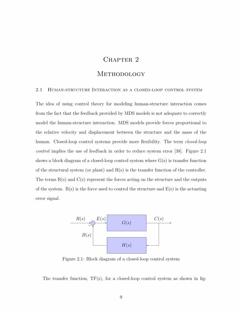
shows a block diagram of a closed-loop control system where G(s) is transfer function

of the structural system (or plant) and H(s) is the transfer function of the controller.

The terms R(s) and C(s) represent the forces acting on the structure and the outputs

of the system. B(s) is the force used to control the structure and E(s) is the actuating

error signal.

G(s)

H(s)

R(s) E(s) C(s)−

B(s)

Figure 2.1: Block diagram of a closed-loop control system

The transfer function, TF(s), for a closed-loop control system as shown in fig-

9

ure 2.1 is defined as:

TF (s) = G(s)1 +G(s)H(s) (2.1)

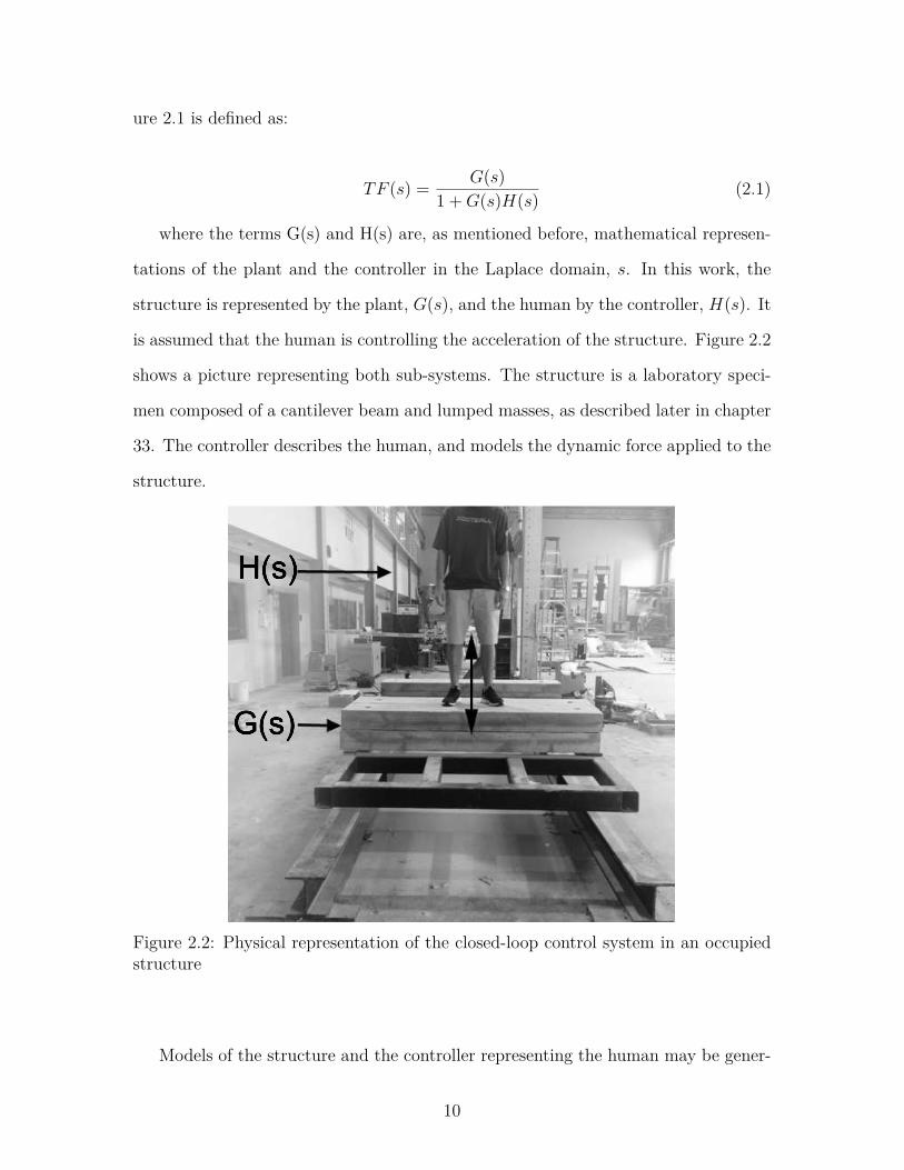
where the terms G(s) and H(s) are, as mentioned before, mathematical represen-

tations of the plant and the controller in the Laplace domain, s. In this work, the

structure is represented by the plant, G(s), and the human by the controller, H(s). It

is assumed that the human is controlling the acceleration of the structure. Figure 2.2

shows a picture representing both sub-systems. The structure is a laboratory speci-

men composed of a cantilever beam and lumped masses, as described later in chapter

33. The controller describes the human, and models the dynamic force applied to the

structure.

Figure 2.2: Physical representation of the closed-loop control system in an occupiedstructure

Models of the structure and the controller representing the human may be gener-

10

ated in order to represent the interaction. The next two sections discuss in detail the

models used for the structure and the controller.

Modeling the structure

The structure G(s) can be modeled as a single or multiple degree of freedom system.

Modeling errors are expected when modeling any type of structural system. There are

errors due to the fact that the model does not accurately describe the behavior of the

structure. Furthermore, uncertainty in the parameters of the model might be present.

Depending on the complexity of the structure, modeling errors can be significant.

The structural system considered for this work (discussed in detail in chapter 3) was

specifically considered because of its simplicity, minimizing the chances of including

modeling errors in the structural system, and allowing the study of closed-loop control

theory in a controlled environment. In its simplest form, the structure can be modeled

as a SDOF. For a SDOF, the term G(s) is defined as:

G(s) =s2

ms

s2 + cs

mss+ ks

ms

(2.2)

where the parameters ms, cs, and ks are the equivalent mass, damping coefficient,

and stiffness of the structure when assumed to be an SDOF system, therefore the

parameters of the model are Θs = {ms, cs, ks}. If the structure is modeled as a

multiple degree of freedom system the parametersms, cs, and ks become matrices. An

alternative way for modeling the structure is using the poles and zeros of the system

[39]. The transfer function of the structure can be expressed using the equation 2.3:

G(s) = Ks2 (s− z1)(s− z2)...(s− zm−1)(s− zm)(s− p1)(s− p2)...(s− pm−1)(s− pm) (2.3)

In this equation, the poles, pi, are roots of the denominator and the zeros, zi,

are roots of the numerator and K is the gain. Each pole of the system contains

information about the natural frequency, ωi, of the structure and its corresponding

11

damping ratio, ζi. In a structural system poles are complex conjugates and the

relationship with the i-th natural frequency and associated damping ratio is:

pi = −ζiωi ±√

(ζiωi)2 − ω2i (2.4)

Therefore, the model of the structure can be expressed in terms of natural fre-

quencies, ωi; damping ratios, ζi; and the gain, K. For a model with two poles and

one zero, the parameters used in the model are Θs = {ω1, ω2, ζ1, ζ2, ωz1, ζz1, K}. An

in-depth discussion of systems modeling using this approach can be found in [39] and

[38].

Modeling the controller

The controller is a decisive part in the closed-loop system. It is a device which

monitors and physically alters the operating conditions of a given dynamical system

[40]. For this research, the controller, H(s), alters the operating conditions of the

structure, G(s). For example, a person standing on a structure will minimize the

vibrations of a structure [41, 11, 13]. The use of controllers has become popular in

the last century, boosted by the development of computers. Application of controllers

involves almost all fields of engineering, such as, aerospace [42], biomechanical [43],

electrical [44], or civil engineering [45]. One of the most common controllers it the

Proportional, Integrative and Derivative (PID) and its derivation, PI and PD. PID

controllers are used for controlling autonomous cars [46], for controlling the amount

of glucose in the blood for ill patients [47], and for the control of Unmaneed Aerial

Vehicles (UAV) [48] among others.

PID controllers use three parameters associated to the state of the error. The

three parameters are the proportional term, Kp; the integrative term, Ti; and the

derivative term, Td. While the proportional term, Kp, multiplies the feedback, the

12

integrative, Ti, and derivative, Td, multiply the integral and derivative of the feedback.

The transfer function for the PID is:

H(s) = Kp(1 + Tds+ 1Tis

) (2.5)

For a PD controller, the transfer function can be represented as:

H(s) = Kp(1 + Tds) (2.6)

For a PI controller, the transfer function can be represented as:

H(s) = Kp(1 + 1Tis

) (2.7)

The model defined in equation 2.1 assumes the use of one controller for each

human. Under this assumption, each person acts as an independent controller, com-

manding a control force on the structure. In the case of groups of people, the i-th

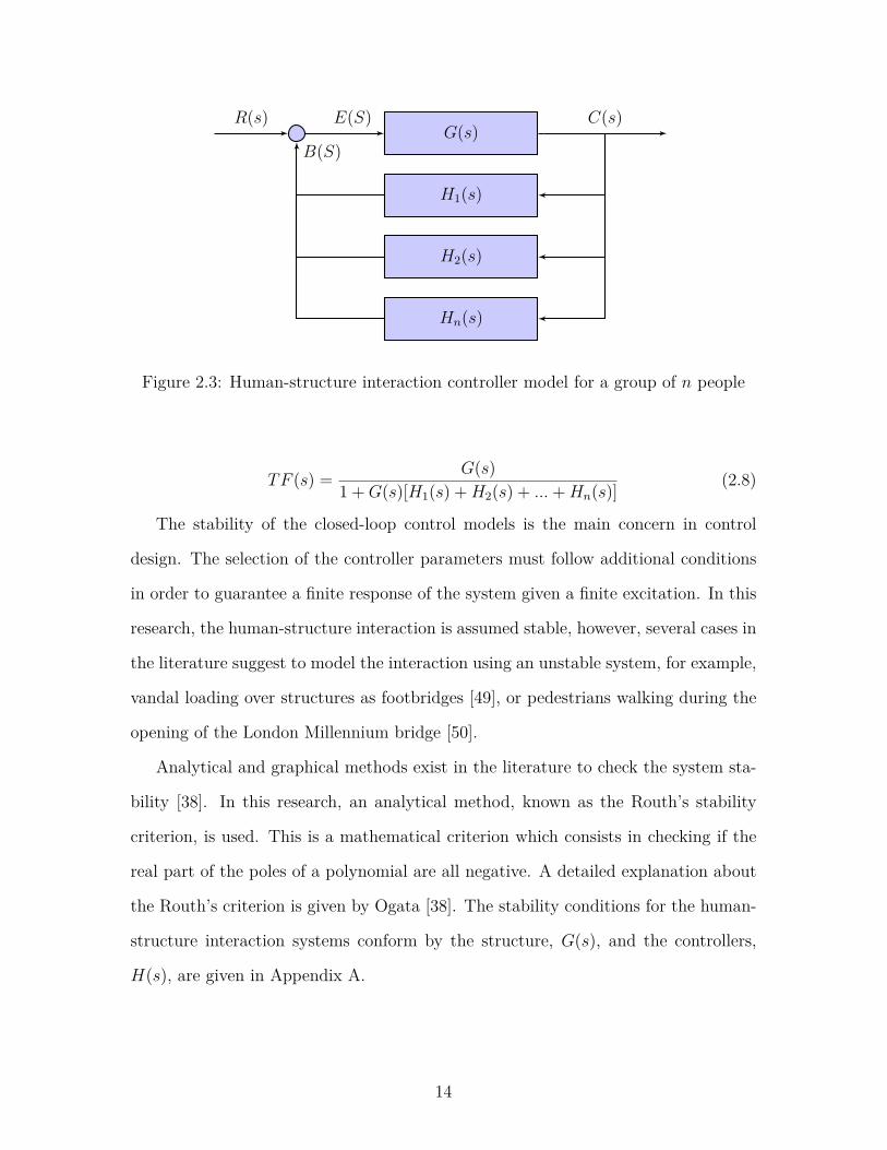
controller, Hi(s), represent a specific person, (i). Figure 2.3 shows a block diagram

of the whole human-structure interaction system when the structure is occupied by

n people acting independently. It is assumed that controllers are acting in parallel,

indicating that the motion of one person has little effect on the motion of the next

person, which is reasonable for standing people.

While this model should be appropriated to model humans acting in sync because

of interactions with the structural system, it will not model interaction between hu-

mans (i.e. people pushing each other). Additional feedback loops could be formulated

to model these interactions.

Therefore, the transfer function of the full HSI system occupied by n indepen-

dently people can be presented as:

13

G(s)

H1(s)

H2(s)

Hn(s)

R(s) E(S) C(s)

B(S)

Figure 2.3: Human-structure interaction controller model for a group of n people

TF (s) = G(s)1 +G(s)[H1(s) +H2(s) + ...+Hn(s)] (2.8)

The stability of the closed-loop control models is the main concern in control

design. The selection of the controller parameters must follow additional conditions

in order to guarantee a finite response of the system given a finite excitation. In this

research, the human-structure interaction is assumed stable, however, several cases in

the literature suggest to model the interaction using an unstable system, for example,

vandal loading over structures as footbridges [49], or pedestrians walking during the

opening of the London Millennium bridge [50].

Analytical and graphical methods exist in the literature to check the system sta-

bility [38]. In this research, an analytical method, known as the Routh’s stability

criterion, is used. This is a mathematical criterion which consists in checking if the

real part of the poles of a polynomial are all negative. A detailed explanation about

the Routh’s criterion is given by Ogata [38]. The stability conditions for the human-

structure interaction systems conform by the structure, G(s), and the controllers,

H(s), are given in Appendix A.

14

2.2 Bayesian Model Updating

The dynamic behavior of the models presented in the previous section depends on

their parameters. In this research, Bayesian inference is used to update the parame-

ters of the models based on experimental data [51, 52]. Bayesian inference is based

on the Bayes theorem:

P (Θ|D,Mj) = P (D|Θ,Mj)P (Θ|Mj)P (D) (2.9)

where P (Θ|D,Mj) is the posterior probability density function (PDF) of the pa-

rameters Θ, for model Mj, given the observation D. P (Θ|Mj) is the prior PDF of

the parameters Θ and it represents the knowledge of the parameters before updating.

P (D|Θ,Mj) is the likelihood of the occurrence of the measurement D given the vector

of parameters Θ and model Mj. P (D) is the probability of the observation D.

It is important to highlight some of the main differences between inference using

classical methods and Bayesian inference. Classical methods assume that here is

one underlining "true" probability distribution describing the parameters and the

experimental data are random draws from this distribution. Bayesian inference is

different. Here, the experimental data, or observations, are "fixed" and the probability

density function is calculated given these observations. Therefore, it is important to

highlight that the results of this research could change if other populations are used

for the experiments. However, the overall procedure and concepts developed here

should be applicable.

Several techniques are available to extract useful information from the posterior

PDF. For example, one can calculate the Maximum A Posteriory (MAP) as a point

estimate of the parameters. In this research, samples of the posterior are obtained to

derive statistics of the parameters, investigate correlations, and fully describe their

probability density functions. The samples are generated using the Markov chain

15

Monte Carlo (MCMC) methodology [53, 54, 55]. The MCMC is a derivation of

the Monte carlo sampling algorithm, where the samples distribution is based on an

equilibrium condition. The Markov chain algorithm defines the probability of the

next step based on the probability of the current step. In particular, the Metropolis

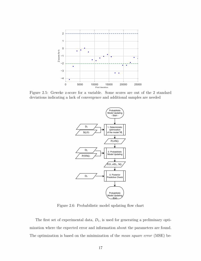
algorithm was used. The convergence of the chains was checked using the method

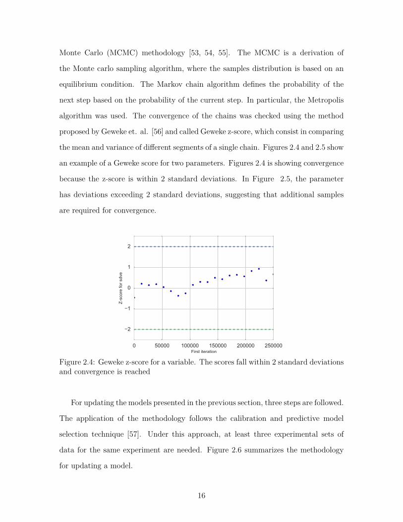
proposed by Geweke et. al. [56] and called Geweke z-score, which consist in comparing

the mean and variance of different segments of a single chain. Figures 2.4 and 2.5 show

an example of a Geweke score for two parameters. Figures 2.4 is showing convergence

because the z-score is within 2 standard deviations. In Figure 2.5, the parameter

has deviations exceeding 2 standard deviations, suggesting that additional samples

are required for convergence.

0 50000 100000 150000 200000 250000First iteration

−2

−1

0

1

2

Z-sc

ore

for s

dve

Figure 2.4: Geweke z-score for a variable. The scores fall within 2 standard deviationsand convergence is reached

For updating the models presented in the previous section, three steps are followed.

The application of the methodology follows the calibration and predictive model

selection technique [57]. Under this approach, at least three experimental sets of

data for the same experiment are needed. Figure 2.6 summarizes the methodology

for updating a model.

16

0 5000 10000 15000 20000 25000First iteration

−4

−3

−2

−1

0

1

2

Z-sc

ore

for k

Figure 2.5: Geweke z-score for a variable. Some scores are out of the 2 standarddeviations indicating a lack of convergence and additional samples are needed

Figure 2.6: Probabilistic model updating flow chart

The first set of experimental data, D1, is used for generating a preliminary opti-

mization where the expected error and information about the parameters are found.

The optimization is based on the minimization of the mean square error (MSE) be-

17

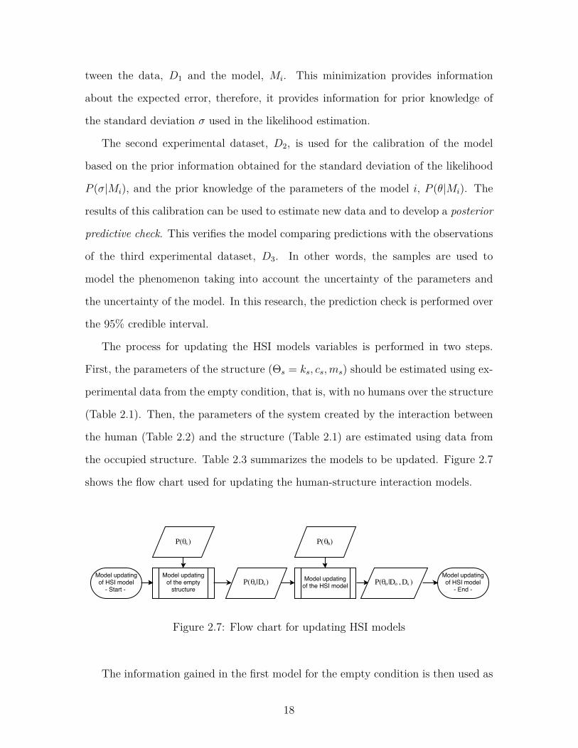
tween the data, D1 and the model, Mi. This minimization provides information

about the expected error, therefore, it provides information for prior knowledge of

the standard deviation σ used in the likelihood estimation.

The second experimental dataset, D2, is used for the calibration of the model

based on the prior information obtained for the standard deviation of the likelihood

P (σ|Mi), and the prior knowledge of the parameters of the model i, P (θ|Mi). The

results of this calibration can be used to estimate new data and to develop a posterior

predictive check. This verifies the model comparing predictions with the observations

of the third experimental dataset, D3. In other words, the samples are used to

model the phenomenon taking into account the uncertainty of the parameters and

the uncertainty of the model. In this research, the prediction check is performed over

the 95% credible interval.

The process for updating the HSI models variables is performed in two steps.

First, the parameters of the structure (Θs = ks, cs,ms) should be estimated using ex-

perimental data from the empty condition, that is, with no humans over the structure

(Table 2.1). Then, the parameters of the system created by the interaction between

the human (Table 2.2) and the structure (Table 2.1) are estimated using data from

the occupied structure. Table 2.3 summarizes the models to be updated. Figure 2.7

shows the flow chart used for updating the human-structure interaction models.

Figure 2.7: Flow chart for updating HSI models

The information gained in the first model for the empty condition is then used as

18

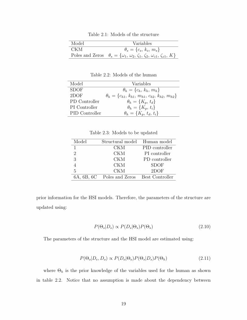
Table 2.1: Models of the structure

Model VariablesCKM θs = {cs, ks, ms}Poles and Zeros θs = {ω1, ω2, ζ1, ζ2, ωz1, ζz1, K}

Table 2.2: Models of the human

Model VariablesSDOF θh = {ch, kh, mh}2DOF θh = {ch1, kh1, mh1, ch2, kh2, mh2}PD Controller θh = {Kp, td}PI Controller θh = {Kp, ti}PID Controller θh = {Kp, td, ti}

Table 2.3: Models to be updated

Model Structural model Human model1 CKM PID controller2 CKM PI controller3 CKM PD controller4 CKM SDOF5 CKM 2DOF6A, 6B, 6C Poles and Zeros Best Controller

prior information for the HSI models. Therefore, the parameters of the structure are

updated using:

P (Θs|Ds) ∝ P (Ds|Θs)P (Θs) (2.10)

The parameters of the structure and the HSI model are estimated using:

P (Θo|De, Do) ∝ P (Do|Θo)P (Θs|Ds)P (Θh) (2.11)

where Θh is the prior knowledge of the variables used for the human as shown

in table 2.2. Notice that no assumption is made about the dependency between

19

parameters of the structure (θs) and parameters of the human (θh). This assumption

will be checked with the PDFs of the posterior once the model is updated.

The prior distributions for the structural parameters (ks, ms, and cs) are defined

based on the physical characteristics of the structure.

2.3 Probabilistic Model Selection

Bayesian probabilistic model selection technique is used to determine which of the

models proposed in the first 5 rows of Table 2.3 has the highest probability given

the observed data. This methodology considers the uncertainty of the model and

the uncertainty associated with each parameter. The probabilistic model selection

is based on the principle proposed by William of Ockham, called Ockham’s razor,

which is well discussed in [58]. This principle states that "a simpler explanation for

some phenomenon is more likely to be accurate than more complicated explanations"

[59]. Therefore, models with a larger number of parameters are "penalized" to avoid

overfitting.

Probabilistic model selection can be derived from the Bayes theorem shown in

equation 2.9:

P (Θ|D,Mj) = P (D|Θ,Mj)P (Θ|Mj)P (D|Mj)

(2.9)

where the denominator, P (D|Mj), is called model evidence and serves as a nor-

malization constant. Therefore:

p(D|Mj) =∫

Θp(D|Θ,Mj)p(Θ|Mj)dΘ (2.12)

Using again Bayes inference, the posterior probability of a model, Mj, given some

observations, D, can be estimated as:

20

P (Mj|D) = P (D|Mj)P (Mj)P (D) (2.13)

If the same dataset, D, is used for updating models Mj and Mk, the posterior

odds ratio between the models is expressed by:

P (Mj|D)P (Mk|D) = P (D|Mj)P (Mj)

P (D|Mk)P (Mk) (2.14)

where the terms P (D|Mj) and P (D|Mk) are calculated following the equation

2.12. The terms P (Mk) and P (Mj) refer to the prior knowledge of each model. In

this research, it is assumed that all the models have the same probability, therefore:

K = P (Mj|D)P (Mk|D) = P (D|Mj)

P (D|Mk) (2.15)

Where the term K is called Bayes Factor. This research uses the widely known

method of Monte Carlo (MC) integration [60] for obtaining the model evidence. The

Vegas algorithm [61], implemented in the package Vegas, in the software Python, is

used for MC integration.

Models are compared based on Kass and Raftery [1] which is a derivation of the

Jeffreys’ scale [62]. This scale classifies the Bayes factor as shown in Table 2.4 using

the natural logarithm of the Bayes Factor, (2Ln(k)).

Table 2.4: Kass and Raftery scale for Bayes factor

2Ln(K) Strength of evidence0 to 2 not worth more than a bare mention2 to 6 Positive6 to 10 Strong>10 Very strong

21

Chapter 3

Experimental testing and updating of empty

structure

The updating of the human-structure interaction models is performed using exper-

imental tests over a configurable structure. This chapter focuses on the description

of the structure, the equipments used, the tests performed, and the model update

process implemented for updating the parameters of the unoccupied structure.

3.1 Lab structure

The structure used in testing is a steel frame specifically designed to represent a range

of dynamic properties representative of flexible slabs; however, a "rigid" behavior

(fn ≈ 10Hz) can also be reached. The experimental setup is light in order to maintain

the ratio between live load and dead load similar to common structures susceptible

to human-induced vibrations. The structure is inspired by an existing experimental

setup at Bucknell University [18].

The frame is a cantilever horizontal truss composed by 5x4x1⁄4′′ steel tubes, built

in the Structures lab at the University of South Carolina as shown in Figure 3.1.

The structure has four supports. Two supports are fixed and located at one end.

The other two can move along the structure in order to modify the cantilever length,

which change the dynamic properties of the structure. Additional concrete blocks are

used to customize the mass. These are heavier than the steel frame and lead to a

better control of the desirable conditions. Changes in the stiffness and mass lead to

22

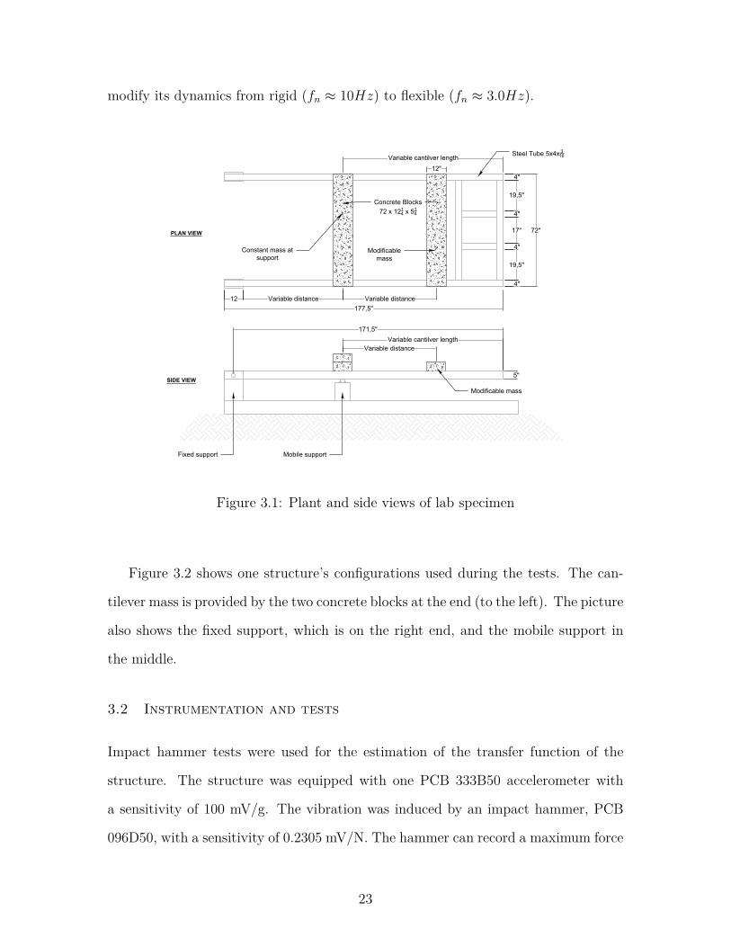
modify its dynamics from rigid (fn ≈ 10Hz) to flexible (fn ≈ 3.0Hz).

177,5"

72"

19,5"

19,5"

17"

171,5"

12 Variable distance

5"

4"

4"

4"

Mobile support

Modificable mass

Variable cantilver length

Variable distance

Variable distance

12"

Variable cantilver length

4"

Constant mass at

support

Modificable

mass

Steel Tube 5x4x

3

16

Block of 72 x 121/4 x 51/4

Concrete Blocks

72 x 12

1

4

x 5

1

4

Fixed support

PLAN VIEW

SIDE VIEW

Human-Structure Interaction Project

- structure for tests -

Concrete: f'c: 4000psi

Block of 72 x 12

1

4

x 5

1

4

Steel: A36

Rectangular Tube 5x4x

3

16

PLAN VIEW

Measure units: inches

SIDE VIEW

Measure units: inches

Figure 3.1: Plant and side views of lab specimen

Figure 3.2 shows one structure’s configurations used during the tests. The can-

tilever mass is provided by the two concrete blocks at the end (to the left). The picture

also shows the fixed support, which is on the right end, and the mobile support in

the middle.

3.2 Instrumentation and tests

Impact hammer tests were used for the estimation of the transfer function of the

structure. The structure was equipped with one PCB 333B50 accelerometer with

a sensitivity of 100 mV/g. The vibration was induced by an impact hammer, PCB

096D50, with a sensitivity of 0.2305 mV/N. The hammer can record a maximum force

23

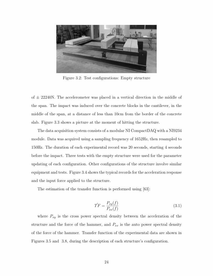
Figure 3.2: Test configurations: Empty structure

of ± 22240N. The accelerometer was placed in a vertical direction in the middle of

the span. The impact was induced over the concrete blocks in the cantilever, in the

middle of the span, at a distance of less than 10cm from the border of the concrete

slab. Figure 3.3 shows a picture at the moment of hitting the structure.

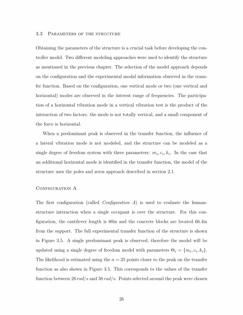
The data acquisition system consists of a modular NI CompactDAQ with a NI9234

module. Data was acquired using a sampling frequency of 1652Hz, then resampled to

150Hz. The duration of each experimental record was 20 seconds, starting 4 seconds

before the impact. Three tests with the empty structure were used for the parameter

updating of each configuration. Other configurations of the structure involve similar

equipment and tests. Figure 3.4 shows the typical records for the acceleration response

and the input force applied to the structure.

The estimation of the transfer function is performed using [63]:

ˆTF = Pxy(f)Pxx(f) (3.1)

where Pxy is the cross power spectral density between the acceleration of the

structure and the force of the hammer, and Pxx is the auto power spectral density

of the force of the hammer. Transfer function of the experimental data are shown in

Figures 3.5 and 3.8, during the description of each structure’s configuration.

24

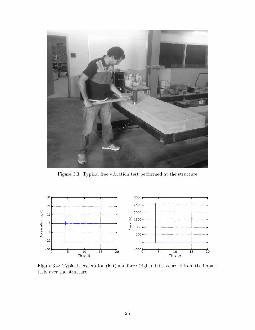
Figure 3.3: Typical free vibration test performed at the structure

0 5 10 15 20Time (s)

−30

−20

−10

0

10

20

30

Acc

ele

rati

on (m/s2)

0 5 10 15 20Time (s)

−500

0

500

1000

1500

2000

2500

3000

Forc

e (N

)

Figure 3.4: Typical acceleration (left) and force (right) data recorded from the impacttests over the structure

25

3.3 Parameters of the structure

Obtaining the parameters of the structure is a crucial task before developing the con-

troller model. Two different modeling approaches were used to identify the structure

as mentioned in the previous chapter. The selection of the model approach depends

on the configuration and the experimental modal information observed in the trans-

fer function. Based on the configuration, one vertical mode or two (one vertical and

horizontal) modes are observed in the interest range of frequencies. The participa-

tion of a horizontal vibration mode in a vertical vibration test is the product of the

interaction of two factors: the mode is not totally vertical, and a small component of

the force is horizontal.

When a predominant peak is observed in the transfer function, the influence of

a lateral vibration mode is not modeled, and the structure can be modeled as a

single degree of freedom system with three parameters: ms, cs, ks. In the case that

an additional horizontal mode is identified in the transfer function, the model of the

structure uses the poles and zeros approach described in section 2.1.

Configuration A

The first configuration (called Configuration A) is used to evaluate the human-

structure interaction when a single occupant is over the structure. For this con-

figuration, the cantilever length is 80in and the concrete blocks are located 66.4in

from the support. The full experimental transfer function of the structure is shown

in Figure 3.5. A single predominant peak is observed, therefore the model will be

updated using a single degree of freedom model with parameters Θs = {ms, cs, ks}.

The likelihood is estimated using the n = 25 points closer to the peak on the transfer

function as also shown in Figure 3.5. This corresponds to the values of the transfer

function between 28 rad/s and 38 rad/s. Points selected around the peak were chosen

26

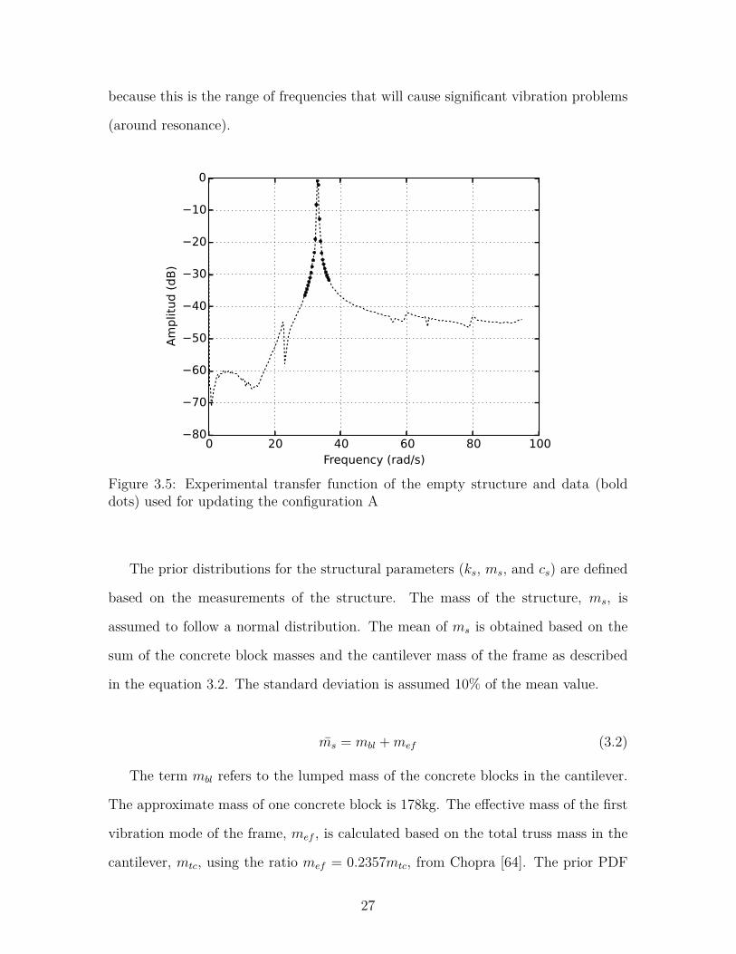
because this is the range of frequencies that will cause significant vibration problems

(around resonance).

0 20 40 60 80 100Frequency (rad/s)

−80

−70

−60

−50

−40

−30

−20

−10

0A

mplit

ud (

dB

)

Figure 3.5: Experimental transfer function of the empty structure and data (bolddots) used for updating the configuration A

The prior distributions for the structural parameters (ks, ms, and cs) are defined

based on the measurements of the structure. The mass of the structure, ms, is

assumed to follow a normal distribution. The mean of ms is obtained based on the

sum of the concrete block masses and the cantilever mass of the frame as described

in the equation 3.2. The standard deviation is assumed 10% of the mean value.

ms = mbl +mef (3.2)

The term mbl refers to the lumped mass of the concrete blocks in the cantilever.

The approximate mass of one concrete block is 178kg. The effective mass of the first

vibration mode of the frame, mef , is calculated based on the total truss mass in the

cantilever, mtc, using the ratio mef = 0.2357mtc, from Chopra [64]. The prior PDF

27

distribution of the stiffness of the structure, ks, is assumed uniform between a range

of 300kN/m and 500kN/m.

The prior information for the damping coefficient, cs, is estimated based on a free

vibration test performed in the structure. A damping ratio of ζ = 0.2% is estimated

using the Free Decay Motion technique such as explained in Chopra [64]. Therefore,

the prior PDF for cs is P (cs) = N(31, 3.1).

The prior distribution of the standard deviation of the likelihood consist of an

Inverse Gamma distribution where the shape parameter, α, is 10, and the scale pa-

rameter, β, is obtained from the minimization of the Mean squared error (MSE)

calculated between the SDOF model and the first set of experimental data. The

minimization uses the Nelder-Mead method [65]. Table 3.1 shows the prior used for

the calibration of the model.

Table 3.1: Prior PDFs used for updating the parameters

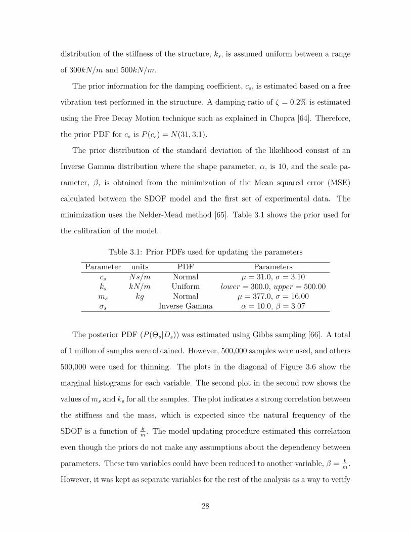
Parameter units PDF Parameterscs Ns/m Normal µ = 31.0, σ = 3.10ks kN/m Uniform lower = 300.0, upper = 500.00ms kg Normal µ = 377.0, σ = 16.00σs Inverse Gamma α = 10.0, β = 3.07

The posterior PDF (P (Θs|Ds)) was estimated using Gibbs sampling [66]. A total

of 1 millon of samples were obtained. However, 500,000 samples were used, and others

500,000 were used for thinning. The plots in the diagonal of Figure 3.6 show the

marginal histograms for each variable. The second plot in the second row shows the

values ofms and ks for all the samples. The plot indicates a strong correlation between

the stiffness and the mass, which is expected since the natural frequency of the

SDOF is a function of km. The model updating procedure estimated this correlation

even though the priors do not make any assumptions about the dependency between

parameters. These two variables could have been reduced to another variable, β = km.

However, it was kept as separate variables for the rest of the analysis as a way to verify

28

−5

0

5

c s[Ns/m

]

1e−2

3.0

3.5

4.0

4.5

ks[N/m

]

1e5

3.0

3.5

4.0

ms[kg]

1e2

2 3 4cs[Ns/m]1e1

1

2

3

4

5

σ

3.5 4.0ks[N/m]1e5

3.5ms[kg] 1e2

1 2 3 4 5σ

Figure 3.6: Marginal histograms and samples generated to updated the SDOF modelof the Configuration A

that the model updating technique was correctly applied. In other words, the ks and

ms parameters should still be correlated once the person steps on the structure and

the combined HSI model is updated. Figure 3.6 also shows no correlations between

the damping to the mass and the stiffness. These results are not surprising because

damping is, in general, a parameter difficult to identify [67].

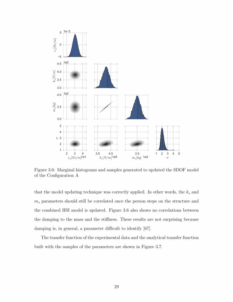
The transfer function of the experimental data and the analytical transfer function

built with the samples of the parameters are shown in Figure 3.7.

29

30 32 34 36 38Frequency (rad/s)

−50

−40

−30

−20

−10

0

Mag

nitu

de (d

B)

Exp. data95% HPD interval

Figure 3.7: Posterior predictive check of the Configuration A

Configuration B

The second structure configuration (called Configuration B) is used to evaluate the

human-structure interaction when groups of two and three occupants are over the

structure. For this configuration, the cantilever length is 100in and the concrete

blocks are located 75in from the support. The full experimental transfer function

of the structure is shown in Figure 3.8. Two close predominant peaks are observed,

therefore the model is updated using a poles and zeros model. The likelihood is

estimated using the n = 100 points closer to the higher peak on the transfer function,

as also shown in Figure 3.8. This corresponds to the values of the transfer function

between 17 rad/s and 32 rad/s.

The prior distributions for the parameters (ω1, ω2, ωz1, ζ1, ζ2, ζz1, K) are defined

based on direct measurements of the transfer function of the structure. The prior

distribution of each frequency (ω1, ω2, ωz1) is obtained from the experimental transfer

function using the peak-peaking method [68]. The priors for damping ratios (ζ1, ζ2,

ζz1) are obtained using uniform distributions over low damping ratios, based on the

experimental tests, and from the previous configuration A.

30

0 20 40 60 80 100Frequency (rad/s)

−80

−70

−60

−50

−40

−30

−20

−10

0

Magnit

ude (

dB

)

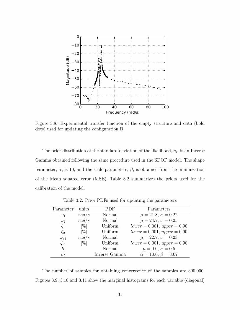
Figure 3.8: Experimental transfer function of the empty structure and data (bolddots) used for updating the configuration B

The prior distribution of the standard deviation of the likelihood, σl, is an Inverse

Gamma obtained following the same procedure used in the SDOF model. The shape

parameter, α, is 10, and the scale parameters, β, is obtained from the minimization

of the Mean squared error (MSE). Table 3.2 summarizes the priors used for the

calibration of the model.

Table 3.2: Prior PDFs used for updating the parameters

Parameter units PDF Parametersω1 rad/s Normal µ = 21.8, σ = 0.22ω2 rad/s Normal µ = 24.7, σ = 0.25ζ1 [%] Uniform lower = 0.001, upper = 0.90ζ2 [%] Uniform lower = 0.001, upper = 0.90ωz1 rad/s Normal µ = 22.7, σ = 0.23ζz1 [%] Uniform lower = 0.001, upper = 0.90K Normal µ = 0.0, σ = 0.5σl Inverse Gamma α = 10.0, β = 3.07

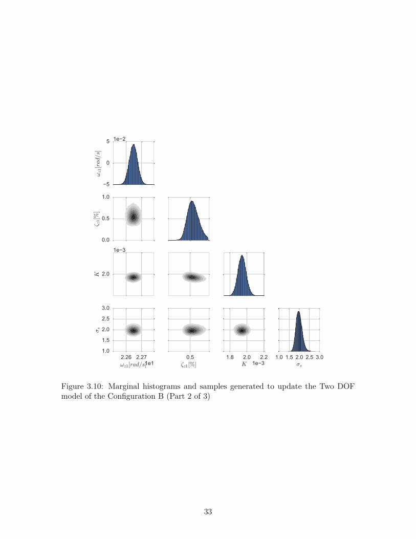
The number of samples for obtaining convergence of the samples are 300,000.

Figures 3.9, 3.10 and 3.11 show the marginal histograms for each variable (diagonal)

31

−5

0

5

ω1[rad/s

]

1e−2

2.45

2.46

2.47

2.48

ω2[rad/s

]

1e1

−0.5

0.0

0.5

1.0

ζ 1[%

]

2.17 2.18 2.19ω1[rad/s]1e1

−2

0

2

4

6

ζ 2[%

]

1e−1

2.46 2.47ω2[rad/s]1e1

0.0 0.5ζ1[%]

−2 0 2 4 6ζ2[%] 1e−1

Figure 3.9: Marginal histograms and samples generated to update the Two DOFmodel of the Configuration B (Part 1 of 3)

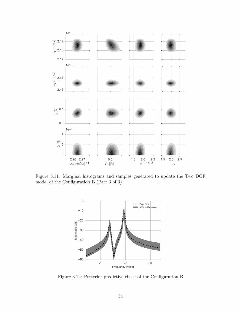
and the samples correlation. No correlation between the parameters is observed,

further than the frequencies and damping of each pole. The posterior predictive

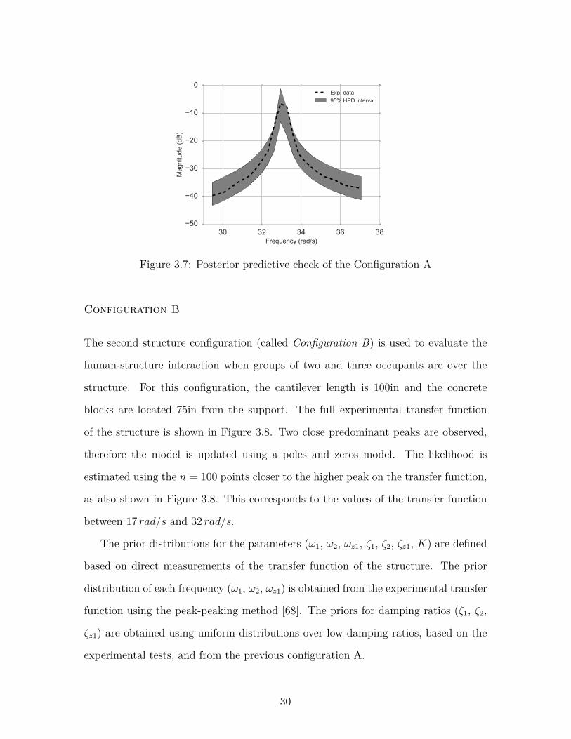
check of the updated model was compared with an unused experimental dataset.

Figure 3.12. shows the 95% HPD interval of the model is compared to the third

experimental dataset.

32

−5

0

5

ωz1[rad/s

]

1e−2

0.0

0.5

1.0

ζ z1[%

]

2.0K

1e−3

2.26 2.27ωz1[rad/s]1e1

1.0

1.5

2.0

2.5

3.0

σs

0.5ζz1[%]

1.8 2.0 2.2K 1e−3

1.0 1.5 2.0 2.5 3.0σs

Figure 3.10: Marginal histograms and samples generated to update the Two DOFmodel of the Configuration B (Part 2 of 3)

33

2.17

2.18

2.19

ω1[rad/s

]

1e1

2.46

2.47

ω2[rad/s

]

1e1

0.0

0.5

ζ 1[%

]

2.26 2.27ωz1[rad/s]1e1

0

2

4

ζ 2[%

]

1e−1

0.5ζz1[%]

1.8 2.0 2.2K 1e−3

1.5 2.0 2.5σs

Figure 3.11: Marginal histograms and samples generated to update the Two DOFmodel of the Configuration B (Part 3 of 3)

20 25 30Frequency (rad/s)

−60

−50

−40

−30

−20

−10

0

Mag

nitu

de (d

B)

Exp. data95% HPD interval

Figure 3.12: Posterior predictive check of the Configuration B

34

3.4 Conclusion remarks

In this chapter, two models of the empty structure were updated based on the transfer

function. Experimental data were obtained using impact hammer tests for inducing

free vibration of the structure. The transfer function of the experimental data was

used for the identification of the parameters of the models using Bayes inference.

The obtained posterior distributions of the parameters of each model will be used as

a prior information of the models updated in the next section (HSI models). The

models updated showed good fit to unused experimental data. The correlations of

the parameters ks and ms for the SDOF model, and ω1 − ζ1 and ω2 − ζ2 for the Two

DOF model result similar to the dependencies found in the literature, which were not

included in the priors.

35

Chapter 4

Results

The model updating and comparison results for models for single individuals over the

structure discussed in Chapter 2 are shown in this section. The models are updated

for single individuals. Models are validated by changing the dynamic characteristics

of the structure and using the model of the person to predict the behavior of the

overall human-structural system. An evaluation of each model is performed using the

model selection technique detailed previously in Section 2.3.

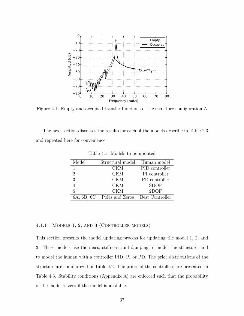
Figure 4.1 shows the transfer functions for the empty and occupied conditions ob-

tained from the experiments of Configuration A. As expected, the occupied structure

has a lower natural frequency than the empty structure. In addition, the damping

ratio is higher when a person stands on the slab, which is unexpected if the person

was only adding mass to the structure. This behavior reflects the observations given

by other researchers reported in the literature [9, 69, 7].

4.1 Parameter updating of the models

The parameters of human-structure interaction models are updated using the method-

ology discussed in Chapter 2. The parameters of the structure, θs = {m, c, k}, are

also updated in this process, however, their priors are the posteriors presented in

Section 3.3. Therefore, sampling is performed for the joint distribution of all the

parameters θs: θ = [θs, θh]. The number of total samples obtained from the Gibbs

sampler to reach convergence is different for each model. Geweke z-score plots [56]

are shown in Appendix B indicating the convergence of each chain.

36

0 10 20 30 40 50 60 70 80Frequency (rad/s)

−80

−70

−60

−50

−40

−30

−20

−10

0

Am

plit

ud (

dB

)

Empty

Occupied

Figure 4.1: Empty and occupied transfer functions of the structure configuration A

The next section discusses the results for each of the models describe in Table 2.3

and repeated here for convenience.

Table 4.1: Models to be updated

Model Structural model Human model1 CKM PID controller2 CKM PI controller3 CKM PD controller4 CKM SDOF5 CKM 2DOF6A, 6B, 6C Poles and Zeros Best Controller

4.1.1 Models 1, 2, and 3 (Controller models)

This section presents the model updating process for updating the model 1, 2, and

3. These models use the mass, stiffness, and damping to model the structure, and

to model the human with a controller PID, PI or PD. The prior distributions of the

structure are summarized in Table 4.2. The priors of the controllers are presented in

Table 4.3. Stability conditions (Appendix A) are enforced such that the probability

of the model is zero if the model is unstable.

37

Table 4.2: Prior PDFs of the structure’s parameters

Parameter units PDF Parameterscs Ns/m Normal µ = 28.9, σ = 4.9ks kN/m Normal µ = 383245.2, σ = 13438.2ms kg Normal µ = 350.9, σ = 12.3σs Normal µ = 2.3, σ = 0.3

Table 4.3: Prior definition for parameters of the PID, PI, and PD controller

Parameter Model Distribution ValuesKp 1, 2, 3 Uniform min = −10E3, max = 10E3Td 1, 3 Uniform min = −10E3, max = 10E3Ti 1, 2 Uniform min = −10E3, max = 10E3

For all models, a total of 500,000 samples were used from the Gibbs sampler in

order to reach convergence, from a total of 1 millon samples generated (500,000 burn-

in samples). The first points of the chains were the best values reported from the

deterministic optimization of the model. Geweke plots are shown in Appendix B.

Table 4.4 summarizes the number of samples and the location of the Geweke z-score

plots in Appendix B.

Table 4.4: Number of samples used and page location of convergence plots

Model Samples Burn-in Geweke z-score1 500,000 500,000 pages 77-812 500,000 500,000 pages 81-843 500,000 500,000 pages 85-88

Figures 4.2, 4.3, 4.4 show the samples for the controllers’ parameters. Figure 4.2

shows a high correlation between ti and td. This is expected because the stability

conditions were established as additional priors to the model. This means that the

human-structure system will be unstable for a set of ti and td values is chosen out of

this region. Within this correlation, one of the parameters can be modeled as a func-

tion of the other. Figure 4.3 shows some correlation between the parameters kp and

ti, however this is not related to the stability conditions of the system implemented

38

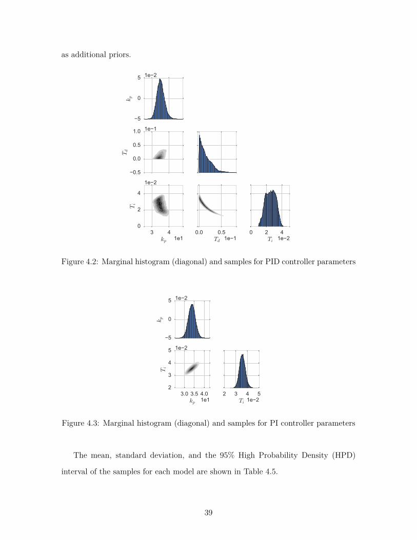
as additional priors.

−5

0

5

kp

1e−2

−0.5

0.0

0.5

1.0Td

1e−1

3 4kp 1e1

0

2

4

Ti

1e−2

0.0 0.5Td 1e−1

0 2 4Ti 1e−2

Figure 4.2: Marginal histogram (diagonal) and samples for PID controller parameters

−5

0

5

kp

1e−2

3.0 3.5 4.0kp 1e1

2

3

4

5

Ti

1e−2

2 3 4 5Ti 1e−2

Figure 4.3: Marginal histogram (diagonal) and samples for PI controller parameters

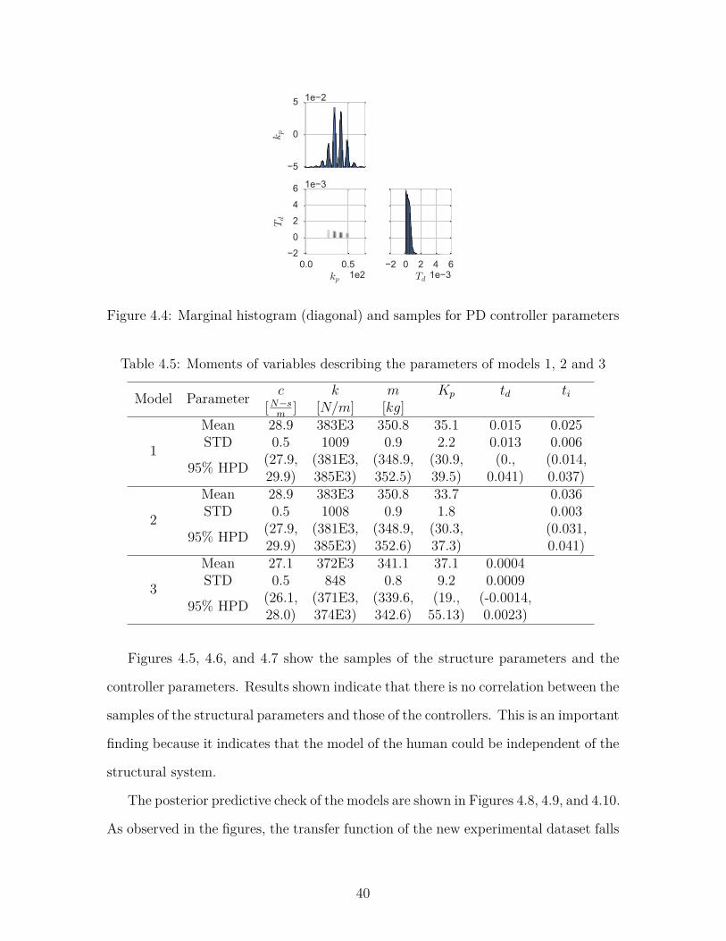
The mean, standard deviation, and the 95% High Probability Density (HPD)

interval of the samples for each model are shown in Table 4.5.

39

−5

0

5

kp

1e−2

0.0 0.5kp 1e2

−2

0

2

4

6

Td

1e−3

−2 0 2 4 6Td 1e−3

Figure 4.4: Marginal histogram (diagonal) and samples for PD controller parameters

Table 4.5: Moments of variables describing the parameters of models 1, 2 and 3

Model Parameter c k m Kp td ti[N−s

m] [N/m] [kg]

1

Mean 28.9 383E3 350.8 35.1 0.015 0.025STD 0.5 1009 0.9 2.2 0.013 0.006

95% HPD (27.9, (381E3, (348.9, (30.9, (0., (0.014,29.9) 385E3) 352.5) 39.5) 0.041) 0.037)

2

Mean 28.9 383E3 350.8 33.7 0.036STD 0.5 1008 0.9 1.8 0.003

95% HPD (27.9, (381E3, (348.9, (30.3, (0.031,29.9) 385E3) 352.6) 37.3) 0.041)

3

Mean 27.1 372E3 341.1 37.1 0.0004STD 0.5 848 0.8 9.2 0.0009

95% HPD (26.1, (371E3, (339.6, (19., (-0.0014,28.0) 374E3) 342.6) 55.13) 0.0023)

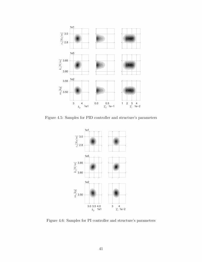
Figures 4.5, 4.6, and 4.7 show the samples of the structure parameters and the

controller parameters. Results shown indicate that there is no correlation between the

samples of the structural parameters and those of the controllers. This is an important

finding because it indicates that the model of the human could be independent of the

structural system.

The posterior predictive check of the models are shown in Figures 4.8, 4.9, and 4.10.

As observed in the figures, the transfer function of the new experimental dataset falls

40

2.8

3.0

c s[Ns/m

]

1e1

3.80

3.85ks[N/m

]

1e5

3 4kp 1e1

3.50

3.55

ms[kg]

1e2

0.0 0.5Td 1e−1

1 2 3 4Ti 1e−2

Figure 4.5: Samples for PID controller and structure’s parameters

2.8

3.0

c s[Ns/m

]

1e1

3.80

3.85

ks[N/m

]

1e5

3.0 3.5 4.0kp 1e1

3.50

ms[kg]

1e2

3 4Ti 1e−2

Figure 4.6: Samples for PI controller and structure’s parameters

41

2.6

2.8

c s[Ns/m

]

1e1

3.70

3.75

ks[N/m

]

1e5

0.0 0.5kp 1e2

3.40

3.42

3.44

ms[kg]

1e2

0 2 4Td 1e−3

Figure 4.7: Samples for PD controller and structure’s parameters

within the 95% HPD interval of the models. However, the confidence interval of

model 3 is significantly wider than the confidence interval of models 1 and 2. The

confidence interval of PID and PI models are similar; therefore, the additional term

td in the PID controller is not affecting the confidence interval of the transfer function

of the system.

42

26 28 30 32 34 36Frequency (rad/s)

−45

−40

−35

−30

Mag

nitu

de (d

B)

Exp. data95% HPD interval

Figure 4.8: Posterior predictive check of model 1

.

26 28 30 32 34 36Frequency (rad/s)

−45

−40

−35

−30

Mag

nitu

de (d

B)

Exp. data95% HPD interval

Figure 4.9: Posterior predictive check of the model 2

.

43

26 28 30 32 34 36Frequency (rad/s)

−60

−50

−40

−30

−20

−10

0

10

Mag

nitu

de (d

B)

Exp. data95% HPD interval

Figure 4.10: Posterior predictive check of the model 3

.

4.1.2 Model 4: MCK and Single degree of freedom system

This model represents the structure with the mass, damping, and stiffness parameters

and proposes the use of a single degree of freedom model for modeling the human. The

convergence of this model was reached using 150,000 samples, after burning 150,000.

The Geweke z-score plots describing the convergence of the MCMC chains can be

found in pages 89-93 of Appendix B.

The prior probability distributions of the stiffness, kh, and the damping constant,

ch, are based on the parameters found in the literature, including those reported in the

left column of the Table 1.2. The prior distribution for the mass of the human, ms, is

a normal distribution with mean 72kg and standard deviation of 1kg. Several papers

have stated the natural frequency of the human for a standing position; therefore, a

prior distribution was used for the natural frequency of the human, ωh =√kh/ms.

Table 4.6 shows the prior used for updating the model.

Figure 4.11 shows the samples for the parameters of the human model. No depen-

dence is found although the natural frequency of the human, ωh is slightly correlating

the parameters ch and kh. The mean, standard deviation and the 95% HPD inter-

44

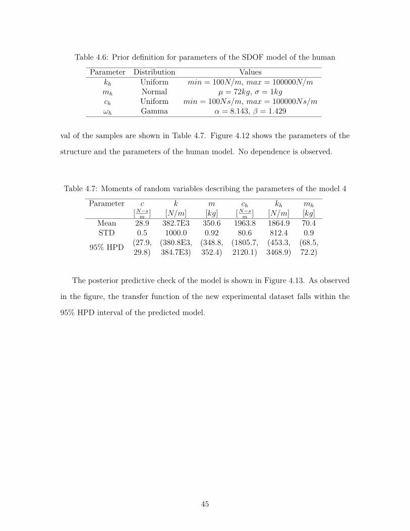
Table 4.6: Prior definition for parameters of the SDOF model of the human

Parameter Distribution Valueskh Uniform min = 100N/m, max = 100000N/mmh Normal µ = 72kg, σ = 1kgch Uniform min = 100Ns/m, max = 100000Ns/mωh Gamma α = 8.143, β = 1.429

val of the samples are shown in Table 4.7. Figure 4.12 shows the parameters of the

structure and the parameters of the human model. No dependence is observed.

Table 4.7: Moments of random variables describing the parameters of the model 4

Parameter c k m ch kh mh

[N−sm

] [N/m] [kg] [N−sm

] [N/m] [kg]Mean 28.9 382.7E3 350.6 1963.8 1864.9 70.4STD 0.5 1000.0 0.92 80.6 812.4 0.9

95% HPD (27.9, (380.8E3, (348.8, (1805.7, (453.3, (68.5,29.8) 384.7E3) 352.4) 2120.1) 3468.9) 72.2)

The posterior predictive check of the model is shown in Figure 4.13. As observed

in the figure, the transfer function of the new experimental dataset falls within the

95% HPD interval of the predicted model.

45

−5

0

5

c h[Ns/m

]

1e−2

−0.5

0.0

0.5

1.0kh[N/m

]

1e4

2.0ch[Ns/m]1e3

6.5

7.0

7.5

mh[kg]

1e1

0.0 0.5kh[N/m]1e4

6.5 7.0 7.5mh[kg] 1e1

Figure 4.11: Marginal histogram (diagonal) and samples for the SDOF model of thehuman

2.8

3.0

c s[Ns/m

]

1e1

3.80

3.85

ks[N/m

]

1e5

2.0ch[Ns/m]1e3

3.50

ms[kg]

1e2

0.0 0.5kh[N/m]1e4

7.0mh[kg] 1e1

Figure 4.12: Samples for SDOF model of the human and structure’s parameters

46

26 28 30 32 34 36Frequency (rad/s)

−44

−42

−40

−38

−36

−34

−32

−30

−28

Mag

nitu

de (d

B)

Exp. data95% HPD interval

Figure 4.13: Posterior predictive check of the model 4

4.1.3 Model 5: MCK and Two degrees of freedom system

This model represents the structure with the mass, dampers and stiffness of a single

degree of freedom system, and proposes the use of a two degree of freedom system

for modeling the human. The convergence of this model was reached using 150,000

samples, after burning 150,000. The Geweke z-score plots describing the convergence

of the MCMC chains can be found in pages 93-98 of Appendix B.

The prior probability density functions of the parameters is based on the values

found in the literature and shown in the right column of the Table 1.2. Additional

priors were defined in order to include the total mass of the human, and the first

natural frequency of the human body. The total mass of the human, mt, is expressed

as equation 4.1. The prior of mt follows a normal distribution with mean µ = 72kg

and σ = 1.0.

mt = mh1 +mh2 (4.1)

The first natural frequency of the human body follows a distribution as presented

in the last section. A uniform distribution is used to constrain the damping ratio

47

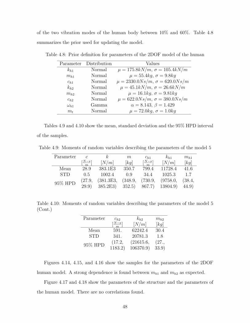
of the two vibration modes of the human body between 10% and 60%. Table 4.8

summarizes the prior used for updating the model.

Table 4.8: Prior definition for parameters of the 2DOF model of the human

Parameter Distribution Valueskh1 Normal µ = 175.8kN/m, σ = 105.4kN/mmh1 Normal µ = 55.4kg, σ = 9.8kgch1 Normal µ = 2330.0Ns/m, σ = 620.0Ns/mkh2 Normal µ = 45.1kN/m, σ = 26.6kN/mmh2 Normal µ = 16.1kg, σ = 9.81kgch2 Normal µ = 622.0Ns/m, σ = 380.0Ns/mωh1 Gamma α = 8.143, β = 1.429mt Normal µ = 72.0kg, σ = 1.0kg

Tables 4.9 and 4.10 show the mean, standard deviation and the 95% HPD interval

of the samples.

Table 4.9: Moments of random variables describing the parameters of the model 5

Parameter c k m ch1 kh1 mh1[N−s

m] [N/m] [kg] [N−s

m] [N/m] [kg]

Mean 28.9 383.1E3 350.7 799.4 11728.4 41.6STD 0.5 1002.4 0.9 34.4 1025.3 1.7

95% HPD (27.9, (381.3E3, (348.9, (730.9, (9758.0, (38.4,29.9) 385.2E3) 352.5) 867.7) 13804.9) 44.9)

Table 4.10: Moments of random variables describing the parameters of the model 5(Cont.)

Parameter ch2 kh2 mh2[N−s

m] [N/m] [kg]

Mean 591. 62242.4 30.4STD 341. 20781.3 1.8

95% HPD (17.2, (21615.6, (27.,1183.2) 106370.9) 33.9)

Figures 4.14, 4.15, and 4.16 show the samples for the parameters of the 2DOF

human model. A strong dependence is found between mh1 and mh2 as expected.

Figure 4.17 and 4.18 show the parameters of the structure and the parameters of

the human model. There are no correlations found.

48

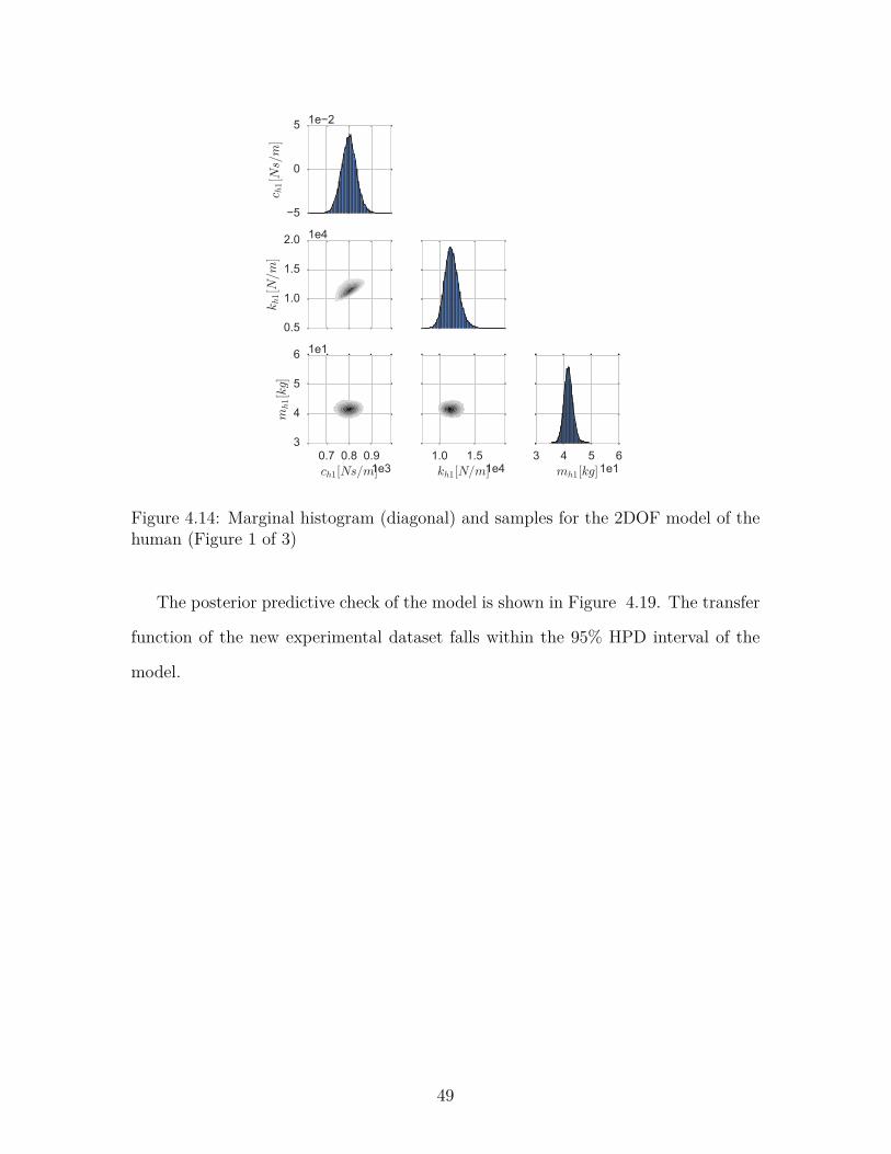
−5

0

5

c h1[Ns/m

]

1e−2

0.5

1.0

1.5

2.0

kh1[N/m

]

1e4

0.7 0.8 0.9ch1[Ns/m]1e3

3

4

5

6

mh1[kg]

1e1

1.0 1.5kh1[N/m]1e4

3 4 5 6mh1[kg]1e1

Figure 4.14: Marginal histogram (diagonal) and samples for the 2DOF model of thehuman (Figure 1 of 3)

The posterior predictive check of the model is shown in Figure 4.19. The transfer

function of the new experimental dataset falls within the 95% HPD interval of the

model.

49

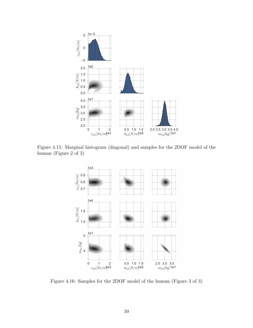
−5

0

5

c h2[Ns/m

]

1e−2

0.0

0.5

1.0

1.5

2.0

kh2[N/m

]

1e5

0 1 2ch2[Ns/m]1e3

2.0

2.5

3.0

3.5

4.0

mh2[kg]

1e1

0.5 1.0 1.5kh2[N/m]1e5

2.0 2.5 3.0 3.5 4.0mh2[kg]1e1

Figure 4.15: Marginal histogram (diagonal) and samples for the 2DOF model of thehuman (Figure 2 of 3)

0.7

0.8

0.9

c h1[Ns/m

]

1e3

1.0

1.5

kh1[N/m

]

1e4

0 1 2ch2[Ns/m]1e3

4

5

mh1[kg]

1e1

0.5 1.0 1.5kh2[N/m]1e5

2.5 3.0 3.5mh2[kg]1e1

Figure 4.16: Samples for the 2DOF model of the human (Figure 3 of 3)

50

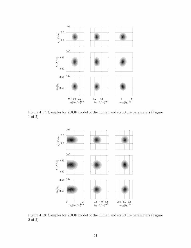
2.8

3.0

c s[Ns/m

]

1e1

3.80

3.85ks[N/m

]

1e5

0.7 0.8 0.9ch1[Ns/m]1e3

3.50

3.55

ms[kg]

1e2

1.0 1.5kh1[N/m]1e4

4 5mh1[kg]1e1

Figure 4.17: Samples for 2DOF model of the human and structure parameters (Figure1 of 2)

2.8

3.0

c s[Ns/m

]

1e1

3.80

3.85

ks[N/m

]

1e5

0 1 2ch2[Ns/m]1e3

3.50

3.55

ms[kg]

1e2

0.5 1.0 1.5kh2[N/m]1e5

2.5 3.0 3.5mh2[kg]1e1

Figure 4.18: Samples for 2DOF model of the human and structure parameters (Figure2 of 2)

51

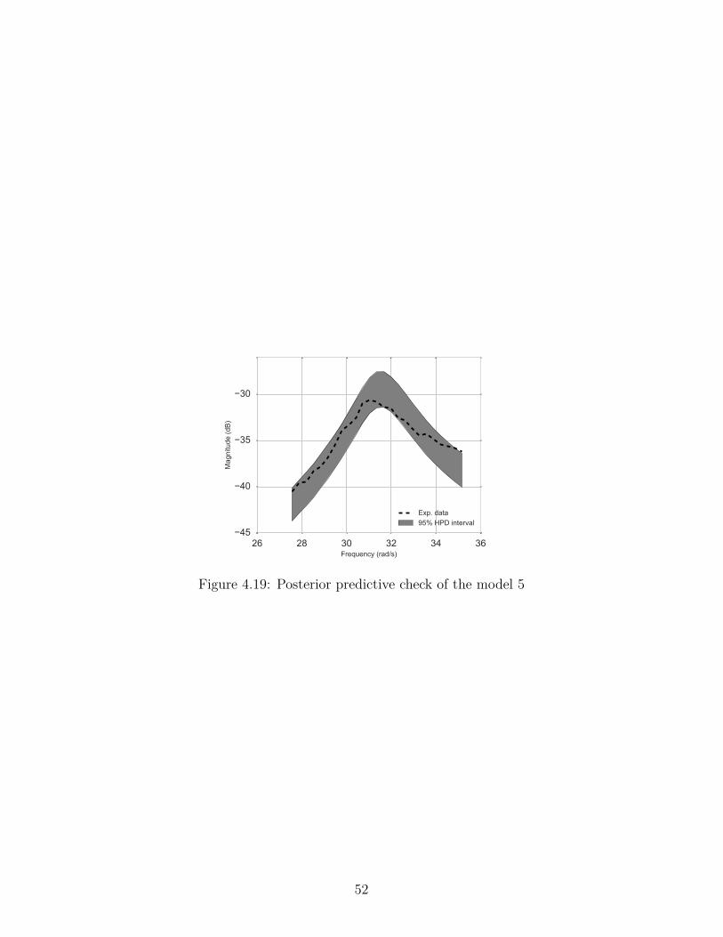
26 28 30 32 34 36Frequency (rad/s)

−45

−40

−35

−30

Mag

nitu

de (d

B)

Exp. data95% HPD interval

Figure 4.19: Posterior predictive check of the model 5

52

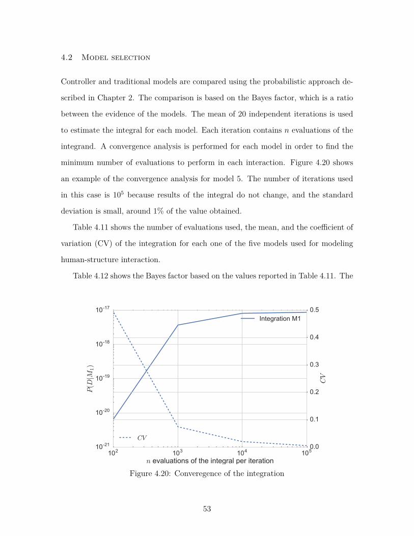
4.2 Model selection

Controller and traditional models are compared using the probabilistic approach de-

scribed in Chapter 2. The comparison is based on the Bayes factor, which is a ratio

between the evidence of the models. The mean of 20 independent iterations is used

to estimate the integral for each model. Each iteration contains n evaluations of the

integrand. A convergence analysis is performed for each model in order to find the

minimum number of evaluations to perform in each interaction. Figure 4.20 shows

an example of the convergence analysis for model 5. The number of iterations used

in this case is 105 because results of the integral do not change, and the standard

deviation is small, around 1% of the value obtained.

Table 4.11 shows the number of evaluations used, the mean, and the coefficient of

variation (CV) of the integration for each one of the five models used for modeling

human-structure interaction.

Table 4.12 shows the Bayes factor based on the values reported in Table 4.11. The

102 103 104 105

n evaluations of the integral per iteration

10-21

10-20

10-19

10-18

10-17

P(D

|M1)

Integration M1

0.0

0.1

0.2

0.3

0.4

0.5

CV

CV

Figure 4.20: Converegence of the integration

53

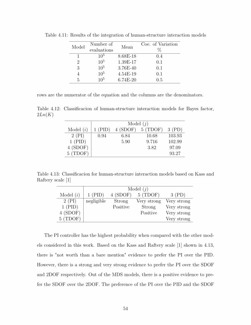
Table 4.11: Results of the integration of human-structure interaction models

Model Number of Mean Coe. of Variationevaluations %

1 105 8.68E-18 0.42 105 1.39E-17 0.13 105 3.76E-40 0.14 105 4.54E-19 0.15 105 6.74E-20 0.5

rows are the numerator of the equation and the columns are the denominators.

Table 4.12: Classificacion of human-structure interaction models for Bayes factor,2Ln(K)

Model (j)Model (i) 1 (PID) 4 (SDOF) 5 (TDOF) 3 (PD)2 (PI) 0.94 6.84 10.68 103.931 (PID) 5.90 9.716 102.994 (SDOF) 3.82 97.095 (TDOF) 93.27

Table 4.13: Classificacion for human-structure interaction models based on Kass andRaftery scale [1]

Model (j)Model (i) 1 (PID) 4 (SDOF) 5 (TDOF) 3 (PD)2 (PI) negligible Strong Very strong Very strong1 (PID) Positive Strong Very strong4 (SDOF) Positive Very strong5 (TDOF) Very strong

The PI controller has the highest probability when compared with the other mod-

els considered in this work. Based on the Kass and Raftery scale [1] shown in 4.13,

there is "not worth than a bare mention" evidence to prefer the PI over the PID.

However, there is a strong and very strong evidence to prefer the PI over the SDOF

and 2DOF respectively. Out of the MDS models, there is a positive evidence to pre-

fer the SDOF over the 2DOF. The preference of the PI over the PID and the SDOF

54

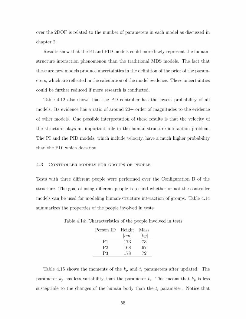
over the 2DOF is related to the number of parameters in each model as discussed in

chapter 2.

Results show that the PI and PID models could more likely represent the human-

structure interaction phenomenon than the traditional MDS models. The fact that

these are new models produce uncertainties in the definition of the prior of the param-

eters, which are reflected in the calculation of the model evidence. These uncertainties

could be further reduced if more research is conducted.

Table 4.12 also shows that the PD controller has the lowest probability of all

models. Its evidence has a ratio of around 20+ order of magnitudes to the evidence

of other models. One possible interpretation of these results is that the velocity of

the structure plays an important role in the human-structure interaction problem.

The PI and the PID models, which include velocity, have a much higher probability

than the PD, which does not.

4.3 Controller models for groups of people

Tests with three different people were performed over the Configuration B of the

structure. The goal of using different people is to find whether or not the controller

models can be used for modeling human-structure interaction of groups. Table 4.14

summarizes the properties of the people involved in tests.

Table 4.14: Characteristics of the people involved in tests

Person ID Height Mass[cm] [kg]

P1 173 73P2 168 67P3 178 72

Table 4.15 shows the moments of the kp and ti parameters after updated. The

parameter kp has less variability than the parameter ti. This means that kp is less

susceptible to the changes of the human body than the ti parameter. Notice that

55

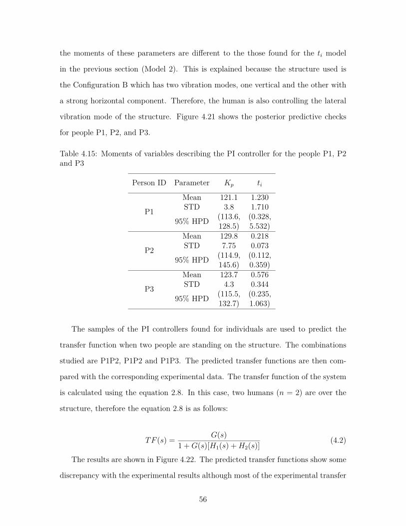
the moments of these parameters are different to the those found for the ti model

in the previous section (Model 2). This is explained because the structure used is

the Configuration B which has two vibration modes, one vertical and the other with

a strong horizontal component. Therefore, the human is also controlling the lateral

vibration mode of the structure. Figure 4.21 shows the posterior predictive checks

for people P1, P2, and P3.

Table 4.15: Moments of variables describing the PI controller for the people P1, P2and P3

Person ID Parameter Kp ti

P1

Mean 121.1 1.230STD 3.8 1.710

95% HPD (113.6, (0.328,128.5) 5.532)

P2

Mean 129.8 0.218STD 7.75 0.073

95% HPD (114.9, (0.112,145.6) 0.359)

P3

Mean 123.7 0.576STD 4.3 0.344

95% HPD (115.5, (0.235,132.7) 1.063)

The samples of the PI controllers found for individuals are used to predict the

transfer function when two people are standing on the structure. The combinations

studied are P1P2, P1P2 and P1P3. The predicted transfer functions are then com-

pared with the corresponding experimental data. The transfer function of the system

is calculated using the equation 2.8. In this case, two humans (n = 2) are over the

structure, therefore the equation 2.8 is as follows:

TF (s) = G(s)1 +G(s)[H1(s) +H2(s)] (4.2)

The results are shown in Figure 4.22. The predicted transfer functions show some

discrepancy with the experimental results although most of the experimental transfer

56

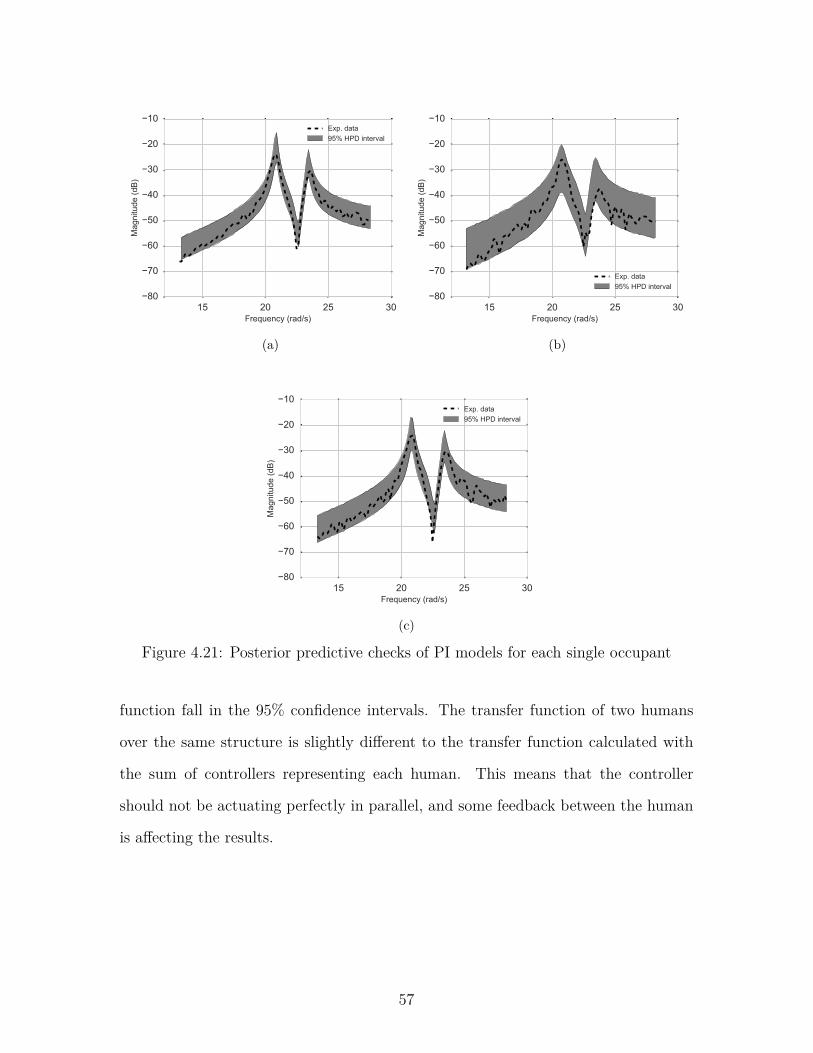
15 20 25 30Frequency (rad/s)

−80

−70

−60

−50

−40

−30

−20

−10M

agni

tude

(dB

)Exp. data95% HPD interval

(a)

15 20 25 30Frequency (rad/s)

−80

−70

−60

−50

−40

−30

−20

−10

Mag

nitu

de (d

B)

Exp. data95% HPD interval

(b)

15 20 25 30Frequency (rad/s)

−80

−70

−60

−50

−40

−30

−20

−10

Mag

nitu

de (d

B)

Exp. data95% HPD interval

(c)

Figure 4.21: Posterior predictive checks of PI models for each single occupant

function fall in the 95% confidence intervals. The transfer function of two humans

over the same structure is slightly different to the transfer function calculated with

the sum of controllers representing each human. This means that the controller

should not be actuating perfectly in parallel, and some feedback between the human

is affecting the results.

57

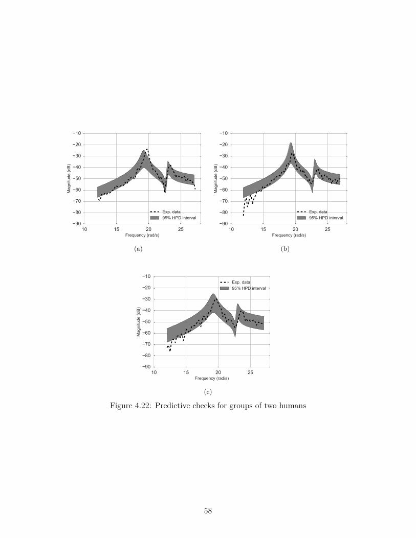
10 15 20 25Frequency (rad/s)

−90

−80

−70

−60

−50

−40

−30

−20

−10

Mag

nitu

de (d

B)

Exp. data95% HPD interval

(a)

10 15 20 25Frequency (rad/s)

−90

−80

−70

−60

−50

−40

−30

−20

−10

Mag

nitu

de (d

B)

Exp. data95% HPD interval

(b)

10 15 20 25Frequency (rad/s)

−90

−80

−70

−60

−50

−40

−30

−20

−10

Mag

nitu

de (d

B)

Exp. data95% HPD interval

(c)

Figure 4.22: Predictive checks for groups of two humans

58

Chapter 5

Conclusions and future work

5.1 Conclusions

The focus of this research is to introduce a new approach based on a closed-loop

control system for modeling the human-structure interaction phenomenon. Within

this approach, the human is modeled as a controller system and the structure as the

system to control. Controller models seek to include a stronger feedback action be-

tween the structure and the human than the traditional mass-damper-spring (MDS)

models. This approach may help explain the changes of the dynamic characteristics

experienced in structures occupied by crowds. This work focuses on standing indi-

viduals but the framework used to update and compare the models can be applied

to other cases.

This research shows that the idea of modeling a standing individual as a controller

works. This is evidenced by comparing the models in a probabilistic way. There is

strong evidence than a PI model is preferred over traditional MDS models.

Three different controllers were updated using a Bayesian probabilistic approach.

The Proportional, Derivative, and Integrative controller, PID, and the proportional

and integrative controller, PI, were able to successfully model the phenomenon. How-

ever, the third controller evaluated, the PD, did not show good fit with the experi-

mental data.

The PI controller has the strongest evidence among the models evaluated. Results

indicate that the integrative term, ti, is significant to the controller. The ti param-

59

eter changes the controller output based on the velocity of the structure, which is

consistent with findings by other authors [36].

Groups of people were modeled using the controller models identified for each

person. The model assumed that the controllers work independently of each other.

Under this assumption, the modeling of groups was explored and its performance was

acceptable. However, peaks of the model’s transfer function are at a slight different

frequency from the peaks of the experimental transfer function. This could be due

to of human-human interactions not modeled.

The Bayesian probabilistic model updating technique enabled the identification

of the parameter’s probability density functions, as well as correlations between the

parameters of human and structure models. These correlations are difficult to pre-

dict from the deterministic models described in the literature review presented in

Chapter 1. Controller models, in general, were found to be independent of the struc-

ture, which means that the parameters of the controller could be developed in a lab

and implemented in other structural models, as long as the stability conditions are

satisfied.

It is important to consider all the stability conditions of the system because they

can strongly affect the performance of a controller. For example, the PD controller

makes the structure unstable when using parameters values near to high probabil-

ity regions. Stability conditions are big constraints of the controller models, and

their formulation lead to additional equations that could reduce the simplicity of the

models.

5.2 Future Work

The main goal of this research was to explore the use of closed-loop control theory

to model the human-structure interaction problem. It is promising that the PI con-

troller has substantial strength in the evidence with respect to the traditional MDS

60

models. Additional work in this field will reduce the model uncertainty by reducing

the probability density function of the priors, which will make the evidence of these

models even higher.

The selected controllers PID, PD, and PI are just a family of controllers of hun-

dreds found in the literature [38]. The exploration of better controllers could reduce

the uncertainty in modeling the phenomenon. For example, adaptive controllers could

introduce the variability of the human body given some characteristics such as the

mass, height, age, or body mass index.

Standing humans were used to validate the methodology applied to this research.

However, problems in the human-structure interaction also involve humans in move-

ment, such as walking and running. The implementation of controller models for this

kind of movements is the natural next step in this research. For modeling a pedes-

trian, the controller and biomechanical model of the human should be combined.

The human-structure interaction in bridges could be explored, for example, using a

combination of the inverted pendulum model of the human body with the controller

actions to maintain stability.

61

Bibliography[1] Robert E Kass and Adrian E Raftery. Bayes factors. Journal of the american

statistical association, 90(430):773–795, 1995.

[2] A. Fitzpatrick, P. Dallard, A. Low, S. Le Bourva, R. Ridsdill, and M. Will-ford. Linking London: The Millennium Bridge. Royal Academy of Engineering,London, UK, 2001.

[3] P. Dallard, A. Fitzpatrick, A. Flint, S. Le Bourva, R. Ridsdill, and M. Willford.The london millennium footbridge. The Structural Engineer, 79:17–33, 2009.

[4] B. S. Morris. An Investigation of Human Induced Vibrations on Clemson Memo-rial Stadium. Master of Science Thesis. Clemson University, 2009.

[5] S. Erlingsson A. Bodare. Rock music induced damage and vibration at nyaullevi stadium. Procedings: Third International Conference on Case Historiesin Geotechnical Engineering, St. Louis, Missouri, pages 671–675, 1993.

[6] JHG Macdonald. Pedestrian-induced vibrations of the clifton suspension bridge,uk. Proceedings of the ICE-Bridge Engineering, 161(2):69–77, 2008.

[7] A. Ortiz, D. Gomez, and P. Thomson. Effect of human-structure interaction onthe dynamic properties of a grandstand. Ingenieria y Competitividad, 14:63–73,2012.

[8] S. Falati. The contribution of non-structural components to the overall dynamicbehaviour of concrete floor slabs. University of Oxford, Oxford, UK, 1999.

[9] E. Agu and M. Kaspersky. Influence of the random dynamic parameters of thehuman body on the dynamic characteristics of the coupled system of structure-crowd. Journal of Sound and Vibration, 330:431–444, 2011.

[10] K. Salyards and Y. Hua. Assessment of dynamic properties of a crowd modelhuman-structure interaction modeling. 89:103–110.

62

[11] Proceedings of the Fourth International Conference on Structural Dynamics,editor. The influence of a group of humans on modal properties of a structure,volume 2, Munich, 2002. Pitman.

[12] N. W. M. Bishop, M. Willford, and R. Pumphrey. Human induced loading offlexible staircases. 18:261–276.

[13] R. Sachse, A. Pavic, and P. Reynolds. Human-structure dynamic interaction incivil engineering dynamics: A literature review. The Shock and Vibration Digest,35:3–18, 2003.

[14] S. Zivanovic, A. Pavic, and P. Reynolds. Vibration serviceability of footbridgesunder human-induced excitation: a literature review. Journal of Sound andVibration, 279:1–74, 2005.

[15] American Society of Civil Engineers ASCE. Minimum Design Loads for Buildingsand Other Structures, ASCE/SEI 7-10. American Society of Civil EngineersASCE, 2013.

[16] International Building Code Inc. International Building Code. InternationalBuilding Code Inc., 2003.

[17] British Standards Institution (BSI). Code of practice for dead and imposed loads.American Society of Civil Engineers ASCE, 2011.

[18] Proceedings of the 31st International Modal Analysis Conference, editor. Exper-imental Results from a Laboratory Test Program to Examine Human-StructureInteraction. Springer, 2013.

[19] J.M.W. Brownjohn. Energy dissipation in one-way slabs with human participa-tion. In Proceedings of the Asia-Pacific Vibration Conference âĂŸ99, Singapore,December.

[20] ISO. Vibration and shock - Mechanical driving point impedance of the humanbody. International Organization for Standardization (ISO), 1981.

[21] L. Sim, A. Blackeborough, and M. Williams. Modelling of joint crowd structuresystem using equivalent reduced-dof system. Shock and Vibration, 14:261–270,2007.

63

[22] Y. Matsumoto and M.J. Griffin. Mathematical models for the apparent massesof standings subjects exposed to vertical whole-body vibration. Journal of Soundand Vibration, 260:431–451, 2003.

[23] Andrew L Smith, Stephen J Hicks, and Paul J Devine. Design of floors forvibration: A new approach. Steel Construction Institute Ascot, Berkshire, UK,2007.

[24] Thomas M Murray. Floor vibrations: The human tolerance side of the equation.In SPIE proceedings series, pages 1–6. Society of Photo-Optical InstrumentationEngineers, 1999.

[25] Institution of Structural Engineers. Dynamic performance requirements for per-manent grandstands subject to crowd action: Interim guidance on assessmentand design. Institution of Structural Engineers, ISE, 2001.

[26] L. Wei and M.J. Griffin. Mathematical models for the apparent mass of the seatedhuman body exposed to vertical vibration. Journal of Sound and Vibration,212:855–874, 1998.

[27] A. Farah. Human response: A criterion for the assessment of structural service-ability.

[28] AJ Thurston. Giovanni borelli and the study of human movement: An historicalreview. Australian and New Zealand journal of surgery, 69(4):276–288, 1999.

[29] Frances A Hellebrandt, Rubye H Tepper, Genevieve L Braun, and Margaret C El-liott. The location of the cardinal anatomical orientation planes passing throughthe center of weight in young adult women. American Journal of Physiology–Legacy Content, 121(2):465–470, 1938.

[30] G Elliot Smith. The human brain. Journal of the Royal Society of Arts,78(4037):570–576, 1930.

[31] David A Winter. Human balance and posture control during standing and walk-ing. Gait & posture, 3(4):193–214, 1995.

[32] Itshak Melzer, N Benjuya, and J Kaplanski. Postural stability in the elderly:a comparison between fallers and non-fallers. Age and ageing, 33(6):602–607,2004.

64

[33] Yifa Jiang Hidenori Kimura. Balance-keeping control of upright standing in bipedhuman beings and its application for stability assessment. INTECH Open AccessPublisher, 2007.

[34] Taesoo Kwon and Jessica Hodgins. Control systems for human running usingan inverted pendulum model and a reference motion capture sequence. In Pro-ceedings of the 2010 ACM SIGGRAPH/Eurographics Symposium on ComputerAnimation, pages 129–138. Eurographics Association, 2010.

[35] Ian D Loram and Martin Lakie. Human balancing of an inverted pendulum:position control by small, ballistic-like, throw and catch movements. The Journalof physiology, 540(3):1111–1124, 2002.

[36] Kimura Hidenori and Yifa Jiang. A pid model of human balance keeping. ControlSystems, IEEE, 26(6):18–23, 2006.

[37] Mateusz Bocian, John HG Macdonald, Jeremy F Burn, and David Redmill.Experimental identification of the behaviour of and lateral forces from freely-walking pedestrians on laterally oscillating structures in a virtual reality envi-ronment. Engineering Structures, 105:62–76, 2015.

[38] K. Ogata. Modern Control Engineering. Prentice-Hall, 2002.

[39] DJ Ewins. Modal testing: theory, practice and application (mechanical engi-neering research studies: engineering dynamics series). 2003.

[40] Graham Clifford Goodwin, Stefan F Graebe, and Mario E Salgado. Controlsystem design, volume 240. Prentice Hall New Jersey, 2001.

[41] Albert R Ortiz and Juan M Caicedo. Comparing closed loop control modelsand mass-spring-damper models for human structure interaction problems. InDynamics of Civil Structures, Volume 2, pages 67–74. Springer, 2015.

[42] John W Smith and Terry Montgomery. Biomechanically induced and controllercoupled oscillations experienced on the f-16xl aircraft during rolling maneuvers.1996.

[43] Hao Ying. Theory and application of a novel fuzzy pid controller using a simpli-fied takagi–sugeno rule scheme. Information Sciences, 123(3):281–293, 2000.

65

[44] Samuel Privara, Jan Široky, Lukáš Ferkl, and Jiří Cigler. Model predictivecontrol of a building heating system: The first experience. Energy and Buildings,43(2):564–572, 2011.

[45] Shirley J Dyke, Juan Martin Caicedo, Gursoy Turan, LA Bergman, and StevenHague. Phase i benchmark control problem for seismic response of cable-stayedbridges. Journal of Structural Engineering, 129(7):857–872, 2003.

[46] Pan Zhao, Jiajia Chen, Yan Song, Xiang Tao, Tiejuan Xu, and Tao Mei. Designof a control system for an autonomous vehicle based on adaptive-pid. Interna-tional Journal of Advanced Robotic Systems, 9, 2012.

[47] Frederick Chee, Tyrone L Fernando, Andrey V Savkin, and Vernon Van Heeden.Expert pid control system for blood glucose control in critically ill patients.Information Technology in Biomedicine, IEEE Transactions on, 7(4):419–425,2003.

[48] B Kada and Y Ghazzawi. Robust pid controller design for an uav flight controlsystem. In Proceedings of the World Congress on Engineering and ComputerScience, volume 2, pages 1–6, 2011.

[49] C Schwartz, A Berger, O Brüls, JL Croisier, B Forthomme, and V Denoël. Ex-perimental study of the human ability to deliberately excite a flexible floor. Re-search and Applications in Structural Engineering, Mechanics and Computation,page 55, 2013.

[50] David E Newland. Vibration of the london millennium footbridge: Part 1–cause.University of Cambridge, 2003.

[51] J. Beck and L. S. Katafygiotis. Updating models and their uncertainties i:Bayesian statistical framework. Journal of Engineering Mechanics, 124:455–461,2009.

[52] S. H. Cheung and J. Beck. Bayesian model updating using hybrid monte carlosimulation with application to structural dynamic models with uncertain param-eters. Journal of Engineering Mechanics, 135:243–225, 2009.

[53] Christian Robert and George Casella. Monte Carlo statistical methods. SpringerScience & Business Media, 2013.

[54] W Keith Hastings. Monte carlo sampling methods using markov chains and theirapplications. Biometrika, 57(1):97–109, 1970.

66

[55] Nicholas Metropolis and Stanislaw Ulam. The monte carlo method. Journal ofthe American statistical association, 44(247):335–341, 1949.

[56] John Geweke et al. Evaluating the accuracy of sampling-based approaches tothe calculation of posterior moments, volume 196. Federal Reserve Bank ofMinneapolis, Research Department Minneapolis, MN, USA, 1991.

[57] Gabriel Terejanu, Todd Oliver, and Chris Simmons. Application of predictivemodel selection to coupled models. arXiv preprint arXiv:1107.0927, 2011.

[58] William H Jefferys and James O Berger. Ockham’s razor and bayesian analysis.American Scientist, 80(1):64–72, 1992.

[59] Phil Gibbs and Sugihara Hiroshi. What is occamâĂŹs razor. Available at:http://math.ucr.edu/home/baez/physics/General/occam.html, 1996.

[60] N. Metropolis and S. Ulam. The monte carlo method. Journal of the AmericanStatistical Association, 4:335–341, 1949.

[61] G Peter Lepage. A new algorithm for adaptive multidimensional integration.Journal of Computational Physics, 27(2):192–203, 1978.

[62] Harold Jeffreys. The theory of probability. OUP Oxford, 1998.

[63] Julius S Bendat and Allan G Piersol. Random data: analysis and measurementprocedures, volume 729. John Wiley & Sons, 2011.

[64] Anil K Chopra. Dynamics of structures, volume 3. Prentice Hall New Jersey,1995.

[65] John A Nelder and Roger Mead. A simplex method for function minimization.The computer journal, 7(4):308–313, 1965.

[66] C. Robert and G. Casella. Monte Carlo Statistical Methods. Springer, 2004.

[67] E. M. Hernandez and N. Polanco. Uncertainty quantification in identified modalparameters using fisher information criterion. In Proceedings of the XXXII In-ternational Modal Analysis Conference, Orlando, FL, February.

[68] Julius S Bendat and Allan G Piersol. Engineering applications of correlation andspectral analysis. New York, Wiley-Interscience, 1980. 315 p., 1, 1980.

67

[69] B. R. Ellis, T. Ji, and J.D. Littler. The response of grandstands to dynamiccrowd loads. Structures and Buildings, 140:355–365, 2000.

68

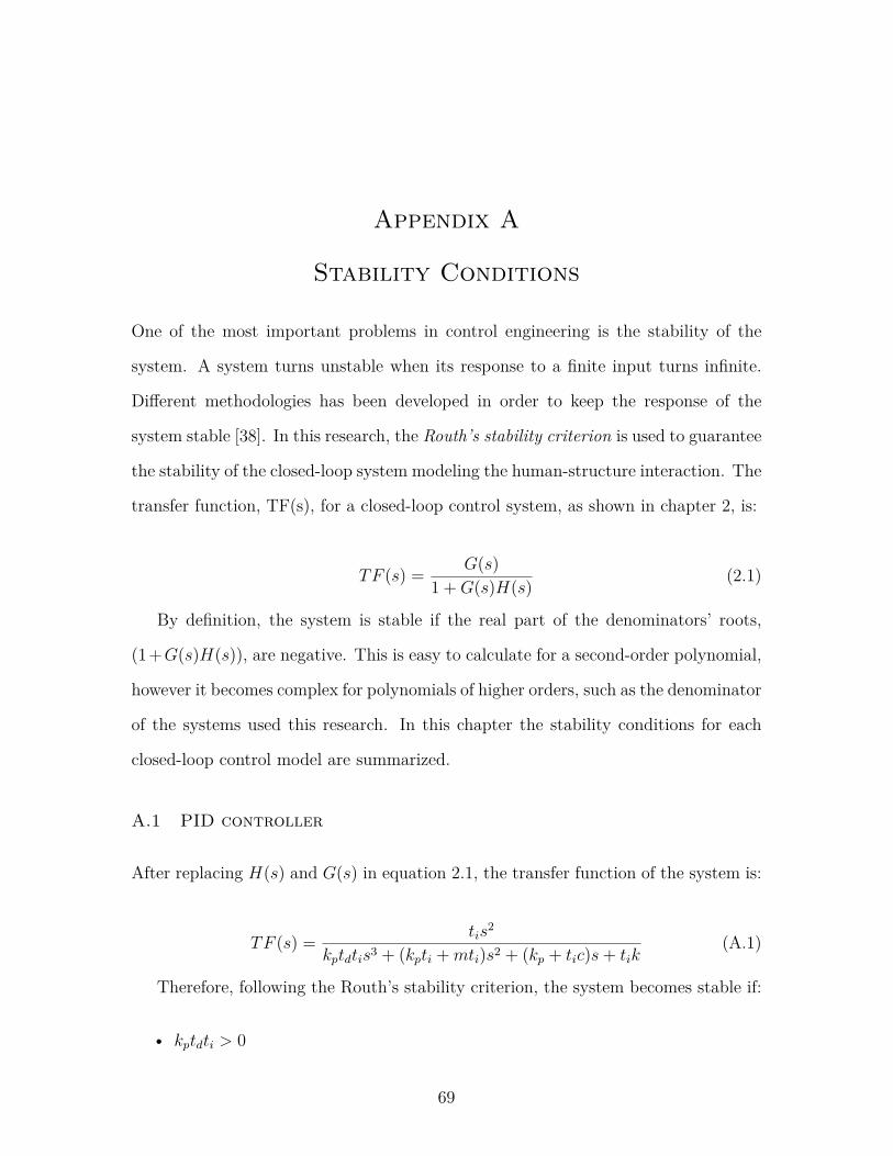
Appendix A

Stability Conditions

One of the most important problems in control engineering is the stability of the

system. A system turns unstable when its response to a finite input turns infinite.

Different methodologies has been developed in order to keep the response of the

system stable [38]. In this research, the Routh’s stability criterion is used to guarantee

the stability of the closed-loop system modeling the human-structure interaction. The

transfer function, TF(s), for a closed-loop control system, as shown in chapter 2, is:

TF (s) = G(s)1 +G(s)H(s) (2.1)

By definition, the system is stable if the real part of the denominators’ roots,

(1+G(s)H(s)), are negative. This is easy to calculate for a second-order polynomial,

however it becomes complex for polynomials of higher orders, such as the denominator

of the systems used this research. In this chapter the stability conditions for each

closed-loop control model are summarized.

A.1 PID controller

After replacing H(s) and G(s) in equation 2.1, the transfer function of the system is:

TF (s) = tis2

kptdtis3 + (kpti +mti)s2 + (kp + tic)s+ tik(A.1)

Therefore, following the Routh’s stability criterion, the system becomes stable if:

• kptdti > 0

69

• kpti +mti > 0

• kp + tic > 0

• tik > 0

• ti[(kp +m)(kp + tic)] > kptdt2i k

A.2 PI controller

After replacing H(s) and G(s) in equation 2.1, the transfer function of the system is:

TF (s) = tis2

ti(kp +m)s2 + (kp + tic)s+ tik(A.2)

Therefore, following the Routh’s stability criterion, the system becomes stable if:

• (kp +m)ti > 0

• kp + tic > 0

• tik > 0

A.3 PD controller

After replacing H(s) and G(s) in equation 2.1, the transfer function of the system is:

TF (s) = s2

kptds3 + (kp +m)s2 + cs+ k(A.3)

Therefore, following the Routh’s stability criterion, the system becomes stable if:

• kptd > 0

• kp +m > 0

• (kp +m)c > (kptd)k

70

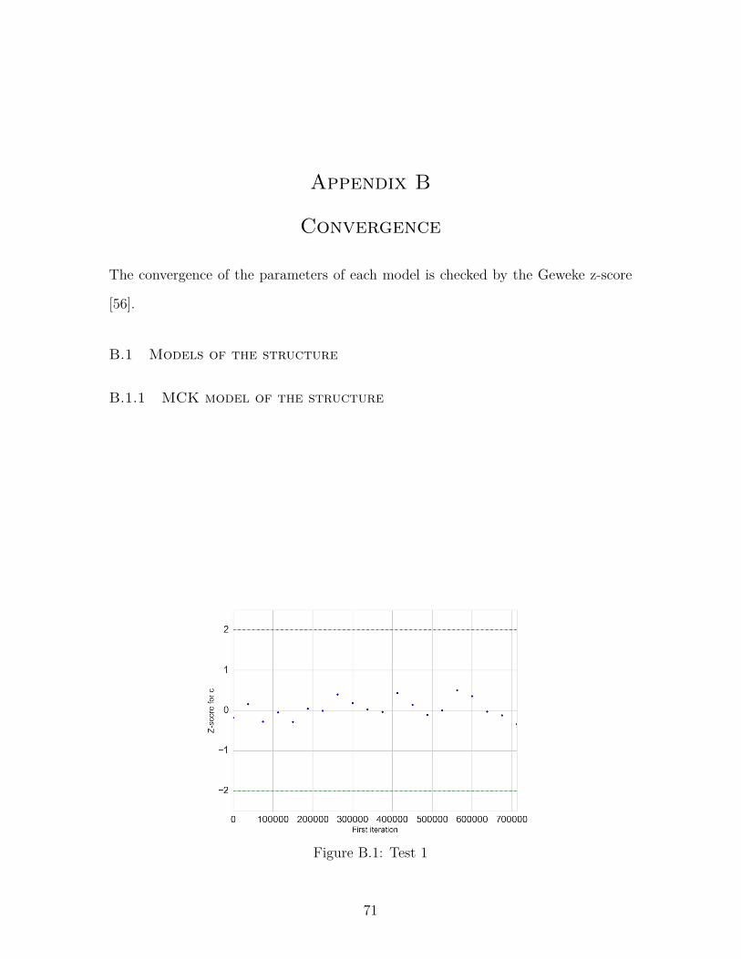
Appendix B

Convergence

The convergence of the parameters of each model is checked by the Geweke z-score

[56].

B.1 Models of the structure

B.1.1 MCK model of the structure

Figure B.1: Test 1

71

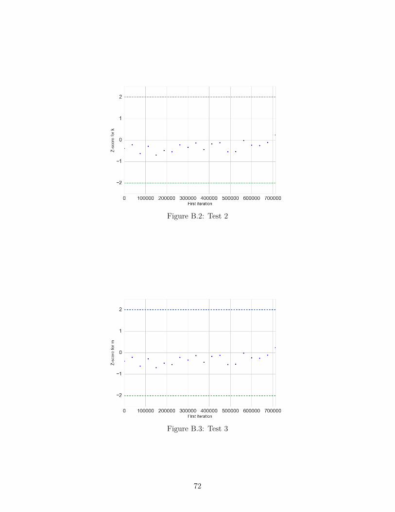
Figure B.2: Test 2

Figure B.3: Test 3

72

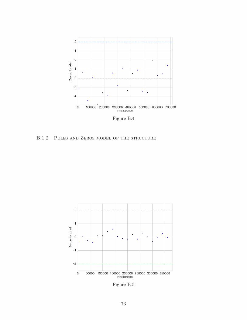
Figure B.4

B.1.2 Poles and Zeros model of the structure

Figure B.5

73

Figure B.6

Figure B.7

74

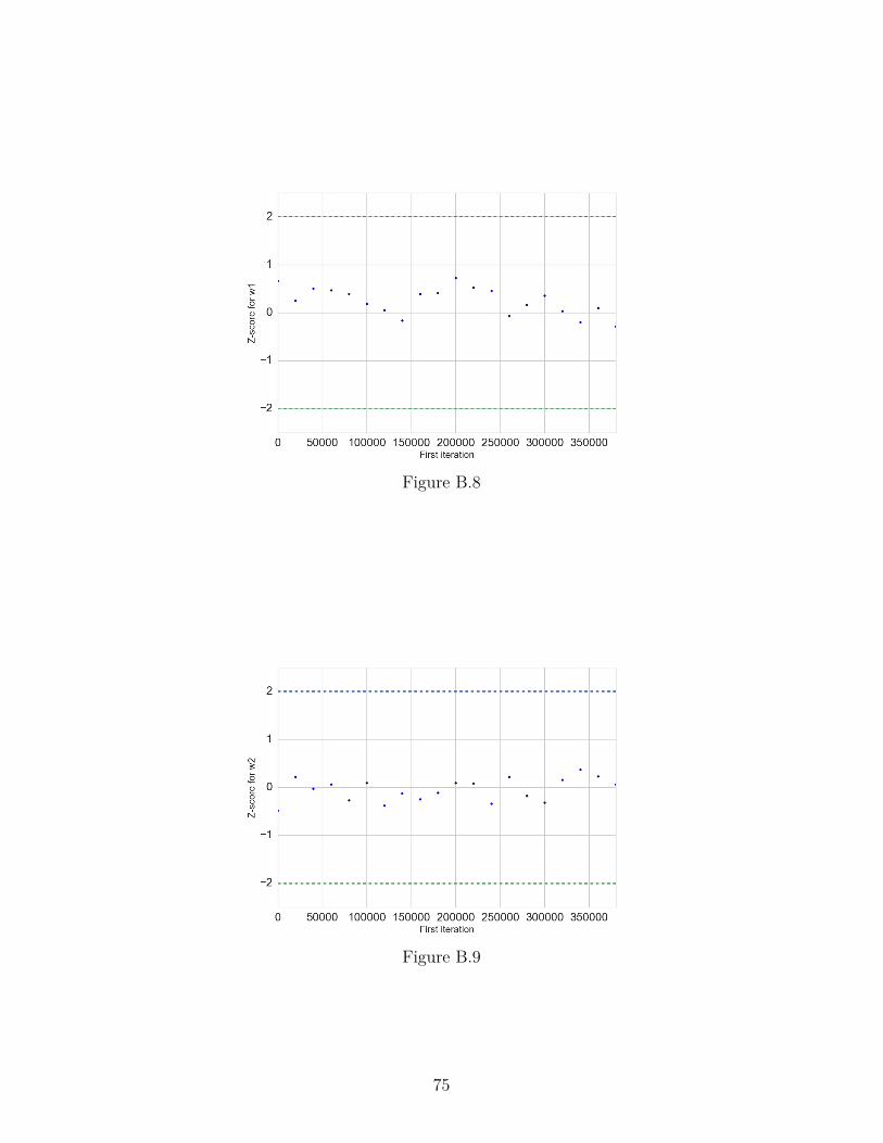
Figure B.8

Figure B.9

75

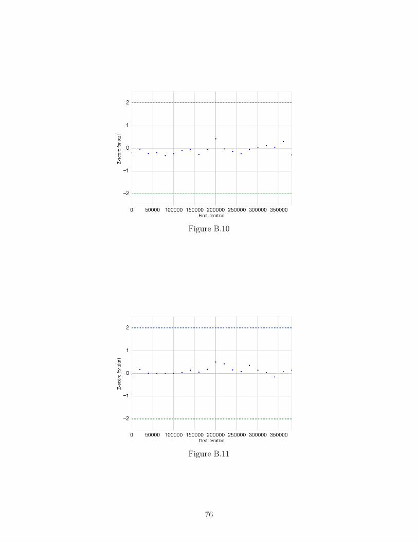
Figure B.10

Figure B.11

76

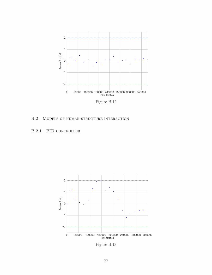
Figure B.12

B.2 Models of human-structure interaction

B.2.1 PID controller

Figure B.13

77

Figure B.14

Figure B.15

78

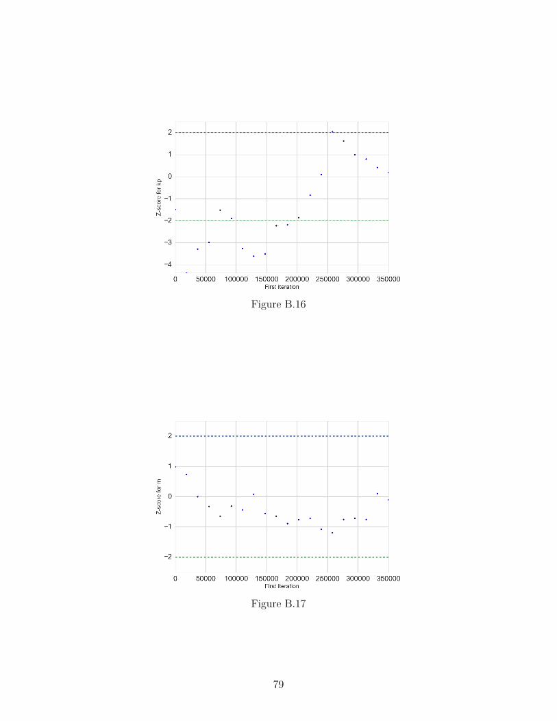
Figure B.16

Figure B.17

79

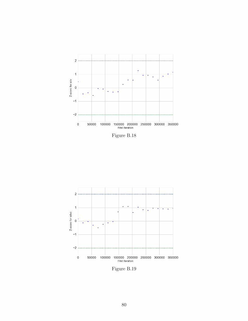
Figure B.18

Figure B.19

80

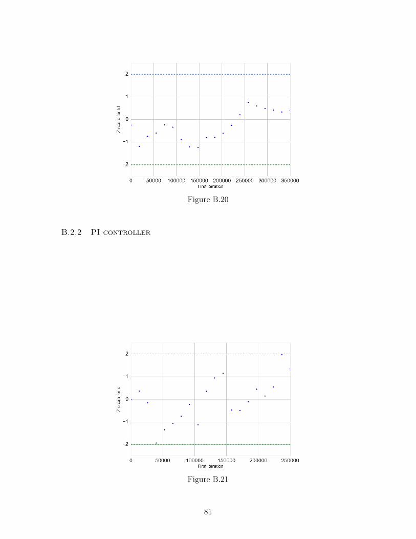
Figure B.20

B.2.2 PI controller

Figure B.21

81

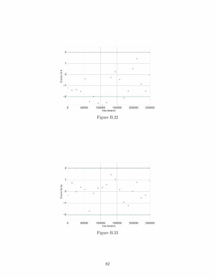
Figure B.22

Figure B.23

82

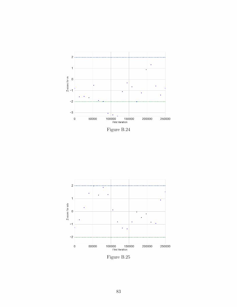
Figure B.24

Figure B.25

83

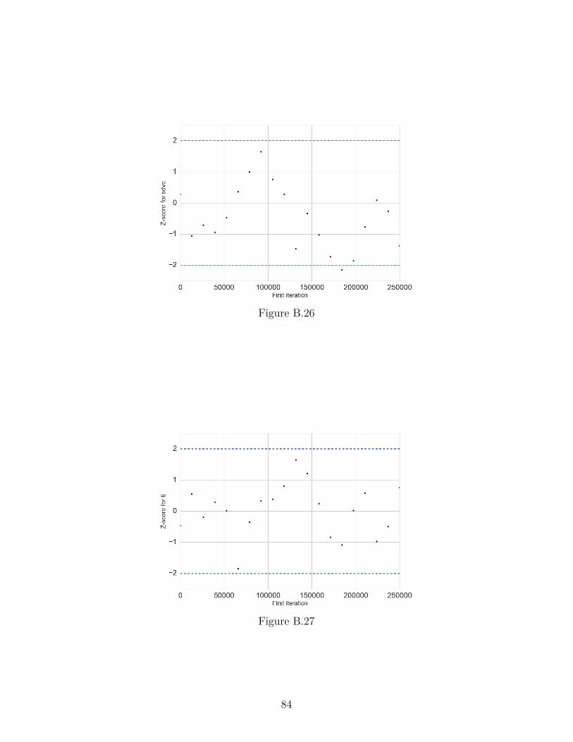
Figure B.26

Figure B.27

84

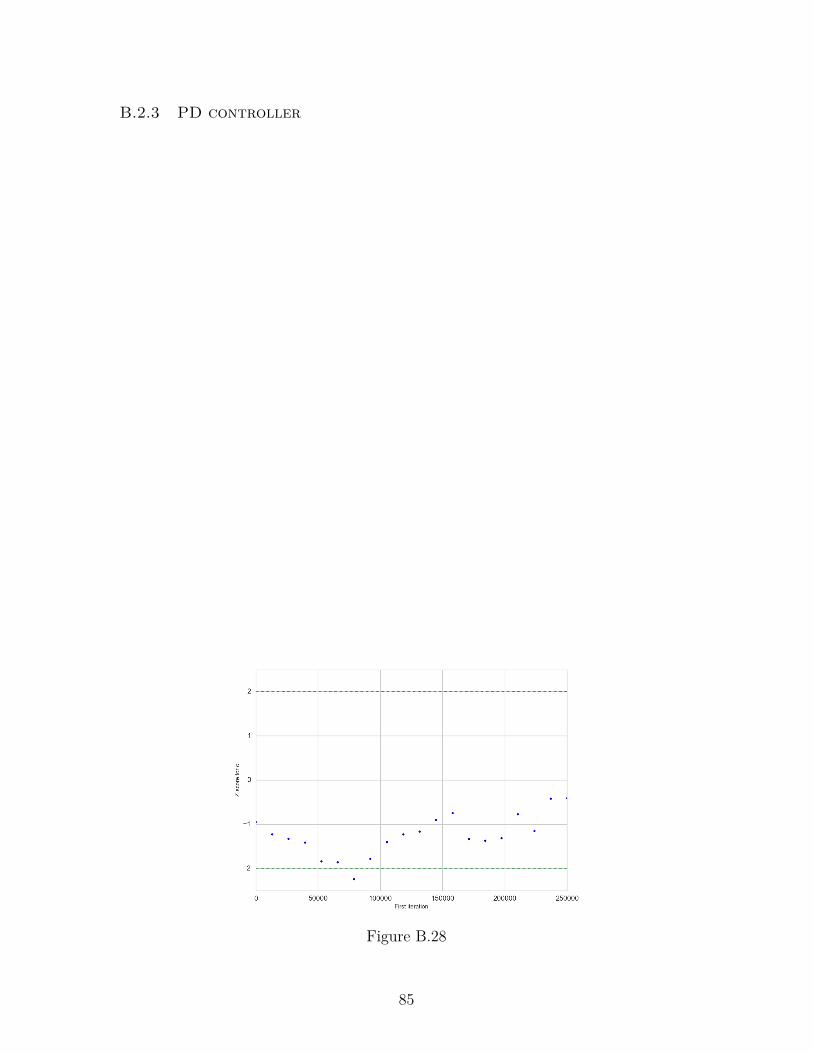
B.2.3 PD controller

Figure B.28

85

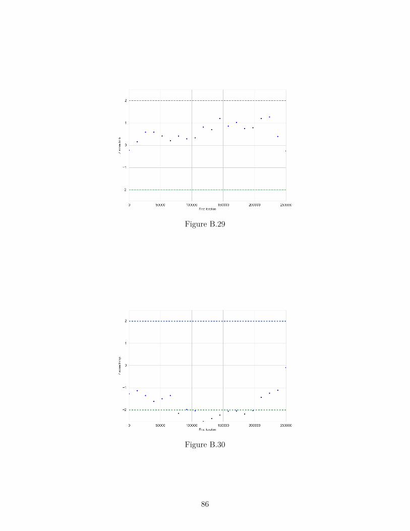
Figure B.29

Figure B.30

86

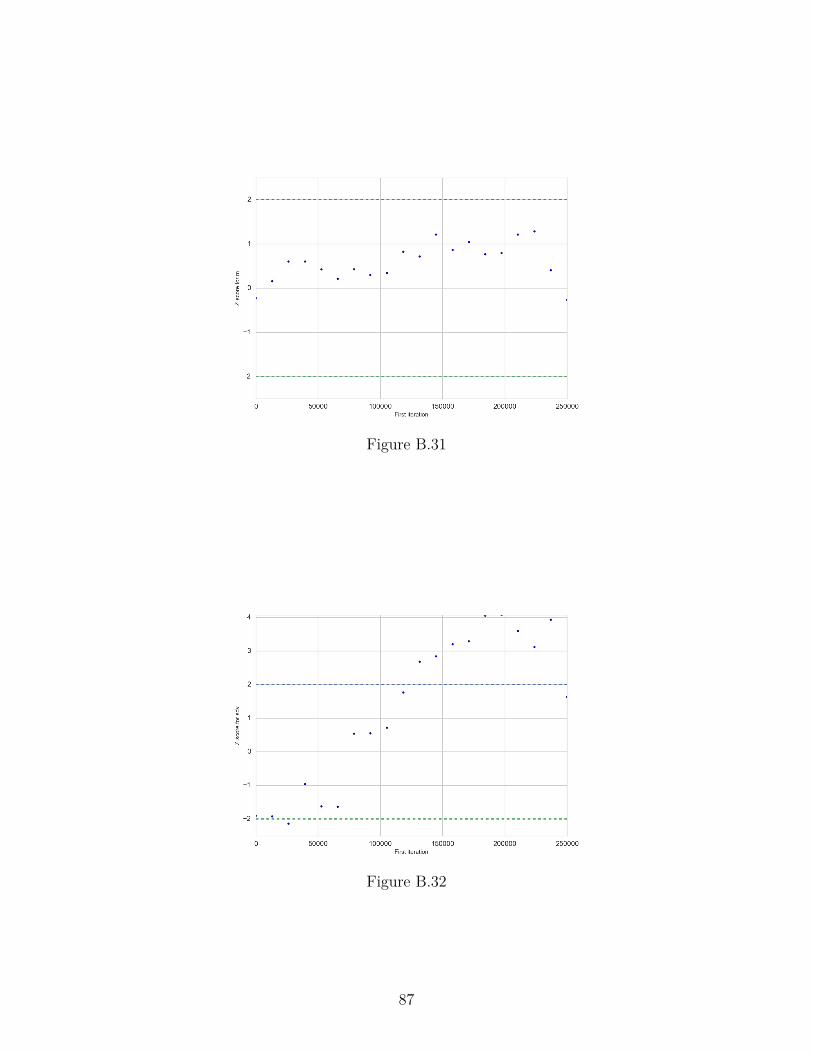
Figure B.31

Figure B.32

87

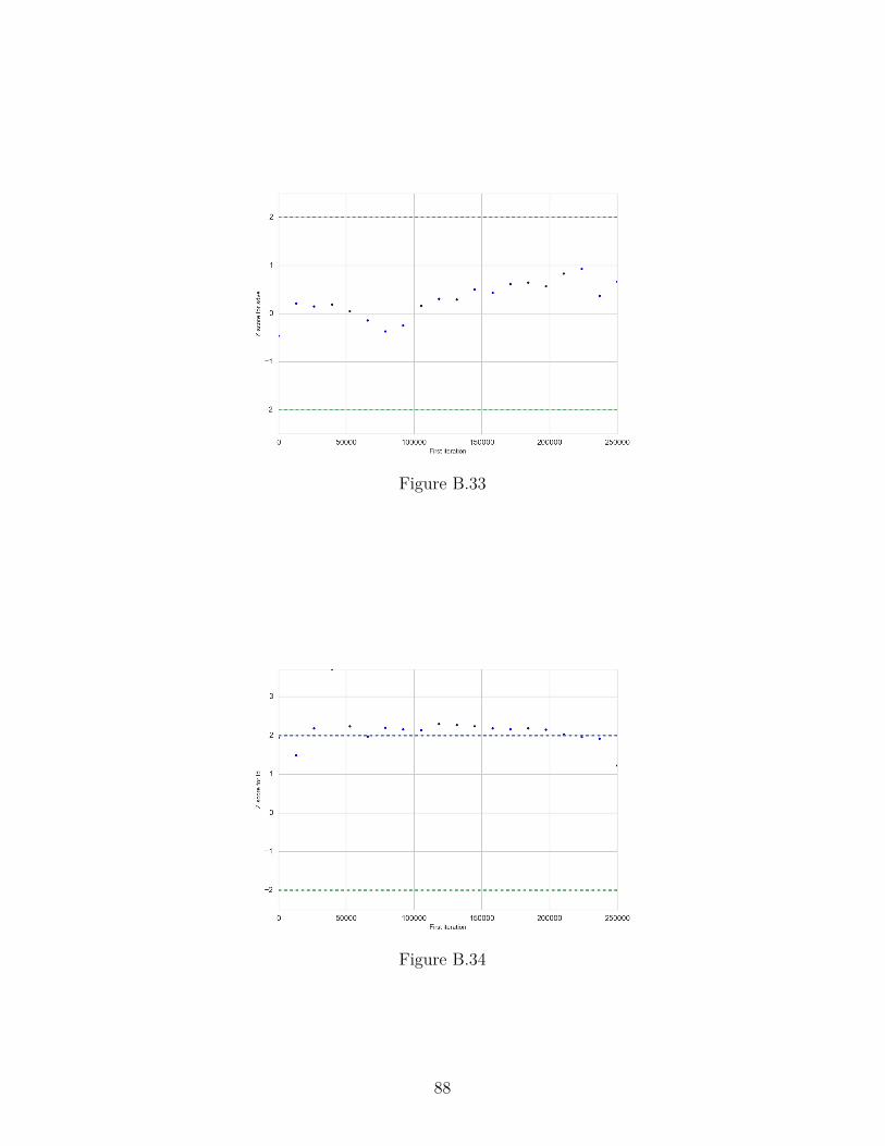
Figure B.33

Figure B.34

88

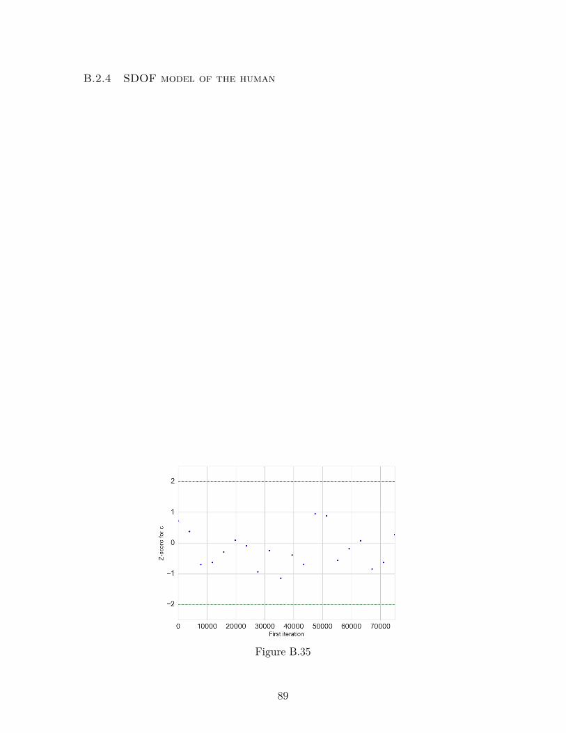
B.2.4 SDOF model of the human

Figure B.35

89

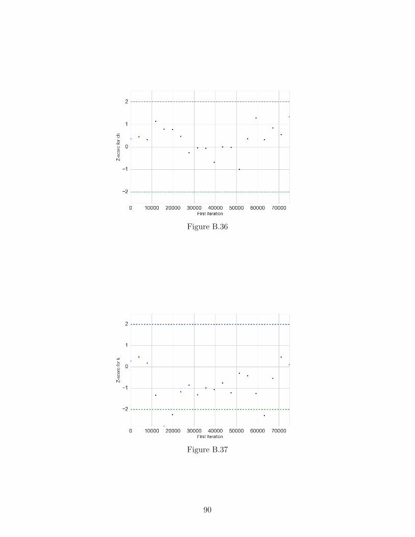
Figure B.36

Figure B.37

90

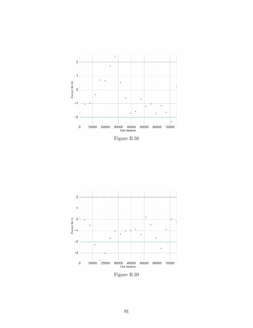
Figure B.38

Figure B.39

91

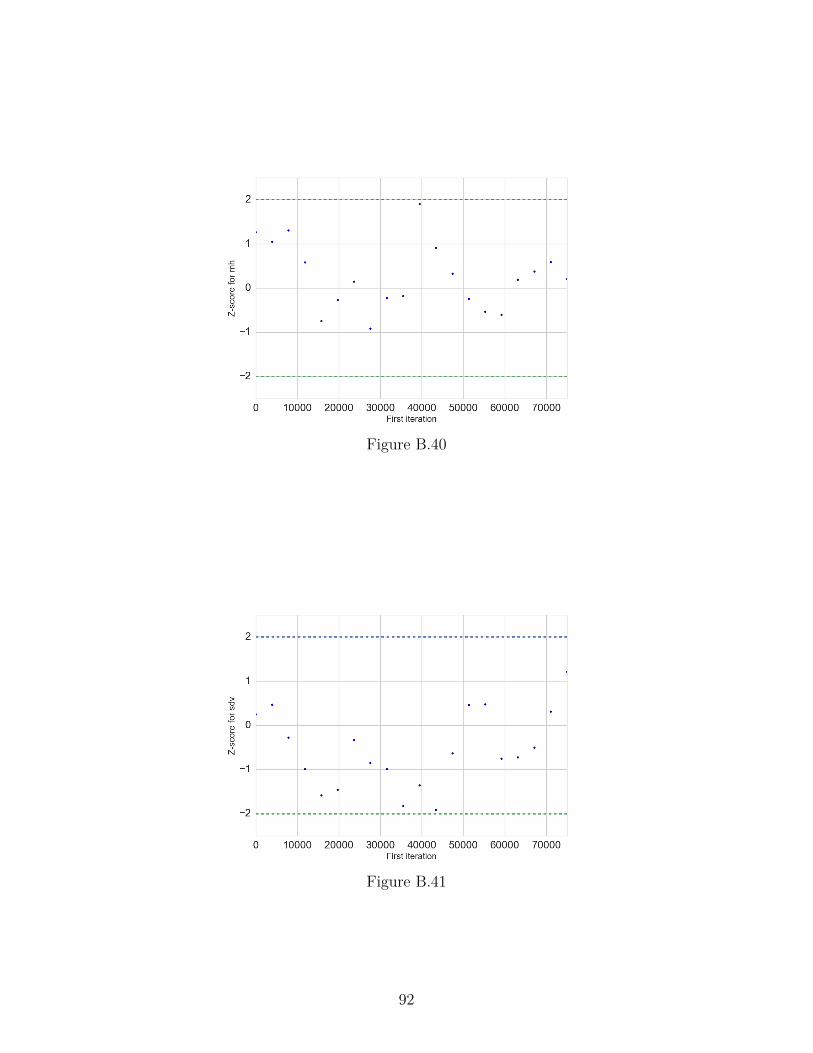
Figure B.40

Figure B.41

92

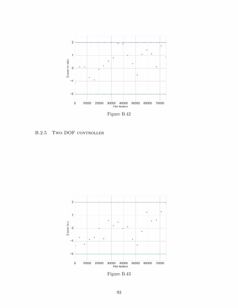
Figure B.42

B.2.5 Two DOF controller

Figure B.43

93

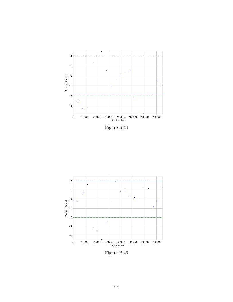
Figure B.44

Figure B.45

94

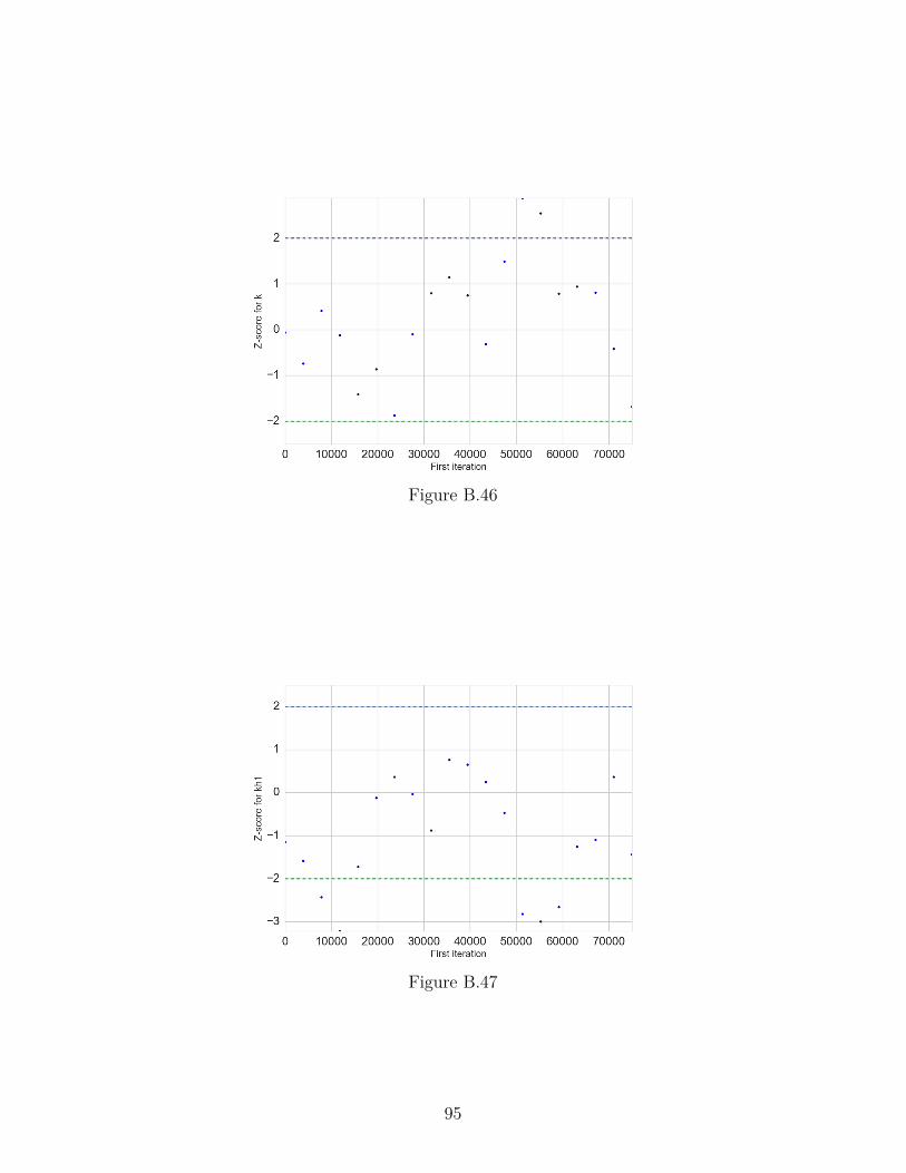
Figure B.46

Figure B.47

95

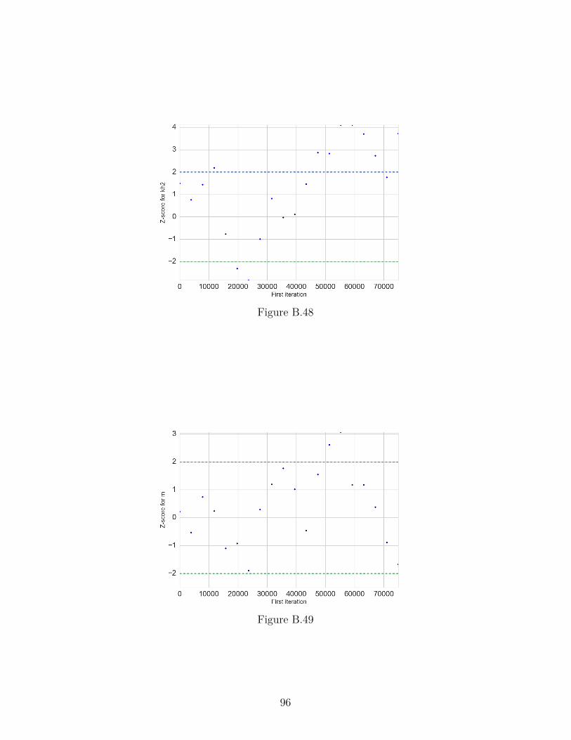
Figure B.48

Figure B.49

96

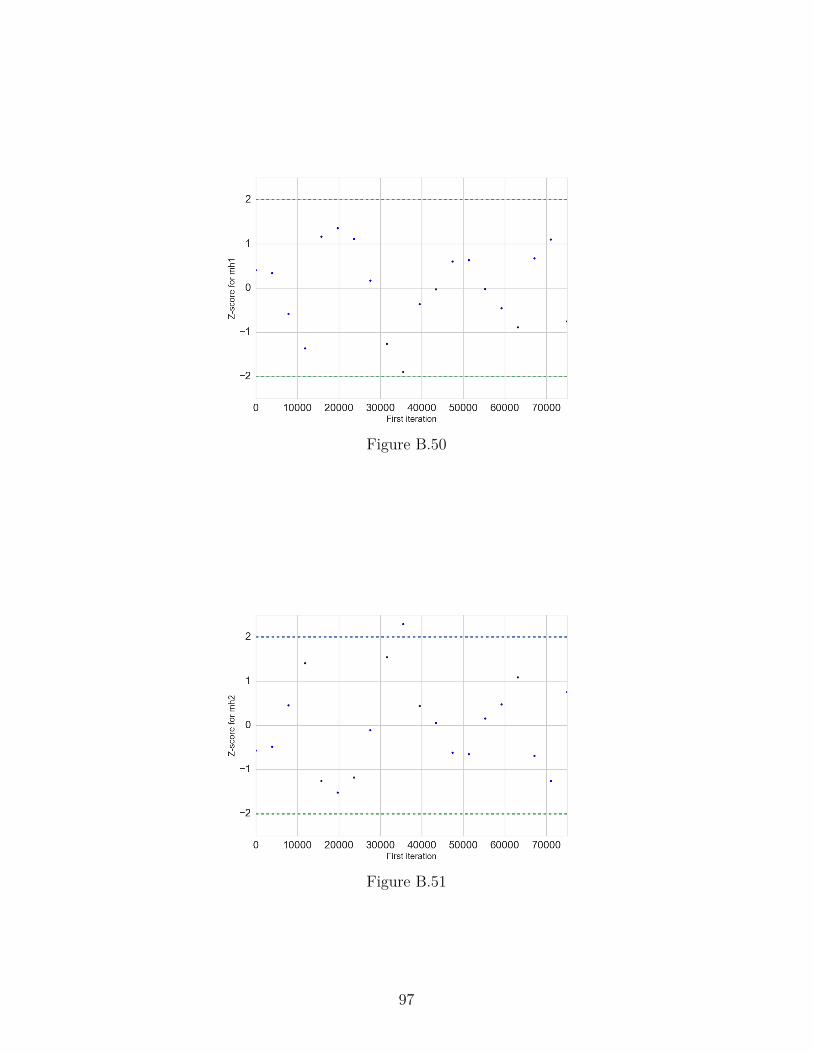
Figure B.50

Figure B.51

97

Figure B.52

Figure B.53

98