Embed Size (px)
Citation preview
NASA/TM-2003-211407
Modeling of Depth Cue Integration in Manual Control Tasks Barbara T. Sweet, Mary K. Kaiser, and Wendy Davis Ames Research Center, Moffett Field, California
National Aeronautics and Space Administration
Ames Research Center Moffett Field, California 94035
May 2003
1 Introduction Psychologists have long recognized that the human visual system has access to multi- ple sources of information specifying depth. These depth cues are usually grouped in terms of their information “type” (that is, physiological, pictorial, or motion), or by the level to which they specify depth (ordinal, relative, or absolute). Any good text- book on visual perception [Bruce, et al. 19961 provides a good overview of these cues and taxonomies. More thorough treatments can be found in the relevant chapters of the Handbook of Perception and Human Performance ([Boff, et al, 19861; see espe- cially the Volume I chapters by Sedgwick, Hochberg, and Arditi). We shall provide a very cursory summary.
1.1 Depth Cue Taxonomies The British philosopher Berkeley [Berkeley, 1709/1910] provided an early taxonomy of depth cues. Berkeley was most concerned with what he termed “primary” depth cues (now more commonly called physiological cues) : accommodation, convergence, and binocular stereopsis. Accommodation refers to the degree to which ocular mus- cles tense or relax to adjust the thickness of the eye’s lens to focus on an object. Convergence is the degree to which the eyes angle toward one another to look at the object. In principle, both accommodation and convergence can provide absolute depth information, although most research suggests that, in practice, these cues play a minor role [Foley, 19801. The third primary (or physiological) depth cue, binocu- lar stereopsis, exploits the disparity information resulting from the displacement of our two eyes. If inter-ocular distance and vergence angle is known, binocular dispar- ity can, in principle, specify absolute depth. At a minimum, it provides compelling relative depth cues to people with functional stereopsis. (Approximately 5% of the population lack this ability and are “stereo blind” [Richards, 19711).
What Berkeley termed “secondary” depth cues are now more commonly called pictorial cues. As might be expected, these refer to the cues resulting from linear perspective, and have been exploited since the Renaissance by artists to convey an impression of depth in two-dimensional depictions. A partial list of these cues include: occlusion (the obscuring object is closer); image size (larger images appear closer); height in the visual field (images closer to the horizon appear more distant); and atmospheric perspective (distant objects lose brightness and contrast due to atmo- spheric attenuation). Occlusion is a good example of an ordinal depth cue: the fact that Object A obscures Object B tells us only that Object A is closer. If one knew the contrast/brightness fall-off function for distance, atmospheric attenuation could,
in principle, specify absolute depth. In practice, it too functions as an ordinal cue. Relative image size and height-in-field generally provide relative depth information (although given additional knowledge, such as absolute object size and eye height respectively, absolute depth could, in theory, be recovered).
The final class of depth cues result from motion. While this can be object motion (e.g., the image velocity of an object falling is inversely proportional t o its distance from the observer), most depth-from-motion results from the motion of the observer through the environment. Psychologists typically describe this information in terms of “motion parallax” (Le., motion lateral to a pair of objects results in greater image velocity for the nearer object) or “optical expansion” (as an observer approaches a pair of objects, the closer one’s image will have a greater radial flow rate). Just as knowing inter-ocular separation and vergence allows one to recover absolute distance from disparity, knowledge of ego-speed allows recovery of absolute distance from motion parallax. Even without such knowledge, motion parallax is a compelling relative depth cue.
1.2 An Alternate Depth Cue Taxonomy More recently, Cutting and Vishton [Cutting and Vishton, 19951 proposed an alter- native, functional analysis of depth cue by examining which cues are more or less useful as a function of context. Obviously, motion depth cues are only informative in situations where the observer (or objects) are moving. But the functional utility of all cues vary depending on situational specifics. For example, accommodation, con- vergence, and stereopsis are only useful at relatively near distances; beyond fifteen feet, all of these cues become Subthreshold (i.e., imperceptible to human observers). Conversely, atmospheric perspective is subthreshold at close distance, and only be- comes a meaningful cue when objects are thousands of meters distant (unless one is in San Francisco on a foggy day).
Cutting and Vishton categorize depth cues into those whose utility is invariant with distance (e.g., occlusion and relative size), those whose utility diminishes with distance (e.g., the physiological depth cues); and those whose utility increases with distance (e.g., atmospheric perspective). They then divide the space surrounding an individual into three functional regions: Personal space (0-2 meters - generally, the region in which a person manipulates objects); Action space (2 - 30 meter - the region in which a person moves quickly to act upon the environment); and Vista space (beyond 30 meters - basically the region in which a person plans future navigation). Cutting and Vishton argue that, because the relative utility of depth cues vary as a function of region, the relative importance (or weighting) the observer places on those
2
cues will likewise vary. This raises the more general question of how observers integrate depth cues.
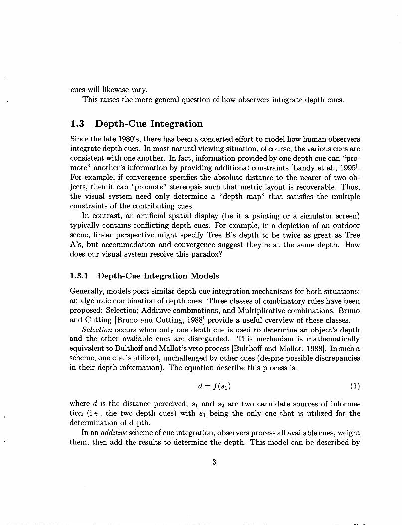
1.3 Depth-Cue Integration Since the late 1980’s, there has been a concerted effort to model how human observers integrate depth cues. In most natural viewing situation, of course, the various cues are consistent with one another. In fact, information provided by one depth cue can ‘(pro- mote” another’s information by providing additional constraints [Landy et al., 19951. For example, if convergence specifies the absolute distance to the nearer of two ob- jects, then it can “promote” stereopsis such that metric layout is recoverable. Thus, the visual system need only determine a ”depth map” that satisfies the multiple constraints of the contributing cues.
In contrast, an artificial spatial display (be it a painting or a simulator screen) typically contains conflicting depth cues. For example, in a depiction of an outdoor scene, linear perspective might specify Tree B’s depth to be twice as great as Tree A’s, but accommodation and convergence suggest they’re at the same depth. How does our visual system resolve this paradox?
1.3.1 Depth-Cue Integration Models
Generally, models posit similar depth-cue integration mechanisms for both situations: an algebraic combination of depth cues. Three classes of combinatory rules have been proposed: Selection; Additive combinations; and Multiplicative combinations. Bruno and Cutting [Bruno and Cutting, 19881 provide a useful overview of these classes.
Selection occurs when only one depth cue is used to determine an object’s depth and the other available cues are disregarded. This mechanism is mathematically equivalent to Bulthoff and Mallot’s veto process [Bulthoff and Mallot, 19881. In such a scheme, one cue is utilized, unchallenged by other cues (despite possible discrepancies in their depth information). The equation describe this process is:
d = f (s1) where d is the distance perceived, s1 and s2 are two candidate sources of informa- tion (i.e., the two depth cues) with s1 being the only one that is utilized for the determination of depth.
In an additive scheme of cue integration, observers process all available cues, weight them, then add the results to determine the depth. This model can be described by
3
the following equation: d = f ( W 1 + w 2 s 2 )
where d is the perceived distance, s1 and s 2 are sources of information, and w1 and w 2 are the weights assigned to each source depth. Note, of course, that Selection is simply a special case of the additive model, in which the weights for all but one cue are set to zero.
The third possible rule class involves the multiplicative combination of depth cues. In these models, observers use some cues to modify information from other cues. A plausible equation for multiplicative integration is:
As Bruno and Cutting acknowledge, hybrid combinatory rules may prove viable, combining addition and multiplication in various way, such as where a particular depth cue (sl) is weighted independently and also influences the weighting of a second depth cue ( sz ) , as in:
Or cues could be weighted both independently and in the context of other cues si- multaneously, as in:
d = f ( W 1 + SlW2S2) (4)
d = f ( W i s 1 + ~ 2 ~ 2 + ~ 1 ~ 1 ~ 2 ~ 2 ) (5)
1.3.2 Cue Integration Findings
While selection is seldom proposed as the primary mechanism for depth cue integra- tion, instances can be found in which selection appears to operate, particularly in the case of cue conflict. For example, Bulthoff and Mallot [Bulthoff and Mallot, 19881 found that if .edge information (i.e., occlusion) is present, it overrides both shape- from-shading and disparate shading-depth information.
More commonly, empirical studies suggest additive combination rules. Bruno and Cutting [Bruno and Cutting, 19881 performed three experiments testing perceived ex- ocentric distances as a function of both static and motion cues (including relative size, height in the projection plane, occlusion, and motion parallax) and found the greatest support for the additive combination rule. Similarly, linear combination rules provide good fits for the combination of stereo disparity and texture gradi- ent [Johnston et al., 19931, texture gradient and motion parallax [Young et al., 19931 and stereo disparity and linear perspective [Stevens and Brooks, 19881.
A number of researchers have reported findings consistent with multiplicative combination rules. Massaro’s fizzy Logical Model of Perception (FLMP) used a
4
specific multiplicative model of cue integration based on fuzzy logic [Massaro, 1988, Massaro and Cohen, 19931 to fit depth judgment data and reported a fit superior to that obtained with linear models. Others have reported superior fits with non- linear models, especially in cases of recovering surface structure from multiple depth cues [Bradshaw and Rogers, 1996, Curran and Johnston, 19941.
A study by Johnston, Cumming, and Landy [Johnston et al., 19941 lends empirical credence to Cutting and Viston’s proposal of contextual cue weighting. Johnston, et al. pitted stereo disparity against motion parallax cues in their task, and varied both the number of frames of animation (to vary the utility of the motion cue) and the observer’s viewing distance (to vary the utility of the disparity cue); they found that observers’ weighting of the two cues varied as a function of condition, with greater weight assigned to the stronger cue.
1.4 Extending Cue Integration to an Active Control Task Both the Cutting and Viston chapter and the Johnston, et al. study recognize that depth-cue integration is unlikely to be a fixed, inflexible process. Rather, our per- ceptual system is sufficiently intelligent to consider the quality and reliability of the various sources of information when deriving an estimate of depth. The Modified Weak h s i o n model proposed by Landy, et al. and Massaro’s FLMP likewise recog- nize that the weighting of cues should be dynamic (i.e., adjusting to accommodate changes in viewing circumstances, and resulting changes in the various cues’ utility).
However, all of this work has examined depth-cue integration in the context of “passive” perception - that is, observers are asked to view displays and make verbal or keyboard responses concerning scene layout or surface curvature. Our goal is to study depth-cue integration in the context of active control, and to model depth perception as one component of the manual control task. In this way, we build upon previous models of depth-cue integration, and expand their application to a dynamic, closed-loop control model.
As we will show, current formulations of depth-cue integration are amenable to inclusion as modules in larger control models. Once the cue-integration module is integrated into the control model, we can examine whether people’s depth-cue inte- gration is impacted, not only by changes in the “quality” of the cue, but also by the utility that information holds for the control task they must perform. Thus, we can investigate whether people’s depth cue integration strategies are merely clever enough to adjust to changes in cue “quality,” or sufficiently intelligent to utilize the cues best suited for the task at hand.
5
2 Depth Cue Control Model In this report, a model is developed that describes the control strategy the human operator adopts in performing a depth control task when two depth cues are available to the operator. It is an extension of a modeling technique that was developed to examine manual control in perspective scene viewing situations [Sweet, 19991. This modeling technique relies heavily on the discipline of manual control, and a particular model of human operator characteristics called the Crossover Model.
In this section, a brief background on the Crossover Model is presented (Sec- tion 2.1). Then, a model of depth-cue integration and control is presented that is based upon the characteristics of the Crossover Model (Section 2.2).
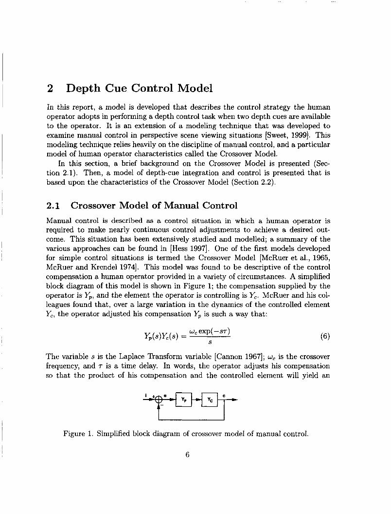
2.1 Crossover Model of Manual Control Manual control is described as a control situation in which a human operator is required to make nearly continuous control adjustments to achieve a desired out- come. This situation has been extensively studied and modelled; a summary of the various approaches can be found in [Hess 19971. One of the first models developed for simple control situations is termed the Crossover Model [McRuer et al., 1965, McRuer and Krendel 19741. This model was found to be descriptive of the control compensation a human operator provided in a variety of circumstances. A simplified block diagram of this model is shown in Figure 1; the compensation supplied by the operator is Yp, and the element the operator is controlling is Y,. McRuer and his col- leagues found that, over a large variation in the dynamics of the controlled element Yc, the operator adjusted his compensation Yp is such a way that:
w, exp( -sr) S
y,(s)yc(s) =
The variable s is the Laplace Transform variable [Cannon 19671; w, is the crossover frequency, and r is a time delay. In words, the operator adjusts his compensation so that thc product of his compensation and the controlled elemcnt will yield an
Figure 1. Simplified block diagram of crossover model of manual control.
6
integrator with a time delay. The crossover frequency wc is defined as the frequency at which the open-loop system transfer function has a magnitude of unity:
The crossover frequency determines the bandwidth of the closed-loop system, or the input frequencies above which effective tracking cannot be accomplished. Typical values for w, range from 1.0 to 6.0 rad/sec, time delays r range from 0.2 to 0.5 seconds [McRuer et al., 19651.
The effects of changing controlled element dynamics can be plainly seen with this model. Consider the case of rate-control (first-order) dynamics (Yc = l/s). This refers to situations in which the rate-of-change of the controlled state is proportional to the control effector displacement. One real-world example of rate control is the lateral control of an automobile; the rate-of-change of direction is proportional to the steering wheel displacement. For this case, the operator would apply the approximate compensation Yp = w,exp(-s~). This type of compensation on the part of the operator is termed proportional compensation; the output of the operator is simply a time delayed (exp(-sr)) and scaled (w,) version of the input.
A second type of dynamics is acceleration-control (second-order); an example is the attitude control or position control of a spacecraft. In these cases, the accelera- tion of the desired state is proportional to the displacement of the control effector. When presented with acceleration-control dynamics ( yC = 1/s2), the operator needs to provide compensation of the approximate form Yp = w,sexp(-s~). This type of compensation is called derivative compensation because of the s term; instead of feeding back position, the operator is feeding back a time delayed derivative of the input, which can also be termed velocity. When using rate-control dynamics, the operator needs to supply only proportional or position information. When the dy- namics become acceleration control, the operator must feed back velocity information instead.
The previous discussion focussed upon the first model developed by McRuer and his colleagues, and was intended to be valid specifically in the frequency range of crossover. Eventually, the model was extended to provide accurate description of the operator at frequencies well above and below the crossover frequency. This new model form was termed the Precision Model; it's basic form is shown below:
7
The terms TL and TI represent the basic lead and lag equalization capabilities the hu- man provides. The terms TK and 7’‘ represent a low-frequency lag-lead equalization that is sometimes observed called the low-frequency “phase droop”. This typically appears when the forcing-function bandwidth increases. The terms TN,, wn, and cn represent the neuromuscular dynamics. K p represents the gain the operator adopts, and T is a lumped time delay representing pure time delays in both the perceptual and neuromuscular systems. Because the experimental measurements spanned a fre- quency range well below and above the crossover frequency, the depth-control model developed here is based upon a simplified version of the Precision Model.
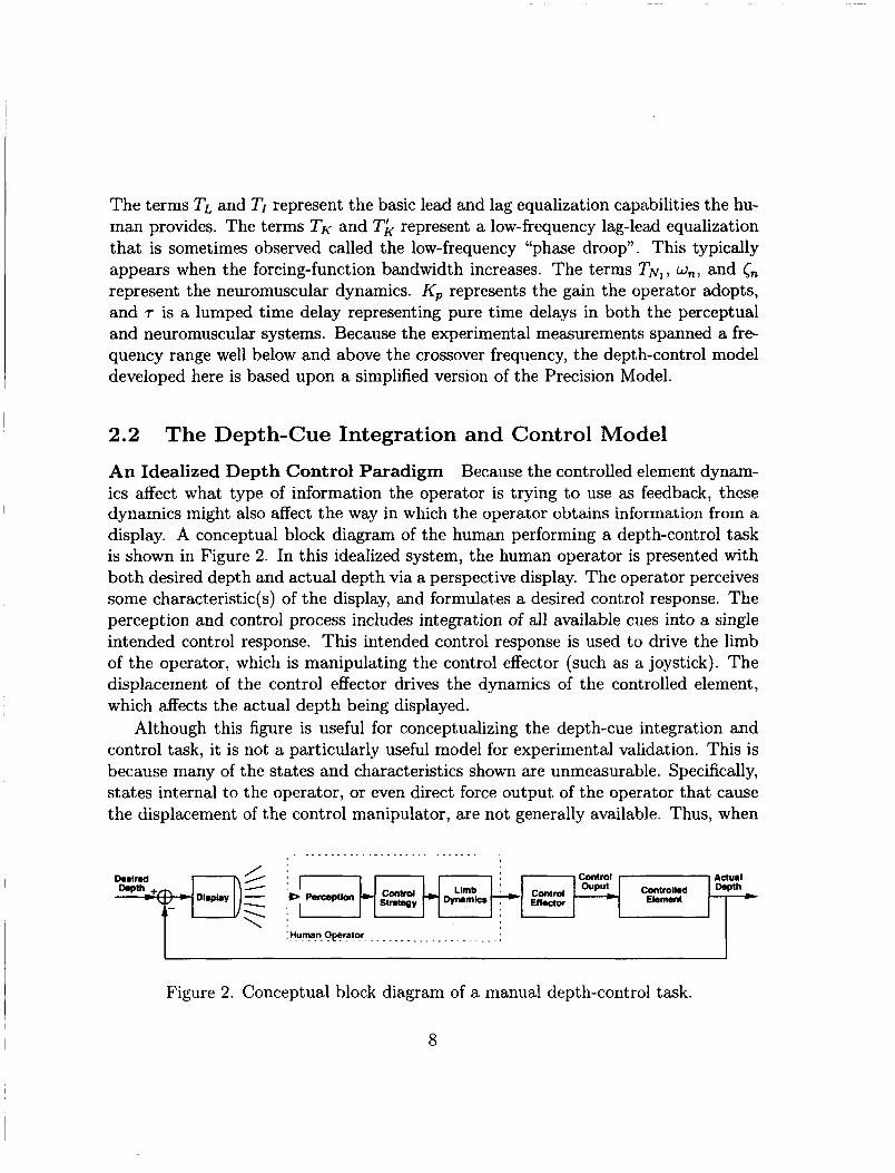
2.2 The Depth-Cue Integration and Control Model An Idealized Depth Control Paradigm Because the controlled element dynam- ics affect what type of information the operator is trying to use as feedback, these dynamics might also affect the way in which the operator obtains information from a display. A conceptual block diagram of the human performing a depth-control task is shown in Figure 2. In this idealized system, the human operator is presented with both desired depth and actual depth via a perspective display. The operator perceives some characteristic(s) of the display, and formulates a desired control response. The perception and control process includes integration of all available cues into a single intended control response. This intended control response is used to drive the limb of the operator, which is manipulating the control effector (such as a joystick). The displacement of the control effector drives the dynamics of the controlled element, which affects the actual depth being displayed.
Although this figure is useful for conceptualizing the depth-cue integration and control task, it is not a particularly useful model for experimental validation. This is because many of the states and characteristics shown are unmeasurable. Specifically, states internal to the operator, or even direct force output of the operator that cause the displacement of the control manipulator, are not generally available. Thus, when
...................................
I :H!.l!ar??pe‘a!?r. ..................... ~ I Figure 2. Conceptual block diagram of a manual depth-control task.
8
stereo
I HUMAN OPERATOR
velocity perception I control I, - I Dosition DerceDtion I . .
(C)
neuromuscular dynamics
remnant (r)
I relative s ize4 ' disturbance ( 2 )
I
-
a P 0 w U U w A
+ z 0 0
_ - P
I
controlled element
dynamics
control
size and disparity disturbance ( X )
ho_
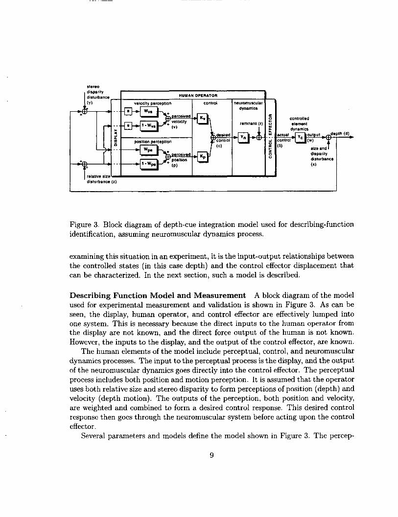
Figure 3. Block diagram of depth-cue integration model used for describing-function identification, assuming neuromuscular dynamics process.
examining this situation in an experiment, it is the input-output relationships between the controlled states (in this case depth) and the control effector displacement that can be characterized. In the next section, such a model is described.
Describing Function Model and Measurement A block diagram of the model used for experimental measurement and validation is shown in Figure 3. As can be seen, the display, human operator, and control effector are effectively lumped into one system. This is necessary because the direct inputs to the human operator from the display are not known, and the direct force output of the human is not known. However, the inputs to the display, and the output of the control effector, are known.
The human elements of the model include perceptual, control, and neuromuscular dynamics processes. The input to the perceptual process is the display, and the output of the neuromuscular dynamics goes directly into the control effector. The perceptual process includes both position and motion perception. It is assumed that the operator uses both relative size and stereo disparity to form perceptions of position (depth) and velocity (depth motion). The outputs of the perception, both position and velocity, are weighted and combined to form a desired control response. This desired control response then goes through the neuromuscular system before acting upon the control effect or.
Several parameters and models define the model shown in Figure 3. The percep
9
tual processes are defined by two weights, W,,, and Wps, which can each have values between zero and one. W,,, is the weighting put on stereo disparity in the velocity perception process; Wps is the weighting of stereo disparity in the position perception process. By constraining the weights to vary between zero and one, the outputs of the perception process are simply weighted sums of the inputs from stereo disparity and relative size, without any gain factors. In the control process, the control strategy of the operator is created by applying gains to velocity K,, and position Kp, then summing these to form a control input. It has long been established in manual con- trol that an operator’s control strategy resembles this block: a linear combination of velocity and position feedback. The neuromuscular process contains a neuromuscular transfer function, Yn (which will be elaborated upon in Section 3.2.2) as well as a source of internal noise T , called remnant.
Characteristics of this model related to the perception, control, and neuromus- cular dynamics can be measured through careful selection and manipulation of the disturbances affecting the displayed depth. An overall disturbance, x, is used to perturb both stereo disparity and relative size simultaneously. At the same time, dis- turbances y and z are used to independently perturb the stereo disparity and relative size, respectively. By examining the interrelationships between the disturbances and the control output of the operator, experimental measurements related to the model parameters and functions (W,,,, Wps, K,,, K p , Yn) can be obtained.
From the block diagram in Figure 3, we can write the following relationships:
By substituting Equations 10, 11 and 12 into Equation 9, we obtain the following expression for S which is only a function of the model parameters and model inputs:
S( 1 + ynYc(sKv + ~ p ) ) = -yn{ ( S K ~ + K ~ ) X + (~Kvwv, + KpWps)~ + ( s K ( 1 - W,,) + Kp(l - WpS)) z } + T (13)
Similarly, substituting Equations 11, 12 and 9 into Equation 10 will yield an expres- sion for d which is only a function of the model parameters and model inputs:
10
+ ( s m - Wu,) + Kp(l - WPS))"] + r } + x (14)
The term 1 + Y,Yn(sKv + K p ) in the previous equations appears repeatedly in the following derivations. A simplifying term will now be defined for ease of interpretation:
A = 1 + YcY,(sKu + K p ) (15)
Taking the cross-spectral densities of Equations 13 and 14 with respect to x will yield:
Taking into account the fact that the disturbances x,, with each other (a,, = = 0), Equation 16 becomes:
y, and z are not correlated
Further assuming that the noise signal T is uncorrelated with 5 (QTZ = 0), and taking the ratios between the two expressions, we get:
The cross-spectral density of 6 can also be derived relative to y and z:

Accounting for the uncorrelated Qr, = 0), the equations become:
J
disturbances (azy = Q,, = aYz = Qr, = Qry =
a& = -+-G(l - W,,) + K p ( 1 - wpS)pz2 A
We can now use these relationships as the basis for empirical modeling based upon experimental measurements of operator response. In the next section, an experiment is described in which these measurements are used to derive the parameters of the depth-cue integration and control model.
12
3 Experiment An experiment was conducted to determine the cross-spectral density estimates pre- viously defined. Both the controlled element dynamics and the viewing distance were manipulated to determine what effect (if any) these variables had on the operator characteristics. In Section 3.1, the experimental protocol is described. The experi- mental results are described in Section 3.2.
3.1 Method 3.1.1 Participants
Eight male, general-aviation pilots participated in the study. They were recruited from a paid contractor pool at Ames Research Center. All had normal or corrected- to-normal visual acuity and good stereo vision (40 seconds of arc or better). Their flight experience ranged from 100 to 4500 logged hours.
3.1.2 Apparatus
The experimental control program was run on a Silicon Graphics Octane computer with an RlOOOO processor. Control inputs were made via a B&G Systems JF3 3-axis joystick. (Only the longitudinal degree of freedom of the stick was used; the lateral and yaw inputs of the stick were disabled.) Stereo images were viewed through Crystal Eyes polarizing shutter glasses. The monitor displayed the views for the left and right eye on alternating refreshes at a rate of 96 Hz, yielding an effective update rate to each eye of 48 Hz. Control data from the joystick was updated at 48 Hz. The images were displayed on a 19-inch diagonal monitor, with a resolution of 1024 (width) by 768 (height) pixels.
3.1.3 Stimuli and Control Tasks
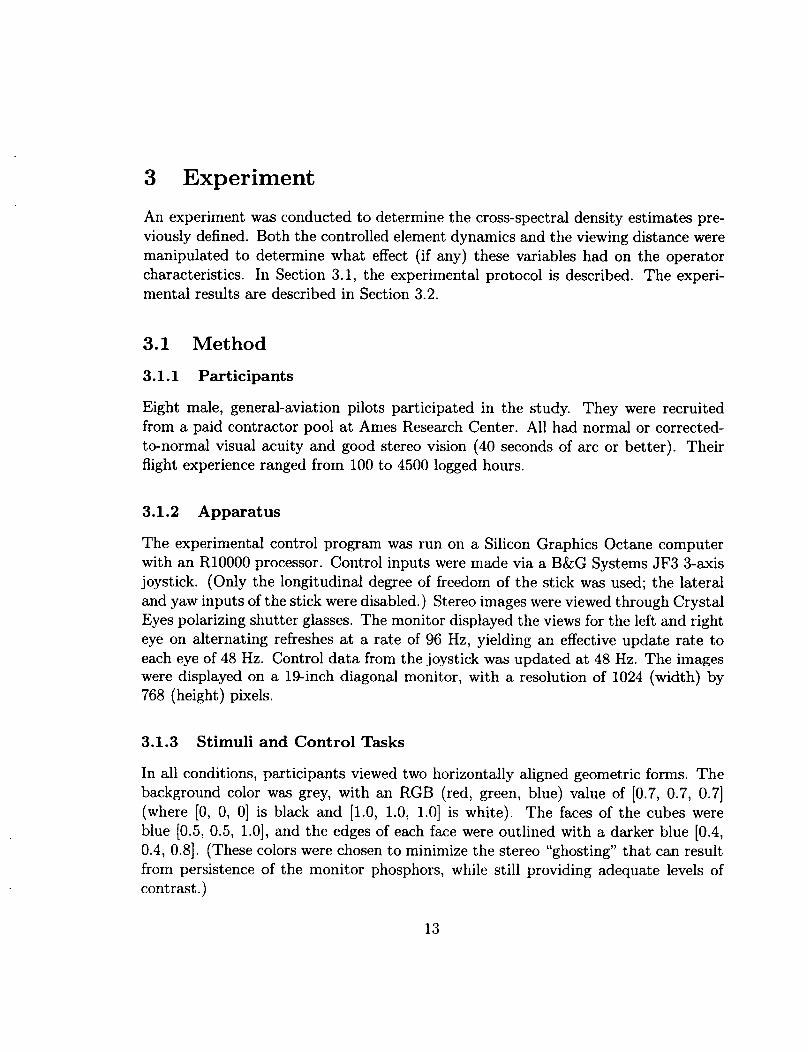
In all conditions, participants viewed two horizontally aligned geometric forms. The background color was grey, with an RGB (red, green, blue) value of [0.7, 0.7, 0.71 (where [0, 0, 01 is black and [1.0, 1.0, 1.01 is white). The faces of the cubes were blue [0.5, 0.5, 1.01, and the edges of each face were outlined with a darker blue [0.4, 0.4, 0.81. (These colors were chosen to minimize the stereo “ghosting” that can result from persistence of the monitor phosphors, while still providing adequate levels of contrast .)
13
The left-hand object served as the “standard” and was rendered at a constant depth. The object on the right was the control target. Participants were instructed to move the joy stick longitudinally (fore and aft) to maintain the target at the same apparent depth as the standard.
Other aspects of the displays and control task were varied as a function of ex- perimental condition. The three experimental factors were: viewing distance; control task dynamics; and disturbance function. We discuss each of these in turn.
Viewing Distance. Participants were seated at two different viewing distances: “near” (22 inches form the screen); and “far” (33 inches from the screen). In the near condition, the display subtended approximately 35 (horizontal) by 26 (verti- cal) degrees. In the far viewing condition, the display subtended approximately 24 (horizontal) by 18 (vertical) degrees.
In the near condition, the objects (at standard depth) were scaled to have a screen image size of 3.0 inches, and were spaced 4.5 inches apart (center to center). The near-viewing scene is shown in Figure 4.
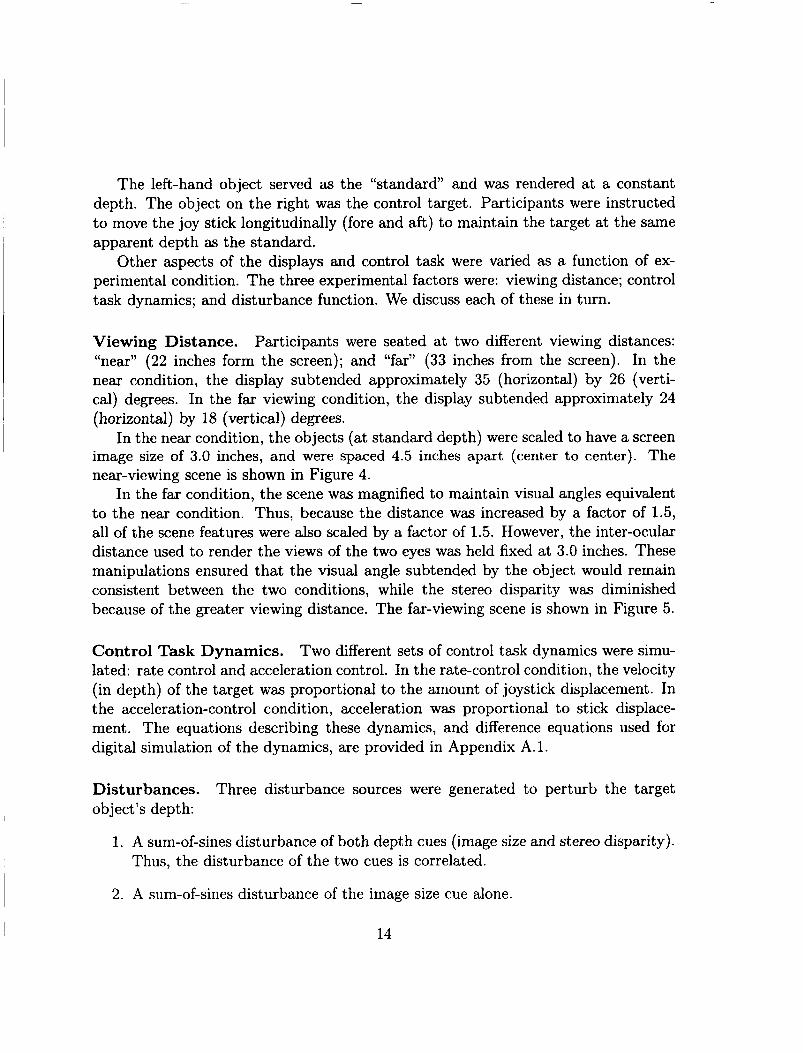
In the far condition, the scene was magnified to maintain visual angles equivalent to the near condition. Thus, because the distance was increased by a factor of 1.5, all of the scene features were also scaled by a factor of 1.5. However, the inter-ocular distance used to render the views of the two eyes was held fixed at 3.0 inches. These manipulations ensured that the visual angle subtended by the object would remain consistent between the two conditions, while the stereo disparity was diminished because of the greater viewing distance. The far-viewing scene is shown in Figure 5.
Control Task Dynamics. Two different sets of control task dynamics were simu- lated: rate control and acceleration control. In the rate-control condition, the velocity (in depth) of the target was proportional to the amount of joystick displacement. In the acceleration-control condition, acceleration was proportional to stick displace- ment. The equations describing these dynamics, and difference equations used for digital simulation of the dynamics, are provided in Appendix A. l .
Disturbances. object’s depth:
Three disturbance sources were generated to perturb the target
1. A sum-of-sines disturbance of both depth cues (image size and stereo disparity). Thus, the disturbance of the two cues is correlated.
2. A sum-of-sines disturbance of the image size cue alone.
14
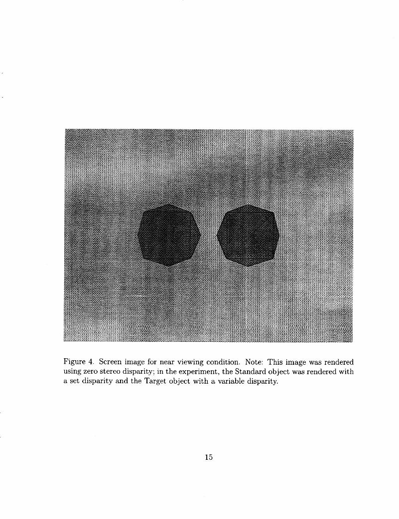
Figure 4. Screen image for near viewing condition. Note: This image was rendered using zero stereo disparity; in the experiment, the Standard object was rendered with a set disparity and the Target object with a variable disparity.
15
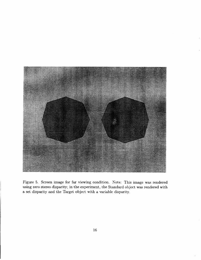
Figure 5. Screen image for far viewing condition. Note: This image was rendered using zero stereo disparity; in the experiment, the Standard object was rendered with a set disparity and the Target object with a variable disparity.
16
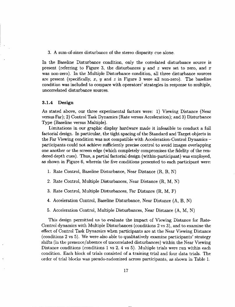
3. A sum-of-sines disturbance of the stereo disparity cue alone.
In the Baseline Disturbance condition, only the correlated disturbance source is present (referring to Figure 3, the disturbances y and z were set to zero, and x was non-zero). In the Multiple Disturbance condition, all three disturbance sources are present (specifically, x, y and z in Figure 3 were all non-zero). The baseline condition was included to compare with operators’ strategies in response to multiple, uncorrelated disturbance sources.
3.1.4 Design
As stated above, our three experimental factors were: 1) Viewing Distance (Near versus Far); 2) Control Task Dynamics (Rate versus Acceleration); and 3) Disturbance Type (Baseline versus Multiple).
Limitations in our graphic display hardware made it infeasible to conduct a full factorial design. In particular, the tight spacing of the Standard and Target objects in the Far Viewing condition was not compatible with Acceleration-Control Dynamics - participants could not achieve sufficiently precise control to avoid images overlapping one another or the screen edge (which completely compromises the fidelity of the ren- dered depth cues). Thus, a partial factorial design (within-participant) was employed, as shown in Figure 6, wherein the five conditions presented to each participant were:
1. Rate Control, Baseline Disturbance, Near Distance (R, B, N)
2. Rate Control, Multiple Disturbances, Near Distance (R, M, N)
3. Rate Control, Multiple Disturbances, Far Distance (R, M, F)
4. Acceleration Control, Baseline Disturbance, Near Distance (A, B, N)
5. Acceleration Control, Multiple Disturbances, Near Distance (A, M, N )
This design permitted us to evaluate the impact of Viewing Distance for Rate- Control dynamics with Multiple Disturbances (conditions 2 vs 3), and to examine the effect of Control Task Dynamics when participants are at the Near Viewing Distance (conditions 2 vs 5). We were also able to qualitatively examine participants’ strategy shifts (in the presence/absence of uncorrelated disturbances) within the Near Viewing Distance conditions (conditions 1 vs 2, 4 vs 5). Multiple trials were run within each condition. Each block of trials consisted of a training trial and four data trials. The order of trial blocks was pseudo-radomized across participants, as shown in Table 1.
17
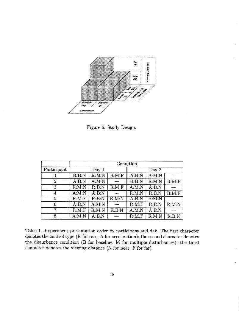
Figure 6. Study Design.
Participant 1 2 3 4 5
Condition
Table 1. Experiment presentation order by participant and day. The first character denotes the control type (R for rate, A for acceleration); the second character denotes the disturbance condition (B for baseline, M for multiple disturbances); the third character denotes the viewing distance (N for near, F for far).
18
3.1.5 Procedure
Participants were given written task instructions describing their task and its dis- cernable variations (i.e., Near and Far viewing, Rate and Acceleration control). A copy of these instructions appears in Appendix A.2. Participants were then given an opportunity to ask questions. Once started, the task was entirely self-paced. The experimenter intervened only to assist with changes in viewing distance as required between blocks of trials.
The experiment took two days for participants to complete; participants experi- enced only one type of control dynamics (Rate or Acceleration) per day. Each day's session began with a brief session of training trials (eight for each of the two or three conditions the participant would see that day). Participants then completed a block of trials (consisting of one training and four data trials) for each condition. This was followed by a thirty-minute lunch break. After lunch, participants completed a second series of blocks. Paticipants were given additional 5-minute breaks between all blocks. Prior to the start of the second day, participants were administered a stereo vision acuity test.
Each data trial lasted four minutes, five seconds. Training trials lasted one minute. Both data and training trials were initiated by the particpant pressing the trigger switch on the joystick. During the first five seconds of both training and data trials, the disturbances ramped linearly from zero to full intensity. Operators were not given feedback on their performance on either training or data trials.
3.2 Results 3.2.1 Statistical Analysis
Two dependent measures were considered: percent of control power correlated with input disturbances, and depth error RMS. These analyses were conducted only on the Multiple Disturbance trial data (i.e., those trials that contained independent disturbances of the stereo'disparity and relative size cues).
Because our design was not a full factorial, two independent ANOVAs (ANalysis Of VAriance) were performed for the percent of control activity measure. The first, using only the rate-control task data, consisted of an 8 x 2 x 2 factorial with repeti- tions, viewing distance (Near versus Far), and disturbance (relative size versus stereo disparity) as factors. The second, using only the near viewing distance data, was an 8 x 2 x 2 factorial with repetitions, control task dynamics (rate versus acceleration), and disturbance (relative versus and stereo disparity) as factors.
19
viewing distance
z E 4 - c 2 3.5.
8 3 - P
- c
2 2.5 c 2 -
k 1 . 5 -
c m
4.5
-
0.5 ' t 4 - - - , - - -0
01 I near far
viewing distance
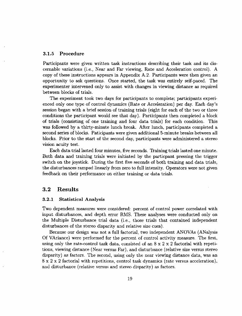
Figure 7. Effect of viewing distance on distance error RMS (a) and percent of control activity correlated with disturbances (b). Standard error bars are shown.
For the depth error RMS, two analyses were performed. The first was an 8 x 2 factorial with repetitions and viewing distance as factors; the second an 8 x 2 factorial with repetitions and control task dynamics as factors.
Effect of Viewing Distance A significant main effect on depth error RMS was found for viewing distance (F[1,7] = 64.06, p < .001), with a smaller error associated with the Near condition as can be seen in Figure 7a. The percent of control activity demonstrated no significant main effect for viewing distance or disturbance source (Figure 7b), but there was a significant interaction (F [1,7] = 14.45, p < . O l ) ; the percent of control activity associated with the two cues is approximately equal in the Near condition, whereas relative size dominates in the Far condition.
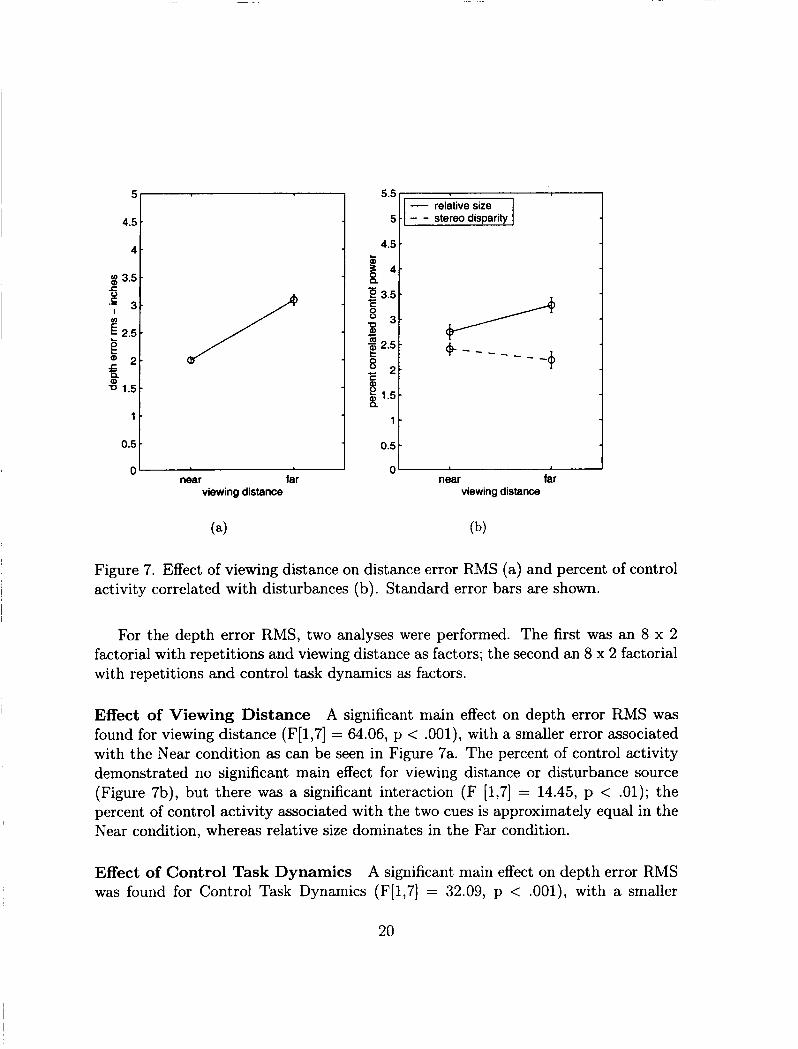
Effect of Control Task Dynamics A significant main effect on depth error RMS was found for Control Task Dynamics (F[1,7] = 32.09, p < . O O l ) , with a smaller
20
5
4.5
4 -
g 3.5 2 '7 3
r
v) E 2.5 9
2 - 5 1.5
1 -
0.5
0
/ I -
-
-
-
-
rate accel
4.5 I 5 -
relative size
0.5 l t
- - P 3.5 8 3- P C
(II 3 2.5
c) 2 - 8 & 1.5-
C
0.
0 rate accel
control task dynamics
-
-
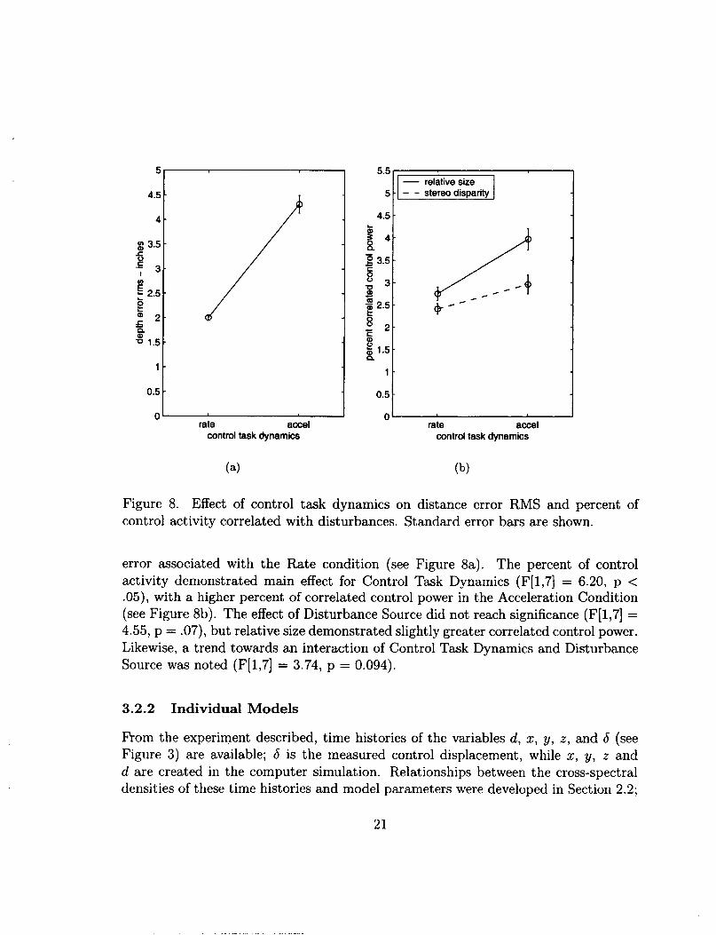
Figure 8. Effect of control task dynamics on distance error RMS and percent of control activity correlated with disturbances. Standard error bars are shown.
error associated with the Rate condition (see Figure sa). The percent of control activity demonstrated main effect for Control Task Dynamics (F[1,7] = 6.20, p < .05), with a higher percent of correlated control power in the Acceleration Condition (see Figure 8b). The effect of Disturbance Source did not reach significance (F[1,7] = 4.55, p = .07), but relative size demonstrated slightly greater correlated control power. Likewise, a trend towards an interaction of Control Task Dynamics and Disturbance Source was noted (F[1,7] = 3.74, p = 0.094).
3.2.2 Individual Models
F'rom the experiment described, time histories of the variables d, x, y, z , and b (see Figure 3) are available; b is the measured control displacement, while x, y, z and d are created in the computer simulation. Relationships between the cross-spectral densities of these time histories and model parameters were developed in Section 2.2;
21
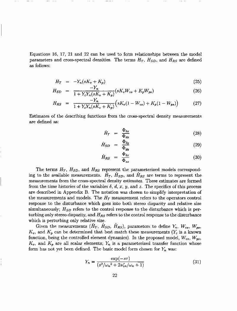
Equations 16, 17, 21 and 22 can be used to form relationships between the model parameters and cross-spectral densities. The terms HT, HSD, and HRS are defined as follows:
Estimates of the describing functions from are defined as:
HT =
h s D =
I;lflS =
the cross-spectral density measurements
The terms HT, H ~ D , and HRS represent the parameterized models correspond- ing to the available measurements. HT, H ~ D , and HRS are terms to represent the measurements from the cross-spectral density estimates. These estimates are formed from the time histories of the variables 6, d, z, y, and z. The specifics of this process are described in Appendix B. The notation was chosen to simplify interpretation of the measurements and models. The HT measurement refers to the operators control response to the disturbance which goes into both stereo disparity and relative size simultaneously; H s D refers to the control response to the disturbance which is per- turbing only stereo disparity, and H R ~ refers to the control response to the disturbance which is perturbing only relative size.
Given the measurements (I?*, HSD, I?Rs), parameters to define Y,; W,,, Wps, K,, and Kp can be determined that best match these measurements (Yc is a known function, being the controlled element dynamics). In the proposed model, W,,, Wps, K,, and Kp are all scalar elements; Yn is a parameterized transfer function whose form has not yet been defined. The basic model form chosen for Yn was:
_ _ exD - ST)
22
The term Y N represents the combination of the neuromotor limb dynamics and control effector. This form was chosen because it generally provided good correspon- dence with the data. Note that the only time delay present in the model is shown in Yn; this time delay is meant to represent the sum of the perceptual and motor delays present in the system. This representation is mathematically equivalent t o putting a separate perceptual delay directly “downstream” of the display, and was done to simplify the model identification.
The parameters of these functions, specifically r , u n , cn , Kp , K,, W,,, and Wps, were determined to best fit the measurements for each operator and condition; Ap- pendix C describes the process used to fit the data. The resulting parameters are presented in Section A.3 of Appendix A, and plots of the measurements and models are shown in Section A.4. Some specific aspects of these parameters will be discussed in the following sections.
Crossover Frequency and Phase Margin Two commonly used metrics in man- ual control are crossover frequency (uc) and phase margin (4m). For this model, the crossover frequency and phase margin of this model are defined by the following relationships:
The crossover frequency determines the bandwidth of the system, or the frequency above which tracking performance starts to degrade. The phase margin is a measure of the stability of the closed-loop system. When the phase margin approaches zero, slight uncertainties in the plant dynamics or variations in loop gain can create unstable closed-loop characteristics.
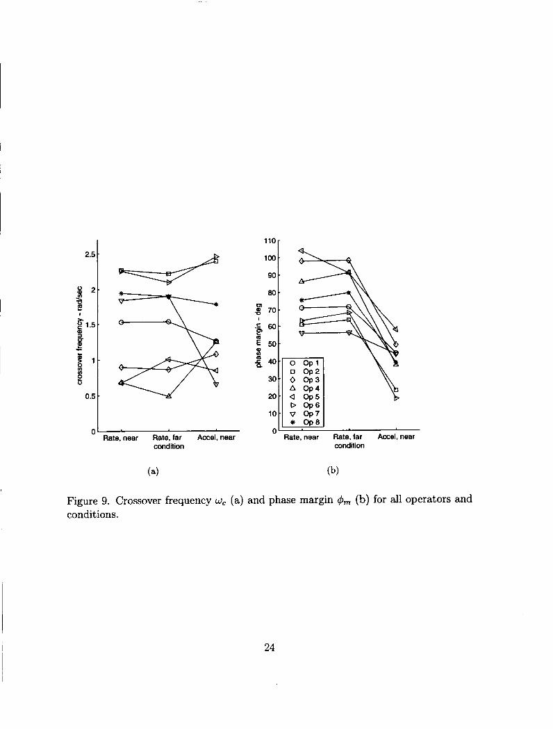
The crossover frequencies and phase margins for all operators and conditions are shown in Figure 9, and Table 6 in Appendix A.
Comparing the two rate-control cases (near and far), it is clear that there is little variation in these parameters (for a particular operator) between the two conditions. Comparing the near rate-control case with the near acceleration-control case, the largest change is a significant drop in the phase margins with the acceleration-control case. This is a natural consequence of the controlled element dynamics. In the acceleration-control case, the controlled element has much more phase lag (90 de- grees) than the rate-control element. Thus, the operator/element system will tend to have more phase lag with the acceleration element than the rate element. Crossover
23
2.5
0 2 - a E 2 1.5 J
I %
c F 5 1 - 0 g
0.5
4 -
-
-
" Rate, near Rate, far Accel, near condition
11Or
condition
(b)
Figure 9. Crossover frequency wc (a) and phase margin & (b) for all operators and conditions.
24
frequencies were generally lower with the acceleration-control dynamics than with rate-control dynamics, as has been observed in previous manual control research.
The observed range of crossover frequencies, phase margins, and trends as a func- tion of controlled element dynamics are all consistent with the body of manual control work that has preceeded this [McRuer et al., 19651. These parameters do little to ex- amine the perceptual and control processes of the operator, which are the subject of the next sections.
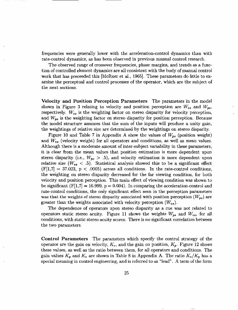
Velocity and Position Perception Parameters The parameters in the model shown in Figure 3 relating to velocity and position perception are V7,, and W,,, respectively. W,, is the weighting factor on stereo disparity for velocity perception, and W,, is the weighting factor on stereo disparity for position perception. Because the model structure assumes that the sum of the inputs will produce a unity gain, the weightings of relative size are determined by the weightings on stereo disparity.
Figure 10 and Table 7 in Appendix A show the values of Wps (position weight) and W,, (velocity weight) for all operators and conditions, as well as mean values. Although there is a moderate amount of inter-subject variability in these parameters, it is clear from the mean values that position estimation is more dependent upon stereo disparity (i.e., Wps > .5), and velocity estimation is more dependent upon relative size (Wvs < .5). Statistical analysis showed this to be a significant effect (F[1,7] = 37.023, p < .0005) across all conditions. In the rate-control conditions, the weighting on stereo disparity decreased for the far viewing condition, for both velocity and position perception. This main effect of viewing condition was shown to be significant (F[1,7] = 16.999, p = 0.004). In comparing the acceleration-control and rate-control conditions, the only significant effect seen in the perception parameters was that the weights of stereo disparity associated with position perception (W,,) are greater than the weights associated with velocity perception ( WVs).
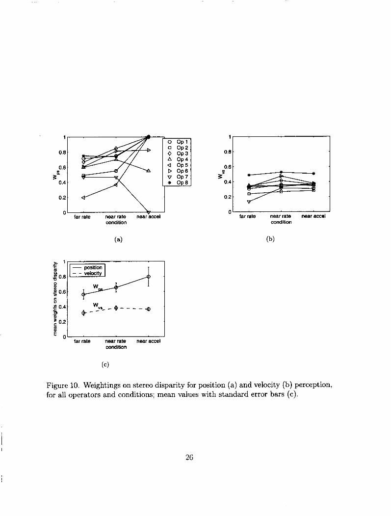
The dependence of operators upon stereo disparity as a cue was not related to operators static stereo acuity. Figure 11 shows the weights Wps and W,,, for all conditions, with static stereo acuity scores. There is no significant correlation between the two parameters.
Control Parameters The parameters which specify the control strategy of the operator are the gain on velocity, K,, and the gain on position, K,. Figure 12 shows these values, as well as the ratio between them, for all operators and conditions. The gain values K p and K, are shown in Table 8 in Appendix A. The ratio K,,/K, has a special meaning in control engineering, and is referred to as “lead”. A term of the form
25
0.4
0.2
0.8
0.6
2 0.4
0.2
I far rate near rate near"acce1
condition
0'
.
.
.
.
4 Op5
v Op7 * Op8
'C 2.' 2: + 0.8
E 2 0.6
d 0.4
0.2
c 0
.c CD al .-
m
g o ~
far rate near rate near accel condition
- far rate near rate near accel condition
Figure 10. Weightings on stereo disparity for position (a) and velocity (b) perception, for all operators and conditions; mean values with standard error bars (c).
26
Near, Rate
1 .
u)
3 3 . 5 .
0
3 8 . 5
Far, Rate
* 8 A a V
Q
0 V
" 5 6 7 8 9 1 0 stereo acuity score
i ' I Far, Rate '
A 3 8 . 5
1
38.5
0
5 6 7 8 9 1 0 stereo acuity score
4 .I, A *.
Q Op5
v Op7 m V
5 6 7 8 9 1 0 stereo acuity score
1
v)
3 3 . 5
0
Near, Rate
5 6 7 8 9 1 0 stereo acuity score
1
3%.5
Near, Accel ---l *
)1 A Q
0 ' I 5 6 7 8 9 10
stereo acuity score
Figure 11. Weightings on stereo disparity versus stereo acuity. The left hand figures (a,c,e) show the weighting W,,, for the three conditions; the right hand figures (b,d,f) show the weighting W,, for all conditions. There is no observable relationship between stereo acuity and reliance on stereo dispa&y as a cue.
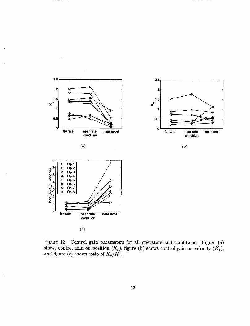
sK, + Kp is labelled a lead network. This is because the output of a circuit with this transfer function would “lead” the input, in phase, because its output is proportional to not only the input, but also to the input velocity. For large values of K, (K, > K p ) , lead is high, and the output largely proportional to the velocity of the input. For the converse case (K , < K p ) , lead is low, and the output is largely proportional to the input. This lead term is clearly visible in the model transfer function to overall depth disturbance (Equation 25). Previous work in manual control has shown that for acceleration-control dynamics, the operator needs to generate additional lead to achieve acceptable levels of closed-loop performance. This is clearly demonstrated in Figure 12; for all operators and conditions, lead dramatically increases for the near acceleration condition.
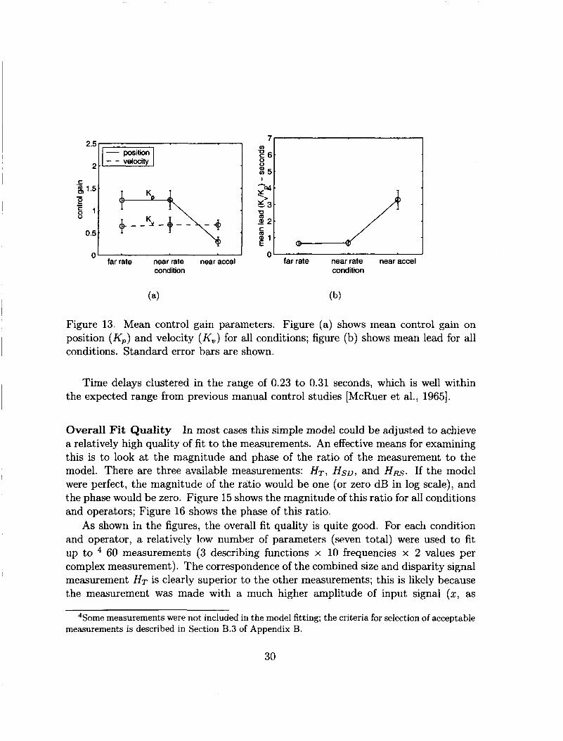
Mean values for these gains and ratios are shown in Figure 13. The increase in lead is clearly shown, but it is more interesting to note that this increase in lead occurs primarily because of a drop in position gain Kp, not from an increase in velocity gain K,. The velocity gain K, remains relatively unchanged with changes in condition.
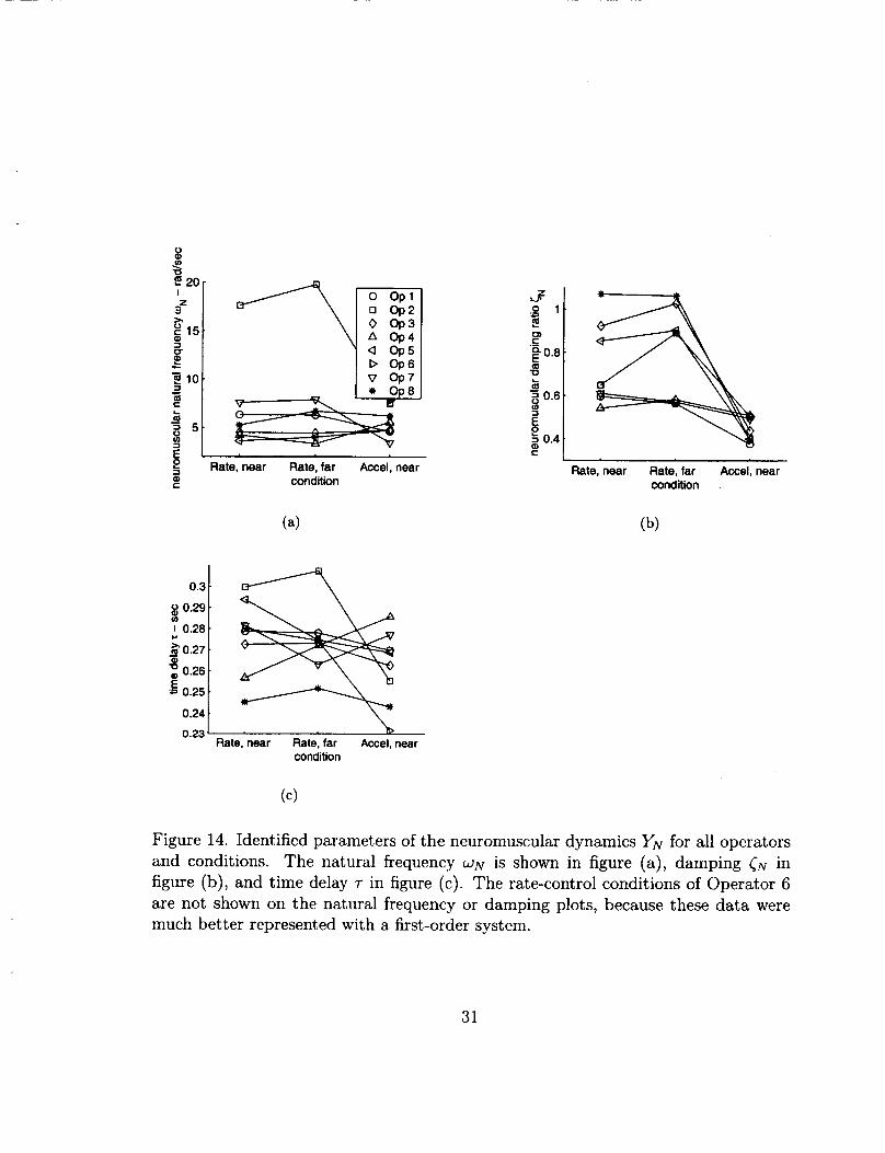
Neuromuscular Parameters The neuromuscular dynamics function Y,, as de- fined in Equation 31, consists of a second-order system in the numerator (assumed to be related to the neuromuscular dynamics of the operator) and a pure time delay. The parameters’ associated with this function, w N , (N, and 7, are shown in Figure 14 and Table 9. As can be seen, for most operators and conditions the natural frequency ( W N ) is in the range2 of 3.5 to 8.0 rad/sec; damping ((N) is higher (> 0.5) for rate control3 conditions than acceration control (< 0.5). Although the second-order neu- romuscular system is required to obtain accurate fits to the measurements, it has little direct effect on the closed-loop system performance. This is because the frequency range in which it operates was above the observed crossover frequency in all cases (the highest observed crossover frequency was 2.45 rad/sec).
‘The rate-control condition data of Operator 6 was better represented by a first-order system in the denominator as opposed to a second-order system. The parameters associated with this first-order term are included in Section A.3.
2These neuromuscular frequencies are lower than the typically observed range of W N of 15 to 20 rad/sec, but similar results have been obtained before [Stapleford et al., 19691. It has been demonstrated that identified values in this range can result from a “pulsive” control strategy, which some operators are known to adopt [Hess 19791.
3The reader might notice that in the rate-control condition, the value of the damping exceeds unity for some operators. In these cases, the neuromotor dynamics no longer consist of a damped oscillatory second-order system, but instead consist of two first-order terms, specified by the roots of the characteristic equation s2/w$ + 2 s c N / w N + 1 = 0.
28
2.5 I 1
1.5.
1 ’ YQ
0.5
21 - 2r--l 2
1.5 Y’
0.5
.. far rate near rate near accel
condition far rate near rate near accel
condition
‘ I 0 O p l 0 o p 2 0 Op3 A Op4 a o p 5 D Op6 v Op7 * Op8
P / P
0 far rate near rate near accel
condition
Figure 12. Control gain parameters for all operators and conditions. Figure (a) shows control gain on position ( K p ) , figure (b) shows control gain on velocity (K,,), and figure (c) shows ratio of K,/Kp.
29
7 ' a
U
0
I
E 6 . position
2.5 2 .(_ - - velocity $ 5 .
' -4. c .- 8 1.5.
2 -
, :!: c E ' . @ l . 0.5
0 0
Figure 13. Mean control gain parameters. Figure (a) shows mean control gain on position ( K p ) and velocity (K,,) for all conditions; figure (b) shows mean lead for all conditions. Standard error bars are shown.
~ /
Time delays clustered in the range of 0.23 to 0.31 seconds, which is well within the expected range from previous manual control studies [McRuer et al., 19651.
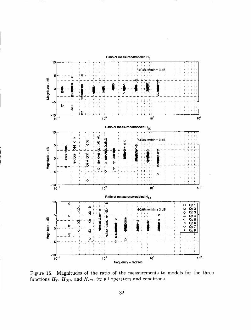
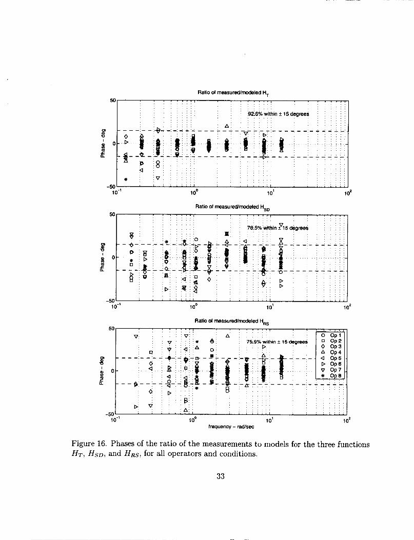
Overall Fit Quality In most cases this simple model could be adjusted to achieve a relatively high quality of fit to the measurements. An effective means for examining this is to look at the magnitude and phase of the ratio of the measurement to the model. There are three available measurements: HT, HsD, and HRs. If the model were perfect, the magnitude of the ratio would be one (or zero dB in log scale), and the phase would be zero. Figure 15 shows the magnitude of this ratio for all conditions and operators; Figure 16 shows the phase of this ratio.
As shown in the figures, the overall fit quality is quite good. For each condition and operator, a relatively low number of parameters (seven total) were used to fit up to 60 measurements (3 describing functions x 10 frequencies x 2 values per complex measurement). The correspondence of the combined size and disparity signal measurement HT is clearly superior to the other measurements; this is likely because the measurement was made with a much higher amplitude of input signal (2, as
4Some measurements were not included in the model fitting; the criteria for selection of acceptable measurements is described in Section B.3 of Appendix B.
30
7- a 005
E t 5 Rate, near Rate, far Accel, near al c condition
~~
Rate, near Rate, far Accel, near condition
8 0.29 . I 0.28.
- 2 0.27 . 0.26.
E 0.25 . 0.24.
u)
a
0.23 ‘ b Rate, near Rate, far Accel, near
condition
Figure 14. Identificd parameters of the neuromuscular dynamics YN for all opcrators and conditions. The natural frequency W N is shown in figure (a), damping <N in figure (b), and time delay 7 in figure (c). The rate-control conditions of Operator 6 are not shown on the natural frequency or damping plots, because these data were much better represented with a first-order system.
31
Ratio of measuredmodeled HT
... 5 -
95.3% mthin f 3 dB
v v
-10 -5L lo-' 1 oo 1 o1
Ratio of measuredlmodeled HSD
1 0'
Ratio of measured/modeled H,,
Figure 15. Magnitudes of the ratio of the measurements to models for the three functions HT, HsD, and HRS, for all operators and conditions.
32
Ratio of measured/modeled H,
. . . . . . . . . . . . . . . . . . . . . . . . . . . _ .
. . . . . . . . . . . . . . . . . .
. . . . . . . . . . . . . .
. . . . . . .
. . . . . . . . . . .
. . . . .
. . . . .
1 0-1 1 oo 1 o1 1 0'
Ratio of measured/modeled H,,
8 A , D V
-50 I
1 0-1 1 oo 1 o1 frequency - rausec
1 0'
Figure 16. Phases of the ratio of the measurements to models for the three functions HT, HsD, and HRS, for all operators and conditions.
opposed to y and z) . This yields a higher signal-tenoise ratio, resulting in smaller variances in measurement.
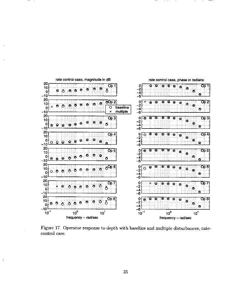
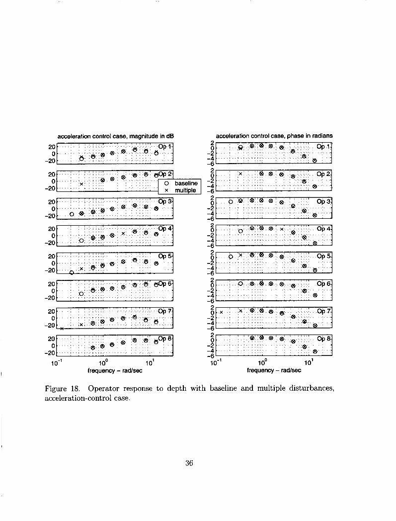
Effects of Disturbances The measurement technique used to determine the indi- vidual responses to stereo disparity and relative size requires that a portion of these cues be independent; that is, the depth consistent with disparity and depth consistent with relative size are rarely identical during the course of a data run. The two base- line disturbance cases were included in the testing to determine if this experimental manipulation produced a different control strategy. The response of the operator HT for the baseline and multiple disturbance cases are shown in Figures 17 and 18 for the rate-control and acceleration-control cases, respectively. As can be seen, there is only a slight variation in these responses from the addition of the multiple disturbances.
34
rate control case, magnitude in dB
10.. 0 .
. . , : . , : , : .:.: ::.:. . . . .
. . .@ . 6: .:.e31 re. e. . . . . . . . . . . . . . . . . . . . . . . . . . . . . . -10'
0.. -2 4 -
20 . . . . . . . . , . . . . . . . . ' Op41 10 . . . . : . : . : .:_ : ::::. . . . : ..:..: .:.::::.:.. . . . . . .
. . . Q . : Q ; . : . @ r .a :. 8;. . . . . . . . . . . . . . . . . . . . . . I p . . . . . ; . . ; . . . . . :. . . . . .:.@ .. :. ....... .O:. . .; . . . . . : . : . : . : . : : : ; : . . . :. : , : . : . : ;e . : . ; . . . . . . . . . . e' .:' ' '. . . . . . . . . .
. . . . . . . . . . . . . . . . . . . . .- 0 . . . . . . . . . . . . .:. . . O Q . . . . . .
-1 0 e3
0 -2 -4
20 10 0
-1 0 20 10 0
..cy .@ . 'e: .:.e, id. *. :. .~ . :. .I. :. I., : _ j .op 4?
. . . . . I . : : . : . ; ; : : : . . :. ... :&j.:.::.::.. ..:. .;
. . . . . : . . ; . ; . :. ; : ; ::. . . . . . . . . . . . . . . . . .e.:. . . . .:. . . . . . . . . . . . . . . . . . . . . . . . . . . . . 6 1 .
20 10 0
-1 0 20 10 0 . . . . . . . . . . . . . . . . . . . .
-10' lo-' 1 oo 10'
frequency - radlsec
rate control case, phase in radians
-4 . . . . ; . . : . : . : . : : : ; : . . . . . :...:.,:.:.:.:..:,: e . . : . . : -6 l
. . . . . . . . . . . . . . . . . . . .
-4 . . . . ; . . ; . : . :. ; ; : ; :. . . . . :. . . ;. . ; ... :. ;$@.:. ~. .;, . .: . . . . . . . . . . . . . . . . . . -6
. . . . . . -4 . . . . ; . . ; . ; .:. . : ; ::. . . . . . . . . . . . . . . . . ,e.: -6
. . . .:. . . . . . . . . . . . . . . . . . . . . . . .
4 . . . . ; . : . : . : . : : : : : . . . . . :. .:..:. :.::::.: @ . . : . . . ' . . . . . . . . . . . . . . . . . . . . -
-6 0
-2 -4 -6 0
-2 -4 -6' lo-' 1 oo 10'
frequency - radsec
Figure 17. Operator response to depth with baseline and multiple disturbances, rate- control case.
35
acceleration control case, magnitude in dB
-2 -4 .
acceleration control case, phase in radians
o . . x . ; .ix;.;.e;;d.@.;. e:. ' .:. ' :. ' :. ...... . . . . " ' 1. . .op z; . . . . . ; . ; . ; .:. ; ; ; ;:. . . . ; .; .:e. ;: . . . . . . . . . . . . .
. . . . . . . . . . . . . . . . . . . . . .@.: . .:. . .: . . . . . . . . . . . . . . . . . . . .
2 0
-2 -4 -6
0. -2 -4
20 0
-20
20 0
-20
20 0
-20
" ' : . : . : . : . . : ! ? - . . .e.... 1 Pa; . . :. . . y; @ ' ;, .;
. . . , . > , . . . ; . : ; . . . . . . . . . . . . . . . . . . . . . . . . . . . . . . . . . . . . . . . . . . . . . . . . . . . . . .
2o . . . . . .u, . . . . . . . . . . . . . . . . . , . , . , ... , , , , . . . . . . . . . . . . . . . . . . . . . . . . . . . . . . . . . - 20 0
-20
20 0
-20 1 0-1 1 oo 1 o1
frequency - radsec
2 0 -2 -4 -6 2 0 -2 -4 -6 2 0
-2 -4 -6
-6' I
Figure 18. acceleration-control case.
Operator response to depth with baseline and multiple disturbances,
36
4 Discussion
The purpose of this study was to develop a model of depth-cue integration in a closed- loop manual control task. The model consists of three basic components: perception, control, and neuromuscular dynamics. The control and neuromuscular dynamics por- tions of our model are derived from manual control research. The perception com- ponent is similar to the additive models previously advanced by Bruno and Cutting, and Clark and Yuille [Bruno and Cutting, 1988, Clark and Yuille, 19901. However, the current model is somewhat more complex than the additive models in that posi- tion and velocity perception are considered to be different processes. Both velocity and position perception are modelled as additive systems, but these two systems are allowed to operate independently. This model is highly effective at describing the input/output relationships of the human operator.
When the model was tested with our data, both the neuromuscular dynamics and control portions of the model behaved in ways consistent with the existing body of manual control research. The neuromuscular dynamics were generally represented with a second-order system and a time delay; because the frequency of the second- order system typically was well above the crossover frequency of the closed-loop sys- tem, it does not particularly impact the closed-loop system performance, and thus will not be discussed further. The control portion of the model consisted of a lead ele- ment, specifically a weighted summation of position and velocity signals. Predictably (from manual control), in rate-control tasks, the control output was dominated by position feedback. In acceleration-control tasks, the output was dominated by veloc- ity feedback (see Figure 12c). There was effectively no change in the model control parameters due to the manipulation of viewing distance; only the manipulation of control task type affected these parameters of the model.
The perception parameter fits of the model revealed some interesting character- istics. First, the perception of position was more dependent upon stereo disparity, and perception of velocity was more dependent upon relative size (refer to Figure 10). This effect was seen in all of the conditions, both near and far viewing distance, and both rate and acceleration control. Secondly, the perception parameters changed sig- nificantly when the viewing distance changed; both position and velocity perception became more reliant upon relative size. Because the viewing distance manipulation did not affect the magnitude of the relative size cue (in visual angle), and did diminish the stereo disparity cue, it follows that operators modified their depth cue integration strategy when the stereo disparity cue became less salient. The perception parame- ters were not affected significantly by the change in control task. Additionally, the perception parameters showed no correlation with static stereo acuity scores of the
37
participants; good static stereo acuity did not imply more reliance upon stereo dis- parity as a cue.
The ANOVA analyses on the outcome variables (depth error rms, percent of con- trol activity correlated with stereo disparity and relative size disturbances) are con- sistent with the modeling results. Depth error rms increased significantly when the viewing distance was increased, due to the fact that the stereo disparity cue becomes less useful. Depth error rms also increased significantly for the acceleration-control task; this is expected from manual control, because the acceleration-control task is more difficult to do than the rate-control task. The other two dependent measures were the percent of control activity correlated with the stereo disparity disturbance, and the percent of control activity correlated with the relative size disturbance. At the far viewing distance, the percent of control activity correlated with relative size in- creased, and the percent of control activity correlated with stereo disparity decreased. This result is completely consistent with the modeling results, which showed that the weighting on relative size increased, and weighting on stereo disparity decreased, in the far viewing condition.
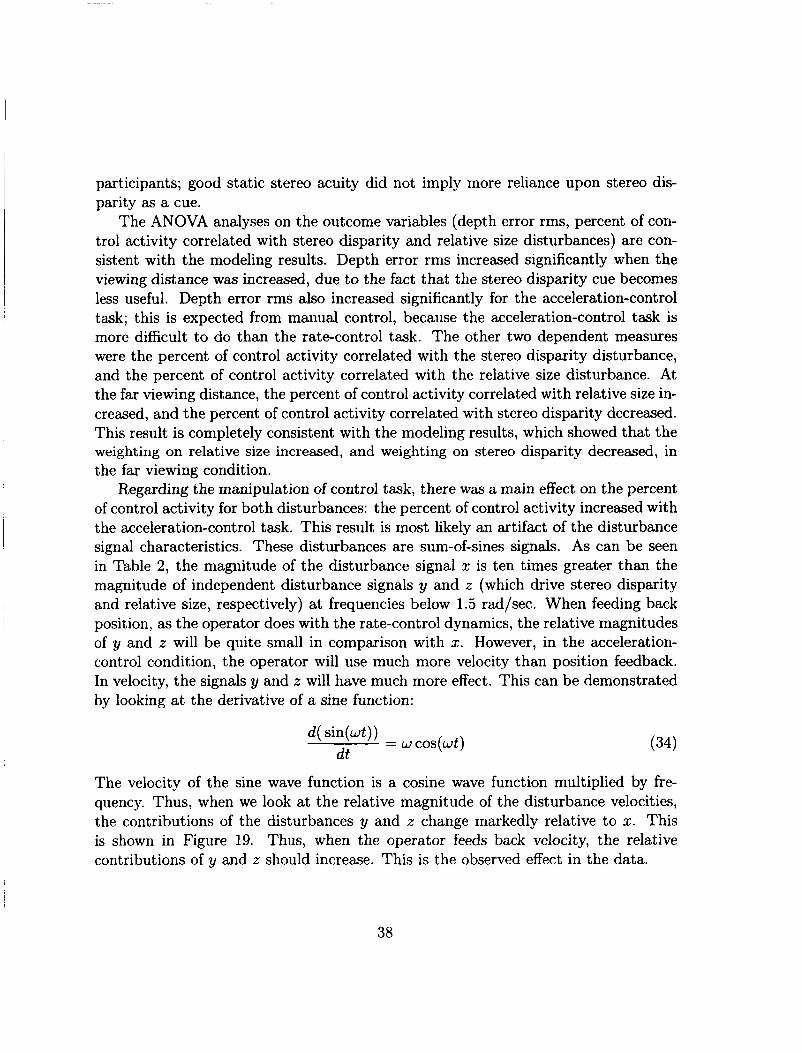
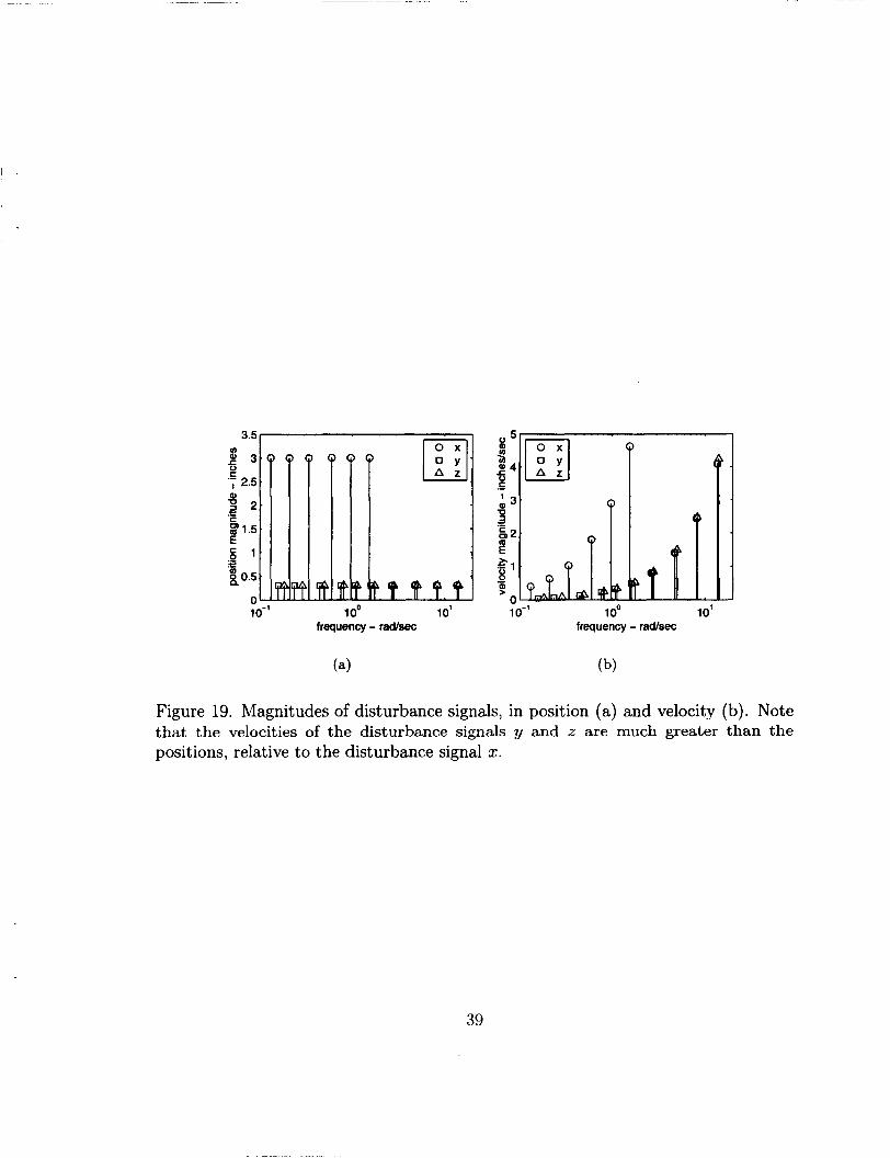
Regarding the manipulation of control task, there was a main effect on the percent of control activity for both disturbances: the percent of control activity increased with the acceleration-control task. This result is most likely an artifact of the disturbance signal characteristics. These disturbances are sum-of-sines signals. As can be seen in Table 2, the magnitude of the disturbance signal x is ten times greater than the magnitude of independent disturbance signals y and z (which drive stereo disparity and relative size, respectively) at frequencies below 1.5 rad/sec. When feeding back position, as the operator does with the rate-control dynamics, the relative magnitudes of y and z will be quite small in comparison with x. However, in the acceleration- control condition, the operator will use much more velocity than position feedback. In velocity, the signals y and z will have much more effect. This can be demonstrated by looking at the derivative of a sine function:
d( sin(&)) dt
= w cos(wt) (34)
The velocity of the sine wave function is a cosine wave function multiplied by fre- quency. Thus, when we look at the relative magnitude of the disturbance velocities, the contributions of the disturbances y and z change markedly relative to x. This is shown in Figure 19. Thus, when the operator feeds back velocity, the relative contributions of y and z should increase. This is the observed effect in the data.
38
frequency - rad/sec
" lo-' 1 0" 10'
frequency - rad/sec
Figure 19. Magnitudes of disturbance signals, in position (a) and velocity (b). Note that the velocities of the disturbance signals y and z are much greater than the positions, relative to the disturbance signal z.
39

5 Conclusions Our depth-cue integration and control model accurately characterizes the activity of the operator over a range of tasks. This model incorporates control and neuromuscu- lar dynamics from previous manual control work with perceptual models suggested by depth-cue integration paradigms. The modelling results suggest that the depth- cue integration strategy of the operator changes as a function of the saliency of the available cues, but does not change as a function of the control task dynamics. The modelling also suggests that the operator depends more on stereo disparity than rel- ative size for position perception, and more on relative size than stereo disparity for velocity perception. As predicted by manual control, the operator uses more velocity information with acceleration-control dynamics than with rate-control dynamics.
Because the operator uses more velocity feedback in acceleration-control tasks, and because velocity perception is more dependent upon relative size than stereo disparity, the results imply that stereo disparity could be a much less useful cue in acceleration-control tasks. Conversely, because accurate position information is necessary for rate-control tasks, and stereo disparity dominates position perception, stereo disparity is probably a highly useful cue for rate-control tasks.
Tests of static stereo acuity were not shown to be predictive of the operators reliance on stereo disparity as a cue.
40
A Experiment Appendix
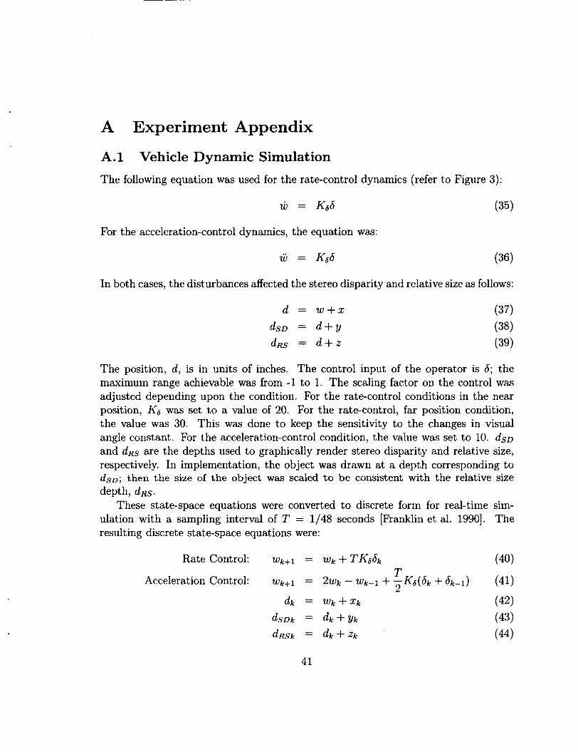
A.l Vehicle Dynamic Simulation The following equation was used for the rate-control dynamics (refer to Figure 3):
For the acceleration-control dynamics, the equation was:
In both cases, the disturbances affected the stereo disparity and relative size as follows:
The position, d , is in units of inches. The control input of the operator is 6; the maximum range achievable was from -1 to 1. The scaling factor on the control was adjusted depending upon the condition. For the rate-control conditions in the near position, Kb was set to a value of 20. For the rate-control, far position condition, the value was 30. This was done to keep the sensitivity to the changes in visual angle constant. For the acceleration-control condition, the value was set to 10. d s o and dRs are the depths used to graphically render stereo disparity and relative size, respectively. In implementation, the object was drawn at a depth corresponding to dsD; then the size of the object was scaled to be consistent with the relative size depth, dRs.
These state-space equations were converted to discrete form for real-time sim- ulation with a sampling interval of T = 1/48 seconds [Franklin et al. 19901. The resulting discrete state-space equations were:
41
i kxi a,, wxi kyi uyi wYi k,, a,, 1 5 3.0 0.13 6 0.3 0.16 7 0.3
wzi 0.18
2 3 4
I 1 1
8 3.0 0.21 9 0.3 0.24 11 0.3 0.29 13 3.0 0.34 17 0.3 0.45 19 0.3 0.50 23 3.0 0.60 29 0.3 0.76 31 0.3 0.81
I 9 11 311 I 0.3 I 8.14 11 313 1 0.3 I 8.19 11 317 1 0.3 I 8.30 1 II I I II I I I 1 I 1
5 6
, I I I I , 1
10 11 521 I 0.3 I 13.64 11 523 I 0.3 1 13.69 11 541 I 0.3 I 14.16
I
37 3.0 0.97 41 0.3 1.07 43 0.3 1.13 59 3.0 1.54 61 0.3 1.60 67 0.3 1.75
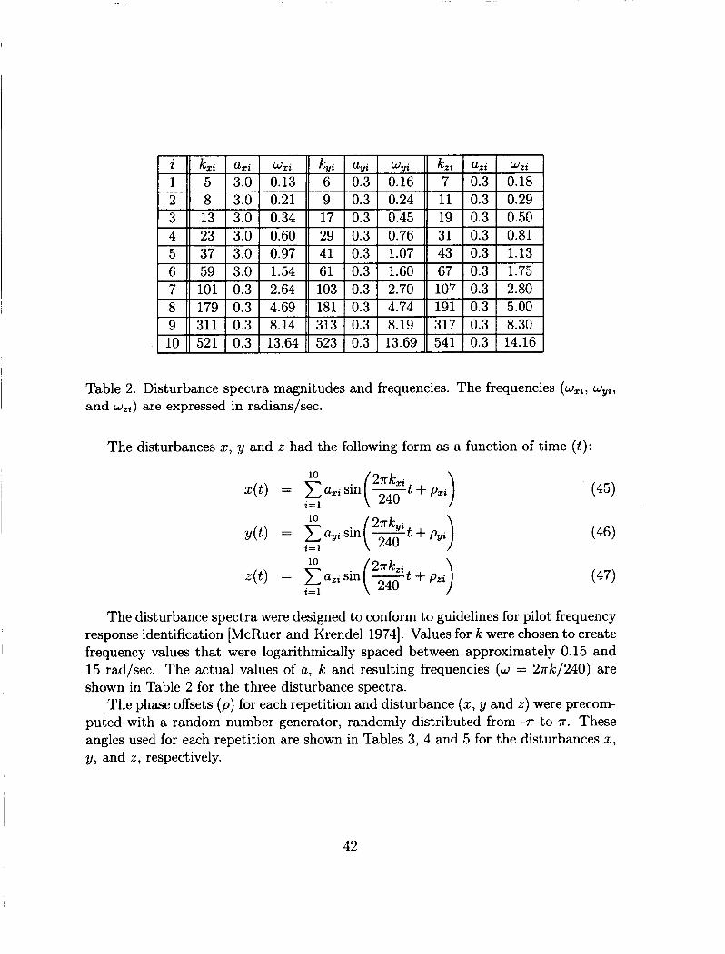
Table 2. Disturbance spectra magnitudes and frequencies. The frequencies (wxi , wyi,
and wZi) are expressed in radians/sec.
7 8
The disturbances z, y and z had the following form as a function of time ( t ) :
101 0.3 2.64 103 0.3 2.70 107 0.3 2.80 179 0.3 4.69 181 0.3 4.74 191 0.3 5.00
The disturbance spectra were designed to conform to guidelines for pilot frequency response identification [McRuer and Krendel 19741. Values for k were chosen to create frequency values that were logarithmically spaced between approximately 0.15 and 15 rad/sec. The actual values of a, k and resulting frequencies (w = 2~k/240) are shown in Table 2 for the three disturbance spectra.
‘lhe phase offsets ( p ) for each repetition and disturbance (z, y and z ) were precom- puted with a random number generator, randomly distributed from -7r to T . These angles used for each repetition are shown in Tables 3, 4 and 5 for the disturbances z, y, and z , respectively.
42
1 2
0.26 5.73 4.92 4.11 3.30 2.49 1.67 0.86 2.11 5.04 1.68 4.60 1.24 4.17 0.81 3.74
3 4
1.18 4.29 1.12 4.23 1.06 4.18 1.01 4.12 2.30 6.20 3.82 1.44 5.35 2.97 0.59 4.49
5 6
I I I I I I I I 9 11 5.86 I 1.86 14.15 10.16 I 2.44 14.73 10.74 13.02 I
. ~. ~ _ _
0.83 3.35 5.86 2.09 4.60 0.83 3.35 5.86 0.96 3.33 5.70 1.78 4.15 0.24 2.60 4.97
I I
10 11 3.73 [ 0.15 I 2.86 I 5.57 I 1.99 14.70 I 1.12 13.82
7 5.07 5.64 8 1.33 1.96
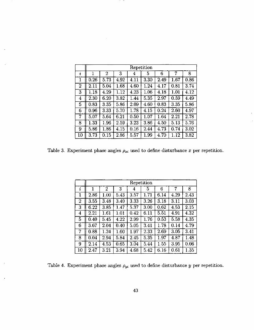
Table 3. Experiment phase angles pzi used to define disturbance 2 per repetition.
I
6.21 0.50 1.07 1.64 2.21 2.78 2.59 3.23 3.86 4.50 5.13 5.76
F I1 ReDetition I
I I I I 10 1) 2.47 I 3.21 13.94 [ 4.68 I 5.42 I 6.16 10.61 I 1.35
Table 4. Experiment phase angles pyi used to define disturbance y per repetition.
43
7- Repetition i 1
1 2 3 4- 5 6 7 8 5.25 3.60 1.96 0.32 4.95 3.31 1.67 0.02
2 3
0.01 1.37 2.73 4.08 5.44 0.51 1.87 3.23 4.72 3.94 3.16 2.39 1.61 0.84 0.06 5.57
4 5 6
3.60 4.98 0.08 1.46 2.84 4.22 5.60 0.70 5.97 3.19 0.40 3.90 1.11 4.61 1.82 5.32 1.36 5.39 3.13 0.87 4.90 2.64 0.39 4.41
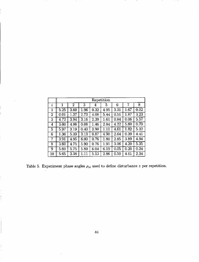
Table 5. Experiment phase angles pzi used to define disturbance z per repetition.
7 8
44
3.91 4.95 6.00 0.76 1.80 2.85 3.89 4.94 3.60 4.75 5.90 0.76 1.91 3.06 4.20 5.35
~
9 5.60 5.75 5.89 6.04 6.19 0.05 0.20 0.34 10 5.65 3.38 1.11 5.13 2.86 0.59 4.61 2.34
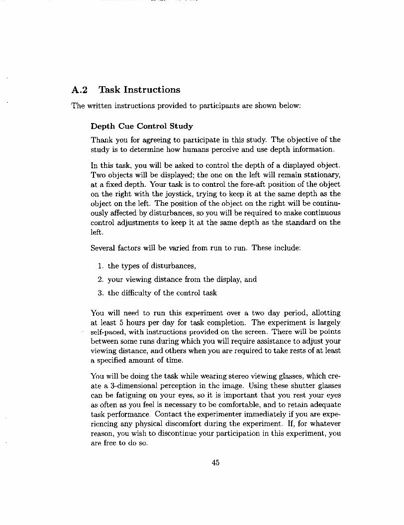
A.2 Task Instructions The written instructions provided to participants are shown below:
Depth Cue Control Study
Thank you for agreeing to participate in this study. The objective of the study is to determine how humans perceive and use depth information.
In this task, you will be asked to control the depth of a displayed object. Two objects will be displayed; the one on the left will remain stationary, at a fixed depth. Your task is to control the fore-aft position of the object on the right with the joystick, trying to keep it at the same depth as the object on the left. The position of the object on the right will be continu- ously affected by disturbances, so you will be required to make continuous control adjustments to keep it at the same depth as the standard on the left.
Several factors will be varied from run to run. These include:
1. the types of disturbances,
2. your viewing distance from the display, and
3. the difficulty of the control task
You will need to run this experiment over a two day period, allotting at least 5 hours per day for task completion. The experiment is largely self-paced, with instructions provided on the screen. There will be points between some runs during which you will require assistance to adjust your viewing distance, and others when you are required to take rests of at least a specified amount of time.
You will be doing the task while wearing stereo viewing glasses, which cre- ate a 3-dimensional perception in the image. Using these shutter glasses can be fatiguing on your eyes, so it is important that you rest your eyes as often as you feel is necessary to be comfortable, and to retain adequate task performance. Contact the experimenter immediately if you are expe- riencing any physical discomfort during the experiment. If, for whatever reason, you wish to discontinue your participation in this experiment, you are free to do so.
45
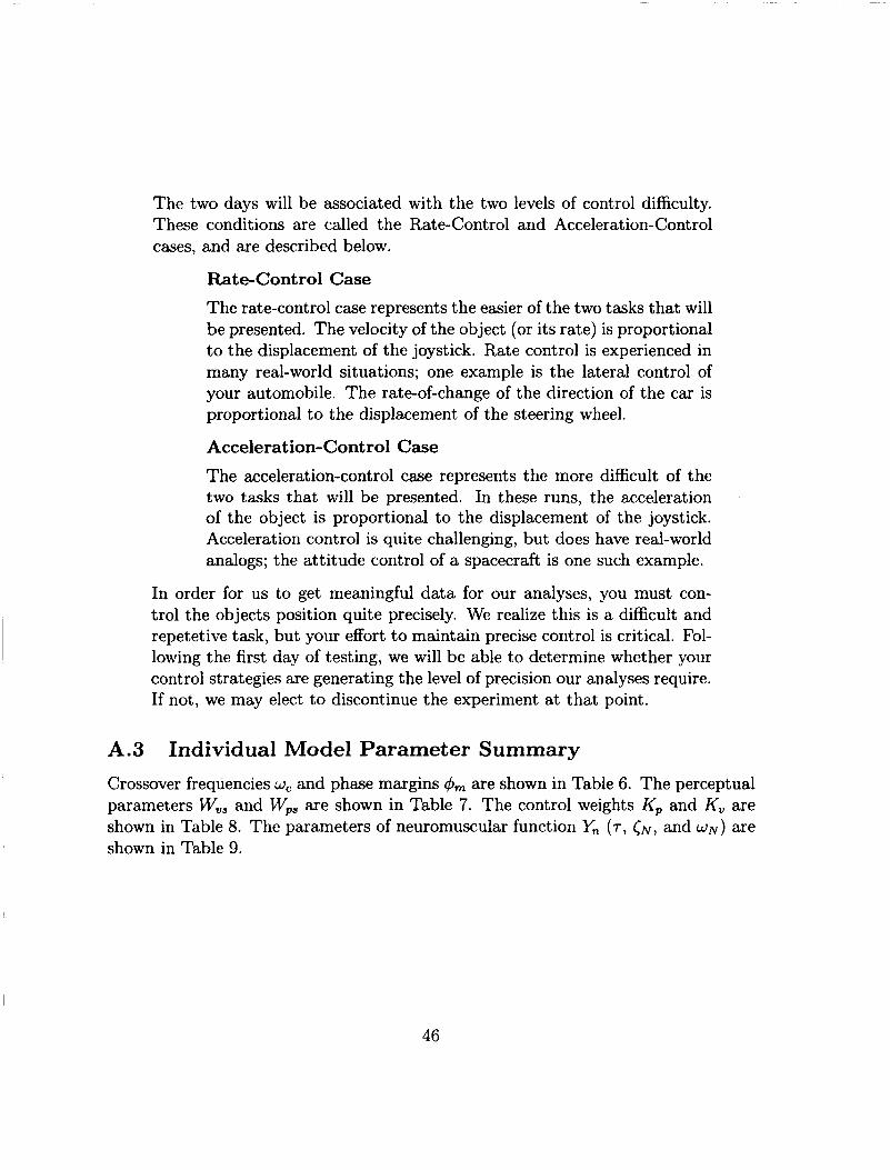
The two days will be associated with the two levels of control difficulty. These conditions are called the Rate-Control and Acceleration-Control cases, and are described below.
Rate-Control Case The rate-control case represents the easier of the two tasks that will be presented. The velocity of the object (or its rate) is proportional to the displacement of the joystick. Rate control is experienced in many real-world situations; one example is the lateral control of your automobile. The rate-of-change of the direction of the car is proportional to the displacement of the steering wheel.
Acceleration-Cont rol Case The acceleration-control case represents the more difficult of the two tasks that will be presented. In these runs, the acceleration of the object is proportional to the displacement of the joystick. Acceleration control is quite challenging, but does have real-world analogs; the attitude control of a spacecraft is one such example.
In order for us to get meaningful data for our analyses, you must con- trol the objects position quite precisely. We realize this is a difficult and repetetive task, but your effort to maintain precise control is critical. Fol- lowing the first day of testing, we will be able to determine whether your control strategies are generating the level of precision our analyses require. If not, we may elect to discontinue the experiment at that point,
A.3 Individual Model Parameter Summary Crossover frequencies w, and phase margins & are shown in Table 6. The perceptual parameters W,,, and W,, are shown in Table 7. The control weights K p and K,, are shown in Table 8. The parameters of neuromuscular function Y, (7, c ~ , and w N ) are shown in Table 9.
46
I 11 Rate, near 11 Rate, far 11 Accel, near I 1
, OP ~c 4m wc dm wc dm ,
I1 I II I I, I I 2 11 2.27 I 60.88 11 2.21 I 63.60 11 2.38 I 23.14 I 1 1.53 71.18 1.53 71.64 1.26 44.43
II I II I 11 I I 5 I] 0.68 I 103.97 11 1.01 I 91.12 11 0.85 I 57.99 1 3 4
0.90 97.95 0.86 98.35 1.08 49.18 0.68 86.20 0.49 91.20 1.24 37.58
I 1 I I 1 I II I I 8 11 1.94 I 75.55 11 1.90 I 79.67 I] 1.79 1 39.04 I 6 7
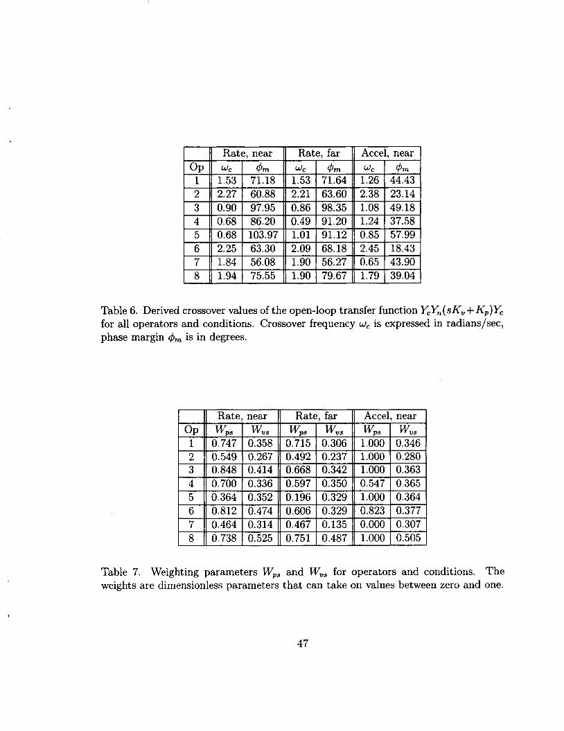
Table 6. Derived crossover values of the open-loop transfer function Y,Yn ( sK,, + K,)Yc for all operators and conditions. Crossover frequency w, is expressed in radians/sec, phase margin drn is in degrees.
2.25 63.30 2.09 68.18 2.45 18.43 1.84 56.08 1.90 56.27 0.65 43.90
6 7 8
Table 7. Weighting parameters W,, and W,,, for operators and conditions. The weights are dimensionless parameters that can take on values between zero and one.
0.812 0.474 0.606 0.329 0.823 0.377 0.464 0.314 0.467 0.135 0.000 0.307 0.738 0.525 0.751 0.487 1.000 0.505
47
I 11 Rate, near 11 Rate, far 11 Accel, near I
4 5 6
0.65 0.29 0.46 0.32 0.23 0.58 0.49 0.71 0.76 0.71 0.06 0.41 1.55 1.76 1.45 1.53 0.91 1.11
7 8
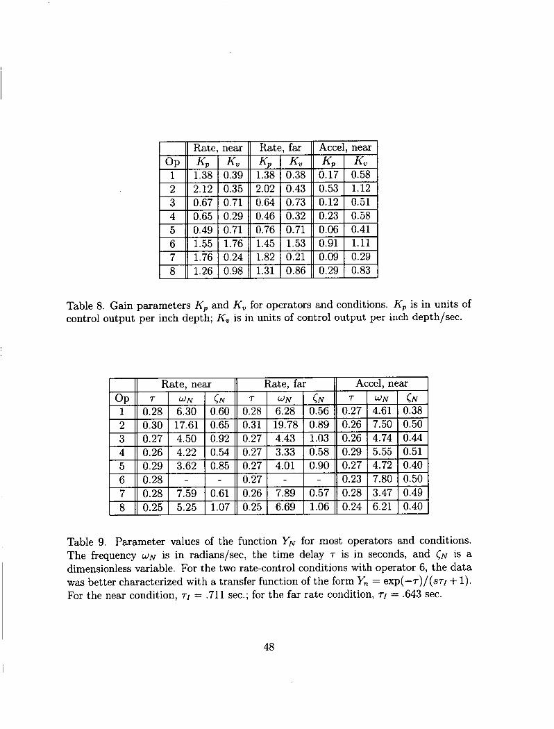
Table 8. Gain parameters K p and K, for operators and conditions. K p is in units of control output per inch depth; K, is in units of control output per inch depth/sec.
I I
1.76 0.24 1.82 0.21 0.09 0.29 1.26 0.98 1.31 0.86 0.29 0.83
Table 9. Parameter values of the function YN for most operators and conditions. The frequency W N is in radians/sec, the time delay T is in seconds, and ( N is a dimensionless variable. For the two rate-control conditions with operator 6, the data was better characterized with a transfer function of the form Y, = exp(-T)/(sq + 1). For the near condition, TI = .711 sec.; for the far rate condition, TI = .643 sec.
48
A.4 Individual Model Fit Plots The model fits are shown in the following figures (Figures 20 through 43). Error bars depict the calculated confidence intervals for each measurement (see Appendix Section B.3.1).
I
49

Operator 1 : rate control, far viewing, multiple disturbances
-1 -0.5 0 0.5 1 1.5 loglo frequency - radlsec
,, H,,measured H,, measured
modeled H,, modeled HRS modeled
I I I I I 1 1
-1 -0.5 0 0.5 1 1.5 loglo frequency - radlsec
-4 '
Figure 20. Experiment model fit results for Opcrator 1, Rate Control, Far Viewing Condition, Multiple Disturbances.
50
Operator 2: rate control, near viewing, multiple disturbances
*O r
. . . . . . . . . . . . . . .
.- -1
8 . . . . . . .
6 . . . . . . .
-0.5 0 0.5 log,o frequency - radsec
. . . . . . . . . . . . . . . . . . . . . . . . . . . . . . . . . . . . . . . . . . . .
. . . . . . . . . . . . . . . . . . . . . . . . . . . . . . . . . . . . . . . . . . . . . . . . . T .
. . . . . . . .
. . . . . . . .
1 1.5
. . . . . . . . . . . . .
-4 ' I
I I I
-1 -0.5 0 0.5 I log,, frequency - radsec
1.5
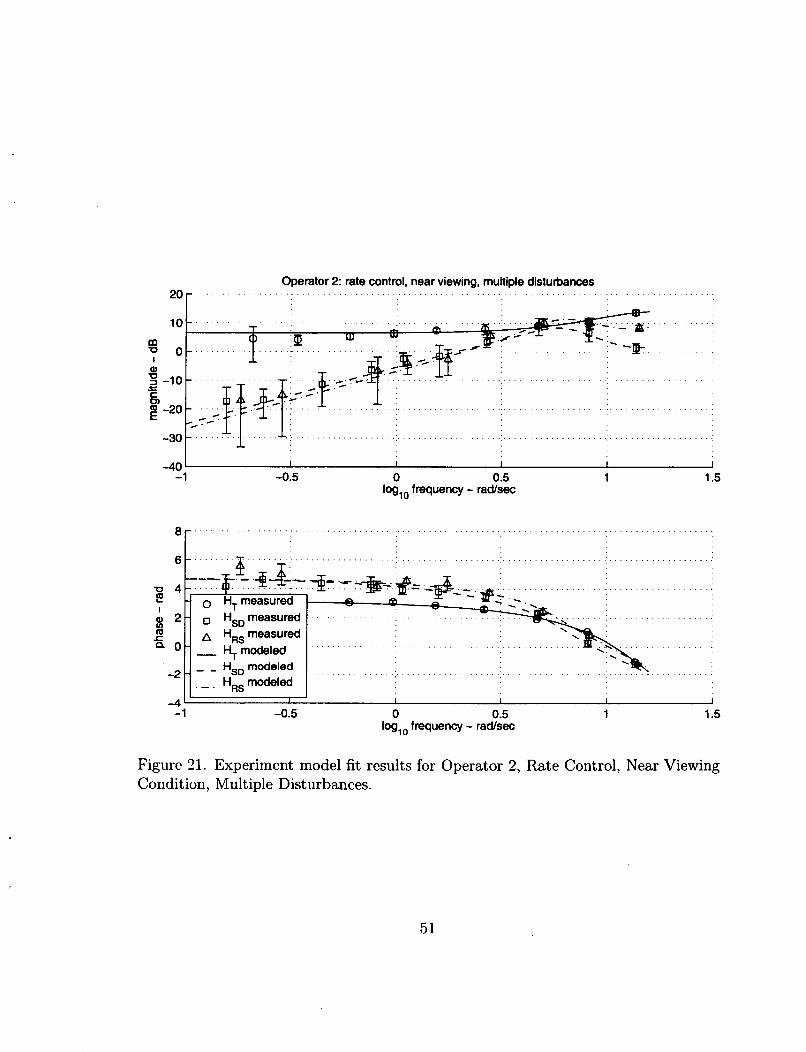
Figure 21. Experiment model fit results for Operator 2, Rate Control, Near Viewing Condition, Multiple Disturbances.
51
Operator 3: rate control, near viewing, multiple disturbances
-1 -0.5 0 0.5 1 1.5 log,, frequency - radsec
-1 -0.5 0 0.5 1 1.5 log,, frequency - radsec
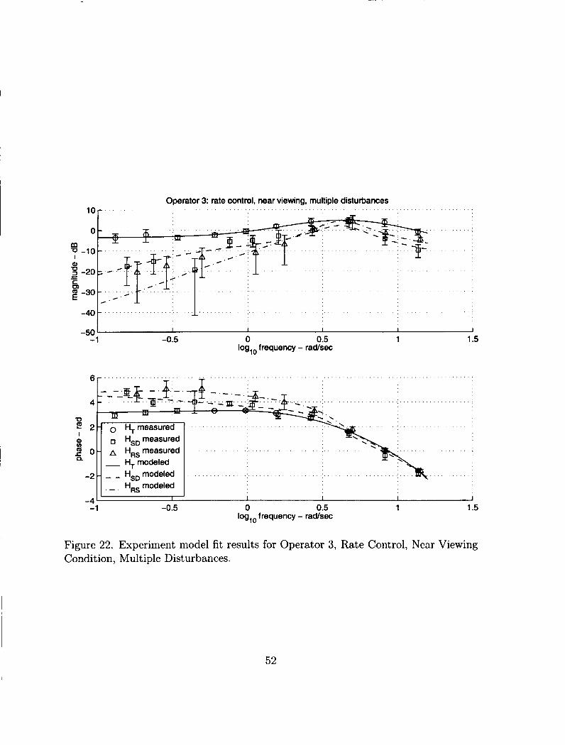
Figure 22. Experiment model fit results for Operator 3, Rate Control, Near Viewing Condition, Multiple Disturbances.
52
Operator 4: rate control, near viewing, multiple disturbances
lor . . . . . . . . i
-40 I I I I I
-1 -0.5 0 0.5 1 1.5
6
4
'0
I 2 2
% 2 0 n
-2
-4 -1
log,o frequency - radsec
-----= =
.
- - H,, modeled HRs modeled
-0.5 0 0.5 log,, frequency - radsec
\, I
1 1.5
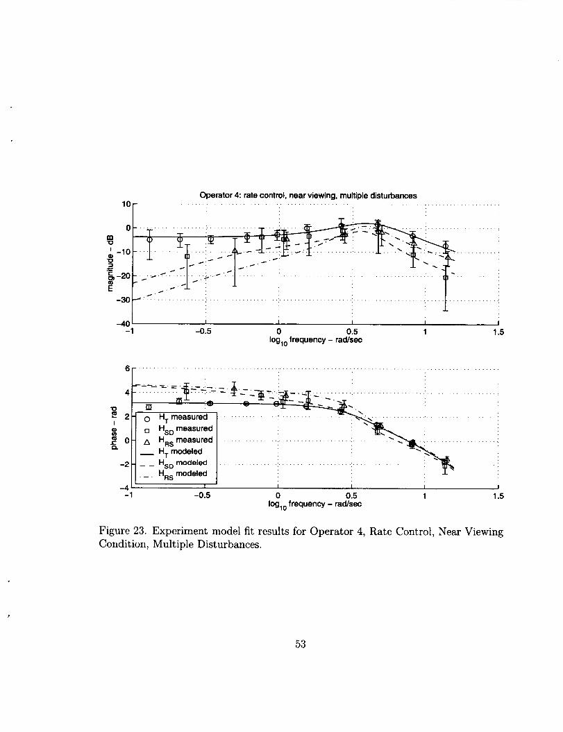
Figure 23. Experiment model fit results for Operator 4, Rate Control, Near Viewing Condition, Multiple Disturbances.
53
Operator 5: rate control, near viewing, multiple disturbances
l o r -
-40 I I 1 1 I
-1 -0.5 0 0.5 1 1.5 log,o frequency - radsec
. . . . . .
. . . . . . .
. . . . . . . . . .
-- -1 -0.5 0 0.5
log,, frequency - radsec 1 1.5
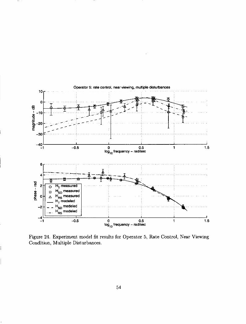
Figure 21. Experiment model fit results for Operator 5, Rate Control, Near Viewing Condition, Multiple Disturbances.
54
2o r
0 -
Operator 6: rate control, near viewing, multiple disturbances
- - H,, modeled - H,, modeled
I I I I 1
-1
e r . . . . . . . . . . , . .
-0.5
. . . . .
0 0.5 log,, frequency - racUsec
1 1.5
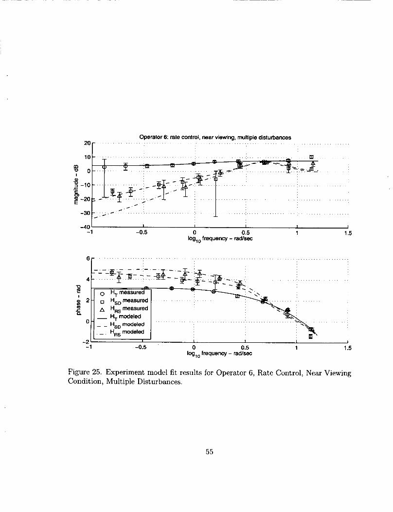
Figure 25. Experiment model fit results for Operator 6, Ratc Control, Near Viewing Condition, Multiple Disturbances.
55
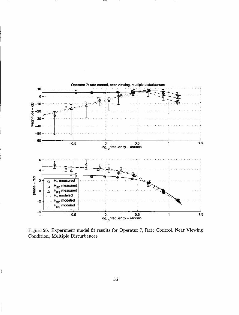
Operator 7: rate control, near viewing, multiple disturbances
Figurc 26. Experiment model fit results for Operator 7, Rate Control, Near Viewing Condition, Multiple Disturbances.
56

Operator 8: rate control, near viewing, multiple disturbances
-3o-..
. . . . . . . . . .
e.... . . . . . . . . . . . . . . . . . . . . . . . . . . . . . . . . . . . . . . . . . . . . . . . . . . . . . . . . . . . . . . . . . . . . . . . . . . . . . . . . . . . . . . . . : I
I I
.- -1 1 1.5 0 0.5
log, frequency - radsec
. - . . . . . . . .
-1 -0.5 0 0.5 1 1.5 log,, frequency - radsec
Figure 27. Experiment model fit results for Operator 8, Rate Control, Near Viewing Condition, Multiple Disturbances.
57
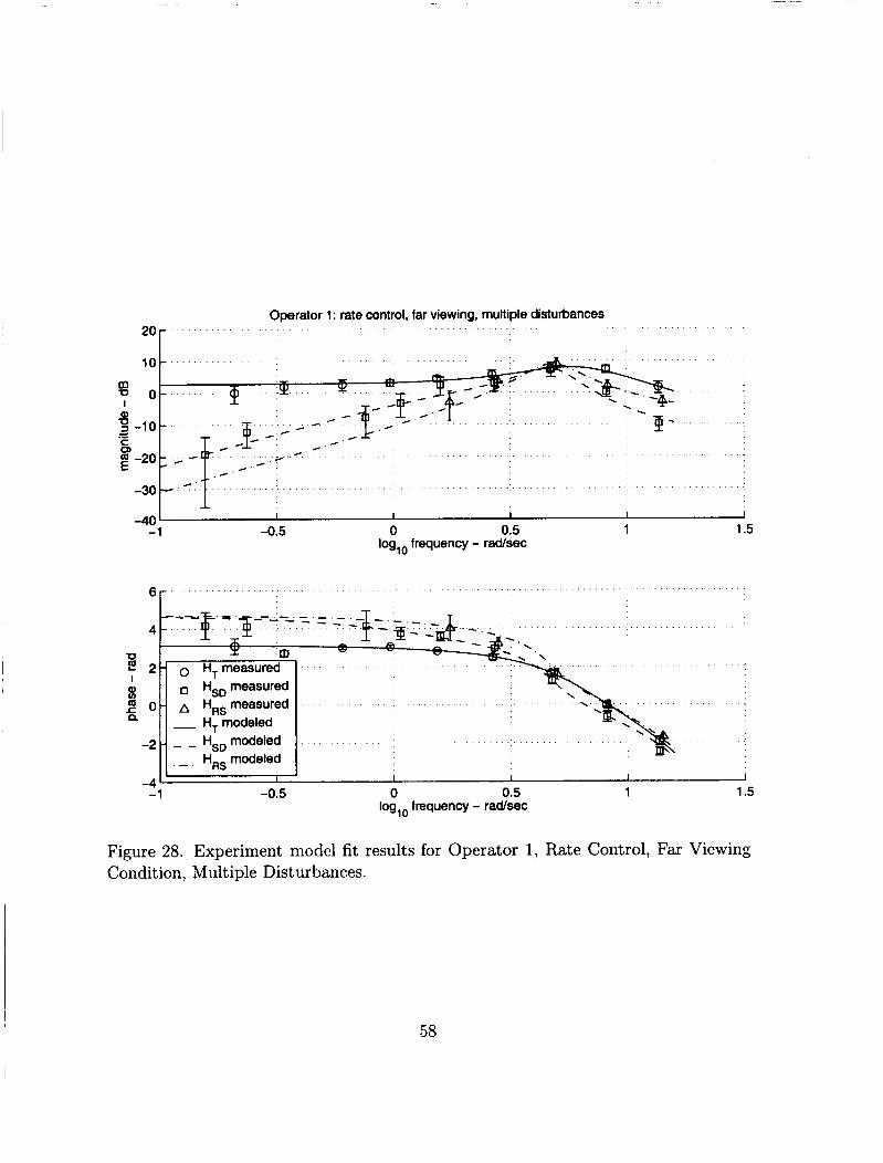
Operator 1 : rate control, far viewing, multiple disturbances
I I I I I -1 -0.5 0 0.5 1 1.5
log,o frequency - radsec
-40
6 r
-1 -0.5 0 0.5 1 I
1.5 log,, frequency - radsec
Figure 28. Experiment modcl fit results for Operator 1, Rate Control, Far Viewing Condition, Multiple Disturbances.
58
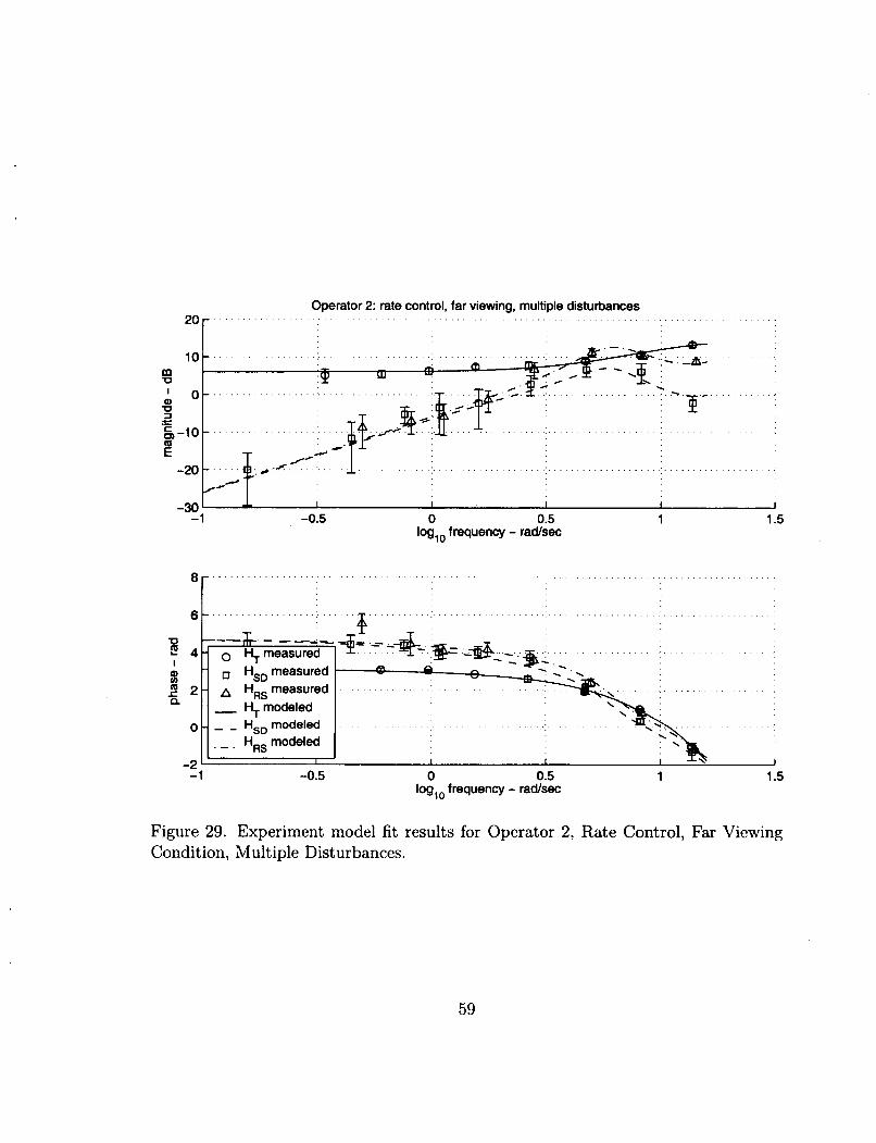
2o r Operator 2: rate control, far viewing, multiple disturbances
n
Cp.; .c.- . . . . . . . . . . . . . . . . . . . . . . . . . . . . . . . . . . . . . . . . . . . . . . . . . . . . . . . .. . . . . . . . . . . . . . . . . : C '
-30 ' I I I 1 1 1
-1 -0.5 0 0.5 1 1.5 log,, frequency - radsec
8 . . . . . . . . . . . . . . . . .: . . . . . . . . . . . . . . . . . . . . . . . . . . . . . . . . . . . . . . . . . . . . . . . . . . . . . . . . . . . . . . . . . . . . . . .
6 . . . . . . . . . . . . . . . _ . _ . . . . . . . . . . . . . . . . . . . . . . . . . . . . . . . . . . . . . . . . . . . . . . . . . . . . . . . . . . . . . . . . . . . . . . . . .
1 -0.5 0 0.5 log,, frequency - radsec
- -1
-1 1.5
Figure 29. Experiment model fit results for Operator 2, Rate Control, Far Viewing Condition, Multiple Disturbances.
59
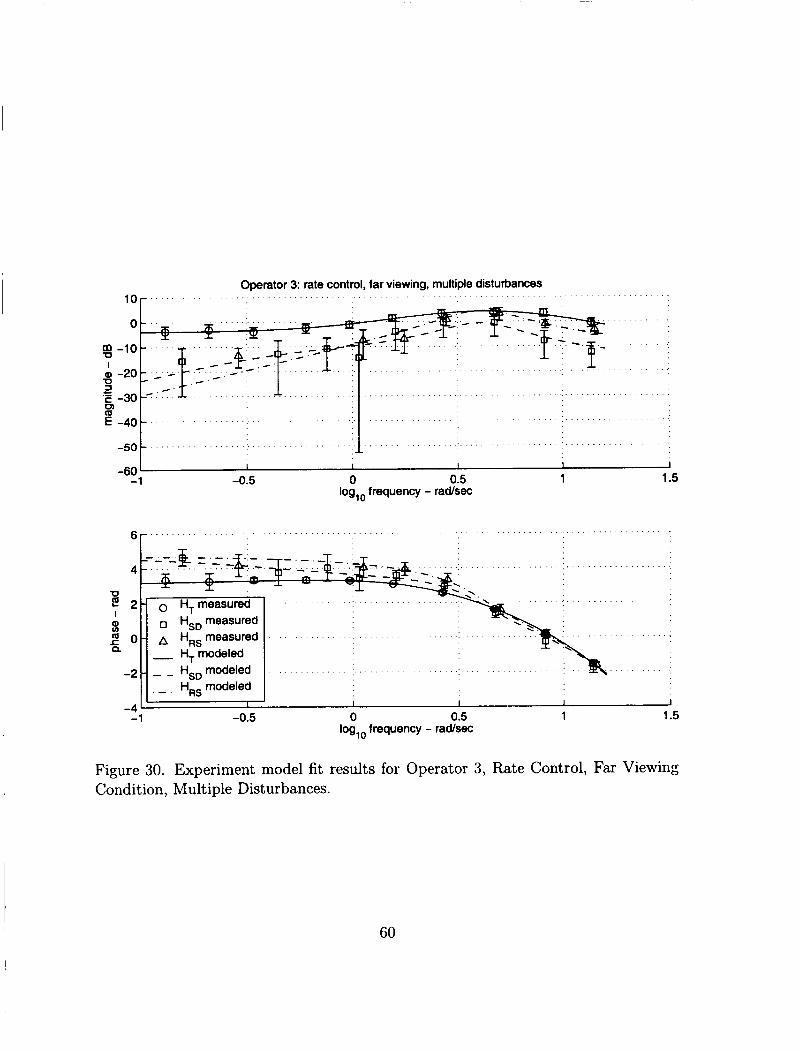
Operator 3: rate control, far viewing, multiple disturbances
-1 -0.5 log,o frequency - radsec
I I I I I 1 1
-1 -0.5 0 0.5 1 1.5 log,o frequency - radsec
-4 ' Figure 30. Experiment model fit results for Operator 3, Rate Control, Far Viewing Condition, Multiple Disturbances.
60

5r Operator 4: rate control, far viewing, multiple disturbances
I
. . . . . . . . . .
. . . . . . . . . .
-1 -0.5 0 0.5 1 1.5 log,, frequency - radsec
-1 -0.5 0 0.5 1 1.5 log,, frequency - radsec
Figure 31. Expcriment model fit results for Operator 4, Rate Control, Far Viewing Condition, Multiple Disturbances.
61
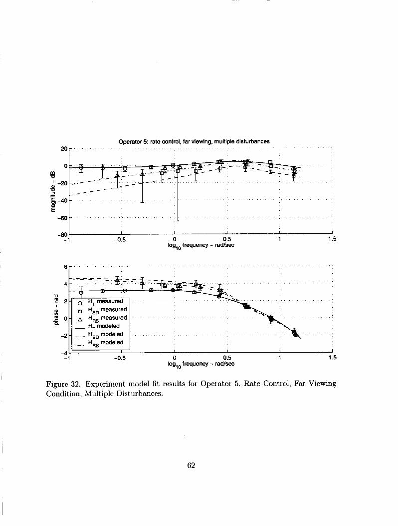
*O r Operator 5: rate control, far viewing, multiple disturbances
I I I I I
-1 -0.5 0 0.5 1 1.5 log,, frequency - radsec
-80
6r
- - - - _ - - - _
-1 -0.5 0 0.5 1 1.5 log,, frequency - radsec
Figure 32. Experiment model fit results for Operator 5, Rate Control, Far Vicwing Condition, Multiple Disturbances.
62

Operator 6: rate control, far viewing, multiple disturbances
-1
I
-0.5
. . . . .
0 0.5 log, frequency - radsec
I 7
H,. measured A H,, measured
1 1.5
, I I I I I I
-1 -0.5 0 0.5 1 1.5 log,o frequency - radsec
Figure 33. Experiment model fit results for Operator 6 , Rate Control, Far Viewing Condition, Multiple Disturbances.
63
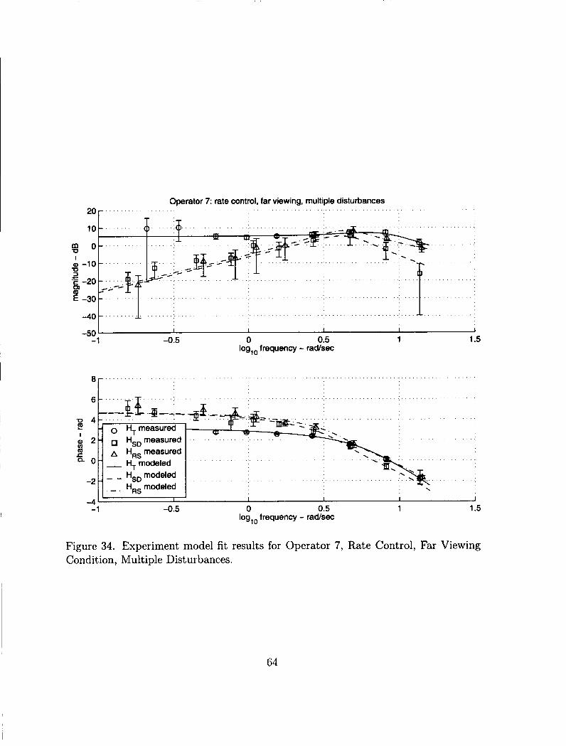
Operator 7: rate control, far viewing, multiple distuibances 20
10
8 0 I
-0 3
0) m
Q) -10
‘E -20
E -30
-40
-50
-
-0.5 0 0.5 1 1.5 log,o frequency - radsec
-1
“1 -- EL@--- - 0 4 2 - 0 H W
2 - HsDmeasured c m A H,, measured
0 - - H,modeled
I
H iD modeled -21- . - . - HRS modeled
. . . . . . . . .
.. . . . . . . . .
-9
-1 -0.5 0 0.5 logto frequency - radsec
1 1.5
Figure 34. Experiment model fit results for Operator 7, Rate Control, Far Viewing Condition, Multiple Disturbances.
64
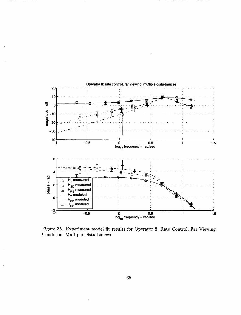
20 r Operator 8: rate control, far viewing, multiple disturbances
-1 -0.5 0 0.5 1 1.5
6
4 U
I 2
3 ' r n.
0
-2 -1
log, , frequency - rad/sec
. . . . . . . . . . . . . . . . . . . . . . . . . . . . . . . . . . . . . . . . . . . . . . . . . . . . . . . . . . . . . . . . . . . . . . _ . . .
. . . . . . . . . . . . . . . . . . . . . . . . . . . . .
-0.5 0 0.5 log,, frequency - radsec
1 1.5
Figure 35. Experiment model fit results for Operator 8, Rate Control, Far Viewing Condition, Multiple Disturbances.
65
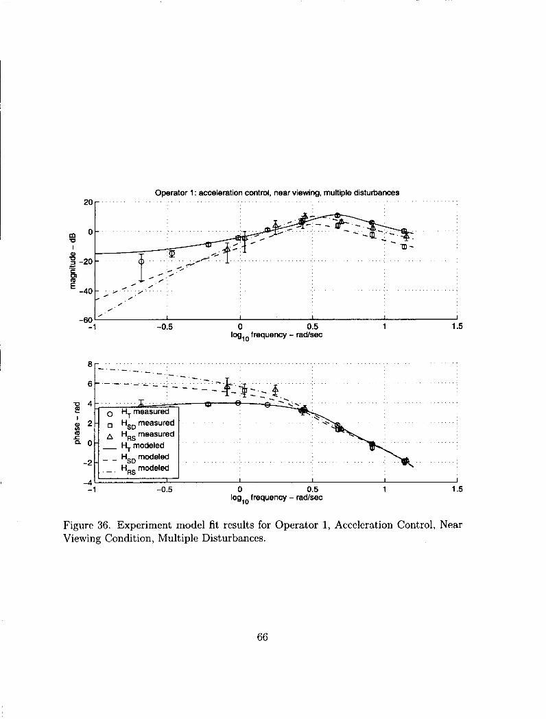
Operator 1 : acceleration control, near viewing, multiple disturt>ances 20 r
/ /
4 -60 I 1 I I I
-1 -0.5 0 0.5 1 1.5 log,, frequency - radsec
- - -
-1 -0.5 log,o 0 frequency - radlsec 1 1.5 0.5
Figure 36. Experiment model fit results for Operator 1, Acceleration Control, Near Viewing Condition, Multiple Disturbances.
66
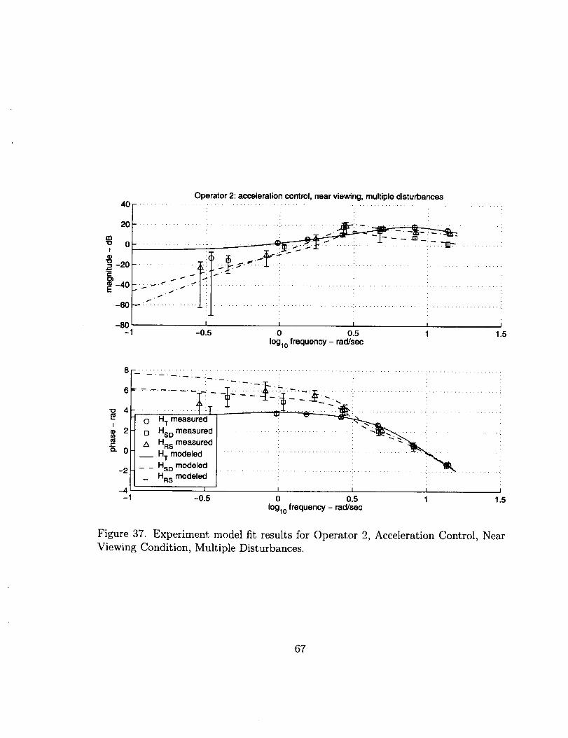
Operator 2: acceleration control, near viewing, multiple disturbances
40 r
_ _ -1 -0.5 0 0.5
log, , frequency - radsec 1 1.5
-1 -0.5 log,, 0 frequency - radsec 0.5 1 1.5
Figure 37. Experiment model fit results for Operator 2, Acceleration Control, Near Viewing Condition, Multiple Disturbances.
67
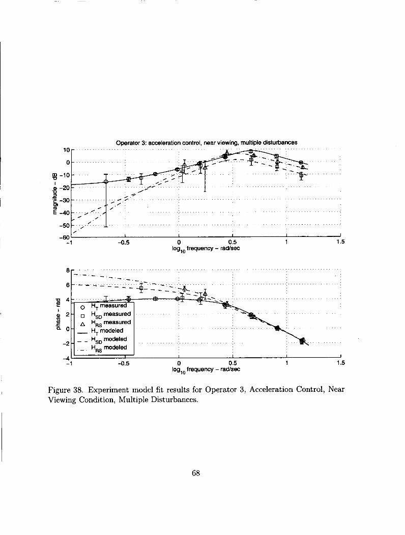
Operator 3: acceleration control, near viewing, multiple disturbances . . . .
I I I I I
-1 -0.5 0 0.5 1 1.5 log,, frequency - radsec
. . . . . . . . . . . . . . . . . . . . . . . . . . . . . . . . . . . _ . _ . _ . . . . . . . . . . . . . . . . . .
-1 -0.5 0 0.5 1 1.5 log,, frequency - radsec
Figure 38. Experiment model fit results for Operator 3, Acceleration Control, Near Viewing Condition, Multiple Disturbances.
68
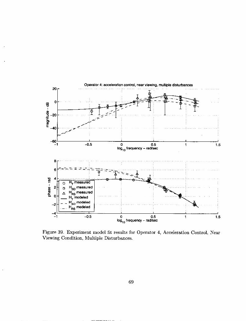
Operator 4: acceleration control, near viewing, multiple disturbances
0 %I
s -20
0
I Q, - .- C
E -40
I 1 I I I
-1 -0.5 0 0.5 1 1.5 log, , frequency - radsec
8 . . . . . . . r
-7
-1 -0.5 0 0.5 log,, frequency - rad/sec
1 1.5
Figure 39. Experiment model fit results for Operator 4, Acceleration Control, Ncar Viewing Condition, Multiple Disturbances.
69
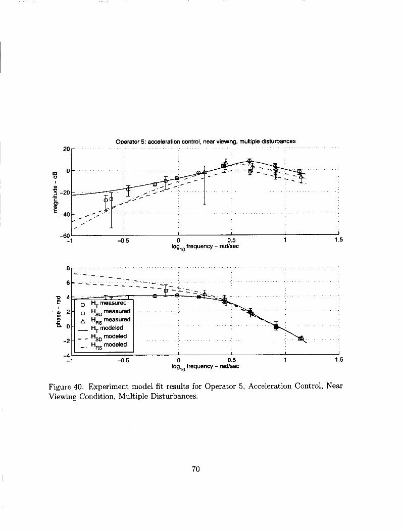
Operator 5: acceleration control, near viewing, multiple disturbances
I I 1 I I -1 -0.5 0 0.5 1 1.5
log,, frequency - radsec
-60'
8 r
- - - - _
-1 -0.5 0 0.5 1 1.5 log, frequency - radsec
Figure 40. Experiment model fit results for Operator 5, Acceleration Control, Near Viewing Condition, Multiple Disturbances.
70

%I I
40 r Operator 6: acceleration control, near viewing, multiple disturbances
20 I- A - -
- - I W
c L
. . . . . . . . . . . . . . . . . . . . . . . . . . . . . . . . . . . . I . . . . . . . . . . . . . . . . . . . . . . . . . . . . . . . . . . . . ; . . . . . . . . . . . . . . . . . . . :
-80 I I I I I
-1 -0.5 0 0.5 1 1.5 log,, frequency - radsec
. . . . . . . . . . . . . . . . . . . . . . . . . . . . . . . . . . . . . . . . . . . . . . . . . . . . . . . . . . . . . . . . . . . . . . . . . . . . . . . . 8r ""
-1 -0.5 0 0.5 1 1.5 log,, frequency - radsec
Figure 41. Experiment model fit results for Operator 6, Acceleration Control, Near Viewing Condition, Multiple Disturbances.
71
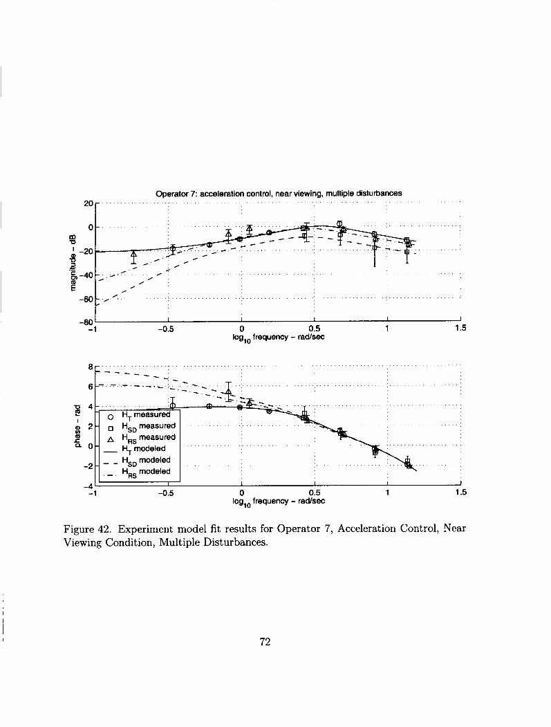
Operator 7: acceleration control, near viewing, multiple disturbances 20 r
-0
I
m c CL
E
t
I 1 1 I I -1 -0.5 0 0.5 1 1.5
-80
log,, frequency - radsec
,, H,, measured A H,, measured
-4' I I I I I I
-1 -0.5 0 0.5 1 1.5 log,,, frequency - radsec
Figure 42. Experiment model fit results for Operator 7, Acceleration Control, Ncar Viewing Condition, Multiple Disturbances.
72

Operator 8: acceleration control, near viewing, multiple disturbances
’ . . . . . . . . . . . . . . . . . . . . . . . . . . . . . . . . . . . . . . . . . . . . . . . . . . . . .
-80 1 1 I I I
-1 -0.5 0 0.5 1 1.5 log,o frequency - rad/sec
8 r
- - - _ - - - _
-1 -0.5 0 0.5 1 1.5 log,, frequency - rad/sec
Figure 43. Experiment model fit results for Operator 8, Acceleration Control, Near Viewing Condition, Multiple Disturbances.
73
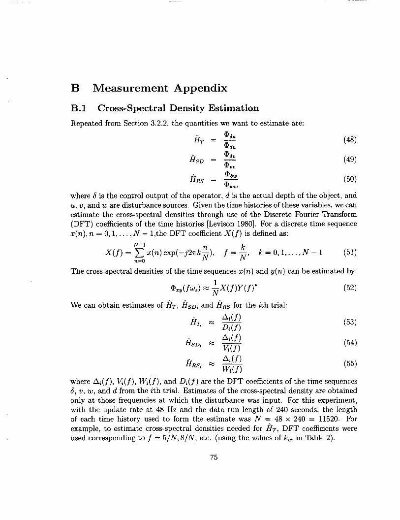
B Measurement Appendix
B.l Cross-Spectral Density Estimation Repeated from Section 3.2.2, the quantities we want to estimate are:
where 6 is the control output of the operator, d is the actual depth of the object, and u, v, and w are disturbance sources. Given the time histories of these variables, we can estimate the cross-spectral densities through use of the Discrete Fourier Transform (DFT) coefficients of the time histories [Levison 19801. For a discrete time sequence s(n), n = 0,1, . . . , N - 1,the DFT coefficient X ( f) is defined as:
k = 0 , 1 , ... , N - 1 (51) n k
X(f) = z(n) exp(-j27rk-), f = - n=O N "
N-1
The cross-spectral densities of the time sequences z(n) and y(n) can be estimated by: 1
@.zy(f%) = --xu N )Y(f I* (52)
We can obtain estimates of HT, Hso, and HRS for the ith trial:
where Ai( f), K( f ) , Wi( f), and Di(f) are the DFT coefficients of'the time sequences 6, v, w, and d from the ith trial. Estimates of the cross-spectral density are obtained only at those frequencies at which the disturbance was input. For this experiment, with the update rate at 48 Hz and the data run length of 240 seconds, the length of each time history used to form the estimate was N = 48 x 240 = 11520. For example, to estimate cross-spectral densities needed for H T , DFT coefficients were used corresponding to f = 5/N, 8/N, etc. (using the values of kui in Table 2).
75
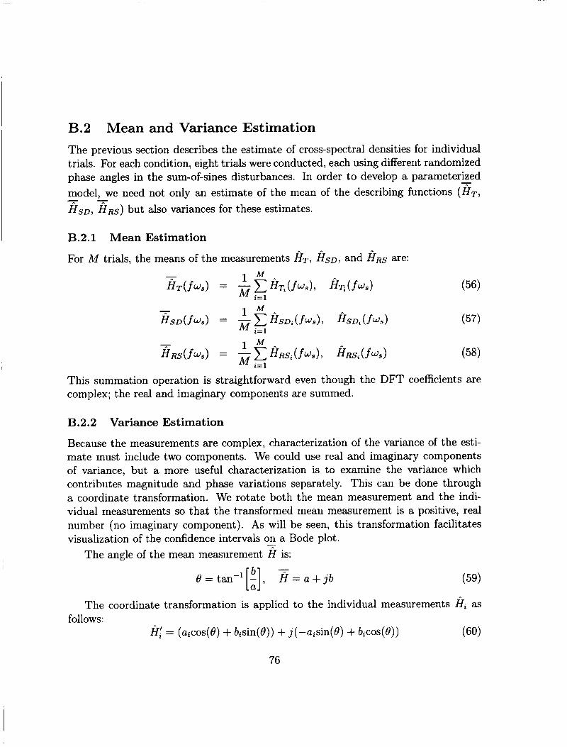
B.2 Mean and Variance Estimation The previous section describes the estimate of cross-spectral densities for individual trials. For each condition, eight trials were conducted, each using different randomized phase angles in the sum-of-sines disturbances. In order to develop a parameterized - model, we need not only an estimate of the mean of the describing functions ( h ~ , H s ~ , ~ R s ) but also variances for these estimates. - -
B.2.1 Mean Estimation
For M trials, the means of the measurements HT, HSD, and HRS are:
l M - f i T ( f u s ) = jj fiT; (fus), fiT; ( J u s )
2 = 1
This summation operation is straightforward even though the DFT coefficients are complex; the real and imaginary components are summed.
B 2.2 Variance Estimation
Because the measurements are complex, characterization of the variance of the esti- mate must include two components. We could use real and imaginary components of variance, but a more useful characterization is to examine the variance which contributes magnitude and phase variations separately. This can be done through a coordinate transformation. We rotate both the mean measurement and the indi- vidual measurements so that the transformed mean measurement is a positive, real number (no imaginary component). As will be seen, this transformation facilitates visualization of the confidence intervals on -. a Bode plot.
The angle of the mean measurement H is:
The coordinate transformation is applied to the individual measurements H, as follows:
H: = (aicos(6) + bisin(0)> + j(-aisin(O) + bicos(8)) (60)
76
where Hi = ai + j b i . It can be easily shown that the transformed mean measurement is: -
H = (61)
We now define the two components of the variance, the variance of the real com- ponent O R , and the variance of the imaginary, component, OR, as:
Standard error is the expected variance of the estimate of the mean, not the trial-to- trial variance, and is defined as:
OR SER = - M - 1
OI SEI = - M - 1
These variances will later prove particularly useful for visualization of error on Bode plots, because the real and imaginary components of these transformed measurements map directly to magnitude and phase. In addition to aiding in the visualization of variance, the transformed variables also can help the experimenter determine possible sources of variance. Highly non-symmetric variances between magnitude and phase components could be an indication of nonstationarity in the models. For example, high phase variance and low magnitude variance could be indicative of variations in time delay of the model. Similarly, high magnitude variances with low phase variances could indicate gain variations.
B.3 Measurement Inclusion Decisions At this point, the variances will be used to determine whether a particular measure- ment should be included in developing model parameters. In some cases, measure- ments have so much noise that their inclusion in model fitting will have a harmful effect on the fidelity of the model. The method used to make these decisions is described in this section.
Having determined estimates of the variances of the measurements, we can develop confidence intervals for the measurements. A 95% confidence interval (a box) around
77
the measurement H’ is defined as:
where t is derived from the student’s t distribution for, in this case, M - 1 degrees of freedom, for t.975. These tables are readily available in statistics textbooks and other math references; [Speigel, M. R., 19961 is one example. Having derived a “box” around the complex measurement, in which we have a 95% confidence that the true value lies within, we can use this information both to determine whether the point is worth including in our model fit, and to help visualize the variance in plots of magnitude and phase.
B.3.1 To Use or Not To Use
For this experiment, the choice to use or not use a particular measurement was based upon this rule: Measurements for which the confidence interval box encloses the origin are not used for model parameter identification.
While other standards could be considered and adhered to, this particular rule makes good practical sense. When the confidence interval box encloses the origin, the phase of the measurement is completely indeterminate; it could be in any quadrant. The magnitude estimate associated with such a measurement is likewise suspect in this case; with the individual measurements pointing in all directions, the magnitude of the sum of the measurements (which occurs in complex vector space) is likely to be highly compromised by the noise. Examples of how to use these techniques to accept or reject measurements, and how to visualize variance on a Bode plot, are shown below.
Example 1: Measurements to be Accepted and Rejected for Parameter Identification For Operator 1, rate-control, far viewing condition, we will examine in more detail how judgements are made on acceptance and rejection of measurements for parameter identification. We will look at two measurements, the measurememt of H s D at 0.45 and 0.76 rad/sec.
78
At 0.76 rad/sec, the individual measurements are:
-0.42255 - 0.19905j -0.032014 - 0.708273’ -0.89315 - 0.33202j -0.73509 + 0.28657j
-0.0075527 + 0.0088635j -0.015362 - 0.71277j
0.16727 - 0.465893’ 0.15769 - 0.63029j -
The mean of this measurement vector is HSD = -0.22259-0.34411i. As described in Section B.2.2, the measurement can be transformed through a rotation angle deter- mined by the mean measurement. After . transformation, this measurement vector becomes:
0.3966 - 0.24673’ 0.6121 + 0.35784 0.7639 - 0.5696j 0.1586 - 0.7729~’
-0.0033 - 0.0112j &,(w = 0.76) =
0.6068 + 0.3742j 0.3003 + 0.3935j I 0.4436 + 0.4747j
The means and variances of these transformed variables are: - HLD = 0.4098
012 = 0.233
2 UR = 0.064596
Confidence intervals can be determined; for 8 measurements, the value of t is 2.36. From Equations 64, 65 and 66 we obtain the confidence intervals in the real and imaginary directions:
CI,t = (0.4098 f 0.212) + j (f0.403) (70)
These confidence intervals, the individual and mean measurements are depicted in Figure 44(a). As can be seen, the confidence interval box does not enclose the origin, therefore we would use this measurement to include in parameter identification.
79
For 0.45 rad/sec, the measurement is:
-0.26292 - 0.19889j 0.20991 - 0.413473’
-0.03099 + 0.25055j 0.18869 + 0.18437j
-0.19518 - 0.474273’ -0.067595 - 0.20504j -0.34576 - 0.22767j -0.079821 + 0.29208j
The mean measurement is HSD = -0.072959-0.099043j. The transformed measure- ment vector is:
H & D ( u = 0.45) =
’ 0.3161 - 0.0937j 0.2084 + 0.4142j
-0.1833 - 0.1735j -0.2604 + 0.0426j 0.4976 + 0.1241j 0.2052 + 0.06723’ 0.3884 - 0.1434j
-0.1878 - 0.2375j The mean and variation of this measurement is:
H k D = 0.1230 C T ~ = 0.085643 a; = 0.044169
The resulting confidence intervals are:
C l ~ t = (0.1230 f 0.244) + j ( f0 .175)
(73)
(74)
The confidence intervals, individual measurements, and mean are depicted in Fig- ure 44(b). As can be seen, the corifidence interval box fully encloses the origin; this point was not used in parameter identification.
Example 2: Bode Plots with Confidence Interval Bars As was mentioned earlier, the characterizations of the real and imaginary confidence intervals are easily incorporated into visualizations of these intervals on Bode plots. Figure 44(b) is re- peated in Figure 45 to better visualize the relationship to the Bode plot. Because the
80
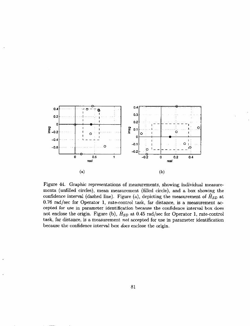
0.4
0.2
0 en m .E -0.2
-0.4
-0.6
- 0 0.5 1
real
- - a . -e -
I 1 I
\ I ' - I
I
I
I . I
I
I ' I
I 0 1
L - - A - 0
n -
0.4
0.3
0.2
B 0.1 E .-
0
-0.1
-0.2
A
I Y 4
I I
-0.2 0 0.2 0.4 real
Figure 44. Graphic representations of measurements, showing individual measure- ments (unfilled circles), mean measurement (filled circle), and a box showing the confidence interval (dashed line). Figure (a), depicting the measurement of H s D at 0.76 rad/sec for Operator 1, rate-control task, far distance, is a measurement ac- cepted for use in parameter identification because the confidence interval box does not enclose the origin. Figure (b), H ~ D at 0.45 rad/sec for Operator 1, rate-control task, far distance, is a measurement not accepted for use in parameter identification because the confidence interval box does enclose the origin.
81
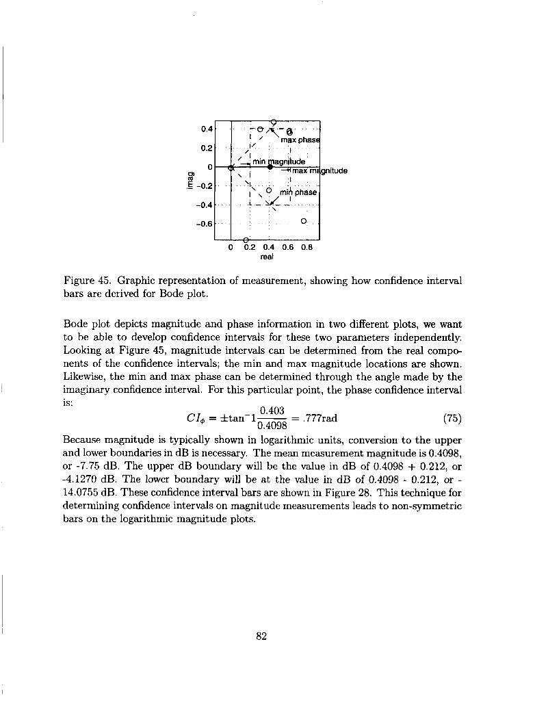
0.4
0.2
0 ' CI) co .E -0.2
-0.4
-0.6
Figure 45. Graphic representation of measurement, showing how confidence interval bars are derived for Bode plot.
Y ' . -e/\- 8 ' / maxphass
I/ I / '
'4 min plagnitude w
\ I 4 max' mz gnitude ;; .
I \I\ \ 0 mi)l phase' '
L - J - - I \
*
0 .
Bode plot depicts magnitude and phase information in two different plots, we want to be able to develop confidence intervals for these two parameters independently. Looking at Figure 45, magnitude intervals can be determined from the real compw nents of the confidence intervals; the min and max magnitude locations are shown. Likewise, the min and max phase can be determined through the angle made by the imaginary confidence interval. For this particular point, the phase confidence interval is:
0.403 0.4098
CI, = ftan-1- = .777rad (75)
Because magnitude is typically shown in logarithmic units, conversion to the upper and lower boundaries in dB is necessary. The mean measurement magnitude is 0.4098, or -7.75 dB. The upper dB boundary will be the value in dB of 0.4098 + 0.212, or -4.1270 dB. The lower boundary will be at the value in dB of 0.4098 - 0.212, or - 14.0755 dB. These confidence interval bars are shown in Figure 28. This technique for determining confidence intervals on magnitude measurements leads to non-symmetric bars on the logarithmic magnitude plots.
82
C Model Parameter Fit Appendix The method for obtaining parameters of the models is described in this section. We want to develop a model that is a function of frequency to fit the measurements. For a set of L measurements, and a model H that is a function of frequency and the parameters that describe it, the maximum likelihood model is achieved by choosing the model parameters to minimize:
- - For the current problem, we have three sets of measurements (k~, H s ~ , and
~ R s ) , and a total of seven parameters (W,,, Wps, K,, Kp, r , uN, and (N) which together specify the corresponding models ( H T , Hso, and HRS; see Equations 25- 27). Numerical optimization techniques are generally used for this type of problem, but the performance of numerical met hods are highly dependent upon choosing initial values of the parameters which are relatively close to the actual values. This situation required a multi-phase procedure to derive the parameters. The first phase was a rough estimate of the parameters affecting HT, through a least-squares technique. The second phase was a rough estimate of the parameters affecting HSO and HRS. The third phase was a numerical search to simultaneously derive parameters to best fit the measurements.
-
C.l
A modified time-domain least-squares parameter identification technique was first used to identify the parameters affecting the model HT. This section contains a description of a this parameter identification technique, then a detailed description of how it was applied to derive parameters associated with HT.
Phase 1: HT model parameter identification :!7 ;
C. l . l Least-squares fitting of transfer function parameters
The basic technique used here is to 1) transform the frequency-domain measurements into a time-domain representation, 2) use the time-domain representation to identify parameters of a discrete transfer function, and 3) transform the discrete transfer function back to a continuous transfer function.
83
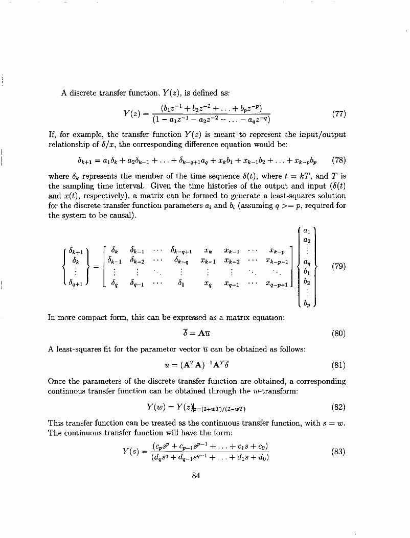
A discrete transfer function, Y ( z ) , is defined as:
(biz-' + + . . . + bpz-P) Y (2 ) = (1 - a l z - 1 - a 2 2 - 2 - . . . - a , z - q )
(77)
If, for example, the transfer function Y ( z ) is meant to represent the input/output relationship of S/z, the corresponding difference equation would be:
b k + l = a l b k + a 2 6 k - l + . . . + b k - q + l a q + X k b l + X k - l b 2 + . . . + X k - p b p (78)
where b k represents the member of the time sequence b( t ) , where t = kT, and T is the sampling time interval. Given the time histories of the output and input ( b ( t ) and z( t ) , respectively), a matrix can be formed to generate a least-squares solution for the discrete transfer function parameters ai and bi (assuming q >= p , required for the system to be causal).
In more compact form, this can be expressed as a matrix equation: - 6 = A E
A least-squares fit for the parameter vector E can be obtained as follows:
E = ( A ~ A ) - ~ A ~ ~
Once the parameters of the discrete transfer function are obtained, a corresponding continuous transfer function can be obtained through the w-transform:
Y ( W ) = Y ( z ) L = ( 2 + W T ) / @ - W T ) (82)
This transfer function can be treated as the continuous transfer function, with s = w. The continuous transfer function will have the form:
(83) (CPSP + c p - 1 s p - 1 + . . . + C I S + cfj) (d,sq + + . . . + dls + do)
Y ( s ) =
84
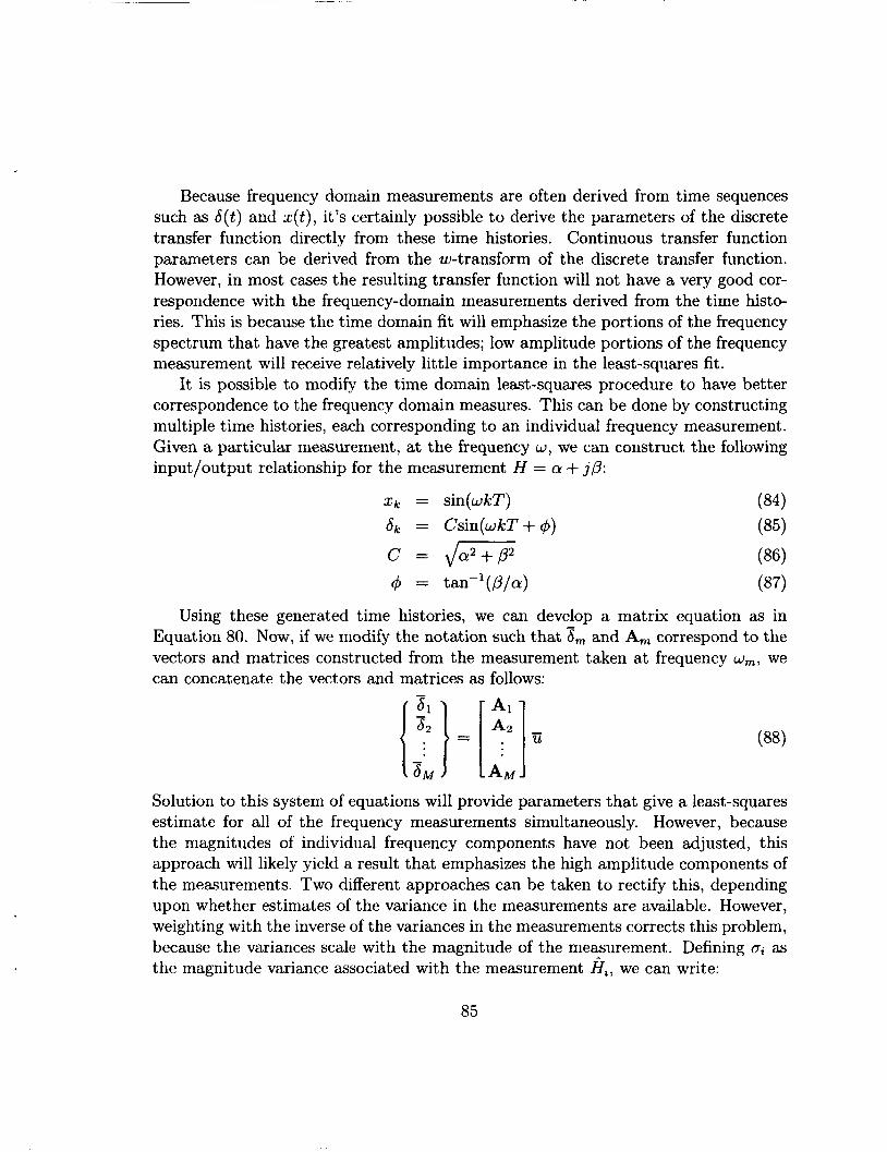
Because frequency domain measurements are often derived from time sequences such as b ( t ) and ~ ( t ) , it's certainly possible to derive the parameters of the discrete transfer function directly from these time histories. Continuous transfer function parameters can be derived from the w-transform of the discrete transfer function. However, in most cases the resulting transfer function will not have a very good cor- respondence with the frequency-domain measurements derived from the time hist+ ries. This is because the time domain fit will emphasize the portions of the frequency spectrum that have the greatest amplitudes; low amplitude portions of the frequency measurement will receive relatively little importance in the least-squares fit.
It is possible to modify the time domain least-squares procedure to have better correspondence to the frequency domain measures. This can be done by constructing multiple time histories, each corresponding to an individual frequency measurement. Given a particular measurement, at the frequency w, we can construct the following input/output relationship for the measurement H = a + j p :
xk = sin(wkT) 6 k = Csin(wkT+q$)
c = da2+p
4 = tan-l(p/a) (87)
Using these generated time histories, we can develop a matrix equation as in Equation 80. Now, if we modify the notation such that 8, and A, correspond to the vectors and matrices constructed from the measurement taken at frequency w,, we can concatenate the vectors and matrices as follows:
Solution to this system of equations will provide parameters that give a least-squares estimate for all of the frequency measurements simultaneously. However, because the magnitudes of individual frequency components have not been adjusted, this approach will likely yield a result that emphasizes the high amplitude components of the measurements. Two different approaches can be taken to rectify this, depending upon whether estimates of the variance in the measurements are available. However, weighting with the inverse of the variances in the measurements corrects this problem, because the variances scale with the magnitude of the measurement. Defining ai as the magnitude variance associated with the measurement Hi, we can write:
85
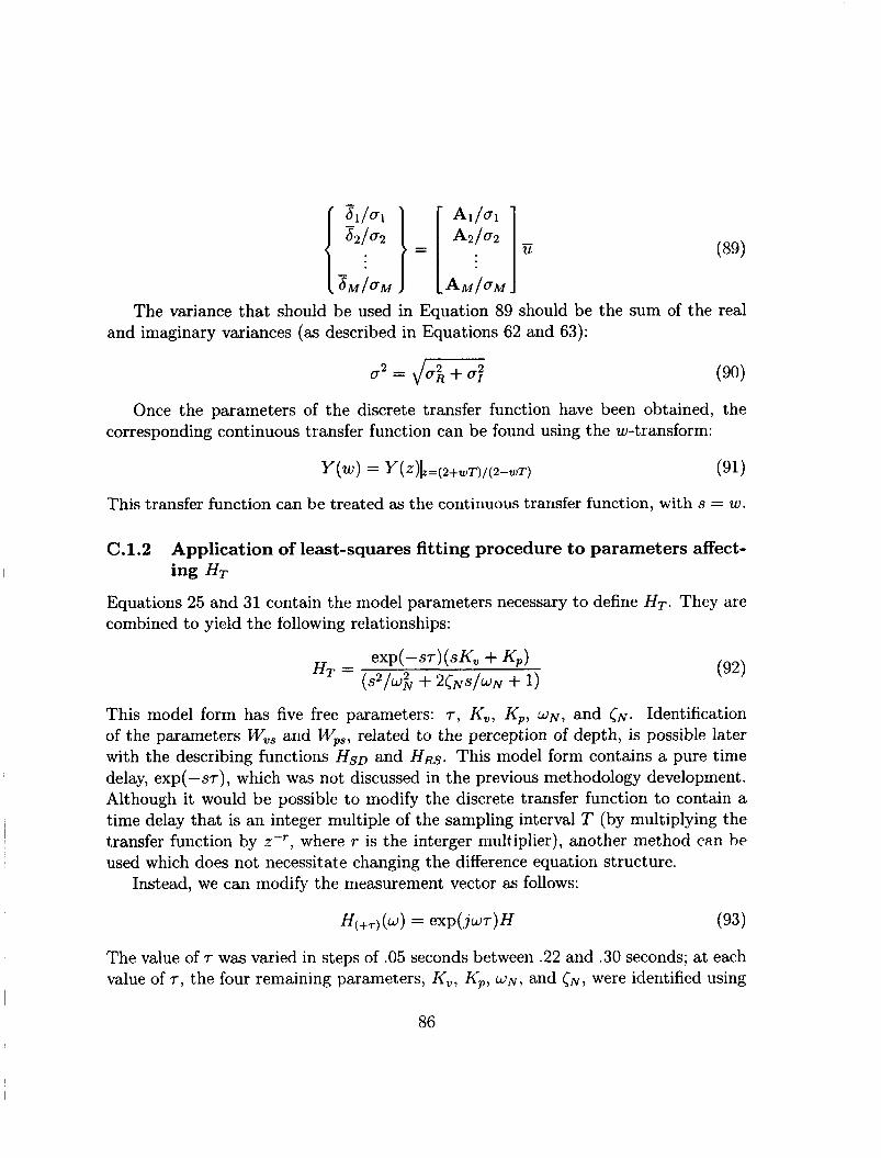
The variance that should be used in Equation 89 should be the sum of the real and imaginary variances (as described in Equations 62 and 63):
(90) 0 2 = &:,+a;
Once the parameters of the discrete transfer function have been obtained, the corresponding continuous transfer function can be found using the w-transform:
y ( w ) = Y(Z)b=(2+wT)/ (2-wT) (91)
This transfer function can be treated as the continuous transfer function, with s = w.
C.1.2 Application of least-squares fitting procedure to parameters affect- ing HT
Equations 25 and 31 contain the model parameters necessary to define HT. They are combined to yield the following relationships:
This model form has five free parameters: r , K,, Kp, W N , and CN. Identification of the parameters W,, and Wps, related to the perception of depth, is possible later with the describing functions HsD and HRs. This model form contains a pure time delay, exp( --ST), which was not discussed in the previous methodology development. Although it would be possible to modify the discrete transfer function to contain a time delay that is an integer multiple of the sampling interval T (by multiplying the transfer function by z-', where T is the interger multiplier), another method can be used which does not necessitate changing the difference equation structure.
Instead, we can modify the measurement vector as follows:
The value of r was varied in steps of .05 seconds between .22 and .30 seconds; at each value of r , the four remaining parameters, K,, K p , W N , and (N, were identified using
86
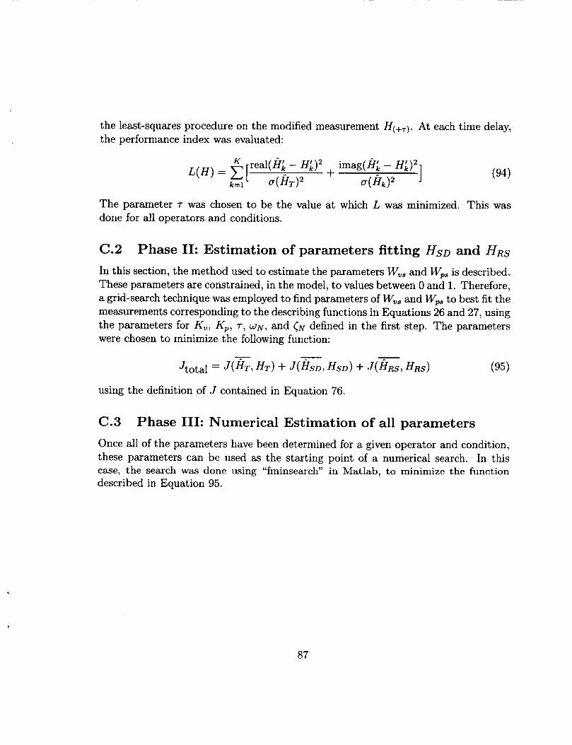
the least-squares procedure on the modified measurement H(+T) . At each time delay, the performance index was evaluated:
The parameter r was chosen to be the value at which L was minimized. This was done for all operators and conditions.
C.2 Phase 11: Estimation of parameters fitting HSO and HRS In this section, the method used to estimate the parameters W,, and W,, is described. These parameters are constrained, in the model, to values between 0 and 1. Therefore, a grid-search technique was employed to find parameters of W,, and W,, to best fit the measurements corresponding to the describing functions in Equations 26 and 27, using the parameters for K,, Kp, 7, W N , and CN defined in the first step. The parameters were chosen to minimize the following function:
- Jtotal= ~(fiT, H T ) + J(Z~ HSO) + J(Z, H R S ) (95)
using the definition of J contained in Equation 76.
C.3 Phase 111: Numerical Estimation of all parameters Once all of the parameters have been determined for a given operator and condition, these parameters can be used as the starting point of a numerical search. In this case, the search was done using “fminsearch” in Matlab, to minimize the function described in Equation 95.
87
References [Berkeley, 1709/1910]
[Boff, et al, 19861
[Bradshaw and Rogers, 19961
[Bruce, et al. 19961
[Bruno and Cutting, 19881
[Bulthoff and Mallot, 19881
[Cannon 19671
[Clark and Yuille, 19901
[Curran and Johnston, 19941
[Cutting and Vishton, 19951
Berkeley, G. (1709/1910). An essay toward a new the- ory of vision. In A New Theory of Vision and Other Writings. London: J.M. Dent and Sons.
Boff, K. R., Kaufman, L., and Thomas, J . P. (Eds.) (1986). Handbook of Perception and Human Perfor- mance. New York: John Wiley and Sons.
Bradshaw, M. F., and Rogers, B. J. (1996). The in- teraction of binocular disparity and motion parallax in the computation of depth. Vision Research, 36(21), 3457-3468.
Bruce, V., Green, P. R., and Georgeson, M. A. (1996). Visual Perception: Physiology, Psychology, and Ecol- ogy. East Sussex, UK: Psychology Press.
Bruno, N., and Cutting J. E. (1988). Minimodularity and the perception of layout. Journal of Experimental Psychology: General, 117(2), 161-170.
Bulthoff, H. H., and Mallot, H. A. (1988). Integra- tion of depth modules: Stereo and shading. Journal of the Optical Society of American A: Optics, Image Science, and Vision, 5(10), 1749-1758.
Cannon, R. H. (1967). Dynamics of Physical Systems. New York: McGraw-Hill.
Clark, J. J., and Yuille, A. L. (1990). Data Fusion for Sensory Information Processing Systems. Boston: Kluwer.
Curran, W., and Johnston, A. (1994). Integration of shading and texture cues: Testing the linear model. Vision Research, 34(14), 1863-1874.
Cutting, J. E., and Vishton, P. M. (1995). Perceiv- ing layout and knowing distances: The integration,
88
[Foley, 19801
relative potency, and contextual used of different in- formation about depth. In W. Epstein & s. Rogers (Eds.) Handbook of Perception and Cognition: Vol- ume 5, Perception of Space and Motion. New York: Academic Press.
Foley, J. M. (1980). Binocular distance perception. Psychological Review, 87, 41 1-435.
[Franklin et al. 19901 Franklin, G. F., Powel1,J. D., and Workman, M. L. (1990). Digital Control of Dynamic Systems. Reading: Addison-Wesley.
[Hess 19791
[Hess 19971
Hess, R. A. (1979). A Rationale for Human Operator Pulsive Control Behavior. In Journal of Guidance and Control, 2(3), 221-227.
Hess, R. A. (1997). Feedback control models - manual control and tracking. In Handbook of Human Factors and Ergonomics, Second Edition, edited by G. Sal- vendy. New York: John Wiley & Sons.
[Johnston et al., 19941 Johnston, E. B., Cumming, B. G., and Landy, M. S. (1994). Integration of stereopsis and motion shape cues. Vision Research, 34( 17), 2259-2275.
Johnston, E. B., Cumming, B. G., and Parker, A. J. (1993). Integration of depth modules: Stereopsis and texture. Vision Research, 33(5/6), 813-826.
Landy, M. S., Maloney, L. T., Johnston, E. B., Young, M. (1995). Measurement and modeling of depth cue combination: In defense of weak fusion. Vision Re- search, 35(3), 389-412.
[Johnston et al., 19931
[Landy et al., 19951
[Levison 19801
[ Levison 19861
Levison, W. H. (1980). Measurement of Human Op- erator Response Behavior. NASA CR-166038.
Levison, W. H. (1980). Some computational tech- niques for estimating human operator describing func- tions. In Proceedings of the Twenty-First Annual Con- ference on Manual Control. NASA CP 2428.
89
~
[Massaro, 19881
[Massaro and Cohen, 19931
[McRuer and Krendel 19741
[McRuer et al., 19651
, [Richards, 19711
I
[Stapleford et al., 19691
[Speigel, M. R., 19961
I [Stevens and Brooks, 19881
[Sweet, 19991
Massaro, D. W. (1988). Ambiguity in perception and experimentation. Journal of Experimental Psychol- ogy: General, 117(4), 417-421.
Massaro, D. W., and Cohen, M. M. (1993). The paradigm and the Fuzzy Logic Model of Perception are alive and well. Journal of Experimental Psychol- ogy: General, 122(1), 115-124.
McRuer, D. T., and E. S. Krendel. (1974). Mathemat- ical Models of Human Pilot Behavior. AGARD-AG- 188.
McRuer, D., E. Krendel, and W. Reisener, Jr. (1965). Human pilot dynamics in compensatory systems. AFFDL-TR-65-15, July, 1965.
Richards, W. (1971). Anomalous stereoscopic depth perception. Journal of the Optical Society of America, 61, 410-414.
Stapleford, R.L., Craig, S. J., and Tennant, J. A. (1969). Measurement of Pilot Describing Functions in Single-Control Multiloop Tasks. NASA CR-1238, Jan- uary 1969.
Spiegel, Murray R. (1996). Mathematical Handbook of Formulas and Tables. pp. 258. New York: McGraw- Hill.
Stevens, K. and Brooks, A. (1988). Integrating stere- opsis with monocular interpretations of planar sur- faces. Vision Research, 28, 371-386.
Sweet, Barbara Townsend (1999). The Identification and Modeling of Visual Cue Usage in Manual Control Task Experiments. NASA/TM-1999-208798, Septem- ber, 1999.
90

[Young et al., 19931 Young, M. J., Landy, M. S., and Maloney, L. T. (1993). A perturbation analysis of depth perception from combinations of texture and motion cues. Vz- sion Research, 33( 18), 2685-2696.
.
91
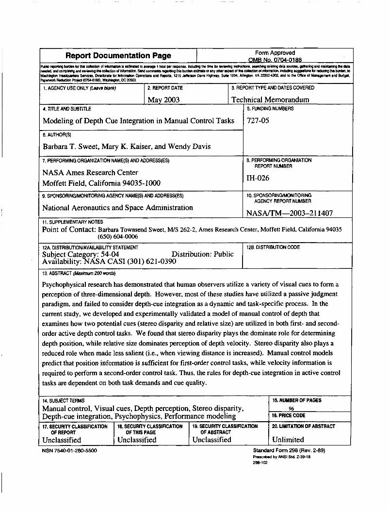
Form Approved Report Documentation Page MS NO. 0704-0188
1. AGENCY USE ONLY (Leave Mank) 2. REPORT DATE 3. REPORT TYPE AND DATES COVERED
May 2003 Technical Memorandum 4. TITLE AND SUBTITLE
Modeling of Depth Cue Integration in Manual Control Tasks
9. SPONSORINGMONITORING AGENCY NAME@) AND ADDRESS(ES)
5. FUNDING NUMBERS
727-05
10. SPONSORlNGlMONlTORlNG I AGENCY REPORT NUMBER
6. AUTHOR(S)
Barbara T. Sweet, Mary K. Kaiser, and Wendy Davis
7. PERFORMING ORGANIZATION NAME(S) AND ADDRESS(ES)
NASA Ames Research Center Moffett Field, California 94035-1000
National Aeronautics and Space Administration NASA/TM-2003-211407
11. SUPPLEMENTARY NOTES
8. PERFORMING ORGANIATION REPORT NUMBER
IH-026
12A. DISTRIBUTION/AVAILABlLlTY STATEMENT Subject Cate ory: 54-04 Distribution: Public Availability: a ASA CAS1 (301) 621-0390
128. DISTRIBUTION CODE
14. SUBJECT TERMS Manual control, Visual cues, Depth perception, Stereo disparity, Depth-cue integration, Psychophysics, Performance modeling
NSN 7540-01 -280-5500
15. NUMBER OF PAGES
16. PRICE CODE 96
Standard Form 298 (Rev. 2-89) PreSCribed by ANSI Std. 2-39-18 298-1Dz
~~
17. SECURITY CLASSIFICATION OF REPORT
Unclassified
18. SECURITY CLASSIFICATION 19. SECURITY CLASSIFICATION 20. LIMITATION OF ABSTRACT OF THIS PAGE OF ABSTRACT
Unclassified Unclassified Unlimited