Embed Size (px)
Citation preview
HAL Id: tel-01539576https://pastel.archives-ouvertes.fr/tel-01539576
Submitted on 15 Jun 2017
HAL is a multi-disciplinary open accessarchive for the deposit and dissemination of sci-entific research documents, whether they are pub-lished or not. The documents may come fromteaching and research institutions in France orabroad, or from public or private research centers.
L’archive ouverte pluridisciplinaire HAL, estdestinée au dépôt et à la diffusion de documentsscientifiques de niveau recherche, publiés ou non,émanant des établissements d’enseignement et derecherche français ou étrangers, des laboratoirespublics ou privés.
Modeling of the atmospheric dispersion of heavy metalsover Poland
Janusz Zysk
To cite this version:Janusz Zysk. Modeling of the atmospheric dispersion of heavy metals over Poland. Ocean, Atmo-sphere. Université Paris-Est, 2016. English. �NNT : 2016PESC1169�. �tel-01539576�

AGH University of Science and Technology
Faculty of Energy and Fuels Department of Sustainable Energy
Development
University Paris-Est Ecole des Ponts ParisTech
Centre d'Enseignement et de Recherche en Environnement
Atmosphérique
DOCTORAL THESIS
Mgr inż. Janusz Zyśk
Fields of study: Chemical Technology at Faculty of Energy and Fuels, Science and technology of the environment at École des Ponts ParisTech
Modelling of atmospheric transport of heavy metals
emitted from Polish power sector
Date of defence 30-06-2016
Supervisors: Prof. dr hab. Janusz Gołaś Professor Christian Seigneur Ph.D., hab.
Auxiliary supervisor: Yelva Roustan Ph.D.
Kraków, 2016

2
Oświadczam, świadomy (-a) odpowiedzialności karnej za poświadczenie nieprawdy, że niniejszą pracę doktorską wykonałem (-am) osobiście i samodzielnie i że nie korzystałem (-am) ze źródeł innych niż wymienione w pracy .
……………………………………………………
podpis autora pracy
3
Content
Introduction ........................................................................................................................ 6 1
PART I Review of the literature of the cycle of heavy metals in the environment ................. 11
Heavy metals in the environment ..................................................................................... 12 2
2.1 Global cycle of heavy metals..................................................................................... 12
2.2 Heavy metals emissions into the atmosphere ............................................................ 14
2.2.1 Natural emissions of heavy metals ..................................................................... 14
2.2.2 Anthropogenic emission of mercury into the air ................................................ 17
2.2.3 Emissions of mercury from coal combustion in the power sector ..................... 26
2.2.4 Anthropogenic emission of lead and cadmium into the air ................................ 30
2.3 Reactions of mercury in the atmospheric gas phase .................................................. 33
2.4 Reactions of mercury in the aqueous phase of the atmosphere ................................. 44
2.5 Mercury transformation in presence of aerosol particles .......................................... 49
2.6 Measurements of deposition and concentration of heavy metals .............................. 50
Overview of existing mercury chemical transport models ............................................... 57 3
Polyphemus air quality system ......................................................................................... 67 4
4.1 Below-cloud scavenging model implemented in the Polyphemus system ................ 69
4.2 Dry deposition models implemented in the Polyphemus system .............................. 73
4.2.1 Dry deposition for gaseous species .................................................................... 73
4.2.2 Dry deposition velocity for aerosols................................................................... 79
PART II Development and application of a new chemical transport model for mercury,
modelling of atmospheric transport of lead and cadmium ....................................................... 81
Distribution of the emissions of heavy metals into the air by the Polish power sector with 5the use of the bottom-up approach ........................................................................................... 82
5.1 Methodology .............................................................................................................. 82
5.2 Results........................................................................................................................ 84
5.3 Implemented chemical scheme of atmospheric mercury........................................... 86
5.3.1 In-cloud scavenging............................................................................................ 96
Simulation setting ............................................................................................................. 98 6
6.1 Domains of simulation............................................................................................... 98
6.2 Input data ................................................................................................................... 99
6.2.1 Land use data ...................................................................................................... 99
6.2.2 Meteorological data ............................................................................................ 99
6.2.3 Boundary and initial concentrations ................................................................... 99
6.2.4 Concentrations of species that react with mercury ........................................... 100
6.2.5 Natural emissions ............................................................................................. 101
6.2.6 Anthropogenic emissions, simulations over Europe ........................................ 103

4
6.2.7 Anthropogenic emissions, simulation over Poland .......................................... 106
Results ............................................................................................................................ 109 7
7.1 Evaluation of intensity of precipitation ................................................................... 111
7.2 Dry deposition velocity for mercury species ........................................................... 112
7.3 Results and evaluation of concentrations of species that react with mercury ......... 114
7.4 Evaluation of mercury concentrations and deposition............................................. 124
7.5 Evaluation of cadmium and lead ambient concentrations and deposition............... 132
7.6 Results of ambient concentrations and deposition of mercury ................................ 135
7.7 Results of ambient concentrations and deposition of cadmium and lead ................ 142
7.8 Sensitivity analysis of the mercury model ............................................................... 144
7.9 Contribution of different sources to mercury deposition in Poland ........................ 156
7.10 The impact of the Polish power sector ................................................................. 157
Conclusions .................................................................................................................... 162 8
References .......................................................................................................................... 167
List of Tables ...................................................................................................................... 183
List of Figures..................................................................................................................... 187
Appendix 1 ......................................................................................................................... 194
5
Acknowledgements
I would like to express my gratitude to Professors Janusz Gołaś and Christan Seignerur for
their guidance as the supervisors of my Thesis. Thank you for helpful discussions and
professional advice during my work on this Thesis.
I would like to express my special appreciation and thanks to Dr. Yelva Roustan, you have
been a tremendous mentor for me. I would like to thank you for encouraging my research and
for allowing me to grow as a research scientist.
I am greatly indebted to Dr. Artur Wyrwa for introducing me into the fascinating world of
science. Your advice on both research as well as on my career has been priceless.
I would also like to thank Professors Louis Jestin, Bruno Sporitsse, Luc Musson-Genon,
Wojciech Suwała, Denis Quelo, Mariusz Filipowicz for their kindness, helpful and
professional advice.
I would like express my appreciation to the late professors Piotr Tomczyk and Adam Guła,
who always surrounded me with unusual kindness.
6
Introduction 1
During the last decades many studies have been conducted to investigate the atmospheric
heavy metals contamination and its deposition to ecosystems.
The increasing attention to mercury pollution has been mainly driven by the growing evidence
of its negative impacts on wildlife, ecosystems and particularly human health. It should be
noted, that after mercury moves through the water chain it can be transformed by aquatic
microorganisms into methylmercury (MeHg), which is much more toxic than the other forms.
Subsequently, MeHg is bioaccumulated in fish and seafood [1]. The predator fish can contain
almost 100% of mercury in methylmercury form. Eventually, it enters the human body with
consumed food. It is then transported by blood and can easily pass the blood-brain barrier and
cause neurotic dysfunctions. It is reported that even relatively low doses can damage the
nervous system. The symptoms that can be observed are: blurred vision, malaise, dysarthria,
paraesthesia, ataxia, impairment of hearing and difficulty in walking. Symptoms appear
slowly and increase gradually along with the amount of mercury accumulated in the body [1].
It should be highlighted, that mercury also passes through the placental barrier and has an
immense negative impact on the foetus, decreasing the IQ of a child. In this way, the
development of whole populations is influenced. It is reported that methylmercury can be the
cause of a cancer, kidney dysfunction, heart and blood system diseases.
The most spectacular poisoning of methylmercury occurred in Minamata in Japan in the
forties, fifties and sixties of the XX century, when the local chemical factory producing
acetaldehyde released the mercury in the industrial water waste into the local gulf since 1932
until 1968. Although, the mercury concentration in water was not so high, it ensued the
accumulation of mercury as methylmercury in fish and shellfish, which finally was consumed
by local people and accumulated in their bodies. Until March 2001 approximately 3000
officially certified patients were identified, among them, 1784 who have already died [2]. The
largest, outbreaks of mercury poisonings occurred in Iraq in winter 1971 -1972 due to the
consumption of seed grain, which had been treated with fungicides containing mercury. It was
estimated that around 40000 individuals were affected, 6300 were hospitalized and 450
people died [3].
Mercury can also enter the human body through inhalation of the vapours. The effects such as
insomnia, memory loss, headaches, tremors are usually short lived. Results of preliminary
studies on the assessment of external effects of anthropogenic mercury emissions have
already been published [4]. It was reported that mercury can affect the function of kidneys,
7
respiratory system, heart and blood system, digestive system, immune system, liver and the
reproductive system.
For the first time ever, a mass cadmium poisoning was documented, in Japan again, in the
Toyama province in 1964. The people felt an intense pain of joints, muscle and spine
therefore the disease was named Itai‑Itai – which in Japanese means intense pain. The reason
for the accumulation of cadmium in the body of the residents in Toyama was the consumption
of the rice, which was polluted by cadmium compounds [5]. Cadmium enters the human body
through the respiratory system, human gastrointestinal tract and skin. The high concentration
of cadmium in the air causes acute poisoning. The symptoms of cough, burning sensation
inside the chest, headache, dizziness, general malaise, chills, sweating, nausea, vomiting and
diarrhea are mainly observed. Long exposure to cadmium, which is contained in the air has
a negative effect on the skeleton (bone structure) and the kidneys. Moreover the positive
correlation between cadmium exposure and cancer of the prostate and lung was observed.
Lead is also a toxic heavy metal which is being emitted into the atmosphere by anthropogenic
as well as natural sources. This heavy metal has effects on the human health even at very low
exposures and causes negative impacts mainly in circulatory, nervous, genitourinary systems.
Intense studies were launched in the 70s of the XX century, which led to determine the dose-
response functions for the impact of lead on the human health. The measurements of lead
content in human blood allows for the quantification of the risk of appearance of health
hazard. Long-term lead exposure can cause the level of lead in the body that finally causes the
disease, which is called lead poisoning. The most common symptoms are insomnia,
hallucinations, cognitive deficit and tremors. Unfortunately, also lead -as in the case
of mercury - passes through the placental barrier and accumulates in the body of infants,
which may lead to many diseases [6].
The harmful influence on humans and the environment of these three heavy metals was
underlined in the Aarhus Protocol on Heavy Metals of 1998. The Parties of this protocol
(including Poland) are obligated to reduce emissions, observe the transport and the amounts
of lead, mercury and cadmium in the environment.
Moreover the European Union has made many efforts to decrease heavy metals emission and
the use of those. The legislation of the European Union draws attention to control the amount
of mercury, lead, cadmium and other heavy metals in air, water and food. The number
of directives linked to mercury, lead and cadmium have given voice to particular concern for
decreasing negative impact of heavy metals and heavy metal compounds on human health.
One can enumerate a numbers of directives and regulations, e.g.:
8
76/768/EEC, 76/769/EEC, 79/117/EEC, 91/188/EEC, 98/8/EC, 2000/53/EC,
2002/95/EC, 2002/96/EC, 2006/66/EC, 2007/51/EC restrict the use of mercury, lead
and cadmium in industry, agriculture, cosmetics;
96/23/EEC, 2000/60/EC, 2001/22/EC, 2006/118/EC/ 2006/1881/EC are dedicated
to mercury, lead and cadmium control in water and food;
80/68/EEC, 98/83/EEC, 2006/118/EC, 2008/105/EC limit heavy metals content
in water, groundwater and drinking water;
2004/107/EC requires to measure the mercury background concentration with spatial
resolution of 100,000km2 and provide the long-term trends of mercury and cadmium
concentration as well as arsenic and nickel in air;
96/61/EC (IPPC), Integrated Pollution Prevention and Control, which order to use the
Best Available Techniques (BAT) to reduce pollutant emissions from power plants,
chlorine production industry and cement production sector;
2001/80/EC (LCP) imposes limits of emissions of PM, which contains mercury, lead,
cadmium and other heavy metals;
Regulation (EC) No 1102/2008 mercury, mercury compounds, substances with
containing more than 95% of mercury are prohibited to be exported out of the EU;
2010/75/EU (IED) replacing i.e. LCP and IPPC which will lead to considerable
emission reduction via review of BREFs and adoption of BAT for industrial activities.
In 2005 the EU launched the “Community Strategy Concerning Mercury” aimed at reduction
of negative impacts of mercury and the risks it poses for the environment and human health.
In conclusion of the revision of this Strategy in 2011, the European Council stressed the
importance for the EU to participate actively in and to give full support to the international
negotiations on a new global mercury convention that have been initiated by UNEP in 2009.
The Minamata Convention on Mercury was prepared during 4 years of intergovernmental
negotiations. It was opened for signature at the conference in Kumamoto, Japan in October
2013 and was signed by nearly 100 countries i.e. China, India, Germany, Brazil, South Africa,
the United States and Poland. The Convention included the actions which should be taken
to protect the human health and the environment from anthropogenic emissions and releases
of mercury and mercury compounds [7].
The monitoring of heavy metals and above all mercury concentration and deposition over
Europe is currently insufficient to provide accurate data on heavy metals concentrations and
depositions. In some parts of Europe, there is a lack of sampling stations and thus such areas
are not covered by monitoring at all. Therefore, it appears interesting to complement the
9
results of measurements by the modelling methods, keeping in mind the remaining
uncertainties of mercury and other heavy metals modelling [8], [9]. The pathway of mercury
dispersion in the atmosphere is complex therefore one of the key issues in reactive dispersion
modelling of mercury is the chemistry model that represents the reactions and mass exchange
between the gaseous, aqueous and particulate phases. During the last few decades, several
chemical schemes have been implemented in different Chemical Transport Models (CTM)
developed to represent the atmospheric dispersion of mercury. Some intercomparison studies
were performed over Europe [10], [11], [12]. These studies were taken into account in the
implementation of a chemistry scheme devoted to mercury within the framework of the
Polyphemus air quality modelling system [13].
Poland is still one of the biggest emitter of mercury, lead and cadmium in Europe mainly due
to emission from coal combustion processes. It should be underlined that the emissions
in Poland systematically decrease mainly due to significant power sector investment in
emission control equipment, which besides limiting emission of pollutants such as PM, SO2
and NOx, reduce significantly the emissions of other air pollutant including Hg, Cd and Pb
[14].
The objectives of this work were twofold: (i) scientific and (ii) practical.
The scientific objective was to develop a model to represent the atmospheric dispersion
of mercury and to implement it in the air quality modelling platform Polyphemus.
The practical objective was to run the model and perform heavy metals dispersion studies
over Europe and detailed studies of the impact of the polish power sector on the air quality
regarding mercury, cadmium and lead.
Some examples of questions that can be asked or hypotheses that can be verified in this work
are presented below:
does the dry deposition of gaseous elemental mercury have the greatest influence
on obtained mercury deposition results?
what is the contribution of different atmospheric reactions to atmospheric mass
balance of reactive mercury?
is most of the deposited mercury in Poland emitted outside Poland?
10
what is the contribution of the power sector plants to local mercury deposition
in Poland?
does the concentration of reactive mercury and lead and cadmium depend strongly
on local emission sources?
Within the scope of this work computing codes have been developed with the use of C/C++
and Fortran programing languages. Several pre-processing programs were written in C/C++ to
prepare and calculate input data to model i.e. (i) dry deposition velocity for gaseous mercury
species; (ii) natural emission and reemission flux of mercury, (iii) anthropogenic emission
of mercury, (iv) boundary and initial contractions of mercury, (v) concentration of chlorine
species, which react with mercury. The Fortran code of the chemical transport model was
implemented in the Polyphemus/Polair3D system and consists of three sections dedicated
to gaseous and aqueous phases and to particulate mercury (please see Appendix 1).
Additionally many C/C++ codes were prepared to process obtained results e.g.: to evaluate
the results of the modelling against observations.
The dissertation consists of two parts.
• Part I is devoted to a literature review of the cycle of heavy metals in the environment.
As the modelling work is based on previous laboratory research, measurements, estimations
and assumptions, a review of the literature regarding emissions, chemistry and measurements
of mercury, lead and cadmium was conducted. The state of the art in the development
of chemical transport mercury models is described.
• Part II is devoted to the development and application of the new chemical transport
model for mercury and modelling of atmospheric transport of lead and cadmium.
This part describes the development and application of the model dedicated for mercury,
cadmium and lead dispersion in the atmosphere. The main assumptions and data used are
presented. The obtained results are presented, evaluated and discussed. The conclusions of the
Thesis, are focused on the obtained results and the scientific achievements completed in this
Thesis.
In this Thesis, the term Polish power sector covers all power, cogeneration (CHP) and
regional/city heating plants located in Poland which use hard or brown coal, as the main fuel.
The main coal-based plants that primarily work for the industry sector but have a part of their
production is designated for the market, are also included in this term.
11
PART I Review of the literature of the
cycle of heavy metals in the
environment

12
Heavy metals in the environment 2
2.1 Global cycle of heavy metals
Heavy metals are emitted to the atmosphere from natural and anthropogenic sources (Figure
2-1). In the atmosphere, cadmium and lead occur only as components of particulate matter
(aerosols). Particulate matter is defined in its simplest form as a microscopic solid or liquid
matter suspended in the Earth's atmosphere. The atmospheric aerosols are composed mainly
of species/compound such as sulphates, nitrates, organics and black carbon. The share
of heavy metals in aerosols is relatively low. Therefore, the atmospheric transport and
behaviour of heavy metals is considered and analysed as linked to the characteristics of
aerosols.
On the other hand, mercury occurs in the atmosphere in three forms:
GEM –gaseous elemental mercury (Hg0(g)), which is a prevailing form of mercury in the
atmosphere.
RGM –reactive gaseous mercury (HgI(g), HgII
(g)) in organic and inorganic compounds. The
inorganic compounds include compounds such as: HgO(g), HgCl2(g), Hg(OH)2(g),
HgBrOH(g), HgBr2(g). The organic compounds are represented mainly by compounds
which include one (monomethyl mercury -MMM) or two (dimethyl mercury -DMM)
methyl groups e.g.: CH3HgCl, CH3HgOH, Hg(CH3)2.
particulate forms of mercury (HgP). The mercury in aerosols could be represented by
compounds such as: HgO, HgSO4.
These three species exhibit different transport characteristics. Gaseous elemental mercury can
be considered as a global pollutant due to its residence time in the atmosphere. Reactive
gaseous and particulate forms of mercury are deposited more quickly by wet and dry
deposition processes than elemental mercury [15], [8].
Heavy metals are removed from the atmosphere through wet and dry deposition process. Wet
deposition is the process of removal of gaseous and particulates matter pollutants from the
atmosphere where condensed water is involved. In this process, water captures pollutants and
together with precipitation pollutants are moved to the Earth surface. This process occurs
where ever precipitations and clouds are present. The pollutants absorbed by clouds are
removed together with the removal of mass (volume) of clouds by precipitation. Precipitation
also absorbs pollutant located below clouds and also remove them. Therefore the wet
deposition can be split between in-cloud (rainout) and below cloud (washout) scavenging. Dry

13
deposition is a transport of gaseous as well as aerosols pollutants to the ground surface where
those are absorbed by soil, water, flora and others materials that cover the ground during
periods without precipitation. The significant part of deposited pollution is (often
immediately) reemitted to the air. The heavy metals in aqueous environments undergo
complex chemical and physical reactions and transformations [6], [16].
The heavy metals included in air as well as deposited to surfaces and transferred to water and
food, may get in the human body, where there are usually accumulated resulting in various
adverse effects, as already mentioned in the introduction chapter.
Figure 2-1. The sources, pathway and sinks of heavy metals in the atmosphere.
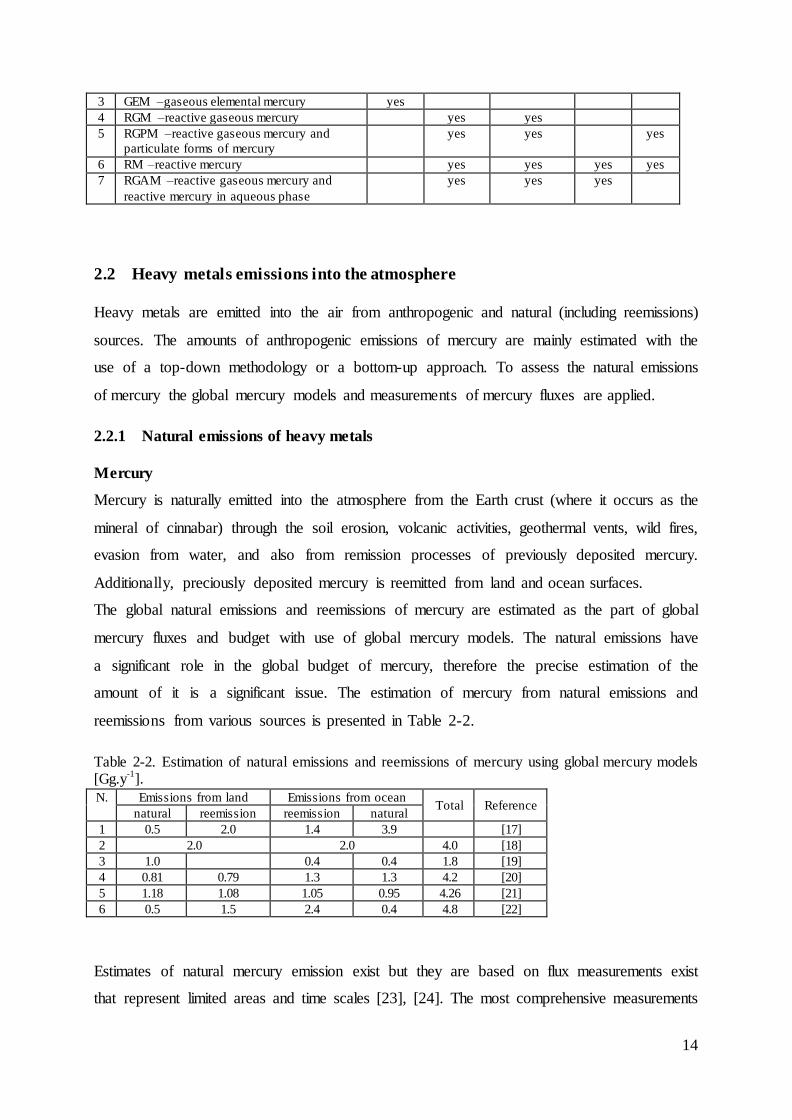
Naming
In the model concentration and deposition of 9 forms or compounds of mercury are being
tracked. Seven in the gas phase i.e. Hg0(g), HgBr(g), HgO(g), HgBrOH(g), HgCl2(g), Hg(OH)2(g),
HgBr2(g), one in the aqueous phase (HgII(aq)) and one in particulate form (HgP). The particulate
form of mercury in the model is additionally split into particulate size sections. As the
mercury occurs in 3 speciation forms in gaseous and aqueous phases, the common names and
acronyms were used to determine chosen mercury forms. The species in gas phase are written
with the index “(g)” and those in the aqueous phase with “(aq)”. In Table 2-1 all acronyms
are listed along with selected species, which are included in them.
Table 2-1. Names and acronyms used in manuscript of various mercury species. “Yes” in table indicates that the specie belongs to a group described by acronym and name.
N
Common names and acronyms
species track in the model
1. Hg0
(g) HgBr(g) HgO(g)
HgBrOH(g)
HgCl2(g)
Hg(OH)2(g)
HgBr2(g)
HgII
(aq) HgP
2 Mercury yes yes yes yes yes
14
3 GEM –gaseous elemental mercury yes
4 RGM –reactive gaseous mercury yes yes
5 RGPM –reactive gaseous mercury and
particulate forms of mercury
yes yes yes
6 RM –reactive mercury yes yes yes yes
7 RGAM –reactive gaseous mercury and
reactive mercury in aqueous phase
yes yes yes
2.2 Heavy metals emissions into the atmosphere
Heavy metals are emitted into the air from anthropogenic and natural (including reemissions)
sources. The amounts of anthropogenic emissions of mercury are mainly estimated with the
use of a top-down methodology or a bottom-up approach. To assess the natural emissions
of mercury the global mercury models and measurements of mercury fluxes are applied.
2.2.1 Natural emissions of heavy metals
Mercury
Mercury is naturally emitted into the atmosphere from the Earth crust (where it occurs as the
mineral of cinnabar) through the soil erosion, volcanic activities, geothermal vents, wild fires,
evasion from water, and also from remission processes of previously deposited mercury.
Additionally, preciously deposited mercury is reemitted from land and ocean surfaces.
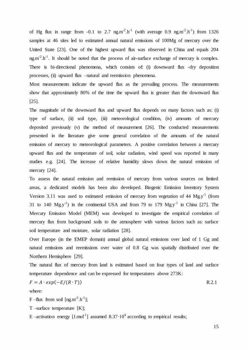
The global natural emissions and reemissions of mercury are estimated as the part of global
mercury fluxes and budget with use of global mercury models. The natural emissions have
a significant role in the global budget of mercury, therefore the precise estimation of the
amount of it is a significant issue. The estimation of mercury from natural emissions and
reemissions from various sources is presented in Table 2-2.
Table 2-2. Estimation of natural emissions and reemissions of mercury using global mercury models [Gg.y
-1].
N. Emissions from land Emissions from ocean Total Reference
natural reemission reemission natural
1 0.5 2.0 1.4 3.9 [17]
2 2.0 2.0 4.0 [18]
3 1.0 0.4 0.4 1.8 [19]
4 0.81 0.79 1.3 1.3 4.2 [20]
5 1.18 1.08 1.05 0.95 4.26 [21]
6 0.5 1.5 2.4 0.4 4.8 [22]
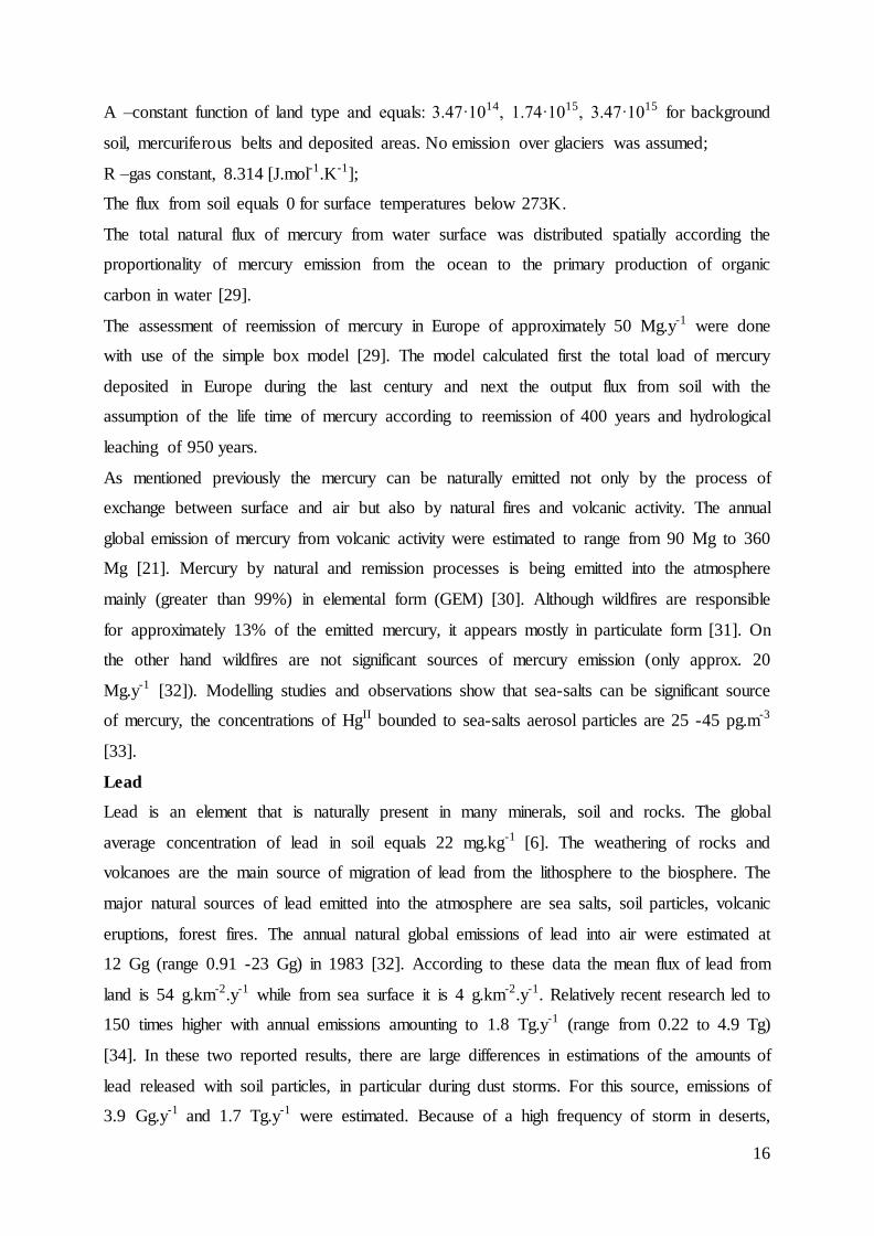
Estimates of natural mercury emission exist but they are based on flux measurements exist
that represent limited areas and time scales [23], [24]. The most comprehensive measurements
15
of Hg flux in range from -0.1 to 2.7 ng.m-2.h-1 (with average 0.9 ng.m-2.h-1) from 1326
samples at 46 sites led to estimated annual natural emissions of 100Mg of mercury over the
United State [23]. One of the highest upward flux was observed in China and equals 204
ng.m-2.h-1. It should be noted that the process of air-surface exchange of mercury is complex.
There is bi-directional phenomena, which consists of: (i) downward flux -dry deposition
processes, (ii) upward flux –natural and reemission phenomena.
Most measurements indicate the upward flux as the prevailing process. The measurements
show that approximately 80% of the time the upward flux is greater than the downward flux
[25].
The magnitude of the downward flux and upward flux depends on many factors such as: (i)
type of surface, (ii) soil type, (iii) meteorological condition, (iv) amounts of mercury
deposited previously (v) the method of measurement [26]. The conducted measurements
presented in the literature give some general correlation of the amounts of the natural
emission of mercury to meteorological parameters. A positive correlation between a mercury
upward flux and the temperature of soil, solar radiation, wind speed was reported in many
studies e.g. [24]. The increase of relative humidity slows down the natural emission of
mercury [24].
To assess the natural emission and remission of mercury from various sources on limited
areas, a dedicated models has been also developed. Biogenic Emission Inventory System
Version 3.11 was used to estimated emission of mercury from vegetation of 44 Mg.y-1 (from
31 to 140 Mg.y-1) in the continental USA and from 79 to 179 Mg.y-1 in China [27]. The
Mercury Emission Model (MEM) was developed to investigate the empirical correlation of
mercury flux from background soils to the atmosphere with various factors such as: surface
soil temperature and moisture, solar radiation [28].
Over Europe (in the EMEP domain) annual global natural emissions over land of 1 Gg and
natural emissions and reemissions over water of 0.8 Gg was spatially distributed over the
Northern Hemisphere [29].
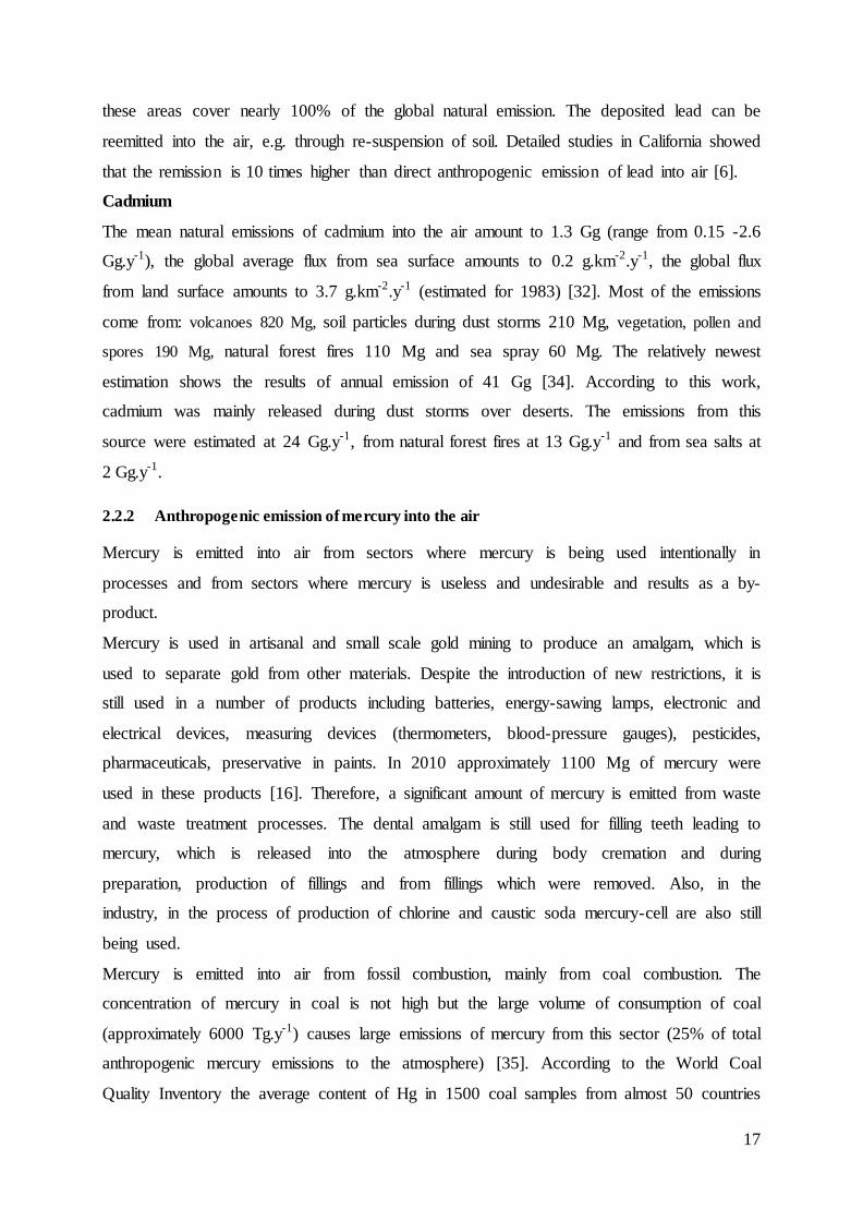
The natural flux of mercury from land is estimated based on four types of land and surface
temperature dependence and can be expressed for temperatures above 273K:
𝐹 = 𝐴 ∙ 𝑒𝑥𝑝(−𝐸/(𝑅 ∙ 𝑇)) R.2.1
where:
F –flux from soil [ng.m-2.h-1];
T –surface temperature [K];
E –activation energy [J.mol-1] assumed 8.37·104 according to empirical results;
16
A –constant function of land type and equals: 3.47·1014, 1.74·1015, 3.47·1015 for background
soil, mercuriferous belts and deposited areas. No emission over glaciers was assumed;
R –gas constant, 8.314 [J.mol-1.K-1];
The flux from soil equals 0 for surface temperatures below 273K.
The total natural flux of mercury from water surface was distributed spatially according the
proportionality of mercury emission from the ocean to the primary production of organic
carbon in water [29].
The assessment of reemission of mercury in Europe of approximately 50 Mg.y-1 were done
with use of the simple box model [29]. The model calculated first the total load of mercury
deposited in Europe during the last century and next the output flux from soil with the
assumption of the life time of mercury according to reemission of 400 years and hydrological
leaching of 950 years.
As mentioned previously the mercury can be naturally emitted not only by the process of
exchange between surface and air but also by natural fires and volcanic activity. The annual
global emission of mercury from volcanic activity were estimated to range from 90 Mg to 360
Mg [21]. Mercury by natural and remission processes is being emitted into the atmosphere
mainly (greater than 99%) in elemental form (GEM) [30]. Although wildfires are responsible
for approximately 13% of the emitted mercury, it appears mostly in particulate form [31]. On
the other hand wildfires are not significant sources of mercury emission (only approx. 20
Mg.y-1 [32]). Modelling studies and observations show that sea-salts can be significant source
of mercury, the concentrations of HgII bounded to sea-salts aerosol particles are 25 -45 pg.m-3
[33].
Lead
Lead is an element that is naturally present in many minerals, soil and rocks. The global
average concentration of lead in soil equals 22 mg.kg-1 [6]. The weathering of rocks and
volcanoes are the main source of migration of lead from the lithosphere to the biosphere. The
major natural sources of lead emitted into the atmosphere are sea salts, soil particles, volcanic
eruptions, forest fires. The annual natural global emissions of lead into air were estimated at
12 Gg (range 0.91 -23 Gg) in 1983 [32]. According to these data the mean flux of lead from
land is 54 g.km-2.y-1 while from sea surface it is 4 g.km-2.y-1. Relatively recent research led to
150 times higher with annual emissions amounting to 1.8 Tg.y-1 (range from 0.22 to 4.9 Tg)
[34]. In these two reported results, there are large differences in estimations of the amounts of
lead released with soil particles, in particular during dust storms. For this source, emissions of
3.9 Gg.y-1 and 1.7 Tg.y-1 were estimated. Because of a high frequency of storm in deserts,
17
these areas cover nearly 100% of the global natural emission. The deposited lead can be
reemitted into the air, e.g. through re-suspension of soil. Detailed studies in California showed
that the remission is 10 times higher than direct anthropogenic emission of lead into air [6].
Cadmium
The mean natural emissions of cadmium into the air amount to 1.3 Gg (range from 0.15 -2.6
Gg.y-1), the global average flux from sea surface amounts to 0.2 g.km-2.y-1, the global flux
from land surface amounts to 3.7 g.km-2.y-1 (estimated for 1983) [32]. Most of the emissions
come from: volcanoes 820 Mg, soil particles during dust storms 210 Mg, vegetation, pollen and
spores 190 Mg, natural forest fires 110 Mg and sea spray 60 Mg. The relatively newest
estimation shows the results of annual emission of 41 Gg [34]. According to this work,
cadmium was mainly released during dust storms over deserts. The emissions from this
source were estimated at 24 Gg.y-1, from natural forest fires at 13 Gg.y-1 and from sea salts at
2 Gg.y-1.
2.2.2 Anthropogenic emission of mercury into the air
Mercury is emitted into air from sectors where mercury is being used intentionally in
processes and from sectors where mercury is useless and undesirable and results as a by-
product.
Mercury is used in artisanal and small scale gold mining to produce an amalgam, which is
used to separate gold from other materials. Despite the introduction of new restrictions, it is
still used in a number of products including batteries, energy-sawing lamps, electronic and
electrical devices, measuring devices (thermometers, blood-pressure gauges), pesticides,
pharmaceuticals, preservative in paints. In 2010 approximately 1100 Mg of mercury were
used in these products [16]. Therefore, a significant amount of mercury is emitted from waste
and waste treatment processes. The dental amalgam is still used for filling teeth leading to
mercury, which is released into the atmosphere during body cremation and during
preparation, production of fillings and from fillings which were removed. Also, in the
industry, in the process of production of chlorine and caustic soda mercury-cell are also still
being used.
Mercury is emitted into air from fossil combustion, mainly from coal combustion. The
concentration of mercury in coal is not high but the large volume of consumption of coal
(approximately 6000 Tg.y-1) causes large emissions of mercury from this sector (25% of total
anthropogenic mercury emissions to the atmosphere) [35]. According to the World Coal
Quality Inventory the average content of Hg in 1500 coal samples from almost 50 countries

18
and regions equals 0.24 mg.kg-1 [36]. The most extensive measurements regarding emissions
of mercury from coal combustion were conducted in the United States [37]. Nearly 28
thousands samples of hard coal (bituminous) and 1 thousand samples of brown coal (lignite)
were analysed. The obtained results of mercury concentration in coal were in the range of 0.0
-1.3 mg.kg-1 and 0.02 -0.75 kg-1 for hard and brown coal, respectively while for both types of
coal average mercury content was observed at 0.11 mg.kg-1. The values of mercury content in
coal of United States are related to dry coal. Analysis of 56 samples in China indicated the
average mercury content at 0.15 mg.kg-1 in raw hard coal and 0.28 mg.kg-1 in raw brown coal
[38]. The results ranged from 0.01 and 0.03 to 1.13 and 1.53 mg.kg-1 for hard and brown coal,
respectively. They also presented a comprehensive review of mercury content in coals from
different countries and regions, which leads to the conclusion that the mercury content in
Polish coals does not differ significantly from global results.
Mercury in coal is hosted in both inorganic and organic compounds. Mercury creates the
inorganic compound mainly in forms of sulfanediide (e.g cinnabar -HgS), sulphate and
chloride. Mercury also occurs in pyrite (FeS2). It was observed that the concentration of
mercury may be a dozen times higher in pyrite compared to directly adjacent coal [39].
Mercury from crude oil and natural gas is removed before final consumption, therefore
combustion-related emissions are relatively low.
Mercury is also included in raw materials that are used in the cement production sector.
Additionally, in this sector mercury is emitted from fossil fuels which are burned to produce
heat. Mining, smelting, and production of iron and non-ferrous metals are also significant
sources of mercury, which is included in ores use. The mercury content into Cu-Ag ores in
Poland reaches even 61 mg.kg-1, with an average value of 0.3 -2 mg.kg-1 depending on the
type of ores and the place of extraction [40]. The Zn-Pb ores includes significantly less
mercury, the measurements did not exceed 0.6 mg.kg-1. Most of the mercury contained in
ores, that are captured and stockpiled or sold to be used intentionally in industrial processes
and products, is eventually released to the air.
Globally, the anthropogenic emissions of mercury into air is about two times lower than by
natural emissions. The global estimations show ~2000 Mg of mercury emitted annually into
air from human activities (Table 2-3). The anthropogenic emissions are estimated in many
countries each year e.g. in all European countries within the EMEP program [14]. Despite
many efforts, which include: (i) international projects where experts are involved, (ii)
measurements of mercury (e.g. emitted, in coal, deposited), (iii) estimates done for specific
19
counties and sectors, the range of possible global emission of mercury is still very wide. For
example, the global emission of mercury is estimated to range from 1010 to 4070 Mg.y-1 in
2010 [35]. The assessment of global anthropogenic emission during the last 2 decades
presented in different publications are listed in Table 2-3.
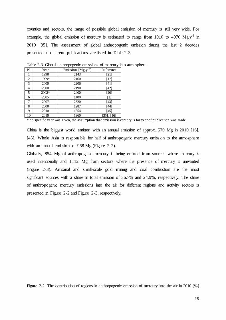
Table 2-3. Global anthropogenic emissions of mercury into atmosphere. N. Year Emission [Mg.y
-1] Reference
1 1998 2143 [21]
2 1999* 2160 [17]
3 2000 2206 [41]
4 2000 2190 [42]
5 2002* 2400 [20]
6 2005 1480 [1]
7 2007 2320 [43]
8 2008 1287 [44]
9 2010 1554 [45]
10 2010 1960 [35], [16]
* no specific year was given, the assumption that emission inventory is for year of publication was made.
China is the biggest world emitter, with an annual emission of approx. 570 Mg in 2010 [16],
[45]. Whole Asia is responsible for half of anthropogenic mercury emission to the atmosphere
with an annual emission of 968 Mg (Figure 2-2).
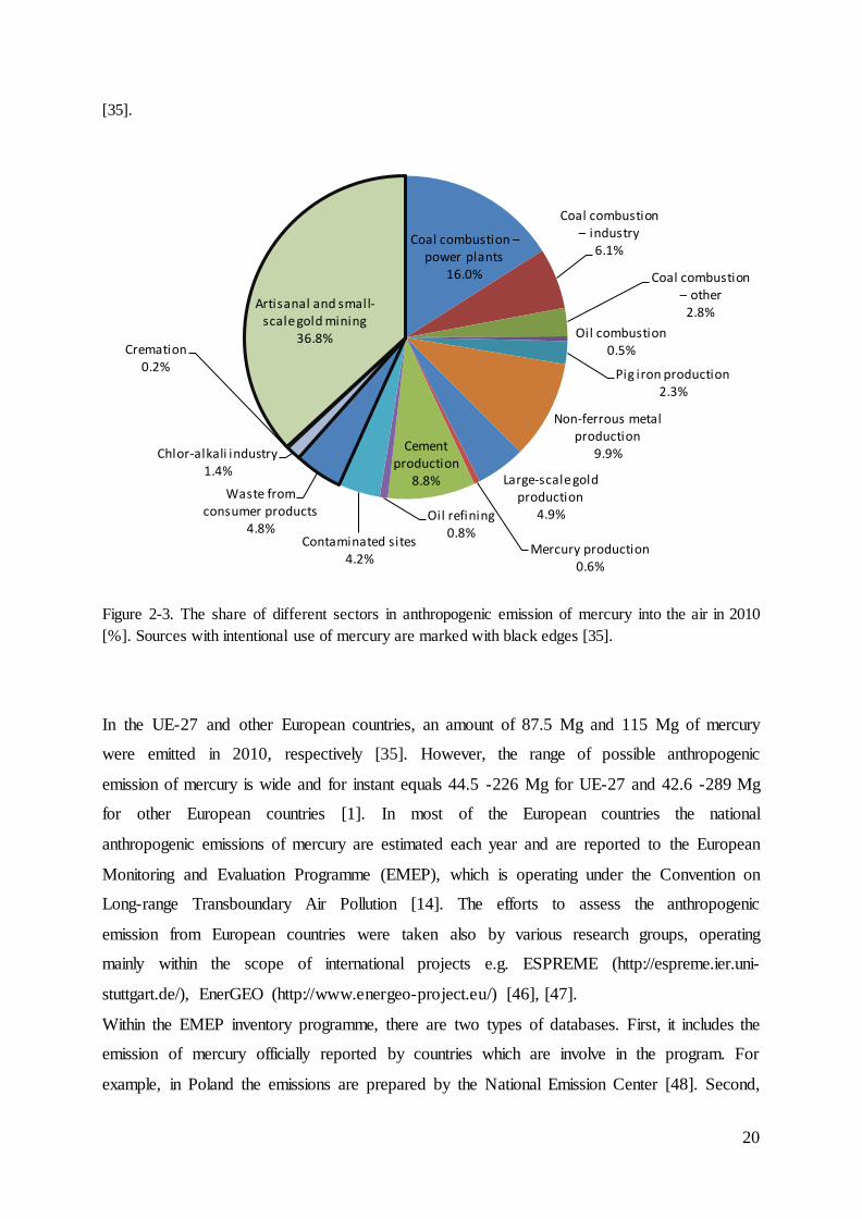
Globally, 854 Mg of anthropogenic mercury is being emitted from sources where mercury is
used intentionally and 1112 Mg from sectors where the presence of mercury is unwanted
(Figure 2-3). Artisanal and small-scale gold mining and coal combustion are the most
significant sources with a share in total emission of 36.7% and 24.9%, respectively. The share
of anthropogenic mercury emissions into the air for different regions and activity sectors is
presented in Figure 2-2 and Figure 2-3, respectively.
Figure 2-2. The contribution of regions in anthropogenic emission of mercury into the air in 2010 [%]
20
[35].
Figure 2-3. The share of different sectors in anthropogenic emission of mercury into the air in 2010
[%]. Sources with intentional use of mercury are marked with black edges [35].
In the UE-27 and other European countries, an amount of 87.5 Mg and 115 Mg of mercury
were emitted in 2010, respectively [35]. However, the range of possible anthropogenic
emission of mercury is wide and for instant equals 44.5 -226 Mg for UE-27 and 42.6 -289 Mg
for other European countries [1]. In most of the European countries the national
anthropogenic emissions of mercury are estimated each year and are reported to the European
Monitoring and Evaluation Programme (EMEP), which is operating under the Convention on
Long-range Transboundary Air Pollution [14]. The efforts to assess the anthropogenic
emission from European countries were taken also by various research groups, operating
mainly within the scope of international projects e.g. ESPREME (http://espreme.ier.uni-
stuttgart.de/), EnerGEO (http://www.energeo-project.eu/) [46], [47].
Within the EMEP inventory programme, there are two types of databases. First, it includes the
emission of mercury officially reported by countries which are involve in the program. For
example, in Poland the emissions are prepared by the National Emission Center [48]. Second,
Coal combustion – power plants
16.0%
Coal combustion – industry
6.1%
Coal combustion – other
2.8%
Oil combustion 0.5%
Pig iron production 2.3%
Non-ferrous metal production
9.9%
Large-scale gold production
4.9%
Mercury production 0.6%
Cement production
8.8%
Oil refining 0.8%
Contaminated sites 4.2%
Waste from consumer products
4.8%
Chlor-alkali industry 1.4%
Cremation 0.2%
Artisanal and small-scale gold mining
36.8%
21
the database includes the mercury emissions over Europe, which were used as the input into
the chemical transport models developed within the EMEP programme. The emissions of
mercury are used in the models after verification of data provided by the national institutions
from each country and in the case of a lack of data for some countries the estimation are
introduced by experts. The estimations are mainly prepared following a top-down approach
with the use of emission factors for defined sources.
The anthropogenic mercury emissions in the European Union (EU-27) were estimated at 100
Mg in 2008 [14]. The emissions of mercury in the European Union countries used in the
EMEP model from 2000 until 2010 decreased by one third from 120 Mg to 80 Mg. In 2010,
the highest emissions of mercury in the EU-27 were in Poland, Italy, Spain and Germany. The
emissions of mercury in European countries, which do not belong to the EU were on the same
level of nearly 60 Mg per year between 2000 -2010 (Table 2-4). In most EU-27 countries, the
reduction of the amount of mercury emitted into the air was noticeable, during the period
2000 - 2010. The most substantial decreases in mercury emission, relatively speaking, were
observed in Malta, Bulgaria and France. During that decade, the estimated amount of mercury
emitted in Germany increased 2.5 times from 3.6 Mg in 2000 to 9.3 Mg in 2010. In EU
countries, the share of 32%, 28% and 8% was estimated in the overall emission of mercury in
sectors where coal is being burned i.e. power sector (SNAP 0101), industrial combustion
(SNAP 03) and residential (SNAP 0202), respectively. In Non-EU countries, a share of 47%
was estimated to come from the power sector, 19% from industrial combustion and almost 6%
from residential. The EU member states emitted 20 Mg of mercury from industrial processes
(SNAP 04) and 4 Mg from waste and waste treatment (SNAP 09) in 2008 (Figure 2-4). The
highest emissions that originated from the power sector were observed in Poland and
Germany in the EU-28, respectively 8.7 and 6.3 Mg of emitted mercury in 2008. The highest
emissions from the residential sector and from industrial combustion were estimated in Italy,
from industrial processes in Spain and waste treatment in UK.
The accurate emission data of mercury form European Countries can be found in the report of
the Netherland’s TNO Institute (Netherlands Organisation for Applied Scientific Research
TNO- www.tno.nl) [49]. The data were prepared based on two different sources:
1. Projection, which was developed based on emission data for 2000, changes in activity
data according to baseline scenarios developed in the context of the Clean Air For
Europe (CAFÉ) program. The data for 2000 were developed with a bottom-up
approach based on activities and appropriate emission factors.

22
2. Reported emission in the context of the EMEP programme for 2007 -note that for
many countries the TNO and EMEP emissions are on the same level (Table 2-4).
The most significant difference was noticed in Russia. TNO estimated the emission in the
European part of Russia to be approximately 92 Mg, which is 4 times higher than EMEP.
Most of the mercury emitted in Russia is coming from the power sector. According to TNO
results, the highest share in the overall mercury emission into air in Europe came from
industry combustion (approx. 47% in EU-28 and 28% in Non-EU countries) and the power
sector (54% in Non-EU and 36% in EU-27).
The results of mercury emissions that were published in papers by IIASA (International
Institute for Applied Systems Analysis) were obtained using the GAINS (Greenhouse Gas and
Air Pollution Interactions and Synergies) integrated modelling tool [46]. GAINS estimates
emissions based on fuels and the sectors activity, emission factors and removal efficiency of
different forms of mercury (GEM, RGM and HgP) by pollution control equipment [45], [47].
According to this estimation Germany represents the major source of mercury emitted into air
within the EU-27 in 2010, with the total emissions being nearly two times higher than the
officially reported data from EMEP and the emissions of mercury form the power sector were
higher in Germany than in Poland (Figure 2-4). Overestimations of emissions of mercury in
Germany using the button-up approach compared to the official data was also reported in
previous work of TNO [49].
Table 2-4. Emission in European Countries in 2000, 2005, 2008 and 2010 according to the assessment of EMEP, TNO, IIASA [Mg], [14], [49], [46]. Only the countries with annual emissions over 2 Mg. Other countries i.e. Austria, Cyprus, Denmark, Estonia, Finland, Latvia, Lithuania, Luxembourg, Malta, The Netherlands, Slovenia, Sweden, Albania, Belarus, Bosnia & Herzegovina, Croatia, Iceland, Macedonia, Moldova, Norway emit together approx. 10 Mg of mercury per year.
N. Country
Source of data
EMEP
reported EMEP data used into EMEP model TNO IIASA
2008 2000 2005 2008 2010 2010 2010
1 Belgium 3.84 2.60 1.80 3.30 2.05 2.74 2.17
2 Bulgaria 1.39 4.20 3.40 1.60 0.88 1.61 3.05
3 Czech Republic 4.11 3.80 3.80 4.10 3.36 3.92 4.56
4 France 4.30 11.00 6.00 4.00 4.18 6.90 5.12
5 Germany 9.80 3.60 3.80 3.80 9.29 9.78 18.24
6 Greece 13.00 13.00 13.00 7.78 7.78 2.52
7 Hungary 3.01 3.60 3.00 3.00 0.78 2.83 2.46
8 Italy 10.38 9.60 10.00 11.00 9.52 10.71 5.88
9 Poland 15.65 26.00 20.00 16.00 14.85 15.83 15.20
10 Portugal 2.29 3.70 3.40 2.60 2.06 2.76 1.75
11 Romania 8.28 6.70 11.00 12.00 5.34 4.13 3.75
12 Slovakia 2.65 5.90 4.00 4.10 1.18 2.72 0.99
13 Spain 9.49 11.00 10.00 7.80 6.34 10.80 6.24
14 United Kingdom 6.52 8.10 7.10 6.20 6.29 7.19 6.02
23
15 Russia (European part) 10.00 14.00 23.00 22.54 92.71 17.26
16 Serbia & Montenegro 1.74 5.50 5.40 5.40 1.65 5.34 2.32
17 Switzerland 1.04 2.20 1.10 1.20 1.05 1.05 0.93
18 Turkey 18.00 20.00 22.00 22.34 22.34 15.11
19 Ukraine 6.79 26.00 6.00 6.80 6.79 7.56 7.54
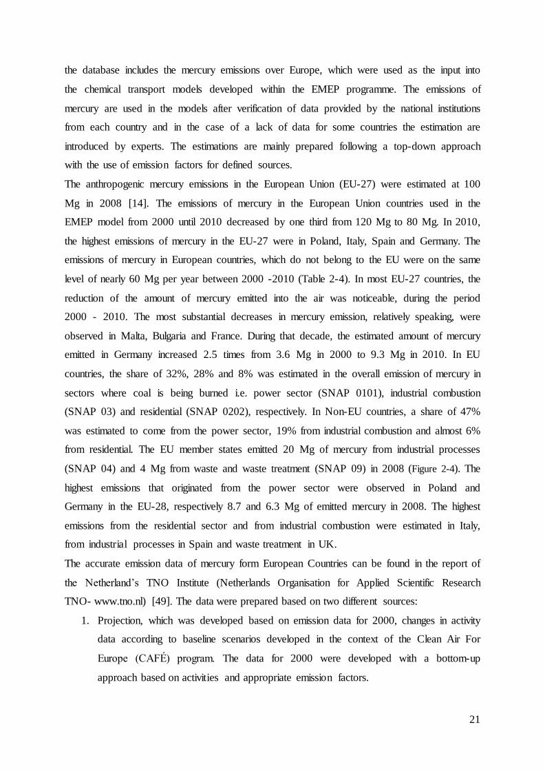
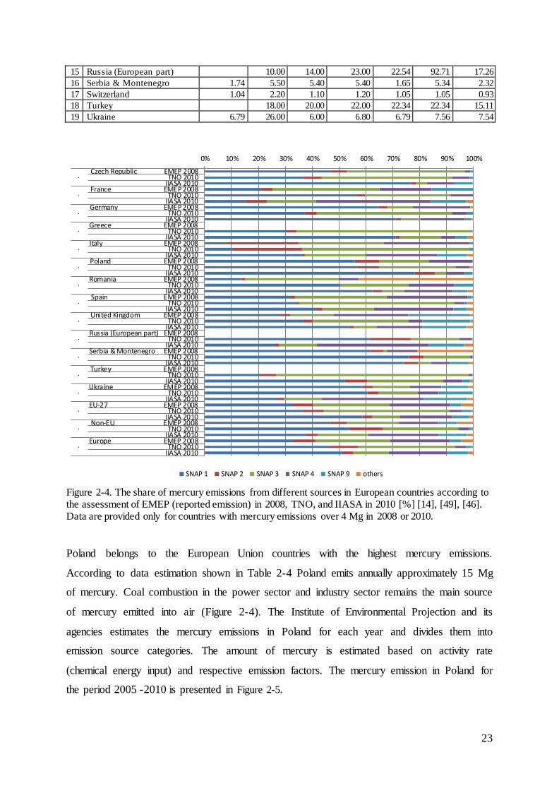
Figure 2-4. The share of mercury emissions from different sources in European countries according to the assessment of EMEP (reported emission) in 2008, TNO, and IIASA in 2010 [%] [14], [49], [46]. Data are provided only for countries with mercury emissions over 4 Mg in 2008 or 2010.
Poland belongs to the European Union countries with the highest mercury emissions.
According to data estimation shown in Table 2-4 Poland emits annually approximately 15 Mg
of mercury. Coal combustion in the power sector and industry sector remains the main source
of mercury emitted into air (Figure 2-4). The Institute of Environmental Projection and its
agencies estimates the mercury emissions in Poland for each year and divides them into
emission source categories. The amount of mercury is estimated based on activity rate
(chemical energy input) and respective emission factors. The mercury emission in Poland for
the period 2005 -2010 is presented in Figure 2-5.
0% 10% 20% 30% 40% 50% 60% 70% 80% 90% 100%
Czech Republic EMEP 2008TNO 2010
IIASA 2010France EMEP 2008
TNO 2010IIASA 2010
Germany EMEP 2008TNO 2010
IIASA 2010Greece EMEP 2008
TNO 2010IIASA 2010
Italy EMEP 2008TNO 2010
IIASA 2010Poland EMEP 2008
TNO 2010IIASA 2010
Romania EMEP 2008TNO 2010
IIASA 2010Spain EMEP 2008
TNO 2010IIASA 2010
United Kingdom EMEP 2008TNO 2010
IIASA 2010Russia (European part) EMEP 2008
TNO 2010IIASA 2010
Serbia & Montenegro EMEP 2008TNO 2010
IIASA 2010Turkey EMEP 2008
TNO 2010IIASA 2010
Ukraine EMEP 2008TNO 2010
IIASA 2010EU-27 EMEP 2008
TNO 2010IIASA 2010
Non-EU EMEP 2008TNO 2010
IIASA 2010Europe EMEP 2008
TNO 2010IIASA 2010
..
..
..
..
..
..
..
..
SNAP 1 SNAP 2 SNAP 3 SNAP 4 SNAP 9 others

24
Figure 2-5. Quantity of mercury emitted into air according to the assessment of Institute of
Environmental Projection and its agencies [kg] [50], [51], [52], [53], [54], [48], [55].
According to the data presented in Figure 2-5 emissions in Poland have decreased significantly
and in 2011 reached the level of 10 Mg. Most of the mercury is being emitted from
combustion in energy and transformation industries (SNAP 01). In this sector, mercury is
emitted from public power plants (SNAP 0101) and district heating plants (SNAP 0102).
Other sources in SNAP 01 i.e.: (i) petroleum refining plants (SNAP 0103), solid fuel
transformation plants (SNAP 0104) and coal mining, oil/gas extraction, pipeline compressors
(SNAP 0105) emit relatively low amounts of mercury. According to the national estimation
from SNAP 0103 -0105, a total of 103 kg and 75 kg of mercury were emitted in 2008 and
2009, respectively. The emissions from public power plants and CHP plants (SNAP 0101)
and district heating plants (SNAP 0102) are presented in Figure 2-6. Emissions from power
plants and CHP were split into fuel types i.e. hard or brown coal. District heating plants use
hard coal (in Poland, one heat plant, which uses brown coal operates and emits approx. 1 kg.y-
1 of mercury). Moreover, significant amounts of mercury are emitted from households (SNAP
0202), process of the production of cement and zinc (SNAP 0303, 0302) and production of
coke and electric furnace steel plant (SNAP 0402).
Figure 2-6. Annual emissons of mercury into air from power plants (PP), CHP (SNAP 0101) and district heating plants (SNAP 0102) in Poland in 2005 -2010 according to estimation of the Institute of Environmental Projection [Mg] [50], [51], [52], [54].
0
5
10
15
20
2005 2006 2007 2008 2009 2010 2011 2012 2013
Mg
SNAP 09SNAP 04SNAP 03SNAP 02SNAP 01
0
2
4
6
8
10
2005 2006 2007 2008 2009 2010
[Mg] district heating plants
PP and CHP brown coal
PP and CHP hard coal
25
As shown in Figure 2-6, the rate of emission of mercury from burning brown and hard coal
changed significantly. In the estimation which was prepared for the years 2005-2008, the
emission factors of 0.0064 and 0.004 kg.TJ-1 were used for hard and brown coal, respectively.
The estimation of mercury emission from power and CHP plants prepared for years 2009 and
2010 were based on updated emission factors of 0.0023 kg.TJ-1 for hard coal and 0.0114
kg.TJ-1 for brown coal [54]. Emission factors of 0.001498 kg.TJ-1 for hard coal and 0.006906
kg.TJ-1 for brown coal were used for 2010 [48].
The values for hard coal are similar and for brown coal are higher compared to factors
provided by the European Environment Agency (EEA) [56]. The EEA recommends to use
emission factors in the range from 0.001 kg.TJ-1 to 0.0023 kg.TJ-1 for hard coal and from
0.0021 kg.TJ-1 to 0.0049 kg.TJ-1 for brown coal, for the power sector in Europe. The high
emission rates originating from brown coal power plants were reported in other studies which
in their estimation were based on the mercury content in Polish coals [57], [58]. The
estimation of mercury emission from the power sector reported in the literature (beyond
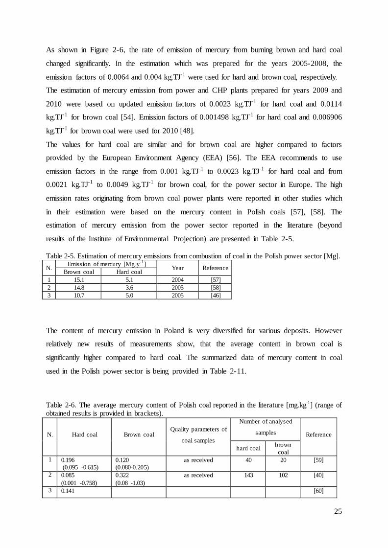
results of the Institute of Environmental Projection) are presented in Table 2-5.
Table 2-5. Estimation of mercury emissions from combustion of coal in the Polish power sector [Mg].
N. Emission of mercury [Mg.y
-1]
Year Reference Brown coal Hard coal
1 15.1 5.1 2004 [57]
2 14.8 3.6 2005 [58]
3 10.7 5.0 2005 [46]
The content of mercury emission in Poland is very diversified for various deposits. However
relatively new results of measurements show, that the average content in brown coal is
significantly higher compared to hard coal. The summarized data of mercury content in coal
used in the Polish power sector is being provided in Table 2-11.
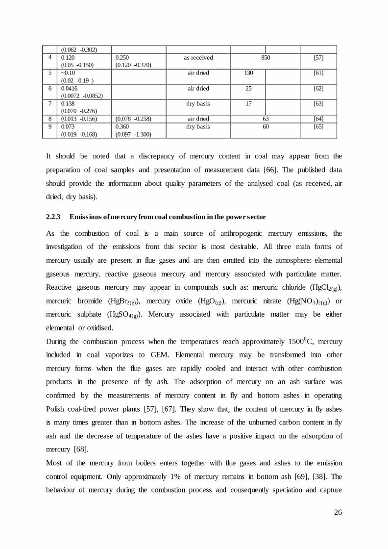
Table 2-6. The average mercury content of Polish coal reported in the literature [mg.kg-1
] (range of obtained results is provided in brackets).
N. Hard coal Brown coal Quality parameters of
coal samples
Number of analysed
samples Reference
hard coal brown
coal
1 0.196
(0.095 -0.615)
0.120
(0.080-0.205)
as received 40 20 [59]
2 0.085
(0.001 -0.758)
0.322
(0.08 -1.03)
as received 143 102 [40]
3 0.141 [60]
26
(0.062 -0.302)
4 0.120
(0.05 -0.150)
0.250
(0.120 -0.370)
as received 850 [57]
5 ~0.10
(0.02 -0.19 )
air dried 130 [61]
6 0.0416
(0.0072 -0.0852)
air dried 25 [62]
7 0.138
(0.070 -0.276)
dry basis 17 [63]
8 (0.013 -0.156) (0.078 -0.258) air dried 63 [64]
9 0.073
(0.019 -0.168)
0.360
(0.097 -1.300)
dry basis 60 [65]
It should be noted that a discrepancy of mercury content in coal may appear from the
preparation of coal samples and presentation of measurement data [66]. The published data
should provide the information about quality parameters of the analysed coal (as received, air
dried, dry basis).
2.2.3 Emissions of mercury from coal combustion in the power sector
As the combustion of coal is a main source of anthropogenic mercury emissions, the
investigation of the emissions from this sector is most desirable. All three main forms of
mercury usually are present in flue gases and are then emitted into the atmosphere: elemental
gaseous mercury, reactive gaseous mercury and mercury associated with particulate matter.
Reactive gaseous mercury may appear in compounds such as: mercuric chloride (HgCl2(g)),
mercuric bromide (HgBr2(g)), mercury oxide (HgO(g)), mercuric nitrate (Hg(NO3)2(g)) or
mercuric sulphate (HgSO4(g)). Mercury associated with particulate matter may be either
elemental or oxidised.
During the combustion process when the temperatures reach approximately 15000C, mercury
included in coal vaporizes to GEM. Elemental mercury may be transformed into other
mercury forms when the flue gases are rapidly cooled and interact with other combustion
products in the presence of fly ash. The adsorption of mercury on an ash surface was
confirmed by the measurements of mercury content in fly and bottom ashes in operating
Polish coal-fired power plants [57], [67]. They show that, the content of mercury in fly ashes
is many times greater than in bottom ashes. The increase of the unburned carbon content in fly
ash and the decrease of temperature of the ashes have a positive impact on the adsorption of
mercury [68].
Most of the mercury from boilers enters together with flue gases and ashes to the emission
control equipment. Only approximately 1% of mercury remains in bottom ash [69], [38]. The
behaviour of mercury during the combustion process and consequently speciation and capture
27
of emitted mercury from the power sector depends on many factors such as coal
characteristics (e.g. chlorine, sulphur content), temperature of combustion, residence time,
type of installed post-combustion controls and flue gas cooling rate in the pathway from the
boiler to the stack [70], [71]. It should be noted that the processes of mercury transformation
in flue gases are very complex and many factors have various influence, at the same time, and
a clear assessment of the impact of a single factor is rather difficult. Additionally, mercury is
transformed through homogeneous and heterogeneous reactions. Therefore, many developed
models of mercury transformation in flue gas, which were designed to predict mercury
speciation, do not give a clear answer about the importance of many factors [72]. Chemical
equilibrium calculations predict the complete oxidising of elemental mercury by chlorine at
temperatures of flue gases below 700K. The rate of oxidised mercury in higher temperatures
depends strongly on the chlorine content in coal, but in temperatures of approx. 1000K the
mercury should appear mainly in elemental form. Simultaneously with Hg0(g)
may appear
small amount of HgO(g) but only Hg0(g) is thermodynamically stable at temperatures above
1000K [70].
The measurement results obtained by the EPA show that the share of reactive mercury
emitted from hard coal plants is higher than from brown coal plants, which may be explained
by the relative high concentrations of halogens (chlorine, bromine) in hard coals resulting in
the oxidisation of Hg0(g) to HgII
(g). Additionally, brown coals have a relatively higher content
of alkaline material such as sodium and calcium, which also react with halogens in flue gases
resulting into lower amount of halogens available to oxidize elemental mercury [73].
Published measurement results prove that higher concentrations of chlorine and hydrogen
chloride promote a mercury oxidation in flue gases [74]. The efficiency of mercury oxidation
of HCl(g) increases together with temperatures of flue gases [75]. In contrary, Cl2(g) is less
effective in mercury oxidation along with an increase of temperature [76].
Furthermore, mercury is oxidised by NO2(g) and O2(g) in flue gases [75]. The compounds of
reactive mercury with oxygen and chlorine may further react with SO2(g) creating mercury
sulphate in the solid phase, which is the most stable form of mercury at temperatures below
490K [77]. Therefore, SO2(g), can promote the oxidation of elemental mercury through
a continuous regeneration of chlorine and hydrogen chloride in flue gases. Unfortunately, the
impact of sulphur in coal and SO2(g) in flue gases is still not completely clear and many
theories exist to explain the role of sulphur and sulphur compounds on mercury oxidation
[78]. Some experiment results show that SO2(g) can inhibit the transformation of Hg0(g) to
HgII(g), which consequently results in lower Hg removal efficiency by existing emission
28
control equipment [37]. The inhibitory effect of SO2(g) could be explained by a theory that
SO2(g) may react with chlorine causing the reduction of the amount of chlorine available to
oxidize elemental mercury or occupies mercury reaction sites on fly-ash carbon. Experiments
and modelling suggest the reaction of mercury oxidation through reactions with chlorine and
hydrogen chloride as the most important in flue gases of coal-fired power plants [37]. Results
of measurements also showed the inhibitory effect of H2O(g) and NO(g) on the mercury
oxidation processes [79].
The speciation of mercury leaving the boiler has a crucial impact on mercury capture in
existing emission control equipment. The general measurement data the of the EPA (US
Environmental Protection Agency) show that ESP (electrostatic precipitators) or FF (fabric
filter) installations are very effective in capturing mercury present in particulate matter.
Reactive mercury is more quickly removed by WFGD (wet flue gas desulfurization) than
elemental mercury due to a significantly better solubility in water [37]. In this study, more
than 230 tests of 81 power units were conducted. Mercury emissions were measured in power
plants for different fuels, boilers and emission controls combinations and are presented in
Table 2-7. The lowest mercury efficiency of mercury by different coal -boiler-control classes
result from speciation of mercury that leaves the boiler. It was observed that the share of
Hg0(g) from brown coal combustion is higher compared to hard coal combustion [37], [58],
[47]. For example in recent estimations, the general share for mercury leaving boilers of the
European power sector -before emission control installations of 55% of GEM, 35% of RGM,
10% of HgP and 60% of GEM, 30% of RGM, 10% of HgP for respectively hard and brown
coal use [47].
It was also observed that the coal cleaning method can lead to significant removal of mercury.
Two measurement campaigns where 50 samples were tested showed reduction values from 3
to 78%, with average removal of 30% and 21%. The physical cleaning of coal is used
primarily to reduce ash and pyritic sulphur. This results in the removal of mercury linked to
sulphur compounds, which are present in coal. Additionally, the lower content of sulphur in
coal may lead to more efficient transformation of elemental mercury into oxidized form, as
SO2(g) is considered as the inhibition of this process [71]. The enrichment process of coal may
remove mercury in coal up to 74% and lead to mercury emission reduction into air up to 85%
[80], [64].
29
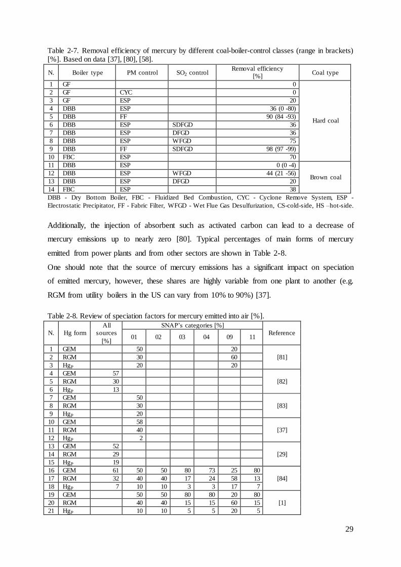
Table 2-7. Removal efficiency of mercury by different coal-boiler-control classes (range in brackets) [%]. Based on data [37], [80], [58].
N. Boiler type PM control SO2 control Removal efficiency
[%] Coal type
1 GF 0
Hard coal
2 GF CYC 0
3 GF ESP 20
4 DBB ESP 36 (0 -80)
5 DBB FF 90 (84 -93)
6 DBB ESP SDFGD 36
7 DBB ESP DFGD 36
8 DBB ESP WFGD 75
9 DBB FF SDFGD 98 (97 -99)
10 FBC ESP 70
11 DBB ESP 0 (0 -4)
Brown coal 12 DBB ESP WFGD 44 (21 -56)
13 DBB ESP DFGD 20
14 FBC ESP 38
DBB - Dry Bottom Boiler, FBC - Fluidized Bed Combustion, CYC - Cyclone Remove System, ESP -
Electrostatic Precipitator, FF - Fabric Filter, WFGD - Wet Flue Gas Desulfurization, CS-cold-side, HS –hot-side.
Additionally, the injection of absorbent such as activated carbon can lead to a decrease of
mercury emissions up to nearly zero [80]. Typical percentages of main forms of mercury
emitted from power plants and from other sectors are shown in Table 2-8.
One should note that the source of mercury emissions has a significant impact on speciation
of emitted mercury, however, these shares are highly variable from one plant to another (e.g.
RGM from utility boilers in the US can vary from 10% to 90%) [37].
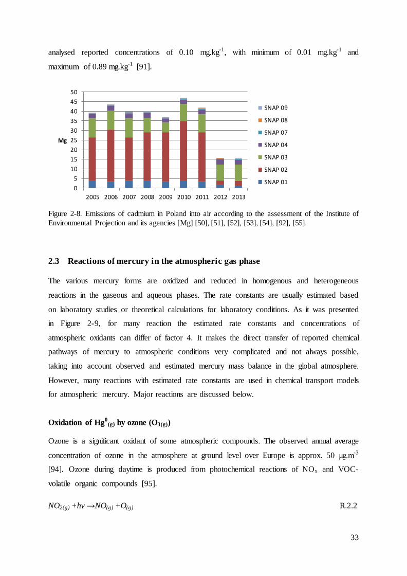
Table 2-8. Review of speciation factors for mercury emitted into air [%].
N. Hg form
All
sources
[%]
SNAP’s categories [%]
Reference 01 02 03 04 09 11
1 GEM 50 20
[81] 2 RGM 30 60
3 HgP 20 20
4 GEM 57
[82] 5 RGM 30
6 HgP 13
7 GEM 50
[83] 8 RGM 30
9 HgP 20
10 GEM 58
[37] 11 RGM 40
12 HgP 2
13 GEM 52
[29] 14 RGM 29
15 HgP 19
16 GEM 61 50 50 80 73 25 80
[84] 17 RGM 32 40 40 17 24 58 13
18 HgP 7 10 10 3 3 17 7
19 GEM 50 50 80 80 20 80
[1] 20 RGM 40 40 15 15 60 15
21 HgP 10 10 5 5 20 5
30
22 GEM 75
[58] 23 RGM 20
24 HgP 5
25 GEM 72
[44] 26 RGM 22
27 HgP 6
28 GEM 60
[47] 29 RGM 33
30 HgP 7
2.2.4 Anthropogenic emission of lead and cadmium into the air
Lead
The extensive global anthropogenic emissions of lead were estimated to equal 330 Gg.y-1 and
120 Gg.y-1, for 1983 and mid-1990s [85], [86]. At that time the main sources of emitted lead
were widely used fuel additives.
In Europe, the most comprehensive database of lead emissions into the air is presented in the
EMEP programme [14]. The emission amounts presented there are the total for countries
(without splitting into source categories), which were used in the EMEP models. The reported
data from particular countries are very fragmentary, unfortunately. According to these data,
the total emission of lead into air from the whole EMEP domain was 7.2 Gg in 2008. In EU-
28, annual emissions were estimated at 2688 Mg.y-1. The highest annual emissions among
EU-28 members states were in Poland, Greece, Bulgaria, Italy, Spain, Germany and France
respectively: 551, 470, 297, 274, 265, 116, 95 Mg. In Russia -2602 Mg, Kazakhstan -670 Mg,
Turkey -380 Mg, Ukraine -213 Mg, Uzbekistan -185 Mg of lead was emitted in 2008. In
2010, EU-28 members emitted 2237 Mg.y-1 and No-EU countries 3389 Mg y-1 [87]. TNO
reported emission for 2010 from EU-28 at 1994 Mg.y-1, wherein emissions in Poland were
estimated at 276 Mg.y-1 [49].
The major sources of lead emitted into the air in EU-28 are: (i) processes of primary and
secondary production of metals (SNAP 0303) -with share in total emissions in 2010 of 34%,
(ii) processes in iron and steel industries and collieries (SNAP 0402) -with share of 18% and
(iii) waste incineration (SNAP 0902) -9% [88].
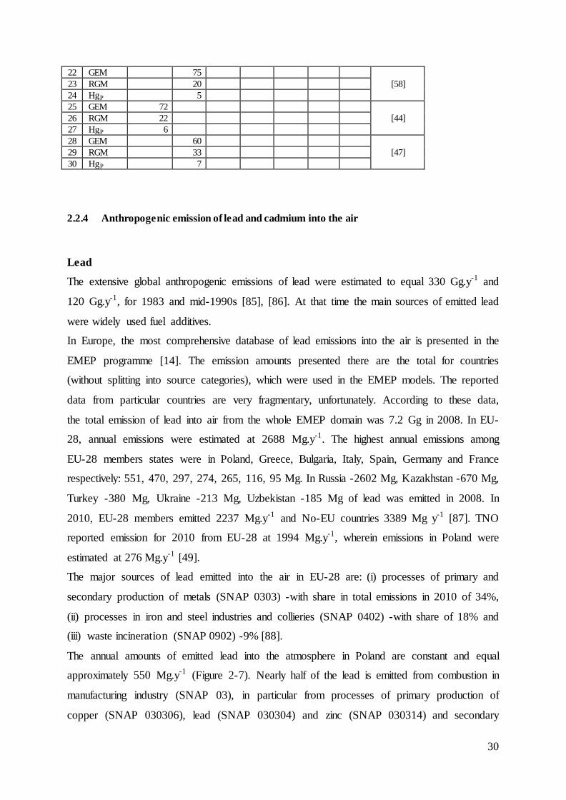
The annual amounts of emitted lead into the atmosphere in Poland are constant and equal
approximately 550 Mg.y-1 (Figure 2-7). Nearly half of the lead is emitted from combustion in
manufacturing industry (SNAP 03), in particular from processes of primary production of
copper (SNAP 030306), lead (SNAP 030304) and zinc (SNAP 030314) and secondary
31
production of copper (SNAP 030309). In Poland were emitted 113 Mg and 14 Mg of lead
from processes of primary and secondary production of copper in 2008, respectively. The
primary production of lead caused emissions into the atmosphere to equal 48 Mg.y-1 and
primary production of zinc 15 Mg.y-1. Annually approximately 111 Mg of lead was released
from coal burning in households (SNAP 0202).
The share of combustion in the energy and transformation industries sector (SNAP 01) in total
emission is relatively small and equals around 5%. Half of this emission, approximately 12
Mg, is coming from district heating plants (SNAP 0102). Public power plants (SNAP 0101)
emitted 8.2 Mg from hard coal and 2 Mg from brown coal combustion in 2008. The annual
emission of lead in the years of 2005 -2013 from public power plants were almost on the same
level. The rather slight variation of emitted amounts between the years resulted from the
activity of fuels. The applied emission factors were constant in the period of 2005 -2013 and
equal 0.009 kg.TJ-1 for hard coal power plants, 0.0038 kg.TJ-1 for brown power plants and
0.1024 kg.TJ-1 for district heat plants where hard coal was being used. The concentration of
lead in world coal ranges from 0.7 to 220 mg.kg-1 [89]. The mean concentration of lead in
coal of the Upper Silesian Coal Basin equals 30.5 mg.kg-1 and in the Polish brown coal 6.27
mg.kg-1 [90], [91]. Lead in the analysed coal of the Upper Silesian Coal Basin is mainly from
inorganic origin.
Figure 2-7. Emission of lead in Poland into air according to the assessment of the Institute of
Environmental Projection and its agencies [Mg] [50], [51], [52], [53], [54], [92], [55].
0
100
200
300
400
500
600
700
2005 2006 2007 2008 2009 2010 2011 2012 2013
Mg
SNAP 09
SNAP 07
SNAP 04
SNAP 03
SNAP 02
SNAP 01

32
Cadmium
The global emissions of cadmium into air were estimated to equal 7570 Mg.y-1, for 1983 [85].
The emissions in the next decade (in mid-1990s) were lower and equalled 2983 Mg.y-1 [86].
The contribution of non-ferrous metal production, stationary fossil fuel combustion, iron and
steel production, cement production and waste disposal in total annual cadmium emissions
were 73%, 23%, 2%, 1% and 1%, respectively.
According to the EMEP database (used in the model), annual emissions of cadmium into air
from whole domain equalled 265 Mg in 2005, 286 Mg in 2008 and 137 Mg in 2010 [14].
Emissions in the EU-28 member states also decreased and equalled 139 Mg.y-1 in 2005, 117
Mg.y-1 in 2008 and 102 Mg.y-1 in 2010. TNO estimated the emission of cadmium in EU-28 at
118 Mg.y-1 in 2010 [49]. Poland is responsible for 35% of this amount. Next in order is
Slovakia where annually 10 times less cadmium is emitted, compared to Poland.
In all EU-28 member states, 27% of total emission derived from residential plants (SNAP
0202), 13% from stationary combustion in manufacturing industries and construction (SNAP
03), 12% from public power sector (SNAP 0101), 10% -from iron and steel production
(SNAP 0402) in 2010 [88].
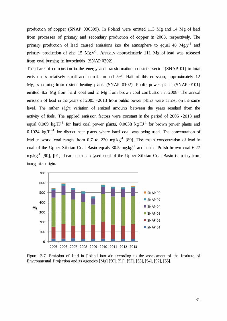
In Poland in the years 2005 -2011 the main source of emission of cadmium was the non-
industrial combustion plants sector (SNAP 02), mainly hard coal combustion in households
(SNAP 0202). The relatively newest estimation prepared for 2012 and 2013 shows about 10
times lower emissions from this sector compared to earlier years [55]. Additionally in 2012
and 2013 the emissions from combustion in energy and transformation (SNAP 01) decreased
significantly. The emissions of cadmium from this sector were 9.3% and 3.0% of the overall
national emissions in Poland in 2008 and 2013, respectively. In this sector, in 2008 cadmium
was released especially from district power plants (SNAP 0102) -1939 kg.y-1 and petroleum
refining plants (SNAP 0103) -1067 kg.y-1. Hard coal power plants emitted 110 kg and brown
coal power plants 68 kg of cadmium in 2008. For power plants based on both hard and brown
coal, 0.0001 kg.TJ-1 and for district heating plants 0.0164 kg.TJ-1 emission factors for years
2005 -2011 were used. [50]. The concentration of cadmium in world coals is very diverse and
ranges from 0.01 up to 300 mg.kg-1 [89]. The Polish coal, both hard and brown is
characterized by comparatively low content of cadmium. The most complex measurement
campaign in Poland including 147 and 108 samples of polish hard and brown coal resulted in
an average concentration of cadmium in hard coal of 0.2 mg.kg-1 and 0.3 mg.kg-1 in brown
coal [93]. In this study, the maximum concentrations of cadmium of 7.7 mg.kg-1 in hard coal
and 2.0 mg.kg-1 in brown coal samples were reported. Another study where 30 samples were
33
analysed reported concentrations of 0.10 mg.kg-1, with minimum of 0.01 mg.kg-1 and
maximum of 0.89 mg.kg-1 [91].
Figure 2-8. Emissions of cadmium in Poland into air according to the assessment of the Institute of
Environmental Projection and its agencies [Mg] [50], [51], [52], [53], [54], [92], [55].
2.3 Reactions of mercury in the atmospheric gas phase
The various mercury forms are oxidized and reduced in homogenous and heterogeneous
reactions in the gaseous and aqueous phases. The rate constants are usually estimated based
on laboratory studies or theoretical calculations for laboratory conditions. As it was presented
in Figure 2-9, for many reaction the estimated rate constants and concentrations of
atmospheric oxidants can differ of factor 4. It makes the direct transfer of reported chemical
pathways of mercury to atmospheric conditions very complicated and not always possible,
taking into account observed and estimated mercury mass balance in the global atmosphere.
However, many reactions with estimated rate constants are used in chemical transport models
for atmospheric mercury. Major reactions are discussed below.
Oxidation of Hg0(g) by ozone (O3(g))
Ozone is a significant oxidant of some atmospheric compounds. The observed annual average
concentration of ozone in the atmosphere at ground level over Europe is approx. 50 µg.m-3
[94]. Ozone during daytime is produced from photochemical reactions of NOx and VOC-
volatile organic compounds [95].
NO2(g) +hv →NO(g) +O(g) R.2.2
0
5
10
15
20
25
30
35
40
45
50
2005 2006 2007 2008 2009 2010 2011 2012 2013
Mg
SNAP 09
SNAP 08
SNAP 07
SNAP 04
SNAP 03
SNAP 02
SNAP 01
34
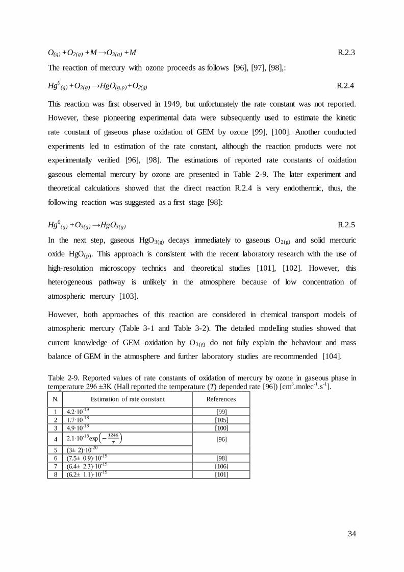
O(g) +O2(g) +M →O3(g) +M R.2.3
The reaction of mercury with ozone proceeds as follows [96], [97], [98],:
Hg0(g) +O3(g) →HgO(g,p)+O2(g) R.2.4
This reaction was first observed in 1949, but unfortunately the rate constant was not reported.
However, these pioneering experimental data were subsequently used to estimate the kinetic
rate constant of gaseous phase oxidation of GEM by ozone [99], [100]. Another conducted
experiments led to estimation of the rate constant, although the reaction products were not
experimentally verified [96], [98]. The estimations of reported rate constants of oxidation
gaseous elemental mercury by ozone are presented in Table 2-9. The later experiment and
theoretical calculations showed that the direct reaction R.2.4 is very endothermic, thus, the
following reaction was suggested as a first stage [98]:
Hg0(g) +O3(g) →HgO3(g) R.2.5
In the next step, gaseous HgO3(g) decays immediately to gaseous O2(g) and solid mercuric
oxide HgO(p). This approach is consistent with the recent laboratory research with the use of
high-resolution microscopy technics and theoretical studies [101], [102]. However, this
heterogeneous pathway is unlikely in the atmosphere because of low concentration of
atmospheric mercury [103].
However, both approaches of this reaction are considered in chemical transport models of
atmospheric mercury (Table 3-1 and Table 3-2). The detailed modelling studies showed that
current knowledge of GEM oxidation by O3(g) do not fully explain the behaviour and mass
balance of GEM in the atmosphere and further laboratory studies are recommended [104].
Table 2-9. Reported values of rate constants of oxidation of mercury by ozone in gaseous phase in temperature 296 ±3K (Hall reported the temperature (T) depended rate [96]) [cm
3.molec
-1.s
-1].
N. Estimation of rate constant References
1 4.2·10-19
[99]
2 1.7·10-18
[105]
3 4.9·10-18
[100]
4 2.1·10-18
exp(−1246
𝑇) [96]
5 (3± 2)·10
-20
6 (7.5± 0.9)·10-19
[98]
7 (6.4± 2.3)·10-19
[106]
8 (6.2± 1.1)·10-19
[101]
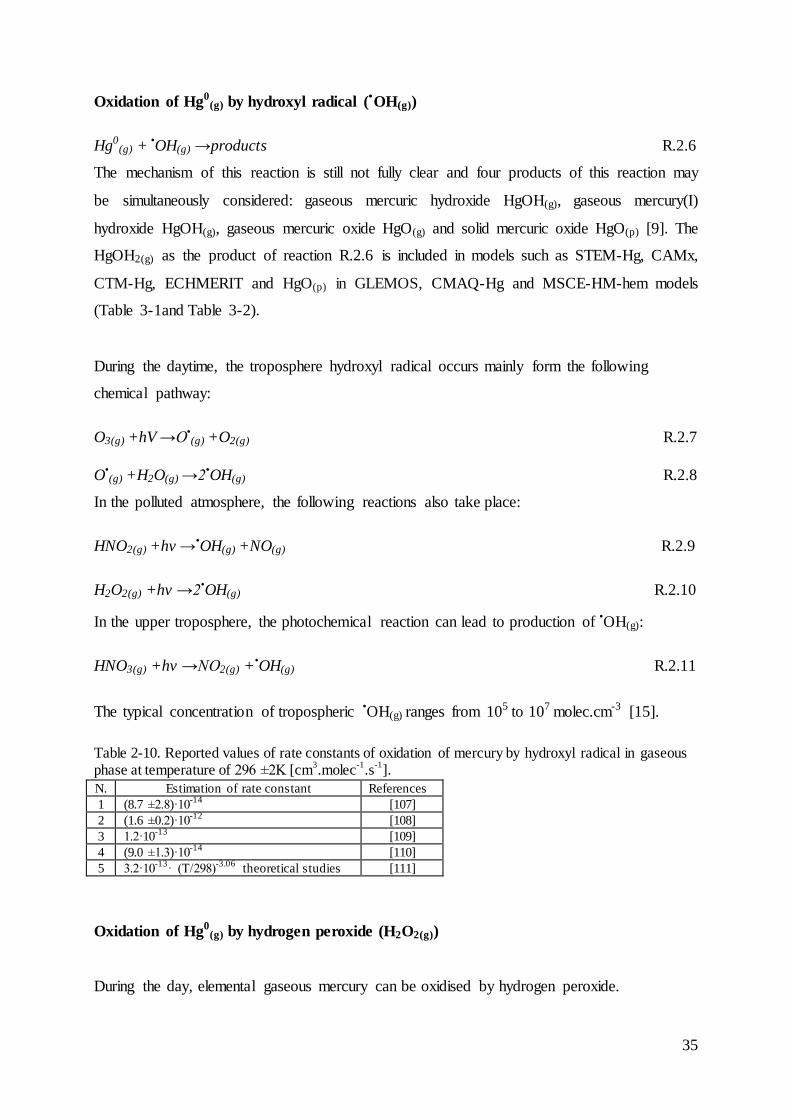
35
Oxidation of Hg0(g) by hydroxyl radical (•OH(g))
Hg0(g) +
•OH(g) →products R.2.6
The mechanism of this reaction is still not fully clear and four products of this reaction may
be simultaneously considered: gaseous mercuric hydroxide HgOH(g), gaseous mercury(I)
hydroxide HgOH(g), gaseous mercuric oxide HgO(g) and solid mercuric oxide HgO(p) [9]. The
HgOH2(g) as the product of reaction R.2.6 is included in models such as STEM-Hg, CAMx,
CTM-Hg, ECHMERIT and HgO(p) in GLEMOS, CMAQ-Hg and MSCE-HM-hem models
(Table 3-1and Table 3-2).
During the daytime, the troposphere hydroxyl radical occurs mainly form the following
chemical pathway:
O3(g) +hV →O•(g) +O2(g)
R.2.7
O•(g) +H2O(g) →2•OH(g)
R.2.8
In the polluted atmosphere, the following reactions also take place:
HNO2(g) +hv →•OH(g) +NO(g) R.2.9
H2O2(g) +hv →2•OH(g) R.2.10
In the upper troposphere, the photochemical reaction can lead to production of •OH(g):
HNO3(g) +hv →NO2(g) +•OH(g) R.2.11
The typical concentration of tropospheric •OH(g) ranges from 105 to 107 molec.cm-3 [15].
Table 2-10. Reported values of rate constants of oxidation of mercury by hydroxyl radical in gaseous phase at temperature of 296 ±2K [cm
3.molec
-1.s
-1].
N. Estimation of rate constant References
1 (8.7 ±2.8)·10-14
[107]
2 (1.6 ±0.2)·10-12
[108]
3 1.2·10-13
[109]
4 (9.0 ±1.3)·10-14
[110]
5 3.2·10-13
· (T/298)-3.06
theoretical studies
[111]
Oxidation of Hg0(g) by hydrogen peroxide (H2O2(g))
During the day, elemental gaseous mercury can be oxidised by hydrogen peroxide.
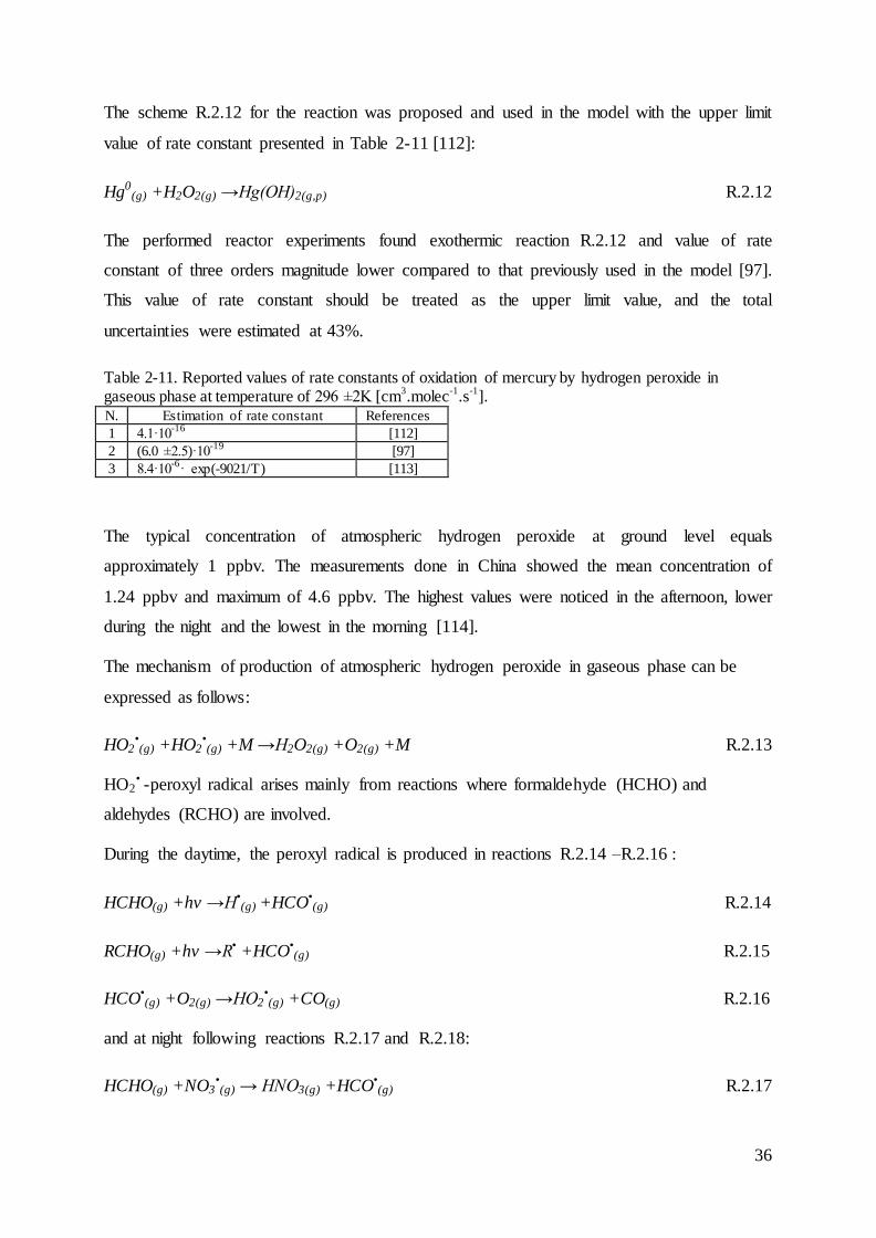
36
The scheme R.2.12 for the reaction was proposed and used in the model with the upper limit
value of rate constant presented in Table 2-11 [112]:
Hg0(g) +H2O2(g) →Hg(OH)2(g,p) R.2.12
The performed reactor experiments found exothermic reaction R.2.12 and value of rate
constant of three orders magnitude lower compared to that previously used in the model [97].
This value of rate constant should be treated as the upper limit value, and the total
uncertainties were estimated at 43%.
Table 2-11. Reported values of rate constants of oxidation of mercury by hydrogen peroxide in gaseous phase at temperature of 296 ±2K [cm
3.molec
-1.s
-1].
N. Estimation of rate constant References
1 4.1·10-16
[112]
2 (6.0 ±2.5)·10-19
[97]
3 8.4·10-6
· exp(-9021/T) [113]
The typical concentration of atmospheric hydrogen peroxide at ground level equals
approximately 1 ppbv. The measurements done in China showed the mean concentration of
1.24 ppbv and maximum of 4.6 ppbv. The highest values were noticed in the afternoon, lower
during the night and the lowest in the morning [114].
The mechanism of production of atmospheric hydrogen peroxide in gaseous phase can be
expressed as follows:
HO2•(g) +HO2
•(g) +M →H2O2(g) +O2(g) +M R.2.13
HO2• -peroxyl radical arises mainly from reactions where formaldehyde (HCHO) and
aldehydes (RCHO) are involved.
During the daytime, the peroxyl radical is produced in reactions R.2.14 –R.2.16 :
HCHO(g) +hv →H•(g) +HCO•
(g) R.2.14
RCHO(g) +hv →R• +HCO•(g) R.2.15
HCO•(g) +O2(g) →HO2
•(g) +CO(g) R.2.16
and at night following reactions R.2.17 and R.2.18:
HCHO(g) +NO3•(g) → HNO3(g) +HCO•
(g) R.2.17
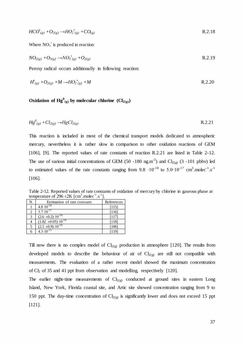
37
HCO•(g) +O2(g) →HO2
•(g) +CO(g)
R.2.18
Where NO3• is produced in reaction:
NO2(g) +O3(g) →NO3•(g) +O2(g) R.2.19
Peroxy radical occurs additionally in following reaction:
H•(g) +O2(g) +M →HO2
•(g) +M R.2.20
Oxidation of Hg0(g) by molecular chlorine (Cl2(g))
Hg0(g) +Cl2(g) →HgCl2(g) R.2.21
This reaction is included in most of the chemical transport models dedicated to atmospheric
mercury, nevertheless it is rather slow in comparison to other oxidation reactions of GEM
[106], [9]. The reported values of rate constants of reaction R.2.21 are listed in Table 2-12.
The use of various initial concentrations of GEM (50 -180 ng.m-3) and Cl2(g) (3 -101 pbbv) led
to estimated values of the rate constants ranging from 9.8 ·10-18 to 5.0·10-17 cm3.molec-1.s-1
[106].
Table 2-12. Reported values of rate constants of oxidation of mercury by chlorine in gaseous phase at temperature of 296 ±2K [cm
3.molec
-1.s
-1].
N. Estimation of rate constant References
1 4.8·10-18
[115]
2 5.7·10-17
[116]
3 (2.6 ±0.2)·10-18
[117]
4 (1.82 ±0.05)·10-19
[118]
5 (2.5 ±0.9)·10-18
[106]
6 4.3·10-15
[119]
Till now there is no complex model of Cl2(g) production in atmosphere [120]. The results from
developed models to describe the behaviour of air of Cl2(g) are still not compatible with
measurements. The evaluation of a rather recent model showed the maximum concentration
of Cl2 of 35 and 41 ppt from observation and modelling, respectively [120].
The earlier night-time measurements of Cl2(g) conducted at ground sites in eastern Long
Island, New York, Florida coastal site, and Artic site showed concentration ranging from 9 to
150 ppt. The day-time concentration of Cl2(g) is significantly lower and does not exceed 15 ppt
[121].
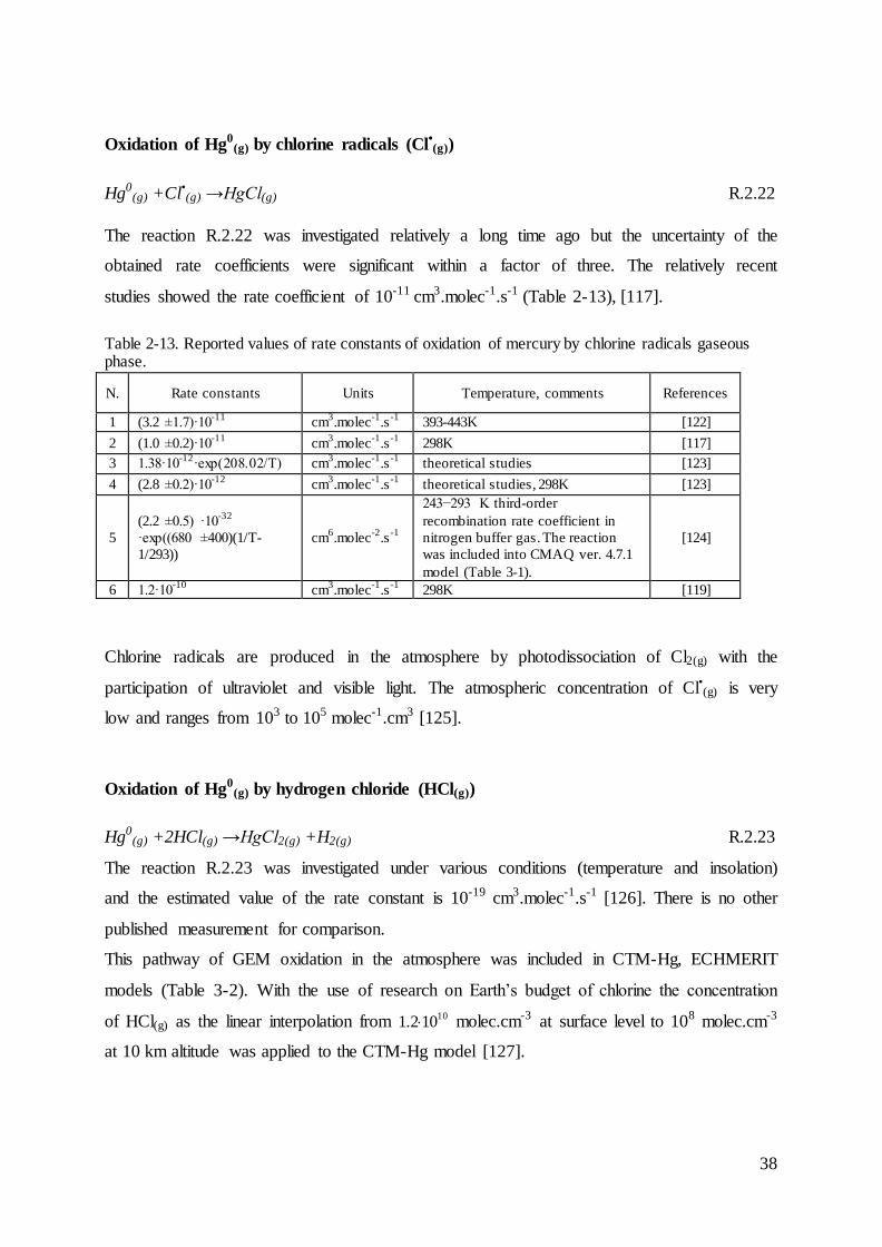
38
Oxidation of Hg0(g) by chlorine radicals (Cl•(g))
Hg0(g) +Cl•(g) →HgCl(g) R.2.22
The reaction R.2.22 was investigated relatively a long time ago but the uncertainty of the
obtained rate coefficients were significant within a factor of three. The relatively recent
studies showed the rate coefficient of 10-11 cm3.molec-1.s-1 (Table 2-13), [117].
Table 2-13. Reported values of rate constants of oxidation of mercury by chlorine radicals gaseous phase.
N. Rate constants Units Temperature, comments References
1 (3.2 ±1.7)·10-11
cm3.molec
-1.s
-1 393-443K [122]
2 (1.0 ±0.2)·10-11
cm3.molec
-1.s
-1 298K [117]
3 1.38·10-12
·exp(208.02/T) cm3.molec
-1.s
-1 theoretical studies [123]
4 (2.8 ±0.2)·10-12
cm3.molec
-1.s
-1 theoretical studies, 298K [123]
5
(2.2 ±0.5) ·10-32
·exp((680 ±400)(1/T-
1/293))
cm6.molec
-2.s
-1
243−293 K third-order
recombination rate coefficient in
nitrogen buffer gas. The reaction
was included into CMAQ ver. 4.7.1
model (Table 3-1).
[124]
6 1.2·10-10
cm3.molec
-1.s
-1 298K [119]
Chlorine radicals are produced in the atmosphere by photodissociation of Cl2(g) with the
participation of ultraviolet and visible light. The atmospheric concentration of Cl•(g) is very
low and ranges from 103 to 105 molec-1.cm3 [125].
Oxidation of Hg0(g) by hydrogen chloride (HCl(g))
Hg0(g) +2HCl(g) →HgCl2(g) +H2(g) R.2.23
The reaction R.2.23 was investigated under various conditions (temperature and insolation)
and the estimated value of the rate constant is 10-19 cm3.molec-1.s-1 [126]. There is no other
published measurement for comparison.
This pathway of GEM oxidation in the atmosphere was included in CTM-Hg, ECHMERIT
models (Table 3-2). With the use of research on Earth’s budget of chlorine the concentration
of HCl(g) as the linear interpolation from 1.21010
molec.cm-3 at surface level to 108 molec.cm-3
at 10 km altitude was applied to the CTM-Hg model [127].
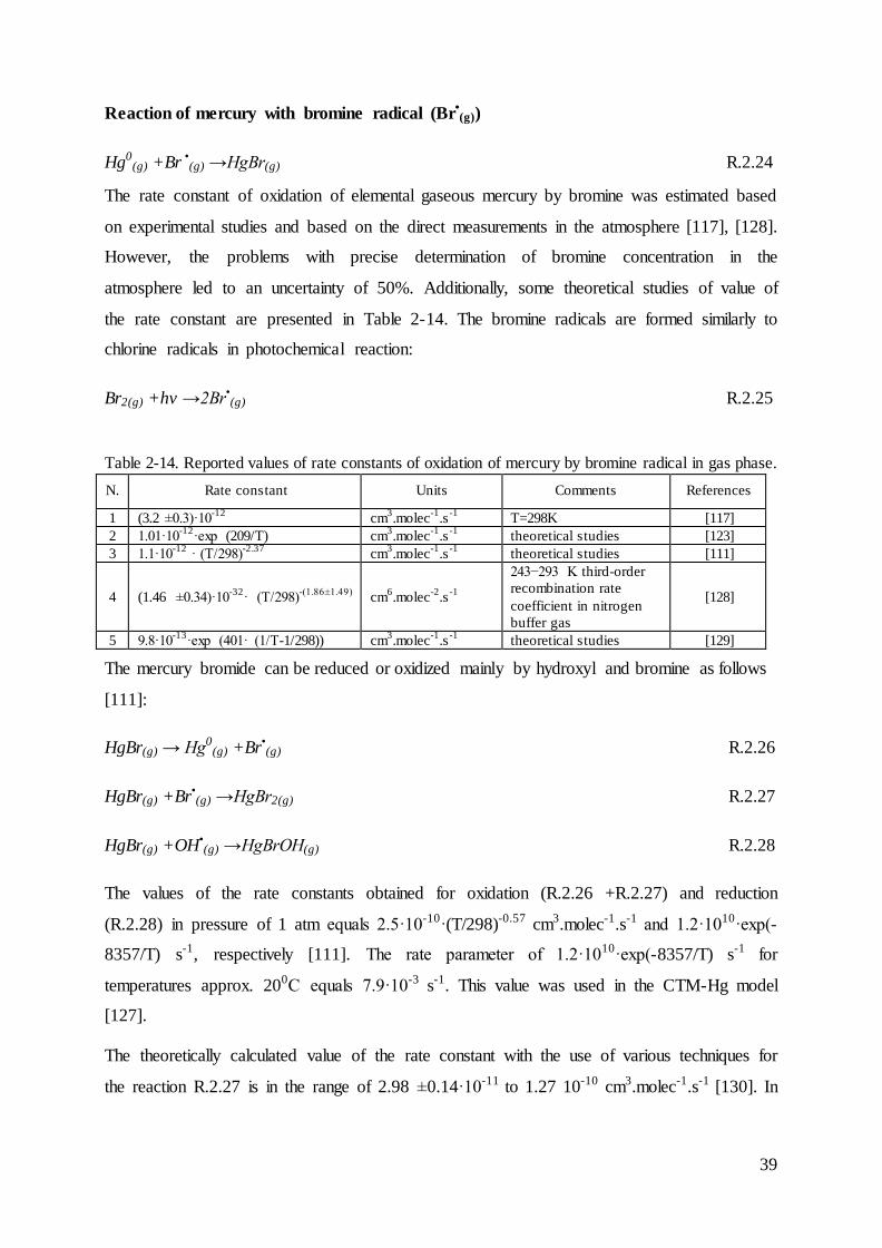
39
Reaction of mercury with bromine radical (Br•(g))
Hg0(g) +Br
•(g) →HgBr(g) R.2.24
The rate constant of oxidation of elemental gaseous mercury by bromine was estimated based
on experimental studies and based on the direct measurements in the atmosphere [117], [128].
However, the problems with precise determination of bromine concentration in the
atmosphere led to an uncertainty of 50%. Additionally, some theoretical studies of value of
the rate constant are presented in Table 2-14. The bromine radicals are formed similarly to
chlorine radicals in photochemical reaction:
Br2(g) +hv →2Br•(g) R.2.25
Table 2-14. Reported values of rate constants of oxidation of mercury by bromine radical in gas phase.
N. Rate constant Units Comments References
1 (3.2 ±0.3)·10-12
cm3.molec
-1.s
-1 T=298K [117]
2 1.01·10-12
·exp
(209/T) cm3.molec
-1.s
-1 theoretical studies [123]
3 1.1·10-12
· (T/298)-2.37
cm3.molec
-1.s
-1 theoretical studies [111]
4 (1.46 ±0.34)·10-32
· (T/298)-(1.86±1.49)
cm6.molec
-2.s
-1
243−293 K third-order
recombination rate
coefficient in nitrogen
buffer gas
[128]
5 9.8·10-13
·exp (401· (1/T-1/298)) cm3.molec
-1.s
-1 theoretical studies [129]
The mercury bromide can be reduced or oxidized mainly by hydroxyl and bromine as follows
[111]:
HgBr(g) → Hg0(g) +Br•
(g) R.2.26
HgBr(g) +Br•(g) →HgBr2(g) R.2.27
HgBr(g) +OH•(g) →HgBrOH(g) R.2.28
The values of the rate constants obtained for oxidation (R.2.26 +R.2.27) and reduction
(R.2.28) in pressure of 1 atm equals 2.5·10-10·(T/298)-0.57 cm3.molec-1.s-1 and 1.2·1010·exp(-
8357/T) s-1, respectively [111]. The rate parameter of 1.2·1010·exp(-8357/T) s-1 for
temperatures approx. 200C equals 7.9·10-3 s-1. This value was used in the CTM-Hg model
[127].
The theoretically calculated value of the rate constant with the use of various techniques for
the reaction R.2.27 is in the range of 2.98 ±0.14·10-11 to 1.27 10-10 cm3.molec-1.s-1 [130]. In
40
the same studies the additional reduction reaction R.2.29 was also proposed with a theoretical
rate constant of 3.89 ±0.17·10-11 cm3.molec-1.s-1 [130].
HgBr(g) +Br•(g) →Hg0
(g) +Br2(g) R.2.29
The ambient concentration of Br•(g)
ranges from 105 molec.cm-3 to 107 molec.cm-3 [117],
[128]. However, it should be noted that the measurements of concentration of bromine and
bromine compounds in the atmosphere are very limited and in some modelling studies the
assumed concentration of Br•(g) equals 0.01 of BrO•
(g) [131], [127].
Oxidation of Hg0
(g) by molecular bromine (Br2(g))
The gaseous mercury dibromide HgBr2(g) can also be produced in reaction:
Hg0(g) +Br2(g) →HgBr2(g) R.2.30
The rate constant less than 0.9 ±02·10-16 cm3.molec-1.s-1 was estimated based on experimental
results at 298K and 0.99 atm [117], [125]. Two other experiments were conducted with Hg0(g)
initial conditions of 93 and 55 ng.m-3, Br2(g) concentration of 2 ppb and 1 ppb at 35% and 30%
relative humidity (RH), respectively [106]. No evidence of Hg0(g) loss in the presence of Br2(g)
was observed, however during the experiments the concentration of RGM and HgP, and
deposition of Hg0(g) were not measured. The theoretical rate constant equals ~2.8·10-19
cm3.molec-1.s-1 at 298K [130]. The atmospheric concentration of Br2(g) ranges from 105
molec.cm-3 to 109 molec.cm-3 [125], [131] .
Oxidation of Hg0(g) by bromine oxide radical (BrO•
(g))
The oxidation of elemental gaseous mercury by BrO•(g), can lead to production of two
chemical compounds [132]:
Hg0(g) +BrO•
(g) →HgO(g) +Br(g) R.2.31
or
Hg0(g) +BrO•
(g) →HgBr(g) +O(g) R.2.32
The experimental works provided to estimate the rate constant of 1.5·10-14 cm3.molec-1.s-1 and
also identify HgBrO(g) and HgOBr(g) as the products of reaction [133]. This homogeneous
reaction is significantly endothermic [129], [133].
The BrO•(g) is produced in the atmosphere in the reaction :
41
Br•(g) +O3(g) →BrO•
(g) +O2(g) R.2.33
The atmospheric concentration of BrO•(g) equals 107 -109 molec.cm-3 [125], [131], [132].
BrO•(g) is mainly produced in height-latitude marine boundary layer at the beginning of the
day [131].
The modelling studies showed that the reactions of elemental gaseous mercury with bromine
and bromine monoxide fulfil the significant role in depletion of GEM during polar spring time
in observed phenomena which are called the atmospheric mercury depletion events (AMDE)
[134].
Oxidation of Hg0(g) by nitrate radical (NO3
•(g))
Hg0(g) +NO3
•(g) →HgO(g) +NO2(g) R.2.34
NO3•(g) is produced in reaction of
NO2(g) +O3(g) →NO3•(g) +O2(g) R.2.35
But during the day, it quickly disappears through photoreactions:
NO3•(g) +hv →NO(g) +O2(g) R.2.36
NO3•(g) +hv →NO2(g) +O(g) R.2.37
Therefore, the reactions of mercury with the nitrate radical occurs mostly at night [15].
The rate constant was assessed of 4·10-15 cm3.molec-1.s-1, but is should be treated as an upper
limit value [135]. Based on this rate constant, a half-life of approximately 20 days of GEM
due to NO3•(g) oxidation, with assumption of NO3
•(g) concentration of 108 molec.cm-3 was
calculated [15].
Other studies on reaction R.2.34 led to obtain three upper limit rate constants of (i) 7·10-15, (ii)
1.3·10-14 and (iii) 3·10-14 cm3.molec-1.s-1 [106].
Till now this reaction was included only in the ECHMERIT model (Table 3-2).
Oxidation of Hg0(g) by molecular iodine (I2(g))
Hg0
(g) +I2 (g) →HgI2(g) R.2.38
Beyond HgI2(g), also HgIO(g) or HgOI(g) were identified as the reaction products [136]. The
estimated value of the rate constant is (1.27 ±0.58)·10-19 cm3.molec-1.s-1. The concentration of
molecular iodine in the coastal air can reach 300 ppt, but usually the measurement stations
noticed concentration of approx. 20 ppt [137].
42
Oxidation of Hg0(g) by molecular fluorine (F2(g))
Hg0(g) +F2(g) →HgF2(g) R.2.39
Several experiments with the use of various initial condition of Hg0(g) (44 -140 ng.m-3) and F2
(4 -29 ppbv) led to estimates of the rate constant in a range from 1.3·10-15 to 2.2·10-15 with an
average of 1.8·10-15 cm3.molec-1.s-1 [106]. The typical average annual concentration of
fluorine in the air should not exceed several µg.m-3. For example in Krakow the annual
average concentration of approx. 1 µg.m-3 was observed [138].
The half-life of atmospheric elemental gaseous mercury due to oxidation in the gaseous phase
are presented in Figure 2-9. The lower half-life indicates the most effective reaction under
atmospheric conditions. The ranges of concentration of most of oxidants are rather wide,
because these atmospheric species are rarely measured, and many possible value of air
concentration are modelled. Extensive measurements of atmospheric ozone result in rather
accurate determination of it ambient concentration. Looking at Figure 2-9, the most effective
oxidation of GEM can be NO3•(g), Br•
(g), Cl•(g), F2(g). However, it should be noted that most of
the presented values of rate constants were calculated based on laboratory or theoretical
studies and these values may not be relevant for atmospheric conditions. The next part of this
manuscript is devoted to a large extent to determine the most appropriate reaction and values
that should be used in the model. Furthermore, sensitivity studies are conducted to determine
the influence of various reactions with different rate constants on modelling results.
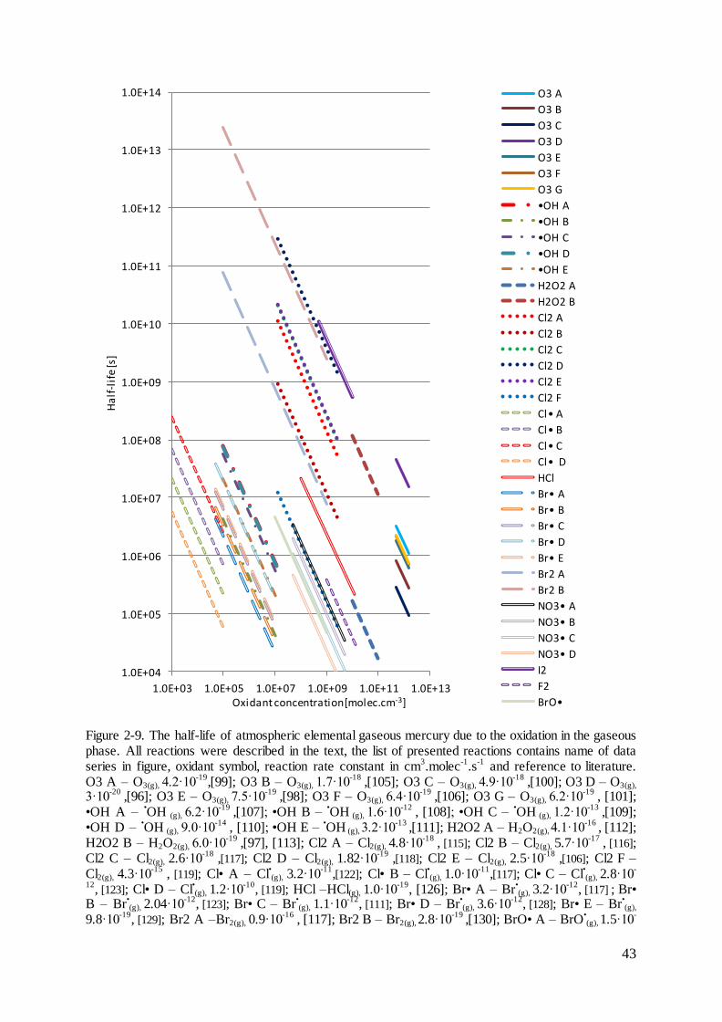
43
Figure 2-9. The half-life of atmospheric elemental gaseous mercury due to the oxidation in the gaseous phase. All reactions were described in the text, the list of presented reactions contains name of data series in figure, oxidant symbol, reaction rate constant in cm
3.molec
-1.s
-1 and reference to literature.
O3 A – O3(g), 4.2·10-19
,[99]; O3 B – O3(g), 1.7·10-18
,[105]; O3 C – O3(g), 4.9·10-18
,[100]; O3 D – O3(g), 3·10
-20 ,[96]; O3 E – O3(g), 7.5·10
-19 ,[98]; O3 F – O3(g), 6.4·10
-19 ,[106]; O3 G – O3(g), 6.2·10
-19 , [101];
•OH A – •OH (g), 6.2·10
-19 ,[107]; •OH B –
•OH (g), 1.6·10
-12 , [108]; •OH C –
•OH (g), 1.2·10
-13 ,[109];
•OH D – •OH (g), 9.0·10
-14 , [110]; •OH E –
•OH (g), 3.2·10
-13 ,[111]; H2O2 A – H2O2(g), 4.1·10
-16 , [112];
H2O2 B – H2O2(g), 6.0·10-19
,[97], [113]; Cl2 A – Cl2(g), 4.8·10-18
, [115]; Cl2 B – Cl2(g), 5.7·10-17
, [116]; Cl2 C – Cl2(g), 2.6·10
-18 ,[117]; Cl2 D – Cl2(g), 1.82·10
-19 ,[118]; Cl2 E – Cl2(g), 2.5·10
-18 ,[106]; Cl2 F –
Cl2(g), 4.3·10-15
, [119]; Cl• A – Cl•(g), 3.2·10
-11,[122]; Cl• B – Cl
•(g), 1.0·10
-11,[117]; Cl• C – Cl
•(g), 2.8·10
-
12, [123]; Cl• D – Cl
•(g), 1.2·10
-10, [119]; HCl –HCl(g), 1.0·10
-19, [126]; Br• A – Br
•(g), 3.2·10
-12, [117] ; Br•
B – Br•(g), 2.04·10
-12, [123]; Br• C – Br
•(g), 1.1·10
-12, [111]; Br• D – Br
•(g), 3.6·10
-12, [128]; Br• E – Br
•(g),
9.8·10-19
, [129]; Br2 A –Br2(g), 0.9·10-16
, [117]; Br2 B – Br2(g), 2.8·10-19
,[130]; BrO• A – BrO•(g), 1.5·10
-
1.0E+04
1.0E+05
1.0E+06
1.0E+07
1.0E+08
1.0E+09
1.0E+10
1.0E+11
1.0E+12
1.0E+13
1.0E+14
1.0E+03 1.0E+05 1.0E+07 1.0E+09 1.0E+11 1.0E+13
Ha
lf-l
ife
[s]
Oxidant concentration[molec.cm-3]
O3 A
O3 B
O3 C
O3 D
O3 E
O3 F
O3 G
•OH A
•OH B
•OH C
•OH D
•OH E
H2O2 A
H2O2 B
Cl2 A
Cl2 B
Cl2 C
Cl2 D
Cl2 E
Cl2 F
Cl• A
Cl• B
Cl• C
Cl• D
HCl
Br• A
Br• B
Br• C
Br• D
Br• E
Br2 A
Br2 B
NO3• A
NO3• B
NO3• C
NO3• D
I2
F2
BrO•
44
14, [133]; NO3• A – NO3
•(g), 4.0·10
-15, [135]; NO3• B – NO3
•(g), 7.0·10
-15,[106]; NO3• C – NO3
•(g),
1.3·10-14
,[106]; NO3• D – NO3•(g), 3.0·10
-14,[106]; I2 – I2 (g), 1.27·10
-19, [136]; F2 – F2 (g), 1.8·10
-15,
[106]. The concentrations of different oxidants were determined based on literature review [121], [15], [125], [114], [132]. Some oxidants appear only at some times of the day or over some areas (sea,
coastal regions) -description in the text.
2.4 Reactions of mercury in the aqueous phase of the atmosphere
Mercury and mercury compounds as well as other elements and compounds (e.g. O3, H2O2,
Br2) present in the atmosphere are dissolvable in water, according to the Henry’s law.
In the aqueous phase as well as in gaseous phase, reactions of oxidation and reduction of
various forms of mercury occurs.
Oxidation of Hg0(aq) by ozone (O3(aq))
The scheme R.2.40 was proposed as the most relevant for the oxidation of Hg0(aq) by O3(aq) of
[139], [15]:
Hg0(aq) +O3(aq) +H+
(aq) →Hg2+(aq) +O2(aq) +OH-
(aq) R.2.40
The value of the rate constant of (4.7 2.2)·107 M-1.s-1of reaction R.2.40 was estimated [140].
Assuming that the atmospheric concentration of ozone in aqueous phase of 4.0·10-10 M, the
half-life of Hg0(aq) due to this oxidation pathway of ~36 s was estimated [15]. Other studies
assumed a higher the concentration of O3(aq) at 6.4·10-9 M in atmospheric water that leads to
half-life of Hg0(aq) of 2.2 s [141]. However, since a very small fraction of Hg0 is present in
water, the half-life of total elemental mercury (gaseous +aqueous) is much longer.
Oxidation of Hg0(aq) by hydroxyl radical (•OH(aq))
The mechanism of the oxidation of mercury by hydroxyl radical proceeds as follows [142]:
Hg0(aq) +
•OH(aq) →Hg+(aq) +OH-
(aq) R.2.41
Hg+(aq) +
•OH(aq) →Hg2+(aq) +OH-
(aq) R.2.42
They estimated the rate constants of 2.0·109 M-1.s-1 for reaction R.2.41. The reaction R.2.42
occurs rather quickly, therefore, the rate of the whole mechanism is controlled by the value of
the rate constant of R.2.41 reaction. With the use of a peak mid-day concentration of 10-12 M
and the value of the rate constants of 2.0·109 M-1.s-1 the half-life of 345 s of Hg0(aq) was

45
estimated due to this pathway [15]. Several experiments conducted in laboratory conditions
led to a similar estimation of this rate constant of (2.4 ±0.3)·109 M-1.s-1 [143].
Oxidation of Hg0(aq) by molecular bromine (Br2(aq))
Hg0(aq) +Br2(aq) →Hg2+
(aq) +2Br-(aq)
R.2.43
Several experiments conducted at pH =2.0 ±0.1, with initial aqueous concentration of 0.13 -
0.21 µM of Hg0(aq), 1.1 mM and 2.21 mM of Br2(aq), allowed one to estimate the value of the
rate constant of 2.0 ±0.03 M-1.s-1 for Hg0(aq) oxidation by Br2(aq) in the aqueous phase [141].
Finally, the rate constant of 0.196 M-1.s-1 was proposed as the most appropriate. Assuming
that a Br2(aq) concentration of 1.7·10-9 M in atmospheric water, the half-life of Hg0(aq) by this
pathway is 66 years.
Oxidation of Hg0(aq) by hypobromous acid (HOBr(aq))
In the aqueous phase, the oxidation of Hg0(aq) by hypobromous acid (R.2.44) takes place
[141]. The value of the rate constant of 0.28 ±0.02 M-1.s-1 for this pathway was estimated,
based on results of experiments conducted under the following conditions: pH=6.8 ±0.1, with
initial aqueous concentration 0.09 -0.17µM of Hg0(aq), 1.1 mM and 2.13 ±0.2 mM of HOBr(aq).
Hg0(aq) +HOBr(aq) →Hg2+
(aq) +OH-(aq) +Br-
(aq) R.2.44
The half-life of Hg0(aq) by this pathway is 53 hours for the value of the rate constant of 0.279
M-1.s-1 and HOBr(aq) aqueous concentration of 1.3·10-5 M.
Oxidation of Hg0(aq) by hypobromite anion (OBr-)
Hg0(aq) +OBr(aq)
- +H(aq)+ →Hg2+
(aq) +Br-(aq) +OH-
(aq) R.2.45
The experiments conducted at pH=11.8 ±0.1, with an initial aqueous concentration 0.091-
0.137 µM of Hg0(aq), 1.21 mM and 2.25 mM of OBr-
(aq) led to the value of the rate constant of
0.27 ±0.04 M-1.s-1 [141].

46
Taking into account the value of the rate constant of 0.273 M-1.s-1 and OBr-(aq) concentration
in atmospheric water of 7.2·10-7 M, the half-life of Hg0(aq) by this pathway equals approx. 41
days [141].
Oxidation of Hg0(aq) by hypochlorous acid (HOCl(aq)) and hypochlorite anion (OCl-)
In the aqueous phase chlorine occurs also as hypochlorous acid (HOCl(aq)) and hypochlorite
anion (OCl-(aq)). The presence of these compounds depends on the pH of the solution:
HOCl(aq) ↔OCl(aq) - +H+
(aq) R.2.46
with the estimated equilibrium constant of KHOCl =3.2·10-8 M [144].
Both species contribute to the oxidation of elemental mercury present in the aqueous phase
[144]:
Hg0(aq) +HOCl(aq) →Hg2+
(aq) +OH-(aq) +Cl-(aq)
R.2.47
and
Hg0(aq) +OCl-(aq) +H+
(aq) →Hg2+(aq) +OH(aq)
- +Cl(aq)- R.2.48
with the rates of (2.09 ±0.06)·106 and (1.99 ±0.05)·106 M-1.s-1 for reactions R.2.47 and R.2.48,
respectively.
They also introduced the effective Henry’s law constant (Heff) taking into account: (i) the
equilibrium R.2.46, (ii) Henry’s law constant of 𝐻𝐶𝑙2=0.076 M.atm-1 for molecular chlorine
(R.2.49) and (iii) equilibrium in the aqueous phase with the constant of 𝐻𝐶𝑙2=5.0·10-4 M2
(R.2.50):
Cl2(g) ↔Cl2(aq) R.2.49
Cl2(aq) +H2O ↔HOCl(aq) +Cl(aq)- +H+
(aq) R.2.50
The effective Henry’s law constant (Heff) [M.atm-1] can be written as:
𝐻𝑒𝑓𝑓 =[𝐶𝑙2(𝑎𝑞)]+[𝐻𝑂𝐶𝑙𝑎𝑞 ]+[𝑂𝐶𝑙
−(𝑎𝑞)]
𝐶𝑙2(𝑔) R.2.51
what finally leads to the following formula:
𝐻𝑒𝑓𝑓 = 𝐻𝐶𝑙2 (1 +𝐻𝐶𝑙2
[𝐶𝑙−(𝑎𝑞)][𝐻+(𝑞𝑞)]+
𝐻𝐶𝑙2𝐾𝐻𝑂𝐶𝑙
[𝐶𝑙−(𝑎𝑞)][𝐻+(𝑞𝑞)]) R.2.52
The estimated half-life of Hg0(aq) by oxidation of chlorine compounds in the aqueous phase is
30 s, assuming a concentration of gaseous Cl2(g) of 15 pptv, chlorine ions Cl-(aq) of 1mM and

47
pH of 4.5 [15]. Assuming a concentration of HOCl(aq) of 1.52·10-9 M and OCl-(aq) of 5.3·10-9
M, this results in a half-life of Hg0(aq) of 215 s and 65 s, respectively [141].
Reduction of Hg2+(aq) by sulfite
Suflite appears in atmospheric water by scavenging of primary pollutant SO2(g). The
solubility of SO2 increases with pH of droplets. In the aqueous phase, two compounds of
mercury and sulphur occur i.e. HgSO3(aq) and Hg(SO3)22-
(aq), which are in equilibrium [145],
[146]:
Hg2+(aq) +SO3
2-(aq) ↔HgSO3(aq) R.2.53
HgSO3(aq) +SO32-
(aq) ↔Hg(SO3)22-
(aq) R.2.54
The value of the equilibrium constants for R.2.53 and R.2.54 are 5.0 ·1012 M-1 and 2.1·1013
M-1, respectively [145], [146].
Mercury(II) sulfite HgSO3(aq) is unstable and decomposes to Hg0(aq) according to the following
pathway:
HgSO3(aq) →Hg0(aq) +products R.2.55
The rate constant of 0.6 s-1 and T·exp((31.971·T -12595)/T) s-1, which can be reduce to
7.7·1013T·exp(-12595/T) s-1 or 0.0106 ±0.0009 s-1 at 250C and pH=3 were reported [145],
[147].
It was reported that mercury(II) sulphite also takes part in the reduction of elemental mercury
and the value of the rate constant of 0.44·10-3 s-1 was estimated [145].
𝐻𝑔(𝑆𝑂3 )2(𝑎𝑞)2− →Hg
0(aq) +products R.2.56
However, later studies reported that the mercury(II) sulphite ion is stable and does dissociate
to yield Hg0(aq) [148], [15].
Reduction of Hg2+(aq) by peroxyl radical (HO2
•(aq))
The reduction of reactive mercury to elemental mercury occurs by the following two steps
(R.2.57 and R.2.58) [149]:

48
Hg2+(aq) +
HO2•(aq) →Hg+
(aq) +O2(aq) +H+(aq) R.2.57
Hg+(aq) +
HO2•(aq) →Hg0
(aq) +O2(aq) +H+(aq) R.2.58
Similar to the reduction of Hg+2(aq) by hydroxyl radical due to a fast reduction of Hg+
(aq),
reaction R.2.57 plays a leading role with the value of a rate constant of 1.7·104 M-1.s-1 or, in
the case when chlorine is present in the system, of 1.1·104 M-1.s-1. However, some studies
concluded that this reaction does not occur under ambient conditions and proposed not to
include it into chemical transport models for atmospheric mercury [150].
Peroxyl radical occurs in the aqueous phase from the scavenging of gaseous OH2•(g) or
production in atmospheric water in photochemical process [151].
Assuming that the concentration in atmospheric water of HO2•(aq) at 10-8 M the half-life of
Hg2+(aq) due to this reduction reaction is estimated to be ~1.5 h [15].
Photoreduction of Hg2+(aq) in aqeouse phase
Mercury dihydroxide Hg(OH)2(aq) was found to be the most photoreactive inorganic mercury
species in the aqueous phase [152]. The photoreduction occurs by the following pathway:
Hg(OH)2(aq) +hv →Hg0(aq) +products R.2.59
Two sets of observations with the use of initial concentration of Hg(OH)2(aq) of 1.0·10-6 M and
1.0·10-7 M enabled to estimate the average value of the rate constant of (1.20 ±0.27)·10-4 s-1.
The calculated value of the rate constant with the use of midday conditions at 600N latitude
equals 3·10-7 s-1. This value determines the half-life of Hg(OH)2(aq) of about 600 sunlight
hours.
Moreover, the photoreduction of reactive mercury to elemental mercury in presence of
dicarboxylic acids (DCA) was discovered and proposed as follows: [153], [154].
Hg2+(aq) +DCA +hv →Hg0
(aq) R.2.60
The rate constants of (i) 1.2·104 M-1.s-1 for ethanedioic acid (HOOC-COOH)(aq), (ii) 1.2·103
M-1.s-1 for propanedioic acid (HOOC-(CH2)-COOH)(aq) and (iii) 2.8·103 M-1.s-1 for
butanedioic acid (HOOC-(CH2)2-COOH)(aq) at pH 3.0, T =296 2 K in a system free of
oxygen and chloride ions were estimated. The ambient concentration of dicarboxylic acids
was observed in a wide range from a few ng.m-3 to a few µg.m-3. Ethanedioic (oxalic) acid is
the prevailing compound of DCA with the share of 50 -75% of the total DCA mass observed
in the air [155].
49
Oxidation of Hg+ to Hg2+
The oxidation of Hg+ to Hg2+ occurs fast and three possible pathways of this process are
presented in the literature. The first considered oxidation of Hg+(aq) by O2(aq) with the value of
the rate constants of 1.0·109 M-1.s-1 [156].
Hg+(aq) +O2(aq) →Hg2+
(aq) +O2-(aq) R.2.61
Another possible pathway with an estimated value of the rate constants of 1.0·1010
M-1.s-1 is
the oxidation of Hg+(aq) by •OH(aq) [142].
Hg+(aq) +
•OH(aq) →Hg2+(aq) +OH-
(aq) R.2.62
Additionally, it was reported that the oxidation of Hg+(aq) by HO2
•(aq) is very fast, however no
value of the constant rate was reported [149].
2.5 Mercury transformation in presence of aerosol particles
Several experiments and theoretical studies were conducted to investigate the sorption
(adsorption and desorption) of various mercury forms in gaseous and aqueous phase
onto/from particulate matter. As mentioned in chapter 2.3 gaseous oxidation products such as
HgO(g) or Hg(OH)2(g) in air are considered to be quickly adsorbed on surfaces, mainly on
aerosols [98]. It should be noted that there is still a lack of knowledge in this area, and further
research is required [96], [157], [98], [158], [104], [102], [103]. However, currently a few
models consider the adsorption of reactive mercury in gaseous phase. They assume simply
that the whole or half amounts of HgO(g) and Hg(OH)2(g) created in reactions is adsorbed on
PM.
The adsorption of elemental mercury in gaseous phase was also found through experimental
and theoretical studies [157], [159]. This process is relatively inefficient and is neglected in
mercury chemical transport models
On the other hand, studies focusing on divalent mercury adsorption in the aqueous phase
showed that up to 35% of mercury can be adsorbed onto atmospheric aerosols [157]. Based
on these experimental and theoretical results, a model of adsorption and desorption of
oxidized mercury on black carbon suspended in atmospheric water was developed and widely
used and in many chemical transport models for mercury [160]. The linear adsorption
isotherm of black carbon in the aqueous phase was defined as follows:
𝐻𝑔𝐵𝐶(𝑎𝑖𝑟) = [𝐻𝑔𝑐𝑝𝑙𝑥][𝐾𝐵𝐶 ] R.2.63

50
where:
𝐻𝑔𝐵𝐶(𝑎𝑖𝑟) –is the concentration of mercury adsorbed on black carbon (BC) as it is considered
as the primary adsorbent of mercury [kgHg.kgBC-1];
𝐾𝐵𝐶 is the adsorption coefficient [mwater3.kgBC
-1];
[𝐻𝑔𝑐𝑝𝑙𝑥] –aqueous concentration of dissolved reactive mercury [kgHg.mwater-3].
The mass of adsorbed mercury per unit of water in cloud was defined and calculated:
[𝐻𝑔𝑝(𝑤)] = [𝐻𝑔𝐵𝐶(𝑎𝑖𝑟)][BC(𝑤) ] R.2.64
[BC(𝑤)] –concentration of black carbon suspended in atmospheric water [kgBC.mwater-3];
[𝐻𝑔𝑝(𝑤)] –concentration of the mercury bound to black carbon suspended in atmospheric
water [kgHg.mwater-3].
Then they introduced the rate constant for adsorption and desorption [s-1]:
𝑘𝑆 =𝑅𝑆/𝐷
𝑡∗·(𝑅𝑆/𝐷+1) R.2.65
𝑘𝑑 =𝑘𝑑
𝑅𝑆/𝐷 R.2.66
where:
𝑡∗ –the time constant, assumed to be 1 hour,
and
𝑅𝑆/𝐷 =[𝐻𝑔𝑝 (𝑤)]
[𝐻𝑔𝑐𝑝𝑙𝑥 ]= 𝐾𝐵𝐶𝐴 · [BC(𝑤)] R.2.67
determines the ratio of adsorbed to dissolved mercury amounts in atmospheric water.
2.6 Measurements of deposition and concentration of heavy metals
The existing networks for monitoring mercury in ambient air and precipitation are mainly
operating in the Northern Hemisphere within regional and national programs such as EMEP
(Europe), UMAQL (US), CAMNet (Canada) and AMAP (Artic). The long-term observations
of mercury were conducted mainly in Europe and North America and also at a few stations
located in Asia and the Artic. However, in many other parts of the world, measurement
networks dedicated to mercury observations do not exist. It should be noted that in the past
few years, intensive efforts were undertaken as part of different regional programs to develop
standard procedures of measurements. However, there is still a lack of worldwide
standardization of measurement methods for mercury and its compounds. Consequently, the
comparison of results of mercury measurements done by different operating networks is very
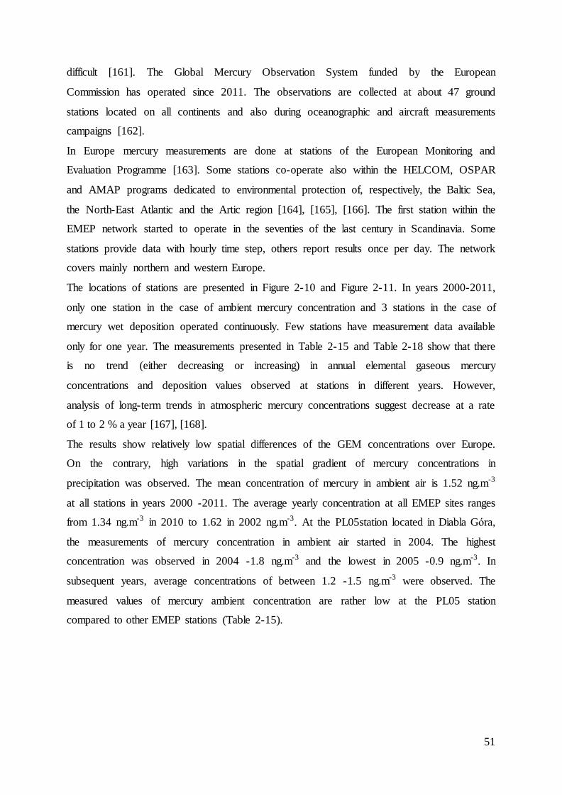
51
difficult [161]. The Global Mercury Observation System funded by the European
Commission has operated since 2011. The observations are collected at about 47 ground
stations located on all continents and also during oceanographic and aircraft measurements
campaigns [162].
In Europe mercury measurements are done at stations of the European Monitoring and
Evaluation Programme [163]. Some stations co-operate also within the HELCOM, OSPAR
and AMAP programs dedicated to environmental protection of, respectively, the Baltic Sea,
the North-East Atlantic and the Artic region [164], [165], [166]. The first station within the
EMEP network started to operate in the seventies of the last century in Scandinavia. Some
stations provide data with hourly time step, others report results once per day. The network
covers mainly northern and western Europe.
The locations of stations are presented in Figure 2-10 and Figure 2-11. In years 2000-2011,
only one station in the case of ambient mercury concentration and 3 stations in the case of
mercury wet deposition operated continuously. Few stations have measurement data available
only for one year. The measurements presented in Table 2-15 and Table 2-18 show that there
is no trend (either decreasing or increasing) in annual elemental gaseous mercury
concentrations and deposition values observed at stations in different years. However,
analysis of long-term trends in atmospheric mercury concentrations suggest decrease at a rate
of 1 to 2 % a year [167], [168].
The results show relatively low spatial differences of the GEM concentrations over Europe.
On the contrary, high variations in the spatial gradient of mercury concentrations in
precipitation was observed. The mean concentration of mercury in ambient air is 1.52 ng.m-3
at all stations in years 2000 -2011. The average yearly concentration at all EMEP sites ranges
from 1.34 ng.m-3 in 2010 to 1.62 in 2002 ng.m-3. At the PL05station located in Diabla Góra,
the measurements of mercury concentration in ambient air started in 2004. The highest
concentration was observed in 2004 -1.8 ng.m-3 and the lowest in 2005 -0.9 ng.m-3. In
subsequent years, average concentrations of between 1.2 -1.5 ng.m-3 were observed. The
measured values of mercury ambient concentration are rather low at the PL05 station
compared to other EMEP stations (Table 2-15).
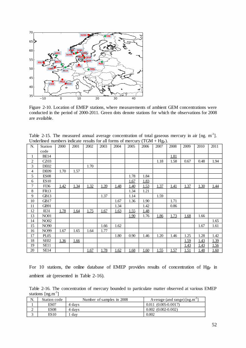
52
Figure 2-10. Location of EMEP stations, where measurements of ambient GEM concentrations were conducted in the period of 2000-2011. Green dots denote stations for which the observations for 2008
are available.
Table 2-15. The measured annual average concentration of total gaseous mercury in air [ng. m-3
]. Underlined numbers indicate results for all forms of mercury (TGM + HgP). N. Station
code
2000 2001 2002 2003 2004 2005 2006 2007 2008 2009 2010 2011
1 BE14 1.81
2 CZ03 1.18 1.58 0.67 0.48 1.94
3 DE02 1.70
4 DE09 1.70 1.57
5 ES08 1.78 1.84
6 ES10 1.67 1.83
7 FI36 1.42 1.34 1.32 1.39 1.48 1.40 1.53 1.37 1.41 1.37 1.30 1.44
8 FR13 1.34 1.21
9 GB13 1.37 1.14 1.59
10 GB17 1.67 1.36 1.90 1.71
11 GB91 1.34 1.42 0.86
12 IE31 1.78 1.64 1.75 1.67 1.63 1.55 1.48
13 NO01 1.90 1.76 1.86 1.73 1.68 1.66
14 NO02 1.65
15 NO90 1.66 1.62 1.67 1.61
16 NO99 1.67 1.65 1.64 1.77
17 PL05 1.80 0.90 1.46 1.20 1.46 1.25 1.28 1.42
18 SE02 1.36 1.66 1.59 1.43 1.39
19 SE11 1.43 1.43 1.56
20 SE14 1.67 1.78 1.62 1.68 1.60 1.55 1.57 1.51 1.48 1.60
For 10 stations, the online database of EMEP provides results of concentration of HgP in
ambient air (presented in Table 2-16).
Table 2-16. The concentration of mercury bounded to particulate matter observed at various EMEP stations [ng.m
-3]
N. Station code Number of samples in 2008 Average (and range) [ng.m-3
]
1 ES07 4 days 0.011 (0.005-0.0017)
2 ES08 4 days 0.002 (0.002-0.002)
3 ES10 1 day 0.002
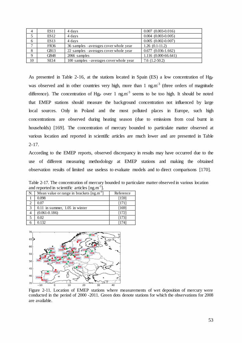
53
4 ES11 4 days 0.007 (0.003-0.016)
5 ES12 4 days 0.004 (0.003-0.005)
6 ES13 4 days 0.005 (0.002-0.007)
7 FR36 36 samples –averages cover whole year 1.26 (0.1-11.2)
8 GB13 22 samples –averages cover whole year 0.677 (0.036-1.662)
9 GB48 2066 samples 1.116 (0.000-66.641)
10 SE14 100 samples –averages cover whole year 7.6 (1.2-50.2)
As presented in Table 2-16, at the stations located in Spain (ES) a low concentration of HgP
was observed and in other countries very high, more than 1 ng.m-3 (three orders of magnitude
difference). The concentration of HgP over 1 ng.m-3 seems to be too high. It should be noted
that EMEP stations should measure the background concentration not influenced by large
local sources. Only in Poland and the most polluted places in Europe, such high
concentrations are observed during heating season (due to emissions from coal burnt in
households) [169]. The concentration of mercury bounded to particulate matter observed at
various location and reported in scientific articles are much lower and are presented in Table
2-17.
According to the EMEP reports, observed discrepancy in results may have occurred due to the
use of different measuring methodology at EMEP stations and making the obtained
observation results of limited use useless to evaluate models and to direct comparisons [170].
Table 2-17. The concentration of mercury bounded to particulate matter observed in various location and reported in scientific articles [ng.m
-3].
N. Mean value or range in brackets [ng.m-3
] Reference
1 0.098 [159]
2 0.07 [171]
3 0.11 in summer, 1.05 in winter [169]
4 (0.061-0.186) [172]
5 0.02 [173]
6 0.132 [174]
Figure 2-11. Location of EMEP stations where measurements of wet deposition of mercury were conducted in the period of 2000 -2011. Green dots denote stations for which the observations for 2008
are available.

54
Table 2-18. The measured annual average concentration of mercury in precipitation in years 2000- 2011 and average from whole period [ng.dm
-3]
N. Station
code
20
00
20
01
20
02
20
03
20
04
20
05
20
06
20
07
20
08
20
09
20
10
20
11
Average
1 BE04 28.6 44.1 27.0 11.9 36.8 29.7
2 BE14 11.1 11.8 10.6 11.2 8.2 9.0 10.6 10.4
3 DE01 9.5 6.3 7.2 9.1 8.1 8.7 8.6 6.3 6.3 6.6 4.3 6.8 7.3
4 DE02 8.4 10.9 11.8 11.5 9.1 9.2 7.0 5.1 10.2 9.2
5 DE03 10.7 8.0 9.3 5.0 8.0 8.2
6 DE07 12.7 9.2 11.0
7 DE08 6.8 8.6 5.9 5.1 7.6 6.8
8 DE09 15.2 9.4 8.7 9.5 10.8 9.5 9.8 7.9 6.9 5.4 9.3
9 ES08 5.2 6.5 9.6 8.7 7.5
10 FI17 5.3 5.3
11 FI36 5.0 5.2 4.7 7.4 6.3 5.6 7.3 5.8 7.5 4.9 3.7 7.1 5.9
12 FR13 9.7 10.7 10.2
13 GB13 4.8 3.3 4.6 6.8 3.4 3.9 4.2 4.4
14 GB17 7.0 3.9 7.1 4.6 5.6 5.1 8.5 6.0
15 GB36 5.9 5.9
16 GB48 3.4 4.6 4.4 3.1 3.2 2.8 3.6
17 GB91 4.7 3.8 4.7 4.6 4.2 5.3 5.4 4.7
18 IE01 63.2 34.6 12.5 36.8
19 IE02 50.0 50.0
20 LV10 25.8 26.0 30.9 37.6 33.0 30.7
21 LV16 28.8 22.0 30.6 27.1
22 NL91 9.8 9.4 9.3 8.6 15.2 15.1 9.6 9.6 10.6 8.8 8.1 8.8 10.2
23 NO01 9.8 8.9 8.1 6.3 6.4 9.4 8.8 5.3 7.9
24 NO99 7.3 7.3 12.8 8.1 8.9
25 PL05 270.9 21.0 11.2 55.1 42.3 31.0 71.9
26 PT02 30.0 26.0 5.0 20.3
27 PT04 5.2 5.2
28 SE02 8.8 9.3 9.1
29 SE05 5.5 6.5 7.2 7.6 6.5 6.9 5.6 6.5
30 SE11 12.5 9.4 9.9 11.6 10.0 7.6 8.7 10.0
31 SE14 12.3 9.0 14.6 18.5 10.0 11.0 8.6 13.7 9.1 8.9 11.6
32 SI08 5.4 5.6 4.2 5.8 5.3
In Poland, the one-hour measurements of atmospheric concentrations of various mercury
forms were conducted for the period 08/2011 -07/2012 in Zabrze and Złoty Potok, which
represent respectively highly urban and background locations [175]. In Zabrze, the average
concentrations of 44.46 pg.m-3 for HgP, 3.14 ng.m-3 for TGM including 3.13 ng.m-3 of GEM
and 17.81 pg.m-3 for RGM were observed during the whole observation campaign period.
During the heating season, the following concentrations were observed: 2.76 ng.m-3 of GEM,
20.03 pg.m-3 of RGM, 64.99 pg.m-3 of HgP. In the summer period, the observed concentration
was higher for GEM and lower for RGM and Hgp respectively 3.44 ng.m-3, 15.21 pg.m-3,
64.50 pg.m-3. In Złoty Potok, the average TGM concentration of 1.84 ng.m-3 during heating
and summer seasons was observed.
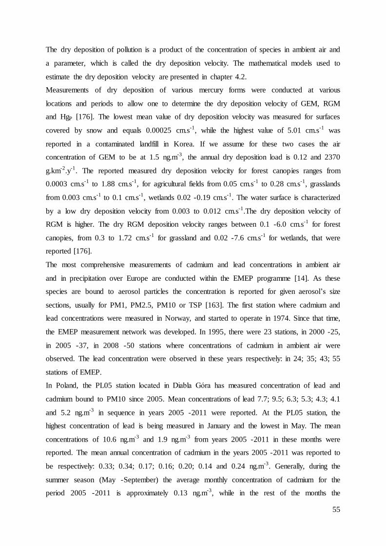
55
The dry deposition of pollution is a product of the concentration of species in ambient air and
a parameter, which is called the dry deposition velocity. The mathematical models used to
estimate the dry deposition velocity are presented in chapter 4.2.
Measurements of dry deposition of various mercury forms were conducted at various
locations and periods to allow one to determine the dry deposition velocity of GEM, RGM
and HgP [176]. The lowest mean value of dry deposition velocity was measured for surfaces
covered by snow and equals 0.00025 cm.s-1, while the highest value of 5.01 cm.s-1 was
reported in a contaminated landfill in Korea. If we assume for these two cases the air
concentration of GEM to be at 1.5 ng.m-3, the annual dry deposition load is 0.12 and 2370
g.km-2.y-1. The reported measured dry deposition velocity for forest canopies ranges from
0.0003 cm.s-1 to 1.88 cm.s-1, for agricultural fields from 0.05 cm.s-1 to 0.28 cm.s-1, grasslands
from 0.003 cm.s-1 to 0.1 cm.s-1, wetlands 0.02 -0.19 cm.s-1. The water surface is characterized
by a low dry deposition velocity from 0.003 to 0.012 cm.s-1.The dry deposition velocity of
RGM is higher. The dry RGM deposition velocity ranges between 0.1 -6.0 cm.s-1 for forest
canopies, from 0.3 to 1.72 cm.s-1 for grassland and 0.02 -7.6 cm.s-1 for wetlands, that were
reported [176].
The most comprehensive measurements of cadmium and lead concentrations in ambient air
and in precipitation over Europe are conducted within the EMEP programme [14]. As these
species are bound to aerosol particles the concentration is reported for given aerosol’s size
sections, usually for PM1, PM2.5, PM10 or TSP [163]. The first station where cadmium and
lead concentrations were measured in Norway, and started to operate in 1974. Since that time,
the EMEP measurement network was developed. In 1995, there were 23 stations, in 2000 -25,
in 2005 -37, in 2008 -50 stations where concentrations of cadmium in ambient air were
observed. The lead concentration were observed in these years respectively: in 24; 35; 43; 55
stations of EMEP.
In Poland, the PL05 station located in Diabla Góra has measured concentration of lead and
cadmium bound to PM10 since 2005. Mean concentrations of lead 7.7; 9.5; 6.3; 5.3; 4.3; 4.1
and 5.2 ng.m-3 in sequence in years 2005 -2011 were reported. At the PL05 station, the
highest concentration of lead is being measured in January and the lowest in May. The mean
concentrations of 10.6 ng.m-3 and 1.9 ng.m-3 from years 2005 -2011 in these months were
reported. The mean annual concentration of cadmium in the years 2005 -2011 was reported to
be respectively: 0.33; 0.34; 0.17; 0.16; 0.20; 0.14 and 0.24 ng.m-3. Generally, during the
summer season (May -September) the average monthly concentration of cadmium for the
period 2005 -2011 is approximately 0.13 ng.m-3, while in the rest of the months the
56
concentration of approximately 0.3 ng.m-3 was reported. The highest monthly average
concentration of 20.7 ng.m-3 and 0.75 ng.m-3 of lead and cadmium was observed at this station
in November 2006. Whereas at all stations of the EMEP, the highest monthly mean
concentration of lead bound to PM10 was reported at the AT02 site located in Austria in
February 2003 and equalled 42.8 ng.m-3. At the same station, the highest monthly mean
concentrations of (i) 24.7 ng.m-3 of lead bound to PM2.5, (ii) 2.00 ng.m-3 of cadmium bound
in PM10 and (iii) 1.27 of cadmium bound to PM2.5 were observed in November 2003.
The concentrations of lead and cadmium in precipitation are observed within the EMEP
programme since 1973 when two stations located in Norway started to operate. In 1990, 27
stations operated, in 2000 and 2005 -57 stations. Nowadays the EMEP network consists of 62
stations spread all over Europe. Over all stations and all years, the average concentrations in
precipitation of lead and cadmium equal 15.9 and 0.22 µg.dm-3, respectively. The average
annual wet deposition of lead at all EMEP stations was 1403 g.km-2.y-1 in 2000, in 2005
-1414 g.km-2.y-1 and 592 g.km-2.y-1 in 2010. For cadmium in these years fluxes of 69.34;
37.76; 37.18; g.km-2.y-1 were measured. The highest average monthly value of cadmium
concentration in precipitation of 37.39 µg.dm-3 was observed at the IT01 station (Italy,
Montelibretti) in January 2007, while for lead 1651.7 µg.dm-3 in August 2002 at the GB14
station (UK, High Muffles). In Poland, the lead and cadmium concentrations in precipitation
have been observed since 1992 at the PL05 station located in Diabla Góra and since 1996 at
the PL04 station in Łeba.
At the PL04, station the maximum monthly average concentrations of Pb in precipitation of
9.64 µg.dm-3 was observed in March 1996 and the highest wet deposition of 400
g.km-2.month-1 was measured in June 2001. At PL05, the maximum observed values were 16
µg.dm-3 and 713 g.km-2.month-1 in December 1992. At this station, the annual wet deposition
systematically decreases. In the nineties the load of wet deposited lead above 2000 g.km-2.y-1
was observed. Whereas in 2011, depositions of only 241 g.km-2.y-1 was measured at the PL05
station.
In the XXI century, the highest monthly cadmium concentrations in precipitation of 0.23
µg.dm-3 and 0.50 µg.dm-3 were observed in February 2006 at the EMEP stations i.e. PL04 and
PL05 operated in Poland. The maximal monthly fluxes of cadmium of 13.1 g.km-2.month-1
and 19.2 g.km-2.month-1 were measured in April 2006 at PL04 and September 2003 at PL05,
respectively. At both stations, the highest wet depositions of cadmium was observed in
November. Since the beginning of the operation of the stations, a downward trend in
measured quantities of deposited cadmium can be observed.
57
Overview of existing mercury chemical transport models 3
The chemical schemes of mercury are usually implemented into the existing modelling
systems developed for traditional pollutants (SO2, NOx, PM, O3). The atmospheric chemistry
of mercury is complex [15], [9]. Thus on one hand, the mercury models should represent well
its real behaviour but on the other the computation time requirements should not be
prohibitive. Many numerical mercury models of Eulerian (ADOM, CAMx, CMAQ-Hg,
CMAQ ver. 4.7.1, CTM-Hg, DEHM, ECHMERIT, GEOS-Chem, GLEMOS, MOZART,
MSCE-HM, MSCE-HM-Hem, STEM-Hg) and Lagrangian (HYSPLIT, RCTM-Hg) types
have been developed to evaluate the atmospheric dispersion and transformation of mercury on
a regional, continental and global scale [10], [11]. Developed models dedicated to
atmospheric mercury consider the main chemical reactions and transformations within the
aqueous and gaseous phases. However, some significant differences can be found, in chemical
reactions taken into account as well as in the value of the kinetic rates. Additionally the
various approaches were used to model the dry and wet deposition fluxes of mercury. The
paragraphs below provide short information on the application and particular properties of
those models. All main chemical reactions and transformations of mercury included in the
considered models are presented in Table 3-1 and Table 3-2.
CMAQ-Hg
The version of the Community Multiscale Air Quality model with mercury scheme (CMAQ-
Hg) was developed by US-EPA. The model has no explicit simulation of cloud-water
transport [160]. The model assumes that the dry deposition of GEM is equivalent to emissions
from natural sources. The dry deposition parameterization for gaseous nitric acid was used for
the calculation of the dry deposition velocity of reactive gaseous mercury. The fields of
concentration of species that react with mercury are generated simultaneously in the same
simulation with the use of the algorithms of a standard CMAQ model. This Eulerian type
model was applied in continental simulation over Europe and North America [177].
CMAQ ver. 4.7.1
In this version of the CMAQ model, significant features devoted to atmospheric mercury were
implemented [178]. Dry deposition of reactive gaseous mercury and gaseous elemental
mercury is calculated with the use of the M3Dry deposition scheme [179]. Therefore
computed dry deposition depends on type of vegetation and stromatal resistance. Dry
58
deposition of HgP is calculated as a function of particle size. Wet deposition of mercury
species is computed based on their concentration in cloud-water and precipitation rate.
CTM-Hg
Global chemical transport model for mercury CTM-Hg was developed by Atmospheric and
Environmental Research, Inc. [180]. The model assumes the following dry deposition
velocities:
-0.25 cm.s-1 for GEM,
-0.01 cm.s-1 over land and 0.01 cm.s-1 over water for Hgp,
-0.01cm.s-1 over land and 0 cm.s-1 over water for GEM.
Another assumption of the model is that below cloud scavenging process due to precipitation
removes 10% of RGM, 50% of Hgp and 0% of GEM.
CAMx
The Comprehensive Air Quality Model with Extensions is an Eulerian photochemical
dispersion model which can be applied from sub-urban to continental scale to compute the
dispersion of gaseous and particulate air pollution [181]. Dry deposition of Hgp and RGM is
calculated with the use of resistance model [182]. The model assumes that dry and wet
deposition of GEM is negligible. In the model, dry deposition of GEM is not computed
because of the assumption that dry deposition of GEM is equivalent to emissions from natural
sources and reemission. CAMx and CMAQ ver. 4.7.1 were used in simulations performed
over the eastern United States.
MSCE-HM
The MSCE-HM model is a three dimensional Eulerian type chemical transport model driven
by off-line meteorological data coming from MM5 developed in the European Monitoring
and Evaluation Programme by the Meteorological Synthesizing Centre-East in Moscow. The
model works in the EMEP grid, which covers the whole Europe with spatial resolution of 50
km x 50 km. Dry deposition is calculated with the use of a resistance model with modification
for aerosols. The wet deposition flux is calculated based on the empirical relationship derived
from measurements [29]. Correlation coefficients of 0.38 and 0.5 were obtained from
comparison for 2003 of measured and modelled mercury concentrations in the air and
precipitation, respectively. The simulation performed for 2008 showed that difference
59
between modeled and observations of mercury concentrations in air and wet deposition do not
exceed 15% and 30% respectively [183].
MSCE-HM-Hem
The model was developed for modelling the Northern Hemisphere and derived directly from
the MSCE-HM model. The dry deposition of RGM is calculated with the use of parameters
for nitric acid. The deposition of GEM to vegetation is calculated based on data of surface
temperature, solar radiation and vegetation type. Value from 0 to 0.03 cm.s-1 for dry velocity
of GEM were obtained. The dry deposition of HgP is estimated from experimental data. The
wet deposition of RGM and HgP is calculated based on an empirical relationship derived from
measurements. The model simulations have been performed over the Northern Hemisphere
with a resolution of 2.50 ×2.50 for the period 1990 -2004. The validation of the modelled
results against measurements showed a high compatibility in the case of GEM concentrations
in air and an overestimation for wet deposition fluxes of mercury [184].
GLEMOS
The Global EMEP Multi-media Modelling System is developed by the Meteorological
Synthesizing Centre -East within the European Monitoring and Evaluation Programme. It can
be used at global and regional scales. The chemical module of mercury is based on previous
developed and tested schemes included in the MSCE-HM-Hem model but new reactions with
bromine and bromine compounds were added [185]. The comparison results obtained from a
simulation run for 2005 against measurement over Europe, North America and Asia showed
to be satisfactory for air concentration and wet deposition [186].
ADOM mercury model
Acid Deposition and Oxidants Model (ADOM) is the Eulerian model developed under the
Canada -Germany Science & Technology Co-operation Agreement. The model considers 14
mercury compounds and 21 chemical reactions. Dry deposition is calculated based on the
resistance model. Mercury scavenging is calculated with the use of sub-models, which
simulate vertical distribution of mercury species in clouds. Results obtained from simulations
performed over Europe showed a rather good agreement with observational data [187].

60
DEHM
The mercury model was also implemented in the Danish Eulerian Hemispheric Model under
the Danish Arctic Monitoring and Assessment Programme [188]. The chemistry of mercury
implemented in DEHM is derived from ADOM model [189]. The dry deposition is calculated
based on resistance model with parameters for HNO3(g). A simple scavenging coefficient
formulation with removal rates for sulphur was applied. The model was run over the Northern
Hemisphere and the obtained results showed that DEHM is able to reproduce patterns due to
the mercury depletion during Polar Sunrise.
STEM-Hg
The Eulerian numerical model dedicated for mercury STEM-Hg is derived from the Sulfur
Transport and Deposition Model (STEM-III), developed at the University of Iowa [190]. The
wet removal rates for RGM and Hgp were assumed to be equal to those of nitric acid and
sulphate, respectively. It was assumed that the dry deposition velocity for GEM equals zero
because dry deposition of GEM is equivalent to emissions from natural sources and
reemission. Dry deposition velocities of RGM and Hgp were assumed to be equal to those of
gaseous HNO3(g) and sulphate, respectively. The model was used to investigate the
atmospheric mercury budget in East Asia.
GEOS-Chem
The GEOS-Chem model is a global 3-D model of atmospheric chemistry and transport
developed mainly by Harvard University [191]. Wet deposition of GEM and dry deposition of
GEM over land is negligible. The dry deposition of GEM to the ocean is modelled with the
use of bidirectional exchange model. For RGM and HgP, scavenging is computed from
precipitation and in convective updrafts and dry deposition is computed with the use of
resistance scheme. The surface resistance for RGM was set to zero. The performed simulation
were used to study global and regional (in China and the US) budget of mercury.
Overestimates of wet deposition of RGM and HgP were observed by a factor of 2 -5 due to
high modeled concentrations of those mercury forms.
61
ECHMERIT
ECHMERIT is a model developed by the Institute of Atmospheric Pollution Research in Italy.
The model calculates the wet and dry deposition of gaseous species and particulate matter.
Mercury in the aqueous phase is considered as one lumped species. The operational validation
of the model performed for 2001 showed an overestimation of wet deposition compared to
stations over Europe and North America [192].
MOZART
Model for Ozone and Related Chemical Tracers (MOZART) is a global transport model
developed by the National Center for Atmospheric Research (NCAR), Geophysical Fluid
Dynamics Laboratory (GFDL) and Max Planck Institute for Meteorology [193]. It was
modified to include gas-phase mercury chemistry [194]. The dry and wet deposition of
reactive gaseous mercury is calculated with the use of parameters previously used for HNO3.
The dry and wet deposition of gaseous elemental mercury was set to 0. The model was run to
investigate the impact of mercury emitted in China on global mercury mass balance and to
generate boundary concentrations for simulation performed over the Great Lakes in the
United States [194].
Following this review of published results of mercury modelling and their operational
validation against measurements in Europe, some general conclusions can be drawn [195],
[196]:
-models do not indicate peaks of concentration of GEM, or if they do then the peaks are
significantly underestimated, but the average annual concentrations correspond well to the
observations;
-there is a good agreement with measurements of mercury bound to aerosols.
-processes (e.g. emissions, meteorological phenomena) that take place outside the modelling
domain have a strong impact on the obtained results;
-the direct anthropogenic emissions in the domain have the strongest impact on the
atmospheric concentration of mercury.
-there is a weak correlation with daily measurements of RGM.
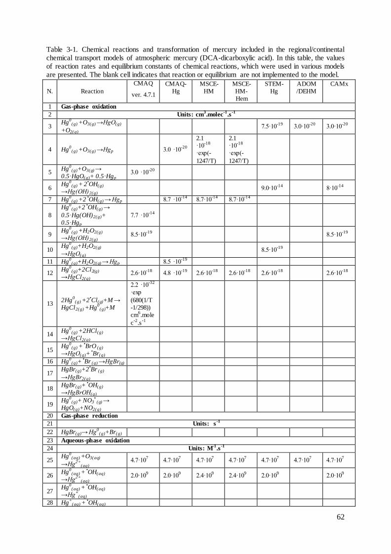
62
Table 3-1. Chemical reactions and transformation of mercury included in the regional/continental chemical transport models of atmospheric mercury (DCA-dicarboxylic acid). In this table, the values of reaction rates and equilibrium constants of chemical reactions, which were used in various models are presented. The blank cell indicates that reaction or equilibrium are not implemented to the model.
N. Reaction
CMAQ
ver. 4.7.1
CMAQ-
Hg
MSCE-
HM
MSCE-
HM-
Hem
STEM-
Hg
ADOM
/DEHM
CAMx
1 Gas-phase oxidation
2 Units: cm3.molec
-1.s
-1
3 Hg
0(g) +O3(g) →HgO(g)
+O2(g) 7.5·10
-19 3.0·10
-20 3.0·10
-20
4 Hg0
(g) +O3(g) →Hgp 3.0 ·10-20
2.1
·10-18
·exp(-
1247/T)
2.1
·10-18
·exp(-
1247/T)
5 Hg
0(g)+O3(g) →
0.5·HgO(g)+ 0.5·Hgp 3.0 ·10
-20
6 Hg
0(g) + 2
•OH(g)
→Hg(OH)2(g) 9.0·10
-14 8·10
-14
7 Hg0
(g) +2 •OH(g) → Hgp 8.7 ·10
-14 8.7·10
-14 8.7·10
-14
8
Hg0
(g)+2 •OH(g) →
0.5·Hg(OH)2(g)+
0.5·Hgp
7.7 ·10-14
9 Hg
0(g) +H2O2(g)
→Hg(OH)2(g) 8.5·10
-19 8.5·10
-19
10 Hg
0(g)+H2O2(g)
→HgO(g) 8.5·10
-19
11 Hg0
(g)+H2O2(g) → Hgp 8.5 ·10-19
12 Hg
0(g)+2Cl2(g)
→HgCl2(g) 2.6·10
-18 4.8 ·10
-19 2.6·10
-18 2.6·10
-18 2.6·10
-18 2.6·10
-18
13 2Hg
0(g) +2
•Cl(g)+M →
HgCl2(g) +Hg0
(g)+M
2.2 ·10-32
·exp
(680(1/T
-1/298))
cm6.mole
c-2
.s-1
14 Hg
0(g) +2HCl(g)
→HgCl2(g)
15 Hg
0(g) +
•BrO (g)
→HgO(g)+ •Br(g)
16 Hg0
(g)+ •Br (g) →HgBr(g)
17 HgBr(g)+2
•Br (g)
→HgBr2(g)
18 HgBr(g)+
•OH(g)
→HgBrOH(g)
19 Hg
0(g)+
NO3
• (g) →
HgO(g)+NO2(g)
20 Gas-phase reduction
21 Units: s-1
22 HgBr(g)→ Hg0
(g)+Br(g)
23 Aqueous-phase oxidation
24 Units: M-1
.s-1
25 Hg
0(aq) +O3(aq)
→Hg2+
(aq) 4.7·10
7 4.7·10
7 4.7·10
7 4.7·10
7 4.7·10
7 4.7·10
7 4.7·10
7
26 Hg
0(aq) +
•OH(aq)
→Hg2+
(aq) 2.0·10
9 2.0·10
9 2.4·10
9 2.4·10
9 2.0·10
9 2.0·10
9
27 Hg
0(aq) +
•OH(aq)
→Hg+
(aq)
28 Hg+
(aq) + •OH(aq)

63
→Hg2+
(aq)
29 Hg
0(aq) +HOCl(aq)
→Hg2+
(aq) 2.09 ·10
6 2.09 ·10
6 2.09·10
6 2.09 ·10
6
30 Hg0
(aq) +OCl- →Hg
2+ 1.99·10
6 1.99 ·10
6 2.0·10
6 2.0·10
6 1.99·10
6 1.99·10
6
31
Hg0
(aq) +HOBr(aq)→
Hg2+
(aq) +Br-(aq)
+OH-(aq)
32 Hg
0(aq) +
•BrO(aq)→
Hg2+
(aq)+Br(aq)-+OH(aq)
-
33 Hg
0(aq) +Br2(aq)→
Hg2+
(aq) +2Br-(aq)
34 Aqueous-phase reduction
35 Units: s-1
36 HgSO3(aq) →Hg0
(aq)
T·exp((31.
971T-
12595)/T)
T·
expt((31.97
1T-12595)/T)
0.0106 0.6 0.0106
37 𝐻𝑔(𝑆𝑂3 )2
2−(aq)
→Hg0
(aq) 4.4·10
-4 4.4·10
-4
38 Hg(OH)2(aq) +hv
→ Hg0
(aq) 6.0 ·10
-7 6.0 ·10
-7 3.0·10
-7
39 Units: M-1
.s-1
40 Hg
2+(aq) +HO2
→ Hg0
(aq) 1.1·10
4 1.7·10
4 1.7·10
4
41 Hg
2+(aq) +DCA +hv
→ Hg0
(aq) 1.2·10
4
42 Gas/liquid equilibria
43 Units: M.atm-1
44 Hg0
(g) ↔Hg0
(aq) 0.11
1.76·10-
23 ·T·exp
(9.08·
(T0/T-1))
1.76·10-
23 ·T·exp
(9.08·
(T0/T-1))
0.11
45 HgO(g) ↔HgO(aq)
46 HgCl2(g) ↔HgCl2(aq) 1.4·106
1.75·10-
16Texp(1
8.75(T0/
T-1))
1.75·10-
16Texp(1
8.75(T0/
T-1))
1.4·106
47 Hg(OH)2(g)
↔ Hg(OH)2(aq)
48 HOBr(g) ↔HOBr(aq)
49 HgBr(g) ↔HgBr(aq)
50 HgBr2(g) ↔HgBr2(aq)
51 HgBrOH(g) ↔
HgBrOH(aq)
52 Aqueous phase equilibria
53 𝐻𝑔(𝑎𝑞)
2+ + 𝑆𝑂3(𝑎𝑞)
2−
↔ 𝐻𝑔𝑆𝑂3 (𝑎𝑞) 5·10
12
M-1
5·1012
M-1
5·1012
M-1
2.1·1013
M-1
2.1·1013
M-1
54 𝐻𝑔𝑆𝑂3 (𝑎𝑞) + 2𝑆𝑂3(𝑎𝑞)
2−
↔ 𝐻𝑔(𝑆𝑂3 )2(𝑎𝑞) 2−
2.5·1011
M-1
2.5·1011
M-1
1.1
·10-21+4pH
·[SO2(g)]2
s-1
1.1
·10-21+4pH
·[SO2(g)]2
s-1
1.0·1010
M-1
1.0·1010
M-1
55 𝐻𝑔𝐶𝑙2 (𝑎𝑞)
↔ 𝐻𝑔(𝑎𝑞)2+ + 2𝐶𝑙(𝑎𝑞)
− 10
-14M
2 10
-14M
2
56 𝐻𝑔𝑛𝐶𝑙𝑚 (𝑑𝑖𝑠)
↔ 𝐻𝑔(𝑎𝑞)2+
f([Cl-1
]) f([Cl-1
]) 10-14
M2
57 𝐻𝑔𝑂𝐻(𝑎𝑞)
+
↔ 𝐻𝑔(𝑎𝑞)2+ + 𝑂𝐻(𝑎𝑞)
−
2.51
·10-11
M
2.51
·10-11
M
2.51
·10-11
M
2.51
·10-11
M 10
-22M
2

64
58 𝐻𝑔(𝑂𝐻)2 (𝑎𝑞)↔ 𝐻𝑔(𝑎𝑞)
2+ + 2𝑂𝐻(𝑎𝑞)−
10-22
M2 10
-22M
2
59 𝐻𝑔(𝑂𝐻)2 (𝑎𝑞)
↔ 𝐻𝑔𝑂𝐻(𝑎𝑞)+ + 𝑂𝐻(𝑎𝑞)
−
6.13
·10--12
M
60 𝐻𝑔𝑂𝐻𝐶𝑙(𝑎𝑞)
↔ 𝐻𝑔𝑂𝐻(𝑎𝑞)+ + 𝐶𝑙(𝑎𝑞)
−
3.72
·10-8
M
3.72
·10-8
M
3.72
·10-8
M
3.72
·10-8
M
61 𝐻𝑔(𝑎𝑞)
2+ + 𝐵𝑟(𝑎𝑞)−
↔ 𝐻𝑔𝐵𝑟(𝑎𝑞)+
62 𝐻𝑔𝐵𝑟(𝑎𝑞)
+ + 𝐵𝑟(𝑎𝑞)−
↔ 𝐻𝑔𝐵𝑟2 (𝑎𝑞)
63 𝐻𝑔𝐵𝑟2 (𝑎𝑞) + 𝐵𝑟(𝑎𝑞)
−
↔ 𝐻𝑔𝐵𝑟3 (𝑎𝑞)−
64 𝐻𝑔𝐵𝑟3 (𝑎𝑞)
− + 𝐵𝑟(𝑎𝑞)−
↔ 𝐻𝑔𝐵𝑟4(𝑎𝑞)2−
65 𝐻𝑂𝐵𝑟(𝑎𝑞)↔ 𝐻(𝑎𝑞)
+ + 𝐵𝑟𝑂(𝑎𝑞)+
66
𝐻(𝑎𝑞)+ + 𝐵𝑟(𝑎𝑞)
−
+ 𝐻𝑔(𝑂𝐻)2(𝑎𝑞)↔ 𝐻𝑔𝐵𝑟𝑂𝐻(𝑎𝑞)
67 𝐻𝑔𝑂𝐻(𝑎𝑞)
+ + 𝑂𝐻(𝑎𝑞)−
↔ 𝐻𝑔(𝑂𝐻)2 (𝑎𝑞)
1.58·1011
M-1
68 𝐻𝑔(𝑎𝑞)
2+ + 𝐶𝑙(𝑎𝑞)−
↔ 𝐻𝑔𝐶𝑙(𝑎𝑞)+
5.8·10
6
M-1
69
𝐻𝑔𝐶𝑙(𝑎𝑞)+ + 𝐶𝑙(𝑎𝑞)
−
↔ 𝐻𝑔𝐶𝑙2 (𝑎𝑞)
2.5·106
M-1
70 Gas/soot equilibria
71 Units: mwater3.mair
-3
72 soot(g) →soot(aq) 5·10
5
5·105
73 Liquid /soot equilibria
74 𝐻𝑔𝑆𝑂3 (𝑎𝑞)↔ 𝐻𝑔𝑆𝑂3(𝑝)
0.2
75 𝐻𝑔𝑆𝑂2 (𝑎𝑞)
2−
↔ 𝐻𝑔𝑆𝑂2 (𝑝)2−
76 𝐻𝑔(𝐻𝑂)2 (𝑎𝑞)↔ 𝐻𝑔(𝐻𝑂)2 (𝑝)
77 𝐻𝑔𝐶𝑙2 (𝑎𝑞)↔ 𝐻𝑔𝐶𝑙2 (𝑝)
78 𝐻𝑔𝐶𝑙𝑚 (𝑎𝑞)↔ 𝐻𝑔𝐶𝑙𝑚 (𝑝)
0.2
79 𝐻𝑔𝑂𝐻𝐶𝑙(𝑎𝑞)↔ 𝐻𝑔𝑂𝐻𝐶𝑙(𝑝)
80 𝐻𝑔𝑂𝐻(𝑎𝑞)
+
↔ 𝐻𝑔𝑂𝐻(𝑝)+
81 𝐻𝑔(𝑎𝑞)𝐼𝐼 ↔ 𝐻𝑔 (𝑝)
𝐼𝐼 45 l.g-1
34 l.g-1
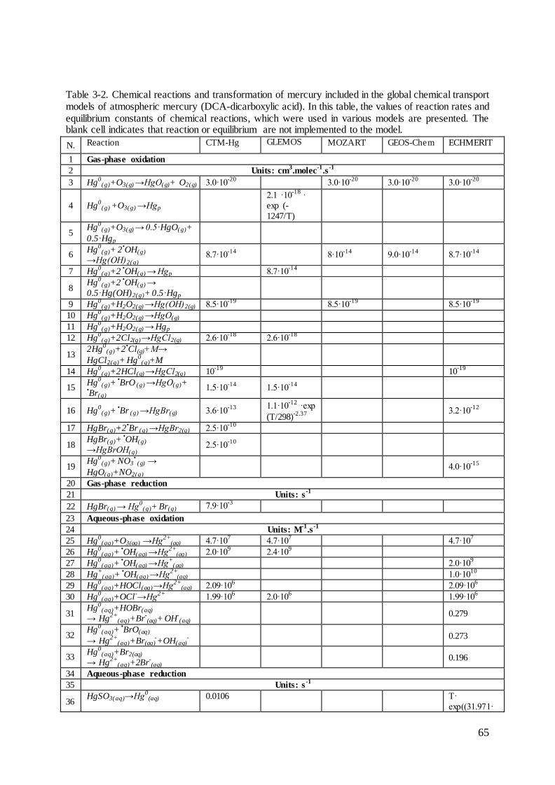
65
Table 3-2. Chemical reactions and transformation of mercury included in the global chemical transport models of atmospheric mercury (DCA-dicarboxylic acid). In this table, the values of reaction rates and equilibrium constants of chemical reactions, which were used in various models are presented. The blank cell indicates that reaction or equilibrium are not implemented to the model.
N. Reaction CTM-Hg GLEMOS MOZART GEOS-Chem ECHMERIT
1 Gas-phase oxidation
2 Units: cm3.molec
-1.s
-1
3 Hg0
(g)+O3(g) →HgO(g)+ O2(g) 3.0·10-20
3.0·10-20
3.0·10-20
3.0·10-20
4 Hg0
(g) +O3(g) →Hgp
2.1 ·10-18
·
exp (-
1247/T)
5 Hg
0(g)+O3(g) → 0.5·HgO(g)+
0.5·Hgp
6 Hg
0(g)+ 2
•OH(g)
→Hg(OH)2(g) 8.7·10
-14 8·10
-14 9.0·10
-14 8.7·10
-14
7 Hg0
(g)+2 •OH(g) → Hgp 8.7·10
-14
8 Hg
0(g)+2
•OH(g) →
0.5·Hg(OH)2(g)+ 0.5·Hgp
9 Hg0
(g)+H2O2(g) →Hg(OH)2(g) 8.5·10-19
8.5·10-19
8.5·10-19
10 Hg0
(g)+H2O2(g) →HgO(g)
11 Hg0
(g)+H2O2(g) → Hgp
12 Hg0
(g)+2Cl2(g) →HgCl2(g) 2.6·10-18
2.6·10-18
13 2Hg
0(g)+2
•Cl(g)+M→
HgCl2(g)+ Hg0
(g)+M
14 Hg0
(g)+2HCl(g) →HgCl2(g) 10-19
10-19
15 Hg
0(g)+
•BrO (g) →HgO(g)+
•Br(g)
1.5·10-14
1.5·10-14
16 Hg0
(g)+ •Br (g) →HgBr(g) 3.6·10
-13
1.1·10-12
·exp
(T/298)-2.37
3.2·10
-12
17 HgBr(g)+2•Br (g) →HgBr2(g) 2.5·10
-10
18 HgBr(g)+
•OH(g)
→HgBrOH(g) 2.5·10
-10
19 Hg
0(g)+
NO3
• (g) →
HgO(g)+NO2(g) 4.0·10
-15
20 Gas-phase reduction
21 Units: s-1
22 HgBr(g) → Hg0
(g)+ Br(g) 7.9·10-3
23 Aqueous-phase oxidation
24 Units: M-1
.s-1
25 Hg0
(aq)+O3(aq) →Hg2+
(aq) 4.7·107 4.7·10
7 4.7·10
7
26 Hg0
(aq)+ •OH(aq) →Hg
2+(aq) 2.0·10
9 2.4·10
9
27 Hg0
(aq)+ •OH(aq) →Hg
+(aq) 2.0·10
9
28 Hg+
(aq)+ •OH(aq) →Hg
2+(aq) 1.0·10
10
29 Hg0
(aq)+HOCl(aq) →Hg2+
(aq) 2.09·106 2.09·10
6
30 Hg0
(aq)+OCl-→Hg
2+ 1.99·10
6 2.0·10
6 1.99·10
6
31 Hg
0(aq)+HOBr(aq)
→ Hg2+
(aq)+Br-(aq)+
OH
-(aq)
0.279
32 Hg
0(aq)+
•BrO(aq)
→ Hg2+
(aq)+Br(aq)-+OH(aq)
-
0.273
33 Hg
0(aq)+Br2(aq)
→ Hg2+
(aq)+2Br-(aq)
0.196
34 Aqueous-phase reduction
35 Units: s-1
36 HgSO3(aq)→Hg
0(aq) 0.0106 T·
exp((31.971·
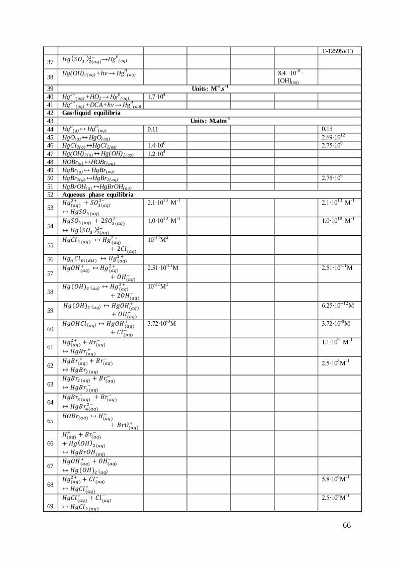
66
T-12595)/T)
37 𝐻𝑔(𝑆𝑂3 )2(𝑎𝑞)
2− →Hg0
(aq)
38 Hg(OH)2(aq) +hv → Hg
0(aq) 8.4 ·10
-8 ·
[OH](aq)
39 Units: M-1
.s-1
40 Hg2+
(aq) +HO2 → Hg0
(aq) 1.7·104
41 Hg2+
(aq) +DCA+hv → Hg0
(aq)
42 Gas/liquid equilibria
43 Units: M.atm-1
44 Hg0
(g) ↔ Hg0
(aq) 0.11 0.13
45 HgO(g) ↔ HgO(aq) 2.69·1012
46 HgCl2(g) ↔HgCl2(aq) 1.4·106 2.75·10
6
47 Hg(OH)2(g) ↔ Hg(OH)2(aq) 1.2·104
48 HOBr(g) ↔HOBr(aq)
49 HgBr(g) ↔ HgBr(aq)
50 HgBr2(g) ↔HgBr2(aq) 2.75·106
51 HgBrOH(g) ↔HgBrOH(aq)
52 Aqueous phase equilibria
53 𝐻𝑔(𝑎𝑞)
2+ + 𝑆𝑂3(𝑎𝑞)
2−
↔ 𝐻𝑔𝑆𝑂3 (𝑎𝑞)
2.1·1013
M-1
2.1·1013
M-1
54 𝐻𝑔𝑆𝑂3 (𝑎𝑞) + 2𝑆𝑂3(𝑎𝑞)
2−
↔ 𝐻𝑔(𝑆𝑂3 )2(𝑎𝑞) 2−
1.0·1010
M-1
1.0·1010
M-1
55 𝐻𝑔𝐶𝑙2 (𝑎𝑞) ↔ 𝐻𝑔(𝑎𝑞)
2 +
+ 2𝐶𝑙(𝑎𝑞)−
10-14
M2
56 𝐻𝑔𝑛𝐶𝑙𝑚 (𝑑𝑖𝑠) ↔ 𝐻𝑔(𝑎𝑞)2 +
57 𝐻𝑔𝑂𝐻(𝑎𝑞)
+ ↔𝐻𝑔(𝑎𝑞)2+
+ 𝑂𝐻(𝑎𝑞)−
2.51·10-11
M 2.51·10-11
M
58 𝐻𝑔(𝑂𝐻)2 (𝑎𝑞) ↔ 𝐻𝑔(𝑎𝑞)
2+
+ 2𝑂𝐻(𝑎𝑞)−
10-22
M2
59 𝐻𝑔(𝑂𝐻)2 (𝑎𝑞) ↔ 𝐻𝑔𝑂𝐻(𝑎𝑞)
+
+ 𝑂𝐻(𝑎𝑞)−
6.25·10--12
M
60 𝐻𝑔𝑂𝐻𝐶𝑙(𝑎𝑞) ↔ 𝐻𝑔𝑂𝐻(𝑎𝑞)
+
+ 𝐶𝑙(𝑎𝑞)−
3.72·10-8
M 3.72·10-8
M
61 𝐻𝑔(𝑎𝑞)
2+ + 𝐵𝑟(𝑎𝑞)−
↔ 𝐻𝑔𝐵𝑟(𝑎𝑞)+
1.1·109 M
-1
62 𝐻𝑔𝐵𝑟(𝑎𝑞)
+ + 𝐵𝑟(𝑎𝑞)−
↔ 𝐻𝑔𝐵𝑟2 (𝑎𝑞)
2.5·108M
-1
63 𝐻𝑔𝐵𝑟2 (𝑎𝑞) + 𝐵𝑟(𝑎𝑞)
−
↔ 𝐻𝑔𝐵𝑟3 (𝑎𝑞)−
64 𝐻𝑔𝐵𝑟3 (𝑎𝑞)
− + 𝐵𝑟(𝑎𝑞)−
↔ 𝐻𝑔𝐵𝑟4(𝑎𝑞)2−
65 𝐻𝑂𝐵𝑟(𝑎𝑞) ↔ 𝐻(𝑎𝑞)
+
+ 𝐵𝑟𝑂(𝑎𝑞)+
66
𝐻(𝑎𝑞)+ + 𝐵𝑟(𝑎𝑞)
−
+ 𝐻𝑔(𝑂𝐻)2(𝑎𝑞)↔ 𝐻𝑔𝐵𝑟𝑂𝐻(𝑎𝑞)
67 𝐻𝑔𝑂𝐻(𝑎𝑞)
+ + 𝑂𝐻(𝑎𝑞)−
↔ 𝐻𝑔(𝑂𝐻)2 (𝑎𝑞)
68 𝐻𝑔(𝑎𝑞)
2+ + 𝐶𝑙(𝑎𝑞)−
↔ 𝐻𝑔𝐶𝑙(𝑎𝑞)+
5.8·106M
-1
69
𝐻𝑔𝐶𝑙(𝑎𝑞)+ + 𝐶𝑙(𝑎𝑞)
−
↔ 𝐻𝑔𝐶𝑙2 (𝑎𝑞)
2.5·106M
-1
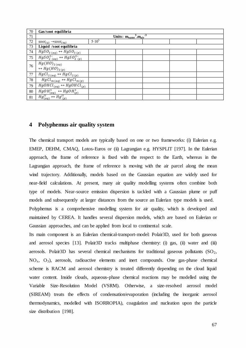
67
70 Gas/soot equilibria
71 Units: mwater3.mair
-3
72 soot(g) →soot(aq) 5·105
73 Liquid /soot equilibria
74 𝐻𝑔𝑆𝑂3 (𝑎𝑞) ↔ 𝐻𝑔𝑆𝑂3 (𝑝)
75 𝐻𝑔𝑆𝑂2 (𝑎𝑞)2− ↔ 𝐻𝑔𝑆𝑂2 (𝑝)
2−
76 𝐻𝑔(𝐻𝑂)2 (𝑎𝑞)↔ 𝐻𝑔(𝐻𝑂)2 (𝑝)
77 𝐻𝑔𝐶𝑙2 (𝑎𝑞) ↔ 𝐻𝑔𝐶𝑙2 (𝑝)
78 𝐻𝑔𝐶𝑙𝑚 (𝑎𝑞) ↔ 𝐻𝑔𝐶𝑙𝑚 (𝑝)
79 𝐻𝑔𝑂𝐻𝐶𝑙(𝑎𝑞) ↔ 𝐻𝑔𝑂𝐻𝐶𝑙(𝑝)
80 𝐻𝑔𝑂𝐻(𝑎𝑞)+ ↔ 𝐻𝑔𝑂𝐻(𝑝)
+
81 𝐻𝑔(𝑎𝑞)𝐼𝐼 ↔ 𝐻𝑔 (𝑝)
𝐼𝐼
Polyphemus air quality system 4
The chemical transport models are typically based on one or two frameworks: (i) Eulerian e.g.
EMEP, DEHM, CMAQ, Lotos-Euros or (ii) Lagrangian e.g. HYSPLIT [197]. In the Eulerian
approach, the frame of reference is fixed with the respect to the Earth, whereas in the
Lagrangian approach, the frame of reference is moving with the air parcel along the mean
wind trajectory. Additionally, models based on the Gaussian equation are widely used for
near-field calculations. At present, many air quality modelling systems often combine both
type of models. Near-source emission dispersion is tackled with a Gaussian plume or puff
models and subsequently at larger distances from the source an Eulerian type models is used.
Polyphemus is a comprehensive modelling system for air quality, which is developed and
maintained by CEREA. It handles several dispersion models, which are based on Eulerian or
Gaussian approaches, and can be applied from local to continental scale.
Its main component is an Eulerian chemical-transport-model: Polair3D, used for both gaseous
and aerosol species [13]. Polair3D tracks multiphase chemistry: (i) gas, (ii) water and (iii)
aerosols. Polair3D has several chemical mechanisms for traditional gaseous pollutants (SO2,
NOx, O3), aerosols, radioactive elements and inert compounds. One gas-phase chemical
scheme is RACM and aerosol chemistry is treated differently depending on the cloud liquid
water content. Inside clouds, aqueous-phase chemical reactions may be modelled using the
Variable Size-Resolution Model (VSRM). Otherwise, a size-resolved aerosol model
(SIREAM) treats the effects of condensation/evaporation (including the inorganic aerosol
thermodynamics, modelled with ISORROPIA), coagulation and nucleation upon the particle
size distribution [198].
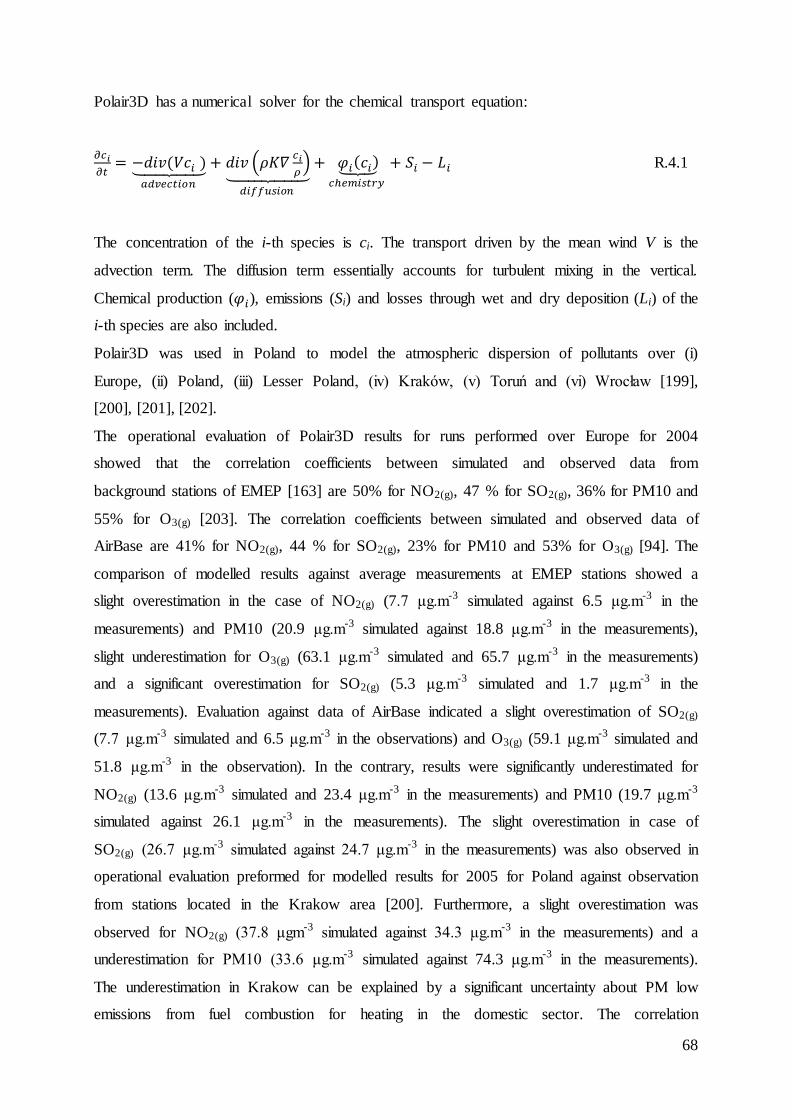
68
Polair3D has a numerical solver for the chemical transport equation:
𝜕𝑐𝑖
𝜕𝑡= −𝑑𝑖𝑣(𝑉𝑐𝑖 )⏟
𝑎𝑑𝑣𝑒𝑐𝑡𝑖𝑜𝑛
+ 𝑑𝑖𝑣 (𝜌𝐾𝛻𝑐𝑖
𝜌)
⏟ 𝑑𝑖𝑓𝑓𝑢𝑠𝑖𝑜𝑛
+ 𝜑𝑖(𝑐𝑖)⏟ 𝑐ℎ𝑒𝑚𝑖𝑠𝑡𝑟𝑦
+ 𝑆𝑖 − 𝐿𝑖 R.4.1
The concentration of the i-th species is ci. The transport driven by the mean wind V is the
advection term. The diffusion term essentially accounts for turbulent mixing in the vertical.
Chemical production (𝜑𝑖), emissions (Si) and losses through wet and dry deposition (Li) of the
i-th species are also included.
Polair3D was used in Poland to model the atmospheric dispersion of pollutants over (i)
Europe, (ii) Poland, (iii) Lesser Poland, (iv) Kraków, (v) Toruń and (vi) Wrocław [199],
[200], [201], [202].
The operational evaluation of Polair3D results for runs performed over Europe for 2004
showed that the correlation coefficients between simulated and observed data from
background stations of EMEP [163] are 50% for NO2(g), 47 % for SO2(g), 36% for PM10 and
55% for O3(g) [203]. The correlation coefficients between simulated and observed data of
AirBase are 41% for NO2(g), 44 % for SO2(g), 23% for PM10 and 53% for O3(g) [94]. The
comparison of modelled results against average measurements at EMEP stations showed a
slight overestimation in the case of NO2(g) (7.7 μg.m-3 simulated against 6.5 μg.m-3 in the
measurements) and PM10 (20.9 μg.m-3 simulated against 18.8 μg.m-3 in the measurements),
slight underestimation for O3(g) (63.1 μg.m-3 simulated and 65.7 μg.m-3 in the measurements)
and a significant overestimation for SO2(g) (5.3 μg.m-3 simulated and 1.7 μg.m-3 in the
measurements). Evaluation against data of AirBase indicated a slight overestimation of SO2(g)
(7.7 μg.m-3 simulated and 6.5 μg.m-3 in the observations) and O3(g) (59.1 μg.m-3 simulated and
51.8 μg.m-3 in the observation). In the contrary, results were significantly underestimated for
NO2(g) (13.6 μg.m-3 simulated and 23.4 μg.m-3 in the measurements) and PM10 (19.7 μg.m-3
simulated against 26.1 μg.m-3 in the measurements). The slight overestimation in case of
SO2(g) (26.7 μg.m-3 simulated against 24.7 μg.m-3 in the measurements) was also observed in
operational evaluation preformed for modelled results for 2005 for Poland against observation
from stations located in the Krakow area [200]. Furthermore, a slight overestimation was
observed for NO2(g) (37.8 μgm-3 simulated against 34.3 μg.m-3 in the measurements) and a
underestimation for PM10 (33.6 μg.m-3 simulated against 74.3 μg.m-3 in the measurements).
The underestimation in Krakow can be explained by a significant uncertainty about PM low
emissions from fuel combustion for heating in the domestic sector. The correlation
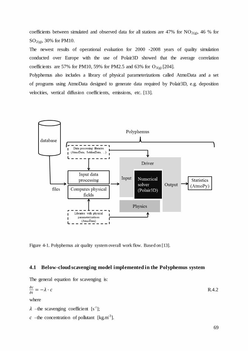
69
coefficients between simulated and observed data for all stations are 47% for NO2(g), 46 % for
SO2(g), 30% for PM10.
The newest results of operational evaluation for 2000 -2008 years of quality simulation
conducted over Europe with the use of Polair3D showed that the average correlation
coefficients are 57% for PM10, 59% for PM2.5 and 63% for O3(g) [204].
Polyphemus also includes a library of physical parameterizations called AtmoData and a set
of programs using AtmoData designed to generate data required by Polair3D, e.g. deposition
velocities, vertical diffusion coefficients, emissions, etc. [13].
Figure 4-1. Polyphemus air quality system overall work flow. Based on [13].
4.1 Below-cloud scavenging model implemented in the Polyphemus system
The general equation for scavenging is:
𝜕𝑐
𝜕𝑡= −𝜆 · 𝑐 R.4.2
where
𝜆 –the scavenging coefficient [s-1
];
𝑐 –the concentration of pollutant [kg.m-3].
70
Wet deposition is split between in-cloud (rainout) and below-cloud (washout) scavenging.
The below-cloud scavenging was calculated based on common algorithms implemented in
Polyphemus for gaseous as well as aerosol species. The in-cloud scavenging is calculated
inside algorithms specific for mercury chemistry and algorithms for lead and cadmium.
Below-cloud scavenging is calculated for gaseous mercury compounds (Hg0
(g), HgO(g),
HgCl2(g), Hg(OH)2(g), HgBr(g), HgBr2(g), HgBrOH(g)).
The below cloud scavenging coefficient [s-1] is given by the following relationship [205]:
𝜆 =10−6∙𝐼
3.6∙ 𝑈∙ 𝜏𝑡𝑟𝑎𝑛𝑠∙ 𝑒𝑥𝑝 (−
𝑧
𝑈∙𝜏𝑡𝑟𝑎𝑛𝑠 ∙𝐻∙𝑅∙𝑇) R.4.3
where:
I –intensity of rain [m.s-1],
U –raindrop terminal fall velocity [m.s-1],
𝜏𝑡𝑟𝑎𝑛𝑠 –the timescale of the mass transfer from the bulk air to the drops [s],
z –the fall distance [m],
𝐻 –Henry’s law constant [mol. m-3.atm-1],
𝑅 –ideal gas law constant [atm. m3.mol-1.K-1],
𝑇 –temperature [K].
The raindrop fall velocity U [m.s1-1] in the model is calculated as a function of the raindrop
diameter [206]:
𝑈 = 4854 ∙ 𝐷 ∙ exp(−195 ∙ D) R.4.4
𝐷 –the raindrop diameter [m].
Additionally, some other functions of the raindrop diameter presented in Table 4-1 were
applied to the model, but then the changes of this parameter are shown in the text.
The drop diameter can be calculated with the use of many various equations presented in
Table 5-6. The model was calculated with the use of the following formula 9.7·10-4
·I0.158
s-1.
However other formulas for drop diameter were also applied to the model to investigate the
sensitivity of the model to this parameter.
The timescale of the mass transfer from the bulk air to the drops is calculated as follows:
𝜏𝑡𝑟𝑎𝑛𝑠 =𝐷
6 𝐾𝑇 R.4.5

71
𝐾𝑇 –is the mass transfer coefficient [m.s-1], which is calculated as follows:
𝐾𝑇 =𝐷𝑔
𝐷∙ 𝑆ℎ R.4.6
where:
𝐷𝑔 –the gas-phase diffusivity [m2.s-1]. A gas phase diffusivity of 0.1194·10-4 m2.s-1 for GEM,
and 0.1628·10-4 m2.s-1 for RGM compounds was assumed [207].
𝑆ℎ –Sherwood Number which represents the ratio of convective to diffusive mass transport.
The Sherwood Number is expressed as follows:
𝑆ℎ = 2 + 0.6 ∙ 𝑅𝑒1/2 ∙ 𝑆𝑐1/3 R.4.7
where the Reynolds number 𝑅𝑒 is defined as follows:
𝑅𝑒 = 𝑈 ∙ 𝐷 𝑣𝑎⁄ R.4.8
and the Schmidt number Sc is calculated as follows:
𝑆𝑐 = 𝑣𝑎 𝐷𝑔⁄ R.4.9
In these calculations 𝑣𝑎 is the kinematic viscosity for air [m2.s-1] and it is calculated as the
ratio of the dynamic viscosity µ [kg.s-1.m-1] and density of the air ρ [kg.m-3].
𝑣𝑎 =𝜇
𝜌 R.4.10
The dynamic viscosity for air µ is calculated with the use of Sutherland's formula:
𝜇 = 𝜇0 ∙𝑇0+𝐶
𝑇+𝐶∙ (
𝑇
𝑇0)2/3
R.4.11
Reference viscosity µ0, reference temperature T0 and Sutherland's constant C – are constants
with defined values for air of: 18.27·106 kg.s-1.m-1, 291.15 K and 120 K, respectively.
Table 4-1. Raindrop velocity [m.s-1
] [208]. N. Raindrop velocity [m.s
-1]
1 142·D0.5
2 9.43·(1-exp((-1000·D/1.77)1.47
))
3 386.577·D0.67
4 4854.1·D ·exp(-195·D)
5
3.075·107·D
2 for D<10
-4
3.8·103·D for 10
-4 <D<10
-3
133.046·D0.5
for D>10-3
6 -0.193+4.96·103·D-9.04·10
5·D
2+5.66·10
7·D
3
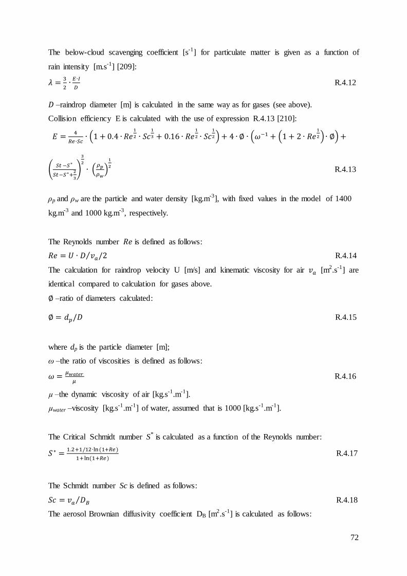
72
The below-cloud scavenging coefficient [s-1] for particulate matter is given as a function of
rain intensity [m.s-1] [209]:
𝜆 =3
2∙𝐸∙𝐼
𝐷 R.4.12
𝐷 –raindrop diameter [m] is calculated in the same way as for gases (see above).
Collision efficiency E is calculated with the use of expression R.4.13 [210]:
𝐸 =4
𝑅𝑒∙𝑆𝑐∙ (1 + 0.4 ∙ 𝑅𝑒
1
2 ∙ 𝑆𝑐1
3 + 0.16 ∙ 𝑅𝑒1
2 ∙ 𝑆𝑐1
2) + 4 ∙ ∅ ∙ (𝜔−1 + (1+ 2 ∙ 𝑅𝑒1
2) ∙ ∅) +
(𝑆𝑡 −𝑆∗
𝑆𝑡−𝑆∗+2
3
)
3
2
∙ (𝜌𝑝
𝜌𝑤)
1
2 R.4.13
ρp and ρw are the particle and water density [kg.m-3], with fixed values in the model of 1400
kg.m-3 and 1000 kg.m-3, respectively.
The Reynolds number 𝑅𝑒 is defined as follows:
𝑅𝑒 = 𝑈 ∙ 𝐷 𝑣𝑎/2⁄ R.4.14
The calculation for raindrop velocity U [m/s] and kinematic viscosity for air 𝑣𝑎 [m2.s-1] are
identical compared to calculation for gases above.
∅ –ratio of diameters calculated:
∅ = 𝑑𝑝/𝐷 R.4.15
where dp is the particle diameter [m];
ω –the ratio of viscosities is defined as follows:
𝜔 =𝜇𝑤𝑎𝑡𝑒𝑟
𝜇 R.4.16
µ –the dynamic viscosity of air [kg.s-1.m-1].
µwater –viscosity [kg.s-1.m-1] of water, assumed that is 1000 [kg.s-1.m-1].
The Critical Schmidt number S* is calculated as a function of the Reynolds number:
𝑆∗ =1.2+1/12∙ln (1+𝑅𝑒)
1+ln (1+𝑅𝑒) R.4.17
The Schmidt number Sc is defined as follows:
𝑆𝑐 = 𝑣𝑎 𝐷𝐵⁄ R.4.18
The aerosol Brownian diffusivity coefficient DB [m2.s-1] is calculated as follows:
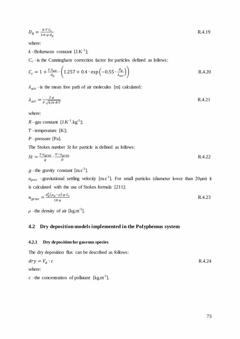
73
𝐷𝐵 =𝑘∙𝑇∙𝐶𝑐
3∙𝜋∙µ∙𝑑𝑝 R.4.19
where:
k –Boltzmann constant [J.K-1];
Cc –is the Cunningham correction factor for particles defined as follows:
𝐶𝑐 = 1 +2∙𝜆𝑎𝑖𝑟
𝑑𝑝∙ (1.257 + 0.4 ∙ exp (−0.55 ∙
𝑑𝑝
𝜆𝑎𝑖𝑟)) R.4.20
𝜆𝑎𝑖𝑟 –is the mean free path of air molecules [m] calculated:
𝜆𝑎𝑖𝑟 =2∙𝜇
𝑃∙√8/𝜋∙𝑅∙𝑇 R.4.21
where:
𝑅 –gas constant [J.K-1.kg-1];
𝑇 –temperature [K];
P –pressure [Pa].
The Stokes number St for particle is defined as follows:
𝑆𝑡 =2∙𝑢𝑔𝑟𝑎𝑣
𝑔∙𝑈−𝑢𝑔𝑟𝑎𝑣
𝐷 R.4.22
𝑔 –the gravity constant [m.s-2].
ugrav –gravitational settling velocity [m.s-1]. For small particles (diameter lower than 20µm) it
is calculated with the use of Stokes formula [211]:
𝑢𝑔𝑟𝑎𝑣 =𝑑𝑝2 (𝜌𝑝−𝜌)∙𝑔∙𝐶𝑐
18∙𝜇 R.4.23
ρ –the density of air [kg.m-3].
4.2 Dry deposition models implemented in the Polyphemus system
4.2.1 Dry deposition for gaseous species
The dry deposition flux can be described as follows:
𝑑𝑟𝑦 = 𝑉𝑑 ∙ 𝑐 R.4.24
where:
𝑐 –the concentration of pollutant [kg.m-3].

74
Figure 4-2. Schematic representation of a resistance model. The description of the resistances is
provided in the text.
The dry deposition velocity Vd [m.s-1] can be expressed with the use of a resistance model
presented in Figure 4-2 as:
𝑉𝑑 =1
𝑅𝑎+𝑅𝑏+𝑅𝑐 R.4.25
𝑅𝑎 , 𝑅𝑏 , 𝑅𝑐 are called the aerodynamic resistance, the quasi-laminar sublayer resistance and the
overall canopy resistance [all in s.m-1], respectively.
The aerodynamic resistance depends only on meteorological conditions and surface
roughness. The aerodynamic resistance is calculated based on the parametric model of vertical
eddy fluxes in the atmosphere for the part of the mass transfer dominated by turbulence [212],
[213].
𝑅𝑎 = (𝐴𝑡𝐴𝑢𝑓ℎ𝑊)−1 R.4.26
𝐴𝑢 =𝜅
𝑙𝑛(𝑧0+𝑍𝑟𝑍𝑟
) R.4.27
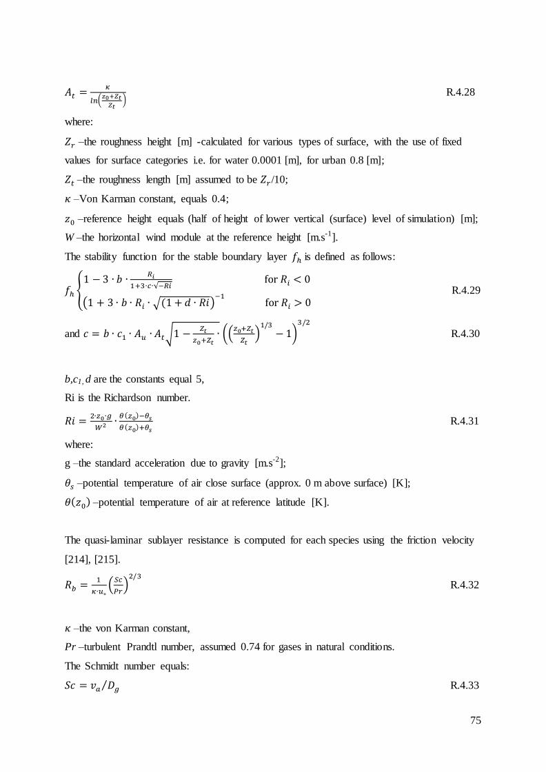
75
𝐴𝑡 =𝜅
𝑙𝑛(𝑧0+𝑍𝑡𝑍𝑡
) R.4.28
where:
𝑍𝑟 –the roughness height [m] -calculated for various types of surface, with the use of fixed
values for surface categories i.e. for water 0.0001 [m], for urban 0.8 [m];
𝑍𝑡 –the roughness length [m] assumed to be 𝑍𝑟/10;
𝜅 –Von Karman constant, equals 0.4;
𝑧0 –reference height equals (half of height of lower vertical (surface) level of simulation) [m];
W –the horizontal wind module at the reference height [m.s-1].
The stability function for the stable boundary layer 𝑓ℎ is defined as follows:
𝑓ℎ {1 − 3 ∙ 𝑏 ∙
𝑅𝑖
1+3∙𝑐∙√−𝑅𝑖 for 𝑅𝑖 < 0
(1 + 3 ∙ 𝑏 ∙ 𝑅𝑖 ∙ √(1 + 𝑑 ∙ 𝑅𝑖)−1 for 𝑅𝑖 > 0
R.4.29
and 𝑐 = 𝑏 ∙ 𝑐1 ∙ 𝐴𝑢 ∙ 𝐴𝑡√1 −𝑍𝑡
𝑧0+𝑍𝑡∙ ((
𝑧0+𝑍𝑡
𝑍𝑡)1/3
−1)3/2
R.4.30
b,c1, d are the constants equal 5,
Ri is the Richardson number.
𝑅𝑖 =2∙𝑧0∙𝑔
𝑊2 ∙𝜃(𝑧0)−𝜃𝑠
𝜃(𝑧0)+𝜃𝑠 R.4.31
where:
g –the standard acceleration due to gravity [m.s-2];
𝜃𝑠 –potential temperature of air close surface (approx. 0 m above surface) [K];
𝜃(𝑧0) –potential temperature of air at reference latitude [K].
The quasi-laminar sublayer resistance is computed for each species using the friction velocity
[214], [215].
𝑅𝑏 =1
𝜅∙𝑢∗(𝑆𝑐
𝑃𝑟)2/3
R.4.32
𝜅 –the von Karman constant,
Pr –turbulent Prandtl number, assumed 0.74 for gases in natural conditions.
The Schmidt number equals:
𝑆𝑐 = 𝑣𝑎 𝐷𝑔⁄ R.4.33
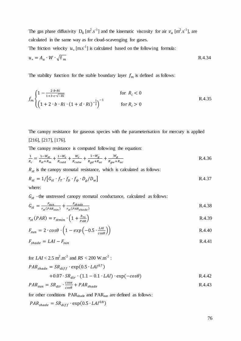
76
The gas phase diffusivity Dg [m2.s-1] and the kinematic viscosity for air 𝑣𝑎 [m2.s-1], are
calculated in the same way as for cloud-scavenging for gases.
The friction velocity 𝑢∗ [m.s-1] is calculated based on the following formula:
𝑢∗ = 𝐴𝑢 ∙ 𝑊 ∙ √f 𝑚 R.4.34
The stability function for the stable boundary layer 𝑓𝑚 is defined as follows:
𝑓𝑚 {1 −
2∙𝑏∙𝑅𝑖
1+3∙𝑐∙√−𝑅𝑖 for 𝑅𝑖 < 0
(1 + 2 ∙ 𝑏 ∙ 𝑅𝑖 ∙ (1 + 𝑑 ∙ 𝑅𝑖)−1
2)−1
for 𝑅𝑖 > 0 R.4.35
The canopy resistance for gaseous species with the parameterisation for mercury is applied
[216], [217], [176].
The canopy resistance is computed following the equation:
1
𝑅𝑐=
1−𝑊𝑠𝑡
𝑅𝑠𝑡+𝑅𝑚+1−𝑊𝑐
𝑅𝑐𝑢𝑡𝑑+
𝑊𝑐
𝑅𝑐𝑢𝑡𝑤+
1−𝑊𝑔
𝑅𝑔𝑑+𝑅𝑎𝑐+
𝑊𝑔
𝑅𝑔𝑤+𝑅𝑎𝑐 R.4.36
𝑅𝑠𝑡 is the canopy stomatal resistance, which is calculated as follows:
𝑅𝑠𝑡 = 1/[𝐺𝑠𝑡 ∙ 𝑓𝑇 ∙ 𝑓𝐷 ∙ 𝑓𝜓 ∙ 𝐷𝑔/𝐷𝑤] R.4.37
where:
𝐺𝑠𝑡 –the unstressed canopy stomatal conductance, calculated as follows:
𝐺𝑠𝑡 =𝐹𝑠𝑢𝑛
𝑟𝑠𝑡(𝑃𝐴𝑅𝑠𝑢𝑛 )+
𝐹𝑠ℎ𝑎𝑑𝑒
𝑟𝑠𝑡(𝑃𝐴𝑅𝑠ℎ𝑎𝑑𝑒 ) R.4.38
𝑟𝑠𝑡 (𝑃𝐴𝑅) = 𝑟𝑠𝑡𝑚𝑖𝑛 ∙ (1 +𝑏𝑟𝑠
𝑃𝐴𝑅) R.4.39
𝐹𝑠𝑢𝑛 = 2 ∙ 𝑐𝑜𝑠𝜃 ∙ (1 − 𝑒𝑥𝑝(−0.5 ∙𝐿𝐴𝐼
𝑐𝑜𝑠𝜃)) R.4.40
𝐹𝑠ℎ𝑎𝑑𝑒 = 𝐿𝐴𝐼 − 𝐹𝑠𝑢𝑛 R.4.41
for LAI < 2.5 m2.m-2 and RS < 200 W.m-2 :
𝑃𝐴𝑅𝑠ℎ𝑎𝑑𝑒 = 𝑆𝑅𝑑𝑖𝑓𝑓 ∙ exp(0.5 ∙ 𝐿𝐴𝐼0.7)
+0.07 ∙ 𝑆𝑅𝑑𝑖𝑟 ∙ (1.1 − 0.1 ∙ 𝐿𝐴𝐼) ∙ exp (−𝑐𝑜𝑠𝜃) R.4.42
𝑃𝐴𝑅𝑠𝑢𝑛 = 𝑆𝑅𝑑𝑖𝑟 ∙𝑐𝑜𝑠𝛼
𝑐𝑜𝑠𝜃+𝑃𝐴𝑅𝑠ℎ𝑎𝑑𝑒 R.4.43
for other conditions PARshade and PARsun are defined as follows:
𝑃𝐴𝑅𝑠ℎ𝑎𝑑𝑒 = 𝑆𝑅𝑑𝑖𝑓𝑓 ∙ exp(0.5 ∙ 𝐿𝐴𝐼0.8)
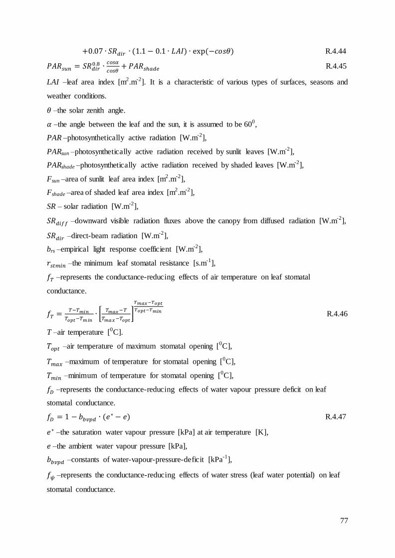
77
+0.07 ∙ 𝑆𝑅𝑑𝑖𝑟 ∙ (1.1 − 0.1 ∙ 𝐿𝐴𝐼) ∙ exp (−𝑐𝑜𝑠𝜃) R.4.44
𝑃𝐴𝑅𝑠𝑢𝑛 = 𝑆𝑅𝑑𝑖𝑟0.8 ∙
𝑐𝑜𝑠𝛼
𝑐𝑜𝑠𝜃+𝑃𝐴𝑅𝑠ℎ𝑎𝑑𝑒 R.4.45
LAI –leaf area index [m2.m-2]. It is a characteristic of various types of surfaces, seasons and
weather conditions.
𝜃 –the solar zenith angle.
𝛼 –the angle between the leaf and the sun, it is assumed to be 600,
PAR –photosynthetically active radiation [W.m-2],
PARsun –photosynthetically active radiation received by sunlit leaves [W.m-2],
PARshade –photosynthetically active radiation received by shaded leaves [W.m-2],
Fsun –area of sunlit leaf area index [m2.m-2],
Fshade –area of shaded leaf area index [m2.m-2],
SR – solar radiation [W.m-2],
𝑆𝑅𝑑𝑖𝑓𝑓 –downward visible radiation fluxes above the canopy from diffused radiation [W.m-2],
𝑆𝑅𝑑𝑖𝑟 –direct-beam radiation [W.m-2],
brs –empirical light response coefficient [W.m-2],
𝑟𝑠𝑡𝑚𝑖𝑛 –the minimum leaf stomatal resistance [s.m-1],
𝑓𝑇 –represents the conductance-reducing effects of air temperature on leaf stomatal
conductance.
𝑓𝑇 =𝑇−𝑇𝑚𝑖𝑛
𝑇𝑜𝑝𝑡−𝑇𝑚𝑖𝑛∙ [
𝑇𝑚𝑎𝑥−𝑇
𝑇𝑚𝑎𝑥−𝑇𝑜𝑝𝑡]
𝑇𝑚𝑎𝑥−𝑇𝑜𝑝𝑡
𝑇𝑜𝑝𝑡−𝑇𝑚𝑖𝑛 R.4.46
T –air temperature [0C].
𝑇𝑜𝑝𝑡 –air temperature of maximum stomatal opening [0C],
𝑇𝑚𝑎𝑥 –maximum of temperature for stomatal opening [0C],
𝑇𝑚𝑖𝑛 –minimum of temperature for stomatal opening [0C],
𝑓𝐷 –represents the conductance-reducing effects of water vapour pressure deficit on leaf
stomatal conductance.
𝑓𝐷 = 1 − 𝑏𝑏𝑣𝑝𝑑 ∙ (𝑒∗ − 𝑒) R.4.47
𝑒∗ –the saturation water vapour pressure [kPa] at air temperature [K],
𝑒 –the ambient water vapour pressure [kPa],
𝑏𝑏𝑣𝑝𝑑 –constants of water-vapour-pressure-deficit [kPa-1],
𝑓𝜓 –represents the conductance-reducing effects of water stress (leaf water potential) on leaf
stomatal conductance.

78
𝑓𝜓 =−0.72−0.0013𝑆𝑅−𝜓𝑐2
𝜓𝑐1−𝜓𝑐2 R.4.48
𝜓𝑐1 , 𝜓𝑐2 –parameters that specify leaf-water-potential dependency [MPa];
𝐷𝑤 –the diffusivity of water vapor [m2.s-1],
𝐷𝑔 –the gas-phase diffusivity of pollutants [m2.s-1],
𝑅𝑎𝑐 –in-canopy aerodynamic resistance [s.m-1]. The value of in-canopy aerodynamic
resistance is calculated as follows:
𝑅𝑎𝑐 =𝑅𝑎𝑐0∙𝐿𝐴𝐼
1 /4
𝑢∗2 R.4.49
𝑅𝑎𝑐0 is the reference value [s.m-1] for in-canopy aerodynamic resistance and its value depends
on land-use coverage. For example, for surface with no canopy (e.g. water, desert) it is set to
0.
𝑢∗ –friction velocity [m.s-1] -corresponding data for different land-use coverage and weather
conditions.
Data of 𝑇𝑜𝑝𝑡 , 𝑇𝑚𝑎𝑥 , 𝑇𝑚𝑖𝑛 , 𝜓𝑐1 , 𝜓𝑐2𝑏𝑏𝑣𝑝𝑑, 𝑧0, brs, 𝑟𝑠𝑡𝑚𝑖𝑛 for various land use coverage [217].
Values for leaf area index LAI are presented in the literature [216].
𝑊𝑠𝑡 –represents the fraction stomatal blocking when leaves are wet. It is calculated:
𝑊𝑠𝑡 = {0
(𝑆𝑅 − 200)/8000.5
𝑆𝑅 ≤ 200
200 < 𝑆𝑅 ≤ 600𝑆𝑅 > 200
R.4.50
𝑊𝑐 –represents the fraction of wet canopy,
𝑊𝑔 –represents the fraction of the wet ground surface.
The corresponding values of 𝑊𝑔,𝑊𝑐 for different humidity conditions are presented in Table
4-2.
Table 4-2 The value of constants for canopy stomatal model.
N. constants Conditions
rainy dewy humid
1 𝑊𝑔 0.9 0.5 0.2
2 𝑊𝑐 0.9 0.7 0.2
𝑅𝑚 is the mesophyll resistance [s.m-1] and values of 500 and 0 were used for elemental and
for reactive mercury, respectively. The mesophyll resistance is characteristic of the chemical
species. Usually, the value of the mesophyll resistance is set on the basis of observation or
through comparison with other species, that have similar chemical properties.
The 𝑅𝑐𝑢𝑡𝑤, 𝑅𝑐𝑢𝑡𝑑, 𝑅𝑔𝑤 , 𝑅𝑔𝑑 are resistances of: the wet cuticle, dry cuticle, wet-ground and
dry-ground, respectively. They are derived from well-known data for sulfur dioxide and

79
ozone [216]. The sulphur dioxide and ozone dry deposition pathway is very highly
documented and has been investigated in many measurement campaigns of dry deposition
made for these species. The model uses results for sulphur dioxide and ozone and sets surface
resistance for other species following their aqueous solubility and their chemical reactivity.
The average dry deposition velocity over Europe for sulphur dioxide and ozone generated
with the use of Polyphemus system are presented in Figure 4-3 and Figure 4-4.
1
𝑅𝑐𝑢𝑡𝑤 (𝑖)=
𝛼(𝑖)
𝑅𝑐𝑢𝑡𝑤(𝑆𝑂2)+
𝛽(𝑖)
𝑅𝑐𝑢𝑡𝑤 (𝑂3) R.4.51
1
𝑅𝑐𝑢𝑡𝑑 (𝑖)=
𝛼(𝑖)
𝑅𝑐𝑢𝑡𝑑 (𝑆𝑂2 )+
𝛽(𝑖)
𝑅𝑐𝑢𝑡𝑑 (𝑂3) R.4.52
1
𝑅𝑔𝑤(𝑖)=
𝛼(𝑖)
𝑅𝑔𝑤(𝑆𝑂2 )+
𝛽(𝑖)
𝑅𝑔𝑤(𝑂3) R.4.53
1
𝑅𝑔𝑑 (𝑖)=
𝛼(𝑖)
𝑅𝑔𝑑 (𝑆𝑂2 )+
𝛽(𝑖)
𝑅𝑔𝑑 (𝑂3) R.4.54
Scaling parameters 𝛼 = 10 and 𝛽 = 10 and 𝛼 = 0 and 𝛽 = 0.2 were set for reactive mercury
and elemental mercury, respectively. The scaling parameters were chosen with the assumption
that reactive mercury is deposited in the same way as HNO3(g) and elemental mercury is
poorly soluble.
Figure 4-3. Annual average dry deposition velocity in 2008 for SO2(g) [cm.s
-1].
Figure 4-4. Annual average dry deposition velocity in 2008 for O3(g) [cm.s
-1].
4.2.2 Dry deposition velocity for aerosols
The dry deposition velocity 𝑉𝑑 [m.s-1] is calculated for aerosols of mercury, lead and
cadmium with the following formula [218]:
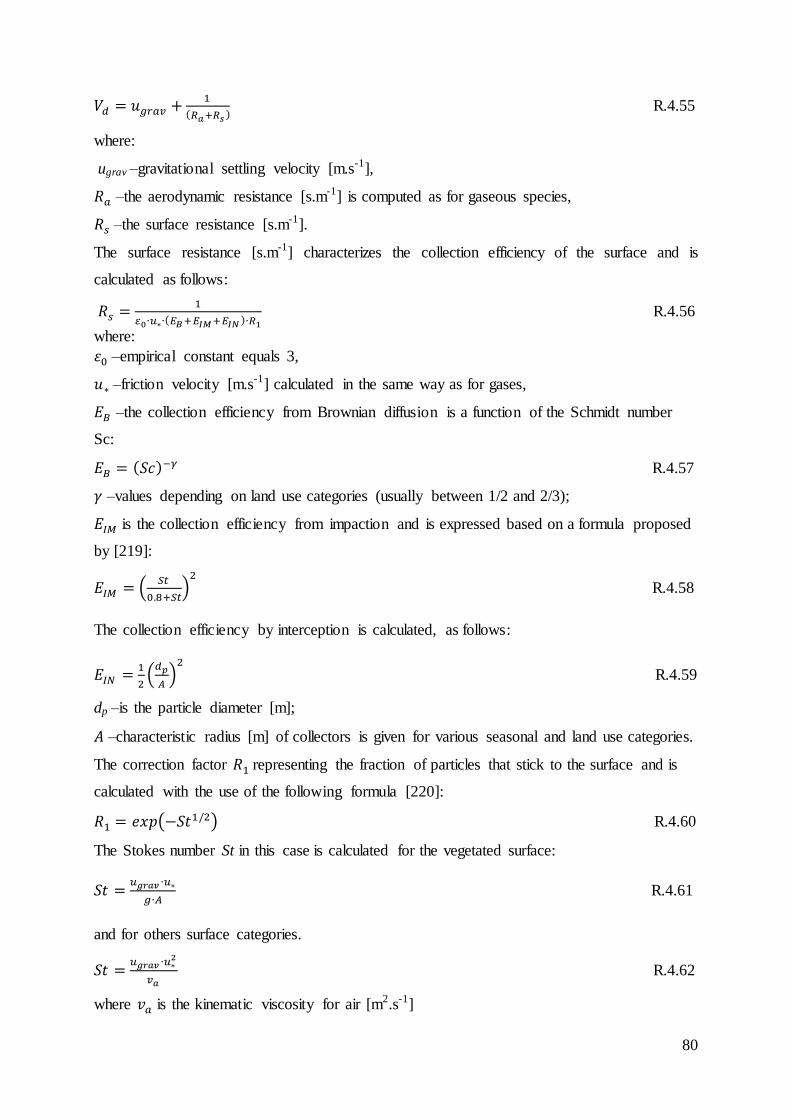
80
𝑉𝑑 = 𝑢𝑔𝑟𝑎𝑣 +1
(𝑅𝑎+𝑅𝑠 ) R.4.55
where:
ugrav –gravitational settling velocity [m.s-1],
𝑅𝑎 –the aerodynamic resistance [s.m-1] is computed as for gaseous species,
𝑅𝑠 –the surface resistance [s.m-1].
The surface resistance [s.m-1] characterizes the collection efficiency of the surface and is
calculated as follows:
𝑅𝑠 =1
𝜀0∙𝑢∗∙(𝐸𝐵+𝐸𝐼𝑀+𝐸𝐼𝑁 )∙𝑅1 R.4.56
where:
𝜀0 –empirical constant equals 3,
𝑢∗ –friction velocity [m.s-1] calculated in the same way as for gases,
𝐸𝐵 –the collection efficiency from Brownian diffusion is a function of the Schmidt number
Sc:
𝐸𝐵 = (𝑆𝑐)−𝛾 R.4.57
𝛾 –values depending on land use categories (usually between 1/2 and 2/3);
𝐸𝐼𝑀 is the collection efficiency from impaction and is expressed based on a formula proposed
by [219]:
𝐸𝐼𝑀 = (𝑆𝑡
0.8+𝑆𝑡)2
R.4.58
The collection efficiency by interception is calculated, as follows:
𝐸𝐼𝑁 =1
2(𝑑𝑝
𝐴)2
R.4.59
dp –is the particle diameter [m];
𝐴 –characteristic radius [m] of collectors is given for various seasonal and land use categories.
The correction factor 𝑅1 representing the fraction of particles that stick to the surface and is
calculated with the use of the following formula [220]:
𝑅1 = 𝑒𝑥𝑝(−𝑆𝑡1/2) R.4.60
The Stokes number St in this case is calculated for the vegetated surface:
𝑆𝑡 =𝑢𝑔𝑟𝑎𝑣 ∙𝑢∗
𝑔∙𝐴 R.4.61
and for others surface categories.
𝑆𝑡 =𝑢𝑔𝑟𝑎𝑣 ∙𝑢∗
2
𝑣𝑎 R.4.62
where 𝑣𝑎 is the kinematic viscosity for air [m2.s-1]
81
PART II Development and application
of a new chemical transport model for
mercury, modelling of atmospheric
transport of lead and cadmium
82
Distribution of the emissions of heavy metals into the air by the Polish 5
power sector with the use of the bottom-up approach
5.1 Methodology
The localization of the heavy metals sources and the speciation of emitted mercury have a
significant impact on the atmospheric transport of heavy metals, particularly from relatively
big sources, which are present in the power sector. Unfortunately, the EMEP programme
provides the total emissions from all sectors with horizontal resolution of 50 km by 50 km
[87]. Therefore, in this part of the manuscript, the vertical and horizontal localization of heavy
metals sources of the power sector will need to be specified. The speciation of emitted
mercury from all individual stacks will also be estimated. To that end, the ENVIRO database
for 2005 has been updated for 2008 in relation to installed boilers and emission controls, as
well as coal consumption and coal chemical energy (activity) based on statistics published for
that year [221], [222], [223], [58], [53]. The updated database for 2008 includes information
about boiler type, coal and chemical energy consumption, PM and SO2 emission control
configuration of 804 main boilers from the Polish power sector. It was assumed that the
chemical energy of coal consumed by heating plants included in the database equals the
chemical energy provided by the national emission inventors, (there is a possibility that some
small heating plants are not included in the database) [53]. National emission inventories
reported low (less than 1%) uncertainty of estimation of chemical energy of coal consumed in
the power sector [48]. The operated boilers were connected to 170 stacks, which are also
included together with a precise location and height in an improved database.
With the use of the chemical energy (activity) of coal consumed and the corresponding
emission factor, the mercury, cadmium and lead emission into the air were calculated for all
boilers. For mercury, two emission factors for 2008 and for 2009 were used. In 2008, they
were 0.0064 and 0.004 kg.TJ-1 for all hard and brown coal power plants, respectively [53].
For 2009, the emission factors were changed for power and CHP plants and amounted to
0.0023 kg.TJ-1 for hard coal and 0.0114 kg.TJ-1 for brown coal [54]. The obtained emissions
of mercury from all boilers installed in the polish power sector were split into three mercury
forms i.e.: (i) gaseous elemental mercury (GEM), (ii) reactive gaseous mercury (RGM) and
(iii) mercury bound to aerosol particles (HgP). The share of three forms of emitted mercury
for different coal -boiler type -emission control configurations were based on information

83
provided from measurement campaigns [37]. The corresponding numbers characterising the
power, CHP and heating plants and emissions of mercury with the use of emission factor for
2008 and 2009 and speciation factors are presented in Table 5-1.
Table 5-1. Aggregated data on power sector, which operated in 2008.
N. Boiler
type
PM
control
SO2
control
Number
of in-
stallation
Thermal
input
[MW]
Activity
[TJ]
Emission of Hg
[kg] Hgp
[%]
RGM
[%]
GEM
[%] EF
2008
EF
2009
1 Hard coal power and CHP plants
2 GF CYC 128 3965 27144 174 62 20 40 40
3 GF ESP 2 199 697 5 2 5 70 25
5 DBB CYC 1 57 116 1 0 20 40 40
6 DBB ESP 175 29489 293218 1877 671 5 60 35
7 DBB FF 10 1101 15154 97 35 5 60 35
8 DBB ESP SDFGD 15 4659 80849 517 185 5 45 50
9 DBB ESP DFGD 4 307 2157 14 5 5 45 50
10 DBB ESP WFGD 47 26226 409326 2620 936 10 35 55
11 DBB FF SDFGD 4 1327 19280 123 44 5 35 60
12 FBC ESP CFB 14 3680 67663 433 155 5 10 85
13 Total for hard coal power
and CHP plants 399 71010 915604 5860 2094
14 Brown coal power plants
15 DBB ESP 7 1982 36541 146 415 5 15 80
16 DBB ESP WFGD 23 17192 347164 1389 3939 5 10 85
17 DBB ESP DFGD 3 1722 37792 151 429 5 10 85
18 FBC ESP CFB 6 3213 100926 404 1145 5 10 85
19 Total for brown coal power
plants 39 24109 522423 2090 5928
20 Hard coal heating plants
21 GF CYC 317 8506 53035 339 20 40 40
22 GF FF 3 66 431 3 5 60 35
23 DBB ESP 40 4998 56191 360 5 60 35
24 DBB ESP WFGD 4 464 4537 29 10 35 55
25 FBC ESP CFB 1 185 2382 15 5 10 85
26 Total for hard coal heating
plants 365 14219 116576 746
27 Brown coal heating plants
28 FBC ESP CFB 1 78 284 1 5 10 85
GF - Grate Firing, DBB - Dry Bottom Boiler, FBC - Fluidized Bed Combustion, CYC - Cyclone Remove
System, ESP - Electrostatic Precipitator, FF - Fabric Filter, SDFGD - Semi Dry Flue Gas Desulfurization, DFGD
- Dry Flue Gas Desulfurization, WFGD - Wet Flue Gas Desulfurization.
The chemical energy of consumed coal by plants included in the database was also used in the
distribution of emitted lead and cadmium to individual stack of the power sector. The
emission factors for cadmium and lead in 2008, which are used to assess the emissions from
814 boilers installed in polish power plants are presented in Table 5-2.
The annual emissions of lead and cadmium from coal based power, cogeneration and heating
plants an equalled to 22148 kg and 2087 kg, in 2008, respectively [53]. The main share falls

84
on the emission of heating plants. In 2008, from these sources about 12938 kg.y-1 of lead and
1909 kg.y-1 of cadmium were released into the atmosphere. In the power sector (SNAP 0101
and SNAP 0102), 129 kg of cadmium and 742 kg of lead are emitted annually also from
combustion of natural gas, biomass, heating oil and coal gas. These emission were not
assigned to point sources and remain in the EMEP gridded inventory.
Table 5-2. Emission factors of lead and cadmium used to estimate emissions from individual boilers installed in the Polish power sector [53].
N. Fuel type Type of plants Emission factors [g.TJ
-1] Emission in 2008 [kg]
Lead Cadmium Lead Cadmium
1 Hard coal Power and CHP plants 8.96 0.12 8203.8 109.9
2 Heating plants 102.4 16.37 11937.4 1909.5
3 Brown
coal
Power plants 3.84 0.13 2006.1 67.9
4 Heating plants 3.87 0.00 1.1 0.0
5.2 Results
Locations of main emitters of mercury, lead and cadmium are presented in Figure 5-1 -Figure
5-4. The vertical distribution of these heavy metals from the power sector is presented in
Figure 5-5.
Figure 5-1. Location and emissions [kg] of main emitters of mercury. Emissions based on emission factors for 2008 (EF2008).
Figure 5-2. Location and emissions [kg] of main emitters of mercury. Emissions based on emission factors for 2009 (EF2009).
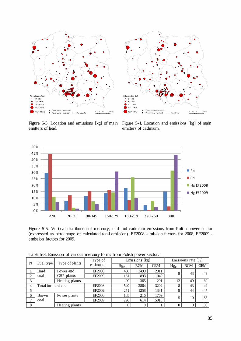
85
Figure 5-3. Location and emissions [kg] of main emitters of lead.
Figure 5-4. Location and emissions [kg] of main emitters of cadmium.
Figure 5-5. Vertical distribution of mercury, lead and cadmium emissions from Polish power sector (expressed as percentage of calculated total emission). EF2008 -emission factors for 2008, EF2009 -emission factors for 2009.
Table 5-3. Emission of various mercury forms from Polish power sector.
N Fuel type Type of plants Type of
estimation
Emissions [kg] Emissions rate [%]
Hgp RGM GEM Hgp RGM GEM
1 Hard
coal
Power and
CHP plants
EF2008 450 2499 2911 8 43 49
2 EF2009 161 893 1040
3 Heating plants 90 365 291 12 49 39
4 Total for hard coal EF2008 540 2864 3202 8 43 49
5 EF2009 251 1258 1331 9 44 47
6 Brown
coal
Power plants EF2008 105 216 1769 5 10 85
7 EF2009 296 614 5018
8 Heating plants 0 0 1 0 0 100
0%
5%
10%
15%
20%
25%
30%
35%
40%
45%
50%
<70 70-89 90-149 150-179 180-219 220-260 300
Pb
Cd
Hg EF2008
Hg EF2009

86
9 Total for hard and brown
coal
EF2008 645 3080 4972 7 35 57
10 EF2009 547 1872 6350 6 21 72
The total emissions of mercury from the power sector where coal is consumed with the use of
emission factors for 2008 and 2009 are almost equal (Table 5-3). It amounted to 8697 kg and
8769 kg, respectively. The significant differences appears in the estimation of emissions of 3
forms of mercury (GEM, RGM and HgP). The coal type, hard or brown, strongly affects the
share of emitted mercury forms. The combustion of brown coal causes high emission of GEM
compared to other forms. Whilst power plants based on hard coal emit nearly the same
amount of GEM and RGM. The emission of HgP in both cases is relatively low, because of
the widespread use of PM emission control systems (Table 5-1). The final speciation of
mercury emitted in the Polish power sector in the case of EF2008 emission factors i.e. 55% of
GEM, 36% of RGM and 9% of HgP is consistent with the results reported in the literature and
presented in Table 2-8 [84], [1], [47]. The results obtained with the emission factors for 2009
(EF2009) show that elemental mercury is prevailing, because mercury is mainly released from
brown coal power plants.
Most of cadmium is emitted from heating plants, which have low stack heights that usually do
not reach 70 meters as was presented in Figure 5-5. Lead is also mainly emitted from plants
which have stack heights lower than 70 meters. The share of these stack heights in total
emissions is 37% and 65% for lead and cadmium, respectively. As mercury is mainly emitted
from big power plants, most of it is released into the air from stacks above 150 meters.
5.3 Implemented chemical scheme of atmospheric mercury
The chemical scheme used in this study takes into account the reactions and transitions of
mercury in the gaseous, aqueous and particulate phases presented in Figure 5-6. This scheme
is an upgraded version of the chemical model previously introduced in the PhD thesis of
Yelva Roustan [224]. The main developments in this model are related to the reactions and
transformations of mercury with bromine. It has been shown, that bromine is more effective
in Hg-oxidation than chlorine to produce HgBr2(g) during coal combustion [225].
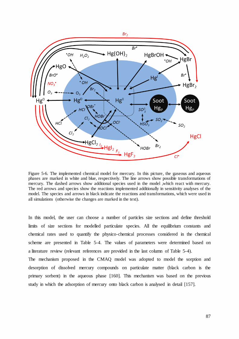
87
Figure 5-6. The implemented chemical model for mercury. In this picture, the gaseous and aqueous phases are marked in white and blue, respectively. The line arrows show possible transformations of mercury. The dashed arrows show additional species used in the model ,which react with mercury. The red arrows and species show the reactions implemented additionally in sensitivity analyses of the model. The species and arrows in black indicate the reactions and transformations, which were used in
all simulations (otherwise the changes are marked in the text).
In this model, the user can choose a number of particles size sections and define threshold
limits of size sections for modelled particulate species. All the equilibrium constants and
chemical rates used to quantify the physico-chemical processes considered in the chemical
scheme are presented in Table 5-4. The values of parameters were determined based on
a literature review (relevant references are provided in the last column of Table 5-4).
The mechanism proposed in the CMAQ model was adopted to model the sorption and
desorption of dissolved mercury compounds on particulate matter (black carbon is the
primary sorbent) in the aqueous phase [160]. This mechanism was based on the previous
study in which the adsorption of mercury onto black carbon is analysed in detail [157].

88
Table 5-4. Physico-chemical processes considered in the mercury chemistry model. In italics are written reaction which are used only in sensitivity studies.
N. Reaction Rate / equilibrium
constant Units Reference
1 Gas-phase oxidation
2 Hg0
(g) + O3(g) →HgO(g) + O2(g) k1=2.1·10
-18·exp(-
1246/T) cm
3.molec
-1.s
-1 [96]
3 Hg0
(g) + 2
•OH(g) →Hg(OH)2(g) k2=8.7·10
-14 cm
3.molec
-1.s
-1 [107]
4 Hg0
(g) + Cl2(g) →HgCl2(g) k3=2.6·10-18
cm3.molec
-1.s
-1 [117]
5 Hg0
(g) + 2HCl(g) →HgCl2(g) + H2(g) k4=10-19
cm3.molec
-1.s
-1 [126]
6 Hg0
(g) +H2O2(g) →Hg(OH)2(g) k4=8.4·10
-6·exp(-
9021/T) cm
3.molec
-1.s
-1 [113]
7 Hg0
(g) +BrO•(g) →HgO(g) + Br(g) k5=1.5·10
-14 cm
3.molec
-1.s
-1 [133]
8 Hg
0(g) +Br
•(g) →HgBr(g) k6=1.46·10
-32· (T/298)
-
1.86
cm6.molec
-2.s
-1 [226]
9 HgBr(g) +Br
•(g) →HgBr2(g) k7=2.5·10
-
10·exp(T/298)
-0.57
cm3.molec
-1.s
-1 [111]
10 HgBr(g) +•OH(g) →HgBrOH(g)
k8=2.5·10-
10·exp(T/298)
-0.57
cm3.molec
-1.s
-1 [111]
11 Hg0
(g)+Br2 (g) →HgBr2(g) k9=0.9·10-16
cm3.molec
-1.s
-1 [117]
12 Hg0
(g) + NO3•(g) →HgO(g) + NO2(g) k10=4.0·10
-15 cm
3.molec
-1.s
-1 [135]
13 Hg0
(g) + I2 (g) → HgI2(g) k11=1.27·10-19
cm3.molec
-1.s
-1 [136]
14 Hg0
(g) + F2(g) → HgF2(g) k12=1.8·10-15
cm3.molec
-1.s
-1 [106]
15 Hg0
(g)+ Cl• (g) →HgCl(g) k13=1.0·10
-11 cm
3.molec
-1.s
-1 [117]
16 Gas-phase reduction
17 HgBr(g) → Hg
0(g) + Br
•(g) k14=1.2·10
10·exp(-
8357/T)
s-1
[111]
18 HgBr(g) + Br•(g) →Hg
0(g) + Br2(g) k15=3.9·10
-11 cm
3.molec
-1.s
-1 [130]
19 Aqueous-phase oxidation
20 Hg
0(aq) +O3(aq) + H
+(aq)
→ Hg
2+(aq) + OH
-(aq)
+
O2(aq) k16=4.7·10
7 M
-1.s
-1 [140]
21 Hg0
(aq) +•OH(aq) →Hg
+(aq) + OH
-(aq) k17=2.0·10
9 M
-1.s
-1 [142]
22 Hg0
(aq) +HOCl(aq) →Hg2+
(aq) +OH-(aq) +Cl
-(aq) k18=2.09·10
6 M
-1.s
-1 [144]
23 Hg
0(aq) +OCl
-(aq) +H
+(aq) →Hg
2+(aq) +OH
-(aq) +
Cl-(aq)
k19=1.99·106 M
-1.s
-1 [144]
24 Hg0
(aq) +HOBr(aq) → Hg2+
(aq) +OH-(aq) +Br
-(aq) k20=0.279 M
-1.s
-1 [141]
25 Hg
0(aq) +OBr
-(aq) +H
+(aq) →Hg
2+(aq) +Br
-(aq) +
OH-(aq)
k21=0.273 M-1
.s-1
[141]
26 Hg0
(aq) +Br2(aq) → Hg2+
(aq) +2Br-(aq) k22=0.196 M
-1.s
-1 [141]
27 Hg+
(aq) +(•OH, O2, HO2
•)(aq) →Hg
2+ (aq) fast
[142]
[149]
[156]
28 Aqueous-phase reduction
29 HgSO3(aq) →Hg
0(aq) + products(SIV)(aq) k23=7.7·10
13T·exp(-
12595/T)
s-1
[147]
30 Hg2+
(aq) +HO2•(aq) →Hg
0(aq) +O2(aq) +H
+(aq) k24=1.1·10
4 M
-1.s
-1 [149]
31 Gas/liquid equilibria
32 O3(g) ↔ O3(aq) H1=1.13·10-2
M.atm-1
[227]
33 SO2(g) ↔ SO2(aq) H2=1.23 M.atm-1
[228]
34 Cl2(g) ↔ Cl2(aq) H3=0.076 M.atm-1
[229]
35 •OH(g) ↔
•OH(aq) H4=25 M.atm
-1 [230]
36 HO2•(g) ↔ HO2
•(aq) H5=2·10
3 M.atm
-1 [231]
37 Br2(g) ↔ Br2(aq) H6=0.76 M.atm-1
[232]
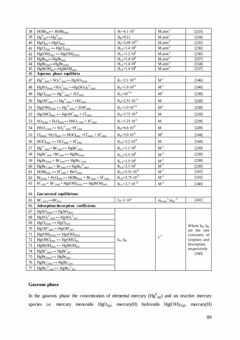
89
38 HOBr(g)↔ HOBr(aq) H7=6.1·103 M.atm
-1 [233]
39 Hg0
(g)↔ Hg0
(aq) H8=0.11 M.atm-1
[234]
40 HgO(g) ↔HgO(aq) H9=2.69·1012
M.atm-1
[235]
41 HgCl2(g) ↔ HgCl2(aq) H10=1.4·106 M.atm
-1 [236]
42 Hg(OH)2(g) ↔ Hg(OH)2(aq) H11=1.2·104 M.atm
-1 [236]
43 HgBr(g)↔HgBr(aq) H12=1.4·106 M.atm
-1 [237]
44 HgBr2(g)↔HgBr2(aq) H13=1.4·106 M.atm
-1 [134]
45 HgBrOH(g)↔HgBrOH(aq) H14=1.4·106 M.atm
-1 [237]
46 Aqueous phase equilibria
47 Hg2+
(aq) + SO32-
(aq) ↔ HgSO3(aq) K1=2.1·1013
M-1
[146]
48 HgSO3(aq) +SO32
(aq) -↔Hg(SO3)2
2-(aq) K2=1.0·10
10 M
-1 [146]
49 HgCl2(aq) ↔ Hg2+
(aq) + 2Cl-(aq) K3=10
-14 M
2 [238]
50 HgOH+
(aq) ↔ Hg2+
(aq) + OH-(aq) K4=2.51·10
-11 M [228]
51 Hg(OH)2(aq) ↔ Hg2+
(aq) + 2OH-(aq) K5=1.0·10
-22 M
2 [238]
52 HgOHCl(aq) ↔ HgOH+
(aq) + Cl-(aq) K6=3.72·10
-8 M [228]
53 SO2(aq) + H2O(aq) ↔ HSO3-(aq) + H
+(aq) K7=1.23·10
-2 M [228]
54 HSO3-(aq) ↔ SO3
2-(aq) +H
+(aq) K8=6.6·10
-8 M [228]
55 Cl2(aq) +H2O(aq) ↔ HOCl(aq) +Cl-(aq) + H
+(aq) K9=5.0·10
-4 M
2 [144]
56 HOCl(aq) ↔ OCl-(aq) + H
+(aq) K10=3.2·10
-8 M [144]
57 Hg2+
(aq) + Br-(aq) ↔ HgBr
+(aq) K11=1.1·10
9 M
-1 [239]
58 HgBr+
(aq) +Br-(aq) ↔ HgBr2(aq) K12=2.5·10
8 M
-1 [239]
59 HgBr2(aq) + Br-(aq) ↔ HgBr3
-(aq) K13=1.5·10
2 M
-1 [239]
60 HgBr3-(aq) + Br
-(aq) ↔ HgBr4
2-(aq) K14=2.3·10
1 M
-1 [239]
61 HOBr(aq) ↔ H+
(aq) + BrO-(aq) K15=2.51·10
-9 M
-1 [141]
62 Br2(aq) + H2O(aq) ↔ HOBr(aq) + Br-(aq) + H
+(aq) K16=5.75·10
-9 M
-1 [141]
63 H+
(aq) + Br-
(aq) + Hg(OH)2(aq) ↔ HgBrOH(aq) K17=2.7·10-12
M-2
[240]
64 Gas/aerosol equilibrium
65 BC (air) ↔BC(w) G1=1·105 mwater
3.mair
-3 [241]
66 Adsorption/desorption coefficients
67 HgSO3(aq) ↔ HgSO3(p)
kS, kD s
-1
Where kS, kD
are the rate
constants of
sorption and
desorption
respectively.
[160]
68 HgSO22-
(aq) ↔ HgSO22-
(p)
69 HgCl2(aq) ↔ HgCl2(p)
70 HgOH+
(aq) ↔HgOH+
(p)
71 Hg(OH)2(aq) ↔ Hg(OH)2(p)
72 HgOHCl(aq) ↔ HgOHCl(p)
73 HgBrOH(aq) ↔ HgBrOH(p)
74 HgBr+
(aq) ↔ HgBr+
(p)
75 HgBr2(aq) ↔ HgBr2(p)
76 HgBr3-(aq) ↔ HgBr3
-(p)
77 HgBr42-
(aq) ↔ HgBr42-
(p)
Gaseous phase
In the gaseous phase the concentration of elemental mercury (Hg0(g)) and six reactive mercury
species i.e. mercury monoxide HgO(g), mercury(II) hydroxide Hg(OH)2(g), mercury(II)

90
chloride HgCl2(g), mercury bromide HgBr(g), mercury(II) bromide HgBr2(g), hydroxy mercury
bromide HgBrOH(g) are modelled. Taken into account the mercury reactions in the gaseous
phase (listed in Table 3-1) the changes of concentrations of considered species are expressed
as follows:
𝑑
𝑑𝑡[𝐻𝑔(𝑔)
0 ] = −𝑗1 − 𝑗2 − 𝑗3 − 𝑗4 − 𝑗5 − 𝑗6 − 𝑗7 + 𝑗15 + 𝑗16 R.5.1
𝑑
𝑑𝑡[𝐻𝑔𝑂(𝑔)] = 𝑗1 + 𝑗6 R.5.2
𝑑
𝑑𝑡[𝐻𝑔(𝑂𝐻)2(𝑔)] = 𝑗2 + 𝑗5 R.5.3
𝑑
𝑑𝑡[𝐻𝑔𝐶𝑙2(𝑔)] = 𝑗3 + 𝑗4 R.5.4
𝑑
𝑑𝑡[𝐻𝑔𝐵𝑟(𝑔)] = 𝑗7 − 𝑗8 − 𝑗9 − 𝑗15 − 𝑗16 R.5.5
𝑑
𝑑𝑡[𝐻𝑔𝐵𝑟2(𝑔)] = 𝑗8 R.5.6
𝑑
𝑑𝑡[𝐻𝑔𝐵𝑟𝑂𝐻(𝑔)] = 𝑗9 R.5.7
where:
j1=k1[Hg0(g)][O3(g)] R.5.8
j2=k2[Hg0(g)][OH(g)] R.5.9
j3=k3[Hg0(g)][Cl2(g)] R.5.10
j4=k4[Hg0(g)][HCl(g)] R.5.11
j5=k5[Hg0(g)][H2O2(g)] R.5.12
j6=k6[Hg0(g)][BrO•
(g)] R.5.13
j7=k7[Hg0(g)][Br•
(g)] R.5.14
j8=k8[HgBr(g)][ Br•(g)] R.5.15
j8=k9[HgBr(g)][ •OH(g)] R.5.16
j15=k15[HgBr(g)] R.5.17
j16=k16[HgBr(g)][Br•(g)] R.5.18
In sensitivity studies, additionally mercury(II) iodide -HgI2(g), mercury(II) fluoride -HgF2(g),
mercury chloride -HgCl(g) are modelled. Accordingly, suitable reaction rates are added to the
model.
Aqueous phase
The reactions and transformations of mercury in the aqueous phase are modelled when
sufficient liquid water is diagnosed in the atmosphere at the beginning or the end of the

91
simulation time step. The cloud presence diagnosis is simply based on a threshold (0.05 g.m-3)
of the liquid water content in the atmosphere.
The concentration of substrates taken part in the aqueous phase are calculated based on
Henry's law and equilibria presented in Table 5-4:
[𝑂3(𝑎𝑞)] = 𝐻1 ∙𝑅∙𝑇
𝑁𝑎𝑣[𝑂3(𝑔)] R.5.19
[𝑆𝑂32−(𝑎𝑞)
] =𝐾7 ∙𝐾8
[𝐻+]2 ∙ 𝐻2 ∙
𝑅∙𝑇
𝑁𝑎𝑣[𝑆𝑂2(𝑔) ] R.5.20
[𝐻𝑂𝐶𝑙(𝑎𝑞)] =𝐾9
[𝐶𝑙−][𝐻+ ]∙ 𝐻3 ∙
𝑅𝑇
𝑁𝑎𝑣[𝐶𝑙2(𝑔)] R.5.21
[𝑂𝐶𝑙(𝑎𝑞)− ] =
𝐾9∙𝐾10[𝐶𝑙− ][𝐻+]2
∙ 𝐻3 ∙𝑅∙𝑇
𝑁𝑎𝑣[𝐶𝑙2(𝑔)] R.5.22
[ 𝑂𝐻𝑛•
(𝑎𝑞)] = 𝐻4 ∙𝑅∙𝑇
𝑁𝑎𝑣[ 𝑂𝐻𝑛•
(𝑔)] R.5.23
[𝐻𝑂2(𝑎𝑞)• ] = 𝐻5 ∙
𝑅∙𝑇
𝑁𝑎𝑣[𝐻𝑂2(𝑔)
• ] R.5.24
[𝐵𝑟2(𝑎𝑞)] = 𝐻6 ∙𝑅∙𝑇
𝑁𝑎𝑣[𝐵𝑟2(𝑔)] R.5.25
[𝐻𝑂𝐵𝑟(𝑎𝑞)] = 𝐻7 ∙𝑅∙𝑇
𝑁𝑎𝑣[𝐻𝑂𝐵𝑟(𝑔)] R.5.26
[𝑂𝐵𝑟(𝑎𝑞)− ] =
𝐾15[𝐻+]
∙ 𝐻7 ∙𝑅∙𝑇
𝑁𝑎𝑣[𝐻𝑂𝐵𝑟(𝑔)] R.5.27
where:
[𝐻+] = 10−𝑝𝐻 R.5.28
R –ideal gas law constant, 82 atm.cm3.mol-1.K-1 or 8.13 J. mol-1.K-1;
Nav –Avogadro constant, 6.022·1023 molec.mol-1;
T –temperature [K];
pH –potential of hydrogen, pH of cloud water, assumed to be 4.5 [195].
In the model only total divalent mercury (HgII(aq)), and elemental mercury Hg0
(aq) are specified
in the aqueous phase. However, at each simulation time steps the concentrations of particular
oxidized mercury compounds i.e. HgSO3(aq), HgSO22-
(aq), Hg(OH)2(aq), HgCl2(aq), HgOHCl(aq),
HgOH+(aq), HgBrOH(aq), HgBr+
(aq), HgBr2(aq), HgBr3-(aq), HgBr4
2-(aq) is calculated, if needed. The
total divalent mercury in the models equals:
[𝐻𝑔𝐼𝐼(𝑎𝑞)
] = [𝐻𝑔2 +(𝑎𝑞)
] + [𝐻𝑔( 𝑆 )(𝑎𝑞)
] + [𝐻𝑔𝐶𝑙2(𝑎𝑞)] + [𝐻𝑔( 𝑂 )(𝑎𝑞)] + [𝐻𝑔( 𝐵𝑟 )(𝑎𝑞)] R.5.29
where:
[𝑯𝒈( 𝑺 )(𝑎𝑞)
] = [𝐻𝑔𝑆𝑂3 (𝑎𝑞)] + [𝐻𝑔(𝑆𝑂3 )2
2−(𝑎𝑞)
] R.5.30
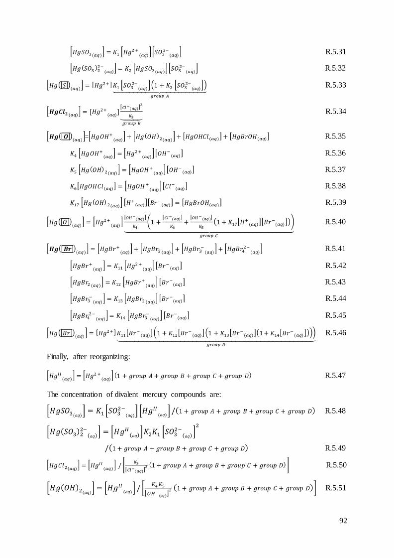
92
[𝐻𝑔𝑆𝑂3(𝑎𝑞)] = 𝐾1 [𝐻𝑔2 +
(𝑎𝑞)][𝑆𝑂3
2−(𝑎𝑞)
] R.5.31
[𝐻𝑔(𝑆𝑂3 )22−
(𝑎𝑞)] = 𝐾2 [𝐻𝑔𝑆𝑂3(𝑎𝑞)][𝑆𝑂3
2−(𝑎𝑞)
] R.5.32
[𝐻𝑔( 𝑆 )(𝑎𝑞)
] = [𝐻𝑔2+ ]𝐾1 [𝑆𝑂32−(𝑎𝑞)
](1 + 𝐾2 [𝑆𝑂32−(𝑎𝑞)])
⏟ 𝑔𝑟𝑜𝑢𝑝 𝐴
R.5.33
[𝑯𝒈𝑪𝒍𝟐 (𝑎𝑞)] = [𝐻𝑔2+
(𝑎𝑞)][𝐶𝑙−(𝑎𝑞)]
2
𝐾3⏟ 𝑔𝑟𝑜𝑢𝑝 𝐵
R.5.34
[𝑯𝒈( 𝑶 )(𝑎𝑞)
]=[𝐻𝑔𝑂𝐻+(𝑎𝑞)
] + [𝐻𝑔(𝑂𝐻)2(𝑎𝑞)] + [𝐻𝑔𝑂𝐻𝐶𝑙(𝑎𝑞)] + [𝐻𝑔𝐵𝑟𝑂𝐻(𝑎𝑞)] R.5.35
𝐾4 [𝐻𝑔𝑂𝐻+(𝑎𝑞)
] = [𝐻𝑔2 +(𝑎𝑞)
][𝑂𝐻−(𝑎𝑞)] R.5.36
𝐾5 [𝐻𝑔(𝑂𝐻) 2(𝑎𝑞)] = [𝐻𝑔𝑂𝐻+(𝑎𝑞)
][𝑂𝐻−(𝑎𝑞)] R.5.37
𝐾6[𝐻𝑔𝑂𝐻𝐶𝑙(𝑎𝑞)] = [𝐻𝑔𝑂𝐻+(𝑎𝑞)
][𝐶𝑙−(𝑎𝑞)] R.5.38
𝐾17 [𝐻𝑔(𝑂𝐻) 2(𝑎𝑞)] [𝐻+(𝑎𝑞)][𝐵𝑟
−(𝑎𝑞)] = [𝐻𝑔𝐵𝑟𝑂𝐻(𝑎𝑞)] R.5.39
[𝐻𝑔( 𝑂 )(𝑎𝑞)
] = [𝐻𝑔2+(𝑎𝑞)
][𝑂𝐻−(𝑎𝑞)]
𝐾4(1 +
[𝐶𝑙−(𝑎𝑞)]
𝐾6+[𝑂𝐻−(𝑎𝑞)]
𝐾5(1 + 𝐾17[𝐻
+(𝑎𝑞)][𝐵𝑟
−(𝑎𝑞)]))
⏟ 𝑔𝑟𝑜𝑢𝑝 𝐶
R.5.40
[𝑯𝒈( 𝑩𝒓 )(𝑎𝑞)
] = [𝐻𝑔𝐵𝑟+(𝑎𝑞)
] + [𝐻𝑔𝐵𝑟2 (𝑎𝑞)] + [𝐻𝑔𝐵𝑟3−(𝑎𝑞)
] + [𝐻𝑔𝐵𝑟42−
(𝑎𝑞)] R.5.41
[𝐻𝑔𝐵𝑟+(𝑎𝑞)
] = 𝐾11 [𝐻𝑔2 +
(𝑎𝑞)][𝐵𝑟−(𝑎𝑞)] R.5.42
[𝐻𝑔𝐵𝑟2 (𝑎𝑞)] = 𝐾12 [𝐻𝑔𝐵𝑟+(𝑎𝑞)
] [𝐵𝑟−(𝑎𝑞)] R.5.43
[𝐻𝑔𝐵𝑟3−(𝑎𝑞)
] = 𝐾13 [𝐻𝑔𝐵𝑟2 (𝑎𝑞)] ⌈𝐵𝑟−(𝑎𝑞)⌉ R.5.44
[𝐻𝑔𝐵𝑟42−
(𝑎𝑞)] = 𝐾14 [𝐻𝑔𝐵𝑟3
−(𝑎𝑞)
] [𝐵𝑟−(𝑎𝑞)] R.5.45
[𝐻𝑔( 𝐵𝑟 )(𝑎𝑞)
] = [𝐻𝑔2+ ]𝐾11[𝐵𝑟−(𝑎𝑞)](1 + 𝐾12[𝐵𝑟
−(𝑎𝑞)](1 + 𝐾13[𝐵𝑟
−(𝑎𝑞)](1+ 𝐾14[𝐵𝑟
−(𝑎𝑞)])))⏟
𝑔𝑟𝑜𝑢𝑝 𝐷
R.5.46
Finally, after reorganizing:
[𝐻𝑔𝐼𝐼(𝑎𝑞)
] = [𝐻𝑔2 +(𝑎𝑞)
](1 + 𝑔𝑟𝑜𝑢𝑝 𝐴 + 𝑔𝑟𝑜𝑢𝑝 𝐵 + 𝑔𝑟𝑜𝑢𝑝 𝐶 + 𝑔𝑟𝑜𝑢𝑝 𝐷) R.5.47
The concentration of divalent mercury compounds are:
[𝐻𝑔𝑆𝑂3(𝑎𝑞)] = 𝐾1 [𝑆𝑂32−
(𝑎𝑞)] [𝐻𝑔𝐼𝐼
(𝑎𝑞)] /(1 + 𝑔𝑟𝑜𝑢𝑝 𝐴 + 𝑔𝑟𝑜𝑢𝑝 𝐵 + 𝑔𝑟𝑜𝑢𝑝 𝐶 + 𝑔𝑟𝑜𝑢𝑝 𝐷) R.5.48
[𝐻𝑔(𝑆𝑂3)22−(𝑎𝑞)] = [𝐻𝑔𝐼𝐼 (𝑎𝑞)]𝐾2𝐾1 [𝑆𝑂3
2−(𝑎𝑞)]2
/(1 + 𝑔𝑟𝑜𝑢𝑝 𝐴 + 𝑔𝑟𝑜𝑢𝑝 𝐵 + 𝑔𝑟𝑜𝑢𝑝 𝐶 + 𝑔𝑟𝑜𝑢𝑝 𝐷) R.5.49
[𝐻𝑔𝐶𝑙2(𝑎𝑞)] = [𝐻𝑔𝐼𝐼(𝑎𝑞)
] / [𝐾3
[𝐶𝑙−(𝑎𝑞)]2 (1 + 𝑔𝑟𝑜𝑢𝑝 𝐴 + 𝑔𝑟𝑜𝑢𝑝 𝐵 + 𝑔𝑟𝑜𝑢𝑝 𝐶 + 𝑔𝑟𝑜𝑢𝑝 𝐷)] R.5.50
[𝐻𝑔(𝑂𝐻)2(𝑎𝑞)] = [𝐻𝑔𝐼𝐼(𝑎𝑞)] / [
𝐾4𝐾5
[𝑂𝐻− (𝑎𝑞)]2 (1 + 𝑔𝑟𝑜𝑢𝑝 𝐴 + 𝑔𝑟𝑜𝑢𝑝 𝐵 + 𝑔𝑟𝑜𝑢𝑝 𝐶 + 𝑔𝑟𝑜𝑢𝑝 𝐷)] R.5.51

93
[𝐻𝑔𝐵𝑟2 (𝑎𝑞)] = [𝐻𝑔𝐼𝐼(𝑎𝑞)] [
1
𝐾12𝐾11 [𝐵𝑟−]2(1 + 𝑔𝑟𝑜𝑢𝑝 𝐴 + 𝑔𝑟𝑜𝑢𝑝 𝐵 + 𝑔𝑟𝑜𝑢𝑝 𝐶 + 𝑔𝑟𝑜𝑢𝑝 𝐷)] R.5.52
[𝐻𝑔𝐵𝑟𝑂𝐻(𝑎𝑞)] = [𝐻𝑔𝐼𝐼(𝑎𝑞)] [𝑂𝐻−(𝑎𝑞)]
2𝐾17[𝐻
+(𝑎𝑞)][𝐵𝑟
−(𝑎𝑞)]
/[𝐾4𝐾5(1 + 𝑔𝑟𝑜𝑢𝑝 𝐴 + 𝑔𝑟𝑜𝑢𝑝 𝐵 + 𝑔𝑟𝑜𝑢𝑝 𝐶 + 𝑔𝑟𝑜𝑢𝑝 𝐷)] R.5.53
The changes of concentrations in the aqueous phase are calculated as follows:
𝑑
𝑑𝑡[𝐻𝑔(𝑎𝑞)
0 ] = −𝑗17 − 𝑗18 − 𝑗19 − 𝑗20 − 𝑗21 − 𝑗22 − 𝑗23 + 𝑗24 + 𝑗25 R.5.54
𝑑
𝑑𝑡[𝐻𝑔𝐼𝐼
(𝑎𝑞)] = −𝑗17 − 𝑗18 − 𝑗19 − 𝑗20 − 𝑗21 − 𝑗22 − 𝑗23 − 𝑗24 − 𝑗25 + 𝑓1
𝑔→𝑎𝑞 + 𝑓2𝑔→𝑎𝑞 −
𝑓2𝑎𝑞→𝑔 + 𝑓3
𝑔→𝑎𝑞 −𝑓3𝑎𝑞→𝑔 +𝑓4
𝑔→𝑎𝑞 +𝑓5𝑔→𝑎𝑞 − 𝑓5
𝑎𝑞→𝑔 + 𝑓6𝑔→𝑎𝑞 + 𝑓6
𝑎𝑞→𝑔 R.5.55
and the changes of gaseous species due to transformation of gaseous to aqueous phase, or
inversely, are calculated in the model:
𝑑
𝑑𝑡[𝐻𝑔𝑂(𝑔)] = −𝑓1
𝑔→𝑎𝑞 𝑁𝑎𝑣 ∙𝑊𝑇
103 R.5.56
𝑑
𝑑𝑡[𝐻𝑔(𝑂𝐻)2(𝑔)] = (−𝑓2
𝑔→𝑎𝑞+𝑓2
𝑎𝑞→𝑔)𝑁𝑎𝑣 ∙𝑊𝑇
103 R.5.57
𝑑
𝑑𝑡[𝐻𝑔𝐶𝑙2(𝑔)] = (−𝑓3
𝑔→𝑎𝑞+𝑓3
𝑎𝑞→𝑔)𝑁𝑎𝑣 ∙𝑊𝑇
103 R.5.58
𝑑
𝑑𝑡[𝐻𝑔𝐵𝑟(𝑔)] = −𝑓4
𝑔→𝑎𝑞 𝑁𝑎𝑣 ∙𝑊𝑇
103 R.5.59
𝑑
𝑑𝑡[𝐻𝑔𝐵𝑟2(𝑔)] = (−𝑓5
𝑔→𝑎𝑞+ 𝑓5
𝑎𝑞→𝑔)𝑁𝑎𝑣 ∙𝑊𝑇
103 R.5.60
𝑑
𝑑𝑡[𝐻𝑔𝐵𝑟𝑂𝐻(𝑔)] = (−𝑓6
𝑔→𝑎𝑞+ 𝑓6
𝑎𝑞→𝑔)𝑁𝑎𝑣 ∙𝑊𝑇
103 R.5.61
where:
j17=k17[Hg0(aq)][O3(aq)] R.5.62
j18=k18[Hg0(aq)][ •OH(aq)] R.5.63
j19=k19[Hg0(aq)][HOCl(aq)] R.5.64
j20=k20[Hg0(aq)][OCl-(aq)] R.5.65
j21=k21[Hg0(aq)][HOBr(aq)] R.5.66
j22=k22[Hg0(aq)][OBr-
(aq)] R.5.67
j23=k23[Hg0(aq)][Br2(aq)] R.5.68
j24=k24[HgSO3(aq)] R.5.69
j25=k25[Hg2+(aq)][HO2
•(aq)] R.5.70
𝑓1𝑔→𝑎𝑞 = 𝑦1
103
𝑁𝑎𝑣[𝐻𝑔𝑂(𝑔)] R.5.71
𝑓2𝑔→𝑎𝑞 = 𝑦2
103
𝑁𝑎𝑣[𝐻𝑔(𝑂𝐻)2(𝑔)] R.5.72

94
𝑓2𝑎𝑞→𝑔 = 𝑦2
1
𝐻11 ∙𝑅∙𝑇[𝐻𝑔(𝑂𝐻)2(𝑎𝑞)] R.5.73
𝑓3𝑔→𝑎𝑞 = 𝑦3
103
𝑁𝑎𝑣[𝐻𝑔𝐶𝑙2(𝑔)] R.5.74
𝑓3𝑎𝑞→𝑔 = 𝑦3
1
𝐻10 ∙𝑅∙𝑇[𝐻𝑔𝐶𝑙2(𝑎𝑞)] R.5.75
𝑓4𝑔→𝑎𝑞 = 𝑦4
103
𝑁𝑎𝑣[𝐻𝑔𝐵𝑟(𝑔)] R.5.76
𝑓5𝑔→𝑎𝑞 = 𝑦5
103
𝑁𝑎𝑣[𝐻𝑔𝐵𝑟2(𝑔)] R.5.77
𝑓5𝑎𝑞→𝑔 = 𝑦5
1
𝐻13 ∙𝑅∙𝑇[𝐻𝑔𝐵𝑟2(𝑎𝑞)] R.5.78
𝑓6𝑔→𝑎𝑞 = 𝑦6
103
𝑁𝑎𝑣[𝐻𝑔𝐵𝑟𝑂𝐻(𝑔)] R.5.79
𝑓6𝑎𝑞→𝑔 = 𝑦6
1
𝐻14 ∙𝑅∙𝑇[𝐻𝑔𝐵𝑟𝑂𝐻(𝑎𝑞)] R.5.80
𝑦𝑎 = (𝐷2
𝐷𝑔 +
4∙𝐷
3∙𝜑∙(8∙𝑅∙𝑇
𝜋∙𝑀𝑎)1/2)
−1
R.5.81
Where:
a ranges from 1 to 6.
𝐷𝑔 –the gas phase diffusivity [m2.s-1]. A gas phase diffusivity of 0.1628·10-4 m2.s-1 for
reactive gaseous mercury compounds was assumed [207], [242],
D –representative raindrop diameter [m] -set to 10 µm,
𝑊𝑇 –the water content in the atmosphere [mwater3.mair
-3],
𝜑 –accommodation coefficient -set to 0.1 for all species of reactive mercury [243],
y –mass transfer coefficient [s-1],
M –molar mass of individual mercury compounds [kg.mol-1].
When the aqueous phase is diagnosed the elemental mercury concentration is distributed into
gaseous (Hg0(g)) and aqueous (Hg0
(aq)) phases.
Assuming that the total of Hg0 (in molec.cm-1) present in the atmosphere is in the gaseous
(Hg0(g)) (in molec.cm-1) or/and in aqueous (Hg0
(aq)) (in M) phases, the following relationship
occurs:
[𝐻𝑔0] = [𝐻𝑔(𝑔)0 ] + [𝐻𝑔(𝑎𝑞)
0 ]𝑁𝑎𝑣 ∙𝑊𝑇
103 R.5.82
and Henry’s law for elemental mercury:
[𝐻𝑔(𝑎𝑞)0 ] = 𝐻8 ∙
𝑅∙𝑇
𝑁𝑎𝑣[𝐻𝑔(𝑔)
0 ] R.5.83
95
then:
[𝐻𝑔(𝑔)0 ] =
1
1+𝐻8 ∙𝑊𝑇 ∙𝑅∙𝑇∙10−3[𝐻𝑔0] R.5.84
[𝐻𝑔(𝑎𝑞)0 ] =
1
𝑁𝑎𝑣∙
𝐻8 ∙𝑅∙𝑇
1+𝐻8 ∙𝑊𝑇 ∙𝑅∙𝑇∙10−3[𝐻𝑔0] R.5.85
In the case when no aqueous phase occurs [𝐻𝑔(𝑔)0 ] is equal to [𝐻𝑔0].
Concentrations of aqueous and gaseous species are expressed in M and in molec.cm-3,
respectively. The rates are expressed in M.s-1 or molec.cm-3.s-1. In the model, the units are
chosen as necessary. No mass transfer from HgII(aq) to HgO(g) and HgBr(g) was assumed,
because of the high solubility of HgO(g) and because HgBr(g) mercury has an oxidation state of
one.
In the case when the aqueous phase does not appear in the next step of a simulation run,
because the liquid water content is below the given threshold, whole divalent mercury in the
aqueous phase is equally splint among gaseous compounds i.e. HgOH2(g), HgCl2(g), HgBr2(g),
HgBrOH(g).
Adsorption/ Desorption
The adsorption (or wider sorption) rates js [M.s-1] of aqueous Hg compounds i.e. HgSO3(aq),
HgSO22-
(aq), Hg(OH)2(aq), HgCl2(aq), HgOHCl(aq), HgOH+(aq), HgBrOH(aq), HgBr+
(aq), HgBr2(aq),
HgBr3-(aq), HgBr4
2-(aq) -the sum was named Hgcplx in [kg.mwater
-3 or M], onto black carbon
aerosol (BC(w)) suspended in atmospheric water is calculated based on the approach described
in chapter 2.5 [160]:
𝑗𝑆 = 𝑘𝑠 · [𝐻𝑔𝑐𝑝𝑙𝑥] R.5.86
where:
𝑘𝑆 =𝐾𝐸𝐶𝐴 ·[BC(𝑤) ]
𝑡∗·(𝐾𝐸𝐶𝐴 ·[BC(𝑤)]+1) R.5.87
[BC(𝑤)] –concentration of black carbon suspended in atmospheric water [kg.mwater-3] which
equals:
[BC(𝑤)] = 𝐺1 · [BC(𝑎𝑖𝑟)] R.5.88
[BC(𝑎𝑖𝑟)] –concentration of black carbon in air [kg.mair-3],
𝐺1 –equilibrium (Table 5-4),
𝐾𝐵𝐶𝐴 –absorption coefficient, assumed to be 680·10-9 mwater3.µgBC
-1 [157], [243],
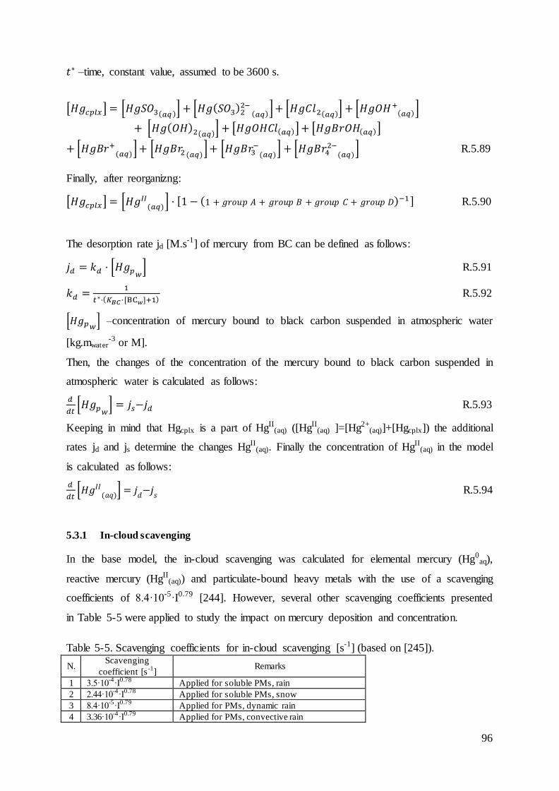
96
𝑡∗ –time, constant value, assumed to be 3600 s.
[𝐻𝑔𝑐𝑝𝑙𝑥] = [𝐻𝑔𝑆𝑂3(𝑎𝑞)] + [𝐻𝑔(𝑆𝑂3)22−(𝑎𝑞)
]+ [𝐻𝑔𝐶𝑙2(𝑎𝑞)] + [𝐻𝑔𝑂𝐻+(𝑎𝑞)
]
+ [𝐻𝑔(𝑂𝐻)2(𝑎𝑞)] + [𝐻𝑔𝑂𝐻𝐶𝑙(𝑎𝑞)]+ [𝐻𝑔𝐵𝑟𝑂𝐻(𝑎𝑞)]
+ [𝐻𝑔𝐵𝑟+(𝑎𝑞)
]+ [𝐻𝑔𝐵𝑟2(𝑎𝑞)]+ [𝐻𝑔𝐵𝑟3−(𝑎𝑞)
] + [𝐻𝑔𝐵𝑟42−(𝑎𝑞)
] R.5.89
Finally, after reorganizng:
[𝐻𝑔𝑐𝑝𝑙𝑥] = [𝐻𝑔𝐼𝐼(𝑎𝑞)
] · [1 − (1 + 𝑔𝑟𝑜𝑢𝑝 𝐴 + 𝑔𝑟𝑜𝑢𝑝 𝐵 + 𝑔𝑟𝑜𝑢𝑝 𝐶 + 𝑔𝑟𝑜𝑢𝑝 𝐷)−1] R.5.90
The desorption rate jd [M.s-1] of mercury from BC can be defined as follows:
𝑗𝑑 = 𝑘𝑑 · [𝐻𝑔𝑝𝑤] R.5.91
𝑘𝑑 =1
𝑡∗·(𝐾𝐵𝐶 ·[BC𝑤]+1) R.5.92
[𝐻𝑔𝑝𝑤] –concentration of mercury bound to black carbon suspended in atmospheric water
[kg.mwater-3 or M].
Then, the changes of the concentration of the mercury bound to black carbon suspended in
atmospheric water is calculated as follows:
𝑑
𝑑𝑡[𝐻𝑔𝑝𝑤
] = 𝑗𝑠−𝑗𝑑 R.5.93
Keeping in mind that Hgcplx is a part of HgII(aq) ([HgII
(aq) ]=[Hg2+(aq)]+[Hgcplx]) the additional
rates jd and js determine the changes HgII(aq). Finally the concentration of HgII
(aq) in the model
is calculated as follows:
𝑑
𝑑𝑡[𝐻𝑔𝐼𝐼
(𝑎𝑞)]= 𝑗
𝑑−𝑗𝑠 R.5.94
5.3.1 In-cloud scavenging
In the base model, the in-cloud scavenging was calculated for elemental mercury (Hg0aq),
reactive mercury (HgII(aq)) and particulate-bound heavy metals with the use of a scavenging
coefficients of 8.4·10-5·I0.79 [244]. However, several other scavenging coefficients presented
in Table 5-5 were applied to study the impact on mercury deposition and concentration.
Table 5-5. Scavenging coefficients for in-cloud scavenging [s-1] (based on [245]).
N. Scavenging
coefficient [s-1
] Remarks
1 3.5·10-4
·I0.78
Applied for soluble PMs, rain
2 2.44·10-4
·I0.78
Applied for soluble PMs, snow
3 8.4·10-5
·I0.79
Applied for PMs, dynamic rain
4 3.36·10-4
·I0.79
Applied for PMs, convective rain
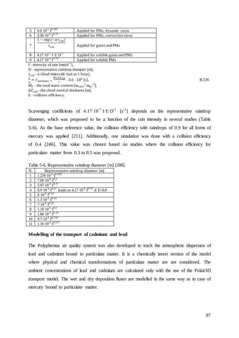
97
5 8.0·10-5
·I0.305
Applied for PMs, dynamic snow
6 3.36·10-4
·I0.79
Applied for PMs, convective snow
7
1 − exp (−𝛼𝜏𝑐𝑙𝑑)
𝜏𝑐𝑙𝑑
Applied for gases and PMs
8 4.17·10-7
·I·E·D-1
Applied for soluble gases and PMs
9 4.17·10-4
·I0.79
Applied for soluble PMs
I –intensity of rain [mm.h-1
],
D –representative raindrop diameter [m],
𝜏𝑐𝑙𝑑 –a cloud timescale (set as 1 hour), 1
𝛼= 𝜏𝑤𝑎𝑠ℎ𝑜𝑢𝑡 =
𝑊𝑇∆𝑍𝑐𝑙𝑑
𝐼· 3.6 · 106 [s], R.5.95
𝑊𝑇 –the total water content [mwater3.mair
-3],
∆𝑍𝑐𝑙𝑑 –the cloud vertical thickness [m],
E –collision efficiency.
Scavenging coefficients of 4.17·10-7·I·E·D-1 [s-1] depends on the representative raindrop
diameter, which was proposed to be a function of the rain intensity in several studies (Table
5-6). As the base reference value, the collision efficiency with raindrops of 0.9 for all forms of
mercury was applied [211]. Additionally, one simulation was done with a collision efficiency
of 0.4 [246]. This value was chosen based on studies where the collision efficiency for
particulate matter from 0.3 to 0.5 was proposed.
Table 5-6. Representative raindrop diameter [m] [208].
N. Representative raindrop diameter [m]
1 1.238·10-3
·I0.182
2 7.88·10-4
·I0.3
3 3.97·10-4
·I0.37
4 0.9·10-3
·I0.21
leads to 4.17·10-4
·I0.79
if E=0.9
5 8·10-4
·I0.34
6 1.3·10-3
·I0.14
7 7·10-4
·I0.25
8 1.18·10-3
·I0.2
9 1.06·10-3
·I0.16
10 9.7·10-4
·I0.158
11 1.16·10-3
·I0.227
Modelling of the transport of cadmium and lead
The Polyphemus air quality system was also developed to track the atmospheric dispersion of
lead and cadmium bound to particulate matter. It is a chemically invert version of the model
where physical and chemical transformations of particulate matter are not considered. The
ambient concentrations of lead and cadmium are calculated only with the use of the Polair3D
transport model. The wet and dry deposition fluxes are modelled in the same way as in case of
mercury bound to particulate matter.
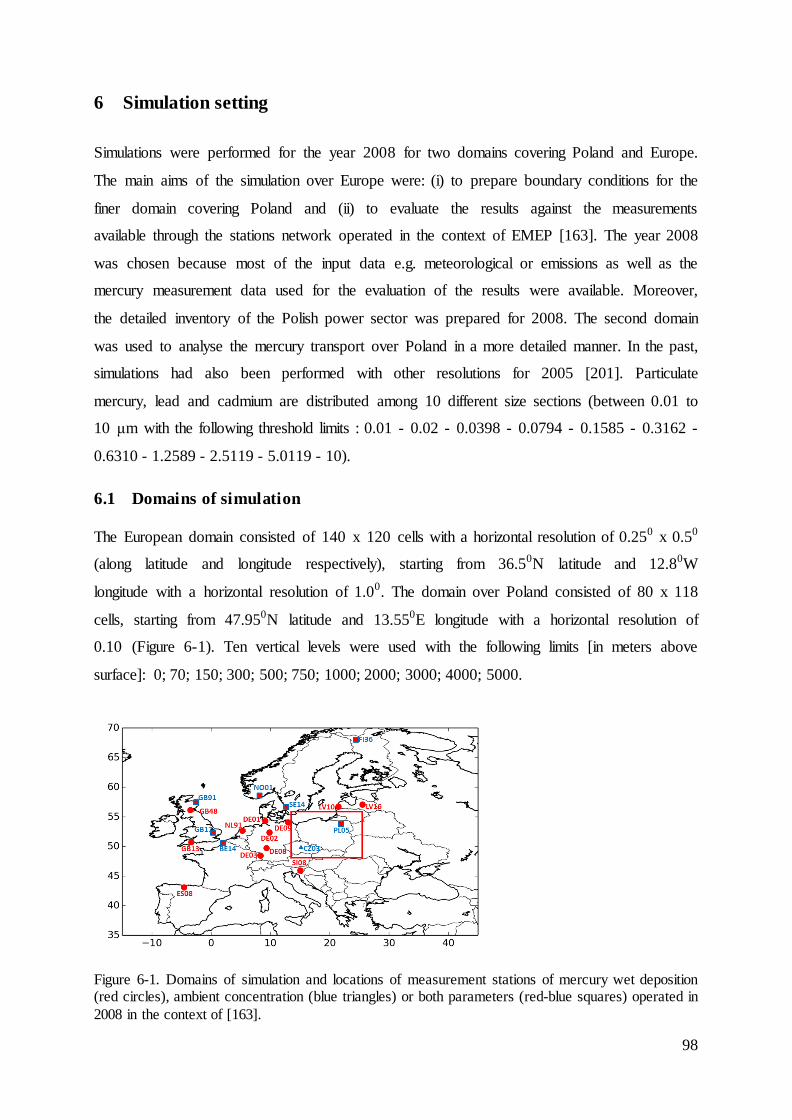
98
Simulation setting 6
Simulations were performed for the year 2008 for two domains covering Poland and Europe.
The main aims of the simulation over Europe were: (i) to prepare boundary conditions for the
finer domain covering Poland and (ii) to evaluate the results against the measurements
available through the stations network operated in the context of EMEP [163]. The year 2008
was chosen because most of the input data e.g. meteorological or emissions as well as the
mercury measurement data used for the evaluation of the results were available. Moreover,
the detailed inventory of the Polish power sector was prepared for 2008. The second domain
was used to analyse the mercury transport over Poland in a more detailed manner. In the past,
simulations had also been performed with other resolutions for 2005 [201]. Particulate
mercury, lead and cadmium are distributed among 10 different size sections (between 0.01 to
10 μm with the following threshold limits : 0.01 - 0.02 - 0.0398 - 0.0794 - 0.1585 - 0.3162 -
0.6310 - 1.2589 - 2.5119 - 5.0119 - 10).
6.1 Domains of simulation
The European domain consisted of 140 x 120 cells with a horizontal resolution of 0.250 x 0.50
(along latitude and longitude respectively), starting from 36.50N latitude and 12.80W
longitude with a horizontal resolution of 1.00. The domain over Poland consisted of 80 x 118
cells, starting from 47.950N latitude and 13.550E longitude with a horizontal resolution of
0.10 (Figure 6-1). Ten vertical levels were used with the following limits [in meters above
surface]: 0; 70; 150; 300; 500; 750; 1000; 2000; 3000; 4000; 5000.
Figure 6-1. Domains of simulation and locations of measurement stations of mercury wet deposition (red circles), ambient concentration (blue triangles) or both parameters (red-blue squares) operated in
2008 in the context of [163].
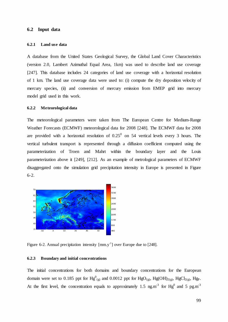
99
6.2 Input data
6.2.1 Land use data
A database from the United States Geological Survey, the Global Land Cover Characteristics
(version 2.0, Lambert Azimuthal Equal Area, 1km) was used to describe land use coverage
[247]. This database includes 24 categories of land use coverage with a horizontal resolution
of 1 km. The land use coverage data were used to: (i) compute the dry deposition velocity of
mercury species, (ii) and conversion of mercury emission from EMEP grid into mercury
model grid used in this work.
6.2.2 Meteorological data
The meteorological parameters were taken from The European Centre for Medium-Range
Weather Forecasts (ECMWF) meteorological data for 2008 [248]. The ECMWF data for 2008
are provided with a horizontal resolution of 0.250 on 54 vertical levels every 3 hours. The
vertical turbulent transport is represented through a diffusion coefficient computed using the
parameterization of Troen and Mahrt within the boundary layer and the Louis
parameterization above it [249], [212]. As an example of metrological parameters of ECMWF
disaggregated onto the simulation grid precipitation intensity in Europe is presented in Figure
6-2.
Figure 6-2. Annual precipitation intensity [mm.y-1
] over Europe due to [248].
6.2.3 Boundary and initial concentrations
The initial concentrations for both domains and boundary concentrations for the European
domain were set to 0.185 ppt for Hg0(g)
and 0.0012 ppt for HgO(g), Hg(OH)2(g), HgCl2(g), HgP.
At the first level, the concentration equals to approximately 1.5 ng.m-3 for Hg0 and 5 pg.m-3
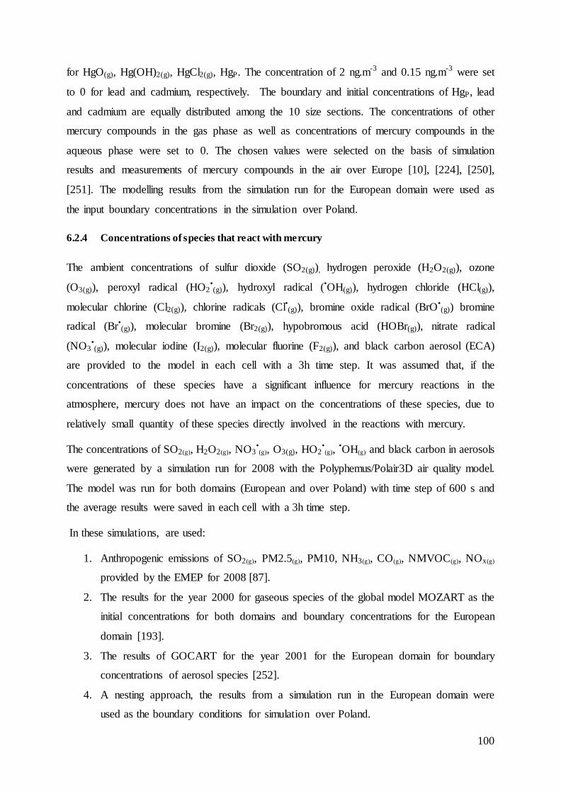
100
for HgO(g), Hg(OH)2(g), HgCl2(g), HgP. The concentration of 2 ng.m-3 and 0.15 ng.m-3 were set
to 0 for lead and cadmium, respectively. The boundary and initial concentrations of HgP, lead
and cadmium are equally distributed among the 10 size sections. The concentrations of other
mercury compounds in the gas phase as well as concentrations of mercury compounds in the
aqueous phase were set to 0. The chosen values were selected on the basis of simulation
results and measurements of mercury compounds in the air over Europe [10], [224], [250],
[251]. The modelling results from the simulation run for the European domain were used as
the input boundary concentrations in the simulation over Poland.
6.2.4 Concentrations of species that react with mercury
The ambient concentrations of sulfur dioxide (SO2(g)), hydrogen peroxide (H2O2(g)), ozone
(O3(g)), peroxyl radical (HO2•(g)), hydroxyl radical (•OH(g)), hydrogen chloride (HCl(g)),
molecular chlorine (Cl2(g)), chlorine radicals (Cl•(g)), bromine oxide radical (BrO•(g)) bromine
radical (Br•(g)), molecular bromine (Br2(g)), hypobromous acid (HOBr(g)), nitrate radical
(NO3•(g)), molecular iodine (I2(g)), molecular fluorine (F2(g)), and black carbon aerosol (ECA)
are provided to the model in each cell with a 3h time step. It was assumed that, if the
concentrations of these species have a significant influence for mercury reactions in the
atmosphere, mercury does not have an impact on the concentrations of these species, due to
relatively small quantity of these species directly involved in the reactions with mercury.
The concentrations of SO2(g), H2O2(g), NO3•(g), O3(g), HO2
•(g),
•OH(g) and black carbon in aerosols
were generated by a simulation run for 2008 with the Polyphemus/Polair3D air quality model.
The model was run for both domains (European and over Poland) with time step of 600 s and
the average results were saved in each cell with a 3h time step.
In these simulations, are used:
1. Anthropogenic emissions of SO2(g), PM2.5(g), PM10, NH3(g), CO(g), NMVOC(g), NOx(g)
provided by the EMEP for 2008 [87].
2. The results for the year 2000 for gaseous species of the global model MOZART as the
initial concentrations for both domains and boundary concentrations for the European
domain [193].
3. The results of GOCART for the year 2001 for the European domain for boundary
concentrations of aerosol species [252].
4. A nesting approach, the results from a simulation run in the European domain were
used as the boundary conditions for simulation over Poland.
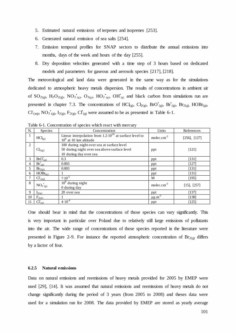
101
5. Estimated natural emissions of terpenes and isoprenes [253].
6. Generated natural emission of sea salts [254].
7. Emission temporal profiles for SNAP sectors to distribute the annual emissions into
months, days of the week and hours of the day [255].
8. Dry deposition velocities generated with a time step of 3 hours based on dedicated
models and parameters for gaseous and aerosols species [217], [218].
The meteorological and land data were generated in the same way as for the simulations
dedicated to atmospheric heavy metals dispersion. The results of concentrations in ambient air
of SO2(g), H2O2(g), NO3•(g), O3(g), HO2
•(g), OH•
(g) and black carbon from simulations run are
presented in chapter 7.3. The concentrations of HCl(g), Cl2(g), BrO•(g), Br•
(g), Br2(g), HOBr(g),
Cl-(aq), NO3•(g), I2(g), F2(g), Cl•(g) were assumed to be as presented in Table 6-1.
Table 6-1. Concentration of species which react with mercury
N. Species Concentration Units References
1 HCl(g)
Linear interpolation from 1.21010
at surface level to
108 at 10 km altitude
molec.cm-3
[256], [127]
2
Cl2(g)
100 during night over sea at surface level
50 during night over sea above surface level
10 during day over sea
ppt [121]
3 BrO•(g) 0.3 ppt [131]
4 Br•(g) 0.003 ppt [127]
5 Br2(g) 0.003 ppt [131]
6 HOBr(g) 1 ppt [131]
7 Cl-(aq) 710
-5 M [195]
8 NO3
•(g)
108 during night
0 during day molec.cm
-3 [15], [257]
9 I2(g) 20 over sea ppt [137]
10 F2(g) 1 µg.m-3
[138]
11 Cl•(g) 4·10
-4 ppt [125]
One should bear in mind that the concentrations of those species can vary significantly. This
is very important in particular over Poland due to relatively still large emissions of pollutants
into the air. The wide range of concentrations of those species reported in the literature were
presented in Figure 2-9. For instance the reported atmospheric concentration of Br2(g) differs
by a factor of four.
6.2.5 Natural emissions
Data on natural emissions and reemissions of heavy metals provided for 2005 by EMEP were
used [29], [14]. It was assumed that natural emissions and reemissions of heavy metals do not
change significantly during the period of 3 years (from 2005 to 2008) and theses data were
used for a simulation run for 2008. The data provided by EMEP are stored as yearly average

102
emission fluxes with a resolution of 50 km x 50 km covering the whole Europe. For mercury
EMEP accepted the global results presented in Table 2-2, row 3 [19]. Those emissions are
distributed over land based on soil temperature and type of land surface: (i) background soil,
(ii) soil of the geochemical mercuriferous belt, (iii) soil of mercury deposited areas and (iv)
glacier with no emission of mercury. The emissions over sea water were distributed based on
the assumption that it is proportional to the emission of organic carbon [258]. The natural
emissions and reemissions of mercury provided by EMEP are around 15% higher than the
anthropogenic emissions in the European domain. It has been assumed that all emissions of
mercury from non-anthropogenic sources were in the form of Hg0(g). The natural emissions
are lowest in northern Europe and increase to the south with the increasing temperature
(Figure 6-3). The natural emissions of lead and cadmium are spatially distributed equally over
the land and water surfaces. The EMEP model, as input data, uses the assumed flux of natural
emission of lead of 160 g.km-2.y-1 from sea surface and 220 g.km-2.y-1 from soil, while no
emissions from the surface covered by snow were implemented. The natural flux of cadmium
was assumed to be 12 g.km-2.y-1 over soil while it was 8 g.km-2.y-1 over sea surface. No
emissions from the surface covered by snow were assumed and used in the EMEP model. The
reemissions of lead and cadmium were calculated based on modelled historical deposition
loads and measurement data. The obtained numerical results are displayed in Figure 6-3,
Figure 6-4 and Figure 6-5. It was assumed that natural emission and reemission fluxes of lead
and cadmium are constant over the period of a year. The amounts of naturally emitted and
reemitted mercury were split into months of the given year with the assumption that in
summer months (April -September) the flux is 4 times higher compared to other months. The
natural emissions and reemissions occur at ground level.
Figure 6-3. Natural emissions and reemissions of mercury over Europe [g.km-2
.y-1
], [29], [14].
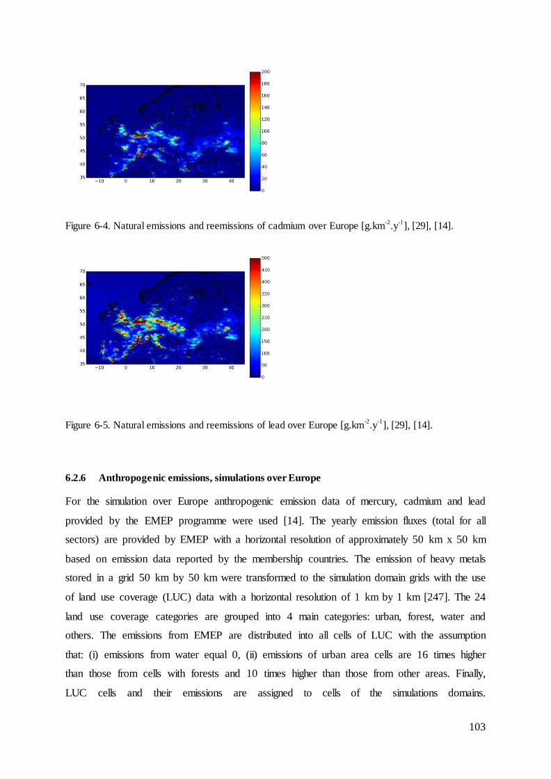
103
Figure 6-4. Natural emissions and reemissions of cadmium over Europe [g.km-2
.y-1
], [29], [14].
Figure 6-5. Natural emissions and reemissions of lead over Europe [g.km-2
.y-1
], [29], [14].
6.2.6 Anthropogenic emissions, simulations over Europe
For the simulation over Europe anthropogenic emission data of mercury, cadmium and lead
provided by the EMEP programme were used [14]. The yearly emission fluxes (total for all
sectors) are provided by EMEP with a horizontal resolution of approximately 50 km x 50 km
based on emission data reported by the membership countries. The emission of heavy metals
stored in a grid 50 km by 50 km were transformed to the simulation domain grids with the use
of land use coverage (LUC) data with a horizontal resolution of 1 km by 1 km [247]. The 24
land use coverage categories are grouped into 4 main categories: urban, forest, water and
others. The emissions from EMEP are distributed into all cells of LUC with the assumption
that: (i) emissions from water equal 0, (ii) emissions of urban area cells are 16 times higher
than those from cells with forests and 10 times higher than those from other areas. Finally,
LUC cells and their emissions are assigned to cells of the simulations domains.
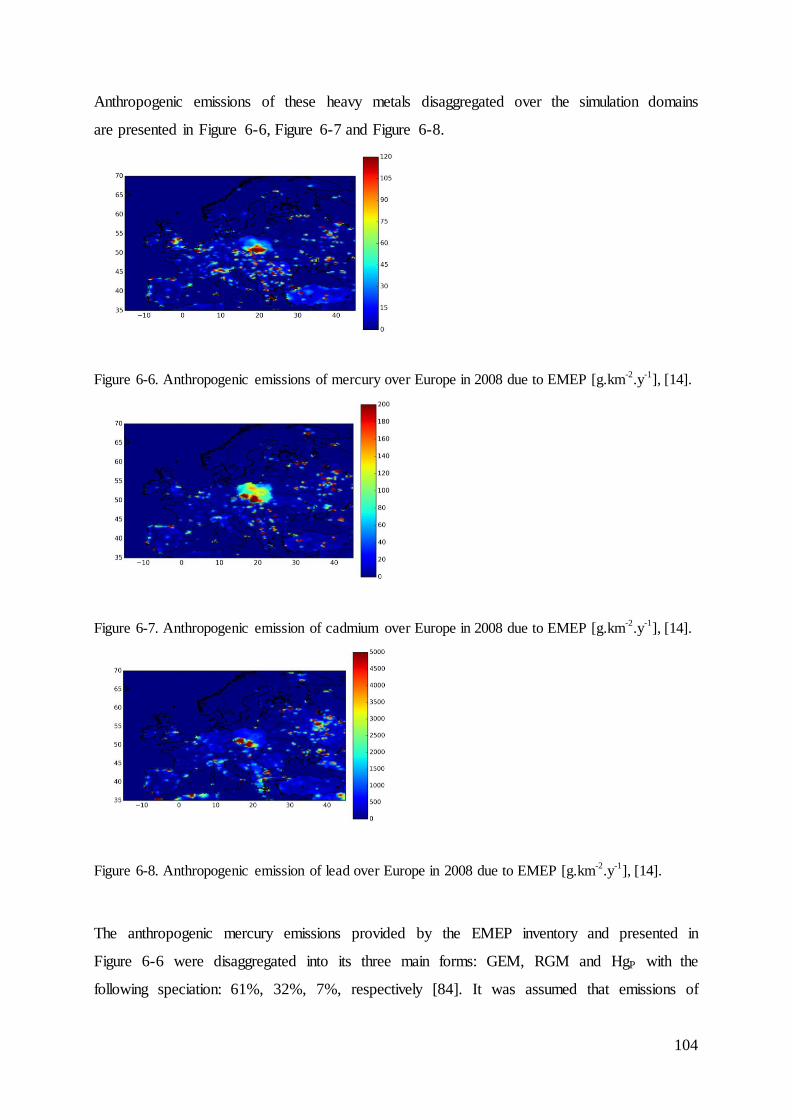
104
Anthropogenic emissions of these heavy metals disaggregated over the simulation domains
are presented in Figure 6-6, Figure 6-7 and Figure 6-8.
Figure 6-6. Anthropogenic emissions of mercury over Europe in 2008 due to EMEP [g.km-2
.y-1
], [14].
Figure 6-7. Anthropogenic emission of cadmium over Europe in 2008 due to EMEP [g.km-2
.y-1
], [14].
Figure 6-8. Anthropogenic emission of lead over Europe in 2008 due to EMEP [g.km-2
.y-1
], [14].
The anthropogenic mercury emissions provided by the EMEP inventory and presented in
Figure 6-6 were disaggregated into its three main forms: GEM, RGM and HgP with the
following speciation: 61%, 32%, 7%, respectively [84]. It was assumed that emissions of
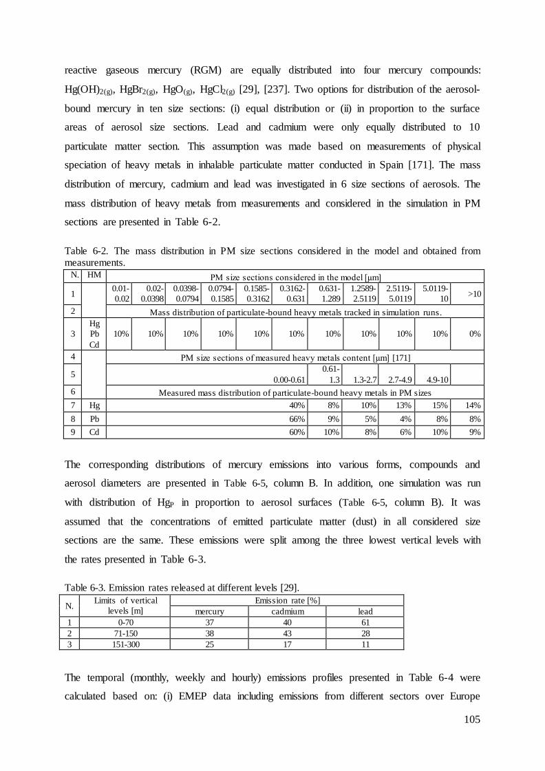
105
reactive gaseous mercury (RGM) are equally distributed into four mercury compounds:
Hg(OH)2(g), HgBr2(g), HgO(g), HgCl2(g) [29], [237]. Two options for distribution of the aerosol-
bound mercury in ten size sections: (i) equal distribution or (ii) in proportion to the surface
areas of aerosol size sections. Lead and cadmium were only equally distributed to 10
particulate matter section. This assumption was made based on measurements of physical
speciation of heavy metals in inhalable particulate matter conducted in Spain [171]. The mass
distribution of mercury, cadmium and lead was investigated in 6 size sections of aerosols. The
mass distribution of heavy metals from measurements and considered in the simulation in PM
sections are presented in Table 6-2.
Table 6-2. The mass distribution in PM size sections considered in the model and obtained from measurements.
N. HM PM size sections considered in the model [µm]
1 0.01-
0.02
0.02-
0.0398
0.0398-
0.0794
0.0794-
0.1585
0.1585-
0.3162
0.3162-
0.631
0.631-
1.289
1.2589-
2.5119
2.5119-
5.0119
5.0119-
10 >10
2 Mass distribution of particulate-bound heavy metals tracked in simulation runs.
3
Hg
Pb
Cd
10% 10% 10% 10% 10% 10% 10% 10% 10% 10% 0%
4 PM size sections of measured heavy metals content [µm] [171]
5 0.00-0.61
0.61-
1.3 1.3-2.7 2.7-4.9 4.9-10
6 Measured mass distribution of particulate-bound heavy metals in PM sizes
7 Hg 40% 8% 10% 13% 15% 14%
8 Pb 66% 9% 5% 4% 8% 8%
9 Cd 60% 10% 8% 6% 10% 9%
The corresponding distributions of mercury emissions into various forms, compounds and
aerosol diameters are presented in Table 6-5, column B. In addition, one simulation was run
with distribution of HgP in proportion to aerosol surfaces (Table 6-5, column B). It was
assumed that the concentrations of emitted particulate matter (dust) in all considered size
sections are the same. These emissions were split among the three lowest vertical levels with
the rates presented in Table 6-3.
Table 6-3. Emission rates released at different levels [29].
N. Limits of vertical
levels [m]
Emission rate [%]
mercury cadmium lead
1 0-70 37 40 61
2 71-150 38 43 28
3 151-300 25 17 11
The temporal (monthly, weekly and hourly) emissions profiles presented in Table 6-4 were
calculated based on: (i) EMEP data including emissions from different sectors over Europe
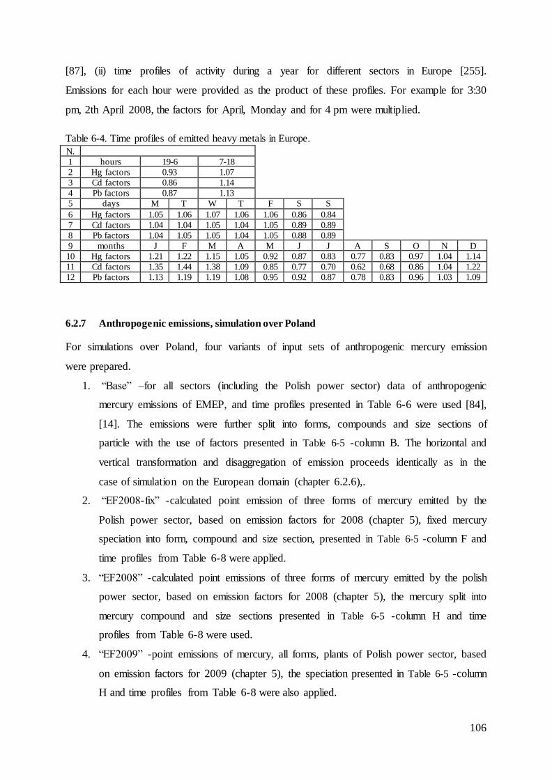
106
[87], (ii) time profiles of activity during a year for different sectors in Europe [255].
Emissions for each hour were provided as the product of these profiles. For example for 3:30
pm, 2th April 2008, the factors for April, Monday and for 4 pm were multiplied.
Table 6-4. Time profiles of emitted heavy metals in Europe.
N.
1 hours 19-6 7-18
2 Hg factors 0.93 1.07
3 Cd factors 0.86 1.14
4 Pb factors 0.87 1.13
5 days M T W T F S S
6 Hg factors 1.05 1.06 1.07 1.06 1.06 0.86 0.84
7 Cd factors 1.04 1.04 1.05 1.04 1.05 0.89 0.89
8 Pb factors 1.04 1.05 1.05 1.04 1.05 0.88 0.89
9 months J F M A M J J A S O N D
10 Hg factors 1.21 1.22 1.15 1.05 0.92 0.87 0.83 0.77 0.83 0.97 1.04 1.14
11 Cd factors 1.35 1.44 1.38 1.09 0.85 0.77 0.70 0.62 0.68 0.86 1.04 1.22
12 Pb factors 1.13 1.19 1.19 1.08 0.95 0.92 0.87 0.78 0.83 0.96 1.03 1.09
6.2.7 Anthropogenic emissions, simulation over Poland
For simulations over Poland, four variants of input sets of anthropogenic mercury emission
were prepared.
1. “Base” –for all sectors (including the Polish power sector) data of anthropogenic
mercury emissions of EMEP, and time profiles presented in Table 6-6 were used [84],
[14]. The emissions were further split into forms, compounds and size sections of
particle with the use of factors presented in Table 6-5 -column B. The horizontal and
vertical transformation and disaggregation of emission proceeds identically as in the
case of simulation on the European domain (chapter 6.2.6),.
2. “EF2008-fix” -calculated point emission of three forms of mercury emitted by the
Polish power sector, based on emission factors for 2008 (chapter 5), fixed mercury
speciation into form, compound and size section, presented in Table 6-5 -column F and
time profiles from Table 6-8 were applied.
3. “EF2008” -calculated point emissions of three forms of mercury emitted by the polish
power sector, based on emission factors for 2008 (chapter 5), the mercury split into
mercury compound and size sections presented in Table 6-5 -column H and time
profiles from Table 6-8 were used.
4. “EF2009” -point emissions of mercury, all forms, plants of Polish power sector, based
on emission factors for 2009 (chapter 5), the speciation presented in Table 6-5 -column
H and time profiles from Table 6-8 were also applied.

107
In the case of using point emissions for power sector (EF2008-fix, EF2008, EF2009) the
EMEP emissions are used for other sectors i.e: (i) non-industrial combustion plants (SNAP 2),
(ii) combustion in manufacturing industry (SNAP 3), (iii) production processes (SNAP 4),
waste treatment and disposal (SNAP 9), (iv) petroleum refining plants (SNAP 0103), (v) solid
fuel transformation plants (SNAP 0104) and (vi) coal mining, oil/gas extraction, pipeline
compressors (SNAP 0105). The time profiles presented in Table 6-7 and speciation factors for
mercury form presented in Table 6-5 -column D for these emission were applied. It was
assumed that the emissions of mercury from sectors beyond the power sector are distributed
equally into two lowest vertical level of the simulation domain. The horizontal disaggregation
of these emissions were done in the same way as for the European domain (chapter 6.2.6).
In conclusion, in the sets “EF2008-fix” and “EF2008”, the emissions from the Polish power
sector (SNAP 0101 and SNAP 0102) are the same while the speciation into mercury form is
different. On the other hand “EF2009” is characterized by different emissions of mercury
from the power sector compared to previous cases.
In the case of the of different emissions from the power sector than EMEP in emission
preprocessing program of Polyphemus, two additional steps were added. At the beginning,
each cell of the EMEP database includes emissions for all sectors, the emissions from the
Polish power sector included in “EF2008-fix”, “EF2008” and “EF2009” were subtracted.
Therefore, to further transformation from the EMEP grid to the simulation domain grid,
disaggregation into forms/compounds of mercury (Table 6-5 -column D) and temporal profiles
(Table 6-7) are applied only for emissions from all sectors beyond the Polish power sectors.
Then, the emissions from the power sector of various mercury forms and compounds with
relevant times profiles are added to individual cells.
The speciation factors presented in Table 2-8 were calculated based on factors proposed in the
literature and emission of mercury in Poland from various source categories [84], [53]. In
emission sets “Base”, “EF2008-fix”, “EF2008” and “EF2009”, the aerosol-bound mercury
was distributed equally among ten size sections (Table 6-5 -columns B, D, F, H). Additional
simulation were run with the use of emissions of HgP distributed among ten size sections of
aerosols in proportion to their surfaces (Table 6-5 -columns C, E, F, I). The emission sets were
named respectively: “Base-PM”, “EF2008-fix-PM”, “EF2008-PM” and “EF2009-PM”.
The simulations for lead and cadmium were run with two types of emissions sets. The first
used only those provided by the EMEP with a resolution of 50 km by 50 km for 2008 for all
sectors and the emitted cadmium and lead were split into vertical levels as presented in Table
6-3 and with temporal profiles presented in Table 6-6. The second simulation was run based
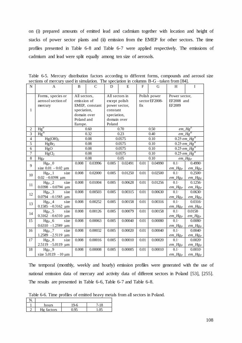
108
on (i) prepared amounts of emitted lead and cadmium together with location and height of
stacks of power sector plants and (ii) emission from the EMEP for other sectors. The time
profiles presented in Table 6-8 and Table 6-7 were applied respectively. The emissions of
cadmium and lead were split equally among ten size of aerosols.
Table 6-5. Mercury distribution factors according to different forms, compounds and aerosol size sections of mercury used in simulation. The speciation in columns B-G –taken from [84]. N A B C D E F G H I
1
Forms, species or
aerosol section of
mercury
All sectors,
emission of
EMEP, constant
speciation,
domain over
Poland and
Europe.
All sectors in
except polish
power sector,
constant
speciation,
domain over
Poland
Polish power
sector EF2008-
fix
Power sector,
EF2008 and
EF2009
2 Hg0 0.60 0.70 0.50 em_Hg
0
3 HgII 0.32 0.23 0.40 em_Hg
II
4 Hg(OH)2 0.08 0.0575 0.10 0.25·em_HgII
5 HgBr2 0.08 0.0575 0.10 0.25·em_HgII
6 HgO 0.08 0.0575 0.10 0.25·em_HgII
7 HgCl2 0.08 0.0575 0.10 0.25·em_HgII
8 HgP 0.08 0.05 0.10 em_HgP
9 HgP_0
size 0.01 - 0.02 μm
0.008 0.03996 0.005 0.02491 0.01 0.04990 0.1·
em_HgP 0.4990·
em_HgP
10 HgP_1 size
0.02 –0.0398 μm
0.008 0.02000 0.005 0.01250 0.01 0.02500 0.1·
em_HgP 0.2500·
em_HgP
11 HgP_2 size
0.0398 - 0.0794 μm
0.008 0.01004 0.005 0.00628 0.01 0.01256 0.1·
em_HgP 0.1256·
em_HgP
12 HgP_3 size
0.0794 –0.1585 μm
0.008 0.00503 0.005 0.00315 0.01 0.00630 0.1·
em_HgP 0.0630·
em_HgP
13 HgP_4 size
0.1585 –0.3162 μm
0.008 0.00252 0.005 0.00158 0.01 0.00316 0.1·
em_HgP 0.0316·
em_HgP
14 HgP_5 size
0.3162 –0.6310 μm
0.008 0.00126 0.005 0.00079 0.01 0.00158 0.1·
em_HgP 0.0158·
em_HgP
15 HgP_6 size
0.6310 –1.2589 μm
0.008 0.00063 0.005 0.00040 0.01 0.00080 0.1·
em_HgP 0.0080·
em_HgP
16 HgP_7 size
1.2589 –2.5119 μm
0.008 0.00032 0.005 0.00020 0.01 0.00040 0.1·
em_HgP 0.0040·
em_HgP
17 HgP_8 size
2.5119 –5.0119 μm
0.008 0.00016 0.005 0.00010 0.01 0.00020 0.1·
em_HgP 0.0020·
em_HgP
18 HgP_9
size 5.0119 –10 μm
0.008 0.00008 0.005 0.00005 0.01 0.00010 0.1·
em_HgP 0.0010·
em_HgP
The temporal (monthly, weekly and hourly) emission profiles were generated with the use of
national emission data of mercury and activity data of different sectors in Poland [53], [255].
The results are presented in Table 6-6, Table 6-7 and Table 6-8.
Table 6-6. Time profiles of emitted heavy metals from all sectors in Poland. N.
1 hours 19-6 7-18
2 Hg factors 0.95 1.05
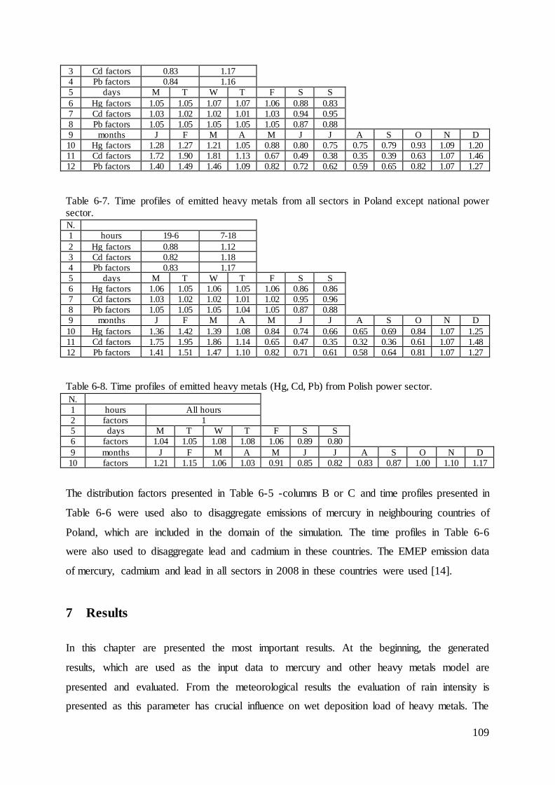
109
3 Cd factors 0.83 1.17
4 Pb factors 0.84 1.16
5 days M T W T F S S
6 Hg factors 1.05 1.05 1.07 1.07 1.06 0.88 0.83
7 Cd factors 1.03 1.02 1.02 1.01 1.03 0.94 0.95
8 Pb factors 1.05 1.05 1.05 1.05 1.05 0.87 0.88
9 months J F M A M J J A S O N D
10 Hg factors 1.28 1.27 1.21 1.05 0.88 0.80 0.75 0.75 0.79 0.93 1.09 1.20
11 Cd factors 1.72 1.90 1.81 1.13 0.67 0.49 0.38 0.35 0.39 0.63 1.07 1.46
12 Pb factors 1.40 1.49 1.46 1.09 0.82 0.72 0.62 0.59 0.65 0.82 1.07 1.27
Table 6-7. Time profiles of emitted heavy metals from all sectors in Poland except national power sector. N.
1 hours 19-6 7-18
2 Hg factors 0.88 1.12
3 Cd factors 0.82 1.18
4 Pb factors 0.83 1.17
5 days M T W T F S S
6 Hg factors 1.06 1.05 1.06 1.05 1.06 0.86 0.86
7 Cd factors 1.03 1.02 1.02 1.01 1.02 0.95 0.96
8 Pb factors 1.05 1.05 1.05 1.04 1.05 0.87 0.88
9 months J F M A M J J A S O N D
10 Hg factors 1.36 1.42 1.39 1.08 0.84 0.74 0.66 0.65 0.69 0.84 1.07 1.25
11 Cd factors 1.75 1.95 1.86 1.14 0.65 0.47 0.35 0.32 0.36 0.61 1.07 1.48
12 Pb factors 1.41 1.51 1.47 1.10 0.82 0.71 0.61 0.58 0.64 0.81 1.07 1.27
Table 6-8. Time profiles of emitted heavy metals (Hg, Cd, Pb) from Polish power sector.
N.
1 hours All hours
2 factors 1
1.07 5 days M T W T F S S
6 factors 1.04 1.05 1.08 1.08 1.06 0.89 0.80
9 months J F M A M J J A S O N D
10 factors 1.21 1.15 1.06 1.03 0.91 0.85 0.82 0.83 0.87 1.00 1.10 1.17
The distribution factors presented in Table 6-5 -columns B or C and time profiles presented in
Table 6-6 were used also to disaggregate emissions of mercury in neighbouring countries of
Poland, which are included in the domain of the simulation. The time profiles in Table 6-6
were also used to disaggregate lead and cadmium in these countries. The EMEP emission data
of mercury, cadmium and lead in all sectors in 2008 in these countries were used [14].
Results 7
In this chapter are presented the most important results. At the beginning, the generated
results, which are used as the input data to mercury and other heavy metals model are
presented and evaluated. From the meteorological results the evaluation of rain intensity is
presented as this parameter has crucial influence on wet deposition load of heavy metals. The
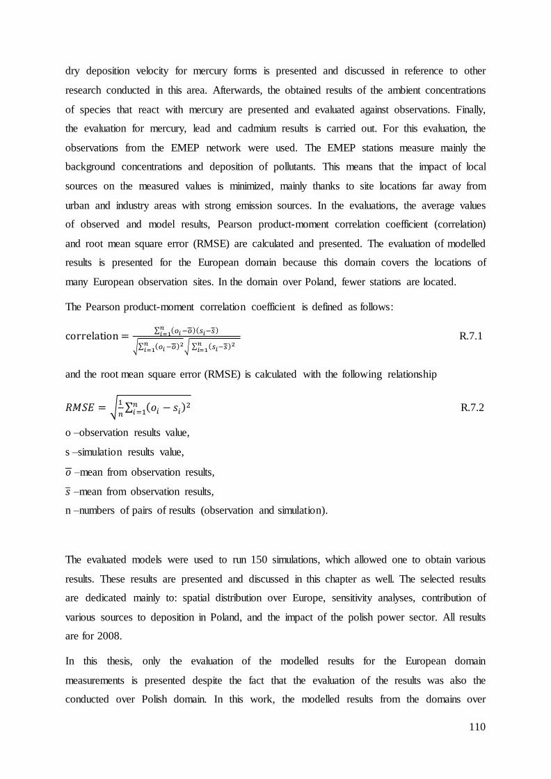
110
dry deposition velocity for mercury forms is presented and discussed in reference to other
research conducted in this area. Afterwards, the obtained results of the ambient concentrations
of species that react with mercury are presented and evaluated against observations. Finally,
the evaluation for mercury, lead and cadmium results is carried out. For this evaluation, the
observations from the EMEP network were used. The EMEP stations measure mainly the
background concentrations and deposition of pollutants. This means that the impact of local
sources on the measured values is minimized, mainly thanks to site locations far away from
urban and industry areas with strong emission sources. In the evaluations, the average values
of observed and model results, Pearson product-moment correlation coefficient (correlation)
and root mean square error (RMSE) are calculated and presented. The evaluation of modelled
results is presented for the European domain because this domain covers the locations of
many European observation sites. In the domain over Poland, fewer stations are located.
The Pearson product-moment correlation coefficient is defined as follows:
correlation =∑ (𝑜𝑖−𝑜)(𝑠𝑖−𝑠)𝑛𝑖=1
√∑ (𝑜𝑖−𝑜)2𝑛
𝑖=1 √ ∑ (𝑠𝑖−𝑠)2𝑛
𝑖=1
R.7.1
and the root mean square error (RMSE) is calculated with the following relationship
𝑅𝑀𝑆𝐸 = √1
𝑛∑ (𝑜𝑖 − 𝑠𝑖)
2𝑛𝑖=1 R.7.2
o –observation results value,
s –simulation results value,
𝑜 –mean from observation results,
𝑠 –mean from observation results,
n –numbers of pairs of results (observation and simulation).
The evaluated models were used to run 150 simulations, which allowed one to obtain various
results. These results are presented and discussed in this chapter as well. The selected results
are dedicated mainly to: spatial distribution over Europe, sensitivity analyses, contribution of
various sources to deposition in Poland, and the impact of the polish power sector. All results
are for 2008.
In this thesis, only the evaluation of the modelled results for the European domain
measurements is presented despite the fact that the evaluation of the results was also the
conducted over Polish domain. In this work, the modelled results from the domains over

111
Europe and Poland and their evaluations for particular stations are quite similar and relatively
small differences have been noticed. The cause for the observed differences in the modelled
results from Eulerian models run which the use of various domains and modelling resolutions
is very complex and may results from several main factors, such as the issue of
representativeness [259]. Therefore the discussion and comparison of results from various
domain sizes and resolutions was omitted here because this was not the aim of this thesis.
7.1 Evaluation of intensity of precipitation
The monthly rain intensity data provided by the ECMWF and processed by Polyphemus
meteorological pre-processing program were compared against measurements conducted at
the EMEP stations [248], [163]. The corresponding results are presented in Table 7-1. In this
table, the results are presented for stations where mercury wet deposition was observed and
aggregated results for all 53 stations operated in 2008 for EMEP and located within the
European domain are also presented.
Table 7-1. Evaluation of monthly results of intensity of precipitation [mm] from the meteorological pre-processing run over the European domain with the use of ECMWF database and measurements of in stations of EMEP [248], [163].
N. Stations
code
Number of
month with
valid
observations
Annual intensity
of precipitation
in EMEP stations
[mm.year-1
]
Annual intensity
of precipitation
used the in
model
[mm.year-1
]
Correlation
coefficient
RMSE
[mm.month-1
]
1 BE14 12 586 1036 0.81 42
2 DE01 12 838 1156 0.96 33
3 DE02 12 658 768 0.87 18
4 DE03 12 1611 1332 0.77 36
5 DE08 12 1119 978 0.34 41
6 DE09 12 533 740 0.67 25
7 ES08 11 1453 1469 0.91 95
8 FI36 12 320 798 0.93 42
9 GB13 12 1227 1303 0.71 32
10 GB17 9 471 626 0.59 29
11 GB48 12 919 1152 0.79 35
12 GB91 12 613 986 0.29 51
13 LV10 12 939 1108 0.96 20
14 LV16 12 824 960 0.82 21
15 NL91 12 771 1119 0.91 34
16 NO01 12 1797 1660 0.95 36
17 PL04 12 674 858 0.89 21
18 PL05 12 592 805 0.54 28
19 SE14 12 718 1228 0.81 54
20 SI08 12 1159 1125 0.71 41
21 All 625 41948 53388 0.79 36
All–results for all observations from 53 stations located inside European domain, where precipitation intensity
was measured together with heavy metals concentrations in precipitation.
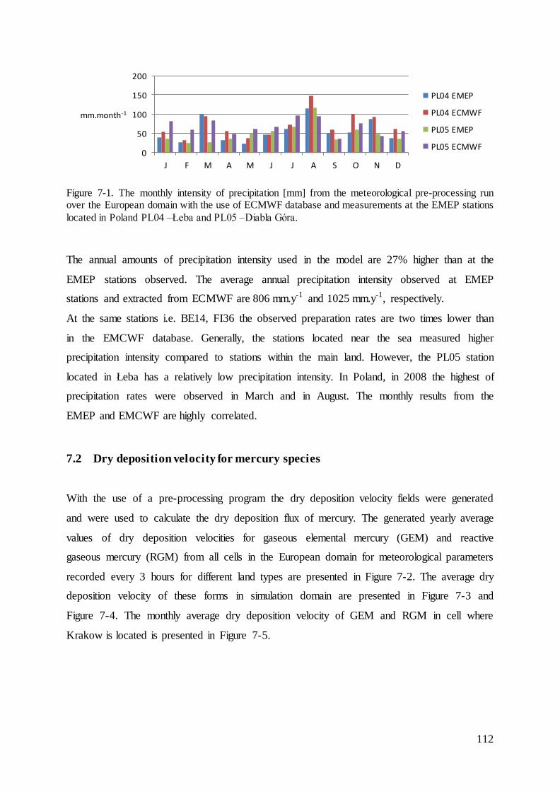
112
Figure 7-1. The monthly intensity of precipitation [mm] from the meteorological pre-processing run over the European domain with the use of ECMWF database and measurements at the EMEP stations
located in Poland PL04 –Łeba and PL05 –Diabla Góra.
The annual amounts of precipitation intensity used in the model are 27% higher than at the
EMEP stations observed. The average annual precipitation intensity observed at EMEP
stations and extracted from ECMWF are 806 mm.y-1 and 1025 mm.y-1, respectively.
At the same stations i.e. BE14, FI36 the observed preparation rates are two times lower than
in the EMCWF database. Generally, the stations located near the sea measured higher
precipitation intensity compared to stations within the main land. However, the PL05 station
located in Łeba has a relatively low precipitation intensity. In Poland, in 2008 the highest of
precipitation rates were observed in March and in August. The monthly results from the
EMEP and EMCWF are highly correlated.
7.2 Dry deposition velocity for mercury species
With the use of a pre-processing program the dry deposition velocity fields were generated
and were used to calculate the dry deposition flux of mercury. The generated yearly average
values of dry deposition velocities for gaseous elemental mercury (GEM) and reactive
gaseous mercury (RGM) from all cells in the European domain for meteorological parameters
recorded every 3 hours for different land types are presented in Figure 7-2. The average dry
deposition velocity of these forms in simulation domain are presented in Figure 7-3 and
Figure 7-4. The monthly average dry deposition velocity of GEM and RGM in cell where
Krakow is located is presented in Figure 7-5.
0
50
100
150
200
J F M A M J J A S O N D
mm.month-1
PL04 EMEP
PL04 ECMWF
PL05 EMEP
PL05 ECMWF

113
Figure 7-2. The average dry deposition velocity of RGM (blue, left axis) and GEM (red, right axis) for
different land types over Europe [cm.s-1
].
Figure 7-3. Annual average dry deposition
velocity of GEM [cm.s-1
].
Figure 7-4. Annual average dry deposition
velocity of RGM [cm.s-1
].
The dry deposition velocity of RGM is around 12 times higher compared to GEM (Figure
7-2). The presented results are consistent with the measurements conducted in many places of
0.0
0.2
0.4
0.6
0.8
1.0
1.2
0.00
0.02
0.04
0.06
0.08
0.10
eve
rgre
en
bro
adle
af t
ree
s
de
cid
uo
us
bro
ad
lea
f tr
ees
bro
adle
af a
nd
nee
dle
lea
f tr
ees
eve
rgre
en
ne
edle
leaf
tre
es
de
cid
uo
us
nee
dle
lea
f t
rees
bro
adle
af t
ree
s w
ith
gro
un
d c
ove
r
gras
slan
d
bro
adle
af s
hru
bs
wit
h p
ere
nn
ial g
rou
nd
co
ver
bro
adle
af s
hru
bs
wit
h b
are
so
il
dw
arf
tree
s a
nd
sh
rub
s w
ith
gro
un
d c
ove
r
bar
e s
oil
and
urb
an
agri
cult
ura
l
wat
er
ice
RGM
cm.s -1
GEM
cm.s -1
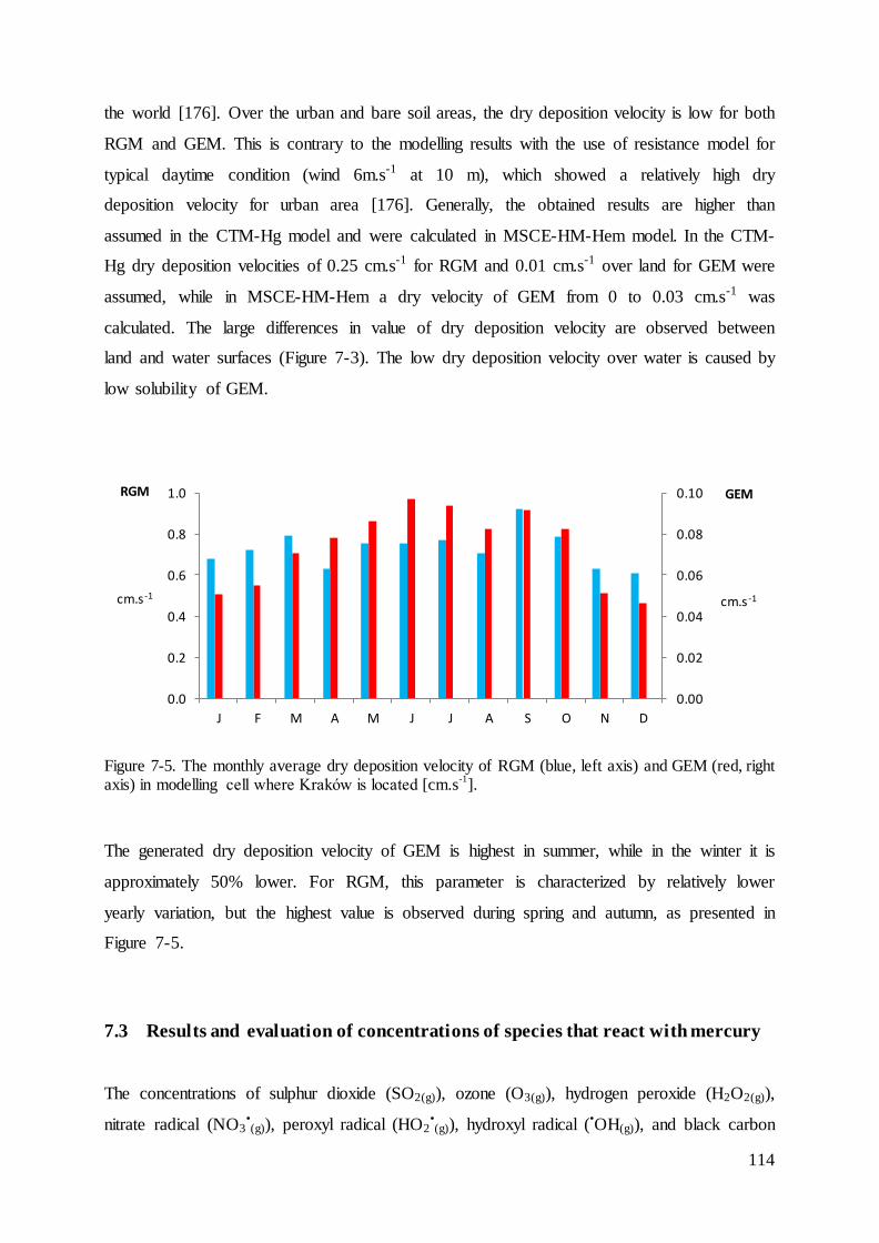
114
the world [176]. Over the urban and bare soil areas, the dry deposition velocity is low for both
RGM and GEM. This is contrary to the modelling results with the use of resistance model for
typical daytime condition (wind 6m.s-1 at 10 m), which showed a relatively high dry
deposition velocity for urban area [176]. Generally, the obtained results are higher than
assumed in the CTM-Hg model and were calculated in MSCE-HM-Hem model. In the CTM-
Hg dry deposition velocities of 0.25 cm.s-1 for RGM and 0.01 cm.s-1 over land for GEM were
assumed, while in MSCE-HM-Hem a dry velocity of GEM from 0 to 0.03 cm.s-1 was
calculated. The large differences in value of dry deposition velocity are observed between
land and water surfaces (Figure 7-3). The low dry deposition velocity over water is caused by
low solubility of GEM.
Figure 7-5. The monthly average dry deposition velocity of RGM (blue, left axis) and GEM (red, right axis) in modelling cell where Kraków is located [cm.s
-1].
The generated dry deposition velocity of GEM is highest in summer, while in the winter it is
approximately 50% lower. For RGM, this parameter is characterized by relatively lower
yearly variation, but the highest value is observed during spring and autumn, as presented in
Figure 7-5.
7.3 Results and evaluation of concentrations of species that react with mercury
The concentrations of sulphur dioxide (SO2(g)), ozone (O3(g)), hydrogen peroxide (H2O2(g)),
nitrate radical (NO3•(g)), peroxyl radical (HO2
•(g)), hydroxyl radical (•OH(g)), and black carbon
0.0
0.2
0.4
0.6
0.8
1.0
0.00
0.02
0.04
0.06
0.08
0.10
J F M A M J J A S O N D
RGM
cm.s -1
GEM
cm.s -1

115
aerosol (BC) are presented in Figure 7-6 -Figure 7-31. The maps of the concentration are
presented for a domain over Poland, while the time profiles of concentrations in cells where
selected stations of EMEP are located and concentrations in 10 vertical levels are the results
of simulations run over the European domain. It should be noted that the concentrations at 10
levels are given in µg.m-3 and the changes of atmospheric pressure and density of air affect
the presented quantitative results. The maps from the European domain are not presented
because similar results for Europe are frequently presented in scientific reports and articles i.e.
EMEP. On the other hand the maps that show the detailed modelled concentrations of
compounds as hydrogen peroxide (H2O2(g)), peroxyl radical (HO2•(g)), hydroxyl radical
(•OH(g)) over Poland have not been presented yet and are, therefore, of interest. The nitrate
radical (NO3•(g)) was presented for the European domain because it was modelled and then
used only in this domain. The nesting approach was applied –the results in the European
domain were used as the boundary condition for the domain over Poland. The evaluation of
modelling results of SO2(g) and O3(g) against observations at EMEP stations was also presented
in Table 7-2, Table 7-3 and Table 7-4. In these tables, the detailed results are presented for
stations where mercury air concentration or wet deposition was measured in 2008 and at all
stations located in Poland. The presented results were shortly discussed, but it should be noted
that the atmospheric behaviour of the considered species is complex and only some possible
mechanisms and explanations are presented without going into details.
Figure 7-6. Annual average
concentrations of SO2(g) [µg.m-3
] in the surface.
Figure 7-7. Monthly average modelled concentrations of SO2 [µg.m
-3] in the surface at selected stations.
0
2
4
6
8
10
J F M A M J J A S O N D
µg.
m-3
BE14 GB17 LV10
NL91 PL05 SE14
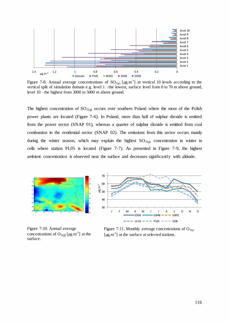
116
Figure 7-8. Annual average concentrations of SO2(g) [µg.m-3
] at vertical 10 levels according to the vertical split of simulation domain e.g. level 1 –the lowest, surface level from 0 to 70 m above ground,
level 10 –the highest from 3000 to 5000 m above ground.
The highest concentration of SO2(g) occurs over southern Poland where the most of the Polish
power plants are located (Figure 7-6). In Poland, more than half of sulphur dioxide is emitted
from the power sector (SNAP 01), whereas a quarter of sulphur dioxide is emitted from coal
combustion in the residential sector (SNAP 02). The emissions from this sector occurs mainly
during the winter season, which may explain the highest SO2(g) concentration in winter in
cells where station PL05 is located (Figure 7-7). As presented in Figure 7-9, the highest
ambient concentration is observed near the surface and decreases significantly with altitude.
Figure 7-10. Annual average
concentrations of O3(g) [µg.m-3
] at the surface.
Figure 7-11. Monthly average concentrations of O3(g)
[µg.m-3
] at the surface at selected stations.
00.20.40.60.811.21.4
level 1level 2level 3level 4level 5level 6level 7level 8level 9level 10
µg.m-3
domain PL05 NO01 ES08 DE03
38
48
58
68
78
J F M A M J J A S O N D
µg.
m-3
ES08 GB48 GB91
LV10 PL05 SI08
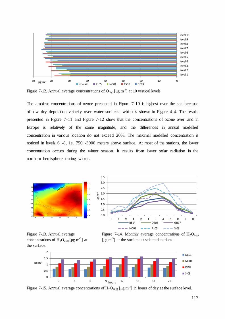
117
Figure 7-12. Annual average concentrations of O3(g) [µg.m-3
] at 10 vertical levels.
The ambient concentrations of ozone presented in Figure 7-10 is highest over the sea because
of low dry deposition velocity over water surfaces, which is shown in Figure 4-4. The results
presented in Figure 7-11 and Figure 7-12 show that the concentrations of ozone over land in
Europe is relatively of the same magnitude, and the differences in annual modelled
concentration in various location do not exceed 20%. The maximal modelled concentration is
noticed in levels 6 -8, i.e. 750 -3000 meters above surface. At most of the stations, the lower
concentration occurs during the winter season. It results from lower solar radiation in the
northern hemisphere during winter.
Figure 7-13. Annual average
concentrations of H2O2(g) [µg.m-3
] at
the surface.
Figure 7-14. Monthly average concentrations of H2O2(g)
[µg.m-3
] at the surface at selected stations.
Figure 7-15. Annual average concentrations of H2O2(g) [µg.m
-3] in hours of day at the surface level.
01020304050607080
level 1
level 2
level 3
level 4
level 5
level 6
level 7
level 8
level 9
level 10
µg.m-3
domain PL05 NO01 ES08 DE03
0.0
0.5
1.0
1.5
2.0
2.5
3.0
3.5
J F M A M J J A S O N D
µg.
m-3
BE14 DE02 GB17
NO01 PL05 SI08
0
0.5
1
1.5
2
0 3 6 9 12 15 18 21
µg.m-3
hours
DE01
NO01
PL05
SI08
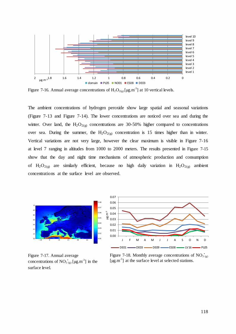
118
Figure 7-16. Annual average concentrations of H2O2(g) [µg.m
-3] at 10 vertical levels.
The ambient concentrations of hydrogen peroxide show large spatial and seasonal variations
(Figure 7-13 and Figure 7-14). The lower concentrations are noticed over sea and during the
winter. Over land, the H2O2(g) concentrations are 30-50% higher compared to concentrations
over sea. During the summer, the H2O2(g) concentration is 15 times higher than in winter.
Vertical variations are not very large, however the clear maximum is visible in Figure 7-16
at level 7 ranging in altitudes from 1000 to 2000 meters. The results presented in Figure 7-15
show that the day and night time mechanisms of atmospheric production and consumption
of H2O2(g) are similarly efficient, because no high daily variation in H2O2(g) ambient
concentrations at the surface level are observed.
Figure 7-17. Annual average
concentrations of NO3•(g) [µg.m
-3] in the
surface level.
Figure 7-18. Monthly average concentrations of NO3•(g)
[µg.m-3
] at the surface level at selected stations.
00.20.40.60.811.21.41.61.82
level 1level 2level 3level 4level 5level 6level 7level 8level 9level 10
µg.m-3
domain PL05 NO01 ES08 DE03
0.00
0.01
0.02
0.03
0.04
0.05
0.06
0.07
J F M A M J J A S O N D
µg.
m-3
DE01 DE03 DE09 ES08 LV16 PL05
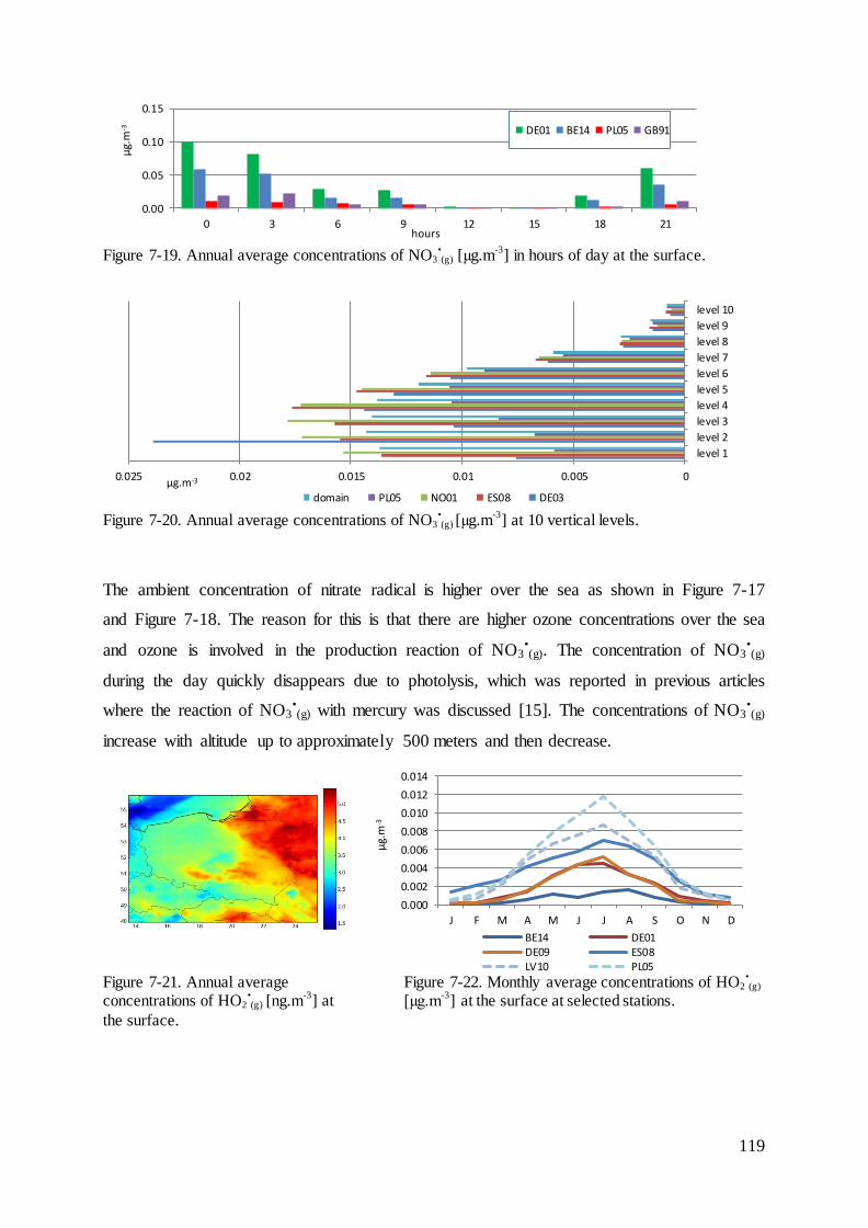
119
Figure 7-19. Annual average concentrations of NO3
•(g) [µg.m
-3] in hours of day at the surface.
Figure 7-20. Annual average concentrations of NO3
•(g) [µg.m
-3] at 10 vertical levels.
The ambient concentration of nitrate radical is higher over the sea as shown in Figure 7-17
and Figure 7-18. The reason for this is that there are higher ozone concentrations over the sea
and ozone is involved in the production reaction of NO3•(g). The concentration of NO3
•(g)
during the day quickly disappears due to photolysis, which was reported in previous articles
where the reaction of NO3•(g)
with mercury was discussed [15]. The concentrations of NO3•(g)
increase with altitude up to approximately 500 meters and then decrease.
Figure 7-21. Annual average concentrations of HO2
•(g) [ng.m
-3] at
the surface.
Figure 7-22. Monthly average concentrations of HO2•(g)
[µg.m-3
] at the surface at selected stations.
0.00
0.05
0.10
0.15
0 3 6 9 12 15 18 21
µg.
m-3
hours
DE01 BE14 PL05 GB91
00.0050.010.0150.020.025
level 1
level 2
level 3
level 4
level 5
level 6
level 7
level 8
level 9
level 10
µg.m-3
domain PL05 NO01 ES08 DE03
0.000
0.002
0.004
0.006
0.008
0.010
0.012
0.014
J F M A M J J A S O N D
µg.
m-3
BE14 DE01DE09 ES08LV10 PL05
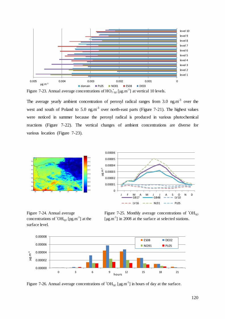
120
Figure 7-23. Annual average concentrations of HO2
•(g) [µg.m
-3] at vertical 10 levels.
The average yearly ambient concentration of peroxyl radical ranges from 3.0 ng.m-3 over the
west and south of Poland to 5.0 ng.m-3 over north-east parts (Figure 7-21). The highest values
were noticed in summer because the peroxyl radical is produced in various photochemical
reactions (Figure 7-22). The vertical changes of ambient concentrations are diverse for
various location (Figure 7-23).
Figure 7-24. Annual average
concentrations of •OH(g) [pg.m
-3] at the
surface level.
Figure 7-25. Monthly average concentrations of •OH(g)
[µg.m-3
] in 2008 at the surface at selected stations.
Figure 7-26. Annual average concentrations of •OH(g) [µg.m
-3] in hours of day at the surface.
00.0010.0020.0030.0040.005
level 1
level 2
level 3
level 4
level 5
level 6
level 7
level 8
level 9
level 10
µg.m-3
domain PL05 NO01 ES08 DE03
0
0.00001
0.00002
0.00003
0.00004
0.00005
0.00006
J F M A M J J A S O N D
µg.
m-3
GB17 GB48 LV10
LV16 NL91 PL05
0.00000
0.00002
0.00004
0.00006
0.00008
0 3 6 9 12 15 18 21
µg.
m-3
hours
ES08 DE02
NO91 PL05
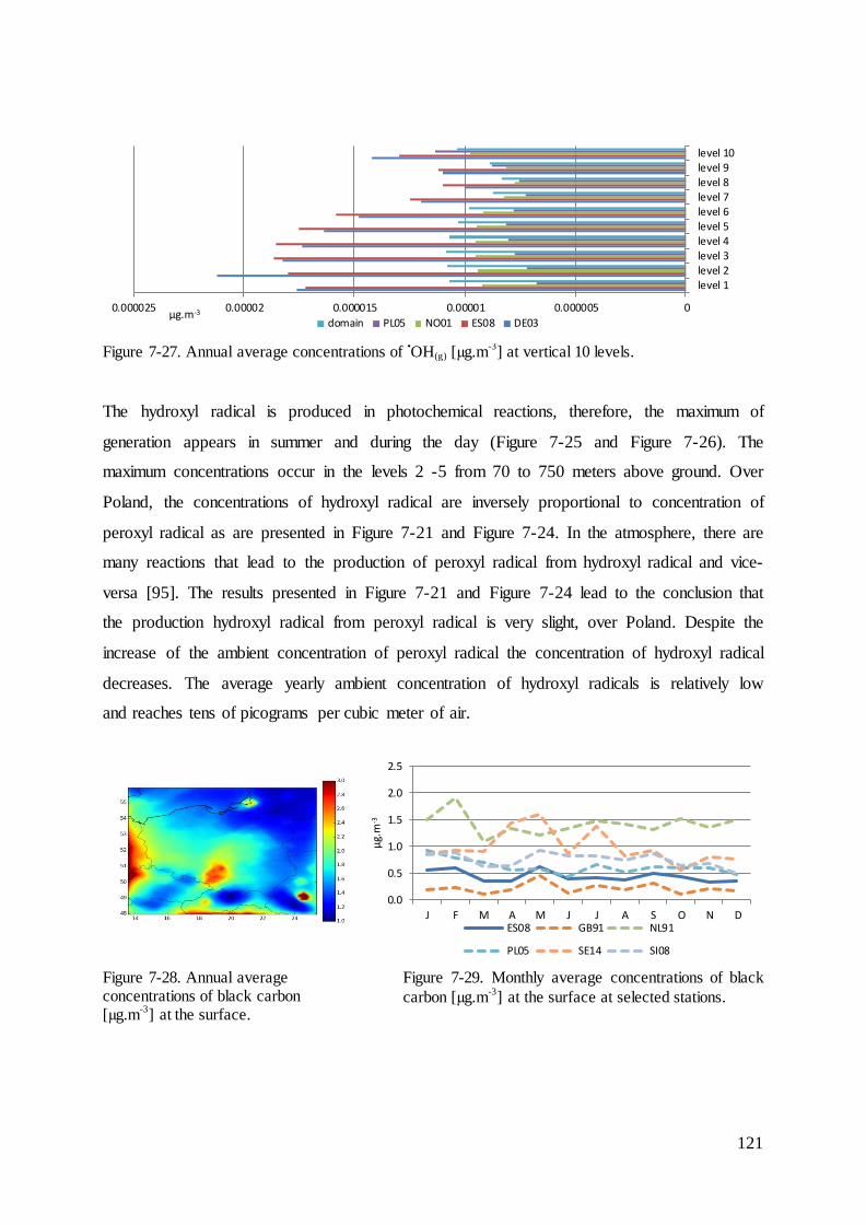
121
Figure 7-27. Annual average concentrations of •OH(g) [µg.m
-3] at vertical 10 levels.
The hydroxyl radical is produced in photochemical reactions, therefore, the maximum of
generation appears in summer and during the day (Figure 7-25 and Figure 7-26). The
maximum concentrations occur in the levels 2 -5 from 70 to 750 meters above ground. Over
Poland, the concentrations of hydroxyl radical are inversely proportional to concentration of
peroxyl radical as are presented in Figure 7-21 and Figure 7-24. In the atmosphere, there are
many reactions that lead to the production of peroxyl radical from hydroxyl radical and vice-
versa [95]. The results presented in Figure 7-21 and Figure 7-24 lead to the conclusion that
the production hydroxyl radical from peroxyl radical is very slight, over Poland. Despite the
increase of the ambient concentration of peroxyl radical the concentration of hydroxyl radical
decreases. The average yearly ambient concentration of hydroxyl radicals is relatively low
and reaches tens of picograms per cubic meter of air.
Figure 7-28. Annual average concentrations of black carbon [µg.m
-3] at the surface.
Figure 7-29. Monthly average concentrations of black
carbon [µg.m-3
] at the surface at selected stations.
00.0000050.000010.0000150.000020.000025
level 1level 2level 3level 4level 5level 6level 7level 8level 9level 10
µg.m-3
domain PL05 NO01 ES08 DE03
0.0
0.5
1.0
1.5
2.0
2.5
J F M A M J J A S O N D
µg.
m-3
ES08 GB91 NL91
PL05 SE14 SI08
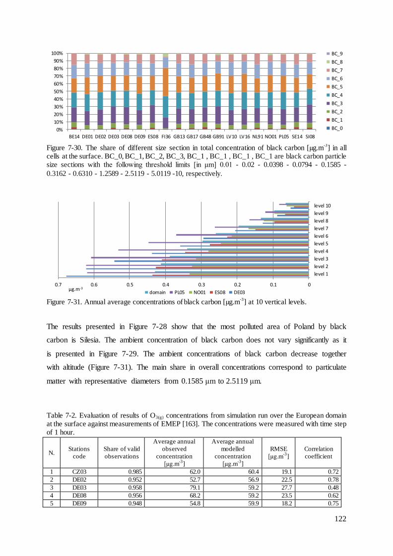
122
Figure 7-30. The share of different size section in total concentration of black carbon [µg.m
-3] in all
cells at the surface. BC_0, BC_1, BC_2, BC_3, BC_1 , BC_1 , BC_1 , BC_1 are black carbon particle size sections with the following threshold limits [in μm] 0.01 - 0.02 - 0.0398 - 0.0794 - 0.1585 -
0.3162 - 0.6310 - 1.2589 - 2.5119 - 5.0119 -10, respectively.
Figure 7-31. Annual average concentrations of
black carbon [µg.m
-3] at 10 vertical levels.
The results presented in Figure 7-28 show that the most polluted area of Poland by black
carbon is Silesia. The ambient concentration of black carbon does not vary significantly as it
is presented in Figure 7-29. The ambient concentrations of black carbon decrease together
with altitude (Figure 7-31). The main share in overall concentrations correspond to particulate
matter with representative diameters from 0.1585 μm to 2.5119 μm.
Table 7-2. Evaluation of results of O3(g) concentrations from simulation run over the European domain at the surface against measurements of EMEP [163]. The concentrations were measured with time step of 1 hour.
N. Stations
code
Share of valid
observations
Average annual
observed
concentration
[µg.m-3
]
Average annual
modelled
concentration
[µg.m-3
]
RMSE
[µg.m-3
]
Correlation
coefficient
1 CZ03 0.985 62.0 60.4 19.1 0.72
2 DE02 0.952 52.7 56.9 22.5 0.78
3 DE03 0.958 79.1 59.2 27.7 0.48
4 DE08 0.956 68.2 59.2 23.5 0.62
5 DE09 0.948 54.8 59.9 18.2 0.75
0%
10%
20%
30%
40%
50%
60%
70%
80%
90%
100%
BE14 DE01 DE02 DE03 DE08 DE09 ES08 FI36 GB13 GB17 GB48 GB91 LV10 LV16 NL91 NO01 PL05 SE14 SI08
BC_9
BC_8
BC_7
BC_6
BC_5
BC_4
BC_3
BC_2
BC_1
BC_0
00.10.20.30.40.50.60.7
level 1
level 2
level 3
level 4
level 5
level 6
level 7
level 8
level 9
level 10
µg.m-3
domain PL05 NO01 ES08 DE03
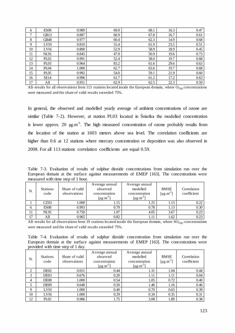
123
6 ES08 0.989 69.0 68.1 16.3 0.47
7 GB13 0.887 60.9 67.8 16.7 0.61
8 GB48 0.977 60.4 62.3 14.9 0.68
9 LV10 0.810 55.4 61.9 23.5 0.51
10 LV16 0.800 52.9 58.9 18.9 0.45
11 NL91 0.845 47.9 50.9 19.6 0.73
12 PL02 0.991 52.4 58.0 19.7 0.68
13 PL03 0.964 83.2 61.6 29.6 0.63
14 PL04 1.000 62.7 63.6 19.7 0.68
15 PL05 0.992 54.0 59.1 21.9 0.60
16 SE14 0.996 61.7 61.2 17.2 0.63
17 All 0.951 62.9 62.5 22.3 0.59
All–results for all observations from 113 stations located inside the European domain, where O3(g) concentrations
were measured and the share of valid results exceeded 75%.
In general, the observed and modelled yearly average of ambient concentrations of ozone are
similar (Table 7-2). However, at station PL03 located in Śnieżka the modelled concentration
is lower approx. 20 µg.m-3. The high measured concentration of ozone probably results from
the location of the station at 1603 meters above sea level. The correlation coefficients are
higher than 0.6 at 12 stations where mercury concentration or deposition was also observed in
2008. For all 113 stations correlation coefficients are equal 0.59.
Table 7-3. Evaluation of results of sulphur dioxide concentrations from simulation run over the European domain at the surface against measurements of EMEP [163]. The concentrations were measured with time step of 1 hour.
N. Stations
code
Share of valid
observations
Average annual
observed
concentration
[µg.m-3
]
Average annual
modelled
concentration
[µg.m-3
]
RMSE
[µg.m-3
]
Correlation
coefficient
1 CZ03 1.000 1.15 1.25 1.13 0.22
6 ES08 0.993 0.79 0.78 1.13 0.30
11 NL91 0.750 1.07 4.05 3.67 0.23
17 All 0.965 0.82 1.11 1.62 0.23
All–results for all observations from 19 stations located inside the European domain, where SO2(g) concentrations
were measured and the share of valid results exceeded 75%.
Table 7-4. Evaluation of results of sulphur dioxide concentration from simulation run over the European domain at the surface against measurements of EMEP [163]. The concentrations were provided with time step of 1 day.
N. Stations
code
Share of valid
observations
Average annual
observed
concentration
[µg.m-3
]
Average annual
modelled
concentration
[µg.m-3
]
RMSE
[µg.m-3
]
Correlation
coefficient
2 DE02 0.651 0.44 1.31 1.04 0.44
3 DE03 0.676 0.20 1.11 1.11 0.04
4 DE08 1.000 0.54 1.05 0.72 0.40
5 DE09 0.648 0.50 1.46 1.16 0.46
9 LV10 1.000 0.40 0.70 0.63 0.39
10 LV16 1.000 0.29 0.34 0.35 0.31
12 PL02 0.986 1.75 3.08 1.89 0.38

124
13 PL03 0.997 1.06 4.79 5.53 0.01
14 PL04 0.989 1.03 1.25 0.84 0.53
15 PL05 0.986 0.58 1.29 1.07 0.51
16 SE14 0.981 0.32 2.78 2.81 0.98
17 All 0.960 0.49 1.30 1.74 0.34
All–results for all observations from 25 stations located inside he European domain, where SO2(g) concentrations
were measured and the share of valid results exceeded 75%.
The modeled results of SO2(g) are in general overestimated by 2.5 times compared to
observations. Moreover, the correlation coefficient is low. In case of evaluation against 1 hour
observation it is equal to 0.23 and for 1 day observation it is 0.34. The performed results of
O3(g) and SO2(g) evaluations agree with previous evaluation which had been done for the
European simulation with the use of Polyphemus air quality system [203], [204]. The
averages results and the correlation coefficient for O3(g) are very satisfactory, while the
modelled SO2(g) is overestimated and the correlation coefficients are around 0.3.
7.4 Evaluation of mercury concentrations and deposition
The mercury dispersion models are usually evaluated against measurements of concentrations
in ambient air and wet deposition (e.g. [183]). Due to the lack of separate measurements of
the atmospheric concentrations of reactive gaseous mercury at the EMEP station, the
concentration of mercury is dominated by a high concentration of elemental gaseous mercury,
which is up to a dozen times higher than the concentration of its other forms. The relatively
long residence time of GEM in the atmosphere makes it rather evenly distributed in the global
atmosphere. Therefore, the modelled concentration of elemental gaseous mercury does not
provide too much information on the scientific correctness of the applied model. However,
elemental gaseous mercury is poorly removed in scavenging processes, therefore mercury
measured in precipitation depends mostly on concentrations of reactive gaseous mercury and
mercury bound to aerosols in ambient air. These forms are dispersed in the atmosphere locally
and their deposition pattern strongly depends on local sources and chemistry of mercury in the
atmosphere.
The results of the model comparison against measurements for wet mercury deposition are
presented in Figure 7-32 and in Table 7-5. To mitigate the influence of the amount of
precipitation, the modelling results named “rain corrected” were multiplied by the ratio of
precipitation measured at EMEP stations and precipitation from meteorological input data
presented in Table 7-1. In Table 7-5 and in Figure 7-33 -Figure 7-51 evaluation results from
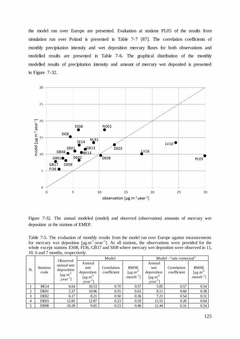
125
the model run over Europe are presented. Evaluation at stations PL05 of the results from
simulation run over Poland is presented in Table 7-7 [87]. The correlation coefficients of
monthly precipitation intensity and wet deposition mercury fluxes for both observations and
modelled results are presented in Table 7-6. The graphical distribution of the monthly
modelled results of precipitation intensity and amount of mercury wet deposited is presented
in Figure 7-32.
Figure 7-32. The annual modeled (model) and observed (observation) amounts of mercury wet
deposition at the stations of EMEP.
Table 7-5. The evaluation of monthly results from the model run over Europe against measurements for mercury wet deposition [µg.m
-2.year
-1]. At all stations, the observations were provided for the
whole except stations ES08, FI36, GB17 and SI08 where mercury wet deposition were observed in 11, 10, 6 and 7 months, respectively.
N. Stations
code
Observed
annual wet
deposition
[µg.m-2
.year-1
]
Model Model –“rain corrected”
Annual
wet
deposition
[µg.m-2
.year-1
]
Correlation
coefficient
RMSE
[µg.m-2
.month-1
]
Annual
wet
deposition
[µg.m-2
.year-1
]
Correlation
coefficient
RMSE
[µg.m-2
.month-1
]
1 BE14 6.64 10.53 0.70 0.57 5.85 0.57 0.54
2 DE01 5.37 10.96 0.55 0.61 8.11 0.60 0.38
3 DE02 6.17 8.21 0.50 0.36 7.21 0.54 0.31
4 DE03 12.85 12.87 0.23 0.59 15.55 0.26 0.64
5 DE08 10.28 9.65 0.23 0.46 12.44 0.31 0.54
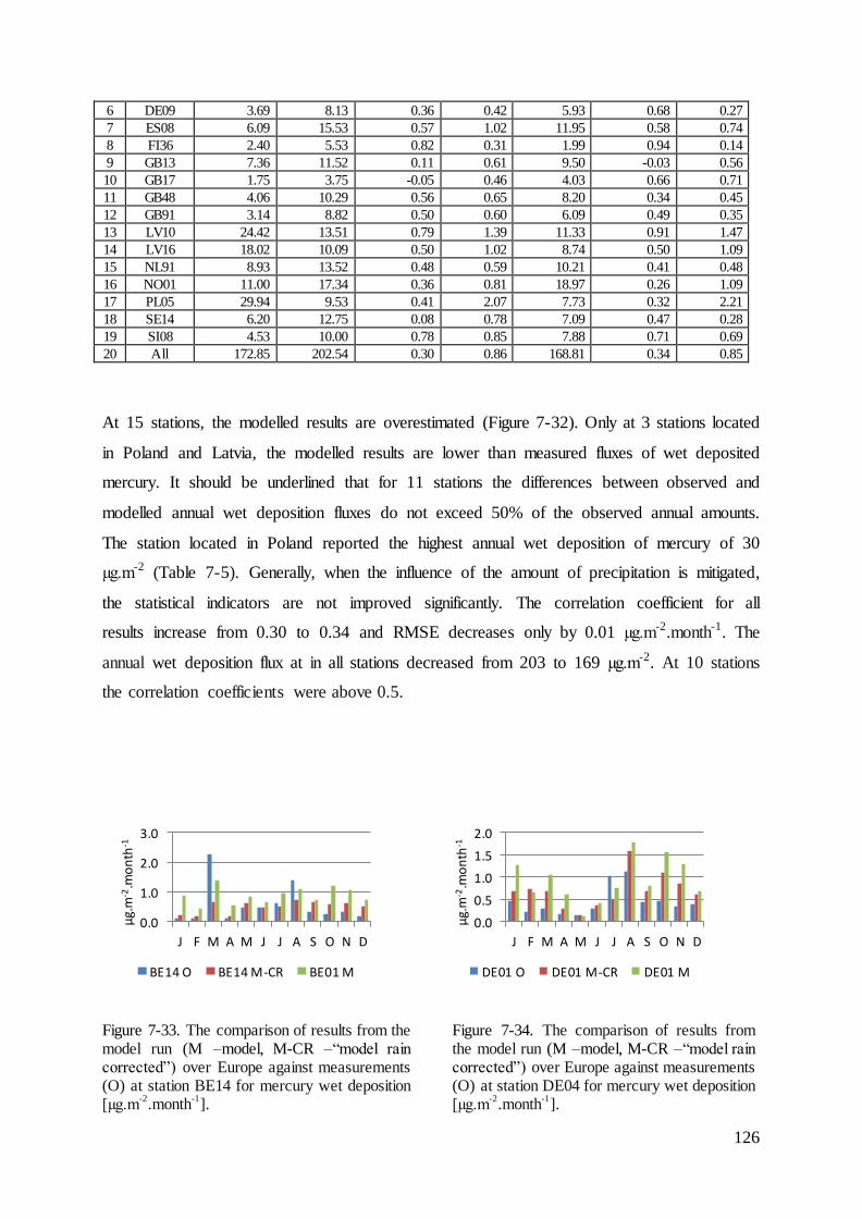
126
6 DE09 3.69 8.13 0.36 0.42 5.93 0.68 0.27
7 ES08 6.09 15.53 0.57 1.02 11.95 0.58 0.74
8 FI36 2.40 5.53 0.82 0.31 1.99 0.94 0.14
9 GB13 7.36 11.52 0.11 0.61 9.50 -0.03 0.56
10 GB17 1.75 3.75 -0.05 0.46 4.03 0.66 0.71
11 GB48 4.06 10.29 0.56 0.65 8.20 0.34 0.45
12 GB91 3.14 8.82 0.50 0.60 6.09 0.49 0.35
13 LV10 24.42 13.51 0.79 1.39 11.33 0.91 1.47
14 LV16 18.02 10.09 0.50 1.02 8.74 0.50 1.09
15 NL91 8.93 13.52 0.48 0.59 10.21 0.41 0.48
16 NO01 11.00 17.34 0.36 0.81 18.97 0.26 1.09
17 PL05 29.94 9.53 0.41 2.07 7.73 0.32 2.21
18 SE14 6.20 12.75 0.08 0.78 7.09 0.47 0.28
19 SI08 4.53 10.00 0.78 0.85 7.88 0.71 0.69
20 All 172.85 202.54 0.30 0.86 168.81 0.34 0.85
At 15 stations, the modelled results are overestimated (Figure 7-32). Only at 3 stations located
in Poland and Latvia, the modelled results are lower than measured fluxes of wet deposited
mercury. It should be underlined that for 11 stations the differences between observed and
modelled annual wet deposition fluxes do not exceed 50% of the observed annual amounts.
The station located in Poland reported the highest annual wet deposition of mercury of 30
µg.m-2 (Table 7-5). Generally, when the influence of the amount of precipitation is mitigated,
the statistical indicators are not improved significantly. The correlation coefficient for all
results increase from 0.30 to 0.34 and RMSE decreases only by 0.01 µg.m-2.month-1. The
annual wet deposition flux at in all stations decreased from 203 to 169 µg.m-2. At 10 stations
the correlation coefficients were above 0.5.
Figure 7-33. The comparison of results from the model run (M –model, M-CR –“model rain corrected”) over Europe against measurements (O) at station BE14 for mercury wet deposition [µg.m
-2.month
-1].
Figure 7-34. The comparison of results from the model run (M –model, M-CR –“model rain corrected”) over Europe against measurements (O) at station DE04 for mercury wet deposition [µg.m
-2.month
-1].
0.0
1.0
2.0
3.0
J F M A M J J A S O N D
µg.
m-2
.mo
nth
-1
BE14 O BE14 M-CR BE01 M
0.0
0.5
1.0
1.5
2.0
J F M A M J J A S O N D
µg.
m-2
.mo
nth
-1
DE01 O DE01 M-CR DE01 M

127
Figure 7-35. The comparison of results from the model run (M –model, M-CR –model “rain corrected”) over Europe against measurements (O) at station BE14 for mercury wet deposition [µg.m
-2.month
-1].
Figure 7-36. The comparison of results from the model run (M –model, M-CR –model “rain corrected”) over Europe against measurements (O) at station DE04 for mercury wet deposition [µg.m
-2.month
-1].
Figure 7-37. The comparison of results from the model run (M –model, M-CR –model “rain corrected”) over Europe against measurements (O) at station DE08 for mercury wet deposition [µg.m
-2.month
-1].
Figure 7-38. The comparison of results from the model run (M –model, M-CR –model “rain corrected”) over Europe against measurements (O) at station DE09 for mercury wet deposition [µg.m
-2.month
-1].
Figure 7-39. The comparison of results from the model run (M –model, M-CR –“model rain corrected”) over Europe against measurements (O) at station ES08 for mercury wet deposition [µg.m
-2.month
-1].
Figure 7-40. The comparison of results from the model run (M –model, M-CR –“model rain corrected”) over Europe against measurements (O) at station FI36 for mercury wet deposition [µg.m
-2.month
-1].
0.0
0.5
1.0
1.5
J F M A M J J A S O N D
µg.
m-2
.mo
nth
-1
DE02 O DE02 M-CR DE02 M
0.0
1.0
2.0
3.0
J F M A M J J A S O N D
µg.
m-2
.mo
nth
-1
DE03 O DE03 M-CR DE03 M
0.0
1.0
2.0
3.0
J F M A M J J A S O N D
µg.
m-2
.mo
nth
-1
DE08 O DE08 M-CR DE08 M
0.0
0.5
1.0
1.5
J F M A M J J A S O N D
µg.
m-2
.mo
nth
-1
DE09 O DE09 M-CR DE09 M
0.0
1.0
2.0
3.0
J F M A M J J A S O N D
µg.
m-2
.mo
nth
-1
ES08 O ES08 M-CR ES08 M
0.0
0.5
1.0
J F M A M J J A S O N D
µg.
m-2
.mo
nth
-1
FI36 O FI36 M-CR FI36 M
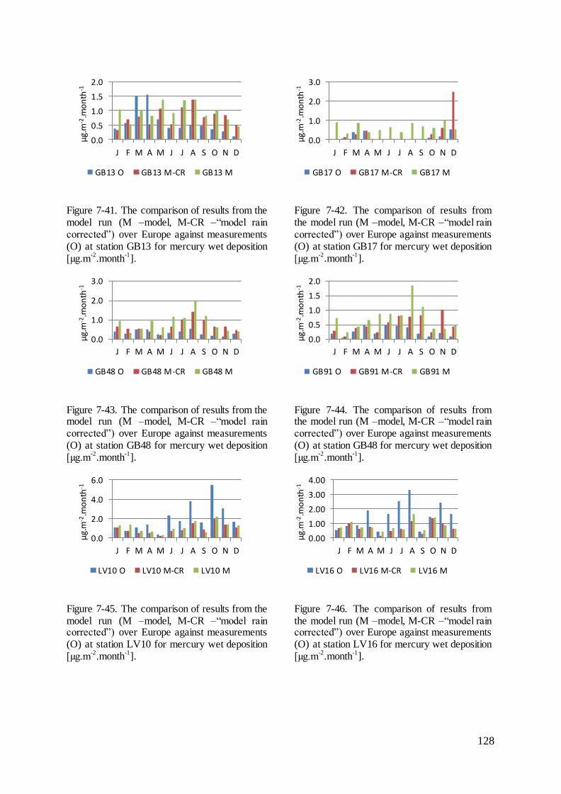
128
Figure 7-41. The comparison of results from the model run (M –model, M-CR –“model rain corrected”) over Europe against measurements (O) at station GB13 for mercury wet deposition [µg.m
-2.month
-1].
Figure 7-42. The comparison of results from the model run (M –model, M-CR –“model rain corrected”) over Europe against measurements (O) at station GB17 for mercury wet deposition [µg.m
-2.month
-1].
Figure 7-43. The comparison of results from the model run (M –model, M-CR –“model rain corrected”) over Europe against measurements (O) at station GB48 for mercury wet deposition [µg.m
-2.month
-1].
Figure 7-44. The comparison of results from the model run (M –model, M-CR –“model rain corrected”) over Europe against measurements (O) at station GB48 for mercury wet deposition [µg.m
-2.month
-1].
Figure 7-45. The comparison of results from the model run (M –model, M-CR –“model rain corrected”) over Europe against measurements (O) at station LV10 for mercury wet deposition [µg.m
-2.month
-1].
Figure 7-46. The comparison of results from the model run (M –model, M-CR –“model rain corrected”) over Europe against measurements (O) at station LV16 for mercury wet deposition [µg.m
-2.month
-1].
0.0
0.5
1.0
1.5
2.0
J F M A M J J A S O N D
µg.
m-2
.mo
nth
-1
GB13 O GB13 M-CR GB13 M
0.0
1.0
2.0
3.0
J F M A M J J A S O N D
µg.
m-2
.mo
nth
-1
GB17 O GB17 M-CR GB17 M
0.0
1.0
2.0
3.0
J F M A M J J A S O N D
µg.
m-2
.mo
nth
-1
GB48 O GB48 M-CR GB48 M
0.0
0.5
1.0
1.5
2.0
J F M A M J J A S O N D
µg.
m-2
.mo
nth
-1
GB91 O GB91 M-CR GB91 M
0.0
2.0
4.0
6.0
J F M A M J J A S O N D
µg.
m-2
.mo
nth
-1
LV10 O LV10 M-CR LV10 M
0.00
1.00
2.00
3.00
4.00
J F M A M J J A S O N D
µg.
m-2
.mo
nth
-1
LV16 O LV16 M-CR LV16 M
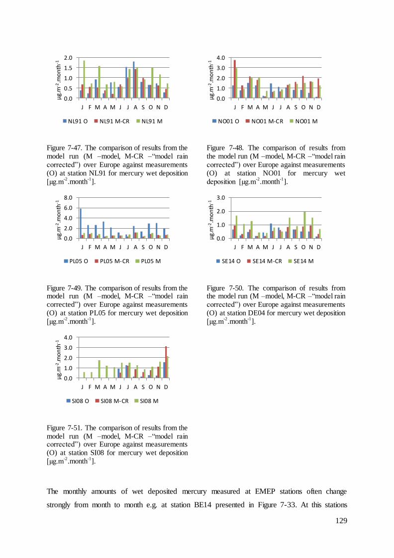
129
Figure 7-47. The comparison of results from the model run (M –model, M-CR –“model rain corrected”) over Europe against measurements (O) at station NL91 for mercury wet deposition [µg.m
-2.month
-1].
Figure 7-48. The comparison of results from the model run (M –model, M-CR –“model rain corrected”) over Europe against measurements (O) at station NO01 for mercury wet deposition [µg.m
-2.month
-1].
Figure 7-49. The comparison of results from the model run (M –model, M-CR –“model rain corrected”) over Europe against measurements (O) at station PL05 for mercury wet deposition [µg.m
-2.month
-1].
Figure 7-50. The comparison of results from the model run (M –model, M-CR –“model rain corrected”) over Europe against measurements (O) at station DE04 for mercury wet deposition [µg.m
-2.month
-1].
Figure 7-51. The comparison of results from the model run (M –model, M-CR –“model rain corrected”) over Europe against measurements (O) at station SI08 for mercury wet deposition [µg.m
-2.month
-1].
The monthly amounts of wet deposited mercury measured at EMEP stations often change
strongly from month to month e.g. at station BE14 presented in Figure 7-33. At this stations
0.0
0.5
1.0
1.5
2.0
J F M A M J J A S O N D
µg.
m-2
.mo
nth
-1
NL91 O NL91 M-CR NL91 M
0.0
1.0
2.0
3.0
4.0
J F M A M J J A S O N D
µg.
m-2
.mo
nth
-1
NO01 O NO01 M-CR NO01 M
0.0
2.0
4.0
6.0
8.0
J F M A M J J A S O N D
µg.
m-2
.mo
nth
-1
PL05 O PL05 M-CR PL05 M
0.0
1.0
2.0
3.0
J F M A M J J A S O N D
µg.
m-2
.mo
nth
-1
SE14 O SE14 M-CR SE14 M
0.0
1.0
2.0
3.0
4.0
J F M A M J J A S O N D
µg.
m-2
.mo
nth
-1
SI08 O SI08 M-CR SI08 M
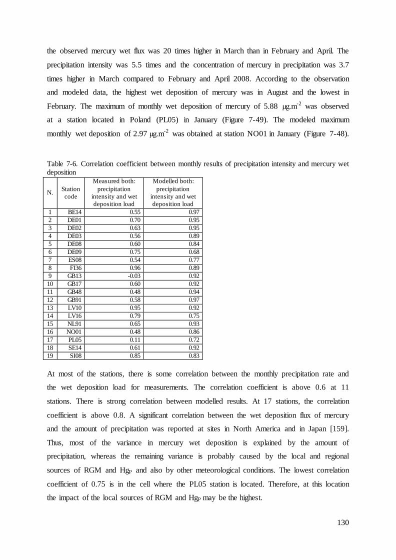
130
the observed mercury wet flux was 20 times higher in March than in February and April. The
precipitation intensity was 5.5 times and the concentration of mercury in precipitation was 3.7
times higher in March compared to February and April 2008. According to the observation
and modeled data, the highest wet deposition of mercury was in August and the lowest in
February. The maximum of monthly wet deposition of mercury of 5.88 µg.m-2 was observed
at a station located in Poland (PL05) in January (Figure 7-49). The modeled maximum
monthly wet deposition of 2.97 µg.m-2 was obtained at station NO01 in January (Figure 7-48).
Table 7-6. Correlation coefficient between monthly results of precipitation intensity and mercury wet deposition
N. Station
code
Measured both:
precipitation
intensity and wet
deposition load
Modelled both:
precipitation
intensity and wet
deposition load
1 BE14 0.55 0.97
2 DE01 0.70 0.95
3 DE02 0.63 0.95
4 DE03 0.56 0.89
5 DE08 0.60 0.84
6 DE09 0.75 0.68
7 ES08 0.54 0.77
8 FI36 0.96 0.89
9 GB13 -0.03 0.92
10 GB17 0.60 0.92
11 GB48 0.48 0.94
12 GB91 0.58 0.97
13 LV10 0.95 0.92
14 LV16 0.79 0.75
15 NL91 0.65 0.93
16 NO01 0.48 0.86
17 PL05 0.11 0.72
18 SE14 0.61 0.92
19 SI08 0.85 0.83
At most of the stations, there is some correlation between the monthly precipitation rate and
the wet deposition load for measurements. The correlation coefficient is above 0.6 at 11
stations. There is strong correlation between modelled results. At 17 stations, the correlation
coefficient is above 0.8. A significant correlation between the wet deposition flux of mercury
and the amount of precipitation was reported at sites in North America and in Japan [159].
Thus, most of the variance in mercury wet deposition is explained by the amount of
precipitation, whereas the remaining variance is probably caused by the local and regional
sources of RGM and HgP and also by other meteorological conditions. The lowest correlation
coefficient of 0.75 is in the cell where the PL05 station is located. Therefore, at this location
the impact of the local sources of RGM and HgP may be the highest.
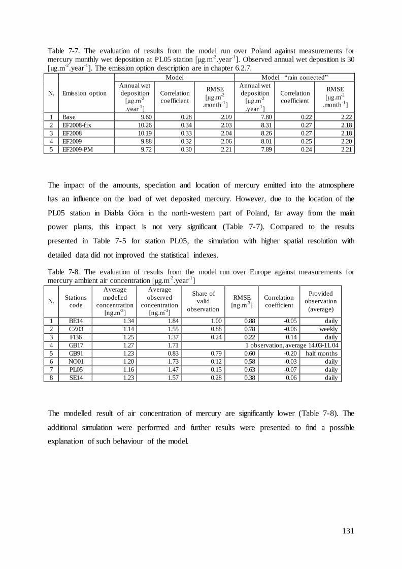
131
Table 7-7. The evaluation of results from the model run over Poland against measurements for mercury monthly wet deposition at PL05 station [µg.m
-2.year
-1]. Observed annual wet deposition is 30
[µg.m-2
.year-1
]. The emission option description are in chapter 6.2.7.
N. Emission option
Model Model –“rain corrected”
Annual wet
deposition
[µg.m-2
.year-1
]
Correlation
coefficient
RMSE
[µg.m-2
.month-1
]
Annual wet
deposition
[µg.m-2
.year-1
]
Correlation
coefficient
RMSE
[µg.m-2
.month-1
]
1 Base 9.60 0.28 2.09 7.80 0.22 2.22
2 EF2008-fix 10.26 0.34 2.03 8.31 0.27 2.18
3 EF2008 10.19 0.33 2.04 8.26 0.27 2.18
4 EF2009 9.88 0.32 2.06 8.01 0.25 2.20
5 EF2009-PM 9.72 0.30 2.21 7.89 0.24 2.21
The impact of the amounts, speciation and location of mercury emitted into the atmosphere
has an influence on the load of wet deposited mercury. However, due to the location of the
PL05 station in Diabla Góra in the north-western part of Poland, far away from the main
power plants, this impact is not very significant (Table 7-7). Compared to the results
presented in Table 7-5 for station PL05, the simulation with higher spatial resolution with
detailed data did not improved the statistical indexes.
Table 7-8. The evaluation of results from the model run over Europe against measurements for mercury ambient air concentration [µg.m
-2.year
-1]
N. Stations
code
Average
modelled
concentration
[ng.m-3
]
Average
observed
concentration
[ng.m-3
]
Share of
valid
observation
RMSE
[ng.m-3
]
Correlation
coefficient
Provided
observation
(average)
1 BE14 1.34 1.84 1.00 0.88 -0.05 daily
2 CZ03 1.14 1.55 0.88 0.78 -0.06 weekly
3 FI36 1.25 1.37 0.24 0.22 0.14 daily
4 GB17 1.27 1.71 1 observation, average 14.03-11.04
5 GB91 1.23 0.83 0.79 0.60 -0.20 half months
6 NO01 1.20 1.73 0.12 0.58 -0.03 daily
7 PL05 1.16 1.47 0.15 0.63 -0.07 daily
8 SE14 1.23 1.57 0.28 0.38 0.06 daily
The modelled result of air concentration of mercury are significantly lower (Table 7-8). The
additional simulation were performed and further results were presented to find a possible
explanation of such behaviour of the model.

132
7.5 Evaluation of cadmium and lead ambient concentrations and deposition
The obtained model results of cadmium and lead air concentrations and wet deposition fluxes
were evaluated against measurements conducted at EMEP stations in 2008. The results of the
air concentrations of cadmium and lead bound to PM10 were taken into accounting for this
evaluation. The evaluation for cadmium air concentrations was done for 19 stations (Table
7-9 and Table 7-10). The other 31 stations measured the cadmium concentrations in other PM
size sections (mostly in total particulate matter) or outside the modelling domain in 2008. The
lead air concentration in PM10 was measured in 2008 at 23 stations located within the
European modelling domain (Table 7-12 and Table 7-13. The other 32 stations measured the
lead concentration outside the domain or in other particulate matter size sections than PM10.
The evaluation of the wet deposition flux was done at 52 stations for both lead and cadmium.
Table 7-9. Evaluation of results of concentrations in ambient air of cadmium bound to PM10 from simulation run over the European domain at the surface against measurements of EMEP [163]. The observed concentrations were provided with time step of 1 day.
N. Stations
code
Share of valid
observation
Average annual
observed
concentration
[ng.m-3
]
Average annual
modelled
concentration
[ng.m-3
]
RMSE
[ng.m-3
]
Correlation
coefficient
1 AT02 0.300 0.15 0.15 0.12 0.63
2 AT05 0.134 0.08 0.08 0.07 0.47
3 AT48 0.153 0.05 0.08 0.05 0.55
4 CZ01 0.139 0.19 0.19 0.16 0.53
5 CZ03 0.525 0.15 0.16 0.08 0.56
6 ES09 0.120 0.03 0.06 0.06 0.53
7 SI08 0.464 0.10 0.13 0.09 0.22
8 All 0.280 0.13 0.14 0.10 0.69
All - results for all observations from 7 stations located inside the European domain, where Cd concentrations
where observed in 2008 and results were provided with temporal resolution of 1 day.
Table 7-10. Evaluation of results of concentrations in ambient air of cadmium bound to PM10 from simulation run over the European domain at the surface against measurements of EMEP [163]. The observed concentrations were provided as the average value 1 week.
N. Stations
code
Share of valid
observation
Average annual
observed
concentration
[ng.m-3
]
Average annual
modelled
concentration
[ng.m-3
]
RMSE
[ng.m-3
]
Correlation
coefficient
1 DE01 1.000 0.08 0.08 0.06 0.58
2 DE02 0.980 0.17 0.15 0.10 0.57
3 DE03 0.942 0.05 0.15 0.10 -0.11
4 DE07 1.000 0.15 0.15 0.07 0.74
5 DE08 1.000 0.09 0.13 0.09 0.05
6 DE09 0.980 0.11 0.12 0.05 0.78
7 GB13 0.365 0.04 0.06 0.02 0.93
8 NO01 0.712 0.03 0.03 0.04 0.27
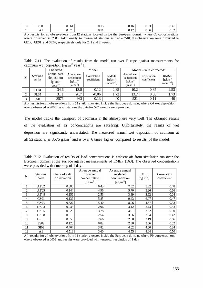
133
9 PL05 0.961 0.15 0.16 0.03 0.41
10 All 0.670 0.11 0.12 0.06 0.52
All- results for all observations from 12 stations located inside the European domain, where Cd concentrations
where observed in 2008. Additionally to presented stations in Table 7-10, the observation were provided in
GB17, GB91 and SK07, respectively only for 2, 1 and 2 weeks.
Table 7-11. The evaluation of results from the model run over Europe against measurements for cadmium wet deposition [µg.m
-2.year
-1].
N. Stations
code
Observed
annual wet
deposition
[g.km-2
.year-1
]
Model Model –“rain corrected”
Annual wet
deposition
[g.km-2
.year-1]
Correlation
coefficient
RMSE
[g.km-2
.month-1]
Annual wet
deposition
[g.km-2
.year-1]
Correlation
coefficient
RMSE
[g.km-2
.month-1]
1 PL04 34.6 13.8 0.12 2.35 10.2 0.35 2.53
2 PL05 31.1 20.7 -0.06 1.72 13.7 0.56 1.73
3 All 3575 663 0.13 40 521 0.11 40
All- results for all observations from 52 stations located inside the European domain, where Cd wet deposition
where observed in 2008. In all stations the data for 597 months were provided.
The model tracks the transport of cadmium in the atmosphere very well. The obtained results
of the evaluation of air concentrations are satisfying. Unfortunately, the results of wet
deposition are significantly understated. The measured annual wet deposition of cadmium at
all 52 stations is 3575 g.km-2 and is over 6 times higher compared to results of the model.
Table 7-12. Evaluation of results of lead concentrations in ambient air from simulation run over the European domain at the surface against measurements of EMEP [163]. The observed concentrations were provided with time step of 1 day.
N. Stations
code
Share of valid
observation
Average annual
observed
concentration
[ng.m-3
]
Average annual
modelled
concentration
[ng.m-3
]
RMSE
[ng.m-3
]
Correlation
coefficient
1 AT02 0.306 6.43 7.52 5.32 0.48
2 AT05 0.144 4.96 5.70 3.86 0.56
3 AT48 0.156 2.56 3.89 2.62 0.24
4 CZ01 0.139 5.85 9.43 6.07 0.47
5 CZ03 0.527 5.40 8.06 4.57 0.32
6 DK03 0.948 2.96 3.12 2.44 0.53
7 DK05 0.926 3.78 4.91 3.62 0.50
8 DK08 0.918 2.54 3.06 3.54 0.42
9 DK31 0.950 2.66 2.50 2.19 0.66
10 ES09 0.120 0.82 2.90 2.66 0.52
11 SI08 0.464 3.82 4.62 4.00 0.24
12 All 0.518 3.60 4.55 4.04 0.50
All -results for all observations from 11 stations located inside the European domain, where Pb concentrations
where observed in 2008 and results were provided with temporal resolution of 1 day

134
Table 7-13. Evaluation of results of lead concentrations in ambient air from simulation run over the European domain at surface against measurements of EMEP [163]. The observed concentrations were provided as the average value 1 week.
N. Stations
code
Share of valid
observation
Average annual
observed
concentration
[ng.m-3
]
Average annual
modelled
concentration
[ng.m-3
]
RMSE
[ng.m-3
]
Correlation
coefficient
1 DE01 1.000 2.88 3.13 1.64 0.61
2 DE02 0.980 4.93 5.85 2.46 0.65
3 DE03 0.942 2.04 8.14 6.16 -0.18
4 DE07 1.000 5.01 5.74 2.76 0.61
5 DE08 1.000 2.96 6.96 4.63 0.16
6 DE09 0.980 3.72 4.19 2.10 0.61
7 GB13 0.365 1.77 3.26 1.72 0.93
8 NO01 0.712 1.06 1.05 1.65 0.28
9 PL05 0.961 5.38 2.92 1.13 0.72
10 All 0.660 3.57 4.97 2.65 0.32
All -results for all observations from 12 stations located inside the European domain, where Pb concentrations
where observed in 2008. Additionally to presented stations in Table 7-13, the observation were provided in
GB17, GB91 and SK07, respectively only for 2, 1 and 2 weeks.
Table 7-14. The evaluation of results from the model run over Europe against measurements for lead wet deposition [µg.m
-2.year
-1].
N. Stations
code
Observed
annual wet
deposition
[g.km-2
.year-1
]
Model Model –“rain corrected”
Annual wet deposition
[g.km-2
.year-1]
Correlation
RMSE [g.km-2
.month-1]
Annual wet deposition
[g.km-2
.year-1]
Correlation coefficient
RMSE [g.km-2
.month-1]
1 PL04 525 438 -0.30 25 329 -0.31 27
2 PL05 409 525 0.56 20 371 0.82 11
3 All 42347 27910 0.30 117 22558 0.34 118
All- results for all observations from 52 stations located inside the European domain, where lead wet deposition
where observed in 2008. In all stations the data for 592 months were provided.
The modelling results of lead air concentrations are overestimated. The correlation
coefficients for the majority of the presented stations are above 0.5 (Table 7-12 Table 7-13).
On the other hand, the modelled amount of lead wet deposition are underestimated.
One very important thing to be noticed, is that an average the observed the air concentration
of cadmium is 30 times lower than the air concentration of lead, while the measured wet
deposition of cadmium is only 12 times lower than the wet deposition of lead. The modelling
ratios of lead and cadmium for both air concentration and wet deposition are approx. 40. This
is understandable because the lead and cadmium in the air are associated together in similar
particles. Therefore, the atmospheric transport, as well as, the removal processes are the same
for both heavy metals. The differences in observation rates may result from different
distributions of lead and cadmium in size sections of particulate matter. Most of cadmium is
associated in PM with a diameter above 10 µm. The measurement of air concentration is

135
given for PM10 while deposition covers all particles, also above 10 µm. The underestimated
results of air concentration and amount of wet deposition of lead and cadmium were obtained
from simulation run with the use of the MSCE-HM model for 2008 [183].
7.6 Results of ambient concentrations and deposition of mercury
The concentration of various mercury forms over Europe at the surface are presented in
Figure 7-52 -Figure 7-54.
Figure 7-52. Annual average concentration of GEM [ng.m-3
] at the surface.
Figure 7-53. Annual average ambient concentration of RGM [pg.m
-3] at the surface.
Figure 7-54. Annual average ambient
concentration of HgP [pg.m-3
] at the surface.
The ambient concentrations of elemental gaseous mercury ranges from 1.10 -1.60 ng.m-3. The
high value is noticed near the boundary of the domain, where the concentration of approx.
1.50 ng.m-3 at the surface level was assumed. Inside the domain, mainly over land the
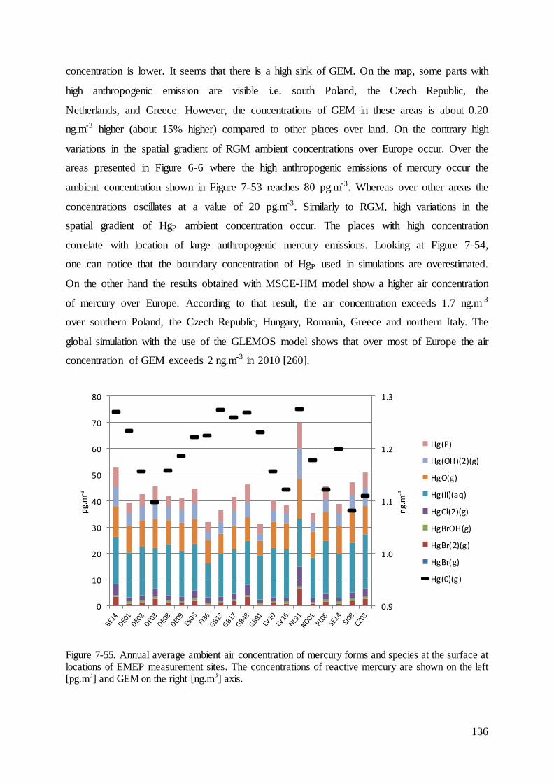
136
concentration is lower. It seems that there is a high sink of GEM. On the map, some parts with
high anthropogenic emission are visible i.e. south Poland, the Czech Republic, the
Netherlands, and Greece. However, the concentrations of GEM in these areas is about 0.20
ng.m-3 higher (about 15% higher) compared to other places over land. On the contrary high
variations in the spatial gradient of RGM ambient concentrations over Europe occur. Over the
areas presented in Figure 6-6 where the high anthropogenic emissions of mercury occur the
ambient concentration shown in Figure 7-53 reaches 80 pg.m-3. Whereas over other areas the
concentrations oscillates at a value of 20 pg.m-3. Similarly to RGM, high variations in the
spatial gradient of HgP ambient concentration occur. The places with high concentration
correlate with location of large anthropogenic mercury emissions. Looking at Figure 7-54,
one can notice that the boundary concentration of HgP used in simulations are overestimated.
On the other hand the results obtained with MSCE-HM model show a higher air concentration
of mercury over Europe. According to that result, the air concentration exceeds 1.7 ng.m-3
over southern Poland, the Czech Republic, Hungary, Romania, Greece and northern Italy. The
global simulation with the use of the GLEMOS model shows that over most of Europe the air
concentration of GEM exceeds 2 ng.m-3 in 2010 [260].
Figure 7-55. Annual average ambient air concentration of mercury forms and species at the surface at locations of EMEP measurement sites. The concentrations of reactive mercury are shown on the left [pg.m
3] and GEM
on the right [ng.m
3] axis.
0.9
1.0
1.1
1.2
1.3
0
10
20
30
40
50
60
70
80n
g.m
-3
pg.
m-3
Hg(P)
Hg(OH)(2)(g)
HgO(g)
Hg(II)(aq)
HgCl(2)(g)
HgBrOH(g)
HgBr(2)(g)
HgBr(g)
Hg(0)(g)
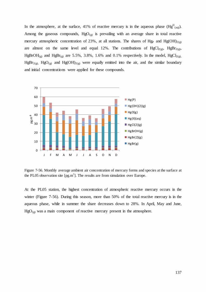
137
In the atmosphere, at the surface, 41% of reactive mercury is in the aqueous phase (HgII(aq)).
Among the gaseous compounds, HgO(g) is prevailing with an average share in total reactive
mercury atmospheric concentration of 23%, at all stations. The shares of HgP and Hg(OH)2(g)
are almost on the same level and equal 12%. The contributions of HgCl2(g), HgBr2(g),
HgBrOH(g) and HgBr(g) are 5.5%, 3.8%, 1.6% and 0.1% respectively. In the model, HgCl2(g),
HgBr2(g), HgO(g) and Hg(OH)2(g) were equally emitted into the air, and the similar boundary
and initial concentrations were applied for these compounds.
Figure 7-56. Monthly average ambient air concentration of mercury forms and species at the surface at
the PL05 observation site [pg.m3]. The results are from simulation over Europe.
At the PL05 station, the highest concentration of atmospheric reactive mercury occurs in the
winter (Figure 7-56). During this season, more than 50% of the total reactive mercury is in the
aqueous phase, while in summer the share decreases down to 28%. In April, May and June,
HgO(g) was a main component of reactive mercury present in the atmosphere.
0
10
20
30
40
50
60
70
J F M A M J J A S O N D
pg.
m-3
Hg(P)
Hg(OH)(2)(g)
HgO(g)
Hg(II)(aq)
HgCl(2)(g)
HgBrOH(g)
HgBr(2)(g)
HgBr(g)
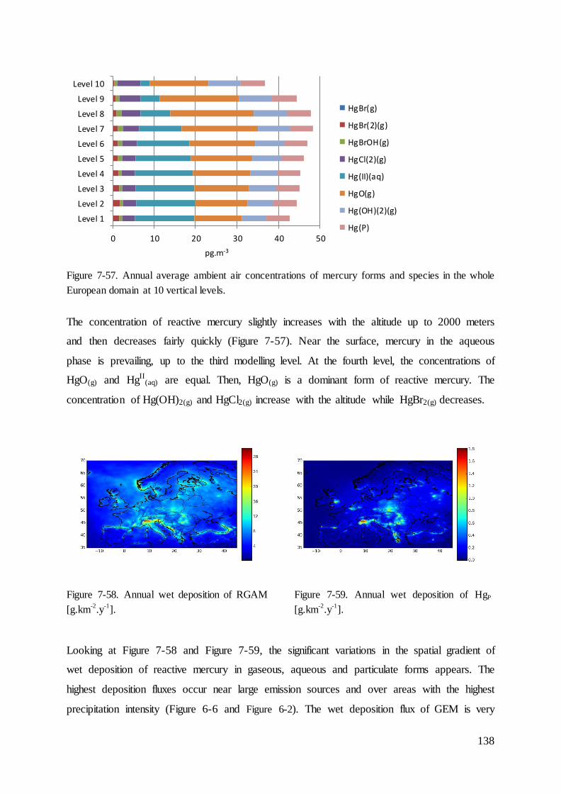
138
Figure 7-57. Annual average ambient air concentrations of mercury forms and species in the whole
European domain at 10 vertical levels.
The concentration of reactive mercury slightly increases with the altitude up to 2000 meters
and then decreases fairly quickly (Figure 7-57). Near the surface, mercury in the aqueous
phase is prevailing, up to the third modelling level. At the fourth level, the concentrations of
HgO(g) and HgII(aq) are equal. Then, HgO(g) is a dominant form of reactive mercury. The
concentration of Hg(OH)2(g) and HgCl2(g) increase with the altitude while HgBr2(g) decreases.
Figure 7-58. Annual wet deposition of RGAM
[g.km-2
.y-1
].
Figure 7-59. Annual wet deposition of HgP
[g.km-2
.y-1
].
Looking at Figure 7-58 and Figure 7-59, the significant variations in the spatial gradient of
wet deposition of reactive mercury in gaseous, aqueous and particulate forms appears. The
highest deposition fluxes occur near large emission sources and over areas with the highest
precipitation intensity (Figure 6-6 and Figure 6-2). The wet deposition flux of GEM is very
0 10 20 30 40 50
Level 1
Level 2
Level 3
Level 4
Level 5
Level 6
Level 7
Level 8
Level 9
Level 10
pg.m-3
HgBr(g)
HgBr(2)(g)
HgBrOH(g)
HgCl(2)(g)
Hg(II)(aq)
HgO(g)
Hg(OH)(2)(g)
Hg(P)
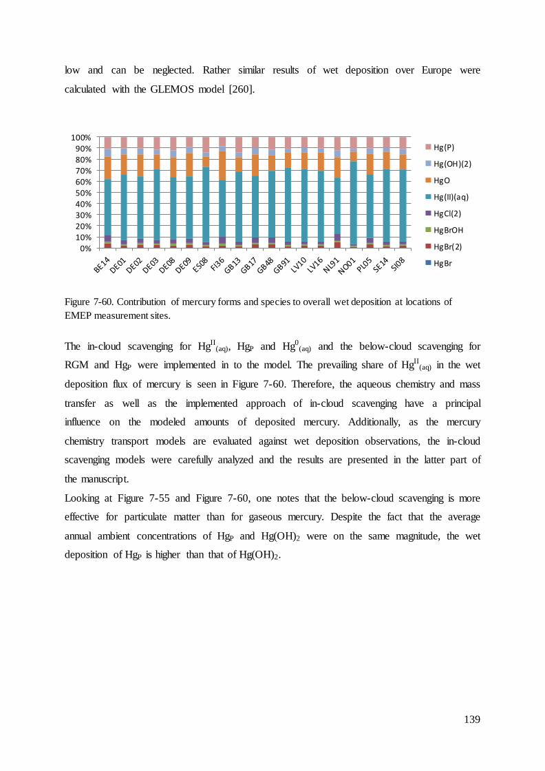
139
low and can be neglected. Rather similar results of wet deposition over Europe were
calculated with the GLEMOS model [260].
Figure 7-60. Contribution of mercury forms and species to overall wet deposition at locations of
EMEP measurement sites.
The in-cloud scavenging for HgII(aq), HgP and Hg0
(aq) and the below-cloud scavenging for
RGM and HgP were implemented in to the model. The prevailing share of HgII(aq) in the wet
deposition flux of mercury is seen in Figure 7-60. Therefore, the aqueous chemistry and mass
transfer as well as the implemented approach of in-cloud scavenging have a principal
influence on the modeled amounts of deposited mercury. Additionally, as the mercury
chemistry transport models are evaluated against wet deposition observations, the in-cloud
scavenging models were carefully analyzed and the results are presented in the latter part of
the manuscript.
Looking at Figure 7-55 and Figure 7-60, one notes that the below-cloud scavenging is more
effective for particulate matter than for gaseous mercury. Despite the fact that the average
annual ambient concentrations of HgP and Hg(OH)2 were on the same magnitude, the wet
deposition of HgP is higher than that of Hg(OH)2.
0%10%20%30%40%50%60%70%80%90%
100%Hg(P)
Hg(OH)(2)
HgO
Hg(II)(aq)
HgCl(2)
HgBrOH
HgBr(2)
HgBr

140
Figure 7-61. Annual dry deposition of GEM [g.km-2
.y-1
].
Figure 7-62. Annual dry deposition of RGM [g.km
-2.y
-1].
Figure 7-63. Annual dry deposition of HgP [g.km
-2.y
-1].
The large local mercury emission sources are not visible in Figure 7-61, and the deposition
process of GEM is mainly led by dry deposition velocity of GEM. GEM is mainly deposited
over the land, because the dry velocity deposition over the land is significantly higher
compared to that oversea. On the contrary, the highest dry depositions of RGM and HgP are
observed near large emission sources (Figure 7-62 and Figure 7-63).
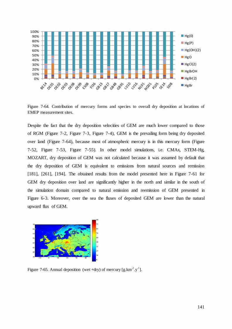
141
Figure 7-64. Contribution of mercury forms and species to overall dry deposition at locations of
EMEP measurement sites.
Despite the fact that the dry deposition velocities of GEM are much lower compared to those
of RGM (Figure 7-2, Figure 7-3, Figure 7-4), GEM is the prevailing form being dry deposited
over land (Figure 7-64), because most of atmospheric mercury is in this mercury form (Figure
7-52, Figure 7-53, Figure 7-55). In other model simulations, i.e. CMAx, STEM-Hg,
MOZART, dry deposition of GEM was not calculated because it was assumed by default that
the dry deposition of GEM is equivalent to emissions from natural sources and remission
[181], [261], [194]. The obtained results from the model presented here in Figure 7-61 for
GEM dry deposition over land are significantly higher in the north and similar in the south of
the simulation domain compared to natural emission and reemission of GEM presented in
Figure 6-3. Moreover, over the sea the fluxes of deposited GEM are lower than the natural
upward flux of GEM.
Figure 7-65. Annual deposition (wet +dry) of mercury [g.km
-2.y
-1].
0%10%20%30%40%50%60%70%80%90%
100%Hg(0)
Hg(P)
Hg(OH)(2)
HgO
HgCl(2)
HgBrOH
HgBr(2)
HgBr
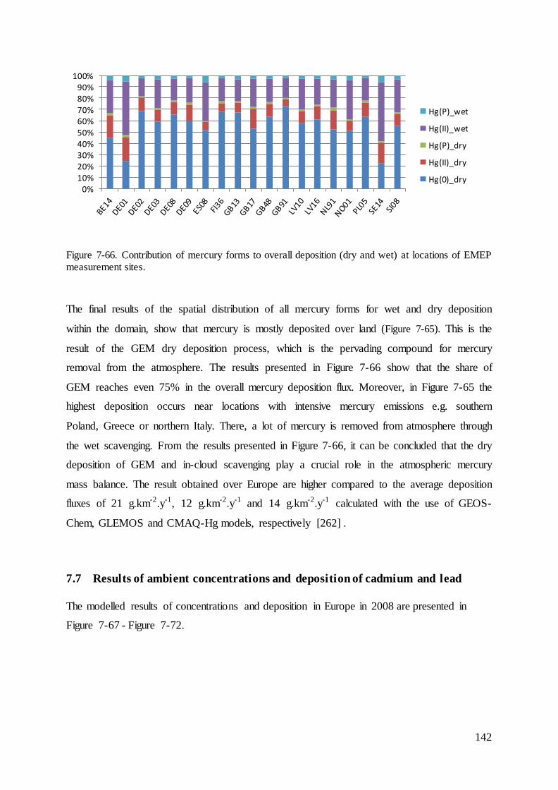
142
Figure 7-66. Contribution of mercury forms to overall deposition (dry and wet) at locations of EMEP measurement sites.
The final results of the spatial distribution of all mercury forms for wet and dry deposition
within the domain, show that mercury is mostly deposited over land (Figure 7-65). This is the
result of the GEM dry deposition process, which is the pervading compound for mercury
removal from the atmosphere. The results presented in Figure 7-66 show that the share of
GEM reaches even 75% in the overall mercury deposition flux. Moreover, in Figure 7-65 the
highest deposition occurs near locations with intensive mercury emissions e.g. southern
Poland, Greece or northern Italy. There, a lot of mercury is removed from atmosphere through
the wet scavenging. From the results presented in Figure 7-66, it can be concluded that the dry
deposition of GEM and in-cloud scavenging play a crucial role in the atmospheric mercury
mass balance. The result obtained over Europe are higher compared to the average deposition
fluxes of 21 g.km-2.y-1, 12 g.km-2.y-1 and 14 g.km-2.y-1 calculated with the use of GEOS-
Chem, GLEMOS and CMAQ-Hg models, respectively [262] .
7.7 Results of ambient concentrations and deposition of cadmium and lead
The modelled results of concentrations and deposition in Europe in 2008 are presented in
Figure 7-67 - Figure 7-72.
0%10%20%30%40%50%60%70%80%90%
100%
Hg(P)_wet
Hg(II)_wet
Hg(P)_dry
Hg(II)_dry
Hg(0)_dry

143
Figure 7-67. Annual average concentration of
cadmium [ng.m-3
] at the surface.
Figure 7-68. Annual average concentration of lead
[ng.m-3
] at the surface.
Figure 7-69. Annual wet deposition of cadmium
[g.km-2
.y-1
].
Figure 7-70. Annual wet deposition of lead
[g.km-2
.y-1
].
Figure 7-71. Annual dry deposition of cadmium
[g.km-2
.y-1
].
Figure 7-72. Annual dry deposition of lead
[g.km-2
.y-1
].
The high variability of average concentration and annual deposition fluxes of cadmium and
lead is noted. The highest concentration and deposition fluxes occurs over industrial areas
where cadmium and lead are intensively released into the atmosphere, mainly by the sector of
production of various metals and alloys. Southern Poland is one of the most polluted areas in
Europe. The ambient concentration of Cd is relatively very low and over a majority of the
simulation domain does not exceed 0.5 ng.m-3. In some areas of the simulation domain, over
4kg.km-2 of lead are deposited during the year. The obtained air concentration spatial
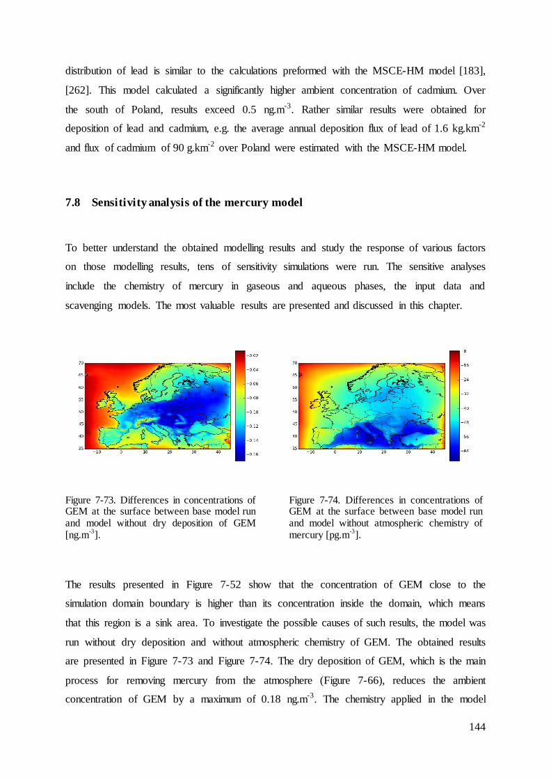
144
distribution of lead is similar to the calculations preformed with the MSCE-HM model [183],
[262]. This model calculated a significantly higher ambient concentration of cadmium. Over
the south of Poland, results exceed 0.5 ng.m-3. Rather similar results were obtained for
deposition of lead and cadmium, e.g. the average annual deposition flux of lead of 1.6 kg.km-2
and flux of cadmium of 90 g.km-2 over Poland were estimated with the MSCE-HM model.
7.8 Sensitivity analysis of the mercury model
To better understand the obtained modelling results and study the response of various factors
on those modelling results, tens of sensitivity simulations were run. The sensitive analyses
include the chemistry of mercury in gaseous and aqueous phases, the input data and
scavenging models. The most valuable results are presented and discussed in this chapter.
Figure 7-73. Differences in concentrations of GEM at the surface between base model run and model without dry deposition of GEM [ng.m
-3].
Figure 7-74. Differences in concentrations of GEM at the surface between base model run and model without atmospheric chemistry of mercury [pg.m
-3].
The results presented in Figure 7-52 show that the concentration of GEM close to the
simulation domain boundary is higher than its concentration inside the domain, which means
that this region is a sink area. To investigate the possible causes of such results, the model was
run without dry deposition and without atmospheric chemistry of GEM. The obtained results
are presented in Figure 7-73 and Figure 7-74. The dry deposition of GEM, which is the main
process for removing mercury from the atmosphere (Figure 7-66), reduces the ambient
concentration of GEM by a maximum of 0.18 ng.m-3. The chemistry applied in the model
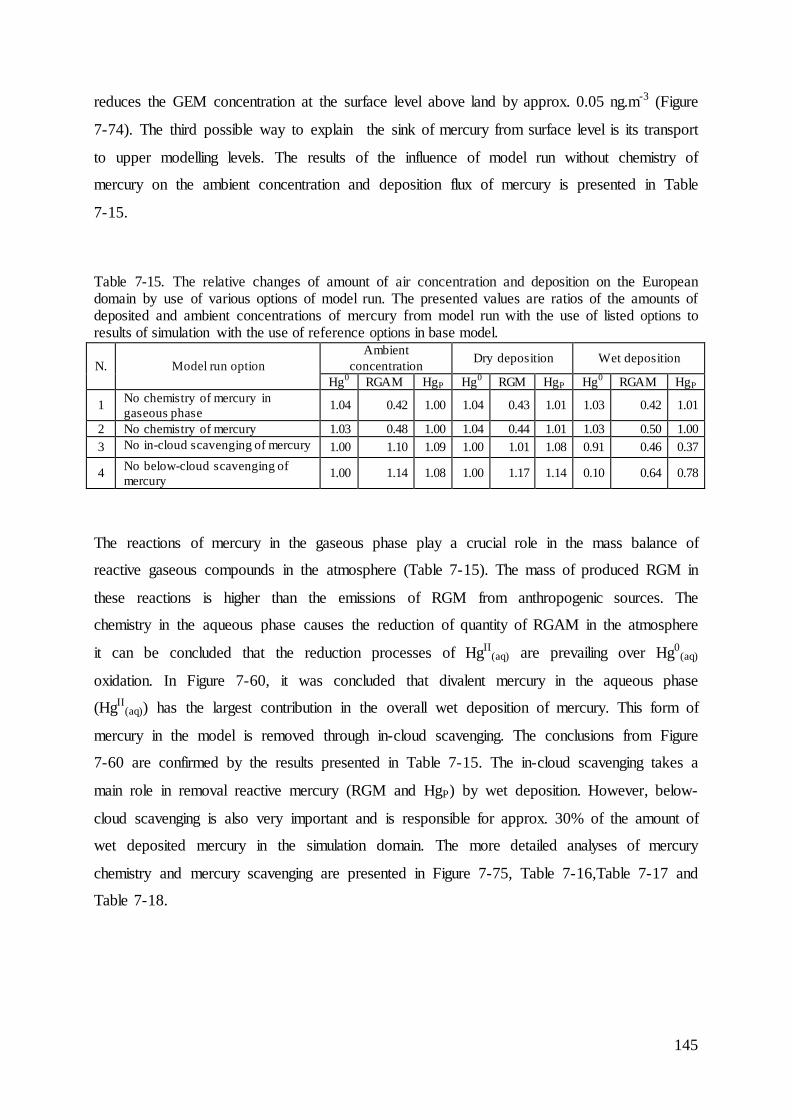
145
reduces the GEM concentration at the surface level above land by approx. 0.05 ng.m-3 (Figure
7-74). The third possible way to explain the sink of mercury from surface level is its transport
to upper modelling levels. The results of the influence of model run without chemistry of
mercury on the ambient concentration and deposition flux of mercury is presented in Table
7-15.
Table 7-15. The relative changes of amount of air concentration and deposition on the European domain by use of various options of model run. The presented values are ratios of the amounts of deposited and ambient concentrations of mercury from model run with the use of listed options to results of simulation with the use of reference options in base model.
N. Model run option
Ambient
concentration Dry deposition Wet deposition
Hg0 RGAM HgP Hg
0 RGM HgP Hg
0 RGAM HgP
1 No chemistry of mercury in
gaseous phase 1.04 0.42 1.00 1.04 0.43 1.01 1.03 0.42 1.01
2 No chemistry of mercury 1.03 0.48 1.00 1.04 0.44 1.01 1.03 0.50 1.00
3 No in-cloud scavenging of mercury 1.00 1.10 1.09 1.00 1.01 1.08 0.91 0.46 0.37
4 No below-cloud scavenging of
mercury 1.00 1.14 1.08 1.00 1.17 1.14 0.10 0.64 0.78
The reactions of mercury in the gaseous phase play a crucial role in the mass balance of
reactive gaseous compounds in the atmosphere (Table 7-15). The mass of produced RGM in
these reactions is higher than the emissions of RGM from anthropogenic sources. The
chemistry in the aqueous phase causes the reduction of quantity of RGAM in the atmosphere
it can be concluded that the reduction processes of HgII(aq) are prevailing over Hg0
(aq)
oxidation. In Figure 7-60, it was concluded that divalent mercury in the aqueous phase
(HgII(aq)) has the largest contribution in the overall wet deposition of mercury. This form of
mercury in the model is removed through in-cloud scavenging. The conclusions from Figure
7-60 are confirmed by the results presented in Table 7-15. The in-cloud scavenging takes a
main role in removal reactive mercury (RGM and HgP) by wet deposition. However, below-
cloud scavenging is also very important and is responsible for approx. 30% of the amount of
wet deposited mercury in the simulation domain. The more detailed analyses of mercury
chemistry and mercury scavenging are presented in Figure 7-75, Table 7-16,Table 7-17 and
Table 7-18.
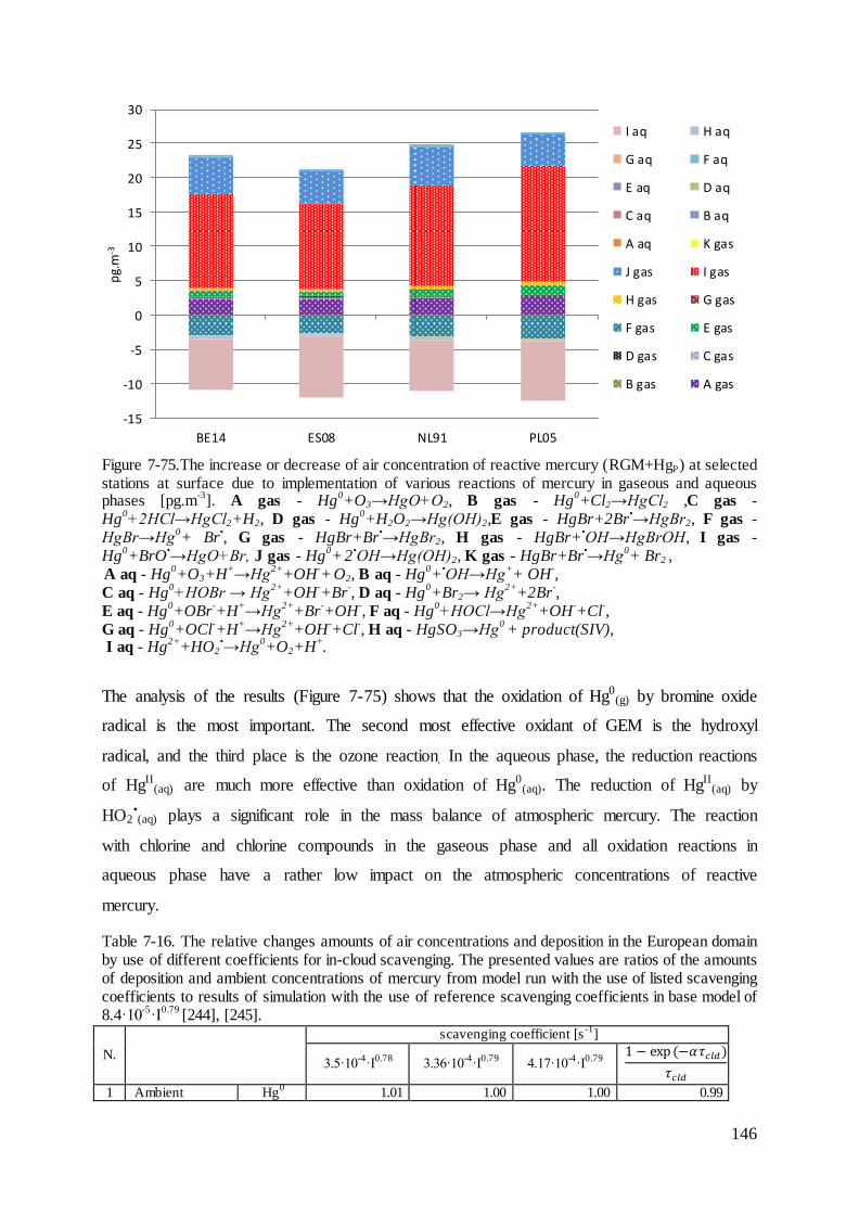
146
Figure 7-75.The increase or decrease of air concentration of reactive mercury (RGM+HgP) at selected stations at surface due to implementation of various reactions of mercury in gaseous and aqueous phases [pg.m
-3]. A gas - Hg
0+O3→HgO+O2, B gas - Hg
0+Cl2→HgCl2 ,C gas -
Hg0+2HCl→HgCl2+H2, D gas - Hg
0+H2O2→Hg(OH)2,E gas - HgBr+2Br
•→HgBr2, F gas -
HgBr→Hg0+ Br
•, G gas - HgBr+Br
•→HgBr2, H gas - HgBr+
•OH→HgBrOH, I gas -
Hg0+BrO
•→HgO+Br, J gas - Hg
0+
2
•OH→Hg(OH)2, K gas - HgBr+Br
•→Hg
0+ Br2 ,
A aq - Hg0+O3+H
+→Hg
2++OH
-+ O2, B aq - Hg
0+
•OH→Hg
++ OH
-,
C aq - Hg0+HOBr → Hg
2++OH
-+Br
-, D aq - Hg
0+Br2→ Hg
2++2Br
-,
E aq - Hg0+OBr
-+H
+→Hg
2++Br
-+OH
-, F aq - Hg
0+HOCl→Hg
2++OH
-+Cl
-,
G aq - Hg0+OCl
-+H
+→Hg
2++OH
-+Cl
-, H aq - HgSO3→Hg
0 + product(SIV),
I aq - Hg2+
+HO2•→Hg
0+O2+H
+.
The analysis of the results (Figure 7-75) shows that the oxidation of Hg0(g) by bromine oxide
radical is the most important. The second most effective oxidant of GEM is the hydroxyl
radical, and the third place is the ozone reaction. In the aqueous phase, the reduction reactions
of HgII(aq) are much more effective than oxidation of Hg0
(aq). The reduction of HgII(aq) by
HO2•(aq) plays a significant role in the mass balance of atmospheric mercury. The reaction
with chlorine and chlorine compounds in the gaseous phase and all oxidation reactions in
aqueous phase have a rather low impact on the atmospheric concentrations of reactive
mercury.
Table 7-16. The relative changes amounts of air concentrations and deposition in the European domain by use of different coefficients for in-cloud scavenging. The presented values are ratios of the amounts of deposition and ambient concentrations of mercury from model run with the use of listed scavenging coefficients to results of simulation with the use of reference scavenging coefficients in base model of 8.4·10
-5·I
0.79 [244], [245].
N.
scavenging coefficient [s-1
]
3.5·10-4
·I0.78
3.36·10-4
·I0.79
4.17·10-4
·I0.79
1 − exp (−𝛼𝜏𝑐𝑙𝑑)
𝜏𝑐𝑙𝑑
1 Ambient Hg0 1.01 1.00 1.00 0.99
-15
-10
-5
0
5
10
15
20
25
30
BE14 ES08 NL91 PL05
pg.
m-3
I aq H aq
G aq F aq
E aq D aq
C aq B aq
A aq K gas
J gas I gas
H gas G gas
F gas E gas
D gas C gas
B gas A gas
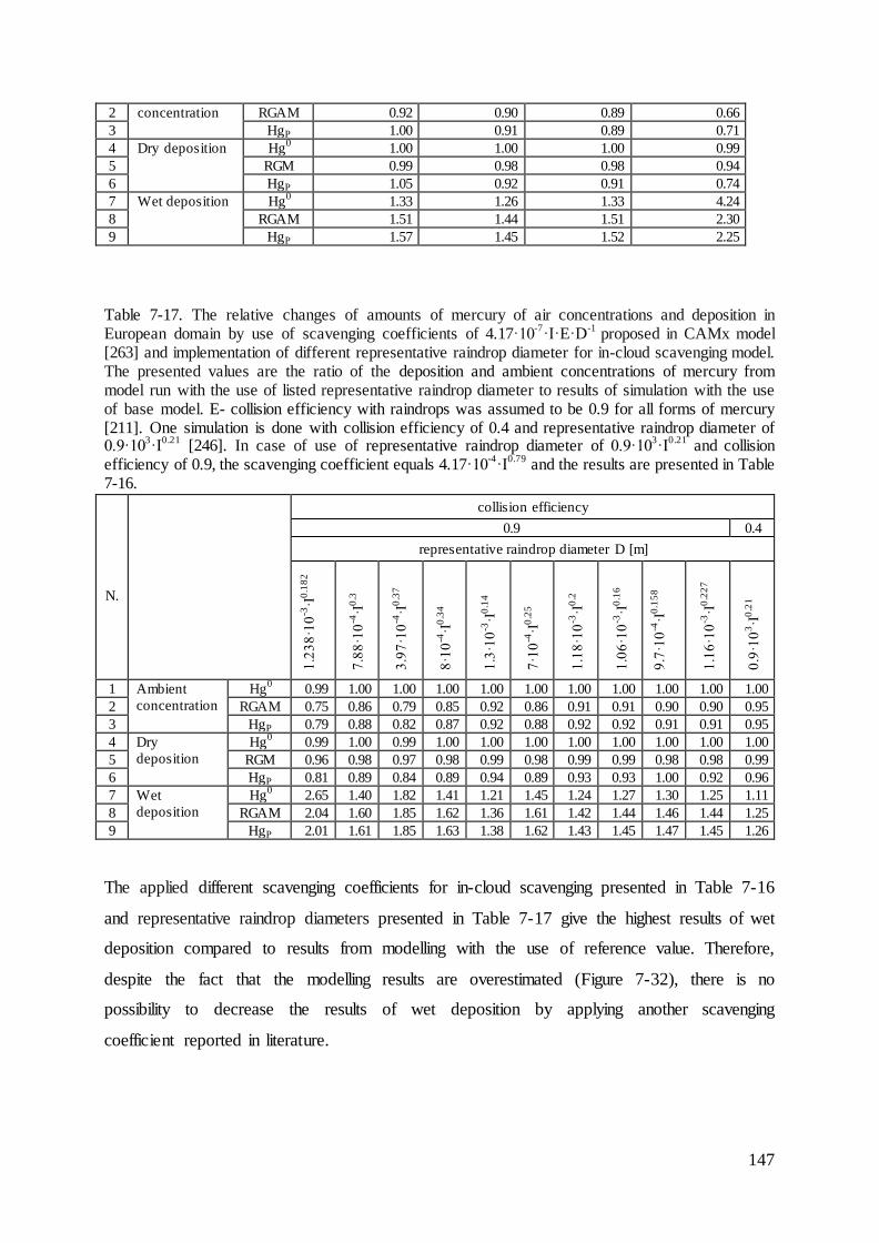
147
2 concentration RGAM 0.92 0.90 0.89 0.66
3 HgP 1.00 0.91 0.89 0.71
4 Dry deposition Hg0 1.00 1.00 1.00 0.99
5 RGM 0.99 0.98 0.98 0.94
6 HgP 1.05 0.92 0.91 0.74
7 Wet deposition Hg0 1.33 1.26 1.33 4.24
8 RGAM 1.51 1.44 1.51 2.30
9 HgP 1.57 1.45 1.52 2.25
Table 7-17. The relative changes of amounts of mercury of air concentrations and deposition in European domain by use of scavenging coefficients of 4.17·10
-7·I·E·D
-1 proposed in CAMx model
[263] and implementation of different representative raindrop diameter for in-cloud scavenging model. The presented values are the ratio of the deposition and ambient concentrations of mercury from model run with the use of listed representative raindrop diameter to results of simulation with the use of base model. E- collision efficiency with raindrops was assumed to be 0.9 for all forms of mercury [211]. One simulation is done with collision efficiency of 0.4 and representative raindrop diameter of 0.9·10
3·I
0.21 [246]. In case of use of representative raindrop diameter of 0.9·10
3·I
0.21 and collision
efficiency of 0.9, the scavenging coefficient equals 4.17·10-4
·I0.79
and the results are presented in Table 7-16.
N.
collision efficiency
0.9 0.4
representative raindrop diameter D [m]
1.2
38
·10
-3·I
0.1
82
7.8
8·1
0-4
·I0
.3
3.9
7·1
0-4
·I0
.37
8·1
0-4
·I0
.34
1.3
·10
-3·I
0.1
4
7·1
0-4
·I0
.25
1.1
8·1
0-3
·I0
.2
1.0
6·1
0-3
·I0
.16
9.7
·10
-4·I
0.1
58
1.1
6·1
0-3
·I0
.22
7
0.9
·10
3·I
0.2
1
1 Ambient
concentration
Hg0 0.99 1.00 1.00 1.00 1.00 1.00 1.00 1.00 1.00 1.00 1.00
2 RGAM 0.75 0.86 0.79 0.85 0.92 0.86 0.91 0.91 0.90 0.90 0.95
3 HgP 0.79 0.88 0.82 0.87 0.92 0.88 0.92 0.92 0.91 0.91 0.95
4 Dry
deposition
Hg0 0.99 1.00 0.99 1.00 1.00 1.00 1.00 1.00 1.00 1.00 1.00
5 RGM 0.96 0.98 0.97 0.98 0.99 0.98 0.99 0.99 0.98 0.98 0.99
6 HgP 0.81 0.89 0.84 0.89 0.94 0.89 0.93 0.93 1.00 0.92 0.96
7 Wet
deposition
Hg0 2.65 1.40 1.82 1.41 1.21 1.45 1.24 1.27 1.30 1.25 1.11
8 RGAM 2.04 1.60 1.85 1.62 1.36 1.61 1.42 1.44 1.46 1.44 1.25
9 HgP 2.01 1.61 1.85 1.63 1.38 1.62 1.43 1.45 1.47 1.45 1.26
The applied different scavenging coefficients for in-cloud scavenging presented in Table 7-16
and representative raindrop diameters presented in Table 7-17 give the highest results of wet
deposition compared to results from modelling with the use of reference value. Therefore,
despite the fact that the modelling results are overestimated (Figure 7-32), there is no
possibility to decrease the results of wet deposition by applying another scavenging
coefficient reported in literature.
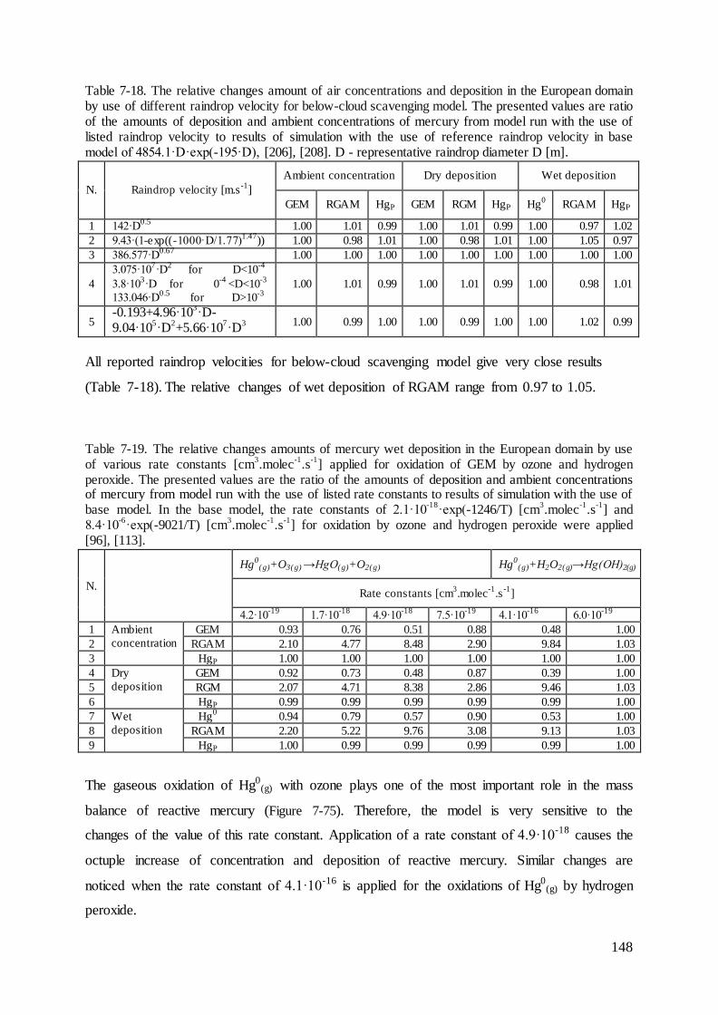
148
Table 7-18. The relative changes amount of air concentrations and deposition in the European domain by use of different raindrop velocity for below-cloud scavenging model. The presented values are ratio of the amounts of deposition and ambient concentrations of mercury from model run with the use of listed raindrop velocity to results of simulation with the use of reference raindrop velocity in base model of 4854.1·D·exp(-195·D), [206], [208]. D - representative raindrop diameter D [m].
N. Raindrop velocity [m.s-1
]
Ambient concentration Dry deposition Wet deposition
GEM RGAM HgP GEM RGM HgP Hg0 RGAM HgP
1 142·D0.5
1.00 1.01 0.99 1.00 1.01 0.99 1.00 0.97 1.02
2 9.43·(1-exp((-1000·D/1.77)1.47
)) 1.00 0.98 1.01 1.00 0.98 1.01 1.00 1.05 0.97
3 386.577·D0.67
1.00 1.00 1.00 1.00 1.00 1.00 1.00 1.00 1.00
4
3.075·107·D
2 for D<10
-4
3.8·103·D for 0
-4 <D<10
-3
133.046·D0.5
for D>10-3
1.00 1.01 0.99 1.00 1.01 0.99 1.00 0.98 1.01
5 -0.193+4.96·10
3·D-
9.04·105·D
2+5.66·10
7·D
3
1.00 0.99 1.00 1.00 0.99 1.00 1.00 1.02 0.99
All reported raindrop velocities for below-cloud scavenging model give very close results
(Table 7-18). The relative changes of wet deposition of RGAM range from 0.97 to 1.05.
Table 7-19. The relative changes amounts of mercury wet deposition in the European domain by use of various rate constants [cm
3.molec
-1.s
-1] applied for oxidation of GEM by ozone and hydrogen
peroxide. The presented values are the ratio of the amounts of deposition and ambient concentrations of mercury from model run with the use of listed rate constants to results of simulation with the use of base model. In the base model, the rate constants of 2.1·10
-18·exp(-1246/T) [cm
3.molec
-1.s
-1] and
8.4·10-6
·exp(-9021/T) [cm3.molec
-1.s
-1] for oxidation by ozone and hydrogen peroxide were applied
[96], [113].
N.
Hg
0(g)+O3(g) →HgO(g)+O2(g) Hg
0(g)+H2O2(g)→Hg(OH)2(g)
Rate constants [cm3.molec
-1.s
-1]
4.2·10-19
1.7·10-18
4.9·10-18
7.5·10-19
4.1·10-16
6.0·10-19
1 Ambient
concentration
GEM 0.93 0.76 0.51 0.88 0.48 1.00
2 RGAM 2.10 4.77 8.48 2.90 9.84 1.03
3 HgP 1.00 1.00 1.00 1.00 1.00 1.00
4 Dry
deposition
GEM 0.92 0.73 0.48 0.87 0.39 1.00
5 RGM 2.07 4.71 8.38 2.86 9.46 1.03
6 HgP 0.99 0.99 0.99 0.99 0.99 1.00
7 Wet
deposition
Hg0 0.94 0.79 0.57 0.90 0.53 1.00
8 RGAM 2.20 5.22 9.76 3.08 9.13 1.03
9 HgP 1.00 0.99 0.99 0.99 0.99 1.00
The gaseous oxidation of Hg0(g) with ozone plays one of the most important role in the mass
balance of reactive mercury (Figure 7-75). Therefore, the model is very sensitive to the
changes of the value of this rate constant. Application of a rate constant of 4.9·10-18 causes the
octuple increase of concentration and deposition of reactive mercury. Similar changes are
noticed when the rate constant of 4.1·10-16 is applied for the oxidations of Hg0(g) by hydrogen
peroxide.
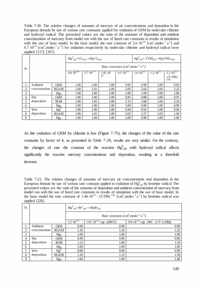
149
Table 7-20. The relative changes of amounts of mercury of air concentrations and deposition in the European domain by use of various rate constants applied for oxidation of GEM by molecular chlorine and hydroxyl radical. The presented values are the ratio of the amounts of deposition and ambient concentrations of mercury from model run with the use of listed rate constants to results of simulation with the use of base model. In the base model, the rate constant of 2.6·10
-18 [cm
3.molec
-1.s
-1] and
8.7·10-14
[cm3.molec
-1.s
-1] for oxidation respectively by molecular chlorine and hydroxyl radical were
applied [117], [107].
N.
Hg0
(g)+Cl2(g)→HgCl2(g) Hg0
(g)+ 2
•OH(g)→Hg(OH)2(g)
Rate constants [cm3.molec
-1.s
-1]
4.8·10-18
5.7·10-17
1.82·10-
19
4.3·10-15
1.6·10-12
1.2·10-13
3.2·10-13
·(T/298)-
3.06
1 Ambient
concentration
GEM 1.00 1.00 1.00 0.92 0.90 1.00 0.93
2 RGAM 1.00 1.01 1.00 2.05 2.64 1.04 2.22
3 HgP 1.00 1.00 1.00 1.00 1.00 1.00 1.00
4 Dry
deposition
GEM 1.00 1.00 1.00 0.95 0.88 1.00 0.91
5 RGM 1.00 1.02 1.00 2.33 2.68 1.04 2.24
6 HgP 1.00 1.00 1.00 1.00 0.99 1.00 0.99
7 Wet
deposition
Hg0 1.00 1.00 1.00 0.94 0.92 1.00 0.94
8 RGAM 1.00 1.01 1.00 2.02 2.27 1.03 1.94
9 HgP 1.00 1.00 1.00 1.00 0.99 1.00 1.00
As the oxidation of GEM by chlorine is low (Figure 7-75), the changes of the value of the rate
constants by factor of 4, as presented in Table 7-20, results are very similar. On the contrary,
the changes of rate the constant of the reaction Hg0(g) with hydroxyl radical affects
significantly the reactive mercury concentrations and deposition, resulting in a threefold
increase.
Table 7-21. The relative changes of amounts of mercury air concentrations and deposition in the European domain by use of various rate constant applied to oxidation of Hg
0(g) by bromine radical. The
presented values are the ratio of the amounts of deposition and ambient concentration of mercury from model run with the use of listed rate constants to results of simulation with the use of base model. In the base model the rate constant of 1.46·10
-32· (T/298)
-1.86 [cm
6.molec
-2.s
-1] by bromine radical was
applied [226].
N. Hg0
(g)+Br •(g) →HgBr(g)
Rate constants [cm3.molec
-1.s
-1]
3.2·10-12
1.01·10-12
·exp
(209/T) 9.8·10-13
·exp (401· (1/T-1/298))
1 Ambient
concentration
GEM 0.99 0.99 0.99
2 RGAM 1.16 1.10 1.22
3 HgP 1.00 1.00 1.00
4 Dry
deposition
GEM 0.99 0.99 0.99
5 RGM 1.13 1.09 1.19
6 HgP 1.00 1.00 1.00
7 Wet
deposition
Hg0 0.99 0.99 0.99
8 RGAM 1.20 1.13 1.28
9 HgP 1.00 1.00 1.00

150
The value applied in the base model for the reference rate constant of GEM oxidation by
bromine radical is the least effective. The application of other possible values of the rate
constant causes the increase of RGAM concentrations and deposition (Table 7-21).
Additional reactions in the gaseous phase were also implemented in to the model. The
oxidation of Hg0(g) by molecular bromine, nitrate radical, molecular iodine, molecular fluorine
and chlorine radicals were separately added to the base model. These reactions were
confirmed in laboratory research studies, however, they have not been widely applied to
mercury chemical transport models (Table 3-1and Table 3-2). The obtained results are
presented in Table 7-22.
Table 7-22. The relative changes amounts of mercury of air concentrations and deposition in the European domain by use of additional reactions of oxidation of Hg
0(g) by molecular bromine, nitrate
radical, molecular iodine, molecular fluorine and chlorine radicals. The presented values are the ratio of the amounts of air concentrations and deposition of mercury from model run with the use of listed reactions to results of simulation with the use of base model (without listed reaction).
N. Reaction
Ambient concentration Dry deposition Wet deposition
GEM RGAM HgP GEM RGM HgP Hg0 RGAM HgP
1 Hg0
(g) +Br2 (g) →HgBr2(g) 1.00 1.00 1.00 1.00 1.00 1.00 1.00 1.00 1.00
2 Hg
0(g) +NO3
•(g) →HgO(g) +
NO2(g) 0.98 1.32 1.00 0.98 1.30 1.00 0.98 1.34 1.00
3 Hg0
(g) +I2 (g) → HgI2(g) 1.00 1.00 1.00 1.00 1.00 1.00 1.00 1.00 1.00
4 Hg0
(g) +F2(g) → HgF2(g) 0.25 12.43 1.00 0.21 12.29 0.99 0.31 15.22 1.34
5 Hg0
(g) + Cl•(g) →HgCl(g) 0.99 1.17 1.00 0.99 1.17 1.00 0.99 1.19 1.00
The oxidation of GEM by molecular bromine and molecular iodine is not very effective. The
changes in depiction of concentrations over the domain are not visible (Table 7-22). The
nitrate radical and chlorine radicals are significant oxidants of Hg0(g). The ambient
concentrations of RGAM increases by 32% and 17%, respectively. The implementation into
the model of the reaction with molecular fluorine causes a large loss of gaseous elemental
mercury and a quick rise of concentration of reactive mercury (RGAM and HgP).
The obtained results from the model run are reconciled with the data presented in Figure 2-9.
The most effective oxidants of GEM may be molecular fluorine, nitrate radical, ozone,
hydroxyl radical and bromine oxide radical. It should be noted that the relatively narrow range
of concentrations of oxidants were used in the model. For many oxidants only one fixed value
of concentration was implemented. The rate constants used in the model were estimated in
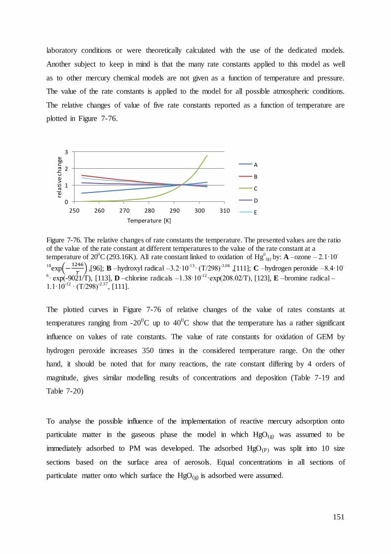
151
laboratory conditions or were theoretically calculated with the use of the dedicated models.
Another subject to keep in mind is that the many rate constants applied to this model as well
as to other mercury chemical models are not given as a function of temperature and pressure.
The value of the rate constants is applied to the model for all possible atmospheric conditions.
The relative changes of value of five rate constants reported as a function of temperature are
plotted in Figure 7-76.
Figure 7-76. The relative changes of rate constants the temperature. The presented values are the ratio of the value of the rate constant at different temperatures to the value of the rate constant at a temperature of 20
0C (293.16K). All rate constant linked to oxidation of Hg
0(g) by: A –ozone – 2.1·10
-
18exp(−
1246
𝑇) ,[96]; B –hydroxyl radical –3.2·10
-13· (T/298)
-3.06 ,[111]; C –hydrogen peroxide –8.4·10
-
6· exp(-9021/T), [113], D –chlorine radicals –1.38·10
-12·exp(208.02/T), [123], E –bromine radical –
1.1·10-12
· (T/298)-2.37
, [111].
The plotted curves in Figure 7-76 of relative changes of the value of rates constants at
temperatures ranging from -200C up to 400C show that the temperature has a rather significant
influence on values of rate constants. The value of rate constants for oxidation of GEM by
hydrogen peroxide increases 350 times in the considered temperature range. On the other
hand, it should be noted that for many reactions, the rate constant differing by 4 orders of
magnitude, gives similar modelling results of concentrations and deposition (Table 7-19 and
Table 7-20)
To analyse the possible influence of the implementation of reactive mercury adsorption onto
particulate matter in the gaseous phase the model in which HgO(g) was assumed to be
immediately adsorbed to PM was developed. The adsorbed HgO(P) was split into 10 size
sections based on the surface area of aerosols. Equal concentrations in all sections of
particulate matter onto which surface the HgO(g) is adsorbed were assumed.
0
1
2
3
250 260 270 280 290 300 310
rela
tive
ch
an
ge
Temperature [K]
A
B
C
D
E
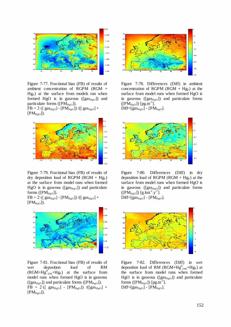
152
Figure 7-77. Fractional bias (FB) of results of ambient concentration of RGPM (RGM + HgP) at the surface from models run when formed HgO is in gaseous ([gasHgO]) and particulate forms ([PMHgO]). FB = 2·([ gasHgO] - [PMHgO]) /([ gasHgO] + [PMHgO]).
Figure 7-78. Differences (Diff) in ambient concentration of RGPM (RGM + HgP) at the surface from model runs when formed HgO is in gaseous ([gasHgO]) and particulate forms ([PMHgO]) [pg.m
-3].
Diff=[gasHgO] - [PMHgO].
Figure 7-79. Fractional bias (FB) of results of dry deposition load of RGPM (RGM + HgP) at the surface from model runs when formed HgO is in gaseous ([gasHgO]) and particulate forms ([PMHgO]). FB = 2·([ gasHgO] - [PMHgO]) /([ gasHgO] + [PMHgO]).
Figure 7-80. Differences (Diff) in dry deposition load of RGPM (RGM + HgP) at the surface from model runs when formed HgO is in gaseous ([gasHgO]) and particulate forms ([PMHgO]) [g.km
-2.y
-1].
Diff=[gasHgO] - [PMHgO].
Figure 7-81. Fractional bias (FB) of results of wet deposition load of RM (RGM+Hg
II(aq)+HgP) at the surface from
model runs when formed HgO is in gaseous ([gasHgO]) and particulate forms ([PMHgO]). FB = 2·([ gasHgO] - [PMHgO]) /([gasHgO] + [PMHgO]).
Figure 7-82. Differences (Diff) in wet deposition load of RM (RGM+Hg
II(aq)+HgP) at
the surface from model runs when formed HgO is in gaseous ([gasHgO]) and particulate forms ([PMHgO]) [pg.m
-3].
Diff=[gasHgO] - [PMHgO].

153
In general, the adsorption of HgO(g) onto particulate matters decreases the concentration and
dry deposition and increases the wet deposition of reactive mercury. The changes in results
are significant in many places of the simulation domain. For example, over the Mediterranean
Sea the ambient concentration of reactive mercury (RGPM) decreased by 28 pg.m-3. The
fractional bias over the majority of the domain does not exceed an absolute value of 0.5 for
concentration as well as for deposition (wet and dry). It should be noted that the concentration
of particulate matter, here assumed to be equal, varies widely for various aerosol size sections.
Generally, a higher concentration is observed for small particles with the representative
diameter up to 2.5 µm. This can cause that most of the mercury will be mainly adsorbed on
very small particles, bearing in mind also that the total area of particles increases with the
decreasing diameter of the particular particles (Table 6-5). Furthermore, the adsorption of
mercury already exists in the process of release of mercury into the atmosphere. For example,
during the coal combustion process in the boiler a part of mercury is adsorbed onto dust. In
the base model the emission of HgP was assumed to be uniform across all considered PM size
sections. Taking into consideration the adsorption process of mercury onto particles of dust,
the model was also run with a distribution of Hgp in proportion to particle surface areas. In
this case, the assumption that the concentration of aerosols is uniform across 10 the size
sections of particulate matter was done. The corresponding results are shown in Figure 7-83 –
Figure 7-88.
Figure 7-83. Fractional bias (FB) of results of ambient concentration of mercury bound to particulate matter at the surface from base model runs when emission of HgP were distributed equally ([HgP(eq)]) and in proportion to aerosol surface areas ([HgP(sf)]). FB = 2·([HgP(eq)] - [HgP(sf)]) /([HgP(eq)] + [HgP(sf)]).
Figure 7-84. Differences (Diff) in ambient concentration of mercury bound to particulate matter at the surface from base model runs when emission of HgP were distributed equally ([HgP(eq)]) and in proportion to aerosol surface areas ([HgP(sf)]) [pg.m
-3].
Diff=[HgP(eq)] - [HgP(sf)].
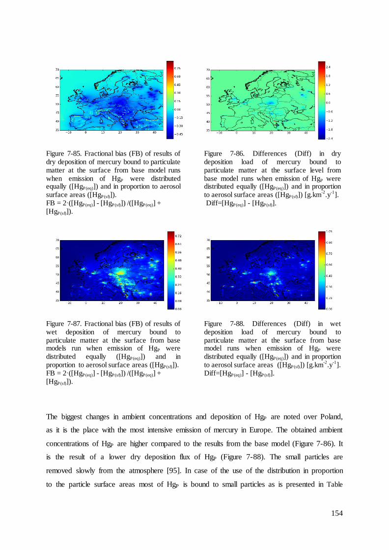
154
Figure 7-85. Fractional bias (FB) of results of dry deposition of mercury bound to particulate matter at the surface from base model runs when emission of HgP were distributed equally ([HgP(eq)]) and in proportion to aerosol surface areas ([HgP(sf)]). FB = 2·([HgP(eq)] - [HgP(sf)]) /([HgP(eq)] + [HgP(sf)]).
Figure 7-86. Differences (Diff) in dry deposition load of mercury bound to particulate matter at the surface level from base model runs when emission of HgP were distributed equally ([HgP(eq)]) and in proportion to aerosol surface areas ([HgP(sf)]) [g.km
-2.y
-1].
Diff=[HgP(eq)] - [HgP(sf)].
Figure 7-87. Fractional bias (FB) of results of wet deposition of mercury bound to particulate matter at the surface from base models run when emission of HgP were distributed equally ([HgP(eq)]) and in proportion to aerosol surface areas ([HgP(sf)]). FB = 2·([HgP(eq)] - [HgP(sf)]) /([HgP(eq)] + [HgP(sf)]).
Figure 7-88. Differences (Diff) in wet deposition load of mercury bound to particulate matter at the surface from base model runs when emission of HgP were distributed equally ([HgP(eq)]) and in proportion to aerosol surface areas ([HgP(sf)]) [g.km
-2.y
-1].
Diff=[HgP(eq)] - [HgP(sf)].
The biggest changes in ambient concentrations and deposition of HgP are noted over Poland,
as it is the place with the most intensive emission of mercury in Europe. The obtained ambient
concentrations of HgP are higher compared to the results from the base model (Figure 7-86). It
is the result of a lower dry deposition flux of HgP (Figure 7-88). The small particles are
removed slowly from the atmosphere [95]. In case of the use of the distribution in proportion
to the particle surface areas most of HgP is bound to small particles as is presented in Table

155
6-5. The modeling results for wet deposition show a high spatial variation over the whole
simulation domain (Figure 7-87 and Figure 7-88).
One of the most important issue in modeling of the quality are the input data used in the
simulation run [183]. As an example of meteorological parameters the evaluation of
precipitation intensity was presented in Table 7-1. The evaluation of ambient concentrations
of the species that react with mercury was presented in chapter 7.3. Moreover, various
combinations of anthropogenic emission of mercury were used in this work (e.g. Table 7-7,
Figure 7-86 ). The sensitivity of the model to changes in input data provided to the model is
presented in Table 7-23.
Table 7-23. The relative changes amounts of mercury air concentrations and deposition in the European domain by use of various input data. The presented values are the ratio of results from base model run with the use of listed changed input data to modelling results with the use of reference input data.
N. Changes in input data
Ambient
concentration Dry deposition Wet deposition
GE
M
RG
AM
HgP GE
M
RG
M
HgP Hg0 RG
AM
HgP
1 Concentration of species which react with
mercury less than 20%
1.01 0.90 1.00 1.01 0.89 1.00 1.01 0.91 1.00
2 Concentration of species which react with
mercury is greater than 20%
0.99 1.09 1.00 0.99 1.11 1.00 0.99 1.09 1.00
3 The boundary concentration of mercury
species less than 20%
0.82 0.84 0.86 0.81 0.84 0.85 0.81 0.82 0.83
4 The boundary concentration of mercury
species is greater than 20%
1.18 1.16 1.14 1.19 1.16 1.15 1.19 1.18 1.17
5 The initial concentration of mercury
species less than 20%
1.00 1.00 1.00 1.00 1.00 1.00 1.00 1.00 1.00
6 The initial concentration of mercury
species is greater than 20%
1.00 1.00 1.00 1.00 1.00 1.00 1.00 1.00 1.00
7 The natural emission of mercury less than
20%
0.99 1.00 1.00 0.99 1.00 1.00 1.00 1.00 1.00
8 The natural emission of mercury is greater
than 20%
1.01 1.00 1.00 1.01 1.00 1.00 1.00 1.00 1.00
9 The anthropogenic emission of mercury
less than 20%
1.00 0.97 0.94 1.00 0.97 0.95 1.00 0.98 0.97
10 The anthropogenic emission of mercury is
greater than 20%
1.00 1.03 1.06 1.00 1.03 1.05 1.00 1.02 1.03
The model is most sensitive to changes to boundary concentrations of mercury. The
decreasing or increasing of concentrations of mercury of 20% at boundaries of modelling
domain, causes the changes in the concentrations of GEM, RGAM and HgP of 18%, 16% and
14%, respectively. The air concentration of mercury oxidation and reduction compounds have
also a significant influence on the quantity of RGAM in the simulation domain. The model
response is a 10% change in the concentration of RGAM due to changes in concentration of
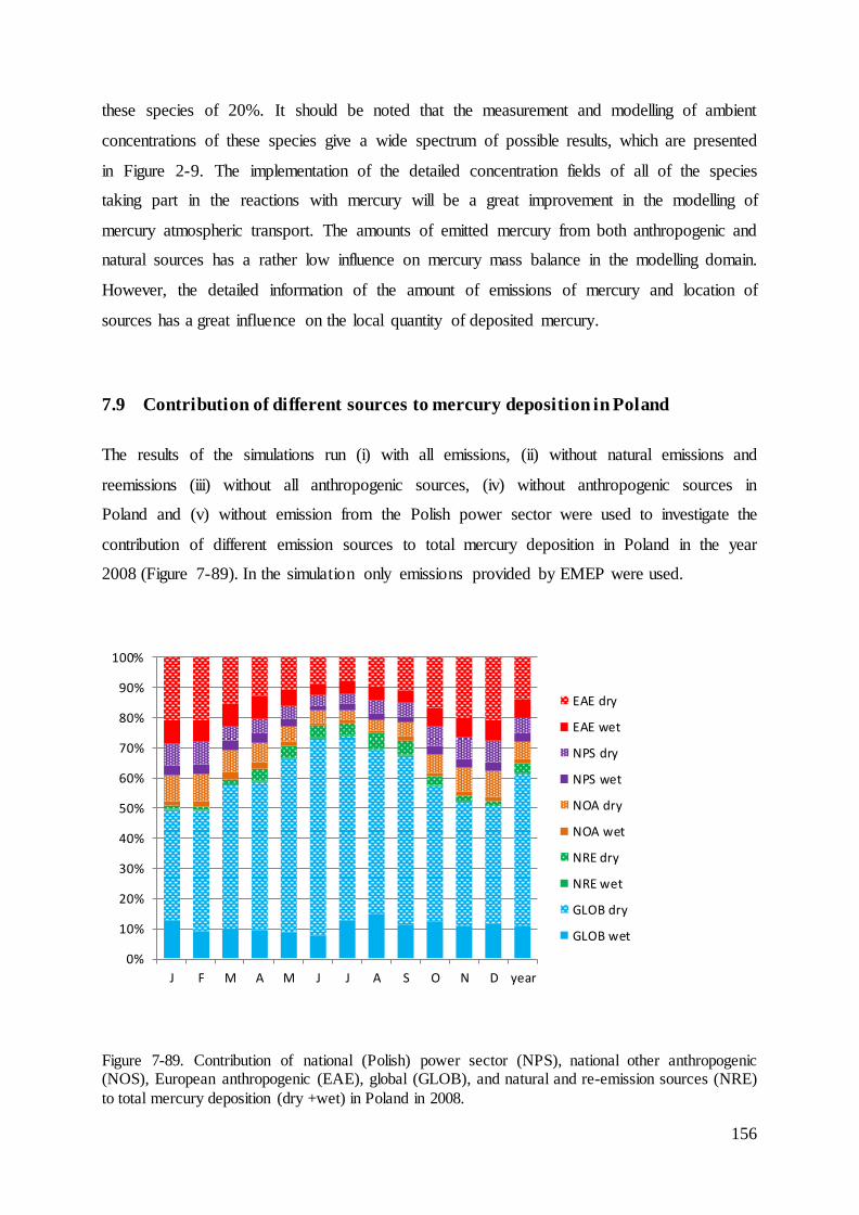
156
these species of 20%. It should be noted that the measurement and modelling of ambient
concentrations of these species give a wide spectrum of possible results, which are presented
in Figure 2-9. The implementation of the detailed concentration fields of all of the species
taking part in the reactions with mercury will be a great improvement in the modelling of
mercury atmospheric transport. The amounts of emitted mercury from both anthropogenic and
natural sources has a rather low influence on mercury mass balance in the modelling domain.
However, the detailed information of the amount of emissions of mercury and location of
sources has a great influence on the local quantity of deposited mercury.
7.9 Contribution of different sources to mercury deposition in Poland
The results of the simulations run (i) with all emissions, (ii) without natural emissions and
reemissions (iii) without all anthropogenic sources, (iv) without anthropogenic sources in
Poland and (v) without emission from the Polish power sector were used to investigate the
contribution of different emission sources to total mercury deposition in Poland in the year
2008 (Figure 7-89). In the simulation only emissions provided by EMEP were used.
Figure 7-89. Contribution of national (Polish) power sector (NPS), national other anthropogenic (NOS), European anthropogenic (EAE), global (GLOB), and natural and re-emission sources (NRE)
to total mercury deposition (dry +wet) in Poland in 2008.
0%
10%
20%
30%
40%
50%
60%
70%
80%
90%
100%
J F M A M J J A S O N D year
EAE dry
EAE wet
NPS dry
NPS wet
NOA dry
NOA wet
NRE dry
NRE wet
GLOB dry
GLOB wet
157
The results in Figure 7-89 show the major contribution of global sources (GLOB) and a rather
low contribution of natural and reemission sources (NRE). The contribution of the Polish
power sector (NPS) varies in different months from 5% to 11% and national other
anthropogenic sources (NOS) from 4% to 10%. The other anthropogenic European sources
(EAE) contribute up to 20% to the overall annual deposition of mercury in Poland. The
highest share of national sources (NPS +NOS) occurs during the winter heating season when
large quantities of coal are combusted in the domestic sector and additionally the power sector
activity is at its highest. The contribution of the national power sector (NPS) to all national
sources varies from 45 to 55%. The majority of mercury is deposited in Poland through dry
deposition process. The dry deposition contribution to the overall deposition ranges from 74%
in January to 86% in June, with the annual average share of 79%. The obtained results of
contribution of national sources are in contradiction with modelling results for 1999, where
the Polish anthropogenic sources contributed the most to the deposition over Poland (range
from 45% according to HYSPLIT model for August to 80% according to MSCE-HM model
in February) [12]. The discrepancies between those results come from the amounts of
deposited GEM from global sources (GLOB). In these models, dry deposition of mercury of 2
-6 g.km-2.y-1 over land was estimated. The results presented in Figure 7-61 show dry
deposition of GEM over land of approx. 29 g.km-2.y-1 [217]. This value of the dry deposition
flux over land compared to recent studies does not seem to be overestimated [264]. The
emissions of mercury in Poland of 25.6 Mg in 2000 were used in those studies, while in this
work national emissions were reduced by 10 Mg (Figure 2-6). The contribution of
anthropogenic European sources (NPS +NOS +EAS) over 50% to the overall mercury
deposition was obtained from simulations preformed with use of GLEMOS model [260]. That
model also calculates the lower dry deposition flux compared to the model presented in this
work. The results presented in Figure 7-89 are similar to the relative contribution of global,
natural and re-emission sources (GLOB +NRE) and anthropogenic sources located in Europe
(NPS +NOS +EAS) in Europe for 2005 obtained with GEOS-Chem, GLEMOS and CMAQ-
Hg models [262].
7.10 The impact of the Polish power sector
The simulation runs over Poland allowed one to estimate the contribution of emissions from
the Polish power sector to the overall deposition and air concentrations of mercury, lead and
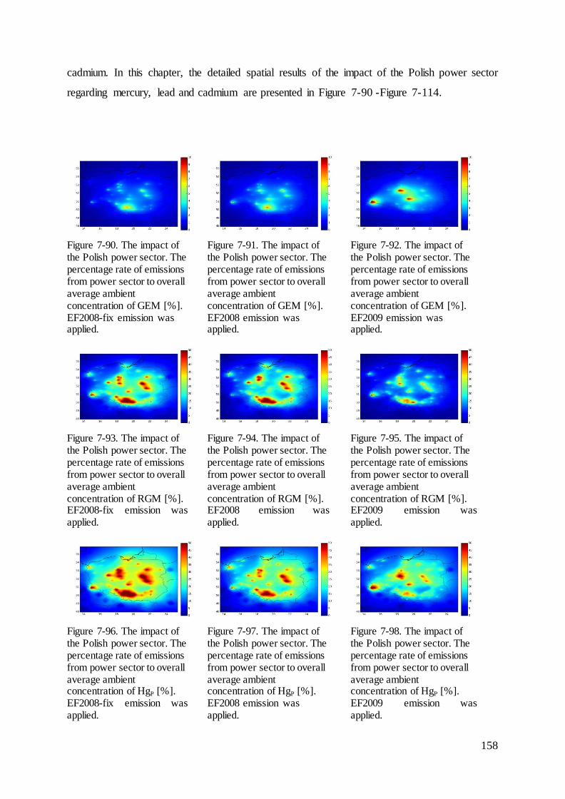
158
cadmium. In this chapter, the detailed spatial results of the impact of the Polish power sector
regarding mercury, lead and cadmium are presented in Figure 7-90 -Figure 7-114.
Figure 7-90. The impact of the Polish power sector. The percentage rate of emissions from power sector to overall average ambient concentration of GEM [%]. EF2008-fix emission was applied.
Figure 7-91. The impact of the Polish power sector. The percentage rate of emissions from power sector to overall average ambient concentration of GEM [%]. EF2008 emission was applied.
Figure 7-92. The impact of the Polish power sector. The percentage rate of emissions from power sector to overall average ambient concentration of GEM [%]. EF2009 emission was applied.
Figure 7-93. The impact of the Polish power sector. The percentage rate of emissions from power sector to overall average ambient concentration of RGM [%]. EF2008-fix emission was applied.
Figure 7-94. The impact of the Polish power sector. The percentage rate of emissions from power sector to overall average ambient concentration of RGM [%]. EF2008 emission was applied.
Figure 7-95. The impact of the Polish power sector. The percentage rate of emissions from power sector to overall average ambient concentration of RGM [%]. EF2009 emission was applied.
Figure 7-96. The impact of the Polish power sector. The percentage rate of emissions from power sector to overall average ambient concentration of HgP [%]. EF2008-fix emission was applied.
Figure 7-97. The impact of the Polish power sector. The percentage rate of emissions from power sector to overall average ambient concentration of HgP [%]. EF2008 emission was applied.
Figure 7-98. The impact of the Polish power sector. The percentage rate of emissions from power sector to overall average ambient concentration of HgP [%]. EF2009 emission was applied.
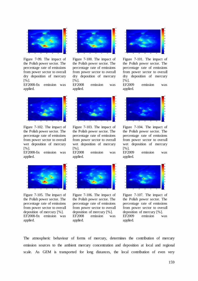
159
Figure 7-99. The impact of the Polish power sector. The percentage rate of emissions from power sector to overall dry deposition of mercury [%]. EF2008-fix emission was applied.
Figure 7-100. The impact of the Polish power sector. The percentage rate of emissions from power sector to overall dry deposition of mercury [%]. EF2008 emission was applied.
Figure 7-101. The impact of the Polish power sector. The percentage rate of emissions from power sector to overall dry deposition of mercury [%]. EF2009 emission was applied.
Figure 7-102. The impact of the Polish power sector. The percentage rate of emissions from power sector to overall wet deposition of mercury [%]. EF2008-fix emission was applied.
Figure 7-103. The impact of the Polish power sector. The percentage rate of emissions from power sector to overall wet deposition of mercury [%]. EF2008 emission was applied.
Figure 7-104. The impact of the Polish power sector. The percentage rate of emissions from power sector to overall wet deposition of mercury [%]. EF2009 emission was applied.
Figure 7-105. The impact of the Polish power sector. The percentage rate of emissions from power sector to overall deposition of mercury [%]. EF2008-fix emission was applied.
Figure 7-106. The impact of the Polish power sector. The percentage rate of emissions from power sector to overall deposition of mercury [%]. EF2008 emission was applied.
Figure 7-107. The impact of the Polish power sector. The percentage rate of emissions from power sector to overall deposition of mercury [%]. EF2009 emission was applied.
The atmospheric behaviour of forms of mercury, determines the contribution of mercury
emission sources to the ambient mercury concentration and deposition at local and regional
scale. As GEM is transported for long distances, the local contribution of even very
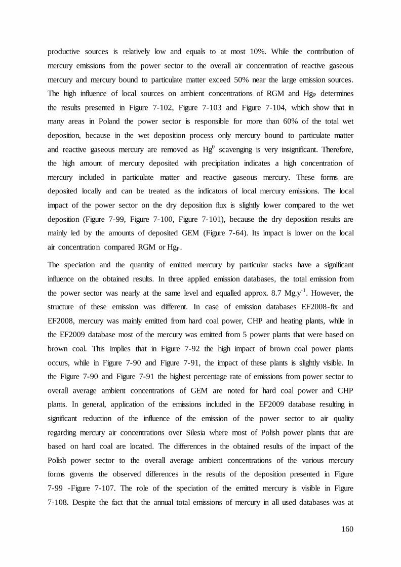
160
productive sources is relatively low and equals to at most 10%. While the contribution of
mercury emissions from the power sector to the overall air concentration of reactive gaseous
mercury and mercury bound to particulate matter exceed 50% near the large emission sources.
The high influence of local sources on ambient concentrations of RGM and HgP determines
the results presented in Figure 7-102, Figure 7-103 and Figure 7-104, which show that in
many areas in Poland the power sector is responsible for more than 60% of the total wet
deposition, because in the wet deposition process only mercury bound to particulate matter
and reactive gaseous mercury are removed as Hg0 scavenging is very insignificant. Therefore,
the high amount of mercury deposited with precipitation indicates a high concentration of
mercury included in particulate matter and reactive gaseous mercury. These forms are
deposited locally and can be treated as the indicators of local mercury emissions. The local
impact of the power sector on the dry deposition flux is slightly lower compared to the wet
deposition (Figure 7-99, Figure 7-100, Figure 7-101), because the dry deposition results are
mainly led by the amounts of deposited GEM (Figure 7-64). Its impact is lower on the local
air concentration compared RGM or HgP.
The speciation and the quantity of emitted mercury by particular stacks have a significant
influence on the obtained results. In three applied emission databases, the total emission from
the power sector was nearly at the same level and equalled approx. 8.7 Mg.y-1. However, the
structure of these emission was different. In case of emission databases EF2008-fix and
EF2008, mercury was mainly emitted from hard coal power, CHP and heating plants, while in
the EF2009 database most of the mercury was emitted from 5 power plants that were based on
brown coal. This implies that in Figure 7-92 the high impact of brown coal power plants
occurs, while in Figure 7-90 and Figure 7-91, the impact of these plants is slightly visible. In
the Figure 7-90 and Figure 7-91 the highest percentage rate of emissions from power sector to
overall average ambient concentrations of GEM are noted for hard coal power and CHP
plants. In general, application of the emissions included in the EF2009 database resulting in
significant reduction of the influence of the emission of the power sector to air quality
regarding mercury air concentrations over Silesia where most of Polish power plants that are
based on hard coal are located. The differences in the obtained results of the impact of the
Polish power sector to the overall average ambient concentrations of the various mercury
forms governs the observed differences in the results of the deposition presented in Figure
7-99 -Figure 7-107. The role of the speciation of the emitted mercury is visible in Figure
7-108. Despite the fact that the annual total emissions of mercury in all used databases was at

161
the same level, the applied speciation of emitted mercury from the power sector was different.
This results in significant differences in the average of results of percentage rate of emissions
from power sector to overall wet and dry deposition of mercury over the whole of Poland
(Figure 7-108). In case of EF2009, emission the impact is lowest (6% to overall deposition)
because in this database the share of reactive mercury (RGM +HgP) to the overall emission
was also lowest and equalled 27%. In contrary, the highest share of reactive mercury of 50 %
was in EF2008-fix. This caused that the yearly average impact of emissions from the power
sector to overall deposition (wet +dry) is 9%. The share of reactive mercury in EF2008 and in
emissions used in model runs over Europe (the results market as NPS) is 42% and 39%,
respectively.
Figure 7-108. The impact of the Polish power sector. The percentage rate of emissions from the power sector to overall wet and dry deposition of mercury [%]. NPS -national power
sector, results from model runs over Europe, presented also in Figure 7-89.
Figure 7-109. The impact of the Polish power sector. The percentage rate of emissions from the power sector to overall average ambient concentration of cadmium [%].
Figure 7-110. The impact of the Polish power sector. The percentage rate of emissions from the power sector to overall dry deposition of cadmium [%].
Figure 7-111. The impact of the Polish power sector. The percentage rate of emissions from the power sector to overall wet deposition of cadmium [%].
0%
5%
10%
15%
20%
25%
J F M A M J J A S O N D
NPS dry
NPS wet
EF2008-fix dry
EF2008-fix wet
EF2008 dry
EF2008 wet
EF2009 dry
EF2009 wet
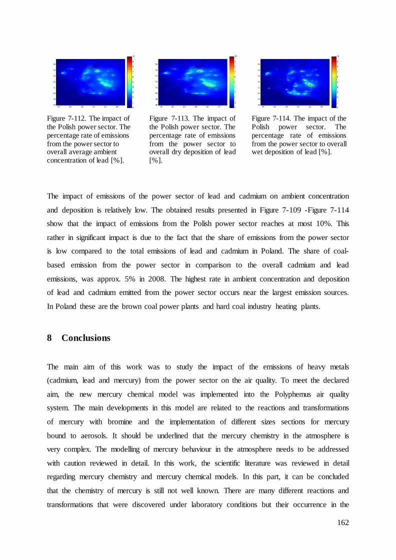
162
Figure 7-112. The impact of the Polish power sector. The percentage rate of emissions from the power sector to overall average ambient concentration of lead [%].
Figure 7-113. The impact of the Polish power sector. The percentage rate of emissions from the power sector to overall dry deposition of lead [%].
Figure 7-114. The impact of the Polish power sector. The percentage rate of emissions from the power sector to overall wet deposition of lead [%].
The impact of emissions of the power sector of lead and cadmium on ambient concentration
and deposition is relatively low. The obtained results presented in Figure 7-109 -Figure 7-114
show that the impact of emissions from the Polish power sector reaches at most 10%. This
rather in significant impact is due to the fact that the share of emissions from the power sector
is low compared to the total emissions of lead and cadmium in Poland. The share of coal-
based emission from the power sector in comparison to the overall cadmium and lead
emissions, was approx. 5% in 2008. The highest rate in ambient concentration and deposition
of lead and cadmium emitted from the power sector occurs near the largest emission sources.
In Poland these are the brown coal power plants and hard coal industry heating plants.
Conclusions 8
The main aim of this work was to study the impact of the emissions of heavy metals
(cadmium, lead and mercury) from the power sector on the air quality. To meet the declared
aim, the new mercury chemical model was implemented into the Polyphemus air quality
system. The main developments in this model are related to the reactions and transformations
of mercury with bromine and the implementation of different sizes sections for mercury
bound to aerosols. It should be underlined that the mercury chemistry in the atmosphere is
very complex. The modelling of mercury behaviour in the atmosphere needs to be addressed
with caution reviewed in detail. In this work, the scientific literature was reviewed in detail
regarding mercury chemistry and mercury chemical models. In this part, it can be concluded
that the chemistry of mercury is still not well known. There are many different reactions and
transformations that were discovered under laboratory conditions but their occurrence in the
163
atmosphere is still not confirmed. Additionally for many reactions, the mechanism as well as
the products of reactions were not fully investigated. For most of the mercury reactions,
distinct values of rate constants exist. It implies that the chemistry of mercury implemented in
the models may affect significantly among models. The models also differ in the way of
calculating the dry and wet deposition of mercury. Additionally, the high uncertainties of the
modelling results are related to the concentrations of compounds that react with mercury.
Some of them are measured rarely and their air concentrations are only modelled. Overall,
there are not many processes regarding mercury modelling which are common to all models.
This causes the results of various models to differ significantly.
In order to analyse the problem of the contribution of heavy metals emitted from the Polish
power sector in more detail, a database of the Polish power sector was prepared. It contains
detailed information about boilers, emission controls equipment, fuel consumption and stack
location. Thanks to this, the emissions of the power sector were desegregated into plants and
speciation of mercury was estimated with a bottom-up approach. The simulations of heavy
metals dispersion into the atmosphere were done on the European domain and the domain
covering Poland with finer resolution. The fields of ambient concentrations and deposition of
mercury over Europe and Poland were modelled. The results revealed the areas that are most
polluted by heavy metals and showed where the Polish power sector has the higher impacts.
The elemental gaseous mercury ambient concentrations are evenly distributed (relatively low
spatial variations exist). On the contrary, high variations in the spatial gradients of reactive
gaseous and particulate forms of mercury air concentrations and deposition fluxes were noted.
This detailed study shows that many components of the developed model have crucial impacts
on the obtained results. In the model of mercury chemistry, the most effective pathway in the
gaseous phase are the oxidation of gaseous elemental mercury by hydroxyl radical, ozone and
most of all bromine oxide radicals, while in the aqueous phase the reduction reactions of
elemental mercury dominate. These reactions have a crucial influence on the mass balance of
reactive mercury, but a rather low influence on gaseous elemental mercury. The significant
impact of the mass balance of gaseous elemental mercury includes the dry deposition process
and implemented values of boundary concentrations. In this model, dry deposition of gaseous
elemental mercury is the prevailing process for removing mercury from the atmosphere. Dry
deposition of GEM over land is equally distributed, due to almost uniform ambient
concentrations of this form. The relatively high dry deposition flux of gaseous elemental
mercury has a huge influence on the presented results and differs significantly from other
models where the dry deposition of GEM is often not taken into account in the models. It was
164
also shown that a change in the calculation of the scavenging coefficients or representative
raindrop diameter for in-cloud scavenging has a significant impact on the amount of wet
deposited reactive mercury. Equally important are also meteorological data, because the wet
deposited amount of mercury is correlated with the precipitation intensity. The natural
emissions as well as anthropogenic emissions have a rather low impact on the mass balance of
mercury in the whole modelling domain, however, they have a crucial impact in particular
areas. The detailed results show that the Polish power sector can be responsible for up to 80%
of wet deposited mercury near large emission sources. However, the contribution from
national sources over whole Poland is low and reaches only 21% during the winter heating
season when large quantities of coal are burned in the domestic sector and additionally the
power sector activity is at its highest. The fact that the spatial variations in GEM
concentrations over Europe are moderate, on the contrary the high concentration of reactive
mercury exists mainly near the emission sources which makes the latter mercury form a more
relevant indicator of coal combustion. This mercury form plays an important role and has a
large impact on mercury air concentrations and deposition, particularly at the local and
regional scales. That is why national estimations of the amounts of emitted mercury should
include the emissions of individual mercury forms and not only total emissions of mercury.
However, the highest share in the total deposition in Poland derives from global sources of
mercury and it is the reason why the adverse impact of mercury in Poland should be mainly
reduced by global efforts to decrease mercury emissions and use.
The impact of emissions of cadmium and lead from the power sector is lower compared to the
obtained results for mercury. The modelling results showed maximal impacts of 30% and
10% for cadmium and lead near large power sector sources on the ambient concentrations and
deposition. The emissions of these heavy metals from the power sector where all plants are
equipped with PM emission control systems are relatively low compared to other sources.
In this work, several scientific achievements were completed. The national emissions of
mercury were split into mercury speciation forms with the use of a bottom-up approach. The
detailed locations of emissions of mercury, lead and cadmium from the power sector was
indicated. An update mercury chemistry model was developed and implemented to
Polyphemus air quality system. For the first time, many reactions of mercury were applied to
the chemical model, i.e. reactions with bromine, fluorine, iodine and chlorine radicals. The
complex chemistry of mercury and bromine compounds were implemented into the model.
The particulate matter dispersion of mercury, lead and cadmium were modelled using 10
particle size sections. The impact of many parts of the model (chemistry, deposition, input
165
data) on the results was investigated. The results on the impact of heavy metals emission from
the Polish power sector and other sources were modelled. It should be emphasized that the
scientific literature was reviewed in detail. However, it should be noted that in this scientific
area there is still some lack of knowledge and the presented results show one possible solution
and should be not treated as better than others obtained by different groups. To better
understand the heavy metals behaviour, the model can be used to support measurements of
mercury. This work shows that wide measurements of heavy metals are very much needed.
The measurement stations in Europe should be mainly located in areas with high
concentrations/deposition which were indicated in the modelling results. Due to a high
uncertainty and simplification in the current assessment of mercury emissions, the amount of
different mercury forms in exhaust gases should be monitored as well.
In conclusion let us come back to the exemplary questions and theses mentioned at the
beginning of this work.
The first of them was “does the dry deposition of gaseous elemental mercury have the
greatest influence on obtained mercury deposition results?”
The obtained results of the model show that the share of dry deposition of gaseous elemental
mercury in the overall mercury deposition over land is the highest. At all stations, on average
nearly 60% of deposited mercury come from dry deposition of GEM. This process has also
the crucial impact on the obtained results of impact of the Polish power sector on mercury
deposition in Poland.
The second question that was asked, was “what is the contribution of different atmospheric
reactions to the atmospheric mass balance of reactive mercury?”.
The contribution of various reactions is very diverse. The most effective reaction of gaseous
elemental mercury is that with bromine oxide radical, it contribute nearly 60% to the
atmospheric production of reactive forms of mercury. The second reaction is the oxidation of
GEM by hydroxyl radical, which contributes 20% of RGM atmospheric production. The
aqueous reduction of HgII(aq) by HO2
•(aq) covers 70% of the mass of the whole atmospheric
flux of reduction of reactive mercury to elemental mercury.
Another thesis was “is most of the deposited mercury in Poland emitted outside Poland?”.
Yes, definitely. Three-quarters of deposited mercury in Poland was emitted outside Poland.
The vast part comes even from outside the modelling domain, that is from outside Europe.
166
The other question that was asked, was “what is the contribution of the power plant sector to
local mercury deposition in Poland?”
Overall taking into account the whole territory of Poland, this contribution in not very high
and reaches 22% of overall deposition in the winter season. However, the results differ very
much for various estimations of emissions the from the power sector. Near the large sources,
the impact is significantly higher and reaches even 60% of the overall wet deposition of
mercury.
The last question was “does the concentration of reactive mercury and lead and cadmium
depend strongly on local emission sources?”.
Yes, the high concentrations of reactive mercury and lead and cadmium are observed over
areas were such species are emitted. In the maps of concentration of those species over
Europe as well as maps showing the impact of the Polish power sector, the red spots indicate
the areas with the high local emissions.
Results obtained in this work are very important in the context of preparing a national strategy
on mercury reduction as they show to what extent mercury concentrations and deposition can
be reduced over Poland by means of cutting national emissions. They also show that mercury,
to a large extent, is a global pollutant and international agreements and strategies on mercury
reduction are necessary to effectively tackle the problem. The model can be used as a tool
supporting decision making to improve the situation in areas with the highest mercury
concentrations and deposition.
167
References
1. AMAP/UNEP, Technical Background Report of the Global Atmospheric Mercury
Assessment, 2008, Arctic Monitoring and Assessment Program/ UNEP Chemical Branch. p. 159.
2. Ministry of the Environment Government of Japan. Minamata Disease The History
and Measures. 2002 [cited 2014; Available from: www.env.go.jp/en/chemi/hs/minamata.html.
3. Bakir, F., Damluji, S., Amin-Zaki, L., Murtadha, M., Khalidi, A., NY., a.-R., Tikriti, S., Dahahir, H., Clarkson, T., Smith, J.,Doherty, R., Methylmercury poisoning in Iraq. Science, 1973. 181 (4096 ): p. 230-241
4. Rabl, A.,Spadaro, J.V., Estimating the uncertainty of damage costs of pollution: A simple transparent method and typical results. Environmental Impact Assessment
Review Volume, 2008. 28: p. 166–183. 5. UNEP, Final review of scientific information on cadmium, 2010, UNEP Chemicals
Branch, DTIE, Geneva, Switzerland. p. 332.
6. UNEP, Final review of scientific information on lead, 2010, UNEP Chemicals Branch, DTIE, Geneva, Switzerland. p. 332.
7. UNEP. Minamata Convention on Mercury 2014; Available from: http://www.mercuryconvention.org/.
8. Lindberg, S.E., Bullock, R., Ebinghaus, R., Engstrom, D., Feng, X., Fitzgerald, W.,
Pirrone, N., Prestbo, E.,Seigneur, C., A Synthesis of Progress and Uncertainties in Attributing the Sources of Mercury in Deposition. A Journal of the Human Environment, 2007. 36 (1): p. 19–33.
9. Subir, M., Ariya, P.A.,Dastoor, A.P., A review of uncertainties in atmospheric modeling of mercury chemistry I. Uncertainties in existing kinetic parameters -
Fundamental limitations and the importance of heterogeneous chemistry. Atmospheric Environment, 2011. 45 ( doi:10.1016/j.atmosenv.2011.04.046).
10. Ryaboshapko, A., Bulloc, R., Ebinghaus, R., Ilyin, I., Lohman, K., Munthe, J.,
Petersen, G., Seigneur, C.,Wangberg, I., Comparison of mercury chemistry models. Atmospheric Environment, 2002. 36: p. 3881–3898.
11. Ryaboshapko, A., Bulloc, R., Christensen, J., Cohen, M., Dastoor, A., Ilyin, I., Petersen, G., Syrakov, D., Artz, R., Davignon, D., Draxler, R.,Munthe, J., Intercomparison study of atmospheric mercury models, 1. Comparison of models with
short-term measurements. Science of the Total Environment, 2007a. 376: p. 228–240. 12. Ryaboshapko, A., Bullock, R., Christensen, J., Cohen, M., Dastoor, A., Ilyin, I.,
Petersen, G., Syrakov, D., Travnikov, O., Artz, R.S., Davignon, D., Draxler, R.R., Munthe, J.,Pacyna, E.J., Intercomparison study of atmospheric mercury models: 2. Modelling results vs. long-term observations and comparison of country deposition
budgets. Science of the Total Environment, 2007b. 377 (2–3): p. 319–333. 13. Mallet, V., Quello, D., Sportisse, B., Ahmed de Biasi, M., Debry, E., Korsakissok, I.,
Wu, L., Roustan, Y., Sartelet, K., Tombette, M.,Foudhil, H., Technical Note: The air quality modeling system Polyphemus. Atmos. Chem. Phys., 2007. 7 (20): p. 5479–5487.
14. EMEP, The European Monitoring and Evaluation Programme 2014. 15. Lin, C.,Pehkonen, S.O., The chemistry of atmospheric mercury: a review.
Atmospheric Environment, 1999. 33: p. 2067-2079

168
16. AMAP/UNEP, Technical Background Report for the Global Mercury Assessment
2013., 2013, Arctic Monitoring and Assessment Programme, Oslo, Norway/UNEP Chemicals Branch, Geneva, Switzerland. p. 263.
17. Bergan, T., Gallardo, L.,Rodhe, H., Mercury in the global troposphere: a three-dimensional model study. Atmospheric Environment, 1999. 33: p. 1575-1585.
18. Shia, R.L., Seigneur, C., Pai, P., Ko, M.,Sze, N.D., Global simulation of atmospheric
mercury concentrations and deposition fluxes. Journal of Geophysical Research, 1999. 104: p. 23747–23760.
19. Lamborg, C.H., Fitzgerald, W.F., O’Donnell, J.,Torgersen, T., A non–steady-state compartmental model of global-scale mercury biogeochemistry with interhemispheric atmospheric gradients. Geochimica et Cosmochimica Acta, 2002. 66 (7): p. 1105–
1118. 20. Mason, R.P.,Sheu, G.R., Role of ocean in the global mercury cycle. Global
Biogeochemical Cycles., 2002. 16 (DOI 10.1029/2001GB001440). 21. Seigneur, C., Vijayaraghavan, K., Lohman, K., Karamchandani, P.,Scott, C., Global
source attribution for mercury deposition in the United States. Environmental Science
& Technology, 2004. 38: p. 555–569. 22. Selin, N.E., Jacob, D.J., Park, R.J., Yantosca, R., M., Strode, S.,Jaegle, L., Chemical
cycling and deposition of atmospheric mercury: Global constraints from observations. Journal of Geophysical Research, 2007. 112 (D02308, doi:10.1029/2006JD007450).
23. Ericksen, J.A., Gustin, M.S., Xin, M., Weisberg, P.J.,Fernandez, G.C.J., Air–soil
exchange of mercury from background soils in the United States. Science of the Total Environment, 2006. 366: p. 851– 863.
24. Wang, D., He, L., Shi, X., Wei, S.,Feng, X., Release flux of mercury from different environmental surfaces in Chongqing, China. Chemosphere, 2006. 64: p. 1845–1854.
25. Kuiken, T., Zhang, H., Gustin, M.,Lindberg, S., Mercury emission from terrestrial
background surfaces in the eastern USA. Part I: Air/surface exchange of mercury within a southeastern deciduous forest (Tennessee) over one year. Applied
Geochemistry, 2008. 23: p. 345–355. 26. Gustin, M.S., Are mercury emissions from geologic sources significant? A status
report. The Science of the Total Environment, 2003. 304: p. 153–167.
27. Quan, J., Zhang, X.,Shim, S.G., Estimation of vegetative mercury emissions in China. Journal of Environmental Sciences, 2008. 20: p. 1070–1074.
28. Scholtza, M.T., Van Heysta, B.J.,Schroederb, W.H., Modelling of mercury emissions from background soils. The Science of the Total Environment, 2003. 3004: p. 185–207.
29. Travnikov, O.,Ilyin, I., Regional Model MSCE-HM of Heavy Metal Transboundary Air Pollution in Europe. Technical Report 6/2005, 2005, EMEP/MSC-E Moscow.
30. Ci, Z., Zhang, X.,Wang, Z., Elemental mercury in coastal seawater of Yellow Sea, China: Temporal variation and airesea exchange. Atmospheric Environment, 2011. 45: p. 183–190.
31. Friedli, H.R., Radke, L.F., Lu, J.Y., Banic, C.M., Leaitch, W.R.,MacPherson, J.I., Mercury emissions from burning of biomass from temperate North American
forests:laboratory and airborne measurements. AE International – North America, 2003. 37: p. 253–267.
32. Nriagu, J.O., A global assessment of natural sources of atmospheric trace metals.
Nature, 1989. 338: p. 47–49. 33. Holmes, C.D., Jacob, D.J., Mason, R.P.,Jaffe, D.A., Sources and deposition of
reactive gaseous mercury in the marine atmosphere. Atmospheric Environment, 2009. 43: p. 2278–2285.
169
34. Richardson, G.M., Garrett, R., Mitchell, I., Mah-Poulson, M.,Hackbarth, T., Critical
review on natural global and regional emissions of six trace metals to the atmosphere. Prepared for the International Lead Zinc Research Organisation, the International
Copper Association, and the Nickel Producers Environmental Research Association. 2001.
35. UNEP, Global Mercury Assessment 2013: Sources, Emissions, Releases and
Environmental Transport, 2013, UNEP Chemicals Branch: Geneva, Switzerland. 36. USGS, Chemical Analyses in the World Coal Quality Inventory, Version 1, Open-File
Report 2010–1196, 2010, U.S. Geological Survey: Reston, Virginia: 2010. 37. USEPA, Control of Mercury Emissions from Coal-Fired Electric Utility Boilers:
Interim Report Including Errata Dated 3-21-02, National Risk Management Research
Laboratory Research Triangle Park, Editor 2002, U.S.-EPA Research and Development. : NC 27711.
38. UNEP, Reducing mercury emissions from coal combustion in the energy sector, U.N.E.P.U. Chemicals, Editor 2011, Department of Environmental Science and Engineering Tsinghua University, Beijing, 100084, China: Geneva, Switzerland. p. 63.
39. Diehl, S.F., Goldhaber, M.B.,Hatch, J.R., Modes of occurrence of mercury and other trace elements in coals from the warrior field, Black Warrior Basin, Northwestern
Alabama. International Journal of Coal Geology, 2004. 59: p. 193– 208. 40. Bojakowska, I.,Karmasz, D., Mercury in raw materials excavated in Poland (in
Polish). in Rtęć w środowisku : identyfikacja zagrożeń dla zdrowia człowieka, L.
Falkowska. 2010, Fundacja Rozwoju Uniwersytetu Gdańskiego: Gdańsk, Poland. p. 145–150.
41. Lohman, K., Seigneur, C., Gustin, M.,Lindberg, S., Sensitivity of the global atmospheric cycle of mercury to emissions. Applied Geochemistry, 2008. 23: p. 454-466.
42. Pacyna, E., Pacyna, J., Steenhuisen, F.,Wilson, S., Global anthropogenic mercury emission inventory for 2000. Atmospheric Environment, 2006. 40 (22): p. 4048–4063
43. Pirrone, N., Cinnirella, S., Feng, X., Finkelman, R.B., Friedli, H.R., Leaner, J., Mason, R., Mukherjee, A.B., Stracher, G.B., Streets, D.G.,Telmer, K., Global mercury emissions to the atmosphere from anthropogenic and natural sources. Atmospheric
Chemistry and Physics, 2010. 10: p. 5951–5964. 44. Muntean, M., Janssens-Maenhout, G., Song , S., Selin, N.E., Olivier, J.G.J., Guizzardi,
D., Maas, R.,Dentener, F., Trend analysis from 1970 to 2008 and model evaluation of EDGARv4 global gridded anthropogenic mercury emissions. Science of the Total Environment, 2014. 494–495: p. 337–350.
45. Rafaj, P., Bertok, I., Cofala, J.,Schöpp, W., Scenarios of global mercury emissions from anthropogenic sources. Atmospheric Environment, 2013. 79: p. 472–479.
46. GAINS. GAINS-model Greenhouse Gas and Air Pollution Interactions and Synergies, IIASA The International Institute for Applied Systems Analysis. 2014; Available from: http://gains.iiasa.ac.at/index.php/gains-europe-online.
47. Rafaj, P., Cofala, J., Kuenen, J., Wyrwa, A.,Zyśk, J., Benefits of European Climate Policies for Mercury Air Pollution. Atmosphere 2014. 5: p. 45–59.
48. KOBIZE, Poland's Informative Inventory Report 2013. Submission under UN ECE Convention on Long-range Transboundary Air Pollution., 2013, National Centre for Emissions Management: Warszawa.
49. Visschedijk, A., van der Gon, H.D., Kuenen, J.,van der Brugh, H., Emissions, emission reductions and cost of options for a revision of UNECE Heavy Metal
Protocol for the priority heavy metals cadmium, mercury and lead, in TNO report2010, TNO: Utrecht.
170
50. NEC/IEP, Atmospheric emission inventory for SO2, NO2, NH3,CO, PM, HM, VOCs in
Poland in 2005 (In Polish), 2009, National Emission Centre: Warszawa. 51. NEC/IEP, Atmospheric emission inventory for SO2, NO2, NH3,CO, PM, HM, VOCs in
Poland in 2006 (In Polish), 2009, National Emission Centre: Warszawa. 52. KASHUE-KOBIZE, Atmospheric emission inventory for SO2, NOx, NH3, CO, PM,
HM, VOCs in Poland in 2008 (In Polish), 2009, Institute of Environmental
Protection: Warszawa. 53. KOBiZE, National emission inventory for SO2, NOx, NH3, CO, PM, HM, VOCs in
2008-2009 in SNAP and NFR classification (in Polish), 2011, National Centre for Emissions Management: Warszawa.
54. KOBiZE, National emission inventory for SO2, NOx, NH3, CO, PM, HM, VOCs in
2009-2010 in SNAP and NFR classification (In Polish), 2012, National Centre for Emissions Management: Warszawa.
55. KOBiZE, National emission inventory for SO2, NOx, NH3, CO, PM, HM, VOCs in 2010-2011 in SNAP and NFR classification (In Polish), 2015, National Centre for Emissions Management: Warszawa.
56. EEA. EMEP/EEA air pollutant emission inventory guidebook - 2009, Technical rapport 9/2009, Chapter 1.A.1. 2009; Available from:
http://www.eea.europa.eu/publications/emep-eea-emission-inventory-guidebook-2009. 57. Wojnar, K.,Wisz, J., Mercury in Polish power sector (In Polish). Energetyka 2006. 4
(622): p. 59–63.
58. Zyśk, J., Wyrwa, A.,Pluta, M., Emissions of mercury from the power sector in Poland. Atmospheric Environment, 2011. 45 (3): p. 605–610.
59. Mniszek, W., Determination of mercury emissions from industrial sources (In Polish). , ed. Z.N.n. 1331995, Gliwice: Politechnika Śląska,.
60. Bojarska, K. Concentration of mercury in Polish hard coals. in MEC3 Third
International Expert’s workshop. 2006. Katowice, Poland. 61. Michalska, A.,Białecka, B., The mercury content in coal and waste from processes of
the coal mining (in Polish). Research Reports Mining And Environment, 2012. 3: p. 73-87.
62. Klojzy-Kaczmarczyk, B.,Mazurek, J., Studies of mercury content in coal intended for
indywidual customers (in Polish). Polityka eneregtyczna, 2013. 16 (4): p. 151-161. 63. Okońska, A., Uruski, Ł., Górecki, J.,Gołaś, J., Mercury in coal – determination of
total mercury in steam coals by cold vapor atomic absorption spectrometry (CV-AAS) (in Polish). Polityka eneregtyczna, 2013. 29 (2): p. 39–49.
64. Wichliński, M., Kobyłecki, R.,Bis, Z., The investigation of mercury contents in Polish
coal samples. Archives of Environmental Protection, 2013. 39 (2): p. 141–150. 65. Misztal, E., Chmielniak, T.,Mazurek, I., Mercury content in Polish coals used in
power sector and possibility of its reduction during treatment of fuels before comustion process (in Polish), in Rtęć w środowisku : identyfikacja zagrożeń dla zdrowia człowieka, L. Falkowska. 2013, Wydawnictwo Uniwersytetu Gdańskiego.:
Gdańsk, Poland. p. 235-246. 66. Dziok, T., Strugała, A.,Rozwadowski, A., Examinations of mercury content in coal –
comments on the way results are presented (in Polish). Polityka eneregtyczna, 2013. 16 (3): p. 273-284.
67. Styszko, K., Stanowski, T., Macherzyński, M., Górecki, J.,Szramowiat, K., Mercury
content in fly ashes from coal-fired power plants (in Polish), in Rtęć w środowisku : identyfikacja zagrożeń dla zdrowia człowieka, L. Falkowska. 2013, Wydawnictwo
Uniwersytetu Gdańskiego.: Gdańsk, Poland. p. 247–252.
171
68. Wilcox, J., Rupp, E., Ying, S.C., Lim a, D.-H., Negreira, A.S., Kirchofer, A., Feng,
F.,Lee, K., Mercury adsorption and oxidation in coal combustion and gasification processes. International Journal of Coal Geology, 2012. 90–91: p. 4–20.
69. Lee, S.J., Seo, Y., Jang, H., Park, K., Baek, J., An, H.S.,Song, K., Speciation and mass distribution of mercury in a bituminous coal-fired power plant. Atmospheric Environment, 2006. 40: p. 2215–2224.
70. Pavlish, J.H., Sondreal, E.A., Mann, M.D., Olson, E.S., Galbreath, K.C., Laudal, D.L.,Benson, S.A., Status review of mercury control options for coal-fired power
plants. Fuel Processing Technology, 2003. 82: p. 89–165. 71. Kolker, A., Senior, C.L.,Quick, J.C., Mercury in coal and the impact of coal quality
on mercury emissions from combustion systems. Applied Geochemistry, 2006. 21: p.
1821–1836. 72. Agarwal, H., Romero, C.E., Rosales, F.H.,Mendoza-Covarrubias, C., A Global Kinetic
Mechanism for the Prediction of Hg Oxidation by a Chlorine Species. Energy Science and Technology, 2012. 4 (1): p. 41-54.
73. UNEP/DTIE, Process Optimization Guidance for Reducing Mercury Emissions from
Coal Combustion in Power Plants, 2010, Division of Technology, Industry and Economics (DTIE) Chemicals Branch: Geneva, Switzerland. p. 94.
74. Wang, Y., Duan, Y., Yang, L., Zhao, C., Shen, X., Zhang, M., Zhuo, Y.,Chen, C., Experimental study on mercury transformation and removal in coal-fired boiler flue gases. Fuel Processing Technology, 2009. 90: p. 643–651.
75. Hall, B., Schager, P.,Lindqvist, O., Chemical Reactions of Mercury in Combustion Flue Gases. Water Air & Soil Pollution, 1991. 56 (1): p. 3-14.
76. Agarwal, H., Stenger, H.G., Wu, S.,Fan, Z., Effects of H2O, SO2, and NO on Homogeneous Hg Oxidation by Cl2. Energy Fuels, 2006. 20 (3): p. 1068–1075.
77. Frandsen, F., Dam-Johansen, K.,Rasmussen, P., Trace elements from combustion and
gasification of coal—An equilibrium approach. Progress in Energy and Combustion Science, 1994. 20: p. 115–138.
78. Cao, Y., Duan, Y., Kellie, S., Li, L., Xu, W., Riley, J.T., Pan, W.-P., Chu, P., Mehta, A.K.,Carty, R., Impact of Coal Chlorine on Mercury Speciation and Emission from a 100-MW Utility Boiler with Cold-Side Electrostatic Precipitators and Low-NOx
Burners. Energy & Fuels, 2005. 19: p. 842-854. 79. Suriyawong, A.,Biswas, P., Homogeneous Mercury Oxidation under Simulated Flue
Gas of Oxy-coal Combustion. Engineering Journal, 2013. 17 (4): p. 35–45. 80. Hławiczka, S., Mercury in the atmospheric environment (in Polish). Works & Studies,
ed. C. Rosik-Dulewska. Vol. 73. 2008, Zabrze: Institute of Environmental Engineering
of the Polish Academy of Sciences. 158. 81. Lindqvist, O., Johanson, K., Aastrup, M., Anderson, A., Bringmark, L., Hovsenius,
G., Hakanson, L., Iverfeld, A., Meili, M.,Timm, B., Mercury in the Swedish environment - recent research on causes, consequences and corrective methods. Water, Air and Soil Pollution,, 1991. 55: p. 1-261.
82. Ryaboshapko, A.,Korolev, V., Mercury in the atmosphere: estimates of model parameters., in Report 7/971997, EMEP/MSC-E: Moscow.
83. Ryaboshapko, A., Ilyin, I., Gusev, A.,Afinogenova, O., Mercury in the atmosphere of europe : concentrations, deposition patterns, transboundary fluxes., 1998, EMEP/MSC-E: Moscow.
84. Pacyna, E., Pacyna, J., Fudala, J., Strzelecka-Jastrząb, E., Hławiczka, S.,Panasiuk, D., Mercury emissions to the atmosphere from anthropogenic sources in Europe in 2000
and their scenarios until 2020. Science of the Total Environment, 2006. 370: p. 147–156.

172
85. Nriagu, J.O.,Pacyna, J.M., Quantitative assessment of worldwide contamination of air,
water and soils by trace metals. Nature, 1988. 333: p. 134–139. 86. Pacyna, J.M.,Pacyna, E.G., An assessment of global and regional emissions of trace
metals to the atmosphere from anthropogenic sources worldwide. Environmental Reviews, 2001. 9: p. 269–298.
87. CEIP/EMEP, The EMEP Centre on Emission Inventories and Projections, 2013.
88. Travnikov, O., Ilyin, I., Rozovskaya, O., Varygina, M., Aas, W., Uggerud, H.T., Mareckova, K.,Wankmueller, R., Long-term Changes of Heavy Metal Transboundary
Pollution of the Environment (1990-2010). EMEP/MSC-E/CCC/CEIP Technical Report 2/2012, 2012, EMEP/MSC-E/MSC-W: Moscow/Oslo.
89. Pacyna, J.M., Atmospheric Emissions of Arsenic, Cadmium, Lead and Mercury from
High Temperature Processes in Power Generation and Industry, in ead, Mercury, Cadmium and Arsenic in the Environment, T.C. Hutchinson and K.M. Meema. 1987,
John Wiley & Sons: Chichester, New York, Brisbane, Toronto,. p. 69–89. 90. Parzentny, H., Lead distribution in coal and coaly shales in the Upper Silesian Coal
Basin. Geological Quarterly, 1994. 38: p. 43–58.
91. Bielowicz, B., Selected harmful elements in Polish lignite (in Polish). Gospodarka Surowcami Mineralnymi, 2013. 29: p. 47–51.
92. KOBiZE, National emission inventory for SO2, NOx, NH3, CO, PM, HM, VOCs in 2010-2011 in SNAP and NFR classification (In Polish), 2013, National Centre for Emissions Management: Warszawa.
93. Bojakowska, I., Cadmium in mineral resources of Poland and its potential emission in the environment (in Polish). Ochrona Środowiska i Zasobów Naturalnych, 2009. 40: p.
22–30. 94. Eionet. AirBase - the European Air quality database. 2011; Available from:
http://acm.eionet.europa.eu/.
95. Markiewicz, M.T., Basics of modeling of the dispersion of pollutants in ambient air (in Polish).2004, Warszawa: Oficyna Wydwnicza Politechniki Warszawskiej
96. Hall, B., The gas phase oxidation of elemental mercury by ozone. . Water, Air, & Soil Pollution, 1995. 80 (1-4): p. 301-315.
97. Tokos, J.J.S., Hall, B., Calhoun, J.A.,Prestbo, E.M., Homogeneous gas-phase reaction
of Hgo with H2O2, O3, CH3I, and (CH3)2S: implications for atmospheric Hg cycling. Atmospheric Environment, 1998. 32: p. 823–827.
98. Pal, B.,Ariya, P.A., Studies of ozone initiated reactions of gaseous mercury: kinetics, product studies, and atmospheric implications. Physical Chemistry Chemical Physics, 2004a. 6: p. 572–579.
99. Slemr, F., Schuster, G.,Seiler, W., Distribution, speciation, and budget of atmospheric mercury. Jurnal of Atmospheric Chemistry, 1985. 3: p. 407–434.
100. Schroeder, W.H., Yarwood, G.,Niki, H., Involving Mercury Species in the Atmosphere - Results from a Literature Survey. Water, Air, & Soil Pollution, 1991. 56: p. 653–666.
101. Snider, G., Raofie, F.,Ariya, P.A., Effects of relative humidity and CO(g) on the O3-
initiated oxidation reaction of Hg0(g): kinetic & product studies. . Physical Chemistry Chemical Physics, 2008. 10 (36): p. 5616–5623.
102. Castro, L., Dommergue, A., Ferrari, C.,Maron, L., A DFT study of the reactions of O3 with Hg(0) or Br-. Atmospheric Environment, 2009. 43: p. 5708–5711.
103. Hynes, A.J., Donohoue, D.L., Goodsite, M.E.,Hedgecock, I.M., Our current
understanding of major chemical and physical processes affecting mercury dynamics in the atmosphere and at the air-water/terrestrial interfaces, in Mercury Fate and
Transport in the Global Atmosphere, N. Pirrone and R. Mason. 2009, Springer: Lodon, New York. p. 427–457.

173
104. Seigneur , C., Vijayaraghavan, K.,Lohman , K., Atmospheirc mercury chemistry:
Sensitivity of global model simulations to chemical reactions. Journal of Geophysical Research, 2006. 111: p. DOI: 10.1029/2005JD006780.
105. Iverfeldt, A.,Lindqvist, O., Atmospheric oxidation of elemental mercury by ozone in the aqueous phase. Atmospheric Environment, 1986. 20: p. 1567-1573.
106. Sumner, A.L., Spicer, C.W., Satola, J., Mangaraj, R., Cowen, K.A., Landis, M.S.,
Stevens, R.K.,Atkeson, T.D., Environmental Chamber Studies of Mercury Reactions in the Atmosphere, in Dynamics of mercury pollution on regional and global scales :
atmospheric processes and human exposures around the world, N. Pirrone and K.R. Mahaffey. 2005, Springer: New York,. p. 193–212.
107. Sommar, J., Gardfeldt, K., Stromberg, D.,Feng, X., A kinetic study of the gas-phase
reaction between the hydroxyl radical and atomic mercury. Atmospheric Environment, 2001. 35: p. 3049–3054.
108. Miller, G.C., Quashnick, J.,Hebert, V., Reaction rate of metallic mercury with hydroxyl radical in the gas phase. Abstract of Papers of American Chemical Society. 2001. U47: p. 221.
109. Bauer, D., D'Ottone, L., Campuzaon-Jos, P.,Hynes, A., Gas phase elemental mercury a comparison of LIF detection techniques and study of the kinetics of reaction with the
hydroxyl radical. Journal of Photochemistry Photobiology, 2003. 157: p. 247-256. 110. Pal, B.,Ariya, P.A., Gas-phase Reaction of Hydroxyl Initiated Reaction of Elemental
Mercury Kinetics and Product Studies. Environmental Science & Technology, 2004b.
38 (21): p. 5555–5566 111. Goodsite, M.E., Plane, J.M.C.,Skov, H., A theoretical study of the oxidation of Hg0 to
HgBr2 in the troposphere. Environmental Science & Technology, 2004. 38: p. 1772–1776.
112. Seigneur, C., Wrobel, J.,Constantinou, E., A chemical kinetic mechanism for
atmospheric inorganic mercury. Environmental Science and Technology, 1994. 28: p. 1589–1597.
113. Travnikov, O.,Ryaboshapko, A., Modeling of mercury hemispheric transport and depositions, in EMEP Raport 6/20022002, EMEP/MSC-E: Moscow.
114. Hua, W., Chen, Z.M., Jie, C.Y., Kondo, Y., Hofzumahaus, A., Takegawa, N., Chang,
C.C., Lu, K.D., Miyazaki, Y., Kita, K., Wang, H.L., Zhang, Y.H.,Hu, M., Atmospheric hydrogen peroxide and organic hydroperoxides during PRIDE-PRD’06, China: their
concentration, formation mechanism and contribution to secondary aerosols. Atmospheric Chemistry and Physics, 2008. 8: p. 6755–6773.
115. Calhoun, J.A.,Prestbo, E., Kinetic study of the gas phase oxidation of elemental
mercury Hg by molecular chlorine (Cl2). Frontier Geosciences, Inc., Seattle, WA, unpublished manuscript. 1998.
116. Spicer, C.W., Satola, J., Abbgy, A.A., Plastridge, R.A.,Cowen, K.A., Kinetics of Gas-Phase Elemental Mercury Reactions with Halogen Species, Ozone, and Nitrate Radical Under Atmospheric Conditions. Final Report to Florida Department of
Environmental Protection under Contract AQ174, 2002, Battelle: Columbus(US). 117. Ariya, P.A., Khalizov, A.,Gidas, A., Reactions of Gaseous Mercury with Atomic and
Molecular Halogens: Kinetics, Product Studies, and Atmospheric Implications. The Journal of Physical Chemistry A,, 2002. 106: p. 7310–7320.
118. Yan, N.-Q., Liu, S.-H.,Chang, S.-G., Method for the Study of Gaseous Oxidants for
the Oxidation of Mercury Gas. Industrial & Engineering Chemistry Research, 2005. 444: p. 5567–5574.
174
119. Byun, Y., Cho, M., Namkung, W., Lee, K., D.J., K.,Shin, D.N., Insight into the unique
oxidation chemistry of elemental mercury by chlorine-containing species: experiment and simulation. Environmental Science & Technology, 2010. 44: p. 1624–1629.
120. Lawler, M.J., Sander, R., Carpenter, L.J., Lee, J.D., Glasow, R., Sommariva, R.,Saltzman, E.S., HOCl and Cl2 observations in marine air. Atmospheric Chemistry and Physics, 2011. 11: p. 7617–7628.
121. Spicer, C.W., Chapman, E.G., Finlayson-Pitts, B.J., Plastridge, R.A., Hubbe, J.M., Fast, J.D.,Berkowitz, C.M., Unexpectedly high concentrations of molecular chlorine
in coastal air. Nature 1998. 394: p. 353–356. 122. Horne, D.G., Gosavi, R.,Strausz, O.P., Reactions of Metal Atoms. I. The Combination
of Mercury and Chlorine Atoms and the Dimerization of HgCl. J. Chem. Phys., 1968.
48 (4758-4764). 123. Khalizov, A.F., Viswanathan, B., Larregaray, P.,Ariya, P.A., A theoretical study on
the reaction of Hg with halogens: Atmospheric implications. Journal of Physical Chemistry A, 2003. 107: p. 6360–6365.
124. Donohoue, D.L., Bauer, D.,Hynes, A., Temperature and pressure dependent rate
coefficients for the reaction of Hg with Cl and the reaction of Cl with Cl: a pulsed laser photolysis-pulsed laser induced fluorescence study. J. Phys. Chem. A,, 2005. 109
(34): p. 7732–7741. 125. Ariya, P.A.,Peterson, K.A., Chemical Transformation of Gaseous Elemental Mercury
in the Atmosphere, in Dynamics of mercury pollution on regional and global scales:
atmospheric processes and human exposures around the world, N. Pirrone and K.R. Mahaffey. 2005, Springer: New York,. p. 261-294.
126. Hall, B.,Bloom, N.S., Annual report to the Electric Power Research, 1993, EPRI: Palo Alto, US.
127. Seigneur, C., Vijayaraghavan, K., Lohman , K.,Levin, L., The AER/EPRI Global
Chemical Transport Model for Mercury (CTM-HG), in Mercury Fate and Transport in the Global Atmosphere, N. Pirrone and R. Mason. 2009, Springer: Lodon, New
York. p. 589–602. 128. Donohoue , D.L., Bauer , D., Cossairt , B.,Hynes , A., Temperature and pressure
dependent rate coefficients for the reaction of Hg with Br and the reaction of Br with
Br: A pulsed laser photolysis - pulsed laser induced fluorescence study. J. Phys, Chem. A., 2006. 110: p. 6623 - 6632.
129. Shepler, B.C., Balabanov, N.B.,Peterson, K.A., Hg + Br ->HgBr recombination and collision-induced dissociation dynamics. Journal of Physical Chemistry, 2007. 127: p. 164–304.
130. Balabanov, N.B., Shepler, B.C.,A., P.K., Accurate Global Potential Energy Surface and Reaction Dynamics for the Ground State of HgBr2. J. Phys. Chem, 2005. 109: p.
765-8773. 131. Yang, X., Cox, R.A., Warwick, N.J., Pyle, J.A., Carver, G.D., O’Connor,
F.M.,Savage, B.H., Tropospheric bromine chemistry and its impacts on ozone: A
model study. Journal of Geophysical Research, 2005. 110: p. D23311. 132. Seigneur , C.,Lohman , K., Effect of bromine chemistry on the atmospheric mercury
cycle. Journal of Geophysical Research, 2008. 113: p. D23309. 133. Raofie, F.,Ariya, P.A., Reactions of BrO with mercury: kinetic studies. Journal de
Physique IV France, 2003. 107: p. 1119–1121.
134. Xie, Z.Q., Sander, R., Poschl, U.,Slemr, F., Simulation of atmospheric mercury depletion events (AMDEs) during polar springtime using the MECCA box model.
Atmospheric Chemistry and Physics, 2008. 8: p. 7165–7180.
175
135. Sommar, J., Hallquist, M., Ljungstrom, E.,Lindqvist, O., On the Gas Phase Reactions
Between Volatile Biogenic Mercury Species and the Nitrate Radical. Journal of Atmospheric Chemistry, 1997. 27: p. 233–247.
136. Raofie, F., Snider, G.,Ariya, P.A., Reaction of gaseous mercury with molecular iodine, atomic iodine, and iodine oxide radicals — Kinetics, product studies, and atmospheric implications. Canadian Journal of Chemistry, 2008. 86 (8): p. 811–820.
137. Huang, R.J., Seitz, K., Neary, T., O’Dowd, C.D., Platt, U.,Hoffmann, T., Observations of high concentrations of I2 and IO in coastal air supporting iodine-oxide driven
coastal new particle formation. Geophysical Research Letters, 2010. 37: p. L03803 (1-5).
138. Turzański, K.P.,Wertz, J., Report about the state of the environment in the Malopolska
voivodeship in 1999 (in Polish), 2000, The Regional Inspectorate of Environmental Protection in Krakow, Małopolska Provincial Office in Krakow: Krakow, Poland.
139. Pleijel, K.,Munthe, J., Modeling the Atmospheric Mercury Cycle - Chemistry in Fog Droplets. Atmospheric Environment, 1995. 29: p. 1441–1457.
140. Munthe, J., The aqueous oxidation of elemental mercury by ozone. Atmospheric
Environment, 1992. 26A: p. 1461–1468. 141. Wang, Z.,Pehkonen, S.O., Oxidation of elemental mercury by aqueous bromine:
atmospheric implications. Atmospheric Environment, 2004. 38: p. 3675–3688. 142. Lin, C.,Pehkonen, S.O., Aqueous free radical chemistry of mercury in the presence of
iron oxides and ambient aerosol. Atmospheric Environment, 1997. 31: p. 4125–4137.
143. Gardfeldt, K., Sommar, J., Stroemberg, D.,Feng, X., Oxidation of atomic mercury by hydroxyl radicals and photoinduced decomposition of methylmercury in the aqueous
phase,. Atmospheric Environment, 2001. 35: p. 3039– 3047. 144. Lin, C.,Pehkonen, S.O., Oxidation of elemental mercury by aqueous chlorine
(HOCl/OCl-): Implications for tropospheric mercury chemistry. Journal of
Geophysical Research, 1998a. 103: p. 28093–28102. 145. Munthe, J., Xiao, Z.F.,Lindqvist, O., The aqueous reduction of divalent mercury by
sulfite. Water, Air, and Soil Pollution, 1991. 56: p. 621–630. 146. Van Loon, L.L., Mader, E.A.,Scott, S.L., Sulfite stabilization and reduction of the
aqueous mercuric ion: kinetic determination of sequential formation constants.
Journal of Physical Chemistry, 2001. 105: p. 3190–3195. 147. Van Loon, L., Mader, E.,Scott, S.L., Reduction of the aqueous mercuric ion by sulfite:
UV spectrum of HgSO3 and its intramolecular redox reaction. Journal of Physical Chemistry, 2000. 104: p. 1621–1626.
148. Munthe, J., The atmospheric chemistry of mercury: kinetic studies of redox reactions
(Chapter II.9). in Mercury Pollution: Integration and Synthesis, C.J. Watras, Huckabee, J.W.,. 1994, Lewis Publisher–CRC Press: Boca Raton, Florida, US. p.
273–279. 149. Pehkonen, S.O.,Lin, C., Aqueous Photochemistry of Mercury with Organic Acids.
Journal of the Air & Waste Management Association, 1998. 48:2: p. 144–150.
150. Gardfeldt, K.,Jonsson, M., Is Bimolecular Reduction of Hg(II) Complexes Possible in Aqueous Systems of Environmental Importance. The Journal of Physical Chemistry A,
2003. 107: p. 4478–4482. 151. Faust, B.C.,Allen, J.M., Aqueous-phase photochemical sources of peroxyl radicals
and singlet molecular oxygen in clouds and fog. Atmospheres 2012. 97 (D12): p.
12913–12926. 152. Xiao, Z.F., Munthe, J., Stromberg, D.,Lindqvist, O., Photochemical behavior of
inorganic Hg compounds in aqueous solution. (Chapter VI.6). in Mercury Pollution:
176
Integration and Synthesis, C.J. Watras, Huckabee, J.W.,. 1994, Lewis Publisher–CRC
Press: Boca Raton, Florida, US. p. 273–279. 153. Xiao, Z.F., Stromberg, D.,Lindqvist, O., Influence of humic substances on photolysis
of divalent mercury in aqueous-solution. Water Air and Soil Pollution, 1995. 80: p. 789–798.
154. Si, L.,Ariya, P.A., Reduction of oxidized mercury species by dicarboxylic acids (C2-
C4): kinetic and product studies. Environmental Science & Technology, 2008. 42: p. 5150–5155.
155. Rozaini, M.Z.H., The Chemistry of Dicarboxylic Acids in the Atmospheric Aerosols (Chapter 11). in Atmospheric Aerosols - Regional Characteristics - Chemistry and Physics., H. Abdul-Razzak. 2012, InTech: Rijeka, Croatia. p. 490.
156. Nazhat, N.B.,Asmus, K.D., Reduction of mercuric chloride by hydrated electrons and reducing radicals in aqueous solutions. Formation and reactions of mercury chloride
(HgCl). The Journal of Physical Chemistry, 1973. 77 (5): p. 614–620. 157. Seigneur, C., Abeck, H., Chia, G., Reinhard, M., Bloom, N.S., Prestbo, E.,Pradeep, S.,
Mercury adsorption to elemental carbon (soot) particles and atmospheric particulate
matter. Atmospheric Environment, 1998. 32: p. 2649–2657. 158. Calvert, J.G.,Lindberg, S.E., Mechanisms of mercury removal by O3 and OH in the
atmosphere. Atmospheric Environment, 2005. 39: p. 3355–3367. 159. Sakata, M.,Marumoto, K., Formation of atmospheric particulate mercury in the Tokyo
metropolitan area. Atmospheric Environment, 2002. 36: p. 239–246.
160. Bullock, R.,Brehme, K., Atmospheric mercury simulation using the CMAQ model formulation description and analysis of wet deposition results. Atmospheric
Environment, 2002. 36: p. 2135–2146. 161. Pirrone, N., Aas, W., Cinnirella, S., Ebinghaus, R., Hedgecock, I.M., Pacyna, J.,
Sprovieri, F.,Sunderland, E.M., Toward the next generation of air quality monitoring:
Mercury. Atmospheric Environment, 2013. 80: p. 599–611. 162. GMOS. Global Mercury Observation System 2014; Available from:
http://www.gmos.eu/. 163. EMEP-CCC. Chemical Co-ordinating Centre of EMEP (CCC). 2013; Available from:
http://www.nilu.no/projects/ccc/index.html.
164. HELCOM. Baltic Marine Environment Protection Commission - Helsinki Commission. 2014; Available from: http://helcom.fi/.
165. OSPAR. The Convention for the Protection of the marine Environment of the North-East Atlantic. 2014.
166. AMAP. Arctic Monitoring and Assessment Programme - an Arctic Council Working
Group. 2014. 167. Slemr, F., Brunke, E.G., Ebinghaus, R.,Kuss, J., Worldwide trend of atmospheric
mercury since 1995. Atmospheric Chemistry and Physics, 2011. 11: p. 4779–4787. 168. Weigelt, A., Ebinghaus, R., Manning, A.J., Derwent, R.G., Simmonds, P.G., Spain,
T.G., Jennings, S.G.,Slemr, F., Analysis and interpretation of 18 years of mercury
observations since 1996 at Mace Head, Ireland. Atmospheric Environment, 2015. 100: p. 85–93.
169. Zielonka, U., Hlawiczka, S., Fudala, J., Wängberg, I.,Munthe, J., Seasonal mercury concentrations measured in rural air in Southern Poland: Contribution from local and regional coal combustion. 2005. 39 (39): p. 7580–7586.
170. Aas, W.,Breivik, K., Heavy metals and POP measurements, 2011. EMEP/CCC-Report 4/2013, 2007, Norwegian Institute for Air Research: Kjeller, Norway. p. 136.
177
171. Alvarez, F.F., Rodrıguez, M.T., Espinosa, A.J.F.,Dabán, A.G., Physical speciation of
arsenic, mercury, lead, cadmium and nickel in inhalable atmospheric particles. Analytica Chimica Acta, 2004. 524: p. 33–40.
172. Pyta, H., Rosik-Dulewska, C.,Czaplicka, M., Speciation of Ambient Mercury in the Upper Silesia Region, Poland. Water, Air, & Soil Pollution,, 2009. 197: p. 233–240.
173. Beldowska, M., Saniewska, D., Falkowska, L.,Lewandowska, A., Mercury in
particulate matter over Polish zone of the southern Baltic Sea. Atmospheric Environment, 2012. 46: p. 397–404.
174. Nowak, B., Korszun-Kłak, K.,Zielonka, U., Long-term measurements of atmospheric mercury species (TGM, TPM) and hg deposition in the Silesian region, Poland – concept of the mercury deposition coefficient. Archives of Environmental Protection,
2014. 40 (3): p. 43 - 60. 175. Pyta, H., The occurrence of different mercury forms in the air of Upper Silesia
Agglomeration and at the station of regional background (in Polish), in Rtęć w środowisku : identyfikacja zagrożeń dla zdrowia człowieka, L. Falkowska. 2013, Wydawnictwo Uniwersytetu Gdańskiego.: Gdańsk, Poland. p. 29–37.
176. Zhang, L., Wright, L.P.,Blanchard, P., A review of current knowledge concerning dry deposition of atmospheric mercury. Atmospheric Environment, 2009. 43: p. 5853–
5864. 177. Lin, C., Pongprieksa, P., Bulloc, R., Lindberg, S., Pehkonen, S.O., Jang, C.,
Braverman, T.,Ho, T., Scientific uncertainties in atmospheric mercury models II,
Sensitivity analysis in the CONUS domain. Atmospheric Environment, 2007. 41: p. 6544–6560.
178. Grant, S.L., Kim, M., Lin, P., Crist, K.C., Ghosh, S.,Kotamarthi, V.R., A simulation study of atmospheric mercury and its deposition in the Great Lakes. Atmospheric Environment, 2014. 94: p. 164–172.
179. Pleim, J.,Byun, D., Application of a new land-surface, dry deposition, and PBL model in the Models-3 Community Multi-scale Air Quality (CMAQ) model system, in Air
pollution modeling and its application XIV, S.E. Gryning and F.A. Schiermeier. 2004, Kluwer Academic Publisher: New York, Boston, Dordrecht, London, Moscow. p. 297–305.
180. Seigneur , C., Vijayaraghavan, K., Lohman , K.,Levin, L., The AER/EPRI Global Chemical Transport Model for Mercury (CTM-HG), in Mercury Fate and Transport
in the Global Atmosphere, N. Pirrone and R. Mason. 2009, Springer: Lodon, New York. p. 589-602.
181. Baker, K.R.,Bash, J.O., Regional scale photochemical model evaluation of total
mercury wet deposition and speciated ambient mercury. Atmospheric Environment, 2012. 49: p. 151-162.
182. Wesely, M.L., Parameterization of surface resistances to gaseous dry deposition in regional-scale numerical models. Atmospheric Environment, 1989. 23 (6): p. 1293–1304.
183. Ilyin, I., Gusev, A., Rozovskaya, O., Shatalov, V., Sokovykh, V.,Travnikov, O., Modelling of heavy metals and persistent organic pollutants: New developments.
Technical Report 1/2010 (Draft), 2010, EMEP/MSC-E Moscow. 184. Travnikov , O.,Ilyin, I., The EMEP/MSC-E Mercury Modeling System, in Mercury
Fate and Transport in the Global Atmosphere, N. Pirrone and R. Mason. 2009,
Springer: Lodon, New York. p. 589–602. 185. Jonson, J.E.E., Travnikov, O.E., Dastoor, A., Gauss, M., Gusev, A., Hollander, A.,
Iyin, I., Lin, C.-J., MacLeod, M., Shatalov, V., Sokovykh, V., Valdebenito, A., Valiyaveetil, S.,Wind, P., Development of the EMEP global modelling framework:
178
Progress report. EMEP/MSC-W Technical Report 1/2010, 2010, EMEP/MSC-
E/MSC-W: Moscow/Oslo. 186. Travnikov, O., Jonson, J.E., Amann, M., Angelbratt, J., Gauss, M., Griesfeller, J.,
Gusev, A., Heyes, C., Ilyin, I., Klimont, Z., Rozovskaya, O., Schulz, M., Simpson, D., Sokovyh, V.,Steensen, B.M., Global scale modelling within EMEP: Progress report. EMEP/MSC-E Technical Report 1/2011, 2011, EMEP/MSC-E/MSC-W:
Moscow/Oslo. 187. Schmolkea, S.R.,Petersen, G., A comprehensive Eulerian modelingframework for
airborne mercury species: comparison of model results with data from measurement campaigns in Europe. Atmospheric Environment, 2003. 37: p. S51–S62.
188. Christensen, J.H., Brandt, J., Frohn, L.M.,Skov, H., Modelling of mercury with the
Danish Eulerian Hemispheric Model. Atmospheric Chemistry and Physics Discussions, 2003. 3: p. 3525–3541.
189. Petersena, G., Bloxamb, R., Wongb, S., Munthec, J., Krugerd, O., Schmolkea, S.R.,Vinod Kumar, A., A comprehensive Eulerian modelling framework for airborne mercury species: model development and applications in Europe. 2001. 35: p. 3063–
3074. 190. Pan, L., Lin, C.-J., Carmichael, G.R., Streets, D.G., Youhua Tang, Y., Jung-Hun Woo
, J.H., S.K, S., Chu, H.W., Ho, T.C., Friedli, H.R.,Feng, X., Study of atmospheric mercury budget in East Asia using STEM-Hg modeling system. Science of the Total Environment, 2010. 408: p. 3277–3291.
191. Wang, L., Wang, S., Zhang, L., Wang, Y., Zhang, Y., Nielsen, C., McElroy, M.B.,Hao, J., Source apportionment of atmospheric mercury pollution in China using
the GEOS-Chem model. Environmental Pollution, 2014. 190: p. 166–175. 192. Jung, G., Hedgecock, I.M.,Pirrone, N., ECHMERIT V1.0 – a new global fully coupled
mercury-chemistry and transport model. Geoscientific Model Development, 2009. 2:
p. 175–195. 193. Horowitz, L.W., Walters, S., Mauzerall, D.L., Emmons, L.K., Rasch, P.J., Granier, C.,
Tie, X., Lamarque, J.F., Schultz, M.G., Tyndall, G.S., Orlando, J.J.,Brasseur, G.P., A global simulation of tropospheric ozone and related tracers: Description and evaluation of MOZART, version 2,. Journal of Geophysical Research, 2003. 108
(D24). 194. Drewniak, B.A., Kotamarthi, V.R., Streets, D., Kim, M.,Crist, K., Estimates of
mercury flux into the United States from non-local and global sources: results from a 3-D CTM simulation. Atmos. Chem. Phys. Discuss, 2008. 8: p. 19861–19890.
195. Ryaboshapko, A., Artz, R., Bullock, R., Christensen, J., Cohen, M., Dastoor, A.,
Davignon, D., Draxler, R., Ilyin, I., Munthe, J., Pacyna, J., Petersen, G., Syrakov, D.,Travnikov, O., Intercomparison study of numerical models for long-range
atmospheric transport of mercury. Stage II : Comparison of modeling results with observations obtained during short-term measuring campaigns., 2003, EMEP/MSC-E.
196. Ilyin, I., Rozovskaya, O.,Travnikov, O., Heavy Metals: Transboundary Pollution of the Environment. EMEP Status Report 2/2008, 2008, MSC-E of EMEP: Moscow.
197. Draxler, R.R.,Rolph, G.D. HYSPLIT (HYbrid Single-Particle Lagrangian Integrated Trajectory) Model access via NOAA ARL READY Website (http://ready.arl.noaa.gov/HYSPLIT.php). 2014.
198. Debry, E., Fahey, K.M., Sartelet, K., Sportisse, B.,Tombette, M., Technical Note: A new Size Resolved Aerosol Model (SIREAM). Atmospheric Chemistry and Physics,
2007. 37: p. 950–966.
179
199. Cuvelier, C., Muntean, M., Thunis, P., Kamiński, J., Wyrwa, A., Łobocki, L.,
Strużewska, J., Zdunek, M., Kamiński, K., Kamiński, W., Petera, J., Piątek, A., Głodek, A., Quelo, D., Śliż, B., Zyśk, J.,Burzyński, J. Air Quality Modelling in the
greater-Kraków area. in Outcome of the Kraków Integrated Project. Particulate Matter: From Emissions to Health Effects. 2006. Krakow.
200. Wyrwa, A., Zyśk, J., Stężąły, A., Śliż, B., Pluta, M., J., B.,Jestin, L. Towards an
Integrated Assessment of Environmental and Health Impact of Energy Sector in Poland. in Environmental Informatics and Systems Research. 2007. Warsaw: Shaker
Verlag 201. Zyśk, J., Wyrwa, A., Roustan, Y.,Pluta, M., Integrated impact analysis of mercury
emitted from the Polish power sector (in Polish). in Rtęć w środowisku : identyfikacja
zagrożeń dla zdrowia człowieka, L. Falkowska. 2010, Fundacja Rozwoju Uniwersytetu Gdańskiego: Gdańsk, Poland. p. 51–56.
202. Jestin, L., Wyrwa, A., Stężały, A., Zyśk, J., Pluta, M.,Śliż, B., Environmental challenges of the Polish energy sector Polish Journal of Environmental Studies, 2010. 19 (2): p. 331–335.
203. Zyśk, J., Stężąły, A., Pluta, M., Wyrwa, A., Roustan, Y.,Sportisse, B., eds. The Polyphemus system to model of transport of pollutants (in Polish). Aktualne problemy
w ochronie powietrza atmosferycznego. , ed. A. Musialik-Piotrowska and J.D. Rutkowski2008, Polskie Zrzeszenie Inżynierów i Techników Sanitarnych.: Wrocław. 191.
204. Lecœur, E.,Seigneur, C., Dynamic evaluation of a multi-year model simulation of particulate matter concentrations over Europe. Atmospheric Chemistry and Physics,
2013. 13: p. 4319–4337. 205. Sportisse, B.,du Bois, L., Numerical and theoretical investigation of a simplified
model for the parameterization of below-cloud scavenging by falling raindrops.
Atmospheric Environment, 2002. 36 (36–37): p. 5719–5727. 206. Uplinger, W.G. A new formula for raindrop terminal velocity. in 20th Conference on
Radar Meteorology. American Meteorological Society. 1981. Boston, Massachusetts, US.
207. USEPA, Mercury StudyReport to Congress. Volume III: Fate and Transport of
Mercury in the Environment, 1997, Office of Air Quality Planning and Standards and Office of Research and Development U.S. Environmental Protection Agency. p. 376.
208. Duhanyan, N.,Roustan, Y., Below-cloud scavenging by rain of atmospheric gases and particulates. Atmospheric Environment, 2011. 45: p. 7201–7217.
209. Seinfeld, J., Atmospheric Physics and Chemistry of Air Pollution1985: Wiley.
210. Slinn, W.G.N., Atmospheric Sciences and Power Production-1979. Chatpter 11 -Precipitation scavenging, 1983, Division of Biomedical Environment Research, U.S.
Department of Energy.: Washington, D.C. US. 211. Seinfeld, J.H.,Pandis, S.N., Atmospheric Chemistry and Physics : from air pollution to
climate change.1997, New York: Wiley-Interscience.
212. Louis, J.F., A parametric model of vertical eddy fluxes in the atmosphere. Boundary-Layer Meteorology, 1979. 17: p. 187–202.
213. Njomgang, H., Mallet, W.,Musson-Genon, L., AtmoData Scientific documentation; Version 1 for AtmoData 1.1, 2007, CEREA – ENPC/EDF R&D: Champs sur Marne.
214. Louis J.F, A parametric model of vertical eddy fluxes in the atmosphere. Bound Layer
Meteor., 1979. 17: p. 187-202. 215. Louis J.F, Tiedtke M.,Geleyn J.F. A short history of the PBL parametrization at the
ECMWF. in ECMWF workshop on planetary boundary layer parametrization. 1982.
180
216. Zhang, L., Moran, M.D., Makar, P.A., Brook, J.R.,Gong, S., Modelling gaseous dry
deposition in AURAMS: a unified regional air-quality modelling system. Atmospheric Environment, 2002a. 36: p. 537–560.
217. Zhang, L., Brook, J.R.,Vet, R., A revised parameterization for gaseous dry deposition in air-quality models. Atmospheric Chemistry and Physics, 2003. 3: p. 2067–2082.
218. Zhang, L., Gong, S., Padro, J.,Berrie, L., A size-segregated particle dry deposition
scheme for an atmospheric aerosol module. Atmospheric Environment, 2001. 35: p. 549–560.
219. Peters, K.,Eiden, R., Modelling the dry deposition velocity of aerosol particles to a spruce forest. Atmospheric Environment, 1992. 26: p. 5555-2564.
220. Slinn, W.G.N., Predictions for particle deposition to vegetative canopies.
Atmospheric Environment, 1982. 16 (7): p. 1785–1794. 221. ENVIRO Database. The database of the Environmental Investments Resource
Optimisation Project. 2007; Available from: http://149.156.122.159:8988/Enviro-Enviro-context-root//home.jsp.
222. ARE, Catalog of Power and Cogeneration Plants year 2009 as at 31.12.2008 (in
Polish). ed. A.R.E. S.A.2009a, Warszawa, Poland. 223. ARE, EMITOR 2008 - The emission of pollution from power and cogeneration plants
(in Polish). ed. A.R.E. S.A.2009b, Warszawa, Poland. 224. Roustan, Y., Bocquet, M., Musson Genon, L.,Sportisse, B. Modeling atmospheric
mercury at European scale with the Chemistry Transport Model Polair 3D. in 2nd
GLOREAM/ EURASAP Workshop. 2005. Copenhagen: National Environmental Research Institute (Denamark).
225. Vosteen, B.W., Kanefke, R.,Köser, H., Bromine-enhanced Mercury Abatement from Combustion Flue Gases –Recent Industrial Applications and Laboratory Research. International Journal for Electricity and Heat Generation, 2006. 86 (3/2006): p. 70-75.
226. Donohoue, D.L., Bauer, D., Cossairt, B.,Hynes, A., Temperature and pressure dependent rate coefficients for the reaction of Hg with Br and the reaction of Br with
Br: A pulsed laser photolysis - pulsed laser induced fluorescence study. The Journal of Physical Chemistry A., 2006. 110: p. 6623–6632.
227. Kosak-Channing, L.F.,Helz, G.R., Solubility of ozone in aqueous solutions of 0–0.6 M
ionic strength at 5–300C. Environmental Science and Technology, 1983. 17: p. 581–591.
228. Smith, R.M.,Martell, A.E., Critical Stability Constants,Vol. 4, Inorganic Complexes1976, New York: Plenum.
229. Lin, C.,Pehkonen, S.O., Two-phase model of mercury chemistry in the atmosphere.
Atmospheric Environment, 1998b. 32: p. 2543–2558. 230. Jacob, D.J., Chemistry of OH in remote clouds and its role in the production of formic
acid and peroxymonosulfate. Journal of Geophysical Research, 1986. 91D: p. 9807–9826.
231. Schwartz, S.E., Gas- and aqueous-phase chemistry of HO2 in liquid water clouds.
Journal of Geophysical Research, 1984. 89 (D7): p. 11589–11598. 232. Dean, J.A., Lange`s Handbook of Chemistry1992, New York ... McGRAWHILL,
INC. 233. Frenzel, A., Scheer, V., Sikorski, R., George, C., Behnke, W.,Zetzsch, C.,
Heterogeneous interconversion reactions of BrNO2, ClNO2, Br2 and Cl2. The Journal
of Physical Chemistry A., 1998. 102: p. 1329–1337. 234. Sanemasa, I., The solubility of elemental mercury vapor in water. Bulletin of the
Chemical Society of Japan 1975. 48: p. 1795–1798.
181
235. Schroeder, W.H.,Munthe, J., Atmospheric Mercury - an overview. Atmospheric
Environment, 1998. 32: p. 809–822. 236. Lindqvist , O.,Rodhe, H., Atmospheric mercury – a review. Vol. 37B. 1985: Tellus.
237. Zyśk, J., Roustan, Y.,Wyrwa, A., Modelling of the atmospheric dispersion of mercury emitted from the power sector in Poland. Atmospheric Environment, 2015. 112: p. 246–256.
238. Sillen, G.L.,Martell, A.E., Stability Constants of Metal Ion Complexes., in Special Publication of the Chemical Society1964: London. p. 17.
239. Hepler, L.G.,Olofsson, G., Mercury. Thermodynamic properties, chemical equilibriums, and standard potentials. Chemical Reviews, 1975. 75: p. 585–602.
240. Poulain, A.J., Garcia, E., Amyot, M., Campbell, P.G.C.,c, P.A.A., Mercury
distribution, partitioning and speciation in coastal vs. inland High Arctic snow. Geochimica et Cosmochimica Acta 2007. 71: p. 3419–3431.
241. Petersen, G., Munthe, J.,Iverfeldt, A., Atmospheric mercury species over Central and Northern Europe. Model calculations and comparison with observations from the nordic air and precipitation network for 1987 and 1988. Atmospheric Environment,
1995. 29: p. 47–67. 242. Massman, W.J., Molecular diffusivities of Hg vapor in air, O2 and N2 near STP and
the kinematic viscosity and thermal diffusivity of air near STP. Atmospheric Environment, 1999. 33 (3): p. 453–457.
243. Roustan, Y., Modélisation de la dispersion atmosphérique du mercure, du plomb et du
cadmium à l'échelle européenne, in ENPC2005: Champ sur Marne. 244. Maryon, R.H., Saltbones, J., Ryall, D.B., Bartnicki, J., Jakobsen, H.A.,Berge, E., An
intercomparison of three long range dispersion models developed for the UK Meteorological Office, DNMI and EMEP. , in UK Met Office Turbulence and Diffusion Note 2341996, UK Meteorological Office.: Bracknell, United Kingdom.
245. Duhanyan, N., Parameterisation of the In-Cloud Wet Scavenging of the Atmosphere, 2012, CEREA , Ecole des Ponts, ParisTech: Champs-sur-Marne, France.
246. Kitada, T.,Nishizawa, M., Modeling study of the long range transport of acidic pollutants over east asia and the west pacific ocean - sensitivity of acid deposition to scavenging model parameters and emission source distribution. Journal of Global
Environment Engineering, 1998. 4 p. 1–29. 247. GLCC/USGS. Global Land Cover Characteristics. 2008; Available from:
http://edc2.usgs.gov/glcc/glcc.php. 248. ECMWF. Provides medium-range weather forecast support to European
meteorological organizations. Available from: www.ecmwf.int.
249. Troen, I.B.,Mahrt, L., A simple model of the atmospheric boundary layer; sensitivity to surface evaporation. Boundary-Layer Meteorology, 1986. 37: p. 129–148.
250. Roustan, Y.,Bocquet, M., Inverse modelling for mercury over Europe. Atmospheric Chemistry and Physics 2006. 6: p. 3085–3098.
251. Ilyin, I., Rozovskaya, O., Travnikov, O.,Aas, W., Heavy Metals: Transboundary
Pollution of the Environment. EMEP Status Report 2/2007, 2007, MSC-E of EMEP: Moscow.
252. Chin, M., Rood, R.B., Lin, S.-J., Muller, J.-F.,Thompson, A.M., Atmospheric sulfur cycle simulated in the global model GOCART: Model description and global properties. . Journal of Geophysical Research: Atmospheres, 2000. 105 (D20): p.
24671–24687. 253. Simpson, D., Winiwarter, W., Borjesson, G., Cinderby, S., Ferreiro, A., Guenther, A.,
Hewitt, C.N., Janson, R., Khalil, M.A.K., Owen, S., Pierce, T.E., Puxbaum, H., Shearer, M., Skiba, U., Steinbrecher, R., Tarrason, L.,Oquist, M.G., Inventorying
182
emissions from nature in Europe. Journal of Geophysical Research: Atmospheres
1999. 104 (D7): p. 8113–8152. 254. Monahan, E.C., Spiel, D.E.,Davidson, K.L., A Model of Marine Aerosol Generation
Via Whitecaps and Wave Disruption, in Oceanic Whitecaps, 1986, Springer Netherlands. p. 167– 174.
255. Friedrich, R.,Reis, S., Emissions of Air Pollutants - Measurements, Calculation,
Uncertainties - Results from the EUROTRAC-2 Subproject GENEMIS,2004, Berlin, Heidelberg, Germany: Springer Publishers.
256. Graede, T.E.,Keene, W.C., The budget and cycle of Earth‘s natural chlorine. Pure and Applied Chemistry, 1996. 68: p. 1689–1697.
257. Stark, H., Brown, S.S., Goldan, P.D., Aldener, M., Kuster, W.C., Jakoubek, R.,
Fehsenfeld, F.C., Meagher, J., Bates, T.S.,Ravishankara, A.R., Influence of nitrate radical on the oxidation of dimethyl sulfide in a polluted marine environment. Journal
of Geophysical Research, 2007. 112 (D10S10): p. 11. 258. Kim, J.P.,Fitzgerald, W.F., Sea-air partitioning of mercury in the Equatorial Pacific
Ocean. Science, 1986. 231: p. 1131-1133.
259. Seigneur, C., Karamchandani, P., Vijayaraghavan, K., Lohman, K., Shia, R.,Levin, L., On the effect of spatial resolution on atmospheric mercury modeling. Science of the
Total Environment, 2003. 304: p. 73–81. 260. Shatalov, V., I., I., A., G., O., R.,O., T., Heavy Metals and Persistent Organic
Pollutants: Model Assessment of Pollution and Research Activities. MSC-E Technical
Report 1/2014, 2014, MCS-E: Moscow. 261. Pan, L., Carmichael, G.R., Adhikary, B., Tang, Y., Streets, D., Wooc, J.-H., Friedlid,
H.R.,Radke, L.F., A regional analysis of the fate and transport of mercury in East Asia and an assessment of major uncertainties. Atmospheric Environment, 2008. 42: p. 1144–1159.
262. Ilyin, I., Rozovskaya, O., Shatalov, V., Sokovykh, V., Travnikov, O., Varygina, M., Aas, W.,Uggerud, H.T., Heavy Metals: Transboundary Pollution of the Environment.
EMEP Status Report 2/2010, 2010, EMEP/MSC-E EMEP-CCC/NILU: Moscow. 263. CAMx, User’s Guide of Comprehensive Air Quality Model, Version 4.20, with
extensions., 2005, ENVIRON International Corporation Novato, US. p. 235.
264. Zhang, L., P. Blanchard, P., Johnson, D., Dastoor, A., Ryzhkov , A., Lin, C.J., Vijayaraghavan, K., Gay, D., Holsen, T.M., Huang, J., Graydon, J.A., St. Louis, V.L.,
Castro, M.S., Miller, E.K., Marsik, F., Luk, J., Poissant, L., Pilote, M.,Zhang, K.M., Assessment of modeled mercury dry deposition over the Great Lakes region. Environmental Pollution, 2012. 161: p. 272–283.
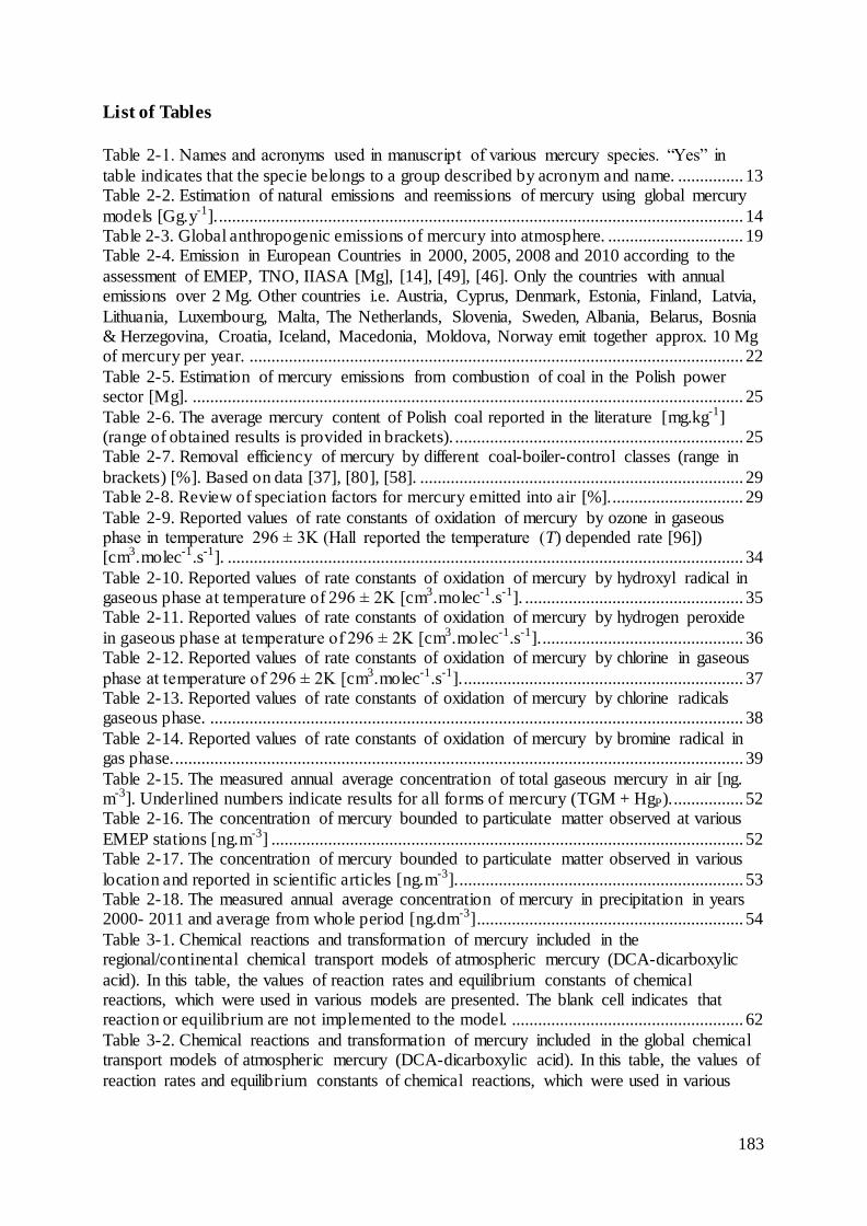
183
List of Tables
Table 2-1. Names and acronyms used in manuscript of various mercury species. “Yes” in
table indicates that the specie belongs to a group described by acronym and name. ............... 13 Table 2-2. Estimation of natural emissions and reemissions of mercury using global mercury
models [Gg.y-1]. ........................................................................................................................ 14 Table 2-3. Global anthropogenic emissions of mercury into atmosphere. ............................... 19 Table 2-4. Emission in European Countries in 2000, 2005, 2008 and 2010 according to the
assessment of EMEP, TNO, IIASA [Mg], [14], [49], [46]. Only the countries with annual emissions over 2 Mg. Other countries i.e. Austria, Cyprus, Denmark, Estonia, Finland, Latvia,
Lithuania, Luxembourg, Malta, The Netherlands, Slovenia, Sweden, Albania, Belarus, Bosnia & Herzegovina, Croatia, Iceland, Macedonia, Moldova, Norway emit together approx. 10 Mg of mercury per year. ................................................................................................................. 22
Table 2-5. Estimation of mercury emissions from combustion of coal in the Polish power sector [Mg]. .............................................................................................................................. 25
Table 2-6. The average mercury content of Polish coal reported in the literature [mg.kg-1] (range of obtained results is provided in brackets). .................................................................. 25 Table 2-7. Removal efficiency of mercury by different coal-boiler-control classes (range in
brackets) [%]. Based on data [37], [80], [58]. .......................................................................... 29 Table 2-8. Review of speciation factors for mercury emitted into air [%]............................... 29
Table 2-9. Reported values of rate constants of oxidation of mercury by ozone in gaseous phase in temperature 296 ± 3K (Hall reported the temperature (T) depended rate [96]) [cm3.molec-1.s-1]. ...................................................................................................................... 34
Table 2-10. Reported values of rate constants of oxidation of mercury by hydroxyl radical in gaseous phase at temperature of 296 ± 2K [cm3.molec-1.s-1]. .................................................. 35 Table 2-11. Reported values of rate constants of oxidation of mercury by hydrogen peroxide
in gaseous phase at temperature of 296 ± 2K [cm3.molec-1.s-1]. .............................................. 36 Table 2-12. Reported values of rate constants of oxidation of mercury by chlorine in gaseous
phase at temperature of 296 ± 2K [cm3.molec-1.s-1]. ................................................................ 37 Table 2-13. Reported values of rate constants of oxidation of mercury by chlorine radicals gaseous phase. .......................................................................................................................... 38
Table 2-14. Reported values of rate constants of oxidation of mercury by bromine radical in gas phase................................................................................................................................... 39
Table 2-15. The measured annual average concentration of total gaseous mercury in air [ng. m-3]. Underlined numbers indicate results for all forms of mercury (TGM + HgP)................. 52 Table 2-16. The concentration of mercury bounded to particulate matter observed at various
EMEP stations [ng.m-3] ............................................................................................................ 52 Table 2-17. The concentration of mercury bounded to particulate matter observed in various
location and reported in scientific articles [ng.m-3]. ................................................................. 53 Table 2-18. The measured annual average concentration of mercury in precipitation in years 2000- 2011 and average from whole period [ng.dm-3] ............................................................. 54
Table 3-1. Chemical reactions and transformation of mercury included in the regional/continental chemical transport models of atmospheric mercury (DCA-dicarboxylic
acid). In this table, the values of reaction rates and equilibrium constants of chemical reactions, which were used in various models are presented. The blank cell indicates that reaction or equilibrium are not implemented to the model. ..................................................... 62
Table 3-2. Chemical reactions and transformation of mercury included in the global chemical transport models of atmospheric mercury (DCA-dicarboxylic acid). In this table, the values of
reaction rates and equilibrium constants of chemical reactions, which were used in various
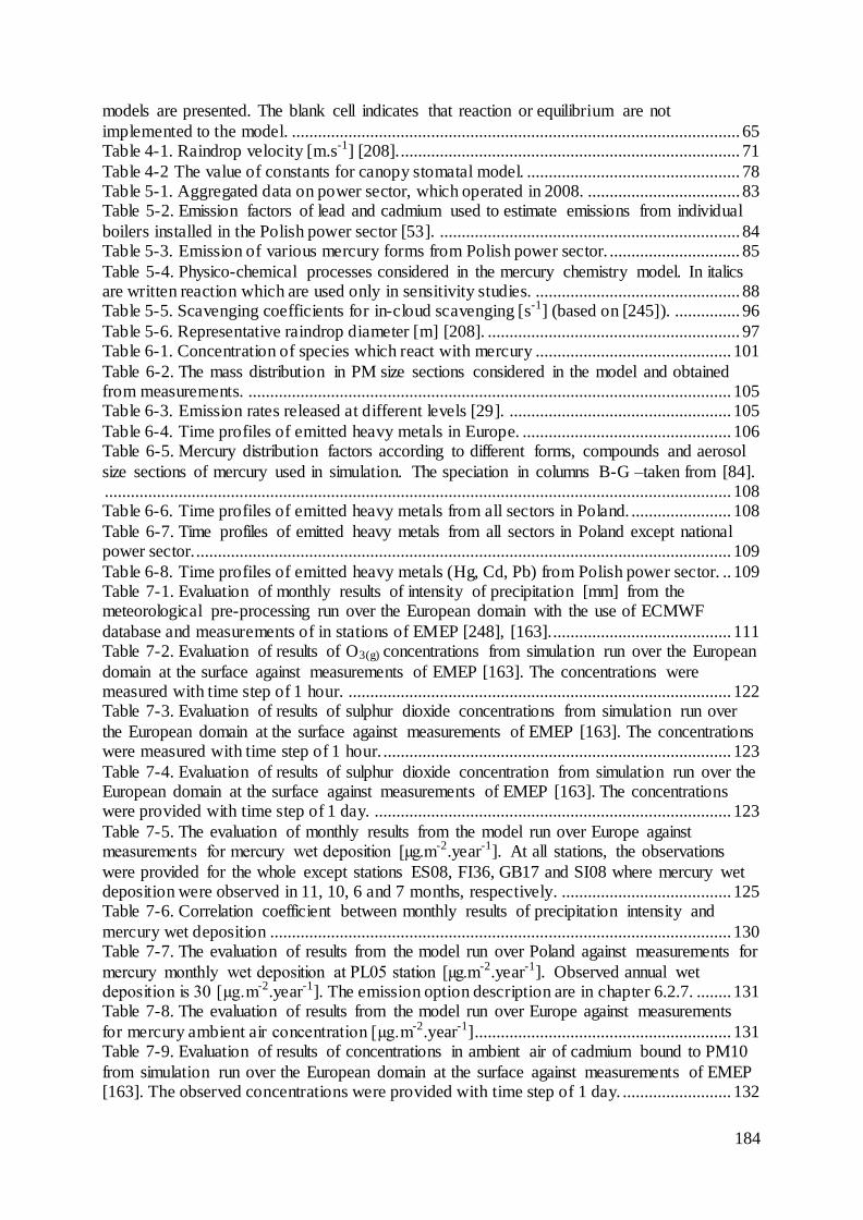
184
models are presented. The blank cell indicates that reaction or equilibrium are not
implemented to the model. ....................................................................................................... 65 Table 4-1. Raindrop velocity [m.s-1] [208]............................................................................... 71
Table 4-2 The value of constants for canopy stomatal model. ................................................. 78 Table 5-1. Aggregated data on power sector, which operated in 2008. ................................... 83 Table 5-2. Emission factors of lead and cadmium used to estimate emissions from individual
boilers installed in the Polish power sector [53]. ..................................................................... 84 Table 5-3. Emission of various mercury forms from Polish power sector. .............................. 85
Table 5-4. Physico-chemical processes considered in the mercury chemistry model. In italics are written reaction which are used only in sensitivity studies. ............................................... 88 Table 5-5. Scavenging coefficients for in-cloud scavenging [s-1] (based on [245]). ............... 96
Table 5-6. Representative raindrop diameter [m] [208]. .......................................................... 97 Table 6-1. Concentration of species which react with mercury ............................................. 101
Table 6-2. The mass distribution in PM size sections considered in the model and obtained from measurements. ............................................................................................................... 105 Table 6-3. Emission rates released at different levels [29]. ................................................... 105
Table 6-4. Time profiles of emitted heavy metals in Europe. ................................................ 106 Table 6-5. Mercury distribution factors according to different forms, compounds and aerosol
size sections of mercury used in simulation. The speciation in columns B-G –taken from [84]. ................................................................................................................................................ 108 Table 6-6. Time profiles of emitted heavy metals from all sectors in Poland. ....................... 108
Table 6-7. Time profiles of emitted heavy metals from all sectors in Poland except national power sector............................................................................................................................ 109
Table 6-8. Time profiles of emitted heavy metals (Hg, Cd, Pb) from Polish power sector. .. 109 Table 7-1. Evaluation of monthly results of intensity of precipitation [mm] from the meteorological pre-processing run over the European domain with the use of ECMWF
database and measurements of in stations of EMEP [248], [163].......................................... 111 Table 7-2. Evaluation of results of O3(g) concentrations from simulation run over the European
domain at the surface against measurements of EMEP [163]. The concentrations were measured with time step of 1 hour. ........................................................................................ 122 Table 7-3. Evaluation of results of sulphur dioxide concentrations from simulation run over
the European domain at the surface against measurements of EMEP [163]. The concentrations were measured with time step of 1 hour. ................................................................................ 123
Table 7-4. Evaluation of results of sulphur dioxide concentration from simulation run over the European domain at the surface against measurements of EMEP [163]. The concentrations were provided with time step of 1 day. .................................................................................. 123
Table 7-5. The evaluation of monthly results from the model run over Europe against measurements for mercury wet deposition [µg.m-2.year-1]. At all stations, the observations
were provided for the whole except stations ES08, FI36, GB17 and SI08 where mercury wet deposition were observed in 11, 10, 6 and 7 months, respectively. ....................................... 125 Table 7-6. Correlation coefficient between monthly results of precipitation intensity and
mercury wet deposition .......................................................................................................... 130 Table 7-7. The evaluation of results from the model run over Poland against measurements for
mercury monthly wet deposition at PL05 station [µg.m-2.year-1]. Observed annual wet deposition is 30 [µg.m-2.year-1]. The emission option description are in chapter 6.2.7. ........ 131 Table 7-8. The evaluation of results from the model run over Europe against measurements
for mercury ambient air concentration [µg.m-2.year-1] ........................................................... 131 Table 7-9. Evaluation of results of concentrations in ambient air of cadmium bound to PM10
from simulation run over the European domain at the surface against measurements of EMEP [163]. The observed concentrations were provided with time step of 1 day. ......................... 132
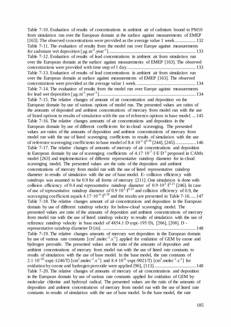
185
Table 7-10. Evaluation of results of concentrations in ambient air of cadmium bound to PM10
from simulation run over the European domain at the surface against measurements of EMEP [163]. The observed concentrations were provided as the average value 1 week.................. 132
Table 7-11. The evaluation of results from the model run over Europe against measurements for cadmium wet deposition [µg.m-2.year-1]........................................................................... 133 Table 7-12. Evaluation of results of lead concentrations in ambient air from simulation run
over the European domain at the surface against measurements of EMEP [163]. The observed concentrations were provided with time step of 1 day. .......................................................... 133
Table 7-13. Evaluation of results of lead concentrations in ambient air from simulation run over the European domain at surface against measurements of EMEP [163]. The observed concentrations were provided as the average value 1 week. .................................................. 134
Table 7-14. The evaluation of results from the model run over Europe against measurements for lead wet deposition [µg.m-2.year-1]. .................................................................................. 134
Table 7-15. The relative changes of amount of air concentration and deposition on the European domain by use of various options of model run. The presented values are ratios of the amounts of deposited and ambient concentrations of mercury from model run with the use
of listed options to results of simulation with the use of reference options in base model. ... 145 Table 7-16. The relative changes amounts of air concentrations and deposition in the
European domain by use of different coefficients for in-cloud scavenging. The presented values are ratios of the amounts of deposition and ambient concentrations of mercury from model run with the use of listed scavenging coefficients to results of simulation with the use
of reference scavenging coefficients in base model of 8.4·10-5·I0.79 [244], [245]. ................. 146 Table 7-17. The relative changes of amounts of mercury of air concentrations and deposition
in European domain by use of scavenging coefficients of 4.17·10-7·I·E·D-1 proposed in CAMx model [263] and implementation of different representative raindrop diameter for in-cloud scavenging model. The presented values are the ratio of the deposition and ambient
concentrations of mercury from model run with the use of listed representative raindrop diameter to results of simulation with the use of base model. E- collision efficiency with
raindrops was assumed to be 0.9 for all forms of mercury [211]. One simulation is done with collision efficiency of 0.4 and representative raindrop diameter of 0.9·103·I0.21 [246]. In case of use of representative raindrop diameter of 0.9·103·I0.21 and collision efficiency of 0.9, the
scavenging coefficient equals 4.17·10-4·I0.79 and the results are presented in Table 7-16. .... 147 Table 7-18. The relative changes amount of air concentrations and deposition in the European
domain by use of different raindrop velocity for below-cloud scavenging model. The presented values are ratio of the amounts of deposition and ambient concentrations of mercury from model run with the use of listed raindrop velocity to results of simulation with the use of
reference raindrop velocity in base model of 4854.1·D·exp(-195·D), [206], [208]. D - representative raindrop diameter D [m]. ................................................................................ 148
Table 7-19. The relative changes amounts of mercury wet deposition in the European domain by use of various rate constants [cm3.molec-1.s-1] applied for oxidation of GEM by ozone and hydrogen peroxide. The presented values are the ratio of the amounts of deposition and
ambient concentrations of mercury from model run with the use of listed rate constants to results of simulation with the use of base model. In the base model, the rate constants of
2.1·10-18·exp(-1246/T) [cm3.molec-1.s-1] and 8.4·10-6·exp(-9021/T) [cm3.molec-1.s-1] for oxidation by ozone and hydrogen peroxide were applied [96], [113].................................... 148 Table 7-20. The relative changes of amounts of mercury of air concentrations and deposition
in the European domain by use of various rate constants applied for oxidation of GEM by molecular chlorine and hydroxyl radical. The presented values are the ratio of the amounts of
deposition and ambient concentrations of mercury from model run with the use of listed rate constants to results of simulation with the use of base model. In the base model, the rate
186
constant of 2.6·10-18 [cm3.molec-1.s-1] and 8.7·10-14 [cm3.molec-1.s-1] for oxidation
respectively by molecular chlorine and hydroxyl radical were applied [117], [107]............. 149 Table 7-21. The relative changes of amounts of mercury air concentrations and deposition in
the European domain by use of various rate constant applied to oxidation of Hg0(g) by bromine
radical. The presented values are the ratio of the amounts of deposition and ambient concentration of mercury from model run with the use of listed rate constants to results of
simulation with the use of base model. In the base model the rate constant of 1.46·10-32· (T/298)-1.86 [cm6.molec-2.s-1] by bromine radical was applied [226]. ..................................... 149
Table 7-22. The relative changes amounts of mercury of air concentrations and deposition in the European domain by use of additional reactions of oxidation of Hg0 by molecular bromine, nitrate radical, molecular iodine, molecular fluorine and chlorine radicals. The
presented values are the ratio of the amounts of air concentrations and deposition of mercury from model run with the use of listed reactions to results of simulation with the use of base
model (without listed reaction)............................................................................................... 150 Table 7-23. The relative changes amounts of mercury air concentrations and deposition in the European domain by use of various input data. The presented values are the ratio of results
from base model run with the use of listed changed input data to modelling results with the use of reference input data...................................................................................................... 155
187
List of Figures
Figure 2-1. The sources, pathway and sinks of heavy metals in the atmosphere. .................... 13
Figure 2-2. The contribution of regions in anthropogenic emission of mercury into the air in 2010 [%] [35]. .......................................................................................................................... 19
Figure 2-3. The share of different sectors in anthropogenic emission of mercury into the air in 2010 [%]. Sources with intentional use of mercury are marked with black edges [35]. .......... 20 Figure 2-4. The share of mercury emissions from different sources in European countries
according to the assessment of EMEP (reported emission) in 2008, TNO, and IIASA in 2010 [%] [14], [49], [46]. Data are provided only for countries with mercury emissions over 4 Mg
in 2008 or 2010......................................................................................................................... 23 Figure 2-5. Quantity of mercury emitted into air according to the assessment of Institute of Environmental Projection and its agencies [kg] [50], [51], [52], [53], [54], [48], [55]. .......... 24
Figure 2-6. Annual emissons of mercury into air from power plants (PP), CHP (SNAP 0101) and district heating plants (SNAP 0102) in Poland in 2005-2010 according to estimation of
the Institute of Environmental Projection [Mg] [50], [51], [52], [54]. ..................................... 24 Figure 2-7. Emission of lead in Poland into air according to the assessment of the Institute of Environmental Projection and its agencies [Mg] [50],[51],[52],[53],[54],[92],[55]. ............... 31
Figure 2-8. Emissions of cadmium in Poland into air according to the assessment of the Institute of Environmental Projection and its agencies [Mg] [50], [51], [52], [53], [54], [92],
[55]. .......................................................................................................................................... 33 Figure 2-9. The half-life of atmospheric elemental gaseous mercury due to the oxidation in the gaseous phase. All reactions were described in the text, the list of presented reactions contains
name of data series in figure, oxidant symbol, reaction rate constant in cm3.molec-1.s-1 and reference to literature. O3 A – O3(g), 4.2·10-19,[99]; O3 B – O3(g), 1.7·10-18
,[105]; O3 C – O3(g),
4.9·10-18 ,[100]; O3 D – O3(g), 3·10-20 ,[96]; O3 E – O3(g), 7.5·10-19
,[98]; O3 F – O3(g), 6.4·10-19
,[106]; O3 G – O3(g), 6.2·10-19 , [101]; •OH A – •OH (g), 6.2·10-19
,[107]; •OH B – •OH (g),
1.6·10-12 , [108]; •OH C – •OH (g), 1.2·10-13
,[109]; •OH D – •OH (g), 9.0·10-14 , [110]; •OH E –
•OH (g), 3.2·10-13 ,[111]; H2O2 A – H2O2(g), 4.1·10-16
, [112]; H2O2 B – H2O2(g), 6.0·10-19 ,[97],
[113]; Cl2 A – Cl2(g), 4.8·10-18 , [115]; Cl2 B – Cl2(g), 5.7·10-17
, [116]; Cl2 C – Cl2(g), 2.6·10-18
,[117]; Cl2 D – Cl2(g), 1.82·10-19 ,[118]; Cl2 E – Cl2(g), 2.5·10-18
,[106]; Cl2 F – Cl2(g), 4.3·10-15 ,
[119]; Cl• A – Cl•(g), 3.2·10-11,[122]; Cl• B – Cl•(g), 1.0·10-11,[117]; Cl• C – Cl•(g), 2.8·10-12, [123]; Cl• D – Cl•(g), 1.2·10-10, [119]; HCl –HCl(g), 1.0·10-19, [126]; Br• A – Br•
(g), 3.2·10-12,
[117] ; Br• B – Br•(g), 2.04·10-12, [123]; Br• C – Br•
(g), 1.1·10-12, [111]; Br• D – Br•(g), 3.6·10-12,
[128]; Br• E – Br•(g), 9.8·10-19, [129]; Br2 A –Br2(g), 0.9·10-16
, [117]; Br2 B – Br2(g), 2.8·10-19
,[130]; BrO• A – BrO•(g), 1.5·10-14, [133]; NO3• A – NO3
•(g), 4.0·10-15, [135]; NO3• B –
NO3•(g), 7.0·10-15,[106]; NO3• C – NO3
•(g), 1.3·10-14,[106]; NO3• D – NO3
•(g), 3.0·10-14,[106];
I2 – I2 (g), 1.27·10-19, [136]; F2 – F2 (g), 1.8·10-15, [106]. The concentrations of different
oxidants were determined based on literature review [121], [15], [125], [114], [132]. Some oxidants appear only at some times of the day or over some areas (sea, coastal regions) -description in the text. .............................................................................................................. 43
Figure 2-10. Location of EMEP stations, where measurements of ambient GEM concentrations were conducted in the period of 2000-2011. Green dots denote stations for
which the observations for 2008 are available. ........................................................................ 52 Figure 2-11 Location of EMEP stations where measurements of wet deposition of mercury were conducted in the period of 2000-2011. Green dots denote stations for which the
observations for 2008 are available. ......................................................................................... 53 Figure 4-1. Polyphemus air quality system overall work flow. Based on [13]. ....................... 69
Figure 4-2. Schematic representation of a resistance model. The description of the resistances is provided in the text. .............................................................................................................. 74

188
Figure 4-3. Annual average dry deposition velocity in 2008 for SO2(g) [cm.s-1]...................... 79
Figure 4-4. Annual average dry deposition velocity in 2008 for O3(g) [cm.s-1]. ....................... 79 Figure 5-1. Location and emissions [kg] of main emitters of mercury. Emissions based on
emission factors for 2008 (EF2008). ........................................................................................ 84 Figure 5-2. Location and emissions [kg] of main emitters of mercury. Emissions based on emission factors for 2009 (EF2009). ........................................................................................ 84
Figure 5-3. Location and emissions [kg] of main emitters of lead........................................... 85 Figure 5-4. Location and emissions [kg] of main emitters of cadmium. ................................. 85
Figure 5-5. Vertical distribution of mercury, lead and cadmium emissions from Polish power sector (expressed as percentage of calculated total emission). EF2008 -emission factors for 2008, EF2009 -emission factors for 2009. ............................................................................... 85
Figure 5-6. The implemented chemical model for mercury. In this picture, the gaseous and aqueous phases are marked in white and blue, respectively. The line arrows show possible
transformations of mercury. The dashed arrows show additional species used in the model ,which react with mercury. The red arrows and species show the reactions implemented additionally in sensitivity analyses of the model. The species and arrows in black indicate the
reactions and transformations, which were used in all simulations (otherwise the changes are marked in the text). ................................................................................................................... 87
Figure 6-1. Domains of simulation and locations of measurement stations of mercury wet deposition (red circles), ambient concentration (blue triangles) or both parameters (red-blue squares) operated in 2008 in the context of [163]. ................................................................... 98
Figure 6-2. Annual precipitation intensity [mm.y-1] over Europe due to [248]. ...................... 99 Figure 6-3. Natural emissions and reemissions of mercury over Europe [g.km-2.y-1] [29], [14].
................................................................................................................................................ 102 Figure 6-4. Natural emissions and reemissions of cadmium over Europe [g.km-2.y-1] [29], [14]. ........................................................................................................................................ 103
Figure 6-5. Natural emissions and reemissions of lead over Europe [g.km-2.y-1]. [29], [14]. 103 Figure 6-6. Anthropogenic emissions of mercury over Europe in 2008 due to EMEP [g.km-2.y-
1] [14]. ..................................................................................................................................... 104 Figure 6-7. Anthropogenic emission of cadmium over Europe in 2008 due to EMEP [g.km-2.y-
1] [14]. ..................................................................................................................................... 104
Figure 6-8. Anthropogenic emission of lead over Europe in 2008 due to EMEP [g.km-2.y-1] [14]. ........................................................................................................................................ 104
Figure 7-1. The monthly intensity of precipitation [mm] from the meteorological pre-processing run over the European domain with the use of ECMWF database and measurements at the EMEP stations located in Poland PL04 –Łeba and PL05 –Diabla Góra.
................................................................................................................................................ 112 Figure 7-2. The average dry deposition velocity of RGM (blue, left axis) and GEM (red, right
axis) for different land types over Europe [cm.s-1]................................................................. 113 Figure 7-3. Annual average dry deposition velocity of GEM [cm.s-1]................................... 113 Figure 7-4 Annual average dry deposition velocity of RGM [cm.s-1]. .................................. 113
Figure 7-5. The monthly average dry deposition velocity of RGM (blue, left axis) and GEM (red, right axis) in modelling cell where Kraków is located [cm.s-1] ..................................... 114
Figure 7-6. Annual average concentrations of SO2(g) [µg.m-3] in the surface. ....................... 115 Figure 7-7. Monthly average modelled concentrations of SO2 [µg.m-3] in the surface at selected stations. ..................................................................................................................... 115
Figure 7-8. Annual average concentrations of SO2(g) [µg.m-3] at vertical 10 levels according to the vertical split of simulation domain e.g. level 1 -the lowest, surface level from 0 to 70 [m]
above ground, level 10 – the highest from 3000 to 5000 [m] above ground ......................... 116

189
The highest concentration of SO2(g) occurs over southern Poland where the most of the Polish
power plants are located (Figure 7-6). In Poland, more than half of sulphur dioxide is emitted from the power sector (SNAP 01), whereas a quarter of sulphur dioxide is emitted from coal
combustion in the residential sector (SNAP 02). The emissions from this sector occurs mainly during the winter season, which may explain the highest SO2(g) concentration in winter in cells where station PL05 is located (Figure 7-7). As presented in Figure 7-9, the highest
ambient concentration is observed near the surface and decreases significantly with altitude. ................................................................................................................................................ 116
Figure 7-10. Annual average concentrations of O3(g) [µg.m-3] at the surface. ....................... 116 Figure 7-11. Monthly average concentrations of O3(g) [µg.m-3] at the surface at selected stations. ................................................................................................................................... 116
Figure 7-12. Annual average concentrations of O3(g) [µg.m-3] at 10 vertical levels............... 117 Figure 7-13. Annual average concentrations of H2O2(g) [µg.m-3] at the surface. ................... 117
Figure 7-14. Monthly average concentrations of H2O2(g) [µg.m-3] at the surface at selected stations. ................................................................................................................................... 117 Figure 7-15. Annual average concentrations of H2O2(g) [µg.m-3] in hours of day at the surface
level. ....................................................................................................................................... 117 Figure 7-16. Annual average concentrations of H2O2(g) [µg.m-3] at 10 vertical levels. ......... 118
Figure 7-17. Annual average concentrationa of NO3•(g) [µg.m-3] in the surface level. .......... 118
Figure 7-18. Monthly average concentrations of NO3•(g) [µg.m-3] at the surface level at
selected stations. ..................................................................................................................... 118
Figure 7-19. Annual average concentrations of NO3•(g) [µg.m-3] in hours of day at the surface.
................................................................................................................................................ 119
Figure 7-20. Annual average concentrations of NO3•(g) [µg.m-3] at 10 vertical levels. .......... 119
Figure 7-21. Annual average concentrations of HO2•(g) [ng.m-3] at the surface. .................... 119
Figure 7-22. Monthly average concentrations of HO2•(g) [µg.m-3] at the surface at selected
stations. ................................................................................................................................... 119 Figure 7-23. Annual average concentrations of HO2
•(g) [µg.m-3] at vertical 10 levels. .......... 120
Figure 7-24. Annual average concentrations of •OH(g) [pg.m-3] at the surface level. ............ 120 Figure 7-25. Monthly average concentrations of •OH(g) [µg.m-3] in 2008 at the surface at selected stations. ..................................................................................................................... 120
Figure 7-26. Annual average concentrations of •OH(g) [µg.m-3] in hours of day at the surface. ................................................................................................................................................ 120
Figure 7-27. Annual average concentrations of •OH(g) [µg.m-3] at vertical 10 levels. ........... 121 Figure 7-28. Annual average concentrations of black carbon [µg.m-3] at the surface. ........ 121 Figure 7-29. Monthly average concentrations of black carbon [µg.m-3] at the surface at
selected stations. ..................................................................................................................... 121 Figure 7-30. The share of different size section in total concentration of black carbon [µg.m-3]
in all cells at the surface. BC_0, BC_1, BC_2, BC_3, BC_1 , BC_1 , BC_1 , BC_1 are black carbon particle size sections with the following threshold limits [in μm] 0.01 - 0.02 - 0.0398 - 0.0794 - 0.1585 - 0.3162 - 0.6310 - 1.2589 - 2.5119 - 5.0119 -10, respectively. .................. 122
Figure 7-31. Annual average concentrations of black carbon [µg.m-3] at 10 vertical levels.. 122 Figure 7-32. The annual modeled (model) and observed (observation) amounts of mercury
wet deposition at the stations of EMEP.................................................................................. 125 Figure 7-33. The comparison of results from the model run (M –model, M-CR –“model rain corrected”) over Europe against measurements (O) at station BE14 for mercury wet
deposition [µg.m-2.month-1]................................................................................................... 126 Figure 7-34. The comparison of results from the model run (M –model, M-CR –“model rain
corrected”) over Europe against measurements (O) at station DE04 for mercury wet deposition [µg.m-2.month-1]................................................................................................... 126
190
Figure 7-35. The comparison of results from the model run (M –model, M-CR –model “rain
corrected”) over Europe against measurements (O) at station BE14 for mercury wet deposition [µg.m-2.month-1].................................................................................................... 127
Figure 7-36. The comparison of results from the model run (M –model, M-CR –model “rain corrected”) over Europe against measurements (O) at station DE04 for mercury wet deposition [µg.m-2.month-1].................................................................................................... 127
Figure 7-37. The comparison of results from the model run (M –model, M-CR –model “rain corrected”) over Europe against measurements (O) at station DE08 for mercury wet
deposition [µg.m-2.month-1].................................................................................................... 127 Figure 7-38. The comparison of results from the model run (M –model, M-CR –model “rain corrected”) over Europe against measurements (O) at station DE09 for mercury wet
deposition [µg.m-2.month-1].................................................................................................... 127 Figure 7-39. The comparison of results from the model run (M –model, M-CR –“model rain
corrected”) over Europe against measurements (O) at station ES08 for mercury wet deposition [µg.m-2.month-1]. .................................................................................................................... 127 Figure 7-40. The comparison of results from the model run (M –model, M-CR –“model rain
corrected”) over Europe against measurements (O) at station FI36 for mercury wet deposition [µg.m-2.month-1]. .................................................................................................................... 127
Figure 7-41. The comparison of results from the model run (M –model, M-CR –“model rain corrected”) over Europe against measurements (O) at station GB13 for mercury wet deposition [µg.m-2.month-1]................................................................................................... 128
Figure 7-42. The comparison of results from the model run (M –model, M-CR –“model rain corrected”) over Europe against measurements (O) at station GB17 for mercury wet
deposition [µg.m-2.month-1]................................................................................................... 128 Figure 7-43. The comparison of results from the model run (M –model, M-CR –“model rain corrected”) over Europe against measurements (O) at station GB48 for mercury wet
deposition [µg.m-2.month-1]................................................................................................... 128 Figure 7-44. The comparison of results from the model run (M –model, M-CR –“model rain
corrected”) over Europe against measurements (O) at station GB48 for mercury wet deposition [µg.m-2.month-1]................................................................................................... 128 Figure 7-45. The comparison of results from the model run (M –model, M-CR –“model rain
corrected”) over Europe against measurements (O) at station LV10 for mercury wet deposition [µg.m-2.month-1]................................................................................................... 128
Figure 7-46. The comparison of results from the model run (M –model, M-CR –“model rain corrected”) over Europe against measurements (O) at station LV16 for mercury wet deposition [µg.m-2.month-1].................................................................................................... 128
Figure 7-47. The comparison of results from the model run (M –model, M-CR –“model rain corrected”) over Europe against measurements (O) at station NL91 for mercury wet
deposition [µg.m-2.month-1].................................................................................................... 129 Figure 7-48. The comparison of results from the model run (M –model, M-CR –“model rain corrected”) over Europe against measurements (O) at station NO01 for mercury wet
deposition [µg.m-2.month-1].................................................................................................... 129 Figure 7-49. The comparison of results from the model run (M –model, M-CR –“model rain
corrected”) over Europe against measurements (O) at station PL05 for mercury wet deposition [µg.m-2.month-1]. .................................................................................................................... 129 Figure 7-50. The comparison of results from the model run (M –model, M-CR –“model rain
corrected”) over Europe against measurements (O) at station DE04 for mercury wet deposition [µg.m-2.month-1]................................................................................................... 129
191
Figure 7-51. The comparison of results from the model run (M –model, M-CR –“model rain
corrected”) over Europe against measurements (O) at station SI08 for mercury wet deposition [µg.m-2.month-1]. .................................................................................................................... 129
Figure 7-52. Annual average concentration of GEM [ng.m-3] at the surface. ........................ 135 Figure 7-53. Annual average ambient concentration of RGM [pg.m-3] at the surface........... 135 Figure 7-54. Annual average ambient concentration of HgP [pg.m-3] at the surface. ............ 135
Figure 7-55. Annual average ambient air concentration of mercury forms and species at the surface at locations of EMEP measurement sites. The concentrations of reactive mercury are
shown on the left [pg.m3] and GEM on the right [ng.m3] axis. .............................................. 136 Figure 7-56. Monthly average ambient air concentration of mercury forms and species at the surface at the PL05 observation site [pg.m3]. The results are from simulation over Europe. 137
Figure 7-57. Annual average ambient air concentrations of mercury forms and species in the whole European domain at 10 vertical levels. ........................................................................ 138
Figure 7-58. Annual wet deposition of RGAM [g.km-2.y-1]................................................... 138 Figure 7-59. Annual wet deposition of HgP [g.km-2.y-1] ........................................................ 138 Figure 7-60. Contribution of mercury forms and species to overall wet deposition at locations
of EMEP measurement sites................................................................................................... 139 Figure 7-61. Annual dry deposition of GEM [g.km-2.y-1]. ..................................................... 140
Figure 7-62. Annual dry deposition of RGM [g.km-2.y-1]. ..................................................... 140 Figure 7-63. Annual dry deposition of HgP [g.km-2.y-1]......................................................... 140 Figure 7-64. Contribution of mercury forms and species to overall dry deposition at locations
of EMEP measurement sites................................................................................................... 141 Figure 7-65. Annual deposition (wet +dry) of mercury [g.km-2.y-1]. ..................................... 141
Figure 7-66. Contribution of mercury forms to overall deposition (dry and wet) at locations of EMEP measurement sites. ...................................................................................................... 142 Figure 7-67. Annual average concentration of cadmium [ng.m-3] at the surface. .................. 143
Figure 7-68. Annual average concentration of lead [ng.m-3] at the surface. .......................... 143 Figure 7-69. Annual wet deposition of cadmium [g.km-2.y-1]................................................ 143
Figure 7-70. Annual wet deposition of lead [g.km-2.y-1]. ............................................... 143 Figure 7-71. Annual dry deposition of cadmium [g.km-2.y-1]. .............................................. 143 Figure 7-72. Annual dry deposition of lead [g.km-2.y-1]. ............................................ 143
Figure 7-73. Differences in concentrations of GEM at the surface between base model run and model without dry deposition of GEM [ng.m-3]..................................................................... 144
Figure 7-74. Differences in concentrations of GEM at the surface between base model run and model without atmospheric chemistry of mercury [pg.m-3]. .................................................. 144 Figure 7-75.The increase or decrease of air concentration of reactive mercury (RGM+HgP) at
selected stations at surface due to implementation of various reactions of mercury in gaseous and aqueous phases [pg.m-3]. A gas - Hg0+O3→HgO+O2, B gas - Hg0+Cl2→HgCl2 ,C gas -
Hg0+2HCl→HgCl2+H2, D gas - Hg0+H2O2→Hg(OH)2,E gas - HgBr+2Br•→HgBr2, F gas - HgBr→Hg0+ Br•, G gas - HgBr+Br•→HgBr2, H gas - HgBr+•OH→HgBrOH, I gas - Hg0+BrO•→HgO+Br, J gas - Hg0+ 2•OH→Hg(OH)2, K gas - HgBr+Br•→Hg0+ Br2 ,...... 146
Figure 7-76. The relative changes of rate constants the temperature. The presented values are the ratio of the value of the rate constant at different temperatures to the value of the rate
constant at a temperature of 200C (293.16K). All rate constant linkeds to oxidation of Hg0 by: A –ozone – 2.1·10-18exp−1246𝑇 ,[96]; B –hydroxyl radical –3.2·10-13· (T/298)-3.06 ,[111]; C
–hydrogen peroxide –8.4·10-6· exp(-9021/T), [113], D –chlorine radicals –1.38·10-
12·exp(208.02/T), [123], E –bromine radical –1.1·10-12 · (T/298)-2.37, [111]. ........................ 151
Figure 7-77. Fractional bias (FB) of results of ambient concentration of RGPM (RGM + HgP) at the surface from models run when formed HgO is in gaseous ([gasHgO]) and particulate forms ([PMHgO]). .................................................................................................................... 152
192
Figure 7-78. Differences (Diff) in ambient concentration of RGPM (RGM + HgP) at the
surface from model runs when formed HgO is in gaseous ([gasHgO]) and particulate forms ([PMHgO]) [pg.m-3]. ................................................................................................................. 152
Figure 7-79. Fractional bias (FB) of results of dry deposition load of RGPM (RGM + HgP) at the surface from model runs when formed HgO is in gaseous ([gasHgO]) and particulate forms ([PMHgO]). ............................................................................................................................... 152
Figure 7-80. Differences (Diff) in dry deposition load of RGPM (RGM + HgP) at the surface from model runs when formed HgO is in gaseous ([gasHgO]) and particulate forms ([PMHgO])
[g.km-2.y-1]. ............................................................................................................................. 152 Figure 7-81. Fractional bias (FB) of results of wet deposition load of RM (RGM+HgII
(aq)+HgP) at the surface from model runs when formed HgO is in gaseous
([gasHgO]) and particulate forms ([PMHgO]). ........................................................................... 152 Figure 7-82. Differences (Diff) in wet deposition load of RM (RGM+HgII
(aq)+HgP) at the
surface from model runs when formed HgO is in gaseous ([gasHgO]) and particulate forms ([PMHgO]) [pg.m-3]. ................................................................................................................. 152 Figure 7-83. Fractional bias (FB) of results of ambient concentration of mercury bound to
particulate matter at the surface from base model runs when emission of HgP were distributed equally ([HgP(eq)]) and in proportion to aerosol surface areas ([HgP(sf)])................................ 153
Figure 7-84. Differences (Diff) in ambient concentration of mercury bound to particulate matter at the surface from base model runs when emission of HgP were distributed equally ([HgP(eq)]) and in proportion to aerosol surface areas ([HgP(sf)]) [pg.m-3]. ............................. 153
Figure 7-85. Fractional bias (FB) of results of dry deposition of mercury bound to particulate matter at the surface from base model runs when emission of HgP were distributed equally
([HgP(eq)]) and in proportion to aerosol surface areas ([HgP(sf)]). ........................................... 154 Figure 7-86. Differences (Diff) in dry deposition load of mercury bound to particulate matter at the surface level from base model runs when emission of HgP were distributed equally
([HgP(eq)]) and in proportion to aerosol surface areas ([HgP(sf)]) [g.km-2.y-1]. ........................ 154 Figure 7-87. Fractional bias (FB) of results of wet deposition of mercury bound to particulate
matter at the surface from base models run when emission of HgP were distributed equally ([HgP(eq)]) and in proportion to aerosol surface areas ([HgP(sf)]). ........................................... 154 Figure 7-88. Differences (Diff) in wet deposition load of mercury bound to particulate matter
at the surface from base model runs when emission of HgP were distributed equally ([HgP(eq)]) and in proportion to aerosol surface areas ([HgP(sf)]) [g.km-2.y-1]. ........................................ 154
Figure 7-89. Contribution of national (Polish) power sector (NPS), national other anthropogenic (NOS), European anthropogenic (EAE), global (GLOB), and natural and re-emission sources (NRE) to total mercury deposition (dry+wet) in Poland in 2008. .............. 156
Figure 7-90. The impact of the Polish power sector. The percentage rate of emissions from power sector to overall average ambient concentration of GEM [%]. ................................... 158
Figure 7-91. The impact of the Polish power sector. The percentage rate of emissions from power sector to overall average ambient concentration of GEM [%]. ................................... 158 Figure 7-92. The impact of the Polish power sector. The percentage rate of emissions from
power sector to overall average ambient concentration of GEM [%]. ................................... 158 Figure 7-93. The impact of the Polish power sector. The percentage rate of emissions from
power sector to overall average ambient concentration of RGM [%]. ................................... 158 Figure 7-94. The impact of the Polish power sector. The percentage rate of emissions from power sector to overall average ambient concentration of RGM [%]. ................................... 158
Figure 7-95. The impact of the Polish power sector. The percentage rate of emissions from power sector to overall average ambient concentration of RGM [%]. ................................... 158
Figure 7-96. The impact of the Polish power sector. The percentage rate of emissions from power sector to overall average ambient concentration of HgP [%]....................................... 158
193
Figure 7-97. The impact of the Polish power sector. The percentage rate of emissions from
power sector to overall average ambient concentration of HgP [%]....................................... 158 Figure 7-98. The impact of the Polish power sector. The percentage rate of emissions from
power sector to overall average ambient concentration of HgP [%]....................................... 158 Figure 7-99. The impact of the Polish power sector. The percentage rate of emissions from power sector to overall dry deposition of mercury [%]. ......................................................... 159
Figure 7-100. The impact of the Polish power sector. The percentage rate of emissions from power sector to overall dry deposition of mercury [%]......................................................... 159
Figure 7-101. The impact of the Polish power sector. The percentage rate of emissions from power sector to overall dry deposition of mercury [%]......................................................... 159 Figure 7-102. The impact of the Polish power sector. The percentage rate of emissions from
power sector to overall wet deposition of mercury [%]. ........................................................ 159 Figure 7-103. The impact of the Polish power sector. The percentage rate of emissions from
power sector to overall wet deposition of mercury [%]. ....................................................... 159 Figure 7-104. The impact of the Polish power sector. The percentage rate of emissions from power sector to overall wet deposition of mercury [%]. ....................................................... 159
Figure 7-105. The impact of the Polish power sector. The percentage rate of emissions from power sector to overall deposition of mercury [%]. ............................................................... 159
Figure 7-106. The impact of the Polish power sector. The percentage rate of emissions from power sector to overall deposition of mercury [%]. ............................................................... 159 Figure 7-107. The impact of the Polish power sector. The percentage rate of emissions from
power sector to overall deposition of mercury [%]. ............................................................... 159 Figure 7-108. The impact of the Polish power sector. The percentage rate of emissions from
the power sector to overall wet and dry deposition of mercury [%]. NPS -national power sector, results from model runs over Europe, presented also in Figure 7-89. ........................ 161 Figure 7-109. The impact of the Polish power sector. The percentage rate of emissions from
the power sector to overall average ambient concentration of cadmium [%]. ....................... 161 Figure 7-110. The impact of the Polish power sector. The percentage rate of emissions from
the power sector to overall dry deposition of cadmium [%]. ................................................. 161 Figure 7-111. The impact of the Polish power sector. The percentage rate of emissions from the power sector to overall wet deposition of cadmium [%]. ................................................. 161
Figure 7-112. The impact of the Polish power sector. The percentage rate of emissions from the power sector to overall average ambient concentration of lead [%]. ............................... 162
Figure 7-113. The impact of the Polish power sector. The percentage rate of emissions from the power sector to overall dry deposition of lead [%]. ......................................................... 162 Figure 7-114. The impact of the Polish power sector. The percentage rate of emissions from
the power sector to overall wet deposition of lead [%]. ......................................................... 162
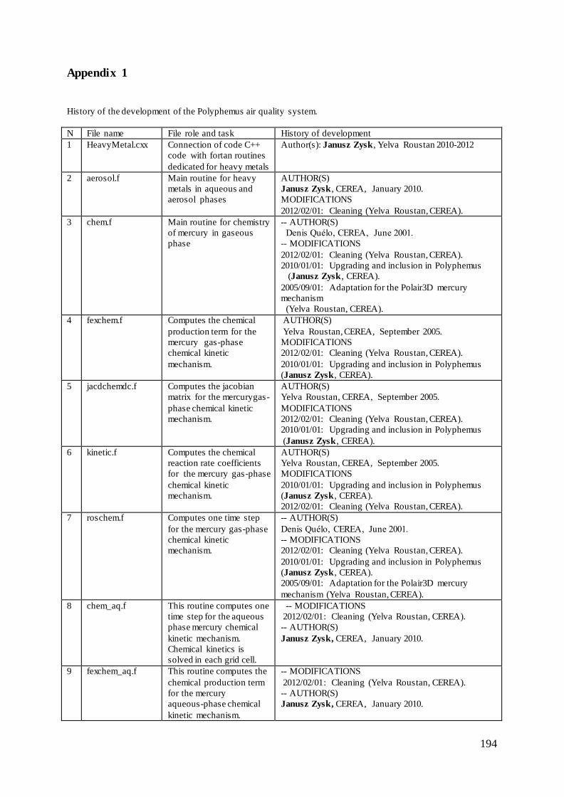
194
Appendix 1
History of the development of the Polyphemus air quality system.
N File name File role and task History of development
1 HeavyMetal.cxx Connection of code C++
code with fortan routines
dedicated for heavy metals
Author(s): Janusz Zysk, Yelva Roustan 2010-2012
2 aerosol.f Main routine for heavy
metals in aqueous and
aerosol phases
AUTHOR(S)
Janusz Zysk, CEREA, January 2010.
MODIFICATIONS
2012/02/01: Cleaning (Yelva Roustan, CEREA).
3 chem.f Main routine for chemistry
of mercury in gaseous
phase
-- AUTHOR(S)
Denis Quélo, CEREA, June 2001.
-- MODIFICATIONS
2012/02/01: Cleaning (Yelva Roustan, CEREA).
2010/01/01: Upgrading and inclusion in Polyphemus
(Janusz Zysk, CEREA).
2005/09/01: Adaptation for the Polair3D mercury
mechanism
(Yelva Roustan, CEREA).
4 fexchem.f Computes the chemical
production term for the
mercury gas-phase
chemical kinetic
mechanism.
AUTHOR(S)
Yelva Roustan, CEREA, September 2005.
MODIFICATIONS
2012/02/01: Cleaning (Yelva Roustan, CEREA).
2010/01/01: Upgrading and inclusion in Polyphemus
(Janusz Zysk, CEREA).
5 jacdchemdc.f Computes the jacobian
matrix for the mercurygas-
phase chemical kinetic
mechanism.
AUTHOR(S)
Yelva Roustan, CEREA, September 2005.
MODIFICATIONS
2012/02/01: Cleaning (Yelva Roustan, CEREA).
2010/01/01: Upgrading and inclusion in Polyphemus
(Janusz Zysk, CEREA).
6 kinetic.f Computes the chemical
reaction rate coefficients
for the mercury gas-phase
chemical kinetic
mechanism.
AUTHOR(S)
Yelva Roustan, CEREA, September 2005.
MODIFICATIONS
2010/01/01: Upgrading and inclusion in Polyphemus
(Janusz Zysk, CEREA).
2012/02/01: Cleaning (Yelva Roustan, CEREA).
7 roschem.f Computes one time step
for the mercury gas-phase
chemical kinetic
mechanism.
-- AUTHOR(S)
Denis Quélo, CEREA, June 2001.
-- MODIFICATIONS
2012/02/01: Cleaning (Yelva Roustan, CEREA).
2010/01/01: Upgrading and inclusion in Polyphemus
(Janusz Zysk, CEREA).
2005/09/01: Adaptation for the Polair3D mercury
mechanism (Yelva Roustan, CEREA).
8 chem_aq.f This routine computes one
time step for the aqueous
phase mercury chemical
kinetic mechanism.
Chemical kinetics is
solved in each grid cell.
-- MODIFICATIONS
2012/02/01: Cleaning (Yelva Roustan, CEREA).
-- AUTHOR(S)
Janusz Zysk, CEREA, January 2010.
9 fexchem_aq.f This routine computes the
chemical production term
for the mercury
aqueous-phase chemical
kinetic mechanism.
-- MODIFICATIONS
2012/02/01: Cleaning (Yelva Roustan, CEREA).
-- AUTHOR(S)
Janusz Zysk, CEREA, January 2010.
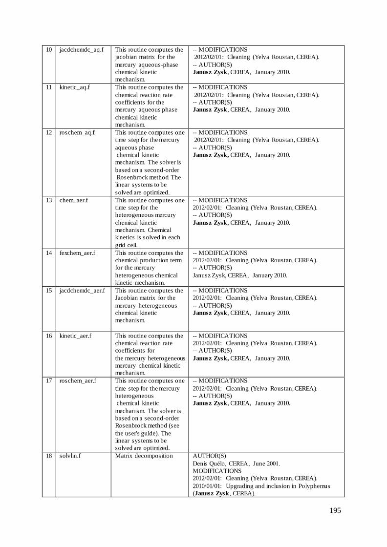
195
10 jacdchemdc_aq.f This routine computes the
jacobian matrix for the
mercury aqueous-phase
chemical kinetic
mechanism.
-- MODIFICATIONS
2012/02/01: Cleaning (Yelva Roustan, CEREA).
-- AUTHOR(S)
Janusz Zysk, CEREA, January 2010.
11 kinetic_aq.f This routine computes the
chemical reaction rate
coefficients for the
mercury aqueous phase
chemical kinetic
mechanism.
-- MODIFICATIONS
2012/02/01: Cleaning (Yelva Roustan, CEREA).
-- AUTHOR(S)
Janusz Zysk, CEREA, January 2010.
12 roschem_aq.f This routine computes one
time step for the mercury
aqueous phase
chemical kinetic
mechanism. The solver is
based on a second-order
Rosenbrock method The
linear systems to be
solved are optimized.
-- MODIFICATIONS
2012/02/01: Cleaning (Yelva Roustan, CEREA).
-- AUTHOR(S)
Janusz Zysk, CEREA, January 2010.
13 chem_aer.f This routine computes one
time step for the
heterogeneous mercury
chemical kinetic
mechanism. Chemical
kinetics is solved in each
grid cell.
-- MODIFICATIONS
2012/02/01: Cleaning (Yelva Roustan, CEREA).
-- AUTHOR(S)
Janusz Zysk, CEREA, January 2010.
14 fexchem_aer.f This routine computes the
chemical production term
for the mercury
heterogeneous chemical
kinetic mechanism.
-- MODIFICATIONS
2012/02/01: Cleaning (Yelva Roustan, CEREA).
-- AUTHOR(S)
Janusz Zysk, CEREA, January 2010.
15 jacdchemdc_aer.f This routine computes the
Jacobian matrix for the
mercury heterogeneous
chemical kinetic
mechanism.
-- MODIFICATIONS
2012/02/01: Cleaning (Yelva Roustan, CEREA).
-- AUTHOR(S)
Janusz Zysk, CEREA, January 2010.
16 kinetic_aer.f This routine computes the
chemical reaction rate
coefficients for
the mercury heterogeneous
mercury chemical kinetic
mechanism.
-- MODIFICATIONS
2012/02/01: Cleaning (Yelva Roustan, CEREA).
-- AUTHOR(S)
Janusz Zysk, CEREA, January 2010.
17 roschem_aer.f This routine computes one
time step for the mercury
heterogeneous
chemical kinetic
mechanism. The solver is
based on a second-order
Rosenbrock method (see
the user's guide). The
linear systems to be
solved are optimized.
-- MODIFICATIONS
2012/02/01: Cleaning (Yelva Roustan, CEREA).
-- AUTHOR(S)
Janusz Zysk, CEREA, January 2010.
18 solvlin.f Matrix decomposition AUTHOR(S)
Denis Quélo, CEREA, June 2001.
MODIFICATIONS
2012/02/01: Cleaning (Yelva Roustan, CEREA).
2010/01/01: Upgrading and inclusion in Polyphemus
(Janusz Zysk, CEREA).

196
2004/08/11: Adaptation for the Polair3D mercury
mechanism (Yelva Roustan, CEREA).
2001/11/05: Adaptation for the EMEP chemical
mechanism (Jaouad Boutahar, CEREA).
ACC CYFRONET AGH (PL-Grid Plus) is acknowledged for the computing time.