Embed Size (px)
Citation preview
ES11023
Examensarbete 30 hpDecember 2011
Modeling of the steam system in a BWR A model of Ringhals 1
Thomas Norberg

Teknisk- naturvetenskaplig fakultet UTH-enheten Besöksadress: Ångströmlaboratoriet Lägerhyddsvägen 1 Hus 4, Plan 0 Postadress: Box 536 751 21 Uppsala Telefon: 018 – 471 30 03 Telefax: 018 – 471 30 00 Hemsida: http://www.teknat.uu.se/student
Abstract
Modeling of the steam system in a BWR - A model ofRinghals 1
Thomas Norberg
A nuclear power plant is a very complex dynamic system with a lot of built inregulators and security systems that make it almost impossible to know by reasoning,exactly how the system dynamics is going to react due to e.g. plant modifications,transients or operator behaviors. A common way to find out is to build a computermodel and simulate the system. This master thesis is about building a dynamic modelof the steam system in the boiling water reactor Ringhals 1. The model has beendeveloped in the modeling-/simulating software Dymola and the components arewritten in the programming language Modelica. The model contains the most criticalcomponents in the steam system from reactor tank to condenser and also the mostimportant parts of the control systems.
The final model has been compared to real power plant data from Ringhals 1 for fullpower operation, reduced power and a turbine trip. During steady state conditionsthe model has good compliance with the available data in most positions of the steamsystem. Due to absence of good data the results of the dynamic verification for thedrop of load and turbine trip is incomplete. Instead the plausibility of the systembehavior has been done. The results are good but the magnitudes of the transientsare impossible to evaluate.
Two major weaknesses have been found during the verification of the model. Theyare the turbine behavior during off-design load and various transients, and the controlof the flow through the tube side of the reheater. The lack of mass flow data is alsomaking it hard to fully trust the model.
The final conclusion is that the steam system model is not ready to take on realproblems, but it is a good basis for further development and utilization. The abovementioned problems have to be looked further into and depending on the intendedusage of the model; it may be necessary to modify it to more exactly describe certainparts of the steam system.
ISSN: 1650-8300, ES11023Examinator: Kjell PernestålÄmnesgranskare: Michael ÖsterlundHandledare: Michael Nordström

Sammanfattning Ett kärnkraftverk är ett väldigt komplext dynamiskt system med mängder av regulatorer och
säkerhetssystem som gör det väldigt svårt att förutspå exakt vad följderna av en
anläggningsförändring, en transient eller ett operatörsingripande kommer att bli i de olika delarna av
systemet. För att undvika händelser som kan störa elproduktionen eller till och med tillfälligt avbryta
den så är det därför väldigt viktigt att man utreder detta innan man hamnar i en specifik situation. Ett
vanligt sätt att göra kvalificerade gissningar för olika händelseförlopp i ett avancerat system är
genom att modellera och simulera det. Därmed kan man redan i förväg utbilda operatörer för olika
händelsescenarion och innan en anläggningsändring utförs är det möjligt att testa dem i modeller
och se hur de påverkar systemet i stort och ifall man dimensionerat komponenterna rätt.
Det här examensarbetet går ut på att bygga en dynamisk modell över ångsystemet i
kokvattenreaktorn Ringhals 1. Målet är att modellera kärnkraftverket från reaktortank till kondensor
och sedan verifiera modellen mot verklig data hämtad från blockdatorn på Ringhals 1. Primärt ska
modellen verifieras mot ett fulldriftsfall men det ska också verifieras mot några av de vanligare
transienterna i ett ångsystem. Dessa är ett lastbortfall; då lasten på generatorn från det yttre nätet
plötsligt sjunker, samt ett turbinsnabbstopp; då all generering av elektricitet stoppas.
Modellen är uppbyggd i Dymola som är både ett textbaserat och grafisk modelleringsprogram.
Programmeringsspråket som modellerna är uppbyggda i är Modelica. Komponenterna är uppbyggda
var för sig och därefter sammankopplade till en större ångsystemmodell. Komponenterna som
används i ångsystemet är tagna ur Modelicas standardbibliotek och Solvinas egenutvecklade
SteamPower-bibliotek. Dessa modeller har sedan modifierats och vidareutvecklats för att fungera i
ångsystemet.
Den färdiga modellen verifierades först mot stabil fullflödesdrift och visade sig kunna beskriva det
verkliga systemet mycket väl. För tolv olika mätpunkter mellan reaktortank och kondensor så skiljer
sig trycket mellan simulering och mätning med maximalt ~1 %. För temperaturerna i systemet så är
motsvarande skillnad maximalt ~4 %, medan 11/12 mätpunkter skiljer sig mindre än 1 %. För fallet
med reducerad effekt är skillnaderna mellan modell och verklighet något större.
Vad gäller den dynamiska verifieringen så är resultaten ofullständiga. Tillgänglig data från Ringhals 1
är samplad med i bästa fall en minuts mellanrum och i många fall mer sällan. Förutom det så är
massflödena i de flesta delar av ångsystemet okända då vi lämnar det designade fullflödesfallet.
Detta gör det omöjligt att verifiera dynamiken i systemet. I stället har en analys av rimligheten i
ångsystemets och reglersystemets beteende gjorts för ett lastfrånslag och ett turbinsnabbstopp.
Resultatet av analysen är i huvudsak goda men det finns en del briser som måste åtgärdas och
storleken på transienterna är omöjliga att bedöma med tanke på bristen på data.
Under verifieringen av modellen har två större brister i modellen framkommit. Den ena är turbinens
beteende då den körs utanför dess nominella effekt samt dess beteende vid transienter, och det
andra är hur det varma flödet genom mellanöverhettarna styrs vid varierande driftfall.
Slutsatsen är att ångsystemmodellen inte är fullt redo att användas i ett skarpt projekt, men att det
är en bra basmodell som går att vidareutveckla efter behov. Det som behöver åtgärdas innan
användning är framför allt de två bristerna nämnda ovan samt att en kalibrering och verifiering av
modellens dynamik måste göras.

Table of Contests I. Nomenclature .................................................................................................................................. 1
II. List of figures ................................................................................................................................... 4
1 Introduction ..................................................................................................................................... 7
1.1 History of nuclear energy ........................................................................................................ 7
1.2 Background .............................................................................................................................. 7
1.3 Problem description ................................................................................................................ 8
1.4 Method .................................................................................................................................... 8
1.5 Delimitations ........................................................................................................................... 8
2 Power plant theory .......................................................................................................................... 9
2.1 Description of the steam system in Ringhals 1 ....................................................................... 9
2.1.1 Reaktor tank (system 211)............................................................................................. 10
2.1.2 Steam transporting system (system 411) ...................................................................... 11
2.1.3 Steam dump system (system 423) ................................................................................ 11
2.1.4 Main steam system (system 412) .................................................................................. 11
2.1.5 Condenser (system 413) ................................................................................................ 13
2.1.6 Control system in Ringhals 1 ......................................................................................... 13
3 Theory ............................................................................................................................................ 15
3.1 Fluid mechanics ..................................................................................................................... 15
3.2 Turbine theory ....................................................................................................................... 16
3.3 Control theory ....................................................................................................................... 18
3.4 Modeling and simulating with Modelica/Dymola ................................................................. 20
3.4.1 Modelica ........................................................................................................................ 20
3.4.2 Dymola ........................................................................................................................... 21
4 Modeling of the steam system ...................................................................................................... 23
4.1 General model structure ....................................................................................................... 23
4.2 Tank ....................................................................................................................................... 23
4.3 Boundary Flow ....................................................................................................................... 24
4.4 Reactor tank .......................................................................................................................... 24
4.5 Pipe ........................................................................................................................................ 25
4.6 Steam valve ........................................................................................................................... 26
4.7 Turbine .................................................................................................................................. 26
4.7.1 High pressure turbine .................................................................................................... 26
4.7.2 Low pressure turbine ..................................................................................................... 27
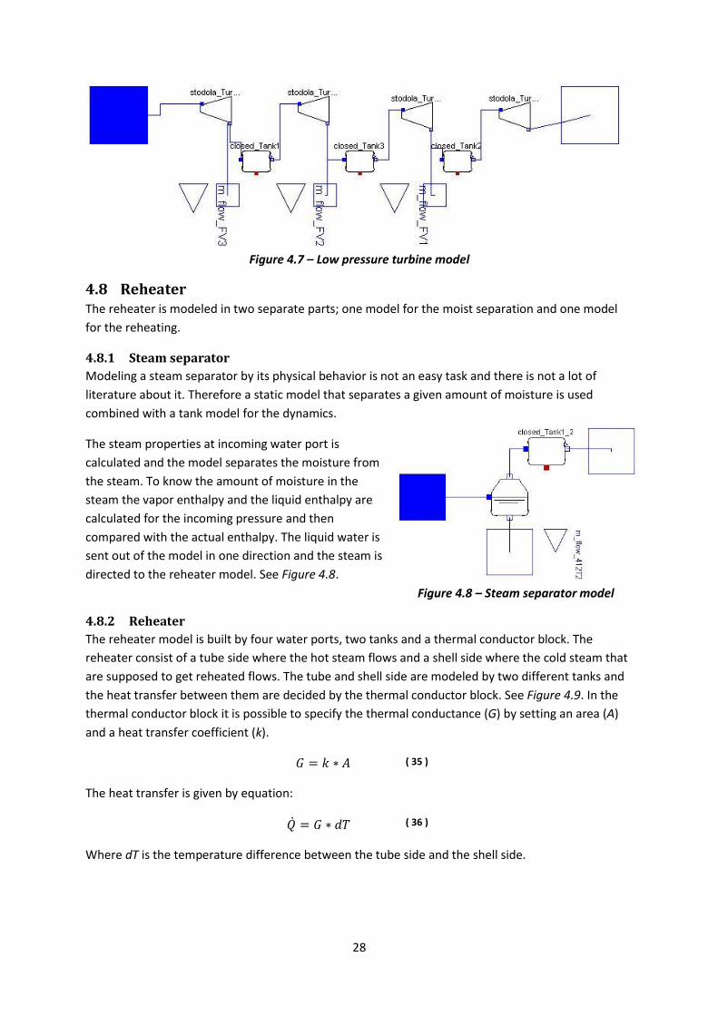
4.8 Reheater ................................................................................................................................ 28
4.8.1 Steam separator ............................................................................................................ 28
4.8.2 Reheater ........................................................................................................................ 28
4.9 Condenser ............................................................................................................................. 29
4.10 The steam system model....................................................................................................... 29
4.11 Modeling of a control system ................................................................................................ 32
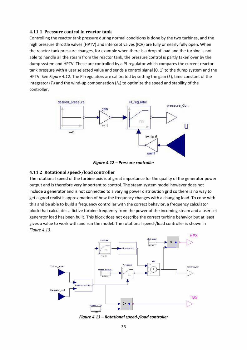
4.11.1 Pressure control in reactor tank .................................................................................... 33
4.11.2 Rotational speed-/load controller ................................................................................. 33
4.11.3 Controller for the warm reheater steam ....................................................................... 34
5 Results ........................................................................................................................................... 35
5.1 Full power .............................................................................................................................. 35
5.2 Reduced power ..................................................................................................................... 39
5.3 Turbine trip ............................................................................................................................ 46
6 Analysis and discussion of the results ........................................................................................... 49
6.1 Quality of data ....................................................................................................................... 49
6.2 Full power .............................................................................................................................. 49
6.3 Reduced power ..................................................................................................................... 50
6.4 Turbine trip ............................................................................................................................ 52
7 Conclusions .................................................................................................................................... 55
8 Future improvements .................................................................................................................... 57
References ............................................................................................................................................. 59
1
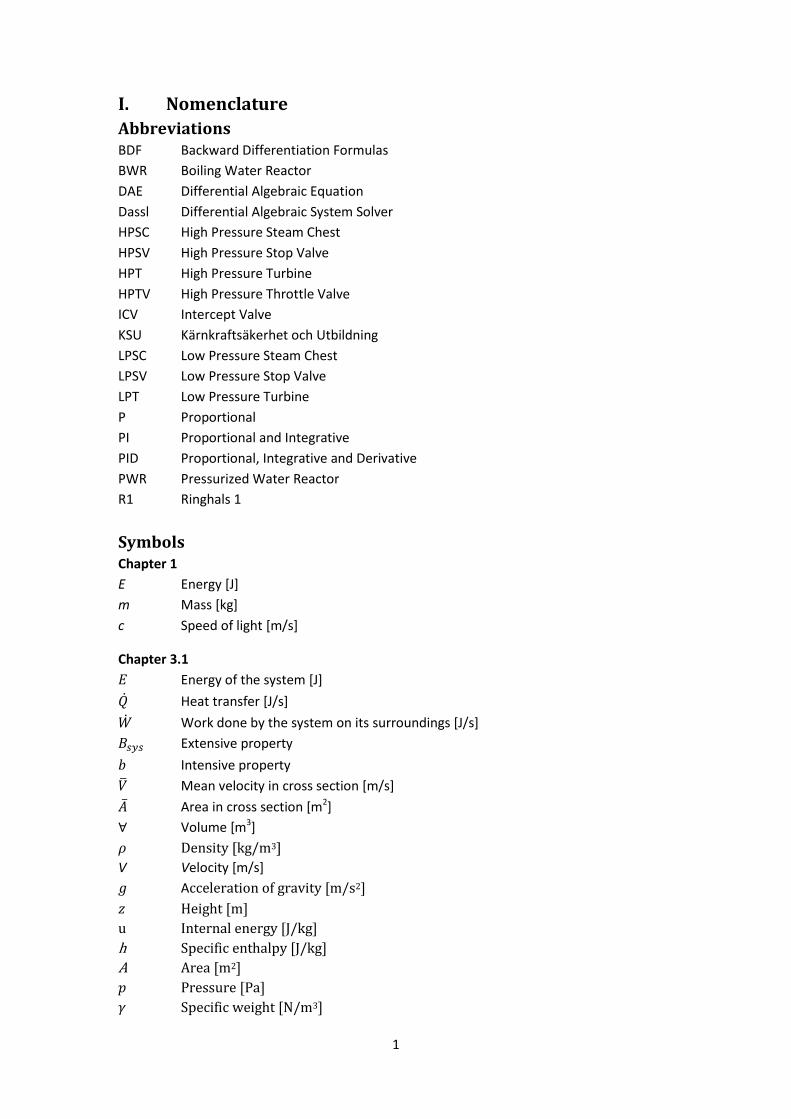
I. Nomenclature
Abbreviations BDF Backward Differentiation Formulas
BWR Boiling Water Reactor
DAE Differential Algebraic Equation
Dassl Differential Algebraic System Solver
HPSC High Pressure Steam Chest
HPSV High Pressure Stop Valve
HPT High Pressure Turbine
HPTV High Pressure Throttle Valve
ICV Intercept Valve
KSU Kärnkraftsäkerhet och Utbildning
LPSC Low Pressure Steam Chest
LPSV Low Pressure Stop Valve
LPT Low Pressure Turbine
P Proportional
PI Proportional and Integrative
PID Proportional, Integrative and Derivative
PWR Pressurized Water Reactor
R1 Ringhals 1
Symbols Chapter 1
E Energy [J]
m Mass [kg]
c Speed of light [m/s]
Chapter 3.1
Energy of the system [J]
Heat transfer [J/s]
Work done by the system on its surroundings [J/s]
Extensive property
Intensive property
Mean velocity in cross section [m/s]
Area in cross section [m2]
Volume [m3]
Density [kg/m3]
V Velocity [m/s]
Acceleration of gravity [m/s2]
Height [m]
u Internal energy [J/kg]
h Specific enthalpy [J/kg]
A Area [m2]
Pressure [Pa]
Specific weight [N/m3]
2
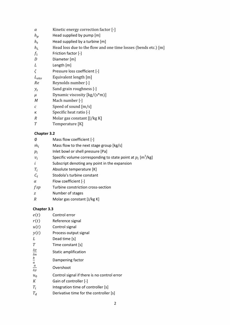
Kinetic energy correction factor [-]
Head supplied by pump [m]
Head supplied by a turbine [m]
Head loss due to the flow and one time losses (bends etc.) [m]
Friction factor [-]
Diameter [m]
Length [m]
Pressure loss coefficient [-]
Equivalent length [m]
Reynolds number [-]
Sand grain roughness [-]
Dynamic viscosity [kg/(s*m)]
Mach number [-]
Speed of sound [m/s]
Specific heat ratio [-]
Molar gas constant [J/kg K]
Temperature [K]
Chapter 3.2
Mass flow coefficient [-]
Mass flow to the next stage group [kg/s]
Inlet bowl or shell pressure [Pa]
Specific volume corresponding to state point at [m3/kg]
Subscript denoting any point in the expansion
Absolute temperature [K]
Stodola’s turbine constant
Flow coefficient [-]
Turbine constriction cross-section
Number of stages
Molar gas constant [J/kg K]
Chapter 3.3
Control error
Reference signal
Control signal
Process output signal
Dead time [s]
Time constant [s]
Static amplification
Dampening factor
Overshoot
Control signal if there is no control error
Gain of controller [-]
Integration time of controller [s]
Derivative time for the controller [s]
3
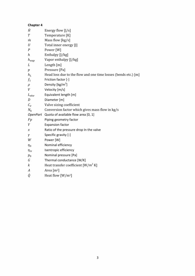
Chapter 4
Energy flow [J/s]
Temperature [K]
Mass flow [kg/s]
Total inner energy [J]
Power [W]
Enthalpy [J/kg]
Vapor enthalpy [J/kg]
Length [m]
Pressure [Pa]
Head loss due to the flow and one time losses (bends etc.) [m]
Friction factor [-]
Density [kg/m3]
Velocity [m/s]
Equivalent length [m]
Diameter [m]
Valve sizing coefficient
Conversion factor which gives mass flow in kg/s
OpenPart Quota of available flow area [0, 1]
Piping geometry factor
Expansion factor
Ratio of the pressure drop In the valve
Specific gravity [-]
Power [W]
Nominal efficiency
Isentropic efficiency
Nominal pressure [Pa]
Thermal conductance [W/K]
Heat transfer coefficient [W/m2 K]
Area [m2]
Heat flow [W/m2]
4
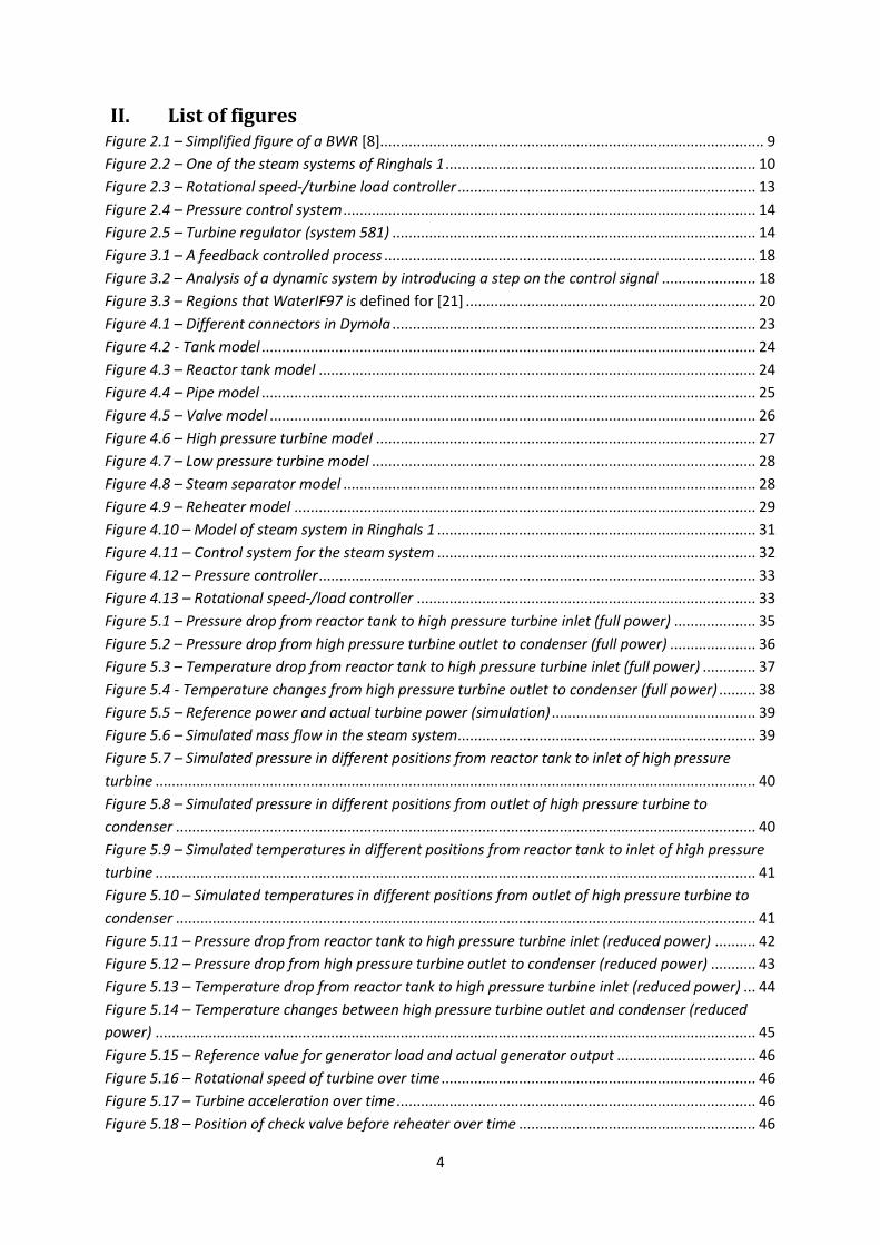
II. List of figures Figure 2.1 – Simplified figure of a BWR [8].............................................................................................. 9
Figure 2.2 – One of the steam systems of Ringhals 1 ............................................................................ 10
Figure 2.3 – Rotational speed-/turbine load controller ......................................................................... 13
Figure 2.4 – Pressure control system ..................................................................................................... 14
Figure 2.5 – Turbine regulator (system 581) ......................................................................................... 14
Figure 3.1 – A feedback controlled process ........................................................................................... 18
Figure 3.2 – Analysis of a dynamic system by introducing a step on the control signal ....................... 18
Figure 3.3 – Regions that WaterIF97 is defined for [21] ....................................................................... 20
Figure 4.1 – Different connectors in Dymola ......................................................................................... 23
Figure 4.2 - Tank model ......................................................................................................................... 24
Figure 4.3 – Reactor tank model ........................................................................................................... 24
Figure 4.4 – Pipe model ......................................................................................................................... 25
Figure 4.5 – Valve model ....................................................................................................................... 26
Figure 4.6 – High pressure turbine model ............................................................................................. 27
Figure 4.7 – Low pressure turbine model .............................................................................................. 28
Figure 4.8 – Steam separator model ..................................................................................................... 28
Figure 4.9 – Reheater model ................................................................................................................. 29
Figure 4.10 – Model of steam system in Ringhals 1 .............................................................................. 31
Figure 4.11 – Control system for the steam system .............................................................................. 32
Figure 4.12 – Pressure controller ........................................................................................................... 33
Figure 4.13 – Rotational speed-/load controller ................................................................................... 33
Figure 5.1 – Pressure drop from reactor tank to high pressure turbine inlet (full power) .................... 35
Figure 5.2 – Pressure drop from high pressure turbine outlet to condenser (full power) ..................... 36
Figure 5.3 – Temperature drop from reactor tank to high pressure turbine inlet (full power) ............. 37
Figure 5.4 - Temperature changes from high pressure turbine outlet to condenser (full power) ......... 38
Figure 5.5 – Reference power and actual turbine power (simulation) .................................................. 39
Figure 5.6 – Simulated mass flow in the steam system ......................................................................... 39
Figure 5.7 – Simulated pressure in different positions from reactor tank to inlet of high pressure
turbine ................................................................................................................................................... 40
Figure 5.8 – Simulated pressure in different positions from outlet of high pressure turbine to
condenser .............................................................................................................................................. 40
Figure 5.9 – Simulated temperatures in different positions from reactor tank to inlet of high pressure
turbine ................................................................................................................................................... 41
Figure 5.10 – Simulated temperatures in different positions from outlet of high pressure turbine to
condenser .............................................................................................................................................. 41
Figure 5.11 – Pressure drop from reactor tank to high pressure turbine inlet (reduced power) .......... 42
Figure 5.12 – Pressure drop from high pressure turbine outlet to condenser (reduced power) ........... 43
Figure 5.13 – Temperature drop from reactor tank to high pressure turbine inlet (reduced power) ... 44
Figure 5.14 – Temperature changes between high pressure turbine outlet and condenser (reduced
power) ................................................................................................................................................... 45
Figure 5.15 – Reference value for generator load and actual generator output .................................. 46
Figure 5.16 – Rotational speed of turbine over time ............................................................................. 46
Figure 5.17 – Turbine acceleration over time ........................................................................................ 46
Figure 5.18 – Position of check valve before reheater over time .......................................................... 46

5
Figure 5.19 – Position of HPTV over time .............................................................................................. 47
Figure 5.20 – Position of HPSV over time .............................................................................................. 47
Figure 5.21 – Pressure in the reactor tank during a turbine trip .......................................................... 47

6
7
1 Introduction
1.1 History of nuclear energy The knowledge about the large amount of energy stored in the atom has been known since the early
1900s. In 1905 Einstein developed his famous equation that says “energy equals mass
times the speed of light squared”, which describes the large amount of energy stored in an atom, but
it took almost thirty years until Enrico Fermi in 1934 discovered fission, which started the era of
nuclear power. In 1942 the first self-supporting nuclear reaction was created. In the beginning most
of the nuclear research was made for military use which in 1945 ended up in the two nuclear bombs
being dropped over Hiroshima and Nagasaki. After the second world war ended a lot of research was
focused on how the nuclear power could be used in the civil society and in 1956 the first large scale
commercial nuclear power plant was started in Sellafield, England and it had a power output of
approximately 50 MWe. [1], [2]
In the 60s, 70s and 80s the number of nuclear power plants in the world increased rapidly. In the late
80s there were over 400 running nuclear power plants in the world [3]. During the 60s and 70s there
was no big focus on nuclear safety but after the accident in Harrisburg in 1979 and especially after
the Tjernobyl accident 1986 strong voices were raised and the power plant expansion slowed down.
The Swedish nuclear power program started in the beginning of the 50s and was in the beginning
focused on producing an atom bomb. This plan was abandoned in 1968. [4] The first nuclear power
plant for electricity and district heating started in Ågesta, Stockholm in 1963 and had a power output
of 65 MW. The first large scale nuclear power plant was Oskarshamn 1 which became operational in
1972 and delivered 450 MWe. The following thirteen years eleven more plants were built; two in
Oskarshamn , two in Barsebäck, four in Ringhals and three in Forsmark. [5], [6]
After the Harrisburg accident the Swedish opinion for nuclear power changed rapidly and in 1980 a
referendum about the future of nuclear power was held and the result was that all the nuclear
power plants that already were planed should be finished, but they should all be closed down before
2010. From here on the Swedish nuclear power industry went into hibernation and not many new
investments were made. Today the two power plants in Barsebäck are the only ones that have been
closed down and the remaining ten reactors are running and have the capacity to deliver ~9400 MWe
[7]. Today the future of nuclear power in Sweden looks much brighter and since the ban of building
new nuclear power plants was lifted in 2009 there is a discussion about replacing the old plants.
All over the world the nuclear power plant industry has had a huge upswing during the 2000s. This
has much to do with the recent environmental debate about lowering the carbon dioxide footprint
and minimizing the pollution. Today there are about 432 commercial nuclear power plants in the
world, divided on 30 countries. The total power output is about 368 000 MWe and stands for
approximately 14 % of the total electricity production in the world. Today there are also 63 nuclear
power plants under construction (64 000 MWe) and about 152 that are planned (171 000 MWe), most
of them in Asia. [7]
1.2 Background A nuclear power plant is a very complex dynamic system with a lot of built-in regulators and security
systems that makes it almost impossible to know by reasoning, exactly what is going to happen due
to plant changes, different transients in the system or operator behaviors. To avoid disruptions and
8
downtime in the power production it is therefore very important to find the answer to that before
making any untested changes in the system. A very common way of making qualified predictions of
the system behavior during different operational conditions in a nuclear power plant is by building a
model that is able to simulate the system. If you have a model that can describe the real system you
can do tests without the risk of disrupting the power generation and harming components. These
kinds of models are also a very important tool in the education of operators.
1.3 Problem description This master thesis is about building a dynamic model of the steam system in the boiling water
reactor, Ringhals 1. The goal is to model the power plant and its control system from reactor tank to
condenser and then verify the model against real operating data.
The model will primarily be built to work for full power conditions but will also be able to describe
common transient in a satisfactorily way. A transient that occur quite frequently in the steam system
of a nuclear power plant is a drop in load. Another is a turbine trip where all ability of power
generation is lost. The model will be tested against both these events.
1.4 Method The approach of the problem is divided into three different parts:
1. Gathering of information:
Information about the steam system of Ringhals 1 is gathered through different system
descriptions from the nuclear power plant. Also useful theory like fluid mechanics, thermo-
dynamics and control theory are studied.
2. Modeling:
The modeling is made by a modeling-/simulating program called Dymola which uses the
programming language Modelica. Existing models and components from the Solvina
developed SteamPower-library is studied and then modified to fit for the steam system
purposes. Finally the components are connected to a steam system model and a control
system is added.
3. Calibration and verification
Real power plant data is taken from the Ringhals 1 nuclear power plant. The model is
calibrated against full power conditions and then compared to data from a drop of load and a
turbine trip.
1.5 Delimitations The steam system in a nuclear power plant is a very large and complex system. To be able to model
the system during the given time frame a few delimitations has been done. They are:
Only one of the two steam systems in Ringhals 1 is modeled. All interaction that normally
occurs between the two steam systems is omitted.
Most safety systems and all auxiliary systems are excluded.
Systems are simplified or excluded from the steam system model.
The control system does only have the most common features and do not handle e.g.
startup conditions.
9
2 Power plant theory There are a lot of different nuclear power plant designs operational in the world today. The most
common are the light water reactors with around 85 % of the market. There are basically two light
water reactor models that are used today; the pressurized water reactor (PWR) with around 60 % of
the market and the boiling water reactor (BWR) with around 21 % of the market. Sweden with its ten
reactors has seven BWRs and three PWRs. This thesis is about the steam system in a BWR (Ringhals
1) so no further discussion of the PWR is made. [8]
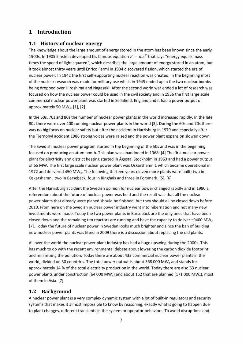
In a BWR the steam is created in the reactor tank by the heat created by nuclear fission. The steam is
then lead to the steam system where the thermal energy of the steam is converted to kinetic energy
in the turbines, which is transformed to electricity in the generator. After the turbines the steam is
condensed in the condenser. From the bottom of the condenser the water is directed into the
reheater-/feed water system where the temperature and pressure are raised to finally be injected
into the reactor tank. See Figure 2.1.
Figure 2.1 – Simplified figure of a BWR [8]
2.1 Description of the steam system in Ringhals 1 The theory and data presented in this section is solely based upon the information from Ringhals and
KSU (Kärnkraftsäkerhet och Utbildning AB) documentation [9], [10], [11], [12], [13] and [14].
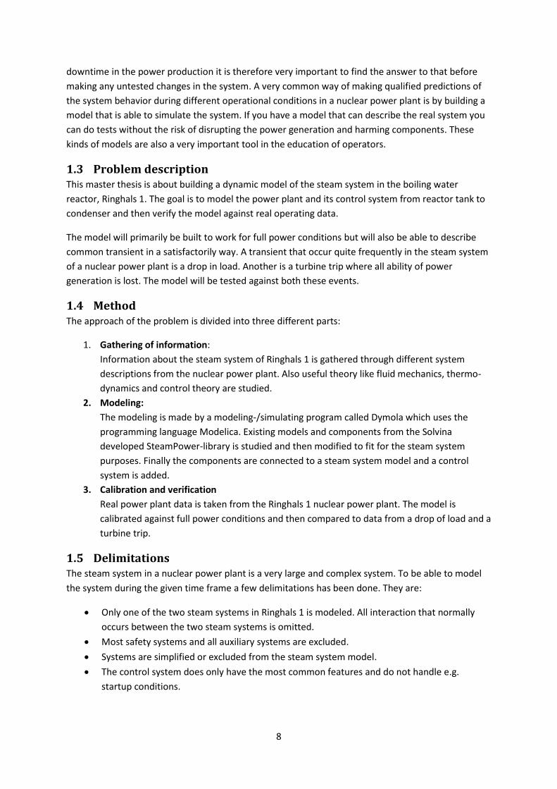
The steam system in a BWR is a complex system containing many components and sub systems. The
main components are the
Reactor tank
Main pipes from reactor to high pressure turbine
10
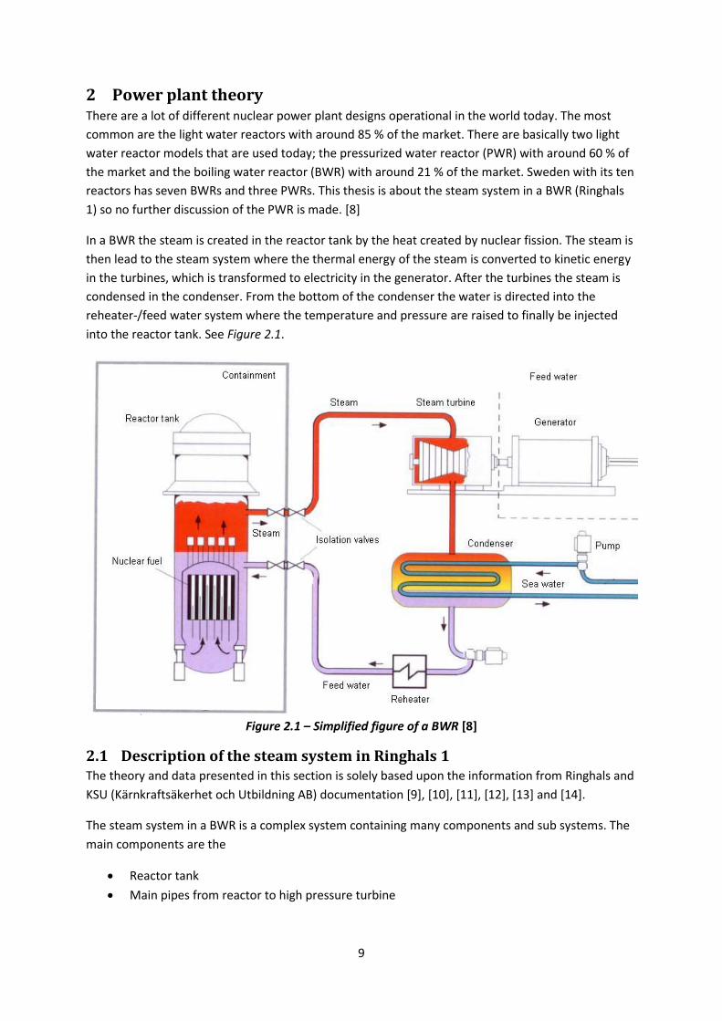
High pressure steam chest containing two high pressure stop valves (HPSV) and four high
pressure throttle valves (HPTV)
High pressure turbine (HPT)
Reheater
Low pressure steam chest containing two low pressure stop valves (LPSV) and two intercept
valves (ICV)
Three Low pressure turbines (LPT)
Condenser
which are shown in Figure 2.2. The figure shows one of the two equivalent steam systems that are
connected to the reactor tank.
Figure 2.2 – One of the steam systems of Ringhals 1
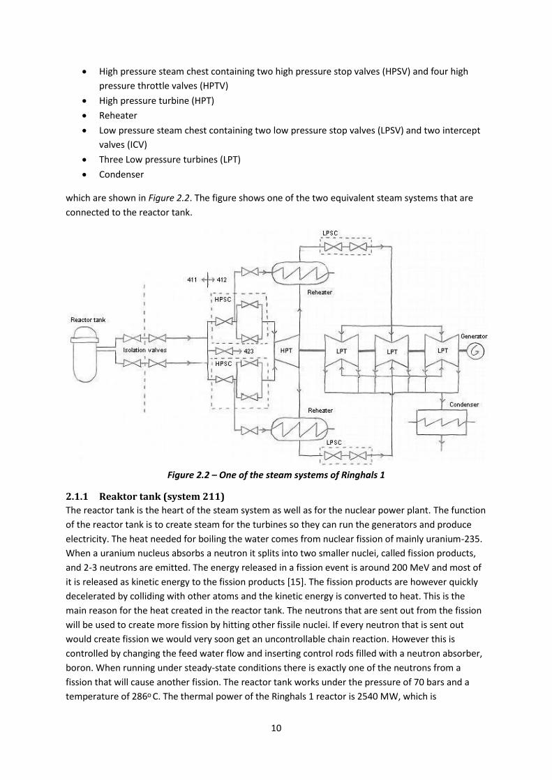
2.1.1 Reaktor tank (system 211)
The reactor tank is the heart of the steam system as well as for the nuclear power plant. The function
of the reactor tank is to create steam for the turbines so they can run the generators and produce
electricity. The heat needed for boiling the water comes from nuclear fission of mainly uranium-235.
When a uranium nucleus absorbs a neutron it splits into two smaller nuclei, called fission products,
and 2-3 neutrons are emitted. The energy released in a fission event is around 200 MeV and most of
it is released as kinetic energy to the fission products [15]. The fission products are however quickly
decelerated by colliding with other atoms and the kinetic energy is converted to heat. This is the
main reason for the heat created in the reactor tank. The neutrons that are sent out from the fission
will be used to create more fission by hitting other fissile nuclei. If every neutron that is sent out
would create fission we would very soon get an uncontrollable chain reaction. However this is
controlled by changing the feed water flow and inserting control rods filled with a neutron absorber,
boron. When running under steady-state conditions there is exactly one of the neutrons from a
fission that will cause another fission. The reactor tank works under the pressure of 70 bars and a
temperature of 286ᵒC. The thermal power of the Ringhals 1 reactor is 2540 MW, which is
11
transformed into approximately 900 MW of electricity. The amount of steam leaving the reactor tank
is approximately 1256 kg/s divided on two identical steam systems/turbine systems.
2.1.2 Steam transporting system (system 411)
When the steam leaves the reactor tank it enters the steam transporting system. Its main function is
to transport the steam from the reactor tank to the main steam system (system 412) and the steam
dump system (system 423).
The steam leaves the reactor tank through eight pipes that are merged to four before leaving the
reactor containment. At the lead-through out of the containment wall there are two safety stop
valves at each pipe; one inside the containment and one just outside. These have the function to
quickly close down and isolate the containment in the event of an accident or error in the reactor
tank or the steam system. The four pipes are then divided on both turbine systems; two to each one.
After leaving the containment the pressure is normally around 67.5 bar and the steam temperature
around 283ᵒC.
The steam transporting system also has a lot of other functions, e.g., supplying the pressure relief
system (system 314) that for some operating conditions has the function to control the reactor tank
pressure. It also has the function to transport steam to other safety systems. [11]
2.1.3 Steam dump system (system 423)
Before the steam reaches the turbines there is a possibility to bypass the turbine and send it directly
to the condenser via the steam dump system. This function is mainly used in the startup and
shutdown of the turbines but also when the turbines will not be able to keep the reactor tank
pressure at a constant level. This often happens when there are transients in the steam system for
example when there is a drop in load or a turbine safety stop.
2.1.4 Main steam system (system 412)
The main steam system starts just before the high pressure steam chest and contains the whole main
turbine systems and has the function to convert the heat energy of the steam to kinetic energy,
which is then transformed to electricity in the generator. In addition, the system includes stop valves,
throttle valves, reheaters and other components that are not of importance in this work.
2.1.4.1 High pressure steam chest (HPSC)
The high pressure steam chest is the first component of the main steam system. Each steam system
has two of them, one for each pipe from the reactor, and they each contain one high pressure stop
valve (HPSV) and two high pressure throttle valves (HPTV).
The main function of the HPSV is to shut down the steam flow to the turbines in case of for example
a grid failure or too high turbine frequency. This is done to protect the turbines. In case of an error in
the steam system the HPSV closes in 0.2 s. In the startup phase of the turbines the HPSV also has the
task of controlling the steam flow to the turbine until the rotational speed reaches 3000 rpm. This is
done to lower the heat stress on the components downstream the HPSV. These valves are fully open
under normal plant conditions.
The main function of the HPTV is to handle the steam control to the turbine during normal operating
conditions. They also work as a backup system for the HPSV in case of an error. The HPTV are nearly
fully open during full power conditions.
12
2.1.4.2 High pressure turbine (HPT)
Ringhals 1 has two identical turbine systems. Each turbine system are built up by one high pressure
turbine and three low pressure turbines on a single axis shared with the generator. The rotational
speed of the turbine is 3000 rpm and the maximum power output is around 450 MW for each
turbine system. Around 15 MW of it is used for in-house purposes.
The high pressure turbine is an action turbine and the steam expands parallel to the axis in one
direction from the steam inlet. The HPT consists of six different turbine stages with a small extraction
of steam after the fifth stage which is used in the high pressure reheater to heat feed water to the
reactor. The inlet pressure and temperature is usually around 63 bar and 278ᵒC and it drops to
around 11.5 bar and 185ᵒC to the outlet. Around 1/3 of the total power output comes from the HPT.
2.1.4.3 Reheater
When the steam leaves the high pressure turbine it contains of around 14 % moisture and has to go
through a reheater with moisture separation in order to avoid corrosion on the blades in the low
pressure turbine. There are two reheaters for each turbine system.
The moisture separator is in the lower part of the reheater, where also the steam enters. It consists
of a layer of demister panels which is a compact grid of stainless steel which makes the moisture
condense. The condensate is then transported to the separator drain tank (412T2). After leaving the
moisture separation part of the reheater the steam is almost dry (~0.1 % moisture).
The reheater part consists of vertical U-tubes where hot steam flows on the tube side and the cold
reheat steam floats on the shell side. The hot steam used for reheating is taken from the steam chest
just after the high pressure stop valve and is available as soon as the stop valves are open. However
under startup conditions when the system is cold there is a throttle valve on each feed line to lower
the heat stress in the reheater. There is also a check valve that prevents the flow of going backwards.
Under normal conditions the hot steam flow is about 23 kg/s in each reheater. The cold reheat steam
has a temperature of around 185ᵒC when it enters the reheater and after getting reheated the
temperature is around 250ᵒC. The pressure drop in the reheater is relatively small (<0.1 bar). The
reheater steam outlet leads into the low pressure steam chest.
2.1.4.4 Low pressure steam chest (LPSC)
After the reheater the steam enters the low pressure steam chest, which contains a low pressure
safety valve (LPSV) and an intercept valve (ICV).
The LPSV has the same main purpose as the HPSV; to protect the turbine in case of error by shutting
down the reheated steam flow to the low pressure turbine. This valve is not as fast as the HPTV, but
closes in about 0.75 seconds. This valve has in contrast to the HPTV no controlling task in the startup
of the turbine.
The ICV is like the HPTV a controlling valve, but it controls the steam flow from the reheater to the
low pressure turbine. The ICV and HPTV are controlled by signals from the “ordered steam flow”-
control system and a feed forward control. During normal power plant conditions the ICV is fully
open. Like the HPTV, the ICV is also a back-up stop valve in case of a turbine error.
13
2.1.4.5 Low pressure turbine (LPT)
The low pressure turbine is a reaction turbine and is constructed so that the steam enters the turbine
in the middle and is then expanded along the axis in both directions. It is constructed like this to
reduce the mechanical load on the turbine axis. Each LPT consist of eight turbine steps in each
direction and after step three, six and seven there are steam extractions, which leads to the low
pressure reheaters in the feed water system. The outlet of each turbine is directly connected to the
condenser. Inlet pressure is around 10-11 bar and the temperature is around 250ᵒC. When leaving
the LPT the steam pressure has dropped to around 0.04 bar and the temperature to 29ᵒC. The steam
then contains about 11 % of moisture. The LPT delivers around 2/3 of the total power output.
2.1.5 Condenser (system 413)
The condenser is located directly under the low pressure turbines and is built up by a large amount of
sea water cooled tubes. When the steam come in contact with these pipes it condenses and flow to
the reheater-/feed water system. To keep a low pressure in the condenser incondensable gases are
constantly sucked out by ejectors. The pressure during normal operating conditions is around 0.04
bar.
2.1.6 Control system in Ringhals 1
In order to maintain stable operating conditions and avoid disruptions in the power generation or
even downtime, an advanced control system is needed. In Ringhals 1 the control systems that is
responsible for the steam systems well-being is regulated by the electrical turbine regulator (system
581). The functions of the system are:
Pressure control of reactor tank
Rotational speed control of the turbines
Turbine load control
Testing and monitoring
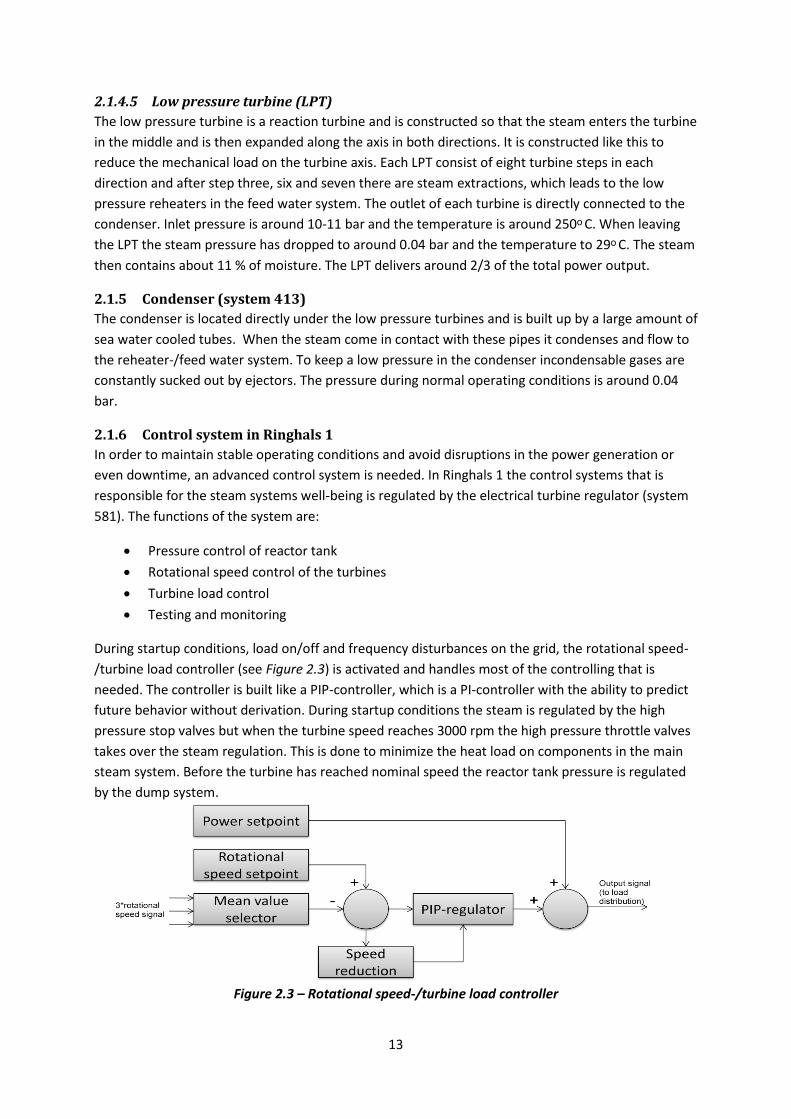
During startup conditions, load on/off and frequency disturbances on the grid, the rotational speed-
/turbine load controller (see Figure 2.3) is activated and handles most of the controlling that is
needed. The controller is built like a PIP-controller, which is a PI-controller with the ability to predict
future behavior without derivation. During startup conditions the steam is regulated by the high
pressure stop valves but when the turbine speed reaches 3000 rpm the high pressure throttle valves
takes over the steam regulation. This is done to minimize the heat load on components in the main
steam system. Before the turbine has reached nominal speed the reactor tank pressure is regulated
by the dump system.
Figure 2.3 – Rotational speed-/turbine load controller
14
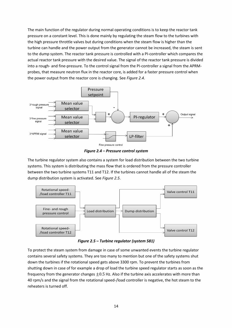
The main function of the regulator during normal operating conditions is to keep the reactor tank
pressure on a constant level. This is done mainly by regulating the steam flow to the turbines with
the high pressure throttle valves but during conditions when the steam flow is higher than the
turbine can handle and the power output from the generator cannot be increased, the steam is sent
to the dump system. The reactor tank pressure is controlled with a PI-controller which compares the
actual reactor tank pressure with the desired value. The signal of the reactor tank pressure is divided
into a rough- and fine-pressure. To the control signal from the PI-controller a signal from the APRM-
probes, that measure neutron flux in the reactor core, is added for a faster pressure control when
the power output from the reactor core is changing. See Figure 2.4.
Figure 2.4 – Pressure control system
The turbine regulator system also contains a system for load distribution between the two turbine
systems. This system is distributing the mass flow that is ordered from the pressure controller
between the two turbine systems T11 and T12. If the turbines cannot handle all of the steam the
dump distribution system is activated. See Figure 2.5.
Figure 2.5 – Turbine regulator (system 581)
To protect the steam system from damage in case of some unwanted events the turbine regulator
contains several safety systems. They are too many to mention but one of the safety systems shut
down the turbines if the rotational speed gets above 3300 rpm. To prevent the turbines from
shutting down in case of for example a drop of load the turbine speed regulator starts as soon as the
frequency from the generator changes Hz. Also if the turbine axis accelerates with more than
40 rpm/s and the signal from the rotational speed-/load controller is negative, the hot steam to the
reheaters is turned off.
15
3 Theory
3.1 Fluid mechanics The term “fluid” is an umbrella term for gases, liquids and plasmas. Fluid mechanics is the branch of
physics concerned with fluids and the forces that work on them in both rest and motion. In this
thesis, fluids in motion are of greatest interest.
The variables that describe the state of a fluid in motion are velocity, pressure, temperature and
density. The relationships between these variables are derived from equations for conservation of
mass, momentum and energy and the ideal gas law. [16]
Conservation of energy ( 1 ) is the first law of thermodynamics and it state that the total energy of a
system remains constant over time. [16]
( 1 )
Where
= energy of the system [J]
= heat transfer [J/s]
= Work done by the system on its surroundings [J/s]
To describe a fluid in motion the control volume approach is often used. This approach focuses on a
specific volume and the flow through it and when applying it the Reynolds transport theorem ( 2 ) is
a very frequently used tool. [16]
( 2 )
where is an extensive property and b is an intensive property
By using Reynolds transport theorem on the conservation of energy equation ( 1 ) one get the energy
principle [16]:
( 3 )
If it is assumed that the flow through the control volume is adiabatic and there is a steady flow
( ) one obtains the energy equation [16]:
( 4 )
where
= head supplied by pump [m]
= head supplied by a turbine [m]
= head loss due to the flow and one time losses (bends etc.) [m]
= kinetic energy correction factor [-]
16
If we also assume a uniform velocity distribution (which is approximately true when turbulent flow),
no shaft work ( ) and no pressure loss due to height differences we get the equation [16]:
( 5 )
where
( 6 )
( 7 )
The friction factor, , is a function of Reynolds number, the equivalent sand grain roughness ( ) and
the pipe diameter (D) [16]:
( 8 )
( 9 )
For Reynolds numbers less than 2300 one can generally say that the flow is laminar and for numbers
over 2300 the flow is turbulent. This is however no fixed limit. The flow can be laminar for Reynolds
numbers far greater than 2000 and turbulent for numbers under 2300, but the probability is much
smaller and the flow will often be very unstable. [16]
For gases, which of course are much more compressible than fluids, the Mach number is of great
importance and is defined as [16]:
( 10 )
( 11 )
where:
= Mach number
= speed of sound
= specific heat ratio
= molar gas constant
If the Mach number is small the fluid can be considered as incompressible. A commonly used limit for
when to start to consider the fluid as compressible is at Mach number 0.3. [16] The speed of sound is
the velocity at which a pressure wave propagates through a fluid.
3.2 Turbine theory Historically when modeling the pressure drop in different turbine steps in a multi-step turbine a
theory called “Constant Flow Coefficient” has often been used. The theory is based on a long known
relationship that says that for a turbine where the steam can expand freely, a pressure-flow relation
in a specific point can be approximated with the equation [17]:
17
( 12 )
where:
= mass flow coefficient
= mass flow to the next stage group [kg/s]
= inlet bowl or shell pressure [Pa]
= specific volume corresponding to state point at [m3/kg]
= subscript denoting any point in the expansion
If it is assumed that steam entering the turbine behaves like an ideal gas one obtains the equation
[17]:
( 13 )
where
= absolute temperature
The expansion in a turbine is approximately adiabatic, i.e. the heat exchange with the surroundings is
zero, which by this theory would mean that the relation between pressure and flow is approximately
linear. This theory is however very simplified and contains a lot of errors. However, in 1927 the
physicist Aurel Stodola empirically found a relationship for how the flow through a multi stage
turbine behaves and stated that [17]:
( 14 )
which is known as the Stodola’s Ellipse.
By introducing a constant in equation ( 14 ) and combining it with equation ( 13 ) one get [17]:
( 15 )
which is called Stodola´s turbine equation and is Stodola’s turbine constant, which is a measure of
the effective flow area through the turbine derived from this expression:
( 16 )
where:
= flow coefficient
= turbine constriction cross-section
= number of stages
= molar gas constant.
18
3.3 Control theory Control systems are today used in every process industry. The tougher competition and harder
environmental requirements have forced industries to automate and optimize their systems with
different control systems, which can handle the process in a much better and more efficient way
than the human personnel. With control systems it is also possible to control processes or events
that are too complex or/and too fast for a human to handle and in that way avoid disruptions in the
power generation in for example a fast transient.
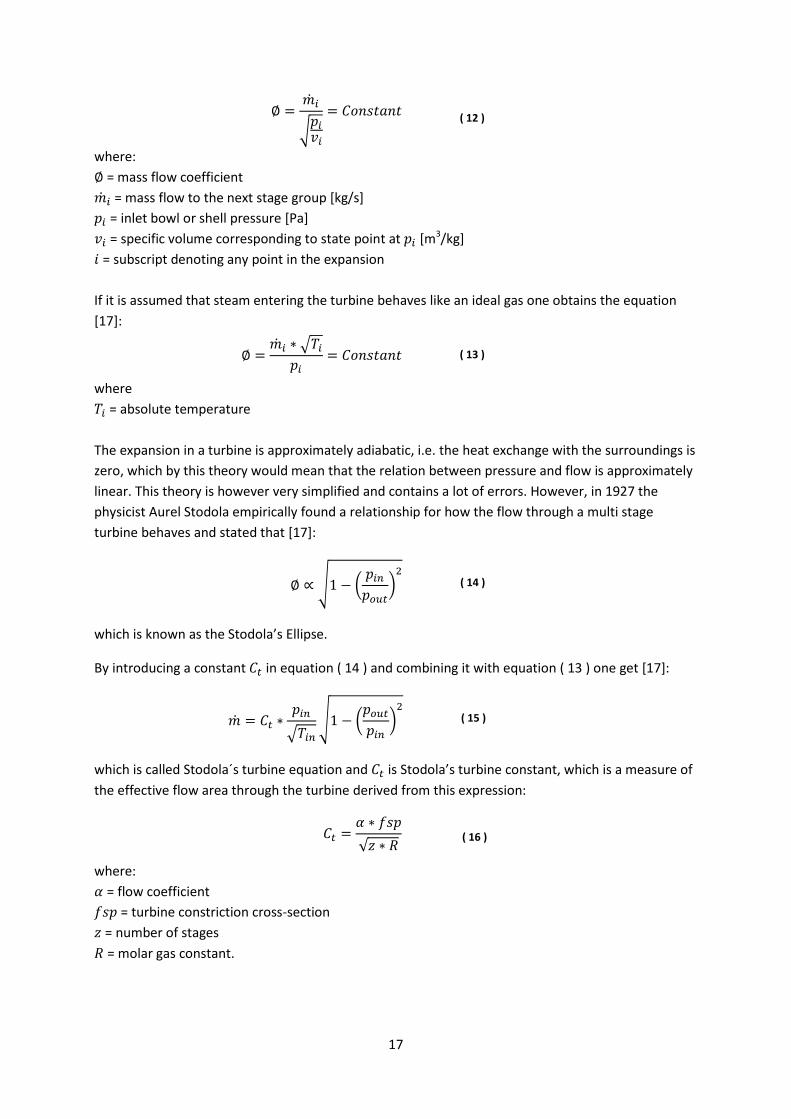
A very common regulator structure is that of feedback control. A reference signal r(t) is sent into the
controller and compared to the process output signal y(t) that you want to control. Depending on the
control error
( 17 )
a control signal is calculated and sent to the process that you want to control. [18] See Figure 3.1
Figure 3.1 – A feedback controlled process
To build a good controller it is not enough to know the process output signal and reference value.
You also need to know the dynamics of the process that you want to control, i.e. how the control
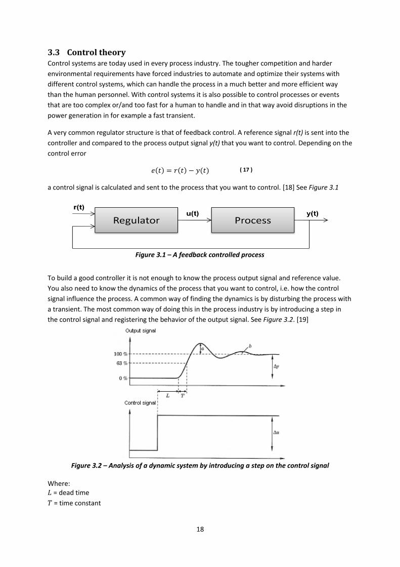
signal influence the process. A common way of finding the dynamics is by disturbing the process with
a transient. The most common way of doing this in the process industry is by introducing a step in
the control signal and registering the behavior of the output signal. See Figure 3.2. [19]
Figure 3.2 – Analysis of a dynamic system by introducing a step on the control signal
Where: = dead time
= time constant
19
= static amplification
= dampening factor
= overshoot.
When the process dynamics is known it is time to choose a suitable controller and give it the proper
control settings. The most common regulator in the industry is the PID-controller. [19] The PID-
controller is a relatively simple controller and it is relatively simple to tune. Another advantage is that
it is cheap compared to the more complex controllers. These advantages have led to that the
industry often use a lot of PID-controllers instead of a few more advance ones. The PID-controller is a
combination of a P-, I- and a D-controller. The P stands for proportional and means that the control
signal is proportional against the control error. According to [19] the equation for the P-controller is
( 18 )
Where is the control signal if there is no control error and is the gain of the controller. The P-
controller will minimize the control error but due to its structure it will not eliminate it. A bigger
will give a smaller control error and a faster system. However when K gets bigger the risk of stability
issues in the model increases.
The I stands for integrating and mean that the control signal is proportional to the integral of the
control error. According to [19] the mathematical structure of the I-controller is
( 19 )
where is the integration time of the controller. In contrast to a P-controller the I-controller is able
to eliminate the control error. The combination of the P- and I-controller to a PI-controller is one of
the most used controllers in process industries today. According to [19] the structure of the PI-
controller is
( 20 )
The D stands for derivative and means that the control signal is proportional to the derivative of the
control error e(t). According to [19] the structure of the D-controller is
( 21 )
where is the derivative time for the controller. The D-controller can by derivation see how the
control error will be in a close future and therefore compensate for that before it happens. The
derivative part stabilizes the PID-controller, but it in some cases, for example when there is much
noise in the signals and when we have large delays in the system, the derivative part will work
against its purpose. Therefore the D-controller part is often omitted in the PID-controller. According
to [19] the mathematical structure of the PID-controller is
( 22 )
20
3.4 Modeling and simulating with Modelica/Dymola The components used in the steam system model are all based on the programming language
Modelica and are built in the modeling program Dymola.
3.4.1 Modelica
Modelica is a non-proprietary, object-oriented, equation-based programming language developed by
the non-profit Modelica Association. The main objective of the language is to be able to model
complex physical systems in a wide range of engineering fields and then be able to reuse and
combine small models/components to bigger ones. [20]
The models are in general not built by algorithms as in traditional programming, but by differential,
algebraic equations (DAE) that describe the physical behavior of the model. These equations are not
solved in any predefined order but are solved based on what information the solver has access to.
This means that the solver can, and often do, manipulate the equations during the simulation so that
it can solve for the desired variables. This is also the main reason to why the models are easy to
reuse and combine with other models to bigger systems. [20]
Modelica Association is also responsible for developing the free Modelica Standard Library, which is a
library of models, components, equations ready to use in your own modeling. The library also
contains a media package which has been of great importance for this master thesis.
3.4.1.1 Media package
The media package contains interface definitions and property models for a wide range of fluids, for
example ideal gases, water models, air models etc. These media packages are possible to import into
your model and together with the correct physical equations simulate the behavior of different
media in a component or system, for example how the pressure changes when steam is expanded in
a turbine model.
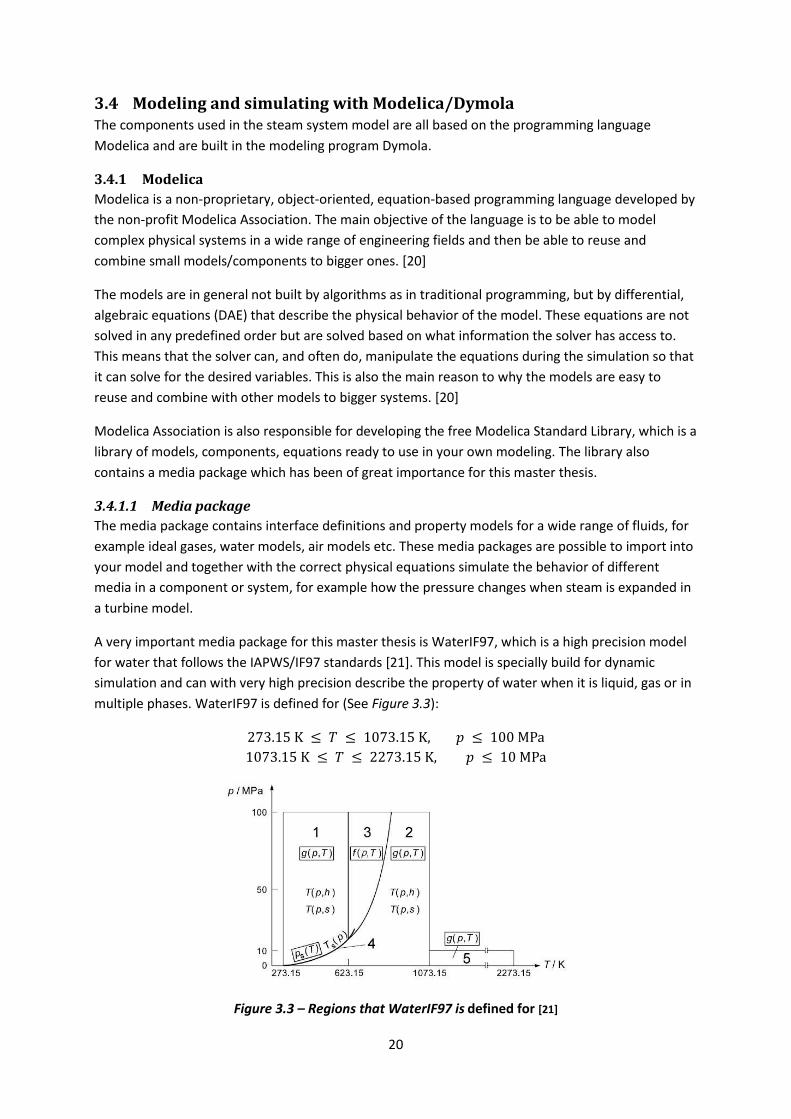
A very important media package for this master thesis is WaterIF97, which is a high precision model
for water that follows the IAPWS/IF97 standards [21]. This model is specially build for dynamic
simulation and can with very high precision describe the property of water when it is liquid, gas or in
multiple phases. WaterIF97 is defined for (See Figure 3.3):
Figure 3.3 – Regions that WaterIF97 is defined for [21]
21
Where region 1 is liquid water, region 2 is steam, region 3 is supercritical steam, region 4 is in two
phase and region 5 is high temperature steam.
3.4.1.2 Steam Power Library
The Steam Power Library is a Modelica library developed by the company Solvina AB and consists of a
series of models and components in the areas regarding fluid mechanics and thermodynamics. These
models are the base for this master thesis.
3.4.2 Dymola
Dymola is a commercial environment for modeling and simulating with Modelica code and is
developed by the Swedish company Dassault Systèmes AB. Neither Modelica nor Dymola are built for
a specific area of engineering, which gives them the opportunity to work for a wide range of fields,
for example thermodynamics, fluid mechanics, automatic control etc.[22] The program is divided into
two main windows; one for modeling and one for simulating. The modeling window is divided into
two main areas; one text editor for writing models by Modelica code and one visual for building
models with already finished blocks of models by dragging them into the working space and
connecting them to each other. The simulation window is there to simulate the models by
numerically solving the differential-algebraic-equations (DAE) that are set up in the models. There
are a wide range of numerical solvers to choose from depending on your preferences. In this master
thesis the solver Dassl has been used.
3.4.2.1 Dassl
According to [23] most numerical solvers, like for example Euler, are created to solve ordinary
differential equations written in standard form
( 23 )
These solvers are however not made for solving implicit systems of differential algebraic equations
(DAE) written in the form of equation ( 24 ), which arise in a lot of physical systems. [23]
( 24 )
Dassl on the other hand is a numerical solver developed by Sandia National Laboratories to solve
these DAE systems. Dassl is a non-fixed step solver and uses backward differentiation formulas (BDF)
to find the solution from one time step to another. Depending on the behavior of the solution Dassl
uses up to five of the previous solved time steps. The length of each step is also dependent on the
behavior of the solution. [23]

22
23
4 Modeling of the steam system
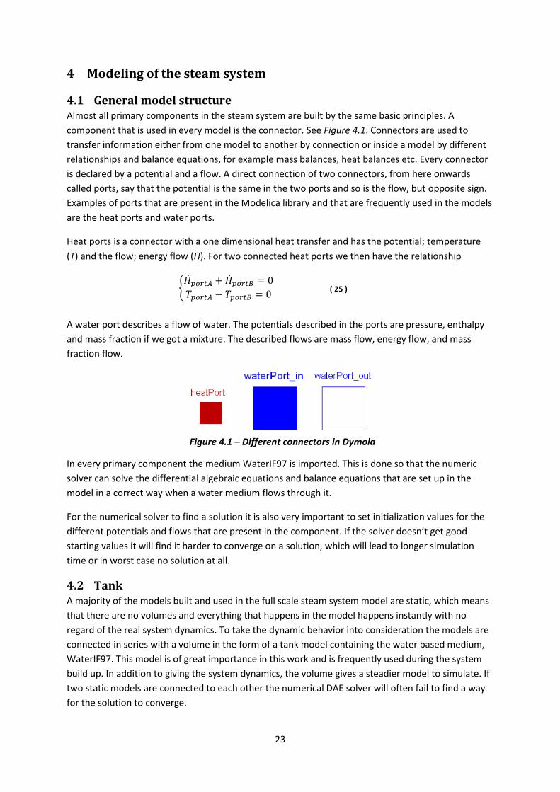
4.1 General model structure Almost all primary components in the steam system are built by the same basic principles. A
component that is used in every model is the connector. See Figure 4.1. Connectors are used to
transfer information either from one model to another by connection or inside a model by different
relationships and balance equations, for example mass balances, heat balances etc. Every connector
is declared by a potential and a flow. A direct connection of two connectors, from here onwards
called ports, say that the potential is the same in the two ports and so is the flow, but opposite sign.
Examples of ports that are present in the Modelica library and that are frequently used in the models
are the heat ports and water ports.
Heat ports is a connector with a one dimensional heat transfer and has the potential; temperature
(T) and the flow; energy flow (H). For two connected heat ports we then have the relationship
( 25 )
A water port describes a flow of water. The potentials described in the ports are pressure, enthalpy
and mass fraction if we got a mixture. The described flows are mass flow, energy flow, and mass
fraction flow.
Figure 4.1 – Different connectors in Dymola
In every primary component the medium WaterIF97 is imported. This is done so that the numeric
solver can solve the differential algebraic equations and balance equations that are set up in the
model in a correct way when a water medium flows through it.
For the numerical solver to find a solution it is also very important to set initialization values for the
different potentials and flows that are present in the component. If the solver doesn’t get good
starting values it will find it harder to converge on a solution, which will lead to longer simulation
time or in worst case no solution at all.
4.2 Tank A majority of the models built and used in the full scale steam system model are static, which means
that there are no volumes and everything that happens in the model happens instantly with no
regard of the real system dynamics. To take the dynamic behavior into consideration the models are
connected in series with a volume in the form of a tank model containing the water based medium,
WaterIF97. This model is of great importance in this work and is frequently used during the system
build up. In addition to giving the system dynamics, the volume gives a steadier model to simulate. If
two static models are connected to each other the numerical DAE solver will often fail to find a way
for the solution to converge.
24
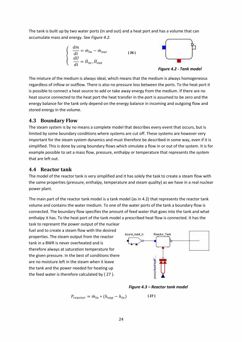
The tank is built up by two water ports (in and out) and a heat port and has a volume that can
accumulate mass and energy. See Figure 4.2.
( 26 )
Figure 4.2 - Tank model
The mixture of the medium is always ideal, which means that the medium is always homogeneous
regardless of inflow or outflow. There is also no pressure loss between the ports. To the heat port it
is possible to connect a heat source to add or take away energy from the medium. If there are no
heat source connected to the heat port the heat transfer in the port is assumed to be zero and the
energy balance for the tank only depend on the energy balance in incoming and outgoing flow and
stored energy in the volume.
4.3 Boundary Flow The steam system is by no means a complete model that describes every event that occurs, but is
limited by some boundary conditions where systems are cut off. These systems are however very
important for the steam system dynamics and must therefore be described in some way, even if it is
simplified. This is done by using boundary flows which simulate a flow in or out of the system. It is for
example possible to set a mass flow, pressure, enthalpy or temperature that represents the system
that are left out.
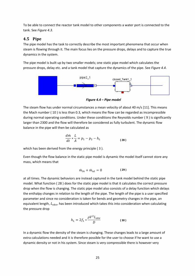
4.4 Reactor tank The model of the reactor tank is very simplified and it has solely the task to create a steam flow with
the same properties (pressure, enthalpy, temperature and steam quality) as we have in a real nuclear
power plant.
The main part of the reactor tank model is a tank model (as in 4.2) that represents the reactor tank
volume and contains the water medium. To one of the water ports of the tank a boundary flow is
connected. The boundary flow specifies the amount of feed water that goes into the tank and what
enthalpy it has. To the heat port of the tank model a prescribed heat flow is connected. It has the
task to represent the power output of the nuclear
fuel and to create a steam flow with the desired
properties. The steam output from the reactor
tank in a BWR is never overheated and is
therefore always at saturation temperature for
the given pressure. In the best of conditions there
are no moisture left in the steam when it leave
the tank and the power needed for heating up
the feed water is therefore calculated by ( 27 ).
Figure 4.3 – Reactor tank model
( 27 )
25
To be able to connect the reactor tank model to other components a water port is connected to the
tank. See Figure 4.3.
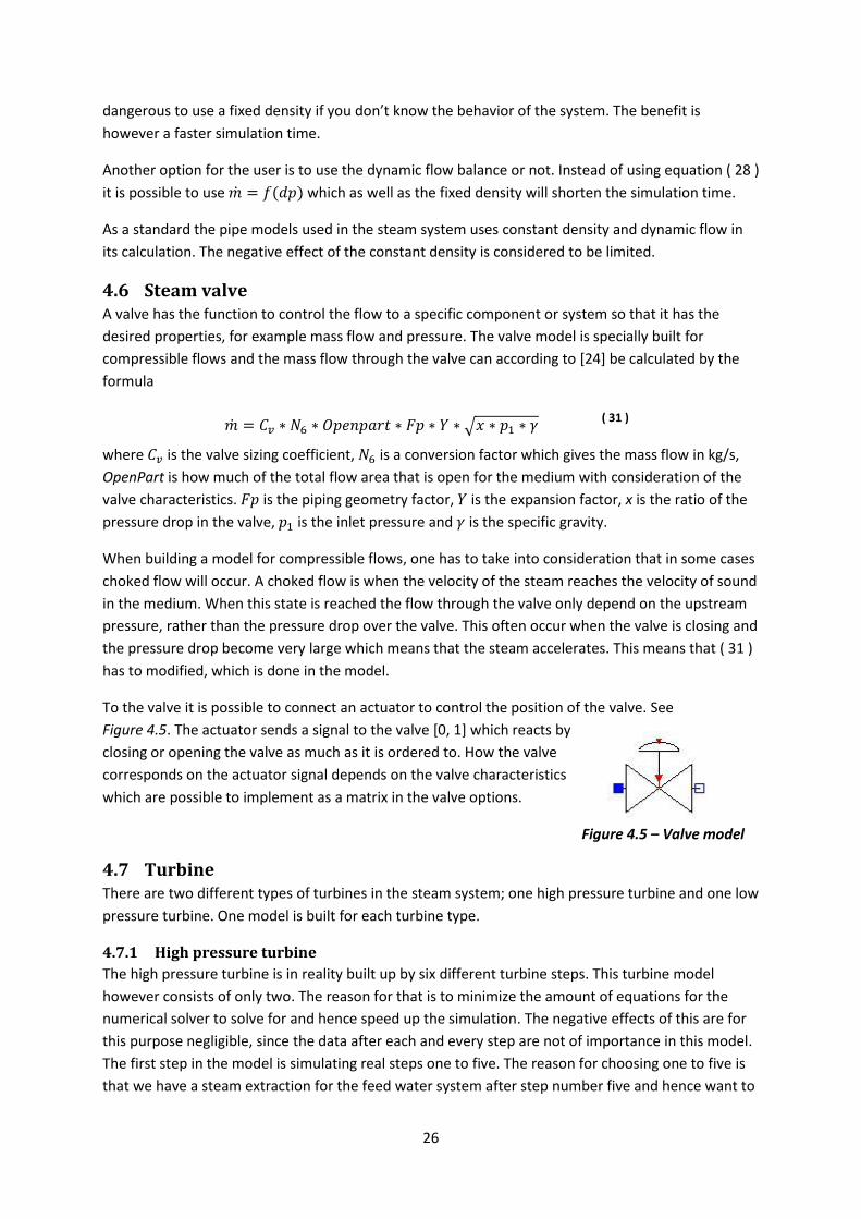
4.5 Pipe The pipe model has the task to correctly describe the most important phenomena that occur when
steam is flowing through it. The main focus lies on the pressure drops, delays and to capture the true
dynamics in the system.
The pipe model is built up by two smaller models; one static pipe model which calculates the
pressure drops, delay etc. and a tank model that capture the dynamics of the pipe. See Figure 4.4.
Figure 4.4 – Pipe model
The steam flow has under normal circumstances a mean velocity of about 40 m/s [11]. This means
the Mach number ( 10 ) is less than 0.3, which means the flow can be regarded as incompressible
during normal operating conditions. Under these conditions the Reynolds number ( 9 ) is significantly
larger than 2300 and the flow will therefore be considered as fully turbulent. The dynamic flow
balance in the pipe will then be calculated as
( 28 )
which has been derived from the energy principle ( 3 ).
Even though the flow balance in the static pipe model is dynamic the model itself cannot store any
mass, which means that
( 29 )
at all times. The dynamic behaviors are instead captured in the tank model behind the static pipe
model. What function ( 28 ) does for the static pipe model is that it calculates the correct pressure
drop when the flow is changing. The static pipe model also consists of a delay function which delays
the enthalpy changes in relation to the length of the pipe. The length of the pipe is a user specified
parameter and since no consideration is taken for bends and geometry changes in the pipe, an
equivalent length, , has been introduced which takes this into consideration when calculating
the pressure drop
( 30 )
In a dynamic flow the density of the steam is changing. These changes leads to a large amount of
extra calculations needed and it is therefore possible for the user to choose if he want to use a
dynamic density or not in his system. Since steam is very compressible there is however very
26
dangerous to use a fixed density if you don’t know the behavior of the system. The benefit is
however a faster simulation time.
Another option for the user is to use the dynamic flow balance or not. Instead of using equation ( 28 )
it is possible to use which as well as the fixed density will shorten the simulation time.
As a standard the pipe models used in the steam system uses constant density and dynamic flow in
its calculation. The negative effect of the constant density is considered to be limited.
4.6 Steam valve A valve has the function to control the flow to a specific component or system so that it has the
desired properties, for example mass flow and pressure. The valve model is specially built for
compressible flows and the mass flow through the valve can according to [24] be calculated by the
formula
( 31 )
where is the valve sizing coefficient, is a conversion factor which gives the mass flow in kg/s,
OpenPart is how much of the total flow area that is open for the medium with consideration of the
valve characteristics. is the piping geometry factor, is the expansion factor, x is the ratio of the
pressure drop in the valve, is the inlet pressure and is the specific gravity.
When building a model for compressible flows, one has to take into consideration that in some cases
choked flow will occur. A choked flow is when the velocity of the steam reaches the velocity of sound
in the medium. When this state is reached the flow through the valve only depend on the upstream
pressure, rather than the pressure drop over the valve. This often occur when the valve is closing and
the pressure drop become very large which means that the steam accelerates. This means that ( 31 )
has to modified, which is done in the model.
To the valve it is possible to connect an actuator to control the position of the valve. See
Figure 4.5. The actuator sends a signal to the valve [0, 1] which reacts by
closing or opening the valve as much as it is ordered to. How the valve
corresponds on the actuator signal depends on the valve characteristics
which are possible to implement as a matrix in the valve options.
Figure 4.5 – Valve model
4.7 Turbine There are two different types of turbines in the steam system; one high pressure turbine and one low
pressure turbine. One model is built for each turbine type.
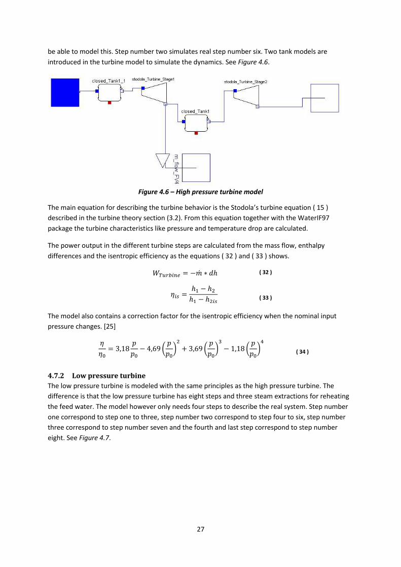
4.7.1 High pressure turbine
The high pressure turbine is in reality built up by six different turbine steps. This turbine model
however consists of only two. The reason for that is to minimize the amount of equations for the
numerical solver to solve for and hence speed up the simulation. The negative effects of this are for
this purpose negligible, since the data after each and every step are not of importance in this model.
The first step in the model is simulating real steps one to five. The reason for choosing one to five is
that we have a steam extraction for the feed water system after step number five and hence want to
27
be able to model this. Step number two simulates real step number six. Two tank models are
introduced in the turbine model to simulate the dynamics. See Figure 4.6.
Figure 4.6 – High pressure turbine model
The main equation for describing the turbine behavior is the Stodola’s turbine equation ( 15 )
described in the turbine theory section (3.2). From this equation together with the WaterIF97
package the turbine characteristics like pressure and temperature drop are calculated.
The power output in the different turbine steps are calculated from the mass flow, enthalpy
differences and the isentropic efficiency as the equations ( 32 ) and ( 33 ) shows.
( 32 )
( 33 )
The model also contains a correction factor for the isentropic efficiency when the nominal input
pressure changes. [25]
( 34 )
4.7.2 Low pressure turbine
The low pressure turbine is modeled with the same principles as the high pressure turbine. The
difference is that the low pressure turbine has eight steps and three steam extractions for reheating
the feed water. The model however only needs four steps to describe the real system. Step number
one correspond to step one to three, step number two correspond to step four to six, step number
three correspond to step number seven and the fourth and last step correspond to step number
eight. See Figure 4.7.
28
Figure 4.7 – Low pressure turbine model
4.8 Reheater The reheater is modeled in two separate parts; one model for the moist separation and one model
for the reheating.
4.8.1 Steam separator
Modeling a steam separator by its physical behavior is not an easy task and there is not a lot of
literature about it. Therefore a static model that separates a given amount of moisture is used
combined with a tank model for the dynamics.
The steam properties at incoming water port is
calculated and the model separates the moisture from
the steam. To know the amount of moisture in the
steam the vapor enthalpy and the liquid enthalpy are
calculated for the incoming pressure and then
compared with the actual enthalpy. The liquid water is
sent out of the model in one direction and the steam is
directed to the reheater model. See Figure 4.8.
Figure 4.8 – Steam separator model
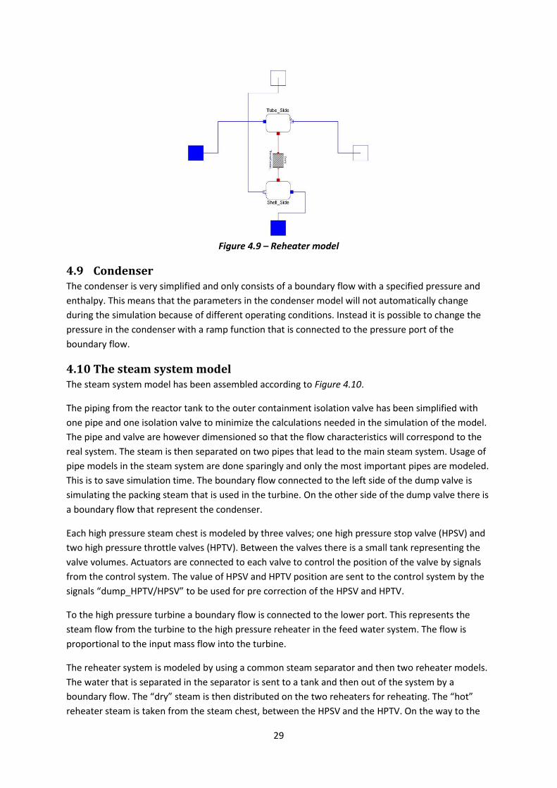
4.8.2 Reheater
The reheater model is built by four water ports, two tanks and a thermal conductor block. The
reheater consist of a tube side where the hot steam flows and a shell side where the cold steam that
are supposed to get reheated flows. The tube and shell side are modeled by two different tanks and
the heat transfer between them are decided by the thermal conductor block. See Figure 4.9. In the
thermal conductor block it is possible to specify the thermal conductance (G) by setting an area (A)
and a heat transfer coefficient (k).
( 35 )
The heat transfer is given by equation:
( 36 )
Where dT is the temperature difference between the tube side and the shell side.
29
Figure 4.9 – Reheater model
4.9 Condenser The condenser is very simplified and only consists of a boundary flow with a specified pressure and
enthalpy. This means that the parameters in the condenser model will not automatically change
during the simulation because of different operating conditions. Instead it is possible to change the
pressure in the condenser with a ramp function that is connected to the pressure port of the
boundary flow.
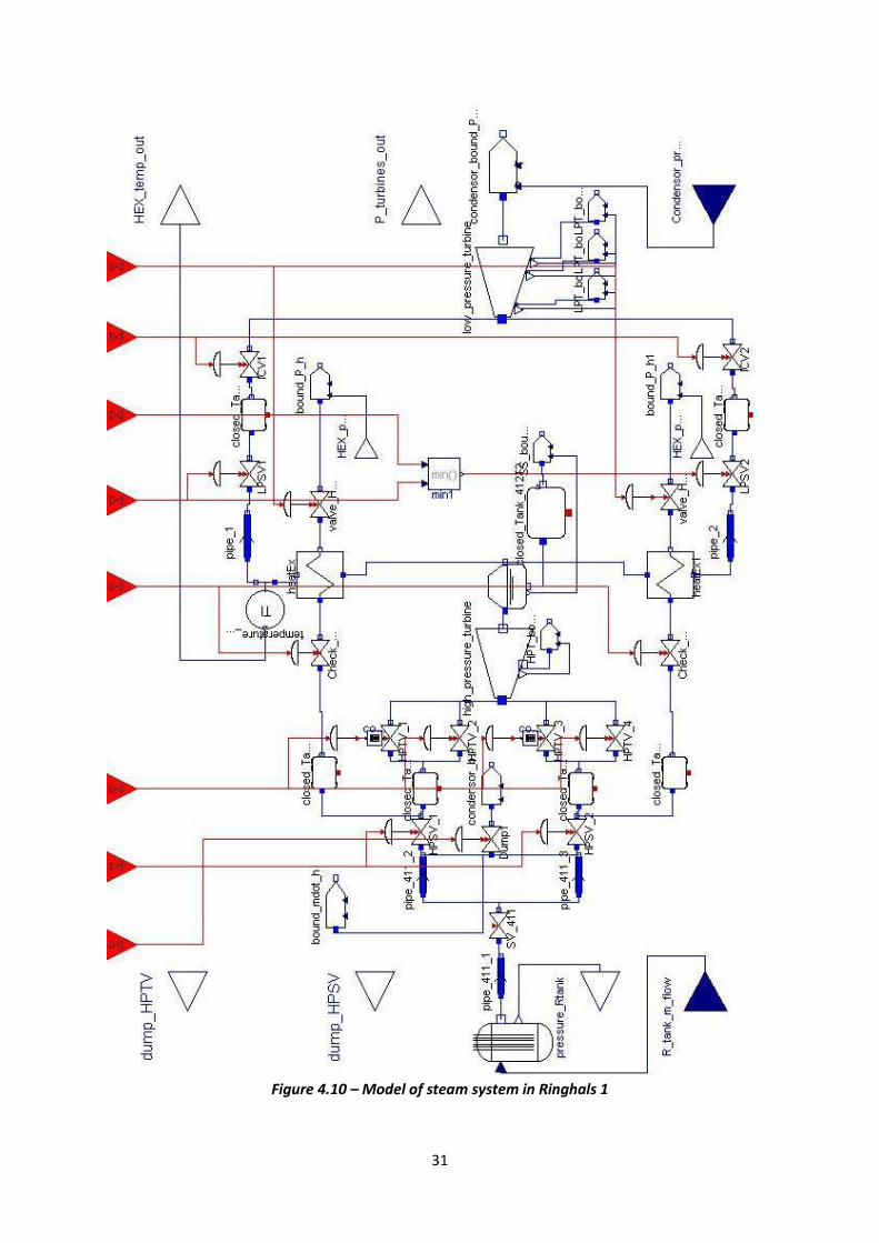
4.10 The steam system model The steam system model has been assembled according to Figure 4.10.
The piping from the reactor tank to the outer containment isolation valve has been simplified with
one pipe and one isolation valve to minimize the calculations needed in the simulation of the model.
The pipe and valve are however dimensioned so that the flow characteristics will correspond to the
real system. The steam is then separated on two pipes that lead to the main steam system. Usage of
pipe models in the steam system are done sparingly and only the most important pipes are modeled.
This is to save simulation time. The boundary flow connected to the left side of the dump valve is
simulating the packing steam that is used in the turbine. On the other side of the dump valve there is
a boundary flow that represent the condenser.
Each high pressure steam chest is modeled by three valves; one high pressure stop valve (HPSV) and
two high pressure throttle valves (HPTV). Between the valves there is a small tank representing the
valve volumes. Actuators are connected to each valve to control the position of the valve by signals
from the control system. The value of HPSV and HPTV position are sent to the control system by the
signals “dump_HPTV/HPSV” to be used for pre correction of the HPSV and HPTV.
To the high pressure turbine a boundary flow is connected to the lower port. This represents the
steam flow from the turbine to the high pressure reheater in the feed water system. The flow is
proportional to the input mass flow into the turbine.
The reheater system is modeled by using a common steam separator and then two reheater models.
The water that is separated in the separator is sent to a tank and then out of the system by a
boundary flow. The “dry” steam is then distributed on the two reheaters for reheating. The “hot”
reheater steam is taken from the steam chest, between the HPSV and the HPTV. On the way to the

30
reheater it passes through a small volume and a check valve. On the other side of the reheater it
passes through another valve. The hot reheater steam flow is controlled by the pressure difference in
the system set by a boundary flow and the opening degree of the valve.
After the reheaters the steam enters a pipe with a temperature sensor and then the low pressure
steam chest, which are built up by two valves with actuators; one low pressure stop valve and one
intercept valve. In between there is also a small tank representing the volumes present in the valves.
The low pressure turbines are modeled with just one turbine model that is scaled up to handle the
amount of steam needed. In the lower end of the turbine model there are three boundary flows that
represent the steam flow to the low pressure reheater in the feed water system. The steam flow is
proportional to the steam flow entering the low pressure turbine. Finally the output of the low
pressure turbine is connected to the condenser.
31
Figure 4.10 – Model of steam system in Ringhals 1
32
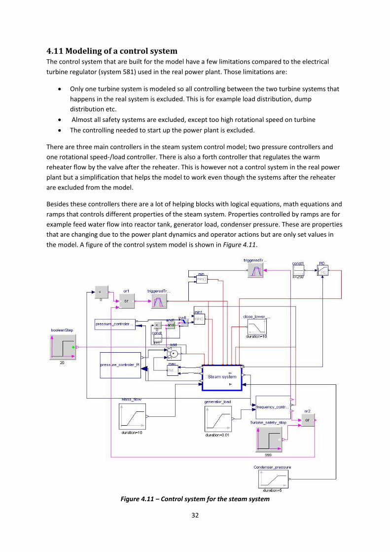
4.11 Modeling of a control system The control system that are built for the model have a few limitations compared to the electrical
turbine regulator (system 581) used in the real power plant. Those limitations are:
Only one turbine system is modeled so all controlling between the two turbine systems that
happens in the real system is excluded. This is for example load distribution, dump
distribution etc.
Almost all safety systems are excluded, except too high rotational speed on turbine
The controlling needed to start up the power plant is excluded.
There are three main controllers in the steam system control model; two pressure controllers and
one rotational speed-/load controller. There is also a forth controller that regulates the warm
reheater flow by the valve after the reheater. This is however not a control system in the real power
plant but a simplification that helps the model to work even though the systems after the reheater
are excluded from the model.
Besides these controllers there are a lot of helping blocks with logical equations, math equations and
ramps that controls different properties of the steam system. Properties controlled by ramps are for
example feed water flow into reactor tank, generator load, condenser pressure. These are properties
that are changing due to the power plant dynamics and operator actions but are only set values in
the model. A figure of the control system model is shown in Figure 4.11.
Figure 4.11 – Control system for the steam system
33
4.11.1 Pressure control in reactor tank
Controlling the reactor tank pressure during normal conditions is done by the two turbines, and the
high pressure throttle valves (HPTV) and intercept valves (ICV) are fully or nearly fully open. When
the reactor tank pressure changes, for example when there is a drop of load and the turbine is not
able to handle all the steam from the reactor tank, the pressure control is partly taken over by the
dump system and HPTV. These are controlled by a PI-regulator which compares the current reactor
tank pressure with a user selected value and sends a control signal [0, 1] to the dump system and the
HPTV. See Figure 4.12. The PI-regulators are calibrated by setting the gain (k), time constant of the
integrator (Ti) and the wind-up compensation (Ni) to optimize the speed and stability of the
controller.
Figure 4.12 – Pressure controller
4.11.2 Rotational speed-/load controller
The rotational speed of the turbine axis is of great importance for the quality of the generator power
output and is therefore very important to control. The steam system model however does not
include a generator and is not connected to a varying power distribution grid so there is no way to
get a good realistic approximation of how the frequency changes with a changing load. To cope with
this and be able to build a frequency controller with the correct behavior, a frequency calculator
block that calculates a fictive turbine frequency from the power of the incoming steam and a user set
generator load has been built. This block does not describe the correct turbine behavior but at least
gives a value to work with and run the model. The rotational speed-/load controller is shown in
Figure 4.13.
Figure 4.13 – Rotational speed-/load controller
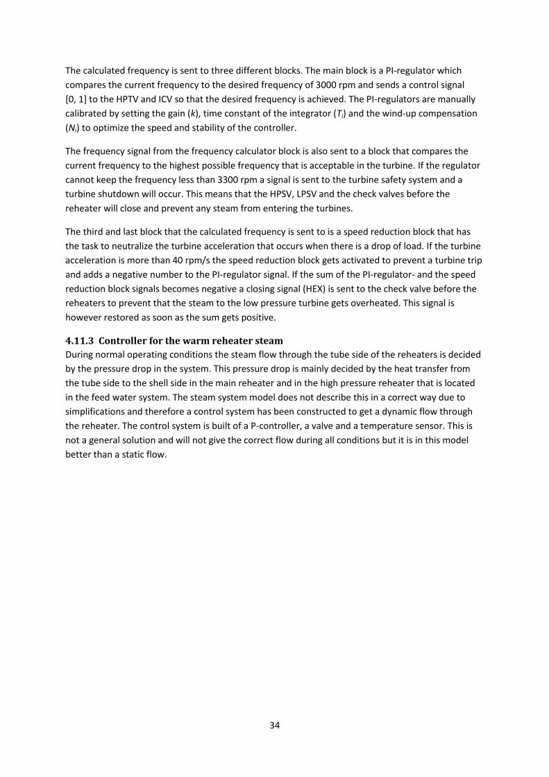
34
The calculated frequency is sent to three different blocks. The main block is a PI-regulator which
compares the current frequency to the desired frequency of 3000 rpm and sends a control signal
[0, 1] to the HPTV and ICV so that the desired frequency is achieved. The PI-regulators are manually
calibrated by setting the gain (k), time constant of the integrator (Ti) and the wind-up compensation
(Ni) to optimize the speed and stability of the controller.
The frequency signal from the frequency calculator block is also sent to a block that compares the
current frequency to the highest possible frequency that is acceptable in the turbine. If the regulator
cannot keep the frequency less than 3300 rpm a signal is sent to the turbine safety system and a
turbine shutdown will occur. This means that the HPSV, LPSV and the check valves before the
reheater will close and prevent any steam from entering the turbines.
The third and last block that the calculated frequency is sent to is a speed reduction block that has
the task to neutralize the turbine acceleration that occurs when there is a drop of load. If the turbine
acceleration is more than 40 rpm/s the speed reduction block gets activated to prevent a turbine trip
and adds a negative number to the PI-regulator signal. If the sum of the PI-regulator- and the speed
reduction block signals becomes negative a closing signal (HEX) is sent to the check valve before the
reheaters to prevent that the steam to the low pressure turbine gets overheated. This signal is
however restored as soon as the sum gets positive.
4.11.3 Controller for the warm reheater steam
During normal operating conditions the steam flow through the tube side of the reheaters is decided
by the pressure drop in the system. This pressure drop is mainly decided by the heat transfer from
the tube side to the shell side in the main reheater and in the high pressure reheater that is located
in the feed water system. The steam system model does not describe this in a correct way due to
simplifications and therefore a control system has been constructed to get a dynamic flow through
the reheater. The control system is built of a P-controller, a valve and a temperature sensor. This is
not a general solution and will not give the correct flow during all conditions but it is in this model
better than a static flow.
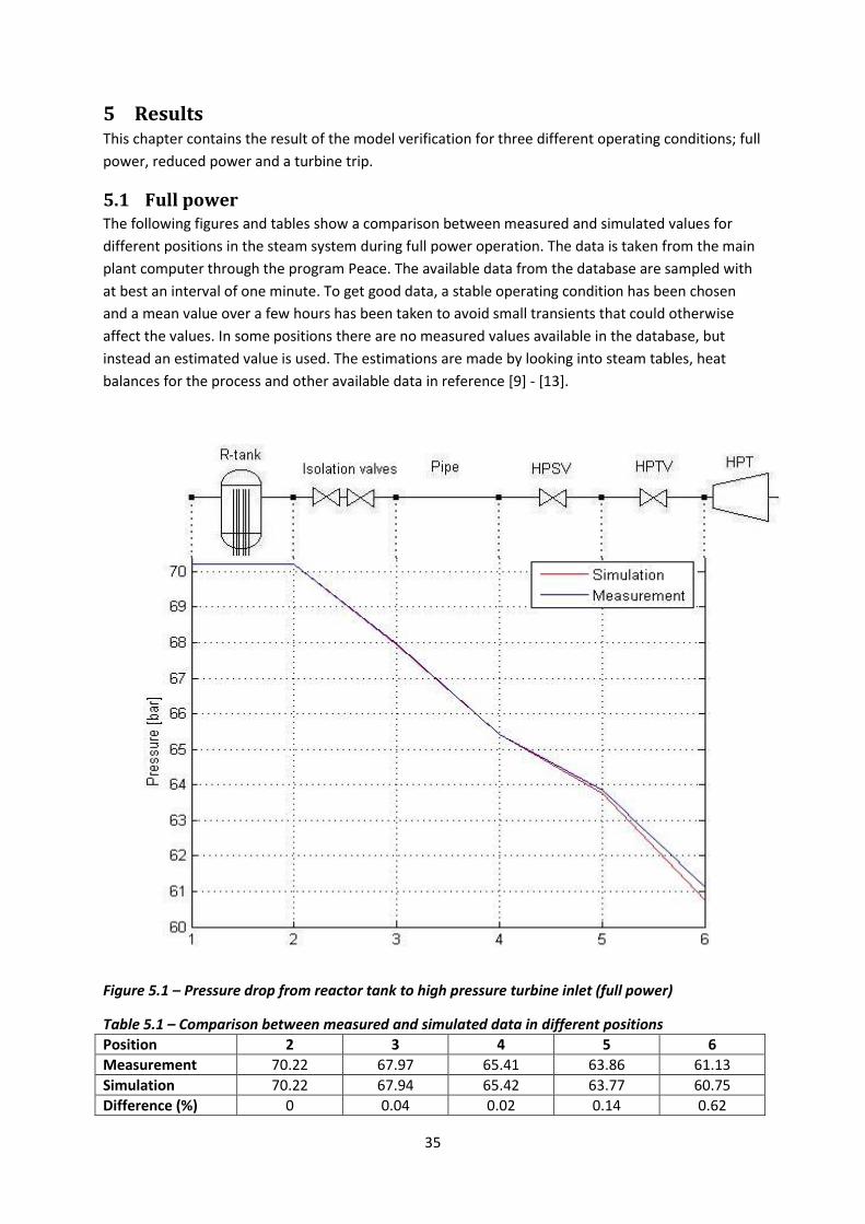
35
5 Results This chapter contains the result of the model verification for three different operating conditions; full
power, reduced power and a turbine trip.
5.1 Full power The following figures and tables show a comparison between measured and simulated values for
different positions in the steam system during full power operation. The data is taken from the main
plant computer through the program Peace. The available data from the database are sampled with
at best an interval of one minute. To get good data, a stable operating condition has been chosen
and a mean value over a few hours has been taken to avoid small transients that could otherwise
affect the values. In some positions there are no measured values available in the database, but
instead an estimated value is used. The estimations are made by looking into steam tables, heat
balances for the process and other available data in reference [9] - [13].
Figure 5.1 – Pressure drop from reactor tank to high pressure turbine inlet (full power)
Table 5.1 – Comparison between measured and simulated data in different positions
Position 2 3 4 5 6
Measurement 70.22 67.97 65.41 63.86 61.13
Simulation 70.22 67.94 65.42 63.77 60.75
Difference (%) 0 0.04 0.02 0.14 0.62
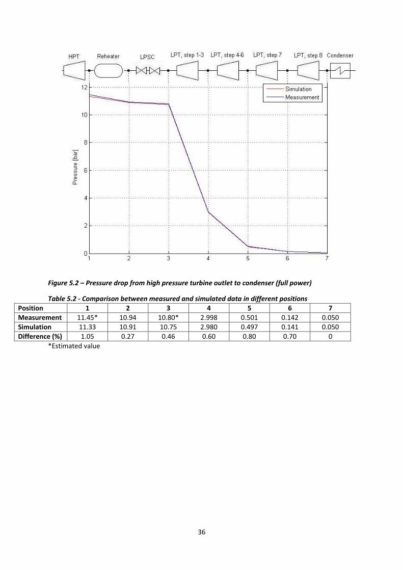
36
Figure 5.2 – Pressure drop from high pressure turbine outlet to condenser (full power)
Table 5.2 - Comparison between measured and simulated data in different positions
Position 1 2 3 4 5 6 7
Measurement 11.45* 10.94 10.80* 2.998 0.501 0.142 0.050
Simulation 11.33 10.91 10.75 2.980 0.497 0.141 0.050
Difference (%) 1.05 0.27 0.46 0.60 0.80 0.70 0
*Estimated value
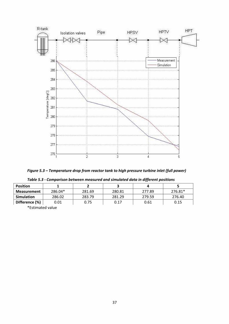
37
Figure 5.3 – Temperature drop from reactor tank to high pressure turbine inlet (full power)
Table 5.3 - Comparison between measured and simulated data in different positions
*Estimated value
Position 1 2 3 4 5
Measurement 286.04* 281.69 280.81 277.89 276.81*
Simulation 286.02 283.79 281.29 279.59 276.40
Difference (%) 0.01 0.75 0.17 0.61 0.15
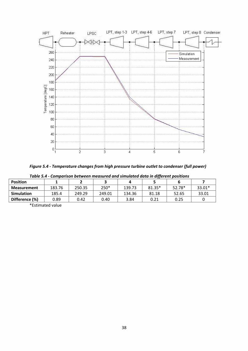
38
Figure 5.4 - Temperature changes from high pressure turbine outlet to condenser (full power)
Table 5.4 - Comparison between measured and simulated data in different positions
Position 1 2 3 4 5 6 7
Measurement 183.76 250.35 250* 139.73 81.35* 52.78* 33.01*
Simulation 185.4 249.29 249.01 134.36 81.18 52.65 33.01
Difference (%) 0.89 0.42 0.40 3.84 0.21 0.25 0
*Estimated value
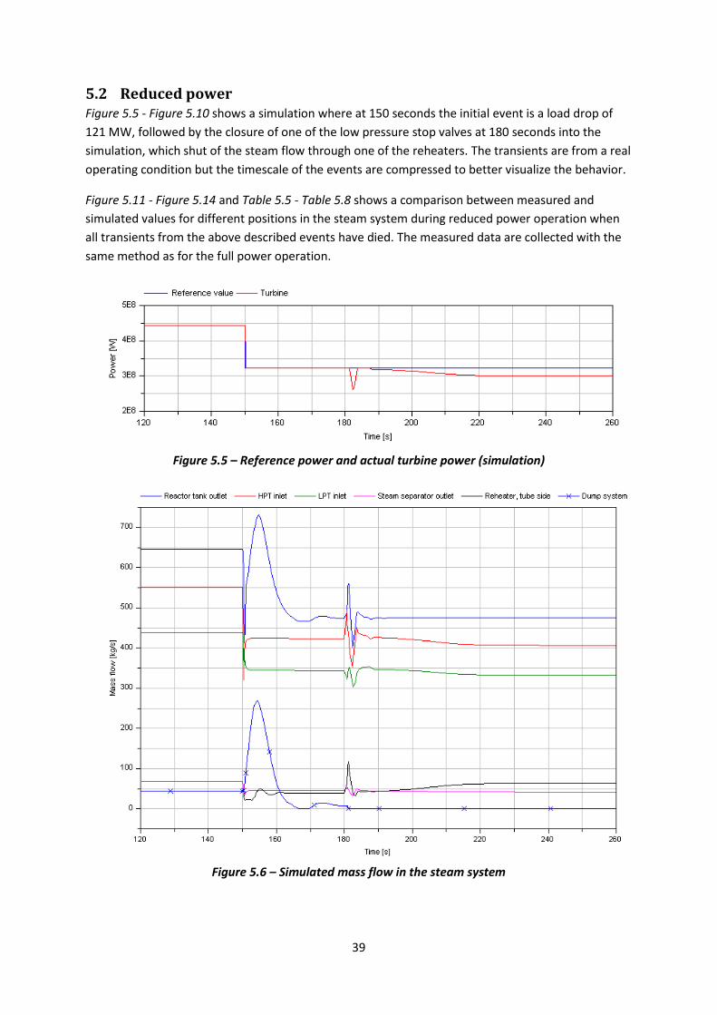
39
5.2 Reduced power Figure 5.5 - Figure 5.10 shows a simulation where at 150 seconds the initial event is a load drop of
121 MW, followed by the closure of one of the low pressure stop valves at 180 seconds into the
simulation, which shut of the steam flow through one of the reheaters. The transients are from a real
operating condition but the timescale of the events are compressed to better visualize the behavior.
Figure 5.11 - Figure 5.14 and Table 5.5 - Table 5.8 shows a comparison between measured and
simulated values for different positions in the steam system during reduced power operation when
all transients from the above described events have died. The measured data are collected with the
same method as for the full power operation.
Figure 5.5 – Reference power and actual turbine power (simulation)
Figure 5.6 – Simulated mass flow in the steam system
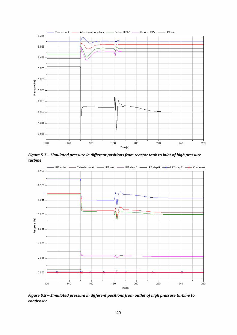
40
Figure 5.7 – Simulated pressure in different positions from reactor tank to inlet of high pressure turbine
Figure 5.8 – Simulated pressure in different positions from outlet of high pressure turbine to condenser
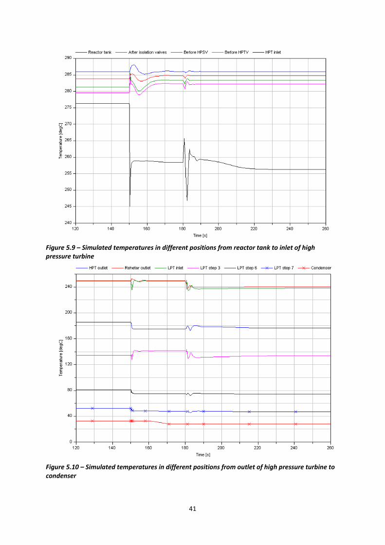
41
Figure 5.9 – Simulated temperatures in different positions from reactor tank to inlet of high pressure turbine
Figure 5.10 – Simulated temperatures in different positions from outlet of high pressure turbine to condenser
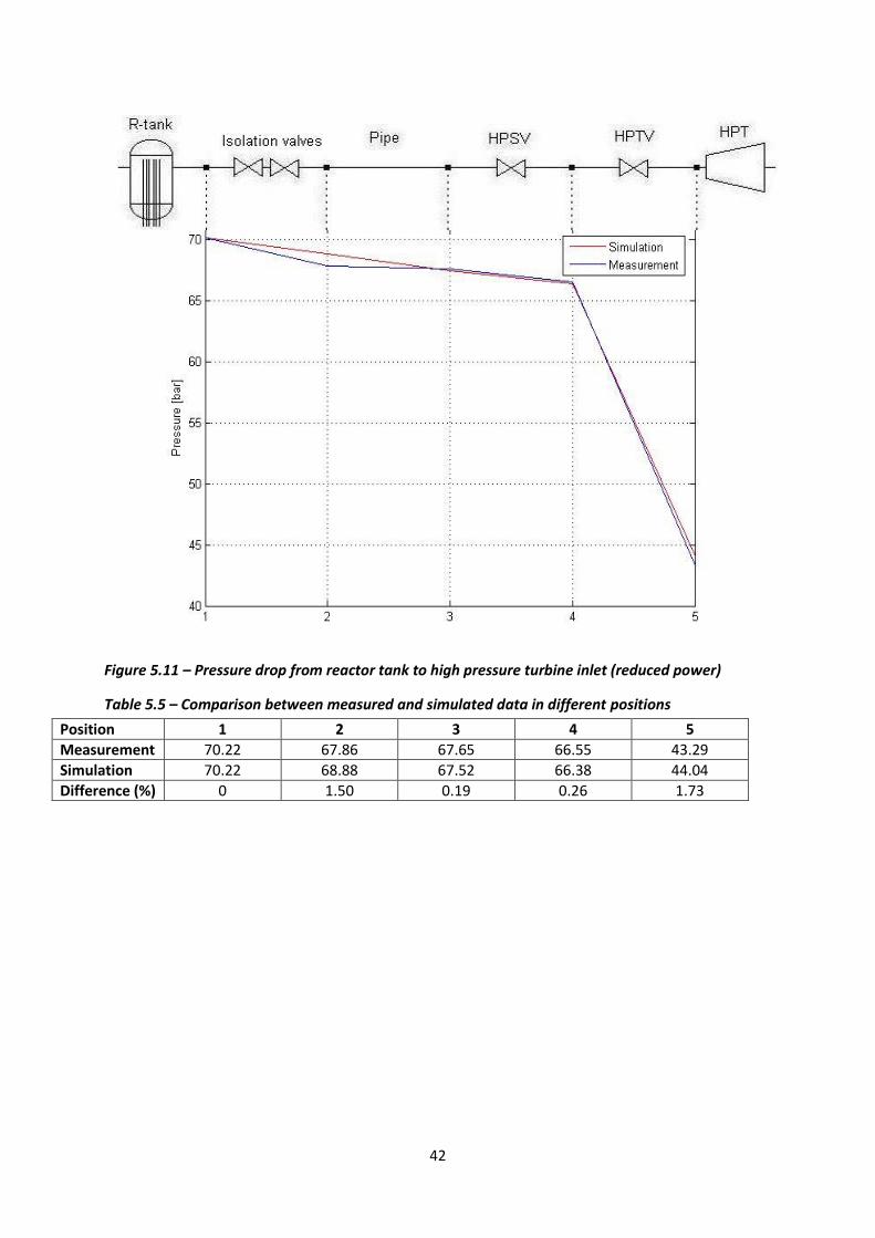
42
Figure 5.11 – Pressure drop from reactor tank to high pressure turbine inlet (reduced power)
Table 5.5 – Comparison between measured and simulated data in different positions
Position 1 2 3 4 5
Measurement 70.22 67.86 67.65 66.55 43.29
Simulation 70.22 68.88 67.52 66.38 44.04
Difference (%) 0 1.50 0.19 0.26 1.73
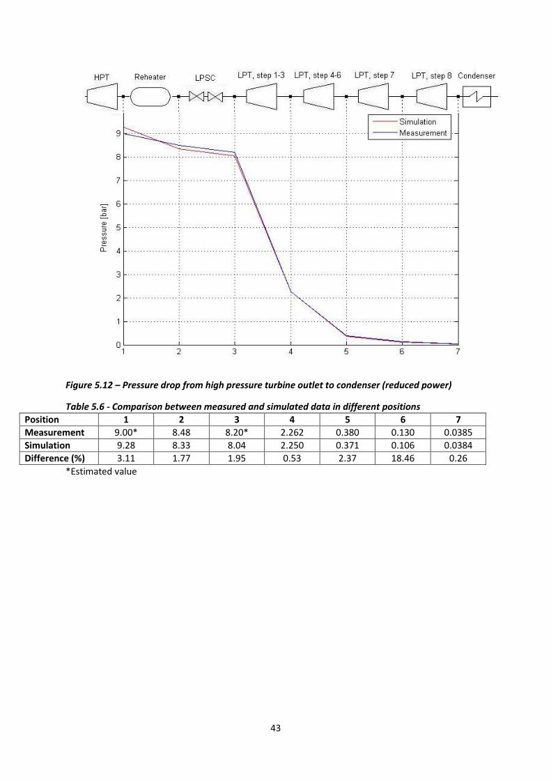
43
Figure 5.12 – Pressure drop from high pressure turbine outlet to condenser (reduced power)
Table 5.6 - Comparison between measured and simulated data in different positions
Position 1 2 3 4 5 6 7
Measurement 9.00* 8.48 8.20* 2.262 0.380 0.130 0.0385
Simulation 9.28 8.33 8.04 2.250 0.371 0.106 0.0384
Difference (%) 3.11 1.77 1.95 0.53 2.37 18.46 0.26
*Estimated value
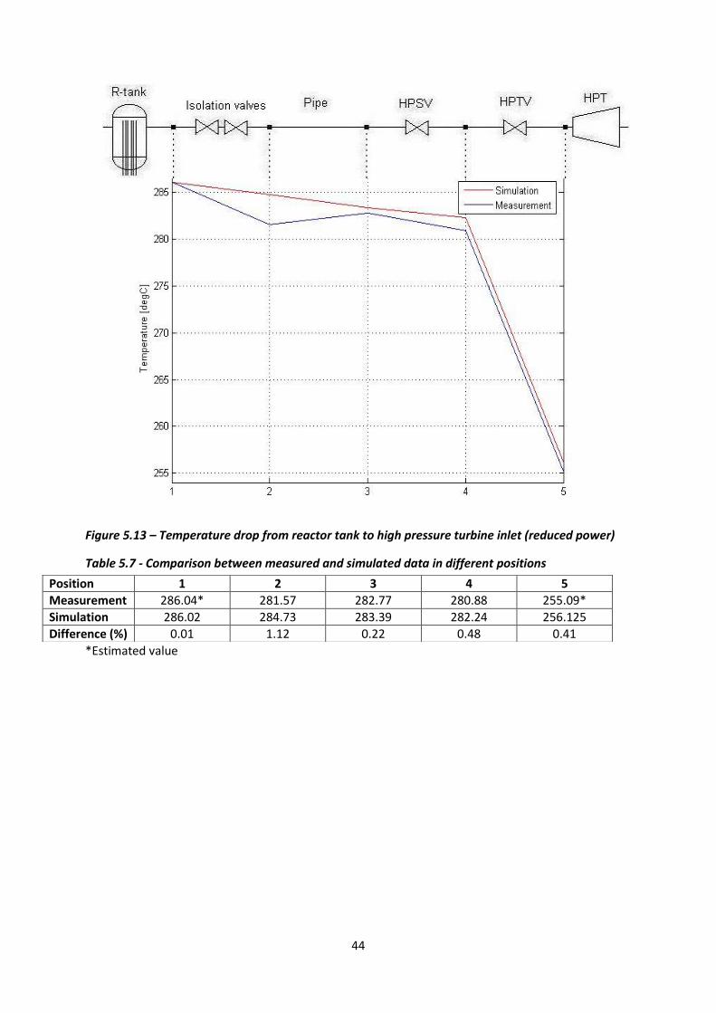
44
Figure 5.13 – Temperature drop from reactor tank to high pressure turbine inlet (reduced power)
Table 5.7 - Comparison between measured and simulated data in different positions
*Estimated value
Position 1 2 3 4 5
Measurement 286.04* 281.57 282.77 280.88 255.09*
Simulation 286.02 284.73 283.39 282.24 256.125
Difference (%) 0.01 1.12 0.22 0.48 0.41
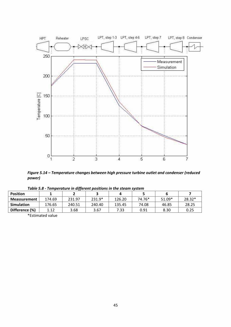
45
Figure 5.14 – Temperature changes between high pressure turbine outlet and condenser (reduced power) Table 5.8 - Temperature in different positions in the steam system
Position 1 2 3 4 5 6 7
Meassurement 174.69 231.97 231.9* 126.20 74.76* 51.09* 28.32*
Simulation 176.65 240.51 240.40 135.45 74.08 46.85 28.25
Difference (%) 1.12 3.68 3.67 7.33 0.91 8.30 0.25
*Estimated value
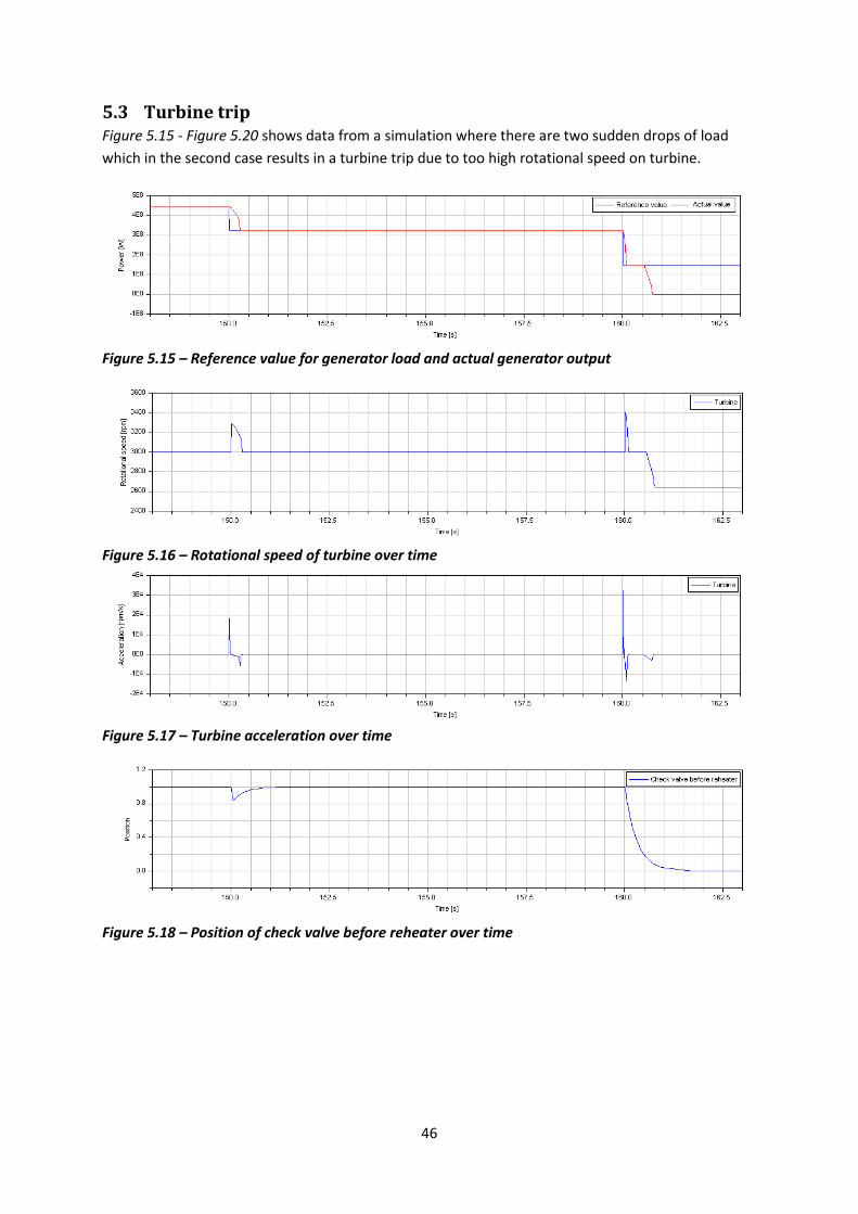
46
5.3 Turbine trip Figure 5.15 - Figure 5.20 shows data from a simulation where there are two sudden drops of load
which in the second case results in a turbine trip due to too high rotational speed on turbine.
Figure 5.15 – Reference value for generator load and actual generator output
Figure 5.16 – Rotational speed of turbine over time
Figure 5.17 – Turbine acceleration over time
Figure 5.18 – Position of check valve before reheater over time
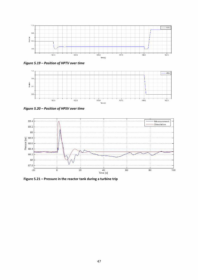
47
Figure 5.19 – Position of HPTV over time
Figure 5.20 – Position of HPSV over time
Figure 5.21 – Pressure in the reactor tank during a turbine trip

48
49
6 Analysis and discussion of the results
6.1 Quality of data As mentioned in chapter 5.1 and 5.2 the available data from Ringhals database for the calibration
and verification of the model is sampled with a frequency of at best one measurement per minute
and in some cases with even lower frequencies. This makes it impossible to register any fast
transients measured in the real steam system and as a result it is impossible to verify the model
behavior in those events.
There is little data available regarding mass flows. The data that is available is the mass flow leaving
the reactor containment through the main steam pipes and the mass flow that leaves the drainage
tank (412T1), located downstream the reheater, on the tube side. Momentary mass flows to the
packing steam, dump system, steam separator, turbine drains etc. are unknown which means that
the flow through the different turbine steps in different moments are only approximated. This makes
it very difficult to calibrate the model and verify that the behavior is correct. For the full power case
different heat balances are available that show mass flows in some of these points. The operating
data do not fully agree with the measured data for pressure, temperature and power output but are
sufficiently good for making an approximation. When the power is reduced and there are transients
in the system these mass flows are unknown and the approximations are made from ratios from the
full power case, and might not be fully correct.
There is also data missing for some other positions, See Table 5.2 - Table 5.8. E.g. the pressure after
the high pressure turbine and pressure before the low pressure turbine are unknown. For these
positions data has been estimated from information in steam tables, heat balances and system
specifications.
6.2 Full power The full power case is not a verification of the model but instead the case which the model has been
calibrated against. All components have been designed for the conditions in the full power case so
the difference between the measured data and the simulation should only differ slightly.
When looking at Figure 5.1 - Figure 5.2 the pressure from reactor tank to condenser varies very
slightly. Table 5.1 - Table 5.2 shows that the largest difference between measured and simulated
pressure is around 1%, but in most positions the difference is significantly smaller. The reason why
the model does not match the data perfectly even though the model has been calibrated with the
measured data from the full power case is due to the complexity of the steam system. When
changing one parameter, for example the length of a pipe or size of a valve, it is not only the pressure
drop in the pipe/valve that changes. The pressure drop propagates to every other part of the system
that is somehow connected to the changed model. The calibration has therefore been a trade-off
between getting the model to fit the data as good as possible and the time available.
When looking at the temperatures in Figure 5.3 - Figure 5.4 and Table 5.3 - Table 5.4 one can see that
the measured and simulated values match each other well except for after step 3 in the low pressure
turbine where the simulated value is almost 4 % lower than the measured. This indicates that the
efficiency in the first step of the low pressure turbine model is too high compared to the real turbine.
Since the steam is still overheated in this data point it is possible for the pressure drop to be correct
even though the temperature drop is not.
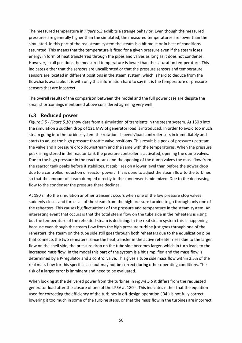
50
The measured temperature in Figure 5.3 exhibits a strange behavior. Even though the measured
pressures are generally higher than the simulated, the measured temperatures are lower than the
simulated. In this part of the real steam system the steam is a bit moist or in best of conditions
saturated. This means that the temperature is fixed for a given pressure even if the steam loses
energy in form of heat transferred through the pipes and valves as long as it does not condense.
However, in all positions the measured temperature is lower than the saturation temperature. This
indicates either that the sensors are uncalibrated or that the pressure sensors and temperature
sensors are located in different positions in the steam system, which is hard to deduce from the
flowcharts available. It is with only this information hard to say if it is the temperature or pressure
sensors that are incorrect.
The overall results of the comparison between the model and the full power case are despite the
small shortcomings mentioned above considered agreeing very well.
6.3 Reduced power Figure 5.5 - Figure 5.10 show data from a simulation of transients in the steam system. At 150 s into
the simulation a sudden drop of 121 MW of generator load is introduced. In order to avoid too much
steam going into the turbine system the rotational speed-/load controller sets in immediately and
starts to adjust the high pressure throttle valve positions. This result is a peak of pressure upstream
the valve and a pressure drop downstream and the same with the temperatures. When the pressure
peak is registered in the reactor tank the pressure controller is activated, opening the dump valves.
Due to the high pressure in the reactor tank and the opening of the dump valves the mass flow from
the reactor tank peaks before it stabilizes. It stabilizes on a lower level than before the power drop
due to a controlled reduction of reactor power. This is done to adjust the steam flow to the turbines
so that the amount of steam dumped directly to the condenser is minimized. Due to the decreasing
flow to the condenser the pressure there declines.
At 180 s into the simulation another transient occurs when one of the low pressure stop valves
suddenly closes and forces all of the steam from the high pressure turbine to go through only one of
the reheaters. This causes big fluctuations of the pressure and temperature in the steam system. An
interesting event that occurs is that the total steam flow on the tube side in the reheaters is rising
but the temperature of the reheated steam is declining. In the real steam system this is happening
because even though the steam flow from the high pressure turbine just goes through one of the
reheaters, the steam on the tube side still goes through both reheaters due to the equalization pipe
that connects the two reheaters. Since the heat transfer in the active reheater rises due to the larger
flow on the shell side, the pressure drop on the tube side becomes larger, which in turn leads to the
increased mass flow. In the model this part of the system is a bit simplified and the mass flow is
determined by a P-regulator and a control valve. This gives a tube side mass flow within 2.5% of the
real mass flow for this specific case but may not be correct during other operating conditions. The
risk of a larger error is imminent and need to be evaluated.
When looking at the delivered power from the turbines in Figure 5.5 it differs from the requested
generator load after the closure of one of the LPSV at 180 s. This indicates either that the equation
used for correcting the efficiency of the turbines in off-design operation ( 34 ) is not fully correct,
lowering it too much in some of the turbine steps, or that the mass flow in the turbines are incorrect
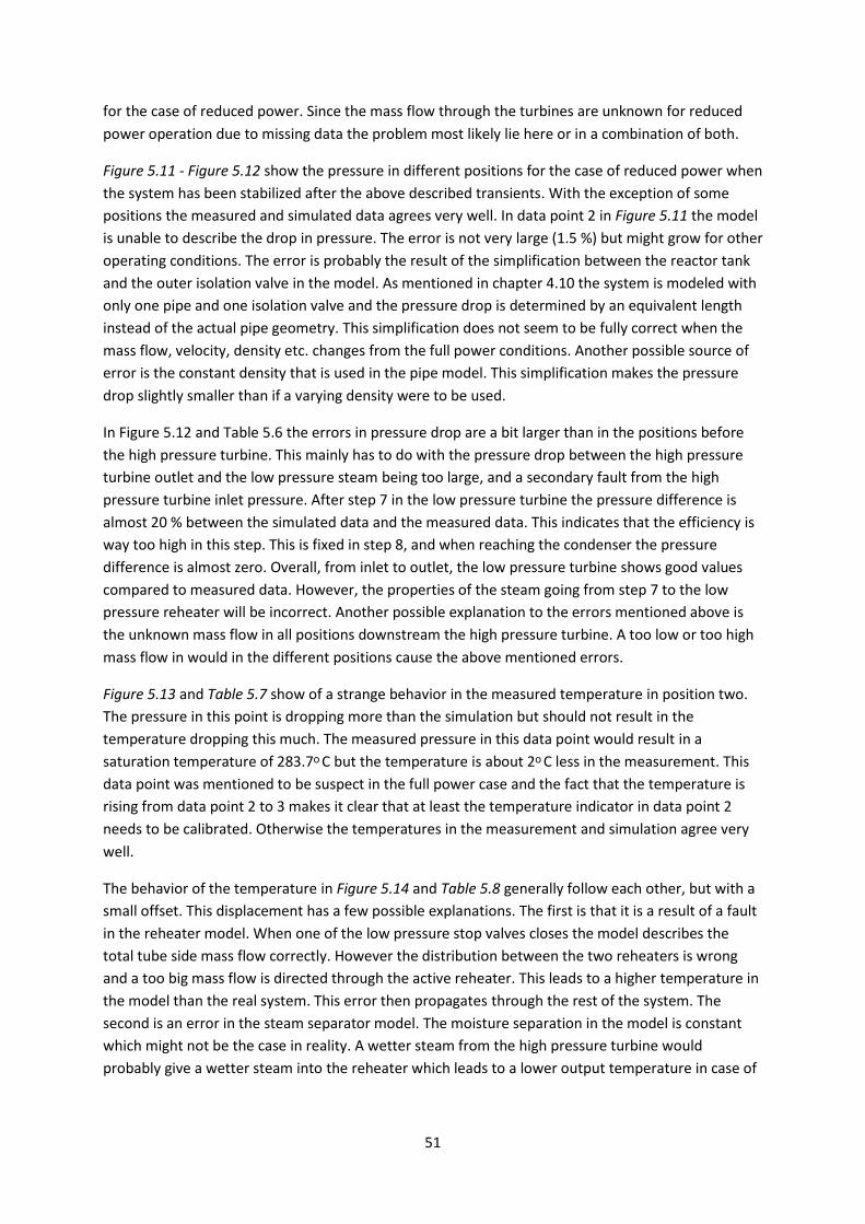
51
for the case of reduced power. Since the mass flow through the turbines are unknown for reduced
power operation due to missing data the problem most likely lie here or in a combination of both.
Figure 5.11 - Figure 5.12 show the pressure in different positions for the case of reduced power when
the system has been stabilized after the above described transients. With the exception of some
positions the measured and simulated data agrees very well. In data point 2 in Figure 5.11 the model
is unable to describe the drop in pressure. The error is not very large (1.5 %) but might grow for other
operating conditions. The error is probably the result of the simplification between the reactor tank
and the outer isolation valve in the model. As mentioned in chapter 4.10 the system is modeled with
only one pipe and one isolation valve and the pressure drop is determined by an equivalent length
instead of the actual pipe geometry. This simplification does not seem to be fully correct when the
mass flow, velocity, density etc. changes from the full power conditions. Another possible source of
error is the constant density that is used in the pipe model. This simplification makes the pressure
drop slightly smaller than if a varying density were to be used.
In Figure 5.12 and Table 5.6 the errors in pressure drop are a bit larger than in the positions before
the high pressure turbine. This mainly has to do with the pressure drop between the high pressure
turbine outlet and the low pressure steam being too large, and a secondary fault from the high
pressure turbine inlet pressure. After step 7 in the low pressure turbine the pressure difference is
almost 20 % between the simulated data and the measured data. This indicates that the efficiency is
way too high in this step. This is fixed in step 8, and when reaching the condenser the pressure
difference is almost zero. Overall, from inlet to outlet, the low pressure turbine shows good values
compared to measured data. However, the properties of the steam going from step 7 to the low
pressure reheater will be incorrect. Another possible explanation to the errors mentioned above is
the unknown mass flow in all positions downstream the high pressure turbine. A too low or too high
mass flow in would in the different positions cause the above mentioned errors.
Figure 5.13 and Table 5.7 show of a strange behavior in the measured temperature in position two.
The pressure in this point is dropping more than the simulation but should not result in the
temperature dropping this much. The measured pressure in this data point would result in a
saturation temperature of 283.7ᵒC but the temperature is about 2ᵒC less in the measurement. This
data point was mentioned to be suspect in the full power case and the fact that the temperature is
rising from data point 2 to 3 makes it clear that at least the temperature indicator in data point 2
needs to be calibrated. Otherwise the temperatures in the measurement and simulation agree very
well.
The behavior of the temperature in Figure 5.14 and Table 5.8 generally follow each other, but with a
small offset. This displacement has a few possible explanations. The first is that it is a result of a fault
in the reheater model. When one of the low pressure stop valves closes the model describes the
total tube side mass flow correctly. However the distribution between the two reheaters is wrong
and a too big mass flow is directed through the active reheater. This leads to a higher temperature in
the model than the real system. This error then propagates through the rest of the system. The
second is an error in the steam separator model. The moisture separation in the model is constant
which might not be the case in reality. A wetter steam from the high pressure turbine would
probably give a wetter steam into the reheater which leads to a lower output temperature in case of
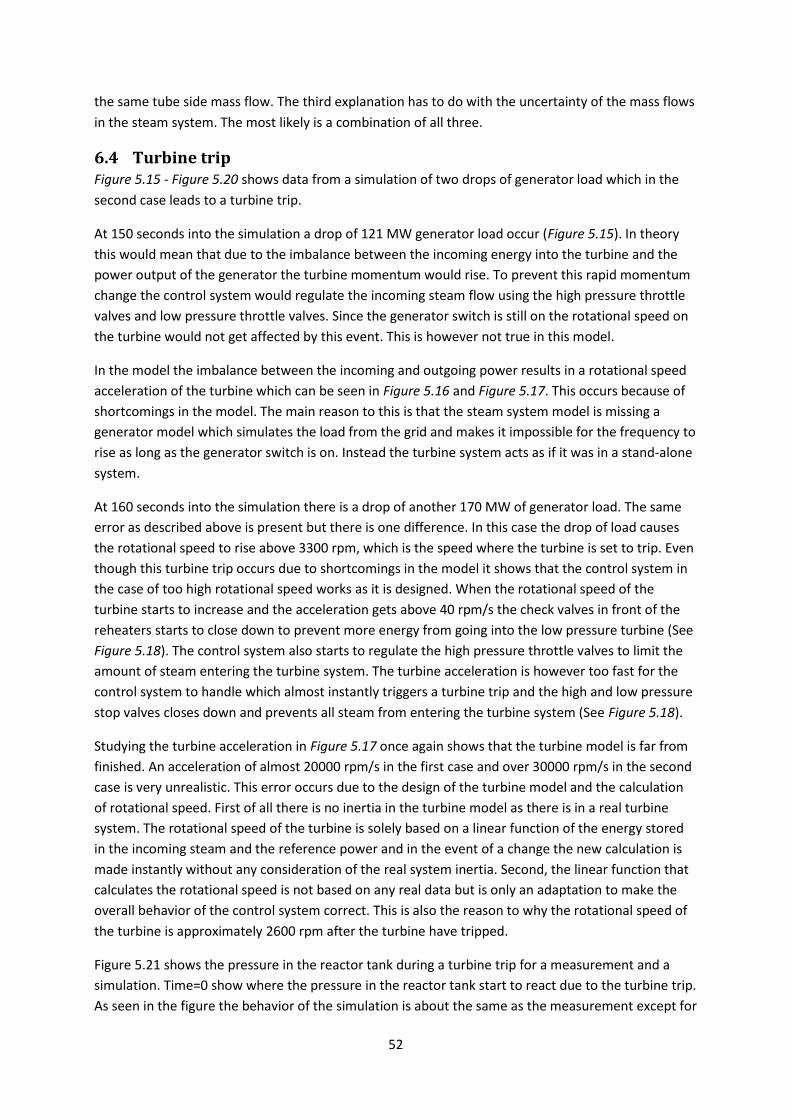
52
the same tube side mass flow. The third explanation has to do with the uncertainty of the mass flows
in the steam system. The most likely is a combination of all three.
6.4 Turbine trip Figure 5.15 - Figure 5.20 shows data from a simulation of two drops of generator load which in the
second case leads to a turbine trip.
At 150 seconds into the simulation a drop of 121 MW generator load occur (Figure 5.15). In theory
this would mean that due to the imbalance between the incoming energy into the turbine and the
power output of the generator the turbine momentum would rise. To prevent this rapid momentum
change the control system would regulate the incoming steam flow using the high pressure throttle
valves and low pressure throttle valves. Since the generator switch is still on the rotational speed on
the turbine would not get affected by this event. This is however not true in this model.
In the model the imbalance between the incoming and outgoing power results in a rotational speed
acceleration of the turbine which can be seen in Figure 5.16 and Figure 5.17. This occurs because of
shortcomings in the model. The main reason to this is that the steam system model is missing a
generator model which simulates the load from the grid and makes it impossible for the frequency to
rise as long as the generator switch is on. Instead the turbine system acts as if it was in a stand-alone
system.
At 160 seconds into the simulation there is a drop of another 170 MW of generator load. The same
error as described above is present but there is one difference. In this case the drop of load causes
the rotational speed to rise above 3300 rpm, which is the speed where the turbine is set to trip. Even
though this turbine trip occurs due to shortcomings in the model it shows that the control system in
the case of too high rotational speed works as it is designed. When the rotational speed of the
turbine starts to increase and the acceleration gets above 40 rpm/s the check valves in front of the
reheaters starts to close down to prevent more energy from going into the low pressure turbine (See
Figure 5.18). The control system also starts to regulate the high pressure throttle valves to limit the
amount of steam entering the turbine system. The turbine acceleration is however too fast for the
control system to handle which almost instantly triggers a turbine trip and the high and low pressure
stop valves closes down and prevents all steam from entering the turbine system (See Figure 5.18).
Studying the turbine acceleration in Figure 5.17 once again shows that the turbine model is far from
finished. An acceleration of almost 20000 rpm/s in the first case and over 30000 rpm/s in the second
case is very unrealistic. This error occurs due to the design of the turbine model and the calculation
of rotational speed. First of all there is no inertia in the turbine model as there is in a real turbine
system. The rotational speed of the turbine is solely based on a linear function of the energy stored
in the incoming steam and the reference power and in the event of a change the new calculation is
made instantly without any consideration of the real system inertia. Second, the linear function that
calculates the rotational speed is not based on any real data but is only an adaptation to make the
overall behavior of the control system correct. This is also the reason to why the rotational speed of
the turbine is approximately 2600 rpm after the turbine have tripped.
Figure 5.21 shows the pressure in the reactor tank during a turbine trip for a measurement and a
simulation. Time=0 show where the pressure in the reactor tank start to react due to the turbine trip.
As seen in the figure the behavior of the simulation is about the same as the measurement except for

53
the magnitude of the over- and undershoots and the time of the fluctuations. This is the result of
limitations in the steam system model. For once, the reactor tank is connected to two turbine strings
in the real power plant. This model only includes one of the strings and the dynamics lost due to this
is not possible to describe. The extra turbine system makes it possible to redirect steam from one
steam system to another in case of transients. This dynamics is very complex and depend on a great
amount of factors, e.g. the load on each individual turbine system and the possibility for one system
to handle a specific amount of extra steam. It also depends on what is happening with the reactor
power directly after the turbine trip. Since the correct control system parameters are unknown it is
also very hard to know if the modeled control system is agreeing with the real one.

54
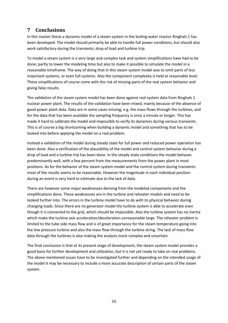
55
7 Conclusions In this master thesis a dynamic model of a steam system in the boiling water reactor Ringhals 1 has
been developed. The model should primarily be able to handle full power conditions, but should also
work satisfactory during the transients; drop of load and turbine trip.
To model a steam system is a very large and complex task and system simplifications have had to be
done; partly to lower the modeling time but also to make it possible to simulate the model in a
reasonable timeframe. The way of doing that in this steam system model was to omit parts of less
important systems, or even full systems. Also the component complexity is held at reasonable level.
These simplifications of course come with the risk of missing parts of the real system behavior and
giving false results.
The validation of the steam system model has been done against real system data from Ringhals 1
nuclear power plant. The results of the validation have been mixed, mainly because of the absence of
good power plant data. Data are in some cases missing, e.g. the mass flows through the turbines, and
for the data that has been available the sampling frequency is once a minute or longer. This has
made it hard to calibrate the model and impossible to verify its dynamics during various transients.
This is of course a big shortcoming when building a dynamic model and something that has to be
looked into before applying the model on a real problem.
Instead a validation of the model during steady state for full power and reduced power operation has
been done. Also a verification of the plausibility of the model and control system behavior during a
drop of load and a turbine trip has been done. In the steady state conditions the model behaves
predominantly well, with a few percent from the measurements from the power plant in most
positions. As for the behavior of the steam system model and the control system during transients
most of the results seems to be reasonable. However the magnitude in each individual position
during an event is very hard to estimate due to the lack of data.
There are however some major weaknesses deriving from the modeled components and the
simplifications done. These weaknesses are in the turbine and reheater models and need to be
looked further into. The errors in the turbine model have to do with its physical behavior during
changing loads. Since there are no generator model the turbine system is able to accelerate even
though it is connected to the grid, which should be impossible. Also the turbine system has no inertia
which make the turbine axis acceleration/deceleration unreasonable large. The reheater problem is
limited to the tube side mass flow and is of great importance for the steam temperature going into
the low pressure turbine and also the mass flow through the turbine string. The lack of mass flow
data through the turbines is also making the analysis more complex and uncertain.
The final conclusion is that at its present stage of development, the steam system model provides a
good basis for further development and utilization, but it is not yet ready to take on real problems.
The above mentioned issues have to be investigated further and depending on the intended usage of
the model it may be necessary to include a more accurate description of certain parts of the steam
system.

56
57
8 Future improvements The steam system in a nuclear power plant is very large and complex and it is therefore almost
impossible to build a comprehensive model that takes all aspects into consideration. There are
however a few improvements to the steam system model that would significantly improve its
reliability.
As mentioned before, the system dynamics need to be verified. To do that better data from
the steam system is needed. Especially data sampled with a higher frequency, but also more
data of the mass flow in various positions in the steam system during reduced power
operation is needed.
Better data also makes it possible to improve the regulator parameters to better fit the real
power plant.
A better modulation of the reheater system that better fit the real behavior.
A better turbine model that can describe the dynamics during off-design operation. Also a
generator switch, turbine inertia and a better way of calculating rotational speed needs to be
implemented.
There are models of a reactor tank, condenser and the feed water system available at
Solvina. By connecting them to the steam system model correctly the model dynamics would
improve and a lot of the static boundary flows would disappear. The risk is however that the
system gets too complex and that the numeric solver will find it hard to converge on a
solution.

58
59
References
[1] The history of nuclear energy. (n.d.). U.S. Department of Energy.
[2] The Engineerer. (1956, 10 05). Retrieved 07 03, 2011
[3] Izobraževalni center za jedrsko tehnologijo. (n.d.). Retrieved 06 16, 2011, from
http://www.icjt.org/
[4] Ny Teknik. (2011, 07 19). Den svenska atombomben. Retrieved 07 25, 2011, from
http://www.nyteknik.se
[5] Vattenfall. (n.d.). Kärnkraftens hitoria i Sverige. Retrieved 06 17, 2011, from
http://www.vattenfall.se/
[6] Strålsäkerhetsmyndigheten. (2011, 07 25). Anläggningar i Sverige. Retrieved from
http://www.stralsakerhetsmyndigheten.se
[7] World Nuclear Assosiation. (n.d.). World Nuclear Power Reactors and Uranium Requirements.
Retrieved 06 16, 2011, from http://www.world-nuclear.org/
[8] Kärnkraftsäkerhet och Utbildning AB. (2005). Världens kärnkraft och olika reaktortyper.
[9] Kärnkraftsäkerhet och Utbildning AB. (2005). Huvudprocessen - Anläggningskännedom.
[10] Kärnkraftsäkerhet och Utbildning AB. (2010). R1 AK1 2010 Bok 11 - Anläggningskännedom.
[11] Ringhals AB. (2010, 11 04). R1 System 411, Huvudångledning. FSAR/Systembeskrivning.
[12] Ringhals AB. (2008, 04 08). R1 System 412. Styrning av ångflöde och mellanöverhettningssystem.
FSAR/Systembeskrivning.
[13] Ringhals AB. (2005, 09 28). R1 System 412. Turbin. FASR/Systembeskrivning.
[14] Ringhals AB. (n.d.). R1 System 581. Elektrisk turbinregulator. FSAR/Systembeskrivning.
[15] Kärnkraftsäkerhet och utbildning AB. (1997). Reaktorfysik - Högre utbildning, H1.
[16] Crowe, C. T., Elger, D. F., & Roberson, J. A. Engineering Fluid Mechanics (Eighth ed.). Wiley.
[17] Cooke, D. H. (1983). Modeling of off-design multistage turbine pressures by Stodola's ellipse.
Houston, Texas: Bechtel Power Corporation.
[18] Glad, T., & Ljung, L. (2006). Reglerteknik - Grundläggande teori (Forth ed.). Danmark:
Studentlitteratur.
[19] Hägglund, T. (1997). Praktisk processreglering (Second ed.). Lund: Studentlitteratur.
[20] Modelica and the Modelica Association. (n.d.). Retrieved from https://www.modelica.org
[21] The International Association for the Properties of Water and Steam. (2007). Revised Release on
the IAPWS Industrial Formulation 1997 for the Thermodynamic Properties of Water and Steam.
Retrieved April 5, 2011, from http://www.iapws.org/

60
[22] Multi-Engineering Modeling and Simulation - Dymola. (n.d.). Retrieved 04 05, 2011, from
http://www.3ds.com/products/catia/portfolio/dymola
[23] Petzold, L. (1982). A Description of DASSL: A Differential/Algebraic System Solver. Sandia
National Laboratories.
[24] Emerson Process Management. (n.d.). Control valve handbook. (Forth).
[25] Na, Z. *., & Ruixian, C. (2002). Analytical solutions and typical characteristics of part-load
performances of single shaft gas turbine and its cogeneration. Beijing, China.