Embed Size (px)
Citation preview
Modeling, Simulation and Optimization of
Residential and Commercial Energy Systems
by
Mohamed Abdussalam Bregaw
Submitted in partial fulfilment of the requirements for the degree of Master of Applied Science
at
Dalhousie University Halifax, Nova Scotia
August 2013
© Copyright by Mohamed Abdussalam Bregaw, 2013
ii
DDEDICATION
I would like to dedicate this research to the spirit of my beloved father, to my
beloved mother, brothers, sisters, to my beloved wife Mbarka and my sweet
daughter Sara.
iii
TABLE OF CONTENTS
LIST OF TABLES ........................................................................................... vi LIST OF FIGURES ......................................................................................... ix
ABSTRACT .................................................................................................... xiii LIST OF ABBREVIATIONS AND SYMBOLS USED ............................. xiv
ACKNOWLEDGEMENTS ......................................................................... xvii CHAPTER 1 INTRODUCTION .................................................................... 1
1.1 MOTIVATION BEHIND THE WORK .................................................................... 1
1.2 THESIS OBJECTIVES AND CONTRIBUTION ..................................................... 1
1.3 THESIS OUTLINE .................................................................................................... 2
CHAPTER 2 LITERATURE REVIEW ....................................................... 4
2.1 INTRODCTION .......................................................................................................... 4
2.2 LOAD MANAGEMENT ............................................................................................... 4
2.3 BASIC DEFINITION .................................................................................................... 5
2.4 REVIEW OF SMART GRID ........................................................................................ 6
2.5 THE THERMAL SYSTEM (HEAT AND TEMPERATURE) ..................................... 7
2.6 MATHMATICAL MODEL OF THERMAL SYSTEM USING SIMSCAPE ............. 7
CHAPTER 3 MODELING OF ELECTRIC WATER HEATER ............11
3.1 INTRODUCTION ....................................................................................................... 11
3.2 MODELING OF (DEWH)........................................................................................... 13
3.2.1 MATHEMATICAL ANALYSIS .......................................................................... 15
3.2.2 ANALYSIS OF CYCLING TIME ........................................................................ 23
3.2.3 COMPARISON OF MODELS ............................................................................. 26
3.2.4 LOAD PROFILE AND ENERGY COST ............................................................. 28
CHAPTER 4 MODELING OF HEATING SYSTEMS .............................31
4.1 INTRODUCTION ....................................................................................................... 31
4.2 DOMESTIC ELECTRIC OVEN (DEO) ..................................................................... 31
4.2.1 INTRODUCTION ................................................................................................. 31
4.2.2 MODELING OF (DEO) ........................................................................................ 32
4.2.3 MATHEMATICAL MODEL OF (DEO) ............................................................. 34
iv
4.2.4 LOAD PROFILE AND ENERGY COST ............................................................. 40
4.3 DOMESTIC ELECTRIC CLOTHES IRON (DECI) .................................................. 44
4.3.1 INTRODUCTION ................................................................................................. 44
4.3.2 MODELING OF (DECI) ....................................................................................... 44
4.3.3 MATHEMATICAL MODEL of DECI ................................................................. 46
4.3.4 LOAD PROFILE AND ENERGY COST ............................................................. 52
4.4 DOMESTIC ELECTRIC BASEBOARD HEATER (DEBH)..................................... 55
4.4.1 INTRODUCTION ................................................................................................. 55
4.4.2 MODEL of DEBH ................................................................................................. 55
4.4.3 MATHEMATICAL MODEL of DEBH ............................................................... 57
4.4.4 LOAD PROFILE AND ENERGY COST ............................................................. 63
4.5 MODEL of LIGHTING ............................................................................................... 68
4.5.1 INTRODUCTION ................................................................................................. 68
4.5.2 MODEL of FLUORESCENT LAMP (F-Lamp) ................................................... 69
4.5.3 MATHEMATICAL MODEL of FLUORESCENT LAMP (FL) ......................... 72
CHAPTER 5 MODELING of MACHINES ...............................................75
5.1 INTRODUCTION ................................................................................................... 75
5.2 MODEL of DOMESTIC ELECTRIC CLOTHES WASHER (DECW) ..................... 76
5.2.1 INTRODUCTION ................................................................................................. 76
5.2.2 MODEL of A SINGLE-PHASE INDUCTION MOTOR of DECW .................... 76
5.2.3 MATHEMATICAL MODEL of A 1-PHASE INDUCTION MOTOR DECW ... 77
5.2.4 LOAD PROFILE AND ENERGY COST ............................................................. 81
5.3 MODEL of DOMESTIC ELECTRIC CLOTHES DRYER (DECD) ......................... 84
5.3.1 INTRODUCTION ................................................................................................. 84
5.3.2 MODEL of DECD ................................................................................................. 84
5.3.3 MATHEMATICAL MODEL of A 1-PHASE INDUCTION MOTOR DECD .... 88
5.3.4 LOAD PROFILE AND ENERGY COST ............................................................. 92
5.4 MODEL of DOMESTIC ELECTRIC DISHWASHER (DEDW) ............................... 96
5.4.1 INTRODUCTION ................................................................................................. 96
5.4.2 MODEL of DEDW Heater .................................................................................... 98
5.4.3 MATHEMATICAL MODEL of A 1-PHASE INDUCTION MOTOR DEDW 101
5.4.4 LOAD PROFILE AND ENERGY COST ........................................................... 105
v
CHAPTER 6 OPTIMIZATION METHOD .............................................110
6.1 INTRODUCTION ..................................................................................................... 110
6.2 MODEL of LINEAR PROGRAMING PROBLEM (LPP) ....................................... 110
6.2.1 MATHEMATICAL MODEL of (BIP) ............................................................... 111
6.2.2 CASE STUDY of RESIDENTIAL ENERGY SYSTEM ................................... 113
6.2.3 CASE STUDY of COMMERCIAL ENERGY SYSTEM .................................. 130
6.2.4 COMPARISON OF MODELS ........................................................................... 133
CHAPTER 7 CONCLUSION AND RECOMMENDATIONS ...............134
7.1 CONCLUSION .......................................................................................................... 134
7.2 RECOMMENDATIONS AND FUTURE WORK.................................................... 135
REFERENCES ...............................................................................................137
APPENDIX A Model of domestic electric oven DEO ..............................144
APPENDIX B Model of domestic electric clothes iron DECI .................148
APPENDIX C Model of domestic electric baseboard heater DEBH .....153
APPENDIX D Model of a 1-phase induction motor of DECW...............158
APPENDIX E Model of a 1-phase induction motor of DECD ................162
APPENDIX F Model of a 1-phase induction motor of DEDW ...............165

vi
LIST OF TABLES
Table 3.1 Thermal to electrical analogies of various parameters ............................................... 11
Table 3.2 DEWH parameters ...................................................................................................... 13
Table 3.3 Known parameters of DEWH ..................................................................................... 17
Table 3.4 The results of equations and simulation in case 1 ...................................................... 22
Table 3.5 The comparison of the simulation results and equations ............................................ 23
Table 3.6 The results of simulation and calculation ................................................................... 24
Table 3.7 The comparison of equations and simulation results .................................................. 25
Table 3.8 The time response in steady-state & transient Conditions .......................................... 25
Table 3.9 The cost-rate of NS power * Rates effective January 1, 2013 [17] ............................ 29
Table 4.1 Model of Domestic Electric Oven specifications ....................................................... 33
Table 4.2 Known parameters of DEO model.............................................................................. 34
Table 4.3 Comparison of the equations and the simulation results ............................................ 38
Table 4.4 Comparison of equations and simulation results in steady-state ................................ 38
Table 4.5 Comparison of the results in transient condition ........................................................ 39
Table 4.6 The time response of the system ................................................................................. 39
Table 4.7 The cost-rate of NS power * Rates effective January 1, 2013 [17] ............................ 42
Table 4.8 Model of Domestic Electric Clothes Iron specifications ............................................ 45
Table 4.9 Comparison of the results of the time duration of the model ............................ 50
Table 4.10 Comparison of the simulation results to equations ................................................... 50
Table 4.11 Comparison of the time response of the system ....................................................... 51
Table 4.12 The cost-rate of NS power * Rates effective January 1, 2013 [17] .......................... 53
Table 4.13 Model of (DEBH) specifications .............................................................................. 56
Table 4.14 Comparison of equations and the simulation results ................................................ 60
Table 4.15 The results of equations and simulation in steady-state condition ........................... 61
Table 4.16 The results of equations and simulation in transient condition. ............................... 62
Table 4.17 Time response of the system ..................................................................................... 62
Table 4.18 The cost-rate of NS power * Rates effective January 1, 2013 [17] .......................... 66
Table 4.19 Simulink model parameters [68] ............................................................................... 71
Table 4.20 V-I Characteristics a 32 W General Electric fluorescent-lamp [61] ......................... 71
vii
Table 4.21 The average operating time and energy use of fluorescent-lamp ............................. 74
Table 5.1 The average operating time / energy consumption of DECW [40] ............................. 77
Table 5.2 Induction motor single-phase capacitor start specifications ........................................ 77
Table 5.3 Comparison of the calculations and the simulation results.......................................... 78
Table 5.4 The cost-rate of NS power * Rates effective January 1, 2013 [17] ............................. 82
Table 5.5 Model of (DECD) heater specifications ...................................................................... 85
Table 5.6 Time duration, power and energy consumption of the DECD heater ......................... 87
Table 5.7 The average operating time and energy consumption of clothes Dryer [40] ............... 88
Table 5.8 Single-phase induction motor capacitor start specifications ....................................... 89
Table 5.9 Comparison of the calculations and the simulation results......................................... 90
Table 5.10 The average operating time and energy use of dishwasher [40] ............................... 96
Table 5.11 Model of (DEDW) heater Specifications.................................................................. 98
Table 5.12 Time duration, power and energy consumption of the DEDW heater ................... 100
Table 5.13 Single-phase induction motor capacitor start specifications of DEDW ................. 101
Table 5.14 Comparison of the calculations and the simulation results..................................... 102
Table 5.15 Comparison between Case 1 and Case 2 ................................................................ 109
Table 5.16 1-phase induction motor capacitor start specifications of DECW .......................... 158
Table 5.17 1-phase induction motor capacitor start specifications of DECD ........................... 162
Table 5.18 1-phase induction motor capacitor start specifications of DEDW ......................... 165
Table 6.1 The cost-rate of NS Power * Rates effective January 1, 2013 [17] .......................... 114
Table 6.2 The average operating time and energy use of residential appliances ...................... 114
Table 6.3 Scenario 1, Load aggregation cost of non-optimized schedule ................................ 116
Table 6.4 Scenario-1 appliances of residential energy system ................................................. 118
Table 6.5 Load aggregation cost of optimized schedule Scenarion-1 ...................................... 120
Table 6.6 Scenario-2 appliances of residential energy system ................................................. 121
Table 6.7 Scenario 2, Load aggregation energy cost of residential sector ............................... 124
Table 6.8 The cost-rate of NS power * Rates effective January 1, 2013 [17] .......................... 125
Table 6.9 Scenario 3, Load aggregation cost of Non-Optimized schedule .............................. 126
Table 6.10 Scenario 3, appliances of residential energy system............................................... 126
viii
Table 6.11 Scenario 3, Load aggregation cost of optimized schedule...................................... 129
Table 6.12 The cost-rate of NS Power * Rates effective January 1, 2013 [17] ........................ 130
Table 6.13 Appliances of commercial energy system a case study .......................................... 130
Table 6.14 Daily load aggregation of energy consumption ...................................................... 132
Table 6.15 Monthly load aggregation of energy (consumption and cost) ................................. 132
ix
LIST OF FIGURES
Figure 2.1 Components of electric power system [5] ................................................................... 4
Figure 2.2 The load shape for standard DSM load management [32] .......................................... 6
Figure 2.3 Steps of deriving system response [80] ....................................................................... 8
Figure 3.1 ETP heat transfer model of electric water heater ...................................................... 11
Figure 3.2 Model of Domestic Electric Water Heater ................................................................ 13
Figure 3.3 State flow model of the thermostat of DEWH .......................................................... 13
Figure 3.4 DEWH Temperature vs. Time full-day ..................................................................... 14
Figure 3.5 Simplified thermal characteristic curve of thermostat (cycling time) ....................... 24
Figure 3.6 Comparison of DEWH model with another literature model .................................... 26
Figure 3.7 Comparison of DEWH model with another literature model .................................... 27
Figure 3.8 Energy Cost Calculator of Electric Water-Heater ..................................................... 28
Figure 3.9 Load profile of DEWH Full Day (Load and Cost vs. time) ...................................... 28
Figure 3.10 Load profile of DEWH Full Day (Load vs. Cost) ................................................... 29
Figure 4.1 Model of Domestic Electric Oven system ................................................................. 32
Figure 4.2 State flow model of the thermostat of DEO .............................................................. 33
Figure 4.3 DEO Temperature vs. Time ...................................................................................... 33
Figure 4.4 Energy Cost Calculator of DEO ................................................................................ 40
Figure 4.5 Load profile of DEO (Load and Cost vs. time) ......................................................... 41
Figure 4.6 Load profile of DEO (Load vs. Cost) Standard tariff ................................................ 41
Figure 4.7 Load profile of DEO (Load vs. Cost) Off-Peak tariff ............................................... 42
Figure 4.8 Model of Domestic Electric Clothes Iron .................................................................. 44
Figure 4.9 State flow of the thermostat of DECI ........................................................................ 45
Figure 4.10 DECI Temperature vs. Time (A) ............................................................................. 45
Figure 4.11 DECI Temperature vs. Time (B) ............................................................................. 46
Figure 4.12 Energy Cost Calculator of DECI ............................................................................. 52
Figure 4.13 Load profile of DECI (Load and Cost vs. time) ...................................................... 52
Figure 4.14 Load profile of DECI (Load vs. Cost) Standard tariff............................................. 53
Figure 4.15 Load profile of DECI (Load vs. Cost) Off-Peak tariff ............................................ 53
x
Figure 4.16 Model of Domestic Electric Baseboard Heater (DEBH) ........................................ 55
Figure 4.17 State flow model of the thermostat of (DEBH) ....................................................... 56
Figure 4.18 DEBH Temperature vs. Time (Run-time = 1hr) ................................................... 56
Figure 4.19 DEBH Temperature vs. Time (Run-time = 5 hrs.) .................................................. 57
Figure 4.20 Energy Cost Calculator of DEBH ........................................................................... 63
Figure 4.21 DEBH (Load and Cost vs. time) Run-time = 1 hr. .................................................. 63
Figure 4.22 DEBH (Load vs. Cost) Standard tariff, Run-time = 1 hr. ....................................... 64
Figure 4.23 DEBH (Load vs. Cost) Off-Peak tariff, Run-time = 1 hr. ....................................... 64
Figure 4.24 DEBH (Load and Cost vs. time) Run-time = 5 hrs. ................................................ 65
Figure 4.25 DEBH (Load vs. Cost) Standard tariff, Run-time = 5 hrs. ...................................... 65
Figure 4.26 DEBH (Load vs. Cost) Off-Peak tariff .................................................................... 65
Figure 4.27 Equivalent circuit of the series resonant parallel loaded ballast and f-lamp [61] ... 70
Figure 4.28 Vs1 (rms) and (rms) of F-lamp ..................................................................... 73
Figure 4.29 Active power and Reactive power of F-lamp for 80.775 kHz ................................ 73
Figure 5.1 Modified version model of a single-phase induction motor of DECW [78] ............. 76
Figure 5.2 System behavior of DECW within run-time 30 min ................................................. 78
Figure 5.3 Case 1- DECW average energy consumption, run-time every day ........................... 79
Figure 5.4 Case 2- DECW average energy consumption, run-time twice a week...................... 80
Figure 5.5 Energy Cost Calculator of DECW ............................................................................ 81
Figure 5.6 Load profile of DECW (Load and Cost vs. time) ..................................................... 81
Figure 5.7 Load profile of DECW (Load vs. Cost) Standard tariff ............................................ 82
Figure 5.8 Load profile of DECW (Load vs. Cost) Off-Peak tariff ............................................ 82
Figure 5.9 Model of Domestic Electric Clothes dryer (heater) .................................................. 84
Figure 5.10 State flow model of the thermostat of (DECD-Heater) ............................................ 85
Figure 5.11 Temperature vs. Time of Clothes dryer Run-time = 1 hour ..................................... 85
Figure 5.12 Modified version model of a single-phase induction motor of DECD [78] ............. 88
Figure 5.13 System behavior of DECD within run-time 30 min ................................................. 89
Figure 5.14 Case 1- DECD average energy consumption, run-time every day ........................... 91
Figure 5.15 Case 2- DECD average energy consumption, run-time twice a week ..................... 91
Figure 5.16 Energy Cost Calculator of DECD ............................................................................ 92
xi
Figure 5.17 Load profile of DECD (Load and Cost vs. time) ..................................................... 93
Figure 5.18 Load profile of DECD (Load vs. Cost) Standard tariff ............................................ 93
Figure 5.19 Load profile of DECD (Load vs. Cost) Off-Peak tariff............................................ 94
Figure 5.20 Model of Domestic Electric Dishwasher (heater) .................................................... 98
Figure 5.21 State flow model of the thermostat of (DEDW-Heater) ........................................... 98
Figure 5.22 Temperature vs. Time of DEDW Run-time = 1.5 hour ............................................ 99
Figure 5.23 Modified version model of a single-phase induction motor of DEDW [78] .......... 101
Figure 5.24 System behavior of DEDW within run-time 30 min .............................................. 102
Figure 5.25 Case 1- DEDW average energy consumption, run-time every day ........................ 103
Figure 5.26 Case 2- DEDW average energy consumption, run-time every day ........................ 104
Figure 5.27 Energy Cost Calculator of DEDW ......................................................................... 105
Figure 5.28 Load profile of DEDW (Load and Cost vs. time) .................................................. 105
Figure 5.29 Load profile of DEDW (Load vs. Cost) Standard tariff ......................................... 106
Figure 5.30 Load profile of DEDW (Load vs. Cost) Off-Peak tariff ........................................ 106
Figure 5.31 Load profile of DEDW (Load and Cost vs. time) .................................................. 107
Figure 5.32 Load profile of DEDW (Load vs. Cost) Standard tariff ......................................... 107
Figure 5.33 Load profile of DEDW (Load vs. Cost) Off-Peak tariff ........................................ 108
Figure 5.34 Developing an equivalent circuit of for single-phase induction motors [18] ......... 158
Figure 6.1 Flowchart of the BIP optimization problem ............................................................ 113
Figure 6.2 Load aggregation cost of non-optimized schedule Scenarion-1 .............................. 115
Figure 6.3 DEWH (A1) Optimized run-time schedule Scenarion-1 ......................................... 117
Figure 6.4 TOU tariff of appliances (A1, A5, and A6) ............................................................ 118
Figure 6.5 TOU tariff of appliances (A7, and A8) ................................................................... 119
Figure 6.6 Load aggregation cost of optimized schedule Scenarion-1 ..................................... 119
Figure 6.7 Off-Peak tariff of appliances (A1, A2 and A3) ....................................................... 121
Figure 6.8 Off-Peak tariff of appliances (A4, A5 and A6) ....................................................... 122
Figure 6.9 Off-Peak tariff of appliances (A7, and A8) ............................................................. 122
Figure 6.10 Load aggregation cost of run-time schedule Scenarion-2 ..................................... 123
Figure 6.11 Load aggregation cost of non-optimized schedule Scenarion-3............................ 125
Figure 6.12 TOU tariff of appliances (A1, A5, and A6) .......................................................... 127
xii
Figure 6.13 TOU tariff of appliances (A7, and A8) ................................................................. 127
Figure 6.14 Load aggregation cost of optimized schedule Scenarion-3 ................................... 128
Figure 6.15 Daily load in commercial energy system of a case study ...................................... 130
Figure 6.16 Monthly load in commercial energy system of a case study ................................. 130
Figure 6.17 Monthly cost in commercial energy system of a case study ................................. 131
Figure 6.18 Monthly energy consumption and cost in commercial energy system.................. 132
xiii
ABSTRACT
A Residential Energy Management System (REMS) in smart grid can be defined as processes
of control systems designed to control, measure, monitor, and modify energy demand and energy
consumption profiles. (REMS) provides capability to manage a daily load curve in order to
reduce power consumption and energy cost. Consequently, (REMS) offers significant benefits
for both the electricity suppliers and consumers in terms of control and schedule time of use of
major appliances in the residential and commercial sectors.
In recent years, however, the rate of energy demand has increased rapidly throughout the
world while the price of energy has been fluctuating. To find the solution for such problems,
(REMS) establishes the optimal daily operation of home appliances. Numerous methods for
(REMS) are used; this thesis analyzes many candidate scenarios during peak and off peak load
periods comparing to the tariff of the residential sector to reduce the usage and its associated
costs. It presents simulated results of proposed (REMS) to provide an automated least cost
demand response. The main approach will be to ensure the satisfaction of the requirements with
constraints on efficient use of energy. In this thesis, multiphasic system behavior and an
individual set of components simulation of smart appliances in residential and commercial
energy systems with a realistic manner are proposed.
xiv
LIST OF ABBREVIATIONS AND SYMBOLS USED
LIST OF ABBREVIATIONS
REMS Residential Energy Management System
DSM Demand-Side Management
EMS Energy management system
ETP The equivalent thermal parameters
WHAM Water Heater Analysis Model
UEC The average annual unit energy consumption
HVAC Heating ventilation and air conditioning
DEWH Domestic Electric Water Heater (A1)
DECW Domestic Electric Clothes Washer (A2)
DECD Domestic Electric Clothes Dryer (A3)
DECI Domestic Electric Clothes Iron (A4)
DEBH Domestic Electric Baseboard Heater (A5)
DEO Domestic Electric Oven (A6)
DEDW Domestic Electric Dishwasher (A7)
F-lamp Fluorescent-lamp (A8)
CFL Compact fluorescent lamps
LED Light emitting diode
LPP Linear Programming problem
LP Linear Programming
BILP Binary Integer Linear Programming
MBLP Mixed Binary Linear Programming
xv
LIST OF SYMBOLS
Hot water temperature in tank (
Ambient air temperature outside tank (
Incoming inlet cold water temperature (
Set-point temperature = ( ) (
Dead band around the Set-point
Low water temperature (
High water temperature (
Average hot water draw per hour
Density of water
V Volume of tank
Specific heat of the water
SA Surface area of tank (m²)
U Heat loss coefficient
R Thermal resistance of tank
Rate of energy input (W); Q = Prated
Prated Power rated input of the heating resistance element
C Thermal capacity of water in the tank
Thermal resistance
Thermal conductance G =A/R where, R is the
thermal resistance of the tank
Time constant
Worming-up time
Number of cycling time
Average power consumption
TOU time of use
EC Energy Consumption
The forward impedance
xvi
The backward impedance
The input impedance
The input power
The air-gap power
The power mechanical
Power losses
Synchronous speed
Rotor speed
The angular synchronous speed
Output torque
The efficiency of the motor
The impedance of the parallel brunch of F-lamp circuit
The impedance of the series brunch of F-lamp circuit
Lamp conductance
Cost function
The TOU electricity price rate in
L Load per appliance

xvii
ACKNOWLEDGEMENTS
I am grateful and would like to express my deepest gratitude to my advisor Dr. Mohamed
El-Hawary for his support, guidance, understanding and patience during my studies and
throughout the research work. I appreciate his consistent support from the first day I applied to
graduate program to these concluding moments. I am also grateful to my committee; Dr. J. Gu
and Dr. W. Phillips for spending their valuable time reading and evaluating my thesis.
I would also like to thank the members of the Electrical and Computer Engineering
Department at Dalhousie University for their continuous help and guidance.
I would like to express my appreciation to my beloved wife Mbarka and my sweet daughter
Sara, for their patience, encouragement and supportive of my studies. I acknowledge my sincere
indebtedness and gratitude to my family, especially my parents, for their encouragement, steady
support and love throughout the research work. I am so proud of my family that shares my
enthusiasm for academic pursuits.
I would like to take this opportunity to thank the Ministry of Education in my country,
Libya, the staff of the Libyan Embassy in Canada and the Canadian Bauru for International
Education, CBIE, for their mental and financial support.
Finally, I cannot close without express my sincere gratitude to my close relative, friends and
colleagues for their support and encouragement.

1
CHAPTER 1 INTRODUCTION
1.1 MOTIVATION BEHIND THE WORK
The energy demand has been growing over the last decades throughout the
world while energy prices have been fluctuating over time. Accordingly,
Residential Energy Management System (REMS) plays a significant role since it
provides the capability to manage the daily load curve in order to reduce power
consumption and energy cost. In addition, REMS offers significant benefits for
both the electricity suppliers and consumers in terms of control and schedule time
of use (TOU) of major appliances in the residential sector as well as in the
commercial sector.
Numerous methods for REMS are used; this study analyzes many candidate
scenarios during peak and off peak load periods comparing to the tariff of
residential and commercial sectors to reduce the usage and its associated costs.
The investigation of modeling and simulation systems requires collecting
some important data in order to design and simulate each model. An individual
physical model in place of aggregated models with acceptable level of accuracy is
used. It is worth mentioning that, instead of taking the parameter values from the
literature, this study examines many mathematical models in order to calculate
the thermal capacitance and the thermal conductance in terms of temperature and
input power. In addition, to determine the appropriate model that reflects the
parameters’ impact as well as the system behavior of each individual model;
multiphasic system behavior and an individual set of components simulation of
appliances with a realistic manner are proposed. On the other hand, the
mathematical model [3] with appropriate modification for obtaining expressions
to calculate approximate temperature and time duration is determined by using a
single-zone lumped-parameter thermal model.
1.2 THESIS OBJECTIVES AND CONTRIBUTION
There are three main objectives of this thesis:
2
First, all modeling of appliances are designed and implemented by using both the
Matlab/Simulink and Matlab/SimScape modeling environments.
The Matlab/Simulink, Matlab/SimScape and MathWorks are used for modeling
of heating systems, where Matlab/SimScape libraries contain many blocks that
can be used for modeling thermal, hydraulic and mechanical components to
model and simulate such systems in order to develop control systems and test
system performance [1, 2].
Second, once the model of appliance is designed and simulated, the next step is to
compare the simulation results to approximate linear equations and exponential
equations; which are derived and used for estimating the amount of temperature,
time duration and power/energy consumption [3].
Third, the main contribution of this study is to determine the optimal solution of
time of use (TOU) in a case of an individual operation as well as in an
aggregating operation, in order to reduce energy cost and to determine the best
operation time by using Linear programming (LP, or linear optimization).
1.3 THESIS OUTLINE
This thesis is divided into seven main chapters. The first chapter presents the
concept of the thesis and the second chapter which includes the literature reviews,
begins with load management principles, basic definitions for power system
evaluation and an introduction to the thermal system (heat and temperature).
The third chapter consists of the modeling of domestic electric water heater
system in details; mathematical model and the system behavior during operation
time. The forth chapter includes the modeling of heating systems such as
domestic oven, domestic baseboard heater and domestic clothes iron; all these
models are discussed in details of mathematical models and the system behavior
during operation time. The fifth chapter contains the modeling of electric
machine systems such as clothes washer, clothes dryer and dishwasher.
The sixth chapter contains an optimization method; the objective function of
this chapter is to analyze many candidate scenarios during peak and off peak load
periods comparing to the tariff of the residential and commercial sectors to
reduce the usage and its associated costs. Thus, the optimization function seeks

3
minimization of costs and the optimal daily operation of home appliances in
order to find the solution for such problems. The main approach will be to ensure
the satisfaction of the requirements with constraints on efficient use of energy [4].
The last chapter provides the conclusion, recommendations, and suggestions
for future studies related to this thesis.
4
CHAPTER 2 LITERATURE REVIEW
2.1 INTRODCTION
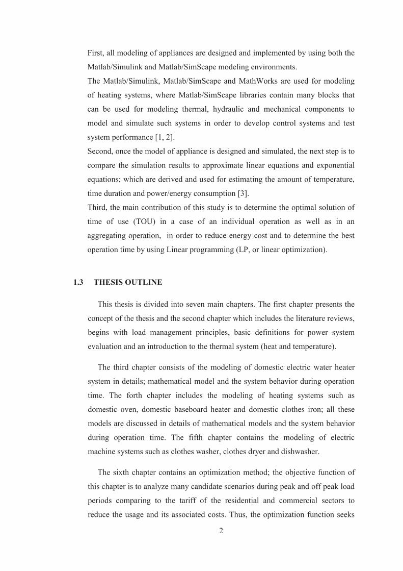
An Electrical power system consists of three components:
Generating Stations.
Transmission Systems.
Distribution Systems.
These three components of power system are integrated together to supply electricity
to the consumers as shown in Figure 1:
Figure 2.1 Components of electric power system [5]
2.2 LOAD MANAGEMENT
In the literatures, Load Management is defined as sets of objectives designed
to control and modify the patterns of demands of various consumers in residential,
commercial and industrial sectors of a power utility. This control and modification
enables the supply system to meet the demand at all times in economic manner. Load
Management can be applied to all the loads experienced by a power utility including
cooling loads, heating loads and lighting loads. These loads vary by day, month and
season. This means that load on the system is always changing with the time and is
Generating Station
Transmission Lines
Distribution System
Consumer
5
never constant. The utility will benefit from load management only to the extent that
the actions taken will move energy consumption away from the utility's peak period
[6].
2.3 BASIC DEFINITION
In order to understand the concept of Load Management clearly, some basic
definitions in electric power systems are discussed [7].
Connected Load: The rating in (kW) of the apparatus installed on
consumer premises.
Maximum Demand: the maximum load, which a consumer uses at any
time.
Demand Factor: The ratio of the maximum demand and connected load
is given as:
Demand factor = Maximum demand / connected load
Load Curve: A curve showing the load demand of a consumer versus the
time in hours of a day.
Load Factor: The ratio of average load to the maximum load.
Load factor = average load / maximum load
Load Shifting: In both residential and commercial sectors, many electric
customers cannot change the time they wash clothes, dishes, having
shower, decades of results confirm that customers find small ways to
manage their time of use in response to dynamic rates. These small
changes add up to dramatic impacts. As a result, we can conclude that
saving money by Shifting Load [5 and 7].
Strategic Conservation: Strategic conservation is the load shape change
that occurs from targeted conservation activities. This strategy is not
traditionally considered by the utilities as a load management option since
it involves a reduction in sales not necessarily accompanied with peak
reduction [5].
6
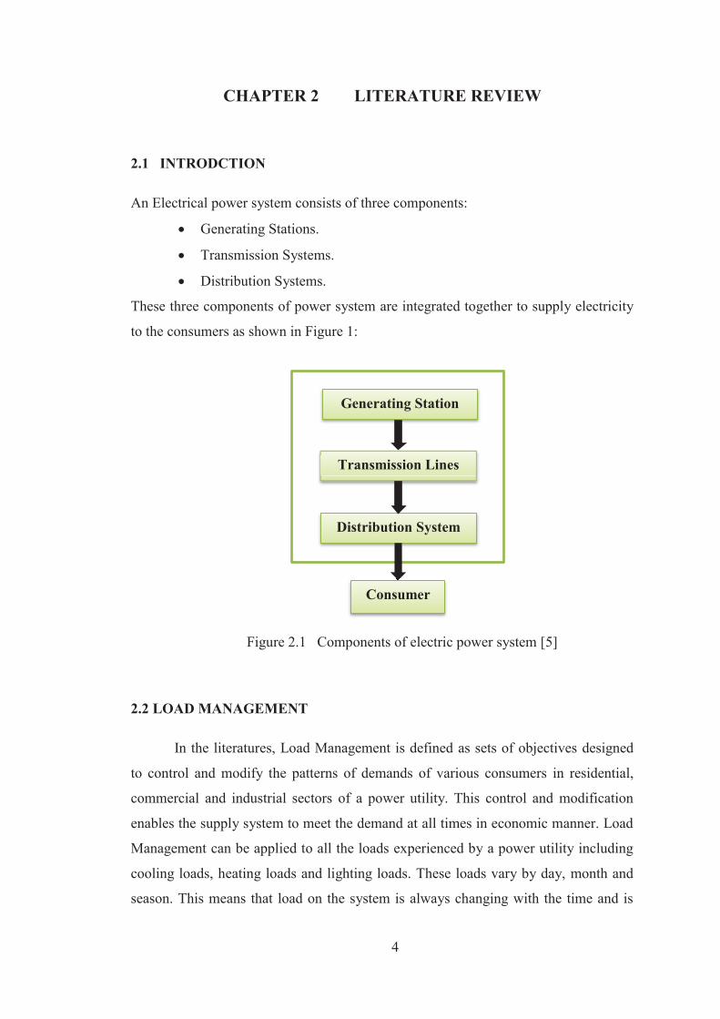
Figure 2.2 The load shape for standard DSM load management [32]
2.4 REVIEW OF SMART GRID
The Smart Grid is characterized by a two-way flow of electricity and information
and will be capable of monitoring everything from power plants to customer
preferences for individual appliances in residential and commercial sectors. It
incorporates into the grid the benefits of distributed computing and communications
to deliver real-time information and enable the near-instantaneous balance of supply
and demand at the device level [8, 9].
7
2.5 THE THERMAL SYSTEM (HEAT AND TEMPERATURE)
Thermal systems are those that involve the transfer of heat from one substance to
another. There are three different ways that heat can flow through conduction,
convection, and radiation. Most thermal processes in process control systems do not
involved radiation heat transfer [10].
Principle of Heat Transfer,
Heat transfer (q) is a thermal energy in transit due to a temperature difference .
Heat transfer (q) is the thermal energy transfer per unit time, can be express as:
(2.1) Where:
: rate of heat flow, kcal/sec (W)
: temperature difference, ºC
K : coefficient, kcal/sec ºC
The coefficient (K) is given by
(For conduction)
(For convection)
Where
: thermal conductivity, kcal/m sec ºC
: area normal to heat flow (m²)
: thickness of conductor, (m)
: convection coefficient, kcal/m² sec ºC
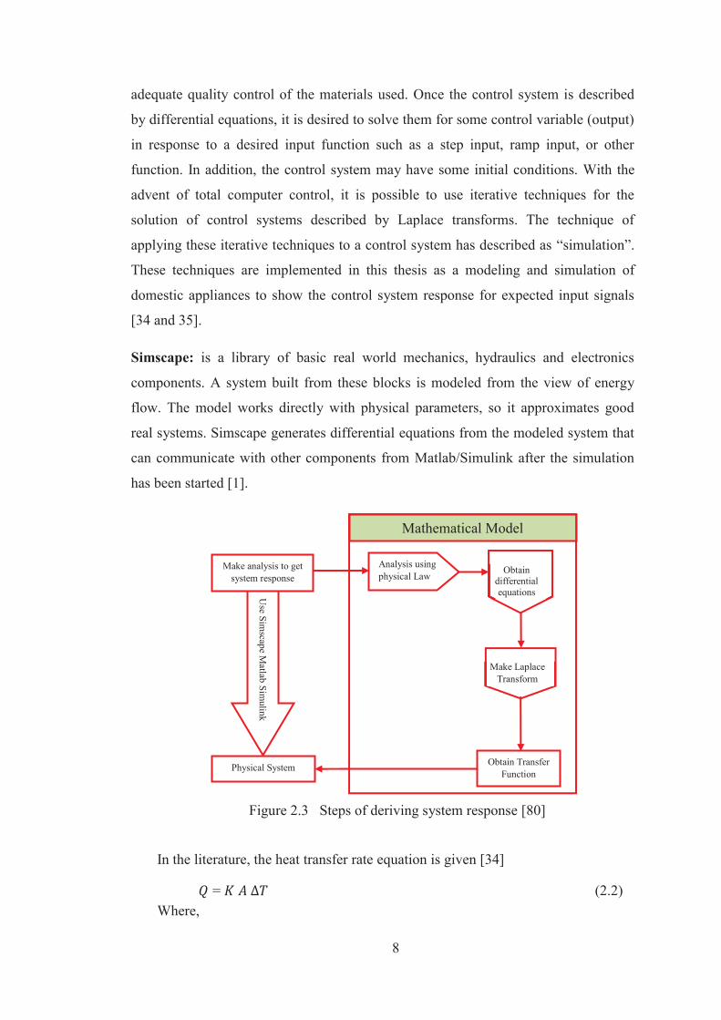
2.6 MATHMATICAL MODEL OF THERMAL SYSTEM USING SIMSCAPE
Differential equations are used to describe physical component in the classical
control system analysis. To get the response of the system we use the steps shown in
figure (2.3) to derive the mathematical model. Most physical systems include some
combination of mechanical, electrical, and hydraulic components. Mathematical
models are used to predict system performance with considerable accuracy and
8
adequate quality control of the materials used. Once the control system is described
by differential equations, it is desired to solve them for some control variable (output)
in response to a desired input function such as a step input, ramp input, or other
function. In addition, the control system may have some initial conditions. With the
advent of total computer control, it is possible to use iterative techniques for the
solution of control systems described by Laplace transforms. The technique of
applying these iterative techniques to a control system has described as “simulation”.
These techniques are implemented in this thesis as a modeling and simulation of
domestic appliances to show the control system response for expected input signals
[34 and 35].
Simscape: is a library of basic real world mechanics, hydraulics and electronics
components. A system built from these blocks is modeled from the view of energy
flow. The model works directly with physical parameters, so it approximates good
real systems. Simscape generates differential equations from the modeled system that
can communicate with other components from Matlab/Simulink after the simulation
has been started [1].
Figure 2.3 Steps of deriving system response [80]
In the literature, the heat transfer rate equation is given [34]
= (2.2) Where,
Use Sim
scape Matlab Sim
ulink
Physical System
Make analysis to get system response
Obtain Transfer Function
Analysis using physical Law Obtain
differential equations
Make Laplace Transform
Mathematical Model
9
: heat generation (W)
: temperature difference (K or ºC)
: heat exchange area (m²)
: heat transfer coefficient
ENERGY EQUATION OF THE THERMAL SYSTEMS:
In order to investigate thermal behavior of the heater, the energy equation of the thermal systems can be predicted from conservation of energy applied to the heater as follows:
Energy Equation of the system is given [11 and 36]
(2.3)
Where
: The rate of heat transfer from the heater
: The rate of electrical energy input to the heater
: Thermal capacity of the heater
: Mass of the heater
: Specific heat
: Temperature variations
By using an energy equation, we can express the rate of temperature change as:
(2.4)
The effect of temperature on electrical resistance of the heater material must be
included and so the energy equation can be expressed as following:
(2.5)
Where
: Applied voltage
10
: Electrical resistance at operating temperature (T)
: Electrical resistance at standard temperature (ºC)
: Temperature coefficient of resistance
Modeling and simulation heating systems class is a challenge to predict the system
behavior. These kind of systems are thermostatic loads, which means their
performances are controlled by a thermostat; such systems include a domestic electric
water heater, space heaters, ovens, refrigerators and air conditioning which is called
heating ventilation and air conditioning (HVAC). In order to investigate the system
behavior and load characteristics, Thermostatic Load Modeling by using thermal
systems network in all modeling of systems is considered.
11
CHAPTER 3 MODELING OF ELECTRIC WATER HEATER
3.1 INTRODUCTION
Numerous models of diverse types of Domestic Electric Water Heaters (DEWHs)
under consideration supply hot water for domestic use have been introduced in the
literature. The objectives of these models are to analyze, calculate the energy
consumption and to control the energy flow. For instance, the Water Heater Analysis
Model (WHAM) was designed to calculate the energy consumption per day [13].
Other models were designed to obtain the EWH demand in order to control it by
means of Demand Side Management (DSM) [12, 25, and 26].
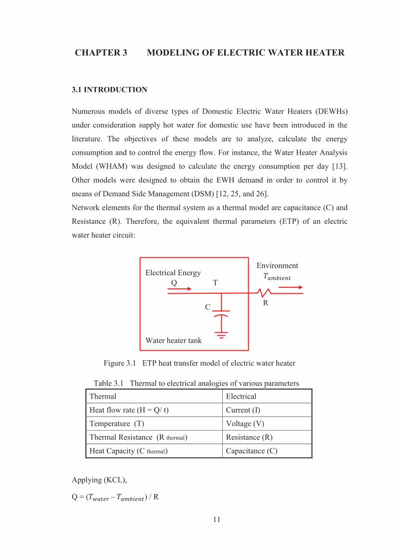
Network elements for the thermal system as a thermal model are capacitance (C) and
Resistance (R). Therefore, the equivalent thermal parameters (ETP) of an electric
water heater circuit:
Environment
R
Figure 3.1 ETP heat transfer model of electric water heater
Table 3.1 Thermal to electrical analogies of various parameters
Thermal Electrical
Heat flow rate (H = Q/ t) Current (I)
Temperature (T) Voltage (V)
Thermal Resistance (R thermal) Resistance (R)
Heat Capacity (C thermal) Capacitance (C)
Applying (KCL),
Q = ( – ) / R
Electrical Energy Q T
C
Water heater tank
12
R = 1/H → Q = ( ) H
For capacitor
Q = T/Xc
Q = + ( – ) H
Methodology
The first-order differential equation (3.1) is used to implement a simple model of
a DEWH, which represents the energy flow [3, 12] as follows:
(3.1)
C = G = SA.U = SA/R H =
Where,
: thermal capacity of water in the tank
: hot water temperature in tank
: ambient air temperature outside tank
: incoming inlet cold water temperature
: average hot water draw per hour
: density of water
: volume of tank
: specific heat of the water
: surface area of tank
: stand-by heat loss coefficient
: thermal resistance of tank
: rate of energy input ; Q = Prated
: power rated input of the heating resistance element
13
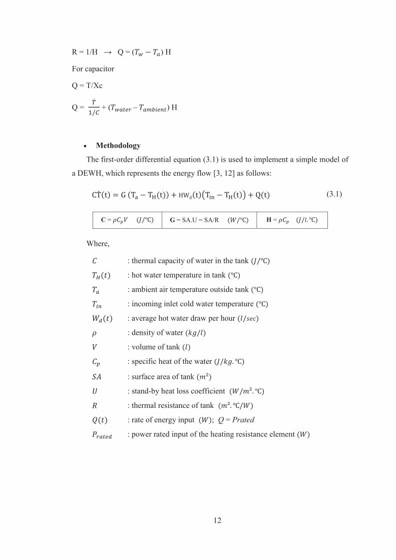
3.2 MODELING OF (DEWH)
Figure 3.2 Model of Domestic Electric Water Heater
Table 3.2 DEWH parameters
Convection Parameters Convective Heat Transfer Thermal Mass
Area
Heat Transfer coefficient
Mass
Specific heat Cp
Initial Temperature
2.8 0.4965 189.27 4181 20
Conduction Parameters Conductive Heat Transfer Thermal Mass
Area
Thickness
Thermal Conductivity
Mass
Specific heat Cp
Initial Temperature
1.1 0.005 0.8 1010 1.04 20
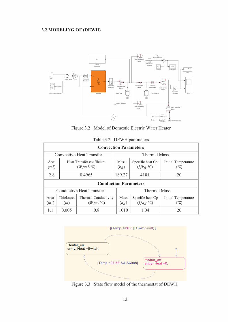
Figure 3.3 State flow model of the thermostat of DEWH
ccc3
To Workspace
Temp
Switch
Heat
Thermostat
Thermal Reference5
Thermal Reference3
Thermal Reference
Thermal Mass1Thermal Mass
Step
f(x)=0
SolverConfiguration
S PS
Simulink-PSConverter5
S PS
Simulink-PSConverter
Scope
792.5
Q on
SPS
PS-SimulinkConverter5
SPS
PS-SimulinkConverter1
SPS
PS-SimulinkConverter
PS Gain1
Operation_interv al
Operation Interval Builder 1
Manual Switch
BAS
Ideal TemperatureSource
TB
A
Ideal TemperatureSensor1
TB
A
Ideal TemperatureSensor
BA
S
Ideal Heat FlowSource
B
AH
Ideal Heat FlowSensor
4000
Gain
BA
Convective HeatTransfer
273
Constant1
293
Constant
BA
ConductiveHeat Transfer
14
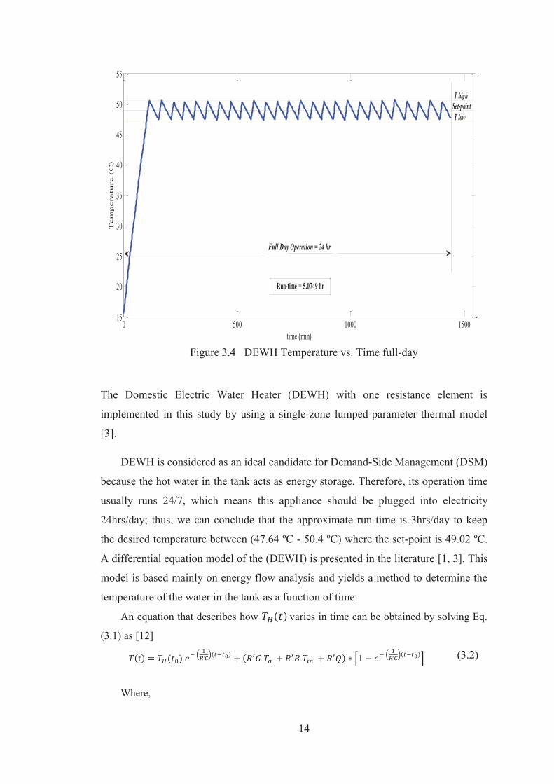
Figure 3.4 DEWH Temperature vs. Time full-day
The Domestic Electric Water Heater (DEWH) with one resistance element is
implemented in this study by using a single-zone lumped-parameter thermal model
[3].
DEWH is considered as an ideal candidate for Demand-Side Management (DSM)
because the hot water in the tank acts as energy storage. Therefore, its operation time
usually runs 24/7, which means this appliance should be plugged into electricity
24hrs/day; thus, we can conclude that the approximate run-time is 3hrs/day to keep
the desired temperature between (47.64 ºC - 50.4 ºC) where the set-point is 49.02 ºC.
A differential equation model of the (DEWH) is presented in the literature [1, 3]. This
model is based mainly on energy flow analysis and yields a method to determine the
temperature of the water in the tank as a function of time.
An equation that describes how varies in time can be obtained by solving Eq.
(3.1) as [12]
(3.2)
Where,
0 500 1000 150015
20
25
30
35
40
45
50
55
time (min)
Tem
pera
ture
(C
)T low
T high
Run-time = 5.0749 hr
Full Day Operation = 24 hr
Set-point
15
: time constant
: incoming water temperature
: ambient air temperature outside tank
: temperature of water in tank at time t
: temperature of water in tank at time t
: energy input rate as a function of time
: thermal resistance
: thermal conductance G =A/R where,
R is the thermal resistance of the tank
: surface area of tank
: stand-by heat loss coefficient
: B =H
: thermal capacitance
The (Q) and (B) values are time dependent. Thus, the energy input (Q) is
dependent on the element condition (on/off), and (B) is a function of the usage of
water. Therefore, the value of (τ) and ( (τ)) must be updated every time there is a
change in (B) or (Q). All other parameters can be measured, and must be known for
accurate prediction of the temperature [12, 13, 14 and 15].
3.2.1 MATHEMATICAL ANALYSIS
The main purpose of this section is to discover and determine the effect of
DEWH parameters during its run-time, by developing simple mathematical equations
that represent the effect of varying parameters on the system behavior such as power
and energy consumption. This can be achieved by deriving equations to obtain
temperature of { , and } and to determine time duration
of , and , the cycling time, and power consumed by DEWH
from the energy flow is also considered.
Consider a DEWH tank that is standing idle. It periodically turns on its heating
element in order to maintain the temperature of the water within a certain range. Thus,
the approximate water temperature at the time (t) is given by solving Eq. (3.1) and
16
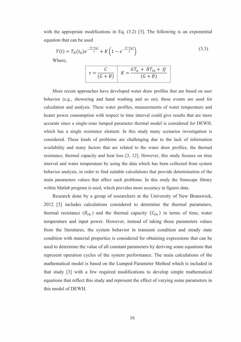
with the appropriate modifications in Eq. (3.2) [3]. The following is an exponential
equation that can be used
(3.3)
Where,
More recent approaches have developed water draw profiles that are based on user
behavior (e.g., showering and hand washing and so on); these events are used for
calculation and analysis. These water profiles, measurements of water temperature and
heater power consumption with respect to time interval could give results that are more
accurate since a single-zone lumped parameter thermal model is considered for DEWH,
which has a single resistance element. In this study many scenarios investigation is
considered. These kinds of problems are challenging due to the lack of information
availability and many factors that are related to the water draw profiles, the thermal
resistance, thermal capacity and heat loss [3, 12]. However, this study focuses on time
interval and water temperature by using the data which has been collected from system
behavior analysis, in order to find suitable calculations that provide determination of the
main parameters values that affect such problems. In this study the Simscape library
within Matlab program is used, which provides more accuracy in figures data.
Research done by a group of researchers at the University of New Brunswick,
2012 [3] includes calculations considered to determine the thermal parameters,
thermal resistance ( ) and the thermal capacity in terms of time, water
temperature and input power. However, instead of taking those parameters values
from the literatures, the system behavior in transient condition and steady state
condition with material properties is considered for obtaining expressions that can be
used to determine the value of all constant parameters by deriving some equations that
represent operation cycles of the system performance. The main calculations of the
mathematical model is based on the Lumped Parameter Method which is included in
that study [3] with a few required modifications to develop simple mathematical
equations that reflect this study and represent the effect of varying some parameters in
this model of DEWH.
17
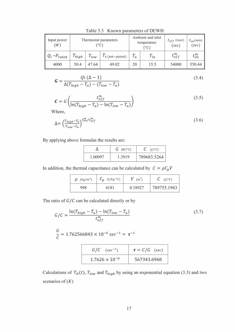
Table 3.3 Known parameters of DEWH
Input power
Thermostat parameters
Ambient and inlet temperature
=
4000 50.4 47.64 49.02 20 15.5 54000 550.44
(3.4)
(3.5)
Where,
(3.6)
By applying above formulas the results are:
1.00097 1.3919 789683.5264
In addition, the thermal capacitance can be calculated by
998 4181 0.18927 789755.1943 The ratio of can be calculated directly or by
(3.7)
Calculations of , and by using an exponential equation (3.3) and two
scenarios of ( )
18
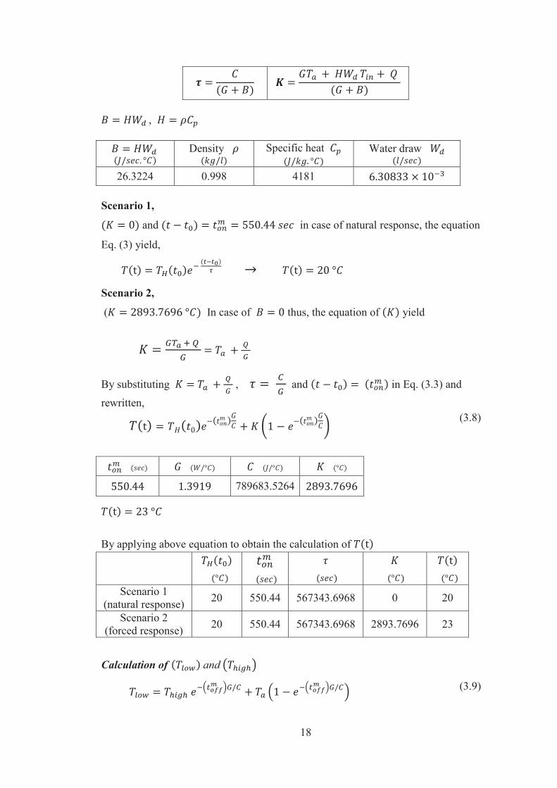
,
Density
Specific heat
Water draw
26.3224 0.998 4181 Scenario 1,
and in case of natural response, the equation
Eq. (3) yield,
Scenario 2,
( In case of thus, the equation of yield
By substituting , and in Eq. (3.3) and
rewritten,
(3.8)
789683.5264
By applying above equation to obtain the calculation of
Scenario 1
(natural response) 20 550.44 567343.6968 0 20
Scenario 2 (forced response) 20 550.44 567343.6968 2893.7696 23
Calculation of and
(3.9)
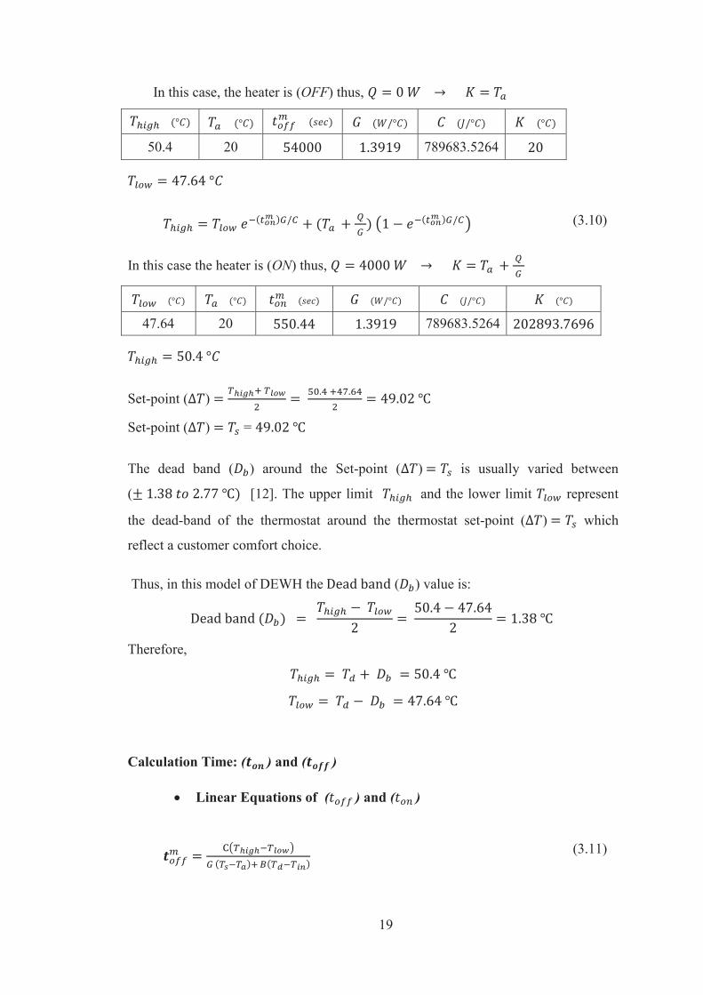
19
In this case, the heater is (OFF) thus,
50.4 20 789683.5264
(3.10)
In this case the heater is (ON) thus,
47.64 20 789683.5264
Set-point ( )
Set-point ( ) =
The dead band ( ) around the Set-point ( ) is usually varied between
( [12]. The upper limit and the lower limit represent
the dead-band of the thermostat around the thermostat set-point ( ) which
reflect a customer comfort choice.
Thus, in this model of DEWH the ( ) value is:
Therefore,
Calculation Time: ( ) and ( )
Linear Equations of ( ) and ( )
(3.11)
20
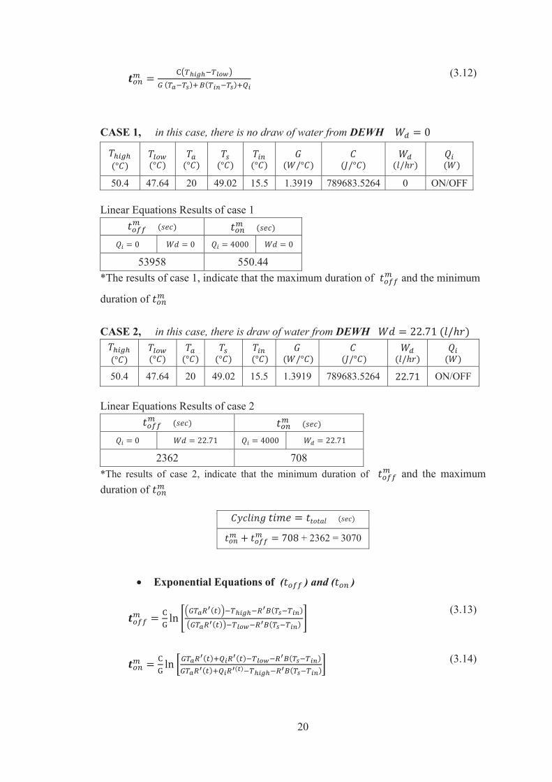
(3.12)
CASE 1, in this case, there is no draw of water from DEWH
50.4 47.64 20 49.02 15.5 1.3919 789683.5264 0 ON/OFF Linear Equations Results of case 1
53958 550.44 *The results of case 1, indicate that the maximum duration of and the minimum
duration of
CASE 2, in this case, there is draw of water from DEWH
50.4 47.64 20 49.02 15.5 1.3919 789683.5264 ON/OFF Linear Equations Results of case 2
2362 708 *The results of case 2, indicate that the minimum duration of and the maximum duration of
+ 2362 = 3070
Exponential Equations of ( ) and ( )
(3.13)
(3.14)
21
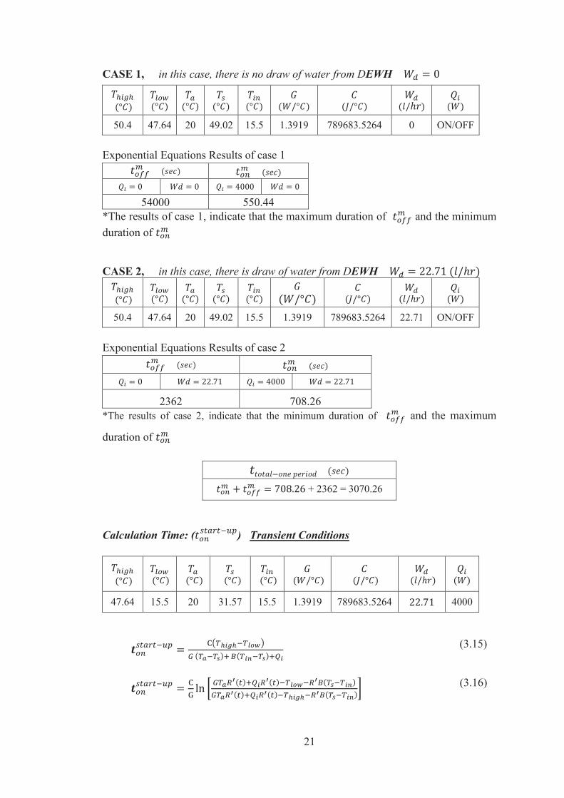
CASE 1, in this case, there is no draw of water from DEWH
50.4 47.64 20 49.02 15.5 1.3919 789683.5264 0 ON/OFF Exponential Equations Results of case 1
54000 550.44
*The results of case 1, indicate that the maximum duration of and the minimum duration of CASE 2, in this case, there is draw of water from DEWH
50.4 47.64 20 49.02 15.5 1.3919 789683.5264 22.71 ON/OFF Exponential Equations Results of case 2
2362 708.26 *The results of case 2, indicate that the minimum duration of and the maximum
duration of
+ 2362 = 3070.26 Calculation Time: ( ) Transient Conditions
47.64 15.5 20 31.57 15.5 1.3919 789683.5264 4000
(3.15)
(3.16)
22
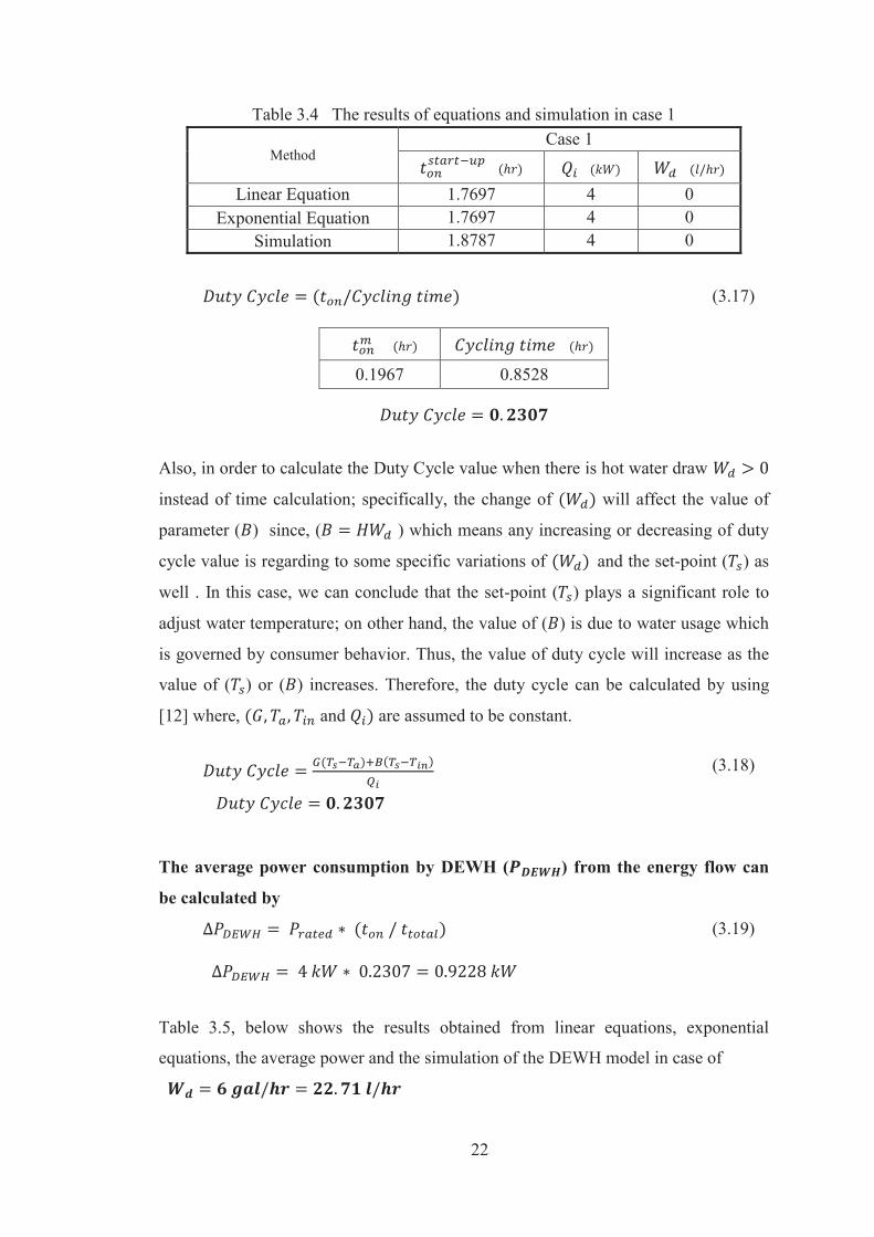
Table 3.4 The results of equations and simulation in case 1
Method Case 1
Linear Equation 1.7697 4 0
Exponential Equation 1.7697 4 0 Simulation 1.8787 4 0
(3.17)
0.1967 0.8528
Also, in order to calculate the Duty Cycle value when there is hot water draw
instead of time calculation; specifically, the change of will affect the value of
parameter ( ) since, ( ) which means any increasing or decreasing of duty
cycle value is regarding to some specific variations of and the set-point ( ) as
well . In this case, we can conclude that the set-point ( ) plays a significant role to
adjust water temperature; on other hand, the value of ( ) is due to water usage which
is governed by consumer behavior. Thus, the value of duty cycle will increase as the
value of ( ) or ( ) increases. Therefore, the duty cycle can be calculated by using
[12] where, and are assumed to be constant.
(3.18)
The average power consumption by DEWH ( ) from the energy flow can
be calculated by
(3.19)
Table 3.5, below shows the results obtained from linear equations, exponential
equations, the average power and the simulation of the DEWH model in case of
23
Table 3.5 The comparison of the simulation results and equations
Method
Linear
Equation 4 1.7697 0.1966 0.6561 0.8527 0.2307 0.9228
Exponential
Equation 4 1.7697 0.1967 0.6561 0.8528 0.2307 0.9228
Simulation 4 1.8787 0.1958 0.6417 0.8375 0.2338 0.9352
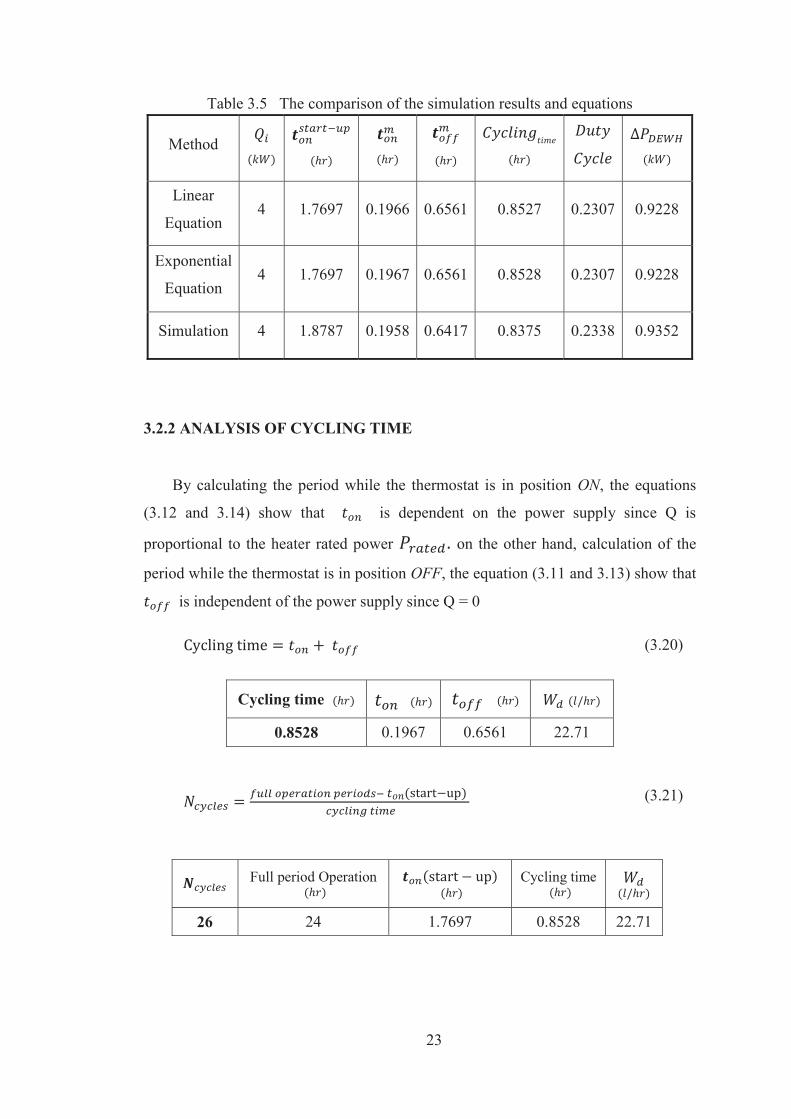
3.2.2 ANALYSIS OF CYCLING TIME
By calculating the period while the thermostat is in position ON, the equations
(3.12 and 3.14) show that is dependent on the power supply since Q is
proportional to the heater rated power on the other hand, calculation of the
period while the thermostat is in position OFF, the equation (3.11 and 3.13) show that
is independent of the power supply since Q = 0
(3.20)
Cycling time
0.8528 0.1967 0.6561 22.71
(3.21)
Full period Operation
Cycling time
26 24 1.7697 0.8528 22.71

24
Figure 3.5 Simplified thermal characteristic curve of thermostat (cycling time)
Figure 3.5, of temperature as a function of time indicates that the DEWH has reached
a steady state condition where the set-point is 49.02 .
= ( ) + (3.22)
6.8839 26 0.1967 1.7697 22.71
Power / Energy consumption of (DEWH):
= (3.23)
Table 3.6 The results of simulation and calculation
method
Calculation 0.7868 4 0.1967 22.71
Simulation 0.7832 4 0.1958 22.71
(3.24)
20.4568 4 5.1142 22.71
0 50 100 150 200 25015
20
25
30
35
40
45
50
55
time (min)
Temp
eratur
e (C)
Set-pointT high
T low
time on
time off
25
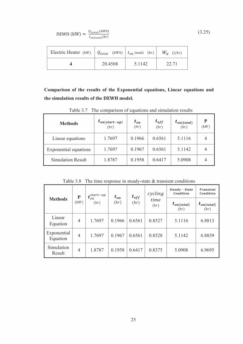
(3.25)
Electric Heater (total)
4 20.4568 5.1142 22.71
Comparison of the results of the Exponential equations, Linear equations and
the simulation results of the model.
Table 3.7 The comparison of equations and simulation results
Methods
P
Linear equations 1.7697 0.1966 0.6561 5.1116 4
Exponential equations 1.7697 0.1967 0.6561 5.1142 4
Simulation Result 1.8787 0.1958 0.6417 5.0908 4
Table 3.8 The time response in steady-state & transient conditions
Methods
Linear Equation 4 1.7697 0.1966 0.6561 0.8527 5.1116 6.8813
Exponential Equation 4 1.7697 0.1967 0.6561 0.8528 5.1142 6.8839
Simulation Result 4 1.8787 0.1958 0.6417 0.8375 5.0908 6.9695
26
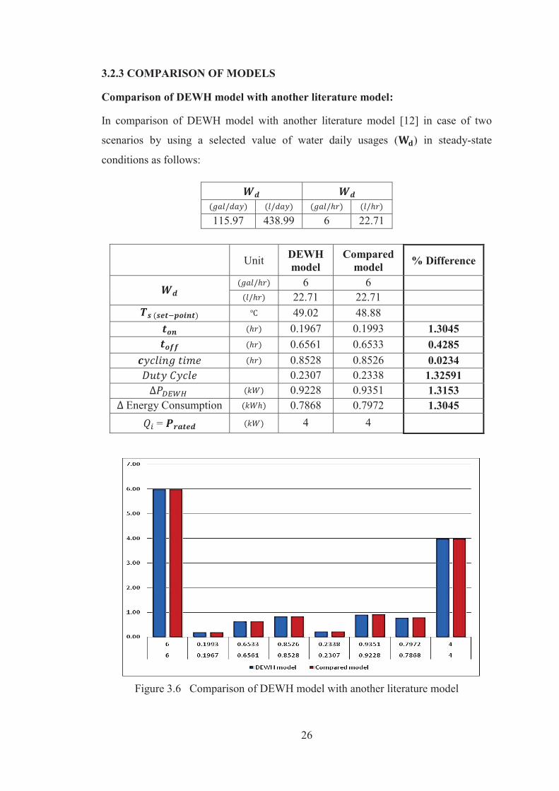
3.2.3 COMPARISON OF MODELS
Comparison of DEWH model with another literature model:
In comparison of DEWH model with another literature model [12] in case of two
scenarios by using a selected value of water daily usages ( ) in steady-state
conditions as follows:
115.97 438.99 6 22.71
Unit DEWH model
Compared model % Difference
6 6
22.71 22.71 49.02 48.88
0.1967 0.1993 1.3045 0.6561 0.6533 0.4285
0.8528 0.8526 0.0234 0.2307 0.2338 1.32591
0.9228 0.9351 1.3153 Energy Consumption 0.7868 0.7972 1.3045
= 4 4
Figure 3.6 Comparison of DEWH model with another literature model
27
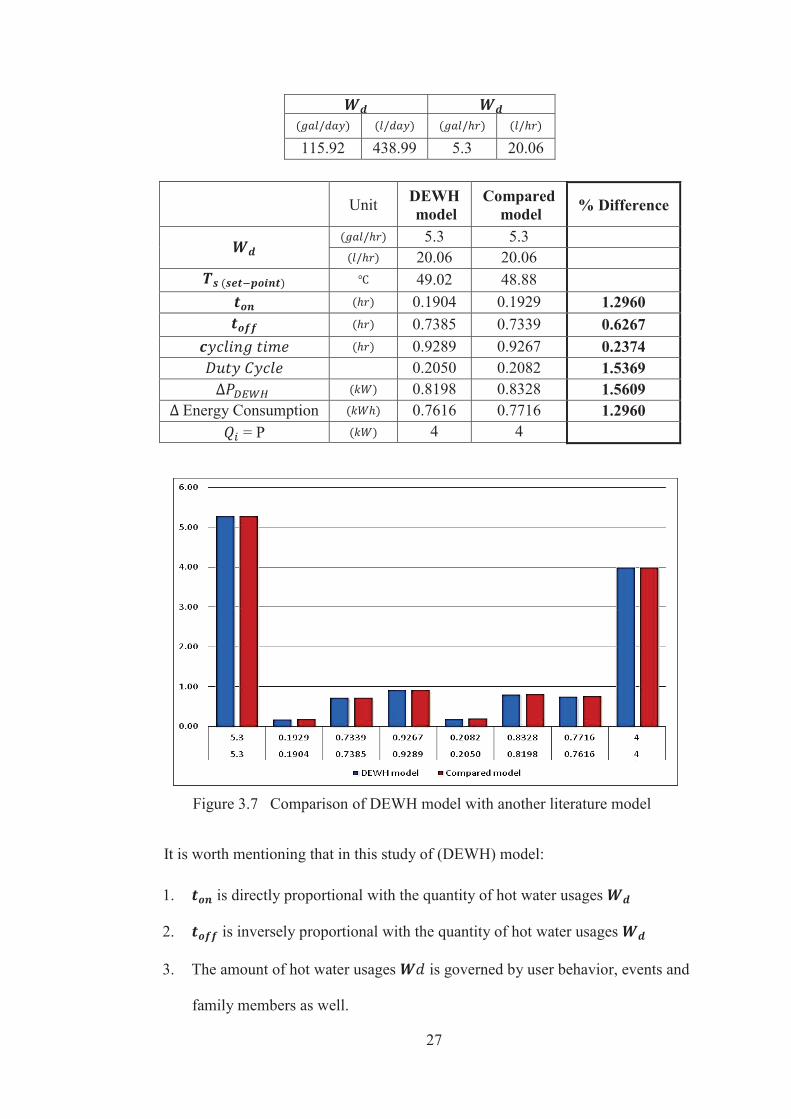
115.92 438.99 5.3 20.06
Unit DEWH model
Compared model % Difference
5.3 5.3
20.06 20.06 49.02 48.88
0.1904 0.1929 1.2960 0.7385 0.7339 0.6267
0.9289 0.9267 0.2374 0.2050 0.2082 1.5369
0.8198 0.8328 1.5609 Energy Consumption 0.7616 0.7716 1.2960
= P 4 4
Figure 3.7 Comparison of DEWH model with another literature model
It is worth mentioning that in this study of (DEWH) model:
1. is directly proportional with the quantity of hot water usages
2. is inversely proportional with the quantity of hot water usages
3. The amount of hot water usages is governed by user behavior, events and
family members as well.

28
4. When there is no water draw , in this case, the minimum duration
of and the maximum duration of occurs.
5. The parameter of thermal conductance (G) is obtained by calculation in terms
of time, temperature and in-put power since in the compared model the value
of parameter (G) is taken directly from literature.
3.2.4 LOAD PROFILE AND ENERGY COST
Figure 3.8 Energy Cost Calculator of Electric Water-Heater
Simulation Results of Electric Water-Heater Full Day (TOU)
Figure 3.9 Load profile of DEWH Full Day (Load and Cost vs. time)
0 1 2 3 4 5 6 7 8 9
x 104
0
1
2x 10
4
Wh
/ d
ay
0 1 2 3 4 5 6 7 8 9
x 104
0
2
4
Co
st (
$/k
Wh
)
0 1 2 3 4 5 6 7 8 9
x 104
0
2
4
Time (sec)
Co
st (
$/k
Wh
)
TOU-Tariff (4 * 1.83 * 0.07213) + (4 * 3.17 * 0.1379) = $ 2.3
Standard Tariff (20.3 * 0.1379) = $ 2.799
(5.0749 * 4) = 20.3 kWh / day
29
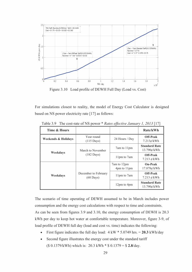
Figure 3.10 Load profile of DEWH Full Day (Load vs. Cost)
For simulations closest to reality, the model of Energy Cost Calculator is designed
based on NS power electricity rate [17] as follows:
Table 3.9 The cost-rate of NS power * Rates effective January 1, 2013 [17]
Time & Hours Rate/kWh
Weekends & Holidays Year round (115 Days) 24 Hours / Day Off-Peak
7.213¢/kWh
Weekdays March to November
(182 Days)
7am to 11pm Standard Rate 13.790¢/kWh
11pm to 7am Off-Peak 7.213 ¢/kWh
Weekdays December to February
(68 Days)
7am to 12pm 4pm to 11pm
On-Peak 17.878¢/kWh
11pm to 7am Off-Peak 7.213 ¢/kWh
12pm to 4pm Standard Rate 13.790¢/kWh
The scenario of time operating of DEWH assumed to be in March includes power
consumption and the energy cost calculations with respect to time and constraints.
As can be seen from figures 3.9 and 3.10, the energy consumption of DEWH is 20.3
kWh per day to keep hot water at comfortable temperature. Moreover, figure 3-9, of
load profile of DEWH full day (load and cost vs. time) indicates the following:
First figure indicates the full day load: 4 kW * 5.0749 hrs. = 20.3 kWh/day
Second figure illustrates the energy cost under the standard tariff
($ 0.1379/kWh) which is: 20.3 kWh * $ 0.1379 = $ 2.8/day.
0 0.2 0.4 0.6 0.8 1 1.2 1.4 1.6 1.8 2
x 104
0
0.5
1
1.5
2
2.5
Wh / day
($/k
Wh
) p
er d
ay
(7am -- 11pm) Standard Tariff ($ 0.1379/kWh)Run-time = 3.17 hrCost = 4 * 3.17 * 0.1379 = $1.75
TOU Tariff, Run-time (5.0749 hrs) * 4kW = 20.3 kWhCost = $ 1.75 + $ 0.53 + $ 0.022 = $ 2.302
(11pm -- 7am) Off-Peak Tariff ($ 0.07213/kWh)Run-time = 4 * 1.83 * 0.07213 = $ 0.53
30
Third figure illustrates the energy cost in variable tariff (TOU) as follows:
Standard: 16 hrs. (7 to 23); ($ 0.1379/kWh) where the (Run-time = 3.17 hr.)
Off-peak: 8 hrs. (23 to 7); ($ 0.07213/kWh) where the (Run-time = 1.83 hr.)
In this Load profile curves the total variable tariff (TOU) calculation is
(4 kW * 1.83 hr. * $ 0.07213) + (4 kW * 3.17 hr. * $ 0.1379) = $ 2.3/day
As a result, we can conclude that the energy cost of run-time of DEWH under the
standard tariff ($0.1379/kWh) equal $2.799/day and the energy cost of run-time of
DEWH under the variable tariff (TOU) equal $2.3/day. Thus, the difference between
two costs is ($ 0.499). In other words, if the customer runs the DEWH under these
constraints of (TOU) he/she will save up to 17.83% per this appliance. However,
calculates an optimal schedule for DEWH based on fluctuating tariffs can suggest
more energy efficient; therefore, this idea will discuss later in the optimization
chapter.
31
CHAPTER 4 MODELING OF HEATING SYSTEMS
4.1 INTRODUCTION
The basic operating principles of the heating systems and lighting systems are
considered in order to design the models that can be implemented and simulated in the
Matlab program; thus, there are four suitable models of these appliances
Domestic Electric Oven (DEO).
Domestic Electric Clothes Iron (DECI).
Domestic Electric Baseboard Heater (DEBH).
Modeling of Lighting (F-Lamp)
In this chapter, all the above appliances are designed, tested and investigated.
This chapter discusses the design of heating system models and a lighting system in
order to investigate the impact of its main parameters on its ability to assist with
reducing energy consumption. In these kinds of systems, the control strategies
developed played a significant role in controlling the major appliances in residential
and commercial sectors.
4.2 DOMESTIC ELECTRIC OVEN (DEO)
4.2.1 INTRODUCTION
Numerous models of diverse types of the Domestic Electric Oven (DEO) have
been introduced in the literature. The objectives of these models differ from one to
another, in order to meet the requirements of the design the purpose of the usage, the
size and the material must be considered in the modeling process.
(DEOs) are common appliances used for many purposes and in the literature, are
defined as thermally insulated chambers used for the heating, baking, cooking [27-28
and 30]. The heater element itself is very essential in an electric oven system but
sometimes can be dangerous if not properly controlled, since the ovens simply run
continuously at various temperatures. Thus, in order to control and regulate the
amount of heat produced, a thermostat is used [29].
32
A thermostat device plays a significant role as a controller, which is used for
regulating the heat intensity with a certain range of a temperature set point; the
thermostat range can be predetermined as required since the user can specify the
temperature, toasting time, and start or stop the heating process at any time [31]. In
fact, many domestic electric ovens that are more conventional have a simple
thermostat. In particular, the task of the thermostat is to turn an electric oven ON/OFF
automatically and select the temperature when a pre-set temperature has been reached.
Thus, we can conclude that the (DEO) is an enclosed compartment where the power
and the temperature can be adjusted for heating, baking and drying / cooking food,
while the oven temperature is regulated by thermostatic control. It is worth
mentioning that the operation time of an electric oven in residential sector is less than
in the commercial sector.
In this study the typical DEO is presented and implemented by using an
approach for identifying the thermal parameters of physical models of a single- zone
lumped-parameter thermal model. This approach has been developed by a group of
researchers at the University of New Brunswick, 2012 [3].
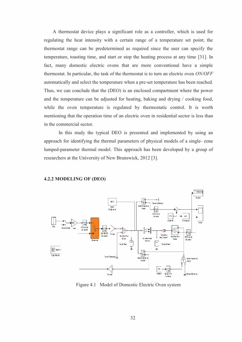
4.2.2 MODELING OF (DEO)
Figure 4.1 Model of Domestic Electric Oven system

33
Table 4.1 Model of Domestic Electric Oven specifications
Convection Parameters
Convective Heat Transfer Thermal Mass Area
Heat Transfer coefficient
Mass
Specific heat Cp
Initial Temperature
0.25 300 22 1005.4 20
Conduction Parameters
Conductive Heat Transfer Thermal Mass Area
Thickness
Thermal Conductivity
Mass
Specific heat Cp
Initial Temperature
1.5 0.04 180 40 502 20
Figure 4.2 State flow model of the thermostat of DEO
Figure 4.3 DEO Temperature vs. Time
0 10 20 30 40 50 60 700
50
100
150
200
250
300
350
400
450
time (min)
Tem
pera
ture
(C
)
T = 400 C, Run-time = 1 hr, N cycles = 9
Lower limitThermostat Set-pointUpper limit
34
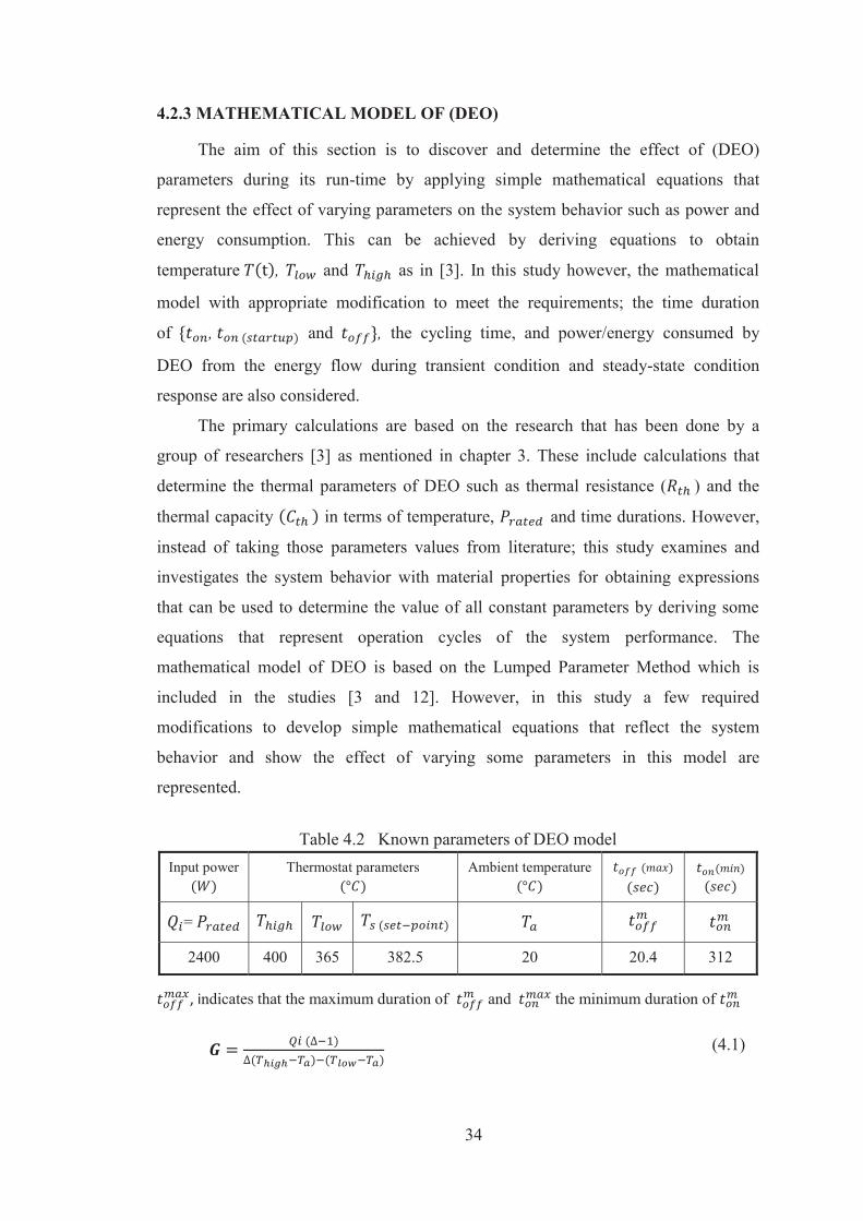
4.2.3 MATHEMATICAL MODEL OF (DEO)
The aim of this section is to discover and determine the effect of (DEO)
parameters during its run-time by applying simple mathematical equations that
represent the effect of varying parameters on the system behavior such as power and
energy consumption. This can be achieved by deriving equations to obtain
temperature , and as in [3]. In this study however, the mathematical
model with appropriate modification to meet the requirements; the time duration
of , and , the cycling time, and power/energy consumed by
DEO from the energy flow during transient condition and steady-state condition
response are also considered.
The primary calculations are based on the research that has been done by a
group of researchers [3] as mentioned in chapter 3. These include calculations that
determine the thermal parameters of DEO such as thermal resistance ( ) and the
thermal capacity in terms of temperature, and time durations. However,
instead of taking those parameters values from literature; this study examines and
investigates the system behavior with material properties for obtaining expressions
that can be used to determine the value of all constant parameters by deriving some
equations that represent operation cycles of the system performance. The
mathematical model of DEO is based on the Lumped Parameter Method which is
included in the studies [3 and 12]. However, in this study a few required
modifications to develop simple mathematical equations that reflect the system
behavior and show the effect of varying some parameters in this model are
represented.
Table 4.2 Known parameters of DEO model
Input power
Thermostat parameters
Ambient temperature
=
2400 400 365 382.5 20 20.4 312
, indicates that the maximum duration of and the minimum duration of (4.1)
35
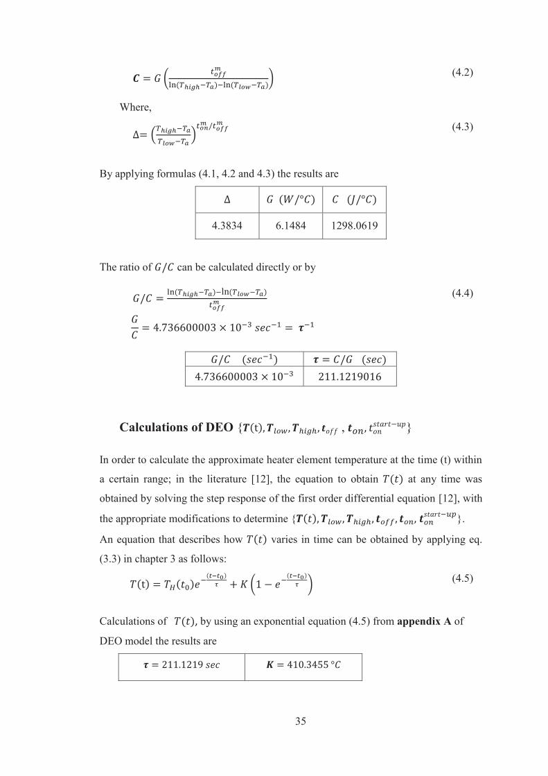
(4.2)
Where,
(4.3)
By applying formulas (4.1, 4.2 and 4.3) the results are
4.3834 6.1484 1298.0619
The ratio of can be calculated directly or by
(4.4)
Calculations of DEO { , }
In order to calculate the approximate heater element temperature at the time (t) within
a certain range; in the literature [12], the equation to obtain at any time was
obtained by solving the step response of the first order differential equation [12], with
the appropriate modifications to determine { }.
An equation that describes how varies in time can be obtained by applying eq.
(3.3) in chapter 3 as follows:
(4.5)
Calculations of , by using an exponential equation (4.5) from appendix A of
DEO model the results are
36
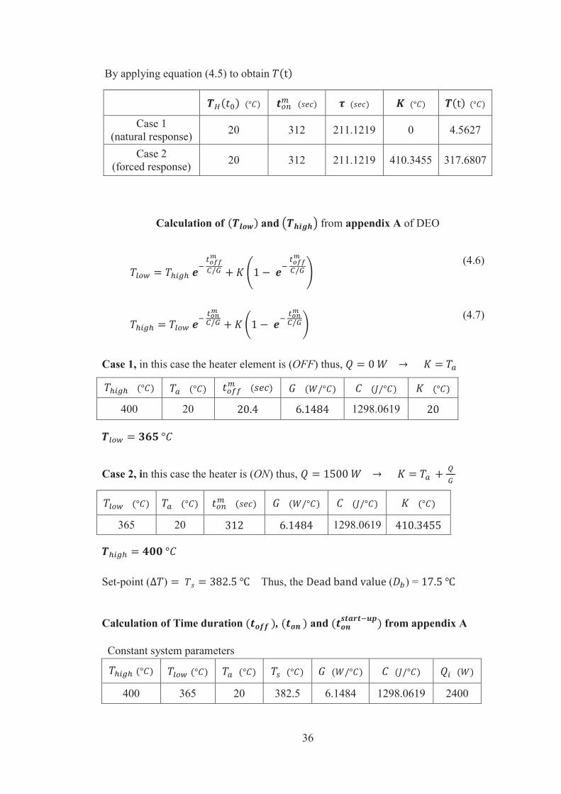
By applying equation (4.5) to obtain
Case 1 (natural response) 20 312 211.1219 0 4.5627
Case 2 (forced response) 20 312 211.1219 410.3455 317.6807
Calculation of and from appendix A of DEO
(4.6)
(4.7)
Case 1, in this case the heater element is (OFF) thus,
400 20 1298.0619
Case 2, in this case the heater is (ON) thus,
365 20 1298.0619
Set-point ( ) Thus, the ( ) =
Calculation of Time duration , and from appendix A Constant system parameters
400 365 20 382.5 6.1484 1298.0619 2400
37
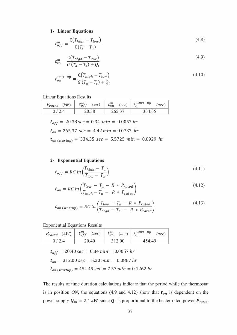
1- Linear Equations
(4.8)
(4.9)
(4.10)
Linear Equations Results
0 / 2.4 20.38 265.37 334.35
2- Exponential Equations
(4.11)
(4.12)
(4.13)
Exponential Equations Results
0 / 2.4 20.40 312.00 454.49
The results of time duration calculations indicate that the period while the thermostat
is in position ON, the equations (4.9 and 4.12) show that is dependent on the
power supply since is proportional to the heater rated power
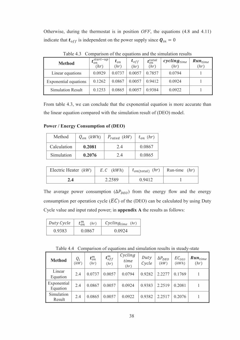
38
Otherwise, during the thermostat is in position OFF, the equations (4.8 and 4.11)
indicate that is independent on the power supply since
Table 4.3 Comparison of the equations and the simulation results
Method
Linear equations 0.0929 0.0737 0.0057 0.7857 0.0794 1
Exponential equations 0.1262 0.0867 0.0057 0.9412 0.0924 1
Simulation Result 0.1253 0.0865 0.0057 0.9384 0.0922 1
From table 4.3, we can conclude that the exponential equation is more accurate than
the linear equation compared with the simulation result of (DEO) model.
Power / Energy Consumption of (DEO)
Method
Calculation 0.2081 2.4 0.0867
Simulation 0.2076 2.4 0.0865
Electric Heater Run-time
2.4 2.2589 0.9412 1
The average power consumption ( ) from the energy flow and the energy
consumption per operation cycle ( ) of the (DEO) can be calculated by using Duty
Cycle value and input rated power; in appendix A the results as follows:
0.9383 0.0867 0.0924
Table 4.4 Comparison of equations and simulation results in steady-state
Method
Linear Equation 2.4 0.0737 0.0057 0.0794 0.9282 2.2277 0.1769 1
Exponential Equation 2.4 0.0867 0.0057 0.0924 0.9383 2.2519 0.2081 1
Simulation Result 2.4 0.0865 0.0057 0.0922 0.9382 2.2517 0.2076 1
39
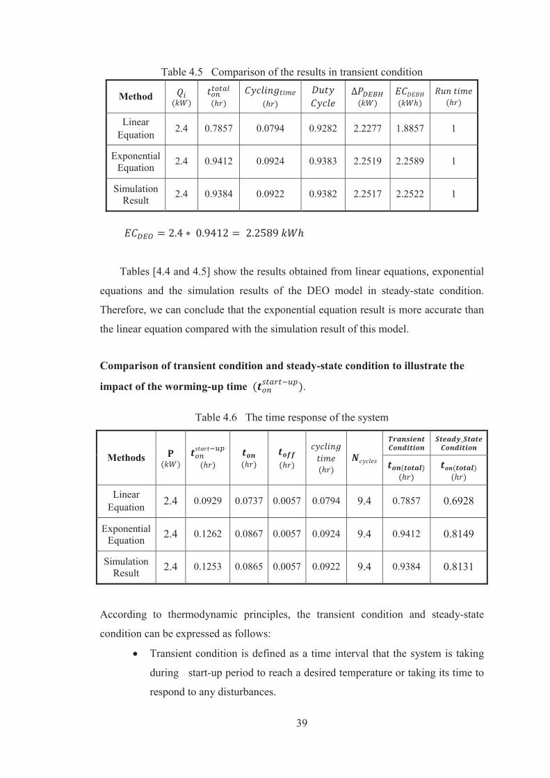
Table 4.5 Comparison of the results in transient condition
Method
Linear Equation 2.4 0.7857 0.0794 0.9282 2.2277 1.8857 1
Exponential Equation 2.4 0.9412 0.0924 0.9383 2.2519 2.2589 1
Simulation Result 2.4 0.9384 0.0922 0.9382 2.2517 2.2522 1
Tables [4.4 and 4.5] show the results obtained from linear equations, exponential
equations and the simulation results of the DEO model in steady-state condition.
Therefore, we can conclude that the exponential equation result is more accurate than
the linear equation compared with the simulation result of this model.
Comparison of transient condition and steady-state condition to illustrate the
impact of the worming-up time .
Table 4.6 The time response of the system
Methods
Linear Equation 2.4 0.0929 0.0737 0.0057 0.0794 9.4 0.7857 0.6928
Exponential Equation 2.4 0.1262 0.0867 0.0057 0.0924 9.4 0.9412 0.8149
Simulation Result 2.4 0.1253 0.0865 0.0057 0.0922 9.4 0.9384 0.8131
According to thermodynamic principles, the transient condition and steady-state
condition can be expressed as follows:
Transient condition is defined as a time interval that the system is taking
during start-up period to reach a desired temperature or taking its time to
respond to any disturbances.
40
Steady-state condition is defined as a condition where the system behavior
is depend on the long run time and will remain stable if there is no
disturbance. Table 4.6, illustrates the time in steady-state condition is obviously less than
the in transient condition; the difference is due to the worming-up
time to reach the set-point temperature. Thus, this period of time in
transient condition should be included in calculation of in order to calculate
the overall energy consumption of the DEO system. In addition, the thermostat time
is much less than the time which indicates the turn-off temperature
differs slightly from the turn-on temperature . This difference is called
hysteresis/dead band of the thermostat around the thermostat set-point. Also, this
difference will prevent the oven from switching rapidly and unnecessarily when the
temperature is near the set-point since, the setting of set-point set by the consumer
choice.
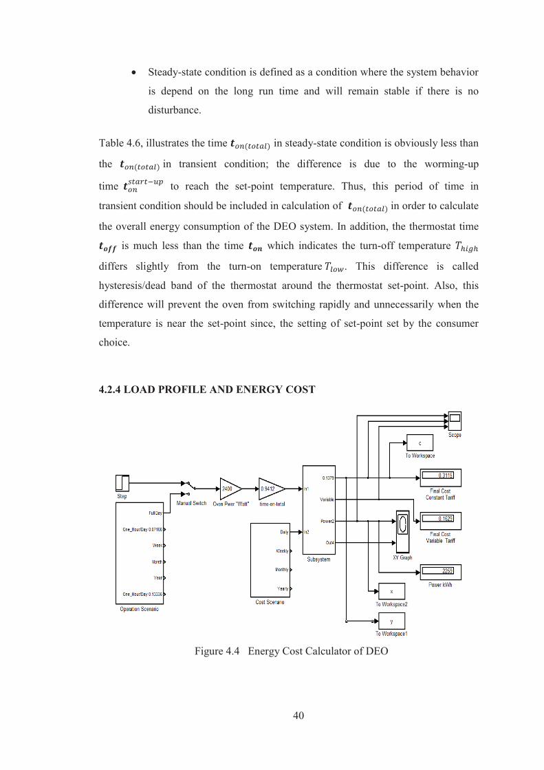
4.2.4 LOAD PROFILE AND ENERGY COST
Figure 4.4 Energy Cost Calculator of DEO
41
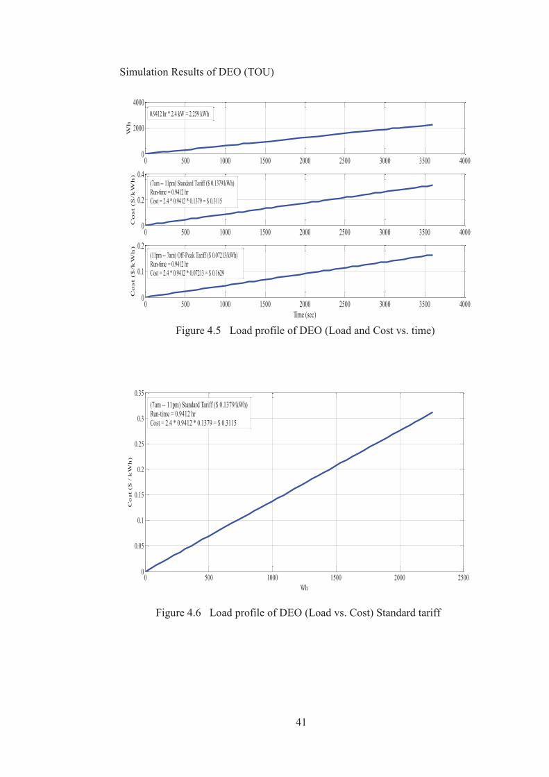
Simulation Results of DEO (TOU)
Figure 4.5 Load profile of DEO (Load and Cost vs. time)
Figure 4.6 Load profile of DEO (Load vs. Cost) Standard tariff
0 500 1000 1500 2000 2500 3000 3500 40000
2000
4000
Wh
0 500 1000 1500 2000 2500 3000 3500 40000
0.2
0.4
Co
st
($/k
Wh
)
0 500 1000 1500 2000 2500 3000 3500 40000
0.1
0.2
Time (sec)
Co
st
($/k
Wh
)
(7am -- 11pm) Standard Tariff ($ 0.1379/kWh)Run-time = 0.9412 hrCost = 2.4 * 0.9412 * 0.1379 = $ 0.3115
(11pm -- 7am) Off-Peak Tariff ($ 0.07213/kWh)Run-time = 0.9412 hrCost = 2.4 * 0.9412 * 0.07213 = $ 0.1629
0.9412 hr * 2.4 kW = 2.259 kWh
0 500 1000 1500 2000 25000
0.05
0.1
0.15
0.2
0.25
0.3
0.35
Wh
Co
st (
$ /
kW
h)
(7am -- 11pm) Standard Tariff ($ 0.1379/kWh)Run-time = 0.9412 hrCost = 2.4 * 0.9412 * 0.1379 = $ 0.3115
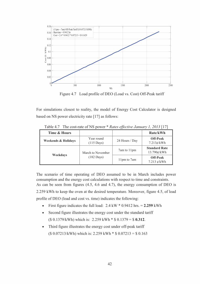
42
Figure 4.7 Load profile of DEO (Load vs. Cost) Off-Peak tariff
For simulations closest to reality, the model of Energy Cost Calculator is designed
based on NS power electricity rate [17] as follows:
Table 4.7 The cost-rate of NS power * Rates effective January 1, 2013 [17] Time & Hours Rate/kWh
Weekends & Holidays Year round (115 Days) 24 Hours / Day Off-Peak
7.213¢/kWh
Weekdays March to November
(182 Days)
7am to 11pm Standard Rate 13.790¢/kWh
11pm to 7am Off-Peak 7.213 ¢/kWh
The scenario of time operating of DEO assumed to be in March includes power consumption and the energy cost calculations with respect to time and constraints. As can be seen from figures (4.5, 4.6 and 4.7), the energy consumption of DEO is
2.259 kWh to keep the oven at the desired temperature. Moreover, figure 4.5, of load
profile of DEO (load and cost vs. time) indicates the following:
First figure indicates the full load: 2.4 kW * 0.9412 hrs. = 2.259 kWh
Second figure illustrates the energy cost under the standard tariff
($ 0.1379/kWh) which is: 2.259 kWh * $ 0.1379 = $ 0.312.
Third figure illustrates the energy cost under off-peak tariff
($ 0.07213/kWh) which is: 2.259 kWh * $ 0.07213 = $ 0.163
0 500 1000 1500 2000 25000
0.02
0.04
0.06
0.08
0.1
0.12
0.14
0.16
0.18
Wh
Co
st (
$ /
kW
h)
(11pm -- 7am) Off-Peak Tariff ($ 0.07213/kWh)Run-time = 0.9412 hrCost = 2.4 * 0.9412 * 0.07213 = $ 0.1629
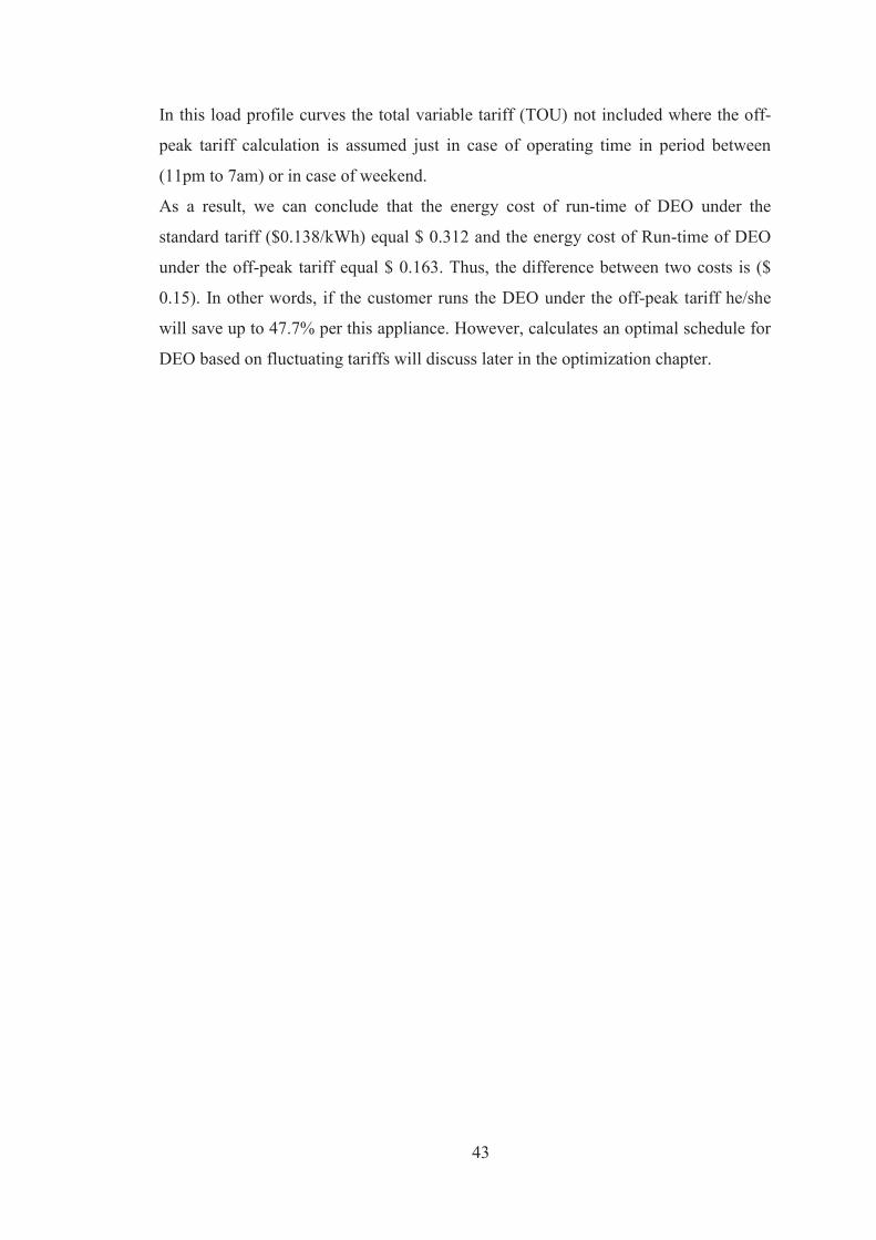
43
In this load profile curves the total variable tariff (TOU) not included where the off-
peak tariff calculation is assumed just in case of operating time in period between
(11pm to 7am) or in case of weekend.
As a result, we can conclude that the energy cost of run-time of DEO under the
standard tariff ($0.138/kWh) equal $ 0.312 and the energy cost of Run-time of DEO
under the off-peak tariff equal $ 0.163. Thus, the difference between two costs is ($
0.15). In other words, if the customer runs the DEO under the off-peak tariff he/she
will save up to 47.7% per this appliance. However, calculates an optimal schedule for
DEO based on fluctuating tariffs will discuss later in the optimization chapter.
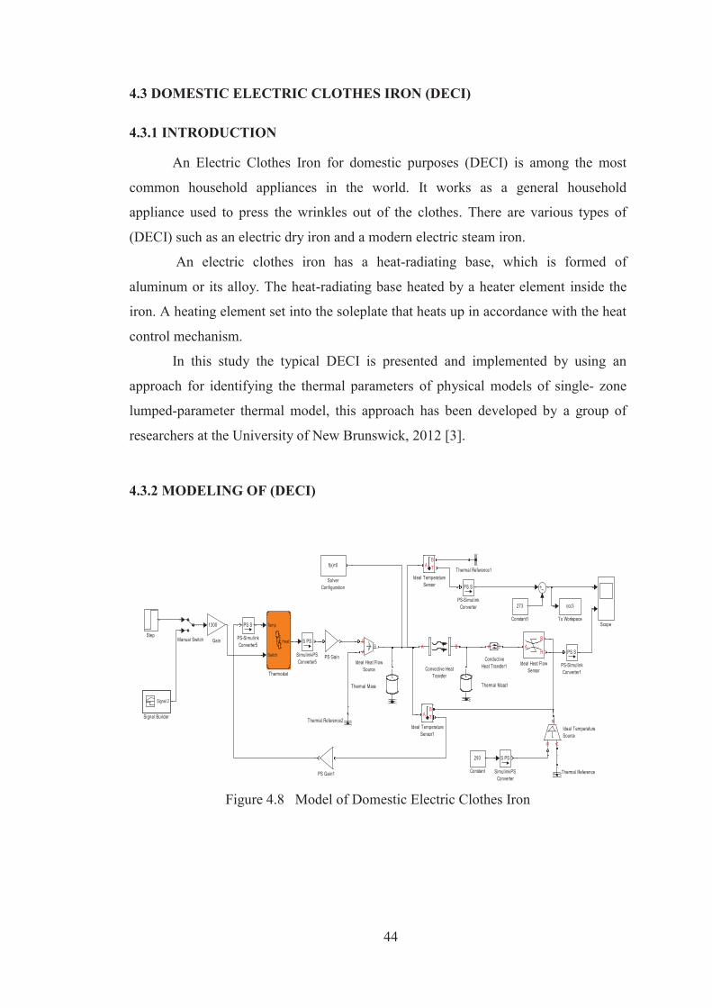
44
4.3 DOMESTIC ELECTRIC CLOTHES IRON (DECI)
4.3.1 INTRODUCTION
An Electric Clothes Iron for domestic purposes (DECI) is among the most
common household appliances in the world. It works as a general household
appliance used to press the wrinkles out of the clothes. There are various types of
(DECI) such as an electric dry iron and a modern electric steam iron.
An electric clothes iron has a heat-radiating base, which is formed of
aluminum or its alloy. The heat-radiating base heated by a heater element inside the
iron. A heating element set into the soleplate that heats up in accordance with the heat
control mechanism.
In this study the typical DECI is presented and implemented by using an
approach for identifying the thermal parameters of physical models of single- zone
lumped-parameter thermal model, this approach has been developed by a group of
researchers at the University of New Brunswick, 2012 [3].
4.3.2 MODELING OF (DECI)
Figure 4.8 Model of Domestic Electric Clothes Iron
ccc3
To WorkspaceTemp
Switch
Heat
Thermostat
Thermal Reference2
Thermal Reference1
Thermal Reference
Thermal Mass1Thermal Mass
Step
f(x)=0
SolverConfiguration
S PS
Simulink-PSConverter5
S PS
Simulink-PSConverter
Signal 2
Signal Builder
ScopeSPS
PS-SimulinkConverter5
SPS
PS-SimulinkConverter1
SPS
PS-SimulinkConverter
PS Gain1
PS Gain
Manual Switch
BAS
Ideal TemperatureSource
TB
A
Ideal TemperatureSensor1
TB
A
Ideal TemperatureSensor
BA
S
Ideal Heat FlowSource
BA
H
Ideal Heat FlowSensor
1300
GainBA
Convective HeatTransfer
273
Constant1
293
Constant
BA
ConductiveHeat Transfer1
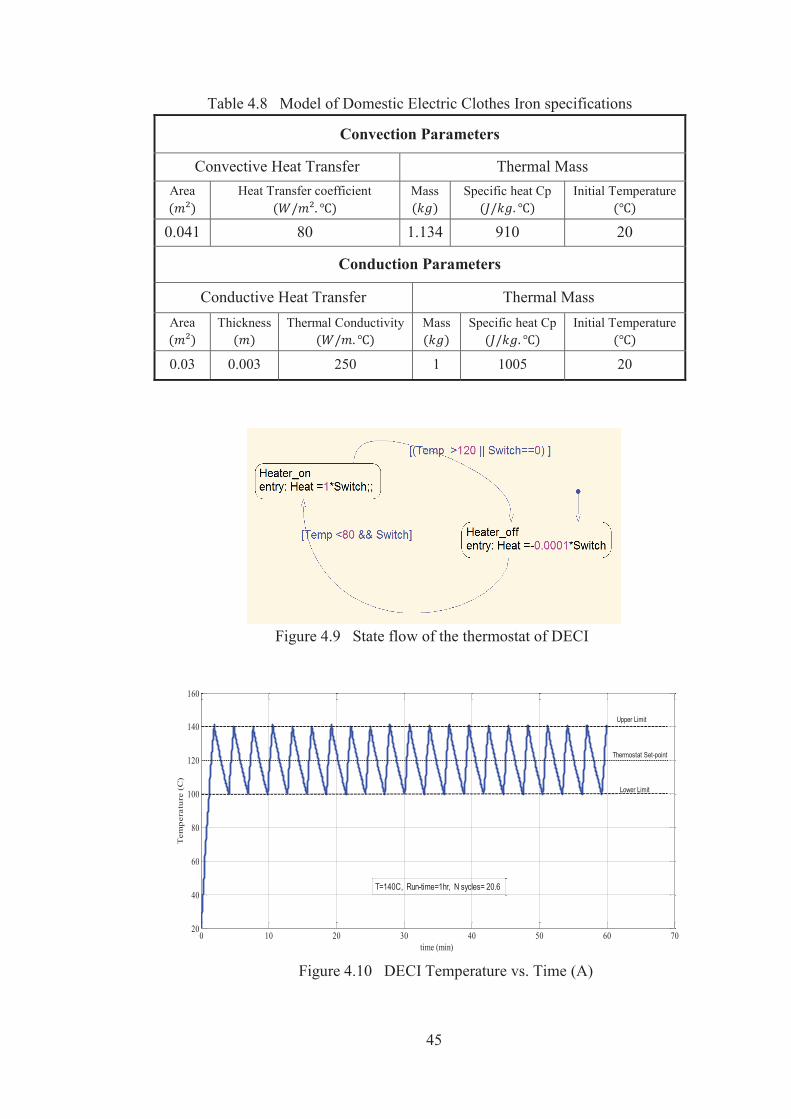
45
Table 4.8 Model of Domestic Electric Clothes Iron specifications
Convection Parameters
Convective Heat Transfer Thermal Mass Area
Heat Transfer coefficient
Mass
Specific heat Cp
Initial Temperature
0.041 80 1.134 910 20
Conduction Parameters
Conductive Heat Transfer Thermal Mass Area
Thickness
Thermal Conductivity
Mass
Specific heat Cp
Initial Temperature
0.03 0.003 250 1 1005 20
Figure 4.9 State flow of the thermostat of DECI
Figure 4.10 DECI Temperature vs. Time (A)
0 10 20 30 40 50 60 7020
40
60
80
100
120
140
160
time (min)
Tem
per
atu
re (
C)
T=140C, Run-time=1hr, N sycles= 20.6
Lower Limit
Upper Limit
Thermostat Set-point

46
Figure 4.11 DECI Temperature vs. Time (B)
A common clothes iron works in a range of approximately (50 to 230 °C). However,
the above figures (4.10 and 4.11) are illustrating just one stage of the user choice in
range of (100 to 140 °C). On the other hand, the plot of temperature as a function of
time shows that the system has reached a steady state.
4.3.3 MATHEMATICAL MODEL of DECI
The aim of this section is to provide, a sample calculation in order to analyse
the DECI system behavior during transient condition and steady-state condition
response.
The primary calculations of a mathematical model of DEIC are based on the Lumped
Parameter Method which is included in studies [3] and [12] as mentioned in chapter 3.
In this section the main parameters of DECI such as thermal resistance ( ) and the
thermal capacity in terms of temperature, and time durations are
calculated. However, instead of taking those parameters values from literature; this
study examines and investigates the system behavior with material properties for
obtaining expressions that can be used to determine the value of all constant
parameters by deriving some equations that represent operation cycles of the system
performance. The mathematical model of DECI is based on the Lumped Parameter
Method which is included in the studies [3 and 12]. However, in this study a few
required modifications to develop simple mathematical equations that reflect the
system behavior and show the effect of varying some parameters in this model are
represented.
0 10 20 30 40 50 6020
40
60
80
100
120
140
160
time (min)
Tem
pera
ture
(C)
Upper Limit
Lower Limit
T=140C, Run-time = 0.5 hr
Thermostat Set-point
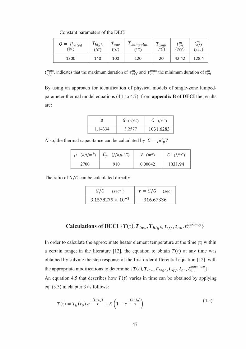
47
Constant parameters of the DECI
1300 140 100 120 20 42.42 128.4
, indicates that the maximum duration of and the minimum duration of
By using an approach for identification of physical models of single-zone lumped-
parameter thermal model equations (4.1 to 4.7); from appendix B of DECI the results
are:
1.14334 3.2577 1031.6283
Also, the thermal capacitance can be calculated by
2700 910 0.00042 1031.94 The ratio of can be calculated directly
Calculations of DECI { , }
In order to calculate the approximate heater element temperature at the time (t) within
a certain range; in the literature [12], the equation to obtain at any time was
obtained by solving the step response of the first order differential equation [12], with
the appropriate modifications to determine { }.
An equation 4.5 that describes how varies in time can be obtained by applying
eq. (3.3) in chapter 3 as follows:
(4.5)
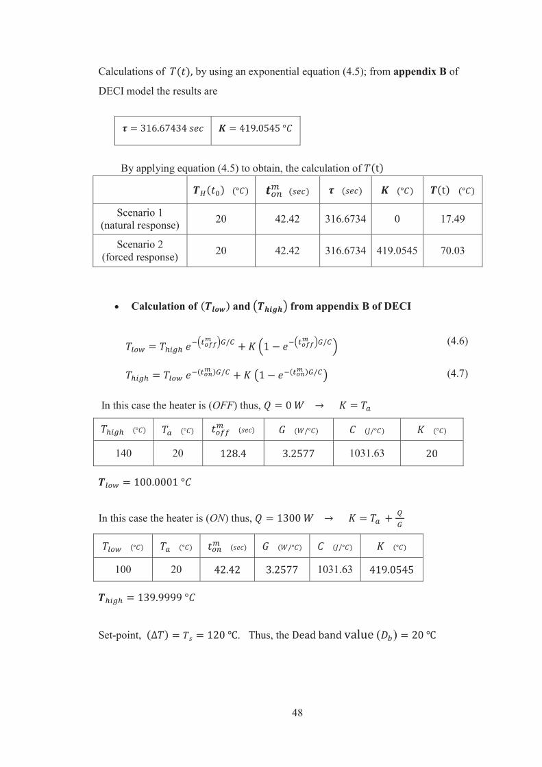
48
Calculations of , by using an exponential equation (4.5); from appendix B of
DECI model the results are
By applying equation (4.5) to obtain, the calculation of
Scenario 1 (natural response) 20 42.42 316.6734 0 17.49
Scenario 2 (forced response) 20 42.42 316.6734 419.0545 70.03
Calculation of and from appendix B of DECI
(4.6)
(4.7)
In this case the heater is (OFF) thus,
140 20 1031.63
In this case the heater is (ON) thus,
100 20 1031.63
Set-point, . Thus, the ( )
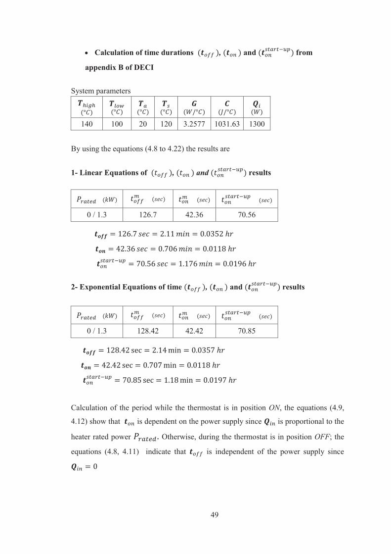
49
Calculation of time durations , and from
appendix B of DECI
System parameters
140 100 20 120 3.2577 1031.63 1300
By using the equations (4.8 to 4.22) the results are
1- Linear Equations of , and results
0 / 1.3 126.7 42.36 70.56
2- Exponential Equations of time , and results
0 / 1.3 128.42 42.42 70.85
Calculation of the period while the thermostat is in position ON, the equations (4.9,
4.12) show that is dependent on the power supply since is proportional to the
heater rated power Otherwise, during the thermostat is in position OFF; the
equations (4.8, 4.11) indicate that is independent of the power supply since

50
Power / Energy consumption of (DECI)
Method
Calculation 0.0153 1.3 0.0118
Simulation 0.0155 1.3 0.0119
(total)
0.3416 1.3 0.2628
Table 4.9 Comparison of the results of the time duration of the model
Method
P
Linear equations 0.0196 0.0118 0.0352 0.2627 1.3
Exponential equations 0.0197 0.0118 0.0357 0.2628 1.3
Simulation Result 0.0197 0.0119 0.0359 0.2648 1.3
The average power consumption from the energy flow and the energy
consumption per operation cycle ( ) of the (DECI) can be calculated by using Duty
Cycle value and input rated power; in appendix B the results as follows:
Table 4.10 Comparison of the simulation results to equations
Method
Linear Equation 1.3 0.0196 0.0118 0.0352 0.047 0.2511 0.3264 0.3415
Exponential Equation 1.3 0.0197 0.0118 0.0357 0.0475 0.2484 0.3229 0.3416
Simulation 1.3 0.0197 0.0119 0.0359 0.0478 0.2490 0.3237 0.3443
Table 4.10, shows the results obtained from linear equations and exponential
equations, the average power, energy consumption and the simulation result of the
DECI model. The results obtained from linear equations and exponential equations
are almost the same as the results obtained from simulation. Thus the mathematical
model has a good agreement with the simulation results.
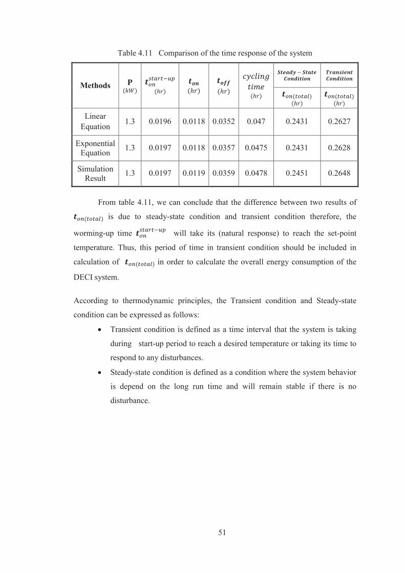
51
Table 4.11 Comparison of the time response of the system
Methods
Linear Equation 1.3 0.0196 0.0118 0.0352 0.047 0.2431 0.2627
Exponential Equation 1.3 0.0197 0.0118 0.0357 0.0475 0.2431 0.2628
Simulation Result 1.3 0.0197 0.0119 0.0359 0.0478 0.2451 0.2648
From table 4.11, we can conclude that the difference between two results of
is due to steady-state condition and transient condition therefore, the
worming-up time will take its (natural response) to reach the set-point
temperature. Thus, this period of time in transient condition should be included in
calculation of in order to calculate the overall energy consumption of the
DECI system.
According to thermodynamic principles, the Transient condition and Steady-state
condition can be expressed as follows:
Transient condition is defined as a time interval that the system is taking
during start-up period to reach a desired temperature or taking its time to
respond to any disturbances. Steady-state condition is defined as a condition where the system behavior
is depend on the long run time and will remain stable if there is no
disturbance.
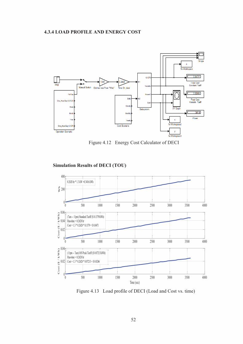
52
4.3.4 LOAD PROFILE AND ENERGY COST
Figure 4.12 Energy Cost Calculator of DECI
Simulation Results of DECI (TOU)
Figure 4.13 Load profile of DECI (Load and Cost vs. time)
0 500 1000 1500 2000 2500 3000 3500 40000
200
400
Wh
0 500 1000 1500 2000 2500 3000 3500 40000
0.02
0.04
0.06
Co
st
($
/ k
Wh
)
0 500 1000 1500 2000 2500 3000 3500 40000
0.02
0.04
Time (sec)
Co
st
($
/ k
Wh
)
0.2628 hr * 1.3 kW =0.3416 kWh
(7am -- 11pm) Standard Tariff ($ 0.1379/kWh)Run-time = 0.2628 hrCost = 1.3 * 0.2628 * 0.1379 = $ 0.0471
(11pm -- 7am) Off-Peak Tariff ($ 0.07213/kWh)Run-time = 0.2628 hrCost = 1.3 * 0.2628 * 0.07213 = $ 0.0246
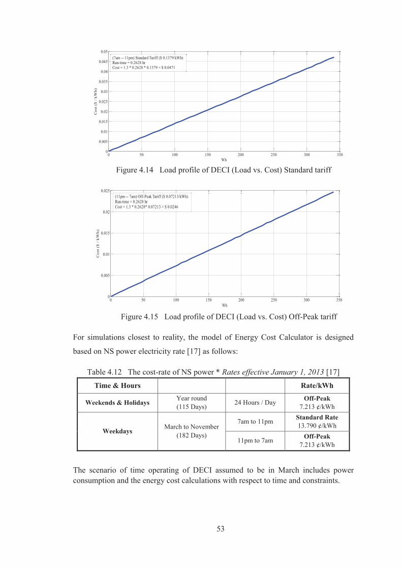
53
Figure 4.14 Load profile of DECI (Load vs. Cost) Standard tariff
Figure 4.15 Load profile of DECI (Load vs. Cost) Off-Peak tariff
For simulations closest to reality, the model of Energy Cost Calculator is designed
based on NS power electricity rate [17] as follows:
Table 4.12 The cost-rate of NS power * Rates effective January 1, 2013 [17] Time & Hours Rate/kWh
Weekends & Holidays Year round (115 Days) 24 Hours / Day Off-Peak
7.213 ¢/kWh
Weekdays March to November
(182 Days)
7am to 11pm Standard Rate 13.790 ¢/kWh
11pm to 7am Off-Peak 7.213 ¢/kWh
The scenario of time operating of DECI assumed to be in March includes power consumption and the energy cost calculations with respect to time and constraints.
0 50 100 150 200 250 300 3500
0.005
0.01
0.015
0.02
0.025
0.03
0.035
0.04
0.045
0.05
Wh
Cos
t ($
/ kW
h)
(7am -- 11pm) Standard Tariff ($ 0.1379/kWh)Run-time = 0.2628 hrCost = 1.3 * 0.2628 * 0.1379 = $ 0.0471
0 50 100 150 200 250 300 3500
0.005
0.01
0.015
0.02
0.025
Wh
Cos
t ($
/ kW
h)
(11pm -- 7am) Off-Peak Tariff ($ 0.07213/kWh)Run-time = 0.2628 hrCost = 1.3 * 0.2628* 0.07213 = $ 0.0246
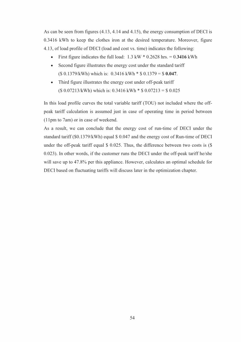
54
As can be seen from figures (4.13, 4.14 and 4.15), the energy consumption of DECI is
0.3416 kWh to keep the clothes iron at the desired temperature. Moreover, figure
4.13, of load profile of DECI (load and cost vs. time) indicates the following:
First figure indicates the full load: 1.3 kW * 0.2628 hrs. = 0.3416 kWh
Second figure illustrates the energy cost under the standard tariff
($ 0.1379/kWh) which is: 0.3416 kWh * $ 0.1379 = $ 0.047.
Third figure illustrates the energy cost under off-peak tariff
($ 0.07213/kWh) which is: 0.3416 kWh * $ 0.07213 = $ 0.025
In this load profile curves the total variable tariff (TOU) not included where the off-
peak tariff calculation is assumed just in case of operating time in period between
(11pm to 7am) or in case of weekend.
As a result, we can conclude that the energy cost of run-time of DECI under the
standard tariff ($0.1379/kWh) equal $ 0.047 and the energy cost of Run-time of DECI
under the off-peak tariff equal $ 0.025. Thus, the difference between two costs is ($
0.023). In other words, if the customer runs the DECI under the off-peak tariff he/she
will save up to 47.8% per this appliance. However, calculates an optimal schedule for
DECI based on fluctuating tariffs will discuss later in the optimization chapter.
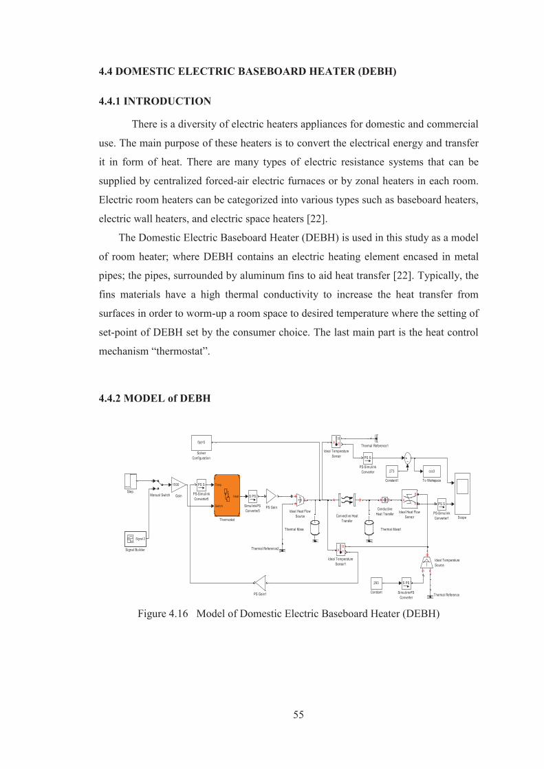
55
4.4 DOMESTIC ELECTRIC BASEBOARD HEATER (DEBH)
4.4.1 INTRODUCTION
There is a diversity of electric heaters appliances for domestic and commercial
use. The main purpose of these heaters is to convert the electrical energy and transfer
it in form of heat. There are many types of electric resistance systems that can be
supplied by centralized forced-air electric furnaces or by zonal heaters in each room.
Electric room heaters can be categorized into various types such as baseboard heaters,
electric wall heaters, and electric space heaters [22].
The Domestic Electric Baseboard Heater (DEBH) is used in this study as a model
of room heater; where DEBH contains an electric heating element encased in metal
pipes; the pipes, surrounded by aluminum fins to aid heat transfer [22]. Typically, the
fins materials have a high thermal conductivity to increase the heat transfer from
surfaces in order to worm-up a room space to desired temperature where the setting of
set-point of DEBH set by the consumer choice. The last main part is the heat control
mechanism “thermostat”.
4.4.2 MODEL of DEBH
Figure 4.16 Model of Domestic Electric Baseboard Heater (DEBH)
ccc3
To WorkspaceTemp
Switch
Heat
Thermostat
Thermal Reference2
Thermal Reference1
Thermal Reference
Thermal Mass1Thermal Mass
Step
f(x)=0
SolverConfiguration
S PS
Simulink-PSConverter5
S PS
Simulink-PSConverter
Signal 2
Signal Builder
Scope
SPS
PS-SimulinkConverter5
SPS
PS-SimulinkConverter1
SPS
PS-SimulinkConverter
PS Gain1
PS Gain
Manual Switch
BAS
Ideal TemperatureSource
TB
A
Ideal TemperatureSensor1
TB
A
Ideal TemperatureSensor
BA
S
Ideal Heat FlowSource
BA
H
Ideal Heat FlowSensor
1500
GainBA
Convective HeatTransfer
273
Constant1
293
Constant
BA
ConductiveHeat Transfer
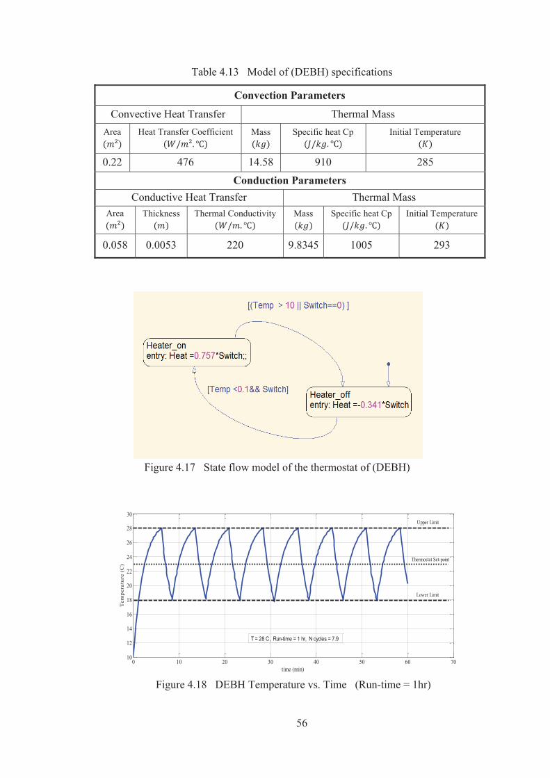
56
Table 4.13 Model of (DEBH) specifications
Convection Parameters
Convective Heat Transfer Thermal Mass Area
Heat Transfer Coefficient
Mass
Specific heat Cp
Initial Temperature
0.22 476 14.58 910 285
Conduction Parameters Conductive Heat Transfer Thermal Mass
Area
Thickness
Thermal Conductivity
Mass
Specific heat Cp
Initial Temperature
0.058 0.0053 220 9.8345 1005 293
Figure 4.17 State flow model of the thermostat of (DEBH)
Figure 4.18 DEBH Temperature vs. Time (Run-time = 1hr)
0 10 20 30 40 50 60 7010
12
14
16
18
20
22
24
26
28
30
time (min)
Tem
pera
ture
(C
)
Upper Limit
Lower Limit
T = 28 C, Run-time = 1 hr, N cycles = 7.9
Thermostat Set-point
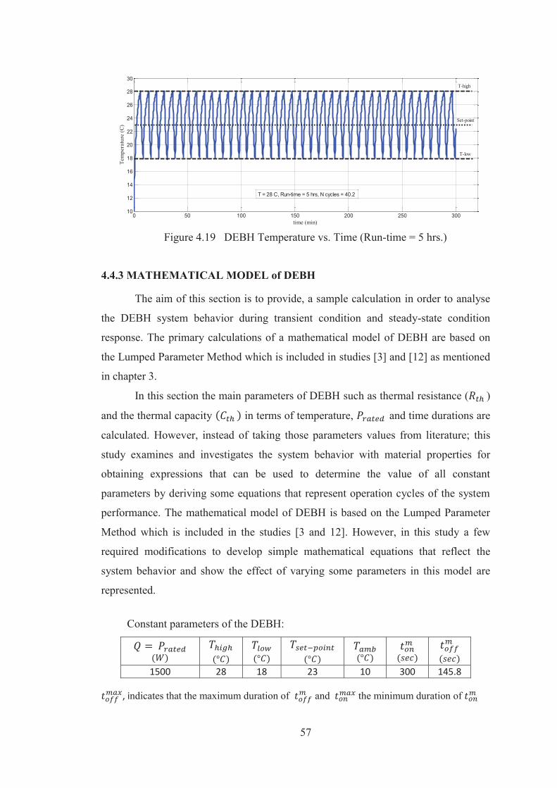
57
Figure 4.19 DEBH Temperature vs. Time (Run-time = 5 hrs.)
4.4.3 MATHEMATICAL MODEL of DEBH
The aim of this section is to provide, a sample calculation in order to analyse
the DEBH system behavior during transient condition and steady-state condition
response. The primary calculations of a mathematical model of DEBH are based on
the Lumped Parameter Method which is included in studies [3] and [12] as mentioned
in chapter 3.
In this section the main parameters of DEBH such as thermal resistance ( )
and the thermal capacity in terms of temperature, and time durations are
calculated. However, instead of taking those parameters values from literature; this
study examines and investigates the system behavior with material properties for
obtaining expressions that can be used to determine the value of all constant
parameters by deriving some equations that represent operation cycles of the system
performance. The mathematical model of DEBH is based on the Lumped Parameter
Method which is included in the studies [3 and 12]. However, in this study a few
required modifications to develop simple mathematical equations that reflect the
system behavior and show the effect of varying some parameters in this model are
represented.
Constant parameters of the DEBH:
1500 28 18 23 10 300 145.8
, indicates that the maximum duration of and the minimum duration of
0 50 100 150 200 250 30010
12
14
16
18
20
22
24
26
28
30
time (min)
Tem
pera
ture
(C)
T = 28 C, Run-time = 5 hrs, N cycles = 40.2
T-high
Set-point
T-low
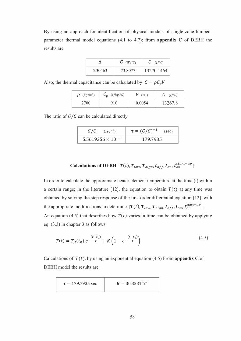
58
By using an approach for identification of physical models of single-zone lumped-
parameter thermal model equations (4.1 to 4.7); from appendix C of DEBH the
results are
5.30463 73.8077 13270.1464
Also, the thermal capacitance can be calculated by
2700 910 0.0054 13267.8 The ratio of can be calculated directly
Calculations of DEBH { }
In order to calculate the approximate heater element temperature at the time (t) within
a certain range; in the literature [12], the equation to obtain at any time was
obtained by solving the step response of the first order differential equation [12], with
the appropriate modifications to determine { }.
An equation (4.5) that describes how varies in time can be obtained by applying
eq. (3.3) in chapter 3 as follows:
(4.5)
Calculations of , by using an exponential equation (4.5) From appendix C of
DEBH model the results are

59
By applying above equation (4.5) to obtain
Scenario 1 (natural response) 10 300 179.7935 0 1.8851
Scenario 2 (forced response) 10 300 179.7935 30.3231 26.49
Calculation of and from appendix C of DEBH
(4.6)
(4.7)
In this case the heater is (OFF) thus,
28 10 13270.1464
In this case the heater is (ON) thus,
18 10 13270.1464
Set-point ( ) Thus, the ( )
Calculation of Time: , and from appendix C of
DEBH
System parameters
28 18 10 23 13270.1464 1500
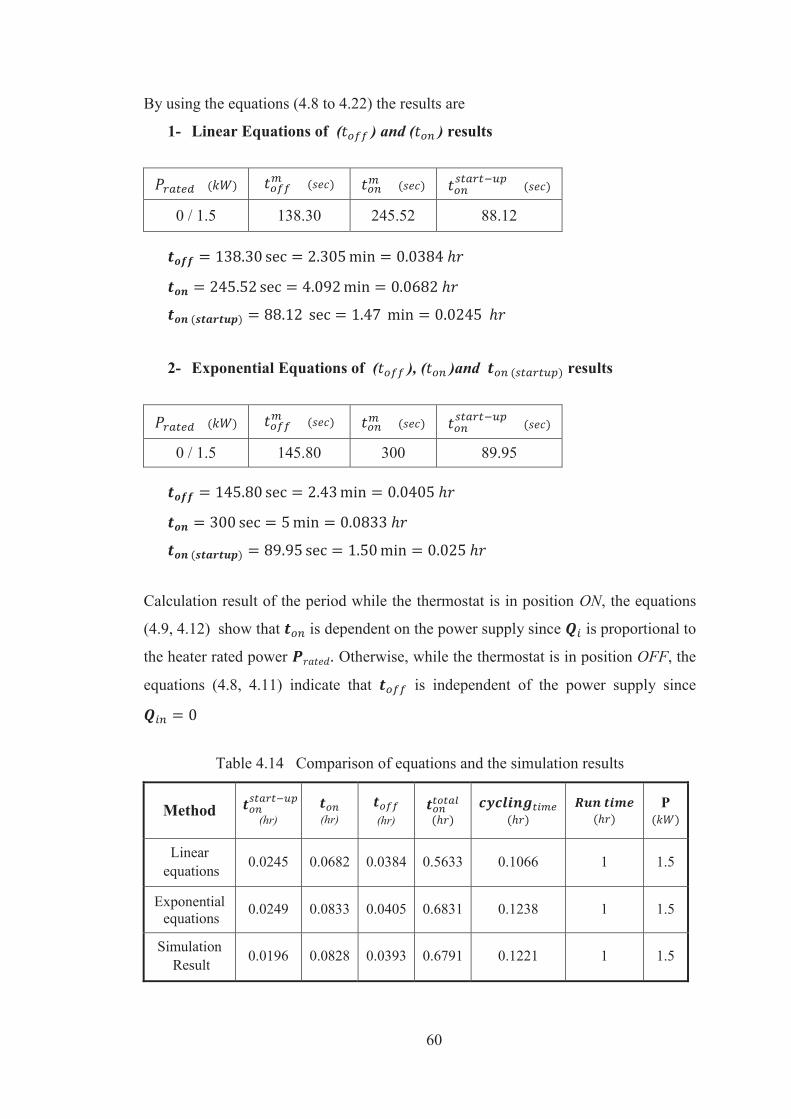
60
By using the equations (4.8 to 4.22) the results are
1- Linear Equations of ( ) and ( ) results
0 / 1.5 138.30 245.52 88.12
2- Exponential Equations of ( ), ( )and results
0 / 1.5 145.80 300 89.95
Calculation result of the period while the thermostat is in position ON, the equations
(4.9, 4.12) show that is dependent on the power supply since is proportional to
the heater rated power Otherwise, while the thermostat is in position OFF, the
equations (4.8, 4.11) indicate that is independent of the power supply since
Table 4.14 Comparison of equations and the simulation results
Method (hr)
(hr)
(hr)
P
Linear equations 0.0245 0.0682 0.0384 0.5633 0.1066 1 1.5
Exponential equations 0.0249 0.0833 0.0405 0.6831 0.1238 1 1.5
Simulation Result 0.0196 0.0828 0.0393 0.6791 0.1221 1 1.5
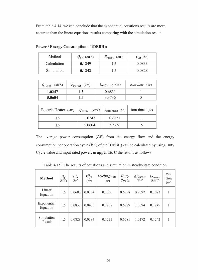
61
From table 4.14, we can conclude that the exponential equations results are more
accurate than the linear equations results comparing with the simulation result.
Power / Energy Consumption of (DEBH):
Method
Calculation 0.1249 1.5 0.0833
Simulation 0.1242 1.5 0.0828
Run-time
1.0247 1.5 0.6831 1 5.0604 1.5 3.3736 5
Electric Heater Run-time
1.5 1.0247 0.6831 1
1.5 5.0604 3.3736 5
The average power consumption ( ) from the energy flow and the energy
consumption per operation cycle ( ) of the (DEBH) can be calculated by using Duty
Cycle value and input rated power; in appendix C the results as follows:
Table 4.15 The results of equations and simulation in steady-state condition
Method
Linear Equation 1.5 0.0682 0.0384 0.1066 0.6398 0.9597 0.1023 1
Exponential Equation 1.5 0.0833 0.0405 0.1238 0.6729 1.0094 0.1249 1
Simulation Result 1.5 0.0828 0.0393 0.1221 0.6781 1.0172 0.1242 1
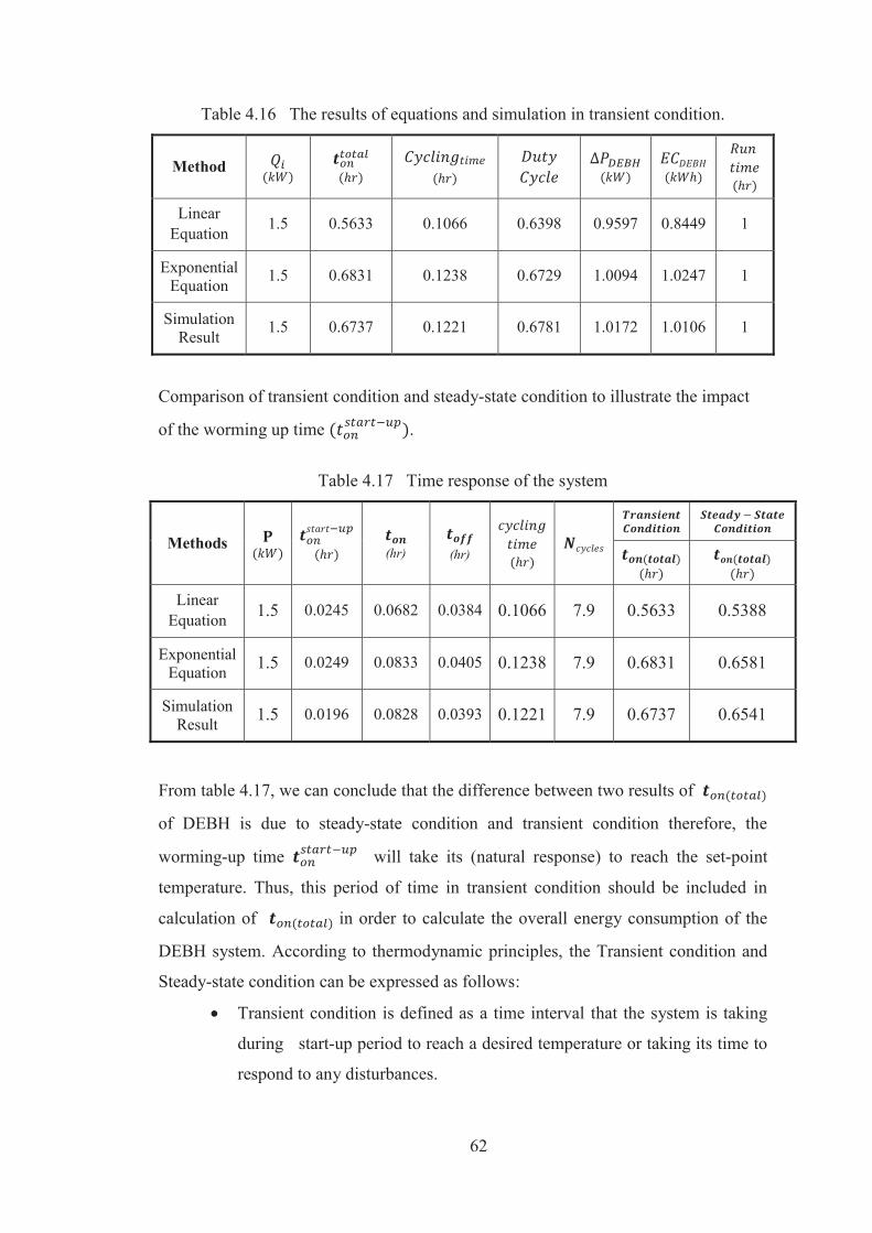
62
Table 4.16 The results of equations and simulation in transient condition.
Method
Linear Equation 1.5 0.5633 0.1066 0.6398 0.9597 0.8449 1
Exponential Equation 1.5 0.6831 0.1238 0.6729 1.0094 1.0247 1
Simulation Result 1.5 0.6737 0.1221 0.6781 1.0172 1.0106 1
Comparison of transient condition and steady-state condition to illustrate the impact
of the worming up time .
Table 4.17 Time response of the system
Methods
(hr)
(hr)
Linear Equation 1.5 0.0245 0.0682 0.0384 0.1066 7.9 0.5633 0.5388
Exponential Equation 1.5 0.0249 0.0833 0.0405 0.1238 7.9 0.6831 0.6581
Simulation Result 1.5 0.0196 0.0828 0.0393 0.1221 7.9 0.6737 0.6541
From table 4.17, we can conclude that the difference between two results of
of DEBH is due to steady-state condition and transient condition therefore, the
worming-up time will take its (natural response) to reach the set-point
temperature. Thus, this period of time in transient condition should be included in
calculation of in order to calculate the overall energy consumption of the
DEBH system. According to thermodynamic principles, the Transient condition and
Steady-state condition can be expressed as follows:
Transient condition is defined as a time interval that the system is taking
during start-up period to reach a desired temperature or taking its time to
respond to any disturbances.
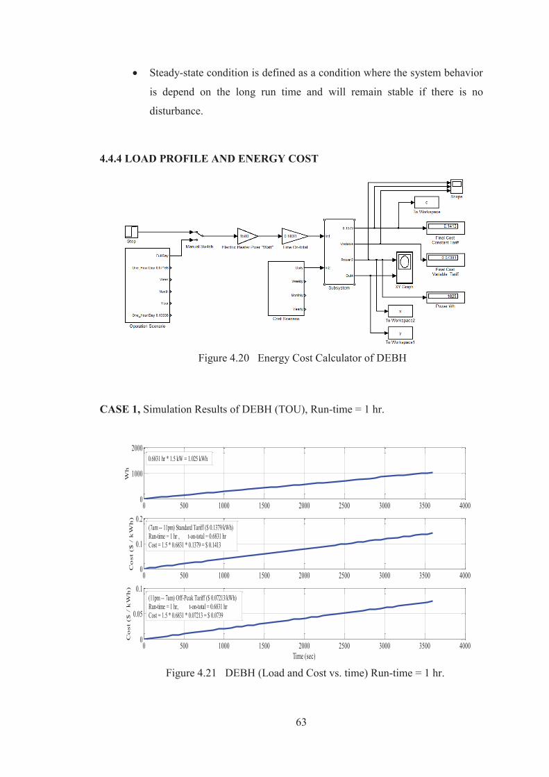
63
Steady-state condition is defined as a condition where the system behavior
is depend on the long run time and will remain stable if there is no
disturbance.
4.4.4 LOAD PROFILE AND ENERGY COST
Figure 4.20 Energy Cost Calculator of DEBH
CASE 1, Simulation Results of DEBH (TOU), Run-time = 1 hr.
Figure 4.21 DEBH (Load and Cost vs. time) Run-time = 1 hr.
0 500 1000 1500 2000 2500 3000 3500 40000
1000
2000
Wh
0 500 1000 1500 2000 2500 3000 3500 40000
0.1
0.2
Co
st
($ /
kW
h)
0 500 1000 1500 2000 2500 3000 3500 40000
0.05
0.1
Time (sec)
Co
st
($ /
kW
h)
0.6831 hr * 1.5 kW = 1.025 kWh
(7am -- 11pm) Standard Tariff ($ 0.1379/kWh)Run-time = 1 hr , t-on-total = 0.6831 hrCost = 1.5 * 0.6831 * 0.1379 = $ 0.1413
(11pm -- 7am) Off-Peak Tariff ($ 0.07213/kWh)Run-time = 1 hr, t-on-total = 0.6831 hrCost = 1.5 * 0.6831 * 0.07213 = $ 0.0739
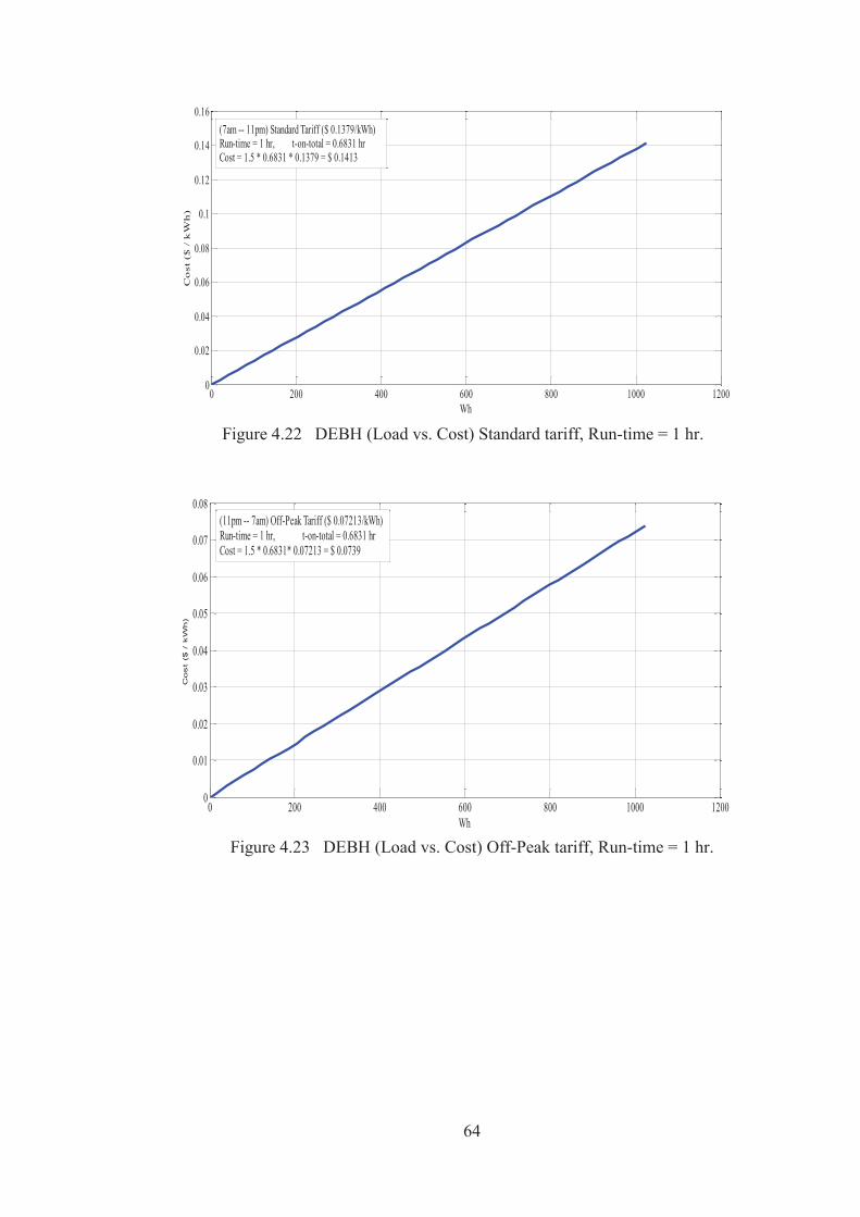
64
Figure 4.22 DEBH (Load vs. Cost) Standard tariff, Run-time = 1 hr.
Figure 4.23 DEBH (Load vs. Cost) Off-Peak tariff, Run-time = 1 hr.
0 200 400 600 800 1000 12000
0.02
0.04
0.06
0.08
0.1
0.12
0.14
0.16
Wh
Co
st (
$ /
kW
h)
(7am -- 11pm) Standard Tariff ($ 0.1379/kWh)Run-time = 1 hr, t-on-total = 0.6831 hrCost = 1.5 * 0.6831 * 0.1379 = $ 0.1413
0 200 400 600 800 1000 12000
0.01
0.02
0.03
0.04
0.05
0.06
0.07
0.08
Wh
Cost
($ /
kW
h)
(11pm -- 7am) Off-Peak Tariff ($ 0.07213/kWh)Run-time = 1 hr, t-on-total = 0.6831 hrCost = 1.5 * 0.6831* 0.07213 = $ 0.0739
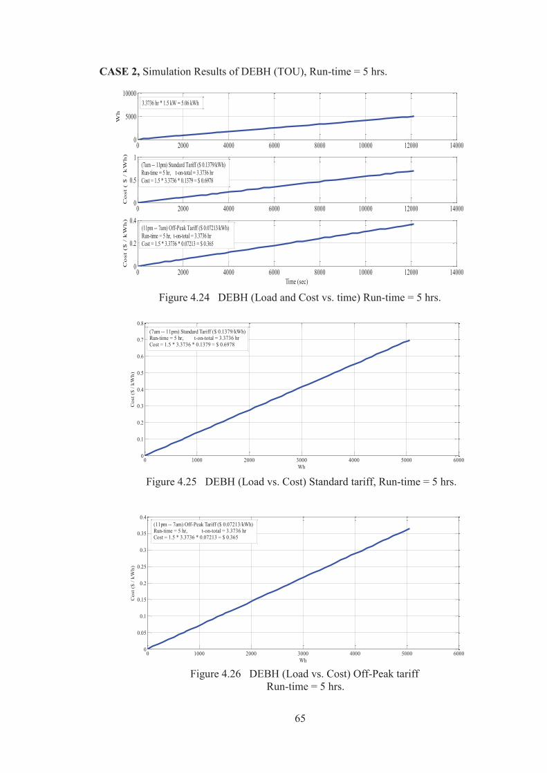
65
CASE 2, Simulation Results of DEBH (TOU), Run-time = 5 hrs.
Figure 4.24 DEBH (Load and Cost vs. time) Run-time = 5 hrs.
Figure 4.25 DEBH (Load vs. Cost) Standard tariff, Run-time = 5 hrs.
Figure 4.26 DEBH (Load vs. Cost) Off-Peak tariff
Run-time = 5 hrs.
0 2000 4000 6000 8000 10000 12000 140000
5000
10000
Wh
0 2000 4000 6000 8000 10000 12000 140000
0.5
1
Co
st (
$ /
kW
h)
0 2000 4000 6000 8000 10000 12000 140000
0.2
0.4
Time (sec)
Co
st (
$ /
kW
h)
3.3736 hr * 1.5 kW = 5.06 kWh
(11pm -- 7am) Off-Peak Tariff ($ 0.07213/kWh)Run-time = 5 hr, t-on-total = 3.3736 hrCost = 1.5 * 3.3736 * 0.07213 = $ 0.365
(7am -- 11pm) Standard Tariff ($ 0.1379/kWh)Run-time = 5 hr, t-on-total = 3.3736 hrCost = 1.5 * 3.3736 * 0.1379 = $ 0.6978
0 1000 2000 3000 4000 5000 60000
0.1
0.2
0.3
0.4
0.5
0.6
0.7
0.8
Wh
Cos
t ($
/ kW
h)
(7am -- 11pm) Standard Tariff ($ 0.1379/kWh)Run-time = 5 hr, t-on-total = 3.3736 hrCost = 1.5 * 3.3736 * 0.1379 = $ 0.6978
0 1000 2000 3000 4000 5000 60000
0.05
0.1
0.15
0.2
0.25
0.3
0.35
0.4
Wh
Cos
t ($
/ kW
h)
(11pm -- 7am) Off-Peak Tariff ($ 0.07213/kWh)Run-time = 5 hr, t-on-total = 3.3736 hrCost = 1.5 * 3.3736 * 0.07213 = $ 0.365
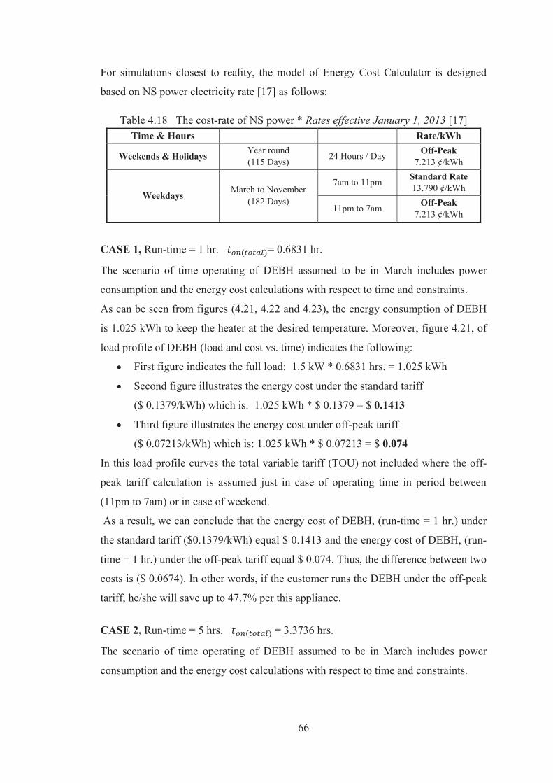
66
For simulations closest to reality, the model of Energy Cost Calculator is designed
based on NS power electricity rate [17] as follows:
Table 4.18 The cost-rate of NS power * Rates effective January 1, 2013 [17] Time & Hours Rate/kWh
Weekends & Holidays Year round (115 Days) 24 Hours / Day Off-Peak
7.213 ¢/kWh
Weekdays March to November
(182 Days)
7am to 11pm Standard Rate 13.790 ¢/kWh
11pm to 7am Off-Peak 7.213 ¢/kWh
CASE 1, Run-time = 1 hr. = 0.6831 hr.
The scenario of time operating of DEBH assumed to be in March includes power
consumption and the energy cost calculations with respect to time and constraints.
As can be seen from figures (4.21, 4.22 and 4.23), the energy consumption of DEBH
is 1.025 kWh to keep the heater at the desired temperature. Moreover, figure 4.21, of
load profile of DEBH (load and cost vs. time) indicates the following:
First figure indicates the full load: 1.5 kW * 0.6831 hrs. = 1.025 kWh
Second figure illustrates the energy cost under the standard tariff
($ 0.1379/kWh) which is: 1.025 kWh * $ 0.1379 = $ 0.1413
Third figure illustrates the energy cost under off-peak tariff
($ 0.07213/kWh) which is: 1.025 kWh * $ 0.07213 = $ 0.074
In this load profile curves the total variable tariff (TOU) not included where the off-
peak tariff calculation is assumed just in case of operating time in period between
(11pm to 7am) or in case of weekend.
As a result, we can conclude that the energy cost of DEBH, (run-time = 1 hr.) under
the standard tariff ($0.1379/kWh) equal $ 0.1413 and the energy cost of DEBH, (run-
time = 1 hr.) under the off-peak tariff equal $ 0.074. Thus, the difference between two
costs is ($ 0.0674). In other words, if the customer runs the DEBH under the off-peak
tariff, he/she will save up to 47.7% per this appliance.
CASE 2, Run-time = 5 hrs. = 3.3736 hrs.
The scenario of time operating of DEBH assumed to be in March includes power
consumption and the energy cost calculations with respect to time and constraints.
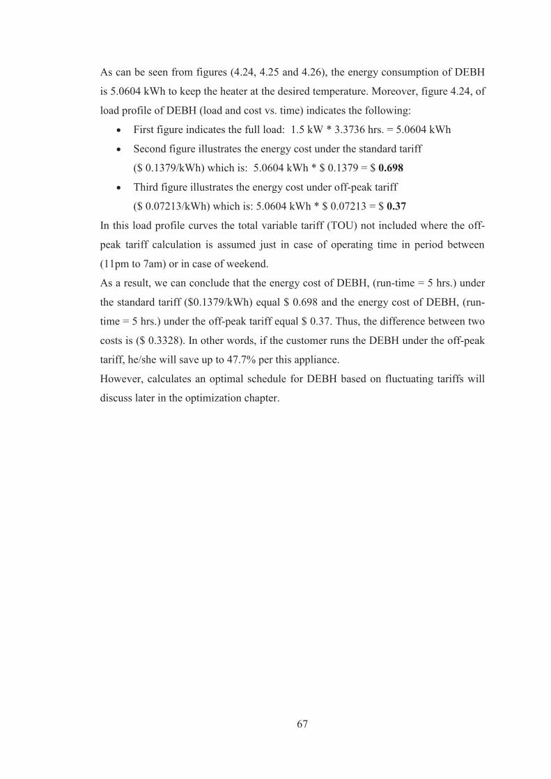
67
As can be seen from figures (4.24, 4.25 and 4.26), the energy consumption of DEBH
is 5.0604 kWh to keep the heater at the desired temperature. Moreover, figure 4.24, of
load profile of DEBH (load and cost vs. time) indicates the following:
First figure indicates the full load: 1.5 kW * 3.3736 hrs. = 5.0604 kWh
Second figure illustrates the energy cost under the standard tariff
($ 0.1379/kWh) which is: 5.0604 kWh * $ 0.1379 = $ 0.698
Third figure illustrates the energy cost under off-peak tariff
($ 0.07213/kWh) which is: 5.0604 kWh * $ 0.07213 = $ 0.37
In this load profile curves the total variable tariff (TOU) not included where the off-
peak tariff calculation is assumed just in case of operating time in period between
(11pm to 7am) or in case of weekend.
As a result, we can conclude that the energy cost of DEBH, (run-time = 5 hrs.) under
the standard tariff ($0.1379/kWh) equal $ 0.698 and the energy cost of DEBH, (run-
time = 5 hrs.) under the off-peak tariff equal $ 0.37. Thus, the difference between two
costs is ($ 0.3328). In other words, if the customer runs the DEBH under the off-peak
tariff, he/she will save up to 47.7% per this appliance.
However, calculates an optimal schedule for DEBH based on fluctuating tariffs will
discuss later in the optimization chapter.
68
4.5 MODEL of LIGHTING
4.5.1 INTRODUCTION
The lighting system plays a significant role in every building, whether it is a
natural or artificial source. Numerous light sources are available across the world; the
most desirable light source is the natural light from sun referred to as daylight;
artificial sources of lighting are incandescent lamps, fluorescent-lamps (F-Lamp),
compact fluorescent lamps (CFL) and light emitting diode (LED), etc.
Fluorescent-lamps have become a major method of lighting systems and have
become widely accepted in both residential and commercial sectors, particularly in
offices, public places, and factories. In addition, fluorescent-lamps commonly are
used in a residential sector. It is preferable to conventional tungsten incandescent
lamps because of their high luminous efficacy (lumens/watts) [58, 59 and 60]. In this
study, the fluorescent-lamp is presented.
Fluorescent-lamp is a device that presents a negative impedance to the power
supply and operating at high frequency (20 kHz or above). According to [59], there
are two fundamental considerations that are used to evaluate electrical characteristic
of any discharge lighting system, the starting and operating scenarios. Thus, the
electrical circuit of the fluorescent lamp must contain some form of current-limiting
such as an auxiliary device, which is commonly called ballast, to provide a positive
resistance or reactance in order to regulate the current flow through the tube [61, 65].
In other words, the ballast provides a suitable starting voltage and positive resistance;
a higher voltage is provided by a capacitor, which is placed in parallel to the lamp; in
this case the ballast is often called electronic ballasts; the positive resistance limits the
ultimate flow of current during lamp operation [61, 62, 65, and 70]. There are two
types of ballasts commonly used in residential and commercial lighting, the line-
frequency conventional electromagnetic ballast and the high-frequency electronic
ballast [65]. Electronic ballasts are more energy-efficient than magnetic ballasts.
Fluorescent lamps are available in many shapes in the market such as linear shapes, U
shapes, long twin-tube shape, compact fluorescent lamps and circular fluorescent
lamps [63, 64, 70 and 71]. The main parts of the fluorescent lamps power circuit are
the ballast and the lamp tube. Thus, the overall power consumption of fluorescent
lighting system is lamp power rated plus the power that is consumed by ballast during
system operation.
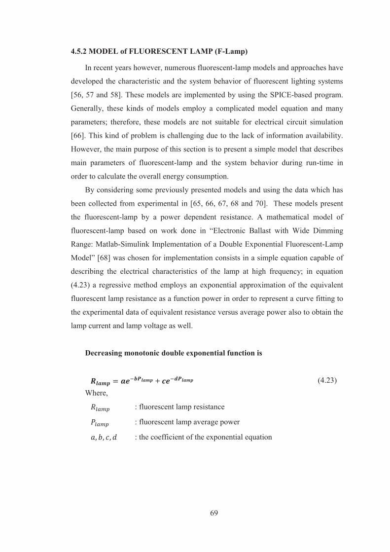
69
4.5.2 MODEL of FLUORESCENT LAMP (F-Lamp)
In recent years however, numerous fluorescent-lamp models and approaches have
developed the characteristic and the system behavior of fluorescent lighting systems
[56, 57 and 58]. These models are implemented by using the SPICE-based program.
Generally, these kinds of models employ a complicated model equation and many
parameters; therefore, these models are not suitable for electrical circuit simulation
[66]. This kind of problem is challenging due to the lack of information availability.
However, the main purpose of this section is to present a simple model that describes
main parameters of fluorescent-lamp and the system behavior during run-time in
order to calculate the overall energy consumption.
By considering some previously presented models and using the data which has
been collected from experimental in [65, 66, 67, 68 and 70]. These models present
the fluorescent-lamp by a power dependent resistance. A mathematical model of
fluorescent-lamp based on work done in “Electronic Ballast with Wide Dimming
Range: Matlab-Simulink Implementation of a Double Exponential Fluorescent-Lamp
Model” [68] was chosen for implementation consists in a simple equation capable of
describing the electrical characteristics of the lamp at high frequency; in equation
(4.23) a regressive method employs an exponential approximation of the equivalent
fluorescent lamp resistance as a function power in order to represent a curve fitting to
the experimental data of equivalent resistance versus average power also to obtain the
lamp current and lamp voltage as well.
Decreasing monotonic double exponential function is
+ (4.23) Where,
: fluorescent lamp resistance
: fluorescent lamp average power
: the coefficient of the exponential equation
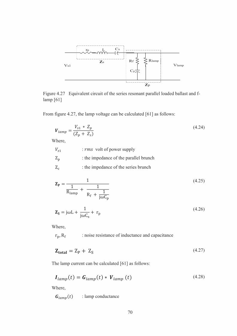
70
Figure 4.27 Equivalent circuit of the series resonant parallel loaded ballast and f-lamp [61]
From figure 4.27, the lamp voltage can be calculated [61] as follows:
(4.24)
Where,
: volt of power supply
: the impedance of the parallel brunch
: the impedance of the series brunch
(4.25)
(4.26)
Where,
: noise resistance of inductance and capacitance
(4.27)
The lamp current can be calculated [61] as follows:
(4.28)
Where,
: lamp conductance
Zp
Zs
Rlamp
Cp
Rf
Cs rp L
Vlamp Vs1
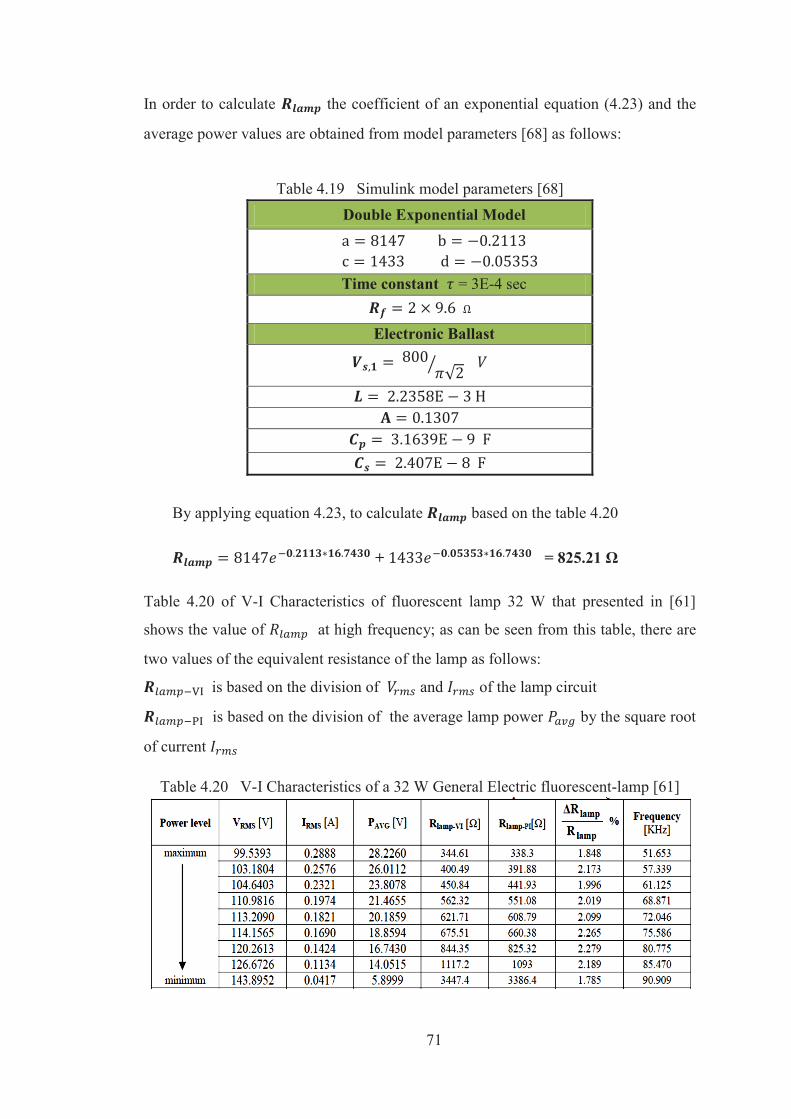
71
In order to calculate the coefficient of an exponential equation (4.23) and the
average power values are obtained from model parameters [68] as follows:
Table 4.19 Simulink model parameters [68] Double Exponential Model
Time constant = 3E-4 sec
Electronic Ballast
By applying equation 4.23, to calculate based on the table 4.20
+ = 825.21 Ω
Table 4.20 of V-I Characteristics of fluorescent lamp 32 W that presented in [61]
shows the value of at high frequency; as can be seen from this table, there are
two values of the equivalent resistance of the lamp as follows:
is based on the division of and of the lamp circuit
is based on the division of the average lamp power by the square root
of current
Table 4.20 V-I Characteristics of a 32 W General Electric fluorescent-lamp [61]
72
4.5.3 MATHEMATICAL MODEL of FLUORESCENT LAMP (FL)
Calculation of equivalent simplified circuit of the series resonant and parallel
load ballast:
In order to calculate the current and lamp voltage we have to calculate the series and
parallel impedances of the lamp circuit as follows:
Assumptions based on table 4.20, V-I Characteristics a 32 W
120 80.775 2.2473E-8 2.9372E-9 2.4E-3 507267 2 9.6
Impedance of parallel brunch can be calculated from equation 4.25
) = )
=
392.8198
Impedance of series brunch can be calculated from equation 4.26
=
=
Total current of the circuit is given by
A
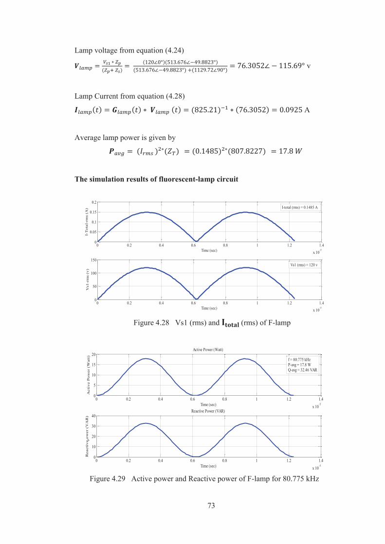
73
Lamp voltage from equation (4.24)
v
Lamp Current from equation (4.28)
A
Average lamp power is given by
The simulation results of fluorescent-lamp circuit
Figure 4.28 Vs1 (rms) and (rms) of F-lamp
Figure 4.29 Active power and Reactive power of F-lamp for 80.775 kHz
0 0.2 0.4 0.6 0.8 1 1.2 1.4
x 10-5
0
0.05
0.1
0.15
0.2
Time (sec)
I-T
otal
-rm
s (A
)
0 0.2 0.4 0.6 0.8 1 1.2 1.4
x 10-5
0
50
100
150
Time (sec)
Vs1
-rm
s (v
)
I-total (rms) = 0.1485 A
Vs1 (rms) = 120 v
0 0.2 0.4 0.6 0.8 1 1.2 1.4
x 10-5
0
5
10
15
20Active Power (Watt)
Time (sec)
Act
ive
Po
wer
(W
att)
0 0.2 0.4 0.6 0.8 1 1.2 1.4
x 10-5
0
10
20
30
40Reactive Power (VAR)
Time (sec)
Rea
ctiv
e Po
wer
(V
AR
)
f = 80.775 kHzP-avg = 17.8 WQ-avg = 32.46 VAR
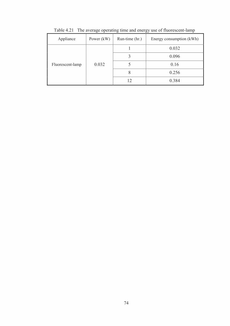
74
Table 4.21 The average operating time and energy use of fluorescent-lamp
Appliance Power (kW) Run-time (hr.) Energy consumption (kWh)
Fluorescent-lamp 0.032
1 0.032
3 0.096
5 0.16
8 0.256
12 0.384
75
CHAPTER 5 MODELING of MACHINES
5.1 INTRODUCTION
In literature , this kind of systems is known as a multi-physical system since it’s
contain mechanical elements, a hydraulic system, a thermal system and the electronic
controls [35]. The basic operating principles of the multi-physical systems is
considered in order to design models that can be implemented and simulated in
Matlab program; thus, a suitable models of the following three appliances are
presented in this chapter:
Domestic Electrical Clothes Washer (DECW)
Domestic Electrical Clothes Dryer (DECD)
Domestic Electrical Dishwasher (DEDW)
In this chapter, all above appliances designed, simulated and investigated.
Moreover, in order to gather enough data to be able to model all the machines, this
chapter discusses the modeling and parameter identification of all above three systems
and investigates the impact of its main parameters on its ability to assist with reducing
energy consumption and more efficiency. A modern dishwasher is assumed to be used
approximately 200 times/year; in this case, it uses 1.05 kWh per cycle, where 0.924
kWh is electricity for heating. A clothes washer and clothes dryer are assumed to be
used approximately 200 times/year; thus, the clothes washer uses 0.95 kWh per cycle,
where 0.76 kWh is electricity for heating; while a clothes dryer uses 2.6 kWh per
cycle [38, 38 and 39]. Therefore, for three cases most of the energy is required for hot
water and hot air rather than for electric motor use [36].

76
5.2 MODEL of DOMESTIC ELECTRIC CLOTHES WASHER (DECW)
5.2.1 INTRODUCTION
A Clothes Washer is a common appliance used for domestic and commercial
purpose. On the other hand, a clothes washer typically contains four parts; mechanical
elements that run the system, a hydraulic system that provides the water to the
laundry, a thermal system that controls the temperature level and the electronic
controls that manage the whole cycle to achieve overall system performance [35, 36].
The motor of the clothes washer has various speeds to operate, a spin speed of 1200
rpm is common and a peak spin speed as high as 1600 rpm. New models have speeds
of 1800-2000 rpm [36, 39]. In this study, DECW (Non- Electric Water Heating) is
presented; the focus of the simulation section was to study and present in details a
performance of a modified version of a single-phase motor [78] of DECW.
5.2.2 MODEL of A SINGLE-PHASE INDUCTION MOTOR of DECW
Figure 5.1 Modified version model of a single-phase induction motor of DECW [78]
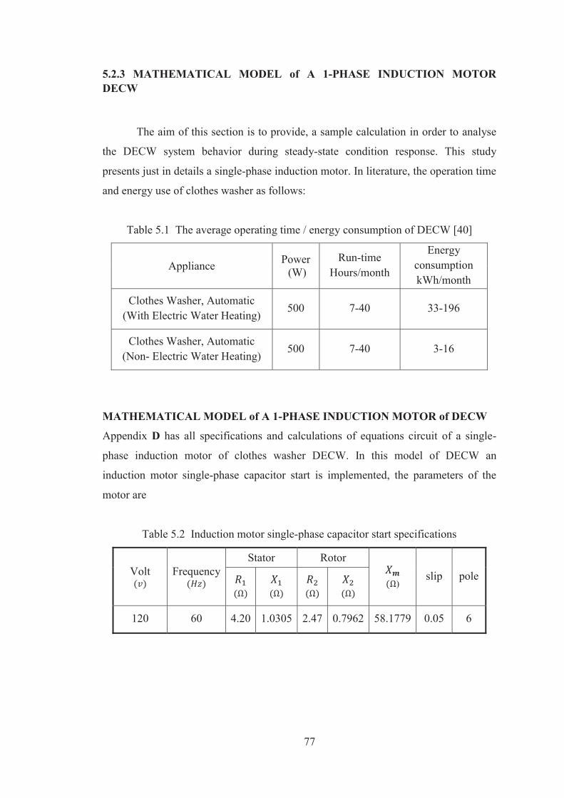
77
5.2.3 MATHEMATICAL MODEL of A 1-PHASE INDUCTION MOTOR DECW
The aim of this section is to provide, a sample calculation in order to analyse
the DECW system behavior during steady-state condition response. This study
presents just in details a single-phase induction motor. In literature, the operation time
and energy use of clothes washer as follows:
Table 5.1 The average operating time / energy consumption of DECW [40]
Appliance Power (W)
Run-time Hours/month
Energy consumption kWh/month
Clothes Washer, Automatic (With Electric Water Heating)
500 7-40 33-196
Clothes Washer, Automatic (Non- Electric Water Heating)
500 7-40 3-16
MATHEMATICAL MODEL of A 1-PHASE INDUCTION MOTOR of DECW
Appendix D has all specifications and calculations of equations circuit of a single-
phase induction motor of clothes washer DECW. In this model of DECW an
induction motor single-phase capacitor start is implemented, the parameters of the
motor are
Table 5.2 Induction motor single-phase capacitor start specifications
Volt
Frequency
Stator Rotor
) slip pole
120 60 4.20 1.0305 2.47 0.7962 58.1779 0.05 6
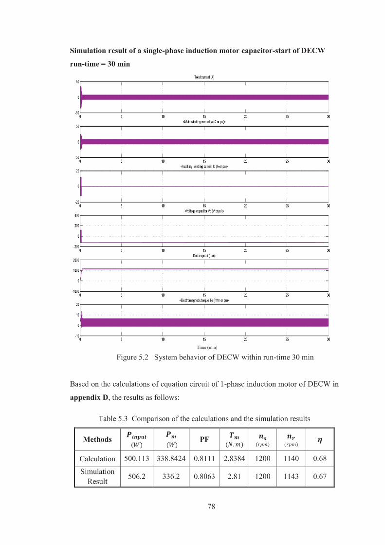
78
Simulation result of a single-phase induction motor capacitor-start of DECW
run-time = 30 min
Time (min)
Figure 5.2 System behavior of DECW within run-time 30 min
Based on the calculations of equation circuit of 1-phase induction motor of DECW in
appendix D, the results as follows:
Table 5.3 Comparison of the calculations and the simulation results
Methods
PF
Calculation 500.113 338.8424 0.8111 2.8384 1200 1140 0.68
Simulation Result 506.2 336.2 0.8063 2.81 1200 1143 0.67
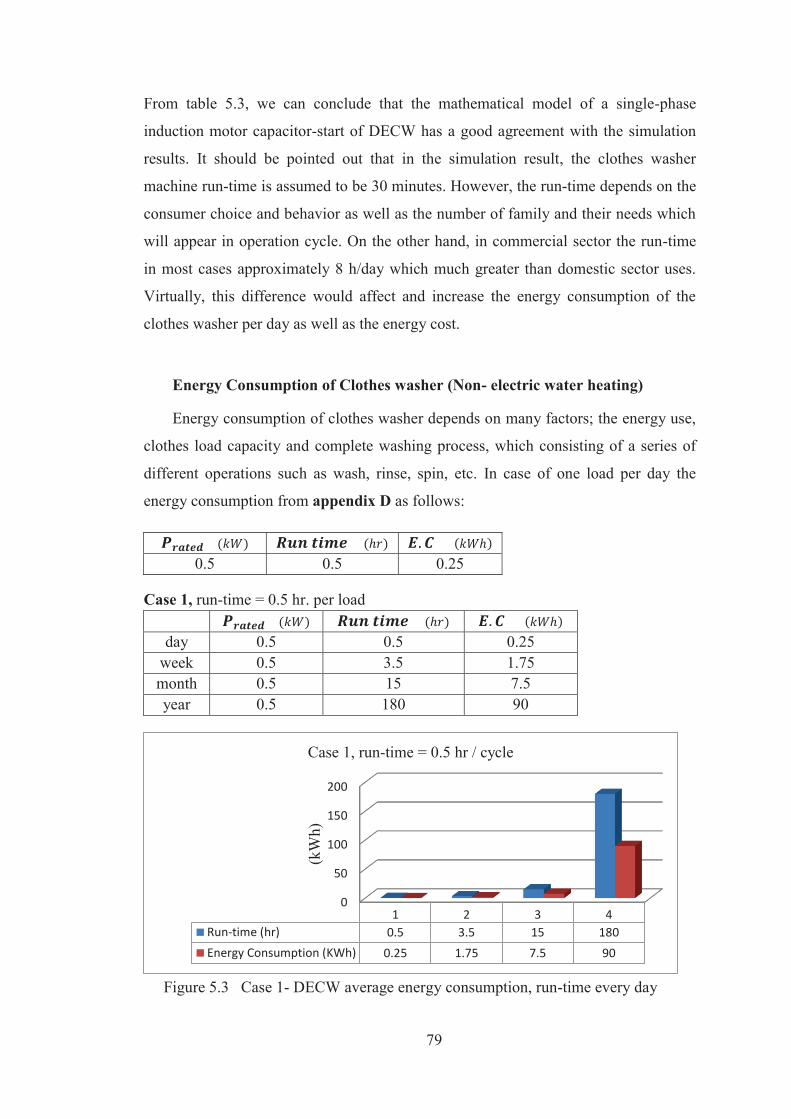
79
From table 5.3, we can conclude that the mathematical model of a single-phase
induction motor capacitor-start of DECW has a good agreement with the simulation
results. It should be pointed out that in the simulation result, the clothes washer
machine run-time is assumed to be 30 minutes. However, the run-time depends on the
consumer choice and behavior as well as the number of family and their needs which
will appear in operation cycle. On the other hand, in commercial sector the run-time
in most cases approximately 8 h/day which much greater than domestic sector uses.
Virtually, this difference would affect and increase the energy consumption of the
clothes washer per day as well as the energy cost.
Energy Consumption of Clothes washer (Non- electric water heating)
Energy consumption of clothes washer depends on many factors; the energy use,
clothes load capacity and complete washing process, which consisting of a series of
different operations such as wash, rinse, spin, etc. In case of one load per day the
energy consumption from appendix D as follows:
0.5 0.5 0.25
Case 1, run-time = 0.5 hr. per load
day 0.5 0.5 0.25
week 0.5 3.5 1.75 month 0.5 15 7.5 year 0.5 180 90
Figure 5.3 Case 1- DECW average energy consumption, run-time every day
0
50
100
150
200
1 2 3 4Run-time (hr) 0.5 3.5 15 180Energy Consumption (KWh) 0.25 1.75 7.5 90
(kW
h)
Case 1, run-time = 0.5 hr / cycle
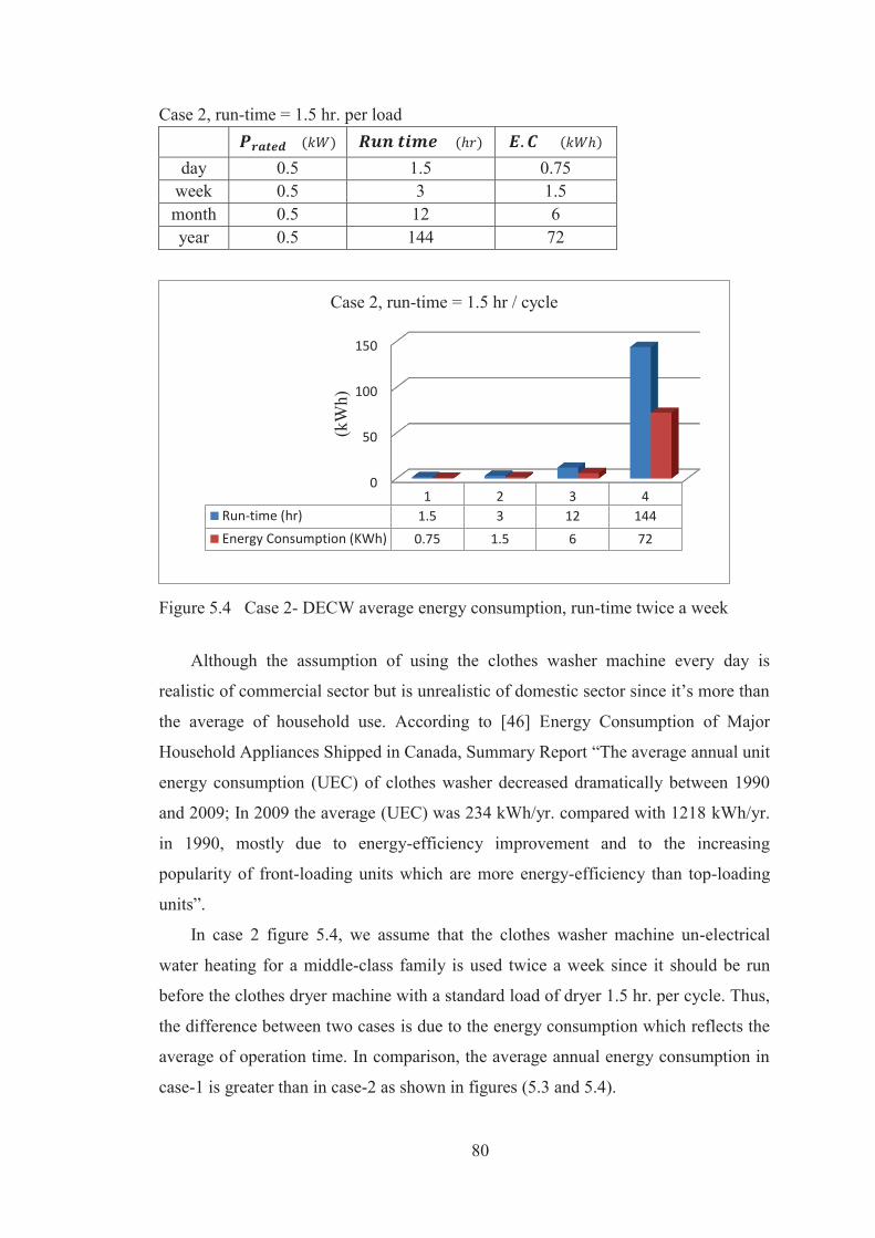
80
Case 2, run-time = 1.5 hr. per load
day 0.5 1.5 0.75 week 0.5 3 1.5 month 0.5 12 6 year 0.5 144 72
Figure 5.4 Case 2- DECW average energy consumption, run-time twice a week
Although the assumption of using the clothes washer machine every day is
realistic of commercial sector but is unrealistic of domestic sector since it’s more than
the average of household use. According to [46] Energy Consumption of Major
Household Appliances Shipped in Canada, Summary Report “The average annual unit
energy consumption (UEC) of clothes washer decreased dramatically between 1990
and 2009; In 2009 the average (UEC) was 234 kWh/yr. compared with 1218 kWh/yr.
in 1990, mostly due to energy-efficiency improvement and to the increasing
popularity of front-loading units which are more energy-efficiency than top-loading
units”.
In case 2 figure 5.4, we assume that the clothes washer machine un-electrical
water heating for a middle-class family is used twice a week since it should be run
before the clothes dryer machine with a standard load of dryer 1.5 hr. per cycle. Thus,
the difference between two cases is due to the energy consumption which reflects the
average of operation time. In comparison, the average annual energy consumption in
case-1 is greater than in case-2 as shown in figures (5.3 and 5.4).
0
50
100
150
1 2 3 4Run-time (hr) 1.5 3 12 144Energy Consumption (KWh) 0.75 1.5 6 72
(kW
h)
Case 2, run-time = 1.5 hr / cycle
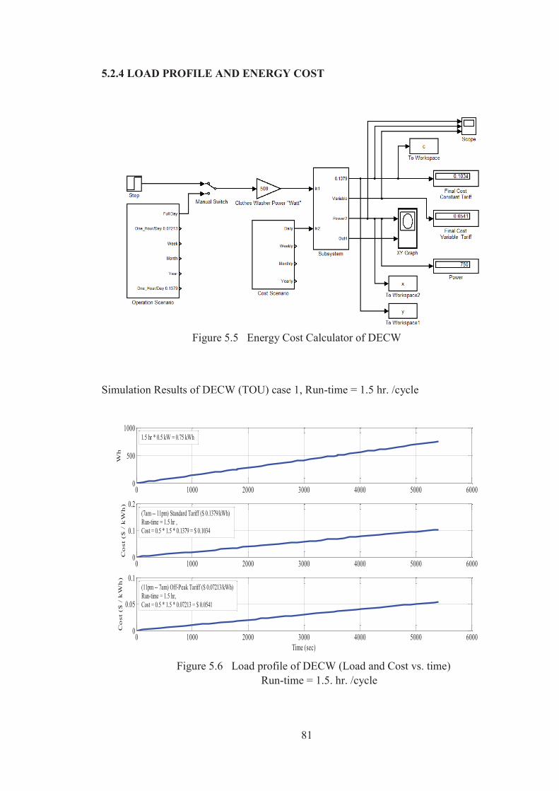
81
5.2.4 LOAD PROFILE AND ENERGY COST
Figure 5.5 Energy Cost Calculator of DECW
Simulation Results of DECW (TOU) case 1, Run-time = 1.5 hr. /cycle
Figure 5.6 Load profile of DECW (Load and Cost vs. time)
Run-time = 1.5. hr. /cycle
0 1000 2000 3000 4000 5000 60000
500
1000
Wh
0 1000 2000 3000 4000 5000 60000
0.1
0.2
Co
st (
$ /
kW
h)
0 1000 2000 3000 4000 5000 60000
0.05
0.1
Time (sec)
Co
st (
$ /
kW
h)
(7am -- 11pm) Standard Tariff ($ 0.1379/kWh)Run-time = 1.5 hr , Cost = 0.5 * 1.5 * 0.1379 = $ 0.1034
(11pm -- 7am) Off-Peak Tariff ($ 0.07213/kWh)Run-time = 1.5 hr, Cost = 0.5 * 1.5 * 0.07213 = $ 0.0541
1.5 hr * 0.5 kW = 0.75 kWh
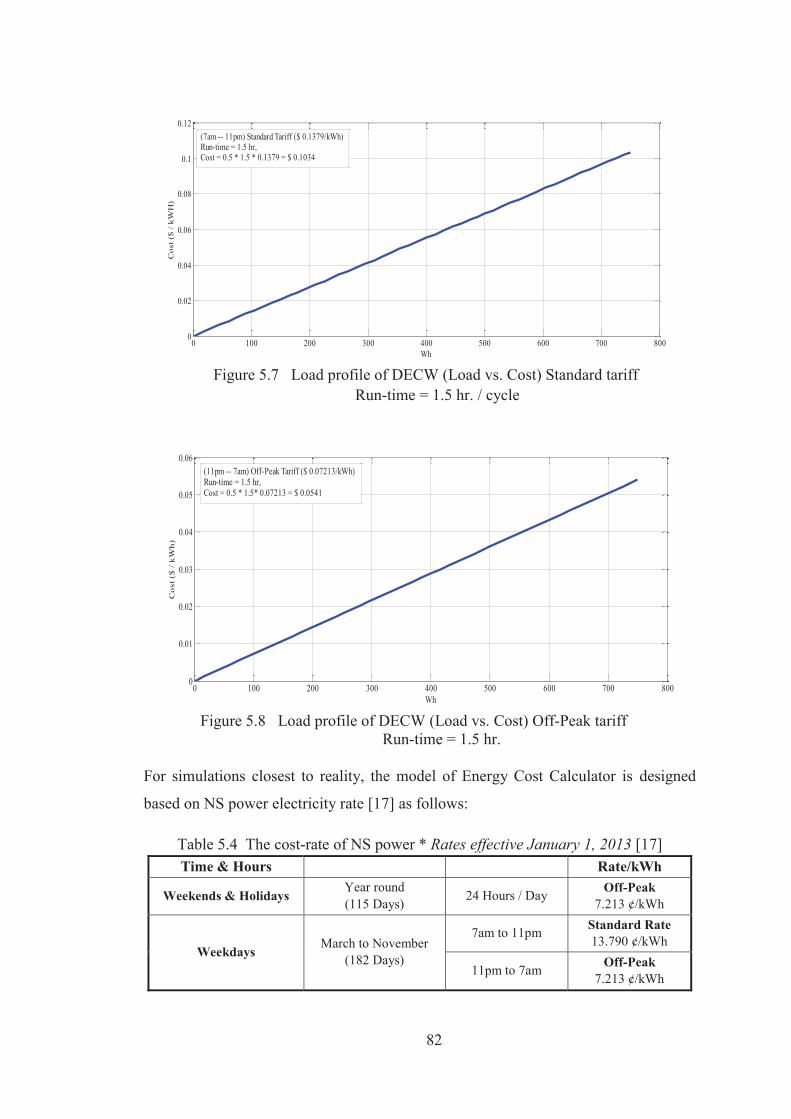
82
Figure 5.7 Load profile of DECW (Load vs. Cost) Standard tariff
Run-time = 1.5 hr. / cycle
Figure 5.8 Load profile of DECW (Load vs. Cost) Off-Peak tariff
Run-time = 1.5 hr.
For simulations closest to reality, the model of Energy Cost Calculator is designed
based on NS power electricity rate [17] as follows:
Table 5.4 The cost-rate of NS power * Rates effective January 1, 2013 [17] Time & Hours Rate/kWh
Weekends & Holidays Year round (115 Days) 24 Hours / Day Off-Peak
7.213 ¢/kWh
Weekdays March to November
(182 Days)
7am to 11pm Standard Rate 13.790 ¢/kWh
11pm to 7am Off-Peak 7.213 ¢/kWh
0 100 200 300 400 500 600 700 8000
0.02
0.04
0.06
0.08
0.1
0.12
Wh
Cos
t ($
/ kW
H)
(7am -- 11pm) Standard Tariff ($ 0.1379/kWh)Run-time = 1.5 hr, Cost = 0.5 * 1.5 * 0.1379 = $ 0.1034
0 100 200 300 400 500 600 700 8000
0.01
0.02
0.03
0.04
0.05
0.06
Wh
Co
st (
$ /
kW
h)
(11pm -- 7am) Off-Peak Tariff ($ 0.07213/kWh)Run-time = 1.5 hr, Cost = 0.5 * 1.5* 0.07213 = $ 0.0541
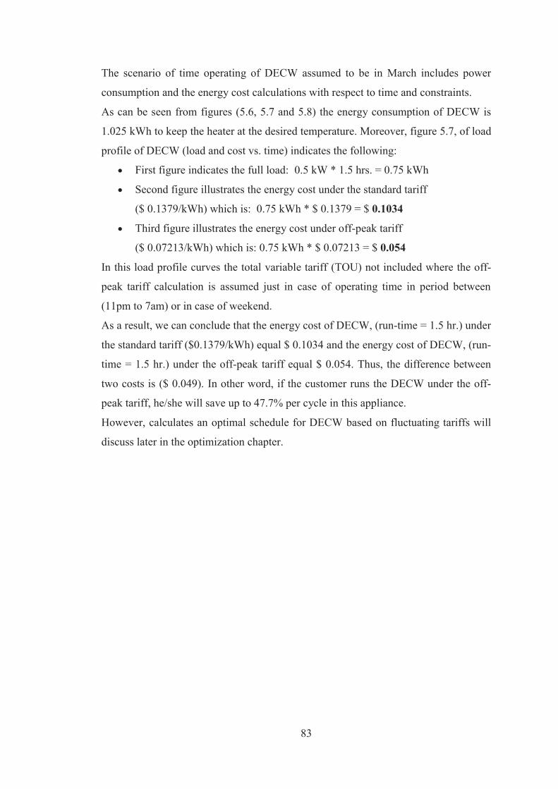
83
The scenario of time operating of DECW assumed to be in March includes power
consumption and the energy cost calculations with respect to time and constraints.
As can be seen from figures (5.6, 5.7 and 5.8) the energy consumption of DECW is
1.025 kWh to keep the heater at the desired temperature. Moreover, figure 5.7, of load
profile of DECW (load and cost vs. time) indicates the following:
First figure indicates the full load: 0.5 kW * 1.5 hrs. = 0.75 kWh
Second figure illustrates the energy cost under the standard tariff
($ 0.1379/kWh) which is: 0.75 kWh * $ 0.1379 = $ 0.1034
Third figure illustrates the energy cost under off-peak tariff
($ 0.07213/kWh) which is: 0.75 kWh * $ 0.07213 = $ 0.054
In this load profile curves the total variable tariff (TOU) not included where the off-
peak tariff calculation is assumed just in case of operating time in period between
(11pm to 7am) or in case of weekend.
As a result, we can conclude that the energy cost of DECW, (run-time = 1.5 hr.) under
the standard tariff ($0.1379/kWh) equal $ 0.1034 and the energy cost of DECW, (run-
time = 1.5 hr.) under the off-peak tariff equal $ 0.054. Thus, the difference between
two costs is ($ 0.049). In other word, if the customer runs the DECW under the off-
peak tariff, he/she will save up to 47.7% per cycle in this appliance.
However, calculates an optimal schedule for DECW based on fluctuating tariffs will
discuss later in the optimization chapter.

84
5.3 MODEL of DOMESTIC ELECTRIC CLOTHES DRYER (DECD)
5.3.1 INTRODUCTION
A clothes dryer, also known as a tumble dryer or drying machine, is a common
appliance for domestic and commercial use. In particular, a clothes dryer is perfectly
co-ordinated with the clothes washer machine, whose task is to remove moisture from
a load of clothes after being cleaned in a clothes washer. A typical clothes dryer
consists of four main parts, including a rotating tumbler, an electric-powered heater,
an induction motor and a set of controls [41, 42].
Rotating tumbler which holds clothes and circulates heated air. Induction motor is used for rotating the tumbler. Electric-heated coils as a heat source to heat up the air. A set of controls. There are several types of clothes dryers available in the market these days for
both domestic and commercial use with special design features that can be modified
according to the user needs and choice such as drying time, temperature setting,
moisture control and load capacity. The main two common types of clothes dryers are
the venting tumble dryer and the condensing tumble dryer. One of the most widely
used in the residential sector is the condensing tumble dryer; the advantage of this
type is that all heat supplied to the dryer eventually ends up in the laundry room [43,
44].However, in this study the domestic electric clothes dryer (DECD) that consists of
an induction motor and a heater is presented.
5.3.2 MODEL of DECD
Figure 5.9 Model of Domestic Electric Clothes dryer (heater)
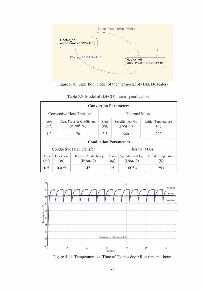
85
Figure 5.10 State flow model of the thermostat of (DECD-Heater)
Table 5.5 Model of (DECD) heater specifications
Convection Parameters
Convective Heat Transfer Thermal Mass
Area
Heat Transfer Coefficient
Mass
Specific heat Cp
Initial Temperature
1.2 70 3.5 640 293
Conduction Parameters
Conductive Heat Transfer Thermal Mass
Area
Thickness
Thermal Conductivity
Mass
Specific heat Cp
Initial Temperature
0.5 0.025 45 15 1005.4 293
Figure 5.11 Temperature vs. Time of Clothes dryer Run-time = 1 hour
0 10 20 30 40 50 6020
25
30
35
40
45
50
55
60
65
time (min)
Tem
per
atu
re (
C)
Set-point
Upper Limit
Run-time = 1 hr, T (setpoint) = 56 C
Lower Limit
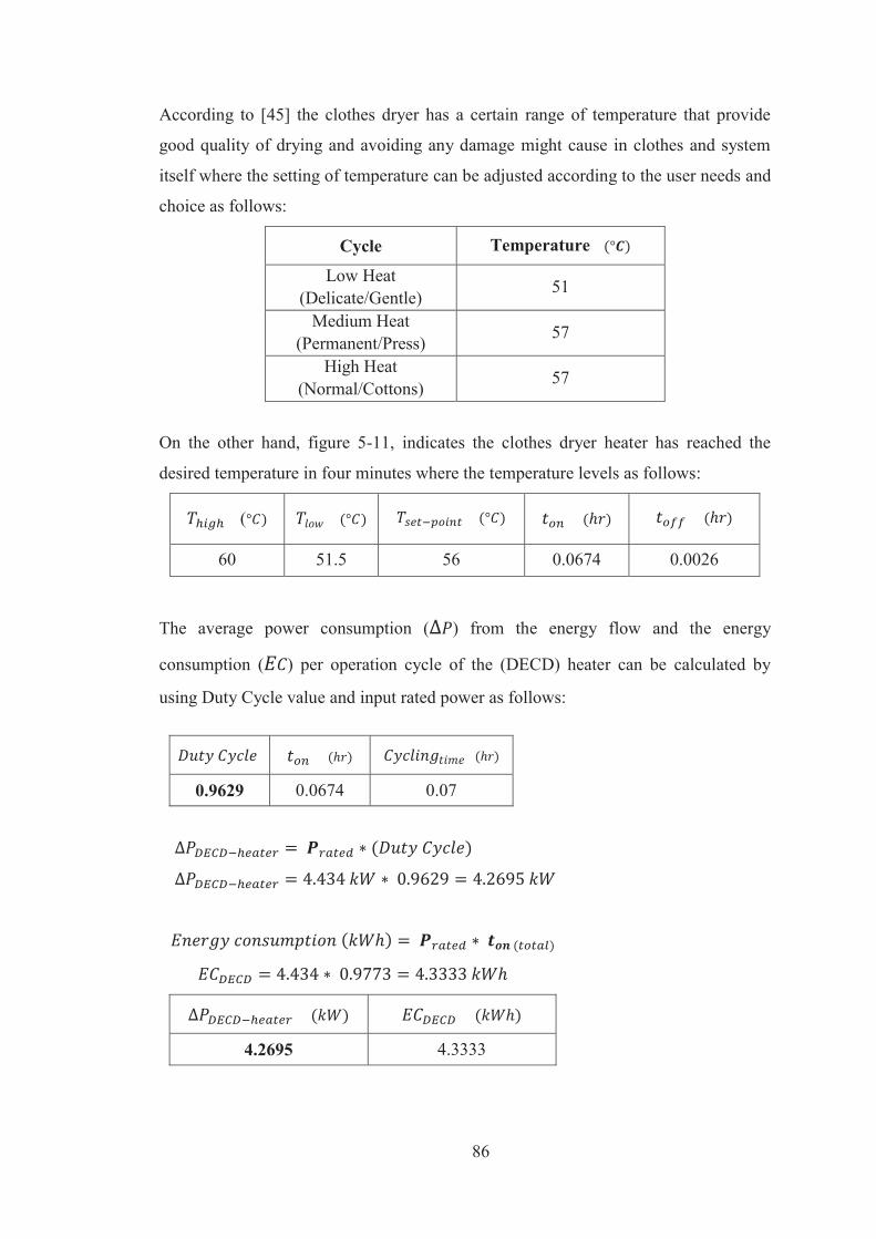
86
According to [45] the clothes dryer has a certain range of temperature that provide
good quality of drying and avoiding any damage might cause in clothes and system
itself where the setting of temperature can be adjusted according to the user needs and
choice as follows:
Cycle Temperature
Low Heat (Delicate/Gentle) 51
Medium Heat (Permanent/Press) 57
High Heat (Normal/Cottons) 57
On the other hand, figure 5-11, indicates the clothes dryer heater has reached the
desired temperature in four minutes where the temperature levels as follows:
(
60 51.5 56 0.0674 0.0026
The average power consumption ( ) from the energy flow and the energy
consumption ( ) per operation cycle of the (DECD) heater can be calculated by
using Duty Cycle value and input rated power as follows:
0.9629 0.0674 0.07
4.2695 4.3333
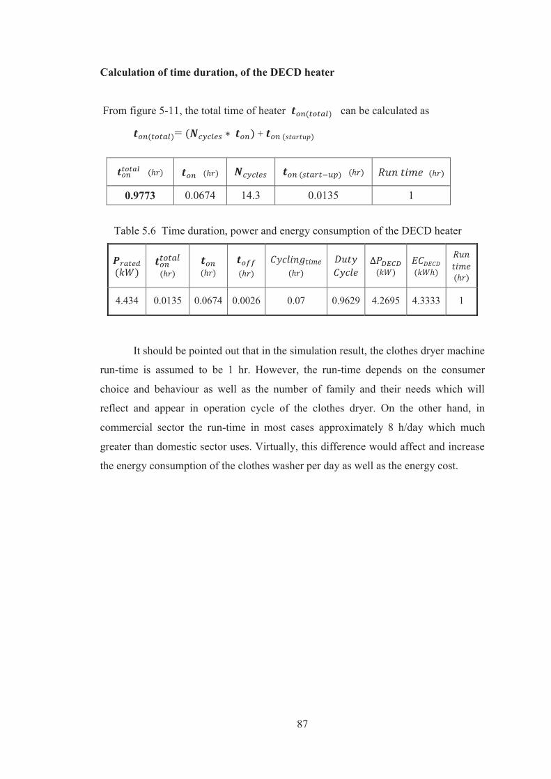
87
Calculation of time duration, of the DECD heater
From figure 5-11, the total time of heater can be calculated as
= +
0.9773 0.0674 14.3 0.0135 1
Table 5.6 Time duration, power and energy consumption of the DECD heater
4.434 0.0135 0.0674 0.0026 0.07 0.9629 4.2695 4.3333 1
It should be pointed out that in the simulation result, the clothes dryer machine
run-time is assumed to be 1 hr. However, the run-time depends on the consumer
choice and behaviour as well as the number of family and their needs which will
reflect and appear in operation cycle of the clothes dryer. On the other hand, in
commercial sector the run-time in most cases approximately 8 h/day which much
greater than domestic sector uses. Virtually, this difference would affect and increase
the energy consumption of the clothes washer per day as well as the energy cost.
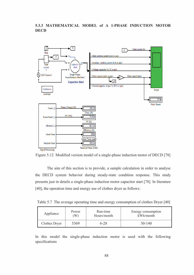
88
5.3.3 MATHEMATICAL MODEL of A 1-PHASE INDUCTION MOTOR DECD
Figure 5.12 Modified version model of a single-phase induction motor of DECD [78]
The aim of this section is to provide, a sample calculation in order to analyse
the DECD system behavior during steady-state condition response. This study
presents just in details a single-phase induction motor capacitor start [78]. In literature
[40], the operation time and energy use of clothes dryer as follows:
Table 5.7 The average operating time and energy consumption of clothes Dryer [40]
Appliance Power (W)
Run-time Hours/month
Energy consumption kWh/month
Clothes Dryer 5369 6-28 30-140
In this model the single-phase induction motor is used with the following specifications
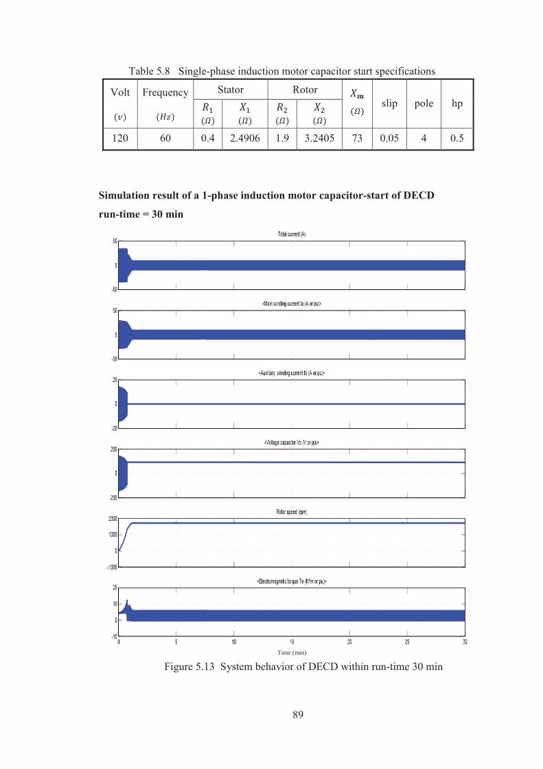
89
Table 5.8 Single-phase induction motor capacitor start specifications
Volt
Frequency
Stator Rotor
slip pole hp
120 60 0.4 2.4906 1.9 3.2405 73 0.05 4 0.5
Simulation result of a 1-phase induction motor capacitor-start of DECD
run-time = 30 min
Time (min)
Figure 5.13 System behavior of DECD within run-time 30 min
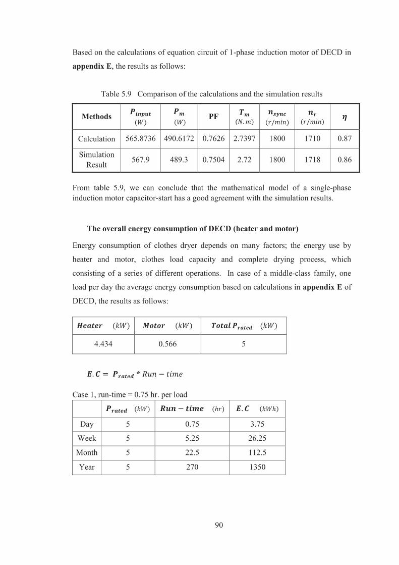
90
Based on the calculations of equation circuit of 1-phase induction motor of DECD in
appendix E, the results as follows:
Table 5.9 Comparison of the calculations and the simulation results
Methods
PF
Calculation 565.8736 490.6172 0.7626 2.7397 1800 1710 0.87
Simulation Result 567.9 489.3 0.7504 2.72 1800 1718 0.86
From table 5.9, we can conclude that the mathematical model of a single-phase induction motor capacitor-start has a good agreement with the simulation results.
The overall energy consumption of DECD (heater and motor)
Energy consumption of clothes dryer depends on many factors; the energy use by
heater and motor, clothes load capacity and complete drying process, which
consisting of a series of different operations. In case of a middle-class family, one
load per day the average energy consumption based on calculations in appendix E of
DECD, the results as follows:
4.434 0.566 5
*
Case 1, run-time = 0.75 hr. per load
Day 5 0.75 3.75
Week 5 5.25 26.25
Month 5 22.5 112.5
Year 5 270 1350
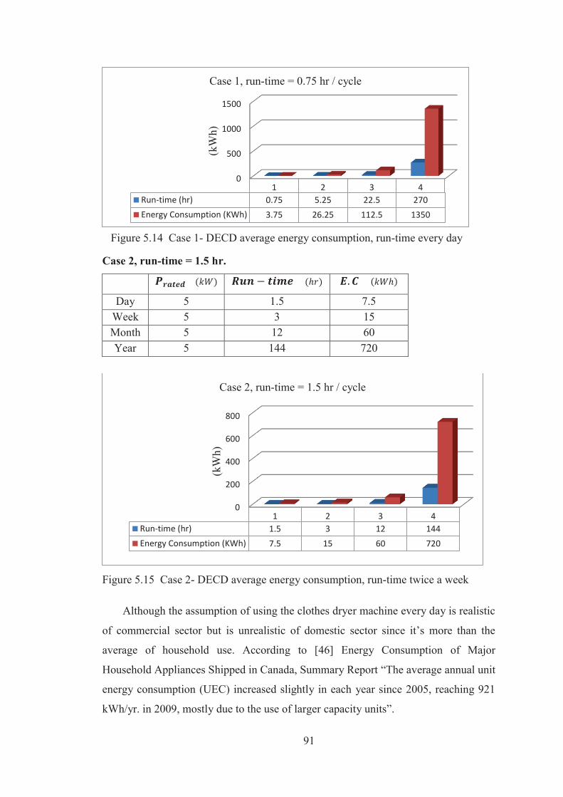
91
Figure 5.14 Case 1- DECD average energy consumption, run-time every day
Case 2, run-time = 1.5 hr.
Day 5 1.5 7.5 Week 5 3 15 Month 5 12 60 Year 5 144 720
Figure 5.15 Case 2- DECD average energy consumption, run-time twice a week
Although the assumption of using the clothes dryer machine every day is realistic
of commercial sector but is unrealistic of domestic sector since it’s more than the
average of household use. According to [46] Energy Consumption of Major
Household Appliances Shipped in Canada, Summary Report “The average annual unit
energy consumption (UEC) increased slightly in each year since 2005, reaching 921
kWh/yr. in 2009, mostly due to the use of larger capacity units”.
0
500
1000
1500
1 2 3 4Run-time (hr) 0.75 5.25 22.5 270Energy Consumption (KWh) 3.75 26.25 112.5 1350
(kW
h)
Case 1, run-time = 0.75 hr / cycle
0
200
400
600
800
1 2 3 4Run-time (hr) 1.5 3 12 144Energy Consumption (KWh) 7.5 15 60 720
(kW
h)
Case 2, run-time = 1.5 hr / cycle
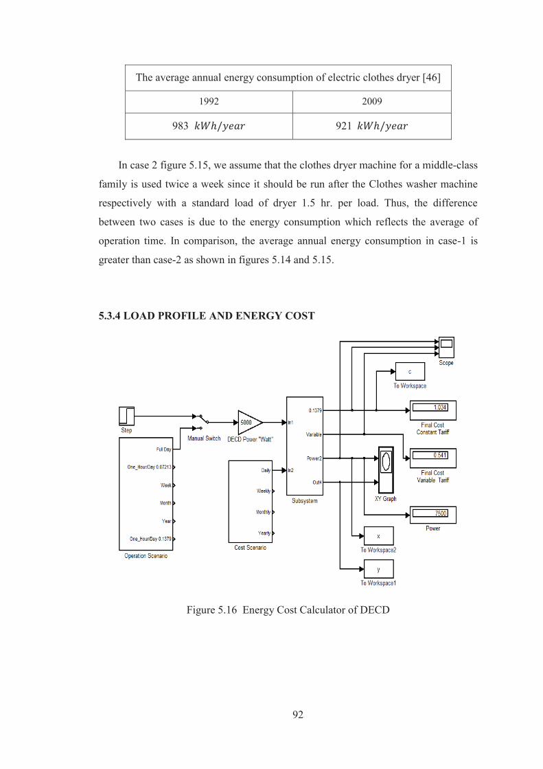
92
The average annual energy consumption of electric clothes dryer [46]
1992 2009
983 921
In case 2 figure 5.15, we assume that the clothes dryer machine for a middle-class
family is used twice a week since it should be run after the Clothes washer machine
respectively with a standard load of dryer 1.5 hr. per load. Thus, the difference
between two cases is due to the energy consumption which reflects the average of
operation time. In comparison, the average annual energy consumption in case-1 is
greater than case-2 as shown in figures 5.14 and 5.15.
5.3.4 LOAD PROFILE AND ENERGY COST
Figure 5.16 Energy Cost Calculator of DECD
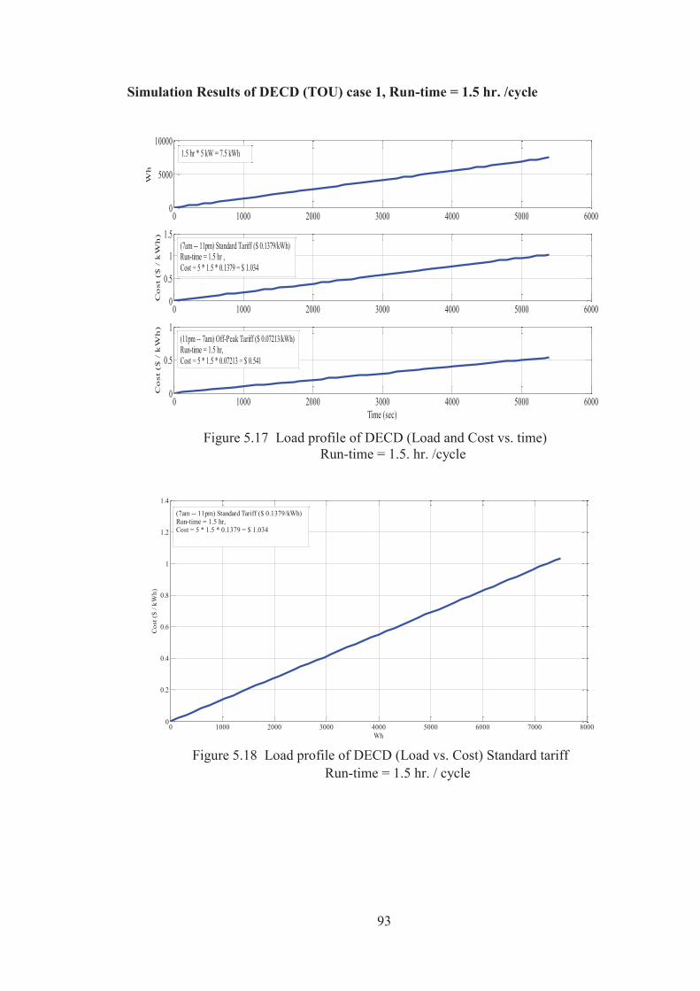
93
Simulation Results of DECD (TOU) case 1, Run-time = 1.5 hr. /cycle
Figure 5.17 Load profile of DECD (Load and Cost vs. time)
Run-time = 1.5. hr. /cycle
Figure 5.18 Load profile of DECD (Load vs. Cost) Standard tariff
Run-time = 1.5 hr. / cycle
0 1000 2000 3000 4000 5000 60000
5000
10000W
h
0 1000 2000 3000 4000 5000 60000
0.5
1
1.5
Co
st
($ /
kW
h)
0 1000 2000 3000 4000 5000 60000
0.5
1
Time (sec)
Co
st
($ /
kW
h)
1.5 hr * 5 kW = 7.5 kWh
(7am -- 11pm) Standard Tariff ($ 0.1379/kWh)Run-time = 1.5 hr , Cost = 5 * 1.5 * 0.1379 = $ 1.034
(11pm -- 7am) Off-Peak Tariff ($ 0.07213/kWh)Run-time = 1.5 hr, Cost = 5 * 1.5 * 0.07213 = $ 0.541
0 1000 2000 3000 4000 5000 6000 7000 80000
0.2
0.4
0.6
0.8
1
1.2
1.4
Wh
Cos
t ($
/ kW
h)
(7am -- 11pm) Standard Tariff ($ 0.1379/kWh)Run-time = 1.5 hr, Cost = 5 * 1.5 * 0.1379 = $ 1.034
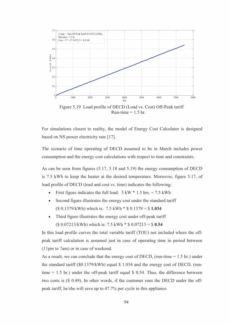
94
Figure 5.19 Load profile of DECD (Load vs. Cost) Off-Peak tariff
Run-time = 1.5 hr.
For simulations closest to reality, the model of Energy Cost Calculator is designed
based on NS power electricity rate [17].
The scenario of time operating of DECD assumed to be in March includes power
consumption and the energy cost calculations with respect to time and constraints.
As can be seen from figures (5.17, 5.18 and 5.19) the energy consumption of DECD
is 7.5 kWh to keep the heater at the desired temperature. Moreover, figure 5.17, of
load profile of DECD (load and cost vs. time) indicates the following:
First figure indicates the full load: 5 kW * 1.5 hrs. = 7.5 kWh
Second figure illustrates the energy cost under the standard tariff
($ 0.1379/kWh) which is: 7.5 kWh * $ 0.1379 = $ 1.034
Third figure illustrates the energy cost under off-peak tariff
($ 0.07213/kWh) which is: 7.5 kWh * $ 0.07213 = $ 0.54
In this load profile curves the total variable tariff (TOU) not included where the off-
peak tariff calculation is assumed just in case of operating time in period between
(11pm to 7am) or in case of weekend.
As a result, we can conclude that the energy cost of DECD, (run-time = 1.5 hr.) under
the standard tariff ($0.1379/kWh) equal $ 1.034 and the energy cost of DECD, (run-
time = 1.5 hr.) under the off-peak tariff equal $ 0.54. Thus, the difference between
two costs is ($ 0.49). In other words, if the customer runs the DECD under the off-
peak tariff, he/she will save up to 47.7% per cycle in this appliance.
0 1000 2000 3000 4000 5000 6000 7000 80000
0.1
0.2
0.3
0.4
0.5
0.6
0.7
Wh
Co
st (
$ /
kW
h)
(11pm -- 7am) Off-Peak Tariff ($ 0.07213/kWh)Run-time = 1.5 hr, Cost = 5 * 1.5* 0.07213 = $ 0.541

95
However, calculates an optimal schedule for DECD based on fluctuating tariffs will
discuss later in the optimization chapter.
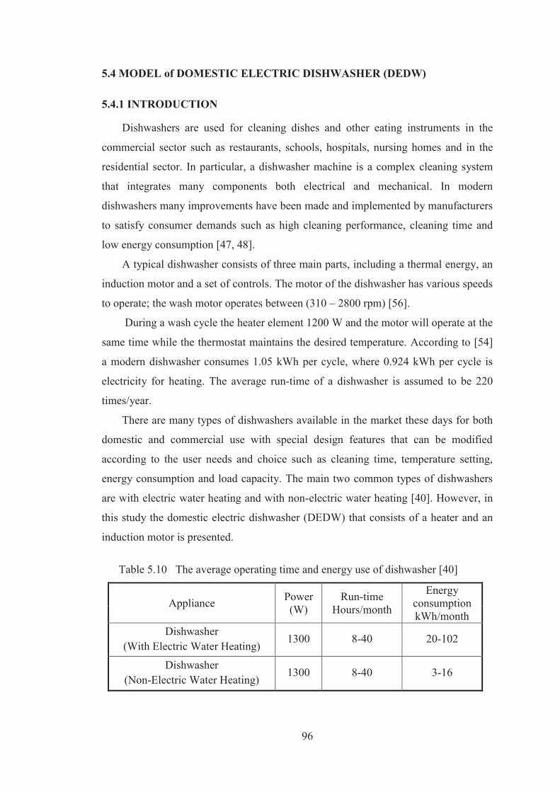
96
5.4 MODEL of DOMESTIC ELECTRIC DISHWASHER (DEDW)
5.4.1 INTRODUCTION
Dishwashers are used for cleaning dishes and other eating instruments in the
commercial sector such as restaurants, schools, hospitals, nursing homes and in the
residential sector. In particular, a dishwasher machine is a complex cleaning system
that integrates many components both electrical and mechanical. In modern
dishwashers many improvements have been made and implemented by manufacturers
to satisfy consumer demands such as high cleaning performance, cleaning time and
low energy consumption [47, 48].
A typical dishwasher consists of three main parts, including a thermal energy, an
induction motor and a set of controls. The motor of the dishwasher has various speeds
to operate; the wash motor operates between (310 – 2800 rpm) [56].
During a wash cycle the heater element 1200 W and the motor will operate at the
same time while the thermostat maintains the desired temperature. According to [54]
a modern dishwasher consumes 1.05 kWh per cycle, where 0.924 kWh per cycle is
electricity for heating. The average run-time of a dishwasher is assumed to be 220
times/year.
There are many types of dishwashers available in the market these days for both
domestic and commercial use with special design features that can be modified
according to the user needs and choice such as cleaning time, temperature setting,
energy consumption and load capacity. The main two common types of dishwashers
are with electric water heating and with non-electric water heating [40]. However, in
this study the domestic electric dishwasher (DEDW) that consists of a heater and an
induction motor is presented.
Table 5.10 The average operating time and energy use of dishwasher [40]
Appliance Power (W)
Run-time Hours/month
Energy consumption kWh/month
Dishwasher (With Electric Water Heating)
1300 8-40 20-102
Dishwasher (Non-Electric Water Heating)
1300 8-40 3-16
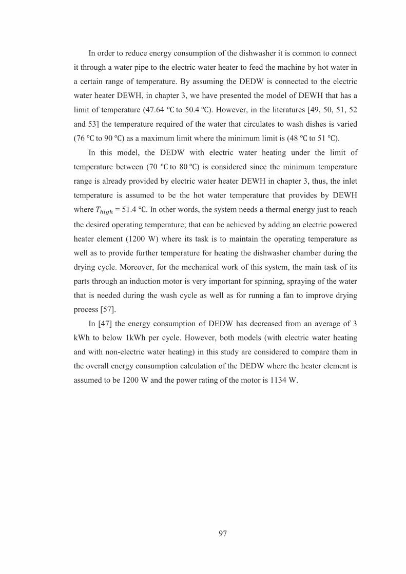
97
In order to reduce energy consumption of the dishwasher it is common to connect
it through a water pipe to the electric water heater to feed the machine by hot water in
a certain range of temperature. By assuming the DEDW is connected to the electric
water heater DEWH, in chapter 3, we have presented the model of DEWH that has a
limit of temperature (47.64 to 50.4 ). However, in the literatures [49, 50, 51, 52
and 53] the temperature required of the water that circulates to wash dishes is varied
(76 to 90 ) as a maximum limit where the minimum limit is (48 to 51 ).
In this model, the DEDW with electric water heating under the limit of
temperature between (70 to 80 ) is considered since the minimum temperature
range is already provided by electric water heater DEWH in chapter 3, thus, the inlet
temperature is assumed to be the hot water temperature that provides by DEWH
where = 51.4 . In other words, the system needs a thermal energy just to reach
the desired operating temperature; that can be achieved by adding an electric powered
heater element (1200 W) where its task is to maintain the operating temperature as
well as to provide further temperature for heating the dishwasher chamber during the
drying cycle. Moreover, for the mechanical work of this system, the main task of its
parts through an induction motor is very important for spinning, spraying of the water
that is needed during the wash cycle as well as for running a fan to improve drying
process [57].
In [47] the energy consumption of DEDW has decreased from an average of 3
kWh to below 1kWh per cycle. However, both models (with electric water heating
and with non-electric water heating) in this study are considered to compare them in
the overall energy consumption calculation of the DEDW where the heater element is
assumed to be 1200 W and the power rating of the motor is 1134 W.
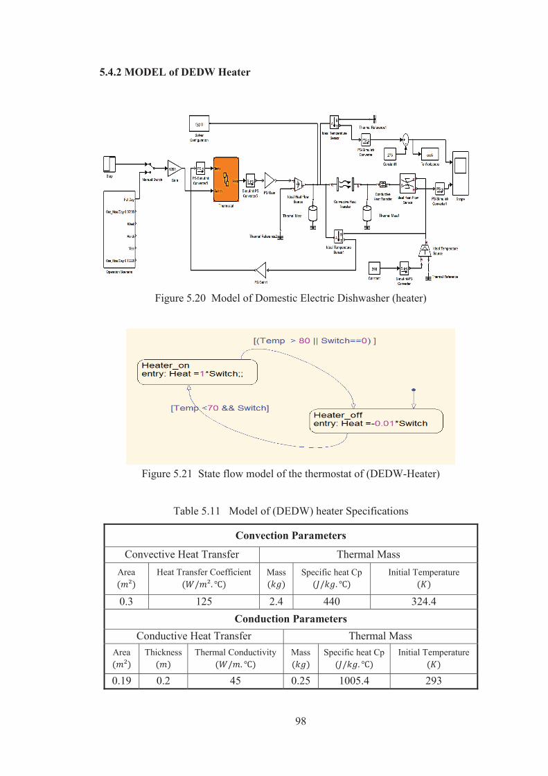
98
5.4.2 MODEL of DEDW Heater
Figure 5.20 Model of Domestic Electric Dishwasher (heater)
Figure 5.21 State flow model of the thermostat of (DEDW-Heater)
Table 5.11 Model of (DEDW) heater Specifications
Convection Parameters
Convective Heat Transfer Thermal Mass Area
Heat Transfer Coefficient
Mass
Specific heat Cp
Initial Temperature
0.3 125 2.4 440 324.4 Conduction Parameters
Conductive Heat Transfer Thermal Mass Area
Thickness
Thermal Conductivity
Mass
Specific heat Cp
Initial Temperature
0.19 0.2 45 0.25 1005.4 293
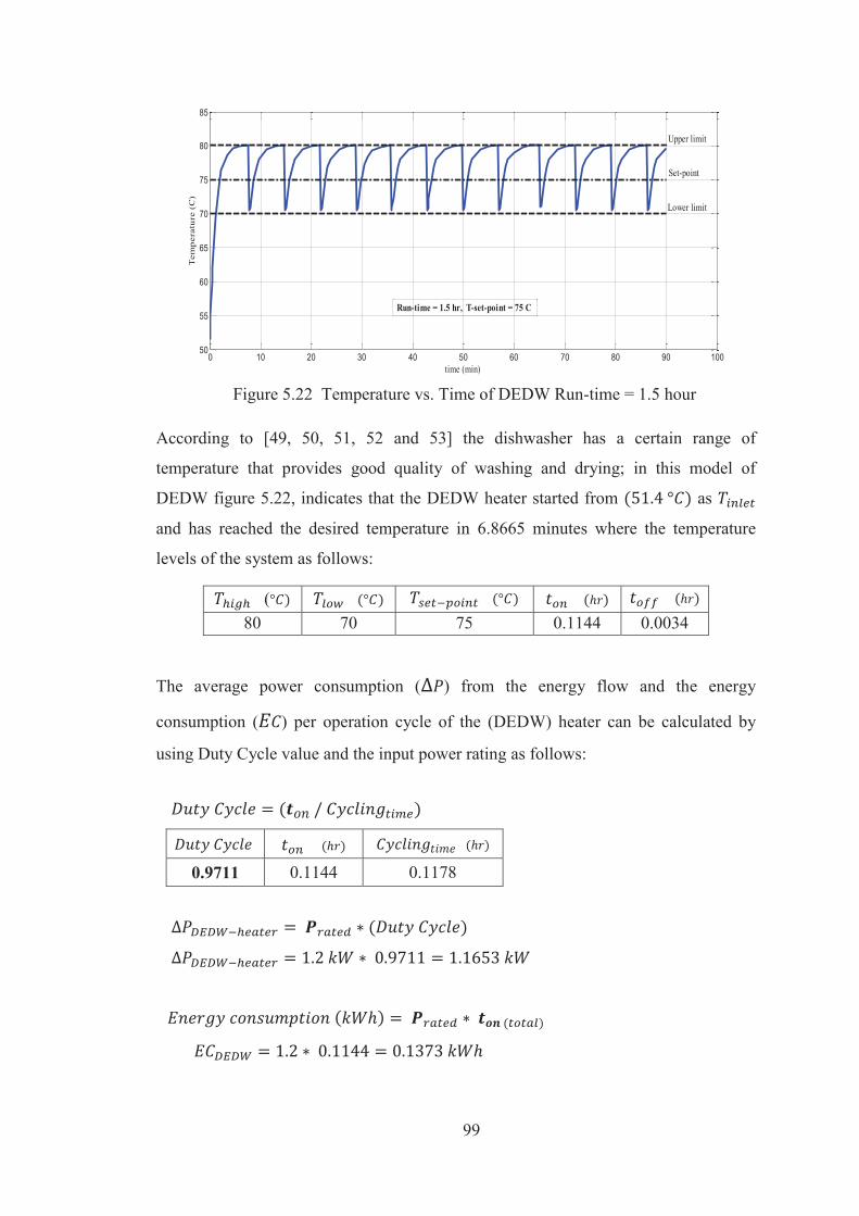
99
Figure 5.22 Temperature vs. Time of DEDW Run-time = 1.5 hour
According to [49, 50, 51, 52 and 53] the dishwasher has a certain range of
temperature that provides good quality of washing and drying; in this model of
DEDW figure 5.22, indicates that the DEDW heater started from as
and has reached the desired temperature in 6.8665 minutes where the temperature
levels of the system as follows:
( 80 70 75 0.1144 0.0034
The average power consumption ( ) from the energy flow and the energy
consumption ( ) per operation cycle of the (DEDW) heater can be calculated by
using Duty Cycle value and the input power rating as follows:
0.9711 0.1144 0.1178
0 10 20 30 40 50 60 70 80 90 10050
55
60
65
70
75
80
85
time (min)
Tem
pera
ture
(C
)
Run-time = 1.5 hr, T-set-point = 75 C
Upper limit
Set-point
Lower limit

100
Calculation of time duration, of the DEDW heater
From figure 5.22, the total time of heater can be calculated as
= +
1.4267 0.1144 12.3 0.0196 1.5
Table 5.12 Time duration, power and energy consumption of the DEDW heater
1.2 1.4267 0.1144 0.0034 0.1178 0.9711 1.1653 0.1373 1.5
It should be pointed out that in the simulation result, the dishwasher machine
run-time is assumed to be 1.5 hr. However, the run-time depends on the consumer
choice and behaviour as well as the number of family and their needs which will
reflect the run-time and appear in operation cycle of the dishwasher. On the other
hand, in commercial sector the run-time in most cases approximately (5 to 6 hr/day)
which much greater than domestic sector uses. Virtually, this difference would affect
and increase the energy consumption of the dishwasher per day as well as the energy
cost.
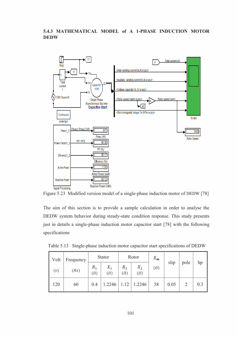
101
5.4.3 MATHEMATICAL MODEL of A 1-PHASE INDUCTION MOTOR DEDW
Figure 5.23 Modified version model of a single-phase induction motor of DEDW [78]
The aim of this section is to provide a sample calculation in order to analyse the
DEDW system behavior during steady-state condition response. This study presents
just in details a single-phase induction motor capacitor start [78] with the following
specifications
Table 5.13 Single-phase induction motor capacitor start specifications of DEDW
Volt
Frequency
Stator Rotor
slip pole hp
120 60 0.4 1.2246 1.12 1.2246 58 0.05 2 0.3
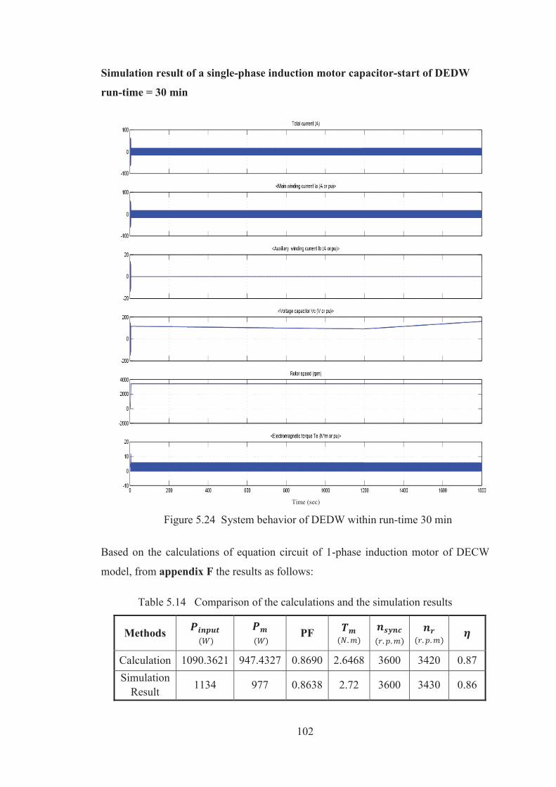
102
Simulation result of a single-phase induction motor capacitor-start of DEDW
run-time = 30 min
Time (sec)
Figure 5.24 System behavior of DEDW within run-time 30 min
Based on the calculations of equation circuit of 1-phase induction motor of DECW
model, from appendix F the results as follows:
Table 5.14 Comparison of the calculations and the simulation results
Methods
PF
Calculation 1090.3621 947.4327 0.8690 2.6468 3600 3420 0.87 Simulation
Result 1134 977 0.8638 2.72 3600 3430 0.86
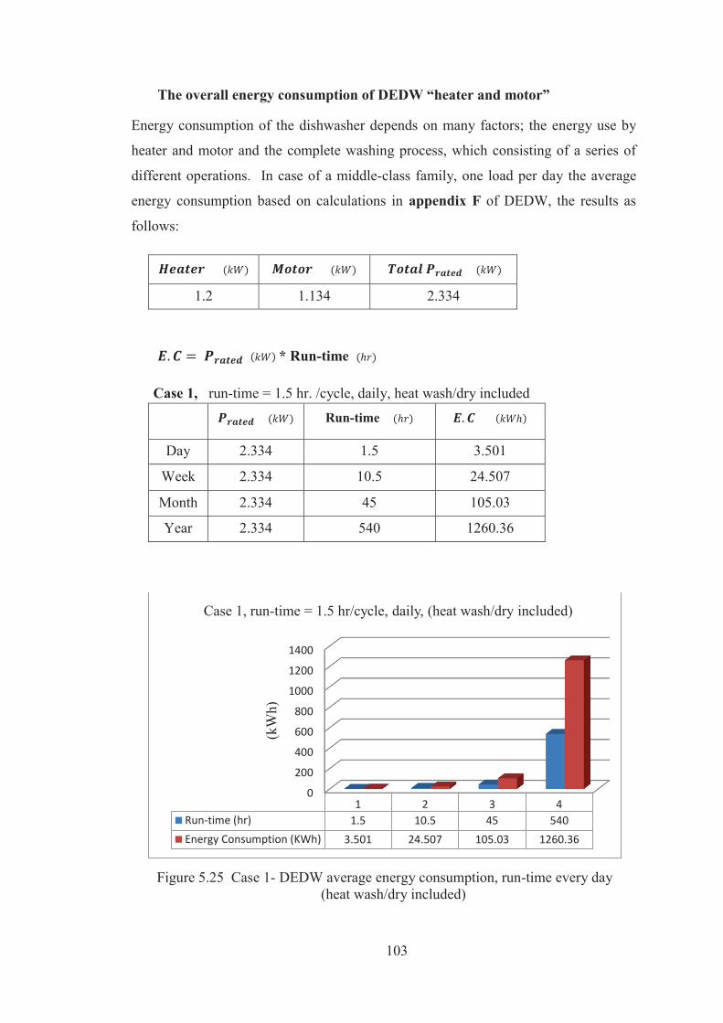
103
The overall energy consumption of DEDW “heater and motor”
Energy consumption of the dishwasher depends on many factors; the energy use by
heater and motor and the complete washing process, which consisting of a series of
different operations. In case of a middle-class family, one load per day the average
energy consumption based on calculations in appendix F of DEDW, the results as
follows:
1.2 1.134 2.334
* Run-time
Case 1, run-time = 1.5 hr. /cycle, daily, heat wash/dry included
Run-time
Day 2.334 1.5 3.501
Week 2.334 10.5 24.507
Month 2.334 45 105.03
Year 2.334 540 1260.36
Figure 5.25 Case 1- DEDW average energy consumption, run-time every day (heat wash/dry included)
0
200
400
600
800
1000
1200
1400
1 2 3 4Run-time (hr) 1.5 10.5 45 540Energy Consumption (KWh) 3.501 24.507 105.03 1260.36
(kW
h)
Case 1, run-time = 1.5 hr/cycle, daily, (heat wash/dry included)
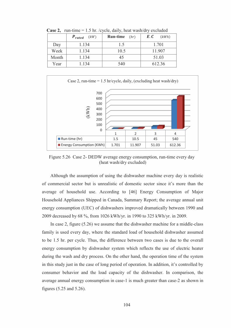
104
Case 2, run-time = 1.5 hr. /cycle, daily, heat wash/dry excluded Run-time
Day 1.134 1.5 1.701 Week 1.134 10.5 11.907 Month 1.134 45 51.03 Year 1.134 540 612.36
Figure 5.26 Case 2- DEDW average energy consumption, run-time every day (heat wash/dry excluded)
Although the assumption of using the dishwasher machine every day is realistic
of commercial sector but is unrealistic of domestic sector since it’s more than the
average of household use. According to [46] Energy Consumption of Major
Household Appliances Shipped in Canada, Summary Report; the average annual unit
energy consumption (UEC) of dishwashers improved dramatically between 1990 and
2009 decreased by 68 %, from 1026 kWh/yr. in 1990 to 325 kWh/yr. in 2009.
In case 2, figure (5.26) we assume that the dishwasher machine for a middle-class
family is used every day, where the standard load of household dishwasher assumed
to be 1.5 hr. per cycle. Thus, the difference between two cases is due to the overall
energy consumption by dishwasher system which reflects the use of electric heater
during the wash and dry process. On the other hand, the operation time of the system
in this study just in the case of long period of operation. In addition, it’s controlled by
consumer behavior and the load capacity of the dishwasher. In comparison, the
average annual energy consumption in case-1 is much greater than case-2 as shown in
figures (5.25 and 5.26).
0100200300400500600700
1 2 3 4Run-time (hr) 1.5 10.5 45 540Energy Consumption (KWh) 1.701 11.907 51.03 612.36
(kW
h)
Case 2, run-time = 1.5 hr/cycle, daily, (excluding heat wash/dry)
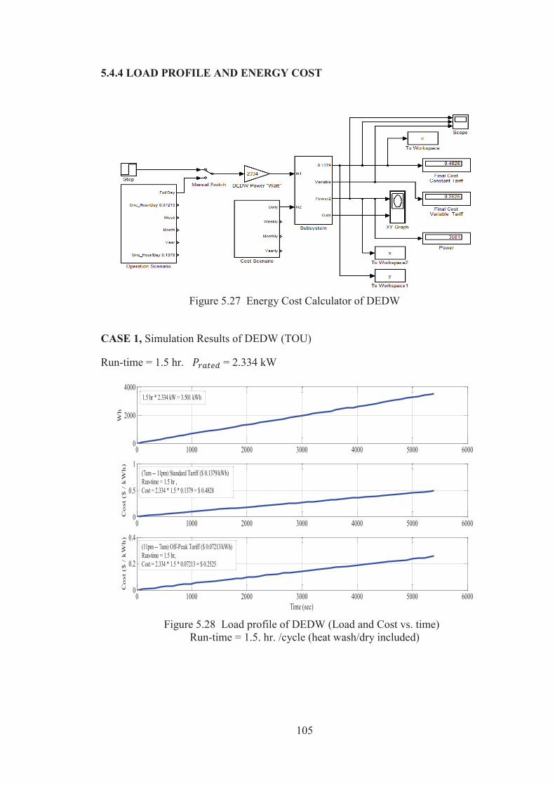
105
5.4.4 LOAD PROFILE AND ENERGY COST
Figure 5.27 Energy Cost Calculator of DEDW
CASE 1, Simulation Results of DEDW (TOU)
Run-time = 1.5 hr. = 2.334 kW
Figure 5.28 Load profile of DEDW (Load and Cost vs. time) Run-time = 1.5. hr. /cycle (heat wash/dry included)
0 1000 2000 3000 4000 5000 60000
2000
4000
Wh
0 1000 2000 3000 4000 5000 60000
0.5
1
Co
st
($ /
kW
h)
0 1000 2000 3000 4000 5000 60000
0.2
0.4
Time (sec)
Co
st
($ /
kW
h)
1.5 hr * 2.334 kW = 3.501 kWh
(7am -- 11pm) Standard Tariff ($ 0.1379/kWh)Run-time = 1.5 hr , Cost = 2.334 * 1.5 * 0.1379 = $ 0.4828
(11pm -- 7am) Off-Peak Tariff ($ 0.07213/kWh)Run-time = 1.5 hr, Cost = 2.334 * 1.5 * 0.07213 = $ 0.2525
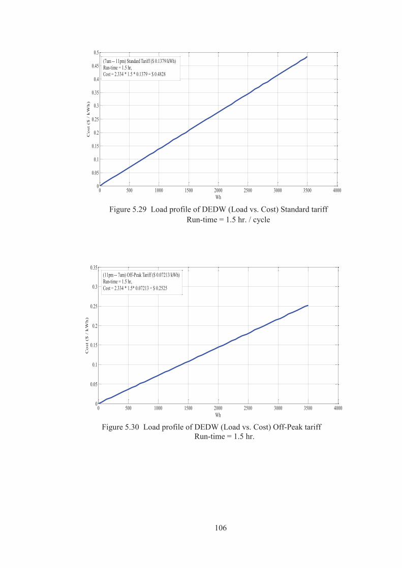
106
Figure 5.29 Load profile of DEDW (Load vs. Cost) Standard tariff
Run-time = 1.5 hr. / cycle
Figure 5.30 Load profile of DEDW (Load vs. Cost) Off-Peak tariff
Run-time = 1.5 hr.
0 500 1000 1500 2000 2500 3000 3500 40000
0.05
0.1
0.15
0.2
0.25
0.3
0.35
0.4
0.45
0.5
Wh
Co
st (
$ /
kW
h)
(7am -- 11pm) Standard Tariff ($ 0.1379/kWh)Run-time = 1.5 hr, Cost = 2.334 * 1.5 * 0.1379 = $ 0.4828
0 500 1000 1500 2000 2500 3000 3500 40000
0.05
0.1
0.15
0.2
0.25
0.3
0.35
Wh
Co
st (
$ /
kW
h)
(11pm -- 7am) Off-Peak Tariff ($ 0.07213/kWh)Run-time = 1.5 hr, Cost = 2.334 * 1.5* 0.07213 = $ 0.2525
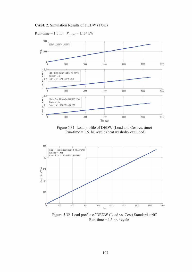
107
CASE 2, Simulation Results of DEDW (TOU)
Run-time = 1.5 hr. = 1.134 kW
Figure 5.31 Load profile of DEDW (Load and Cost vs. time)
Run-time = 1.5. hr. /cycle (heat wash/dry excluded)
Figure 5.32 Load profile of DEDW (Load vs. Cost) Standard tariff
Run-time = 1.5 hr. / cycle
0 1000 2000 3000 4000 5000 60000
0.2
0.4
Co
st
($ /
kW
h)
0 1000 2000 3000 4000 5000 60000
0.1
0.2
Time (sec)
Co
st
($ /
kW
h)
0 1000 2000 3000 4000 5000 60000
1000
2000W
h
1.5 hr * 1.134 kW = 1.701 kWh
(7am -- 11pm) Standard Tariff ($ 0.1379/kWh)Run-time = 1.5 hr , Cost = 1.134 * 1.5 * 0.1379 = $ 0.2346
(11pm -- 7am) Off-Peak Tariff ($ 0.07213/kWh)Run-time = 1.5 hr, Cost = 1.134 * 1.5 * 0.07213 = $ 0.1227
0 200 400 600 800 1000 1200 1400 1600 18000
0.05
0.1
0.15
0.2
0.25
Wh
Co
st (
$ /
kW
h)
(7am -- 11pm) Standard Tariff ($ 0.1379/kWh)Run-time = 1.5 hr, Cost = 1.134 * 1.5 * 0.1379 = $ 0.2346
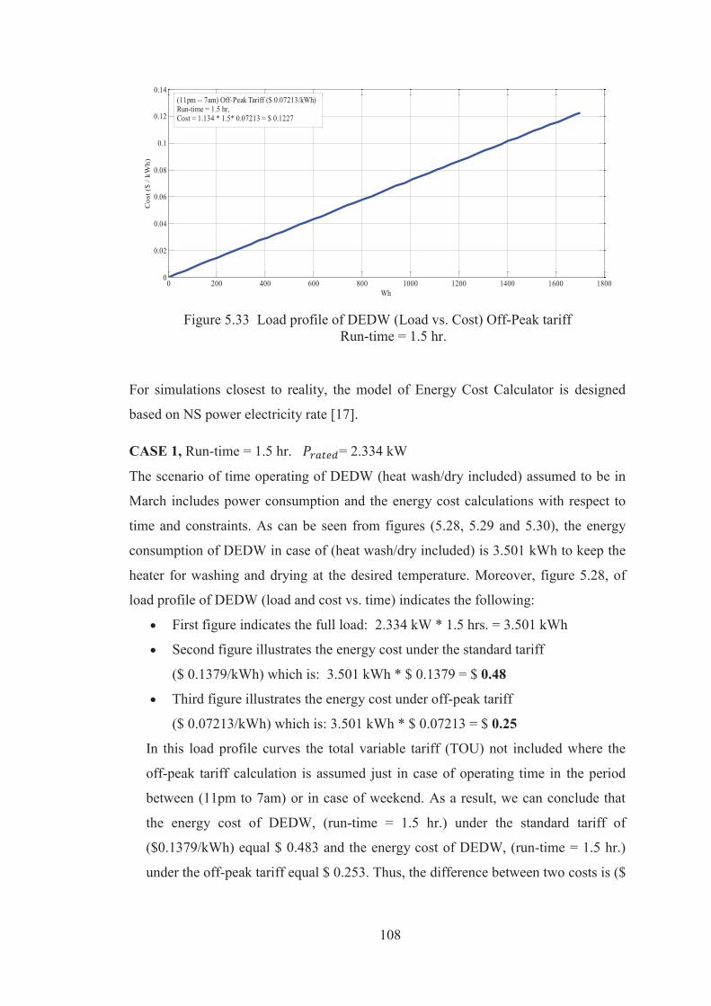
108
Figure 5.33 Load profile of DEDW (Load vs. Cost) Off-Peak tariff
Run-time = 1.5 hr.
For simulations closest to reality, the model of Energy Cost Calculator is designed
based on NS power electricity rate [17].
CASE 1, Run-time = 1.5 hr. = 2.334 kW
The scenario of time operating of DEDW (heat wash/dry included) assumed to be in
March includes power consumption and the energy cost calculations with respect to
time and constraints. As can be seen from figures (5.28, 5.29 and 5.30), the energy
consumption of DEDW in case of (heat wash/dry included) is 3.501 kWh to keep the
heater for washing and drying at the desired temperature. Moreover, figure 5.28, of
load profile of DEDW (load and cost vs. time) indicates the following:
First figure indicates the full load: 2.334 kW * 1.5 hrs. = 3.501 kWh
Second figure illustrates the energy cost under the standard tariff
($ 0.1379/kWh) which is: 3.501 kWh * $ 0.1379 = $ 0.48
Third figure illustrates the energy cost under off-peak tariff
($ 0.07213/kWh) which is: 3.501 kWh * $ 0.07213 = $ 0.25
In this load profile curves the total variable tariff (TOU) not included where the
off-peak tariff calculation is assumed just in case of operating time in the period
between (11pm to 7am) or in case of weekend. As a result, we can conclude that
the energy cost of DEDW, (run-time = 1.5 hr.) under the standard tariff of
($0.1379/kWh) equal $ 0.483 and the energy cost of DEDW, (run-time = 1.5 hr.)
under the off-peak tariff equal $ 0.253. Thus, the difference between two costs is ($
0 200 400 600 800 1000 1200 1400 1600 18000
0.02
0.04
0.06
0.08
0.1
0.12
0.14
Wh
Cos
t ($
/ kW
h)
(11pm -- 7am) Off-Peak Tariff ($ 0.07213/kWh)Run-time = 1.5 hr, Cost = 1.134 * 1.5* 0.07213 = $ 0.1227
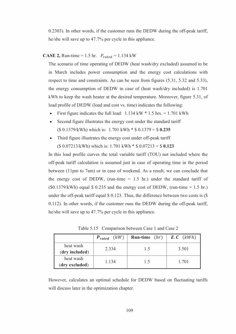
109
0.2303). In other words, if the customer runs the DEDW during the off-peak tariff,
he/she will save up to 47.7% per cycle in this appliance.
CASE 2, Run-time = 1.5 hr. = 1.134 kW
The scenario of time operating of DEDW (heat wash/dry excluded) assumed to be
in March includes power consumption and the energy cost calculations with
respect to time and constraints. As can be seen from figures (5.31, 5.32 and 5.33),
the energy consumption of DEDW in case of (heat wash/dry included) is 1.701
kWh to keep the wash heater at the desired temperature. Moreover, figure 5.31, of
load profile of DEDW (load and cost vs. time) indicates the following:
First figure indicates the full load: 1.134 kW * 1.5 hrs. = 1.701 kWh
Second figure illustrates the energy cost under the standard tariff
($ 0.1379/kWh) which is: 1.701 kWh * $ 0.1379 = $ 0.235
Third figure illustrates the energy cost under off-peak tariff
($ 0.07213/kWh) which is: 1.701 kWh * $ 0.07213 = $ 0.123
In this load profile curves the total variable tariff (TOU) not included where the
off-peak tariff calculation is assumed just in case of operating time in the period
between (11pm to 7am) or in case of weekend. As a result, we can conclude that
the energy cost of DEDW, (run-time = 1.5 hr.) under the standard tariff of
($0.1379/kWh) equal $ 0.235 and the energy cost of DEDW, (run-time = 1.5 hr.)
under the off-peak tariff equal $ 0.123. Thus, the difference between two costs is ($
0.112). In other words, if the customer runs the DEDW during the off-peak tariff,
he/she will save up to 47.7% per cycle in this appliance.
Table 5.15 Comparison between Case 1 and Case 2
Run-time
heat wash (dry included)
2.334 1.5 3.501
heat wash (dry excluded)
1.134 1.5 1.701
However, calculates an optimal schedule for DEDW based on fluctuating tariffs
will discuss later in the optimization chapter.
110
CHAPTER 6 OPTIMIZATION METHOD
6.1 INTRODUCTION
In recent years, however, the rate of energy demand has increased rapidly
throughout the world while the price of energy has been fluctuating. In energy
management system (EMS) whether residential sector or commercial sector the
ultimate goal is to make the best choice by selecting the best least costly decision
among the set of permissible decisions under conditions; that can be achieved by
finding the optimal time operating of certain appliances under the condition that
they satisfy the consumer choice and reduce the overall power consumption and
energy cost.
The particular problem of this chapter is time operating and energy cost under
conditions. To find the optimal solution for such problems, (REMS) establishes
the optimal daily operation of home appliances. Therefore, this study analyzes
many candidate scenarios during peak and off peak load periods comparing to the
tariff of the residential sector in Nova Scotia based on electricity rate of NS Power
[17] to reduce the usage and its associated costs. It presents simulated results of
proposed (REMS) to provide an automated least cost demand response. The main
approach will be to ensure the satisfaction of the requirements with constraints on
efficient use of energy.
6.2 MODEL of LINEAR PROGRAMING PROBLEM (LPP)
For this optimization method that is applicable for the solution of a Linear
Programming problem (LPP) where all functions are involved, the objective
function and the constraints must be a linear functions of the decision variables
[72, 73 and 74].
Linear Programming (LP) model
A linear Programming (LP) model is a technique for optimization of a linear
objective function, subject to linear equality and linear inequality constraints, in
order to achieve the best optimal solution of the problem such as a maximum
profit or a minimum cost [74, 76].
111
Integer programming (IP) model
An integer programming (IP) model is a linear programming model with the
additional requirement that all of the variables are integers [74, 76].
Binary integer programming (BIP) model
A binary integer programming (BIP) model is an integer programming model
where each variable has a value of (0 or 1) / (on or off). In other words, this may
represent the selection of many situations depends on the problem [74, 75 and 76].
A Linear Programming Problem (LPP) in standard form as a vector and matrix
Subject to:
(6.1)
Where,
: an n-dimensional column vector
: an n-dimensional row vector
: an matrix
: an m-dimensional column vector
: means that each component of is non-negative
6.2.1 MATHEMATICAL MODEL of (BIP)
The power consumption scheduling problem is formed as a binary-integer linear
programming model. The daily power consumption tasks are based on the run-time
(starting-time and ending-time). In this problem the objective is to minimize the daily
energy cost.
112
Problem Formulation
In this case study of residential energy system and commercial energy system;
the objective of the problem formulation is to determine the optimal time schedule
operating of appliances which optimize the total energy consumption in order to
reduce its associated cost
Subject to:
U
(6.2)
Where, the vectors are ( and the matrix is
The cost rate of electricity is constant every hour thus; the sampling period is 1 hr.
therefore, 24hr. /day
Switching/decision variable
The cost function is given by
= (6.3)
Where,
L : load per appliance (kW)
: TOU electricity cost rate in ($/kWh)
TOU electricity price rate is varied in every season; for instance, in summer is given
by two periods, Standard Tariff and Off-Peak Tariff as follows:
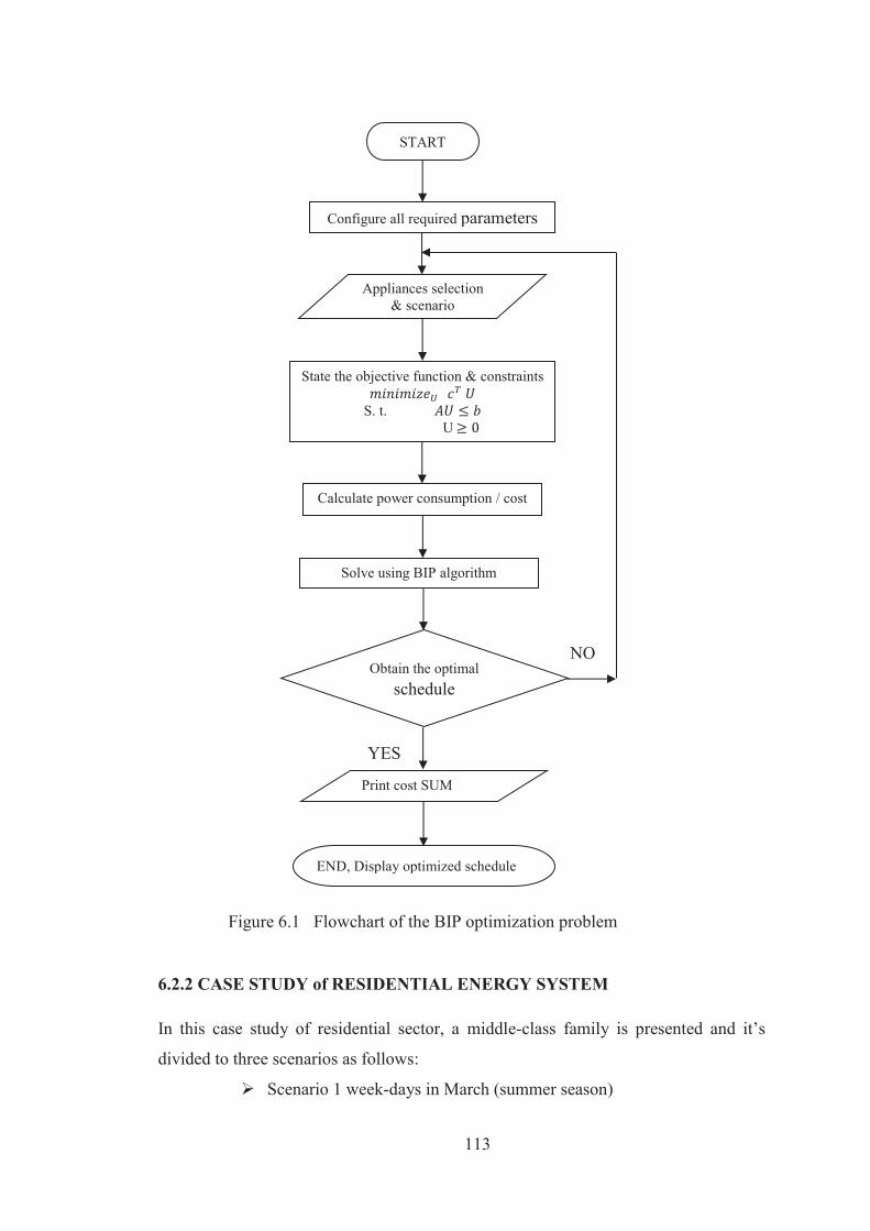
113
Figure 6.1 Flowchart of the BIP optimization problem
6.2.2 CASE STUDY of RESIDENTIAL ENERGY SYSTEM
In this case study of residential sector, a middle-class family is presented and it’s
divided to three scenarios as follows:
Scenario 1 week-days in March (summer season)
State the objective function & constraints
S. t. U
Appliances selection & scenario
Configure all required parameters
START
Calculate power consumption / cost
Solve using BIP algorithm
Obtain the optimal schedule
Print cost SUM
END, Display optimized schedule
YES
NO
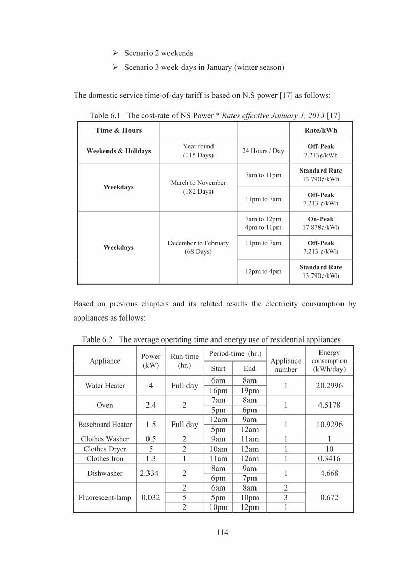
114
Scenario 2 weekends
Scenario 3 week-days in January (winter season)
The domestic service time-of-day tariff is based on N.S power [17] as follows:
Table 6.1 The cost-rate of NS Power * Rates effective January 1, 2013 [17]
Time & Hours Rate/kWh
Weekends & Holidays Year round (115 Days) 24 Hours / Day Off-Peak
7.213¢/kWh
Weekdays March to November
(182 Days)
7am to 11pm Standard Rate 13.790¢/kWh
11pm to 7am Off-Peak 7.213 ¢/kWh
Weekdays December to February
(68 Days)
7am to 12pm 4pm to 11pm
On-Peak 17.878¢/kWh
11pm to 7am
Off-Peak 7.213 ¢/kWh
12pm to 4pm Standard Rate 13.790¢/kWh
Based on previous chapters and its related results the electricity consumption by
appliances as follows: Table 6.2 The average operating time and energy use of residential appliances
Appliance Power (kW)
Run-time (hr.)
Period-time (hr.) Appliance
number
Energy consumption (kWh/day) Start End
Water Heater 4 Full day 6am 8am 1 20.2996 16pm 19pm
Oven 2.4 2 7am 8am 1 4.5178 5pm 6pm
Baseboard Heater 1.5 Full day 12am 9am 1 10.9296 5pm 12am Clothes Washer 0.5 2 9am 11am 1 1 Clothes Dryer 5 2 10am 12am 1 10 Clothes Iron 1.3 1 11am 12am 1 0.3416
Dishwasher 2.334 2 8am 9am 1 4.668 6pm 7pm
Fluorescent-lamp 0.032 2 6am 8am 2
0.672 5 5pm 10pm 3 2 10pm 12pm 1
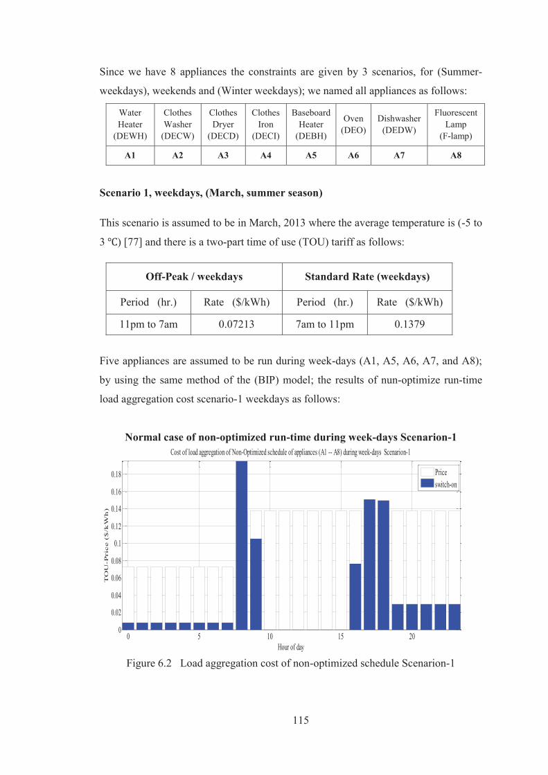
115
Since we have 8 appliances the constraints are given by 3 scenarios, for (Summer-
weekdays), weekends and (Winter weekdays); we named all appliances as follows:
Water Heater
(DEWH)
Clothes Washer
(DECW)
Clothes Dryer
(DECD)
Clothes Iron
(DECI)
Baseboard Heater
(DEBH)
Oven (DEO)
Dishwasher (DEDW)
Fluorescent Lamp
(F-lamp)
A1 A2 A3 A4 A5 A6 A7 A8
Scenario 1, weekdays, (March, summer season)
This scenario is assumed to be in March, 2013 where the average temperature is (-5 to
3 ) [77] and there is a two-part time of use (TOU) tariff as follows:
Off-Peak / weekdays Standard Rate (weekdays)
Period (hr.) Rate ($/kWh) Period (hr.) Rate ($/kWh)
11pm to 7am 0.07213 7am to 11pm 0.1379
Five appliances are assumed to be run during week-days (A1, A5, A6, A7, and A8);
by using the same method of the (BIP) model; the results of nun-optimize run-time
load aggregation cost scenario-1 weekdays as follows:
Normal case of non-optimized run-time during week-days Scenarion-1
Figure 6.2 Load aggregation cost of non-optimized schedule Scenarion-1
0 5 10 15 200
0.02
0.04
0.06
0.08
0.1
0.12
0.14
0.16
0.18
Hour of day
TO
U-P
rice (
$/k
Wh
)
Cost of load aggregation of Non-Optimized schedule of appliances (A1 -- A8) during week-days Scenarion-1
Priceswitch-on
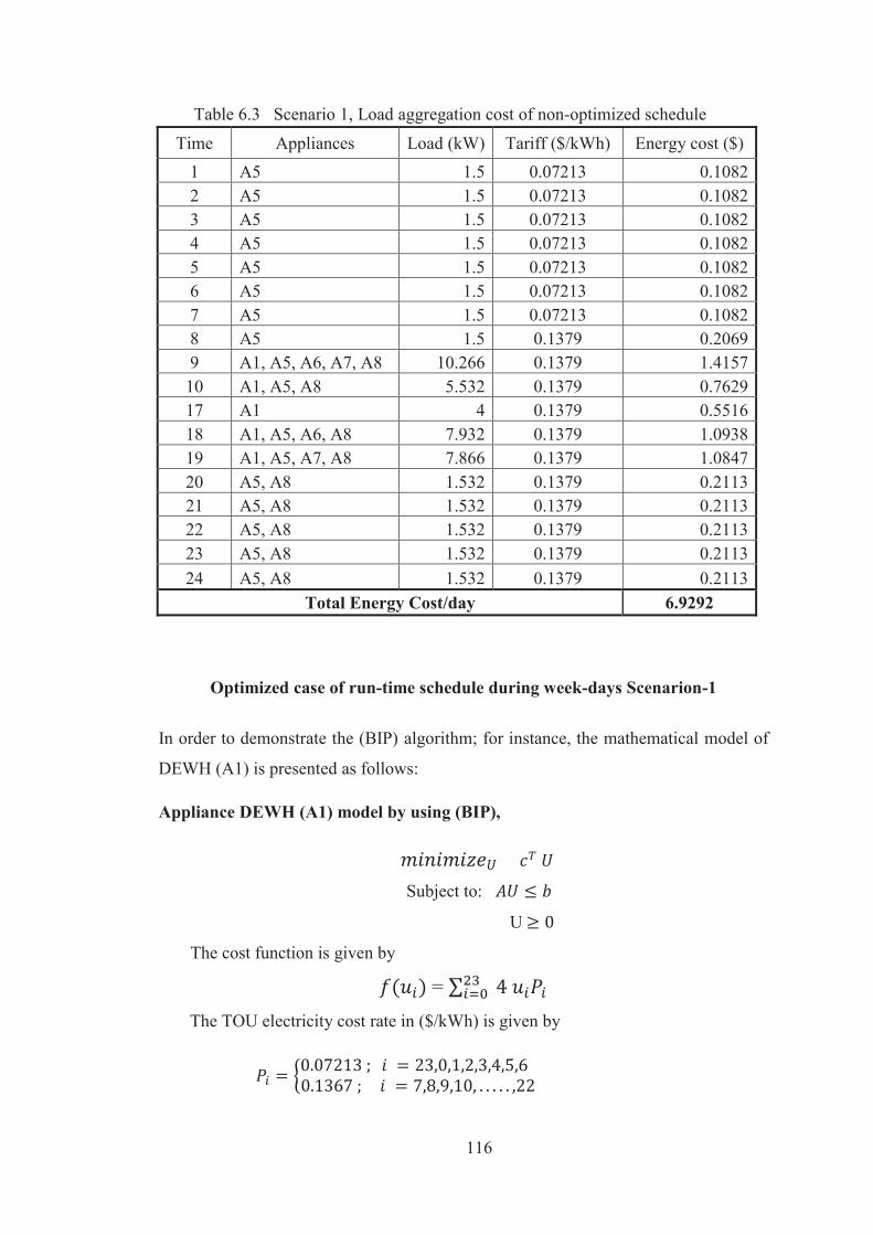
116
Table 6.3 Scenario 1, Load aggregation cost of non-optimized schedule
Time Appliances Load (kW) Tariff ($/kWh) Energy cost ($) 1 A5 1.5 0.07213 0.1082 2 A5 1.5 0.07213 0.1082 3 A5 1.5 0.07213 0.1082 4 A5 1.5 0.07213 0.1082 5 A5 1.5 0.07213 0.1082 6 A5 1.5 0.07213 0.1082 7 A5 1.5 0.07213 0.1082 8 A5 1.5 0.1379 0.2069 9 A1, A5, A6, A7, A8 10.266 0.1379 1.4157 10 A1, A5, A8 5.532 0.1379 0.7629 17 A1 4 0.1379 0.5516 18 A1, A5, A6, A8 7.932 0.1379 1.0938 19 A1, A5, A7, A8 7.866 0.1379 1.0847 20 A5, A8 1.532 0.1379 0.2113 21 A5, A8 1.532 0.1379 0.2113 22 A5, A8 1.532 0.1379 0.2113 23 A5, A8 1.532 0.1379 0.2113 24 A5, A8 1.532 0.1379 0.2113
Total Energy Cost/day 6.9292
Optimized case of run-time schedule during week-days Scenarion-1
In order to demonstrate the (BIP) algorithm; for instance, the mathematical model of
DEWH (A1) is presented as follows:
Appliance DEWH (A1) model by using (BIP),
Subject to:
U
The cost function is given by
= The TOU electricity cost rate in ($/kWh) is given by
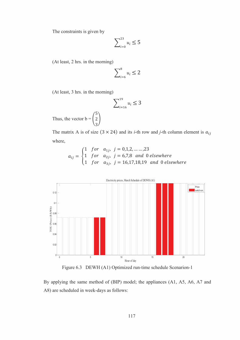
117
The constraints is given by
(At least, 2 hrs. in the morning)
(At least, 3 hrs. in the morning)
Thus, the vector b =
The matrix A is of size and its i-th row and j-th column element is
where,
Figure 6.3 DEWH (A1) Optimized run-time schedule Scenarion-1
By applying the same method of (BIP) model; the appliances (A1, A5, A6, A7 and
A8) are scheduled in week-days as follows:
0 5 10 15 200
0.02
0.04
0.06
0.08
0.1
0.12
Hour of day
TO
U-P
rice
($
/kW
h)
Electricity prices, March Schedule of DEWH (A1)
Priceswitch-on
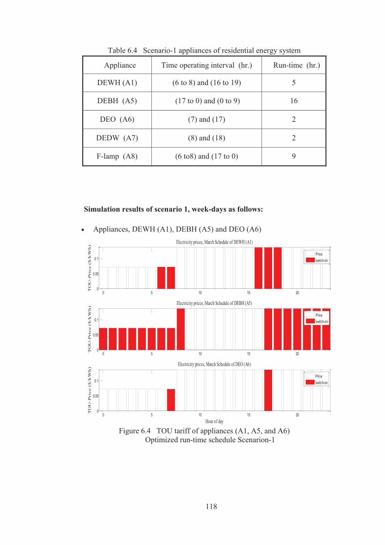
118
Table 6.4 Scenario-1 appliances of residential energy system
Appliance Time operating interval (hr.) Run-time (hr.)
DEWH (A1) (6 to 8) and (16 to 19) 5
DEBH (A5) (17 to 0) and (0 to 9) 16
DEO (A6) (7) and (17) 2
DEDW (A7) (8) and (18) 2
F-lamp (A8) (6 to8) and (17 to 0) 9
Simulation results of scenario 1, week-days as follows:
Appliances, DEWH (A1), DEBH (A5) and DEO (A6)
Figure 6.4 TOU tariff of appliances (A1, A5, and A6)
Optimized run-time schedule Scenarion-1
0 5 10 15 200
0.05
0.1
TO
U-P
rice (
$/k
Wh
)
Electricity prices, March Schedule of DEWH (A1)
Priceswitch-on
0 5 10 15 200
0.05
0.1
TO
U-P
rice (
$/k
Wh
)
Electricity prices, March Schedule of DEBH (A5)
Priceswitch-on
0 5 10 15 200
0.05
0.1
Hour of day
TO
U-P
rice (
$/k
Wh
)
Electricity prices, March Schedule of DEO (A6)
Priceswitch-on
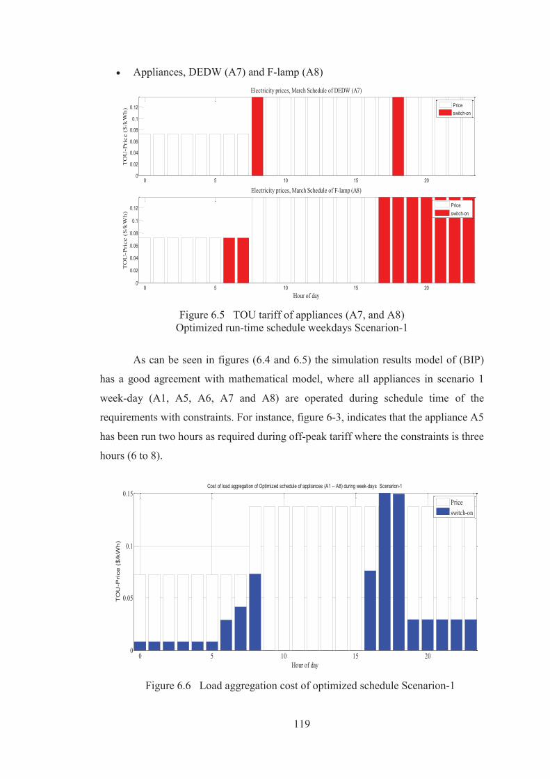
119
Appliances, DEDW (A7) and F-lamp (A8)
Figure 6.5 TOU tariff of appliances (A7, and A8)
Optimized run-time schedule weekdays Scenarion-1
As can be seen in figures (6.4 and 6.5) the simulation results model of (BIP)
has a good agreement with mathematical model, where all appliances in scenario 1
week-day (A1, A5, A6, A7 and A8) are operated during schedule time of the
requirements with constraints. For instance, figure 6-3, indicates that the appliance A5
has been run two hours as required during off-peak tariff where the constraints is three
hours (6 to 8).
Figure 6.6 Load aggregation cost of optimized schedule Scenarion-1
0 5 10 15 200
0.02
0.04
0.06
0.08
0.1
0.12
TO
U-P
rice
($
/kW
h)
Electricity prices, March Schedule of DEDW (A7)
Priceswitch-on
0 5 10 15 200
0.02
0.04
0.06
0.08
0.1
0.12
Hour of day
TO
U-P
rice
($
/kW
h)
Electricity prices, March Schedule of F-lamp (A8)
Priceswitch-on
0 5 10 15 200
0.05
0.1
0.15
Hour of day
TO
U-P
rice
($
/kW
h)
Cost of load aggregation of Optimized schedule of appliances (A1 -- A8) during week-days Scenarion-1
Priceswitch-on
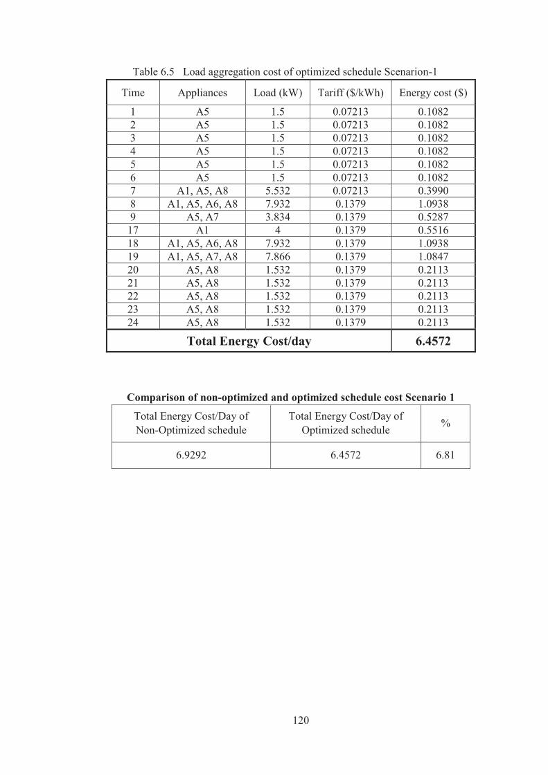
120
Table 6.5 Load aggregation cost of optimized schedule Scenarion-1
Time Appliances Load (kW) Tariff ($/kWh) Energy cost ($)
1 A5 1.5 0.07213 0.1082 2 A5 1.5 0.07213 0.1082 3 A5 1.5 0.07213 0.1082 4 A5 1.5 0.07213 0.1082 5 A5 1.5 0.07213 0.1082 6 A5 1.5 0.07213 0.1082 7 A1, A5, A8 5.532 0.07213 0.3990 8 A1, A5, A6, A8 7.932 0.1379 1.0938 9 A5, A7 3.834 0.1379 0.5287 17 A1 4 0.1379 0.5516 18 A1, A5, A6, A8 7.932 0.1379 1.0938 19 A1, A5, A7, A8 7.866 0.1379 1.0847 20 A5, A8 1.532 0.1379 0.2113 21 A5, A8 1.532 0.1379 0.2113 22 A5, A8 1.532 0.1379 0.2113 23 A5, A8 1.532 0.1379 0.2113 24 A5, A8 1.532 0.1379 0.2113
Total Energy Cost/day 6.4572
Comparison of non-optimized and optimized schedule cost Scenario 1
Total Energy Cost/Day of Non-Optimized schedule
Total Energy Cost/Day of Optimized schedule %
6.9292 6.4572 6.81
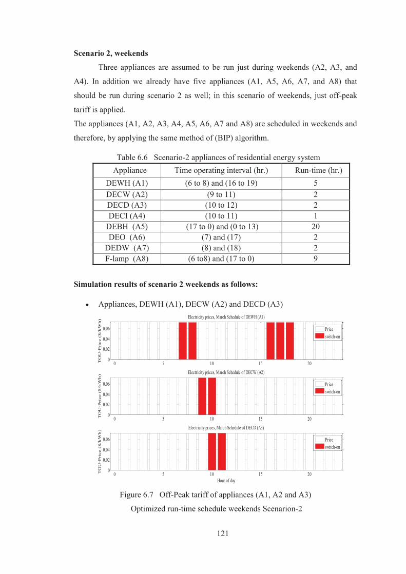
121
Scenario 2, weekends
Three appliances are assumed to be run just during weekends (A2, A3, and
A4). In addition we already have five appliances (A1, A5, A6, A7, and A8) that
should be run during scenario 2 as well; in this scenario of weekends, just off-peak
tariff is applied.
The appliances (A1, A2, A3, A4, A5, A6, A7 and A8) are scheduled in weekends and
therefore, by applying the same method of (BIP) algorithm.
Table 6.6 Scenario-2 appliances of residential energy system Appliance Time operating interval (hr.) Run-time (hr.)
DEWH (A1) (6 to 8) and (16 to 19) 5 DECW (A2) (9 to 11) 2 DECD (A3) (10 to 12) 2 DECI (A4) (10 to 11) 1
DEBH (A5) (17 to 0) and (0 to 13) 20 DEO (A6) (7) and (17) 2
DEDW (A7) (8) and (18) 2 F-lamp (A8) (6 to8) and (17 to 0) 9
Simulation results of scenario 2 weekends as follows:
Appliances, DEWH (A1), DECW (A2) and DECD (A3)
Figure 6.7 Off-Peak tariff of appliances (A1, A2 and A3)
Optimized run-time schedule weekends Scenarion-2
0 5 10 15 200
0.02
0.04
0.06
TO
U-P
rice (
$/k
Wh
) Electricity prices, March Schedule of DEWH (A1)
Priceswitch-on
0 5 10 15 200
0.02
0.04
0.06
TO
U-P
rice (
$/k
Wh
) Electricity prices, March Schedule of DECW (A2)
Priceswitch-on
0 5 10 15 200
0.02
0.04
0.06
Hour of day
TO
U-P
rice (
$/k
Wh
) Electricity prices, March Schedule of DECD (A3)
Priceswitch-on
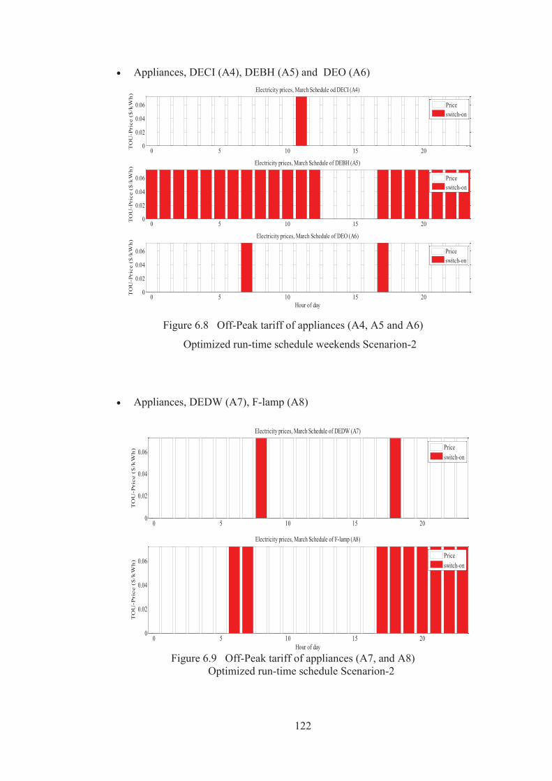
122
Appliances, DECI (A4), DEBH (A5) and DEO (A6)
Figure 6.8 Off-Peak tariff of appliances (A4, A5 and A6)
Optimized run-time schedule weekends Scenarion-2
Appliances, DEDW (A7), F-lamp (A8)
Figure 6.9 Off-Peak tariff of appliances (A7, and A8)
Optimized run-time schedule Scenarion-2
0 5 10 15 200
0.02
0.04
0.06
TO
U-P
rice
($
/kW
h)
Electricity prices, March Schedule od DECI (A4)
Priceswitch-on
0 5 10 15 200
0.02
0.04
0.06
TO
U-P
rice
($
/kW
h)
Electricity prices, March Schedule of DEBH (A5)
Priceswitch-on
0 5 10 15 200
0.02
0.04
0.06
Hour of day
TO
U-P
rice
($
/kW
h)
Electricity prices, March Schedule of DEO (A6)
Priceswitch-on
0 5 10 15 200
0.02
0.04
0.06
TO
U-P
rice (
$/k
Wh
)
Electricity prices, March Schedule of DEDW (A7)
Priceswitch-on
0 5 10 15 200
0.02
0.04
0.06
Hour of day
TO
U-P
rice (
$/k
Wh
)
Electricity prices, March Schedule of F-lamp (A8)
Priceswitch-on
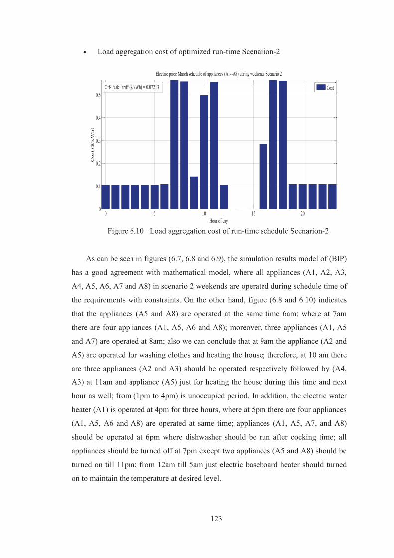
123
Load aggregation cost of optimized run-time Scenarion-2
Figure 6.10 Load aggregation cost of run-time schedule Scenarion-2
As can be seen in figures (6.7, 6.8 and 6.9), the simulation results model of (BIP)
has a good agreement with mathematical model, where all appliances (A1, A2, A3,
A4, A5, A6, A7 and A8) in scenario 2 weekends are operated during schedule time of
the requirements with constraints. On the other hand, figure (6.8 and 6.10) indicates
that the appliances (A5 and A8) are operated at the same time 6am; where at 7am
there are four appliances (A1, A5, A6 and A8); moreover, three appliances (A1, A5
and A7) are operated at 8am; also we can conclude that at 9am the appliance (A2 and
A5) are operated for washing clothes and heating the house; therefore, at 10 am there
are three appliances (A2 and A3) should be operated respectively followed by (A4,
A3) at 11am and appliance (A5) just for heating the house during this time and next
hour as well; from (1pm to 4pm) is unoccupied period. In addition, the electric water
heater (A1) is operated at 4pm for three hours, where at 5pm there are four appliances
(A1, A5, A6 and A8) are operated at same time; appliances (A1, A5, A7, and A8)
should be operated at 6pm where dishwasher should be run after cocking time; all
appliances should be turned off at 7pm except two appliances (A5 and A8) should be
turned on till 11pm; from 12am till 5am just electric baseboard heater should turned
on to maintain the temperature at desired level.
0 5 10 15 200
0.1
0.2
0.3
0.4
0.5
Hour of day
Co
st (
$/k
Wh
)
Electric price March schedule of appliances (A1--A8) during weekends Scenario 2
CostOff-Peak Tariff ($/kWh) = 0.07213
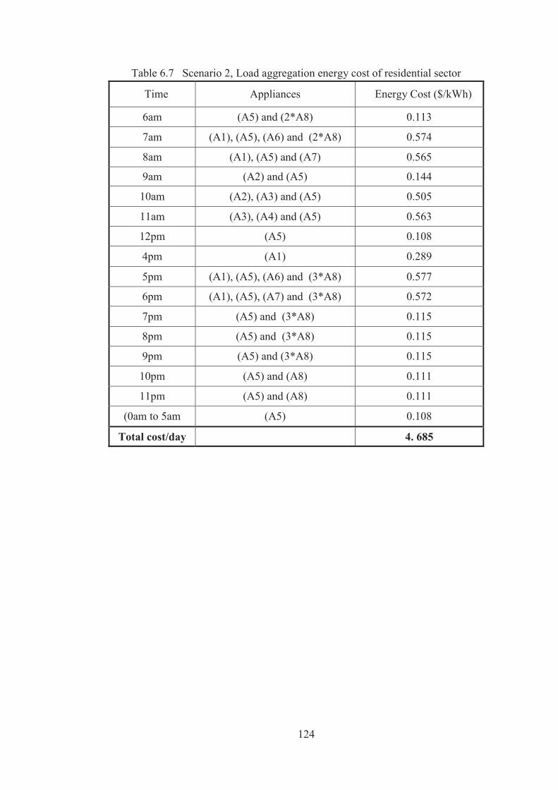
124
Table 6.7 Scenario 2, Load aggregation energy cost of residential sector
Time Appliances Energy Cost ($/kWh)
6am (A5) and (2*A8) 0.113
7am (A1), (A5), (A6) and (2*A8) 0.574
8am (A1), (A5) and (A7) 0.565
9am (A2) and (A5) 0.144
10am (A2), (A3) and (A5) 0.505
11am (A3), (A4) and (A5) 0.563
12pm (A5) 0.108
4pm (A1) 0.289
5pm (A1), (A5), (A6) and (3*A8) 0.577
6pm (A1), (A5), (A7) and (3*A8) 0.572
7pm (A5) and (3*A8) 0.115
8pm (A5) and (3*A8) 0.115
9pm (A5) and (3*A8) 0.115
10pm (A5) and (A8) 0.111
11pm (A5) and (A8) 0.111
(0am to 5am (A5) 0.108
Total cost/day 4. 685
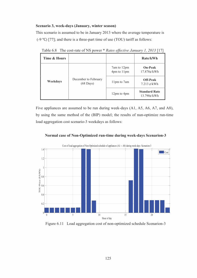
125
Scenario 3, week-days (January, winter season)
This scenario is assumed to be in January 2013 where the average temperature is
(-9 ) [77]; and there is a three-part time of use (TOU) tariff as follows:
Table 6.8 The cost-rate of NS power * Rates effective January 1, 2013 [17]
Time & Hours Rate/kWh
Weekdays December to February
(68 Days)
7am to 12pm 4pm to 11pm
On-Peak 17.878¢/kWh
11pm to 7am Off-Peak 7.213 ¢/kWh
12pm to 4pm Standard Rate 13.790¢/kWh
Five appliances are assumed to be run during week-days (A1, A5, A6, A7, and A8),
by using the same method of the (BIP) model; the results of nun-optimize run-time
load aggregation cost scenario-3 weekdays as follows:
Normal case of Non-Optimized run-time during week-days Scenarion-3
Figure 6.11 Load aggregation cost of non-optimized schedule Scenarion-3
0 5 10 15 200
0.2
0.4
0.6
0.8
1
1.2
1.4
Hour of day
TO
U-P
rice (
$/k
Wh
)
Cost of load aggregation of Non-Optimized schedule of appliances (A1 -- A8) during week-days Scenarion-3
Cost
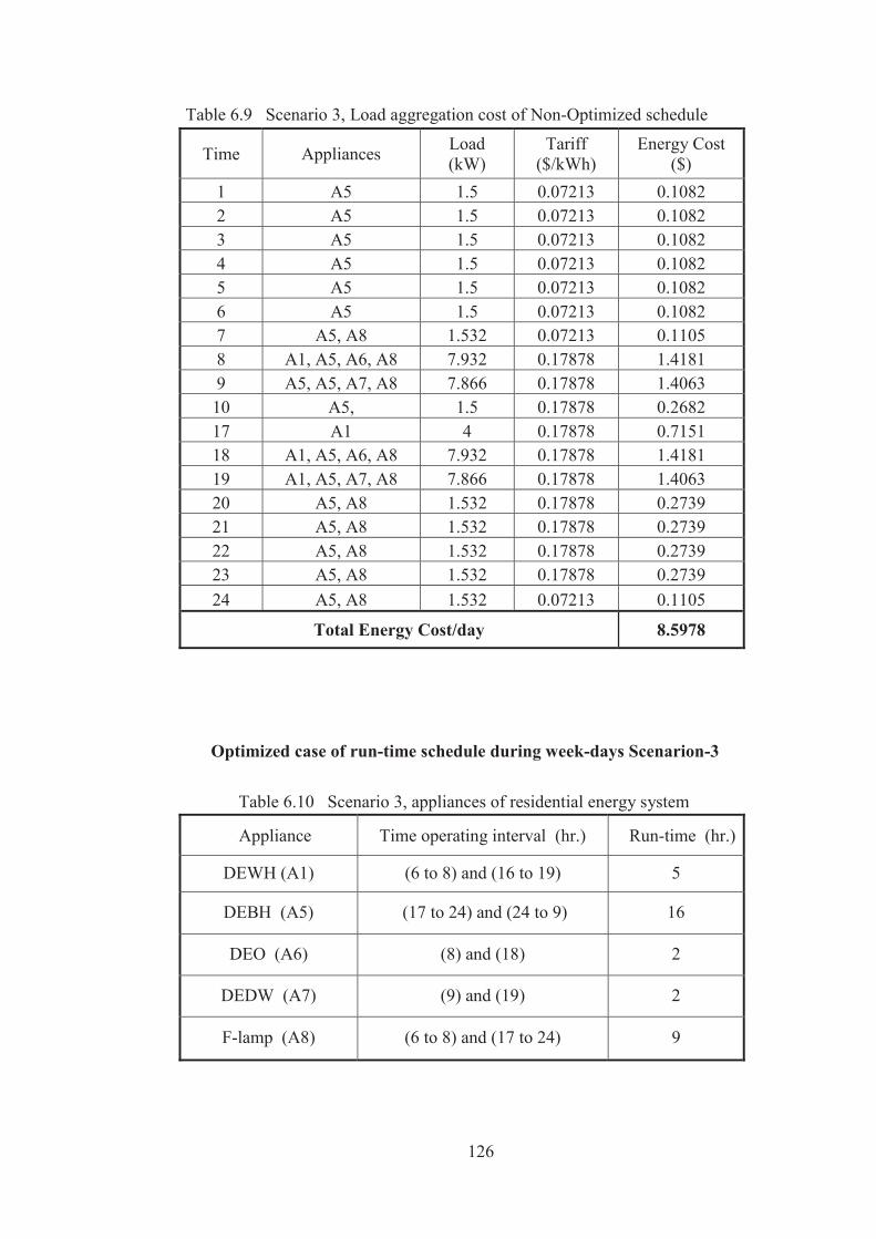
126
Table 6.9 Scenario 3, Load aggregation cost of Non-Optimized schedule
Time Appliances Load (kW)
Tariff ($/kWh)
Energy Cost ($)
1 A5 1.5 0.07213 0.1082 2 A5 1.5 0.07213 0.1082 3 A5 1.5 0.07213 0.1082 4 A5 1.5 0.07213 0.1082 5 A5 1.5 0.07213 0.1082 6 A5 1.5 0.07213 0.1082 7 A5, A8 1.532 0.07213 0.1105 8 A1, A5, A6, A8 7.932 0.17878 1.4181 9 A5, A5, A7, A8 7.866 0.17878 1.4063 10 A5, 1.5 0.17878 0.2682 17 A1 4 0.17878 0.7151 18 A1, A5, A6, A8 7.932 0.17878 1.4181 19 A1, A5, A7, A8 7.866 0.17878 1.4063 20 A5, A8 1.532 0.17878 0.2739 21 A5, A8 1.532 0.17878 0.2739 22 A5, A8 1.532 0.17878 0.2739 23 A5, A8 1.532 0.17878 0.2739 24 A5, A8 1.532 0.07213 0.1105
Total Energy Cost/day 8.5978
Optimized case of run-time schedule during week-days Scenarion-3
Table 6.10 Scenario 3, appliances of residential energy system
Appliance Time operating interval (hr.) Run-time (hr.)
DEWH (A1) (6 to 8) and (16 to 19) 5
DEBH (A5) (17 to 24) and (24 to 9) 16
DEO (A6) (8) and (18) 2
DEDW (A7) (9) and (19) 2
F-lamp (A8) (6 to 8) and (17 to 24) 9
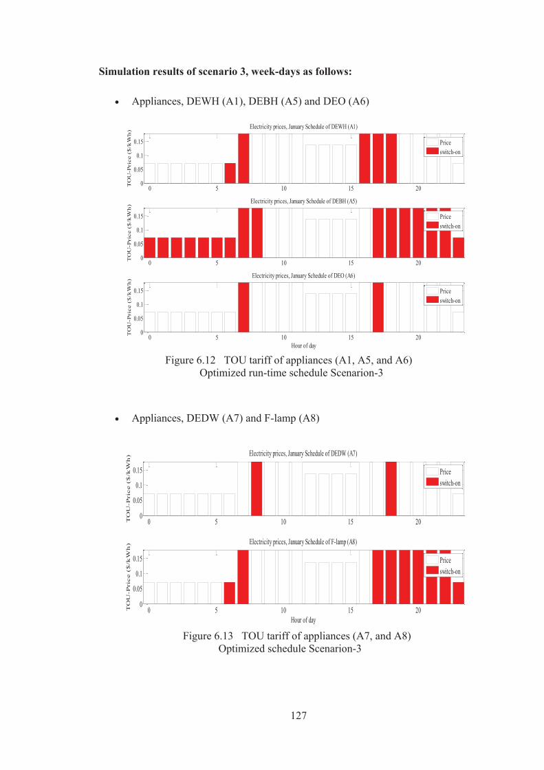
127
Simulation results of scenario 3, week-days as follows:
Appliances, DEWH (A1), DEBH (A5) and DEO (A6)
Figure 6.12 TOU tariff of appliances (A1, A5, and A6)
Optimized run-time schedule Scenarion-3
Appliances, DEDW (A7) and F-lamp (A8)
Figure 6.13 TOU tariff of appliances (A7, and A8)
Optimized schedule Scenarion-3
0 5 10 15 200
0.05
0.1
0.15
TO
U-P
rice
($
/kW
h) Electricity prices, January Schedule of DEWH (A1)
Priceswitch-on
0 5 10 15 200
0.05
0.1
0.15
TO
U-P
rice
($
/kW
h)
Electricity prices, January Schedule of DEBH (A5)
Priceswitch-on
0 5 10 15 200
0.05
0.1
0.15
Hour of day
TO
U-P
rice
($
/kW
h)
Electricity prices, January Schedule of DEO (A6)
Priceswitch-on
0 5 10 15 200
0.05
0.1
0.15
TO
U-P
rice (
$/k
Wh
) Electricity prices, January Schedule of DEDW (A7)
Priceswitch-on
0 5 10 15 200
0.05
0.1
0.15
Hour of day
TO
U-P
rice (
$/k
Wh
) Electricity prices, January Schedule of F-lamp (A8)
Priceswitch-on
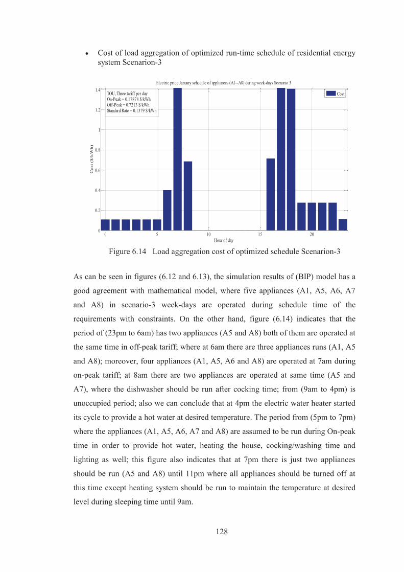
128
Cost of load aggregation of optimized run-time schedule of residential energy system Scenarion-3
Figure 6.14 Load aggregation cost of optimized schedule Scenarion-3
As can be seen in figures (6.12 and 6.13), the simulation results of (BIP) model has a
good agreement with mathematical model, where five appliances (A1, A5, A6, A7
and A8) in scenario-3 week-days are operated during schedule time of the
requirements with constraints. On the other hand, figure (6.14) indicates that the
period of (23pm to 6am) has two appliances (A5 and A8) both of them are operated at
the same time in off-peak tariff; where at 6am there are three appliances runs (A1, A5
and A8); moreover, four appliances (A1, A5, A6 and A8) are operated at 7am during
on-peak tariff; at 8am there are two appliances are operated at same time (A5 and
A7), where the dishwasher should be run after cocking time; from (9am to 4pm) is
unoccupied period; also we can conclude that at 4pm the electric water heater started
its cycle to provide a hot water at desired temperature. The period from (5pm to 7pm)
where the appliances (A1, A5, A6, A7 and A8) are assumed to be run during On-peak
time in order to provide hot water, heating the house, cocking/washing time and
lighting as well; this figure also indicates that at 7pm there is just two appliances
should be run (A5 and A8) until 11pm where all appliances should be turned off at
this time except heating system should be run to maintain the temperature at desired
level during sleeping time until 9am.
0 5 10 15 200
0.2
0.4
0.6
0.8
1
1.2
1.4
Hour of day
Co
st (
$/k
Wh
)
Electric price January schedule of appliances (A1--A8) during week-days Scenario 3
CostTOU, Three tariff per day
On-Peak = 0.17878 $/kWhOff-Peak = 0.7213 $/kWhStandard Rate = 0.1379 $/kWh
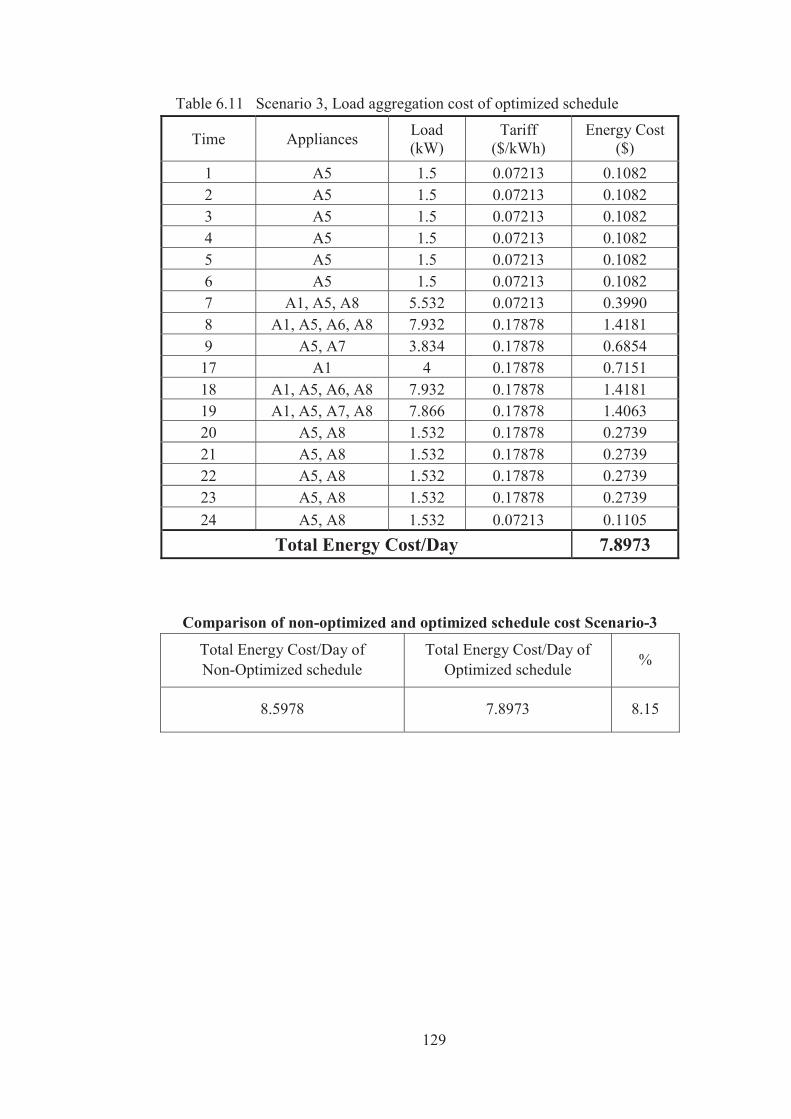
129
Table 6.11 Scenario 3, Load aggregation cost of optimized schedule
Time Appliances Load (kW)
Tariff ($/kWh)
Energy Cost ($)
1 A5 1.5 0.07213 0.1082 2 A5 1.5 0.07213 0.1082 3 A5 1.5 0.07213 0.1082 4 A5 1.5 0.07213 0.1082 5 A5 1.5 0.07213 0.1082 6 A5 1.5 0.07213 0.1082 7 A1, A5, A8 5.532 0.07213 0.3990 8 A1, A5, A6, A8 7.932 0.17878 1.4181 9 A5, A7 3.834 0.17878 0.6854 17 A1 4 0.17878 0.7151 18 A1, A5, A6, A8 7.932 0.17878 1.4181 19 A1, A5, A7, A8 7.866 0.17878 1.4063 20 A5, A8 1.532 0.17878 0.2739 21 A5, A8 1.532 0.17878 0.2739 22 A5, A8 1.532 0.17878 0.2739 23 A5, A8 1.532 0.17878 0.2739 24 A5, A8 1.532 0.07213 0.1105
Total Energy Cost/Day 7.8973
Comparison of non-optimized and optimized schedule cost Scenario-3
Total Energy Cost/Day of Non-Optimized schedule
Total Energy Cost/Day of Optimized schedule %
8.5978 7.8973 8.15
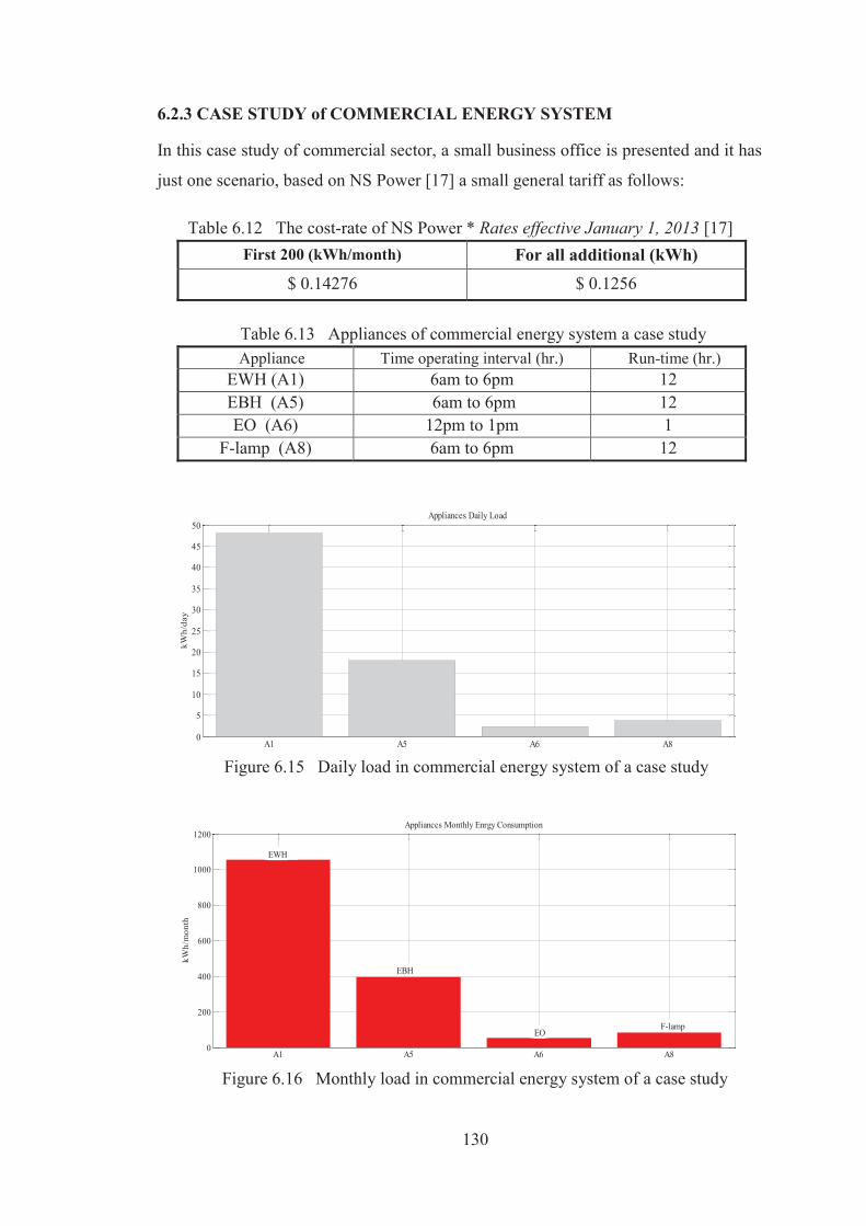
130
6.2.3 CASE STUDY of COMMERCIAL ENERGY SYSTEM
In this case study of commercial sector, a small business office is presented and it has
just one scenario, based on NS Power [17] a small general tariff as follows:
Table 6.12 The cost-rate of NS Power * Rates effective January 1, 2013 [17] First 200 (kWh/month) For all additional (kWh)
$ 0.14276 $ 0.1256
Table 6.13 Appliances of commercial energy system a case study Appliance Time operating interval (hr.) Run-time (hr.)
EWH (A1) 6am to 6pm 12 EBH (A5) 6am to 6pm 12 EO (A6) 12pm to 1pm 1
F-lamp (A8) 6am to 6pm 12
Figure 6.15 Daily load in commercial energy system of a case study
Figure 6.16 Monthly load in commercial energy system of a case study
A1 A5 A6 A80
5
10
15
20
25
30
35
40
45
50Appliances Daily Load
kWh/
day
A1 A5 A6 A80
200
400
600
800
1000
1200Appliances Monthly Enrgy Consumption
kWh/
mon
th
F-lampEO
EBH
EWH
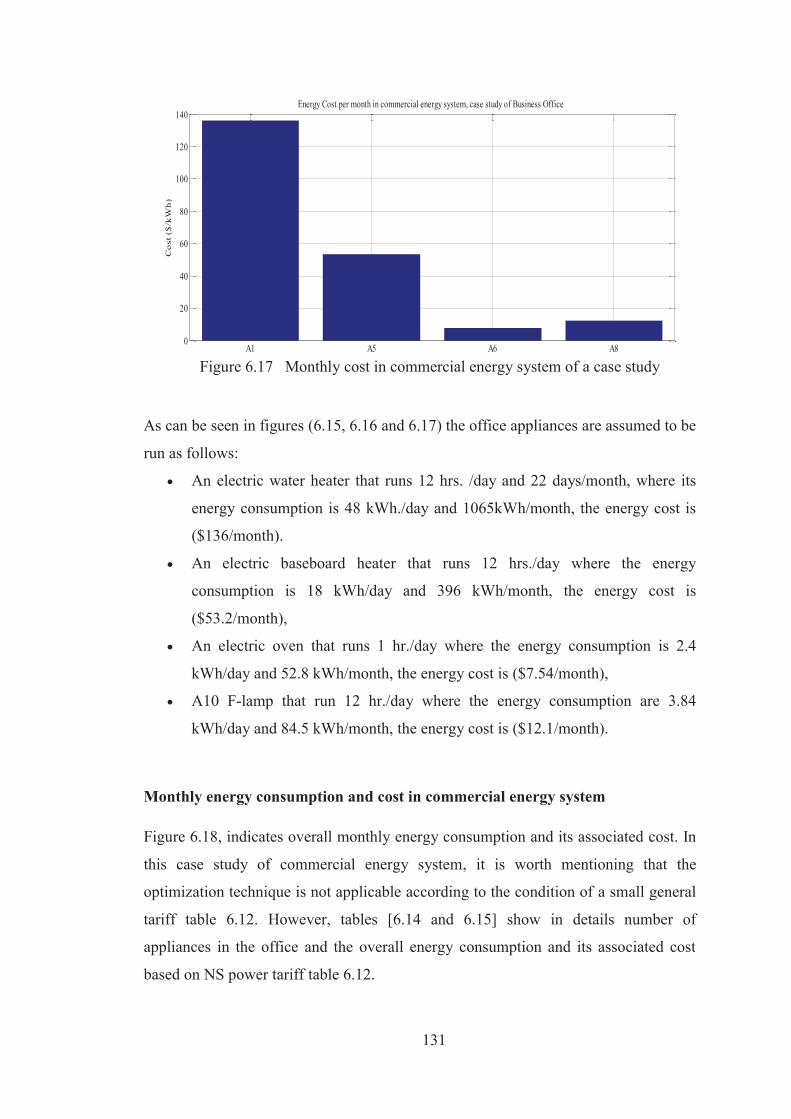
131
Figure 6.17 Monthly cost in commercial energy system of a case study
As can be seen in figures (6.15, 6.16 and 6.17) the office appliances are assumed to be
run as follows:
An electric water heater that runs 12 hrs. /day and 22 days/month, where its
energy consumption is 48 kWh./day and 1065kWh/month, the energy cost is
($136/month).
An electric baseboard heater that runs 12 hrs./day where the energy
consumption is 18 kWh/day and 396 kWh/month, the energy cost is
($53.2/month),
An electric oven that runs 1 hr./day where the energy consumption is 2.4
kWh/day and 52.8 kWh/month, the energy cost is ($7.54/month),
A10 F-lamp that run 12 hr./day where the energy consumption are 3.84
kWh/day and 84.5 kWh/month, the energy cost is ($12.1/month).
Monthly energy consumption and cost in commercial energy system
Figure 6.18, indicates overall monthly energy consumption and its associated cost. In
this case study of commercial energy system, it is worth mentioning that the
optimization technique is not applicable according to the condition of a small general
tariff table 6.12. However, tables [6.14 and 6.15] show in details number of
appliances in the office and the overall energy consumption and its associated cost
based on NS power tariff table 6.12.
A1 A5 A6 A80
20
40
60
80
100
120
140Energy Cost per month in commercial energy system, case study of Business Office
Co
st (
$/k
Wh
)

132
Figure 6.18 Monthly energy consumption and cost in commercial energy system
of a case study
Table 6.14 Daily load aggregation of energy consumption
Appliance kW Time operating interval (hr.)
Run-time (hr./day)
Appliance number kWh/day
EWH (A1) 4 6am to 6pm 12 1 48
EBH (A5) 1.5 6am to 6pm 12 3 54
EO (A6) 2.4 12pm to 1pm 1 1 2.4
F-lamp (A8) 0.032 6am to 6pm 12 10 3.84
Total energy consumption 108.2
Table 6.15 Monthly load aggregation of energy (consumption and cost)
Appliance kW Time operating interval (hr.)
Run-time (hr./month)
appliance number kWh/month
EWH (A1) 4 6am to 6pm 264 1 1056
EBH (A5) 1.5 6am to 6pm 264 3 1188
EO (A6) 2.4 12pm to 1pm 22 1 52.8 F-lamp (A8) 0.032 6am to 6pm 264 10 84.48
Total energy consumption (kWh/month) 2381.3
Total energy cost ($/month) 302.52
12
1
2
3
4
0
200
400
600
800
1000
1200
A1
A5
A6
A8
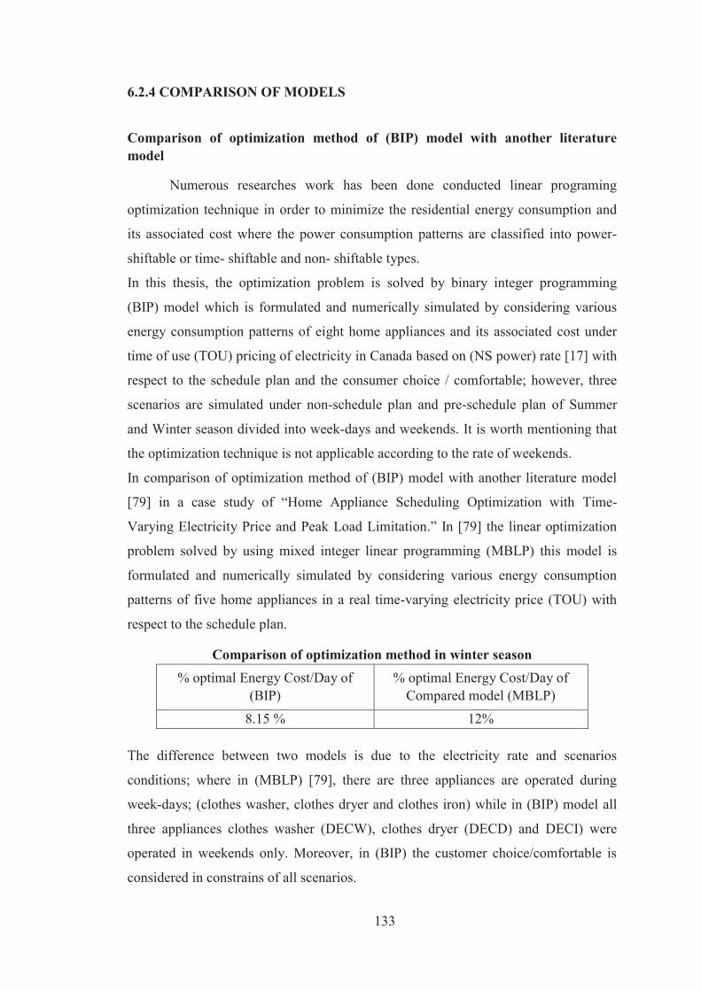
133
6.2.4 COMPARISON OF MODELS
Comparison of optimization method of (BIP) model with another literature model
Numerous researches work has been done conducted linear programing
optimization technique in order to minimize the residential energy consumption and
its associated cost where the power consumption patterns are classified into power-
shiftable or time- shiftable and non- shiftable types.
In this thesis, the optimization problem is solved by binary integer programming
(BIP) model which is formulated and numerically simulated by considering various
energy consumption patterns of eight home appliances and its associated cost under
time of use (TOU) pricing of electricity in Canada based on (NS power) rate [17] with
respect to the schedule plan and the consumer choice / comfortable; however, three
scenarios are simulated under non-schedule plan and pre-schedule plan of Summer
and Winter season divided into week-days and weekends. It is worth mentioning that
the optimization technique is not applicable according to the rate of weekends.
In comparison of optimization method of (BIP) model with another literature model
[79] in a case study of “Home Appliance Scheduling Optimization with Time-
Varying Electricity Price and Peak Load Limitation.” In [79] the linear optimization
problem solved by using mixed integer linear programming (MBLP) this model is
formulated and numerically simulated by considering various energy consumption
patterns of five home appliances in a real time-varying electricity price (TOU) with
respect to the schedule plan.
Comparison of optimization method in winter season % optimal Energy Cost/Day of
(BIP) % optimal Energy Cost/Day of
Compared model (MBLP) 8.15 % 12%
The difference between two models is due to the electricity rate and scenarios
conditions; where in (MBLP) [79], there are three appliances are operated during
week-days; (clothes washer, clothes dryer and clothes iron) while in (BIP) model all
three appliances clothes washer (DECW), clothes dryer (DECD) and DECI) were
operated in weekends only. Moreover, in (BIP) the customer choice/comfortable is
considered in constrains of all scenarios.
134
CHAPTER 7 CONCLUSION AND RECOMMENDATIONS
7.1 CONCLUSION
This study examines mathematical modeling and simulation of some
appliances that can be used for domestic and commercial purpose in order to analyze
and simulate the behaviour of each system in terms of input power; The domestic
electric water heater (DEWH), domestic electric oven (DEO), domestic electric
baseboard heater (DEBH) and domestic electric clothes iron (DECI) are modeled and
a mathematical model for each system is derived; simulation results are compared
with approximate linear equations and exponential equations, which are derived and
used for estimating the amount of temperature, time duration and power consumption.
The simulation results have a good agreement with a mathematical model; also, we
can conclude that the exponential equations are more accurate in some cases
compared to the linear equations and the simulated model results. In particular, the
domestic electric water heater model in this study has been compared to another
literature model.
On the other hand, electric machine systems such as domestic electric clothes
washer (DECW), clothes electric clothes dryer (DECD) and domestic electric
dishwasher (DEDW) are modeled and simulated in details of mathematical models
and the system behaviour during operation time. All modeling of appliances are
designed and implemented by using both the Matlab/Simulink and Matlab/SimScape
environments in order to develop control systems of heating cycles in these machines
and test the system performance of single-phase induction motors model. In addition,
fluorescent-lamp (F-lamp) has been presented as a model of lighting system by
analysing the equivalent simplified circuit of the series resonant parallel loaded ballast
and fluorescent lamp.
Multiphasic system behavior and an individual set of components simulation
of appliances is presented in a realistic manner and examined in this thesis in order to
determine the appropriate model that reflects the parameters’ impact as well as the
system behavior of each individual model. Thus, the main parameters and system
behaviour of each model in transient condition and steady-state condition were
discussed in depth to observe the power consumption of each appliance. Therefore,
135
this thesis presented and implemented an approach for identifying of physical models
of a single-zone lumped-parameter thermal model; this approach has been developed
by a group of researchers at the University of New Brunswick, 2012.
This thesis focused on energy consumption of residential and commercial
sectors, in order to reduce energy cost, and a time of use (TOU) problem solution was
optimized to determine the best operation time schedule; in a case of an individual
operating as well as in an aggregating operation during Summer and Winter, Linear
Binary Integer Programming optimization technique (BIP) was implemented for both
an individual physical model and aggregated models to reduce energy consumption
and its associated cost during peak period with respect the schedule plan and the
customer choice and behavior.
Many candidate scenarios were analyzed during peak and off peak load
periods comparing to the tariff of the residential and commercial sectors to reduce the
usage and its associated costs. Thus, the optimization function seeks minimization of
costs and the optimal daily operation of home appliances in order to find the solution
for such problems. The main approach was to ensure the satisfaction of the
requirements with constraints on efficient use of energy. The optimal solution of
(TOU) problem has been achieved by using (BIP) algorithm based on pricing of
electricity in Canada (NS power) rate with respect the schedule plan and the consumer
choice/comfortable.
7.2 RECOMMENDATIONS AND FUTURE WORK
Recommendations and suggestions for future studies related to this thesis are as follows:
Further research is recommended to implement cooling systems in residential
and commercial sectors.
Load flow study of residential sector in large scale such as a small village.
Load flow study for commercial sector in large business and industrial.
Adding different power sources such as wind and solar as an alternative source
in a smart grid in order to reduce the electricity consumption.

136
In a smart grid environment load shifting techniques could be used during
peak period.
Applying other optimization technique on TOU problem in residential and
commercial sectors
137
REFERENCES
[1] Pavlúsová, A., Foltin, M., & Ernek, M. Modelling of Heating Systems.
available on line (2010) http://phobos.vscht.cz/konference_matlab/MATLAB09/prispevky/080_pavlusova.pdf
[2] Dukkipati, R. V. (2006). Analysis and design of control systems using MATLAB [electronic resource]. New Age International.
[3] Shaad, M., Momeni, A., Diduch, C. P., Kaye, M., & Chang, L. (2012, April). Parameter identification of thermal models for domestic electric water heaters in a direct load control program. In Electrical & Computer Engineering (CCECE), 2012 25th IEEE Canadian Conference on (pp. 1-5). IEEE.
[4] Velez, V. (2010). Design of a Control Strategy for Optimal Operation of an Autonomous Distributed Generation System for Electricity and Heat (Master’s thesis, Delft University of Technology)
[5] Gellings, C. W., & Chamberlin, J. H. (1993). Demand-side management: concepts and methods. (2nd Edition). Lilburn, Georgia: Fairmont Press
[6] Davis, M. W., Diedzic, M. J., & Krupa, T. J. (1983). The economics of direct control of residential loads on the design and operation of the distribution system, Part I, part II and III,: load characteristics. IEEE Trans. Power Appar. Syst.;(United States), 102(3).
[7] Al-Shakarchi, M., & Abu-Zeid, N. (2002). A Study of Load management by Direct Control for Jordan's Electrical Power System. Journal of Science & Technology, 7(2).
[8] The Smart Grid: An Introduction, U.S. Department of Energy, available on line (2010) http://www.oe.energy.gov/DocumentsandMedia/DOE_SG_Book
[9] Paracha, Z. J., & Doulai, P. (1998, March). Load management: techniques and methods in electric power system. In Energy Management and Power Delivery, 1998. Proceedings of EMPD'98. 1998 International Conference on (Vol. 1, pp. 213-217). IEEE.
[10] Wadhwa, C. L. (1989). Generation, distribution and utilization of electrical energy. New Age International. Reprint 2005
[11] Rathakrishnan, E. (2005). Fundamentals of Engineering Thermodynamics. PHI Learning.
138
[12] Elamari, K. I. (2011). Using Electric Water Heaters (EWHs) for Power Balancing and Frequency Control in PV-Diesel Hybrid Mini-Grids (Master’s thesis, Concordia University).
[13] Aguilar, C., White, D. J., & Ryan, D. (2005). Domestic Hot Water Heating and Water Heater Energy Consumption in Canada. CBEEDAC 2005–RP-02.
[14] Nehrir, M. H., Jia, R., Pierre, D. A., & Hammerstrom, D. J. (2007, June). Power management of aggregate electric water heater loads by voltage control. In Power Engineering Society General Meeting, 2007. IEEE (pp. 1-6). IEEE.
[15] Van Tonder, J. C., & Lane, I. E. (1996). A load model to support demand management decisions on domestic storage water heater control strategy. Power Systems, IEEE Transactions on, 11(4), 1844-1849.
[16] Paull, L., MacKay, D., Li, H., & Chang, L. (2009, May). A water heater model for increased power system efficiency. In Electrical and Computer Engineering, 2009. CCECE'09. Canadian Conference on (pp. 731-734). IEEE.
[17] “Nova Scotia Power, Time of Day Rates” available on line (2013) http://www.nspower.ca/en/home/residential/homeheatingproducts/electricalthermalstorage/timeofdayrates.aspx
[18] El-Hawary, M. E. (2000). Electrical energy systems. Boca Raton, Fla.: CRC Press.
[19] Moholkar, A., Klinkhachorn, P., & Feliachi, A. (2004, October). Effects of dynamic pricing on residential electricity bill. In Power Systems Conference and Exposition, 2004. IEEE PES (pp. 1030-1035). IEEE.
[20] Ha, L. D., Ploix, S., Zamai, E., & Jacomino, M. (2006, September). Tabu search for the optimization of household energy consumption. In Information Reuse and Integration, 2006 IEEE International Conference on (pp. 86-92). IEEE.
[21] Li, Y., & Trayer, M. (2012, January). Automated residential demand response: Algorithmic implications of pricing models. In Consumer Electronics (ICCE), 2012 IEEE International Conference on (pp. 626-629). IEEE.
[22] U.S. Department of Energy, “Electric Resistance Heating” available on line (2013) http://energy.gov/energysaver/articles/electric-resistance-heating
[23] Sallam, A. A., & Malik, O. P. (2011). Electric distribution systems (Vol. 68). Wiley. com.
139
[24] Wittmann, T. (2008). Agent-based models of energy investment decisions [electronic resource]. Springer.
[25] Van Harmelen, G., & Delport, G. J. (1999). Multi-level expert-modelling for the evaluation of hot water load management opportunities in South Africa. Power Systems, IEEE Transactions on, 14(4), 1306-1311.
[26] Moreau, A. (2011). Control strategy for domestic water heaters during peak periods and its impact on the demand for electricity. Energy Procedia, 12, 1074-1082.
[27] Adegbola, A. A., Adogbeji, O. V., Abiodun, O. I., & Olaoluwa, S. (2012). DESIGN, CONSTRUCTION AND PERFORMANCE EVALUATION OF LOW COST ELECTRIC BAKING OVEN. Innovative Systems Design and Engineering, 3(11), 38-49.
[28] Adegbola, A. A., Adogbeji, O. V., Abiodun, O. I., & Olaoluwa, S. (2012). DESIGN, CONSTRUCTION AND PERFORMANCE EVALUATION OF LOW COST ELECTRIC BAKING OVEN. Innovative Systems Design and Engineering, 3(11), 38-49.
[29] Graham, P. (2009). Eco-Design of Energy-using products (EuP) Directive–regulations and studies| Policies| BIS.
[30] Mistry, H., Dey, S., Bishnoi, P., & Castillo, J. L. (2006). Modeling of transient natural convection heat transfer in electric ovens. Applied thermal engineering, 26(17), 2448-2456.
[31] Corkidi, S. Q., & Americas, R. T. A. C. (2007). Toaster Oven Control System Using MC9S08QD2.
[32] Gomez-Exposito, A., Conejo, A. J., & Cañizares, C. (Eds.). (2008). Electric energy systems: analysis and operation. CRC Press.
[33] Goodwin, G. C., Graebe, S. F., & Salgado, M. E. (2001). Control system design (Vol. 240). Upper Saddle River: Prentice Hall.
[34] Ogata, K. (2010). Modern Control Engineering.
[35] LMS INTRNATIONAL “system-simulation” available on line (2013) http://www.lmsintl.com/system-simulation
[36] McDonald, A., Friskney, S., & Ulrich, D. (1989). Thermal model of the dishwasher heater in air. IEEE transactions on industry applications, 25(6), 1176-1180.
[37] 2010 Buildings Energy Data Book, March 2011, available on line (2013) http://buildingsdatabook.eren.doe.gov/docs%5CDataBooks%5C2010_BEDB.pdf
140
[38] Persson, T. (2007). Dishwasher and washing machine heated by a hot water circulation loop. Applied thermal engineering, 27(1), 120-128.
[39] Persson, T., & Rönnelid, M. (2007). Increasing solar gains by using hot water to heat dishwashers and washing machines. Applied thermal engineering, 27(2), 646-657.
[40] “Common Household Appliance Energy Use” available on line (2013) http://www.ase.org/resources/day-life
[41] Bassily, A. M., & Colver, G. M. (2003). Performance analysis of an electric clothes dryer. Drying technology, 21(3), 499-524.
[42] Bansal, P., Vineyard, E., & Abdelaziz, O. (2011). Advances in household appliances-A review. Applied Thermal Engineering, 31(17), 3748-3760.
[43] Advanced Thermal Imaging “Clothes Dryer” available on line (January 2013) http://www.advancedthermalimaging.ca/default2.asp?active_page_id=104
[44] Stawreberg, L., & Nilsson, L. (2010). Modelling of specific moisture extraction rate and leakage ratio in a condensing tumble dryer. Applied Thermal Engineering, 30(14), 2173-2179.
[45] General Electric Appliance “Dryer explanation of temperatures” available on line (March 2013) http://www.geappliances.com/search/fast/infobase/10000971.htm
[46] Energy Consumption of Major Household Appliances Shipped in Canada, Summary Report for 1990–2009. Natural Resources Canada, Office of Energy Efficiency. available on line (March 2013) http://oee.nrcan.gc.ca/publications/statistics/cama11/chapter6.cfm?attr=0 http://oee.nrcan.gc.ca/publications/statistics/cama11/chapter3.cfm?attr=0
[47] Minde, M. (2011) Validation of Dishwasher CFD Model Using PIV. (Master’s thesis, Luleå University of Technology)
[48] Tsouknidas, P., & Zhang, X. (2010). Dishwasher improvement at ASKO-Developing a simplified test method to determine the influence of spray arm speed and pressure.
[49] Dishwashers Key Product, available on line (January 2013) http://www.energystar.gov/index.cfm?c=dishwash.pr_crit_dishwashers
[50] Mohsenian-Rad, A., Wong, V. W., Jatskevich, J., Schober, R., & Leon-Garcia, A. (2010). Autonomous demand-side management based on game-theoretic energy consumption scheduling for the future smart grid. Smart Grid, IEEE Transactions on, 1(3), 320-331.
[51] Dishwasher - Poor Wash Performance, available on line (January 2013) http://www.geappliances.com/search/fast/infobase/10000390.htm
141
[52] Reduce Hot Water Use for Energy Savings, available on line (January 2013) http://energy.gov/energysaver/articles/reduce-hot-water-use-energy-savings
[53] Dishwasher Technical Information, available on line (January 2013) http://www.comdac.com/literature/maytag/mdbh965aws-service.pdf
[54] Kim, M., Kim, M. S., & Chung, J. D. (2004). Transient thermal behavior of a water heater system driven by a heat pump. International journal of refrigeration, 27(4), 415-421.
[55] Luo, Q., & Ariyur, K. B. (2011, September). Smart grid stabilization approaches. In Control Applications (CCA), 2011 IEEE International Conference on (pp. 252-257). IEEE.
[56] Electrolux Service Data Sheet of Dishwasher, available on line (January 2013) ftp://ftp.electrolux-na.com/prodinfo_pdf/kinston/0165400716.pdf
[57] Fox, D. B., Sutter, D., & Tester, J. W. (2011). The thermal spectrum of low temperature energy use in the United States. Energy & Environmental Science, 4(10), 3731-3740.
[58] Park, Y.S. (2010). "Fluorescent lamp and manufacturing method thereof." U.S. Patent No.7,727,042
[59] Hammer, E. E., & McGowan, T. K. (1985). Characteristics of various F40 fluorescent systems at 60 Hz and high frequency. Industry Applications, IEEE Transactions on, (1), 11-16.
[60] Li, Z., Mok, P. K., Ki, W. H., & Sin, J. K. O. (1997, June). A simple method to design resonant circuits of electronic ballast for fluorescent lamps. In Circuits and Systems, 1997. ISCAS'97., Proceedings of 1997 IEEE International Symposium on (Vol. 3, pp. 1744-1747). IEEE.
[61] Javidbakht, S. (2007). Design of a Controller to Control Light Level in a Commercial Office (Doctoral dissertation, Wright State University).
[62] Wakabayashi, F. T., & Canesin, C. A. (2005). An improved design procedure for LCC resonant filter of dimmable electronic ballasts for fluorescent lamps, based on lamp model. Power Electronics, IEEE Transactions on, 20(5), 1186-1196.
[63] Lighting Research Center, available on line (April 2013) http://www.lrc.rpi.edu/resources/publications/lpbh/062Fluorescent.pdf
[64] Chondrakis, N. G., & Topalis, F. V. (2009). Starting characteristics of fluorescent tubes and compact fluorescent lamps operating with electronic ballasts. Measurement, 42(1), 78-86.
142
[65] Cheng, C. A., Liang, T. J., Chuang, C. M., & Chen, J. F. (2001). A novel method of using second-order lamp model to design dimmable fluorescent lamps electronic ballast. In Industrial Electronics Society, 2001. IECON'01. The 27th Annual Conference of the IEEE (Vol. 2, pp. 1033-1037). IEEE.
[66] Onishi, N., Shiomi, T., Okude, A., & Yamauchi, T. (1999, March). A fluorescent lamp model for high frequency wide range dimming electronic ballast simulation. In Applied Power Electronics Conference and Exposition, 1999. APEC'99. Fourteenth Annual (Vol. 2, pp. 1001-1005). IEEE.
[67] Cervi, M., Seidel, A. R., Bisogno, F. E., & do Prado, R. N. (2002, October). Fluorescent lamp model based on the equivalent resistance variation. In Industry Applications Conference, 2002. 37th IAS Annual Meeting. Conference Record of the (Vol. 1, pp. 680-684). IEEE.
[68] Perdigao, M., & Saraiva, E. S. (2005). Electronic Ballast with Wide Dimming Range: Matlab-Simulink Implementation of a Double Exponential Fluorescent-Lamp Model.
[69] Perdigao, M., & Saraiva, E. S. (2004, September). Matlab-simulink fluorescent-lamp models. In Universities Power Engineering Conference, 2004. UPEC 2004. 39th International (Vol. 2, pp. 855-859). IEEE.
[70] Gordon, G. (2010). Interior lighting for designers. Wiley. com.
[71] Universal Lighting Technologies “Electronic Fluorescent Ballasts” available on line (March 2013) http://www.unvlt.com/literature/navigator/pdfs/Sect_2_Electronic.pdf
[72] Rao, S. S. (2009). Engineering optimization: theory and practice. John Wiley & Sons.
[73] Pedregal, P. (2003). Introduction to optimization (Vol. 46). Springer.
[74] Luenberger, D. G., & Ye, Y. (2008). Linear and nonlinear programming (Vol. 116). Springer.
[75] Schrijver, A. (1998). Theory of linear and integer programming. Wiley. com.
[76] Gass, S. I. (2003). Linear programming: methods and applications. Courier Dover Publications.
[77] Monthly Average Weather for Halifax, Canada, available on line (April 2013) http://www.weather.com/weather/wxclimatology/monthly/graph/CAXX0183
143
[78] Single-Phase Asynchronous Motor in Capacitor-Start, available on line (April 2013) http://www.mathworks.com/help/physmod/powersys/examples/single-phase-asynchronous-machine.html
[79] Yu, T., Kim, D. S., & Son, S. Y. (2013). Home Appliance Scheduling Optimization with Time-Varying Electricity Price and Peak Load Limitation, The 2nd International Conference on Information Science and Technology, IST 2013, ASTL Vol. 23, pp. 196 - 199, 2013 available on line (July 2013) http://onlinepresent.org/proceedings/vol23_2013/56.pdf
[80] Mohamed, M. M., & Hamdan, M. A. (2010, August). Development of control system for two degree of freedom hydraulic motion base. In Mechanical and Electronics Engineering (ICMEE), 2010 2nd International Conference on (Vol. 2, pp. V2-166). IEEE.
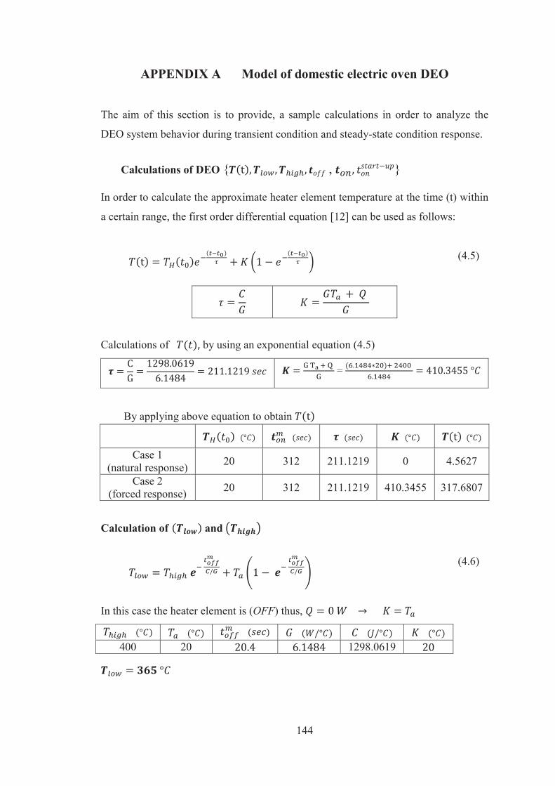
144
APPENDIX A Model of domestic electric oven DEO
The aim of this section is to provide, a sample calculations in order to analyze the
DEO system behavior during transient condition and steady-state condition response.
Calculations of DEO { , }
In order to calculate the approximate heater element temperature at the time (t) within
a certain range, the first order differential equation [12] can be used as follows:
(4.5)
Calculations of , by using an exponential equation (4.5)
=
By applying above equation to obtain
Case 1 (natural response) 20 312 211.1219 0 4.5627
Case 2 (forced response) 20 312 211.1219 410.3455 317.6807
Calculation of and
(4.6)
In this case the heater element is (OFF) thus,
400 20 1298.0619

145
(4.7)
In this case the heater is (ON) thus,
365 20 1298.0619
Set-point ( )
Thus, the ( ) is:
Therefore,
Calculation of Time duration , and
1- Linear Equations
(4.8)
(4.9)
(4.10)
Constant system parameters
400 365 20 382.5 6.1484 1298.0619 2400
Linear Equations Results
0 / 2.4 20.38 265.37 334.35
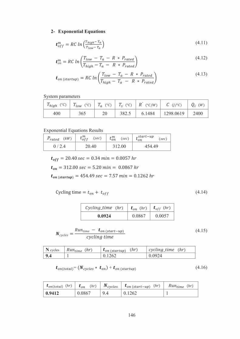
146
2- Exponential Equations
(4.11)
(4.12)
(4.13)
System parameters
′
400 365 20 382.5 6.1484 1298.0619 2400
Exponential Equations Results
0 / 2.4 20.40 312.00 454.49
(4.14)
0.0924 0.0867 0.0057
(4.15)
N cycles 9.4 1 0.1262 0.0924
= + (4.16)
0.9412 0.0867 9.4 0.1262 1

147
Power / Energy Consumption of DEO
= (4.17)
Method
Calculation 0.2081 2.4 0.0867
(4.18)
Run-time
2.2589 2.4 0.9412 1
(4.19)
Electric Heater Run-time
2.4 2.2589 0.9412 1
(4.20)
0.9383 0.0867 0.0924
(4.21)
The Energy consumption by DEO can be calculated as follows:
(4.22)
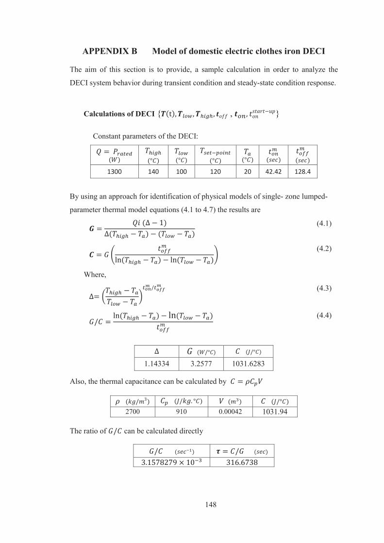
148
APPENDIX B Model of domestic electric clothes iron DECI
The aim of this section is to provide, a sample calculation in order to analyze the
DECI system behavior during transient condition and steady-state condition response.
Calculations of DECI { , }
Constant parameters of the DECI:
1300 140 100 120 20 42.42 128.4
By using an approach for identification of physical models of single- zone lumped-
parameter thermal model equations (4.1 to 4.7) the results are
(4.1)
(4.2)
Where,
(4.3)
(4.4)
1.14334 3.2577 1031.6283
Also, the thermal capacitance can be calculated by
2700 910 0.00042 1031.94
The ratio of can be calculated directly

149
Calculations of DECI { , }
(4.5)
Calculations of , by using an exponential equation (4.5)
=
By applying above equation to obtain, the calculation of
Scenario 1
(natural response) 20 42.42 316.6738 0 17.49
Scenario 2 (forced response) 20 42.42 316.6738 419.0545 70.03
Calculation of temperatures and
(4.6)
In this case the heater is (OFF) thus,
140 20 1031.63
(4.7)
In this case the heater is (ON) thus,
100 20 1031.63
Set-point ( )
Thus, the Dead band value ( ) is
Therefore,
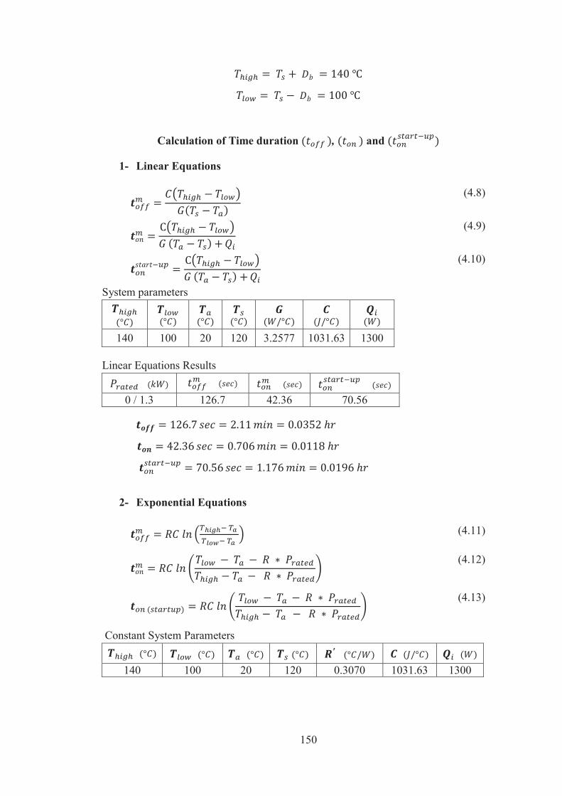
150
Calculation of Time duration , and
1- Linear Equations
(4.8)
(4.9)
(4.10)
System parameters
140 100 20 120 3.2577 1031.63 1300
Linear Equations Results
0 / 1.3 126.7 42.36 70.56
2- Exponential Equations
(4.11)
(4.12)
(4.13)
Constant System Parameters ′
140 100 20 120 0.3070 1031.63 1300
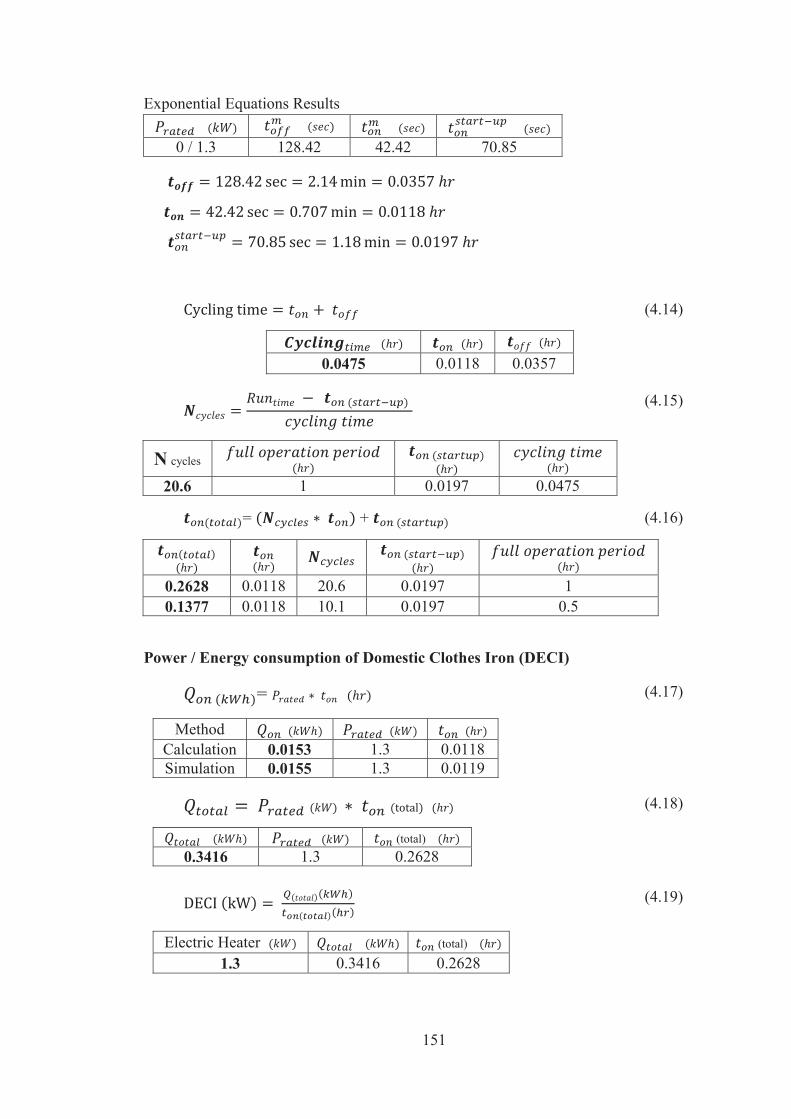
151
Exponential Equations Results
0 / 1.3 128.42 42.42 70.85
(4.14)
0.0475 0.0118 0.0357
(4.15)
N cycles
20.6 1 0.0197 0.0475
= + (4.16)
0.2628 0.0118 20.6 0.0197 1 0.1377 0.0118 10.1 0.0197 0.5
Power / Energy consumption of Domestic Clothes Iron (DECI)
= (4.17)
Method Calculation 0.0153 1.3 0.0118 Simulation 0.0155 1.3 0.0119
(4.18)
(total) 0.3416 1.3 0.2628
(4.19)
Electric Heater (total) 1.3 0.3416 0.2628
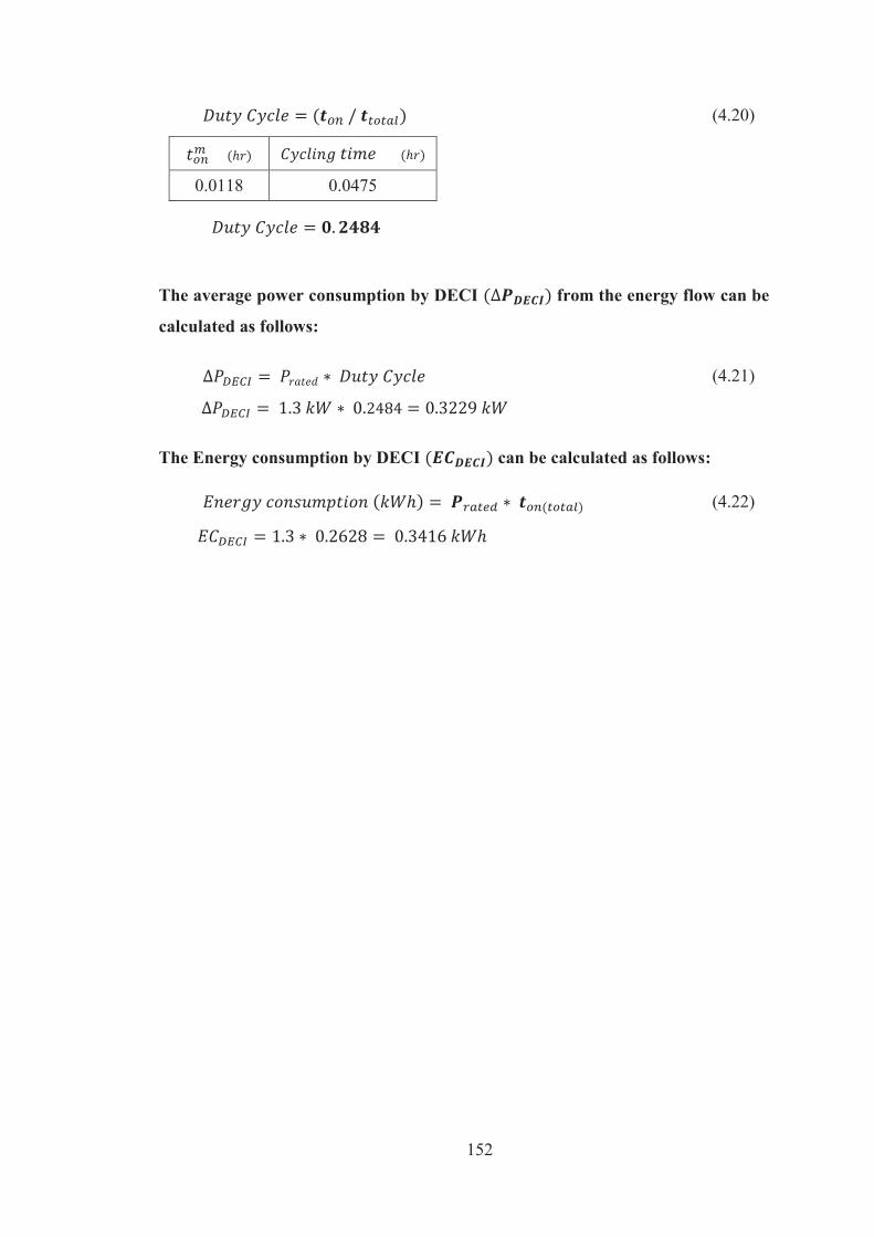
152
(4.20)
0.0118 0.0475
The average power consumption by DECI from the energy flow can be
calculated as follows:
(4.21)
The Energy consumption by DECI can be calculated as follows:
(4.22)
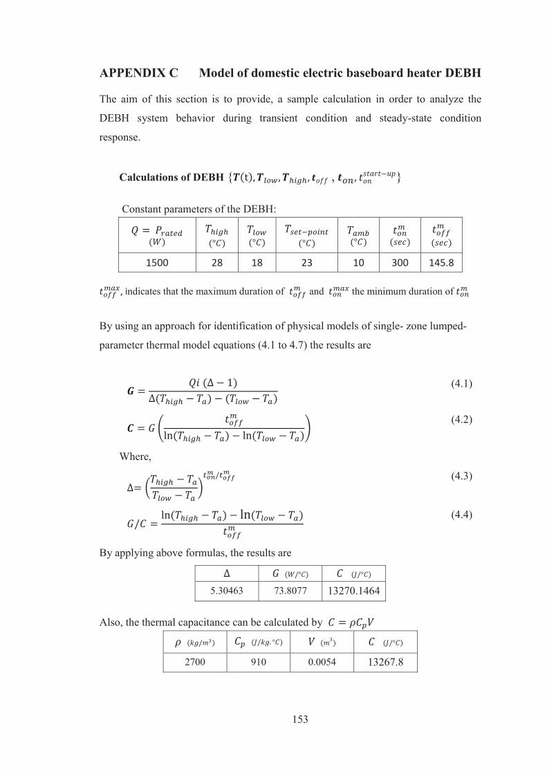
153
APPENDIX C Model of domestic electric baseboard heater DEBH
The aim of this section is to provide, a sample calculation in order to analyze the
DEBH system behavior during transient condition and steady-state condition
response.
Calculations of DEBH { , }
Constant parameters of the DEBH:
1500 28 18 23 10 300 145.8
, indicates that the maximum duration of and the minimum duration of
By using an approach for identification of physical models of single- zone lumped-
parameter thermal model equations (4.1 to 4.7) the results are
(4.1)
(4.2)
Where,
(4.3)
(4.4)
By applying above formulas, the results are
5.30463 73.8077 13270.1464
Also, the thermal capacitance can be calculated by
2700 910 0.0054 13267.8
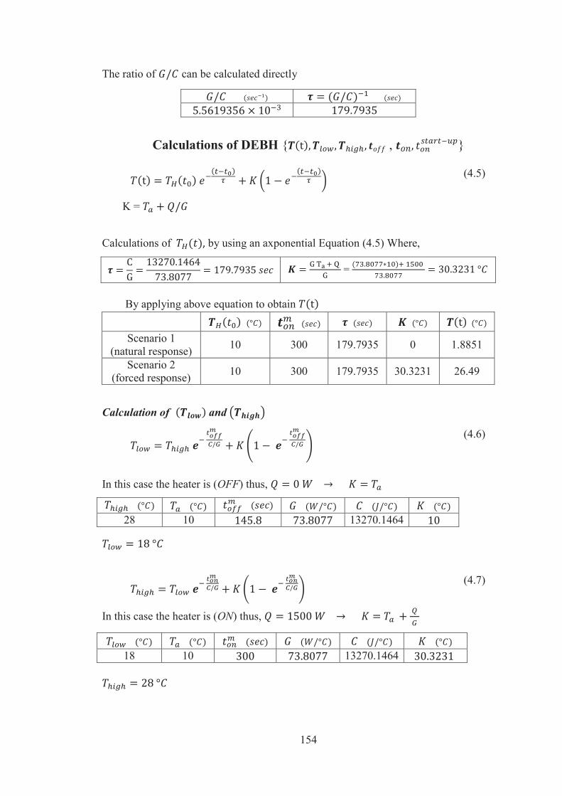
154
The ratio of can be calculated directly
Calculations of DEBH { , }
(4.5)
K =
Calculations of , by using an axponential Equation (4.5) Where,
=
By applying above equation to obtain
Scenario 1 (natural response) 10 300 179.7935 0 1.8851
Scenario 2 (forced response) 10 300 179.7935 30.3231 26.49
Calculation of and
(4.6)
In this case the heater is (OFF) thus,
28 10 13270.1464
(4.7)
In this case the heater is (ON) thus,
18 10 13270.1464
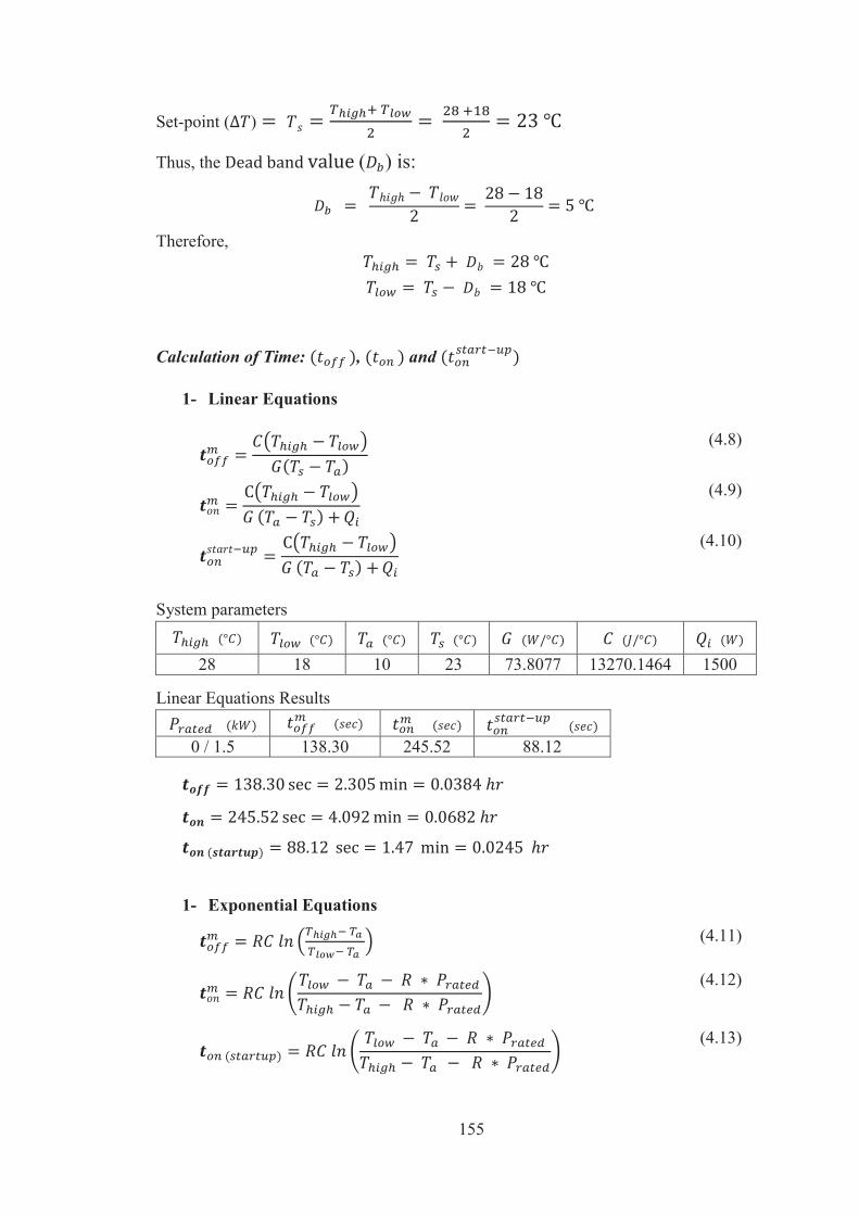
155
Set-point ( )
Thus, the ( ) is:
Therefore,
Calculation of Time: , and
1- Linear Equations
(4.8)
(4.9)
(4.10)
System parameters
28 18 10 23 73.8077 13270.1464 1500
Linear Equations Results
0 / 1.5 138.30 245.52 88.12
1- Exponential Equations
(4.11)
(4.12)
(4.13)
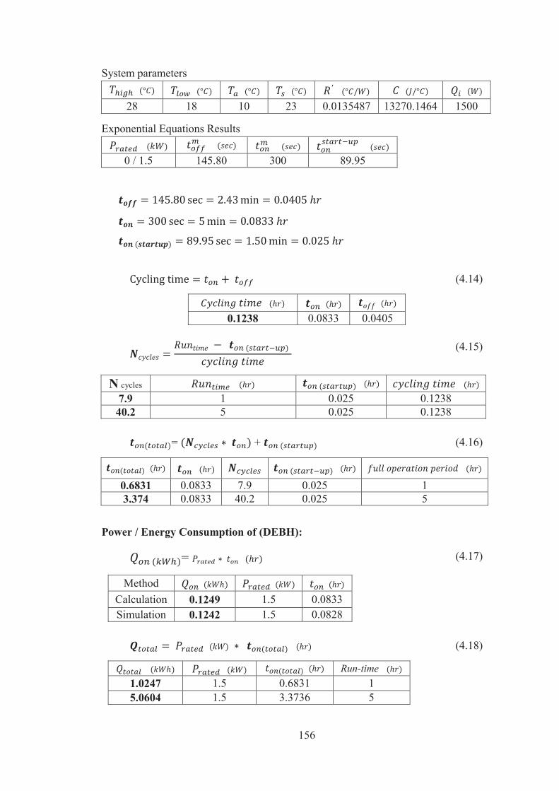
156
System parameters ′
28 18 10 23 0.0135487 13270.1464 1500
Exponential Equations Results
0 / 1.5 145.80 300 89.95
(4.14)
0.1238 0.0833 0.0405
(4.15)
N cycles 7.9 1 0.025 0.1238 40.2 5 0.025 0.1238
= + (4.16)
0.6831 0.0833 7.9 0.025 1 3.374 0.0833 40.2 0.025 5
Power / Energy Consumption of (DEBH):
= (4.17)
Method Calculation 0.1249 1.5 0.0833 Simulation 0.1242 1.5 0.0828
(4.18)
Run-time 1.0247 1.5 0.6831 1 5.0604 1.5 3.3736 5
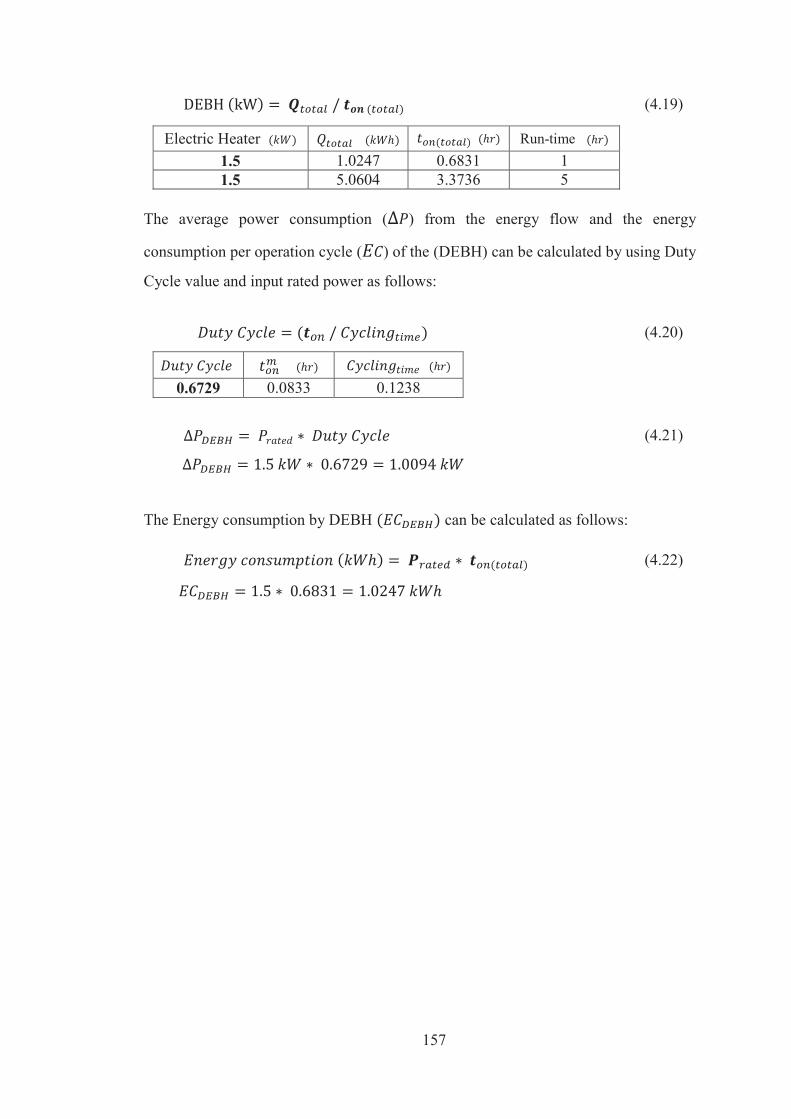
157
(4.19)
Electric Heater Run-time 1.5 1.0247 0.6831 1 1.5 5.0604 3.3736 5
The average power consumption ( ) from the energy flow and the energy
consumption per operation cycle ( ) of the (DEBH) can be calculated by using Duty
Cycle value and input rated power as follows:
(4.20)
0.6729 0.0833 0.1238
(4.21)
The Energy consumption by DEBH can be calculated as follows:
(4.22)
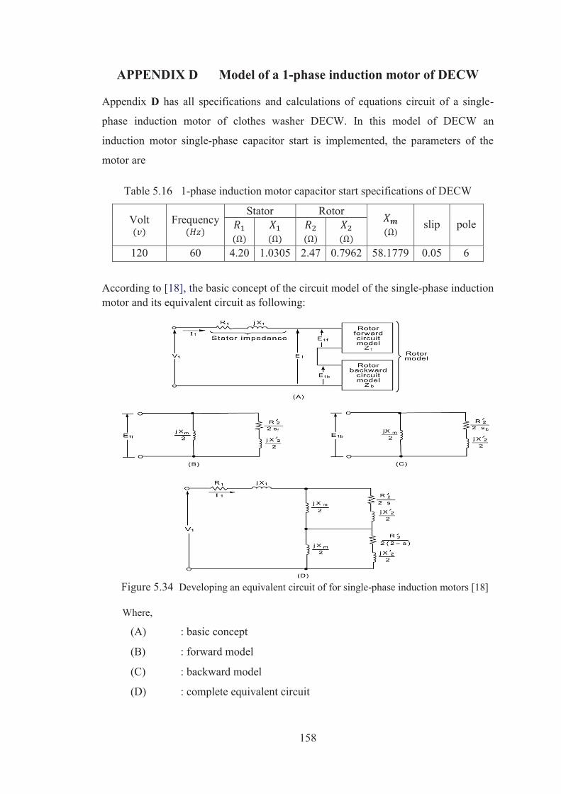
158
APPENDIX D Model of a 1-phase induction motor of DECW
Appendix D has all specifications and calculations of equations circuit of a single-
phase induction motor of clothes washer DECW. In this model of DECW an
induction motor single-phase capacitor start is implemented, the parameters of the
motor are
Table 5.16 1-phase induction motor capacitor start specifications of DECW
Volt
Frequency
Stator Rotor ) slip pole
120 60 4.20 1.0305 2.47 0.7962 58.1779 0.05 6
According to [18], the basic concept of the circuit model of the single-phase induction motor and its equivalent circuit as following:
Figure 5.34 Developing an equivalent circuit of for single-phase induction motors [18]
Where,
(A) : basic concept
(B) : forward model
(C) : backward model
(D) : complete equivalent circuit
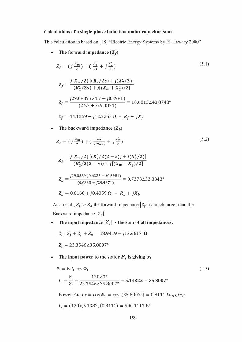
159
Calculations of a single-phase induction motor capacitor-start
This calculation is based on [18] “Electric Energy Systems by El-Hawary 2000”
The forward impedance ( )
(5.1)
=
The backward impedance ( )
(5.2)
=
As a result, the forward impedance is much larger than the
Backward impedance The input impedance is the sum of all impedances:
=
The input power to the stator is giving by
(5.3)
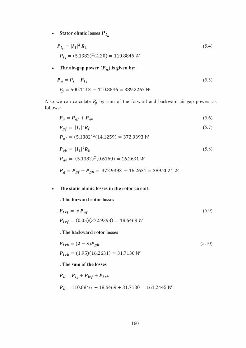
160
Stator ohmic losses
(5.4)
The air-gap power is given by:
(5.5)
Also we can calculate by sum of the forward and backward air-gap powers as follows:
(5.6)
(5.7)
(5.8)
The static ohmic losses in the rotor circuit:
. The forward rotor losses
(5.9)
. The backward rotor losses
(5.10)
. The sum of the losses
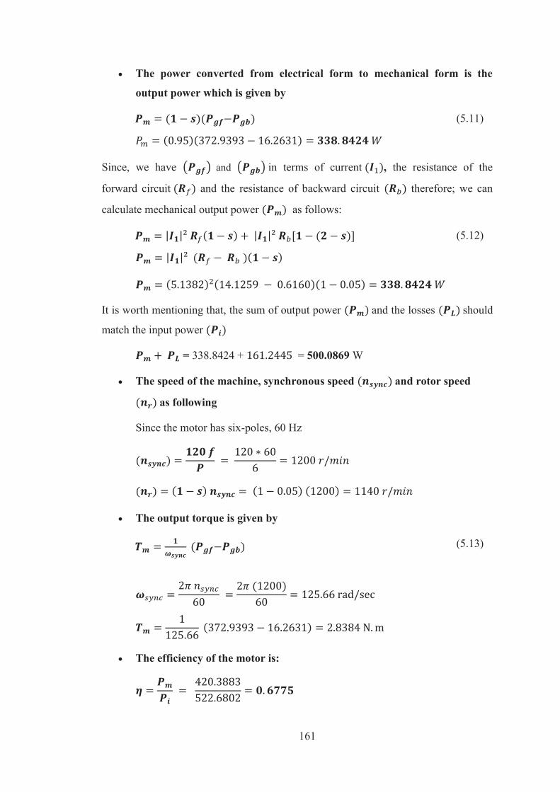
161
The power converted from electrical form to mechanical form is the
output power which is given by
(5.11)
Since, we have and in terms of current , the resistance of the
forward circuit and the resistance of backward circuit therefore; we can
calculate mechanical output power as follows:
(5.12)
It is worth mentioning that, the sum of output power and the losses should
match the input power
= 338.8424 + = 500.0869 W
The speed of the machine, synchronous speed and rotor speed
as following
Since the motor has six-poles, 60 Hz
The output torque is given by
(5.13)
The efficiency of the motor is:
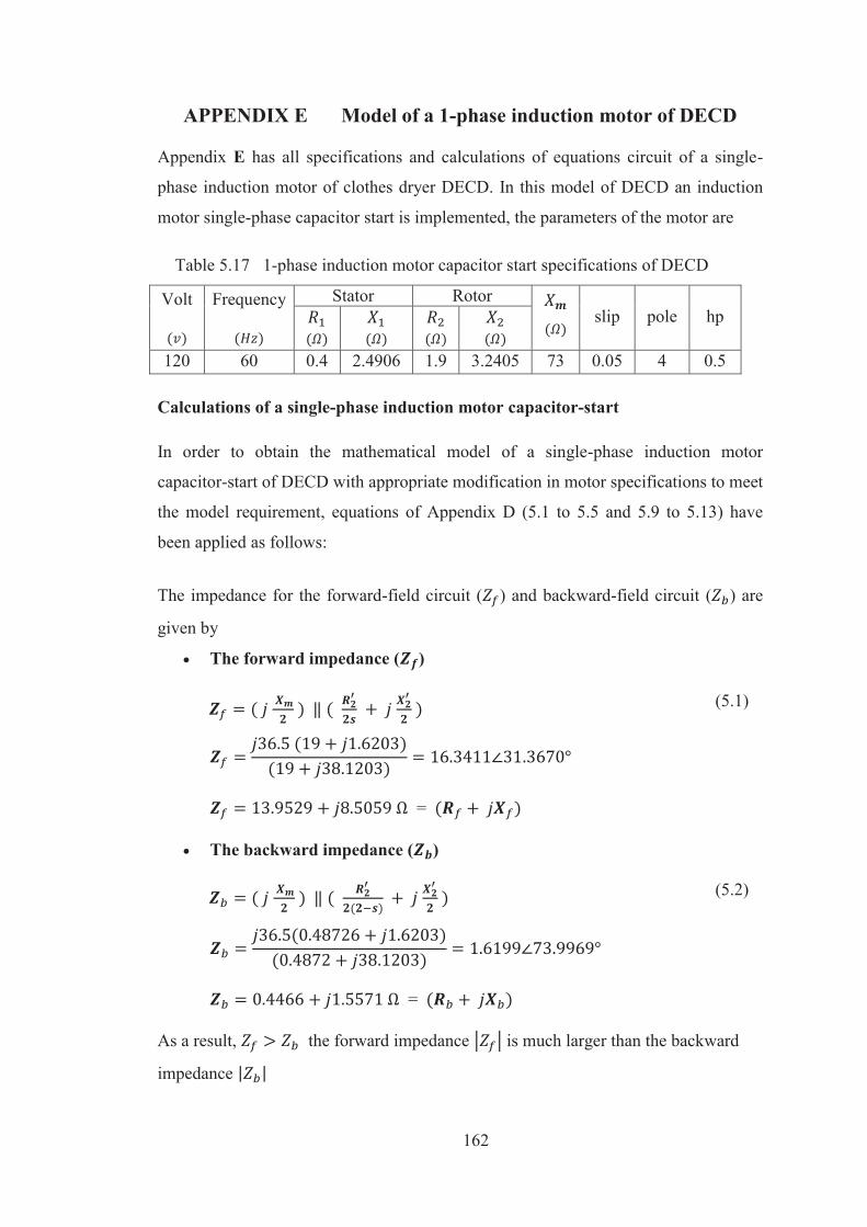
162
APPENDIX E Model of a 1-phase induction motor of DECD
Appendix E has all specifications and calculations of equations circuit of a single-
phase induction motor of clothes dryer DECD. In this model of DECD an induction
motor single-phase capacitor start is implemented, the parameters of the motor are
Table 5.17 1-phase induction motor capacitor start specifications of DECD
Volt
Frequency
Stator Rotor
slip pole hp
120 60 0.4 2.4906 1.9 3.2405 73 0.05 4 0.5
Calculations of a single-phase induction motor capacitor-start
In order to obtain the mathematical model of a single-phase induction motor
capacitor-start of DECD with appropriate modification in motor specifications to meet
the model requirement, equations of Appendix D (5.1 to 5.5 and 5.9 to 5.13) have
been applied as follows:
The impedance for the forward-field circuit ( ) and backward-field circuit ( ) are
given by
The forward impedance ( )
(5.1)
=
The backward impedance ( )
(5.2)
=
As a result, the forward impedance is much larger than the backward
impedance
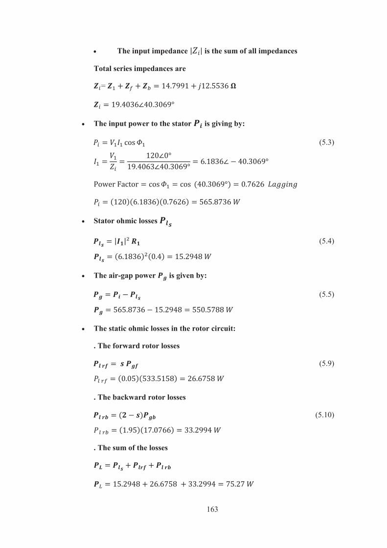
163
The input impedance is the sum of all impedances
Total series impedances are
=
The input power to the stator is giving by:
(5.3)
Stator ohmic losses
(5.4)
The air-gap power is given by:
(5.5)
The static ohmic losses in the rotor circuit:
. The forward rotor losses
(5.9)
. The backward rotor losses
(5.10)
. The sum of the losses
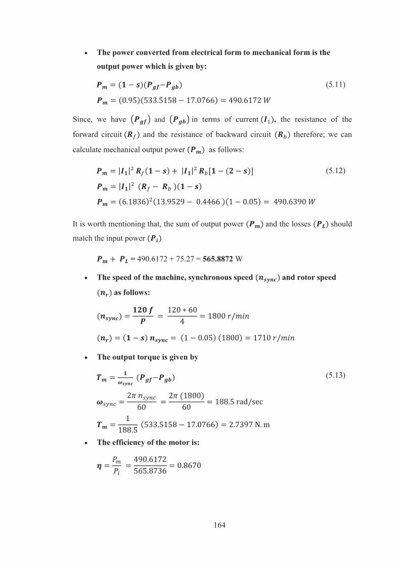
164
The power converted from electrical form to mechanical form is the
output power which is given by:
(5.11)
Since, we have and in terms of current , the resistance of the
forward circuit and the resistance of backward circuit therefore; we can
calculate mechanical output power as follows:
(5.12)
It is worth mentioning that, the sum of output power and the losses should
match the input power
= 490.6172 + 75.27 = 565.8872 W
The speed of the machine, synchronous speed and rotor speed
as follows:
The output torque is given by
(5.13)
The efficiency of the motor is:
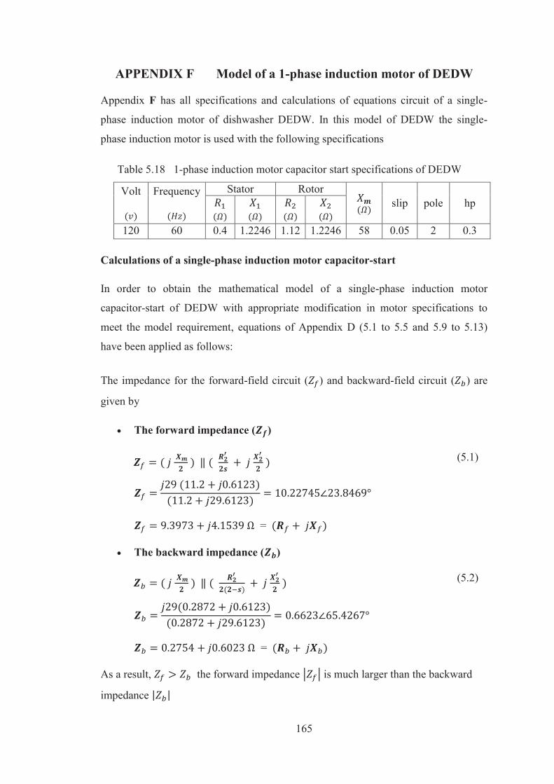
165
APPENDIX F Model of a 1-phase induction motor of DEDW
Appendix F has all specifications and calculations of equations circuit of a single-
phase induction motor of dishwasher DEDW. In this model of DEDW the single-
phase induction motor is used with the following specifications
Table 5.18 1-phase induction motor capacitor start specifications of DEDW
Volt
Frequency
Stator Rotor slip pole hp
120 60 0.4 1.2246 1.12 1.2246 58 0.05 2 0.3
Calculations of a single-phase induction motor capacitor-start
In order to obtain the mathematical model of a single-phase induction motor
capacitor-start of DEDW with appropriate modification in motor specifications to
meet the model requirement, equations of Appendix D (5.1 to 5.5 and 5.9 to 5.13)
have been applied as follows:
The impedance for the forward-field circuit ( ) and backward-field circuit ( ) are
given by
The forward impedance ( )
(5.1)
=
The backward impedance ( )
(5.2)
=
As a result, the forward impedance is much larger than the backward
impedance
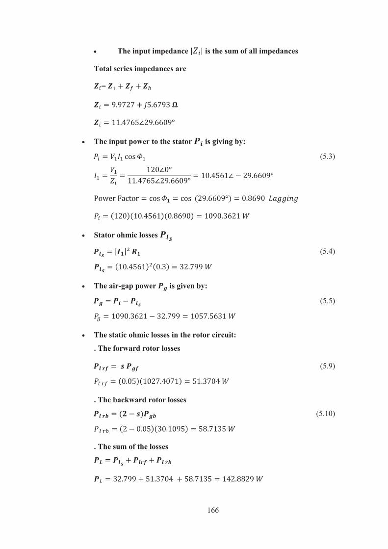
166
The input impedance is the sum of all impedances
Total series impedances are
=
The input power to the stator is giving by:
(5.3)
Stator ohmic losses
(5.4)
The air-gap power is given by:
(5.5)
The static ohmic losses in the rotor circuit:
. The forward rotor losses
(5.9)
. The backward rotor losses
(5.10)
. The sum of the losses
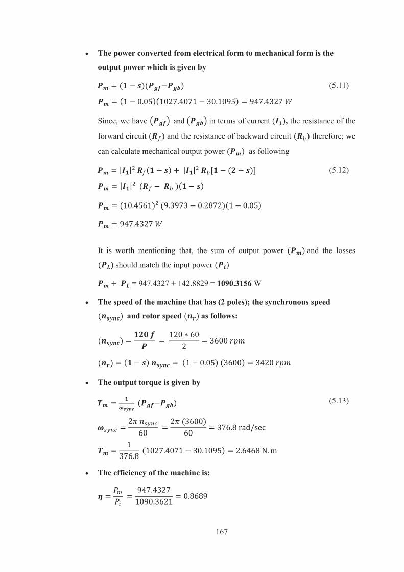
167
The power converted from electrical form to mechanical form is the
output power which is given by
(5.11)
Since, we have and in terms of current , the resistance of the
forward circuit and the resistance of backward circuit therefore; we
can calculate mechanical output power as following
(5.12)
It is worth mentioning that, the sum of output power and the losses
should match the input power
= 947.4327 + 142.8829 = 1090.3156 W
The speed of the machine that has (2 poles); the synchronous speed
and rotor speed as follows:
The output torque is given by
(5.13)
The efficiency of the machine is: