This document is made available electronically by the Minnesota Legislative Reference Library as part of an ongoing digital archiving project. http://www.leg.state.mn.us/lrl/lrl.asp

MODELING STRATEGIES FORPROJECTING VEGETATION TRENDS

IN AN AREA OF NORTHEASTERNMINNESOTA

May, 1977

! •

MODELING STRATEGIES FORPROJECTING VEGETATION TRENDS

IN AN AREA OF NORTHEASTERNMINNESOTA

written by

Reed Sloss

for the

Regional Copper-Nickel Study

and submitted to

Dr. E.J. CushingDept. Ecol. and Behav. BioI.College of Biological SciencesUniversity of Minnesota

for academic credit

in May, 1977

- -c ontents _.-

Introduvv.J..on

Successional models

Succession in the Mine Site

The model of Shugart ~ ale (1973)(description and problems)

The cover-state replacement process(introduction of an alternate

model)

Applying the alternate model

Modeling management in the MlNESlTE Area

Modeling natural succession in theMlNESlTE Area.

Fire, drought, and epidemics

Conclusion,.'

Literature cited

Appendix: Solving a system of lineardifferential equations

1-8

3-5

5-8

9-15

16-20

21-32.

22-29

29-32

31

33-34

35-36

37-40

In 1974 at the request of the Minnesota Environmental.

Quali-~ Council, the State Legislat~re established the Regional

Copper-Nickel St~dy to conduct a regional study of the possible

impacts resulting from potential copper~nickel development in

northeastern Minnesota. A major objective of this study is

~o characterize terrestrial life as it exists now and,will

exist in the future prio,r to development. The accomplishment

of this objective is dependent upon the development of a process

that will accurately predict trends in vegetation--i.e. a math­

ematical model that simulates succession. In this report I

attempt to explore the possibilities of modifying proposed

successional models found in the literature to suit this purpose.

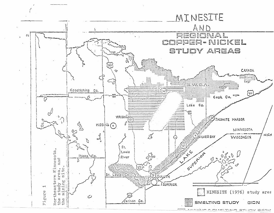
Simplifying the task of 'characterizing terrestrial life

in a 2000-square-mile study area, the Copper-Nickel Study team

has focused its attention on a 560-square-mile area where mining

development is most probable and for which data are immediately

available (Fig. 1). Such data include the land-ownership, soil

type, and vegetation cover type assigned to each one-hectare

unit within this area. It is this MlNESITE Area for which

successional modeling will be examined (MlNESITE, 1976).

1

E

SIT

tM,r~l CAA/\DA

Af0.1!;~I!;?::~/"?_---W:::r~SN'-.j _~

I

~

~

------------ ... , -_ .

.\\---

[I~

N ----....... ~- '" -, - r-~i'.r-

If \··~·····f\~~~l. ~.t·1 cj" 1~...~ <~Jt::::j)j::::;:::I:~.

!~t

I, l, \ /,,; Lai\'e Co. IL' /I ~... " (;' ~"\m . ."

" A -J--- ~! V\i\aa{4§s:: .': <' /' '.I. @ ( . ;,'i' '; ,. :%/r"'ONITE HN\80R /HliaeJt-!G f. , ,Ir-r- .... ;,~ ·

I \ I 'Y , • 'y> /01 ~. ~-~'-r-t- ,y.r:«,\~ MlNNESOTA.

j ! ) Jf · 6 ~~ '~~VEIlBAV /" WIS(ONSIN-7 M1Cti

91

I I: &~k /' /I ~ : ~~~)\ ..,./

i \ LO~li! ~ .1 .~. ~~~~ /(. • if D /g'd ..~O._.-! : CJ;:::J , <::.l~~~ 0- ,.,./ ,0 .J\"Q 0 D e;, ~ /CD :=: ~~. -~. ~"\ \:-, './ ~ u a f:::/},,-y§ cd ,. I :>A~ ~~\'~~ .~~ AA Y'). ..~. ~~, 0 Cr-S c1

•., ... ill I ~~~.,~\'~ ~ D~" \?' /" tj.J ~~ ro -P I I ~~%~~~ t:'~~" ,. / /~.' ~.~ ~!:~..t'i~~~0%~' ~ / <\~j,~r~\~LuL .h cD I .~\~\ '. '.,,, "h\' •. . T ' nQ) b.D I ~:\\·':.\J.,.r<.. " ., I.p :>. r I " "\" '. j '1- /

M (j)''O .~ ' ,":. ~'.I;.:) .I SUPEf\lDf\ j "> l' -_?' •cd .-.( h : )\~\

~, ~ t·g l ~,. ...' I MlNESITE (1976) study are2~+.~ (;) Ie.

~ ~ ~ l ..-e;rlton Co., rmEl____~ ~ 7~._~_~_~~_~__~_________ r.~.~~··~··~·- ~ 5ME~i~G STUDY GIO

Successional Models.

Modeling strategy is dictated by the reali ty to be described

and an understanding of that reality. Given that:

generali-'cy measures the applicabili ty of the model indifferent locations,

realism measures the degree to which the model correspondsto the biological concep~s it represents, and

preci.sion is the closeness of model predictions to observed data,

three possible modeling s~rat~gies exist according to Levins' (1966)

widely-quoted classification.. Each strategy sacrifices one of

the above qualities so that the other two are maximized. Because

the basic purpose of a successional model in our context is the

accurate prediction of changes in vegetation over a relatively

short period of time (25-100 years) in a particular region of

northeastern Minnesota, a modeling strategy that sacrifices

generality to realism and precision seems most appropriate. In

this case, the most important parameters of these successional

processes need to be identified and accurately measured. Yet

succession is a poorly understood phenomenon, and consequently

it is difficult to identify the parameters let alone isolate the

more important ones. Hence, modelers of succession have resorted

to using the second modeling strategy (sacrificing realism to

generality and precision) in hopes that the unrealistic assumptions

implied by the general mathematical equations they use will affect

one another so that usefulL'predictions from the model can be obtained.

"'-.

Proposed successional models have talten on a varie"'ty of

forms. As outlined by May (1973), general mathematical models

are of four basic typese In both deterministic models, where

the dependent variables are continuous, and stochastic models,

~here they are discrete, the independent variable may be either

continuous (as in differential equations) or discrete (as in

difference equations). In a successional model proposed by

Shugart,Crow, and Hett (1973), a continuous dependent variable--

the acreage of land dominated by a particular forest type--depends

on the continuous variable of time. The flow of land between forest

type compartments is described by a set of first-order linear

differential equations. Similarly, Bledsoe and Van Dyne (1971)

used such a compartment model to describe the abstract flow of

energy or biomass from species to succeeding species during

oldfield succession. In the stochastic models of Horn (1975)

and Waggoner and Stephens (1970 )., the probabilities that a certain

tree or plot dominated by a particular species is replaced by

another is described by a finite Markov process. The dependent

and independent variables are discrete. In the successional

model by Leak (1970), probabilities that each tree in a forest

will either produce one offspring that becomes established,

produce no offspring, or die over the discrete interval of one

year are given by species-specific birth and death rates. Finally,

a complex stochastic model that indirectly simulates forest

succession by modeling tree growth was proposed by Botkin, J'anak,

and Wallis (1972). The model lumps deterministic equati.ons for

radial growth and growth in height. competition, and environmental

effects. But tree birth and death are determined by species-

specific probabilities so that both the dependent variable, the

number of trees on a plot, and independent variable--time--are

discrete.

Succession on the Mine Site.

Because the MINESITE Area is relatively large and thus

heterogeneous, the most appropriate model would seem at the

outset to be a form like that of Shugart et e1. (1973) or a

Markov model scaled up from describing the dynamics within a

particular forest to describing the dyna~ics of many forest

types within a region. In either case, the very large number

of concrete vegetation types occupying particular unit areas

are grouped into a finite number of abstract cover types.

Succession is then modeled in some deterministic or stochastic

fashion, while the total area of a region, constant over time,

is partitioned among cover types. The basic structure of this

model is described diagrammatically by what Shugart et ala (1973)

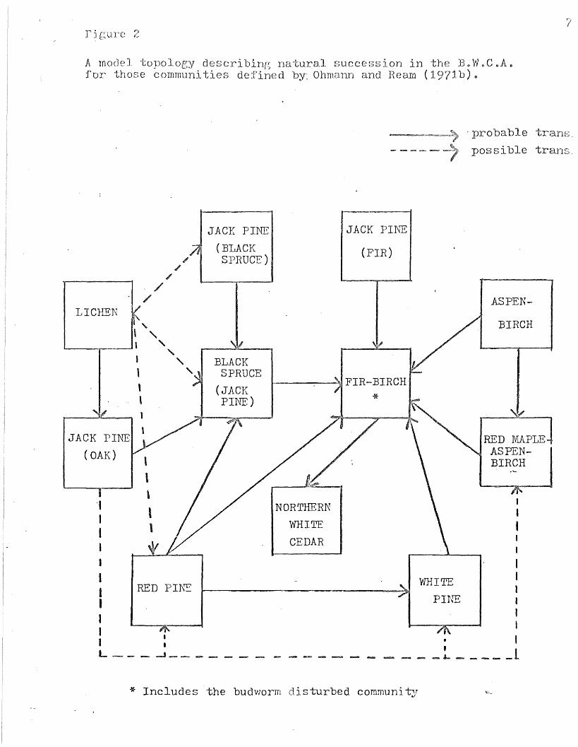
term a "model topology." In such a diagram (Fig. 2), the boxes

represent particular cover types, whereas the arrows represent

.5

the flow of area from dominance by one cover type to that

another.

6

A logical approach on the MlNESITE B. would involve ling

succession as it occurs naturally in the absence of natural or

unnatural perturba~ions. Disturbances could then be incorporated

later. Two basic problems are inherent in this technique. First,

natural succession in northeastern Mim1esota has not, as ye-t, been

well documented. Two recent studies (Heinselman 1973, Ohmann and

Ream 1-971a, 1971b) examine natural succession in the Boundary

Waters Canoe Area (BWCA) north of the MINESITE Area. A model

topology on the probable dynamics of eleven statistically-defined

cover types, is displayed in Figure 2. The magnitude of each

arrow is not known. Stressing the importance of fire in natural

ecosystems, Heinselman questions the existence of a true climax

conrrnuni ty for the area. Rather he views- climax on a regional

scale as a mosaic of cover types with no appreciable n~t change

in the total area occupied by each over time in the absence of

fire exclusion by man.

A second problem of modeling succession exists because the

forests on the MlNESITE Area are not 'virgin' (i.e. undisturbed

by European man). Natural succession may not be predictable even

by the best models for this intensively managed area where

L....

clearcutting is the most fre'quently used silvicultural system.

'7

A model topology describing natural succession in the B .. W C A.l'Dr those communities defined by~ Ohmann and Iteam (1971b) •

. probable trans.

pas sible trans.

PIKE

III)

I

IIII,II

_~ l

\'-mITE

NORTHERNWHI~~

CEDAR

RED PI1\~

IIL- __ --I _

JACK PINE JACK PII'1~

(BLACK (FIR)" SPRUCE)

//

// ASPEN-

LICHEN'\. BIRCH,", ,

"I " BLACK, , SPRUCE, (JACK, PINE) *

JACK PI1\TE RED MAPLE

(OAK) ASPEN-BIRCH

'* Includes the budworm disturbed COffiITlUni ty

Indeed, the accuracy of predicting future trends in vegetation

will rely heavily on an abili ty to predict fut-ure management

policies.

Within the framework of the modeling objective and these

associated problems, the remainder of th~s report will deal

with the advantages, disadvantages, and possible alternatives

to the deterministic model of Shugart et ale (1973).

8

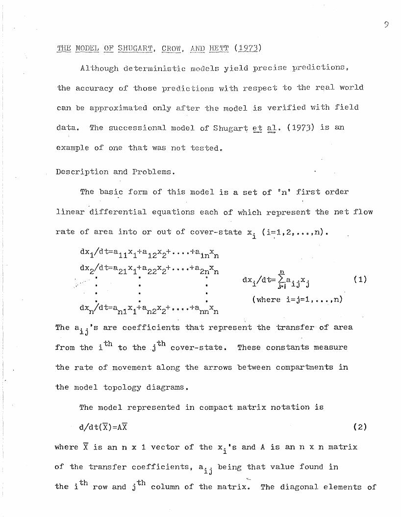
~rHE MODEL OF-- --- -- ---~-----

Although deterministic Is yield c predictions,

9

the accuracy of those pre tions with respect to the r~al world

can be approximated only after the model is verified with field

data. The successional model of Shugar~

example of one that was not tested.

Description and Problems.

ale (1973) is an

The basic form of this model is a set of in' :first order

linear differential equations each of which represent the net :flow

rate of area into or out of cover-state x. (i=l,2,o •• ,n).1

dXl/dt=al1xl+a12x2+o .•• +alnxn

dX2/dt=a21xl+a22x2+····+a2nxn

•

•• •dXn/dt=anlxl+an2x2+····+annxn

n

dX./dt= La. ~X.1 j .. J lJ J

(where i=j=l, •• ~,n)

(1)

The a .. 's are coefficients that represent the transfer' of arealJ

f' th .th t th .th t t Th t trom e 1 a e.J cover-s a e. ese cons an 8 measure

the rate of movement along the arrows bet~een compartments in

the model topology diagrams.

The model represented in compact matrix notation is

d/dt(X)=AX (2)

where X is an n x 1 vector of the x. •s and A is an nxn matrix1

of the transfer coefficients, a .. being that value found inlJ.th .th

L.

the 1 row and J column of the matrix .. The diagonal elements of

10

this matrix (a .. ) have negative values and represent an output11

thflow of area from the i state or these values are zero in the

case of a climax state This flow is partitioned as i~puts of

area among the remaining states 80 thai; the sum of all column

elements is zerOe

(3)(for all i, j=l'lIme,n)n

La..=0i,.=\ lJ

Applying equation :3 over all colums implies that area can neither

enter nor leave the system or the region being modeled, which is

reasonablee Such a system is said to be closed (Bledsoe and

Van Dyne, 1971) and has the general solution:

n Aotx.=}:C .. e J ,

1 j::1 1J

where the ~.'s are the eigenvalues of matrix A and the C.. 'sJ lJ

(4)

are constants that depend on the initial distribution of ~he

region's area among the cover-states.

Each defined forest type '01' the region in question is

further divided by Shugart et ~. into three size classes--

seedling, pole, and saw-timber. Growth in these vegetation

~es is then simulated over the region if each of the size

catagories represents a separate cover-state and thus one in

the set of differential equations. As growth proceeds over

time, area would flow from seedling, through pole, to the

saw-timber size cover-state for any particular forest type.

The task of obtaining a matrix of trm!sfer coefficients

simplified by assuming that one forest type replaces 'another

only after that earlier forest type has reached saw-timber size m

The ae .§s are ~hen found by first measuring average gro~th inlJ '

stands that make up a forest type and, second, by finding the

probabilities- that one forest type is succeeded by another

(possibly measured by an average number of stems of the latter

found in the understories below the ~orrner)", The first step

isolates the diagonal elements of the coefficient matrix,

simplifying equation 1 to:

11

dX./dt=a .. x. with the solution1 11 1

-a·" tx.=x. e 111 10

where x. is the initial acreage in the i th cover-state. 'The10

diagonal coefficient, a .. , then is the reciprocal value of the11

time i~ takes for 63 percent of the initial area to leave the

i th cover-state because for a .. =l/t,11

- (a .. ) ( l/a .. ) -1 37 ( " )x.t=x. e 11 11 =X. e =. x. iD

1- 10 10 10

Coefficients other than the diagonals are determined by mult-

(6)

iplying the probability (p .. ) that the jth cover-state replaces1J

the i th forest saw-timber size cover-state by the diagonal

element of the latter:

aij=Pijaii·

Some time constants (l/a .. ) and transition probabilities11

(p .. ) used by Shugart et ale (1973) are shown in Tables 1 and 2.1J - -

According to the form of the model just described, the

'rable 1

darea ocsuccee

rcentars)eomes OC

e (1

The time consby one coveE.Lccording j~o S

Forest seedl

Aspen--- ---------------J

20 65

Jack pine 30 30 701------------;--------

Fir~spruce 30 45 cl

Northern hardwoods 100 100 2501-------------1---- -~-- ------- - --- ----~ ------11

Red pine

White pine

Black spruce

WamapaCK

Whi te cedar -..

100

100

80

100

57

100 100 300

150 200 1}50

80 80 24-0

100 90 290

1.15 1000 1172

Table 2

The probabilities that the row cover~£tate8 are succeeded by thecoluw1 cover-states according to Shug~rt ale (1973).

Succeeding state Birch-

.~ Red White N-&hard- Sugar Fir- Black ash- Whi ~e

'/;~% '/; nine nine woods HernIoe}r maple spruce spruce hemlock cedarAspen lIf~5 .55 .4

---:

-- - -~---,--

Jack pine 1-.. a

~- - - -- - _._._-- - --- .~-_.-

~J- ----.- -- -----

f{eq pine 1 .. 0- ---- -~_._----- --------- -- -- - ~- --...----

White·7 .2 .1pine I

;

.- -----_.~-- - -- -- ---- --..-

Northern 1.0hardwoods l

--- ----- ------_._--- f

Tamarack .8 .2....-- -- - ------ ----- ---- _._---------- ----~-_...- ---._-- - I

Whi te--i

1 .. 0 i

cedar !:

Statebeing

d

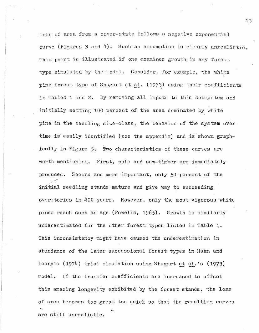
loss of area from a cover-s follows a e

:1

curve (Figures 3 and 4). Such an assumption is cle unre

This point illustrated if one examines growth in any fore

tJ~e simulated by the model. Consider, for example, the white

pine forest type of Shugart ~,,(1973) using their coeff'icients

in Tables 1 and 2. By removing all inputs to this subsystem and

initially setting 100 percent of the area dominated by white

pine in the seedling size-class, the behavior of the system over

time is· easily identified (see the appendiX) and is'shovffi graph-

ically in Figure 5. Two characteristics of these curves are

worth mentioning. First, pole and saw-timber are immediately

produced. Second and more important, only 50 percent OI the

initial seedling stan~s mature and give way to succeeding

overstories in 400 years. However, only the most vigorous white

pines reach such an age (Fowells, 1965). Growth is 'similarly

underestimated for the other forest. types listed in Table ~.

This inconsistency might have caused the underestimation in

abundffi1ce of the later successional forest types in Hahn and

Leary's (1974) trial simulation using Shugart et al.'s (1973)--model. If the transfer coefficients are increased to o£fset

this amazing longevity exhibited by the forest stands, ~he loss

of area becomes too great too quick so that the resulting curves

are still unrealistic.

1LI

Pigure J

s as implet al model

PercentTa-marack 60seedli:ngare a left 4·0

80

20

o '''''---r--_---.--"ii--_,20 .40 60 80 100

Time (years)

100

~rhe 58

area

-0 4---......-~_-_--__-_20 40 60 80 iDa

Time (years)

80

20

The loss of jack pine seedlarea to the j pole CDver-state as implied by the Shugartet tl model (197J).

100

-PercentJack pine ·60seedlingarea left 40

Figure 5

The decay of area from a white pine cover-state subsystem of theShugart et ale model (1973).- -

100

90

80

70

50

40

30

20

10

100L..

200 JOO

Time (years)

XXX){tXX seedling.

Ji.,(j,aJif1JJ,. pole- timber

oo00סס0 saw -timber

500

How does a curve behave which describes, over time, the

16

decrease in t;he area of a cover~· that results from stand

growth and mortality? As I have just shovm, the assumption that

the curve is negatively exponen'tial (as in -the model of Shugart

et m (1973)), is unrealistic. Nevertheless, such a simpli-

fication is probably acceptable over a very large and hetero-

geneous region. Over such a region, areas occupied by each

forest type are composed of many different stands of varying

ages and composition, occur on varying soil types and topography,

and are subjected to varying climatic and other environmental

conditions. These many stands are analogous to a population

of phenotypically varying individuals. Mortality in such a

population is often described by a continuous constant percent

decrease in numbers over time, i.e. a negative exponential

function (Lotka, 1925). The exponential curve then is a sim-

plification of the complex cover-state behavior that attempts

to account for heterogeneity over the region.

Instead of accounting for heterogeneity outright, an

alternative approach to describing the cover-state replacement

process involves building heterogeneity into a simpler math-

ematical system that describes replacement in a very homogeneous

region. For reasons that will become evident as this discussion

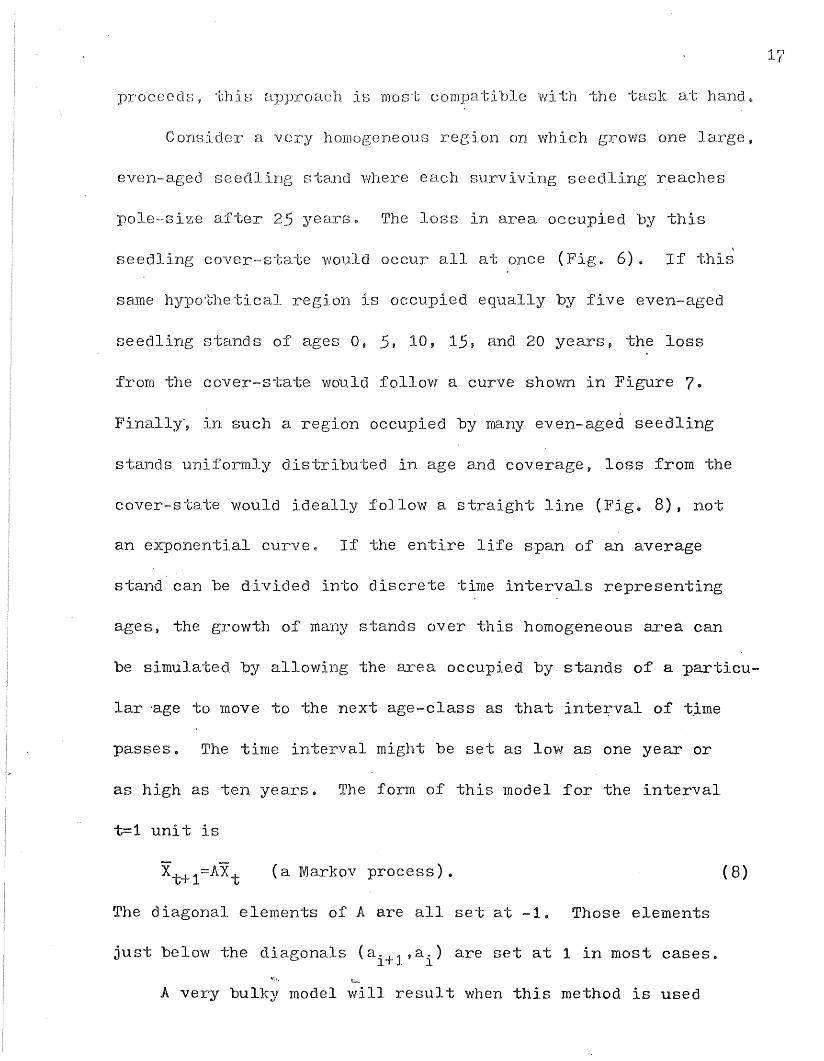
proceeds, 'this most c the at hand

Cons homogeneous region on which grows one large,

even-aged se stand where each surv seedling reaches

pole-size a.fter arse The loss in area occupied by this

\

seedling cover-state would occur all at once (Fig. 6). 1£ this

sarne hypothe region occupied equally by five even-aged

seedling stands of ages 0, 5, 10, 15, and 20 years, the loss

£rom the cover-state would follow a curve shovm in Figure 7.

Finally', in such a region occupied by many even-aged seedling

stands uniformly distributed in age and coverage, loss from the

cover-state would ideally follow a straight line (Fig. 8), not

an exponential curvee If the entire life span of an average

stand can be divided into discrete time intervals representing

ages, the growth of many stands over this homogeneous area can

be simulated by allowing the area occupied by stands of a -particu-

lar 'age to move to the next age-class as that interval of t~me

passes. The time interval might be set as low as one year or

as high as ten years. The form of this model for the interval

t=1 uni t is

(a Markov process). (8)

The diagonal elements of A are all set at -1. Those elements

just below the diagonals (a O +1 ,a.) are set at 1 in most cases.1 J. 1

It:....

A ve1--Y bulky model will result when this method is used

18

3010 15 205

20

80

60

%1. 00 ..d r, '-'"V" ,~. n r"f4. t}OOt::JfJ.X?O:T(>o:::e>CC:OQO'~~xtl

FiglJre 6

Loss in ar~~ from a seedlingcover-state i~ a homogeneousregion is occupied by oneeven~~aged seedling stand",-1t-

Time (years)

20

40

60

f---,----,.----r-----r--'~.~

5· 10 15 20 25 30

%area

100J,,{, 8<,,!

region ~

itt=()

Figure 7

Loss in area from a seedlingcover-state if a homogeneousis equally occupied by 0, 510, 15, and 20 year old even­aged seedling stands.*

Time (years)

Figure 8

Loss in area from a seedlingcover-state if a homogeneousregion is equally occupiedby seedling stands of allage9 between a and 25 years.*

% area100

80

60

40

20

*In this homogeneous region,surviving- seec.lings becomepole size in 25 years.

5 10 15 20 25, 30>:>,

Time (years)

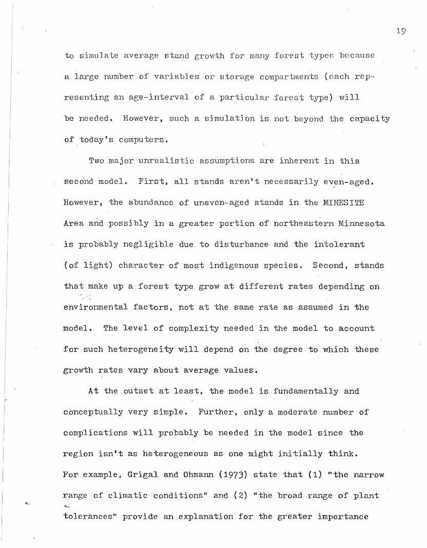
to simulate average stand growth for many forest types because

a large number of variables or storage compartments (each rep-~

resenting an age-interval of a particular forest type) w,ill

be needed. However, such a simulation is not beyond the capacity

of today's computers.

Two major unrealistic assumptions are inherent in this

second model. First, all stands aren't necessarily ev~n-aged.

However, the abundance of uneven-aged stands in the MINESITE

Area and possibly in a greater portion of northeastern Minnesota

is probably negligible due to disturbance and the intolerant

(of light) character of most indigenous species. Second, stands

that make up a forest type grow at different rates depending ont' ..

environmental ,factors" not at the same rate as assumed in the

model. The level of complexity needed in the model to account

for such heterogeneity will depend on the degree to which these

growth rates vary about average values.

At the outset at least, the model is fundamentally and

conceptually very simple. Further, only a moderate number of

complications will probably be needed in the model since the

region isn't as heterogeneous as one might initially think.

For example, Grigal and Ohmann (1973) state that (1) "the narrow

range of climatic conditions" and (2) "the broad range of plant

tolerances" provide an explanation for the greater importance

19

20

of disturbance over other environmental factors in determining

the composition of plant communities in the BWCA. Disturbance

would tend to reduce regional heterogeniety. More importantly,

timber management in the area dramatically simplifies the complex

process of cover type replacement by maintaining most forest stands

in an even-aged structure.

21

~Phough stand age is often an important parameter of stand

growth, growth is usually measured in terms of the average size

of the -trees composing the stand--specifically the average diameter

at breast height (dbh). The Copper-Nickel Study group has rec­

ognized five size categories--seedling (0-1" dbh), sapling (1-5" dbh) ,

pole (5-9" dbh), small saw (9-15"dbh), and a large saw-timber

size class (15+" dbh). The problem with the alternate model then

becomes one of relating stand age to the average dbh of trees in

the stand"

The site index of a forest stand (the predicted average

height of dominant trees at 50 years of age) gives a relative

measure of an area's suitability for supporting the particular

tree sources composing the stand.. This value is obtained from

pUblished species-specific site index curves or from knowledge of

the site itself--its soil type, topography, or its effect on other

species growing in the area.. If average stand dbh could be used

in place of stand height in obtaining site index values, radial

growth in many stands over a region could be modeled by further

partitioning stands of a cover type into groups found on excellent,

good, fair, and poor sites. Unfortunately, the average diameter

of trees in a stand over time strongly depends on density.. Although

height growth may be great in stands on good sites, radial growth

22

will be very slow if the stand is too heavily stocked.

A definite relation between height and diameter may exist

for the more intolerffiit species such as jack pine, aspen, and

paper birch as natural thinning lessens the effects of crowding

on tree diameter. Still, crowding in th~ stands of more tolerant

trees will arrest radial growth. Properly managed stands, however,

are periodically thinned to maximize growth. The stanqs are thinned

to a pres.cribed density or basal area at a specific age. This

unnatural thinning may also allow diameter to be roughly related

to height.

Modeling Management in the MINESITE Area.

Obviously forest management doesn't always strictly follow

prescribed guidelines. Such guidelines are also subject to change.

It's not.the purpose of this report to determine the extent that

such guidelines are followed or change, however. Instead, an

example of how the model might be applied to adequately stocked

stands in managed forests using present guidelines is' provided.

A model topology corresponding to the forest type management

policies used in the Superior National Forest is shown in Figure 9.

(Over 70 percent of the MINESITE Area is located in the Superior

National Forest and is intensively managed by the U.S. Forest

Service). This figure shows the flow of land between forestt:-'-_

types when various stands reach rotation age. A few of these

2J

VlHlTESPRUCE . <IQ9:J

all sites~

all sites

LOVlI~ND

HA RD'!l OODS

ASPEN

ASPEN

S . I :.c::60

CONIFERSWAIlP

all sites

ASPEN

ASPEN

S "I .~70

s I.~80

LOWLANDBLACKSPRUCES.I."=)O

LOWLANDBLACrSPRUCE

S .1 •~50

PAPERBIRCHS .. I 60

PAPERBIRCH

s.I.<'60

I A reo~el topolo[y describinr how de d forest types ( 2~)should be manaEed the Supe or Na st (S , 1975)The cjrcled numbers are the stand rotation ages in years",S.I.=site index (in feet)

JACKPINE

UPLAND s .. I ..~40BLACK RED

SPRUCE PINE

S .. I .< 50 JACKPINE

S.I.~50

UPLANDBLACI{SPRUCE "mITE

S.1.>50JACK PINE less)PIl\TE

all sitess.I.c.6p

BLACYSPRUCE

S.J .~23

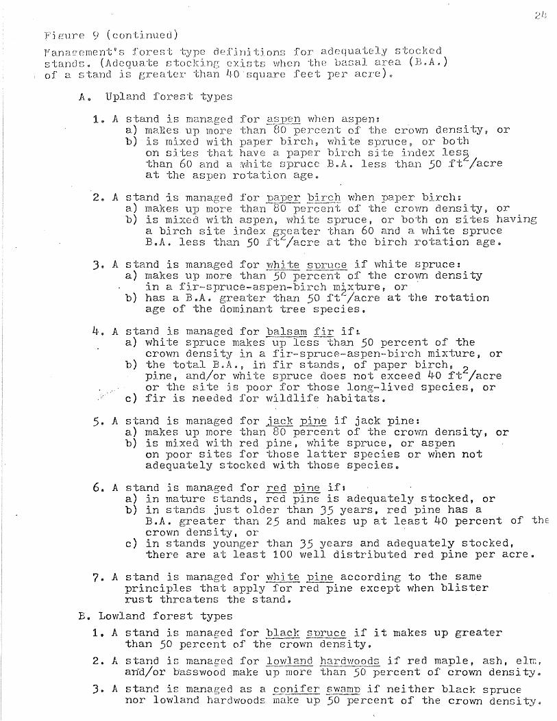
Fjgure 9 (continued)

fana~ementOs forest def tions adequate s ekedstands. (Adequate s e sts when the basal area (B Ap)of a stand is ater than 40 'square et per acre)

A. Upland forest types

1. A stand is d for when aspen:a) maRes up more than percent of the crown density, orb) is d with paper birch, white spruce, or both

on sites that have a birch site index les~than 60 and a spruce B@A$ less than 50 £t-/acreat the aspen rotation ageo

2. A stand is managed fora) makes up more thanb) is mixed with aspen,

a birch site indexB.A. less than 50

when paper birch:of the crOVffi densi ty, or

spruce, or both on sites havingthan 60 and a white spruceat the birch rotation age.

3- A stand is managed for whi~e if white spruce:a) makes up more than 50 perc the cro~vn densi ty

. in a fir-spruce-aspen-birch m~xture, orb) has a B.A. greater than 50 ft-jacre at the rotation

age of the dominant tree species.

4. A stand is managed for balsam fir ifta) white spruce makes up less than 50 percent of the

crom1 density in a fir-spruce-aspen-birch mixture, orb) the total B.A., in fir stands, of paper birch, 2

pine, and/or white spruce does not exceed 40 :ft /acreor the site is poor for those long-lived species, or

c) :fir is needed for wildlife habitats.

5. A stand is managed for jack Rine if jack pine:a) makes up more than 80 percent of the crown density, orb) is mixed with red pine, white spruce, or aspen

on poor sites for those latter species or when notadequately stocked with those species~

6. A stand is managed for red pine ifsa) in mature stands, red pine is adequately stocked, orb) in stands just older than 35 years, red pine has a

B.A. greater than 25 and makes up at least 40 percent of thecro~~ density, or

c) in stands younger than 35 years and adequately stocked,there are at least 100 well distributed red pine per acre.

7. A stand is managed for white pine according to the sameprinciples that apply for red pine except when blisterrust threatens the stand.

B. Lowland forest types

1. A stand is mana[!ed for black snruce if it makes up greaterthan 50 percent of the-crovm density.

2. A stand is managed for lowland har9woods if red maple, ash, el~f

and/or basswood make up more than 50 percent of crovm density.

3. A stand is managed as a conifer swamn if neither black sprucenor lowland hardwoods rna}r,:e up 50 percent of the crovvn densi

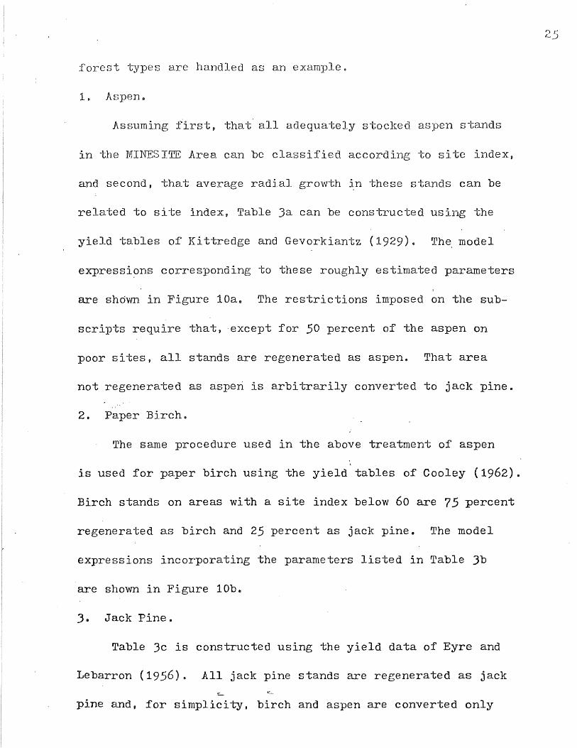
forest types are handled as an exam})le.

1. Aspen.

Assuming first, that' all adequately stocked aspen stands

in the MlNESITE Area can be classified according to site index,

and second, that average radial growth in these stands can be

related to site index, Table 3a can be constructed using the

yield tables of Kittredge and Gevorkiantz (1929). Th~ model

expressi~ns corresponding to these roughly estimated parameters

are shown in Figure 10a. The restrictions imposed on the 8ub-

scripts require that, except for 50 percent of the aspen on

poor sites, all stands are regenerated as aspen. That area

not regenerated as asperi is arbitrarily converted to jack pine.

"

2. Paper Birch.

The same procedure used in the above treatment of aspen

is used for paper birch using the yield tables of Cooley (1962).

Birch stands on areas with a site index below 60 are 75 percent

regenerated as birch and 25 percent as jack pine. The model

expressions incorporating the parameters listed in Table Jb

are shown in Figure lOb.

J. Jack Pine.

Table 3c is constructed using the yield data of Eyre and

Lebarron (1956). All jack pine stands are regenerated as jack

pine and, for simplicity, birch and aspen are converted only

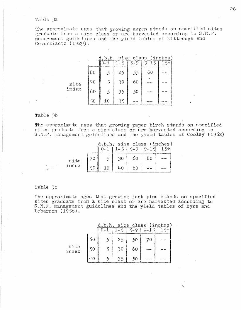
~r3.blc 3a

The approx sgraduate a size c sma.nagement guic3cl andGev (1)

on sare d accordyi Id tables of Ki

c ed 8iS.N F.

dge and

8i tE~index

'" b.,h" size class (in,Qb~

0 1 1 .5 5-9]c_ 9-15 15+

80 5 55 60 --

70 5 30 60 -- --60 5 35 50 - --50 10 35 -- -- ._-

Table Jb

The approximate ages that growing paper birch stands on specifiedsites graduate from a size class or are harvested according toSeN.F. management guidelines and the yield tables of Cooley (1962)

d.b.h. size class (inches)

si teindex

I 0 ... 1. 1-5 5-9 9-15~

70 5 30 60 80 --50 10 Lj-o 60 -- --

Table 3c

The approximate ages that growing jack pine stands on specifiedsites graduate from a size class or are harvested according toS .. N.F. management guidelines and the yield tables of Eyre andLebax'ron (1956).

deb .. h. size class (inches)

si-teindex

] 0-1 1-5 15-9 0-1 c::,' 15+.... -'

60 5 f 25 50 70 --50 5 30 60 -- --

I

J.}o J 5 I 35 50 -- I --

r lOa

5 arssome multiple

j 3,- elil,12j 1

j 1 for j=2,3,e.e,121=12 for j

A,?O. (t)1

The model equations for aspen usingand the parameters lis dof five years)"

ac~ '-' ofthe j aspen

1) age c s on A80.{S .. I.2:80 Jat tirne=t+5

A60. (t)l

j-1 for j=2 3,@"",101=10 j=1 i,j=1;2'Glo",,10

4) A501 Ct+5) =

A50 .. (t+5) =J '

( • .5)(A507(t) )

A50.(t) i=j-1 for'j=2,3, ••• ,71

i,j=1 ,1 2, .. e.,7

For any 5 year interval t:

aspen

aspen

aspen

... aspen

1-

seedling acreage= A801 (t)+A701 (t)+A601 (t)+ ~A50. (t)I:" l

5 b ~

sapling acreage=~A80.(t)+LA70. (t)+ A60. (t)+~A50. (t)"'1. 1 Z 1 1.... 1

II 12-

pole acreage=,zA80. (t)+,ZA70. (t)fQ 1 '1 1

small saw acreage= A8012 (t)

Figure lOb

The model equations for paper birch using a time interval of 5years and the parameters listed in table Jb.

1) PB70j(t+5) = PB70. (t) i=j-l for j=2,J, .... ,16i,j=1,2,tle.~16

1 i=16 for j=l

2) PESO. (t+S) ~FBSO. (t) i=j-l for j=2,3, ••• ,12::::onlyJ 1 i,j=1,2, .• ",12PB501(t+5) = ( .. 2S) (FB5012 ( t) )

For any 5 year interval t:

paper birch

paper birch

paper birch

paper birch

:l

seedling acreage= PB701(t)+~PB50.(t), ,1

sapling acreage=~PB70.(t)+~PB50.(t)2. 1 :3 l'

I;L 12

pole acreage=~PB70.(t):t ~PB50. (t)7 l «j l

small saw 'acreage=~PB70.(t)&::- t~.l.

Figure 10c

~Phe model equand the pararne

for j using a time interval 5 years

i=j 1 for j ,3'0&i=11+ for j=l

,14

= JPS012(t) + ( S)(A507(t» + ( 25)(PB5012(t))

- JP50.(t) j ,3,eeo,121

2) ,JP.501 (t+.5)

JP50j(t+5)

3)"JP40 j (t+S) = JP40. (t)1

j-l f'or j=2,3'11 e,10o j

For any 5 year interval ts

jack pine

jack pine

jack pine

jack pine

seedling acre JP601(t)+ JP501(t)+ JP401(t)6 -,

sapling acre = JP60.(t)+~JP50.(t)+~JP40. (t)1 ~ l' 2 1

12 10

pole acreage JP60. (t)+ <:"JP.50. (t)+L"JP40. (t)1 1 1 ~ 1

14small saw acreage= <:JP60. (t)

II 1

.. I"

to med ium site ,j model e ssions

are shown in Figure lOc

,This procedure could be repeated for some of the other

forest types using, for example t the data of Meyer (1929)

white spruce and fir. Fox and Kruse (1939) for black spruce,

and Eyre and Zehngraff (191}8) for red pine e The poin-tto be

made is this: the model's flexibility enables the use~ to easily

express when forests are harvested and the extent that a forest

..type is regenerated as the same or some other type.

Certainly not all stands are harvested at rotation age.

Many stands are lost to succeeding understories because no

markets exist for the overstory trees. Assuming that most stands

are harvested at rotation age and properly. regenerated, the model

at least provides a framework on which to base less optimistic

views of future management. Leuschner (1972) used a variety

of management strategies in his model to obtain a rough 'estimate

of future volumes of Lake States aspen. Likewise, in order that

a good estimate of management's effects on MlNESITE Area vegetation

is obtained, model simulations should be run incorporating different

management strategies.

Modeling Natural Succession in the MINESITE Area.

The portion of the region not subject to intensive management

~or one reason or another is subject to natural succession. In

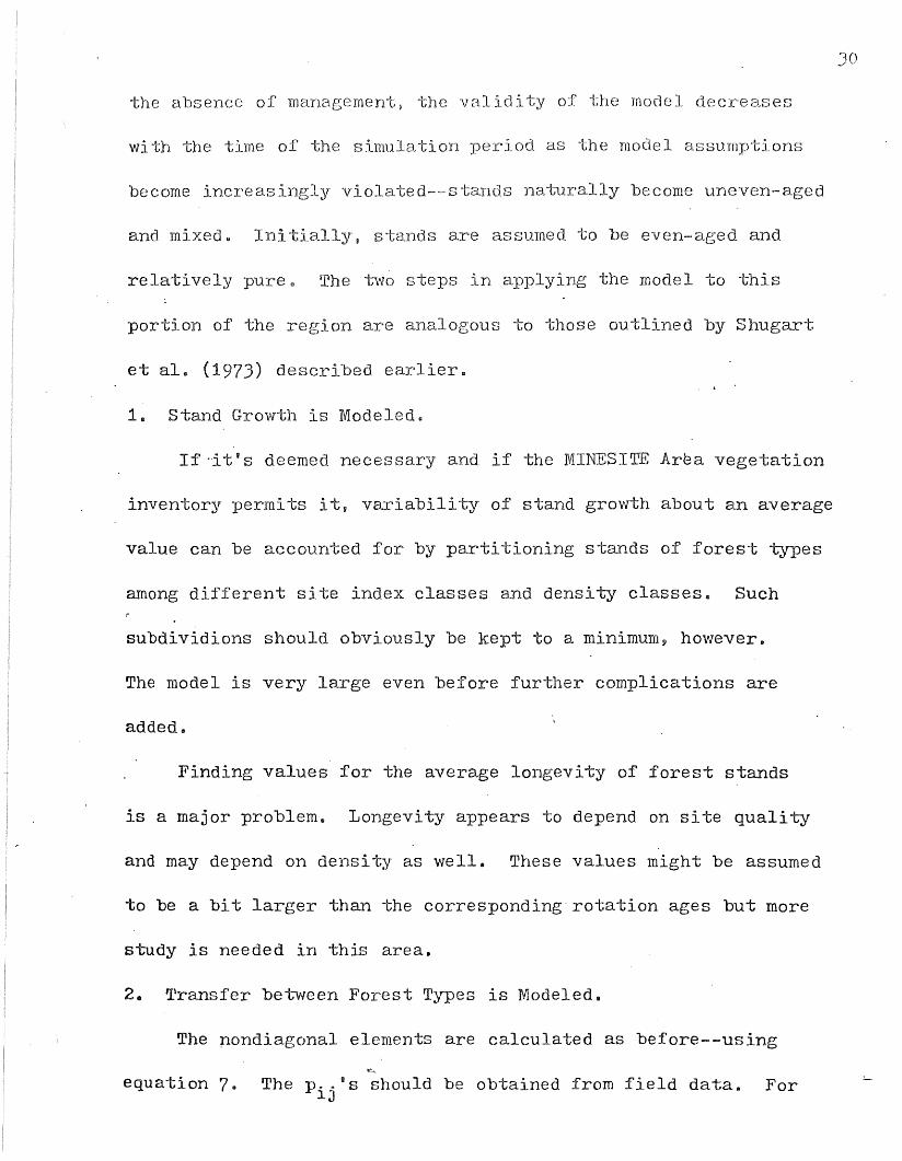
the absence of management, the v ity of model creases

30

with the time of simulation ad as the model assumptions

become increasingly violated-~-stands naturally become uneven-aged

and mixed. Initially, stands are assumed to be even-aged and

relatively puree The two steps in applying the model to this

portion of the region are analogous to those outlined by Shugart

et ale (1973) described earlier.

1. Stand Growth is Modeled.

If-it's deemed necessary and if the MINESlTE Area vegetation

inventory permits it, variability of stand growth about an average

value can be accounted for by partitioning stands of forest types

among different site index classes and density classes. Such

subdividions should obviously be kept to a minimum, however.

The model is very large even before further complications are

added"

Finding values for the average longevity of forest stands

is a major problem. Longevity appears to depend on site quality

and may depend on density as well. These values might be assumed

to be a bit larger than the corresponding" rotation ages but more

study is needed in this area.

2. Transfer between Forest Types is Modeled.

The pondiagonal elements are calculated as before--using

equation 7 ..""~

The p .. 8 S should be obtained from field data .. ForlJ

example p inselman (1959) used observed dominance of 0

31

species in understories to reflect the de e to which those

species would replace aspen overstories in Minnesota. His results

are listed in Table 4 ..

Fire, Drought, and Epidemics ..

It is suggested that the quency and effect on vegetation

of fire, drought, and epidemics be ascertained from th.e past

history of the area. These effects can then be expressed in

the model by discontinuous mem1S. As in the case of modeling

different management strategies with different simulations,

the effect ffi1d timing of these factors can also be added dif-

.ferently in a number of simulations to arrive at an overall

average effeQt of each factor.

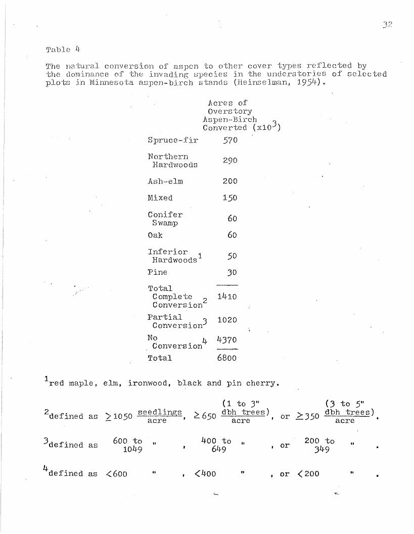
Table 1.1.

'J~he natural conversionthe dominance theplots in Minneso

Spruce

NorthernHardwoods

:Mixed

ConiferSwamp

Oak

cover s re cted byin the unders s of selec d(Heinselman, 195J+)

Acres ofOvers tory

.Aspen~Birch

Converted (xl0J )570

290

200

150

60

60

Inferior 1Hardwoods

Pine

TotalComplete 2Conversion

PartialConversion3

No 4Conversion

Total

50

30

1410

1020

4370

6800

1red maple, elm, ironwood, black and pin cherry.

2defined as >1050 ~>eedlings- acre'

(1 to 3" (3 to 5"2. 650 dbh trees), or >350 dbh trees)

acre acre

3defined as 600 to1049 "

400 to649 " , or 200 to

349 "

4defined as <600 " (400 " , or <200 " •

CONCLUSION

The model of Shugart, Crow, and Hett (1973) is not reccownended

for use by the Copper-Nickel Study team for projecting yegetative

trends in the MIIlliSITE Area. It is neither immediately evident

nor has it been demonstrated that this model accurately simu~a-tes

natural succession over a large region. Also, by focusing on

MINESITE's (1976) smaller and intensively managed region, the

study group can collect a mass of data allowing them to at least

qualitatively project, over a relatively short period of time,

what will becom~ of the many forest stands. The exponential

increase or decrease in the cover-state area implied by the

model of Shugart et ale (1973) would only prove to obscure these

.'

qualitative projections.

Instead, a Markov model is recommended. By reducing the

system of linear differential equations to one of linear dif-

ference equations, the important factors affecting growth and

replacement of forest stands can be more easily incorporated

into a simulation.

The present and future state of the area's vegetation is

greatly dependent on present and future forest management.

It is believed that different management policies and their

manifestations can be better simulated by the Markov model.

In ~act, the more linportant the role that management plays in

shaIJing the ve on the h will be the e to leh

the Marltov mod as ons are met, and thus the more

the model will in obtaining projectionso

One should remain critical of the abili ty of the S"A~"l'J-_

~ al~ (1973) model -to simulate natural succession", The same

holds even more so for the Markov model even when its i:nherent

assumptions are valid. As equations are added ~o account for

the fact that not all stands are pure or grow at similar rates,

the simulations may become more realistic.I

Still,the success

of this model, like the many other successional models which

embody the second Levins (1966) modeling strategy, depends

largely on whether urrrealistic effects inherent from the un-

realistic.assump~ionscancel each other.

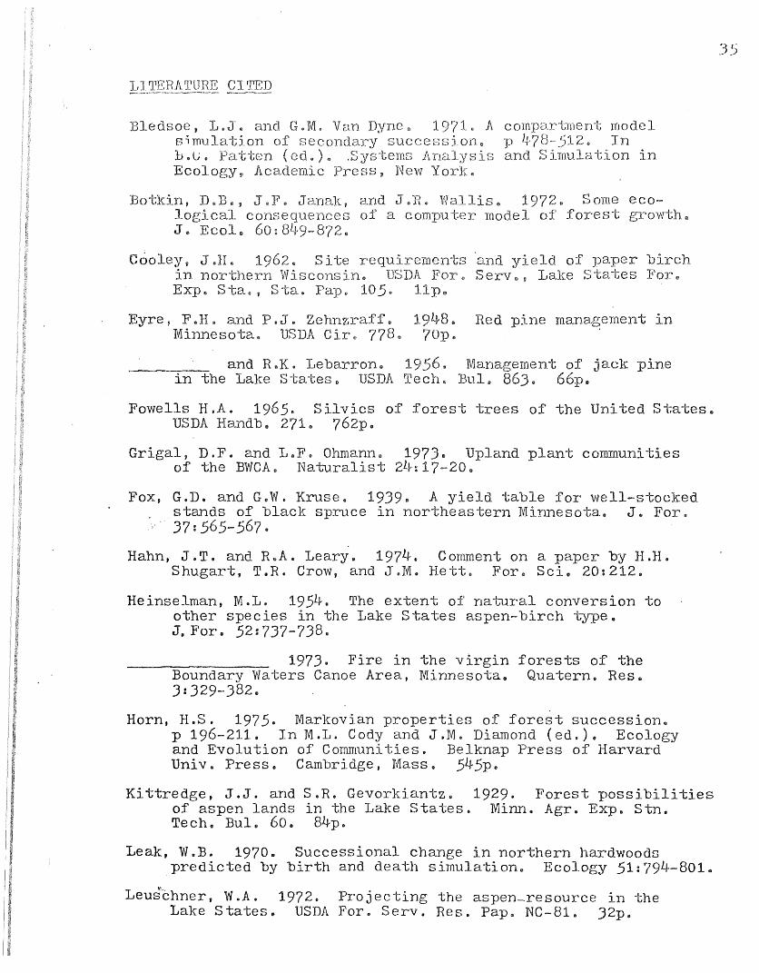
Bledsoe, L .J' It and G Msimulation of sech~G. ( de)Ecology, Ac c

Van Dynesucees

.Sys·t;emr::;SS, New

A cp

modelInon in

.35

Botkin, DuBm, J.F Janak,logical consequencesJ. Ecole 60:849-872

a cliSe 1972@ Some eco­

model of fores-t gl"ovrth

Cooley, J 1962. Sitein northern Wisconsin.Exp" S-ta. t Stag Pap. 105.

Eyre, F.R. and P.J. Zehnzraff.Minnesota.. USDA Cir., 778

191+8 II

JrOp •

yield of paper birchS erv m, LaJre S ta-tes For €I

Red pine management in

__~_ and R.K. Lebarron~

in the Lake States. USDA19360 Management of jack pine

ch. Bul. 863. 66pu

Fowells H.A. 1965. Silvics of forest trees of the United States.USDA Handb. 271€1 762pe

Grigal, D.F. and L.F'. Ohmann. 1973. Upland plant communitiesof the BWCA. Naturalist 24:17-20.

Fox, G.D. and G.W. Kruse. 1939. A yield table for well-stockedstands of black spruce in northeastern Mirmesotae J. For.

,>' 37: 565-567.

Hahn, J.Te and R.A. Leary. 1974. Comment on a paper by H.H.Shugart, T.R. Crow, and J.M. Bette For. Sci. 20:212.

Heinselman, M.L. 1954. The extent of nat~ral conversion toother species in the Lake States aspen-birch type.J. For. 52:737-738.

1973. Fire in the virgin forests of theBoundary Waters Canoe Area, Minnesota. Quatern. Rese3:]29-382.

Horn, H.S. 1975. Markovian properties of forest succession.p 196-211. In M.L. Cody and J.M. Diamond (ed.). Ecologyand Evolution of Communities. Belknap Press of HarvardUniv. Press. Cambridge, Mass. 545p.

Kittredge, J.3. and S.R. Gevorkiantze 1929. Forest possibilitiesof aspen lands in the Lake States. Minn. Agr. Exp .. Sm.Tech. Bul. 60. 84p.

Leak, W.B. 1970. Successional change in northern hardwoodspredicted by birth and death simulation. Ecology 51:794-801.

Leu~:tchner, W.A. 1972. Projecting the aspen-resource in theLake States. USDA For .. Serv .. Res. Pap. NC-81.. J2p.

Levins, R 1966. Thebiology. Am. Sci

of model build1

in population

36

Latka, ADJ. 1925. Elements of PhysicalWilkins. BaIt. Md@ 46op.

ology, Williams and

For" Serv",

Ohmann, IJ .17 • R R Ream 197 Wilderness ecology: amethod sampling and summarizing plant communityclassifica USDA Serv Rese e Nc-49 14pe

1971b. Wilderness ecology: virginBoundary Waters Canoe Area. USDA

NC-63e SSp.

May, R.M. 1973e Stability and Complexity in :Model Ec.osystems.Princeton Press Princeton, NDJ. 235p.

Meyer, W.R. 1929. Yields of second-growth spruce and fir inthe Northeast. USDA Tech. Bul. 142. 52pe

MINESITE. 1976. The MINESITE Data Manual.. Minn.: DNR Div ..Minerals.

Shugart, H.H., T.R. Crow, and J.M. Hett. 1973. Forest suc­cession models: a rationale and methodology for modelingforest succession over large regionse For. Sci. 19:20)-212.

1974. Reply to J.T.Hahn and R.AD Leary on forest succession models. For. Sci.

,,20: 213"

Superior National Forest. 1975. Silvicultural Guides Summary.USDA For. Serve 45p.

Waggoner, P .. E.. and G.R. Stephens. 1970.. Transition probabilitiesfor a forest. Nature 255:1160-1161.

3?

Shugart et

Solving a System of LinearDifferential Equ ons

• didn;t obtain an explicit solution for

their model Numerical approximation techniques were us~d instead

An explicit solu on for a small subset of the set of differential

equations can easily found, however, by applying techniques

found in any introductory texbook of linear algebra or differential

equations. Such is done below so that growth and decay of white

pine stm1ds over a region can be visualized as predicted by the

model in the absence of input acreages from other cover types.

The ~hree equations that describe the growth of white pine

stands are

,seedling

pole

saw

dX1/dt=(-1/100)X1

dX2/dt=(1/100)X1+(-1/150 )X2

dXJ/dt=(1/150)x2+~-1/200)XJ

or

. [-1/100 . a ad/dt(X) = 1/100 -1/150 0

a 1/150 -1/200

x = AX

This system is co~plicatec because the second and third equations

contain variables other than that variable in the differential.

1£ the matrix A is similar to a diagonal watrix, D, ~ade

un of its e:genvalues, the syste~ can be reduced to eliminate

these other variables. All ~·s ttat are solutio~2 G~ 'det(~I _~)=~t~, ~

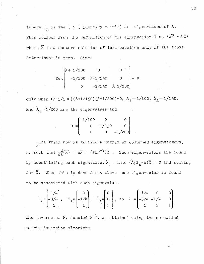
(~here I is the 3 x 3 identityn

ix) are eigenvalues of A

)B

This follows from the defini on of the eigenvector X as (I AX :::: AXe

where X is a nonzero solution of this equation only if the above

determinant is zero Since

A+ 1/100 0 0

Det -1/100 A+l/150 0 == 0

0 -1/150 A+1/200,

only when (A+l/100){A+l/150)(A+l/200)==O,A1==-1/100, ~2==-1/150,

and ~==~'1/200 are the eigenvalues and

[

-1/100 0 0 ]

D == 0 -1/150 . 0

o 0 -t/200 li

.+he trick now is to find a matrix of colu~ned eigenvectors,

d ­P, such that dt(X) Such eigenvectors are Iound

by substi tuting each eigenvalue, ~~ , into (Ai. In-A)X == 0 and solving

for X. When this is done for A above, one eigenvector is found

to be associated with each eigenvalue.

[1/4] ::A; [-1~4] , XA3{ 1JI

[1/4 0

1];:).,'" - 3~~ Jso :;: = -3~4 -1/4

1

The inverse of F, denoted 1'-1, as obtaineci using the so-called

matrix inversion alsorith~.

rlh (' 0 1 0 0 1 0 0 I l~ 0 0lineZlr I

I[J/Lf _1/i! C· 0 1 0 1"0\'1 0 1 0 1-16 12 0

transformations I

1 1 1 0 () 1 0 0 :1 : 4/3 ' -LJ, 1

[ Ji0 0]so 1 -1f 12 0::::

" ., _l~ 1.-:.,/_)

Tin2..11y, sett=_:;'I~......,T_ 1,':i th OJ'

dt P-l-;;

:::: ).:::: DY , the Iollowing

e:;,:pressions 2.re ot·tc:..':nec'1:

r:l" ~ /-: -!- - ( 1 11 f"\ 0 \ ... rL· J 1 \..~ lJ - - /- '~I : J 1 ';:.:.- tn solutio:!

\':i th solution

\':i th solution

,T ==C e (;-1/100) tJ 1 1

"I -c (-1/150)tY2-'2e

_0 (-1/200) tYJ-''"'3e . •

-1-'\t =T _,r - -or X ==?Y, an explicit solution for the subset

}:2 == ( - J /L:_ )y 1- ( l/h )y 2

or

or

or

Xl:::: ( 1/L~ )C1 8 ( -1/100 ) t

]{ :::: ( _3/1.~ )C e ( -1/100) t2 1

... ( ~ /L!_) C2 8 (-1/150) t,

"'r ::::(' e(-1/100)t + C e(-1/1:C')tJ~3 '"'1 2

..L r~ ,. (-J/200)t• v~·_

-'

,..l~r::-('< ,O!~.J..'- .J..lr.\"" __ 10.- '_' •• \,.., ,",-, __ ,-,..

( 1 /1 ,.... r\ ) .J.."'or _ ( 1 r'. r ":::c. ,- " - - - l-..... 1-\--~-1-

:' A 11 ' ,. , ...:-~",.....=/ _-:,--r '\.:- \- __ '. \... -;- " -- .- ,.., ..

I '-

.., 11" ,-I v

.... _"." " ~ ( -1,1 ~ Cr ) ','.. "": - •• ' ... I

, 1/1[" '-:... I .. /""r'..;.• r: r ' 'I ~ " - '-.' - _, . / L ... .',.., r " _ .. - - / t: 1-,-- ,- \ .;~,

•