Modeling Technology Adoption Decisions: An Analysis … · Modeling Technology Adoption Decisions: An Analysis of High Yielding Variety Seeds in India During the Green Revolution

Modeling Technology Adoption Decisions:An Analysis of High Yielding Variety Seeds in India

During the Green Revolution

Sarah Baird

April 11, 2003

1 Introduction

Understanding how individuals make the transition out of poverty is one of the main moti-vations for studying development economics. The introduction of a new technology is oftenperceived as a mechanism that can ignite this transition. However, in order for the new tech-nology to serve this purpose it must be adopted and distilled within the local community.One of the most studied, and by many considered one of the most successful, instances ofnew technology adoption came with the introduction of high yielding variety (HYV) seeds inIndia in the late 1960s, an event referred to as the Green Revolution. These HYVs promotedrapid economic growth in many areas and helped feed the ever growing population.

Although there have been many studies attempting to explain the rapid transition fromtraditional varieties to the HYVs, there is still ongoing debate over what the key deter-minants really were. Emerging from the recent literature are two competing explanations,namely learning and experience versus input availability and prices. The former explanationsees uncertainty and inexperience with the new technology as initially delaying adoption.As a farmer learns more, either through own experience or neighbor experience, the scaleof adoption increases. Alternatively, since HYVs require an increase in inputs such as fer-tilizer, the latter approach characterizes the adoption decision as one of constrained profitmaximization. A farmer maximizes profits in a world with changing product and factorprices subject to certain constraints such as fertilizer availability and irrigation assets. Thismodel suggests that as either input prices decline or these constraints are relaxed, farmerswill increase adoption of the new technology.

Using panel data from India corresponding with the onset of the Green Revolution, thispaper will investigate these competing explanations as to what drives a farmer’s decisionwhether or not to adopt the higher yielding varieties. Looking at alternative theoreticalmodels and their ensuing empirical specifications, this paper hopes to unravel which modelbest captures the adoption decision.

1

2 Literature Review

Economic analysis of technology adoption has traditionally focused on imperfect information,uncertainty, institutional constraints and inadequate human capital as potential explanationsfor delayed adoption decisions. Other explanations have included inadequate schooling (Fos-ter and Rosenzweig (1996)), and infrastructure (Kohli and Singh (1997)). Recently, however,an influential body of literature on technology adoption has focused on the effect of sociallearning on adoption decisions. The basic motivation behind this literature is the idea thata farmer in a village observes the behavior of neighboring farmers, including their experi-mentation with new technology. Once a year’s harvest is realized, the farmer then updateshis priors concerning the technology which may increase his probability of adopting the newtechnology in the subsequent year.

Besley and Case (1993) use a model of learning where the profitability of adoption isuncertain and exogenous. Looking at a village in India, they find that once farmers’ dis-cover the true profitability of adopting the new technology, they are more likely to adopt.Alternatively, Foster and Rosenzweig (1995) and Conley and Udry (2002) use a target-inputmodel of new technology which assumes that the best use of inputs is what is unknown andstochastic. Applying this model to HYV adoption in India, Foster and Rosenzweig (1995)find that initially farmers may not adopt a new technology because of imperfect knowledgeabout management of the new technology; however, adoption eventually occurs due to ownexperience and neighbors’ experience. Similarly, Conley and Udry (2002), looking at Pineap-ple cultivation in Ghana, analyze whether an individual farmer’s fertilizer use responds tochanges in information about the fertilizer productivity of his neighbor. They found thata farmer increases (decreases) his fertilizer use when a neighbor experienced higher thanexpected profits using more (less) fertilizer than he did, indicating the importance of sociallearning. Both these models, however, assume that input prices are fixed. In addition theyignore potential constraints on the supply of inputs and other localized conditions. AlthoughFoster and Rosenzweig (1995) claim these assumptions are not empirically important, in thecontext of the adoption of HYVs, input prices and availability may be a critical factor indetermining adoption.

The potential importance of inputs in HYV adoption leads to another body of literaturewhich focuses on factor availability and accumulation as the motivating forces for technologyadoption, especially in reference to HYV adoption in India. Kohli and Singh (1997) foundthat inputs played a large role in the rapid adoption of HYVs in the Punjab. They claimthat the effort made by the Punjab’s government to make the technological innovations andtheir complementary inputs more easily and cheaply available allowed the technology todiffuse faster there than in the rest of India. Butzer et al (2002) use a choice of techniqueframework to characterize the decision to adopt HYVs in India. They find that since HYVsrequire higher levels of fertilizer and irrigation to realize their yield potential, their introduc-tion corresponded with a large jump in the demand for fertilizer and irrigated land. Theythen concluded that it was this factor accumulation that drove the rapid rate of adoptionand subsequent growth in agriculture. McGuirk and Mundlak (1991) also use a choice oftechnique framework in a study of the transformation of Punjab agriculture during the GreenRevolution and find that the short period of transition from the use of traditional varieties

2

to the adoption of HYVs was largely determined by the availability of irrigation facilities andfertilizer. This result partially stems from the fact that, as mentioned before, to fully utilizethe yield potential of HYVs, it is necessary to apply considerably larger doses of fertilizerand water per unit of land. Moreover, HYV yields are sensitive to both under and over useof inputs. These results point to the fact that access to inputs may very well affect the rateof adoption.

Although there has been extensive evidence for both learning and the availability of inputsas driving HYV adoption, little work has been done trying to compare these alternativemodels. This paper proposes to fill in this gap by confronting these alternative models, andseeing which provides a more convincing story for the adoption of HYVs in India during theyears 1968-1971. Specifically this paper will focus on the models presented by McGuirk andMundlak (1991) and Foster and Rosenzweig (1995) to establish a framework that providesempirically implementable tests of the significance of both inputs and learning on technologyadoption decisions.

3 The Model

Economic modeling of technology adoption has taken many different forms. In terms of anal-ysis of HYV adoption in India during the Green Revolution, there are two models that seemparticularly pertinent, namely a choice of technique approach based on profit maximizationand a target input model that focuses on learning.

3.1 The Price Model

The choice of technique approach, such as that used by McGuirk and Mundlak (1991), focuseson choosing inputs to maximize profits. In this framework the resulting maximization leadsto a decision rule that emphasizes prices, input constraints and environmental factors as thekey determinants of the scale of adoption. To see this, consider McGuirk and Mundlak’s(1991) model where one chooses fixed (b) and variable (v) inputs to maximize profits giventhe available technology (T) and the implemented technology (Fl(·)). In this specification plis the price of the product of technique l, w is the price vector of the variable inputs, b is thevalue of the constraint for the fixed factors of production, λ is a vector of shadow prices forthe constraints, and C represents the characteristics of the environment in which techniquel is implemented. The resulting Lagrangian to be maximized is:

maxvl,bl

, L =∑l

plFl(vl, bl, C)−∑l

wvl + λ(b−∑l

bl) (1)

subject to Fl(·) ∈ T ; vl ≥ 0; bl ≥ 0. The first order conditions are as follows:

plFvl − w ≤ 0 (2)

plFbl − λ ≤ 0 (3)

3

∑(Lvlvl + Lblbl) = 0 (4)

vl ≤ 0, bl ≤ 0 (5)

∑bl − b ≤ 0 (6)

λ(∑

bl − b) = 0 (7)

where Fvl and Fbl are vectors of first partial derivatives. Using these first order conditionsone can characterize the solution to the optimization problem as v∗l (s), b

∗l (s), λ

∗l (s) where s

represents the exogenous variables, s = (b, p, w, C, T ). What this indicates is that a profitmaximizing agent’s decision depends on the available technology (T ), the environment (C),the constraints (b) and the product and input prices. Putting this into a dynamic framework,one can see that at each time t, farmers will decide how to allocate their area among cropsand techniques given their time t information set. Assuming that T remains constant overtime, one can rewrite the vector of state variables as s = (bt, pt, wt, Ct, T ).

Using these results, for a given technology l, the time t decision rule by farmer j can becharacterized as:

Hjt = ht(bjt, wjt, pjt, Cjt, T ) (8)

where, for this particular specification, Hjt is the number of hectares dedicated to HYVs byfarmer j at time t. What this decision rule indicates in relation to HYV adoption in Indiais that, given that HYVs are sensitive to fertilizer use, a farmer’s decision to adopt HYVsdepends not only on the product price, but also on the price and constraints associated withinputs, such as fertilizer.

In the context of this model it is important to note that although fertilizer is a variableinput in the sense that it can be altered from one planting period to a next, given theimportance of timing in planting decisions, it can not be altered within a season. Thisrigidity indicates it is fixed temporarily. In addition, the decision rule shows that for anytime t planting decision, the choice of the scale of HYV adoption may be determined by theprice or supply of fertilizer. If the constraint (b) is binding, as is likely the case with Indiaduring 1968-1971 since fertilizer was rationed, one would expect the coefficient on price to bezero when estimating the decision rule. Alternatively, if the coefficient on price is found to besignificantly different from zero, price may be driving the scale of adoption. As indicated byequation (8), the choice of the scale of HYV adoption is also influenced by the environment inwhich the farmer is planting. For example, local soil conditions and expectations over rainfallmay affect the degree of uncertainty associated with HYVs. Overall, this model characterizesthe HYV adoption decision as one stemming from maximization over the choice of inputs,a maximization problem determined by product and factor prices, constraints on factors ofproduction, and the relevant characteristics of the surrounding environment.

4

3.2 The Learning Model

Although this rule characterizes the adoption decision, it does not take into account certainfactors, such as learning, that could be at the heart of the adoption process. The target-inputmodel, on the other hand, provides a framework which allows for the possibility of learningfrom the experience of neighboring farmers and own experience through Bayesian updatingabout optimal input use. Following Foster and Rosenzweig’s (1995) approach, the targetinput model assumes that farmers know the production technology up to the distribution ofan optimal or target input. After each harvest, a farmer observes what the optimal inputlevel was and can then make inferences about the systematic component of the target. Inaddition, Foster and Rosenzweig (1995) modify the target input model slightly to make itmore applicable to the context of HYV adoption by assuming (i) the scale of operation isendogenous and influences the precision of new information, (ii) farmers can use new andtraditional technologies simultaneously and (iii) farmers can engage in strategic behavior.

The following description draws directly from Foster and Rosenzweig (1995), but attemptsto simplify and focus their approach to place emphasis on the components of the model thatare important for the subsequent empirical analysis. For a more complete treatment of thetheory one can refer to Foster and Rosenzweig (1995).

One can write the target input use for farmer j per hectare i in time t as follows:

θijt = θ∗ + uijt (9)

where θ∗ is the mean optimal level of the input, θ is the actual optimal, and u is assumed tobe an IID normal random variable with variance σ2

u. Farmers are assumed to know σ2u and

have priors over θ∗ that are distributed N(θjt, σ2θjt). For the traditional varieties the output

is assumed to be a constant, ηa, since unlike with HYVs, the traditional variety yields arenot sensitive to the level of inputs. On the other hand, the amount of output produced oneach hectare of land planted with HYVs is random based on input use. The yield (Y ) perhectare i planted with HYV seeds by farmer j can be written as:

Yijt = ηh − (θijt − θijt)2 (10)

where θijt denotes the actual level of input use, and ηh is the mean yield from HYV seeds.This specification assumes that the loss associated with suboptimal inputs is quadratic.Given the expected yield written above, expected profits can be written as a function of thefarmers posterior distribution for θ∗j at time t:

πjt = (ηh − σ2θjt − σ2

u)Hjt + ηaAjt + uj + εjt (11)

where Hjt is the total number of hectares planted with HYV by farmer j in time t, uj is anindividual fixed effect, Ajt is the potential scale of operation, and E(εjt) = 0.

So far the underlying assumption behind this model is that the choice of θijt is optimalgiven farmer j′s priors over θ∗. This assumption clearly separates this model from the choiceof technique approach since, by contending that the choice of θijt is optimal, this modelignores that farmer j′s choice of θijt may be constrained by the availability and access toinputs. In the case of India from 1968-1971 this may be particularly relevant with respect

5

to fertilizer, since fertilizer during this time was rationed. Although this will not influenceprofits directly, it will affect the choice of Hjt. In addition, this model assumes that inputprices are fixed. Allowing for varying input prices is clearly going to affect the profit functionboth directly, as a cost, and indirectly through the scale of Hjt, which is implicitly modeledin the choice of technique approach.

On the other hand, what this model does do is incorporate learning through the conceptof Bayesian updating. As opposed to decision making based on input prices and availabilityconstraints, in this case a farmer’s decision is based largely on evolving knowledge about thenew technology. The idea is that once a year’s harvest has been realized, the ex post optimalinput levels are revealed. Each farmer then updates his priors concerning the optimal inputuse through Bayesian updating. The updating is based on the precision of the signal fromown experience, which increases proportionally with the number of hectares planted, and theprecision of the signal from neighbors’ experience. One can then write the updated varianceof farmer j′s prior as:

σ2θjt =

1

p+ p0Sjt + pvS−jt(12)

where p is the precision of the farmer’s initial priors, p0 is the precision of information foreach hectare planted by j on his own farm, Sjt is the cumulative number of hectares plantedby farmer j up to time t, and pv is the precision of information from an increase in the averagecumulative experience of other farmers in the village, S−jt. As experience increases, farmersbecome increasingly knowledgeable about θ∗, and are therefore more confident experimentingwith the new technology.

Combining equations (12) and (11) the profit function can be characterized as:

πjt = π(Hjt, Sjt, Sjt, Aj, uj, εjt) (13)

Unlike the profit function stemming from the previous model, here profit is seen as a functionof experience, the potential scale of operation and an individual fixed effect.

Using this profit function one can derive an adoption decision rule that incorporateslearning. A farmer will choose Hjt to maximize expected discounted profits. With δ as thediscount factor one can write the value function faced by farmer j at time t as:

Vjt = maxHjt

Et

T∑t=1

δt−1(πjt(Hjt, Sjt, S−jt, Ajt, uj, εjt)) (14)

Replacing πjt in equation (14) with its specification in equations (12) and (11) leads to thefollowing Bellman equation:

Vjt = maxHj

Et[(ηh − σ2u −

1

p+ p0Sjt + pvS−jt)Hjt + ηaAj + uj + εjt] + δVjt+1 (15)

This formulation points to the presence of strategic behavior in the affect of learning onadoption. For example, if the decision maker takes into account they he may learn fromothers’ experience, he may decide to adopt at a later date because the increased knowledge

6

will reduce his investment costs. On the other hand, expected learning increases the marginalbenefit of adoption which should accelerate his adoption decision.

From equation (15) one can write the resulting adoption decision as follows:

Hjt = ht(Sjt, S−jt, Aj, A−jt, uj) (16)

This final decision rule, which corresponds to that specified by Foster and Rosenzweig (1995),considers own and neighbors’ experience, as well as own and neighbors’ potential scale ofoperation, as the key factors determining the scale of adoption. The intuition behind thisdecision rule is that, assuming that HYVs are more profitable than traditional varieties, asone experiments with the new technology he will become more knowledgeable about boththe benefits of the new technology and the optimal level of inputs associated with the newtechnology, which will result in increased adoption. The decision rule also indicates that one’sneighbor’s decision to adopt the new technology influences one’s own adoption decision. Overtime this affect can be either increasing or decreasing. For example, this affect will increaseover time if the effects of experience on the cost of learning dominate those arising from thediminishing returns to experience given adoption.

A farmer’s assets also influence adoption in that they increase adoption and the modelsuggests there are increasing returns to experience with the new technology. Moreover, aneighbor’s assets also potentially affect adoption. The sign of this affect depends on whetherreturns to experience are increasing (positive) or decreasing (negative) in experience. Finally,the decision to adopt in this choice of technique framework in influenced by one’s owncharacteristics, such as entrepreneurship, which are captured in the individual fixed effect.

Comparing equations (8) and (16), one can see that these two models result in verydifferent decision rules. The target input model emphasizes learning and the potential scaleof operation, while the choice of technique approach focuses on prices, the environment, andconstraints as the key determinants of adoption. These two decision rules will guide theempirical analysis.

4 Data and Descriptive Statistics

4.1 Data

The main data source for this paper comes from the Additional Rural Income Survey (ARIS),undertaken by the National Council of Applied Economic Research (NCAER) This data set,compiled using a national variable probability survey, describes rural households and villagesin India beginning in the crop year 1968-1969, a time period corresponding to the onset ofthe Green Revolution. Overall, this panel data set provides information on 4,118 householdsfor the crop years 1968-1969, 1969-1970, and 1970-1971. One important characteristic ofthis data is that it can be aggregated at the village, district and state level using sampleweights. This allows one to look at cross-household learning effects as well as potential statelevel effects.

To complement this data I plan to use the Rural Economic and Demography Survey(REDS) conducted by NCAER in 1981-1982. This survey provides additional information

7

on around half of the households interviewed in the third around of the ARIS, those in whichthe household head remained the same up through 1981. This additional data providesinformation on assets such as land, equipment, and animals inherited prior to 1968. Thesevariables will be used to construct instruments to coincide with the earlier panel. Matchingthis data with the ARIS data results in a sample size of 2,177 households over three years.Although one may be concerned that this subset of households is somehow biased, Fosterand Rosenzweig (1996) provide thorough evidence that this is a representative sample of theARIS data. Given that the REDS data strengthens the analysis, this subset of the datawill be used in the analysis. Finally, information on fertilizer prices and state level fertilizerconsumption were taken from a Survey of the Fertilizer Sector in India put out by the WorldBank in 1979. The main source of data for this survey came from various issues of FertilizerStatistics.

4.2 Survey Design

Before turning to the variables of interest, it is useful to comment on the structure of thesurvey design and some potential estimation problems that might follow. The survey wasconducted using a stratified random sample that both oversampled households in areas wherehigh yielding varieties (HYV) are predominantly cultivated and oversampled high and middleincome households. The rationale for the former was that one of the main purposes of thesurvey was to see to what extent cultivators of HYV have benefited as compared with farmersof traditional varieties. The justification for the latter was that households from high andmiddle income groups consisted of only 10% of total households. Without over sampling,only about 500 of the over 5000 households would be from these income groups. In orderto prevent this sampling bias from leading to biases in the estimates, household weights aregiven, where relatively smaller weights correspond to households from higher income groups.Since HYV adoption may be more likely to occur with wealthier households, it is importantto incorporate the oversample, making sure to utilize the weights in determining means andaggregates.

Households were selected using a multiple stage sample design. First, villages in Indiawere split into three strata, the first corresponding to Intensive Agricultural District Program(IADP) villages, the second to Intensive Agricultural Areas Program (IAAP) villages andthe third to other villages. In Stratum 1 (the IADP villages) about 3-5 villages were chosenrandomly from each of the 16 districts. Each village was separated into three income groupsand then 20-30 households were chosen based on the oversampling method explained above.From each of Stratum 2 and 3 households were selected using a three-stage sample designwhere first a C.D. block was selected, then villages within the block were randomly chosen,and finally households within the village were selected. More information on the surveydesign can be obtained from NCAER.

Even with such a carefully designed survey, the sample design does leave room for poten-tial estimation problems, namely from errors relating to sampling, non-response, reportingand processing. In terms of non-response, 997 of the 5115 households were eliminated eitherdue to non-response during one of the three rounds or as a result of missing or inconsistentinformation. In order to address this attrition, household weights were adjusted. As long as

8

there was not some systematic relationship between nonresponse households, adjusting theweights should not introduce estimation problems. Turning to the issue of random sampling,if the villages chosen by the government for implementation of the IADP are not random,there may be some problem attempting to compare adoption of HYVs between IAAP andIADP villages.

4.3 Descriptive Statistics

The ARIS data set includes both village and household level characteristics that will beuseful in the analysis. Turning first to village level data, there are 254 villages includedin the survey with populations ranging from 130 to 24,710. Variables recorded for thesevillages include total population, distance to the nearest town, sources of credit available inthe village, the distance to the nearest bank, whether an education institute or a health centerexists in the village, and whether programs by the Agricultural Extension Service (AES) areorganized in the village. Table 1 presents summary statistics for some of the importantvillage characteristics. These variables help give insight into the economic conditions of thevillage and are assumed to stay constant over the three year period.

In addition to these variables, a dummy variable for weather is included for each ofthe three years. It takes on a value of one if the crops were adversely affected by weatherconditions in the year and is zero otherwise. Looking across all the villages one finds that108 of the 254 villages experienced bad weather in 1968, as opposed to 78 and 54 villagesin 1969 and 1970 respectively. One will have to keep in mind the relatively bad weather in1968 when analyzing the results.

Table 1: Village Level Characteristics (254 Total Villages)

Variable Exists in Village Percent of VillagesTractor Used 92 36%Bank 140 55%Money Lender 200 79%Post Office 95 37%Education 233 92%Health Center 64 25%AES 140 55%IADP 963 22%

Out of the 254 villages a total of 2,177 households, those that have reliable data forall three years of the survey and can be matched to the REDS data, are included in theanalysis. Out of these households, over 75% of the heads of household are farmers and mostof them derive the majority of their income from agriculture. Given the high prevalence offarmers in these villages, it is clear that the introduction of HYVs should have a noticeableimpact. Variables included in the data to help capture this effect include gross cropped area,amount of land planted with HYV as a percentage of total land, HYV use over the years,gross investment in farm equipment, gross investment in irrigation assets, and investment inlivestock. Table 2 provides summary statistics for some of these variables.

9

Table 2: Land/Investment Descriptive Statistics (area in hectares, investment in rupees),N=2,177

Variable Mean Min Max Std.ErrorGross Cropped Area(1968) 3.649 0 96.5 5.392Gross Cropped Area(1969) 3.517 0 51.6 4.710Gross Cropped Area(1970) 3.820 0 73.65 5.260Gross Investment in Farm Equipment(1968) 70.12 -16000 8000 655.8Gross Investment in Farm Equipment(1969) 45.80 -136 14446 376.01Gross Investment in Farm Equipment(1970) 111.75 -585 32025 1420Investment in Livestock(1968) 37.34 -1550 4450 323.9Investment in Livestock(1969) 48.96 -4600 3401 346.8Investment in Livestock(1970) 71.73 -2500 3700 408.7Gross Investment in Irrigation Assets(1968) 9.91 0 3000 108.8Gross Investment in Irrigation Assets(1969) 108.8 0 14000 730.8Gross Investment in Irrigation Assets(1970) 123.8 -4000 14000 742.1

Turning now to HYV use, out of the households that used HYVs, HYV seeds were plantedon 20.97%, 17.54%, and 44.40% of their land in 1968, 1969, and 1970 respectively. Overall,HYV acreage changed from 5% of cultivated area in 1968-1969, to 4% in 1969-1970 thenrose all the way to 17% by 1970-1971. It is interesting that adoption and acreage dropped inthe second year, making one wonder if adverse weather conditions in 1968 helped drive thisresult. In addition, among farmers in villages in which at least one farmer cultivated withHYV seeds by 1970, 22% were using HYV seeds in 1968, 27% had used the seeds by 1969,and 39% had used them by 1970. In following with Foster and Rosenzweig (1995), and giventhat detailed data on agroclimatic conditions is unavailable, it is this sample (households invillages where at least one farmer adopted in 1970-1971) that will be the focus of the analysis.This limits the analysis to 101 of the 254 villages and a total of 1,301 households over thethree year period. The rationale behind emphasizing this subset of the data is that thelearning model implies that HYVs will be used only when, under optimal use, they are moreprofitable than the traditional variety. Nevertheless, given that this strategy ignores a lot ofpotentially valuable information, a logit on the adoption decision will be implemented usingdata on households in all villages. This additional regression will hopefully unravel someof the reasons driving the adoption decision, as well as indicate what the analysis fails tocapture by dropping the villages where no household adopts. Overall, the statistics presentedabove indicate that adoption took place fairly rapidly, making informational barriers andtraditional explanations for delayed adoption seem less likely.

On the other hand, given the importance of inputs for the productivity of HYV, limitedinitial access to items such as fertilizer as well as changing prices may explain the short delaythen subsequent rapid adoption. Looking at fertilizer prices for the years 1961-1975 one cansee that fertilizer prices declined until 1966 and then began to rise. However, the wholesaleprice of agriculture commodities grew at a more rapid rate. As a result of this trend, theratio of these two price remained below the 1961-1962 level. Figure 1 illustrates this trend.It is of particular interest that during the years of this study the ratio was steadily declining.

10

Figure 1: Ratio of fertilizer price to wholesale price of agriculture commodities

Although this trend in prices indicate their potential importance, much analysis of thetime focuses on fertilizer rationing, and hence availability, as a critical determinant of adop-tion. Table 3 shows the statewise consumption of fertilizer in India from 1967-1971. In orderto make these numbers comparable I have normalized them by dividing the state consump-tion of fertilizer by the 1969 percentage share of State to all India gross cropped area.

11

Table 3: Statewise Normalized Consumption of Fertilizer in ’000 tons

State 1967-1968 1968-1969 1969-1970 1970-1971Madhya Pradesh 1.76 2.56 4.16 6.48Rajasthan 2.6 3.13 4.38 5.63Uttar Pradesh 14.1 24.39 32.95 29.5Assam 5.45 8.18 6.35 8.18Bihar 6.52 10.15 16.67 15Orissa 4.65 5.58 6.05 6.51West Bengal 9.36 11.28 11.06 16.81Haryana 14.48 16.21 17.59 24.14Himachal Pradesh .91 2.73 3.64 5.45Jammu and Kashmir .91 8.18 3.64 4.55Punjab 28.33 49.44 48.33 59.17Andhra Pradesh 16.42 37.41 38.64 34.94Kerala 28.89 37.78 40.00 31.67Mysore 8.51 15.82 19.7 23.28Tamil Nadu 37.80 43.90 54.15 63.17Gujarat 17.50 18.46 20.77 31.73Maharashtra 14.71 10.07 12.61 16.72

Note: The state consumption of fertilizer is in ’000 tons and is normalized bydividing total consumption by the 1969 percentage share of State to all Indiagross cropped area

As one can see fertilizer consumption varies dramatically over time and across states. Al-though one may argue that consumption does not reflect supply, since fertilizer was rationedit is logical to conclude that consumption in a state reflects the supply in that state. Tofurther support this claim, looking at India level data on the availability and consumptionof nitrogen, a key component of fertilizer, total availability and consumption were virtuallyidentical for the years of study. Also, although I unfortunately do not have data for therelevant years, statewise installed capacity for nitrogen in 1978 shows, for example, thatMaharashtra has 13.3% of total capacity, while Orissa only has 4.9%, numbers that reflectconsumption percentages in that year. Other papers, such as Mundlak and McGuirk (1991),also rely on the assertion that the consumption of fertilizer in an area reflects the local supplyin their analysis.

12

5 Analysis

From the models presented previously, two decision rules, those shown in equations (17) and(18), emerged.

Hjt = ht(bjt, wjt, pjt, Cjt, T ) (17)

Hjt = ht(Sjt, S−jt, Aj, A−jt, uj) (18)

Equation (17) corresponds to the choice of technique approach (Price Model) and equation(18) corresponds to the target-input model (Learning Model).

The basic strategy for the following analysis will involve first providing an econometricspecification of equation (17), the price model. Once describing the testable version of equa-tion (18), the learning model, the residuals from estimating equation (17) will be regressedon the variables involved in the learning model. The idea behind this approach is that if thelearning model correctly characterizes the adoption process, then the learning variables notutilized in the price model should be significant in explaining the adoption decision. If thisis the case, the learning variables should partially explain the error term from the estimationof the decision rule indicated in equation (17), which ignores any impact of learning. Ifthe experience variables do explain the residuals it points to the learning model as perhapsthe appropriate model for characterizing the adoption process. On the other hand, if thesevariables are insignificant it either indicates that the learning model is inappropriate andthe price approach should be considered more seriously, or, alternatively, that the empiri-cal characterization of the experience variables does not actually capture this effect. If thelearning model does appear to play some role on characterizing the adoption decision, I willestimate a testable version of equation (18) and then investigate whether the variables fromthe price model can explain the residuals resulting from this estimation.

Having experimented with both models, an overall model will be implemented in anattempt to capture both specifications within a single analysis. This model will be usedto test the restrictions that correspond to each of the models and to see if point estimateschange in this new framework. Finally, to complement the analysis, a logit of the adoptiondecision over households in all villages will be used.

It is important to note that equation (17) and equation (18) are not mutually exclusive.They have one variable in common, namely irrigation assets, which is viewed as a constraintin equation (17) and a factor determining the potential scale of operation in equation (18).This variable will be used in estimating both models, but will be omitted when looking athow the alternative model explains the resulting residuals.

5.1 Price Model: Pooled OLS Analysis

5.1.1 Econometric Specification: Price Model

Following McGuirk and Mundlak (1991) one can implement equation (17) with the followinglinearization:

Hjt = α0 + α1Pjt + α2Bjt + α3Cjt + εjt (19)

13

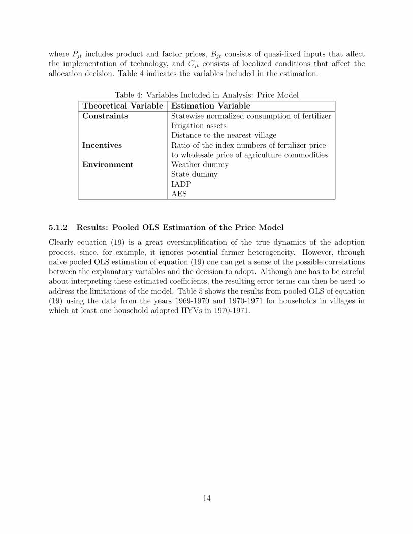
where Pjt includes product and factor prices, Bjt consists of quasi-fixed inputs that affectthe implementation of technology, and Cjt consists of localized conditions that affect theallocation decision. Table 4 indicates the variables included in the estimation.

Table 4: Variables Included in Analysis: Price Model

Theoretical Variable Estimation VariableConstraints Statewise normalized consumption of fertilizer

Irrigation assetsDistance to the nearest village

Incentives Ratio of the index numbers of fertilizer priceto wholesale price of agriculture commodities

Environment Weather dummyState dummyIADPAES

5.1.2 Results: Pooled OLS Estimation of the Price Model

Clearly equation (19) is a great oversimplification of the true dynamics of the adoptionprocess, since, for example, it ignores potential farmer heterogeneity. However, throughnaive pooled OLS estimation of equation (19) one can get a sense of the possible correlationsbetween the explanatory variables and the decision to adopt. Although one has to be carefulabout interpreting these estimated coefficients, the resulting error terms can then be used toaddress the limitations of the model. Table 5 shows the results from pooled OLS of equation(19) using the data from the years 1969-1970 and 1970-1971 for households in villages inwhich at least one household adopted HYVs in 1970-1971.

14

Table 5: Pooled OLS Estimates: Dependent Variable is the number of hectares planted withHYVs (N=2,602)

Explanatory Variable Pooled OLS EstimatesIrrigation Assets 0.0032

(1.46)Price -55.53

(6.61)*Weather 3.25

(0.32)E Fertilizer 5.48

(3.12)*AES -10.85

(1.24)IADP 45.73

(4.67)*Nearest Village 0.024

(0.89)

Note: Absolute t-statistics derived from Huber-White robust standard errorsare in parenthesis.* significant at the 5% level

As one can see price, expected fertilizer and whether or not it is an IADP village arehighly correlated with the decision to plant HYVs. Although I do not want to emphasizethe values of the coefficients, since this analysis ignores many issues related to bias, I willbriefly look at the numbers. A 1% increase in the relative price of fertilizer results in a0.56 hectare decline in the number of hectares planted with HYVs. Given that the price offertilizer appears to be a fairly important variable, it would be very helpful to the analysisto obtain more disaggregated numbers. As for fertilizer, an increase in supply by 100 tons(normalized by the percent of State to all-India gross cropped area) results in a 0.55 hectareincrease in the number of hectares planted with HYVs.

In addition, a state dummy (not included in the table) was included in the estimation toget a sense of the importance of regional differences. The results were significant for all statesindicating that more state level data, such as soil quality and the length of the cropping sea-son, might improve the analysis. Running a similar regression for the Punjab, McGuirk andMundlak (1991) get similar significance results. Instead of using prices, however, McGuirkand Mundlak (1991) create a yield equation to calculate expected revenue. Since I do nothave data on yields, it is promising that the t-statistic above reflects their revenue results.

It is also particularly interesting that being an IADP village is highly correlated withplanting HYVs. Being a household in an IADP village means you are over 45% more likelyto adopt HYVs. Since this program was implemented to assist villages with adopting HYVs,one wonders if the experience variables in the learning model are in fact captured here bythe presence of the IADP. Before more closely examining this question, I will turn to theimplementation of the learning decision rule.

15

5.1.3 Econometric Specification: Learning Model

Following Foster and Rosenzweig (1995), the linear approximation of equation (18) may bewritten as:

Hjt = βt + α0tSjt + α1tS−jt + α2Ajt + α3A−jt + uj + εjt (20)

where, as mentioned before, Sjt is own experience, S−jt is average neighbor experience, Ajtrepresents one’s own potential scale of operation and A−jt is average neighbors’ potentialscale of operation. Table 6 details the relationship between these theoretical variables andthose used in the estimation.

Table 6: Variables Included in Analysis: Learning Model

Theoretical Variable Estimation VariablePotential Scale of Operation (own) Value of farm equipment (rupees)

Value of livestock assets (rupees)Value of irrigation assets (rupees)

Potential Scale of Operation (neighbor) Average value of neighbor farm equipment (rupees)Average value of neighbor livestock assets (rupees)Average value of irrigation assets (rupees)

Own Experience Lagged cumulative HYV (hectares)Neighbor Experience Lagged village average cumulative sum of hectares

cultivated under HYV

As mentioned in the summary, if the target input model correctly characterizes the adop-tion process, then the learning variables in equation (20) should be significant in explainingthe adoption decision. If this is the case, the learning variables should partially explain theerror terms from the pooled OLS estimation of (19) implemented above, which ignores anyimpact of learning. If the experience variables are explaining the residuals it points to thelearning model as perhaps the appropriate model for characterizing the adoption process.On the other hand, if these variables are insignificant it either indicates that the learningmodel is inappropriate and the price approach should be considered more seriously, or, al-ternatively, that the empirical characterization of the experience variables does not actuallycapture this effect.

5.1.4 Results: Does learning explain the residuals from the pooled OLS esti-mation of the price model?

The results from regressing the pooled OLS residuals from estimation of equation (19) onthe variables in Table 6 for the years 1969-1970 and 1970-1971 for households from villageswhere at least one household adopted HYVs are shown in Table 7. Instruments are used forreasons discussed in the next section.

16

Table 7: Pooled OLS: Dependent Variable is residuals from estimation of equation (19)(N=2,602)

Explanatory Variable Experience Assets/Experience Assets/Experience(Own) (Own/Neighbor)

Intercept -19.89 -34.02 -43.25(5.70)* (9.28)* (7.95)*

Own Experience 0.83 0.75 0.84(27.67)* (27.51)* (28.06)*

Neighbor Experience -0.38 -0.38(5.94)* (5.74)*

Farm Equipment (own) 0.0027 0.0021(3.47)* (2.80)*

Farm Animals (own) 0.0038 0.0045(1.53) (1.78)

Farm Equipment (neighbor) 0.012(5.12)*

Farm Animals (neighbor) 0.0091(1.26)

Note: Absolute t-statistics derived from Huber-White robust standard errorsare in parentheses. All variables are treated as endogenous. Instruments includeinherited assets (prior to 1968), lagged asset flows (change in assets from 68-89 to 69-70),lagged profits (1968), lagged village HYV use (1968) and weighted averages of these byvillage.* significant at the 5% level

As one can see from Table 7, both own and neighbor experience are highly significantin explaining the residuals from the initial pooled OLS, whether assets are included or not.A one year increase in own experience increases adoption by about 0.8 hectares, while aone year increase in neighbor experience decreases the scale of adoption by 0.38 hectares.What these results may indicate is that a model that ignores these experience variables incharacterizing the adoption decision fails to capture a lot of relevant information. What isparticularly interesting is that, as mentioned above, the coefficient on neighbor experienceis negative both with and without the inclusion of assets. As mentioned in the analysis,the neighbor experience variable has two potential effects on adoption that go in oppositedirections. The negative sign indicates that perhaps farmers who have neighbors that areexperimenting a lot with the new HYVs are themselves delaying adoption decisions, sincethe knowledge that accumulates over time will reduce investment costs at a later date. Whatthis behavior points to is that farmers do not want to risk adopting the new technology untilthey see how their neighbors fare.

As for assets, only the equipment variables appear to matter. A increased investmentof 100 rupees in own equipment leads to around a 0.25 hectare, depending on whetherneighbor variables are included or not, increase in HYV plantation. A 100 rupee increasein investment by neighbors in equipment leads to a 1.2 hectare increase in HYV plantation.

17

The significance of these results, as opposed to the influence of livestock, potentially suggestthat equipment is a better indicator of wealth and the potential scale of operation.

5.2 Price Model: Fixed Effect Analysis

So far the analysis has ignored the issue of farmer heterogeneity, which makes the previousresults suggestive at best. For example, it is likely that there is some omitted variablecorrelated with the error term, such as farmer skill, which is also correlated with learningand experience. In order to correct for this one can introduce an individual fixed effect intoequation (19). Taking first differences the resulting estimating equation can be written as:

∆Hjt = α0 + α1∆Pjt + α2∆Bjt + α3∆Cjt + ∆εjt (21)

Unfortunately, taking first differences means that coefficients on time invariant variablescannot be estimated, therefore variables such as whether or not it is an IADP village areexcluded from the analysis. Fertilizer prices are also excluded from this regression since theycould only be found at an all India level. Considering only two years of data can be usedin the analysis, the aggregate price acts simply like an intercept and provides no interestinginformation. In order to include weather in the fixed effect analysis two new weather dummyvariables were created. If weather was good in 1969 and bad in 1970 the variable ’AdverseWeather in 1970’ takes on a value of one. Alternatively, if weather was bad in 1969 and goodin 1970 ’Adverse Weather in 1969’ takes on a value of one. If it weather was the same for ahousehold in both years the variables take on a value of zero.

5.2.1 Results: First Differenced Estimation of the Price Model

Table 8 shows the results from estimation of equation (21), both with and without theinclusion of state dummy variables, for the change in the scale of adoption from 1969-1970to 1970-1971, again only looking at households in villages where at least one householdadopted.

18

Table 8: First Differences: Dependent Variable is the change in number of hectares plantedwith HYV (N=1,301)

Explanatory Variable First Differences First Differences(No State Dummy) (State Dummy)

Intercept 61.65(7.00)*

Irrigation Assets 0.013 0.013(1.78) (1.75)

E Fertilizer 5.10 28.03(3.76)* (1.37)

Adverse Weather in 1970 -21.74 -17.55(0.83) (0.54)

Adverse Weather in 1969 -30.07 -19.43(1.92) (1.18)


As one can see from the first column of Table 8, even with the introduction of an individualfixed effect, expected fertilizer supply is still strongly positively significant in determiningHYV adoption. The coefficient stays almost the same, dropping only from 5.48 to 5.10.This again indicates that an increase in supply by 100 tons (normalized by the percent ofState to all-India gross cropped area) results in over a 0.5 hectare increase in the number ofhectares planted with HYVs. Although the weather results are not significant at the 5% level,looking at ’Adverse weather in 1969’ (which is significant at a 10% level), one can see thatbad weather in 1969 decreased the percent of hectares planted with HYV by 30% withoutthe inclusion of the state dummy and over 19% with the inclusion of the state dummy. Thisresult points to the fact that bad weather in 1969 may have made farmers’ less successfulwith the HYVs, therefore causing them to decrease the scale of adoption. However, weatherwas only marginally worse in 1969, as compared with 1970, which makes me less concernedthat the weather shock in 1969 is driving the results. If the adverse weather in 1969 was moresevere, as it was in 1968, I would be more concerned that I was measuring the differentiallevel of the shock, as opposed to differential adoption. More detailed weather data wouldhelp address this concern.

Once the state dummy variables are included all the explanatory variables lose their sig-nificance. This result indicates the potential importance of regional differences not capturedin the data. For example, a t-statistic of 6.57 corresponding with Punjab, a state that expe-rienced larger growth than most of the rest of India during this time, indicates that certaincharacteristics of Punjab are causing increased adoption. Additional state level variablesthat might explain, for example, Punjab’s rapid growth, and additional state level variationin adoption decisions would lead to a more robust analysis.

Another possible reason for this lack of significance is that by taking first differences andincluding state dummys the regression is losing a lot of its power. When the state dummys

19

are added the model becomes very restrictive. Some more thought needs to be given to thetradeoff between bias and efficiency.

5.2.2 Results: Does learning explain the residuals from the first differencedestimation of the price model?

Even with the inclusion of a fixed effect in the price model, the differenced experiencevariables should partially explain the resulting residuals if learning is important. Usinginstrumental variables (for reasons discussed in the next section), Table 9 shows the resultsfrom regressing the resulting residuals from estimation of equation (21) on the differencedexperience variables. Again, the data used is the change from 1969-1970 to 1970-1971 forthe same subgroup of households. Results are given both with and without the inclusion ofa state dummy and with and without neighbor variables.

Table 9: IV First Differences: Dependent Variable is the residual from estimating equation(21) (N=1,301)

Explanatory Variable IV FD IV FD IV FD IV FDOwn Own/State W/Neighbor W/Neighbor/State

Constant -50.59 -30.18 -11.09 4.38(8.82)* (2.68)* (0.82) (0.15)

Own Experience (t) 0.63 1.16 2.18 1.18(1.51) (2.63)* (1.72) (1.12)

Own Experience (t-1) 0.48 1.46 2.91 1.02(0.76) (2.42)* (1.74) (1.22)

Neighbor Experience (t) -1.10 -1.08(0.85) (0.99)

Neighbor Experience (t-1) -1.93 -1.91(0.92) (1.02)

Farm Equipment (own) -0.020 0.0012 0.069 0.037)(0.69) (0.046) (1.20) (0.77)

Farm Animals (own) 0.19 0.039 0.0009 0.13(2.52)* (0.51) (0.0039) (0.73)

Farm Equipment (neighbor) -0.26 -0.089(2.77)* (1.33)

Farm Animals (neighbor) -0.053 -0.17(0.23) (0.78)


20

Looking at Table 9, one can see that when neighbor variables are excluded, own experienceis significant when a state dummy is present. Looking at this result, a one year increase intime t experience leads to an increase of 1.16 hectares planted with HYVs, while a one yearincrease in time t − 1 experience leads to a 1.46 hectare increase in HYV plantation. Thisresult shows that the effect of own experience on the scale of HYV adoption is declining overtime. When the state dummy is not included, the effect of own experience on adoption isno longer significant and it is in fact increasing over time. Although these results points tothe importance of learning, they do not give any indication of what made the farmer decideto adopt in the first place. Again, considering that over a third of the state dummies weresignificant, state level variables may shed light upon what initially leads to adoption.

Once neighbor variables are included, however, virtually all variables lose significance.Neighbor farm equipment is the only variable that appears to be significant, and once statedummies are added that too becomes insignificant. One potential reason for this resultcould be that neighbor experience and own experience are both driven by some similarunderlying variable. It could then be this variable that is actually driving the adoptiondecision. Alternatively, this again could reflect a lack of power in the regression.

Even though the results are not significant, neighbor experience has a negative effect onadoption, as it did with the pooled model results. Excluding the state dummy variable, aone year increase in time t neighbor experience decreases own HYV adoption by 1.1 hectares,while time t− 1 neighbor experience decreases adoption by 1.93 hectares.

5.3 Learning Model: IV Fixed Effect Analysis

5.3.1 Estimating Learning

Although not conclusive, the results thus far indicate that the own experience variables dohave some explanatory power. Given this evidence, the next step is to compare the previousresults to those emerging from the learning model through estimation of equation (20).Looking at equation (20), one can see that the presence of an individual fixed effect wouldmake the results from a pooled OLS regression biased and potentially indicative of spuriouscorrelations, as opposed to any causation. This fixed effect captures, for example, a farmer’snatural ability to be more profitable or his entrepreneurship. Both of these will affect Hjt,but can not be easily measured.

In order to remove the fixed effect, uj, one can use first differences. It is importantto point out that first differencing is done instead of fixed effects since strictly exogenousinstruments are not available. Unfortunately, this means that any village effects which areconstant over time can not be estimated. The differenced equation can be written:

∆Hjt = α0t+1Sjt+1 − α0tSjt + α1t+1S−jt+1 − α1tS−jt + α2∆Ajt + α3∆A−jt + εjt (22)

which gets rid of the fixed effect. Following Foster and Rosenzweig (1995) the coefficientsboth on own and neighbor experience are kept separate over time. The reason for this is thatthe model indicates that experience effects may increase or decrease over time. For example,they will increase over time if the effects of experience on the cost of learning dominate thosearising from the diminishing returns to experience given adoption.

21

If the orthogonality condition, E(∆x′it∆εit) = 0, held one could just use the pooled OLSestimator from the regression of ∆yit on ∆xit, as with the differenced price model. In thisparticular case, however, the assumption above is violated since it is very possible that thedifferenced HYV shocks are correlated with most of the right hand side variables. To see thisfirst consider the asset variables. Since they are determined simultaneously with the HYVadoption decision, it is unclear which way the causation goes. Similarly, in terms of neighborexperience, it is possible that ones’ choice to adopt HYVs is influencing his neighbor, asopposed to the other way round. Finally, one’s own prior experience becomes endogenousonce first differencing is used. For the mathematics of this see Chamberlain (1982).

Assuming that sequential moment conditions hold, but that the assumption of strictexogeneity fails, consistent estimation involves differencing combined with instrumental vari-ables. Using the first differenced equation, the orthogonality condition becomesE(X ′is∆εit) =0, for s = 1, 2, . . . , t− 1. What this implies is that at time t, one can use any past values ofX as instruments.

Denoting Z as the matrix of instruments one can write the moment condition as:

E[(Y −XB)Z] = 0 (23)

which leads to a sample moment of:

g(b) =J∑j=1

T∑t=1

(Yjt −Xjtb)Zjt (24)

One then wants to find b to minimize g (if g is just-identified one can find g(b) = 0).Since in this case T = 3 and there is a lagged dependent variable, estimation of the

equation ∆Yit = ∆Xit + ∆uit becomes 2SLS on a cross section, where both lagged valuesand changes in lagged values are used as instruments for Xi3 − Xi2. As a result of thisendogeneity, changes from period two to one can not be analyzed.

5.3.2 Results: Pooled IV Estimation of the Learning Model (ignoring the fixedeffect)

Before turning to estimation of equation (22), I will first estimate equation (20), ignoring thepresence of the fixed effect, uj. Although Foster and Rosenzweig (1995) do not consider thisin their analysis, given that I implemented a pooled estimation of the price model, a pooledanalysis here will be useful for comparison. Table 10 shows the results from estimation ofequation (20), ignoring the fixed effect, for the years 1969-1970 and 1970-1971. Again thedata used in the analysis covers the sample of households in villages where at least onehousehold adopted the new technology. Instruments included in the analysis are inheritedassets prior to 1968, lagged asset flows for the change in assets from 1968-1969 to 1969-1970, lagged profits (1968), lagged village HYV use (1968) and the weighted average of thesevariables by village. An over-identification test indicated that the instruments were valid.

22

Table 10: Learning Model: Dependent Variable is the number of hectares planted with HYV(N=2,602)

Explanatory Variable Pooled 2SLS Pooled 2SLS(W/Neighbor)

Constant 9.73 1.00(3.73)* (0.43)

Own Experience (t) .9739 0.77(15.91)* (9.13)*

Neighbor Experience (t) 0.97(3.07)*

Farm Equipment (own) 0.0004 0.0008(1.55) (2.33)*

Irrigation Assets (own) .0033 .0009(3.26)* (0.87)

Farm Animals (own) .0012 .0009(1.15) (0.62)

Farm Equipment (neighbor) 0.0022(1.34)

Irrigation Assets (neighbor) -0024(1.28)

Farm Animals (neighbor) -0.0259(2.42)*


Looking at Table 10, one can see that without the presence of a fixed effect both ownand neighbor experience appear to be highly significant. It is interesting that neighborexperience now has a positive effect, with a one year increase in neighbor experience resultingin an increase of 0.97 hectares planted with the HYVs. Excluding neighbor experience,the coefficient on own experience has a similar magnitude. When estimated along withneighbor experience, the affect of own experience drops slightly to a 0.77 hectare increase ofHYV planting. Excluding neighbors, investment in irrigation assets also affects the scale ofadoption with a 100 rupee increase in irrigation investment leading to a .33 hectare increasein HYV adoption. This result reflects the fact that decent irrigation facilities are importantfor HYVs to achieve their yield potential. It would be interesting to have data on irrigationinvestment by the village itself, since village irrigation resources may also play a role indetermining adoption.

23

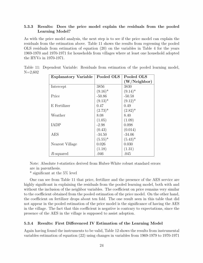
5.3.3 Results: Does the price model explain the residuals from the pooledLearning Model?

As with the price model analysis, the next step is to see if the price model can explain theresiduals from the estimation above. Table 11 shows the results from regressing the pooledOLS residuals from estimation of equation (20) on the variables in Table 4 for the years1969-1970 and 1970-1971 for households from villages where at least one household adoptedthe HYVs in 1970-1971.

Table 11: Dependent Variable: Residuals from estimation of the pooled learning model,N=2,602

Explanatory Variable Pooled OLS Pooled OLS(W/Neighbor)

Intercept 3856 3830(9.16)* (9.14)*

Price -50.86 -50.58(9.13)* (9.12)*

E Fertilizer 0.47 0.49(2.73)* (2.82)*

Weather 8.08 8.40(1.05) (1.09)

IADP -2.98 0.098(0.43) (0.014)

AES -34.50 -34.06(5.55)* (5.43)*

Nearest Village 0.026 0.030(1.18) (1.31)

R-squared .046 .045


One can see from Table 11 that price, fertilizer and the presence of the AES service arehighly significant in explaining the residuals from the pooled learning model, both with andwithout the inclusion of the neighbor variables. The coefficient on price remains very similarto the coefficient obtained from the pooled estimation of the price model. On the other hand,the coefficient on fertilizer drops about ten fold. The one result seen in this table that didnot appear in the pooled estimation of the price model is the significance of having the AESin the village. The fact that this coefficient is negative is contrary to expectations, since thepresence of the AES in the village is supposed to assist adoption.

5.3.4 Results: First Differenced IV Estimation of the Learning Model

Again having found the instruments to be valid, Table 12 shows the results from instrumentalvariables estimation of equation (22) using changes in variables from 1969-1979 to 1970-1971

24

for the sample of households in villages where at least one household adopted.

Table 12: Instrumental Variables First Differences: Dependent Variable is the change inHYV (hectares) (N=1,301)

Explanatory Variable IV First Differences IV First Differences(including neighbor experience)

Constant 12.32 61.16(2.20)* (2.19)*

Own Experience (t) 1.52 0.36(3.76)* (1.97)*

Own Experience (t-1) 1.77 0.43(2.93)* (1.72)

Neighbor Experience (t) 0.26(1.09)

Neighbor Experience (t-1) 0.53(1.37)

Farm Equipment (own) 0.042 0.073(1.16) (0.71)

Irrigation Assets (own) 0.060 0.031(1.73) (0.39)

Farm Animals (own) 0.082 -0.091(1.09) (0.22)

Farm Equipment (neighbor) -0.67(2.13)*

Irrigation Assets (neighbor) 0.22(1.44)

Farm Animals (neighbor) -0.20(0.40)


First, looking only at own characteristics, Table 12 shows that own experience is signif-icant, but declining over time. Similarly, once neighbor characteristics are included, ownexperience declines over time; however, it loses some of its significance. As compared to thepooled results, the coefficients on own and experience variables are larger. Moreover, neigh-bor experience now has a positive coefficient. The significance of these results correspond tothose found by Foster and Rosenzweig (1995) and also reflect the implications of the model,since farmers having more prior experience with HYV seeds tend to use more in the currentperiod. Looking at Foster and Rosenzweig’s (1995) results, one finds, for example a coeffi-cient of .95 and a t-statistic of 4.48 for own experience in time t, while I found a coefficient

25

of 1.52 and a t-statistic of 3.76. The results also indicate that own experience is decreasingover time. This result points to the fact that the effect of experience on the cost of learningis dominated by the costs from the diminishing returns to experience given adoption.

Neighbor experience variables also decline over time and are positive as expected, but areinsignificant. This result could reflect an identification problem characterizing the learninggroup since the set of neighbors from whom an individual can learn is difficult to defineand it is hard to distinguish learning from other phenomena that may give rise to similarobserved outcomes. Here the learning group is defined as people within the same village, anassumption that becomes more problematic as the size of the village grows. Trying to takevillage size into account may help to better capture learning. Or, as mentioned in the contextof the previous model, the key determinant of adoption may not be experience, but someunderlying cause of experience. To support this claim, if social learning is included in theestimation, that is farmer j′s time t decision is influenced by his neighbors’ time t decision,then not surprisingly the neighbor experience variables are highly significant. This resultpotentially stems from similar unobservables driving the results. Finally, the only significantasset variable is average neighbor equipment, again pointing to equipment as perhaps thebest reflection of wealth.

5.3.5 Results: Does the price model explain the residuals from the differencedlearning model?

Once again regressing the resulting residuals from estimation of equation (22) on the differ-enced time variant variables from the price model can give insight into whether the pricemodel correctly characterizes the adoption decision. Table 13 shows the results from thisestimation using changes from 1969-1970 to 1970-1971 for households from villages where atleast one household adopted in the final year.

Table 13: First Differences: The dependent variables are the residuals from estimatingequation (22) (N=1,301)

Explanatory Variable First Differences First Differences(W/Neighbor)

Intercept -9.40 12.86(1.07) (0.65)

E Fertilizer 4.53 0.33(3.33)* (0.11)

Adverse Weather in 1970 -1.24 -63.84(.047) (1.08)

Adverse Weather in 1969 3.31 -41.85(0.21) (1.18)

R-squared .0087 .0018

Note: Absolute t-statistics derived from Huber-White robust standarderrors are in parenthesis.* significant at the 5% level

26

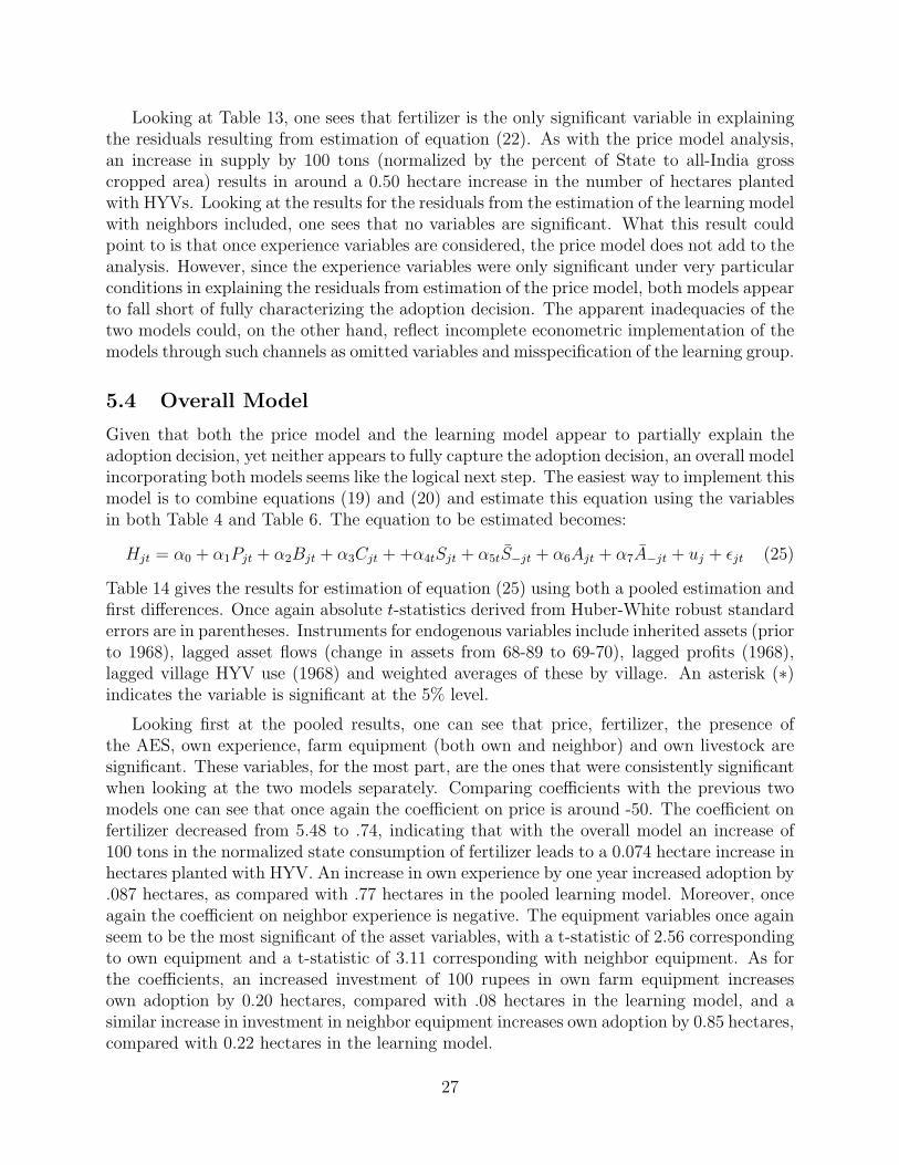
Looking at Table 13, one sees that fertilizer is the only significant variable in explainingthe residuals resulting from estimation of equation (22). As with the price model analysis,an increase in supply by 100 tons (normalized by the percent of State to all-India grosscropped area) results in around a 0.50 hectare increase in the number of hectares plantedwith HYVs. Looking at the results for the residuals from the estimation of the learning modelwith neighbors included, one sees that no variables are significant. What this result couldpoint to is that once experience variables are considered, the price model does not add to theanalysis. However, since the experience variables were only significant under very particularconditions in explaining the residuals from estimation of the price model, both models appearto fall short of fully characterizing the adoption decision. The apparent inadequacies of thetwo models could, on the other hand, reflect incomplete econometric implementation of themodels through such channels as omitted variables and misspecification of the learning group.

5.4 Overall Model

Given that both the price model and the learning model appear to partially explain theadoption decision, yet neither appears to fully capture the adoption decision, an overall modelincorporating both models seems like the logical next step. The easiest way to implement thismodel is to combine equations (19) and (20) and estimate this equation using the variablesin both Table 4 and Table 6. The equation to be estimated becomes:

Hjt = α0 + α1Pjt + α2Bjt + α3Cjt + +α4tSjt + α5tS−jt + α6Ajt + α7A−jt + uj + εjt (25)

Table 14 gives the results for estimation of equation (25) using both a pooled estimation andfirst differences. Once again absolute t-statistics derived from Huber-White robust standarderrors are in parentheses. Instruments for endogenous variables include inherited assets (priorto 1968), lagged asset flows (change in assets from 68-89 to 69-70), lagged profits (1968),lagged village HYV use (1968) and weighted averages of these by village. An asterisk (∗)indicates the variable is significant at the 5% level.

Looking first at the pooled results, one can see that price, fertilizer, the presence ofthe AES, own experience, farm equipment (both own and neighbor) and own livestock aresignificant. These variables, for the most part, are the ones that were consistently significantwhen looking at the two models separately. Comparing coefficients with the previous twomodels one can see that once again the coefficient on price is around -50. The coefficient onfertilizer decreased from 5.48 to .74, indicating that with the overall model an increase of100 tons in the normalized state consumption of fertilizer leads to a 0.074 hectare increase inhectares planted with HYV. An increase in own experience by one year increased adoption by.087 hectares, as compared with .77 hectares in the pooled learning model. Moreover, onceagain the coefficient on neighbor experience is negative. The equipment variables once againseem to be the most significant of the asset variables, with a t-statistic of 2.56 correspondingto own equipment and a t-statistic of 3.11 corresponding with neighbor equipment. As forthe coefficients, an increased investment of 100 rupees in own farm equipment increasesown adoption by 0.20 hectares, compared with .08 hectares in the learning model, and asimilar increase in investment in neighbor equipment increases own adoption by 0.85 hectares,compared with 0.22 hectares in the learning model.

27

Table 14: Overall Model Analysis: Dependent variable is the decision to adopt HYVs(N=1,301 households)

Explanatory Variable Pooled FDIntercept 3908 70.32

(9.09)* (2.02)*Price -51.86

(9.13)*E Fertilizer 0.74 -0.66

(3.76)* (0.018)Weather 8.94

(1.15)IADP 12.44

(1.68)AES -24.35

(3.58)*Nearest Village 0.010

(0.42)Adverse Weather in 1970 -59.52

(1.64)Adverse Weather in 1969 -36.67

(0.87)Own Experience (t) 0.087 0.38

(28.24)* (2.04)*Own Experience (t-1) 0.45

(1.79)Neighbor Experience (t) -0.097 0.23

(1.39) (0.92)Neighbor Experience (t-1) 0.49

(1.18)Farm Equipment (own) 0.0020 0.060

(2.56)* (0.59)Irrigation Assets (own) 0.0028 0.032

(1.68) (0.41)Farm Animals (own) 0.0056 -0.11

(2.18)* (0.28)Farm Equipment (neighbor) 0.0085 -0.64

(3.11)* (2.08)*Irrigation Assets (neighbor) 0.0051 0.21

(1.81) (1.44)Farm Animals (neighbor) 0.0028 -0.16

(0.36) (0.32)

28

Turning now to the estimation in first differences, one sees that only time t own experienceand neighbor farm equipment come out as significant. The coefficient on own experience issimilar to that found in the learning model, 0.38 as opposed to 0.37. Similarly, the coefficienton neighbor farm equipment hardly changes. Here it is -0.64 as opposed to -0.67. It isinteresting that the coefficient on fertilizer is negative and not significant.

Combining the models helps give a sense of which variables are really driving the adoptiondecision. For the most part both the coefficients and the signs of the coefficients do not changedramatically from the original models to this combined overall model. In addition, similarvariables appear to be significant. In the future it would be useful to try to incorporate thetwo models into a more sophisticated overall model.

5.5 Binary Response Analysis: Logit Model

So far this paper has focused on determinants of the number of hectares planted with HYVsby households in villages where at least one household adopts in 1970, but it has not lookeddirectly at the decision to adopt HYVs in a given year. Given that there are a lot of zeros inthe data a logit analysis looking at households in all villages will help give a sense of whatdrives the decision whether or not to adopt the new technology. In implementing the logitmodel I will look at two subsets of the data. The first estimate will look at the entire sampleof villages as a way to get a better sense of what drives both households and villages decisionto adopt HYVs. The second estimate will look at the decision to adopt using the same sampleas the previous analysis, that is, households in villages where at least one household adopts in1970. Within these samples I am going to look at a pooled logit, an unobserved effects logitmodel, and a logit on the cross section for 1970. Having estimated these models, however, Ifound that both the cross section analysis and the unobserved effects model resulted in nosignificant results so I have not reported them here. The results for the pooled logit modelfor the two subsamples are given in Table 15.

29

Table 15: Pooled Logit Analysis: Dependent variable is the decision to adopt HYVsExplanatory Variable All Villages (N=2,177 hh) Villages (N=1,301 hh)

Intercept -12.66 35.38(1.26) (3.45)*

Price -0.13 -0.50(0.96) (3.65)*

E Fertilizer 0.013 0.0041(2.89)* (0.81)

Weather -0.011 -0.28(0.07) (1.53)

IADP 0.98 0.93(6.42)* (5.42)*

AES -0.094 0.082(0.68) (0.51)

Nearest Village 0.0018 .0003(3.93) (0.60)

Own Experience (t) 0.0072 0.0067(5.38)* (6.30)*

Neighbor Experience (t) 0.0040 -0.0006(1.48) (0.26)

Farm Equipment (own) 0.0000 -0.0000(0.41) (0.11)

Irrigation Assets (own) -0.0000 0.0001(0.081) (1.86)

Farm Animals (own) 0.0001 0.0001(2.90)* (2.45)*

Farm Equipment (neighbor) 0.0001 0.0002(2.01)* (2.73)*

Irrigation Assets (neighbor) 0.0001 -0.0000(1.24) (0.051)

Farm Animals (neighbor) 0.0005 0.0003(3.30)* (2.05)*

Note: Absolute t-statistics derived from standard errorsare in parentheses. Instruments for endogenous variables includeinherited assets (prior to 1968), lagged asset flows (change in assets from 68-89 to 69-70),lagged profits (1968), lagged village HYV use (1968) and weighted averages of these byvillage.* significant at a 5% level

First looking at the results from Table 15 for all villages, one can see that fertilizer, beingan IADP village, own experience, own and neighbor livestock, and neighbor farm equipmentare significant. The signs on all these variables, as expected, are positive. It is interestingthat price, although it has the expected sign, does not come out as significant. Although

30

price played an important role in determining the number of hectares planted with HYVs, itappears to play a less important role in the actual decision about whether or not to adopt. Inaddition, livestock, as opposed to equipment or irrigation assets, appears to be the importantasset variable in this estimation. Finally, being an IADP village appears to be extremelyrelevant to the adoption decision. Given that this has been a consistent result throughoutthe analysis, subsequent research is needed comparing IADP and non-IADP villages to seewhat factors are underlying this result

Now, turning to the results for the subset of villages where at least one household adoptedthe new technology, one can see that price, being an IADP village, own experience, ownand neighbor farm animals, and neighbor farm equipment are significant. The sign andsignificance of these results are similar to the results when all villages were included. Thereis, however, one interesting difference, namely that in this case price, not fertilizer, is found tobe significant. When looking at all villages it was the opposite way around. One possible wayto interpret this result is that that access to fertilizer determines whether the new technologyenters a village, while price determines whether an individual household in a village wheresome households are adopting chooses to adopt.

Overall, the logit model allows one to get a better sense of what factors are actuallydriving the decision whether or not to adopt the new technology, as opposed to the scale ofadoption. Given that there are a lot of zeros in the data, this is an important distinction tomake. Moreover, by separating villages where some households adopt from those where nohousehold adopts allows one to get a sense of not only why households adopt, but also whatcauses the new technology to enter a village as a whole.

6 Conclusion

Both the target-input model (Learning Model) and the choice of technique approach (PriceModel) have been used to model decisions on whether or not to adopt a new technology.Both models lead to decision rules that emphasize certain characteristics as the key deter-minants underlying adoption decisions. The price model emphasizes changing prices, inputconstraints, and the local environment, while the learning model focuses on indicators ofexperience and wealth. From the previous analysis, one can see that both models captureimportant aspects of the adoption decision; however, they each disregard components of thealternative model that are significant.

Given the seeming importance of both models, an overall model was implemented thatincorporated aspects of both the learning and price model. The results from this estimationreinforced the fact that variables in both models are relevant to the adoption decision, andhelped give a better sense of the actual significance and magnitude of these explanatoryvariables. Moreover, the estimation of a logit model showed that perhaps the factors de-termining whether or not to adopt differ from those determining the scale of adoption. Inaddition, the logit analysis pointed to the fact that the subset of data used in the analysiscan lead to different conclusions, therefore indicating the importance of both clearly definingand providing a rationale for the data used in each estimation.

Overall, looking at the results it appears that additional state level data, as well as amore precise characterization of the learning group, would improve the analysis. In addi-

31

tion, since some of the time-invariant village characteristics appear to be important, tryingto model farmer heterogeneity would allow one to take the pooled OLS estimates more seri-ously. Moreover, given the apparent complexity of the adoption decision process, attemptsto model and analyze such decisions requires a very precise specification of the surroundingenvironment. This specification must consider the local conditions in which the technologyis being implemented, as well as the characteristics of the technology itself.

In conclusion, the results indicate that both the learning model and the price modelcapture certain aspects of the adoption decision concerning high yielding variety seeds inIndia. It is clear, however, that additional research needs to be done to more carefully andfully characterize the adoption decision. Since the successful adoption of new technology isan essential part of poverty reduction in today’s society, the development of a more com-plete model could then be used to characterize and test adoption decisions taking placetoday. A better understanding of this process would then promote policy makers’ successfulimplementation of new technologies.

32

References

Bandiera, O. and I. Rasul (2002). Social networks and technology adoption in northernMozambique. Technical Report 3341, CEPR Discussion Paper.

Besley, T. and A. Case (1993). Modeling technology adoption in developing countries. Amer-ican Economic Review 83 (2), 396–402.

Bumb, B. (1979). Survey of the fertilizer sector in India. Technical Report 331, World Bank,Washington, D.C.

Chandhok, H. Wholesale Price Statistics India 1947-1978, Volume 1. Economic and ScientificResearch Foundation.

Conley, T. and C. Udry (2000). Learning about a new technology: Pineapple in Ghana.Technical report, Working Paper-Yale University.

Dasgupta, B. (1977). Agrarian change and the new technology in India. Geneva, Switzerland:United Nations Research Institute for Social Development.

Feder, G., R. Just, and D. Zilberman (1985). Adoption of agriculture innovations in devel-oping countries: A survey. Economic Development and Cultural Change 33 (2), 255–298.

Foster, A. and M. Rosenzweig (1995). Learning by doing and learning from others: Humancapital and technical change in agriculture. Journal of Political Economy 103 (6), 1176–1209.

Foster, A. D. and M. R. Rosenzweig (1996). Technical change and human-capital returns andinvestments: Evidence from the green revolution. The American Economic Review 86 (4),931–953.

Kohli, D. and N. Singh (1997). The green revolution in Punjab, India: The economicsof technical change. Technical report, Conference on Agriculture of the Punjab at TheSouthern Asian Institute, Columbia University.

McGuirk, A. and Y. Mundlak (1991). Incentives and constraints in the transformation ofPunjab agriculture. Research Report 87, International Food Policy Research Institute,Washington D.C.

Mundlak, Y. (1992). Agricultural productivity and economic policies: Concepts and mea-surements. Technical report, OECD-Development Center Series.

Mundlak, Y., D. Larson, and R. Butzer. Agricultural dynamics in Thailand, Indonesia, andthe Philippines.

Shah, C. H. and C. N. Vakil (Eds.) (1979). Agriculture Development of India: Policy andProblems. New Delhi: Orient Longman Limited.

33

Sunding, D. and D. Zilberman (2002). The agriculture innovation process: Research andtechnology adoption in a changing agricultural sector.

Wooldridge, J. M. (2002). Econometric Analysis of Cross Section and Panel Data. Cam-bridge, MA: The MIT Press.

34

Documents

Modeling Technology Adoption Decisions: An Analysis … · Modeling Technology Adoption Decisions: An Analysis of High Yielding Variety Seeds in India During the Green Revolution