Embed Size (px)
Citation preview
University of South FloridaScholar Commons
Graduate Theses and Dissertations Graduate School
January 2012
Modeling Travel Time and Reliability on UrbanArterials for Recurrent ConditionsProny Bonnaire FilsUniversity of South Florida, [email protected]
Follow this and additional works at: http://scholarcommons.usf.edu/etd
Part of the American Studies Commons, Civil Engineering Commons, and the Urban Studiesand Planning Commons
This Dissertation is brought to you for free and open access by the Graduate School at Scholar Commons. It has been accepted for inclusion inGraduate Theses and Dissertations by an authorized administrator of Scholar Commons. For more information, please [email protected].
Scholar Commons CitationBonnaire Fils, Prony, "Modeling Travel Time and Reliability on Urban Arterials for Recurrent Conditions" (2012). Graduate Thesesand Dissertations.http://scholarcommons.usf.edu/etd/3984
Modeling Travel Time and Reliability on Urban Arterials for Recurrent Conditions
by
Prony Bonnaire Fils
A dissertation submitted in partial fulfillment
of the requirements for the degree of
Doctor of Philosophy
Department of Civil and Environmental Engineering
College of Engineering
University of South Florida
Co-Major Professor: Jian John Lu, Ph.D.
Co-Major Professor: Pei-Sung Lin, Ph.D.
Rebecca Wooten, Ph.D.
Abdul Pinjari, Ph.D.
Yu Zhang, Ph.D.
Kingsley Reeves, Ph.D.
Date of Approval:
April 30, 2012
Keywords: Multiple Linear Regression, Correlation,
Buffer Time, Influencing Factors, Transportation Planning
Copyright © 2012, Prony Bonnaire Fils

Dedication
This dissertation is dedicated to my wonderful wife Fhadia, my lovely kids
Prudny and Nyrdia, my dedicated parents Leonie and Victor with appreciation for the
support, help, prayer, and encouragement that I have received during the years that I have
devoted for the doctorate degree.
Acknowledgements
I express my thanks and gratitude to my co-major professors Dr. Pei Sung Lin
and Dr. John Lu for their guidance and support on this dissertation. They were very
patient spending a lot of time over the past four years to supervise my study, discuss
research issues, offer insights and suggestions, and invaluable input. Special thanks also
to my other committee members for their advice and their input. First of all, I thank Dr.
Rebecca Wooten who analyzed the statistical and mathematical data from the single
linear regression to the multiple regression analysis. My thanks to Dr. Yu Zhang for her
comments, criticism, and help to improve the model framework and the travel time
reliability threshold. Similarly, cheers and thanks to Dr. Abdul Pinjari who commented
on the selected factors included in the model and provided advice to improve the
literature review and the model. I also thank Dr. Kingsley Reeves who expressed at the
proposal defense the inclusion of the signal timing in the selected factors. Furthermore, I
owe a big word of thanks to Sensys Networks to let me access their travel time database
through the ATTS (Arterial Travel Time System). My thanks also to Sarasota County
Traffic Operations Division that provided the traffic data needed for the model
validation and robustness. Thank you to the many others, too many to name, who have
played some role in making this doctoral research effort possible.
Finally, many thanks, hugs, and kisses go out to my wonderful wife Fhadia, my
lovely kids Prudny and Nyrdia who supported and tolerated me in the last four years and
enabled me to reach this milestone in my life.
i
Table of Contents
List of Tables ..................................................................................................................... iii
List of Figures .................................................................................................................... vi
Abstract ............................................................................................................................ viii
Chapter 1- Introduction ........................................................................................................1
1.1 Context ...............................................................................................................1
1.2 Background and Problem Statement ..................................................................2
1.2.1 Urban Arterials and Travel Time Reliability ......................................2
1.2.2 Travel Time Reliability and Road Users in the Coming Years ..........5
1.3 Research Objectives ...........................................................................................8
1.3.1 Adaptability of Model .......................................................................10
1.3.2 Generality of Model ..........................................................................10
1.3.3 Robustness of Model.........................................................................10
1.3.4 Accuracy of Model ...........................................................................10
1.4 Dissertation Outline .........................................................................................11
Chapter 2- Literature Review .............................................................................................13
2.1 Previous Studies on Travel Time Reliability ...................................................13
2.2 Previous Travel Time Reliability Calculation Methods ..................................23
Chapter 3- Methodology ....................................................................................................31
3.1 Influencing Factors ..........................................................................................31
3.2 Statistical Methods and Analysis .....................................................................35
3.2.1 Travel Time Reliability Calculation Method ....................................36
3.2.2 Correlation among Reliable Travel Times and Influencing
Factors ...............................................................................................37
3.2.3 Linear Relationship between Dependent and Independent
Variables ...........................................................................................38
3.2.4 The Wrong Signs in the Linear Regression Model ...........................40
3.3 Alternative Models...........................................................................................41
3.3.1 Simultaneous Equation Models (SEM) ............................................41
3.3.2 Count Data Models ...........................................................................43
3.3.3 The Poisson Distribution ..................................................................43
3.3.4 The Negative Binomial Regression Model .......................................44
3.3.5 Discrete Outcome Models.................................................................44
3.4 Different Steps for the Model Equation ...........................................................46
ii
Chapter 4- Data Collection ................................................................................................48
4.1 Geographic Areas.............................................................................................48
4.2 Time Elements .................................................................................................51
4.2.1 Month of the Year .............................................................................52
4.2.2 Days of the Week ..............................................................................52
4.2.3 Time Periods...………………….......................................................52
4.3 Data Collection Method ...................................................................................52
4.4 Alternative Travel Time Data Collection Methods .........................................57
Chapter 5- Statistical Results and Discussion ....................................................................60
5.1 Travel Time and Reliable Travel Time Data Analysis ....................................60
5.2 Single Linear Regression and Correlation Analysis ........................................71
5.3 Multiple Linear Regression Analysis...............................................................75
5.4 Interaction Effects in the Regression Model ....................................................98
5.5 Model Validation ...........................................................................................100
5.6 Generality of the Model .................................................................................103
5.7 Scenarios-Marginal Effects ............................................................................107
5.8 Guidance on Roadway Design, Traffic Design, Traffic Operations, and
Access Management ......................................................................................109
Chapter 6- Limitations and Contributions .......................................................................111
6.1 Summary of Limitations ................................................................................111
6.2 Summary of Contributions .............................................................................112
6.3 Implications and Recommendations for Future Research .............................113
References ........................................................................................................................115
Appendices .......................................................................................................................119
Appendix A- Travel Times for the Segments for Peak Periods - Driving
Westward .......................................................................................................120
Appendix B- Travel Times for the Segments for Peak Periods - Driving
Eastward .........................................................................................................125
Appendix C- List of Acronyms............................................................................129
Appendix D- Third Party Permissions……………………………………....... 131
About the Author ................................................................................................... End Page
iii
List of Tables
Table 1: Travel Time Reliability Measures Recommended by Different Sources ............29
Table 2: Segment Attributes ..............................................................................................51
Table 3: Travel Time Reliability Thresholds and Buffer Times for the Segments ...........71
Table 4: Single Linear Regression and Correlation among Factors ..................................73
Table 5: Independent Variables (Factors) by Order of Significance .................................75
Table 6: Description of Selected Independent Variables ...................................................76
Table 7: Summary Output # 1 ............................................................................................77
Table 8: ANOVA # 1 (Analysis of Variance) ...................................................................77
Table 9: First Linear Regression Analysis .........................................................................78
Table 10: Summary Output # 2 ..........................................................................................78
Table 11: ANOVA # 2 (Analysis of Variance) .................................................................78
Table 12: Second Linear Regression Analysis ..................................................................79
Table 13: Summary Output # 3 ..........................................................................................79
Table 14: ANOVA # 3 (Analysis of Variance) .................................................................79
Table 15: Third Linear Regression Analysis .....................................................................80
Table 16: Summary Output # 4 ..........................................................................................80
Table 17: ANOVA # 4 (Analysis of Variance) .................................................................80
Table 18: Fourth Linear Regression Analysis ...................................................................81
Table 19: Summary Output # 5 ..........................................................................................81
iv
Table 20: ANOVA # 5 (Analysis of Variance) .................................................................82
Table 21: Fifth Linear Regression Analysis ......................................................................82
Table 22: Summary Output # 6 ..........................................................................................83
Table 23: ANOVA # 6 (Analysis of Variance) .................................................................83
Table 24: Sixth Linear Regression Analysis ......................................................................84
Table 25: Summary Output # 7 ..........................................................................................84
Table 26: ANOVA # 7 (Analysis of Variance) .................................................................84
Table 27: Seventh Linear Regression Analysis .................................................................85
Table 28: Summary Output # 8 ..........................................................................................85
Table 29: ANOVA # 8 (Analysis of Variance) .................................................................86
Table 30: Eighth Linear Regression Analysis ...................................................................86
Table 31: Summary Output # 9 ..........................................................................................87
Table 32: ANOVA # 9 (Analysis of Variance) .................................................................87
Table 33: Ninth Linear Regression Analysis .....................................................................88
Table 34: Summary Output # 10 ........................................................................................88
Table 35: ANOVA # 10 (Analysis of Variance) ...............................................................88
Table 36: Tenth Linear Regression Analysis .....................................................................89
Table 37: Summary Output # 11 ........................................................................................89
Table 38: ANOVA # 11 (Analysis of Variance) ...............................................................90
Table 39: Eleventh Linear Regression Analysis ................................................................90
Table 40: Summary Output # 12 ........................................................................................91
Table 41: ANOVA # 12 (Analysis of Variance) ...............................................................91
Table 42: Twelfth Linear Regression Analysis .................................................................92
v
Table 43: Summary Output # 13 ........................................................................................92
Table 44: ANOVA # 13 (Analysis of Variance) ...............................................................92
Table 45: Thirteenth Linear Regression Analysis .............................................................93
Table 46: Summary Output # 14 ........................................................................................94
Table 47: ANOVA # 14 (Analysis of Variance) ...............................................................94
Table 48: Fourteenth Linear Regression Analysis .............................................................95
Table 49: Summary Output # 15 ........................................................................................95
Table 50: ANOVA # 15 (Analysis of Variance) ...............................................................96
Table 51: Independent Variables (Factors) by Order of Significance ...............................97
Table 52: Description of Variables Including Interaction X3X2 ........................................99
Table 53: Summary Output # 16 ........................................................................................99
Table 54: ANOVA # 16 (Analysis of Variance) .............................................................100
Table 55: Attributes of Segment # 9008 ..........................................................................102
Table 56: Segment Attributes for Model Generality and Robustness .............................106
Table 57: Travel Time Reliability Comparison for Model Generality and Robustness ..107
Table 58: Travel Time Reliability Comparison for the Segments by Modifying X15 .....108
Table 59: Travel Time Reliability Comparison for the Segments by Modifying X1 .......109
Table 60: Travel Time Reliability Comparison for the Corridor
by Modifying X1 & X15....................................................................................109
vi
List of Figures
Figure 1: Probability Density Function of the Standard Lognormal Distribution .............20
Figure 2: Reliability Measures Compared to Average Congestion Measures ...................24
Figure 3: Performance Measure Distribution ....................................................................28
Figure 4: Factors Affecting Travel Time Reliability .........................................................34
Figure 5: Model Framework………………………………………………………….......47
Figure 6: Telegraph Canyon Rd., Chula Vista County, CA ……………………………..49
Figure 7: Telegraph Canyon Rd-Geometric Design Layout ..............................................50
Figure 8: Wireless Sensors and Access Points Deployed for ATTS……………………..54
Figure 9: 90th Percentile Travel Time for ATTS ..............................................................55
Figure 10: Car in Segments for ATTS ...............................................................................56
Figure 11: Travel Times for Morning Peak Time Periods (Driving West) .......................60
Figure 12: Travel Times for Afternoon Peak Time Periods (Driving West) .....................61
Figure 13: Travel Times for Morning Peak Time Periods (Driving East) .........................61
Figure 14: Travel Times for Afternoon Peak Time Periods (Driving East) ......................62
Figure 15: Buffer Time (sec.) for Segment # 9008 for Peak Periods (Driving West) .......63
Figure 16: Buffer Time (sec.) for Segment # 8007 for Peak Periods (Driving West) .......63
Figure 17: Buffer Time (sec.) for Segment # 7006 for Peak Periods (Driving West) .......64
Figure 18: Buffer Time (sec.) for Segment # 6005 for Peak Periods (Driving West) .......64
Figure 19: Buffer Time (sec.) for Segment # 5004 for Peak Periods (Driving West) .......65
Figure 20: Buffer Time (sec.) for Segment # 4003 for Peak Periods (Driving West) .......65
vii
Figure 21: Buffer Time (sec.) for Segment # 3002 for Peak Periods (Driving West) .......66
Figure 22: Buffer Time (sec.) for Segment # 2001 for Peak Periods (Driving West) .......66
Figure 23: Buffer Time (sec.) for Segment # 1002 for Peak Periods (Driving East) ........67
Figure 24: Buffer Time (sec.) for Segment # 2003 for Peak Periods (Driving East) ........67
Figure 25: Buffer Time (sec.) for Segment # 3004 for Peak Periods (Driving East) ........68
Figure 26: Buffer Time (sec.) for Segment # 4005 for Peak Periods (Driving East) ........68
Figure 27: Buffer Time (sec.) for Segment # 5006 for Peak Periods (Driving East) ........69
Figure 28: Buffer Time (sec.) for Segment # 6007 for Peak Periods (Driving East) ........69
Figure 29: Buffer Time (sec.) for Segment # 7008 for Peak Periods (Driving East) ........70
Figure 30: Buffer Time (sec.) for Segment # 8009 for Peak Periods (Driving East) ....... 70
Figure 31: Travel Times Reliability Comparison for the Segments
between Observed and Estimated Data..........................................................102
Figure 32: Travel Times Reliability Comparison for the Corridor
between Observed and Estimated Data..........................................................103
Figure 33: Selected Corridors from Sarasota County, FL ...............................................105
viii
Abstract
Travel time reliability is defined as the consistency or dependability in travel times
during a specified period of time under stated conditions, and it can be used for evaluating
the performance of traffic networks based on LOS (Level of Service) of the HCM
(Highway Capacity Manual). Travel time reliability is also one of the most understood
measures for road users to perceive the current traffic conditions, and help them make
smart decisions on route choices, and hence avoid unnecessary delays (Liu & Ma, 2009).
Therefore, travel time reliability on urban arterials has become a major concern for daily
commuters, business owners, urban transportation planners, traffic engineers, MPO
(Metropolitan Planning Organization) members as congestion has grown substantially over
the past thirty (30) years in urban areas of every size.
Many studies have been conducted in the past on travel time reliability without a
full analysis or explanation of the fundamental traffic and geometric components of the
corridors. However, a generalized model which captures the different factors that influence
travel time reliability such as posted speed, access density, arterial length, traffic
conditions, signalized intersection spacing, roadway and intersection geometrics, and signal
control settings is still lacking. Specially, there is a need that these factors be weighted
according to their impacts.
This dissertation by using a linear regression model has identified 10 factors that
influence travel time reliability on urban arterials. The reliability is measured in term of
ix
travel time threshold, which represents the addition of the extra time (buffer or cushion
time) to average travel time when most travelers are planning trips to ensure on-time
arrival. “Reliable” segments are those on which travel time threshold is equal to or lowers
than the sum of buffer time and average travel time.
After validation many scenarios are developed to evaluate the influencing factors
and determine appropriate travel times reliability. The linear regression model will help 1)
evaluate strategies and tactics to satisfy the travel time reliability requirements of users of
the roadway network—those engaged in person transport in urban areas 2) monitor the
performance of road network 3) evaluate future options 4) provide guidance on
transportation planning, roadway design, traffic design, and traffic operations features.
1
Chapter 1- Introduction
1.1 Context
Travel time is one of the most important measurements for evaluating the
operating efficiency of traffic networks and accurate and reliable travel time information
has become increasingly important for traffic engineers, daily commuters, residents,
business owners, MPO members etc. Chen et al. (2003) stated that travel time reliability
is “an important measure of service quality for travelers”. Personal and business travelers
value reliability because it allows them to make better use of their own time. Shippers
and freight carriers require predictable travel times to remain competitive. Reliability is
also a valuable service that can be provided on privately-financed or privately operated
highways.1 Nam et al. (2006) argued that travelers’ tastes for travel time and travel time
reliability vary across times of day and that route choice is based on a combination of
travel time, travel time reliability, and cost.
However, the travel time experienced by a traveler making a trip on an arterial
segment is not just the result of his or her own travel choices (destination, mode, route,
speed), but also the choices of many other travelers, not necessarily only those traveling
the same segment. Moreover, a substantial component of driver behavior may not be
classified as rational choice behavior, but rather a product of the different characteristics
of individual drivers; for example attention level, driving style, risk assessment, and their
1 FHWA. Travel Time Reliability: Making it There on Time, All the Time, 2006.
2
vehicles, such as acceleration and deceleration capabilities (Van Lint, J.,2004). Finally,
travel time reliability on an arterial segment is also determined by processes completely
beyond the control of individual or groups of drivers or even the organization responsible
for the road facility such as weather, calamities, incidents and accidents, traffic patterns,
seasonal patterns and so on. Therefore, the travel time reliability on arterial networks is
usually not only a function of traffic flow, driver behavior, traffic composition, link
capacity and speed limit, but also involves numerous other factors such as signal timing,
roadway and intersection geometries, adjacent land use and development, median type,
signalized intersection spacing, and conflicting traffic from cross streets.
It is almost impossible to predict the traffic-influencing events (traffic incidents,
weather, and work zones), behaviors (both rational and irrational) of all individual drivers
in a road network, and all external circumstances that may affect travel time reliability. In
this dissertation, the linear regression model seeks to deduce the general relationships
among factors that influence travel time reliability on urban arterials. Many studies have
been conducted in the past on travel time reliability, but most are focused on freeways
and non-recurrent factors on arterials. Conversely, the impact of recurrent factors on
travel time reliability on urban arterials is still a very complex and challenging problem.
1.2 Background and Problem Statement
1.2.1 Urban Arterials and Travel Time Reliability
Arterial roads, or arterial thoroughfares, are high-capacity urban roads whose
primary function is to deliver traffic from collector roads to freeways, and between major
activity centers of a metropolitan area at the highest level of service possible. As such,
many arteries are limited-access roads, or feature restrictions on private access. They
3
normally are divided into two classes, major (principal) and minor, and their design
ranging from four to eight through lanes is very challenging to transportation
professionals working in the design field. As described by ITE (Institute of
Transportation Engineers):
….Urban arterials streets often present the most challenging type of
geometric design because of the need to provide safe and efficient
operations for multiple types of users under unusual and constrained
conditions. In addition, the designer must be prepared to apply criteria for
differing types of arterial design features to address transitions as an
arterial moves through varying types and densities of land uses that often
exist along arterial corridors in urban settings (Institute of Transportation
Engineers, Urban Street Geometric Design Handbook, 2008. p.7).
Urban arterials are the main thoroughfares on which U.S. motorists do most of
their driving. According to HCM 2000 urban arterials are signalized streets that primarily
serve through-traffic and that secondarily provide access to abutting properties, with
signal spacing of 2.0 mi or less.2 Today, U.S. motorists travel almost 80 percent more
mile on urban arterials compared with rural arterials and most of urban arterials were not
originally designed to accommodate today’s heavy traffic.3 Instead, they have evolved as
urban and suburban traffic has increased. Consequently, congestion has not only grown
substantially over the past 30 years in cities of every size, it has become more volatile as
well.4 According to Texas Transportation Institute‘s researchers, congestion levels in 85
2 Highway Capacity Manual (HCM) 2000.
3 Insurance Institute for Highway Safety” Traffic Engineering Approaches to Reduce Crashes on Urban
Arterial Roads”, April 2000. 4 Texas Transportation Institute, 2011 Annual Urban Mobility Report.
4
of the largest metropolitan areas have grown in almost every year in all population group
from 1982 to 2010.5 In 2010, the amount of average delay endured by the average
commuter was 34 hours, up from 14 hours in 1982. The cost of congestion is more than $
100 billion, nearly $750 for every commuter according to the 2010 Annual Urban
Mobility Report.
This trend is expected to continue as America becomes increasingly urbanized, 85
percent by 2020.6 The increasing congestion levels have influenced travel time reliability,
which is significant to all the transportation system users whether they are vehicle
drivers, transit riders, freight shippers, or even air travelers. Moreover, travel times are so
unreliable on U.S. highways that travelers must plan for these problems by leaving early
just to avoid being late. This means extra time out of everyone's day that must be devoted
to travel; even if it means getting somewhere early, that is still time travelers could be
using for other endeavors. The urban arterial network is so unreliable commuters could
be late for work or after-work appointments, business travelers could be late for
meetings, and truckers could incur extra charges by not delivering their goods on time.
There is considerable evidence from stated preference survey results related to
demand estimation for toll roads and public transport projects that traveler’s willingness
to pay, extends to reliability of travel time, especially for time-sensitive trips.7 The
willingness to pay for reductions in the day-to-day variability of travel time is referred to
as VOR (value of reliability). Some U.S studies have found that users place a value on
travel time variability of more than twice the value placed on the average travel time.8 In
5 Texas Transportation Institute, 2011 Annual Urban Mobility Report.
6 Human Development Reports.
7 Monitoring and Modeling Travel Time Reliability, Transport Futures, Feb. 2008
8 Ibid
5
addition, traffic professionals recognize the importance of travel time reliability because
it better quantifies the benefits of traffic management and operation activities than simple
averages.
In addition to having a value to users, in terms of travel time certainty and travel
time reductions due to reduced in average trip times, reliability has an indirect impact on
trip costs, by potentially reducing fuel consumption, vehicle emissions and public
transport operating costs.9
Therefore determining the different factors that influence travel time reliability on
urban arterials is significant. Road agencies and authorities have an interest and
responsibility to address the factors that cause unreliable travel time. The reliability
measure should provide information about the amount of time that should be budgeted
for a trip. The calculation process for any specific measure formulation should control for
variations that are not relevant to the trip planning decision, although these elements will
vary. This may include factors such as day-to-day and time variations (because travel
decisions may be made with knowledge of the day and time) and variation in road
characteristics (because travelers typically examine their trip travel time rather than each
road section separately) (Lomax et al., 2003).
1.2.2 Travel Time Reliability and Road Users in the Coming Years
The FHWA (Federal Highway Administration) projects that between 1998 and
2020 domestic freight volumes will grow by more than 65 percent, increasing from 13.5
billion tons to 22.5 billion tons.10
FHWA expects trucks to move over 75 percent more
9 Texas Transportation Institute, 2011 Annual Urban Mobility Report.
10Monitoring and Modeling Travel Time Reliability, Transport Futures, Feb. 2008
6
tons in 2020, capturing a somewhat larger share of total freight tonnage than currently.
This rapid growth in truck volume can be attributed to a number of factors including the
shift of significant freight activity from rail and other modes to truck, and the changes in
the economy and business practices such as just-in-time deliveries of inventory items that
increase delivery frequencies (Polzin, S., 2006). To carry this freight, truck VMT
(Vehicle Mile Travelled) is expected to grow at a rate of more than three percent annually
over the same period (DRI-WEFA, 2000).
E-business is expected to increase significantly over the next decades and will
influence the land use patterns and VMT. The shopping from home (via catalogs, cable
television shows, and the internet) and highly efficient package delivery companies, such
as Federal Express and United Parcel Service, will increase trips from local businesses to
homes. It will also drive freight supply and demand away from long-haul carriers toward
less-than-truck load or smaller truck freight shipments as a significant portion of all types
of retailing required next-day delivery, same-day delivery, and just-in-time delivery.
The demographic shifts likely to occur between 2000 and 2020 in the U.S.
population will also generate more traffic on urban roadways and increase congestion.
The U.S. Census Bureau projects the U.S. population will be somewhat better off
economically, older, better educated, households will be smaller and household vehicle
ownership to increase.11
In the coming years, the number of older drivers on the road is
expected to at least double. This increase is attributable to both the overall increase in the
older population, as well as the anticipated trend for older women to drive in greater
proportions than their previous cohorts (Pisarski, A., 2006). These household
11
U.S. Census Bureau, U.S. Population Projection by Age, Sex
7
composition shifts, changes in labor force participation and household income, and shifts
in licensing and vehicle ownership all will affect transportation and individual mobility,
which is expected to increase the highway VMT by 60 percent in 202012
(3,881 billion
compared with 2.631 billion in 2000).
At the same time, researchers and practitioners are aware of the impacts of travel
time reliability and consequently have adjusted their methodologies. For instance, in
transportation planning, incorporating the value of travel time reliability has been found
to significantly enhance mode choice models (Pinjari & Bhat, 2006; Liu et al., 2007). The
second Strategic Highway Research Program (SHRP2) determines reliability as one of
the four transportation factors that needs to be addressed when making a highway
capacity expansion decision.13
Additionally, reliability research is developing the means
for state DOTs and Metropolitan Planning Organizations to fully integrate mobility and
reliability performance measures and strategies into the transportation planning
processes. Studies are under way to include reliability factors into the Highway Capacity
Manual. A guide on roadway design features will be written to support the reduction of
delays that reduce travel time reliability so that such features can be considered for
inclusion in the AASHTO Policy on Geometric Design of Highways and Streets.14
Reliability requirements for personal trips vary considerably depending on trip
type (commuter trips, medical appointments, school trips, attending places of worship,
day-care pickup, and social/recreational), time of day (peak period versus off-peak) and
the travel setting and conditions. Reliability requirements vary depending on the portion
12
U.S Department of Energy/Energy Information Administration 13
Cambridge Systematics, Inc., High Street Consulting Group, TransTech Management, Inc., Spy Pond
Parterners, Ross & Associates. Performance Measure Framework for Highway Capacity Decision Making.
Washington, D.C.: Transportation Research Board of National Academies, 2009. NCHRP Report 618 14
Transportation Research Board, Updating Reliability Research in SHRP 2, January 2011
8
of the road network used, geographic areas (urban or rural), and the factors that
contribute to the uncertainty of arrival time on these arterials, such as rail road crossing,
number of signalized intersections, signal timing cycle length, posted speed, roadway
characteristics, school bus stops.
Reliability requirements for business trips (freight carriers, shippers, truckers)
vary also depending on the situation and business characteristics (small businesses,
family owned businesses). Transportation agencies must understand these different user
requirements if they expect to meet them effectively. As pointed out by TRB
(Transportation Research Board).
….Actions taken by transportation agencies to reduce congestion should
effectively improve travel time reliability. To assure the effectiveness of
those actions, the user requirements regarding travel time reliability must
be understood. Different users of the highway network have different
requirements for travel time reliability. Moreover, the requirements of
each user depend on the situation. A trucker faced with just-in-time
delivery has different travel time reliability requirements than an empty
backhaul of a mom-and-pop trucking business. Service level agreements
for just-in-time delivery can impose severe penalties for not being on time
(Transportation Research Board, in SHRP 2 L11, Evaluating Alternative
Operations Strategies to Improve Travel Time Reliability, 2010).
1.3 Research Objectives
The dissertation will address travel time reliability on major urban arterials. We
adhere to the definition for arterials given in the Highway Capacity Manual 2000:
9
“Arterials are signalized streets that primarily serve through-traffic and that secondarily
provide access to abutting properties, with signal spacing of 2.0 mi or less”. Travel time
the time it takes a typical commuter to move from the beginning to the end of a corridor
(Florida Department of Transportation, 2000) and travel time reliability is defined as the
consistency or dependability in travel times during a specific period of time under stated
conditions. This consistency has to consider the travel time threshold due to the impact of
the influencing factors.
The reliability is measured in term of travel time threshold, which typically
represents the addition of the extra time (or cushion time) to the average travel time when
most travelers are planning trips to ensure on-time arrival. “Reliable” segments are those
on which travel time threshold is equal to or lowers than the buffer time added to the
average travel time.
Reliability is concerned with three key elements of this definition:
First, reliability is a probability which is concerned with meeting the
specific probability of consistency or dependability at a statistical
confidence level.
Second, reliability applies to a defined threshold and specific time periods.
Third, reliability is restricted to operation under stated conditions. This
constraint is necessary because it is impossible to design a system for
unlimited conditions.
The main objective of this dissertation is to develop a travel time reliability model
that is adaptive, general, robust, and accurate to identify the linear relationship between
10
the continuous dependent variable (travel time reliability) and other independent
variables (the different factors that influence travel time reliability) on urban arterials.
1.3.1 Adaptability of Model
“Traffic processes are characterized by constant change, due to structural changes
in both traffic demand patterns as well as traffic supply characteristics. The model should
be able to track these changes and adapt accordingly to preserve its validity” (Van Lint, J.
W.C., 2004).
1.3.2 Generality of Model
The model will be general, and not-location-specific, at least in terms of
mathematical structure and the overall input-output relationships. For example, an urban
arterial model should be applicable on different arterial networks, with different
geometrical properties (number of lanes, access density). A model that requires specific
design for every location is not likely to be successfully deployed on a large scale.
1.3.3 Robustness of Model
If the data to the model is corrupt, which is a common problem in real-time traffic
data collection systems, the model should be able to produce reasonable outcomes (which
could even be a message indicating something is wrong).
1.3.4 Accuracy of Model
The difference between what actually happened and the information (in the case
of travel time) should be as small as possible, which is subject to location and application
specific circumstances. Roughly, model output errors can be categorized into two types:
11
structural errors (bias) and random errors (variance). Put simply, an accurate model
makes small (quantitative mistakes), in terms of both bias and variance.
This travel time reliability model will be useful to:
evaluate strategies and tactics to satisfy the travel time reliability
requirements of users of the urban roadway networks,
monitor the performance of road networks,
evaluate future roadway improvement options,
provide guidance on planning, geometric and traffic designing, and traffic
operations features.
1.4 Dissertation Outline
Chapter 1 explained the importance of travel time reliability measurements for
technical and non-technical audiences. After the definition of urban arterials from HCM,
this chapter outlined the increasing impacts of U.S motorists traveling on these arterials
(congestion has grown and become more volatile). The importance of travel time
reliability for road users in the coming years is also described. The research objectives,
which describe a new travel time threshold (reliability) based on the buffer index, the
buffer time, and the average travel time, are included in this chapter. In addition, the
theoretical and practical relevance of the model are illustrated.
Chapter 2 is the literature review where previous studies on travel time reliability
and previous travel time reliability calculation methods are described. The advantages
and disadvantages of these studies and calculation methods are also analyzed.
12
Chapter 3 is the methodology where the statistical analysis (single and multiple
linear regressions), the selected influencing factors, and model framework are explained
in details.
In chapter 4, the data collection architecture (geographic areas, time elements),
the data collection methods (comparison between the selected data collection method and
other alternative methods) are analyzed.
Chapter 5 is the statistical results of the data and discussion. The travel time
reliability threshold for each segment, the buffer index and buffer time for each segment,
the correlation among contributing factors, the model linear regression equation, model
validation, model generality and robustness, scenarios analysis, guidance on roadway
design, traffic design are part of this chapter.
Finally, in chapter 6 the limitations and the main contributions of this dissertation
to the state-of-the-art are presented and guidelines for future research are outlined.
This dissertation is concluded with Appendix A (Travel Times for the Segments
Driving Westward), Appendix B (Travel Times for the Segments Driving Eastward),
Appendix C (List of Acronyms), and Appendix D (Third Party Permission).
13
Chapter 2-Literature Review
2.1 Previous Studies on Travel Time Reliability
Although research on travel time reliability for freeways is very rich, research on
arterial travel time reliability is quite limited. Prediction of travel time is potentially more
challenging for arterials than for freeways because vehicles traveling on arterials are
subject not only to queuing delay but also to signal delays as well as delays caused by
vehicles from the cross streets ( Yang, J., 2006).
Abishai Polus (1979) in “A study of Travel Time and Reliability on Arterial
Routes” analyzed travel time and operational reliability on arterial routes. Reliability is
viewed in terms of the consistency of operation of the route under investigation and
defined in terms of the inverse of the standard deviation of the travel time distribution.
Under certain assumptions, travel time behavior on an arterial route is seen to closely
follow a gamma distribution; the reliability measure can be derived accordingly. Utilizing
arterial travel time data from the Chicago area, both a regression and a statistical model
are shown to serve as efficient techniques in predicting reliability. The prediction models
are evaluated.
Fu et al. (2001) in “An Adaptive Model for Real-Time Estimation of Overflow
Queues on Congested Arterials “presented a model that can be used to estimate one of the
congestion measures, namely real-time overflow queue at signalized arterial approaches.
The model is developed on the basis of flow conservation, assuming that time-varying
traffic arterials can be obtained from loop detectors located at signalized approaches and
14
signal control information is available online. A conventional microscopic simulation
model is used to generate data for evaluation of the proposed model. A variety of
scenarios representing variation in traffic control, level of traffic congestion and data
availability are simulated and analyzed.
The “Modeling Network Travel Time Reliability under Stochastic Demand” study
conducted by Stephen Clark and David Watling in 2003 proposed a method for
estimating the probability distribution of total network travel time in the light of normal
day-to-day variations in the travel demand matrix over a road traffic network. A solution
method is proposed, based on a single run of a standard traffic assignment model, which
operates in two stages. In stage one, moments of the travel time distribution are computed
by an analytic method, based on the multivariate moments of the link flow vector. In
stage two, a flexible family of density functions is fitted to these moments. Stephen Clark
and David Watling discussed how the resulting distribution may in practice be used to
characterize unreliability. Illustrative numerical tests are reported on a simple network,
where the method is seen to provide a means of identifying sensitive or vulnerable links
and for the examining the impact on network reliability of changes to link capacities.
Van Zuylen, H. J. et al. (2005) stated that traffic operations on weaving sections
are characterized by intense lane changing maneuvers and complex vehicle interactions,
which can lead to certain variations in travel time. One of the factors affecting the travel
time variability of weaving sections is the length of the weaving section. In “Travel Time
Variability of Freeways Weaving Sections Control in Transportation Systems”, the
relation between weaving section length and travel time variability is investigated. This is
done based on both a simulation approach and on empirical data. Both indicate a
15
relationship between a certain weaving section length threshold and travel time
variability increases. These implications of this (preliminary) result are discussed for
geometric design purposes and for possible control applications, which can reduce the
travel time variability in the short weaving sections.
Van Lint J.W. et al. (2005) in “Monitoring and Predicting Freeway Travel Time
Reliability: Using Width and Skew of Day-to-Day Travel Time Distribution” proposed
many different aspects of the day-to-day travel time distribution as indicators of
reliability. Mean and variance do not provide much insight because those metrics tend to
obscure important aspects of the distribution under specific circumstances. It is argued
that both skew and width of this distribution are relevant indicators for unreliability;
therefore, two reliability metrics are proposed. These metrics are based on three
characteristic percentiles: the 10th
, 50th
, and 90th
percentiles for a given route and TOD-
DOW (Time of Day-Day of Week) period. High values of either metric indicate high
travel time unreliability. However, the weight of each metric on travel time reliability
may be application or context specific. The practical value of these particular metrics is
that they can be used to construct so-called reliability maps, which not only visualize the
unreliability of travel times for a given DOW-TOD period but also help identify DOW-
TOD periods in which congestion will likely set in (or dissolve). That means
identification of the uncertainty of start, end, and, hence, length of morning and afternoon
peak hours. Combined with a long-term travel time prediction model, the metrics can be
used to predict travel time (un)reliability. Finally, the metrics may be used in discrete
choice models as explanatory variables for driver uncertainty.
16
Nam Doohee et al. (2005) in “Estimation of Value of Travel Time Reliability”
expressed reliability in terms of standard deviation and maximum delay that was
measured based on triangular distribution. In order to estimate value of time and value of
reliability, the multinomial and Nested Logit models were used. The analysis results
revealed that reliability is an important factor affecting mode choice decisions. Since
values of reliability were higher than values of time, the policy to increase travel time
reliability gained more benefit than to reduce the travel time at the same level of
improvement.
Al-Deek et al. (2006) in “Using Real-Life Dual-Loop Detector Data to Develop
New Methodology for Estimating Freeway Travel Time Reliability” stated that travel
time reliability captures the variability experienced by individual travelers, and it is an
indicator of the operational consistency of a facility over an extended period. A roadway
segment is considered 100% reliable if its travel time is less than or equal to the travel
time at the posted speed limit. Weekends had a different peak period, so this study
focuses on weekdays. The freeway corridor is a collection of links arranged and designed
to achieve desired functions with acceptable performance and reliability. The relationship
between the freeway corridor system reliability and the reliability of its links is often
misunderstood. For example, the following statement is false: “If all of the links in a
system have 95% reliability at a given time, then the reliability of the system is 95% for
that time.”
In 2006, Jiann-Shiou Yang in a research project entitled “A Nonlinear State Space
Approach to Arterial Travel Time Prediction” focused on the modeling and the prediction
of arterial section travel times via the time series analysis and Kalman recursions
17
techniques. The ARIMA (Autoregressive Integrated Moving Average) model and
properties are introduced and its state-space representation is also derived. The developed
state-space model is then further used in the Kalman filter formulation to perform one-
state-ahead Travel Time Prediction. The performance is conducted on a section of
Minnesota State Highway 194, one of the most heavily congested corridors in the area.
During the modeling process, Jiann-Shiou Yang used the information criteria to select
model orders, while the model parameter values were estimated via the Hannan-Rissanen
algorithm. The models developed were further validated via both the residual analysis
and portmanteau test. The project found, in general, the ARIMA time series models
produce reasonably good prediction results for most of the road sections studied. The
project also demonstrated the potential and effectiveness of using the time series
modeling in the prediction of arterial travel time.
In 2007, the Transportation Research Center at University of Florida has
conducted various research sponsored by FDOT (Florida Department of Transportation)
for freeways and arterials in Florida.15
Using four factors (congestion, work zones,
weather, and incidents) that may affect travel time, models for estimating the travel time
reliability on freeway facilities were developed. Furthermore, three parts of travel time
(travel time in motion, waiting time in queue, and moving time in queue) were estimated
separately and then combined together to estimate travel time on arterials.
Sumalee and Watling (2007) proposed the efficient partition-based method to
evaluate the transport network from the view point of travel time reliability after the
disasters. The algorithm will dissect and classify the network states into reliable,
15
Transportation Research Center, University of Florida, “Travel Time Reliability Models for Freeways and
Arterials.” 2007
18
unreliable, and un-determined partitions. By postulating the monotone property of the
reliability function, each reliable and/or unreliable state can be used to determine a
number of other reliable and/or unreliable states without evaluating all of them with an
equilibrium assignment procedure. It also proposes the cause-based failure framework for
representing dependent link degradation probabilities. The algorithm and framework
proposed are tested with a medium size test network to illustrate the performance of the
algorithm.
Shao et al. (2007) proposed a travel time reliability-based traffic assignment
model to investigate the rain effects on risk-taking behaviors of different road users in
networks with day-to-day demand fluctuations and variations in travel time. In view of
the rain effects, road users' perception errors on travel time and risk-taking behavior on
path choices are incorporated in the proposed model with the use of a Logit-based
stochastic user equilibrium framework. A numerical example is illustrated for assessment
of the rain effects on road networks with uncertainty.
Lyman and Bertini (2008) in “Using Travel Time Reliability Measures to
Improve Regional Transportation Planning and Operations” examined the use of
measured travel time reliability indices for improving real-time transportation
management and traveler using archived ITS (Intelligence Transportation System) data.
Beginning with a literature review of travel time reliability and its value as a congestion
measure, Lyman and Bertini described twenty regional transportation plans from across
the nation. Then, a case study using data from Portland, Oregon, several reliability
measures are tested including travel time, 95th
percentile travel time, travel time index,
buffer index, planning time index, and congestion frequency. The buffer index is used to
19
prioritize freeway corridors according to travel time reliability. They concluded that MPO
should use travel time reliability in the following ways: 1) incorporate it as a system-wide
goal; 2) evaluate roadway segments according to travel time reliability measures; and 3)
prioritize the capacity expansion of roadway segments using these measures.
Tu Huizhao et al. (2008) in “Travel Time Reliability Model on Freeways”
clarified the attributes of reliability and proposed a new analytical formula to express
travel time unreliability in terms of these elements, in which the travel time (un)reliability
is computed as the sum over the products of the consequences (variability or uncertainty)
and corresponding probabilities of traffic breakdown (instability). The travel time
reliability model is considered as a function of a variety of factors. In essence, these
factors are conditionals, that is, the function expresses travel time reliability for a certain
inflow level, given certain circumstances. These circumstances include road
characteristics and all other relevant factors like traffic control measures, the prevailing
traffic state (congested or not), and possibly external factors such as weather and
luminance. The model is validated and calibrated on the basis of the empirical data
collected from Regiolab-Delft traffic monitoring system. The researchers found that both
the probability of traffic breakdown and travel time unreliability increase with the
increasing inflows.
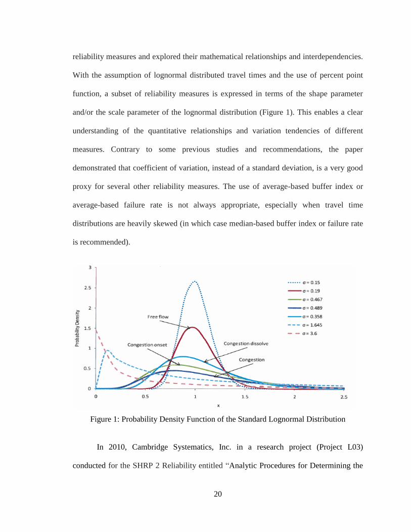
Pu Wenjing (2010) in “Analytic Relationships between Travel Time Reliability
Measures” analyzed the measures used in transportation engineering including the 90th
or
95th
percentile travel time, standard deviation, coefficient of variation, buffer index,
planning time index, travel time index, skew statistic, misery index, frequency of
congestion, on-time arrival, and others. The paper analytically examined a number of
20
reliability measures and explored their mathematical relationships and interdependencies.
With the assumption of lognormal distributed travel times and the use of percent point
function, a subset of reliability measures is expressed in terms of the shape parameter
and/or the scale parameter of the lognormal distribution (Figure 1). This enables a clear
understanding of the quantitative relationships and variation tendencies of different
measures. Contrary to some previous studies and recommendations, the paper
demonstrated that coefficient of variation, instead of a standard deviation, is a very good
proxy for several other reliability measures. The use of average-based buffer index or
average-based failure rate is not always appropriate, especially when travel time
distributions are heavily skewed (in which case median-based buffer index or failure rate
is recommended).
Figure 1: Probability Density Function of the Standard Lognormal Distribution
In 2010, Cambridge Systematics, Inc. in a research project (Project L03)
conducted for the SHRP 2 Reliability entitled “Analytic Procedures for Determining the
21
Impacts of Reliability Mitigation Strategies” analyzed the effects of nonrecurring
congestion such as incidents, weather, work zones, special events, traffic control devices,
fluctuations in demand, and bottlenecks. This project defined reliability, explained the
importance of travel time distributions for measuring reliability, and recommended
specific reliability performance measures. This study reexamined the contribution of the
various causes of nonrecurring congestion, especially those listed above. The research
focused primarily on urban freeway sections although some attention was given to rural
highways and urban arterials. Numerous actions that can potentially reduce nonrecurring
congestion were identified with an indication of their relative importance. Models for
predicting nonrecurring congestion were developed using three methods, all based on
empirical procedures. The first involved before and after studies; the second was termed a
“data poor” approach and resulted in a parsimonious and easy-to-apply set of models; the
third was entitled a “data rich model” and used cross-section inputs including data on
selected factors known to directly affect nonrecurring congestion. An important
conclusion of the study is travel time reliability can be improved by reducing demand,
increasing capacity, and enhancing operations.
In 2010, a research project conducted by Northwestern University entitled
“Providing Reliable Route Guidance: Phase II” had the overarching goal to enhance
travel reliability of highway users by providing them with reliable route guidance
produced from newly developed routing algorithms that are validated and implemented
with real traffic data. Phase I of the project (funded by CCITT in 2008) is focused on
demonstrating the value of reliable route guidance through the development and
dissemination of Chicago Testbed for Reliable Routing (CTR). Phase II aims at bringing
22
the implementation of reliable routing technology to the next stage through initial
deployment of CTR. The first objective in Phase II is to create a travel reliability
inventory (TRI) of Northeastern Illinois using CTR by collaborating with public agencies
such as Illinois Department of Transportation (IDOT), Chicago Transit Authority (CTA)
and Chicago Traffic Management Authority (CTMA). TRI documents travel reliability
indices (e.g., 95 percentile route travel times) between heavily-traveled origins-
destination pairs in the region, which are of interest to not only individual travel decision-
making, but also regional transportation planning and traffic operations/management. The
second objective is to perform an initial market test in order to understand users’ need for
and response to reliability information and reliable route guidance. To these ends, the
following research activities are proposed to further develop CTR: (1) Implement and test
the latest reliable routing algorithms that are suitable for large-scale applications and (2)
develop a web-based version of CTR and host the service at Northwestern University’s
Translab Website.
In 2010, Virginia Tech in a research project (Project L10) conducted for SHRP 2
Reliability entitled “Feasibility of Using In-Vehicle Video Data to Explore How to
Modify Driver Behavior that Causes Non-Recurring Congestion” examined the causes of
incidents on nonrecurring congestion and driver error on incidents and determined the
feasibility of using in-vehicle video data to make inferences about driver behavior that
would allow investigation of the relationship between observable driver behavior and
nonrecurring congestion to improve travel time reliability.
This project examined existing studies that had used video cameras and other
onboard devices to collect data, and it determined the potential for using these data to
23
explore how to modify driver behavior in an attempt to reduce nonrecurring congestion.
The research team made inferences to identify driver behaviors that contribute to crashes
and near crashes, and they proposed countermeasures to modify those behaviors. The
report provided technical guidance on the features and technologies, as well as
supplementary data sets, which researchers and practicing professionals should consider
when designing instrumented in-vehicle data collection studies. Also presented is a new
modeling approach for travel time reliability performance measurement.
Though, these recent studies on the topic provide reasonable methodologies for
travel time reliability, a generalized model which captures the different factors that
influence travel time reliability such as posted speed, access density, arterial length,
traffic conditions, signalized intersection spacing, roadway and intersection geometrics,
and signal control settings is still lacking. Specially, there is a need that these factors be
weighted according to their impacts.
2.2 Previous Travel Time Reliability Calculation Methods
The Federal Highway Administration is encouraging agencies to adopt travel time
reliability measures to better manage and operate their transportation system. They came
out with the following reliability calculation methods:
24
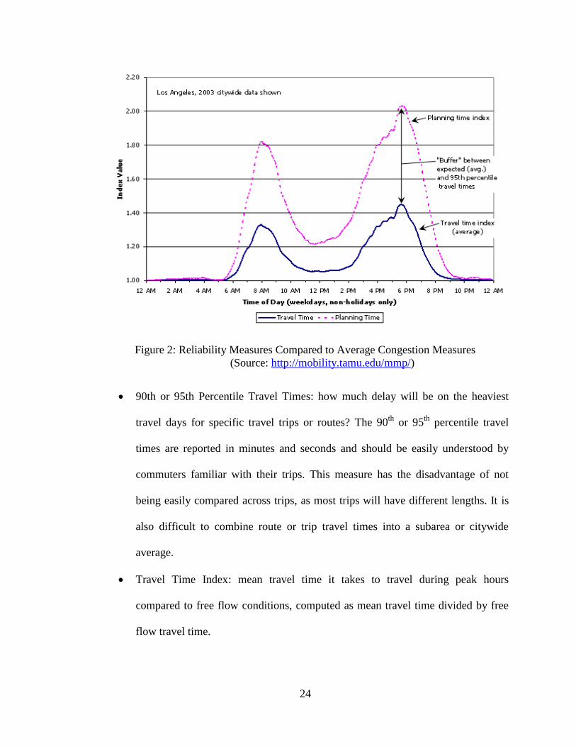
Figure 2: Reliability Measures Compared to Average Congestion Measures
(Source: http://mobility.tamu.edu/mmp/)
90th or 95th Percentile Travel Times: how much delay will be on the heaviest
travel days for specific travel trips or routes? The 90th
or 95th
percentile travel
times are reported in minutes and seconds and should be easily understood by
commuters familiar with their trips. This measure has the disadvantage of not
being easily compared across trips, as most trips will have different lengths. It is
also difficult to combine route or trip travel times into a subarea or citywide
average.
Travel Time Index: mean travel time it takes to travel during peak hours
compared to free flow conditions, computed as mean travel time divided by free
flow travel time.
25
Buffer Index: represents the extra buffer time (or time cushion) that most travelers
add to their average travel time when planning trips to ensure on-time arrival.
This extra time is added to account for any unexpected delay. The buffer index is
expressed as a percentage and its value increases as reliability worsens. The
buffer index is computed as difference between 95th
percentile travel time and
mean travel time, divided by mean travel time.
Planning Time Index: represents the total travel time that should be planned when
an adequate buffer time is included. The planning time index differs from the
buffer index in that it includes typical delay as well as unexpected delay. Thus,
the planning time index compares near-worst case travel time to a travel time in
light or free-flow traffic. Planning time index is computed as 95th
percentile travel
time divided by free-flow travel time.
For travelers who are familiar with everyday congestion (e.g., commuters), Buffer
Time Index would be a preferred travel time reliability measure since it is based on
average travel time; for those who are not familiar with that, planning time index may be
preferred as it is based on free flow travel time (Pu, W., 2010).
Frequency of congestion: the frequency when congestion exceeds some expected
threshold. This is typically expressed as the percent of days or time that travel
times exceed X minutes or travel speeds fall below Y mph. The frequency of
congestion measure is relatively easy to compute if continuous traffic data is
available, and it is typically reported for weekdays during peak traffic periods.
Traffic professionals have come to recognize the importance of travel time
reliability because it better quantifies the benefits of traffic management and operation
26
activities than simple averages and have, consequently, adopted other travel time
reliability calculation methods.
Standard Deviation: A widely employed measurement of variability or diversity
used in statistics and probability theory. It shows how much variation or
"dispersion" there is from the average (mean, or expected value). It is sometimes
used as a proxy for other reliability measures and is a convenient measure when
calculating reliability of travel time using classical or statistical models (Dowling
et al., 2009). The standard deviation has the disadvantage of treating late and early
arrivals with equal weight while the public cares much about late arrival. It is not
either easily related to everyday commuting experiences.
Coefficient of Variation: This is a ratio of standard deviation to the mean. The
coefficient of variation has the same disadvantages as the standard deviation.
Percent Variation: The average and standard deviation values combined in a ratio
to produce a value that the 1998 California Transportation Plan calls percent
variation. This is the form of the statistical measure coefficient of variation.
Percent Variation= (Standard Deviation/Average travel time)*100%.
Thus, mathematically, it has the same characteristics as the coefficient of
variation. However, because the percent variation is expressed as a percentage of
average travel time, it is easily understood by the public (Pu W., 2010).
Failure Rate (Percent of On-Time Arrival): On-time arrival estimates the
percentage of time that a traveler arrives on time based on an acceptable lateness
27
threshold.16
Failure rate=100%-percent of on-time arrival. The threshold travel
time to determine an on-time arrival ranges from 110 to 113 percent of average
travel time.
Florida Reliability Method: The Florida measure uses a percentage of the average
travel time in the peak to estimate the limit of the acceptable additional travel time
range.17
The sum of the additional travel time and the average time define the
expected time. Travel times longer than the expected time would be termed
“unreliable.” This calculation method has the disadvantage of using travel time
rather than travel rate. One adjustment that might be needed for real-time
monitoring systems is to use travel rate rather than travel time. Travel rate
variations provide a length-neutral way of grading the system performance that
can be easily calculated and communicated to travelers (Lomax et al., 2003).
Florida Reliability Statistic (% of unreliable trips) =100% - (percent of trips with
travel times greater than expected).
The Urban Mobility Study Report in “The Keys to Estimating Mobility in Urban
Areas” suggested a threshold of 10 percent higher than the average travel time (or
travel rate)18
for travel time reliability. However, the 10 percent late arrival has
the disadvantage of being relatively conservative for some applications.
Stephen Clark and David Watling used the probability distribution of the actual
values of the performance measure to define unreliability. For them, the planning
16
Cambridge Systematics, Inc.; Dowling Associates, Inc; System Metrics Group, Inc.; Texas
Transportation Institute. Cost-Effective Performance Measures for Travel Time Delay, Variation, and
Reliability. Washington, D.C.: TRB, 2008. NCHRP Report 618. 17
Florida Department of Transportation. Florida’s Mobility Performance Measures Program. Summary
Report. Office of state Transportation Planner, Tallahassee, Florida, August 2000 18
The Keys to Estimating Mobility in Urban Areas: Applying Definitions and Measures That Everyone
Understands, 1998 (http://mobility.tamu.edu).
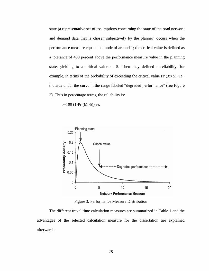
28
state (a representative set of assumptions concerning the state of the road network
and demand data that is chosen subjectively by the planner) occurs when the
performance measure equals the mode of around 1; the critical value is defined as
a tolerance of 400 percent above the performance measure value in the planning
state, yielding to a critical value of 5. Then they defined unreliability, for
example, in terms of the probability of exceeding the critical value Pr (M>5), i.e.,
the area under the curve in the range labeled “degraded performance” (see Figure
3). Thus in percentage terms, the reliability is:
ρ=100 (1-Pr (M>5)) %.
Figure 3: Performance Measure Distribution
The different travel time calculation measures are summarized in Table 1 and the
advantages of the selected calculation measure for the dissertation are explained
afterwards.
29
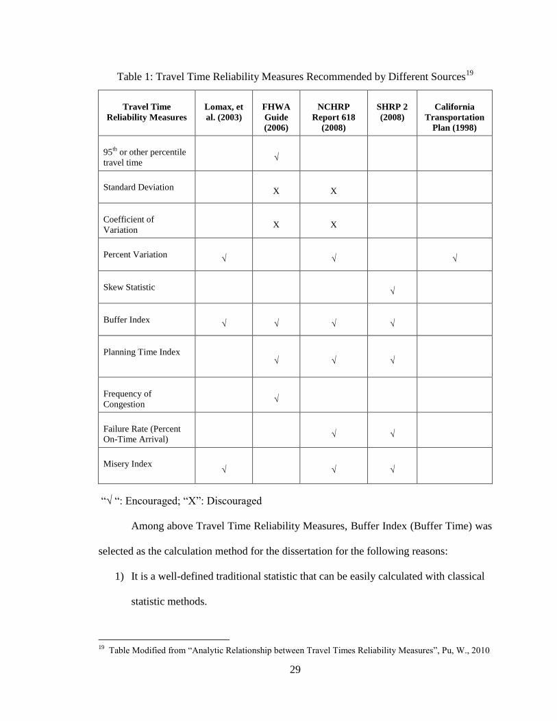
Table 1: Travel Time Reliability Measures Recommended by Different Sources19
“√ “: Encouraged; “X”: Discouraged
Among above Travel Time Reliability Measures, Buffer Index (Buffer Time) was
selected as the calculation method for the dissertation for the following reasons:
1) It is a well-defined traditional statistic that can be easily calculated with classical
statistic methods.
19
Table Modified from “Analytic Relationship between Travel Times Reliability Measures”, Pu, W., 2010
Travel Time
Reliability Measures
Lomax, et
al. (2003)
FHWA
Guide
(2006)
NCHRP
Report 618
(2008)
SHRP 2
(2008)
California
Transportation
Plan (1998)
95th
or other percentile
travel time √
Standard Deviation X X
Coefficient of
Variation X X
Percent Variation √ √ √
Skew Statistic √
Buffer Index √ √ √ √
Planning Time Index √ √ √
Frequency of
Congestion √
Failure Rate (Percent
On-Time Arrival) √ √
Misery Index √ √ √
30
2) “Reliability” itself is a term of art that may have little meaning to the traveling
public (Texas A&M University Traveler Information and Travel Time
Reliability). Travelers do obtain considerable information about reliability from
their own daily experiences. However, an overall lack of knowledge exists about
what reliability information is useful to travelers, how best to communicate it to
them, how reliability information impacts traveler choices and demand at given
times on particular facilities, and how communicating information about
reliability affects system performance, particularly in terms of recurrent and
nonrecurring highway congestion.20
The buffer index (buffer time) could be used
as an effective communication tool since nontechnical audiences can easily
understand the term.
3) It is typically reported for weekdays during peak traffic periods.
4) It is recommended by The FHWA (Federal Highway Administration) Guide
(2006), NCHRP (National Cooperative Highway Research Program) Report 618
(2008), Lomax, et al. (2003), and SHRP (Strategic Highway Research Program) 2
(2008).
5) It has been mainly applied on freeways and will be experimented on arterials.
6) Finally, from the road user perspective (demand side) a key focus in travel time
reliability is the net effect on a user’s trip through the network, i.e. on travel from
origin to destination. The buffer time could help the advised commuter track his
daily travel time and adjust his driving time accordingly.
20
Texas A&M University, Traveler Information and Travel Time Reliability, 2010.
31
Chapter 3-Methodology
From Sensys Networks aggregate output record, 3,503 travel time data sets were
selected for 2 consecutive weeks in 5 minutes interval for statistical analysis. The data
processing was conducted in Microsoft EXCEL (from Q1 Macros 2010) with proper data
arrangements among different worksheets. These data are integrated into the reliability
equation to determine the reliable travel times based on the travel time thresholds. The
reliable travel times are integrated along with the influencing factors (described below)
into the linear regression equations to generate the correlation among factors and the
equation for the model.
3.1 Influencing Factors
Access Density, which is the number of access points divided by the length of the
segment, refers to the legal limitation or restriction of access from private
properties to public rights-of-way. The quality of flow, capacity, travel time,
Level of Service, and safety of a highway can be greatly affected by the degree
and manner of access control along it.
Annual Average Daily Traffic (AADT) is a measure used primarily in
transportation planning and transportation engineering. AADT is the total volume
of vehicle traffic of a highway or road for a year divided by 365 days. AADT is a
useful and simple measurement of how busy the road is and has influencing
impacts on average travel time and travel speed.
32
Posted Speed is a primary factor in highway design and is usually equal to or
lowers than the design speed. The level of service provided by a facility is
directly related to the speeds of operation provided by it. When roads are
planned, the selected design/posted speed is based on several factors, including
but not limited to: geometric design of road features, travel time, safety, and
anticipated traffic volume. The design/posted speed may also depend on the
topography, particularly in cases where limited funds are available. The
design/posted speed should be compatible with the expectations of nearly all
drivers and consistent with the functional classification and location of the
highway or street.
Intersection Traffic Control consists of traffic control signals that offer an
effective method for controlling traffic at an intersection, and they eliminate
many conflicts to different approaches at different times. Traffic control signals
are usually described as either pre-timed or traffic-actuated. Each may be used in
isolated (independent) or signal-system operations. When properly installed and
operated at appropriate locations, traffic signals provide a number of significant
benefits:
1) With appropriate physical designs, control measures, and signal
timing, the capacity of critical intersection movements is increased.
2) When properly coordinated, signals can provide for nearly
continuous movement of through traffic along an arterial at a
designed speed under favorable traffic conditions.
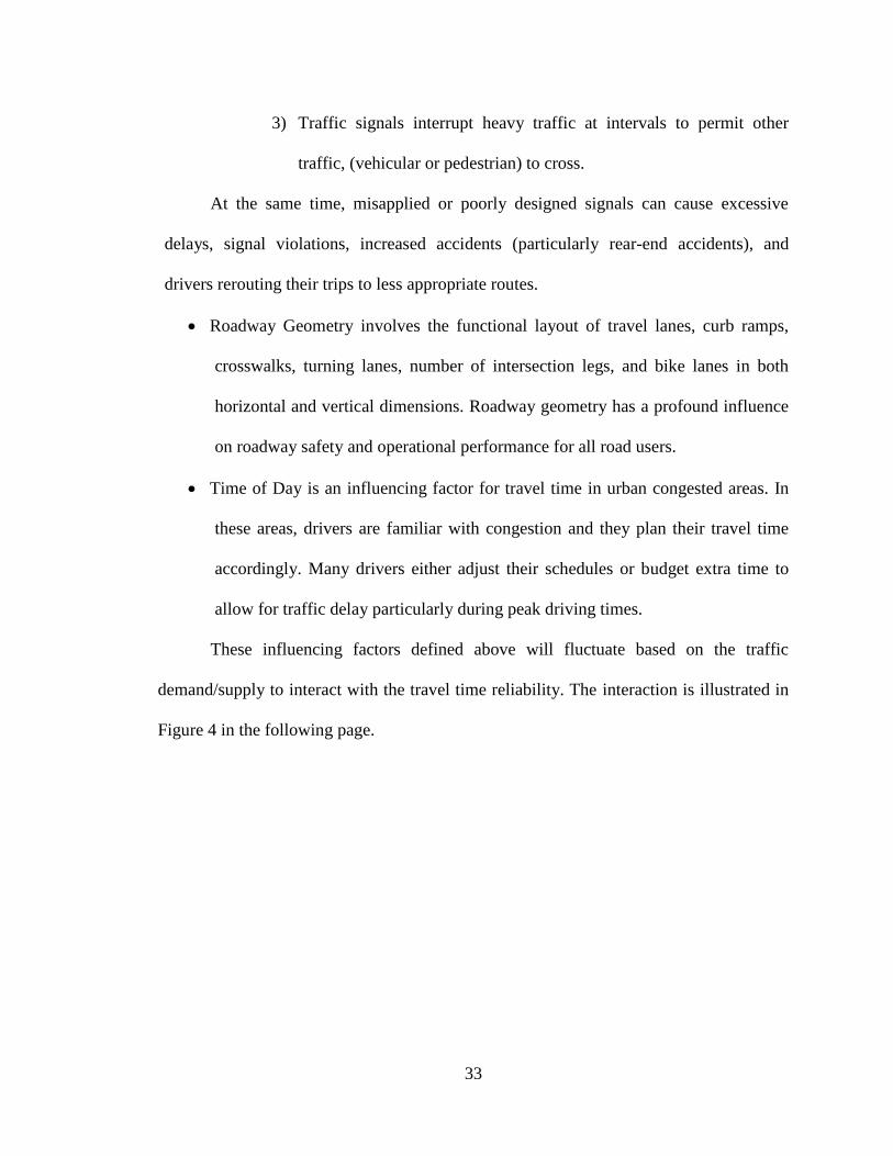
33
3) Traffic signals interrupt heavy traffic at intervals to permit other
traffic, (vehicular or pedestrian) to cross.
At the same time, misapplied or poorly designed signals can cause excessive
delays, signal violations, increased accidents (particularly rear-end accidents), and
drivers rerouting their trips to less appropriate routes.
Roadway Geometry involves the functional layout of travel lanes, curb ramps,
crosswalks, turning lanes, number of intersection legs, and bike lanes in both
horizontal and vertical dimensions. Roadway geometry has a profound influence
on roadway safety and operational performance for all road users.
Time of Day is an influencing factor for travel time in urban congested areas. In
these areas, drivers are familiar with congestion and they plan their travel time
accordingly. Many drivers either adjust their schedules or budget extra time to
allow for traffic delay particularly during peak driving times.
These influencing factors defined above will fluctuate based on the traffic
demand/supply to interact with the travel time reliability. The interaction is illustrated in
Figure 4 in the following page.
34
Figure 4: Factors Affecting Travel Time Reliability
35
3.2 Statistical Methods and Analysis
According to the American Heritage Dictionary of the English Language (New
College Edition, 1981), statistics is the mathematical science dealing with the collection,
analysis, and interpretation of numerical data using the theory of probability, especially
with methods for drawing inferences about characteristics of a population from
examination of a random sample. Statistical analysis refers to a collection of methods
used to process large amounts of data and report overall trends. Statistical methods are
used in research to summarize or describe a collection of data, especially to communicate
the results of experiments. In addition, patterns in the data may be modeled
(formalization of relationships between variables in the form of mathematical equations)
in a way that accounts for randomness and uncertainty in the observations and are then
used to draw inferences about the process or population being studied. Statistical analysis
and statistical methods are particularly useful in describing and illustrating some of the
tools commonly used for transportation data especially in travel time reliability
monitoring system. As outlined by North Carolina State University in a study conducted
for Transportation Research Board, SHRP 2 entitled” Monitoring Programs for Mobility
and Travel Time Reliability”, 2010:
……Combining travel time data with data on the other (explanatory)
variables is important in the design of a reliability monitoring system. The
design of a travel time reliability monitoring system requires the use of
statistics to develop a sampling plan for locating traffic detectors and
collecting travel time data—this includes determining appropriate
geographic and time scales. Statistical methods also provide insight
36
regarding the selection, validation, and application of appropriate
measures of travel time reliability, as well as for estimating models of
travel time reliability that reflect key factors.
3.2.1 Travel Time Reliability Calculation Method
Buffer time, a reliability measure recommended by USDOT, NCHRP, SHRP2,
and Lenox et al. is selected for the dissertation. The buffer time represents the extra time
(buffer or cushion time) that most travelers add to their average travel time when
planning trips to ensure on-time arrival. The buffer index, another reliability measure, is
expressed as a percentage and its value increases as reliability gets worse. A segment is
considered reliable when travel time threshold is equal to or lowers than the summation
of the buffer time and the average travel time.
The buffer index is computed as follows:
Buffer index (%) =
.sec
.sec.sec95
timetravelaverage
timetravelaveragetimetravelpercentileth [1]
where 95th
percentile travel time indicates how bad delay will be on the heaviest travel
days and is a translation of a standard “I can be late to work 1 day a month (1 day out of
20± work days) without getting into too much trouble” (Lomax et al., 2003).
The buffer time is computed as follows:
Buffer time (seconds) =95th
percentile travel times (sec.)-average travel time (sec) [2]
37
From [2], travel time reliability threshold (in seconds) for the dissertation is
deducted as follows:
Travel time threshold (reliability) ≤ buffer time + average travel time [3].
3.2.2 Correlation among Reliable Travel Times and Influencing Factors
Correlation among reliable travel times and influencing factors is calculated by
using ANOVA (Analysis of Variance) and Pearson Product Moment. In statistics, the
Pearson product-moment correlation coefficient (sometimes referred to as the MCV or
PMCC) (r) measures the strength and the direction of a linear relationship between two
variables X and Y. When measured in a population the Pearson Product Moment
correlation is designated by the Greek letter rho (ρ). When computed in a sample, it is
designated by the letter r and is sometimes called "Pearson's r." Pearson's correlation
reflects the degree of linear relationship between two variables. It ranges from “-1 to +1”.
This range helps understand the strength of relationship – rather, the strength of linear
relationship between the variables. The closer the coefficients are to +1.0 or –1.0, the
greater the strength of the linear relationship. Correlation coefficients in the range of -1.0
to - 0.65 or 1.0 to 0.65 mean that the variables are highly correlated. In the particular
case of high correlation among variables, one variable provides no additional information
over and above its perfectly correlated counterpart. A detailed analysis of the
multicollinearity among independent variables will be performed to determine whether
some variables should be dropped from the model.
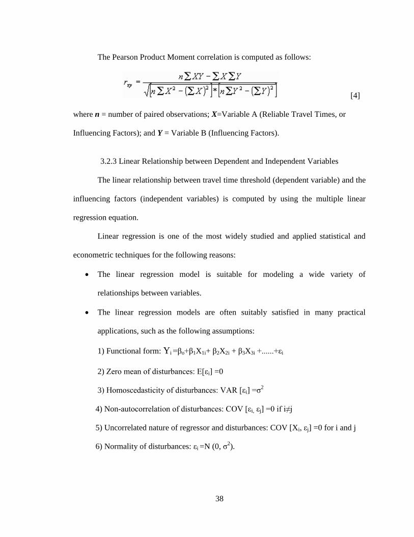
38
The Pearson Product Moment correlation is computed as follows:
[4]
where n = number of paired observations; X=Variable A (Reliable Travel Times, or
Influencing Factors); and Y = Variable B (Influencing Factors).
3.2.3 Linear Relationship between Dependent and Independent Variables
The linear relationship between travel time threshold (dependent variable) and the
influencing factors (independent variables) is computed by using the multiple linear
regression equation.
Linear regression is one of the most widely studied and applied statistical and
econometric techniques for the following reasons:
The linear regression model is suitable for modeling a wide variety of
relationships between variables.
The linear regression models are often suitably satisfied in many practical
applications, such as the following assumptions:
1) Functional form: Yi =βo+β1X1i+ β2X2i + β3X3i +......+εi
2) Zero mean of disturbances: E[εi] =0
3) Homoscedasticity of disturbances: VAR [εi] =σ2
4) Non-autocorrelation of disturbances: COV [εi, εj] =0 if i≠j
5) Uncorrelated nature of regressor and disturbances: COV [Xi, εj] =0 for i and j
6) Normality of disturbances: εi =N (0, σ2).
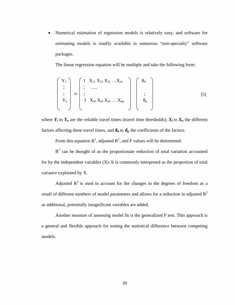
39
Numerical estimation of regression models is relatively easy, and software for
estimating models is readily available in numerous “non-specialty” software
packages.
The linear regression equation will be multiple and take the following form:
Y1 1 X11 X21 X31 …Xn1 ß0 : : …
: = : : [5] Yn 1 Xn1 Xn2 Xn3 ….Xnp ßp
where Yi to Yn are the reliable travel times (travel time thresholds); Xi to Xn the different
factors affecting these travel times, and ß0 to ßp the coefficients of the factors.
From this equation R2, adjusted R
2, and F values will be determined.
R2 can be thought of as the proportionate reduction of total variation accounted
for by the independent variables (X). It is commonly interpreted as the proportion of total
variance explained by X.
Adjusted R2
is used to account for the changes in the degrees of freedom as a
result of different numbers of model parameters and allows for a reduction in adjusted R2
as additional, potentially insignificant variables are added.
Another measure of assessing model fit is the generalized F test. This approach is
a general and flexible approach for testing the statistical difference between competing
models.
40
3.2.4 The Wrong Signs in the Linear Regression Model
In a multiple linear regression model coefficients often have signs that are
contrary to expectations. There is a variety of reasons that multiple linear regression
produces the “wrong sign” for some coefficients (Mullet, 1976):
Computational error. Some computational procedures for computing least squares
have problems with precision when the magnitudes of variables differ drastically. To
avoid this problem, it is recommended to convert variables to standard form (e.g., 0
mean and unit variance) for calculations and convert back to the original form for
displaying the coefficients (Pazzani & Bay, 1999).
Coefficients that do not significantly differ from zero. In this case, the sign of the
coefficient does not matter because it is too small to significantly affect the equation.
One recommended way to avoid this problem is to eliminate the irrelevant variables
from forward stepwise regression methods where a variable is included in the model
only if it significantly improves the fit of the model of the data (Draper & Smith,
1981).
Multicollinearity. Multicollinarity causes inflated standard errors, which in turn
make it more likely an “incorrect sign”. When two or more explanatory variables are
not independent, the sign of the coefficients of one of the variables may differ from
the sign of that coefficient if the variable were the only explanatory variable. One
approach to deal with this problem is to manually eliminate some of the variables
from the analysis (Pazzani & Bay, 1999).
41
Nonlinearity. If the true relationship between the dependent variable and the
explanatory is nonlinear, the coefficients can be biased with changing (different or
wrong) signs.
The variable in question is a proxy for another variable. In some cases the
variable in question may be highly correlated with other variables which have
been excluded from the analysis. Such variables are also known as “confounding
variables”. The wrong sign might be attributable to an excluded confounding
variable (Rinott & Tam, 2003).
Improper interpretation of parameters. The interpretation of a parameter is
entirely dependent upon the model in which the parameter appears.
Even with “incorrect signs”, the model still may be useful for prediction in the
region of X-values from which the model was built, e.g., the model is still useful as a
predictive model, as long as the extrapolation does not go beyond the region of the data.
3.3 Alternative Models
3.3.1 Simultaneous Equation Models (SEM)
Simultaneous equation models are a form of statistical model in the form of a set
of linear simultaneous equations. They are often used in interrelated transportation data
modeling, such as the interrelation between travel time from home to an activity and the
duration of the activity and the interrelation of average vehicle speeds by lane with the
vehicle speeds in adjacent lanes.
Unlike the single-equation model in which a dependent (Y) variable is a function
of independent (X) variables, other Y variables are among the independent variables in
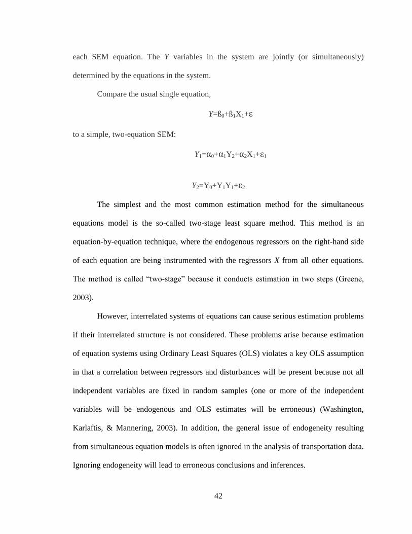
42
each SEM equation. The Y variables in the system are jointly (or simultaneously)
determined by the equations in the system.
Compare the usual single equation,
Y=ß0+ß1X1+ε
to a simple, two-equation SEM:
Y1=α0+α1Y2+α2X1+ε1
Y2=Y0+Y1Y1+ε2
The simplest and the most common estimation method for the simultaneous
equations model is the so-called two-stage least square method. This method is an
equation-by-equation technique, where the endogenous regressors on the right-hand side
of each equation are being instrumented with the regressors X from all other equations.
The method is called “two-stage” because it conducts estimation in two steps (Greene,
2003).
However, interrelated systems of equations can cause serious estimation problems
if their interrelated structure is not considered. These problems arise because estimation
of equation systems using Ordinary Least Squares (OLS) violates a key OLS assumption
in that a correlation between regressors and disturbances will be present because not all
independent variables are fixed in random samples (one or more of the independent
variables will be endogenous and OLS estimates will be erroneous) (Washington,
Karlaftis, & Mannering, 2003). In addition, the general issue of endogeneity resulting
from simultaneous equation models is often ignored in the analysis of transportation data.
Ignoring endogeneity will lead to erroneous conclusions and inferences.
43
3.3.2 Count Data Models
Count data consist of non-negative integer values and are encountered frequently
in the modeling of transportation related-phenomena. Examples of count data variables in
transportation include the number of driver route changes per week, the number of trip
departure changes per week, drivers’ frequency of use of Intelligent Transportation
Systems (ITS) technologies over the same period, number of vehicles waiting in queue,
and the number of accidents observed on road segments per year. Count data regression
is as simple as estimation in the linear regression model, if there are no additional
complications such as endogeneity, panel data, etc. (Cameron, 2009) A common mistake
is to model count data as continuous data by applying standard least squares regression.
This is not correct because regression models yield predicted values that are non-integers
and can also predict values that are negative, both of which are inconsistent with count
data (Washington et al., 2003). These limitations make standard regression analysis
inappropriate for modeling count data without modifying dependent variables.
Count data are properly modeled by using a number of methods, the most popular
of which are Poisson and negative binomial regression models.
3.3.3 The Poisson Distribution
The Poisson distribution or Poisson law of small numbers is a discrete probability
distribution that expresses the probability of a given number of events occurring in a
fixed interval of time and/or space if these events occur with a known average rate and
independently of the time since the last event. The Poisson distribution can also be used
for the number of events in other specified intervals such as distance, area or volume.
One requirement of the Poisson distribution is that the mean of the count process equals
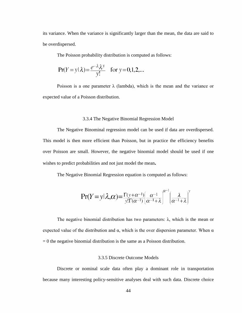
44
its variance. When the variance is significantly larger than the mean, the data are said to
be overdispersed.
The Poisson probability distribution is computed as follows:
Poisson is a one parameter λ (lambda), which is the mean and the variance or
expected value of a Poisson distribution.
3.3.4 The Negative Binomial Regression Model
The Negative Binominal regression model can be used if data are overdispersed.
This model is then more efficient than Poisson, but in practice the efficiency benefits
over Poisson are small. However, the negative binomial model should be used if one
wishes to predict probabilities and not just model the mean.
The Negative Binomial Regression equation is computed as follows:
The negative binomial distribution has two parameters: λ, which is the mean or
expected value of the distribution and α, which is the over dispersion parameter. When α
= 0 the negative binomial distribution is the same as a Poisson distribution.
3.3.5 Discrete Outcome Models
Discrete or nominal scale data often play a dominant role in transportation
because many interesting policy-sensitive analyses deal with such data. Discrete choice
45
models are statistical procedures that model choices made by people among a finite set of
alternatives. The attributes of the alternatives can differ over people; e.g., cost and time
for travel to work by car, bus, and rail are different for each person depending on the
location of home and work of that person. Discrete choice models have been used to
examine the choice of which car to buy (Train & Winston, 2007), where to go to college,
(Fuller, Manski, & Wise, 1982) which mode of transport (car, bus, rail) to take to work
(Train,1978), the number of vehicles a household chooses to own (Train, 1986) among
numerous other applications. While regression analysis examines “how much”, discrete
choice analysis examines “which”. In addition, discrete choice analysis examines
situations in which the potential outcomes are discrete, such that the optimum is not
characterized by standard first-order conditions.
The discrete outcome models are most often estimated using standard maximum
likelihood procedure, such estimation referred to as a Probit regression.
Suppose response variable Y is binary, that it can have only two possible
outcomes, which denote as 1 and 0. For example, Y may represent presence/absence of a
certain condition, success/failure of some device or answer yes/no on a survey. A vector
h of regressors X is assumed to influence the outcome Y. Specifically, the model takes the
following form:
Pr (Y=1/X) =Φ (X’β),
where Pr denotes probability, and Φ is the Cumulative Distribution Function (CDF) of
the standard normal distribution. The parameters β are typically estimated by maximum
likelihood.
46
Binary and Multinomial Probit Models are the most common discrete outcome
models. A distinction is often drawn between binary models (models that consider two
discrete outcomes) and multinomial models (models that consider three or more discrete
outcomes) because the derivation between the two can vary significantly (Washington et
al., 2003).
As described above, these alternative models to the linear regression are widely
used and applied in many transportation data analysis and modeling. However, it is
obvious that the linear regression is most suited for modeling linear relationships between
dependent and independent variables.
3.4 Different Steps for the Model Equation
1) Collect travel times data and select potential contributing factors.
2) Establish Travel Time Reliability Thresholds and run the single linear regression
to determine the correlation among factors.
3) Determine reliable travel times (travel time thresholds).
4) Run multiple linear regression to eliminate the non-contributing factors and build
the linear regression model.
5) Validate the model.
6) Report graphically the travel time reliability for the system.
7) Verify the generality and robustness of the model
8) Develop a list of scenario for Marginal Effects.
9) Provide guidance on Transportation Planning, Roadway Design, Traffic Design,
Access Management, and Traffic Operations features.
The model framework is illustrated in Figure 5.
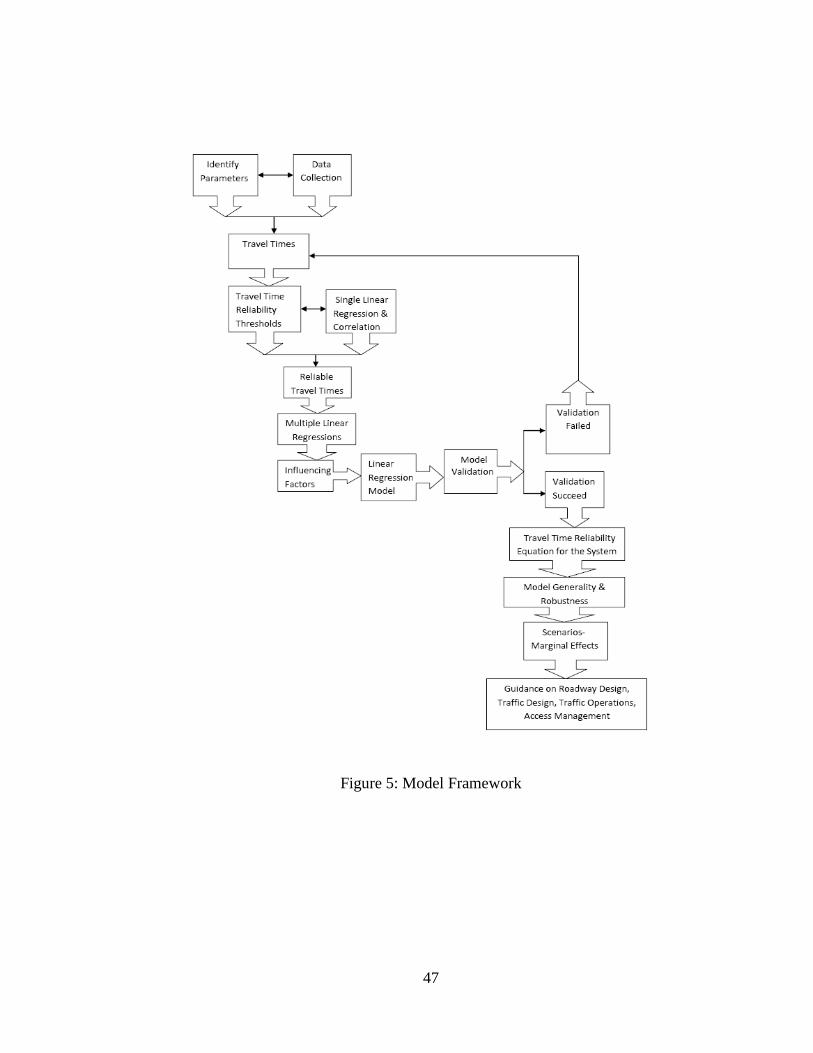
47
Figure 5: Model Framework
48
Chapter 4- Data Collection
4.1 Geographic Areas
A portion of Telegraph Canyon, a major urban arterial of 3.76 miles long located
in Chula Vista County, CA was selected for the data analysis. The selected portion (from
Rutgers Avenue to Halecrest Dr./ Canyon Plaza) is a West/East through route that consists
of 8 segments and 9 signalized intersections and is connected to two access controlled
corridors (South Bay Expy-125 and Jacob Dekema Fwy I-805). This is a six lane divided
roadway with divers traffic and geometric characteristics, adjacent land use and
development features. Additional lanes are available for the turning movements at
intersection approaches and vehicles-actuated signal timing plans are operated in
coordination mode for all intersections. Figure 6 highlights the 3. 76 mile corridor (in
green on the map) and the travel time data (median travel time, 80th
and 90th
percentiles,
vehicles in segment, and Level of Service) for segment # 7006. In addition, Figure 7
shows the geometric layout (number of lanes for the major road and the cross streets,
number of exclusive right and left turn lanes, number of intersection legs) of the corridor
and the different segment attributes are illustrated in Table 2.
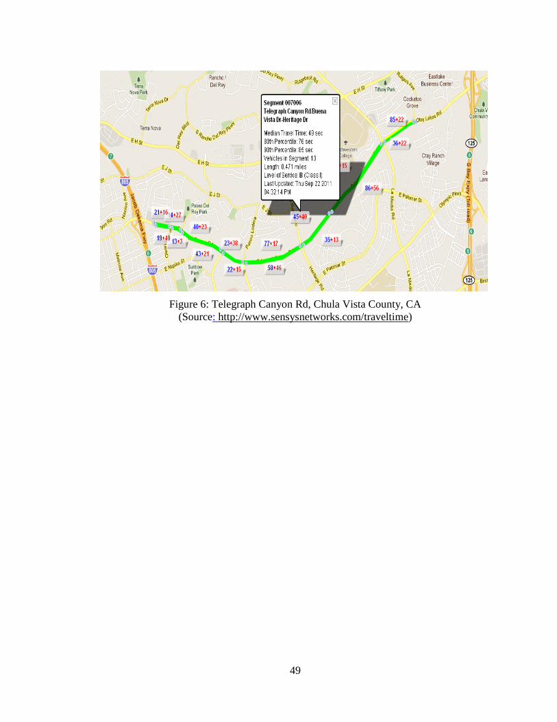
49
Figure 6: Telegraph Canyon Rd, Chula Vista County, CA
(Source: http://www.sensysnetworks.com/traveltime)
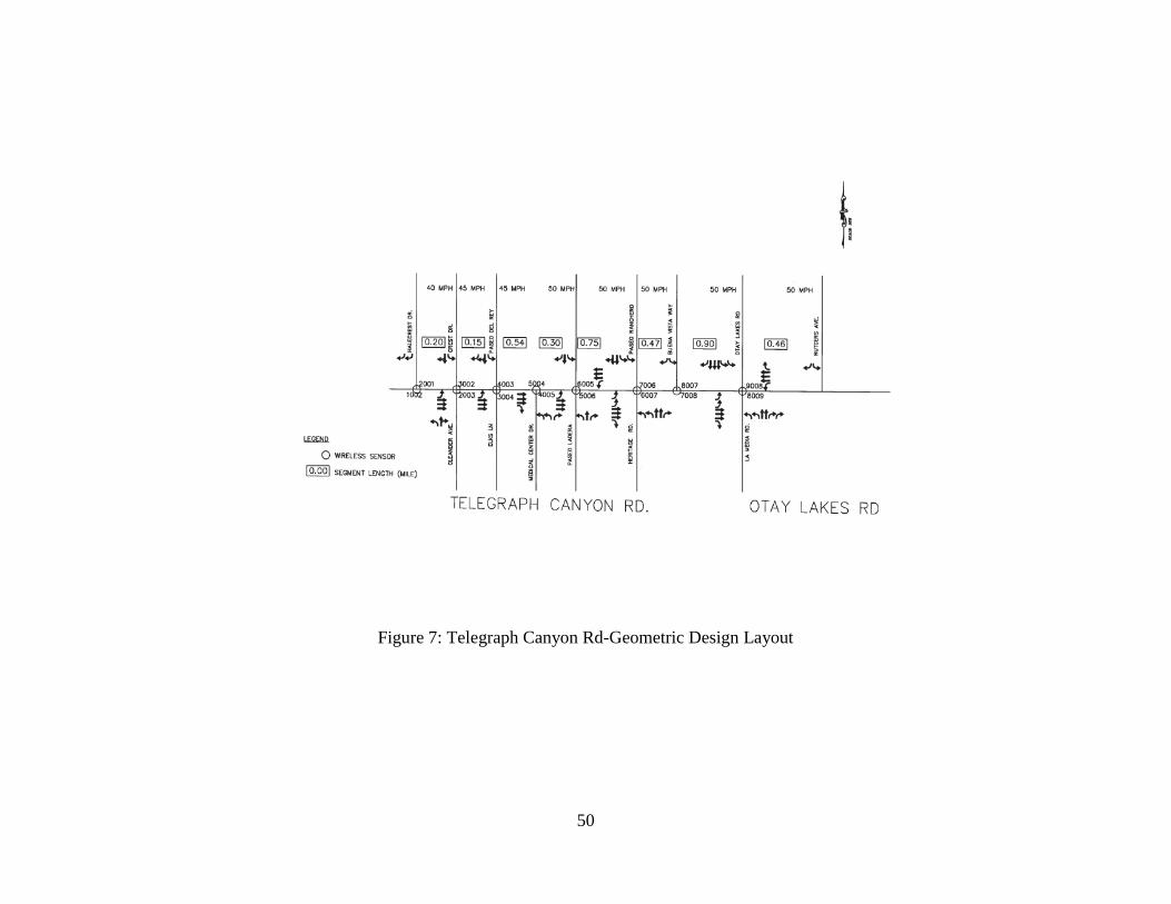
50
Figure 7: Telegraph Canyon Rd-Geometric Design Layout
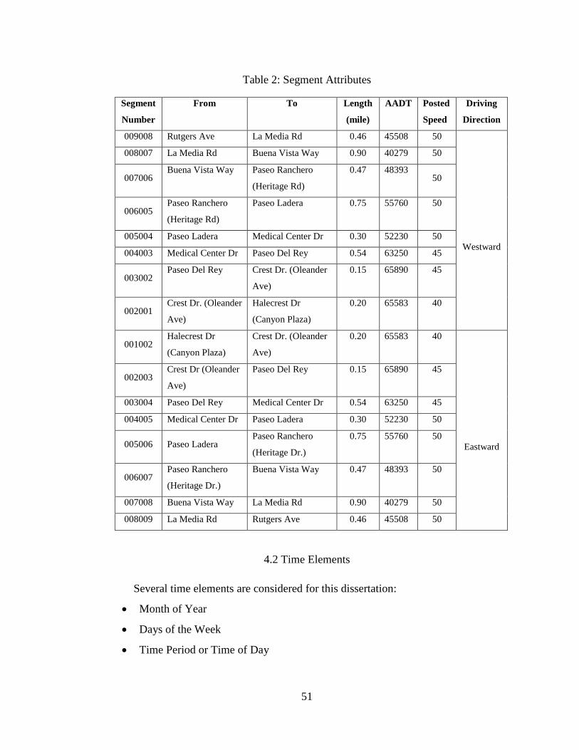
51
Table 2: Segment Attributes
Segment
Number
From To Length
(mile)
AADT Posted
Speed
Driving
Direction
009008 Rutgers Ave La Media Rd 0.46 45508 50
Westward
008007 La Media Rd Buena Vista Way 0.90 40279 50
007006 Buena Vista Way Paseo Ranchero
(Heritage Rd)
0.47 48393 50
006005 Paseo Ranchero
(Heritage Rd)
Paseo Ladera 0.75 55760 50
005004 Paseo Ladera Medical Center Dr 0.30 52230 50
004003 Medical Center Dr Paseo Del Rey 0.54 63250 45
003002 Paseo Del Rey Crest Dr. (Oleander
Ave)
0.15 65890 45
002001 Crest Dr. (Oleander
Ave)
Halecrest Dr
(Canyon Plaza)
0.20 65583 40
001002 Halecrest Dr
(Canyon Plaza)
Crest Dr. (Oleander
Ave)
0.20 65583 40
Eastward
002003 Crest Dr (Oleander
Ave)
Paseo Del Rey 0.15 65890 45
003004 Paseo Del Rey Medical Center Dr 0.54 63250 45
004005 Medical Center Dr Paseo Ladera 0.30 52230 50
005006 Paseo Ladera Paseo Ranchero
(Heritage Dr.)
0.75 55760 50
006007 Paseo Ranchero
(Heritage Dr.)
Buena Vista Way 0.47 48393 50
007008 Buena Vista Way La Media Rd 0.90 40279 50
008009 La Media Rd Rutgers Ave 0.46 45508 50
4.2 Time Elements
Several time elements are considered for this dissertation:
Month of Year
Days of the Week
Time Period or Time of Day

52
4.2.1 Month of the Year
For the purpose of this dissertation, the month of May, which is commonly
considered “average” or “typical” annual traffic condition for this area, was selected.
4.2.2 Days of the Week
This dissertation is focused on the middle weekdays (i.e., Tuesday, Wednesday,
and Thursday) for data collection. Monday, Friday, and holidays are excluded because of
their high variation from typical day-to-day operating conditions during the middle of the
week.
4.2.3 Time Periods
Morning Peak Period: between 6:00 am to 9:00 am
Afternoon Peak Period: between 4:00 pm to 7:00 pm
These time periods correspond to the local traffic condition and congestion
patterns for the geographic area considered.
4.3 Data Collection Method
Collection and reduction of traffic data covers a wide range of techniques and
technologies from simple manual techniques (often aided by a variety of handheld or
other devices for recording the data) to complex use of the ever-expanding technologies
of sensors, detectors, transmission, and computer equipment (Roess, Prassas, et
McShane, 2010). Travel times data used for this dissertation are from Sensys Networks
archives. For the ATTS (Arterial Travel Time System), Sensys Networks implements
VD240 wireless vehicle detention system, which is easily scalable from stop bar
detection to advance detection with the addition of a few in-pavement sensors. Arrays of
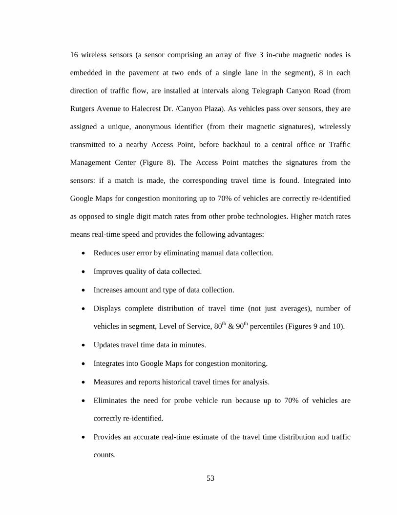
53
16 wireless sensors (a sensor comprising an array of five 3 in-cube magnetic nodes is
embedded in the pavement at two ends of a single lane in the segment), 8 in each
direction of traffic flow, are installed at intervals along Telegraph Canyon Road (from
Rutgers Avenue to Halecrest Dr. /Canyon Plaza). As vehicles pass over sensors, they are
assigned a unique, anonymous identifier (from their magnetic signatures), wirelessly
transmitted to a nearby Access Point, before backhaul to a central office or Traffic
Management Center (Figure 8). The Access Point matches the signatures from the
sensors: if a match is made, the corresponding travel time is found. Integrated into
Google Maps for congestion monitoring up to 70% of vehicles are correctly re-identified
as opposed to single digit match rates from other probe technologies. Higher match rates
means real-time speed and provides the following advantages:
Reduces user error by eliminating manual data collection.
Improves quality of data collected.
Increases amount and type of data collection.
Displays complete distribution of travel time (not just averages), number of
vehicles in segment, Level of Service, 80th
& 90th
percentiles (Figures 9 and 10).
Updates travel time data in minutes.
Integrates into Google Maps for congestion monitoring.
Measures and reports historical travel times for analysis.
Eliminates the need for probe vehicle run because up to 70% of vehicles are
correctly re-identified.
Provides an accurate real-time estimate of the travel time distribution and traffic
counts.
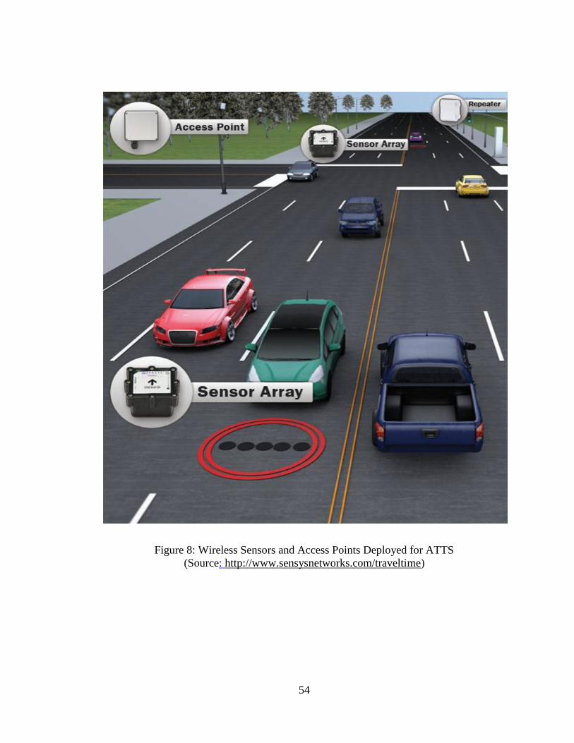
54
Figure 8: Wireless Sensors and Access Points Deployed for ATTS
(Source: http://www.sensysnetworks.com/traveltime)
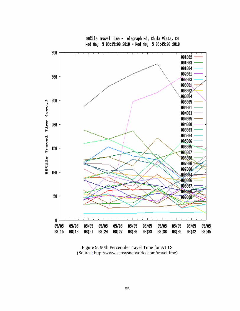
55
Figure 9: 90th Percentile Travel Time for ATTS
(Source: http://www.sensysnetworks.com/traveltime)
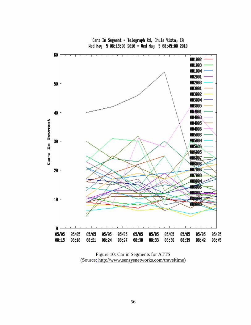
56
Figure 10: Car in Segments for ATTS
(Source: http://www.sensysnetworks.com/traveltime)
57
Other transportation data such as AADTs (major and minor roads), posted speeds,
signal timing cycle lengths were provided by Chula Vista County Traffic Operations. In
addition, geometric design data such as exclusive turn lanes (right and left), number of
intersection legs, number of lane at intersections, access density, right and left turn lane
lengths for major and minor roads are collected from Google.
4.4 Alternative Travel Time Data Collection Methods
License Plate Recognition (LPR)
LPR systems use the license plate number as the identifying signature. At each
end A and B, a vehicle presence detector triggers a camera, which records the
time and captures an image of the vehicle. Optical Character Recognition (OCR)
software processes the image to produce an alphanumeric sequence, presumably
the license plate number (Kavaler et al., 2009). Matching is error-prone: in one
trial conducted by Florida Department of Transportation in 2006 OCR software
misread 50% of the license numbers.21
Electronic Toll Collection Tag Readers (ETC)
RFID (Radio-Frequency Identification) tags for toll collection can be read and
time stamped by readers placed at the two ends A and B. The matching is better
than LPR because OCR errors are avoided. However, the scheme can only be
used when there is a sufficient penetration rate of tags.
Bluetooth
Some drivers use a Bluetooth device to connect “hands-free” with their cell
phone. The radio connection uses a 48-bit address unique to the device. If a
21
Florida Department of Transportation. LPR Field Test Results Report, August 2006.
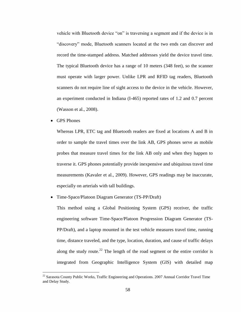
58
vehicle with Bluetooth device “on” is traversing a segment and if the device is in
“discovery” mode, Bluetooth scanners located at the two ends can discover and
record the time-stamped address. Matched addresses yield the device travel time.
The typical Bluetooth device has a range of 10 meters (348 feet), so the scanner
must operate with larger power. Unlike LPR and RFID tag readers, Bluetooth
scanners do not require line of sight access to the device in the vehicle. However,
an experiment conducted in Indiana (I-465) reported rates of 1.2 and 0.7 percent
(Wasson et al., 2008).
GPS Phones
Whereas LPR, ETC tag and Bluetooth readers are fixed at locations A and B in
order to sample the travel times over the link AB, GPS phones serve as mobile
probes that measure travel times for the link AB only and when they happen to
traverse it. GPS phones potentially provide inexpensive and ubiquitous travel time
measurements (Kavaler et al., 2009). However, GPS readings may be inaccurate,
especially on arterials with tall buildings.
Time-Space/Platoon Diagram Generator (TS-PP/Draft)
This method using a Global Positioning System (GPS) receiver, the traffic
engineering software Time-Space/Platoon Progression Diagram Generator (TS-
PP/Draft), and a laptop mounted in the test vehicle measures travel time, running
time, distance traveled, and the type, location, duration, and cause of traffic delays
along the study route.22
The length of the road segment or the entire corridor is
integrated from Geographic Intelligence System (GIS) with detailed map
22
Sarasota County Public Works, Traffic Engineering and Operations. 2007 Annual Corridor Travel Time
and Delay Study.
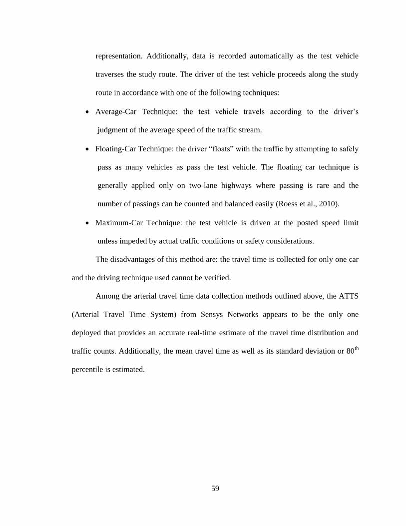
59
representation. Additionally, data is recorded automatically as the test vehicle
traverses the study route. The driver of the test vehicle proceeds along the study
route in accordance with one of the following techniques:
Average-Car Technique: the test vehicle travels according to the driver’s
judgment of the average speed of the traffic stream.
Floating-Car Technique: the driver “floats” with the traffic by attempting to safely
pass as many vehicles as pass the test vehicle. The floating car technique is
generally applied only on two-lane highways where passing is rare and the
number of passings can be counted and balanced easily (Roess et al., 2010).
Maximum-Car Technique: the test vehicle is driven at the posted speed limit
unless impeded by actual traffic conditions or safety considerations.
The disadvantages of this method are: the travel time is collected for only one car
and the driving technique used cannot be verified.
Among the arterial travel time data collection methods outlined above, the ATTS
(Arterial Travel Time System) from Sensys Networks appears to be the only one
deployed that provides an accurate real-time estimate of the travel time distribution and
traffic counts. Additionally, the mean travel time as well as its standard deviation or 80th
percentile is estimated.
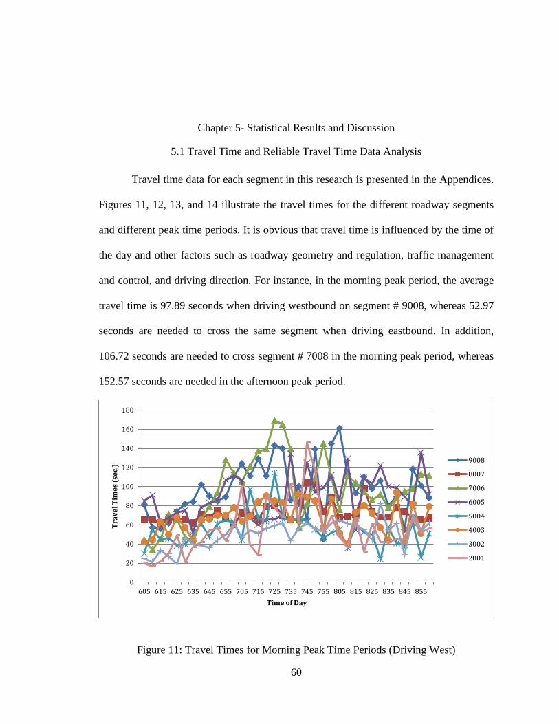
60
Chapter 5- Statistical Results and Discussion
5.1 Travel Time and Reliable Travel Time Data Analysis
Travel time data for each segment in this research is presented in the Appendices.
Figures 11, 12, 13, and 14 illustrate the travel times for the different roadway segments
and different peak time periods. It is obvious that travel time is influenced by the time of
the day and other factors such as roadway geometry and regulation, traffic management
and control, and driving direction. For instance, in the morning peak period, the average
travel time is 97.89 seconds when driving westbound on segment # 9008, whereas 52.97
seconds are needed to cross the same segment when driving eastbound. In addition,
106.72 seconds are needed to cross segment # 7008 in the morning peak period, whereas
152.57 seconds are needed in the afternoon peak period.
Figure 11: Travel Times for Morning Peak Time Periods (Driving West)
0
20
40
60
80
100
120
140
160
180
605 615 625 635 645 655 705 715 725 735 745 755 805 815 825 835 845 855
Tra
ve
l Tim
es
(se
c.)
Time of Day
9008
8007
7006
6005
5004
4003
3002
2001
61
Figure 12: Travel Times for Afternoon Peak Time Periods (Driving West)
Figure 13: Travel Times for Morning Peak Time Periods (Driving East)
0
20
40
60
80
100
120
140
160
180
200
400 410 420 430 440 450 500 510 520 530 540 550 600 610 620 630 640 650 700
Tra
ve
l Tim
es
(se
c.)
Time of Day
9008
8007
7006
6005
5004
4003
3002
2001
0
20
40
60
80
100
120
140
160
180
605 615 625 635 645 655 705 715 725 735 745 755 805 815 825 835 845 855
Trv
ae
l Tim
es
(se
c.)
Time of Day
1002
2003
3004
4005
5006
6007
7008
8009
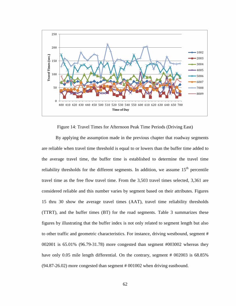
62
Figure 14: Travel Times for Afternoon Peak Time Periods (Driving East)
By applying the assumption made in the previous chapter that roadway segments
are reliable when travel time threshold is equal to or lowers than the buffer time added to
the average travel time, the buffer time is established to determine the travel time
reliability thresholds for the different segments. In addition, we assume 15th
percentile
travel time as the free flow travel time. From the 3,503 travel times selected, 3,361 are
considered reliable and this number varies by segment based on their attributes. Figures
15 thru 30 show the average travel times (AAT), travel time reliability thresholds
(TTRT), and the buffer times (BT) for the road segments. Table 3 summarizes these
figures by illustrating that the buffer index is not only related to segment length but also
to other traffic and geometric characteristics. For instance, driving westbound, segment #
002001 is 65.01% (96.79-31.78) more congested than segment #003002 whereas they
have only 0.05 mile length differential. On the contrary, segment # 002003 is 68.85%
(94.87-26.02) more congested than segment # 001002 when driving eastbound.
0
50
100
150
200
250
400 410 420 430 440 450 500 510 520 530 540 550 600 610 620 630 640 650 700
Tra
ve
l Tim
es
(se
c.)
Time of Day
1002
2003
3004
4005
5006
6007
7008
8009
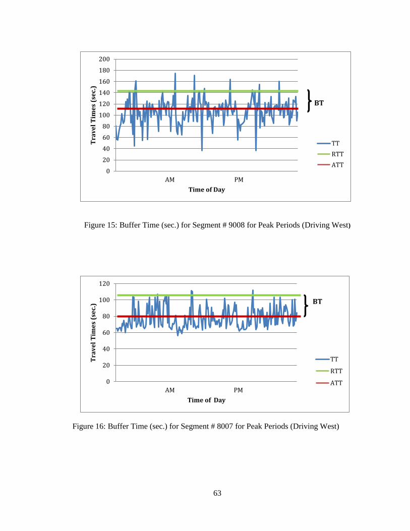
63
Figure 15: Buffer Time (sec.) for Segment # 9008 for Peak Periods (Driving West)
Figure 16: Buffer Time (sec.) for Segment # 8007 for Peak Periods (Driving West)
0
20
40
60
80
100
120
140
160
180
200
Tra
ve
l T
ime
s (s
ec.
)
Time of Day
TT
RTT
ATT
BT
0
20
40
60
80
100
120
Tra
ve
l T
ime
s (s
ec.
)
Time of Day
TT
RTT
ATT
BT
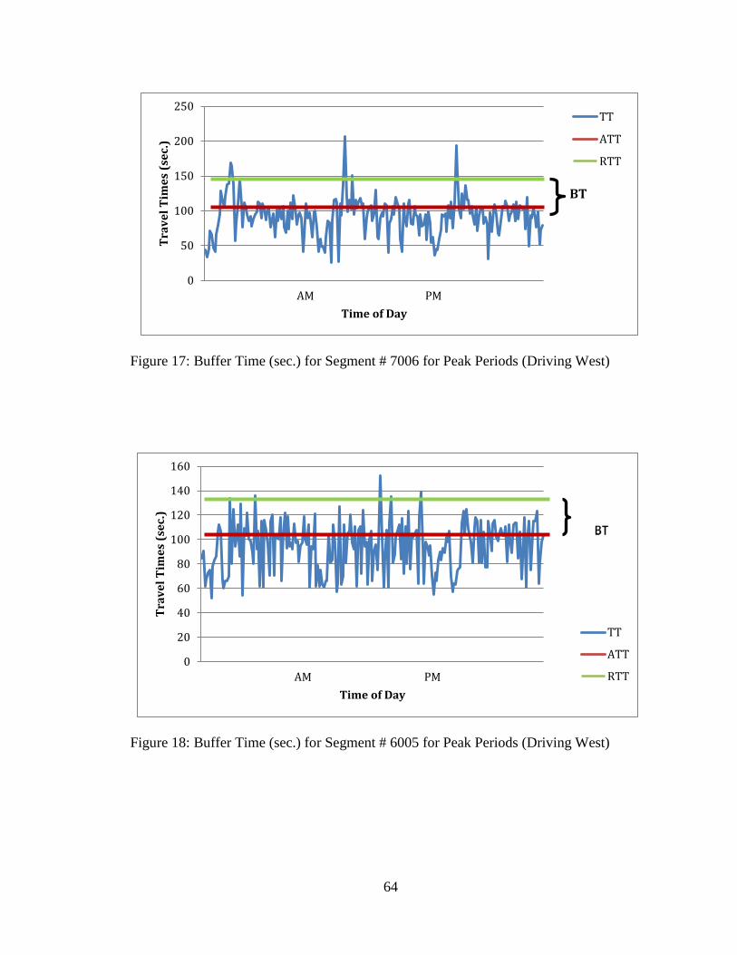
64
Figure 17: Buffer Time (sec.) for Segment # 7006 for Peak Periods (Driving West)
Figure 18: Buffer Time (sec.) for Segment # 6005 for Peak Periods (Driving West)
0
50
100
150
200
250
Tra
ve
l T
ime
s (s
ec.
)
Time of Day
TT
ATT
RTT
BT
0
20
40
60
80
100
120
140
160
Tra
ve
l T
ime
s (s
ec.
)
Time of Day
TT
ATT
RTT
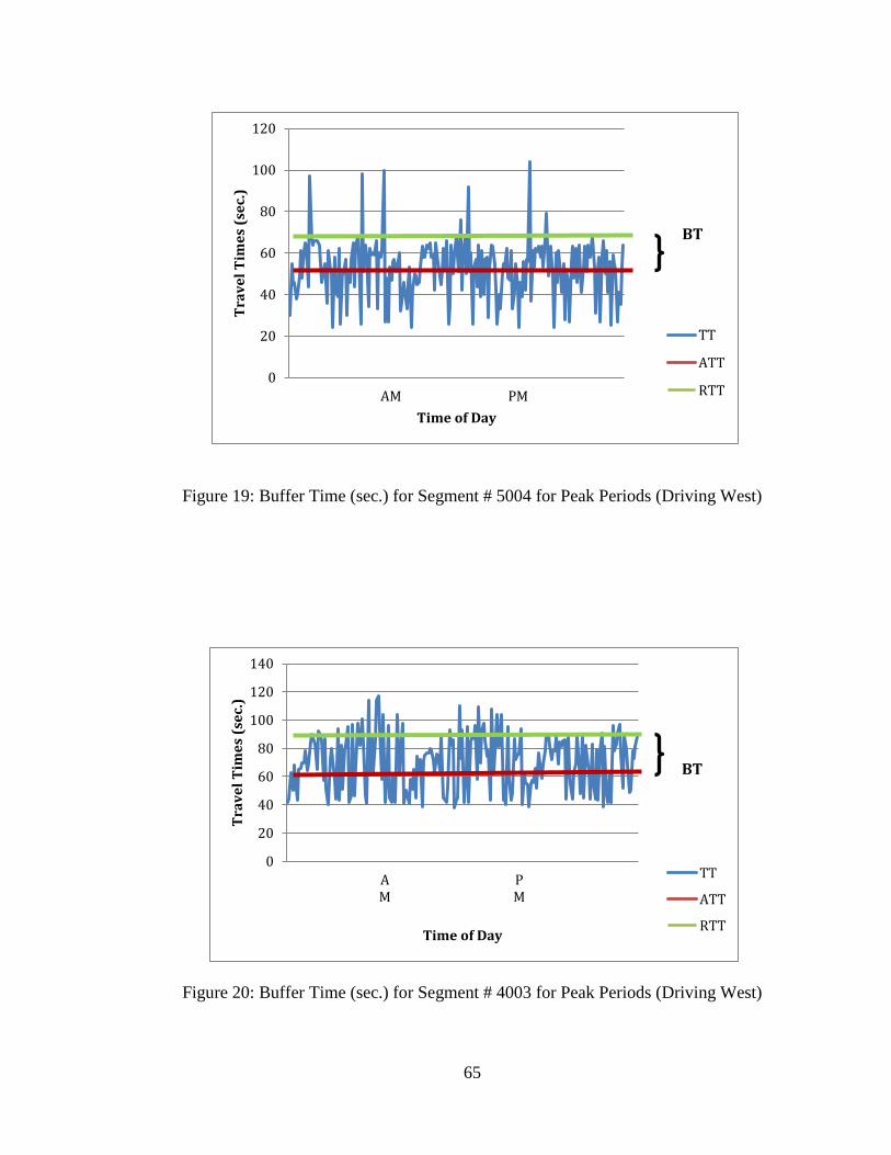
65
Figure 19: Buffer Time (sec.) for Segment # 5004 for Peak Periods (Driving West)
Figure 20: Buffer Time (sec.) for Segment # 4003 for Peak Periods (Driving West)
0
20
40
60
80
100
120
Tra
ve
l T
ime
s (s
ec.
)
Time of Day
TT
ATT
RTT
BT
0
20
40
60
80
100
120
140
AM
PM
Tra
ve
l T
ime
s (s
ec.
)
Time of Day
TT
ATT
RTT
BT
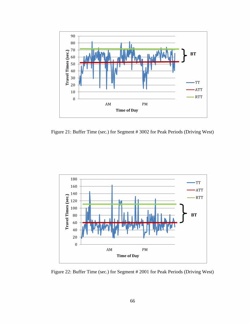
66
Figure 21: Buffer Time (sec.) for Segment # 3002 for Peak Periods (Driving West)
Figure 22: Buffer Time (sec.) for Segment # 2001 for Peak Periods (Driving West)
0
10
20
30
40
50
60
70
80
90
Tra
ve
l T
ime
s (s
ec.
)
Time of Day
TT
ATT
RTT
BT
0
20
40
60
80
100
120
140
160
180
Tra
ve
l T
ime
s (s
ec.
)
Time of Day
TT
ATT
RTT
BT
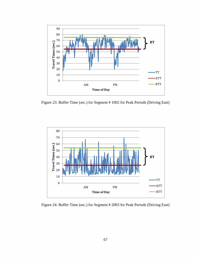
67
Figure 23: Buffer Time (sec.) for Segment # 1002 for Peak Periods (Driving East)
Figure 24: Buffer Time (sec.) for Segment # 2003 for Peak Periods (Driving East)
0
10
20
30
40
50
60
70
80
90
Tra
ve
l T
ime
s (s
ec.
)
Time of Day
TT
ATT
RTT
BT
0
10
20
30
40
50
60
70
80
Tra
ve
l T
ime
s (s
ec.
)
Time of Day
TT
ATT
RTT
BT
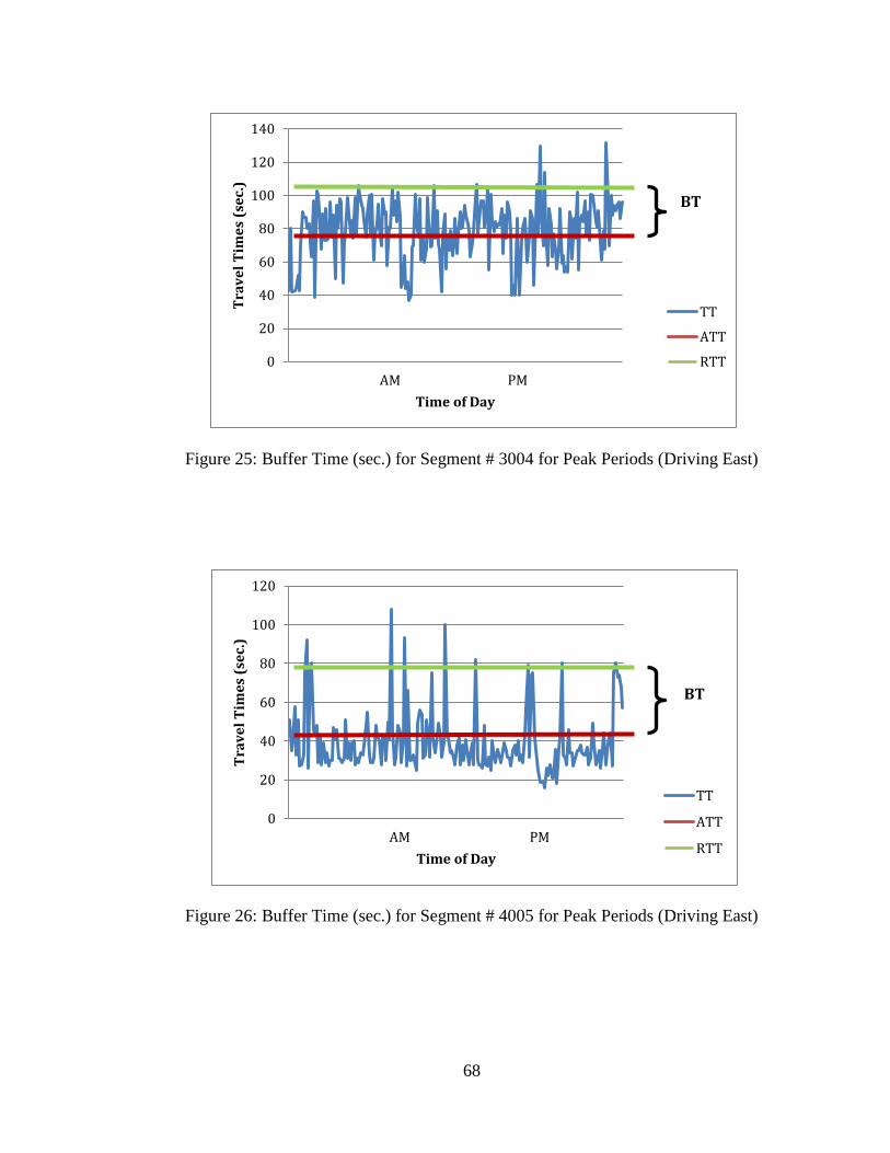
68
Figure 25: Buffer Time (sec.) for Segment # 3004 for Peak Periods (Driving East)
Figure 26: Buffer Time (sec.) for Segment # 4005 for Peak Periods (Driving East)
0
20
40
60
80
100
120
140
Tra
ve
l T
ime
s (s
ec.
)
Time of Day
TT
ATT
RTT
BT
0
20
40
60
80
100
120
Tra
ve
l T
ime
s (s
ec.
)
Time of Day
TT
ATT
RTT
BT
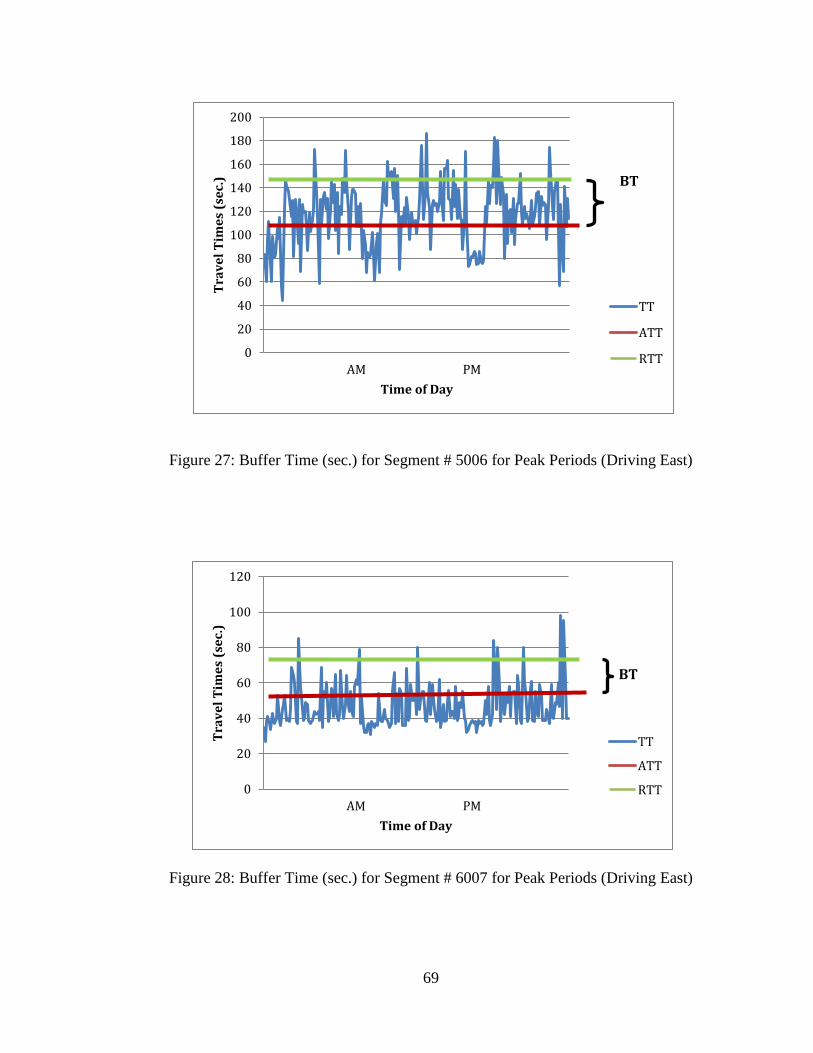
69
Figure 27: Buffer Time (sec.) for Segment # 5006 for Peak Periods (Driving East)
Figure 28: Buffer Time (sec.) for Segment # 6007 for Peak Periods (Driving East)
0
20
40
60
80
100
120
140
160
180
200
Tra
ve
l T
ime
s (s
ec.
)
Time of Day
TT
ATT
RTT
BT
0
20
40
60
80
100
120
Tra
ve
l T
ime
s (s
ec.
)
Time of Day
TT
ATT
RTT
BT
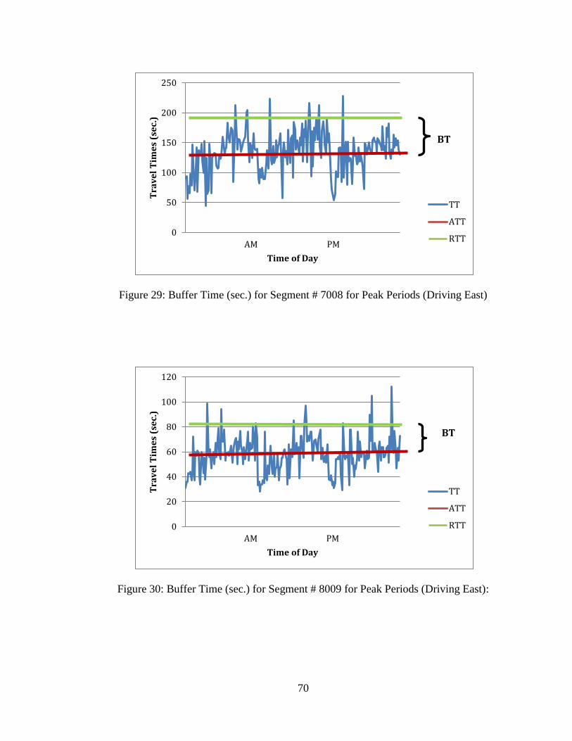
70
Figure 29: Buffer Time (sec.) for Segment # 7008 for Peak Periods (Driving East)
Figure 30: Buffer Time (sec.) for Segment # 8009 for Peak Periods (Driving East):
0
50
100
150
200
250
Tra
ve
l T
ime
s (s
ec.
)
Time of Day
TT
ATT
RTT
BT
0
20
40
60
80
100
120
Tra
ve
l T
ime
s (s
ec.
)
Time of Day
TT
ATT
RTT
BT
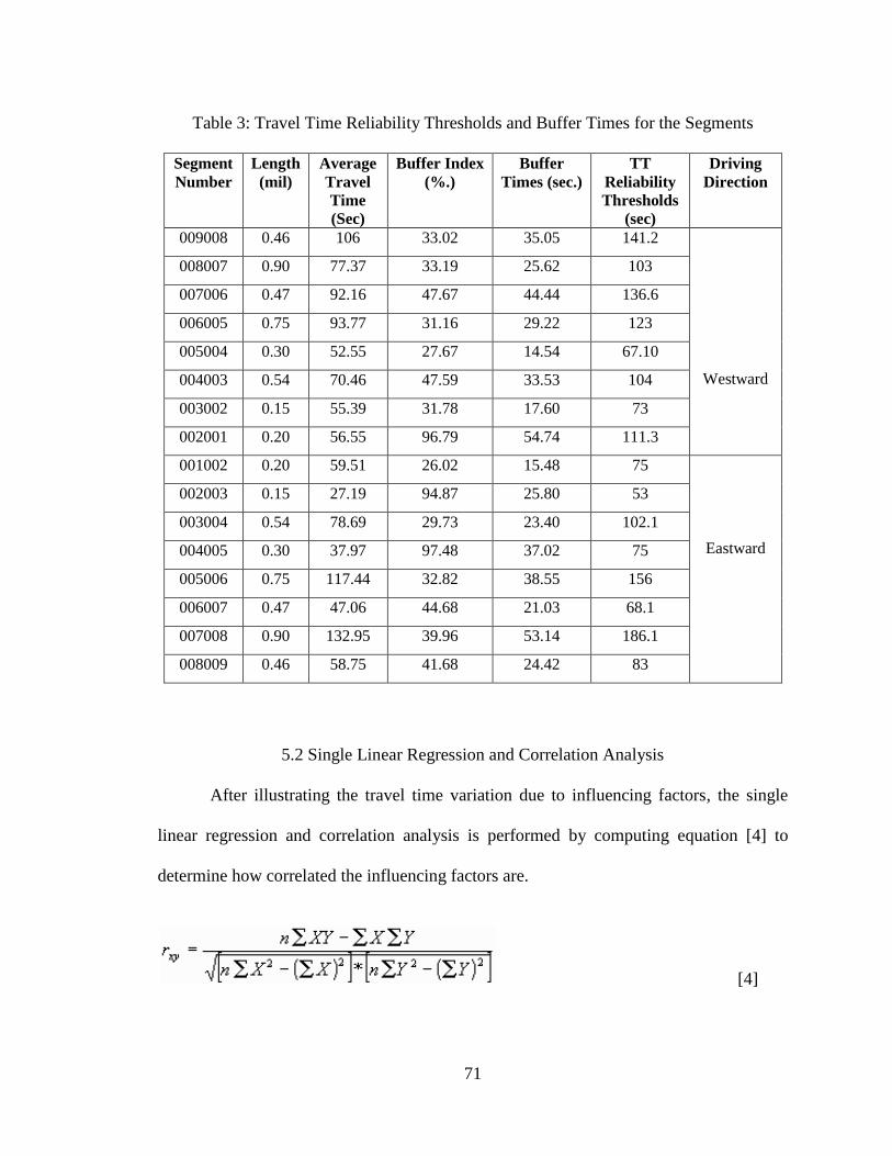
71
Table 3: Travel Time Reliability Thresholds and Buffer Times for the Segments
Segment
Number
Length
(mil)
Average
Travel
Time
(Sec)
Buffer Index
(%.)
Buffer
Times (sec.)
TT
Reliability
Thresholds
(sec)
Driving
Direction
009008 0.46 106 33.02 35.05 141.2
Westward
008007 0.90 77.37 33.19 25.62 103
007006 0.47 92.16 47.67 44.44 136.6
006005 0.75 93.77 31.16 29.22 123
005004 0.30 52.55 27.67 14.54 67.10
004003 0.54 70.46 47.59 33.53 104
003002 0.15 55.39 31.78 17.60 73
002001 0.20 56.55 96.79 54.74 111.3
001002 0.20 59.51 26.02 15.48 75
Eastward
002003 0.15 27.19 94.87 25.80 53
003004 0.54 78.69 29.73 23.40 102.1
004005 0.30 37.97 97.48 37.02 75
005006 0.75 117.44 32.82 38.55 156
006007 0.47 47.06 44.68 21.03 68.1
007008 0.90 132.95 39.96 53.14 186.1
008009 0.46 58.75 41.68 24.42 83
5.2 Single Linear Regression and Correlation Analysis
After illustrating the travel time variation due to influencing factors, the single
linear regression and correlation analysis is performed by computing equation [4] to
determine how correlated the influencing factors are.
[4]
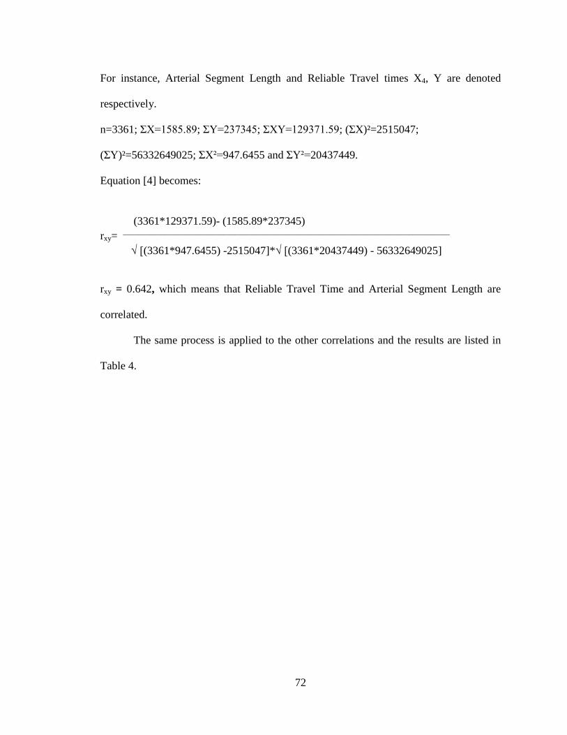
72
For instance, Arterial Segment Length and Reliable Travel times X4, Y are denoted
respectively.
n=3361; ΣΧ=1585.89; ΣY=237345; ΣΧY=129371.59; (ΣX)²=2515047;
(ΣY)²=56332649025; ΣX²=947.6455 and ΣY²=20437449.
Equation [4] becomes:
(3361*129371.59)- (1585.89*237345)
rxy= ________________________________________________________________________________________
√ [(3361*947.6455) -2515047]*√ [(3361*20437449) - 56332649025]
rxy = 0.642, which means that Reliable Travel Time and Arterial Segment Length are
correlated.
The same process is applied to the other correlations and the results are listed in
Table 4.
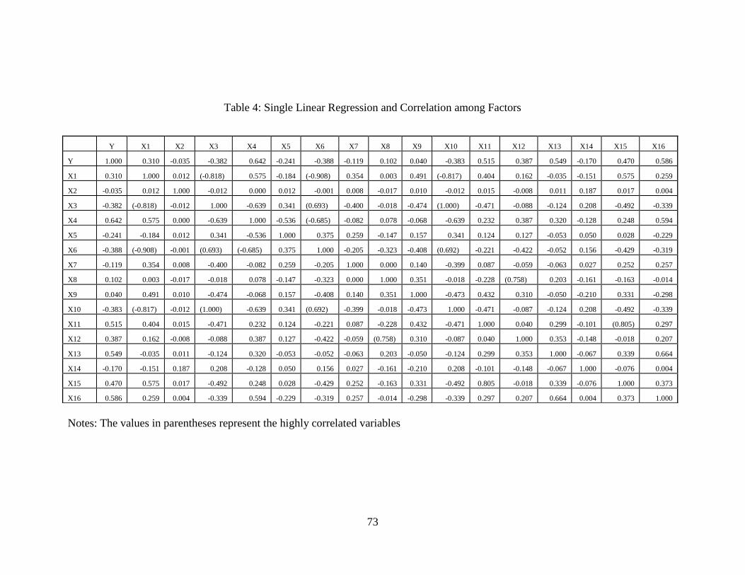
73
Table 4: Single Linear Regression and Correlation among Factors
Notes: The values in parentheses represent the highly correlated variables
Y X1 X2 X3 X4 X5 X6 X7 X8 X9 X10 X11 X12 X13 X14 X15 X16
Y 1.000 0.310 -0.035 -0.382 0.642 -0.241 -0.388 -0.119 0.102 0.040 -0.383 0.515 0.387 0.549 -0.170 0.470 0.586
X1 0.310 1.000 0.012 (-0.818) 0.575 -0.184 (-0.908) 0.354 0.003 0.491 (-0.817) 0.404 0.162 -0.035 -0.151 0.575 0.259
X2 -0.035 0.012 1.000 -0.012 0.000 0.012 -0.001 0.008 -0.017 0.010 -0.012 0.015 -0.008 0.011 0.187 0.017 0.004
X3 -0.382 (-0.818) -0.012 1.000 -0.639 0.341 (0.693) -0.400 -0.018 -0.474 (1.000) -0.471 -0.088 -0.124 0.208 -0.492 -0.339
X4 0.642 0.575 0.000 -0.639 1.000 -0.536 (-0.685) -0.082 0.078 -0.068 -0.639 0.232 0.387 0.320 -0.128 0.248 0.594
X5 -0.241 -0.184 0.012 0.341 -0.536 1.000 0.375 0.259 -0.147 0.157 0.341 0.124 0.127 -0.053 0.050 0.028 -0.229
X6 -0.388 (-0.908) -0.001 (0.693) (-0.685) 0.375 1.000 -0.205 -0.323 -0.408 (0.692) -0.221 -0.422 -0.052 0.156 -0.429 -0.319
X7 -0.119 0.354 0.008 -0.400 -0.082 0.259 -0.205 1.000 0.000 0.140 -0.399 0.087 -0.059 -0.063 0.027 0.252 0.257
X8 0.102 0.003 -0.017 -0.018 0.078 -0.147 -0.323 0.000 1.000 0.351 -0.018 -0.228 (0.758) 0.203 -0.161 -0.163 -0.014
X9 0.040 0.491 0.010 -0.474 -0.068 0.157 -0.408 0.140 0.351 1.000 -0.473 0.432 0.310 -0.050 -0.210 0.331 -0.298
X10 -0.383 (-0.817) -0.012 (1.000) -0.639 0.341 (0.692) -0.399 -0.018 -0.473 1.000 -0.471 -0.087 -0.124 0.208 -0.492 -0.339
X11 0.515 0.404 0.015 -0.471 0.232 0.124 -0.221 0.087 -0.228 0.432 -0.471 1.000 0.040 0.299 -0.101 (0.805) 0.297
X12 0.387 0.162 -0.008 -0.088 0.387 0.127 -0.422 -0.059 (0.758) 0.310 -0.087 0.040 1.000 0.353 -0.148 -0.018 0.207
X13 0.549 -0.035 0.011 -0.124 0.320 -0.053 -0.052 -0.063 0.203 -0.050 -0.124 0.299 0.353 1.000 -0.067 0.339 0.664
X14 -0.170 -0.151 0.187 0.208 -0.128 0.050 0.156 0.027 -0.161 -0.210 0.208 -0.101 -0.148 -0.067 1.000 -0.076 0.004
X15 0.470 0.575 0.017 -0.492 0.248 0.028 -0.429 0.252 -0.163 0.331 -0.492 0.805 -0.018 0.339 -0.076 1.000 0.373
X16 0.586 0.259 0.004 -0.339 0.594 -0.229 -0.319 0.257 -0.014 -0.298 -0.339 0.297 0.207 0.664 0.004 0.373 1.000
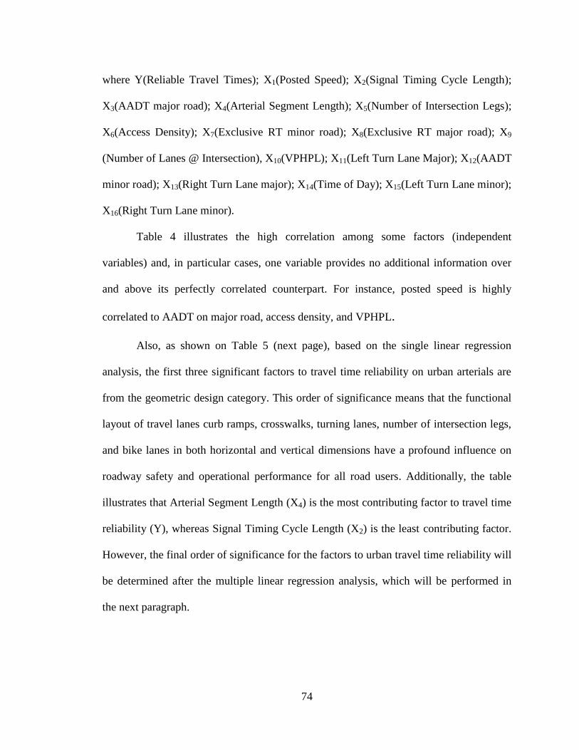
74
where Y(Reliable Travel Times); X1(Posted Speed); X2(Signal Timing Cycle Length);
X3(AADT major road); X4(Arterial Segment Length); X5(Number of Intersection Legs);
X6(Access Density); X7(Exclusive RT minor road); X8(Exclusive RT major road); X9
(Number of Lanes @ Intersection), X10(VPHPL); X11(Left Turn Lane Major); X12(AADT
minor road); X13(Right Turn Lane major); X14(Time of Day); X15(Left Turn Lane minor);
X16(Right Turn Lane minor).
Table 4 illustrates the high correlation among some factors (independent
variables) and, in particular cases, one variable provides no additional information over
and above its perfectly correlated counterpart. For instance, posted speed is highly
correlated to AADT on major road, access density, and VPHPL.
Also, as shown on Table 5 (next page), based on the single linear regression
analysis, the first three significant factors to travel time reliability on urban arterials are
from the geometric design category. This order of significance means that the functional
layout of travel lanes curb ramps, crosswalks, turning lanes, number of intersection legs,
and bike lanes in both horizontal and vertical dimensions have a profound influence on
roadway safety and operational performance for all road users. Additionally, the table
illustrates that Arterial Segment Length (X4) is the most contributing factor to travel time
reliability (Y), whereas Signal Timing Cycle Length (X2) is the least contributing factor.
However, the final order of significance for the factors to urban travel time reliability will
be determined after the multiple linear regression analysis, which will be performed in
the next paragraph.
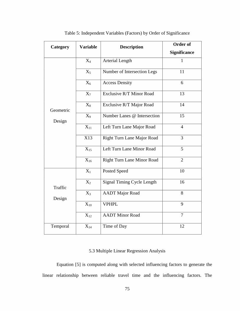
75
Table 5: Independent Variables (Factors) by Order of Significance
5.3 Multiple Linear Regression Analysis
Equation [5] is computed along with selected influencing factors to generate the
linear relationship between reliable travel time and the influencing factors. The
Category Variable Description Order of
Significance
Geometric
Design
X4 Arterial Length 1
X5 Number of Intersection Legs 11
X6 Access Density 6
X7 Exclusive R/T Minor Road 13
X8 Exclusive R/T Major Road 14
X9 Number Lanes @ Intersection 15
X11 Left Turn Lane Major Road 4
X13 Right Turn Lane Major Road 3
X15 Left Turn Lane Minor Road 5
X16 Right Turn Lane Minor Road 2
Traffic
Design
X1 Posted Speed 10
X2 Signal Timing Cycle Length 16
X3 AADT Major Road 8
X10 VPHPL 9
X12 AADT Minor Road 7
Temporal X14 Time of Day 12
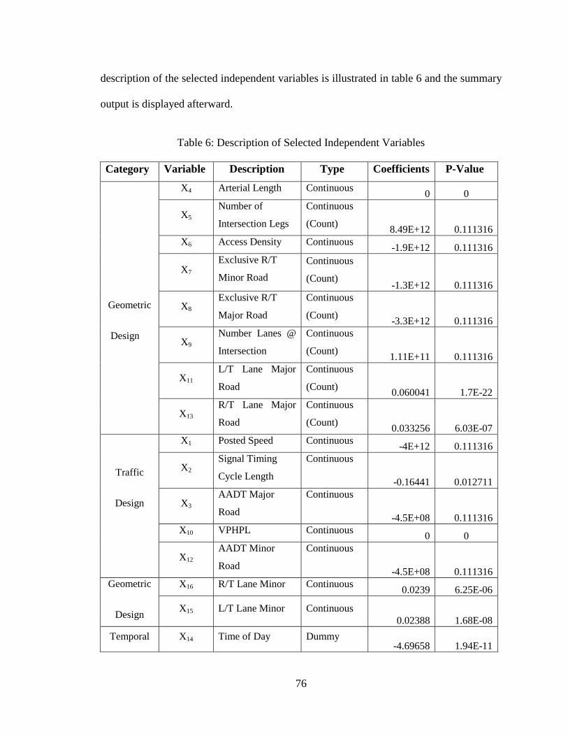
76
description of the selected independent variables is illustrated in table 6 and the summary
output is displayed afterward.
Table 6: Description of Selected Independent Variables
Category Variable Description Type Coefficients P-Value
Geometric
Design
X4 Arterial Length Continuous 0 0
X5 Number of
Intersection Legs
Continuous
(Count) 8.49E+12 0.111316
X6 Access Density Continuous -1.9E+12 0.111316
X7 Exclusive R/T
Minor Road
Continuous
(Count) -1.3E+12 0.111316
X8 Exclusive R/T
Major Road
Continuous
(Count) -3.3E+12 0.111316
X9 Number Lanes @
Intersection
Continuous
(Count) 1.11E+11 0.111316
X11 L/T Lane Major
Road
Continuous
(Count) 0.060041 1.7E-22
X13 R/T Lane Major
Road
Continuous
(Count) 0.033256 6.03E-07
Traffic
Design
X1 Posted Speed Continuous -4E+12 0.111316
X2 Signal Timing
Cycle Length
Continuous
-0.16441 0.012711
X3 AADT Major
Road
Continuous
-4.5E+08 0.111316
X10 VPHPL Continuous 0 0
X12 AADT Minor
Road
Continuous
-4.5E+08 0.111316
Geometric
Design
X16 R/T Lane Minor Continuous 0.0239 6.25E-06
X15 L/T Lane Minor Continuous
0.02388 1.68E-08
Temporal X14 Time of Day Dummy -4.69658 1.94E-11
77
Table 7: Summary Output # 1
Multiple R 0.825
R-Square 0.681
Adjusted R-Square 0.679
Standard Error 18.720
Observations 3362
Table 8: ANOVA # 1 (Analysis of Variance)
df SS MS F
Regression 16 2508728 156795 511.29
Residuals 3347 1173025 350.47
Total 3363 3681753
As shown in Table 6, Left Turn Lane on Major Road (X11), Right Turn Lane on
Major Road (X13), Time of Day (X14), Left Turn Lane on Minor Road (X15), and Right
Turn Lane on Minor Road (X16) five of the selected independent variables, are significant
to the model. The nonsignificance of the other variables does not mean they do not
influence travel time reliability on the corridor rather their influences are explained by
other factors to which they are highly correlated.
The equation for the normal multiple regression is:
Y=2.04 X10¹⁴
+0.060X11-4.05X1008
X12+0.03X13+4.69X14+0.02X15+0.02X16+ε [5].
In addition, Table 7 shows 68.1% of the variance in travel time reliability is explained by
the selected independent variables. The other 31.9% remains unexplained.
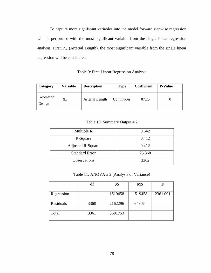
78
To capture more significant variables into the model forward stepwise regression
will be performed with the most significant variable from the single linear regression
analysis. First, X4 (Arterial Length), the most significant variable from the single linear
regression will be considered.
Table 9: First Linear Regression Analysis
Category Variable Description Type Coefficient P-Value
Geometric
Design
X4 Arterial Length Continuous 87.25 0
Table 10: Summary Output # 2
Table 11: ANOVA # 2 (Analysis of Variance)
df SS MS F
Regression 1 1519458 1519458 2361.091
Residuals 3360 2162296 643.54
Total 3361 3681753
Multiple R 0.642
R-Square 0.412
Adjusted R-Square 0.412
Standard Error 25.368
Observations 3362
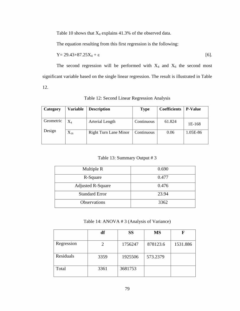
79
Table 10 shows that X4 explains 41.3% of the observed data.
The equation resulting from this first regression is the following:
Y= 29.43+87.25X4 + ε [6].
The second regression will be performed with X4 and X6 the second most
significant variable based on the single linear regression. The result is illustrated in Table
12.
Table 12: Second Linear Regression Analysis
Category Variable Description Type Coefficients P-Value
Geometric
Design
X4 Arterial Length Continuous 61.824 1E-168
X16 Right Turn Lane Minor Continuous 0.06 1.05E-86
Table 13: Summary Output # 3
Multiple R 0.690
R-Square 0.477
Adjusted R-Square 0.476
Standard Error 23.94
Observations 3362
Table 14: ANOVA # 3 (Analysis of Variance)
df SS MS F
Regression 2 1756247
878123.6
1531.886
Residuals 3359 1925506
573.2379
Total 3361 3681753
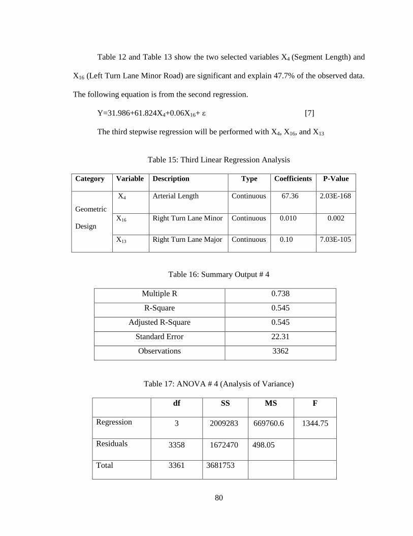
80
Table 12 and Table 13 show the two selected variables X4 (Segment Length) and
X16 (Left Turn Lane Minor Road) are significant and explain 47.7% of the observed data.
The following equation is from the second regression.
Y=31.986+61.824X4+0.06X16+ ε [7]
The third stepwise regression will be performed with X4, X16, and X13
Table 15: Third Linear Regression Analysis
Category Variable Description Type Coefficients P-Value
Geometric
Design
X4 Arterial Length Continuous 67.36 2.03E-168
X16 Right Turn Lane Minor Continuous 0.010 0.002
X13 Right Turn Lane Major Continuous 0.10 7.03E-105
Table 16: Summary Output # 4
Multiple R 0.738
R-Square 0.545
Adjusted R-Square 0.545
Standard Error 22.31
Observations 3362
Table 17: ANOVA # 4 (Analysis of Variance)
df SS MS F
Regression 3 2009283
669760.6
1344.75
Residuals 3358 1672470
498.05
Total 3361 3681753
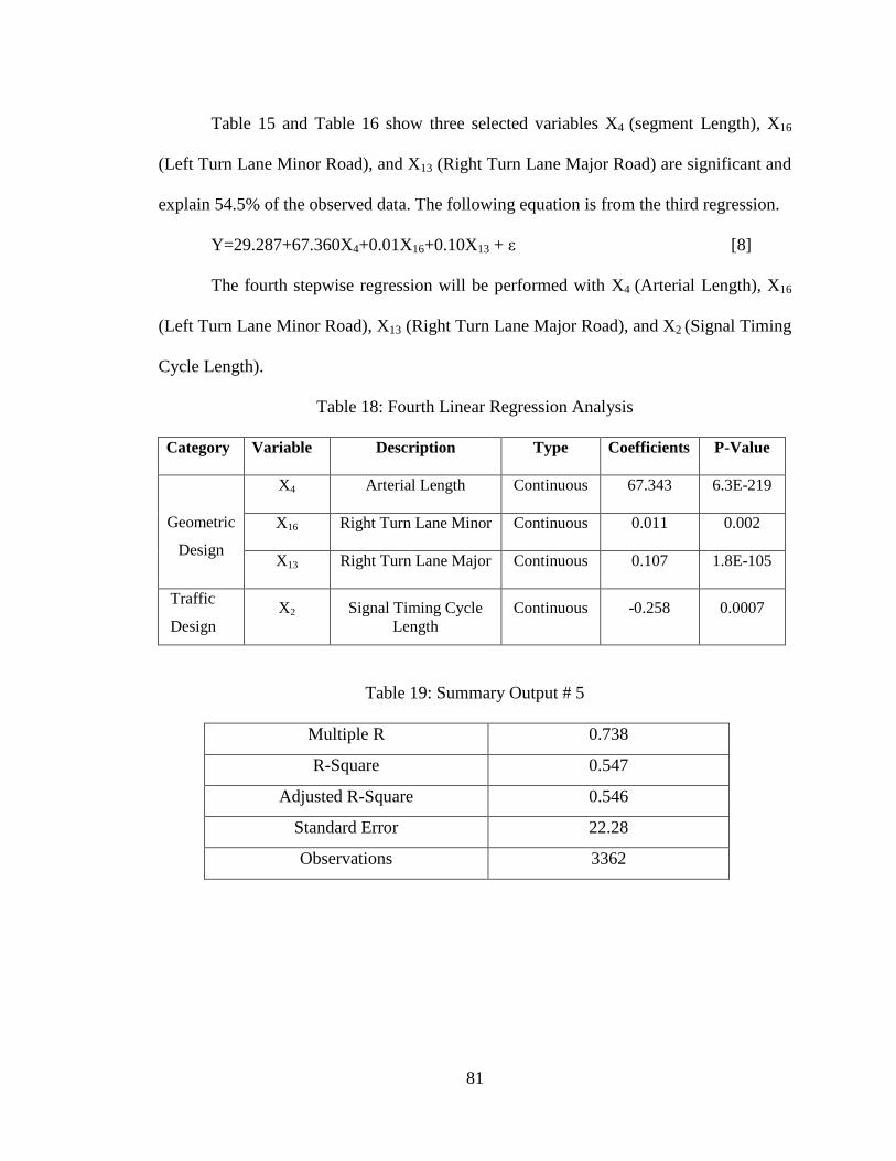
81
Table 15 and Table 16 show three selected variables X4 (segment Length), X16
(Left Turn Lane Minor Road), and X13 (Right Turn Lane Major Road) are significant and
explain 54.5% of the observed data. The following equation is from the third regression.
Y=29.287+67.360X4+0.01X16+0.10X13 + ε [8]
The fourth stepwise regression will be performed with X4 (Arterial Length), X16
(Left Turn Lane Minor Road), X13 (Right Turn Lane Major Road), and X2 (Signal Timing
Cycle Length).
Table 18: Fourth Linear Regression Analysis
Category Variable Description Type Coefficients P-Value
Geometric
Design
X4 Arterial Length Continuous 67.343 6.3E-219
X16 Right Turn Lane Minor Continuous 0.011 0.002
X13 Right Turn Lane Major Continuous 0.107 1.8E-105
Traffic
Design
X2 Signal Timing Cycle
Length
Continuous -0.258 0.0007
Table 19: Summary Output # 5
Multiple R 0.738
R-Square 0.547
Adjusted R-Square 0.546
Standard Error 22.28
Observations 3362
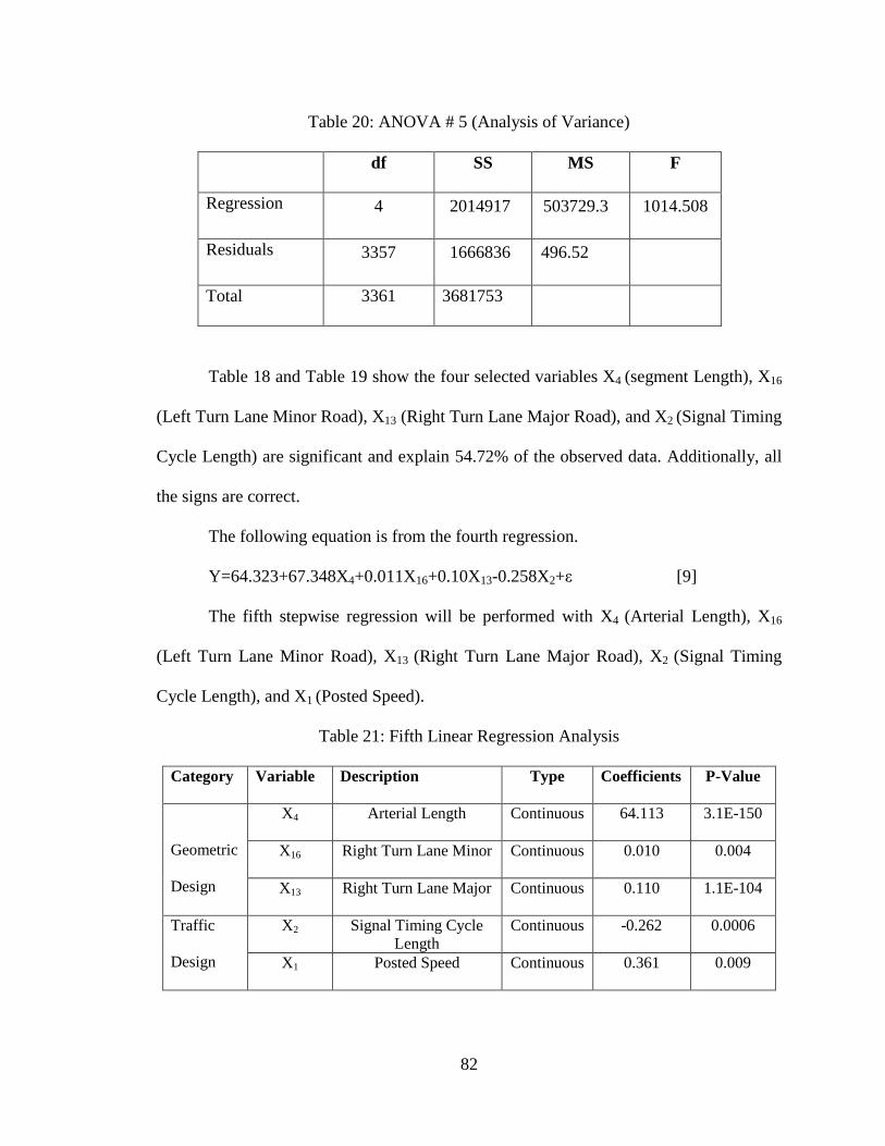
82
Table 20: ANOVA # 5 (Analysis of Variance)
df SS MS F
Regression 4 2014917
503729.3
1014.508
Residuals 3357 1666836
496.52
Total 3361 3681753
Table 18 and Table 19 show the four selected variables X4 (segment Length), X16
(Left Turn Lane Minor Road), X13 (Right Turn Lane Major Road), and X2 (Signal Timing
Cycle Length) are significant and explain 54.72% of the observed data. Additionally, all
the signs are correct.
The following equation is from the fourth regression.
Y=64.323+67.348X4+0.011X16+0.10X13-0.258X2+ε [9]
The fifth stepwise regression will be performed with X4 (Arterial Length), X16
(Left Turn Lane Minor Road), X13 (Right Turn Lane Major Road), X2 (Signal Timing
Cycle Length), and X1 (Posted Speed).
Table 21: Fifth Linear Regression Analysis
Category Variable Description Type Coefficients P-Value
Geometric
Design
X4 Arterial Length Continuous 64.113 3.1E-150
X16 Right Turn Lane Minor Continuous 0.010 0.004
X13 Right Turn Lane Major Continuous 0.110 1.1E-104
Traffic
Design
X2 Signal Timing Cycle
Length
Continuous -0.262 0.0006
X1 Posted Speed Continuous 0.361 0.009
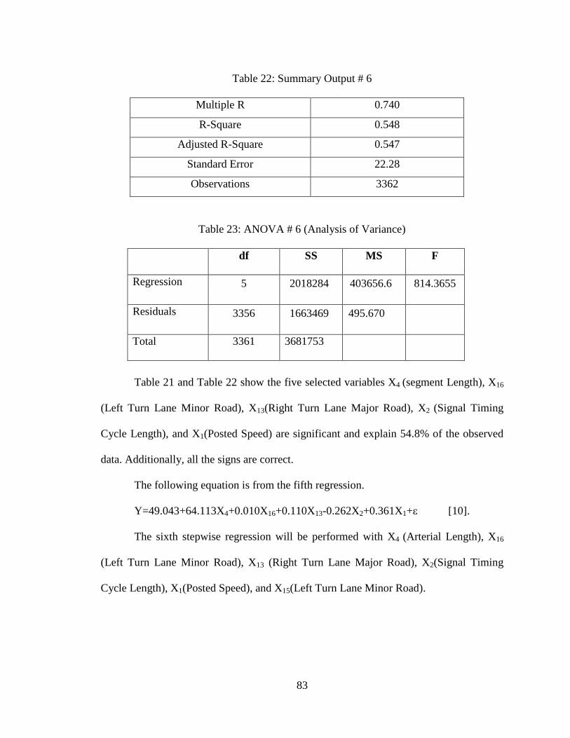
83
Table 22: Summary Output # 6
Multiple R 0.740
R-Square 0.548
Adjusted R-Square 0.547
Standard Error 22.28
Observations 3362
Table 23: ANOVA # 6 (Analysis of Variance)
df SS MS F
Regression 5 2018284
403656.6
814.3655
Residuals 3356 1663469
495.670
Total 3361 3681753
Table 21 and Table 22 show the five selected variables X4 (segment Length), X16
(Left Turn Lane Minor Road), X13(Right Turn Lane Major Road), X2 (Signal Timing
Cycle Length), and X1(Posted Speed) are significant and explain 54.8% of the observed
data. Additionally, all the signs are correct.
The following equation is from the fifth regression.
Y=49.043+64.113X4+0.010X16+0.110X13-0.262X2+0.361X1+ε [10].
The sixth stepwise regression will be performed with X4 (Arterial Length), X16
(Left Turn Lane Minor Road), X13 (Right Turn Lane Major Road), X2(Signal Timing
Cycle Length), X1(Posted Speed), and X15(Left Turn Lane Minor Road).
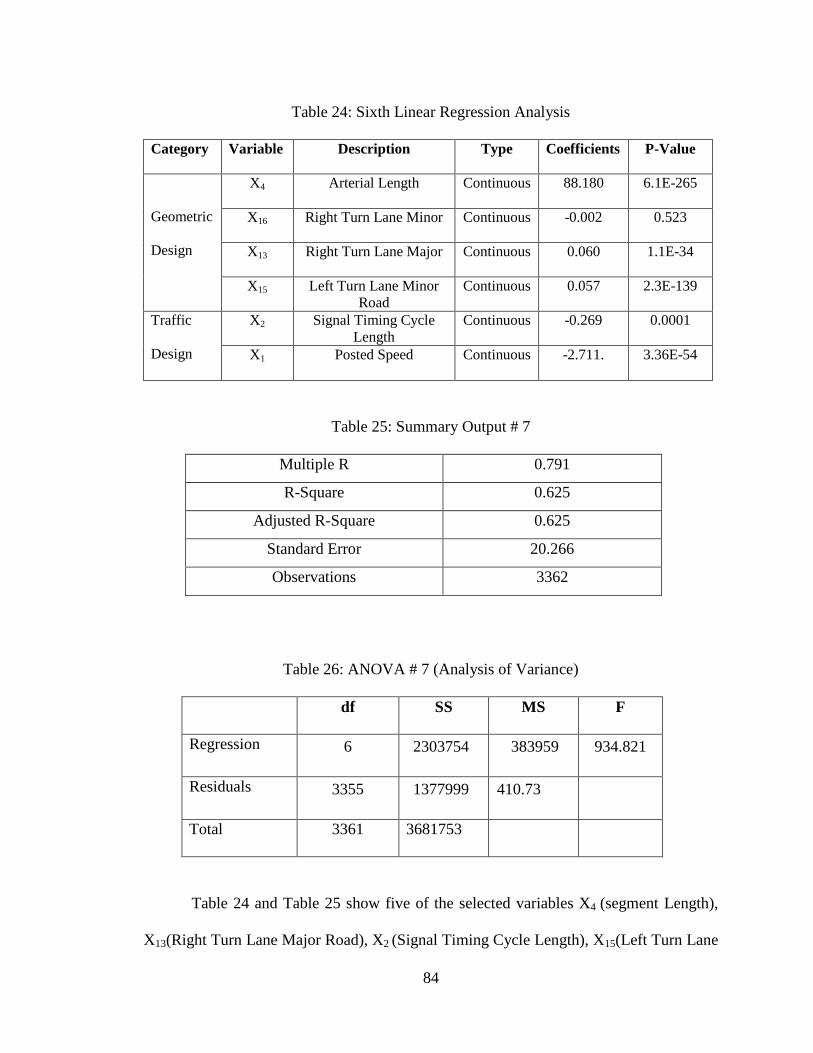
84
Table 24: Sixth Linear Regression Analysis
Category Variable Description Type Coefficients P-Value
Geometric
Design
X4 Arterial Length Continuous 88.180 6.1E-265
X16 Right Turn Lane Minor Continuous -0.002 0.523
X13 Right Turn Lane Major Continuous 0.060 1.1E-34
X15 Left Turn Lane Minor
Road
Continuous 0.057 2.3E-139
Traffic
Design
X2 Signal Timing Cycle
Length
Continuous -0.269 0.0001
X1 Posted Speed Continuous -2.711. 3.36E-54
Table 25: Summary Output # 7
Multiple R 0.791
R-Square 0.625
Adjusted R-Square 0.625
Standard Error 20.266
Observations 3362
Table 26: ANOVA # 7 (Analysis of Variance)
df SS MS F
Regression 6 2303754
383959
934.821
Residuals 3355 1377999
410.73
Total 3361 3681753
Table 24 and Table 25 show five of the selected variables X4 (segment Length),
X13(Right Turn Lane Major Road), X2 (Signal Timing Cycle Length), X15(Left Turn Lane
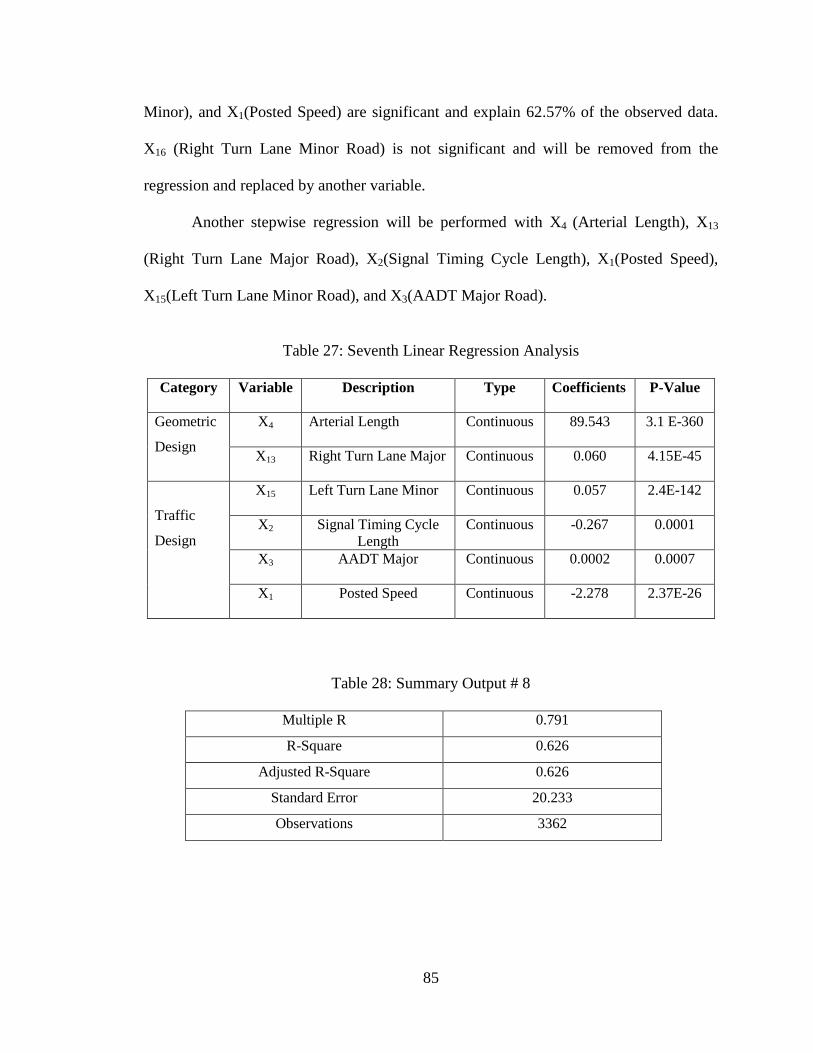
85
Minor), and X1(Posted Speed) are significant and explain 62.57% of the observed data.
X16 (Right Turn Lane Minor Road) is not significant and will be removed from the
regression and replaced by another variable.
Another stepwise regression will be performed with X4 (Arterial Length), X13
(Right Turn Lane Major Road), X2(Signal Timing Cycle Length), X1(Posted Speed),
X15(Left Turn Lane Minor Road), and X3(AADT Major Road).
Table 27: Seventh Linear Regression Analysis
Category Variable Description Type Coefficients P-Value
Geometric
Design
X4 Arterial Length Continuous 89.543 3.1 E-360
X13 Right Turn Lane Major Continuous 0.060 4.15E-45
Traffic
Design
X15 Left Turn Lane Minor Continuous 0.057 2.4E-142
X2 Signal Timing Cycle
Length
Continuous -0.267 0.0001
X3 AADT Major Continuous 0.0002 0.0007
X1 Posted Speed Continuous -2.278 2.37E-26
Table 28: Summary Output # 8
Multiple R 0.791
R-Square 0.626
Adjusted R-Square 0.626
Standard Error 20.233
Observations 3362
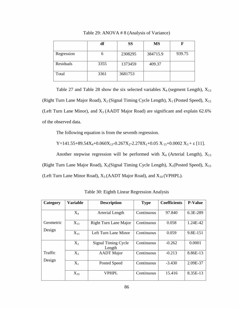
86
Table 29: ANOVA # 8 (Analysis of Variance)
df SS MS F
Regression 6 2308295
384715.9
939.75
Residuals 3355 1373459
409.37
Total 3361 3681753
Table 27 and Table 28 show the six selected variables X4 (segment Length), X13
(Right Turn Lane Major Road), X2 (Signal Timing Cycle Length), X1 (Posted Speed), X15
(Left Turn Lane Minor), and X3 (AADT Major Road) are significant and explain 62.6%
of the observed data.
The following equation is from the seventh regression.
Y=141.55+89.54X4+0.060X13-0.267X2-2.278X1+0.05 X 15+0.0002 X3 + ε [11].
Another stepwise regression will be performed with X4 (Arterial Length), X13
(Right Turn Lane Major Road), X2(Signal Timing Cycle Length), X1(Posted Speed), X15
(Left Turn Lane Minor Road), X3 (AADT Major Road), and X10 (VPHPL).
Table 30: Eighth Linear Regression Analysis
Category Variable Description Type Coefficients P-Value
Geometric
Design
X4 Arterial Length Continuous 97.840 6.3E-289
X13 Right Turn Lane Major Continuous 0.058 1.24E-42
X15 Left Turn Lane Minor Continuous 0.059 9.8E-151
Traffic
Design
X2 Signal Timing Cycle
Length
Continuous -0.262 0.0001
X3 AADT Major Continuous -0.213 8.86E-13
X1 Posted Speed Continuous -3.430 2.09E-37
X10 VPHPL Continuous 15.416 8.35E-13
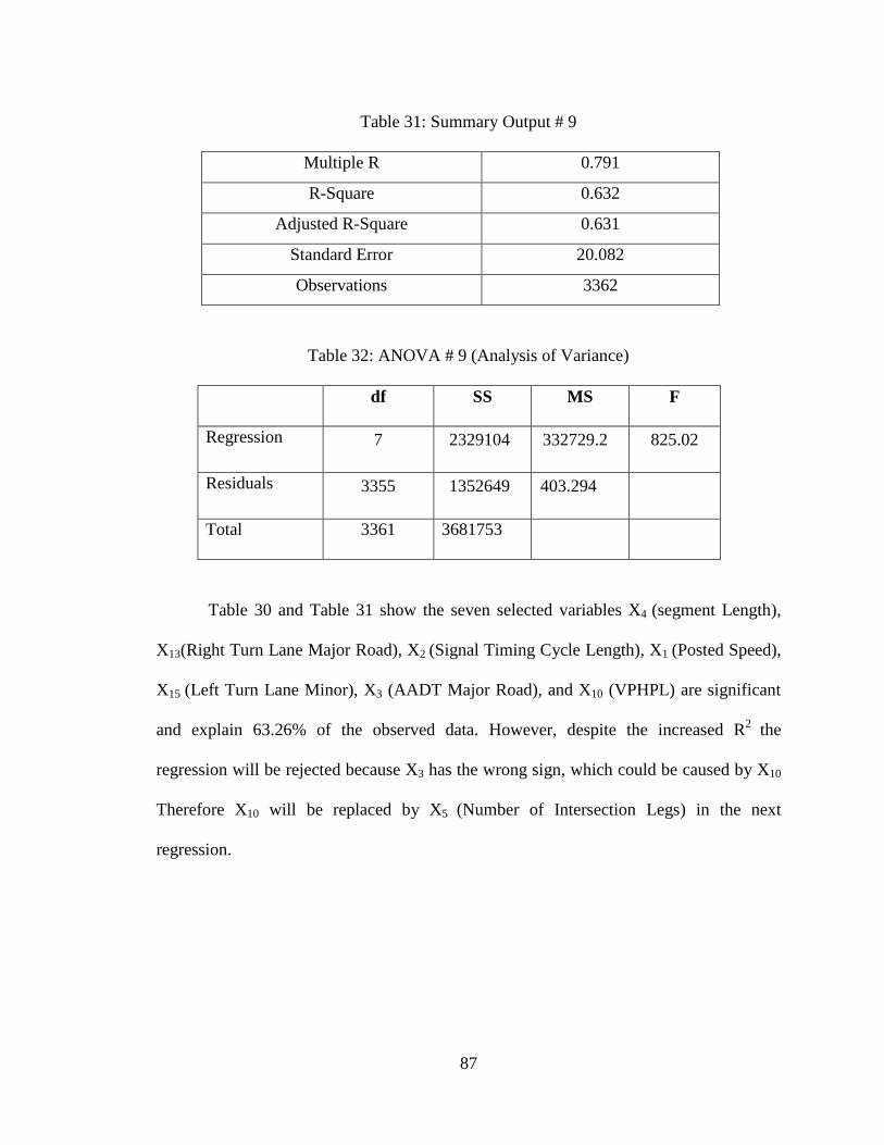
87
Table 31: Summary Output # 9
Multiple R 0.791
R-Square 0.632
Adjusted R-Square 0.631
Standard Error 20.082
Observations 3362
Table 32: ANOVA # 9 (Analysis of Variance)
df SS MS F
Regression 7 2329104
332729.2
825.02
Residuals 3355 1352649
403.294
Total 3361 3681753
Table 30 and Table 31 show the seven selected variables X4 (segment Length),
X13(Right Turn Lane Major Road), X2 (Signal Timing Cycle Length), X1 (Posted Speed),
X15 (Left Turn Lane Minor), X3 (AADT Major Road), and X10 (VPHPL) are significant
and explain 63.26% of the observed data. However, despite the increased R2
the
regression will be rejected because X3 has the wrong sign, which could be caused by X10
Therefore X10 will be replaced by X5 (Number of Intersection Legs) in the next
regression.
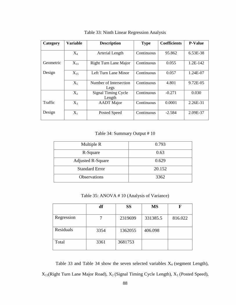
88
Table 33: Ninth Linear Regression Analysis
Category Variable Description Type Coefficients P-Value
Geometric
Design
X4 Arterial Length Continuous 95.862 6.53E-38
X13 Right Turn Lane Major Continuous 0.055 1.2E-142
X15 Left Turn Lane Minor Continuous 0.057 1.24E-07
X5 Number of Intersection
Legs
Continuous 4.801 9.72E-05
Traffic
Design
X2 Signal Timing Cycle
Length
Continuous -0.271 0.030
X3 AADT Major Continuous 0.0001 2.26E-31
X1 Posted Speed Continuous -2.584 2.09E-37
Table 34: Summary Output # 10
Multiple R 0.793
R-Square 0.63
Adjusted R-Square 0.629
Standard Error 20.152
Observations 3362
Table 35: ANOVA # 10 (Analysis of Variance)
df SS MS F
Regression 7 2319699
331385.5
816.022
Residuals 3354 1362055
406.098
Total 3361 3681753
Table 33 and Table 34 show the seven selected variables X4 (segment Length),
X13(Right Turn Lane Major Road), X2 (Signal Timing Cycle Length), X1 (Posted Speed),
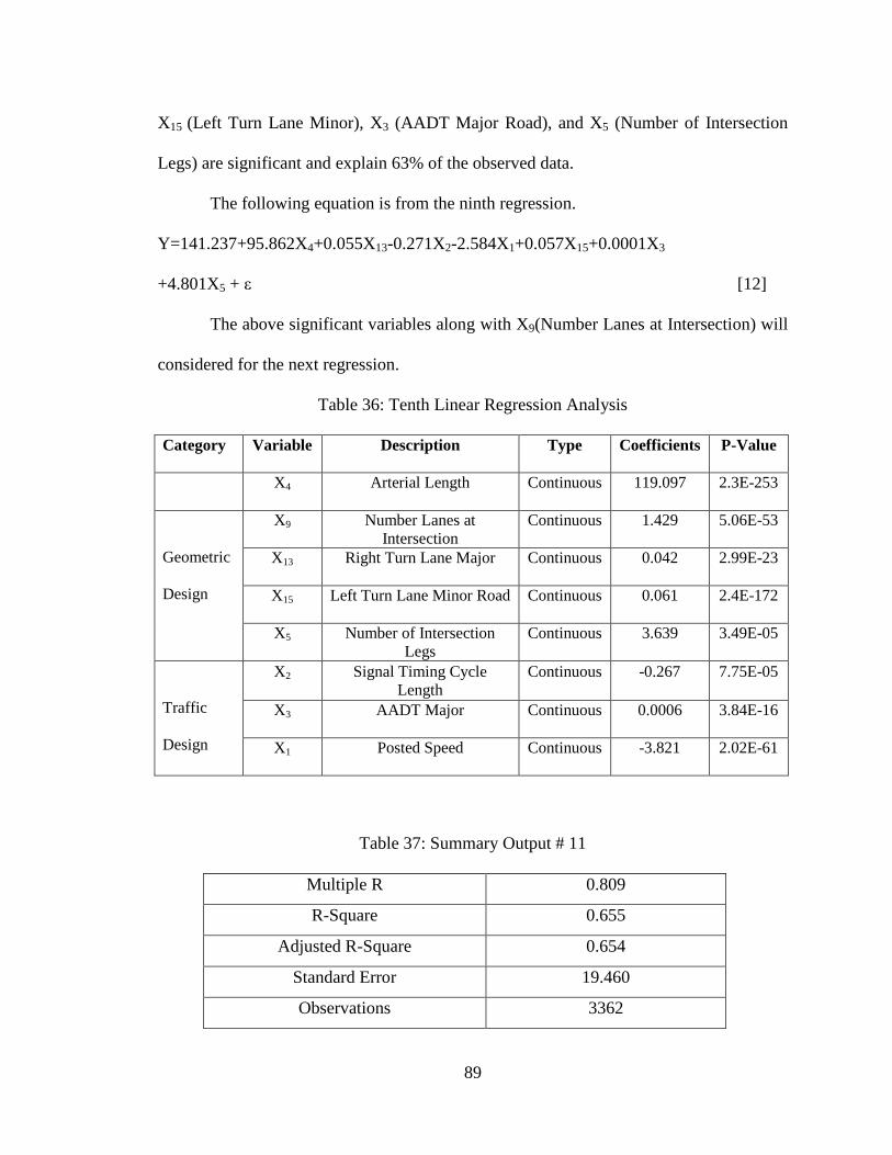
89
X15 (Left Turn Lane Minor), X3 (AADT Major Road), and X5 (Number of Intersection
Legs) are significant and explain 63% of the observed data.
The following equation is from the ninth regression.
Y=141.237+95.862X4+0.055X13-0.271X2-2.584X1+0.057X15+0.0001X3
+4.801X5 + ε [12]
The above significant variables along with X9(Number Lanes at Intersection) will
considered for the next regression.
Table 36: Tenth Linear Regression Analysis
Category Variable Description Type Coefficients P-Value
X4 Arterial Length Continuous 119.097 2.3E-253
Geometric
Design
X9 Number Lanes at
Intersection
Continuous 1.429 5.06E-53
X13 Right Turn Lane Major Continuous 0.042 2.99E-23
X15 Left Turn Lane Minor Road Continuous 0.061 2.4E-172
X5 Number of Intersection
Legs
Continuous 3.639 3.49E-05
Traffic
Design
X2 Signal Timing Cycle
Length
Continuous -0.267 7.75E-05
X3 AADT Major Continuous 0.0006 3.84E-16
X1 Posted Speed Continuous -3.821 2.02E-61
Table 37: Summary Output # 11
Multiple R 0.809
R-Square 0.655
Adjusted R-Square 0.654
Standard Error 19.460
Observations 3362
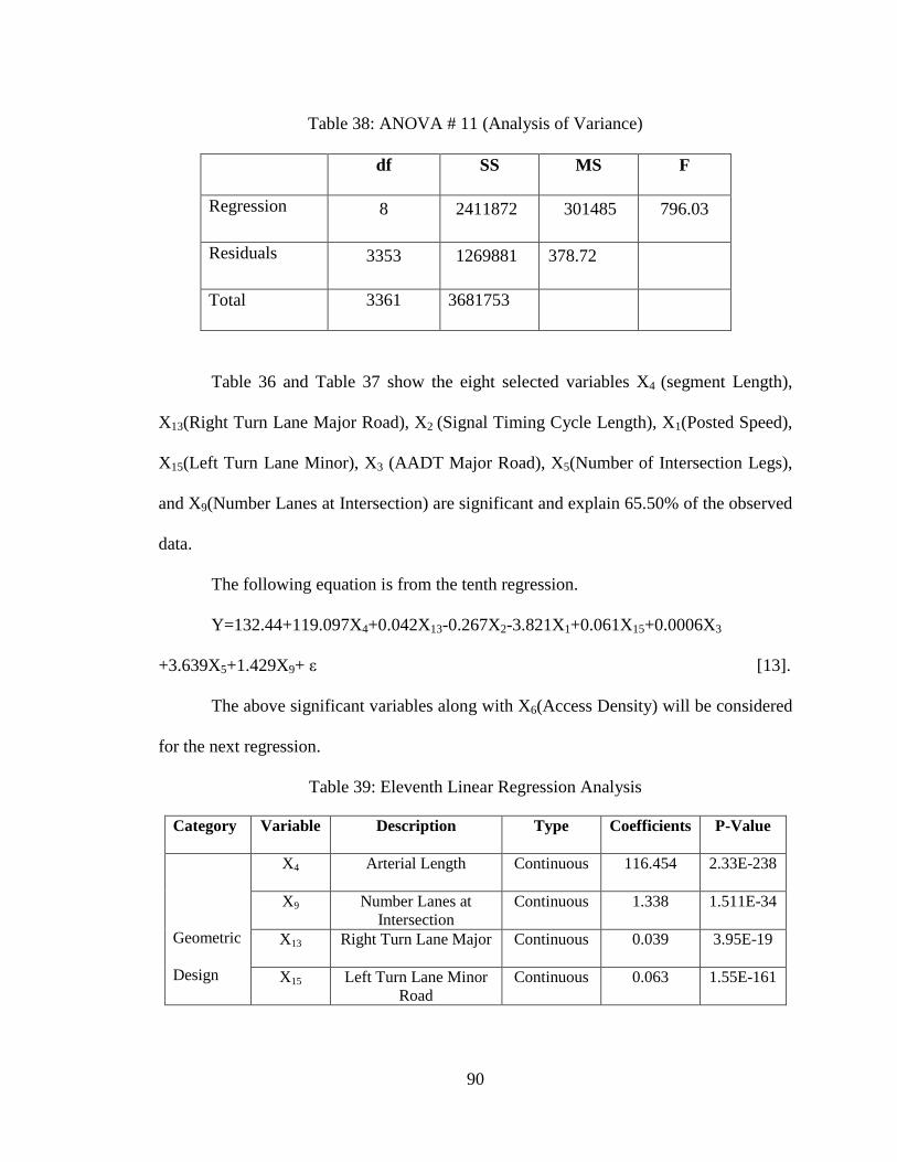
90
Table 38: ANOVA # 11 (Analysis of Variance)
df SS MS F
Regression 8 2411872
301485
796.03
Residuals 3353 1269881
378.72
Total 3361 3681753
Table 36 and Table 37 show the eight selected variables X4 (segment Length),
X13(Right Turn Lane Major Road), X2 (Signal Timing Cycle Length), X1(Posted Speed),
X15(Left Turn Lane Minor), X3 (AADT Major Road), X5(Number of Intersection Legs),
and X9(Number Lanes at Intersection) are significant and explain 65.50% of the observed
data.
The following equation is from the tenth regression.
Y=132.44+119.097X4+0.042X13-0.267X2-3.821X1+0.061X15+0.0006X3
+3.639X5+1.429X9+ ε [13].
The above significant variables along with X6(Access Density) will be considered
for the next regression.
Table 39: Eleventh Linear Regression Analysis
Category Variable Description Type Coefficients P-Value
Geometric
Design
X4 Arterial Length Continuous 116.454 2.33E-238
X9 Number Lanes at
Intersection
Continuous 1.338 1.511E-34
X13 Right Turn Lane Major Continuous 0.039 3.95E-19
X15 Left Turn Lane Minor
Road
Continuous 0.063 1.55E-161
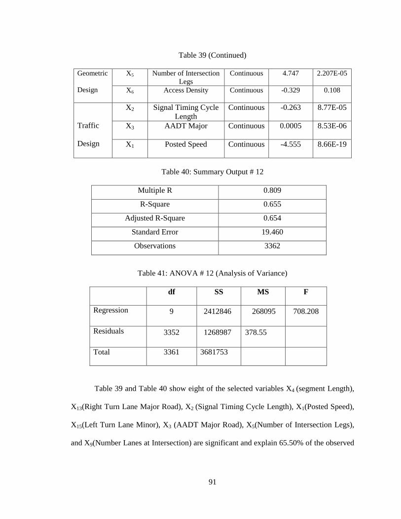
91
Table 39 (Continued)
Geometric
Design
X5 Number of Intersection
Legs
Continuous 4.747 2.207E-05
X6 Access Density Continuous -0.329 0.108
Traffic
Design
X2 Signal Timing Cycle
Length
Continuous -0.263 8.77E-05
X3 AADT Major Continuous 0.0005 8.53E-06
X1 Posted Speed Continuous -4.555 8.66E-19
Table 40: Summary Output # 12
Multiple R 0.809
R-Square 0.655
Adjusted R-Square 0.654
Standard Error 19.460
Observations 3362
Table 41: ANOVA # 12 (Analysis of Variance)
df SS MS F
Regression 9 2412846
268095
708.208
Residuals 3352 1268987
378.55
Total 3361 3681753
Table 39 and Table 40 show eight of the selected variables X4 (segment Length),
X13(Right Turn Lane Major Road), X2 (Signal Timing Cycle Length), X1(Posted Speed),
X15(Left Turn Lane Minor), X3 (AADT Major Road), X5(Number of Intersection Legs),
and X9(Number Lanes at Intersection) are significant and explain 65.50% of the observed
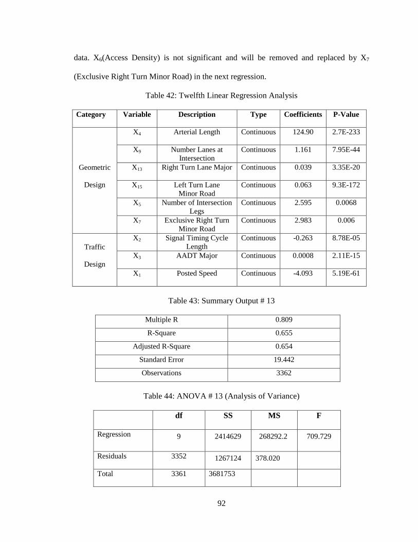
92
data. X6(Access Density) is not significant and will be removed and replaced by X7
(Exclusive Right Turn Minor Road) in the next regression.
Table 42: Twelfth Linear Regression Analysis
Category Variable Description Type Coefficients P-Value
Geometric
Design
X4 Arterial Length Continuous 124.90 2.7E-233
X9 Number Lanes at
Intersection
Continuous 1.161 7.95E-44
X13 Right Turn Lane Major Continuous 0.039 3.35E-20
X15 Left Turn Lane
Minor Road
Continuous 0.063 9.3E-172
X5 Number of Intersection
Legs
Continuous 2.595 0.0068
X7 Exclusive Right Turn
Minor Road
Continuous 2.983 0.006
Traffic
Design
X2 Signal Timing Cycle
Length
Continuous -0.263 8.78E-05
X3 AADT Major Continuous 0.0008 2.11E-15
X1 Posted Speed Continuous -4.093 5.19E-61
Table 43: Summary Output # 13
Multiple R 0.809
R-Square 0.655
Adjusted R-Square 0.654
Standard Error 19.442
Observations 3362
Table 44: ANOVA # 13 (Analysis of Variance)
df SS MS F
Regression 9 2414629
268292.2
709.729
Residuals 3352 1267124
378.020
Total 3361 3681753
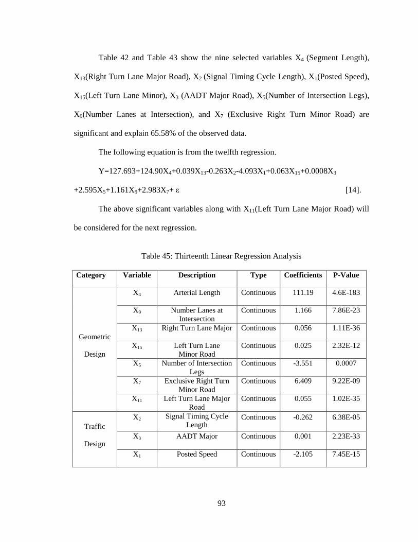
93
Table 42 and Table 43 show the nine selected variables X4 (Segment Length),
X13(Right Turn Lane Major Road), X2 (Signal Timing Cycle Length), X1(Posted Speed),
X15(Left Turn Lane Minor), X3 (AADT Major Road), X5(Number of Intersection Legs),
X9(Number Lanes at Intersection), and X7 (Exclusive Right Turn Minor Road) are
significant and explain 65.58% of the observed data.
The following equation is from the twelfth regression.
Y=127.693+124.90X4+0.039X13-0.263X2-4.093X1+0.063X15+0.0008X3
+2.595X5+1.161X9+2.983X7+ ε [14].
The above significant variables along with X11(Left Turn Lane Major Road) will
be considered for the next regression.
Table 45: Thirteenth Linear Regression Analysis
Category Variable Description Type Coefficients P-Value
Geometric
Design
X4 Arterial Length Continuous 111.19 4.6E-183
X9 Number Lanes at
Intersection
Continuous 1.166 7.86E-23
X13 Right Turn Lane Major Continuous 0.056 1.11E-36
X15 Left Turn Lane
Minor Road
Continuous 0.025 2.32E-12
X5 Number of Intersection
Legs
Continuous -3.551 0.0007
X7 Exclusive Right Turn
Minor Road
Continuous 6.409 9.22E-09
X11 Left Turn Lane Major
Road
Continuous 0.055 1.02E-35
Traffic
Design
X2 Signal Timing Cycle
Length Continuous -0.262 6.38E-05
X3 AADT Major Continuous 0.001 2.23E-33
X1 Posted Speed Continuous -2.105 7.45E-15
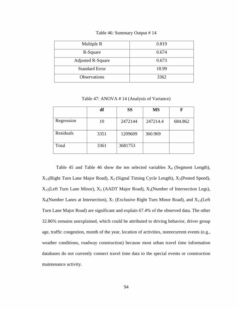
94
Table 46: Summary Output # 14
Multiple R 0.819
R-Square 0.674
Adjusted R-Square 0.673
Standard Error 18.99
Observations 3362
Table 47: ANOVA # 14 (Analysis of Variance)
df SS MS F
Regression 10 2472144
247214.4
684.862
Residuals 3351 1209609
360.969
Total 3361 3681753
Table 45 and Table 46 show the ten selected variables X4 (Segment Length),
X13(Right Turn Lane Major Road), X2 (Signal Timing Cycle Length), X1(Posted Speed),
X15(Left Turn Lane Minor), X3 (AADT Major Road), X5(Number of Intersection Legs),
X9(Number Lanes at Intersection), X7 (Exclusive Right Turn Minor Road), and X11(Left
Turn Lane Major Road) are significant and explain 67.4% of the observed data. The other
32.86% remains unexplained, which could be attributed to driving behavior, driver group
age, traffic congestion, month of the year, location of activities, nonrecurrent events (e.g.,
weather conditions, roadway construction) because most urban travel time information
databases do not currently connect travel time data to the special events or construction
maintenance activity.
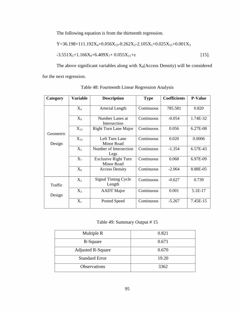
95
The following equation is from the thirteenth regression.
Y=36.198+111.192X4+0.056X13-0.262X2-2.105X1+0.025X15+0.001X3
-3.551X5+1.166X9+6.409X7+ 0.055X11+ε [15].
The above significant variables along with X6(Access Density) will be considered
for the next regression.
Table 48: Fourteenth Linear Regression Analysis
Category Variable Description Type Coefficients P-Value
Geometric
Design
X4 Arterial Length Continuous 785.581 0.820
X9 Number Lanes at
Intersection
Continuous -0.054 1.74E-32
X13 Right Turn Lane Major Continuous 0.056 6.27E-08
X15 Left Turn Lane
Minor Road
Continuous 0.020 0.0006
X5 Number of Intersection
Legs
Continuous -1.354 6.57E-43
X7 Exclusive Right Turn
Minor Road
Continuous 0.068 6.97E-09
X6 Access Density Continuous -2.064 8.88E-05
Traffic
Design
X2 Signal Timing Cycle
Length Continuous -0.627 0.739
X3 AADT Major Continuous 0.001 5.1E-17
X1 Posted Speed Continuous -5.267 7.45E-15
Table 49: Summary Output # 15
Multiple R 0.821
R-Square 0.671
Adjusted R-Square 0.670
Standard Error 19.20
Observations 3362
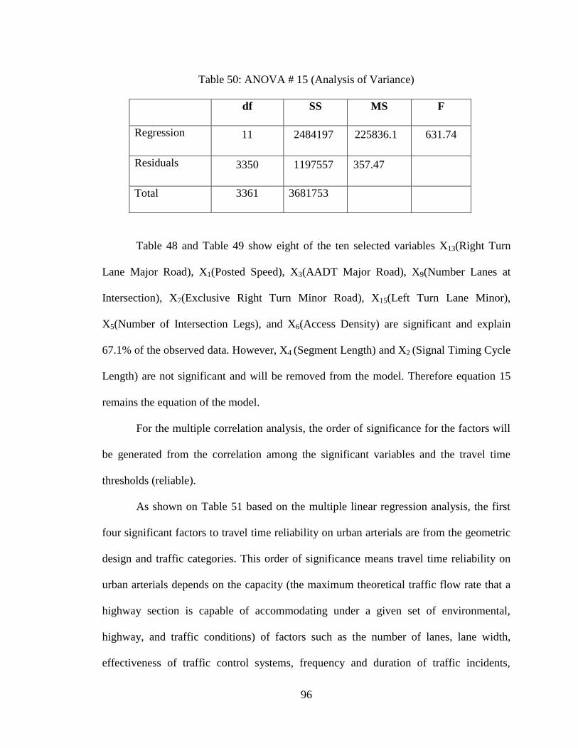
96
Table 50: ANOVA # 15 (Analysis of Variance)
df SS MS F
Regression 11 2484197
225836.1
631.74
Residuals 3350 1197557
357.47
Total 3361 3681753
Table 48 and Table 49 show eight of the ten selected variables X13(Right Turn
Lane Major Road), X1(Posted Speed), X3(AADT Major Road), X9(Number Lanes at
Intersection), X7(Exclusive Right Turn Minor Road), X15(Left Turn Lane Minor),
X5(Number of Intersection Legs), and X6(Access Density) are significant and explain
67.1% of the observed data. However, X4 (Segment Length) and X2 (Signal Timing Cycle
Length) are not significant and will be removed from the model. Therefore equation 15
remains the equation of the model.
For the multiple correlation analysis, the order of significance for the factors will
be generated from the correlation among the significant variables and the travel time
thresholds (reliable).
As shown on Table 51 based on the multiple linear regression analysis, the first
four significant factors to travel time reliability on urban arterials are from the geometric
design and traffic categories. This order of significance means travel time reliability on
urban arterials depends on the capacity (the maximum theoretical traffic flow rate that a
highway section is capable of accommodating under a given set of environmental,
highway, and traffic conditions) of factors such as the number of lanes, lane width,
effectiveness of traffic control systems, frequency and duration of traffic incidents,
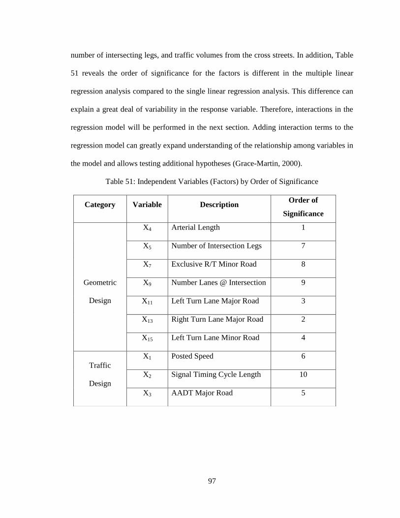
97
number of intersecting legs, and traffic volumes from the cross streets. In addition, Table
51 reveals the order of significance for the factors is different in the multiple linear
regression analysis compared to the single linear regression analysis. This difference can
explain a great deal of variability in the response variable. Therefore, interactions in the
regression model will be performed in the next section. Adding interaction terms to the
regression model can greatly expand understanding of the relationship among variables in
the model and allows testing additional hypotheses (Grace-Martin, 2000).
Table 51: Independent Variables (Factors) by Order of Significance
Category Variable Description Order of
Significance
Geometric
Design
X4 Arterial Length 1
X5 Number of Intersection Legs 7
X7 Exclusive R/T Minor Road 8
X9 Number Lanes @ Intersection 9
X11 Left Turn Lane Major Road 3
X13 Right Turn Lane Major Road 2
X15 Left Turn Lane Minor Road 4
Traffic
Design
X1 Posted Speed 6
X2 Signal Timing Cycle Length 10
X3 AADT Major Road 5
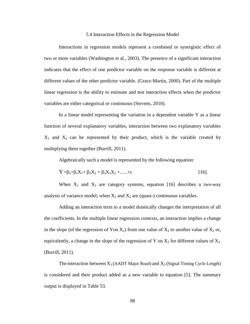
98
5.4 Interaction Effects in the Regression Model
Interactions in regression models represent a combined or synergistic effect of
two or more variables (Washington et al., 2003). The presence of a significant interaction
indicates that the effect of one predictor variable on the response variable is different at
different values of the other predictor variable. (Grace-Martin, 2000). Part of the multiple
linear regression is the ability to estimate and test interaction effects when the predictor
variables are either categorical or continuous (Stevens, 2010).
In a linear model representing the variation in a dependent variable Y as a linear
function of several explanatory variables, interaction between two explanatory variables
X1 and X2 can be represented by their product, which is the variable created by
multiplying them together (Burrill, 2011).
Algebraically such a model is represented by the following equation:
Y =βo+β1X1+ β2X2 + β3X1X2 +......+ε [16].
When X1 and X2 are category systems, equation [16] describes a two-way
analysis of variance model; when X1 and X2 are (quasi-) continuous variables.
Adding an interaction term to a model drastically changes the interpretation of all
the coefficients. In the multiple linear regression contexts, an interaction implies a change
in the slope (of the regression of Yon X1) from one value of X2 to another value of X2 or,
equivalently, a change in the slope of the regression of Y on X2 for different values of X1.
(Burrill, 2011).
The interaction between X3 (AADT Major Road) and X2 (Signal Timing Cycle Length)
is considered and their product added as a new variable to equation [5]. The summary
output is displayed in Table 53.
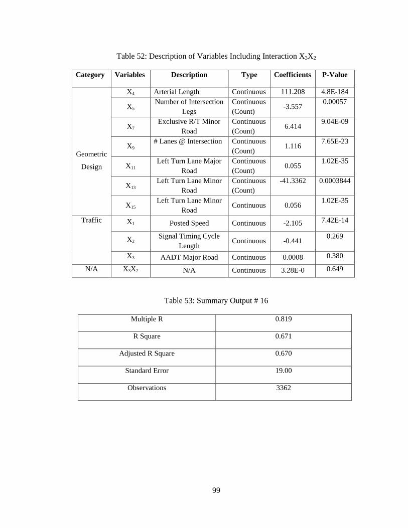
99
Table 52: Description of Variables Including Interaction X3X2
Category Variables Description Type Coefficients P-Value
Geometric
Design
X4 Arterial Length Continuous 111.208 4.8E-184
X5 Number of Intersection
Legs
Continuous
(Count) -3.557
0.00057
X7 Exclusive R/T Minor
Road
Continuous
(Count) 6.414
9.04E-09
X9 # Lanes @ Intersection Continuous
(Count) 1.116
7.65E-23
X11 Left Turn Lane Major
Road
Continuous
(Count) 0.055
1.02E-35
X13 Left Turn Lane Minor
Road
Continuous
(Count)
-41.3362
0.0003844
X15 Left Turn Lane Minor
Road Continuous 0.056
1.02E-35
Traffic
X1 Posted Speed Continuous -2.105 7.42E-14
X2 Signal Timing Cycle
Length Continuous -0.441
0.269
X3 AADT Major Road Continuous 0.0008 0.380
N/A X3X2 N/A Continuous 3.28E-0 0.649
Table 53: Summary Output # 16
Multiple R 0.819
R Square 0.671
Adjusted R Square 0.670
Standard Error 19.00
Observations 3362
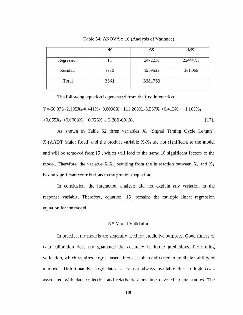
100
Table 54: ANOVA # 16 (Analysis of Variance)
df SS MS
Regression 11 2472218 224447.1
Residual 3350 1209535 361.055
Total 3361 3681753
The following equation is generated from the first interaction
Y=-60.373 -2.105X1-0.441X2+0.0008X3+111.208X4-3.557X5+6.413X7++1.165X9
+0.055X11+0.0008X13+0.025X15+3.28E-6X3X6 [17].
As shown in Table 52 three variables X2 (Signal Timing Cycle Length),
X3(AADT Major Road) and the product variable X2X3 are not significant to the model
and will be removed from [5], which will lead to the same 10 significant factors to the
model. Therefore, the variable X2X3, resulting from the interaction between X2 and X3,
has no significant contributions to the previous equation.
In conclusion, the interaction analysis did not explain any variation in the
response variable. Therefore, equation [15] remains the multiple linear regression
equation for the model.
5.5 Model Validation
In practice, the models are generally used for predictive purposes. Good fitness of
data calibration does not guarantee the accuracy of future predictions. Performing
validation, which requires large datasets, increases the confidence in prediction ability of
a model. Unfortunately, large datasets are not always available due to high costs
associated with data collection and relatively short time devoted to the studies. The
101
validation process establishes the credibility of the model by demonstrating its ability to
replicate actual traffic patterns. Validating the model requires comparing travel time
estimated by the model to observed travel time on the roadway. Validation is typically an
iterative process linked to calibration. If the analyst finds that the model output and the
independent data are in acceptable agreement, the model can be considered validated
(Pedersen & Sandahl, 1982).
Reasonableness checks and sensibility checks are normally two types of
validation checks that include steps such as the comparison of rates and checking of the
total regional values and logic tests. The analyst evaluates the models in terms of
acceptable levels of errors, ability to perform according to theoretical and logical
expectations, and consistency of model results with the assumptions used in generating
the results (Wegmann & Everett, 2008).
Sensibility checks are tests that check the responses to the transportation system
and socioeconomic or political changes. Sensibility is often expressed as the elasticity of
the variable.
In any accuracy check errors associated with the ground counts need to be taken
into account. These errors are due to equipment malfunction, the inappropriate use of
daily and seasonal factors to estimate AADT, and the absence of good classification data
to correct axle count to vehicles.
To validate the model, reliable travel time data collected for two different weeks
are incorporated into the linear regression equation of the model and the outputs are
compared to the estimated reliable travel times.
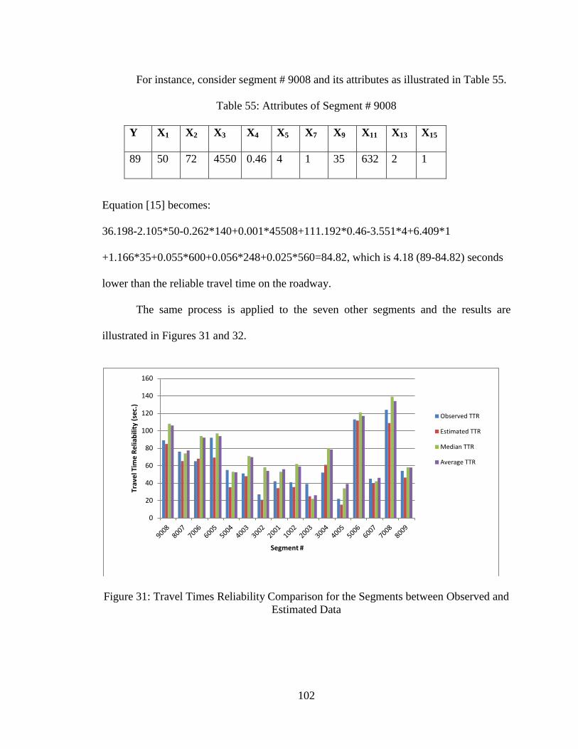
102
For instance, consider segment # 9008 and its attributes as illustrated in Table 55.
Table 55: Attributes of Segment # 9008
Y X1 X2 X3 X4 X5 X7 X9 X11 X13 X15
89 50 72 4550 0.46 4 1 35 632 2 1
Equation [15] becomes:
36.198-2.105*50-0.262*140+0.001*45508+111.192*0.46-3.551*4+6.409*1
+1.166*35+0.055*600+0.056*248+0.025*560=84.82, which is 4.18 (89-84.82) seconds
lower than the reliable travel time on the roadway.
The same process is applied to the seven other segments and the results are
illustrated in Figures 31 and 32.
Figure 31: Travel Times Reliability Comparison for the Segments between Observed and
Estimated Data
0
20
40
60
80
100
120
140
160
Trav
el T
ime
Re
liab
ility
(se
c.)
Segment #
Observed TTR
Estimated TTR
Median TTR
Average TTR
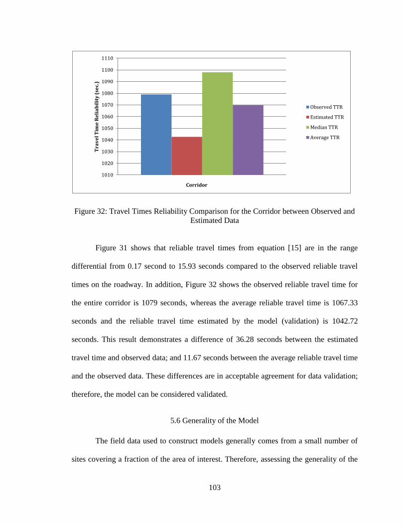
103
Figure 32: Travel Times Reliability Comparison for the Corridor between Observed and
Estimated Data
Figure 31 shows that reliable travel times from equation [15] are in the range
differential from 0.17 second to 15.93 seconds compared to the observed reliable travel
times on the roadway. In addition, Figure 32 shows the observed reliable travel time for
the entire corridor is 1079 seconds, whereas the average reliable travel time is 1067.33
seconds and the reliable travel time estimated by the model (validation) is 1042.72
seconds. This result demonstrates a difference of 36.28 seconds between the estimated
travel time and observed data; and 11.67 seconds between the average reliable travel time
and the observed data. These differences are in acceptable agreement for data validation;
therefore, the model can be considered validated.
5.6 Generality of the Model
The field data used to construct models generally comes from a small number of
sites covering a fraction of the area of interest. Therefore, assessing the generality of the
1010
1020
1030
1040
1050
1060
1070
1080
1090
1100
1110
Tra
ve
l Tim
e R
eli
ab
ilit
y (
sec.
)
Corridor
Observed TTR
Estimated TTR
Median TTR
Average TTR
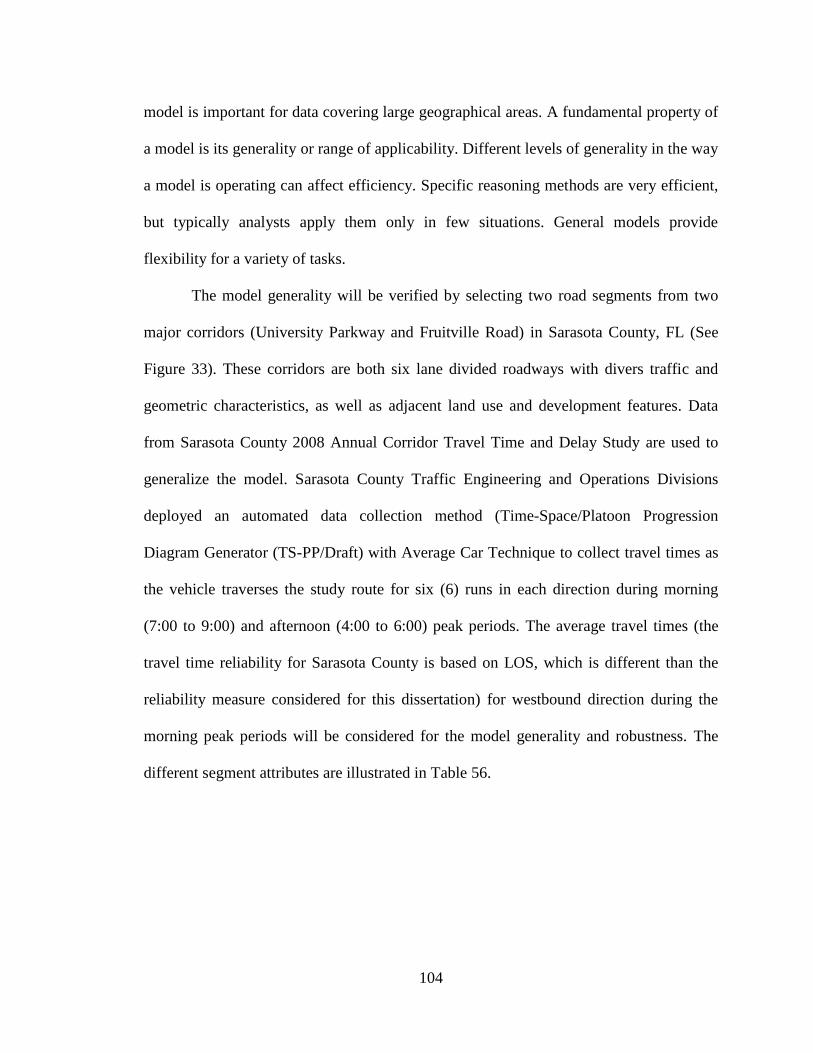
104
model is important for data covering large geographical areas. A fundamental property of
a model is its generality or range of applicability. Different levels of generality in the way
a model is operating can affect efficiency. Specific reasoning methods are very efficient,
but typically analysts apply them only in few situations. General models provide
flexibility for a variety of tasks.
The model generality will be verified by selecting two road segments from two
major corridors (University Parkway and Fruitville Road) in Sarasota County, FL (See
Figure 33). These corridors are both six lane divided roadways with divers traffic and
geometric characteristics, as well as adjacent land use and development features. Data
from Sarasota County 2008 Annual Corridor Travel Time and Delay Study are used to
generalize the model. Sarasota County Traffic Engineering and Operations Divisions
deployed an automated data collection method (Time-Space/Platoon Progression
Diagram Generator (TS-PP/Draft) with Average Car Technique to collect travel times as
the vehicle traverses the study route for six (6) runs in each direction during morning
(7:00 to 9:00) and afternoon (4:00 to 6:00) peak periods. The average travel times (the
travel time reliability for Sarasota County is based on LOS, which is different than the
reliability measure considered for this dissertation) for westbound direction during the
morning peak periods will be considered for the model generality and robustness. The
different segment attributes are illustrated in Table 56.
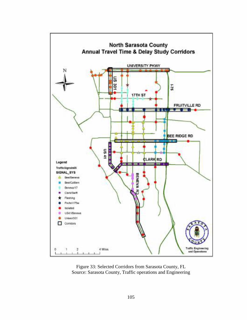
105
Figure 33: Selected Corridors from Sarasota County, FL
Source: Sarasota County, Traffic operations and Engineering
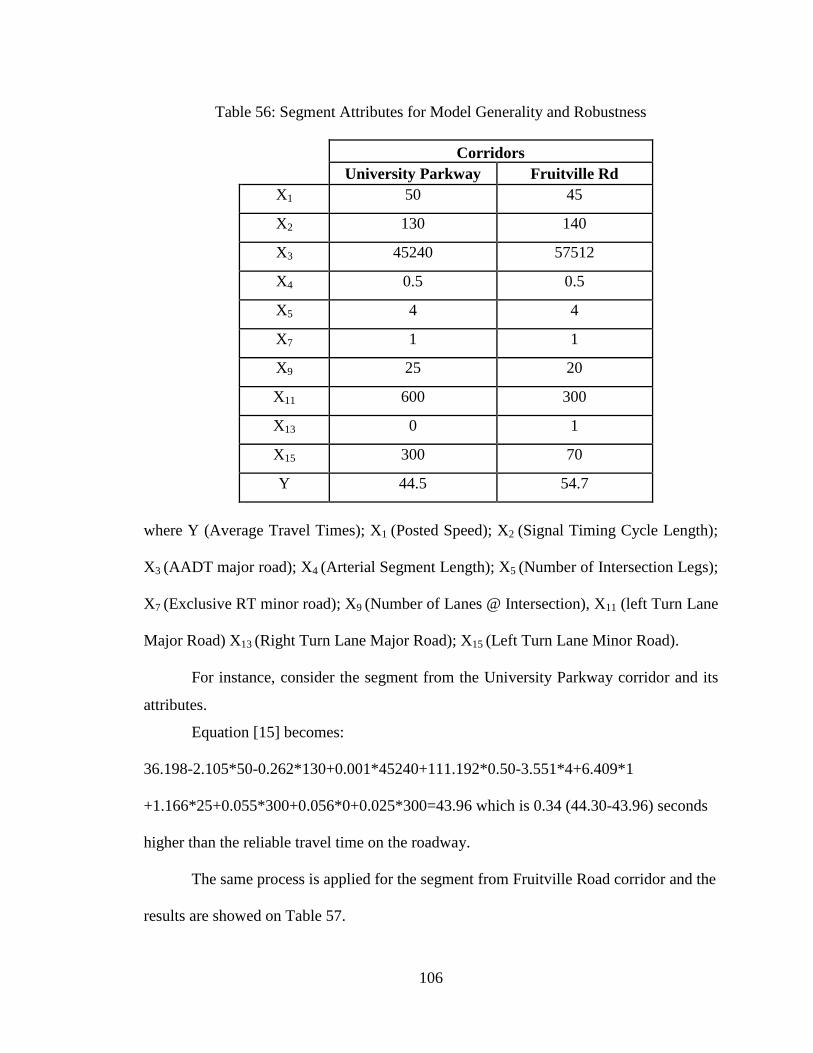
106
Table 56: Segment Attributes for Model Generality and Robustness
Corridors
University Parkway Fruitville Rd
X1 50 45
X2 130 140
X3 45240 57512
X4 0.5 0.5
X5 4 4
X7 1 1
X9 25 20
X11 600 300
X13 0 1
X15 300 70
Y 44.5 54.7
where Y (Average Travel Times); X1 (Posted Speed); X2 (Signal Timing Cycle Length);
X3 (AADT major road); X4 (Arterial Segment Length); X5 (Number of Intersection Legs);
X7 (Exclusive RT minor road); X9 (Number of Lanes @ Intersection), X11 (left Turn Lane
Major Road) X13 (Right Turn Lane Major Road); X15 (Left Turn Lane Minor Road).
For instance, consider the segment from the University Parkway corridor and its
attributes.
Equation [15] becomes:
36.198-2.105*50-0.262*130+0.001*45240+111.192*0.50-3.551*4+6.409*1
+1.166*25+0.055*300+0.056*0+0.025*300=43.96 which is 0.34 (44.30-43.96) seconds
higher than the reliable travel time on the roadway.
The same process is applied for the segment from Fruitville Road corridor and the
results are showed on Table 57.
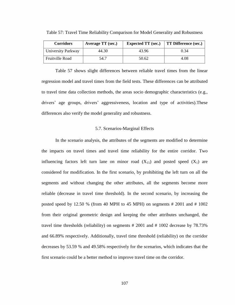
107
Table 57: Travel Time Reliability Comparison for Model Generality and Robustness
Table 57 shows slight differences between reliable travel times from the linear
regression model and travel times from the field tests. These differences can be attributed
to travel time data collection methods, the areas socio demographic characteristics (e.g.,
drivers’ age groups, drivers’ aggressiveness, location and type of activities).These
differences also verify the model generality and robustness.
5.7. Scenarios-Marginal Effects
In the scenario analysis, the attributes of the segments are modified to determine
the impacts on travel times and travel time reliability for the entire corridor. Two
influencing factors left turn lane on minor road (X15) and posted speed (X1) are
considered for modification. In the first scenario, by prohibiting the left turn on all the
segments and without changing the other attributes, all the segments become more
reliable (decrease in travel time threshold). In the second scenario, by increasing the
posted speed by 12.50 % (from 40 MPH to 45 MPH) on segments # 2001 and # 1002
from their original geometric design and keeping the other attributes unchanged, the
travel time thresholds (reliability) on segments # 2001 and # 1002 decrease by 78.73%
and 66.89% respectively. Additionally, travel time threshold (reliability) on the corridor
decreases by 53.59 % and 49.58% respectively for the scenarios, which indicates that the
first scenario could be a better method to improve travel time on the corridor.
Corridors Average TT (sec.) Expected TT (sec.) TT Difference (sec.)
University Parkway 44.30 43.96 0.34
Fruitville Road 54.7 50.62 4.08
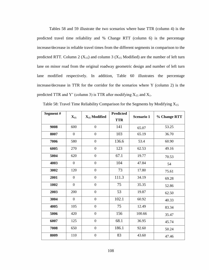
108
Tables 58 and 59 illustrate the two scenarios where base TTR (column 4) is the
predicted travel time reliability and % Change RTT (column 6) is the percentage
increase/decrease in reliable travel times from the different segments in comparison to the
predicted RTT. Column 2 (X15) and column 3 (X15 Modified) are the number of left turn
lane on minor road from the original roadway geometric design and number of left turn
lane modified respectively. In addition, Table 60 illustrates the percentage
increase/decrease in TTR for the corridor for the scenarios where Y (column 2) is the
predicted TTR and Y’ (column 3) is TTR after modifying X15 and X1.
Table 58: Travel Time Reliability Comparison for the Segments by Modifying X15
Segment # X15 X15 Modified
Predicted
TTR Scenario 1 % Change RTT
9008 600 0 141 65.07 53.25
8007 0 0 103 65.19 36.70
7006 580 0 136.6 53.4 60.90
6005 270 0 123 62.53 49.16
5004 620 0 67.1 19.77 70.53
4003 0 0 104 47.84 54
3002 120 0 73 17.80 75.61
2001 0 0 111.3 34.19 69.28
1002 0 0 75 35.35 52.86
2003 200 0 53 19.87 62.50
3004 0 0 102.1 60.92 40.33
4005 105 0 75 12.49 83.34
5006 420 0 156 100.66 35.47
6007 125 0 68.1 36.95 45.74
7008 650 0 186.1 92.60 50.24
8009 110 0 83 43.60 47.46
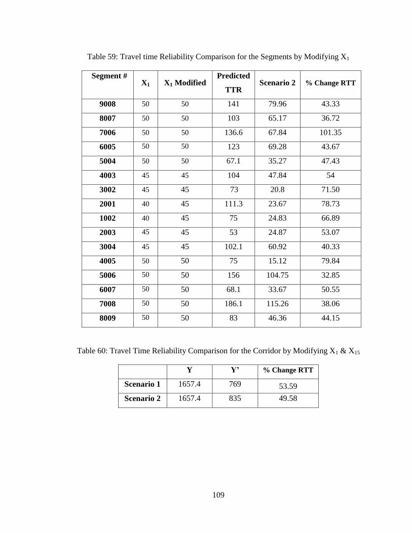
109
Table 59: Travel time Reliability Comparison for the Segments by Modifying X1
Segment # X1 X1 Modified
Predicted
TTR Scenario 2 % Change RTT
9008 50 50 141 79.96 43.33
8007 50 50 103 65.17 36.72
7006 50 50 136.6 67.84 101.35
6005 50 50 123 69.28 43.67
5004 50 50 67.1 35.27 47.43
4003 45 45 104 47.84 54
3002 45 45 73 20.8 71.50
2001 40 45 111.3 23.67 78.73
1002 40 45 75 24.83 66.89
2003 45 45 53 24.87 53.07
3004 45 45 102.1 60.92 40.33
4005 50 50 75 15.12 79.84
5006 50 50 156 104.75 32.85
6007 50 50 68.1 33.67 50.55
7008 50 50 186.1 115.26 38.06
8009 50 50 83 46.36 44.15
Table 60: Travel Time Reliability Comparison for the Corridor by Modifying X1 & X15
Y Y’ % Change RTT
Scenario 1 1657.4 769 53.59
Scenario 2 1657.4 835 49.58

110
5.8 Guidance on Roadway Design, Traffic Design, Traffic
Operations, and Access Management
Two distinct approaches characterize and define improving travel time reliability
on urban arterials. First, newly constructed facilities in newly acquired rights of way
allow for additional capacity and network connections. Second, existing facilities in the
urban area can be upgraded both in design and operational aspects to provide increased
capacity, safety, congestion reduction walkability, or other goals. These two design
approaches are necessary to meet different users of the urban highway network who have
different requirements for travel time reliability. Conversely, in practice, many
professionals working in the design field have been oriented toward only one of the
approaches with little contact or interest of the other type of design.
In summary, to improve travel time on urban corridors:
All the segments on existing facilities and their attributes should be considered
separately and traffic operations on the entire corridor should be coordinated. In
the case of an already coordinated corridor, increasing the green split and retiming
the signals can decrease travel time. However, increasing the green split could
have an important effect on average delay.
For new facilities to be built in newly acquired rights of way, the segment length
should be longer than 0.50 miles and the posted speed in the range of 45 MPH to
55 MPH. Building frontage roads that run parallel to the urban arterials can
decrease the access density at the focal points between interchanges and these
arterials where new shopping centers, industrial parks, and office complexes are
increasingly located.
111
Chapter 6- Limitations and Contributions
6.1 Summary of Limitations
This dissertation has some limitations:
First, some variables have signs that are contrary to expectations and the
dissertation did not provide a full explanation of these “wrong signs”, which
could be attributed to the following:
1) Lurking variables: the variable in question is a proxy for other
variables that are excluded from the analysis.
2) Multicollinarity: When two or more explanatory variables are not
independent, the sign of the coefficients of one of the variables
may differ from the sign of that coefficient if the variable were the
only explanatory variable. That is confounded variable.
Second, travel time data was collected on one corridor. Even though over 3,500
data sets were collected and analyzed, travel time data on several corridors with
divers attributes could help compare these factors variation on different corridors.
Third, other potential significant factors were not considered such as lane width
and median type. The former varies from 10 feet to 12 feet on most urban
arterials. This minor difference in width can be significant on travel time
reliability in industrial areas with high truck volumes. The later consisting of
OWLTL or TWLTL (one- or two-way left- turn lanes), flush median, raised
112
median among others is correlated to access density, which in return is a
significant factor to travel time reliability.
Fourth, the model is a better tool for LRPT (Long Range Transportation Planning)
purposes than daily traffic/ roadway design applications.
6.2 Summary of Contributions
Despite these limitations, the dissertation offered several contributions to the
State-of-the-Art, which are listed below:
A Linear Regression Model that identifies 10 factors that significantly influence
travel time reliability on urban arterials for recurrent conditions. Arterial Segment
Length is the most contributing factor whereas signal timing cycle length is the
least contributing factor. Identifying these factors is a key contribution to HCM
and AASHTO where studies are being conducted to include reliability factors into
roadway design features. By explaining 67.4% of the observed data, this model
outperforms current models and performs well or better than a range of state-of-
the-art travel time reliability models described in the literature review.
The correlation among the influencing factors, which is necessary for traffic
operations, traffic design, and long range transportation planning. The correlation
explains the contributing impacts of other factors on travel time reliability
improvement on a corridor by modifying one factor. In other words, the resulting
travel time reliability improvement is due not only to the modified factor but also
to other factors that are correlated to it.
113
The travel time reliability threshold based on buffer time (travel time reliability
calculation method) was experimented on urban arterials. Unlike many other
travel time reliability measures, the buffer time can be easily communicated to
technical audiences (e.g., traffic engineers, transportation planners, MPO
members) and non-technical audiences (e.g., daily travelers, business owners,
truck drivers), in particular, policy makers should funding be needed to improve
travel time reliability on a corridor.
The linear regression model has demonstrated the importance of a new data
collection method, the VD240 wireless vehicle detention system from Sensys
Networks ATTS. Compared to other travel time data collection methods, the
ATTS appears to be the one deployed that provides an accurate real-time estimate
of the travel time distribution and traffic counts. Additionally, the mean travel
time as well as its standard deviation or 80th
percentile is estimated. The model
was proved to be neither “black-box” or location-specific by demonstrating its
robustness and generality in comparison to other travel time data collected in
different urban arterials.
6.3 Implications and Recommendations for Future Research
This dissertation has established baselines for researches to identify the other
influencing factors which represent 32.6% of the observed data. These factors
could be attributed to driving behavior, driver group age, traffic congestion,
inadequate lane capacity, month of the year, location of activities, special events
or non-recurrent events (e.g., crashes, rain, and construction/maintenance
activity).
114
Further research need to be conducted on the correlation between the number of
exclusive left turn lane from cross streets and travel time reliability on the major
arterials. This dissertation has demonstrated that adding an exclusive left turn lane
on a cross street to improve traffic operations features can hamper travel time
reliability on the main street. This research should include left turn lane volume
on cross street, AADT on cross street, and exclusive left turn signal timing cycle
length.
The equation from the model can be considered as theoretical and for practical
applications, the influencing factors with low coefficients can be removed.
Urban travel time databases from Sensys Networks ATTS need to include non-
recurrent events (e.g., crashes, rain, roadway construction/maintenance activity),
and special events information. This information could help identify other
contributing factors to travel time reliability on urban arterials.
Peak hour traffic volumes and vehicle traffic composition (% of heavy trucks)
should be considered as potential influencing factors instead of AADs and
VPHPL if these data are available.
Quality of signal timing (good coordination versus bad coordination) and
functionality of the detectors should be considered as potential influencing factors
instead of signal timing cycle length if these data are available.
Left/Right turn lane major (minor) road can be considered as dummy variable
instead of continuous variable and land use to be considered as a potential
influencing factor.
115
References
1. Aiken, L. S., and West, S. G. (1991). Multiple regression: Testing and
interpreting interactions. Sage Publications, Newbury Park, London.
2. Al-Deek, H. and Emam, E. (2006). New methodology for estimating reliability
in transportation networks with degraded link capacities. Journal of Intelligent
Transportation Systems, 10 (3), 117-129.
3. Boyles, S., Voruganti, A., and Waller, S. (2010). Quantifying Travel time
Variability in Transportation networks. Center for Transportation Research,
University of Texas, Austin, Texas.
4. Chen, C., Skabardonis, A., and Varaiya, P., (2003). Travel Time Reliability as a
Measure of Service. Transportation Research Record 1855, Transportation
Research Board, Washington, DC, pp. 74-79.
5. Clark, S. D., and .Watling, D.P. (2005). Modeling Travel Time Reliability under
Stochastic Demand. Transportation Research. Pat B: Methodological 39(2), pp.
119-140.
6. Cambridge Systematics, Inc., High Street Consulting Group, TransTech
Management, Inc., Spy Pond Partners, Ross & Associates (2009). Performance
Measure Framework for Highway Capacity Decision Making, NCHRP Report
618, Transportation Research Board of National Academies, Washington, DC.
7. Cambridge Systematics, Inc.; Dowling Associates, Inc.; System Metrics Group,
Inc.; Texas Transportation Institute (2008). Cost-Effective Performance
Measures for Travel Time Delay, Variation, and Reliability, NCHRP Report
618, Transportation Research Board, Washington, DC.
8. Dawson, J. F., & Richter, A. W. (2006). Probing three-way interactions in
moderated multiple regression: Development and application of a slope
difference test. Journal of Applied Psychology, 91, pp. 917-926.
9. Dowling, R. et al., (2009). Reliability Breakpoints on Freeways. Paper # 09-
0813, Transportation Research Board, Washington, DC.
116
10. Elefteriandou, L., and Xu, H. (2007). Travel Time Reliability Models for
Freeways and Arterials. Transportation Research Center, University of Florida,
Gainesville, FL. http://www.dot.state.fl.u PL/FDOT_BD545_70_rptb.pdf.
11. Florida Department of Transportation (DFOT) (2000). The Florida reliability
method: In Florida’s mobility performance measures program. Available at:
http://www.dot.state.fl.us/planning/statistics/mobilitymeasures/reliability.pdf,
accessed on June 2008.
12. Frey, W. H., (2003). Boomers and Seniors in the Suburbs: aging Patterns in
census 2000. Brookings Census 2000 Series, Washington D.C.: Brookings
Institute-Center on Urban and Metropolitan Policy.
13. Garber, J. G., and Hoel, L. (2009). Traffic and Highway Engineering, 4th
edition
2nd
Edition, Cengage Learning Press, Toronto, Canada.
14. Hollander, Y. (2006). Direct Versus Indirect Models for the Effects of
Unreliability. Transportation Research A, Vol. 40, Issue 9, pp. 699-711.
15. Highway Capacity Manual, 4th
Edition (2000). Transportation Research Board,
National Research Council, Washington DC.
16. Insurance Institute for Highway Safety (2000). Traffic Engineering Approaches
to Reduce Crashes on Urban Arterial Roads. Available at:
http://www.highwaysafetyihs_traffic_approaches.pdf, accessed on October
2008.
17. Kavaler, R., Kwong, K., and Raman, A. (2009). Arterials Performance
Measurement with Wireless Magnetic Sensors. Journal of the American Society
of Civil Engineers, Volume 1: Highway Transportation, pp. 377-385.
18. Liping, F., Hellinga, B., and Yongliang, Z. (2001). An Adaptive Model for Real-
Time Estimation of Overflow Queues on Congested Arterials. Intelligent
Transportation Systems, pp. 219-226.
19. Liu, H., Vant Lint, H. and Zuylen, H. (2006). Neutral Network Based Traffic
Flow for Urban Arterial Travel Time Prediction. Faculty of Civil Engineering
and Geosciences, Delft University of Technology.
20. Lomax, T., Schrank, D., and Turner, S. (2003). Selecting Travel Time
Reliability Measures. Available at: http://tti.tamu.edu/documents/TTI-2003-
3.pdf, accessed on February 2010.
117
21. Lomax, J., Schrank, D., and Eisele, W. (2005). The Keys to Estimating Mobility
in Urban Areas: Applying Definitions and Measures That Everyone
Understands. Texas Transportation Institute, The Texas A&M University
System. Available at: (http://mobility.tamu.edu).
22. Lowrey, A. (2011). Your Commute is Killing You: Long Commutes Cause
Obesity, Neck Pain, Loneliness, Divorce, Stress and Insomnia. Slate. Available
at: http://www.slate.com/id/2295603.
23. McShane, W., and Crowley, K. (1976). Regularity of Some Detector-Observed
Arterial Traffic Volume Characteristics. Transportation Research Record 596,
Transportation Research Board, Washington DC, pp. 33-37.
24. Miou, S. P. (1994). The Relationship between Truck Accidents and Geometric
Design on Road Sections: Poisson versus Negative Binomial Regressions.
Accident Analysis and Prevention 26, 471-482.
25. Myers, R. H. (1990). Classical and Modern Regression with Applications, 2nd
Edition, Duxbury Press, Belmont, CA.
26. Nam, D., Park, D., and Khamkongkhun, A. (2005). Estimation of Value of
Travel Time Reliability. Journal of Advanced Transportation, Vol. 39, Issue 1,
pp. 39-61.
27. Pedersen, N. and Sandahl, D. (1982). Highway Traffic Data for Urbanized Area
Project Planning and Design. NCHRP Report 255. Transportation Research
Board. Washington, DC.
28. O’Shea, J., Rioux, T., and Machemehl, R. (2001). Project 0-1846: Development
of Design Guidelines for the Provision of Median Access on Principal Arterials.
Center for Transportation Research, University of Texas, Austin.
29. Pisarski, A. (2006). Commuting in America III. Available at:
http://www.trb.org/Main/Public/Blurbs/156993.aspx, accessed on April 2007.
30. Pu, W. (2010). Analytic Relationships between Travel Time Reliability
Measures. Transportation Research Record 2254, Transportation Research
Board, Washington, DC, pp 122-130.
31. Texas Transportation Institute. 2007 Annual Urban Mobility Report. Available
at: http://mobility.tamu.edu/ums/report, accessed on October 2009.
32. Texas Transportation Institute. 2011 Annual Urban Mobility Report. Available
at: http://mobility.tamu.edu/ums/report, accessed on February 2012.
118
33. Tobin, J. (1958). Estimation of Relationships for Limited Dependent Variables.
Econometrica 26, pp. 24-36.
34. Train, K. (1978). A Validation Test of a Disaggregate Mode Choice Model
Transportation Research, Vol. 12, pp. 167-174).
35. Train, K. and Winston, C. (2007). Vehicle Choice Behavior and the Declining
Market Share of US Automakers. International Economic Review, Vol. 48, No.
4, pp. 1469-1496.
36. U.S. Census Bureau, U.S. Population Projection by Age, Sex. Available at:
http://www.census.gov/, accessed on February 2010.
37. U.S. Department of Transportation, Federal Highway Administration (FHWA)
(2006). Travel Time Reliability: Making it There on Time, All the Time.
Available at http://ops.fhwa.dot.gov/publications/tt_reliability/TTR_Report.htm
Accessed on January 2007.
38. Van Lint, J.W.C., (2004). Reliable Travel Time Prediction for Freeways.
Dissertation submitted in fulfillment of the Ph.D. in Civil Engineering, Delft
University of Technology, Netherlands.
39. Washburn, S.S., McLeod, D.S., and Courage, K. G. (2002). Adaptation of the
HCM2000 Planning Level Analysis of Two-Lane and Multilane Highways in
Florida. Transportation Research Record 1902, Transportation Research Board,
Washington, DC, pp. 62-68.
40. Washington, S. P., M., Karlaftis, G. M., and Mannering F. L. (2003). Statistical
and Econometric Methods for Transportation Data Analysis. Chapman and Hall
Press, Boca Raton, FL.
41. Yang, J.-S., (2006). A Nonlinear State Space Approach to Arterial Travel Time
Prediction. Department of Electrical & Computer Engineering, University of
Minnesota, Duluth. http://conservancy.umn.edu/bitstream/1020/1/200605.pdf.
42. Wasson, J.S, Sturdevant, J. and Bullock, D. (2008). Real-Time Travel Times
Estimates Using Media Access Control Address Matching. ITE Journal,
Volume: 78, Issue: 6, pp.20-23.
43. Williams, W. and Welch, H. (1997). Sensitivity of Transport Investment Benefits
to the Evaluation of Small Travel-Time Savings. Journal of Transport
Economics and Policy, Vol. 31, No. 3, Sept., pp. 231-254.

119
Appendices
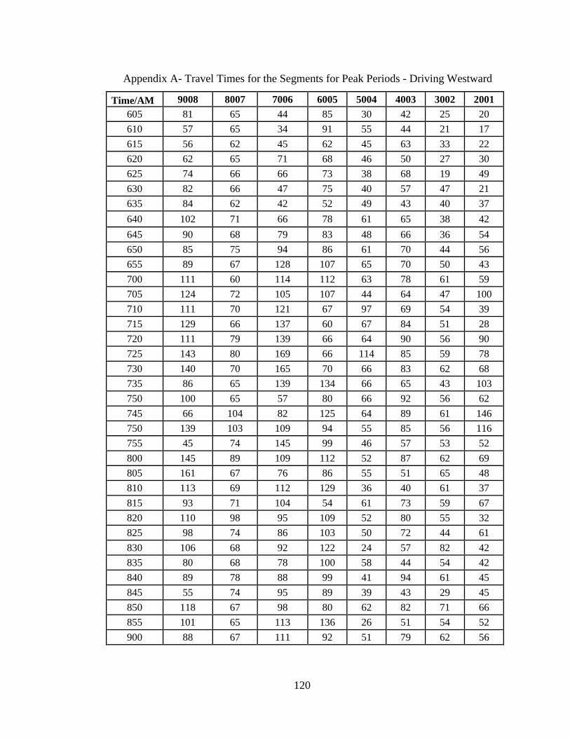
120
Appendix A- Travel Times for the Segments for Peak Periods - Driving Westward
Time/AM 9008 8007 7006 6005 5004 4003 3002 2001
605 81 65 44 85 30 42 25 20
610 57 65 34 91 55 44 21 17
615 56 62 45 62 45 63 33 22
620 62 65 71 68 46 50 27 30
625 74 66 66 73 38 68 19 49
630 82 66 47 75 40 57 47 21
635 84 62 42 52 49 43 40 37
640 102 71 66 78 61 65 38 42
645 90 68 79 83 48 66 36 54
650 85 75 94 86 61 70 44 56
655 89 67 128 107 65 70 50 43
700 111 60 114 112 63 78 61 59
705 124 72 105 107 44 64 47 100
710 111 70 121 67 97 69 54 39
715 129 66 137 60 67 84 51 28
720 111 79 139 66 64 90 56 90
725 143 80 169 66 114 85 59 78
730 140 70 165 70 66 83 62 68
735 86 65 139 134 66 65 43 103
750 100 65 57 80 66 92 56 62
745 66 104 82 125 64 89 61 146
750 139 103 109 94 55 85 56 116
755 45 74 145 99 46 57 53 52
800 145 89 109 112 52 87 62 69
805 161 67 76 86 55 51 65 48
810 113 69 112 129 36 40 61 37
815 93 71 104 54 61 73 59 67
820 110 98 95 109 52 80 55 32
825 98 74 86 103 50 72 44 61
830 106 68 92 122 24 57 82 42
835 80 68 78 100 58 44 54 42
840 89 78 88 99 41 94 61 45
845 55 74 95 89 39 43 29 45
850 118 67 98 80 62 82 71 66
855 101 65 113 136 26 51 54 52
900 88 67 111 92 51 79 62 56
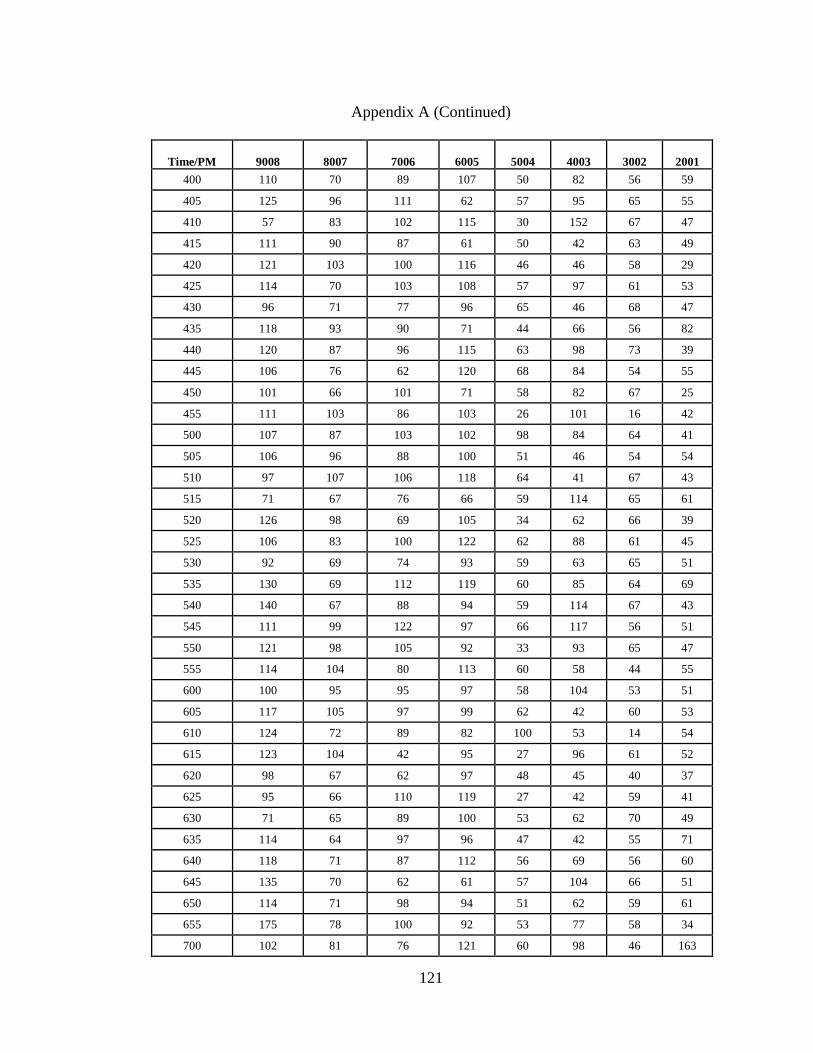
121
Appendix A (Continued)
Time/PM
9008
8007
7006
6005
5004
4003
3002
2001
400 110 70 89 107 50 82 56 59
405 125 96 111 62 57 95 65 55
410 57 83 102 115 30 152 67 47
415 111 90 87 61 50 42 63 49
420 121 103 100 116 46 46 58 29
425 114 70 103 108 57 97 61 53
430 96 71 77 96 65 46 68 47
435 118 93 90 71 44 66 56 82
440 120 87 96 115 63 98 73 39
445 106 76 62 120 68 84 54 55
450 101 66 101 71 58 82 67 25
455 111 103 86 103 26 101 16 42
500 107 87 103 102 98 84 64 41
505 106 96 88 100 51 46 54 54
510 97 107 106 118 64 41 67 43
515 71 67 76 66 59 114 65 61
520 126 98 69 105 34 62 66 39
525 106 83 100 122 62 88 61 45
530 92 69 74 93 59 63 65 51
535 130 69 112 119 60 85 64 69
540 140 67 88 94 59 114 67 43
545 111 99 122 97 66 117 56 51
550 121 98 105 92 33 93 65 47
555 114 104 80 113 60 58 44 55
600 100 95 95 97 58 104 53 51
605 117 105 97 99 62 42 60 53
610 124 72 89 82 100 53 14 54
615 123 104 42 95 27 96 61 52
620 98 67 62 97 48 45 40 37
625 95 66 110 119 27 42 59 41
630 71 65 89 100 53 62 70 49
635 114 64 97 96 47 42 55 71
640 118 71 87 112 56 69 56 60
645 135 70 62 61 57 104 66 51
650 114 71 98 94 51 62 59 61
655 175 78 100 92 53 77 58 34
700 102 81 76 121 60 98 46 163
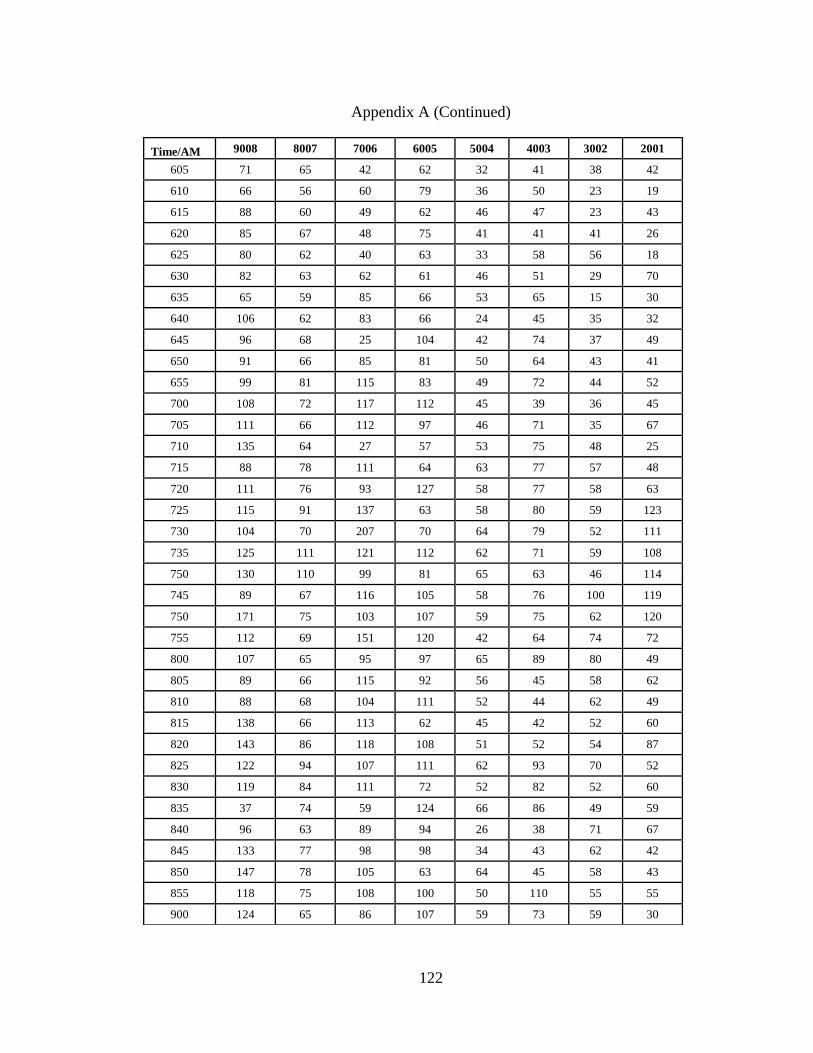
122
Appendix A (Continued)
Time/AM 9008 8007 7006 6005 5004 4003 3002 2001
605 71 65 42 62 32 41 38 42
610 66 56 60 79 36 50 23 19
615 88 60 49 62 46 47 23 43
620 85 67 48 75 41 41 41 26
625 80 62 40 63 33 58 56 18
630 82 63 62 61 46 51 29 70
635 65 59 85 66 53 65 15 30
640 106 62 83 66 24 45 35 32
645 96 68 25 104 42 74 37 49
650 91 66 85 81 50 64 43 41
655 99 81 115 83 49 72 44 52
700 108 72 117 112 45 39 36 45
705 111 66 112 97 46 71 35 67
710 135 64 27 57 53 75 48 25
715 88 78 111 64 63 77 57 48
720 111 76 93 127 58 77 58 63
725 115 91 137 63 58 80 59 123
730 104 70 207 70 64 79 52 111
735 125 111 121 112 62 71 59 108
750 130 110 99 81 65 63 46 114
745 89 67 116 105 58 76 100 119
750 171 75 103 107 59 75 62 120
755 112 69 151 120 42 64 74 72
800 107 65 95 97 65 89 80 49
805 89 66 115 92 56 45 58 62
810 88 68 104 111 52 44 62 49
815 138 66 113 62 45 42 52 60
820 143 86 118 108 51 52 54 87
825 122 94 107 111 62 93 70 52
830 119 84 111 72 52 82 52 60
835 37 74 59 124 66 86 49 59
840 96 63 89 94 26 38 71 67
845 133 77 98 98 34 43 62 42
850 147 78 105 63 64 45 58 43
855 118 75 108 100 50 110 55 55
900 124 65 86 107 59 73 59 30
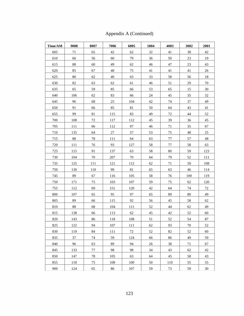
123
Appendix A (Continued)
Time/AM 9008 8007 7006 6005 5004 4003 3002 2001
605 71 65 42 62 32 41 38 42
610 66 56 60 79 36 50 23 19
615 88 60 49 62 46 47 23 43
620 85 67 48 75 41 41 41 26
625 80 62 40 63 33 58 56 18
630 82 63 62 61 46 51 29 70
635 65 59 85 66 53 65 15 30
640 106 62 83 66 24 45 35 32
645 96 68 25 104 42 74 37 49
650 91 66 85 81 50 64 43 41
655 99 81 115 83 49 72 44 52
700 108 72 117 112 45 39 36 45
705 111 66 112 97 46 71 35 67
710 135 64 27 57 53 75 48 25
715 88 78 111 64 63 77 57 48
720 111 76 93 127 58 77 58 63
725 115 91 137 63 58 80 59 123
730 104 70 207 70 64 79 52 111
735 125 111 121 112 62 71 59 108
750 130 110 99 81 65 63 46 114
745 89 67 116 105 58 76 100 119
750 171 75 103 107 59 75 62 120
755 112 69 151 120 42 64 74 72
800 107 65 95 97 65 89 80 49
805 89 66 115 92 56 45 58 62
810 88 68 104 111 52 44 62 49
815 138 66 113 62 45 42 52 60
820 143 86 118 108 51 52 54 87
825 122 94 107 111 62 93 70 52
830 119 84 111 72 52 82 52 60
835 37 74 59 124 66 86 49 59
840 96 63 89 94 26 38 71 67
845 133 77 98 98 34 43 62 42
850 147 78 105 63 64 45 58 43
855 118 75 108 100 50 110 55 55
900 124 65 86 107 59 73 59 30
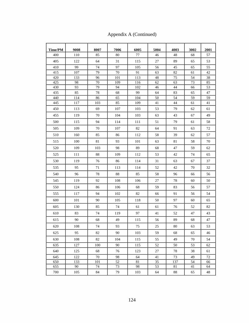
124
Appendix A (Continued)
Time/PM
9008
8007
7006
6005
5004
4003
3002
2001
400 110 85 80 77 46 48 68 57
405 122 64 31 115 27 89 65 53
410 99 74 97 105 56 45 65 55
415 107 79 70 91 63 82 61 42
420 133 96 101 113 48 75 54 38
425 98 70 109 116 62 63 73 85
430 93 79 94 102 46 44 66 53
435 85 78 68 99 64 83 65 47
440 114 86 65 104 50 54 59 59
445 117 103 85 109 41 44 61 41
450 113 69 107 103 53 79 62 61
455 119 70 104 103 63 43 67 49
500 115 94 114 111 51 79 61 58
505 109 70 107 82 64 91 63 72
510 160 85 86 112 58 39 62 57
515 100 81 93 101 63 81 58 70
520 109 103 98 89 68 47 59 62
525 111 88 109 112 53 42 74 65
530 119 76 86 114 31 63 67 37
535 95 71 113 114 52 42 70 32
540 96 78 88 85 58 96 66 56
545 119 92 108 106 27 78 60 50
550 124 86 106 68 59 83 56 57
555 117 94 102 82 66 91 56 54
600 101 90 105 118 50 97 60 65
605 130 85 74 61 61 76 52 82
610 83 74 119 97 41 52 47 43
615 90 68 49 115 56 89 68 47
620 108 74 93 75 25 80 63 53
625 95 82 90 103 59 68 65 46
630 108 82 104 115 55 49 70 54
635 127 100 90 115 52 50 53 62
640 125 68 76 123 27 78 38 61
645 122 70 98 64 41 73 49 72
650 133 101 52 81 35 137 54 66
655 90 74 73 98 53 81 41 64
700 105 84 79 103 64 88 65 48
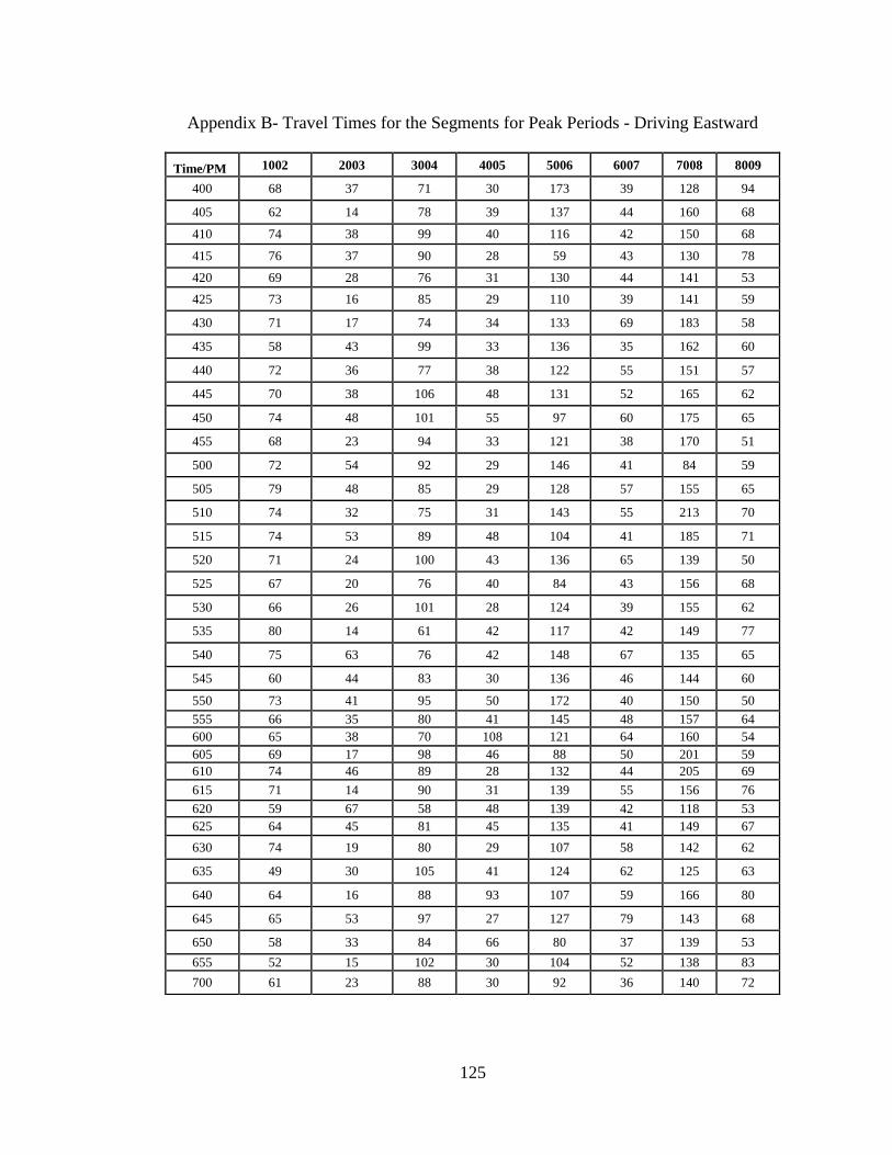
125
Appendix B- Travel Times for the Segments for Peak Periods - Driving Eastward
Time/PM 1002 2003 3004 4005 5006 6007 7008 8009
400 68 37 71 30 173 39 128 94
405 62 14 78 39 137 44 160 68
410 74 38 99 40 116 42 150 68
415 76 37 90 28 59 43 130 78
420 69 28 76 31 130 44 141 53
425 73 16 85 29 110 39 141 59
430 71 17 74 34 133 69 183 58
435 58 43 99 33 136 35 162 60
440 72 36 77 38 122 55 151 57
445 70 38 106 48 131 52 165 62
450 74 48 101 55 97 60 175 65
455 68 23 94 33 121 38 170 51
500 72 54 92 29 146 41 84 59
505 79 48 85 29 128 57 155 65
510 74 32 75 31 143 55 213 70
515 74 53 89 48 104 41 185 71
520 71 24 100 43 136 65 139 50
525 67 20 76 40 84 43 156 68
530 66 26 101 28 124 39 155 62
535 80 14 61 42 117 42 149 77
540 75 63 76 42 148 67 135 65
545 60 44 83 30 136 46 144 60
550 73 41 95 50 172 40 150 50
555 66 35 80 41 145 48 157 64
600 65 38 70 108 121 64 160 54
605 69 17 98 46 88 50 201 59
610 74 46 89 28 132 44 205 69
615 71 14 90 31 139 55 156 76
620 59 67 58 48 139 42 118 53
625 64 45 81 45 135 41 149 67
630 74 19 80 29 107 58 142 62
635 49 30 105 41 124 62 125 63
640 64 16 88 93 107 59 166 80
645 65 53 97 27 127 79 143 68
650 58 33 84 66 80 37 139 53
655 52 15 102 30 104 52 138 83
700 61 23 88 30 92 36 140 72
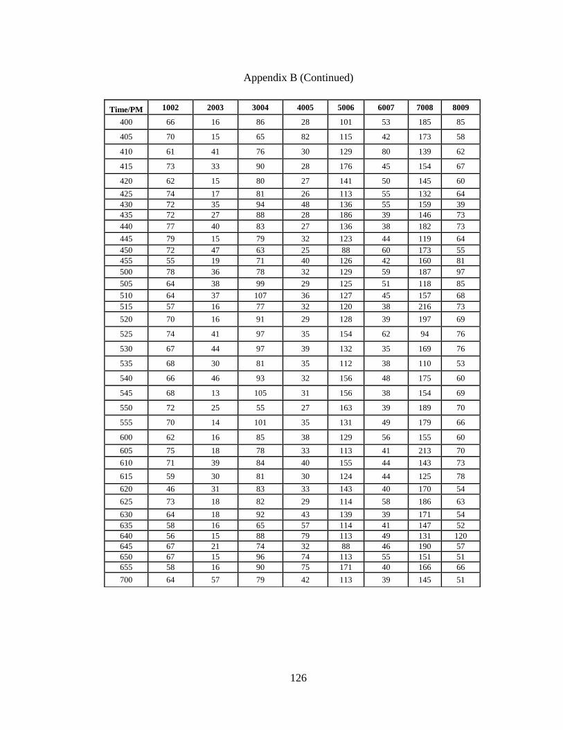
126
Appendix B (Continued)
Time/PM 1002 2003 3004 4005 5006 6007 7008 8009
400 66 16 86 28 101 53 185 85
405 70 15 65 82 115 42 173 58
410 61 41 76 30 129 80 139 62
415 73 33 90 28 176 45 154 67
420 62 15 80 27 141 50 145 60
425 74 17 81 26 113 55 132 64
430 72 35 94 48 136 55 159 39
435 72 27 88 28 186 39 146 73
440 77 40 83 27 136 38 182 73
445 79 15 79 32 123 44 119 64
450 72 47 63 25 88 60 173 55
455 55 19 71 40 126 42 160 81
500 78 36 78 32 129 59 187 97
505 64 38 99 29 125 51 118 85
510 64 37 107 36 127 45 157 68
515 57 16 77 32 120 38 216 73
520 70 16 91 29 128 39 197 69
525 74 41 97 35 154 62 94 76
530 67 44 97 39 132 35 169 76
535 68 30 81 35 112 38 110 53
540 66 46 93 32 156 48 175 60
545 68 13 105 31 156 38 154 69
550 72 25 55 27 163 39 189 70
555 70 14 101 35 131 49 179 66
600 62 16 85 38 129 56 155 60
605 75 18 78 33 113 41 213 70
610 71 39 84 40 155 44 143 73
615 59 30 81 30 124 44 125 78
620 46 31 83 33 143 40 170 54
625 73 18 82 29 114 58 186 63
630 64 18 92 43 139 39 171 54
635 58 16 65 57 114 41 147 52
640 56 15 88 79 113 49 131 120
645 67 21 74 32 88 46 190 57
650 67 15 96 74 113 55 151 51
655 58 16 90 75 171 40 166 66
700 64 57 79 42 113 39 145 51
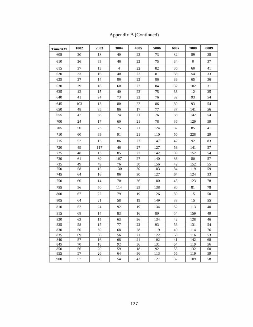
127
Appendix B (Continued)
Time/AM 1002 2003 3004 4005 5006 6007 7008 8009
605 20 18 40 22 73 32 89 38
610 26 33 46 22 75 34 0 37
615 37 13 4 22 82 36 60 41
620 33 16 40 22 81 38 54 33
625 27 14 86 22 86 39 65 36
630 29 18 60 22 84 37 102 31
635 42 15 40 22 75 38 12 35
640 41 24 73 22 76 32 93 54
645 103 13 80 22 86 39 93 54
650 48 35 86 17 77 37 141 56
655 47 38 74 21 76 38 142 54
700 24 17 60 21 78 36 129 59
705 50 23 75 21 124 37 85 41
710 60 39 91 21 110 50 228 29
715 52 13 86 27 147 42 92 83
720 49 117 46 27 127 58 141 57
725 48 13 85 27 142 39 152 54
730 61 39 107 27 140 36 80 57
735 49 49 76 30 156 42 152 55
750 58 15 130 30 183 84 119 59
745 64 16 86 30 127 64 124 33
750 60 14 70 36 180 45 123 78
755 56 50 114 25 138 80 81 78
800 67 22 79 19 126 59 15 50
805 64 21 58 19 149 38 15 55
810 52 24 92 19 134 52 113 40
815 68 14 83 16 80 54 159 49
820 63 15 63 26 134 42 128 46
825 58 15 77 22 93 53 131 54
830 50 69 68 28 119 49 114 76
835 69 56 56 21 122 58 116 53
840 57 16 68 21 102 41 142 68
845 70 18 92 36 131 54 119 56
850 56 20 59 18 92 55 132 60
855 57 26 64 36 113 55 119 59
900 57 60 54 42 127 37 109 58
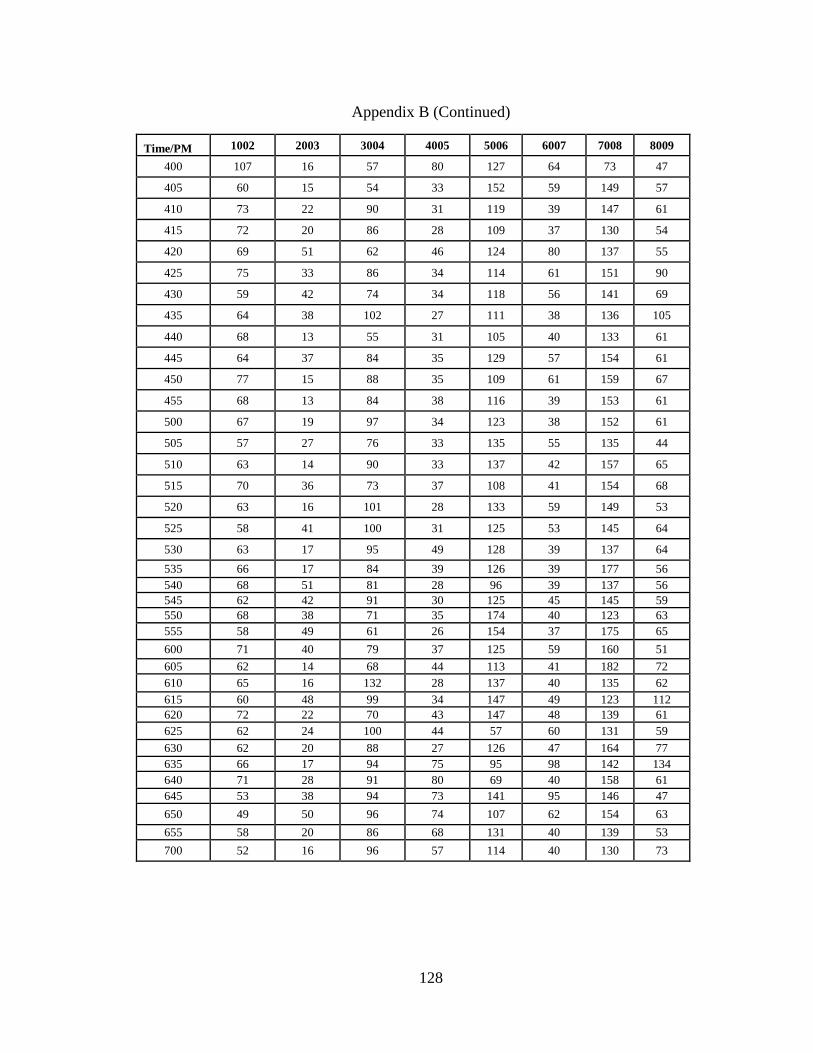
128
Appendix B (Continued)
Time/PM 1002 2003 3004 4005 5006 6007 7008 8009
400 107 16 57 80 127 64 73 47
405 60 15 54 33 152 59 149 57
410 73 22 90 31 119 39 147 61
415 72 20 86 28 109 37 130 54
420 69 51 62 46 124 80 137 55
425 75 33 86 34 114 61 151 90
430 59 42 74 34 118 56 141 69
435 64 38 102 27 111 38 136 105
440 68 13 55 31 105 40 133 61
445 64 37 84 35 129 57 154 61
450 77 15 88 35 109 61 159 67
455 68 13 84 38 116 39 153 61
500 67 19 97 34 123 38 152 61
505 57 27 76 33 135 55 135 44
510 63 14 90 33 137 42 157 65
515 70 36 73 37 108 41 154 68
520 63 16 101 28 133 59 149 53
525 58 41 100 31 125 53 145 64
530 63 17 95 49 128 39 137 64
535 66 17 84 39 126 39 177 56
540 68 51 81 28 96 39 137 56
545 62 42 91 30 125 45 145 59
550 68 38 71 35 174 40 123 63
555 58 49 61 26 154 37 175 65
600 71 40 79 37 125 59 160 51
605 62 14 68 44 113 41 182 72
610 65 16 132 28 137 40 135 62
615 60 48 99 34 147 49 123 112
620 72 22 70 43 147 48 139 61
625 62 24 100 44 57 60 131 59
630 62 20 88 27 126 47 164 77
635 66 17 94 75 95 98 142 134
640 71 28 91 80 69 40 158 61
645 53 38 94 73 141 95 146 47
650 49 50 96 74 107 62 154 63
655 58 20 86 68 131 40 139 53
700 52 16 96 57 114 40 130 73
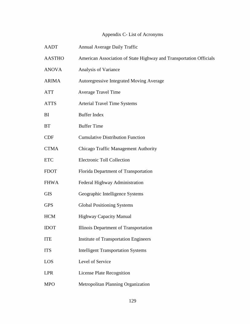
129
Appendix C- List of Acronyms
AADT Annual Average Daily Traffic
AASTHO American Association of State Highway and Transportation Officials
ANOVA Analysis of Variance
ARIMA Autoregressive Integrated Moving Average
ATT Average Travel Time
ATTS Arterial Travel Time Systems
BI Buffer Index
BT Buffer Time
CDF Cumulative Distribution Function
CTMA Chicago Traffic Management Authority
ETC Electronic Toll Collection
FDOT Florida Department of Transportation
FHWA Federal Highway Administration
GIS Geographic Intelligence Systems
GPS Global Positioning Systems
HCM Highway Capacity Manual
IDOT Illinois Department of Transportation
ITE Institute of Transportation Engineers
ITS Intelligent Transportation Systems
LOS Level of Service
LPR License Plate Recognition
MPO Metropolitan Planning Organization
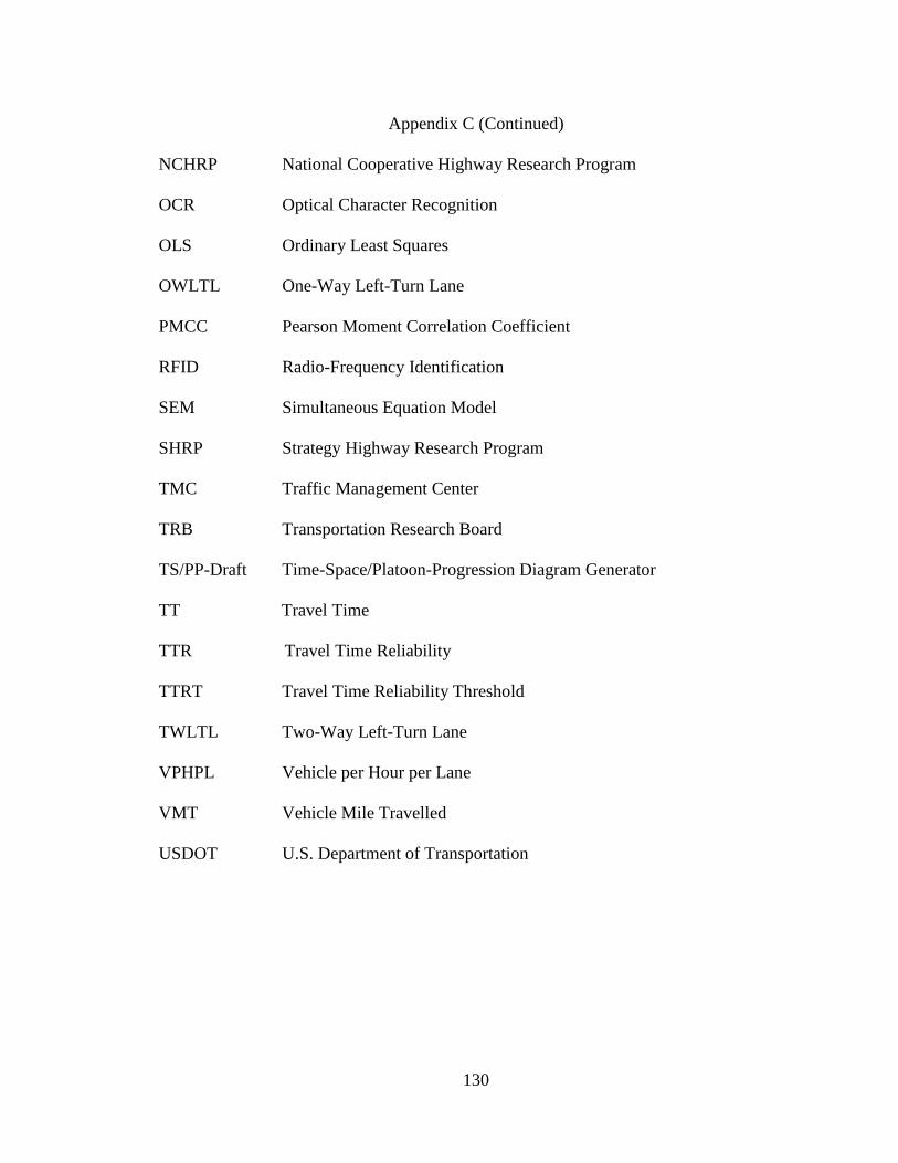
130
Appendix C (Continued)
NCHRP National Cooperative Highway Research Program
OCR Optical Character Recognition
OLS Ordinary Least Squares
OWLTL One-Way Left-Turn Lane
PMCC Pearson Moment Correlation Coefficient
RFID Radio-Frequency Identification
SEM Simultaneous Equation Model
SHRP Strategy Highway Research Program
TMC Traffic Management Center
TRB Transportation Research Board
TS/PP-Draft Time-Space/Platoon-Progression Diagram Generator
TT Travel Time
TTR Travel Time Reliability
TTRT Travel Time Reliability Threshold
TWLTL Two-Way Left-Turn Lane
VPHPL Vehicle per Hour per Lane
VMT Vehicle Mile Travelled
USDOT U.S. Department of Transportation
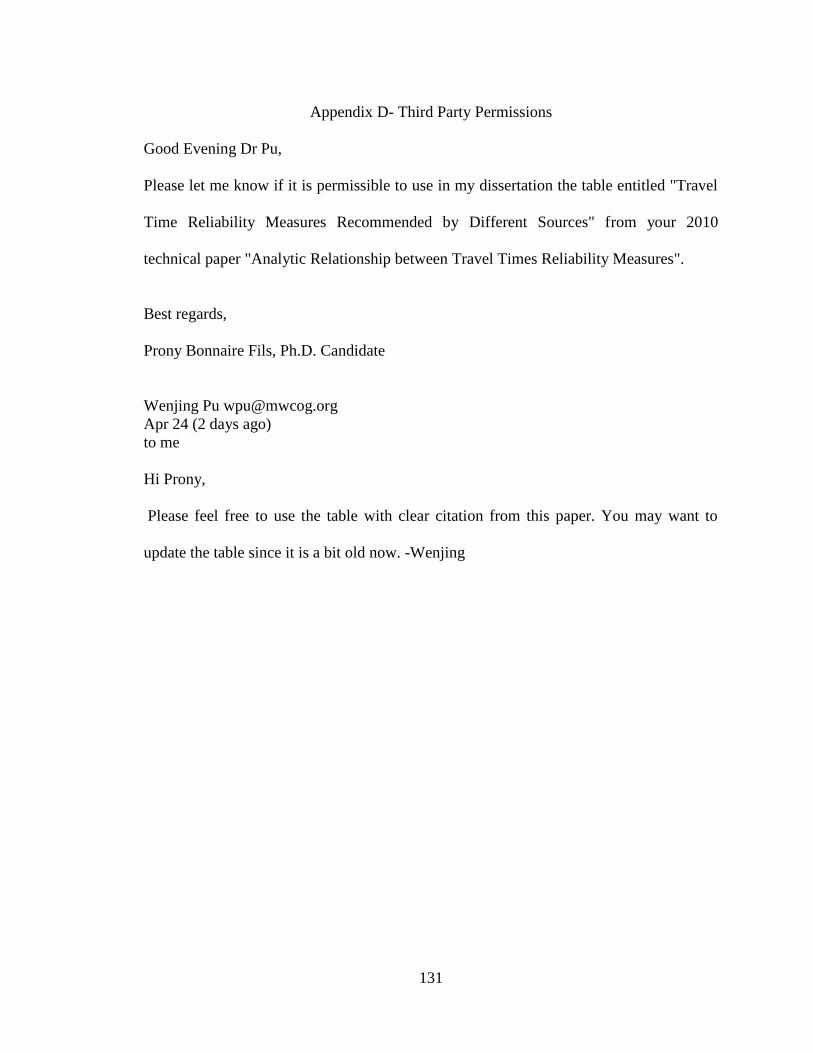
131
Appendix D- Third Party Permissions
Good Evening Dr Pu,
Please let me know if it is permissible to use in my dissertation the table entitled "Travel
Time Reliability Measures Recommended by Different Sources" from your 2010
technical paper "Analytic Relationship between Travel Times Reliability Measures".
Best regards,
Prony Bonnaire Fils, Ph.D. Candidate
Wenjing Pu [email protected]
Apr 24 (2 days ago)
to me
Hi Prony,
Please feel free to use the table with clear citation from this paper. You may want to
update the table since it is a bit old now. -Wenjing

About the Author
Prony received his Bachelor of Science in Civil Engineering from G.O.C
University (Haiti) in 1994 and his Master of Science in Transportation Management from
Universite Libre de Bruxelles (Free University of Brussels, Belgium) in 2000. He has
over 15 years of professional experience in transportation planning and engineering,
working for private, local/state agencies in Haiti and United States. Mr. Prony is very
passionate about doing research and working as an international consultant in the third
world where the transportation expertise available is defective. He is convinced that will
be the most effective way, as a transportation professional, to save lives, preserve the
environment, improve quality of life and contribute to social equality.