Modeling Visual Patterns by Integrating Descriptive and

International Journal of Computer Vision 53(1), 5–29, 2003c© 2003 Kluwer Academic Publishers. Manufactured in The Netherlands.

Modeling Visual Patterns by Integrating Descriptiveand Generative Methods

CHENG-EN GUODepartment of Computer Science, University of California, Los Angeles, CA, USA

[email protected]

SONG-CHUN ZHUDepartment of Computer Science and Department of Statistics, University of California,

Los Angeles, CA, [email protected]

YING NIAN WUDepartment of Statistics, University of California, Los Angeles, CA, USA

[email protected]

Received July 9, 2001; Revised October 7, 2002; Accepted October 24, 2002

Abstract. This paper presents a class of statistical models that integrate two statistical modeling paradigms in theliterature: (I) Descriptive methods, such as Markov random fields and minimax entropy learning (Zhu, S.C., Wu,Y.N., and Mumford, D. 1997. Neural Computation, 9(8)), and (II) Generative methods, such as principal componentanalysis, independent component analysis (Bell, A.J. and Sejnowski, T.J. 1997. Vision Research, 37:3327–3338),transformed component analysis (Frey, B. and Jojic, N. 1999. ICCV), wavelet coding (Mallat, S. and Zhang, Z. 1993.IEEE Trans. on Signal Processing, 41:3397–3415; Chen, S., Donoho, D., and Saunders, M.A. 1999. Journal onScientific Computing, 20(1):33–61), and sparse coding (Olshausen, B.A. and Field, D.J. 1996. Nature, 381:607–609;Lewicki, M.S. and Olshausen, B.A. 1999. JOSA, A. 16(7):1587–1601). In this paper, we demonstrate the integratedframework by constructing a class of hierarchical models for texton patterns (the term “texton” was coined bypsychologist Julesz in the early 80s). At the bottom level of the model, we assume that an observed texture image isgenerated by multiple hidden “texton maps”, and textons on each map are translated, scaled, stretched, and orientedversions of a window function, like mini-templates or wavelet bases. The texton maps generate the observed imageby occlusion or linear superposition. This bottom level of the model is generative in nature. At the top level of themodel, the spatial arrangements of the textons in the texton maps are characterized by minimax entropy principle,which leads to embellished versions of Gibbs point process models (Stoyan, D., Kendall, W.S., and Mecke, J. 1985.Stochastic Geometry and its Applications). The top level of the model is descriptive in nature. We demonstrate theintegrated model by a set of experiments.

Keywords: descriptive models, generative models, Gibbs point processes, Markov chain Monte Carlo, Markovrandom fields, minimax entropy learning, perceptual organization, texton models, visual learning

6 Guo, Zhu and Wu

1. Introduction

What a vision algorithm can accomplish depends cru-cially upon how much it knows about the contents ofthe visual scenes, and the knowledge can be mathemat-ically represented by general and parsimonious modelsthat can realistically characterize visual patterns in theensemble of images. Due to the variations of the pat-terns across scenes and the richness of details withineach scene, the models are often statistical in nature.Existing methods for statistical modeling can be gen-erally divided into two categories. In this paper, wecall one category the descriptive methods and the othercategory the generative methods.1

Descriptive methods construct the model for a visualpattern by imposing statistical constraints on featuresextracted from signals. Descriptive methods includeMarkov random fields, minimax entropy learning (Zhuet al., 1997), deformable models, etc. For example, re-cent methods on texture modeling all fall into this cat-egory (Heeger and Bergen, 1995; Zhu et al., 1997; DeBonet and Viola, 1997; Portilla and Simoncelli, 2000)These models are built on pixel intensities or some de-terministic transforms of the original signals, such aslinear filtering. The shortcomings of descriptive meth-ods are two-fold. First, they do not capture high levelsemantics in visual patterns, which are often very im-portant in human perception. For example, a descriptivemodel of texture can realize a cheetah skin pattern withimpressive synthesis results but it does not have explicitnotion of individual blobs. Second, as descriptive mod-els are built directly on the original signals, the resultingprobability densities are often of very high dimensionsand the sampling and inference are computationallyexpensive. It is desirable to have dimension reductionor sparse representation so that the models can be builtin a low dimensional space that often better reflects theintrinsic complexity of the pattern.

In contrast to descriptive methods, generative meth-ods postulate hidden variables as the causes for thecomplicated dependencies in raw signals, and thusthe models are hierarchical. Generative methods arewidely used in vision and image analysis. For ex-ample, principle component analysis (PCA), indepen-dent component analysis (ICA) (Bell and Sejnowski,1997), transformed component analysis (TCA) (Freyand Jojic, 1999), wavelet image representation (Mallatand Zhang, 1993; Chen et al., 1999), sparse coding(Olshausen and Field, 1996; Lewicki and Olshausen,1999), and the random collage model for generic

natural images (Lee et al., 2001). The hidden vari-ables employed to represent or generate the observedimage usually follow very simple models. However, ex-isting generative models appear to suffer from an over-simplified assumption that the hidden variables are in-dependent and identically distributed.2 As a result, theyare not sophisticated enough to model realistic visualpatterns. For example, a wavelet image coding modelcan easily reconstruct an observed image, but it can-not synthesize a texture pattern through independentrandom sampling because the spatial relationships be-tween the wavelet coefficients are not captured.

The two modeling paradigms were developed al-most independently by somewhat disjoint communitiesworking on different problems, and their relationshiphas yet to be explored. In this paper, we present a classof probabilistic models that integrate both descriptiveand generative methods, as well as the algorithm forcomputational inference.

The proposed method can be viewed from the fol-lowing four perspectives:

First, it combines the advantages of both descriptiveand generative methods, and provides a general schemefor modeling sophisticated visual patterns. In computervision, a fundamental observation, stated in Marr’s pri-mal sketch paradigm (Marr, 1982), is that natural visualpatterns consist of multiple layers of stochastic pro-cesses. For example, Fig. 1 displays two natural images.When we look at the ivy-wall image, we perceive notonly the texture “impression” in terms of pixel inten-sities, but we also see the repeated elements in the ivyand bricks. To capture the hierarchical notion, we pro-pose a multi-layer generative model as shown in Fig. 2.Inspired by the seminal work of Olshausen and Field(1996), we assume that an image is generated by a fewlayers of stochastic processes and each layer consists ofa finite number of distinct but similar elements, called“textons” (following the terminology of Julesz). In ourexperiments, each texton covers more than 100 pix-els on average, so the layered representation achievesnearly 100-fold dimension reduction or sparsity. Withsparse representation, the next step should be the mod-eling of the spatial arrangements based on geometricfeatures. In particular, the textons at each layer arecharacterized by Markov random field (MRF) mod-els through the minimax entropy learning (Zhu et al.,1997), and previous MRF texture models can be con-sidered special cases where the models have only onelayer and each “texton” is just a pixel. See also a recentpaper of ours (Wu et al., 2002) that is directly built

Modeling Visual Patterns by Integrating Descriptive and Generative Methods 7

Figure 1. Two examples of natural patterns with layered structures. We not only perceive the texture impression in terms of pixel intensities,but also the repeated texture elements.

ψ (T ; )1 1Iψ2

T 2

(T ; )I ψ2 2ψ1T 1

. . .. ..

...

...

..... . . . . .. . ...

...

... ... . .

.. .. .. . .

..... . . ..

.. n+

I

Figure 2. A generative model for an image I consists of multiplelayers of texton maps I(Tl ; �l ), l = 1, . . . , L superimposed withocclusion plus a background texture image n.

on the work of Olshausen and Field (1996), where thegeometry of the elongate linear bases is characterizedby a causal sketch model. We feel that the integratedmodel is a natural next step for the linear superpositionmodels in wavelet and sparse coding.

It is our belief that descriptive models can be pre-cursors of generative models and both are ingredientsof the integrated learning process. In visual learning,the model can be initially built on image intensitiesvia some features computed deterministically from theimage intensities. Then we can replace the features byhidden causes, and such a process would incremen-tally discover more abstract elements or concepts suchas textons, curves, flows, and so on, where elements at

the more abstract levels become causes for the elementsof lower abstractions. For instance, the flows generatecurves, and the curves generate textons, which in turngenerate pixel intensities. At each stage, the elementsat the most abstract level have no further hidden causesand thus can be characterized by a descriptive modelbased on some deterministic features, and such mod-els can be derived by the minimax entropy principle asdemonstrated in Wu et al. (1999). When a new hiddenlevel of elements is introduced, it replaces the currentdescriptive model by a simplified one. The learningprocess evolves until the descriptive model for the mostabstract elements becomes simple enough for a certainvision purpose.

Second, the integrated scheme provides a represen-tational definition of “textons”. Texton has been an im-portant notion in texture perception and early vision.Unfortunately, it was only expressed vaguely in psy-chology (Julesz, 1981), and a precise definition of tex-ton has yet to be found. In this paper, we argue thata definition of “texton” is possible only in the con-text of a generative model. In this paper, in contrastto the constraint-based clustering method by Leungand Malik (1996, 1999) and Malik et al. (1999), tex-tons are naturally embedded in a generative modeland are inferred as hidden variables of the generativemodel. This is consistent with the philosophy of ICA(Frey and Jojic, 1999), TCA (Frey and Jojic, 1999) andsparse coding (Olshausen and Field, 1996; Lewicki andOlshausen, 1999). In this paper, the textons are definedin terms of image bases or window functions. In a re-lated paper of ours (Zhu et al., 2002), we explored otherdefinitions of textons, such as combinations of linearbases, local elements of shape and shading, etc.

Third, we present a Gestalt ensemble to characterizethe hidden texton maps as attributed point processes.

8 Guo, Zhu and Wu

The Gestalt ensemble corresponds to the grand canon-ical ensemble in statistical physics (Chandler, 1987),and it differs from traditional Gibbs models by hav-ing an unknown number of textons whose neighbor-hood changes dynamically. The relationships betweenneighboring textons are captured by some Gestalt laws,such as proximity, continuity, etc.

Fourth, we adapt a stochastic gradient algorithm(Gu, 1998) for learning and inference. In the algorithm,we simplify the original likelihood function and solvethe simplified maximum likelihood problem first. Start-ing from the initial solution, we then use the stochasticgradient algorithm to find refined solutions.

We demonstrate the proposed modeling methodon texture images. For an input texture image, thelearning algorithm can achieve the following fourobjectives:

1. Learning the appearance of textons for each stochas-tic process. Textons of the same stochastic processare translated, scaled, stretched, and oriented ver-sions of a window function, like mini-templates orwavelet bases.

2. Inferring the hidden texton maps, each of which con-sists of an unknown number of similar textons thatare related to each other by affine transformations.

3. Learning the minimax entropy models for thestochastic processes that generate the textons maps.

4. Verifying the learned window functions and gener-ative models through stochastic sampling.

Recently, a variety of texture synthesis techniqueshave been proposed, notably the successful methodsof Efros and Freeman (2001) and Xu et al. (2000),which are based on rearranging local image patches.Our work, however, is more concerned with learningparsimonious and sufficient models for texture patterns.Such models can be useful for image understanding incomputer vision, and it may also lead to more graphicsapplications because the models may capture visuallymeaningful dimensions.

The paper is organized as follows. Section 2 intro-duces the background on both generative and descrip-tive methods. Section 3 discusses a hierarchical modelfor texture. Section 4 studies Gestalt ensembles formodeling texton processes. Then Section 5 presents anintegrated modeling scheme. Section 6 presents the al-gorithm for inferential computation. Some experimentsare shown in Section 7. We conclude the paper with adiscussion in Section 8.

2. Background on Descriptive andGenerative Models

Given a set of images I = {Iobs1 , . . . , Iobs

M }, whereIobs

m , m = 1, . . . , M are considered realizations ofsome underlying stochastic process governed by afrequency distribution f (I). The objective of visuallearning is to estimate a parsimonious probabilisticmodel p(I) based on I so that p(I) approaches f (I) byminimizing a Kullback-Leibler divergence KL( f ‖p)from f to p (Cover and Thomas, 1994),

K L( f ‖p) =∫

f (I) logf (I)

p(I)dI

= E f [log f (I)] − E f [log p(I)]. (1)

In practice, the expectation E f [log p(I)] is replaced bya sample average. Thus we have the standard maximumlikelihood estimator (MLE),

p∗ = arg minp∈�p

KL( f ‖p) ≈ arg maxp∈�p

M∑m=1

log p(Iobs

m

),

(2)

where �p is the family of distributions where p∗ issearched for. One general procedure is to search for p ina sequence of nested probability families of increasingcomplexities,

�0 ⊂ �1 ⊂ · · · ⊂ �K → � f f,

where K indexes the dimensionality of the space. Forexample, K could be the number of free parameters ina model. As K increases, the probability family shouldbe general enough to approach f to an arbitrary presetprecision.

There are two choices of families for �p in the lit-erature.

The first choice is the exponential family, which canbe derived by the descriptive method through maxi-mum entropy, and has its root in statistical mechanics(Chandler, 1987). A descriptive method extracts a setof K feature statistics as deterministic transforms of animage I, denoted by φk(I), k = 1, . . . , K . Then it con-structs a model p by imposing descriptive constraintsso that p reproduces the observed statistics hobs

k ex-tracted from I,

E p[φk(I)] = hobsk + 1

M

M∑m=1

φk(Iobs

m

) ≈ E f [φk(I)] = hk,

k = 1, . . . , K . (3)


One may consider hk as a projected statistics of f (I),thus when M is large enough, p and f will have thesame projected (marginal) statistics on the K chosen di-mensions. By the maximum entropy principle (Jaynes,1957), this leads to the Gibbs model,

p(I;β) = 1

Z (β)exp

{−

K∑k=1

βkφk(I)

}.

The parameters β = (β1, . . . , βK ) are Lagrange multi-pliers and they are computed by solving the constraintequations (3). The K features are chosen by a minimumentropy principle (Zhu et al., 1997).

The descriptive learning method augments the di-mension of the space �p by increasing the number offeature statistics and generates a sequence of exponen-tial families,

�d1 ⊂ �d

2 ⊂ · · · �dK → � f f.

This family includes all the MRF and minimax entropymodels for texture (Zhu et al., 1997). For example, atype of descriptive model for texture chooses φ j (I) asthe histograms of responses from some Gabor filters.

The second choice is the mixture family, which can bederived by integration or summation over some hiddenvariables W = (w1, . . . , wK ),

p(I; ) =∫

p(I, W ; ) dW

=∫

p(I | W ; �)p(W ;β) dW.

The parameters of a generative model include two parts = (�,β). It assumes a joint probability distributionp(I, W ; ), and that W generates I through a condi-tional model p(I | W ; �) with parameters �. The hid-den variables are characterized by a model p(W ;β).W should be inferred from I in a probabilistic man-ner, and this is in contrast to the deterministic featuresφk(I), k = 1, . . . , K in descriptive models. The gen-erative method incrementally adds hidden variables toaugment the space �p and thus generates a sequenceof mixture families,

�g1 ⊂ �

g2 ⊂ · · · ⊂ �

gK → � f f.

For example, principal component analysis, waveletimage coding (Mallat and Zhang, 1993; Chen et al.,1999), and sparse coding (Olshausen and Field, 1996;

Lewicki and Olshausen, 1999) all assume a linear addi-tive model where an image I is the result of linear super-position of some window functions �k, k = 1, . . . , K ,plus a Gaussian noise process n.

I =K∑

k=1

ak�k + n,

where ak, k = 1, . . . , K are the coefficients, �k are theeigen vectors in PCA, wavelet bases in image coding,or over-complete basis for sparse coding. The hiddenvariables are the K coefficients of bases plus the noise,so W = (a1, . . . , aK , n).3 The coefficients are assumedto be independently and identically distributed,

ak ∼ p(ak) = 1

Zexp{−λo|ak |ρ}, k = 1, . . . , K ,

where Z is a normalizing factor. The norm ρ = 1 forsparse coding (Olshausen and Field, 1996; Lewicki andOlshausen, 1999) and basis pursuit (Chen et al., 1999),and ρ = 2 for principal component analysis. Thus wehave a simple distribution for W ,

p(W ;β)

= 1

Z

k∏k=1

exp{−λo|ak |ρ}∏(x,y)

exp

{−n2(x, y)

2σ 2o

}.

In this example, the parameters are the K bases plusthe parameters in p(W ;β), = {�1, . . . , �K , λo, σo}.There are also occlusion models with randomly posi-tioned discs called random collage or deadleaf models(see Lee et al. (2001) and refs. therein).

In this model p(W ;β) is from the exponential family.However, in the literature, hidden variables ak, k =1, . . . , K are assumed to be iid Gaussian or Laplaciandistributed. Thus the concept of descriptive models aretrivialized.

3. A Multi-Layered GenerativeModel for Texture

We focus on a multi-layer generative model for textureimages and we believe that the same modeling methodcan be applied to other patterns such as object shapes.An image I is assumed to be generated by L layers ofstochastic processes, and each layer consists of a finitenumber of distinct but similar elements, called “tex-tons”. Figure 3 shows three typical examples of texture

10 Guo, Zhu and Wu

Figure 3. Texture images with texton processes. Each texton is represented by a rectangle window.

images, and each texton is represented by a rectangularwindow. A layered model is shown in Fig. 2.

Textons at layer l are image patches transformedfrom a square template �l . The j-th texton in layerl is identified by six transformation variables,

tl j = (xl j , yl j , σl j , τl j , θl j , Al j ), (4)

where (xl j , yl j ) represents the texton center location,σl j the scale (or size), τl j the “stretch” (aspect ratio ofheight versus width), θl j the orientation, and Al j forphotometric transforms such as lighting variability. tl j

defines an affine transform denoted by G[tl j ], and thepixels covered by a texton tl j is denoted by Dl j . Thusthe image patch IDl j of a texton tl j is

IDl j = G[tl j ] � �l , ∀ j, ∀l,

where � denotes the transformation operator. Textonexamples of a circular template at different scales,stretches, and orientations are shown in Fig. 4.

We define the collection of all textons in layer l as atexton map,

Tl = (nl , {tl j , j = 1 . . . nl}), l = 1 . . . L ,

where nl is the number of textons in layer l.In each layer, the texton map Tl and the template �l

generate an image Il = I(Tl ; �l) deterministically. Ifseveral texton patches overlap at site (x, y) in Il , the

Figure 4. A template � and its three transformed copies. (a) template �; (b) scaled copy; (c) stretched copy; (d) scaled/stretched/rotated copy.

pixel value is taken as average,

Il(x, y) =∑nl

j=1 δ((x, y) ∈ Dl j )IDl j (x, y)∑nlj=1 δ((x, y) ∈ Dl j )

,

where δ(•) = 1 if • is true, otherwise δ(•) = 0. Inimage Il , pixels not covered by any texton patches aretransparent. The image I is generated in the followingway,

I(T; �) = I(T1; �1) � I(T2; �2) � · · · � I(TL ; �L ),

and Iobs = I(T; �) + n. (5)

The symbol � denotes occlusion (or linear addition),i.e. I1 � I2 means I1 occludes I2. I(T; �) is called areconstructed image and n is assumed to be Gaussiannoise process n(x, y) ∼ N (0, σ 2

0 ), ∀(x, y), although ingeneral it should be a stochastic texture. Thus pixelvalue at site (x, y) in the image I is the same as the toplayer image at that point, while uncovered pixels areonly modeled by noises.

In this generative model, the hidden variables are

T = (L , {(Tl , dl) : l = 1, . . . , L}, n),

where dl indexes the order (or relative depth) of the l-thlayer.

To simplify computation, we assume that L = 2and the two stochastic layers are called “background”and “foreground” respectively. The two texton processTl , l = 1, 2 are assumed to be independent of each


other. This assumption seems okay for simple texturepatterns studied in this paper, but for more sophisti-cated patterns, it is certainly necessary to have morelevels and to consider the dependencies among theselevels.

Thus the likelihood for an observable image I can becomputed

p(I; ) =∫

p(I | T; �)p(T;β)dT, (6)

=∫

p(I | T1, T2; �)2∏

l=1

p(Tl ;βlo,βl)dT1dT2,

(7)

where � = (�1, �2) be texton templates and β =(β1o,β1, β2o,β2) the parameters for the two texton pro-cesses which we shall discuss in the next section, andσ 2 the variance of the noise. The generative part of themodel is a conditional probability p(I | T1, T2; �),

p(Iobs | T1, T2; �) ∝ exp

{−‖Iobs − I(T1, T2; �)‖2

2σ 2

},

(8)

where I (T1, T2; �) is the reconstructed image fromthe two hidden layers without noise (see Eq. (5)). Asthe generative model is very simple, the texture pat-tern should be captured by the spatial arrangements oftextons in models p(Tl ; βlo,βl), l = 1, 2, which are inmuch lower dimensional spaces and are more semanti-cally meaningful than previous Gibbs models on pixels(Zhu et al., 1997).

In the next section, we discuss the modelp(Tl ; βlo,βl), l = 1, 2 for the texton processes.

Figure 5. Three typical ensembles in statistical mechanics.

4. A Descriptive Model of Texton Processes

As the texton processes Tl are not generated by fur-ther hidden layers in the model,4 they can be charac-terized by descriptive models in exponential families.In this section, we first review some background onthree physical ensembles, and then introduce a Gestaltensemble for texton process. Finally we show someexperiments for realizing the texton processes.

4.1. Background: The Physics Foundationfor Visual Modeling

There are two main differences between a texton pro-cess Tl and a conventional texture defined on a lattice� ⊂ Z2.

• A texton process has an unknown number of ele-ments and each element has several attributes tl j ,while a texture image has a fixed number of pixelsand each pixel has only one variable for intensity.

• The neighborhood of a texton can change dependingon their relative positions, scales, and orientations,while pixels always have fixed neighborhoods.

Although a texton process is more complicated than atexture image, they share a common property that theyall have large number of elements and global patternsarise from simple local interactions between elements.Thus a well-suited theory for studying these patternsis statistical physics—a subject studying macroscopicproperties of a system involving a huge number of el-ements (Chandler, 1987).

To understand the intuitive ideas behind various tex-ture and texton models, we find it revealing to discussthree physical ensembles which are shown in Fig. 5.

1. Micro-canonical ensemble. Figure 5(a) is an insu-lated system of N elements. The elements could be

12 Guo, Zhu and Wu

atoms or molecules in systems such as solid ferro-magnetic material, fluid, or gas. N is nearly infinity,say N = 1023. The system is decided by a configura-tion S = (xN , mN ), where xN describes the coordinatesof the N elements and mN their momenta. The systemis subject to some global constraints ho = (N , E, V ).That is, the number of elements N , the total system en-ergy E , and total volume V are fixed. When it reachesequilibrium, this insulated system is characterized bya so-called micro-canonical ensemble,

�mcn = {S : h(S) = ho, f (S; ho) = 1/|�mcn|}.

S is a microscopic state or instance, and h(S) is themacroscopic summary of the system. The state S isassumed to be uniformly distributed within �mcn , thusit is associated with a uniform probability f (S; ho). Thesystem is identified by ho.

2. Canonical ensemble. Figure 5(b) illustrates asmall subsystem embedded in a micro-canonical en-semble. The subsystem has n � N elements, fixed vol-ume v � V and energy e. It can exchanges energythrough the wall with the remaining elements whichis called the “heat bath” or “reservoir”. At thermody-namic equilibrium, the microscopic state s = (xn, mn)for the small system is characterized by a canonicalensemble with a Gibbs model p(s;β),

�cn ={

s; p(s;β) = 1

Zexp{−βe(s)}

}.

In our recent paper on texture modeling (Wu et al.,1999), the micro-canonical ensemble is mapped to aJulesz ensemble where S = I is an infinite image on2D plane Z2, and ho is a collection of Gabor filteredhistograms. The canonical ensemble is mapped to aFRAME model (Zhu et al., 1997) with s = I� beingan image on a finite lattice �. Intuitively, s is a smallpatch of S viewed from a window �. The intrinsic re-lationship between the two ensembles is that the Gibbsmodel p(s;β) in �cn is derived as a conditional distri-bution of f (S; ho) in �mcn. There is a duality betweenho and β (see Wu et al. (1999) and refs therein).

3. Grand-Canonical ensemble. Figure 5(c) illus-trates a third system where the subsystem is open andcan exchange not only energy but also elements withthe bath. So v is fixed, but n and e may vary. Thismodels liquid or gas materials. At equilibrium, the mi-croscopic state s for this small system is governed by adistribution p(s; βo,β) with βo controlling the density

of elements in s. Thus a grand-canonical ensemble is

�gd = {s = (n, xn, mn); p(s; βo,β)}

The grand-canonical ensemble is a mathematicalmodel for visual patterns with varying numbers ofelements, thus lays the foundation for modeling tex-ton processes. In the next subsection, we map thegrand-canonical ensemble to a Gestalt ensemblein visual modeling.

4.2. The Gestalt Ensemble

Without loss of generality, we represent a spatial pat-tern by a set of attributed elements called textons as itwas discussed in Section 3. To simplify notation, weconsider only one texton layer on a lattice �,

T = (n, {t j = (x j , y j , σ j , τ j , θ j , A j ), j = 1, . . . , n}).

For a texton map T, we define a neighborhood system∂(T).

∂(T) = {∂t : t ∈ T, ∂t ⊂ T}

where ∂t is a set of neighboring textons for each textont . In this paper, we use the nearest neighborhood. Be-cause each texton covers a 15 × 15 patch on average, apair of adjacent textons captures image features at thescale of often more than 30 × 30 pixels.

There are a few different ways of defining ∂(T). Onemay treat each texton as a point, and compute a Voronoidiagram or Delaunay triangularization which providesgraph structures for the neighborhood. For example, aVoronoi neighborhood was used in Ahuja and Tuceryan(1989) for grouping dot patterns. However, for textons,we need to consider other attributes such as orienta-tion in defining neighborhood. Figure 6(a) shows atexton t . The plane is separated into four quadrantsrelative to the two axes of the rectangle. In each quad-rant, the nearest texton is considered as the neighbortexton. Unlike the Markov random field on image lat-tice, the texton neighborhood is no longer translationinvariant.

The above neighborhood is defined deterministi-cally. In more general settings, ∂(T) shall be repre-sented by a set of hidden variables that can be inferredfrom T. Thus a texton may have a varying numberof neighbors referenced by some indexing or addressvariables. These address variables could be decided


Figure 6. Texton neighborhood. (a) a texton has four neighbors; (b) Four measurements between texton t1 and its neighbor t2, dc, dm , α,and γ .

probabilistically depending on the relative positions,orientations, and scales or intensities. This leads to theso-called mixed Markov random field and is beyond thescope of this paper. Mumford and Fridman discussedsuch cases in other context (see Fridman (2000)).

For a texton t1 and its neighbor t2 ∈ ∂t , we measurefive features shown in Fig. 6(b), which capture variousGestalt properties:

1. dc: Distance between two centers, which measuresproximity.

2. dm : Gap between two textons, which measures con-nectedness and continuation.

3. α: Angle of a neighbor relative to the main axis of thereference texton. This is mostly useful in quadrantsI and III. α/dc measures the curvature of possiblecurves formed by the textons, or co-linearity andco-circularity in the Gestalt language.

4. γ : Relative orientations between the two textons.This is mostly useful for neighbors in quadrants IIand IV and measures parallelism.

5. r : Size ratio which denotes the similarity of textonsizes. r is the width of t2 divided by the width of t1for neighbors in quadrants I and III and r is lengthof t2 divided by the length of t1 for neighbors inquadrants II and IV.

Thus a total of 4 × 5 = 20 pairwise features are com-puted for each texton plus two features of each textonitself: The orientation θ j and a two dimensional featureconsisting of the scale and stretch (σ j , τ j ). Followingthe notation of descriptive models in Section 2, we de-note these features by

φ(k)(t | ∂t), for k = 1, . . . , 22.

We compute 21 one dimensional marginal histo-grams and a two-dimensional histogram for (σ j , τ j ),

averaged over all textons.

H (k)(z) =n∑

j=1

δ(z − φ(k)(t j | ∂t j )

), ∀k.

We denote these histograms by

H (T) = (H (1), . . . , H (22)

), and h(T) = 1

nH (T).

The vector length of h(T) is the total number of bins inall histograms. One may choose other features and highorder statistics as well. In the vision literature, Steven(1978) was perhaps the earliest attempt to characterizespatial patterns using histogram of attributes (see Marr(1982) for some examples).

The distribution of T is characterized by a statisti-cal ensemble in correspondence to the grand-canonicalensemble in Fig. 5(c). We call it a Gestalt ensemble ona finite lattice � as it is the general representation forvarious Gestalt patterns,

A Gestalt ensemble = �gst = {T : p(T; βo,β)}. (9)

The Gestalt ensemble is governed by a Gibbs distri-bution,

p(T; βo,β) = 1

Zexp{−βon− < β, H (T) >}, (10)

where Z is the partition function, and βo is a parametercontrolling texton density. We can rewrite the vectorvalued potential functions β as energy functions β (k)(),then we have

p(T; βo,β)

= 1

Zexp

{−βon −

n∑j=1

K=22∑k=1

β(k)(φ(k)(t j | t∂ j ))}

.

14 Guo, Zhu and Wu

This model provides a rigorous way for integratingmultiple feature statistics into one probability model,and generalizes existing point processes (Stoyan et al.,1985).

The probability p(T; βo,β) is derived in the Ap-pendix from the Julesz ensemble (or micro-canonicalensemble). We first define a close system with N � nelements on a lattice �, and we assume the density oftextons is fixed

limN→∞

N

|�| = ρ, as N → ∞, and � → Z2.

Thus we obtain a Julesz ensemble on Z2 (Wu et al.,1999),

A Julesz ensemble = � jlz = {T∞ : h(T∞)

= ho, N → ∞, f (T∞; ho)},

where ho = (ρ, h) is the macroscopic summary of thesystem state T∞. On any finite image, a texton processshould be a conditional density of f (T∞; ho). There isa one-to-one correspondence between ho = (ρ, h) andthe parameters (βo,β) (see Appendix for details).

We can learn the parameters (βo,β) and select effec-tive features φ(k) by the descriptive method—the mini-max entropy learning paradigm (Zhu et al., 1997). In thefollowing subsection, we discuss some computationalissues as well as experiments for learning p(T; βo,β),and simulating the Gestalt ensembles.

4.3. Experiment I: Learning and SamplingGestalt Ensembles

Suppose we have a set of texton maps, Tm on lattice�m, , m = 1, . . . , M , which are assumed to be inde-pendent realizations of the same texton processes. Inthis section, we assume these texton maps are knownand they are manually drawn by a human observer.In the next section, the texton maps are estimated in aBayesian inference step and thus the learning of the de-scriptive models for the texton maps shall be integratedwith the estimation of the hidden texton maps. As longas the observation is large enough, i.e.

∑Mm=1 |�m | is

large enough, we can estimate a texton model on a stan-dard lattice � by the maximum likelihood estimator

(MLE),

(βo,β)∗ = arg maxL(βo,β),(11)

L(βo,β) =M∑

m=1

log p(Tm ; βo,β).

Thus by steepest ascent, let τ be time steps, we have,

dβo

dτ= ∂L

∂βo= E p[n]

|�| −∑M

m=1 nm∑Mm=1 |�m | ,

dβ

dτ= ∂L

∂β= E p[h(T)] − 1

M

M∑m=1

h(Tm).

Due to the concavity of the log-likelihood with respectto (βo,β), the solution is unique under mild regularityconditions. The expectation E p[n] and E p[h(T)] oftenhave to be estimated from Monte Carlo simulations asit is the case with texture learning (Zhu et al., 1997).

There are two different methods for simulating aGestalt ensemble due to the fundamental link betweenthe micro-canonical (Julesz) and grand-canonical(Gestalt) ensembles. In the first method, one can sim-ulate a Julesz ensemble with a fixed number of tex-tons on a large lattice. A Markov chain Monte Carlo(MCMC) algorithm for sampling a Julesz ensemble oftexture images was presented by Zhu et al. (2000). Thendifferent patches of the large synthesized texton mapwill be used as samples from p(T; βo,β). The secondmethod samples from p(T; βo,β) directly and thus theMarkov chain should have a death/birth dynamics toadjust the number of textons. We choose the secondmethod because we can learn the parameter simulta-neously as we draw samples from the model. Brieflystated, the Markov chain process includes two types ofdynamics

1. A death/birth process: This is simulated by a re-versible jump (Green, 1995) that deletes or adds atexton.

2. A diffusion process: This updates the position, ori-entation, scale, and stretch of the textons by Gibbssampler (Geman and Geman, 1984).

We show four typical examples for learning and sam-pling p(T; βo,β) in Figs. 7–10. The first example inFig. 7 is a cheetah skin pattern with textons (see therectangles) being the blobs. Figure 7(a) is the observedimage with textons illustrated by the rectangular win-dows. Figures 7(b)–(f) are typical texton maps sampled


Figure 7. (a) The observed image with textons illustrated by the rectangular windows. (b)–(f) are typical texton maps sampled from a Gibbsmodel p(T; βo,β) at various stages τ = 0, . . . , 234 of the learning procedure.

Figure 8. The simulation of a regular grid pattern at various stages τ = 0, . . . , 147 of the learning procedure.

from a Gibbs model p(T; βo,β) at various stages of thelearning procedure. At step τ = 234, the synthesizedtexton map has statistics close to the observed with<5% error in histograms. The spatial arrangements ofthe cheetah blobs are very random and this pattern isthe easiest one among the four example.

Figure 8 shows a very regular point pattern. It ismuch harder to simulate this pattern as it is extremely“cold”. Thus a special annealing strategy is employedto sample this pattern. In each picture, we show the 4neighbors for one texton.

Strictly speaking, the wood pattern in Fig. 9 and thecrack pattern in Fig. 10 are not point processes. Thetextons form lines and curves for the trees and randomgraphs for the cracks. Thus it is desirable to introduceanother layer of representation. In this experiment, weintend to demonstrate that such global curve and graphpatterns can still be effectively characterized by thetexton processes through Gestalt models.

The simulated patterns for woods and cracks inFigs. 9 and 10 expose two drawbacks of the cur-rent texton models. First, the rectangular window

16 Guo, Zhu and Wu

Figure 9. Markov chain Monte Carlo simulation of a woods pattern at various stages τ = 0, . . . , 332 of the learning procedure.

Figure 10. Markov chain Monte Carlo simulation of a crack pattern at various stages τ = 0, . . . , 202 of the learning procedure.

representation is too rigid and often leaves some smallgaps when two windows are supposed to be alignedseamlessly. To solve this problem, we should introducemore sophisticated texton representation as a linear su-perposition of wavelet bases. Second, the vertices andjunctions in the crack pattern are missing, because weassume all textons play the same role. To solve thisproblem, we will have to label the textons as edge tex-tons or vertex textons and then define neighborhood for

each type of textons respectively. We shall address thetwo problems in future research.

5. An Integrated Model

After discussing the descriptive models for the hiddentexton layers, we now return to the integrated frame-work presented in Section 3.


The generative model for an observed image Iobs isrewritten from Eq. (7),

p(Iobs; )=∫

p(Iobs | T1, T2; �)

×2∏

l=1

p(Tl ; βlo,βl) dT1dT2. (12)

We follow the ML-estimate in Eq. (2),

∗ = arg max∈�

gK

log p(Iobs; ).

The parameters include the texton templates �l ,the Lagrange multipliers (βlo,βl), l = 1, 2 for twoGestalt ensembles, and the variance of the Gaussiannoise, σ 2,

= (�,β, σ ), � = (�1, �2),

and β = (β1o,β1, β2o,β2).

To maximize the log-likelihood, we take the deriva-tive with respect to , and set it to zero. Let T =(T1, T2),

∂ log p(Iobs; )

∂

=∫

∂ log p(Iobs, T; )

∂p(T | Iobs; ) dT

=∫ [

∂ log p(Iobs | T; �)

∂+

2∑l=1

∂ log p(Tl ;βl)

∂

]

× p(T | Iobs; ) dT

= E p(T|Iobs;)

[∂ log p(Iobs | T; �)

∂

+2∑

l=1

∂ log p(Tl ;βl)

∂

]= 0.

In the literature, there are two well-known methodsfor solving the above equation. One is the EM algo-rithm (Dempster et al., 1977), and the other is dataaugmentation (Tanner, 1996) in the Bayesian context.We propose to use a stochastic gradient algorithm (Gu,1998) which is more effective for our problem.

A Stochastic Gradient Algorithm

Step 0. Initialize the hidden texton maps T and the tem-plates � using a simplified likelihood as discussedin the next section. Set β = 0.Repeat Steps I and II below iteratively (like EM-algorithm).

Step I. With the current = (�,β, σ ), obtain a sam-ple of texton maps from the posterior probability

Tsynm ∼ p(T | Iobs; ) ∝ p(Iobs | T1, T2; �)

× p(T1; β1o,β1)p(T2; β2o,β2), m = 1, . . . , M.

(13)

This is Bayesian inference. The sampling pro-cess is realized by a Monte Carlo Markov chainwhich simulates a random walk with two types ofdynamics.5

• I(a). A diffusion dynamics realized by aGibbs sampler—sampling (relaxing) the trans-form group for each texton. For example, movetextons, update their scales and rotate them,etc.

• I(b). A jump dynamics—adding or removing atexton (death/birth) by reversible jumps (Green,1995).

Step II. We treat Tsynm , m = 1, . . . , M as “observa-

tions”, and estimate the integration in Eq. (13).We learn = (�,β, σ ) of the texton templates andGibbs models respectively by gradient ascent:

• II(a). Update the texton templates � by maximiz-ing

∑Mm=1 log p(Iobs | Tsyn

m ; �); this is a modelfitting process. In our experiment, the texton tem-plates �1, �2 are represented by 15 × 15 win-dows and thus there are 2 × 225 unknowns.6 Thesize of the windows seem adequate for our experi-ments, but for textures with larger local structures,we need to increase the window size. The trans-parency of the template is also learned. For eachpixel in the foreground template, there is a booleanvariable which indicates whether the pixel is trans-parent or not. Originally for all the pixels in theforeground template the transparency indicator isequal to 0. If we set the transparency equal to 1then that pixel is not used in composing the fore-ground. A Gibbs sampler is used to decide thetransparency indicators.

• II(b). Update βlo,βl , l = 1, 2 by maximizing∑Mm=1 log p(Tsyn

m ; βlo,βl). This is exactly the

18 Guo, Zhu and Wu

maximum entropy learning process in the descrip-tive method (see Eq. (11)) except that the textonprocesses are given by Step I.

• II(c). Update σ for the noise process.

In Step I, we choose to sample M = 1 example eachtime. There are two reasons for this choice. (1) Theimages are usually quite large and stationary, there-fore, spatial averaging for one image already has largesample effect. (2) The iterative algorithm is cumula-tive. If the learning rate in Steps II(a) and II(b) is slowenough, then the long run behavior also exhibits largesample effect. It has been proved in statistics (Gu,1998) that such an algorithm converges to the opti-mal if the step size in Step II satisfies some mildconditions.

The following are some useful observations.

1. Descriptive model is part of the integrated learn-ing framework, in terms of both representation andcomputing (Step II(b)).

2. Bayesian vision inference is a sub-task (Step I) ofthe integrated learning process. A vision system,machine or biological, evolves by learning genera-tive models p(I; ) and makes inference about theworld T using the current imperfect knowledge —the Bayesian view of vision. What are missing inthis learning paradigm are “discovery process” thatintroduces new hidden variables.

In this paper, we separate the learning of the tem-plates � and the learning of β for computational effi-ciency. That is, we iterate Steps I and II while fixingβlo = 2.0 and βl = 0, i.e., we only control the den-sity of the textons. After that, we learn βl based onthe sampled texton maps, while keeping the learned �

fixed.

6. Effective Inference by Simplified Likelihood

In this section, we address some computational issuesin the integrated model, and propose a method for ini-tializing the stochastic gradient algorithm (in Step 0).

6.1. Initialization by LikelihoodSimplification and Clustering

The stochastic algorithm presented in the above sec-tion needs a long “burn-in” period if it starts from an

arbitrary condition. To accelerate the computation, weuse a simplified likelihood in Step 0 of the stochasticgradient algorithm. Thus given an input image Iobs, ourobjective is to compute some good initial texton tem-plates �1, �2 and hidden texton maps T1, T2, beforethe iterative process in Steps I and II.

A close examination reveals that the computa-tional complexity is largely due to the complexcoupling between the textons in both the generativemodel p(I | T1, T2; �) and the descriptive modelsp(T1; β1o,β1) and p(T2; β2o,β2). Thus we simplifyboth models by decoupling the textons.

Firstly, we decouple the textons in p(T1; β1o,β1)and p(T2; β2o,β2). We fix the total number of textonsn1 +n2 to an excessive number, thus we do not need tosimulate the death-birth process. We set β1 and β2 to0, therefore p(Tl ; βlo, βl) becomes a uniform distribu-tion and the texton elements are decoupled from spatialinteractions.

Secondly, we decouple the textons in p(Iobs | T1,

T2; �). Instead of using the image generating modelin Eq. (5) which implicitly imposes couplings betweentexton elements through Eq. (8), we adopt a constraint-based model

p(Iobs | T, �) ∝

× exp

{−

2∑l=1

nl∑j=1

∥∥IobsDl j

− G[Tl j ] � �l

∥∥2/2σ 2

},

(14)

where IobsDl j

is the image patch of the domain Dl j in theobserved image. For pixels in Iobs not covered by anytextons, a uniform distribution is assumed to introducea penalty.

We run the stochastic gradient algorithm on the de-coupled log-likelihood, which reduces to a conven-tional clustering problem. We start with two randomtexton maps and the algorithm iterates the followingtwo steps.

I. Given �1 and �2, the algorithm runs a Gibbs sam-pler to change each texton tl j respectively, by mov-ing, rotating, scaling and stretching the rectangle,and changing the cluster into which each textonfalls according to the simplified model of Eq. (14).Thus the texton windows intend to cover the entireobserved image, and at the same time try to formtight clusters around �.


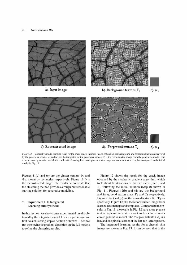
Figure 11. Result of the initial clustering algorithm, which provides a rough but reasonable starting solution for generative modeling. Theinitial clustering algorithm simplifies the models by decoupling the textons to accelerate the computation.

II. Given T1 and T2, the algorithm updates the texton�1 and �2 by averaging

�l = 1

nl

nl∑j=1

G−1[Tl j ] � IobsDl j

, l = 1, 2,

where G−1[Tl j ] is the inverse transformation. Thelayer order d1 and d2 are not needed for the simpli-fied model.

This initialization algorithm for computing (T1, T2,

�1, �2) resembles the transformed component analysis(Frey and Jojic, 1999). It is also inspired by a clusteringalgorithm by Leung and Malik (1999), which did notengage hidden variables, and thus compute a variety oftextons � at different scales and orientations. See alsothe work of Miller (2002). We also experimented withrepresenting the texton template � by a set of Gabor

bases instead of a 15×15 window. However, the resultswere not as encouraging as in this generative model.

6.2. Experiment II: Texton Clustering

In this subsection, we present one experiment for ini-tialization and clustering using the method outlined inSection 6.1.

Figure 11 shows an experiment on the initializationalgorithm for a crack pattern. 1055 textons are usedwith the template size of 15 × 15. The number of tex-tons is as twice as necessary to cover the whole image.In optimizing the likelihood in Eq. (14), an anneal-ing scheme is utilized with the temperature decreasingfrom 4 to 0.5. The sampling process converges to aresult shown in Fig. 11.

Figure 11(a) is the input image; Figs. 11(b) and(d) are the texton maps T1 and T2 respectively.

20 Guo, Zhu and Wu

Figure 12. Generative model learning result for the crack image. (a) input image, (b) and (d) are background and foreground textons discoveredby the generative model, (c) and (e) are the templates for the generative model, (f) is the reconstructed image from the generative model. Dueto an accurate generative model, the results after learning have more precise texton maps and accurate texton templates compared to the initialresults in Fig. 11.

Figures 11(c) and (e) are the cluster centers �1 and�2, shown by rectangles respectively. Figure 11(f) isthe reconstructed image. The results demonstrate thatthe clustering method provides a rough but reasonablestarting solution for generative modeling.

7. Experiment III: IntegratedLearning and Synthesis

In this section, we show some experimental results ob-tained by the integrated model. For an input image, wefirst do a clustering step as Section 6 showed. Then werun the stochastic gradient algorithm on the full modelsto refine the clustering results.

Figure 12 shows the result for the crack imageobtained by the stochastic gradient algorithm, whichtook about 80 iterations of the two steps (Step I andII), following the initial solution (Step 0) shown inFig. 11. Figures 12(b) and (d) are the backgroundand foreground texton maps T1 and T2 respectively.Figures 12(c) and (e) are the learned textons �1, �2 re-spectively. Figure 12(f) is the reconstructed image fromlearned texton maps and templates. Compared to the re-sults in Fig. 11, the results in Fig. 12 have more precisetexton maps and accurate texton templates due to an ac-curate generative model. The foreground texton �2 is abar, and one pixel at corner of the left-top is transparent.

The integrated learning results for a cheetah skinimage are shown in Fig. 13. It can be seen that in the


Figure 13. Generative model learning result for a cheetah skin image. See Fig. 12 caption for explanations.

foreground template, the surround pixels are learned asbeing transparent and the blob is exactly computed asthe texton. Figure 14 are the results for a brick image.No point in the template is transparent for the gap linesbetween bricks.

Figure 15 shows the learning of another short crackpatterns. Figure 16 displays a pine corn pattern. Theseeds and the black intervals are separated cleanly, andthe reconstructed image keeps most of the pine struc-tures. However the pine corn seeds are learnt as thebackground textons and the gaps between pine cornsare treated as foreground textons.

We also do one experiment on a bark image (Fig. 17).The result shows that the details of the bark are notmodeled well. For such patterns, the linear superposi-tion of the templates might do a better job. We shallinvestigate this issue in our future work.

We extend our model to three layers, i.e. L = 3 anddo one experiment on a pattern of text (Fig. 18), whichhas white background and two type of letters as fore-

ground. Figure 19 shows the learning process. Threetemplates—white background, letter ‘A’ and letter ‘B’were inferred gradually.

After the parameters � and β of a generative modelare estimated, new random samples could be drawnfrom the generative model. This proceeds in three steps:First, texton maps are sampled from the Gibbs modelsp(T1;β1) and p(T2;β2) respectively. Second, back-ground and foreground images are synthesized fromthe texton maps and texton templates. Third, the finalimage is generated by combining these two images ac-cording to the occlusion model.

We show synthesis experiments on three patterns.

1. Figures 20 and 21 are two synthesis examples ofthe two layered model for the cheetah skin pattern.The templates used here are the learned results inFig. 13.

2. Figure 22 shows texture synthesis for the crack pat-tern computed in Fig. 15.

22 Guo, Zhu and Wu

Figure 14. Generative model learning result for a brick image. See Fig. 12 caption for explanations.

3. Figure 23 displays texture synthesis for the brickpattern in Fig. 14. To capture the vertical andhorizontal distances of the brick, we add four moreneighbors in addition to four nearest neighbors tothe feature space. The new four neighbors are thosenearest neighbors which have the same orientationas the concerned texton. The T-junctions are not cap-tured because we do not have such feature statistics.

Note that, in these texture synthesis experiments, theMarkov chain operates with meaningful textons insteadof pixels.

8. Discussion

In this paper, we present a class of statistical mod-els for visual patterns. The models integrate and ex-tend descriptive and generative methods, and provide amathematical definition for textons and their perceptual

organizations. The hierarchical model can be consid-ered as a generalization of the hidden Markov model,and the hidden Markov structure is non-causal in ourmodel.

The model has some advantages over previous puredescriptive method with Markov random fields on pixelintensities. First, from the representational perspec-tive, the neighborhood in the texton map are muchsmaller than the pixel neighborhood in FRAME model(Zhu et al., 1997). The generative method capturesmore semantically meaningful elements on the tex-ton maps. Second, from the computational perspective,the Markov chain operating the texton maps can movetextons according to affine transforms and can add ordelete a texton by death/birth dynamics, thus it is muchmore effective than the Markov chain used in traditionalMarkov random fields which flips one pixel intensityat a time.

We show that the integration of descriptive and gen-erative methods is a natural path for visual learning.


Figure 15. Generative model learning result for a crack image. See Fig. 12 caption for explanations.

Figure 16. Generative model learning result for a pine corn image. See Fig. 12 caption for explanations.

24 Guo, Zhu and Wu

Figure 17. Generative model learning result for a bark image. The details of the bark are not modeled well by our current generativemodel.

Figure 18. A text file with two foreground letters to test our modelon three layers textons.

We argue that a vision system could evolve by pro-gressively replacing descriptive models with generativemodels, which realizes a transition from empirical andstatistical models to physical and semantical models.

The following are important issues that should beaddressed in future research.

First, the Gestalt model based on nearest neighbors istoo simple for many spatial patterns. We need to intro-duce more descriptive feature statistics for descriptivemodeling, or replace it with more abstract conceptssuch as curves and graphs as another hierarchy of gen-erative model. We also need to explore more efficientinference and synthesis algorithms for Gestalt model.

Second, the model for local textons based on im-age windows is quite limited. In a recent paper (Zhuet al., 2002), we explore combination of linear bases,and local shape and shading models. We also exploremotion elements. But there is still much work to bedone in order to find good local descriptors in term ofgenerative models.

Third, some texture patterns (like foliage) are intrin-sically complex (e.g., with a huge number of leaves),so that there may not exist low dimensional sparse rep-resentation in terms of textons. Such patterns may haveto be modeled by the descriptive FRAME model (Zhu


Figure 19. Generative model learning result for a text image. Six main steps are shown to illustrate the improving of textons and templateswith learning.

Figure 20. An example of a randomly synthesized cheetah skin image. (a) and (b) are the background and foreground texton maps respectivelysampled from p(Tl ; βlo,βl ); (d) and (e) are synthesized background and foreground images from the texton map and templates in (c); (f) is thefinal random synthesized image from the generative model.

26 Guo, Zhu and Wu

Figure 21. Second example of a randomly synthesized cheetah skin image.

Figure 22. An example of a randomly synthesized crack image. See Fig. 20 notation for explanations.


Figure 23. An example of a randomly synthesized brick image. See Fig. 20 notation for explanations.

et al., 1997). On the other hand, some patterns maycontain clear textons amid stochastic background (liketwigs and straws), and in that case, the noise in the gen-erative part of the model should be replaced by FRAMEmodel (Zhu et al., 1997).

Appendix: Deriving the Gibbs Modelfor Texton Process

A texton pattern on a large lattice � → Z is summarizedby a Julesz ensemble (or micro-canonical ensemble),

��(N , H) = {T� : N (T�) = N , H(T�) = H}

where � is a large lattice (or more rigorously, � → Z),T� is the texton map defined on lattice �, with N (T�)being the number of textons on T�, and H(T�) thecollection of the 22 histograms of Gestalt features. Nand H are two parameters that defines the Julesz en-semble ��(N , H).

Now, suppose we look at all the large texton mapsT� in the Julesz ensemble ��(N , H) through a smallwindow �0 ⊂ �, and we are interested in the fre-quency distribution of all the small texton maps thatwe see from this window. This frequency distributionis called the Gestalt ensemble (or the grand-canonicalensemble). In probabilistic language, let T� be a ran-

dom texton map sampled from the uniform distributionover the Julesz ensemble ��(N , H), and let T�0 be thepart of the large T� on the small lattice �0, then weare interested in the probability distribution of T�0 .

For a T� ∈ ��(N , H), if T�0 = T0 for a specificT0, then N (T�\�0 ) = N − N (T0) and H(T�\�0 ) =H − H(T0), where � \ �0 is the rest of the lattice.Clearly, the number of large texton maps in ��(N , H)with T0 on�0 is the same as the number of textons mapsT�\�0 in ��\�0 (N − N (T0), H − H(T0)). Therefore,the frequency of T0

p(T0) ∝ |��\�0 (N − N (T0), H − H(T0))|,

A Taylor expansion of log p(T0) at (N , H) gives

log p(T0) = C − ∂ log |��\�0 (N , H)|∂ N

N (T0)

−∂ log |��\�0 (N , H)|∂H

H (T0)

= C − β0 N (T0) − βH(T0),

where C is a constant, β0 and β are identified with thederivatives of the log of the volumes of the Julesz en-semble ��(N , H) with respect to N and H. Therefore,the Gibbs form of the p(T0) is derived.

28 Guo, Zhu and Wu

Acknowledgments

The authors would like to thank the three reviewers fortheir helpful comments. This work is supported par-tially by NSF grants IIS 98-77-127, IIS-00-92-664, andDMS-0072538, and an ONR grant N000140-110-535.

Notes

1. There is a third category of methods that can be called discrimi-native. The goal of discriminative methods is not for modeling vi-sual patterns explicitly but for approximating the posterior prob-abilities directly, for example, pattern recognition, feed-forwardneural networks and classification trees, etc. Thus we choose notto discuss it because our focus is on statistical modeling. See,however, Tu and Zhu (2002) that incorporates the discriminativemethods in Markov chain Monte Carlo posterior sampling.

2. Interested readers are referred to a recent paper (Roweis andGhahramani, 1999) for discussion of the problem with existinggenerative models.

3. In PCA, since the bases are orthogonal, ak can be computed astransform, but for over-complete basis, the ak have to be inferred.

4. We may introduce additional layers of hidden variables for curveprocesses that render the textons. But our model stops at the textonlevel in this paper.

5. This sampling process is almost identical to the simulation ofthe Gestalt ensemble in Section 4.3, except that a likelihoodp(Iobs | T1, T2; �) is engaged in the posterior p(T | Iobs; ).

6. Each point in the window can be transparent, and thus the shapeof the texton can change during the learning process.

References

Ahuja, N. and Tuceryan, M. 1989. Extraction of early perceptualstruct. in dot patterns. CVGIP, 48.

Bell, A.J. and Sejnowski, T.J. 1997. The independent componentsof natural images are edge filters. Vision Research, 37:3327–3338.

Bergen, J. and Adelson, E. 1988. Early vision and texture perception.Nature, 333:363–364.

Chandler, D. 1987. Introduction to Modern Statistical Mechanics.Oxford University Press.

Chen, S., Donoho, D., and Saunders, M.A. 1999. Atomic decom-position by basis pursuit. SIAM Journal on Scientific Computing,20(1):33–61.

Cover, T. and Thomas, J.A. 1994. Elements of Information Theory.De Bonet, J.S. and Viola, P. 1997. A non-parametric multi-scale sta-

tistical model for natural images. Advances in Neural InformationProcessing, 10.

Dempster, A.P., Laird, N.M., and Rubin, D.B. 1977. Maximum like-lihood from incomplete data via the EM algorithm. Journal of theRoyal Statistical Society Series B, 39:1–38.

Duda, R., Hart, P., and Stork, D. 2000. Pattern Classification andScene Analysis. 2nd edn., John Wiley & Sons.

Efros, A.A. and Freeman, W.T. 2001. Image quilting for texture syn-thesis and transfer. SIGGRAPH.

Frey, B. and Jojic, N. 1999. Transformed component analysis: Jointestimation of spatial transforms and image components. ICCV.

Fridman, A. 2000. Mixed Markov Models, Doctoral dissertation,Division of Applied Math, Brown University.

Geman, S. and Geman, D. 1984. Stochastic relaxation, Gibbs distri-butions and the Bayesian restoration of images. IEEE Trans. PAMI6:721–741.

Gilks, W.R. and Roberts, R.O. 1997. Strategies for improvingMCMC, chapter 6 in W.R. Gilks et al. (Eds.) Markov Chain MonteCarlo in Practice, Chapman & Hall.

Green, P.J. 1995. Reversible jump Markov chain Monte Carlocomputation and Bayesian model determination, Biometrika,82:711–732.

Gu, M.G. 1998. A stochastic approximation algorithm with MCMCmethod for incomplete data estimation problems. Preprint, Dept.of Math. and Stat., McGill Univ.

Heeger, D.J. and Bergen, J.R. 1995. Pyramid-based texture analy-sis/synthesis. SIGGRAPHS.

Jaynes, E.T. 1957. Information theory and statistical mechanics.Physical Review 106:620–630.

Julesz, B. 1981. Textons, the elements of texture perception and theirinteractions. Nature, 290:91–97.

Koffka, K. 1935. Principles of Gestalt Psychology.Lee, A.B., Mumford, D.B., and Huang, J.G. 2001. Occlusion models

for natural images: A statistical study of a scale-invariant deadleaves model. Int’l J. of Computer Vision, 41(1/2):35–59.

Leung, T. and Malik, J. 1996. Detecting, localizing and groupingrepeated scene elements from an image. In Proc. 4th ECCV,Cambridge, UK.

Leung, T. and Malik, J. 1999. Recognizing surface using three-dimensional textons. In Proc. of 7th ICCV, Corfu, Greece.

Lewicki, M.S. and Olshausen, B.A. 1999. A probabilistic frame-work for the adaptation and comparison of image codes. JOSA, A.16(7):1587–1601.

Malik, J. and Perona, P. 1990. Preattentive texture discriminationwith early vision mechanisms. J. of Optical Society of America A,7(5).

Malik, J., Belongie, S., Shi, J., and Leung, T. 1999. Textons, contoursand regions: Cue integration in image segmentation. ICCV.

Mallat, S. and Zhang, Z. 1993. Matching pursuit in a time-frequencydictionary. IEEE Trans. on Signal Processing, 41:3397–3415.

Marr, D. Vision. W.H. Freeman and Company.Miller, E.G. 2002. Learning from one example in machine vision

by sharing probability densities. Ph.D. Thesis, MassachusettsInstitute of Technology.

Olshausen, B.A. and Field, D.J. 1996. Emergence of simple-cellreceptive field properties by learning a sparse code for naturalimages” Nature, 381:607–609.

Roweis, S. and Ghahramani, Z. 1999. A unifying review of linearGaussian models. Neural Computation, 11(2).

Portilla, J. and Simoncelli, E.P. 2000. A parametric texture modelbased on joint statistics of complex wavelet coefficients. IJCV,40(1):47–70.

Steven, K.A. 1978. Computation of locally parallel structure. Biol.Cybernetics, 29:19–28.

Stoyan, D., Kendall, W.S., and Mecke, J. 1985. Stochastic Geometryand its Applications.

Tanner, M. 1996. Tools for Statistical Inference. Springer.Tu, Z. and Zhu, S.C. 2002. Image Segmentation by Data-Driven

Markov Chain Monte Carlo. IEEE Trans. PAMI, 24(5):657–673.


Wu, Y.N., Zhu, S.C., and Liu, X.W. 1999. Equivalence of Julesz andGibbs Ensembles. ICCV.

Wu, Y.N., Zhu, S.C., and Guo, C. 2002. Statistical modeling oftexture sketch. ECCV.

Xu, Y.Q., Guo, B.N., and Shum, H.Y. 2000. Chaos mosaic: Fast andmemory efficient texture synthesis. MSR TR-2000-32.

Zhu, S.C. 1999. Embedding Gestalt Laws in Markov RandomFields. IEEE Trans. PAMI. 21(11):1170–1187.

Zhu, S.C. and Guo, Cheng-en. 2001. Conceptualization andmodeling of visual patterns. In Proc. of 3rd Int’l Workshop

on Perceptual Organization in Computer Vision, Vancouver,Canada.

Zhu, S.C., Guo, C., Wu, Y.N., and Wang, Y. 2002. What are textons?ECCV.

Zhu, S.C., Liu, X.W., and Wu, Y.N. 2000. Exploring Julesz textureensemble by effective Markov Chain Monte Carlo. IEEE Trans.PAMI, 22(6):554–569.

Zhu, S.C., Wu, Y.N., and Mumford, D. 1997. Minimax entropy prin-ciple and its application to texture modeling. Neural Computation,9(8):1627–1660.

Documents

Modeling Visual Patterns by Integrating Descriptive and