Modeling with Normalized Random Measure Mixture …economia.unipv.it/pagp/pagine_personali/alijoi/Publications_files/... · 2013, Vol. 28, No. 3, 313–334 DOI: 10.1214/13-STS416

Statistical Science2013, Vol. 28, No. 3, 313–334DOI: 10.1214/13-STS416© Institute of Mathematical Statistics, 2013

Modeling with Normalized RandomMeasure Mixture ModelsErnesto Barrios, Antonio Lijoi1, Luis E. Nieto-Barajas and Igor Prünster1

Abstract. The Dirichlet process mixture model and more general mixturesbased on discrete random probability measures have been shown to be flex-ible and accurate models for density estimation and clustering. The goal ofthis paper is to illustrate the use of normalized random measures as mixingmeasures in nonparametric hierarchical mixture models and point out howpossible computational issues can be successfully addressed. To this end,we first provide a concise and accessible introduction to normalized randommeasures with independent increments. Then, we explain in detail a particu-lar way of sampling from the posterior using the Ferguson–Klass representa-tion. We develop a thorough comparative analysis for location-scale mixturesthat considers a set of alternatives for the mixture kernel and for the non-parametric component. Simulation results indicate that normalized randommeasure mixtures potentially represent a valid default choice for density es-timation problems. As a byproduct of this study an R package to fit thesemodels was produced and is available in the Comprehensive R Archive Net-work (CRAN).

Key words and phrases: Bayesian nonparametrics, completely randommeasure, clustering, density estimation, Dirichlet process, increasing addi-tive process, latent variables, mixture model, normalized generalized gammaprocess, normalized inverse Gaussian process, normalized random measure,normalized stable process.

1. INTRODUCTION

The Dirichlet process mixture model (DPM), intro-duced by Lo (1984), currently represents the most pop-ular Bayesian nonparametric model. It is defined as

f (x) =!

k(x|θ)P (dθ),(1)

where k is a parametric kernel and P is a random prob-ability whose distribution is the Dirichlet process prior

Ernesto Barrios is Professor and Luis E. Nieto-Barajas isProfessor, Department of Statistics, ITAM, Mexico D.F.(e-mail: [email protected]; [email protected]). AntonioLijoi is Professor of Probability and MathematicalStatistics, Department of Economics and Management,University of Pavia, Italy (e-mail: [email protected]). IgorPrünster is Professor of Statistics, Department ofEconomics and Statistics, University of Torino, Italy(e-mail: [email protected]).

1Also affiliated with Collegio Carlo Alberto, Moncalieri, Italy.

with (finite) parameter measure α, in symbols P ∼ Dα .It is often useful to write α = aP0 where P0 = E[P ] isa probability measure and a is in (0,+∞). In otherwords, the DPM is a mixture of a kernel k with mix-ing distribution a Dirichlet process. See also Berry andChristensen (1979) for an early contribution to DPM.

Alternatively, the DPM can also be formulated asa hierarchical model (Ferguson, 1983). In this case,Xi, θi for i = 1, . . . , n,

Xi |θiind∼ k(·|θi ),

θi |P i.i.d.∼ P ,(2)

P ∼ Dα.

The hierarchical representation of the DPM explicitlydisplays features of the model that are relevant forpractical purposes. Indeed, Escobar and West (1995)developed an MCMC algorithm for simulating fromthe posterior distribution. This contribution paved theway for extensive uses of the DPM, and semiparamet-

313

http://www.imstat.org/sts/

http://dx.doi.org/10.1214/13-STS416

http://www.imstat.org

mailto:[email protected]




314 BARRIOS, LIJOI, NIETO-BARAJAS AND PRÜNSTER

ric variations of it, in many different applied contexts.See MacEachern and Müller (2000) and Müller andQuintana (2004) for reviews of the most remarkableachievements, both computational and applied, in thefield. The main idea behind Escobar and West’s al-gorithm is represented by the marginalization of theinfinite dimensional random component, namely, theDirichlet process P , which leads to work with gener-alized Pólya urn schemes. If the centering measure P0is further chosen to be the conjugate prior for kernel k,then one can devise a Gibbs sampler whose implemen-tation is straightforward. In particular, the typical setupin applications involves a normal kernel: if the loca-tion (or location-scale) mixture of normals is combinedwith a conjugate normal (or normal-gamma) probabil-ity measure P0, the full conditional distributions can bedetermined, thus leading to a simple Gibbs sampler.

Given the importance of the DPM model, much at-tention has been devoted to the development of alter-native and more efficient algorithms. According to theterminology of Papaspiliopoulos and Roberts (2008),these can be divided into two classes: marginal andconditional methods. Marginal methods, such as theEscobar and West algorithm, integrate out the Dirich-let process in (2) and resort to the predictive distribu-tions, within a Gibbs sampler, to obtain posterior sam-ples. In this framework an important advance is due toMacEachern and Müller (1998): they solve the issue ofproviding algorithms, which effectively tackle the casewhere the kernel k and P0 are not a conjugate pair. Onthe other hand, conditional methods work directly on(2) and clearly have to face the problem of samplingthe trajectories of an infinite-dimensional random ele-ment such as the Dirichlet process. The first contribu-tions along this line are given in Muliere and Tardella(1998) and Ishwaran and James (2001) who use trun-cation arguments. Exact simulations can be achievedby the retrospective sampling technique introduced inPapaspiliopoulos and Roberts (2008) and slice sam-pling schemes as in Walker (2007).

In this paper we focus on mixture models moregeneral than the DPM, namely, mixtures with mixingmeasure given by normalized random measures withindependent increments (NRMI), namely, a class ofrandom probability measures introduced in Regazzini,Lijoi and Prünster (2003). Several applications of spe-cific members of this class, or closely related distribu-tions, are now present in the literature and deal withspecies sampling problems, mixture models, cluster-ing, reliability and models for dependence. See Lijoiand Prünster (2010) for references. Here we describe

in detail a conditional algorithm which allows oneto draw posterior simulations from mixtures basedon a general NRMI. As we shall point out, it worksequally well regardless of k and P0 forming a con-jugate pair or not and readily yields credible inter-vals. Our description is a straightforward implemen-tation of the posterior characterization of NRMI pro-vided in James, Lijoi and Prünster (2009) combinedwith the representation of an increasing additive pro-cess given in Ferguson and Klass (1972). The R pack-age BNPdensity, available in the ComprehensiveR Archive Network (CRAN), implements this algo-rithm. For contributions containing thorough and in-sightful comparisons of algorithms for Bayesian non-parametric mixture models, both marginal and condi-tional, the reader is referred to Papaspiliopoulos andRoberts (2008) and Favaro and Teh (2013).

The BNPdensity package is used to carry out acomparative study that involves a variety of data setsboth real and simulated. For the real data sets we showthe impact of choosing different kernels and comparethe performance of location-scale nonparametric mix-tures. We also examine different mixing measures andshow some advantages and disadvantages fitting thedata and the number of induced clusters. Model perfor-mance is assessed by referring to conditional predictiveordinates and to suitable numerical summaries of thesevalues. For the simulated examples, we rely on the rel-ative mean integrated squared error to measure the per-formance of NRMI mixtures with respect to competingmethods such as kernel density estimators, Bayesianwavelets and finite mixtures of normals. The outcomeclearly shows that NRMI mixtures, and in particularmixtures of stable NRMIs, potentially represent a validdefault choice for density estimation problems.

The outline of the paper is as follows. We providein Section 2 an informal review of normalized randommeasures and highlight their uses for Bayesian non-parametric inference. Particular emphasis is given tothe posterior representation since it plays a key role inthe elaboration of the sampling scheme that we use; inSection 3 a conditional algorithm for simulating fromthe posterior of NRMI mixtures is described in greatdetail; Section 4 contains a comprehensive data analy-sis highlighting the potential of NRMI mixtures.

2. DIRICHLET PROCESS AND NRMIS

A deeper understanding of NRMI mixture modelsdefined in (1) is eased by an accessible introductionto the notions of completely random measures and

NRMI MIXTURE MODELS 315

NRMIs. This section aims at providing a concise re-view of the most relevant distributional properties ofcompletely random measures and NRMIs in view oftheir application to Bayesian inference. These are alsoimportant for addressing the computational issues weshall focus on in later sections.

2.1 Exchangeability and Discrete NonparametricPriors

In order to best describe the nonparametric priors weare going to deal with, we first recall the notion of ex-changeability, its implication in terms of Bayesian in-ference and some useful notation. Let (Yn)n≥1 be an(ideally) infinite sequence of observations, defined onsome probability space (#,F ,P ), with each Yi takingvalues in Y (a complete and separable metric space en-dowed with its Borel σ -algebra). While in a frequentistsetting one typically assumes that the Yi ’s are indepen-dent and identically distributed (i.i.d.) with some fixedand unknown distribution, in a Bayesian approach theindependence is typically replaced by a weaker as-sumption of conditional independence, given a ran-dom probability distribution on Y, which correspondsto assuming exchangeable data. Formally, this corre-sponds to an invariance condition according to which,for any n ≥ 1 and any permutation π of the indices1, . . . , n, the probability distribution of (Y1, . . . , Yn)coincides with the distribution of (Yπ(1), . . . , Yπ(n)).Then, the celebrated de Finetti representation theoremstates that the sequence (Yn)n≥1 is exchangeable if andonly if its distribution can be represented as a mixtureof sequences of i.i.d. random variables. In other terms,(Yn)n≥1 is exchangeable if and only if there exists aprobability distribution Q on the space of probabilitymeasures on Y, say, PY, such that

Yi |P i.i.d.∼ P , i = 1, . . . , n,(3)

P ∼ Q

for any n ≥ 1. Hence, P is a random probability mea-sure on Y, namely, a random element on (#,F ,P )taking values in PY (endowed with the topology ofweak convergence). The probability distribution Q ofP is also termed de Finetti measure and represents theprior distribution in a Bayesian setup. Whenever Q de-generates on a finite-dimensional subspace of PY, theinferential problem is usually called parametric. Onthe other hand, when the support of Q is infinite di-mensional, then this is typically referred to as a non-parametric inferential problem. It is generally agreedthat having a large topological support is a desirable

property for a nonparametric prior (see, e.g., Ferguson,1974).

In the context of nonparametric mixture models,which identify the main focus of the paper, a key roleis played by discrete nonparametric priors Q, that is,priors which select discrete distributions with probabil-ity 1. Clearly, any random probability measure P asso-ciated to a discrete prior Q can be represented as

P ="

j≥1

pjδZj ,(4)

where (pj )j≥1 is a sequence of nonnegative ran-dom variables such that

#j≥1 pj = 1, almost surely,

(Zj )j≥1 is a sequence of random variables taking val-ues in Y and δZ is the Dirac measure.

As far as the observables Yi ’s are concerned, thediscrete nature of P in (4) implies that any sampleY1, . . . , Yn in (3) will feature ties with positive prob-ability and, therefore, display r ≤ n distinct observa-tions Y ∗

1 , . . . , Y ∗r with respective frequencies n1, . . . , nr

such that#r

i=1 ni = n. Such a grouping lies at the heartof Bayesian nonparametric procedures for clusteringpurposes. Henceforth, Rn will denote the random vari-able identifying the number of distinct values appear-ing in the sample Y1, . . . , Yn.

The simplest and most familiar illustration one canthink of is the Dirichlet process prior introduced byFerguson (1973), which represents the cornerstoneof Bayesian Nonparametrics. Its original definitionwas given in terms of a consistent family of finite-dimensional distributions that coincide with multivari-ate Dirichlet distributions. To make this explicit, intro-duce the (d − 1)-variate Dirichlet probability densityfunction on the (d − 1)-dimensional unit simplex

h(p; c) = '(#d

i=1 ci)$d

i=1 '(ci)p

c1−11 · · ·pcd−1−1

d−1

·%

1 −d−1"

i=1

pi

&cd−1

,

where c = (c1, . . . , cd) ∈ (0,∞)d and p = (p1, . . . ,pd−1).

DEFINITION 1 (Ferguson, 1973). Let α be somefinite and nonnull measure on Y such that α(Y) = a.Suppose the random probability measure P has distri-bution Q such that, for any choice of a (measurable)partition {A1, . . . ,Ad} of Y and for any d ≥ 1, one has

Q'(

P :'P(A1), . . . ,P (Ad)

) ∈ B*)

(5)=

!

Bh(p;α)dp1 · · · dpd−1,


where α = (α(A1), . . . ,α(Ad)). Then P is termed aDirichlet process with base measure α.

Note that α/a =: P0 defines a probability measureon Y and it coincides with the expected value of aDirichlet process, that is, P0 = E[P ], for this reasonis often referred to as the prior guess at the shape of P .Henceforth, we shall denote more conveniently thebase measure α of P as aP0. Also note that the Dirich-let process has large support and it, thus, shares oneof the properties that makes the use of nonparametricpriors attractive. Indeed, if the support of P0 coincideswith Y, then the support of the Dirichlet process prior(in the weak convergence topology) coincides with thewhole space PY. In other words, the Dirichlet processprior assigns positive probability to any (weak) neigh-borhood of any given probability measure in PY, thusmaking it a flexible model for Bayesian nonparametricinference.

As shown in Blackwell (1973), the Dirichlet processselects discrete distributions on Y with probability 1and, hence, admits a representation of the form (4).An explicit construction of the pj ’s in (4) leading tothe Dirichlet process has been provided by Sethuraman(1994) who relied on a stick-breaking procedure. Thisarises when the sequence of random probability masses(pj )j≥1 is defined as

p1 = V1,(6)

pj = Vj

j−1+

i=1

(1 − Vi), j = 2,3, . . . ,

with the Vi’s being i.i.d. and beta distributed with pa-rameter (1, a), and when the locations (Zj )j≥1 arei.i.d. from P0. Under these assumptions (4) yields arandom probability measure that coincides, in distribu-tion, with a Dirichlet process with base measure aP0.

A nice and well-known feature about the Dirichletprocess is its conjugacy. Indeed, if P in (3) is a Dirich-let process with base measure aP0, then the posteriordistribution of P , given the data Y1, . . . , Yn, still coin-cides with the law of a Dirichlet process with param-eter measure (a + n)Pn where Pn = aP0/(a + n) +#n

i=1 δYi /(a + n), where δy denotes a point mass aty ∈ Y. On the basis of this result, one easily determinesthe predictive distributions associated to the Dirichletprocess and for any A in Y, one has

P [Yn+1 ∈ A|Y1, . . . , Yn](7)

= a

a + nP0(A) + n

a + n

1n

r"

j=1

njδY ∗j(A),

where, again, the Y ∗j ’s with frequency nj denote the

r ≤ n distinct observations within the sample. Hence,the predictive distribution appears as a convex linearcombination of the prior guess at the shape of P and ofthe empirical distribution.

From (4) it is apparent that a decisive issue whendefining a discrete nonparametric prior is the deter-mination of the probability masses pj ’s, while at thesame time preserving a certain degree of mathemati-cal tractability. This is in general quite a challengingtask. For instance, the stick-breaking procedure is use-ful to construct a wide range of discrete nonparametricpriors as shown in Ishwaran and James (2001). How-ever, only for a few of them is it possible to establishrelevant distributional properties such as, for example,the posterior or predictive structures. See Favaro, Lijoiand Prünster (2012) for a discussion on this issue. Also,as extensively discussed in Lijoi and Prünster (2010),a key tool for defining tractable discrete nonparamet-ric priors (4) is given by completely random measures,a concept introduced in Kingman (1967). Since it is es-sential for the construction of the class of NRMIs con-sidered in the paper, in the following section we con-cisely recall the basics and refer the interested readerto Kingman (1993) for an exhaustive account.

2.2 CRM and NRMI

Denote first by MY the space of boundedly finitemeasures on Y, this meaning that for any µ in MY andany bounded set A in Y one has µ(A) < ∞. Moreover,MY can be endowed with a suitable topology that al-lows one to define the associated Borel σ -algebra. SeeDaley and Vere-Jones (2008) for technical details.

DEFINITION 2. A random element µ, defined on(#,F ,P ) and taking values in MY, is called a com-pletely random measure (CRM) if, for any n ≥ 1 andA1, . . . ,An in Y, with Ai ∩ Aj = ∅ for any i = j , therandom variables µ(A1), . . . , µ(An) are mutually in-dependent.

Hence, a CRM is simply a random measure, whichgives rise to independent random variables when eval-uated over disjoint sets. In addition, it is well knownthat if µ is a CRM on Y, then

µ ="

i≥1

JiδZi +M"

i=1

Viδzi ,

where (Ji)i≥1, (Vi)i≥1 and (Zi)i≥1 are independentsequences of random variables and the jump points{z1, . . . , zM} are fixed, with M ∈ {0,1, . . .} ∪ {∞}. If


M = 0, then µ has no fixed jumps and the Laplacetransform of µ(A), for any A in Y, admits the follow-ing representation:

E,e−λµ(A)-

(8)= exp

.−

!

R+×A

,1 − e−λv-

ν(dv,dy)

/

for any λ > 0, with ν being a measure on R+ × Y suchthat

!

B

!

R+min{v,1}ν(dv,dy) < ∞(9)

for any bounded B in Y. The measure ν is referred toas the Lévy intensity of µ and, by virtue of (8), it char-acterizes the CRM µ. This is extremely useful from anoperational point of view since a single measure en-codes all the information about the distribution of thejumps (Ji)i≥1 and locations (Zi)i≥1 of µ. The measureν will be conveniently rewritten as

ν(dv,dy) = ρ(dv|y)α(dy),(10)

where ρ is a transition kernel on R+ × Y controllingthe jump intensity and α is a measure on Y determiningthe locations of the jumps. Two popular examples aregamma and stable processes. The former correspondsto the specification ρ(dv|y) = e−v dv/v, whereas thelatter arises when ρ(dv|y) = γ v−1−γ dv/'(1−γ ), forsome γ ∈ (0,1). Note that if µ is a gamma CRM, then,for any A, µ(A) is gamma distributed with shape pa-rameter α(A) and scale 1. On the other hand, if µ is astable CRM, then µ(A) has a positive stable distribu-tion.

Since µ is a discrete random measure almost surely,one can then easily guess that discrete random proba-bility measures (4) can be obtained by suitably trans-forming a CRM. The most obvious transformation is“normalization,” which yields NRMIs. As a prelimi-nary remark, it should be noted that “normalization”is possible when the denominator µ(Y) is positive andfinite (almost surely). Such a requirement can be ex-pressed in terms of the Lévy intensity, in particular, αbeing a finite measure and

0R+ ρ(dv|y) = ∞ for any

y ∈ Y are simple sufficient conditions for the normal-ization to be well defined. The latter condition essen-tially requires the CRM to jump infinitely often on anybounded set and is sometimes referred to as infiniteactivity. See Regazzini, Lijoi and Prünster (2003) andJames, Lijoi and Prünster (2009) for necessary and suf-ficient conditions. One can now provide the definitionof a NRMI.

DEFINITION 3. Let µ be a CRM with Lévy inten-sity (10) such that 0 < µ(Y) < ∞ almost surely. Then,the random probability measure

P = µ

µ(Y)(11)

is named a normalized random measure with indepen-dent increments (NRMI).

It is apparent that a NRMI is uniquely identifiedby the Lévy intensity ν of the underlying CRM. Ifρ(dv|y) in (10) does not depend on y, which meansthat the distribution of the jumps of µ are indepen-dent of their locations, then the CRM µ and the cor-responding NRMI (11) are called homogeneous. Oth-erwise they are termed nonhomogeneous. Moreover,it is worth pointing out that all NRMI priors share asupport property analogous to the one recalled for theDirichlet process prior. Specifically, if the support ofthe base measure coincides with Y, then the corre-sponding NRMI has full weak support PY.

Note that the Dirichlet process can be defined as anNRMI: indeed, it coincides, in distribution, with a nor-malized gamma CRM as shown in Ferguson (1973).If ν(dv,dy) = e−vv−1 dv aP0(dy), then (11) yieldsa Dirichlet process with base measure aP0. Anotherearly use of (11) can be found in Kingman (1975),where the NRMI obtained by normalizing a stableCRM is introduced. The resulting random probabilitymeasure will be denoted as N-stable.

In the sequel particular attention will be devoted togeneralized gamma NRMIs (Lijoi, Mena and Prünster,2007) since they are analytically tractable and includemany well-known priors as special cases. This class ofNRMIs is obtained by normalizing generalized gammaCRMs that were introduced in Brix (1999) and arecharacterized by a Lévy intensity of the form

ρ(dv)α(dx) = e−κv

'(1 − γ )v1+γdv aP0(dx),(12)

whose parameters κ ≥ 0 and γ ∈ [0,1) are suchthat at least one of them is strictly positive and withbase measure α = aP0, where a ∈ (0,∞) and P0is a probability distribution on Y. The correspond-ing generalized gamma NRMI will be denoted asP ∼ NGG(a,κ,γ ;P0). Within this class of priorsone finds the following special cases: (i) the Dirichletprocess which is a NGG(a,1,0;P0) process; (ii) thenormalized inverse Gaussian (N-IG) process (Lijoi,Mena and Prünster, 2005), which corresponds to aNGG(1,κ,1/2;P0) process; (iii) the N-stable process


(Kingman, 1975) which arises as NGG(1,0,γ ;P0). Asa side remark, we observe that either κ or a can befixed according to one’s convenience. Loosely speak-ing, this is due to the fact that the normalization oper-ation implies the loss of “one degree of freedom” asa reference to the Dirichlet process might clarify. Forexample, we mentioned that the Dirichlet case ariseswhen κ is set equal to 1, but this choice is only due toconvenience. Indeed, a Dirichlet process is obtained,as long as γ = 0, whatever the value κ takes on. SeePitman (2003) and Lijoi, Mena and Prünster (2007)for detailed explanations. For our purposes it is worthsticking to the redundant parameterization since it al-lows us to recover immediately all three specific caseslisted above, which would be cumbersome with thealternative parameterization usually adopted, that is,NGG(1,β,γ ;P0) with β = κγ /γ . The role of theseparameters is best understood by looking at the induced(prior) distribution of the number of distinct values Rn

in an sample Y1, . . . , Yn. Indeed, one has that κ (or,equivalently, a) affects the location: a larger κ (or a)shifts the distribution of Rn to the right, implying alarger expected number of distinct values. In contrast,γ allows to tune the flatness of the distribution of Rn:the bigger γ , the flatter is the distribution of Rn so thata large value of γ corresponds to a less informativeprior for the number of distinct values in Y1, . . . , Yn.This also explains why the Dirichlet process, whichcorresponds to γ = 0, yields the most highly-peakeddistribution for Rn. See also Lijoi, Mena and Prünster(2007) for a graphical display of these behaviors.

Also, variations of NRMI have already appeared inthe literature. In Nieto-Barajas, Prünster and Walker(2004) weighted versions of NRMIs are considered. Tobe more specific, letting h be some nonnegative func-tion defined on Y, a normalized weighted CRM is ob-tained, for any B in Y, as

P (B) =0B h(y)µ(dy)

0Y h(y)µ(dy)

.

The function h can be seen as a perturbation of theCRM and in Nieto-Barajas and Prünster (2009) thesensitivity of posterior inference with respect to (w.r.t.)h is examined. Another related class is represented byPoisson–Kingman models (Pitman, 2003), where oneessentially conditions on µ(Y) and then mixes with re-spect to some probability measure on R+.

REMARK 1. If Y = Rm, one can also considerthe càdlàg random distribution function induced by µ,namely, M := {M(s) = µ((−∞, s1] × · · · ×

(−∞, sm]) : s = (s1, . . . , sm) ∈ Rm}, known in the lit-erature as the increasing additive process or indepen-dent increment process. See Sato (1990) for details.One can then associate to the NRMI random probabil-ity measure in (11) the corresponding NRMI randomcumulative distribution function

F (s) = M(s)

Tfor any s ∈ Rm,(13)

where T := lims→∞ M(s) and the limit is meantas componentwise. The original definition of NRMIin Regazzini, Lijoi and Prünster (2003) was givenin terms of increasing additive processes. The def-inition on more abstract spaces adopted here, andused also, for example, in James, Lijoi and Prünster(2009), allows us to bypass some tedious technicalities.Nonetheless, we preserve the term NRMI, although onabstract spaces one should refer to normalized CRMrather than to “increments.”

REMARK 2. Although the previous examples dealwith homogeneous CRMs and NRMIs, nonhomoge-neous CRMs are also very useful for the constructionof nonparametric priors. This is apparent in contribu-tions to Bayesian nonparametric inference for survivalanalysis. See Lijoi and Prünster (2010). Hence, giventhe importance of nonhomogeneous structures in someother contexts, it seems worth including these in ourtreatment.

2.3 Posterior Distribution of a NRMI

The posterior distribution associated to an exchange-able model as in (3) is a preliminary step for attain-ing Bayesian inferential results of interest and, there-fore, represents an object of primary importance. In thecase of NRMIs, the determination of the posterior dis-tribution is a challenging task since one cannot relydirectly on Bayes’ theorem (the model is not domi-nated) and, with the exception of the Dirichlet process,NRMIs are not conjugate as shown in James, Lijoi andPrünster (2006). Nonetheless, a posterior characteriza-tion has been established in James, Lijoi and Prünster(2009) and it turns out that, even though NRMIs arenot conjugate, they still enjoy a sort of “conditionalconjugacy.” This means that, conditionally on a suit-able latent random variable, the posterior distributionof a NRMI coincides with the distribution of a NRMIhaving fixed points of discontinuity located at the ob-servations. Such a simple structure suggests that whenworking with a general NRMI, instead of the Dirichlet


process, one faces only one additional layer of diffi-culty represented by the marginalization with respectto the conditioning latent variable.

Before stating the main result we recall that, due tothe discreteness of NRMIs, ties will appear with pos-itive probability in Y = (Y1, . . . , Yn) and, therefore,the sample information can be encoded by the Rn =r distinct observations (Y ∗

1 , . . . , Y ∗r ) with frequencies

(n1, . . . , nr) such that#r

j=1 nj = n. Moreover, intro-duce the nonnegative random variable U such that thedistribution of [U |Y] has density, w.r.t. the Lebesguemeasure, given by

fU |Y(u) ∝ un−1 exp(−ψ(u)

* r+

j=1

τnj

'u|Y ∗

j

),(14)

where τnj (u|Y ∗j ) = 0 ∞

0 vnj e−uvρ(dv|Y ∗j ) and ψ is the

Laplace exponent of µ as in (8). Finally, in the follow-ing we assume the probability measure P0 defining thebase measure of a NRMI to be nonatomic.

THEOREM 1 (James, Lijoi and Prünster, 2009). Let(Yn)n≥1 be as in (3) where P is a NRMI defined in (11)with Lévy intensity as in (10). Then the posterior dis-tribution of the unnormalized CRM µ, given a sampleY, is a mixture of the distribution of [µ|U,Y] with re-spect to the distribution of [U |Y]. The latter is identi-fied by (14), whereas [µ|U,Y] is equal in distributionto a CRM with fixed points of discontinuity at the dis-tinct observations Y ∗

j ,

µ∗ +r"

j=1

J ∗j δY ∗

j(15)

such that:

(a) µ∗ is a CRM characterized by the Lévy intensity

ν∗(dv,dy) = e−uvρ(dv|y)α(dy);(16)

(b) the jump height J ∗j corresponding to Y ∗

j hasdensity, w.r.t. the Lebesgue measure, given by

f ∗j (v) ∝ vnj e−uvρ

'dv|Y ∗

j

).(17)

(c) µ∗ and J ∗j , j = 1, . . . , r , are independent.

Moreover, the posterior distribution of the NRMI P ,conditional on U , is given by

[P |U,Y] d= wµ∗

µ∗(X)+ (1 − w)

#ri=1 J ∗

i δY ∗i#r

l=1 J ∗l

,(18)

where w = µ∗(X)/(µ∗(X) + #rl=1 J ∗

l ).

In order to simplify the notation, in the statementwe have omitted explicit reference to the dependenceon [U |Y] of both µ∗ and {J ∗

i : i = 1, . . . , r}. However,such a dependence is apparent from (16) and (17).From Theorem 1 follows is apparent that the onlyquantity needed for deriving explicit expressions forparticular cases of NRMI is the Lévy intensity (10). Forinstance, in the case of normalized generalized gammaNRMI, NGG(a,κ,γ ;P0) one has that the unnormal-ized posterior CRM µ∗ in (15) is characterized by aLévy intensity of the form

ν∗(dv,dy) = e−(κ+u)v

'(1 − γ )v1+γdv aP0(dy).(19)

Moreover, the distribution of the jumps (17) corre-sponding to the fixed points of discontinuity Y ∗

i ’s in(15) reduce to a gamma distribution with density

f ∗j (v) = (κ + u)nj−γ

'(nj − γ )vnj−γ−1e−(κ+u)v.(20)

Finally, the conditional distribution of the latent vari-able U given Y (14) is given by

fU |Y(u)(21)

∝ un−1(u + κ)rγ−n exp.− a

γ(u + κ)γ

/

for u > 0. The availability of this posterior characteri-zation makes it then possible to determine several im-portant quantities such as the predictive distributionsand the induced partition distribution. See James, Li-joi and Prünster (2009) for general NRMI and Lijoi,Mena and Prünster (2007) for the subclass of general-ized gamma NRMI.

2.4 NRMI Mixture Models

Discrete nonparametric priors are particularly effec-tive when used for modelling latent variables withinhierarchical mixtures. The most popular of these mod-els is the DPM due to Lo (1984) and displayed in (2).Its most natural generalization corresponds to allowingany NRMI to act as a nonparametric mixing measure.In view of the result on the posterior characterizationof NRMIs, such a program is also feasible from a prac-tical perspective.

We start by describing the NRMIs mixture model insome detail. First, let us introduce a change in the no-tation. In order to highlight that the law of a NRMIsacts as the de Finetti measure at a latent level, we de-note the elements of the exchangeable sequence byθi instead of Yi , for i = 1,2, . . . . Then, consider a


NRMI P and convolute it with a suitable density ker-nel k(·|θ), thus obtaining the random mixture densityf (x) = 0

0 k(x|θ)P (dθ). This can equivalently be writ-ten in a hierarchical form as

Xi |θiind∼ k(·|θi ), i = 1, . . . , n,

θi |P i.i.d.∼ P , i = 1, . . . , n,(22)

P ∼ NRMI .

In the sequel, we take kernels defined on X ⊆ R andNRMIs defined on Y = 0 ⊆ Rm. Consequently, in-stead of describing the results in terms of the randommeasures µ and P , we will work with correspondingdistribution functions M and F , respectively, for thesake of simplicity in the presentation (see Remark 1).It is worth noting that the derivations presented herecarry over to general spaces in a straightforward way.

As for the base measure of the NRMI P0 on 0,we denote its density (w.r.t. the Lebesgue measure) byf0. When P0 depends on a further hyperparameter φ,we will use the symbol f0(·|φ). The case m = 2 typ-ically corresponds to the specification of a nonpara-metric model for the location and scale parameters ofthe mixture, that is, θ = (µ,σ ). This will be used toillustrate the algorithm in Section 4, where we applyour proposed modeling to simulated and real data sets.In order to distinguish the hyperparameters for loca-tion and scale, we will use the notation f0(µ,σ |φ) =f 1

0 (µ|σ,ϕ)f 20 (σ |ς). In applications a priori indepen-

dence between µ and σ is commonly assumed.The most popular uses of mixtures of discrete ran-

dom probability measures, such as the one displayedin (22), relate to density estimation and data clustering.The former can be addressed by evaluating

fn(x) = E'f (x)|X1, . . . ,Xn

)(23)

for any x in X. As for the latter, if Rn is the numberof distinct latent values θ∗

1 , . . . , θ∗Rn

out of a sample ofsize n, one can deduce a partition of the observationssuch that any two Xi and Xj belong to the same clusterif the corresponding latent variables θi and θj coincide.Then, it is interesting to determine an estimate Rn ofthe number of clusters into which the data are grouped.In the examples we will illustrate Rn is set equal to themode of Rn|X, with X := (X1, . . . ,Xn) representingthe observed sample. Both estimation problems can befaced by relying on the simulation algorithm that willbe detailed in the next section.

3. POSTERIOR SIMULATION OF NRMI MIXTURES

Our main aim is to provide a general algorithm todraw posterior inferences with the mixture model (22),for any choice of the mixing NRMI and of the kernel.A further byproduct of our algorithm is the possibil-ity of determining credible intervals. The main blockof the conditional algorithm presented in this sectionis the posterior representation provided in Theorem 1.In fact, in order to sample from the posterior distribu-tion of the random mixture model (22), given a sampleX1, . . . ,Xn, a characterization of the posterior distri-bution of the mixing measure at the higher stage of thehierarchy is needed. We rely on the posterior represen-tation, conditional on the unobservable variables θ :=(θ1, . . . , θn), of the unnormalized process M , since thenormalization can be carried out within the algorithm.

For the implementation of a Gibbs sampling schemewe use the distributions of

[M|X, θ] and [θ |X, M].(24)

For illustration we shall detail the algorithm when P ∼NGG(a,κ,γ ;P0) and provide explicit expressions foreach of the distributions in (24). Nonetheless, as al-ready recalled, the algorithm can be implemented forany NRMI: one just needs to plug in the correspondingLévy intensity.

Due to conditional independence properties, the con-ditional distribution of M , given X and θ , does not de-pend on X, that is, [M|X, θ] = [M|θ ]. Now, by Theo-rem 1, the posterior distribution function [M|θ ] is char-acterized as a mixture in terms of a latent variable U ,that is, through [M|U, θ ] and [U |θ ]. Specifically, theconditional distribution of M , given U and θ , is an-other CRM with fixed points of discontinuity at the dis-tinct θi’s, namely, {θ∗

1 , . . . , θ∗r }, given by

M∗+(s) := M∗(s) +

r"

j=1

J ∗j I(−∞,s]

'θ∗j

),(25)

where (−∞, s] = {y ∈ Rm :yi ≤ si, i = 1, . . . ,m} andIA denotes the indicator function of a set A. Recall thatin the NGG(a,κ,γ ;P0) case, M∗ has Lévy intensity asin (19) and the density of the jumps J ∗

j is (20). Finally,the conditional distribution of U , given θ , is then (21).

The second conditional distribution [θ |X, M] in-volved in the Gibbs sampler in (24) consists of con-ditional independent distributions for each θi , whosedensity is given by

fθi |Xi,M(s) ∝ k(Xi |s)M∗

+{s}(26)


for i = 1, . . . , n, where the set {s} corresponds to them-variate jump locations s ∈ Rm of the posterior pro-cess M∗

+.In the following we will provide a way of simulating

from each of the distributions (25), (21) and (26).

3.1 Simulating [M|U, θ]Since the distribution of the process M , given U

and θ , is the distribution function associated to a CRM,we need to sample its trajectories. Algorithms for sim-ulating such processes usually rely on inverse Lévymeasure techniques as is the case for the algorithmsdevised in Ferguson and Klass (1972) and in Wolpertand Ickstadt (1998). According to Walker and Damien(2000), the former is more efficient in the sense thatit has a better performance with a small number ofsimulations. Therefore, for simulating from the condi-tional distribution of M we follow the Ferguson andKlass device. Their idea is based on expressing thepart without fixed points of discontinuity of the poste-rior M∗

+, which in our case is M∗, as an infinite sumof random jumps Jj that occur at random locationsϑj = (ϑ

(1)j , . . . ,ϑ

(m)j ), that is,

M∗(s) =∞"

j=1

Jj I(−∞,s](ϑj ).(27)

The positive random jumps are ordered, that is, J1 ≥J2 ≥ · · ·, since the Jj ’s are obtained as ξj = N(Jj ),where N(v) = ν∗([v,∞),Rm) and ξ1, ξ2, . . . are jumptimes of a standard Poisson process of unit rate, that

is, ξ1, ξ2 − ξ1, . . .i.i.d.∼ ga(1,1). Here ga(a, b) denotes

a gamma distribution with shape and scale parametersa and b. The random locations ϑj , conditional on thejump sizes Jj , are obtained from the distribution func-tion Fϑj |Jj , given by

Fϑj |Jj (s) = ν∗(dJj , (−∞, s])ν∗(dJj ,Rm)

.

Therefore, the Jj ’s can be obtained by solving theequations ξi = N(Ji). This can be accomplished bycombining quadrature methods to approximate the in-tegral (see, e.g., Burden and Faires, 1993) and a nu-merical procedure to solve the equation. Moreover,when one is dealing with a homogeneous NRMI thejumps are independent of the locations and, therefore,Fϑj |Jj = Fϑj does not depend on Jj , implying that thelocations are i.i.d. samples from P0. For an extension ofthe Ferguson–Klass device to general space see Orbanzand Williamson (2011).

In our specific case where M is a generalized gammaprocess, the functions N and Fϑ take on the form

N(v) = a

'(1 − γ )

! ∞

ve−(κ+u)xx−(1+γ ) dx,

(28)Fϑ (s) =

!

(−∞,s]P0(dy),

and all above described steps become straightforward.As for the part of M∗

+ concerning the fixed pointsof discontinuity, the distribution of the jumps at thefixed locations will depend explicitly on the underlyingLévy intensity as can be seen from (17). In the NGGcase they reduce to the gamma distributions displayedin (20).

Now, combining the two parts of the process, withand without fixed points of discontinuity, the overallposterior representation of the process M will be

M∗+(s) =

"

j

Jj I(−∞,s](ϑj ),

having set {Jj }j≥1 = {J ∗1 , . . . , J ∗

r , J1, . . .} and also{ϑj }j≥1 = {θ∗

1 , . . . , θ∗r ,ϑ1, . . .}.

REMARK 3. A fundamental merit of Ferguson andKlass’ representation, compared to similar algorithms,is the fact that the random heights Ji are obtained in adescending order. Therefore, one can truncate the se-ries (27) at a certain finite index ℓ in such a way thatthe relative error between

#j≤ℓ Jj and

#j≤ℓ+1 Jj is

smaller than ε, for any desired ε > 0. This, on the onehand, guarantees that the highest jumps are not left outand, on the other hand, allows us to control the size ofthe ignored jumps. Argiento, Guglielmi and Pievatolo(2010) provide an upper bound for the ignored jumpsizes.

As mentioned before, the generalized gamma NRMIdefines a wide class of processes which include gamma,inverse Gaussian and stable processes. To appreciatebetter the difference between these processes, considerthe function N in (28). This function is depicted inFigure 1 for the three cases with parameters fixed insuch a way that the corresponding NRMIs (Dirichlet,normalized inverse Gaussian and normalized stable)share the same baseline probability measure P0 = α/aand have the same mean and variance structures. SeeLijoi, Mena and Prünster (2005) and James, Lijoi andPrünster (2006) for the relevant explicit expressionsneeded to fix the parameters. In particular, Figure 1 isdisplayed in two panels which represent close-up viewsto the upper left and bottom right tails of the graph.


FIG. 1. Function N in (28) for three special cases of generalized gamma processes: gamma process with (a,κ,γ ) = (2,1,0) (solid line);inverse Gaussian process with (a,κ,γ ) = (1,0.126,0.5) (dashed line); and stable process with (a,κ,γ ) = (1,0,0.666) (dotted line). In allthe cases, the prior mean and variance of P (A) obtained by normalization are the same, for any A.

The function N defines the height of the jumps inthe part of the process without fixed points of discon-tinuity, that is, Ji = N−1(ξi ). To help intuition, imag-ine horizontal lines going up in Figure 1. The valuesin the y-axis correspond to the Poisson process jumpsand, for each of them, there is a value in the x-axis cor-responding to the jump sizes of the process. Lookingat the right panel in Figure 1, we can see that the sta-ble process has the largest jumps followed closely bythe inverse Gaussian process. On the other hand, theleft panel shows the concentration of the sizes of thejumps of the (unnormalized) CRMs around the origin.Hence, the stable CRM tends to have a larger numberof jumps of “small” size when compared to the Dirich-let process, with the N-IG process again in an interme-diate position. As shown in Kingman (1975), this dif-ferent behavior also impacts the normalized weights.To grasp the idea, let the Ji ’s be the jump sizes ofthe CRM and pi = Ji/

#k≥1 Jk are the normalized

jumps. Moreover, (p(j))j≥1 is the sequence obtainedby considering the pj ’s in decreasing order so thatp(1) > p(2) > · · · . One then has p(j) ∼ exp{−j/a} asj → ∞, almost surely, in the Dirichlet case, whereasp(j) ∼ ξ(γ )j−1/γ as j → ∞, almost surely, in theN-stable case. Here ξ(γ ) is a positive random vari-able. Hence, for j large enough the atom Z(j) as-

sociated to the weight p(j) is less likely to be ob-served in the Dirichlet case rather than in the N-stablecase. These arguments can be suitably adapted and theconclusion can be extended to the case where the N-stable is replaced by a NGG(a,κ,γ ,P0) process, forany γ ∈ (0,1). An important well-known implicationof this different behavior concerns the distribution ofthe number of distinct values Rn: clearly, for both theDirichlet and the NGG(a,κ,γ ,P0) (with γ > 0) pro-cesses Rn diverges as n diverges; however, the rate atwhich the number of clusters Rn increases is slowerin the Dirichet than in the NGG case, being, respec-tively, log(n) and nγ . Moreover, in order to gain a fullunderstanding of the role of γ in determining the clus-tering structure featured by models defined either asin (3) or (22), one has to consider the influence γ hason the sizes of the clusters. To this end, it is useful torecall that when γ > 0 a reinforcement mechanism oflarger clusters takes place. A concise description is asfollows: Consider a configuration reached after sam-pling n values, and denote by ni and nj the sizes of theith and j th cluster, respectively, with ni > nj . Then,the ratio of the probabilities that the (n + 1)th sam-pled value will belong to the ith or j th clusters coin-cides with (ni − γ )/(nj − γ ), an increasing function


of γ , with its lowest value corresponding to the Dirich-let process, that is, γ = 0. For instance, if ni = 2 andnj = 1, the probability of sampling a value belong-ing to the ith cluster is twice the probability of get-ting a value belonging to the j th cluster in the Dirich-let case, whereas it is three times larger for γ = 1/2and five times larger for γ = 3/4. This implies that asγ increases, the clusters tend to be much more con-centrated with a very large number of small clustersand very few groups having large frequencies. In otherwords, a mass reallocation occurs and it penalizes clus-ters with smaller sizes while reinforcing larger clusters,which are interpreted as those having stronger empiri-cal evidence. On the other hand, κ (or a) does not haveany significant impact on the balancedness of the parti-tion sets. This mechanism is far from being a drawbackand Lijoi, Mena and Prünster (2007) have shown that itis beneficial when drawing inference on the number ofcomponents in a mixture. Finally, it is worth stressingthat, in general, the unevenness of partition configura-tions is an unavoidable aspect of nonparametric modelsbeyond the specific cases we are considering here. Thisis due to the fact that, with discrete nonparametric pri-ors, Rn increases indefinitely with n. Hence, for any nthere will always be a positive probability that a newvalue is generated and, even if at different rates, newvalues will be continuously added, making it impos-sible to obtain models with (a priori) balanced parti-tions. If one needs balancedness even a priori, a finite-dimensional model is more appropriate.

3.2 Simulating [U |θ]Since the conditional density of U given in (21)

is univariate and continuous, there are several waysof drawing samples from it. Damien, Wakefield andWalker (1999), for instance, propose to introduce uni-form latent variables to simplify the simulation. How-ever, in our experience, this procedure increases theautocorrelation in the chain, thus leading to a slowermixing. Additionally, the values of this conditionaldensity explode for sample sizes larger than 100.An alternative procedure consists of introducing aMetropolis–Hastings (M–H) step (see, e.g., Tierney,1994). M–H steps usually work fine as long as the pro-posal distribution is adequately chosen, and since theyrely only on ratios of the desired density, this solvesthe overflow problem for large values of n.

In our approach we propose to use a M–H step withproposal distribution that follows a random walk. SinceU takes only positive values, we use a gamma proposaldistribution centered at the previous value of the chain

and with coefficient of variation equal 1/√

δ. Specifi-cally, at iteration [t +1] simulate u! ∼ ga(δ, δ/u[t]) andset u[t+1] = u! with acceptance probability given by

q1'u!, u[t])

(29)

= min.

1,fU |θ (u!)ga(u[t]|δ, δ/u!)fU |θ (u[t])ga(u!|δ, δ/u[t])

/,

where ga(·|a, b) denotes the density function of agamma random variable whose expected value is a/b.The parameter δ controls the acceptance rate of the M–H step being higher for larger values. It is suggested touse δ ≥ 1.

3.3 Resampling the Unique Values θ∗j

It is well known that discrete nonparametric priors,as is the case of NRMIs, induce some effect whencarrying out posterior inference via simulation. Thisis called by some authors the “sticky clusters effect.”Bush and MacEachern (1996) suggested an importantacceleration step to overcome this problem by resam-pling the location of the fixed jumps θ∗

j from its condi-tional distribution given the cluster configuration (c.c.),which in this case takes on the form

fθ∗j |X,c.c.(s) ∝ f0(s)

+

i∈Cj

k(Xi |s),(30)

where Cj = {i : θi = θ∗j }. Also recall that θ∗

j = (θ∗j1,

. . . , θ∗jm) ∈ Rm with m ≥ 1. For the case m = 2 of

location-scale mixture, that is, θ = (µ,σ ), we suggestto use a M–H step with joint proposal distribution forthe pair (µ,σ ) whose density we denote in generalby g. In particular, at iteration [t +1] one could sampleθ∗! = (µ∗!

j ,σ ∗!j ) by first taking σ ∗!

j ∼ ga(δ, δ/σ ∗[t]j ) and

then, conditionally on σ ∗!j , take µ∗!

j from the marginalbase measure on µ, f 1

0 , specified in such a way thatits mean coincides with Xj and its standard deviationwith ησ ∗!

j /√

nj , where Xj = 1nj

#i∈Cj

Xi . Finally, set

θ∗[t+1]j = θ∗!

j with acceptance probability given by

q2'θ∗!, θ∗[t])

(31)

= min.

1,fθ∗

j |X,c.c.(θ!)

fθ∗j |X,c.c.(θ

∗[t])g(θ∗[t])g(θ !)

/.

For the examples considered in this paper we use δ = 4and η = 2 to produce a moderate acceptance probabil-ity.


3.4 Simulating [θ |X,M]Since M∗

+ is a pure jump process, the support of theconditional distribution of θi are the locations of thejumps of M∗

+, that is, {ϑj }, and, therefore,

fθi |Xi,M(s) ∝

"

j

k(Xi |s)Jjδϑj(ds).(32)

Simulating from this conditional distribution isstraightforward: one just needs to evaluate the right-hand side of the expression above and normalize.

3.5 Updating the Hyperparameters of P0

As pointed out by one of the referees, in general thehyperparameters φ of the base measure density f0(·|φ)

affect the performance of nonparametric mixtures. Forthe location-scale mixture case, that is, m = 2 withθ = (µ,σ ) and f0(µ,σ |φ) = f 1

0 (µ|σ,ϕ)f 20 (σ |ς), it

turns out that the subset of parameters ϕ pertaining tothe locations µ have a higher impact. By assuming inaddition a priori independence between µ and σ , theconditional posterior distribution of ϕ, given the ob-served data and the rest of the parameters, only de-pends on the distinct µi’s, say, µ∗

j , for j = 1, . . . , r .The simplest way to proceed is to consider a conju-gate prior f (ϕ) for a sample µ∗

1, . . . ,µ∗r from f 1

0 (µ|ϕ).Clearly such a prior depends on the particular choice off 1

0 and some examples will be considered in Section 4.

3.6 Computing a Path of f (x)

Once we have a sample from the posterior distribu-tion of the process M , the desired path from the poste-rior distribution of the random density f , given in (22),can be expressed as a discrete mixture of the form

f'x|M∗

+,φ) =

"

j

k(x|ϑj )Jj

#l Jl

.(33)

3.7 General Algorithm

An algorithm for simulating from the posterior dis-tributions (24) can be summarized as follows. Giventhe starting points θ

[0]1 , . . . , θ [0]

n , with the correspond-ing unique values θ

∗[0]j and frequencies n

[0]j , for j =

1, . . . , r , and given u[0], at iteration [t + 1]:1. Sample the latent U |θ : simulate a proposal value

U∗ ∼ ga(δ, δ/U [t]) and take U [t+1] = U∗ withprobability q1(U

∗,U [t]), otherwise take U [t+1] =U [t], where the acceptance probability q1 is givenin (29).

2. Sample trajectories of the part of the process with-out fixed points of discontinuity M∗: simulate ζj ∼ga(1,1) and find J

[t+1]j by solving numerically the

equation#j

l=1 ζl = N(Jj ); simulate ϑ[t+1]j from

P0. The function N is given in (28). Stop simulatingwhen Jℓ+1/

#ℓj=1 Jj < ε, say, ε = 0.0001.

3. Resample the unique values {θ∗j }: record the unique

values θ∗[t]j from {θ [t]

1 , . . . , θ [t]n } and their frequency

n[t]j . If m = 2 with k(·|θ) parameterized in terms

of mean and standard deviation (θ = (µ,σ )), simu-late a pair (µ∗!

j ,σ ∗!j ) from a joint proposal (see Sec-

tion 3.3) and then set θ∗[t+1]j equal to θ∗!

j with prob-

ability q2(θ∗!, θ∗[t]). Otherwise take θ

∗[t+1]j = θ

∗[t]j .

The acceptance probability q2 is given in (31).4. Sample the fixed jumps of the process, {J ∗

j }: for

each θ∗[t+1]j with frequency n

[t+1]j , j = 1, . . . , r ,

sample the jump J∗[t+1]j ∼ ga(n[t+1]

j − γ ,κ +u[t+1]).

5. Update the hyperparameters φ of f0(θ |φ): in partic-ular, for the case of m = 2 with θ = (µ,σ ) simulatea value ϕ[t+1] from its conditional posterior distri-bution as described in Section 3.5.

6. Sample the latent vector θ : for each i = 1, . . . , n,sample θ

[t+1]i from its discrete conditional density

given in (32) by evaluating the kernel k(Xi |·) at thedifferent jump locations {ϑ [t+1]

j } = {θ∗[t+1]1 , . . . ,

θ∗[t+1]r ,ϑ

[t+1]j , . . .} and weights {J [t+1]

j } = {J ∗[t+1]1 ,

. . . , J ∗[t+1]r , J

[t+1]1 , . . .}.

7. Compute a path of the desired random density func-tion f (x|(M∗

+)[t+1]) as in (33).

Repeat steps 1 to 7 for t = 1, . . . , T . Note that thevalues of δ and η can be used to tune the acceptanceprobability in the M–H steps. The values suggestedhere are those considered more appropriate accordingto our experience. The performance of this algorithmdepends on the particular choices of the density kernel,the NRMI driving measure and the data set at hand. Inorder to assess the mixing of the chains, one can resortto the effective sample size (ESS) implemented in theR package library coda. In our context the natural pa-rameter to consider for assessing the mixing is given bythe total jump sizes of the NRMI process

#j Jj . First

note that the conjugacy of the Dirichlet process yieldsa simpler posterior representation (independent of thelatent variable U ) and recall also that the jumps are in-dependent of the locations. Therefore, the samples areindependent and the ESS coincides with the number


of iterations of the chain. For the other NRMIs this isnot the case: the posterior representation depends onthe latent variable U and, moreover, the distribution ofthe jumps depends on the θ∗

j ’s. For instance, for thetwo real data sets considered in Section 4.1, for chainsof length 4500 (obtained from 20,000 iterations withburn-in of 2000 and keeping every 4th iteration), theESS was around 1250 for the N-IG process and for theassociated latent variable U , the value of the ESS was1500.

4. COMPARING NRMI MIXTURES

In this section we provide a comprehensive illustra-tion of NRMI mixtures using the R package BNPden-sity, which implements the general algorithm out-lined in Section 3.7. The aim of such a study is twofold:on the one hand, it illustrates the potential and flexi-bility of NRMI mixture models in terms of fitting andcapturing the appropriate number of clusters in a dataset for different choices of kernels and mixing NRMI;on the other hand, we also compare the performance ofNRMI mixtures with respect to other alternative den-sity estimates.

To implement the algorithm described in the previ-ous section, we first specify the mixture kernel k(·|θ).We will consider, in total, a set of four kernels param-eterized in terms of mean µ and standard deviation σsuch that θ = (µ,σ ). Two of these kernels have sup-port R and the other two have support R+. They are asfollows:

(i) Normal kernel:

k(x|µ,σ ) = 1√2πb

exp.− 1

2b2 (x − a)2/IR(x),

with a = µ and b = σ .(ii) Double exponential kernel:

k(x|µ,σ ) = 12b

exp.−1

b|x − a|

/IR(x),

with a = µ and b = σ/√

2.(iii) Gamma kernel:

k(x|µ,σ ) = ba

'(a)xa−1e−bxIR+(x),

with a = µ2/σ 2 and b = µ/σ 2.(iv) Log-normal kernel:

k(x|µ,σ ) = 1

x√

2πbexp

.− 1

2b2 (logx − a)2/IR+(x),

with a = log( µ√1+σ 2/µ2

) and b =1

log(1 + σ 2

µ2 ).

As for the NRMI mixing measure, we will re-sort to different members of the class NGG(a,κ,γ ;P0): the Dirichlet process NGG(a,1,0;P0), the N-IG process NGG(1,κ,1/2;P0), the N-stable processNGG(1,0,γ ; P0). Their parameters will be fixedto obtain mixtures with a prior expected number ofcomponents E(Rn) equal to any desired number c ∈{1, . . . , n}, where n denotes the sample size. This strat-egy allows one to effectively compare different priorsgiven they induce a priori the same expected numberof mixture components. See Lijoi, Mena and Prünster(2007) for details on this procedure. As for the basemeasure P0 of the NRMIs to be considered, we willassume a priori independence between µ and σ so thatf0(µ,σ |φ) = f 1

0 (µ|ϕ)f 20 (σ |ς). In particular, we will

take f 20 (σ |ς) = ga(σ |ς1,ς2), with shape ς1 and scale

ς2 fixed a priori to specify a certain knowledge in thedegree of smoothness. For f 1

0 we will consider two op-tions with support R and R+, respectively. These areas follows:

(a) Normal base measure for µ:

f 10 (µ|ϕ) = N(µ|ϕ1,ϕ2),

where ϕ1 and ϕ2 are the mean and precision, respec-tively. The conjugate prior distribution for ϕ is thenf (ϕ) = N(ϕ1|ψ1,ψ2ϕ2)ga(ϕ2|ψ3,ψ4) and the (condi-tional) posterior distribution, needed for the hyperpa-rameter updating (see Section 3.5), are given by

f'ϕ|µ∗) = N

2ϕ1

333ψ2ψ1 + rµ∗

ψ2 + r, (ψ2 + r)ϕ2

4

· ga

%

ϕ2

333ψ3 + r

2,ψ4 + 1

2

r"

j=1

'µ∗

j − µ∗)2

+ ψ2r(µ∗ − ψ1)

2

2(ψ2 + r)

&

.

(b) Gamma base measure for µ:

f 10 (µ|ϕ) = ga(µ|1,ϕ),

where ϕ corresponds to the scale parameter. The conju-gate prior for ϕ is f (ϕ) = ga(ϕ|ψ1,ψ2) and the (condi-tional) posterior distribution is f (ϕ|µ∗) = ga(ϕ|ψ1 +r,ψ2 + #r

j=1 µ∗j ). Clearly, this choice is reasonable

only for experiments leading to positive outcomes.

Since we aim at comparing the performance ofNRMI mixtures in terms of density estimates, we alsoneed to specify measures of goodness of fit. We willuse two different measures for the real data and the


simulated data. In the former case, we resort to the con-ditional predictive ordinates (CPOs) statistics, whichare now widely used in several contexts for model as-sessment. See, for example, Gelfand, Dey and Chang(1992). For each observation i, the CPO statistic is de-fined as follows:

CPOi = f'xi |D(−i)) =

!k(xi |θ)P

'dθ |D(−i)),

where D(−i) denotes the observed sample D with theith case excluded and P (dθ |D(−i)) the posterior den-sity of the model parameters θ based on data D(−i). Byrewriting the statistic CPOi as

CPOi =2! 1

k(xi |θ)P (dθ |D)

4−1,

it can be easily approximated by Monte Carlo as

CPOi =%

1T

T"

t=1

1k(xi |θ [t])

&−1

,

where {θ [t], t = 1,2, . . . , T } is an MCMC sample fromP (θ |D). We will summarize the CPOi , i = 1, . . . , n,values in two ways, as an average of the logarithm ofCPOs (ALCPO) and as the median of the logarithmof CPOs (MLCPO). The average of log-CPOs is alsocalled the average of log-pseudo marginal likelihoodand is denoted by ALPML.

In contrast, when considering simulated data, thetrue model, say, f ∗, is known and, hence, it is possi-ble to use the mean integrated squared error (MISE)for model comparison. If we denote by fn the densityestimate conditional on a sample of size n from f ∗,then the MISE is defined as

MISE = E.! (

fn(x) − f ∗(x)*2 dx

/.

Like in other approaches to density estimation (see,e.g., Müller and Vidakovic, 1998; Roeder and Wasser-man, 1997), the standard method to compare with isthe kernel density estimator (Silverman, 1986). There-fore, instead of the MISE, we report the relative MISE(RMISE) defined as the ratio of the MISE obtainedwith the NRMI mixture model and the MISE obtainedwith the kernel density estimator with standard band-width.

We are now in a position to illustrate our method-ology. We first provide the analysis of two real datasets popular in the mixture modeling literature, namely,the galaxy data and the enzyme data. See Richardsonand Green (1997). Then, we perform an extensive sim-ulation study by considering the models dealt with in

Marron and Wand (1992). In analyzing the real data wefocus on the performance of different NRMI mixtures,by varying kernel and mixing NRMI, and illustrate theflexibility of the algorithm. Later, through the simula-tion study we aim at comparing NRMI mixtures withother methods used in the literature. For this purposewe fix a single NRMI mixture. Such a choice, basedon the results of the real data examples and on ourprevious experience, exhibits good and robust perfor-mances, thus making it a valid default model.

4.1 Real Data

4.1.1 Galaxy data. For illustration of the algorithmand analysis of NRMI mixtures we start with somereal data. The first data set we consider is the widelystudied galaxy data set. Data consist of velocities of82 distant galaxies diverging from our own galaxy.Typically this density has been estimated by consid-ering mixtures of normal kernels (Escobar and West,1995; Richardson and Green, 1997; Lijoi, Mena andPrünster, 2005): given the data range from 9.2 to 34,clearly away from zero, it is possible to use kernelswith support R. Here, we compare the normal kernelwith another kernel with real support, namely, the dou-ble exponential kernel. These two kernels are writtenin mean and standard deviation parameterization as incases (i) and (ii) above. In terms of mixing measureswe compare two options: the Dirichlet process withspecifications NGG(3.641,1,0;P0) and the N-IG pro-cess with specifications NGG(1,0.015,1/2;P0). Theprior parameters of the two processes were determinedso as to obtain an expected number of a priori com-ponents equal to 12, roughly twice the typically es-timated number of components, which is between 4and 6. It is worth noting that with such a prior spec-ification the N-stable process would correspond to aNGG(1,0,0.537;P0). This essentially coincides withthe above N-IG specification which indeed has a smallvalue of κ and γ = 1/2, and is therefore omitted.

For the base measure P0 we took f 20 (σ |ς) =

ga(σ |ς1,ς2) with two specifications for (ς1,ς2),namely, (1,1) and (0.1,0.1), and the gamma specifi-cation in case (b) above for f 1

0 (µ|ϕ) with a vague hy-perprior on the scale parameter ϕ, namely, ψ1 = ψ2 =0.01. In neither case P0 is conjugate w.r.t. the kerneland in addition to the standard deviations, it forces alsothe means of the mixture components to be positive asrequired. The Gibbs sampler was run for 20,000 iter-ations with a burn-in of 2000 sweeps. One simulationevery 4th after burn-in was kept, resulting in 4500 iter-ations to compute the estimates.


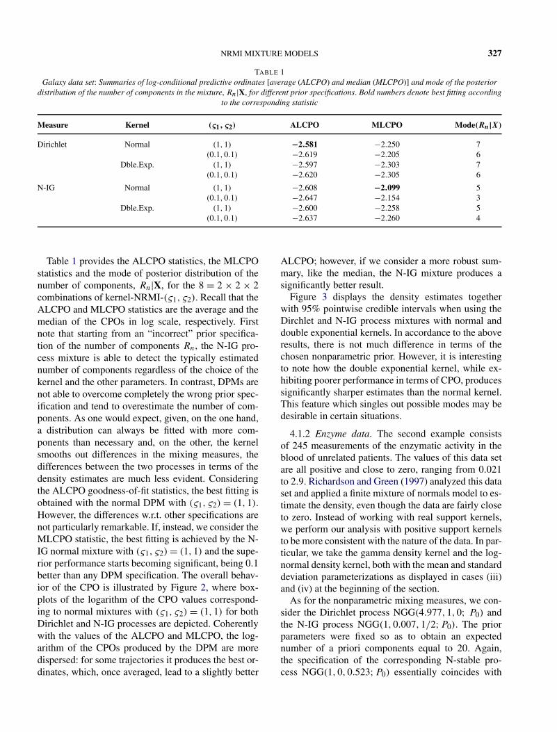
TABLE 1Galaxy data set: Summaries of log-conditional predictive ordinates [average (ALCPO) and median (MLCPO)] and mode of the posterior

distribution of the number of components in the mixture, Rn|X, for different prior specifications. Bold numbers denote best fitting accordingto the corresponding statistic

Measure Kernel (ς1,ς2) ALCPO MLCPO Mode(Rn|X)

Dirichlet Normal (1,1) −2.581 −2.250 7(0.1,0.1) −2.619 −2.205 6

Dble.Exp. (1,1) −2.597 −2.303 7(0.1,0.1) −2.620 −2.305 6

N-IG Normal (1,1) −2.608 −2.099 5(0.1,0.1) −2.647 −2.154 3

Dble.Exp. (1,1) −2.600 −2.258 5(0.1,0.1) −2.637 −2.260 4

Table 1 provides the ALCPO statistics, the MLCPOstatistics and the mode of posterior distribution of thenumber of components, Rn|X, for the 8 = 2 × 2 × 2combinations of kernel-NRMI-(ς1,ς2). Recall that theALCPO and MLCPO statistics are the average and themedian of the CPOs in log scale, respectively. Firstnote that starting from an “incorrect” prior specifica-tion of the number of components Rn, the N-IG pro-cess mixture is able to detect the typically estimatednumber of components regardless of the choice of thekernel and the other parameters. In contrast, DPMs arenot able to overcome completely the wrong prior spec-ification and tend to overestimate the number of com-ponents. As one would expect, given, on the one hand,a distribution can always be fitted with more com-ponents than necessary and, on the other, the kernelsmooths out differences in the mixing measures, thedifferences between the two processes in terms of thedensity estimates are much less evident. Consideringthe ALCPO goodness-of-fit statistics, the best fitting isobtained with the normal DPM with (ς1,ς2) = (1,1).However, the differences w.r.t. other specifications arenot particularly remarkable. If, instead, we consider theMLCPO statistic, the best fitting is achieved by the N-IG normal mixture with (ς1,ς2) = (1,1) and the supe-rior performance starts becoming significant, being 0.1better than any DPM specification. The overall behav-ior of the CPO is illustrated by Figure 2, where box-plots of the logarithm of the CPO values correspond-ing to normal mixtures with (ς1,ς2) = (1,1) for bothDirichlet and N-IG processes are depicted. Coherentlywith the values of the ALCPO and MLCPO, the log-arithm of the CPOs produced by the DPM are moredispersed: for some trajectories it produces the best or-dinates, which, once averaged, lead to a slightly better

ALCPO; however, if we consider a more robust sum-mary, like the median, the N-IG mixture produces asignificantly better result.

Figure 3 displays the density estimates togetherwith 95% pointwise credible intervals when using theDirchlet and N-IG process mixtures with normal anddouble exponential kernels. In accordance to the aboveresults, there is not much difference in terms of thechosen nonparametric prior. However, it is interestingto note how the double exponential kernel, while ex-hibiting poorer performance in terms of CPO, producessignificantly sharper estimates than the normal kernel.This feature which singles out possible modes may bedesirable in certain situations.

4.1.2 Enzyme data. The second example consistsof 245 measurements of the enzymatic activity in theblood of unrelated patients. The values of this data setare all positive and close to zero, ranging from 0.021to 2.9. Richardson and Green (1997) analyzed this dataset and applied a finite mixture of normals model to es-timate the density, even though the data are fairly closeto zero. Instead of working with real support kernels,we perform our analysis with positive support kernelsto be more consistent with the nature of the data. In par-ticular, we take the gamma density kernel and the log-normal density kernel, both with the mean and standarddeviation parameterizations as displayed in cases (iii)and (iv) at the beginning of the section.

As for the nonparametric mixing measures, we con-sider the Dirichlet process NGG(4.977,1,0; P0) andthe N-IG process NGG(1,0.007,1/2;P0). The priorparameters were fixed so as to obtain an expectednumber of a priori components equal to 20. Again,the specification of the corresponding N-stable pro-cess NGG(1,0,0.523;P0) essentially coincides with


FIG. 2. Galaxy data set: Box-plot of the logarithm of the conditional predictive ordinates for DPM and N-IG mixtures, with normal kerneland (ς1,ς2) = (1,1).

the above N-IG process and is therefore omitted. Notethat such a value for the prior expected number of com-ponents is much larger than the typically 2 or 3 com-ponents estimated for this data set. As for the basemeasure P0, we took f 2

0 (σ |ς) = ga(σ |ς1,ς2) with twopossible sets of values for the hyperparameters, thatis, (ς1,ς2) = (4,1) and (ς1,ς2) = (0.5,0.5). More-over, for µ the gamma specification in (b) is adoptedwith a vaguely informative hyperprior on the scale,namely, ψ1 = ψ2 = 0.01. We remark that, as in theprevious example, these choices give rise to base mea-sures that are not conjugate for the kernel. The Gibbssampler was run for 20,000 iterations with a burn-inof 2000 sweeps, keeping one simulation of every 4th,ending up with 4500 iterations to compute the esti-mates.

Table 2 provides the ALCPO statistics, the MLCPOstatistics and the mode of the posterior distribution ofthe number of components for the 8 = 2×2×2 combi-nations of kernel-NRMI-(ς1,ς2), respectively. Let usfirst focus on the estimated number of components.In this case, starting from a “strongly incorrect” priorspecification of the number of components, the abil-ity of N-IG mixtures to overcome misspecifications

becomes even more apparent. Indeed, it can be seenthat the N-IG mixture estimates at least 3 fewer com-ponents than the DPM, for any choice of the kernelsand of the base measures hyperparameters. Having es-tablished the better performance of the N-IG mixtures,we have a closer look at the impact of the kernels andhyperparameter specifications in Figure 4. We displaythe corresponding complete posterior distributions ofthe number of components. The gamma kernel dis-plays a better performance in locating the number ofcomponents with, additionally, a lower variability, re-gardless of the hyperparameters choice. With respectto the choice of hyperparameters in the distribution ofσ , the ones generating larger values with higher vari-ability are superior. When looking at the density esti-mates the differences are, as in the previous example,less apparent. In terms of the ALCPO goodness-of-fitstatistics, the best fitting is obtained through the DPMwith lognormal kernel and (ς1,ς2) = (0.5,0.5), but thedifferences with respect to the other specifications areminimal. Nonetheless, it is worth pointing out that thiscorresponds to the case which has the worst behavior interms of estimation of the number of components. Onthe one side, this confirms that using more componentsthan necessary does not impact the fit in terms of den-


FIG. 3. Galaxy data set: Posterior density estimates with (ς1,ς2) = (1,1) corresponding to the DPM (top row) and the N-IG mixture(bottom row) with normal kernel (left column) and double exponential kernel (right column).

sity estimation. On the other hand, it represents an indi-cation that goodness-of-fit summaries have to be han-dled with some care to understand the numerical out-put. If we consider the MLCPO statistic, the best fittingis achieved by the model one would actually expect onthe basis of the analysis of the posterior distributionof the number of components, namely, the N-IG pro-cess mixture with gamma kernel and (ς1,ς2) = (4,1).Moreover, its superiority is quite significant w.r.t. allother specifications. This enforces our previous com-

ment concerning the care needed in drawing conclu-sions from numerical summaries of the fit.

4.2 Simulation Study

We now provide an extensive simulation studyand use it also for comparing the performance ofNRMI mixtures with other density estimation meth-ods. Marron and Wand (1992) considered a set of 15densities with different behaviors, which are challeng-ing to estimate. These densities are either unimodal,


TABLE 2Enzyme data set: Summaries of log-conditional predictive ordinates [average (ALCPO) and median (MLCPO)] and mode of the posterior

distribution of the number of components in the mixture, Rn|X, for different prior specifications. Bold numbers denote best fitting accordingto the corresponding statistic

Measure Kernel (ς1,ς2) ALCPO MLCPO Mode(Rn|X)

Dirichlet Gamma (4,1) −0.227 0.204 5(0.5,0.5) −0.218 0.126 13

Log.N. (4,1) −0.216 0.054 8(0.5,0.5) −0.205 0.006 14

N-IG Gamma (4,1) −0.217 0.275 2(0.5,0.5) −0.213 0.233 5

Log.N. (4,1) −0.210 0.065 5(0.5,0.5) −0.208 0.048 8

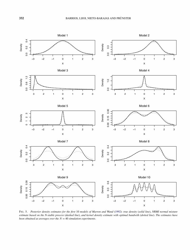
multimodal, symmetric and/or skewed. According toMarron and Wand (1992), the last 5 densities arestrongly multimodal and are difficult to recover withmoderate sample sizes. Therefore, we concentrate ontheir first 10 densities to test the performance of NRMImixtures. For each of the 10 models, the simulationstudy was based on N = 40 simulation experimentsand for each experiment a sample of size n = 250 wasdrawn from the model.

We considered NRMI mixtures with a normal ker-nel (i) and a N-stable process NGG(1,0,0.396;P0)

as mixing measure. This choice of the parameter γ =0.396 implies that the a priori expected number ofcomponents is equal to 10, which seems a reasonabledefault choice. As for the base measure P0, we tookf 2

0 (σ |ς) = ga(σ |1,1), whereas for µ we adopted thenormal specification in (a). As for the latter, the hy-perparameters of the normal-gamma prior on (ϕ1,ϕ2)are ψ1 = 0, ψ2 = 0.01, ψ3 = 0.1 and ψ4 = 0.1. It isimportant to note that these prior specifications werethe same for all 10 models and, hence, all experi-ments: the idea is to verify its performance as a de-fault choice rather than tailoring the model on eachspecific example. As we mentioned at the beginning ofthe section, since these are simulation experiments, onecan compute the relative mean integrated squared error(RMISE) as a measure of goodness of fit. As bench-marking nonparametric kernel density estimator, w.r.t.which the RMISE is computed, we considered the op-timal bandwidth given in Silverman (1986) which isσ = s2(1.06)2n−2/5, with s2 being the sample vari-ance. For each case the Gibbs sampler was run for10,000 iterations with a burn-in of 1000 sweeps andone simulation every 4th was taken for computing theestimates.

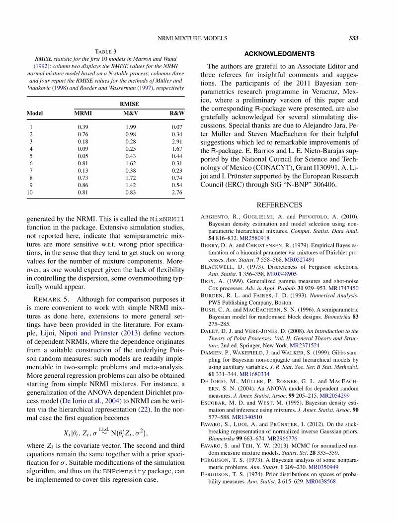
Table 3 summarizes the results in terms of RMISE.For comparison purposes we have also included theRMISE obtained by Müller and Vidakovic (1998) us-ing Bayesian wavelets and those obtained by Roederand Wasserman (1997) using finite mixture of normals.In a private communication, Müller and Vidakovic in-formed us of a minor problem with the RMISE valuesoriginally reported in Müller and Vidakovic (1998): thevalues in Table 3 are the correct ones obtained fromtheir model. Figure 5 displays the true density (solidline) and the estimated densities resulting from ourNRMI mixture (dashed line) and the kernel density es-timates with optimal bandwith (dotted line) for models1–10. The numbers reported in Table 3 and the densityestimates in Figure 5 are averages over the 40 experi-ments.

From Table 3 we can observe that the approach ofRoeder and Wasserman (1997) improves on the kerneldensity estimator in 7 of the 10 models. In particular,they fail to provide a good fit for those densities that arequite spiky (models 3, 4 and 10). Also, the wavelets ap-proach of Müller and Vidakovic (1998) have the bestbehavior precisely for these spiky models producingthe smallest RMISE. The NRMI normal mixtures per-forms significantly better than the kernel density esti-mator in all 10 models, the highest RMISE being 0.86.This is also apparent in Figure 5. Moreover, it reachesthe smallest RMISE in 6 of the 10 models comparedto all its competitors. However, rather than focusing onbest performances, it is important to stress that the es-timates yielded by the approaches of R&W and M&Vare, in some cases, significantly worse than the kerneldensity estimator. Hence, NRMI mixtures give the best


FIG. 4. Enzyme data set: Posterior distribution for the number of components, Rn|X, for the N-IG process mixture: gamma kernel (toprow) and log-normal kernel (bottom row) with (ς1,ς2) = (4,1) (left column) and (ς1,ς2) = (0.5,0,5) (right column).

result in 6 cases (models 3–5, 7, 8 and 10), but, moreimportantly, yield at least second-best results in all theother cases and there is always quite some gap betweenits RMISE and the one of the worse estimate. In sum-mary, the flexibility of the NRMI mixtures makes it avaluable alternative to more standard methods. In par-ticular, the N-stable mixtures could be considered as adefault model, which works reasonably well regardlessof whether the density is unimodal, multimodal, spikyor flat.

REMARK 4. NRMI mixtures with nonparametricspecification of both location and scale parametersconsidered in this section correspond to the MixN-RMI2 function in the R-package BNPdensity. Ad-ditionally, the package also includes semi-parametricNRMI mixtures, in which the location and the scaleare modeled, respectively, according to an NRMI anda parametric distribution. Such a specification corre-sponds to a common value of the smoothing parame-ter σ for all mixture components and to locations µj ’s


FIG. 5. Posterior density estimates for the first 10 models of Marron and Wand (1992): true density (solid line), NRMI normal mixtureestimate based on the N-stable process (dashed line), and kernel density estimate with optimal bandwith (dotted line). The estimates havebeen obtained as averages over the N = 40 simulation experiments.


TABLE 3RMISE statistic for the first 10 models in Marron and Wand(1992): column two displays the RMISE values for the NRMI

normal mixture model based on a N-stable process; columns threeand four report the RMISE values for the methods of Müller and

Vidakovic (1998) and Roeder and Wasserman (1997), respectively

RMISE

Model MRMI M&V R&W

1 0.39 1.99 0.072 0.76 0.98 0.343 0.18 0.28 2.914 0.09 0.25 1.675 0.05 0.43 0.446 0.81 1.62 0.317 0.13 0.38 0.238 0.73 1.72 0.749 0.86 1.42 0.54

10 0.81 0.83 2.76

generated by the NRMI. This is called the MixNRMI1function in the package. Extensive simulation studies,not reported here, indicate that semiparametric mix-tures are more sensitive w.r.t. wrong prior specifica-tions, in the sense that they tend to get stuck on wrongvalues for the number of mixture components. More-over, as one would expect given the lack of flexibilityin controlling the dispersion, some oversmoothing typ-ically would appear.

REMARK 5. Although for comparison purposes itis more convenient to work with simple NRMI mix-tures as done here, extensions to more general set-tings have been provided in the literature. For exam-ple, Lijoi, Nipoti and Prünster (2013) define vectorsof dependent NRMIs, where the dependence originatesfrom a suitable construction of the underlying Pois-son random measures: such models are readily imple-mentable in two-sample problems and meta-analysis.More general regression problems can also be obtainedstarting from simple NRMI mixtures. For instance, ageneralization of the ANOVA dependent Dirichlet pro-cess model (De Iorio et al., 2004) to NRMI can be writ-ten via the hierarchical representation (22). In the nor-mal case the first equation becomes

Xi |θi ,Zi,σi.i.d.∼ N

'θ ′iZi,σ

2),

where Zi is the covariate vector. The second and thirdequations remain the same together with a prior speci-fication for σ . Suitable modifications of the simulationalgorithm, and thus on the BNPdensity package, canbe implemented to cover this regression case.

ACKNOWLEDGMENTS

The authors are grateful to an Associate Editor andthree referees for insightful comments and sugges-tions. The participants of the 2011 Bayesian non-parametrics research programme in Veracruz, Mex-ico, where a preliminary version of this paper andthe corresponding R-package were presented, are alsogratefully acknowledged for several stimulating dis-cussions. Special thanks are due to Alejandro Jara, Pe-ter Müller and Steven MacEachern for their helpfulsuggestions which led to remarkable improvements ofthe R-package. E. Barrios and L. E. Nieto-Barajas sup-ported by the National Council for Science and Tech-nology of Mexico (CONACYT), Grant I130991. A. Li-joi and I. Prünster supported by the European ResearchCouncil (ERC) through StG “N-BNP” 306406.

REFERENCES

ARGIENTO, R., GUGLIELMI, A. and PIEVATOLO, A. (2010).Bayesian density estimation and model selection using non-parametric hierarchical mixtures. Comput. Statist. Data Anal.54 816–832. MR2580918

BERRY, D. A. and CHRISTENSEN, R. (1979). Empirical Bayes es-timation of a binomial parameter via mixtures of Dirichlet pro-cesses. Ann. Statist. 7 558–568. MR0527491

BLACKWELL, D. (1973). Discreteness of Ferguson selections.Ann. Statist. 1 356–358. MR0348905

BRIX, A. (1999). Generalized gamma measures and shot-noiseCox processes. Adv. in Appl. Probab. 31 929–953. MR1747450

BURDEN, R. L. and FAIRES, J. D. (1993). Numerical Analysis.PWS Publishing Company, Boston.

BUSH, C. A. and MACEACHERN, S. N. (1996). A semiparametricBayesian model for randomised block designs. Biometrika 83275–285.

DALEY, D. J. and VERE-JONES, D. (2008). An Introduction to theTheory of Point Processes. Vol. II, General Theory and Struc-ture, 2nd ed. Springer, New York. MR2371524

DAMIEN, P., WAKEFIELD, J. and WALKER, S. (1999). Gibbs sam-pling for Bayesian non-conjugate and hierarchical models byusing auxiliary variables. J. R. Stat. Soc. Ser. B Stat. Methodol.61 331–344. MR1680334

DE IORIO, M., MÜLLER, P., ROSNER, G. L. and MACEACH-ERN, S. N. (2004). An ANOVA model for dependent randommeasures. J. Amer. Statist. Assoc. 99 205–215. MR2054299

ESCOBAR, M. D. and WEST, M. (1995). Bayesian density esti-mation and inference using mixtures. J. Amer. Statist. Assoc. 90577–588. MR1340510

FAVARO, S., LIJOI, A. and PRÜNSTER, I. (2012). On the stick-breaking representation of normalized inverse Gaussian priors.Biometrika 99 663–674. MR2966776

FAVARO, S. and TEH, Y. W. (2013). MCMC for normalized ran-dom measure mixture models. Statist. Sci. 28 335–359.

FERGUSON, T. S. (1973). A Bayesian analysis of some nonpara-metric problems. Ann. Statist. 1 209–230. MR0350949

FERGUSON, T. S. (1974). Prior distributions on spaces of proba-bility measures. Ann. Statist. 2 615–629. MR0438568

http://www.ams.org/mathscinet-getitem?mr=2580918












FERGUSON, T. S. (1983). Bayesian density estimation by mixturesof normal distributions. In Recent Advances in Statistics 287–302. Academic Press, New York. MR0736538

FERGUSON, T. S. and KLASS, M. J. (1972). A representationof independent increment processes without Gaussian compo-nents. Ann. Math. Statist. 43 1634–1643. MR0373022

GELFAND, A. E., DEY, D. K. and CHANG, H. (1992). Model de-termination using predictive distributions with implementationvia sampling-based methods. In Bayesian Statistics 4 147–167.Oxford Univ. Press, New York. MR1380275

ISHWARAN, H. and JAMES, L. F. (2001). Gibbs sampling methodsfor stick-breaking priors. J. Amer. Statist. Assoc. 96 161–173.MR1952729

JAMES, L. F., LIJOI, A. and PRÜNSTER, I. (2006). Conjugacy asa distinctive feature of the Dirichlet process. Scand. J. Stat. 33105–120. MR2255112

JAMES, L. F., LIJOI, A. and PRÜNSTER, I. (2009). Posterior anal-ysis for normalized random measures with independent incre-ments. Scand. J. Stat. 36 76–97. MR2508332

KINGMAN, J. F. C. (1967). Completely random measures. PacificJ. Math. 21 59–78. MR0210185

KINGMAN, J. F. C. (1975). Random discrete distribution. J. Roy.Statist. Soc. Ser. B 37 1–22.

KINGMAN, J. F. C. (1993). Poisson Processes. Oxford Studies inProbability 3. Oxford Univ. Press, New York. MR1207584

LIJOI, A., MENA, R. H. and PRÜNSTER, I. (2005). Hierarchi-cal mixture modeling with normalized inverse-Gaussian priors.J. Amer. Statist. Assoc. 100 1278–1291. MR2236441

LIJOI, A., MENA, R. H. and PRÜNSTER, I. (2007). Controllingthe reinforcement in Bayesian non-parametric mixture models.J. R. Stat. Soc. Ser. B Stat. Methodol. 69 715–740. MR2370077

LIJOI, A. and PRÜNSTER, I. (2010). Models beyond the Dirich-let process. In Bayesian Nonparametrics (N. L. Hjort, C. C.Holmes, P. Müller and S. G. Walker, eds.) 80–136. CambridgeUniv. Press, Cambridge. MR2730661

LIJOI, A., NIPOTI, B. and PRÜNSTER, I. (2013). Bayesian infer-ence with dependent normalized completely random measures.Bernoulli. To appear. DOI:10.3150/13-BEJ521.

LO, A. Y. (1984). On a class of Bayesian nonparametric estimates.I. Density estimates. Ann. Statist. 12 351–357. MR0733519

MACEACHERN, S. N. and MÜLLER, P. (1998). Estimating mix-tures of Dirichlet process models. J. Comput. Graph. Statist. 7223–238.

MACEACHERN, S. and MÜLLER, P. (2000). Efficient MCMCschemes for robust model extensions using encompassingDirichlet process mixture models. In Robust Bayesian Analy-sis. Lecture Notes in Statist. 152 295–315. Springer, New York.MR1795222

MARRON, J. S. and WAND, M. P. (1992). Exact mean integratedsquared error. Ann. Statist. 20 712–736. MR1165589

MULIERE, P. and TARDELLA, L. (1998). Approximating distri-butions of random functionals of Ferguson–Dirichlet priors.Canad. J. Statist. 26 283–297. MR1648431

MÜLLER, P. and QUINTANA, F. A. (2004). NonparametricBayesian data analysis. Statist. Sci. 19 95–110. MR2082149

MÜLLER, P. and VIDAKOVIC, B. (1998). Bayesian inference withwavelets: Density estimation. J. Comput. Graph. Statist. 7 456–468.

NIETO-BARAJAS, L. E., PRÜNSTER, I. and WALKER, S. G.(2004). Normalized random measures driven by increasing ad-ditive processes. Ann. Statist. 32 2343–2360. MR2153987

NIETO-BARAJAS, L. E. and PRÜNSTER, I. (2009). A sensitivityanalysis for Bayesian nonparametric density estimators. Statist.Sinica 19 685–705. MR2514182

ORBANZ, P. and WILLIAMSON, S. (2011). Unit–rate Poisson rep-resentations of completely random measures. Technical report.

PAPASPILIOPOULOS, O. and ROBERTS, G. O. (2008). Retrospec-tive Markov chain Monte Carlo methods for Dirichlet processhierarchical models. Biometrika 95 169–186. MR2409721

PITMAN, J. (2003). Poisson–Kingman partitions. In Statistics andScience: A Festschrift for Terry Speed (D. R. Goldstein, ed.).Institute of Mathematical Statistics Lecture Notes—MonographSeries 40 1–34. IMS, Beachwood, OH. MR2004330

REGAZZINI, E., LIJOI, A. and PRÜNSTER, I. (2003). Distribu-tional results for means of normalized random measures withindependent increments. Ann. Statist. 31 560–585. MR1983542

RICHARDSON, S. and GREEN, P. J. (1997). On Bayesian analysisof mixtures with an unknown number of components. J. Roy.Statist. Soc. Ser. B 59 731–792. MR1483213

ROEDER, K. and WASSERMAN, L. (1997). Practical Bayesiandensity estimation using mixtures of normals. J. Amer. Statist.Assoc. 92 894–902. MR1482121

SATO, K. (1990). Lévy Processes and Infinitely Divisible Distribu-tions. Cambridge Univ. Press, Cambridge.

SETHURAMAN, J. (1994). A constructive definition of Dirichletpriors. Statist. Sinica 4 639–650. MR1309433

SILVERMAN, B. W. (1986). Density Estimation for Statistics andData Analysis. Chapman & Hall, London. MR0848134

TIERNEY, L. (1994). Markov chains for exploring posterior distri-butions. Ann. Statist. 22 1701–1762. MR1329166

WALKER, S. G. (2007). Sampling the Dirichlet mixture modelwith slices. Comm. Statist. Simulation Comput. 36 45–54.MR2370888

WALKER, S. and DAMIEN, P. (2000). Representations of Lévyprocesses without Gaussian components. Biometrika 87 477–483. MR1782492

WOLPERT, R. L. and ICKSTADT, K. (1998). Poisson/gamma ran-dom field models for spatial statistics. Biometrika 85 251–267.MR1649114












http://dx.doi.org/10.3150/13-BEJ521



















Documents

Modeling with Normalized Random Measure Mixture …economia.unipv.it/pagp/pagine_personali/alijoi/Publications_files/... · 2013, Vol. 28, No. 3, 313–334 DOI: 10.1214/13-STS416