Bayesian nonparametric estimators derived from …economia.unipv.it/alijoi/Publications_files/10_AoAP2008_bis.pdf · The Appendix contains a short review of generalized factorial

The Annals of Applied Probability2008, Vol. 18, No. 4, 1519–1547DOI: 10.1214/07-AAP495© Institute of Mathematical Statistics, 2008

BAYESIAN NONPARAMETRIC ESTIMATORS DERIVED FROMCONDITIONAL GIBBS STRUCTURES

BY ANTONIO LIJOI,1 IGOR PRÜNSTER2 AND STEPHEN G. WALKER

Università degli Studi di Pavia, Università degli Studi di Torinoand University of Kent

We consider discrete nonparametric priors which induce Gibbs-type ex-changeable random partitions and investigate their posterior behavior in de-tail. In particular, we deduce conditional distributions and the correspondingBayesian nonparametric estimators, which can be readily exploited for pre-dicting various features of additional samples. The results provide useful toolsfor genomic applications where prediction of future outcomes is required.

1. Introduction. Random partitions and their associated probability distribu-tions play an important role in a variety of research areas. In population genetics,for example, models for random partitions are useful in order to describe the allo-cation of a sample of n genes into a number of distinct alleles. See, for example,[10, 33]. In machine learning theory, probabilistic models for linguistic applica-tions (such as, e.g., speech and handwriting recognition, machine translation) areoften based on a suitable clustering structure for a set of words. See, for example,[34, 35]. In Bayesian nonparametric inference, a discrete nonparametric prior iscommonly employed in complex hierarchical mixture models and it induces anexchangeable random partition for the latent variables: this provides an effectivetool for inferring on the clustering structure of the observations. Such an approachis due to [21] and has been extended in various directions. See, for example, [12,13, 19, 22]. Other important areas of applications include storage problems, ex-cursion theory, combinatorics and statistical physics. See the comprehensive andstimulating monograph by Pitman [29] and references therein.

An early and well-known model which describes the grouping of n objects intok distinct classes is due to [7] and leads to the Ewens sampling formula. The ba-sic assumption is that individuals are sequentially sampled from an infinite setof different species and the proportion pi with which the ith species is presentin the population is random. Then, if (Wk)k≥1 is a sequence of independent and

Received May 2007; revised September 2007.1Also affiliated with CNR-IMATI, Milan, Italy. Supported by MiUR, Grant 2006/134525.2Also affiliated with Collegio Carlo Alberto and ICER, Turin, Italy. Supported by MiUR, Grant

2006/133449.AMS 2000 subject classifications. 62G05, 62F15, 60G57.Key words and phrases. Bayesian nonparametrics, Dirichlet process, exchangeable random par-

titions, generalized factorial coefficients, generalized gamma process, population genetics, speciessampling models, two parameter Poisson–Dirichlet process.

1519

http://www.imstat.org/aap/

http://dx.doi.org/10.1214/07-AAP495

http://www.imstat.org

http://www.ams.org/msc/

1520 A. LIJOI, I. PRÜNSTER AND S. G. WALKER

identically distributed random variables with Beta(1, θ) distribution, the randomproportions are defined as

p1 = W1, pj = Wj

j−1∏k=1

(1 − Wk) ∀j ≥ 2.(1)

Now, if X1, . . . ,Xn is a sample of n individuals drawn from the population, setMn := (M1,n, . . . ,Mn,n) where Mj,n is the number of species represented j timesin the sample of size n. Hence, the distribution of Mn is supported by all thosevectors mn = (m1,n, . . . ,mn,n) for which

∑ni=1 imi,n = n. The Ewens sampling

formula provides the probability distribution of the random vector Mn under (1)and it coincides with

Pr[Mn = mn] = n!(θ)n

n∏j=1

θmj,n

jmj,nmj,n!(2)

where (θ)n = θ(θ + 1) · · · (θ + n − 1) for any θ > 0. We also agree on set-ting (θ)0 := 1. See also [2] for a derivation of (2). Obviously, to the distribu-tion of Mn there corresponds a distribution of the vector (Kn,Nn) where Kn isthe number of distinct species detected among the n observations in the sampleand Nn = (N1,n, . . . ,NKn,n) is the vector of frequencies with which each dis-tinct species is observed. Such a correspondence is one-to-one and, conditionalon Kn, the distribution of Nn, is supported on the set �n,Kn := {(n1, . . . , nKn

) ∈{1, . . . , n}Kn :

∑Kn

j=1 nj = n}. In particular, for the Ewens sampling formula (2)there corresponds the probability distribution

Pr[Kn = k,Nn = (n1, . . . , nKn)] = θk

(θ)n

k∏j=1

(nj − 1)!(3)

for any k ∈ {1, . . . , n} and (n1, . . . , nk) ∈ �n,k . The parameter θ , in genetic ap-plications, is interpreted as the mutation rate of each gene into new allelic types.Formula (3) has a further interesting combinatorial interpretation. If θ is a positiveinteger, then θk ∏k

j=1(nj −1)! is the number of colored permutations of {1, . . . , n}into k cycles with respective lengths n1, . . . , nk , each cycle being labeled by any ofthe θ available colors. Accordingly, (3) is the probability distribution of a randompermutation with colored cycles. See [3, 29] for exhaustive accounts on the Ewenssampling formula.

The distribution of the vector (Kn,Nn) takes on the name of exchangeable par-tition probability function (EPPF), a notion introduced by Pitman in [26] and fur-ther studied in a series of subsequent papers; see [29] and references therein. Themain object of investigation of the present paper is a family of EPPFs, introducedand thoroughly investigated in [9], which generalize the Ewens sampling scheme.Our aim is to establish distributional properties of such EPPFs which allow, givena sample, to make predictions according to a Bayesian nonparametric procedure.

CONDITIONAL GIBBS STRUCTURES 1521

The concrete motivation for this study is provided by the straightforward applica-bility of the results to inference in genetic experiments. As a matter of fact, an im-portant setting where our findings can be usefully applied relates to gene detectionin expressed sequence tags (EST) experiments. ESTs are produced by sequencingrandomly selected cDNA clones from a cDNA library. Given an initial EST dataset of size n, one is interested in the prediction of the outcomes of further samplingfrom the library. For instance, interest lies in the estimation of the number of newunique genes in a possible additional sample of size m: nonparametric frequentistestimators, however, yield completely unstable estimates when m > 2n. See [25]for a discussion of this phenomenon. In contrast, for the corresponding Bayesiannonparametric estimators proposed in [20], and based on Gibbs partitions, the rel-ative dimension of m with respect to n is not an issue. Indeed, we will show thatthe EPPF, whenever analytically available, yields straightforward and coherent an-swers to this and other related prediction problems.

In Section 2 we recall the concepts of exchangeable random partition and EPPFand the definition of the class of exchangeable Gibbs random partitions. In Sec-tion 3 we derive distributional results for the corresponding EPPFs conditionallyon a sample: we obtain expressions for the predictive distribution of future ob-servations given the past, then focus on the probability distribution of the randompartition restricted to those observations yielding new distinct species in the futuresample and, finally, face the problem of determining the probability that specificobserved species will not appear in the future sample. In Section 4 we illustratehow our results can be applied in the context of EST analysis of cDNA libraries.The Appendix contains a short review of generalized factorial coefficients and theproofs.

2. Exchangeable Gibbs random partitions. A random partition of the set ofnatural numbers N is defined as a consistent sequence � = {�n}∞n=1 of randomelements, with �n taking values in the set of all partitions of [n] := {1, . . . , n}into some number of disjoint nonempty blocks. Consistency in this setting impliesthat each �n is obtained from �n+1 by discarding the integer n + 1. A randompartition � is exchangeable if, for each n, the probability distribution of �n isinvariant under all permutations of (1, . . . , n). To be more precise, let {Aj }kj=1denote a partition of the set [n], and let the Aj ’s be indexed by [k] in order of theirleast elements. In order to describe the property of exchangeability for � let usintroduce a sequence of functions �

(n)k : �n,k → R+ such that:

(i) �(1)1 (1) = 1;

(ii) for any (n1, . . . , nk) ∈ �n,k , k ∈ {1, . . . , n} and n ≥ 1 one has

�(n)k (n1, . . . , nk) = �

(n)k

(nρ(1), . . . , nρ(k)

)where ρ is an arbitrary permutation of the indices (1, . . . , k);


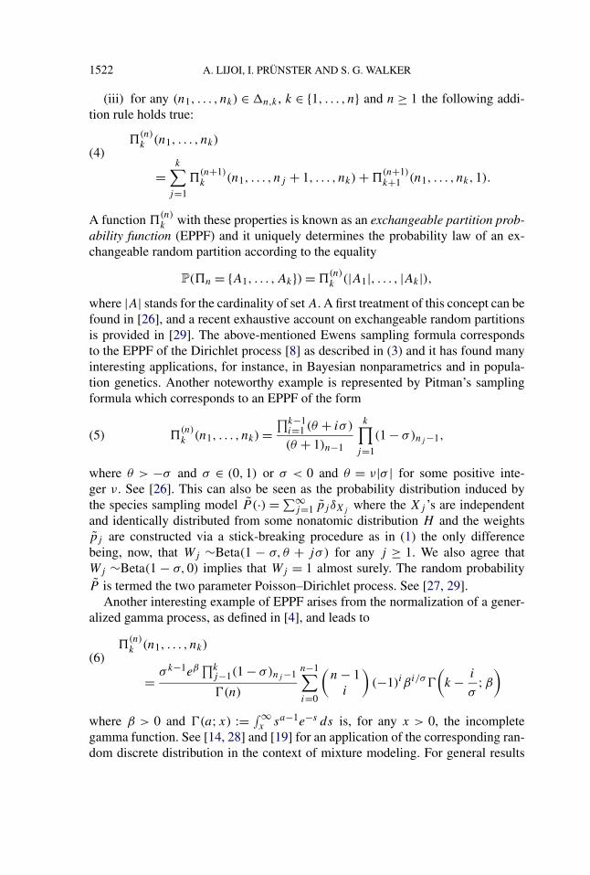
(iii) for any (n1, . . . , nk) ∈ �n,k , k ∈ {1, . . . , n} and n ≥ 1 the following addi-tion rule holds true:

�(n)k (n1, . . . , nk)

(4)

=k∑

j=1

�(n+1)k (n1, . . . , nj + 1, . . . , nk) + �

(n+1)k+1 (n1, . . . , nk,1).

A function �(n)k with these properties is known as an exchangeable partition prob-

ability function (EPPF) and it uniquely determines the probability law of an ex-changeable random partition according to the equality

P(�n = {A1, . . . ,Ak}) = �(n)k (|A1|, . . . , |Ak|),

where |A| stands for the cardinality of set A. A first treatment of this concept can befound in [26], and a recent exhaustive account on exchangeable random partitionsis provided in [29]. The above-mentioned Ewens sampling formula correspondsto the EPPF of the Dirichlet process [8] as described in (3) and it has found manyinteresting applications, for instance, in Bayesian nonparametrics and in popula-tion genetics. Another noteworthy example is represented by Pitman’s samplingformula which corresponds to an EPPF of the form

�(n)k (n1, . . . , nk) =

∏k−1i=1 (θ + iσ )

(θ + 1)n−1

k∏j=1

(1 − σ)nj−1,(5)

where θ > −σ and σ ∈ (0,1) or σ < 0 and θ = ν|σ | for some positive inte-ger ν. See [26]. This can also be seen as the probability distribution induced bythe species sampling model P (·) = ∑∞

j=1 pj δXjwhere the Xj ’s are independent

and identically distributed from some nonatomic distribution H and the weightspj are constructed via a stick-breaking procedure as in (1) the only differencebeing, now, that Wj ∼Beta(1 − σ, θ + jσ ) for any j ≥ 1. We also agree thatWj ∼Beta(1 − σ,0) implies that Wj = 1 almost surely. The random probabilityP is termed the two parameter Poisson–Dirichlet process. See [27, 29].

Another interesting example of EPPF arises from the normalization of a gener-alized gamma process, as defined in [4], and leads to

�(n)k (n1, . . . , nk)

(6)

= σk−1eβ ∏kj−1(1 − σ)nj−1

(n)

n−1∑i=0

(n − 1

i

)(−1)iβi/σ

(k − i

σ;β

)

where β > 0 and (a;x) := ∫ ∞x sa−1e−s ds is, for any x > 0, the incomplete

gamma function. See [14, 28] and [19] for an application of the corresponding ran-dom discrete distribution in the context of mixture modeling. For general results


concerning random probability measures derived via normalization procedures see[15–17, 28, 31].

The examples we have briefly illustrated so far share a common structure. In-deed, one may note that each EPPF in (3), (5) and (6) arises as a product of twofactors: the first one depends only on (n, k) and the second one depends on thefrequencies (n1, . . . , nk) via the product

∏kj=1(1 − σ)nj−1. This structure is the

main ingredient for defining a general family of exchangeable random partitions,namely the Gibbs-type random partitions.

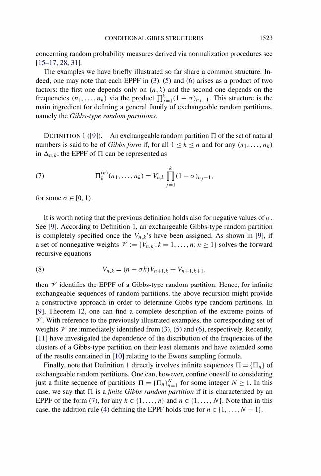
DEFINITION 1 ([9]). An exchangeable random partition � of the set of naturalnumbers is said to be of Gibbs form if, for all 1 ≤ k ≤ n and for any (n1, . . . , nk)

in �n,k , the EPPF of � can be represented as

�(n)k (n1, . . . , nk) = Vn,k

k∏j=1

(1 − σ)nj−1,(7)

for some σ ∈ [0,1).

It is worth noting that the previous definition holds also for negative values of σ .See [9]. According to Definition 1, an exchangeable Gibbs-type random partitionis completely specified once the Vn,k’s have been assigned. As shown in [9], ifa set of nonnegative weights V := {Vn,k :k = 1, . . . , n;n ≥ 1} solves the forwardrecursive equations

Vn,k = (n − σk)Vn+1,k + Vn+1,k+1,(8)

then V identifies the EPPF of a Gibbs-type random partition. Hence, for infiniteexchangeable sequences of random partitions, the above recursion might providea constructive approach in order to determine Gibbs-type random partitions. In[9], Theorem 12, one can find a complete description of the extreme points ofV . With reference to the previously illustrated examples, the corresponding set ofweights V are immediately identified from (3), (5) and (6), respectively. Recently,[11] have investigated the dependence of the distribution of the frequencies of theclusters of a Gibbs-type partition on their least elements and have extended someof the results contained in [10] relating to the Ewens sampling formula.

Finally, note that Definition 1 directly involves infinite sequences � = {�n} ofexchangeable random partitions. One can, however, confine oneself to consideringjust a finite sequence of partitions � = {�n}Nn=1 for some integer N ≥ 1. In thiscase, we say that � is a finite Gibbs random partition if it is characterized by anEPPF of the form (7), for any k ∈ {1, . . . , n} and n ∈ {1, . . . ,N}. Note that in thiscase, the addition rule (4) defining the EPPF holds true for n ∈ {1, . . . ,N − 1}.


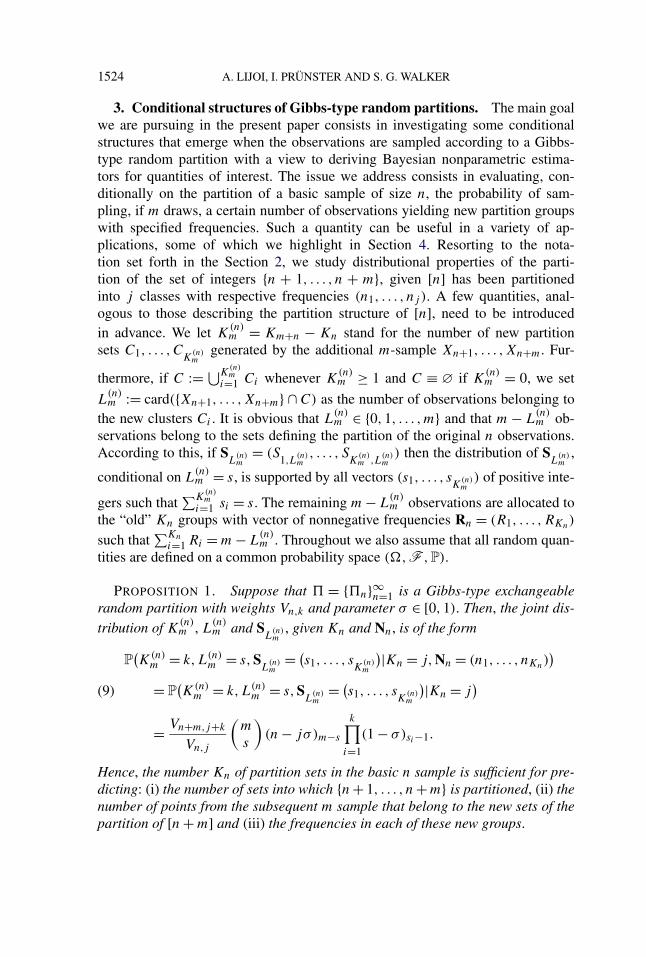
3. Conditional structures of Gibbs-type random partitions. The main goalwe are pursuing in the present paper consists in investigating some conditionalstructures that emerge when the observations are sampled according to a Gibbs-type random partition with a view to deriving Bayesian nonparametric estima-tors for quantities of interest. The issue we address consists in evaluating, con-ditionally on the partition of a basic sample of size n, the probability of sam-pling, if m draws, a certain number of observations yielding new partition groupswith specified frequencies. Such a quantity can be useful in a variety of ap-plications, some of which we highlight in Section 4. Resorting to the nota-tion set forth in the Section 2, we study distributional properties of the parti-tion of the set of integers {n + 1, . . . , n + m}, given [n] has been partitionedinto j classes with respective frequencies (n1, . . . , nj ). A few quantities, anal-ogous to those describing the partition structure of [n], need to be introducedin advance. We let K

(n)m = Km+n − Kn stand for the number of new partition

sets C1, . . . ,CK(n)m

generated by the additional m-sample Xn+1, . . . ,Xn+m. Fur-

thermore, if C := ⋃K(n)m

i=1 Ci whenever K(n)m ≥ 1 and C ≡ ∅ if K

(n)m = 0, we set

L(n)m := card({Xn+1, . . . ,Xn+m} ∩ C) as the number of observations belonging to

the new clusters Ci . It is obvious that L(n)m ∈ {0,1, . . . ,m} and that m − L

(n)m ob-

servations belong to the sets defining the partition of the original n observations.According to this, if S

L(n)m

= (S1,L

(n)m

, . . . , SK

(n)m ,L

(n)m

) then the distribution of SL

(n)m

,

conditional on L(n)m = s, is supported by all vectors (s1, . . . , sK(n)

m) of positive inte-

gers such that∑K

(n)m

i=1 si = s. The remaining m − L(n)m observations are allocated to

the “old” Kn groups with vector of nonnegative frequencies Rn = (R1, . . . ,RKn)

such that∑Kn

i=1 Ri = m − L(n)m . Throughout we also assume that all random quan-

tities are defined on a common probability space (�,F ,P).

PROPOSITION 1. Suppose that � = {�n}∞n=1 is a Gibbs-type exchangeablerandom partition with weights Vn,k and parameter σ ∈ [0,1). Then, the joint dis-tribution of K

(n)m , L

(n)m and S

L(n)m

, given Kn and Nn, is of the form

P(K(n)

m = k,L(n)m = s,S

L(n)m

= (s1, . . . , sK(n)

m

)|Kn = j,Nn = (n1, . . . , nKn))

= P(K(n)

m = k,L(n)m = s,S

L(n)m

= (s1, . . . , sK(n)

m

)|Kn = j)

(9)

= Vn+m,j+k

Vn,j

(m

s

)(n − jσ )m−s

k∏i=1

(1 − σ)si−1.

Hence, the number Kn of partition sets in the basic n sample is sufficient for pre-dicting: (i) the number of sets into which {n + 1, . . . , n + m} is partitioned, (ii) thenumber of points from the subsequent m sample that belong to the new sets of thepartition of [n + m] and (iii) the frequencies in each of these new groups.


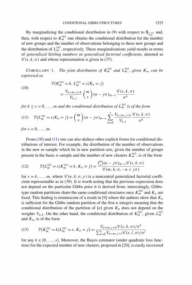
By marginalizing the conditional distribution in (9) with respect to SL

(n)m

and,

then, with respect to K(n)m one obtains the conditional distribution for the number

of new groups and the number of observations belonging to these new groups andthe distribution of L

(n)m , respectively. These marginalizations yield results in terms

of generalized Stirling numbers or generalized factorial coefficients, denoted asC (s, k, σ ) and whose representation is given in (37).

COROLLARY 1. The joint distribution of K(n)m and L

(n)m , given Kn, can be

expressed as

P(K(n)

m = k,L(n)m = s|Kn = j

)(10)

= Vn+m,j+k

Vn,j

(m

s

)(n − jσ )m−s

C (s, k, σ )

σ k

for k ≤ s = 0, . . . ,m and the conditional distribution of L(n)m is of the form

P(L(n)

m = s|Kn = j) =

(m

s

)(n − jσ )m−s

s∑k=0

Vn+m,j+k

Vn,j

C (s, k, σ )

σ k(11)

for s = 0, . . . ,m.

From (10) and (11) one can also deduce other explicit forms for conditional dis-tributions of interest. For example, the distribution of the number of observationsin the new m-sample which lie in new partition sets, given the number of groupspresent in the basic n-sample and the number of new clusters K

(n)m , is of the form

P(L(n)

m = s|K(n)m = k,Kn = j

) =(ms

)(n − jσ )m−sC (s, k, σ )

C (m, k;σ,−n + jσ )(12)

for s = k, . . . ,m, where C (n, k;σ, γ ) is a noncentral generalized factorial coeffi-cient representable as in (39). It is worth noting that the previous expression doesnot depend on the particular Gibbs prior it is derived from: interestingly, Gibbs-type random partitions share the same conditional structures once K

(n)m and Kn are

fixed. This finding is reminiscent of a result in [9] where the authors show that Kn

is sufficient for the Gibbs random partition of the first n integers meaning that theconditional distribution of the partition of [n] given Kn does not depend on theweights Vn,k . On the other hand, the conditional distribution of K

(n)m , given L

(n)m

and Kn, is of the form

P(K(n)

m = k|L(n)m = s,Kn = j

) = Vn+m,j+kC (s, k, σ )/σ k∑sl=0 Vn+m,j+lC (s, l, σ )/σ l

(13)

for any k ∈ {0, . . . , s}. Moreover, the Bayes estimator (under quadratic loss func-tion) for the expected number of new clusters, proposed in [20], is easily recovered


from (10) as

E(K(n)

m |Kn = j) =

m∑k=0

kVn+m,j+k

Vn,j

C (m, k;σ,−n + jσ )

σ k.(14)

Often interest relies also in determining an estimator for the number of observa-tions in the subsequent m-sample that will belong to new species. For instance, ingenomic applications this can be seen as a better measure of redundancy of a cer-tain library. For this purpose, one can resort to (11) and the corresponding Bayesestimator is given by

E(L(n)

m |Kn = j) =

m∑s=0

s

(m

s

)(n − jσ )m−s

s∑k=0

Vn+m,j+k

Vn,j

C (s, k, σ )

σ k.(15)

Then, E(L(n)m |Kn = j)/m is the expected proportion of genes in the new sample

which do not coincide with previously observed ones. The expression in (15) ad-mits a noteworthy simplification as outlined in the following proposition: indeed,the Bayes estimator is m times the probability that the (n+ 1)th draw yields a newcluster, given that j distinct clusters are generated by the first n observations.

PROPOSITION 2. For any j ∈ {1, . . . , n} and m ≥ 1 one has

E(L(n)

m |Kn = j) = m

Vn+1,j+1

Vn,j

.(16)

All the previous expressions are easily available for the three examples we havementioned in Section 2. We first focus our attention on the Dirichlet process whichrepresents the most well-known case. Indeed, from (3) one finds out that Vn,k =θk/(θ)n and, for instance, (9) reduces to

P(L(n)

m = s,K(n)m = k,S

L(n)m

= (s1, . . . , sK(n)

m

)|Kn = j)

(17)

= θk

(θ + n)m

(m

s

)(n)m−s

k∏i=1

(si − 1)!.

Note that simple algebra leads to rewrite the above expression as

(m

s

)(1 − n

θ + n

)k{

(θ + n)k

(θ + n)s

k∏i=1

(si − 1)!}

(n)m−s

(θ + n + s)m−s

=(

m

s

)pθ(n,m, k, s, sk)

where it can be immediately seen that the term in curly brackets on the left-handside is the sampling formula in (9) with θ +n in the place of θ being the total massparameter of the Dirichlet process conditioned on a sample of size n. Hence, the


quantity pθ(n,m, k, s, sk) can be interpreted as the probability of drawing, condi-tional on the n past observations, a specific sample of size m of which s belong tothe new k groups of the partition with vector of frequencies sk = (s1, . . . , sk) andthe other m− s coincide with any of the conditioning n observations. On the otherhand, recall that limσ→0

C (n,k,σ )

σ k = |s(n, k)| where s(·, ·) stands for the Stirlingnumber of the first kind. This allows to determine the expressions appearing in(10) and (11). Indeed, one has

P(K(n)

m = k,L(n)m = s|Kn = j

) =(

m

s

)θk(n)m−s

(θ + n)m|s(n, k)|

and, using the definition of the signless Stirling number of the first kind accordingto which

s∑i=0

θi |s(s, i)| = (θ)s(18)

(see, e.g., [6], page 2536), one has

P(L(n)

m = s|Kn = j) =

(m

s

)(n)m−s

(θ + n + s)m−s

(θ)s

(θ + n)s=

(m

s

)qθ (n,m, s)

where it is apparent that qθ (n,m, s) is the probability, conditional on a sample ofsize n, of observing a specific m-sample containing s elements not contained inthe conditioning n-sample.

REMARK 1. It is important to note that the conditional structure of the Dirich-let process does not depend on Kn: it only depends on the size of the basic samplen. This is, indeed, a characterizing property of the Dirichlet process as shown in[36]. Such a property simplifies the mathematical expressions but represents a seri-ous drawback for applications. Indeed, it is reasonable to expect that Kn influencesprediction of the clustering structure of future observations: the larger Kn the morenew clusters K

(n)m and the more observations belonging to these new clusters L

(n)m

one would expect. This is the reason which explains the interest in a more generalfamily of partition distributions such as those of Gibbs-type for which predictiondepends on Kn. Finally, it is worth recalling that the Dirichlet process can be seenas a two parameter Poisson–Dirichlet process with parameter (θ,0). Hence, whenwe deal with the Poisson–Dirichlet process in the sequel, the Dirichlet process casecan be recovered by letting σ → 0.

REMARK 2. All the quantities described up to now, and developed in the nextsubsections, depend on the analysis of the conditional structure of a Gibbs-typerandom partition. Investigation of the conditional structure for the sequence ofblocks (Kn)n≥1 is pursued in [9] where the authors do consider the conditionaldistribution of the number of groups in the partition of [n], given the number of


blocks in which [n+m] is partitioned. In our setting, where prediction is the mainfocus, we are more interested in evaluating conditional probabilities (or expecta-tions) for the partition of future observations given the partition structure of pastobservations. And we also consider other relevant quantities, besides the numberof groups. It might be that starting from the conditional characterizations providedby [9] one can derive formulae analogous to those we are now going to estab-lish, but we find our approach more direct and particularly suited to the specificprediction problems we have in mind.

3.1. The process generating new clusters. We are now going to consider animportant quantity which describes the partition structure of observations gener-ating new groups in a further sampling procedure, conditional on the partitiongenerated by the first n observations. In particular we are able to point out a sort ofreproducibility of the Gibbs structure as established by the following proposition.

PROPOSITION 3. Let � = {�n}∞n=1 be a Gibbs-type random exchange-able partition whose EPPF is characterized by the set of weights {Vn,k :k =1, . . . , n;n ≥ 1} and by the parameter σ ∈ (0,1). Then

P(K(n)

m = k,SL

(n)m

= (s1, . . . , sK(n)

m

)∣∣L(n)m = s,Kn = j,Nn = (n1, . . . , nj )

)(19)

= Vn+m,j+k∑si=0 Vn+m,j+iC (s, i, σ )/σ i

k∏i=1

(1 − σ)si−1

for any s ∈ {1, . . . ,m}, k ∈ {1, . . . , s}, j ∈ {1, . . . , n}, (n1, . . . , nj ) ∈ �n,j and(s1, . . . , sk) ∈ �s,k . Consequently the partition of the observations which belong tothe new partition sets is, conditional on the basic sample of size n, a finite Gibbs-type random partition with weights {Vs,k(m,n, j) : s = 1, . . . ,m;k = 1, . . . , s} de-fined by

Vs,k(m,n, j) = Vn+m,j+k∑si=0 Vn+m,j+i

C (s,i,σ )

σ i

(20)

and with parameter σ ∈ [0,1).

Note from (19), again, that

P(K(n)

m = k,SL

(n)m

= (s1, . . . , sK(n)

m

)∣∣L(n)m = s,Kn = j,Nn = (n1, . . . , nj )

)= P

(K(n)

m = k,SL

(n)m

= (s1, . . . , sK(n)m

)∣∣L(n)

m = s,Kn = j).

The finiteness of the random partition described by (19) is obvious, since it takesvalues on the space of all partitions of [s], with 1 ≤ s ≤ m. Moreover, the particularstructure featured by the conditional distribution in (19) motivates the followingdefinition.


DEFINITION 2. The conditional probability distribution

�(s)k (s1, . . . , sk;m,n, j)

(21):= P

(K(n)

m = k,SL

(n)m

= (s1, . . . , sK(n)

m

)∣∣L(n)m = s,Kn = j

),

with 1 ≤ s ≤ m and 1 ≤ k ≤ s, is termed conditional EPPF.

Hence, the probability distribution in (19) is a conditional EPPF giving rise to afinite Gibbs-type random partition. Even if the structure of �

(s)k (s1, . . . , sk;m,n, j)

is quite general, one might wonder whether it is possible to provide more informa-tion about its Vs,k(m,n, j) weights in some particular cases. For example, it wouldbe interesting to ascertain when Vs,k(m,n, j) does not depend on m and n, so that�

(s)k (s1, . . . , sk;m,n, j) = �

(s)k (s1, . . . , sk; j), which means that the conditional

EPPF is that corresponding to an infinite Gibbs partition. This leads us to state thefollowing:

COROLLARY 2. The conditional EPPF �(s)k (s1, . . . , sk;m,n, j) does not de-

pend directly on m and n if and only if it is determined from a two-parameterPoisson–Dirichlet random partition.

Having the conditional EPPF �(s)k at hand, one can compute some other in-

teresting conditional distributions in a straightforward way. For example, if onecombines the expression for �

(s)k with Corollary 1 it is immediate to check that

P(S

L(n)m

= (s1, . . . , sK

m(n)

)|K(n)m = k,L(n)

m = s,Kn = j)

= σk

C (s, k, σ )

k∏i=1

(1 − σ)si−1

is an expression for the conditional distribution of detecting a particular configu-ration (s1, . . . , sk) for the observations belonging to the new partition sets, giventhe number of new sets, the number of observations falling into these sets and thebasic n-sample.

All the sampling formulae we have deduced so far have important applicationsin Bayesian nonparametrics and population genetics. In Bayesian nonparametrics,random discrete distributions are commonly employed in order to define a clus-tering structure either at the level of the observations or at the level of the latentvariables in a complex hierarchical model. In particular any EPPF corresponds tosome random discrete distribution and it represents, together with all the expres-sions for the conditional distributions we have obtained, a useful tool for specifyingprior opinions on the clustering of the data. In population genetics, the concept ofconditional EPPF can be seen as follows. Given a sample of size n containing j

distinct species with absolute frequencies n1, . . . , nj , a new sample of size m is to


be drawn. Given that s of the m observations contribute to generating newly ob-served species, that is, they belong to new distinct clusters, one might be interestedin evaluating the probability that the s observations are grouped into k clusters withrespective frequencies s1, . . . , sk . The answer to such a question is provided by aconditional EPPF. The other distributions, discussed previously, provide a widerange of sampling formulae which answer similar types of problems. In the fol-lowing subsection we focus attention on some noteworthy particular cases, namelythe Poisson–Dirichlet distribution, the two-parameter Poisson–Dirichlet distribu-tion and the generalized gamma partition distribution.

3.2. Illustrative examples. We start our illustrations by considering the two-parameter Poisson–Dirichlet process due to [26]. The EPPF of this process is alsoknown as Pitman sampling formula. Basing upon Proposition 1, one has

P(K(n)

m = k,L(n)m = s,S

L(n)m

= (s1, . . . , sK(n)

m

)|Kn = j)

(22)

=∏k−1

i=0 (θ + jσ + iσ )

(θ + n)m

(m

s

)(n − jσ )m−s

k∏i=1

(1 − σ)si−1

and it is possible to derive explicit expressions for all the sampling formulae setforth in Section 2. First note that from properties of generalized factorial coeffi-cients, one has

s∑k=0

Vn+m,j+k

C (s, k, σ )

σ k= σ j

(θ + n)m

σ∑k=0

(θ

σ

)j+k

C (s, k, σ )

=∏j−1

i=0 (θ + iσ )

(θ + n)m

σ∑k=0

(θ

σ+ j

)k

C (s, k, σ )

=∏j−1

i=0 (θ + iσ )

(θ + n)m(θ + jσ )s

= Vn+m,j (θ + jσ )s.

According to this equality, from (11) one has

P[L(n)

m = s|Kn = j] = 1

(θ + n)m

(m

s

)(n − jσ )m−s(θ + jσ )s.(23)

Now, (23) yields an estimate for the expected number of observations which donot coincide with the previously observed ones which, by virtue of Proposition 2,coincides with

E[L(n)

m |Kn = j] = m(θ + jσ )

θ + n.(24)


Consider now the conditional EPPF in (19), which is associated to the processgenerating the new clusters as explained in Section 3.1. We know by Corollary 2that in the two-parameter Poisson–Dirichlet case the Vs,k(m,n, j) weights do notdepend on m and n. Their specific form is easily seen to be

Vs,k(m,n, j) = Vn+m,j+k∑si=0 Vn+m,j+iσ−iC (s, i, σ )

= Vn+m,j+k

Vn+m,j (θ + jσ )s

=∏j+k−1

i=j (θ + iσ )

(θ + jσ )s=

∏k−1i=0 (θ + jσ + iσ )

(θ + jσ )s

with the proviso that∏s−1

i=s (θ + jσ + i) ≡ 1. Hence, the conditional Pitman sam-pling formula is given by

�(s)k (s1, . . . , sk;m,n, j) =

∏k−1l=0 (θ + jσ + lσ )

(θ + jσ )s

k∏i=1

(1 − σ)si−1.(25)

Now set θ ′ = θ + jσ and note that the conditional EPPF of a Poisson–Dirichletprocess with parameter (θ, σ ) is again a Poisson–Dirichlet process with an updatedparameter (θ ′, σ ). This can be seen as a quasi-conjugacy of the two-parameterPoisson–Dirichlet process, where by quasi-conjugacy we mean that the processgenerating the new observations is of the same form as the prior process with up-dated parameters. Hence, at this stage one can equivalently re-express Corollary 2above in a language quite familiar in Bayesian nonparametrics as follows:

COROLLARY 2′ . The only quasi-conjugate Gibbs-type prior is the two-parameter Poisson–Dirichlet process.

Note that the quasi-conjugacy of the two-parameter Poisson–Dirichlet processwas first shown in Pitman ([28], Corollary 20) by means of different techniques,whereas the characterization as the only quasi-conjugate Gibbs prior is new. Withthe Poisson–Dirichlet process with parameter (θ,0), that is, the Dirichlet processprior with parameter measure having total mass θ > 0, some useful simplificationsoccur. For example, the conditional EPPF is

�(s)k (s1, . . . , sk;m,n, j) = θk ∏k

i=1(si − 1)!∑si=0 θi |s(s, i)| = θk

(θ)s

k∏i=1

(si − 1)!(26)

which replicates the unconditional form of the EPPF in (3) and, as expected, doesnot depend on (m,n, j). From a Bayesian nonparametric perspective, this is notsurprising given the conjugacy of the Dirichlet process (see [8]). Indeed, this isjust a reformulation, in a different context, of the fact that given a sample from theDirichlet process, its conditional distribution is again a Dirichlet process. More-over,

P(S

L(n)m

= (s1, . . . , sK

m(n)

)|K(n)m = k,L(n)

m = s,Kn = j) =

∏ki=1(si − 1)!|s(s, k)| .


A further example of exchangeable Gibbs-type random partition for which closed-form expressions of sampling formulae are available is the generalized gammadistribution (6). The conditional EPPF of the corresponding random partition isgiven by

�(s)k (s1, . . . , sk;m,n, j)

= σk ∑n+m−1i=0

(n+m−1i

)(−1)iβi/σ(j + k − i/σ ;β)∑s

i=0 C (s, i, σ )∑n+m−1

l=0

(n+m−1l

)(−1)lβl/σ(j + i − l/σ ;β)

(27)

×k∏

i=1

(1 − σ)si−1

and all sampling distributions described in Section 2 can be derived in a straight-forward way.

3.3. Looking backward. In this section we face the problem of determiningthe probability that certain specific observations, present in the basic sample, arenot re-observed in the additional m-sample. This is tantamount to deriving theprobability that the new observations belong either to new clusters or to specified“old” clusters.

Let A1, . . . ,Aj be the classes of Kn = j sets into which the first n observations,

or n integers {1, . . . , n}, are clustered. Define M(n,j)r := M

(n,j)r (i1, . . . , ir ) to be,

for any (i1, . . . , ir ) ∈ {1, . . . , j}r such that ik �= il for any l �= k, the event whichis true if and only if none of the m observations belongs to any of the sets Ai

where i /∈ {i1, . . . , ir}. That is, M(n,j)r is true if the m new observations belong

either to “new” clusters or to the specified “old” clusters Ai1, . . . ,Air . We are nowinterested in evaluating the probability of such an event. Obviously, one has r ∈{1, . . . , j} and recall that of the m new observations m−s are the ones belonging tothe “old” clusters. Correspondingly, we set �r = ( i1, . . . , ir ) to be the vector offrequencies, that is, il = card({n + 1, . . . , n + m} ∩ Ail ) ≥ 0 for any l = 1, . . . , r

and∑r

l=1 il = m − s. Hence, it can be seen that

P(Kn = j,Nn = nj ,L

(n)m = s,K(n)

m = k,SL

(m)n

= sK

(m)n

,�r = λr

)(28)

= Vn+m,j+k

k∏r=1

(1 − σ)sr−1

r∏l=1

(1 − σ)nil+λil

−1

j∏l=r+1

(1 − σ)nil−1.

From (28) a number of interesting distributions can be derived. They typicallyprovide information about the possibility of not re-observing certain “old” speciesin a subsequent “new” sample. The main result of the subsection we wish to stateis the following:


PROPOSITION 4. Given that the basic n-sample is partitioned into Kn = j

classes, A1, . . . ,Aj , with frequencies (n1, . . . , nj ), the probability that the obser-vations from the subsequent m-sample contain either elements from Ai1, . . . ,Air ,with r ∈ {1, . . . , j}, or from new clusters is given by

P(M(n,j)

r

∣∣Kn = j,Nn = nj

)(29)

=m∑

k=0

Vn+m,j+k

Vn,j

C (m, k;σ, rσ − ∑rl=1 nil )

σ k.

For the two-parameter Poisson–Dirichlet process, one has

Vn+m,j+k

Vn,jσ k= (θ + 1)n−1

∏j+k−1i=1 (θ + iσ )

σ k(θ + 1)n+m−1∏k−1

i=1 (θ + iσ )

=∏k−1

i=0 (θ + jσ + iσ )

σ k(θ + n)m= ((θ + jσ )/σ )k

(θ + n)m.

Hence, combining (29) with the definition of noncentral generalized factorial co-efficient (38) in the Appendix, one has

P(M(n,j)

r

∣∣Kn = j,Nn = nj

)= 1

(θ + n)m

m∑k=0

(θ + jσ

σ

)k

C

(m,k;σ, rσ −

r∑l=1

nil

)(30)

= (θ + (j − r)σ + ∑rl=1 nil )m

(θ + n)m.

Such a simple expression provides the conditional probability that no integer in{n+1, . . . , n+m} will belong to any of the sets Ai , with i /∈ {i1, . . . , ir}, generatedby [n]. In other terms, of the j clusters associated to the (conditioning) partition of[n], at most the r clusters with indexes i1, . . . , ir do possibly contain integers from{n + 1, . . . , n + m}.

3.4. The case σ < 0. In the previous subsections we have focused on Gibbsrandom partitions with σ ∈ [0,1). See Definition 1. The nonnegativity of σ

ensures that (7) defines the probability distribution of an infinite exchange-able partition. On the other hand, when σ < 0 Lemma 8 in [9] entails thatthe weights V = {Vn,k :k = 1, . . . , n;n ≥ 1} in (7) are mixtures of the weightsV (ν) = {Vn,k(ν) :k = 1, . . . , n;n ≥ 1}, for ν = 1,2, . . . , and Vn,k(ν) = |σ |kν(ν −1) · · · (ν − k + 1)/(ν|σ |)n. Thus, the Vn,k(ν)’s correspond, for each ν = 1,2, . . . ,

to the weights of Pitman’s sampling formula (25) and imply that the number ofdistinct species in the population is ν. See [9] for details. According to Theo-rem 12(i) in [9], V arises as a mixture of the weights V (1), . . . , V (N∗), where


N∗ ∈ {1,2, . . .} ∪ {∞} and one can, then, obtain the same results as stated inthe present section, with the proviso that Kn < N∗ + 1. If N∗ = ∞, then norelevant change occurs. In particular, a slight modification of the proof allowsone to recover the characterization of Corollary 2, with the conditional EPPF�

(s)k (s1, . . . , sk;m,n, j) being defined for any j < N∗ + 1. Note that, in this case,

the two-parameter Poisson–Dirichlet model coincides with symmetric Dirichletdistributions. See [29].

4. Application to the analysis of EST data. In this section we show howGibbs priors can be applied in a straightforward way to the analysis of ExpressedSequence Tags (ESTs). ESTs are generated by partially sequencing randomly iso-lated gene transcripts that have been converted into cDNA. From their introductionin [1], ESTs have played an important role in the identification, discovery and char-acterization of organisms as they provide an attractive and efficient alternative tofull genome sequencing. The resulting transcript sequences and their correspond-ing abundances are the main focus of interest providing the identification and levelof expression of genes. Given a cDNA library and an initial sample of reads ofsize n, the main statistical issues to be faced are of predictive nature in the sensethat various features of a possible additional sample of size m are to be predicted.See, for example, [23, 24, 32]. Such features include, for instance: (i) the expectednumber of new genes meant as an estimate of the number of new unique genes tobe detected in the additional EST survey; (ii) the expected number of genes whichdo not coincide with genes already present in the initial sample; (iii) the proba-bility that certain specific genes, present in the basic sample, do not appear in theadditional sample. Based on these estimates important decisions are to be taken.For instance, researchers have to decide: (i) whether to proceed with sequencingfrom a certain library; (ii) whether to carry out a “normalization” protocol (an ex-pensive procedure which aims at making the frequencies of genes in the librarymore uniform); (iii) which libraries, among several ones concerning the same or-ganism, are less redundant in the sense that they deliver more information from anadditional sample.

The Bayesian nonparametric framework based on Gibbs-type random proba-bility measures represents a natural, and at the same time powerful, approach fordealing with these kinds of problems since it conveys, in a statistically rigorousway, the information present in the initial sample into prediction. In particular, wefocus on the two-parameter Poisson–Dirichlet process, which stands out for itsmathematical tractability.

In order to illustrate the results of the previous section we first deal with a sim-ple numerical example and then analyze some real EST data. The informationprovided by an EST data set sequenced from a cDNA library is summarized by thesize of the sample n, the number of different cDNA fragments j , each of whichrepresents a unique gene and their corresponding expression levels. Recalling the


notation set in the Introduction, Mi,n stands for the number of clusters of size i

with the initial n-sample: within the EST framework Mi,n is now the number ofgenes with expression level i. For our purposes it is useful to convert the Mi,n’sinto the Ni,n’s, the frequencies (or expression levels) of the various unique genes:hence, the sample information is given by n, j and (n1, . . . , nj ). We then assumethe EST data are an exchangeable sequence with nonparametric prior given bythe two-parameter Poisson–Dirichlet process. This implies that the clustering ofthe ESTs follows a two-parameter Poisson–Dirichlet random partition (5). Such asetup postulates the sequence of tags to be extendible to infinity: however, interestrelies in computing estimates for m up to the size of the library, which is alwaysfinite implying finiteness of all the estimates. In order to specify the prior parame-ters θ and σ we resort to an empirical Bayes approach as in [20]. Hence, we fixσ and θ so to maximize (5) corresponding to the observed sample (j, n1, . . . , nj ),that is,

(σ , θ ) = arg max(σ,θ)

∏j−1i=1 (θ + iσ )

(θ + 1)n−1

j∏i=1

(1 − σ)ni−1.(31)

Given this, the model is completely specified and attention can be focused on pre-dicting various features of a future sample of size m.

4.1. Numerical example. Here we compare predictions arising from two dif-ferent basic samples both of size n = 100. The sample sequenced from library 1is composed of j = 59 unique genes with m1,100 = 40, m2,100 = 10, m3,100 = 4,m4,100 = 2, m5,100 = 2, m10,100 = 1, whereas the sample sequenced from library2 consists of j = 37 unique genes such that m1,100 = 20, m2,100 = 5, m3,100 = 4,m4,100 = 3, m5,100 = 2, m6,100 = 1, m10,100 = 1, m20,100 = 1. It is to be noted thatthe first one features a higher number of unique genes and the expression levels ofthe genes is remarkably lower. The average expression level, n/j , is 1.69 for thesample taken from library 1 and 2.7 for the sample sequenced from library 2. Theparameters for Pitman’s sampling formula are set according to (31), which yields(σ1, θ1) = (0.34,33) and (σ2, θ2) = (0.26,12) for the two cases. Furthermore, weconsider an additional sample of size m = 100.

The expected number of new genes in the additional m-sample can be immedi-ately derived from (14) and is given by

E[K(n)

m |Kn = j] =

m∑k=1

k(j + θ/σ)k

(θ + n)mC (n, k;σ,−n + jσ ).(32)

In our case the estimator leads to predict 33 and 15 new unique genes, respectively.This is in accordance with the intuition, which leads to guess a higher number ofnew genes for library 1, since the basic sample featured 59 unique ones in contrastwith 37 of library 2. A second quantity of interest is the expected number of genes,in the additional sample, which do not coincide with previously observed ones.


Such an expression is given in (24) and it can be seen as a better measure ofredundancy of the library since, in contrast to (32), it takes also the expressionlevels of the new genes into account. In our case E[L(n)

m |Kn = j ] yields 40 forlibrary 1 and 19 for library 2. At first glance these estimates may seem low sinceone would expect the difference E[L(n)

m |Kn = j ] − E[K(n)m |Kn = j ] to be larger.

However, it is reasonable that only a few new unique genes will have expressionlevels greater than 1: otherwise they would have been discovered already in thebasic sample. Combining the two estimates one can obtain a plug-in estimator ofthe average expression level of the new unique genes in the additional sample asAm := E[L(n)

m |Kn = j ]/E[K(n)m |Kn = j ], which in our case are equal to 1.21 for

library 1 and 1.28 for library 2. If one is interested in the overall average expressionlevel after n + m = 200 reads, the estimator

An+m := (n + m)/(j + E

[K(n)

m |Kn = j])

(33)

yields 2.17 for library 1 and 3.85 for library 2.Another important aspect to look at is represented by the frequency configura-

tions of the new unique genes in the additional sample. In particular, one is inter-ested in establishing which type of configurations are more likely to appear. Bythe above considerations, it is clear that these will have a few numbers of uniquegenes with significant expression level (which have “escaped” being sequenced inthe basic sample) and all the others with expression level 1. For detecting such afeature, we work conditionally on K

(n)m and on L

(n)m which leads to the following

probability distribution for SL

(n)m

P(Ss = (s1, . . . , sk)|K(n)

m = k,L(n)m = s,Kn = j

)(34)

= σk

C (s, k, σ )

k∏i=1

(1 − σ)si−1.

It is then reasonable to set K(n)m equal to the expected number of new unique genes

arising from (32) and L(n)m equal to the expected number of genes which coincide

with any of the newly observed genes, given in (24) with σ = σ and θ = θ asin (31). Denote these values by km and sm, respectively. Given this we considerthe ratio of the distribution in (34) for two configurations S

1

smand S

2

kmas an in-

dex for establishing which configuration is more likely to appear. From (34) oneimmediately obtains

I (n)m (S

1

sm,S

2

km) :=

∏smi=1(1 − σ)s1

i −1∏km

i=1(1 − σ)s2i −1

(35)

where obviously∑km

i=1 sri = sm. Let us first consider library 1 and compare S

1

40given by 32 genes with expression level 1 and 1 gene with expression level 8 with


S2

40 such that 26 genes are observed once and 7 twice. Then, I(100)100 (S

1

40,S2

40) =34346, that is, the unbalanced configuration with only one gene having expres-sion level 8 is 34346 times more likely than most balanced configuration. If wecompare the first configuration with S

3

40 given by 31 genes with expression level1 and two genes with expression levels 4 and 5, respectively, then it appears thatconfiguration 1 is “only” 60 times more likely. For library 2, things are quite dif-ferent, even though the unbalanced configuration still predominates. By compar-ing S

1

19 given by 14 genes with expression level 1 and 1 gene with expression

level 5 with S2

19, where 11 genes are observed once and 4 genes twice, one has

I(100)100 (S

1

19,S2

19) = 44. This means that the odds in favor of the unbalanced config-uration with respect to the most balanced are “only” 44. By taking an intermediateconfiguration such as 13 genes observed once and two observed 2 and 4 times,respectively, the odds reduce to 5.

Finally, it is also worth looking backward, in the sense of determining probabil-ities that certain genes present in the initial sample will not be re-observed in theadditional survey of size m. Since one is typically interested in probabilities con-cerning the most highly expressed genes, or the genes with expression level 1, it isuseful to order the frequencies in the initial sample in increasing order and denotethem by n(1), n(2), . . . , n(j). Then, from (30), the probability of not re-observingthe j − r most highly expressed genes is given by

(θ + (j − r)σ + ∑ri=1 n(i))m

(θ + n)m.(36)

In order to avoid that probabilities take on too-low values, set m = 10. As for li-brary 1, the probability of not observing the unique gene with expression level 10is 0.482, whereas the probability of not observing the 40 genes with expressionlevel 1 is 0.118. It is also worth noting that the probability of not observing certainspecific 10 genes with expression level 1 (out of the 40 present in the initial sam-ple) is given by 0.611. From this, one can see that it is more likely to re-observea gene with expression level a than a genes with expression level 1: this appearsto be a reasonable and, indeed, desirable feature for a model dealing with speciesprediction problems. As for library 2, one can, for instance, compute that the prob-ability of not re-observing the unique gene with expression level 20 is 0.156, whilethe probability of not re-sequencing the 20 genes with expression level 1 is 0.257.Again, the probability attached to highly expressed genes is more than proportionalwith respect to genes with expression level 1. Finally, note that these probabilitiesare not directly comparable between libraries: this is due to the fact that library 1exhibits a higher estimate of new genes to be discovered in the additional sampleand also a higher number of observations which belong to these new clusters: con-sequently, it is natural that the probabilities of not re-observing certain genes arealways higher for library 1.


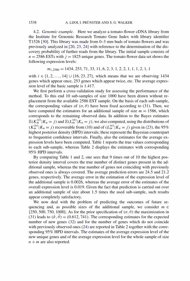
4.2. Genomic example. Here we analyze a tomato-flower cDNA library fromthe Institute for Genomic Research Tomato Gene Index with library identifierT1526 [30]. This library was made from 0–3 mm buds of tomato flowers and waspreviously analyzed in [20, 23, 24] with reference to the determination of the dis-covery probability of further reads from the library. The initial sample consists ofn = 2586 ESTs with j = 1825 unique genes. The tomato flower data set shows thefollowing expression levels:

mi,2586 = 1434,253,71,33,11,6,2,3,1,2,2,1,1,1,2,1,1

with i ∈ {1,2, . . . ,14} ∪ {16,23,27}, which means that we are observing 1434genes which appear once, 253 genes which appear twice, etc. The average expres-sion level of the basic sample is 1.417.

We first perform a cross-validation study for assessing the performance of themethod. To this end 10 sub-samples of size 1000 have been drawn without re-placement from the available 2586 EST sample. On the basis of each sub-sample,the corresponding values of (σ, θ) have been fixed according to (31). Then, wehave computed the estimators for an additional sample of size m = 1586, whichcorresponds to the remaining observed data. In addition to the Bayes estimatesE(K

(n)m |Kn = j) and E(L

(n)m |Kn = j), we also computed, using the distributions of

(K(n)m |Kn = j) recoverable from (10) and of (L

(n)m |Kn = j) given in (23), the 95%

highest posterior density (HPD) intervals; these represent the Bayesian counterpartto frequentist confidence intervals. Finally, also the estimates for the average ex-pression levels have been computed. Table 1 reports the true values correspondingto each sub-sample, whereas Table 2 displays the estimates with corresponding95% HPD intervals.

By comparing Table 1 and 2, one sees that 9 times out of 10 the highest pos-terior density interval covers the true number of distinct genes present in the ad-ditional sample, whereas the true number of genes not coinciding with previouslyobserved ones is always covered. The average prediction errors are 24.5 and 21.2genes, respectively. The average error in the estimation of the expression level ofthe additional sample is 0.0026, whereas the average error of the estimates of theoverall expression level is 0.019. Given the fact that prediction is carried out overan additional sample of size about 1.5 times the used sub-sample, such resultsappear completely satisfactory.

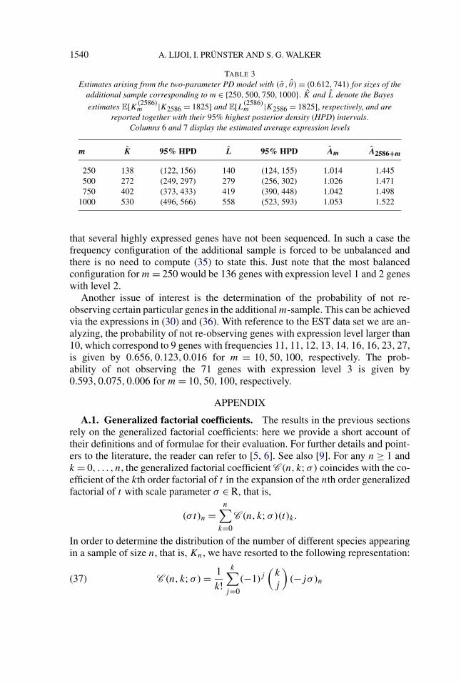
We now deal with the problem of predicting the outcomes of future se-quencing and, as possible sizes of the additional sample, we consider m ∈{250,500,750,1000}. As for the prior specification of (σ, θ) the maximization in(31) leads to (σ , θ ) = (0.612,741). The corresponding estimates for the expectednumber of new genes (32) and for the number of genes which do not coincidewith previously observed ones (24) are reported in Table 2 together with the corre-sponding 95% HPD intervals. The estimates of the average expression level of thenew unique genes and of the average expression level for the whole sample of sizen + m are also reported.


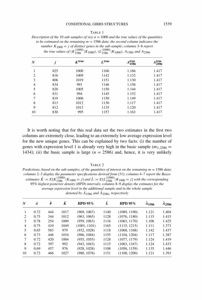
TABLE 1Description of the 10 sub-samples of size n = 1000 and the true values of the quantities

to be estimated on the remaining m = 1586 data: the second column indicates thenumber K1000 = j of distinct genes in the sub-sample; columns 3–6 report

the true values of (K(1000)1586 |K1000), (L

(1000)1586 |K1000), A1586 and A2586

N j Ktrue Ltrue Atrue1586 Atrue

2586

1 825 1000 1166 1.166 1.4172 816 1009 1142 1.132 1.4173 806 1019 1151 1.130 1.4174 834 991 1146 1.156 1.4175 820 1005 1150 1.144 1.4176 831 994 1145 1.152 1.4177 819 1006 1150 1.149 1.4178 813 1012 1130 1.117 1.4179 812 1013 1135 1.120 1.417

10 830 995 1157 1.163 1.417

It is worth noting that for this real data set the two estimates in the first twocolumns are extremely close, leading to an extremely low average expression levelfor the new unique genes. This can be explained by two facts: (i) the number ofgenes with expression level 1 is already very high in the basic sample (m1,2586 =1434); (ii) the basic sample is large (n = 2586) and, hence, it is very unlikely

TABLE 2Predictions, based on the sub-samples, of the quantities of interest on the remaining m = 1586 data:columns 2–3 display the parameter specifications derived from (31); columns 4–7 report the Bayes

estimates K := E[K(1000)1586 |K1000 = j ] and L := E[L(1000)

1586 |K1000 = j ] with the corresponding95% highest posterior density (HPD) intervals; columns 8–9 display the estimates for the

average expression level in the additional sample and in the whole sampledenoted by A1586 and A2586, respectively

N σ θ K HPD 95% L HPD 95% A1586 A2586

1 0.72 444 1017 (969, 1067) 1140 (1089, 1190) 1.121 1.4042 0.75 344 1012 (963, 1065) 1128 (1076, 1180) 1.115 1.4153 0.78 254 1009 (959, 1063) 1116 (1063, 1170) 1.106 1.4254 0.75 410 1049 (1001, 1101) 1165 (1115, 1215) 1.111 1.3735 0.65 583 979 (932, 1028) 1118 (1068, 1168) 1.142 1.4376 0.73 446 1034 (986, 1084) 1155 (1104, 1204) 1.117 1.3877 0.72 420 1004 (955, 1055) 1128 (1077, 1179) 1.124 1.4198 0.72 397 992 (943, 1043) 1115 (1063, 1167) 1.124 1.4339 0.69 457 976 (928, 1028) 1108 (1056, 1159) 1.135 1.446

10 0.72 466 1027 (980, 1078) 1151 (1100, 1200) 1.121 1.393


TABLE 3Estimates arising from the two-parameter PD model with (σ , θ ) = (0.612,741) for sizes of the

additional sample corresponding to m ∈ {250,500,750,1000}. K and L denote the Bayes

estimates E[K(2586)m |K2586 = 1825] and E[L(2586)

m |K2586 = 1825], respectively, and arereported together with their 95% highest posterior density (HPD) intervals.

Columns 6 and 7 display the estimated average expression levels

m K 95% HPD L 95% HPD Am A2586+m

250 138 (122, 156) 140 (124, 155) 1.014 1.445500 272 (249, 297) 279 (256, 302) 1.026 1.471750 402 (373, 433) 419 (390, 448) 1.042 1.498

1000 530 (496, 566) 558 (523, 593) 1.053 1.522

that several highly expressed genes have not been sequenced. In such a case thefrequency configuration of the additional sample is forced to be unbalanced andthere is no need to compute (35) to state this. Just note that the most balancedconfiguration for m = 250 would be 136 genes with expression level 1 and 2 geneswith level 2.

Another issue of interest is the determination of the probability of not re-observing certain particular genes in the additional m-sample. This can be achievedvia the expressions in (30) and (36). With reference to the EST data set we are an-alyzing, the probability of not re-observing genes with expression level larger than10, which correspond to 9 genes with frequencies 11,11,12,13,14,16,16,23,27,is given by 0.656,0.123,0.016 for m = 10,50,100, respectively. The prob-ability of not observing the 71 genes with expression level 3 is given by0.593,0.075,0.006 for m = 10,50,100, respectively.

APPENDIX

A.1. Generalized factorial coefficients. The results in the previous sectionsrely on the generalized factorial coefficients: here we provide a short account oftheir definitions and of formulae for their evaluation. For further details and point-ers to the literature, the reader can refer to [5, 6]. See also [9]. For any n ≥ 1 andk = 0, . . . , n, the generalized factorial coefficient C (n, k;σ) coincides with the co-efficient of the kth order factorial of t in the expansion of the nth order generalizedfactorial of t with scale parameter σ ∈ R, that is,

(σ t)n =n∑

k=0

C (n, k;σ)(t)k.

In order to determine the distribution of the number of different species appearingin a sample of size n, that is, Kn, we have resorted to the following representation:

C (n, k;σ) = 1

k!k∑

j=0

(−1)j(

k

j

)(−jσ )n(37)


with the proviso that C (0,0;σ) = 1 and C (n,0;σ) = 0 for all n ≥ 1. It is tobe noted that C slightly differs from the definition of generalized factorial coef-ficient C(n, k;σ) as given, for example, in [5, 6]. Indeed, one has C (n, k;σ) =(−1)n−kC(n, k;σ).

Besides C (n, k;σ) we consider another quantity C (n, k;σ, γ ) which is knownas noncentral generalized factorial coefficient. It is defined as the coefficient of thekth order factorial of t in the expansion of the nth order noncentral generalizedfactorial of t , with scale parameter σ and noncentrality parameter γ , that is,

(σ t − γ )n =n∑

k=0

C (n, k;σ, γ )(t)k.(38)

Note that in [5] the definition of noncentral generalized factorial coefficient des-ignates a quantity C(n, k;σ, γ ) = (−1)n−kC (n, k;σ, γ ). From (2.60) in [5] it isseen that it can be represented as

C (n, k;σ, γ ) = 1

k!k∑

j=0

(−1)j(

k

j

)(−σj − γ )n(39)

and this can be usefully employed in order to evaluate the probability of discover-ing a new species. Moreover, from (2.56) in [5] it is possible to establish a connec-tion between noncentral and central generalized factorial coefficients

C (n, k;σ, γ ) =n∑

s=k

(n

s

)C (s, k;σ)(−γ )n−s .(40)

Finally we briefly recall the relation to Stirling numbers. Indeed,

limσ→0

C (n, k;σ)

σ k= |s(n, k)|

where, as before, |s(n, k)| is the signless Stirling number of the first kind. More-over, one has

limσ→0

C (n, k;σ, γ )

σ k=

n∑i=k

(n

i

)|s(i, k)|(−γ )n−i .

A.2. Multivariate Chu–Vandermonde formula. Here we present a multi-variate version of the celebrated Chu–Vandermonde identity. In, for example, [5]the following version of the Chu–Vandermonde identity is presented:

[a + b]n =n∑

r=0

(n

r

)[a]r [b]n−r(41)

for any a and b in R, where [x]n := x(x − 1) · · · (x − n + 1) stands for the de-scending factorial. Since a multivariate version in terms of rising factorials seemsnot readily available in the literature we present it together with a proof.


LEMMA A.1. For each q, j ≥ 1, set Aj,q = {(q1, . . . , qj ) : qi ≥ 0,∑j

i=1 qi =q}. Then

∑(q1,...,qj )∈Aj,q

(q

q1 · · ·qj

) j∏i=1

(ai)ni+qi−1 =(n − j +

j∑i=1

ai

)q

j∏i=1

(ai)ni−1(42)

where (n1, . . . , nj ) is such that ni > 0, for i = 1, . . . , j and∑j

i=1 ni = n.

PROOF. Since (a+n)(a)

= (a)n = (−1)n[−a]n, from identity (41) one deducesthat

(a + b)n =n∑

r=0

(n

r

)(a)r(b)n−r .(43)

The proof now follows by inductive reasoning. Suppose the identity holds true forj − 1, that is,

∑(q1,...,qj−1)∈Aj−1,q

q!q1! · · ·qj−2!qj−1!(aj−1)nj−1+qj−1−1

j−2∏i=1

(ai)ni+qi−1

=(n − (j − 1) +

j−1∑i=1

ai

)q

j−1∏i=1

(ai)ni−1,

and we show it holds for j as well. Indeed, observe that

∑(q1,...,qj )∈Aj,q

q!q1! · · ·qj−1!qj !(aj )nj+qj−1

j−1∏i=1

(ai)ni+qi−1

=q∑

qj−1=0

q!qj−1!(q − qj−1)!(aj−1)nj−1+qj−1−1

× ∑(q1,...,qj−1)∈Aj−1,q−qj−1

(q − qj−1)!q1! · · ·qj−2!qj !(aj )nj+qj−1

j−2∏i=1

(ai)ni+qi−1.

By the induction hypothesis, the second factor above equals(n − nj−1 − (j − 1) +

j∑i=1

ai − aj−1

)q−qj−1

(aj )nj−1

j−2∏i=1

(ai)ni−1.

Finally the proof is completed by virtue of (43), after noting that

(aj−1)nj−1+qj−1−1 = (aj−1)nj−1−1(nj−1 − 1 + aj−1)qj−1 . �

Lemma A.1 can also be proved by combining the last relation displayed in theproof with the definition of the multinomial-Dirichlet distribution, according towhich

∑(q1,...,qj )∈Aj,q

( qq1···qj

)∏ji=1(ai)ni+qi−1/(n − j + ∑j

i=1 ai)q = 1.


A.3. Proofs.

PROOF OF PROPOSITION 1. An obvious point to start from is the following: ifwe have seen n observations partitioned into j distinct groups, then the conditionalprobability that the next q ≥ 1 observations provide no new groups is

∏ql=1(1 −

Vn+l,j+1/Vn+l−1,j ) which, using the recursive formula (8) for Vn,k , is given by

P(K(n)

q = 0|Kn = j,Nn = nj

)

=q∏

l=1

(n + l − 1 − jσ )Vn+l,j

Vn+l−1,j

= (n − jσ )qVn+q,j

Vn,j

.

On the other hand, suppose we have seen n + q observations yielding Kn+q = j

groups. Then the conditional probability of obtaining K(n+q)s = k new groups of

sizes s1, . . . , sk from the next s observations, where none of these coincides withthe first n + q , is given by

Vn+q+s,j+k

Vn+q,j

k∏i=1

(1 − σ)si−1

where s1 + · · · + sk = s. If we now set q + s = m, the conditional probabilityof obtaining new groups with respective frequencies s1, . . . , sk in the m obser-vations following on from n, given Kn = j , is, due to exchangeability, foundby multiplying the two conditional probabilities above and including the

(ms

)term. Hence one achieves (9). Note that an alternative proof can be given byconsidering the joint distribution of (Kn,Nn,K

(n)m ,L

(n)m ,S

K(n)m

,�j ) where j =(λ

1,m−L(n)m

, . . . , λj,m−L

(n)m

) is the vector of nonnegative integers denoting the num-ber of new observations in each of the j groups into which the first n observationsare partitioned, and then by using Lemma A.1. �

PROOF OF PROPOSITION 2. The proof works by induction. Let us first notethat for any m ≥ 1 one has

L(n)m+1 = L(n)

m + Hn,m

where Hn,m = IXcn(Xn+m+1) and Xn = {X1, . . . ,Xn}. Let us first fix m = 1 and

determine

E[L

(n)2 |Kn = j

] = E[L

(n)1 |Kn = j

] + E[Hn,1|Kn = j ].The first summand is clearly equal to Vn+1,j+1/Vn,j . As for the second summand,one can use the assumption of exchangeability which yields

E[Hn,1|Kn = j ] = E[IXcn(Xn+2)|Kn = j ]

= E[IXcn(Xn+1)|Kn = j ]

= Vn+1,j+1

Vn,j

.


Hence, (16) holds true for m = 2. Now, suppose (16) is valid for m and let us showthis implies it is still true for m + 1. This means we shall determine

E[L

(n)m+1|Kn = j

] = E[L(n)

m |Kn = j] + E[Hn,m|Kn = j ].

By assumption, E[L(n)m |Kn = j ] = mVn+1,j+1/Vn,j . Moreover, exchangeability

again entails that the second summand above is Vn+1,j+1/Vn,j and the conclusionfollows. �

PROOF OF PROPOSITION 3. This is straightforward and follows from takingthe ratio between (9) and (11) in Corollary 1. �

PROOF OF COROLLARY 2. Let

fj,σ (s, k) := Vn+m,j+k∑si=0 Vn+m,j+iσ−iC (s, i;σ)

which, by assumption, does not depend on n and m. Then, if s = 2 and k = 2

Vn+m,(j−2)+2∑2i=0 Vn+m,(j−2)+iσ−iC (2, i;σ)

= fj−2,σ (2,2)

and, with s = 2 k = 1

Vn+m,(j−2)+1∑2i=0 Vn+m,(j−2)+iσ−iC (2, i;σ)

= fj−2,σ (2,1).

If we, now, consider the ratio of these two expressions, we obtain the identity

Vn+m,j

Vn+m,j−1= fj−2,σ (2,2)

fj−2,σ (2,1).

From this, one sees that

Vn+m,j

Vn+m,2=

j∏i=3

Vn+m,i

Vn+m,i−1=

j−2∏i=1

fi,σ (2,2)

fi,σ (2,1)

so that Vn+m,j = Vn+m,2∏j−2

i=1 (fi,σ (2,2)/fi,σ (2,1)) = g1(n + m)g2(j) for somefunctions g1 and g2. By a result of Kerov ([18], Theorem 7.1) (see also [9]) thisentails that the weights Vn,k are those from the two-parameter Poisson–Dirichletprocess. �

PROOF OF PROPOSITION 4. Consider the expression displayed in (28) andsum with respect to all vector sk in �s,k to obtain

P(Kn = j,Nn = nj ,L

(n)m = s,K(n)

m = k,�r = λr

)(44)

= Vn+m,j+k

C (s, k, σ )

σ k

r∏l=1

(1 − σ)nil+λil

−1

j∏l=r+1

(1 − σ)nil−1.


Now exploit Lemma 1 in order to integrate out �r thus obtaining

P(Kn = j,Nn = nj ,L

(n)m = s,K(n)

m = k,M(n)r

)(45)

= Vn+m,j+k

C (s, k, σ )

σ k

(r∑

l=1

nil − rσ

)m−s

j∏i=1

(1 − σ)ni−1.

Finally, integrating out L(n)m and K

(n)m and summing over k = 0, . . . ,m one has

P(Kn = j,Nn = nj ,M

(n)r

)(46)

=j∏

i=1

(1 − σ)ni−1

m∑k=0

Vn+m,j+k

σ kC

(m,k;σ, rσ −

r∑l=1

nil

).

Hence, the ratio of (46) over the EPPF �(n)j (n1, . . . , nj ) yields the result in (29).

�

Acknowledgments. The authors are grateful to two anonymous referees fortheir valuable comments and suggestions. Special thanks also to Ramsés H. Menafor helpful advice.

REFERENCES

[1] ADAMS, M., KELLEY, J., GOCAYNE, J., MARK, D., POLYMEROPOULOS, M., XIAO, H.,MERRIL, C., WU, A., OLDE, B., MORENO, R., KERLAVAGE, A., MCCOMBE, W.and VENTER, J. (1991). Complementary DNA sequencing: Expressed sequence tagsand human genome project. Science 252 1651–1656.

[2] ANTONIAK, C. E. (1974). Mixtures of Dirichlet processes with applications to Bayesian non-parametric problems. Ann. Statist. 2 1152–1174. MR0365969

[3] ARRATIA, R., BARBOUR, A. D. and TAVARÉ, S. (2003). Logarithmic Combinatorial Struc-tures: A Probabilistic Approach. EMS, Zürich. MR2032426

[4] BRIX, A. (1999). Generalized gamma measures and shot-noise Cox processes. Adv. in Appl.Probab. 31 929–953. MR1747450

[5] CHARALAMBIDES, C. A. (2005). Combinatorial Methods in Discrete Distributions. Wiley,Hoboken, NJ. MR2131068

[6] CHARALAMBIDES, C. A. and SINGH, J. (1988). A review of the Stirling numbers, theirgeneralizations and statistical applications. Commun. Statist. Theory Methods 17 2533–2595. MR0955350

[7] EWENS, W. J. (1972). The sampling theory of selectively neutral alleles. Theor. Popul. Biol. 387–112. MR0325177

[8] FERGUSON, T. S. (1973). A Bayesian analysis of some nonparametric problems. Ann. Statist.1 209–230. MR0350949

[9] GNEDIN, A. and PITMAN, J. (2005). Exchangeable Gibbs partitions and Stirling triangles.Zap. Nauchn. Sem. POMI 325 83–102, 244–245. MR2160320

[10] GRIFFITHS, R. C. and LESSARD, S. (2005). Ewens’ sampling formula and related formulae:combinatorial proofs, extensions to variable population size and applications to ages ofalleles. Theor. Popul. Biol. 68 167–177.

http://www.ams.org/mathscinet-getitem?mr=0365969









[11] GRIFFITHS, R. C. and SPANÒ, D. (2007). Record indices and age-ordered frequencies inexchangeable Gibbs partitions. Electron. J. Probab. 12 1101–1130. MR2336601

[12] ISHWARAN, H. and JAMES, L. F. (2001). Gibbs sampling methods for stick-breaking priors.J. Amer. Statist. Assoc. 96 161–173. MR1952729

[13] ISHWARAN, H. and JAMES, L. F. (2003). Generalized weighted Chinese restaurant processesfor species sampling mixture models. Statist. Sinica 13 1211–1235. MR2026070

[14] JAMES, L. F. (2002). Poisson process partition calculus with applications to exchangeablemodels and Bayesian nonparametrics. Manuscript. Available at http://arxiv.org/pdf/math.PR/0205093.

[15] JAMES, L. F., LIJOI, A. and PRÜNSTER, I. (2006). Conjugacy as a distinctive feature of theDirichlet process. Scand. J. Statist. 33 105–120. MR2255112

[16] JAMES, L. F., LIJOI, A. and PRÜNSTER, I. (2008). Posterior analysis for normalized randommeasures with independent increments. Scand. J. Statist. To appear.

[17] KINGMAN, J. F. C. (1975). Random discrete distributions (with discussion). J. Roy. Statist.Soc. Ser. B 37 1–22. MR0368264

[18] KEROV, S. (1995). Coherent random allocations and the Ewens–Pitman sampling formula.PDMI Preprint, Steklov Math. Institute, St. Petersburg.

[19] LIJOI, A., MENA, R. H. and PRÜNSTER, I. (2006). Controlling the reinforcement in Bayesianmixture models. J. Roy. Statist. Soc. Ser. B 69 715–740. MR2370077

[20] LIJOI, A., MENA, R. H. and PRÜNSTER, I. (2007). Bayesian nonparametric estimation of theprobability of discovering new species. Biometrika 94 769–786.

[21] LO, A. Y. (1984). On a class of Bayesian nonparametric estimates. I. Density estimates. Ann.Statist. 12 351–357. MR0733519

[22] LO, A. Y. and WENG, C.-S. (1989). On a class of Bayesian nonparametric estimates. II. Haz-ard rate estimates. Ann. Inst. Statist. Math. 41 227–245. MR1006487

[23] MAO, C. X. (2004). Prediction of the conditional probability of discovering a new class. J.Amer. Statist. Assoc. 99 1108–1118. MR2109499

[24] MAO, C. X. and LINDSAY, B. G. (2002). A Poisson model for the coverage problem with agenomic application. Biometrika 89 669–682. MR1929171

[25] MAO, C. X. (2007). Estimating species accumulation curves and diversity indices. Statist.Sinica 17 761–775.

[26] PITMAN, J. (1995). Exchangeable and partially exchangeable random partitions. Probab. The-ory Related Fields 102 145–158. MR1337249

[27] PITMAN, J. (1996). Some developments of the Blackwell–MacQueen urn scheme. Statistics,Probability and Game Theory. Papers in Honor of David Blackwell (T. S. Ferguson et al.,eds.). Lecture Notes Monograph Series 30 245–267. IMS, Hayward, CA. MR1481784

[28] PITMAN, J. (2003). Poisson–Kingman partitions. Science and Statistics: A Festschrift for TerrySpeed (D. R. Goldstein, ed.). Lecture Notes Monograph Series 40 1–34. IMS, Beachwood,OH. MR2004330

[29] PITMAN, J. (2006). Combinatorial Stochastic Processes. Springer, Berlin. MR2245368[30] QUACKENBUSH, J., CHO, J., LEE, D., LIANG, F., HOLT, I., KARAMYCHEVA, S., PARVIZI,

B., PERTEA, G., SULTANA, R. and WHITE, J. (2000). The TIGR gene indices: Analysisof gene transcript sequences in highly sampled eukaryotic species. Nucleic Acids Res. 29159–164.

[31] REGAZZINI, E., LIJOI, A. and PRÜNSTER, I. (2003). Distributional results for means ofrandom measures with independent increments. Ann. Statist. 31 560–585. MR1983542

[32] SUSKO, E. and ROGER, A. J. (2004). Estimating and comparing the rates of gene discoveryand expressed sequence tag (EST) frequencies in EST surveys. Bioinformatics 20 2279–2287.




http://arxiv.org/pdf/math.PR/0205093













http://arxiv.org/pdf/math.PR/0205093


[33] TAVARÉ, E. and EWENS, W. J. (1998). The Ewens sampling formula. In Encyclopedia ofStatistical Science (S. Kotz, C. B. Read and D. L. Banks, eds.) 2 update 230–234. Wiley,New York. MR1605063

[34] TEH, Y. W. (2006) A hierarchical Bayesian language model based on Pitman–Yor processes.Coling ACL Proceedings 44 985–992.

[35] TEH, Y. W, JORDAN, M. I., BEAL, M. J. and BLEI, D. M. (2006). Hierarchical Dirichletprocesses. J. Amer. Statist. Assoc. 101 1566–1581. MR2279480

[36] ZABELL, S. L. (1982). W. E. Johnson’s “sufficientness” postulate. Ann. Statist. 10 1090–1099.MR0673645

A. LIJOI

DIPARTIMENTO DI ECONOMIA POLITICA

E METODI QUANTITATIVI

UNIVERSITÀ DEGLI STUDI DI PAVIA

VIA SAN FELICE 527100 PAVIA

ITALY

E-MAIL: [email protected]

I. PRÜNSTER

DIPARTIMENTO DI STATISTICA

E MATEMATICA APPLICATA

UNIVERSITÀ DEGLI STUDI DI TORINO

PIAZZA ARBARELLO 810122 TORINO

ITALY


S. G. WALKER

INSTITUTE OF MATHEMATICS, STATISTICS

AND ACTUARIAL SCIENCE

UNIVERSITY OF KENT

KENT CT2 7NZUNITED KINGDOM





mailto:[email protected]



Documents

Bayesian nonparametric estimators derived from …economia.unipv.it/alijoi/Publications_files/10_AoAP2008_bis.pdf · The Appendix contains a short review of generalized factorial