MOX–Report No. 10/2007

Modelling and Numerical Simulation forYacht Engineering

Nicola Parolini, Alfio Quarteroni

MOX, Dipartimento di Matematica “F. Brioschi”Politecnico di Milano, Via Bonardi 29 - 20133 Milano (Italy)

mox@mate.polimi.it http://mox.polimi.it

Modelling and Numerical Simulation for Yacht Engineering

N. Parolini(1), A. Quarteroni(1,2)

31st May 2007

(1) CMCS - Institut d’Analyse et Calcul ScientifiqueEcole Polytechnique Federale de LausanneStation 8, CH-1015, Lausanne, Switzerland

(2) MOX– Modellistica e Calcolo ScientificoDipartimento di Matematica “F. Brioschi”

Politecnico di Milano

via Bonardi 9, 20133 Milano, Italy

Abstract

In the past few years, Computational Fluid Dynamics (CFD) has become anessential tool in the design and optimization of racing sailboats and in particularAmerica’s Cup yachts. The prevalent role of CFD in the design process is demon-strated by the number of numerical simulations on different boat features, rangingfrom hull and appendage design to sail optimization, that each America’s Cup syn-dicate carries on during the boat design and its further development.

In this work, we report some of the numerical results obtained in the frameworkof the research partnership between the Ecole Polytechnique Federale de Lausanne(EPFL) and the Alinghi Team, in preparation to the 32nd edition of the America’sCup. A particular attention is devoted to the innovative aspects of the numericalmodels that have been recently developed.

Introduction

An America’s Cup yacht is a very sophisticated system that should operate optimallyin a wide range of sailing conditions. The different components (above and beneath thewater surface) of a sailing yacht interact one another through several complex relations.The design of an America’s Cup yacht must account for this complexity and requiresto set up suitable (experimental and numerical) tools able to describe as accurately aspossible the system, in order to achieve an optimal configuration.

To give an idea of the complex interactions that should be taken into account inthe design process, let us bound to a simple example. One way to reduce the viscousresistance on the hull, that is the force in the course direction given by frictional effects,

1

WL

Upwind legs

Downwind legs Wind

Star

t/Fin

ish

line

DistanceMark

Outer

CommitteeRace

Boat

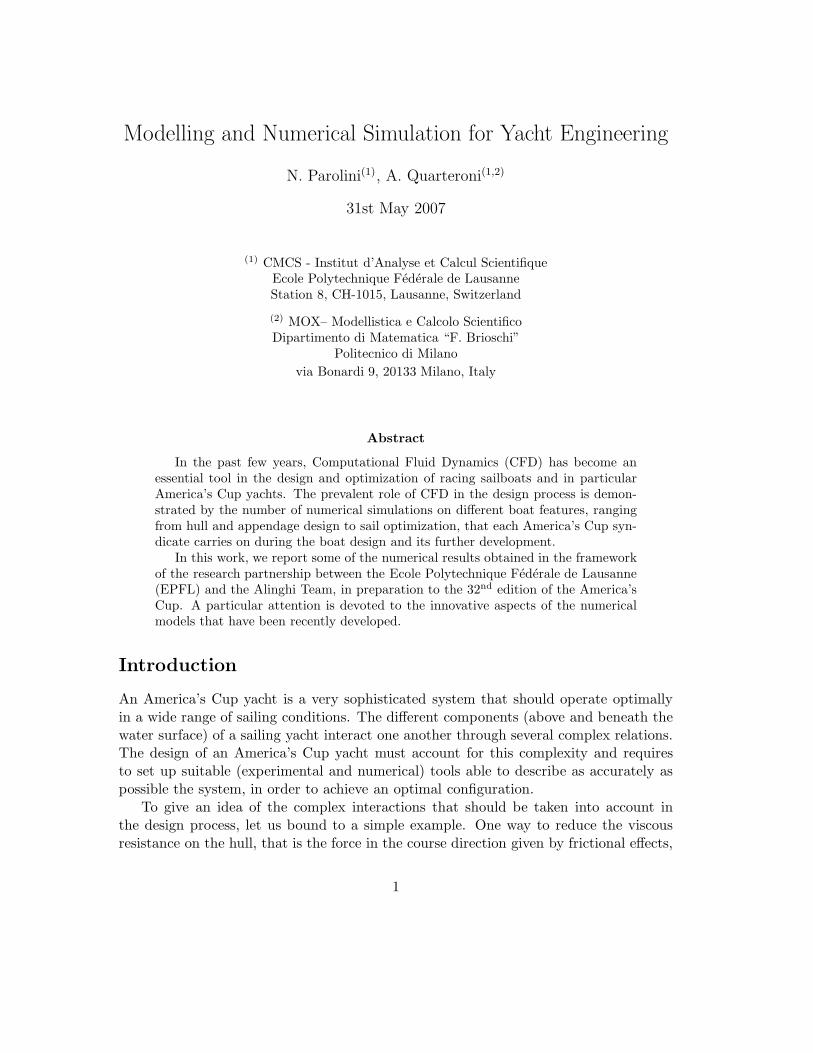
Figure 1: America’s Cup race course.

is reducing its wetted surface. This can be accomplished by reducing its beam (width),keeping the same boat length. A reduction of beam decreases the heeling stability (i.e.the stability around the longitudinal centerline of the boat) and, consequently, the forceson the sails. We can see how a single change involves a domino effect on different areasof the design process.

In America’s Cup match race, two buoys at a distance of 3.1 nautical miles arepositioned in the wind direction. Three laps between the two buoys have to be completed,resulting in three upwind and three downwind legs (see Figure 1).

Upwind and downwind sailing call for different sailing techniques and the design of theboat should accommodate the conflicting requirements arising from the two regimes. Forthe sail rig, this problem is overcome through the use of different sets of sails (main andgenoa for upwind sailing, main and spinnaker/gennaker for downwind sailing). On theother hand, in the underwater part, the possible changes during the race are restrictedto the trimming of rudder and keel trim tab. Yacht appendices have to be designedto perform in both downwind sailing, where minimal drag should be attained, and inupwind sailing, where they have to resist the forces and moments generated by the sails.

Moreover, an America’s cup yacht is constrained by the rules of the InternationalAmerica’s Cup Class (IACC), which was first introduced in 1992 and since then it hascontinuously evolved from one edition to the next. For the 32nd America’s Cup editionthat will take place in Valencia (Spain) during the summer 2007, a new edition (Version5) of the IACC rules has been released. The major changes with respect to the previousversion include a 1 tonne reduction of the boat displacement, deeper keels (+100 mm)and an increase in the maximum total sail area by around 50 m2 downwind. Thesechanges should make the racing closer with boats able to accelerate more readily andstand a better chance of closing the gap on the leading boat on the downwind leg.

The IACC rules impose severe restrictions on a number of design factors, not only ongeometrical dimensions (depth, displacement, sail area), but also on flow control devices(e.g. number of underwater moving surfaces) and materials. The main rule that playsa crucial role in the evolution to the current America’s Cup configuration is known as

2

AerodynamicLift

AerodynamicDrag

AerodynamicSide Force

Side ForceHydrodynamic

AerodynamicThrust

HydrodynamicDrag Hydromechanic

Righting Moment

Heeling MomentAerodynamic

Angle

BoatVelocity

Yaw

WindApparent

Apparent

Wind AngleWindTrue

AngleWindTrueCourse

of the boat

CenterlineBoat

M hDh

Da

La

Sa

Sh

T a

M h

βy

βAW

βTWV b

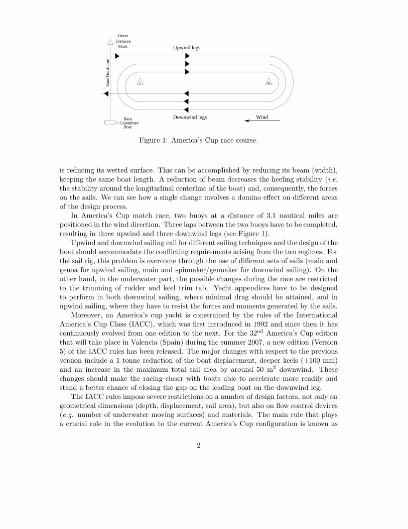
Figure 2: Forces and moments on the water plane.

“the Formula” and is in fact an inequality involving a relation between boat length Lb,sail area As and displacement D:

Lb + 1.25√

As − 9.8 3√

D

0.686≤ 24 m (1)

A longer boat can be realized at the expense of lowering the sail area or increasing thedisplacement. Further unilateral constraints are dictated for boat length, beam, draftand displacement.

The standard approach adopted in the America’s Cup design teams to evaluatewhether a design change (and all the other design modifications that this change implies)is globally advantageous, is based on the use of a Velocity Prediction Program (VPP),which can be used to estimate the boat speed (and, in certain cases, the boat attitude) forany prescribed wind condition and sailing angle βTW (the angle between the centerlineof the boat and the wind direction). A numerical prediction of boat speed and attitudecan be obtained by modeling the balance between the aerodynamic and hydrodynamicforces acting on the boat. A diagram representing the hydrodynamic and aerodynamicforce as well as moment components acting in the water plane is presented in Fig. 2.

On the water plane, a steady sailing condition is obtained imposing two force balancesin x direction (aligned with the boat velocity) and y direction (normal to x on the waterplane) and a heeling moment balance around the centerline of the boat:

Dh + T a = 0,

Sh + Sa = 0, (2)

Mh + Ma = 0,

3

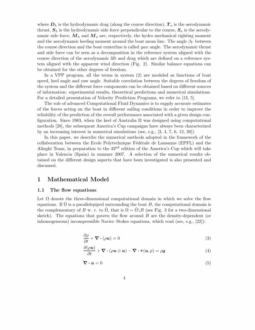
where Dh is the hydrodynamic drag (along the course direction), T a is the aerodynamicthrust, Sh is the hydrodynamic side force perpendicular to the course, Sa is the aerody-namic side force, Mh and Ma are, respectively, the hydro mechanical righting momentand the aerodynamic heeling moment around the boat mean line. The angle βY betweenthe course direction and the boat centerline is called yaw angle. The aerodynamic thrustand side force can be seen as a decomposition in the reference system aligned with thecourse direction of the aerodynamic lift and drag which are defined on a reference sys-tem aligned with the apparent wind direction (Fig. 2). Similar balance equations canbe obtained for the other degrees of freedom.

In a VPP program, all the terms in system (2) are modeled as functions of boatspeed, heel angle and yaw angle. Suitable correlation between the degrees of freedom ofthe system and the different force components can be obtained based on different sourcesof information: experimental results, theoretical predictions and numerical simulations.For a detailed presentation of Velocity Prediction Programs, we refer to [13, 5].

The role of advanced Computational Fluid Dynamics is to supply accurate estimatesof the forces acting on the boat in different sailing conditions in order to improve thereliability of the prediction of the overall performance associated with a given design con-figuration. Since 1983, when the keel of Australia II was designed using computationalmethods [28], the subsequent America’s Cup campaigns have always been characterizedby an increasing interest in numerical simulations (see, e.g., [3, 4, 7, 6, 12, 20]).

In this paper, we describe the numerical methods adopted in the framework of thecollaboration between the Ecole Polytechnique Federale de Lausanne (EPFL) and theAlinghi Team, in preparation to the 32nd edition of the America’s Cup which will takeplace in Valencia (Spain) in summer 2007. A selection of the numerical results ob-tained on the different design aspects that have been investigated is also presented anddiscussed.

1 Mathematical Model

1.1 The flow equations

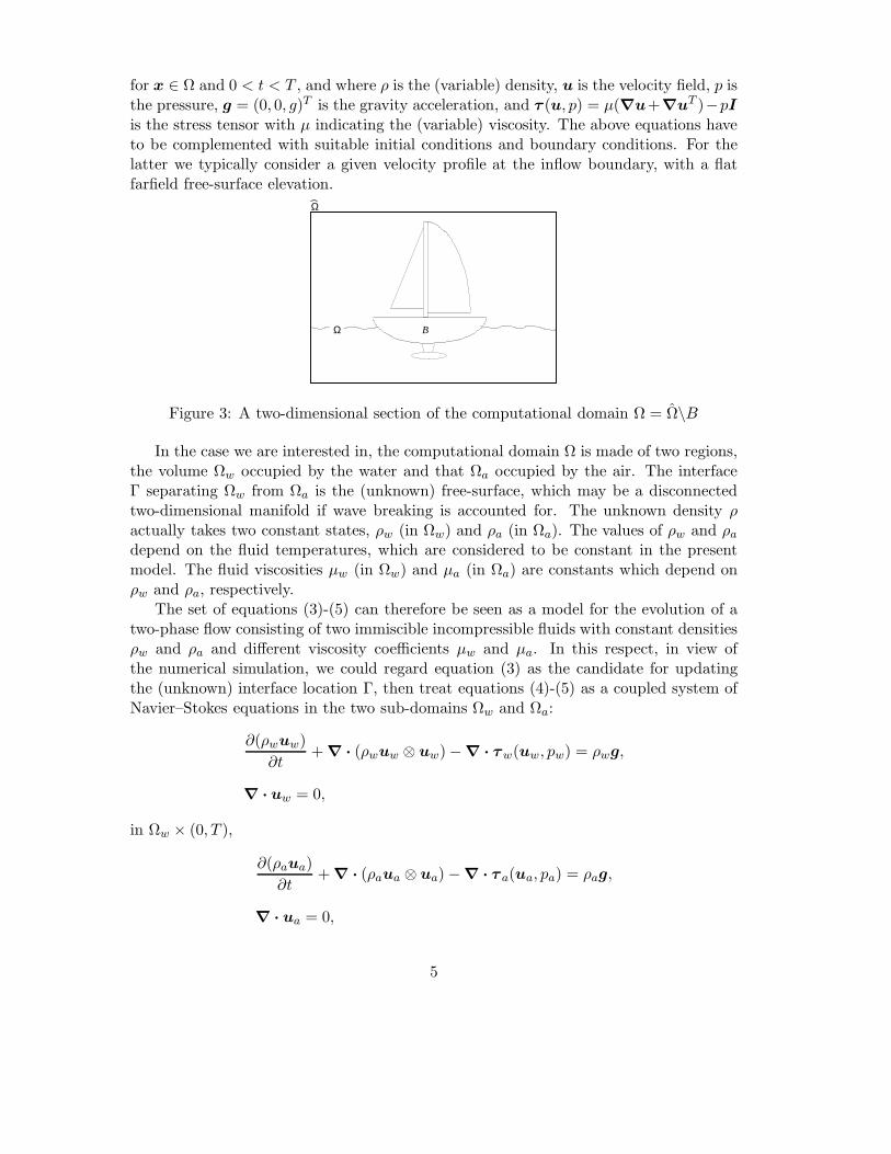
Let Ω denote the three-dimensional computational domain in which we solve the flowequations. If Ω is a parallelepiped surrounding the boat B, the computational domain isthe complementary of B w. r. to Ω, that is Ω = Ω\B (see Fig. 3 for a two-dimensionalsketch). The equations that govern the flow around B are the density-dependent (orinhomogeneous) incompressible Navier–Stokes equations, which read (see, e.g., [22]):

∂ρ

∂t+ ∇ · (ρu) = 0 (3)

∂(ρu)

∂t+ ∇ · (ρu ⊗ u) − ∇ · τ (u, p) = ρg (4)

∇ · u = 0 (5)

4

for x ∈ Ω and 0 < t < T , and where ρ is the (variable) density, u is the velocity field, p isthe pressure, g = (0, 0, g)T is the gravity acceleration, and τ (u, p) = µ(∇u+∇uT )−pI

is the stress tensor with µ indicating the (variable) viscosity. The above equations haveto be complemented with suitable initial conditions and boundary conditions. For thelatter we typically consider a given velocity profile at the inflow boundary, with a flatfarfield free-surface elevation.

Ω

BΩ

Figure 3: A two-dimensional section of the computational domain Ω = Ω\B

In the case we are interested in, the computational domain Ω is made of two regions,the volume Ωw occupied by the water and that Ωa occupied by the air. The interfaceΓ separating Ωw from Ωa is the (unknown) free-surface, which may be a disconnectedtwo-dimensional manifold if wave breaking is accounted for. The unknown density ρactually takes two constant states, ρw (in Ωw) and ρa (in Ωa). The values of ρw and ρa

depend on the fluid temperatures, which are considered to be constant in the presentmodel. The fluid viscosities µw (in Ωw) and µa (in Ωa) are constants which depend onρw and ρa, respectively.

The set of equations (3)-(5) can therefore be seen as a model for the evolution of atwo-phase flow consisting of two immiscible incompressible fluids with constant densitiesρw and ρa and different viscosity coefficients µw and µa. In this respect, in view ofthe numerical simulation, we could regard equation (3) as the candidate for updatingthe (unknown) interface location Γ, then treat equations (4)-(5) as a coupled system ofNavier–Stokes equations in the two sub-domains Ωw and Ωa:

∂(ρwuw)

∂t+ ∇ · (ρwuw ⊗ uw) − ∇ · τw(uw, pw) = ρwg,

∇ · uw = 0,

in Ωw × (0, T ),

∂(ρaua)

∂t+ ∇ · (ρaua ⊗ ua) − ∇ · τ a(ua, pa) = ρag,

∇ · ua = 0,

5

in Ωa × (0, T ). We have set τw(uw, pw) = µw(∇uw + ∇uwT )− pwI, while τ a(ua, pa) is

defined similarly.The free surface Γ is a sharp interface between Ωw and Ωa, on which the normal

components of the two velocities ua · n and uw · n should agree. Furthermore, thetangential components must match as well since the two flows are incompressible. Thuswe have the following kinematic condition

ua = uw on Γ. (6)

Moreover, the forces acting on the fluid at the free-surface are in equilibrium. Thisis a dynamic condition and means that the normal forces on either side of Γ are ofequal magnitude and opposed direction, while the tangential forces must agree in bothmagnitude and direction:

τ a(ua, pa) · n = τw(uw, pw) · n + κσn on Γ, (7)

where σ is the surface tension coefficient, that is a force per unit length of a free surfaceelement acting tangential to the free-surface. It is a property of the liquid and dependson the temperature as well as on other factors. The quantity κ in (7) is the curvatureof the free-surface, κ = R−1

t1 + R−1t2 , where Rt1 and Rt2 are radii of curvature along the

coordinates (t1, t2) of the plane tangentially to the free-surface (orthogonal to n).

1.2 Modelling turbulence and transition

The flow around an IACC boat in standard race regime exhibits turbulent behaviourover the vast majority of the yacht surface. Turbulent flows are characterized by beinghighly unsteady, three-dimensional, containing vortices and coherent structures whichstretch and increase the intensity of turbulence. Even more importantly, they fluctuateon a broad range of scales (in space and time). This feature makes the so-called directnumerical simulation (DNS) unaffordable. The adoption of a RANS (Reynolds AveragedNavier-Stokes) model is then required to deal with the turbulent nature of the flow.

The SST (Shear Stress Transport) model proposed by Menter [18] is an eddy-viscositymodel defined as a combination of a k−ω model (in the inner boundary layer) and k−εmodel (in the outer region of and outside of the boundary layer). A blending functionensures a smooth transition between the two models.

The k−ε model has two main weaknesses: it over-predicts the shear stress in adversepressure gradient flows because of too large length scale (due to low dissipation) and itrequires near-wall modification (i.e. low-Reynolds number damping terms). The k − ωmodel is better at predicting adverse pressure gradient flow and the standard modelof Wilcox [29] does not use any damping functions. However, the disadvantage of thestandard k − ω model is that it depends on the free-stream value of ω [17]. In orderto improve both the k − ε and the k − ω model, Menter [18] combines the two models.Prior to that, it is convenient to transform the k− ε model into a k−ω model using therelation ω = ε/(cµk).

6

The two partial differential equations governing the turbulent kinetic energy k andthe turbulent frequency ω then reads:

D(ρk)

Dt= Pk − Dk + ∇ · ((µ + σkµt)∇k) (8)

D(ρω)

Dt= αρ

Pk

µt− Dω + Cdω + ∇ · ((µ + σkµt)∇ω)

where Pk and PΩ are production terms, Dk and Dω destruction ones and Cdω resultsfrom transforming the ε equation into an equation for ω. The coefficients in the SSTmodel are obtained by combining the value of the coefficients of the standard k − ω (inthe near wall region) to those of the k − ε model by using a blending function F1. Werefer to [18] for a detailed description of the model and its parameters.

Eddy-viscosity turbulence models, such as the one described here, are nowadayswidely adopted for the simulation of turbulent flows in engineering applications. Indeed,they are able to recover with an acceptable accuracy the global behaviour related to theturbulence nature of a flow. In particular, in presence of walls, they supply an accuratedescription of turbulent boundary layers.

The laminar-turbulent transition is physical phenomenon as complex as turbulenceitself since involves the nonlinear interaction of flow perturbations that eventually evolvestowards a fully turbulent behaviour. Many models for transition prediction have beenproposed in the past decades [26, 15, 25, 16]. However, only recently transition modelshave been fully integrated into RANS solver. Among them, the Langtry-Menter tran-sition model [19] is based on a transport equation for the turbulence intermittency γwhich can be used to trigger transition locally. The intermittency function is coupledwith the SST turbulence model introduced above by turning on the production termof the turbulent kinetic energy downstream of the transition point. In addition to thetransport equation for the intermittency, a second transport equation is solved in termsof the transition onset momentum-thickness Reynolds number Reθt. This is done in or-der to capture the non-local influence of the turbulence intensity, which changes due tothe decay of the turbulence kinetic energy in the freestream, as well as due to changes inthe free-stream velocity outside the boundary layer. This additional transport equationis an essential part of the model as it relates the empirical correlation to the onset crite-ria in the intermittency equation and allows the model to be used in general geometrieswithout interaction from the user.

The intermittency equation is given by

D(ργ)

Dt= Pγ − Eγ + ∇ ·

((µ +

µt

σf

)∇γ

)(9)

where Pγ and Eγ are the production and destruction/relaminization terms, respec-tively. The production term Pγ is activated based on the value of the local vorticityReynolds number. The onset criterion depends on the local value of the transition onsetmomentum-thickness Reynolds number Reθt which is computed by solving the following

7

transport equation

D(ρReθt)

Dt= Pθt + ∇ ·

(σθt(µ + µt)∇Reθt

). (10)

The source term Pθt is defined as

Pθt = cθtρ

t

(Reθt − Reθt

)(1 − Fθt)

where Reθt is calculated from empirical correlation and Fθt is a suitable blending func-tion. Note that the empirical correlation is used only in the source term of the transportequation for transition onset momentum thickness Reynolds number (10).

The interplay between the transition model and the SST turbulence model leads tothe following modifications in equations (8):

D(ρk)

Dt= Pk − Dk + ∇ · ((µ + σkµt)∇k) (11)

D(ρω)

Dt= αρ

Pk

µt− Dω + Cdω + ∇ · ((µ + σkµt)∇ω)

with

Pk = γPk,

Dk = min(max(γ, 0.1), 1.0)Dk ,

F1 = max(F1, e

−(ρy√

k/120µ)8)

,

and where Pk and Dk are the original production and destruction terms for the SSTmodel and F1 replaces the original SST blending function F1.

The CFD solver used in this work is Ansys-CFX. The RANS equations, as well as allthe partial differential equations required in the turbulence, transition and free-surfacemodels, are solved using a vertex-based finite volume method [24]. The free-surface istracked using the Volume of Fluid (VOF) method [10].

1.3 Coupling with a 6-DOF rigid body dynamical system

The attitude of the boat advancing in calm water or wavy sea is strictly correlatedwith its performances. For this reason, a state-of-the-art numerical tool for yacht designpredictions should be able to account for the boat motion. This requires the couplingbetween the fluid solver and a code able to compute the structure dynamics. In the caseat hand, the structural deformations can be neglected and only the rigid body motionof the boat in the six degrees of freedom is considered.

Following the approach adopted in [1, 2], two orthogonal cartesian reference systemsare considered: an inertial reference system (O,X, Y,Z) which moves forward with themean boat speed and a body-fixed reference system (G,x, y, z), whose origin is theboat center of mass G, which translates and rotates with the boat. The XY plane

8

in the inertial reference system is parallel to the undisturbed water surface and theZ − axis points upward. The body-fixed x-axis is directed from bow to stern, y ispositive starboard and z upwards.

The dynamics of the boat in the 6 degrees of freedom is determined by integrating theequations of variation of linear and angular momentum in the inertial reference system,as follows

mXG = F (12)

¯T ¯I ¯T−1Ω + Ω × ¯T ¯I ¯T−1Ω = MG (13)

where m is the boat mass, XG is the linear acceleration of the center of mass, F is theforce acting on the boat, Ω and Ω are the angular acceleration and velocity, respectively,MG is the moment with respect to G acting on the boat, ¯I is the tensor of inertia ofthe boat about the body-fixed reference system axes and ¯T is the transformation matrixbetween the body-fixed and the inertial reference system ([1] for details).

The forces and moments acting on the boat are given by

F = F Flow + mg + F Ext

MG = MFlow + (XExt − XG) × F Ext

where F Flow and MFlow are the force and moment, respectively, due to the interactionwith the flow and F Ext is an external forcing term (which may model, e.g., the windforce on sails) while XExt is its application point.

To integrate in time the equations of motion, the second order ordinary differentialequations (12-13) are formulated as systems of first order ODE. If we consider, forexample, the linear momentum equation (12), it can be rewritten as

mY G = F , (14)

XG = Y G, (15)

where Y G denotes the linear velocity of the center of mass. This system is solved usingan explicit 2-step Adam-Bashforth scheme for the velocity

Y n+1 = Y n +∆t

2m(3F n − F n−1),

and a Crank-Nicholson scheme for the position of the center of mass

Xn+1 = Xn +∆t

2(Y n+1 + Y n).

For a convergence analysis of the scheme (as well as for a detailed description of theintegration scheme for the angular momentum equation), we refer to [14], where it isshown that second-order accuracy in time is obtained. Moreover, the schemes featuresadequate stability properties. Indeed, the stability restriction on time step are less severethan the time step required to capture the physical time evolution.

9

In the coupling with the flow solver, the 6-DOF dynamical system receives at eachtime step the value of the forces and moments acting on the boat and returns values ofnew position as well as linear and angular velocity. In the flow solver, these data are usedto update the computational grid (by a mesh motion strategy based on elastic analogy)and the flow equations are solved on the new domain through an Arbitrary LagrangianEulerian (ALE) approach.

2 Numerical Results

The numerical techniques described in the previous sections represent a relevant con-tribution for the improvement of the CFD technology adopted for IACC yacht design.In this section, we present an overview of the numerical results obtained on differentdesign aspects during the preparation for the 2007 edition of the America’s Cup, incollaboration with the Alinghi Team, defender of the Cup. In the same context, anadvanced model for the simulation of the fluid-structure interaction between the flexiblesails and the wind has been developed. The results of the research on this subject willbe presented in a later paper [8].

2.1 Appendages optimization

One of the design areas where CFD simulations play a crucial role is the optimization ofthe appendages. Keel, bulb, winglets and rudder should be shaped and sized (within thedegrees of freedom left by the strict IACC rules) in order to guarantee global optimalperformances.

Full-scale tests are still an invaluable ingredient of the design process: the finalstep for taking every important design choice is always testing full scale on the realboat. Several days of testing, with the two boats differing by the design detail underinvestigation, are planned during every America’s Cup campaign by all the syndicates.

Although the final choice between two keel designs is customary taken on the groundof two-boat testing comparisons and sailors’ preference, the way the two final keel shapesare defined is determined by a deep numerical simulation analysis where many hundredsof different keel shapes are considered as candidates.

The design analyses that can be carried out by CFD simulations cover all the possibledesign variables that define a set of appendages. The great advantage of the numericalapproach relies on the possibility to test several different configurations and to have acomplete picture of the flow behaviour at every time instant.

Information about local distribution of flow quantities (such as, e.g. pressure, vor-ticity and turbulence intensity) can be very useful to improve the hydrodynamic perfor-mances. These information can be hardly obtained during a full-scale test and even ina fully equipped experimental facility (wind tunnel or towing tank) each of these datarequires the setup of suitable measurement equipments. On the other hand, numeri-cal simulations supply as outcome a complete database of relevant quantities about theconsidered flow problem.

10

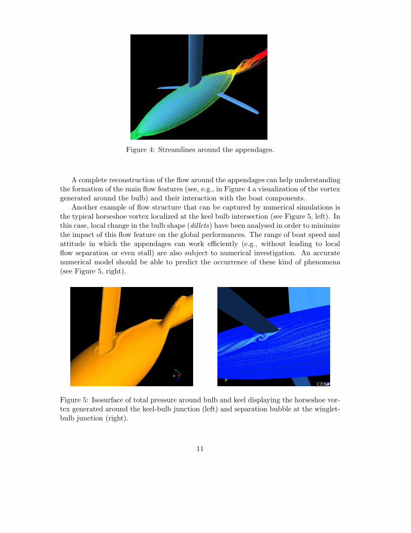
Figure 4: Streamlines around the appendages.

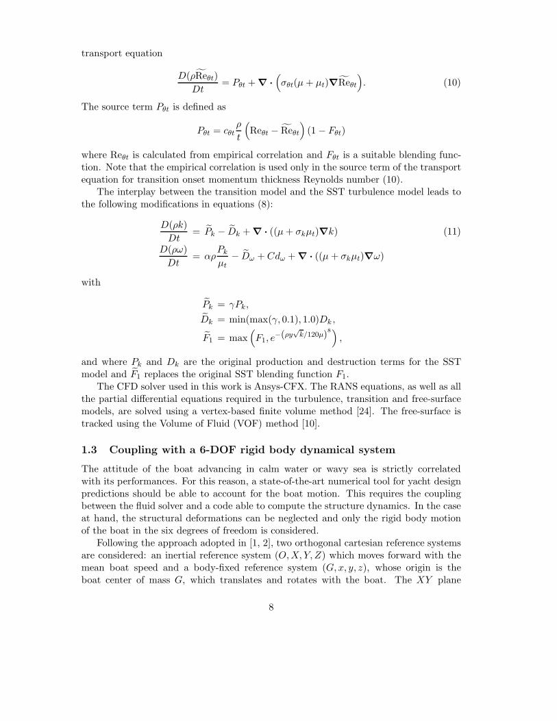
A complete reconstruction of the flow around the appendages can help understandingthe formation of the main flow features (see, e.g., in Figure 4 a visualization of the vortexgenerated around the bulb) and their interaction with the boat components.

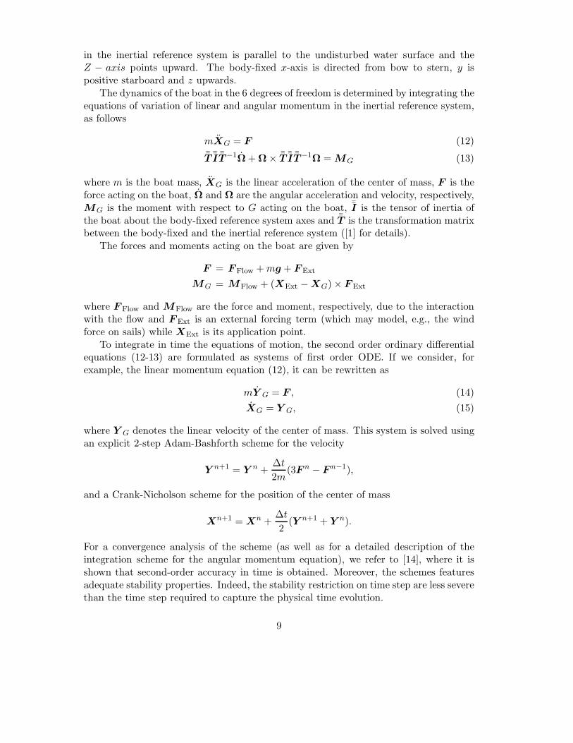
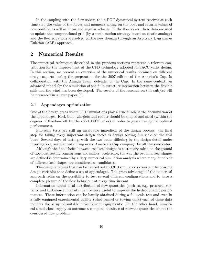
Another example of flow structure that can be captured by numerical simulations isthe typical horseshoe vortex localized at the keel bulb intersection (see Figure 5, left). Inthis case, local change in the bulb shape (dillets) have been analysed in order to minimizethe impact of this flow feature on the global performances. The range of boat speed andattitude in which the appendages can work efficiently (e.g., without leading to localflow separation or even stall) are also subject to numerical investigation. An accuratenumerical model should be able to predict the occurrence of these kind of phenomena(see Figure 5, right).

Figure 5: Isosurface of total pressure around bulb and keel displaying the horseshoe vor-tex generated around the keel-bulb junction (left) and separation bubble at the winglet-bulb junction (right).

11

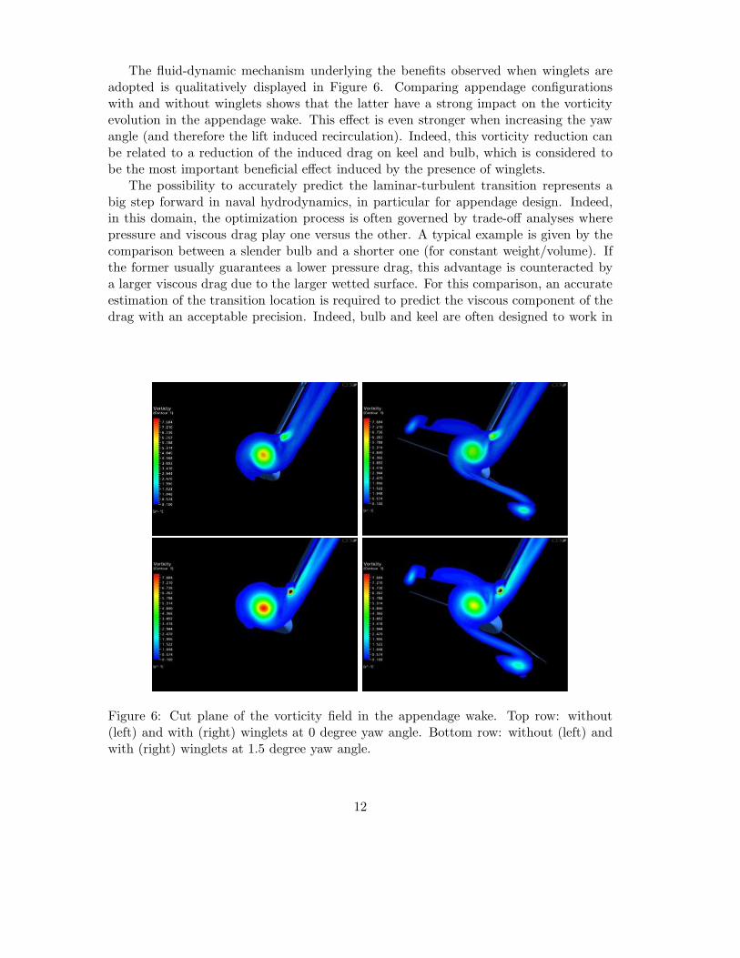
The fluid-dynamic mechanism underlying the benefits observed when winglets areadopted is qualitatively displayed in Figure 6. Comparing appendage configurationswith and without winglets shows that the latter have a strong impact on the vorticityevolution in the appendage wake. This effect is even stronger when increasing the yawangle (and therefore the lift induced recirculation). Indeed, this vorticity reduction canbe related to a reduction of the induced drag on keel and bulb, which is considered tobe the most important beneficial effect induced by the presence of winglets.

The possibility to accurately predict the laminar-turbulent transition represents abig step forward in naval hydrodynamics, in particular for appendage design. Indeed,in this domain, the optimization process is often governed by trade-off analyses wherepressure and viscous drag play one versus the other. A typical example is given by thecomparison between a slender bulb and a shorter one (for constant weight/volume). Ifthe former usually guarantees a lower pressure drag, this advantage is counteracted bya larger viscous drag due to the larger wetted surface. For this comparison, an accurateestimation of the transition location is required to predict the viscous component of thedrag with an acceptable precision. Indeed, bulb and keel are often designed to work in

Figure 6: Cut plane of the vorticity field in the appendage wake. Top row: without(left) and with (right) winglets at 0 degree yaw angle. Bottom row: without (left) andwith (right) winglets at 1.5 degree yaw angle.

12

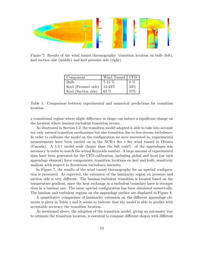
Figure 7: Results of the wind tunnel thermography: transition location on bulb (left),keel suction side (middle) and keel pressure side (right).

Component Wind Tunnel CFD

Bulb 7-15 % 8 %Keel (Pressure side) 12-23% 24%Keel (Suction side) 62 % 57%

Table 1: Comparison between experimental and numerical predictions for transitionlocation.

a transitional regime where slight difference in shape can induce a significant change onthe location where laminar-turbulent transition occurs.

As illustrated in Section 1.2, the transition model adopted is able to take into accountnot only natural transition mechanisms but also transition due to free-stream turbulence.In order to calibrate the model on the configuration we were interested in, experimentalmeasurements have been carried on in the NCR’s 9m × 9m wind tunnel in Ottawa(Canada). A 1.5:1 model scale (larger than the full scale!) of the appendages wasnecessary in order to match the actual Reynolds number. A large amount of experimentaldata have been generated for the CFD calibration, including global and local (on eachappendage element) force components, transition locations on keel and bulb, sensitivityanalysis with respect to freestream turbulence intensity.

In Figure 7, the results of the wind tunnel thermography for an upwind configura-tion is presented. As expected, the extension of the laminarity region on pressure andsuction side is very different. The laminar-turbulent transition is located based on thetemperature gradient, since the heat exchange in a turbulent boundary layer is strongerthan in a laminar one. The same upwind configuration has been simulated numerically.The laminar and turbulent regions on the appendage surface are displayed in Figure 8.

A quantitative comparison of laminarity extension on the different appendage ele-ments is given in Table 1 and it seems to indicate that the model is able to predict withacceptable accuracy the transition location.

As mentioned above, the adoption of the transition model, giving an automatic wayto estimate the transition location, is essential to compare different shapes with different

13

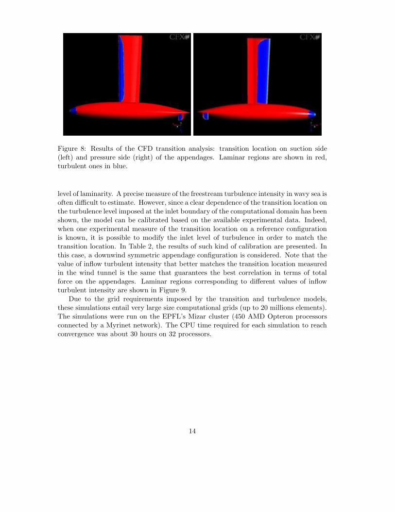
Figure 8: Results of the CFD transition analysis: transition location on suction side(left) and pressure side (right) of the appendages. Laminar regions are shown in red,turbulent ones in blue.

level of laminarity. A precise measure of the freestream turbulence intensity in wavy sea isoften difficult to estimate. However, since a clear dependence of the transition location onthe turbulence level imposed at the inlet boundary of the computational domain has beenshown, the model can be calibrated based on the available experimental data. Indeed,when one experimental measure of the transition location on a reference configurationis known, it is possible to modify the inlet level of turbulence in order to match thetransition location. In Table 2, the results of such kind of calibration are presented. Inthis case, a downwind symmetric appendage configuration is considered. Note that thevalue of inflow turbulent intensity that better matches the transition location measuredin the wind tunnel is the same that guarantees the best correlation in terms of totalforce on the appendages. Laminar regions corresponding to different values of inflowturbulent intensity are shown in Figure 9.

Due to the grid requirements imposed by the transition and turbulence models,these simulations entail very large size computational grids (up to 20 millions elements).The simulations were run on the EPFL’s Mizar cluster (450 AMD Opteron processorsconnected by a Myrinet network). The CPU time required for each simulation to reachconvergence was about 30 hours on 32 processors.

14

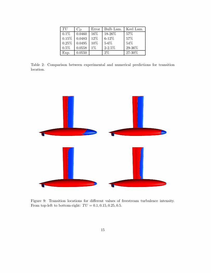
TU CD Error Bulb Lam. Keel Lam.

0.1% 0.0460 16% 18-26% 57%0.15% 0.0483 12% 6-12% 57%0.25% 0.0495 10% 5-6% 54%0.5% 0.0558 1% 2-2.5% 29-36%

Exp. 0.0550 2% 27-30%

Table 2: Comparison between experimental and numerical predictions for transitionlocation.

Figure 9: Transition locations for different values of freestream turbulence intensity.From top-left to bottom-right: TU = 0.1, 0.15, 0.25, 0.5.

15

2.2 Free-surface simulations

The wave drag can be quite significant fraction on an America’s Cup hull, as much as the60% of the total resistance at 10 knots of boat speed. An accurate determination of thiscomponent is important when comparing the performances of two hull designs. Localshape modifications require accurate analysis tools to correctly predict the performancedifferences deriving from these subtle changes.

In a typical hull design process, designers explore the performance of a family of hullshapes through a fast free-surface potential solver (see, e.g., [23]) to determine a set ofcandidates to be tested in the towing tank.

Numerical simulations based on RANS models are integrated into the design processin different ways: on one hand, they can be used to decrease the number of candidateshapes for which models are to be constructed and tested in the towing tank; moreover,they can be used to evaluate the free-surface flow in conditions where codes based onthe panel method are unable to resolve critical differences due to viscous effects.

Hereafter, we present some numerical investigations carried out on the Series 60benchmark hull with the model described in Section 1 where free-surface phenomenaplay a crucial role. Results on America’s Cup hulls with comparisons with towing tankmeasurements are also presented and discussed.

2.2.1 Series 60 - Steady simulations

We first consider a standard free-surface test case for naval applications, that is the flowaround the Series 60 CB = 0.6 hull for which many experimental and numerical dataare available (see, e.g., [27, 11, 1]). For the present study, the flow was computed at aReynolds number Re=4 · 106 and a Froude number Fr=0.316.

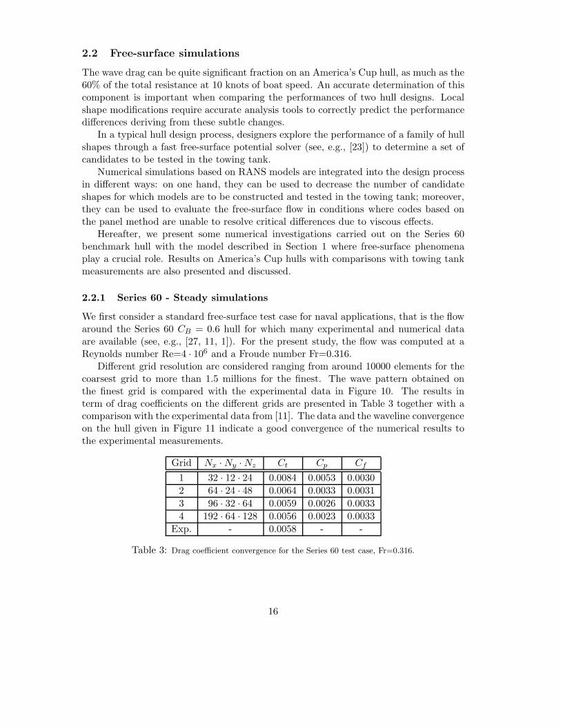
Different grid resolution are considered ranging from around 10000 elements for thecoarsest grid to more than 1.5 millions for the finest. The wave pattern obtained onthe finest grid is compared with the experimental data in Figure 10. The results interm of drag coefficients on the different grids are presented in Table 3 together with acomparison with the experimental data from [11]. The data and the waveline convergenceon the hull given in Figure 11 indicate a good convergence of the numerical results tothe experimental measurements.

Grid Nx · Ny · Nz Ct Cp Cf

1 32 · 12 · 24 0.0084 0.0053 0.0030

2 64 · 24 · 48 0.0064 0.0033 0.0031

3 96 · 32 · 64 0.0059 0.0026 0.0033

4 192 · 64 · 128 0.0056 0.0023 0.0033

Exp. - 0.0058 - -

Table 3: Drag coefficient convergence for the Series 60 test case, Fr=0.316.

16

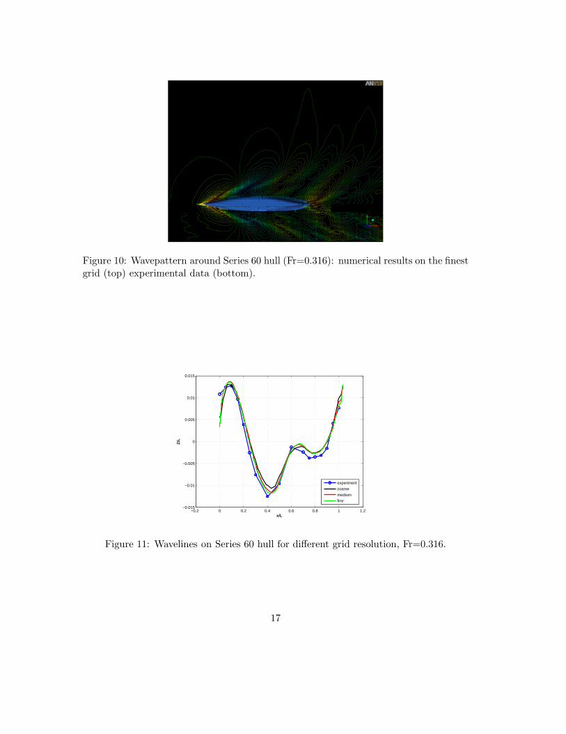
Figure 10: Wavepattern around Series 60 hull (Fr=0.316): numerical results on the finestgrid (top) experimental data (bottom).

−0.2 0 0.2 0.4 0.6 0.8 1 1.2−0.015

−0.01

−0.005

0

0.005

0.01

0.015

x/L

Z/L

experiment

coarse

medium

fine

Figure 11: Wavelines on Series 60 hull for different grid resolution, Fr=0.316.

17

2.2.2 Series 60 - Dynamics in calm water

A complete set of validation studies on the coupling between the flow solver and the6-DOF dynamical system has been carried out for the prediction of the ship’s runningattitude using the Series 60 hull. For a detailed description of the results we refer to[14].

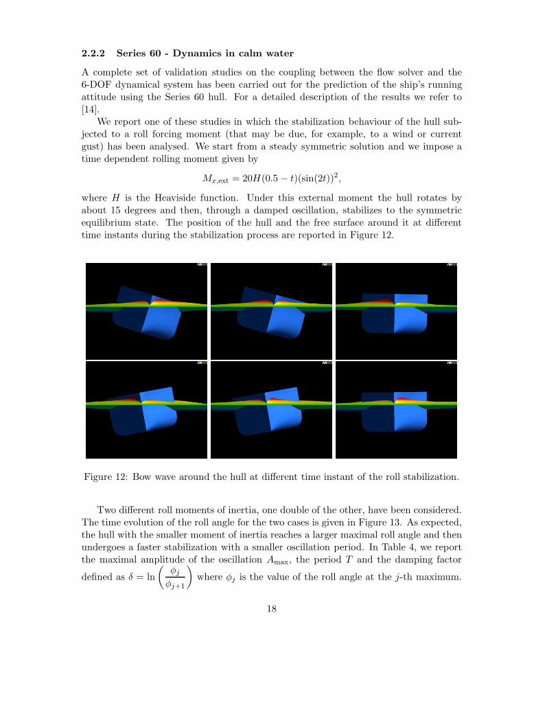
We report one of these studies in which the stabilization behaviour of the hull sub-jected to a roll forcing moment (that may be due, for example, to a wind or currentgust) has been analysed. We start from a steady symmetric solution and we impose atime dependent rolling moment given by

Mx,ext = 20H(0.5 − t)(sin(2t))2,

where H is the Heaviside function. Under this external moment the hull rotates byabout 15 degrees and then, through a damped oscillation, stabilizes to the symmetricequilibrium state. The position of the hull and the free surface around it at differenttime instants during the stabilization process are reported in Figure 12.

Figure 12: Bow wave around the hull at different time instant of the roll stabilization.

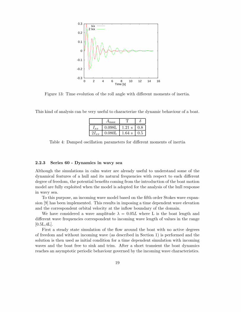
Two different roll moments of inertia, one double of the other, have been considered.The time evolution of the roll angle for the two cases is given in Figure 13. As expected,the hull with the smaller moment of inertia reaches a larger maximal roll angle and thenundergoes a faster stabilization with a smaller oscillation period. In Table 4, we reportthe maximal amplitude of the oscillation Amax, the period T and the damping factor

defined as δ = ln

(φj

φj+1

)where φj is the value of the roll angle at the j-th maximum.

18

-0.3

-0.2

-0.1

0

0.1

0.2

0.3

0 2 4 6 8 10 12 14 16 Time [s]

Ixx2 Ixx

Figure 13: Time evolution of the roll angle with different moments of inertia.

This kind of analysis can be very useful to characterize the dynamic behaviour of a boat.

Amax T δ

Ixx 0.098L 1.21 s 0.8

2Ixx 0.080L 1.64 s 0.5

Table 4: Damped oscillation parameters for different moments of inertia

2.2.3 Series 60 - Dynamics in wavy sea

Although the simulations in calm water are already useful to understand some of thedynamical features of a hull and its natural frequencies with respect to each differentdegree of freedom, the potential benefits coming from the introduction of the boat motionmodel are fully exploited when the model is adopted for the analysis of the hull responsein wavy sea.

To this purpose, an incoming wave model based on the fifth order Stokes wave expan-sion [9] has been implemented. This results in imposing a time dependent wave elevationand the correspondent orbital velocity at the inflow boundary of the domain.

We have considered a wave amplitude λ = 0.05L where L is the boat length anddifferent wave frequencies correspondent to incoming wave length of values in the range[0.5L,4L].

First a steady state simulation of the flow around the boat with no active degreesof freedom and without incoming wave (as described in Section 1) is performed and thesolution is then used as initial condition for a time dependent simulation with incomingwaves and the boat free to sink and trim. After a short transient the boat dynamicsreaches an asymptotic periodic behaviour governed by the incoming wave characteristics.

19

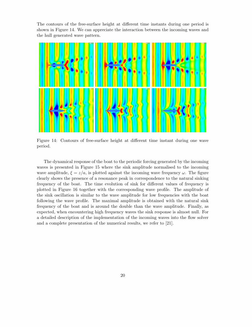
The contours of the free-surface height at different time instants during one period isshown in Figure 14. We can appreciate the interaction between the incoming waves andthe hull generated wave pattern.

Figure 14: Contours of free-surface height at different time instant during one waveperiod.

The dynamical response of the boat to the periodic forcing generated by the incomingwaves is presented in Figure 15 where the sink amplitude normalised to the incomingwave amplitude, ξ = z/a, is plotted against the incoming wave frequency ω. The figureclearly shows the presence of a resonance peak in correspondence to the natural sinkingfrequency of the boat. The time evolution of sink for different values of frequency isplotted in Figure 16 together with the corresponding wave profile. The amplitude ofthe sink oscillation is similar to the wave amplitude for low frequencies with the boatfollowing the wave profile. The maximal amplitude is obtained with the natural sinkfrequency of the boat and is around the double than the wave amplitude. Finally, asexpected, when encountering high frequency waves the sink response is almost null. Fora detailed description of the implementation of the incoming waves into the flow solverand a complete presentation of the numerical results, we refer to [21].

20

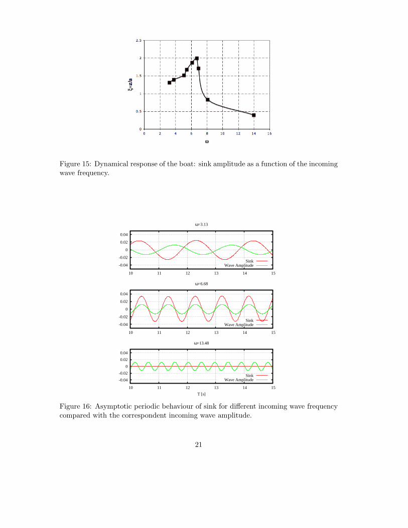
Figure 15: Dynamical response of the boat: sink amplitude as a function of the incomingwave frequency.

-0.04

-0.02

0

0.02

0.04

10 11 12 13 14 15

ω=3.13

SinkWave Amplitude

-0.04

-0.02

0

0.02

0.04

10 11 12 13 14 15

ω=6.68

SinkWave Amplitude

-0.04

-0.02

0

0.02

0.04

10 11 12 13 14 15

T [s]

ω=13.48

SinkWave Amplitude

Figure 16: Asymptotic periodic behaviour of sink for different incoming wave frequencycompared with the correspondent incoming wave amplitude.

21

2.2.4 IACC hull

The numerical scheme presented here for the prediction of boat dynamics can be apowerful tool in America’s Cup yacht design. Many potential applications are beingexplored and range from the dynamic response in waves to manoeuvring. We expectthis kind of numerical investigation could become the standard in the coming years.

Thus far, in the context of the America’s Cup design, this approach has been used toreproduce towing tank experiments. Two IACC hull shapes, that will be referred to asHull 1 and Hull 2, have been considered. The two hulls have different bow designs andtowing tank experiments have been carried out to estimate drag and sink at differentboat speeds.

Numerical simulations have been carried out with a similar setup as the one used forthe Series 60 study, with just the sink degree of freedom activated, since in the towingtank the trim, as well as the other degrees of freedom, were fixed.

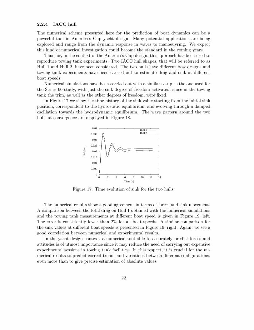
In Figure 17 we show the time history of the sink value starting from the initial sinkposition, correspondent to the hydrostatic equilibrium, and evolving through a dampedoscillation towards the hydrodynamic equilibrium. The wave pattern around the twohulls at convergence are displayed in Figure 18.

0

0.005

0.01

0.015

0.02

0.025

0.03

0.035

0.04

0 2 4 6 8 10 12 14

Sink

[m

]

Time [s]

Hull 1Hull 2

Figure 17: Time evolution of sink for the two hulls.

The numerical results show a good agreement in terms of forces and sink movement.A comparison between the total drag on Hull 1 obtained with the numerical simulationsand the towing tank measurements at different boat speed is given in Figure 19, left.The error is consistently lower than 2% for all boat speeds. A similar comparison forthe sink values at different boat speeds is presented in Figure 19, right. Again, we see agood correlation between numerical and experimental results.

In the yacht design context, a numerical tool able to accurately predict forces andattitudes is of utmost importance since it may reduce the need of carrying out expensiveexperimental sessions in towing tank facilities. In this respect, it is crucial for the nu-merical results to predict correct trends and variations between different configurations,even more than to give precise estimation of absolute values.

22

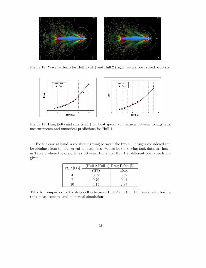
Figure 18: Wave patterns for Hull 1 (left) and Hull 2 (right) with a boat speed of 10 kts.

Figure 19: Drag (left) and sink (right) vs. boat speed: comparison between towing tankmeasurements and numerical predictions for Hull 1.

For the case at hand, a consistent rating between the two hull designs considered canbe obtained from the numerical simulations as well as for the towing tank data, as shownin Table 5 where the drag deltas between Hull 2 and Hull 1 at different boat speeds aregiven.

BSP [kts](Hull 2-Hull 1) Drag Delta [N]

CFD Exp.

4 0.62 0.327 0.79 0.4110 4.15 2.87

Table 5: Comparison of the drag deltas between Hull 2 and Hull 1 obtained with towingtank measurements and numerical simulations.

23

Conclusions

In this work, we have presented some of the most recent results on numerical fluid-dynamic modelling obtained in the framework of the collaboration between the EcolePolytechnique Federale de Lausanne and the Alinghi Team in preparation of the 32nd

edition of the America’s Cup.We have highlighted the importance that CFD analysis is achieving in the design

process of a racing yacht, devoting a particular attention to those modelling techniquesthat represent a step forward in this field.

Among them, we have presented and discussed through numerical examples the re-cent advances in transition modelling and its coupling with standard eddy-viscosityturbulence models. We have shown how accurate predictions on transition location canplay a key role in the optimization of the appendages.

Finally, the coupling of a RANS solver with a 6-DOF dynamical model of the boat hasbeen presented together with recent results of free-surface simulations of boat dynamicsin calm and wavy water.

Acknowledgements

The authors wish to acknowledge the Alinghi Design Team for the support in explainingthe complexity of America’s Cup yacht design and Dr. Davide Detomi for his cooperationin this project. We also thank master students Matteo Lombardi and Simone Piazza fortheir contribution to the implementation of the 6-DOF dynamical system. This workhas been funded by the Swiss Confederation’s innovation promotion agency (KTI/CTI)through grant CTI-6972.1.

References

[1] R. Azcueta. Computation of Turbulent Free-Surface Flows Around Ships and Float-

ing Bodies. Phd thesis, 2001.

[2] R. Azcueta. RANSE Simulations for Sailing Yachts Including Dynamic Sinkage &Trim and Unsteady Motions in Waves. In High Performance Yacht Design Confer-

ence, pages 13–20, Auckland, 2002.

[3] C. W. Boppe. Elements of Hull Optimization and Integration for Stars & Stripes.In Proceedings of the Symposium on Hydrodynamic Performance Enhancement for

Marine Applications, 1988.

[4] M. Caponnetto, A. Castelli, R. Dupont, B. Bonjour, P.-L. Mathey, S. Sanche, andM. L. Sawley. Sailing Yacht Design Using Advanced Numerical Flow Techniques.In Proceedings of the 14th Chesapeake Sailing Yacht Symposium, Annapolis, USA,1999.

24

[5] A. Claughton. Developments in the IMS VPP Formulations. In Proceedings of the

14th Chesapeake Sailing Yacht Symposium, Anapolis, USA, 1999.

[6] G. W. Cowles, N. Parolini, and M. L. Sawley. Numerical Simulation using RANS-based Tools for America’s Cup design. In Proceedings of the 16th Chesapeake Sailing

Yacht Symposium, Annapolis, USA, 2003.

[7] F. Jr. DeBord, J. Reichel, B. Rosen, and C. Fassardi. Design Optimization for theInternational America’s Cup Class. In Transactions of the 2002 SNAME Annual

Meeting, Boston, 2002.

[8] D. Detomi, N. Parolini, and A. Qaurteroni. Fluid-Structure Interaction Algorithmsfor Sailing Yacht Engineering. 2007. In preparation.

[9] J. D. Fenton. A Fifth-Order Stokes Theory for Steadywaves. J. Waterway, Port,

Coastal and Ocean Engineering, 111:216–234, 1985.

[10] C. W. Hirt and B. D. Nichols. Volume of Fluid (VOF) Method for the Dynamicsof Free Boundaries. J. Comp. Phys., 39:201–225, 1981.

[11] C. E. Janson, K. J. Kim, and L. Larsson. Non-Linear Wave Pattern Calculationsfor the Series 60, CB=0.60 Hull. In CFD Workshop, Tokyo, 1994.

[12] P. Jones and R. Korpus. America’s Cup class Yacht Design Using Viscous FlowCFD. In Proceedings of the 16th Chesapeake Sailing Yacht Symposium, Annapo-lis,USA, 2001.

[13] J. E. Kerwin. A Velocity Prediction Program for Ocean Racing Yachts. TechnicalReport 78-11, 1978. MIT Pratt Project Report.

[14] M. Lombardi. Simulazione Numerica della Dinamica di uno Scafo. Master thesis,Politecnico di Milano, 2006.

[15] R. E. Mayle. The Role of Laminar-Turbulent Transition in Gas Turbine Engines.J. Turbomachinery, 113:509–537, 1991.

[16] R. E. Mayle and A. Schulz. The Path to Predicting Bypass Transition. J. Turbo-

machinery, 119:405–411, 1997.

[17] F. R. Menter. Improved Two-Equation k-ω Turbulence Model for AerodynamicFlows. Technical report, 1992. NASA TM-103975.

[18] F. R. Menter. Two-Equation Eddy-Viscosity Turbulence Models for EngineeringApplications. AIAA Journal, 32(8):1598–1605, 1994.

[19] F. R. Menter, R. Langtry, S. Volker, and P. G. Huang. Transition Modelling forGeneral Purpose CFD Codes. In ERCOFTAC Int. Symp. Engineering Turbulence

Modelling and Measurements, 2005.

25

[20] N. Parolini and A. Quarteroni. Mathematical Models and Numerical Simulationsfor the America’s Cup. Comp. Meth. Appl. Mech. Eng., 173:1001–1026, 2005.

[21] S. Piazza. Simulazioni Numeriche della Dinamica di uno scafo in Mare Ondoso.Master thesis, Politecnico di Milano, 2007.

[22] A. Quarteroni and A. Valli. Numerical Approximation of Partial Differential Equa-

tions, volume 23 of Springer Series in Computational Mathematics. Springer-Verlag,Berlin, 1994.

[23] B. S. Rosen, J. P. Laiosa, W. H. Davis, and D. Stavetski. Splash Free-SurfaceCode Methodology for Hydrodynamic Design and Analysis of IACC Yachts. InProceedings of the 11th Chesapeake Sailing Yacht Symposium, Anapolis, USA, 1993.

[24] G. E. Schneider and M. J. Raw. Control Volume Finite-Element Method for HeatTransfer and Fluidflow Using Colocated Variables. Num. Heat Trans., 11:363–400,1987.

[25] K. Sieger, R. Schiele, F. Kaufmann, S. Wittig, and W. Rodi. A Two-Layer Tur-bulence Model for the Calculation of Transitional Boundary-Layers. ERCOFTAC

bulletin, 24:44–47, 1995.

[26] A. M. O. Smith and N. Gamberoni. Transition, Pressure Gradient and StabilityTheory. Technical report, 1956. Douglas Aircraft Company, Long Beach, Calif.Rep. ES 26388.

[27] Y. Toda, F. Stern, and J. Longo. Mean-flow Measurement in the Boundary Layerand Wake and Wave Field of a Series 60 CB = 0.6 Ship Model. Part 1: FroudeNumbers 0.16 and 0.36. J. Ship Research, 36(4):360–377, 1992.

[28] P. van Oossanen and P.N. Joubert. The Development of the Winged Keel forTwelve-Metre Yachts. J. Fluid Mech., 173:55–71, 1986.

[29] D. C. Wilcox. Reassessment of the Scale-Determining Equation for Advanced Tur-bulence Models. AIAA Journal, 26:1299–1310, 1988.

26