Modelling Antarctic and Greenland volume changes … et al 2004.pdf · Modelling Antarctic and Greenland volume changes during the 20th and 21st centuries forced by GCM time slice

www.elsevier.com/locate/gloplacha

Global and Planetary Change 42 (2004) 83–105

Modelling Antarctic and Greenland volume changes during the

20th and 21st centuries forced by GCM time slice integrations

Philippe Huybrechtsa,b,*, Jonathan Gregoryc,d, Ives Janssensb, Martin Wilde

aAlfred-Wegener-Institut fur Polar- und Meeresforschung, Postfach 120161, D-27515 Bremerhaven, GermanybDepartement Geografie, Vrije Universiteit Brussel, Pleinlaan 2, B-1050 Brussels, Belgium

cHadley Centre for Climate Prediction and Research, Meteorological Office, London Road, RG12 2SY Bracknell, UKdDepartment of Meteorology, University of Reading, Earley Gate, P.O. Box 243, RG6 6BB Reading, UK

e Institute for Atmospheric and Climate Science ETH, Swiss Federal Institute of Technology, Winterthurerstrasse 190,

CH-8057 Zurich, Switzerland

Received 7 May 2003; received in revised form 19 September 2003; accepted 21 November 2003

Abstract

Current and future volume changes of the Greenland and Antarctic ice sheets depend on modern mass balance changes and

on the ice-dynamic response to the environmental forcing on time scales as far back as the last glacial period. Here we focus on

model predictions for the 20th and 21st centuries using 3-D thermomechanical ice sheet/ice shelf models driven by climate

scenarios obtained from General Circulation Models. High-resolution anomaly patterns from the ECHAM4 and HadAM3H

time slice integrations are scaled with time series from a variety of lower-resolution Atmosphere–Ocean General Circulation

Models (AOGCM) to obtain the spread of results for the same emission scenario and the same set of ice-sheet model

parameters. Particular attention is paid to the technique of pattern scaling and on how GCM based predictions differ from older

ice-sheet model results based on more parameterised mass-balance treatments. As a general result, it is found that the effect of

increased precipitation on Antarctica dominates over the effect of increased melting on Greenland for the entire range of

predictions, so that both polar ice sheets combined would gain mass in the 21st century. The results are very similar for both

time-slice patterns driven by the underlying time evolution series with most of the scatter in the results caused by the variability

in the lower-resolution AOGCMs. Combining these results with the long-term background trend yields a 20th and 21st century

sea-level trend from polar ice sheets that is however not significantly different from zero.

D 2004 Elsevier B.V. All rights reserved.

Keywords: Polar ice sheets; Climate change; Sea level rise; Greenhouse warming; Numerical modeling; Mass balance

0921-8181/$ - see front matter D 2004 Elsevier B.V. All rights reserved.

doi:10.1016/j.gloplacha.2003.11.011

* Corresponding author. Alfred-Wegener-Institut fur Polar- und

Meeresforschung, Postfach 120161, D-27515 Bremerhaven, Ger-

many. Tel.: +49-471-4831-1194; fax: +49-471-4831-1149.

E-mail address: [email protected]

(P. Huybrechts).

1. Introduction

By far the largest amount of continental water is

stored in the ice sheets of Antarctica and Greenland,

which would add some 70 m to global sea level rise if

they were to melt entirely. The average rate of mass

exchange between these ice sheets and the oceans

corresponds to about 6.5 mm/year of sea level change,

P. Huybrechts et al. / Global and Planetary Change 42 (2004) 83–10584

or 65 cm per century, implying that even relatively

small imbalances between the average yearly snowfall

and mass loss by surface melting and ice flow across

grounding lines can have a significant effect, both for

societies and the environment (Church et al., 2001).

Despite considerable progress in observational data

over the last decade, in particular from remote sensing

platforms, the question of whether the polar ice sheets

are in balance with the present-day climate can still

not be answered with confidence (Rignot and Thom-

as, 2002), although large overall imbalances are

increasingly considered unlikely. Large uncertainties

are associated with future model predictions of ice

sheet response, related to issues such as the evolution

of greenhouse gas concentrations, the climate sensi-

tivity to these changes, and the way such climate

changes will affect the surface mass balance compo-

nents of snow accumulation and meltwater runoff,

which primarily determine volume changes on time

scales less than a century (Huybrechts and de Wolde,

1999).

From a modeling point of view, it is convenient to

distinguish between four components determining

current and future volume changes of the polar ice

sheets. The first component is the long-term back-

ground evolution as a result of ongoing ice-dynamic

adjustment to past environmental changes as far back

as the last glacial period. Superimposed on this long-

term trend is the effect of modern mass-balance

changes during the 20th and 21st centuries. Any

deviation from their long-term average has an imme-

diate effect on ice volume and thus on sea level. In

addition, there is the ice-dynamic response to these

modern surface mass-balance changes due to varia-

tions in the velocity field associated with changes in

ice thickness and surface slope. As a fourth compo-

nent one should also consider the possibility of

‘unexpected ice-dynamic responses’, which may or

may not be related to contemporary climate changes,

and which find their origin in variations at the ice

sheet base or at the grounding line. Examples are the

inferred thinning of the Pine Island and Thwaites

sectors of the West Antarctic ice sheet (Shepherd et

al., 2002) or the oscillatory behaviour of the Siple

Coast ice streams (Joughin et al., 2002). Linked to this

last category is the possibility of unstable behaviour,

most importantly of a collapse of the West Antarctic

ice sheet, but such behaviour is considered to be very

unlikely during the 21st century (Vaughan and

Spouge, 2002; Bindschadler and Bentley, 2002).

The distinction between the long-term trend and the

response to 20th/21st century mass-balance changes is

admittedly somewhat arbitrary, but is convenient to

make from a modeling point of view because detailed

forcing can only be generated for these centuries,

whereas the long-term background forcing needs to

be reconstructed from proxy data, and is therefore less

detailed.

In this paper, we concentrate especially on the

second and third components involving 20th and

21st century mass-balance changes and the ice-dy-

namic response these may entail. We use output from

a suite of available General Circulation Models

(GCMs) to prescribe climate changes over the ice

sheets in an attempt to more realistically reproduce the

spatial and temporal patterns of surface mass-balance

changes. This approach bypasses many of the short-

comings evident in older work, which considered

uniform or zonal averaged temperature changes and/

or applied precipitation changes proportional to tem-

perature changes (e.g. Huybrechts et al., 1991; De

Wolde et al., 1997; Van de Wal and Oerlemans, 1997;

Huybrechts and de Wolde, 1999). The latter studies

were therefore unable to deal with the effects of

changes in atmospheric circulation which could cru-

cially impact on patterns of precipitation rate and

temperature change, cf. Van der Veen (2002) for a

critical assessment of sources of uncertainty in this

older type of studies.

In recent years, several studies were performed that

incorporated GCM output to force mass-balance

changes. O’Farrell et al. (1997) forced an Antarctic

ice sheet model with the transient accumulation field

from a climate change simulation by the CSIRO Mk2

Atmosphere –Ocean General Circulation Model

(AOGCM), and found equivalent sea-level lowerings

of up to 50 cm after 500 years of integration. Van de

Wal et al. (2001) linearly interpolated between two

high-resolution GCM time slices from the ECHAM4

model (Wild and Ohmura, 2000) to obtain 70 years of

Greenland ice sheet evolution. Their results highlight-

ed the important role played by precipitation

increases, which were found to largely compensate

for increased runoff by the time of doubled CO2

conditions. Huybrechts et al. (2002) and Fichefet et

al. (2003) interactively coupled a Greenland ice sheet

P. Huybrechts et al. / Global and Planetary Change 42 (2004) 83–105 85

model with an AOGCM to additionally investigate the

effect of varying fresh-water fluxes on the oceanic

circulation for the time period between 1970 and

2100. The latter work represents a further step to

more fully investigate the interactions between the ice

sheets, atmosphere, and ocean, but such simulations

cannot be performed for long time periods and/or

many climate scenarios because of the high compu-

tational cost involved.

The experiments discussed in this paper do not

consider atmosphere or ocean feedback, but extend on

work performed for the IPCC Third Assessment

Report (Church et al., 2001). It uses the same ice

sheet models and the same approach to derive the

climate forcing, in which anomaly patterns from high-

resolution time slice simulations are scaled with time

series for a representative range of lower-resolution

AOGCMs. The time-slice patterns have however been

complemented with HadAM3H data from the Hadley

Centre model to enable a comparison with the IPCC

work that was based only on ECHAM4 output from

the Max Planck Institute model. The ice sheet models

have also been updated from Huybrechts and de

Wolde (1999) as described in Huybrechts (2002) to

incorporate new geometric datasets, a higher resolu-

tion of 20 km for Antarctica, updated accumulation

datasets, and an improved melt and runoff model. The

long-term background trend is analysed from the

glacial cycle experiments in the latter study, which

runs also serve as initial condition for the experiments

discussed here. In order to better quantify the uncer-

tainty introduced solely by the inter-model variability

in climate response from current GCMs, all experi-

ments were performed for the same emission scenario

and the same set of ice-sheet and mass-balance model

parameters. For Antarctica, the 20th/21st century

simulations did not consider the effect of changes in

basal melting below the ice shelves, as these have

been investigated elsewhere and do not directly con-

tribute to sea-level changes (Warner and Budd, 1998;

Huybrechts and de Wolde, 1999).

2. The ice sheet model

The three-dimensional ice-dynamics models for

Antarctica and Greenland are identical to those de-

scribed in Huybrechts and de Wolde (1999) with all of

the updates as presented in Huybrechts (2002). The

models consist of components describing the ice flow,

the solid Earth response, and the mass-balance at the

ice–atmosphere and ice–ocean interfaces. In the

models, the flow is calculated in both the grounded

ice, where it results from basal sliding and deforma-

tion, and, for Antarctica, in a coupled ice shelf to

enable free migration of the grounding line. The flow

is thermomechanically coupled by simultaneous solu-

tion of the heat equation with the velocity equations,

using Glen’s flow law and an Arrhenius-type depen-

dence of the rate factor on temperature. Isostatic

compensation of the bedrock takes into account the

flexure of the rigid lithosphere and the viscous re-

sponse of the underlying asthenosphere. Both models

have a horizontal resolution of 20 km with 31 vertical

layers in the ice, and another 9 layers in the bedrock

for the calculation of the heat conduction in the crust.

In the context of this paper, these ice-sheet models are

used to determine the long-term background trend by

simulating the Antarctic and Greenland ice sheets

over the last few glacial cycles, and to determine the

dynamic response to current and future mass balance

changes.

The mass-balance model distinguishes between

snow accumulation, rainfall, and meltwater runoff,

which components are all parameterized in terms of

temperature. The melt- and runoff model is based on

the positive degree-day method and is identical to the

recalibrated version as described in Janssens and

Huybrechts (2000). It takes into account the process

of meltwater retention by refreezing and capillary

forces in the snowpack. This method to calculate

the melt has been shown to be sufficiently accurate

for most practical purposes, and seems more justified

on physical grounds than often assumed (Ohmura,

2001). It moreover ensures that the calculations can

take place on the detailed grids of the ice-sheet

models so that one can properly incorporate the

feedback of local elevation changes on the melt rate,

features which cannot be represented well on the

generally much coarser grid of a climate model.

The melt model employed here has a somewhat larger

sensitivity to temperature changes than older degree-

day models, and its sensitivity also rises more quickly

for positive perturbations. This is to a large extent due

to the separate treatment of the rain fraction, which is

generally found to contribute more to runoff than to


accumulation, and which fraction was often neglected

in comparable mass-balance models previously.

Inputs to the mass-balance model are the mean annual

precipitation rate and the mean monthly surface

temperature.

3. Climate forcing

To derive the climate forcing over the ice sheets we

tried to make optimal use of currently available GCM

simulations. Even for historical climate changes over

the 20th century, an alternative is hardly available as

there exist no direct observations of mass-balance

changes over the ice sheets and there are only very

limited records of basic climatic variables such as

temperature and precipitation, most of them from the

coast. The only other option would be to use meteo-

rological re-analyses such as from ECMWF and

NCEP-NCAR, but these only exist for the last 20 to

40 years and are known to have deficiencies over the

ice sheets because of little observational constraint

and questionable parameterizations, probably more so

for Antarctica than for Greenland (Bromwich et al.,

1998; Hanna and Valdes, 2001).

Direct coupling between GCMs and ice-sheet

models would be desirable but is not yet feasible

because of the wide gap between typical GCM reso-

lutions in the range of 100–500 km and the much

finer grids required for ice-sheet models to properly

deal with the width of ablation zones and the chan-

neling of the flow at the margin.

In our analysis, we make a distinction between the

patterns of climate change on the one hand, and the

transient climate evolution over time on the other. The

former are derived from GCM simulations at the

highest horizontal resolution currently used in climate

modeling, but such simulations can only be performed

for short periods of time. We therefore adopt a method

to scale these anomaly patterns with ice-sheet aver-

aged variables obtained from transient AOGCMs at

lower resolution in order to produce continuous forc-

ing under conditions of climate change.

3.1. Climate anomaly patterns

The climate anomaly patterns are derived from so-

called time-slice experiments (Cubasch et al., 1995).

Thereby a high-resolution atmospheric model is run

for a limited time window, using prescribed boundary

conditions of sea surface temperature (SST) and sea-

ice distribution, which are derived from a lower-

resolution, transient coupled atmosphere–ocean sce-

nario run. Model resolutions of typically 50–100 km

in polar regions allow for a more realistic topography

crucial to better resolving temperature gradients and

orographic forcing of precipitation along the steep

margins of the polar ice sheets.

We used time-slice output from a present-day and a

21st-century climatic change experiment from two

available models. Both model experiments were set

up in a similar way. The present-day experiments use

observationally constrained SST as boundary condi-

tion, to which anomalies from the lower-resolution

driving AOGCM are added to produce boundary

conditions for the high-resolution model during the

anomaly period.

The first model is the ECHAM4 GCM developed

at the Max Planck Institute in Hamburg (Roeckner et

al., 1996). This model is implemented on a spectral

T106 (f 1.125j� 1.125j) resolution. The transient

scenario run was performed with ECHAM4 at T42

(f 2.8j) resolution coupled to the OPYC3 ocean

model (Roeckner et al., 1999). This coupled experi-

ment takes into account a gradual increase in CO2 and

other greenhouse gas concentrations according to the

IPCC scenario IS92a (Leggett et al., 1992). The two

time slice experiments were run for 10 years each for

the decades 1971–1980 and 2041–2050, at which

time the CO2 concentration is expected to double. The

present-day experiment used the Atmospheric Model

Intercomparison Project (AMIP) SST climatology,

superimposed with detrended SST variabilities from

the lower-resolution AOGCM transient run. The 21st-

century climatic change time-slice experiment used

the SST obtained through a superposition of the AMIP

SST climatology with the mean SST changes between

the present-day period and the 21st century climate

change period and the SST variabilities for the 21st

century climate change period, both taken from the

coupled lower resolution transient experiment. In this

paper we use the differences of the time slices

averaged over both decades, taken to be centred over

the years 1975 and 2045, respectively. The resulting

anomaly patterns of precipitation and temperature

over Greenland and Antarctica were discussed in


more detail in Wild and Ohmura (2000) and Wild et

al. (2003).

The second model is the HadAM3H GCM devel-

oped at the Hadley Centre for Climate Prediction and

Research. The high resolution time slice run is per-

formed with the atmospheric component only at

1.875j� 1.25j resolution. This is done for the periods1960–1990 and 2070–2100, respectively, hence the

present-day patterns are also conveniently centred at

the year 1975, though the period separating the two

time slices is 40 years longer compared to the

ECHAM4 time slices (2085 against 2045). The 30-

year time-slice window also ensures statistically more

significant results than was possible for the 10-year

period of the ECHAM4 results for reasons of shortage

of CPU time. The driving AOGCM is HadCM3 at

2.5j� 3.75j horizontal resolution (Pope et al., 2000;

Gordon et al., 2000). In this experiment, the SRES A2

scenario was used (Nakicenovic et al., 2000), similar

to the older IS92a scenario used for the ECHAM4

results. Both the control and anomaly runs are the

means over an ensemble of three independent runs,

which further reduces statistical noise. The HadAM3H

2071–2100 SST fields were constructed by adding

HadCM3 SST anomalies to HadISST (observed SSTs)

for 1961–1990. This was done in such a way as to

preserve the HadCM3 trend through the period 2071–

2100, but retain the interannual variability of HadISST.

The HadAM3H sea ice concentrations were derived in

the same way from HadISST sea ice. Large local

changes are associated with the retreat of sea ice.

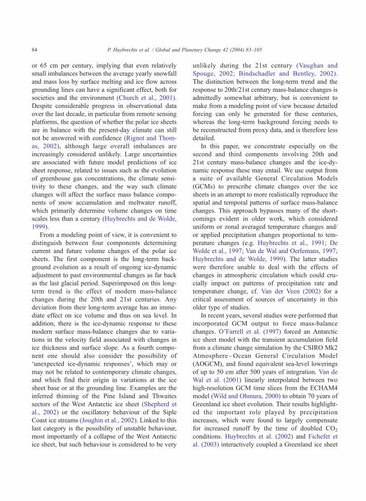
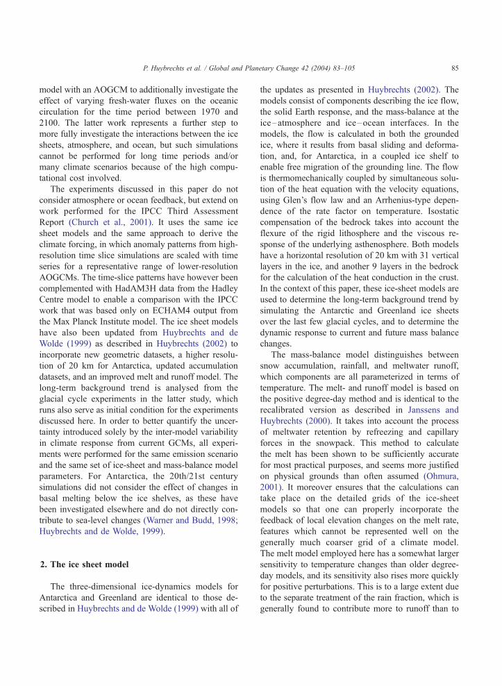
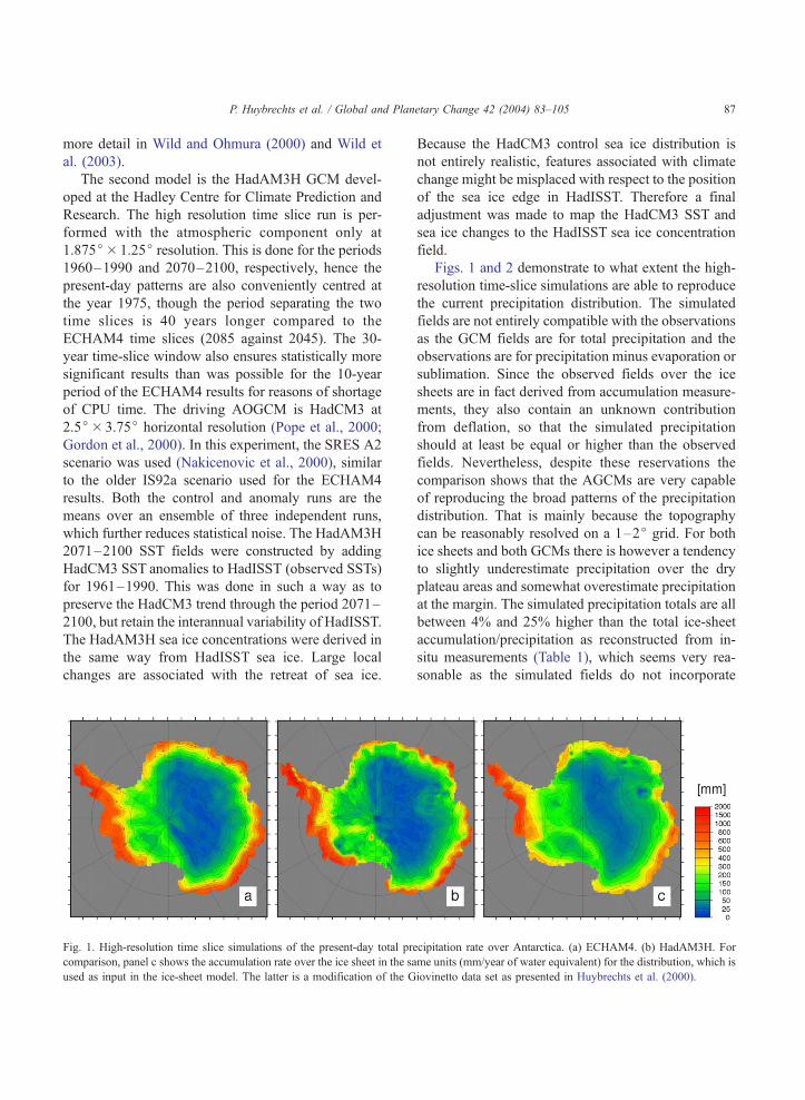
Fig. 1. High-resolution time slice simulations of the present-day total pre

comparison, panel c shows the accumulation rate over the ice sheet in the sa

used as input in the ice-sheet model. The latter is a modification of the G

Because the HadCM3 control sea ice distribution is

not entirely realistic, features associated with climate

change might be misplaced with respect to the position

of the sea ice edge in HadISST. Therefore a final

adjustment was made to map the HadCM3 SST and

sea ice changes to the HadISST sea ice concentration

field.

Figs. 1 and 2 demonstrate to what extent the high-

resolution time-slice simulations are able to reproduce

the current precipitation distribution. The simulated

fields are not entirely compatible with the observations

as the GCM fields are for total precipitation and the

observations are for precipitation minus evaporation or

sublimation. Since the observed fields over the ice

sheets are in fact derived from accumulation measure-

ments, they also contain an unknown contribution

from deflation, so that the simulated precipitation

should at least be equal or higher than the observed

fields. Nevertheless, despite these reservations the

comparison shows that the AGCMs are very capable

of reproducing the broad patterns of the precipitation

distribution. That is mainly because the topography

can be reasonably resolved on a 1–2j grid. For both

ice sheets and both GCMs there is however a tendency

to slightly underestimate precipitation over the dry

plateau areas and somewhat overestimate precipitation

at the margin. The simulated precipitation totals are all

between 4% and 25% higher than the total ice-sheet

accumulation/precipitation as reconstructed from in-

situ measurements (Table 1), which seems very rea-

sonable as the simulated fields do not incorporate

cipitation rate over Antarctica. (a) ECHAM4. (b) HadAM3H. For

me units (mm/year of water equivalent) for the distribution, which is

iovinetto data set as presented in Huybrechts et al. (2000).

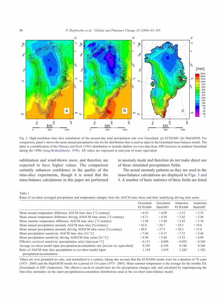
Fig. 2. High-resolution time slice simulations of the present-day total precipitation rate over Greenland. (a) ECHAM4. (b) HadAM3H. For

comparison, panel c shows the mean annual precipitation rate for the distribution that is used as input in the Greenland mass-balance model. The

latter is a modification of the Ohmura and Reeh (1991) distribution to include shallow ice-core data from AWI traverses in northern Greenland

during the 1990s (Jung-Rothenhausler, 1998). All values are expressed in mm/year of water equivalent.


sublimation and wind-blown snow, and therefore are

expected to have higher values. The comparison

certainly enhances confidence in the quality of the

time-slice experiments, though it is noted that the

mass-balance calculations in this paper are performed

Table 1

Rates of ice-sheet averaged precipitation and temperature changes from th

Mean annual temperature difference AGCM time slice [jC/century]Mean annual temperature difference driving AOGCM time series [jC/cenMean summer temperature difference AGCM time slice [jC/century]Mean annual precipitation anomaly AGCM time slice [%/century]

Mean annual precipitation anomaly driving AOGCM time series [%/centu

Mean precipitation sensitivity AGCM time slice [%/jC]Mean precipitation sensitivity driving AOGCM time series [%/jC]Effective sea-level sensitivity (precipitation only) [mm/year/jC]Average ice-sheet model input precipitation/accumulation rate [m/year ice

Ratio of AGCM time slice precipitation to ice-sheet model input

precipitation/accumulation

Values are over grounded ice only, and normalized to a century, taking int

(1975–2045) and the HadAM3H results for a period of 110 years (1975–

(Greenland) or DJF (Antarctica). The effective sea-level sensitivities are

time-slice anomalies on the input precipitation/accumulation distributions

in anomaly mode and therefore do not make direct use

of these simulated precipitation fields.

The actual anomaly patterns as they are used in the

mass-balance calculations are displayed in Figs. 3 and

4. A number of basic statistics of these fields are listed

e AGCM time slices and their underlying driving time series

Greenland

ECHAM4

Greenland

HadAM3

Antarctica

ECHAM4

Antarctica

HadAM3

+ 4.83 + 4.09 + 2.53 + 3.35

tury] + 4.71 + 4.58 + 3.42 + 3.48

+ 3.94 + 3.44 + 2.83 + 3.34

+ 42.4 + 20.7 + 19.5 + 19.6

ry] + 49.8 + 27.5 + 20.2 + 15.0

+ 7.60 + 4.71 + 7.31 + 5.46

+ 8.96 + 5.44 + 5.53 + 4.09

� 0.133 � 0.090 � 0.492 � 0.369

equivalent] 0.356 0.356 0.186 0.186

1.154 1.039 1.242 1.102

o account that the ECHAM4 results were for a duration of 70 years

2085). Mean summer temperature is the average for the months JJA

for precipitation changes only and calculated by superimposing the

used in the ice-sheet mass-balance model.

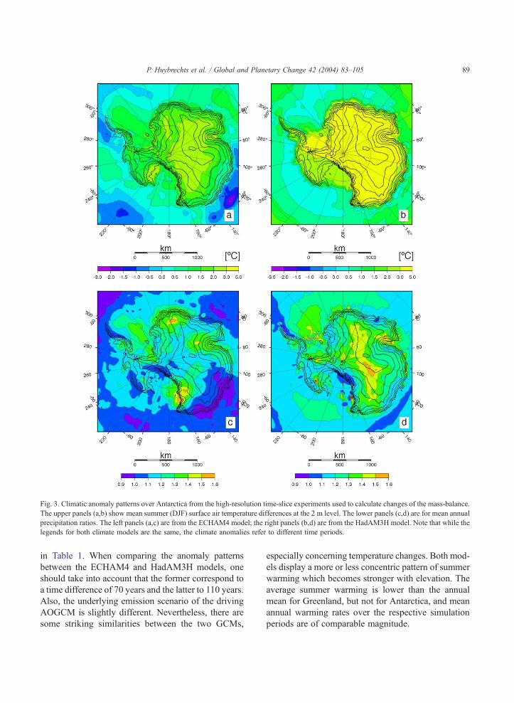
Fig. 3. Climatic anomaly patterns over Antarctica from the high-resolution time-slice experiments used to calculate changes of the mass-balance.

The upper panels (a,b) show mean summer (DJF) surface air temperature differences at the 2 m level. The lower panels (c,d) are for mean annual

precipitation ratios. The left panels (a,c) are from the ECHAM4 model; the right panels (b,d) are from the HadAM3H model. Note that while the

legends for both climate models are the same, the climate anomalies refer to different time periods.


in Table 1. When comparing the anomaly patterns

between the ECHAM4 and HadAM3H models, one

should take into account that the former correspond to

a time difference of 70 years and the latter to 110 years.

Also, the underlying emission scenario of the driving

AOGCM is slightly different. Nevertheless, there are

some striking similarities between the two GCMs,

especially concerning temperature changes. Both mod-

els display a more or less concentric pattern of summer

warming which becomes stronger with elevation. The

average summer warming is lower than the annual

mean for Greenland, but not for Antarctica, and mean

annual warming rates over the respective simulation

periods are of comparable magnitude.

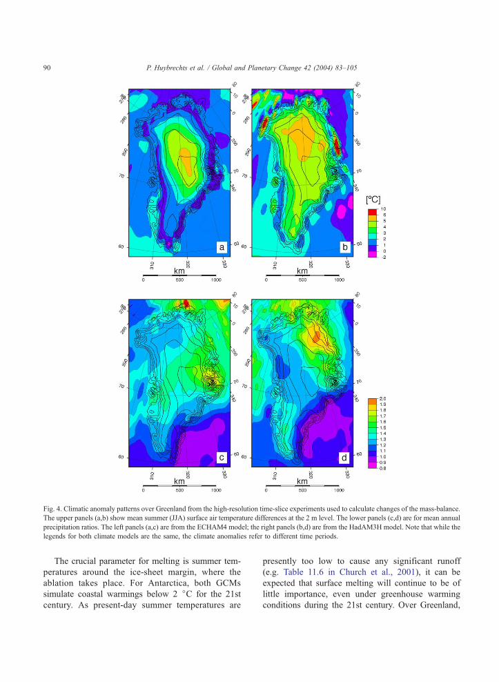
Fig. 4. Climatic anomaly patterns over Greenland from the high-resolution time-slice experiments used to calculate changes of the mass-balance.

The upper panels (a,b) show mean summer (JJA) surface air temperature differences at the 2 m level. The lower panels (c,d) are for mean annual

precipitation ratios. The left panels (a,c) are from the ECHAM4 model; the right panels (b,d) are from the HadAM3H model. Note that while the

legends for both climate models are the same, the climate anomalies refer to different time periods.


The crucial parameter for melting is summer tem-

peratures around the ice-sheet margin, where the

ablation takes place. For Antarctica, both GCMs

simulate coastal warmings below 2 jC for the 21st

century. As present-day summer temperatures are

presently too low to cause any significant runoff

(e.g. Table 11.6 in Church et al., 2001), it can be

expected that surface melting will continue to be of

little importance, even under greenhouse warming

conditions during the 21st century. Over Greenland,


both AGCMs likewise simulate comparatively little

summer warming over the ablation zone, which is

equally found to be in the range of 0–3 jC, with the

lower values for the ECHAM4 experiment. The

smaller increase in the summer temperature around

the margin may be due to dampening from the nearby

ocean, which hardly warms in both experiments, or

dampening over a melting ice surface as its temper-

ature is limited to the melting point and therefore

cannot rise further. A thorough meteorological expla-

nation of this feature has however not yet been given.

Concerning precipitation changes under enhanced

greenhouse warming conditions, both time-slice

experiments agree that the ice-sheet averaged values

should increase by amounts of between 20% and

40% per century (Table 1). These increases are

related to slight poleward displacements of polar

lows and the higher moisture-holding capacity of

the warmer air. There is some qualitative agreement

that the relative precipitation increase is stronger

over higher elevations, but in general both AGCM

patterns show relatively little resemblance, though

the normalized average rate of Antarctic precipitation

increase is for both time-slice experiments almost the

same at a little less than 20% per century. The

maximum predicted local precipitation increase is

at most a doubling by the end of the 21st century

as occurring in northeast Greenland in the

HadAM3H model. On average, the predicted precip-

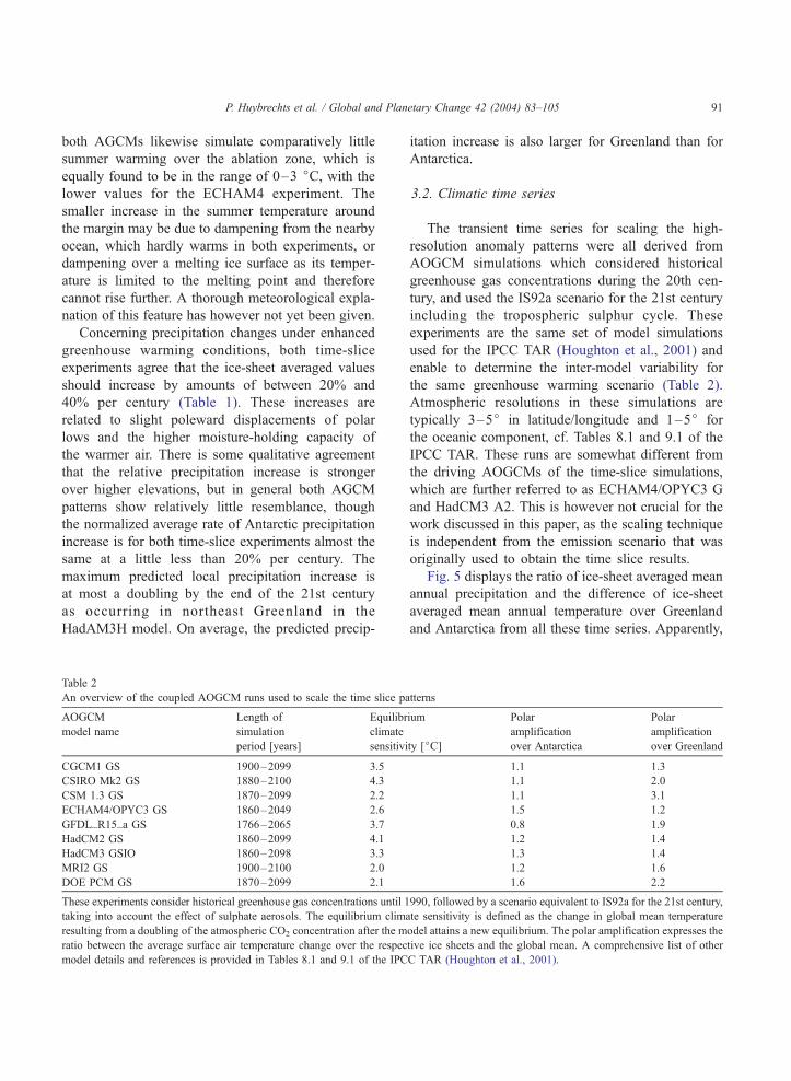
Table 2

An overview of the coupled AOGCM runs used to scale the time slice pa

AOGCM

model name

Length of

simulation

period [years]

Equilibr

climate

sensitivi

CGCM1 GS 1900–2099 3.5

CSIRO Mk2 GS 1880–2100 4.3

CSM 1.3 GS 1870–2099 2.2

ECHAM4/OPYC3 GS 1860–2049 2.6

GFDL_R15_a GS 1766–2065 3.7

HadCM2 GS 1860–2099 4.1

HadCM3 GSIO 1860–2098 3.3

MRI2 GS 1900–2100 2.0

DOE PCM GS 1870–2099 2.1

These experiments consider historical greenhouse gas concentrations until 1

taking into account the effect of sulphate aerosols. The equilibrium clima

resulting from a doubling of the atmospheric CO2 concentration after the m

ratio between the average surface air temperature change over the respec

model details and references is provided in Tables 8.1 and 9.1 of the IPC

itation increase is also larger for Greenland than for

Antarctica.

3.2. Climatic time series

The transient time series for scaling the high-

resolution anomaly patterns were all derived from

AOGCM simulations which considered historical

greenhouse gas concentrations during the 20th cen-

tury, and used the IS92a scenario for the 21st century

including the tropospheric sulphur cycle. These

experiments are the same set of model simulations

used for the IPCC TAR (Houghton et al., 2001) and

enable to determine the inter-model variability for

the same greenhouse warming scenario (Table 2).

Atmospheric resolutions in these simulations are

typically 3–5j in latitude/longitude and 1–5j for

the oceanic component, cf. Tables 8.1 and 9.1 of the

IPCC TAR. These runs are somewhat different from

the driving AOGCMs of the time-slice simulations,

which are further referred to as ECHAM4/OPYC3 G

and HadCM3 A2. This is however not crucial for the

work discussed in this paper, as the scaling technique

is independent from the emission scenario that was

originally used to obtain the time slice results.

Fig. 5 displays the ratio of ice-sheet averaged mean

annual precipitation and the difference of ice-sheet

averaged mean annual temperature over Greenland

and Antarctica from all these time series. Apparently,

tterns

ium

ty [jC]

Polar

amplification

over Antarctica

Polar

amplification

over Greenland

1.1 1.3

1.1 2.0

1.1 3.1

1.5 1.2

0.8 1.9

1.2 1.4

1.3 1.4

1.2 1.6

1.6 2.2

990, followed by a scenario equivalent to IS92a for the 21st century,

te sensitivity is defined as the change in global mean temperature

odel attains a new equilibrium. The polar amplification expresses the

tive ice sheets and the global mean. A comprehensive list of other

C TAR (Houghton et al., 2001).

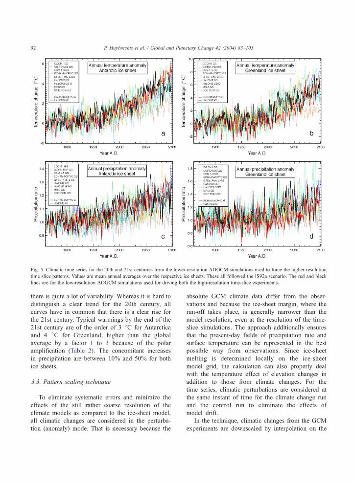
Fig. 5. Climatic time series for the 20th and 21st centuries from the lower-resolution AOGCM simulations used to force the higher-resolution

time slice patterns. Values are mean annual averages over the respective ice sheets. These all followed the IS92a scenario. The red and black

lines are for the low-resolution AOGCM simulations used for driving both the high-resolution time-slice experiments.


there is quite a lot of variability. Whereas it is hard to

distinguish a clear trend for the 20th century, all

curves have in common that there is a clear rise for

the 21st century. Typical warmings by the end of the

21st century are of the order of 3 jC for Antarctica

and 4 jC for Greenland, higher than the global

average by a factor 1 to 3 because of the polar

amplification (Table 2). The concomitant increases

in precipitation are between 10% and 50% for both

ice sheets.

3.3. Pattern scaling technique

To eliminate systematic errors and minimize the

effects of the still rather coarse resolution of the

climate models as compared to the ice-sheet model,

all climatic changes are considered in the perturba-

tion (anomaly) mode. That is necessary because the

absolute GCM climate data differ from the obser-

vations and because the ice-sheet margin, where the

run-off takes place, is generally narrower than the

model resolution, even at the resolution of the time-

slice simulations. The approach additionally ensures

that the present-day fields of precipitation rate and

surface temperature can be represented in the best

possible way from observations. Since ice-sheet

melting is determined locally on the ice-sheet

model grid, the calculation can also properly deal

with the temperature effect of elevation changes in

addition to those from climate changes. For the

time series, climatic perturbations are considered at

the same instant of time for the climate change run

and the control run to eliminate the effects of

model drift.

In the technique, climatic changes from the GCM

experiments are downscaled by interpolation on the


ice-sheet model grid and subsequent superimposition

onto the climatic representations employed by the ice-

sheet model. For temperature, the following relation

was used:

Tsurð/; k; tÞ¼ Tsurð/; k; presentÞpar þ ½Tsurð/; k; anomalyÞ� Tsurð/; k; presentÞ�time slice

� ½T icesur ðtÞscenario � T ice

sur ðtÞcontrol�AOGCM time series

½T icesurðanomalyÞ � T ice

sur ðpresentÞ�driving AOGCM time series

ð1Þ

where Tsur is the mean monthly surface temperature

referred to the initial ice-sheet topography, Tsur(/,k,present)par is present-day mean monthly sur-

face temperature obtained from parameterisations as

a function of latitude and elevation (Huybrechts

and de Wolde, 1999), [Tsur(/,k,anomaly)� Tsur(/,k,present)] the mean monthly anomaly pattern

from either high-resolution AGCM as shown in

Figs. 3 and 4, and Tsurice are mean annual ice-sheet

averaged temperature from the respective lower-

resolution AOGCM experiments. The driving

AOGCMs are either ECHAM4/OPYC3 G or

HadCM3 A2 as described above and the forcing

time series are those listed in Table 2. Present-day

is referred to the year 1975, which is also conve-

niently situated in the middle of the period 1960–

1990 of the climatological reference period. The

anomaly and present periods are those over which

the respective GCM averages were considered. We

opted to scale the time slices relative to the

corresponding ice-sheet averages of the driving

AOGCM rather than of the time slices themselves,

which are somewhat different, because the former

were obtained for similar resolutions as the forcing

AOGCMs, and because this approach ensures

that the anomaly pattern would be exactly repro-

duced during the anomaly period were the time

slice forced by their own driving AOGCM. The

actual surface temperature required for the melt-

and runoff model additionally incorporates the

effect of changes in surface elevation with the

same lapse rate as for the surface temperature

parameterisations.

For precipitation, we used ratios rather than

differences to avoid the possibility of obtaining

negative precipitation in the event that the AGCM

control field deviates significantly from the ob-

served field:

Pð/; k; tÞ ¼ Pð/; k; presentÞobserved

�f Pð/; k; anomalyÞPð/; k; presentÞ

� �time slice

�1

� �

�

PiceðtÞscenarioPiceðtÞcontrol

� 1

" #AOGCM timeseries

PiceðanomalyÞPiceðpresentÞ

� 1

� �driving AOGCM time series

þ 1

9>>>>=>>>>;

ifPð/; k; anomalyÞPð/; k; presentÞ

� �time slice

> 1

where P is precipitation rate and all the subscripts

have the same meaning as in Eq. (1). In this case all

values of P are considered as mean annual values

because reliable information on the monthly distri-

bution of the observed precipitation is not available.

Also, the yearly mass balance does not depend very

strongly on the monthly distribution of precipitation,

which only enters the calculations via the depth of

the snow layer in which percolation can take place,

and via the rain fraction. The latter depends on

surface air temperature and is therefore obtained by

assuming an even distribution of precipitation during

the year. Summing and subtracting 1 is required to

preserve the sign of the fractional increase/decrease

with respect to unity.

To avoid negative precipitation, the scaling tech-

nique needs to take into account the inverse of the

precipitation pattern ratio when this ratio is between 0

and 1 as follows:

Pð/; k; tÞ ¼ Pð/; k; presentÞobserved

� 1

Pð/; k; anomalyÞPð/; k; presentÞ

� �time slice

� 1

0BB@

1CCA

8>><>>:

�

PiceðtÞscenarioPiceðtÞcontrol

� 1

" #AOGCM timeseries

PiceðanomalyÞPiceðpresentÞ

� 1

� �driving AOGCM time series

þ 1

9>>>>=>>>>;

�1

ifPð/; k; anomalyÞPð/; k; presentÞ

� �time slice

< 1

ð2Þ

ð3Þ


The pattern scaling technique is subject to several

assumptions. The most important is probably that

patterns of climate change are necessarily conserved

in time. Such a pattern may however arise from various

competing processes with different sign, and obvious-

ly there is no guarantee that all these processes would

scale in time at the same rate. For instance the

technique cannot distinguish between precipitation

and evaporation/sublimation because a sublimation

climatology is not available for the present time. Using

total precipitation ratios to force an observed accumu-

lation field which already includes the effects of

sublimation thus necessarily assumes that both precip-

itation and sublimation change by the same fraction,

and thus that their relative importance is conserved

under conditions of climate change. Fortunately this

seems to be roughly the case. Wild et al. (2003) found

that total precipitation and sublimation varied by a

similar fraction between the two ECHAM4 time slices

for both ice sheets, but such behaviour is not given by

definition.

The scaling method for temperature also works

best when the anomaly pattern is positive, which is

also generally the case over both ice sheets. If it were

negative, and when the forcing AOGCM time series is

also negative, the result would be a positive temper-

ature change that is probably not realistic. Eqs. (1)–

(3) fail when the ice-sheet averaged temperature

differences or precipitation ratios of the driving

AOGCMs are respectively negative or less than unity,

but that is not the case for both climate models either.

Table 1 indicates how the ECHAM4 andHadAM3H

time slice experiments combine with their underlying

driving time series of ECHAM4/OPYC3 G and

HadCM3 A2 to provide the mean precipitation sensi-

tivity to temperature changes. For Greenland, the GCM

thermodynamic and circulation responses give a range

of 5–9%/jC of precipitation increase, somewhat less

than indicated by ice-cores for the glacial– interglacial

transition (Kapsner et al., 1995; Cuffey and Clow,

1997), but more than for Holocene variability and

values used in earlier studies (e.g. Huybrechts and de

Wolde, 1999). For Antarctica, on the other hand, the

precipitation sensitivity from 21st century time slice

simulations of the order 4–7%/jC is more in accord

with those inferred from glacial/interglacial contrasts

from ice cores (Yiou et al., 1985), which several studies

suggested follows a Clausius–Clapeyron argument

(accumulation is proportional to the saturated vapour

pressure of the air circulating above the surface inver-

sion layer). The Clausius–Clapeyron average sensitiv-

ity was found to be 5.9% for a uniform 1 jC warming

(Huybrechts and Oerlemans, 1990). The sensitivity

range however additionally varies by scaling with the

variety of AOGCMs as temperature and precipitation

are treated independently.

4. Results

The results distinguish between the long-term ice-

dynamic evolution from past climate changes,

extracted from the experiments discussed in Huy-

brechts (2002), and the effects of modern mass-

balance changes as obtained in this study.

4.1. Contributions to global sea-level change

Fig. 6 shows the predicted volume changes ex-

pressed in equivalent sea-level changes for the time

period between 1860 and 2100 for the two AGCM

time slices (panels a and b) forced by the full set of

AOGCM time series. The range is quite large, solely

reflecting AOGCM inter-model uncertainty in the

climate response for the same greenhouse warming

scenario. All simulations have in common that Green-

land will shrink both during the 20th and 21st century,

and thus contribute positively to sea level, and that

Antarctica will grow, and thus contribute negatively to

sea level. There is also an acceleration in the response

for the 21st century. Typically, mass balance changes

cause a Greenland contribution of + 2 to + 7 cm

between 1975 and 2100, and an Antarctic contribution

of between � 2 and � 14 cm. Also, both ice sheets

combined would contribute negatively to sea level for

the 21st century, and this applies to the majority of

individual AOGCM time series.

Combining these results with the long-term back-

ground trend does not change the picture for Green-

land as its background evolution is very small, but

gives a less negative sea-level contribution for Ant-

arctica. Here, the background trend of about + 2.5 cm

per century dominates over the modern mass-balance

effect for most of the 20th century, but is of opposite

sign. It is only counterbalanced by modern mass-

balance changes for the second half of the 21st

Fig. 6. Volume changes of the Antarctic and Greenland ice sheets expressed in equivalent sea-level change for the various experiments. The

results include the ice-dynamic effect from contemporary mass-balance changes but not the background trend resulting from past environmental

changes, which is shown separately by the thick black lines. Stippled lines refer to the Greenland ice sheet; the full lines are for the Antarctic ice

sheet. The reference time is 1975 A.D. for all experiments. Ice-volume changes were transformed into worldwide sea-level changes by assuming

an ice density of 910 kg m� 3 and a constant oceanic surface area of 3.62� 108 km2, or 71% of the Earth’s surface.


century. Whereas the different time series produce a

wide range of results, the results for the two time

slices scaled to the same time series are quite similar,

as was already evident from the similarity between

ice-sheet averaged values for both AGCMs as given

in Table 1.

The mass-balance only results are very similar to

those reported for an identical exercise performed for

the IPCC TAR (Church et al., 2001) despite a higher

model resolution for Antarctica, new precipitation

datasets, and a somewhat more sophisticated melt-

and runoff model. As such, they represent a revision

to many of the earlier assessments that predicted that

both ice sheets would about balance one another. The

negative sea-level contribution from the polar ice

sheets found here is mainly because of the larger

accumulation increases predicted by GCMs and be-

cause of the lower summer warming over coastal

Greenland, where it counts most for ablation. It is

interesting to note that a recent calculation with the


ECHAM4 time slices at the time of CO2 doubling

(f 2045) yielded a mass gain also for the Greenland

ice sheet for the first half of the 21st century (Wild et

al., 2003). These authors used another model for

ablation, but also a higher local Greenland resolution

of 2 km which they found decreased the size of the

ablation zone, and therefore of total runoff, a feature

already noted in earlier work by Reeh and Starzer

(1996) and Van de Wal and Ekholm (1996).

On average, combining the mass-balance compo-

nents with the background evolution for both ice sheets

gives a slightly positive contribution to sea level during

the 20th century ( + 1.8 cm) and a slightly negative

contribution during the 21st century (� 0.4 cm), but

the associated error bars do not enable us to distinguish

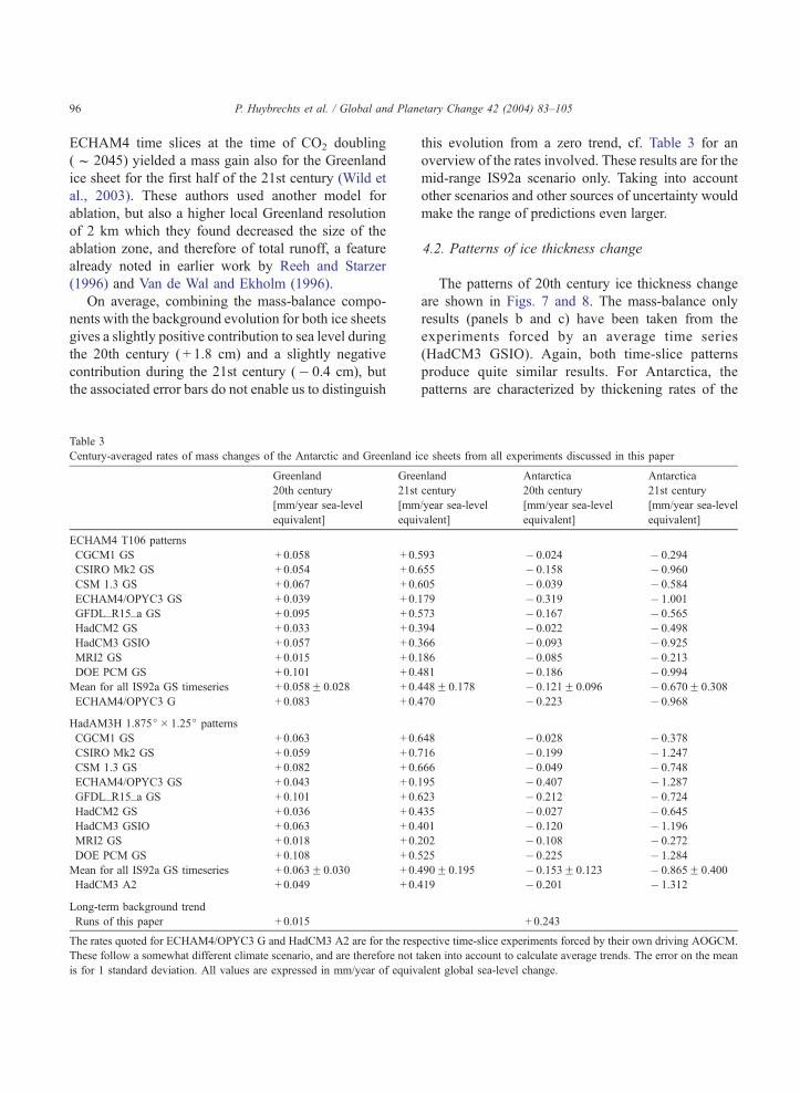
Table 3

Century-averaged rates of mass changes of the Antarctic and Greenland i

Greenland

20th century

[mm/year sea-level

equivalent]

Gree

21st

[mm

equi

ECHAM4 T106 patterns

CGCM1 GS + 0.058 + 0.

CSIRO Mk2 GS + 0.054 + 0.

CSM 1.3 GS + 0.067 + 0.

ECHAM4/OPYC3 GS + 0.039 + 0.

GFDL_R15_a GS + 0.095 + 0.

HadCM2 GS + 0.033 + 0.

HadCM3 GSIO + 0.057 + 0.

MRI2 GS + 0.015 + 0.

DOE PCM GS + 0.101 + 0.

Mean for all IS92a GS timeseries + 0.058F 0.028 + 0.

ECHAM4/OPYC3 G + 0.083 + 0.

HadAM3H 1.875j� 1.25j patterns

CGCM1 GS + 0.063 + 0.

CSIRO Mk2 GS + 0.059 + 0.

CSM 1.3 GS + 0.082 + 0.

ECHAM4/OPYC3 GS + 0.043 + 0.

GFDL_R15_a GS + 0.101 + 0.

HadCM2 GS + 0.036 + 0.

HadCM3 GSIO + 0.063 + 0.

MRI2 GS + 0.018 + 0.

DOE PCM GS + 0.108 + 0.

Mean for all IS92a GS timeseries + 0.063F 0.030 + 0.

HadCM3 A2 + 0.049 + 0.

Long-term background trend

Runs of this paper + 0.015

The rates quoted for ECHAM4/OPYC3 G and HadCM3 A2 are for the resp

These follow a somewhat different climate scenario, and are therefore not t

is for 1 standard deviation. All values are expressed in mm/year of equiv

this evolution from a zero trend, cf. Table 3 for an

overview of the rates involved. These results are for the

mid-range IS92a scenario only. Taking into account

other scenarios and other sources of uncertainty would

make the range of predictions even larger.

4.2. Patterns of ice thickness change

The patterns of 20th century ice thickness change

are shown in Figs. 7 and 8. The mass-balance only

results (panels b and c) have been taken from the

experiments forced by an average time series

(HadCM3 GSIO). Again, both time-slice patterns

produce quite similar results. For Antarctica, the

patterns are characterized by thickening rates of the

ce sheets from all experiments discussed in this paper

nland

century

/year sea-level

valent]

Antarctica

20th century

[mm/year sea-level

equivalent]

Antarctica

21st century

[mm/year sea-level

equivalent]

593 � 0.024 � 0.294

655 � 0.158 � 0.960

605 � 0.039 � 0.584

179 � 0.319 � 1.001

573 � 0.167 � 0.565

394 � 0.022 � 0.498

366 � 0.093 � 0.925

186 � 0.085 � 0.213

481 � 0.186 � 0.994

448F 0.178 � 0.121F 0.096 � 0.670F 0.308

470 � 0.223 � 0.968

648 � 0.028 � 0.378

716 � 0.199 � 1.247

666 � 0.049 � 0.748

195 � 0.407 � 1.287

623 � 0.212 � 0.724

435 � 0.027 � 0.645

401 � 0.120 � 1.196

202 � 0.108 � 0.272

525 � 0.225 � 1.284

490F 0.195 � 0.153F 0.123 � 0.865F 0.400

419 � 0.201 � 1.312

+ 0.243

ective time-slice experiments forced by their own driving AOGCM.

aken into account to calculate average trends. The error on the mean

alent global sea-level change.

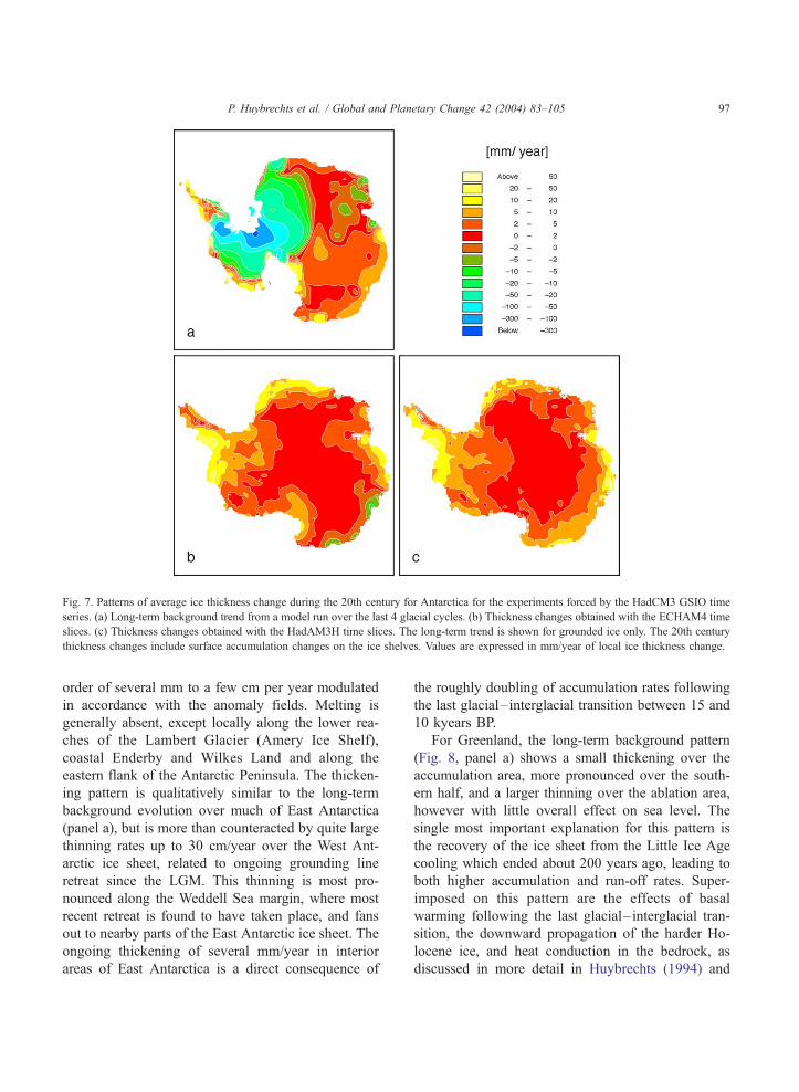
Fig. 7. Patterns of average ice thickness change during the 20th century for Antarctica for the experiments forced by the HadCM3 GSIO time

series. (a) Long-term background trend from a model run over the last 4 glacial cycles. (b) Thickness changes obtained with the ECHAM4 time

slices. (c) Thickness changes obtained with the HadAM3H time slices. The long-term trend is shown for grounded ice only. The 20th century

thickness changes include surface accumulation changes on the ice shelves. Values are expressed in mm/year of local ice thickness change.


order of several mm to a few cm per year modulated

in accordance with the anomaly fields. Melting is

generally absent, except locally along the lower rea-

ches of the Lambert Glacier (Amery Ice Shelf),

coastal Enderby and Wilkes Land and along the

eastern flank of the Antarctic Peninsula. The thicken-

ing pattern is qualitatively similar to the long-term

background evolution over much of East Antarctica

(panel a), but is more than counteracted by quite large

thinning rates up to 30 cm/year over the West Ant-

arctic ice sheet, related to ongoing grounding line

retreat since the LGM. This thinning is most pro-

nounced along the Weddell Sea margin, where most

recent retreat is found to have taken place, and fans

out to nearby parts of the East Antarctic ice sheet. The

ongoing thickening of several mm/year in interior

areas of East Antarctica is a direct consequence of

the roughly doubling of accumulation rates following

the last glacial– interglacial transition between 15 and

10 kyears BP.

For Greenland, the long-term background pattern

(Fig. 8, panel a) shows a small thickening over the

accumulation area, more pronounced over the south-

ern half, and a larger thinning over the ablation area,

however with little overall effect on sea level. The

single most important explanation for this pattern is

the recovery of the ice sheet from the Little Ice Age

cooling which ended about 200 years ago, leading to

both higher accumulation and run-off rates. Super-

imposed on this pattern are the effects of basal

warming following the last glacial–interglacial tran-

sition, the downward propagation of the harder Ho-

locene ice, and heat conduction in the bedrock, as

discussed in more detail in Huybrechts (1994) and

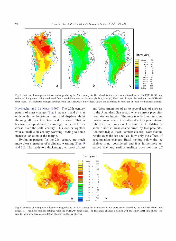
Fig. 8. Patterns of average ice thickness change during the 20th century for Greenland for the experiments forced by the HadCM3 GSIO time

series. (a) Long-term background trend from a model run over the last two glacial cycles. (b) Thickness changes obtained with the ECHAM4

time slices. (c) Thickness changes obtained with the HadAM3H time slices. Values are expressed in mm/year of local ice thickness change.


Huybrechts and Le Meur (1999). The 20th century

pattern of mass changes (Fig. 8, panels b and c) is at

odds with the long-term trend and displays slight

thinning all over the Greenland ice sheet. That is

because precipitation is on average predicted to de-

crease over the 20th century. This occurs together

with a small 20th century warming leading to some

increased ablation at the margin.

Evolution patterns for the 21st century are much

more clear signatures of a climatic warming (Figs. 9

and 10). This leads to a thickening over most of East

Fig. 9. Patterns of average ice thickness change during the 21st century fo

series. (a) Thickness changes obtained with the ECHAM4 time slices. (b

results include surface accumulation changes on the ice shelves.

and West Antarctica of up to several tens of cm/year

in the Amundsen Sea sector, where current precipita-

tion rates are highest. Thinning is only found in some

coastal areas where it is either due to a precipitation

ratio less than unity (Wilkes Land in ECHAM4), or

some runoff in areas characterized by low precipita-

tion rates (Siple Coast, Lambert Glacier). Note that the

results over the ice shelves show only the effects of

accumulation changes. Basal melting below the ice

shelves is not considered, and it is furthermore as-

sumed that any surface melting does not run off

r Antarctica for the experiments forced by the HadCM3 GSIO time

) Thickness changes obtained with the HadAM3H time slices. The

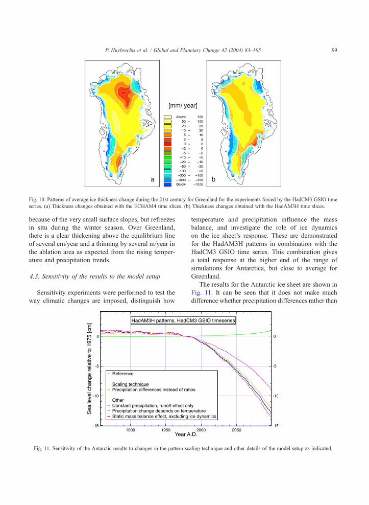
Fig. 10. Patterns of average ice thickness change during the 21st century for Greenland for the experiments forced by the HadCM3 GSIO time

series. (a) Thickness changes obtained with the ECHAM4 time slices. (b) Thickness changes obtained with the HadAM3H time slices.


because of the very small surface slopes, but refreezes

in situ during the winter season. Over Greenland,

there is a clear thickening above the equilibrium line

of several cm/year and a thinning by several m/year in

the ablation area as expected from the rising temper-

ature and precipitation trends.

4.3. Sensitivity of the results to the model setup

Sensitivity experiments were performed to test the

way climatic changes are imposed, distinguish how

Fig. 11. Sensitivity of the Antarctic results to changes in the pattern sca

temperature and precipitation influence the mass

balance, and investigate the role of ice dynamics

on the ice sheet’s response. These are demonstrated

for the HadAM3H patterns in combination with the

HadCM3 GSIO time series. This combination gives

a total response at the higher end of the range of

simulations for Antarctica, but close to average for

Greenland.

The results for the Antarctic ice sheet are shown in

Fig. 11. It can be seen that it does not make much

difference whether precipitation differences rather than

ling technique and other details of the model setup as indicated.


precipitation ratios are imposed. This variant was

implemented by a modification of Eq. (1) in which T

was replaced by P. The reason for the similar response

is that on average the precipitation distribution from

the AGCM time slice is very close to the observed

precipitation distribution, in which case both methods

can be interchanged. The precipitation increase in this

experiment is also a bit larger than that derived from

the saturation vapour pressure argument used in older

work (e.g. Huybrechts and de Wolde, 1999) to link

precipitation changes to temperature changes. This

larger sensitivity suggests that in a warmer climate

changes in atmospheric circulation and increased

moisture advection (less sea ice, warmer ocean sur-

face) can also become important to enhance precipita-

tion, in particular close to the ice-sheet margin, but the

result obtained here is also in part because of the

HadAM3H/HadCM3 GSIO combination, which al-

ready has a higher than average precipitation increase.

For Antarctica, excluding the ice-dynamic response to

the imposed mass-balance changes hardly affects the

result because of the small ice-dynamic response

( < 5%) discussed for the century time scale in previous

work (Huybrechts and de Wolde, 1999). The contri-

bution from runoff is also small at less than + 1 cm of

sea level rise, or about 7% of the precipitation re-

sponse, as evident from the constant precipitation

experiment.

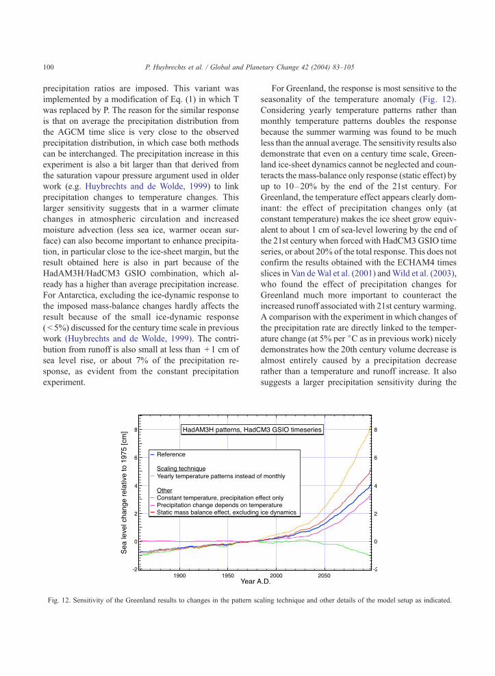
Fig. 12. Sensitivity of the Greenland results to changes in the pattern sc

For Greenland, the response is most sensitive to the

seasonality of the temperature anomaly (Fig. 12).

Considering yearly temperature patterns rather than

monthly temperature patterns doubles the response

because the summer warming was found to be much

less than the annual average. The sensitivity results also

demonstrate that even on a century time scale, Green-

land ice-sheet dynamics cannot be neglected and coun-

teracts the mass-balance only response (static effect) by

up to 10–20% by the end of the 21st century. For

Greenland, the temperature effect appears clearly dom-

inant: the effect of precipitation changes only (at

constant temperature) makes the ice sheet grow equiv-

alent to about 1 cm of sea-level lowering by the end of

the 21st century when forced with HadCM3GSIO time

series, or about 20% of the total response. This does not

confirm the results obtained with the ECHAM4 times

slices in Van deWal et al. (2001) andWild et al. (2003),

who found the effect of precipitation changes for

Greenland much more important to counteract the

increased runoff associated with 21st century warming.

A comparison with the experiment in which changes of

the precipitation rate are directly linked to the temper-

ature change (at 5% per jC as in previous work) nicely

demonstrates how the 20th century volume decrease is

almost entirely caused by a precipitation decrease

rather than a temperature and runoff increase. It also

suggests a larger precipitation sensitivity during the

aling technique and other details of the model setup as indicated.


21st century than suggested from late Holocene ice-

core records, from which the 5% value was inferred

(Clausen et al., 1988).

4.4. Comparison with observations

A comparison of the simulations with observations

can only be made for the 20th century, but is hampered

by the scarcity of data in both space and time. Never-

theless, available measurements allow us to assess

qualitative aspects of the results obtained in this paper.

A distinction should be made between meteorological

or climate data on temperature and precipitation

changes, to be compared to the climate forcing, and

observations on surface elevation changes, to be com-

pared to the final results.

Direct meteorological series are however few, and

are almost exclusively limited to coastal stations.

Longer series only exist for Greenland, but are often

not homogenous. For Antarctica, such records only

extend back to the International Geophysical Year of

1957–1958. Additional insight is available from me-

teorological re-analyses (ECMWF, NCEP-NCAR)

and AGCM simulations driven by observed SSTs,

but only for the second half of the 20th century.

Accumulation estimates from shallow ice cores, on

the other hand, cover longer time periods but are

limited to a few sites only.

The general picture that can be distilled from these

data is in reasonable agreement with many aspects

derived from the GCMs in this paper forced by

historical greenhouse gas concentrations. Various

sources indicate that Greenland is a regional exception

to the warming trend observed in many other places

on Earth for much of the second half of the 20th

century. Hanna and Cappelen (2003) found a signif-

icant cooling trend between 1958 and 2001 in coastal

southern Greenland of � 1.3 jC in contrast to a

global warming trend over the same period. Brom-

wich et al. (1993) found a decreasing trend in precip-

itation of about 15% between 1963 and 1988. Results

from long-term (1950–1991) climate simulations with

the T63 resolution CSIRO9 AGCM forced by ob-

served SST also indicate that net accumulation de-

creased in analogy with a decreasing surface

temperature over the ice sheet and a cooling over

the surrounding ocean (Smith, 1999). The cooling

over the 41-year period was found to be 0.66 jC with

a precipitation decrease of 13% over the ice sheet

consistent with the results from Bromwich et al.

(1993). Bales et al. (2001) report a decreasing trend

in accumulation in a location in northwest Greenland

for the second half of the 20th century of 25%.

Although these observations do not span the whole

20th century, they certainly do not contradict the most

conspicuous feature of the climate forcing found in

this study, namely the decreasing precipitation trend

on average, which resulted in a thinning over the

accumulation zone from 20th century mass balance

changes alone. The small overall warming trend

predicted by most of the AOGCMs over Greenland

for the whole of the 20th century, on the other hand, is

also supported by the few long temperature records

available from coastal sites (Box, 2002).

Available data from Antarctica are all indicative of

a mean warming trend concomitant with an increase

of precipitation during the 20th century, but with

highly variable regional responses. Turner et al.

(2002) derived a spatially weighted warming trend

of 0.176 jC per decade between 1958 and 2002 over

all of Antarctica, less than the + 1.2 jC for all

Antarctic stations between 1959 and 1996 (Vaughan

et al., 2001). Since most of these stations are at the

coast, this is consistent with a weak cooling over the

interior of the Antarctic continent (Thompson and

Solomon, 2002). The most significant warming oc-

curred over the Antarctic Peninsula, especially at its

western side where the trend is + 0.56 jC per decade

for 1951–2001 or a total of + 2.8 jC. This local trendis completely missing from the GCM derived forcing

used here, a feature already discussed for comparable

GCM results obtained for the second half of the 20th

century elsewhere (Connolley and O’Farrell, 1998;

Vaughan et al., 2001). Our 20th century precipitation

forcing however agrees better with the increasing

trend of 5% over all of Antarctica established from

moisture budget analysis between 1955 and 1975

(Bromwich and Robasky, 1993). Such a positive trend

is confirmed by an increase in snow accumulation at

South Pole station since 1965 of possibly up to 30%

as derived from ice cores (Mosley-Thompson et al.,

1999). Significant increases of snow accumulation of

up to 20% since the 1960s were also derived from

four ice cores in Wilkes Land (Morgan et al., 1991),

together with a smaller, but still significant increase

for all of the 20th century. Simulations with CSIRO9


T63 forced with observed SSTs over the period

1950–1991 (Smith et al., 1998) gave an average

Antarctic warming of + 0.74 jC, or + 0.18 jC per

decade, with a concomitant increase of accumulation

of 4.1%, or 1% per decade. The average precipitation

trend from all our simulations with the two time-slice

patterns scaled by all AOGCMs was 2.7% for the

whole 20th century, lower than some of the numbers

cited above but representative for a longer period

(Table 3).

The combined present-day evolution patterns (long-

term and 20th century) of Antarctic and Greenland ice

thickness change (Figs. 7 and 8) also seem to share

many of the features derived from recent observational

data, in particular from repeated airborne laser altimeter

and satellite radar altimeter measurements over the last

decade (Rignot and Thomas, 2002). These indicate a

slight mass loss for the Greenland ice sheet equal to

about + 0.1 mm/year of sea level change, together with

a clear mass loss for West Antarctica and no clear trend

yet for East Antarctica. The spatial pattern for Green-

land agrees rather well with these direct measurements

for the nineties, showing a slight thickening or an

approximate balance for the accumulation zone togeth-

er with a general pattern of thinning for the ablation

zone. The only deviation to this general picture is the

stronger thinning exceeding 1 m/year close to the coast

in southeast Greenland (Krabill et al., 2000). This

feature is therefore likely to be of ice-dynamic origin

for a mechanism not incorporated in the modeling (the

category of ‘unexpected ice-dynamic responses’ as

discussed in the introduction). The same remark applies

to the inferred late 20th century pattern of changes of

the West Antarctic ice sheet, where available data seem

to point to a thickening in the north (Siple Coast ice

streams) and a thinning in the west (in particular for the

Amundsen Sea sector). That is different from what the

modeling produces, probably for similar reasons as for

southeast Greenland.

The small thickening over large parts of the East

Antarctic plateau, on the other hand, both from the

long-term response as from 20th century mass-bal-

ance changes, seems to agree better with ERS1/2 data

obtained between 1992 and 1996 (Wingham et al.,

1998). It should however be noted that the modeling

results refer to a century trend, whereas the observa-

tional data are only for one or two decades at most,

and therefore of too short a duration to confidently

distinguish between short-term variability and the

longer-term trend. In addition, the altimetry data are

for surface elevation. They are therefore contaminated

by an unknown component from crustal uplift when

compared with ice thickness changes, though model-

ing studies indicate that bedrock changes are usually

an order of magnitude smaller than ice thickness

changes on a century time scale (Huybrechts and Le

Meur, 1999).

5. Summary and conclusion

Pattern scaling appears to be a useful technique to

predict climatic changes over the ice sheets. Although

the technique should be used with care, and full

interactive coupling with transient AOGCMs at high

resolution would be preferable, the strength of the

method is its flexibility to generalise to other climate

scenarios while at the same time incorporating tem-

poral and spatial patterns of climate change in the best

possible way from current GCM simulations.

A very robust feature of all experiments for the

21st century is that the Antarctic ice sheet is pre-

dicted to grow and the Greenland ice sheet is

predicted to shrink because of the dominance of

increased precipitation and increased runoff, respec-

tively. These trends are significantly different from

zero within 2 sigma error bars (Table 3). Trends

from mass-balance changes alone are also significant

for the 20th century but the process for the Green-

land ice sheet is found to be different, with decreased

precipitation rather than increased runoff as the

major source of the mass loss. For the majority of

driving AOGCMs, the Antarctic response is larger

than for Greenland, so that the combined sea-level

contribution from polar ice sheets during the 21st

century from mass-balance changes alone is nega-

tive. This conclusion no longer holds when including

the background trends found in this study, that are in

the middle of the IPCC TAR range obtained from all

methods, in which case both ice sheets combined

would yield an evolution that is indistinguishable

from a zero trend. Ice-dynamic effects to the im-

posed 20th and 21st century mass changes are of

second-order importance.

The experiments discussed here considered only

one emission scenario and one set of ice-sheet model


and mass-balance model parameters and therefore

highlight the uncertainty introduced by the variability

in the climate models. It is certainly comforting that

most of the variability comes from the spread of

inherent climate sensitivity of the underlying

AOGCM simulations. There is a great similarity in

both qualitative aspects of the patterns as in average

changes over time for both time-slice patterns forced

by the same AOGCM time series. More AGCM

patterns should however be used in future work to

confirm whether this is a robust result or whether this

outcome was overly conditioned by the choice of

model and the specific pattern scaling method

employed.

The experiments with the ECHAM4 time slice

patterns (Wild and Ohmura, 2000) were used as the

base for the IPCC TAR projections of sea-level rise

from the polar ice sheets (Church et al., 2001), albeit

with some slight changes in the ice-sheet and mass-

balance models. To do that, these results were

regressed against global mean temperature to enable

further scaling to take into account the complete range

of IPCC temperature predictions for the most recent

SRES scenarios. Taking into account the background

evolution and various other sources of uncertainty,

this yielded a predicted Antarctic contribution to

global sea-level change between 1990 and 2100 of

between � 19 and + 5 cm, which range can be

considered as a 95% confidence interval. For Green-

land, the range was � 2 to + 9 cm. Most of this

spread came from the climate sensitivity of the forcing

AOGCMs, and less from the emission scenario or the

uncertainty in the ice-sheet models.

For the runs in this paper we find a total range of

polar ice-sheet response of between + 5 and � 12 cm

during the period 1990–2100 for any combination of

both ice sheet results together. Including the long-term

background trend the range is between + 8 and � 9

cm, not significantly different from zero but with a

slightly higher mean than in the IPCC TAR. This

leaves thermal expansion of the seawater and melting

of mountain glaciers and small ice caps as major

sources of sea level rise during the 21st century. In

the IPCC TAR, using the same set of AOGCMs as

used in this paper, the corresponding sea-level con-

tributions from the latter sources were found to be in

the ranges + 0.11–0.43 m and + 0.01–0.23 cm,

respectively. For sustained greenhouse warming con-

ditions beyond the 21st century, however, the approx-

imate balance between the two polar ice sheets may

no longer hold and both ice masses may significantly

start to melt at rates of up to 10 mm/year of sea level

rise (Huybrechts and de Wolde, 1999).

Acknowledgements

This work was performed within the scope of the

German HGF-Strategiefonds Projekt 2000/13 SEAL

(Sea Level Change), and the Belgian Global Change

and Sustainable Development Programme (Federal

Office for Scientific, Technical, and Cultural Affairs,

Prime Minister’s Service) under contracts CG/DD/

09B and EV/03/9B. We are grateful to David Hassell,

Richard Jones and James Murphy for HadAM3H data.

Work at the Hadley Centre was supported by the UK

Department for Environment, Food and Rural Affairs

under contract PECD 7/12/37 and by the Government

Meteorological Research and Development

Programme. The high resolution ECHAM experi-

ments became possible through the generous comput-

ing resources provided by the Swiss Center for

Scientific Computing CSCS, and through the support

of the National Center for Competence in Climate

Research (NCCR Climate).

References

Bales, R.C., Mosley-Thompson, E., McConnell, J.R., 2001. Vari-

ability of accumulation in northwest Greenland over the last 250

years. Geophysical Research Letters 28 (14), 2679–2682.

Bindschadler, R.A., Bentley, C.R., 2002. On thin ice? Scientific

American (12), 66–73.

Box, J.E., 2002. Survey of Greenland instrumental temperature

records: 1873–2001. International Journal of Climatology 22,

1829–1847.

Bromwich, D.H., Robasky, F.M., 1993. Recent precipitation trends

over the polar ice sheets. Meteorology and Atmospheric Physics

51, 259–274.

Bromwich, D.H., Robasky, F.M., Keen, R.A., Bolzan, J.F., 1993.

Modeled variations of precipitation over the Greenland ice

sheet. Journal of Climate 6, 1253–1268.

Bromwich, D.H., Cullather, R.I., van Woert, M.L., 1998. Antarctic

precipitation and its contribution to the global sea-level budget.

Annals of Glaciology 27, 220–226.

Church, J.A., Gregory, J.M., Huybrechts, P., Kuhn, M., Lambeck,

K., Nhuan, M.T., Qin, D., Woodworth, P.L., 2001. Changes in

sea level. In: Houghton, J.T., Ding, Y., Griggs, D.J., Noguer,


M., Van der Linden, P.J., Dai, X., Maskell, K., Johnson, C.A.

(Eds.), Climate Change 2001: The Scientific Basis: Contribu-

tion of Working Group I to the Third Assessment Report of

the Intergovernmental Panel on Climate Change. Cambridge

Univ. Press, Cambridge, pp. 639–694.

Clausen, H.B., Gundestrup, N.S., Johnsen, S.J., Bindschadler, R.A.,

Zwally, H.J., 1988. Glaciological investigations in the crete area,

central Greenland. A search for a new drilling site. Annals of

Glaciology 10, 10–15.

Connolley, W.M., O’Farrell, S.P., 1998. Comparison of warming

trends over the last century around Antarctica from three cou-

pled models. Annals of Glaciology 27, 565–570.

Cubasch, U., Waszkewitz, J., Hegerl, G.C., Perlwitz, J., 1995. Re-

gional climate changes as simulated in time-slice experiments.

Climatic Change 31, 273–304.

Cuffey, K.M., Clow, G.D., 1997. Temperature, accumulation, and

ice sheet elevation in central Greenland through the last degla-

cial transition. Journal of Geophysical Research 102 (C12),

26383–26396.

De Wolde, J., Huybrechts, P., Oerlemans, J., van de Wal, R.S.W.,

1997. Projections of global mean sea level rise calculated with a

2D energy-balance climate model and dynamic ice sheet models.

Tellus 49A (4), 486–502.

Fichefet, T., Poncin, C., Goosse, H., Huybrechts, P., Janssens, I.,

Le Treut, H., 2003. Implications of changes in freshwater

flux from the Greenland ice sheet for the climate of the 21st

century. Geophysical Research Letters 30 (17), 1911 (doi:

10.1029/2003GL017826).

Gordon, C., Cooper, C., Senior, C.A., Banks, H., Gregory, J.M.,

Johns, T.C., Mitchell, J.F.B., Wood, R.A., 2000. The simulation

of SST, sea ice extents and ocean heat transports in a version of

the Hadley Centre coupled model without flux adjustments.

Climate Dynamics 16, 147–168.

Hanna, E., Cappelen, J., 2003. Recent cooling in coastal southern

Greenland and relation with the North Atlantic Oscillation.

Geophysical Research Letters 30 (3), 1132 (doi:10.1029/

2002GL015797).

Hanna, E., Valdes, P., 2001. Validation of ECMWF (re)analysis

surface climate data, 1979–98, for Greenland and implications

for mass balance modelling of the ice sheet. International Jour-

nal of Climatology 21, 171–195.

Houghton, J.T., Ding, Y., Griggs, D.J., Noguer, M., Van der Linden,

P.J., Dai, X., Maskell, K., Johnson, C.A. (Eds.), 2001. Climate

Change 2001: The Scientific Basis: Contribution of Working

Group I to the Third Assessment Report of the Intergovernmental

Panel on Climate Change. Cambridge Univ. Press, Cambridge,

881 pp.

Huybrechts, P., 1994. The present evolution of the Greenland ice

sheet: an assessment by modelling. Global and Planetary

Change 9 (1–2), 39–51.

Huybrechts, P., 2002. Sea-level changes at the LGM from ice-

dynamic reconstructions of the Greenland and Antarctic ice

sheets during the glacial cycles. Quaternary Science Reviews

21 (1–3), 203–231.

Huybrechts, P., de Wolde, J., 1999. The dynamic response of the

Greenland and Antarctic ice sheets to multiple-century climatic

warming. Journal of Climate 12 (8), 2169–2188.

Huybrechts, P., Le Meur, E., 1999. Predicted present-day evolution

patterns of ice thickness and bedrock elevation over Greenland

and Antarctica. Polar Research 18 (2), 299–308.

Huybrechts, P., Oerlemans, J., 1990. Response of the Antarctic Ice

Sheet to future greenhouse warming. Climate Dynamics 5,

93–102.

Huybrechts, P., Letreguilly, A., Reeh, N., 1991. The Greenland ice

sheet and greenhouse warming. Global and Planetary Change

Section 3 (4), 399–412.

Huybrechts, P., Steinhage, D., Wilhelms, F., Bamber, J.L., 2000.

Balance velocities and measured properties of the Antarctic ice

sheet from a new compilation of gridded datasets for modeling.


Huybrechts, P., Janssens, I., Poncin, C., Fichefet, T., 2002. The re-

sponse of the Greenland ice sheet to climate changes in the 21st

century by interactive coupling of an AOGCM with a thermo-

mechanical ice-sheet model. Annals of Glaciology 35, 409–415.

Janssens, I., Huybrechts, P., 2000. The treatment of meltwater re-

tention in mass-balance parameterizations of the Greenland ice

sheet. Annals of Glaciology 31, 133–140.

Joughin, I., Tulaczyk, S., Bindschadler, R.A., Price, S., 2002.

Changes in west Antarctic ice stream velocities: observation

and analysis. Journal of Geophysical Research 107 (B11),

2289 (doi:10.1029/2001JB001029).

Jung-Rothenhausler, F., 1998. Remote sensing and GIS studies

in North-East Greenland. Berichte zur Polarforschung 280,

161 pp.

Kapsner, W.R., Alley, R.B., Shuman, C.A., Anandakrishnan, S.,

Grootes, P.M., 1995. Dominant influence of atmospheric circu-

lation on snow accumulation in Greenland over the past 18,000

years. Nature 373, 52–54.

Krabill, W.B., Abdalati, W., Frederick, E., Manizade, S., Martin, C.,

Sonntag, J., Swift, R., Thomas, R.H., Wright, W., Yungel, J.,

2000. Greenland ice sheet: high-elevation balance and periph-

eral thinning. Science 289, 428–430.

Leggett, J., Pepper, W.J., Swart, R.J., 1992. Emissions scenarios for

IPCC: an update. In: Houghton, J.T., Callander, B.A., Varney,

S.K. (Eds.), Climate Change 1992, The Supplementary Report

to the IPCC Scientific Assessment. Cambridge Univ. Press,

Cambridge, pp. 69–96.

Morgan, V.I., Goodwin, I.D., Etheridge, D.M., Wookey, C.W.,

1991. Evidence from Antarctic ice cores for recent increases

in snow accumulation. Nature 354, 58–60.

Mosley-Thompson, E., Paskievitch, J.F., Gow, A.J., Thompson,

L.G., 1999. Late 20th century increase in South Pole accumu-

lation. Journal of Geophysical Research 104 (D4), 3877–3886.

Nakicenovic, N., et al., 2000. IPCC Special Report on Emissions

Scenarios. Cambridge Univ. Press, Cambridge, 599 pp.

O’Farrell, S.P., McGregor, J.L., Rotstayn, L.D., Budd, W.F., Zweck,

C., Warner, R.C., 1997. Impact of transient increases in atmo-

spheric CO2 on the accumulation and mass balance of the Ant-

arctic ice sheet. Annals of Glaciology 25, 137–144.

Ohmura, A., 2001. Physical basis for the temperature-based

melt-index method. Journal of Applied Meteorology 40 (4),

753–761.

Ohmura, A., Reeh, N., 1991. New precipitation and accumulation

maps for Greenland. Journal of Glaciology 37, 140–148.


Pope, V.D., Gallani, M.L., Rowntree, P.R., Stratton, R.A., 2000.

The impact of new physical parametrizations in the Hadley

Centre climate model—HadAM3. Climate Dynamics 16,

123–146.

Reeh, N., Starzer, W., 1996. Spatial resolution of ice-sheet topo-

graphy: influence on Greenland mass-balance modelling. Rap-

port-Grønlands Geologiske Undersøgelse (53), 85–94.

Rignot, E.J., Thomas, R.H., 2002. Mass balance of polar ice sheets.

Science 297, 1502–1506.

Roeckner, E., et al., 1996. The atmospheric general circulation

model ECHAM-4: model description and simulation of pres-

ent-day climate. Max-Planck-Institut fur Meteorologie, Ham-

burg, Report 218, 90 pp.

Roeckner, E., Bengtsson, L., Feichter, J., Lelieveld, J., Rohde, H.,

1999. Transient climate change simulations with a coupled at-

mosphere–ocean GCM including the tropospheric sulfur cycle.

Journal of Climate, 3004–3032.

Shepherd, A., Wingham, D.J., Mansley, J.A.D., 2002. Inland thin-

ning of the Amundsen Sea sector, West Antarctica. Geophysical

Research Letters 29 (10) (doi:10.1029/2001GL014183).

Smith, I.N., 1999. Estimating mass balance components of the

Greenland ice sheet from a long-term GCM simulation. Global

and Planetary Change 20, 19–32.

Smith, I.N., Budd, W.F., Reid, P., 1998. Model estimates of Ant-

arctic accumulation rates and their relationship to temperature

changes. Annals of Glaciology 27, 246–250.

Thompson, D.W.J., Solomon, S., 2002. Interpretation of recent

southern hemisphere climate change. Science 296, 895–899.

Turner, J., King, J.C., Lachlan-Cope, T.A., Jones, P.D., 2002.

Recent temperature trends in the Antarctic. Nature 418,

291–292.

Van de Wal, R.S.W., Ekholm, S., 1996. On elevation models as

input for mass balance calculations of the Greenland ice sheet.


Van de Wal, R.S.W., Oerlemans, J., 1997. Modelling the short term

response of the Greenland ice sheet to global warming. Climate

Dynamics 13, 733–744.

Van de Wal, R.S.W., Wild, M., de Wolde, J., 2001. Short-term

volume changes of the Greenland ice sheet in response to dou-

bled CO2 conditions. Tellus 53B, 94–102.

Van der Veen, C.J., 2002. Polar ice sheets and global sea level: how

well can we predict the future? Global and Planetary Change 32,

165–194.

Vaughan, D.G., Spouge, J., 2002. Risk estimation of collapse of the

West Antarctic ice sheet. Climatic Change 52, 65–91.

Vaughan, D.G., Marshall, G.J., Connolley, W.M., King, J.C., Mul-

vaney, R., 2001. Devil in the detail. Science 293, 1777–1779.

Warner, R.C., Budd, W.F., 1998. Modelling the long-term response

of the Antarctic ice sheet to global warming. Annals of Glaci-

ology 27, 161–168.

Wild, M., Ohmura, A., 2000. Changes in mass balance of the polar

ice sheets and sea level under greenhouse warming as projected

in high resolution GCM simulations. Annals of Glaciology 30,

197–203.

Wild, M., Calanca, P., Scherrer, S.C., Ohmura, A., 2003. Effects of

polar ice sheets on global sea level in high-resolution green-

house scenarios. Journal of Geophysical Research 108 (D5),

4165 (doi:10.1029/2002JD002451).

Wingham, D.J., Ridout, A.J., Scharroo, R., Arthern, R.J., Shum,

C.K., 1998. Antarctic elevation change from 1992 to 1996.

Science 282, 456–458.

Yiou, F., Raisbeck, G.M., Bourles, D., Lorius, C., Barkov, N.I.,

1985. 10Be in ice at Vostok Antarctica during the last climatic

cycle. Nature 316, 616–617.

Documents

Modelling Antarctic and Greenland volume changes … et al 2004.pdf · Modelling Antarctic and Greenland volume changes during the 20th and 21st centuries forced by GCM time slice