The Cryosphere, 6, 553–571, 2012www.the-cryosphere.net/6/553/2012/doi:10.5194/tc-6-553-2012© Author(s) 2012. CC Attribution 3.0 License.

The Cryosphere

Modelling borehole temperatures in Southern Norway – insightsinto permafrost dynamics during the 20th and 21st century

T. Hipp, B. Etzelmuller, H. Farbrot, T. V. Schuler, and S. Westermann

Department of Geosciences, University of Oslo, Oslo, Norway

Correspondence to:T. Hipp (tobias.hipp@geo.uio.no)

Received: 30 December 2011 – Published in The Cryosphere Discuss.: 27 January 2012Revised: 20 April 2012 – Accepted: 28 April 2012 – Published: 23 May 2012

Abstract. This study aims at quantifying the thermal re-sponse of mountain permafrost in southern Norway tochanges in climate since 1860 and until 2100. A tran-sient one-dimensional heat flow model was used to simulateground temperatures and associated active layer thicknessesfor nine borehole locations, which are located at differentelevations and in substrates with different thermal proper-ties. The model was forced by reconstructed air temperaturesstarting from 1860, which approximately coincides with theend of the Little Ice Age in the region. The impact of cli-mate warming on mountain permafrost to 2100 is assessedby using downscaled air temperatures from a multi-modelensemble for the A1B scenario. Borehole records over threeconsecutive years of ground temperatures, air temperaturesand snow cover data served for model calibration and vali-dation. With an increase of air temperature of∼1.5◦C over1860–2010 and an additional warming of∼2.8◦C until 2100,we simulate the evolution of ground temperatures for eachborehole location. In 1860 the lower limit of permafrost wasestimated to be ca. 200 m lower than observed today. Accord-ing to the model, since the approximate end of the Little IceAge, the active-layer thickness has increased by 0.5–5 m and>10 m for the sites Juvvasshøe and Tron, respectively. Themost pronounced increases in active layer thickness weremodelled for the last two decades since 1990 with increaserates of +2 cm yr−1 to +87 cm yr−1 (20–430 %). Accordingto the A1B climate scenario, degradation of mountain per-mafrost is suggested to occur throughout the 21st century atmost of the sites below ca. 1800 m a.s.l. At the highest loca-tions at 1900 m a.s.l., permafrost degradation is likely to oc-cur with a probability of 55–75 % by 2100. This implies thatmountain permafrost in southern Norway is likely to be con-fined to the highest peaks in the western part of the country.

1 Background and objectives

Permafrost in general and mountain permafrost in particu-lar experiences increasing interest due to its sensitivity toclimate variation and importance for geomorphologic andgeotechnical processes (Harris et al., 2009), such as slope sta-bility and natural hazards (Gude and Barsch, 2005; Huggel etal., 2010; Gruber et al., 2004a; Fischer et al., 2006; Haeberli,1992). There is a need to address the response of ground tem-peratures (GT) to climate forcing, especially the modulationof the response of GTs to the effect of snow cover and differ-ent types of surficial material and bedrock.

This study aims at the quantification of subsurface warm-ing and changes in active layer thickness (ALT) over aca. 250 yr period from the approximate end of the Little IceAge (LIA) in the mid 19th century to 2100 at three high-mountain sites in Southern Norway. Significant warming oc-curred during that period and is expected to continue. In rela-tion to these changes, we intend to identify the possible zona-tions of former, present and future permafrost. Finally, weaim to characterise these responses for different environmen-tal settings in terms of bedrock properties, sediment-coverand snow. We suggest that these assessments are fundamen-tal prerequisites for spatially distributed permafrost mod-elling in Scandinavia, and for understanding geomorpholog-ical process patterns and ultimately landscape development(Berthling and Etzelmuller, 2011).

One-dimensional heat flow models have been applied invarious permafrost studies to assess the response of per-mafrost to climate change, such as for arctic permafrost(Burn and Zhang, 2009; Etzelmuller et al., 2011; Osterkampand Romanovsky, 1999; Romanovsky et al., 2007; Sazonovaet al., 2004; Zhang et al., 2006, 2008) and mountain per-mafrost in the European Alps (Engelhardt et al., 2010;

Published by Copernicus Publications on behalf of the European Geosciences Union.

554 T. Hipp et al.: Modelling borehole temperatures in Southern Norway

Fig. 1.Location of the study sites and boreholes in Norway(a). As a rough estimate of possible permafrost distribution all areas with MAAT< −3◦C during the last normal period 1961–1990 are shown in blue (Etzelmuller et al., 2003). Local site overview of(b) Juvvasshøe,(c) Jetta and(d) Tron, each indicating the locations of boreholes (BH), where GST measurements (MTD) andTAIR , GST and snow depthmeasurements are performed.

Gruber and Hoelzle, 2008; Gruber et al., 2004b; Hoelzle etal., 2001; Luetschg et al., 2008; Noetzli and Gruber, 2009;Noetzli et al., 2007; Scherler et al., 2010; Stocker-Mittaz etal., 2002).

In this study, we apply a 1-D heat flow model (Etzelmulleret al., 2011; Farbrot et al., 2007) to simulate GTs and ALTfor the time period of 1860 until 2100 in the mountains ofSouthern Norway. In addition to the existing PACE borehole(Isaksen et al., 2001) in 2008 12 shallow boreholes have beenestablished recording GT, GST andTAIR at three differentmountain areas in Southern Norway. Forcing the calibratedmodel using reconstructed and projectedTAIR series, we as-sess how sensitive GT and ALT react to warming at the in-vestigated sites, including an assessment of model limitationsand related uncertainties of our approach.

2 Setting, instrumentation and climate at the study sites

We use borehole measurements from three locations inSouthern Norway in this study (Fig. 1a): Juvvasshøe(61◦40′ N, 08◦22′ E, 1894 m a.s.l.), Jetta (61◦53′ N, 9◦17′ E,1560 m a.s.l.) and Tron (62◦10′ N, 10◦41′ E, 1640 m a.s.l.).At these sites, ground temperature records are available at13 borehole locations covering the period September 2008to July 2011. At Juvvasshøe, the PACE borehole groundtemperature data is available from 1999 (Isaksen et al., 2001,2007). Data from all boreholes were used in this chapter togive an introduction to the climate and geomorphological set-tings at the study sites. However, only a selection of nineboreholes (Table 1) was used for the modelling study.

The Cryosphere, 6, 553–571, 2012 www.the-cryosphere.net/6/553/2012/

T. Hipp et al.: Modelling borehole temperatures in Southern Norway 555

2.1 The borehole sites and instrumentation

At Juvvasshøe (1894 m) (Fig. 1b) first ground temperaturemeasurements started by Ødegard et al. (1992) and the laterdrilling of the 129 m deep PACE borehole (Harris et al.,2001; Isaksen et al., 2001). The site is characterised by exten-sive block fields at higher elevations and finer till material atlower elevations (Ødegard et al., 1988). Six boreholes weredrilled in addition to the existing PACE boreholes, resultingin an altitudinal transect from 1894 m a.s.l. (PACE) down to1307 m a.s.l. (Juv-BH6) (Fig. 1b). The boreholes have differ-ent stratigraphies: PACE, Juv-BH1 and Juv-BH3 are locatedin block fields; Juv-BH4 was drilled in bedrock and Juv-BH6in a sand- to gravel-rich ground moraine.

At Jetta (Fig. 1c) block fields are present down to ele-vations of 1500 m and 1100 m a.s.l. on the north and southexposition, respectively, with thicknesses ranging from 3 to10 m (Bø, 1998). Three boreholes were drilled 10 m intobedrock at 1560 m a.s.l. (Jet-BH1), 1450 m a.s.l. (Jet-BH2)and 1218 m a.s.l. (Jet-BH3), respectively.

Tron (Fig. 1d) is located further east in a more continen-tal climate setting. Two boreholes were drilled 10 m intofine-grained morainic material (Tro-BH1, Tro-BH2), whilethe uppermost borehole (Tro-BH1, 1640 m) was drilled 30 minto a block field.

At all boreholes, GST,TAIR and snow depth (SD) arerecorded. Following the approach by Lewkowicz (2008)Maxim© iButton temperature loggers (±0.5◦C accuracy) atfixed heights above the ground surface (10, 20, 30, 40, 50,60, 80, 100, 120 cm) were used to extract SD. At PACE andTron automatic weather stations record several meteorologi-cal variables to characterise the surface energy balance.

2.2 Climate and ground thermal conditions at thestudy sites

The sites are situated along a continentality gradient from amore maritime influenced climate at Juvvasshøe to a morecontinental climate setting at Tron (Farbrot et al., 2011). Theentire observation period from September 2008 to July 2011was divided into three parts (S1: September 2008 to August2009; S2: September 2009 to August 2010; S3: September2010 to July 2011) to analyse the inter-annual variation (Ta-ble 1). As S3 does not cover a complete seasonal cycle, it isnot used for comparison orn-factor calculations.

At Juvvasshøe MAATs during S1 ranged from−3.4◦C to−0.6◦C and during S2 from−4.5◦C to −2.3◦C between1894 m a.s.l. and 1307 m a.s.l. At higher elevations snowcover is highly variable and generally thin (<20 cm) due tostrong redistribution by wind (Fig. 2a). A thick snow coveris found at lower elevations (70–140 cm) (Table 1, Fig. 2b).The lower limit of permafrost along the instrumented slopeis at ca. 1450 m a.s.l. (Farbrot et al., 2011). Permafrost thick-ness at the PACE borehole was estimated to be approxi-mately 380 m (Isaksen et al., 2001). During the study period,

observed ALT varied between 1.6 m (Juv-BH1) (Fig. 2a)and 8.6 m (Juv-BH4). The mean annual ground temperatureat 10 m depth (MAGT10) ranges from−2.5◦C to −0.3◦Cwithin permafrost and reaches up to +1.7◦C (Juv-BH6) innon-permafrost areas (Table 1).

At Jetta, MAATs between−2.2◦C to −0.2◦C wererecorded during S1 and−3.7◦C to −1.6 ◦C during S2 be-tween 1560 m a.s.l. to 1218 m a.s.l. (Table 1). A long-lasting,thick snow cover (>140 cm) is recorded at the uppermostborehole (Jet-BH1) (Fig. 2c), while Jet-BH3 had no signif-icant snow cover due to strong wind drift (Fig. 2d). There-fore, despite the lower elevation, the GST recorded at Jet-BH3 is even lower than at Jet-BH1 during S2. The MAGT10increases from−0.8◦C at Jet-BH1 to ca. 1.7◦C at Jet-BH3during the observation period (Table 1). An ALT of ca. 6.9 to9 m was recorded at Jet-BH1 (Table 3, Fig. 2c) while sea-sonal frost penetrates down to 6 to 9 m depth at Jet-BH3(Fig. 2d).

At Tron, MAAT during S1 ranged from 3.6◦C to−0.9◦C and during S2 from−4.5◦C to −2.3◦C between1640 m a.s.l. to 1589 m a.s.l. (Table 1). Tro-BH1 and Tro-BH2 show thick and long-lasting snow cover during both sea-sons (>90 cm) (Fig. 2e, f). Permafrost was found at the up-permost borehole with GTs only slightly below 0◦C down toa depth of 30 m (Fig. 2e). Despite lower MAAT and MAGSTin S2, the ALT at Tron-BH1 slightly increased from 10.7 mto 11.1 m (Fig. 2e). Along the north slope of Tron, compara-tively low MAGST of −0.4◦C to−0.7◦C were recorded byminiature temperature loggers down to 1450 m a.s.l., indicat-ing the possible presence of permafrost (Farbrot et al., 2011).Seasonal frost dominates at the lower borehole (Tro-BH2)with freezing depths of ca. 1.5 m to 4 m (Fig. 2f). Similarlyan increase of freezing depths was observed during S2 andS3 (Fig. 2f).

2.3 Seasonal variations

The air temperature records for different sites and seasonsdisplay the influence of continentality as well as stronginter-annual variations. To better analyse these differences,we calculated anomalies of mean monthly air tempera-tures (MMAT) for all three sites for 2008–2011 with re-spect to the climate normal 1961–1990 (Fig. 3). Despite thelower elevation of Tronfjell,TAIR is similar or lower than atJuvvasshøe and Jetta (Fig. 3a). Using altitudinal lapse ratesderived from observations (Farbrot et al., 2011), MAAT at1640 m a.s.l. is−2.3,−2.2 and−3.8◦C at Juvvasshøe, Jettaand Tron, respectively. The MAAT of S1 was by 1.0◦C to1.7◦C higher than the last normal period 1961–1990. TheMAAT of S2, however, was−0.5◦C lower at Juvvasshøe and0.3◦C to 0.4◦C higher at the other sites. The largest devia-tion to the normal is found during winter of S2 where temper-atures during December to February are up to 4.5◦C lowerthan normal (Fig. 3b). In general, S2 was on average 1.4◦Cto 1.1◦C colder than S1.

www.the-cryosphere.net/6/553/2012/ The Cryosphere, 6, 553–571, 2012

556 T. Hipp et al.: Modelling borehole temperatures in Southern Norway

Fig. 2. Thermal regime of permafrost and non-permafrost borehole sites at Juvvasshøe(a, b), Jetta(c, d) and Tron(e, f) comprising GT,GST,TAIR and snow depth (SD). The upper panel in each figure showsTAIR (red line), GST (blue line) and SD (grey area). The lower panelin each figure represents a depth-time diagram of GT.

The borehole temperatures show different susceptibili-ties to inter-annual variability depending on the strength ofcoupling between GST andTAIR (Fig. 4). Boreholes hav-ing a close atmosphere-ground coupling show much lowerGSTs and GTs in S2. The GSTs of S2 at Juv-BH3 and thebedrock site Juv-BH4 were by 0.6◦C and 2.1◦C lower, re-spectively, than during S1 (Table 1). While Jet-BH1 showsa rather constant MAGST during both seasons due to exten-sive snow cover (Table 1), strong variations at Jet-BH3 with+0.5◦C during S1 and−1.0◦C during S2 (Table 1) demon-strate closer coupling between atmosphere and ground sur-face (Fig. 4).

3 Methods

3.1 1-D numerical heat flow model

For this study, we used a one-dimensional transient heatflow model, which was previously applied in similar stud-

ies (Farbrot et al., 2007; Etzelmuller et al., 2011). Assumingheat conduction as the only process of energy transfer themodel is solving the heat conduction equation (Williams andSmith, 1989)

ρ ceff∂T

∂t=

∂

∂z

(k∂T

∂z

)(1)

describing the evolution of the ground temperatureT overtime t and depthz, where specific heat capacityceff (Jkg−1 K−1), thermal conductivityk (W K−1 m−1) and den-sity ρ (kg m−3) are the main thermo-physical properties ofthe ground. All borehole stratigraphies were implementedin the model at a spatial resolution of1z= 0.1 m by as-signing ground thermal properties according to the observedstratigraphy (Table 2). The heat conduction Eq. (1) is thensolved using finite differences along the borehole profile toa depth of 150 m. The volumetric water content (VWC) isconsidered in the model as a constant. The effect of latentheat due to freezing and thawing of the ground is accounted

The Cryosphere, 6, 553–571, 2012 www.the-cryosphere.net/6/553/2012/

T. Hipp et al.: Modelling borehole temperatures in Southern Norway 557

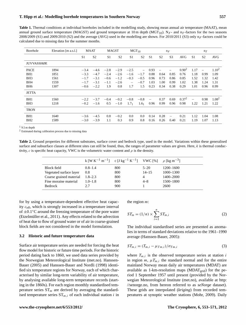
Table 1.Thermal conditions at individual boreholes included in the modelling study, showing mean annual air temperature (MAAT), meanannual ground surface temperature (MAGST) and ground temperature at 10 m depth (MGT10). NF - and nT -factors for the two seasons2008/2009 (S1) and 2009/2010 (S2) and the average (AVG) used in the modelling are shown. For 2010/2011 (S3) only nF -factors could becalculated due to missing data for the summer months.

Borehole Elevation [m a.s.l.] MAAT MAGST MGT10 nF nT

S1 S2 S1 S2 S1 S2 S1 S2 S3 AVG S1 S2 AVG

JUVVASSHØE

PACE 1894 −3.4 −4.6 −2.8 −2.9 −2.5 – 0.93 – – 0.902 1.17 – 1.102

BH1 1851 −3.3 −4.7 −2.4 −2.6 −1.6 −1.7 0.88 0.64 0.85 0.76 1.18 0.99 1.09BH3 1561 −1.7 −3.1 −0.6 −1.2 −0.3 −0.5 0.96 0.73 0.86 0.85 1.52 1.32 1.42BH4 1559 −1.7 −3.1 −1.1 −2.6 − −0.7 1.03 1.00 0.99 1.02 1.38 1.24 1.31BH6 1307 −0.6 −2.2 1.9 0.8 1.7 1.5 0.23 0.34 0.38 0.29 1.01 0.96 0.99

JETTA

BH1 1560 −2.2 −3.7 −0.4 −0.2 −0.8 −0.8 − 0.37 0.69 0.372 − 0.98 1.082

BH3 1218 −0.2 −1.6 0.5 −1.0 1.71 1.61 0.96 0.99 0.96 0.98 1.22 1.21 1.22

TRON

BH1 1640 −3.6 −4.5 0.8 −0.2 0.0 0.0 0.14 0.28 − 0.21 1.12 1.04 1.08BH2 1589 −3.0 −3.9 1.1 0.3 0.9 0.8 0.16 0.26 0.40 0.21 1.19 1.07 1.13

1 9.5 m depth2 Estimated during calibration process due to missing data

Table 2. Ground properties for different substrates, surface cover and bedrock type, used in the model. Variations within these generalisedsurface and subsurface classes at different sites can still be found, thus, the ranges of parameter values are given. Here,k is thermal conduc-tivity, c is specific heat capacity, VWC is the volumetric water content andρ is the density.

k [W K−1 m−1] c [J kg−1 K−1] VWC [%] ρ [kg m−3]

Block field 0.8–1.4 800 5–20 1200–1600Vegetated surface layer 0.8 800 14–15 1000–1300Coarse grained material 1.8–2.3 800 4 1400–2000Fine moraine material 1.0–1.8 800 4–8 1500–1800Bedrock 2.7 900 1 2600

for by using a temperature-dependent effective heat capac-ity ceff, which is strongly increased in a temperature intervalof ±0.1◦C around the freezing temperature of the pore water(Etzelmuller et al., 2011). Any effects related to the advectionof heat due to flow of ground water or of air in coarse-grainedblock fields are not considered in the model formulation.

3.2 Historic and future temperature data

Surface air temperature series are needed for forcing the heatflow model for historic or future time periods. For the historicperiod dating back to 1860, we used data series provided bythe Norwegian Meteorological Institute (met.no). Hanssen-Bauer (2005) and Hanssen-Bauer and Nordli (1998) identi-fied six temperature regions for Norway, each of which char-acterised by similar long-term variability of air temperature,by analysing available long-term temperature records (start-ing in the 1860s). For each region monthly standardised tem-perature series STm are derived by averaging the standard-ised temperature series STm,i of each individual stationi in

the regionm:

STm = (1/n) ×

n∑i=1

STm,i (2)

The individual standardised series are presented as anoma-lies in terms of standard deviations relative to the 1961–1990average (Hanssen-Bauer, 2005):

STm,i = (Tm,i − µT m,i)/σT m,i (3)

whereTm,i is the observed temperature series at stationi

in region m, µTm,i the standard normal and for the entiremainland Norway mean daily air temperatures (MDAT) areavailable as 1-km-resolution maps (MDATgrid) for the pe-riod 1 September 1957 until present (provided by the Nor-wegian Meteorological Institute (met.no), available athttp://senorge.no, from hereon referred to asseNorgedataset).These grids are interpolated (kriging) from recorded tem-peratures at synoptic weather stations (Mohr, 2009). Daily

www.the-cryosphere.net/6/553/2012/ The Cryosphere, 6, 553–571, 2012

558 T. Hipp et al.: Modelling borehole temperatures in Southern Norway

Table 3. Model performance in terms of ground surface temperature (GST), ground temperature (GT) and active layer thickness (ALT) atboreholes included in the modelling study. Model performance for GST and GT is expressed in terms of Nash-Sutcliffe model efficiency.Modelled and observed ALT is presented in absolute values. For GT, both the calibration (C) and the validation (V) periods are listed. Forthe GST the model was run with the averagedn-factors and ME calculated for each season individually.

GST GT ALTmeas[m] ALT mod [m]

S1 S2 S3 C V S1/S2/S3 S1/S2/S3

JUVVASSHØE

PACE 0.89 0.85 – 0.88 0.84 2.2/2.3/– 2.1 /2.1 /–BH1 0.89 0.86 0.89 0.84 0.82 1.4/1.5/1.6 1.4/1.3/1.2BH3 0.88 0.86 0.92 0.90 0.89 8.5/6.8/5.6 8.2/6.4/5.4BH4 – 0.92 0.96 0.99∗ 0.93∗ –/8.6/6.6 –/8.4/6.7BH6 0.91 0.88 0.89 0.92 0.90 – –

JETTA

BH1 0.87 0.85 0.80 0.91 0.90 8.0/7.3/6.9 8.1/7.9/6.7BH3 0.96 0.95 0.91 0.95 0.93 – –

TRON

BH1 0.71 0.81 – 0.92 0.89 10.7/11.1/– 11.7/10.7/–BH2 0.90 0.92 0.80 0.85 0.82 – –

∗Calibration: S2; Validation: S3

Fig. 3. (a)Mean monthly air temperatures for the PACE borehole atJuvvasshøe, Tron-BH1 and Jet-BH1 during the last normal period1961–1990.(b) Monthly air temperature deviations from the normal1961–1990 at the PACE borehole for S1 (black) and S2 (grey).

air temperatures from 1957 to 2008 were generated for theboreholes PACE, Jet-BH1 and Tro-BH1 using linear regres-sions between measured temperatures during 2008 to 2011and those extracted fromseNorgefor the corresponding lo-

cation. This procedure worked well for PACE withr2= 0.8

and a RMSE of 3.1◦C. For Jet-LB1 and Tro-BH1, however,the relation between observed air temperature and the corre-spondingseNorgevalue is nonlinear, displaying a sharp bendat low temperatures. This characteristic is associated with thefrequent occurrence of temperature inversions during winter(Farbrot et al., 2011), which are not captured by theseNorgedataset. To cope with this problem, two separate linear re-gressions were performed for each site, one above and onebelow a threshold temperature (−10◦C and−5◦C for Tro-BH1 and Jet-BH1, respectively).

For the normal period 1961–1990 mean monthly val-ues (MATi,1961−1990) and monthly standard deviations(σ 1961−1990) were calculated from these daily air tempera-tures. STm was used to construct a time series of monthlyair temperatures at the stationi (MAT i) from the early 1860suntil today at the stationi by (Hanssen-Bauer, 2005):

MAT i = MAT1961−1990+ STm × σ1961−1990 (4)

The observed temperature lapse rates during 2008–2010 of0.5, 0.6 and 0.8◦C 100 m−1 at Juvvasshøe, Jetta and Tron,respectively (Farbrot et al., 2011), were used to transfer theso-constructed MATi time series locally to the other boreholelocations. The historic air temperature series used as inputdata for the modelling, therefore, consists of monthly valuesuntil 2008 and measured daily values for 2008–2011.

Concerning the future air temperature series for the cli-mate change model runs, the rather moderate A1B emissionscenario was chosen. The A1B scenario assumes balanceduse of all energy sources with an increase in renewable

The Cryosphere, 6, 553–571, 2012 www.the-cryosphere.net/6/553/2012/

T. Hipp et al.: Modelling borehole temperatures in Southern Norway 559

energy sources, therefore, assuming a decrease of CO2 emis-sions by mid 21st century (IPCC, 2007). The likely rangeof the global mean temperature change from 1990 to 2100 ofthe A1B scenario is between +1.7◦C and +4.4◦C, with a bestestimate of +2.8◦C (IPCC, 2007). Temperatures from an en-semble of>30 different GCMs were empirically-statisticallydownscaled to the weather stationFokstugu(Benestad, 2005,2011), which is located between the Jetta and Tron sites, andused to drive the ground heat flow model. The measured dailyair temperatures of S1 and S2 at each borehole were corre-lated to Fokstugu yieldingr2-values of>0.9. This allowedthe construction of air temperature scenarios for each indi-vidual borehole from 2010 until 2100 by correcting for aconstant bias, specific for each site.

The following air temperature data series are, therefore,available as input data for the historic and future permafrostmodelling studies: a time series of monthly means from 1860to 2008, measured daily means from 2008 until 2011 andmonthly means from 2012 until 2100.

3.3 Model initialization and boundary conditions

The finite-difference scheme for solving Eq. (1) requiresboundary conditions at the upper and lower ends ofthe domain. Here, we used a geothermal heat flow ofQgeo= 33 mW m−2 (Isaksen et al., 2001) as lower boundarycondition and GST as upper boundary condition.

The atmosphere-ground coupling is an important factorfor prescribing appropriate upper boundary conditions forthe heat flow model. The relation betweenTAIR and GSTvaries strongly from borehole to borehole, depending onsnow and surface cover (Fig. 4). Historical and future timeseries of GST were generated from the reconstructedTAIRand downscaled future temperatures, respectively, usingn-factors.n-factors are considered as transfer functions relatingTAIR to GST during freezing (nF) and thawing (nT) condi-tions (Smith and Riseborough, 2002; Lunardini, 1978). Then-factors were derived from measured daily GST andTAIRat each borehole by calculating the ratios of annual sums offreezing (FDD) and thawing degree days (TDD) of GST tothose ofTAIR :

nF =FDDS

FDDA(5)

nT =TDDS

TDDA(6)

where indices S and A refer to the temperature at the groundsurface and the air, respectively (Riseborough, 2007). FDDand TDD were calculated for the whole year and not based onfreezing and thawing seasons at the ground surface, using av-erage daily air temperatures. Sites having a thick snow coverare characterised by a GST> TAIR during large parts of thewinter and, therefore,nF < 1.nT > 1 indicates a higher GST

thanTAIR during summer, which can be the case at bedrocksites in the absence of vegetation or on south-facing slopes.

The reconstruction of historic permafrost conditions em-ploys monthly air temperatures, whereasn-factors were de-termined from diurnal data. We investigated the possible ef-fect of this inconsistency in temporal resolution on then-factor values by recalculatingn-factors based on monthlydata. We found that the values deviate by less than 9 % and,therefore, we use the samen-factors throughout our study,regardless of whether they are applied to monthly or dailytemperatures. For the long-term modelling, mean values ofnF andnT of S1 and S2 were used (Table 1), assuming rep-resentativeness of our observation period.nF-values rangefrom 0.2 and 0.4 at boreholes with a thick snow cover (Tro-BH1, Tro-BH2, Jet-BH1, Jet-BH2 and Juv-BH6) and from0.8 to 1.0 where snow cover was moderate (Table 1).nT-values>1.2 were obtained for bedrock boreholes withoutvegetation cover.

The model was initialised in two different ways, one forthe calibration and validation procedure and the other onefor the historical permafrost modelling. Simulations of S1and S2 were initialised from observed profiles of GT whichwere extrapolated to the full depth assuming a linear gra-dient. Long-term simulations were started from steady-statecorresponding to the mean air temperature of the decade1860–1869. To account for seasonal variations a second de-gree Fourier curve function,

T = a0 +

2∑i=1

aicos(i w t)+ bisin (i w t) (7)

is fitted to the observed dailyTAIR of S1 (fit parametersai ,bi , ω). The higher degree function was chosen to appropri-ately represent the asymmetric seasonal cycle introduced bythe long and cold winter season. Using (a1,a2, b1, b2, ω)from the fit anda0 = MAT1860−1869, we generate a time se-ries of air temperatures, which the model is forced with untilno more changes in GTs occur.

3.4 Model calibration

In absence of detailed data on the thermal properties of thesubsurface (in terms ofc, k, ρ and VWC), we empiricallydetermined the values by adjusting until satisfying agree-ment between model results and available observations overthe calibration period. We selected S1 as calibration period,while S2 and S3 were kept as independent control for sub-sequent model validation (see following section). For cali-bration, the model was forced by the measured ground sur-face temperature as upper boundary condition. A manual,stepwise optimization procedure was applied to avoid erro-neous parameter calibration which may result from compen-sating effects. Our approach to deal with this problem wasto pre-select narrow ranges of plausible values for the pa-rameters from literature (Williams and Smith, 1989). Within

www.the-cryosphere.net/6/553/2012/ The Cryosphere, 6, 553–571, 2012

560 T. Hipp et al.: Modelling borehole temperatures in Southern Norway

Fig. 4. Relationships between GST vs.TAIR during the observation period 2008-2010 at the modelled boreholes. Black crosses: measured;red crosses: modelled. The snow-rich sites are clearly visible at the sharp kink atTAIR ∼ 0◦C. The best correlations are found at sites withthin or no snow cover, (PACE, Juv-BH1, Juv-BH3 to BH6). At sites with a long-lasting, thick snow cover (e.g., Tro-BH1, Jet-BH1), then-factor-based GST model can still reproduce the GST pattern.

these ranges, we accepted only small changes that did notrequire large changes in related parameters to achieve im-proved performance. As such, for example, a wrong choicefor heat capacity may cause an exaggerated phase shift of GTwith respect to GST which, in turn, may partly be compen-sated for by enhanced heat conduction. Previous sensitivitytesting revealed that within the given bounds, modelled GTwere most sensitive to changes in heat conductivity and wa-ter content, while heat capacity and density are robustly con-strained by literature values. Therefore, after assignment ofplausible starting values to the parameters, calibration wasperformed by systematically changingk and VWC over thegiven ranges aiming for improving the agreement betweenmodelled and observed GTs at different depth levels. Subse-quently, minor adjustments were made toceff andρ to fine-tune the model performance. The agreement between model

and observation was quantified at each individual depth interms of the Nash-Sutcliffe model efficiency coefficient (ME)(Nash and Sutcliffe, 1970). For bedrock, values for thermalconductivity and density were measured at Juv-BH4 and atall sites at Jetta by the Norwegian Geological Survey (NGU)and these observations served as initial guesses for the cal-ibration. A time series of measured soil moisture (O. Hum-lum, personal communication, 2011) in the vicinity of somesites (Juv-BH1, Tro-BH1) served as an estimate for the wa-ter content in the near-surface sediments. Adopted values forthe different materials are shown in Table 2, while depth-averaged values of the ME for each borehole are presentedin Table 3.

In total, only slight changes to the starting values had tobe applied to achieve satisfactory agreement between mod-elled and observed GT. We defined satisfaction as ME> 0.7

The Cryosphere, 6, 553–571, 2012 www.the-cryosphere.net/6/553/2012/

T. Hipp et al.: Modelling borehole temperatures in Southern Norway 561

Fig. 5.Modelled vs. measured GST for the period 2008–2011 at modelled boreholes. In general, agreement between modelled and observedvalues is good with a Nash-Sutcliffe model efficiency coefficient ME> 0.80 (except for Tro-BH1). At bedrock sites and where the influenceof snow cover was limited, an even better agreement was achieved (Juv-BH4, Jet-BH3) with ME> 0.90.

and/or when further changes of parameter values did notyield better model performance. Nevertheless, we empha-size that the obtained set of parameter values for each siterepresent one possible set that yields satisfactory agreementbetween model and observations. However, as symptomaticfor calibrating numerical models, different sets may exist(Beven and Freer, 2001) and calibrated values may be erro-neous. Therefore, transferability of parameter values to otherregions is restricted and site-specific calibration is necessary.

3.5 Model validation

For our validation procedure we followed Rykiel’s (1996)suggestion that the meaning of validation is that a “model isacceptable for its intended use because it meets specified per-formance requirements” in terms of operational validation.For our study the correspondence between measured and ob-served GT is expressed by the depth-averaged values of the

Nash-Sutcliffe model efficiency coefficient (ME). Again, werequire ME> 0.7.

To validate the reliability of the GST model, it was runfor each season individually using the averagen-factors fromS1 and S2 (Table 1). For most boreholes a good correspon-dence between modelled and measured GSTs was achievedwith ME > 0.8 (Table 3, Fig. 5). Since S3 was not includedin the averagen-factor calculation, it represents an addi-tional independent validation period. Despite some differ-ences in the snow conditions, the model reproduced GSTsof S3 equally well (Table 3). The highest values of ME> 0.9were achieved at bedrock sites with negligible winter snowcover (Juv-BH4, Jet-BH3). The measured GTs of the valida-tion period (S2–S3) were well reproduced by the calibratedmodel yielding depth-averaged ME-values ranging from 0.81to 0.93 (Fig. 6, Table 3). The ME values vary with depth be-tween 0.6 at 10 m and>0.9 close to the ground surface.

To better estimate the model performance on a long-termscale, the model was run from 1860 until 2009 using the

www.the-cryosphere.net/6/553/2012/ The Cryosphere, 6, 553–571, 2012

562 T. Hipp et al.: Modelling borehole temperatures in Southern Norway

reconstructedTAIR series and results compared to the mea-sured GTs of S1. In the case of the PACE borehole mod-elled and measured GTs of the entire series 1999–2009 werecompared down to a depth of 100 m (Fig. 7). The mea-sured MAGTs were reproduced with a RMSE of 0.6–0.7◦C(ME > 0.8) in the uppermost part (0 to 1 m depth) and 0.1–0.3◦C (ME> 0.6) at a depth between 5 and 10 m (Fig. 7).

4 Results

4.1 Historical and future air temperature trends

The historical air temperature series show temperatureincreases of 1.4◦C to 2.1◦C (+0.9◦C (100 yr−1) and+1.4◦C (100 yr−1)) between 1860–1870 and 2008–2009 atJuvvasshøe and Tron, respectively. During the last decade(2000–2010), only positive deviations ofTAIR to the climatenormal 1961–1990 were observed at all sites (Fig. 8). Inthe period 1860s until 2000–2009 the strongest warming oc-curred during spring with +2.1◦C at both sites. The morecontinental site Tron, however, shows strong increases of airtemperature both in winter as well as in spring with +1.8 and+1.9◦C, respectively.

The median of the downscaled future temperatures indi-cates a further warming of +2.8◦C of the decadal means2001–2010 until 2091–2100. The 10th percentile shows thesame warming trend, the 90th percentile, however, shows anincrease of +3.3◦C. The deviation of the median to the cli-mate normal 1961–1990 amounts to +3.8◦C and +4.2◦C atJuvvasshøe (Fig. 8b) and Tron (Fig. 8c), respectively.

4.2 Historic permafrost development

4.2.1 Mountain permafrost after the Little Ice Age

From the initial situation in 1860, rough estimates on thelower altitudinal limit of mountain permafrost after the LIAcan be made. The model results suggest the presence of per-mafrost at Juvvasshøe at ca. 1300 m a.s.l. (Juv-BH6). Themodelled ALT range from 0.5 m at 1900 m a.s.l. (Juv-BH1)to ca. 3 m at 1300 m a.s.l (Juv-BH6). The greatest ALT(close to 4 m) was modelled for the bedrock site (Juv-BH4).At Tron, permafrost thicknesses of up to 90 m and ALT ofca. 1.3 m to 6 m were modelled. According to the model re-sults, the altitudinal zone of the lower limit of permafrost atthis site was below ca. 1300 m a.s.l.

4.2.2 Ground temperatures

According to the model results for the period from 1860 to2009, GTs were increasing at all depths. At all boreholes,most significant increases in GT occurred in the last twodecades (since 1990). The model results show an increasein GT at 10 m depth since the 1860s by about 0.9◦C to1.5◦C at Juvvasshøe/Jetta and 0.1◦C to 0.7◦C at Tron. GTs

at 100 m depth increased in the range of 0.4◦C to 1.0◦C atJuvvasshøe and Jetta and 0.1◦C to 0.4◦C at Tron. Modelledwarming was strongest for the bedrock borehole (Juv-BH4)with +1.5◦C and +0.5◦C at 10 m and 100 m depth, respec-tively.

4.2.3 Active layer thickness

Depending on location, elevation and stratigraphy, differentALT behaviour is indicated by the model results. A character-istic pattern is observed at all boreholes, with a comparativelyslow ALT increase until ca. 1990 and accelerated increase inALT until 2009.

Trends of ALT increase were, therefore, dderived for thetwo periods 1860–1864 until 1986–1990 and 1986–1990 un-til 2009. The non-parametric Mann-Kendall test was used totest these trends for significance (1 % level). At Juvvasshøeand Jetta all trends of ALT increase during both periods havebeen proven significant, while at Tron only the trend for thelater period is significant.

At Juvvasshøe the lowermost borehole (Juv-BH6) showsa very rapid ALT increase and permafrost degradation priorto the end of the 19th century. The increase in ALT until1990 was only +0.1 m (13 %,∼0.1 cm yr−1) at Juv-BH1 and+0.2 m (15 %,∼0.1 cm yr−1) at PACE (Fig. 9a). The lowerboreholes (Juv-BH3 and Juv-BH4) show a stronger increaseof ALT with +0.9 m resulting in a rate of∼0.6 cm yr−1 (27 %at Juv-BH3, 24 % at Juv-BH4). The model results indicatea pronounced ALT increase at all boreholes until 2009 inthe range of +0.4 to +4.1 m (50–90 %, 2–22 cm yr−1). ThePACE borehole shows higher mean inter-annual variation ofALT than Juv-BH1 with +40 cm yr−1 and +20 cm yr−1, re-spectively. Although Juv-BH3 was drilled in coarse materialand Juv-BH4 in bedrock they show a similar ALT evolution,the latter, however, having continuously larger ALT (average+0.4 m) and a much higher mean inter-annual variation of70 cm yr−1 compared to 30 cm yr−1.

As all boreholes are drilled in bedrock at Jetta, the ALTis more sensitive to climate variations and a more rapid in-crease during the last 150 yr was modelled. Until 1990, theALT increased by +1.1 m (27 %,∼1 cm yr−1) at Jet-BH1 and+2.2 m (40 %,∼2 cm yr−1) at Jet-BH3, respectively. Duringthe period 1990 until 2009, the strongest increase of ALT of+2.7 m (50 %, +14 cm yr−1) was modelled at Jet-BH1, whilepermafrost degraded completely at Jet-BH3 (Fig. 9b).

At Tron the strongest increases in ALT were modelledwith +1.1 m (110 %, +0.8 cm yr−1) until 1990 (Fig. 9c).Since 1990, the model indicates a rapid warming of per-mafrost with an ALT reaching a depth of 10–11 m as mea-sured today, resulting in an ALT increase of nearly +9 m(430 %, +87 cm yr−1). This development agrees well withobservations indicating the possible beginning of a talik de-velopment (see Fig. 2e) (Farbrot et al., 2011).

The Cryosphere, 6, 553–571, 2012 www.the-cryosphere.net/6/553/2012/

T. Hipp et al.: Modelling borehole temperatures in Southern Norway 563

Fig. 6. Left panels: Measured (solid lines) and modelled (dashed lines) ground temperatures (GT) at 1 m (red), 5 m (black) and 10 m (blue)depth during calibration (shaded area) and validation period. At Juv-BH4, data from S1 is not available and S2 served as calibration and S3as validation period. Right panels: Scatter plots showing measured against modelled GTs of validation period for all depths, including thedepth-averaged Nash-Sutcliffe model efficiency coefficients (ME).

www.the-cryosphere.net/6/553/2012/ The Cryosphere, 6, 553–571, 2012

564 T. Hipp et al.: Modelling borehole temperatures in Southern Norway

Fig. 7. Comparison of modelled to measured GTs during S1 after150 model years. The model was run from steady state conditionsfor 1860 until 2008 using the reconstructedTAIR series. Both, theseasonal dynamics during 1999–2008 at PACE(a) as well as theMAGTs (b) were reproduced with good accuracy (RMSE<0.7◦C)to a depth of 100 m (at PACE).

Fig. 8. (a)Historic air temperature series at the uppermost boreholeat Juvvasshøe (black) and Tron (blue). The bold line represents the7-yr Gaussian-filtered series. For 2010 onwards, the figure showsthe median (bold black), 90 percentile (red) and 10 percentile (blue)of the downscaledTAIR ensemble for Juv-BH1. The lower panelsshow the deviations of MAAT from the 1961–1990 climate normalat Juvvasshøe(b) and Tron(c).

4.3 Future permafrost development

4.3.1 Ground temperatures

According to modelled GT until 2100, warming will con-tinue beyond that found for 2000–2009. The model suggeststhat GTs at Juv-BH1 will increase by +1.9◦C and +1.1◦Cat 30 m and 100 m depth until 2100, respectively. Juv-BH4shows the same warming at 100 m depth, but a more pro-nounced increase in GT at 30 m with +2.6◦C.

4.3.2 Active layer thickness

The model results are indicative for permafrost degradationalso above 1800 m a.s.l. until 2100. Permafrost at lower ele-vations (Juv-BH3 and Juv-BH4) degrades completely before2050 (Fig. 9a). At the bedrock site at Jetta the rapid AL thick-ening rates at Jet-BH1 will continue and the development ofa talik until the end of the 2020s is predicted by the model(Fig. 9b).

While the air temperature increase in the climate changescenario shows a linear development and even a decrease inthe warming rate (see Fig. 8a), the ALT displays a nonlin-ear response at most sites (Fig. 9). The ALT of Juv-BH1 in-creases linearly by another 70 cm from 2010 until mid-2070s.Although the climate change scenario includes a decrease inthe warming rate at this point, a rapid degradation of per-mafrost subsequently takes place until the end of this cen-tury, with a linear increase of ALT by>40 cm yr−1. A simi-lar development can be observed at the PACE borehole withhigher thickening rates and a permafrost degradation at themid-2060s.

Running the model with the 90th and 10th percentiles ofthe downscaled temperature ensemble yields an estimationof the possible range of developments. The 90th percentilecauses a fast degradation of permafrost at all boreholes bylatest mid of this century (Fig. 9a). Considering the moder-ate warming projections (10th percentile), permafrost at Juv-BH1 and PACE is warming at a slow rate without degradationoccurring.

4.3.3 Probable future of permafrost at the PACE andJuv-BH1 boreholes

Concerning the projected air temperate, there are uncertain-ties related to the different formulations of the GCMs them-selves, as well as to the empirical-statistical downscaling pro-cedure (Benestad, 2011). Although only one emission sce-nario is considered here (A1B), the uncertainties lead to con-siderable spread of projected temperature. In order to quan-tify the effects of this uncertainty on modelled ALT and GT,the development of GT and ALT until 2100 were simulatedfor all percentiles of the projectedTAIR-ensemble in steps of5 %. From these results, we identify the percentiles which areassociated disappearance of the active layer in the years 2050and 2100, respectively. This analysis is used to estimate the

The Cryosphere, 6, 553–571, 2012 www.the-cryosphere.net/6/553/2012/

T. Hipp et al.: Modelling borehole temperatures in Southern Norway 565

Fig. 9.Reconstructed and projected active layer thickness (ALT) from 1860 to 2100 at Juvvasshøe(a), Jetta(b) and Tron(c). Projected ALTwas modelled using the ensemble-medianTAIR (bold dashed lines). ForJuv-BH1 and PACE, also shown are ALT according to the 90 and10 percentiles (shading) of theTAIR ensemble.(a). The bold lines represent a 7-yr Gaussian-filtered series, measured ALT are marked bycrosses. The model indicates the permafrost degradation at Tron by the year 2010. Therefore, no projection was applied for Tr-BH1.

probabilities for transition of permafrost to talik at Juv-BH1and PACE in the years 2050 and 2100 (Fig. 10).

For the PACE borehole, a talik evolution until 2100 wasmodelled already using the 25th percentile resulting in a highprobability of 70–75 % (Fig. 9). According to the classifica-tion proposed by the IPCC (IPCC, 2007), this situation is,

therefore,likely to occur for the given emission scenario.However, at Juv-BH1 a talik will have developed in 2100with a probability of 50–55 %, and is classifiedas likely tooccur as not. The probabilities for talik evolution until 2050is 35–40 % for PACE and 20–25 % for Juv-BH1, respec-tively and, therefore,unlikely (Fig. 10). According to these

www.the-cryosphere.net/6/553/2012/ The Cryosphere, 6, 553–571, 2012

566 T. Hipp et al.: Modelling borehole temperatures in Southern Norway

Fig. 10. Probability of permafrost degradation (no refreezing ofthe active layer) until 2050 (black) and 2100 (white) at Juv-BH1(squares) and PACE (circles). The assessment is derived from modelresults for all percentiles of theTAIR ensemble (in steps of 5 %) andthe probability is defined as the percentile at which seasonal re-freezing of the active layer does not occur anymore. Vertical linesmark the probability of this event occurring by 2050 (dashed) and2100 (dotted), respectively.

model results, above 1800 m a.s.l, where stable and con-tinuous mountain permafrost is found today, discontinuousmountain permafrost is to be expected by the end of the 21stcentury.

5 Discussion

5.1 Model uncertainties due to snow cover, soil watercontent variability and model approach

A major source of uncertainty is related to the parameterisa-tion of using constantn-factors. It is uncertain how well thesnow conditions of the historic and future model period arerepresented by the averagen-factor from S1 and S2. A 10-yr record (1999–2008) of GST andTAIR is available at thePACE borehole (Isaksen et al., 2011), which enables an esti-mate for the decadal variation ofn-factors and put the period2008–2010 into context. A meannF-factor of 0.91 (0.89–0.98) andnT-factor of 1.12 (1.02–1.26) was derived fromthe records. The meannF- and nT-factors for 2008–2010(Table 1), therefore, are within the variation of the period1999–2009. Based on these minimum and maximum valuesan uncertainty analysis was conducted to give a quantitativeestimate on the error that can be expected fromn-factors.For that purpose, the model was run for the PACE bore-hole for 1999–2010 separately, both with the minimum andmaximumn-factors. This implies running the model withthe coldest (nF = 0.98;nT = 1.02) and warmest (nF = 0.89;

nT = 1.26) possible GST conditions. The differences in GTsexpressed in the absolute error between the two model runswere calculated for each depth individually. A change in ALTof <50 cm and changes in MAGT of 0.7◦C to 0.4◦C at thesurface and 10 m depth, respectively, were introduced. Thedepth-averaged ME varies by less than 0.15 between the ex-treme value model runs. The PACE borehole represents asite with relatively constantnF-factors due to the negligi-ble snow cover. At sites with higher snow cover and, thus,smallernF-factors (particularly Tro-BH2, Jet-BH1 and Tro-BH6), our measurements suggest a higher interannual vari-ability of thenF-factors (Table 1), most likely caused by dif-ferent wind redistribution of snow. However, the good agree-ment of modelled long-term subsurface temperatures withmeasured GT gives us confidence that then-factors assumedin the model runs are a good representation of long-term av-eragen-factors.

Some deviations of modelled from observed GTs are ob-served during periods of thawing and freezing, presumablycaused by our assumption of constant VWC. At sites whereVWC>15 %, the model underestimates the duration of thezero-curtain effect (see Fig. 5). Further, our model neglectsadvective heat transport and changes of ice-content in theground are not recognised in the model. Our modelling doesnot account for these processes and, therefore, rather repre-sents a minimum estimate for the increase of GT. A thirdprocess not included in the model is 3D-effects due to lateralvariation of either topography or snow cover.

The aim of this study was to assess the long-term trendsof permafrost temperature and its altitudinal distribution. Weassume conduction and latent heat effects as main factors,which is in agreement with studies showing that conductionand latent heat effects attribute for most of the heat flow pro-cesses (Kane et al., 2001; Weismuller et al., 2011). Both soilwater/ice content and snow conditions on the long-term areafflicted with uncertainties. For this study, we suggest that theaveragen-factor value we used provides a useful approxima-tion to address the snow influence on GST. The constancyof soil water content may be responsible for slight devia-tions during periods of zero-curtain. Nevertheless, observedGT, ALT and GT amplitudes were reproduced reasonablywell according to the ME measure used in this study. Long-term data are not available, which e.g., could aid possibletrends ofn-factors or soil water content, so we do not knowif and how trends and inter-annual variations would inter-fere with each other and affect our result. Moreover, at oursites and generally in most high-mountain settings in Scan-dinavia, coarse-grained near-surface material or bedrock isdominating. Thus, the soil water content is relatively low andthe effect of water flow on GT is considered minor. Further-more, the boreholes have been drilled in flat topography, indoing so, 3D-effects are largely avoided. Processes of lateralheat transfer along a slope and air convection within the porespace of block fields seem not important.

The Cryosphere, 6, 553–571, 2012 www.the-cryosphere.net/6/553/2012/

T. Hipp et al.: Modelling borehole temperatures in Southern Norway 567

Even with the stated simplifications, modelled GTs agreewell with observations and the present borehole temperaturedistributions are reproduced when simulating the evolutionsince 1870. These results suggest, therefore, that our simpleapproach is capable of capturing the dominating processeswithin the time scale considered.

5.2 Uncertainties of reconstructed and projected airtemperature series

The method by Hanssen-Bauer and Nordli (1998) has provenuseful in reconstructing reliable air temperature time series(Farbrot and Hanssen-Bauer, 2009). However, it introducesuncertainty due to the spatial and temporal interpolation ofair temperatures.

Before daily values become available in 1957, the model isrun with monthly data. To test the possible error introducedby the discontinuity in temporal resolution, the period 2008–2010 was simulated with monthly means. The model resultdoes not show any deviation to those obtained when usingthe daily resolution input data.

Uncertainties related to the interpolation in mountain to-pography arise from unknown lapse rates during inversions(Tveito and Førland, 1999), which are observed frequently,especially during calm winter days. The temperature fieldsused in this study for the long-term record are based on con-stant lapse rates, which may produce too cold SAT in highelevations (e.g., Tveito and Førland, 1999). However, gener-ally a good fit has been achieved when comparing measuredand interpolated air temperature, indicating the mean tem-perature trends being well represented (Tveito and Førland,1999).

In our study, we employ ensemble estimates of futureTAIRevolution to illustrate and assess the uncertainty of the fu-ture GT evolution. Ensemble analysis has proven powerfulin assessing uncertainties of projectedTAIR evolution. How-ever, there are several ways to define an ensemble, each ofwhich refers to a different cause of uncertainty. In detail,the ensemble may consist of GCM realisations for a multi-tude of emission scenarios, thereby uncovering the range ofexpected outcomes for the discrete emission scenarios de-fined by IPCC (2007). Furthermore, aTAIR ensemble mayalso consist of many realisations for one single emission sce-nario, but from a multitude of GCMs. The combination ofboth would also be possible, though we regard that possibil-ity as little instructive. Here, we have focused on illustratingthe uncertainty related to the choice of GCM for a given sce-nario rather than on the uncertainty related to future emis-sions. Namely, we have chosen the A1B scenario for whichempirically-statistically downscaled time series ofTAIR areavailable for a multi-model ensemble (Benestad, 2011).

5.3 Influence of ground properties on thermal regime

GTs respond differently to warming, depending on the sur-face material, ground properties and soil water content. Theinter-annual change of ALT was calculated and averagedfor the period 1860–2009 for all boreholes at Juvvasshøe.Borehole Juv-BH4, which does not have significant snowcover and is located in bedrock, shows the highest varia-tion of 0.7 m yr−1. Much lower inter-annual ALT variationsof 0.2 m yr−1–0.3 m yr−1 were modelled for boreholes cov-ered by block fields. This reflects how the block fields actas a buffer dampening the effect of the air temperature fluc-tuations on GT (Harris and Pedersen, 1998; Juliussen andHumlum, 2008). At Juv-BH4, however, no such buffer layerexists causing a more direct response of the ALT to changesin TAIR .

Despite their proximity, the boreholes PACE and Juv-BH1show different thermal regimes and ALT developments inpast and future due to differences in volumetric water con-tent. A large part of the energy transferred into the groundat Juv-BH1 is consumed for melting ground ice. This ex-plains the reduced inter-annual variability of ALT and theless pronounced increase in ALT in the past and future. Fur-thermore, the nonlinear response in ALT is attributed to themelting of ice within the ground. After melting of ground ice,more energy is available to efficiently warm the ground. Sim-ilar effects have been observed in North-America (Smith etal., 2010) and Russia (Romanovsky et al., 2010), where thenonlinear response of GT and ALT to warming are clearlyattributable to water content. Similar results have been foundcomparing the impact of the extreme summer of 2003 on theALT of bedrock and block field sites in the Swiss Alps (Von-der Muhll et al., 2007).

Several other studies have attempted to quantify the im-pact of climate change on permafrost conditions, distributionand ALT. Stendel and Christensen (2002) predicted a generalincrease of ALT of up to 30–40 % until the end of the 21stcentury in the Northern Hemisphere. Zhang et al. (2008) esti-mated the ALT increase in Canada to 14–30 % by 2050 com-pared to a permafrost baseline in the 1990s. For Svalbard,similar changes for the ALT evolution during the 21st centurywere modelled (Etzelmuller et al., 2011). In our study, theALT increased by 65 % to 180 % at the boreholes where per-mafrost still is expected by 2050. Even the results using the10th percentile of the climate change models indicate an ALTincrease of 44 % at the PACE borehole. This implies a highsensitivity of warm mountain permafrost to climate change,comparable to coastal areas, e.g., on Svalbard (Etzelmulleret al., 2011). Furthermore, many of the assessments men-tioned above were made for Arctic lowlands, where large ar-eas with fine-grained and organic-rich sediments are present.Organic components in the near-surface layer are known toeffectively damp the GT response to warming (Williams andSmith, 1989). In mountain areas, significant accumulation oforganic material is rare and restricted to special topographic

www.the-cryosphere.net/6/553/2012/ The Cryosphere, 6, 553–571, 2012

568 T. Hipp et al.: Modelling borehole temperatures in Southern Norway

and geomorphic settings. However, block fields may have aneffect similar to that of organic material in Arctic lowlands,i.e., retarding the GT-response to climate signals and coolingthe ground, as discussed above.

In summary our modelling study shows a high sensitivityof mountain permafrost and high probabilities of degradationat elevation levels below ca. 1800 m a.s.l. in Southern Nor-way. Simulated GTs at bedrock sites are generally more sen-sitive to climate change than those at sites within block fieldsor finer-grained sediment cover.

5.4 Altitudinal changes of mountain permafrost duringthe modelling period

This study indicates a major change of the ground thermalregime since the end of the LIA. At that time, sporadic todiscontinuous permafrost conditions seem to have been morewidespread at elevations of around 1300 m a.s.l., where weonly find permafrost as isolated patches at present (Sollidet al., 2003). This translates to the lower permafrost zonebeing approximately 200 m lower during the LIA than atpresent. At Juvvasshøe, this zone between 1300 m a.s.l. upto 1500 m a.s.l. is dominated by block lobes, which maybe inactive today, but are shaped by an earlier high-activeperiglacial environment. Further climate warming wouldmove this zone up-slope. The model results of this study in-dicate that the lower limit of the discontinuous permafrostzone may rise up to above 1800 m a.s.l., thus, ca. 250 mhigher than today. With such a scenario, major changes inperiglacial processes are expected.

As our results are derived from 1-D modelling at the pointscale, these implications on the spatial distribution of moun-tain permafrost have to be treated with care. The large spa-tial heterogeneity of parameters that strongly influence per-mafrost distribution such as snow cover, surface cover andground parameters were not considered in these estimations,as recently documented by Gubler et al. (2011) for sites inSwitzerland and Etzelmuller et al. (2007) in Iceland. There-fore, a simple point-to-area extrapolation is problematic.However, we have three main reasons to consider this set-up as sufficient to give estimations on the altitudinal changesof mountain permafrost since the LIA in these very particu-lar mountain areas: (1) The 13 boreholes cover a large alti-tudinal range from 1900 m a.s.l. to ca. 1200 m a.s.l., rangingfrom continuous permafrost to no permafrost, (2) Farbrot etal. (2011) clearly documented consistent altitudinal trends inGT on an annual average, and (3) even if a borehole locationis not representative for the local variability of surface char-acteristics, the GT signal in greater depth will be integratedover a larger surface area.

6 Conclusions and perspectives

A one-dimensional heat flow model was successfully appliedto quantify the changes in the thermal regime from 1860 un-til the end of this century at three mountain sites in southernNorway. The model was calibrated to the individual boreholesettings of the study sites and, therefore, is not directly trans-ferable to other regions. However, the settings of the studysites in terms of climate, geomorphology and surface coverare representative for a number of different alpine mountainareas in southern Norway.

The model was forced with reconstructed air temperatureseries over 1860–2009 and successfully reproduced the ver-tical ground temperature profiles as measured in 2009 witha good accuracy (ME∼ 0.8). This confirms the appropriate-ness of the model to accurately model the permafrost thermalregime over long time scales.

The following conclusions can be drawn from this study:

– From 1860 until ca. 1990 a comparatively small in-crease in active layer thickness was modelled wherepermafrost exists, with values ranging from 0.1 cm yr−1

to +2 cm yr−1 (20–68 %). Since ca. 1990 ALT-changerates of +2 cm yr−1 to +87 cm yr−1 (20–430 %) weremodelled. The model results indicate permafrostdegradation at boreholes below ca. 1450–1500 m atJuvvasshøe and Jetta and below ca. 1600 at Tron.

– Model results suggest that GT at 10 m depth increasedby +0.9◦C to +1.5◦C over 1860–2009. The largest partof this warming occurred after 1990.

– Our study successfully simulated the nonlinear responseof ground temperature and active layer thickness toincreasing air temperatures, due to the thermal iner-tia of ice-containing ground material. In our sites, thisresponse is related mainly to block fields and coarseground moraine sites containing ice.

– The modelling study implies that the altitudinal zonecovering the lower limit of permafrost at the approxi-mate end of the Little Ice Age was about 200 m lowerthan today in the field area.

– According to the A1B climate scenario, degradationof mountain permafrost is suggested to occur through-out the 21st century at most of the sites belowca. 1800 m a.s.l. By the end of this century, the highestlocations (Juv-BH1, PACE) will experience pronouncedALT-increases of up to 10 m or the development oftaliks. This implies an upward shift of the lower per-mafrost zone to around 1800 to 1900 m a.s.l. by the endof the 21st century, again depending on sediment char-acteristics and snow cover development.

The Cryosphere, 6, 553–571, 2012 www.the-cryosphere.net/6/553/2012/

T. Hipp et al.: Modelling borehole temperatures in Southern Norway 569

The modelled past and possible future changes in GT andALT have geomorphologic and geotechnical implications,since the ground thermal regime is a major controlling factorfor geomorphologic processes and landscape development(Berthling and Etzelmuller, 2011). As alpine rock faces arewidespread in the study area between 1900 and 2400 m a.s.l,our study suggests major impacts on the geotechnical prop-erties and stability of rock walls. This relationship is well-documented in literature (Davies et al., 2001; Gruber et al.,2004a) and has to be evaluated in future research. Especiallythe modelled long period of stable permafrost and a sub-sequent sudden and quick degradation results in challengesfor engineering, natural hazard prediction and mitigation. Fi-nally, our study provides important insights in the range ofthermo-physical parameters in a wide range of bedrock andsurficial material relevant for mountain areas in SouthernNorway. These provide important constraints for spatial nu-merical permafrost modelling.

Acknowledgements.This study was part of the CRYOLINK project(“Permafrost and seasonal frost in Southern Norway”) funded bythe Norwegian Research Council (grant number 185987/V30) andthe Department of Geosciences, University of Oslo (UiO). Specialthanks go to Rune S. Ødegard from the University College inGjøvik, Norway, for crucial support in field logistics, especially inrelation with establishing of the borehole network. Ketil Isaksen(Norwegian Meteorological Institute, Norway) is thanked forvaluable logistical support and providing updated temperaturerecords from the PACE boreholes. R. Benestad kindly providedan empirically down-scaled multi-model ensemble ofTAIR forFokkstua, Southern Norway. Kjersti Gisnas (UiO) contributedduring field work. Several land owners at Tron and Juvvasshøeaccepted drilling and instrumentation on their properties. TheGeological Survey of Norway (NGU) did the measurements ofdensity and thermal characteristics of the samples from the bedrockborehole cores retrieved from the Juvvasshøe (BH5) and the Jettaboreholes. Five anonymous reviewers gave constructive comments,thereby significantly improving the revised manuscript. Likewise,the editor Stephan Gruber is acknowledged for numerous and veryuseful suggestions to improve the paper. We want to thank allmentioned individuals and institutions.

Edited by: S. Gruber

References

Benestad, R. E.: Climate change scenarios for northern Europefrom multi-model IPCC AR4 climate simulations, Geophys. Res.Lett., 32, L17704,doi:10.1029/2005GL023401, 2005.

Benestad, R. E.: A new global set of downscaledtemperature scenarios, J. Climate, 24, 2080–2098,doi:10.1175/2010JCLI3687.1, 2011.

Berthling, I. and Etzelmuller, B.: The concept of cryo-conditioning in landscape evolution, Quaternary Res., 75, 378–384,doi:10.1016/j.yqres.2010.12.011, 2011.

Beven, K. and Freer, J.: Equifinality, data assimilation, and uncer-tainty estimation in mechanistic modelling of complex environ-

mental systems using the GLUE methodology, J. Hydrol., 249,11–29,doi:10.1016/S0022-1694(01)00421-8, 2001.

Burn, C. R. and Zhang, Y.: Permafrost and climate change at Her-schel Island (Qikiqtaruq), Yukon Territory, Canada, J. Geophys.Res.-Earth, 114, F02001,doi:10.1029/2008JF001087, 2009.

Bø, M. R.: Permafrost studies on Jetta in northern Gudbrandsdalen,central Norway (in Norwegian), Master’s thesis, University ofOslo, 127 pp., 1998.

Christiansen, H. H., Etzelmuller, B., Isaksen, K., Juliussen, H., Far-brot, H., Humlum, O., Johansson, M., Ingeman-Nielsen, T., Kris-tensen, L., Hjort, J., Holmlund, P., Sannel, A. B. K., Sigsgaard,C., Akerman, H. J., Foged, N., Blikra, L. H., Pernosky, M. A., andOdegard, R. S.: The Thermal State of Permafrost in the NordicArea during the International Polar Year 2007–2009, PermafrostPeriglac., 21, 156–181,doi:10.1002/Ppp.687, 2010.

Davies, M. C. R., Hamza, O., and Harris, C.: The effect of rise inmean annual temperature on the stability of rock slopes contain-ing ice-filled discontinuities, Permafrost Periglac., 12, 137–144,doi:10.1002/ppp.378, 2001.

Engelhardt, M., Hauck, C., and Salzmann, N.: Influence ofatmospheric forcing parameters on modelled mountain per-mafrost evolution, Meteorol. Z., 19, 491–500,doi:10.1127/0941-2948/2010/0476, 2010.

Etzelmuller, B., Farbrot, H., Gudmundsson, A., Humlum, O.,Tveito, O. E., and Bjornsson, H.: The regional distribution ofmountain permafrost in Iceland, Permafrost Periglac., 18, 185–199,doi:10.1002/Ppp.583, 2007.

Etzelmuller, E., Schuler, T. V., Isaksen, K., Christiansen, H. H., Far-brot, H., and Benestad, R.: Modeling the temperature evolutionof Svalbard permafrost during the 20th and 21st century, TheCryosphere, 5, 67–79,doi:10.5194/tc-5-67-2011, 2011.

Farbrot, H., Etzelmuller, B., Schuler, T. V., Gudmundsson, A.,Eiken, T., Humlum, O., and Bjornsson, H.: Thermal char-acteristics and impact of climate change on mountain per-mafrost in Iceland, J. Geophys. Res.-Earth, 112, F03S90,doi:10.1029/2006jf000541, 2007.

Farbrot, H. and Hanssen-Bauer, I.: A simple station-based empirical model for local snow conditions,Norwegian Meteorological Institute, met.no Report3/2009,http://met.no/Forskning/Publikasjoner2009/filestore/metnoRapport32009mod.pdf,2009.

Farbrot, H., Hipp, T., Etzelmuller, B., Isaksen, K., Ødegard, R.S., Schuler, T. V., and Humlum, O.: Air and ground tempera-ture variations observed along elevation and continentality gra-dients in Southern Norway, Permafrost Periglac., 22, 343–360,doi:10.1002/ppp.733, 2011.

Fischer, L., Kaab, A., Huggel, C., and Noetzli, J.: Geology, glacierretreat and permafrost degradation as controlling factors ofslope instabilities in a high-mountain rock wall: the MonteRosa east face, Nat. Hazards Earth Syst. Sci., 6, 761–772,doi:10.5194/nhess-6-761-2006, 2006.

Gruber, S. and Hoelzle, M.: The cooling effect of coarse blocksrevisited: a modeling study of a purely conductive mechanism,in: Proceedings Ninth International Conference on Permafrost,edited by: Kane, D. L. and Hinkel, K. M., Fairbanks, Institute ofNorthern Engineering, University of Alaska Fairbanks, 29 June– 3 July, Fairbanks,Alaska, 557–561, 2008.

Gruber, S., Hoelzle, M., and Haeberli, W.: Permafrost thaw anddestabilization of Alpine rock walls in the hot summer of 2003,

www.the-cryosphere.net/6/553/2012/ The Cryosphere, 6, 553–571, 2012

570 T. Hipp et al.: Modelling borehole temperatures in Southern Norway

Geophys. Res. Lett., 31, L13504,doi:10.1029/2004gl020051,2004a.

Gruber, S., Hoelzle, M., and Haeberli, W.: Rock-wall temper-atures in the Alps: modelling their topographic distributionand regional differences, Permafrost Periglac., 15, 299–307,doi:10.1002/ppp.501, 2004b.

Gubler, S., Fiddes, J., Keller, M., and Gruber, S.: Scale-dependent measurement and analysis of ground surface temper-ature variability in alpine terrain, The Cryosphere, 5, 431–443,doi:10.5194/tc-5-431-2011, 2011.

Gude, M. and Barsch, D.: Assessment of geomorphic hazardsin connection with permafrost occurrence in the Zugspitzearea (Bavarian Alps, Germany), Geomorphology, 66, 85–93,doi:10.1016/j.geomorph.2004.03.013, 2005.

Haeberli, W.: Construction, environmental problems and naturalhazards in periglacial mountain belts, Permafrost Periglac., 3,111–124,doi:10.1002/ppp.3430030208, 1992.

Hanssen-Bauer, I.: Regional temperature and precipitaion series forNorway: Analyses of time-series updated to 2004, NorwegianMeteorological Institute, 2005.

Hanssen-Bauer, I. and Nordli, P. Ø.: Annual and seasonal temper-ature variations in Norway 1876-1997m, DNMI Report, Norwe-gian Meteorological Institute, 1998.

Harris, C., Haeberli, W., Vonder Muhll, D., and King, L.: Per-mafrost monitoring in the high mountains of Europe: the PACEProject in its global context, Permafrost Periglac., 12, 3–11,doi:10.1002/ppp.377, 2001.

Harris, C., Arenson, L. U., Christiansen, H. H., Etzelmuller, B.,Frauenfelder, R., Gruber, S., Haeberli, W., Hauck, C., Holzle,M., Humlum, O., Isaksen, K., Kaab, A., Kern-Lutschg, M. A.,Lehning, M., Matsuoka, N., Murton, J. B., Notzli, J., Phillips,M., Ross, N., Seppala, M., Springman, S. M., and Vonder Muhll,D.: Permafrost and climate in Europe: Monitoring and modellingthermal, geomorphological and geotechnical responses, Earth-Sci. Rev., 92, 117–171,doi:10.1016/j.earscirev.2008.12.002,2009.

Harris, S. A. and Pedersen, D. E.: Thermal regimes beneathcoarse blocky materials, Permafrost Periglac., 9, 107–120, doi:10.1002/(sici)1099-1530(199804/06)9:2<107::aid-ppp277>3.0.co;2-g, 1998.

Hoelzle, M., Mittaz, C., Etzelmuller, B., and Haeberli, W.: SurfaceEnergy Fluxes and Distribution Models of Permafrost in Euro-pean Mountain Areas: an Overview of Current Developments,Permafrost Periglac., 12, 53–68,doi:10.1002/ppp.385, 2001.

Huggel, C., Salzmann, N., Allen, S., Caplan-Auerbach, J., Fis-cher, L., Haeberli, W., Larsen, C., Schneider, D., and Wes-sels, R.: Recent and future warm extreme events and high-mountain slope stability, Philos T. Roy. Soc. A, 368, 2435–2459,doi:10.1098/rsta.2010.0078, 2010.

IPCC: Summary for Policymakers, in: Climate Change 2007: ThePhysical Science Basis, in: Contribution of Working Group I tothe Fourth Assessment Report of the Intergovernmental Panel onClimate Change, edited by: Solomon, S., Qin, D., Manning, M.,Chen, Z., Marquis, M., Averyt, K. B., Tignor, M., and Miller, H.L., Cambridge University Press, Cambridge, UK and New York,NY, USA, 2007.

Isaksen, K., Vonder Muhll, D., Gubler, H., Kohl, T., and Sol-lid, J. L.: Ground surface-temperature reconstruction basedon data from a deep borehole in permafrost at Jansson-

haugen, Svalbard, Ann. Glaciol., 31, 2000, 31, 287–294,doi:10.3189/172756400781820291, 2000.

Isaksen, K., Holmlund, P., Sollid, J. L., and Harris, C.: Three deepalpine-permafrost boreholes in Svalbard and Scandinavia, Per-mafrost Periglac., 12, 13–25,doi:10.1002/ppp-380, 2001.

Isaksen, K., Hauck, C., Gudevang, E., Ødegard, R. S., and Sol-lid, J. L.: Mountain permafrost distribution on Dovrefjell andJotunheimen, southern Norway, based on BTS and DC resis-tivity tomography data, Norsk Geogr. Tidsskr., 56, 122–136,doi:10.1080/002919502760056459, 2002.

Isaksen, K., Heggem, E. S. F., Bakkehoi, S., Odegard, R. S.,Eiken, T., Etzelmuller, B., and Sollid, J. L.: Mountain per-mafrost and energy balance on Juvvasshoe, southern Norway,8th International Conference on Permafrost, Zurich, Switzerland,ISI:000185049300083, 467–472, 2003.

Isaksen, K., Benestad, R. E., Harris, C., and Sollid, J. L.: Recent ex-treme near-surface permafrost temperatures on Svalbard in rela-tion to future climate scenarios, Geophys. Res. Lett., 34, L17502,doi:10.1029/2007gl031002, 2007.

Isaksen, K., Ødegard, R. S., Etzelmuller, B., Hilbich, C., Hauck, C.,Farbrot, H., Eiken, T., Hygen, H. O., and Hipp, T.: Degradingmountain permafrost in Southern Norway: spatial and temporalvariability of mean ground temperatures, 1999–2009, PermafrostPeriglac., 22, 361–377,doi:10.1002/ppp.728, 2011.

Juliussen, H. and Humlum, O.: Thermal regime of openwork blockfields on the mountains Elgahogna and Sølen, central-easternNorway, Permafrost Periglac., 19, 1–18,doi:10.1002/ppp.607,2008.

Kane, D., Hinkel, K. M., Goering, D., Hinzman, L., and Out-calt, S.: Non-conductive heat transfer associated with frozensoils, Global Planet. Change, 29, 275–292,doi:10.1016/S0921-8181(01)00095-9, 2001.

Lewkowicz, A. G.: Evaluation of Miniature Temperature-loggersto Monitor Snowpack Evolution at Mountain PermafrostSites, Northwestern Canada, Permafrost Periglac., 19, 323–331,doi:10.1002/ppp.625, 2008.

Luetschg, M., Lehning, M., and Haeberli, W.: A sensitivity studyof factors influencing warm/thin permafrost in the Swiss Alps,J. Glaciol., 54, 696–704,doi:10.3189/002214308786570881,2008.

Lunardini, V. J.: Theory of N-factors, Third International Confer-ence on Permafrost, Edmonton, Canada, 1, National ResearchCouncil of Canada, Ottawa, 40–46, 1978.

Mohr, M.: Comparison of Versions 1.1 and 1.0 of Gridded Tem-perature and Precipitation Data for Norway, Norwegian Meteo-rological Institute, met.no Note No. 19/2009, 44 pp.,http://met.no/filestore/note19-09.pdf, 2009.

Nash, J. E. and Sutcliffe, J. V.: River flow forecasting through con-ceptual models part I – A discussion of principles, J. Hydrol., 10,282–290,doi:10.1016/0022-1694(70)90255-6, 1970.

Noetzli, J. and Gruber, S.: Transient thermal effects in Alpine per-mafrost, The Cryosphere, 3, 85–99,doi:10.5194/tc-3-85-2009,2009.

Noetzli, J., Gruber, S., Kohl, T., Salzmann, N., and Haeberli, W.:Three-dimensional distribution and evolution of permafrost tem-peratures in idealized high-mountain topography, J. Geophys.Res.-Earth, 112, F02S13,doi:10.1029/2006JF000545, 2007.

Osterkamp, T. E. and Romanovsky, V. E.: Evidence for warm-ing and thawing of discontinuous permafrost in Alaska,

The Cryosphere, 6, 553–571, 2012 www.the-cryosphere.net/6/553/2012/

T. Hipp et al.: Modelling borehole temperatures in Southern Norway 571

Permafrost Periglac., 10, 17–37,doi:10.1002/(sici)1099-1530(199901/03)10:1<17::aid-ppp303>3.0.co;2-4, 1999.

Ødegard, R. S., Liestøl, O., and Sollid, J. L.: Periglacial forms re-lated to terrain parameters in Jotunheimen, Southern Norway,5th International Conference on Permafrost, Trondheim, Nor-way, 59–61, 1988.

Ødegard, R. S., Sollid, J. L., and Liestøl, O.: Groundtemperature measurements in mountain permafrost, Jotun-heimen, southern Norway, Permafrost Periglac., 3, 231–234,doi:10.1002/ppp.3430030310, 1992.

Ødegard, R. S., Hoelzle, M., Vedel Johansen, K., and Sollid, J. L.:Permafrost mapping and prospecting in Southern Norway, NorskGeogr. Tidsskr., 50, 41–53,doi:10.1080/00291959608552351,1996.

Ødegard, R. S., Isaksen, K., Mastervik, M., Billdal, L., Engler, M.,and Sollid, J. L.: Comparison of BTS and Landsat TM data fromJotunheimen, southern Norway, Norsk Geogr. Tidsskr., 53, 226–233,doi:10.1080/002919599420811, 1999.

Riseborough, D.: The effect of transient conditions on an equilib-rium permafrost-climate model, Permafrost Periglac., 18, 21–32,doi:10.1002/ppp.579, 2007.

Romanovsky, V. E., Sazonova, T. S., Balobaev, V. T., Shender, N.I., and Sergueev, D. O.: Past and recent changes in air and per-mafrost temperatures in eastern Siberia, Global Planet. Change,56, 399–413,doi:10.1016/j.gloplacha.2006.07.022, 2007.

Romanovsky, V. E., Drozdov, D. S., Oberman, N. G., Malkova,G. V., Kholodov, A. L., Marchenko, S. S., Moskalenko, N. G.,Sergeev, D. O., Ukraintseva, N. G., Abramov, A. A., Gilichinsky,D. A., and Vasiliev, A. A.: Thermal state of permafrost in Russia,Permafrost Periglac., 21, 136–155,doi:10.1002/ppp.683, 2010.

Rykiel, E. J.: Testing ecological models: the meaning of validation,Ecol. Model., 90, 229–244,doi:10.1016/0304-3800(95)00152-2,1996.

Sazonova, T. S., Romanovsky, V. E., Walsh, J. E., and Sergueev, D.O.: Permafrost dynamics in the 20th and 21st centuries along theEast Siberian transect, J. Geophys. Res.-Atmos., 109, D01108,doi:10.1029/2003JD003680, 2004.

Scherler, M., Hauck, C., Hoelzle, M., Stahli, M., and Volksch,I.: Meltwater infiltration into the frozen active layer at analpine permafrost site, Permafrost Periglac., 21, 325–334,doi:10.1002/ppp.694, 2010.

Smith, M. W. and Riseborough, D. W.: Climate and the limitsof permafrost: a zonal analysis, Permafrost Periglac., 13, 1–15,doi:10.1002/ppp.410, 2002.

Smith, S. L., Romanovsky, V. E., Lewkowicz, A. G., Burn, C. R.,Allard, M., Clow, G. D., Yoshikawa, K., and Throop, J.: Ther-mal state of permafrost in North America: a contribution tothe international polar year, Permafrost Periglac., 21, 117–135,doi:10.1002/ppp.690, 2010.

Sollid, J. L., Isaksen, K., Eiken, T., and Ødegard, R. S.: The transi-tion zone of mountain permafrost on Dovrefjell, southern Nor-way, in: Permafrost, Proceedings of the Eighth InternationalConference on Permafrost, 21–25 July 2003, Zurich, Switzer-land, edited by: Phillips, M., Springman, S. M., and Arenson,L. U., A.A. Balkema, Lisse, 1085–1090, 2003.

Stendel, M. and Christensen, J. H.: Impact of global warming onpermafrost conditions in a coupled GCM, Geophys. Res. Lett.,29, 1632,doi:10.1029/2001gl014345, 2002.

Stocker-Mittaz, C., Hoelzle, M., and Haeberli, W.: Modelling alpinepermafrost distribution based on energy-balance data: a first step,Permafrost Periglac., 13, 271–282,doi:10.1002/ppp.426, 2002.

Tveito, O. E. and Førland, E. J.: Mapping temperatures in Norwayapplying terrain information, geostatistics and GIS, Norsk Geogr.Tidsskr., 53, 202–212,doi:10.1080/002919599420794, 1999.

Vonder Muhll, D., Noetzli, J., Roer, I., Makowski, K., and Delaloye,R.: Permafrost in Switzerland 2002/2003 and 2003/2004, Glacio-logical Report (Permafrost), No. 3/4 of the Cryospheric Com-mission (CC) of the Swiss Academy of Sciences (ScNat) andDepartment of Geography, University of Zurich, 106 pp., 2007.

Weismuller, J., Wollschlager, U., Boike, J., Pan, X., Yu, Q., andRoth, K.: Modeling the thermal dynamics of the active layerat two contrasting permafrost sites on Svalbard and on the Ti-betan Plateau, The Cryosphere, 5, 741–757,doi:10.5194/tc-5-741-2011, 2011.

Williams, P. J. and Smith, W.: The Frozen Earth, Cambridge Uni-versity Press, 306 pp., 1989.

Zhang, Y., Chen, W. J., and Riseborough, D. W.: Temporal andspatial changes of permafrost in Canada since the end ofthe Little Ice Age, J. Geophys. Res.-Atmos., 111, D22103,doi:10.1029/2006JD007284, 2006.

Zhang, Y., Chen, W. J., and Riseborough, D. W.: Transient projec-tions of permafrost distribution in Canada during the 21st cen-tury under scenarios of climate change, Global Planet. Change,60, 443–456,doi:10.1016/j.gloplacha.2007.05.003, 2008.

www.the-cryosphere.net/6/553/2012/ The Cryosphere, 6, 553–571, 2012