Embed Size (px)
Citation preview
MODELLING CROSS-SHORETRANSPORT OF GRADED
SEDIMENTS UNDER WAVESW. van de Wardt
2018

II
MODELLING CROSS-SHORETRANSPORT OF GRADED SEDIMENTS
UNDER WAVESMASTER THESIS
Varsseveld, October 2018
Author
Willeke van de Wardt
Graduation committee
Dr. ir. J.S. Ribberink (University of Twente)
Dr. ir. J.J. van der Werf (University of Twente, Deltares)
Dr. ir. J. van der Zanden (University of Twente)
Cover photo: NatBG.com - © 2016
ABSTRACT
It is important that the development of the coastline is constantly monitored, and that the effects ofinterventions, such as nourishments, can be accurately predicted by morphological models. A widelyused morphodynamic model by coastal engineers is DELFT3D (Lesser et al., 2004). Both the coastlineand these nourishments contain sand with varying grain sizes (mixed sediment). Hence the model ofDELFT3D needs to work with these mixed sediments to determine the evolution of the long-term mor-phodynamics of the beach profile. The objective of this thesis is to investigate the difference betweenmodelled transport rates using a single-fraction approach and multi-fraction approach, and compar-ing these rates to wave flume data (Van der Zanden et al., 2017). This is done with DELFT3D, usingformulations for bed-load transport by Van Rijn (2007c).
First, two stand-alone MATLAB models for bed-load transport were used to compare the results ofa single-fraction approach and multi-fraction approach to a database containing data from gradedsediment transport experiments in oscillatory flow tunnels (Van der Werf et al., 2009). The bed-loadtransport models that were used were the bed-load transport formulations by Van Rijn (2007c) andthe SANTOSS model (Van der A et al., 2013). The Van Rijn model gave comparable results for boththe single-fraction and multi-fraction approach, giving only slightly better results for the multi-fractionapproach. For the SANTOSS model, the multi-fraction approach evidently gave a better approxima-tion of the measured bed-load transport rates. Additionally, the SANTOSS model gave the best resultswhen compared to the database
Before any analysis of the transport rates using DELFT3D took place, the hydrodynamics were re-calibrated. Previously, Schnitzler (2015) already modified formulations in DELFT3D to obtain betterresults for regular breaking waves. Since the data were not processed till after these modifications,recalibration was required. Generally, DELFT3D replicated the wave height and undertow velocitiesaccurately, with exception of the undertow velocities at two of the twelve locations. At these twolocations the measurements were underestimated.
Subsequently, DELFT3D was used to model both bed-load and suspended-load using a single-fractionand multi-fraction approach. When modelling the current-related suspended sediment transport andbed-load transport, little difference was noticed between the two approaches. The wave-related andtotal transport rates did show differences between the two approaches, where the single-fraction gavewave-related suspended sediment transport rates 3 times larger than the multi-fraction approach. Ithas not yet been discovered whether these differences can be attributed to grading effects or an errorin DELFT3D.
Based on the results of the bed-load transport rates and current-related suspended sediment transportrates, it does not really seem important whether a single-fraction or multi-fraction approach is used.The logical follow-up step would be to implement the SANTOSS bed-load transport formulations inDELFT3D, as this bed-load transport model showed larger differences between the single-fraction andmulti-fraction approach.
ii

PREFACE
This report is the result of my master thesis project which was carried out during a period of eightmonths at Deltares in Delft. This report is the completion of my master Water Engineering and Man-agement at the University of Twente. The last months have given me more insight about the modellingof cross-shore transport of graded sediments under waves, and the opportunity was given to apply thetheoretical knowledge that was obtained during the courses followed during my bachelor and mastertrack.
I would like to thank my graduation committee, starting with Joep van der Zanden. During the prepa-ration process of this thesis project, the path towards his office was regularly walked. Even after heleft the university he provided me with many ideas on the subject and was always available for ques-tions, which have helped me to complete this thesis project. When working at Deltares, Jebbe van derWerf was the man to go to when things would not go as planned, or when there were new results tobe discussed. These discussions provided new insights and were used as input for this research. Lastbut not least, I would like to thank Jan Ribberink for his input and broad knowledge on the subject.Due to his many years of experience, he was a very useful source of information.
I have had a splendid time at Deltares, for which I am very grateful. I would like to thank my fel-low students at Deltares for showing me around in Delft and their distraction from the work whenthings got tough. We have had inspirational discussions and much fun over coffee, and struggledwith graduation problems together. Finally, I would like to thank my friends, family, and saxophonecolleagues from SHOT for their support and very welcome distractions during this graduation process.
I hope you enjoy reading this report as much as I enjoyed working on it.
Willeke van de Wardt
Varsseveld, October 2018
iii
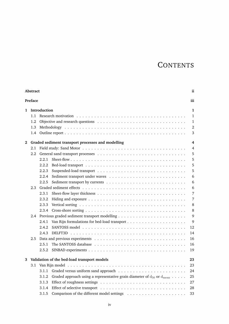
CONTENTS
Abstract ii
Preface iii
1 Introduction 11.1 Research motivation . . . . . . . . . . . . . . . . . . . . . . . . . . . . . . . . . . . . . 11.2 Objective and research questions . . . . . . . . . . . . . . . . . . . . . . . . . . . . . . 11.3 Methodology . . . . . . . . . . . . . . . . . . . . . . . . . . . . . . . . . . . . . . . . . 21.4 Outline report . . . . . . . . . . . . . . . . . . . . . . . . . . . . . . . . . . . . . . . . . 3
2 Graded sediment transport processes and modelling 42.1 Field study: Sand Motor . . . . . . . . . . . . . . . . . . . . . . . . . . . . . . . . . . . 42.2 General sand transport processes . . . . . . . . . . . . . . . . . . . . . . . . . . . . . . 5
2.2.1 Sheet-flow . . . . . . . . . . . . . . . . . . . . . . . . . . . . . . . . . . . . . . . 52.2.2 Bed-load transport . . . . . . . . . . . . . . . . . . . . . . . . . . . . . . . . . . 52.2.3 Suspended-load transport . . . . . . . . . . . . . . . . . . . . . . . . . . . . . . 52.2.4 Sediment transport under waves . . . . . . . . . . . . . . . . . . . . . . . . . . 62.2.5 Sediment transport by currents . . . . . . . . . . . . . . . . . . . . . . . . . . . 6
2.3 Graded sediment effects . . . . . . . . . . . . . . . . . . . . . . . . . . . . . . . . . . . 62.3.1 Sheet-flow layer thickness . . . . . . . . . . . . . . . . . . . . . . . . . . . . . . 72.3.2 Hiding and exposure . . . . . . . . . . . . . . . . . . . . . . . . . . . . . . . . . 72.3.3 Vertical sorting . . . . . . . . . . . . . . . . . . . . . . . . . . . . . . . . . . . . 82.3.4 Cross-shore sorting . . . . . . . . . . . . . . . . . . . . . . . . . . . . . . . . . . 8
2.4 Previous graded sediment transport modelling . . . . . . . . . . . . . . . . . . . . . . . 92.4.1 Van Rijn formulations for bed-load transport . . . . . . . . . . . . . . . . . . . . 92.4.2 SANTOSS model . . . . . . . . . . . . . . . . . . . . . . . . . . . . . . . . . . . 122.4.3 DELFT3D . . . . . . . . . . . . . . . . . . . . . . . . . . . . . . . . . . . . . . . 14
2.5 Data and previous experiments . . . . . . . . . . . . . . . . . . . . . . . . . . . . . . . 162.5.1 The SANTOSS database . . . . . . . . . . . . . . . . . . . . . . . . . . . . . . . 162.5.2 SINBAD experiments . . . . . . . . . . . . . . . . . . . . . . . . . . . . . . . . . 19
3 Validation of the bed-load transport models 233.1 Van Rijn model . . . . . . . . . . . . . . . . . . . . . . . . . . . . . . . . . . . . . . . . 23
3.1.1 Graded versus uniform sand approach . . . . . . . . . . . . . . . . . . . . . . . 243.1.2 Graded approach using a representative grain diameter of d50 or dmean . . . . . 253.1.3 Effect of roughness settings . . . . . . . . . . . . . . . . . . . . . . . . . . . . . 273.1.4 Effect of selective transport . . . . . . . . . . . . . . . . . . . . . . . . . . . . . 283.1.5 Comparison of the different model settings . . . . . . . . . . . . . . . . . . . . 33
iv
CONTENTS V
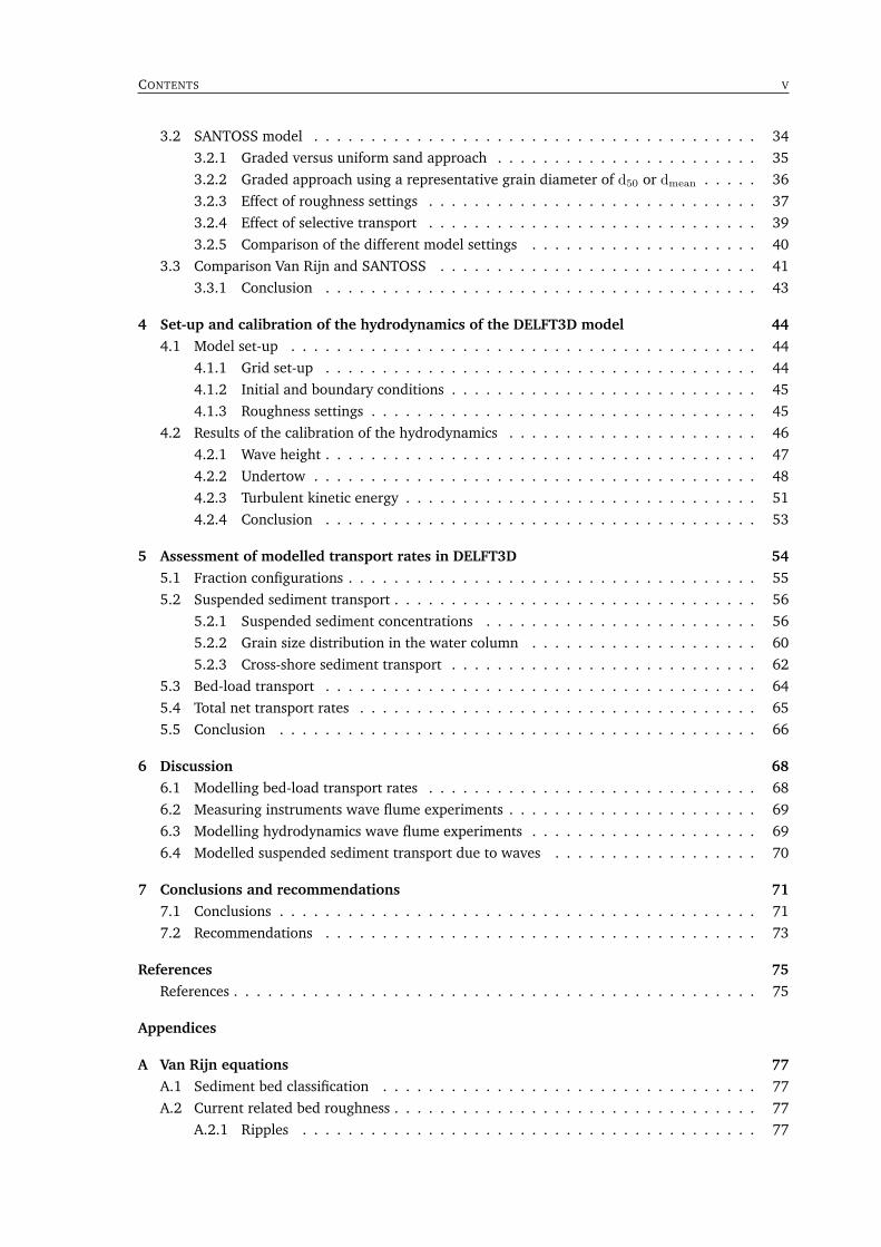
3.2 SANTOSS model . . . . . . . . . . . . . . . . . . . . . . . . . . . . . . . . . . . . . . . 343.2.1 Graded versus uniform sand approach . . . . . . . . . . . . . . . . . . . . . . . 353.2.2 Graded approach using a representative grain diameter of d50 or dmean . . . . . 363.2.3 Effect of roughness settings . . . . . . . . . . . . . . . . . . . . . . . . . . . . . 373.2.4 Effect of selective transport . . . . . . . . . . . . . . . . . . . . . . . . . . . . . 393.2.5 Comparison of the different model settings . . . . . . . . . . . . . . . . . . . . 40
3.3 Comparison Van Rijn and SANTOSS . . . . . . . . . . . . . . . . . . . . . . . . . . . . 413.3.1 Conclusion . . . . . . . . . . . . . . . . . . . . . . . . . . . . . . . . . . . . . . 43
4 Set-up and calibration of the hydrodynamics of the DELFT3D model 444.1 Model set-up . . . . . . . . . . . . . . . . . . . . . . . . . . . . . . . . . . . . . . . . . 44
4.1.1 Grid set-up . . . . . . . . . . . . . . . . . . . . . . . . . . . . . . . . . . . . . . 444.1.2 Initial and boundary conditions . . . . . . . . . . . . . . . . . . . . . . . . . . . 454.1.3 Roughness settings . . . . . . . . . . . . . . . . . . . . . . . . . . . . . . . . . . 45
4.2 Results of the calibration of the hydrodynamics . . . . . . . . . . . . . . . . . . . . . . 464.2.1 Wave height . . . . . . . . . . . . . . . . . . . . . . . . . . . . . . . . . . . . . . 474.2.2 Undertow . . . . . . . . . . . . . . . . . . . . . . . . . . . . . . . . . . . . . . . 484.2.3 Turbulent kinetic energy . . . . . . . . . . . . . . . . . . . . . . . . . . . . . . . 514.2.4 Conclusion . . . . . . . . . . . . . . . . . . . . . . . . . . . . . . . . . . . . . . 53
5 Assessment of modelled transport rates in DELFT3D 545.1 Fraction configurations . . . . . . . . . . . . . . . . . . . . . . . . . . . . . . . . . . . . 555.2 Suspended sediment transport . . . . . . . . . . . . . . . . . . . . . . . . . . . . . . . . 56
5.2.1 Suspended sediment concentrations . . . . . . . . . . . . . . . . . . . . . . . . 565.2.2 Grain size distribution in the water column . . . . . . . . . . . . . . . . . . . . 605.2.3 Cross-shore sediment transport . . . . . . . . . . . . . . . . . . . . . . . . . . . 62
5.3 Bed-load transport . . . . . . . . . . . . . . . . . . . . . . . . . . . . . . . . . . . . . . 645.4 Total net transport rates . . . . . . . . . . . . . . . . . . . . . . . . . . . . . . . . . . . 655.5 Conclusion . . . . . . . . . . . . . . . . . . . . . . . . . . . . . . . . . . . . . . . . . . 66
6 Discussion 686.1 Modelling bed-load transport rates . . . . . . . . . . . . . . . . . . . . . . . . . . . . . 686.2 Measuring instruments wave flume experiments . . . . . . . . . . . . . . . . . . . . . . 696.3 Modelling hydrodynamics wave flume experiments . . . . . . . . . . . . . . . . . . . . 696.4 Modelled suspended sediment transport due to waves . . . . . . . . . . . . . . . . . . 70
7 Conclusions and recommendations 717.1 Conclusions . . . . . . . . . . . . . . . . . . . . . . . . . . . . . . . . . . . . . . . . . . 717.2 Recommendations . . . . . . . . . . . . . . . . . . . . . . . . . . . . . . . . . . . . . . 73
References 75References . . . . . . . . . . . . . . . . . . . . . . . . . . . . . . . . . . . . . . . . . . . . . . 75
Appendices
A Van Rijn equations 77A.1 Sediment bed classification . . . . . . . . . . . . . . . . . . . . . . . . . . . . . . . . . 77A.2 Current related bed roughness . . . . . . . . . . . . . . . . . . . . . . . . . . . . . . . . 77
A.2.1 Ripples . . . . . . . . . . . . . . . . . . . . . . . . . . . . . . . . . . . . . . . . 77
VI CONTENTS
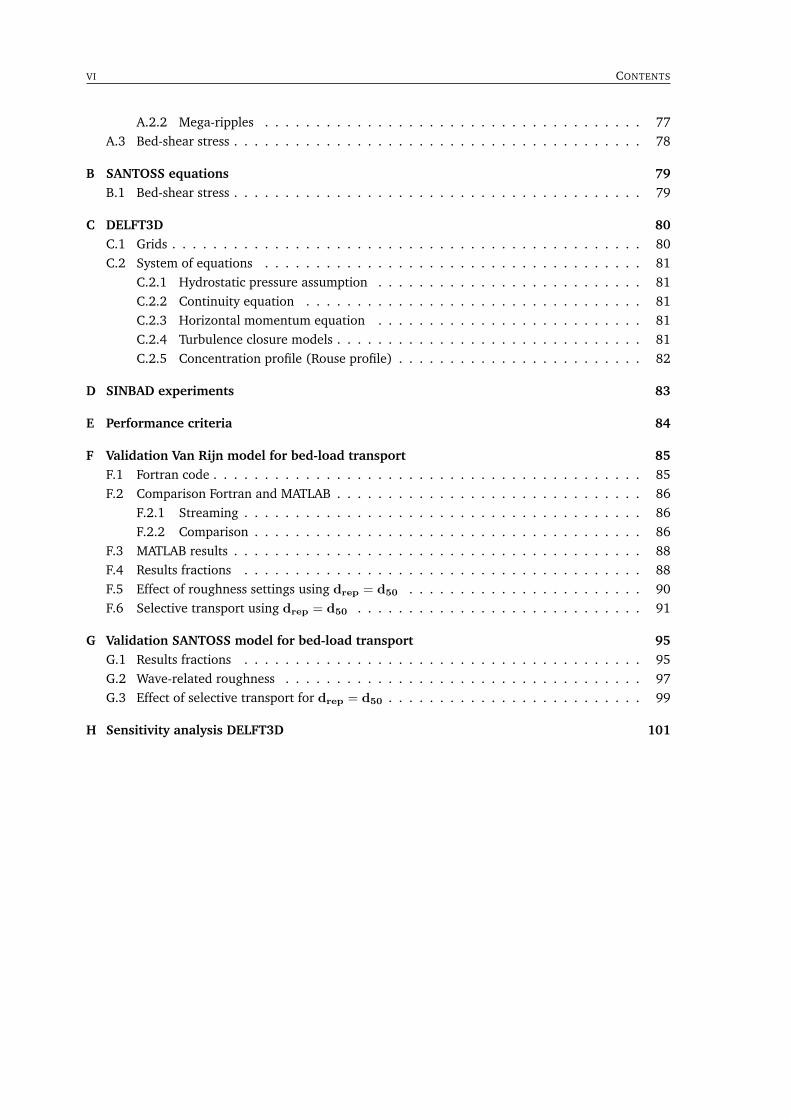
A.2.2 Mega-ripples . . . . . . . . . . . . . . . . . . . . . . . . . . . . . . . . . . . . . 77A.3 Bed-shear stress . . . . . . . . . . . . . . . . . . . . . . . . . . . . . . . . . . . . . . . . 78
B SANTOSS equations 79B.1 Bed-shear stress . . . . . . . . . . . . . . . . . . . . . . . . . . . . . . . . . . . . . . . . 79
C DELFT3D 80C.1 Grids . . . . . . . . . . . . . . . . . . . . . . . . . . . . . . . . . . . . . . . . . . . . . . 80C.2 System of equations . . . . . . . . . . . . . . . . . . . . . . . . . . . . . . . . . . . . . 81
C.2.1 Hydrostatic pressure assumption . . . . . . . . . . . . . . . . . . . . . . . . . . 81C.2.2 Continuity equation . . . . . . . . . . . . . . . . . . . . . . . . . . . . . . . . . 81C.2.3 Horizontal momentum equation . . . . . . . . . . . . . . . . . . . . . . . . . . 81C.2.4 Turbulence closure models . . . . . . . . . . . . . . . . . . . . . . . . . . . . . . 81C.2.5 Concentration profile (Rouse profile) . . . . . . . . . . . . . . . . . . . . . . . . 82
D SINBAD experiments 83
E Performance criteria 84
F Validation Van Rijn model for bed-load transport 85F.1 Fortran code . . . . . . . . . . . . . . . . . . . . . . . . . . . . . . . . . . . . . . . . . . 85F.2 Comparison Fortran and MATLAB . . . . . . . . . . . . . . . . . . . . . . . . . . . . . . 86
F.2.1 Streaming . . . . . . . . . . . . . . . . . . . . . . . . . . . . . . . . . . . . . . . 86F.2.2 Comparison . . . . . . . . . . . . . . . . . . . . . . . . . . . . . . . . . . . . . . 86
F.3 MATLAB results . . . . . . . . . . . . . . . . . . . . . . . . . . . . . . . . . . . . . . . . 88F.4 Results fractions . . . . . . . . . . . . . . . . . . . . . . . . . . . . . . . . . . . . . . . 88F.5 Effect of roughness settings using drep = d50 . . . . . . . . . . . . . . . . . . . . . . . 90F.6 Selective transport using drep = d50 . . . . . . . . . . . . . . . . . . . . . . . . . . . . 91
G Validation SANTOSS model for bed-load transport 95G.1 Results fractions . . . . . . . . . . . . . . . . . . . . . . . . . . . . . . . . . . . . . . . 95G.2 Wave-related roughness . . . . . . . . . . . . . . . . . . . . . . . . . . . . . . . . . . . 97G.3 Effect of selective transport for drep = d50 . . . . . . . . . . . . . . . . . . . . . . . . . 99
H Sensitivity analysis DELFT3D 101
1INTRODUCTION
As climate induced effects may result in a sea level rise and more extreme weather events, it is es-sential that the morphological effects of mitigating measures, for example nourishments, can be pre-dicted accurately to guarantee the safety of the human population living near the coast. Profoundunderstanding of mixed sediment transport behaviour is especially relevant in the view of nourish-ments, because the coastal regions consists of a vast variety of grain sizes, where the grain size ofsand nourishments may also differ from the grain size at the pre-nourished beach (Huisman et al.,2016). Additionally, the differences in bed compositions and the rate at which sediment transporttakes place along the coast affect the ecology within that region and the habitat of fish and benthicspecies (Knaapen et al., 2003).
1.1 RESEARCH MOTIVATION
Up till today, numerical models aiming to determine the morphological evolution of coastlines usuallyassume that the bed consists of a single grain size. However, this is not true as the coastal region con-sists of sand with different grain sizes and thus mixed (or graded) sediment is present. As the transportprocesses for graded sediment differ substantially from uniform sediment, it is of the essence that mor-phodynamic models are able to predict these transport processes for graded sediment accurately. Anexample of such a morphodynamic model which can simulate hydrodynamic flows, sediment trans-port, and morphological changes, is DELFT3D (Lesser et al., 2004). Currently, this model has beenparametrised on the basis of experimental data that was primarily obtained under steady flow con-ditions or in oscillatory flow tunnels. With newly obtained wave flume data, this model can now bevalidated for graded sediment transport processes by waves, to investigate the effect on the modelresults when using a graded sediment approach instead of a uniform sediment approach. Chapter 2further elaborates on graded sediment transport processes, available models and data.
1.2 OBJECTIVE AND RESEARCH QUESTIONS
The objective of this thesis is stated as follows:
Assessment of DELFT3D for cross-shore graded sediment transport under waves.
To achieve the research objective, two research questions are formulated:
1. How well do practical models for bed-load transport predict oscillatory sheet-flow transport ofmixed sediments and how can these models be improved?
2. What are the effects of using a graded sediment approach instead of a uniform approach inDELFT3D regarding the (a) suspended sediment concentrations, (b) suspended sediment grainsizes, and (c) cross-shore net total sediment transport?
1
2 CHAPTER 1. INTRODUCTION
1.3 METHODOLOGY
In this section, a methodology per research question is provided.
RESEARCH QUESTION 1
How well do practical models for bed-load transport predict oscillatory sheet-flow transport of mixed sed-iments and how can these models be improved?
Two models were used to model bed-load transport, namely the model by Van Rijn (2007c) andthe SANTOSS model by Van der A et al. (2013). Both models have already been used to computegraded sediment transport rates in the past. The SANTOSS database (Van der Werf et al., 2009) wasused to validate the practical models. The experiments included in this database were carried out inoscillatory flow tunnels where predominantly bed-load takes place. Both models were validated usingthe same approach:
1. First, the graded sediment was treated as uniform, which means that no distinction was madebetween the different grain sizes per fraction, and only one representative grain diameter wasused for the entire mixture,
2. Subsequently, the bed-load transport rates were validated with a graded sediment approach,where a distinction was made between the grain size per fraction.
3. Next, different approaches for the grain roughness were used.
4. Finally, the effects of the correction factors for selective transport were investigated.
RESEARCH QUESTION 2
After computing the bed-load transport rates in stand-alone MATLAB models using either SANTOSSor Van Rijn, both the bed-load and suspended sediment transport were computed using DELFT3D.DELFT3D is a suitable model to model the transport rates, as it is able to calculate flows, waves,sediment transport rates and morphological changes (Lesser et al., 2004). During a large scale waveflume experiment, data were obtained regarding the transport rates of graded sediment under wavesaround a breaker bar. Research question 2 is stated as follows:
What are the effects of using a graded sediment approach instead of a uniform approach in DELFT3Dregarding the (a) suspended sediment concentrations, (b) suspended sediment grain sizes, and (c) cross-shore net total sediment transport?
Without allowing any morphological changes in DELFT3D, first the suspended sediment concentra-tions in the water column were investigated. This was done by comparing the modelled concentrationsusing a graded approach to the measured concentrations. Additionally, the behaviour and contributionof the different fractions was analysed to obtain a better comprehension of graded sediment transportprocesses. Next, the modelled dm in the water column using a graded approach was compared to thedata and its behaviour was analysed.
Finally, the cross-shore graded sediment transport was analysed in terms of (1) the suspendedsediment transport due to currents, (2) the suspended sediment transport due to waves, (3) the bed-load transport due to currents and waves, and (4) the net total sediment transport. This was donefor both the transport per fraction and total transport of all fractions, where the results of the gradedapproach were compared to those of the uniform approach.
CHAPTER 1. OUTLINE REPORT 3
1.4 OUTLINE REPORT
In Chapter 2 a literature review is provided on graded sediment transport processes and graded sedi-ment modelling. In Chapter 3 the bed-load transport models of Van Rijn and SANTOSS are validatedusing data obtained in oscillatory flow tunnel experiments. In Chapter 4 the hydrodynamics withinDELFT3D are calibrated, where after in Chapter 5 the computed sediment transport rates using agraded and uniform sand approach are compared to each other and to the data which were obtainedduring wave flume experiments. In Chapter 6 the results, performance of the models, and any uncer-tainties are discussed, followed by the conclusions and recommendations in Chapter 7.
2GRADED SEDIMENT TRANSPORT PROCESSES AND
MODELLING
In this chapter, first an example of a field study is presented where both cross-shore and long-shoresediment sorting has taken place. Hereafter, the processes regarding sediment transport are explained,starting with the general sand transport processes and followed by graded sediment effects. Subse-quently, Section 2.4 provides information about previous graded sediment transport modelling and themodels used within this thesis project. Finally, the datasets which are used to validate the sedimenttransport rates are presented.
2.1 FIELD STUDY: SAND MOTOR
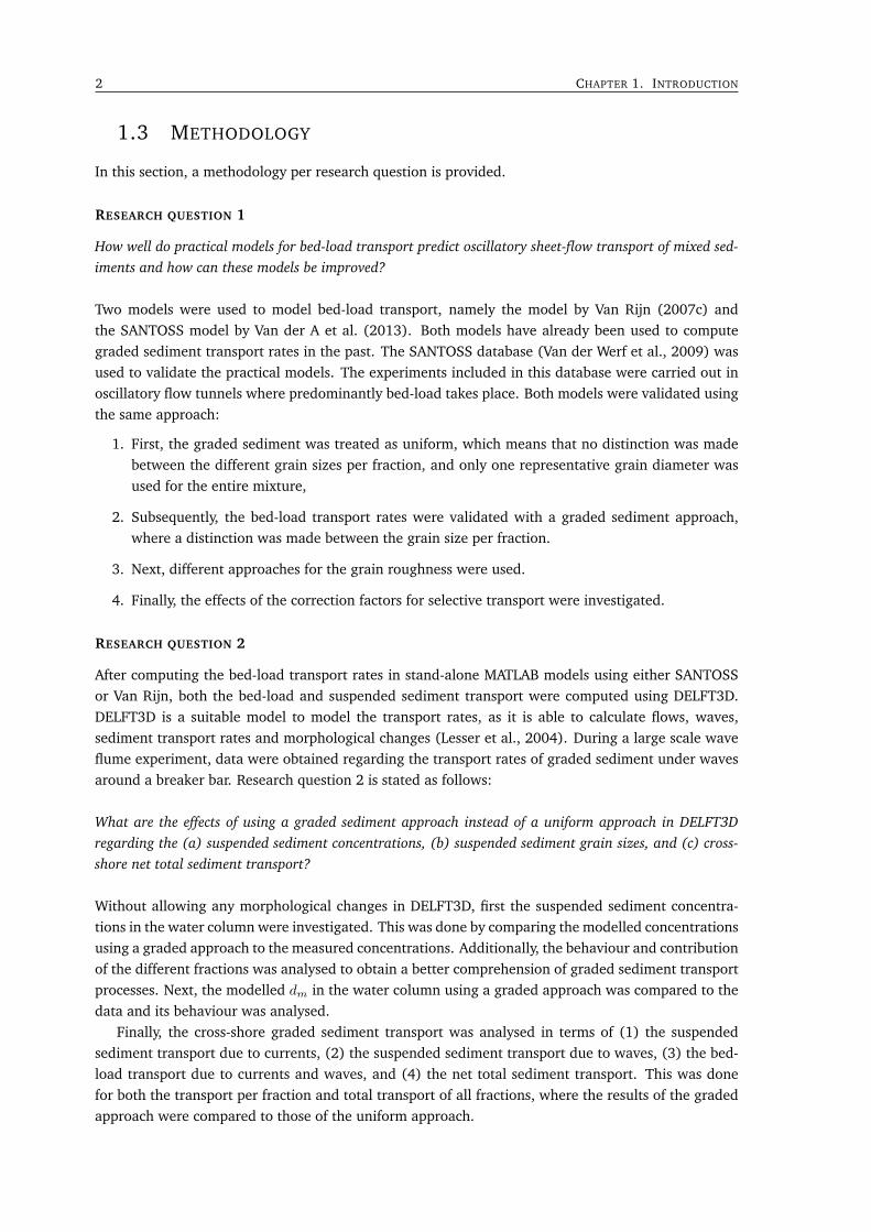
An example of a large-scale nourishment is the Sand Motor (The Netherlands), which was appliedbetween April and August 2011. Here the beach and dune region consisted of fine sand (100-200µm),the swash and surf zone of fine to medium sand (200-400µm) and the region offshore till a depthof 10m of finer sand again (100-300µm). The nourishment had an average median grain size d50 ofabout 278µm. The differences in grain sizes and the development of the nourishment were monitoreda while after the intervention to observe the influence of graded sediment effects (Fig. 2.1). Itwas found that selective transport of the finer sediment and the bed-shear stresses caused by thehydrodynamic forcing were the drivers of spatial heterogeneity regarding grain sizes. Figure 2.1 showsthe spatial distribution of the grain sizes at the site of the Sand Motor right before (left) and threeyears after (right) the application of the nourishment, with the dominant wave direction towards theNorth-East. Despite the well mixed sediment that was used for the Sand Motor, the longshore profileclearly shows sorting, with coarsening at the bulge and finer sand further North.
Figure 2.1: D50 along the site of the Sand Motor before and after its application (Huisman et al., 2016)
4
CHAPTER 2. GENERAL SAND TRANSPORT PROCESSES 5
2.2 GENERAL SAND TRANSPORT PROCESSES
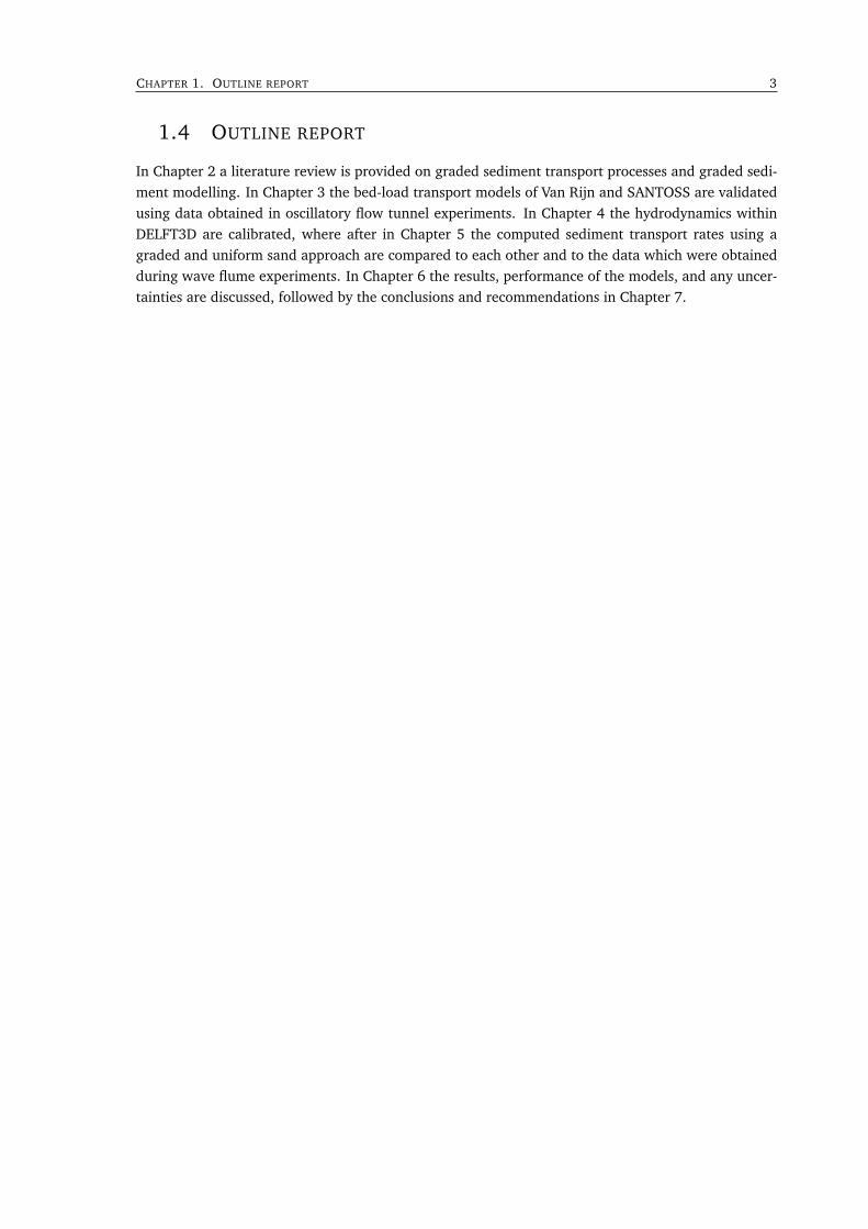
Sediment can be transported by currents and waves. For grains to be set into motion, enough forcemust be exerted on the bed, causing the lift and drag forces on a grain to be larger than the gravita-tional and frictional forces, causing the moment of incipient motion. When high flow velocities arepresent, sheet-flow may occur (Section 2.2.1). Sediment can be transported as bed-load or suspended-load, which is shown in Figure 2.2.
Figure 2.2: Modes of sediment transport (Indiawrm, 2015)
2.2.1 SHEET-FLOW
Sheet-flow occurs when the flow is very strong and bed-forms such as ripples are washed out. Whenthis occurs, a plain bed remains and the sand is transported in a sediment-water mixture, which isup to a few centimetres thick. Sheet-flow transport is characterized by very high sediment transportrates. Hence it is of importance that the sediment transport in these regimes can be predicted andmodelled accurately (Wright, 2002). When the flow velocity increases, sediment is entrained andthe concentration decreases in the lower part of the sheet flow layer, which is called the pick-uplayer. Once the flow velocity decreases again, the sediment settles and the concentration increasesonce again in this pick-up layer. The concentration in the top layer is in phase with the flow velocity,whereas the concentration in the pick-up layer is in anti-phase.
2.2.2 BED-LOAD TRANSPORT
Bed-load is the fraction of transported grains that are still in contact in the bed and move by rolling,sliding and jumping (saltation) over each other (The Open University, 1999) (Fig. 2.2). Rolling andsliding occurs when the there are low flow velocities, whereas saltation takes place with higher flowvelocities.
2.2.3 SUSPENDED-LOAD TRANSPORT
A different mode of transport besides bed-load is suspended-load. Large orbital velocities and highlevels of turbulence create higher bed-shear stresses, creating the potential for the sediment to bepicked up by the flow. After the grain has been picked up, it will be entrained higher into the watercolumn due to turbulent mixing, where the upward force exceeds the gravitational force (Ribberink,
6 CHAPTER 2. GRADED SEDIMENT TRANSPORT PROCESSES AND MODELLING
2011). Grains that are in suspension have been separated from the bed and are transported higher upin the water column, and only when the flow slackens, these grains regain contact with the bed (TheOpen University, 1999).
2.2.4 SEDIMENT TRANSPORT UNDER WAVES
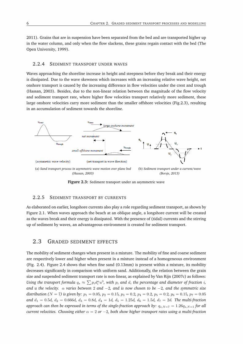
Waves approaching the shoreline increase in height and steepness before they break and their energyis dissipated. Due to the wave skewness which increases with an increasing relative wave height, netonshore transport is caused by the increasing difference in flow velocities under the crest and trough(Hassan, 2003). Besides, due to the non-linear relation between the magnitude of the flow velocityand sediment transport rate, where higher flow velocities transport relatively more sediment, theselarge onshore velocities carry more sediment than the smaller offshore velocities (Fig.2.3), resultingin an accumulation of sediment towards the shoreline.
(a) Sand transport process in asymmetric wave motion over plane bed(Hassan, 2003)
(b) Sediment transport under a current/wave(Borsje, 2013)
Figure 2.3: Sediment transport under an asymmetric wave
2.2.5 SEDIMENT TRANSPORT BY CURRENTS
As elaborated on earlier, longshore currents also play a role regarding sediment transport, as shown byFigure 2.1. When waves approach the beach at an oblique angle, a longshore current will be createdas the waves break and their energy is dissipated. With the presence of (tidal) currents and the stirringup of sediment by waves, an advantageous environment is created for sediment transport.
2.3 GRADED SEDIMENT EFFECTS
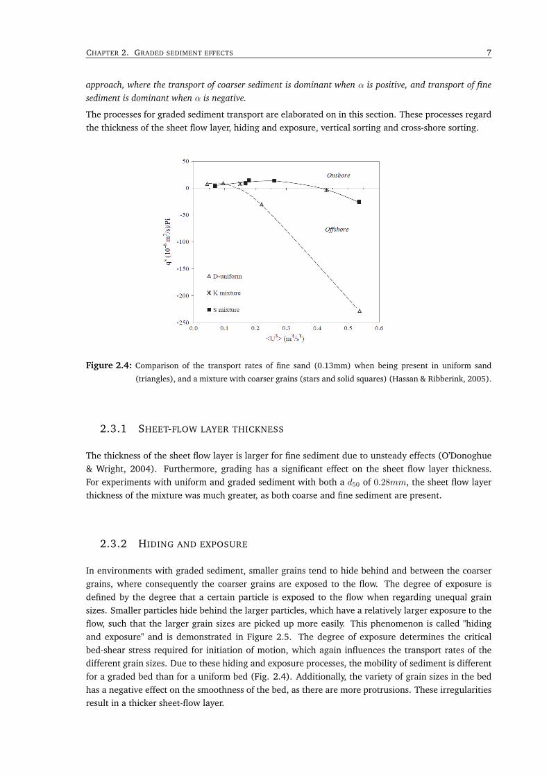
The mobility of sediment changes when present in a mixture. The mobility of fine and coarse sedimentare respectively lower and higher when present in a mixture instead of a homogeneous environment(Fig. 2.4). Figure 2.4 shows that when fine sand (0.13mm) is present within a mixture, its mobilitydecreases significantly in comparison with uniform sand. Additionally, the relation between the grainsize and suspended sediment transport rate is non-linear, as explained by Van Rijn (2007c) as follows:Using the transport formula qs ≈
∑pid
αi u
3, with pi and di the percentage and diameter of fraction i,and u the velocity. α varies between 2 and −2, and is now chosen to be −2, and the symmetric sizedistribution (N = 7) is given by: p1 = 0.05, p2 = 0.15, p3 = 0.2, p4 = 0.2, p5 = 0.2, p6 = 0.15, p7 = 0.05
and d1 = 0.5d, d2 = 0.666d, d3 = 0.8d, d4 = 1d, d5 = 1.25d, d6 = 1.5d, d7 = 2d. The multi-fractionapproach can then be expressed in terms of the single-fraction approach by: qs,N=7 = 1.26qs,N=1 for allcurrent velocities. Choosing either α = 2 or −2, both show higher transport rates using a multi-fraction
CHAPTER 2. GRADED SEDIMENT EFFECTS 7
approach, where the transport of coarser sediment is dominant when α is positive, and transport of finesediment is dominant when α is negative.
The processes for graded sediment transport are elaborated on in this section. These processes regardthe thickness of the sheet flow layer, hiding and exposure, vertical sorting and cross-shore sorting.
Figure 2.4: Comparison of the transport rates of fine sand (0.13mm) when being present in uniform sand
(triangles), and a mixture with coarser grains (stars and solid squares) (Hassan & Ribberink, 2005).
2.3.1 SHEET-FLOW LAYER THICKNESS
The thickness of the sheet flow layer is larger for fine sediment due to unsteady effects (O’Donoghue& Wright, 2004). Furthermore, grading has a significant effect on the sheet flow layer thickness.For experiments with uniform and graded sediment with both a d50 of 0.28mm, the sheet flow layerthickness of the mixture was much greater, as both coarse and fine sediment are present.
2.3.2 HIDING AND EXPOSURE
In environments with graded sediment, smaller grains tend to hide behind and between the coarsergrains, where consequently the coarser grains are exposed to the flow. The degree of exposure isdefined by the degree that a certain particle is exposed to the flow when regarding unequal grainsizes. Smaller particles hide behind the larger particles, which have a relatively larger exposure to theflow, such that the larger grain sizes are picked up more easily. This phenomenon is called "hidingand exposure" and is demonstrated in Figure 2.5. The degree of exposure determines the criticalbed-shear stress required for initiation of motion, which again influences the transport rates of thedifferent grain sizes. Due to these hiding and exposure processes, the mobility of sediment is differentfor a graded bed than for a uniform bed (Fig. 2.4). Additionally, the variety of grain sizes in the bedhas a negative effect on the smoothness of the bed, as there are more protrusions. These irregularitiesresult in a thicker sheet-flow layer.

8 CHAPTER 2. GRADED SEDIMENT TRANSPORT PROCESSES AND MODELLING
Figure 2.5: Hiding and exposure of sediment particles in a mixture (Hassan, 2003).
2.3.3 VERTICAL SORTING
Vertical sorting may take place in environments where different grain sizes are present, and bed forms(ripples) may be formed. An armouring layer of immobile large grains can be formed on top of thesmaller grains, preventing them from being transported by the flow, even though their threshold forinitiation of motion has been exceeded. Furthermore, sorting processes take place around ripples,where for river dunes coarsening takes place at the bottom. However, lab experiments have providedresults where coarsening actually takes place on top of ripples (Cáceres et al., 2018). It is still unclearhow such processes affect the net transport rates of graded sand in a sand ripple regime and howthese sorting processes take place in coastal environments.
2.3.4 CROSS-SHORE SORTING
Besides vertical sorting, also cross-shore sorting takes places as an effect of graded sand transport.This is illustrated by Figure 2.6, with larger grain sizes landwards and finer sand further seawards.This is caused by the currents approaching the shoreline, which have the capacity to transport coarsesand. The offshore directed bottom current however, is weaker and only able to transport the finergrains. Fine grains are more easily eroded, resulting in coarsening of the shoreline (Hassan, 2003).
Figure 2.6: Cross-shore sorting as an effect of graded sand transport (Hassan, 2003).
CHAPTER 2. PREVIOUS GRADED SEDIMENT TRANSPORT MODELLING 9
2.4 PREVIOUS GRADED SEDIMENT TRANSPORT MODELLING
Two models that can be used to model bed-load transport for graded sediment are the formulations byVan Rijn (2007c) and the SANTOSS model by Van der A et al. (2013). The main difference betweenthese two bed-load transport models, is the incorporation of formulations for phase lag effects in theSANTOSS model, which are not included in the bed-load transport formulations by (Van Rijn, 2007c).These phase lag effects are covered in Section 2.4.2. Furthermore, DELFT3D is an often used modelwhen modelling both the bed-load and suspended transport. In this section information is providedabout these three different models.
2.4.1 VAN RIJN FORMULATIONS FOR BED-LOAD TRANSPORT
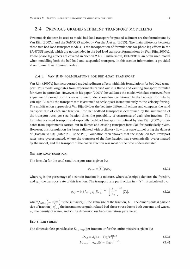
Van Rijn (2007c) has incorporated graded sediment effects within his formulations for bed-load trans-port. This model originates from experiments carried out in a flume and existing transport formulaefor rivers in particular. However, in his paper (2007c) he validates the model with data retrieved fromexperiments carried out in a wave tunnel under sheet-flow conditions. In the bed-load formula byVan Rijn (2007a) the transport rate is assumed to scale quasi-instantaneously to the velocity forcing.The multifraction approach of Van Rijn divides the bed into different fractions and computes the sandtransport rate of each size fraction. The net bedload transport is determined by the summation ofthe transport rates per size fraction times the probability of occurrence of each size fraction. Theformulae for sand transport and especially bed-load transport as defined by Van Rijn (2007c) origi-nates from experiments carried out in flumes and existing transport formulae for particularly rivers.However, this formulation has been validated with oscillatory flow in a wave tunnel using the datasetof (Hassan, 2003) (Table 2.1, Code P9F). Validation then showed that the modelled total transportrates were overestimated, where the transport of the fine fraction was systematically overestimatedby the model, and the transport of the coarse fraction was most of the time underestimated.
NET BED-LOAD TRANSPORT
The formula for the total sand transport rate is given by:
qb,tot =∑
pjqb,j (2.1)
where pj is the percentage of a certain fraction in a mixture, where subscript j denotes the fraction,and qb,j the transport rate of this fraction. The transport rate per fraction in m2s−1 is calculated by:
qb,j = 0.5fsilt,jdj [D∗,j ]−0.3
[τ ′b,cwρw
]0.5[Tj ], (2.2)
wherefsilt,j(
= dsand
dj
)is the silt factor, dj the grain size of the fraction, D∗,j the dimensionless particle
size of fraction j, τ ′b,cw the instantaneous grain-related bed-shear stress due to both currents and waves,ρw the density of water, and Tj the dimensionless bed-shear stress parameter.
BED-SHEAR STRESS
The dimensionless particle size D∗,j/rep per fraction or for the entire mixture is given by:
D∗,j = dj [(s− 1)g/v2]1/3 (2.3)
D∗,rep = drep[(s− 1)g/v2]1/3, (2.4)
10 CHAPTER 2. GRADED SEDIMENT TRANSPORT PROCESSES AND MODELLING
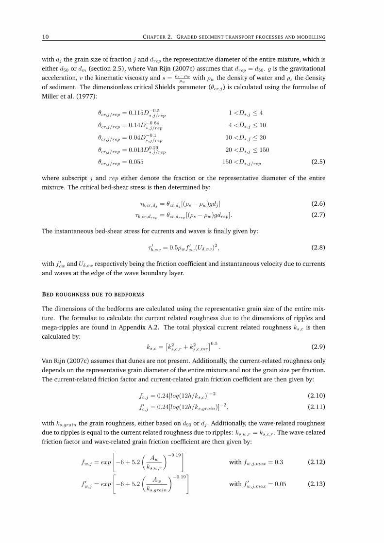
with dj the grain size of fraction j and drep the representative diameter of the entire mixture, which iseither d50 or dm (section 2.5), where Van Rijn (2007c) assumes that drep = d50. g is the gravitationalacceleration, v the kinematic viscosity and s = ρs−ρw
ρwwith ρw the density of water and ρs the density
of sediment. The dimensionless critical Shields parameter (θcr,j) is calculated using the formulae ofMiller et al. (1977):
θcr,j/rep = 0.115D−0.5∗,j/rep 1 <D∗,j ≤ 4
θcr,j/rep = 0.14D−0.64∗,j/rep 4 <D∗,j ≤ 10
θcr,j/rep = 0.04D−0.1∗,j/rep 10 <D∗,j ≤ 20
θcr,j/rep = 0.013D0.29∗,j/rep 20 <D∗,j ≤ 150
θcr,j/rep = 0.055 150 <D∗,j/rep (2.5)
where subscript j and rep either denote the fraction or the representative diameter of the entiremixture. The critical bed-shear stress is then determined by:
τb,cr,dj = θcr,dj [(ρs − ρw)gdj ] (2.6)
τb,cr,drep = θcr,drep [(ρs − ρw)gdrep]. (2.7)
The instantaneous bed-shear stress for currents and waves is finally given by:
τ ′b,cw = 0.5ρwf′cw(Uδ,cw)2, (2.8)
with f ′cw and Uδ,cw respectively being the friction coefficient and instantaneous velocity due to currentsand waves at the edge of the wave boundary layer.
BED ROUGHNESS DUE TO BEDFORMS
The dimensions of the bedforms are calculated using the representative grain size of the entire mix-ture. The formulae to calculate the current related roughness due to the dimensions of ripples andmega-ripples are found in Appendix A.2. The total physical current related roughness ks,c is thencalculated by:
ks,c =[k2s,c,r + k2s,c,mr
]0.5. (2.9)
Van Rijn (2007c) assumes that dunes are not present. Additionally, the current-related roughness onlydepends on the representative grain diameter of the entire mixture and not the grain size per fraction.The current-related friction factor and current-related grain friction coefficient are then given by:
fc,j = 0.24[log(12h/ks,c)]−2 (2.10)
f ′c,j = 0.24[log(12h/ks,grain)]−2, (2.11)
with ks,grain the grain roughness, either based on d90 or dj . Additionally, the wave-related roughnessdue to ripples is equal to the current related roughness due to ripples: ks,w,r = ks,c,r. The wave-relatedfriction factor and wave-related grain friction coefficient are then given by:
fw,j = exp
[−6 + 5.2
(Awks,w,r
)−0.19]with fw,j,max = 0.3 (2.12)
f ′w,j = exp
[−6 + 5.2
(Aw
ks,grain
)−0.19]with f ′w,j,max = 0.05 (2.13)
CHAPTER 2. PREVIOUS GRADED SEDIMENT TRANSPORT MODELLING 11
with Aw the representative orbital excursion amplitude. Finally the friction coefficient due to currentsand waves is given by:
f ′c,w,j = αβf ′c + (1− α)f ′w, (2.14)
with β a coefficient related to the vertical structure of the velocity profile (Appendix A.2), and α:
α =|Unet|
|Unet|+ Uw, (2.15)
with Uw is the representative orbital velocity amplitude and |Unet| the net current velocity.
SELECTIVE TRANSPORT
In sediment mixtures, selective transport takes place due to grading effects. This involves hiding andexposure, where smaller grains are hidden behind coarser grains and are thus less exposed to the flow.Additionally, coarser grains endure a larger amount of fluid drag. Van Rijn (2007c) corrects for thesetwo effect of selective transport due to grading effects using two correction factors:
1. The hiding and exposure factor by Egiazaroff (1965):
ξj =
[log(19)
log(19dj/drep)
]2, (2.16)
which expresses to what extent the particles are exposed to the flow, as the smaller grains maybe hidden behind the larger grains.
2. The correction factor for the effective grain-shear stress by Day (1980):
λj =
(djdrep
)0.25
, (2.17)
which represents the amount of fluid drag to which a particle is exposed.
DIMENSIONLESS BED-SHEAR STRESS PARAMETER
Van Rijn introduces four methods to determine the dimensionless bed-shear stress parameter Tj .Methods A and B both use the drep approach for the critical bed-shear stress, whereas methods Cand D use the dj approach. The difference between method A and B lies within the correction factorfor the effective grain-shear stress which is present in the former and absent in the latter. Method Aand B are respectively given by the following formulae:
Method A: Tj = λj
τ ′b,cw − ξj(
djdrep
)τb,cr,drep(
djdrep
)τb,cr,drep
(2.18)
Method B: Tj =
τ ′b,cw − ξj(
djdrep
)τb,cr,drep(
djdrep
)τb,cr,drep
. (2.19)
Methods C and D differ as method C uses the correction factor for hiding and exposure by (Egiazaroff,1965) which is absent in method D. Method C and D are respectively given by the following formulae:
Method C: Tj =
[τ ′b,cw − ξjτb,cr,dj
τb,cr,dj
](2.20)
Method D: Tj =
[τ ′b,cw − τb,cr,dj
τb,cr,dj
](2.21)
In his paper, Van Rijn (2007c) recommends to use method A.
12 CHAPTER 2. GRADED SEDIMENT TRANSPORT PROCESSES AND MODELLING
2.4.2 SANTOSS MODEL
The SANTOSS model incorporates graded sediment effects by first calculating the net transport ratesper fraction, and then determining the total net transport rate by summing these rates per fraction(Van der A et al., 2013). Additionally graded sediment effects are incorporated, such as a correctionfactor for hiding and exposure. The model calculates the near-bed transport under waves and currentsand determines the total net sand transport rate by calculating the difference between the sand trans-port during the positive crest half-cycle and negative trough half-cycle. The formula takes hiding andexposure, and phase lag effects into account, as the sand transport during each half-cycle consists ofsediment which is transported during the present cycle and sand that has not yet settled down in theprevious half-cycle. Previously this model was already used for graded sediment conditions by Van derA et al. (2013) and gave fairly good results for the net total transport (89% in a factor 2 interval fromthe data). However, the transport rates per fraction are still unknown and graded sediment effectsneed to be examined more thoroughly.
NET BED-LOAD TRANSPORT
The formula for the net transport rate as used in the SANTOSS model is given by:
−→Φ =
M∑j=1
pj
−→qs,j√(s− 1)gd3j
(2.22)
where pj is the percentage of a fraction in the mixture, −→qs,j the transport of this fraction, dj the grainsize of the fraction, s the ratio between the densities of water and sediment, and M the total numberof fractions. This equation is then rewritten for the non-dimensional net transport rates, such that:
−→Φ =
M∑j=1
pj
√|θc,j |Tc(Ωcc,j + Tc
2TcuΩtc,j)
−→θ c,j
|θc,j | +√|θt,j |Tt(Ωtt,j + Tt
2TtuΩct,j)
−→θ t,j
|θt,j |
T(2.23)
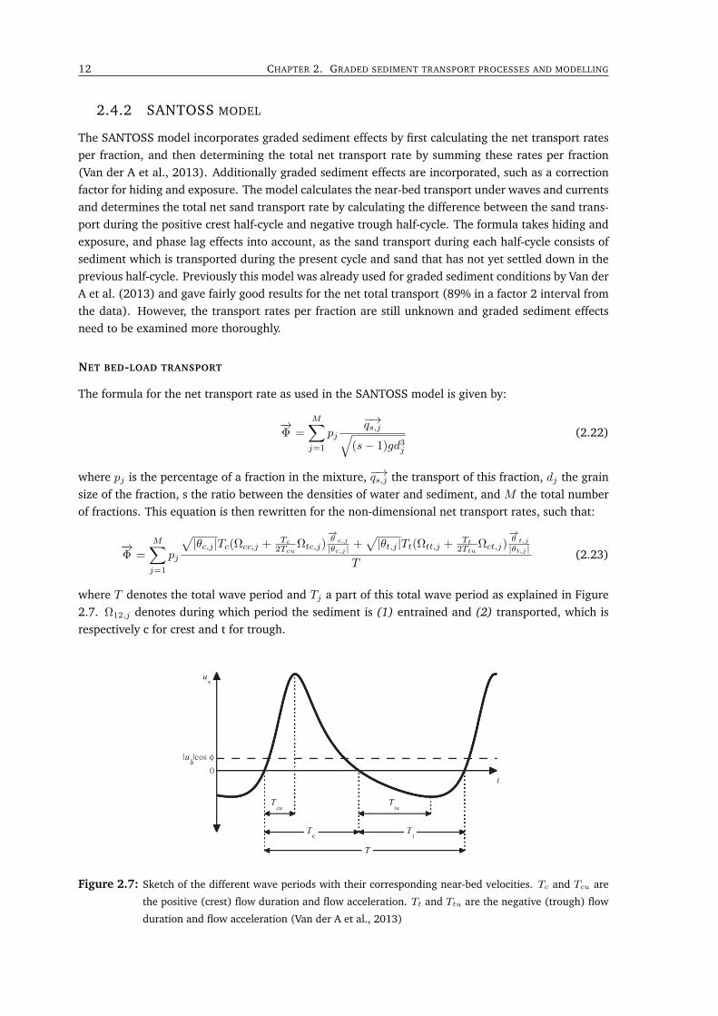
where T denotes the total wave period and Tj a part of this total wave period as explained in Figure2.7. Ω12,j denotes during which period the sediment is (1) entrained and (2) transported, which isrespectively c for crest and t for trough.
Figure 2.7: Sketch of the different wave periods with their corresponding near-bed velocities. Tc and Tcu are
the positive (crest) flow duration and flow acceleration. Tt and Ttu are the negative (trough) flow
duration and flow acceleration (Van der A et al., 2013)
CHAPTER 2. PREVIOUS GRADED SEDIMENT TRANSPORT MODELLING 13
BED-SHEAR STRESS
The vector for the dimensionless bed-shear stress is given by:
−→θi,j =
12fwδi,j |ui,r|ui,rx + τwRe
(s− 1)gdj,12fwδi,j |ui,r|ui,ry
(s− 1)gdj
, (2.24)
where i denotes the wave crest or trough, |ui,r| is the representative half-cycle orbital velocity, andui,rx and ui,ry the representative combined wave-current velocity in the x and y direction. τwRe is acontribution related to progressive surface waves and is absent in the case of oscillatory flow tunnelexperiments and fcwi is the friction factor due to currents and waves.
BED ROUGHNESS
The bed roughness consists of the current-related roughness and the wave-related roughness. Thefriction factor due to currents and waves fδwi is given by:
fcwi = αfci + (1− α)fwi (2.25)
where subscript i denotes the crest (c) or trough (t) period, and α is given by Equation 2.15. Further-more the current-related friction factor is calculated assuming a logarithmic profile:
fci = 2
[0.4
ln(30δ/ks,δ)
]2(2.26)
where δ is the distance between the bed and the top of the wave boundary layer, and ks,δ is the currentrelated roughness (Appendix B.1). Finally the wave friction factor is given by: fwi = exp
[−6 + 5.2
(Aw
ks,w
)−0.19]fwi,max = 0.3
where Aw is the peak orbital diameter, and ks,w the wave related roughness (Appendix B.1).
HIDING AND EXPOSURE
Hiding and exposure is incorporated in the SANTOSS model by correction factor λ for the effectiveShields parameter by Day (1980) (Eq. 2.17), where Van der A et al. (2013) suggests that drep = dmean.The effective Shields parameter is then determined by:
|θi,j,eff | = λj |θi,j | (2.27)
The effective Shields parameter is embedded in the formula determining the sand load entrained in aflow during each half-cycle:
Ωi,j =
0 if |θi,j,eff | ≤ θcr,jm(|θi,j,eff | − θcr,j)n if |θi,j,eff | > θcr,j
(2.28)
PHASE LAG
Whether sediment is transported during the current or successive crest or trough cycle depends onthe phase lag parameter. This parameter is calculated per sediment fraction and are given by thefollowing formulae:
Pc,j =
α( 1−ξuc
cw)( η
2(Tc−Tcu)wsc,j) if η > 0 (ripple regime)
α( 1−ξuc
cw)( δsc
2(Tc−Tcu)wsc,j) if η = 0 (sheet flow regime)
(2.29)
14 CHAPTER 2. GRADED SEDIMENT TRANSPORT PROCESSES AND MODELLING
Pt,j =
α( 1+ξuc
cw)( η
2(Tt−Ttu)wst,j) if η > 0 (ripple regime)
α( 1+ξuc
cw)( δst
2(Tt−Ttu)wst,j) if η = 0 (sheet flow regime)
(2.30)
where α is the calibration coefficient, η the ripple height, ξ accounts for the shape of the velocity andthe concentration profile, δsi the sheet flow layer thickness for the half cycle, and wsi the sedimentsettling velocity within the half cycle. When Pi > 1 there is an exchange of sand between cycles.How much sand is transported within a cycle is determined by 1
Pi. The amount of sand that stays in
suspension until the next cycle is given by 1− 1Pi
. The different wave periods with their correspondingnear-bed velocities are schematised in Figure 2.7.
2.4.3 DELFT3D
In this section general information about equations solved by the model are explained, followed byspecific formulae used for modelling of the hydrodynamics, and finally concluding with equations forthe suspended sediment transport. DELFT3D uses the formulations by Van Rijn (1993) to computethe bed-load transport.
COORDINATE SYSTEM
DELFT3D uses a grid to solve the equations per grid cell (Fig. C.1). The equations can be solved on anumber of grids, namely Cartesian rectangular, orthogonal curvilinear (boundary fitted), or sphericalgrid (Lesser et al., 2004). The hereafter stated equations are applicable for a Cartesian rectangulargrid. For the vertical grid direction a boundary fitted (σ-coordinate) approach is used (Fig. C.2).
2.4.3.1 HYDRODYNAMICS
The DELFT3D-FLOW module is used to solve the unsteady shallow-water equations and compute thesediment transport rates. The set of equations used to solve the shallow-water equations are found insection C.2 and comprises the hydrostatic pressure assumption, continuity and horizontal momentumequations, and turbulence closure model.
WAVES
DELFT3D models the forcing caused by short waves instead of modelling individual waves. Theenergy of these short waves travels with the group velocity. The short wave energy balance is givenby (Deltares, 2018):
∂E
∂t+
∂
∂x(ECgcos(α)) +
∂
∂y(ECgsin(α)) = −Dw, (2.31)
with E the short-wave energy, Cg the group celerity, α the wave direction, and Dw the dissipationof wave energy. Originally, DELFT3D is designed for irregular waves, as is the formulation for theenergy dissipation. In contradiction with irregular waves, regular waves all break at the same loca-tion. Therefore, Schnitzler (2015) proposed an adaption of the current formulations for the energydissipation based on the formulations by Van Rijn and Wijnberg (1996):
Dw =1
4αrolρwg
1
TH2maxQb, (2.32)
with αrol the roller dissipation coefficient, T the wave period, Hmax the maximum wave height, andQb = 1 when waves break and Qb = 0 when waves are not breaking. Qb was adapted such that waves
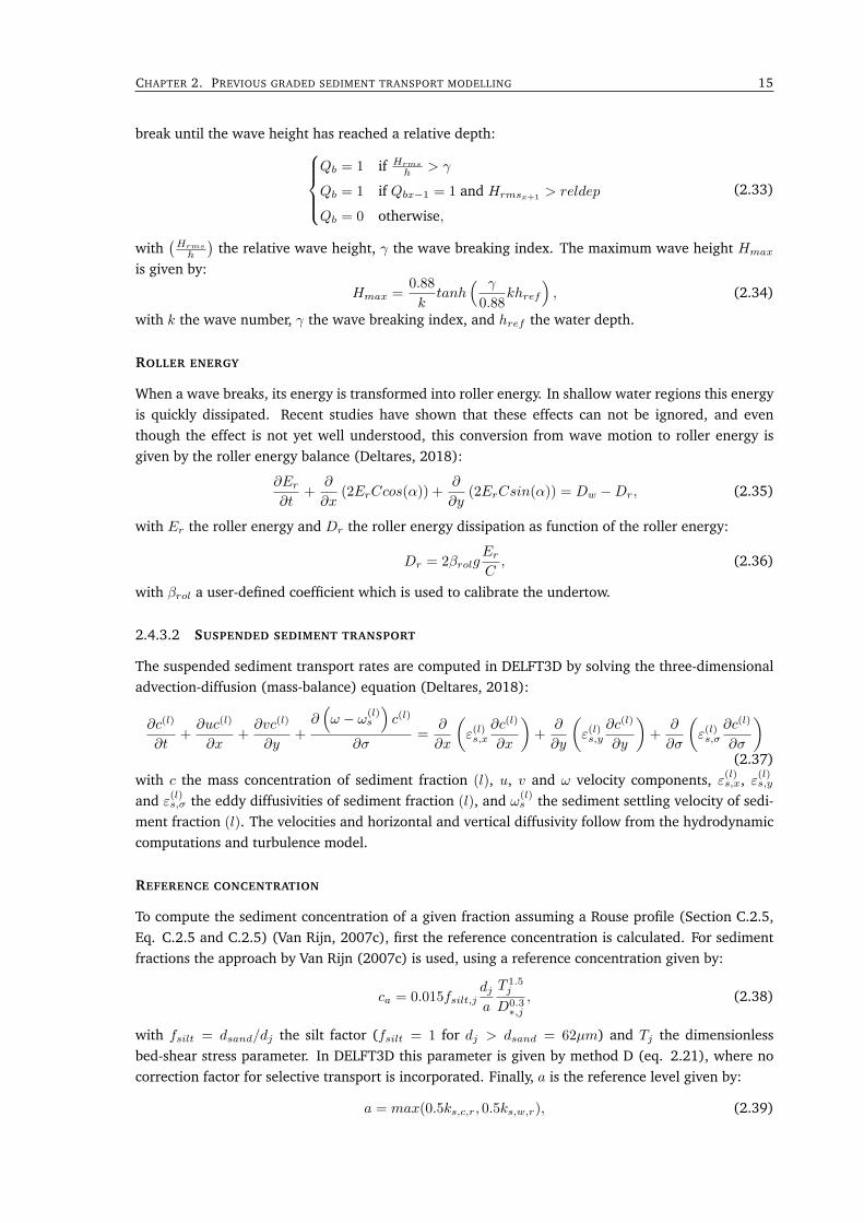
CHAPTER 2. PREVIOUS GRADED SEDIMENT TRANSPORT MODELLING 15
break until the wave height has reached a relative depth:Qb = 1 if Hrms
h > γ
Qb = 1 if Qbx−1 = 1 and Hrmsx+1 > reldep
Qb = 0 otherwise,
(2.33)
with(Hrms
h
)the relative wave height, γ the wave breaking index. The maximum wave height Hmax
is given by:
Hmax =0.88
ktanh
( γ
0.88khref
), (2.34)
with k the wave number, γ the wave breaking index, and href the water depth.
ROLLER ENERGY
When a wave breaks, its energy is transformed into roller energy. In shallow water regions this energyis quickly dissipated. Recent studies have shown that these effects can not be ignored, and eventhough the effect is not yet well understood, this conversion from wave motion to roller energy isgiven by the roller energy balance (Deltares, 2018):
∂Er∂t
+∂
∂x(2ErCcos(α)) +
∂
∂y(2ErCsin(α)) = Dw −Dr, (2.35)
with Er the roller energy and Dr the roller energy dissipation as function of the roller energy:
Dr = 2βrolgErC, (2.36)
with βrol a user-defined coefficient which is used to calibrate the undertow.
2.4.3.2 SUSPENDED SEDIMENT TRANSPORT
The suspended sediment transport rates are computed in DELFT3D by solving the three-dimensionaladvection-diffusion (mass-balance) equation (Deltares, 2018):
∂c(l)
∂t+∂uc(l)
∂x+∂vc(l)
∂y+∂(ω − ω(l)
s
)c(l)
∂σ=
∂
∂x
(ε(l)s,x
∂c(l)
∂x
)+
∂
∂y
(ε(l)s,y
∂c(l)
∂y
)+
∂
∂σ
(ε(l)s,σ
∂c(l)
∂σ
)(2.37)
with c the mass concentration of sediment fraction (l), u, v and ω velocity components, ε(l)s,x, ε(l)s,yand ε(l)s,σ the eddy diffusivities of sediment fraction (l), and ω(l)
s the sediment settling velocity of sedi-ment fraction (l). The velocities and horizontal and vertical diffusivity follow from the hydrodynamiccomputations and turbulence model.
REFERENCE CONCENTRATION
To compute the sediment concentration of a given fraction assuming a Rouse profile (Section C.2.5,Eq. C.2.5 and C.2.5) (Van Rijn, 2007c), first the reference concentration is calculated. For sedimentfractions the approach by Van Rijn (2007c) is used, using a reference concentration given by:
ca = 0.015fsilt,jdja
T 1.5j
D0.3∗,j, (2.38)
with fsilt = dsand/dj the silt factor (fsilt = 1 for dj > dsand = 62µm) and Tj the dimensionlessbed-shear stress parameter. In DELFT3D this parameter is given by method D (eq. 2.21), where nocorrection factor for selective transport is incorporated. Finally, a is the reference level given by:
a = max(0.5ks,c,r, 0.5ks,w,r), (2.39)
16 CHAPTER 2. GRADED SEDIMENT TRANSPORT PROCESSES AND MODELLING
with a minimum value of 0.01 m, and ks,c,r and ks,w,r given by equation A.2, assuming ks,c,r = ks,w,r
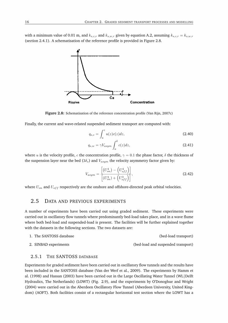
(section 2.4.1). A schematisation of the reference profile is provided in Figure 2.8.
Figure 2.8: Schematisation of the reference concentration profile (Van Rijn, 2007c)
Finally, the current and wave-related suspended sediment transport are computed with:
qs,c =
∫ z
a
u(z)c(z)dz, (2.40)
qs,w = γVasym
∫ δ
a
c(z)dz, (2.41)
where u is the velocity profile, c the concentration profile, γ = 0.1 the phase factor, δ the thickness ofthe suspension layer near the bed (3δs) and Vasym the velocity asymmetry factor given by:
Vasym =
[(U4on
)−(U4off
)][(U3
on) +(U3off
)] , (2.42)
where Uon and Uoff respectively are the onshore and offshore-directed peak orbital velocities.
2.5 DATA AND PREVIOUS EXPERIMENTS
A number of experiments have been carried out using graded sediment. These experiments werecarried out in oscillatory flow tunnels where predominantly bed-load takes place, and in a wave flumewhere both bed-load and suspended-load is present. The facilities will be further explained togetherwith the datasets in the following sections. The two datasets are:
1. The SANTOSS database (bed-load transport)
2. SINBAD experiments (bed-load and suspended transport)
2.5.1 THE SANTOSS DATABASE
Experiments for graded sediment have been carried out in oscillatory flow tunnels and the results havebeen included in the SANTOSS database (Van der Werf et al., 2009). The experiments by Hamm etal. (1998) and Hassan (2003) have been carried out in the Large Oscillating Water Tunnel (WL|DelftHydraulics, The Netherlands) (LOWT) (Fig. 2.9), and the experiments by O’Donoghue and Wright(2004) were carried out in the Aberdeen Oscillatory Flow Tunnel (Aberdeen University, United King-dom) (AOFT). Both facilities consist of a rectangular horizontal test section where the LOWT has a
CHAPTER 2. DATA AND PREVIOUS EXPERIMENTS 17
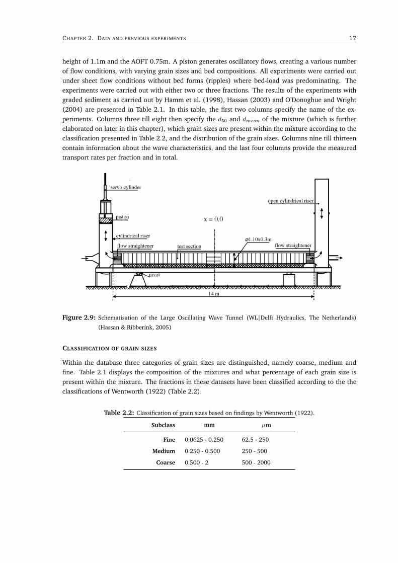
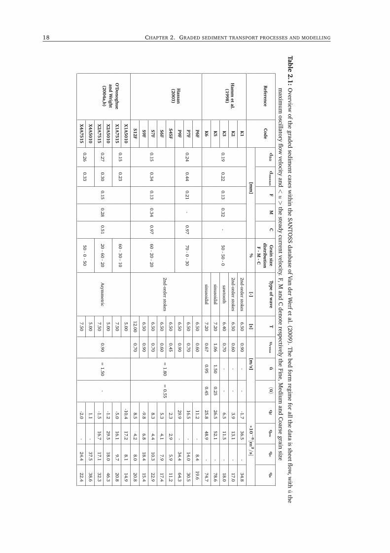
height of 1.1m and the AOFT 0.75m. A piston generates oscillatory flows, creating a various numberof flow conditions, with varying grain sizes and bed compositions. All experiments were carried outunder sheet flow conditions without bed forms (ripples) where bed-load was predominating. Theexperiments were carried out with either two or three fractions. The results of the experiments withgraded sediment as carried out by Hamm et al. (1998), Hassan (2003) and O’Donoghue and Wright(2004) are presented in Table 2.1. In this table, the first two columns specify the name of the ex-periments. Columns three till eight then specify the d50 and dmean of the mixture (which is furtherelaborated on later in this chapter), which grain sizes are present within the mixture according to theclassification presented in Table 2.2, and the distribution of the grain sizes. Columns nine till thirteencontain information about the wave characteristics, and the last four columns provide the measuredtransport rates per fraction and in total.
Figure 2.9: Schematisation of the Large Oscillating Wave Tunnel (WL|Delft Hydraulics, The Netherlands)
(Hassan & Ribberink, 2005)
CLASSIFICATION OF GRAIN SIZES
Within the database three categories of grain sizes are distinguished, namely coarse, medium andfine. Table 2.1 displays the composition of the mixtures and what percentage of each grain size ispresent within the mixture. The fractions in these datasets have been classified according to the theclassifications of Wentworth (1922) (Table 2.2).
Table 2.2: Classification of grain sizes based on findings by Wentworth (1922).
Subclass mm µm
Fine 0.0625 - 0.250 62.5 - 250
Medium 0.250 - 0.500 250 - 500
Coarse 0.500 - 2 500 - 2000
18 CHAPTER 2. GRADED SEDIMENT TRANSPORT PROCESSES AND MODELLING
Table2.1:
Overview
ofthegraded
sediment
casesw
ithinthe
SAN
TOSS
databaseofVan
derW
erfetal.(2009).
Thebed
formregim
efor
allthedata
issheet
flow,w
ithu
the
maxim
umoscillatory
flowvelocity
and<u>
thesteady
currentvelocity.
F,Mand
Cdenote
respectivelythe
Fine,Medium
andC
oarsegrain
size
Referen
ceC
oded
50
dm
ean
FM
CG
rainsize
distribution
F-
M-
C
Typeof
wave
Tu
rm
su
〈u〉
qf
qm
qc
qs
[mm
]%
[-][s]
[m/s]
∗10−
6[m
2/s]
Ham
met
al.(1998)
K1
0.190.22
0.130.32
-50
-50-0
2nd-orderstokes
6.500.90
--
-1.736.5
-34.8
K2
2nd-orderstokes
6.500.60
--
3.913.1
-17.0
K3
sawtooth
6.400.70
--
6.511.5
-18.0
K5
sinusoidal7.20
1.061.50
0.2526.5
52.1-
78.6
K6
sinusoidal7.20
0.670.95
0.4525.8
48.9-
74.7
Hassan
(2003)
P6F
0.240.44
0.21-
0.9770
-0-30
2nd-orderstokes
6.500.60
=1.80
=0.55
11.2-
8.419.6
P7F6.50
0.7016.5
-14.0
30.5
P9F6.50
0.9029.9
-34.4
64.3
S45F
0.150.34
0.130.34
0.9760
-20-20
6.500.45
2.32.9
5.911.2
S6F6.50
0.605.3
4.17.9
17.4
S7F6.50
0.708.3
4.410.3
22.9
S9F6.50
0.90-9.8
6.818.4
15.4
S12F12.00
0.708.5
4.28.0
20.8
O’D
onoghu
ean
dW
right(2004a,b)
X1A
50100.15
0.23
0.150.28
0.51
60-30
-10
Asym
metric
5.00
0.90=
1.50-
-10.417.2
8.114.9
X1A
75157.50
-5.016.1
9.720.8
X2A
50100.27
0.3020
-60-20
5.00-1.2
29.518.0
46.3
X2A
75157.50
-1.516.7
17.132.3
X4A
50100.26
0.3350
-0-50
5.001.1
-37.5
38.6
X4A
75157.50
-2.0-
24.422.4
CHAPTER 2. DATA AND PREVIOUS EXPERIMENTS 19
d50 AND dmean
The values of d50 as used in the experiments are presented with the other oscillatory flow tunnel datain Table 2.1. These values are based on the sieve curves where 50% of the mixture is finer than d50.Additionally a weighted mean grain diameter is calculated (dmean =
∑pj ∗ dj) for every dataset.
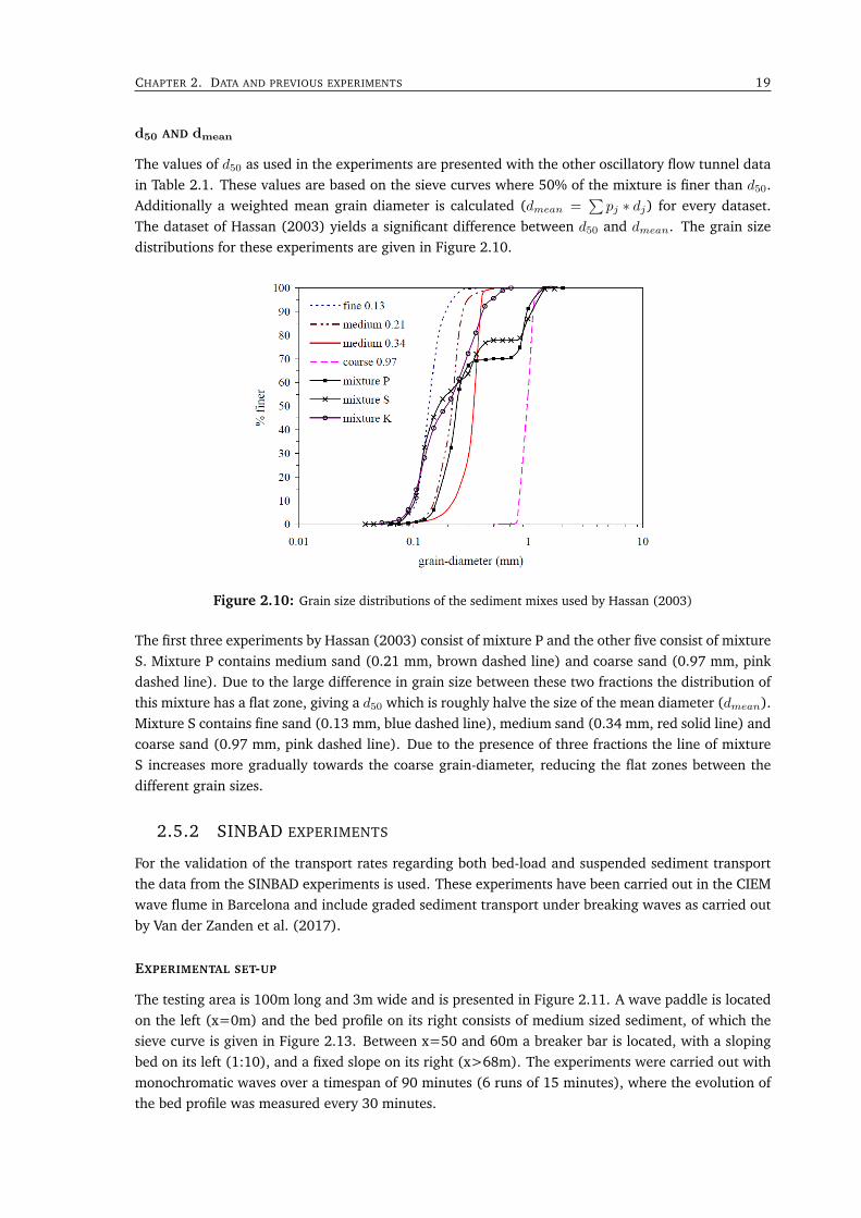
The dataset of Hassan (2003) yields a significant difference between d50 and dmean. The grain sizedistributions for these experiments are given in Figure 2.10.
Figure 2.10: Grain size distributions of the sediment mixes used by Hassan (2003)
The first three experiments by Hassan (2003) consist of mixture P and the other five consist of mixtureS. Mixture P contains medium sand (0.21 mm, brown dashed line) and coarse sand (0.97 mm, pinkdashed line). Due to the large difference in grain size between these two fractions the distribution ofthis mixture has a flat zone, giving a d50 which is roughly halve the size of the mean diameter (dmean).Mixture S contains fine sand (0.13 mm, blue dashed line), medium sand (0.34 mm, red solid line) andcoarse sand (0.97 mm, pink dashed line). Due to the presence of three fractions the line of mixtureS increases more gradually towards the coarse grain-diameter, reducing the flat zones between thedifferent grain sizes.
2.5.2 SINBAD EXPERIMENTS
For the validation of the transport rates regarding both bed-load and suspended sediment transportthe data from the SINBAD experiments is used. These experiments have been carried out in the CIEMwave flume in Barcelona and include graded sediment transport under breaking waves as carried outby Van der Zanden et al. (2017).
EXPERIMENTAL SET-UP
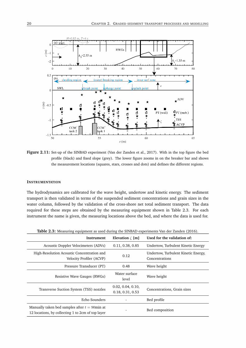
The testing area is 100m long and 3m wide and is presented in Figure 2.11. A wave paddle is locatedon the left (x=0m) and the bed profile on its right consists of medium sized sediment, of which thesieve curve is given in Figure 2.13. Between x=50 and 60m a breaker bar is located, with a slopingbed on its left (1:10), and a fixed slope on its right (x>68m). The experiments were carried out withmonochromatic waves over a timespan of 90 minutes (6 runs of 15 minutes), where the evolution ofthe bed profile was measured every 30 minutes.
20 CHAPTER 2. GRADED SEDIMENT TRANSPORT PROCESSES AND MODELLING
Figure 2.11: Set-up of the SINBAD experiment (Van der Zanden et al., 2017). With in the top figure the bed
profile (black) and fixed slope (grey). The lower figure zooms in on the breaker bar and shows
the measurement locations (squares, stars, crosses and dots) and defines the different regions.
INSTRUMENTATION
The hydrodynamics are calibrated for the wave height, undertow and kinetic energy. The sedimenttransport is then validated in terms of the suspended sediment concentrations and grain sizes in thewater column, followed by the validation of the cross-shore net total sediment transport. The datarequired for these steps are obtained by the measuring equipment shown in Table 2.3. For eachinstrument the name is given, the measuring locations above the bed, and where the data is used for.
Table 2.3: Measuring equipment as used during the SINBAD experiments Van der Zanden (2016).
Instrument Elevation ζ [m] Used for the validation of:
Acoustic Doppler Velocimeters (ADVs) 0.11, 0.38, 0.85 Undertow, Turbulent Kinetic Energy
High-Resolution Acoustic Concentration andVelocity Profiler (ACVP)
0.12Undertow, Turbulent Kinetic Energy,Concentrations
Pressure Transducer (PT) 0.48 Wave height
Resistive Wave Gauges (RWGs)Water surface
levelWave height
Transverse Suction System (TSS) nozzles0.02, 0.04, 0.10,0.18, 0.31, 0.53
Concentrations, Grain sizes
Echo Sounders - Bed profile
Manually taken bed samples after t = 90min at12 locations, by collecting 1 to 2cm of top layer
- Bed composition
CHAPTER 2. DATA AND PREVIOUS EXPERIMENTS 21
REGULAR BREAKING WAVES
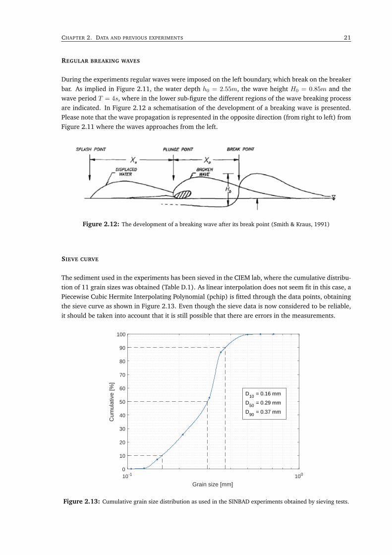
During the experiments regular waves were imposed on the left boundary, which break on the breakerbar. As implied in Figure 2.11, the water depth h0 = 2.55m, the wave height H0 = 0.85m and thewave period T = 4s, where in the lower sub-figure the different regions of the wave breaking processare indicated. In Figure 2.12 a schematisation of the development of a breaking wave is presented.Please note that the wave propagation is represented in the opposite direction (from right to left) fromFigure 2.11 where the waves approaches from the left.
Figure 2.12: The development of a breaking wave after its break point (Smith & Kraus, 1991)
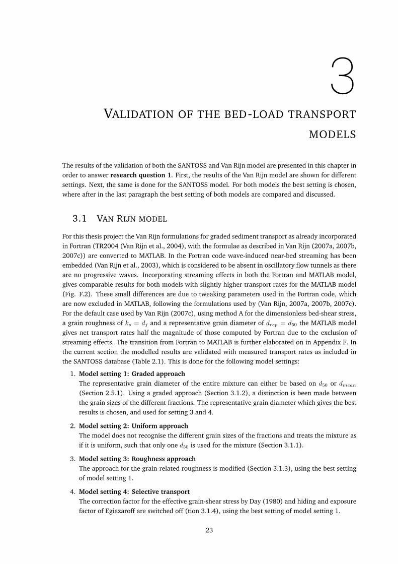
SIEVE CURVE
The sediment used in the experiments has been sieved in the CIEM lab, where the cumulative distribu-tion of 11 grain sizes was obtained (Table D.1). As linear interpolation does not seem fit in this case, aPiecewise Cubic Hermite Interpolating Polynomial (pchip) is fitted through the data points, obtainingthe sieve curve as shown in Figure 2.13. Even though the sieve data is now considered to be reliable,it should be taken into account that it is still possible that there are errors in the measurements.
10-1 100
Grain size [mm]
0
10
20
30
40
50
60
70
80
90
100
Cum
ulat
ive
[%]
D10 = 0.16 mm
D50 = 0.29 mm
D90 = 0.37 mm
Figure 2.13: Cumulative grain size distribution as used in the SINBAD experiments obtained by sieving tests.

22 CHAPTER 2. GRADED SEDIMENT TRANSPORT PROCESSES AND MODELLING
NET SEDIMENT TRANSPORT
The volumetric total sediment transport rates qtot(x) were determined by measuring the changes inthe bed-profile and solving the Exner equation:
qtot(x) = qtot(x−∆x) + ∆x(1− ε0)∆zbed(x)
∆t(2.43)
Where ∆x is the horizontal resolution of zbed measurements (=0.02 m), ε0 the porosity (=0.4),∆zbed(x) the change in bed level and ∆t the time interval between two measurements (=30 min.).The bed-load transport rates are then determined by subtracting the suspended sediment transportrates from the total net transport rates.
BED-LEVEL EVOLUTION AND CROSS-SHORE SORTING
Before any measurement were done regarding transport rates, waves were generated for 105 minutesto create a reference profile (Van der Zanden et al., 2017). At the start (t=0 min.) and end (t=90min.) the bed profile was measured, showing accretion on the breaker-bar and erosion behind thisbar. Additionally, fining has taken place on top of the breaker-bar (x=55.5 m), with coarsening rightbefore the top of the bar (x=54.5 m).
3VALIDATION OF THE BED-LOAD TRANSPORT
MODELS
The results of the validation of both the SANTOSS and Van Rijn model are presented in this chapter inorder to answer research question 1. First, the results of the Van Rijn model are shown for differentsettings. Next, the same is done for the SANTOSS model. For both models the best setting is chosen,where after in the last paragraph the best setting of both models are compared and discussed.
3.1 VAN RIJN MODEL
For this thesis project the Van Rijn formulations for graded sediment transport as already incorporatedin Fortran (TR2004 (Van Rijn et al., 2004), with the formulae as described in Van Rijn (2007a, 2007b,2007c)) are converted to MATLAB. In the Fortran code wave-induced near-bed streaming has beenembedded (Van Rijn et al., 2003), which is considered to be absent in oscillatory flow tunnels as thereare no progressive waves. Incorporating streaming effects in both the Fortran and MATLAB model,gives comparable results for both models with slightly higher transport rates for the MATLAB model(Fig. F.2). These small differences are due to tweaking parameters used in the Fortran code, whichare now excluded in MATLAB, following the formulations used by (Van Rijn, 2007a, 2007b, 2007c).For the default case used by Van Rijn (2007c), using method A for the dimensionless bed-shear stress,a grain roughness of ks = dj and a representative grain diameter of drep = d50 the MATLAB modelgives net transport rates half the magnitude of those computed by Fortran due to the exclusion ofstreaming effects. The transition from Fortran to MATLAB is further elaborated on in Appendix F. Inthe current section the modelled results are validated with measured transport rates as included inthe SANTOSS database (Table 2.1). This is done for the following model settings:
1. Model setting 1: Graded approachThe representative grain diameter of the entire mixture can either be based on d50 or dmean(Section 2.5.1). Using a graded approach (Section 3.1.2), a distinction is been made betweenthe grain sizes of the different fractions. The representative grain diameter which gives the bestresults is chosen, and used for setting 3 and 4.
2. Model setting 2: Uniform approachThe model does not recognise the different grain sizes of the fractions and treats the mixture asif it is uniform, such that only one d50 is used for the mixture (Section 3.1.1).
3. Model setting 3: Roughness approachThe approach for the grain-related roughness is modified (Section 3.1.3), using the best settingof model setting 1.
4. Model setting 4: Selective transportThe correction factor for the effective grain-shear stress by Day (1980) and hiding and exposurefactor of Egiazaroff are switched off (tion 3.1.4), using the best setting of model setting 1.
23
24 CHAPTER 3. VALIDATION OF THE BED-LOAD TRANSPORT MODELS
An overview of these four main settings with their sub settings is provided in Table 3.1. The perfor-mance of the model regarding the net transport rates per model setting is presented in Table 3.2 atthe end of this chapter, with the results per fraction in Table F.3 in appendix F.
Table 3.1: Different model settings to compute the net transport rates with the Van Rijn model. drep denotes
the representative grain diameter of the entire mixture, dj the grain size used per fraction, Tj the
method for the dimensionless bed-shear stress parameter (Section 2.4.1), ks thes approach used for
the grain roughness, τb,cr the critical bed-shear stress (section 2.4.1), and Section in which section
the results are presented and discussed. The best setting is denoted in grey.
Name Setting No. # drep dj Tj ks τb,cr Section
Gradedapproach
1.1 d50 djA dj
(dj
drep
)τb,cr,drep 3.1.2
1.2 dmean dj
Uniformapproach
2.1 d50- - dj
(dj
drep
)τb,cr,drep 3.1.1
2.2 dmean
Grainroughness
3.1 d50 djA d90
(dj
drep
)τb,cr,drep 3.1.3
3.2 dmean dj
Selectivetransport
4.1 d50 dj B dj
(dj
drep
)τb,cr,drep
3.1.4
4.2 d50 dj C dj τb,cr,dj
4.3 d50 dj D dj τb,cr,dj
4.4 dmean dj B dj
(dj
drep
)τb,cr,drep
4.5 dmean dj C dj τb,cr,dj
4.6 dmean dj D dj τb,cr,dj
DEFAULT SETTING VAN RIJN
Regarding method A for the dimensionless bed-shear stress parameter which incorporates the correc-tion factor by Egiazaroff and a correction factor for the effective grain-shear stress, the model seemsto give accurate results for steady flow with the presence and absence of waves (Van Rijn, 2007c). Ad-ditionally, using a grain roughness of dj yields better results for very graded beds, hence Aj (methodA, where the subscript denotes the roughness approach dj) is the standard setting used by Van Rijn(2007c). Furthermore drep = d50, which makesAj using d50 the initial setting used within this section.
3.1.1 GRADED VERSUS UNIFORM SAND APPROACH
Distinguishing between different fractions instead of using one grain size for the entire mixture, willshow to what extend graded effects do play a role within the Van Rijn model using the SANTOSSdatabase. When assuming only one fraction, the formula for the dimensionless bed-shear stress pa-rameter for all four methods simply transforms into:
Tj =[τ ′b,cw − τb,cr]
τb,cr(3.1)
The initial setting, using method A with grain roughness dj and a representative grain diameter of d50,is compared to the setting where the mixture is treated as uniform sediment. This uniform sedimentalso uses a representative grain diameter of d50 and a grain roughness of d50 as no distinction is madebetween the roughness per fraction.
CHAPTER 3. VAN RIJN MODEL 25
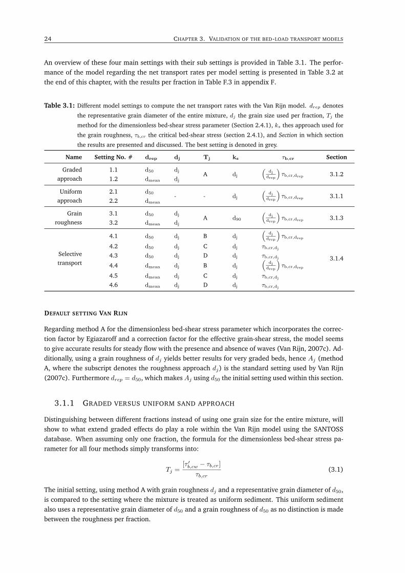
MODELLED TRANSPORT RATES
In Figure 3.1 the calculated transport rates are plotted as function of the measured transport rates,where the black solid line denotes the line of perfect fit and the black dashed line the Factor 2 interval.
-5 0 5 10 15
Measured: qs (m2/s) 10-5
-5
0
5
10
15
Cal
cula
ted:
qs (
m2/s
)
10-5 Aj; Graded (setting 1.1)
O'D. and W. (2004), d50 = 0.15mm
O'D. and W. (2004), d50 = 0.27mm
O'D. and W. (2004), d50 = 0.26mm
-5 0 5 10 15
Measured: qs (m2/s) 10-5
-5
0
5
10
1510-5 Uniform (setting 2.1)
Hamm et al. (1998), d50 = 0.19mm
Hassan (2003), d50 = 0.24mm
Hassan (2003), d50 = 0.15mm
Figure 3.1: Net total transport rates for the graded (setting 1.1) and uniform (setting 2.1) approach using a
representative grain diameter of d50. Setting 1.1 uses method A for the dimensionless bed-shear
stress parameter and dj for the grain related roughness, hence Aj .
Comparison of the net total transport rates of both the graded and uniform sand approach showsthat the differences in transport rates between these two settings are limited. This might be due toa number of factors, namely how the transport rates are affected by the choice of formula for the di-mensionless bed-shear stress parameter, how the critical and effective bed-shear stress are determined,how the grain-related roughness affects the sediment transport rates, or how hiding and exposure isincorporated in the model. The performance of the different settings is presented in Table 3.2.
3.1.2 GRADED APPROACH USING A REPRESENTATIVE GRAIN DIAMETER OF d50 OR
dmean
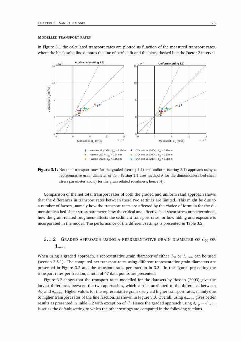
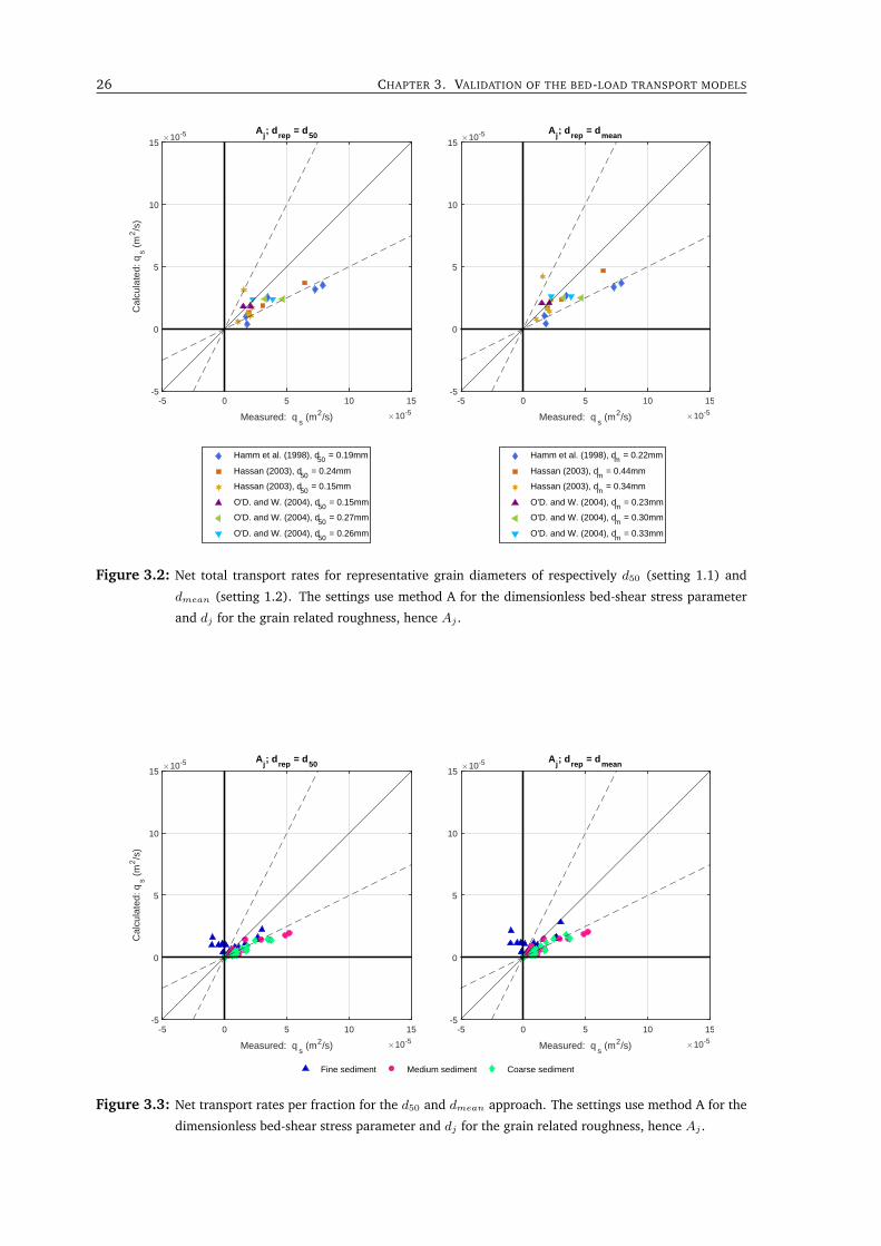
When using a graded approach, a representative grain diameter of either d50 or dmean can be used(section 2.5.1). The computed net transport rates using different representative grain diameters arepresented in Figure 3.2 and the transport rates per fraction in 3.3. In the figures presenting thetransport rates per fraction, a total of 47 data points are presented.
Figure 3.2 shows that the transport rates modelled for the datasets by Hassan (2003) give thelargest differences between the two approaches, which can be attributed to the difference betweend50 and dmean. Higher values for the representative grain size yield higher transport rates, mainly dueto higher transport rates of the fine fraction, as shown in Figure 3.3. Overall, using dmean gives betterresults as presented in Table 3.2 with exception of r2. Hence the graded approach using drep = dmean
is set as the default setting to which the other settings are compared in the following sections.
26 CHAPTER 3. VALIDATION OF THE BED-LOAD TRANSPORT MODELS
-5 0 5 10 15
Measured: qs (m2/s) 10-5
-5
0
5
10
15C
alcu
late
d: q
s (m
2/s
)10-5 A
j; d
rep = d
50
Hamm et al. (1998), d50 = 0.19mm
Hassan (2003), d50 = 0.24mm
Hassan (2003), d50 = 0.15mm
O'D. and W. (2004), d50 = 0.15mm
O'D. and W. (2004), d50 = 0.27mm
O'D. and W. (2004), d50 = 0.26mm
-5 0 5 10 15
Measured: qs (m2/s) 10-5
-5
0
5
10
1510-5 A
j; d
rep = d
mean
Hamm et al. (1998), dm = 0.22mm
Hassan (2003), dm = 0.44mm
Hassan (2003), dm = 0.34mm
O'D. and W. (2004), dm = 0.23mm
O'D. and W. (2004), dm = 0.30mm
O'D. and W. (2004), dm = 0.33mm
Figure 3.2: Net total transport rates for representative grain diameters of respectively d50 (setting 1.1) and
dmean (setting 1.2). The settings use method A for the dimensionless bed-shear stress parameter
and dj for the grain related roughness, hence Aj .
-5 0 5 10 15
Measured: qs (m2/s) 10-5
-5
0
5
10
15
Cal
cula
ted:
qs (
m2/s
)
10-5 Aj; d
rep = d
50
-5 0 5 10 15
Measured: qs (m2/s) 10-5
-5
0
5
10
1510-5 A
j; d
rep = d
mean
Fine sediment Medium sediment Coarse sediment
Figure 3.3: Net transport rates per fraction for the d50 and dmean approach. The settings use method A for the
dimensionless bed-shear stress parameter and dj for the grain related roughness, hence Aj .
CHAPTER 3. VAN RIJN MODEL 27
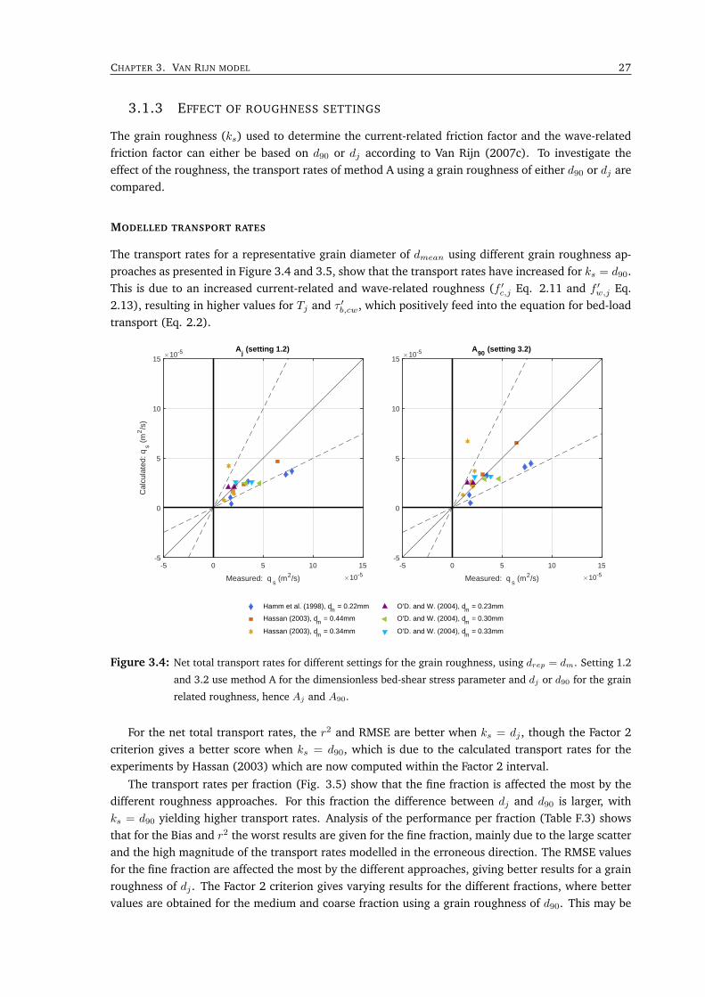
3.1.3 EFFECT OF ROUGHNESS SETTINGS
The grain roughness (ks) used to determine the current-related friction factor and the wave-relatedfriction factor can either be based on d90 or dj according to Van Rijn (2007c). To investigate theeffect of the roughness, the transport rates of method A using a grain roughness of either d90 or dj arecompared.
MODELLED TRANSPORT RATES
The transport rates for a representative grain diameter of dmean using different grain roughness ap-proaches as presented in Figure 3.4 and 3.5, show that the transport rates have increased for ks = d90.This is due to an increased current-related and wave-related roughness (f ′c,j Eq. 2.11 and f ′w,j Eq.2.13), resulting in higher values for Tj and τ ′b,cw, which positively feed into the equation for bed-loadtransport (Eq. 2.2).
-5 0 5 10 15
Measured: qs (m2/s) 10-5
-5
0
5
10
15
Cal
cula
ted:
qs (
m2/s
)
10-5 Aj (setting 1.2)
O'D. and W. (2004), dm = 0.23mm
O'D. and W. (2004), dm = 0.30mm
O'D. and W. (2004), dm = 0.33mm
-5 0 5 10 15
Measured: qs (m2/s) 10-5
-5
0
5
10
1510-5 A
90 (setting 3.2)
Hamm et al. (1998), dm = 0.22mm
Hassan (2003), dm = 0.44mm
Hassan (2003), dm = 0.34mm
Figure 3.4: Net total transport rates for different settings for the grain roughness, using drep = dm. Setting 1.2
and 3.2 use method A for the dimensionless bed-shear stress parameter and dj or d90 for the grain
related roughness, hence Aj and A90.
For the net total transport rates, the r2 and RMSE are better when ks = dj , though the Factor 2criterion gives a better score when ks = d90, which is due to the calculated transport rates for theexperiments by Hassan (2003) which are now computed within the Factor 2 interval.
The transport rates per fraction (Fig. 3.5) show that the fine fraction is affected the most by thedifferent roughness approaches. For this fraction the difference between dj and d90 is larger, withks = d90 yielding higher transport rates. Analysis of the performance per fraction (Table F.3) showsthat for the Bias and r2 the worst results are given for the fine fraction, mainly due to the large scatterand the high magnitude of the transport rates modelled in the erroneous direction. The RMSE valuesfor the fine fraction are affected the most by the different approaches, giving better results for a grainroughness of dj . The Factor 2 criterion gives varying results for the different fractions, where bettervalues are obtained for the medium and coarse fraction using a grain roughness of d90. This may be
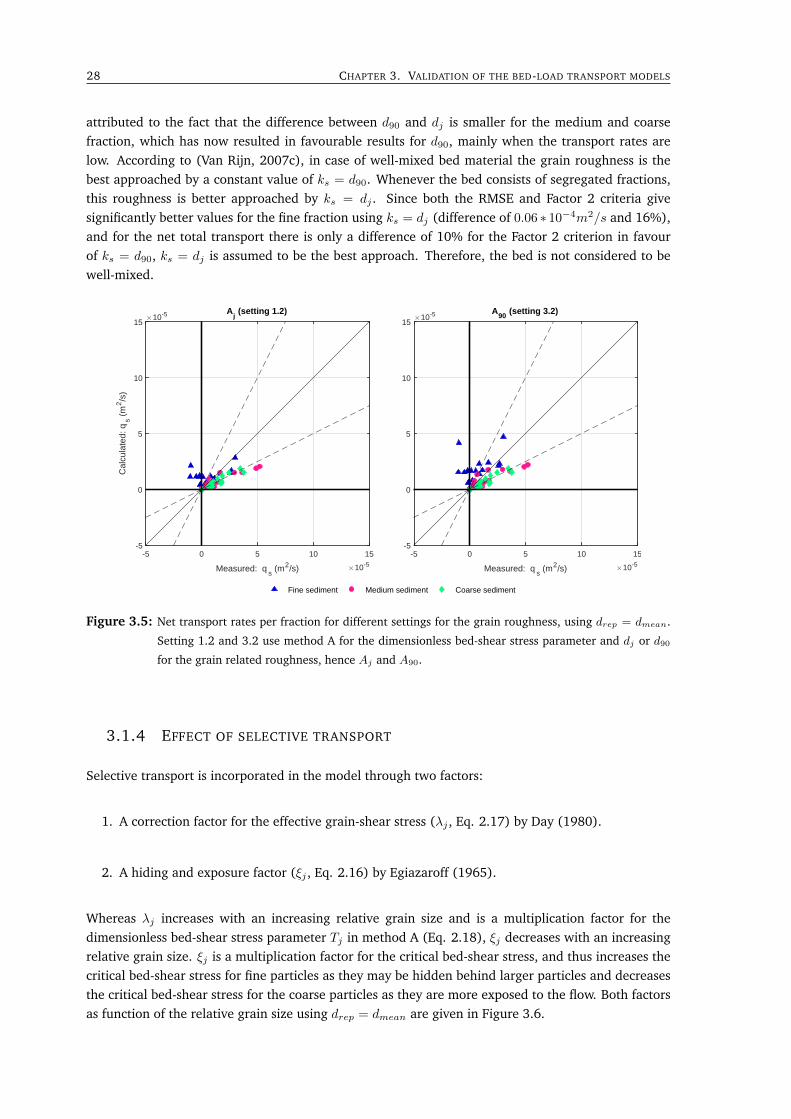
28 CHAPTER 3. VALIDATION OF THE BED-LOAD TRANSPORT MODELS
attributed to the fact that the difference between d90 and dj is smaller for the medium and coarsefraction, which has now resulted in favourable results for d90, mainly when the transport rates arelow. According to (Van Rijn, 2007c), in case of well-mixed bed material the grain roughness is thebest approached by a constant value of ks = d90. Whenever the bed consists of segregated fractions,this roughness is better approached by ks = dj . Since both the RMSE and Factor 2 criteria givesignificantly better values for the fine fraction using ks = dj (difference of 0.06 ∗ 10−4m2/s and 16%),and for the net total transport there is only a difference of 10% for the Factor 2 criterion in favourof ks = d90, ks = dj is assumed to be the best approach. Therefore, the bed is not considered to bewell-mixed.
-5 0 5 10 15
Measured: qs (m2/s) 10-5
-5
0
5
10
15
Cal
cula
ted:
qs (
m2/s
)
10-5 Aj (setting 1.2)
-5 0 5 10 15
Measured: qs (m2/s) 10-5
-5
0
5
10
1510-5 A
90 (setting 3.2)
Fine sediment Medium sediment Coarse sediment
Figure 3.5: Net transport rates per fraction for different settings for the grain roughness, using drep = dmean.
Setting 1.2 and 3.2 use method A for the dimensionless bed-shear stress parameter and dj or d90for the grain related roughness, hence Aj and A90.
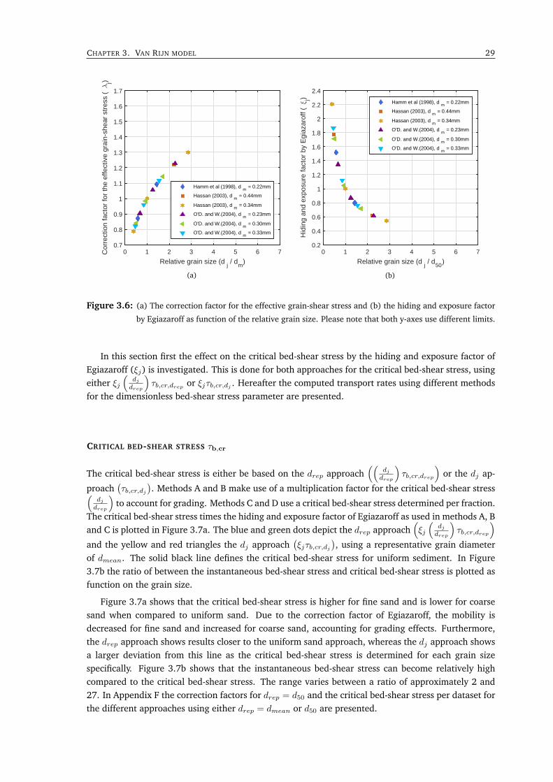
3.1.4 EFFECT OF SELECTIVE TRANSPORT
Selective transport is incorporated in the model through two factors:
1. A correction factor for the effective grain-shear stress (λj , Eq. 2.17) by Day (1980).
2. A hiding and exposure factor (ξj , Eq. 2.16) by Egiazaroff (1965).
Whereas λj increases with an increasing relative grain size and is a multiplication factor for thedimensionless bed-shear stress parameter Tj in method A (Eq. 2.18), ξj decreases with an increasingrelative grain size. ξj is a multiplication factor for the critical bed-shear stress, and thus increases thecritical bed-shear stress for fine particles as they may be hidden behind larger particles and decreasesthe critical bed-shear stress for the coarse particles as they are more exposed to the flow. Both factorsas function of the relative grain size using drep = dmean are given in Figure 3.6.
CHAPTER 3. VAN RIJN MODEL 29
0 1 2 3 4 5 6 7
Relative grain size (dj / d
m)
0.7
0.8
0.9
1
1.1
1.2
1.3
1.4
1.5
1.6
1.7
Cor
rect
ion
fact
or fo
r th
e ef
fect
ive
grai
n-sh
ear
stre
ss (
j)
Hamm et al (1998), dm
= 0.22mm
Hassan (2003), dm
= 0.44mm
Hassan (2003), dm
= 0.34mm
O'D. and W.(2004), dm
= 0.23mm
O'D. and W.(2004), dm
= 0.30mm
O'D. and W.(2004), dm
= 0.33mm
(a)
0 1 2 3 4 5 6 7
Relative grain size (dj / d
50)
0.2
0.4
0.6
0.8
1
1.2
1.4
1.6
1.8
2
2.2
2.4
Hid
ing
and
expo
sure
fact
or b
y E
giaz
arof
f (j)
Hamm et al (1998), dm
= 0.22mm
Hassan (2003), dm
= 0.44mm
Hassan (2003), dm
= 0.34mm
O'D. and W.(2004), dm
= 0.23mm
O'D. and W.(2004), dm
= 0.30mm
O'D. and W.(2004), dm
= 0.33mm
(b)
Figure 3.6: (a) The correction factor for the effective grain-shear stress and (b) the hiding and exposure factor
by Egiazaroff as function of the relative grain size. Please note that both y-axes use different limits.
In this section first the effect on the critical bed-shear stress by the hiding and exposure factor ofEgiazaroff (ξj) is investigated. This is done for both approaches for the critical bed-shear stress, usingeither ξj
(djdrep
)τb,cr,drep or ξjτb,cr,dj . Hereafter the computed transport rates using different methods
for the dimensionless bed-shear stress parameter are presented.
CRITICAL BED-SHEAR STRESS τb,cr
The critical bed-shear stress is either be based on the drep approach((
djdrep
)τb,cr,drep
)or the dj ap-
proach(τb,cr,dj
). Methods A and B make use of a multiplication factor for the critical bed-shear stress(
djdrep
)to account for grading. Methods C and D use a critical bed-shear stress determined per fraction.
The critical bed-shear stress times the hiding and exposure factor of Egiazaroff as used in methods A, Band C is plotted in Figure 3.7a. The blue and green dots depict the drep approach
(ξj
(djdrep
)τb,cr,drep
)and the yellow and red triangles the dj approach
(ξjτb,cr,dj
), using a representative grain diameter
of dmean. The solid black line defines the critical bed-shear stress for uniform sediment. In Figure3.7b the ratio of between the instantaneous bed-shear stress and critical bed-shear stress is plotted asfunction on the grain size.
Figure 3.7a shows that the critical bed-shear stress is higher for fine sand and is lower for coarsesand when compared to uniform sand. Due to the correction factor of Egiazaroff, the mobility isdecreased for fine sand and increased for coarse sand, accounting for grading effects. Furthermore,the drep approach shows results closer to the uniform sand approach, whereas the dj approach showsa larger deviation from this line as the critical bed-shear stress is determined for each grain sizespecifically. Figure 3.7b shows that the instantaneous bed-shear stress can become relatively highcompared to the critical bed-shear stress. The range varies between a ratio of approximately 2 and27. In Appendix F the correction factors for drep = d50 and the critical bed-shear stress per dataset forthe different approaches using either drep = dmean or d50 are presented.
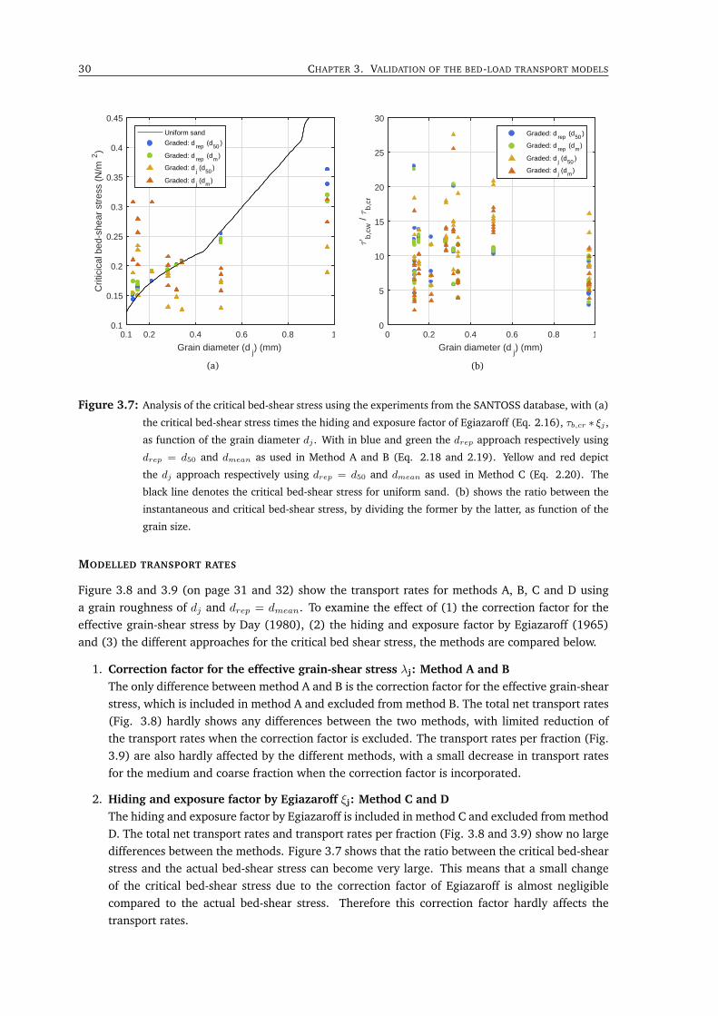
30 CHAPTER 3. VALIDATION OF THE BED-LOAD TRANSPORT MODELS
0.1 0.2 0.4 0.6 0.8 1
Grain diameter (dj) (mm)
0.1
0.15
0.2
0.25
0.3
0.35
0.4
0.45
Crit
icic
al b
ed-s
hear
str
ess
(N/m
2)
Uniform sand
Graded: drep
(d50
)
Graded: drep
(dm
)
Graded: dj (d
50)
Graded: dj (d
m)
(a)
0 0.2 0.4 0.6 0.8 1
Grain diameter (dj) (mm)
0
5
10
15
20
25
30
' b,cw
/ b,
cr
Graded: drep
(d50
)
Graded: drep
(dm
)
Graded: dj (d
50)
Graded: dj (d
m)
(b)
Figure 3.7: Analysis of the critical bed-shear stress using the experiments from the SANTOSS database, with (a)
the critical bed-shear stress times the hiding and exposure factor of Egiazaroff (Eq. 2.16), τb,cr ∗ ξj ,
as function of the grain diameter dj . With in blue and green the drep approach respectively using
drep = d50 and dmean as used in Method A and B (Eq. 2.18 and 2.19). Yellow and red depict
the dj approach respectively using drep = d50 and dmean as used in Method C (Eq. 2.20). The
black line denotes the critical bed-shear stress for uniform sand. (b) shows the ratio between the
instantaneous and critical bed-shear stress, by dividing the former by the latter, as function of the
grain size.
MODELLED TRANSPORT RATES
Figure 3.8 and 3.9 (on page 31 and 32) show the transport rates for methods A, B, C and D usinga grain roughness of dj and drep = dmean. To examine the effect of (1) the correction factor for theeffective grain-shear stress by Day (1980), (2) the hiding and exposure factor by Egiazaroff (1965)and (3) the different approaches for the critical bed shear stress, the methods are compared below.
1. Correction factor for the effective grain-shear stress λj: Method A and BThe only difference between method A and B is the correction factor for the effective grain-shearstress, which is included in method A and excluded from method B. The total net transport rates(Fig. 3.8) hardly shows any differences between the two methods, with limited reduction ofthe transport rates when the correction factor is excluded. The transport rates per fraction (Fig.3.9) are also hardly affected by the different methods, with a small decrease in transport ratesfor the medium and coarse fraction when the correction factor is incorporated.
2. Hiding and exposure factor by Egiazaroff ξj: Method C and DThe hiding and exposure factor by Egiazaroff is included in method C and excluded from methodD. The total net transport rates and transport rates per fraction (Fig. 3.8 and 3.9) show no largedifferences between the methods. Figure 3.7 shows that the ratio between the critical bed-shearstress and the actual bed-shear stress can become very large. This means that a small changeof the critical bed-shear stress due to the correction factor of Egiazaroff is almost negligiblecompared to the actual bed-shear stress. Therefore this correction factor hardly affects thetransport rates.
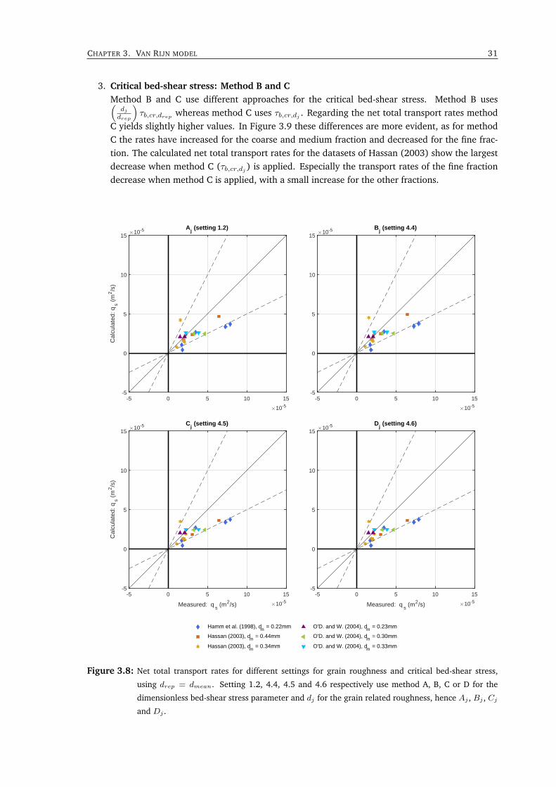
CHAPTER 3. VAN RIJN MODEL 31
3. Critical bed-shear stress: Method B and CMethod B and C use different approaches for the critical bed-shear stress. Method B uses(
djdrep
)τb,cr,drep whereas method C uses τb,cr,dj . Regarding the net total transport rates method
C yields slightly higher values. In Figure 3.9 these differences are more evident, as for methodC the rates have increased for the coarse and medium fraction and decreased for the fine frac-tion. The calculated net total transport rates for the datasets of Hassan (2003) show the largestdecrease when method C (τb,cr,dj ) is applied. Especially the transport rates of the fine fractiondecrease when method C is applied, with a small increase for the other fractions.
-5 0 5 10 15
10-5
-5
0
5
10
15
Cal
cula
ted:
qs (
m2/s
)
10-5 Aj (setting 1.2)
-5 0 5 10 15
10-5
-5
0
5
10
1510-5 B
j (setting 4.4)
-5 0 5 10 15
Measured: qs (m2/s) 10-5
-5
0
5
10
15
Cal
cula
ted:
qs (
m2/s
)
10-5 Cj (setting 4.5)
O'D. and W. (2004), dm = 0.23mm
O'D. and W. (2004), dm = 0.30mm
O'D. and W. (2004), dm = 0.33mm
-5 0 5 10 15
Measured: qs (m2/s) 10-5
-5
0
5
10
1510-5 D
j (setting 4.6)
Hamm et al. (1998), dm = 0.22mm
Hassan (2003), dm = 0.44mm
Hassan (2003), dm = 0.34mm
Figure 3.8: Net total transport rates for different settings for grain roughness and critical bed-shear stress,
using drep = dmean. Setting 1.2, 4.4, 4.5 and 4.6 respectively use method A, B, C or D for the
dimensionless bed-shear stress parameter and dj for the grain related roughness, hence Aj , Bj , Cj
and Dj .
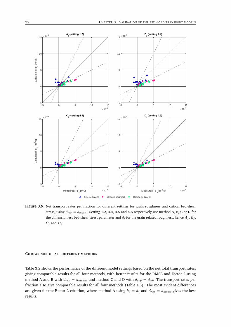
32 CHAPTER 3. VALIDATION OF THE BED-LOAD TRANSPORT MODELS
-5 0 5 10 15
10-5
-5
0
5
10
15C
alcu
late
d: q
s (m
2/s
)10-5 A
j (setting 1.2)
-5 0 5 10 15
10-5
-5
0
5
10
1510-5 B
j (setting 4.4)
-5 0 5 10 15
Measured: qs (m2/s) 10-5
-5
0
5
10
15
Cal
cula
ted:
qs (
m2/s
)
10-5 Cj (setting 4.5)
-5 0 5 10 15
Measured: qs (m2/s) 10-5
-5
0
5
10
1510-5 D
j (setting 4.6)
Fine sediment Medium sediment Coarse sediment
Figure 3.9: Net transport rates per fraction for different settings for grain roughness and critical bed-shear
stress, using drep = dmean. Setting 1.2, 4.4, 4.5 and 4.6 respectively use method A, B, C or D for
the dimensionless bed-shear stress parameter and dj for the grain related roughness, hence Aj , Bj ,
Cj and Dj .
COMPARISON OF ALL DIFFERENT METHODS
Table 3.2 shows the performance of the different model settings based on the net total transport rates,giving comparable results for all four methods, with better results for the RMSE and Factor 2 usingmethod A and B with drep = dmean, and method C and D with drep = d50. The transport rates perfraction also give comparable results for all four methods (Table F.3). The most evident differencesare given for the Factor 2 criterion, where method A using ks = dj and drep = dmean gives the bestresults.
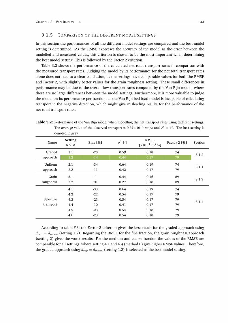
CHAPTER 3. VAN RIJN MODEL 33
3.1.5 COMPARISON OF THE DIFFERENT MODEL SETTINGS
In this section the performances of all the different model settings are compared and the best modelsetting is determined. As the RMSE expresses the accuracy of the model as the error between themodelled and measured values, this criterion is chosen to be the most important when determiningthe best model setting. This is followed by the Factor 2 criterion.
Table 3.2 shows the performance of the calculated net total transport rates in comparison withthe measured transport rates. Judging the model by its performance for the net total transport ratesalone does not lead to a clear conclusion, as the settings have comparable values for both the RMSEand Factor 2, with slightly better values for the grain roughness setting. These small differences inperformance may be due to the overall low transport rates computed by the Van Rijn model, wherethere are no large differences between the model settings. Furthermore, it is more valuable to judgethe model on its performance per fraction, as the Van Rijn bed-load model is incapable of calculatingtransport in the negative direction, which might give misleading results for the performance of thenet total transport rates.
Table 3.2: Performance of the Van Rijn model when modelling the net transport rates using different settings.
The average value of the observed transport is 0.32 ∗ 10−4 m2/s and N = 19. The best setting is
denoted in grey.
NameSettingNo. #
Bias [%] r2 [-]RMSE
[∗10−4 m2/s]Factor 2 [%] Section
Gradedapproach
1.1 -28 0.59 0.18 743.1.2
1.2 -14 0.44 0.17 79
Uniformapproach
2.1 -34 0.64 0.19 743.1.1
2.2 -11 0.42 0.17 79
Grainroughness
3.1 -1 0.44 0.16 893.1.3
3.2 20 0.27 0.18 89
Selectivetransport
4.1 -33 0.64 0.19 74
3.1.4
4.2 -22 0.54 0.17 79
4.3 -23 0.54 0.17 79
4.4 -10 0.41 0.17 79
4.5 -23 0.54 0.18 79
4.6 -23 0.54 0.18 79
According to table F.3, the Factor 2 criterion gives the best result for the graded approach usingdrep = dmean (setting 1.2). Regarding the RMSE for the fine fraction, the grain roughness approach(setting 2) gives the worst results. For the medium and coarse fraction the values of the RMSE arecomparable for all settings, where setting 4.1 and 4.4 (method B) give higher RMSE values. Therefore,the graded approach using drep = dmean (setting 1.2) is selected as the best model setting.
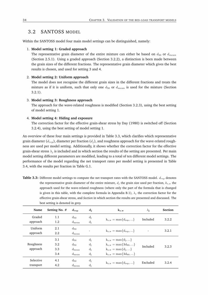
34 CHAPTER 3. VALIDATION OF THE BED-LOAD TRANSPORT MODELS
3.2 SANTOSS MODEL
Within the SANTOSS model four main model settings can be distinguished, namely:
1. Model setting 1: Graded approachThe representative grain diameter of the entire mixture can either be based on d50 or dmean(Section 2.5.1). Using a graded approach (Section 3.2.2), a distinction is been made betweenthe grain sizes of the different fractions. The representative grain diameter which gives the bestresults is chosen, and used for setting 3 and 4.
2. Model setting 2: Uniform approachThe model does not recognise the different grain sizes in the different fractions and treats themixture as if it is uniform, such that only one d50 or dmean is used for the mixture (Section3.2.1).
3. Model setting 3: Roughness approachThe approach for the wave-related roughness is modified (Section 3.2.3), using the best settingof model setting 1.
4. Model setting 4: Hiding and exposureThe correction factor for the effective grain-shear stress by Day (1980) is switched off (Section3.2.4), using the best setting of model setting 1.
An overview of these four main settings is provided in Table 3.3, which clarifies which representativegrain diameter (drep), diameter per fraction (dj), and roughness approach for the wave-related rough-ness are used per model setting. Additionally, it shows whether the correction factor for the effectivegrain-shear stress λj is included and in which section the results of the setting are presented. Per mainmodel setting different parameters are modified, leading to a total of ten different model settings. Theperformance of the model regarding the net transport rates per model setting is presented in Table3.4, with the results per fraction in Table G.1.
Table 3.3: Different model settings to compute the net transport rates with the SANTOSS model. drep denotes
the representative grain diameter of the entire mixture, dj the grain size used per fraction, ks,w the
approach used for the wave-related roughness (where only the part of the formula that is changed
is given in this table, with the complete formula in Appendix B.1), λj the correction factor for the
effective grain-shear stress, and Section in which section the results are presented and discussed. The
best setting is denoted in grey.
Name Setting No. # drep dj ks,w λj Section
Gradedapproach
1.1 d50 djks,w = maxdrep, ... Included 3.2.2
1.2 dmean dj
Uniformapproach
2.1 d50- ks,w = maxdrep, ... - 3.2.1
2.2 dmean
Roughnessapproach
3.1 d50 dj ks,w = maxdj, ...
Included 3.2.33.2 d50 dj ks,w = max3d90, ...3.3 dmean dj ks,w = maxdj, ...3.4 dmean dj ks,w = max3d90, ...
Selectivetransport
4.1 d50 djks,w = maxdrep, ... Excluded 3.2.4
4.2 dmean dj
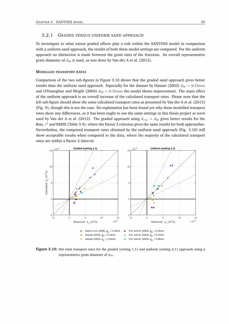
CHAPTER 3. SANTOSS MODEL 35
3.2.1 GRADED VERSUS UNIFORM SAND APPROACH
To investigate to what extent graded effects play a role within the SANTOSS model in comparisonwith a uniform sand approach, the results of both these model settings are compared. For the uniformapproach no distinction is made between the grain sizes of the fractions. An overall representativegrain diameter of d50 is used, as was done by Van der A et al. (2013).
MODELLED TRANSPORT RATES
Comparison of the two sub-figures in Figure 3.10 shows that the graded sand approach gives betterresults than the uniform sand approach. Especially for the dataset by Hassan (2003) d50 = 0.15mm
and O’Donoghue and Wright (2004) d50 = 0.15mm the model shows improvement. The main effectof the uniform approach is an overall increase of the calculated transport rates. Please note that theleft sub-figure should show the same calculated transport rates as presented by Van der A et al. (2013)(Fig. 9), though this is not the case. No explanation has been found yet why these modelled transportrates show any differences, as it has been ought to use the same settings in this thesis project as wereused by Van der A et al. (2013). The graded approach using drep = d50 gives better results for theBias, r2 and RMSE (Table 3.4), where the Factor 2 criterion gives the same results for both approaches.Nevertheless, the computed transport rates obtained by the uniform sand approach (Fig. 3.10) stillshow acceptable results when compared to the data, where the majority of the calculated transportrates are within a Factor 2 interval.
-5 0 5 10 15
Measured: qs (m2/s) 10-5
-5
0
5
10
15
Cal
cula
ted:
qs (
m2/s
)
10-5 Graded (setting 1.1)
O'D. and W. (2004), d50 = 0.15mm
O'D. and W. (2004), d50 = 0.27mm
O'D. and W. (2004), d50 = 0.26mm
-5 0 5 10 15
Measured: qs (m2/s) 10-5
-5
0
5
10
1510-5 Uniform (setting 2.1)
Hamm et al. (1998), d50 = 0.19mm
Hassan (2003), d50 = 0.24mm
Hassan (2003), d50 = 0.15mm
Figure 3.10: Net total transport rates for the graded (setting 1.1) and uniform (setting 2.1) approach using a
representative grain diameter of d50.
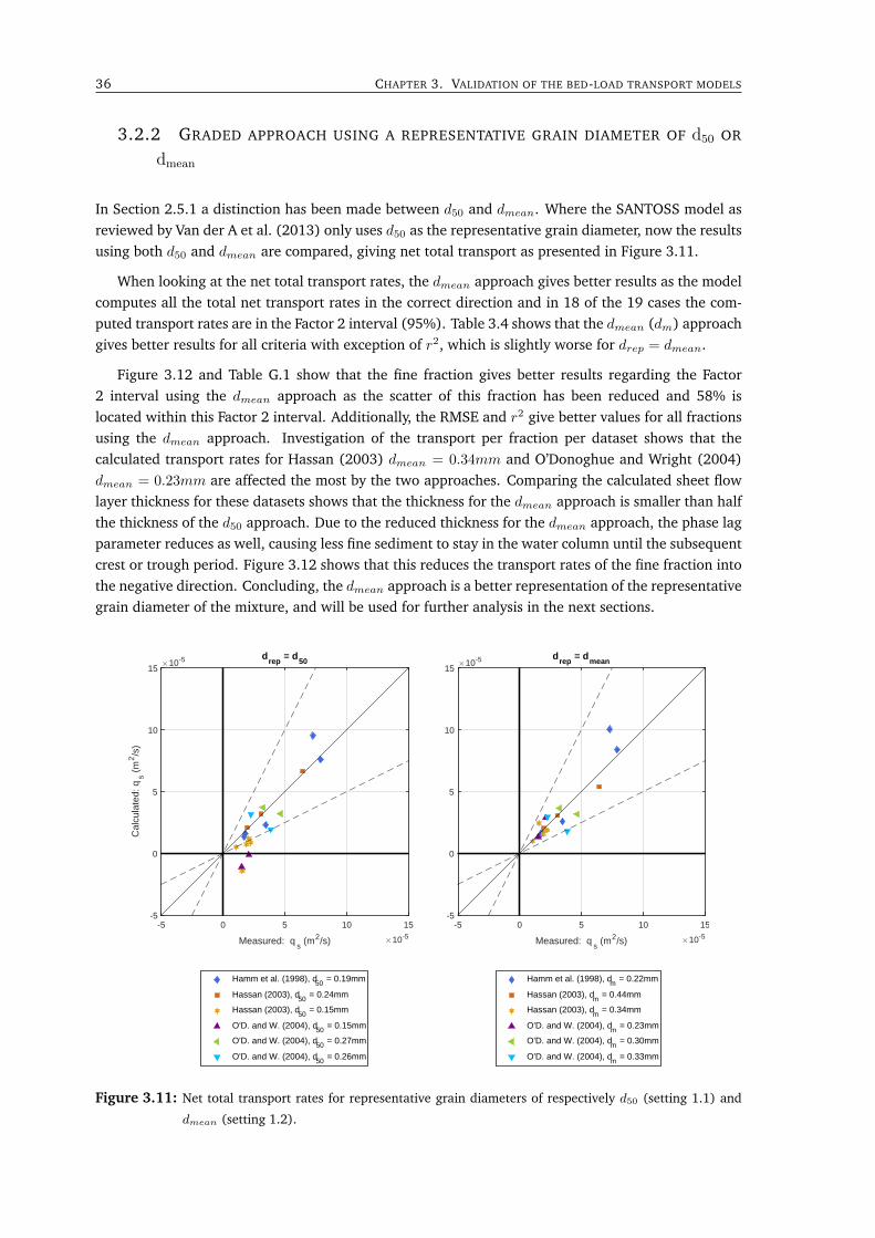
36 CHAPTER 3. VALIDATION OF THE BED-LOAD TRANSPORT MODELS
3.2.2 GRADED APPROACH USING A REPRESENTATIVE GRAIN DIAMETER OF d50 OR
dmean
In Section 2.5.1 a distinction has been made between d50 and dmean. Where the SANTOSS model asreviewed by Van der A et al. (2013) only uses d50 as the representative grain diameter, now the resultsusing both d50 and dmean are compared, giving net total transport as presented in Figure 3.11.
When looking at the net total transport rates, the dmean approach gives better results as the modelcomputes all the total net transport rates in the correct direction and in 18 of the 19 cases the com-puted transport rates are in the Factor 2 interval (95%). Table 3.4 shows that the dmean (dm) approachgives better results for all criteria with exception of r2, which is slightly worse for drep = dmean.
Figure 3.12 and Table G.1 show that the fine fraction gives better results regarding the Factor2 interval using the dmean approach as the scatter of this fraction has been reduced and 58% islocated within this Factor 2 interval. Additionally, the RMSE and r2 give better values for all fractionsusing the dmean approach. Investigation of the transport per fraction per dataset shows that thecalculated transport rates for Hassan (2003) dmean = 0.34mm and O’Donoghue and Wright (2004)dmean = 0.23mm are affected the most by the two approaches. Comparing the calculated sheet flowlayer thickness for these datasets shows that the thickness for the dmean approach is smaller than halfthe thickness of the d50 approach. Due to the reduced thickness for the dmean approach, the phase lagparameter reduces as well, causing less fine sediment to stay in the water column until the subsequentcrest or trough period. Figure 3.12 shows that this reduces the transport rates of the fine fraction intothe negative direction. Concluding, the dmean approach is a better representation of the representativegrain diameter of the mixture, and will be used for further analysis in the next sections.
-5 0 5 10 15
Measured: qs (m2/s) 10-5
-5
0
5
10
15
Cal
cula
ted:
qs (
m2/s
)
10-5 drep
= d50
Hamm et al. (1998), d50 = 0.19mm
Hassan (2003), d50 = 0.24mm
Hassan (2003), d50 = 0.15mm
O'D. and W. (2004), d50 = 0.15mm
O'D. and W. (2004), d50 = 0.27mm
O'D. and W. (2004), d50 = 0.26mm
-5 0 5 10 15
Measured: qs (m2/s) 10-5
-5
0
5
10
1510-5 d
rep = d
mean
Hamm et al. (1998), dm = 0.22mm
Hassan (2003), dm = 0.44mm
Hassan (2003), dm = 0.34mm
O'D. and W. (2004), dm = 0.23mm
O'D. and W. (2004), dm = 0.30mm
O'D. and W. (2004), dm = 0.33mm
Figure 3.11: Net total transport rates for representative grain diameters of respectively d50 (setting 1.1) and
dmean (setting 1.2).
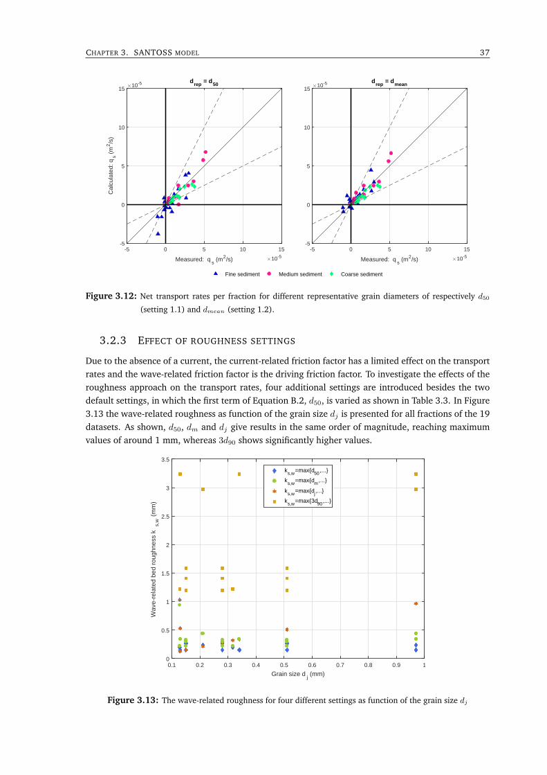
CHAPTER 3. SANTOSS MODEL 37
-5 0 5 10 15
Measured: qs (m2/s) 10-5
-5
0
5
10
15
Cal
cula
ted:
qs (
m2/s
)
10-5 drep
= d50
-5 0 5 10 15
Measured: qs (m2/s) 10-5
-5
0
5
10
1510-5 d
rep = d
mean
Fine sediment Medium sediment Coarse sediment
Figure 3.12: Net transport rates per fraction for different representative grain diameters of respectively d50(setting 1.1) and dmean (setting 1.2).
3.2.3 EFFECT OF ROUGHNESS SETTINGS
Due to the absence of a current, the current-related friction factor has a limited effect on the transportrates and the wave-related friction factor is the driving friction factor. To investigate the effects of theroughness approach on the transport rates, four additional settings are introduced besides the twodefault settings, in which the first term of Equation B.2, d50, is varied as shown in Table 3.3. In Figure3.13 the wave-related roughness as function of the grain size dj is presented for all fractions of the 19datasets. As shown, d50, dm and dj give results in the same order of magnitude, reaching maximumvalues of around 1 mm, whereas 3d90 shows significantly higher values.
0.1 0.2 0.3 0.4 0.5 0.6 0.7 0.8 0.9 1
Grain size dj (mm)
0
0.5
1
1.5
2
2.5
3
3.5
Wav
e-re
late
d be
d ro
ughn
ess
k s
,w (
mm
)
ks,w=maxd50 ,...
ks,w=maxdm ,...
ks,w=maxdj,...
ks,w=max3d90 ,...
Figure 3.13: The wave-related roughness for four different settings as function of the grain size dj
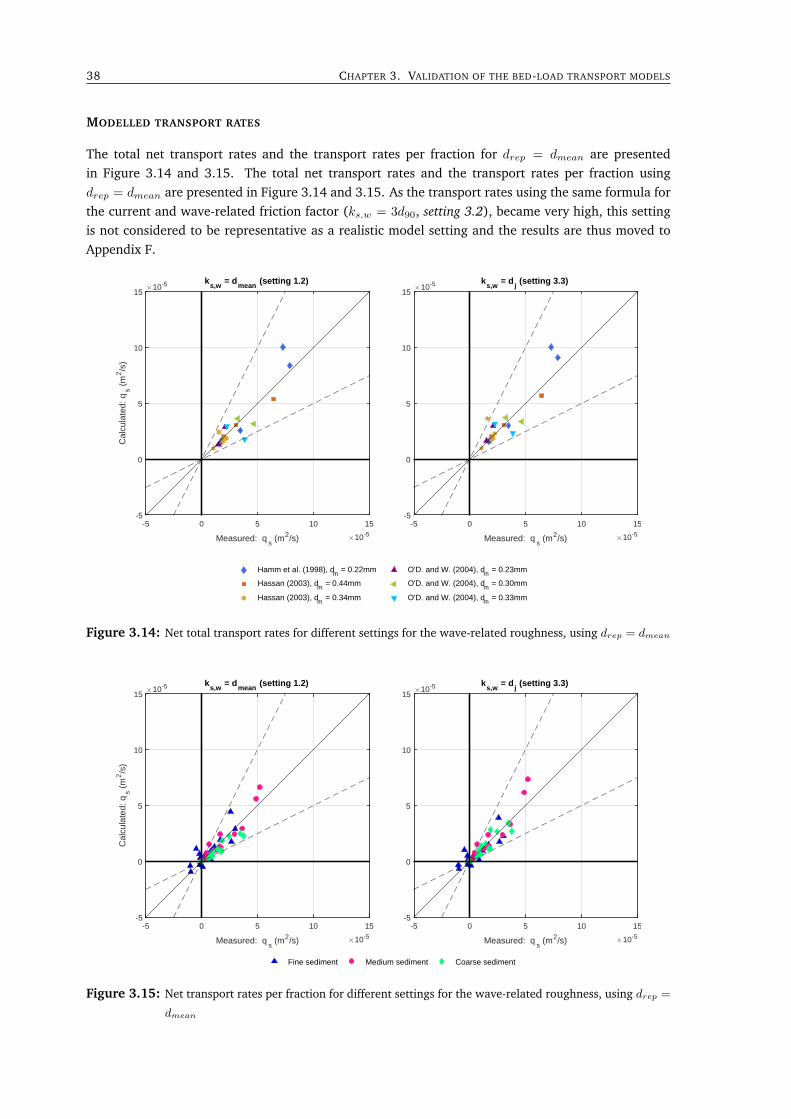
38 CHAPTER 3. VALIDATION OF THE BED-LOAD TRANSPORT MODELS
MODELLED TRANSPORT RATES
The total net transport rates and the transport rates per fraction for drep = dmean are presentedin Figure 3.14 and 3.15. The total net transport rates and the transport rates per fraction usingdrep = dmean are presented in Figure 3.14 and 3.15. As the transport rates using the same formula forthe current and wave-related friction factor (ks,w = 3d90, setting 3.2), became very high, this settingis not considered to be representative as a realistic model setting and the results are thus moved toAppendix F.
-5 0 5 10 15
Measured: qs (m2/s) 10-5
-5
0
5
10
15
Cal
cula
ted:
qs (
m2/s
)
10-5 ks,w
= dmean
(setting 1.2)
Hamm et al. (1998), dm = 0.22mm
Hassan (2003), dm = 0.44mm
Hassan (2003), dm = 0.34mm
-5 0 5 10 15
Measured: qs (m2/s) 10-5
-5
0
5
10
1510-5 k
s,w = d
j (setting 3.3)
O'D. and W. (2004), dm = 0.23mm
O'D. and W. (2004), dm = 0.30mm
O'D. and W. (2004), dm = 0.33mm
Figure 3.14: Net total transport rates for different settings for the wave-related roughness, using drep = dmean
-5 0 5 10 15
Measured: qs (m2/s) 10-5
-5
0
5
10
15
Cal
cula
ted:
qs (
m2/s
)
10-5 ks,w
= dmean
(setting 1.2)
-5 0 5 10 15
Measured: qs (m2/s) 10-5
-5
0
5
10
1510-5 k
s,w = d
j (setting 3.3)
Fine sediment Medium sediment Coarse sediment
Figure 3.15: Net transport rates per fraction for different settings for the wave-related roughness, using drep =
dmean
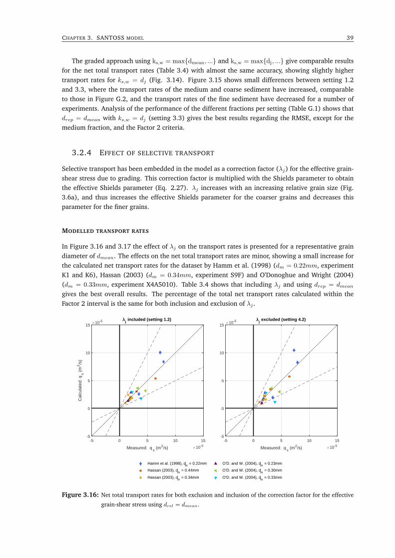
CHAPTER 3. SANTOSS MODEL 39
The graded approach using ks,w = maxdmean, ... and ks,w = maxdj, ... give comparable resultsfor the net total transport rates (Table 3.4) with almost the same accuracy, showing slightly highertransport rates for ks,w = dj (Fig. 3.14). Figure 3.15 shows small differences between setting 1.2and 3.3, where the transport rates of the medium and coarse sediment have increased, comparableto those in Figure G.2, and the transport rates of the fine sediment have decreased for a number ofexperiments. Analysis of the performance of the different fractions per setting (Table G.1) shows thatdrep = dmean with ks,w = dj (setting 3.3) gives the best results regarding the RMSE, except for themedium fraction, and the Factor 2 criteria.
3.2.4 EFFECT OF SELECTIVE TRANSPORT
Selective transport has been embedded in the model as a correction factor (λj) for the effective grain-shear stress due to grading. This correction factor is multiplied with the Shields parameter to obtainthe effective Shields parameter (Eq. 2.27). λj increases with an increasing relative grain size (Fig.3.6a), and thus increases the effective Shields parameter for the coarser grains and decreases thisparameter for the finer grains.
MODELLED TRANSPORT RATES
In Figure 3.16 and 3.17 the effect of λj on the transport rates is presented for a representative graindiameter of dmean. The effects on the net total transport rates are minor, showing a small increase forthe calculated net transport rates for the dataset by Hamm et al. (1998) (dm = 0.22mm, experimentK1 and K6), Hassan (2003) (dm = 0.34mm, experiment S9F) and O’Donoghue and Wright (2004)(dm = 0.33mm, experiment X4A5010). Table 3.4 shows that including λj and using drep = dmean
gives the best overall results. The percentage of the total net transport rates calculated within theFactor 2 interval is the same for both inclusion and exclusion of λj .
-5 0 5 10 15
Measured: qs (m2/s) 10-5
-5
0
5
10
15
Cal
cula
ted:
qs (
m2/s
)
10-5 j included (setting 1.2)
O'D. and W. (2004), dm = 0.23mm
O'D. and W. (2004), dm = 0.30mm
O'D. and W. (2004), dm = 0.33mm
-5 0 5 10 15
Measured: qs (m2/s) 10-5
-5
0
5
10
1510-5 j
excluded (setting 4.2)
Hamm et al. (1998), dm = 0.22mm
Hassan (2003), dm = 0.44mm
Hassan (2003), dm = 0.34mm
Figure 3.16: Net total transport rates for both exclusion and inclusion of the correction factor for the effective
grain-shear stress using drel = dmean.
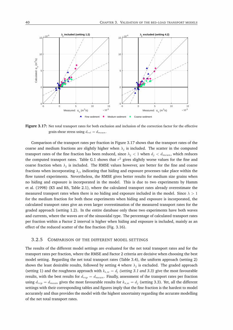
40 CHAPTER 3. VALIDATION OF THE BED-LOAD TRANSPORT MODELS
-5 0 5 10 15
Measured: qs (m2/s) 10-5
-5
0
5
10
15C
alcu
late
d: q
s (m
2/s
)10-5 j
included (setting 1.2)
-5 0 5 10 15
Measured: qs (m2/s) 10-5
-5
0
5
10
1510-5 j
excluded (setting 4.2)
Fine sediment Medium sediment Coarse sediment
Figure 3.17: Net total transport rates for both exclusion and inclusion of the correction factor for the effective
grain-shear stress using drel = dmean.
Comparison of the transport rates per fraction in Figure 3.17 shows that the transport rates of thecoarse and medium fractions are slightly higher when λj is included. The scatter in the computedtransport rates of the fine fraction has been reduced, since λj < 1 when dj < dmean, which reducesthe computed transport rates. Table G.1 shows that r2 gives slightly worse values for the fine andcoarse fraction when λj is included. The RMSE values however, are better for the fine and coarsefractions when incorporating λj , indicating that hiding and exposure processes take place within theflow tunnel experiments. Nevertheless, the RMSE gives better results for medium size grains whenno hiding and exposure is incorporated in the model. This is due to two experiments by Hammet al. (1998) (K5 and K6, Table 2.1), where the calculated transport rates already overestimate themeasured transport rates when there is no hiding and exposure included in the model. Since λ > 1
for the medium fraction for both these experiments when hiding and exposure is incorporated, thecalculated transport rates give an even larger overestimation of the measured transport rates for thegraded approach (setting 1.2). In the entire database only these two experiments have both wavesand currents, where the waves are of the sinusoidal type. The percentage of calculated transport ratesper fraction within a Factor 2 interval is higher when hiding and exposure is included, mainly as aneffect of the reduced scatter of the fine fraction (Fig. 3.16).
3.2.5 COMPARISON OF THE DIFFERENT MODEL SETTINGS
The results of the different model settings are evaluated for the net total transport rates and for thetransport rates per fraction, where the RMSE and Factor 2 criteria are decisive when choosing the bestmodel setting. Regarding the net total transport rates (Table 3.4), the uniform approach (setting 2)shows the least desirable results, followed by setting 4 where λj is excluded. The graded approach(setting 1) and the roughness approach with ks,w = dj (setting 3.1 and 3.3) give the most favourableresults, with the best results for drep = dmean. Finally, assessment of the transport rates per fractionusing drep = dmean gives the most favourable results for ks,w = dj (setting 3.3). Yet, all the differentsettings with their corresponding tables and figures imply that the fine fraction is the hardest to modelaccurately and thus provides the model with the highest uncertainty regarding the accurate modellingof the net total transport rates.
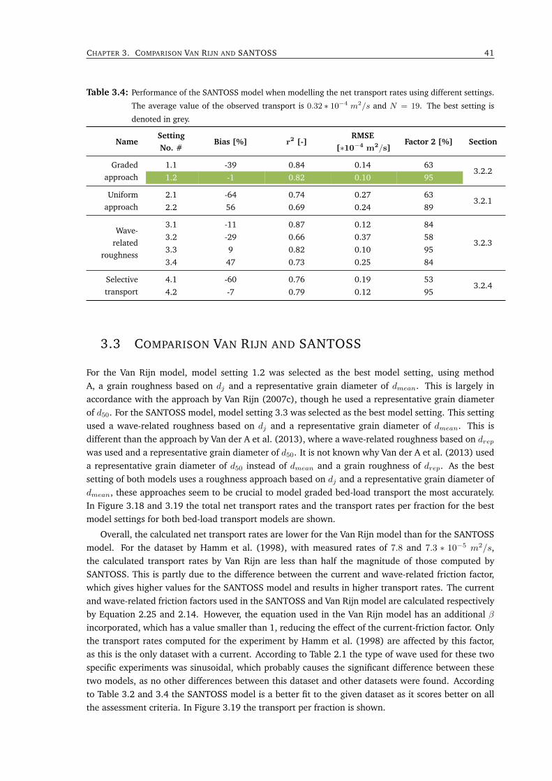
CHAPTER 3. COMPARISON VAN RIJN AND SANTOSS 41
Table 3.4: Performance of the SANTOSS model when modelling the net transport rates using different settings.
The average value of the observed transport is 0.32 ∗ 10−4 m2/s and N = 19. The best setting is
denoted in grey.
NameSettingNo. #
Bias [%] r2 [-]RMSE
[∗10−4 m2/s]Factor 2 [%] Section
Gradedapproach
1.1 -39 0.84 0.14 633.2.2
1.2 -1 0.82 0.10 95
Uniformapproach
2.1 -64 0.74 0.27 633.2.1
2.2 56 0.69 0.24 89
Wave-related
roughness
3.1 -11 0.87 0.12 84
3.2.33.2 -29 0.66 0.37 58
3.3 9 0.82 0.10 95
3.4 47 0.73 0.25 84
Selectivetransport
4.1 -60 0.76 0.19 533.2.4
4.2 -7 0.79 0.12 95
3.3 COMPARISON VAN RIJN AND SANTOSS
For the Van Rijn model, model setting 1.2 was selected as the best model setting, using methodA, a grain roughness based on dj and a representative grain diameter of dmean. This is largely inaccordance with the approach by Van Rijn (2007c), though he used a representative grain diameterof d50. For the SANTOSS model, model setting 3.3 was selected as the best model setting. This settingused a wave-related roughness based on dj and a representative grain diameter of dmean. This isdifferent than the approach by Van der A et al. (2013), where a wave-related roughness based on drepwas used and a representative grain diameter of d50. It is not known why Van der A et al. (2013) useda representative grain diameter of d50 instead of dmean and a grain roughness of drep. As the bestsetting of both models uses a roughness approach based on dj and a representative grain diameter ofdmean, these approaches seem to be crucial to model graded bed-load transport the most accurately.In Figure 3.18 and 3.19 the total net transport rates and the transport rates per fraction for the bestmodel settings for both bed-load transport models are shown.
Overall, the calculated net transport rates are lower for the Van Rijn model than for the SANTOSSmodel. For the dataset by Hamm et al. (1998), with measured rates of 7.8 and 7.3 ∗ 10−5 m2/s,the calculated transport rates by Van Rijn are less than half the magnitude of those computed bySANTOSS. This is partly due to the difference between the current and wave-related friction factor,which gives higher values for the SANTOSS model and results in higher transport rates. The currentand wave-related friction factors used in the SANTOSS and Van Rijn model are calculated respectivelyby Equation 2.25 and 2.14. However, the equation used in the Van Rijn model has an additional βincorporated, which has a value smaller than 1, reducing the effect of the current-friction factor. Onlythe transport rates computed for the experiment by Hamm et al. (1998) are affected by this factor,as this is the only dataset with a current. According to Table 2.1 the type of wave used for these twospecific experiments was sinusoidal, which probably causes the significant difference between thesetwo models, as no other differences between this dataset and other datasets were found. Accordingto Table 3.2 and 3.4 the SANTOSS model is a better fit to the given dataset as it scores better on allthe assessment criteria. In Figure 3.19 the transport per fraction is shown.
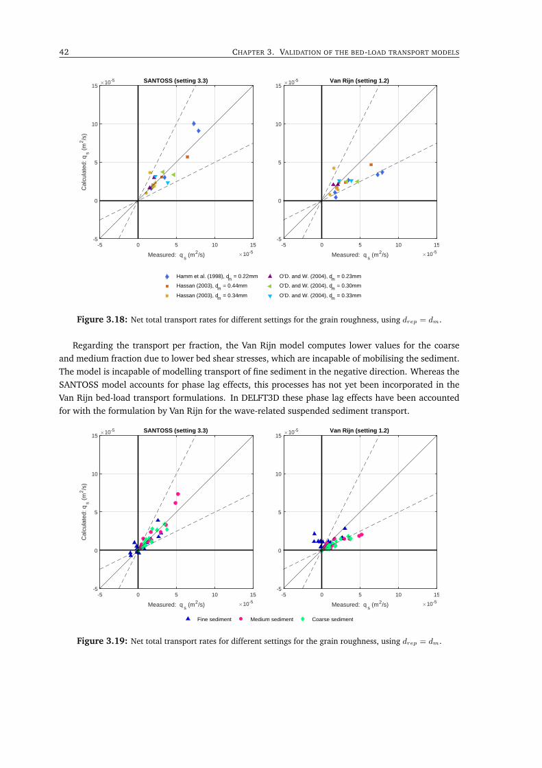
42 CHAPTER 3. VALIDATION OF THE BED-LOAD TRANSPORT MODELS
-5 0 5 10 15
Measured: qs (m2/s) 10-5
-5
0
5
10
15C
alcu
late
d: q
s (m
2/s
)10-5 SANTOSS (setting 3.3)
O'D. and W. (2004), dm = 0.23mm
O'D. and W. (2004), dm = 0.30mm
O'D. and W. (2004), dm = 0.33mm
-5 0 5 10 15
Measured: qs (m2/s) 10-5
-5
0
5
10
1510-5 Van Rijn (setting 1.2)
Hamm et al. (1998), dm = 0.22mm
Hassan (2003), dm = 0.44mm
Hassan (2003), dm = 0.34mm
Figure 3.18: Net total transport rates for different settings for the grain roughness, using drep = dm.
Regarding the transport per fraction, the Van Rijn model computes lower values for the coarseand medium fraction due to lower bed shear stresses, which are incapable of mobilising the sediment.The model is incapable of modelling transport of fine sediment in the negative direction. Whereas theSANTOSS model accounts for phase lag effects, this processes has not yet been incorporated in theVan Rijn bed-load transport formulations. In DELFT3D these phase lag effects have been accountedfor with the formulation by Van Rijn for the wave-related suspended sediment transport.
-5 0 5 10 15
Measured: qs (m2/s) 10-5
-5
0
5
10
15
Cal
cula
ted:
qs (
m2/s
)
10-5 SANTOSS (setting 3.3)
-5 0 5 10 15
Measured: qs (m2/s) 10-5
-5
0
5
10
1510-5 Van Rijn (setting 1.2)
Fine sediment Medium sediment Coarse sediment
Figure 3.19: Net total transport rates for different settings for the grain roughness, using drep = dm.
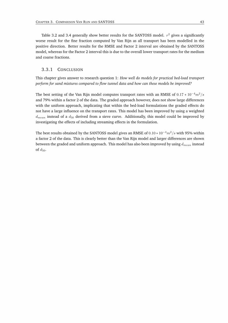
CHAPTER 3. COMPARISON VAN RIJN AND SANTOSS 43
Table 3.2 and 3.4 generally show better results for the SANTOSS model. r2 gives a significantlyworse result for the fine fraction computed by Van Rijn as all transport has been modelled in thepositive direction. Better results for the RMSE and Factor 2 interval are obtained by the SANTOSSmodel, whereas for the Factor 2 interval this is due to the overall lower transport rates for the mediumand coarse fractions.
3.3.1 CONCLUSION
This chapter gives answer to research question 1: How well do models for practical bed-load transportperform for sand mixtures compared to flow tunnel data and how can these models be improved?
The best setting of the Van Rijn model computes transport rates with an RMSE of 0.17 ∗ 10−4m2/s
and 79% within a factor 2 of the data. The graded approach however, does not show large differenceswith the uniform approach, implicating that within the bed-load formulations the graded effects donot have a large influence on the transport rates. This model has been improved by using a weighteddmean instead of a d50 derived from a sieve curve. Additionally, this model could be improved byinvestigating the effects of including streaming effects in the formulation.
The best results obtained by the SANTOSS model gives an RMSE of 0.10 ∗ 10−4m2/s with 95% withina factor 2 of the data. This is clearly better than the Van Rijn model and larger differences are shownbetween the graded and uniform approach. This model has also been improved by using dmean insteadof d50.
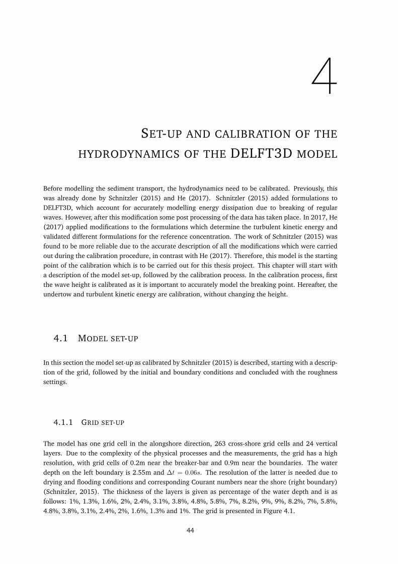
4SET-UP AND CALIBRATION OF THE
HYDRODYNAMICS OF THE DELFT3D MODEL
Before modelling the sediment transport, the hydrodynamics need to be calibrated. Previously, thiswas already done by Schnitzler (2015) and He (2017). Schnitzler (2015) added formulations toDELFT3D, which account for accurately modelling energy dissipation due to breaking of regularwaves. However, after this modification some post processing of the data has taken place. In 2017, He(2017) applied modifications to the formulations which determine the turbulent kinetic energy andvalidated different formulations for the reference concentration. The work of Schnitzler (2015) wasfound to be more reliable due to the accurate description of all the modifications which were carriedout during the calibration procedure, in contrast with He (2017). Therefore, this model is the startingpoint of the calibration which is to be carried out for this thesis project. This chapter will start witha description of the model set-up, followed by the calibration process. In the calibration process, firstthe wave height is calibrated as it is important to accurately model the breaking point. Hereafter, theundertow and turbulent kinetic energy are calibration, without changing the height.
4.1 MODEL SET-UP
In this section the model set-up as calibrated by Schnitzler (2015) is described, starting with a descrip-tion of the grid, followed by the initial and boundary conditions and concluded with the roughnesssettings.
4.1.1 GRID SET-UP
The model has one grid cell in the alongshore direction, 263 cross-shore grid cells and 24 verticallayers. Due to the complexity of the physical processes and the measurements, the grid has a highresolution, with grid cells of 0.2m near the breaker-bar and 0.9m near the boundaries. The waterdepth on the left boundary is 2.55m and ∆t = 0.06s. The resolution of the latter is needed due todrying and flooding conditions and corresponding Courant numbers near the shore (right boundary)(Schnitzler, 2015). The thickness of the layers is given as percentage of the water depth and is asfollows: 1%, 1.3%, 1.6%, 2%, 2.4%, 3.1%, 3.8%, 4.8%, 5.8%, 7%, 8.2%, 9%, 9%, 8.2%, 7%, 5.8%,4.8%, 3.8%, 3.1%, 2.4%, 2%, 1.6%, 1.3% and 1%. The grid is presented in Figure 4.1.
44
CHAPTER 4. MODEL SET-UP 45
Figure 4.1: Grid dimensions as used for the SINBAD experiments (Schnitzler, 2015).
4.1.2 INITIAL AND BOUNDARY CONDITIONS
At the start of the model computations initial conditions are imposed on the model. The initial waterlevel is set to 0m and as the water was at rest when the measurements were taken and sediment hadtime to settle, the sediment concentration in the water column is set to 0 kg/m3. On the left sideof the model (x=0m) an open boundary is located where the waves are generated (H = 0.80m andT = 4s). As the waves measured in the wave flume are not exactly equal to 0.85m, this value is set to0.80m in the model.
4.1.3 ROUGHNESS SETTINGS
Before any computations can be carried out, the bed roughness needs to be established. The roughnessregions along the bed profile together with the type of roughness and its value are displayed in Table4.1.
Table 4.1: Different roughness regions along the bed profile.
x < 8m x = 38− 68m x > 68m
Type of bottom Smooth concrete SandSand covered withplastic, iron and
concrete tiles
Type of roughness Chezy Bed-forms Chezy
Value 85m1/2/s
Roughness approach by(Van Rijn, 2007a) forbed-forms (Appendix
A.2)
45m1/2/s
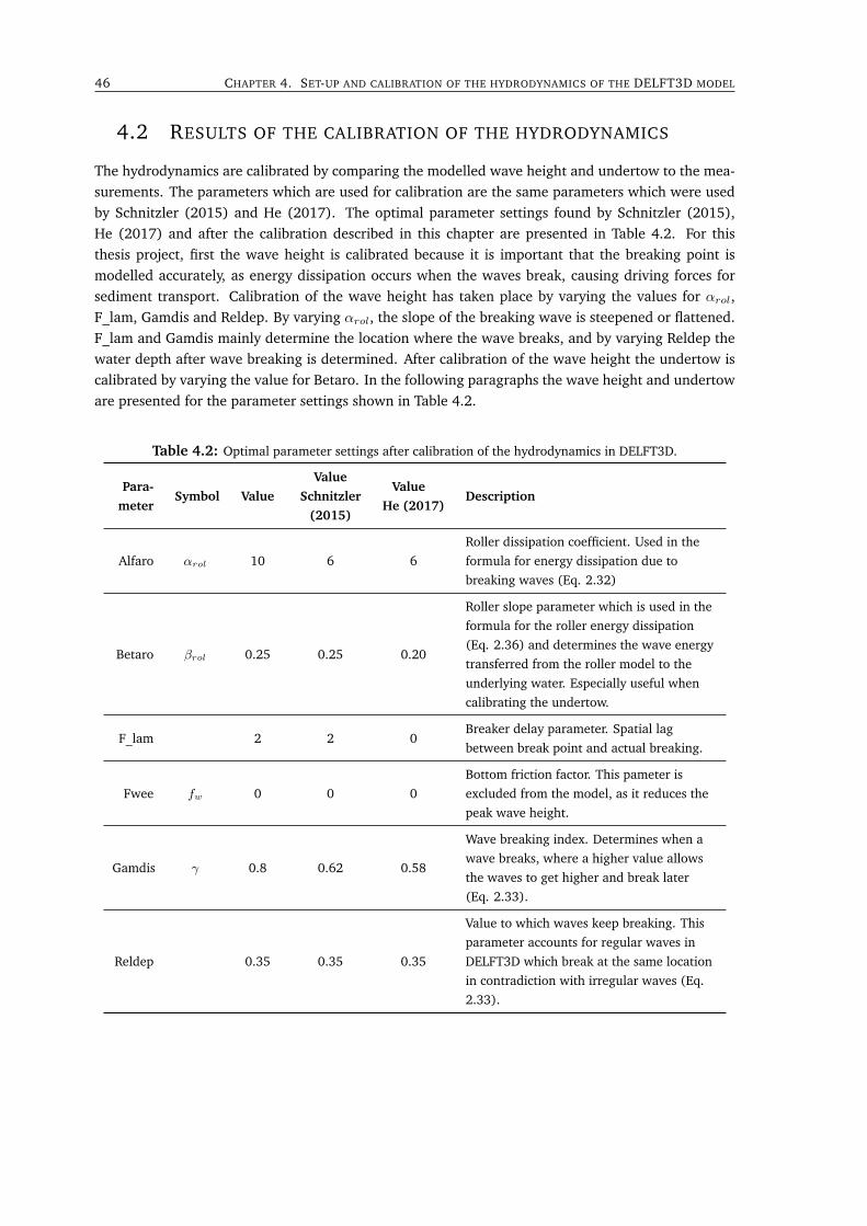
46 CHAPTER 4. SET-UP AND CALIBRATION OF THE HYDRODYNAMICS OF THE DELFT3D MODEL
4.2 RESULTS OF THE CALIBRATION OF THE HYDRODYNAMICS
The hydrodynamics are calibrated by comparing the modelled wave height and undertow to the mea-surements. The parameters which are used for calibration are the same parameters which were usedby Schnitzler (2015) and He (2017). The optimal parameter settings found by Schnitzler (2015),He (2017) and after the calibration described in this chapter are presented in Table 4.2. For thisthesis project, first the wave height is calibrated because it is important that the breaking point ismodelled accurately, as energy dissipation occurs when the waves break, causing driving forces forsediment transport. Calibration of the wave height has taken place by varying the values for αrol,F_lam, Gamdis and Reldep. By varying αrol, the slope of the breaking wave is steepened or flattened.F_lam and Gamdis mainly determine the location where the wave breaks, and by varying Reldep thewater depth after wave breaking is determined. After calibration of the wave height the undertow iscalibrated by varying the value for Betaro. In the following paragraphs the wave height and undertoware presented for the parameter settings shown in Table 4.2.
Table 4.2: Optimal parameter settings after calibration of the hydrodynamics in DELFT3D.
Para-meter
Symbol ValueValue
Schnitzler(2015)
ValueHe (2017)
Description
Alfaro αrol 10 6 6Roller dissipation coefficient. Used in theformula for energy dissipation due tobreaking waves (Eq. 2.32)
Betaro βrol 0.25 0.25 0.20
Roller slope parameter which is used in theformula for the roller energy dissipation(Eq. 2.36) and determines the wave energytransferred from the roller model to theunderlying water. Especially useful whencalibrating the undertow.
F_lam 2 2 0Breaker delay parameter. Spatial lagbetween break point and actual breaking.
Fwee fw 0 0 0Bottom friction factor. This pameter isexcluded from the model, as it reduces thepeak wave height.
Gamdis γ 0.8 0.62 0.58
Wave breaking index. Determines when awave breaks, where a higher value allowsthe waves to get higher and break later(Eq. 2.33).
Reldep 0.35 0.35 0.35
Value to which waves keep breaking. Thisparameter accounts for regular waves inDELFT3D which break at the same locationin contradiction with irregular waves (Eq.2.33).
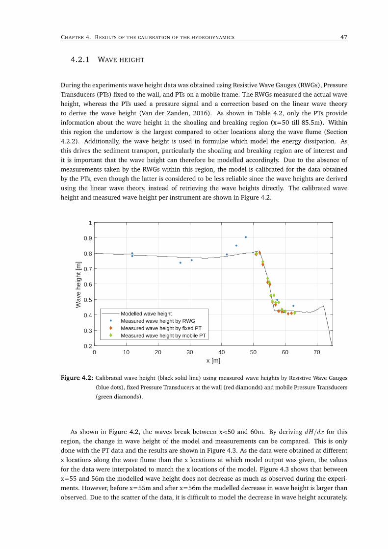
CHAPTER 4. RESULTS OF THE CALIBRATION OF THE HYDRODYNAMICS 47
4.2.1 WAVE HEIGHT
During the experiments wave height data was obtained using Resistive Wave Gauges (RWGs), PressureTransducers (PTs) fixed to the wall, and PTs on a mobile frame. The RWGs measured the actual waveheight, whereas the PTs used a pressure signal and a correction based on the linear wave theoryto derive the wave height (Van der Zanden, 2016). As shown in Table 4.2, only the PTs provideinformation about the wave height in the shoaling and breaking region (x=50 till 85.5m). Withinthis region the undertow is the largest compared to other locations along the wave flume (Section4.2.2). Additionally, the wave height is used in formulae which model the energy dissipation. Asthis drives the sediment transport, particularly the shoaling and breaking region are of interest andit is important that the wave height can therefore be modelled accordingly. Due to the absence ofmeasurements taken by the RWGs within this region, the model is calibrated for the data obtainedby the PTs, even though the latter is considered to be less reliable since the wave heights are derivedusing the linear wave theory, instead of retrieving the wave heights directly. The calibrated waveheight and measured wave height per instrument are shown in Figure 4.2.
0 10 20 30 40 50 60 70
x [m]
0.2
0.3
0.4
0.5
0.6
0.7
0.8
0.9
1
Wav
e he
ight
[m]
Modelled wave heightMeasured wave height by RWGMeasured wave height by fixed PTMeasured wave height by mobile PT
Figure 4.2: Calibrated wave height (black solid line) using measured wave heights by Resistive Wave Gauges
(blue dots), fixed Pressure Transducers at the wall (red diamonds) and mobile Pressure Transducers
(green diamonds).
As shown in Figure 4.2, the waves break between x≈50 and 60m. By deriving dH/dx for thisregion, the change in wave height of the model and measurements can be compared. This is onlydone with the PT data and the results are shown in Figure 4.3. As the data were obtained at differentx locations along the wave flume than the x locations at which model output was given, the valuesfor the data were interpolated to match the x locations of the model. Figure 4.3 shows that betweenx=55 and 56m the modelled wave height does not decrease as much as observed during the experi-ments. However, before x=55m and after x=56m the modelled decrease in wave height is larger thanobserved. Due to the scatter of the data, it is difficult to model the decrease in wave height accurately.
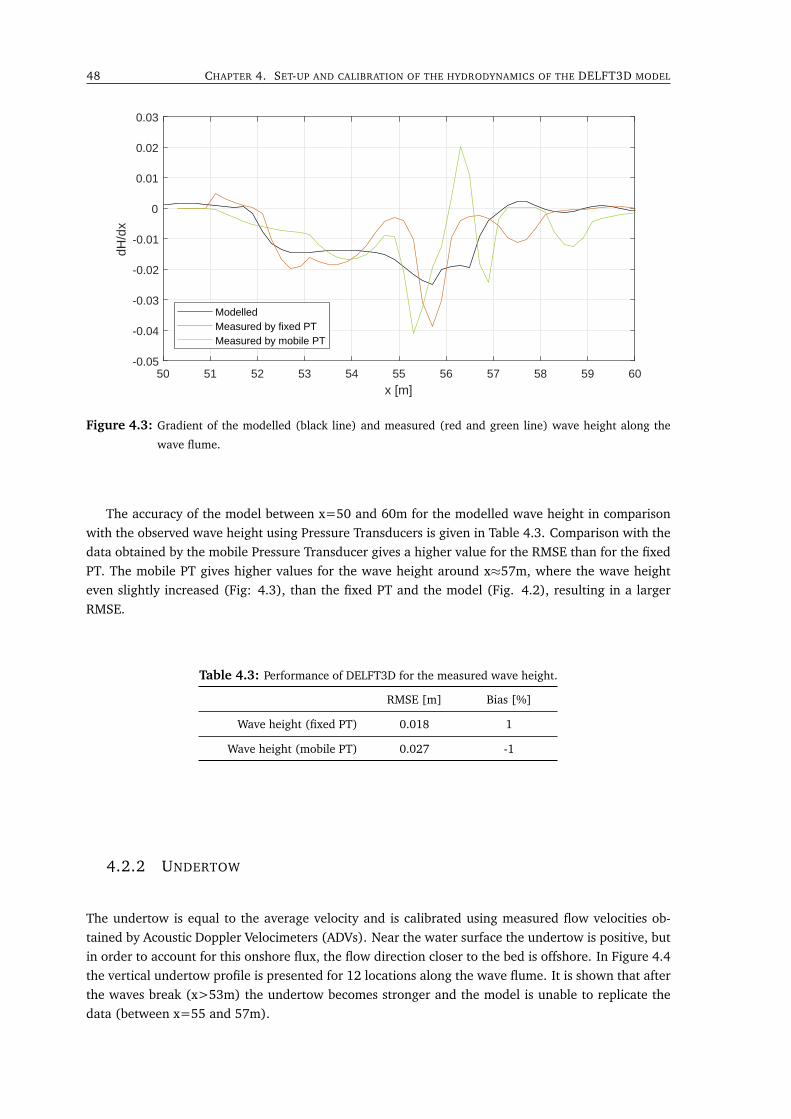
48 CHAPTER 4. SET-UP AND CALIBRATION OF THE HYDRODYNAMICS OF THE DELFT3D MODEL
50 51 52 53 54 55 56 57 58 59 60
x [m]
-0.05
-0.04
-0.03
-0.02
-0.01
0
0.01
0.02
0.03dH
/dx
ModelledMeasured by fixed PTMeasured by mobile PT
Figure 4.3: Gradient of the modelled (black line) and measured (red and green line) wave height along the
wave flume.
The accuracy of the model between x=50 and 60m for the modelled wave height in comparisonwith the observed wave height using Pressure Transducers is given in Table 4.3. Comparison with thedata obtained by the mobile Pressure Transducer gives a higher value for the RMSE than for the fixedPT. The mobile PT gives higher values for the wave height around x≈57m, where the wave heighteven slightly increased (Fig: 4.3), than the fixed PT and the model (Fig. 4.2), resulting in a largerRMSE.
Table 4.3: Performance of DELFT3D for the measured wave height.
RMSE [m] Bias [%]
Wave height (fixed PT) 0.018 1
Wave height (mobile PT) 0.027 -1
4.2.2 UNDERTOW
The undertow is equal to the average velocity and is calibrated using measured flow velocities ob-tained by Acoustic Doppler Velocimeters (ADVs). Near the water surface the undertow is positive, butin order to account for this onshore flux, the flow direction closer to the bed is offshore. In Figure 4.4the vertical undertow profile is presented for 12 locations along the wave flume. It is shown that afterthe waves break (x>53m) the undertow becomes stronger and the model is unable to replicate thedata (between x=55 and 57m).
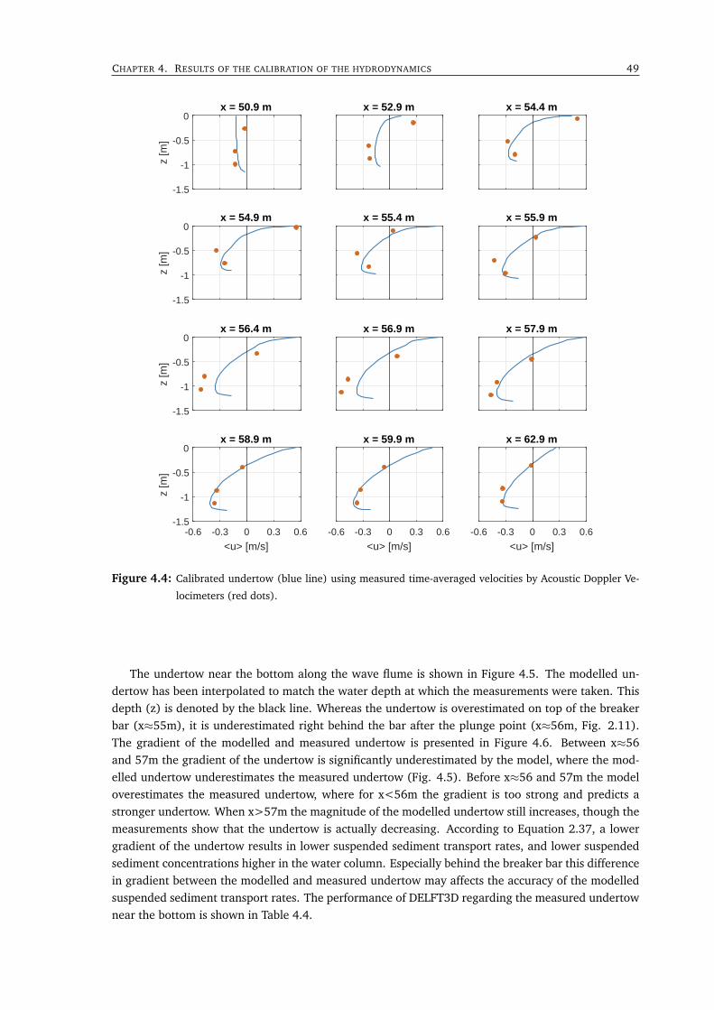
CHAPTER 4. RESULTS OF THE CALIBRATION OF THE HYDRODYNAMICS 49
-1.5
-1
-0.5
0
z [m
]
x = 50.9 m x = 52.9 m x = 54.4 m
-1.5
-1
-0.5
0
z [m
]
x = 54.9 m x = 55.4 m x = 55.9 m
-1.5
-1
-0.5
0
z [m
]
x = 56.4 m x = 56.9 m x = 57.9 m
-0.6 -0.3 0 0.3 0.6
<u> [m/s]
-1.5
-1
-0.5
0
z [m
]
x = 58.9 m
-0.6 -0.3 0 0.3 0.6
<u> [m/s]
x = 59.9 m
-0.6 -0.3 0 0.3 0.6
<u> [m/s]
x = 62.9 m
Figure 4.4: Calibrated undertow (blue line) using measured time-averaged velocities by Acoustic Doppler Ve-
locimeters (red dots).
The undertow near the bottom along the wave flume is shown in Figure 4.5. The modelled un-dertow has been interpolated to match the water depth at which the measurements were taken. Thisdepth (z) is denoted by the black line. Whereas the undertow is overestimated on top of the breakerbar (x≈55m), it is underestimated right behind the bar after the plunge point (x≈56m, Fig. 2.11).The gradient of the modelled and measured undertow is presented in Figure 4.6. Between x≈56and 57m the gradient of the undertow is significantly underestimated by the model, where the mod-elled undertow underestimates the measured undertow (Fig. 4.5). Before x≈56 and 57m the modeloverestimates the measured undertow, where for x<56m the gradient is too strong and predicts astronger undertow. When x>57m the magnitude of the modelled undertow still increases, though themeasurements show that the undertow is actually decreasing. According to Equation 2.37, a lowergradient of the undertow results in lower suspended sediment transport rates, and lower suspendedsediment concentrations higher in the water column. Especially behind the breaker bar this differencein gradient between the modelled and measured undertow may affects the accuracy of the modelledsuspended sediment transport rates. The performance of DELFT3D regarding the measured undertownear the bottom is shown in Table 4.4.
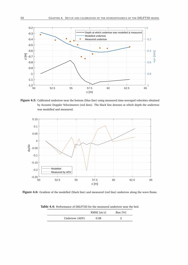
50 CHAPTER 4. SET-UP AND CALIBRATION OF THE HYDRODYNAMICS OF THE DELFT3D MODEL
50 52.5 55 57.5 60 62.5 65
x [m]
-1.2
-1.1
-1
-0.9
-0.8
-0.7
-0.6
-0.5
-0.4
-0.3
-0.2z
[m]
-1
-0.8
-0.6
-0.4
-0.2
0
<u>
[m/s
]
Depth at which undertow was modelled & measuredModelled undertowMeasured undertow
Figure 4.5: Calibrated undertow near the bottom (blue line) using measured time-averaged velocities obtained
by Acoustic Doppler Velocimeters (red dots). The black line denotes at which depth the undertow
was modelled and measured.
50 52.5 55 57.5 60 62.5 65
x [m]
-0.25
-0.2
-0.15
-0.1
-0.05
0
0.05
0.1
0.15
du/d
x
ModelledMeasured by ADV
Figure 4.6: Gradient of the modelled (black line) and measured (red line) undertow along the wave flume.
Table 4.4: Performance of DELFT3D for the measured undertow near the bed.
RMSE [m/s] Bias [%]
Undertow (ADV) 0.08 2
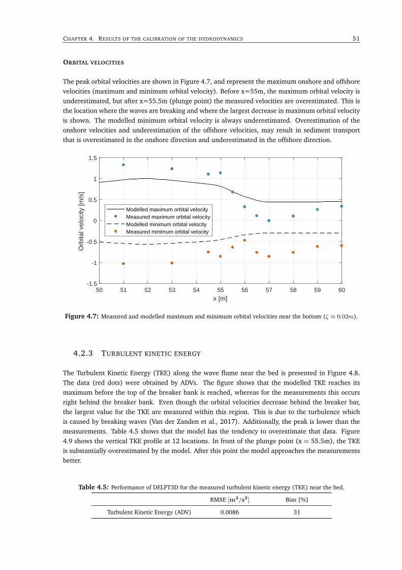
CHAPTER 4. RESULTS OF THE CALIBRATION OF THE HYDRODYNAMICS 51
ORBITAL VELOCITIES
The peak orbital velocities are shown in Figure 4.7, and represent the maximum onshore and offshorevelocities (maximum and minimum orbital velocity). Before x=55m, the maximum orbital velocity isunderestimated, but after x=55.5m (plunge point) the measured velocities are overestimated. This isthe location where the waves are breaking and where the largest decrease in maximum orbital velocityis shown. The modelled minimum orbital velocity is always underestimated. Overestimation of theonshore velocities and underestimation of the offshore velocities, may result in sediment transportthat is overestimated in the onshore direction and underestimated in the offshore direction.
50 51 52 53 54 55 56 57 58 59 60
x [m]
-1.5
-1
-0.5
0
0.5
1
1.5
Orb
ital v
eloc
ity [m
/s]
Modelled maximum orbital velocityMeasured maximum orbital velocityModelled minimum orbital velocityMeasured minimum orbital velocity
Figure 4.7: Measured and modelled maximum and minimum orbital velocities near the bottom (ζ ≈ 0.02m).
4.2.3 TURBULENT KINETIC ENERGY
The Turbulent Kinetic Energy (TKE) along the wave flume near the bed is presented in Figure 4.8.The data (red dots) were obtained by ADVs. The figure shows that the modelled TKE reaches itsmaximum before the top of the breaker bank is reached, whereas for the measurements this occursright behind the breaker bank. Even though the orbital velocities decrease behind the breaker bar,the largest value for the TKE are measured within this region. This is due to the turbulence whichis caused by breaking waves (Van der Zanden et al., 2017). Additionally, the peak is lower than themeasurements. Table 4.5 shows that the model has the tendency to overestimate that data. Figure4.9 shows the vertical TKE profile at 12 locations. In front of the plunge point (x ≈ 55.5m), the TKEis substantially overestimated by the model. After this point the model approaches the measurementsbetter.
Table 4.5: Performance of DELFT3D for the measured turbulent kinetic energy (TKE) near the bed.
RMSE [m2/s2] Bias [%]
Turbulent Kinetic Energy (ADV) 0.0086 31
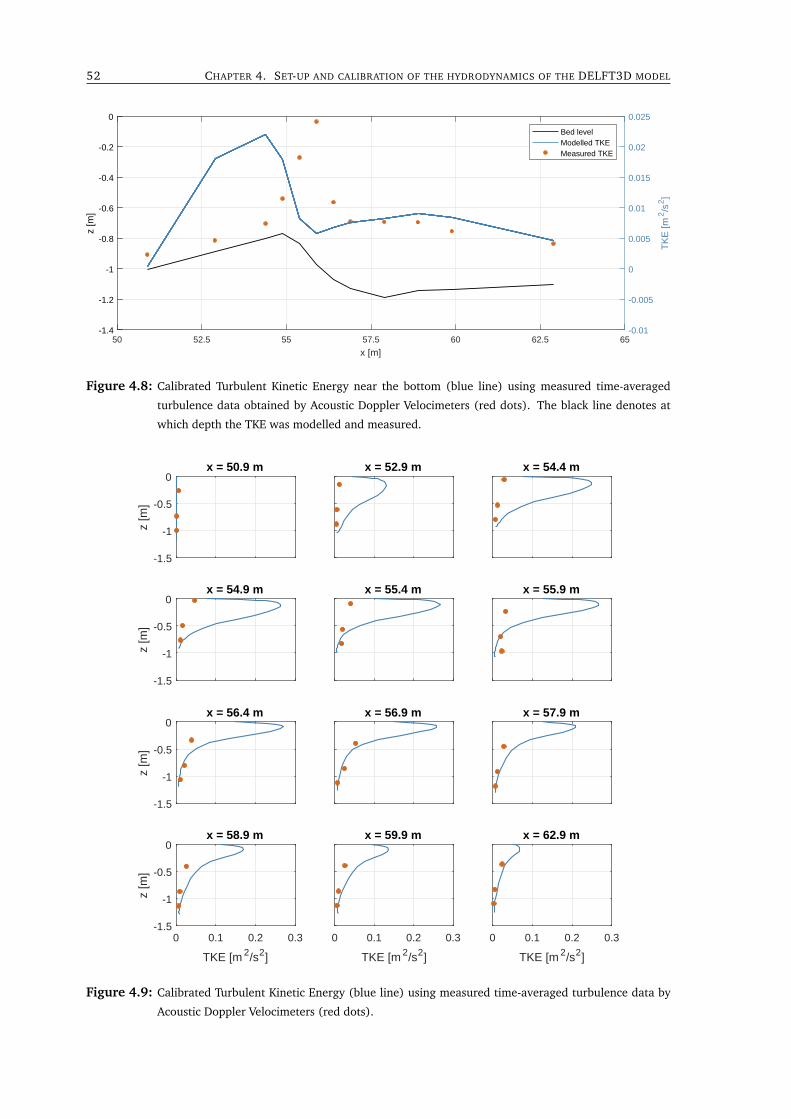
52 CHAPTER 4. SET-UP AND CALIBRATION OF THE HYDRODYNAMICS OF THE DELFT3D MODEL
50 52.5 55 57.5 60 62.5 65
x [m]
-1.4
-1.2
-1
-0.8
-0.6
-0.4
-0.2
0
z [m
]
-0.01
-0.005
0
0.005
0.01
0.015
0.02
0.025
TK
E [m
2/s
2]
Bed levelModelled TKEMeasured TKE
Figure 4.8: Calibrated Turbulent Kinetic Energy near the bottom (blue line) using measured time-averaged
turbulence data obtained by Acoustic Doppler Velocimeters (red dots). The black line denotes at
which depth the TKE was modelled and measured.
-1.5
-1
-0.5
0
z [m
]
x = 50.9 m x = 52.9 m x = 54.4 m
-1.5
-1
-0.5
0
z [m
]
x = 54.9 m x = 55.4 m x = 55.9 m
-1.5
-1
-0.5
0
z [m
]
x = 56.4 m x = 56.9 m x = 57.9 m
0 0.1 0.2 0.3
TKE [m 2/s2]
-1.5
-1
-0.5
0
z [m
]
x = 58.9 m
0 0.1 0.2 0.3
TKE [m 2/s2]
x = 59.9 m
0 0.1 0.2 0.3
TKE [m 2/s2]
x = 62.9 m
Figure 4.9: Calibrated Turbulent Kinetic Energy (blue line) using measured time-averaged turbulence data by
Acoustic Doppler Velocimeters (red dots).
CHAPTER 4. RESULTS OF THE CALIBRATION OF THE HYDRODYNAMICS 53
4.2.4 CONCLUSION
The calibrated wave heights approaches the measured wave heights by the Pressure Transducersneatly. Keeping in mind that there might be an error in these measurements as they have been derivedindirectly by using the linear wave theory, the model approaches the wave height in the shoaling andbreaking region pretty well.
The undertow near the bottom was mainly overestimated in front of the breaker bar, whereasit was underestimated right behind the breaker bar. This was also seen in the vertical undertowprofile, where right after the plunge point the model was unable to approach the larger values for theundertow. Calibration of the TKE showed that peak values were obtained right before the top of thebreaker bar, whereas the data showed a peak right behind the breaker bar.
Overall, the wave height and undertow were modelled quite accurately by DELFT3D. With a Biasbetween -1 and 2%, the model does not have the tendency to systematically over- or under-predictthe data. With wave heights varying between 0.8 and 0.4m during wave breaking, and values for theRMSE of 0.018 and 0.027m depending on the device which is used, the model is able to accuratelymodel the wave height in the breaker zone. The RMSE of the modelled undertow near the bedis relatively higher than for the wave height, with a value of 0.082 m/s and a modelled undertowvarying between -0.15 and -0.45m/s. The modelled gradient of the undertow near the bed was lesssteep than the data, and behind the breaker bar the undertow was underestimated. This has effect onthe suspended sediment transport and vertical concentration profile, which is further elaborated onin the next chapter.
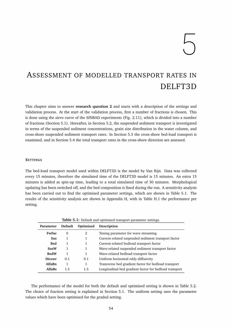
5ASSESSMENT OF MODELLED TRANSPORT RATES IN
DELFT3D
This chapter aims to answer research question 2 and starts with a description of the settings andvalidation process. At the start of the validation process, first a number of fractions is chosen. Thisis done using the sieve curve of the SINBAD experiments (Fig. 2.11), which is divided into a numberof fractions (Section 5.1). Hereafter, in Section 5.2, the suspended sediment transport is investigatedin terms of the suspended sediment concentrations, grain size distribution in the water column, andcross-shore suspended sediment transport rates. In Section 5.3 the cross-shore bed-load transport isexamined, and in Section 5.4 the total transport rates in the cross-shore direction are assessed.
SETTINGS
The bed-load transport model used within DELFT3D is the model by Van Rijn. Data was collectedevery 15 minutes, therefore the simulated time of the DELFT3D model is 15 minutes. An extra 15minutes is added as spin-up time, leading to a total simulated time of 30 minutes. Morphologicalupdating has been switched off, and the bed composition is fixed during the run. A sensitivity analysishas been carried out to find the optimised parameter settings, which are shown in Table 5.1. Theresults of the sensitivity analysis are shown in Appendix H, with in Table H.1 the performance persetting.
Table 5.1: Default and optimised transport parameter settings.
Parameter Default Optimised Description
FwFac 0 2 Tuning parameter for wave streamingSus 1 1 Current-related suspended sediment transport factorBed 1 1 Current-related bedload transport factor
SusW 1 1 Wave-related suspended sediment transport factorBedW 1 1 Wave-related bedload transport factor
Dicouv 0.1 0.1 Uniform horizontal eddy diffusivityAlfaBn 1 1 Transverse bed gradient factor for bedload transportAlfaBs 1.5 1.5 Longitudinal bed gradient factor for bedload transport
The performance of the model for both the default and optimised setting is shown in Table 5.2.The choice of fraction setting is explained in Section 5.1. The uniform setting uses the parametervalues which have been optimised for the graded setting.
54
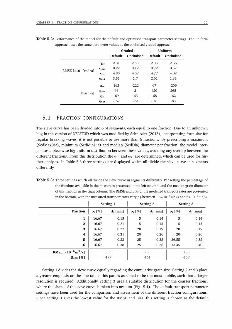
CHAPTER 5. FRACTION CONFIGURATIONS 55
Table 5.2: Performance of the model for the default and optimised transport parameter settings. The uniform
approach uses the same parameter values as the optimised graded approach.
Graded UniformDefault Optimised Default Optimised
RMSE [∗10−5m2/s]
qsc 2.31 2.53 2.35 2.66qsw 0.22 0.19 0.72 0.57qb 4.80 4.07 4.77 4.09qtot 3.55 1.7 2.61 1.35
Bias [%]
qsc 162 -222 67 -209qsw 44 3 420 268qb -69 -63 -68 -62qtot -157 -72 -141 -83
5.1 FRACTION CONFIGURATIONS
The sieve curve has been divided into 6 of segments, each equal to one fraction. Due to an unknownbug in the version of DELFT3D which was modified by Schnitzler (2015), incorporating formulae forregular breaking waves, it is not possible to use more than 6 fractions. By prescribing a maximum(SedMaxDia), minimum (SedMinDia) and median (SedDia) diameter per fraction, the model inter-polates a piecewise log-uniform distribution between these values, avoiding any overlap between thedifferent fractions. From this distribution the d10 and d90 are determined, which can be used for fur-ther analysis. In Table 5.3 three settings are displayed which all divide the sieve curve in segmentsdifferently.
Table 5.3: Three settings which all divide the sieve curve in segments differently. Per setting the percentage of
the fractions available in the mixture is presented in the left column, and the median grain diameter
of this fraction in the right column. The RMSE and Bias of the modelled transport rates are presented
in the bottom, with the measured transport rates varying between −6∗10−5m2/s and 6∗10−5m2/s.
Setting 1 Setting 2 Setting 3
Fraction pj [%] dj [mm] pj [%] dj [mm] pj [%] dj [mm]
1 16.67 0.15 5 0.14 5 0.14
2 16.67 0.21 5 0.15 5 0.15
3 16.67 0.27 20 0.19 20 0.19
4 16.67 0.31 20 0.26 20 0.26
5 16.67 0.33 25 0.32 36.55 0.32
6 16.67 0.38 25 0.36 13.45 0.40
RMSE [∗10−5m2/s] 3.63 3.65 3.55
Bias [%] -177 -161 -157
Setting 1 divides the sieve curve equally regarding the cumulative grain size. Setting 2 and 3 placea greater emphasis on the fine tail as this part is assumed to be the most mobile, such that a largerresolution is required. Additionally, setting 3 uses a suitable distribution for the coarser fractions,where the shape of the sieve curve is taken into account (Fig. 5.1). The default transport parametersettings have been used for the comparison and assessment of the different fraction configurations.Since setting 3 gives the lowest value for the RMSE and Bias, this setting is chosen as the default
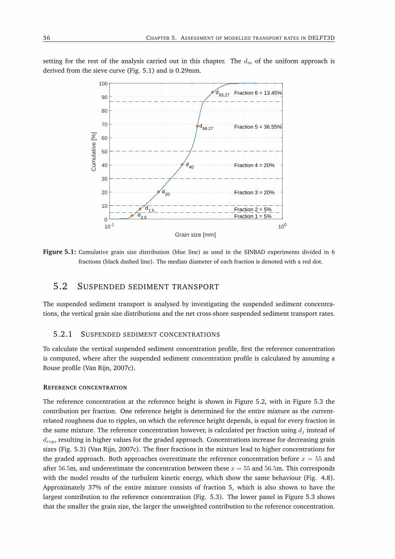
56 CHAPTER 5. ASSESSMENT OF MODELLED TRANSPORT RATES IN DELFT3D
setting for the rest of the analysis carried out in this chapter. The dm of the uniform approach isderived from the sieve curve (Fig. 5.1) and is 0.29mm.
10-1 100
Grain size [mm]
0
10
20
30
40
50
60
70
80
90
100
Cum
ulat
ive
[%]
Fraction 1 = 5%Fraction 2 = 5%
Fraction 3 = 20%
Fraction 4 = 20%
Fraction 5 = 36.55%
Fraction 6 = 13.45%
d2.5
d7.5
d20
d40
d68.27
d93.27
Figure 5.1: Cumulative grain size distribution (blue line) as used in the SINBAD experiments divided in 6
fractions (black dashed line). The median diameter of each fraction is denoted with a red dot.
5.2 SUSPENDED SEDIMENT TRANSPORT
The suspended sediment transport is analysed by investigating the suspended sediment concentra-tions, the vertical grain size distributions and the net cross-shore suspended sediment transport rates.
5.2.1 SUSPENDED SEDIMENT CONCENTRATIONS
To calculate the vertical suspended sediment concentration profile, first the reference concentrationis computed, where after the suspended sediment concentration profile is calculated by assuming aRouse profile (Van Rijn, 2007c).
REFERENCE CONCENTRATION
The reference concentration at the reference height is shown in Figure 5.2, with in Figure 5.3 thecontribution per fraction. One reference height is determined for the entire mixture as the current-related roughness due to ripples, on which the reference height depends, is equal for every fraction inthe same mixture. The reference concentration however, is calculated per fraction using dj instead ofdrep, resulting in higher values for the graded approach. Concentrations increase for decreasing grainsizes (Fig. 5.3) (Van Rijn, 2007c). The finer fractions in the mixture lead to higher concentrations forthe graded approach. Both approaches overestimate the reference concentration before x = 55 andafter 56.5m, and underestimate the concentration between these x = 55 and 56.5m. This correspondswith the model results of the turbulent kinetic energy, which show the same behaviour (Fig. 4.8).Approximately 37% of the entire mixture consists of fraction 5, which is also shown to have thelargest contribution to the reference concentration (Fig. 5.3). The lower panel in Figure 5.3 showsthat the smaller the grain size, the larger the unweighted contribution to the reference concentration.
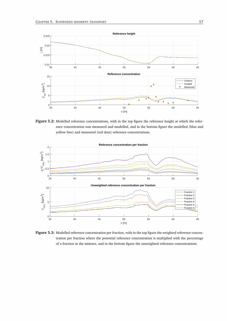
CHAPTER 5. SUSPENDED SEDIMENT TRANSPORT 57
35 40 45 50 55 60 650.01
0.015
0.02
0.025
[m]
Reference height
35 40 45 50 55 60 65
x [m]
0
5
10
15
Cre
f [kg/
m3]
Reference concentration
UniformGradedMeasured
Figure 5.2: Modelled reference concentrations, with in the top figure the reference height at which the refer-
ence concentration was measured and modelled, and in the bottom figure the modelled (blue and
yellow line) and measured (red dots) reference concentrations.
35 40 45 50 55 60 650
0.5
1
1.5
2
pj*C
ref,j
[kg/
m3]
Reference concentration per fraction
35 40 45 50 55 60 65
x [m]
0
5
10
Cre
f,j [k
g/m
3]
Unweighted reference concentration per fraction
Fraction 1Fraction 2Fraction 3Fraction 4Fraction 5Fraction 6
Figure 5.3: Modelled reference concentration per fraction, with in the top figure the weighted reference concen-
tration per fraction where the potential reference concentration is multiplied with the percentage
of a fraction in the mixture, and in the bottom figure the unweighted reference concentrations.
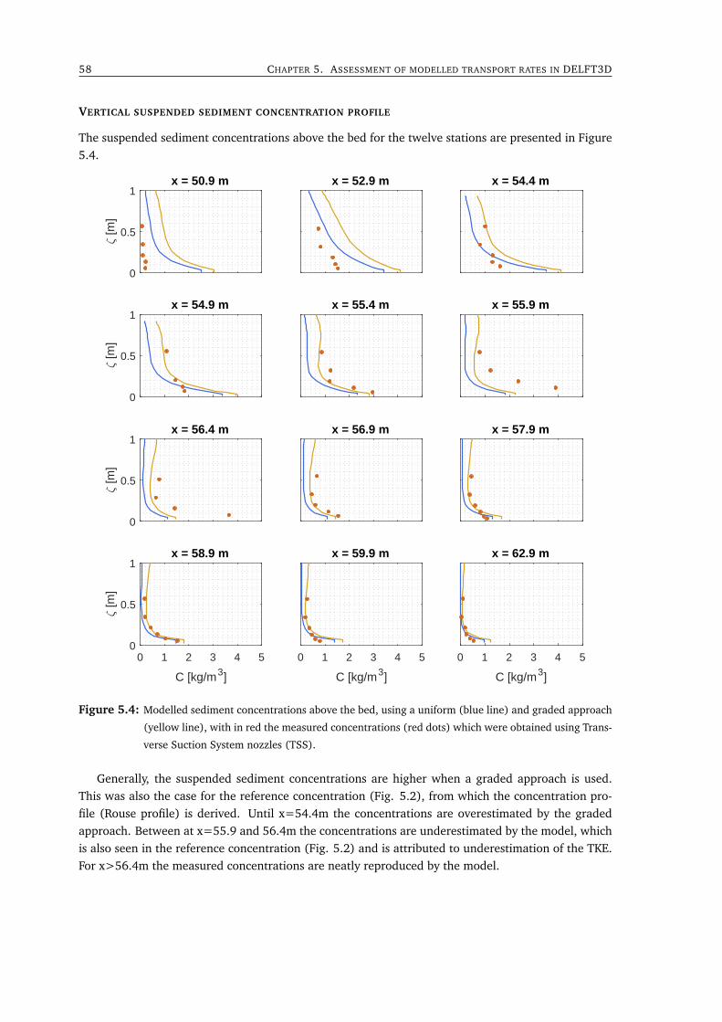
58 CHAPTER 5. ASSESSMENT OF MODELLED TRANSPORT RATES IN DELFT3D
VERTICAL SUSPENDED SEDIMENT CONCENTRATION PROFILE
The suspended sediment concentrations above the bed for the twelve stations are presented in Figure5.4.
0
0.5
1
[m]
x = 50.9 m x = 52.9 m x = 54.4 m
0
0.5
1
[m]
x = 54.9 m x = 55.4 m x = 55.9 m
0
0.5
1
[m]
x = 56.4 m x = 56.9 m x = 57.9 m
0 1 2 3 4 5
C [kg/m3]
0
0.5
1
[m]
x = 58.9 m
0 1 2 3 4 5
C [kg/m3]
x = 59.9 m
0 1 2 3 4 5
C [kg/m3]
x = 62.9 m
Figure 5.4: Modelled sediment concentrations above the bed, using a uniform (blue line) and graded approach
(yellow line), with in red the measured concentrations (red dots) which were obtained using Trans-
verse Suction System nozzles (TSS).
Generally, the suspended sediment concentrations are higher when a graded approach is used.This was also the case for the reference concentration (Fig. 5.2), from which the concentration pro-file (Rouse profile) is derived. Until x=54.4m the concentrations are overestimated by the gradedapproach. Between at x=55.9 and 56.4m the concentrations are underestimated by the model, whichis also seen in the reference concentration (Fig. 5.2) and is attributed to underestimation of the TKE.For x>56.4m the measured concentrations are neatly reproduced by the model.
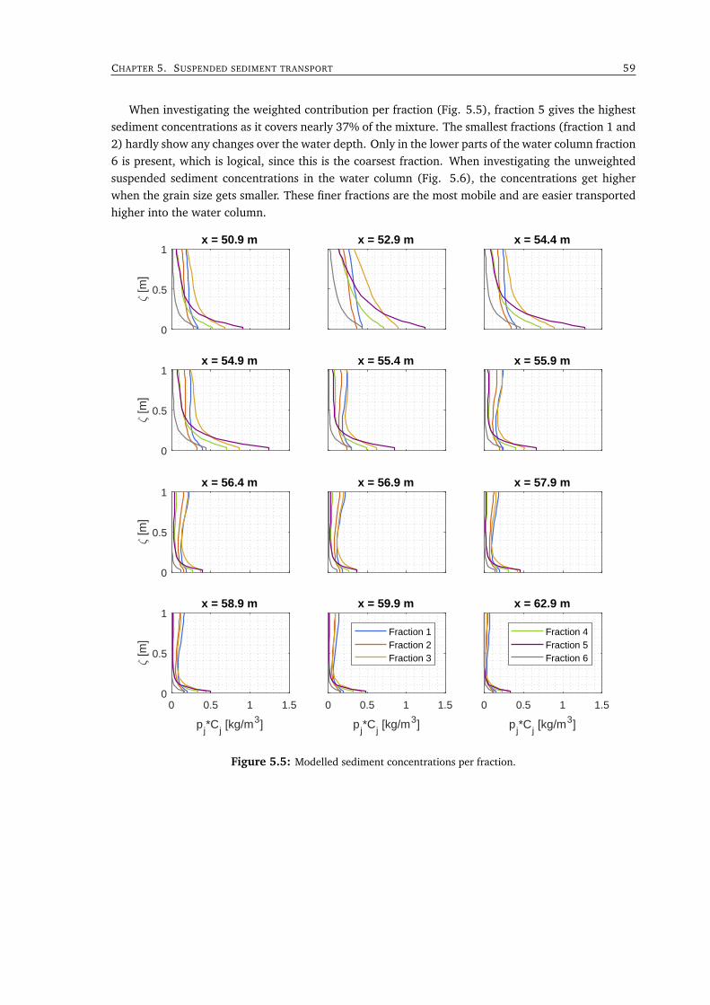
CHAPTER 5. SUSPENDED SEDIMENT TRANSPORT 59
When investigating the weighted contribution per fraction (Fig. 5.5), fraction 5 gives the highestsediment concentrations as it covers nearly 37% of the mixture. The smallest fractions (fraction 1 and2) hardly show any changes over the water depth. Only in the lower parts of the water column fraction6 is present, which is logical, since this is the coarsest fraction. When investigating the unweightedsuspended sediment concentrations in the water column (Fig. 5.6), the concentrations get higherwhen the grain size gets smaller. These finer fractions are the most mobile and are easier transportedhigher into the water column.
0
0.5
1
[m]
x = 50.9 m x = 52.9 m x = 54.4 m
0
0.5
1
[m]
x = 54.9 m x = 55.4 m x = 55.9 m
0
0.5
1
[m]
x = 56.4 m x = 56.9 m x = 57.9 m
0 0.5 1 1.5
pj*C
j [kg/m3]
0
0.5
1
[m]
x = 58.9 m
0 0.5 1 1.5
pj*C
j [kg/m3]
x = 59.9 m
Fraction 1Fraction 2Fraction 3
0 0.5 1 1.5
pj*C
j [kg/m3]
x = 62.9 m
Fraction 4Fraction 5Fraction 6
Figure 5.5: Modelled sediment concentrations per fraction.
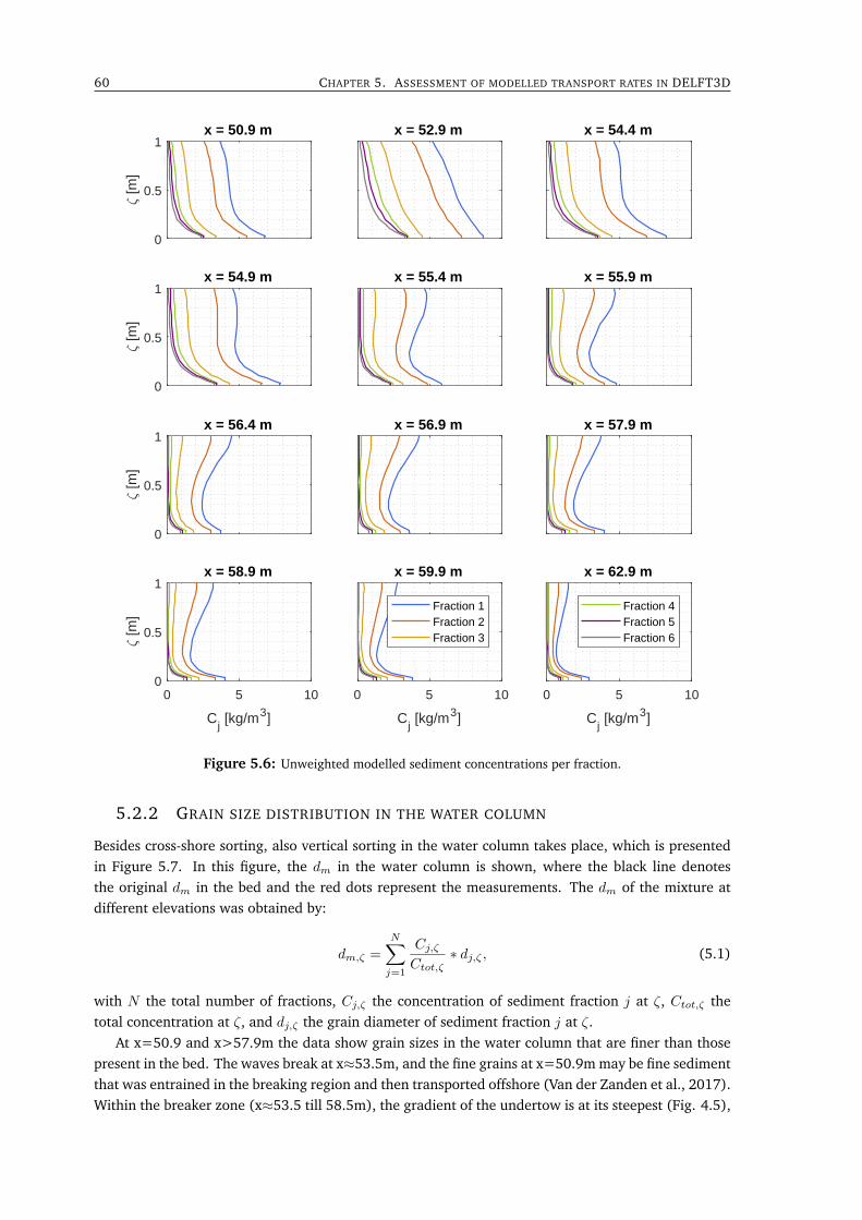
60 CHAPTER 5. ASSESSMENT OF MODELLED TRANSPORT RATES IN DELFT3D
0
0.5
1 [m
]x = 50.9 m x = 52.9 m x = 54.4 m
0
0.5
1
[m]
x = 54.9 m x = 55.4 m x = 55.9 m
0
0.5
1
[m]
x = 56.4 m x = 56.9 m x = 57.9 m
0 5 10
Cj [kg/m3]
0
0.5
1
[m]
x = 58.9 m
0 5 10
Cj [kg/m3]
x = 59.9 m
Fraction 1Fraction 2Fraction 3
0 5 10
Cj [kg/m3]
x = 62.9 m
Fraction 4Fraction 5Fraction 6
Figure 5.6: Unweighted modelled sediment concentrations per fraction.
5.2.2 GRAIN SIZE DISTRIBUTION IN THE WATER COLUMN
Besides cross-shore sorting, also vertical sorting in the water column takes place, which is presentedin Figure 5.7. In this figure, the dm in the water column is shown, where the black line denotesthe original dm in the bed and the red dots represent the measurements. The dm of the mixture atdifferent elevations was obtained by:
dm,ζ =
N∑j=1
Cj,ζCtot,ζ
∗ dj,ζ , (5.1)
with N the total number of fractions, Cj,ζ the concentration of sediment fraction j at ζ, Ctot,ζ thetotal concentration at ζ, and dj,ζ the grain diameter of sediment fraction j at ζ.
At x=50.9 and x>57.9m the data show grain sizes in the water column that are finer than thosepresent in the bed. The waves break at x≈53.5m, and the fine grains at x=50.9m may be fine sedimentthat was entrained in the breaking region and then transported offshore (Van der Zanden et al., 2017).Within the breaker zone (x≈53.5 till 58.5m), the gradient of the undertow is at its steepest (Fig. 4.5),
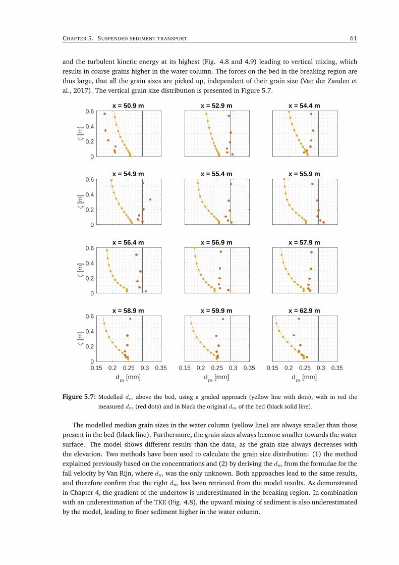
CHAPTER 5. SUSPENDED SEDIMENT TRANSPORT 61
and the turbulent kinetic energy at its highest (Fig. 4.8 and 4.9) leading to vertical mixing, whichresults in coarse grains higher in the water column. The forces on the bed in the breaking region arethus large, that all the grain sizes are picked up, independent of their grain size (Van der Zanden etal., 2017). The vertical grain size distribution is presented in Figure 5.7.
0
0.2
0.4
0.6
[m]
x = 50.9 m x = 52.9 m x = 54.4 m
0
0.2
0.4
0.6
[m]
x = 54.9 m x = 55.4 m x = 55.9 m
0
0.2
0.4
0.6
[m]
x = 56.4 m x = 56.9 m x = 57.9 m
0.15 0.2 0.25 0.3 0.35
dm
[mm]
0
0.2
0.4
0.6
[m]
x = 58.9 m
0.15 0.2 0.25 0.3 0.35
dm
[mm]
x = 59.9 m
0.15 0.2 0.25 0.3 0.35
dm
[mm]
x = 62.9 m
Figure 5.7: Modelled dm above the bed, using a graded approach (yellow line with dots), with in red the
measured dm (red dots) and in black the original dm of the bed (black solid line).
The modelled median grain sizes in the water column (yellow line) are always smaller than thosepresent in the bed (black line). Furthermore, the grain sizes always become smaller towards the watersurface. The model shows different results than the data, as the grain size always decreases withthe elevation. Two methods have been used to calculate the grain size distribution: (1) the methodexplained previously based on the concentrations and (2) by deriving the dm from the formulae for thefall velocity by Van Rijn, where dm was the only unknown. Both approaches lead to the same results,and therefore confirm that the right dm has been retrieved from the model results. As demonstratedin Chapter 4, the gradient of the undertow is underestimated in the breaking region. In combinationwith an underestimation of the TKE (Fig. 4.8), the upward mixing of sediment is also underestimatedby the model, leading to finer sediment higher in the water column.
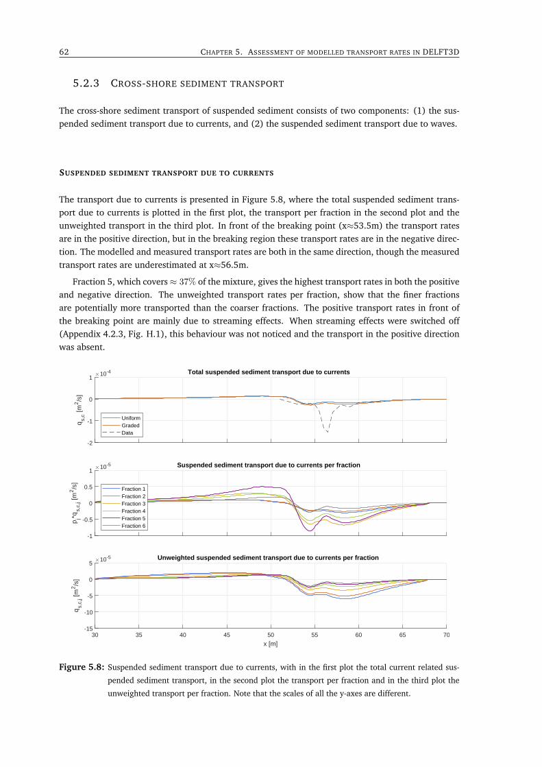
62 CHAPTER 5. ASSESSMENT OF MODELLED TRANSPORT RATES IN DELFT3D
5.2.3 CROSS-SHORE SEDIMENT TRANSPORT
The cross-shore sediment transport of suspended sediment consists of two components: (1) the sus-pended sediment transport due to currents, and (2) the suspended sediment transport due to waves.
SUSPENDED SEDIMENT TRANSPORT DUE TO CURRENTS
The transport due to currents is presented in Figure 5.8, where the total suspended sediment trans-port due to currents is plotted in the first plot, the transport per fraction in the second plot and theunweighted transport in the third plot. In front of the breaking point (x≈53.5m) the transport ratesare in the positive direction, but in the breaking region these transport rates are in the negative direc-tion. The modelled and measured transport rates are both in the same direction, though the measuredtransport rates are underestimated at x≈56.5m.
Fraction 5, which covers≈ 37% of the mixture, gives the highest transport rates in both the positiveand negative direction. The unweighted transport rates per fraction, show that the finer fractionsare potentially more transported than the coarser fractions. The positive transport rates in front ofthe breaking point are mainly due to streaming effects. When streaming effects were switched off(Appendix 4.2.3, Fig. H.1), this behaviour was not noticed and the transport in the positive directionwas absent.
-2
-1
0
1
qs,
c [m
2/s
]
10-4 Total suspended sediment transport due to currents
UniformGradedData
-1
-0.5
0
0.5
1
pj*q
s,c,
j [m2/s
]
10-5 Suspended sediment transport due to currents per fraction
Fraction 1Fraction 2Fraction 3Fraction 4Fraction 5Fraction 6
30 35 40 45 50 55 60 65 70
x [m]
-15
-10
-5
0
5
qs,
c,j [m
2/s
]
10-5 Unweighted suspended sediment transport due to currents per fraction
Figure 5.8: Suspended sediment transport due to currents, with in the first plot the total current related sus-
pended sediment transport, in the second plot the transport per fraction and in the third plot the
unweighted transport per fraction. Note that the scales of all the y-axes are different.
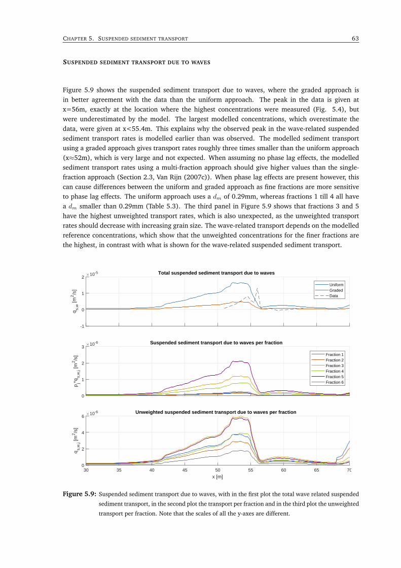
CHAPTER 5. SUSPENDED SEDIMENT TRANSPORT 63
SUSPENDED SEDIMENT TRANSPORT DUE TO WAVES
Figure 5.9 shows the suspended sediment transport due to waves, where the graded approach isin better agreement with the data than the uniform approach. The peak in the data is given atx=56m, exactly at the location where the highest concentrations were measured (Fig. 5.4), butwere underestimated by the model. The largest modelled concentrations, which overestimate thedata, were given at x<55.4m. This explains why the observed peak in the wave-related suspendedsediment transport rates is modelled earlier than was observed. The modelled sediment transportusing a graded approach gives transport rates roughly three times smaller than the uniform approach(x≈52m), which is very large and not expected. When assuming no phase lag effects, the modelledsediment transport rates using a multi-fraction approach should give higher values than the single-fraction approach (Section 2.3, Van Rijn (2007c)). When phase lag effects are present however, thiscan cause differences between the uniform and graded approach as fine fractions are more sensitiveto phase lag effects. The uniform approach uses a dm of 0.29mm, whereas fractions 1 till 4 all havea dm smaller than 0.29mm (Table 5.3). The third panel in Figure 5.9 shows that fractions 3 and 5have the highest unweighted transport rates, which is also unexpected, as the unweighted transportrates should decrease with increasing grain size. The wave-related transport depends on the modelledreference concentrations, which show that the unweighted concentrations for the finer fractions arethe highest, in contrast with what is shown for the wave-related suspended sediment transport.
-1
0
1
2
qs,
w [m
2/s
]
10-5 Total suspended sediment transport due to waves
UniformGradedData
0
1
2
3
pj*q
s,w
,j [m2/s
]
10-6 Suspended sediment transport due to waves per fraction
Fraction 1Fraction 2Fraction 3Fraction 4Fraction 5Fraction 6
30 35 40 45 50 55 60 65 70
x [m]
0
2
4
6
qs,
w,j [m
2/s
]
10-6 Unweighted suspended sediment transport due to waves per fraction
Figure 5.9: Suspended sediment transport due to waves, with in the first plot the total wave related suspended
sediment transport, in the second plot the transport per fraction and in the third plot the unweighted
transport per fraction. Note that the scales of all the y-axes are different.
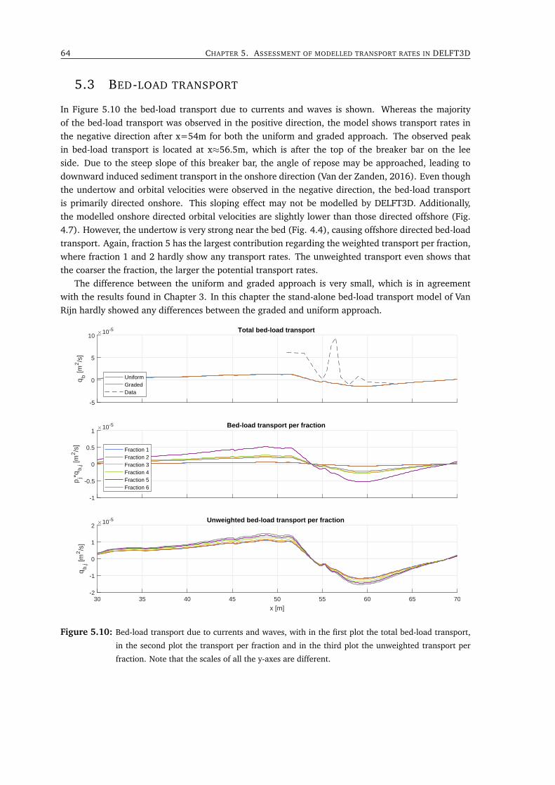
64 CHAPTER 5. ASSESSMENT OF MODELLED TRANSPORT RATES IN DELFT3D
5.3 BED-LOAD TRANSPORT
In Figure 5.10 the bed-load transport due to currents and waves is shown. Whereas the majorityof the bed-load transport was observed in the positive direction, the model shows transport rates inthe negative direction after x=54m for both the uniform and graded approach. The observed peakin bed-load transport is located at x≈56.5m, which is after the top of the breaker bar on the leeside. Due to the steep slope of this breaker bar, the angle of repose may be approached, leading todownward induced sediment transport in the onshore direction (Van der Zanden, 2016). Even thoughthe undertow and orbital velocities were observed in the negative direction, the bed-load transportis primarily directed onshore. This sloping effect may not be modelled by DELFT3D. Additionally,the modelled onshore directed orbital velocities are slightly lower than those directed offshore (Fig.4.7). However, the undertow is very strong near the bed (Fig. 4.4), causing offshore directed bed-loadtransport. Again, fraction 5 has the largest contribution regarding the weighted transport per fraction,where fraction 1 and 2 hardly show any transport rates. The unweighted transport even shows thatthe coarser the fraction, the larger the potential transport rates.
The difference between the uniform and graded approach is very small, which is in agreementwith the results found in Chapter 3. In this chapter the stand-alone bed-load transport model of VanRijn hardly showed any differences between the graded and uniform approach.
-5
0
5
10
qb [m
2/s
]
10-5 Total bed-load transport
UniformGradedData
-1
-0.5
0
0.5
1
pj*q
b,j [m
2/s
]
10-5 Bed-load transport per fraction
Fraction 1Fraction 2Fraction 3Fraction 4Fraction 5Fraction 6
30 35 40 45 50 55 60 65 70
x [m]
-2
-1
0
1
2
qb,
j [m2/s
]
10-5 Unweighted bed-load transport per fraction
Figure 5.10: Bed-load transport due to currents and waves, with in the first plot the total bed-load transport,
in the second plot the transport per fraction and in the third plot the unweighted transport per
fraction. Note that the scales of all the y-axes are different.
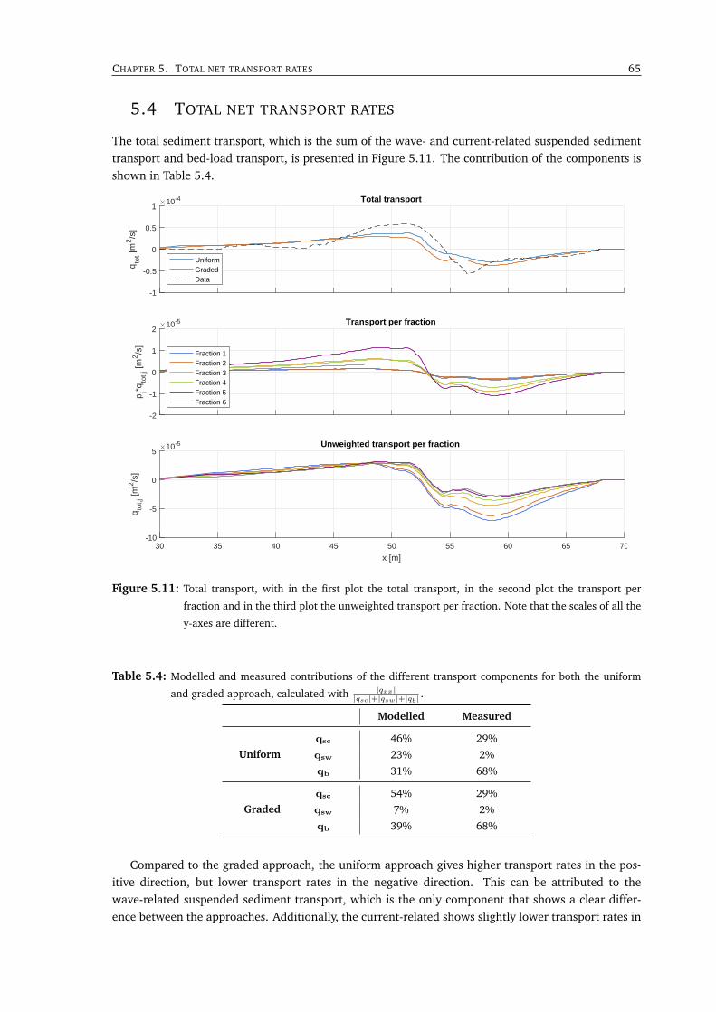
CHAPTER 5. TOTAL NET TRANSPORT RATES 65
5.4 TOTAL NET TRANSPORT RATES
The total sediment transport, which is the sum of the wave- and current-related suspended sedimenttransport and bed-load transport, is presented in Figure 5.11. The contribution of the components isshown in Table 5.4.
-1
-0.5
0
0.5
1
qto
t [m2/s
]
10-4 Total transport
UniformGradedData
-2
-1
0
1
2
pj*q
tot,j
[m2/s
]
10-5 Transport per fraction
Fraction 1Fraction 2Fraction 3Fraction 4Fraction 5Fraction 6
30 35 40 45 50 55 60 65 70
x [m]
-10
-5
0
5
qto
t,j [m
2/s
]
10-5 Unweighted transport per fraction
Figure 5.11: Total transport, with in the first plot the total transport, in the second plot the transport per
fraction and in the third plot the unweighted transport per fraction. Note that the scales of all the
y-axes are different.
Table 5.4: Modelled and measured contributions of the different transport components for both the uniform
and graded approach, calculated with |qxx||qsc|+|qsw|+|qb|
.
Modelled Measured
Uniformqsc 46% 29%
qsw 23% 2%
qb 31% 68%
Gradedqsc 54% 29%
qsw 7% 2%
qb 39% 68%
Compared to the graded approach, the uniform approach gives higher transport rates in the pos-itive direction, but lower transport rates in the negative direction. This can be attributed to thewave-related suspended sediment transport, which is the only component that shows a clear differ-ence between the approaches. Additionally, the current-related shows slightly lower transport rates in
66 CHAPTER 5. ASSESSMENT OF MODELLED TRANSPORT RATES IN DELFT3D
the negative direction for the uniform approach. However, it is doubted whether DELFT3D calculatesthe wave-related suspended sediment transport correctly. When this is not the case and the valuesare incorrect, there is no distinct difference between the graded and uniform approach. According toTable 5.4, qsw provides the smallest contribution to the total modelled transport rates.
The weighted transport per fraction shows the highest transport rates for fraction 5, with thelargest difference before the breaking point (x≈53.5m), mainly caused by the bed-load transport andsuspended sediment transport due to currents which are both modelled onshore. At x=56.5m the peakin the offshore directed transport is underestimated by both the uniform and graded approach. This isdue to underestimation of the current-related suspended sediment transport and the concentrations.The unweighted transport shows that the fine fraction potentially gives higher transport rates, andthat the fine fractions are also the quickest to reverse the direction.
5.5 CONCLUSION
This chapter gives answer to research questions 2: What are the effects of using a graded sediment ap-proach instead of a uniform approach in DELFT3D regarding the (a) suspended sediment concentrations,(b) suspended sediment grain sizes, and (c) cross-shore net total sediment transport?
The modelled reference concentrations underestimate the observed reference concentrations be-tween x=55 and 56.6m. At these locations the observed turbulent kinetic energy is very strong, andreaches its maximum values. This energy may enhance the concentrations as more sediment is mo-bilised (Van der Zanden et al., 2017). However, these effects are not incorporated in the formula forthe reference concentration. The reference concentration using a graded approach is slightly higher,which is possibly due to the fine fractions which are easily mobilised. The vertical concentration pro-files show that the concentrations of the graded approach are always higher than that of the uniformapproach. As the reference concentrations are already higher for the graded approach, the rest ofthe profile also gives higher concentrations than the uniform approach. From x=50.9 till 54.4m bothapproaches overestimate the measured concentrations, but the overall concentrations of the uniformapproach are lower, and are thus in better agreement with the data. At x=55.9 and 56.4m bothapproaches underestimate the measured concentrations. At both locations the undertow is underes-timated by the model, leading to discrepancies between the modelled and measured concentrations.After x=56.4m the graded approach seems to perform better for the given dataset.
The modelled grain sizes in the water column are larger than the data at x=50.9m, but are finerat all other locations, and are always finer than the dm in the bed. The observed grain sizes measuredat x=50.9m may be fine sediment that was entrained in the breaker zone, but was then transportedoffshore. Due to larger values for the turbulent kinetic energy a lot of vertical mixing takes place,resulting in coarser grains higher in the water column. Underestimation of this energy may probablyalso cause the underestimation in grain sizes in the water column.
Both the uniform and graded approach give comparable results for the current-related suspendedsediment transport and bed-load transport, where observed peaks in the data are not replicated bythe model. Chapter 3 already showed hardly any differences between the uniform and graded ap-proach for the modelled bed-load transport rates using Van Rijn (2007c). For the current-relatedsuspended sediment transport, this is due to the underestimation of the gradient of the undertowat x≈56.5m. The bed-load transport rates for both approaches however, are modelled in the wrongdirection (x≈56.5m). This may be attributed to the the slope on the lee side of the breaker bar (x=55till 57m), where downward induced bed-load transport in the onshore direction takes place duringthe experiment. This effect is not incorporated in DELFT3D, and as the offshore directed undertow
CHAPTER 5. CONCLUSION 67
velocities are strong at this location, bed-load transport is modelled in the offshore direction. Onlythe wave-related suspended sediment transport shows a clear difference between the two approaches,where it is unknown whether this is actually due to grading effects or a bug in DELFT3D. DELFT3Duses a different method to calculated this transport component than was shown in Section 2.4.3,which is based on the reference concentatraton and Van Rijn’s mixing coefficient, so the calculatedconcentrations presented in Section 5.2.1 are not one-to-one linked with the wave-related suspendedsediment transport. Additionally, fraction 5 shows the largest unweighted transport, which does notseem logical, assuming that fine fractions are mobilised more easily. Analysis of the total transportrates has shown that the graded approach gives smaller transport rates in the onshore direction, butlarger transport rates in the offshore direction when compared to the uniform approach. This effectcan be attributed to the difference in wave-related suspended sediment transport, where the transportin the positive direction is larger for the uniform approach.
6DISCUSSION
During this research, some uncertainties were encountered. These uncertainties are discussed conse-quently for (1) the modelling of the bed-load transport rates, (2) the measurements taken during thewave-flume experiments, (3) the modelling of the hydrodynamics and (3) the modelled suspendedsediment transport due to waves.
6.1 MODELLING BED-LOAD TRANSPORT RATES
A number of remarks can be made regarding the modelling of bed-load transport with the SANTOSSand Van Rijn model.
VAN RIJN MODEL: CONVERSION FROM FORTRAN TO MATLAB
In the formulations of the Fortran code (TR2004 (Van Rijn et al., 2004)), a number of tweakingparameters was used by Van Rijn to enhance the models performance. Furthermore, streaming ef-fects due to free-surface waves were included, though for the oscillatory flow tunnel experiments thiseffect was assumed to be absent due to the absence of these waves. Both these aspects are now ex-cluded from the MATLAB code, yielding differences between the computed transport rates by Fortranand MATLAB. Excluding streaming effects reduced the bed-load transport rates by a factor 1.5 to 2(Appendix F), and compared to the SANTOSS model the transport rates computed by Van Rijn arerelatively low.
WAVE-RELATED SUSPENDED SEDIMENT TRANSPORT VAN RIJN
The bed-load transport computed in DELFT3D consists of 3 components, namely the (1) bed-loadtransport due to waves, (2) bed-load transport due to currents and (3) suspended sediment transportdue to waves. Within the formulation of this last component a factor for the wave asymmetry isincorporated, and this is the only component in which phase lag effects are incorporated. In the stand-alone bed-load transport model for Van Rijn, only the bed-load transport due to currents and waves iscalculated, ignoring the wave-related suspended sediment transport and any phase lag effects. Section3.1 showed that all the sediment transport rates were always modelled in the positive direction, eventhough some transport of the fine fraction was measured in the negative direction. This impliesthat phase lag effects should be incorporated in the stand-alone bed-load transport formulations,since during the experiments phase lag effects were noticed in the transport of suspended sedimenttransport.
CALIBRATION AND VALIDATION OF THE SANTOSS MODEL
The SANTOSS model was originally calibrated and validated with the dataset used for this thesis.Though the performance of the model for the different fractions had not yet been calibrated and
68
CHAPTER 6. MEASURING INSTRUMENTS WAVE FLUME EXPERIMENTS 69
validated before, it only seems reasonable that the total net transport rates are in accordance withthe used database. Therefore, comparing the performance of the SANTOSS and Van Rijn model tothis database is unfavourable for the latter, as the transport rates computed by the Van Rijn were notcalibrated using this dataset.
DIFFERENCE BETWEEN UNIFORM AND GRADED APPROACH
The SANTOSS model shows clear differences between the uniform and graded approach, which is notthe case for the Van Rijn model. When using a uniform approach in SANTOSS, the bed-load transportrates increase. Within SANTOSS, sediment transport of the fine fraction has been modelled in both thepositive and negative direction due to phase lag effects. These phase lag effects only apply when finesand stays in the water column until the consecutively crest our trough cycle. Generally, the mediangrain size of a mixture (drep) is larger than that of the fine fraction when using the graded approach.So when the mixtures are treated as uniform, the grain diameters are possibly too large to stay in thewater column until the consecutive cycle. When the transport rates of the different fractions within amixture were modelled in both the positive and negative direction, the sum of these transport ratesresulted in a net positive transport rate. However, when no phase lag effects are endured and thetransport is only in one direction, the uniform approach may result in higher magnitudes of the nettotal transport rates. The Van Rijn formula does not take phase lag effects into account, and thetransport rates of the different fractions are all in the same direction. This may explain why thedifference between the uniform and graded approach is small using the Van Rijn model.
6.2 MEASURING INSTRUMENTS WAVE FLUME EXPERIMENTS
It is possible that there were errors in the data measured during the experiments. The data used tocalibrate the wave height were measured with resistive wave gauges and pressure transducers. It wasassumed that the largest transport rates were generated in the wave breaking region, which made itimportant to model the wave height accurately in this region. As resistive wave gauge measurementswere absent at this location, the model was calibrated for the pressure transducers. However, aroundthe breaking point the measured wave height by the different instruments differ about 0.1m, whichis a significant difference and introduces an uncertainty within the model. Furthermore, the waveheight was obtained indirectly by the pressure transducers, as the linear wave theory was required tocalculate the wave height.
6.3 MODELLING HYDRODYNAMICS WAVE FLUME EXPERIMENTS
During the SINBAD experiments, regular waves were used in combination with a breaker bar witha slope 1:10. The bed level increased from x=30 till 55m, after which the bed level decreased fromx=55 till 57m with approximately 0.5m. Firstly, DELFT3D was designed for irregular wave conditions.Even though Schnitzler (2015) modified the formulations for the wave height of regular breakingwaves, there are still formulations in DELFT3D which were adapted for irregular waves (Deltares,2018). Secondly, DELFT3D assumes shallow water, which reduces the vertical momentum equationto the hydrostatic pressure equation (Lesser et al., 2004). This means that the vertical accelerationsare neglected, as they are assumed to be small compared to the gravitational acceleration. However,due to the large undertow velocities, vertical acceleration effects may play a role in these experiments.
70 CHAPTER 6. DISCUSSION
6.4 MODELLED SUSPENDED SEDIMENT TRANSPORT DUE TO WAVES
When modelling the wave-related suspended sediment transport in DELFT3D, the uniform approachshows transport rates about three times larger than the graded approach. Due to the non-linearrelation between the grain size and suspended sediment transport, the graded approach should givelarger transport rates than the uniform approach (Section 2.3). However, this is not the case whenphase lag effects prove to be important. Furthermore, the unweighted transport rates per fractionshow that the finer fractions do not give the highest values, though this is expected as fine sediment ismore mobile than coarse sediment. Investigation of the source code of DELFT3D has not yet providedany explanation as to why this happens. Besides the fact that DELFT3D does not use the concentrationprofile which was calculated in Section 5.2, but uses the reference concentration and Van Rijn’s mixingdistribution, it can still not be explained why there is such a difference between the uniform andgraded approach.
7CONCLUSIONS AND RECOMMENDATIONS
7.1 CONCLUSIONS
The objective of this research was: Assessment of DELFT3D for cross-shore graded sediment transportunder waves. This objective has been achieved by answering two research questions.
RESEARCH QUESTION 1
How well do practical models for bed-load transport predict oscillatory sheet-flow transport of mixed sed-iments and how can these models be improved?
To answer this research question, the modelled bed-load transport rates by the Van Rijn and SANTOSSmodel have been validated using oscillatory flow tunnel data. Both models gave the best results whena graded approach was used, together with a representative grain diameter of dmean. This graindiameter is the weighted mean diameter of all fractions. The best setting of the Van Rijn modelcomputes transport rates with an RMSE of 0.17 ∗ 10−4m2/s and 79% within a factor 2 of the data.Using this model, only a small difference in computed transport rates was observed between theuniform and graded approach. The best results obtained by the SANTOSS model gave an RMSE of0.10 ∗ 10−4m2/s with 95% within a factor 2 of the data. Here the difference between the uniform andgraded approach was larger than for the Van Rijn model.
RESEARCH QUESTION 2
What are the effects of using a graded sediment approach instead of a uniform approach in DELFT3Dregarding the (a) suspended sediment concentrations, (b) suspended sediment grain sizes, and (c) cross-shore net total sediment transport?
In front of the breaker bar (x≈55m) the model has difficulties reproducing the reference concentra-tions, as it systematically overestimates the measured reference concentrations. Around the plungepoint (x≈55.5m), where the highest concentrations were measured, the model underestimates thedata. The reference concentration using a graded approach is slightly higher, which is possibly dueto the fine fractions which are easily mobilised. The concentration profiles are derived from the ref-erence concentration, and also underestimate the data between x=55 and 56.5m. As the referenceconcentrations are higher using the graded approach, the same occurs for the vertical concentrationprofile. Further behind the breaker bar (x>65.5m) the shape of the concentration profile is steeper,which is in better agreement with the data than before the breaker bar. Both the graded and uniformapproach give accurate results regarding the measured concentrations further behind the breaker bar.
Due to the high undertow velocities, a lot of mixing occurs and relatively coarse sediment is ob-served high in the water column. DELFT3D has problems replicating these data as the modelled grain
71
72 CHAPTER 7. CONCLUSIONS AND RECOMMENDATIONS
sizes become smaller towards the water surface, which gives large differences between the modelledand measured grain sizes.
The total net transport rates are split up in 3 components, namely: (1) current-related suspendedsediment transport, (2) wave-related suspended sediment transport and (3) current- and wave-relatedbed-load transport. The current-related suspended sediment transport gives comparable transportrates for the uniform and graded approach, with underestimation of the observed peak transport dueto underestimation of the gradient of the undertow. The unweighted transport per fraction showsthat the finer fractions give higher transport rates and have the highest potential to be transported assuspended sediment transport due to currents.
The wave-related suspended sediment transport shows transport rates for the graded approachthat are three times lower than for the uniform approach. When phase lag effects are ignored, agraded approach should give higher transport rates than the uniform approach due to non-linearitybetween grain sizes and transport rates. However, when phase lag effects do become important, largerdifferences between the uniform and graded approach may be observed. Another explanation could bethat DELFT3D calculated this transport component differently for the uniform and graded approach,or that there is a bug in the model. The maximum wave-related suspended sediment transport ismodelled too early by both models. This is in agreement with the reference concentrations andvertical concentration profiles to which the suspended sediment transport due to waves is related.
The uniform and graded approach give comparable results for the bed-load transport rates, whichis in agreement with the results obtained in Chapter 3. The measured and modelled transport are notin the same direction, which may be attributed to the slope of the breaker bar on the lee side whichinduces downward onshore sediment transport. However, due to the strong undertow near the bedin the offshore direction, DELFT3D models the transport offshore. The unweighted transport showsthat the coarser the grains, the higher the transport rates. It is possible that the streaming near thebed is so strong that it does not matter for the model what the size of the grains is, as it is transportedanyway.
The total transport rates show that when the transport is directed onshore, the uniform approachgives higher transport rates, whereas for transport in the offshore direction the graded approach giveshigher values. This effect can be attributed to the wave-related suspended sediment transport andas it is unknown whether DELFT3D computes the wave-related transport correctly, nothing can beconcluded for certain about the differences in total net transport rates. Fraction 5 shows the largestcontribution to the weighted transport, as it covers nearly 37 % of the mixture. The unweighted trans-port shows the highest transport rates for the fine sediment, which is expected since these fractionsare more mobile. Finally, the finer fractions also are the first to change direction and are the mostsensitive to flow velocities.
From the conclusions drawn previously, the final conclusion can be drawn that graded sedimenttransport rates can indeed be modelled by DELFT3D, whereas the uniform and graded approach bothgive comparable results. There is no clear improvement using the graded approach with respectto the uniform approach. When there is more clarity about the computation of the wave-relatedsuspended sediment transport within DELFT3D and what established the differences between the twoapproaches, more conclusions can be drawn regarding the performance of the model. However, basedon the modelled suspended sediment transport rates due to currents and the bed-load transport ratesdue to currents and waves, the graded approach does not seem necessary to replicate the transportrates which were observed during the SINBAD experiments.
CHAPTER 7. RECOMMENDATIONS 73
7.2 RECOMMENDATIONS
Based on the results, discussion and conclusion, some recommendations can be done.
IMPROVING HYDRODYNAMICS
Between x=55 and 57m the gradient of the undertow is significantly underestimated by the model.This gradient causes mixing effects of suspended sediment, leading to larger concentrations in thewater column. At the locations where the gradient is underestimated, the concentrations are under-estimated as well and therefore also the suspended sediment transport rates. It is recommended thatfirst the hydrodynamics are properly modelled, before the formulations for sediment transport aremodified.
SUSPENDED SEDIMENT TRANSPORT DUE TO WAVES
When modelling the sediment transport rates with DELFT3D, the wave-related suspended sedimenttransport rates for the graded approach were three times lower than for the uniform approach. Thiscan either mean that the graded approach is strongly affected by phase lag effects, or that DELFT3Dcalculates this component differently for both the uniform and graded approach. The latter shouldnot be true, as the transport rates are based on the reference concentration and mixing coefficient forboth approaches. Therefore it is recommended to carry out further research on how these differentvalues for the transport rates were obtained.
SANTOSS GRADED SEDIMENT APPROACH IMPLEMENTATION IN DELFT3D
Due to the limited time available for this thesis project, it has been decided to not implement theSANTOSS formulations for graded sediment transport in DELFT3D. Validation of the stand-alone bed-load transport models however, showed that he SANTOSS model gives better results than Van Rijnwhen validated with the SANTOSS database. Therefore, it would be interesting to investigate theeffects on the transport rates in DELFT3D when the SANTOSS formulations for graded sedimenttransport are used instead of Van Rijn.
OTHER EXPERIMENTS WITH GRADED SEDIMENT
It would be interesting to model graded sediment transport using another dataset, which is differentthan the SINBAD experiments for the following aspects:
1. Irregular wavesThe SINBAD experiments use regular waves, whereas DELFT3D was designed for irregularwaves. Even though Schnitzler (2015) modified a number of hydrodynamic formulations inorder to make DELFT3D suitable for regular wave conditions, the model was still designed andparametrised for irregular waves, and it would be useful to carry out an experiment with irreg-ular waves.
2. Positive bed slopeThe bed profile as used in the experiments first has a positive slope towards the breaker bar, butafter x=55m there is a negative bed slope. This slope may be the cause of the observed onshoredirected bed-load transport, even though larger orbital velocities near the bottom are directedin the offshore direction. Excluding this extra complication makes it easier to analyse gradingeffects. Additionally, a more gentle slope could be applied in the bed.

74 CHAPTER 7. CONCLUSIONS AND RECOMMENDATIONS
3. Non-breaking wavesBreaking waves also introduce an extra complicated situation, where a lot of mixing due to highvelocities for the undertow and turbulent kinetic energy takes place. Excluding this from theexperiments, makes it possible to solely focus on grading effects.
4. Larger variety of grain sizes in the bedThe sediment used for this experiment was not very graded. Therefore, experiments that areused for the purpose of analysing graded sediment effects, should have a larger spread in grainsizes. As a reference the SANTOSS database can be used (Table 2.1).
REFERENCES 75
REFERENCES
Borsje, B. (2013). Marine Dynamics, Chapter 7: Sand transport processes and models. In Marinedynamics (pp. 1–23).
Cáceres, I., Cooke, R., Thorne, P., Hurther, D., & Sánchez-Arcilla, A. (2018). Ripple Complex Experi-ments (RIPCOM). Data report UPC. (Tech. Rep.).
Chai, T., & Draxler, R. R. (2014). Root mean square error (RMSE) or mean absolute error (MAE)?-Arguments against avoiding RMSE in the literature. Geoscientific Model Development, 7(3),1247–1250. doi: 10.5194/gmd-7-1247-2014
Day, T. J. (1980). A study of the transport of graded sediments. (Tech. Rep.).Deltares. (2018). Delft3D-Flow user manual. , 710.Egiazaroff, I. V. (1965). Calculation of nonuniform sediment concentrations. Journal of the Hydraulics
Division, 91(4), 225–247.Hamm, L., Katapodi, I., Dohmen-Janssen, M., Ribberink, J., Samothrakis, P., Cloin, B., . . . Hein, R.
(1998). Grain size, gradation and density effects on sediment transport processes in oscillatoryflow conditions. Data report, Part I.WL|Delft Hydraulics, the Netherlands. (Tech. Rep.). DelftHydraulics.
Hassan, W. N. (2003). Transport of size-graded and uniform sediments under oscillatory sheet-flowconditions (Unpublished doctoral dissertation). University of Twente.
Hassan, W. N., & Ribberink, J. S. (2005). Transport processes of uniform and mixed sands in oscilla-tory sheet flow. Coastal Engineering, 52(9), 745–770. doi: 10.1016/j.coastaleng.2005.06.002
He, M. (2017). Improving Suspended Sediment Transport Models for Breaking Wave Conditions (Tech.Rep.).
Huisman, B. J., de Schipper, M. A., & Ruessink, B. G. (2016). Sediment sorting at the Sand Motorat storm and annual time scales. Marine Geology, 381, 209–226. Retrieved from http://
dx.doi.org/10.1016/j.margeo.2016.09.005 doi: 10.1016/j.margeo.2016.09.005Indiawrm. (2015). Hydrological Information system.Knaapen, M. A. F., Holzhauer, H., Hulscher, S., Baptist, M., DeVries, M., & Van Ledden, M. (2003).
On the modelling of biological effects on morphology. In River, coastal and estuarine morphody-namics, barcelona, spain (pp. 773–783).
Lesser, G. R., Roelvink, J. A., van Kester, J. A., & Stelling, G. S. (2004). Development and validation of athree-dimensional morphological model. Coastal Engineering, 51(8-9), 883–915. doi: 10.1016/j.coastaleng.2004.07.014
Miller, M. C., Mc Cave, I. N., & Komar, P. D. (1977). Threshold of sediment motion under unidirec-tional current. Sedimentology, 24(4), 507–527.
O’Donoghue, T., & Wright, S. (2004). Concentrations in oscillatory sheet flow for well sorted andgraded sands. Coastal Engineering, 50(3), 117–138. doi: 10.1016/j.coastaleng.2003.09.004
Ribberink, J. S. (1998). Bed-load transport for steady flows and unsteady oscillatory flows. CoastalEngineering, 34(1-2), 59–82. doi: 10.1016/S0378-3839(98)00013-1
Ribberink, J. S. (2011). River Dynamics II : Transport Processes and Morphology (No. March).Schnitzler, B. (2015). Modelling sand transport under breaking waves (Tech. Rep.).Smith, E. R., & Kraus, N. C. (1991). Laboratory study of wave breaking over bars and artificial reefs.
Waterways, Port, Coastal, and Ocean Engineering, 117, 307–325.The Open University. (1999). Waves, Tides and Shallow Water Processes (2nd ed.). Oxford:
Butterworth-Heinemann.Van der A, D. A., Ribberink, J. S., Van der Werf, J. J., O’Donoghue, T., Buijsrogge, R. H., & Kranenburg,
W. M. (2013). Practical sand transport formula for non-breaking waves and currents. Coastal
76 CHAPTER 7. CONCLUSIONS AND RECOMMENDATIONS
Engineering, 76, 26–42. Retrieved from http://dx.doi.org/10.1016/j.coastaleng.2013.01
.007 doi: 10.1016/j.coastaleng.2013.01.007Van der Werf, J. J., Schretlen, J. J., Ribberink, J. S., & O’Donoghue, T. (2009). Database of full-
scale laboratory experiments on wave-driven sand transport processes. Coastal Engineering,56(7), 726–732. Retrieved from http://dx.doi.org/10.1016/j.coastaleng.2009.01.008
doi: 10.1016/j.coastaleng.2009.01.008Van der Zanden, J. (2016). Sand Transport Processes in the Surf and Swash Zones (Unpublished
doctoral dissertation).Van der Zanden, J., Van der A, D. A., Hurther, D., Cáceres, I., O’Donoghue, T., Hulscher, S. J., & Rib-
berink, J. S. (2017). Bedload and suspended load contributions to breaker bar morphodynamics.Coastal Engineering, 129(September), 74–92. doi: 10.1016/j.coastaleng.2017.09.005
Van Rijn, L. C. (1993). Principles of Sediment Transport in Rivers, Estuaries and Coastal Seas. doi:10.1002/9781444308785
Van Rijn, L. C. (2007a). Unified View of Sediment Transport by Currents and Waves.I: Initiation of Motion, Bed Roughness, and Bed-Load Transport. Journal of HydraulicEngineering, 133(6), 649–667. Retrieved from http://ascelibrary.org/doi/10.1061/
%28ASCE%290733-9429%282007%29133%3A7%28776%29 doi: 10.1061/(ASCE)0733-9429(2007)133:7(776)
Van Rijn, L. C. (2007b). Unified View of Sediment Transport by Currents andWaves. II: Suspended Transport. Journal of Hydraulic Engineering, 133(7), 668–689. Retrieved from http://ascelibrary.org/doi/10.1061/%28ASCE%290733
-9429%282007%29133%3A7%28776%29 doi: 10.1061/(ASCE)0733-9429(2007)133:7(776)
Van Rijn, L. C. (2007c). Unified View of Sediment Transport by Currents and Waves. III: Graded Beds.Journal of Hydraulic Engineering, 133(7), 761–775. Retrieved from http://ascelibrary.org/
doi/10.1061/%28ASCE%290733-9429%282007%29133%3A7%28776%29 doi: 10.1061/(ASCE)0733-9429(2007)133:7(776)
Van Rijn, L. C., Walstra, D., & van Ormondt, M. (2004). Description of TRANSPOR2004 and Imple-mentation in Delft3D-ONLINE. (November), 77.
Van Rijn, L. C., Walstra, D. J., Grasmeijer, B., Sutherland, J., Pan, S., & Sierra, J. P. (2003). Thepredictability of cross-shore bed evolution of sandy beaches at the time scale of storms andseasons using process-based profile models. Coastal Engineering, 47(3), 295–327. doi: 10.1016/S0378-3839(02)00120-5
Van Rijn, L. C., & Wijnberg, K. M. (1996). One-dimensional modelling of individual waves andwave-induced longshore currents in the surf zone. Coastal Engineering, 28(1-4), 121–145. doi:10.1016/0378-3839(96)00014-2
Walstra, D., van Ormondt, M., & Roelvink, J. (2004). Shoreface Nourishment Scenarios (Tech. Rep.).Wentworth, C. K. (1922). A Scale of Grade and Class Terms for Clastic Sediments. The journal of
geology.
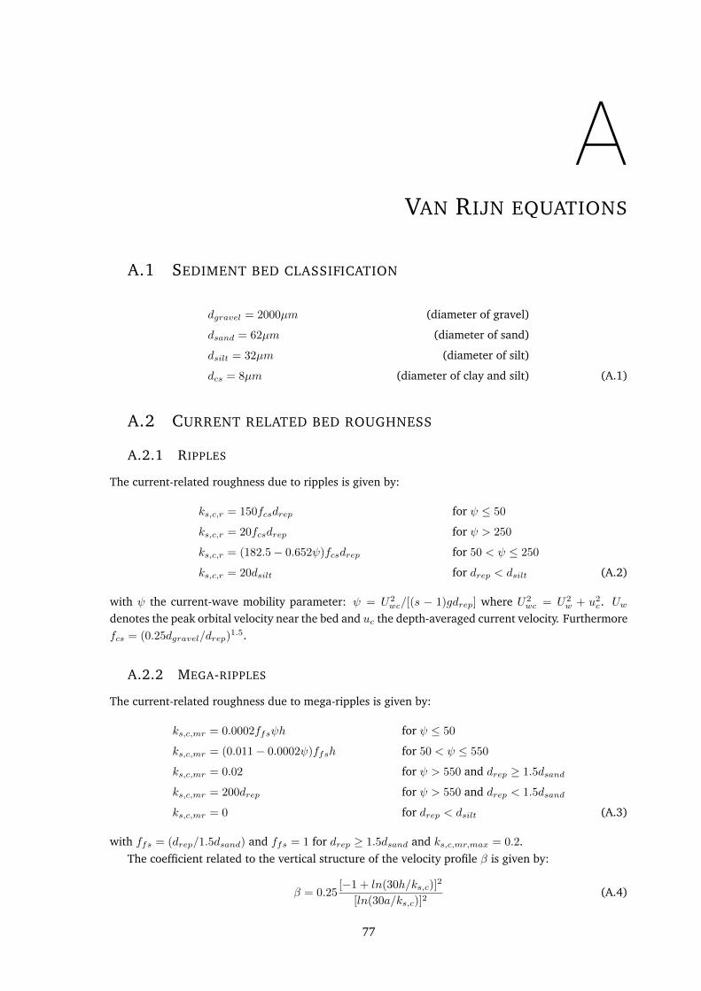
AVAN RIJN EQUATIONS
A.1 SEDIMENT BED CLASSIFICATION
dgravel = 2000µm (diameter of gravel)
dsand = 62µm (diameter of sand)
dsilt = 32µm (diameter of silt)
dcs = 8µm (diameter of clay and silt) (A.1)
A.2 CURRENT RELATED BED ROUGHNESS
A.2.1 RIPPLES
The current-related roughness due to ripples is given by:
ks,c,r = 150fcsdrep for ψ ≤ 50
ks,c,r = 20fcsdrep for ψ > 250
ks,c,r = (182.5− 0.652ψ)fcsdrep for 50 < ψ ≤ 250
ks,c,r = 20dsilt for drep < dsilt (A.2)
with ψ the current-wave mobility parameter: ψ = U2wc/[(s − 1)gdrep] where U2
wc = U2w + u2c . Uw
denotes the peak orbital velocity near the bed and uc the depth-averaged current velocity. Furthermorefcs = (0.25dgravel/drep)
1.5.
A.2.2 MEGA-RIPPLES
The current-related roughness due to mega-ripples is given by:
ks,c,mr = 0.0002ffsψh for ψ ≤ 50
ks,c,mr = (0.011− 0.0002ψ)ffsh for 50 < ψ ≤ 550
ks,c,mr = 0.02 for ψ > 550 and drep ≥ 1.5dsand
ks,c,mr = 200drep for ψ > 550 and drep < 1.5dsand
ks,c,mr = 0 for drep < dsilt (A.3)
with ffs = (drep/1.5dsand) and ffs = 1 for drep ≥ 1.5dsand and ks,c,mr,max = 0.2.The coefficient related to the vertical structure of the velocity profile β is given by:
β = 0.25[−1 + ln(30h/ks,c)]
2
[ln(30a/ks,c)]2(A.4)
77
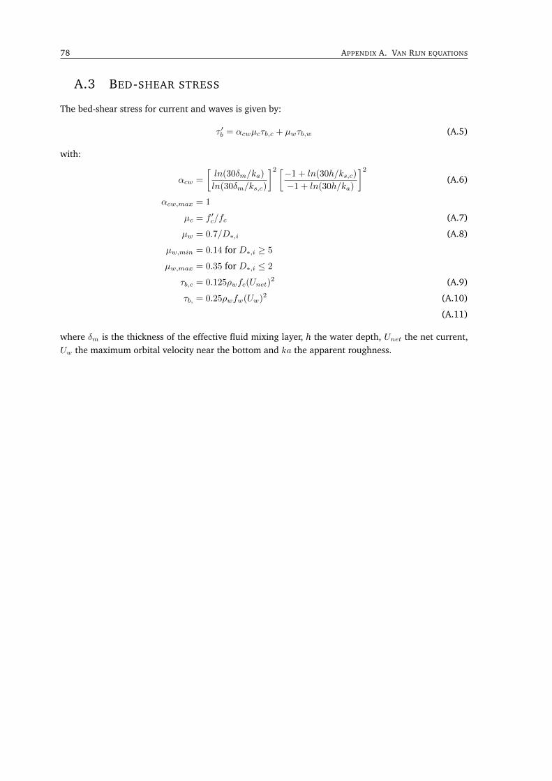
78 APPENDIX A. VAN RIJN EQUATIONS
A.3 BED-SHEAR STRESS
The bed-shear stress for current and waves is given by:
τ ′b = αcwµcτb,c + µwτb,w (A.5)
with:
αcw =
[ln(30δm/ka)
ln(30δm/ks,c)
]2 [−1 + ln(30h/ks,c)
−1 + ln(30h/ka)
]2(A.6)
αcw,max = 1
µc = f ′c/fc (A.7)
µw = 0.7/D∗,i (A.8)
µw,min = 0.14 for D∗,i ≥ 5
µw,max = 0.35 for D∗,i ≤ 2
τb,c = 0.125ρwfc(Unet)2 (A.9)
τb, = 0.25ρwfw(Uw)2 (A.10)
(A.11)
where δm is the thickness of the effective fluid mixing layer, h the water depth, Unet the net current,Uw the maximum orbital velocity near the bottom and ka the apparent roughness.
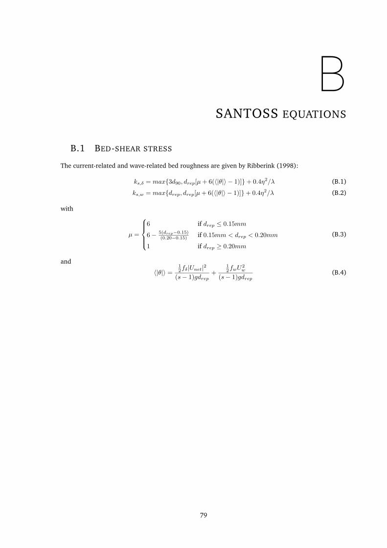
BSANTOSS EQUATIONS
B.1 BED-SHEAR STRESS
The current-related and wave-related bed roughness are given by Ribberink (1998):
ks,δ = max3d90, drep[µ+ 6(〈|θ|〉 − 1)]+ 0.4η2/λ (B.1)
ks,w = maxdrep, drep[µ+ 6(〈|θ|〉 − 1)]+ 0.4η2/λ (B.2)
with
µ =
6 if drep ≤ 0.15mm
6− 5(drep−0.15)(0.20−0.15) if 0.15mm < drep < 0.20mm
1 if drep ≥ 0.20mm
(B.3)
and
〈|θ|〉 =12fδ|Unet|
2
(s− 1)gdrep+
12fwU
2w
(s− 1)gdrep(B.4)
79
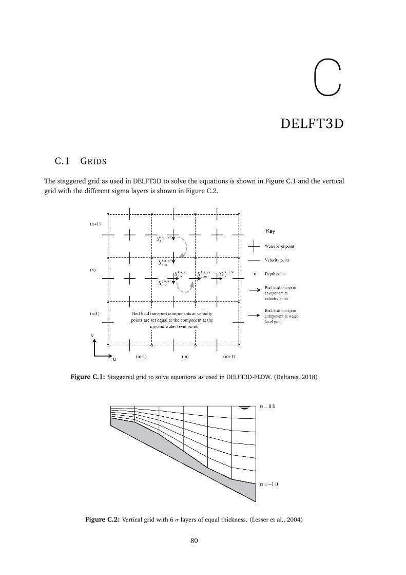
CDELFT3D
C.1 GRIDS
The staggered grid as used in DELFT3D to solve the equations is shown in Figure C.1 and the verticalgrid with the different sigma layers is shown in Figure C.2.
Figure C.1: Staggered grid to solve equations as used in DELFT3D-FLOW. (Deltares, 2018)
Figure C.2: Vertical grid with 6 σ layers of equal thickness. (Lesser et al., 2004)
80
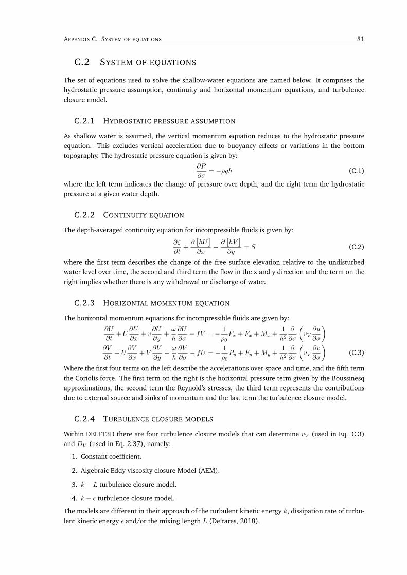
APPENDIX C. SYSTEM OF EQUATIONS 81
C.2 SYSTEM OF EQUATIONS
The set of equations used to solve the shallow-water equations are named below. It comprises thehydrostatic pressure assumption, continuity and horizontal momentum equations, and turbulenceclosure model.
C.2.1 HYDROSTATIC PRESSURE ASSUMPTION
As shallow water is assumed, the vertical momentum equation reduces to the hydrostatic pressureequation. This excludes vertical acceleration due to buoyancy effects or variations in the bottomtopography. The hydrostatic pressure equation is given by:
∂P
∂σ= −ρgh (C.1)
where the left term indicates the change of pressure over depth, and the right term the hydrostaticpressure at a given water depth.
C.2.2 CONTINUITY EQUATION
The depth-averaged continuity equation for incompressible fluids is given by:
∂ζ
∂t+∂[hU]
∂x+∂[hV]
∂y= S (C.2)
where the first term describes the change of the free surface elevation relative to the undisturbedwater level over time, the second and third term the flow in the x and y direction and the term on theright implies whether there is any withdrawal or discharge of water.
C.2.3 HORIZONTAL MOMENTUM EQUATION
The horizontal momentum equations for incompressible fluids are given by:
∂U
∂t+ U
∂U
∂x+ v
∂U
∂y+ω
h
∂U
∂σ− fV = − 1
ρ0Px + Fx +Mx +
1
h2∂
∂σ
(vV
∂u
∂σ
)∂V
∂t+ U
∂V
∂x+ V
∂V
∂y+ω
h
∂V
∂σ− fU = − 1
ρ0Py + Fy +My +
1
h2∂
∂σ
(vV
∂v
∂σ
)(C.3)
Where the first four terms on the left describe the accelerations over space and time, and the fifth termthe Coriolis force. The first term on the right is the horizontal pressure term given by the Boussinesqapproximations, the second term the Reynold’s stresses, the third term represents the contributionsdue to external source and sinks of momentum and the last term the turbulence closure model.
C.2.4 TURBULENCE CLOSURE MODELS
Within DELFT3D there are four turbulence closure models that can determine vV (used in Eq. C.3)and DV (used in Eq. 2.37), namely:
1. Constant coefficient.
2. Algebraic Eddy viscosity closure Model (AEM).
3. k − L turbulence closure model.
4. k − ε turbulence closure model.
The models are different in their approach of the turbulent kinetic energy k, dissipation rate of turbu-lent kinetic energy ε and/or the mixing length L (Deltares, 2018).
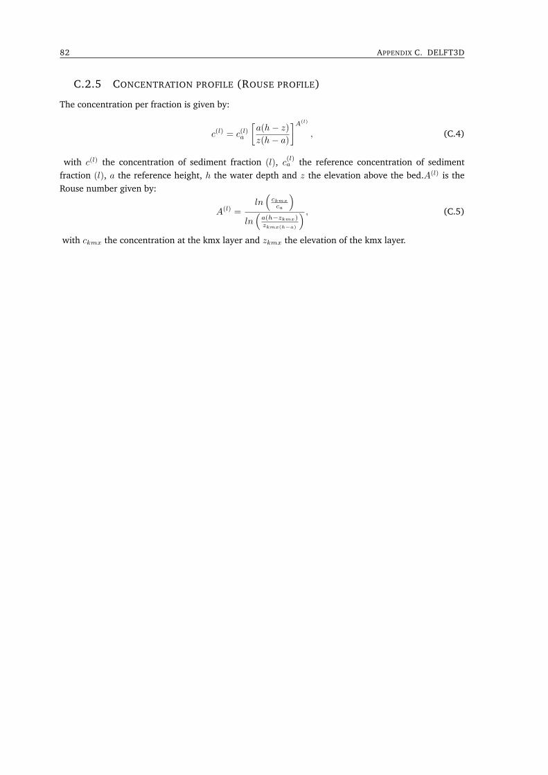
82 APPENDIX C. DELFT3D
C.2.5 CONCENTRATION PROFILE (ROUSE PROFILE)
The concentration per fraction is given by:
c(l) = c(l)a
[a(h− z)z(h− a)
]A(l)
, (C.4)
with c(l) the concentration of sediment fraction (l), c(l)a the reference concentration of sedimentfraction (l), a the reference height, h the water depth and z the elevation above the bed.A(l) is theRouse number given by:
A(l) =ln(ckmx
ca
)ln(a(h−zkmx)zkmx(h−a)
) , (C.5)
with ckmx the concentration at the kmx layer and zkmx the elevation of the kmx layer.
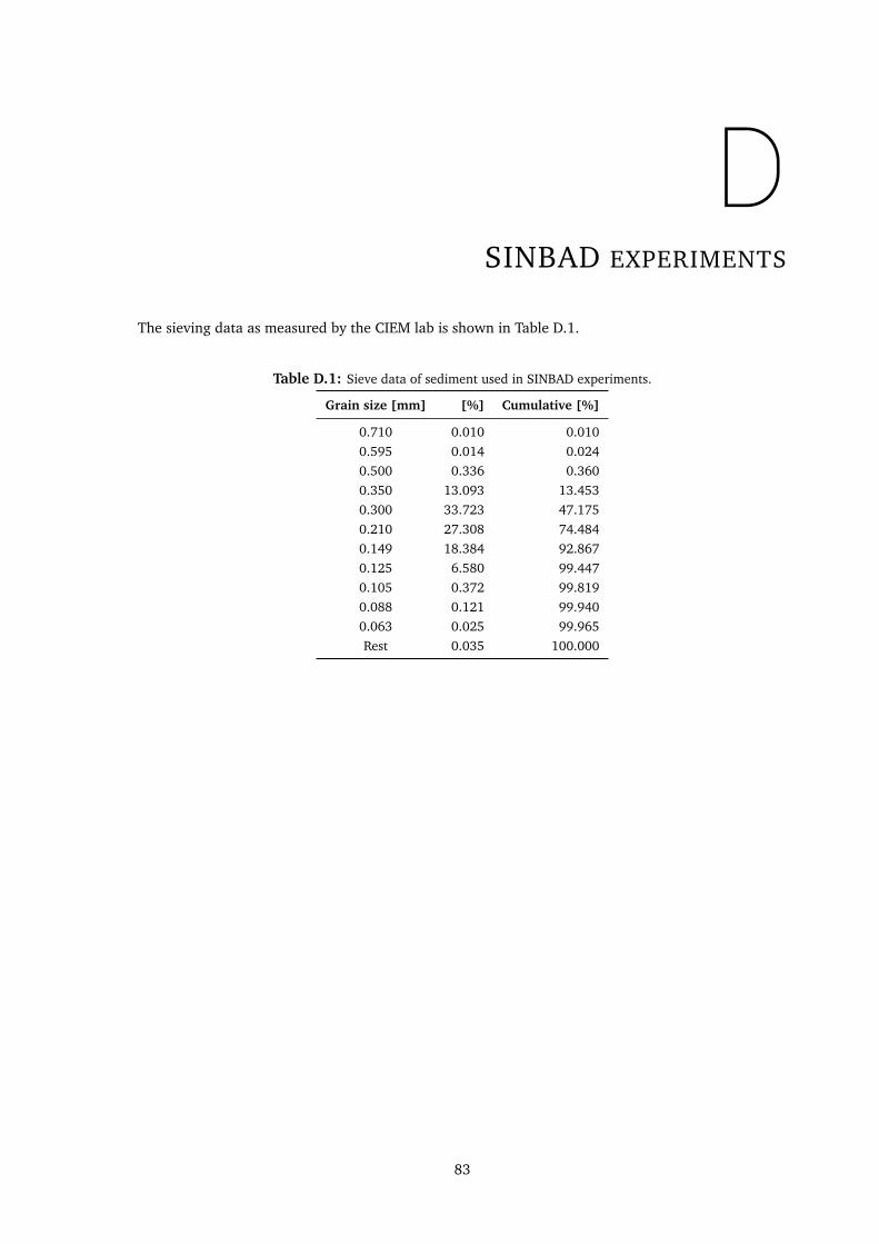
DSINBAD EXPERIMENTS
The sieving data as measured by the CIEM lab is shown in Table D.1.
Table D.1: Sieve data of sediment used in SINBAD experiments.
Grain size [mm] [%] Cumulative [%]
0.710 0.010 0.0100.595 0.014 0.0240.500 0.336 0.3600.350 13.093 13.4530.300 33.723 47.1750.210 27.308 74.4840.149 18.384 92.8670.125 6.580 99.4470.105 0.372 99.8190.088 0.121 99.9400.063 0.025 99.965Rest 0.035 100.000
83
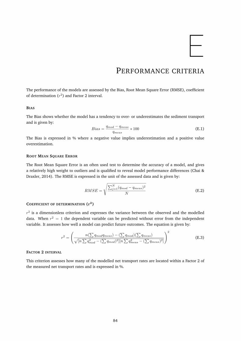
EPERFORMANCE CRITERIA
The performance of the models are assessed by the Bias, Root Mean Square Error (RMSE), coefficientof determination (r2) and Factor 2 interval.
BIAS
The Bias shows whether the model has a tendency to over- or underestimates the sediment transportand is given by:
Bias =qmod − qmeas
qmeas∗ 100 (E.1)
The Bias is expressed in % where a negative value implies underestimation and a positive valueoverestimation.
ROOT MEAN SQUARE ERROR
The Root Mean Square Error is an often used test to determine the accuracy of a model, and givesa relatively high weight to outliers and is qualified to reveal model performance differences (Chai &Draxler, 2014). The RMSE is expressed in the unit of the assessed data and is given by:
RMSE =
√∑Nj=1(qmod − qmeas)2
N(E.2)
COEFFICIENT OF DETERMINATION (r2)
r2 is a dimensionless criterion and expresses the variance between the observed and the modelleddata. When r2 = 1 the dependent variable can be predicted without error from the independentvariable. It assesses how well a model can predict future outcomes. The equation is given by:
r2 =
(n(∑qmodqmeas)− (
∑qmod)(
∑qmeas)√
[n∑q2mod − (
∑qmod)2][n
∑q2meas − (
∑qmeas)2]
)2
(E.3)
FACTOR 2 INTERVAL
This criterion assesses how many of the modelled net transport rates are located within a Factor 2 ofthe measured net transport rates and is expressed in %.
84
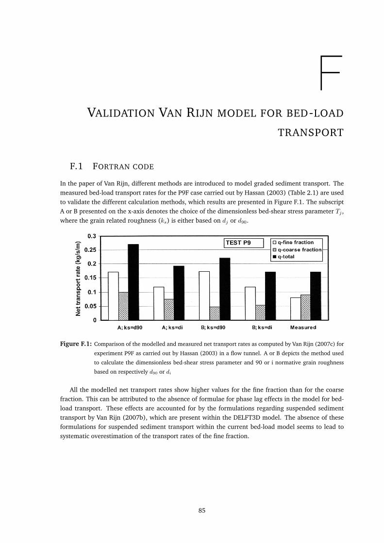
FVALIDATION VAN RIJN MODEL FOR BED-LOAD
TRANSPORT
F.1 FORTRAN CODE
In the paper of Van Rijn, different methods are introduced to model graded sediment transport. Themeasured bed-load transport rates for the P9F case carried out by Hassan (2003) (Table 2.1) are usedto validate the different calculation methods, which results are presented in Figure F.1. The subscriptA or B presented on the x-axis denotes the choice of the dimensionless bed-shear stress parameter Tj ,where the grain related roughness (ks) is either based on dj or d90.
Figure F.1: Comparison of the modelled and measured net transport rates as computed by Van Rijn (2007c) for
experiment P9F as carried out by Hassan (2003) in a flow tunnel. A or B depicts the method used
to calculate the dimensionless bed-shear stress parameter and 90 or i normative grain roughness
based on respectively d90 or di
All the modelled net transport rates show higher values for the fine fraction than for the coarsefraction. This can be attributed to the absence of formulae for phase lag effects in the model for bed-load transport. These effects are accounted for by the formulations regarding suspended sedimenttransport by Van Rijn (2007b), which are present within the DELFT3D model. The absence of theseformulations for suspended sediment transport within the current bed-load model seems to lead tosystematic overestimation of the transport rates of the fine fraction.
85
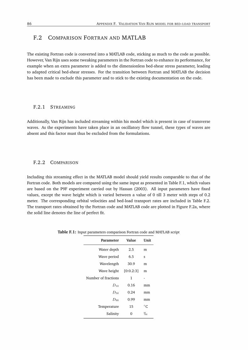
86 APPENDIX F. VALIDATION VAN RIJN MODEL FOR BED-LOAD TRANSPORT
F.2 COMPARISON FORTRAN AND MATLAB
The existing Fortran code is converted into a MATLAB code, sticking as much to the code as possible.However, Van Rijn uses some tweaking parameters in the Fortran code to enhance its performance, forexample when an extra parameter is added to the dimensionless bed-shear stress parameter, leadingto adapted critical bed-shear stresses. For the transition between Fortran and MATLAB the decisionhas been made to exclude this parameter and to stick to the existing documentation on the code.
F.2.1 STREAMING
Additionally, Van Rijn has included streaming within his model which is present in case of transversewaves. As the experiments have taken place in an oscillatory flow tunnel, these types of waves areabsent and this factor must thus be excluded from the formulations.
F.2.2 COMPARISON
Including this streaming effect in the MATLAB model should yield results comparable to that of theFortran code. Both models are compared using the same input as presented in Table F.1, which valuesare based on the P9F experiment carried out by Hassan (2003). All input parameters have fixedvalues, except the wave height which is varied between a value of 0 till 3 meter with steps of 0.2meter. The corresponding orbital velocities and bed-load transport rates are included in Table F.2.The transport rates obtained by the Fortran code and MATLAB code are plotted in Figure F.2a, wherethe solid line denotes the line of perfect fit.
Table F.1: Input parameters comparison Fortran code and MATLAB script
Parameter Value Unit
Water depth 2.5 m
Wave period 6.5 s
Wavelength 30.9 m
Wave height [0:0.2:3] m
Number of fractions 1 -
D10 0.16 mm
D50 0.24 mm
D90 0.99 mm
Temperature 15 C
Salinity 0 h
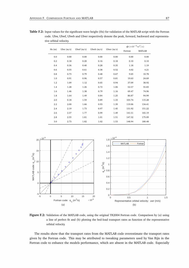
APPENDIX F. COMPARISON FORTRAN AND MATLAB 87
Table F.2: Input values for the significant wave height (Hs) for validation of the MATLAB script with the Fortran
code. Ubw, Ubwf, Ubwb and Ubwr respectively denote the peak, forward, backward and representa-
tive orbital velocity.
Hs (m) Ubw (m/s) Ubwf (m/s) Ubwb (m/s) Ubwr (m/s)qb (∗10−6m2/s)
Fortran MATLAB
0.0 0.00 0.00 0.00 0.00 0.00 0.00
0.2 0.18 0.20 0.16 0.18 0.10 0.10
0.4 0.36 0.40 0.28 0.35 1.18 1.19
0.6 0.55 0.61 0.38 0.52 4.02 4.21
0.8 0.73 0.79 0.48 0.67 9.65 10.78
1.0 0.91 0.96 0.57 0.81 19.63 24.69
1.2 1.09 1.12 0.65 0.94 37.09 38.92
1.4 1.28 1.26 0.72 1.06 52.57 55.83
1.6 1.46 1.38 0.79 1.16 69.47 74.96
1.8 1.64 1.49 0.84 1.25 86.87 94.99
2.0 0.18 1.59 0.89 1.33 103.74 115.28
2.2 2.00 1.66 0.93 1.39 119.06 134.41
2.4 2.19 1.73 0.97 1.45 131.92 151.22
2.6 2.37 1.77 0.99 1.49 141.51 165.19
2.8 2.55 1.81 1.01 1.51 147.32 175.09
3.0 2.73 1.82 1.02 1.53 148.94 180.48
-5 0 5 10 15 20
Fortran code: qs (m2/s) 10-5
-5
0
5
10
15
20
MA
TLA
B c
ode:
qs (
m2/s
)
10-5
(a)
0 0.5 1 1.5
Representative orbital velocity: uwr (m/s)
0
0.2
0.4
0.6
0.8
1
1.2
1.4
1.6
1.8
qs (
m2/s
)
10-4
MATLAB Fortran
(b)
Figure F.2: Validation of the MATLAB code, using the original TR2004 Fortran code. Comparison by (a) using
a line of perfect fit and (b) plotting the bed-load transport rates as function of the representative
orbital velocity.
The results show that the transport rates from the MATLAB code overestimate the transport ratesgiven by the Fortran code. This may be attributed to tweaking parameters used by Van Rijn in theFortran code to enhance the models performance, which are absent in the MATLAB code. Especially
88 APPENDIX F. VALIDATION VAN RIJN MODEL FOR BED-LOAD TRANSPORT
when the significant wave height and thus the orbital velocities are larger, the MATLAB code yieldsrelatively higher transport rates than the Fortran code. Nevertheless, as shown in the previous chapterwith the validation of the SANTOSS model, the transport rates hardly ever exceed 10∗10−5m/s, and isnot expected to do so either for the formulations by Van Rijn. In Figure F.2b the net bed-load transportis plotted as function of the representative orbital velocity. The actual representative orbital velocityfor this particular case (P9F, Table 2.1) is 1.32m/s, with a transport rate of 10− 11 ∗ 10−5m2/s.
F.3 MATLAB RESULTS
As streaming is not present within oscillatory flow tunnels, this term is now excluded from the modeland set to 0 m/s, resulting in the transport rates presented in Figure F.3.
A; ks=d90 A; ks=dj B; ks=d90 B; ks=dj Measured0
0.05
0.1
0.15
0.2
0.25
0.3
Net
tran
spor
t rat
e [k
g/s/
m] Fine fraction
Coarse fractionTotal net transport
Figure F.3: Comparison of the modelled and measured net transport rates as computed using the formulation
by Van Rijn (2007c) for experiment P9F as carried out by Hassan (2003) in a flow tunnel. A or
B depicts the method used to calculate the dimensionless bed-shear stress parameter and 90 or i
normative grain roughness based on respectively d90 or di
Due to the absence of streaming effects, the MATLAB model gives lower transport rates than theFortran code. Nevertheless, Figure F.3 seems to catch the patterns as presented in Figure F.1, wherethe proportions between the transport rates of the different fractions show clear resemblances. Thetransport rates however, are systematically overestimated in the Fortran code and underestimated inthe MATLAB model.
F.4 RESULTS FRACTIONS
The performance per fraction for the different model settings is presented in Table F.3.

APPENDIX F. RESULTS FRACTIONS 89
Tabl
eF.
3:Pe
rfor
man
ceof
the
Van
Rijn
mod
elw
hen
mod
ellin
gth
etr
ansp
ort
per
frac
tion
usin
gdi
ffer
ent
sett
ings
.he
aver
age
valu
eof
the
obse
rved
tran
spor
tis
0.32∗10−4m
2/s.
F,M
and
Cre
spec
tive
lyde
note
the
Fine
,Med
ium
and
Coa
rse
frac
tion
,and
N=
19.
Bia
s[%
]r2
[-]
RM
SE[∗10−4m
2/s]
Fact
or2
[%]
Nam
eSe
ttin
gN
o.#
FM
CF
MC
FM
CF
MC
Gra
ded
appr
oach
1.1
-125
-37
-44
0.21
0.88
0.92
0.11
0.13
0.09
5326
16
1.2
-120
-29
-37
0.18
0.87
0.88
0.11
0.13
0.08
5337
37
Gra
inro
ughn
ess
3.1
-118
-26
-43
0.18
0.83
0.91
0.14
0.12
0.09
3737
21
3.2
-108
-15
-36
0.14
0.78
0.87
0.17
0.12
0.08
3737
42
Hid
ing
and
expo
sure
4.1
-128
-41
-52
0.22
0.85
0.92
0.11
0.14
0.11
5315
0
4.2
-121
-28
-38
0.19
0.92
0.92
0.11
0.11
0.08
4737
32
4.3
-121
-28
-38
0.19
0.91
0.92
0.10
0.12
0.08
4737
32
4.4
-119
-30
-44
0.17
0.82
0.9
0.13
0.13
0.09
4737
16
4.5
-121
-28
-38
0.19
0.91
0.92
0.11
0.12
0.08
4737
32
4.6
-121
-28
-38
0.19
0.91
0.92
0.11
0.12
0.08
4737
32
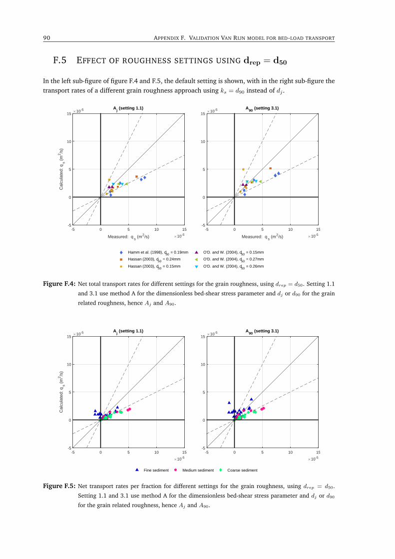
90 APPENDIX F. VALIDATION VAN RIJN MODEL FOR BED-LOAD TRANSPORT
F.5 EFFECT OF ROUGHNESS SETTINGS USING drep = d50
In the left sub-figure of figure F.4 and F.5, the default setting is shown, with in the right sub-figure thetransport rates of a different grain roughness approach using ks = d90 instead of dj .
-5 0 5 10 15
Measured: qs (m2/s) 10-5
-5
0
5
10
15
Cal
cula
ted:
qs (
m2/s
)
10-5 Aj (setting 1.1)
O'D. and W. (2004), d50 = 0.15mm
O'D. and W. (2004), d50 = 0.27mm
O'D. and W. (2004), d50 = 0.26mm
-5 0 5 10 15
Measured: qs (m2/s) 10-5
-5
0
5
10
1510-5 A
90 (setting 3.1)
Hamm et al. (1998), d50 = 0.19mm
Hassan (2003), d50 = 0.24mm
Hassan (2003), d50 = 0.15mm
Figure F.4: Net total transport rates for different settings for the grain roughness, using drep = d50. Setting 1.1
and 3.1 use method A for the dimensionless bed-shear stress parameter and dj or d90 for the grain
related roughness, hence Aj and A90.
-5 0 5 10 15
10-5
-5
0
5
10
15
Cal
cula
ted:
qs (
m2/s
)
10-5 Aj (setting 1.1)
-5 0 5 10 15
10-5
-5
0
5
10
1510-5 A
90 (setting 3.1)
Fine sediment Medium sediment Coarse sediment
Figure F.5: Net transport rates per fraction for different settings for the grain roughness, using drep = d50.
Setting 1.1 and 3.1 use method A for the dimensionless bed-shear stress parameter and dj or d90for the grain related roughness, hence Aj and A90.
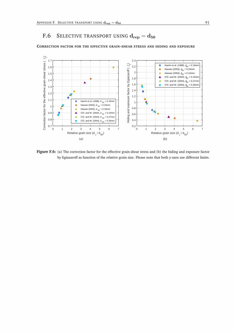
APPENDIX F. SELECTIVE TRANSPORT USING drep = d50 91
F.6 SELECTIVE TRANSPORT USING drep = d50
CORRECTION FACTOR FOR THE EFFECTIVE GRAIN-SHEAR STRESS AND HIDING AND EXPOSURE
0 1 2 3 4 5 6 7
Relative grain size (dj / d
50)
0.7
0.8
0.9
1
1.1
1.2
1.3
1.4
1.5
1.6
1.7
Cor
rect
ion
fact
or fo
r th
e ef
fect
ive
grai
n-sh
ear
stre
ss (
j)
Hamm et al. (1998), d50
= 0.19mm
Hassan (2003), d50
= 0.24mm
Hassan (2003), d50
= 0.15mm
O'D. and W. (2004), d50
= 0.15mm
O'D. and W. (2004), d50
= 0.27mm
O'D. and W. (2004), d50
= 0.26mm
(a)
0 1 2 3 4 5 6 7
Relative grain size (dj / d
50)
0.2
0.4
0.6
0.8
1
1.2
1.4
1.6
1.8
2
2.2
2.4
Hid
ing
and
expo
sure
fact
or b
y E
giaz
arof
f (j)
Hamm et al. (1998), d50 = 0.19mm
Hassan (2003), d50 = 0.24mm
Hassan (2003), d50 = 0.15mm
O'D. and W. (2004), d50 = 0.15mm
O'D. and W. (2004), d50 = 0.27mm
O'D. and W. (2004), d50 = 0.26mm
(b)
Figure F.6: (a) The correction factor for the effective grain-shear stress and (b) the hiding and exposure factor
by Egiazaroff as function of the relative grain size. Please note that both y-axes use different limits.
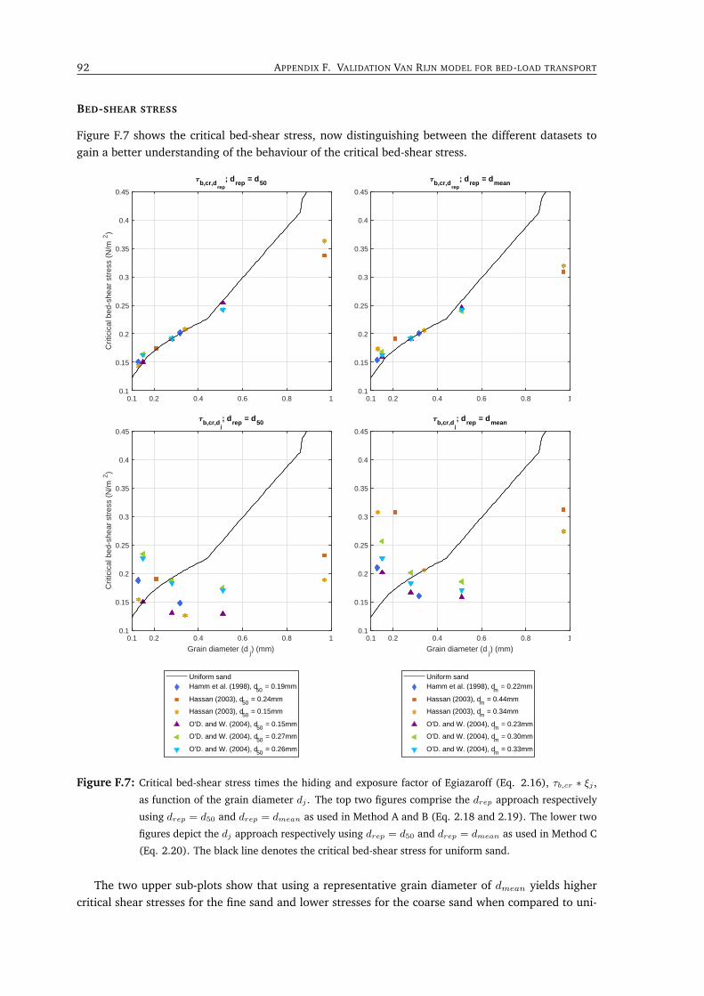
92 APPENDIX F. VALIDATION VAN RIJN MODEL FOR BED-LOAD TRANSPORT
BED-SHEAR STRESS
Figure F.7 shows the critical bed-shear stress, now distinguishing between the different datasets togain a better understanding of the behaviour of the critical bed-shear stress.
0.1 0.2 0.4 0.6 0.8 10.1
0.15
0.2
0.25
0.3
0.35
0.4
0.45
Crit
icic
al b
ed-s
hear
str
ess
(N/m
2)
b,cr,drep
; drep
= d50
0.1 0.2 0.4 0.6 0.8 10.1
0.15
0.2
0.25
0.3
0.35
0.4
0.45b,cr,d
rep
; drep
= dmean
0.1 0.2 0.4 0.6 0.8 1
Grain diameter (dj) (mm)
0.1
0.15
0.2
0.25
0.3
0.35
0.4
0.45
Crit
icic
al b
ed-s
hear
str
ess
(N/m
2)
b,cr,dj
; drep
= d50
Uniform sandHamm et al. (1998), d50 = 0.19mm
Hassan (2003), d50 = 0.24mm
Hassan (2003), d50 = 0.15mm
O'D. and W. (2004), d50 = 0.15mm
O'D. and W. (2004), d50 = 0.27mm
O'D. and W. (2004), d50 = 0.26mm
0.1 0.2 0.4 0.6 0.8 1
Grain diameter (dj) (mm)
0.1
0.15
0.2
0.25
0.3
0.35
0.4
0.45b,cr,d
j
; drep
= dmean
Uniform sandHamm et al. (1998), dm = 0.22mm
Hassan (2003), dm = 0.44mm
Hassan (2003), dm = 0.34mm
O'D. and W. (2004), dm = 0.23mm
O'D. and W. (2004), dm = 0.30mm
O'D. and W. (2004), dm = 0.33mm
Figure F.7: Critical bed-shear stress times the hiding and exposure factor of Egiazaroff (Eq. 2.16), τb,cr ∗ ξj ,
as function of the grain diameter dj . The top two figures comprise the drep approach respectively
using drep = d50 and drep = dmean as used in Method A and B (Eq. 2.18 and 2.19). The lower two
figures depict the dj approach respectively using drep = d50 and drep = dmean as used in Method C
(Eq. 2.20). The black line denotes the critical bed-shear stress for uniform sand.
The two upper sub-plots show that using a representative grain diameter of dmean yields highercritical shear stresses for the fine sand and lower stresses for the coarse sand when compared to uni-
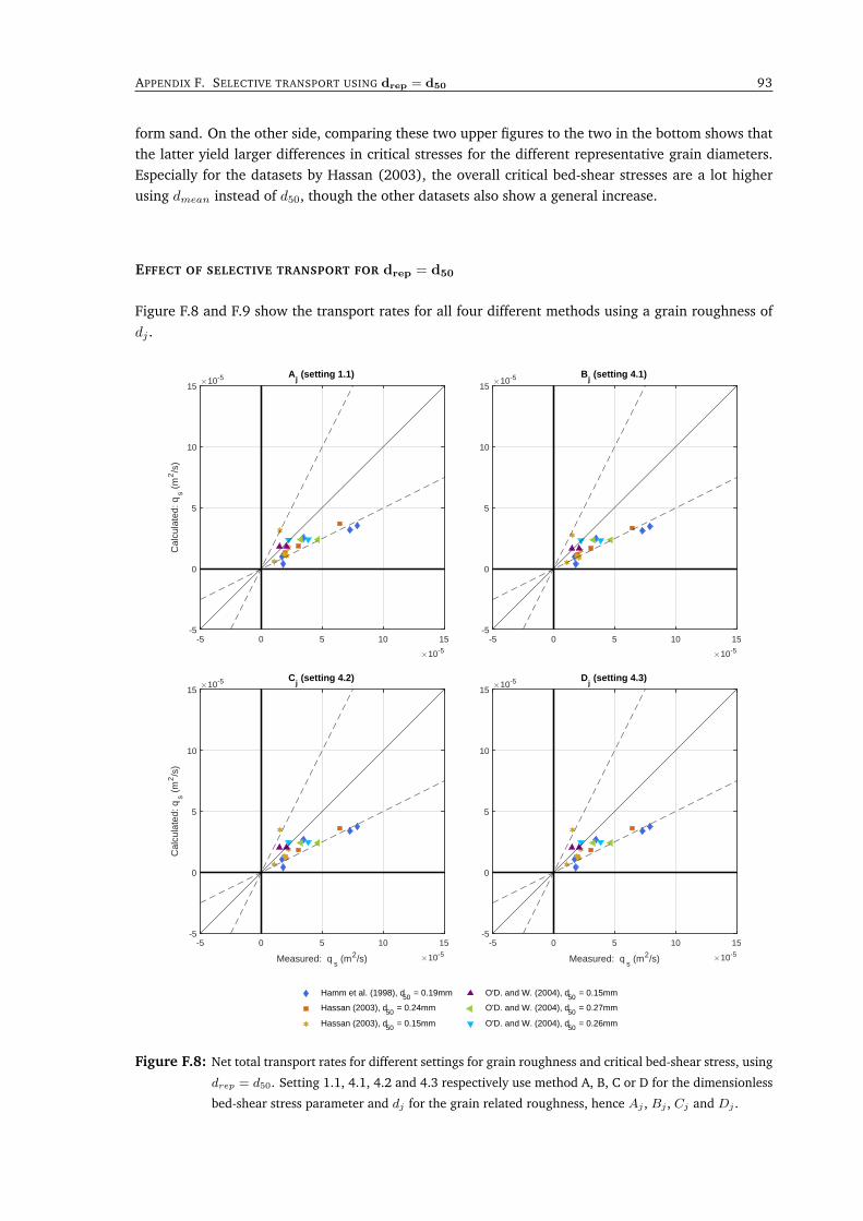
APPENDIX F. SELECTIVE TRANSPORT USING drep = d50 93
form sand. On the other side, comparing these two upper figures to the two in the bottom shows thatthe latter yield larger differences in critical stresses for the different representative grain diameters.Especially for the datasets by Hassan (2003), the overall critical bed-shear stresses are a lot higherusing dmean instead of d50, though the other datasets also show a general increase.
EFFECT OF SELECTIVE TRANSPORT FOR drep = d50
Figure F.8 and F.9 show the transport rates for all four different methods using a grain roughness ofdj .
-5 0 5 10 15
10-5
-5
0
5
10
15
Cal
cula
ted:
qs (
m2/s
)
10-5 Aj (setting 1.1)
-5 0 5 10 15
10-5
-5
0
5
10
1510-5 B
j (setting 4.1)
-5 0 5 10 15
Measured: qs (m2/s) 10-5
-5
0
5
10
15
Cal
cula
ted:
qs (
m2/s
)
10-5 Cj (setting 4.2)
O'D. and W. (2004), d50 = 0.15mm
O'D. and W. (2004), d50 = 0.27mm
O'D. and W. (2004), d50 = 0.26mm
-5 0 5 10 15
Measured: qs (m2/s) 10-5
-5
0
5
10
1510-5 D
j (setting 4.3)
Hamm et al. (1998), d50 = 0.19mm
Hassan (2003), d50 = 0.24mm
Hassan (2003), d50 = 0.15mm
Figure F.8: Net total transport rates for different settings for grain roughness and critical bed-shear stress, using
drep = d50. Setting 1.1, 4.1, 4.2 and 4.3 respectively use method A, B, C or D for the dimensionless
bed-shear stress parameter and dj for the grain related roughness, hence Aj , Bj , Cj and Dj .
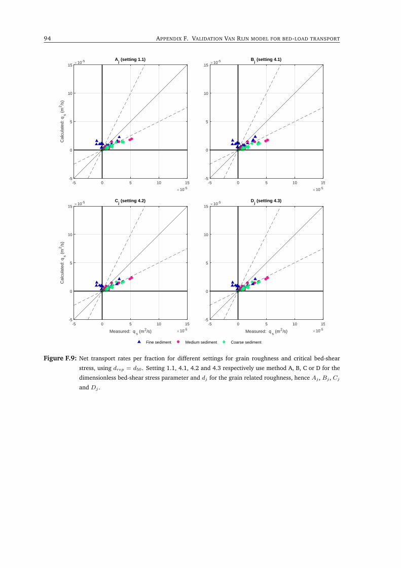
94 APPENDIX F. VALIDATION VAN RIJN MODEL FOR BED-LOAD TRANSPORT
-5 0 5 10 15
10-5
-5
0
5
10
15C
alcu
late
d: q
s (m
2/s
)10-5 A
j (setting 1.1)
-5 0 5 10 15
10-5
-5
0
5
10
1510-5 B
j (setting 4.1)
-5 0 5 10 15
Measured: qs (m2/s) 10-5
-5
0
5
10
15
Cal
cula
ted:
qs (
m2/s
)
10-5 Cj (setting 4.2)
-5 0 5 10 15
Measured: qs (m2/s) 10-5
-5
0
5
10
1510-5 D
j (setting 4.3)
Fine sediment Medium sediment Coarse sediment
Figure F.9: Net transport rates per fraction for different settings for grain roughness and critical bed-shear
stress, using drep = d50. Setting 1.1, 4.1, 4.2 and 4.3 respectively use method A, B, C or D for the
dimensionless bed-shear stress parameter and dj for the grain related roughness, hence Aj , Bj , Cj
and Dj .
GVALIDATION SANTOSS MODEL FOR BED-LOAD
TRANSPORT
G.1 RESULTS FRACTIONS
The performance per fraction for the different model settings is presented in Table G.1.
95
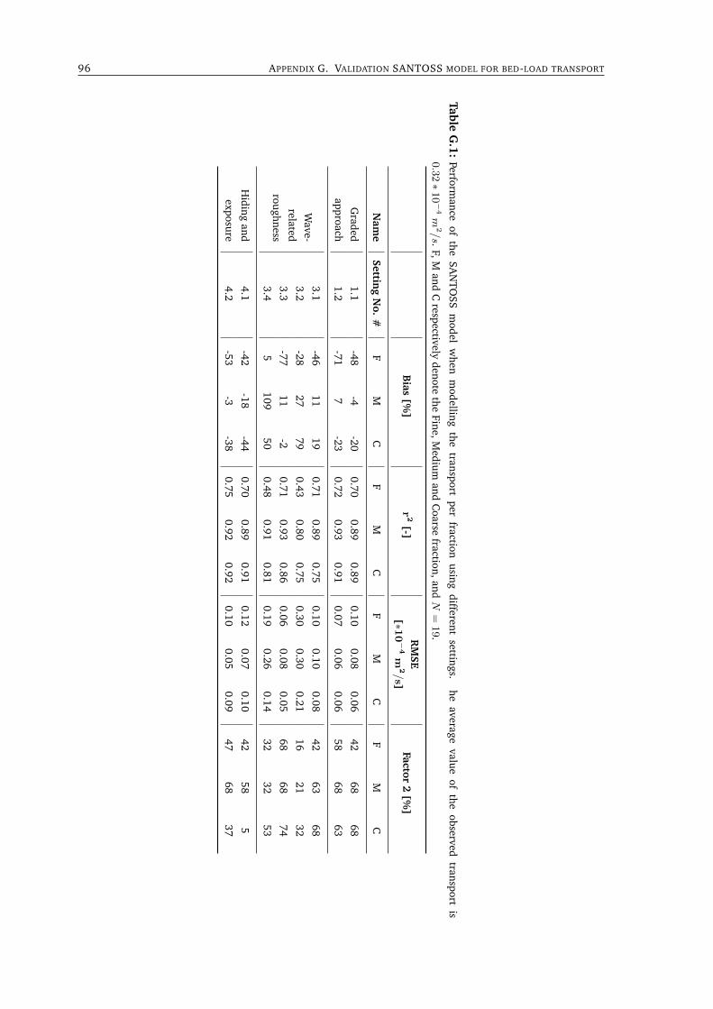
96 APPENDIX G. VALIDATION SANTOSS MODEL FOR BED-LOAD TRANSPORT
TableG
.1:Perform
anceof
theSA
NTO
SSm
odelw
henm
odellingthe
transportper
fractionusing
differentsettings.
heaverage
valueof
theobserved
transportis
0.32∗10−4m
2/s.
F,Mand
Crespectively
denotethe
Fine,Medium
andC
oarsefraction,and
N=
19.
Bias
[%]
r2
[-]R
MSE
[∗10−4m
2/s]
Factor2
[%]
Nam
eSettin
gN
o.#
FM
CF
MC
FM
CF
MC
Graded
approach1.1
-48-4
-200.70
0.890.89
0.100.08
0.0642
6868
1.2-71
7-23
0.720.93
0.910.07
0.060.06
5868
63
Wave-
relatedroughness
3.1-46
1119
0.710.89
0.750.10
0.100.08
4263
68
3.2-28
2779
0.430.80
0.750.30
0.300.21
1621
32
3.3-77
11-2
0.710.93
0.860.06
0.080.05
6868
74
3.45
10950
0.480.91
0.810.19
0.260.14
3232
53
Hiding
andexposure
4.1-42
-18-44
0.700.89
0.910.12
0.070.10
4258
5
4.2-53
-3-38
0.750.92
0.920.10
0.050.09
4768
37
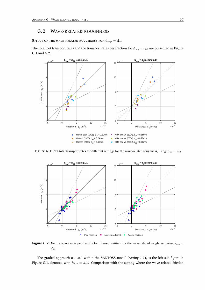
APPENDIX G. WAVE-RELATED ROUGHNESS 97
G.2 WAVE-RELATED ROUGHNESS
EFFECT OF THE WAVE-RELATED ROUGHNESS FOR drep = d50
The total net transport rates and the transport rates per fraction for drep = d50 are presented in FigureG.1 and G.2.
-5 0 5 10 15
Measured: qs (m2/s) 10-5
-5
0
5
10
15
Cal
cula
ted:
qs (
m2/s
)
10-5 ks,w
= d50
(setting 1.1)
O'D. and W. (2004), d50 = 0.15mm
O'D. and W. (2004), d50 = 0.27mm
O'D. and W. (2004), d50 = 0.26mm
-5 0 5 10 15
Measured: qs (m2/s) 10-5
-5
0
5
10
1510-5 k
s,w = d
j (setting 3.1)
Hamm et al. (1998), d50 = 0.19mm
Hassan (2003), d50 = 0.24mm
Hassan (2003), d50 = 0.15mm
Figure G.1: Net total transport rates for different settings for the wave-related roughness, using drep = d50
-5 0 5 10 15
Measured: qs (m2/s) 10-5
-5
0
5
10
15
Cal
cula
ted:
qs (
m2/s
)
10-5 ks,w
= d50
(setting 1.1)
-5 0 5 10 15
Measured: qs (m2/s) 10-5
-5
0
5
10
1510-5 k
s,w = d
j (setting 3.1)
Fine sediment Medium sediment Coarse sediment
Figure G.2: Net transport rates per fraction for different settings for the wave-related roughness, using drep =
d50
The graded approach as used within the SANTOSS model (setting 1.1), is the left sub-figure inFigure G.1, denoted with ks,w = d50. Comparison with the setting where the wave-related friction
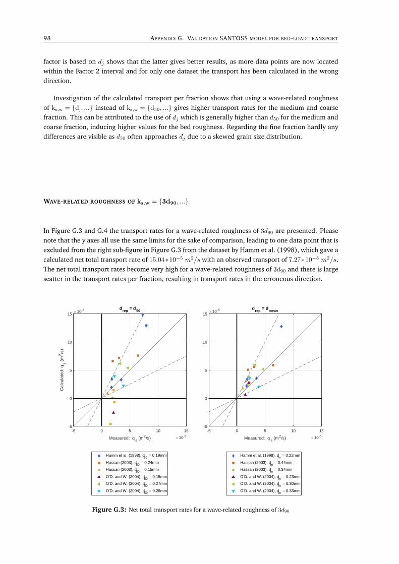
98 APPENDIX G. VALIDATION SANTOSS MODEL FOR BED-LOAD TRANSPORT
factor is based on dj shows that the latter gives better results, as more data points are now locatedwithin the Factor 2 interval and for only one dataset the transport has been calculated in the wrongdirection.
Investigation of the calculated transport per fraction shows that using a wave-related roughnessof ks,w = dj, ... instead of ks,w = d50, ... gives higher transport rates for the medium and coarsefraction. This can be attributed to the use of dj which is generally higher than d50 for the medium andcoarse fraction, inducing higher values for the bed roughness. Regarding the fine fraction hardly anydifferences are visible as d50 often approaches dj due to a skewed grain size distribution.
WAVE-RELATED ROUGHNESS OF ks,w = 3d90, ...
In Figure G.3 and G.4 the transport rates for a wave-related roughness of 3d90 are presented. Pleasenote that the y axes all use the same limits for the sake of comparison, leading to one data point that isexcluded from the right sub-figure in Figure G.3 from the dataset by Hamm et al. (1998), which gave acalculated net total transport rate of 15.04∗10−5 m2/s with an observed transport of 7.27∗10−5 m2/s.The net total transport rates become very high for a wave-related roughness of 3d90 and there is largescatter in the transport rates per fraction, resulting in transport rates in the erroneous direction.
-5 0 5 10 15
Measured: qs (m2/s) 10-5
-5
0
5
10
15
Cal
cula
ted:
qs (
m2/s
)
10-5 drep
= d50
Hamm et al. (1998), d50 = 0.19mm
Hassan (2003), d50 = 0.24mm
Hassan (2003), d50 = 0.15mm
O'D. and W. (2004), d50 = 0.15mm
O'D. and W. (2004), d50 = 0.27mm
O'D. and W. (2004), d50 = 0.26mm
-5 0 5 10 15
Measured: qs (m2/s) 10-5
-5
0
5
10
1510-5 d
rep = d
mean
Hamm et al. (1998), dm = 0.22mm
Hassan (2003), dm = 0.44mm
Hassan (2003), dm = 0.34mm
O'D. and W. (2004), dm = 0.23mm
O'D. and W. (2004), dm = 0.30mm
O'D. and W. (2004), dm = 0.33mm
Figure G.3: Net total transport rates for a wave-related roughness of 3d90
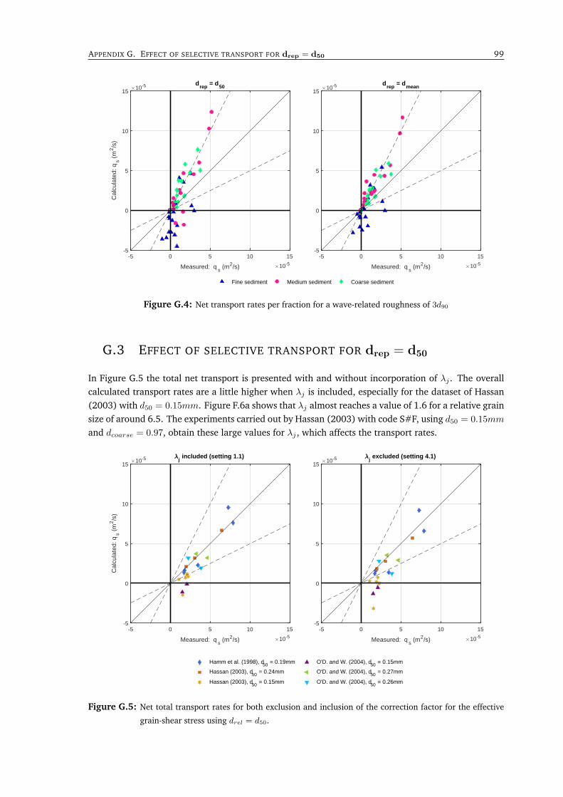
APPENDIX G. EFFECT OF SELECTIVE TRANSPORT FOR drep = d50 99
-5 0 5 10 15
Measured: qs (m2/s) 10-5
-5
0
5
10
15
Cal
cula
ted:
qs (
m2/s
)
10-5 drep
= d50
-5 0 5 10 15
Measured: qs (m2/s) 10-5
-5
0
5
10
1510-5 d
rep = d
mean
Fine sediment Medium sediment Coarse sediment
Figure G.4: Net transport rates per fraction for a wave-related roughness of 3d90
G.3 EFFECT OF SELECTIVE TRANSPORT FOR drep = d50
In Figure G.5 the total net transport is presented with and without incorporation of λj . The overallcalculated transport rates are a little higher when λj is included, especially for the dataset of Hassan(2003) with d50 = 0.15mm. Figure F.6a shows that λj almost reaches a value of 1.6 for a relative grainsize of around 6.5. The experiments carried out by Hassan (2003) with code S#F, using d50 = 0.15mm
and dcoarse = 0.97, obtain these large values for λj , which affects the transport rates.
-5 0 5 10 15
Measured: qs (m2/s) 10-5
-5
0
5
10
15
Cal
cula
ted:
qs (
m2/s
)
10-5 j included (setting 1.1)
O'D. and W. (2004), d50 = 0.15mm
O'D. and W. (2004), d50 = 0.27mm
O'D. and W. (2004), d50 = 0.26mm
-5 0 5 10 15
Measured: qs (m2/s) 10-5
-5
0
5
10
1510-5 j
excluded (setting 4.1)
Hamm et al. (1998), d50 = 0.19mm
Hassan (2003), d50 = 0.24mm
Hassan (2003), d50 = 0.15mm
Figure G.5: Net total transport rates for both exclusion and inclusion of the correction factor for the effective
grain-shear stress using drel = d50.
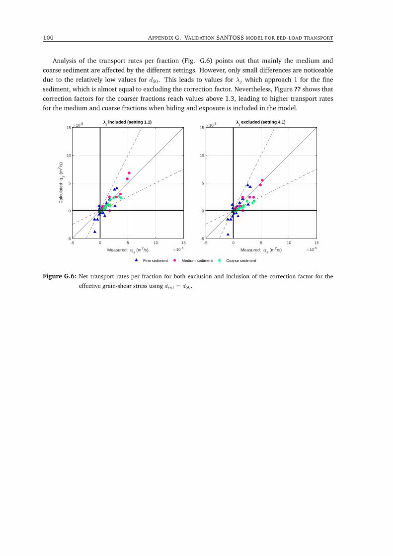
100 APPENDIX G. VALIDATION SANTOSS MODEL FOR BED-LOAD TRANSPORT
Analysis of the transport rates per fraction (Fig. G.6) points out that mainly the medium andcoarse sediment are affected by the different settings. However, only small differences are noticeabledue to the relatively low values for d50. This leads to values for λj which approach 1 for the finesediment, which is almost equal to excluding the correction factor. Nevertheless, Figure ?? shows thatcorrection factors for the coarser fractions reach values above 1.3, leading to higher transport ratesfor the medium and coarse fractions when hiding and exposure is included in the model.
-5 0 5 10 15
Measured: qs (m2/s) 10-5
-5
0
5
10
15
Cal
cula
ted:
qs (
m2/s
)
10-5 j included (setting 1.1)
-5 0 5 10 15
Measured: qs (m2/s) 10-5
-5
0
5
10
1510-5 j
excluded (setting 4.1)
Fine sediment Medium sediment Coarse sediment
Figure G.6: Net transport rates per fraction for both exclusion and inclusion of the correction factor for the
effective grain-shear stress using drel = d50.
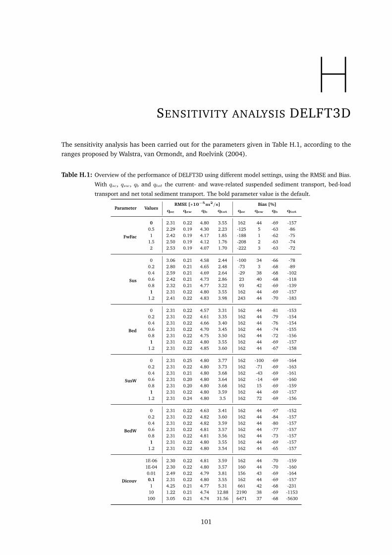
HSENSITIVITY ANALYSIS DELFT3D
The sensitivity analysis has been carried out for the parameters given in Table H.1, according to theranges proposed by Walstra, van Ormondt, and Roelvink (2004).
Table H.1: Overview of the performance of DELFT3D using different model settings, using the RMSE and Bias.
With qsc, qsw, qb and qtot the current- and wave-related suspended sediment transport, bed-load
transport and net total sediment transport. The bold parameter value is the default.
Parameter ValuesRMSE [∗10−5m2/s] Bias [%]
qsc qsw qb qtot qsc qsw qb qtot
FwFac
0 2.31 0.22 4.80 3.55 162 44 -69 -1570.5 2.29 0.19 4.30 2.23 -125 5 -63 -861 2.42 0.19 4.17 1.85 -188 1 -62 -75
1.5 2.50 0.19 4.12 1.76 -208 2 -63 -742 2.53 0.19 4.07 1.70 -222 3 -63 -72
Sus
0 3.06 0.21 4.58 2.44 -100 34 -66 -780.2 2.80 0.21 4.65 2.48 -73 3 -68 -890.4 2.59 0.21 4.69 2.64 -29 38 -68 -1020.6 2.42 0.21 4.73 2.86 23 40 -68 -1180.8 2.32 0.21 4.77 3.22 93 42 -69 -1391 2.31 0.22 4.80 3.55 162 44 -69 -157
1.2 2.41 0.22 4.83 3.98 243 44 -70 -183
Bed
0 2.31 0.22 4.57 3.31 162 44 -81 -1530.2 2.31 0.22 4.61 3.35 162 44 -79 -1540.4 2.31 0.22 4.66 3.40 162 44 -76 -1540.6 2.31 0.22 4.70 3.45 162 44 -74 -1550.8 2.31 0.22 4.75 3.50 162 44 -72 -1561 2.31 0.22 4.80 3.55 162 44 -69 -157
1.2 2.31 0.22 4.85 3.60 162 44 -67 -158
SusW
0 2.31 0.25 4.80 3.77 162 -100 -69 -1640.2 2.31 0.22 4.80 3.73 162 -71 -69 -1630.4 2.31 0.21 4.80 3.68 162 -43 -69 -1610.6 2.31 0.20 4.80 3.64 162 -14 -69 -1600.8 2.31 0.20 4.80 3.68 162 15 -69 -1591 2.31 0.22 4.80 3.59 162 44 -69 -157
1.2 2.31 0.24 4.80 3.5 162 72 -69 -156
BedW
0 2.31 0.22 4.63 3.41 162 44 -97 -1520.2 2.31 0.22 4.82 3.60 162 44 -84 -1570.4 2.31 0.22 4.82 3.59 162 44 -80 -1570.6 2.31 0.22 4.81 3.57 162 44 -77 -1570.8 2.31 0.22 4.81 3.56 162 44 -73 -1571 2.31 0.22 4.80 3.55 162 44 -69 -157
1.2 2.31 0.22 4.80 3.54 162 44 -65 -157
Dicouv
1E-06 2.30 0.22 4.81 3.59 162 44 -70 -1591E-04 2.30 0.22 4.80 3.57 160 44 -70 -1600.01 2.49 0.22 4.79 3.81 156 43 -69 -1640.1 2.31 0.22 4.80 3.55 162 44 -69 -1571 4.25 0.21 4.77 5.31 661 42 -68 -231
10 1.22 0.21 4.74 12.88 2190 38 -69 -1153100 3.05 0.21 4.74 31.56 6471 37 -68 -5630
101
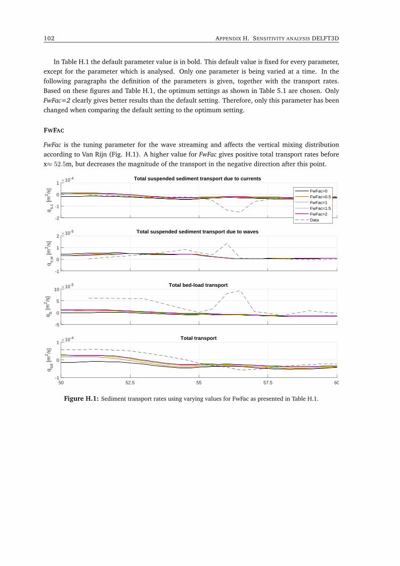
102 APPENDIX H. SENSITIVITY ANALYSIS DELFT3D
In Table H.1 the default parameter value is in bold. This default value is fixed for every parameter,except for the parameter which is analysed. Only one parameter is being varied at a time. In thefollowing paragraphs the definition of the parameters is given, together with the transport rates.Based on these figures and Table H.1, the optimum settings as shown in Table 5.1 are chosen. OnlyFwFac=2 clearly gives better results than the default setting. Therefore, only this parameter has beenchanged when comparing the default setting to the optimum setting.
FWFAC
FwFac is the tuning parameter for the wave streaming and affects the vertical mixing distributionaccording to Van Rijn (Fig. H.1). A higher value for FwFac gives positive total transport rates beforex≈ 52.5m, but decreases the magnitude of the transport in the negative direction after this point.
-2
-1
0
1
qs,
c [m
2/s
]
10-4 Total suspended sediment transport due to currents
FwFac=0FwFac=0.5FwFac=1FwFac=1.5FwFac=2Data
-1
0
1
2
qs,
w [m
2/s
]
10-5 Total suspended sediment transport due to waves
-5
0
5
10
qb [m
2/s
]
10-5 Total bed-load transport
50 52.5 55 57.5 60-1
0
1
qto
t [m2/s
]
10-4 Total transport
Figure H.1: Sediment transport rates using varying values for FwFac as presented in Table H.1.
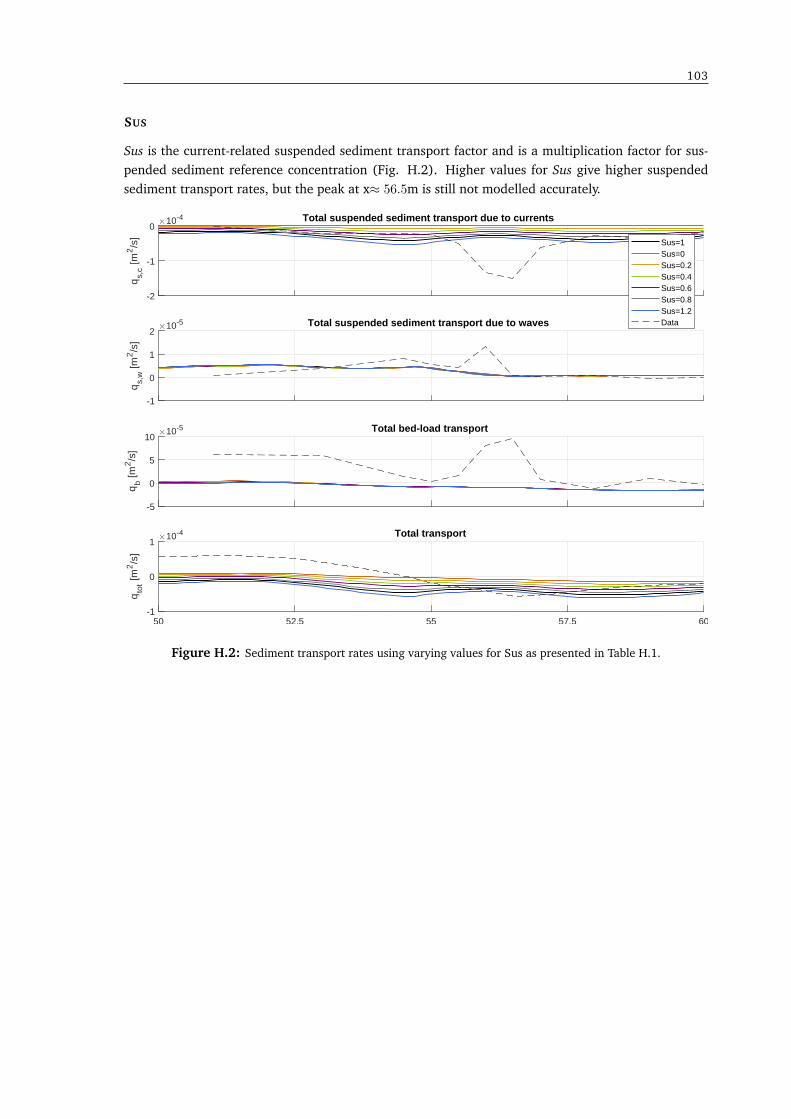
103
SUS
Sus is the current-related suspended sediment transport factor and is a multiplication factor for sus-pended sediment reference concentration (Fig. H.2). Higher values for Sus give higher suspendedsediment transport rates, but the peak at x≈ 56.5m is still not modelled accurately.
-2
-1
0
qs,
c [m
2/s
]
10-4 Total suspended sediment transport due to currents
Sus=1Sus=0Sus=0.2Sus=0.4Sus=0.6Sus=0.8Sus=1.2Data
-1
0
1
2
qs,
w [m
2/s
]
10-5 Total suspended sediment transport due to waves
-5
0
5
10
qb [m
2/s
]
10-5 Total bed-load transport
50 52.5 55 57.5 60-1
0
1
qto
t [m2/s
]
10-4 Total transport
Figure H.2: Sediment transport rates using varying values for Sus as presented in Table H.1.
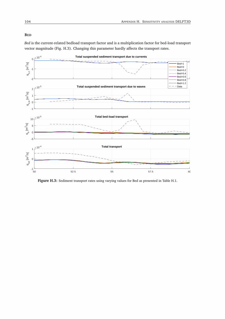
104 APPENDIX H. SENSITIVITY ANALYSIS DELFT3D
BED
Bed is the current-related bedload transport factor and is a multiplication factor for bed-load transportvector magnitude (Fig. H.3). Changing this parameter hardly affects the transport rates.
-2
-1
0
qs,
c [m
2/s
]
10-4 Total suspended sediment transport due to currents
Bed=1Bed=0Bed=0.2Bed=0.4Bed=0.6Bed=0.8Bed=1.2Data
-1
0
1
2
qs,
w [m
2/s
]
10-5 Total suspended sediment transport due to waves
-5
0
5
10
qb [m
2/s
]
10-5 Total bed-load transport
50 52.5 55 57.5 60-1
0
1
qto
t [m2/s
]
10-4 Total transport
Figure H.3: Sediment transport rates using varying values for Bed as presented in Table H.1.
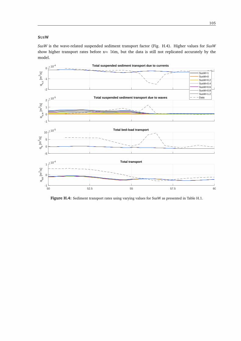
105
SUSW
SusW is the wave-related suspended sediment transport factor (Fig. H.4). Higher values for SusWshow higher transport rates before x≈ 56m, but the data is still not replicated accurately by themodel.
-2
-1
0
qs,
c [m
2/s
]
10-4 Total suspended sediment transport due to currents
SusW=1SusW=0SusW=0.2SusW=0.4SusW=0.6SusW=0.8SusW=1.2Data
-1
0
1
2
qs,
w [m
2/s
]
10-5 Total suspended sediment transport due to waves
-5
0
5
10
qb [m
2/s
]
10-5 Total bed-load transport
50 52.5 55 57.5 60-1
0
1
qto
t [m2/s
]
10-4 Total transport
Figure H.4: Sediment transport rates using varying values for SusW as presented in Table H.1.

106 APPENDIX H. SENSITIVITY ANALYSIS DELFT3D
BEDW
BedW is the wave-related bedload sediment transport factor (Fig. H.5). As for Bed, BedW also hardlyaffects the transport rates.
-2
-1
0
qs,
c [m
2/s
]
10-4 Total suspended sediment transport due to currents
BedW=1BedW=0BedW=0.2BedW=0.4BedW=0.6BedW=0.8BedW=1.2Data
-1
0
1
2
qs,
w [m
2/s
]
10-5 Total suspended sediment transport due to waves
-5
0
5
10
qb [m
2/s
]
10-5 Total bed-load transport
50 52.5 55 57.5 60-1
0
1
qto
t [m2/s
]
10-4 Total transport
Figure H.5: Sediment transport rates using varying values for BedW as presented in Table H.1.
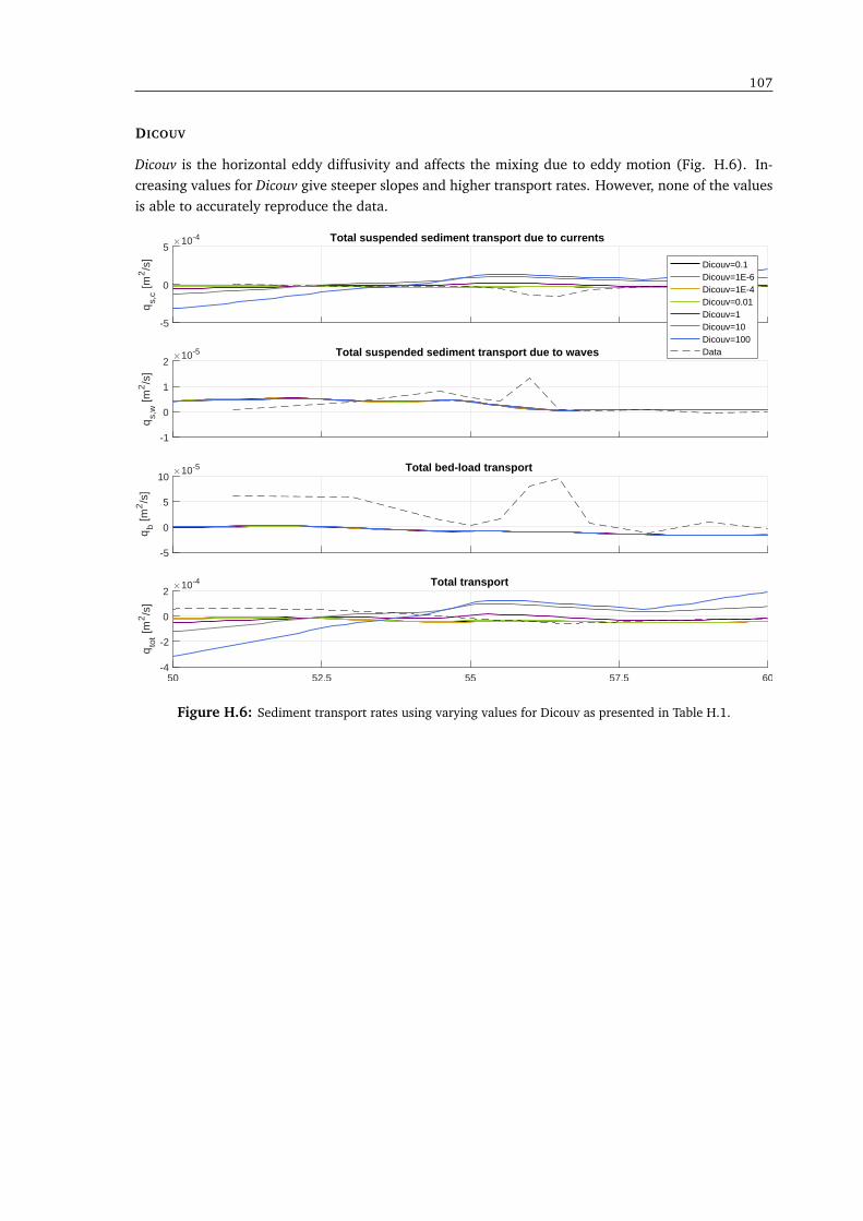
107
DICOUV
Dicouv is the horizontal eddy diffusivity and affects the mixing due to eddy motion (Fig. H.6). In-creasing values for Dicouv give steeper slopes and higher transport rates. However, none of the valuesis able to accurately reproduce the data.
-5
0
5
qs,
c [m
2/s
]
10-4 Total suspended sediment transport due to currents
Dicouv=0.1Dicouv=1E-6Dicouv=1E-4Dicouv=0.01Dicouv=1Dicouv=10Dicouv=100Data
-1
0
1
2
qs,
w [m
2/s
]
10-5 Total suspended sediment transport due to waves
-5
0
5
10
qb [m
2/s
]
10-5 Total bed-load transport
50 52.5 55 57.5 60-4
-2
0
2
qto
t [m2/s
]
10-4 Total transport
Figure H.6: Sediment transport rates using varying values for Dicouv as presented in Table H.1.