ww.sciencedirect.com

b i o s y s t em s e n g i n e e r i n g 1 1 6 ( 2 0 1 3 ) 9 7e1 1 0

Available online at w

journal homepage: www.elsev ier .com/locate/ issn/15375110

Research Paper

Modelling economic impacts of deficit irrigatedmaize in Brazil with consideration of differentrainfall regimes

Goncalo C. Rodrigues a, Juliano D. Martins b, Francisco G. da Silva a,Reimar Carlesso b, Luis S. Pereira a,*aCEER e Biosystems Engineering, Instituto Superior de Agronomia, Universidade de Lisboa,

Tapada da Ajuda, 1349-017 Lisboa, PortugalbCentro de Ciencia Rural, Universidade Federal de Santa Maria, Camobi, Santa Maria 91170-900, Rio Grande do Sul,

Brazil

a r t i c l e i n f o

Article history:

Received 10 December 2012

Received in revised form

19 April 2013

Accepted 3 July 2013

Published online 2 August 2013

* Corresponding author.E-mail addresses: gc.rodrigues@live.com.

1537-5110/$ e see front matter ª 2013 IAgrEhttp://dx.doi.org/10.1016/j.biosystemseng.20

Deficit irrigation is often required to cope with droughts and limited water availability.

However, to select an appropriate irrigation management, it is necessary to assess when

economic impacts of deficit irrigation are acceptable. Thus, the main goal of this study was

to evaluate economic water productivity for maize submitted to various levels of water

deficits and different irrigation systems. The study was based on two different experiments

conducted in Southern Brazil, one using sprinkler irrigation to supplement rainfall and the

other using drip irrigation with precipitation excluded by a rainfall shelter to simulate

cultivation under dry conditions. Water productivity indicators were calculated referring

to: a) actual field collected data, including yields, commodity prices and production costs;

and b) a sensitivity analysis to commodity prices and production costs. Alternative centre-

pivot irrigation scenarios were also developed to assess their feasibility in terms of water

use and productivity when irrigation is used to supplement rainfall or when rainfall is

scarce. Results show that the feasibility of deficit irrigation is highly influenced by com-

modity prices and by the irrigation (and water) costs when the irrigation costs are a large

part of the production costs. Results also show that deficit irrigation applied when rainfall

is abundant is easier to implement than deficit irrigation where rainfall is very scarce,

when only a mild stress is economically viable. For well-designed and managed centre-

pivot systems, results confirm that adopting deficit irrigation when rainfall is scarce is

less attractive than under conditions of irrigation to supplement rainfall. It could be

concluded that farmers are unlikely to choose a deficit irrigation strategy unless they are

facing reduced water availability for irrigation.

ª 2013 IAgrE. Published by Elsevier Ltd. All rights reserved.

pt, luis.santospereira@gmail.com (L.S. Pereira).. Published by Elsevier Ltd. All rights reserved.13.07.001

Nomenclature

Ainv investment annuity, BRL year�1

BWU beneficial water use, m3

BWUF beneficial water use fraction, dimensionless

Ca investment annuity per unit of irrigated area,

BRL ha�1 year�1

Cd energy demand tax, BRL kW�1

Cen annual energy costs, BRL ha�1 year�1

Cinv investment costs, BRL

Cm annual maintenance costs, BRL ha�1 year�1

CRF capital recovery factor, dimensionless

CU Christiansen coefficient of uniformity, %

DU distribution uniformity, %

ETo reference evapotranspiration, mm

ETa actual crop evapotranspiration, mm

EWP economic water productivity, BRLm�3

EWPBWU economic water productivity relative to beneficial

water use, BRLm�3

EWPIrrig irrigation economic water productivity, BRLm�3

EWPRfull-cost economic water productivity ratio considering

all production costs, dimensionless

EWPRirrig-cost economic water productivity ratio

considering only irrigation costs,

dimensionless

fr mulch fraction of the ground surface covered by mulch,

dimensionless

feff mulch fraction of the ground surface that is effectively

covered by mulch, dimensionless

IWU irrigation water use, m3

NIR net irrigation requirements, mm

TAW total available soil water, mm

TWU total water use, m3

WP water productivity, kgm�3

WPBWU water productivity relative to beneficial water use,

kgm�3

WPIrrig irrigation water productivity, kgm�3

Ya actual crop yield, kg ha�1

Acronyms

ISR irrigation in supplement to rainfall

ILR irrigation with very low rainfall

BRL Brazilian Real

b i o s y s t em s e n g i n e e r i n g 1 1 6 ( 2 0 1 3 ) 9 7e1 1 098

1. Introduction values (Lorite, Mateos, Orgaz, & Fereres, 2007; Rodrigues &

At present, more than 1.5 billion ha are used worldwide for

crop production and there is little scope for further expansion

of agricultural land; increasing land productivity, mainly

adopting irrigation, is definitely required. According to FAO

(2012), the world agricultural production has grown between

2.5 and 3 times over the last 50 years while the cultivated area

has grown only 12%. More than 40% of the global increase in

food production came from irrigated areas. However, at global

level, agricultural water use represents 70% of all water use.

Thus, and because water scarcity is increasing, the need to

optimise water withdrawal is also increasing, mainly for irri-

gation purposes (Pereira, Cordery, & Iacovides, 2009). Conse-

quently, farmers are forced to adopt an optimised irrigation

management in order to decrease the water demand while

increasing land and water productivity.

One commonly used technique that aims to decrease

water use is deficit irrigation. This approach consists of

deliberately applying irrigation depths smaller than those

required to fully satisfy the crop water requirements, thus

affecting evapotranspiration and consequently yields, but

keeping a positive return from the irrigated crop (Pereira,

Oweis, & Zairi, 2002). By avoiding water stress during

drought-sensitive stages, deficit irrigation also aims to maxi-

mise water productivity (Geerts & Raes, 2009; Kang, Shi, &

Zhang, 2000). However, particularly in arid regions, appro-

priate management is necessary to control effects of reduced

irrigation on soil salinity (Pereira, Goncalves, Dong, Mao, &

Fang, 2007; Xu et al., 2013). Moreover, depending upon water

management and available rainfall during the crop season,

the impacts of deficit irrigation on yields and related farmer

incomesmay ormay not be negative, also depending upon the

adopted irrigation scheduling, production costs and yield

Pereira, 2009). Katerji, Mastrorilli, and Chernic (2010) have

shown that maize water productivity (WP) varies with total

available soil water (TAW), with a high TAW favouring crop

responses to deficit irrigation. Various studies have been

developed to assess impacts of deficit irrigation on maize

yields and economic returns (Domınguez, de Juan, Tarjuelo,

Martınez, & Martınez-Romero, 2012; Farre & Faci, 2009;

Payero, Melvin, Irmak, & Tarkalson, 2006; Popova, Eneva, &

Pereira, 2006). These studies clearly demonstrate that the

feasibility of deficit irrigation strategies depends greatly upon

the crop variety and the adopted crop and irrigation man-

agement, mainly referring to when those deficits are applied,

e.g., Grassini et al. (2011) referred to the possibility of reducing

irrigation depths by 25% throughout the crop cycle except for a

�14 to þ7 d window around silking, during which crops must

be fully irrigated.

Another way to achieve efficient water use is through

increasing WP, including the related economic results; how-

ever the termWPmay be used with different meanings and at

various scales, which may lead to contradictory in-

terpretations. Various studies (Abd El-Wahed & Ali, 2013;

Bouman, 2007; Grassini et al., 2011; Molden et al., 2010; Playan

& Mateos, 2006; Zwart & Bastiaanssen, 2004) refer to factors

influencing WP, including irrigation management (e.g., sup-

plemental and deficit irrigation), irrigation systems and their

performance, crop varieties, soil fertility and TAW, pest and

diseases, and soilewater conservation practices (e.g., tillage

and mulching). Pereira, Cordery, and Iacovides (2012) defined

WP in agriculture as the ratio between the actual yield ach-

ieved (Ya) and the total water use (TWU). These authors, and

also van Halsema and Vincent (2012), emphasised that WP

enables an appropriate thinking about both the numerator

and the denominator, i.e., on both crop growth and yield and

b i o s y s t em s e n g i n e e r i n g 1 1 6 ( 2 0 1 3 ) 9 7e1 1 0 99

water use processes. Though expressing WP without assess-

ing the related economic impacts may lead to some misun-

derstanding, Pereira et al. (2012) also developed some

indicators relating to economic water productivity.

Since the economic value of water is of great importance in

a world where water scarcity is growing, it is imperative to

maximise the farmer’s income that results fromwater savings

while taking into account the irrigation system performance.

Grassini et al. (2011) reported that the quantification of water

use and WP in actual irrigated cropping systems provides

critical information to guide policies and regulations about

water use and allocation with the goal of maintaining or

increasing productivity while protecting natural resources. In

order to achieve improved WP, farmers may upgrade/

modernise their irrigation systems since the improvement of

irrigation performance, mainly the distribution uniformity, is

essential to reduce water demand at the farm level (Brennan,

2007; Pereira et al., 2002). This implies improved design,

appropriate selection of the irrigation equipment and careful

maintenance.When better distribution uniformity is attained,

conditions exist to achieve improved beneficial water use

(Pereira et al., 2012). However, there is a contradiction be-

tween economic results and the adoption of technologies that

provide water saving as reported by Darouich, Goncalves,

Muga, and Pereira (2012) in relation to modernising surface

irrigation systems; hence, efforts are required to help farmers

investing to achieve better irrigation performance.

Currently, farmers are investing in irrigation modernisa-

tion by switching from labour demanding and poorer per-

forming systems to automated ones, such as sprinkler and

drip irrigation systems, in order to improve water savings and

reduce labour and production costs. However, changes in

irrigation systems must consider the need to achieve the best

possible distribution uniformity. Several studies have

assessed impacts of irrigation non-uniformity on crop yields

and evidenced its importance (Brennan, 2007; Dechmi, Playan,

Cavero, Faci, & Martınez-Cob, 2003; Lopez-Mata, Tarjuelo, de

Juan, Ballesteros, & Domınguez, 2010; Mantovani, Villalobos,

Orgaz, & Fereres, 1995; Salmeron, Urrego, Isla, & Cavero,

2012; Sanchez, Zapata, & Faci, 2010).

Many sprinkler systems have neither been properly

designed or operated according to the design rules, or their

operation has been hampered by poor maintenance. This re-

sults in inadequate pressures and discharges along the sys-

tem, leading to actual application rates deviating from the

designed ones (Pereira, 1999). Poorly designed or managed set

sprinkler systems with low irrigation uniformity may lead to

wasted water and energy as well as to yield losses (Dechmi

et al., 2003; Salmeron et al., 2012; Salvador, Martınez-Cob,

Cavero, & Playan, 2011). By contrast, well-designed and

managed centre-pivot systems may provide highly uniform

water application (Valın, Cameira, Teodoro, & Pereira, 2012).

Drip irrigation systems have proved to be an effective

alternative in terms of distribution uniformity and water

saving. However, the performance of these systems depends

greatly on the quality of design and equipment selected

(Evans,Wu, & Smajstrala, 2007; Keller & Bliesner, 1990; Pedras,

Pereira, & Goncalves, 2009; Pereira, 1999). Although drip irri-

gation can provide highly uniform water application when a

good design is adopted, related objectives must combine with

appropriate irrigation scheduling in practice (Barragan, Cots,

Monserrat, Lopez, & Wu, 2010).

Brazil has 12% of the worldwide availability of water re-

sources and the potential for expansion of irrigated agricul-

ture is around 30 million ha (MIN, 2008), which represents an

additional 25.5 million ha considering the current irrigated

area of approximately 4.5 million ha. Despite the large po-

tential of soils for sustainable irrigation development, only a

small fraction is exploited. Therefore in Brazil the ratio of

irrigated area/irrigable area is small (about 10%), resulting in

a very low value of irrigated land area per capita at

0.018 ha person�1, the lowest in South America (ANA, 2009).

About 90% of the irrigated area was developed by private en-

terprise, and less than 10% through public projects. According

to the last agricultural census (IBGE, 2009), the irrigation

methods used in Brazil are distributed as follows: 24.35% by

flooding, 5.76% by furrow, 18.86% by centre-pivot sprinkling,

35.32% with other sprinkler methods, 7.36% by drip irrigation

and 8.35% with other methods. In the last 10 years there has

been an increase of 39% in the number of farmers using irri-

gation and of 42% in the total irrigated area, thus resulting an

average growth rate of 150,000 ha per year.

Centre-pivot systems are replacing surface and other

sprinkler irrigation systems due to easy automation, coverage

of a large area, reliability of the systems, high application

uniformity, and the ability to operate these systems on rela-

tively rough topography (Montero, Martınez, Valiente,

Moreno, & Tarjuelo, 2013; Valın et al., 2012). In Brazil, centre-

pivot systems irrigate an estimated area of 840,000 ha,

mainly in the Central-West region of the country, due to these

advantages and potential for achieving high water distribu-

tion uniformity (Sandri & Cortez, 2009). The area irrigated by

centre-pivots is rapidly increasing, with 300 new systems

(about 20,000 ha) installed in 2012 in Rio Grande do Sul State,

where the study reported here was developed.

Recent studies have assessed the impacts of centre-pivot

systems in terms of distribution uniformity, energy costs and

crop profitability. Lopez-Mata et al. (2010) concluded that

improving a centre-pivot to increase the water application

uniformity from 75 to 95% may increase the crop gross

margin by up to 27%. Ortız, de Juan, and Tarjuelo (2010)

analysed the effect of water application uniformity on the

uniformity of soil water content and crop yields for a centre-

pivot system irrigating sugar beet. The authors concluded

that yields were affected more by the amount of water

available in the soil than by the slight differences in soil

water uniformity, hence calling attention to the importance

of irrigation scheduling. Montero et al. (2013) analysed the

main factors influencing annual water application costs in

centre-pivot systems and determined themost cost-effective

centre-pivot design. They concluded that the cost of water

application with centre-pivot machines was quite sensitive

to the uniformity of water application. They also observed

that, to achieve high distribution uniformity, it is very

important to adopt a proper nozzle package and to perform

maintenance regularly. Moreno, Medina, Ortega, and

Tarjuelo (2012) developed a methodology for relating water

application costs in centre-pivot systems with hydraulic

factors, mainly relative to the pump and the pipe system,

which mainly relate to energy costs. However, the approach

b i o s y s t em s e n g i n e e r i n g 1 1 6 ( 2 0 1 3 ) 9 7e1 1 0100

did not lead to a clear assessment of the relationships be-

tween water saving, investments and yield incomes. Never-

theless, results agree with earlier analyses relating to

sprinkler systems (Mantovani et al., 1995; Pereira et al., 2002;

Tarjuelo, Montero, Carrion, Honrubia, & Calvo, 1999).

Considering the aspects analysed above and previous de-

velopments by Rodrigues and Pereira (2009), the main goal of

this study is to assess the economic impacts of water deficits,

irrigation systems performance, commodity prices, produc-

tion costs and water prices upon the physical and economic

water productivity of irrigated maize. The application data

used in this study are from two experimental maize fields in

Santa Maria (Southern Brazil), one irrigated by a set sprinkler

system to supplement rainfall, and the other by a drip system

where rainfall was excluded through use of a rainfall shelter,

as described by Martins et al. (2013). These two experiments

made it possible to assess impacts of deficit irrigation

comparing situations when rainfall is abundant or scarce.

Data were used to develop several alternative centre-pivot

irrigation scenarios in the form of different irrigation man-

agement options, in order to assess the economic feasibility of

deficit irrigation.

2. Materials and methods

2.1. Experimental area and irrigation experiments

The experimental study was conducted at the Department of

Agricultural Engineering, Federal University of Santa Maria

(UFSM), Santa Maria, Brazil, located in the Central Depression

of Rio Grande do Sul State. The climate is subtropical humid, a

“cfa” according to the climatic classification of Koppen,

without a dry season and with hot summers (Moreno, 1961).

During the summer months, when the atmospheric evapo-

rative demand is very high, dry spells often occur and rainfall

is not sufficient to meet crop needs.

During 2010/2011 growing season, two maize experiments

were conducted: one with irrigation to supplement rainfall

(ISR) using a set sprinkler system, and the other with very low

rainfall (ILR) by using a drip irrigation system under a rainfall

shelter. ISR represents rainfall conditions of Southern Brazil,

while ILR simulates conditions from dry central Brazil. Con-

ducting the experiments under different rainfall conditions

allows an improved basis for the use of the Sistema Irriga�(Carlesso, Petry, & Trois, 2009) under different climatic con-

ditions and for various irrigation strategies throughout Brazil.

Sistema Irriga� is presently monitoring more than 90,000 ha

each year in Brazil, including southern areaswith high rainfall

and areas in Central Brazil with very low rainfall. The ISR

experiments were conducted with three irrigation treatments

and 3 replications, with plots of 12� 12 m2, irrigated with a set

sprinkler system consisting of 4 sectorial sprinklers per plot

with an average application rate of 14.83 mmh�1. The ILR

experiments were performed with drip irrigation in an area

protected by a rainfall shelter that covered the experimental

area when rainfall occurred; rainfall was only allowed during

the initial crop stage to ensure adequate and uniform estab-

lishment of the crop. The experiments consisted of four irri-

gation treatmentswith 4 replications, with experimental plots

of 3� 6 m2. The irrigation system consisted of pressure

compensating in-line dripperswith a discharge of 1.3 l h�1 and

an application rate of 13 mmh�1. The experiments are

described in detail by Martins et al. (2013) including the cali-

bration and validation of the water balance model SIMDualKc

(Rosa et al., 2012) used in the present analysis.

Adopting the ISR and ILR experiments to base an analysis

of deficit irrigation strategies when rainfall is abundant or is

scarce is preferable to just performing simulations with actual

weather data because it allows the crop responses to these

different strategies to be captured. In subtropical areas the

main factor differentiating the crop demand for irrigation is

rainfall because it is the main factor controlling the avail-

ability of soil water (Rossato, Alvala, & Tomasella, 2004) and

the spatial variability of ETo is much smaller than the vari-

ability of precipitation. This has already been observed for the

irrigated areas monitored with the Sistema Irriga�; a better

model parameterisation for both high and low rainfall con-

ditions was intended when installing the experiments and

analysing them with the model SIMDualKc (Martins et al.,

2013).

Both experiments were conducted with mulch sincemaize

is generally cultivated in Brazil with direct seeding. Oats

(Avena strigosa) crop residues were used for ISR (5 t ha�1 of dry

biomass spread over all the soil surface, so the cover fraction fr

mulch¼ 1.0, and achieving an effective soil coverage feff

mulch¼ 0.9); beans (Phaseolus vulgaris L.) crop residues were

used for ILR (3 t ha�1 of dry biomass, fr mulch¼ 1.0 and feff

mulch¼ 0.8). The hybrid AG8011YG was used for ISR and the

hybrid P1630H was used for ILR. In both cases the plant den-

sity was 6.5 plantsm�2. Observations comprised irrigation

water depths applied, soil water content down to 0.90 m depth

using a calibrated set of FDR (Frequency Domain Reflectom-

etry) sensors, crop height, leaf area index (LAI), ground cover

fraction and yields. Detailed information on the experiments

and results has been published by Martins et al (2013). Main

results for all treatments, either observed or obtainedwith the

model SIMDualKc, are given in Table 1: net and gross irrigation

depths (NIWU & IWU, mm), precipitation (P, mm), total water

use (TWU, mm), actual evapotranspiration (ETa, mm), bene-

ficial water use fraction (BWUF) and actual yield (Ya, kg ha�1).

These results show that ISR treatments were without or with

only a mild water deficit while the ILR treatments all achieved

deficit, which increased from ILR1 to ILR4. TWU was obtained

by the sumof IWU, P and the variation of the soil water storage

between planting and harvesting.

The irrigation and production costs were set for each

treatment, taking into account the water and labour costs,

nutrients applied, seeds, machinery, energy required for irri-

gation and the investment andmaintenance required for each

system (Table 2). Data for labour, machinery and harvest costs

were obtained from regional data (CONAB, 2010). Costs con-

cerning seeds, fertilisers and irrigation were obtained from

the experimental data.

2.2. Water productivity and water use indicators

Water productivity (WP) concepts apply to various definitions

of water use and at various scales. Therefore, it is of great

importance to properly define the related concepts used in

Table 1 e Irrigation water use and grain yield relative to each treatment.

Treatment Irrigation to supplement rainfall Deficit irrigation with very low rainfall

ISR1 ISR2 ISR3 ILR1 ILR2 ILR3 ILR4

Net irrigation (NIWU, mm) 328 234 91 389 316 218 113

Gross irrigation (IWU, mm) 431 307 120 463 376 259 134

Rainfall (mm) 415 415 415 73 73 73 73

Total water use (TWU, mm) 853 732 615 539 468 421 329

Actual evapotranspiration (ETa, mm) 502 497 479 365 361 342 272

Beneficial water use fraction (BWUF) 0.59 0.68 0.78 0.68 0.77 0.81 0.83

Actual grain yield (Ya, kg ha�1) 13,212 12,548 12,011 9190 8340 7650 5312

Adapted from Martins et al., 2013.

b i o s y s t em s e n g i n e e r i n g 1 1 6 ( 2 0 1 3 ) 9 7e1 1 0 101

this study. Here, following Pereira et al. (2012), WP (kgm�3) is

defined as the ratio between the actual crop yield (Ya, kg) and

the total water use (TWU, m3), thus:

WP ¼ Ya

TWU(1)

When considering only the irrigation water use (IWU, m3), the

result is the irrigation water productivity (WPIrrig, kgm�3):

WPIrrig ¼ Ya

IWU(2)

Pereira et al. (2012) proposed new water use indicators

which include consideration of water reuse and aim to assist

in identifying and providing clear distinctions between bene-

ficial and non-beneficial water use because, from the water

economy perspective, it is important to recognise both. The

beneficial water use fraction (BWUF) may be defined as the

fraction of TWU that is used to produce the actual yield. In the

present situation, because there is no need for leaching or

Table 2 e Operation and irrigation costs used insimulations.

Items Costs

Operation costs

Machinery (BRL ha�1)a 204.00

Labour (BRL ha�1) 47.00

Seeds (BRL ha�1)

Set sprinkler 233.00

Drip 208.00

Fertilisers (BRL ha�1)

Set sprinkler 1108.00

Drip 797.00

Harvest (BRL ha�1) 265.00

Irrigation costs

Investment annuity (BRL ha�1 year�1)

Set sprinkler 441.00

Drip 778.00

Annual maintenance costs (BRL ha�1 year�1)

Set sprinkler 137.50

Drip 225.00

Water (BRLm�3) 0.005

Electricity (BRL kWh�1) 0.31

Labour (BRL ha�1) 40.00

a 1 BRL¼ 0.48 USD.

other processes such as runoff, and the presence of mulch

helps limit ET from weeds, the beneficial water use corre-

sponds to the actual ET. Thus, as an alternative to Eqs. (1) and

(2), WP may be computed in relation to the beneficial water

use (BWU, m3), thus

WPBWU ¼ Ya

BWU(3)

The water productivity may be considered not only in

physical terms, as above, but also in economic terms.

Replacing the numerator of Eq. (1) by the monetary value of

the achieved yield, the economic water productivity (EWP,

BRLm�3) is defined by:

EWP ¼ ValueðYaÞTWU

(4)

The monetary value refers to the Brazilian Real (BRL), for

which the exchange rate is 1 BRL¼ 0.48 USD (as of December

2012). When considering IWU or BWU only, this gives:

EWPIrrig ¼ ValueðYaÞTWU

(5)

EWPBWU ¼ ValueðYaÞBWU

(6)

It is important to consider the economic issues relating to

water productivity since the objective of a farmer is to achieve

the best income and profit. As for this study, the economics of

production is better considered when expressing both the

numerator and the denominator of Eq. (4) in monetary terms,

respectively the yield value and the TWU cost (including all

the farming costs), thus yielding the economic water pro-

ductivity ratio (EWPRfull-cost):

EWPRfull�cost ¼ ValueðYaÞCostðTWUÞ (7)

EWPRfull-cost allows assessment of whether a given man-

agement option leads to positive (EWPR� 1) or negative

(EWPR< 1) income since it compares the value of production

with the farming costs. If, as an alternative, one considers the

irrigation costs only, it results in:

EWPRirrig�cost ¼ ValueðYaÞCostðIWUÞ (8)

As referred to above, data on Ya, IWU, TWU and BWUF

(Table 1) were obtained from computing the soil water balance

Table 3 e Irrigation system scenarios

Sprinkler package Systemscenario

Irrigatedarea

Average landslope (%)

Pivot pointpressure (kPa)

CU (%) DU (%) Ca

(BRL ha�1 year�1)aCm

(BRL ha�1 year�1)a

Senninger�

Super Spray

S1 32.13 1.46 290 95.27 90.79 385 53

S2 46.34 1.52 385 96.51 93.00 369 51

S3 65.03 2.47 455 95.98 91.83 291 40

S4 81.27 0.65 410 96.61 93.01 269 37

S5 110.22 1.47 430 96.31 92.65 254 35

Nelson�

Rotator R3000

R1 32.13 1.46 330 92.16 87.80 417 56

R2 46.34 1.52 410 95.83 91.68 395 53

R3 65.03 2.47 480 93.73 89.81 314 42

R4 81.27 0.65 440 95.27 91.45 289 39

R5 110.22 1.47 470 94.19 90.48 272 37

CU¼Christiansen coefficient of uniformity; DU¼ distribution uniformity; Ca¼ investment annuity per unit of irrigated area; Cm¼ annual

maintenance costs.

a 1 BRL¼ 0.48 USD.

b i o s y s t em s e n g i n e e r i n g 1 1 6 ( 2 0 1 3 ) 9 7e1 1 0102

(Martins et al., 2013). The monetary values of yields were

computed using a grain price of 0.40 BRL kg�1. The irrigation

and production costs are summarised in Table 2.

2.3. Alternative irrigation system scenarios

In order to assess the impacts of adopting centre-pivot sys-

tems, themost common system for maize in Brazil at present,

several scenarios were developed that allow the economic

results of the corresponding investment to be assessed.

Simulation scenarios were created with irrigated areas, land

slopes, pivot point pressures and sprinkler packages corre-

sponding to five different centre-pivot systems in operation in

Rio Grande do Sul monitored by Sistema Irriga�. Data

collected from field assessments included the irrigated area,

pipe sizes, working pressure and discharge, and pump char-

acteristics. The simulation scenarios were developed with the

model DEPIVOT (Valın et al., 2012) using the actual system

characteristics.

The model DEPIVOT consists of a simulation package

developed in Visual Basic and database in Access. It allows

alternative sprinkler packages to be developed and compared

based on irrigation performance, including potential runoff.

The model comprises five main sub-models for: (a) computa-

tion of the gross irrigation requirements; (b) sizing the lateral

pipe spans through the hydraulics computation of the friction

losses and respective operative simulation considering the

effects of topography; (c) selecting a sprinkler package with

computation of pressure and discharge at each outlet and

including the consideration of pressure regulators; (d) verifi-

cation of the sprinkler package through estimation of runoff

potential by comparing application and infiltration rates at

selected locations along the lateral; and (e) estimating uni-

formity performance indicators expected when in operation.

The user should verify if performance is within target values

set at the start and should develop and compare alternative

sprinkler packages until appropriate conditions are obtained

(Valın et al., 2012).

DEPIVOT was adopted in this study to create alternative

sprinkler packages and to compare various working condi-

tions, mainly relating to pressure at the pivot point, pressure

variation due to land elevation and the area irrigated. Hence,

different sprinkler packages were created adopting equip-

ment from two major sprinkler manufacturers: Super Spray

(S) from Senninger� and Rotators R3000 (R) from Nelson�. The

corresponding irrigation systems scenarios are presented in

Table 3, which includes the irrigated area, average slope, pivot

point pressure, distribution uniformity (DU) and Christiansen

coefficient of uniformity (CU).

Investment costs (Cinv, BRL) were computed for each sys-

tem scenario. They comprise the pump and respective pipe

system, the conveyance and distribution pipe and the centre-

pivot costs, including the selected sprinkler package. The in-

vestment annuity Ainv (BRL year�1) relative to the investment

cost Cinv is:

Ainv ¼ CRF Cinv (9)

where CRF is the capital recovery factor. Ainv was computed

considering a life-time n¼ 24 years for the pump and respec-

tive pipe system, the conveyance and distribution pipe and

the centre-pivot equipment, and a life-time n¼ 12 years for

the sprinklers. An interest rate, i, of 5% was considered. CRF

was then calculated from the life-time and the interest rate as:

CRF ¼ ið1þ iÞnð1þ iÞn � 1

(10)

The investment annuity per unit of irrigated area is Ca

(BRL ha�1 year�1) and is the ratio of Ainv to the irrigated area.

The investment annuity values are presented in Table 2 for

the set sprinkler and drip systems used in experiments, and in

Table 3 for the various centre-pivot scenarios.

The operation costs were obtained from the sum of the

annual energy costs (Cen), the energy demand tax (Cd), and the

annual maintenance costs (Cm). Cen is calculated as:

Cen ¼ PErTi (11)

where P is the power of the pumping station (kW), Er is the

energy rate (BRL kWh�1) and Ti is the total annual operation

time (h) of the pump. The energy cost per unit of irrigated area

(BRLha�1) is calculated by dividing the annual energy cost Cen

by the irrigated area. Calculations were based upon the energy

prices in Southern Brazil. The energy demand tax, Cd, is the

fixed amount per kW charged by the regional authorities to

b i o s y s t em s e n g i n e e r i n g 1 1 6 ( 2 0 1 3 ) 9 7e1 1 0 103

operate the pump; the value used herein is 10.07 BRL kW�1. The

annualmaintenance costs (Cm)were assumed to be equal to 1%

of the investment cost and are also included in Tables 2 and 3.

3. Results

3.1. Water productivity

Considering the actual commodity prices, where the unit

value ofmaize grain is of 0.40 BRL kg�1, results for the physical

(WP, WPIrrig and WPBWU) and economical (EWP, EWPIrrig and

EWPBWU) water productivity for all the field treatments (Table

1) are presented in Table 4. An analysis of variance (ANOVA)

was used to test all water productivity indicators for treat-

ment differences using the least significant differencemethod

with P< 0.05.

Results in Table 4 show that adopting a deficit irrigation

strategy when farming maize often leads to higher WP and

WPIrrig when compared with full irrigation. This is particularly

evident for WPIrrig because it depends only from the irrigation

water use. WP for ISR treatments varied from 1.55 to

1.95 kgm�3, with the highest value for ISR3. For ILR, because

TWU is smaller (Table 1), WP results were generally higher

than for ISR, ranging from 1.61 to 1.82 kgm�3, with ILR3

leading to the highestWP results but with the lowest value for

the more stressed treatment ILR4. WP values obtained in this

study compare well with the values proposed by Kiziloglu,

Sahin, Kuslu, and Tunc (2009), with 1.50 kgm�3 for full irri-

gation, and by Rodrigues and Pereira (2009) with 1.72 kgm�3

for deficit irrigation, both under sprinkler irrigation. However,

these WP values for sprinkler irrigation are slightly higher

than those obtained by O’Neill, Humphreys, Louis, and

Katupitiya (2008), with 1.4 kgm�3 for full irrigation. As for

drip systems, results are comparable with the ones proposed

by Karam, Breidy, Stephan, and Rouphael (2003), ranging from

1.54 to 1.68 kgm�3 and from 1.87 to 1.88 kgm�3 for full and

deficit irrigation, respectively. Other authors also present

similar values for drip irrigation, such as O’Neill et al. (2008)

with 1.7 kgm�3 for full irrigation, and Sampathkumar,

Pandian, Ranghaswamy, and Manickasundaram (2012)

ranging from 1.60 to 1.72 kgm�3 and 1.80 to 1.92 kgm�3 for

full and deficit irrigation, respectively.

WPIrrig values ranged from 3.07 to 10.05 kgm�3 for ISR

while they varied from 1.99 to 3.95 kgm�3 for ILR. Higher

values of WPIrrig for ISR resulted from high precipitation

Table 4 e Physical and economic water productivity (WP and E

Treat. WP (kg m�3) WPIrrig (kg m�3) WPBWU (kg m�3)

ISR ILR ISR ILR ISR ILR

1 1.55a 1.71a,b 3.07a 1.99a 2.63a 2.52a 0

2 1.71a 1.80a 4.08a 2.24a 2.52a 2.33a,b 0

3 1.95c 1.82a 10.05b 2.95a 2.51a 2.24b 0

4 e 1.61b e 3.95a e 1.95c

Within column, values with the same letter are not significantly differen

WPIrrig¼ irrigation water productivity; WPBWU¼water productivity relat

productivity EWPBWU¼ economic water productivity relative to the benefi

received during the farming season, which contrasted with

ILR experiments, conducted without rainfall for most of time,

which led to smaller differences between WP and WPIrrig for

ILR. For both irrigation systems, deficit irrigation strategies

generally lead to higher WPIrrig due to lower TWU and low

yield losses, as previously discussed by Rodrigues and Pereira

(2009). However, this assumption contrasts with the results

presented by other authors (Abd El-Wahed & Ali, 2013;

Igbadun, Salim, Tarimo, & Mahoo, 2008), where WPIrrigdecreased with the increase of water deficits due to higher

yield losses.

WPBWU showed a contrasting behaviour as it decreased

with higher deficits. Thismay be explained by the fact that the

rate of yield decrease is higher than the one for BWU, thus

leading to higher WPBWU values for the irrigation treatments

receiving more water and yielding more (ISR1 and ILR1).

EWP for ISR varied from 0.62 to 0.78 BRLm�3 while it

ranged from 0.65 to 0.73 BRLm�3 for ILR. EWPIrrig ranged from

1.23 to 4.02 BRLm�3 and from 0.79 to 1.58 BRLm�3 for ISR and

ILR, respectively. The full irrigation treatment under the

sprinkler system (ISR1) had the lowest EWP value among all

treatments and systems. As for WPIrrig, EWPIrrig increased at a

smaller rate for ILR compared to ISR due to reduced rainfall

contribution to ET. However, this indicator showed a similar

behaviour for both ISR and ILR, which reflects the effect of a

smaller denominator when deficit irrigation is considered.

EWP values were also in accordance with the ones presented

by Rodrigues and Pereira (2009) for Portugal. As forWPBWU, the

behaviour of EWPBWU is contrasting, i.e., because BWU corre-

sponds to the water used for achieving the desired yield,

EWPBWU decreases when water deficits increase.

To assess the feasibility of different irrigation strategies in

terms of defining the economic return threshold at which

farming becomes profitable, the economic water productivity

ratio (EWPR) was used, particularly the indicators EWPRirrig-

cost and EWPRfull-cost that compare the yield values per unit of

irrigation and of farming costs respectively. Table 5 shows the

variation of both indicators for all the irrigation experiments.

When considering the irrigation costs only, EWPRIrrig-cost was

larger when adopting moderate deficit irrigation for the ISR

treatments (ISR3 in Table 5); however, differences between

treatments were small. For the ILR deficit irrigation treat-

ments EWPRIrrig-cost was larger for ILR1 and decreased when

water deficits increased, with the lowest values for ILR4. Re-

sults indicate that moderate to heavy deficits are less profit-

able than mild ones. Apparently, results are in accordance

WP) for all treatments.

EWP (BRL m�3) EWPIrrig (BRL m�3) EWPBWU (BRL m�3)

ISR ILR ISR ILR ISR ILR

.62a 0.68a 1.23a 0.79a 1.05a 1.01a

.69a 0.72a 1.63a 0.89a 1.01a 0.93a,b

.78a 0.73a 4.02b 1.18a 1.00a 0.89b

0.65a e 1.58a e 0.78c

t at p< 0.05.

ive to the beneficial water use; EWPIrrig¼ irrigation economic water

cial water use.

Table 5e Comparison between economicwater productivity ratio for irrigation costs (EWPRirrig-cost) and total farming costs(EWPRfull-cost) for all the irrigation experiments.

Treatment EWPRfull-cost EWPRIrrig-cost Treatment EWPRfull-cost EWPRIrrig-cost

ISR1 1.83 7.00 ILR1 1.27 3.36

ISR2 1.75 6.95 ILR2 1.16 3.09

ISR3 1.71 7.16 ILR3 1.06 2.84

ILR4 0.74 1.99

b i o s y s t em s e n g i n e e r i n g 1 1 6 ( 2 0 1 3 ) 9 7e1 1 0104

with those obtained by Abd El-Wahed and Ali (2013). The

difference in behaviour between ISR and ILR indicates that

EWPRIrrig-cost is particularly sensitive to the amount of rainfall

that is available for the crop in addition to irrigation. These

results show that it is probable that this indicator should not

be used to compare situations referring to supplemental irri-

gation with those where irrigation is largely the main source

for evapotranspiration.

Results for EWPRfull-cost (Table 5) show a different behav-

iour relative to EWPRIrrig-cost when considering the ISR treat-

ments. Values tend to decrease from a maximum for full

irrigation to smaller values relative to deficit irrigation. This is

probably due to the fact that irrigation costs in Southern Brazil

play a minor role in the total farming costs. The EWPRfull-cost

values ranged from 1.71 to 1.83 for ISR and from 0.74 to 1.27 for

the ILR experiments, with smaller values for the larger deficit

treatments. These lower values for ILR are due to less water

availability, thus smaller ETa and smaller yields (Table 1). The

adoption of irrigation at large deficits when rainfall is lacking,

as simulated for ILR4, leads to a negative income (EWPR< 1.0).

In other words, for the conditions observed, yield losses due to

high irrigation deficits are not acceptable when the rainfall

contribution is small.

3.2. Assessing the impacts of commodity prices andfarming costs

Changes in commodity prices and in production costs may

have strong effects onwater use and economic results. Higher

commodity prices may lead farmers to increase the optimal

levels of input use, thus achieving higher yields (Finger, 2012).

To better understand the effects of these economic factors, a

sensitivity analysis was conducted considering various levels

of change of commodity prices combined with various levels

of increase/decrease of production costs, mainly water and

labour costs. The analysis was performed by assessing the

impacts on EWPRfull-cost due to increasing the present com-

modity prices and production costs by 20, 50 and 100% and

decreasing by 20 and 50% (Table 6).

As shown in Table 5, the EWPRfull-cost ranged from 0.74 to

1.83 for the current commodity prices and production costs.

The lower ratio refers to treatment ILR4 due to the low yield

achieved as a consequence of a very high irrigation deficit in

absence of rainfall. When cutting commodity prices by half,

EWPRfull-cost decreased to values not exceeding 0.93 for treat-

ment ISR1 (Table 6). A further reduction would occur if the

production costs were to increase by 100%; the highest value

would then be 0.88 for ISR1. Lower values were obtained for all

other treatments, particularly for the ILR ones. By contrast,

considering a decrease of only 20% on the commodity prices,

all ISR treatments would have positive but low incomes (Table

6). ILR1 then had EWPRfull-cost slightly above 1.0, thus showing

it to be somewhat sensitive to commodity price changes.

However, because it involves low water availability and high

ET deficits, ILR1 is very sensitive to market variations. This

indicates that economic results are particularly sensitive to

commodity prices as already observed by Rodrigues, Silva, and

Pereira (2010) for Portugal in a period when maize prices were

lower than at present. These results are however different

from but not opposed to those by Cortignani and Severini

(2009) for Italy, where the adoption of deficit irrigation is

mainly motivated by less water availability for irrigation and

is favoured by higher commodity prices.

Variations due to labour and water costs were relatively

small because their share in the production costs is small. For

the present commodity prices, if those production costs

increased by 100%, EWPRfull-cost would decrease by 3.1e4.6%

only; similarly, if thewater and labour costs decrease to half of

the actual values, EWPRfull-cost would increase by 1.6e1.9%.

If the commodity price were to increase by 20%, all treat-

ments, except ILR4, would lead to positive incomes, even for

increased production costs (Table 6). Nevertheless, the treat-

ment ILR4 has shown EWPRfull-cost values close to 1. An increase

of commodity prices by 50% would lead to EWPRfull-cost values

ranging from 1.08 to 2.64 if water and labour costs increase

100%, and ranging from1.13 to 2.79 if the production costswere

to decrease to half of the present values. If production costs

were to double, EWPRfull-cost would be improved by between

44.5 and 45.2% when commodity prices increased by 50%.

Summarising, results show that the viability of deficit irrigation

is extremely dependent of commodity prices, while changes in

water and labour costs have a low impact on related economic

results. This behaviour is due to the price structure actually

prevailing in maize farming in Brazil. Results also show that

deficit irrigation results are highly influenced by the availability

of rainfall in addition to irrigation, i.e., deficit irrigation with

supplemental irrigation is more easily viable.

Results presented by other authors on the effects of irri-

gation costs, mainly water prices, are somewhat contradic-

tory. Gomez-Limon and Riesgo (2004) have shown a great

impact of water prices on irrigation water use though the ef-

fect depended upon the orientation of farming and the

structure of production costs. Bazzani et al. (2005) have also

shown a great impact of water prices onwater use but varying

with the farming systems considered. Bartolini, Bazzani,

Gallerani, Raggi, and Viaggi (2007) suggested that a water

price increment has a lower effect than a production cost in-

crease; however, the water costs considered were quite low.

By contrast, Huffaker and Whittlesey (2003) concluded that

increasing the cost of applied water may be an effective water

Table 6 e Sensitivity analysis of the economicwater productivity ratio, when considering the total farming costs (EWPRfull-

cost), to commodity prices and production costs.

Treatments Changes in water and irrigation labour costs

þ100% þ50% þ20% No change �20% �50%

50% Decrease in commodity prices

ISR1 0.88 0.90 0.91 0.91 0.92 0.93

ISR2 0.85 0.86 0.87 0.88 0.88 0.89

ISR3 0.83 0.84 0.85 0.85 0.86 0.87

ILR1 0.61 0.62 0.63 0.63 0.64 0.65

ILR2 0.56 0.57 0.58 0.58 0.58 0.59

ILR3 0.51 0.52 0.53 0.53 0.53 0.54

ILR4 0.36 0.36 0.37 0.37 0.37 0.38

20% Decrease in commodity prices

ISR1 1.41 1.43 1.45 1.46 1.47 1.49

ISR2 1.36 1.38 1.39 1.40 1.41 1.43

ISR3 1.32 1.35 1.36 1.37 1.38 1.39

ILR1 0.98 1.00 1.01 1.01 1.02 1.03

ILR2 0.90 0.91 0.92 0.93 0.94 0.95

ILR3 0.82 0.83 0.84 0.85 0.85 0.86

ILR4 0.57 0.58 0.59 0.59 0.60 0.60

Present commodity prices

ISR1 1.76 1.79 1.81 1.83 1.84 1.86

ISR2 1.69 1.72 1.74 1.75 1.77 1.79

ISR3 1.66 1.68 1.70 1.71 1.72 1.74

ILR1 1.22 1.24 1.26 1.27 1.28 1.29

ILR2 1.12 1.14 1.15 1.16 1.17 1.18

ILR3 1.03 1.04 1.05 1.06 1.07 1.08

ILR4 0.72 0.73 0.74 0.74 0.74 0.75

20% Increase in commodity prices

ISR1 2.11 2.15 2.18 2.19 2.21 2.23

ISR2 2.03 2.07 2.09 2.11 2.12 2.14

ISR3 1.99 2.02 2.04 2.05 2.07 2.09

ILR1 1.47 1.49 1.51 1.52 1.53 1.55

ILR2 1.34 1.37 1.38 1.39 1.40 1.42

ILR3 1.23 1.25 1.26 1.27 1.28 1.30

ILR4 0.86 0.87 0.88 0.89 0.89 0.90

50% Increase in commodity prices

ISR1 2.64 2.69 2.72 2.74 2.76 2.79

ISR2 2.54 2.59 2.61 2.63 2.65 2.68

ISR3 2.48 2.52 2.55 2.56 2.58 2.61

ILR1 1.83 1.87 1.89 1.90 1.92 1.94

ILR2 1.68 1.71 1.73 1.74 1.75 1.77

ILR3 1.54 1.56 1.58 1.59 1.60 1.62

ILR4 1.08 1.09 1.10 1.11 1.12 1.13

100% Increase in commodity prices

ISR1 3.52 3.59 3.63 3.65 3.68 3.72

ISR2 3.39 3.45 3.48 3.51 3.53 3.57

ISR3 3.31 3.36 3.40 3.42 3.44 3.48

ILR1 2.44 2.49 2.52 2.54 2.56 2.58

ILR2 2.24 2.28 2.31 2.32 2.34 2.37

ILR3 2.05 2.09 2.11 2.12 2.14 2.16

ILR4 1.43 1.46 1.47 1.48 1.49 1.50

b i o s y s t em s e n g i n e e r i n g 1 1 6 ( 2 0 1 3 ) 9 7e1 1 0 105

conservation policy, i.e., the impacts of water costs may be

important in terms of water use. Also, Kampas, Petsakos, and

Rozakis (2012) state that deficit irrigation is highly dependent

upon the irrigation and water costs. Thus, considering the

results above, where impacts of commodity prices are much

more relevant than those of irrigation and water costs due to

the low share of related costs in the production costs, is

important to assess the possible impacts of changing that

share fraction. This is shown in Fig. 1, where changes in

EWPRfull-cost are presented as a function of the irrigation costs

share in the total production costs for all the ISR and ILR

treatments considering the current commodity prices.

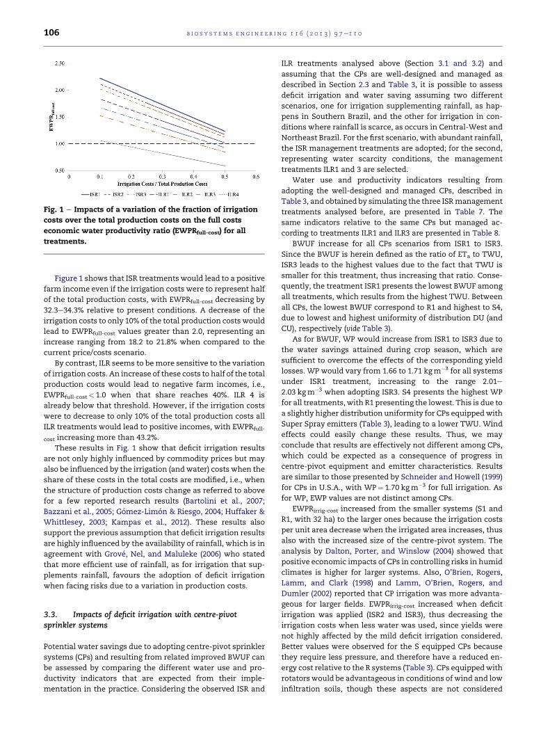
Fig. 1 e Impacts of a variation of the fraction of irrigation

costs over the total production costs on the full costs

economic water productivity ratio (EWPRfull-cost) for all

treatments.

b i o s y s t em s e n g i n e e r i n g 1 1 6 ( 2 0 1 3 ) 9 7e1 1 0106

Figure 1 shows that ISR treatments would lead to a positive

farm income even if the irrigation costs were to represent half

of the total production costs, with EWPRfull-cost decreasing by

32.3e34.3% relative to present conditions. A decrease of the

irrigation costs to only 10% of the total production costs would

lead to EWPRfull-cost values greater than 2.0, representing an

increase ranging from 18.2 to 21.8% when compared to the

current price/costs scenario.

By contrast, ILR seems to bemore sensitive to the variation

of irrigation costs. An increase of these costs to half of the total

production costs would lead to negative farm incomes, i.e.,

EWPRfull-cost< 1.0 when that share reaches 40%. ILR 4 is

already below that threshold. However, if the irrigation costs

were to decrease to only 10% of the total production costs all

ILR treatments would lead to positive incomes, with EWPRfull-

cost increasing more than 43.2%.

These results in Fig. 1 show that deficit irrigation results

are not only highly influenced by commodity prices but may

also be influenced by the irrigation (andwater) costs when the

share of these costs in the total costs are modified, i.e., when

the structure of production costs change as referred to above

for a few reported research results (Bartolini et al., 2007;

Bazzani et al., 2005; Gomez-Limon & Riesgo, 2004; Huffaker &

Whittlesey, 2003; Kampas et al., 2012). These results also

support the previous assumption that deficit irrigation results

are highly influenced by the availability of rainfall, which is in

agreement with Grove, Nel, and Maluleke (2006) who stated

that more efficient use of rainfall, as for irrigation that sup-

plements rainfall, favours the adoption of deficit irrigation

when facing risks due to a variation in production costs.

3.3. Impacts of deficit irrigation with centre-pivotsprinkler systems

Potential water savings due to adopting centre-pivot sprinkler

systems (CPs) and resulting from related improved BWUF can

be assessed by comparing the different water use and pro-

ductivity indicators that are expected from their imple-

mentation in the practice. Considering the observed ISR and

ILR treatments analysed above (Section 3.1 and 3.2) and

assuming that the CPs are well-designed and managed as

described in Section 2.3 and Table 3, it is possible to assess

deficit irrigation and water saving assuming two different

scenarios, one for irrigation supplementing rainfall, as hap-

pens in Southern Brazil, and the other for irrigation in con-

ditions where rainfall is scarce, as occurs in Central-West and

Northeast Brazil. For the first scenario, with abundant rainfall,

the ISR management treatments are adopted; for the second,

representing water scarcity conditions, the management

treatments ILR1 and 3 are selected.

Water use and productivity indicators resulting from

adopting the well-designed and managed CPs, described in

Table 3, and obtained by simulating the three ISRmanagement

treatments analysed before, are presented in Table 7. The

same indicators relative to the same CPs but managed ac-

cording to treatments ILR1 and ILR3 are presented in Table 8.

BWUF increase for all CPs scenarios from ISR1 to ISR3.

Since the BWUF is herein defined as the ratio of ETa to TWU,

ISR3 leads to the highest values due to the fact that TWU is

smaller for this treatment, thus increasing that ratio. Conse-

quently, the treatment ISR1 presents the lowest BWUF among

all treatments, which results from the highest TWU. Between

all CPs, the lowest BWUF correspond to R1 and highest to S4,

due to lowest and highest uniformity of distribution DU (and

CU), respectively (vide Table 3).

As for BWUF, WP would increase from ISR1 to ISR3 due to

the water savings attained during crop season, which are

sufficient to overcome the effects of the corresponding yield

losses. WP would vary from 1.66 to 1.71 kgm�3 for all systems

under ISR1 treatment, increasing to the range 2.01e

2.03 kgm�3 when adopting ISR3. S4 presents the highest WP

for all treatments, with R1 presenting the lowest. This is due to

a slightly higher distribution uniformity for CPs equippedwith

Super Spray emitters (Table 3), leading to a lower TWU. Wind

effects could easily change these results. Thus, we may

conclude that results are effectively not different among CPs,

which could be expected as a consequence of progress in

centre-pivot equipment and emitter characteristics. Results

are similar to those presented by Schneider and Howell (1999)

for CPs in U.S.A., with WP¼ 1.70 kgm�3 for full irrigation. As

for WP, EWP values are not distinct among CPs.

EWPRirrig-cost increased from the smaller systems (S1 and

R1, with 32 ha) to the larger ones because the irrigation costs

per unit area decrease when the irrigated area increases, thus

also with the increased size of the centre-pivot system. The

analysis by Dalton, Porter, and Winslow (2004) showed that

positive economic impacts of CPs in controlling risks in humid

climates is higher for larger systems. Also, O’Brien, Rogers,

Lamm, and Clark (1998) and Lamm, O’Brien, Rogers, and

Dumler (2002) reported that CP irrigation was more advanta-

geous for larger fields. EWPRirrig-cost increased when deficit

irrigation was applied (ISR2 and ISR3), thus decreasing the

irrigation costs when less water was used, since yields were

not highly affected by the mild deficit irrigation considered.

Better values were observed for the S equipped CPs because

they require less pressure, and therefore have a reduced en-

ergy cost relative to the R systems (Table 3). CPs equippedwith

rotators would be advantageous in conditions of wind and low

infiltration soils, though these aspects are not considered

Table 7eWater use and productivity indicators relative to the centre-pivot systemsdescribed in Table 3when adopting themanagement scenarios ISR1, 2 and 3 for irrigation in supplement of rainfall.

System symbol Super spray emitters Rotator R3000 sprinklers

S1 S2 S3 S4 S5 R1 R2 R3 R4 R5

Irrigated area (ha) 32.13 46.34 65.03 81.27 110.2 32.13 46.34 65.03 81.27 110.2

ISR1

BWUF 0.641 0.648 0.644 0.648 0.647 0.631 0.644 0.638 0.643 0.640

WP 1.69 1.71 1.70 1.71 1.70 1.66 1.69 1.68 1.69 1.68

EWP 0.67 0.68 0.68 0.68 0.68 0.66 0.68 0.67 0.68 0.67

EWPRirrig-cost 4.78 4.81 5.18 6.33 5.40 4.51 4.65 5.02 6.10 5.21

EWPRfull-cost 1.63 1.63 1.67 1.78 1.70 1.60 1.61 1.66 1.76 1.68

ISR2

BWUF 0.728 0.735 0.731 0.735 0.734 0.719 0.731 0.725 0.730 0.727

WP 1.84 1.85 1.85 1.85 1.85 1.81 1.84 1.83 1.84 1.84

EWP 0.74 0.74 0.74 0.74 0.74 0.73 0.74 0.73 0.74 0.73

EWPRirrig-cost 5.39 5.43 5.97 7.18 6.29 5.07 5.23 5.77 6.89 6.06

EWPRfull-cost 1.63 1.64 1.68 1.77 1.71 1.60 1.62 1.67 1.75 1.69

ISR3

BWUF 0.805 0.808 0.806 0.808 0.807 0.800 0.806 0.803 0.806 0.804

WP 2.02 2.03 2.02 2.03 2.02 2.01 2.02 2.01 2.02 2.02

EWP 0.81 0.81 0.81 0.81 0.81 0.80 0.81 0.81 0.81 0.81

EWPRirrig-cost 7.19 7.29 8.48 9.73 9.17 6.75 6.96 8.09 9.26 8.77

EWPRfull-cost 1.71 1.72 1.78 1.83 1.80 1.69 1.70 1.76 1.81 1.79

BWUF¼ beneficial water use fraction; WP¼water productivity; EWP¼ economic water productivity; EWPRirrig-cost¼ economic water produc-

tivity ratio for irrigation costs; EWPRfull-cost¼ economic water productivity ratio for total farming costs.

b i o s y s t em s e n g i n e e r i n g 1 1 6 ( 2 0 1 3 ) 9 7e1 1 0 107

here. EWPRfull-cost showed very similar behaviour among all

CPs, with only very small differences between S and R

equipped systems (Table 7), and with all values largely above

1.0, thus indicating that farm returns would be always posi-

tive. The very small differences in EWPRfull-cost among all

systems are due to the fact that irrigation costs constitute only

a small share of the production costs and differ little among

Table 8eWater use and productivity indicators relative to the cmanagement scenarios ILR1 and 3 for irrigation when rainfall

System symbol Super spray emitters

S1 S2 S3 S4

Irrigated area (ha) 32.13 46.34 65.03 81.27 1

ILR1

BWUF 0.724 0.738 0.731 0.739

WP 1.82 1.86 1.84 1.86

EWP 0.73 0.74 0.74 0.74

EWPRirrig-cost 3.02 3.03 3.23 3.99

EWPRfull-cost 1.22 1.22 1.25 1.35

ILR3

BWUF 0.851 0.863 0.856 0.863

WP 1.90 1.93 1.91 1.93

EWP 0.76 0.77 0.77 0.77

EWPRirrig-cost 3.39 3.42 3.78 4.52

EWPRfull-cost 1.13 1.13 1.17 1.23

BWUF¼ beneficial water use fraction; WP¼water productivity; EWP¼ ec

tivity ratio for irrigation costs; EWPRfull-cost¼ economic water productivit

treatments (Table 3). Results allow the ISR3 management

(mild deficit) to be identified as the scenario that would lead to

higher economic results when compared with ISR1 and 2.

However differences are small and farmers would probably

select this management if water availability for irrigation is

limited, as referred to by Cortignani and Severini (2009) for

Italy.

entre-pivot systemsdescribed in Table 3when adopting theis lacking.

Rotator R3000 sprinklers

S5 R1 R2 R3 R4 R5

10.2 32.13 46.34 65.03 81.27 110.2

0.736 0.703 0.730 0.717 0.728 0.721

1.85 1.77 1.84 1.81 1.83 1.82

0.74 0.71 0.73 0.72 0.73 0.73

3.35 2.85 2.94 3.14 3.85 3.24

1.27 1.19 1.20 1.24 1.33 1.25

0.861 0.834 0.855 0.845 0.854 0.849

1.92 1.86 1.91 1.89 1.91 1.90

0.77 0.75 0.77 0.76 0.76 0.76

3.98 3.19 3.29 3.64 4.34 3.84

1.19 1.11 1.12 1.16 1.22 1.18

onomic water productivity; EWPRirrig-cost¼ economic water produc-

y ratio for total farming costs.

b i o s y s t em s e n g i n e e r i n g 1 1 6 ( 2 0 1 3 ) 9 7e1 1 0108

When using well-designed and managed CPs under condi-

tions of scarce rainfall (Table 8), BWUF increases from a range

of 0.703e0.739 when adopting ILR1 to the range 0.834e0.863 for

ILR3. These results relate to a lower TWU for ILR3, which leads

to an increase in the ratio of ETa to TWU, and thus BWUF. WP

and EWP increased similarly to BWUF, reaching higher values

for S4 and the lowest for R1, due to highest and lowest DU and

CU, respectively (vide Table 3). The behaviour of BWUF,WP and

EWP indicators is therefore similar to those analysed for the ISR

treatments but indicators are slightly higher since less water is

used with ILR treatments.

As for BWUF, WP increases from ILR1 to ILR3, ranging from

1.77 to 1.86 kgm�3 and from 1.86 to 1.93 kgm�3, respectively.

These results are in accordance with those presented by

Goyne and McIntyre (2002) for Australian conditions. EWP

would slightly improve from the range of 0.71e0.74 BRLm�3 to

0.73e0.77 BRLm�3 when changing to ILR3 instead of ILR1.

EWPRirrig-cost increasedwhen an irrigation at a larger deficit

was considered (ILR3). Since less water is being used, adopting

ILR3 would lead to a decrease of the irrigation costs, which

could compensate for the yield losses associated with this

treatment. Higher EWPRirrig-cost values were observed for

Spray compared to Rotator equipped systems due to the low

energy demand, as referred to above for the ISR cases. How-

ever, EWPRfull-cost values followed a different pattern: adopt-

ing ILR3 instead of ILR1 treatment leads to lower EWPRfull-cost

for all centre-pivot alternatives, decreasing from the range

1.19e1.35 to 1.11e1.23. These results show that, when

considering the total production costs, the yield losses due to

higher irrigation deficits may not be acceptable when the

rainfall contribution is small, unless farmers have not got

enough water available for irrigation. However, results do not

allow definitive conclusions, particularly taking into account

the impacts of changing commodity prices and production

costs as analysed in Section 3.2.

When comparing the water productivity indicators result-

ing from adopting CPs, under abundant (ISR) and scarce (ILR)

rainfall, results presented in Tables 7 and 8 show that ILR

management leads to higher BWUF, WP and EWP values than

ISR1 and 2 due to less water application. However, ISR3, a

management strategy with mild deficit irrigation, shows

higher values for the same indicators. This results from the

fact that abundant rainfall mitigates the impact of deficit

irrigation.

By contrast, the EWPRirrig-cost values are much higher,

about double, when comparing results for irrigation to sup-

plement rainfall (ISR treatments) with irrigation when rainfall

is scarce (ILR). This indicates that the use of irrigation and

rainfall together when the latter is abundant results in higher

production values when compared with the applied irrigation

water in the case of scarce rainfall. Since farmers search for

profit, and considering that ILR1 has a EWPRirrig-cost higher

than ILR3, i.e., EWPRirrig-cost decreases for heavier deficits, this

indicates that farmers would not be likely to choose a deficit

irrigation strategy unless reduced water availability would

induce them to do so. However, for a use of irrigation and

rainfall together, EWPRirrig-cost are higher for mild deficits ISR2

and 3. In this case, though, the EWPRfull-cost are higher for the

management strategies leading to higher yields and having a

higher TWU for both ISR and ILR management strategies.

Moreover, the EWPRfull-cost values for ISR are higher than

those for ILR for more than 50%. These results confirm that

adopting deficit irrigation when rainfall is scarce is less

attractive than under conditions of irrigation to supplement

rainfall, when irrigation controls the risk of crop failure

(Dalton et al., 2004). It is likely that mild deficit irrigation and

carefully designed irrigation schedules may lead to improved

irrigation water use under scarce rainfall conditions (e.g.

Grassini et al., 2011), not high deficit irrigation, which would

have high impacts on yields and farm returns and could have

effects on soil salinity. The adoption of improved irrigation

and agronomic factors needs to be given appropriate consid-

eration, which implies adequate support to farmers (Ali &

Talukder, 2008; Molden et al., 2010; Pereira et al., 2012).

4. Conclusions

This study shows that economic water use and productivity

indicators may be appropriate tools for assessing the impacts

of deficit irrigation, particularly the economic water produc-

tivity ratio, which represents the yield values per unit of

farming costs (EWPRfull-cost) This indicator appears to be

adequate for assessing the feasibility of deficit irrigation as

influenced by commodity prices, and water and labour costs.

Results show that the viability of deficit irrigation is extremely

dependent upon the commodity prices, while changes in

water and labour costs have a low impact on related economic

results. This behaviour is due to the price structure prevailing

in maize farming in Brazil. However, a increase in the share

that irrigation costs represent of total production costs would

lead to a significant impact of irrigation costs over EWPRfull-

cost. These results also support the assumption that deficit

irrigation is favoured by the adoption of irrigation to supple-

ment rainfall, especially when facing risks due to a variation

in production costs.

The investment in well-designed and managed centre-

pivot systems may lead to high irrigation uniformity

depending on the irrigation system characteristics. Results

show that using centre-pivot systems is appropriate for both

rainfall regimes considered and best results refer to mild

deficit irrigation. Large deficits lead to reduced economic re-

sults. When rainfall is scarce, results confirm that adopting

deficit irrigation is less attractive than under conditions of

irrigation to supplement rainfall; hence farmers would not be

likely to choose a deficit irrigation strategy unless they were

facing reduced water availability.

This assessment shows that deficit irrigation requires

appropriate support to farmers in order to make better se-

lections and adoptions of improved agronomic practices,

better performing irrigation systems and irrigation schedules

that avoid stress during critical periods.

Acknowledgements

This study was funded by the Project FCT/CAPES e 2011/2012,

Proc.� 4.4.1.00 a Brazil and Portugal bilateral cooperation project

funded by CAPES, Brazil, and FCT, Portugal. Scholarships

b i o s y s t em s e n g i n e e r i n g 1 1 6 ( 2 0 1 3 ) 9 7e1 1 0 109

provided to G.C. Rodrigues by FCT and J.D.Martins by CAPES are

acknowledged. The review and comments by Paula Paredes are

acknowledged.

r e f e r e n c e s

Abd El-Wahed, M. H., & Ali, E. A. (2013). Effect of irrigationsystems, amounts of irrigation water and mulching on cornyield, water use efficiency and net profit. Agricultural WaterManagement, 120, 64e71.

Ali, M. H., & Talukder, M. S. U. (2008). Increasing waterproductivity in crop production e a synthesis. AgriculturalWater Management, 95, 1201e1213.

ANA. (2009). Conjuntura dos recursos hıdricos no Brasil. Brasılia, DF:Agencia Nacional de Aguas (206 pp.).

Barragan, J., Cots, L. I., Monserrat, J., Lopez, R., & Wu, I. P. (2010).Water distribution uniformity and scheduling in micro-irrigation systems for water saving and environmentalprotection. Biosystems Engineering, 107, 202e211.

Bartolini, F., Bazzani, G. M., Gallerani, V., Raggi, M., & Viaggi, D.(2007). The impact of water and agriculture policy scenarios onirrigated farming systems in Italy: an analysis based on farmlevel multi-attribute linear programming models. AgriculturalSystems, 93(1e3), 90e114.

Bazzani, G. M., DiPasquale, S., Gallerani, V., Morganti, S.,Raggi, M., & Viaggi, D. (2005). The sustainability of irrigatedagricultural systems under the Water Framework Directive:first results. Environmental Modelling & Software, 20, 165e175.

Bouman, B. A. M. (2007). A conceptual framework for theimprovement of crop water productivity at different spatialscales. Agricultural Systems, 93, 43e60.

Brennan, D. (2007). Factors affecting the economic benefits ofsprinkler uniformity and their implications for irrigationwater use. Irrigation Science, 26, 109e119.

Carlesso, R., Petry, M. T., & Trois, C. (2009). The use of ameteorological station network to provide crop waterrequirement information for irrigation management. InComputer and computing technologies in agriculture II, Vol. 1.Springer. IFIP Advances in Information and CommunicationTechnology, 293, 19e27.

CONAB. (2010). Custos de Producao. Brasilia, Brazil: CompanhiaNacional de Abastecimento, Ministerio da Agricultura,Pecuaria e Abastecimento. http://www.conab.gov.br/conteudos.php?a¼545&t¼2 Accessed 01.04.12.

Cortignani, R., & Severini, S. (2009). Modeling farm-level adoptionof deficit irrigation using positive mathematical programming.Agricultural Water Management, 96, 1785e1791.

Dalton, T. J., Porter, G. A., & Winslow, N. G. (2004). Riskmanagement strategies in humid production regions: acomparison of supplemental irrigation and crop insurance.Agricultural and Resource Economics Review, 33(2), 220e232.

Darouich, H., Goncalves, J. M., Muga, A., & Pereira, L. S. (2012).Water saving vs. farm economics in cotton surface irrigation:an application of multicriteria analysis. Agricultural WaterManagement, 115, 223e231.

Dechmi, F., Playan, E., Cavero, J., Faci, J. M., & Martınez-Cob, A.(2003). Wind effects on solid set sprinkler irrigation depth andyield of maize (Zea mays). Irrigation Science, 22(2), 67e77.

Domınguez, A., de Juan, J. A., Tarjuelo, J. M., Martınez, R. S., &Martınez-Romero, A. (2012). Determination of optimalregulated deficit irrigation strategies for maize in a semi-aridenvironment. Agricultural Water Management, 110, 67e77.

Evans, R. G., Wu, I.-P., & Smajstrala, A. G. (2007). Microirrigationsystems. In G. J. Hoffman, R. G. Evans, M. E. Jensen,D. L. Martin, & R. L. Elliot (Eds.), Design and operation of farmirrigation systems (2nd ed.). (pp. 632e683) St. Joseph, MI: ASABE.

FAO. (2012). FAO statistical yearbook 2012. Rome: Food andAgriculture Organization of the United Nations.

Farre, I., & Faci, J.-M. (2009). Deficit irrigation in maize forreducing agricultural water use in a Mediterraneanenvironment. Agricultural Water Management, 96, 383e394.

Finger, R. (2012). Modeling the sensitivity of agricultural water usetoprice variability and climate changee anapplication toSwissmaize production.AgriculturalWaterManagement, 109, 135e143.

Geerts, S., & Raes, D. (2009). Deficit irrigation as an on-farmstrategy to maximize crop water productivity in dry areas.Agricultural Water Management, 96, 1275e1284.

Gomez-Limon, J. A., & Riesgo, L. (2004). Irrigation water pricing:differential impacts on irrigated farms. Agricultural Economics,31, 47e66.

Goyne, P. J., & McIntyre, G. T. (2002). Improving on farm irrigationwater use efficiency in the Queensland cotton and grain industries(pp. 1e8). Queensland Department of Primary Industries,Agency for Food and Fibre Sciences, Farming SystemsInstitute and the Australian Cotton CRC.

Grassini, P., Yang, H., Irmak, S., Thorburn, J., Burr, C., &Cassman, K. G. (2011). High-yield irrigated maize in theWestern U.S. Corn Belt: II. Irrigation management and cropwater productivity. Field Crops Research, 130, 133e141.

Grove, B., Nel, F., & Maluleke, H. H. (2006). Stochastic efficiencyanalysis of alternative water conservation strategies. Agrekon:Agricultural Economics Research, Policy and Practice in SouthernAfrica, 45(1), 50e59.

van Halsema, G. E., & Vincent, L. (2012). Efficiency andproductivity terms for water management: a matter ofcontextual relativism versus general absolutism. AgriculturalWater Management, 108, 9e15.

Huffaker, R., & Whittlesey, N. (2003). A theoretical analysis ofeconomic incentive policies encouraging agricultural waterconservation. International Journal of Water ResourcesDevelopment, 19(1), 37e53.

IBGE. (2009). Censo Agropecuario 2006. Brasılia, Brasil: GrandesRegioes e Unidades da Federacao, Instituto Brasileiro degeografia e Estatıstica (775 pp.).

Igbadun, H. E., Salim, B. A., Tarimo, A. K. P. R., & Mahoo, H. F.(2008). Effects of deficit irrigation scheduling on yields and soilwater balance of irrigated maize. Irrigation Science, 27, 11e23.

Kampas, A., Petsakos, A., & Rozakis, S. (2012). Price inducedirrigation water saving: unravelling conflicts and synergiesbetween European agricultural and water policies for a GreekWater District. Agricultural Systems, 113, 28e38.

Kang, S., Shi, W., & Zhang, J. (2000). An improved water-useefficiency for maize grown under regulated deficit irrigation.Field Crops Research, 67, 207e214.

Karam, F., Breidy, J., Stephan, C., & Rouphael, J. (2003).Evapotranspiration, yield and water use efficiency of dripirrigated corn in the Bekaa Valley of Lebanon. AgriculturalWater Management, 63, 125e137.

Katerji, N., Mastrorilli, M., & Chernic, H. E. (2010). Effects of corndeficit irrigation and soil properties on water use efficiency. A25-year analysis of a Mediterranean environment using theSTICS model. European Journal of Agronomy, 32, 177e185.

Keller, J., & Bliesner, R. D. (1990). Sprinkle and trickle irrigation.(652 pp.). New York: Van Nostrand Reinhold.

Kiziloglu, F. M., Sahin, U., Kuslu, Y., & Tunc, T. (2009).Determining watereyield relationship, water use efficiency,crop and pan coefficients for silage maize in a semiarid region.Irrigation Science, 27, 129e137.

Lamm, F. R., O’Brien, D. M., Rogers, D. H., & Dumler, T. J. (2002).Sensitivity of center pivot sprinkler and SDI economic comparisons.ASAE meeting paper no. MC02-201. St. Joseph: Mich.

Lopez-Mata, E., Tarjuelo, J. M., de Juan, J. A., Ballesteros, R., &Domınguez, A. (2010). Effect of irrigation uniformity on theprofitability of crops.AgriculturalWaterManagement, 98, 190e198.

b i o s y s t em s e n g i n e e r i n g 1 1 6 ( 2 0 1 3 ) 9 7e1 1 0110

Lorite, I. J., Mateos, L., Orgaz, F., & Fereres, E. (2007). Assessingdeficit irrigation strategies at the level of an irrigation district.Agricultural Water Management, 91, 51e60.

Mantovani, E. C., Villalobos, F. J., Orgaz, F., & Fereres, E. (1995).Modelling the effects of sprinkler irrigation uniformity on cropyield. Agricultural Water Management, 27, 243e257.

Martins, J. D., Rodrigues, G. C., Paredes, P., Carlesso, R.,Oliveira, Z. B., Knies, A. E., et al. (2013). Dual crop coefficientsfor maize in southern Brazil: model testing for sprinkler anddrip irrigation and mulched soil. Biosystems Engineering, 115(3),291e310.

MIN. (2008). A irrigacao no Brasil. Situacao e diretrizes. Brasilia,Brazil: Ministerio da Integracao Nacional.

Molden, D., Oweis, T., Steduto, P., Bindraban, P., Hanjra, M. A., &Kijne, J. (2010). Improving agricultural water productivity:between optimism and caution. Agricultural WaterManagement, 97, 528e535.

Montero, J., Martınez, A., Valiente, M., Moreno, M. A., &Tarjuelo, J. M. (2013). Analysis of water application costs witha centre pivot system for irrigation of crops in Spain. IrrigationScience, 31(3), 507e521.

Moreno, J. A. (1961). Clima do Rio Grande do Sul. Porto Alegre:Secretaria de Agricultura (42 pp.).

Moreno, M. A., Medina, D., Ortega, J. F., & Tarjuelo, J. M. (2012).Optimal design of center pivot systems with water suppliedfrom wells. Agricultural Water Management, 107, 112e121.

O’Brien, D. M., Rogers, D. H., Lamm, F. R., & Clark, G. A. (1998). Aneconomic comparison of subsurface drip and center pivotsprinkler irrigation systems. Applied Engineering in Agriculture,14, 391e398.

O’Neill, C. J., Humphreys, E., Louis, J., & Katupitiya, A. (2008).Maize productivity in southern New South Wales underfurrow and pressurised irrigation. Australian Journal ofExperimental Agriculture, 48(3), 285e295.

Ortız, J. N., de Juan, J. A., & Tarjuelo, J. M. (2010). Analysis of waterapplication uniformity from a centre pivot irrigator and itseffect on sugar beet (Beta vulgaris L.) yield. BiosystemsEngineering, 105, 367e379.

Payero, J. O., Melvin, S. R., Irmak, S., & Tarkalson, D. (2006). Yieldresponse of corn to deficit irrigation in a semiarid climate.Agricultural Water Management, 84, 101e112.

Pedras, C. M. G., Pereira, L. S., & Goncalves, J. M. (2009). MIRRIG: adecision support system for design and evaluation ofmicroirrigation systems. Agricultural Water Management, 96,691e701.

Pereira, L. S. (1999). Higher performance through combinedimprovements in irrigation methods and scheduling: adiscussion. Agricultural Water Management, 40, 153e169.

Pereira, L. S., Cordery, I., & Iacovides, I. (2009). Coping with waterscarcity. Addressing the challenges. Dordrecht: Springer (382 pp.).

Pereira, L. S., Cordery, I., & Iacovides, I. (2012). Improvedindicators of water use performance and productivity forsustainable water conservation and saving. Agricultural WaterManagement, 108, 39e51.

Pereira, L. S., Goncalves, J. M., Dong, B., Mao, Z., & Fang, S. X. (2007).Assessing basin irrigation and scheduling strategies for savingirrigation water and controlling salinity in the Upper YellowRiver Basin, China. Agricultural Water Management, 93, 109e122.

Pereira, L. S., Oweis, T., & Zairi, A. (2002). Irrigation managementunder water scarcity. Agricultural Water Management, 57,175e206.

Playan, E., & Mateos, L. (2006). Modernization and optimization ofirrigation systems to increase water productivity. AgriculturalWater Management, 80, 100e116.

Popova, Z., Eneva, S., & Pereira, L. S. (2006). Model validation, cropcoefficients and yield response factors for maize irrigationscheduling based on long-term experiments. BiosystemsEngineering, 95(1), 139e149.

Rodrigues, G. C., & Pereira, L. S. (2009). Assessing economicimpacts of deficit irrigation as related to water productivityand water costs. Biosystems Engineering, 103(4), 536e551.

Rodrigues, G. C., Silva, F. G., & Pereira, L. S. (2010). Assessing thefeasibility of deficit irrigation under drought conditions. InA. Lopez-Francos (Ed.). Options Mediterraneennes Series A: Vol.95. Economics of drought and drought preparedness in a climatechange context (pp. 285e291).

Rosa, R. D., Paredes, P., Rodrigues, G. C., Alves, I., Fernando, R. M.,Pereira, L. S., et al. (2012). Implementing the dual cropcoefficient approach in interactive software. 1. Backgroundand computational strategy. Agricultural Water Management,103, 8e24.

Rossato, L., Alvala, R. C. S., & Tomasella, J. (2004). Variacaoespaco-temporal da umidade do solo no Brasil: Analise dascondicoes medias para o perıodo de 1971e1990. RevistaBrasileira de Meteorologia, 19(2), 113e122.

Salmeron,M., Urrego, Y. F., Isla, R., & Cavero, J. (2012). Effect of non-uniform sprinkler irrigation and plant density on simulatedmaize yield. Agricultural Water Management, 113, 1e9.

Salvador, R., Martınez-Cob, A., Cavero, J., & Playan, E. (2011).Seasonal on-farm irrigation performance in the Ebro basin(Spain): crops and irrigation systems. Agricultural WaterManagement, 98, 577e587.

Sampathkumar, T., Pandian, B. J., Ranghaswamy, M. V., &Manickasundaram, P. (2012). Yield and water relations ofcottonemaize cropping sequence under deficit irrigationusing drip system. Irrigation and Drainage, 61, 208e219.

Sanchez, I., Zapata, N., & Faci, J. M. (2010). Combined effect oftechnical, meteorological and agronomical factors on solid-setsprinkler irrigation: I. Irrigation performance and soil waterrecharge in alfalfa and maize. Agricultural Water Management,97, 1571e1581.

Sandri, D., & Cortez, D. A. (2009). Parametros de desempenho dedezasseis equipamentos de irrigacao por pivocentral. Ciencia eAgrotecnologia, 33, 271e278.

Schneider, A. D., & Howell, T. A. (1999). Lepa and spray irrigationfor grain crops. Journal of Irrigation and Drainage Engineering,125(4), 167e172.

Tarjuelo, J. M., Montero, J., Carrion, P. A., Honrubia, F. T., &Calvo, M. A. (1999). Irrigation uniformity with medium sizesprinklers. Part II. Influence of wind and other factors onwater distribution. Transactions of ASAE, 42(3), 677e689.

Valın, M. I., Cameira, M. R., Teodoro, P. R., & Pereira, L. S. (2012).DEPIVOT: a model for center-pivot design and evaluation.Computers and Electronics in Agriculture, 87, 159e170.

Xu, X., Huang, G., Sun, C., Pereira, L. S., Ramos, T. B., Huang, Q.,et al. (2013). Assessing the effects of water table depth onwater use, soil salinity and wheat yield: searching for a targetdepth for irrigated areas in the upper Yellow River basin.Agricultural Water Management, 125, 46e60.

Zwart, S. J., & Bastiaanssen, W. M. G. (2004). Review of measuredcrop water productivity values for irrigated wheat, rice, cottonand maize. Agricultural Water Management, 69, 115e133.