Modelling Extreme Multivariate Events

Modelling Extreme Multivariate EventsAuthor(s): Stuart G. Coles and Jonathan A. TawnSource: Journal of the Royal Statistical Society. Series B (Methodological), Vol. 53, No. 2(1991), pp. 377-392Published by: Wiley for the Royal Statistical SocietyStable URL: http://www.jstor.org/stable/2345748 .

Accessed: 28/06/2014 19:06

Your use of the JSTOR archive indicates your acceptance of the Terms & Conditions of Use, available at .http://www.jstor.org/page/info/about/policies/terms.jsp

.JSTOR is a not-for-profit service that helps scholars, researchers, and students discover, use, and build upon a wide range ofcontent in a trusted digital archive. We use information technology and tools to increase productivity and facilitate new formsof scholarship. For more information about JSTOR, please contact [email protected].

.

Wiley and Royal Statistical Society are collaborating with JSTOR to digitize, preserve and extend access toJournal of the Royal Statistical Society. Series B (Methodological).

http://www.jstor.org

This content downloaded from 185.31.195.188 on Sat, 28 Jun 2014 19:06:21 PMAll use subject to JSTOR Terms and Conditions

http://www.jstor.org/action/showPublisher?publisherCode=black

http://www.jstor.org/action/showPublisher?publisherCode=rss

http://www.jstor.org/stable/2345748?origin=JSTOR-pdf

http://www.jstor.org/page/info/about/policies/terms.jsp


J. R. Statist. Soc. B (1991) 53, No. 2, pp. 377-392

Modelling Extreme Multivariate Events

By STUART G. COLES and JONATHAN A. TAWNt

University of Sheffield, UK

[Received June 1989. Final revision January 1990]

SUMMARY The classical treatment of multivariate extreme values is through componentwise ordering, though in practice most interest is in actual extreme events. Here the point process of observations which are extreme in at least one component is considered. Parametric models for the dependence between components must satisfy certain constraints. Two new techniques for generating such models are presented. Aspects of the statistical estimation of the resulting models are discussed and are illustrated with an application to oceanographic data.

Keywords: EXTREME VALUE THEORY; GENERALIZED PARETO DISTRIBUTION; MAXIMUM LIKELIHOOD; MULTIVARIATE ORDERING; NON-HOMOGENEOUS POISSON PROCESS; SIMPLEX MEASURES

1. INTRODUCTION

Recently there have been significant advances in the modelling procedures available for univariate extreme values. Two approaches, in particular, have been advocated in preference to the classical procedure of fitting a generalized extreme value distribution to the annual maxima of a series. One approach is based on the asymptotic joint distribution of a fixed number of extreme order statistics (Weissman, 1978; Smith, 1986; Tawn, 1988a). An alternative method is to model independent exceedances of a suitably high threshold using a generalized Pareto distribution (GPD) (Pickands, 1975; Davison and Smith, 1990). Through the inclusion of additional relevant data both procedures lead to greater estimation precision than the classical approach. Here our aim is to develop procedures which offer similar improvements to the analysis of multivariate extreme value data.

Problems concerning environmental extremes are often multivariate in character. An example is wind speed data where maximum hourly gusts, maximum hourly mean speeds and the dependence between them are relevant to building safety. Problems involving spatial dependence are also of much interest to engineers: for example, floods may occur at several sites along a coastline, or at various rain-gauges in a national network. In such situations knowledge of the spatial dependence of extremes is essential for regional risk assessment. Correct modelling of spatial dependence also leads to greater estimation precision of marginal parameters.

To date, the analysis of multivariate extreme values has been based on a componentwise ordering: for an independent and identically distributed (IID) vector series (1Yi, 1, .. ., Yi,p), i = 1, . . ., n, the vector of componentwise maxima, Mn, is given by Mn =

tAddress for correspondence: Department of Probability and Statistics, University of Sheffield, Sheffield, S3 7RH, UK.

? 1 991 Royal Statistical Society 0035-9246/91/53377 $2.00



378 COLES AND TAWN [No. 2,

(Mn, 1. . .. Mn,p) where Mnj = max{I Yj,. . ., Ynsj }. Under general conditions Mn, suitably normalized, converges in distribution to a member of the class of multivariate extreme value distributions. These distributions have received theoretical considera- tion (de Haan and Resnick, 1977; Resnick, 1987), and recent papers have explored their statistical application (Tawn, 1988b, 1990; Smith et al., 1990). In applications Mn is generally taken as the vector of annual maxima for the relevant variables, although Mn may not correspond to an observed event. As with the classical univariate approach this procedure is wasteful of data. A further weakness with existing applications is that the margins are estimated as a preliminary step to esti- mating the dependence structure so that any potential for improving marginal estimation precision by incorporating dependence is lost.

To develop a procedure which utilizes more of the available data, and permits simultaneous estimation of the marginal and dependence structures, we exploit a representation in de Haan (1985). This is based on the limiting point process of actual observations which are extreme in at least one margin, giving a multivariate analogue of the GPD, and has the advantage that it does not require multivariate ordering (Barnett, 1976). In Section 2 the point process representation is reviewed and its con- nections with componentwise ordering and convex hulls are examined. With standardized margins the limiting point process is a non-homogeneous Poisson process whose intensity is characterized by a constrained measure on the unit simplex. This measure embodies the dependence structure of large observations. Two new techniques for generating suitably constrained parametric models for the measure are presented and demonstrated in Sections 3 and 4 respectively. Aspects of the statistical estimation of these models are discussed in Section 5 and are illustrated, in Section 6, with a trivariate application to oceanographic data.

2. POINT PROCESS THEORY OF MULTIVARIATE EXTREMES

In essence our approach follows de Haan and Resnick (1977), de Haan (1985) and Resnick (1987). Let X1, X2, ... be a sequence of IID random vectors on RP whose distribution function F is in the domain of attraction of a multivariate extreme value distribution G. We suppose that the marginal components are identically distributed with a unit Frechet distribution: exp( - 1 /x), x > 0. This assumption is not restrictive because a suitable transformation can be applied otherwise.

Consider the process of points Pn , on RP , where Pn = {n 'Xi: i= 1, . . ., n}. The choice of divisor n to normalize the X variables results from the max-stability property of unit Frechet variables. Then Pn converges in distribution to a non- homogeneous Poisson process P on RP \ {O}. Defining pseudoradial and angular co- ordinates

p

ri= >3X,j/n, wi,j=Xi,j/nr, i=1,. . .,n, j=1,. . .,p, (2.1) j=l

where Xijj is thejth component of Xi, the intensity measure it of the limiting process P then satisfies

dr ,(drxdw) = 2 dH(w). (2.2)



1991] MODELLING EXTREME MULTIVARIATE EVENTS 379

Here H is a positive finite measure on the (p - 1)-dimensional unit simplex,

p Sp = ((W19 ... ., Wp): E j= 1,Wj > 0, j= 19 .. ., 9p}.

j=1

By equation (2.2) it factorizes into a known function of the radial component and a measure H of the angular components, which describes the dependence structure of all extreme observations. Although an arbitrary finite positive measure, H must satisfy

wjdH(w)= 1, j=1,. ...,p, (2.3)

in order that the margins have the correct form. The only constraints on H are given by equation (2.3) so no finite parameterization exists for this measure.

If the effects of a storm can be thought of as additive representation (2.1) has a simple interpretation: ri is a standardized measure of the strength of the ith spatial storm over the sites and wij is the relative strength on this storm at sitej. This formula- tion differs from that of de Haan and Resnick who transform to standard polar co- ordinates.

The representation for limiting distributions of componentwise maxima is a consequence of the limiting Poisson process with intensity (2.2). This is seen by taking A = RP \{(0,xl) x . .. x (O,xp)}. Then, as n -oo,Pr(nXiA, i=1, . . ., n) exp{-,(A)}, where

it (A) = d| r dH(w) r2 Ar

= 0

drdH ) s r= min (x/w,) r

I V<P

= | max (wj/xj) dH(w).

As Pr(n-XXi A, i=1, .. . , n) = Pr(n-1Mj,n < X, X = 1, .. . , p), any limit distribution of normalized componentwise maxima, with unit Frechet margins, is of the form G(x) = exp{- V(x)} where

V(x) = max (wj/xj) dH(w) (2.4)

for some measure Hsatisfying constraints (2.3). This is Pickands's (1981) representation theorem for multivariate extreme value distributions with unit Frechet margins.

Following de Haan and Resnick (1977) we call Vthe exponent measure. Pickands's statement of equation (2.4) was given for unit exponential margins and in terms of a dependence function related to V. For technical reasons we work in terms of the exponent measure instead of Pickands's dependence function; see Section 3. Further- more, except for the bivariate case, the dependence function has no concise expression for unit Frechet margins.




Various other probabilities of interest can also be calculated from equation (2.2). For example, the region A could be taken to be a convex hull in RP. In some cases closed form expressions can be found: an example is the region A = {u e RP: sj-1 u1/xj x I} as

,u (A) = d2 dH(w) Sp r = (El jw/x) -l r

- | ( E wj/xj) dH(w)

p

j=1

For more complicated regions numerical integration of the measure over the region will generally be- necessary.

3. TECHNIQUES FOR MODELLING THE MEASURE

A simple nonparametric procedure for modelling the measure function H is described by de Haan (1985). For simultaneous estimation of marginal and dependence structures parametric procedures are preferable. Thus we concentrate on developing suitably flexible parametric models for the measure H. Parametric measures on the simplex have been developed for the study of compositional data (Aitchison, 1986), but these models are not suitable for the present application because of constraints (2.3). Therefore in this section we develop techniques which considerably simplify the non-trivial problem of generating parametric measures which satisfy constraints (2.3).

3.1. Relating Exponent Measure V to Measure H We restrict ourselves to the class of models for which the exponent measure Vis dif-

ferentiable; thus Hhas densities on the interior, and on each of the lower dimensional boundaries, of the unit simplex Sp. For each j = 1, .. .,p, let c = { il, . . ., ij }be an index variable over the subsets, of sizej, of the set cp = {1, . . ., p } and let Sj,= {w E Sp: Wk = 0, k c }. For each c with I c I =j, Sj,c is isomorphic to the (j - 1)-dimensional unit simplex Sj. The measure has a density hj,c on each of the subspaces Sjc. Where convenient, the domain of hj,c will be taken as either Sj,c or Sj. The density hj,c describes the dependence structure for events which are extreme only in the components c = { il, . . ., ij} . Such a hierarchy of densities is required to describe dependence when the marginal components need not all be extreme simultaneously.

Theorem 1. Let V and H be the exponent measure and measure function defined by equation (2.4), and let hj,c be the class of densities of H defined previously. Then forc= {il,... .,im}

a v . (m + 1) ..aim lxi) , -i

31




on {xeRP+: xr=0 if rgc). A proof of this result is given in Appendix A. In the bivariate case this result reduces to that obtained by Pickands (1981). The

importance of theorem 1 is that densities of all orders for the measure H may be obtained for any closed form multivariate extreme value distribution. For example, consider Gumbel's (1960) multivariate logistic model with exponent measure

p llr

V(x)= (Z Xr) r > 1. (3.2) \j= 1 /

Applying equation (3.1) gives hj, cO j < p, and

p-l p -(r+1) P llr-p

p(w)= {fl (jr-i)] (fi wj) ( W - , weSp.

In contrast, if r= 1 in equation (3.2), so that the variables are independent, then hl,( )1 for all i and hj, c-0 for all ] > 1, so the measure places all mass on the vertices of Sp The drawback to the use of theorem 1 is that it can be applied only to multivariate extreme value distributions, of which very few have been explicitly obtained; see Tawn (1990) and Joe (1989).

3.2. Parametric Models for the Measure by Transformation An alternative technique for generating parametric measures is motivated by

Pickands's representation which, in its full generality, characterizes multivariate extreme value distributions with exponential margins but arbitrary means. Equiva- lently, if X' has unit Frechet margins, with ith-component scale parameter equal to mi, then X' has a multivariate extreme value distribution if and only if its joint distribution function can be expressed as

Gx (x') = exp - m 1axp (j dH*(u)},

where Is uj dH*(u) = mj and H* is a positive finite measure on Sp . Transformation of X' to a random vector X with unit Frechet margins, Xj = Xj/mj, j= 1,.. .,p, gives a representation for the distribution function of X in the form

Gx(x)=exp- max( Ul dH*(u) 3 (3.3)

Thus equation (3.3) is a representation for multivariate extreme value distributions, with unit Frechet margins, in terms of a finite measure H* whose only constraint is to be positive over Sp. The equivalence of equations (3.3) and (2.4) is exploited in theorem 2 to show that any positive function h * on Sp , corresponding to the density of H*, may be transformed into a measure density hp,CP which satisfies constraints (2.3). We adopt the notation h hp, c if all the mass is in the interior of the simplex. Also, let mw denote Emi wi, the scalar product of m and w.

Theorem 2. If h * is any positive function on Sp, with finite first moments, then




h(w) = (m w) ]J) mjh( m w '**'m w )'.4 j=1

where

Mi uj h*(u) du, i=1, .. *.p, (3.5) SI

satisfies constraints (2.3) and is therefore the density of a valid measure function H.

This result is also proved in Appendix A. Theorem 2 can be used to generate a rich class of parametric models for the measure

on the interior of Sp. Though not stated here we have generalized this result to generate models with mass on the boundaries of Sp. The only practical restriction in each case is the necessity to calculate the integrals (3.5), either by numerical integration or, preferably, analytically. Take for example

P P h *(w)= H{ , (ai)3 r(ci-) H wjai-19 aj > o j=l,9. ..,gp, weSp.

j=I j=I

By equation (3.5) mj = aj /(a l), and from equation (3.4) it follows that

h(w) = 1 1j F(al+l)f) ,awi'-I wES,,, (3.6)

is a valid measure density. This model will be discussed in Section 4.

4. MODELS FOR THE MEASURE

As no finite parametric family exists we apply the results of Section 3 to develop a few flexible families of models which cover a broad range of possible structures.

4.1. Asymmetric Logistic Model Tawn (1990) developed the asymmetric logistic model as a multivariate extreme

value distribution with much flexibility and capacity for physical interpretation. The joint distribution function of this model has the form

G(x) = exp [- E E (O0/i1Xi)YC ] C iec J

where C is the set of all non-empty subsets of { 1,. . ., p } and the parameters are constrained by rc > 1 for allceC, c =Oific, c O , c 0, i= 1, . . .,p and cecOi,c= 1. Applying theorem 1 gives the class of measure densities, for w E Sj,cg

hj C(W= (w) (krc-1) ( oj i __1c i) /r (4.1) {k = 3 iEc )iEc ,' lec




This model has a density on Sp, and on each lower dimensional boundary of Sp. Each density is a form of weighted logistic density (3.2). A special case of equation (4.1), for

0j, = 1, i= 1, . ., pand r, = r, is the logistic model. Further properties of the model

are discussed in Tawn (1990).

4.2. Negative Asymmetric Logistic Model A model obtained by Joe (1989), with similar structure to the asymmetric logistic

model, has distribution function

G(x) = exp [- E~- + E - )ICI E (.c j=lI Xi cEC: Ic12 iEc xi

with parameter constraints given by rc < 0 for all c E C, Oic =0 if i g c, Oi c > O for all c EC, EcEc( - 1)IcIiOc < 1. Again by theorem 1, for w E Sj c,

hj, c(w) =

~ ( 1Id fl 1 kr)1 (l~ r(F -(r +I) (,dr1 1/rd-

dE t

~H (1 kd ) 3 (isd ) (Wi) Yi E dEC: k=I iec iec iec ccd

(4.2)

Because of the similarity of equations (4.1) and (4.2) we term this model the negative asymmetric logistic model.

4.3. Dirichlet Model In Section 3, by application of theorem 2, measure density (3.6) was obtained. This

model has the important feature of being asymmetric, allowing for non- exchangeability of the variables, yet having its mass confined to the interior of Sp. For the symmetric model with a = a, = . . . = acp both total independence and complete dependence are attained as limiting cases by taking a - 0 and a -+ oo respectively.

For p =2 density (3.6) gives a new bivariate extreme value distribution. The exponent measure with unit Frechet margins is

V(xI ,x2) = L1-Be( a+1,a2; aX1 +IBe al,a2+1; :3 X

where a,, a2 > 0, a = (al, a2)' and

Be(al, c2; u) = I(al 1+a2)

|u -I(I-W) 2- dw r(a1l) F(C1) 0~ al1-Wa- w

a normalized incomplete beta function. The extension to general multivariate extreme value distributions is complicated although numerically feasible.

4.4. Bilogistic Model Proposed by Smith (1990), the bilogistic model is an asymmetric generalization of

the logistic model. The model is motivated by the representation for max-stable processes (de Haan, 1984) and has exponent measure of the form




V(xI,x2)= max [(1 (1- )(-j)3ds (0<a?1, 0<0,S1)

Even in this bivariate case no closed form expression can be obtained for the measure density which must be calculated numerically from the mixed derivative of V; see equation (3.1).

4.5. Nested Logistic Model Generalizing the logistic model, McFadden (1978) developed a class of models

which involve hierarchical dependence. Tawn (1990) described a physical motivation for these. A special trivariate case of this model has exponent measure V(x) = {(xi-' + x29-)s/r + X3-s} 's, r > s > 1. The pair (1, 2) has logistic dependence, parameter r, whereas both other pairs have logistic dependence, parameter s; hence (1, 2) has greatest dependence. The trivariate logistic model is obtained when s = r. By equation (3.1) the corresponding measure is easily obtained. It places all mass in the interior of S3 but is slightly unwieldy. Obvious counterparts of this model in higher dimensions, and with higher level hierarchical dependence, are not discussed here.

4.6. Time Series Logistic Model A quite different approach to generating parametric measures uses the theory of

domains of attraction for multivariate extreme densities. The technique is illustrated by the following example. Let X1, . . ., Xp be a first-order Markov process repre- senting observations of a propagating sea storm at sites ordered along a coast. Suppose that the pairs (Xj, Xj+ 1) follow a bivariate extreme value distribution with unit Frechet margins and logistic dependence structure, parameter rj, whose joint and marginal densities we denote by fj and f respectively. Then the joint density of X1, ...Xp is

j=I f(Xj)

Adapting the arguments of Resnick (1987), Smith (1989) and equation (3.1) gives lim {tP+1 g(tX1, . ., txUp)} = (xl)-(P+1) h{xl/(x-1),. . . xp/(x 1)}. t- oo

Hence

h() - PI, (rjw j (Wj-j r+ W-rj+ l)lXrj-2 WEiSpg (4.3)

for rj > 1. Here dependence decays with lag. An extension of this model, not examined here, is based on a higher order Markov sequence with the associated joint density of consecutive values taken as multivariate extreme value with unit Frechet margins.

5. ESTIMATION

A natural approach to fitting the models of Section 4 is maximum likelihood




applied to the likelihood function of the limiting Poisson process of Section 2. Initially we derive the likelihood for XI, . . ., X, a sequence of IID random vectors, with each marginal component having a unit Frechet distribution. By the results of Section 2, for large n, the points of Pn = {n - 'Xi: i = 1, .. ., n} in aregionA, bounded away from 0 by a distance dependent on the rate of convergence, are approximately a non-homogeneous Poisson process with intensity satisfying equation (2.2). Take {n -'Xi, i= 1, ..., nA} to be the points of Pn in A. The likelihood over A, LA, is

nA

LA(0; {n - 'Xi}) = exp { - ,u(A)} II t (dri xdw) (5.1) i=1

where 0 are the measure parameters and ri and wi are defined by equations (2.1). More generally let {Yj, i= 1, . . ., n} be IID random vectors on RP. Simultaneous

estimation of the marginal and dependence parameters requires an appropriate choice for the region A and a transformation to unit Frechet margins to be included in equation (5.1). The region A = RP \ {(O, v1) x . .. x (0, vp)}, with thresholds v1,

vp, contains all observations which are large in at least one margin. This ensures that the set of points in A is invariant to the marginal transformations (5.3). The marginal transformations above a high threshold, u;, are determined by the conditional distribution of threshold exceedances. Pickands (1975) showed that these have a GPD form: Pr(Yj > YI Yj > uj) = {1 -kj(y-u)/aI1}l/ki, aj > 0, kj(y-uj)/ua < 1. Thus for Yj > uj

Pr(Yj > y) = p{l-k,(y-u1)/u1}'. (5.2) Here pj = Pr(Yj > uj) is estimated as the proportion of points exceeding uj.

Marginally points below the threshold are relatively dense, so we transform these components using the empirical distribution function. Hence,

X (Yj) = (log[l {-2Y- j /I lk,])- if Yj > uj;, .3 = { ( -[log{R(Yj)/(n+ 1)}]- iff Yj <, u (

has a unit Frechet distribution where R(Yj) denotes the rank of Yj. Thus the thresholds for the limiting process are given by vj = n - 'Xj(uj), though checks are required to ensure that these are sufficiently high for equation (2.2) to be valid in A.

Incorporating equations (2.2) and (5.3) into likelihood function (5.1) gives, for Cartesian components, the likelihood function LA(O, a, k; {Yi}) as

nA exp{ - V(v)}IT h(wi)(nr)-(P+l)

i=l

fi [of- lpjkXi21 exp(1/Xjj){1 - exp( - I/Xij)}1-k] (5.4) j=1,.., X,j > nvj

where Xi = (Xi, , . . ., Xi p) is the transformation of Yi given by equations (5.3). Generally maximum likelihood estimators behave regularly provided that

marginally kj < -, j= 1, . . ., p (Smith, 1985). However, in some cases dependence parameters are superefficient. For example in equation (3.2) as r l 1 there is a dis- continuity in the associated measure densities: thus within the logistic model any vertex mass implies r= 1, corresponding to independence of the variables. Tawn (1988b, 1990) discusses this problem further.




As a result of simultaneous estimation covariate modelling and optimal tests of homogeneity of marginal parameters are possible; thus the common characteristics underlying many environmental processes can be exploited. For example, along coastlines it has been found that the generalized extreme value shape parameter for sea-levels is approximately constant (Graff, 1981). Even in the absence of such structure simultaneous estimation gives more precise marginal estimates than univariate GPD analyses as dependence between variables allows transfer of information from one margin to another.

6. OCEANOGRAPHIC APPLICATION

Our data, for the years 1970-76 and 1980-88, consist of simultaneous hourly surge level observations at three sites on the English east coast: Immingham, Lowestoft and Sheerness. The surge levels at a site are defined as the residuals after removal of the astronomically induced tidal component from the sea-level observations. As extreme surges which occur near high tide can cause serious flooding it is important to have both marginal and spatial understanding of this process.

For each site, owing to temporal dependence, extreme surges occur in clusters, forming storms. Consequently, some form of data filtering is necessary to ensure independence of the marginal observations. Simple univariate declustering techniques have been used by Tawn (1988a) and Davison and Smith (1990) for this. An additional feature which must be accounted for in the multivariate case is the time for storm propagation. Here, multivariate declustering is achieved by assuming that independent spatial storms last a standard length of r hours. The components of each vector in the declustered series are taken as the maximum surge level at each site over a r-hour event. This approach identifies the total number of independent observations, or equivalently events, n = (number of hourly observations)/ir required for transformations (5.3) and likelihood (5.4). To ensure marginal independence and to allow for propagation time we follow Tawn (1988a) and take X = 40 h.

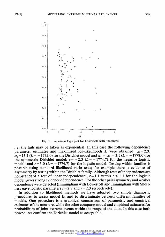
As a preliminary step, GPD analyses were performed on each margin. This serves two purposes. Firstly, appropriate thresholds ui can be determined; in this case 0.8 m, 0.9 m and 1.0 m at Immingham, Lowestoft and Sheerness respectively. Cor- responding numbers of independent exceedances were 98, 82 and 89 from 131 independent events which exceeded at least one threshold. A second use of this preliminary investigation is for verification of model validity. On the basis of the marginal GPD fits the vector observations in the bivariate and trivariate cases were transformed to (r, w) using equations (5.3) and (2.1). For bivariate cases Joe et al. (1989) have suggested plotting w, against log r as a diagnostic aid. Fig. 1 shows this for Lowestoft with Sheerness. The apparent independence of r and w, suggests that the asymptotic property (2.2) applies above the chosen thresholds. Similar conclu- sions were drawn from plots in the other bivariate cases although these do not exhibit the asymmetry of w, in Fig. 1. The w, versus log r plot can be further used to identify whether mass is on the boundaries of w. For example in Fig. 1 very few points are near the boundaries, suggesting that models with all mass in the interior of S2 are appropriate, namely the Dirichlet and symmetric versions of the two logistic models.

Concentrating on the Lowestoft with Sheerness case, standard likelihood ratio tests gave no significant evidence against taking the shape parameter k= 0 in each margin,




WI . 0

*

0. 9

* *

0.8

O. * * *

0.7 ** **

**** *

0.6 ~~* * ,, **

}*~~~~~~

0.5 *2*t * 0.6* * * * *

** *

0.5 * I * * *** * *

0.3 0 Ir-rr**

* *

**~~~ **

* ** * * * *

o.i~~ *

3 4 5 ~~6 7 8 9

tog R

Fig. 1. w, versus log r plot for Lowestoft with Sheerness

i.e. the tails may be taken as exponential. In this case the following dependence parameter estimates and maximized log-likelihoods L were obtained: a, = 2.3, a2 = 13.1 (L = - 1775.0) for the Dirichlet model and a,l = Ca2 = 3.5 (L = - 1778.0) for the symmetric Dirichlet model; r = -2.3 (L =- 1774.7) for the negative logistic model; and r = 3. 0 (L = - 1774.7) for the logistic model. Testing within families is possible using standard likelihood ratio tests; for example there is evidence of asymmetry by testing within the Dirichlet fami'ly. Although tests of i'ndependence are non-standard a test of 'near independence', r = 1.1I versus r > 1.1I for the logilstic model, gives strong evidence of dependence. For the other pairs symmetry and weaker dependence were detected (Immingham with Lowestoft and Immingham with Sheer- ness gave logistic parameters r = 2.7 and r = 2.3 respectively).

In addition to likelihood methods we have adopted two silmple diagnostic procedures to assess model fit and to discrilminate between different families of models. One procedure is a graphical comparison of parametric and empirical estimates of the measure, while the other compares model and empirical estimates for probabilities of joint extreme events within the range of the data. In this case both vprocedures confirm the Dirichlet model as acceptable.




W2 1. 0

0. 9-

0. 8

0. 7- *

0. 6 0.6 * * * * *

* *

0.5 * **

* *2

0.5 *I*

*** * **t* \

0.4 * * * ** **

* * * *\

* ** * **** ** ** \

0. 3 2 * 3 * * 4* * \ *

,> *

*8

* * * * * * *N F \

0.2 - * * t \

O F w * * ** * F ***+ **\

* Y

00 0.1 0.2 0.3 0.4 0.5 0.6 0.7 0.8 0.9 0

WI

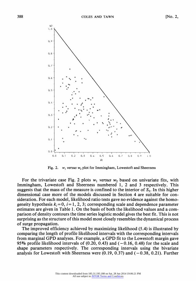
Fig. 2. w, versus w2 plot for Immingham, Lowestoft and Sheerness

For the trivariate case Fig. 2 plots w1 versus w2 based on univariate fits, with Immingham, Lowestoft and Sheerness numbered 1, 2 and 3 respectively. This suggests that the mass of the measure is confined to the interior of S3. In this higher dimensional case more of the models discussed in Section 4 are suitable for con- sideration. For each model, likelihood ratio tests gave no evidence against the homogeneity hypothesis ki = 0, i = 1, 2, 3; corresponding scale and dependence parameter estimates are given in Table 1. On the basis of both the likelihood values and a comparison of density contours the time series logistic model gives the best fit. This is not surprising as the structure of this model most closely resembles the dynamical process of surge propagation.

The improved efficiency achieved by maximizing likelihood (5.4) is illustrated by comparing the length of profile likelihood intervals with the corresponding intervals from marginal GPD analyses. For example, a GPD fit to the Lowestoft margin gave 95% profile likelihood intervals of (0.20, 0.43) and (- 0.16, 0.48) for the scale and shape parameters respectively. The corresponding intervals using the bivariate analysis for Lowestoft with Sheerness were (0.19, 0.37) and (- 0.38, 0.21). Further



1991] MODELLING EXTREME MULTIVARIATE EVENTS 389 TABLE 1

Estimated dependence models

Model L Parameter estimates Marginal (a,, o2, a3) Dependence

Symmetric logistic -2845.1 0.25, 0.30, 0.34 r=2.5 Symmetric negative logistic -2844.4 0.27, 0.29, 0.37 r= - 1.9 Dirichlet - 2837.3 0.26, 0.30, 0.37 a = 1.8, a2 = 4.4, a3 3.7 Dirichlet (a2=at3=4) -2837.5 0.26, 0.30, 0.37 a1= 1.8, a=4.0 Nested logistic -2827.0 0.26, 0.30, 0.35 r=3.1, s=2.4 Time series logistic -2822.5 0.27, 0.32, 0.36 r1 = 2.8, r2 = 3.3

evidence of the increased precision obtained by using simultaneous estimation comes from simulation studies in which substantial reductions in mean-squared errors of marginal parameter estimates were found.

ACKNOWLEDGEMENTS

S. G. Coles's work was carried out while under the funding of a Science and Engineering Research Council award. We would like to thank Dr C. W. Anderson, the Editor and a referee for helpful discussions and suggestions, and the Proudman Oceanographic Laboratory for providing the data.

APPENDIX A

Proof of Theorem I Let C be the set of all non-empty subsets of { 1, . . ., p }. Consider the partition (C1, .

Cp) of C where Cj is the set of subsets of { 1, . . .,p } of sizej. An alternative expression for the exponent measure, equation (2.4), is obtained by the following steps: first split equation (2.4) into a sum of integrals over each boundary space; then transform each integrand into Cartesian components and further separate the integrals by use of the inclusion-exclusion formula. This leads to

p

V(x) = E E, 2(_l)jdj-1I(c;d) (A. 1) j=1 ceCCdCc:

d?0

where, if d C c = {t1, . .,t

00 l00 l00 Ix, ul (U lj) (j) du I(c; d) = . .. . .. hj,4 C ~ j u1Y~~d o o x1, XtIdI I j U 1

and lj is the j-dimensional unit vector. Now define the operator

DM C- , ax( aX. Xr=? if rax

wherec= {el,..,lm} and I = m. Then, if ce d, Dm,e{I(c;d)} 0 and, if jC d, Dm,e{I(c; d)} -Dm, {I(c; c)}. Hence, by equation (A. 1),




p

Dm, {V(x)} = > z E (_-1)id-I Dm,e{I(c;d)}

j=1 ceC dCc: d*0

p

= Z Z (_)IdI-1Dm e{I(c; c)} j=1 ceCj dCc:

c C d

=E i z i

(r-m)(-1) Dm,e{I(c; c)}. j=1 cceC, r=mrm

But as

E jm8 l)- 9-)M- if j = m

then

Dm,e{V(x)}= (-1)m1 >Dm,e{I(c;c)} CECm

= (-)I)m- Dm, e{I(; c-)}

= - (Zxi)() hm, s . EX EXI

Proof of Theorem 2 Let h* be any positive function on Sp with finite first moments mj, given by equation (3.5).

Then by equation (3.3)

G(x) = exp

-s

max i h*(u) du}

(A.2) ( SP \mixj/

is a multivariate extreme value distribution with unit Frechet margins. Applying the change of variables uj = mj wj /(m.w), j= 1,. . ., p, in equation (A.2) gives

G(x) = exp - max(-W')h*( Ml WI MP ) -d dw)

where J(w) is the Jacobian of the transformation u -- w. By comparison with equation (2.4) it follows that

h(w) = - ( ) h * MIW MP mpwp)

is a measure density on Sp satisfying constraints (2.3). It remains to evaluate J(w). As

auJ/aw = mj{m.w+(mp-mj)wj }/(m.w)2I j=1,. .P

()ujlaWk = (mp-Mk)wj/(M.W)2, j, k= 1,.. .,p, j k, letting w* = (wl, . . ., wp1)', m* = (mp-m1, . . . mp-mp1)', and Ij bethej xj identity matrix it follows that

P-1 J(w) = (m.w)2(1 -p) I mj det{(m-w)IP + w-m* }




-=(m.w)' (tI in)det{Ip1 1+(w.ma)/(m.w)}

= (mW)1 -P (IT mj) det{ I- + (mw*.w)/(m.w)}

by use of a special case of a determinant property in Mardia et al. (1979). Hence

J(w) = (mw) P(FI mjI){1 +(mp-mw)/(m.w)}

p

- (m.w)-P]7 mi. j=1

REFERENCES

Aitchison, J. (1986) The Statistical Analysis of Compositional Data. London: Chapman and Hall. Barnett, V. (1976) The ordering of multivariate data (with discussion). J. R. Statist. Soc. A, 139,

318-354. Davison, A. C. and Smith, R. L. (1990) Models for exceedances over high thresholds (with discussion).

J. R. Statist. Soc. B, 52, 393-442. Graff, J. (1981) An investigation of the frequency distributions of annual maxima at ports around Great

Britain. Est. Coast. Shelf Sci., 12, 389-449. Gumbel, E. J. (1960) Distributions de valeurs extremes en plusieurs dimensions. Publ. Inst. Statist.

Paris, 9, 171-173. de Haan, L. (1984) A spectral representation for max-stable processes. Ann. Probab., 12, 1194-1204.

(1985) Extremes in higher dimensions: the model and some statistics. Proc. 45th Sess. Int. Statist. Inst., paper 26.3.

de Haan, L. and Resnick, S. I. (1977) Limit theory for multivariate sample extremes. Z. Wahrsch. Theor., 40, 317-337.

Joe, H. (1989) Families of min-stable multivariate exponential and multivariate extreme value distributions. Statist. Probab. Lett., 9, 75-82.

Joe, H., Smith, R. L. and Weissman, I. (1989) Bivariate threshold methods for extremes. J. R. Statist. Soc. B, to be published.

Mardia, K. V., Kent, J. T. and Bibby, J. M. (1979) Multivariate Analysis, A.2.3.n. London: Academic Press.

McFadden, D. (1978) Modelling the choice of residential location. In Spatial Interaction Theory and Planning Models (eds A. Karlqvist, L. Lundquist, F. Snickers and J. Weibull), pp. 75-96. Amsterdam: North-Holland.

Pickands, J. (1975) Statistical inference using extreme order statistics. Ann. Statist., 3, 119-131. (1981) Multivariate extreme value distributions. Proc. 43rd Sess. Int. Statist. Inst., 859-878.

Resnick, S. I. (1987) Extreme Values, Regular Variation, and Point Processes. New York: Springer. Smith, R. L. (1985) Maximum likelihood estimation in a class of non-regular cases. Biometrika, 72,

67-90. (1986) Extreme value theory based on the r largest annual events. J. Hydrol., 86, 27-43. (1989) The extremal index for a Markov chain. Submitted to J. Appl. Probab. (1990) Extreme value theory. In Handbook of Applicable Mathematics (ed. W. Ledermann), vol.

7. Chichester: Wiley. Smith, R. L., Tawn, J. A. and Yuen, H. K. (1990) Statistics of multivariate extremes. Int. Statist. Inst.

Rev., 58, 47-58.




Tawn, J. A. (1988a) An extreme value theory model for dependent observations. J. Hydrol., 101, 227-250.

(1988b) Bivariate extreme value theory: models and estimation. Biometrika, 75, 397-415. (1990) Modelling multivariate extreme value distributions. Biometrika, 77, 245-253.

Weissman, I. (1978) Estimation of parameters and quantiles based on the k largest observations. J. Am. Statist. Ass., 73, 812-815.



Documents

Modelling Extreme Multivariate Events