Embed Size (px)
Citation preview
Modelling freight transport demand and
reference dependent choice behaviour
Lorenzo Masiero
Submitted for the degree of Ph.D. in Economics
Faculty of Economics
University of Lugano, Switzerland
Thesis Committee:
Prof. Rico Maggi, supervisor, University of Lugano
Prof. Massimo Filippini, internal examiner, University of Lugano
Prof. Romeo Danielis, external examiner, University of Trieste
July 2010


To my family


Acknowledgments
First of all, I would like to thank my supervisor, Prof. Rico Maggi; without his
encouragement and inestimable support this thesis would not have been possible.
I am deeply grateful to Prof. Massimo Filippini for having accepted the role of internal
examiner of my thesis. I am also particularly grateful to Prof. Romeo Danielis for having
agreed to be part of the thesis committee as external examiner and for helping me with his
advise in a very early stage of my thesis.
During my doctoral studies I had the opportunity to visit the Institute of Transport and
Logistics Studies (ITLS) at University of Sydney thanks to a grant founded by the Swiss
National Science Foundation. I owe my deepest gratitude to the director of ITLS, Prof.
David Hensher, who supervised me during the whole year of my stay and contributed
significantly to the value of my thesis.
Professor Aura Reggiani encouraged me to continue my studies after the Master. Her
superb teaching skills and her strong academic research have been crucial towards my
decision to pursuit a PhD degree. I will never be able to thank her enough.
I am indebted to my colleagues at the IRE in Lugano and at the ITLS in Sydney. They
helped me through numerous conversations supporting every step of my doctoral studies
with their friendship.
Finally, I would like to thank my friends and my family for their unlimited support and
much appreciated encouragement.

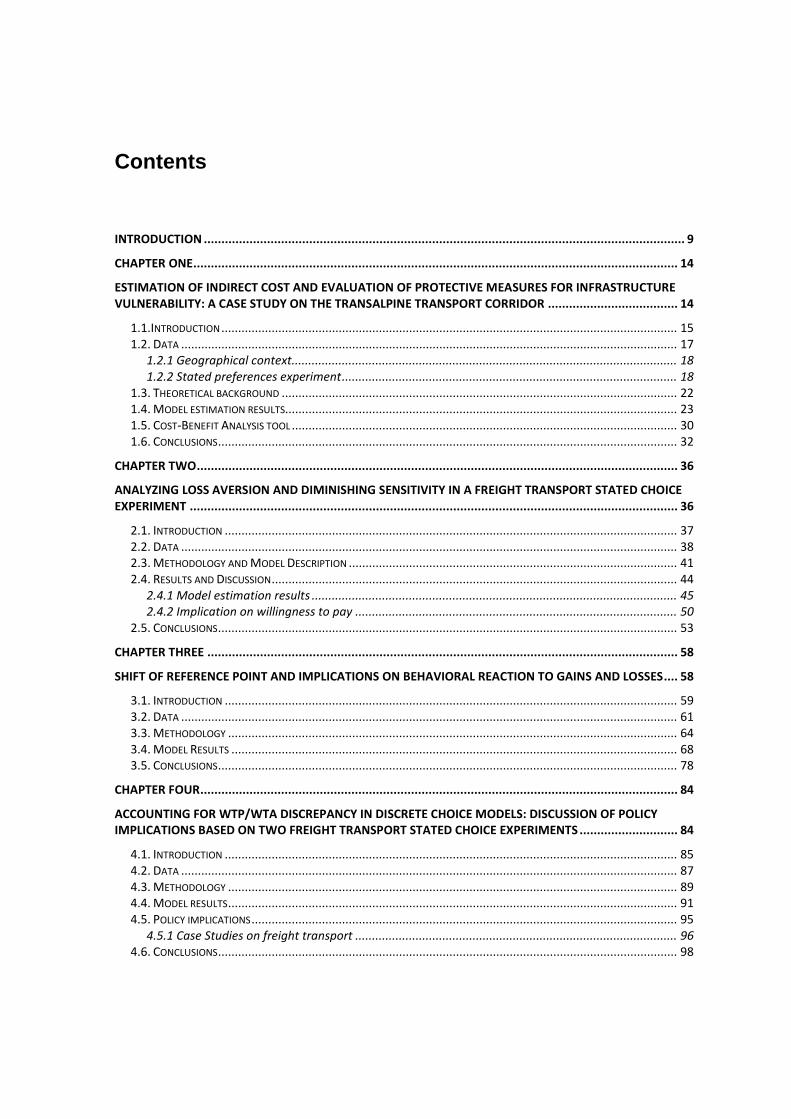
Contents
INTRODUCTION ......................................................................................................................................... 9
CHAPTER ONE .......................................................................................................................................... 14
ESTIMATION OF INDIRECT COST AND EVALUATION OF PROTECTIVE MEASURES FOR INFRASTRUCTURE VULNERABILITY: A CASE STUDY ON THE TRANSALPINE TRANSPORT CORRIDOR ..................................... 14
1.1.INTRODUCTION ........................................................................................................................................ 15 1.2. DATA .................................................................................................................................................... 17
1.2.1 Geographical context................................................................................................................... 18 1.2.2 Stated preferences experiment .................................................................................................... 18
1.3. THEORETICAL BACKGROUND ...................................................................................................................... 22 1.4. MODEL ESTIMATION RESULTS..................................................................................................................... 23 1.5. COST-BENEFIT ANALYSIS TOOL ................................................................................................................... 30 1.6. CONCLUSIONS ......................................................................................................................................... 32
CHAPTER TWO ......................................................................................................................................... 36
ANALYZING LOSS AVERSION AND DIMINISHING SENSITIVITY IN A FREIGHT TRANSPORT STATED CHOICE EXPERIMENT ........................................................................................................................................... 36
2.1. INTRODUCTION ....................................................................................................................................... 37 2.2. DATA .................................................................................................................................................... 38 2.3. METHODOLOGY AND MODEL DESCRIPTION .................................................................................................. 41 2.4. RESULTS AND DISCUSSION ......................................................................................................................... 44
2.4.1 Model estimation results ............................................................................................................. 45 2.4.2 Implication on willingness to pay ................................................................................................ 50
2.5. CONCLUSIONS ......................................................................................................................................... 53
CHAPTER THREE ...................................................................................................................................... 58
SHIFT OF REFERENCE POINT AND IMPLICATIONS ON BEHAVIORAL REACTION TO GAINS AND LOSSES .... 58
3.1. INTRODUCTION ....................................................................................................................................... 59 3.2. DATA .................................................................................................................................................... 61 3.3. METHODOLOGY ...................................................................................................................................... 64 3.4. MODEL RESULTS ..................................................................................................................................... 68 3.5. CONCLUSIONS ......................................................................................................................................... 78
CHAPTER FOUR ........................................................................................................................................ 84
ACCOUNTING FOR WTP/WTA DISCREPANCY IN DISCRETE CHOICE MODELS: DISCUSSION OF POLICY IMPLICATIONS BASED ON TWO FREIGHT TRANSPORT STATED CHOICE EXPERIMENTS ............................ 84
4.1. INTRODUCTION ....................................................................................................................................... 85 4.2. DATA .................................................................................................................................................... 87 4.3. METHODOLOGY ...................................................................................................................................... 89 4.4. MODEL RESULTS ...................................................................................................................................... 91 4.5. POLICY IMPLICATIONS ............................................................................................................................... 95
4.5.1 Case Studies on freight transport ................................................................................................ 96 4.6. CONCLUSIONS ......................................................................................................................................... 98

9
Introduction
The thesis focuses on discrete choice models for freight transport demand with a particular
emphasis on the estimation of willingness to pay (WTP) and willingness to accept (WTA)
measures. In order to cope with the research objective, I extend the classic discrete choice
model specifications towards the frontier of the current literature on asymmetric model
specifications in stated choice experiments with a reference pivoted design.
Discrete choice models investigate and explain the choice of an individual (or group of
individuals) among alternatives. In this framework, the alternatives must be mutually
exclusive, exhaustive and the number of alternatives must be finite (Train, 2003).
Academic interest on discrete choice models has origins in mathematical psychology. In
particular, Thurstone (1927) states the law of comparative judgment, that is a
measurement model involving the comparison between two items with respect to
magnitude of stimuli. Luce (1959) proposes the choice axiom to characterize a choice
probability law that defines two fundamental properties regarding dominated and
undominated alternatives. Marschak (1960) formulates an interpretation of utility instead
of stimuli and formulated a derivation from utility maximization giving the starting point
for the so called random utility models (RUMs).
McFadden (1974) introduces the multinomial logit model and its estimation based on the
restricted assumptions about the error term of the utility that must be independent and
identically distributed (iid assumption). The independence assumption was relaxed by
McFadden (1978) through the derivation of the generalized extreme value (GEV) model, a
large class of models that allows correlation among the error terms of the alternatives.
Mixed logit models were introduced in the 1980s by Boyd and Mellman (1980), Cardell
and Dunbar (1980) and accurately investigated by Train, McFadden and Ben-Akiva
(1987a). This class of models is extremely general and flexible, McFadden and Train
(2000) prove that any random utility model can be approximated by a mixed logit model.
The main power of mixed logit models is that they solve three typical problems of logit
10 Modelling freight transport demand and reference dependent choice behaviour
models. That is, they allow for random taste variation, for correlation in unobserved
factors over time and they allow unrestricted substitution patterns (Train, 2003).
According to prospect theory (Kahneman and Tversky, 1979; Tversky and Kahneman,
1991; Tversky and Kahneman, 1992), individual choice behaviour is subject to a concept
referred to as reference dependency. This concept, when framed within the idea of utility
maximization, suggests that when evaluating different outcomes, individuals tend to
distinguish differently between positive (gains) and negative (losses) deviations from
some base reference alternative. This result leads to the notion that utility should be
centred on this base reference point and then be defined in terms of domains of gains and
losses surrounding this reference point. In this context, two fundamental findings have
been found to characterize individual’s utility functions; that individuals i) experience loss
aversion (i.e., they evaluate higher weights for losses than for gains), and ii) experience
diminishing sensitivity to both gains and losses (i.e., decreasing marginal values in both
positive and negative domains). The implications of these two characteristics when
considered together, imply firstly the marginal utility of individuals for gains and losses
are different and secondly, that these marginal utilities can be considered as non-linear. In
turn, this implies that the demand curves for individual respondents should be considered
to be kinked with the elbow of the kink centred at the site of the reference alternative.
Since the formalization of prospect theory, reference dependence has been tested in
several studies through the use of different interview procedures, with particular reference
to contingent evaluation (e.g., Bishop and Heberlein, 1979; Rowe et al., 1980) and
laboratory experiments (e.g., Bateman et al., 1997).
Stated choice experiments (SCE) currently represent the primary method for collecting
data for the purpose of analysing and understanding choice behaviour. These experiments
present surveyed respondents with hypothetical choice situations with the resulting model
estimation relying on the Random Utility Model framework (McFadden, 1974). The need
to firstly, approximate the reality as much as possible in order to increase the behavioural
meaning of the results and secondly, accommodate the prospect theory reference
dependence assumption, has resulted in increasing attention being given not only towards
modelling the impacts of prospect theory, but also towards generating SCE designs that
are pivoted around individual specific reference alternatives (see, for example, Hensher,
Introduction 11
2008; Rose et al., 2008). According to a pivot-design the utility function associated to
each hypothetical alternative can then be specified in terms of gains and losses around the
reference alternative values, either in terms of absolute levels or percentages.
The research is divided into four chapters, each one corresponding to a paper submitted to
a refereed journal. The same dataset has been used for all the four papers. The data was
obtained from a stated choice survey in a freight transport context conducted in the Ticino
region (Switzerland) in 2008. The experiment was part of the project NFP54 “Sustainable
Development of the Built Environment”, founded by the Swiss National Science
Foundation, aimed to analyze the infrastructure vulnerability of the Gotthard corridor, one
of the most important European transport corridors. In particular, the fourth paper,
presented in Chapter four, includes a further dataset (collected in 2003) which has been
combined to the former one in order to validate the robustness of the results obtained.
The focus of the first paper is to model the freight transport demand according to classical
mixed logit model specifications and to integrate the model estimates, such as willingness
to pay measures, in a cost-benefit analysis tool. The second paper investigates loss
aversion and diminishing sensitivity, and analyzes their implications on willingness to pay
and willingness to accept measures in a reference pivoted choice experiment in a freight
transport framework. The third paper focuses on individual reactions, in a freight choice
context, to a negative change in the reference alternative values, identifying the
behavioural implications in terms of loss aversion and diminishing sensitivity. Finally, the
fourth paper proposes a comparison of willingness to pay and willingness to accept
measures estimated from models with both symmetric and reference dependent utility
specifications within two different freight transport stated choice experiments.
References
Bateman, I., Munro, A., Rhodes, B., Starmer, C., Sugden, R., 1997. A test of the theory of
reference-dependent preferences. Quarterly Journal of Economics 112, 479–505.
Bishop, R.C., Heberlein, T.A., 1979. Measuring values of extramarket goods: are indirect
measures biased? American Journal of Agricultural Economics 61, 926–930.
12 Modelling freight transport demand and reference dependent choice behaviour
Boyd, J., Mellman, J., 1980. The effect to fuel economy standards on the U.S. automotive
market: A hedonic demand analysis. Transportation Research Part A 14, pp. 367-378.
Cardell, S., Dunbar F., 1980. Measuring the societal impacts of automobile downsizing.
Transportation Research Part A 14, pp. 423-434.
Hensher, D.A., 2008. Joint estimation of process and outcome in choice experiments and
implications for willingness to pay. Journal of Transport Economics and Policy 42 (2),
297-322.
Kahneman, D., Tversky A., 1979. Prospect Theory: an analysis of decision under risk.
Econometrica 47 (2), 263–291.
Luce, D., 1959. Individual Choice Behavior. John Wiley and Sons, New York.
Marschak, J., 1960. Binary choice constraints on random utility indications. In K. Arrow,
ed., Stanford Symposium on Mathematical Methods in the Social Sciences. Staford
University Press, Stenford, CA, pp. 312-329.
McFadden, D., 1974. Conditional logit analysis of qualitative choice behavior. In:
Zarembka, P. (Ed.), Frontiers in Econometrics. Academic Press, New York.
McFadden, D., 1978. Modelling the Choice of Residential Location. In Spatial Interaction
Theory and Residential Location. A. Karlquist et al., eds. North Holland, Amsterdam, pp.
75-96.
McFadden, D., Train, k., 2000. Mixed MNL models of discrete response. Journal of
Applied Econometrics 15, pp. 447-470.
Rose, J.M., Bliemer, M.C., Hensher, Collins, A. T., 2008. Designing efficient stated
choice experiments in the presence of reference alternatives. Transportation Research B
42(4), 395-406.
Rowe, R.D., D’Arge, R.C., Brookshire, D.S., 1980. An experiment on the economic value
of visibility. Journal of Environmental Economics and Management 7, 1–19.
Thurstone, L., 1927. A law of comparative judgement. Psychological Review 34, pp. 273-
286.
Train, K., 2003. Discrete Choice Methods with Simulation. Cambridge University Press,
Cambridge.

Introduction 13
Train, K., McFadden D., Ben-Akiva, M., 1987a. The demand for local telephone service:
A fully discrete model of residential calling patterns and service choice. Rand Journal of
Economics 18, pp. 109-123.
Tversky, A., Kahneman, D., 1991. Loss aversion in riskless choice: A reference-
dependent model. Quarterly Journal of Economics 106, 1039–1061.
Tversky, A., Kahneman, D., 1992. Advances in Prospect Theory: Cumulative
Representation of Uncertainty. Journal of Risk and Uncertainty 5, 297-323.
14
Chapter One
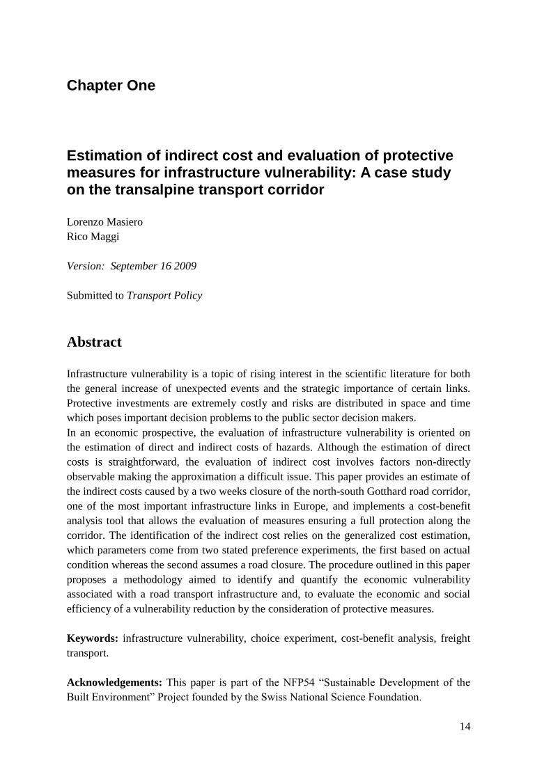
Estimation of indirect cost and evaluation of protective measures for infrastructure vulnerability: A case study on the transalpine transport corridor
Lorenzo Masiero
Rico Maggi
Version: September 16 2009
Submitted to Transport Policy
Abstract
Infrastructure vulnerability is a topic of rising interest in the scientific literature for both
the general increase of unexpected events and the strategic importance of certain links.
Protective investments are extremely costly and risks are distributed in space and time
which poses important decision problems to the public sector decision makers.
In an economic prospective, the evaluation of infrastructure vulnerability is oriented on
the estimation of direct and indirect costs of hazards. Although the estimation of direct
costs is straightforward, the evaluation of indirect cost involves factors non-directly
observable making the approximation a difficult issue. This paper provides an estimate of
the indirect costs caused by a two weeks closure of the north-south Gotthard road corridor,
one of the most important infrastructure links in Europe, and implements a cost-benefit
analysis tool that allows the evaluation of measures ensuring a full protection along the
corridor. The identification of the indirect cost relies on the generalized cost estimation,
which parameters come from two stated preference experiments, the first based on actual
condition whereas the second assumes a road closure. The procedure outlined in this paper
proposes a methodology aimed to identify and quantify the economic vulnerability
associated with a road transport infrastructure and, to evaluate the economic and social
efficiency of a vulnerability reduction by the consideration of protective measures.
Keywords: infrastructure vulnerability, choice experiment, cost-benefit analysis, freight
transport.
Acknowledgements: This paper is part of the NFP54 “Sustainable Development of the
Built Environment” Project founded by the Swiss National Science Foundation.

Estimation of indirect cost and evaluation of protective measures for infrastructure vulnerability 15
1.1. Introduction
Interruptions in infrastructure networks generate considerable economic and social
damages at the regional and national level according to the overall dependency of the
network on certain links and the risk associated with this interruption. In the context of
increasingly vulnerable networks due to climate change, the attention on transport
network reliability has grown substantially in the recent years in the international science
community (Bell and Iida 2003, Nicholson and Dante 2004). Berdica (2002) introduces
the road transport vulnerability as a complement of reliability, that is, the non-operability
of a system due to incidents caused by either natural or man-made hazards.
Vulnerability assessment of a given transport infrastructure is mostly oriented on an
engineering approach and regards the identification of the weakest points in a
transportation network. Numerous methods have been proposed based on, for example,
connectivity reliability (Bell and Ida, 1997), capacity reliability (Cheng et al., 2002) or
accessibility index (Taylor et al., 2006).
In an economic prospective, the evaluation of infrastructure vulnerability is oriented on
the estimation of direct and indirect costs of hazards. The former are associated with
damages on the infrastructure caused by an unexpected event whereas the latter regard the
consequences that the damaged infrastructure provokes on the society that depends on it.
Although the estimation of direct costs is straightforward, the evaluation of indirect cost
involves factors non-directly observable making the approximation a difficult issue.
D’Este and Taylor (2003) proposed to calculate the loss of amenity of a link interruption
as the change in generalized cost weighted by travel demand. Different algorithms have
been proposed, as, for example, the short path algorithm. However, Taylor and D'Este
(2004) recognized the limit in using algorithms as estimates of change in the utility of
travel.
The estimation of the cost associated with an interruption of an infrastructure link is
necessary in order to evaluate the desirability of any protective measure that allows a
reduction of the vulnerability of the network to which it belongs. In this sense, a given
vulnerability of a network represents a level of (expected) direct and indirect cost of a
given hazard risk. Reducing vulnerability via costly protective measures can lead, as a
16 Modelling freight transport demand and reference dependent choice behaviour
function of the type of measure implemented, to an increased reliability (hazards have less
or no consequences due to increased protection) or an increased resilience (networks
recover faster from hazards).1 We will concentrate here on the evaluation of protective
measures creating “perfect” reliability (equivalent to a full insurance policy). This does
not imply that we advocate zero vulnerability networks. Rather, a cost-benefit analysis of
full protection measures on a given link will reveal whether this is economically justified
and will in consequence contribute to move towards an economically optimal reliability.
A methodology that allows the economic evaluation of the optimal reliability is still
needed and required.
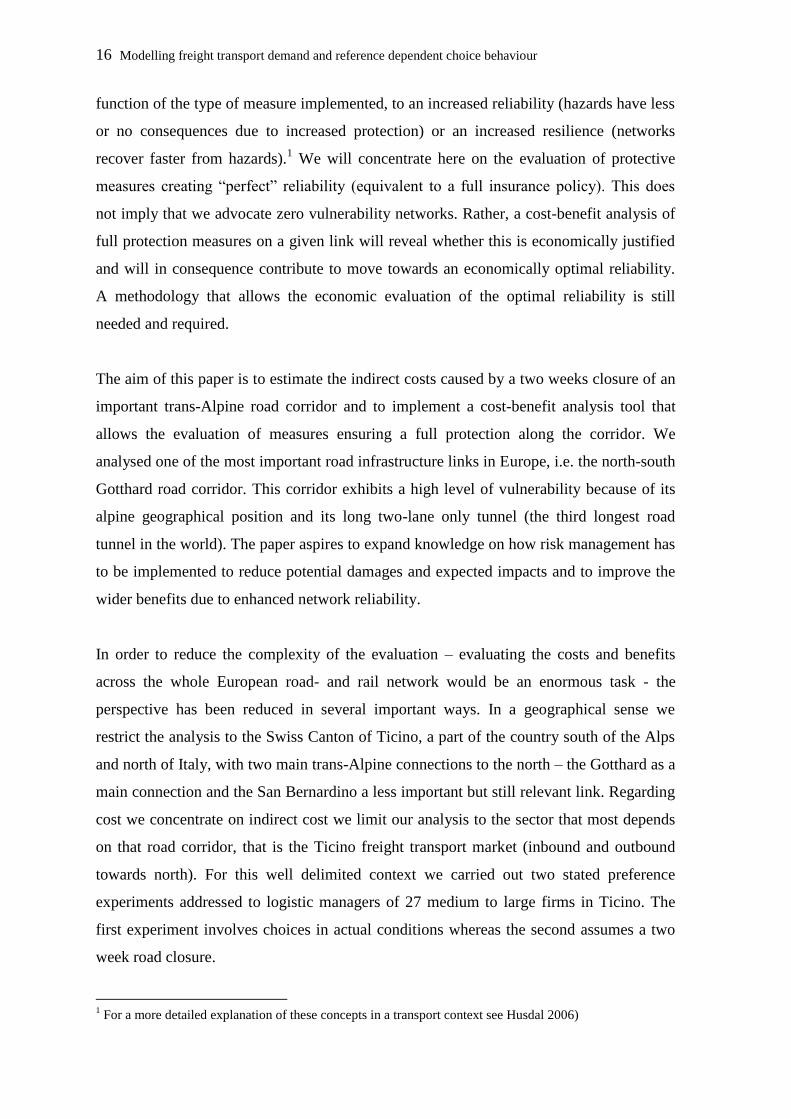
The aim of this paper is to estimate the indirect costs caused by a two weeks closure of an
important trans-Alpine road corridor and to implement a cost-benefit analysis tool that
allows the evaluation of measures ensuring a full protection along the corridor. We
analysed one of the most important road infrastructure links in Europe, i.e. the north-south
Gotthard road corridor. This corridor exhibits a high level of vulnerability because of its
alpine geographical position and its long two-lane only tunnel (the third longest road
tunnel in the world). The paper aspires to expand knowledge on how risk management has
to be implemented to reduce potential damages and expected impacts and to improve the
wider benefits due to enhanced network reliability.
In order to reduce the complexity of the evaluation – evaluating the costs and benefits
across the whole European road- and rail network would be an enormous task - the
perspective has been reduced in several important ways. In a geographical sense we
restrict the analysis to the Swiss Canton of Ticino, a part of the country south of the Alps
and north of Italy, with two main trans-Alpine connections to the north – the Gotthard as a
main connection and the San Bernardino a less important but still relevant link. Regarding
cost we concentrate on indirect cost we limit our analysis to the sector that most depends
on that road corridor, that is the Ticino freight transport market (inbound and outbound
towards north). For this well delimited context we carried out two stated preference
experiments addressed to logistic managers of 27 medium to large firms in Ticino. The
first experiment involves choices in actual conditions whereas the second assumes a two
week road closure.
1 For a more detailed explanation of these concepts in a transport context see Husdal 2006)

Estimation of indirect cost and evaluation of protective measures for infrastructure vulnerability 17
Discrete choice model specification allows the generalized cost estimation through the
derivation of the willingness to pay measures. Indeed, stated preference experiments are
the most common techniques used in willingness to pay derivation and they allow to
investigate the consumer behaviour in situations where few (or even none) data are
available.
The cost benefit analysis is based on the change that an unexpected road interruption
caused in the freight transport generalized cost. The evaluation of the economic
sustainability of the risks identified along the corridor is then carried out by comparing the
increase in the generalized cost with the cost of the protective measures. Finally, a cost
benefit analysis tool is provided as a valid support of policy decision makers.
The paper is organized as follows. In section two we provide a brief geographical
description of the infrastructure and we introduce the data. In section three we outline the
discrete choice theoretical formulation. We present and discuss the model results in
section four. The cost benefit analysis is performed in section five along with the
introduction of the tool. Finally, conclusion and suggestion for further research are given
in section six.
1.2. Data
The study concerns a choice based experiment, analysing the economic impact of a
hypothetical closure of the Gotthard corridor2. Consequently we investigated the possible
adaptive behavioural patterns of different actors in the face of disastrous and/or risky
events. The investigation is based on the method of stated preferences. We basically want
to model by means of an experimental design how the different actors react to the closure
of this important road link across the Alps.
2 The experiment began with some pilot interviews during February 2008, officially started in March 2008
and was finally concluded in June 2008.

18 Modelling freight transport demand and reference dependent choice behaviour
1.2.1 Geographical context
Due to its strategic position the corridor is one of the most important links between the
north and the south of Europe. It represents a very important element of the national and
international road and rail network facilitating transport and economic interaction between
the north and the south of Europe.
Today, roughly 200 km of the Swiss national highway network are exposed to natural
hazards, or in other words, every ninth kilometres leads through hazardous areas and
hence needs protection. A total of 137 galleries protect the traffic, more than 90 of them
are rock fall protection measures. Additionally there are constructive measures directly in
the hazard zones, such as protection nets, anchors, etc. The maintenance of these
protection measures costs 30 Mio CHF every year3.
Between 1994 and 2004 freight transport by road and rail across the Alps grew by 68%
(rail traffic plus 25%, road traffic plus 60%). Today, the Alps are crossed each year by
about 10 million trucks, a third of which passes through Switzerland, 85% of these using
the Gotthard route4.
1.2.2 Stated preferences experiment
We introduced the experiment by conducting an interview with the logistics managers of
the most concerned industries (manufacturing) asking them about their general logistics
and transportation framework and typical transportation relations across the Alps5. These
managers were then confronted with alternative transportation services described by the
use of three attributes, respectively, cost, time and punctuality. Cost and time attributes are
pivoted to the reference values according to the levels shown in Table 1, whereas
punctuality is expressed in absolute values.
3 “La A2 a Gurtnellen un anno dopo la frana”. Comunicato Stampa, Ufficio federale delle strade USTRA.
4 MONITRAF, Synthesebericht, Monitraf Aktivitäten und Ergebnisse, Endbericht, febbraio 2008,
Innsbruck/Zürich. 5 The decision to concentrate on the freight transport sector stems from past studies demonstrating that the
passenger sector (tourism and business travel) exhibit almost negligible additional costs in the sequel of past
closures. In particular, we refer to the closure of two months occurred in November 2001 following a frontal
truck crash inside the 17 km long tunnel.
Estimation of indirect cost and evaluation of protective measures for infrastructure vulnerability 19
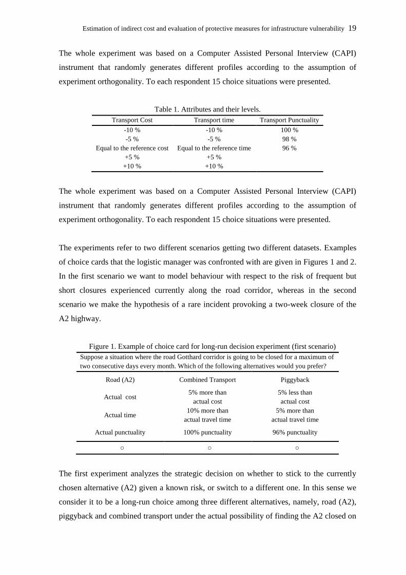
The whole experiment was based on a Computer Assisted Personal Interview (CAPI)
instrument that randomly generates different profiles according to the assumption of
experiment orthogonality. To each respondent 15 choice situations were presented.
Table 1. Attributes and their levels.
Transport Cost Transport time Transport Punctuality
-10 % -10 % 100 %
-5 % -5 % 98 %
Equal to the reference cost Equal to the reference time 96 %
+5 % +5 %
+10 % +10 %
The whole experiment was based on a Computer Assisted Personal Interview (CAPI)
instrument that randomly generates different profiles according to the assumption of
experiment orthogonality. To each respondent 15 choice situations were presented.
The experiments refer to two different scenarios getting two different datasets. Examples
of choice cards that the logistic manager was confronted with are given in Figures 1 and 2.
In the first scenario we want to model behaviour with respect to the risk of frequent but
short closures experienced currently along the road corridor, whereas in the second
scenario we make the hypothesis of a rare incident provoking a two-week closure of the
A2 highway.
Figure 1. Example of choice card for long-run decision experiment (first scenario)
Suppose a situation where the road Gotthard corridor is going to be closed for a maximum of
two consecutive days every month. Which of the following alternatives would you prefer?
Road (A2) Combined Transport Piggyback
Actual cost 5% more than
actual cost
5% less than
actual cost
Actual time 10% more than
actual travel time
5% more than
actual travel time
Actual punctuality 100% punctuality 96% punctuality
o o o
The first experiment analyzes the strategic decision on whether to stick to the currently
chosen alternative (A2) given a known risk, or switch to a different one. In this sense we
consider it to be a long-run choice among three different alternatives, namely, road (A2),
piggyback and combined transport under the actual possibility of finding the A2 closed on

20 Modelling freight transport demand and reference dependent choice behaviour
a specific day. The road (A2) alternative remains fixed during the whole experiment since
it describes the reference alternative. Its characteristics are those described by logistic
managers for the typical transportation service across the Alps.
The second experiment regards a short-run decision since we make the hypothesis of a
two-week road closure - a rare event calling for a short term reaction. This choice
situation is characterized by four alternatives, namely, road (A13), new road (regulated
A13), piggyback and combined transport. In this second experiment the reference
alternative is represented by the road (A13) alternative (that is the San Bernardino
corridor) since it is the immediate re-routing alternative chosen by most road users when
the Gotthard road corridor is closed.
Figure 2. Example of choice card for short-run decision experiment (second scenario)
Suppose a situation where the road Gotthard corridor is closed for two weeks.
Which of the following alternatives would you prefer?
Road (A13) Piggyback Combined Transport New Road
(regulated A13)
Transitional
cost
10% less than
transitional cost
5% less than
transitional cost
10% more than
transitional cost
Transitional
travel time
10% more than
transitional travel time
5% more than
transitional travel time
Equal to
transitional travel time
Transitional
punctuality 98% punctuality 96% punctuality 100% punctuality
o o o o
In order to quantify the cost and time for the reference alternative (San Bernardino) we
used the additional cost and the additional time with respect to Gotthard corridor resulting
from a previous survey with six of the most important shippers in Ticino. There, all
interviewed shippers replied with very similar additional cost and time, respectively 300
CHF and 5 hours more for a detour via the San Bernardino route rather than along the
Gotthard corridor. We get the values for the road (A13) alternative by summing these
additional cost and time to the original reference values. Regarding the punctuality we
assume a decrease of 2% with respect to the original value, with a minimum level fixed to
the lowest level considered, that is, 96% of transports being punctual. This statement has
been confirmed by the shippers interviewed, in particular if we consider the high volume
of flows that occurs in a similar situation. To be noted that the validity of the transitional
values is restricted to the closure period, that is fourteen days. The new road (regulated

Estimation of indirect cost and evaluation of protective measures for infrastructure vulnerability 21
A13) alternative has been introduced to simulate a congestion free San Bernardino
alternative (assume a sort of priority policy for trucks) with the original punctuality
maintained.
The sample is composed by 27 firms active in the manufacturing sector and, as mentioned
before, all of them based in Ticino. The typical transport service described by logistic
managers is reported in Table 2. As expected, cost and time vary substantially since they
are characterized by the distance between origin and destination and by the weight of the
shipment, whereas punctuality is very homogenous and apart from two cases stating a
90% of punctuality in the transportation services all others are between 95 and 100
percent. This is in line with previous studies (see, for example, Bolis and Maggi 2003 and
Maggi and Rudel 2008) and confirms the high level of importance that a logistics manager
puts on a quality attribute like punctuality.
Table 2. Sample descriptive statistics of typical transport service
Variable Mean Median Std.Dev. Minimum Maximum
Cost (CHF) 1300.15 1000 1152.95 136 5400
Time (hr) 33.35 24 27.30 2 96
Punctuality (%) 96.52 98 3.04 90 100
Weight (ton) 7.1309 5.50 7.17 0.04 25
Distance O-D (km) 474.33 300 332.62 92 1360
MADD 2.29 2 0.97 1 5
Damage (%) 0.97 0.4 1.98 0 10
Value (CHF/kg) 203.28 40 487.38 0.36 2400
The descriptives for the damage and loss variables report a very low occurrence, with a
sample mean of 0.97% and a median of 0.4%. The damage and loss attribute is widely
used but a matter of debate in literature because of its inconsistency and its frequent
insignificance in the model estimation. In fact, it is meaningless to have a systematic
damage or loss in the transport service because shippers/forwarders will self insure via a
systematic solution, for instance a different packaging, or a different truck, or even a
different mode of transport. Indeed, accidental damages might be happening but remain an
occasional feature and not a characteristic of a transport service. For this reason, we chose
to not include this attribute in our experiment. The descriptive statistics collected during
the analysis confirm this decision.
Finally, from revealed market shares obtained for the whole logistic in the entire sample
results, as expected, that the majority of the transport services rely on road alternative

22 Modelling freight transport demand and reference dependent choice behaviour
while the rest uses combined transport, either via rail or via ship and air. The piggyback
alternative is not relevant confirming the weakness characterizing it due to technical
problems and high operational cost.
1.3. Theoretical background
In a stated choice experiment, the respondent n is supposed to select the alternative j that
maximizes his utility,
nj nj njU β x ε (1)
where nj njV β x is the systematic part of the utility and njε is the random term that is
Independent and Identically Distributed (IID) extreme value type 1. The estimation of the
beta coefficients relies on the class of Random Utility Models (McFadden, 1974).
An advanced and widely used discrete choice model is the Random Parameter Logit
(RPL) model, which allows for taste heterogeneity among respondents by letting the beta
parameters randomly vary across the sample population (see Hensher and Green, 2003 for
a detailed discussion). The following equation describes the choice probability for a RPL
model:
exp( )( ) ( )
exp( )
n ninj
n njj
P f d
β x
β ββ x
(2)
where parameters β are drawn by continuous distributions (e.g. normal, log-normal,
triangular etc.). The selection of a specific distribution, whenever possible, is based on
previous knowledge or on particular behavioural assumptions. However, if no particular
hypotheses are available or required, the selection is arbitrary and generally based on the
goodness of fit of the data.
In a context of stated choice with repeated choice situations, an additional and
indispensable feature of RPL models is the capability to deal with the panel structure by

Estimation of indirect cost and evaluation of protective measures for infrastructure vulnerability 23
constraining the random parameters to be constant over choice situations. The choice
probability in Equation (2) becomes then:
exp( )( ) ( )
exp( )
n nitnj
tn njt
j
P f d
β xβ β
β x (3)
where t = 1,…,T indicates the number of choice situations. Since in any RPL model the
choice probability integral has no closed form solutions, the estimation process is based
on simulations and the log-likelihood takes the following form:
1 exp( )ln
exp( )
n nitn
n r tn njt
j
LLR
β x
β x (4)
where, r = 1,…,R indicates the simulation draw. The following models are based on 200
Halton draws6.
1.4. Model estimation results
Different Panel RPL models were estimated7 for the two scenarios and the selection was
based according to both model fit indicators and behavioural meaning. Specifically, the
evaluation of the model goodness of fit is provided by the final log-likelihood as well as
the McFadden pseudo ρ2 and the Akaike’s Information Criterion (AIC).
The estimation of the utility functions for the first scenario is based on the following panel
RPL specification:
( ) ( )
( ) ( )
( ) ( )
(PB) PB C PB T PB P PB
(CT) CT C CT T CT P CT
(RD) C RD T RD P RD D W
C T P
C T P
C T P D W
PB PB
CT CT
RD RD n n
n
n
n
V ASC
V ASC
V
(5)
6 See Train (2003) for details.
7 Models estimation is performed by Nlogit 4.
24 Modelling freight transport demand and reference dependent choice behaviour
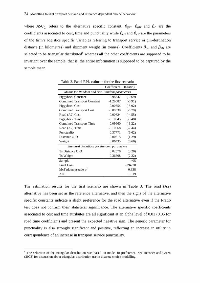
where ASC(j) refers to the alternative specific constant, β(j)C, β(j)T and βP are the
coefficients associated to cost, time and punctuality while βnD and βnW are the parameters
of the firm’s logistics specific variables referring to transport service origin-destination
distance (in kilometres) and shipment weight (in tonnes). Coefficients βnD and βnW are
selected to be triangular distributed8 whereas all the other coefficients are supposed to be
invariant over the sample, that is, the entire information is supposed to be captured by the
sample mean.
Table 3. Panel RPL estimate for the first scenario
Coefficient (t-ratio)
Means for Random and Non-Random parameters
Piggyback Constant -0.98342 (-0.69)
Combined Transport Constant -1.29087 (-0.91)
Piggyback Cost -0.00554 (-5.92)
Combined Transport Cost -0.00539 (-5.79)
Road (A2) Cost -0.00624 (-4.55)
Piggyback Time -0.10645 (-3.48)
Combined Transport Time -0.09660 (-3.22)
Road (A2) Time -0.10668 (-2.44)
Punctuality 0.37771 (6.62)
Distance O-D 0.00315 (1.29)
Weight 0.06435 (0.60)
Standard deviations for Random parameters
Ts Distance O-D 0.02570 (3.20)
Ts Weight 0.36608 (2.22)
Sample 405
Final Log-l -294.70
McFadden pseudo ρ2 0.338
AIC 1.519
The estimation results for the first scenario are shown in Table 3. The road (A2)
alternative has been set as the reference alternative, and then the signs of the alternative
specific constants indicate a slight preference for the road alternative even if the t-ratio
test does not confirm their statistical significance. The alternative specific coefficients
associated to cost and time attributes are all significant at an alpha level of 0.01 (0.05 for
road time coefficient) and present the expected negative sign. The generic parameter for
punctuality is also strongly significant and positive, reflecting an increase in utility in
correspondence of an increase in transport service punctuality.
8 The selection of the triangular distribution was based on model fit preference. See Hensher and Green
(2003) for discussion about triangular distribution use in discrete choice modelling.
Estimation of indirect cost and evaluation of protective measures for infrastructure vulnerability 25
The coefficients associated with the two firm specific variables show a mean not
statistically different from zero, however they capture a significant heterogeneity among
respondents, indicating that part of the respondents prefer to switch to rail-based
alternatives as either the transport distance or the shipment weight increases.
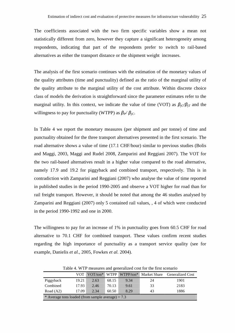
The analysis of the first scenario continues with the estimation of the monetary values of
the quality attributes (time and punctuality) defined as the ratio of the marginal utility of
the quality attribute to the marginal utility of the cost attribute. Within discrete choice
class of models the derivation is straightforward since the parameter estimates refer to the
marginal utility. In this context, we indicate the value of time (VOT) as βjC/βjT and the
willingness to pay for punctuality (WTPP) as βP/ βjC.
In Table 4 we report the monetary measures (per shipment and per tonne) of time and
punctuality obtained for the three transport alternatives presented in the first scenario. The
road alternative shows a value of time (17.1 CHF/hour) similar to previous studies (Bolis
and Maggi, 2003, Maggi and Rudel 2008, Zamparini and Reggiani 2007). The VOT for
the two rail-based alternatives result in a higher value compared to the road alternative,
namely 17.9 and 19.2 for piggyback and combined transport, respectively. This is in
contradiction with Zamparini and Reggiani (2007) who analyse the value of time reported
in published studies in the period 1990-2005 and observe a VOT higher for road than for
rail freight transport. However, it should be noted that among the 46 studies analysed by
Zamparini and Reggiani (2007) only 5 contained rail values, , 4 of which were conducted
in the period 1990-1992 and one in 2000.
The willingness to pay for an increase of 1% in punctuality goes from 60.5 CHF for road
alternative to 70.1 CHF for combined transport. These values confirm recent studies
regarding the high importance of punctuality as a transport service quality (see for
example, Danielis et al., 2005, Fowkes et al. 2004).
Table 4. WTP measures and generalized cost for the first scenario
VOT VOT/ton* WTPP WTPP/ton* Market Share Generalized Cost
Piggyback 19.21 2.63 68.15 9.34 24 1901
Combined 17.93 2.46 70.13 9.61 33 2183
Road (A2) 17.09 2.34 60.50 8.29 43 1886
* Average tons loaded (from sample average) = 7.3
26 Modelling freight transport demand and reference dependent choice behaviour
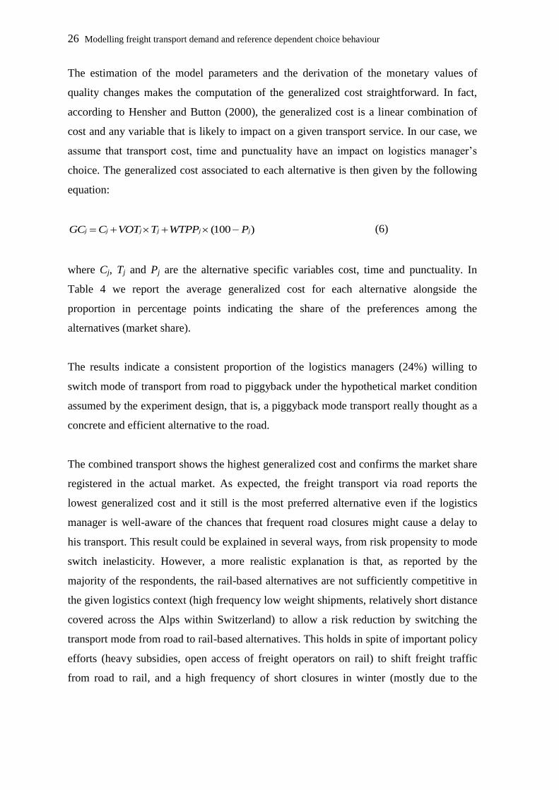
The estimation of the model parameters and the derivation of the monetary values of
quality changes makes the computation of the generalized cost straightforward. In fact,
according to Hensher and Button (2000), the generalized cost is a linear combination of
cost and any variable that is likely to impact on a given transport service. In our case, we
assume that transport cost, time and punctuality have an impact on logistics manager’s
choice. The generalized cost associated to each alternative is then given by the following
equation:
(100 )j j j j j jGC C VOT T WTPP P (6)
where Cj, Tj and Pj are the alternative specific variables cost, time and punctuality. In
Table 4 we report the average generalized cost for each alternative alongside the
proportion in percentage points indicating the share of the preferences among the
alternatives (market share).
The results indicate a consistent proportion of the logistics managers (24%) willing to
switch mode of transport from road to piggyback under the hypothetical market condition
assumed by the experiment design, that is, a piggyback mode transport really thought as a
concrete and efficient alternative to the road.
The combined transport shows the highest generalized cost and confirms the market share
registered in the actual market. As expected, the freight transport via road reports the
lowest generalized cost and it still is the most preferred alternative even if the logistics
manager is well-aware of the chances that frequent road closures might cause a delay to
his transport. This result could be explained in several ways, from risk propensity to mode
switch inelasticity. However, a more realistic explanation is that, as reported by the
majority of the respondents, the rail-based alternatives are not sufficiently competitive in
the given logistics context (high frequency low weight shipments, relatively short distance
covered across the Alps within Switzerland) to allow a risk reduction by switching the
transport mode from road to rail-based alternatives. This holds in spite of important policy
efforts (heavy subsidies, open access of freight operators on rail) to shift freight traffic
from road to rail, and a high frequency of short closures in winter (mostly due to the

Estimation of indirect cost and evaluation of protective measures for infrastructure vulnerability 27
heavy snowfall) and in summer (caused by the long queues at the tunnel bottleneck
leading to a postponing of departure).
According to the objective of quantifying the economic vulnerability of the road
infrastructure under an unexpected and long closure, we set the average generalized cost
of a freight transport via road, 1886 CHF, as the starting point of the cost-benefit
analysis9.
In order to obtain the monetary values for time and punctuality associated with an
unexpected total closure of the road Gotthard corridor for two consecutive weeks, we
introduce the logistics managers to the second scenario. The specification of the panel
RPL model is given by:
( ) ( )
( ) ( )
( ) ( )
( ) ( )
( ) NR C NR T NR P NR
( PB) PB C PB T PB P PB
( CT) CT C CT T CT P CT
( RD) C RD T RD
C T P
C T P
C T P
C T
NR NR
PB PB
CT CT
RD RD
n TrNR Tr Tr Tr Tr Tr Tr Tr
n Tr Tr Tr Tr Tr Tr Tr Tr
n Tr Tr Tr Tr Tr Tr Tr Tr
n Tr Tr Tr Tr Tr
V ASC
V ASC
V ASC
V
P RD D WP MD D Wn nTr Tr MD
(7)
where the two rail-based alternatives share now the choice set with two road alternatives,
road via A13 (TrRD) and new road (TrNR). The suffix “Tr” indicates that the attributes
(as well as the coefficients and the utility functions) refer to the transitional detour values.
We also introduce a further logistics characteristic of the firm, called maximum acceptable
delivery delay (MADD), which is a 5 point discrete variable and expresses the delay
tolerance allowed by the client, during an unexpected event, without any additional charge
to be paid by the supplier.
The logistics managers were then faced with the updated reference alternative profile, and
they were reminded that these new conditions hold just for two transitional and
consecutive weeks. The results for this second scenario are shown in Table 5. The sign
and the magnitude of the alternative specific constants indicate the new road (regulated
9 In order to verify that our insistence on the frequent risk of short closures had not influenced the
respondents’ parameters we also have derived the generalized cost by using a dataset collected among Swiss
firms aimed to evaluate the quality attributes in freight transport (described in Rudel and Maggi, 2008).
Even running different specification models the resulting generalized cost was very similar to the one
obtained with this first scenario.
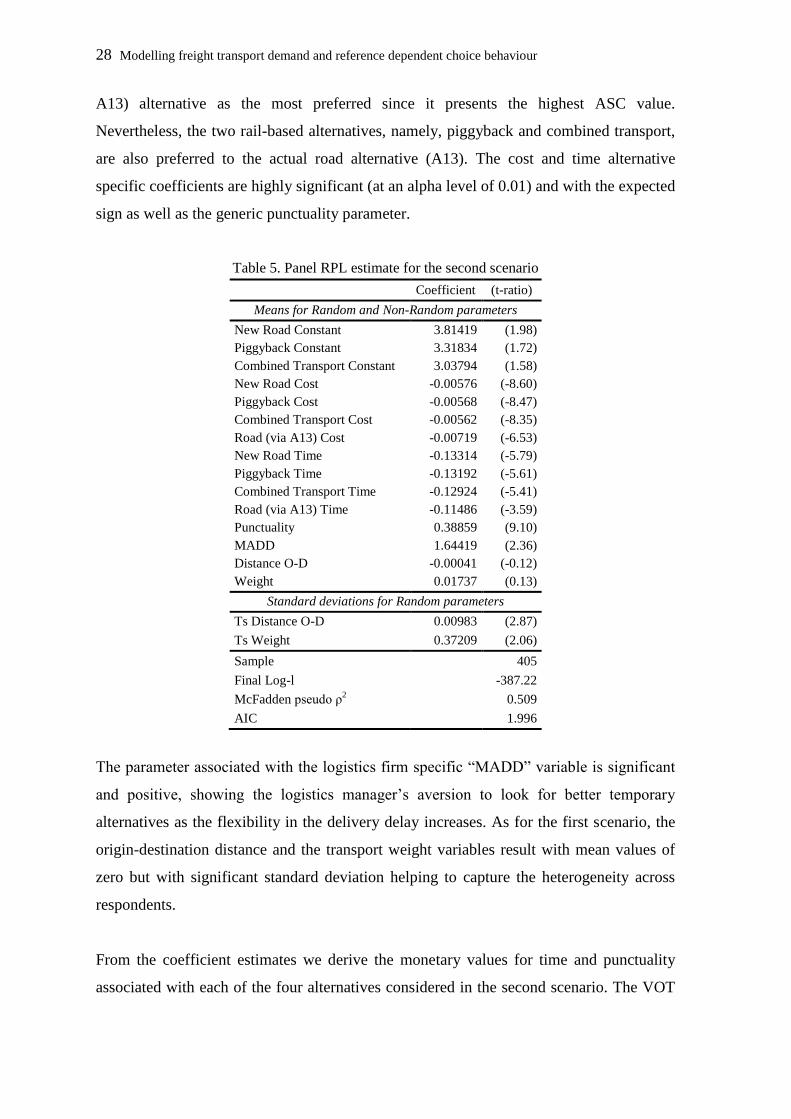
28 Modelling freight transport demand and reference dependent choice behaviour
A13) alternative as the most preferred since it presents the highest ASC value.
Nevertheless, the two rail-based alternatives, namely, piggyback and combined transport,
are also preferred to the actual road alternative (A13). The cost and time alternative
specific coefficients are highly significant (at an alpha level of 0.01) and with the expected
sign as well as the generic punctuality parameter.
Table 5. Panel RPL estimate for the second scenario
Coefficient (t-ratio)
Means for Random and Non-Random parameters
New Road Constant 3.81419 (1.98)
Piggyback Constant 3.31834 (1.72)
Combined Transport Constant 3.03794 (1.58)
New Road Cost -0.00576 (-8.60)
Piggyback Cost -0.00568 (-8.47)
Combined Transport Cost -0.00562 (-8.35)
Road (via A13) Cost -0.00719 (-6.53)
New Road Time -0.13314 (-5.79)
Piggyback Time -0.13192 (-5.61)
Combined Transport Time -0.12924 (-5.41)
Road (via A13) Time -0.11486 (-3.59)
Punctuality 0.38859 (9.10)
MADD 1.64419 (2.36)
Distance O-D -0.00041 (-0.12)
Weight 0.01737 (0.13)
Standard deviations for Random parameters
Ts Distance O-D 0.00983 (2.87)
Ts Weight 0.37209 (2.06)
Sample 405
Final Log-l -387.22
McFadden pseudo ρ2 0.509
AIC 1.996
The parameter associated with the logistics firm specific “MADD” variable is significant
and positive, showing the logistics manager’s aversion to look for better temporary
alternatives as the flexibility in the delivery delay increases. As for the first scenario, the
origin-destination distance and the transport weight variables result with mean values of
zero but with significant standard deviation helping to capture the heterogeneity across
respondents.
From the coefficient estimates we derive the monetary values for time and punctuality
associated with each of the four alternatives considered in the second scenario. The VOT
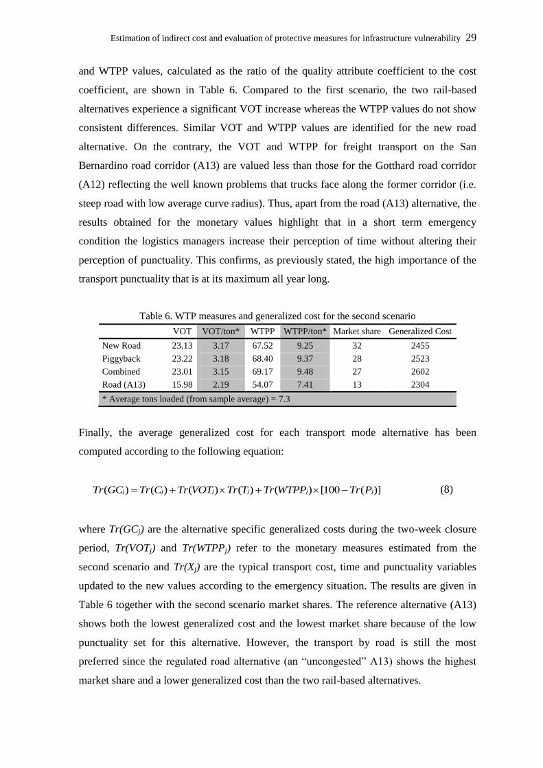
Estimation of indirect cost and evaluation of protective measures for infrastructure vulnerability 29
and WTPP values, calculated as the ratio of the quality attribute coefficient to the cost
coefficient, are shown in Table 6. Compared to the first scenario, the two rail-based
alternatives experience a significant VOT increase whereas the WTPP values do not show
consistent differences. Similar VOT and WTPP values are identified for the new road
alternative. On the contrary, the VOT and WTPP for freight transport on the San
Bernardino road corridor (A13) are valued less than those for the Gotthard road corridor
(A12) reflecting the well known problems that trucks face along the former corridor (i.e.
steep road with low average curve radius). Thus, apart from the road (A13) alternative, the
results obtained for the monetary values highlight that in a short term emergency
condition the logistics managers increase their perception of time without altering their
perception of punctuality. This confirms, as previously stated, the high importance of the
transport punctuality that is at its maximum all year long.
Table 6. WTP measures and generalized cost for the second scenario
VOT VOT/ton* WTPP WTPP/ton* Market share Generalized Cost
New Road 23.13 3.17 67.52 9.25 32 2455
Piggyback 23.22 3.18 68.40 9.37 28 2523
Combined 23.01 3.15 69.17 9.48 27 2602
Road (A13) 15.98 2.19 54.07 7.41 13 2304
* Average tons loaded (from sample average) = 7.3
Finally, the average generalized cost for each transport mode alternative has been
computed according to the following equation:
( ) ( ) ( ) ( ) ( ) [100 ( )]j j j j j jTr GC Tr C Tr VOT Tr T Tr WTPP Tr P (8)
where Tr(GCj) are the alternative specific generalized costs during the two-week closure
period, Tr(VOTj) and Tr(WTPPj) refer to the monetary measures estimated from the
second scenario and Tr(Xj) are the typical transport cost, time and punctuality variables
updated to the new values according to the emergency situation. The results are given in
Table 6 together with the second scenario market shares. The reference alternative (A13)
shows both the lowest generalized cost and the lowest market share because of the low
punctuality set for this alternative. However, the transport by road is still the most
preferred since the regulated road alternative (an “uncongested” A13) shows the highest
market share and a lower generalized cost than the two rail-based alternatives.

30 Modelling freight transport demand and reference dependent choice behaviour
In general, the additional generalized cost estimated is approximately 600 CHF per
transport. In particular, the value of travel time saving increases consistently while the
willingness to pay for 1 percent more of punctuality is more stable.
1.5. Cost-Benefit Analysis tool
The construction of this module relies on the results of both stated choice experiments
described in the previous sections. In particular, the module is built in order to estimate
the indirect user cost of a two week closure of the road Gotthard corridor10
. The results
obtained from the first scenario provide the starting value for the generalized cost in an
everyday condition while the results obtained from the second scenario are used in the
estimation of the additional generalized cost. Figure 3 shows how the main worksheet
appears to the user. A detailed help page is also provided by clicking the apposite button.
The structure of the module is organized in six sections:
1. Scenario setting: shows the alternatives and the attributes used in the
estimation modelling. Zero correspond to the default values, by inputting
different values (either positive or negative) we generate a scenario;
2. Closure details: allows different closure period settings and changes in traffic
flow and reference generalized cost;
3. Market shares: shows the market shares in percentage and in number11 for
both default and scenario values;
4. Generalized cost: shows the additional generalized cost12 caused by a two-
week closure of the road corridor for the Ticino economy;
5. Cost-benefit analysis for critical points in the Gotthard corridor: allows the
computation of the net present values of the selected measures aimed to
reduce the whole vulnerability of the road Gotthard corridor;
10
The tool is available upon request from the corresponding author. 11
The source of the total amount of trucks passing through the Gotthard corridor is the last AQGV 04
census. We consider only trucks departing from or arriving to Ticino. This amount is inputted in the cell
called N and it is free to be changed by the user. 12
The reference value is put into the cell GC_Gotthard and stems from the first scenario results.
Estimation of indirect cost and evaluation of protective measures for infrastructure vulnerability 31
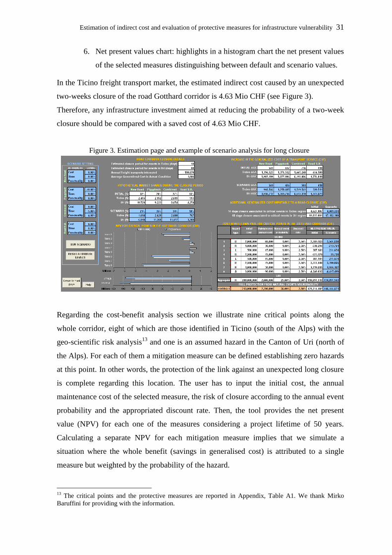
6. Net present values chart: highlights in a histogram chart the net present values
of the selected measures distinguishing between default and scenario values.
In the Ticino freight transport market, the estimated indirect cost caused by an unexpected
two-weeks closure of the road Gotthard corridor is 4.63 Mio CHF (see Figure 3).
Therefore, any infrastructure investment aimed at reducing the probability of a two-week
closure should be compared with a saved cost of 4.63 Mio CHF.
Figure 3. Estimation page and example of scenario analysis for long closure
Regarding the cost-benefit analysis section we illustrate nine critical points along the
whole corridor, eight of which are those identified in Ticino (south of the Alps) with the
geo-scientific risk analysis13
and one is an assumed hazard in the Canton of Uri (north of
the Alps). For each of them a mitigation measure can be defined establishing zero hazards
at this point. In other words, the protection of the link against an unexpected long closure
is complete regarding this location. The user has to input the initial cost, the annual
maintenance cost of the selected measure, the risk of closure according to the annual event
probability and the appropriated discount rate. Then, the tool provides the net present
value (NPV) for each one of the measures considering a project lifetime of 50 years.
Calculating a separate NPV for each mitigation measure implies that we simulate a
situation where the whole benefit (savings in generalised cost) is attributed to a single
measure but weighted by the probability of the hazard.
13
The critical points and the protective measures are reported in Appendix, Table A1. We thank Mirko
Baruffini for providing with the information.
32 Modelling freight transport demand and reference dependent choice behaviour
Assuming a low discount rate of 0.025 and a realistically low event probability of 0.01,
measures 3 and 5 against landslides and measure 4 against debris flow result in a positive
NPVs. Together they would reduce the risk of closure by 6%. The other measures show
negative NPV. This implies that large investments, like e.g. the hypothetical one in URI,
or smaller ones in Ticino but for low event probability are not justified if we consider only
the indirect benefit for Ticino. Expanding the analysis and adding the direct benefits and
above all indirect benefits for the rest of Switzerland, and Europe (transit traffic accounts
for 50% of the trans-Alpine passages) might change the results significantly in favour of
the measures.
By changing the infrastructure parameters the user can explore alternative policy measures
that might lead to different vulnerability outcomes changing the economic efficiency of a
given protective measure. For example, by assuming a ten percent cost reduction for the
piggyback alternative and, a five percent time reduction and a four percent punctuality
increase for the combined transport alternative, the cost of a two-week road closure would
be 4 Mio CHF (see Figure 3), that is, 13.4 percent less than the actual estimated loss. This
makes the net present value of protective measure 4 not positive anymore.
Finally, the versatility of the module allows the integration of any further information
gathered about the exact number of sensible points located along the Gotthard road
corridor and the exact monetary value of each measure aimed at mitigating the risk of a
long closure.
1.6. Conclusions
This paper has investigated the economic consequences associated with a two-week
closure of the Gotthard road corridor, and has analysed the economic efficiency of
different protective measures through the implementation of a cost-benefit analysis.
Due to its geographical location and to the seventeen kilometres long two-lane tunnel, the
Gotthard corridor experiences a high degree of vulnerability towards unexpected events.
In fact, in recent years two disastrous events occurred. In November 2001, a head-on

Estimation of indirect cost and evaluation of protective measures for infrastructure vulnerability 33
collision between two trucks inside the tunnel caused a two months road interruption
while, in May 2006, a rock fall caused a closure of one month.
We provide the indirect cost in the economic sector that most heavily depends on the road
corridor, that is, the Ticino freight transport market. The identification of the indirect cost
relies on the generalized cost estimation, which parameters come from two stated
preference experiments, the first based on actual condition whereas the second assumes a
road closure.
The results indicate that a two-week closure of the Gotthard road corridor generates an
indirect user cost to the Canton Ticino of 4.63 Mio CHF. As a consequence, the cost of
any measure avoiding this risk has to be compared with the potential benefit of saving at
least this sum (if benefits to other regions and direct benefits are neglected). In this
context, nine critical points along the corridor were identified and the cost-benefit analysis
indicates a positive net value for three protective measures resulting in a reduction of the
road closure risk of six percent.
The implementation of the cost-benefit tool is essential in testing different scenarios
useful in the evaluation of different policy setting. In fact, the tool lets the service
transport parameters, cost, time and punctuality, free to change. For example, an
improvement of the rail-based alternatives in term of cost, time and punctuality can reduce
significantly the road vulnerability.
The procedure outlined in this paper proposes a methodology aimed to identify and
quantify the economic vulnerability associated with a road transport infrastructure and, to
evaluate the economic and social efficiency of a vulnerability reduction by the
consideration of protective measures. Nevertheless, this procedure should be considered
as a starting point and further improvements are strongly recommended. We suggest the
extension of the economic loss with the estimation of the direct cost. It would be also
interesting to enlarge the analysis to a wider geographical area in order to cover a better
proportion of the potential infrastructure consumers. Finally, the integration of this
module in a GIS environment would make the practitioner confident with the
geographical context and the related hazards.
34 Modelling freight transport demand and reference dependent choice behaviour
References
Bell M.G.H., Iida Y., 1997. Transportation Network Analysis. Wiley, Chichester, West Sussex.
Bell M.G.H., Iida Y., 2003. The Network Reliability of Transport: Proceedings of the 1st
International Symposium on Transportation Network Reliability (INSTR), Pergamon, Oxford.
Berdica, K., 2002. An introduction to road vulnerability: what has been done, is done and should
be done. Transport Policy 9, 117-127.
Bolis, S., Maggi R., 2003. Logistics Strategy and Transport Service Choices-An Adaptive Stated
Preference Experiment. In: Growth and Change - A journal of Urban and Regional Policy, Special
Issue STELLA FG 1, (34) 4.
Chen, A., Yang, H., Lo, H.K., Tang, W.H., 2002. Capacity reliability of a road network: an
assessment methodology and numerical results. Transportation Research Part B 36(3), 225–252.
Danielis, R., Marcucci, E., Rotaris, L., 2005. Logistics managers' stated preferences for freight
service attributes. Transportation Research Part E 41(3), 201-215.
D’Este, G M and Taylor, M A P (2003). Network vulnerability: an approach to reliability analysis
at the level of national strategic transport networks. In: Bell M.G.H., Iida Y. (Eds.), The Network
Reliability of Transport: Proceedings of the 1st International Symposium on Transportation
Network Reliability (INSTR). Pergamon, Oxford.
Fowkes, A.S., Firmin, P.E., Tweddle, G., Whiteing, A.E., 2004. How Highly Does the Freight
Transport Industry Value Journey Time Reliability - and for What Reasons? International Journal
of Logistics: Research and Applications 7, 33-44.
Hensher, D.A., Button, K.J., 2000. Handbook of transport modelling. Emerald Group Publishing.
Hensher, D.A., Greene, W.H., 2003. Mixed logit models: state of practice. Transportation 30(2),
133-176.
Husdal, J., 2004. Reliability/vulnerability versus cost/benefit. In: Nicholson A.J., Dante, A.,
(Eds.), Proceedings of the Second International Symposium on Transportation Network Reliability
(INSTR). Department of Civil Engineering, University of Canterbury, Christchurch, New Zealand.
Maggi, R., Rudel, R., 2008. The Value of Quality Attributes in Freight Transport: Evidence from
an SP-Experiment in Switzerland. In: Ben-Akiva, M.E., Meersman, H., van de Voorde E. (Eds.),
Recent Developments in Transport Modelling. Emerald Group Publishing Limited.
McFadden, D., 1974. Conditional logit analysis of qualitative choice behavior. In: Zarembka, P.
(Ed.), Frontiers in Econometrics. Academic Press, New York.
Nicholson, A.J., Dante, A., 2004. Proceedings of the Second International Symposium on
Transportation Network Reliability (INSTR). Department of Civil Engineering, University of
Canterbury, Christchurch, New Zealand.
Estimation of indirect cost and evaluation of protective measures for infrastructure vulnerability 35
Taylor, M.A.P., D’Este, G.M., 2004. Critical infrastructure and transport network vulnerability:
developing a method for diagnosis and assessment. In: Nicholson, A.J., Dante, A. (Eds.),
Proceedings of the Second International Symposium on Transportation Network Reliability
(INSTR). Department of Civil Engineering, University of Canterbury, Christchurch, New Zealand.
Taylor, M.A.P., Sekhar, S.V.C., D’Este, G.M., 2006. Application of Accessibility Based Methods
for Vulnerability Analysis of Strategic Road Networks. Networks and Spatial Economics 6, 267-
291.
Train, K., 2003. Discrete Choice Methods with Simulation. Cambridge University Press,
Cambridge.
Zamparini, L., Reggiani A., 2007. Freight Transport and the Value of Travel Time Savings: A
Meta-analysis of Empirical Studies. Transport Reviews, 27(5), 621-636.
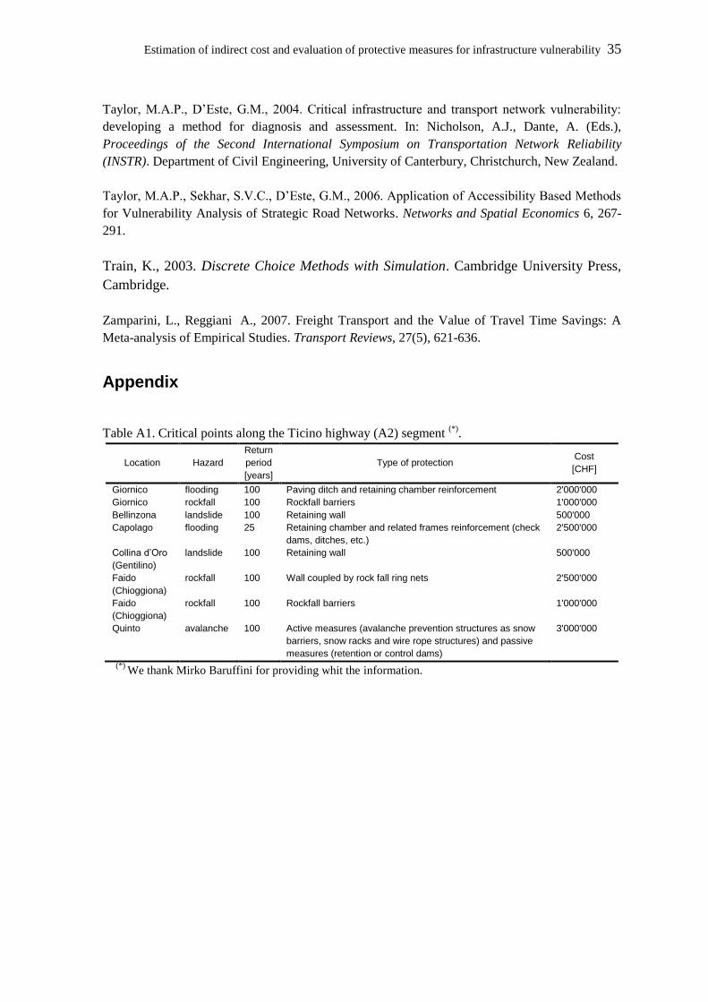
Appendix
Table A1. Critical points along the Ticino highway (A2) segment (*)
.
Location Hazard
Return
period
[years]
Type of protection Cost
[CHF]
Giornico flooding 100 Paving ditch and retaining chamber reinforcement 2'000'000
Giornico rockfall 100 Rockfall barriers 1'000'000
Bellinzona landslide 100 Retaining wall 500'000
Capolago flooding 25 Retaining chamber and related frames reinforcement (check
dams, ditches, etc.)
2'500'000
Collina d’Oro
(Gentilino)
landslide 100 Retaining wall 500'000
Faido
(Chioggiona)
rockfall 100 Wall coupled by rock fall ring nets 2'500'000
Faido
(Chioggiona)
rockfall 100 Rockfall barriers 1'000'000
Quinto avalanche 100 Active measures (avalanche prevention structures as snow
barriers, snow racks and wire rope structures) and passive
measures (retention or control dams)
3'000'000
(*)
We thank Mirko Baruffini for providing whit the information.

36
Chapter Two
Analyzing loss aversion and diminishing sensitivity in a freight transport stated choice experiment
Lorenzo Masiero
David A. Hensher
Version: February 19 2010
Published: Transportation Research Part A 44(5), 349–358
Abstract
Choice behaviour might be determined by asymmetric preferences whether the consumers
are faced with gains or losses. This paper investigates loss aversion and diminishing
sensitivity, and analyzes their implications on willingness to pay and willingness to accept
measures in a reference pivoted choice experiment in a freight transport framework. The
results suggest a significant model fit improvement when preferences are treated as
asymmetric, proving both loss aversion and diminishing sensitivity. The implications on
willingness to pay and willingness to accept indicators are particular relevant showing a
remarkable difference between symmetric and asymmetric model specifications. Not
accounting for loss aversion and diminishing sensitivity, when present, produces
misleading results and might affect significantly the policy decisions.
Keywords: freight transport, choice experiments, willingness to pay, preference
asymmetry
Acknowledgements: This research is funded by a “Prospective Researcher” grant of the
Swiss National Science Foundation. We thank Rico Maggi for his support and
encouragement. The advice of two referees is appreciated.
Analizying loss aversion and diminishing sensitivity in a freight transport stated choice experiment 37
2.1. Introduction
Reference dependence, loss aversion and diminishing sensitivity are three essential
characteristics that Prospect Theory (Kahneman and Tversky, 1979) defines for a utility
function in a decision under risk framework14
. In particular, an individual decision making
process involves the evaluation of gains and losses defined in relation to a reference point
(reference dependence), with a higher evaluation for losses than gains (loss aversion) and
decreasing marginal values in both positive and negative domains (diminishing
sensitivity).
The increasing popularity of designing stated choice experiments pivoted on a reference
alternative (see for example, Rose et al., 2008) has led to a growing interest in deriving
discrete choice models that could accommodate the prospect theory reference dependence
assumption. In this context, Hess et al. (2008) estimate models that include different
parameters for positive and negative deviations from the reference value, and they
demonstrate the existence of loss aversion identifying asymmetric preferences on both
commuting and non-commuting car travellers.
The idea of an asymmetric S-shaped utility function, concave above the reference point
and convex below it, is given in Kahneman and Tversky (1979), and formalized as a two-
part cumulative function in Tversky and Kahneman (1992). Lanz et al. (2009) test loss
aversion and diminishing sensitivity in an environmental water supply choice experiment,
by means of appropriate linear and nonlinear transformation of the utility function.
The presence of loss aversion has a direct influence on one of the most crucial topics in
discrete choice modelling, the estimation of willingness to pay (WTP) and willingness to
accept (WTA), and in particular, the relation between the two measures. Indeed, in a
reference pivoted choice model that does not take into account preference asymmetry, the
ratio of WTA to WTP is equal to one. Conversely, the literature presents a variety of
studies that set the WTA/WTP ratio to a higher factor (see for example, Boyce et al. 1992
and Horowitz and McConnell 2002).
14
For an application in a risk-less choice situation see Tversky and Kahneman (1991).

38 Modelling freight transport demand and reference dependent choice behaviour
The aim of this paper is to investigate loss aversion through asymmetric preferences and
diminishing sensitivity by nonlinear asymmetric preferences, and to analyze their
implications on WTP and WTA measures in a freight transport choice experiment. The
literature on freight transport is poor compared with the passenger transport sector, due we
suspect to the complexity of the supply-chain system and the greater effort required in
sourcing and getting the cooperation of organisations (in contrast to individuals) in data
collection. Zamparini and Reggiani (2007) provide a review of value of time savings in
freight transport studies, with the majority based on stated choice experiments.
Discontinuity in utility functions has been proposed by Swait (2001) through the concept
of “cut-offs” and has been applied to the freight sector by Danielis and Marcucci (2007).
However, to the best of our knowledge, no previous studies on freight transport focus on
the analysis of asymmetric preferences and decreasing marginal utility, and how these
behavioural conditions affect the estimation of measures such as WTP and WTA, which
are commonly used by policy makers.
Furthermore, particular attention is given to the punctuality attribute, as an indicator of
freight transport service quality. Although a few recent studies mention its relevance (see
for example, Danielis et al. 2005 and Fowkes 2007) a more in depth analysis is required to
better understand the potential of this variable.
The paper is organised as follows. In section two we introduce the choice experiment and
present the data’s descriptive statistics. We then outline the methodology and present the
model derivation in section three. The results are illustrated and discussed in section four.
Finally the conclusions are provided in section five.
2.2. Data
The data was obtained from a stated choice survey in a freight transport context conducted
in the Ticino region (Switzerland) in 2008. The experiment was part of a project15
aimed
to analyze the infrastructure vulnerability of the Ghottard corridor, one of the most
important European transport corridors.
15
NFP54 “Sustainable Development of the Built Environment”, founded by the Swiss National Science
Foundation. For more details about the study see Maggi et al. (2009) and Masiero and Maggi (2009).
Analizying loss aversion and diminishing sensitivity in a freight transport stated choice experiment 39
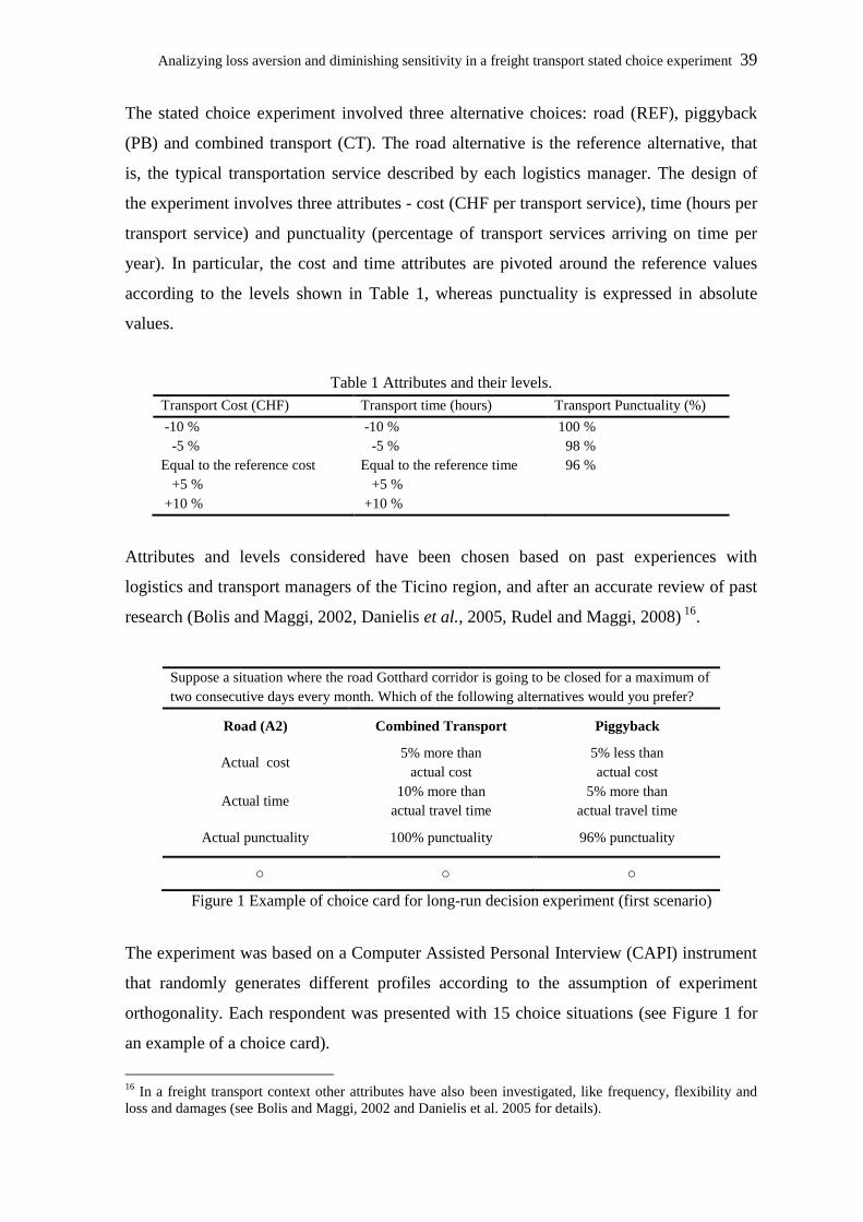
The stated choice experiment involved three alternative choices: road (REF), piggyback
(PB) and combined transport (CT). The road alternative is the reference alternative, that
is, the typical transportation service described by each logistics manager. The design of
the experiment involves three attributes - cost (CHF per transport service), time (hours per
transport service) and punctuality (percentage of transport services arriving on time per
year). In particular, the cost and time attributes are pivoted around the reference values
according to the levels shown in Table 1, whereas punctuality is expressed in absolute
values.
Table 1 Attributes and their levels.
Transport Cost (CHF) Transport time (hours) Transport Punctuality (%)
-10 % -10 % 100 %
-5 % -5 % 98 %
Equal to the reference cost Equal to the reference time 96 %
+5 % +5 %
+10 % +10 %
Attributes and levels considered have been chosen based on past experiences with
logistics and transport managers of the Ticino region, and after an accurate review of past
research (Bolis and Maggi, 2002, Danielis et al., 2005, Rudel and Maggi, 2008) 16
.
Suppose a situation where the road Gotthard corridor is going to be closed for a maximum of
two consecutive days every month. Which of the following alternatives would you prefer?
Road (A2) Combined Transport Piggyback
Actual cost 5% more than
actual cost
5% less than
actual cost
Actual time 10% more than
actual travel time
5% more than
actual travel time
Actual punctuality 100% punctuality 96% punctuality
o o o
Figure 1 Example of choice card for long-run decision experiment (first scenario)
The experiment was based on a Computer Assisted Personal Interview (CAPI) instrument
that randomly generates different profiles according to the assumption of experiment
orthogonality. Each respondent was presented with 15 choice situations (see Figure 1 for
an example of a choice card).
16
In a freight transport context other attributes have also been investigated, like frequency, flexibility and
loss and damages (see Bolis and Maggi, 2002 and Danielis et al. 2005 for details).
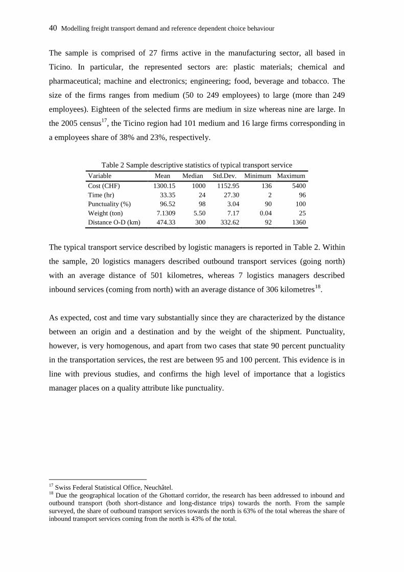
40 Modelling freight transport demand and reference dependent choice behaviour
The sample is comprised of 27 firms active in the manufacturing sector, all based in
Ticino. In particular, the represented sectors are: plastic materials; chemical and
pharmaceutical; machine and electronics; engineering; food, beverage and tobacco. The
size of the firms ranges from medium (50 to 249 employees) to large (more than 249
employees). Eighteen of the selected firms are medium in size whereas nine are large. In
the 2005 census17
, the Ticino region had 101 medium and 16 large firms corresponding in
a employees share of 38% and 23%, respectively.
Table 2 Sample descriptive statistics of typical transport service
Variable Mean Median Std.Dev. Minimum Maximum
Cost (CHF) 1300.15 1000 1152.95 136 5400
Time (hr) 33.35 24 27.30 2 96
Punctuality (%) 96.52 98 3.04 90 100
Weight (ton) 7.1309 5.50 7.17 0.04 25
Distance O-D (km) 474.33 300 332.62 92 1360
The typical transport service described by logistic managers is reported in Table 2. Within
the sample, 20 logistics managers described outbound transport services (going north)
with an average distance of 501 kilometres, whereas 7 logistics managers described
inbound services (coming from north) with an average distance of 306 kilometres18
.
As expected, cost and time vary substantially since they are characterized by the distance
between an origin and a destination and by the weight of the shipment. Punctuality,
however, is very homogenous, and apart from two cases that state 90 percent punctuality
in the transportation services, the rest are between 95 and 100 percent. This evidence is in
line with previous studies, and confirms the high level of importance that a logistics
manager places on a quality attribute like punctuality.
17
Swiss Federal Statistical Office, Neuchâtel. 18
Due the geographical location of the Ghottard corridor, the research has been addressed to inbound and
outbound transport (both short-distance and long-distance trips) towards the north. From the sample
surveyed, the share of outbound transport services towards the north is 63% of the total whereas the share of
inbound transport services coming from the north is 43% of the total.
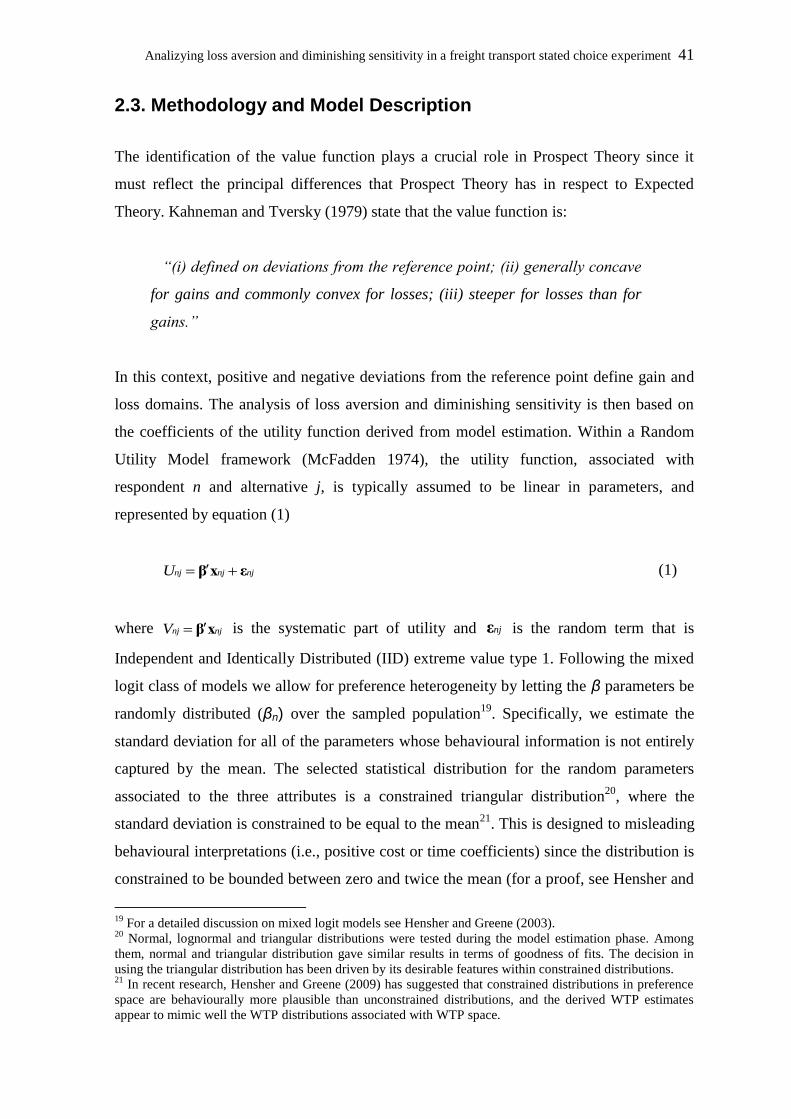
Analizying loss aversion and diminishing sensitivity in a freight transport stated choice experiment 41
2.3. Methodology and Model Description
The identification of the value function plays a crucial role in Prospect Theory since it
must reflect the principal differences that Prospect Theory has in respect to Expected
Theory. Kahneman and Tversky (1979) state that the value function is:
“(i) defined on deviations from the reference point; (ii) generally concave
for gains and commonly convex for losses; (iii) steeper for losses than for
gains.”
In this context, positive and negative deviations from the reference point define gain and
loss domains. The analysis of loss aversion and diminishing sensitivity is then based on
the coefficients of the utility function derived from model estimation. Within a Random
Utility Model framework (McFadden 1974), the utility function, associated with
respondent n and alternative j, is typically assumed to be linear in parameters, and
represented by equation (1)
nj nj njU β x ε (1)
where nj njV β x is the systematic part of utility and njε is the random term that is
Independent and Identically Distributed (IID) extreme value type 1. Following the mixed
logit class of models we allow for preference heterogeneity by letting the β parameters be
randomly distributed (βn) over the sampled population19
. Specifically, we estimate the
standard deviation for all of the parameters whose behavioural information is not entirely
captured by the mean. The selected statistical distribution for the random parameters
associated to the three attributes is a constrained triangular distribution20
, where the
standard deviation is constrained to be equal to the mean21
. This is designed to misleading
behavioural interpretations (i.e., positive cost or time coefficients) since the distribution is
constrained to be bounded between zero and twice the mean (for a proof, see Hensher and
19
For a detailed discussion on mixed logit models see Hensher and Greene (2003). 20
Normal, lognormal and triangular distributions were tested during the model estimation phase. Among
them, normal and triangular distribution gave similar results in terms of goodness of fits. The decision in
using the triangular distribution has been driven by its desirable features within constrained distributions. 21
In recent research, Hensher and Greene (2009) has suggested that constrained distributions in preference
space are behaviourally more plausible than unconstrained distributions, and the derived WTP estimates
appear to mimic well the WTP distributions associated with WTP space.
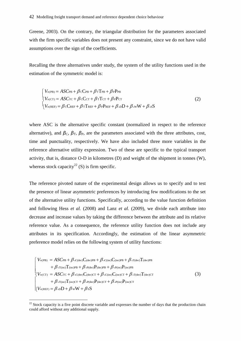
42 Modelling freight transport demand and reference dependent choice behaviour
Greene, 2003). On the contrary, the triangular distribution for the parameters associated
with the firm specific variables does not present any constraint, since we do not have valid
assumptions over the sign of the coefficients.
Recalling the three alternatives under study, the system of the utility functions used in the
estimation of the symmetric model is:
(PB) PB C PB T PB P PB
(CT) TC C CT T CT P CT
(REF) C REF T REF P REF D W S
C T P
C T P
C T P D W Sn n n
n
n
n
V ASC
V ASC
V
(2)
where ASC is the alternative specific constant (normalized in respect to the reference
alternative), and βC, βT, βP, are the parameters associated with the three attributes, cost,
time and punctuality, respectively. We have also included three more variables in the
reference alternative utility expression. Two of these are specific to the typical transport
activity, that is, distance O-D in kilometres (D) and weight of the shipment in tonnes (W),
whereas stock capacity22
(S) is firm specific.
The reference pivoted nature of the experimental design allows us to specify and to test
the presence of linear asymmetric preferences by introducing few modifications to the set
of the alternative utility functions. Specifically, according to the value function definition
and following Hess et al. (2008) and Lanz et al. (2009), we divide each attribute into
decrease and increase values by taking the difference between the attribute and its relative
reference value. As a consequence, the reference utility function does not include any
attributes in its specification. Accordingly, the estimation of the linear asymmetric
preference model relies on the following system of utility functions:
(PB) PB C(dec) (dec)PB C(inc) (inc)PB T(dec) (dec)PB
T(inc) (inc)PB P(dec) (dec)PB P(inc) (inc)PB
(CT) TC C(dec) (dec)CT C(inc) (inc)CT T(dec) (dec)CT
C C T
T P P
C C T
n n n
n n n
n n n
n
n
V ASC
V ASC
T(inc) (inc)CT P(dec) (dec)CT P(inc) (inc)CT
(REF) D W S
T P P
D W S
n n n
nnV
(3)
22
Stock capacity is a five point discrete variable and expresses the number of days that the production chain
could afford without any additional supply.

Analizying loss aversion and diminishing sensitivity in a freight transport stated choice experiment 43
where X(dec)j = max(XREF – Xj, 0) and X(inc)j = max(Xj – XREF, 0).
A further extension to the model described in (3) involves the analysis of potential
nonlinearities in the form of the utility function in both domains of gains and losses. The
approach used is a version of a piecewise linear approximation which entails the
estimation of different values for different ranges of the selected attribute. Here, instead of
different ranges of the attribute, we consider different ranges of the attribute levels since
we are interested in preference nonlinearity around a reference point. It is worth noting
that the piecewise linear approximation approach has the advantage of maintaining the
utility function linear in the parameters, and the capability to detect significant
nonlinearities with a small number of ranges (Ben-Akiva and Lerman 1985).
Nonlinearity is introduced in the punctuality attribute identifying two decrease and two
increase levels, with respect to the reference point23
. That is, P(dec--) refers to decreases
from 3 percent up to 4 percent, P(dec-) to decreases up to 2 percent, P(inc+) to increases
up to 2 percent and P(inc++) to increases from 3 percent up to 10 percent24
. The utility
function for the nonlinear asymmetric preference model can be written as follows:
(PB) PB C(dec) (dec)PB C(inc) (inc)PB T(dec) (dec)PB T(inc) (inc)PB
P(dec--) (dec--)PB P(dec-) (dec-)PB P(inc+) (inc+)PB P(inc++) (inc++)PB
(CT) TC C(dec
C C T T
P P P P
n n n n
n n n n
n
n
n
V ASC
V ASC
) (dec)CT C(inc) (inc)CT T(dec) (dec)CT T(inc) (inc)CT
P(dec--) (dec--)CT P(dec-) (dec-)CT P(inc+) (inc+)CT P(inc++) (inc++)CT
(REF) D W S
C C T T
P P P P
D W S
n n n
n n n n
n n nnV
(4)
where,
( )
( )
( )
( )
4 ( ) 3
2 ( ) 1
1 ( ) 2
3 ( ) 10
dec j j REF
dec j j REF
j REF
inc j j REF
inc j j REF
P if P P
P if P PP P
P if P P
P if P P
(5)
23
Preliminary analysis showed a non significant nonlinearity for cost and time attributes. Therefore, they are
treated as linear but asymmetric. 24
A model with three parameters in the punctuality gains domain has also been estimated. The coefficient
associated with an increase from 3% to 4% was statistically not different from the coefficient associated
with an increase from 5% to 10% (the 77% of the distribution lies in the range -4% to +4%). Since both
models lead to similar interpretation of the results, the selection is based on the model fit.
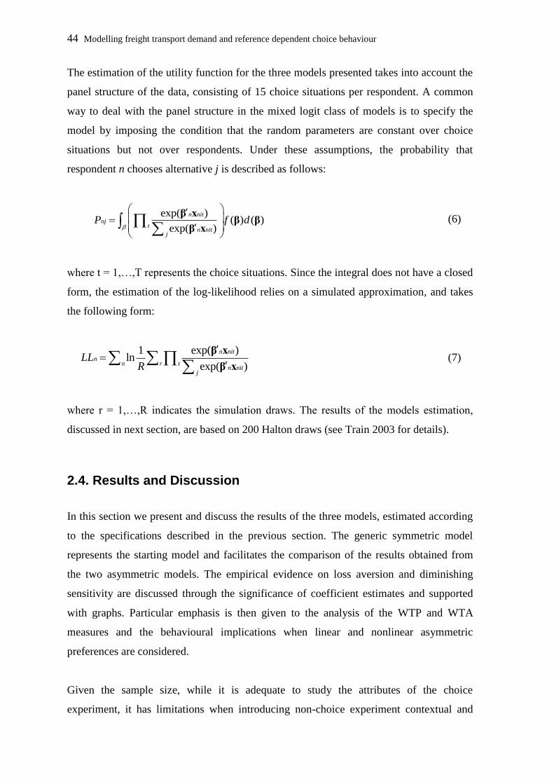
44 Modelling freight transport demand and reference dependent choice behaviour
The estimation of the utility function for the three models presented takes into account the
panel structure of the data, consisting of 15 choice situations per respondent. A common
way to deal with the panel structure in the mixed logit class of models is to specify the
model by imposing the condition that the random parameters are constant over choice
situations but not over respondents. Under these assumptions, the probability that
respondent n chooses alternative j is described as follows:
exp( )( ) ( )
exp( )
n nitnj
tn nit
j
P f d
β xβ β
β x (6)
where t = 1,…,T represents the choice situations. Since the integral does not have a closed
form, the estimation of the log-likelihood relies on a simulated approximation, and takes
the following form:
1 exp( )ln
exp( )
n nitn
n r tn nit
j
LLR
β x
β x (7)
where r = 1,…,R indicates the simulation draws. The results of the models estimation,
discussed in next section, are based on 200 Halton draws (see Train 2003 for details).
2.4. Results and Discussion
In this section we present and discuss the results of the three models, estimated according
to the specifications described in the previous section. The generic symmetric model
represents the starting model and facilitates the comparison of the results obtained from
the two asymmetric models. The empirical evidence on loss aversion and diminishing
sensitivity are discussed through the significance of coefficient estimates and supported
with graphs. Particular emphasis is then given to the analysis of the WTP and WTA
measures and the behavioural implications when linear and nonlinear asymmetric
preferences are considered.
Given the sample size, while it is adequate to study the attributes of the choice
experiment, it has limitations when introducing non-choice experiment contextual and
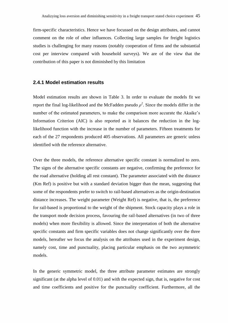
Analizying loss aversion and diminishing sensitivity in a freight transport stated choice experiment 45
firm-specific characteristics. Hence we have focussed on the design attributes, and cannot
comment on the role of other influences. Collecting large samples for freight logistics
studies is challenging for many reasons (notably cooperation of firms and the substantial
cost per interview compared with household surveys). We are of the view that the
contribution of this paper is not diminished by this limitation
2.4.1 Model estimation results
Model estimation results are shown in Table 3. In order to evaluate the models fit we
report the final log-likelihood and the McFadden pseudo ρ2. Since the models differ in the
number of the estimated parameters, to make the comparison more accurate the Akaike’s
Information Criterion (AIC) is also reported as it balances the reduction in the log-
likelihood function with the increase in the number of parameters. Fifteen treatments for
each of the 27 respondents produced 405 observations. All parameters are generic unless
identified with the reference alternative.
Over the three models, the reference alternative specific constant is normalized to zero.
The signs of the alternative specific constants are negative, confirming the preference for
the road alternative (holding all rest constant). The parameter associated with the distance
(Km Ref) is positive but with a standard deviation bigger than the mean, suggesting that
some of the respondents prefer to switch to rail-based alternatives as the origin-destination
distance increases. The weight parameter (Weight Ref) is negative, that is, the preference
for rail-based is proportional to the weight of the shipment. Stock capacity plays a role in
the transport mode decision process, favouring the rail-based alternatives (in two of three
models) when more flexibility is allowed. Since the interpretation of both the alternative
specific constants and firm specific variables does not change significantly over the three
models, hereafter we focus the analysis on the attributes used in the experiment design,
namely cost, time and punctuality, placing particular emphasis on the two asymmetric
models.
In the generic symmetric model, the three attribute parameter estimates are strongly
significant (at the alpha level of 0.01) and with the expected sign, that is, negative for cost
and time coefficients and positive for the punctuality coefficient. Furthermore, all the
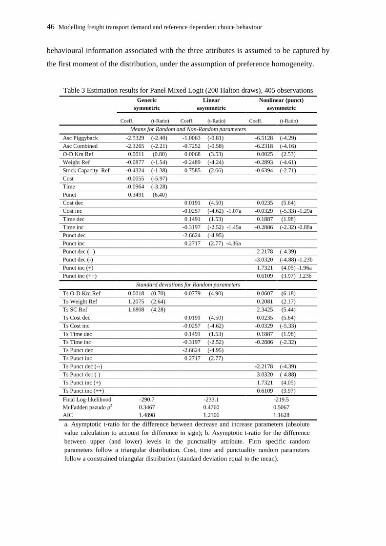
46 Modelling freight transport demand and reference dependent choice behaviour
behavioural information associated with the three attributes is assumed to be captured by
the first moment of the distribution, under the assumption of preference homogeneity.
Table 3 Estimation results for Panel Mixed Logit (200 Halton draws), 405 observations
Generic
symmetric
Linear
asymmetric
Nonlinear (punct)
asymmetric
Coeff. (t-Ratio) Coeff. (t-Ratio) Coeff. (t-Ratio)
Means for Random and Non-Random parameters
Asc Piggyback -2.5329 (-2.40) -1.0063 (-0.81) -6.5128 (-4.29)
Asc Combined -2.3265 (-2.21) -0.7252 (-0.58) -6.2318 (-4.16)
O-D Km Ref 0.0011 (0.80) 0.0068 (3.53) 0.0025 (2.53)
Weight Ref -0.0877 (-1.54) -0.2489 (-4.24) -0.2893 (-4.61)
Stock Capacity Ref -0.4324 (-1.38) 0.7585 (2.66) -0.6394 (-2.71)
Cost -0.0055 (-5.97)
Time -0.0964 (-3.28)
Punct 0.3491 (6.40)
Cost dec 0.0191 (4.50) 0.0235 (5.64)
Cost inc -0.0257 (-4.62) -1.07a -0.0329 (-5.33) -1.29a
Time dec 0.1491 (1.53) 0.1887 (1.98)
Time inc -0.3197 (-2.52) -1.45a -0.2886 (-2.32) -0.88a
Punct dec -2.6624 (-4.95)
Punct inc 0.2717 (2.77) -4.36a
Punct dec (--) -2.2178 (-4.39)
Punct dec (-) -3.0320 (-4.88) -1.23b
Punct inc (+) 1.7321 (4.05) -1.96a
Punct inc (++) 0.6109 (3.97) 3.23b
Standard deviations for Random parameters
Ts O-D Km Ref 0.0018 (0.70) 0.0779 (4.90) 0.0607 (6.18)
Ts Weight Ref 1.2075 (2.64) 0.2081 (2.17)
Ts SC Ref 1.6808 (4.28) 2.3425 (5.44)
Ts Cost dec 0.0191 (4.50) 0.0235 (5.64)
Ts Cost inc -0.0257 (-4.62) -0.0329 (-5.33)
Ts Time dec 0.1491 (1.53) 0.1887 (1.98)
Ts Time inc -0.3197 (-2.52) -0.2886 (-2.32)
Ts Punct dec -2.6624 (-4.95)
Ts Punct inc 0.2717 (2.77)
Ts Punct dec (--) -2.2178 (-4.39)
Ts Punct dec (-) -3.0320 (-4.88)
Ts Punct inc (+) 1.7321 (4.05)
Ts Punct inc (++) 0.6109 (3.97)
Final Log-likelihood -290.7 -233.1 -219.5
McFadden pseudo ρ2 0.3467 0.4760 0.5067
AIC 1.4898 1.2106 1.1628
a. Asymptotic t-ratio for the difference between decrease and increase parameters (absolute
value calculation to account for difference in sign); b. Asymptotic t-ratio for the difference
between upper (and lower) levels in the punctuality attribute. Firm specific random
parameters follow a triangular distribution. Cost, time and punctuality random parameters
follow a constrained triangular distribution (standard deviation equal to the mean).

Analizying loss aversion and diminishing sensitivity in a freight transport stated choice experiment 47
The results for the first estimated asymmetric preference model (cited as linear
asymmetric in Table 3) show a substantial increase in the model fit, quantifiable by the
reduction of the AIC measure from 1.49 for the generic symmetric model to 1.21 for the
linear asymmetric model. The parameter estimates are all significant at an alpha level of
0.05 except for the coefficient associated to the “time decrease” attribute that shows a
weak significance. The negative (positive) sign for the coefficients related to increases
(decreases) in time and cost is consistent with common behavioural judgments. In the
same way, we find a positive sign associated to an increase in punctuality, and vice versa.
Following Hess et al. (2008), we report the asymptotic t-ratio test in order to evaluate the
significance of the difference between decrease and increase parameters25
. The asymptotic
t-ratio for the difference between decrease and increase parameters results in a weak
significance for cost and time attributes, and a strong significance for the punctuality
attribute. Hence the marginal (dis)utility experiences significant asymmetries with respect
to the reference point in situations where the respondent is faced with either a gain or a
loss. Notably, in all the three attributes considered, the absolute values of the parameter
associated with a loss, namely, β(inc) for time and cost and β(dec) for punctuality, are larger
than those associated with a gain (β(dec) for time and cost and β(inc) for punctuality),
suggesting that the utility functions are steeper in the losses than in the gains domain. This
proves the presence of loss aversion among the respondent preferences.
By taking the ratio in absolute values, |du/dX(loss)|/|du/dX(gain)|, we are able to quantify
the degree of asymmetry, which assumes a value greater than zero in the case of loss
aversion. Regarding the linear asymmetric model, the asymmetry ratio for the cost
attribute (βC(inc)/βC(dec)) is 1.35, meaning that the disutility of an increase in the transport
cost is, in terms of absolute value, 35% higher than the utility associated to a decrease of
the same amount. In the same way, the ratio for transport time is 2.14 while it is 9.80 for
punctuality. The particularly high degree of punctuality asymmetry reflects the essential
role that this attribute plays in the decision process of logistics managers (see Puckett and
Hensher 2008), who are extremely averse to a loss in transport service punctuality (more
details are given in Figure 2 by comparing the two asymmetric model results).
25 The test statistic for ˆ ˆi j is given by: ˆ ˆ ˆ ˆvari j i j , where
ˆ ˆ ˆ ˆ ˆ ˆvar( ) var( ) var( ) 2cov( , )i j i j i j .

48 Modelling freight transport demand and reference dependent choice behaviour
The third model specification, described in equations (4) and (5), introduces nonlinearity
in the punctuality attribute by means of a piecewise linear transformation. The model
estimates are shown in the last column of Table 3, cited as “Nonlinear (punct)
asymmetric”. Overall, the model is a significant improvement in the goodness of fit
compared with the previous linear asymmetric model, with a McFadden pseudo ρ2 of 0.51
and an AIC measure of 1.16. All the parameter estimates result in at least statistical
significance at an alpha level of 0.05, and all the estimated attribute coefficients are
coherent in sign.
Preference asymmetry in cost parameters is slightly more evident than in the previous
model as stated by the asymptotic t-ratio for difference that is now significant at an alpha
level of 0.2. On the opposite side, the strength of the difference between decrease and
increase time coefficients is weaker than the linear asymmetric model even if now they
both results significant at the 0.05 alpha level. Also for this model, the magnitude of the
coefficients associated to negative and positive deviations from the reference point
indicate a steeper marginal utility in the losses domain, matching the Prospect theory loss
aversion assumption. In particular, the asymmetry ratio reports values of 1.40 and 1.52,
for cost and time attributes, respectively.
Nonlinearity in the punctuality attribute is confirmed by the strong significance of the four
parameters and their coherence in sign, with the two decrease parameters showing a
negative sign in contrast to a positive sign for the two increase coefficients. The
asymmetry in the respondent preferences is confirmed by the significance of the
asymptotic t-ratio test. Here, we also report the test statistic results for the difference
between the two increase levels as well as for the two decrease levels26
. The test indicates
a strong significant difference between the two increase parameters, and a weak
significance between the two decrease parameters.
The functional form of the marginal utility associated with the punctuality attribute can be
derived by analyzing the model estimates. In this context, diminishing sensitivity is
characterized by a concave form (βP(inc++) < βP(inc+)) in the gains domain and a convex
form (βP(dec- -) < βP(dec-.)) in the losses domain. From the model results (Table 3), both
26
In this case the null hypothesis is 0 ˆ ˆ: i jH and the test statistic is:
ˆ ˆ ˆ ˆvari j i j , where ˆ ˆ ˆ ˆ ˆ ˆvar( ) var( ) var( ) 2cov( , )i j i j i j .
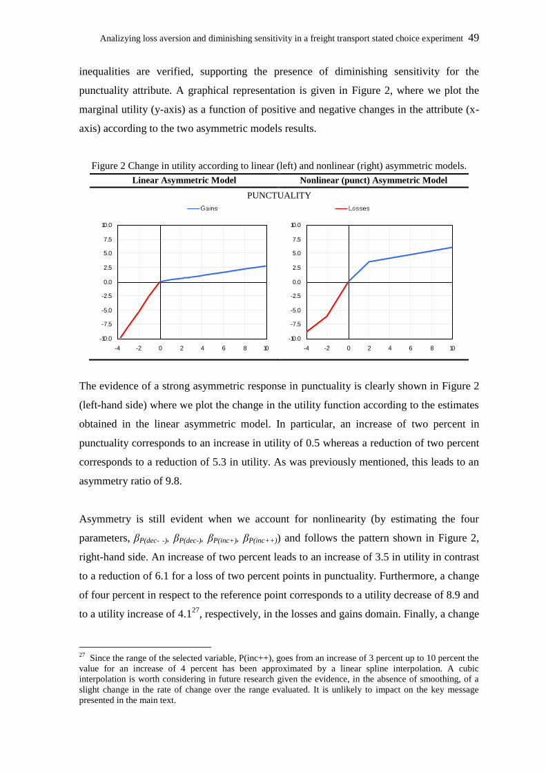
Analizying loss aversion and diminishing sensitivity in a freight transport stated choice experiment 49
inequalities are verified, supporting the presence of diminishing sensitivity for the
punctuality attribute. A graphical representation is given in Figure 2, where we plot the
marginal utility (y-axis) as a function of positive and negative changes in the attribute (x-
axis) according to the two asymmetric models results.
Figure 2 Change in utility according to linear (left) and nonlinear (right) asymmetric models.
Linear Asymmetric Model Nonlinear (punct) Asymmetric Model
PUNCTUALITY
The evidence of a strong asymmetric response in punctuality is clearly shown in Figure 2
(left-hand side) where we plot the change in the utility function according to the estimates
obtained in the linear asymmetric model. In particular, an increase of two percent in
punctuality corresponds to an increase in utility of 0.5 whereas a reduction of two percent
corresponds to a reduction of 5.3 in utility. As was previously mentioned, this leads to an
asymmetry ratio of 9.8.
Asymmetry is still evident when we account for nonlinearity (by estimating the four
parameters, βP(dec- -), βP(dec-), βP(inc+), βP(inc++)) and follows the pattern shown in Figure 2,
right-hand side. An increase of two percent leads to an increase of 3.5 in utility in contrast
to a reduction of 6.1 for a loss of two percent points in punctuality. Furthermore, a change
of four percent in respect to the reference point corresponds to a utility decrease of 8.9 and
to a utility increase of 4.127
, respectively, in the losses and gains domain. Finally, a change
27
Since the range of the selected variable, P(inc++), goes from an increase of 3 percent up to 10 percent the
value for an increase of 4 percent has been approximated by a linear spline interpolation. A cubic
interpolation is worth considering in future research given the evidence, in the absence of smoothing, of a
slight change in the rate of change over the range evaluated. It is unlikely to impact on the key message
presented in the main text.
-10.0
-7.5
-5.0
-2.5
0.0
2.5
5.0
7.5
10.0
-4 -2 0 2 4 6 8 10
-10.0
-7.5
-5.0
-2.5
0.0
2.5
5.0
7.5
10.0
-4 -2 0 2 4 6 8 10

50 Modelling freight transport demand and reference dependent choice behaviour
of two percent in punctuality gives an asymmetry ratio of 1.75 while a change of four
percent results in a value of 2.15.
The asymmetric and nonlinear specifications capture both loss aversion and diminishing
sensitivity, the two fundamental Prospect Theory assumptions that lead to the classical
asymmetric s-shape functional form.
2.4.2 Implication on willingness to pay
The investigation of WTP (or its counterpart WTA), as an indicator of the monetary value
of a selected attribute, plays a crucial role in discrete choice modelling. WTP is the ratio
of the marginal (dis)utility of an attribute to the marginal (dis)utility of the cost attribute.
In the linear additive random utility model, the derivation of WTP is straightforward since
the estimated coefficients are, by definition, marginal (dis)utilities. Nevertheless, the
computation requires some expedients when the coefficients are treated as random
parameters that involve the use of either the conditional or unconditional parameter
estimates28
. The estimation of the monetary values for the two asymmetric models is
based on the former method. Hensher et al. (2006) compare both approaches and illustrate
the benefits of the conditional parameter estimates.
In a symmetric model, willingness to accept (WTA) is equal to WTP and the monetary
values for the two quality attributes, time (T) and punctuality (P), are as follows:
( ) ( )ˆ ˆ
T T t cWTP WTA (8)
( ) ( )ˆ ˆ
P P p cWTP WTA (9)
The estimation of two different parameters with positive and negative deviations from the
reference point implies a different computation for both WTP and WTA, making the
equality imposed by the symmetric model free to change. For the linear asymmetric
model, specified in equation (3), the estimation is then based on equations (10) and (11).
28
See Hensher and Greene (2003) for a detailed discussion.
Analizying loss aversion and diminishing sensitivity in a freight transport stated choice experiment 51
( ) ( ) ( )ˆ ˆ
T t dec c incWTP (10a)
( ) ( ) ( )ˆ ˆ
T t inc c decWTA (10b)
( ) ( ) ( )ˆ ˆ
P p inc c incWTP (11a)
( ) ( ) ( )ˆ ˆ
P p dec c decWTA (11b)
The WTP and WTA for time are provided from equations (10a) and (10b). Punctuality,
however, in the nonlinear asymmetric model, is a nonlinear effect, and hence the
monetary measures for punctuality involve a differentiation among the four parameters
estimated (βP(dec- -), βP(dec-), βP(inc+), βP(inc++)). The WTP and WTA for the nonlinear and
asymmetric punctuality attribute are defined in (12) and (13).
( ) ( ) ( )ˆ ˆ
P p inc c incWTP (12a)
( ) ( ) ( )ˆ ˆ
P p dec c decWTA (12b)
( ) ( ) ( )ˆ ˆ
P p inc c incWTP (12c)
( ) ( ) ( )ˆ ˆ
P p dec c decWTA (12d)
The results for the WTP and WTA measures from the three different models are
summarized in Table 4. As is common practice in a freight transport context, we also
report the estimates expressed in CHF per tonne29
. The estimate of the value of time
savings for the generic symmetric model is 17.4 CHF/hour (16.3 USD/hour) which is in
line with others previous studies (Bolis and Maggi, 2003, Zamparini and Reggiani, 2007).
Willingness to pay for punctuality is 63 CHF (58.9 USD) per percentage point. Maggi and
Rudel (2008) find a value of 48 CHF (44.9 USD).
The relevance of punctuality (or reliability) in freight transport is confirmed from the data,
and is consistent with evidence from other studies (see for example, Fowkes et al. 2004,
Danielis et al. 2005, and Fowkes 2007). Puckett and Hensher (2008) also discuss the
importance of reliability but find relatively small values.
29
The calculation is based on the sample median; that is 5.5 tonne per shipment.
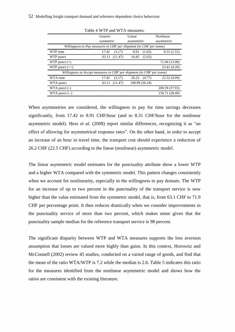
52 Modelling freight transport demand and reference dependent choice behaviour
Table 4 WTP and WTA measures.
Generic
symmetric
Linear
asymmetric
Nonlinear
asymmetric
Willingness to Pay measures in CHF per shipment (in CHF per tonne)
WTP time 17.42 (3.17) 8.91 (1.62) 8.31 (1.51)
WTP punct 63.11 (11.47) 14.45 (2.63)
WTP punct (+) 71.94 (13.08)
WTP punct (++) 23.41 (4.26)
Willingness to Accept measures in CHF per shipment (in CHF per tonne)
WTA time 17.42 (3.17) 26.22 (4.77) 22.52 (4.09)
WTA punct 63.11 (11.47) 198.99 (36.18)
WTA punct (-) 208.59 (37.93)
WTA punct (--) 156.71 (28.49)
When asymmetries are considered, the willingness to pay for time savings decreases
significantly, from 17.42 to 8.91 CHF/hour (and to 8.31 CHF/hour for the nonlinear
asymmetric model). Hess et al. (2008) report similar differences, recognizing it as “an
effect of allowing for asymmetrical response rates”. On the other hand, in order to accept
an increase of an hour in travel time, the transport cost should experience a reduction of
26.2 CHF (22.5 CHF) according to the linear (nonlinear) asymmetric model.
The linear asymmetric model estimates for the punctuality attribute show a lower WTP
and a higher WTA compared with the symmetric model. This pattern changes consistently
when we account for nonlinearity, especially in the willingness to pay domain. The WTP
for an increase of up to two percent in the punctuality of the transport service is now
higher than the value estimated from the symmetric model, that is, from 63.1 CHF to 71.9
CHF per percentage point. It then reduces drastically when we consider improvements in
the punctuality service of more than two percent, which makes sense given that the
punctuality sample median for the reference transport service is 98 percent.
The significant disparity between WTP and WTA measures supports the loss aversion
assumption that losses are valued more highly than gains. In this context, Horowitz and
McConnell (2002) review 45 studies, conducted on a varied range of goods, and find that
the mean of the ratio WTA/WTP is 7.2 while the median is 2.6. Table 5 indicates this ratio
for the measures identified from the nonlinear asymmetric model and shows how the
ratios are consistent with the existing literature.
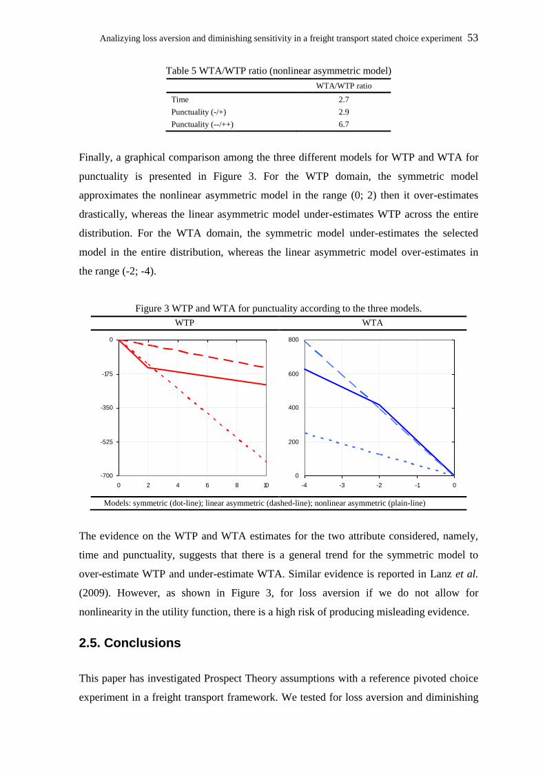
Analizying loss aversion and diminishing sensitivity in a freight transport stated choice experiment 53
Table 5 WTA/WTP ratio (nonlinear asymmetric model)
WTA/WTP ratio
Time 2.7
Punctuality (-/+) 2.9
Punctuality (--/++) 6.7
Finally, a graphical comparison among the three different models for WTP and WTA for
punctuality is presented in Figure 3. For the WTP domain, the symmetric model
approximates the nonlinear asymmetric model in the range (0; 2) then it over-estimates
drastically, whereas the linear asymmetric model under-estimates WTP across the entire
distribution. For the WTA domain, the symmetric model under-estimates the selected
model in the entire distribution, whereas the linear asymmetric model over-estimates in
the range (-2; -4).
Figure 3 WTP and WTA for punctuality according to the three models.
WTP WTA
Models: symmetric (dot-line); linear asymmetric (dashed-line); nonlinear asymmetric (plain-line)
The evidence on the WTP and WTA estimates for the two attribute considered, namely,
time and punctuality, suggests that there is a general trend for the symmetric model to
over-estimate WTP and under-estimate WTA. Similar evidence is reported in Lanz et al.
(2009). However, as shown in Figure 3, for loss aversion if we do not allow for
nonlinearity in the utility function, there is a high risk of producing misleading evidence.
2.5. Conclusions
This paper has investigated Prospect Theory assumptions with a reference pivoted choice
experiment in a freight transport framework. We tested for loss aversion and diminishing
-700
-525
-350
-175
0
0 2 4 6 8 10
0
200
400
600
800
-4 -3 -2 -1 0

54 Modelling freight transport demand and reference dependent choice behaviour
sensitivity within a random parameters model as a deviation from the reference
alternative.
The results suggest a significant and strong improvement in the goodness of fit of the
model when preferences are asymmetric. Loss aversion is reaffirmed for all the three
choice experiment attributes (cost, time and punctuality) included in the analysis, with the
asymmetry producing a steeper utility function for losses than for gains, which are
particularly marked for the punctuality attribute. For the three attributes in both the
positive and negative domains, a piecewise linear approximation was tested as a way to
capture nonlinearity. The cost and time attributes do not show significant nonlinearity, so
they are treated as asymmetric but linear in the two domains. Punctuality, on the other
hand, presents evidence of nonlinearity in the gains as well as in the losses domain,
confirmed by the increase in the model fit and by the asymptotic t statistic. Specifically,
the utility function shows a concave form for values above zero and a convex form for
values below zero, suggesting that respondents experience diminishing sensitivity in terms
of the marginal disutility of punctuality.
Loss aversion and diminishing sensitivity have a significant impact on willingness to pay
and willingness to accept. The classic symmetric model shows a tendency to over-estimate
WTP and under-estimate WTA. The model estimates show a consistent disparity between
the two measures, resulting in a WTA/WTP ratio of 2.7 for time and 2.9 and 6.7 for
punctuality up to 2 percent and between 2 percent and 10 percent, respectively.
The relevance of the behavioural contributions of Prospect Theory, embedded in an
individual output/price context, is reaffirmed in a firm’s logistic profit/cost context,
raising concerns about the symmetric specification commonly used in freight demand
studies. Indeed, the majority of the studies that estimate WTP are based on stated choice
experiments with symmetric specifications in utility expressions. The findings in this
paper on WTP, a common measure in calculating user benefits, raise questions about the
errors induced by the linear assumption, in the evaluation of new infrastructure via cost
benefit analysis and more generally, on all the situations where WTP and WTA measures
are required as part of a policy decision process.
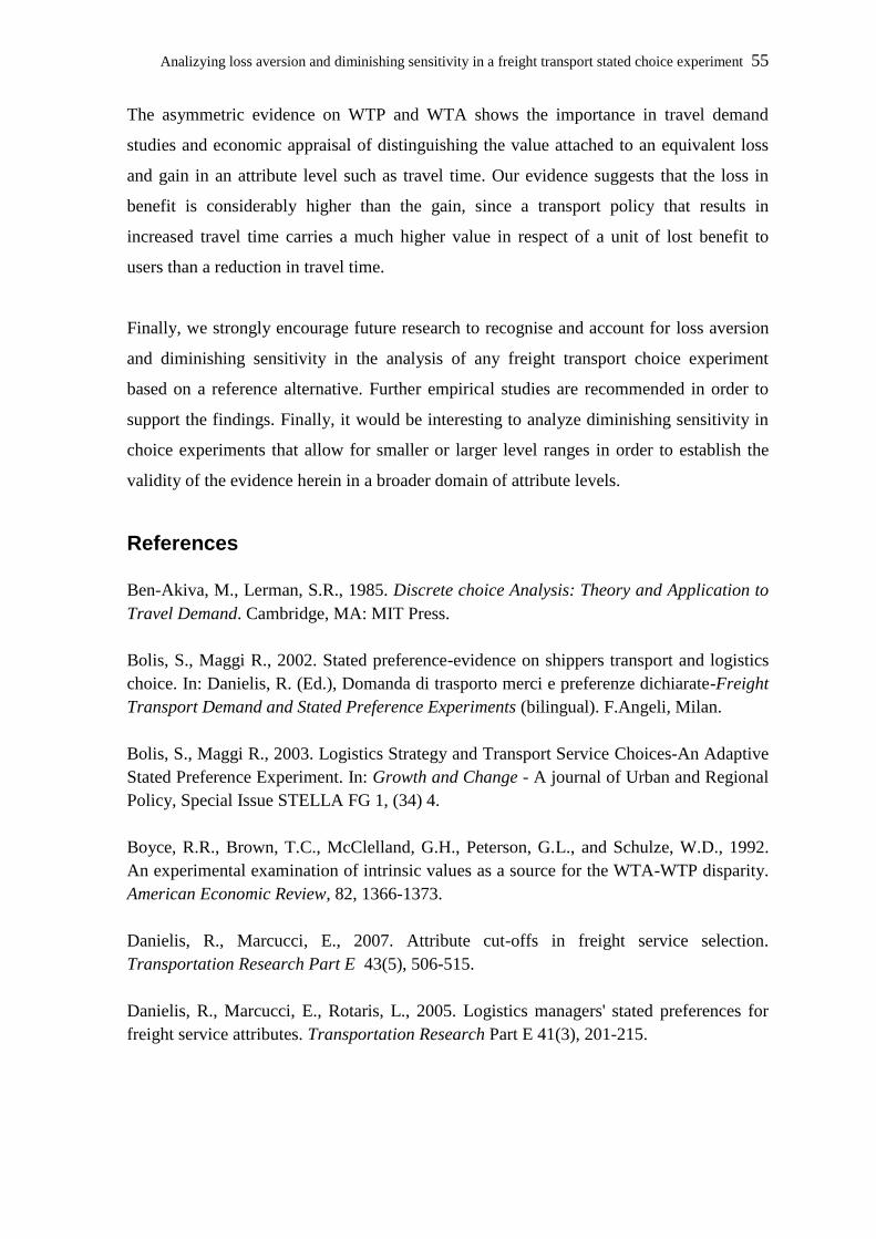
Analizying loss aversion and diminishing sensitivity in a freight transport stated choice experiment 55
The asymmetric evidence on WTP and WTA shows the importance in travel demand
studies and economic appraisal of distinguishing the value attached to an equivalent loss
and gain in an attribute level such as travel time. Our evidence suggests that the loss in
benefit is considerably higher than the gain, since a transport policy that results in
increased travel time carries a much higher value in respect of a unit of lost benefit to
users than a reduction in travel time.
Finally, we strongly encourage future research to recognise and account for loss aversion
and diminishing sensitivity in the analysis of any freight transport choice experiment
based on a reference alternative. Further empirical studies are recommended in order to
support the findings. Finally, it would be interesting to analyze diminishing sensitivity in
choice experiments that allow for smaller or larger level ranges in order to establish the
validity of the evidence herein in a broader domain of attribute levels.
References
Ben-Akiva, M., Lerman, S.R., 1985. Discrete choice Analysis: Theory and Application to
Travel Demand. Cambridge, MA: MIT Press.
Bolis, S., Maggi R., 2002. Stated preference-evidence on shippers transport and logistics
choice. In: Danielis, R. (Ed.), Domanda di trasporto merci e preferenze dichiarate-Freight
Transport Demand and Stated Preference Experiments (bilingual). F.Angeli, Milan.
Bolis, S., Maggi R., 2003. Logistics Strategy and Transport Service Choices-An Adaptive
Stated Preference Experiment. In: Growth and Change - A journal of Urban and Regional
Policy, Special Issue STELLA FG 1, (34) 4.
Boyce, R.R., Brown, T.C., McClelland, G.H., Peterson, G.L., and Schulze, W.D., 1992.
An experimental examination of intrinsic values as a source for the WTA-WTP disparity.
American Economic Review, 82, 1366-1373.
Danielis, R., Marcucci, E., 2007. Attribute cut-offs in freight service selection.
Transportation Research Part E 43(5), 506-515.
Danielis, R., Marcucci, E., Rotaris, L., 2005. Logistics managers' stated preferences for
freight service attributes. Transportation Research Part E 41(3), 201-215.
56 Modelling freight transport demand and reference dependent choice behaviour
Fowkes, A.S., 2007. The design and interpretation of freight stated preference
experiments seeking to elicit behavioural valuations of journey attributes. Transportation
Research Part B 41(9), 966-980.
Fowkes, A.S., Firmin, P.E., Tweddle, G., Whiteing, A.E., 2004. How Highly Does the
Freight Transport Industry Value Journey Time Reliability - and for What Reasons?
International Journal of Logistics: Research and Applications 7, 33-44.
Hensher, D.A., Greene, W.H., 2003. Mixed logit models: state of practice. Transportation
30(2), 133-176.
Hensher, D.A., Greene, W.H., 2009. Taming analytical distributions: valuation in WTP
and utility space in the presence of taste and scale heterogeneity, Institute of Transport
and Logistics Studies, University of Sydney, July.
Hensher, D.A., Greene, W.H., Rose, J.M., 2006. Deriving willingness-to-pay estimates of
travel time savings from individual-based parameters. Environment and Planning A
38(12), 2365 – 2376.
Hess, S., Rose, J.M., Hensher, D.A., 2008. Asymmetric preference formation in
willingness to pay estimates in discrete choice models. Transportation Research Part E
44(5), 847–863.
Horowitz, J., McConnell, K.E., 2002. A Review of WTA-WTP Studies. Journal of
Environmental Economics and Management 44, 426-47.
Kahneman, D., Tversky A., 1979. Prospect Theory: an analysis of decision under risk.
Econometrica 47 (2), 263–291.
Maggi, R., Rudel, R., 2008. The Value of Quality Attributes in Freight Transport:
Evidence from an SP-Experiment in Switzerland. In: Ben-Akiva, M.E., Meersman, H.,
van de Voorde E. (Eds.), Recent Developments in Transport Modelling. Emerald Group
Publishing Limited.
Maggi, R., Masiero, L., Baruffini, M., Thuering M., 2009. Evaluation of the optimal
resilience for vulnerable infrastructure networks. An interdisciplinary pilot study on the
transalpine transportation corridors. Swiss National Science Foundation, NRP 54
“Sustainable Development of the Built Environment”, Project 405 440, Final Scientific
Report.
McFadden, D., 1974. Conditional logit analysis of qualitative choice behavior. In:
Zarembka, P. (Ed.), Frontiers in Econometrics. Academic Press, New York.
Analizying loss aversion and diminishing sensitivity in a freight transport stated choice experiment 57
Masiero, L., Maggi, R., 2009. Estimation of indirect cost and evaluation of protective
measures for infrastructure vulnerability: A case study on the transalpine transport
corridor. Submitted for publication, September.
Lanz, B., Provins, A., Bateman, I., Scarpa, R., Willis, K., Ozdemiroglu, E., 2009.
Investigating willingness to pay – willingness to accept asymmetry in choice experiments.
Paper selected for presentation at the International Choice Modelling Conference 2009,
Leeds (UK).
Puckett, S.M., Hensher, D.A., 2008. The role of attribute processing strategies in
estimating the preferences of road freight stakeholders under variable road user charges.
Transportation Research E 44(3), 379-395.
Rose, J.M., Bliemer, M.C., Hensher, Collins, A. T., 2008. Designing efficient stated
choice experiments in the presence of reference alternatives. Transportation Research B
42(4), 395-406.
Swait, J., 2001. A Non-compensatory Choice Model Incorporating Attribute Cutoffs.
Transportation Research B 35(10), 903-928.
Train, K., 2003. Discrete Choice Methods with Simulation. Cambridge University Press,
Cambridge.
Tversky, A., Kahneman, D., 1991. Loss aversion in riskless choice: A reference-
dependent model. Quarterly Journal of Economics 106, 1039–1061.
Tversky, A., Kahneman, D., 1992. Advances in Prospect Theory: Cumulative
Representation of Uncertainty. Journal of Risk and Uncertainty 5, 297-323.
Zamparini, L., Reggiani, A., 2007. The value of travel time in passenger and freight
transport: An overview. In: van Geenhuizen, M., Reggiani, A., Rietveld, P. (Eds.), Policy
analysis of transport networks. Ashgate, Aldershot.
58
Chapter Three
Shift of reference point and implications on behavioral reaction to gains and losses
Lorenzo Masiero
David A. Hensher
Version: April 29 2010
Submitted to Transportation
Abstract
It is widely recognized that individual decision making is subject to the evaluation of
gains and losses around a reference point. The estimation of discrete choice models
increasingly use data from stated choice experiments which are pivoted around a reference
alternative. However, to date, the specification of a reference alternative in transport
studies is fixed, whereas it is common to observe individuals adjusting their preferences
according to a change in their reference point. This paper focuses on individual reactions,
in a freight choice context, to a negative change in the reference alternative values,
identifying the behavioural implications in terms of loss aversion and diminishing
sensitivity. The results show a significant adjustment in the valuation of gains and losses
around a shifted reference alternative. In particular, we find an average increase in loss
aversion for cost and time attributes, and a substantial decrease for punctuality. These
findings are translated to significant differences in the willingness to pay and willingness
to accept measures, providing supporting evidence of respondents’ behavioural reaction.
Keywords: Willingness to pay, gains and losses, freight choice, reference alternative
Acknowledgements: This research is funded by a “Prospective Researcher” grant of the
Swiss National Science Foundation. We thank Rico Maggi for his support and
encouragement. This research was undertaken during a one year research period at ITLS.

Shift of reference point and implications on behavioural reaction to gains and losses 59
3.1. Introduction
The importance of considering the individual’s choice behaviour as a decision based on
the distinction between positive (gains) and negative (losses) deviations from a specific
individual reference value has been formulated in prospect theory (Kahneman and
Tversky, 1979), and introduced in both risky choices (Kahneman and Tversky, 1979;
Tversky and Kahneman, 1992) and risk-less choices (Tversky and Kahneman, 1991). In
this context, prospect theory defines two fundamental assumptions involving the utility
function, namely loss aversion, where individuals tend to evaluate losses higher than
gains, and diminishing sensitivity where individuals show decreasing marginal values in
both positive and negative domains.
Application of prospect theory can be found in several economic fields such as, for
example, financial markets (e.g., Benartzi and Thaler, 1995), labour economics (e.g.,
Camerer et al., 1997), health economics (Samuelson and Zeckhauser, 1988) and
macroeconomics (e.g., Shea, 1995). Furthermore, the plausibility of the prospect theory
has been reinforced using a range of different data types and interview procedures, such as
contingent valuation (Rowe et al., 1980) or laboratory experiments (e.g., Bateman et al.,
1997).
The recent estimation of discrete choice models with a reference dependence specification
has empirically reinforced the plausibility of prospect theory assumptions within the
framework of reference pivoted experimental designs (see for example, Hess et al., 2008;
Lanz et al., 2009; Masiero and Hensher, 2009). The utility function is expressed in terms
of gains and losses around a reference alternative, without loosing the linearity in the
parameters assumption underlying the Random Utility Model (McFadden, 1974). Such a
specification nests the commonly used specification obtained by imposing equality
constraints between the absolute values of the parameter estimates associated with gains
and losses.
The improved statistical performance of the reference dependence specification in terms
of overall model fit, and the increasing use of reference pivoted experimental designs as
techniques to add realism for respondents (Rose et al., 2008), are increasing the role
played by the specification of the reference alternative in the model estimation process

60 Modelling freight transport demand and reference dependent choice behaviour
(see for example, Hess and Rose, 2009 and Rose et al., 2008). However, a crucial issue
associated with the reference alternative is the specification of reference values in change
contexts or in any framework that might involve a change in the initial values of the
reference alternative (e.g. actual values versus expected values). Kahneman and Tversky
(1979) note that:
“... A change of reference point alters the preference order for prospect … A discrepancy
between the reference point and the current asset position may also arise because of
recent changes in the wealth to which one has not yet adapted …The location of the
reference point, and the manner in which choice problems are coded and edited emerge
as critical factors in the analysis of decision.”
Very few studies have analysed the individual adaptation process followed by a change of
the reference point. In this context, Arkes et al. (2008) conducted a survey to study the
individual’s adaptation after experiencing losses or gains in a stock price. Schwartz et al.
(2008) illustrate an approach designed to identify, and hence adjust, the change in the
utility perceived after a shift of the reference point in a medical decision making process.
As far as we are aware, there are no studies that have investigated the implications on the
utility function of changes in parameter estimates when the reference point is shifted.
The aim of this paper is to analyse the impact of a negative shift of the reference point on
preference formation in terms of loss aversion and diminishing sensitivity, in a stated
choice experiment framework. In particular, we refer to a pooled dataset consisting of two
freight transport choice experiments with designs pivoted around two different reference
alternatives, where one is the actual (or initial) reference alternative and the other is the
expected (or shifted) reference alternative30
. The identification of potential implications is
based on the estimation and comparison of the marginal (dis)utilities associated with the
gains and losses. We formulate and test different hypotheses of behavioural reaction and
present the implications as willingness to pay and willingness to accept measures.
The paper is organised as follows. In section two we describe the two choice experiments
and the context of the survey. Section three provides an overview of the methodology
30
The survey was conducted within the National Research Program NRP 54 - Sustainable Development of
the Built Environment - granted by the Swiss National Science Foundation.
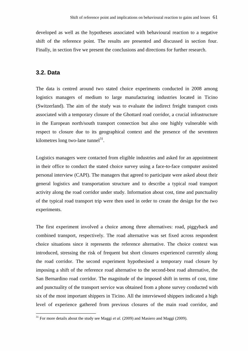
Shift of reference point and implications on behavioural reaction to gains and losses 61
developed as well as the hypotheses associated with behavioural reaction to a negative
shift of the reference point. The results are presented and discussed in section four.
Finally, in section five we present the conclusions and directions for further research.
3.2. Data
The data is centred around two stated choice experiments conducted in 2008 among
logistics managers of medium to large manufacturing industries located in Ticino
(Switzerland). The aim of the study was to evaluate the indirect freight transport costs
associated with a temporary closure of the Ghottard road corridor, a crucial infrastructure
in the European north/south transport connection but also one highly vulnerable with
respect to closure due to its geographical context and the presence of the seventeen
kilometres long two-lane tunnel31
.
Logistics managers were contacted from eligible industries and asked for an appointment
in their office to conduct the stated choice survey using a face-to-face computer assisted
personal interview (CAPI). The managers that agreed to participate were asked about their
general logistics and transportation structure and to describe a typical road transport
activity along the road corridor under study. Information about cost, time and punctuality
of the typical road transport trip were then used in order to create the design for the two
experiments.
The first experiment involved a choice among three alternatives: road, piggyback and
combined transport, respectively. The road alternative was set fixed across respondent
choice situations since it represents the reference alternative. The choice context was
introduced, stressing the risk of frequent but short closures experienced currently along
the road corridor. The second experiment hypothesised a temporary road closure by
imposing a shift of the reference road alternative to the second-best road alternative, the
San Bernardino road corridor. The magnitude of the imposed shift in terms of cost, time
and punctuality of the transport service was obtained from a phone survey conducted with
six of the most important shippers in Ticino. All the interviewed shippers indicated a high
level of experience gathered from previous closures of the main road corridor, and
31
For more details about the study see Maggi et al. (2009) and Masiero and Maggi (2009).
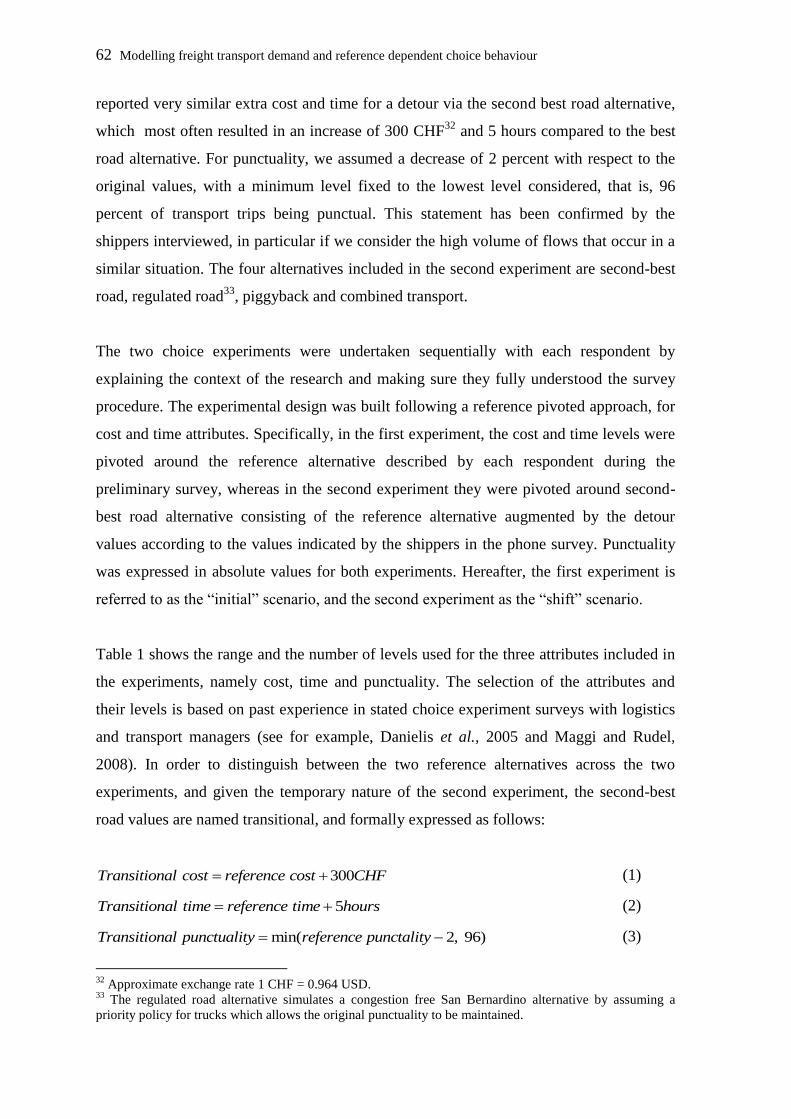
62 Modelling freight transport demand and reference dependent choice behaviour
reported very similar extra cost and time for a detour via the second best road alternative,
which most often resulted in an increase of 300 CHF32
and 5 hours compared to the best
road alternative. For punctuality, we assumed a decrease of 2 percent with respect to the
original values, with a minimum level fixed to the lowest level considered, that is, 96
percent of transport trips being punctual. This statement has been confirmed by the
shippers interviewed, in particular if we consider the high volume of flows that occur in a
similar situation. The four alternatives included in the second experiment are second-best
road, regulated road33
, piggyback and combined transport.
The two choice experiments were undertaken sequentially with each respondent by
explaining the context of the research and making sure they fully understood the survey
procedure. The experimental design was built following a reference pivoted approach, for
cost and time attributes. Specifically, in the first experiment, the cost and time levels were
pivoted around the reference alternative described by each respondent during the
preliminary survey, whereas in the second experiment they were pivoted around second-
best road alternative consisting of the reference alternative augmented by the detour
values according to the values indicated by the shippers in the phone survey. Punctuality
was expressed in absolute values for both experiments. Hereafter, the first experiment is
referred to as the “initial” scenario, and the second experiment as the “shift” scenario.
Table 1 shows the range and the number of levels used for the three attributes included in
the experiments, namely cost, time and punctuality. The selection of the attributes and
their levels is based on past experience in stated choice experiment surveys with logistics
and transport managers (see for example, Danielis et al., 2005 and Maggi and Rudel,
2008). In order to distinguish between the two reference alternatives across the two
experiments, and given the temporary nature of the second experiment, the second-best
road values are named transitional, and formally expressed as follows:
300Transitional cost reference cost CHF (1)
5Transitional time reference time hours (2)
min( 2, 96)Transitional punctuality reference punctality (3)
32
Approximate exchange rate 1 CHF = 0.964 USD. 33
The regulated road alternative simulates a congestion free San Bernardino alternative by assuming a
priority policy for trucks which allows the original punctuality to be maintained.
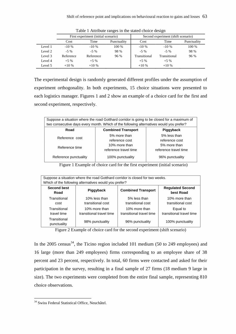
Shift of reference point and implications on behavioural reaction to gains and losses 63
Table 1 Attribute ranges in the stated choice design
First experiment (initial scenario) Second experiment (shift scenario)
Cost Time Punctuality Cost Time Punctuality
Level 1 -10 % -10 % 100 % -10 % -10 % 100 %
Level 2 -5 % -5 % 98 % -5 % -5 % 98 %
Level 3 Reference Reference 96 % Transitional Transitional 96 %
Level 4 +5 % +5 % +5 % +5 %
Level 5 +10 % +10 % +10 % +10 %
The experimental design is randomly generated different profiles under the assumption of
experiment orthogonality. In both experiments, 15 choice situations were presented to
each logistics manager. Figures 1 and 2 show an example of a choice card for the first and
second experiment, respectively.
Suppose a situation where the road Gotthard corridor is going to be closed for a maximum of
two consecutive days every month. Which of the following alternatives would you prefer?
Road Combined Transport Piggyback
Reference cost 5% more than
reference cost
5% less than
reference cost
Reference time 10% more than
reference travel time
5% more than
reference travel time
Reference punctuality 100% punctuality 96% punctuality
Figure 1 Example of choice card for the first experiment (initial scenario)
Suppose a situation where the road Gotthard corridor is closed for two weeks.
Which of the following alternatives would you prefer?
Second best
Road Piggyback Combined Transport
Regulated Second
best Road
Transitional
cost
10% less than
transitional cost
5% less than
transitional cost
10% more than
transitional cost
Transitional
travel time
10% more than
transitional travel time
10% more than
transitional travel time
Equal to
transitional travel time
Transitional
punctuality 98% punctuality 96% punctuality 100% punctuality
Figure 2 Example of choice card for the second experiment (shift scenario)
In the 2005 census34
, the Ticino region included 101 medium (50 to 249 employees) and
16 large (more than 249 employees) firms corresponding to an employee share of 38
percent and 23 percent, respectively. In total, 60 firms were contacted and asked for their
participation in the survey, resulting in a final sample of 27 firms (18 medium 9 large in
size). The two experiments were completed from the entire final sample, representing 810
choice observations.
34
Swiss Federal Statistical Office, Neuchâtel.
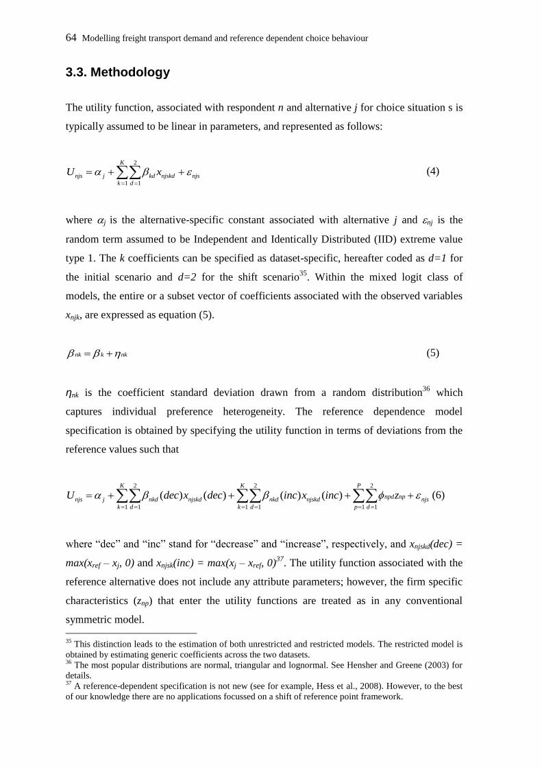
64 Modelling freight transport demand and reference dependent choice behaviour
3.3. Methodology
The utility function, associated with respondent n and alternative j for choice situation s is
typically assumed to be linear in parameters, and represented as follows:
2
1 1
K
njs j kd njskd njs
k d
U x
(4)
where j is the alternative-specific constant associated with alternative j and nj is the
random term assumed to be Independent and Identically Distributed (IID) extreme value
type 1. The k coefficients can be specified as dataset-specific, hereafter coded as d=1 for
the initial scenario and d=2 for the shift scenario35
. Within the mixed logit class of
models, the entire or a subset vector of coefficients associated with the observed variables
xnjk, are expressed as equation (5).
nk k nk (5)
ηnk is the coefficient standard deviation drawn from a random distribution36
which
captures individual preference heterogeneity. The reference dependence model
specification is obtained by specifying the utility function in terms of deviations from the
reference values such that
2 2 2
1 1 1 1 1 1
( ) ( ) ( ) ( )K K P
npd npnjs j nkd njskd nkd njskd njs
k d k d p d
U dec x dec inc x inc z
(6)
where “dec” and “inc” stand for “decrease” and “increase”, respectively, and xnjskd(dec) =
max(xref – xj, 0) and xnjsk(inc) = max(xj – xref, 0)37
. The utility function associated with the
reference alternative does not include any attribute parameters; however, the firm specific
characteristics (znp) that enter the utility functions are treated as in any conventional
symmetric model.
35
This distinction leads to the estimation of both unrestricted and restricted models. The restricted model is
obtained by estimating generic coefficients across the two datasets. 36
The most popular distributions are normal, triangular and lognormal. See Hensher and Greene (2003) for
details. 37
A reference-dependent specification is not new (see for example, Hess et al., 2008). However, to the best
of our knowledge there are no applications focussed on a shift of reference point framework.
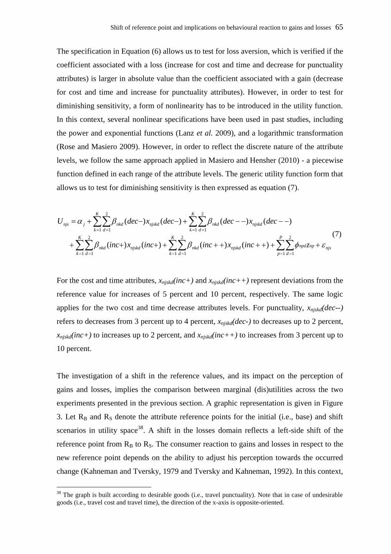
Shift of reference point and implications on behavioural reaction to gains and losses 65
The specification in Equation (6) allows us to test for loss aversion, which is verified if the
coefficient associated with a loss (increase for cost and time and decrease for punctuality
attributes) is larger in absolute value than the coefficient associated with a gain (decrease
for cost and time and increase for punctuality attributes). However, in order to test for
diminishing sensitivity, a form of nonlinearity has to be introduced in the utility function.
In this context, several nonlinear specifications have been used in past studies, including
the power and exponential functions (Lanz et al. 2009), and a logarithmic transformation
(Rose and Masiero 2009). However, in order to reflect the discrete nature of the attribute
levels, we follow the same approach applied in Masiero and Hensher (2010) - a piecewise
function defined in each range of the attribute levels. The generic utility function form that
allows us to test for diminishing sensitivity is then expressed as equation (7).
2 2
1 1 1 1
2 2 2
1 1 1 1 1 1
( ) ( ) ( ) ( )
( ) ( ) ( ) ( )
K K
njs j nkd njskd nkd njskd
k d k d
K K P
npd npnkd njskd nkd njskd njs
k d k d p d
U dec x dec dec x dec
inc x inc inc x inc z
(7)
For the cost and time attributes, xnjskd(inc+) and xnjskd(inc++) represent deviations from the
reference value for increases of 5 percent and 10 percent, respectively. The same logic
applies for the two cost and time decrease attributes levels. For punctuality, xnjskd(dec--)
refers to decreases from 3 percent up to 4 percent, xnjskd(dec-) to decreases up to 2 percent,
xnjskd(inc+) to increases up to 2 percent, and xnjskd(inc++) to increases from 3 percent up to
10 percent.
The investigation of a shift in the reference values, and its impact on the perception of
gains and losses, implies the comparison between marginal (dis)utilities across the two
experiments presented in the previous section. A graphic representation is given in Figure
3. Let RB and RS denote the attribute reference points for the initial (i.e., base) and shift
scenarios in utility space38
. A shift in the losses domain reflects a left-side shift of the
reference point from RB to RS. The consumer reaction to gains and losses in respect to the
new reference point depends on the ability to adjust his perception towards the occurred
change (Kahneman and Tversky, 1979 and Tversky and Kahneman, 1992). In this context,
38
The graph is built according to desirable goods (i.e., travel punctuality). Note that in case of undesirable
goods (i.e., travel cost and travel time), the direction of the x-axis is opposite-oriented.
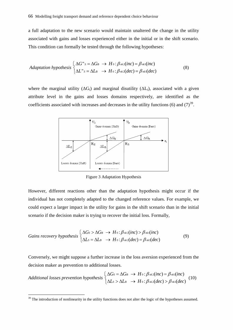
66 Modelling freight transport demand and reference dependent choice behaviour
a full adaptation to the new scenario would maintain unaltered the change in the utility
associated with gains and losses experienced either in the initial or in the shift scenario.
This condition can formally be tested through the following hypotheses:
Adaptation hypothesis 0 2 1
0 2 1
" : ( ) ( )
" : ( ) ( )
S B nk nk
S B nk nk
G G H inc inc
L L H dec dec
(8)
where the marginal utility (ΔGi) and marginal disutility (ΔLi), associated with a given
attribute level in the gains and losses domains respectively, are identified as the
coefficients associated with increases and decreases in the utility functions (6) and (7)39
.
Figure 3 Adaptation Hypothesis
However, different reactions other than the adaptation hypothesis might occur if the
individual has not completely adapted to the changed reference values. For example, we
could expect a larger impact in the utility for gains in the shift scenario than in the initial
scenario if the decision maker is trying to recover the initial loss. Formally,
Gains recovery hypothesis 0 2 1
0 2 1
: ( ) ( )
: ( ) ( )
S B nk nk
S B nk nk
G G H inc inc
L L H dec dec
(9)
Conversely, we might suppose a further increase in the loss aversion experienced from the
decision maker as prevention to additional losses.
Additional losses prevention hypothesis 0 2 1
0 2 1
: ( ) ( )
: ( ) ( )
S B nk nk
S B nk nk
G G H inc inc
L L H dec dec
(10)
39
The introduction of nonlinearity in the utility functions does not alter the logic of the hypotheses assumed.
Shift of reference point and implications on behavioural reaction to gains and losses 67
The estimation of the utility parameters associated with gains and losses, and their
comparison across the two scenarios, allow us to test the hypotheses formulated, as well
as any other pattern not discussed.
Given the panel structure of the data collected from the two stated choice experiments and
the use of the mixed logit class of models, the estimation of the utility parameters is
derived from the maximization of the following simulated log likelihood:
1 exp( ' )ln
exp( ' )
j n njs n nn
n r sj n njs n n
j
LLR
α β x φ z
α β x φ z (11)
where s = 1, …, S represent the number of choice situations whereas r = 1, …, R refers to
the number of draws. Within the Random Utility Model framework, the coefficients are
estimated along with the scale parameter, which reflects the variance of the unobserved
component of the utility. Since different data sets have potentially different variances for
unobserved utility, the comparison of the magnitude of the coefficients is possible only if
the scale difference between the two data sets is taken into account. In this context, several
techniques have been proposed in order to cope with difference in scale in jointly
estimated choice models that use revealed preferences (RP) and stated preferences (SP)
data (see for example, Swait and Louviere, 1993; Hensher and Bradley, 1993; Ben-Akiva
and Morikawa, 1997). In this paper we refer to the approach recently used by Hensher
(2008) which takes into account difference in scale by estimating the scale parameter for
one of the two datasets considered in the pooled data40
. According to Bhat and Castelar
(2002), the scale parameter is expressed as follows:
, ,[(1 ) ]njs njs SPi j njs SPi i = 1, 2 (12)
where ,njs SPi is a dummy variable that takes the value 1 for the observations associated
with the dataset with the scale parameter normalised to 1, and zero otherwise. The
parameter j is derivable by introducing in one of the two data sets (arbitrarily selected) a
40
It should be noted that in our context the aim is different from a typical RP and SP joint estimation. We
are not interested to enrich the data with additional and complementary information, but we are instead
looking at the comparison of coefficient magnitudes from different datasets.
68 Modelling freight transport demand and reference dependent choice behaviour
set of alternative-specific constants (ASC) that have a zero mean and free variance
(Brownstone et al., 2000). In fact, the following relation holds:
6 1.28255j ASCj ASCj (13)
where ASCj are the standard deviations of the alternative-specific constants introduced in
data set i. In our case we estimate the scale parameter associated with the first data set,
referring to the initial scenario, consisting of three alternatives, two hypothetical
alternatives and the reference alternative respectively. From a preliminary analysis we
noticed that the ASCs associated with the two hypothetical alternatives were not
statistically different to one another. We decided then to nest the two hypothetical
alternatives by constraining the estimation of only two additional ASCs, one for the
reference alternative, and the other for the two hypothetical alternatives.41
3.4. Model Results
We estimated three pairs of panel mixed logit models using 500 Halton draws42
with
results summarised in Table 2. The first pair of models (M1 and M2) refers to linear
symmetric specifications given in equation (4); that is the classic form of specification
commonly used in discrete choice modeling. We then introduce the reference dependence
models M3 and M4 defined in equation (6) that allows us to test for loss aversion. The last
pair of models (M5 and M6) is of the form in equation (7), and still based on the reference
dependence specification, but with the integration of attribute piecewise transformations
in order to capture potential nonlinearities that are compatible with the diminishing
sensitivity prospect theory assumption.
The difference within each pair of models is that the first model has generic-specific
coefficient estimates (a restricted model), whereas in the second model the coefficients are
treated as dataset-specific (an unrestricted model). This allows us to obtain an immediate,
41
Note that the assumption of having different variance among alternatives leads to the estimation of a
heteroskedastic choice model. In our case, we normalize the variance in respect to the four alternatives
associated to the second dataset obtaining a constrained heterskedastic choice models. 42
See Train (2003) for details about Halton sequence. All models were estimated using a pre-release version
of Nlogit 5.
Shift of reference point and implications on behavioural reaction to gains and losses 69
but overall, test on the hypothesis of adaptation by comparing the model fits within each
pair of models.
In terms of goodness of fit we report the log-likelihood at convergence, the McFadden
pseudo ρ2 and the Akaike’s Information Criterion (AIC) (normalised for sample size) (see
Table 2). The best model in explaining the data is model M6 which reports a McFadden
pseudo ρ2 of 0.600 and an AIC index of 1.626 versus a McFadden pseudo ρ2
of 0.542 and
an AIC index of 1.820 obtained for model M2 which shows the poorest model fit
measures among the six models estimated. Introducing nonlinearity in the reference
dependence specification (models M5 and M6) increases, in general, the goodness of
model fits in respect to the linear asymmetric specifications (models M3 and M4), and
both specifications outperform substantially the symmetric ones (models M1 and M2).
However, a first interesting result is provided from the comparison, within the three pairs
of models, of the AIC index which in its calculation account for both a reduction in the
log-likelihood and an increase in the number of parameters estimated. According to the
AIC index, model M1 is preferred to M2, suggesting that there are no overall significant
differences between the coefficients associated with the initial and shift scenarios. We
observe exactly the opposite result once we introduce the reference dependence
specifications, where models M4 and M6 outperform models M3 and M5 respectively43
.
For each of the six models, we have estimated the scale parameters for the three
alternatives associated with the initial scenario, with the aim of levelling any unobserved
variance difference between the two datasets, making possible the comparison between
coefficient estimates. From the scale parameters that are statistically significant different
from one at a confidence level of 0.1, we observe that they all are smaller than one,
suggesting a greater variance of the unobserved effects for the initial scenario than for the
shift scenario. Although it is plausible to expect a difference in scale between two datasets
we had no expectation about the magnitude associated with the stated preferences
structure of the experiment in both scenarios.
43
More formal t-tests are provided further in this section (see Table 3).
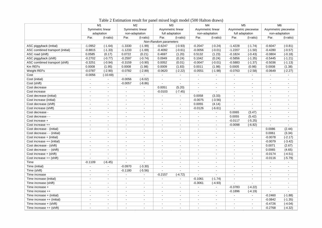
Table 2 Estimation result for panel mixed logit model (500 Halton draws) M1 M2 M3 M4 M5 M6
Symmetric linear Symmetric linear Asymmetric linear Asymmetric linear Asymmetric piecewise Asymmetric piecewise
adaptation non-adaptation full adaptation non-adaptation full adaptation non-adaptation
Par. (t-ratio) Par. (t-ratio) Par. (t-ratio) Par. (t-ratio) Par. (t-ratio) Par. (t-ratio)
Non-Random parameters
ASC piggyback (initial) -1.0952 (-1.64) -1.3330 (-1.99) -0.6247 (-0.93) -0.2047 (-0.24) -1.4228 (-1.74) -0.6047 (-0.81)
ASC combined transport (initial) -0.8815 (-1.33) -1.1233 (-1.69) -0.4092 (-0.61) -0.0056 (-0.01) -1.2207 (-1.50) -0.4280 (-0.57)
ASC road (shift) 0.0585 (0.17) 0.0722 (0.21) 0.4697 (1.20) 0.5132 (1.23) -0.1824 (-0.43) -0.0804 (-0.18)
ASC piggyback (shift) -0.2702 (-0.77) -0.2597 (-0.74) 0.0949 (0.24) 0.1042 (0.24) -0.5856 (-1.35) -0.5445 (-1.21)
ASC combined transport (shift) -0.3251 (-0.94) -0.3159 (-0.90) 0.0052 (0.01) -0.0047 (-0.01) -0.5883 (-1.37) -0.5036 (-1.13)
Km REFs 0.0008 (1.95) 0.0008 (1.98) 0.0009 (1.83) 0.0011 (1.98) 0.0005 (0.98) 0.0008 (1.38)
Weight REFs -0.0787 (-2.90) -0.0782 (-2.89) -0.0620 (-2.22) -0.0551 (-1.98) -0.0763 (-2.58) -0.0649 (-2.27)
Cost -0.0056 (-10.69) - - - - - - - - - -
Cost (initial) - - -0.0056 (-6.02) - - - - - - - -
Cost (shift) - - -0.0057 (-8.86) - - - - - - - -
Cost decrease - - - - 0.0051 (5.20) - - - - - -
Cost increase - - - - -0.0103 (-7.45) - - - - - -
Cost decrease (initial) - - - - - - 0.0058 (3.33) - - - -
Cost increase (initial) - - - - - - -0.0075 (-3.56) - - - -
Cost decrease (shift) - - - - - - 0.0055 (4.14) - - - -
Cost increase (shift) - - - - - - -0.0126 (-6.61) - - - -
Cost decrease - - - - - - - - - 0.0065 (3.47) - -
Cost decrease - - - - - - - - - - 0.0055 (5.42) - -
Cost increase + - - - - - - - - -0.0117 (-5.25) - -
Cost increase ++ - - - - - - - - -0.0098 (-6.82) - -
Cost decrease - (initial) - - - - - - - - - - 0.0086 (2.44)
Cost decrease - - (initial) - - - - - - - - - - 0.0061 (3.34)
Cost increase + (initial) - - - - - - - - - - -0.0078 (-2.17)
Cost increase ++ (initial) - - - - - - - - - - -0.0079 (-3.42)
Cost decrease - (shift) - - - - - - - - - - 0.0071 (2.67)
Cost decrease - - (shift) - - - - - - - - - - 0.0065 (4.65)
Cost increase + (shift) - - - - - - - - - - -0.0174 (-4.51)
Cost increase ++ (shift) - - - - - - - - - - -0.0116 (-5.79)
Time -0.1109 (-6.45) - - - - - - - - - -
Time (initial) - - -0.0970 (-3.30) - - - - - - - -
Time (shift) - - -0.1180 (-5.56) - - - - - - - -
Time increase - - - - -0.2157 (-4.72) - - - - - -
Time increase (initial) - - - - - - -0.1061 (-1.74) - - - -
Time increase (shift) - - - - - - -0.3061 (-4.93) - - - -
Time increase + - - - - - - - - -0.3783 (-4.22) - -
Time increase ++ - - - - - - - - -0.1896 (-4.19) - -
Time increase + (initial) - - - - - - - - - - -0.2460 (-1.88)
Time increase ++ (initial) - - - - - - - - - - -0.0842 (-1.35)
Time increase + (shift) - - - - - - - - - - -0.4726 (-4.04)
Time increase ++ (shift) - - - - - - - - - - -0.2768 (-4.32)
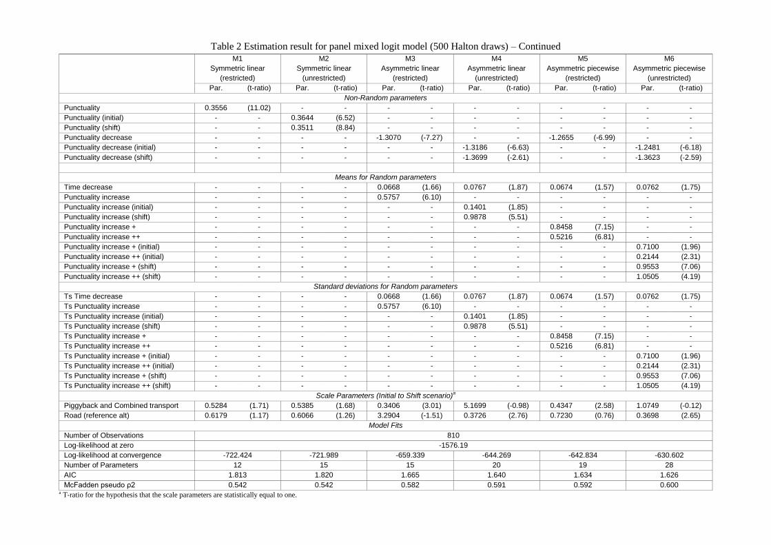
Table 2 Estimation result for panel mixed logit model (500 Halton draws) – Continued
M1 M2 M3 M4 M5 M6
Symmetric linear Symmetric linear Asymmetric linear Asymmetric linear Asymmetric piecewise Asymmetric piecewise
(restricted) (unrestricted) (restricted) (unrestricted) (restricted) (unrestricted)
Par. (t-ratio) Par. (t-ratio) Par. (t-ratio) Par. (t-ratio) Par. (t-ratio) Par. (t-ratio)
Non-Random parameters
Punctuality 0.3556 (11.02) - - - - - - - - - -
Punctuality (initial) - - 0.3644 (6.52) - - - - - - - -
Punctuality (shift) - - 0.3511 (8.84) - - - - - - - -
Punctuality decrease - - - - -1.3070 (-7.27) - - -1.2655 (-6.99) - -
Punctuality decrease (initial) - - - - - - -1.3186 (-6.63) - - -1.2481 (-6.18)
Punctuality decrease (shift) - - - - - - -1.3699 (-2.61) - - -1.3623 (-2.59)
Means for Random parameters
Time decrease - - - - 0.0668 (1.66) 0.0767 (1.87) 0.0674 (1.57) 0.0762 (1.75)
Punctuality increase - - - - 0.5757 (6.10) - - - - - -
Punctuality increase (initial) - - - - - - 0.1401 (1.85) - - - -
Punctuality increase (shift) - - - - - - 0.9878 (5.51) - - - -
Punctuality increase + - - - - - - - - 0.8458 (7.15) - -
Punctuality increase ++ - - - - - - - - 0.5216 (6.81) - -
Punctuality increase + (initial) - - - - - - - - - - 0.7100 (1.96)
Punctuality increase ++ (initial) - - - - - - - - - - 0.2144 (2.31)
Punctuality increase + (shift) - - - - - - - - - - 0.9553 (7.06)
Punctuality increase ++ (shift) - - - - - - - - - - 1.0505 (4.19)
Standard deviations for Random parameters
Ts Time decrease - - - - 0.0668 (1.66) 0.0767 (1.87) 0.0674 (1.57) 0.0762 (1.75)
Ts Punctuality increase - - - - 0.5757 (6.10) - - - - - -
Ts Punctuality increase (initial) - - - - - - 0.1401 (1.85) - - - -
Ts Punctuality increase (shift) - - - - - - 0.9878 (5.51) - - - -
Ts Punctuality increase + - - - - - - - - 0.8458 (7.15) - -
Ts Punctuality increase ++ - - - - - - - - 0.5216 (6.81) - -
Ts Punctuality increase + (initial) - - - - - - - - - - 0.7100 (1.96)
Ts Punctuality increase ++ (initial) - - - - - - - - - - 0.2144 (2.31)
Ts Punctuality increase + (shift) - - - - - - - - - - 0.9553 (7.06)
Ts Punctuality increase ++ (shift) - - - - - - - - - - 1.0505 (4.19)
Scale Parameters (Initial to Shift scenario)a
Piggyback and Combined transport 0.5284 (1.71) 0.5385 (1.68) 0.3406 (3.01) 5.1699 (-0.98) 0.4347 (2.58) 1.0749 (-0.12)
Road (reference alt) 0.6179 (1.17) 0.6066 (1.26) 3.2904 (-1.51) 0.3726 (2.76) 0.7230 (0.76) 0.3698 (2.65)
Model Fits
Number of Observations 810
Log-likelihood at zero -1576.19
Log-likelihood at convergence -722.424 -721.989 -659.339 -644.269 -642.834 -630.602
Number of Parameters 12 15 15 20 19 28
AIC 1.813 1.820 1.665 1.640 1.634 1.626
McFadden pseudo ρ2 0.542 0.542 0.582 0.591 0.592 0.600 a T-ratio for the hypothesis that the scale parameters are statistically equal to one.
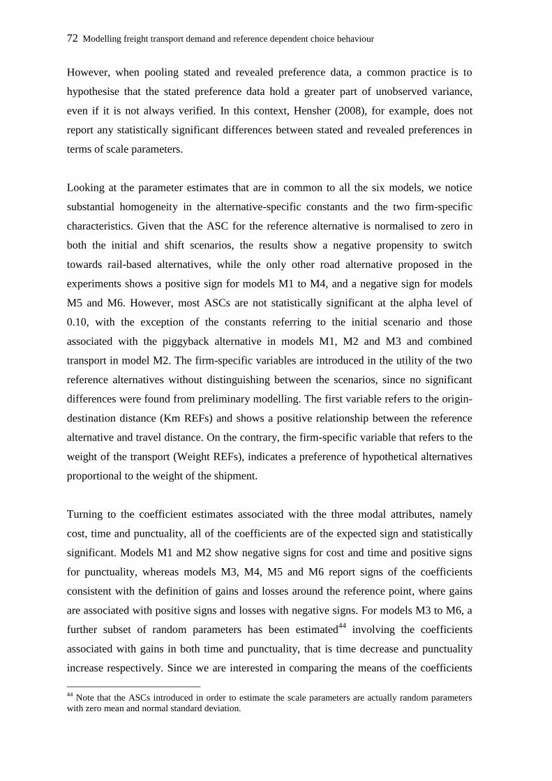
72 Modelling freight transport demand and reference dependent choice behaviour
However, when pooling stated and revealed preference data, a common practice is to
hypothesise that the stated preference data hold a greater part of unobserved variance,
even if it is not always verified. In this context, Hensher (2008), for example, does not
report any statistically significant differences between stated and revealed preferences in
terms of scale parameters.
Looking at the parameter estimates that are in common to all the six models, we notice
substantial homogeneity in the alternative-specific constants and the two firm-specific
characteristics. Given that the ASC for the reference alternative is normalised to zero in
both the initial and shift scenarios, the results show a negative propensity to switch
towards rail-based alternatives, while the only other road alternative proposed in the
experiments shows a positive sign for models M1 to M4, and a negative sign for models
M5 and M6. However, most ASCs are not statistically significant at the alpha level of
0.10, with the exception of the constants referring to the initial scenario and those
associated with the piggyback alternative in models M1, M2 and M3 and combined
transport in model M2. The firm-specific variables are introduced in the utility of the two
reference alternatives without distinguishing between the scenarios, since no significant
differences were found from preliminary modelling. The first variable refers to the origin-
destination distance (Km REFs) and shows a positive relationship between the reference
alternative and travel distance. On the contrary, the firm-specific variable that refers to the
weight of the transport (Weight REFs), indicates a preference of hypothetical alternatives
proportional to the weight of the shipment.
Turning to the coefficient estimates associated with the three modal attributes, namely
cost, time and punctuality, all of the coefficients are of the expected sign and statistically
significant. Models M1 and M2 show negative signs for cost and time and positive signs
for punctuality, whereas models M3, M4, M5 and M6 report signs of the coefficients
consistent with the definition of gains and losses around the reference point, where gains
are associated with positive signs and losses with negative signs. For models M3 to M6, a
further subset of random parameters has been estimated44
involving the coefficients
associated with gains in both time and punctuality, that is time decrease and punctuality
increase respectively. Since we are interested in comparing the means of the coefficients
44
Note that the ASCs introduced in order to estimate the scale parameters are actually random parameters
with zero mean and normal standard deviation.
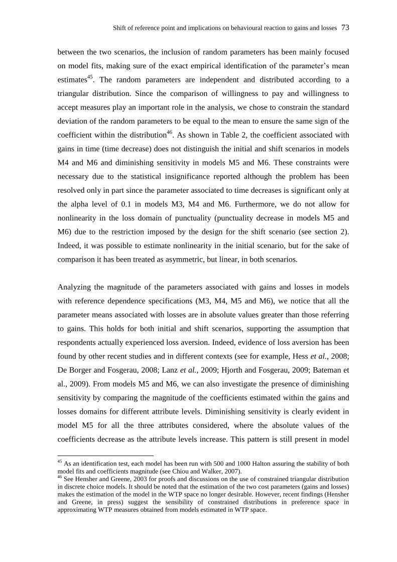
Shift of reference point and implications on behavioural reaction to gains and losses 73
between the two scenarios, the inclusion of random parameters has been mainly focused
on model fits, making sure of the exact empirical identification of the parameter’s mean
estimates45
. The random parameters are independent and distributed according to a
triangular distribution. Since the comparison of willingness to pay and willingness to
accept measures play an important role in the analysis, we chose to constrain the standard
deviation of the random parameters to be equal to the mean to ensure the same sign of the
coefficient within the distribution46
. As shown in Table 2, the coefficient associated with
gains in time (time decrease) does not distinguish the initial and shift scenarios in models
M4 and M6 and diminishing sensitivity in models M5 and M6. These constraints were
necessary due to the statistical insignificance reported although the problem has been
resolved only in part since the parameter associated to time decreases is significant only at
the alpha level of 0.1 in models M3, M4 and M6. Furthermore, we do not allow for
nonlinearity in the loss domain of punctuality (punctuality decrease in models M5 and
M6) due to the restriction imposed by the design for the shift scenario (see section 2).
Indeed, it was possible to estimate nonlinearity in the initial scenario, but for the sake of
comparison it has been treated as asymmetric, but linear, in both scenarios.
Analyzing the magnitude of the parameters associated with gains and losses in models
with reference dependence specifications (M3, M4, M5 and M6), we notice that all the
parameter means associated with losses are in absolute values greater than those referring
to gains. This holds for both initial and shift scenarios, supporting the assumption that
respondents actually experienced loss aversion. Indeed, evidence of loss aversion has been
found by other recent studies and in different contexts (see for example, Hess et al., 2008;
De Borger and Fosgerau, 2008; Lanz et al., 2009; Hjorth and Fosgerau, 2009; Bateman et
al., 2009). From models M5 and M6, we can also investigate the presence of diminishing
sensitivity by comparing the magnitude of the coefficients estimated within the gains and
losses domains for different attribute levels. Diminishing sensitivity is clearly evident in
model M5 for all the three attributes considered, where the absolute values of the
coefficients decrease as the attribute levels increase. This pattern is still present in model
45
As an identification test, each model has been run with 500 and 1000 Halton assuring the stability of both
model fits and coefficients magnitude (see Chiou and Walker, 2007). 46
See Hensher and Greene, 2003 for proofs and discussions on the use of constrained triangular distribution
in discrete choice models. It should be noted that the estimation of the two cost parameters (gains and losses)
makes the estimation of the model in the WTP space no longer desirable. However, recent findings (Hensher
and Greene, in press) suggest the sensibility of constrained distributions in preference space in
approximating WTP measures obtained from models estimated in WTP space.
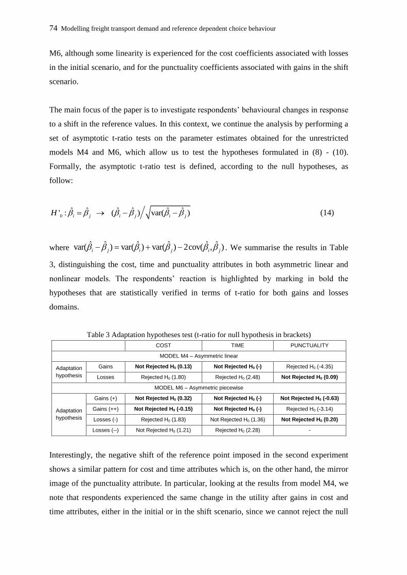
74 Modelling freight transport demand and reference dependent choice behaviour
M6, although some linearity is experienced for the cost coefficients associated with losses
in the initial scenario, and for the punctuality coefficients associated with gains in the shift
scenario.
The main focus of the paper is to investigate respondents’ behavioural changes in response
to a shift in the reference values. In this context, we continue the analysis by performing a
set of asymptotic t-ratio tests on the parameter estimates obtained for the unrestricted
models M4 and M6, which allow us to test the hypotheses formulated in (8) - (10).
Formally, the asymptotic t-ratio test is defined, according to the null hypotheses, as
follow:
0ˆ ˆ ˆ ˆ ˆ ˆ' : ( ) var( )i j i j i jH (14)
where ˆ ˆ ˆ ˆ ˆ ˆvar( ) var( ) var( ) 2cov( , )i j i j i j . We summarise the results in Table
3, distinguishing the cost, time and punctuality attributes in both asymmetric linear and
nonlinear models. The respondents’ reaction is highlighted by marking in bold the
hypotheses that are statistically verified in terms of t-ratio for both gains and losses
domains.
Table 3 Adaptation hypotheses test (t-ratio for null hypothesis in brackets)
COST TIME PUNCTUALITY
MODEL M4 – Asymmetric linear
Adaptation
hypothesis
Gains Not Rejected H0 (0.13) Not Rejected H0 (-) Rejected H0 (-4.35)
Losses Rejected H0 (1.80) Rejected H0 (2.48) Not Rejected H0 (0.09)
MODEL M6 – Asymmetric piecewise
Adaptation
hypothesis
Gains (+) Not Rejected H0 (0.32) Not Rejected H0 (-) Not Rejected H0 (-0.63)
Gains (++) Not Rejected H0 (-0.15) Not Rejected H0 (-) Rejected H0 (-3.14)
Losses (-) Rejected H0 (1.83) Not Rejected H0 (1.36) Not Rejected H0 (0.20)
Losses (--) Not Rejected H0 (1.21) Rejected H0 (2.28) -
Interestingly, the negative shift of the reference point imposed in the second experiment
shows a similar pattern for cost and time attributes which is, on the other hand, the mirror
image of the punctuality attribute. In particular, looking at the results from model M4, we
note that respondents experienced the same change in the utility after gains in cost and
time attributes, either in the initial or in the shift scenario, since we cannot reject the null
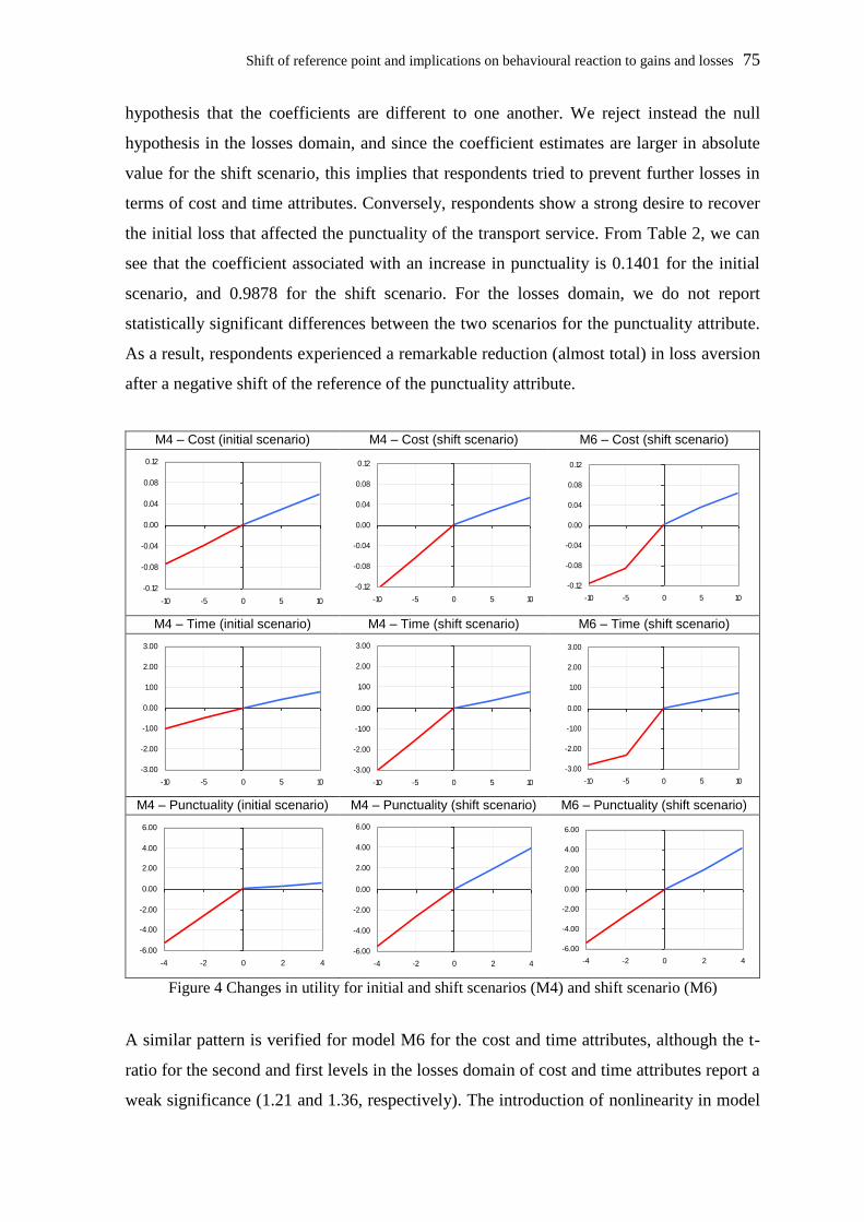
Shift of reference point and implications on behavioural reaction to gains and losses 75
hypothesis that the coefficients are different to one another. We reject instead the null
hypothesis in the losses domain, and since the coefficient estimates are larger in absolute
value for the shift scenario, this implies that respondents tried to prevent further losses in
terms of cost and time attributes. Conversely, respondents show a strong desire to recover
the initial loss that affected the punctuality of the transport service. From Table 2, we can
see that the coefficient associated with an increase in punctuality is 0.1401 for the initial
scenario, and 0.9878 for the shift scenario. For the losses domain, we do not report
statistically significant differences between the two scenarios for the punctuality attribute.
As a result, respondents experienced a remarkable reduction (almost total) in loss aversion
after a negative shift of the reference of the punctuality attribute.
M4 – Cost (initial scenario) M4 – Cost (shift scenario) M6 – Cost (shift scenario)
M4 – Time (initial scenario) M4 – Time (shift scenario) M6 – Time (shift scenario)
M4 – Punctuality (initial scenario) M4 – Punctuality (shift scenario) M6 – Punctuality (shift scenario)
Figure 4 Changes in utility for initial and shift scenarios (M4) and shift scenario (M6)
A similar pattern is verified for model M6 for the cost and time attributes, although the t-
ratio for the second and first levels in the losses domain of cost and time attributes report a
weak significance (1.21 and 1.36, respectively). The introduction of nonlinearity in model
-0.12
-0.08
-0.04
0.00
0.04
0.08
0.12
-10 -5 0 5 10
-0.12
-0.08
-0.04
0.00
0.04
0.08
0.12
-10 -5 0 5 10
-0.12
-0.08
-0.04
0.00
0.04
0.08
0.12
-10 -5 0 5 10
-3.00
-2.00
-1.00
0.00
1.00
2.00
3.00
-10 -5 0 5 10
-3.00
-2.00
-1.00
0.00
1.00
2.00
3.00
-10 -5 0 5 10
-3.00
-2.00
-1.00
0.00
1.00
2.00
3.00
-10 -5 0 5 10
-6.00
-4.00
-2.00
0.00
2.00
4.00
6.00
-4 -2 0 2 4
-6.00
-4.00
-2.00
0.00
2.00
4.00
6.00
-4 -2 0 2 4
-6.00
-4.00
-2.00
0.00
2.00
4.00
6.00
-4 -2 0 2 4
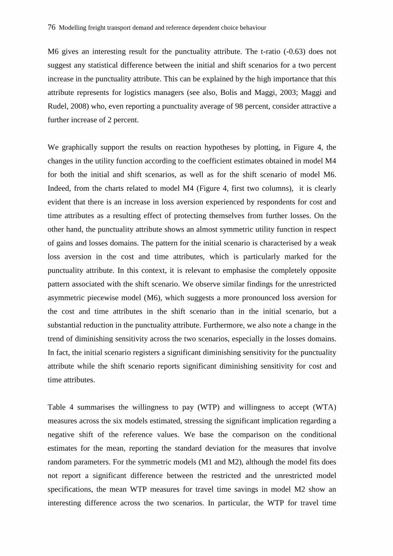
76 Modelling freight transport demand and reference dependent choice behaviour
M6 gives an interesting result for the punctuality attribute. The t-ratio (-0.63) does not
suggest any statistical difference between the initial and shift scenarios for a two percent
increase in the punctuality attribute. This can be explained by the high importance that this
attribute represents for logistics managers (see also, Bolis and Maggi, 2003; Maggi and
Rudel, 2008) who, even reporting a punctuality average of 98 percent, consider attractive a
further increase of 2 percent.
We graphically support the results on reaction hypotheses by plotting, in Figure 4, the
changes in the utility function according to the coefficient estimates obtained in model M4
for both the initial and shift scenarios, as well as for the shift scenario of model M6.
Indeed, from the charts related to model M4 (Figure 4, first two columns), it is clearly
evident that there is an increase in loss aversion experienced by respondents for cost and
time attributes as a resulting effect of protecting themselves from further losses. On the
other hand, the punctuality attribute shows an almost symmetric utility function in respect
of gains and losses domains. The pattern for the initial scenario is characterised by a weak
loss aversion in the cost and time attributes, which is particularly marked for the
punctuality attribute. In this context, it is relevant to emphasise the completely opposite
pattern associated with the shift scenario. We observe similar findings for the unrestricted
asymmetric piecewise model (M6), which suggests a more pronounced loss aversion for
the cost and time attributes in the shift scenario than in the initial scenario, but a
substantial reduction in the punctuality attribute. Furthermore, we also note a change in the
trend of diminishing sensitivity across the two scenarios, especially in the losses domains.
In fact, the initial scenario registers a significant diminishing sensitivity for the punctuality
attribute while the shift scenario reports significant diminishing sensitivity for cost and
time attributes.
Table 4 summarises the willingness to pay (WTP) and willingness to accept (WTA)
measures across the six models estimated, stressing the significant implication regarding a
negative shift of the reference values. We base the comparison on the conditional
estimates for the mean, reporting the standard deviation for the measures that involve
random parameters. For the symmetric models (M1 and M2), although the model fits does
not report a significant difference between the restricted and the unrestricted model
specifications, the mean WTP measures for travel time savings in model M2 show an
interesting difference across the two scenarios. In particular, the WTP for travel time
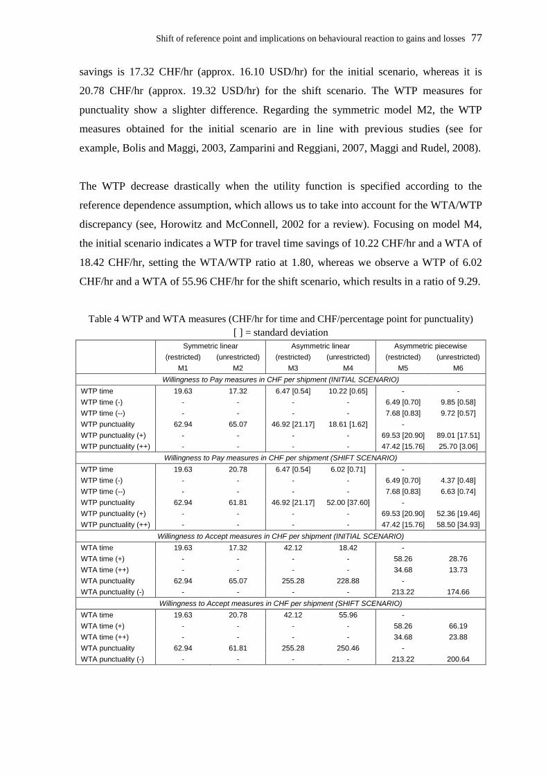
Shift of reference point and implications on behavioural reaction to gains and losses 77
savings is 17.32 CHF/hr (approx. 16.10 USD/hr) for the initial scenario, whereas it is
20.78 CHF/hr (approx. 19.32 USD/hr) for the shift scenario. The WTP measures for
punctuality show a slighter difference. Regarding the symmetric model M2, the WTP
measures obtained for the initial scenario are in line with previous studies (see for
example, Bolis and Maggi, 2003, Zamparini and Reggiani, 2007, Maggi and Rudel, 2008).
The WTP decrease drastically when the utility function is specified according to the
reference dependence assumption, which allows us to take into account for the WTA/WTP
discrepancy (see, Horowitz and McConnell, 2002 for a review). Focusing on model M4,
the initial scenario indicates a WTP for travel time savings of 10.22 CHF/hr and a WTA of
18.42 CHF/hr, setting the WTA/WTP ratio at 1.80, whereas we observe a WTP of 6.02
CHF/hr and a WTA of 55.96 CHF/hr for the shift scenario, which results in a ratio of 9.29.
Table 4 WTP and WTA measures (CHF/hr for time and CHF/percentage point for punctuality)
[ ] = standard deviation
Symmetric linear Asymmetric linear Asymmetric piecewise
(restricted) (unrestricted) (restricted) (unrestricted) (restricted) (unrestricted)
M1 M2 M3 M4 M5 M6
Willingness to Pay measures in CHF per shipment (INITIAL SCENARIO)
WTP time 19.63 17.32 6.47 [0.54] 10.22 [0.65] - -
WTP time (-) - - - - 6.49 [0.70] 9.85 [0.58]
WTP time (--) - - - - 7.68 [0.83] 9.72 [0.57]
WTP punctuality 62.94 65.07 46.92 [21.17] 18.61 [1.62] -
WTP punctuality (+) - - - - 69.53 [20.90] 89.01 [17.51]
WTP punctuality (++) - - - - 47.42 [15.76] 25.70 [3.06]
Willingness to Pay measures in CHF per shipment (SHIFT SCENARIO)
WTP time 19.63 20.78 6.47 [0.54] 6.02 [0.71] -
WTP time (-) - - - - 6.49 [0.70] 4.37 [0.48]
WTP time (--) - - - - 7.68 [0.83] 6.63 [0.74]
WTP punctuality 62.94 61.81 46.92 [21.17] 52.00 [37.60] -
WTP punctuality (+) - - - - 69.53 [20.90] 52.36 [19.46]
WTP punctuality (++) - - - - 47.42 [15.76] 58.50 [34.93]
Willingness to Accept measures in CHF per shipment (INITIAL SCENARIO)
WTA time 19.63 17.32 42.12 18.42 -
WTA time (+) - - - - 58.26 28.76
WTA time (++) - - - - 34.68 13.73
WTA punctuality 62.94 65.07 255.28 228.88 -
WTA punctuality (-) - - - - 213.22 174.66
Willingness to Accept measures in CHF per shipment (SHIFT SCENARIO)
WTA time 19.63 20.78 42.12 55.96 -
WTA time (+) - - - - 58.26 66.19
WTA time (++) - - - - 34.68 23.88
WTA punctuality 62.94 61.81 255.28 250.46 -
WTA punctuality (-) - - - - 213.22 200.64

78 Modelling freight transport demand and reference dependent choice behaviour
A similar structure for the WTP and WTA for travel time is outlined by model M6,
although the diminishing sensitivity reported for time and cost attributes reveals a larger
WTA/WTP discrepancy in the proximity of the reference values, both within and across
the initial and shift scenarios. The consequence of a negative shift of the reference point
suggests, therefore, a significant and substantial increase of the WTA/WTP ratio for travel
time, where respondents experienced a lower WTP and a higher WTA with respect to the
initial scenario. Reflecting the reaction hypotheses, the behavioural response to a negative
shift of the reference value in terms of WTP and WTA for transport service punctuality
shows an opposite pattern. In fact, the WTA/WTP discrepancy exhibits a general
reduction passing from a ratio of 12.29 for the initial scenario in model M4 to 4.81 for the
shift scenario. It is interesting to note the change in the respondents’ behaviour highlighted
by the introduction of nonlinearity in model M6. In this case, for the initial scenario, the
WTP for punctuality is particularly high for an increase of two percentage points (89.01
CHF/percentage point), but decrease dramatically for larger increases (25.70
CHF/percentage point), reflecting the very high sample median of 98 percent for the
reference transport service. Nevertheless, we observe a levelling of these two values for
the shift scenario (52.36 and 58.50 CHF/percentage point, respectively) which imposed a
reduction of two percentage points over the reference alternative values.
3.5. Conclusions
This paper has investigated the reaction experienced by decision makers facing a negative
shift of the reference point within a reference pivoted stated choice experiment framework.
The analysis has been based on two choice experiments conducted amongst logistics
managers, and collected in Switzerland in 2008. The experiments were designed to
identify the indirect freight transport costs associated with a temporary closure of the main
reference road alternative. The first experiment reflected the initial conditions, and hence
was designed around the typical (or initial) reference alternative. We then introduced the
hypothesis of road closure and updated the initial reference alternative values according to
the second best road alternative (shifted or expected reference alternative) values which
were then used to pivot the design of the second stated choice experiment.
Shift of reference point and implications on behavioural reaction to gains and losses 79
Under an assumption of prospect theory, a change in the reference point affects the
structure of individuals’ preferences. In order to investigate any potential reaction within
the sample interviewed, we pooled the data from the two experiments and estimated three
pairs of models. Within each pair of models, the distinction has been made by performing
the restricted and unrestricted model specifications, where the restriction involved the
specification of generic coefficients across the two datasets. The first pair of models
assumed a symmetric specification. We introduced the reference dependence specification
in the second pair of models, and estimated linear asymmetric parameters for both gains
and losses. In the third pair of models, we further allowed for asymmetric nonlinearity in
gains and losses domains by estimating, through a piecewise transformation, different
parameters for different attribute levels.
The model results for the two reference-dependent specifications indicate that respondents
experienced a significant reaction when facing a negative shift of the reference point. The
unrestricted version of the models outperforms the restricted one, providing significant
support to the prospect theory assumption regarding the alteration of respondent
preference structure. From a comparison of the parameter estimates, we observed that
respondents, on average, increased their loss aversion for cost and time attributes
reflecting a willingness to prevent further losses. On the contrary, for the punctuality
attribute, we registered a decrease in the loss aversion due to a considerable increase in the
marginal utility associated with gains reasonably explained as the propensity to recover
the initial loss. These results not only confirm the priority of the punctuality attribute
within the logistics managers’ choice of freight transport services but also indicate that a
small decrease in the punctuality quality has a high impact on preference formation, even
for a limited timeframe, as supposed in our study.
The results obtained for the symmetric specifications do not indicate any statistically
significant reaction in terms of model performance. We note therefore a clear difficulty of
the classic economic theory in capturing changes in behaviour under a shift reference point
context, although this is not surprising given the symmetric structure of these
specifications.
The estimates of WTP and WTA measures from the reference dependence models report a
WTA substantially higher than the WTP, which is in line with expectations. Comparing
80 Modelling freight transport demand and reference dependent choice behaviour
the two scenarios, the results suggest that a negative shift of the reference point causes a
reduction in the WTP and an increase in the WTA for travel time, and an overall increase
of the WTP, and a slight increase of the WTA for transport service punctuality. The
significance of the differences in terms of WTP and WTA measures across the two
scenarios is a relevant finding. Policy makers should therefore consider the consumers
potential reactions in any context involving a shift of the reference point. In particular, we
think about reference pivoted stated choice experiments studying the introduction of toll
roads or congestion pricing schemes in general. In these cases, particular attention should
be addressed to the specification of the reference values.
Further research is suggested in order to support these findings in different empirical
contexts. Given that our study was based on a shift of the reference point in the short run
and limited in time, we recognise the relevance of these findings in choices affecting
everyday life concerning transitional road detours for infrastructures maintenance, and we
advise the implementation of cost benefit analysis studies in this direction. However, we
also suggest the need for further investigation in a context involving a permanent shift of
the reference point, such as the introduction of pricing schemes. Finally, the analysis of a
positive shift of the reference point would be of interest in order to support recent findings
(e.g., Arkes et al. 2008), noting that individuals tend to adapt more completely to gains
(positive shifts) than to losses (negative shifts).
References
Arkes, H.R., Hirshleifer, D, Jiang, D. and Lim, S., 2008. Reference Point Adaptation:
Tests in the Domain of Security Trading. Organizational Behavior and Human Decision
Processes, 105, 67-81.
Bateman, I., Munro, A., Rhodes, B., Starmer, C. and Sugden, R., 1997. A test of the theory
of reference-dependent preferences. Quarterly Journal of Economics 112, 479–505.
Bateman, I.J., Brett, D.H., Andrew J.P. and Simon J., 2009. Reducing gain-loss
asymmetry: A virtual reality choice experiment valuing land use change. Paper selected
for presentation at the International Choice Modelling Conference 2009, Leeds (UK).
Bhat, C.R. and Castelar, S., 2002. A unified mixed logit framework for modeling revealed
and stated preferences: formulation and application to congestion pricing analysis in the
San Francisco Bay area. Transportation Research Part B 36, 577–669.
Shift of reference point and implications on behavioural reaction to gains and losses 81
Ben-Akiva, M., Bradley M., Morikawa T., Benjamin J., Novak T., Oppewal H. and Rao
V., 1994. Combining revealed and stated preferences data. Marketing Letters 5(4), 335-
349.
Benartzi, S. and Thaler, R.H., 1995. Myopic loss aversion and the equity premium puzzle.
Quarterly Journal of Economics, 110(1), 73 – 92.
Bolis, S. and Maggi R., 2003. Logistics Strategy and Transport Service Choices-An Adaptive
Stated Preference Experiment. In: Growth and Change - A journal of Urban and Regional Policy,
Special Issue STELLA FG 1, (34) 4.
Brownstone, D., Bunch, D.S. and Train, K., 2000. Joint mixed logit models of stated and
revealed preferences for alternative-fuel vehicles. Transportation Research Part B 34,
315–338.
Camerer, C., Babcock, L., Loewenstein, G. and Thaler, R.H., 1997. Labor supply of New
York City cabdrivers: One day at time. Quarterly Journal of Economics, 112(2), 407 –
442.
Chiou, L. and Walker, J.L., 2007. Masking identification of discrete choice models under
simulation methods. Journal of Econometrics 141, 683-703.
Danielis, R., Marcucci, E. and Rotaris, L., 2005. Logistics managers' stated preferences for
freight service attributes. Transportation Research Part E 41(3), 201-215.
De Borger, B. and Fosgerau, M., 2008. The trade-off between money and travel time: a
test of the theory of reference-dependent preferences. Journal of Urban Economics 64,
101-115.
Hensher, D.A., 2008. Empirical approaches to combining revealed and stated preference
data: Some recent developments with reference to urban mode choice. Research in
transportation Economics 23, 23-29.
Hensher, D.A. and Bradley, M., 1993. Using stated response data to enrich revealed
preference discrete choice models. Marketing Letters 4(2), 139-152.
Hensher, D.A. and Greene, W.H., 2003. Mixed logit models: state of practice.
Transportation 30(2), 133-176.
Hensher, D.A. and Greene, W.H. (in press) Valuation of Travel Time Savings in WTP and
Preference Space in the Presence of Taste and Scale Heterogeneity, Journal of Transport
Economics and Policy,
82 Modelling freight transport demand and reference dependent choice behaviour
Hess, S. and Rose, J.M., 2009. Should reference alternatives in pivot design SC surveys be
treated differently? Transportation Research Board Annual Meeting, Washington DC,
January.
Hess, S., Rose, J.M. and Hensher, D.A., 2008. Asymmetric preference formation in
willingness to pay estimates in discrete choice models. Transportation Research Part E
44(5), 847-863.
Hjorth, K. and Fosgerau, M., 2009. Determinants of the degree of loss aversion. Paper
selected for presentation at the International Choice Modelling Conference 2009, Leeds
(UK).
Horowitz, J. and McConnell, K.E., 2002. A Review of WTA-WTP Studies. Journal of
Environmental Economics and Management 44, 426-47.
Kahneman, D. and Tversky A., 1979. Prospect Theory: an analysis of decision under risk.
Econometrica 47 (2), 263–291.
Lanz, B., Provins, A., Bateman, I., Scarpa, R., Willis, K. and Ozdemiroglu, E., 2009.
Investigating willingness to pay – willingness to accept asymmetry in choice experiments.
Paper selected for presentation at the International Choice Modelling Conference 2009,
Leeds (UK).
Maggi, R. and Rudel, R., 2008. The Value of Quality Attributes in Freight Transport:
Evidence from an SP-Experiment in Switzerland. In: Ben-Akiva, M.E., Meersman, H., van
de Voorde E. (Eds.), Recent Developments in Transport Modelling. Emerald Group
Publishing Limited.
Maggi, R., Masiero, L., Baruffini, M. and Th ring M., 2009. Evaluation of the optimal
resilience for vulnerable infrastructure networks. An interdisciplinary pilot study on the
transalpine transportation corridors. Swiss National Science Foundation, NRP 54
“Sustainable Development of the Built Environment”, Project 405 440, Final Scientific
Report.
Masiero, L. and Hensher, D.A., 2010. Analyzing loss aversion and diminishing sensitivity
in a freight transport stated choice experiment, Transportation Research Part A 44 349–
358.
Masiero, L. and Maggi, R., 2009. Estimation of indirect cost and evaluation of protective
measures for infrastructure vulnerability: A case study on the transalpine transport
corridor. Istituto Ricerche Economiche, University of Lugano, September.
McFadden, D., 1974. Conditional logit analysis of qualitative choice behavior. In:
Zarembka, P. (Ed.), Frontiers in Econometrics. Academic Press, New York.
Shift of reference point and implications on behavioural reaction to gains and losses 83
Rose, J.M., Bliemer, M.C.J., Hensher, D.A. and Collins, A.T., 2008. Designing efficient
stated choice experiments in the presence of reference alternatives. Transportation
Research Part B 42(4), 395-406.
Rose, J.M. and Masiero, L., 2009. A comparison of prospect theory in WTP and
preference space. Institute of Transport and Logistics Studies, University of Sydney,
October.
Rowe, R.D., D’Arge, R.C. and Brookshire, D.S., 1980. An experiment on the economic
value of visibility. Journal of Environmental Economics and Management 7, 1–19.
Samuelson, W. and Zeckhauser, R., 1988. Status Quo Bias in Decision Making. Journal of
Risk and Uncertainty, 1, 7 – 59.
Schwartz, A., Goldberg, J. and Hazen, G., 2008. Prospect theory, reference points, and
health decisions. Judgement and Decision Making 3(2), 174-180.
Shea, J., 1995. Union contracts and the life-cycle/permanent-income hypothesis. American
Economic Review, 85, 186 – 200.
Swait, J. and Louviere, J.J., 1993. The role of the scale parameter in the estimation and
comparison of multinomial logit models. Journal of Marketing Research 30(3), 305-314.
Train, K., 2003. Discrete Choice Methods with Simulation. Cambridge University Press,
Cambridge.
Tversky, A. and Kahneman, D., 1991. Loss aversion in riskless choice: A reference-
dependent model. Quarterly Journal of Economics 106, 1039-1061.
Tversky A. and Kahneman, D., 1992. Advances in Prospect Theory: Cumulative
Representation of Uncertainty. Journal of Risk and Uncertainty 5, 297-323.
Zamparini, L. and Reggiani, A., 2007. The value of travel time in passenger and freight
transport: An overview. In: van Geenhuizen, M., Reggiani, A., Rietveld, P. (Eds.), Policy
analysis of transport networks. Ashgate, Aldershot.
84
Chapter Four
Accounting for WTP/WTA discrepancy in discrete choice models: Discussion of policy implications based on two freight transport stated choice experiments
Lorenzo Masiero
Rico Maggi
Version: May 14 2010
To be presented at the Kuhmo-Nectar Conference on Transport Economics 2010,
Valencia, July 2010.
Abstract
A key input in cost-benefit analysis is represented by the marginal rate of substitution
which expresses the willingness to pay, or its counterpart willingness to accept, for both
market and non-market goods. The consistent discrepancy between these two measures
observed in the literature suggests the need to estimate reference dependent models able to
capturing loss aversion by distinguishing the value attached to a gain from the value
attached to a loss according to reference dependent theory. This paper proposes a
comparison of willingness to pay and willingness to accept measures estimated from
models with both symmetric and reference dependent utility specifications within two
different freight transport stated choice experiments. The results show that the reference
dependent specification outperforms the symmetric specification and they prove the
robustness of reference dependent specification over datasets designed according different
attributes levels ranges. Moreover we demonstrate the policy relevance of asymmetric
specifications illustrating the strong implications for cost-benefit analysis in two case
studies.
Keywords: WTP/WTA discrepancy, freight choice, policy evaluation
Accounting for WTP/WTA discrepancy in discrete choice models: Discussion of policy implications 85
4.1. Introduction
A key input in the economic evaluation of transport measures is represented by the
marginal rate of substitution which expresses the willingness to pay (WTP), or its
counterpart willingness to accept (WTA), for both market and non-market goods. Indeed,
in the analysis of travel demand a lot of effort has been put into modelling individual
preferences in order to obtain the trade-off between time and cost, commonly known as
value of travel time saving (VTTS). In this context, Hensher (2001) reports that in the
quantification of user benefits for transport project appraisal the VTTS accounts for 60 per
cent. Mackie et al. (2001) indicate that around the 80 per cent of the monetised benefits
within cost-benefit analysis (CBA) is attributable to VTTS.
Revealed preferences (RP) and stated preferences (SP) are the main methods for collecting
data suitable for the estimation of WTP and WTA measures within the discrete choice
class of models (McFadden, 1974; Train et al., 1987; Ben-Akiva et al., 1993). In
particular, stated choice experiments have become a consolidate instrument that allow for
the analysis of individual preferences by letting the respondent choose among a set of
hypothetical choice situations.
Increasing attention has been paid to generating experiment designs by pivoting the
hypothetical situations around individual specific reference alternatives. However, the data
collected are typically modelled in the same way as data collected from RP or non-pivoted
SP. That is by letting the utility function be symmetric in respect to positive and negative
deviations from the reference alternative levels. Within symmetric utility specification the
WTA value results to be the mirror of the WTP value, which results in line within the
Hicksian surplus theory in a context where WTP and WTA are small relative to the
income (see Randall and Stoll, 1980 for a proof). However, the consistent discrepancy
between WTP and WTA measures observed in the literature47
suggests the need to
estimate asymmetric models able to capturing loss aversion by distinguishing the value
attached to a gain from the value attached to a loss according to reference dependent
theory (Kahneman and Tversky, 1979; Tversky and Kahneman, 1991; Tversky and
Kahneman, 1992). In this regards, recent studies have analysed reference dependent utility
47
A review by Horowitz and McConnell (2002) based on 45 studies sets the median of the ratio WTA/WTP
to 2.6.
86 Modelling freight transport demand and reference dependent choice behaviour
specifications in a stated choice framework supporting the hypothesis that classic
symmetric models tend to over-estimate WTP and under-estimate WTA (see for example,
Hess et al. 2008; De Borger and Fosgerau, 2008; Masiero and Hensher, 2010). Indeed, the
direct relationship between loss aversion and WTA/WTP discrepancy has been tested and
proved in a laboratory experiment (Bateman el al., 1997) and in a stated choice experiment
(De Borger and Fosgerau, 2008).
Although well recognized and discussed in several papers (see for example, Hanemann,
1991; Brown and Gregory, 1999; Graves, 2009a; Graves, 2009b) the divergence between
WTP and WTA is not taken into account in the majority of the discrete choice models
specification carrying potential upward biased estimates of WTP measures for policy
makers. On the other hand, the estimation of reference dependent discrete choice models
re-opens the debate on which measure between WTP and WTA is most desirable in the
economic evaluation of transport projects.
In this paper we propose a comparison of WTA and WTP measures estimated from
models with both symmetric and reference dependent utility specifications within two
different freight transport stated choice experiments conducted among Swiss logistics
managers in 2003 and 2008, respectively. In this context, the freight transport sector
occupies a minor part in the research literature involving the transport sector in general.
However, the impact of the value of freight transport time saving (VFTTS) in the
evaluation of the profitability of investments in transport infrastructures must not be
neglected since it can represent up to 50 per cent of the potential VTTS (Zamparini and
Reggiani, 2007). In particular, we focus the analysis on proving the robustness of the loss
aversion validity (and WTA/WTP divergence) within pivoted freight transport stated
choice experiments defined under different experimental design assumptions. The results
are based on the estimation of random parameters logit models on both the single dataset
collected in 2003 and the pooled dataset containing the two stated choice experiments.
In the derivation of WTP and WTA measures, the selection of the density function for the
random parameters has a great impact. Indeed, if all parameters are set as random then the
estimation of the marginal rate of substitution involves the ratio of two random
distributions which present substantial evaluation problems. Train and Weeks (2005)
proposed the estimation of discrete choice models in WTP space overcoming the problem

Accounting for WTP/WTA discrepancy in discrete choice models: Discussion of policy implications 87
of ratio distributions by involving the WTP distribution directly in the model estimation.
However, the estimation of models in WTP space requires the normalization of the model
for the cost attribute. This is a restriction for reference dependent models that have two
cost attributes, for gains and losses respectively (see Rose and Masiero, 2009). Masiero
and Hensher (2010) specify a reference dependent model where the random parameters
are assumed to be triangular distributed and constraining the standard deviation of the
coefficient to be equal to the mean. Although the use of constrained triangular distribution
leads to desirable estimates of the parameters since it avoids the estimation of irrational
values (i.e. positive coefficient for cost and time), the heterogeneity across the sample is
only assumed and not estimated. In order to analyse the spread of the random parameters
distribution when respondent face with gains and losses we decide to fix the cost
parameter and let the attribute associated to the other parameters to be Normal distributed.
This method has good properties in terms of model identification, WTP estimation and
rational assumption about the cost coefficient (see Revelt and Train, 2000).
A specific purpose of this paper is to discuss the policy implications that arise from the
WTA/WTP discrepancy. In this context, we propose to reconsider the concept of WTP and
WTA use in transport investment appraisal focusing the discussion on the rationale of
using asymmetric WTP and WTA instead of symmetric WTP. We illustrate the argument
with two hypothetical infrastructure investments, one for improvement of the current
situation, the other for maintenance.
The paper is organized as follows. In section two we describe the two stated choice
experiments used in the analysis. The methodological background is presented in section
three whereas the models estimates are shown in section four along with comments on the
results. In section five we outline the potential policy implications associated to
WTA/WTP discrepancy. Conclusions and final remarks are provided in section six.
4.2. Data
The data refers to two freight transport stated choice experiments conducted among Swiss
logistics managers in 2003 and 2008, S-2003 and S-2008 respectively. The first dataset
referred to the evaluation of relevant service characteristics in freight transport (see Maggi
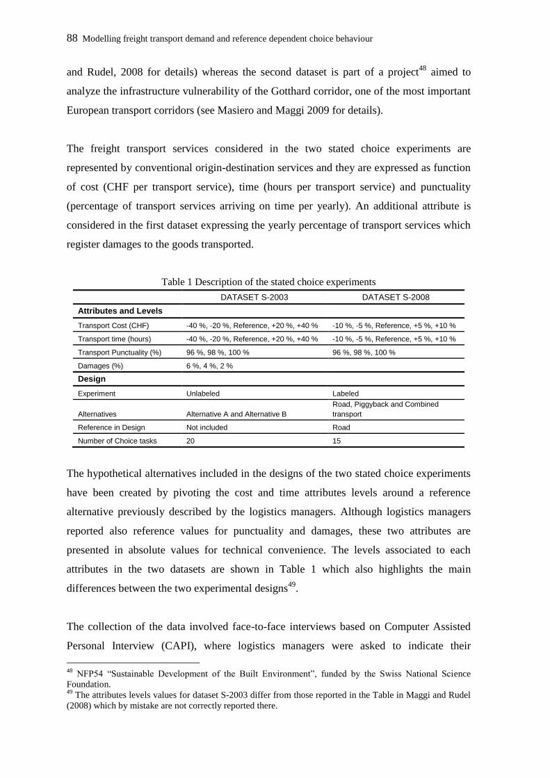
88 Modelling freight transport demand and reference dependent choice behaviour
and Rudel, 2008 for details) whereas the second dataset is part of a project48
aimed to
analyze the infrastructure vulnerability of the Gotthard corridor, one of the most important
European transport corridors (see Masiero and Maggi 2009 for details).
The freight transport services considered in the two stated choice experiments are
represented by conventional origin-destination services and they are expressed as function
of cost (CHF per transport service), time (hours per transport service) and punctuality
(percentage of transport services arriving on time per yearly). An additional attribute is
considered in the first dataset expressing the yearly percentage of transport services which
register damages to the goods transported.
Table 1 Description of the stated choice experiments
DATASET S-2003 DATASET S-2008
Attributes and Levels
Transport Cost (CHF) -40 %, -20 %, Reference, +20 %, +40 % -10 %, -5 %, Reference, +5 %, +10 %
Transport time (hours) -40 %, -20 %, Reference, +20 %, +40 % -10 %, -5 %, Reference, +5 %, +10 %
Transport Punctuality (%) 96 %, 98 %, 100 % 96 %, 98 %, 100 %
Damages (%) 6 %, 4 %, 2 %
Design
Experiment Unlabeled Labeled
Alternatives Alternative A and Alternative B
Road, Piggyback and Combined
transport
Reference in Design Not included Road
Number of Choice tasks 20 15
The hypothetical alternatives included in the designs of the two stated choice experiments
have been created by pivoting the cost and time attributes levels around a reference
alternative previously described by the logistics managers. Although logistics managers
reported also reference values for punctuality and damages, these two attributes are
presented in absolute values for technical convenience. The levels associated to each
attributes in the two datasets are shown in Table 1 which also highlights the main
differences between the two experimental designs49
.
The collection of the data involved face-to-face interviews based on Computer Assisted
Personal Interview (CAPI), where logistics managers were asked to indicate their
48
NFP54 “Sustainable Development of the Built Environment”, funded by the Swiss National Science
Foundation. 49
The attributes levels values for dataset S-2003 differ from those reported in the Table in Maggi and Rudel
(2008) which by mistake are not correctly reported there.
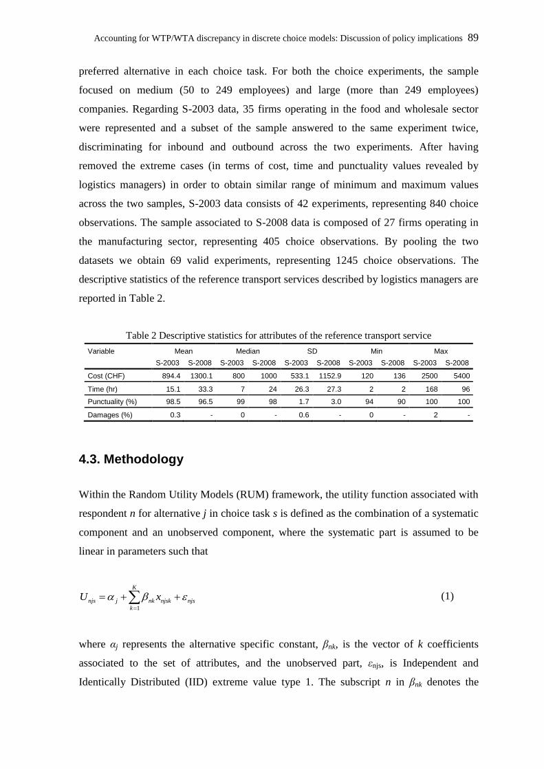
Accounting for WTP/WTA discrepancy in discrete choice models: Discussion of policy implications 89
preferred alternative in each choice task. For both the choice experiments, the sample
focused on medium (50 to 249 employees) and large (more than 249 employees)
companies. Regarding S-2003 data, 35 firms operating in the food and wholesale sector
were represented and a subset of the sample answered to the same experiment twice,
discriminating for inbound and outbound across the two experiments. After having
removed the extreme cases (in terms of cost, time and punctuality values revealed by
logistics managers) in order to obtain similar range of minimum and maximum values
across the two samples, S-2003 data consists of 42 experiments, representing 840 choice
observations. The sample associated to S-2008 data is composed of 27 firms operating in
the manufacturing sector, representing 405 choice observations. By pooling the two
datasets we obtain 69 valid experiments, representing 1245 choice observations. The
descriptive statistics of the reference transport services described by logistics managers are
reported in Table 2.
Table 2 Descriptive statistics for attributes of the reference transport service
Variable Mean Median SD Min Max
S-2003 S-2008 S-2003 S-2008 S-2003 S-2008 S-2003 S-2008 S-2003 S-2008
Cost (CHF) 894.4 1300.1 800 1000 533.1 1152.9 120 136 2500 5400
Time (hr) 15.1 33.3 7 24 26.3 27.3 2 2 168 96
Punctuality (%) 98.5 96.5 99 98 1.7 3.0 94 90 100 100
Damages (%) 0.3 - 0 - 0.6 - 0 - 2 -
4.3. Methodology
Within the Random Utility Models (RUM) framework, the utility function associated with
respondent n for alternative j in choice task s is defined as the combination of a systematic
component and an unobserved component, where the systematic part is assumed to be
linear in parameters such that
1
K
njs j nk njsk njs
k
U x
(1)
where αj represents the alternative specific constant, βnk, is the vector of k coefficients
associated to the set of attributes, and the unobserved part, εnjs, is Independent and
Identically Distributed (IID) extreme value type 1. The subscript n in βnk denotes the
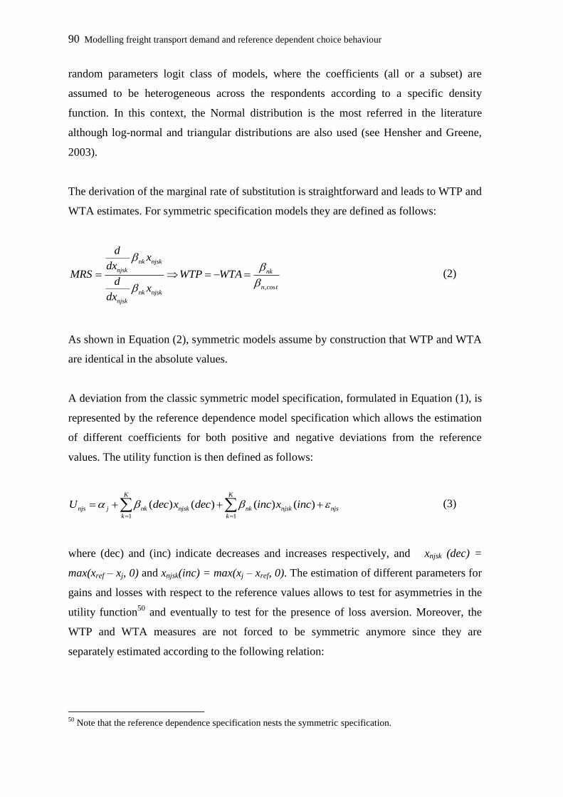
90 Modelling freight transport demand and reference dependent choice behaviour
random parameters logit class of models, where the coefficients (all or a subset) are
assumed to be heterogeneous across the respondents according to a specific density
function. In this context, the Normal distribution is the most referred in the literature
although log-normal and triangular distributions are also used (see Hensher and Greene,
2003).
The derivation of the marginal rate of substitution is straightforward and leads to WTP and
WTA estimates. For symmetric specification models they are defined as follows:
,cos
nk njsk
njsk nk
n tnk njsk
njsk
dx
dxMRS WTP WTA
dx
dx
(2)
As shown in Equation (2), symmetric models assume by construction that WTP and WTA
are identical in the absolute values.
A deviation from the classic symmetric model specification, formulated in Equation (1), is
represented by the reference dependence model specification which allows the estimation
of different coefficients for both positive and negative deviations from the reference
values. The utility function is then defined as follows:
1 1
( ) ( ) ( ) ( )K K
njs j nk njsk nk njsk njs
k k
U dec x dec inc x inc
(3)
where (dec) and (inc) indicate decreases and increases respectively, and xnjsk (dec) =
max(xref – xj, 0) and xnjsk(inc) = max(xj – xref, 0). The estimation of different parameters for
gains and losses with respect to the reference values allows to test for asymmetries in the
utility function50
and eventually to test for the presence of loss aversion. Moreover, the
WTP and WTA measures are not forced to be symmetric anymore since they are
separately estimated according to the following relation:
50
Note that the reference dependence specification nests the symmetric specification.

Accounting for WTP/WTA discrepancy in discrete choice models: Discussion of policy implications 91
For undesirable goods: ( ) ( )
,cos ( ) ,cos ( )
; nk dec nk inc
n t inc n t dec
WTP WTA
(4)
For desirable goods: ( ) ( )
,cos ( ) ,cos ( )
; nk inc nk dec
n t inc n t dec
WTP WTA
(5)
The relationship between loss aversion and WTA/WTP divergence can then be easily
proved from Equations (4) and (5). In fact, loss aversion holds if the absolute value of the
coefficient associated to losses is bigger than the absolute value of the coefficient
associated to gains. That is, for undesirable goods: |βnk(inc)| >| βnk(dec)|; whereas for
desirable goods: |βnk(dec)| >| βnk(inc)|. If loss aversion holds for both goods in the numerator
and the cost attribute then WTA > WTP.
Given the panel structure of the data and the use of the random parameters logit class of
models, the estimation of the utility parameters is derived from the maximization of the
following simulated log likelihood:
1 exp( )ln
exp( )
j n njsn
n r sj n njs
j
LLR
α β x
α β x (6)
where s = 1, …, S represent the number of choice situations whereas r = 1, …, R refers to
the number of draws51
.
4.4. Model results
The estimation of symmetric and reference dependent models is performed firstly on the
S-2003 data and then on a joint dataset, where we pooled S-2003 and S-2008 data (for
model estimation based on S-2008 see Masiero and Hensher (2010)52
). This allows us to
test for robustness of reference dependent specification across different datasets. The
estimation of the models for the pooled dataset includes also the computation of the scale
51
Refer to Train (2003) for details. 52
Note that Masiero and Hensher (2010) use constrained triangular distribution for random parameters
whereas here we use unconstrained normal distributions for attribute parameters and a fixed cost coefficient.

92 Modelling freight transport demand and reference dependent choice behaviour
parameters for the three alternatives of dataset S-2008 in order to take into account the
difference in the scale associated to different datasets. In doing this, we normalize the
scale of S-2003 dataset to one upon the second dataset53
. The estimation of the models is
based on 500 Halton draws and performed using Nlogit 4.
The model results are shown in Table 3. The first two columns (M1 and M2) refer to
symmetric model specification and reference dependent model specification for S-2003
data whereas the last two columns (M3 and M4) refer to the same models specification but
for the pooled dataset. The overall evaluation of model fits is based on the log-likelihood
at convergence, the Akaike’s Information Criterion (AIC) and the McFadden pseudo rho
squared (ρ2).
Comparing these three measures we register that the reference dependent model
specification outperforms the symmetric one in both the datasets used. In particular, the
McFadden pseudo ρ2 rises from 0.7267 to 0.7446 for S-2003 data and from 0.6651 to
0.6943 for the pooled dataset. These findings exclude the hypothesis that the restricted
symmetric models are more parsimonious than the unrestricted reference dependent
models.
The scale parameters estimated for the alternatives of dataset S-2008 within the joint
estimation result statistically different from 1 providing evidence for a significant
difference in the scale of the two datasets used in the analysis. In particular, the scale
parameters for piggyback and combined transport alternatives indicate that the unobserved
effects are characterized by a considerably lower variance compared to dataset S-2003. On
the contrary the unobserved effects associated to the reference alternative report a bigger
variance if compared with the alternatives in dataset S-2003.
Examining the coefficient estimates for the symmetric models (M1 and M3) associated
with the attributes we observe that they all are of the expected sign that is, negative for
damages, cost and time attributes and positive for punctuality. Both mean and standard
deviation (for random parameters) estimates result statistically significant at an alpha level
53
See Hensher (2008) for details.
Accounting for WTP/WTA discrepancy in discrete choice models: Discussion of policy implications 93
of 0.05 except for the standard deviation of the time parameter in S-2003 data which
results statistically significant at an alpha level of 0.10.
Table 3 Model results
M1 M2 M3 M4
Symmetric
Reference
Dependent Symmetric
Reference
Dependent
Par. (t-ratio) Par. (t-ratio) Par. (t-ratio) Par. (t-ratio)
Means for Random and Non-Random parameters
ASC Alternative A 0.1223 (0.93) 0.1284 (1.16) 0.1480 (1.52) 0.1599 (1.36)
ASC Piggyback - - - - -1.0933 (-1.71) 0.8495 (1.05)
ASC Combined transport - - - - -0.8716 (-1.37) 1.0408 (1.28)
Cost -0.0038 (-12.59) - - -0.0036 (-12.68) - -
Time -0.0691 (-2.91) - - -0.0740 (-3.49) - -
Punctuality 0.2890 (6.37) - - 0.2880 (9.45) - -
Damages -0.3959 (-10.76) -0.4870 (-10.39) -0.4042 (-10.74) -0.5303 (-10.54)
Cost decrease - - 0.0033 (5.69) - - 0.0041 (6.71)
Cost increase - - -0.0052 (-7.88) - - -0.0060 (-8.56)
Time decrease - - 0.0662 (1.82) - - 0.0809 (2.49)
Time increase - - -0.0718 (-2.39) - - -0.1315 (-2.83)
Punctuality decrease - - -0.3454 (-2.94) - - -0.6127 (-4.15)
Punctuality increase - - 0.2640 (2.11) - - 0.2272 (2.76)
Standard deviations for Random parameters
Ns Time 0.0586 (1.92) - -
0.0850
4 (3.32) - -
Ns Punctuality 0.3395 (5.90) - - - - - -
Ns Time decrease - - 0.0772 (2.78) - - 0.1017 (2.76)
Ns Time increase - - 0.1013 (1.91) - - 0.1807 (2.75)
Ns Punctuality decrease - - 0.6099 (5.18) - - 0.8077 (5.52)
Ns Punctuality increase - - 0.3812 (3.15) - - 0.3215 (4.10)
Scale parameters
Scale ALT Piggyback - - - - 19.384 (-2.00)a 15.952 (-2.54)
a
Scale ALT Combined transport - - - - 6.854 (-2.70) a 6.704 (-2.14)
a
Scale ALT Reference - - - - 0.417 (2.59) a 0.297 (2.86)
a
Conditional WTP measures [standard deviation]
Travel Time 17.69 [7.22] 12.61 [6.16] 20.39 [12.49] 13.23 [6.33]
Punctuality 62.80 [48.70] 52.44 [36.57] 79.16 [0.00] 36.30 [27.13]
Conditional WTA measures [standard deviation]
Travel Time 17.69 [7.22] 21.72 [13.52] 20.39 [12.49] 32.71 [24.23]
Punctuality 62.80 [48.70] 101.65 [137.57] 79.16 [0.00] 152.22 [146.38]
Model Fits
Number of Observations 840 840 1245 1245
Log-likelihood Restricted -1351.93 -1351.93 -2003.75 -2003.75
Log-likelihood at convergence -369.48 -345.28 -671.13 -612.47
Number of Parameters 7 12 11 17
AIC normalized 0.8964 0.8507 1.0958 1.0112
McFadden pseudo ρ2 0.7267 0.7446 0.6651 0.6943
a The t-ratio is calculated on the assumption that the scale parameter is different from one.
94 Modelling freight transport demand and reference dependent choice behaviour
Looking at the reference dependent model specifications (M2 and M4), where cost, time
and punctuality attributes are defined in terms of gains and losses, we observe a similar
consistency. That is, parameters associated with gains (cost decrease, time decrease and
punctuality increase) are positive in sign whereas the parameters associated with losses
(cost increase, time increase and punctuality decrease) are negative in sign. Moreover, we
find that loss aversion holds for all the three attributes and in both dataset specifications.
In fact, the parameters associated with losses are in absolute value bigger than the
parameters associated with gains. The standard deviation for the random parameters
results higher for the parameters associated with losses meaning that the preferences of the
logistics managers are more heterogeneous when logistics managers are faced with losses.
The conditional estimates for WTP measures from symmetric models are in line with
current research literature (see Zamparini and Reggiani (2007) for a review). In particular,
the willingness to pay for time is 17.7 CHF/hour54
and 20.4 CHF/hour for symmetric
models M1 and M3, respectively. The willingness to pay for punctuality is a key factor, as
reported in similar studies (e.g., Danielis et al., 2005; Fowkes, 2007), for logistics
managers who show a considerable sensitivity regarding punctuality of the transport
service. For symmetric models the WTP for punctuality reaches 62.8 CHF and 79.16 CHF
per percentage point for M1 and M3, respectively.
Looking at the reference dependent model specifications in M2 and M4, we are able to
distinguish between WTP and WTA. In particular, referring to the estimates for the pooled
dataset (M4) we find that the WTP for time is 13.23 CHF/hour whereas the WTA for time
is 32.71 CHF/hour. On the other hand, the WTP for punctuality is 36.30 CHF for an
increase in punctuality by one percentage point whereas the WTA is 152.22 CHF for a
decrease of punctuality of one percentage point. Punctuality still remains a crucial factor,
especially when logistics managers are faced with a reduction of this service attribute. The
WTA/WTP discrepancy registered is fairly marked for both the marginal rates of
substitution considered. In this context, the ratio WTA/WTP is 2.5 for time and 4.2 for
punctuality which results in line with past studies (see for example, Horowitz and
McConnell (2002) for a review).
54
Approximate monthly average exchange rate for April 2010, 1 CHF = 0.93 USD.
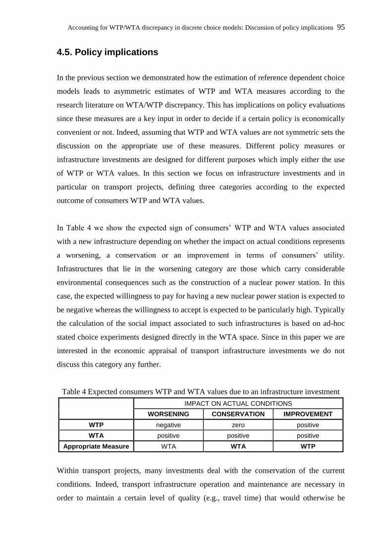
Accounting for WTP/WTA discrepancy in discrete choice models: Discussion of policy implications 95
4.5. Policy implications
In the previous section we demonstrated how the estimation of reference dependent choice
models leads to asymmetric estimates of WTP and WTA measures according to the
research literature on WTA/WTP discrepancy. This has implications on policy evaluations
since these measures are a key input in order to decide if a certain policy is economically
convenient or not. Indeed, assuming that WTP and WTA values are not symmetric sets the
discussion on the appropriate use of these measures. Different policy measures or
infrastructure investments are designed for different purposes which imply either the use
of WTP or WTA values. In this section we focus on infrastructure investments and in
particular on transport projects, defining three categories according to the expected
outcome of consumers WTP and WTA values.
In Table 4 we show the expected sign of consumers’ WTP and WTA values associated
with a new infrastructure depending on whether the impact on actual conditions represents
a worsening, a conservation or an improvement in terms of consumers’ utility.
Infrastructures that lie in the worsening category are those which carry considerable
environmental consequences such as the construction of a nuclear power station. In this
case, the expected willingness to pay for having a new nuclear power station is expected to
be negative whereas the willingness to accept is expected to be particularly high. Typically
the calculation of the social impact associated to such infrastructures is based on ad-hoc
stated choice experiments designed directly in the WTA space. Since in this paper we are
interested in the economic appraisal of transport infrastructure investments we do not
discuss this category any further.
Table 4 Expected consumers WTP and WTA values due to an infrastructure investment
IMPACT ON ACTUAL CONDITIONS
WORSENING CONSERVATION IMPROVEMENT
WTP negative zero positive
WTA positive positive positive
Appropriate Measure WTA WTA WTP
Within transport projects, many investments deal with the conservation of the current
conditions. Indeed, transport infrastructure operation and maintenance are necessary in
order to maintain a certain level of quality (e.g., travel time) that would otherwise be
96 Modelling freight transport demand and reference dependent choice behaviour
impossible to maintain due to the constant increase of traffic flows. These infrastructure
investments can often be very expensive, depending on the transport network involved,
and the convenience of the investment needs to be evaluated. In this case, the willingness
to pay is expected to be zero since we are asking the users to face a situation where the
quality of service remains stable at the actual level. Therefore, the user benefit associated
with such investments should be calculated using their willingness to accept for a loss in
service quality (e.g., an increase in the travel time) which would be the consequence if the
investment were not realized.
The typical situation in the economic appraisal of a transport project is however the
evaluation of an investment against an improvement of the actual condition. This is the
case of a new transport infrastructure, where the willingness to pay is now positive and
reflects the maximum (marginal) amount that consumers are willing to pay for the
improvement (e.g., a reduction of the travel time). Therefore, the willingness to pay should
be used in the computation of user benefits.
4.5.1 Case Studies on freight transport
Based on the estimates from models M3 and M4 (reported in Table 3) we illustrate the
implication of WTA/WTP discrepancy in the case of hypothetical policy measures for
freight transport in Switzerland. In particular, we compare two cost-benefit analyses
(CBA) distinguishing between the two categories highlighted in Table 4, conservation and
improvement, respectively.
We hypothesize two different large investments along the Gotthard corridor which is the
most important link across the Alpine region. The first investment refers to the
construction of a second “Gotthard road tunnel” increasing the number of lanes from two
to four representing a significant improvement in terms of travel time and punctuality. The
second investment consists of protective galleries and tunnels on the north and south
access to the Gotthard road tunnel. This represents a maintenance intervention assuming
that climate change leads to a dramatic increase of hazards.
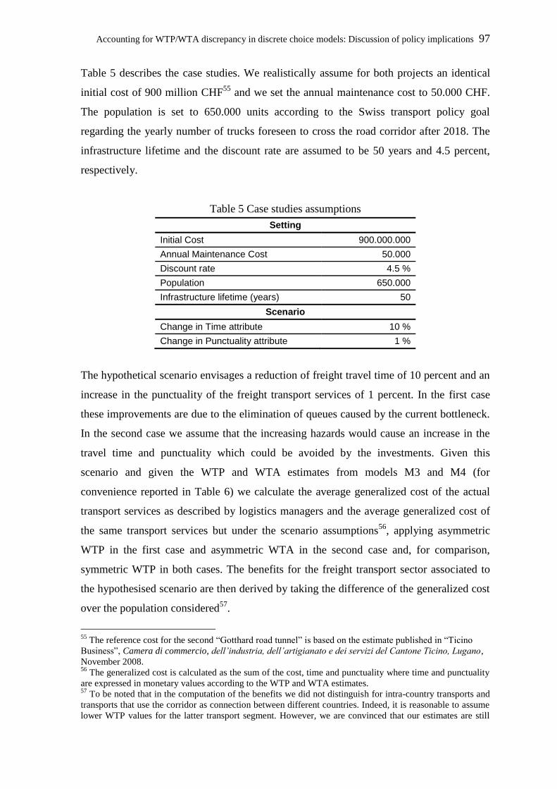
Accounting for WTP/WTA discrepancy in discrete choice models: Discussion of policy implications 97
Table 5 describes the case studies. We realistically assume for both projects an identical
initial cost of 900 million CHF55
and we set the annual maintenance cost to 50.000 CHF.
The population is set to 650.000 units according to the Swiss transport policy goal
regarding the yearly number of trucks foreseen to cross the road corridor after 2018. The
infrastructure lifetime and the discount rate are assumed to be 50 years and 4.5 percent,
respectively.
Table 5 Case studies assumptions
Setting
Initial Cost 900.000.000
Annual Maintenance Cost 50.000
Discount rate 4.5 %
Population 650.000
Infrastructure lifetime (years) 50
Scenario
Change in Time attribute 10 %
Change in Punctuality attribute 1 %
The hypothetical scenario envisages a reduction of freight travel time of 10 percent and an
increase in the punctuality of the freight transport services of 1 percent. In the first case
these improvements are due to the elimination of queues caused by the current bottleneck.
In the second case we assume that the increasing hazards would cause an increase in the
travel time and punctuality which could be avoided by the investments. Given this
scenario and given the WTP and WTA estimates from models M3 and M4 (for
convenience reported in Table 6) we calculate the average generalized cost of the actual
transport services as described by logistics managers and the average generalized cost of
the same transport services but under the scenario assumptions56
, applying asymmetric
WTP in the first case and asymmetric WTA in the second case and, for comparison,
symmetric WTP in both cases. The benefits for the freight transport sector associated to
the hypothesised scenario are then derived by taking the difference of the generalized cost
over the population considered57
.
55
The reference cost for the second “Gotthard road tunnel” is based on the estimate published in “Ticino
Business”, Camera di commercio, dell’industria, dell’artigianato e dei servizi del Cantone Ticino, Lugano,
November 2008. 56
The generalized cost is calculated as the sum of the cost, time and punctuality where time and punctuality
are expressed in monetary values according to the WTP and WTA estimates. 57
To be noted that in the computation of the benefits we did not distinguish for intra-country transports and
transports that use the corridor as connection between different countries. Indeed, it is reasonable to assume
lower WTP values for the latter transport segment. However, we are convinced that our estimates are still

98 Modelling freight transport demand and reference dependent choice behaviour
Table 6 Case studies results
CASE 1
IMPROVEMENT
CASE 2
MAINTENANCE CASE 1 = CASE 2
Asymmetric WTP Asymmetric WTA Symmetric WTP = WTA
Travel Time 13.23 32.71 20.39
Punctuality 36.30 152.22 79.16
Net Present Value - 57 million 1,988 million 698 million
These results shown in Table 6 demonstrate the relevance of estimating WTP and WTA
separately and applying them appropriately. Using the traditional approach, and hence
overestimating WTP for an improvement and underestimating WTA for maintenance, both
projects would be accepted. Applying asymmetric WTP for the improvement results in a
negative net present value demonstrating that 900 million investment is not justified for a
10 % and a 1% percent improvement in travel time and punctuality, respectively. On the
other hand, an equally expensive maintenance investment with same impact is largely
justified. In a general sense it is therefore demonstrated that applying symmetric WTP
may lead in different contexts to significant over or under investments.
4.6. Conclusions
This paper has investigated the policy implications of WTA/WTP discrepancy in a freight
transport context. The analysis has focused on the estimation of discrete choice models for
two freight transport stated choice experiments. In particular, we estimated a set of random
parameters logit models comparing between the classic symmetric specification which
does not distinguish between WTP and WTA, and the reference dependent specification
which relaxes the symmetry assumption allowing for the estimation of different
parameters associated to gains and losses. We outlined then the policy implications
supporting the discussion with hypothetical examples on the freight transport sector in
Switzerland.
The results show that the reference dependent specification outperforms the symmetric
specification and they prove the robustness of a reference dependent specification for
datasets designed to accommodate different attribute level ranges. Loss aversion has been
conservative since we fixed the population to 650.000, the Swiss policy objective, representing around the
50 percent of the actual figure.
Accounting for WTP/WTA discrepancy in discrete choice models: Discussion of policy implications 99
registered for all attributes investigated in the analysis leading to a significant WTA/WTP
discrepancy. As a consequence, our results confirm the findings reported in the recent
research literature that is, that symmetric models tend to overestimate WTP values and to
underestimate WTA values.
The policy implications associated with WTP and WTA measures estimated from
reference dependent choice models are indeed interesting. The paper defined three main
categories of infrastructure projects labelled worsening, conservation and improvement,
respectively. For each category, the two measures (WTP and WTA) have been discussed
and the most appropriate measure for the evaluation of the investment has been selected.
The focus has then been on two categories that typically reflect transport projects, that is,
transport infrastructures aimed to conserve or to improve the actual quality of the service.
We pointed out a major difference between these two categories suggesting that the
infrastructures aimed to conserve the actual conditions should be evaluated using the
consumers WTA (contradicting the current state-of-the-art which apply the WTP) whereas
the infrastructures aimed to improve the actual conditions should be evaluated, as classic
research literature states, using the consumers WTP. However, using symmetric WTP
estimates will underestimate the benefit of the latter kind of investment. Based on
reference dependent model estimates and given our distinction for the type of
infrastructure we conclude that the evaluation of investments aimed to conserve (improve)
the actual conditions is underestimated (overestimated) if current guidelines apply.
Finally, we strongly encourage policy oriented analysts to estimate reference dependent
choice models appropriately derived from reference pivoted choice experiments. The
persistence in using symmetric discrete choice models as an instrument for deriving
marginal substitution effects for policy purpose might most probably lead to biased
evaluation in the form of significant overestimation or underestimation of the economic
benefits of transport projects.
References
Bateman, I., Munro, A., Rhodes, B., Starmer, C., Sugden, R., 1997. A test of the theory of
reference-dependent preferences. Quarterly Journal of Economics 112, 479–505.
Ben-Akiva, M., Bolduc, D., Bradley, M., 1993. Estimation of travel mode choice models
with randomly distributed value of time. Transportation Research Record 1413, 88-97.

100 Modelling freight transport demand and reference dependent choice behaviour
Brown, T.C., Gregory, R., 1999. Why the WTA-WTP disparity matters. Ecological
Economics 28, 323-335.
Danielis, R., Marcucci, E., Rotaris, L., 2005. Logistics managers' stated preferences for
freight service attributes. Transportation Research Part E 41(3), 201-215.
De Borger, B., Fosgerau, M., 2008. The trade-off between money and travel time: a test of
the theory of reference-dependent preferences. Journal of Urban Economics 64, 101-115.
Graves, P.E., 2009a. If the large WTA-WTP gap for public goods is real (and there are
good reasons to think so) conventional welfare measures are simply incorrect. The
Selected Works of PHILIP E GRAVES, Available at:
http://works.bepress.com/philip_graves/35.
Graves, P.E., 2009b. The WTA-WTP Gap and Welfare Measures for Public Goods. The
Selected Works of PHILIP E GRAVES, Available at:
http://works.bepress.com/philip_graves/41.
Fowkes, A.S., 2007. The design and interpretation of freight stated preference experiments
seeking to elicit behavioural valuations of journey attributes. Transportation Research Part
B 41(9), 966-980.
Hanemann, M., 1991. Willingness to pay and willingness to accept: How much can they
differ? The American Economic Review 81(3), 635-647.
Hensher, D.A., 2001. Measurement of the valuation of travel time savings. Journal of
Transport Economics and Policy 35(1), 71-98.
Hensher, D.A., 2008. Empirical approaches to combining revealed and stated preference
data: Some recent developments with reference to urban mode choice. Research in
transportation Economics 23, 23-29.
Hensher, D.A., Greene, W.H., 2003. Mixed logit models: state of practice. Transportation
30(2), 133-176.
Hess, S., Rose, J.M., Hensher, D.A., 2008. Asymmetric preference formation in
willingness to pay estimates in discrete choice models. Transportation Research Part E
44(5), 847–863.
Horowitz, J., McConnell, K.E., 2002. A Review of WTA-WTP Studies. Journal of
Environmental Economics and Management 44, 426-47.
Kahneman, D., Tversky A., 1979. Prospect Theory: an analysis of decision under risk.
Econometrica 47 (2), 263–291.
Accounting for WTP/WTA discrepancy in discrete choice models: Discussion of policy implications 101
Mackie, P.J., Jara-Diaz, S., Fowkes, A.S., 2001. The value of travel time savings in
evaluation. Transportation Research Part E 37(2-3), 91-106.
Maggi, R., Rudel, R., 2008. The Value of Quality Attributes in Freight Transport:
Evidence from an SP-Experiment in Switzerland. In: Ben-Akiva, M.E., Meersman, H., van
de Voorde E. (Eds.), Recent Developments in Transport Modelling. Emerald Group
Publishing Limited.
Masiero, L., Maggi, R., 2009. Estimation of indirect cost and evaluation of protective
measures for infrastructure vulnerability: A case study on the transalpine transport
corridor. Submitted for publication, September.
Masiero, L., Hensher, D.A., 2010. Analyzing loss aversion and diminishing sensitivity in a
freight transport stated choice experiment. Transportation Research Part A 44(5), 349–
358.
McFadden, D., 1974. Conditional logit analysis of qualitative choice behavior. In:
Zarembka, P. (Ed.), Frontiers in Econometrics. Academic Press, New York.
Train, K.E., Weeks, M., 2005. Discrete choice models in preference space and
willingness-to-pay space. In: R. Scarpa and A. Alberini (Eds.), Application of simulation
methods in environmental and resource economics. Springer Publisher, Dordrecht.
Randall, A., Stoll, J.R., 1980. Consumer’s surplus in commodity space. The American
Economic Review 70(3), 449-455.
Revelt, D., Train, K.E., 2000. Customer-specific taste parameters and mixed logit. WP
E00-274, Department of Economics, University of California at Berkeley, CA.
Rose, J.M., Masiero, L., 2009. A comparison of prospect theory in WTP and preference
space. Institute of Transport and Logistics Studies, University of Sydney, October.
Train, K.E., McFadden D., Ben-Akiva, M., 1987. The demand for local telephone service:
A fully discrete model of residential calling patterns and service choice. Rand Journal of
Economics 18, 109-123.
Tversky, A., Kahneman, D., 1991. Loss aversion in riskless choice: A reference-dependent
model. Quarterly Journal of Economics 106, 1039–1061.
Tversky, A., Kahneman, D., 1992. Advances in Prospect Theory: Cumulative
Representation of Uncertainty. Journal of Risk and Uncertainty 5, 297-323.

102 Modelling freight transport demand and reference dependent choice behaviour
Zamparini, L., Reggiani, A., 2007. The value of travel time in passenger and freight
transport: An overview. In: van Geenhuizen, M., Reggiani, A., Rietveld, P. (Eds.), Policy
analysis of transport networks. Ashgate, Aldershot.