287

Australian Meteorological and Oceanographic Journal 62 (2012) 287–304

Modelling low-level boundary layer structure in complex terrain: verification of TAPM meteorological predictions in

the Canberra region

(Manuscript received September 2009; revised September 2012)

John R. Taylor, Annette L. Hirsch1 and Barbara A. BurnsSchool of Physical, Environmental and Mathematical Sciences

University of New South Wales Canberra, Canberra1currently at ARC Centre of Excellence for Climate System Science

University of New South Wales, Sydney

Introduction

The structure of the statically stable nocturnal boundary layer is critical in determining dispersion. Dispersion is generally poorest when the static stability of the boundary layer is high (Kukkonen et al. 2005) and accurate simulation of this condition should be a key performance parameter for any air quality modelling system. Unfortunately, the light wind, strongly stable boundary layer regime is well known to be particularly challenging for prognostic meteorological modelling (Holtslag 2006). These models generally rely on Monin-Obukhov similarity theory to calculate the surface fluxes and surface layer temperature and humidity profiles (Luhar et al. 2009), and the flux-gradient relations presently

used in the models were not determined under strongly stable conditions in complex terrain. The inadequacy of the surface layer scaling may be magnified if the model predicts stronger low level winds and the mixing produced by these stronger winds modifies or suppresses buoyancy and terrain driven flows. Terrain driven flows can result in complex nocturnal wind regimes when synoptic scale forcing is weak; see for example Mahrt et al. (2001). Here we investigate the performance of a representative prognostic model in an area, and season, in which strongly stable conditions are prevalent. The model used is The Air Pollution Model (TAPM) developed by the Commonwealth Scientific and Industrial Research Organisation (CSIRO). TAPM, described in detail in Hurley (2008a), solves the governing fluid dynamical and scalar transport equations with boundary conditions provided by a surface energy and water balance scheme, and vegetation, terrain and synoptic-scale meteorological datasets. Model output is typically used

Corresponding author address: School of Physical, Environmental and Mathematical Sciences, UNSW Canberra, PO Box 7916, Canberra BC, ACT 2610Email: j.taylor@adfa.edu.au

The performance of the meteorological component of The Air Pollution Model (TAPM) in the Canberra region is assessed using temperature and wind profiles from a Radio Acoustic Sounding System (RASS) and high frequency Doppler so-dar. The region has relatively complex terrain and the period of the study included a significant fraction of time where winds were light and the boundary layer was strongly stable. Overall, TAPM’s performance was similar to that found in other verification studies which have compared TAPM vertical wind profiles against ob-servations. However, when a bulk Richardson number was used to classify the boundary layer into three classes (unstable, neutral and weakly stable, and strong-ly stable), it was found that model performance was poorer for the strongly stable class. The observed nocturnal cooling was greater than that predicted by TAPM and the model did not generate the complex vertical wind profiles which occur under strongly stably-stratified conditions at the site. Problems with TAPM simu-lations under light wind stable conditions have been observed in regions with simple terrain before, but this study indicates that they are exacerbated by the more complex terrain, and associated terrain-driven flows.

288 Australian Meteorological and Oceanographic Journal 62:4 December 2012

to provide meteorological conditions for the evaluation of environmental impacts. TAPM has widespread acceptance within industry and government in Australia. For example, the Department of Environment and Conservation, New South Wales, (2005) recommends TAPM simulations as a source of meteorological information in the absence of in-situ data. TAPM’s performance has been evaluated in a large number of verification studies (Hurley 2008b). Some of these (for example, Edwards et al. 2004; Physick et al. 2004; Taylor et al. 2005) have compared wind profiles from TAPM with those from ground-based remote sensing instruments such as Doppler sodars and electromagnetic (EM) wind profilers. The locations for these studies had relatively simple terrain and, in general, the authors reported good model performance. For example, in the Kalgoorlie region of Western Australia, Edwards et al. (2004) found that the root mean square error (RMSE, defined in Appendix 1) between model and observations for wind speed was less than 3 m s–1 for heights up to 600 m. Taylor et al. (2005) compared data from an EM wind profiler with winds from TAPM simulations centred on Wagga Wagga Airport in New South Wales. For heights up to 1800 m they found RMSE for the two horizontal wind components of less than 4 m s–1. The agreement between model and observations in these studies can be compared with the expected accuracy of the wind profilers. Taylor et al. (2005) compared the winds from their sodar with those from Bureau of Meteorology balloon flights launched less than 1 km from the sodar location. RMSE for heights up to 600 m was always less than 1.4 m s–1. In simulations centred on Christchurch, New Zealand, with more complex terrain, Zawar-Reza et al. (2005a and 2005b), found that TAPM has reasonable overall performance, but an investigation of specific cases showed that performance was poorer on nights when a stagnant cold pool was observed to form in the study area. Zawar-Reza et al. (2005b) also compared the performance of two models, TAPM and the Fifth Generation NCAR/Pennsylvania State University Mesocale Model (MM5) (Grell et al. 1994). They found the overall performance of MM5 better and that MM5 captured a cold pool case that was not reproduced by TAPM. In another urban area study, Tang et al. (2009) compared the performance of TAPM and MM5 in simulating the meteorology in the Gothenburg region in Sweden and found that the performance of TAPM and MM5 was generally comparable, but that both models significantly underestimated the frequency of low night-time wind speeds. In the second of these studies MM5 used the MRL (Hong and Pan 1996) planetary boundary layer scheme to parameterise boundary layer turbulence; Zawar-Reza et al. (2005b) did not specify the scheme used in their MM5 simulations. The apparent problem of TAPM in reproducing low overnight wind speeds led Luhar et al. (2009) to compare TAPM predictions and observational data for 10 m wind speed from the Cooperative Atmosphere–Surface Exchange Study 1999 and from the UK Meteorological Office Cardington monitoring facility (see Luhar et al. 2009,

for details of the sites, instrumentation and data for these two studies). Both locations had simple, flat terrain. They tested the sensitivity of the 10 m wind speed frequency distributions produced by TAPM to a number of factors, but found that the most significant was the replacement, under high stability conditions, of the stability function for momentum from Beljaars and Holtslag (1991), with an alternative function which better captured the observed behavior of the momentum flux at the two sites. With the modified relationship there was an improvement in the agreement between the observed and modelled wind speed distributions at the two locations. A similar modification was incorporated into version four of TAPM (Hurley 2008a). Previous work suggests that the performance of TAPM under strongly stable conditions in complex terrain needs further investigation. In particular, we wished to see whether the modifications to the surface layer parameterisation in TAPM Version 4 could also result in realistic simulations under strongly stable situations in a complex terrain situation. To explore this problem, we compare vertical profiles of wind and temperature from TAPM for a site in the Canberra region with profiles acquired from a Doppler sodar and Radio Acoustic Sounding System (RASS). Our study covers the four-month period from 1 May to 31 August 2008. We describe the study site, the instrumentation and the TAPM simulations in the next section, followed by a comparison between the observations and simulations.

Location and methods

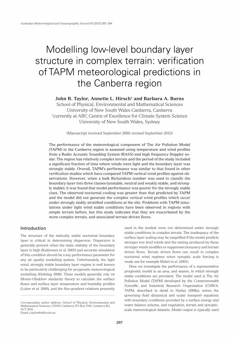
Study site and instrumentationAlthough the outer computational grid for the TAPM simulations takes in most of southeastern Australia (Fig. 1(a)), the high-resolution simulation focuses on the Canberra region. The major topographic features are oriented approximately north–south (Fig. 1(b)) with the Great Dividing Range to the east, and the Brindabella Range to the west. The regional scale drainage in the Canberra region is fed by a large cold air source area to the south confined between these two major ranges. The measurement site is located in the Majura Valley (Fig. 1(b)), at the School of Physical, Environmental and Mathematical Sciences (PEMS) field station, approximately 3 km northwest of Canberra International Airport. Site elevation is 580 m. The Majura Valley slopes down to the south or southeast, towards the Molonglo River. Overall, the combination of regional scale drainage from the south or southeast, and local scale drainage flow from the north or northwest, means that the study site has the potential for complex buoyancy driven flows under stable, light wind conditions, and these are observed. Southwesterly winds generated by synoptic-scale pressure systems tend to be blocked or deflected by the Brindabella range to the west, so that the prevailing winds are from the northwest. Two profiling instruments were located at the study site: a high-frequency Doppler sodar for winds; and a continuous

Taylor et al: Modelling low-level boundary layer structure in complex terrain 289

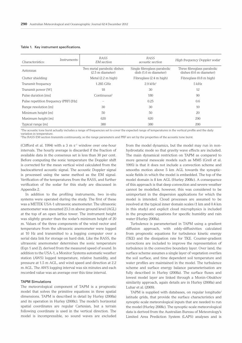
wave EM, pulsed acoustic RASS for temperature. Both these instruments were developed within the School of PEMS. Table 1 summarises the instruments’ specifications including the minimum and maximum vertical ranges and range resolution. The sodar has been operational for some time and Taylor et al. (2005) give results of a comparison of winds from a similar sodar (but operating at 1.875 kHz) with winds from Bureau of Meteorology radar tracked balloons. The RASS is a newer instrument which measures the Doppler shift on a continuous EM wave scattered from a vertically projected acoustic tone burst and uses this Doppler shift to determine the speed of sound. The speed of sound in air is determined primarily by temperature (Clifford et al. 1994), so, by measuring the Doppler shift as a function of time after the transmission of the acoustic tone burst, the RASS gives a vertical profile of temperature. A typical sound speed is used to convert the time after transmission of the tone burst to range, height above the ground for this vertically pointing system. The temperature derived from the RASS is called the sonic temperature, TS (Kaimal and Gaynor 1991) and is related to the thermodynamic temperature, T, by

Ts = 1+ γ w /γ d − ε( )q / ε⎡⎣ ⎤⎦T ...(1)

where γw and γd are the ratios of specific heats for water vapour and dry air respectively, ε is the ratio of the molecular weight of water to that for dry air. TS and T are in Kelvin. Equation 1 follows from Kaimal and Gaynor (1991) with the approximation that e / p = q / ε where p is the pressure, e is water vapour partial pressure and q is the specific humidity. The ratio γw/γd in Eqn 1 is numerically equal to 0.952. If it is replaced with 1, Eqn 1 defines the virtual temperature (Stull 1988). The approximation that a RASS measures virtual temperature is often used in the literature (Clifford et al. 1994). The sonic temperature can be calculated from the speed of sound using

Ts = γ dRd( )−1 c2, ...(2)

where Rd is the specific gas constant for dry air and c is the speed of sound. Both the RASS and sodar operate continuously. The sodar operation cycles around the vertical and two orthogonal oblique antennas. Doppler spectra from each antenna, at each height, are running averaged and the frequency shift that maximises the correlation between the averaged spectra and an ideal received spectrum gives the Doppler shift. The extracted Doppler shifts are block averaged to give a one-minute wind speed record which is archived for later processing. For comparison with TAPM, one-hour weighted average wind speeds are computed from these one-minute records. The weighting uses a quality factor primarily based on the signal-to-noise ratio and received signal power. Wind records are only accepted if the average weighting factor for an hour exceeds a set threshold. In the RASS processing chain, Doppler shifts are extracted from spectra of the EM signal using a multiple-Gaussian fit. The extracted Doppler shifts are then consensus averaged

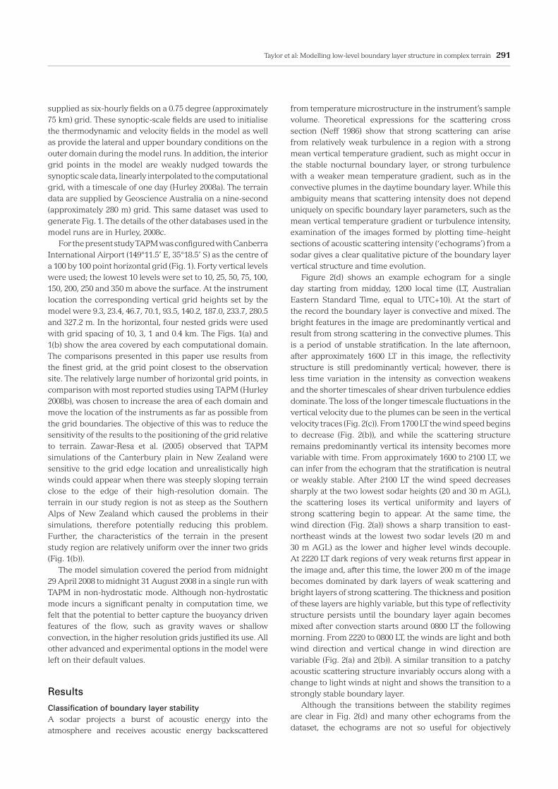
Fig. 1. Location and terrain for TAPM simulations. The first panel (a) shows the terrain in grayscale and the ma-jor inland river systems of southeastern Australia (in blue). The black squares on the first panel shows the outer three computational domains (10 km, 3 km and 1 km grid spacing). Second panel (b) is a higher resolution view of the inner two computational do-mains (1 km and 0.4 km resolution); location for ob-servations, and the grid center. The three black arrows show the direction of drainage in the three river sys-tems, from left to right: Murrumbidgee, Queanbeyan and Molonglo. The contours were derived from the Geoscience Australia nine-second digital elevation model used in the TAPM simulations. The maps were generated using the Generic Mapping Tools (Wessel and Smith 1998).

(a) Elevation

(b) Elevation

290 Australian Meteorological and Oceanographic Journal 62:4 December 2012

(Clifford et al. 1994) with a 3 m s–1 window over one-hour intervals. The hourly average is discarded if the fraction of available data in the consensus set is less than 30 per cent. Before computing the sonic temperature the Doppler shift is corrected for the mean vertical wind calculated from the backscattered acoustic signal. The acoustic Doppler signal is processed using the same method as the EM signal. Verification of the temperatures from the RASS, and further verification of the sodar for this study are discussed in Appendix 2. In addition to the profiling instruments, two in-situ systems were operated during the study. The first of these was a METEK USA-1 ultrasonic anemometer. The ultrasonic anemometer was mounted 23.3 m above ground level (AGL) at the top of an open lattice tower. The instrument height was slightly greater than the sodar’s minimum height of 20 m. Values of the three components of the wind vector and temperature from the ultrasonic anemometer were logged at 10 Hz and transmitted to a logging computer over a serial data link for storage on hard disk. Like the RASS, the ultrasonic anemometer determines the sonic temperature (Eqn 1 and 2), derived from the measured speed of sound. In addition to the USA-1, a Monitor Systems automatic weather station (AWS) logged temperature, relative humidity, and pressure at 1.5 m AGL, and wind speed and direction at 2.2 m AGL. The AWS logging interval was six minutes and each recorded value was an average over this time interval.

TAPM SimulationsThe meteorological component of TAPM is a prognostic model that solves the primitive equations in three spatial dimensions. TAPM is described in detail by Hurley (2008a) and its operation in Hurley (2008c). The model’s horizontal spatial coordinates are regular Cartesian, but a terrain following coordinate is used in the vertical direction. The model is incompressible, so sound waves are excluded

from the model dynamics, but the model may run in non-hydrostatic mode so that gravity wave effects are included. The main dynamical restriction on TAPM as compared to more general mesocale models such as MM5 (Grell et al. 1995) is that it does not include a convection scheme and smooths motion above 5 km AGL towards the synoptic-scale fields in which the model is embedded. The top of the model domain is 8 km AGL (Hurley 2008c). A consequence of this approach is that deep convection and severe weather cannot be modelled, however, this was considered to be unimportant in the dispersion applications for which the model is intended. Cloud processes are assumed to be resolved at the typical inner domain scales (1 km and 0.4 km in this study) and explicit cloud microphysics is included in the prognostic equations for specific humidity and rain water (Hurley 2008a). Turbulence is parameterised in TAPM using a gradient diffusion approach, with eddy-diffusivities calculated from prognostic equations for turbulence kinetic energy (TKE) and the dissipation rate for TKE. Counter-gradient corrections are included to improve the representation of turbulence in the convective boundary layer. Over land, the surface scheme assumes a single layer of vegetation overlies the soil surface, and time dependent soil temperature and water profiles are maintained in the model. The turbulence scheme and surface energy balance parameterisation are fully described in Hurley (2008a). The surface fluxes and lowest model layer are linked through a Monin-Obukhov similarity approach, again details are in Hurley (2008a) and Luhar et al. (2009). TAPM is supplied with databases, on regular longitude/latitude grids, that provide the surface characteristics and synoptic-scale meteorological inputs that are needed to run the model (Hurley 2008c). The synoptic-scale meteorological data is derived from the Australian Bureau of Meteorology’s Limited Area Prediction System (LAPS) analyses and is

Instruments:Characteristics:

RASS EM section

RASSacoustic section High frequency Doppler sodar

AntennasTwo metal parabolic dishes

(2.5 m diameter)Single fibreglass parabolic

dish (1.6 m diameter)Three fibreglass parabolic

dishes (0.6 m diameter)

Clutter shielding Metal (2.2 m high) Fibreglass (2.4 m high) Fibreglass (0.8 m high)

Transmit frequency 1.285 GHz 2.9 kHz1 5 kHz

Transmit power [W] 18 30 12

Pulse duration [ms] Continuous2 180 90

Pulse repetition frequency (PRF) [Hz] – 0.25 0.6

Range resolution [m] 30 30 10

Minimum height [m] 50 50 20

Maximum height [m] 620 620 290

Typical range [m] 380 380 200

1The acoustic tone burst actually includes a range of frequencies set to cover the expected range of temperatures in the vertical profile and the daily variation in temperature.2The RASS EM section transmits continuously, so the range parameters and PRF are set by the properties of the acoustic tone burst.

Table 1. Key instrument specifications.

Taylor et al: Modelling low-level boundary layer structure in complex terrain 291

supplied as six-hourly fields on a 0.75 degree (approximately 75 km) grid. These synoptic-scale fields are used to initialise the thermodynamic and velocity fields in the model as well as provide the lateral and upper boundary conditions on the outer domain during the model runs. In addition, the interior grid points in the model are weakly nudged towards the synoptic scale data, linearly interpolated to the computational grid, with a timescale of one day (Hurley 2008a). The terrain data are supplied by Geoscience Australia on a nine-second (approximately 280 m) grid. This same dataset was used to generate Fig. 1. The details of the other databases used in the model runs are in Hurley, 2008c. For the present study TAPM was configured with Canberra International Airport (149°11.5’ E, 35°18.5’ S) as the centre of a 100 by 100 point horizontal grid (Fig. 1). Forty vertical levels were used; the lowest 10 levels were set to 10, 25, 50, 75, 100, 150, 200, 250 and 350 m above the surface. At the instrument location the corresponding vertical grid heights set by the model were 9.3, 23.4, 46.7, 70.1, 93.5, 140.2, 187.0, 233.7, 280.5 and 327.2 m. In the horizontal, four nested grids were used with grid spacing of 10, 3, 1 and 0.4 km. The Figs. 1(a) and 1(b) show the area covered by each computational domain. The comparisons presented in this paper use results from the finest grid, at the grid point closest to the observation site. The relatively large number of horizontal grid points, in comparison with most reported studies using TAPM (Hurley 2008b), was chosen to increase the area of each domain and move the location of the instruments as far as possible from the grid boundaries. The objective of this was to reduce the sensitivity of the results to the positioning of the grid relative to terrain. Zawar-Resa et al. (2005) observed that TAPM simulations of the Canterbury plain in New Zealand were sensitive to the grid edge location and unrealistically high winds could appear when there was steeply sloping terrain close to the edge of their high-resolution domain. The terrain in our study region is not as steep as the Southern Alps of New Zealand which caused the problems in their simulations, therefore potentially reducing this problem. Further, the characteristics of the terrain in the present study region are relatively uniform over the inner two grids (Fig. 1(b)). The model simulation covered the period from midnight 29 April 2008 to midnight 31 August 2008 in a single run with TAPM in non-hydrostatic mode. Although non-hydrostatic mode incurs a significant penalty in computation time, we felt that the potential to better capture the buoyancy driven features of the flow, such as gravity waves or shallow convection, in the higher resolution grids justified its use. All other advanced and experimental options in the model were left on their default values.

Results

Classification of boundary layer stabilityA sodar projects a burst of acoustic energy into the atmosphere and receives acoustic energy backscattered

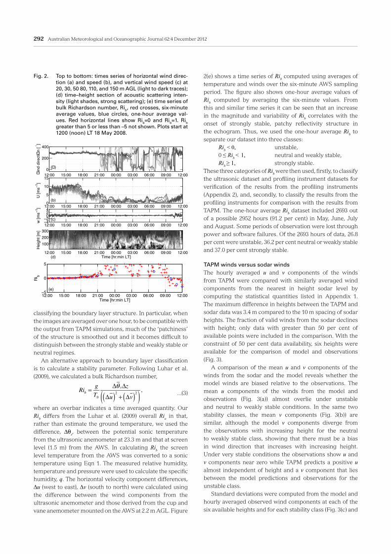
from temperature microstructure in the instrument’s sample volume. Theoretical expressions for the scattering cross section (Neff 1986) show that strong scattering can arise from relatively weak turbulence in a region with a strong mean vertical temperature gradient, such as might occur in the stable nocturnal boundary layer, or strong turbulence with a weaker mean temperature gradient, such as in the convective plumes in the daytime boundary layer. While this ambiguity means that scattering intensity does not depend uniquely on specific boundary layer parameters, such as the mean vertical temperature gradient or turbulence intensity, examination of the images formed by plotting time–height sections of acoustic scattering intensity (‘echograms’) from a sodar gives a clear qualitative picture of the boundary layer vertical structure and time evolution. Figure 2(d) shows an example echogram for a single day starting from midday, 1200 local time (LT, Australian Eastern Standard Time, equal to UTC+10). At the start of the record the boundary layer is convective and mixed. The bright features in the image are predominantly vertical and result from strong scattering in the convective plumes. This is a period of unstable stratification. In the late afternoon, after approximately 1600 LT in this image, the reflectivity structure is still predominantly vertical; however, there is less time variation in the intensity as convection weakens and the shorter timescales of shear driven turbulence eddies dominate. The loss of the longer timescale fluctuations in the vertical velocity due to the plumes can be seen in the vertical velocity traces (Fig. 2(c)). From 1700 LT the wind speed begins to decrease (Fig. 2(b)), and while the scattering structure remains predominantly vertical its intensity becomes more variable with time. From approximately 1600 to 2100 LT, we can infer from the echogram that the stratification is neutral or weakly stable. After 2100 LT the wind speed decreases sharply at the two lowest sodar heights (20 and 30 m AGL), the scattering loses its vertical uniformity and layers of strong scattering begin to appear. At the same time, the wind direction (Fig. 2(a)) shows a sharp transition to east-northeast winds at the lowest two sodar levels (20 m and 30 m AGL) as the lower and higher level winds decouple. At 2220 LT dark regions of very weak returns first appear in the image and, after this time, the lower 200 m of the image becomes dominated by dark layers of weak scattering and bright layers of strong scattering. The thickness and position of these layers are highly variable, but this type of reflectivity structure persists until the boundary layer again becomes mixed after convection starts around 0800 LT the following morning. From 2220 to 0800 LT, the winds are light and both wind direction and vertical change in wind direction are variable (Fig. 2(a) and 2(b)). A similar transition to a patchy acoustic scattering structure invariably occurs along with a change to light winds at night and shows the transition to a strongly stable boundary layer. Although the transitions between the stability regimes are clear in Fig. 2(d) and many other echograms from the dataset, the echograms are not so useful for objectively

292 Australian Meteorological and Oceanographic Journal 62:4 December 2012

classifying the boundary layer structure. In particular, when the images are averaged over one hour, to be compatible with the output from TAPM simulations, much of the ‘patchiness’ of the structure is smoothed out and it becomes difficult to distinguish between the strongly stable and weakly stable or neutral regimes. An alternative approach to boundary layer classification is to calculate a stability parameter. Following Luhar et al. (2009), we calculated a bulk Richardson number,

...(3)Rib =gT0

Δθ sΔz

Δu( )2 + Δv( )2( ) ,where an overbar indicates a time averaged quantity. Our Rib differs from the Luhar et al. (2009) overall Rio in that, rather than estimate the ground temperature, we used the difference, Δθs, between the potential sonic temperature from the ultrasonic anemometer at 23.3 m and that at screen level (1.5 m) from the AWS. In calculating Rib the screen level temperature from the AWS was converted to a sonic temperature using Eqn 1. The measured relative humidity, temperature and pressure were used to calculate the specific humidity, q. The horizontal velocity component differences, Δu (west to east), Δv (south to north) were calculated using the difference between the wind components from the ultrasonic anemometer and those derived from the cup and vane anemometer mounted on the AWS at 2.2 m AGL. Figure

2(e) shows a time series of Rib computed using averages of temperature and winds over the six-minute AWS sampling period. The figure also shows one-hour average values of Rib computed by averaging the six-minute values. From this and similar time series it can be seen that an increase in the magnitude and variability of Rib correlates with the onset of strongly stable, patchy reflectivity structure in the echogram. Thus, we used the one-hour average Rib to separate our dataset into three classes:

Rib < 0, unstable,0 ≤ Rib < 1, neutral and weakly stable,Rib ≥ 1, strongly stable.

These three categories of Rib were then used, firstly, to classify the ultrasonic dataset and profiling instrument datasets for verification of the results from the profiling instruments (Appendix 2), and, secondly, to classify the results from the profiling instruments for comparison with the results from TAPM. The one-hour average Rib dataset included 2693 out of a possible 2952 hours (91.2 per cent) in May, June, July and August. Some periods of observation were lost through power and software failures. Of the 2693 hours of data, 26.8 per cent were unstable, 36.2 per cent neutral or weakly stable and 37.0 per cent strongly stable.

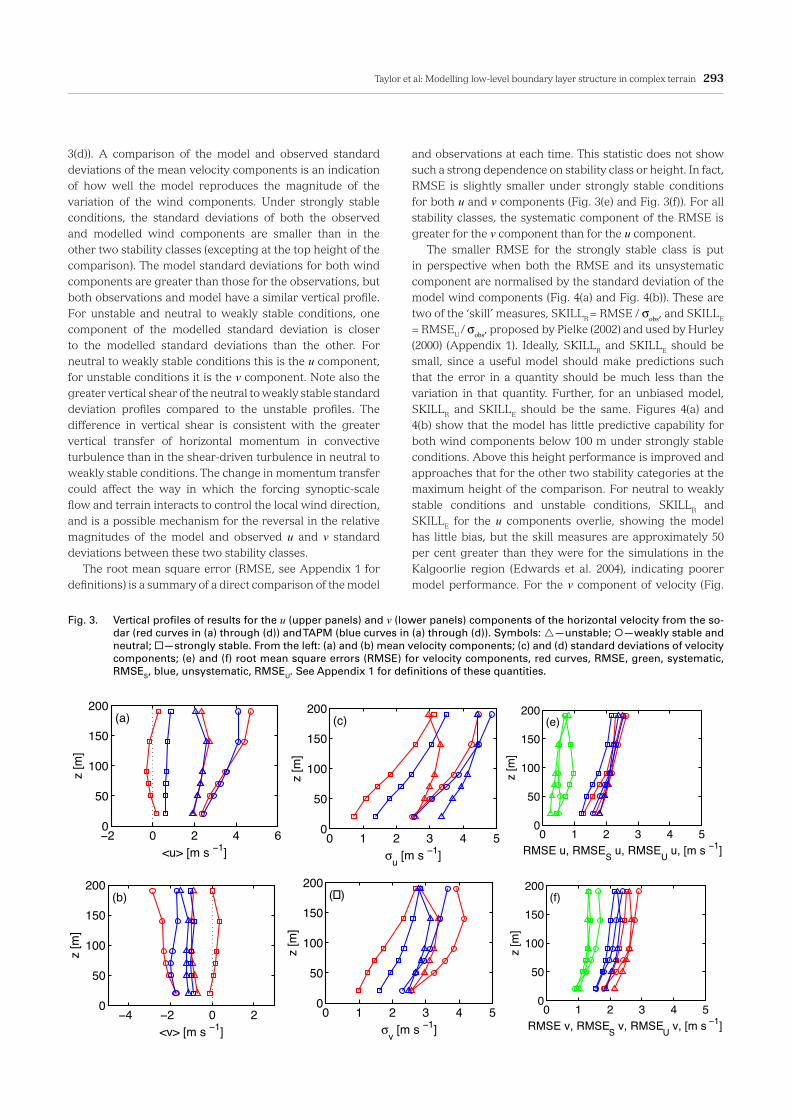
TAPM winds versus sodar winds The hourly averaged u and v components of the winds from TAPM were compared with similarly averaged wind components from the nearest in height sodar level by computing the statistical quantities listed in Appendix 1. The maximum difference in heights between the TAPM and sodar data was 3.4 m compared to the 10 m spacing of sodar heights. The fraction of valid winds from the sodar declines with height; only data with greater than 50 per cent of available points were included in the comparison. With the constraint of 50 per cent data availability, six heights were available for the comparison of model and observations (Fig. 3). A comparison of the mean u and v components of the winds from the sodar and the model reveals whether the model winds are biased relative to the observations. The mean u components of the winds from the model and observations (Fig. 3(a)) almost overlie under unstable and neutral to weakly stable conditions. In the same two stability classes, the mean v components (Fig. 3(b)) are similar, although the model v components diverge from the observations with increasing height for the neutral to weakly stable class, showing that there must be a bias in wind direction that increases with increasing height. Under very stable conditions the observations show u and v components near zero while TAPM predicts a positive u almost independent of height and a v component that lies between the model predictions and observations for the unstable class. Standard deviations were computed from the model and hourly averaged observed wind components at each of the six available heights and for each stability class (Fig. 3(c) and

Fig. 2. Top to bottom: times series of horizontal wind direc-tion (a) and speed (b), and vertical wind speed (c) at 20, 30, 50 80, 110, and 150 m AGL (light to dark traces); (d) time–height section of acoustic scattering inten-sity (light shades, strong scattering); (e) time series of bulk Richardson number, Rib, red crosses, six-minute average values, blue circles, one-hour average val-ues. Red horizontal lines show Rib=0 and Rib=1. Rib greater than 5 or less than –5 not shown. Plots start at 1200 (noon) LT 18 May 2008.

Time [hr:min LT]

Hei

ght [

m]

(d)12:00 15:00 18:00 21:00 00:00 03:00 06:00 09:00 12:00

100200300

12:00 15:00 18:00 21:00 00:00 03:00 06:00 09:00 12:00−4−2

024

w [m

s−1]

(c)

12:00 15:00 18:00 21:00 00:00 03:00 06:00 09:00 12:000

5

10

15

U [m

s−1]

(b)

12:00 15:00 18:00 21:00 00:00 03:00 06:00 09:00 12:000

200

400

�ind

dire

cti�

n [° ]

(�)

12:00 15:00 18:00 21:00 00:00 03:00 06:00 09:00 12:00−5

0

5

Time [hr:min LT]

Ri b

(e)

Taylor et al: Modelling low-level boundary layer structure in complex terrain 293

3(d)). A comparison of the model and observed standard deviations of the mean velocity components is an indication of how well the model reproduces the magnitude of the variation of the wind components. Under strongly stable conditions, the standard deviations of both the observed and modelled wind components are smaller than in the other two stability classes (excepting at the top height of the comparison). The model standard deviations for both wind components are greater than those for the observations, but both observations and model have a similar vertical profile. For unstable and neutral to weakly stable conditions, one component of the modelled standard deviation is closer to the modelled standard deviations than the other. For neutral to weakly stable conditions this is the u component, for unstable conditions it is the v component. Note also the greater vertical shear of the neutral to weakly stable standard deviation profiles compared to the unstable profiles. The difference in vertical shear is consistent with the greater vertical transfer of horizontal momentum in convective turbulence than in the shear-driven turbulence in neutral to weakly stable conditions. The change in momentum transfer could affect the way in which the forcing synoptic-scale flow and terrain interacts to control the local wind direction, and is a possible mechanism for the reversal in the relative magnitudes of the model and observed u and v standard deviations between these two stability classes. The root mean square error (RMSE, see Appendix 1 for definitions) is a summary of a direct comparison of the model

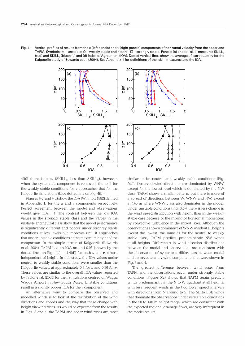
and observations at each time. This statistic does not show such a strong dependence on stability class or height. In fact, RMSE is slightly smaller under strongly stable conditions for both u and v components (Fig. 3(e) and Fig. 3(f)). For all stability classes, the systematic component of the RMSE is greater for the v component than for the u component. The smaller RMSE for the strongly stable class is put in perspective when both the RMSE and its unsystematic component are normalised by the standard deviation of the model wind components (Fig. 4(a) and Fig. 4(b)). These are two of the ‘skill’ measures, SKILLR = RMSE / σobs, and SKILLE

= RMSEU / σobs, proposed by Pielke (2002) and used by Hurley (2000) (Appendix 1). Ideally, SKILLR and SKILLE should be small, since a useful model should make predictions such that the error in a quantity should be much less than the variation in that quantity. Further, for an unbiased model, SKILLR and SKILLE should be the same. Figures 4(a) and 4(b) show that the model has little predictive capability for both wind components below 100 m under strongly stable conditions. Above this height performance is improved and approaches that for the other two stability categories at the maximum height of the comparison. For neutral to weakly stable conditions and unstable conditions, SKILLR and SKILLE for the u components overlie, showing the model has little bias, but the skill measures are approximately 50 per cent greater than they were for the simulations in the Kalgoorlie region (Edwards et al. 2004), indicating poorer model performance. For the v component of velocity (Fig.

Fig. 3. Vertical profiles of results for the u (upper panels) and v (lower panels) components of the horizontal velocity from the so-dar (red curves in (a) through (d)) and TAPM (blue curves in (a) through (d)). Symbols: —unstable; ¡—weakly stable and neutral; ¨—strongly stable. From the left: (a) and (b) mean velocity components; (c) and (d) standard deviations of velocity components; (e) and (f) root mean square errors (RMSE) for velocity components, red curves, RMSE, green, systematic, RMSES, blue, unsystematic, RMSEU. See Appendix 1 for definitions of these quantities.

−2 0 2 4 60

50

100

150

200

<u> [m s −1]

z [m

]

(a)

−4 −2 0 20

50

100

150

200

<v> [m s −1]

z [m

]

(b)

0 1 2 3 4 50

50

100

150

200

σu [m s −1]

z [m

]

(c)

0 1 2 3 4 50

50

100

150

200

σv [m s −1]

z [m

]

(�)

−2 0 2 4 60

50

100

150

200

<u> [m s −1]

z [m

]

(a)

−4 −2 0 20

50

100

150

200

<v> [m s −1]

z [m

]

(b)

0 1 2 3 4 50

50

100

150

200

σu [m s −1]

z [m

]

(c)

0 1 2 3 4 50

50

100

150

200

σv [m s −1]

z [m

]

(�)

−2 0 2 4 60

50

100

150

200

<u> [m s −1]

z [m

]

(a)

−4 −2 0 20

50

100

150

200

<v> [m s −1]

z [m

]

(b)

0 1 2 3 4 50

50

100

150

200

σu [m s −1]

z [m

]

(c)

0 1 2 3 4 50

50

100

150

200

σv [m s −1]

z [m

]

(�)

−2 0 2 4 60

50

100

150

200

<u> [m s −1]

z [m

]

(a)

−4 −2 0 20

50

100

150

200

<v> [m s −1]

z [m

]

(b)

0 1 2 3 4 50

50

100

150

200

σu [m s −1]

z [m

]

(c)

0 1 2 3 4 50

50

100

150

200

σv [m s −1]

z [m

]

(�)

0 1 2 3 4 50

50

100

150

200

RMSE v, RMSES v, RMSEU v, [m s −1]

z [m

](f)

0 1 2 3 4 50

50

100

150

200

RMSE u, RMSES u, RMSEU u, [m s −1]

z [m

]

(e)

0 1 2 3 4 50

50

100

150

200

RMSE v, RMSES v, RMSEU v, [m s −1]

z [m

]

(f)

0 1 2 3 4 50

50

100

150

200

RMSE u, RMSES u, RMSEU u, [m s −1]

z [m

]

(e)

294 Australian Meteorological and Oceanographic Journal 62:4 December 2012

4(b)) there is bias, (SKILLE less than SKILLR), however, when the systematic component is removed, the skill for the weakly stable conditions for v approaches that for the Kalgoorlie simulations (blue dotted line on Fig. 4(b)). Figures 4(c) and 4(d) show the IOA (Willmott 1982) defined in Appendix 1, for the u and v components respectively. Perfect agreement between the model and observations would give IOA = 1. The contrast between the low IOA values in the strongly stable class and the values in the unstable and neutral class show that the model performance is significantly different and poorer under strongly stable conditions at low levels but improves until it approaches that under unstable conditions at the maximum height of the comparison. In the simple terrain of Kalgoorlie (Edwards et al. 2004), TAPM had an IOA around 0.95 (shown by the dotted lines on Fig. 4(c) and 4(d)) for both u and v, almost independent of height. In this study, the IOA values under neutral to weakly stable conditions were smaller than the Kalgoorlie values, at approximately 0.9 for u and 0.86 for v. These values are similar to the overall IOA values reported by Taylor et al. (2005) for their simulations centred on Wagga Wagga Airport in New South Wales. Unstable conditions result in a slightly poorer IOA for the v component. An alternative way to compare the observed and modelled winds is to look at the distribution of the wind directions and speeds and the way that these change with height via wind roses. As would be expected from the results in Figs. 3 and 4, the TAPM and sodar wind roses are most

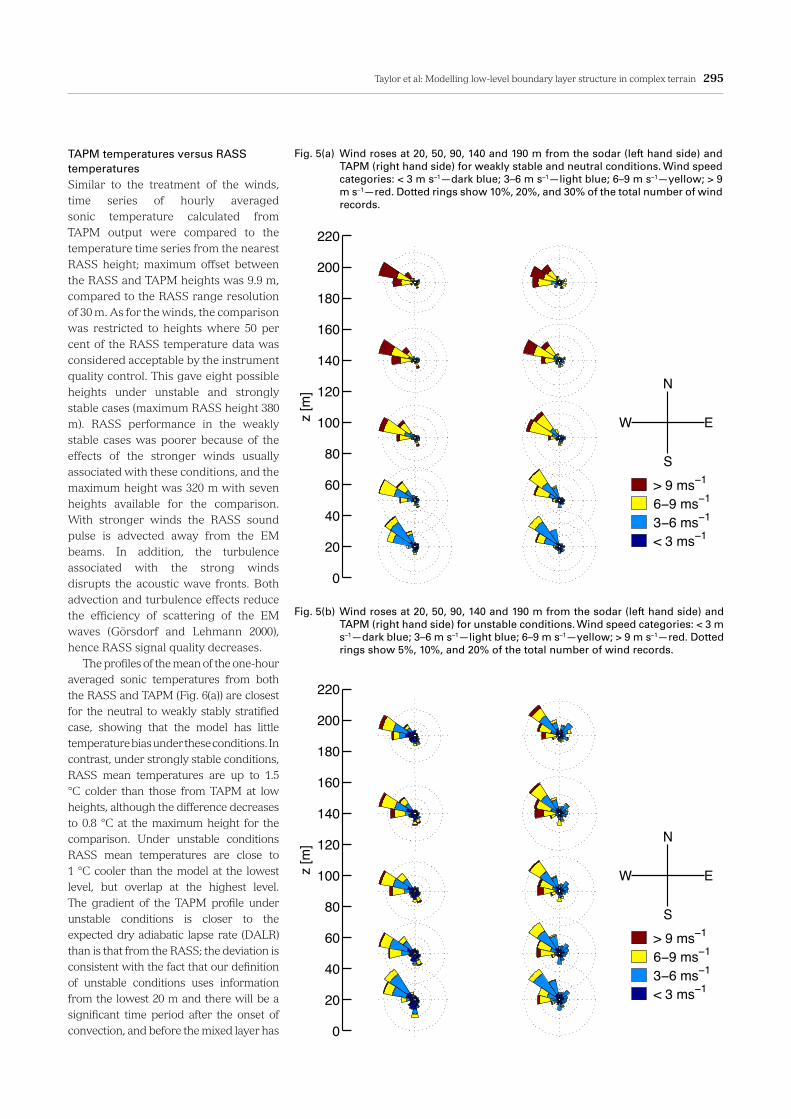
similar under neutral and weakly stable conditions (Fig. 5(a)). Observed wind directions are dominated by WNW, except for the lowest level which is dominated by the NW class. TAPM shows a similar pattern, but there is more of a spread of directions between W, WNW and NW, except at 140 m where WNW class also dominates in the model. Under unstable conditions (Fig. 5(b)), there is less change in the wind speed distribution with height than in the weakly stable case because of the mixing of horizontal momentum by convective turbulence in the mixed layer. Although the observations show a dominance of WNW winds at all heights except the lowest, the same as for the neutral to weakly stable class, TAPM predicts predominantly NW winds at all heights. Differences in wind direction distributions between the model and observations are consistent with the observation of systematic differences between model and observed u and v wind components that were shown in Fig. 3 and 4. The greatest difference between wind roses from TAPM and the observations occur under strongly stable conditions. Figure 5(c) shows that TAPM again predicts winds predominantly in the N to W quadrant at all heights, with less frequent winds in the two lower speed intervals with directions from N around to S. The SE to ESE winds that dominate the observations under very stable conditions in the 50 to 140 m height range, which are consistent with the expected regional drainage flows, are very infrequent in the model results.

Fig. 4. Vertical profiles of results from the u (left panels) and v (right panels) components of horizontal velocity from the sodar and TAPM. Symbols: —unstable; ¡—weakly stable and neutral; ̈ —strongly stable. Panels: (a) and (b) ‘skill’ measures SKILLR (red) and SKILLE (blue); (c) and (d) Index of Agreement (IOA). Dotted vertical lines show the average of each quantity for the Kalgoorlie study of Edwards et al. (2004). See Appendix 1 for definitions of the ‘skill’ measures and the IOA.

0.4 0.6 0.8 10

50

100

150

200

IOA

z [m

]

(c)

0.4 0.6 0.8 10

50

100

150

200

IOA

z [m

](d)

0 0.5 1 1.5 20

50

100

150

200

SKILLR, SKILLE

z [m

]

(a)

0 0.5 1 1.5 20

50

100

150

200

SKILLR, SKILLE

z [m

]

(b)

Taylor et al: Modelling low-level boundary layer structure in complex terrain 295

Fig. 5(a) Wind roses at 20, 50, 90, 140 and 190 m from the sodar (left hand side) and TAPM (right hand side) for weakly stable and neutral conditions. Wind speed categories: < 3 m s–1—dark blue; 3–6 m s–1—light blue; 6–9 m s–1—yellow; > 9 m s–1—red. Dotted rings show 10%, 20%, and 30% of the total number of wind records.

0

20

40

60

80

100

120

140

160

180

200

220

< 3 ms−13−6 ms−16−9 ms−1> 9 ms−1

N

S

W Ez [m

]

0

20

40

60

80

100

120

140

160

180

200

220

< 3 ms−13−6 ms−16−9 ms−1> 9 ms−1

N

S

W Ez [m

]

Fig. 5(b) Wind roses at 20, 50, 90, 140 and 190 m from the sodar (left hand side) and TAPM (right hand side) for unstable conditions. Wind speed categories: < 3 m s–1—dark blue; 3–6 m s–1—light blue; 6–9 m s–1—yellow; > 9 m s–1—red. Dotted rings show 5%, 10%, and 20% of the total number of wind records.

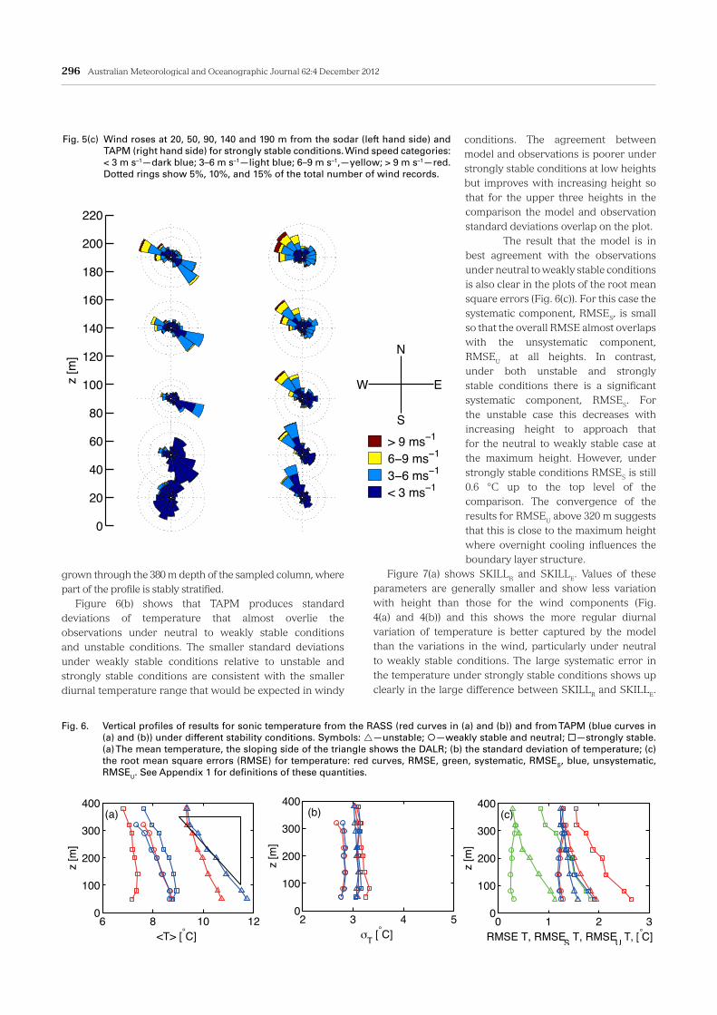
TAPM temperatures versus RASS temperaturesSimilar to the treatment of the winds, time series of hourly averaged sonic temperature calculated from TAPM output were compared to the temperature time series from the nearest RASS height; maximum offset between the RASS and TAPM heights was 9.9 m, compared to the RASS range resolution of 30 m. As for the winds, the comparison was restricted to heights where 50 per cent of the RASS temperature data was considered acceptable by the instrument quality control. This gave eight possible heights under unstable and strongly stable cases (maximum RASS height 380 m). RASS performance in the weakly stable cases was poorer because of the effects of the stronger winds usually associated with these conditions, and the maximum height was 320 m with seven heights available for the comparison. With stronger winds the RASS sound pulse is advected away from the EM beams. In addition, the turbulence associated with the strong winds disrupts the acoustic wave fronts. Both advection and turbulence effects reduce the efficiency of scattering of the EM waves (Görsdorf and Lehmann 2000), hence RASS signal quality decreases. The profiles of the mean of the one-hour averaged sonic temperatures from both the RASS and TAPM (Fig. 6(a)) are closest for the neutral to weakly stably stratified case, showing that the model has little temperature bias under these conditions. In contrast, under strongly stable conditions, RASS mean temperatures are up to 1.5 °C colder than those from TAPM at low heights, although the difference decreases to 0.8 °C at the maximum height for the comparison. Under unstable conditions RASS mean temperatures are close to 1 °C cooler than the model at the lowest level, but overlap at the highest level. The gradient of the TAPM profile under unstable conditions is closer to the expected dry adiabatic lapse rate (DALR) than is that from the RASS; the deviation is consistent with the fact that our definition of unstable conditions uses information from the lowest 20 m and there will be a significant time period after the onset of convection, and before the mixed layer has

296 Australian Meteorological and Oceanographic Journal 62:4 December 2012

0

20

40

60

80

100

120

140

160

180

200

220

< 3 ms−13−6 ms−16−9 ms−1> 9 ms−1

N

S

W Ez [m

]

Fig. 5(c) Wind roses at 20, 50, 90, 140 and 190 m from the sodar (left hand side) and TAPM (right hand side) for strongly stable conditions. Wind speed categories: < 3 m s–1—dark blue; 3–6 m s–1—light blue; 6–9 m s–1,—yellow; > 9 m s–1—red. Dotted rings show 5%, 10%, and 15% of the total number of wind records.

Fig. 6. Vertical profiles of results for sonic temperature from the RASS (red curves in (a) and (b)) and from TAPM (blue curves in (a) and (b)) under different stability conditions. Symbols: —unstable; ¡—weakly stable and neutral; ¨—strongly stable. (a) The mean temperature, the sloping side of the triangle shows the DALR; (b) the standard deviation of temperature; (c) the root mean square errors (RMSE) for temperature: red curves, RMSE, green, systematic, RMSES, blue, unsystematic, RMSEU. See Appendix 1 for definitions of these quantities.

6 8 10 120

100

200

300

400

<T> [°C]

z [m

]

(a)

2 3 4 50

100

200

300

400

σT [ °C]

z [m

]

(b)

0 1 2 30

100

200

300

400

RMSE T, RMSES T, RMSEU T, [°C]

z [m

]

(c)

6 8 10 120

100

200

300

400

<T> [°C]

z [m

]

(a)

2 3 4 50

100

200

300

400

σT [ °C]

z [m

]

(b)

0 1 2 30

100

200

300

400

RMSE T, RMSES T, RMSEU T, [°C]

z [m

]

(c)

6 8 10 120

100

200

300

400

<T> [°C]

z [m

]

(a)

2 3 4 50

100

200

300

400

σT [ °C]

z [m

]

(b)

0 1 2 30

100

200

300

400

RMSE T, RMSES T, RMSEU T, [°C]

z [m

]

(c)

conditions. The agreement between model and observations is poorer under strongly stable conditions at low heights but improves with increasing height so that for the upper three heights in the comparison the model and observation standard deviations overlap on the plot. The result that the model is in best agreement with the observations under neutral to weakly stable conditions is also clear in the plots of the root mean square errors (Fig. 6(c)). For this case the systematic component, RMSES, is small so that the overall RMSE almost overlaps with the unsystematic component, RMSEU at all heights. In contrast, under both unstable and strongly stable conditions there is a significant systematic component, RMSES. For the unstable case this decreases with increasing height to approach that for the neutral to weakly stable case at the maximum height. However, under strongly stable conditions RMSES is still 0.6 °C up to the top level of the comparison. The convergence of the results for RMSEU above 320 m suggests that this is close to the maximum height where overnight cooling influences the boundary layer structure.

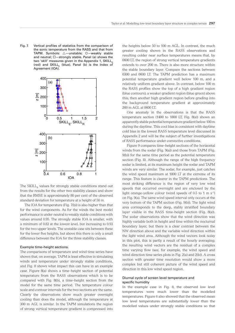
Figure 7(a) shows SKILLR and SKILLE. Values of these parameters are generally smaller and show less variation with height than those for the wind components (Fig. 4(a) and 4(b)) and this shows the more regular diurnal variation of temperature is better captured by the model than the variations in the wind, particularly under neutral to weakly stable conditions. The large systematic error in the temperature under strongly stable conditions shows up clearly in the large difference between SKILLR and SKILLE.

grown through the 380 m depth of the sampled column, where part of the profile is stably stratified. Figure 6(b) shows that TAPM produces standard deviations of temperature that almost overlie the observations under neutral to weakly stable conditions and unstable conditions. The smaller standard deviations under weakly stable conditions relative to unstable and strongly stable conditions are consistent with the smaller diurnal temperature range that would be expected in windy

Taylor et al: Modelling low-level boundary layer structure in complex terrain 297

The SKILLR values for strongly stable conditions stand out from the results for the other two stability classes and show that the RMSE is approximately 80 per cent of the observed standard deviation for temperature at a height of 50 m. The IOA for temperature (Fig. 7(b)) is also higher than that for the wind components. As for the winds the best model performance is under neutral to weakly stable conditions with values around 0.95. The strongly stable IOA is smaller, with a minimum of 0.83 at the lowest level, but increasing to 0.93 for the two upper levels. The unstable case sits between these for the lower five heights, but above this there is only a small difference between the IOA for the three stability classes.

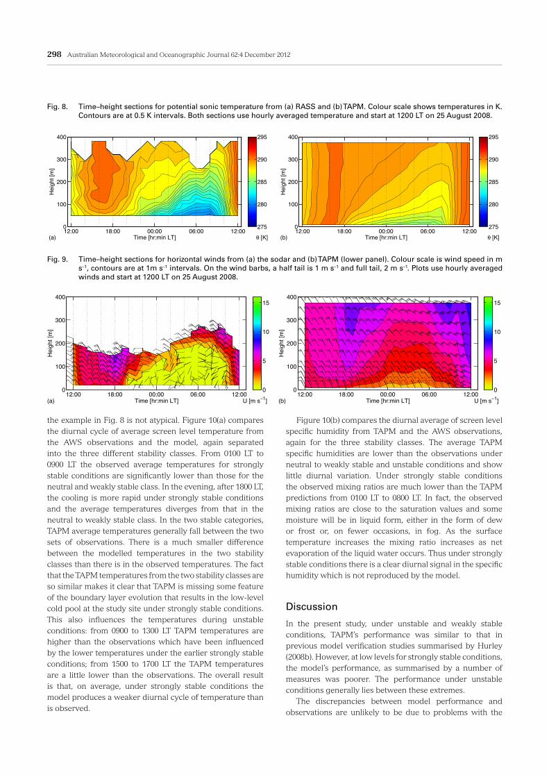
Example time–height sections. The comparisons of temperature and wind time series have shown that, on average, TAPM is least effective in simulating winds and temperature under strongly stable conditions, and Fig. 8 shows what impact this can have in an example case. Figure 8(a) shows a time–height section of potential temperature from the RASS observations which is to be compared with Fig. 8(b), a time–height section from the model for the same time period. The temperature colour scale and contour intervals for the two sections are the same. Clearly the observations show much greater overnight cooling than does the model, although the temperature at 300 m AGL is similar. In the TAPM simulations the region of strong vertical temperature gradient is compressed into

the heights below 50 to 100 m AGL. In contrast, the much greater cooling shown in the RASS observations and resulting colder near surface temperatures means that, by 0600 LT, the region of strong vertical temperature gradients extends to over 200 m. There is also more structure within the stable boundary layer. Compare the sections between 0300 and 0600 LT. The TAPM prediction has a maximum potential temperature gradient well below 100 m, and a relatively uniform gradient above. In contrast, below 100 m the RASS profiles show the top of a high gradient region (blue contours); a weaker gradient region (blue green) above this; then another high gradient region before grading into the background temperature gradient at approximately 260 m AGL at 0600 LT. One anomaly in the observations is that the RASS temperature section (1400 to 1800 LT, Fig. 8(a)) shows an apparently stable potential temperature gradient below 100 m during the daytime. This cool bias is consistent with daytime cold bias in the lowest RASS temperature level discussed in Appendix 2 and will be the subject of further investigations of RASS performance under convective conditions. Figure 9 compares time–height sections of the horizontal winds from the sodar (Fig. 9(a)) and those from TAPM (Fig. 9(b)) for the same time period as the potential temperature section (Fig. 8). Although the range of the high frequency sodar is limited, at its maximum height the sodar and TAPM winds are very similar. The sodar, for example, just catches the wind speed maximum at 1800 LT at the extreme of its range. This feature is clearer in the TAPM predictions. The most striking difference is the region of very low wind speeds that occurred overnight and are enclosed by the light orange–yellow colour (wind speeds of 0.5 to 1 m s–1) on Fig. 9(a). The same wind speed interval only occurs at the very bottom of the TAPM section (Fig. 9(b)). The light wind area corresponds to the deep, stably stratified boundary layer visible in the RASS time–height section (Fig. 8(a)). The sodar observations show that the wind direction was highly variable both in height and time within the nocturnal boundary layer, but there is a clear contrast between the NW direction above and the variable wind direction within the light wind area. Although the wind vectors look noisy in this plot, this is partly a result of the hourly averaging; the resulting wind vectors are the residual of a complex time varying flow (see, for example, the wind speed and wind direction time series plots in Fig. 2(a) and 2(b)). A cross section with greater time resolution would show a more complex but still coherent picture of the wind speed and direction in this low wind speed region.

Diurnal cycle of screen level temperature and specific humidityIn the example case in Fig. 8, the observed low level temperatures were much lower than the modelled temperatures. Figure 6 also showed that the observed mean low level temperatures are substantially lower than the modelled values under strongly stable conditions so that

0.4 0.6 0.8 10

100

200

300

400

IOA

z [m

]

(b)

0 0.5 1 1.5 20

100

200

300

400

SKILLE, SKILLR

z [m

]

(a)

Fig. 7. Vertical profiles of statistics from the comparison of the sonic temperature from the RASS and that from TAPM. Symbols: —unstable; ¡—weakly stable and neutral; ¨—strongly stable. Panel (a) shows the two ‘skill’ measures given in the Appendix 1, SKILLR (red) and SKILLE (blue). Panel (b) is the Index of Agreement (IOA).

0.4 0.6 0.8 10

100

200

300

400

IOA

z [m

]

(b)

0 0.5 1 1.5 20

100

200

300

400

SKILLE, SKILLR

z [m

]

(a)

298 Australian Meteorological and Oceanographic Journal 62:4 December 2012

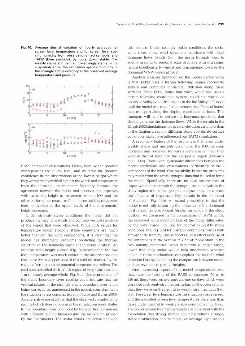
the example in Fig. 8 is not atypical. Figure 10(a) compares the diurnal cycle of average screen level temperature from the AWS observations and the model, again separated into the three different stability classes. From 0100 LT to 0900 LT the observed average temperatures for strongly stable conditions are significantly lower than those for the neutral and weakly stable class. In the evening, after 1800 LT, the cooling is more rapid under strongly stable conditions and the average temperatures diverges from that in the neutral to weakly stable class. In the two stable categories, TAPM average temperatures generally fall between the two sets of observations. There is a much smaller difference between the modelled temperatures in the two stability classes than there is in the observed temperatures. The fact that the TAPM temperatures from the two stability classes are so similar makes it clear that TAPM is missing some feature of the boundary layer evolution that results in the low-level cold pool at the study site under strongly stable conditions. This also influences the temperatures during unstable conditions: from 0900 to 1300 LT TAPM temperatures are higher than the observations which have been influenced by the lower temperatures under the earlier strongly stable conditions; from 1500 to 1700 LT the TAPM temperatures are a little lower than the observations. The overall result is that, on average, under strongly stable conditions the model produces a weaker diurnal cycle of temperature than is observed.

Figure 10(b) compares the diurnal average of screen level specific humidity from TAPM and the AWS observations, again for the three stability classes. The average TAPM specific humidities are lower than the observations under neutral to weakly stable and unstable conditions and show little diurnal variation. Under strongly stable conditions the observed mixing ratios are much lower than the TAPM predictions from 0100 LT to 0800 LT. In fact, the observed mixing ratios are close to the saturation values and some moisture will be in liquid form, either in the form of dew or frost or, on fewer occasions, in fog. As the surface temperature increases the mixing ratio increases as net evaporation of the liquid water occurs. Thus under strongly stable conditions there is a clear diurnal signal in the specific humidity which is not reproduced by the model.

Discussion

In the present study, under unstable and weakly stable conditions, TAPM’s performance was similar to that in previous model verification studies summarised by Hurley (2008b). However, at low levels for strongly stable conditions, the model’s performance, as summarised by a number of measures was poorer. The performance under unstable conditions generally lies between these extremes. The discrepancies between model performance and observations are unlikely to be due to problems with the

Fig. 8. Time–height sections for potential sonic temperature from (a) RASS and (b) TAPM. Colour scale shows temperatures in K. Contours are at 0.5 K intervals. Both sections use hourly averaged temperature and start at 1200 LT on 25 August 2008.

12:00 18:00 00:00 06:00 12:000

100

200

300

400

Time [hr:min LT]

Hei

ght [

m]

θ [K](a)

275

280

285

290

295

Fig. 9. Time–height sections for horizontal winds from (a) the sodar and (b) TAPM (lower panel). Colour scale is wind speed in m s–1, contours are at 1m s–1 intervals. On the wind barbs, a half tail is 1 m s–1 and full tail, 2 m s–1. Plots use hourly averaged winds and start at 1200 LT on 25 August 2008.

12:00 18:00 00:00 06:00 12:000

100

200

300

400

Time [hr:min LT]

Hei

ght [

m]

U [m s−1](a)

0

5

10

15

12:00 18:00 00:00 06:00 12:000

100

200

300

400

Time [hr:min LT]

Hei

ght [

m]

θ [K](b)

275

280

285

290

295

12:00 18:00 00:00 06:00 12:000

100

200

300

400

Time [hr:min LT]

Hei

ght [

m]

U [m s−1](b)

0

5

10

15

Taylor et al: Modelling low-level boundary layer structure in complex terrain 299

RASS and sodar observations. Firstly, because the greatest discrepancies are at low level, and we have the greatest confidence in the observations at the lowest height where they were directly verified against the winds and temperature from the ultrasonic anemometer. Secondly, because the agreement between the model and observations improves with increasing height to the extent that the IOA and the other performance measures for all three stability categories tend to overlap at the upper levels of the instruments’ height coverage. Under strongly stable conditions the model did not produce the very light winds and complex vertical structure of the winds that were observed. While IOA values for temperature under strongly stable conditions are much better than for the wind components, it is clear that the model has systematic problems predicting the thermal structure of the boundary layer at the study location. An example time–height section (Fig. 8) showed that the low level temperature was much colder in the observations and that there was a deeper pool of this cold air, marked by the region of strong positive potential temperature gradient. The cold pool coincided with a thick region of very light, less than 1 m s–1 hourly average winds (Fig. 9(a)). Under-prediction of the stable boundary layer cooling could indicate that the vertical mixing in the strongly stable boundary layer is not being correctly parameterised in the model, consistent with the situation in less complex terrain (Poulos and Burns 2003). An alternative possibility is that the observed complex wind regime (which does not occur in the simulations) contributes to the boundary layer cold pool by transporting air masses with different cooling histories into the air column probed by the instruments. The sodar winds are consistent with

this picture. Under strongly stable conditions the sodar wind roses show wind directions consistent with local drainage flows (winds from the north through west to south), grading to regional scale drainage with increasing height (southeasterly winds) and transitioning towards the dominant WNW winds at 190 m. Another possible limitation on the model performance is that TAPM uses a terrain following sigma coordinate system and computes ‘horizontal’ diffusion along these surfaces. Zängl (2002) found that MM5, which also uses a terrain following coordinate system, could not reproduce observed valley wind circulations in the Inn Valley in Europe until the model was modified to remove the effects of lateral heat transport along the sloping coordinate surfaces. This transport will tend to reduce the buoyancy gradients that should generate the drainage flows. While the terrain in the Zängl (2002) simulations had greater elevation variations than in the Canberra region, diffusion along coordinate surface could potentially have influenced our TAPM simulations. A secondary feature of the results was that, even under weakly stable and unstable conditions, the IOA between modelled and observed for winds were smaller than they were in the flat terrain in the Kalgoorlie region (Edwards et al. 2004). There were systematic differences between the model predictions and observations, particularly of the v component of the wind. One possibility is that the problems may result from the actual synoptic data that is used to force the model. Specifically, there are no local observations of upper winds to constrain the synoptic-scale analysis in the study region and so the synoptic analyses may not capture the influence of large-scale high terrain in the southeast of Australia (Fig. 1(a)). A second possibility is that the model is not fully capturing the influence of the dominant local terrain feature, Mount Ainslie, on winds at the study location. As discussed in the comparison of TAPM winds, the observed wind direction bias of the model (illustrated by the wind roses, Fig. 5(a) for neutral to weakly stable conditions and Fig. 5(b) for unstable conditions) varies with atmospheric stability. This supports a local effect because of the differences in the vertical mixing of momentum in the two stability categories. Wind data from a longer range, lower frequency sodar would help understand whether either of these mechanisms can explain the model’s wind direction bias by extending the comparison between model and observations to greater heights. One interesting aspect of the model temperatures was that, over the heights of the RASS comparison (50 m to 320 m), these were, on average, warmer on days which were classified as strongly stratified on the basis of the observations, than they were on the neutral to weakly stratified days (Fig. 6(a)). For screen level temperature this situation was reversed, and the modelled screen level temperatures were less than those under neutral to weakly stable conditions (Fig. 10(a)). The cooler screen level temperatures are consistent with the expectation that strong surface cooling produces strongly stable stratification, and the model, on average, captures this

Fig. 10. Average diurnal variation of hourly averaged (a) screen level temperature and (b) screen level spe-cific humidity from observations (red symbols) and TAPM (blue symbols). Symbols: —unstable; ¡—weakly stable and neutral; ¨—strongly stable. In (b) + symbols show the saturation specific humidity in the strongly stable category at the observed average temperature and pressure.

300 Australian Meteorological and Oceanographic Journal 62:4 December 2012

trend in low-level cooling if not its magnitude. The warmer temperatures in the 50 to 320 m height range for the strongly stable conditions could be a result of warmer temperatures in this layer on the previous day. These warmer daytime temperatures would be expected under the fair weather, clear sky conditions that generally precede the development of a strong stable boundary layer overnight. TAPM not only does not generate sufficient low-level cooling after these days, but also concentrates the cooling in a shallow nocturnal boundary layer, thus leaving the warmer modelled temperatures between 50 m and 320 m.

Conclusions

Some previous studies with TAPM have indicated that the model has problems with strongly stable stratifications. Here we have investigated this problem at a site which might be considered to represent typical inland complex terrain in Australia and have confirmed the problem by direct comparison of TAPM output with wind and temperature observations from a sodar and RASS. When the observations show that the boundary layer is very stable, the model boundary layer is very similar to that under neutral to weakly stable conditions. That is, the observed and modelled systems differ in a fundamental way. Our results show that the model fails to capture the complex light winds and deeper region of stable temperature gradients in the strongly stable boundary layer that result from the combination of local surface cooling and terrain driven drainage flows. The problem with the model performance under strongly stable regime remains after the incorporation of the modified flux-gradient relations for momentum based on Luhar et al. (2009) in TAPM v4. These flux-gradient adjustments were successful in improving TAPM’s performance under stable conditions in simple terrain. Our results show that in locations with complex terrain where strongly stable conditions are likely to occur, unverified TAPM meteorological simulations results should be treated with caution if they are being used as a basis for dispersion predictions. In the particular case that we reported on, TAPM predicted wind speeds of 3 to 4 m s–1 and a layer of high static stability below 50 m AGL in the fully developed nocturnal boundary layer. The observations had a layer of one-hour averaged wind speeds less than 1 m s–1 and static stability comparable to the maximum in the TAPM simulations up to 260 m AGL. In this case the actual dispersion environment for any source discharging into the stable boundary layer would probably have been much different from that predicted by the model. The results of this study suggest that while TAPM, and other prognostic models, continue to have difficulties modelling the strongly stable boundary layer in complex terrain, the identification of the occurrence of strongly stable conditions should be a routine part of the process of environmental monitoring associated with their application. To help in this task we have shown that strongly stable

conditions can be identified using a bulk Richardson number based on relatively routine meteorological measurements; mean wind and temperatures at 1 to 2 m AGL and at 20 m AGL.

Acknowledgements

This work was started while Annette Hirsch was supported by a University of New South Wales Canberra summer undergraduate research scholarship. Barbara Burns was partially supported by ARC Discovery Grant DP0558793. The assistance of Phil Donohue, Hans Lawatsch, Ray Lawton and Colin Symons from the School of PEMS Mechanical and Electronics Workshops in the development of the RASS is gratefully acknowledged. Jason Sharples, two referees, and the editor made helpful comments on the manuscript.

ReferencesBeljaars, A.C.M. and Holtslag, A.A.M. 1991. Flux parameterization over

land surfaces for atmospheric models. J. Appl. Meteorol., 30, 327–41. Clifford, S.F., Kaimal, J.C., Lataitas, R.J. and Strauch, R.G. 1994. Ground-

based remote profiling in atmospheric studies; an overview. Proceed-ings of the IEEE, 82, 313–55.

Department of Environment and Conservation (NSW), 2005. Approved Methods for the Assessment of Air Pollutants in NSW, available from http://www.environment.nsw.gov.au/air/appmethods.htm, accessed 18/12/2010.

Edwards, M., Hurley, P. and Physick, W. 2004. Verification of TAPM me-teorological predictions using sodar data in the Kalgoorlie region. Aust. Meteorol. Mag., 53, 29–37.

Görsdorf , U. and Lehmann, V. 2000. Enhanced accuracy of RASS-mea-sured Temperatures due to an improved range correction. J. Atmos. Oceanic Tech., 17, 406–16.

Grell, G.A., Dudhia, J. and Stauffer, D.R. 1994. A description of the fifth-generation Penn State/NCAR Mesoscale Model (MM5), NCAR Tech-nical Note NCAR/TN-398+STR, National Centre for Atmospheric Re-search, Boulder Co.

Holtslag, B. 2006. GEWEX Atmospheric Boundary-Layer Study (GABLS). Bound. Lay. Met., 118, 243–6.

Hong, S. and Pan, H. 1996. Non-local boundary layer vertical diffusion in a medium-range forecast model. Mon. Weather Rev., 124, 2322–39.

Hurley, P. 2000. Verification of TAPM meteorological predictions in the Melbourne region for a winter and summer month. Aust. Meteorol. Mag., 49, 97–1007.

Hurley, P. 2008a. TAPMV4. Part 1: Technical Description, CSIRO Marine and Atmospheric Research Paper, No 25, available from http://www.cmar.csiro.au/research/tapm/, accessed 18/12/2010.

Hurley, P. 2008b. TAPMV4. Part 2: summary of some Verification Studies, CSIRO Marine and Atmospheric Research Paper, No 26, available from http://www.cmar.csiro.au/research/tapm/, accessed 18/12/2010.

Hurley, P. 2008c. TAPMV4. User Manual, CSIRO Marine and Atmospheric Research Internal Report, No 5, available from http://www.cmar.csiro.au/research/tapm/, accessed 18/12/2010.

Kaimal, J.C. and Gaynor, J.E. 1991. Another look at sonic thermometry. Bound. Lay. Met., 56, 401–10.

Kukkonen, J. , Pohjola, M., Sokhi, R.S., Luhana, L., Kitwiroon, N., Fragk-ou, L., Rantamäki, M., Berge, E., Ødegaard, V., Slørdal, L.H., Denby, B. and Finardi, S. 2005. Analysis and evaluation of selected local-scale PM10 air pollution episodes in four European cities: Helsinki, London, Milan and Oslo. Atmos. Environ., 39, 2759–73.

Luhar, A.K., Hurley, P. and Rayner, K.N. 2009. Modelling near-surface low winds over land under stable conditions: sensitivity tests, flux-gradient relationships and stability parameters. Bound. Lay. Met., 130, 249–74, DOI10.1007/s10546-008-9341-7.

Taylor et al: Modelling low-level boundary layer structure in complex terrain 301

Mahrt, L., Vickers, D., Nalamura, R., Soler, M.R., Sun, J., Burns, B. and Lenschow, D.H. 2001. Shallow drainage flows. Bound. Lay. Met., 101, 243–60.

Neff, W.D. and Coulter, R.L. 1986. Acoustic remote sensing. In Probing the atmospheric boundary layer. Lenschow, D.H., ed. Boston, MA, Ameri-can Meteorological Society.

Physick, W.L., Rayner, K.N., Mountford, P., and Edwards, M. 2004. Obser-vations and modeling of dispersion meteorology in the Pilbara region. Aust. Meteorol. Mag., 53, 175–87.

Pielke, R.A. (2002), Mesoscale Meteorological Modeling, Second Edition. San Diego, California, Academic Press.

Poulos, G.S. and Burns, S.P. 2003. An evaluation of bulk Ri-based surface layer flux formulas for stable and very stable conditions with intermit-tent turbulence. J. Atmos. Sci., 60, 2523–37.

Stull, R.B. 1988. An Introduction to Boundary Layer Meteorology, Dor-drecht, The Netherlands, Kluwer Academic Publishers.

Tang, L., Miao, J.-F. and Chen, D. 2009. Performance of TAPM against MM5 at urban scale during GÖTE2001 campaign. Boreal Environ. Res., 14, 338–50.

Taylor, J.R., Zawa-Resa, P., Low, D.J. and Aryal, P. 2005. Verification of a mesoscale model using boundary layer wind profiler data. Pro-ceedings of the Australian Institute of Physics 16th Biennial Congress, Canberra, ACT, 31 January to 4 February, 2005. Available from http://aipcongress2005.anu.edu.au/index.php?req=CongressProceedings, accessed 18/12/2010.

Wessel, P and Smith, W.H.F. 1998. New, improved version of Generic Mapping Tools released. EOS, Trans., Am. Geophys. Union, 79, 579.

Willmott, C.J. 1982. Some comments on the evaluation of model perfor-mance. Bull. Am. Meteorol. Soc., 63, 1309–13.

Zängl, G. 2002. An improved method for computing horizontal diffusion in a sigma-coordinate model and its application to simulations over mountainous topography. Mon. Weather Rev., 130, 1423–32.

Zawar-Reza, P., Kingham, K. and Pearce, J. 2005a. Evaluation of a year-long dispersion modelling of PM10 using the mesoscale model TAPM for Christchurch, New Zealand. Sci. Total Environ., 349, 249–59.

Zawar-Reza, P., Titov, M. and Sturman, A. 2005b. Dispersion modeling of PM10 for Christchurch, New Zealand: An intercomparison between MM5 and TAPM. Proceedings of the 17th International Clean air and Environment Conference, Hobart 3–6 May 2005. Available from http://services.niwa.co.nz/ncces/air-quality/co1x0405_p19.pdf, accessed 17/08/2009.

Appendix 1: Definitions of verification statistics

The statistical quantities used in the comparison of TAPM predictions, Pi , and the observations, Oi , were based on work by Willmott (1982) and Pielke (2002) and presented by Hurley (2000). For completeness we give the definitions here. In the following, N stands of the number of observations, and is a predicted value based on a linear regression between the model and observations with slope b and intercept a. The means of the observations and the predictions are:

O = 1N

Oi ,i=1

N∑ P = 1N

Pi ,i=1

N∑and their standard deviations are:

σ obs =1

N −1Oi −O( )2

i=1

N∑⎛⎝⎜

⎞⎠⎟

12, σ model =

1N −1

Pi − P( )2

i=1

N∑⎛⎝⎜

⎞⎠⎟

12.

The root mean square error, RMSE, is

RMSE = 1N

Pi −Oi( )2i=1

N∑⎛⎝⎜

⎞⎠⎟12

and can be considered to have contributions from a

systematic component, RMSES that measures the linear bias of the model and an unsystematic component, RMSEU that measures the model uncertainty,

RMSEs =1N

P̂i −Oi( )2

i=1

N∑⎛⎝⎜

⎞⎠⎟

12, RMSEU = 1

NP̂i − Pi( )2

i=1

N∑⎛⎝⎜

⎞⎠⎟

12.

A general measure of the quality of the model predictions is the index of agreement, IOA, (Willmott 1982)

IOA = 1−Pi −Oi( )2i=1

N∑Pi −O + Oi −O( )2i=1

N∑.

An IOA of 1 shows perfect agreement between the model and observations. Pielke (2002) suggests other model performance measures. Two indices compare the root mean square errors (overall and the unsystematic component) with the standard deviation of the observations:

SKILLR = RMSEσ obs

, SKILLE = RMSEU

σ obs

.

Small values of SKILLR and SKILLE show that the errors in a model’s prediction of a quantity are much smaller than the observed variation of the quantity; this is a desirable property of a simulation. Although Hurley (2000) and Pielke (2002) call SKILLR and SKILLE measures of model skill, neither quantity involves a comparison of a model forecast with a baseline forecast, so they are not measures of skill in a formal sense (see, for example, www.cawcr.gov.au/projects/verification). We have retained the term SKILL in the definitions above to consistent with earlier TAPM verification studies.

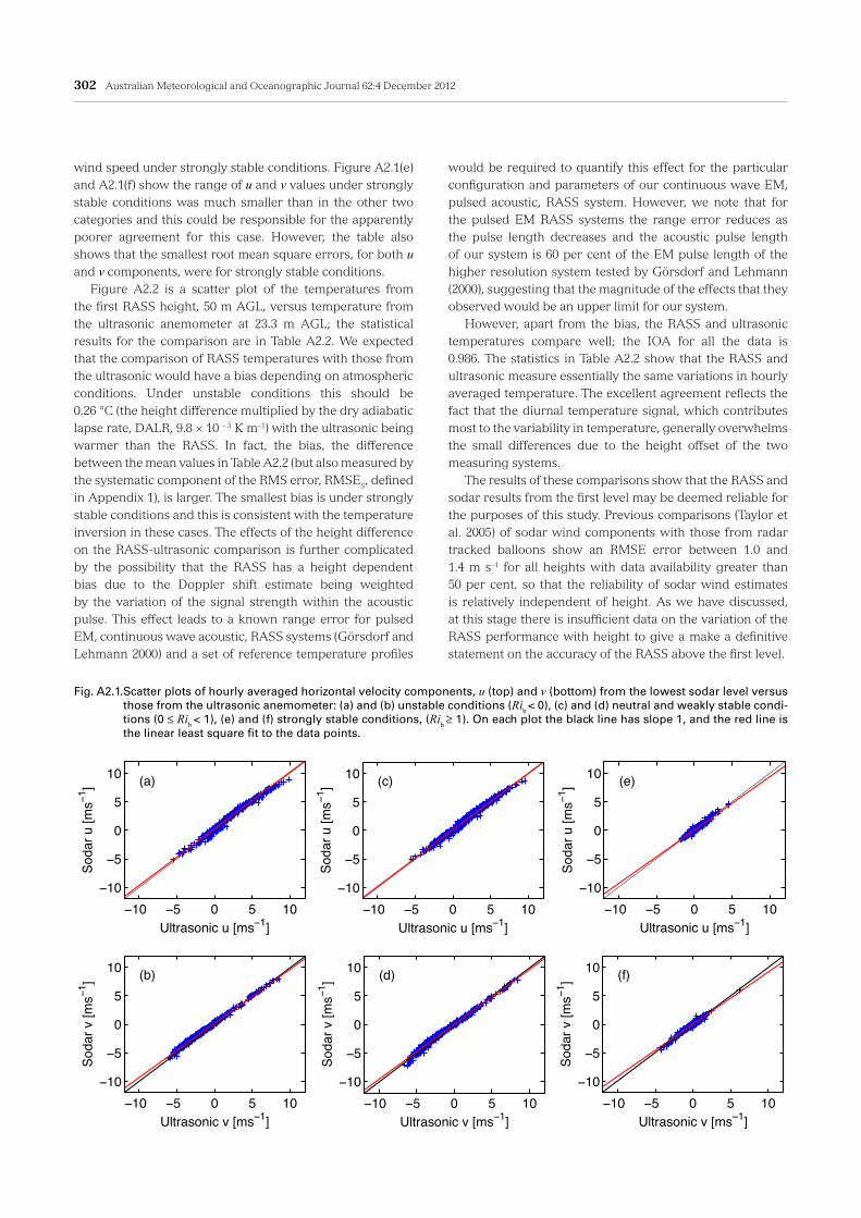
Appendix 2: Verification of the sodar and RASS against the ultrasonic anemometerAn important component of model verification is an assessment of the reliability of the observations. Radiosondes or wind finding balloons are not routinely launched at Canberra Airport, therefore, the best test of the performance of the profiling instruments available for the present experiment is to compare the wind speed and temperature data with that from the ultrasonic anemometer. The sodar wind time series from 20 m AGL (the minimum sodar range) can be compared directly with that from the ultrasonic anemometer located at 23.3 m AGL. We treat the ultrasonic data as the ‘true’ values and that from the sodar as the model results, then use the same analytical approach as that of Hurley (2000) to compare the two datasets. The definitions of all statistical quantities are given in Appendix 1 of this paper. For consistency with the later comparisons with TAPM output, one-hour averaged values are used. Before the comparison was made any one-hour periods during which rain occurred were excluded as the sodar’s performance in rain is limited by the noise of raindrops falling on the parabolic reflectors in the antennas. Figure A2.1 shows correlation plots for the two velocity components from the sodar for each stability class and Table A2.1 gives a summary of the agreement between the datasets. The minimum Index of Agreement (IOA), 0.980, is for the u-component of the

302 Australian Meteorological and Oceanographic Journal 62:4 December 2012

wind speed under strongly stable conditions. Figure A2.1(e) and A2.1(f) show the range of u and v values under strongly stable conditions was much smaller than in the other two categories and this could be responsible for the apparently poorer agreement for this case. However, the table also shows that the smallest root mean square errors, for both u and v components, were for strongly stable conditions. Figure A2.2 is a scatter plot of the temperatures from the first RASS height, 50 m AGL, versus temperature from the ultrasonic anemometer at 23.3 m AGL; the statistical results for the comparison are in Table A2.2. We expected that the comparison of RASS temperatures with those from the ultrasonic would have a bias depending on atmospheric conditions. Under unstable conditions this should be 0.26 °C (the height difference multiplied by the dry adiabatic lapse rate, DALR, 9.8 × 10 – 3 K m–1) with the ultrasonic being warmer than the RASS. In fact, the bias, the difference between the mean values in Table A2.2 (but also measured by the systematic component of the RMS error, RMSES, defined in Appendix 1), is larger. The smallest bias is under strongly stable conditions and this is consistent with the temperature inversion in these cases. The effects of the height difference on the RASS-ultrasonic comparison is further complicated by the possibility that the RASS has a height dependent bias due to the Doppler shift estimate being weighted by the variation of the signal strength within the acoustic pulse. This effect leads to a known range error for pulsed EM, continuous wave acoustic, RASS systems (Görsdorf and Lehmann 2000) and a set of reference temperature profiles

Fig. A2.1. Scatter plots of hourly averaged horizontal velocity components, u (top) and v (bottom) from the lowest sodar level versus those from the ultrasonic anemometer: (a) and (b) unstable conditions (Rib < 0), (c) and (d) neutral and weakly stable condi-tions (0 ≤ Rib < 1), (e) and (f) strongly stable conditions, (Rib ≥ 1). On each plot the black line has slope 1, and the red line is the linear least square fit to the data points.

−10 −5 0 5 10−10

−5

0

5

10

Ultrasonic u [ms−1]

Soda

r u [m

s−1] (a)

−10 −5 0 5 10−10

−5

0

5

10

Ultrasonic v [ms−1]

Soda

r v [m

s−1] (b)

−10 −5 0 5 10−10

−5

0

5

10

Ultrasonic u [ms−1]

Soda

r u [m

s−1] (c)

−10 −5 0 5 10−10

−5

0

5

10

Ultrasonic v [ms−1]

Soda

r v [m

s−1] (d)

−10 −5 0 5 10−10

−5

0

5

10

Ultrasonic u [ms−1]

Soda

r u [m

s−1] (e)

−10 −5 0 5 10−10

−5

0

5

10

Ultrasonic v [ms−1]

Soda

r v [m

s−1] (f)

−10 −5 0 5 10−10

−5

0

5

10

Ultrasonic u [ms−1]

Soda

r u [m

s−1] (e)

−10 −5 0 5 10−10

−5

0

5

10

Ultrasonic v [ms−1]

Soda

r v [m

s−1] (f)

−10 −5 0 5 10−10

−5

0

5

10

Ultrasonic u [ms−1]

Soda

r u [m

s−1] (a)

−10 −5 0 5 10−10

−5

0

5

10

Ultrasonic v [ms−1]

Soda

r v [m

s−1] (b)

−10 −5 0 5 10−10

−5

0

5

10

Ultrasonic u [ms−1]

Soda

r u [m

s−1] (c)

−10 −5 0 5 10−10

−5

0

5

10

Ultrasonic v [ms−1]

Soda

r v [m

s−1] (d)

−10 −5 0 5 10−10

−5

0

5

10

Ultrasonic u [ms−1]

Soda

r u [m

s−1] (a)

−10 −5 0 5 10−10

−5

0

5

10

Ultrasonic v [ms−1]

Soda

r v [m

s−1] (b)

−10 −5 0 5 10−10

−5

0

5

10

Ultrasonic u [ms−1]

Soda

r u [m

s−1] (c)

−10 −5 0 5 10−10

−5

0

5

10

Ultrasonic v [ms−1]

Soda

r v [m

s−1] (d)

−10 −5 0 5 10−10

−5

0

5

10

Ultrasonic u [ms−1]

Soda

r u [m

s−1] (a)

−10 −5 0 5 10−10

−5

0

5

10

Ultrasonic v [ms−1]

Soda

r v [m

s−1] (b)

−10 −5 0 5 10−10

−5

0

5

10

Ultrasonic u [ms−1]

Soda

r u [m

s−1] (c)

−10 −5 0 5 10−10

−5

0

5

10

Ultrasonic v [ms−1]

Soda

r v [m

s−1] (d)

would be required to quantify this effect for the particular configuration and parameters of our continuous wave EM, pulsed acoustic, RASS system. However, we note that for the pulsed EM RASS systems the range error reduces as the pulse length decreases and the acoustic pulse length of our system is 60 per cent of the EM pulse length of the higher resolution system tested by Görsdorf and Lehmann (2000), suggesting that the magnitude of the effects that they observed would be an upper limit for our system. However, apart from the bias, the RASS and ultrasonic temperatures compare well; the IOA for all the data is 0.986. The statistics in Table A2.2 show that the RASS and ultrasonic measure essentially the same variations in hourly averaged temperature. The excellent agreement reflects the fact that the diurnal temperature signal, which contributes most to the variability in temperature, generally overwhelms the small differences due to the height offset of the two measuring systems. The results of these comparisons show that the RASS and sodar results from the first level may be deemed reliable for the purposes of this study. Previous comparisons (Taylor et al. 2005) of sodar wind components with those from radar tracked balloons show an RMSE error between 1.0 and 1.4 m s–1 for all heights with data availability greater than 50 per cent, so that the reliability of sodar wind estimates is relatively independent of height. As we have discussed, at this stage there is insufficient data on the variation of the RASS performance with height to give a make a definitive statement on the accuracy of the RASS above the first level.

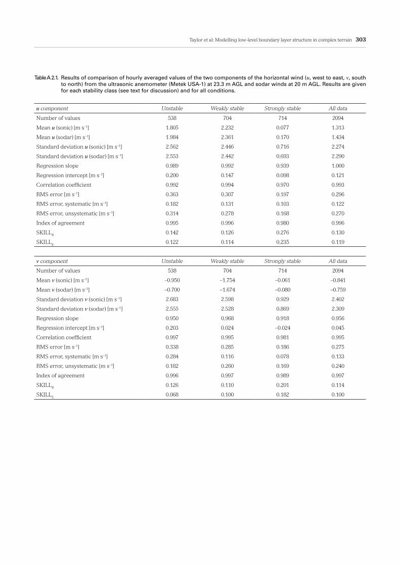
Taylor et al: Modelling low-level boundary layer structure in complex terrain 303

Table A 2.1. Results of comparison of hourly averaged values of the two components of the horizontal wind (u, west to east, v, south to north) from the ultrasonic anemometer (Metek USA-1) at 23.3 m AGL and sodar winds at 20 m AGL. Results are given for each stability class (see text for discussion) and for all conditions.

u component Unstable Weakly stable Strongly stable All data

Number of values 538 704 714 2094

Mean u (sonic) [m s–1] 1.805 2.232 0.077 1.313

Mean u (sodar) [m s–1] 1.984 2.361 0.170 1.434

Standard deviation u (sonic) [m s–1] 2.562 2.446 0.716 2.274

Standard deviation u (sodar) [m s–1] 2.553 2.442 0.693 2.290

Regression slope 0.989 0.992 0.939 1.000

Regression intercept [m s–1] 0.200 0.147 0.098 0.121

Correlation coefficient 0.992 0.994 0.970 0.993

RMS error [m s–1] 0.363 0.307 0.197 0.296

RMS error, systematic [m s–1] 0.182 0.131 0.103 0.122

RMS error, unsystematic [m s–1] 0.314 0.278 0.168 0.270

Index of agreement 0.995 0.996 0.980 0.996

SKILLR 0.142 0.126 0.276 0.130

SKILLE 0.122 0.114 0.235 0.119

v component Unstable Weakly stable Strongly stable All data

Number of values 538 704 714 2094

Mean v (sonic) [m s–1] –0.950 –1.754 –0.061 –0.841

Mean v (sodar) [m s–1] –0.700 –1.674 –0.080 –0.759

Standard deviation v (sonic) [m s–1] 2.683 2.598 0.929 2.402

Standard deviation v (sodar) [m s–1] 2.555 2.528 0.869 2.309

Regression slope 0.950 0.968 0.918 0.956

Regression intercept [m s–1] 0.203 0.024 –0.024 0.045

Correlation coefficient 0.997 0.995 0.981 0.995

RMS error [m s–1] 0.338 0.285 0.186 0.275

RMS error, systematic [m s–1] 0.284 0.116 0.078 0.133

RMS error, unsystematic [m s–1] 0.182 0.260 0.169 0.240

Index of agreement 0.996 0.997 0.989 0.997

SKILLR 0.126 0.110 0.201 0.114

SKILLE 0.068 0.100 0.182 0.100

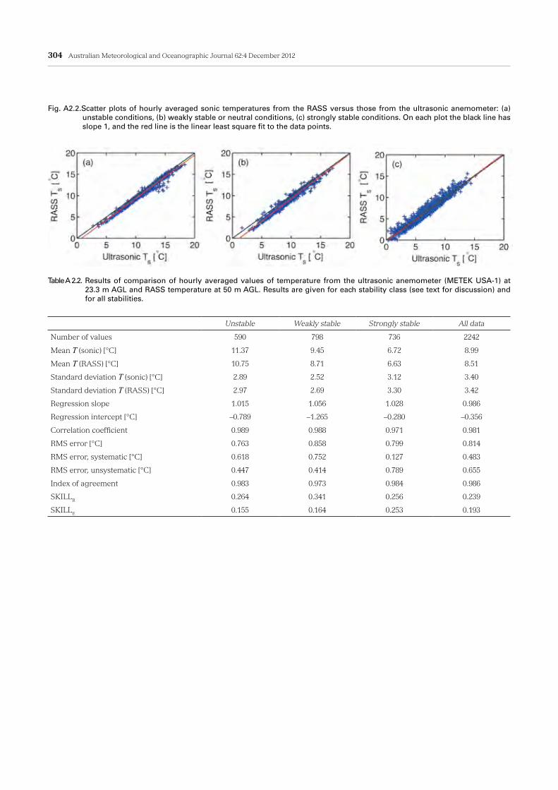
304 Australian Meteorological and Oceanographic Journal 62:4 December 2012

Table A 2.2. Results of comparison of hourly averaged values of temperature from the ultrasonic anemometer (METEK USA-1) at 23.3 m AGL and RASS temperature at 50 m AGL. Results are given for each stability class (see text for discussion) and for all stabilities.

Unstable Weakly stable Strongly stable All data

Number of values 590 798 736 2242

Mean T (sonic) [°C] 11.37 9.45 6.72 8.99

Mean T (RASS) [°C] 10.75 8.71 6.63 8.51

Standard deviation T (sonic) [°C] 2.89 2.52 3.12 3.40

Standard deviation T (RASS) [°C] 2.97 2.69 3.30 3.42

Regression slope 1.015 1.056 1.028 0.986

Regression intercept [°C] –0.789 –1.265 –0.280 –0.356

Correlation coefficient 0.989 0.988 0.971 0.981

RMS error [°C] 0.763 0.858 0.799 0.814

RMS error, systematic [°C] 0.618 0.752 0.127 0.483

RMS error, unsystematic [°C] 0.447 0.414 0.789 0.655

Index of agreement 0.983 0.973 0.984 0.986

SKILLR 0.264 0.341 0.256 0.239

SKILLE 0.155 0.164 0.253 0.193

Fig. A2.2.Scatter plots of hourly averaged sonic temperatures from the RASS versus those from the ultrasonic anemometer: (a) unstable conditions, (b) weakly stable or neutral conditions, (c) strongly stable conditions. On each plot the black line has slope 1, and the red line is the linear least square fit to the data points.