?

Modelling mechanisms with causal cycles

?

Brendan Clarke, Bert Leuridan & Jon Williamson

Draft of September 30, 2013

Abstract

Mechanistic philosophy of science views a large part of scientific activityas engaged in modelling mechanisms. While science textbooks tend to offerqualitative models of mechanisms, there is increasing demand for models fromwhich one can draw quantitative predictions and explanations. Casini et al.(2011) put forward the Recursive Bayesian Net (RBN) formalism as well suitedto this end. The RBN formalism is an extension of the standard Bayesiannet formalism, an extension that allows for modelling the hierarchical natureof mechanisms. Like the standard Bayesian net formalism, it models causalrelationships using directed acyclic graphs. Given this appeal to acyclicity,causal cycles pose a prima facie problem for the RBN approach. This paperargues that the problem is a significant one given the ubiquity of causal cyclesin mechanisms, but that the problem can be solved by combining two sorts ofsolution strategy in a judicious way.

§1Introduction

The concept of ‘complex-system mechanism’, which is commonly defined such thata mechanism’s behaviour is realized by the organized behaviour of its componentparts, plays an increasingly important role in philosophy of science. A natural ques-tion to ask is how mechanisms can or should be modelled. Adequately modellingmechanisms is a precondition for succesful mechanistic prediction, interventionand/or explanation. Non-formal models of mechanisms have been discussed atlength in philosophy of science; see for example Glennan (2005), Bechtel and Abra-hamsen (2005), and Craver (2006). Some authors have posited the need, however,to develop formal models of mechanisms that might be used to draw quantitative,as well as qualitative, inferences from the model (Lazebnik, 2002; Bechtel, 2011).In this paper, we will elaborate one possible formal approach: mechanisms can bemodelled by means of Recursive Bayesian Networks (RBNs). The RBN formalismis an extension of the standard Bayesian net formalism. In contrast with standardBayesian nets, RBNs can be used to model the hierarchical nature of mechanisms.This approach to modelling mechanisms was originally put forward by Casini et al.(2011). One limitation of that work, however, was that it lacked a principled wayof handling mechanisms that involve causal cycles. The primary aim of this paperis to provide such an account. Given the ubiquity of cycles in mechanisms (see

§3), this is an important step forward in the development of the RBN approach tomechanistic modelling.

The structure of the paper is as follows. §2 and §3 together motivate our project,in that they substantiate the need for an RBN account that can handle cycles. Assuch, they make clear both why Casini et al. (2011) have provided an interestingapproach to mechanistic modelling, and in what ways their account should bemodified to be useful when modelling cases from scientific practice. In §2 we willhighlight three important features of mechanisms as they are discussed in recentphilosophy of science. It will emerge that the machinery of Recursive BayesianNetworks will be well suited to modelling mechanisms—on the condition that theacyclicity assumption, inherited from standard Bayesian networks, is dropped. In§3 we will argue that cycles are everywhere in the sciences, in particular in thebiomedical and the biological sciences. We also offer a threefold classificationof cycles. We then discuss three mereologically nested examples of biomedicalmechanisms with cycles, drawn from recent sleep research, in some detail. In §4 weintroduce the framework of Recursive Bayesian Networks and the ordinary causalBayesian networks to which they are related. We also show how they may be usedfor inference (e.g., prediction). Finally, we show that the cycles discussed in §3 posea conundrum for RBNs as defined in Casini et al. (2011), which are assumed to beacyclic. In §5 we sketch two ways to handle causal cycles in ordinary causal Bayesiannets. The first is a discussion of the extent to which well-known results (relating tod-separation and the Causal Markov Condition) carry over from the acyclic to thecyclic case. The second makes use of Dynamic Bayesian Nets (DBNs). Both thesesolutions are then incorporated in the RBN framework in §6, thus allowing forRecursive Bayesian Networks that contain cycles. Which solution to apply dependson the type of problem that is studied, as well as on pragmatic considerations, suchas the granularity of analysis that is required. We distinguish between static anddynamic problems, relate them to the three-fold classification of cycles offered in§3, and provide examples of how they can be handled. Finally, in §7, we summarizeour approach and make some concluding remarks.

Before we start, we would like to make two terminological and two substantiveremarks. The first remark concerns the notion ‘recursive’. In the older literatureon structural equation modelling and causal Bayesian nets, this was often used inthe sense of ‘acyclic’ (see, e.g., Spirtes, 1995). Hence one may worry that ‘cyclicRecursive Bayesian Net’ is a contradiction in terms. As RBNs use ‘recursive’ ina different sense—the more standard sense of a recursive or inductive definition,which can appeal to another instance of itself—this worry should not arise.

The second remark concerns the notion of ‘cyclicity’ itself. The topic of cycliccausality is studied in diverse domains, ranging from AI and computer science,through philosophy of science, to a wide range of empirical sciences. In thesedomains, several synonyms (or close proxies) for ‘cyclicity’ are used, among which‘bidirectionality’ and ‘feedback’ are the most common ones. Since ‘bidirectionalarcs’ are often used in the literature on causal discovery to denote the existenceof (unobserved) confounding factors instead of bidirectional causal influences, andsince ‘bidirectional causality’ often refers to ‘atomic’ cycles of the form A � B(where A is a direct cause of B and vice versa), we will avoid using the word‘bidirectionality’. In §3, we will touch on the notion of ‘feedback’ in more detail,distinguishing three types of feedback and elucidating their links with ‘cyclicity’.

The third remark relates to the precise goal of our paper, which is modellingmechanisms. We do not intend to tackle issues of causal (or mechanism) discov-

ery, such as specifying algorithms for inferring RBNs from observational and/orexperimental data. We presuppose the mechanism is known (be it completely orincompletely, fallibly or infallibly) and ask how we can best model it so as to drawquantitative inferences. This account may then serve as a basis for further researchon formal methods for mechanism discovery.1

The fourth remark concerns the interpretation of causality. In the mechanisticliterature, Woodward’s interventionist account of causality is relatively widespread(see Woodward, 2003, for the interventionist account; see e.g., Glennan, 2002,Woodward, 20022, Craver, 2007 and Leuridan, 2010, for appeals to the interven-tionist account of causality within a mechanistic framework). As is well known,Woodward’s account nicely fits the causal Bayesian nets literature.3 Another inter-pretation that has been proposed with an eye to causal Bayesian nets is the epistemicaccount, according to which causation is a feature of the way we represent the worldrather than the world itself, yet it is objective in the sense that if two agents with thesame evidence disagree regarding a causal claim, one may be right and the otherwrong; see Williamson (2005, chapter 9). In this paper, we will not adopt a specificaccount of causality. Any account that suits the causal Bayesian nets framework,such as the two just mentioned, can be chosen.

In the interest of readability, we aim to keep the paper as non-technical aspossible. Further technical details concerning the frameworks we use can be foundin the references.

§2Importance for philosophy of science

The concept of ‘complex-system mechanism’ plays an increasingly important role inphilosophy of science. In this paper, we will not survey the overwhelming literatureon mechanisms (see for example Machamer et al., 2000, Glennan, 1996, Glennan,2002, Bechtel and Abrahamsen, 2005). Rather, we will focus on two recent worksin the mechanistic tradition, one by Carl Craver and one by William Bechtel, andfocus on three key features of mechanisms and mechanistic models they discuss.These three features will set the agenda for our paper.

In his book Explaining the Brain, Craver (2007) gives a very detailed account ofmechanisms. A first feature that emerges from his work, is that mechanisms are hi-erarchically organized. As we wrote above, mechanisms are commonly defined suchthat their higher-level behaviour is realized by the organized lower-level behavioursof their component parts. This hierarchical structure need not be confined to twolevels. The behaviours of a mechanism’s components may themselves be mechanis-tically explicable as well. In fact, there may be a whole series of nested mechanisms

1Note that, as with all models, a recursive Bayesian network model only models some aspects ofa mechanism. The main goal is to model the hierarchical structure of the mechanism together withthe causal structure at each level of the hierarchy, in such a way that the model can be used to drawquantitative inferences. See Casini et al. (2011) for a fuller presentation of the motivation behind this sortof model, and §7 of this paper for pointers to possible limitations of the RBN approach.

2Woodward’s concept of ‘mechanism’, or more precisely: of ‘mechanistic model’, is not explicitlymulti-level or hierarchical, in contrast to those on which we focus in this paper. In the next section,the hierarchical nature will serve as one of the main reasons to adopt the RBN approach to mechanisticmodelling.

3As such, his account of causality also forms the starting point for causal Bayes net accounts of thestructure of scientific theories (see Leuridan, 2014).

S‐ing

X11‐ing

X22‐ing

X33‐ing

X44‐ing

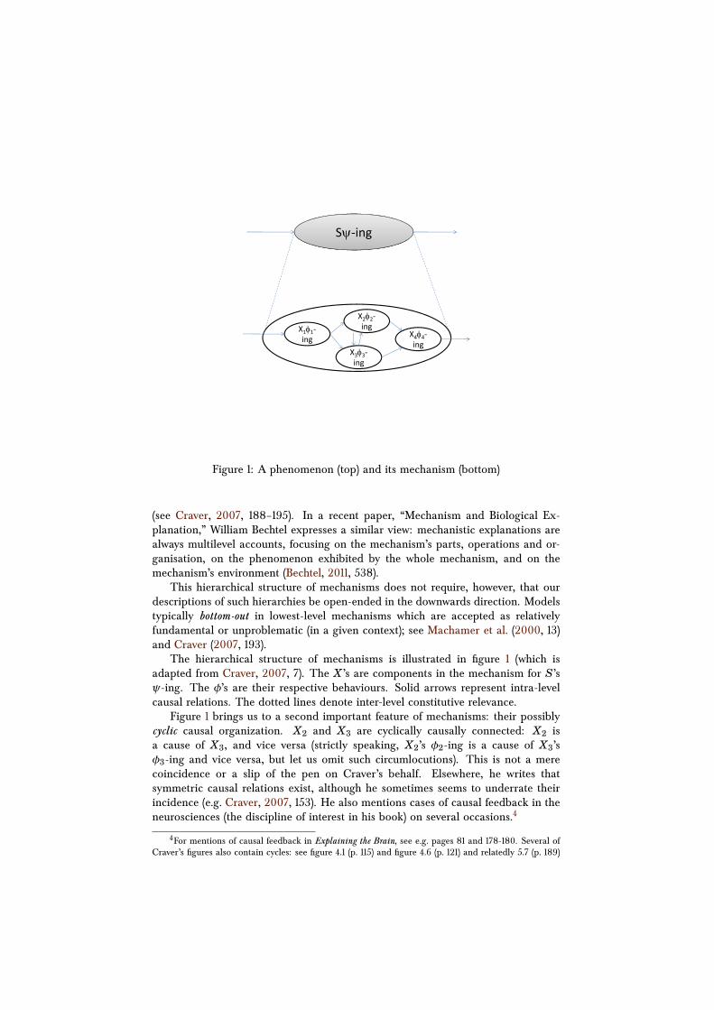
Figure 1: A phenomenon (top) and its mechanism (bottom)

(see Craver, 2007, 188–195). In a recent paper, “Mechanism and Biological Ex-planation,” William Bechtel expresses a similar view: mechanistic explanations arealways multilevel accounts, focusing on the mechanism’s parts, operations and or-ganisation, on the phenomenon exhibited by the whole mechanism, and on themechanism’s environment (Bechtel, 2011, 538).

This hierarchical structure of mechanisms does not require, however, that ourdescriptions of such hierarchies be open-ended in the downwards direction. Modelstypically bottom-out in lowest-level mechanisms which are accepted as relativelyfundamental or unproblematic (in a given context); see Machamer et al. (2000, 13)and Craver (2007, 193).

The hierarchical structure of mechanisms is illustrated in figure 1 (which isadapted from Craver, 2007, 7). The X ’s are components in the mechanism for S’sψ-ing. The φ’s are their respective behaviours. Solid arrows represent intra-levelcausal relations. The dotted lines denote inter-level constitutive relevance.

Figure 1 brings us to a second important feature of mechanisms: their possiblycyclic causal organization. X2 and X3 are cyclically causally connected: X2 isa cause of X3, and vice versa (strictly speaking, X2’s φ2-ing is a cause of X3’sφ3-ing and vice versa, but let us omit such circumlocutions). This is not a merecoincidence or a slip of the pen on Craver’s behalf. Elsewhere, he writes thatsymmetric causal relations exist, although he sometimes seems to underrate theirincidence (e.g. Craver, 2007, 153). He also mentions cases of causal feedback in theneurosciences (the discipline of interest in his book) on several occasions.4

4For mentions of causal feedback in Explaining the Brain, see e.g. pages 81 and 178-180. Several ofCraver’s figures also contain cycles: see figure 4.1 (p. 115) and figure 4.6 (p. 121) and relatedly 5.7 (p. 189)

Bechtel attaches great importance to cyclicity. A crucial feature of biological or-ganisms is ‘their autonomy—their ability to maintain themselves as systems distinctfrom their environment by directing the flow of matter and energy so as to buildand repair themselves’ (Bechtel, 2011, 535). For this autonomy, cyclic organization ispivotal: ‘Autonomous systems must employ a nonsequential or cyclic organizationsuch as negative feedback . . . ’ (Bechtel, 2011, 544). Mechanisms cannot be modelledmerely sequentially without loss of crucial information.

A third important feature, which is heavily stressed by Bechtel (2011, 536–537),is that to adequately model a mechanism, one has to model not only its qualitativeaspects, but also its quantitative aspects. Bechtel proposes computational modelingand dynamic systems analysis as methods to account for the non-qualitative aspectsof mechanisms. We will propose a different approach here: an approach based oncausal Bayesian nets.

As we shall see in §4, causal Bayesian nets can model both the qualitativeaspects of causal structures by means of a causal graph and their quantitativeaspects by means of the associated probability distribution. Hence this approachwould automatically meet Bechtel’s call for a quantitative account of mechanisms.Following Casini et al. (2011), we use Recursive Bayesian Nets (RBNs) instead ofstandard causal Bayesian nets so as to account for the mechanisms’ hierarchicalorganization (§4). In order to account for the mechanisms’ possibly cyclic causalorganisation, we will explore existing solutions to the problem of cyclicity in causalBayesian nets (§5) and incorporate these in the RBN framework (§6). As a result, weprovide a formal account of mechanisms that combines all three features discussedabove.

But first we shall explore the abundance of cyclic mechanisms in the sciencesand distinguish between several types of causal cycles, as this will influence thechoice of technical solution in each context (§3).

§3Importance for the sciences

Although not every causal relationship of interest to the sciences exhibits cyclicity,very many causes of practical importance do. A bibliographic search in the ISIWeb of Science for “topic=(causal feedback)” on the 4th of November 2011 yielded1,161 hits in disciplines as diverse as cell biology, biochemistry, molecular biology,neuroscience, environmental studies, psychology and social psychology, while awider search in all of the ISI’s databases yielded a total of 1,603 hits. Cycles areeverywhere in the sciences.

They are particularly prevalent in the biomedical and biological sciences. Ex-amples include metabolic cycles (such as Krebs’ cycle), organismal life cycles (suchas the malaria-causing organisms of the genus Plasmodium), homeostatic pathways(such as blood glucose regulation) and pathological processes. A survey of the 790images contained in a recent medical textbook, Davidson’s Principles & Practice ofMedicine, 20th edition (Boon et al., 2006), revealed a total of 154 images that con-tained some graphical representation of causal processes. 51 of these figures (33%)were at least partially cyclic, conveying knowledge about the regulation of the cell

and 5.8 (p. 194). Moreover, figure 3.2 (p. 71) and relatedly 4.1 (p. 166), leave open the possibility of causalfeedback.

cycle, the life-cycles of various pathogenic organisms, the homeostasis of fat, fluidsand ions, the arrangement of hormone systems and the development of disease.

A simple example of this kind of cycle is post-traumatic raised intracranialpressure. Here, trauma to the head may cause swelling of the brain. This swellingincreases the pressure within the fixed volume of the skull. The consequence of thisincreased intracranial pressure is to reduce cerebral perfusion, which in turn causescerebral hypoxia. This hypoxic insult causes damage to the brain cells, which leadsto further swelling.

One interesting feature of these causal cycles concerns the way that the organ-isation of parts and operations governs the type of feedback seen in that cycle.Three arrangements are possible. Negative-feedback cycles are those in which theproperties of the parts in the cycle tend to maintain the status quo by virtue ofthe organisation of their operations. Thus, the higher level phenomena producedby negative-feedback cycles tend to be stable, as in the case of many metabolicand homeostatic processes.5 With respect to medicine, this means that negative-feedback cycles are typically physiological, rather than disease-producing. Secondare positive-feedback cycles. Here, the organisation of parts and operations tendsto produce divergence from equilibrium of one or more parts over time. Thesekinds of cycles are typically associated with the production of identifiable diseasestates, such as the head trauma example given above.6 In this case, the degrees ofswelling, intracranial pressure, and cellular damage will tend to increase, while cere-bral perfusion and oxygenation will tend to decrease. The higher level phenomenaproduced by positive-feedback cycles thus demonstrate exponential growth overtime—at least until restrained by external factors. Finally, a third kind of cycleexists in which the organisation of the cycle neither tends to produce movementtowards, or away from, equilibrium. In these kinds of contingent-feedback cycles, theactual direction of change is predominantly governed by factors extrinsic to thecycle. For example, the parts of a parasitic life-cycle are largely governed by factorsexternal to that cycle, meaning that either positive or negative feedback may occurin different instantiations.7

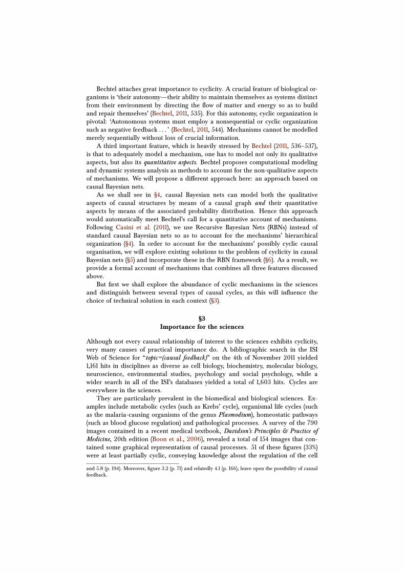
The type of feedback seen in a particular cycle partly depends on the mannerin which we investigate that cycle. For example, an oscillating system studied overdurations much shorter than its period may appear to demonstrate positive feed-back, yet will appear to show negative feedback if studied at much longer durations.An example of this granularity in the description of feedback can be seen in thepathway by which the concentration of thyroid hormones is maintained (see figure2). The secretion of thyrotropin-releasing hormone (TRH) from the hypothalamusstimulates the pituitary gland to secrete thyroid-stimulating hormone (TSH). In turn,this causes the thyroid to secrete the hormone thyroxine.8 The resultant increase

5This property of negative feedback systems to tend toward equilibrium is the case when there is nosignificant delay in the system. When delay is present, as it is in many biological systems, oscillationswill tend to arise. We would like to thank Mike Joffe for pressing us on this issue.

6However, this is not always the case. For instance, various positive feedback loops in pregnancyserve to appropriately maintain hormone levels.

7These kinds of contingent-feedback cycles are, in other words, more sensitive to background con-ditions than the other two kinds. This makes them unstable, in Mitchell’s sense of stability as describingthe sensitivity of relations to their background conditions (Mitchell, 2009, 56). This should be discrimi-nated from robustness, which describes the degree to which a function is maintained when one or moreconstitutive elements are disrupted (Mitchell, 2009, 69-73).

8This cycle is more complicated than suggested above. For example, the thyroid secretes twohormones—T3 and T4—which can be interconverted, and feedback occurs at various intermediate

���

���

�

�������

�

�

Figure 2: Thyroxine example. TRH: thyrotropin-releasing hormone; TSH: thyroid-stimulating hormone.

in circulating thyroxine levels inhibits the secretion of TRH by the hypothalamus,which has the effect, via reduced TSH secretion, of reducing the concentrationof thyroxine. When viewed over the long-term, this is a negative-feedback cycle,as the concentrations of each of the hormones involved tend towards equilibrium.However, at very short durations, individual parts of the mechanism may undergochanges away from their equilibrium point. Thus, the type of feedback modelleddepends on the granularity with which we investigate a phenomenon of interest.Modelling feedback, as with many other considerations in mechanistic modelling,also depends on pragmatic factors such as the required level of detail.

Given this brief introduction to cycles in practice, the remainder of this sectionwill discuss three mereologically nested examples of biomedical mechanisms withcycles, drawn from recent work in sleep research.

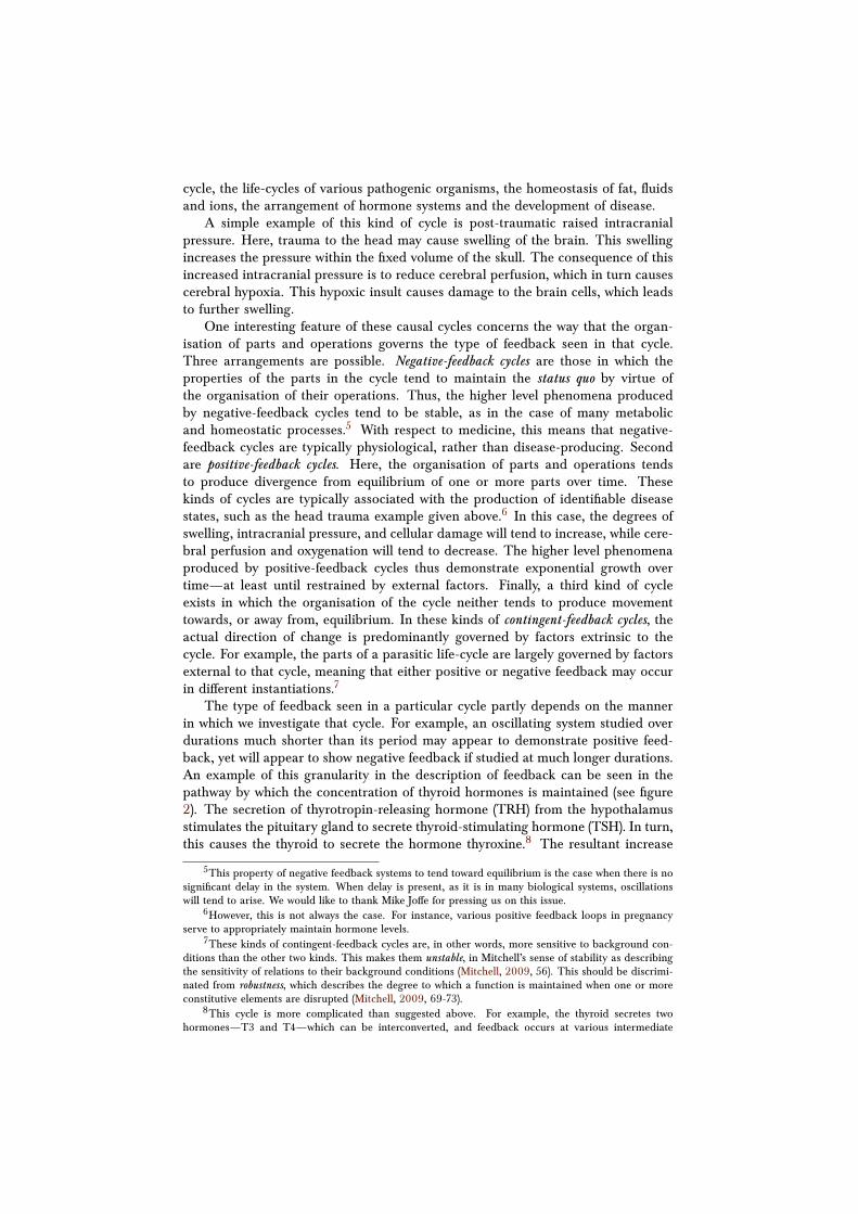
Public health example

Insufficient sleep is correlated with mortality (Grandner et al., 2010). However, themechanism underlying this association is highly complex and poorly understood.As figure 3 suggests, an extensive network of social, psychological and pathologicalstates causally interact with both sleep and mortality. The duration and qualityof sleep interact cyclically with a range of mortality-associated physiological andsocial outcomes including obesity, cardiovascular disease, stress and metabolic dys-function (indicated by edges C and E, figure 3). To illustrate this, consider therelationship between insufficient sleep and cardiovascular disease. Broadly, whilecardiovascular disease causes impaired sleep (perhaps by causing chest pain orshortness of breath while lying down), impaired sleep may also cause cardiovascu-lar disease (perhaps by increasing blood pressure).

points in the cycle. But this simple version is adequate for our discussion.

Figure 3: Figure showing cyclical interactions between sleep and health outcomes(Grandner et al., 2010, 200). Reprinted from Sleep Medicine Reviews, 14(3), MichaelA. Grandner, Lauren Hale, Melisa Moore and Nirav P. Patel, Mortality associatedwith short sleep duration: The evidence, the possible mechanisms, and the future,pages 191-203. Copyright 2010, with permission from Elsevier.

�������������

����������������������

�����������

���

�����

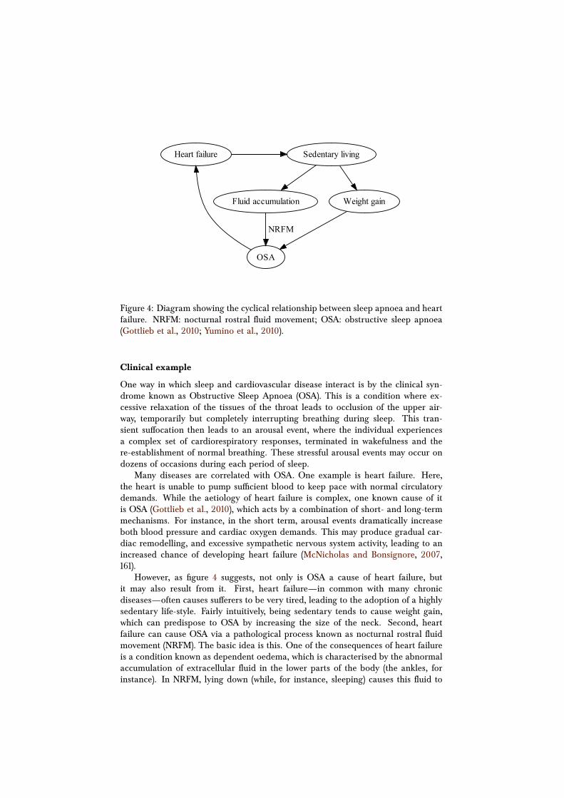
Figure 4: Diagram showing the cyclical relationship between sleep apnoea and heartfailure. NRFM: nocturnal rostral fluid movement; OSA: obstructive sleep apnoea(Gottlieb et al., 2010; Yumino et al., 2010).

Clinical example

One way in which sleep and cardiovascular disease interact is by the clinical syn-drome known as Obstructive Sleep Apnoea (OSA). This is a condition where ex-cessive relaxation of the tissues of the throat leads to occlusion of the upper air-way, temporarily but completely interrupting breathing during sleep. This tran-sient suffocation then leads to an arousal event, where the individual experiencesa complex set of cardiorespiratory responses, terminated in wakefulness and there-establishment of normal breathing. These stressful arousal events may occur ondozens of occasions during each period of sleep.

Many diseases are correlated with OSA. One example is heart failure. Here,the heart is unable to pump sufficient blood to keep pace with normal circulatorydemands. While the aetiology of heart failure is complex, one known cause of itis OSA (Gottlieb et al., 2010), which acts by a combination of short- and long-termmechanisms. For instance, in the short term, arousal events dramatically increaseboth blood pressure and cardiac oxygen demands. This may produce gradual car-diac remodelling, and excessive sympathetic nervous system activity, leading to anincreased chance of developing heart failure (McNicholas and Bonsignore, 2007,161).

However, as figure 4 suggests, not only is OSA a cause of heart failure, butit may also result from it. First, heart failure—in common with many chronicdiseases—often causes sufferers to be very tired, leading to the adoption of a highlysedentary life-style. Fairly intuitively, being sedentary tends to cause weight gain,which can predispose to OSA by increasing the size of the neck. Second, heartfailure can cause OSA via a pathological process known as nocturnal rostral fluidmovement (NRFM). The basic idea is this. One of the consequences of heart failureis a condition known as dependent oedema, which is characterised by the abnormalaccumulation of extracellular fluid in the lower parts of the body (the ankles, forinstance). In NRFM, lying down (while, for instance, sleeping) causes this fluid to

migrate up from the lower part of the body towards the head and neck. Here, thefluid accumulates in the soft tissues of the throat, producing an enlargement of thesoft tissues in an analogous way to obesity, and similarly increasing the chances ofairway obstruction (Yumino et al., 2010). Heart failure, via both weight gain andNRFM, causes OSA, while OSA, via a series of complex processes associated witharousal events, causes heart failure.

Neuroscience example

A neurologically important feature of normal NREM sleep is the slow wave-likerhythm in which neurones across the cortex ‘beat’ at a frequency of about 1Hz.9 Thisslow wave sleep is thought to be causally significant in consolidating new memories(Marshall et al., 2006). This oscillation comes about from a cycle that obtainsbetween three populations of neurones (Crunelli and Hughes, 2010), as describedin figure 5. First, two populations of neocortical neurones—‘a subset of pyramidalneurons in layers 2/3 and 5 and a group of Martinotti cells that is exclusivelylocated in layer 5’ (Crunelli and Hughes, 2010, 11)—and a group of thalamic cells,known as cortically projecting thalamic (CT) neurones, act as intrinsic pacemakers,spontaneously generating a slow oscillation. Together, the effect of these pacingcells is to stimulate two populations of nerves in the thalamus—the CT and nucleusreticularis thalami (NRT) neurones. In turn, these thalamic cells, once stimulated inthis way, evoke a strong oscillatory response from the thalamus more broadly. Thishas the effect of stimulating ‘virtually all cortical neurones’ (Crunelli and Hughes,2010, 10) to produce the <1Hz oscillation seen on EEG. This waveform thereforearises by virtue of the cyclical interactions between three different populations ofneurones, as Crunelli and Hughes suggest: ‘the full EEG manifestation of the slowrhythm requires the essential dynamic tuning provided by their complex synapticinteractions’ (Crunelli and Hughes, 2010, 14).

§4Recursive Bayesian networks

In this section we will introduce Recursive Bayesian networks and see that causalcycles present a prima facie problem for this formalism.

Origins

Bayesian networks were developed in the 1980s in order to facilitate, among otherthings, quantitative reasoning about causal relationships (Pearl, 1988).10 A causally-interpreted Bayesian net uses a directed acyclic graph (DAG) to represent qualitativecausal relationships and the probability distribution of each variable conditional onits parents to represent quantitative relationships amongst the variables. The Re-cursive Bayesian Network (RBN) formalism was developed to model nested causalrelationships such as [smoking causing cancer] causes tobacco advertising restrictions

9Similar examples of neurological oscillators are also discussed by Bechtel (2011, 548-549).10Structural equation modelling had previously been put forward for this purpose. But structural

equation models attempt to model deterministic relationships between cause and effect (with error termswhich are usually assumed to be independent and normally distributed), while Bayesian networks seekto represent the probability distribution of the variables in question. In general it is harder to devise anaccurate model of deterministic relationships than it is to determine probabilistic relationships betweencause and effect.

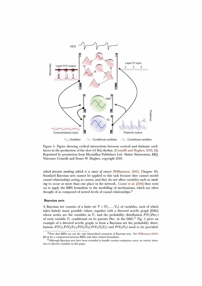
Figure 5: Figure showing cyclical interactions between cortical and thalamic oscil-lators in the production of the slow (<1 Hz) rhythm. (Crunelli and Hughes, 2010, 14).Reprinted by permission from Macmillan Publishers Ltd: Nature Neuroscience, 13(1),Vincenzo Crunelli and Stuart W. Hughes, copyright 2010.

which prevent smoking which is a cause of cancer (Williamson, 2005, Chapter 10).Standard Bayesian nets cannot be applied to this task because they cannot modelcausal relationships acting as causes, and they do not allow variables such as smok-ing to occur at more than one place in the network. Casini et al. (2011) then wenton to apply the RBN formalism to the modelling of mechanisms, which are oftenthought of as composed of nested levels of causal relationships.11

Bayesian nets

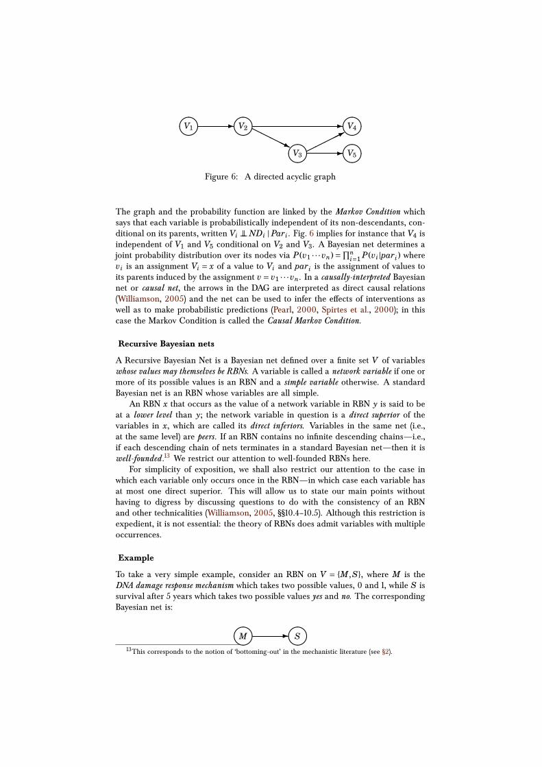
A Bayesian net consists of a finite set V = {V1, . . . ,Vn} of variables, each of whichtakes finitely many possible values, together with a directed acyclic graph (DAG)whose nodes are the variables in V , and the probability distribution P(Vi|Pari)of each variable Vi conditional on its parents Pari in the DAG.12 Fig. 6 gives anexample of a directed acyclic graph; to form a Bayesian net the probability distri-butions P(V1),P(V2|V1),P(V3|V2),P(V4|V2V3) and P(V5|V3) need to be provided.

11Note that RBNs are not the only hierarchical extension of Bayesian nets. See Williamson (2005,§10.2) for a comparison between RBNs and other related formalisms.

12Although Bayesian nets have been extended to handle certain continuous cases, we restrict atten-tion to discrete variables in this paper.

����V1 -����

V2 HHHHHj

-����V4

����V3��

���*

-����V5

Figure 6: A directed acyclic graph

The graph and the probability function are linked by the Markov Condition whichsays that each variable is probabilistically independent of its non-descendants, con-ditional on its parents, written Vi ⊥⊥NDi |Pari . Fig. 6 implies for instance that V4 isindependent of V1 and V5 conditional on V2 and V3. A Bayesian net determines ajoint probability distribution over its nodes via P(v1 · · ·vn)=∏n

i=1 P(vi|pari) wherevi is an assignment Vi = x of a value to Vi and pari is the assignment of values toits parents induced by the assignment v = v1 · · ·vn. In a causally-interpreted Bayesiannet or causal net, the arrows in the DAG are interpreted as direct causal relations(Williamson, 2005) and the net can be used to infer the effects of interventions aswell as to make probabilistic predictions (Pearl, 2000, Spirtes et al., 2000); in thiscase the Markov Condition is called the Causal Markov Condition.

Recursive Bayesian nets

A Recursive Bayesian Net is a Bayesian net defined over a finite set V of variableswhose values may themselves be RBNs. A variable is called a network variable if one ormore of its possible values is an RBN and a simple variable otherwise. A standardBayesian net is an RBN whose variables are all simple.

An RBN x that occurs as the value of a network variable in RBN y is said to beat a lower level than y; the network variable in question is a direct superior of thevariables in x, which are called its direct inferiors. Variables in the same net (i.e.,at the same level) are peers. If an RBN contains no infinite descending chains—i.e.,if each descending chain of nets terminates in a standard Bayesian net—then it iswell-founded .13 We restrict our attention to well-founded RBNs here.

For simplicity of exposition, we shall also restrict our attention to the case inwhich each variable only occurs once in the RBN—in which case each variable hasat most one direct superior. This will allow us to state our main points withouthaving to digress by discussing questions to do with the consistency of an RBNand other technicalities (Williamson, 2005, §§10.4–10.5). Although this restriction isexpedient, it is not essential: the theory of RBNs does admit variables with multipleoccurrences.

Example

To take a very simple example, consider an RBN on V = {M,S}, where M is theDNA damage response mechanism which takes two possible values, 0 and 1, while S issurvival after 5 years which takes two possible values yes and no. The correspondingBayesian net is:

����M -����

S13This corresponds to the notion of ‘bottoming-out’ in the mechanistic literature (see §2).

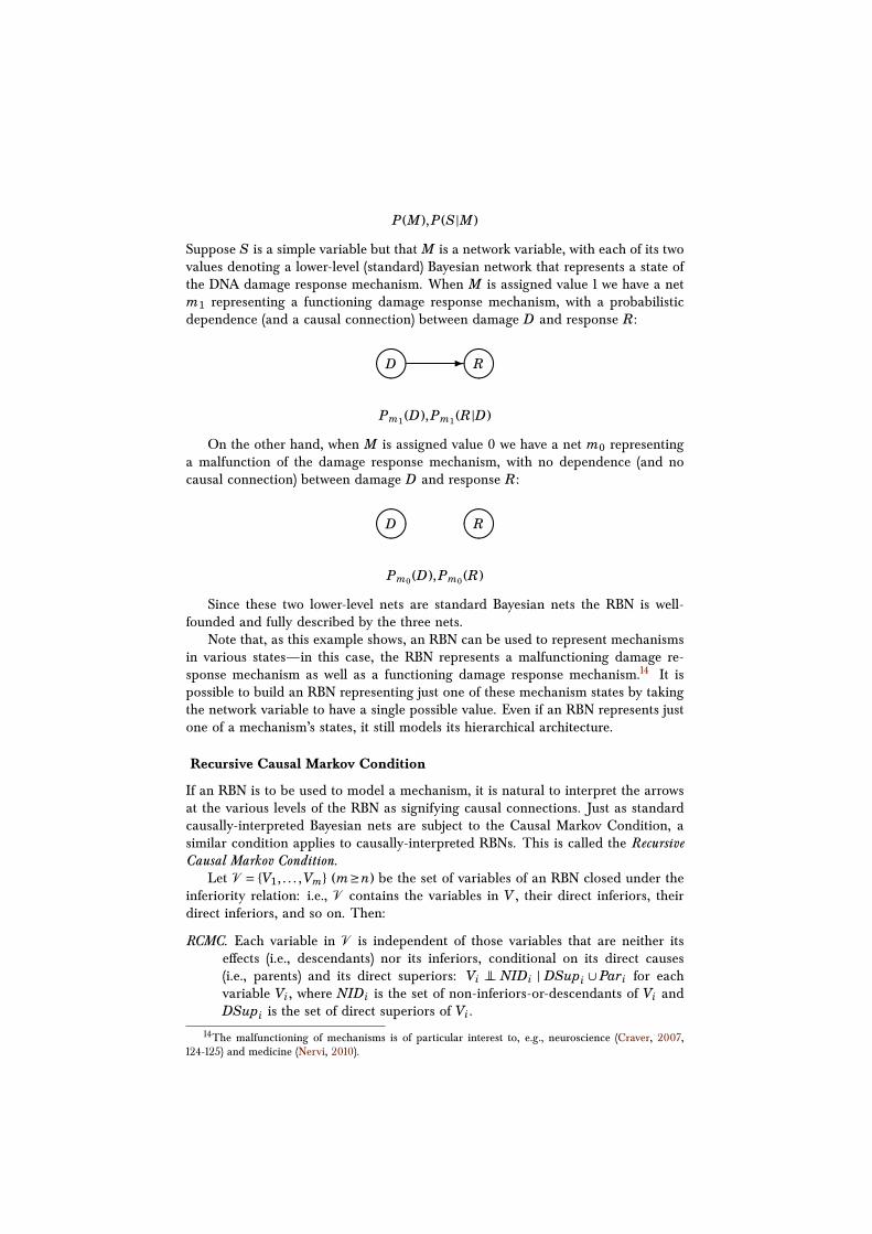
P(M),P(S|M)

Suppose S is a simple variable but that M is a network variable, with each of its twovalues denoting a lower-level (standard) Bayesian network that represents a state ofthe DNA damage response mechanism. When M is assigned value 1 we have a netm1 representing a functioning damage response mechanism, with a probabilisticdependence (and a causal connection) between damage D and response R:

����D -����

R

Pm1 (D),Pm1 (R|D)

On the other hand, when M is assigned value 0 we have a net m0 representinga malfunction of the damage response mechanism, with no dependence (and nocausal connection) between damage D and response R:

����D ����

R

Pm0 (D),Pm0 (R)

Since these two lower-level nets are standard Bayesian nets the RBN is well-founded and fully described by the three nets.

Note that, as this example shows, an RBN can be used to represent mechanismsin various states—in this case, the RBN represents a malfunctioning damage re-sponse mechanism as well as a functioning damage response mechanism.14 It ispossible to build an RBN representing just one of these mechanism states by takingthe network variable to have a single possible value. Even if an RBN represents justone of a mechanism’s states, it still models its hierarchical architecture.

Recursive Causal Markov Condition

If an RBN is to be used to model a mechanism, it is natural to interpret the arrowsat the various levels of the RBN as signifying causal connections. Just as standardcausally-interpreted Bayesian nets are subject to the Causal Markov Condition, asimilar condition applies to causally-interpreted RBNs. This is called the RecursiveCausal Markov Condition.

Let V = {V1, . . . ,Vm} (m≥n) be the set of variables of an RBN closed under theinferiority relation: i.e., V contains the variables in V , their direct inferiors, theirdirect inferiors, and so on. Then:

RCMC. Each variable in V is independent of those variables that are neither itseffects (i.e., descendants) nor its inferiors, conditional on its direct causes(i.e., parents) and its direct superiors: Vi ⊥⊥ NIDi | DSupi ∪Pari for eachvariable Vi , where NIDi is the set of non-inferiors-or-descendants of Vi andDSupi is the set of direct superiors of Vi .

14The malfunctioning of mechanisms is of particular interest to, e.g., neuroscience (Craver, 2007,124-125) and medicine (Nervi, 2010).

Note that, while some authors treat the Causal Markov Condition as a necessarytruth, others argue against its universal validity (see, e.g., Williamson, 2005). Wetreat the Causal Markov Condition and RCMC as modelling assumptions, in need oftesting or justification, rather than necessary truths.

Inference

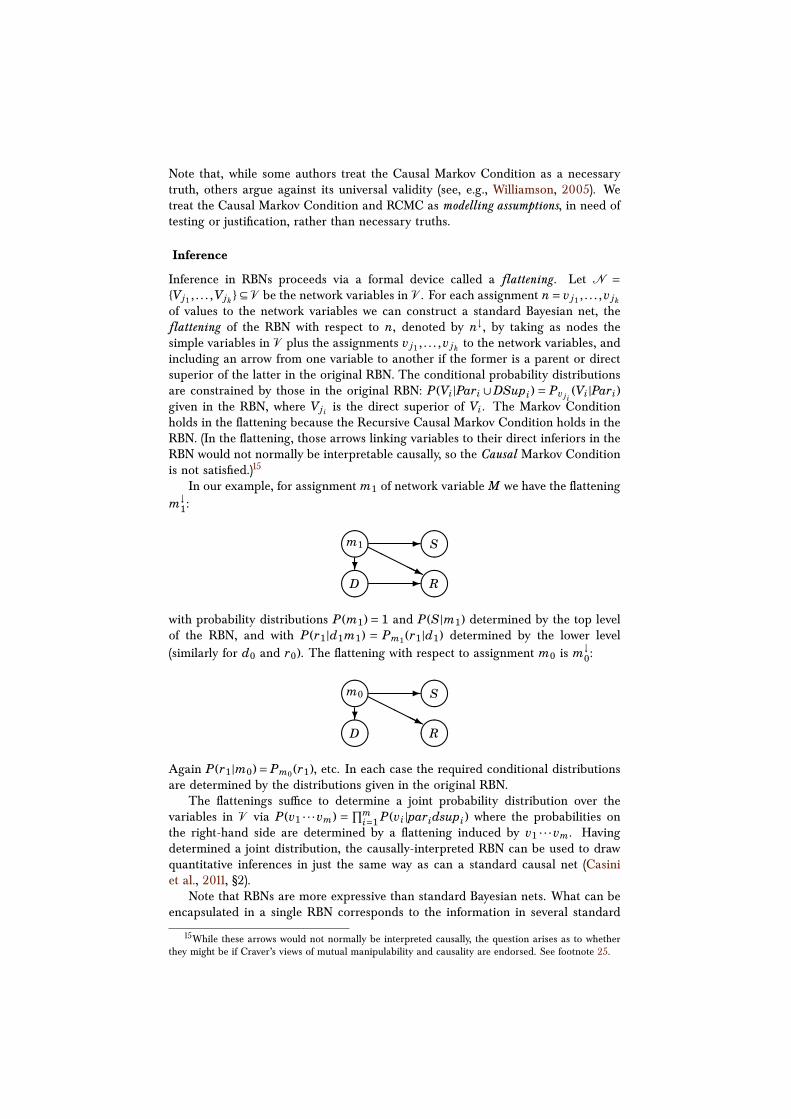
Inference in RBNs proceeds via a formal device called a flattening . Let N ={Vj1 , . . . ,Vjk }⊆ V be the network variables in V . For each assignment n = v j1 , . . . ,v jk

of values to the network variables we can construct a standard Bayesian net, theflattening of the RBN with respect to n, denoted by n↓, by taking as nodes thesimple variables in V plus the assignments v j1 , . . . ,v jk to the network variables, andincluding an arrow from one variable to another if the former is a parent or directsuperior of the latter in the original RBN. The conditional probability distributionsare constrained by those in the original RBN: P(Vi|Pari ∪DSupi) = Pv ji

(Vi|Pari)given in the RBN, where Vj i is the direct superior of Vi . The Markov Conditionholds in the flattening because the Recursive Causal Markov Condition holds in theRBN. (In the flattening, those arrows linking variables to their direct inferiors in theRBN would not normally be interpretable causally, so the Causal Markov Conditionis not satisfied.)15

In our example, for assignment m1 of network variable M we have the flatteningm↓

1:

����m1 -

?HHH

HHj

����S

����D -����

R

with probability distributions P(m1) = 1 and P(S|m1) determined by the top levelof the RBN, and with P(r1|d1m1) = Pm1 (r1|d1) determined by the lower level(similarly for d0 and r0). The flattening with respect to assignment m0 is m↓

0:

����m0 -

?HHH

HHj

����S

����D ����

R

Again P(r1|m0)= Pm0 (r1), etc. In each case the required conditional distributionsare determined by the distributions given in the original RBN.

The flattenings suffice to determine a joint probability distribution over thevariables in V via P(v1 · · ·vm) = ∏m

i=1 P(vi|paridsupi) where the probabilities onthe right-hand side are determined by a flattening induced by v1 · · ·vm. Havingdetermined a joint distribution, the causally-interpreted RBN can be used to drawquantitative inferences in just the same way as can a standard causal net (Casiniet al., 2011, §2).

Note that RBNs are more expressive than standard Bayesian nets. What can beencapsulated in a single RBN corresponds to the information in several standard

15While these arrows would not normally be interpreted causally, the question arises as to whetherthey might be if Craver’s views of mutual manipulability and causality are endorsed. See footnote 25.

Bayesian nets (the flattenings). In many cases the flattenings are mutually inconsis-tent, so cannot themselves be combined into a single standard Bayesian net.

Causal cycles

We are now in a position to see why causal cycles pose a conundrum for RBNswhen used to model mechanisms. As we have seen, mechanisms with causal cyclesare ubiquitous. Now, an RBN models causality at each level using directed acyclicgraphs. It is important that the graph be acyclic because of the connection betweenRBNs and standard Bayesian nets: an RBN with a cyclic causal graph would leadto flattenings that themselves have cycles; these flattenings would fail to qualifyas standard Bayesian nets and hence it would not be possible to define a jointdistribution in the way described; therefore one would not be able to use the RBNfor inference. Because causal cycles cannot be modelled directly in RBNs, it seemsthat RBNs cannot be suitable for modelling mechanisms after all.

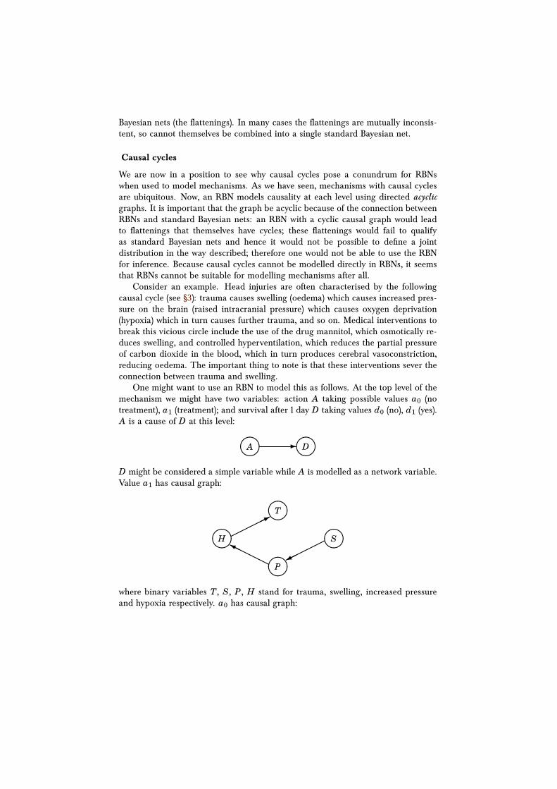
Consider an example. Head injuries are often characterised by the followingcausal cycle (see §3): trauma causes swelling (oedema) which causes increased pres-sure on the brain (raised intracranial pressure) which causes oxygen deprivation(hypoxia) which in turn causes further trauma, and so on. Medical interventions tobreak this vicious circle include the use of the drug mannitol, which osmotically re-duces swelling, and controlled hyperventilation, which reduces the partial pressureof carbon dioxide in the blood, which in turn produces cerebral vasoconstriction,reducing oedema. The important thing to note is that these interventions sever theconnection between trauma and swelling.

One might want to use an RBN to model this as follows. At the top level of themechanism we might have two variables: action A taking possible values a0 (notreatment), a1 (treatment); and survival after 1 day D taking values d0 (no), d1 (yes).A is a cause of D at this level:

����A -����

D

D might be considered a simple variable while A is modelled as a network variable.Value a1 has causal graph:

����T

����H ��

���*

����S���

�������PHH

HHHY

where binary variables T, S, P, H stand for trauma, swelling, increased pressureand hypoxia respectively. a0 has causal graph:

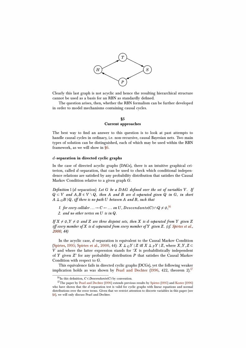
����T H

HHHHj����H ��

���*

����S���

�������PHH

HHHY

Clearly this last graph is not acyclic and hence the resulting hierarchical structurecannot be used as a basis for an RBN as standardly defined.

The question arises, then, whether the RBN formalism can be further developedin order to model mechanisms containing causal cycles.

§5Current approaches

The best way to find an answer to this question is to look at past attempts tohandle causal cycles in ordinary, i.e. non-recursive, causal Bayesian nets. Two maintypes of solution can be distinguished, each of which may be used within the RBNframework, as we will show in §6.

d-separation in directed cyclic graphs

In the case of directed acyclic graphs (DAGs), there is an intuitive graphical cri-terion, called d-separation, that can be used to check which conditional indepen-dence relations are satisfied by any probability distribution that satisfies the CausalMarkov Condition relative to a given graph G.

Definition 1 (d-separation) Let G be a DAG defined over the set of variables V . IfQ ⊂ V and A,B ∈ V \ Q, then A and B are d-separated given Q in G, in shortA ⊥⊥ GB |Q, iff there is no path U between A and B, such that

1. for every collider . . .→ C ← . . . on U , Descendants(C)∩Q 6= ;,162. and no other vertex on U is in Q.

If X 6= ;,Y 6= ; and Z are three disjoint sets, then X is d-separated from Y given Ziff every member of X is d-separated from every member of Y given Z. (cf. Spirtes et al.,2000, 44)

In the acyclic case, d-separation is equivalent to the Causal Markov Condition(Spirtes, 1995; Spirtes et al., 2000, 44): X ⊥⊥ GY | Z iff X ⊥⊥ PY | Z, where X ,Y , Z ⊂V and where the latter expression stands for ‘X is probabilistically independentof Y given Z’ for any probability distribution P that satisfies the Causal MarkovCondition with respect to G.

This equivalence fails in directed cyclic graphs (DCGs), yet the following weakerimplication holds as was shown by Pearl and Dechter (1996, 422, theorem 2).17

16In this definition, C ∈Descendants(C) by convention.17The paper by Pearl and Dechter (1996) extends previous results by Spirtes (1995) and Koster (1996)

who have shown that the d-separation test is valid for cyclic graphs with linear equations and normaldistributions over the error terms. Given that we restrict attention to discrete variables in this paper (see§4), we will only discuss Pearl and Dechter.

Given a (possibly cyclic) graph and associated probability distribution, if X ⊥⊥ GY |Z, then X ⊥⊥ PY | Z, provided that (i) the variables in V all have a discrete andfinite domain, (ii) the values of the variables of the system are uniquely determinedby the disturbances, and (iii) the disturbances are uncorrelated.18 In other words,even in the cyclic case the independencies induced by G can be read off directly bymeans of the d-separation criterion.19

Pearl and Dechter implicitly assume that the causal structure in question ‘is sta-ble’ (1996, 421) and has reached ‘equilibrium’ (1996, 423)—cf. condition (ii) above:once the values of the disturbances are given, the values of all variables are uniquelydetermined. Their approach to the problem of cyclicity in ordinary Bayesian netshas a problem, however. As Neal (2000) has shown, their theorem is not true ingeneral. He gives an example of a graph and an associated set of equations thatsatisfy the three conditions specified above, yet in which there are two variablesthat are d-separated by a third variable without being probabilistically indepen-dent conditional on that third variable. One possible way to salvage Pearl andDechter’s theorem is to require ‘not only that [the disturbances] U1, . . . ,Un uniquelydetermine [the endogenous variables] X1, . . . , Xn, but also that this unique solutionfor X1, . . . , Xn can be obtained by a procedure in which the X i are updated in ac-cordance with the causal structure of the network. In such a casual [sic] dynamicalprocedure, each X i is repeatedly replaced by the value computed for it from thecorresponding Ui and the current values of its parents, according to the equationfor that X i , until a stable state is reached.’ (Neal, 2000, 90)

One way to do this, is by making use of Dynamic Causal Bayesian nets.

Dynamic Bayesian Nets

Dynamic Bayesian nets (DBNs) were developed in the late 1980s to model the changein a probability distribution over time (Dean and Kanazawa, 1989, §5). More recentdevelopments can be found in Friedman et al. (1998), Ghahramani (1998), Murphy(2002), Bouchaffra (2010) and Doshi-Velez et al. (2011) for instance.

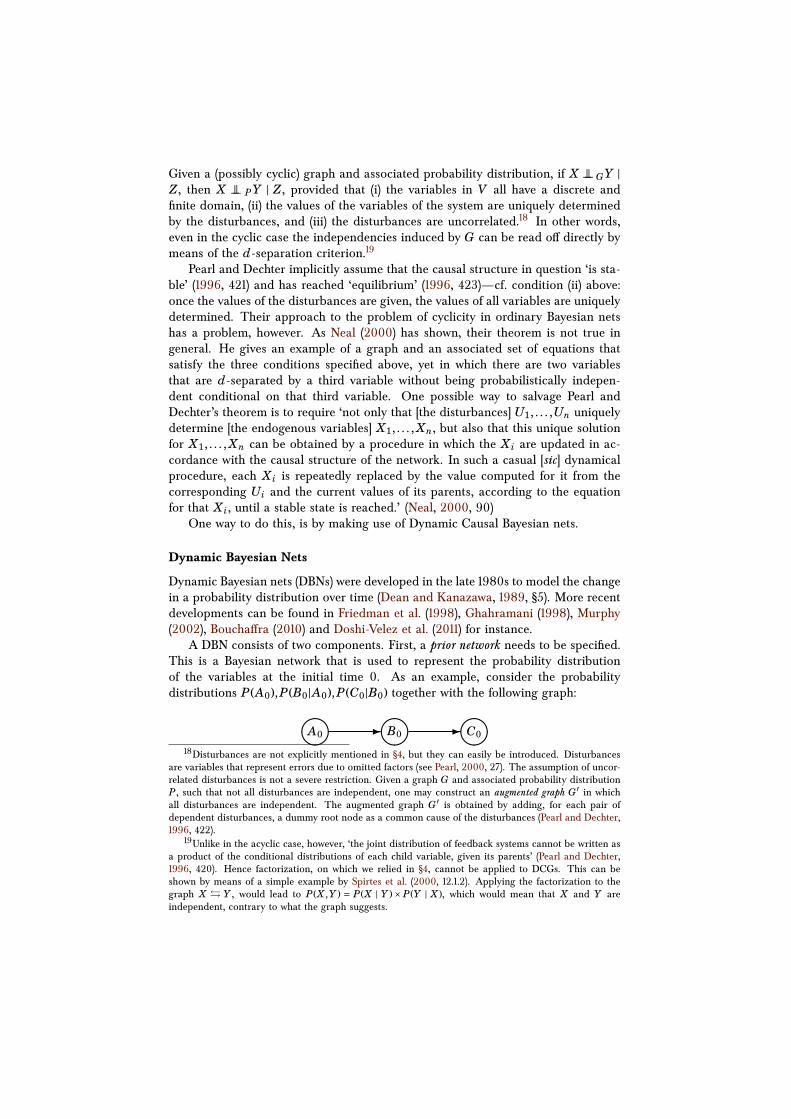
A DBN consists of two components. First, a prior network needs to be specified.This is a Bayesian network that is used to represent the probability distributionof the variables at the initial time 0. As an example, consider the probabilitydistributions P(A0),P(B0|A0),P(C0|B0) together with the following graph:

����A0 -����

B0 -����C0

18Disturbances are not explicitly mentioned in §4, but they can easily be introduced. Disturbancesare variables that represent errors due to omitted factors (see Pearl, 2000, 27). The assumption of uncor-related disturbances is not a severe restriction. Given a graph G and associated probability distributionP, such that not all disturbances are independent, one may construct an augmented graph G′ in whichall disturbances are independent. The augmented graph G′ is obtained by adding, for each pair ofdependent disturbances, a dummy root node as a common cause of the disturbances (Pearl and Dechter,1996, 422).

19Unlike in the acyclic case, however, ‘the joint distribution of feedback systems cannot be written asa product of the conditional distributions of each child variable, given its parents’ (Pearl and Dechter,1996, 420). Hence factorization, on which we relied in §4, cannot be applied to DCGs. This can beshown by means of a simple example by Spirtes et al. (2000, 12.1.2). Applying the factorization to thegraph X � Y , would lead to P(X ,Y ) = P(X | Y )×P(Y | X ), which would mean that X and Y areindependent, contrary to what the graph suggests.

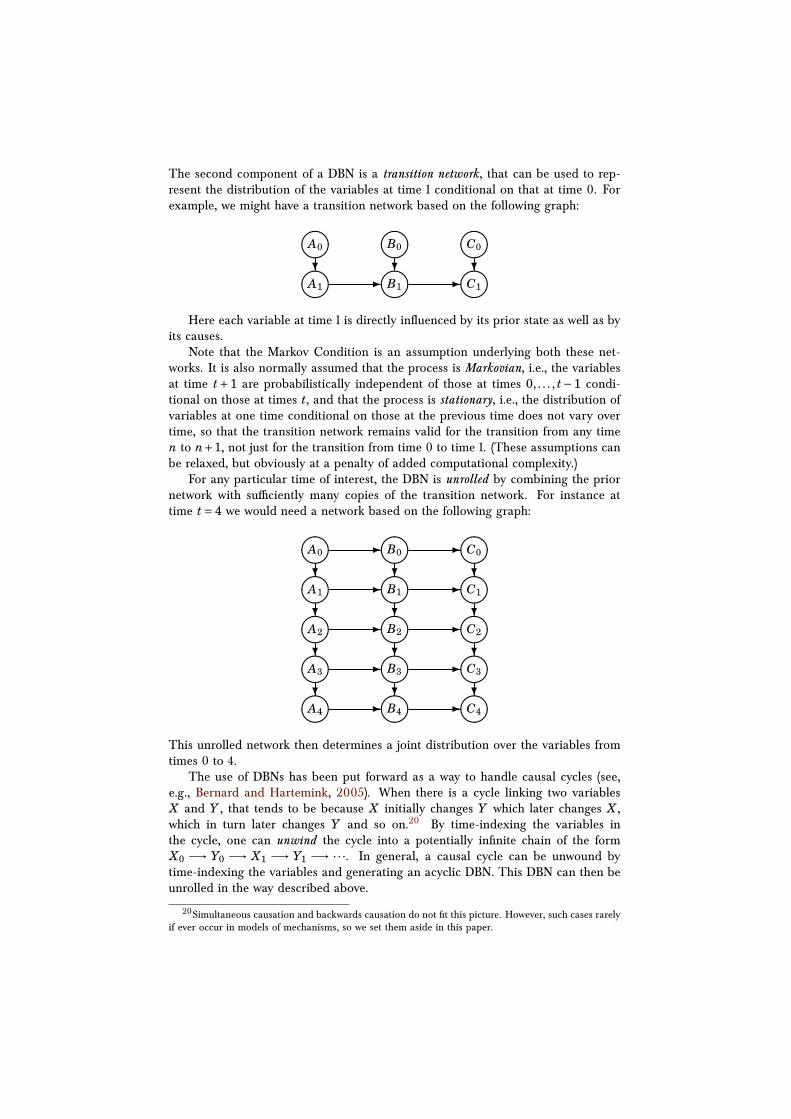
The second component of a DBN is a transition network, that can be used to rep-resent the distribution of the variables at time 1 conditional on that at time 0. Forexample, we might have a transition network based on the following graph:

����A0

?����B0

?����C0

?

����A1 -����

B1 -����C1

Here each variable at time 1 is directly influenced by its prior state as well as byits causes.

Note that the Markov Condition is an assumption underlying both these net-works. It is also normally assumed that the process is Markovian, i.e., the variablesat time t+1 are probabilistically independent of those at times 0, . . . , t−1 condi-tional on those at times t, and that the process is stationary, i.e., the distribution ofvariables at one time conditional on those at the previous time does not vary overtime, so that the transition network remains valid for the transition from any timen to n+1, not just for the transition from time 0 to time 1. (These assumptions canbe relaxed, but obviously at a penalty of added computational complexity.)

For any particular time of interest, the DBN is unrolled by combining the priornetwork with sufficiently many copies of the transition network. For instance attime t = 4 we would need a network based on the following graph:

����A0 -

?����B0 -

?����C0

?

����A1 -

?����B1 -

?����C1

?

����A2 -

?����B2 -

?����C2

?

����A3 -

?����B3 -

?����C3

?

����A4 -����

B4 -����C4

This unrolled network then determines a joint distribution over the variables fromtimes 0 to 4.

The use of DBNs has been put forward as a way to handle causal cycles (see,e.g., Bernard and Hartemink, 2005). When there is a cycle linking two variablesX and Y , that tends to be because X initially changes Y which later changes X ,which in turn later changes Y and so on.20 By time-indexing the variables inthe cycle, one can unwind the cycle into a potentially infinite chain of the formX0 −→ Y0 −→ X1 −→ Y1 −→ ·· ·. In general, a causal cycle can be unwound bytime-indexing the variables and generating an acyclic DBN. This DBN can then beunrolled in the way described above.

20Simultaneous causation and backwards causation do not fit this picture. However, such cases rarelyif ever occur in models of mechanisms, so we set them aside in this paper.

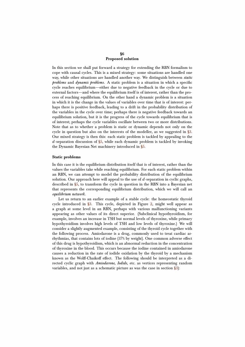
§6Proposed solution

In this section we shall put forward a strategy for extending the RBN formalism tocope with causal cycles. This is a mixed strategy: some situations are handled oneway, while other situations are handled another way. We distinguish between staticproblems and dynamic problems. A static problem is a situation in which a specificcycle reaches equilibrium—either due to negative feedback in the cycle or due toexternal factors—and where the equilibrium itself is of interest, rather than the pro-cess of reaching equilibrium. On the other hand a dynamic problem is a situationin which it is the change in the values of variables over time that is of interest: per-haps there is positive feedback, leading to a drift in the probability distribution ofthe variables in the cycle over time; perhaps there is negative feedback towards anequilibrium solution, but it is the progress of the cycle towards equilibrium that isof interest; perhaps the cycle variables oscillate between two or more distributions.Note that as to whether a problem is static or dynamic depends not only on thecycle in question but also on the interests of the modeller, as we suggested in §3.Our mixed strategy is then this: each static problem is tackled by appealing to thed-separation discussion of §5, while each dynamic problem is tackled by invokingthe Dynamic Bayesian Net machinery introduced in §5.

Static problems

In this case it is the equilibrium distribution itself that is of interest, rather than thevalues the variables take while reaching equilibrium. For each static problem withinan RBN, we can attempt to model the probability distribution of the equilibriumsolution. Our approach here will appeal to the use of d-separation in cyclic graphs,described in §5, to transform the cycle in question in the RBN into a Bayesian netthat represents the corresponding equilibrium distribution, which we will call anequilibrium network.

Let us return to an earlier example of a stable cycle: the homeostatic thyroidcycle introduced in §3. This cycle, depicted in Figure 2, might well appear asa graph at some level in an RBN, perhaps with various malfunctioning variantsappearing as other values of its direct superior. (Subclinical hypothyroidism, forexample, involves an increase in TSH but normal levels of thyroxine, while primaryhypothyroidism involves high levels of TSH and low levels of thyroxine.) We willconsider a slightly augmented example, consisting of the thyroid cycle together withthe following process. Amiodarone is a drug, commonly used to treat cardiac ar-rhythmias, that contains lots of iodine (37% by weight). One common adverse effectof this drug is hypothyroidism, which is an abnormal reduction in the concentrationof thyroxine in the blood. This occurs because the iodine contained in amiodaronecauses a reduction in the rate of iodide oxidation by the thyroid by a mechanismknown as the Wolff-Chaikoff effect. The following should be interpreted as a di-rected cyclic graph with Amiodarone, Iodide, etc. as vertices representing randomvariables, and not just as a schematic picture as was the case in section §3):

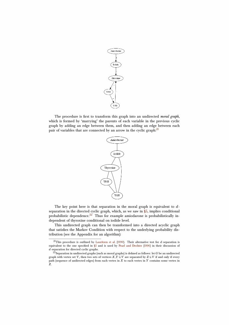
The procedure is first to transform this graph into an undirected moral graph,which is formed by ‘marrying’ the parents of each variable in the previous cyclicgraph by adding an edge between them, and then adding an edge between eachpair of variables that are connected by an arrow in the cyclic graph:21

The key point here is that separation in the moral graph is equivalent to d-separation in the directed cyclic graph, which, as we saw in §5, implies conditionalprobabilistic dependence.22 Thus for example amiodarone is probabilistically in-dependent of thyroxine conditional on iodide level.

This undirected graph can then be transformed into a directed acyclic graphthat satisfies the Markov Condition with respect to the underlying probability dis-tribution (see the Appendix for an algorithm):

21This procedure is outlined by Lauritzen et al. (1990). Their alternative test for d-separation isequivalent to the one specified in §5 and is used by Pearl and Dechter (1996) in their discussion ofd-separation for directed cyclic graphs.

22Separation in undirected graphs (such as moral graphs) is defined as follows: let G be an undirectedgraph with vertex set V , then two sets of vertices X ,Y ⊆ V are separated by Z ⊆ V if and only if everypath (sequence of undirected edges) from each vertex in X to each vertex in Y contains some vertex inZ.

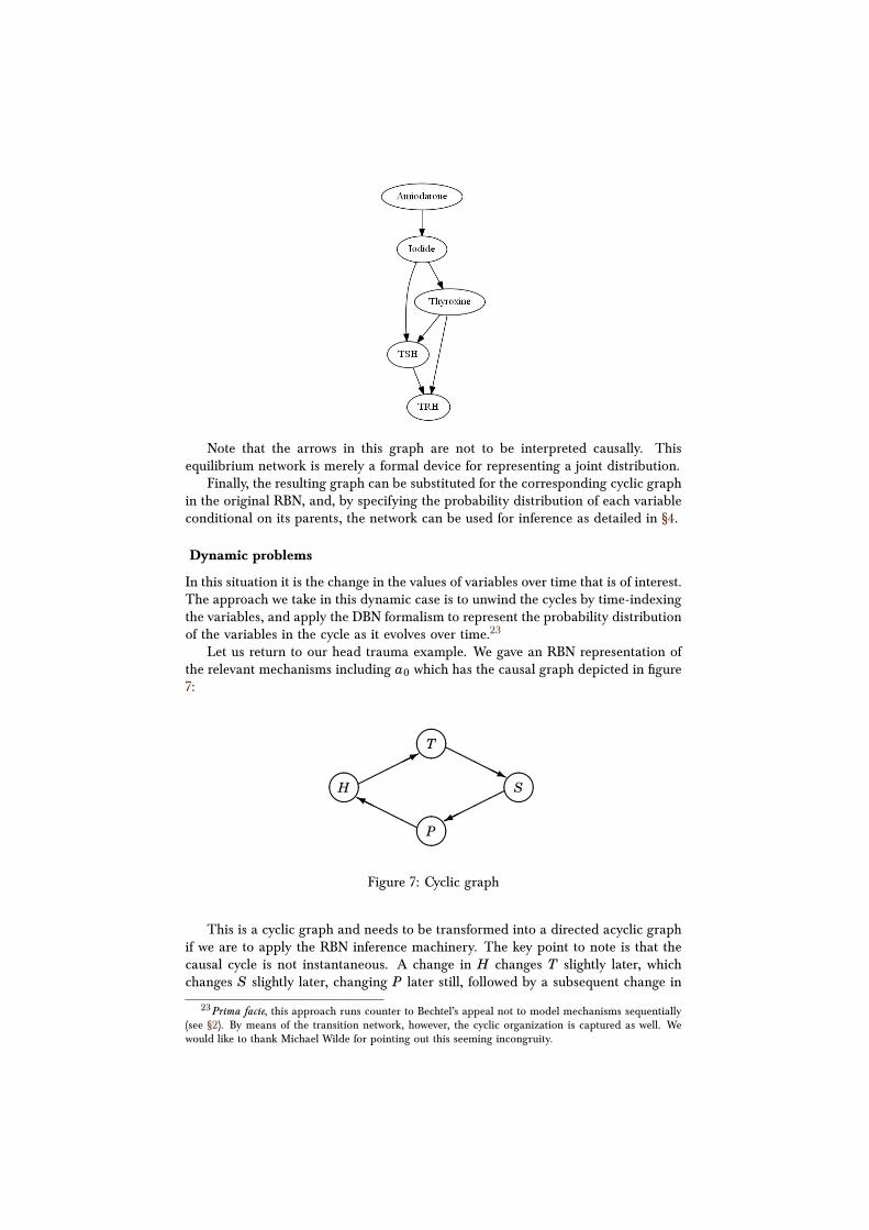
Note that the arrows in this graph are not to be interpreted causally. Thisequilibrium network is merely a formal device for representing a joint distribution.

Finally, the resulting graph can be substituted for the corresponding cyclic graphin the original RBN, and, by specifying the probability distribution of each variableconditional on its parents, the network can be used for inference as detailed in §4.

Dynamic problems

In this situation it is the change in the values of variables over time that is of interest.The approach we take in this dynamic case is to unwind the cycles by time-indexingthe variables, and apply the DBN formalism to represent the probability distributionof the variables in the cycle as it evolves over time.23

Let us return to our head trauma example. We gave an RBN representation ofthe relevant mechanisms including a0 which has the causal graph depicted in figure7:

����T HHH

HHj����H ��

���*

����S��

��������PH

HHHHY

Figure 7: Cyclic graph

This is a cyclic graph and needs to be transformed into a directed acyclic graphif we are to apply the RBN inference machinery. The key point to note is that thecausal cycle is not instantaneous. A change in H changes T slightly later, whichchanges S slightly later, changing P later still, followed by a subsequent change in

23Prima facie, this approach runs counter to Bechtel’s appeal not to model mechanisms sequentially(see §2). By means of the transition network, however, the cyclic organization is captured as well. Wewould like to thank Michael Wilde for pointing out this seeming incongruity.

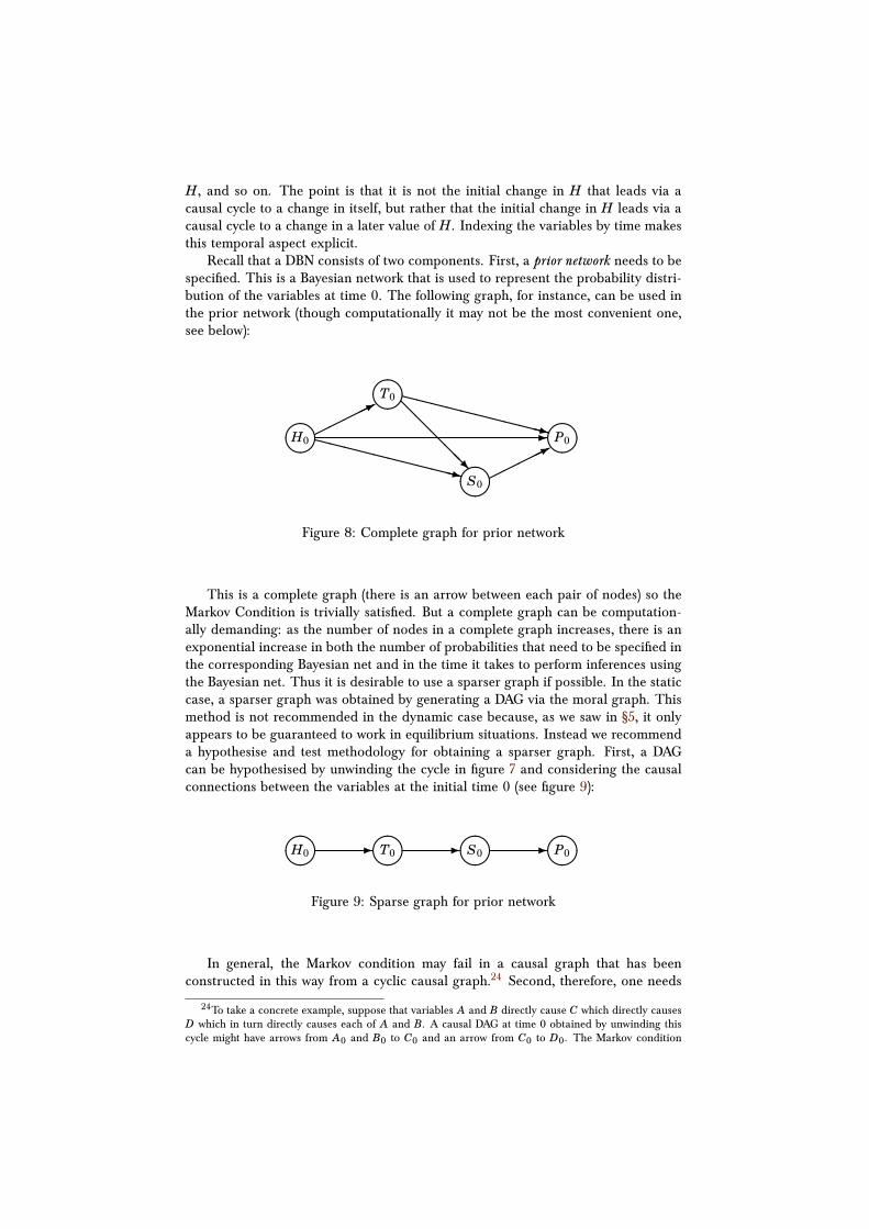
H, and so on. The point is that it is not the initial change in H that leads via acausal cycle to a change in itself, but rather that the initial change in H leads via acausal cycle to a change in a later value of H. Indexing the variables by time makesthis temporal aspect explicit.

Recall that a DBN consists of two components. First, a prior network needs to bespecified. This is a Bayesian network that is used to represent the probability distri-bution of the variables at time 0. The following graph, for instance, can be used inthe prior network (though computationally it may not be the most convenient one,see below):

����T0@@@@@R

XXXXXXXXXXXz����H0���

��*

XXXXXXXXXXXz

-����P0

����S0��

���*

Figure 8: Complete graph for prior network

This is a complete graph (there is an arrow between each pair of nodes) so theMarkov Condition is trivially satisfied. But a complete graph can be computation-ally demanding: as the number of nodes in a complete graph increases, there is anexponential increase in both the number of probabilities that need to be specified inthe corresponding Bayesian net and in the time it takes to perform inferences usingthe Bayesian net. Thus it is desirable to use a sparser graph if possible. In the staticcase, a sparser graph was obtained by generating a DAG via the moral graph. Thismethod is not recommended in the dynamic case because, as we saw in §5, it onlyappears to be guaranteed to work in equilibrium situations. Instead we recommenda hypothesise and test methodology for obtaining a sparser graph. First, a DAGcan be hypothesised by unwinding the cycle in figure 7 and considering the causalconnections between the variables at the initial time 0 (see figure 9):

����H0 -����

T0 -����S0 -����

P0

Figure 9: Sparse graph for prior network

In general, the Markov condition may fail in a causal graph that has beenconstructed in this way from a cyclic causal graph.24 Second, therefore, one needs

24To take a concrete example, suppose that variables A and B directly cause C which directly causesD which in turn directly causes each of A and B. A causal DAG at time 0 obtained by unwinding thiscycle might have arrows from A0 and B0 to C0 and an arrow from C0 to D0. The Markov condition

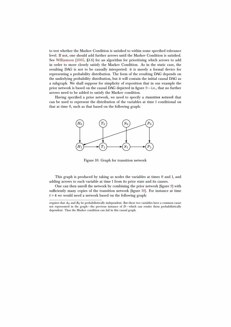
to test whether the Markov Condition is satisfied to within some specified tolerancelevel. If not, one should add further arrows until the Markov Condition is satisfied.See Williamson (2005, §3.6) for an algorithm for prioritising which arrows to addin order to more closely satisfy the Markov Condition. As in the static case, theresulting DAG is not to be causally interpreted: it is merely a formal device forrepresenting a probability distribution. The form of the resulting DAG depends onthe underlying probability distribution, but it will contain the initial causal DAG asa subgraph. We shall suppose for simplicity of exposition that in our example theprior network is based on the causal DAG depicted in figure 9—i.e., that no furtherarrows need to be added to satisfy the Markov condition.

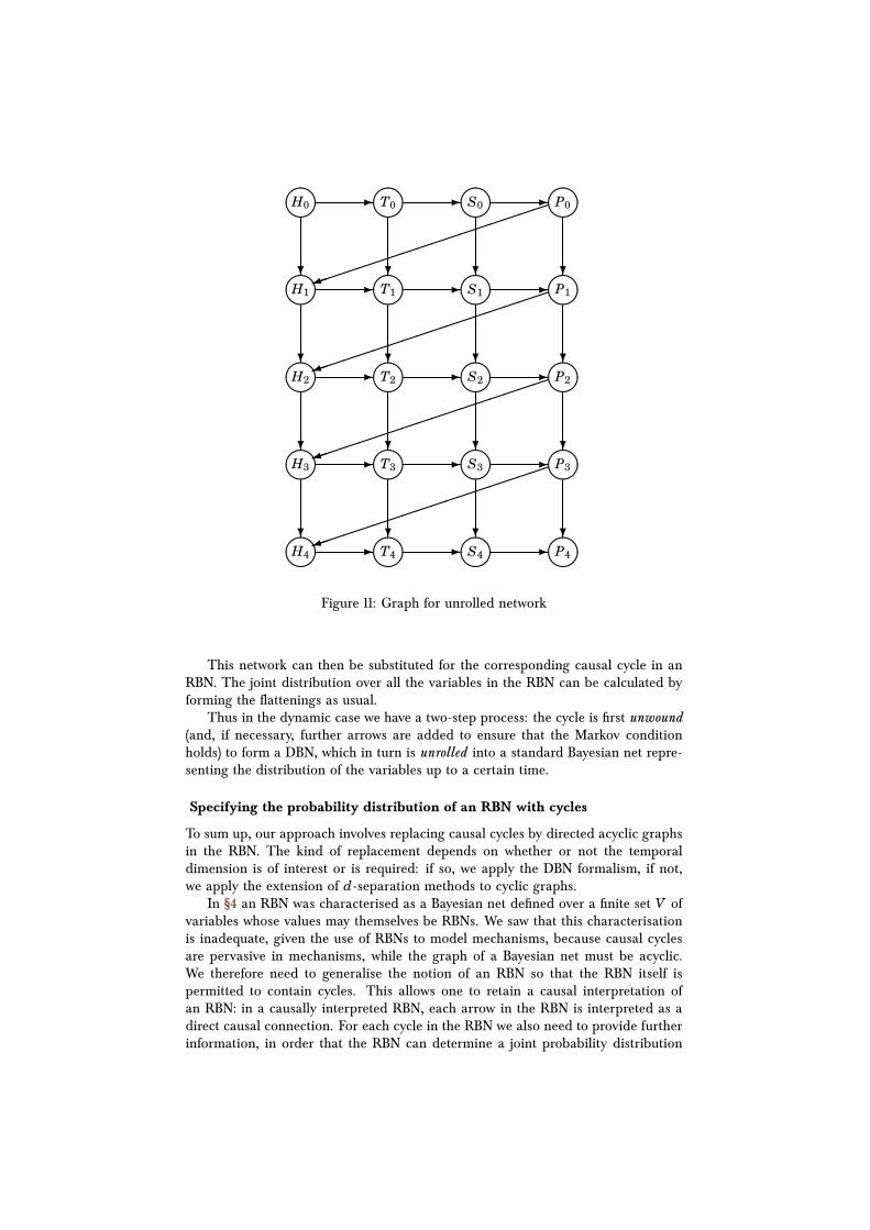
Having specified a prior network, we need to specify a transition network thatcan be used to represent the distribution of the variables at time 1 conditional onthat at time 0, such as that based on the following graph:

����H0

?

����T0

?

����S0

?

����P0�����������������)?

����H1 -����

T1 -����S1 -����

P1

Figure 10: Graph for transition network

This graph is produced by taking as nodes the variables at times 0 and 1, andadding arrows to each variable at time 1 from its prior state and its causes.

One can then unroll the network by combining the prior network (figure 9) withsufficiently many copies of the transition network (figure 10). For instance at timet = 4 we would need a network based on the following graph:

requires that A0 and B0 be probabilistically independent. But these two variables have a common causenot represented in the graph—the previous instance of D—which can render them probabilisticallydependent. Thus the Markov condition can fail in this causal graph.

����H0 -

?

����T0 -

?

����S0 -

?

����P0�����������������)?

����H1 -

?

����T1 -

?

����S1 -

?

����P1�����������������)?

����H2 -

?

����T2 -

?

����S2 -

?

����P2�����������������)?

����H3 -

?

����T3 -

?

����S3 -

?

����P3�����������������)?

����H4 -����

T4 -����S4 -����

P4

Figure 11: Graph for unrolled network

This network can then be substituted for the corresponding causal cycle in anRBN. The joint distribution over all the variables in the RBN can be calculated byforming the flattenings as usual.

Thus in the dynamic case we have a two-step process: the cycle is first unwound(and, if necessary, further arrows are added to ensure that the Markov conditionholds) to form a DBN, which in turn is unrolled into a standard Bayesian net repre-senting the distribution of the variables up to a certain time.

Specifying the probability distribution of an RBN with cycles

To sum up, our approach involves replacing causal cycles by directed acyclic graphsin the RBN. The kind of replacement depends on whether or not the temporaldimension is of interest or is required: if so, we apply the DBN formalism, if not,we apply the extension of d-separation methods to cyclic graphs.

In §4 an RBN was characterised as a Bayesian net defined over a finite set V ofvariables whose values may themselves be RBNs. We saw that this characterisationis inadequate, given the use of RBNs to model mechanisms, because causal cyclesare pervasive in mechanisms, while the graph of a Bayesian net must be acyclic.We therefore need to generalise the notion of an RBN so that the RBN itself ispermitted to contain cycles. This allows one to retain a causal interpretation ofan RBN: in a causally interpreted RBN, each arrow in the RBN is interpreted as adirect causal connection. For each cycle in the RBN we also need to provide furtherinformation, in order that the RBN can determine a joint probability distribution

and thereby be used for quantitative inference. If there is no equilibrium state of thevariables in the cycle then we have a dynamic problem, so we must specify a priorBayesian network and transition network involving the peers of the variables in thecycle. If there is an equilibrium state, then the particular application will determinewhether a dynamic approach or a static approach is required. In this case one mayneed to specify an equilibrium network, i.e., a Bayesian network representing theequilibrium state of the variables in and around the cycle, instead of, or as well as,a prior network and a transition network.

In Williamson (2005, Chapter 10) it was suggested that, in cases where a prob-ability distribution is constrained—rather than uniquely determined—by availablequantitative information, one should use maximum entropy methods to determinea particular probability distribution that satisfies those constraints. Of course thereis some controversy concerning maximum entropy methods (see, e.g., Seidenfeld,1987; Williamson, 2010). But if this route is accepted, then the prior, transition andequilibrium networks can be generated as needed, on the fly, from the constraintsimposed by the probability distribution of each variable conditional on its parentsgiven in the (possibly cyclic) RBN: the graphs in the networks can be constructedas outlined above, while the probability distribution of each variable conditional onits parents in the graph can be chosen to be the distribution, from all those thatsatisfy constraints specified in the RBN, that has maximum entropy.

We should note that it is common to distinguish single-case models from genericmodels. The former kind of model represents a particular case while the latter isrepeatedly instantiatable. An RBN is a generic model of a mechanism: it can beinstantiated in a variety of single cases. But often it is only in the context of aparticular instantiation that one can determine whether one is tackling a static ora dynamic problem. This is because, at least in contingent cycles, as to whetherthere is an equilibrium state or not can depend on the particular case. Moreover,the particular problem can influence whether one is concerned with the progresstowards equilibrium or the equilibrium itself. Hence an RBN can be viewed as aschematic representation of a mechanism, with the details to be filled in accordingto the application in question.

Note too that arrows in the RBN model of a mechanism are all causally in-terpreted, but when the above strategy for handling cycles is executed, arrows inthe resulting network may no longer all be causal. Thus when using a cyclic RBNto predict the effects of an intervention, for instance, one must first perform theintervention on the cyclic RBN (deleting arrows into the node which is set by theintervention; Pearl, 2000, pp. 22–23), and only then apply the strategy for han-dling cycles. Finally, the inference methods of §4 may be applied, requiring furthertransformations in order to produce the flattenings.

These two points reinforce the claim that it is the (possibly cyclic) RBN that isthe fundamental model of the mechanism, with transformations of this section and§4 to be applied only when required for inference in particular applications.

Related work

As far as we are aware, there is only one other attempt to use hierarchical versionsof Bayesian nets to model mechanisms for the purpose of quantitative inference.Gebharter and Kaiser (2012) do not adopt the RBN framework but rather representmechanisms by a hierarchy of disjoint causal Bayesian networks. This has its ad-vantages and its disadvantages over our RBN approach. On the one hand they do

not need a modelling assumption such as RCMC to tie the levels of the mechanismtogether, so their assumptions are weaker. On the other hand, it is not possibleunder their approach to represent the joint distribution over all the variables in thehierarchy; this results in a narrower range of inferences that can be drawn from theirrepresentation. For instance, one cannot use the value of a variable at one level ofthe hierarchy to help predict the value of a variable at another level, in the absenceof a single causal network that includes both variables. The authors recognise theimportance of handling cycles appropriately in order to model mechanisms, andthey recommend a time-indexing approach similar to that which we advocate inthe case of dynamic problems. We would argue that this is not the appropriatestrategy in the case of static problems, because it introduces irrelevant details intothe representation and because it can lead to unnecessary computational cost.

§7Summary and concluding remarks

In this paper, we have presented one possible quantitative approach to modellingmechanisms, which makes use of Recursive Bayesian nets. Causal cycles, if presentin the RBN, are replaced by directed acyclic graphs in order to perform inferenceusing inference techniques for standard Bayesian nets. The kind of replacementdepends on whether or not the temporal dimension is of interest or is required: ifso, we apply the DBN formalism, if not, we apply the extension of d-separationmethods to cyclic graphs.

To end this paper, we would like to suggest some questions for further research.First, it would be interesting to further explore the consequences of our approachfor philosophy of science. For instance, we hypothesise that the RBN frameworkmay shed further light on Craver’s mutual manipulability account of constitutive rel-evance (and vice versa). Interventions on causal Bayesian nets have been discussedextensively (see Pearl, 2000 and Spirtes et al., 2000). These notions carry over,mutatis mutandis, to RBNs, and may help to analyse Craver’s notion of ‘interlevelintervention’ and the interlevel experiments on which it is based.25

Second, the merits and disadvantages of our approach as compared to otherquantitative accounts of mechanistic modelling should be further explored. In §6we briefly discussed the work of Gebharter and Kaiser (2012). Yet the preciserelation between our account and, for example, Bechtel’s dynamic systems analysis(mentioned in §2) remains an open question.

Third, RBNs open up the possibility of algorithms for mechanism discovery.The advent of causal Bayesian nets led to a range of algorithms for causal discovery(see, e.g., Spirtes et al., 2000, 2010). Because of the close relation between RBNsand Bayesian nets, it is plausible that algorithms for learning causal structure mightbe extended to algorithms for learning causal and mechanistic structure simulta-neously. The main task would be to distinguish between causal and superiority(i.e., mechanistic hierarchy) relations. The difference between causal manipulationand mutual manipulability might offer a starting point in this respect. If progresscan be made here, it could have enormous payoffs for those—such as bioinformat-ics researchers and pharmaceutical companies—who are engaged in ‘closing the

25For a detailed account of mutual manipulability, see Craver (2007, 152–160). For a recent criticaldiscussion of Craver’s claim that interlevel constitutive relations cannot be causal, and whether this claimis compatible with his mutual manipulability account of constitutive relevance, see Leuridan (2012).

inductive loop’ by automating both scientific experimentation and scientific discov-ery.

Finally, the limits of our approach should be further explored. On the non-formal side, we fully acknowledge that our framework leaves out some interestingfeatures of mechanisms that are captured by alternative ways of representing them.For example, a large part of the functioning of a mechanism depends on the spatialorganization of its lower-level components, yet neither causal Bayesian nets norRecursive Bayesian Nets offer a natural way of representing this spatial organization.Likewise, mechanistic diagrams such as those presented in §3 are often easier tograsp and to (humanly) reason with than ordinary or Recursive Bayesian Nets.(See Perini, 2005a,b,c for interesting discussions of the role of diagrams and visualrepresentations in scientific reasoning; see also, among many others, Craver, 2006and Bechtel and Abrahamsen, 2005 for a discussion of diagrams in mechanisticcontexts.)

On the formal side, we treat the Causal Markov Condition and the RecursiveCausal Markov Condition as modelling assumptions rather than necessary truths.Whereas the limits of the former have been discussed extensively in the literature,26

those of the latter remain to be inspected in detail.Also on the formal side, the question arises as to how the framework presented

here can be extended to handle certain continuous cases. Modelling continuouscases with cyclic causality by means of discrete variables may lead to problems;for example, spurious instabilities may arise in the model even when the originalsystem itself is stable (see Pearl and Dechter, 1996, 425). Yet we do not expect anymajor difficulties here. Causal Bayesian nets can easily be defined over continuousvariables (see footnote 12) and in fact, the problem of automated causal discoveryis often easier in the continuous case (e.g., assuming normally distributed variables)than in the discrete case. Likewise, RBNs can easily be defined over continuousvariables as well. Our choice to restrict ourselves to the discrete case was motivatedby our endeavour to limit technicalities as far as possible.

Appendix: Transforming a moral graph into a directed acyclic graph

Here we present the algorithm of Williamson (2005, §5.7) for transforming an undi-rected graph G into a directed acyclic graph H which preserves the required in-dependencies (Williamson, 2005, Theorem 5.3): if Z d-separates X from Y in thedirected acyclic graph H then X and Y are separated by Z in the undirected graphG ; this separation in G implies that X and Y are probabilistically independent con-ditional on Z; hence, d-separation in H implies that X and Y are probabilisticallyindependent conditional on Z. Thus H can be used as the graph of a Bayesiannetwork.

An undirected graph is triangulated if for every cycle involving four or morevertices there is an edge in the graph between two vertices that are non-adjacent inthe cycle. The first step of the procedure is to construct a triangulated graph G T

from the undirected graph G . One of a number of standard triangulation algorithmscan be applied to construct G T (see, e.g., Neapolitan, 1990, §3.2.3; Cowell et al.,1999, §4.4.1).

26See, among others, Hausman and Woodward (1999, 2004a,b), Cartwright (2001, 2002), Williamson(2005) and Steel (2006).

Next, re-order the variables in V according to maximum cardinality search withrespect to G T : choose an arbitrary vertex as V1; at each step select the vertexwhich is adjacent to the largest number of previously numbered vertices, breakingties arbitrarily. Let D1, . . . ,Dl be the cliques (i.e., maximal complete subgraphs)of G T , ordered according to highest labelled vertex. Let E j = D j ∩ (

⋃ j−1i=1 D i) and

F j = D j\E j , for j = 1, . . . , l.Finally, construct a directed acyclic graph H as follows. Take variables in V

as vertices. Step 1: add an arrow from each vertex in E j to each vertex in F j , forj = 1, . . . , l. Step 2: add further arrows to ensure that there is an arrow betweeneach pair of vertices in D j, j = 1, . . . , l, taking care that no cycles are introduced(there is always some orientation of an added arrow which will not yield a cycle).

Acknowledgements

We would like to thank Lorenzo Casini, George Darby, Phyllis Illari, Mike Joffe,Federica Russo, and Michael Wilde for their helpful comments on this paper. JonWilliamson’s research is supported by the UK Arts and Humanities Research Coun-cil. Bert Leuridan is Postdoctoral Fellow of the Research Foundation—Flanders(FWO).

Bibliography

Bechtel, W. (2011). Mechanism and biological explanation. Philosophy of Science,78(4):533–557.

Bechtel, W. and Abrahamsen, A. (2005). Explanation: a mechanist alternative.Studies in History and Philosophy of Biological and Biomedical Sciences, 36(2):421–441.

Bernard, A. and Hartemink, A. (2005). Informative structure priors: Joint learn-ing of dynamic regulatory networks from multiple types of data. In Altman, R.,Dunker, A. K., Hunter, L., Jung, T., and Klein, T., editors, Proceedings of the Pa-cific Symposium on Biocomputing (PSB05), pages 459–470, Hackensack, NJ. WorldScientific.

Boon, N. A., Colledge, N. R., Walker, B. R., and Hunter, J. A., editors (2006).Davidson’s Principles & Practice of Medicine. Churchill Livingstone, Edinburgh,20th edition.

Bouchaffra, D. (2010). Topological dynamic bayesian networks. In Proceedings of theTwentieth International Conference on Pattern Recognition, pages 898–901. IEEE.

Cartwright, N. (2001). What is wrong with Bayes nets? The Monist, 84(2):242–264.Cartwright, N. (2002). Against modularity, the causal Markov condition, and anylink between the two: Comments on Hausman and Woodward. The BritishJournal for the Philosophy of Science, 53(3):411–453.

Casini, L., Illari, P. M., Russo, F., and Williamson, J. (2011). Models for prediction,explanation and control: recursive Bayesian networks. Theoria, 26(1):5–33.

Cowell, R. G., Dawid, A. P., Lauritzen, S. L., and Spiegelhalter, D. J. (1999). Proba-bilistic networks and expert systems. Springer-Verlag, Berlin.

Craver, C. F. (2006). When mechanistic models explain. Synthese, 153(3):355–376.Craver, C. F. (2007). Explaining the Brain: Mechanisms and the Mosaic Unity ofNeuroscience. Clarendon Press, Oxford.

Crunelli, V. and Hughes, S. W. (2010). The slow (<1 Hz) rhythm of non-REM sleep:a dialogue between three cardinal oscillators. Nature Neurosciences, 13(1):9–17.

Dean, T. and Kanazawa, K. (1989). A model for reasoning about persistence andcausation. Computational Intelligence, 5(3):142–150.

Doshi-Velez, F., Wingate, D., Tenenbaum, J., and Roy, N. (2011). Infinite dynamicbayesian networks. In Getoor, L. and Scheffer, T., editors, Proceedings of the 28thInternational Conference on Machine Learning (ICML), pages 913–920. Omnipress.

Friedman, N., Murphy, K. P., and Russell, S. J. (1998). Learning the structure of dy-namic probabilistic networks. In Cooper, G. F. and Moral, S., editors, Proceedingsof the Fourteenth Conference on Uncertainty in Artificial Intelligence (UAI), pages139–147, San Mateo, CA. Morgan Kaufmann.

Gebharter, A. and Kaiser, M. I. (2012). Causal graphs and mechanisms. In Hüt-temann, A., Kaiser, M. I., and Scholz, O., editors, Explanation in the SpecialSciences. The Case of Biology and History, Synthese Library. Springer, Dordrecht.

Ghahramani, Z. (1998). Learning dynamic bayesian networks. In Giles, C. and Gori,M., editors, Adaptive Processing of Sequences and Data Structures, volume 1387 ofLecture Notes in Computer Science, pages 168–197. Springer Berlin / Heidelberg.10.1007/BFb0053999.

Glennan, S. S. (1996). Mechanisms and the nature of causation. Erkenntnis, 44(1):49–71.

Glennan, S. S. (2002). Rethinking mechanistic explanation. Philosophy of Science,69(3):S342–S353.

Glennan, S. S. (2005). Modeling mechanisms. Studies in History and Philosophy ofBiological and Biomedical Sciences, 36(2):443–464.

Gottlieb, D. J., Yenokyan, G., Newman, A. B., O’Connor, G. T., Punjabi, N. M.,Quan, S. F., Redline, S., Resnick, H. E., Tong, E. K., Diener-West, M., and Shahar,E. (2010). Prospective study of obstructive sleep apnea and incident coronaryheart disease and heart failure. Circulation, 122(4):352–360.

Grandner, M., Hale, L., Moore, M., and Patel, N. V. (2010). Mortality associatedwith short sleep duration: The evidence, the possible mechanisms, and the future.Sleep Medicine Reviews, 14(3):191–203.

Hausman, D. M. and Woodward, J. (1999). Independence, invariance and the causalMarkov condition. The British Journal for the Philosophy of Science, 50(4):521–583.

Hausman, D. M. and Woodward, J. (2004a). Manipulation and the causal Markovcondition. Philosophy of Science, 55(5):147–161.

Hausman, D. M. and Woodward, J. (2004b). Modularity and the causal Markovcondition: a restatement. The British Journal for the Philosophy of Science, 55(1):147–161.

Koster, J. T. A. (1996). Markov properties of nonrecursive causal models. Annals ofStatistics, 24(5):2148–2177.

Lauritzen, S., Dawid, A., Larsen, B., and Leimer, H.-G. (1990). Independence prop-erties of directed Markov fields. Networks, 20(5):491–505.

Lazebnik, Y. (2002). Can a biologist fix a radio?—or, what I learned while studyingapoptosis. Cancer Cell, 2:179–182.

Leuridan, B. (2010). Can mechanisms really replace laws of nature? Philosophy ofScience, 77(3):317–340.

Leuridan, B. (2012). Three problems for the mutual manipulability account of con-stitutive relevance in mechanisms. The British Journal for the Philosophy of Science,63(2):399–427.

Leuridan, B. (2014). The structure of scientific theories, explanation, and unifica-

tion. A causal-structural account. The British Journal for the Philosophy of Science.forthcoming.

Machamer, P., Darden, L., and Craver, C. F. (2000). Thinking about mechanisms.Philosophy of Science, 67(1):1–25.

Marshall, L., Helgadóttir, H., Mölle, M., and Born, J. (2006). Boosting slowoscilllations during sleep potentiates memory. Nature, 444(7119):610–613.

McNicholas, W. and Bonsignore, M. (2007). Sleep apnoea as an independent riskfactor for cardiovascular disease: current evidence, basic mechanisms and re-search priorities. European Respiratory Journal, 29(1):156–178.

Mitchell, S. (2009). Unsimple Truths: Science, Complexity, and Policy. University ofChicago Press, Chicago, IL.

Murphy, K. P. (2002). Dynamic Bayesian Networks: Representation, Inference andLearning. PhD thesis, Computer Science, University of California, Berkeley.

Neal, R. (2000). On deducing conditional independence from d-separation incausal graphs with feedback: The uniqueness condition is not suffient. Journal ofArtificial Intelligence Research, 12:87–91.

Neapolitan, R. E. (1990). Probabilistic reasoning in expert systems: theory and algo-rithms. Wiley, New York.

Nervi, M. (2010). Mechanisms, malfunctions and explanation in medicine. Biologyand Philosophy, 25(2):215–228.

Pearl, J. (1988). Probabilistic Reasoning in Intelligent Systems: Networks of PlausibleInference. Morgan Kaufmann, San Mateo, CA.

Pearl, J. (2000). Causality: Models, Reasoning, and Inference. Cambridge UniversityPress, Cambridge.

Pearl, J. and Dechter, R. (1996). Identifying independencies in causal graphs withfeedback. In In Uncertainty in Artificial Intelligence: Proceedings of the TwelfthConference, pages 420–426, San Mateo, CA. Morgan Kaufmann.

Perini, L. (2005a). Explanation in two dimensions: Diagrams and biological expla-nation. Biology and Philosophy, 20(2-3):257–269.

Perini, L. (2005b). The truth in pictures. Philosophy of Science, 72(1):262–285.Perini, L. (2005c). Visual representations and confirmation. Philosophy of Science,72(5):913–926.

Seidenfeld, T. (1987). Entropy and uncertainty. In MacNeill, I. B. and Umphrey, G. J.,editors, Foundations of Statistical Inference, pages 259–287. D. Reidel, Dordrecht.

Spirtes, P. (1995). Directed cyclic graphical representation of feedback models. InBesnard, P. and Hanks, S., editors, Proceedings of the Eleventh Conference on Un-certainty in Artificial Intelligence, pages 491–498. Morgan Kaufmann, San Mateo,CA.

Spirtes, P., Glymour, C., and Scheines, R. (2000). Causation, Prediction, and Search.MIT Press, Cambridge, MA.

Spirtes, P., Glymour, C., Scheines, R., and Tillman, R. (2010). Automated search forcausal relations—theory and practice. In Dechter, R., Geffner, H., and Halpern,J. Y., editors, Heuristics, probability and causality: a tribute to Judea Pearl, pages467–506. College Publications, London.

Steel, D. (2006). Comment on Hausman & Woodward on the causal Markov condi-tion. British Journal for the Philosophy of Science, 57(1):219–231.

Williamson, J. (2005). Bayesian nets and causality: philosophical and computationalfoundations. Oxford University Press, Oxford.

Williamson, J. (2010). In defence of objective Bayesianism. Oxford University Press,Oxford.

Woodward, J. (2002). What is a mechanism? A counterfactual account. Philosophyof Science, 69(3):S366–S377.

Woodward, J. (2003). Making Things Happen. A Theory of Causal Explanation. Ox-ford University Press, New York.

Yumino, D., Redolfi, S., Ruttanaumpawan, P., Su, M., Smith, S., Newton, G. E., Mak,S., and Bradley, T. D. (2010). Nocturnal rostral fluid shift. Circulation, 121(14):1598–1605.