Embed Size (px)
Citation preview

Modelling of a power system for a new airborne radar system using Saber® Focused on the Multiphase Transformer Rectifier Unit Master of Science Thesis
Andreas Bergqvist Niklas Janehag Division of Electric Power Engineering Department of Environment and Energy CHALMERS UNIVERSITY OF TECHNOLOGY Göteborg, Sweden, 2009


Modelling of a power system for a new airborne radar system using Saber®
Focused on the Multiphase Transformer Rectifier Unit
Master Thesis in Electrical Engineering by:
ANDREAS BERGQVIST
NIKLAS JANEHAG
Division of Electric Power Engineering
Department of Environment and Energy
Chalmers University of Technology
Carried out at:
SAAB MICROWAVE SYSTEMS
GÖTEBORG, SWEDEN

MODELLING OF A POWER SYSTEM FOR A NEW AIRBORNE RADAR SYSTEM USING SABER®
FOCUSED ON THE MULTIPHASE TRANSFORMER RECTIFIER UNIT
Andreas Bergqvist
Niklas Janehag
© Andreas Bergqvist and Niklas Janehag
Examiner: Torbjörn Thiringer Division of Electric Power Engineering Chalmers University of Technology SE-412 96 Gothenburg
Supervisors: Johan Fält DD/MRC Saab Microwave Systems Solhusgatan 7, Kallebäck SE-412 89 Gothenburg
Johan Arvidsson DD/MR Saab Microwave Systems Solhusgatan 7, Kallebäck SE-412 89 Gothenburg
Bo Nettelblad DD/MR Saab Microwave Systems Solhusgatan 7, Kallebäck SE-412 89 Gothenburg
Andreas Karvonen Division of Electric Power Engineering Chalmers University of Technology SE-412 96 Gothenburg
Printed by:
Chalmers Reproservice
Göteborg, Sweden 2009

Abstract This M.Sc. thesis focuses on the modelling and verification of a 54-pulse step-down AutoTransformer Rectifier Unit (ATRU) used in the power system of the airborne early warning and control system ERIEYE®. A BLDC generator and a PI-controller with abc to dq transformation is designed in Saber® and used in the implementation of the entire radar power system supplying three power units mainly consisting of large capacitor banks and step-down DC/DC converters as loads.
The system using a 54-pulse step-down ATRU has been evaluated and compared to an older system incorporating 6-pulse rectification and it was clearly seen that using the newer system improves the quality of the current drawn from the BLDC generator. The 5th and 7th harmonic of the voltage and current were reduced by 90%.
The M.Sc. thesis has also resulted in a fully functioning and verified model of the 54-pulse step-down ATRU with a PI-controlled BLDC generator and three power units as loads.
An evaluation of sharing and administrating Saber® models within a company with high security demands has been carried out. It was shown that this can be done in a safe and effective way.
Keywords: Airborne radar, Autotransformer rectifier unit, ATRU, ERIEYE, Multiphase transformer rectifier unit, MPTR, Saber.

Acknowledgements We have received a lot of help from the entire DD/MR department but some people that deserve special thanks are Johan Fält who employed us and Torbjörn Thiringer who has been our examiner. Our supervisors Johan Arvidsson and Bo Nettelblad from Saab Microwave Systems and Andreas Karvonen from Chalmers who have answered many questions and supported us throughout the M.Sc. thesis. Claes-Göran Sköld from Saab Microwave Systems who have spent many hours in the lab supporting us with measurements on the Multiphase Transformer Rectifier and answered many questions we have had. Frank Lehmann from Synopsys who has answered many questions about Saber® and helped us in acquiring the customized BLDC generator model. We would also like to thank Örjan Söderholm, Patrik Björklund and Stefan Lundh for the visit at Saab Aerosystems in Linköping and the opportunity to see the assembly of the ERIEYE® radar system in the Saab 2000 aircraft.

Acronyms
AC Alternating Current
ATRU AutoTransformer Rectifier Unit
BLDC BrushLess DirectCurrent
DC Direct Current
DS Direct Symmetric
DVM Digital Voltage Meter
ERIEYE® Airborne Radar System
MAST Hardware desqription language
MCT Magnetic Component Tool
MPTR MultiPhase Transformer Rectifier
PSU Power Supply Unit
SMPS Switched Mode Power Supply
THD Total Harmonic Distortion


Table of Contents 1 Introduction.....................................................................................................................................................1
1.1 Background ............................................................................................................................................1 1.2 Objectives...............................................................................................................................................1 1.3 Outline of thesis .....................................................................................................................................1
2 Theory..............................................................................................................................................................3
2.1 AC/DC conversion .................................................................................................................................3 2.1.1 Operation of a Direct Symmetric Autotransformer Rectifier Unit...........................................3 2.1.2 Different winding configurations.............................................................................................4 2.1.3 Voltage step up/down ..............................................................................................................5 2.1.4 54-pulse Autotransformer Rectifier Unit .................................................................................6
2.1.4.1 Derivation of the 27-phase autotransformer winding configuration.........................................6 2.2 The ERIEYE® distributed power system ............................................................................................10
3 Measurements ...............................................................................................................................................11
3.1 Measurement equipment and setup ......................................................................................................11 3.2 No load losses ......................................................................................................................................13 3.3 Losses with load...................................................................................................................................14
3.3.1 Measurements with one PSU/6 connected.............................................................................15 3.3.2 Measurements with two PSU/6 connected.............................................................................15 3.3.3 Measurements with three PSU/6 connected...........................................................................15
4 Simulations ....................................................................................................................................................17
4.1 Designing the MPTR in Saber® ..........................................................................................................17 4.1.1 Autotransformer.....................................................................................................................17 4.1.2 Rectifier bridges.....................................................................................................................20 4.1.3 Input and output filters...........................................................................................................21
4.2 No load losses ......................................................................................................................................22 4.3 Losses with load...................................................................................................................................24
4.3.1 Simulations with one PSU/6 connected .................................................................................25 4.3.2 Simulations with two PSU/6 connected.................................................................................28 4.3.3 Simulations with three PSU/6 connected...............................................................................33
4.4 Designing the Saab 2000 generator using Saber® ...............................................................................35 4.4.1 Generator ...............................................................................................................................35 4.4.2 PI-regulator ............................................................................................................................35 4.4.3 Cable ......................................................................................................................................36
4.5 Benefits of using MPTR.......................................................................................................................37 4.6 Simulation of the ERIEYE® power system.........................................................................................46
5 Saber® models at Saab Group.....................................................................................................................53
5.1 Protection of Saber® models ...............................................................................................................53 5.2 Sharing Saber® models within the Saab Group...................................................................................54
6 Discussion ......................................................................................................................................................55
7 Conclusion .....................................................................................................................................................57
8 Proposed further work .................................................................................................................................59
9 References......................................................................................................................................................61
A Password protection of Saber® models ........................................................................................................ I
A.1 Example of the c-code for password protection ..................................................................................... I A.2 Example of the MAST code for password protection ............................................................................ I
B Measurement setup...................................................................................................................................... III
C abc to dq coordinate transformation schematics ........................................................................................V
D ERIEYE® power system schematics.........................................................................................................VII


Chapter 1. Introduction
1
1 Introduction
1.1 Background Situations that are difficult, expensive or dangerous to realize in a laboratory are beneficial to be able to simulate first using an accurate software model. During the fall of 2008, a M.Sc. thesis was conducted at Saab Microwave Systems (SMW) where the usability of the multidomain simulation software from Synopsys called Saber® was evaluated [1]. One of the conclusions was to start using Saber® at SMW as a tool to simulate larger parts of the electric power system, thereby making the design process easier and quicker. This M.Sc. thesis is a continuation of the previous work and focuses mainly on modelling a MultiPhase Transformer Rectifier unit (MPTR) which is used to convert AC to DC. Also an investigation is performed how Saber® can be used to encrypt and share models within the Saab Group.
In the new airborne radar system the radar system are fed from the same generators as the flight avionics which has resulted in new and more stringent requirements on power quality. The requirement that current harmonics from the radar system must not influence the rest of the electrical system is an important aspect within this area. Furthermore the generator feeding the MPTR will operate in a variable frequency range (360-800Hz) instead of at a fixed frequency (400Hz) as in the previous radar systems which had a dedicated generator for this purpose.
The length of the cables between the generator and the MPTR will differ depending on which airplane the radar system is installed in. Simulations of different scenarios and configurations of the entire radar power system have because of this become even more important.
1.2 Objectives The M.Sc. thesis shall result in a Saber® model of the MPTR that can be used when simulating and evaluating different scenarios and parameter changes that can occur. The last part of the thesis aims at evaluating the possibilities to share Saber® models in a safe way within the Saab Group.
1.3 Outline of thesis The first part of the thesis is devoted to giving an overview of scientific papers and other information about AutoTransformer Rectifier Units (ATRU’s), MPTR, Saber®, ERIEYE®, power distribution in aircrafts and the behaviour and theory behind the hysteresis loop in soft magnetic materials. Basic electrical and magnetic circuits were simulated in Saber® using templates and the Magnetic Component Tool (MCT) followed by the implementation and simulation of an 18-pulse ATRU and an 18-pulse step-down ATRU. The simulations were then expanded into implementing and simulating the 54-pulse step-down MPTR in Saber® using the MCT. Measurements were carried out on the MPTR to verify the Saber® model. Components such as non ideal diodes in the rectifier unit and a PI-controlled generator feeding the MPTR were then added to the model.
To evaluate the possibilities to share Saber® models within the Saab Group and with customers, the safety features such as encryption and password protection of the Saber® models have been investigated.

1.3. Outline of thesis
2

Chapter 2. Theory
3
2 Theory
2.1 AC/DC conversion For variable frequency systems the AC/DC conversion is used to generate a DC bus which supplies power to the secondary step-down DC/DC converters. There exists two alternative ways to achieve this. One is by using switched active front-ends and the other is by using a AutoTransformer Rectifier Unit (ATRU) which is a passive solution. A Switched Mode Power Supply (SMPS) requires more development to meet the requirements in reliability for aircraft applications [2]. The ATRU is a well known component and has proven reliability [3],[4]. Since there is no need for galvanic isolation an autotransformer can be used to reduce the kVA rating, size and weight. Due to the high requirements for input harmonics and output voltage ripple for the AC/DC converter, an 18-pulse AutoTransformer Rectifier Unit (ATRU) or more is often used in aircraft applications.
2.1.1 Operation of a Direct Symmetric Autotransformer Rectifier Unit In an 18-pulse Direct Symmetric AutoTransformer Rectifier Unit (DS ATRU) a multiphase autotransformer is used to create two additional three phase systems (six additional phases), one leading the supply voltage by 40º and the other lagging by 40º with amplitudes equal to the supply voltage [2],[5]. The input voltages (Vain, Vbin and Vcin) have the same magnitude and phase as the output voltages (namned Va, Vb and Vc in Figure 2.1, Figure 2.2 and Figure 2.3). The winding configuration of the autotransformer results in three 3-phase systems (nine phases in total) that are connected to the three diode bridges (consisting of 18 diodes in total). Each of the diode bridges is conducting one third of the load and each diode is carrying the full load current during 40º. The load is directly connected to the diode bridges as seen in Figure 2.1, hence the term direct symmetric is used.
Multiphaseautotransformer
Vain
Vbin
Vcin
Va+40
Vb+40
Vc+40
Va
Vb
Vc
Va-40
Vb-40
Vc-40
Compensating inductors
Leading bridge
R
S
T
Vdc+
Vdc-
Through bridge
R
S
T
Vdc+
Vdc-
Lagging bridge
R
S
T
Vdc+
Vdc-
Figure 2.1: Block diagram of a DS ATRU

2.1. AC/DC conversion
4
2.1.2 Different winding configurations Additional 3-phase systems can be created using different types of winding configurations. Examples of possible winding configurations in an 18-pulse DS ATRU are T-Delta, Delta, and Polygon. See Figure 2.2 where the different winding topologies are shown. Figure 2.3 shows how the different winding configurations build up nine phases shifted by 40º using a vector phase diagram.
VbVc
Vc-40
Va+40 Va-40
Vb+40
Vb-40Vc+40Vc
Vc+40 Vb-40
Vb
Vb+40
Va-40Va+40
Vc-40
Va
Vc+40 Vb-40
Vc
Vc-40
Va+40
Vb
Vb+40
Va-40
Figure 2.2: T-Delta, Delta and Polygon winding configurations (parallel windings are located at the same
E-core leg)
Va
VbVc
Vc-40
Va+40 Va-40
Vb+40
Vb-40Vc+40
Va
Va-40
Vb+40
Vb
Vb-40Vc+40
Vc
Vc-40
Va+40
Va
Va-40
Vb+40
Vb
Vb-40Vc+40
Vc
Vc-40
Va+40
Figure 2.3: T-Delta, Delta and Polygon vector diagrams
The Delta and T-Delta configurations offer the lowest power rating (small physical size of the transformer) and the polygon configuration offers the lowest number of unconnected windings per 3-phase transformer leg (high manufacturability, low leakage inductance) [2]. Since the sensitivity for leakage inductance increases at higher frequency the polygon configuration is preferred in a 360-800Hz system [5].

Chapter 2. Theory
5
2.1.3 Voltage step up/down All three winding configurations can be modified in order to achieve higher or lower output voltage and this requires an increased number of windings because none of the output voltages are now in phase with the input voltages (Vain, Vbin and Vcin). The procedure preserves the 40º angle between the nine phases while meeting the required voltage level. Figure 2.4 shows the vector diagram for the polygon ATRU in the step-down configuration. As mentioned above none of the three created 3-phase systems are now in phase with the supply voltage. This creates additional harmonics on the input of the ATRU due to imbalance in impedances [2].
Vain
VbinVcin
Va
Va-40
Va+40
Vb+40
Vb
Vb-40
Vc+40
Vc
Vc-40
Figure 2.4: Step-down Polygon vector diagram

2.1. AC/DC conversion
6
2.1.4 54-pulse Autotransformer Rectifier Unit Instead of building an ATRU that produces nine AC voltages that are rectified to form a DC voltage, an ATRU that produces and rectifies 27 AC voltages (henceforth called MPTR) can be built to achieve a DC output voltage with less ripple. This requires 54 diodes instead of 18 and a more complex winding configuration of the multiphase autotransformer.
2.1.4.1 Derivation of the 27-phase autotransformer winding configuration
Assume an E-core with one winding (N=72 turns) on each leg connected in delta and fed with 3-phase AC as seen in Figure 2.5. The input phase voltages are in this case
°∠=→
902.1 UV ain (2.1)
°−∠=→
302.1 UV bin (2.2)
°−∠=→
1502.1 UV cin (2.3)
which results in the line to line voltages
°−∠⋅=→
602.13 UV ab (2.4)
°∠⋅=→
02.13 UV cb (2.5)
°∠⋅=→
602.13 UV ca . (2.6)
The line to line voltages can also be expressed as
dt
dNV ab
1
→→
=φ
(2.7)
dt
dNV cb
2
→→
−=φ
(2.8)
dt
dNV ca
3
→→
=φ
(2.9)
and due to a balanced 3-phase system the sum of the flux change must be zero.
0321 =++→→→φφφ (2.10)

Chapter 2. Theory
7
1 2 3
1 2 3
Vain
VbinVcin
1
2
3
2.5.a: E-core 2.5.b: Delta connection
Figure 2.5: E-core (a) that shows the fluxes and leg numbers and delta connection (b) that shows the phases and leg numbers
The objective is to create 27 output voltages separated by α=360/27≈13.333° with magnitude U in order to achieve the desired DC voltage level after rectification. Since the magnitudes of the input voltages in this case are 1.2U a step-down structure is needed. Figure 2.6 shows how Va1 to Va5 are built up using a vector diagram.
Output Va1 is created by connecting Vain to a new winding with n1 turns on leg 1. Magnitude and angle are given by
abaina VN
nVV
→→→+= 1
1 . (2.11)
Choosing n1=8 results in
°∠=→
41.83007.11 UV a .
Output Va2 is created by connecting Va1 to a new winding with n2 turns on leg 1 and n3 turns on leg 2. Magnitude and angle are given by
cbabaa VN
nV
N
nVV
→→→→++= 32
12 . (2.12)
Choosing n2=2 and n3=7 results in
°∠=→
97.69011.12 UV a .
Output Va3 is created by connecting Va2 to a new winding with n4 turns on leg 2 and n5 turns on leg 1. Magnitude and angle are given by
abcbaa VN
nV
N
nVV
→→→→++= 54
23 . (2.13)

2.1. AC/DC conversion
8
Choosing n4=5 and n5=4 results in
°∠=→
17.57012.13 UV a .
Output Va4 is created by connecting Va3 to a new winding with n6 turns on leg 1 and n7 turns on leg 2. Magnitude and angle are given by
cbabaa VN
nV
N
nVV
→→→→++= 76
34 . (2.14)
Choosing n6=6 and n7=3 results in
°∠=→
13.44005.14 UV a .
Output Va5 is created by connecting Va4 to a new winding with n8 turns on leg 2 and n9 turns on leg 1. Magnitude and angle are given by
abcbaa VN
nV
N
nVV
→→→→++= 98
45 . (2.15)
Choosing n8=1 and n9=8 results in
°∠=→
3015 UV a .
Va1- to Va5- is designed in the same way (equal number of windings and turns) but leg 3 is used instead of leg 1. Figure 2.6 shows how Va1- to Va5- are built up using a vector diagram.
caaina VN
nVV
→→
−
→−= 1
1 (2.16)
[ ] °∠=⇒= −
→59.96007.18 11 UVn a
cbcaaa VN
nV
N
nVV
→→
−
→
−
→−−= 32
12 (2.17)
[ ] °∠=⇒== −
→03.110011.17,2 232 UVnn a
cacbaa VN
nV
N
nVV
→→
−
→
−
→−−= 54
23 (2.18)
[ ] °∠=⇒== −
→83.122012.14,5 354 UVnn a
cbcaaa VN
nV
N
nVV
→→→
−
→−−= 76
34 (2.19)
[ ] °∠=⇒== −
→87.135005.13,6 476 UVnn a
cacbaa VN
nV
N
nVV
→→
−
→
−
→−−= 98
45 (2.20)
[ ] °∠=⇒== −
→15018,1 598 UVnn a
Chapter 2. Theory
9
Vain
VbinVcin
Va1Va2
Va3
Va4
Va5
Va1-Va2-
Va3-
Va4-
Va5-
n1
n2n3 n4 n5
n6n7 n8
n9
n1
n2n3n4n5
n6n7n8
n9
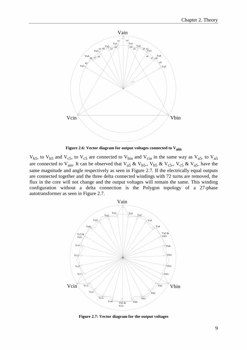
Figure 2.6: Vector diagram for output voltages connected to Vain
Vb5- to Vb5 and Vc5- to Vc5 are connected to Vbin and Vcin in the same way as Va5- to Va5 are connected to Vain. It can be observed that Va5 & Vb5-, Vb5 & Vc5-, Vc5 & Va5- have the same magnitude and angle respectively as seen in Figure 2.7. If the electrically equal outputs are connected together and the three delta connected windings with 72 turns are removed, the flux in the core will not change and the output voltages will remain the same. This winding configuration without a delta connection is the Polygon topology of a 27-phase autotransformer as seen in Figure 2.7.
Vain
VbinVcin
Va1Va2
Va3
Vb1
Vb2
Vb3
Vc3
Vc2
Vc1
Va4
Va5 & Vb5-
Vb4Vb5 & Vc5-
Va1-Va2-
Va3-
Va4-
Vc5 & Va5-
Vc4
Vb1-
Vb2-
Vb3-
Vb4-
Vc1-
Vc2-
Vc3-Vc4-
Figure 2.7: Vector diagram for the output voltages

2.2. The ERIEYE® distributed power system
10
2.2 The ERIEYE® distributed power system The complete system for converting AC to DC in an ERIEYE® radar system, see Figure 2.8, consists of two variable frequency 200V 3-phase BLDC generators feeding the left and right MPTR respectively. Before reaching the MPTR the generated AC supply voltage passes through a relay which opens when a fault is detected. Since the MPTR includes an autotransformer there is no galvanic isolation between the input and output of the MPTR. Each MPTR supplies three power units (PSU/6), mainly consisting of a large capacitor bank and step-down DC/DC converters that transforms the 270VDC bus voltage to 42VDC. The transmitting radar modules are fed with 42VDC from the six PSU/6’s.
In order to protect the PSU/6’s the MPTR has a supervision sensing overvoltages, overcurrents or overtemperatures. There is no protection if there is a shortcircuit in the MultiPhase Transformer itself. To protect other airplane equipment the supervision board also monitors voltage distortion.
Relay L Relay R
MPTR L MPTR R
Generator L Generator R
PSU/6 2 PSU/6 3PSU/6 1 PSU/6 4 PSU/6 5 PSU/6 6Super-vision
200VAC 200VAC
200VAC200VAC
270VDC 270VDC
42VDC42VDC 42VDC 42VDC 42VDC42VDCPSU
Status signals Status signals
Figure 2.8: Overview of the ERIEYE® distributed power system

Chapter 3. Measurements
11
3 Measurements Measurements were carried out at different frequencies and loads in order to validate our software model of the MPTR designed using Saber®. No load losses were measured and compared to the no load losses in the simulations. The results were used to design the hysteresis loop in chapter 4.1.1. Load losses and voltage drop for the MPTR were measured and compared to the designed model in Saber®.
3.1 Measurement equipment and setup All the used measurement equipment is listed below and their position is shown in Appendix B. The symbol explanations are as follows:
Equipment under test
Equipment under test number symbol:
1. MPTR
2. PSU/6
3. PSU/6
4. PSU/6
5. PSU Frame
6. Supervision
Test instruments
Test instrument number symbol:
1. Oscilloscope LeCroy 9354TM PA3704
2. Current Probe Digital Kyoritsu
3. Current Probe Hioki 3274
4. Current Probe Hioki 3274
5. Current Probe Hioki 3274
6. Current Probe Supply Hioki 3269
7. Differential Probe LeCroy AP031
8. Differential Probe LeCroy AP031
9. DVM Fluke 87
10. DVM Fluke 87
11. DC Power Source 28V Delta SM7020 DC Power Source 28V Delta SM35-45
12. AC Power Source Pacific 390AMX
13. Power Quality Analyzer Norma 4000
nn
nn

3.1. Measurement equipment and setup
12
Test cables
Cable number symbol:
1. AC Power input cable MPTR
2. DC Power input cable PSU/6
3. DC Power input cable PSU/6
4. DC Power input cable PSU/6
5. MPTR X5 cable
6. MPTR X1 to PSU P7 cable
7. PSU P1 cable
8. PSU P2 cable
9. Output cable PSU/6
10. Output cable PSU/6
11. Output cable PSU/6
Test boxes
Test boxes number symbol:
1. MPTR Input Power Relay
2. MPTR output connection box
3. PSU Fault indicator box
4. PSU P8 jumper
5. Cooling air monitoring
6. Water cooled resistive load
nn
nn

Chapter 3. Measurements
13
3.2 No load losses During the no load measurements the MPTR (equipment 1) was fed with a variable frequency generator (test instrument 12) set to 115V phase voltage. Input currents were measured with current probes (test instruments 3, 4 and 5). The power quality analyzer (test instrument 13) was connected to the current probes and the input voltages. A digital voltage meter (test instrument 9) was connected to the MPTR output.
The results from no load measurements of the MPTR at different frequencies can be seen in Table 3.1. Since magnetic flux is inversely proportional to the frequency the no load losses (hysteresis losses) decreases as the frequency increases. Overall, the results from the measurements agreed well with theory and expectations.
Table 3.1: Measured data for no load losses at different frequencies
Frequency (Hz)
Active power (W)
Reactive power (VAr)
Apparent power (VA)
Current (A)
Output DC voltage (V)
360 139.4 -383 414 1.20 273.2
400 101.3 -545 557 1.62 273.2
498 74.2 -819 742 2.39 273.2
577 64.6 -1013 1017 2.95 273.2
700 60.6 -1292 1293 3.75 273.2
800 61.1 -1504 1506 4.37 273.2
3.3. Losses with load
14
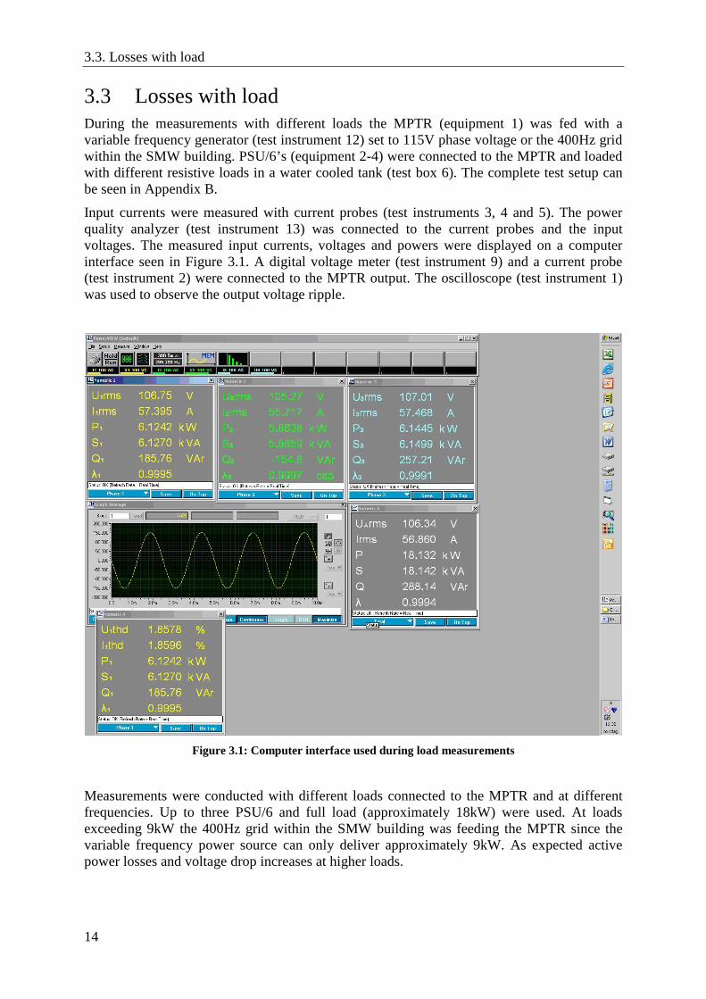
3.3 Losses with load During the measurements with different loads the MPTR (equipment 1) was fed with a variable frequency generator (test instrument 12) set to 115V phase voltage or the 400Hz grid within the SMW building. PSU/6’s (equipment 2-4) were connected to the MPTR and loaded with different resistive loads in a water cooled tank (test box 6). The complete test setup can be seen in Appendix B.
Input currents were measured with current probes (test instruments 3, 4 and 5). The power quality analyzer (test instrument 13) was connected to the current probes and the input voltages. The measured input currents, voltages and powers were displayed on a computer interface seen in Figure 3.1. A digital voltage meter (test instrument 9) and a current probe (test instrument 2) were connected to the MPTR output. The oscilloscope (test instrument 1) was used to observe the output voltage ripple.
Figure 3.1: Computer interface used during load measurements
Measurements were conducted with different loads connected to the MPTR and at different frequencies. Up to three PSU/6 and full load (approximately 18kW) were used. At loads exceeding 9kW the 400Hz grid within the SMW building was feeding the MPTR since the variable frequency power source can only deliver approximately 9kW. As expected active power losses and voltage drop increases at higher loads.

Chapter 3. Measurements
15
3.3.1 Measurements with one PSU/6 connected
Table 3.2: Measured data with one PSU/6 connected at 498Hz and different loads
Frequency (Hz)
Reactive input power (kVAr)
Active input power (kW)
Active output power (kW)
Efficiency (%)
Input phase
voltage (V)
Input current
(A)
Input current THD (%)
Output DC
voltage (V)
Output DC
voltage ripple (V)
498 -0.830 0.297 0.189 63.64 114.89 2.559 20.595 270.7 N/A
498 -0.620 3.998 3.814 95.40 114.42 11.787 9.763 264.1 1.867
498 -0.657 5.990 5.801 96.84 114.11 17.749 7.557 263.1 N/A
3.3.2 Measurements with two PSU/6 connected
Table 3.3: Measured data with two PSU/6 connected at different frequencies and loads
Frequency (Hz)
Reactive input power (kVAr)
Active input power (kW)
Active output power (kW)
Efficiency (%)
Input phase
voltage (V)
Input current
(A)
Input current THD (%)
Output DC
voltage (V)
Output DC
voltage ripple (V)
360 0.781 8.969 8.664 96.60 113.61 26.415 6.967 261.4 2.273
400 0.175 12.028 11.752 97.71 109.97 36.475 2.255 252.5 1.477
498 -0.831 0.445 0.323 72.58 114.86 2.738 22.406 270.2 1.091
498 -0.735 8.974 8.726 97.24 113.69 26.398 6.067 261.7 1.906
800 -1.074 8.912 8.697 97.59 113.66 26.324 N/A 261.6 1.781
3.3.3 Measurements with three PSU/6 connected
Table 3.4: Measured data with three PSU/6 connected at 400Hz
Frequency (Hz)
Reactive input power (kVAr)
Active input power (kW)
Active output power (kW)
Efficiency (%)
Input phase
voltage (V)
Input current
(A)
Input current THD (%)
Output DC
voltage (V)
Output DC
voltage ripple (V)
400 0.288 18.132 17.566 96.88 106.34 56.860 1.860 243.5 1.477

3.3. Losses with load
16

Chapter 4. Simulations
17
4 Simulations The MPTR model in Saber® was built based on the internal documents [6]-[13] and measurements of no load losses in chapter 3.2 due to lack of information about the core material in the autotransformer core. Different simulations were conducted in order to verify different aspects of the MPTR-model designed in Saber® against measurements of the MPTR.
4.1 Designing the MPTR in Saber®
4.1.1 Autotransformer Based on the theory presented in chapter 2.1.4, equation (2.1) to (2.20) and internal documents[6],[7],[8] at SMW the Magnetic Component Tool (MCT) in Saber® was used to design the 3/27-phase autotransformer core and windings. MCT is a powerful tool enabling the user to easily specify core geometry, laminations, airgaps, hysteresis loop, type and layout of windings and dielectric layers between/around windings.
In order to create 27 output voltages with a magnitude giving 270VDC after rectification from a 200V 3-phase input source (phase magnitude 163.3V) 18 windings at each core leg were needed. Like the autotransformer in the real MPTR the windings were implemented as foil made of copper surrounded by semiconducting layers according to internal documents. The core were implemented as laminated steel with square shaped cross-sectional area, thickness of lamination and stacking factor according to internal documents. The hysteresis loop was based on the results presented in Table 3.1 and the user interface for core and hysteresis loop implementation is seen in Figure 4.1.
4.1.a: Core interface in MCT 4.1.b: Hysteresis interface in MCT
Figure 4.1: MCT interfaces in Saber®
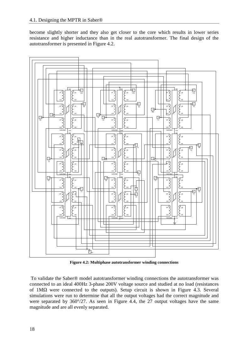
Since Saber® only supports 7 windings on one core leg when designing the model with the Magnetic Component Tool each of the core legs had to be divided into three series connected sections with six windings on each section. Because of this the lengths of the windings
4.1. Designing the MPTR in Saber®
18
become slightly shorter and they also get closer to the core which results in lower series resistance and higher inductance than in the real autotransformer. The final design of the autotransformer is presented in Figure 4.2.
trafo10at3
p3
m3
p6
m6
p2
m2 m5
p5
mm
mp
p1
m1 m4
p4
trafo10at3
p3
m3
p6
m6
p2
m2 m5
p5
mm
mp
p1
m1 m4
p4
trafo10at3
p3
m3
p6
m6
p2
m2 m5
p5
mm
mp
p1
m1 m4
p4
trafo10at2
p3
m3
p6
m6
p2
m2 m5
p5
mm
mp
p1
m1 m4
p4
trafo10at2
p3
m3
p6
m6
p2
m2 m5
p5
mm
mp
p1
m1 m4
p4
trafo10at2
p3
m3
p6
m6
p2
m2 m5
p5
mm
mp
p1
m1 m4
p4
trafo10at1
p3
m3
p6
m6
p2
m2 m5
p5
mm
mp
p1
m1 m4
p4
trafo10at1
p3
m3
p6
m6
p2
m2 m5
p5
mm
mp
p1
m1 m4
p4
trafo10at1
p3
m3
p6
m6
p2
m2 m5
p5
mm
mp
p1
m1 m4
p4
R1
S8
Vain
R5
S6
R3
T8
S1
T4
R9
T2
R4
S9
R7
T6
S4
S3
S7
T9
R2
S5
Vbin
R8
T1
Vcin
T5
R6
T3
S2
T7
Figure 4.2: Multiphase autotransformer winding connections
To validate the Saber® model autotransformer winding connections the autotransformer was connected to an ideal 400Hz 3-phase 200V voltage source and studied at no load (resistances of 1MΩ were connected to the outputs). Setup circuit is shown in Figure 4.3. Several simulations were run to determine that all the output voltages had the correct magnitude and were separated by 360°/27. As seen in Figure 4.4, the 27 output voltages have the same magnitude and are all evenly separated.

Chapter 4. Simulations
19
Three Phasea
b
cn
MPT1
R1
S8
Vain
R5
S6
R3
T8
S1
T4
R9
T2
R4
S9
R7
T6
S4
S3
S7
T9
R2
S5
Vbin
R8
T1
Vcin
T5
R6
T3
S2
T7
1meg
1meg
1meg
1meg
1meg
1meg
1meg
1meg
1meg
1meg
1meg
1meg
1meg
1meg
1meg
1meg
1meg
1meg
1meg
1meg
1meg
1meg
1meg
1meg
1meg
1meg
1meg
Figure 4.3: 3/27-phase autotransformer test setup at no load
Vol
tag
e (
V)
-150.0
-100.0
-50.0
0.0
50.0
100.0
150.0
t(s)47.0m 47.2m 47.4m 47.6m 47.8m 48.0m 48.2m 48.4m 48.6m 48.8m 49.0m 49.2m 49.4m 49.6m 49.8m 50.0m
Voltage (V) : t(s)
R1
S1
T1
R2
S2
T2
R3
S3
T3
R4
S4
T4
R5
S5
T5
R6
S6
T6
R7
S7
T7
R8
S8
T8
R9
S9
T9
Figure 4.4: Output voltages from the 3/27-phase autotransformer at no load

4.1. Designing the MPTR in Saber®
20
4.1.2 Rectifier bridges Three diode bridges consisting of 18 diodes each are the rectifying units of the MPTR [6],[9] as seen in Figure 4.5. Saber® provides several different methods to implement diodes, among these are different templates and the power diode tool. Both the power diode tool and the ideal diode template were investigated. Since the operating frequency was between 360-800Hz the recovery losses were negligible and a simpler model could be used without losing any accuracy in the simulations. The I-V characteristics of the diodes were determined from [10] and implemented in the ideal diode template.
pwld
pwld
pwld
pwld
pwld
pwld
pwld
pwld
pwld
pwld
pwld
pwld
pwld
pwld
pwld
pwld
pwld
pwld
1 2 3 4 5 6 7 8 9
dc+
dc-
Figure 4.5: Diode rectifier bridge

Chapter 4. Simulations
21
4.1.3 Input and output filters The MPTR has filters on the input and output terminals [6],[11],[12],[13]. The output filter has a smoothing function on the rectified voltage and consists of inductors and capacitances implemented in Saber® as seen in Figure 4.7. Common mode voltages are suppressed and the generator and flight avionics are protected from high frequency harmonics by the input filter. The inductive part of the input filter was designed using MCT and the complete input filter is presented in Figure 4.6.
trafo
10in
putfi
lter m
m
mp
p1 m1
trafo
10in
putfi
lter m
m
mp
p1 m1
trafo
10in
putfi
lter m
m
mp
p1 m1
Vain
Vbin
Vcin
Vaout
Vbout
Vcout
Figure 4.6: MPTR AC input filter

4.2. No load losses
22
4.2 No load losses Several simulations with no load were carried out for two reasons; to determine if the losses at no load agreed with the measured no load losses (thereby determining if the hysteresis loop designed using MCT were correct) and that the simulated DC output voltage of the MPTR complied with the measured DC output voltage (thereby determining that the threshold voltage implemented in the ideal diode template were correct). The test setup used in Saber® is shown in Figure 4.7. Both measured and simulated DC output voltage was 273.2V for frequencies between 360-800Hz. Figure 4.8 shows the simulated output DC voltage at 498Hz.
Rectifier1
1
2
3
4
5
6
7
8
9
dc+
dc-
Rectifier2
1
2
3
4
5
6
7
8
9
dc+
dc-
Rectifier3
1
2
3
4
5
6
7
8
9
dc+
dc-
Three Phasea
b
cn
MPT1
R1
S8
Vain
R5
S6
R3
T8
S1
T4
R9
T2
R4
S9
R7
T6
S4
S3
S7
T9
R2
S5
Vbin
R8
T1
Vcin
T5
R6
T3
S2
T7
1meg
ACInputFilter1
Vain
Vbin
Vcin
Vaout
Vbout
VcoutSoftStarter1
Vain
Vbin
Vaout
Vbout
Vcin Vcout
MPTR
Figure 4.7: MPTR at no load connected to an ideal 3-phase voltage source
Results from simulations of the MPTR no load losses at different frequencies and a comparison against the measured losses can be seen in Table 4.1. At no load, the input power and the losses are equal. The losses at no load are mainly caused by hysteresis losses in the autotransformer core since other losses such as winding and diode losses are negligible due to low current.
Several corrections of the hysteresis loop were made to match the measured no load losses. As seen in Table 4.1, measurements and simulations agree well for all frequencies. This indicates that both the width and the total area of the DC-hysteresis loop designed in Saber® are correct. Final design of the hysteresis loop is shown in Figure 4.1.

Chapter 4. Simulations
23
Trafo10noload
t(s)0.18 0.181 0.182 0.183 0.184 0.185 0.186 0.187 0.188 0.189 0.19 0.191 0.192 0.193 0.194 0.195 0.196 0.197 0.198 0.199
Vol
tag
e (
V)
272.0
272.2
272.4
272.6
272.8
273.0
273.2
273.4
273.6
273.8
274.0Voltage (V) : t(s)
VDC_out
Figure 4.8: Output DC voltage of the MPTR at no load and 498Hz
Table 4.1: Simulated and measured data for no load losses at different frequencies
Frequency (Hz)
Measured active input power (W)
Simulated active input power (W)
Difference (W)
Difference (%)
360 139.4 130.56 8.84 6.77
400 101.3 100.85 0.45 0.44
498 74.2 81.39 -7.19 -8.83
577 64.6 72.79 -8.19 -11.25
700 60.6 62.60 -2.00 -3.19
800 61.1 59.79 1.31 2.19

4.3. Losses with load
24
4.3 Losses with load When performing measurements on the MPTR at SMW purely resistive loads were connected to the PSU/6’s. A PSU/6 is a power unit consisting of a number of converters fed by a large capacitor bank. In order to simulate this scenario in Saber® equivalent circuits of the PSU/6’s capacitive behaviour had to be designed. Based on circuit diagram [14] the PSU/6’s were implemented with a capacitor and two inductors. The filterboards were designed using circuit diagram [15] and connected between the MPTR and PSU/6’s according to Figure 4.9.
In chapter 3.3 voltage drop and power losses at different frequencies and loads were measured on the MPTR. Several simulations were run with the same frequency and magnitude of the input voltage and active output power of the MPTR as in each measurement case. For a specific load and frequency case in the measurement chapter the ideal voltage source seen in Figure 4.9 was implemented with the measured input voltage and the given frequency. To get the same active output power for each case in the simulations as in the measurements a resistance causing this was calculated and implemented after the PSU/6’s as seen in Figure 4.9. The resistance for each PSU/6 load can be seen in Table 4.2, Table 4.3 and Table 4.4. Since an ideal voltage source with no internal inductance was used the input current THD was higher in the simulations compared to the measurements for all load cases.
Rectifier1
1
2
3
4
5
6
7
8
9
dc+
dc-
Rectifier2
1
2
3
4
5
6
7
8
9
dc+
dc-
Rectifier3
1
2
3
4
5
6
7
8
9
dc+
dc-
Three Phasea
b
cn
MPT1
R1
S8
Vain
R5
S6
R3
T8
S1
T4
R9
T2
R4
S9
R7
T6
S4
S3
S7
T9
R2
S5
Vbin
R8
T1
Vcin
T5
R6
T3
S2
T7
ACInputFilter1
Vain
Vbin
Vcin
Vaout
Vbout
Vcout
SoftStarter1
Vain
Vbin
Vaout
Vbout
Vcin Vcout
PSU/6
PSU/6
MPTR
PSU/6FILTERBOARD
FILTERBOARD
FILTERBOARD
Figure 4.9: MPTR connected to an ideal 3-phase voltage source and three PSU/6’s with resistive loads

Chapter 4. Simulations
25
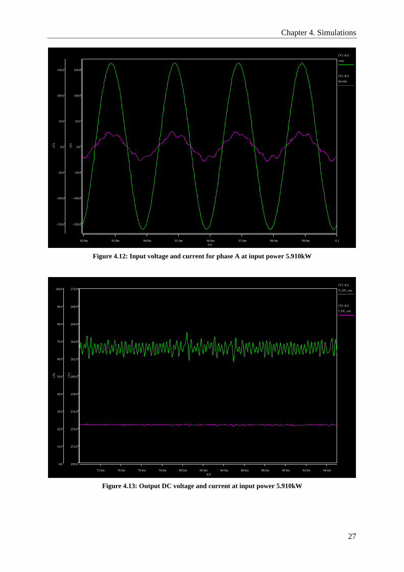
4.3.1 Simulations with one PSU/6 connected The results from the simulations in Saber® with one PSU/6 connected are seen in Table 4.2. The simulated voltage drop across the MPTR is very similar to the measured voltage drop seen in Table 3.2 with one PSU/6 connected. The losses were lower in the simulations compared to the measurements. The simulated input current also has higher THD but the waveshape of the input current depends on both the power source and the connected load.
Table 4.2: Simulated data with one PSU/6 connected at 498Hz and different loads
Frequency (Hz)
Active input power (kW)
Active output power (kW)
Efficiency (%)
Input phase
voltage (V)
Input current
(A)
Input current THD %
Output DC
voltage (V)
Output DC
voltage ripple (V)
PSU/6 load (Ω)
498 3.904 3.797 97.25 114.42 11.744 17.68 264.4 2.088 18.477
498 5.910 5.776 97.73 114.11 17.457 14.59 263.2 1.900 12.013
Input voltages and currents for phase A to the MPTR for the simulated cases are shown in Figure 4.10 and Figure 4.12 while the output DC voltages and currents are shown in Figure 4.11 and Figure 4.13.

4.3. Losses with load
26
t(s)92.0m 93.0m 94.0m 95.0m 96.0m 97.0m 98.0m 99.0m 0.1
(V
)
-150.0
-100.0
-50.0
0.0
50.0
100.0
150.0 (
A)
-150.0
-100.0
-50.0
0.0
50.0
100.0
150.0
(V) : t(s)
vain
(A) : t(s)
i(vain)
Figure 4.10: Input voltage and current for phase A at input power 3.904kW
t(s)72.0m 74.0m 76.0m 78.0m 80.0m 82.0m 84.0m 86.0m 88.0m 90.0m 92.0m 94.0m
(V
)
250.0
252.0
254.0
256.0
258.0
260.0
262.0
264.0
266.0
268.0
270.0
(A
)
0.0
10.0
20.0
30.0
40.0
50.0
60.0
70.0
80.0
90.0
100.0(V) : t(s)
V_DC_out
(A) : t(s)
I_DC_out
Figure 4.11: Output DC voltage and current at input power 3.904kW
Chapter 4. Simulations
27
t(s)92.0m 93.0m 94.0m 95.0m 96.0m 97.0m 98.0m 99.0m 0.1
(V
)
-150.0
-100.0
-50.0
0.0
50.0
100.0
150.0 (
A)
-150.0
-100.0
-50.0
0.0
50.0
100.0
150.0
(V) : t(s)
vain
(A) : t(s)
i(vain)
Figure 4.12: Input voltage and current for phase A at input power 5.910kW
t(s)72.0m 74.0m 76.0m 78.0m 80.0m 82.0m 84.0m 86.0m 88.0m 90.0m 92.0m 94.0m
(V
)
250.0
252.0
254.0
256.0
258.0
260.0
262.0
264.0
266.0
268.0
270.0
(A
)
0.0
10.0
20.0
30.0
40.0
50.0
60.0
70.0
80.0
90.0
100.0(V) : t(s)
V_DC_out
(A) : t(s)
I_DC_out
Figure 4.13: Output DC voltage and current at input power 5.910kW

4.3. Losses with load
28
4.3.2 Simulations with two PSU/6 connected The results from the simulations in Saber® with two PSU/6 connected seen in Table 4.3 complied fairly well with the measurements carried out at SMW seen in Table 3.3. The simulated voltage drop across the MPTR is very similar to the measured voltage drop with two PSU/6 connected. The losses were lower in the simulations compared to the measurements. At 360Hz and 400Hz the DC output voltage ripple had a harmonic content not seen in the measurements. This is probably caused by the higher inductance of the simulated autotransformer (see chapter 4.1.1) not matching the output filter of the MPTR. The simulated input current also has higher THD (significantly higher for 360Hz) but the waveshape of the input current depends on both the power source and the connected load. As stated in chapter 4.3 an ideal voltage source was used in these simulations.
Table 4.3: Simulated data with two PSU/6 connected at different frequencies and loads
Frequency (Hz)
Active input power (kW)
Active output power (kW)
Efficiency (%)
Input phase
voltage (V)
Input current
(A)
Input current THD (%)
Output DC
voltage (V)
Output DC
voltage ripple (V)
PSU/6 load (Ω)
360 8.850 8.642 97.64 113.61 26.642 20.91 261.6 4.102 15.843
400 11.992 11.763 98.09 109.97 36.582 9.791 252.7 3.221 10.884
498 8.861 8.709 98.28 113.69 26.093 9.027 261.8 1.961 15.766
800 8.847 8.690 98.23 113.66 26.087 6.261 261.7 1.130 15.807
Input voltages and currents for phase A to the MPTR for the simulated cases are shown in Figure 4.14, Figure 4.16, Figure 4.18 and Figure 4.20 while the output voltages and currents are shown in Figure 4.15, Figure 4.17, Figure 4.19 and Figure 4.21.

Chapter 4. Simulations
29
t(s)0.189 0.19 0.191 0.192 0.193 0.194 0.195 0.196 0.197 0.198 0.199 0.2
(V
)
-150.0
-100.0
-50.0
0.0
50.0
100.0
150.0 (
A)
-150.0
-100.0
-50.0
0.0
50.0
100.0
150.0
(V) : t(s)
vain
(A) : t(s)
i(vain)
Figure 4.14: Input voltage and current for phase A 360Hz
t(s)70.0m 72.0m 74.0m 76.0m 78.0m 80.0m 82.0m 84.0m 86.0m 88.0m 90.0m 92.0m 94.0m
(V)
250.0
252.0
254.0
256.0
258.0
260.0
262.0
264.0
266.0
268.0
270.0
(A)
0.0
10.0
20.0
30.0
40.0
50.0
60.0
70.0
80.0
90.0
100.0
(V) : t(s)
V_DC_out
(A) : t(s)
I_DC_out
Figure 4.15: Output DC voltage and current for 360Hz input

4.3. Losses with load
30
t(s)90.0m 91.0m 92.0m 93.0m 94.0m 95.0m 96.0m 97.0m 98.0m 99.0m
(V
)
-150.0
-100.0
-50.0
0.0
50.0
100.0
150.0 (
A)
-150.0
-100.0
-50.0
0.0
50.0
100.0
150.0
(V) : t(s)
vain
(A) : t(s)
i(vain)
Figure 4.16: Input voltage and current for phase A 400Hz
t(s)72.0m 74.0m 76.0m 78.0m 80.0m 82.0m 84.0m 86.0m 88.0m 90.0m 92.0m 94.0m
(V
)
250.0
252.0
254.0
256.0
258.0
260.0
262.0
264.0
266.0
268.0
270.0
(A
)
0.0
10.0
20.0
30.0
40.0
50.0
60.0
70.0
80.0
90.0
100.0(V) : t(s)
V_DC_out
(A) : t(s)
I_DC_out
Figure 4.17: Output DC voltage and current for 400Hz input

Chapter 4. Simulations
31
(A)
-150.0
-100.0
-50.0
0.0
50.0
100.0
150.0
t(s)92.0m 93.0m 94.0m 95.0m 96.0m 97.0m 98.0m 99.0m 0.1
(V)
-150.0
-100.0
-50.0
0.0
50.0
100.0
150.0
(V) : t(s)
vain
(A) : t(s)
i(vain)
Figure 4.18: Input voltage and current for phase A 498Hz
t(s)72.0m 74.0m 76.0m 78.0m 80.0m 82.0m 84.0m 86.0m 88.0m 90.0m 92.0m 94.0m
(V
)
250.0
252.0
254.0
256.0
258.0
260.0
262.0
264.0
266.0
268.0
270.0
(A
)
0.0
10.0
20.0
30.0
40.0
50.0
60.0
70.0
80.0
90.0
100.0(V) : t(s)
V_DC_out
(A) : t(s)
I_DC_out
Figure 4.19: Output DC voltage and current for 498Hz input

4.3. Losses with load
32
t(s)95.0m 95.5m 96.0m 96.5m 97.0m 97.5m 98.0m 98.5m 99.0m 99.5m 0.1
(V
)
-150.0
-100.0
-50.0
0.0
50.0
100.0
150.0 (
A)
-150.0
-100.0
-50.0
0.0
50.0
100.0
150.0
(V) : t(s)
vain
(A) : t(s)
i(vain)
Figure 4.20: Input voltage and current for phase A 800Hz
t(s)72.0m 74.0m 76.0m 78.0m 80.0m 82.0m 84.0m 86.0m 88.0m 90.0m 92.0m 94.0m
(V
)
250.0
252.0
254.0
256.0
258.0
260.0
262.0
264.0
266.0
268.0
270.0
(A
)
0.0
10.0
20.0
30.0
40.0
50.0
60.0
70.0
80.0
90.0
100.0(V) : t(s)
V_DC_out
(A) : t(s)
I_DC_out
Figure 4.21: Output DC voltage and current for 800Hz input

Chapter 4. Simulations
33
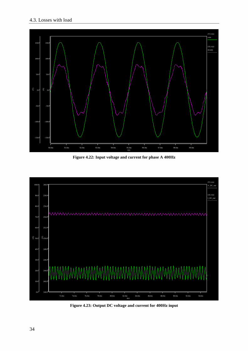
4.3.3 Simulations with three PSU/6 connected The results from the simulation in Saber® with three PSU/6 connected are seen in Table 4.4. The simulated voltage drop across the MPTR is exactly the same as the measured voltage drop with three PSU/6 connected. The losses were lower in the simulations compared to the measurements.
Table 4.4: Measured data with three PSU/6 connected at 400Hz
Frequency (Hz)
Active input power (kW)
Active output power (kW)
Efficiency (%)
Input phase
voltage (V)
Input current
(A)
Input current THD (%)
Output DC
voltage (V)
Output DC
voltage ripple (V)
PSU/6 load (Ω)
400 17.925 17.561 97.96 106.34 56.305 6.530 243.5 2.638 10.146
Input voltage and current for phase A to the MPTR for the simulated case are shown in Figure 4.22 while the output voltage and current are shown in Figure 4.23.
4.3. Losses with load
34
t(s)90.0m 91.0m 92.0m 93.0m 94.0m 95.0m 96.0m 97.0m 98.0m 99.0m
(V
)
-150.0
-100.0
-50.0
0.0
50.0
100.0
150.0 (
A)
-150.0
-100.0
-50.0
0.0
50.0
100.0
150.0
(V) : t(s)
vain
(A) : t(s)
i(vain)
Figure 4.22: Input voltage and current for phase A 400Hz
t(s)72.0m 74.0m 76.0m 78.0m 80.0m 82.0m 84.0m 86.0m 88.0m 90.0m 92.0m 94.0m
(V
)
240.0
242.0
244.0
246.0
248.0
250.0
252.0
254.0
256.0
258.0
260.0
(A
)
0.0
10.0
20.0
30.0
40.0
50.0
60.0
70.0
80.0
90.0
100.0(V) : t(s)
V_DC_out
(A) : t(s)
I_DC_out
Figure 4.23: Output DC voltage and current for 400Hz input

Chapter 4. Simulations
35
4.4 Designing the Saab 2000 generator using Saber®
4.4.1 Generator The following parameters for the generator in the Saab 2000 aircraft were given [16]:
• Type of generator: Brushless DC
• Operating frequency range: 380-606Hz
• kVA rating: 45kVA @ 404-480Hz
60kVA @ 480-606Hz
Rating degraded linearly to 36kVA between 380-404Hz
• Power factor: 0.85 (lagging)
• Number of poles: 4
In order to build a model of the generator in Saber®, at least inertia, line to line inductance and resistance have to be known. Under the assumption of an efficiency of 90%, power factor 0.85 at 606Hz and rated power, the resistance and inductance was determined to 62mΩ and 0.102mH respectively. The inertia was set to 50µkgms2.
In a Brushless DC generator the output voltages are proportional to the angular velocity on the shaft. Since the output voltages shall be constant for the entire operating frequency range, field weakening of the BLDC generator needs to be implemented.
In the BLDC generator model that comes with Saber® the back-emf constant (ke) is a
parameter that cannot be altered during simulation. The output voltage will therefore be proportional to the frequency. After contact with Synopsys [17] a model with ke as an input
variable was provided and a simplified model of field weakening during simulation can be implemented.
4.4.2 PI-regulator To keep a constant output voltage (200V) from the BLDC generator regardless of the angular velocity and current (internal voltage drop), a PI-regulator controlling the back-emf constant (ke) was designed.
The angle of the rotor, the three output voltages and currents from the BLDC generator are measured and by using abc to dq coordinate transformation [18] the voltages can be transformed as
+−
+−
+−
+
+
+=
c
b
a
q
d
V
V
V
V
V
6sin
6
5sin
2
3sin
6cos
6
5cos
2
3cos
3
2πϕπϕπϕ
πϕπϕπϕ (4.1)
and the currents can be transformed as
+−
+−
+−
+
+
+=
c
b
a
q
d
I
I
I
I
I
6sin
6
5sin
2
3sin
6cos
6
5cos
2
3cos
3
2πϕπϕπϕ
πϕπϕπϕ (4.2)

4.4. Designing the Saab 2000 generator using Saber®
36
where Vd, Vq and Id, Iq are DC quantities that can be controlled with a PI-regulator. Implementation of the coordinate transformation in Saber® according to (4.1) and (4.2) can be seen in Appendix C. The complete control circuit including PI-regulator with anti-windup and control signal limiter implemented in Saber® can be seen in Figure 4.24.
Keout
Vdi
n
diff
Σ+1
+1
in1 out
in2
Σ+1
+1
in1 out
in2
diff
k:1000
k:100
ks
integk:10
c_constant
244
Iqin
mult
in1
in2
c_constant
0.12369m
mult
k:3/2
in1
in2
Σ+1
+1
in1 out
in2
wrm Figure 4.24: PI-regulator with anti-windup
4.4.3 Cable Since the generator is located at the motor some distance from the MPTR the non idealities of the cable connecting the generator and the MPTR needs to be accounted for. A template modelling a screened cylindrical 3-phase cable was chosen. The phase conductors (also cylindrical) have a crossectional area of 20mm2 and are made of copper. Semiconducting layers surround each phase.
The chosen template takes many parameters into account. Series resistance and capacitance, inductance and conductance between phases are modelled. Capacitance, inductance and conductance between each phase and ground (screen) are also modelled. Although no significant difference where noticed between the different cable templates an advanced cable template was chosen since the simulation time only increased slightly.

Chapter 4. Simulations
37
4.5 Benefits of using MPTR In chapter 1.1 the importance to avoid interference of sensitive electric devices such as flight avionics connected to the same generator as the radar power system was stated.
In the previous ERIEYE® radar power system each of the PSU/6’s had a 6-pulse rectifier bridge and the six PSU/6’s was fed from one dedicated generator running at 400Hz.
To compare the two methods of AC/DC conversion a model representing half the previous radar power system (three PSU/6’s) was built in Saber®. The MPTR model was removed and the PSU/6’s were replaced by the ones used in the older radar power system [19]. The filterboards were replaced by three PSU/6 input line filters and nine inductors [20],[21]. Connecting the new system to the Saab 2000 BLDC generator designed in chapter 4.4.1 resulted in the circuit seen in Figure 4.25. Circuits used in Saber® for comparison are shown in Figure 4.25 and Figure 4.26.
Shield Shield
cable_em4s
m_0
m_1
m_2
m_3
p_0
p_1
p_2
p_3
PSU/6
angw_pulse
initial:0
pulse:1564.51319*498/498
NS
sin_bldc_3p_ke
r:2*62.45179ml :2*0.10165m
p:4j:5e-5
t3
t2
wrm
t1
thetarm
c_constant
0.231524*400/498
pwld
pwld
pwld
pwld
pwld
pwld
Line filter
pwld
pwld
pwld
PSU/6pw
ld
pwld
pwld
Line filter
pwld
pwld
Line filter
pwld
pwld
pwld
pwld
PSU/6
Figure 4.25: Saab 2000 generator connected to the previous PSU/6’s with resistive loads

4.5. Benefits of using MPTR
38
Rectifier1
1
2
3
4
5
6
7
8
9
dc+
dc-
Rectifier2
1
2
3
4
5
6
7
8
9
dc+
dc-
Rectifier3
1
2
3
4
5
6
7
8
9
dc+
dc-
MPT1
R1
S8
Vain
R5
S6
R3
T8
S1
T4
R9
T2
R4
S9
R7
T6
S4
S3
S7
T9
R2
S5
Vbin
R8
T1
Vcin
T5
R6
T3
S2
T7
NS
sin_bldc_3p_ke
r:2*62.45179ml:2*0.10165m
p:4j:5e-5
t3
t2
wrm
t1
thetarm
angw_pulse
initial:0
pulse:1564.51319*498/498
Sh ie ld Shie ld
cable_em4s
m_0
m_1
m_2
m_3
p_0
p_1
p_2
p_3
ACInputFilter1
Vain
Vbin
Vcin
Vaout
Vbout
Vcout
PSU/6
MPTR
PSU/6
PSU/6
FILTERBOARD
FILTERBOARD
FILTERBOARD
c_constant
0.239338*400/498
Figure 4.26: MPTR connected to the Saab 2000 generator and three PSU/6’s with resistive loads
The generator was set to 400Hz or 498Hz and 200V. Those two frequencies were chosen since the new system mostly operates at 498Hz and the previous system only operates at 400Hz. Furthermore measurements have been conducted at SMW on the previous system connected to the Saab 2000 generator running at 400Hz.
Figure 4.31 shows the results from the measurement with purely resistive load (21.4kW) connected to the PSU/6’s. The waveshapes of the voltage and current are very similar to the simulated ones of the previous radar power system at 20kW presented in Figure 4.30. The THD for the voltage and current at the generator in this system is mainly determined by the line inductors and the parameters of the generator. The I-V characteristics of the diodes and the capacitive and inductive content of the PSU/6’s have very small influence on the THD at the generator. Since the measured voltage and current THD agrees fairly well with simulated THD (seen in Figure 4.32, Figure 4.33 and Table 4.5) and the value of the line inductors are known, the Saab 2000 generator designed in chapter 4.4.1 probably is accurate enough to be used in an ERIEYE® power system simulation.
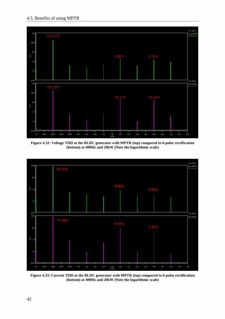
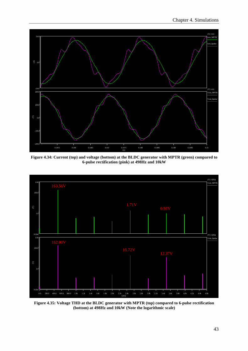
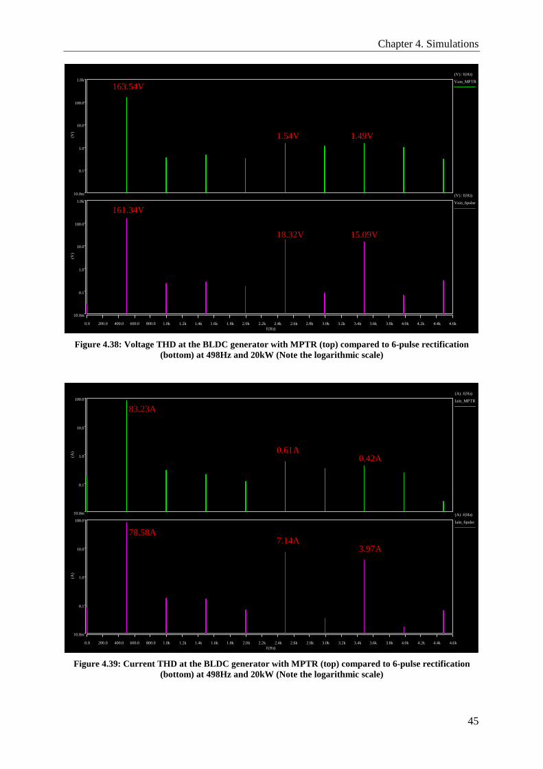
The simulated waveforms of the voltages and currents at the generator were compared at full and half load (20kW & 10kW) connected to three PSU/6’s for the two different ERIEYE® power systems. As expected the improvement of using a MPTR were significant, resulting in a much smoother voltage and current waveshape and lower THD as can be seen in Figure 4.27 to Figure 4.30, Figure 4.32 to Figure 4.39 and Table 4.5.

Chapter 4. Simulations
39
Table 4.5: Voltage and current THD for different frequencies and loads
MPTR 10kW 400Hz
6-pulse 10kW 400Hz
MPTR 20kW 400Hz
6-pulse 20kW 400Hz
MPTR 10kW 498HZ
6-pulse 10kW 498Hz
MPTR 20kW 498Hz
6-pulse 20kW 498Hz
Voltage THD (%)
2.008 13.86 2.329 15.73 1.939 13.05 2.445 15.19
Current THD (%)
2.345 24.09 1.356 13.64 2.179 17.9 1.179 10.45
(V
)
-200.0
-100.0
0.0
100.0
200.0
t(s)0.1455 0.146 0.1465 0.147 0.1475 0.148 0.1485 0.149 0.1495 0.15
(A
)
-50.0
0.0
50.0
(V) : t(s)
Vain_MPTR
Vain_6pulse
(A) : t(s)
Iain_MPTR
Iain_6pulse
Figure 4.27: Current (top) and voltage (bottom) at the BLDC generator with MPTR (green) compared to
6-pulse rectification (pink) at 400Hz and 10kW

4.5. Benefits of using MPTR
40
(V
)
10.0m
1.0
100.0
1.0k
f(Hz)0.0 200.0 400.0 600.0 800.0 1.0k 1.2k 1.4k 1.6k 1.8k 2.0k 2.2k 2.4k 2.6k 2.8k 3.0k 3.2k 3.4k 3.6k
(V
)
10.0m
1.0
100.0
1.0k
(V) : f(Hz)
Vain_6pulse
(V) : f(Hz)
Vain_MPTR
Figure 4.28: Voltage THD at the BLDC generator with MPTR (top) compared to 6-pulse rectification
(bottom) at 400Hz and 10kW (Note the logarithmic scale)
(A
)
10.0m
0.1
1.0
10.0
100.0
1.0k
f(Hz)0.0 200.0 400.0 600.0 800.0 1.0k 1.2k 1.4k 1.6k 1.8k 2.0k 2.2k 2.4k 2.6k 2.8k 3.0k 3.2k 3.4k 3.6k
(A
)
10.0m
0.1
1.0
10.0
100.0
1.0k
(A) : f(Hz)
Iain_6pulse
(A) : f(Hz)
Iain_MPTR
Figure 4.29: Current THD at the BLDC generator with MPTR (top) compared to 6-pulse rectification
(bottom) at 400Hz and 10kW (Note the logarithmic scale)
163.33V
1.40V 1.35V
161.81V
17.23V 13.37V
39.69A
41.76A
0.69A 0.46A
8.39A 4.40A

Chapter 4. Simulations
41
(V
)
-200.0
-100.0
0.0
100.0
200.0
t(s)0.1455 0.146 0.1465 0.147 0.1475 0.148 0.1485 0.149 0.1495 0.15
(A
)
-100.0
0.0
100.0
(V) : t(s)
Vain_MPTR
Vain_6pulse
(A) : t(s)
Iain_MPTR
Iain_6pulse
Figure 4.30: Current (top) and voltage (bottom) at the BLDC generator with MPTR (green) compared to
6-pulse rectification (pink) at 400Hz and 20kW
4.27.a: Voltage, current and power 4.27.b: Voltage and current THD
Figure 4.31: Measurements of the previous radar power system connected to a Saab 2000 generator
4.5. Benefits of using MPTR
42
f(Hz)0.0 200.0 400.0 600.0 800.0 1.0k 1.2k 1.4k 1.6k 1.8k 2.0k 2.2k 2.4k 2.6k 2.8k 3.0k 3.2k 3.4k 3.6k
(V
)
10.0m
0.1
1.0
10.0
100.0
1.0k
(V
)
10.0m
0.1
1.0
10.0
100.0
1.0k
(V) : f(Hz)
Vain_6pulse
(V) : f(Hz)
Vain_MPTR
Figure 4.32: Voltage THD at the BLDC generator with MPTR (top) compared to 6-pulse rectification
(bottom) at 400Hz and 20kW (Note the logarithmic scale)
(A
)
10.0m
0.1
1.0
10.0
100.0
f(Hz)0.0 200.0 400.0 600.0 800.0 1.0k 1.2k 1.4k 1.6k 1.8k 2.0k 2.2k 2.4k 2.6k 2.8k 3.0k 3.2k 3.4k 3.6k
(A
)
10.0m
0.1
1.0
10.0
100.0
(A) : f(Hz)
Iain_6pulse
(A) : f(Hz)
Iain_MPTR
Figure 4.33: Current THD at the BLDC generator with MPTR (top) compared to 6-pulse rectification
(bottom) at 400Hz and 20kW (Note the logarithmic scale)
163.27V
1.81V 1.35V
161.29V
18.55V 15.45V
83.05A
0.98A 0.52A
77.40A 9.10A
5.10A
Chapter 4. Simulations
43
(V
)
-200.0
-100.0
0.0
100.0
200.0
t(s)0.1455 0.146 0.1465 0.147 0.1475 0.148 0.1485 0.149 0.1495 0.15
(A
)
-50.0
0.0
50.0
(V) : t(s)
Vain_MPTR
Vain_6pulse
(A) : t(s)
Iain_MPTR
Iain_6pulse
Figure 4.34: Current (top) and voltage (bottom) at the BLDC generator with MPTR (green) compared to
6-pulse rectification (pink) at 498Hz and 10kW
(V
)
10.0m
1.0
100.0
1.0k
f(Hz)0.0 200.0 400.0 600.0 800.0 1.0k 1.2k 1.4k 1.6k 1.8k 2.0k 2.2k2.4k 2.6k 2.8k 3.0k 3.2k 3.4k 3.6k 3.8k 4.0k 4.2k 4.4k 4.6k
(V
)
10.0m
1.0
100.0
1.0k
(V) : f(Hz)
Vain_6pulse
(V) : f(Hz)
Vain_MPTR
Figure 4.35: Voltage THD at the BLDC generator with MPTR (top) compared to 6-pulse rectification
(bottom) at 498Hz and 10kW (Note the logarithmic scale)
163.56V
1.71V 0.93V
162.00V
16.72V 12.37V

4.5. Benefits of using MPTR
44
(A
)
10.0m
0.1
1.0
10.0
100.0
f(Hz)0.0 200.0 400.0 600.0 800.0 1.0k 1.2k 1.4k 1.6k 1.8k 2.0k 2.2k2.4k 2.6k 2.8k 3.0k 3.2k 3.4k 3.6k 3.8k 4.0k 4.2k 4.4k 4.6k
(A
)
10.0m
0.1
1.0
10.0
100.0
(A) : f(Hz)
Iain_6pulse
(A) : f(Hz)
Iain_MPTR
Figure 4.36: Current THD at the BLDC generator with MPTR (top) compared to 6-pulse rectification
(bottom) at 498Hz and 10kW (Note the logarithmic scale)
(V
)
-200.0
-100.0
0.0
100.0
200.0
t(s)0.14525 0.1455 0.14575 0.146 0.14625 0.1465 0.14675 0.147 0.14725 0.1475 0.14775 0.148 0.14825 0.1485 0.14875 0.149 0.14925 0.1495 0.14975 0.15
(A
)
-100.0
-50.0
0.0
50.0
100.0
(V) : t(s)
Vain_MPTR
Vain_6pulse
(A) : t(s)
Iain_MPTR
Iain_6pulse
Figure 4.37: Current (top) and voltage (bottom) at the BLDC generator with MPTR (green) compared to
6-pulse rectification (pink) at 498Hz and 20kW
41.61A
0.72A 0.28A
41.09A 6.54A
3.26A
Chapter 4. Simulations
45
(V
)
10.0m
0.1
1.0
10.0
100.0
1.0k
f(Hz)0.0 200.0 400.0 600.0 800.0 1.0k 1.2k 1.4k 1.6k 1.8k 2.0k 2.2k2.4k 2.6k 2.8k 3.0k 3.2k 3.4k 3.6k 3.8k 4.0k 4.2k 4.4k 4.6k
(V
)
10.0m
0.1
1.0
10.0
100.0
1.0k
(V) : f(Hz)
Vain_6pulse
(V) : f(Hz)
Vain_MPTR
Figure 4.38: Voltage THD at the BLDC generator with MPTR (top) compared to 6-pulse rectification
(bottom) at 498Hz and 20kW (Note the logarithmic scale)
(A
)
10.0m
0.1
1.0
10.0
100.0
f(Hz)0.0 200.0 400.0 600.0 800.0 1.0k 1.2k 1.4k 1.6k 1.8k 2.0k 2.2k2.4k 2.6k 2.8k 3.0k 3.2k 3.4k 3.6k 3.8k 4.0k 4.2k 4.4k 4.6k
(A
)
10.0m
0.1
1.0
10.0
100.0
(A) : f(Hz)
Iain_6pulse
(A) : f(Hz)
Iain_MPTR
Figure 4.39: Current THD at the BLDC generator with MPTR (top) compared to 6-pulse rectification
(bottom) at 498Hz and 20kW (Note the logarithmic scale)
163.54V
1.54V 1.49V
161.34V
18.32V 15.09V
83.23A
78.58A
0.61A 0.42A
7.14A 3.97A

4.6. Simulation of the ERIEYE® power system
46
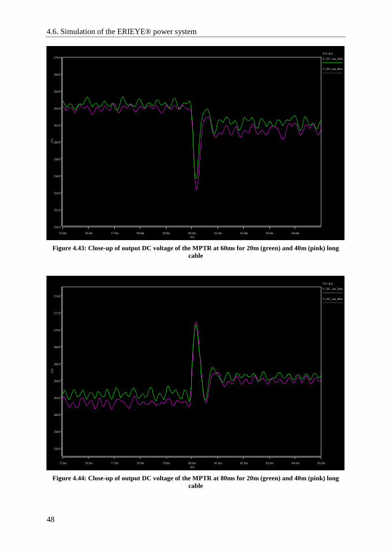
4.6 Simulation of the ERIEYE® power system The MPTR were connected to the PI-controlled BLDC generator through a 3-phase shielded cable described in chapter 4.4 and implemented in Saber® as seen in Appendix D. The three PSU/6’s were connected to switched resistive loads altering the power output from the MPTR between full (20kW) and half load (10kW). The torque on the generator shaft was studied for the whole simulation and is presented in Figure 4.40. Voltage levels and transients were observed at the MPTR input and output for different cable lengths (20&40m) between the generator and the MPTR.
DC output voltage of the MPTR during the whole simulation for the two different cable lengths are shown in Figure 4.41. Before 40ms the generator is running at no load and 498Hz. At 40ms a load step (10kW) with a risetime of 0.1ms is applied and DC output voltages are shown in Figure 4.42. Figure 4.43 presents another identical load step of 10kW added at 60ms causing the system to run at full load. At 80ms the load is shifted back to 10kW presented in Figure 4.44. At 100ms a speed step with the rise time of 1ms is applied to the generator and the frequency is increased from 498Hz to 577Hz. DC voltage levels during this transition can be seen in Figure 4.45. At 120ms the load is yet again increased to 20kW as seen in Figure 4.46.
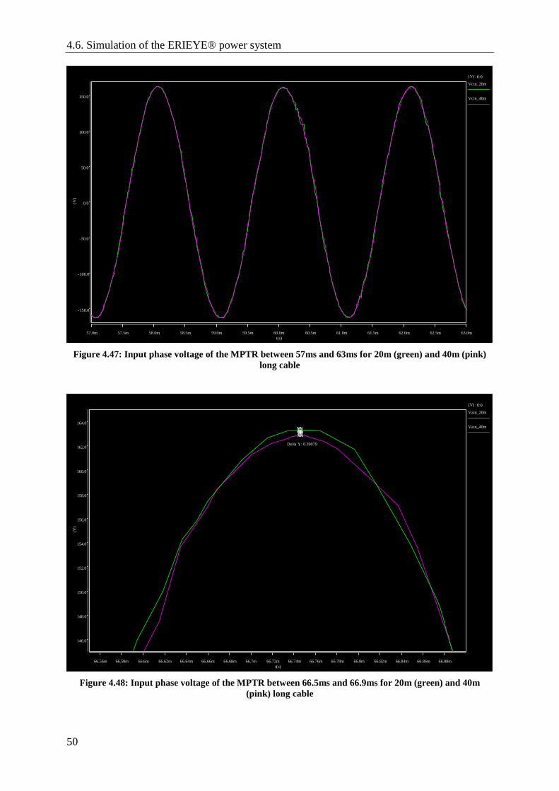
The AC input phase voltage of the MPTR during load step from 10kW to 20kW (498Hz) for the two different cable lengths are shown in Figure 4.47. The load step causes a small distortion on the input voltage. The difference (0.39V) in magnitude of the input voltage at full load and 498Hz for the two cables is presented in Figure 4.48. Figure 4.49 shows the input phase voltages for the two cable lengths during the speed step. The input phase voltages during the speed step are kept constant by the PI-regulator.
t(s)40.0m 50.0m 60.0m 70.0m 80.0m 90.0m 0.1 0.11 0.12 0.13
(N
.m)
-20.0
-18.0
-16.0
-14.0
-12.0
-10.0
-8.0
-6.0
-4.0
-2.0
0.0(N.m) : t(s)
Torque_shaft(Nm)
Figure 4.40: Torque on the BLDC generator shaft

Chapter 4. Simulations
47
t(s)40.0m 50.0m 60.0m 70.0m 80.0m 90.0m 0.1 0.11 0.12 0.13
(V
)
255.0
260.0
265.0
270.0
(V) : t(s)
V_DC_out_20m
V_DC_out_40m
Figure 4.41: Output DC voltage of the MPTR for 20m (green) and 40m (pink) long cable
t(s)36.0m 37.0m 38.0m 39.0m 40.0m 41.0m 42.0m 43.0m 44.0m
(V
)
255.0
260.0
265.0
270.0
275.0(V) : t(s)
V_DC_out_20m
V_DC_out_40m
Figure 4.42: Close-up of output DC voltage of the MPTR at 40ms for 20m (green) and 40m (pink) long
cable
4.6. Simulation of the ERIEYE® power system
48
t(s)55.0m 56.0m 57.0m 58.0m 59.0m 60.0m 61.0m 62.0m 63.0m 64.0m
(V
)
250.0
252.0
254.0
256.0
258.0
260.0
262.0
264.0
266.0
268.0
270.0(V) : t(s)
V_DC_out_20m
V_DC_out_40m
Figure 4.43: Close-up of output DC voltage of the MPTR at 60ms for 20m (green) and 40m (pink) long
cable
t(s)75.0m 76.0m 77.0m 78.0m 79.0m 80.0m 81.0m 82.0m 83.0m 84.0m 85.0m
(V
)
256.0
258.0
260.0
262.0
264.0
266.0
268.0
270.0
272.0
274.0
(V) : t(s)
V_DC_out_20m
V_DC_out_40m
Figure 4.44: Close-up of output DC voltage of the MPTR at 80ms for 20m (green) and 40m (pink) long
cable

Chapter 4. Simulations
49
t(s)95.0m 96.0m 97.0m 98.0m 99.0m 0.1 0.101 0.102 0.103 0.104
(V
)
255.0
260.0
265.0
270.0
275.0(V) : t(s)
V_DC_out_20m
V_DC_out_40m
Figure 4.45: Close-up of output DC voltage of the MPTR at 100ms for 20m (green) and 40m (pink) long
cable
t(s)0.116 0.118 0.12 0.122 0.124
(V
)
250.0
252.0
254.0
256.0
258.0
260.0
262.0
264.0
266.0
268.0
270.0(V) : t(s)
V_DC_out_20m
V_DC_out_40m
Figure 4.46: Close-up of output DC voltage of the MPTR at 120ms for 20m (green) and 40m (pink) long
cable
4.6. Simulation of the ERIEYE® power system
50
t(s)57.0m 57.5m 58.0m 58.5m 59.0m 59.5m 60.0m 60.5m 61.0m 61.5m 62.0m 62.5m 63.0m
(V
)
-150.0
-100.0
-50.0
0.0
50.0
100.0
150.0
(V) : t(s)
Vcin_20m
Vcin_40m
Figure 4.47: Input phase voltage of the MPTR between 57ms and 63ms for 20m (green) and 40m (pink)
long cable
(V
)
146.0
148.0
150.0
152.0
154.0
156.0
158.0
160.0
162.0
164.0
t(s)66.56m 66.58m 66.6m 66.62m 66.64m 66.66m 66.68m 66.7m 66.72m 66.74m 66.76m 66.78m 66.8m 66.82m 66.84m 66.86m 66.88m
(V) : t(s)
Vain_20m
Vain_40m
Delta Y: 0.39079
Figure 4.48: Input phase voltage of the MPTR between 66.5ms and 66.9ms for 20m (green) and 40m
(pink) long cable

Chapter 4. Simulations
51
t(s)95.0m 96.0m 97.0m 98.0m 99.0m 0.1 0.101 0.102 0.103 0.104
(V
)
-150.0
-100.0
-50.0
0.0
50.0
100.0
150.0
(V) : t(s)
Vcin_20m
Vcin_40m
Figure 4.49: Input phase voltage of the MPTR between 95ms and 105ms for 20m (green) and 40m (pink)
long cable

4.6. Simulation of the ERIEYE® power system
52

Chapter 5. Saber® models at Saab Group
53
5 Saber® models at Saab Group At a company that is conducting research and development on high technology products such as Saab Group it is important to protect information and models of products at the same time as product development and research is made as quick and efficient as possible. To allow this an evaluation of the capabilities of protecting and sharing models in Saber® have been conducted.
5.1 Protection of Saber® models It is possible to protect Saber® models by encrypting them using the Encryption Tool in Model Architect [22],[23]. The .sin file that is going to be encrypted shall be selected and the start and stop point for the encryption shall be selected. The top part containing template, constants, variables, input and output pins shall not be encrypted. Starting point for the encryption shall be selected right below these and the stopping point at the bottom of the file as seen in Figure 5.1a. When the model is encrypted the option to save the unencrypted model as a .bak file appears. The encrypted file can be seen in Figure 5.1b.
There are two different ways to set one or several passwords for the model. One way is to create a .c file which then is compiled to a .dll file. Some extra code also needs to be added in the MAST code of the Saber® model. An example of such a c-code and the extra MAST code is found in Appendix A. Another way to do this is to add the password check directly in the MAST code.
5.1.a: Unencrypted MAST code [23] 5.1.b: Encrypted MAST code
Figure 5.1: Example of unencrypted (a) and encrypted (b) MAST code from Saber Encryption Tool

5.2. Sharing Saber® models within the Saab Group
54
5.2 Sharing Saber® models within the Saab Group The possibility to make a site library that specific users have access to is excellent with Saber®. A folder containing the schematics and symbols has to be created and a new environmental variable has to be added in Windows with the variable name: “AI_SITE_PATH” and the variable value: “(the path to the site library)”. When Saber® Sketch is opened a file named aimpart.site is created in the site directory. In parts gallery a new site library shall be created. To get access to the site library the user has to have access to the folder and then specify the user variable under environmental variables in windows [22],[23].
It is good if only one or a few persons that work as administrators have the possibility to write to the site library and that the rest of the users only have reading rights to prevent unintended changes or deletion of models.
It is not possible to run the models if you do not have access to the site library. One way to be able to run the model even if there is no access to the site library is to copy the files directly to the local model library and run them from there.
At Saab Microwave Systems it is possible to specify which people that shall have write permission to a folder/area and who shall have read permission so that they can open the files or copy it to their own computers [24].
Chapter 6. Discussion
55
6 Discussion The first part of the M.Sc. thesis was devoted to literature studies to get an understanding of how the AutoTransformer Rectifier Unit (ATRU) works and also what has been previously done within this field. There were some articles that described 18-pulse ATRU’s in a good way [2],[3],[4],[5]. After acquiring knowledge about the theory behind the ATRU, basic electric and magnetic circuits were implemented in Saber® to get more knowledge how the program worked. After evaluation of the different functionalities incorporated in Saber® the decision was made to implement the MultiPhase Transformer Rectifier unit (MPTR) using the Magnetic Component tool (MCT) instead of using templates. The reason behind this decision was that the MCT is better suited for modelling the MPTR due to its detailed graphical user interface and the possibility to implement the windings as foil. Developing the MPTR model in Saber® was made in small steps so it was easy to verify and see if anything was wrong. However, one drawback with the MCT is that it is only possible to implement a maximum of 7 windings on each transformer leg. Since the MPTR has 18 windings on each leg they had to be divided into 6 groups of windings and put on three equivalent legs in series.
The realization was made according to the timeplan that was set at the beginning of the M.Sc. thesis. During the thesis work additional objectives were added such as modelling the Saab 2000 BLDC generator, control circuit to the generator and the cable between the generator and MPTR. These objectives were added since when the MPTR was designed and implemented in Saber® the point of interest was turned towards how much the MPTR improves the quality of the reflected voltage towards the generator compared to the previous radar power system that uses 6-pulse rectification. A great amount of work was put into trying to find all parameters for the BLDC generators that are used in Saab 2000 aircraft. Since those parameters were not provided by either Saab or the manufacturer some assumptions had to be made. Based on the ratings of the BLDC generator and an estimated efficiency of 90%, the most important parameters were determined. To be able to implement field weakening during simulation it was necessary to be able to control the back-emf constant (ke). Saber® does not
have any BLDC generator where the back-emf constant (ke) can be changed during
simulation, but after contact with Synopsys a BLDC generator model with a simplified version of field weakening was delivered [17]. A control circuit that uses abc to dq coordinate transformation seen in Appendix C and a PI-controller seen in Figure 4.24 was designed and implemented together with the new BLDC regulator as seen in Appendix D.
Saber® is a mixed domain simulation software with possibilities to implement electrical, magnetic, mechanical and control signals as they are into one single model.
Possibilities of protection and sharing of Saber® models were evaluated through contacts with Frank Lehmann at Synopsys [23] and the IT support at Saab Microwave Systems (SMW) [24].

Chapter 6. Discussion
56

Chapter 7. Conclusion
57
7 Conclusion The hysteresis loop was implemented and matched against the real one through evaluation of no load losses of the MPTR at different frequencies. The no load losses from the measurements complied well with the no load losses in the simulations verifying the hysteresis loop.
In Figure 4.4 it is shown that the winding configuration is correct since the magnitudes of the 27 phases are equal and that their phaseshift is 360°/27.
The levels of the simulated output DC voltages agree well with the measurements confirming that the implementation of the diodes in the rectifier bridges is correct. Since the frequency is low it was sufficient to use a diode template in Saber® not modelling recovery losses.
Measurements and simulations of the voltage drop over the MPTR complied well regardless of frequency and load. Losses at load proved to be higher in measurements than in simulations. The equipment with the lowest accuracy in the measurement setup is the currentprobes which were used to measure the input current. If the measured input current would have been 1% lower the measured and simulated MPTR losses would have agreed much better.
The BLDC generator model together with the abc to dq coordinate transformation and a PI-controller made simulations with switching loads and varying speeds possible while maintaining constant AC output voltage from the BLDC generator.
Simulations with the previous radar power system fed with a Saab 2000 generator were carried out and it agreed well with measurements that had been carried out at SMW earlier. This indicates that the designed BLDC generator in Saber® resembles the generator installed in a Saab 2000 aircraft. When comparing the previous radar power system with 6-pulse rectification and the new radar power system with MPTR it was shown that the new system had much lower THD content in the voltage and current on the feeding side towards the BLDC generator. The 5th and 7th harmonics were reduced by 90% in the new radar power system using the MPTR.
The simulations with different cable lengths between the BLDC generator and MPTR showed that at load switching and speed steps the behaviour was similar for the two cable lengths.
Encrypting Saber® models is easily done by using the Encryption Tool in Model Architect. Adding password protection of models is done by writing some extra code directly in the MAST code seen in Appendix A.2 or by writing c-code and compiling it to a .dll file seen in Appendix A.1.

Chapter 7. Conclusion
58

Chapter 8. Proposed further work
59
8 Proposed further work A more exact model of the BLDC generator and the behaviour of the control circuit are of great interest when modelling the system. To be able to do this, it is essential to get access to more information than the authors of this M.Sc. thesis have had access to. To mention some, such information would be the layout and properties of the control circuits, inertia and viscous damping of the BLDC generator.
Building an exact model of the PSU and the load profile of the transmitting/receiving modules of the radar are also of great interest.

Chapter 8. Proposed further work
60

Chapter 9. References
61
9 References
[1] Bengtsson Marcus, Isaksson Daniel, “Modelling a Distributed Power System in Saber® - Focused on Power Conversion, Cable Characteristics and Usability of Saber® for Saab Microwave Systems”, M.sc. thesis, Department of Environment and Energy, Chalmers University of Technology, Göteborg, 2008.
[2] Uan-Zo-Li A, Burgos R.P., Lacaux F., Roshan A., Wang F., Boroyevich D., “Analysis of New Step-up and Step-down Direct Symmetric 18-pulse Topologies for Aircraft Autotransformer-Rectifier Units”, Power Electronics Specialists Conference, 2005. PESC '05. IEEE 36th, pages 1142-1148, 16 June 2005.
[3] Burgos R.P., Uan-Zo-Li A., Lacaux F., Roshan A., Wang F., Boroyevich D., “New Step-Up and Step-Down 18-Pulse Direct Asymmetric Autotransformer Rectifier Units”, Power Electronics Specialists Conference, 2005. PESC '05. IEEE 36th, pages 1149 – 1155, 16 June 2005.
[4] Uan-Zo-Li A, Burgos R.P., Wang F., Boroyevich D., Lacaux F., Tardy A., “Comparision of Prospective Topologies for Aircraft Autotransformer-Rectifier Units”, Industrial Electronics Society, 2003. IECON '03. The 29th Annual Conference of the IEEE, pages 1122 - 1127 Vol.2, 2-6 Nov. 2003.
[5] Uan-Zo-Li A, Burgos R.P., Zhu H., Roshan A., Lacaux F., Wang F., Boroyevich D. “Analysis of New 18-Pulse Direct Symmetric Autotransformer Rectifiers with Dual AC-Voltage Feeding Capability”, Industrial Electronics Society, 2005. IECON 2005. 31st Annual Conference of IEEE, pages 531-536, 6-10 Nov. 2005.
[6] Qvarnström Ola, Klavmark Mats, “Multi-Phase Transformer Rectifier (MPTR) Description”, Document no (internal SMW): 1551-BMK90557/1 Uen Rev. B, 2008-04-09.
[7] “Article specification, strip wound, type E-core”, Internal SMW
[8] “3/27-fastransformator lindningsdata”, Internal SMW
[9] ”Rectifier board Circuit Diagram”, Internal SMW
[10] ”Advanced Power Technology APT30D60BHB 600V 2x30A Ultrafast Soft Recovery Rectifier Diodes”, Internal SMW
[11] “MPTR Circuit Diagram”, Internal SMW
[12] “Filter Circuit Diagram”, Internal SMW
[13] “MPTR Supervision Circuit Diagram”, Internal SMW
[14] ”Switchboard Circuit Diagram”, Internal SMW
[15] “Filterboard”, Internal SMW
[16] Lund Stefan, Mail contact about the generator in the Saab 2000 aircraft, Saab Aerosystems, Linköping, Sweden, 2009-04-21.
[17] Lehmann Frank, Contact about getting a customized BLDC generator, Synopsys Inc, Munich, Germany, 2009.
[18] Harnefors Lennart, “Control of Variable-Speed Drives”, Applied Signal and Control, Department of electronics, Mälardalen University, Västerås, Sweden, 2002-09-01.

Chapter 9. References
62
[19] “Switchboard Circuit Diagram”, Internal SMW
[20] “Power Supply Unit Circuit Diagram”, Internal SMW
[21] “Line Filter Circuit Diagram”, Internal SMW
[22] Synopsys Saber® User Guide.
[23] Lehmann Frank, WebEx example, Synopsys Inc, Munich, Germany, 2009.
[24] IT Support, Oral information, Saab Microwave Systems, Gothenburg, Sweden, 2009.

Appendix A. Password protection of Saber® models
I
A Password protection of Saber® models A.1 Example of the c-code for password protection
__declspec(dllexport) LICFILE(double* in,int* nin,int* ifl,int* nifl,double* out,int* nout,int* ofl,int* nofl,double* aundef,int* ier) if ( in[0] == 12345 ) out[0] = 1; else out[0] = 0;
[23]
A.2 Example of the MAST code for password protection encrypted template resistor_saab p m = res, password1, password2 number res = 1000 number password1, password2 electrical p,m foreign LICFILE # declare the foreign subroutine number func_val parameters func_val = LICFILE(password1) if (func_val ~= 1) error("Password1 is wrong! Model cannot be used!") if (password2 ~= 12345) error("Password2 (MAST-check) is wrong! Model cannot be used!") equations i(p->m)+= v(p,m)/res
[23]

Appendix A. Password protection of Saber® models
II

Appendix B. Measurement setup
III
B Measurement setup
Figure B.1: Measurement setup
Wa
ter-cooled R
esistive load
Osc. a
nd BW
-lim
iter 1, 10, 30M
Hz
DV
M
Status
indicator
MP
TR
Pow
er rela
y
Cooling
air
AM
X
390
2x3x230/400VA
C 50H
z 32A
28VD
C C
oil current
FB
X_A
CJB
_TR
AN
S_P
ER
M_28
3x115/400VA
C 400H
z 63A
Pow
er A
nalyser
FB
X_A
CJB
_TR
AN
S_P
ER
M_28V
(+
28VD
C)
X5
X2
X3
X4
X6
X1
P5
PS
U 3
P5
P5
P4
P4
P4
P3
P1
P2
P8
P7
PS
U 1
PS
U 2
FB
X_M
PT
R_28V
_RT
N (+
28VD
C
RT
N)
DC
JB_F
BX
_28V_R
TN
12
13
1
1
FB
X_P
UB
_28V (+
28VD
C)
11 +
-
10
Pressure a
nd tem
p cooling a
ir
3 4 5
9
DV
M
Re
m se
nse
Te
st box
7
6
DC
_supply
3
3 4
5
6
2
8
Diff.
probe
Diff.
probe
DC
JB_F
BX
_28V_R
TN
(+28V
DC
RT
N)
AC
JB_M
PT
R_L_
TR
AN
S_P
ER
M_N
MP
TR
_L_SH
UT
_DO
WN
2
7 8
1
2
3
4
5
6
7
11 10
8
9
Com
puter
Com
puter
Com
puter
3
2
1
5
6
4

Appendix B. Measurement setup
IV

Appendix C. abc to dq coordinate transformation schematics
V
C abc to dq coordinate transformation schematics
c_constant
(5*3.141592654)/6
Σ+1
+1
+1
in1
in2
in3
sinin out
Vol
tage
toC
ontr
olIn
terf
ace
+ -
v2va
r
c_constant
3.141592654/6
mult
in1
in2
mult
in1
in2
c_constant
(5*3.141592654)/6
Σ+1
+1
in1 out
in2
Σ+1
+1
in1 out
in2
sinin out
c_constant
(3*3.141592654)/2
Σ+1
+1
in1 out
in2
mult
in1
in2
mult
in1
in2
Vol
tage
toC
ontr
olIn
terf
ace
+ -
v2va
r
cos
c_constant
3.141592654/6
Σ+1
+1
+1
in1
in2
in3
cos
Σ+1
+1
in1 out
in2
cos
Σ+1
+1
in1 out
in2
k:2
mult
in1
in2
Vol
tage
toC
ontr
olIn
terf
ace
+ -
v2va
r
c_constant
(3*3.141592654)/2
sinin out
Σ+1
+1
in1 out
in2
mult
in1
in2
Va
in
Vb
in
Vci
n
Vd
Vq
An
gu
larp
os.
sinin out
mult
in1
in2
cos
mult
in1
in2
c_constant
(5*3.141592654)/6
c_constant
(3*3.141592654)/2
Σ+1
+1
in1 out
in2
Σ+1
+1
+1
in1
in2
in3
Σ+1
+1
in1 out
in2
Σ+1
+1
in1 out
in2
mult
in1
in2
c_constant
(5*3.141592654)/6
Σ+1
+1
in1 out
in2
cos
c_constant
(3*3.141592654)/2
Σ+1
+1
in1 out
in2
mult
in1
in2
c_constant
3.141592654/6
Σ+1
+1
+1
in1
in2
in3
sinin out
mult
in1
in2
c_constant
3.141592654/6
cos
mult
in1
in2
Σ+1
+1
in1 out
in2
sinin out
Id
Iq
Cur
rent
toC
ontr
olIn
terf
ace
i2va
r
Cur
rent
toC
ontr
olIn
terf
ace
i2va
r
Cur
rent
toC
ontr
olIn
terf
ace
i2va
r
Ico
ut
Ibo
ut
Iao
ut
IainIbinIcin Figure C.1: abc to dq coordinate transformation

Appendix C. abc to dq coordinate transformation schematics
VI

Appendix D. ERIEYE® power system schematics
VII
D ERIEYE® power system schematics
Figure D.1: MPTR fed with a PI controlled BLDC generator through a shielded 3phase cable and connected to three PSU/6’s
Rectifier1
123456789
dc+
dc-
Rectifier2
123456789
dc+
dc-
Rectifier3
123456789
dc+
dc-
MP
T1
R1
S8
Vain
R5
S6
R3
T8
S1
T4
R9
T2
R4
S9
R7
T6
S4
S3
S7
T9
R2
S5
Vb
in
R8
T1
Vcin
T5
R6
T3
S2
T7
NS
sin_bldc_3p_ke
r:2*62.45179ml:2
*0.1
01
65
mp:4
j:5e-5
t3 t2
wrm
t1
thetarm
an
gw
_p
uls
e
initia
l:0p
uls
e:-2
48
.18
58
diff
An
gu
lar
Ve
loc
ityto
Co
ntro
l
+-w_
rad
ps
2v
ar
Co
ntro
lto
An
gu
lar
Ve
loc
ity
+-
va
r2w
_ra
dp
s
An
gu
lar
Ve
loc
ityto
Co
ntro
l
+-w_
rad
ps
2v
ar
an
gw
_p
uls
e
initia
l:0
pu
lse
:15
64
.51
31
9
load
time
trafo
10
lpp
i
Sh
ield
Sh
ield
ca
ble
_e
m4
s
m_
0
m_
1
m_
2
m_
3
p_
0
p_
1
p_
2
p_
3
AC
Inp
utF
ilter1
Vain
Vb
in
Vcin
Vao
ut
Vb
ou
t
Vco
ut
load
time
trafo
10
lpp
i
load
time
trafo
10
lpp
i
PS
U/6
MP
TR
PS
U/6
PS
U/6
FILT
ER
BO
AR
D
FILT
ER
BO
AR
D
FILT
ER
BO
AR
D
abc/d
q1
Vain
Vb
in
Vcin
Vd
Vq
An
gu
larpo
s.
IdIq
Icou
t
Ibo
ut
Iaou
tIain
Ibin
IcinP
I con
troller1
Keo
ut
Vd
in
Iqin
wrm