Embed Size (px)
Citation preview
MODELLING OF LOSSES IN MULTI-STAGE AXIAL
COMPRESSORS WITH SUBSONIC CONDITIONS
William James Swift
B. Eng (Mechanical)
Thesis submitted in partial fulfilment of the requirements for the degree
Master of Engineering
School of Mechanical and Materials Engineering
at the
Potchefstroom University for Christian Higher Education
Promoter: Dr. B.W. Botha
Potchefstroom
2003
ABSTRACT
ABSTRACT
Naine: W.J. Swift
Title: Modelling of losses in multi-stage axial compressors with subsonic conditions
Date: October 2003
The need was identified to develop an analytical performance prediction code for subsonic multi-
stage axial compressors that can be included in network analysis software. It was found that
performance calculations based on an elementary one-dimensional meanline prediction method
could achieve remarkable accuracy, provided that sound models are used for the losses, deviation
and the onset of rotating stall. Consequently, this study focuses on gaining more expertise on the
modelling of losses in such compressors through investigating the mechanisms responsible, the
methods of predicting them, their implementation and possible usage.
Internal losses are seen as mechanisms that increase the entropy of the working fluid through the
compressor and it was found that, at a fundamental level, all internal losses are a direct result of
viscous shearing that occurs wherever there are velocity gradients. Usually the methodology
employed to predict the magnitudes of these mechanisms uses theoretically separable loss
components, ignoring the mechanisms with negligible velocity gradients. For this study these
components were presented as: Blade profile losses, endwall losses including tip leakage and
secondary losses, part span shroud losses, other losses, losses due to high subsonic Mach numbers
and incidence loss. A preliminary performance prediction code, with the capability of
interchanging of the different loss models, is presented. Verification was done by comparing the
results with those predicted by a commercial software package and the loss models were
evaluated according to their ease of implementation and deviation from the predictions of the
commercial package. Conclusions were made about the sensitivity of performance prediction to
using the different loss models.
Furthermore, the combination of loss models that include the most parameters and gave the best
comparison to the commercial software predictions was selected in the code to perform
parametric studies of the loss parameters on stage efficiency. This was done to illustrate the
ability of the code for performing such studies to be used as an aid in understanding compressor
design and performance or for basic optimization problems.
It can therefore be recommended that the preliminary code can be implemented in an engineering
tool or network analysis software. This may however require further verification, with a broader
Modelling of losses in multi-sfage axial compressors with subsonic conditions ii School of Mechanical and Materials Engineering

ABSTRACT
spectrum of test cases, for increased confidence as well as further study regarding aspects like
multi-stage annulus blockage and deviation.
Keywords:
Loss, axial, compressor, modelling, performance, prediction, subsonic, meanline, mechanisms
Modelling of losses in multi-stage axial compressors with subsonic conditions iii School of Mechanical and Materials Engineering
UITTREKSEL
UITTREKSEL
Naam: W.J. Swift
Titel: Modellering van verliese in multi-stadium aksiale kompressors met subsoniese kondisies
Datum: Oktober 2003
Die behoefte is gei'dentifiseer om 'n analitiese kode te ontwikkel wat die werkvemgting van 'n
subsoniese multi-stadium aksiale kompressor kan voorspel en ingesluit kan word in netwerk
analise sagteware. Daar is gevind dat werkvemgtingsberekeninge gehaseer op elementbre
eendimensionele voorspellings, by die gemiddelde radius, merkwaardige akkuraatheid kan
oplewer, mits geskikte modelle vir die verliese, deviasie en roterende stol gebruik word.
Gevolglik fokus hierdie studie daarop om kundigheid aangaande die verliese in sulke
kompressors te verbeter deur die verantwoordelike meganismes, die metodes om hulle te
voorspel, die implementering en moontlike gebruike daarvan te ondersoek.
Interne verliese word beskou as enige meganisme wat die entropie van die vloeier deur die
kompressor verhoog en daar is gevind dat, op 'n fundamentele vlak, alle interne verliese 'n
direkte resultaat van viskeuse skuifspanning is. Dit kom voor waar daar snelheidsgradiente
teenwoordig is. Gewoonlik maak die metodologie om hierdie meganismes te voorspel gebruik
van teoreties skeihare verlieskomponente. Die komponente wat in hierdie studie gebruik word is:
Lemprofiel verliese, annulus verliese insluitende tiplekkasie en sekondsre verliese,
deelspanmantel verliese, ander verliese, verliese a.g.v hoe subsoniese Mach getalle en invalshoek
verliese. 'n Voorlopige kode, vir die voorspelling van kompressor werkvemgting, is voorgestel
en het die vermoe om tussen verskillende verliesmodelle te mil. Die verifikasie van hierdie kode
is gedoen deur die resultate te vergelyk met die van 'n kommersiele sagteware pakket en die
verliesmodelle is geevalueer volgens hulle eenvoud en afwyking van die kommersiele pakket se
voorspellings. Gevolgtrekkings is daarna gemaak oor die sensitiwiteit van werkvemgting t.0.v.
die gebruik van die verskillende verliesmodelle.
Verder is die kombinasie van die verliesmodelle, wat die meeste parameters bevat en die beste
vergelyk het met die voorspellings van die kommersiele sagteware, geselekteer vir gebruik in die
kode om parametries studies te doen van die uitwerking van die verliesparameters op die stadium
effektiwiteit. Dit is gedoen om die vermoe van die kode om as hulpmiddel in kompressor
ontwerp en basiese optimeringsprobleme te illustreer.
Modelling of losses in multi-stage axial compresson with subsonic conditions iv School of Mechanical and Materials Engineering
ABSTRACT
Na aanleiding van bogenoemde kan dit dus voorgestel word dat die voorlopige kode
ge'implementeer kan word in 'n ingenieursnutspakket of netwerk analise sagteware. Daar word
egter verder voorgestel dat verdere verifikasie, met meer toetsgevalle, gedoen word om die
vertroue in akkuraatheid van die voorlopige kode te versterk en dat verdere studie op aspekte soos
multi-stadium annulus blokkasie en deviasie aandag moet geniet.
Sleutelwoorde:
Verlies, aksiaal, kompressor, modelle~ing, werkvemgting, voorspelling, subsonies, meganismes
e lng o osses m nical and Materials Eng~neenng

ACKNOWLEDGEMENTS
ACKNOWLEDGEMENTS
I thank my Heavenly Father for his guidance throughout this study as well as the opportunities
and talents he has given me.
I would also like to thank my parents for their understanding and support through some of the
difficult and Gustrating times.
Furthermore, a special thanks to Petro for her love and companionship throughout the past two
years. Her strength and support contributed greatly to the successful completion of this study. I
also thank her family for their love and support.
Thanks Gareth for your blatant wit and optimism and your gift for seeing the lighter side of life.
Thank you to Dr. Barend Botha, my promoter, for his guidance on a professional and personal
level as well as his special ability to uplift and motivate in even the worst of times. His
contribution to my growth as a researcher and person is greatly appreciated.
Finally, I thank my friends and colleagues for making the past two years more pleasurable and the
university for the working environment and financial support.
TABLE OF CONTENTS
TABLE OF CONTENTS
.. ABSTRACT .................................................................................................................................... 11
UITTREKSEL .............................................................................................................................. iv
......................................................................................................... ACKNOWLEDGEMENTS vi
.. TABLE OF CONTENTS ............................................................................................................ v i ~
LIST OF FIGURES ....................................................................................................................... x
... LIST OF TABLES ...................................................................................................................... xiu
NOMENCLATURE ................................................................................................................... xiv
Chapter 1: INTRODUCTION ..................................................................................................... 1
1.1 Background ..................................................................................................................... 1
1.2 Outcomes of this study .................................................................................................... 1
1.3 The axial compressor ....................................................................................................... 2
1.4 Loss and compressor performance .................................................................................. 3
1.5 The concept of loss .......................................................................................................... 4
1.6 Introduction to loss modelling ......................................................................................... 5
. . 1.7 Primary restrictions ......................................................................................................... 6
1.8 Contributions of this study ............................................................................................ 7
1.9 Study Outline ................................................................................................................... 7
Chapter 2: LOSS MECHANISMS .............................................................................................. 8
2.1 Introduction ..................................................................................................................... 8
2.2 Entropy production in boundary layers ........................ ........................................ 9
2.3 Entropy production in the mixing processes ................................................................. 10
2.4 Summary and conclusions ............................................................................................. 11
Chapter 3: LOSS PREDICTION METHODS ......................................................................... 12
3.1 Introduction ................................................................................................................... 12
3.2 Blade profile losses ........................................................................................................ 13
Modelling of losses in multi-stage axial compresson with subsonic conditions vii School of Mechanical and Materials Engineering
TABLE OF CONTENTS
3.3 Endwall losses ............................................................................................................... 19
3.5 Other losses ................................................................................................................... 29
............................................................... 3.6 Losses due to High Subsonic Mach Numbers 31
. . ........................................................................................ 3.7 Off-minimum loss predxtion 32
3.8 Summary and conclusions ............................................................................................. 33
Chapter 4: PERFORMANCE PREDICTION ......................................................................... 35
4.1 Introduction ................................................................................................................. 35
4.2 Method of performance prediction ................................................................................ 35
4.3 Ideal stage analysis ........................................................................................................ 36
4.4 Real stage parameters .................................................................................................. 40
4.5 Loss and efficiency ........................................................................................................ 47
4.6 Summary and conclusions ............................................................................................. 48
Chapter 5: IMPLEMENTATION ............................................................................................. 49
5.1 Introduction ................................................................................................................. 49
5.2 Methodology ................................................................................................................. 49
5.3 The loss models .................................... : ........................................................................ 51
5.4 The performance prediction code .................................................................................. 54
5.5 Summary and conclusions ........................................................................................... 58
Chapter 6: VERIFICATION AND EVALUATION ............................................................... 60
6.1 Introduction ................................................................................................................... 60
6.2 Methodology ........................................................................................................... 60
6.3 Single stage verification and loss model evaluation ...................................................... 63
6.4 Multi-stage compressor performance prediction ........................................................... 77
6.5 Summary and conclusions ............................................................................................. 79
Chapter 7: PARAMETRIC STUDIES ..................................................................................... 81
7.1 Introduction ................................................................................................................... 81
7.2 Methodology ............................................................................................................... 81
Modelling of losses in multi-stage axial compressors with subsonic conditions viii School of Mechanical and Materials Engineering
TABLE OF CONTENTS
7.3 The influence of some loss parameters on stage efficiency .......................................... 82
7.4 Illustrative parametric case study .................................................................................. 89
7.5 Summary and conclusions ............................................................................................. 91
Chapter 8: CONCLUSION ....................................................................................................... 93
8.1 Summary ....................................................................................................................... 93
..................................................................................................................... 8.2 Conclusion 94
8.3 Recommendations for further research .......................................................................... 95
REFERENCES ............................................................................................................................ 96
Appendi A: ADDITIONAL LOSS MODEL INFORMATION ............................................ 99
.......... Appendix B: ADDITIONAL PERFORMANCE PREDICTION INFORMATION 108
Appendix C: ADDITIONAL IMPLEMENTATION INFORMATION ............................. 113
Appendix D: ADDITIONAL VERIFICATION AND EVALUATION INFORMATION 150
Modelling of lasses in multi-stage axial compresson with subsonic conditions ix School of Mechanical and Materials Engineering
LIST OF FIGURES
LIST OF FIGURES
.................................................. Figure 1.1. Illustration of a typical multi-stage axial compressor 2
............................ Figure 1.2. Operating line at constant rotational speed for stage or compressor 3
.............................................................. Figure 1.3. Loss representation in adiabatic compression 4
....................... Figure 2.1. Entropy contours between blade rows in a 31 stage axial compressor 8
....................................................... Figure 2.2. Diagram to indicate divisions of loss mechanisms 8
Figure 2.3. Velocity profile on blade section due to endwall ......................................................... 9
..... Figure 2.4. Schematic of boundary layers in axial compressor on a (a) blade and (b) endwall 9
Figure 2.5. Leakage flow over compressor rotor tip ..................................................................... 11
................................................................................................ Figure 3.1. Cascade nomenclature 12
Figure 3.2: (a) Cascade blade surface velocity distribution (b) Wake development in flow across
cascade blades ........................................................................................................................ 14
Figure 3.3. Three dimensional flow effects according to Howell .............................................. 21
............................ Figure 3.4. Moment coefficient for frictional torque on smooth rotating disks 31
Figure 3.5: Loss coefficient presentation at minimum and off-minimum loss condition, showing
the effect of Mach number ................................................................................................... 32
Figure 4.1: Conventional description of flow on surface of revolution and on meridional plane 35
Figure 4.2. Axial compressor stage velocity triangles .................................................................. 37
Figure 4.3. Changes in fluid properties and velocities ................................................................. 38
Figure 4.4. Mollier diagram of compression ................................................................................ 38
Figure 6.1. Illustrates inputs and model selection for a bladerow in NREC ................................ 61
Figure 6.2. Graphical representation of test compressor as given by NREC ................................ 62
Figure 6.3: Comparison between constant blade profile and variable blade profile efficiency . .
prediction ............................................................................................................................... 62
Figure 6.4: Minimum loss incidence angle at design and off-design conditions according to
NREC and EES for (a) rotor and (b) stator ............................................................................ 65
Figure 6.5: Deviation angle at design and off-design conditions according to NREC and EES for
(a) rotor and (b) stator ............................................................................................................ 66
Figure 6.6: Comparison of profile loss predictions from the various models used in this study for
the rotor .................................................................................................................................. 68
Figure 6.7: Comparison of profile loss predictions from the various models used in this study for
the stator ................................................................................................................................. 69
Figure 6.8. Comparison of incidence loss predictions from the various models for the rotor ...... 70
Modelling of losses in multi-stage axial compresson with subsonic conditions X School of Mechanical and Materials Engineering
LIST OF FIGURES
Figure 6.9: Comparison of off-minimum loss predictions from the various models for the stator - 3
Figure 6.10: Comparison of the endwall loss predictions from the various models for the rotor 72
Figure 6.1 1: Comparison of the endwall loss predictions from the various models for the stator73
Figure 6.12: Comparison of total-to-total adiabatic efficiency predictions for a stage using
different loss models ................................................................................................. 75
Figure 6.13: Comparison of stage efficiency prediction between NREC and EES for constant
speed lines ................................................................................................................ 76
Figure 6.14: Comparison of stage pressure ratio prediction between NREC and EES for constant
speed lines ................................................................................................................ 76
Figure 6.15: Comparison of compressor total-to-total adiabatic efficiency prediction between
NREC and EES for constant speed lines ..................................................................... 78
Figure 6.16: Comparison of compressor pressure ratio prediction between NREC and EES for
constant speed lines .................................................................................................. 78
Figure 7.1: Effect of varying axial spacing between bladerows on stage total-to-total adiabatic
efficiency ............................................................................................................... 83
Figure 7.2: Effect of varying tip clearance of bladerows on stage total-to-total adiabatic
efficiency ................................................................................................................. 84
Figure 7.3: Effect of varying maximum blade thickness on stage total-to-total adiabatic
efficiency ............................................................................................................... 85
Figure 7.4: Effect of varying blade chord on stage total-to-total adiabatic efficiency ............... 85
Figure 7.5: Effect of varying blade pitch on stfige total-to-total adiabatic efficiency ........... ...... 86
Figure 7.6: Effect of varying blade surface roughness on stage total-to-total adiabatic efficiency
Figure 7.7: Effect of varying rotor part span shroud chord on stage total-to-total adiabatic
efficiency ............................................................................................................... 88
Figure 7.8: Effect of varying blade pitch on stage total-to-total adiabatic efficiency ................. 88
Figure 7.9: Effect of varying rotor part span shroud thickness on stage total-to-total adiabatic
efficiency ............................................................................................................. 88
Figure 7.10: The effect of varying the rotor inlet blade angle on the magnitudes of the loss
components ........................................................................................................... 89
Figure 7.1 1: Effect of varying rotor inlet blade angle on total entropy change through the rotor 90
Figure 7.12: Effect of varying rotor inlet blade angle on stage total entropy change ................... 90
Figure 7.13: Effect of varying rotor inlet blade angle on stage total-to-total adiabatic efficiency91
Figure 7.14: Effect of varying rotor inlet blade angle on stage total-to-total pressure ratio ......... 91
Modelling of losses in multi-stage axial compresson with subsonic conditions xi School of Mechanical and Materials Enginee~g
LIST OF FIGURES
e.< Figure A.2.1. Koch and Smith correlation for - ................................................................... 101 C
.................................................................... Figure A.2.2. Koch and Smith correlation for Hce 101
Figure A.2.3: Effect of inlet Mach number on nominal trailing edge momentum thickness and
form factor ........................................................................................................................... 102
Figure A.2.4: Effect of streamtube height variation on calculated trailing edge momentum
thickness .............................................................................................................................. 102
.... Figure A.2.5. Effect of streamtube height variation on calculated trailing edge form factor 102
FigureA.2.6: Effect of Reynolds number and surface finish on calculated trailing edge
momentum thickness ........................................................................................................... 103
Figure A.3.1. Tip leakage viewed as a jet in a cross flow ......................................................... 104
..................................................... Figure A.4.1. Sum of the endwall displacement thickness 106
FigureA.4.2: Effect of axial gap between blade row edges on endwall boundary layer
displacement thickness ........................................................................................................ 107
Figure A.4.3. Sum of hub and tip endwall boundary layer tangential force thicknesses ........... 107
Figure B.1 . 1. Minimum loss incidence angle slope factor ........................................................ 108
Figure B.1.2: Minimum loss incidence angle for 10% thickness to chord ratio NACA 65 blades
........................................................................................................................................ 108
Figure B.1.3. Correction factor for different thickness to chord ratios ...................................... 108
Figure B.2.1. Slope factor at unity solidity ................................................................................ 109
Figure B.2.2. Solidity exponent in deviation angle rule .......................................................... 109
FigureB.2.3: Basic variation for the NACA-65 blade profile with a ten percent thickness
distribution ........................................................................................................................... 109
Figure B.2.4: Correction necessary for blades with a maximum thickness other than 10 percent
............................................................................................................................................. 109
Figure B.2.5. Slope of the deviation angle variation at the minimum-loss incidence angle ...... 110
.................... Figure B.3.1. Modified correlation of Koch according to Casey for diffuser data 111
Figure B.3.2. Reynolds number correction factor ..................................................................... 111
Figure B.3.3. Correction factor for tip clearance effects ........................................................... 112
Figure B.3.4. Correction factor for axial spacing between the blade rows ................................ 112
Figure C . 1.1 : Basic code algorithm ........................................................................................... 113
Figure C.2.1. EES lookup table for compressor inlet user input ............................................... 115
Figure (2.2.2. Part of EES lookup table for stage user input, each row represents a stage ........ 115
Modelling of losses in multi-stage axial compressom with subsonic conditions xii School of Mechalucal and Materials Engineering
LIST OF TABLES
LIST OF TABLES
Table 3.1 : Tip gap loss coefficients and discharge coefficients ................................................ 27
Table 5.1 : Loss models implemented for evaluation ................................................................. 50
Table 6.1 : Ideal stage parameter verification at the design point .............................................. 64
Table 6.2. Loss model combinations used for stage performance prediction ............................ 74
Table C.2.1. User supplied variables ........................................................................................... 114
Table D.1.1. Test compressor input values .................................................................................. 150
Table D.2.1. Ideal stage parameter verification at a reduced mass flow ..................................... 152
Table D.2.2. Ideal stage parameter verification at an increased mass flow ................................. 153
Modelling of losses in multi-stage axial compresson with subsonic canditions xiii School o f Mechanical and Materials Engineering

NOMENCLATURE
NOMENCLATURE
Velocity of sound
Gap loss coefficients
Annulus area
Blade passage area
Shroud frontal area
Aspect ratio
Blade axial spacing
Blade chord
Absolute velocity
Base pressure coefficient
Discharge coefficient
Annulus drag coefficient
Secondary loss drag coefficient
Shroud drag coefficient
Skin friction coefficient
Blade lift coefficient
Moment coefficient
Static pressure rise coefficient
Blade surface length
Diffusion ratio, diameter
Equivalent diffusion ratio
Drag force
Blade staggered spacing
Specific enthalpy, blade height
Boundary layer form factor
Annulus height
Blade incidence angle
Constant value
Centreline average of roughness particles
Madelling of losses in multi-stage axial compresson with subsonic conditions X ~ V School of Mechanical and Materials Engineering
NOMENCLATURE
Equivalent sand roughness
Endwall loss kaction
Mach number
Number of blades
Pressure
Pressure ratio
Dynamic head
Distance in radial direction, radius
Gas constant
Reference tip radius
Reynolds number
Reynolds number based on momentum thickness
Blade pitch, specific entropy
Blade or part span shroud thickness
Temperature
Tangential blade speed
Arbitrary velocity
Blade surface velocity
via Leakage jet velocity
vm, Maximum suction surface velocity
v~ Velocity in blade passage
W Relative velocity, Work
w, Flow velocity inside tip gap
w* Normal jet velocity in tip gap
WUep Useful power
AW,,,, Windage power loss
Greek symbols
a Absolute flow angle
P Relative flow angle
17 Efficiency
6 Dimensionless axial component of absolute velocity, flow coefficient
Madelling of losses in multi-stage axial compresson with subsonic conditions XV School of Mechanical and Materials Engineering
NOMENCLATURE
Y Ratio of specific heats - 6 Boundary layer displacement thickness
E Throat width
6 Dimensionless radius
6, Entropy loss coefficient
e Boundary layer momentum thickness
em, , Blade camber angle
5 Blade stagger angle
v P Kinematic viscosity, - P
"t Tangential force thickness
P Fluid density
Po Fluid density in blade passage
Energy loss coefficient
Efficiency
Stage loading coefficient
Blade solidity
Pressure loss coefficient, rotor angular velocity
Blade circulation
Tip clearance
Blade metal angle
Sub - and superscripts
In the absolute frame
Wake
Freestream
Hub
Isentropic
Vector mean value
Maximum condition or value
Minimum condition or value
Pressure surface
rms Root mean square
Modelling of losses in multi-stage axial campsson with subsonic conditions X V ~ School of Mechanical and Materials Engineering
NOMENCLATURE
In the relative frame
Suction surface
Shroud
Tip
Based on rothalpy
Trailing edge
Tangential direction, momentum thickness
Cartesian coordinates with z in the axial direction
Averaged value, average
Vector mean condition
Stagnation condition
Inlet into blade rotor or stage
Outlet from rotor and inlet to stator
Outlet from stator and stage
Modelling of lasses in multi-stage axial eampmsoa with subsonic conditions xvii School of Mechanical and Materials Engineering

haptw 1
INTRODUCTION
Chapter I aims at providing the reader with an introduction to the thesis. This is done by
describing the background leading to the study as well as giving the reader a short overview of
the main concepts contained in the study. Further aspects that receive attention are the primary
restrictions, contributions and outline of the study as given in the thesis.
Madelling of losses in multi-stage axial compresson with subsonic conditions School of Mechanical and Materials Engineering
CHAPTER 1 INTRODUCTION
1.1 Background
Flownex (M-Tech Industrial (Pty) Ltd., 2003) is a general network analysis code that solves the
flow, pressure and temperature distribution in arbitrary-structured thermal-fluid networks. One of
the components that may be included in such a network is the axial compressor. Flownex
currently uses turbomachine performance maps obtained kom the manufacturer to predict the
performance of an axial compressor. These maps are a graphical representation of the machine
performance over a range of ambient temperatures, rotational speeds and mass flow rates.
This method is, however, not always satisfactory because turbomachine manufacturers are often
reluctant to supply detail performance information about their products and the required maps
might therefore not always be available. Another drawback is the fact that performance maps are
characteristic to a specific machine. This severely limits their use as optimization or preliminary
design tools because new maps have to be obtained each time geometrical changes are made.
One possibility to resolve these issues is to develop a performance prediction model and integrate
it into the Flownex source code. Geometrical changes to the turbo machine can be made directly
in Flownex and the influence of these changes can be seen immediately, not only on the
compressor performance, but also on the performance of the network as a whole. Song et al.
(2001:90) pointed out some of the advantages of integrating multi-stage axial compressor
performance prediction with network analysis.
It must be clearly stated that the author is aware of the extreme complexity involved in accurately
predicting the performance of multi-stage axial compressors. Sophisticated axial compressor
performance prediction models are routinely used within the gas turbine industry; however, there
are very few models published in the open literature. Casey (1987:273), however, demonstrated
that performance calculations based on an elementary one-dimensional meanline prediction
method could achieve remarkable accuracy, provided that sound models are used for the losses,
deviation and the onset of rotating stall.
1.2 Outcomes of this study
It was concluded that detail studies of loss, deviation and stall are necessary to gain confidence in
attempting performance prediction for axial compressors. A primary and secondary outcome was
subsequently identified.
Modelling of losses in multi-stage axial compresson with subsonic conditions 1 Schwl of Mechanical and Materials Engineefmg
CHAPTER 1 INTRODUCTION
The primary outcome of the study is the comprehensive understanding of the sources and
mechanisms that cause loss, and the investigation of the available models that describes them.
The secondary outcome can be defined as the generation of a meanline performance prediction
code, with emphasis on the modelling of the losses from the knowledge gained while satisfying
the primary outcome. This code can possibly be used for predicting and investigating axial
compressor losses and the relative influence of parameter changes on these losses. A sound
methodology for loss modelling can then be deducted from, for instance, parametric studies of the
influence of the loss variables on compressor performance. This methodology can then be
adapted and incorporated, through further studies, into a more complex performance prediction
model for use in applications like Flownex.
1.3 The axial compressor
Modem axial flow compressors are normally built up of a number of stages. Each stage consists
of a row of rotating blades (rotor blades) and a row of fixed blades (stator blades). The rotating
blades are attached to a number of disks mounted on a central shaft forming the rotor. The stator
blades are fastened to the inside of the compressor casing. Usually, there is a gradual decrease in
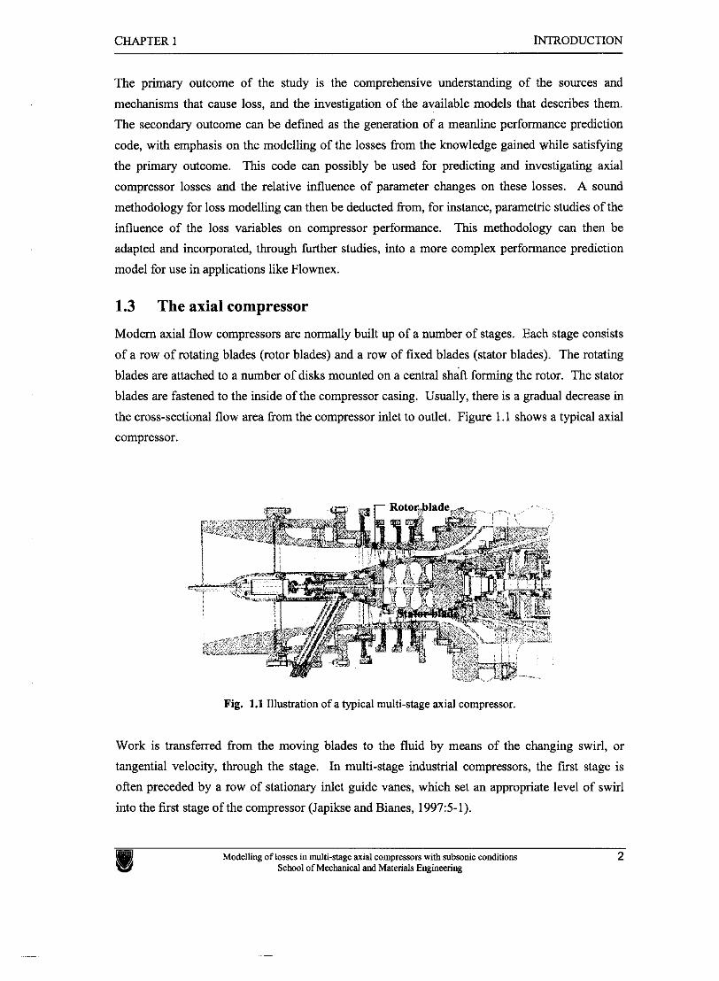
the cross-sectional flow area from the compressor inlet to outlet. Figure 1.1 shows a typical axial
compressor.
Fig. 1.1 Illustration of a typical multi-stage axial compressor.
Work is transferred from the moving blades to the fluid by means of the changing swirl, or
tangential velocity, through the stage. In multi-stage industrial compressors, the first stage is
often preceded by a row of stationary inlet guide vanes, which set an appropriate level of swirl
into the first stage of the compressor (Japikse and Bianes, 1997:5-1).
Modelling of losses in multi-stage axial compressors with subsonic conditions 2 School of Mechanical and Materials Engineering
CHAPTER 1 INTRODUCTION
1.4 Loss and compressor performance
An axial compressor is designed according to certain requirements. During operation at the
design point it delivers the required pressure ratio at a specified rotational speed and mass flow
rate at maximum compressor efficiency.
Several conflicting definitions exist for the 'correct' inlet flow angle chosen during the design
phase of axial compressor bladerows. Cumpsty (1989:164) gives a detail summary of these, but
states that the differences in the definitions are relatively unimportant because of the similarity in
results. Due to the difficulty arising from such a wide array of definitions etc. and the fact that
the prediction of the losses are dependent on these values (see Chapter 4), this study will assume
the definition proposed by Cumpsty and given by Lieblein (1956). It gives the design point inlet
angle in terms of the angle at which the absolute minimum blade profile loss will occur.
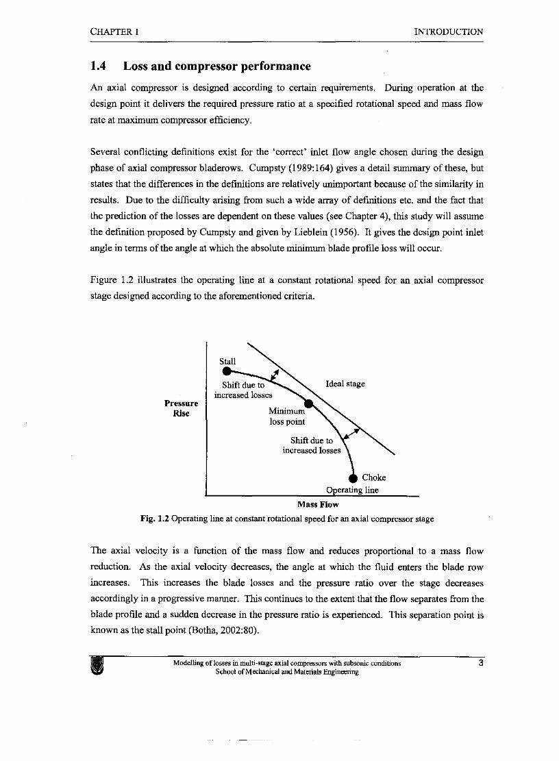
Figure 1.2 illustrates the operating line at a constant rotational speed for an axial compressor
stage designed according to the aforementioned criteria.
Pressure Rise
increased losses
increased losses
I & Choke I Operating line
Mass Flow
Fig. 1.2 Operating line at constant rotational speed for an axial compressor stage
The axial velocity is a function of the mass flow and reduces proportional to a mass flow
reduction. As the axial velocity decreases, the angle at which the fluid enters the blade row
increases. This increases the blade losses and the pressure ratio over the stage decreases
accordingly in a progressive manner. This continues to the extent that the flow separates from the
blade profile and a sudden decrease in the pressure ratio is experienced. This separation point is
known as the stall point (Botha, 2002:XO).
CHAPTER 1 INTRODUCTION
As the mass flow increases, the axial velocity is increased leading to a smaller fluid entry angle.
This continues with a proportional increase in losses until a critical mass flow is reached and a
further mass flow increase through the blades is not possible. At this point the blades start to
choke and a sharp increase in loss and decrease in pressure ratio is experienced.
1.5 The concept of loss
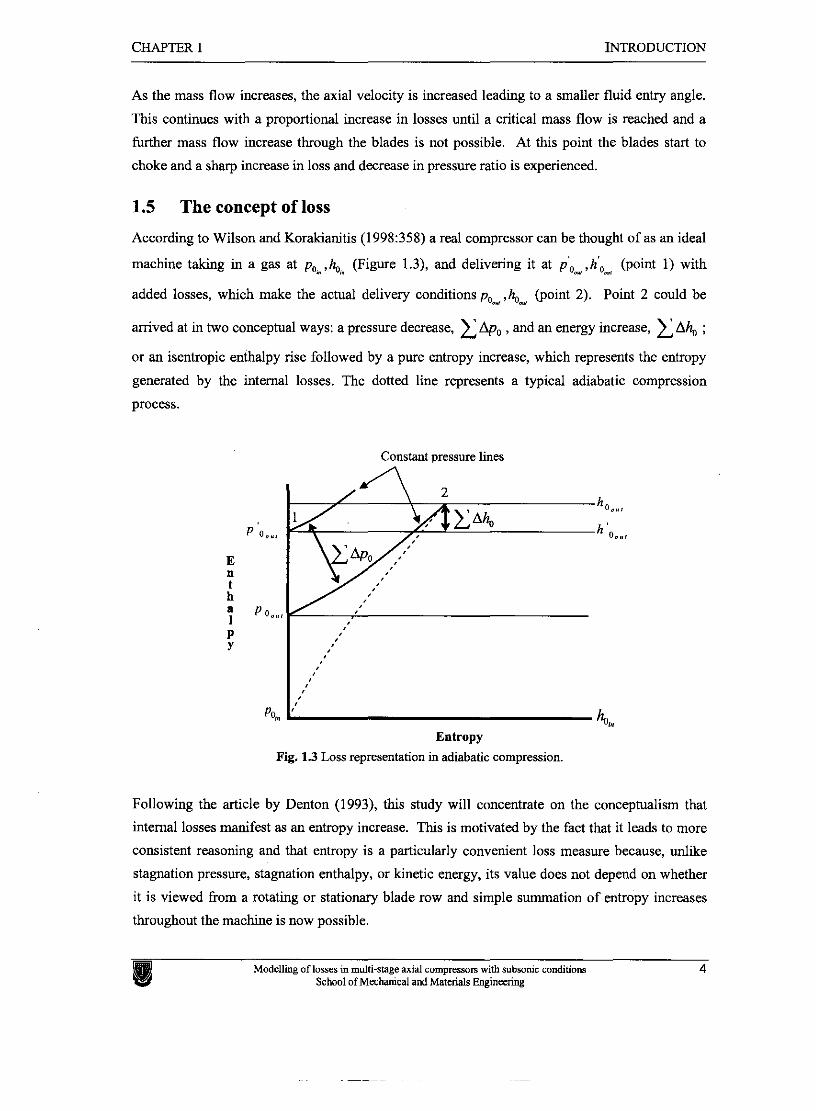
According to Wilson and Korakianitis (1998:358) a real compressor can be thought of as an ideal
machine taking in a gas at p, ,hoam (Figure 1.3), and delivering it at p,,u, ,h',_, (point 1) with
added losses, which make the actual delivery conditions pooe, ,hoe", (point 2). Point 2 could be
arrived at in two conceptual ways: a pressure decrease, Ap, , and an energy increase, Ah, ;
or an isentropic enthalpy rise followed by a pure entropy increase, which represents the entropy
generated by the internal losses. The dotted line represents a typical adiabatic compression
process.
Constant Dressure lines
/ 2 hoeu ,
p 0.". h'O0",
Po, J' "oh
Entropy
Fig. 1.3 Loss representation in adiabatic compression.
Following the article by Denton (1993), this study will concentrate on the conceptualism that
internal losses manifest as an entropy increase. This is motivated by the fact that it leads to more
consistent reasoning and that entropy is a particularly convenient loss measure because, unlike
stagnation pressure, stagnation enthalpy, or kinetic energy, its value does not depend on whether
it is viewed from a rotating or stationary blade row and simple summation of entropy increases
throughout the machine is now possible.
Modelling of losses in multi-stage axial compressan with subsonic conditions 4 School of Mechanical and Materials Engineeting
CHAPTER 1 INTRODUCTION
According to Denton (1993:625), entropy creation or internal losses is a direct result of the
following fluid dynamic processes:
1. Viscous fiction (shearing), e.g., boundary layers and mixing,
2. Heat transfer across finite temperature differences, e.g., from mainstream flow to
flow of coolant gas, and
3. Non-equilibrium processes such as vely rapid expansion or shock waves.
For an adiabatic, subsonic axial compressor, only viscous shearing is responsible for entropy
increase.
Another source of loss can be mechanical fiction losses in external bearings or seals. These
losses increase the compressor's power requirements and are also called mechanical losses or
external losses. They do not contribute to the entropy increase of the fluid.
1.6 Introduction to loss modelling
In an attempt to quantify the internal loss generation in axial compressors, various authors
defined certain loss components and modelled their influence separately. The classifications are
not always precise, and at times different authors present different groupings. In any case, it is
physically impossible to separate the effects of an individual loss type from those of its
interaction with other dissipative phenomena.
The common loss components are profile loss, endwall loss and shock loss. In a fully subsonic
compressor, shock losses do not occur. Profile loss is usually taken to be the loss generated in the
blade boundary layers well away from the endwalls. It is often assumed that the loss here is two-
dimensional. This is done to make use of two-dimensional cascade tests or boundary layer
calculations for modelling purposes. The extra mixing loss at the blade trailing edge is usually
included in the profile loss. Sometimes, endwall loss is further broken down into more
theoretically separable components called tip leakage or clearance loss, annulus boundary layer
loss and secondary loss. Secondary loss arises partly from the secondary flows generated from
interaction between the annulus boundary layers and the blade rows. Profile loss, endwall loss
and tip leakage loss are in many compressors comparable in magnitude, accounting for about one
third of the total loss.
Denton (1993:621) stated that some purely analytical models of the loss components were
formulated from basic principles, but these were usually highly idealized. Another method would
be to use numerical solutions for the loss prediction. Unfortunately, they are computationally
very intensive and are consequently not suitable for the preliminary design phase.
Modelling of losses in multi-st?ge axial compressors with subsonic conditions 5 School of Mechanical and Matelials Engineering
CHAPTER 1 INTRODUCTION
Because of the aforementioned reasons, loss prediction methods remain very dependent on
correlations from test data. The NACA-65 series, C-series and double-circular-arc @CA) blade
profile families were used extensively in cascades for obtaining data for correlation purposes.
Cumpsty (1989:140) presents a detail discussion on the blade profile families and clearly points
out the geometrical and performance differences between various profiles. He concluded that
blade shape has a quite small effect on the deviation, pressure rise and loss as long as the flow
remains subsonic over the whole blade section.
1.7 Primary restrictions
For this study it is assumed that the flow through an axial compressor is adiabatic, thus the
compressor is isolated from its surroundings and no heat is supplied to or rejected from the
system.
It is also assumed that the conditions throughout the compressor are fully subsonic. The reason
for this restriction is that, although the losses could relatively easily be included to accommodate
transonic Mach numbers, the performance prediction and the non-loss correlations involved
change dramatically due to the use of other blade profiles etc. Separate studies are therefore
recommended for including transonic and supersonic loss modelling. Consequently, it is assumed
that the compressor or stage absolute inlet axial Mach number will, in this study, not exceed 0.8
to stay clear of supersonic patches forming on the blades with high relative velocity. This
assumption is based on the discussion given in Section 3.6 regarding losses due to high subsonic
Mach numbers.
The present study is not concerned with predicting mechanical or external losses and it is treated
as a constant input if necessary. The manufacturers of the bearings or seals usually provide
values for these losses.
Further constraints are that it does not attempt to deal with losses due to, for example,
mismatching between stages at part speed operation or improper selection of blade shapes for the
aerodynamic environment. Only losses in the stable operating range are modelled, therefore, no
blade rows are stalled. These constraints were partly adopted from Koch and Smith (1976:411) in
order not to stray too much from the most common loss correlation restrictions.
Losses due to inlet ducting, inlet guide vanes or discharge diffusers are also excluded from the
investigation because it is thought that these components are not essentially part of all
compressors and the literature for modelling them is abundant.
Modelling of losses in multi-stage axial campresson with subsonic conditions 6 School o f Mechanical and Materials E n g i i e e ~ g
CHAPTER 1 INTRODUCTION
1.8 Contributions of this study
The study will aim at improving axial compressor expertise through investigating and serving as a
reference on loss mechanisms, methods of predicting their magnitudes, their implementation and
their possible use. The possibility of developing performance prediction software, with general
applicability to subsonic multi-stage compressors with different geometries and working fluids
will be investigated. Further investigations will also include the evaluation of different loss
models and parametric studies reflecting the influence of input variable changes on particularly
the loss magnitudes and this relation to other performance variables.
1.9 Study Outline
Chapter 1 aimed at providing the reader with the background to this study as well as a short
introduction and overview of the basics regarding axial compressors and their losses. Chapter 2
describes the loss mechanisms found in an axial compressor. In Chapter 3 the loss models
published in the open literature for predicting the losses produced by the various loss mechanisms
are reviewed and some are discussed in detail. Chapter 4 presents the reader with a method of
performance prediction and indicates where and how the loss models fit in. In Chapter 5 some
issues regarding the implementation of the concepts and equations given in Chapters 3 and 4 are
discussed. Chapter 6 verifies the validity and accuracy of the code by comparing its results to
those from a commercial software package and evaluation of the different loss models are done.
In Chapter 7 parametric studies are conducted and some conclusions are made about the role that
each model and other relevant parameters play in loss and performance. Chapter 8 contains
conclusions and recommendations for future work on improving the loss prediction models, and
our understanding of it, as well as some remarks on compressor performance prediction as a
whole.
Modelling of losses in multi-stage axial compresson with subsonic conditions 7 School of Mechanical and Materials Engineering
Chapter 2
OSS MECHmISMS
The mechanisms mainly responsible for the losses in subsonic axial compressors are presented in
Chapter 2. The mechanisms that are commonly used in loss modelling are then described in
more detail.
Modelling of losses in multi-stage axial compresson with subsonic conditions School of Mechanical and Materials Engineering
CHAPTER 2 LOSS MECHANISMS
2.1 Introduction
Chapter 1 gave a brief overview of multi-stage axial compressors, the losses that occur in them,
the influence on performance and how these losses are currently conceptualized and modelled. It
was seen that at the fundamental level for an adiabatic, subsonic axial compressor, all the loss
mechanisms could be related to viscous shearing. Viscous shearing occurs wherever there are
velocity gradients, but its magnitude is only of concern in regions where these gradients are very
steep (Cumpsty, 1989:28).
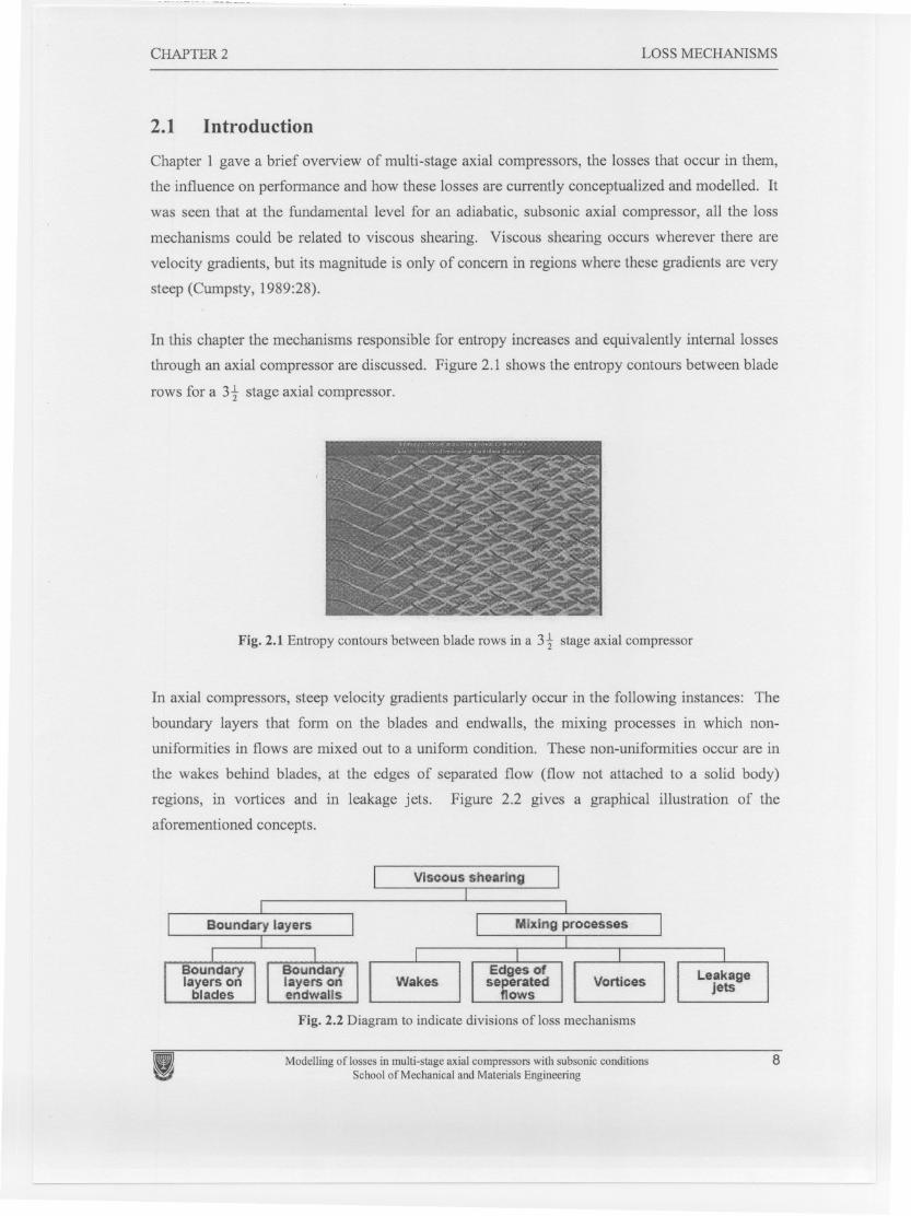
In this chapter the mechanisms responsible for entropy increases and equivalently internal losses
through an axial compressor are discussed. Figure 2.1 shows the entropy contours between blade
rows for a 3t stage axial compressor.
Fig. 2.1 Entropy contours between blade rows in a 3t stage axial compressor
In axial compressors, steep velocity gradients particularly occur in the following instances: The
boundary layers that form on the blades and endwalls, the mixing processes in which non-
uniformities in flows are mixed out to a uniform condition. These non-uniformities occur are in
the wakes behind blades, at the edges of separated flow (flow not attached to a solid body)
regions, in vortices and in leakage jets. Figure 2.2 gives a graphical illustration of the
aforementioned concepts.
Viscous shearing
Fig. 2.2 Diagram to indicate divisions of loss mechanisms
I Modelling oflosses in multi-stage axial compressors with subsonic conditionsSchool of Mechanical and Materials Engineering
8

CHAPTER 2 LOSS MECHANISMS
2.2 Entropy production in boundary layers
Figure 2.3 represents a blade section moving through initially undisturbed fluid.
Velocity profile due to
__r
Uniform - inflow Wake velocity -J,- -
*
Fig. 2.3 Velocity profile on blade section due to endwall
According to Shames (1992:131) real fluids "stick" to the surface of a solid body. At Point A on
the blade section the fluid velocity must be equal to zero relative to the blade and at a
comparatively short distance away, it is almost equal to the initial fluid velocity. This is
illustrated in the velocity profile of the diagram. It can be seen that there is a thin region, called
the boundary layer, adjacent to the boundary, where sizable velocity gradients must be present.
Consequently, high shear stresses, which oppose the motion of the fluid, occur, resulting in a rise
in the internal energy and entropy of the fluid At some point the shear stresses become too big
and there is a transition from laminar to turbulent flow. Boundary layers grow progressively
along a solid body.
When the flow angle, of the fluid relative to the blade, becomes too large the flow will separate
from the boundary causing added entropy production due to mixing. During this condition the
entropy increases rapidly, with respect to the separation, and the blade section stalls. Similarly,
boundary layers form on the endwalls of the compressor. Figure 2.4 illustrates axial compressor
boundary layers in which entropy is generated.
Transition
I (b) Viscous regions in the meridionai
(a) Bladeto-blade boundary layers plane
Fig. 2.4 Schematic of boundary layers in axial compressor on a (a) blade and (b) endwall
Modelling of losses in multi-stage axial compressors with subsonic conditions 9 ScbDal of Mechanical and Materials Engineering
CHAPTER 2 LOSS MECHANISMS
Compared with other viscous regions in compressors the understanding and prediction of axial
blade boundary layers away from the endwalls is good although also influenced by the magnitude
of the other loss mechanisms in the compressor. A thorough description thereof can be found in
Cumpsty (1989:331). Unfortunately, this is not the case for the endwall region due to the extreme
complexity of the flow and its interaction with the mixing processes and the blade boundary
layer.
2.3 Entropy production in the mixing processes
Relatively high rates of shearing occur in wakes, at the edges of separated regions, in vortices and
in leakage jets. Such phenomena are usually associated with turbulent flow and therefore the
local entropy creation rates may be considerable.
The flow processes involved are extremely complex and often unsteady. A thorough
understanding and an accurate analytical means of predicting them in axial compressors are
therefore not yet available, especially in the endwall regions. Consequently, this study will not
attempt to give a detail discussion on all the different mixing mechanisms and more attention will
be given to the methods of predicting them macroscopically by correlation in the next chapter.
Two special cases that are, however, presented are wake mixing behind a blade trailing edge and
tip clearance.
For a blade in subsonic flow, about one third of the total two-dimensional entropy generation is
due to the mixing of the blade boundary layers behind the trailing edge in the wake. Denton
(1993:653) gives the basic theory of entropy creation due to the mixing out of a wake and
employs the conservation of mass and momentum over a control volume at the trailing edge in
incompressible flow. This analysis includes detail about the blade boundary layers and also the
base pressure acting on the trailing edge.
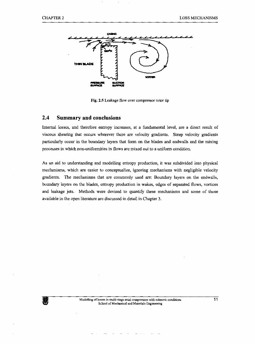
The flow and entropy creation mechanisms through a tip clearance are well understood for
unshrouded compressor blades. In this case, the axial velocity of the flow leaking over the tips is
certain to be less than that of the mainstream and may even be directed upstream. There is a
vortex sheet at their interface and this rolls up into a concentrated vortex as the flow moves
downstream. The total entropy production depends on the leakage flow rate and the difference
between the velocity of the mainstream flow and the leakage flow. Figure 2.5 shows a two-
dimensional illustration of the flow over an unshrouded blade.
Modelling of losses in multi-stage axial compressan with subsonic conditions 10 School of Mechanical and Materials Engineering
CHAPTER 2 LOSS MECHANISMS
Fig. 2.5 Leakage flow over compressor rotor tip
2.4 Summary and conclusions
Internal losses, and therefore entropy increases, at a fundamental level, are a direct result of
viscous shearing that occurs wherever there are velocity gradients. Steep velocity gradients
particularly occur in the boundary layers that form on the blades and endwalls and the mixing
processes in which non-uniformities in flows are mixed out to a uniform condition.
As an aid to understanding and modelling entropy production, it was subdivided into physical
mechanisms, which are easier to conceptualize, ignoring mechanisms with negligible velocity
gradients. The mechanisms that are commonly used are: Boundary layers on the endwalls,
boundary layers on the blades, entropy production in wakes, edges of separated flows, vortices
and leakage jets. Methods were devised to quantify these mechanisms and some of those
available in the open literature are discussed in detail in Chapter 3.
Modelling of losses in multi-stage axial compresson with subsonic conditions 11 School of Mechanical and Materials Engineering
Chapter 3
LOSS PREBIGTXQN METHODS
Chapter 3 presents the reader with a comprehensive literature survey regarding loss prediction
methods for subsonic axial compressors. The loss mechanisms are interactive and complex by
nature and methods of predicting them rely greatly on empirical correlations. Also, the open
literature is rather d i f i e d and the main groupings used in this chapter are: Blade profile losses,
endwall losses including literature on tip leakage and secondary losses, part span shroud losses,
other losses, losses due to high subsonic much numbers and off-minimum losses.
Modelling of lasses in multi-stage axial compresson with subsonic conditions School of Mechanical and Materials Engineering
CHAPTER 3 LOSS PREDICTION METHODS
3.1 Introduction
The mechanisms mainly responsible for the losses in subsonic axial compressors were presented
in Chapter 2. They are interactive and complex by nature and methods of predicting them rely
greatly on empirical correlations. A thorough knowledge about the origin of these models is
crucial due to the high degree of empirical reliance and therefore, l i i t e d general applicability.
The literature on loss prediction methods for axial compressors is rather diffused and many of the
models used in the industry are propriety information and not available in the open literature for
evaluation. Several authors furthermore also used different nomenclature, units, and sign
conventions.
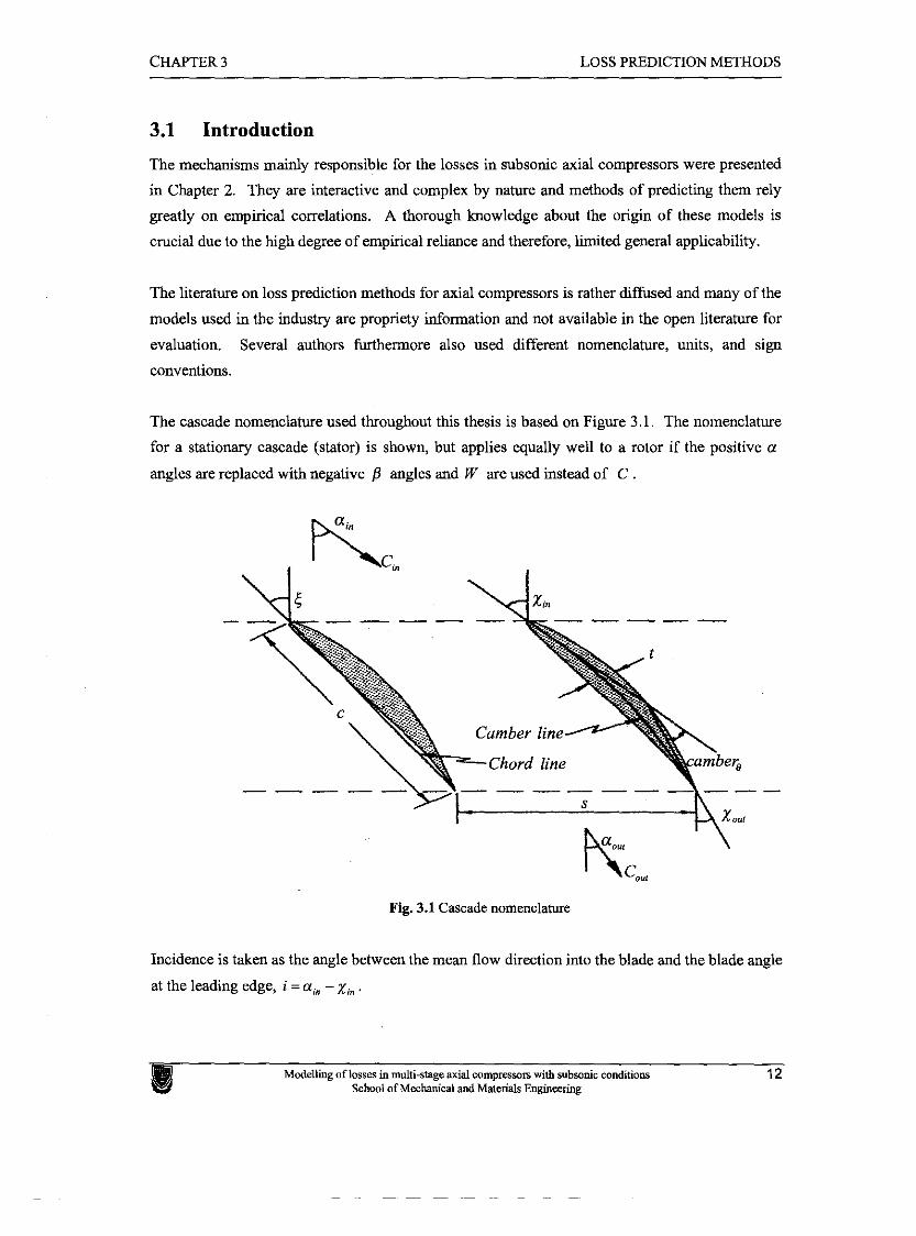
The cascade nomenclature used throughout this thesis is based on Figure 3.1. The nomenclature
for a stationary cascade (stator) is shown, but applies equally well to a rotor if the positive a
angles are replaced with negative P angles and W are used instead of C .
Fig. 3.1 Cascade nomenclature
Incidence is taken as the angle between the mean flow direction into the blade and the blade angle
at the leading edge, i =a, -xi".
CHAPTER 3 LOSS PREDICTION METHODS
In most instances the methodology employed to predict the minimum total losses uses a
superposition of theoretically separable loss components. More specifically, for this study they
will be presented under the following headings:
Blade profile losses
Endwall losses including literature on tip leakage and secondary losses
Part span shroud losses
Other losses
Losses due to high subsonic mach numbers
The prediction of the off-minimum losses are presented in a separate section and are mostly
modelled with the use of a correlation that is, among others, a function of the minimum profile
loss or variables contained in the minimum blade profile loss. Sometimes, this loss is called an
incidence loss. The available literature, on these categories, is discussed chronologically in the
following sections and the work of some of the contributing authors is presented in detail.
3.2 Blade profile losses
Howell (1945) attempted to estimate this loss in terms of the familiar drag and lift coefficients
used for aircraft analysis. In calculating the blade profile loss, most correlations, however, use a
technique developed by Lieblein (1959) using a diffusion factor that is a function of the
maximum relative flow velocity in the blade passage, and relative inlet and exit flow velocities.
Koch and Smith (1976), who presented the most comprehensive model, performed operations
similar to Lieblein, but accounted for compressibility, Reynolds number and streamtube
contraction effects found in real compressors. Starke (1980) adapted the purely two-dimensional
Lieblein correlations to account for quasi-two-dimensional flow often found across compressor
blade sections. Denton (1993) emphasized the importance of understanding the physical origins
of loss rather than to rely on conventional correlations. He defined loss in terms of entropy
increase and derived the relationship of this to the more familiar loss coefficients. Swan (1961),
Cetin et al. (1989), Konig et al. (1993) and Roy and Kumar (1999) used the same basic principles
as Lieblein, but obtained correlations for transonic compressor blades and are therefore not
considered for this study. These articles did, however, make a valuable contribution to the
author's insight into compressor losses.
Denton's (1993:633-636) model support the conceptualism of loss being equivalent to entropy
production, and this study would seem incomplete without giving it the necessary attention.
However, his model is not directly used in the study and the discussion of his work follows in
Modelling of lasses in multi-stage axial compresson with subsonic wnditions 13 School of Mechanical and Materials Engineering
CHAPTER 3 LOSS PREDICTION METHODS
Appendix A. The models of Lieblein and Koch and Smith are discussed in more detail in the
following sections.
3.2.1 Lieblein
Lieblein (1959) derived a method from cascade tests, which satisfactorily describes the low-speed
relationship between blade-element loading and losses at any flow conditions (Swan, 1961:322).
Some of his work and comments from other authors are presented here and the restrictions of his
results are stated clearly. Hirsch and Denton showed in 1981 that Lieblein's model is as reliable
as more modem correlations (Casey, 1987:275).
Lieblein showed that the losses around the blade profile appeared as a boundary layer momentum
thickness, 8,, in the wake behind the blade. He also showed that as the aerodynamic loading on
a compressor blade increased, the diffusion on the sation-surface increased, but that on the
pressure-surface stayed approximately constant.
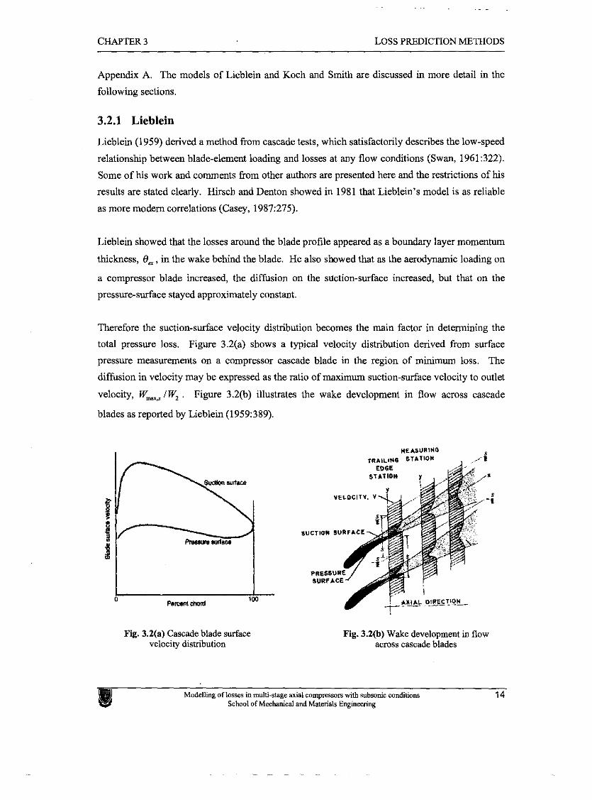
Therefore the suction-surface velocity distribution becomes the main factor in determining the
total pressure loss. Figure 3.2(a) shows a typical velocity distribution derived from surface
pressure measurements on a compressor cascade blade in the region of minimum loss. The
diffusion in velocity may be expressed as the ratio of maximum suction-surface velocity to outlet
velocity, Wm,s IW2 . Figure 3.2(b) illustrates the wake development in flow across cascade
blades as reported by Lieblein (1959:389).
Fig. 3.2(a) Cascade blade surface velocity distribution
TRAILING STAT'oU
$TATION )I
Fig. 3.2(b) Wake development in flow across cascade blades
CHAPTER 3 LOSS PREDICTION METHODS
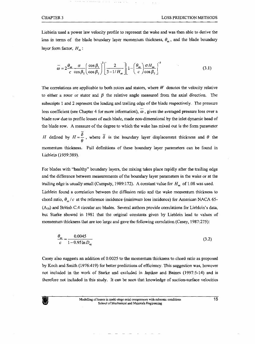
Lieblein used a power law velocity profile to represent the wake and was then able to derive the
loss in terms of the blade boundary layer momentum thickness, 0,, and the blade boundary
layer form factor, H, :
3 - 8. [ c 0 s p l j [ 2 ] 1 1 - [ + ) ~ ] 0 = 2-- -
c cosp, cosp, 3-1/H, 1
The correlations are applicable to both rotors and stators, where W denotes the velocity relative
to either a rotor or stator and p the relative angle measured kom the axial direction. The
subscripts 1 and 2 represent the leading and trailing edge of the blade respectively. The pressure
loss coefficient (see Chapter 4 for more information), o , gives the averaged pressure loss over a
blade row due to profile losses of each blade, made non-dimensional by the inlet dynamic head of
the blade row. A measure of the degree to which the wake has mixed out is the form parameter - 6
H defined by H =- , where 6 is the boundary layer displacement thickness and 0 the 0
momentum thickness. Full definitions of these boundary layer parameters can be found in
Lieblein (1959:389).
For blades with "healthy" boundary layers, the mixing takes place rapidly afier the trailing edge
and the difference between measurements of the boundary layer parameters in the wake or at the
trailing edge is usually small (Cumpsty, 1989:172). A constant value for H , of 1.08 was used
Lieblein found a correlation between the diffusion ratio and the wake momentum thickness to
chord ratio, 0, / c at the reference incidence (minimum loss incidence) for American NACA 65-
(Ale) and British C.4 circular arc blades. Several authors provide correlations for Lieblein's data,
but Starke showed in 1981 that the original constants given by Lieblein lead to values of
momentum thickness that are too large and gave the following correlation (Casey, 1987:275):
Casey also suggests an addition of 0.0025 to the momentum thickness to chord ratio as proposed
by Koch and Smith (1976:419) for better predictions of efficiency. This suggestion was, however
not included in the work of Starke and excluded in Japikse and Baines (19975-14) and is
therefore not included in this study. It can be seen that knowledge of suction-surface velocities
Modelling of lasses in multi-stag axial compressors with subsank conditions 15 School of Mechanical and Materials Engineering
CHAPTER 3 LOSS PREDICTION METHODS
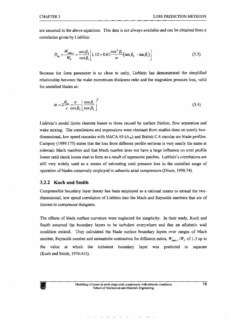
are assumed in the above equations. This data is not always available and can be obtained from a
correlation given by Lieblein:
cos2 p, 1.12 + 0.61-----(tanp, - tan P , ) I
u 1
Because the form parameter is so close to unity, Lieblein has demonstrated the simplified
relationship between the wake momentum thickness ratio and the stagnation pressure loss, valid
for unstalled blades as:
2 0, 0 I cosp, I =2---- -- c cos PZ Leos ~2 1
Lieblein's model limits element losses to those caused by surface fiction, flow separation and
wake mixing. The correlations and expressions were obtained from studies done on purely two-
dimensional, low speed cascades with NACA 65-(Alo) and British C.4 circular arc blade profiles.
Cumpsty (1989:175) states that the loss from different profile sections is very nearly the same at
subsonic Mach numbers and that Mach number does not have a large influence on total profile
losses until shock losses start to form as a result of supersonic patches. Lieblein's correlations are
still very widely used as a means of estimating total pressure loss in the unstalled range of
operation of blades commonly employed in subsonic axial compressors (Dixon, 1998:74).
3.2.2 Koch and Smith
Compressible boundary layer theory has been employed as a rational means to extend the two-
dimensional, low speed correlation of Lieblein into the Mach and Reynolds numbers that are of
interest to compressor designers.
The effects of blade surface curvature were neglected for simplicity. In their study, Koch and
Smith assumed the boundary layers to be turbulent everywhere and that an adiabatic wall
condition existed. They calculated the blade surface boundary layers over ranges of Mach
number, Reynolds number and streamtube contraction for diffusion ratios, W-,, I W, of 1.3 up to
the value at which the turbulent boundary layer was predicted to separate
(Koch and Smith, 1976:413).
Modelling of losses in multi-stage axial compresson with subsonic conditions 16 School of Mechanical and Materials Engineering
CHAPTER 3 LOSS PREDICTION METHODS
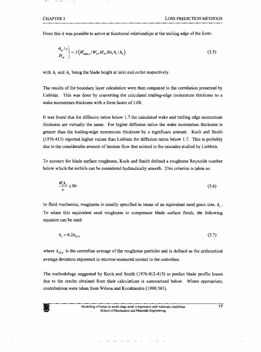
From this it was possible to arrive at functional relationships at the trailing edge of the form:
with h, and h, being the blade height at inlet and outlet respectively
The results of the boundary layer calculation were then compared to the correlation presented by
Lieblein. This was done by converting the calculated trailing-edge momentum thickness to a
wake momentum thickness with a form factor of 1.08.
It was found that for difision ratios below 1.7 the calculated wake and trailing edge momentum
thickness are virtually the same. For higher diffusion ratios the wake momentum thickness is
greater than the trailing-edge momentum thickness by a significant amount. Koch and Smith
(1976:413) reported higher values than Lieblein for diffusion ratios below 1.7. This is probably
due to the considerable amount of laminar flow that existed in the cascades studied by Lieblein.
To account for blade surface roughness, Koch and Smith defined a roughness Reynolds number
below which the airfoils can be considered hydraulically smooth. This criterion is taken as:
In fluid mechanics, roughness is usually specified in terms of an equivalent sand grain size, k, .
To relate this equivalent sand roughness to compressor blade surface finish, the following
equation can be used:
where kc, is the centreline average of the roughness particles and is defined as the arithmetical
average deviation expressed in microns measured normal to the centreline.
The methodology suggested by Koch and Smith (1976:412-415) to predict blade profile losses
due to the results obtained from their calculations is summarized below. Where appropriate,
contributions were taken from Wilson and Korakianitis (1998:361).
Modelling of losses in multi-stage axial compresson with subsonic conditions 17 School of Mecbnical and Materials Engineering
CHAPTER 3 LOSS PREDICTION METHODS
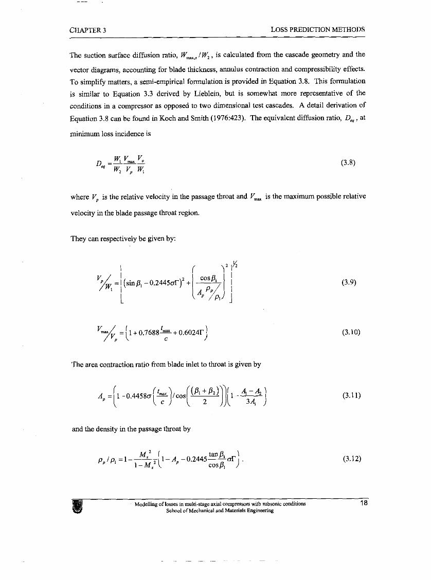
%he suction surface diffusion ratio, W-$ 1 W, , is calculated h m the cascade geometry and the
vector diagrams, accounting for blade thickness, annulus contraction and compressibility effects.
To simplify matters, a semi-empirical formulation is provided in Equation 3.8. This formulation
is similar to Equation 3.3 derived by Lieblein, but is somewhat more representative of the
conditions in a compressor as opposed to two dimensional test cascades. A detail derivation of
Equation 3.8 can be found in Koch and Smith (1976:423). The equivalent diffusion ratio, D, , at
minimum loss incidence is
where V, is the relative velocity in the passage throat and V,, is the maximum possible relative
velocity in the blade passage throat region.
They can respectively be given by:
The area contraction ratio fiom blade inlet to throat is given by
and the density in the passage throat by
Modelling of losses in multi-stage axial compressors with subsonic wnditions 18 School of Mechanical and Materials Engineering
CHAPTER 3 LOSS PREDICTION METHODS
The circulation, r , for a two-dimensional, incompressible cascade is given by
The ratio of trailing edge momentum thickness to chord length, 8 , l c , and trailing edge form
factor, H , can found from Figure A.2.1 and Figure A.2.2 in Appendix A.2. These correlations
given are for nominal conditions for a Reynolds number of 1 x lo6 , hydraulically smooth blades,
a streamtube height ratio, h, 14, of 1, and a Mach number of 0.05. Corrections have to be
applied for conditions other than nominal and the correctional multiplier correlation figures are
also given in Appendix A.2.
With the new values for trailing-edge momentum thickness to chord ratio, O,e / c , and form factor,
H,e , known, a new trailing-edge freestream velocity can be determined from iteration and
therefore changes to the initial estimate for the diffusion ratio. This continues until all the
trailing-edge parameters converge.
It is now possible to estimate the total pressure loss by calculating the mixing of the freestream
and the boundary layers in a control volume analysis. According to Wilson and Korakianitis
(1998:362), the use of Equation 3.1, derived by Lieblein, is satisfactory to calculate the total
pressure loss, but with, O,, l c , instead of 8, I c .
3.3 Endwall losses
The endwall loss is the most difficult loss component to understand and predict and virtually all
prediction methods rely on very little underlying physics. Much effort and many papers have
been directed to endwall flows in cascades. Unfortunately, these flows are not representative of
the flow in compressor blade rows and the correlations derived from them should be used with
the greatest caution. (Cumpsty, 1989:355)
Hiibner and Fottner (1996:2) also states that: "...the flow in the endwall region is not well
understood in spite of the research over a period of more than two human generations. However
the process of loss generation still remains not very clear up to now and thus the losses cannot be
predicted with reasonable accuracy."
Modelling of lasses in multi-stage axial compresson with subsonic conditions 19 School of Mechanical and Materials Engineering
CHAPTER 3 LOSS PREDICTION METHODS
Classic denominations of endwall losses are: annulus boundary layer loss, tip clearance loss and
secondary loss. The term secondary loss is also sometimes used to describe all the losses in the
endwall region. The effects of tip clearance are overwhelming on the endwall flow development
and on the blade-to-blade flow near the tip and it would be somewhat artificial to treat it in a
separate section as is done in many instances in the literature.
The first modelling of tip clearance losses in compressor cascades seems to be that done by Betz
in 1926. Chauvin, Cyrus and Senoo published reviews in the 1980's on improved correlations
(Hiibner and Fottner, 1996:8).
Early methods by Betz, Vavra, and Lakshrninarayana, referenced by Hiibner and Fottner (1996:9)
tended to work in terms of the induced drag on the blades, analogous to the drag on an aircraft
wing. This is, however an inviscid effect. Rains assumed the kinetic energy of the leakage flow
driven by the pressure difference between the pressure and suction side as lost. Another method
is to consider the pressure rise of the cascade in terms of the blade loading and authors following
this approach are: Bauermeister, Scholz, Baljk, Grieb, Hultsch and Sauer and Cyrus (Hiibner and
Fottner (1996:9).
More recent studies, for example by Storer in 1991 and Papailiou in 1995, measured the tip
leakage flow in great detail and modelled it in terms of the mixing loss between the tip leakage
and the main flow. Denton (1993:638) states that there is no known work on the flow processes
over shrouded compressor blades and the current study confirms this.
Several methods that calculate the annulus boundary layer displacement thickness via a two-
dimensional boundary layer calculation along the whole endwall of a compressor has been
published e.g. De Ruyck and Hirsh (1983). Denton (1993:640) states that such methods that use
conventional boundary layer theory must be regarded as dubious, because during their interaction
with the blade rows, the boundary layers cannot be considered as conventional boundary layers.
Their reasonable predictions are a result of considerable empiricism.
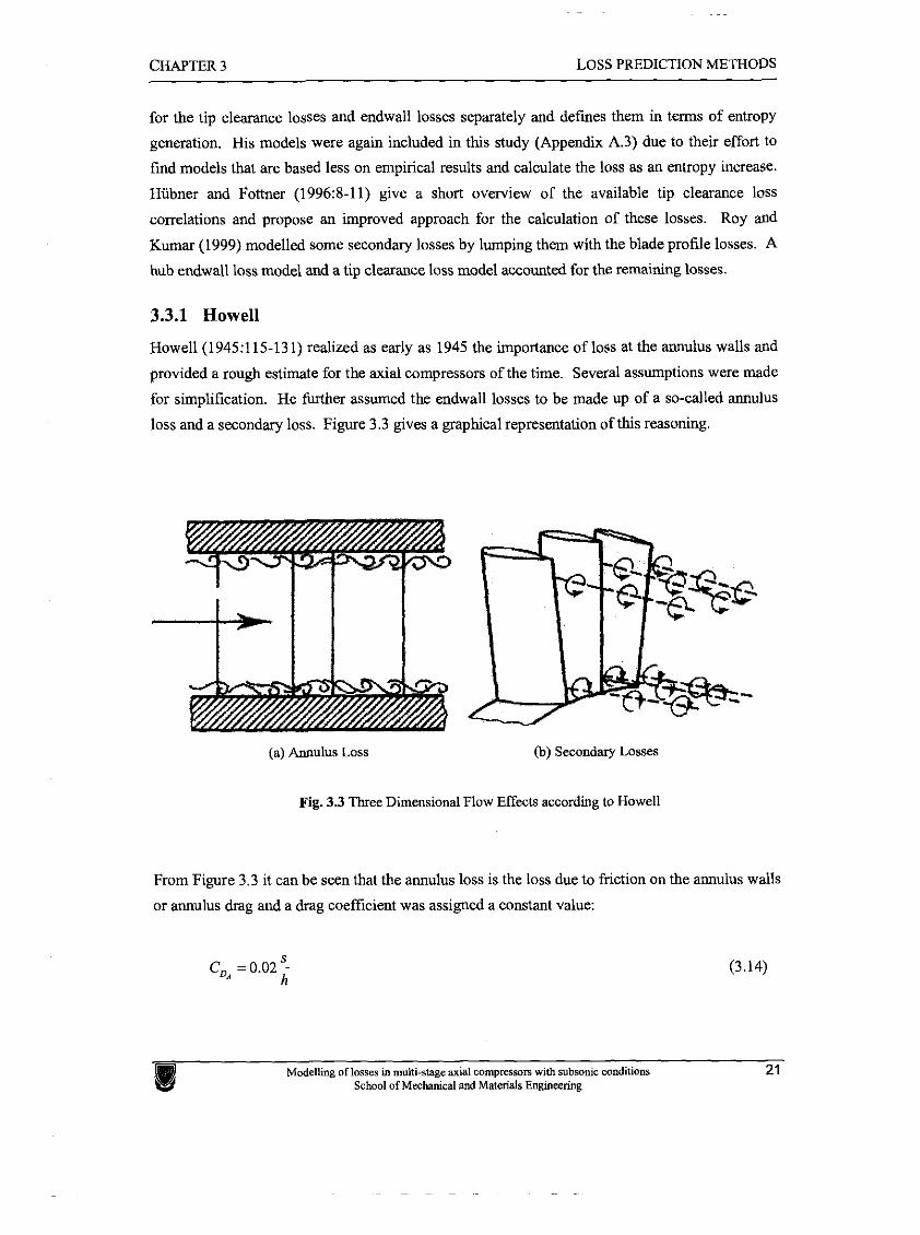
The models of the following authors are discussed in detail and are thought to be a good
representation of a lump of the work done: Howell assumed the endwall loss to be made up of
friction at the annulus walls and a secondary loss that was greatly influenced by the tip clearance
(Cohen et al, 1996:210). Koch and Smith (1976:416) relate the loss of efficiency due to the
presence of endwall effects to two properties of an endwall boundary layer, i.e. the averaged
displacement thickness and the tangential-force thickness. Denton (1993:640) presents models
Modelling of losses in multisfage axial compressors with subsonic conditions 20 School of Mechanical and Materials Engineering
CHAPTER 3 LOSS PREDICTION METHODS
for the tip clearance losses and endwall losses separately and defines them in t m s of entropy
generation. His models were again included in this study (Appendix A.3) due to their effort to
find models that are based less on empirical results and calculate the loss as an entropy increase.
Hiibner and Fottner (19963-11) give a short overview of the available tip clearance loss
correlations and propose an improved approach for the calculation of these losses. Roy and
&mar (1999) modelled some secondary losses by lumping them with the blade profile losses. A
hub endwall loss model and a tip clearance loss model accounted for the remaining losses.
3.3.1 Howell
Howell (1945:115-13 1) realized as early as 1945 the importance of loss at the annulus walls and
provided a rough estimate for the axial compressors of the time. Several assumptions were made
for simplification. He further assumed the endwall losses to be made up of a so-called annulus
loss and a secondary loss. Figure 3.3 gives a graphical representation of this reasoning.
(a) Annulus Loss (b) Secondary Losses
Fig. 3.3 Three Dimensional Flow Effects according to Howell
From Figure 3.3 it can be seen that the annulus loss is the loss due to friction on the annulus walls
or annulus drag and a drag coefficient was assigned a constant value:
Modelling of lasses in multi-stage axial compresson ~4th subsonic conditions 21 School of Mechanical and Materials Engineering
CHAPTER 3 LOSS PREDICTION METHODS
In turn, the secondary loss drag coefficient was related to the reduction in blade circulation in the
blade end region and was derived by analogy with the trailing vortex loss behind aircraft. With
and C, the blade lift coefficient outside the endwall region calculated from:
with the value of the vector mean angle, P, , calculated from:
1 (3.17) tanp, =- tan^, +tan&)
2
The mean pressure loss coefficient over a blade row due to the endwall losses can now be
calculated from:
Cumpsty (1989:337) stated that, although there are no grounds on which the model for the
secondary losses can be proven accurate, nor to believe the separation of loss into two
components, this did provide a way of introducing the loss of approximately the right magnitude.
He also states that later work confirmed that the secondary losses were actually proportional to
the square of the lift coefficient as shown in Equation 3.15.
3.3.2 Koch and Smith
The influence of the endwall boundary layer is modelled in terms of its averaged displacement
thickness, 6 , which contributes directly to an efficiency decrease, but is partly offset by the
reduction in the tangential blade force in the boundary layer (Japikse and Baines, 1997527).
The displacement thickness is a measure of the mass flow reduction caused by the presence of the
endwall boundaty layer, compared to the mass flow if the free-stream flow profiles (flow without
endwall losses) were extended to the wall. Another variable, the tangential-force thickness, v,, is
Modelling of losses in multi-sfage axial compresson with subsonic conditions School of Mechanical and Materials Engineen'ng
CHAPTER 3 LOSS PREDICTION METHODS
introduced and represents the reduction of the tangential component of blade force from its free-
stream value due to the presence of an endwall boundary layer.
Koch and Smith (1976:416) made detailed measurements of the flow profiles in several low-
speed multistage compressors for the hub and casing boundary layers behind both rotors and
stators. Values for 6 and v, were deduced from these measurements. The thickness of the hub
and casing boundary layers were added and represented by 26 , and the rotor and stator exit -
values were averaged and normalized by the averaged staggered spacing, g = scost , at the mean
diameter. They found that by assuming v, to be a fixed fraction of 6 , it was possible, with the
help of a representative profile model, to construct fairly accurate pressure rise and efficiency
h characteristic curves for a series of stages with aspect ratios, -, varying from 2 to 5 and tip
C
clearances varying from 0.8-3.6 percent annulus height. Their resulting correlations are given in - -
26 2v Appendix A.4. It shows -=- and I plotted against the stage static pressure rise coefficient
g g
relative to the maximum static pressure rise coefficient which the stage is capable of as well as a
correction for the axial spacing of the blade rows.
The stage stagnation-to-stagnation efficiency can now be calculated from
where q is the stage efficiency and q, is the free-stream efficiency, i.e. the efficiency if there
were no endwall losses, and g/ha is the weighted average rotor and stator mean diameter
staggered spacing to annulus height ratio. The weighting function is again the blade row inlet
dynamic heads.
Koch and Smith (1976:318) realize that their model is of limited swpe and questionable general
applicability. They suggest that the model should not be used for aspect ratios less than unity.
For calculating the free stream axial velocity, due to blockage from the boundary layer, for use in
26 . other models like the profile loss model, - IS taken as 0.17 if the value deduced from the
h
figures is greater than 0.17.
Modelling of lasses in multi-stage axial campresson with subsonic conditions 23 School of Mechanical and Materials Engineering
CHAPTER 3 LOSS PREDICTION METHODS
3.3.3 Hiibner and Fottner
Hiibner and Fottner (19963) classified some loss correlations for the endwall losses into two
groups. They state that the one group (Vavra in reference to Mehldahl- 1960, Vavra in reference
to Rains - 1960, Scholz - 1965, Balje - 1968, Lakshminaraya - 1970, Grieh - 1975, Storer and
Cumpsty - 1993) considers the loss as a linear superposition of the secondary and the tip
clearance losses:
In this case the secondary losses are the endwall without a tip gap.
The second group (Bauermeister - 1963, Hultsch and Sauer - 1979, Cyrus - 1992) looks at the hub
and the tip region separately and defines the mean value as the total endwall loss:
They compared the correlations of Equation 3.20 and Equation 3.21 with experimental
measurements from a highly loaded, linear cascade with high speed flow and NACA 65-K48
profiles. It was noted that the definition, as presented by Equation 3.20, was physically not well
founded and suggested the use of the definition given by Equation 3.21. The reason is that the
endwall losses are a strong function of the tip clearance.
The correlation of Bauermeister was identified as the best to start from for an improvement.
Hiibner and Fottner (1996:10,11) changed Bauermeister's correlating parameters for the
secondary losses of the tip region according to their experimental data and experience. Thus, the
endwall loss is given by Equation 3.21 where:
and
Modelling of losses in multi-stage axial compresson with subsonic conditions 24 School of Mechanical and Materials Engineering
CHAPTER 3 LOSS PREDICTION METHODS
The subtraction of the 90 degrees is necessary because their angles were measured with respect to
the tangential direction. For this study, the relative flow angles for the rotor are negative,
therefore absolute values are used.
3.3.4 Roy and Kumar
The profile model used by Roy and Kumar was based on the model proposed by Leiblein with
0 different values for - applicable to transonic blades. It is, however, fundamentally based on
C
models obtained from subsonic tests. It is also the only model included in this study that
explicitly gives a magnitude to the loss due to tip clearance. It must be stated that every effort
was made to. follow the literature carefully, but that some error might have slipped in due to
limited detail and unclear nomenclature supplied by the authors. A boundary layer loss model
(from the hub), transposed to the midspan section, and a tip clearance loss model accounted for
the endwall losses.
The boundary layer endwall loss model is based on a model presented by Vavra in 1960. The
effect of aspect ratio has been included and then the loss was transposed to the midspan section to
give:
It is suggested that Equation 3.24 be used only for AR < 2.0 and that for high aspect ratio blades
a different model may be necessary.
The tip clearance loss model is based on an assumption that the kinetic energy in the gap flow
normal to the blade chord is lost due to the interaction between the tip leakage flow and the main
flow. The most important factors in the model are the prediction of the mass flow through the
clearance and the magnitude of the velocity component of the leakage jet normal to the tip
clearance. The high velocity leakage jet mixes with the main flow to result in high shearing
losses and ultimately flow separation (Roy and Kumar, 1999:Z).
Modelling of losses in multi-stage axial compressors with subsonic conditions 25 School afMechanical and Materials Engineering
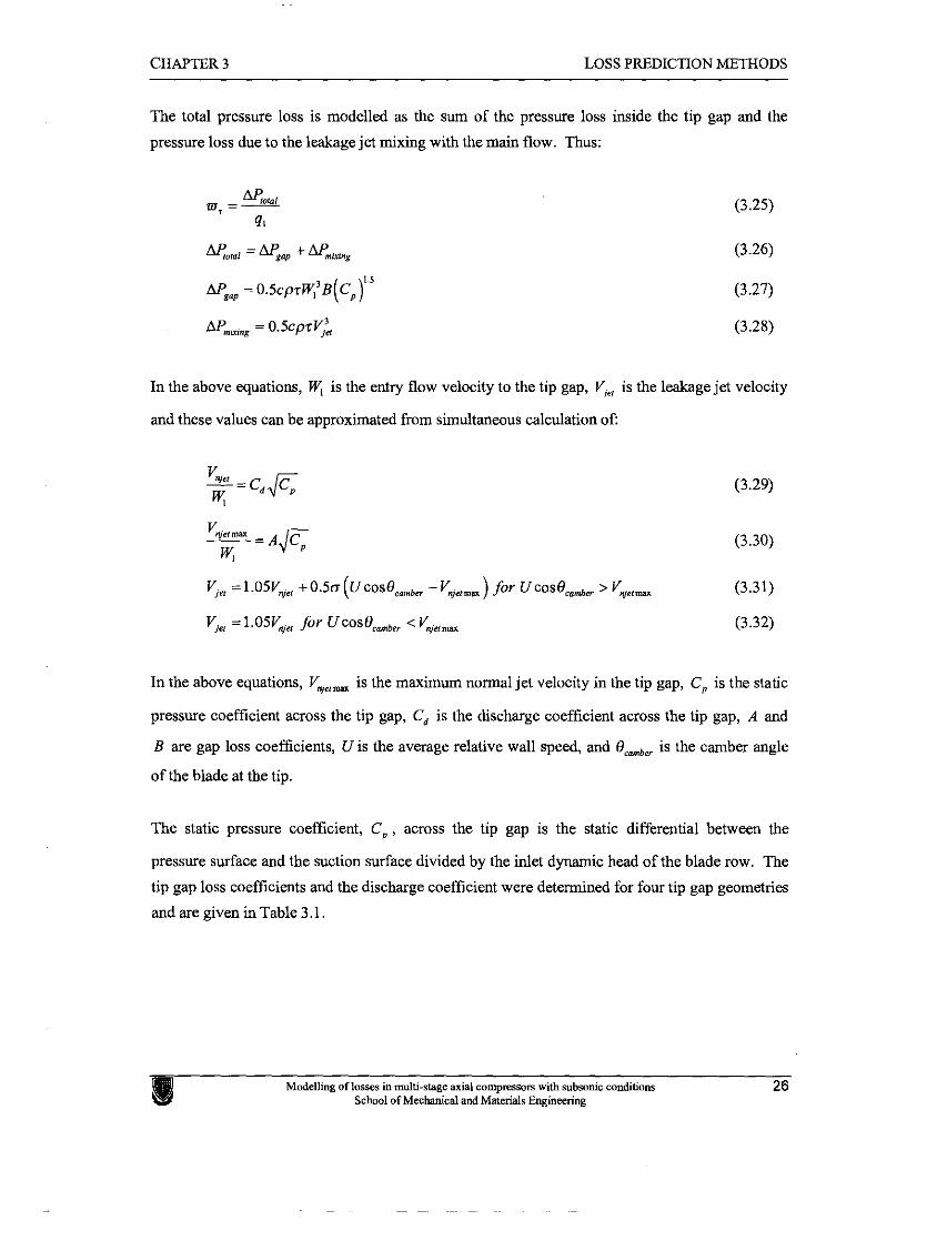
CHAPTER 3 LOSS PREDICTION METHODS
The total pressure loss is modelled as the sum of the pressure loss inside the tip gap and the
pressure loss due to the leakage jet mixing with the main flow. Thus:
AP,,,, = o S C ~ T ~ . ~ ,
In the above equations, W, is the entry flow velocity to the tip gap, V,, is the leakage jet velocity
and these values can he approximated from simultaneous calculation of:
In the above equations, V , , , is the maximum normal jet velocity in the tip gap, C , is the static
pressure coefficient across the tip gap, Cd is the discharge coefficient across the tip gap, A and
B are gap loss coefficients, U is the average relative wall speed, and O,,,, is the camber angle
of the blade at the tip.
The static pressure coefficient, C, , across the tip gap is the static differential between the
pressure surface and the suction surface divided by the inlet dynamic head of the blade row. The
tip gap loss coefficients and the discharge coefficient were determined for four tip gap geometries
and are given in Table 3.1.
Modelling of losses in multi-stage axial compresson with subsonic conditions 26 School of Mechanical and Materials Engineering
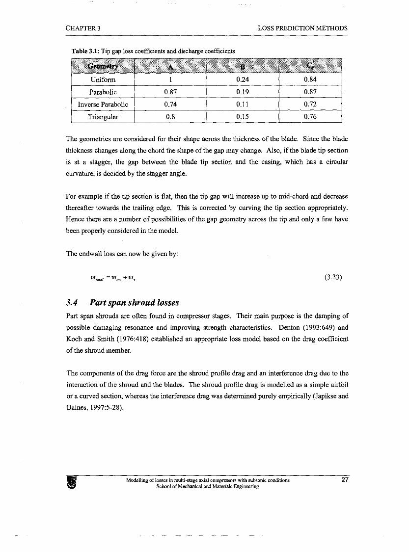
CHAPTER 3 LOSS PREDICTION METHODS - -
Table 3.1: Tip gap loss coefficients and discharge coefficients
The geometries are considered for their shape across the thickness of the blade. Since the blade
thickness changes along the chord the shape of the gap may change. Also, if the blade tip section
is at a stagger, the gap between the blade tip section and the casing, which has a circular
curvature, is decided by the stagger angle.
Geometry
Uniform
Parabolic
Inverse Parabolic
Triangular
For example if the tip section is flat, then the tip gap will increase up to mid-chord and decrease
thereafter towards the trailing edge. This is corrected by curving the tip section appropriately.
Hence there are a number of possibilities of the gap geometry across the tip and only a few have
been properly considered in the model.
B A
The endwall loss can now be given by:
cd
1
0.87
0.74
0.8
3.4 Part span shroud losses Part span shrouds are often found in compressor stages. Their main purpose is the damping of
possible damaging resonance and improving strength characteristics. Denton (1993:649) and
Koch and Smith (1976:418) established an appropriate loss model based on the drag coefficient
of the shroud member.
The components of the drag force are the shroud profile drag and an interference drag due to the
interaction of the shroud and the blades. The shroud profile drag is modelled as a simple airfoil
or a curved section, whereas the interference drag was determined purely empirically (Japikse and
Baines, 19975-28).
0.24
0.19
0.11
0.15
Modelling of losses in multi-stage axial compresson with subsonic conditions 27 School of Mechanical and Materials Engineering
0.84
0.87
0.72
0.76
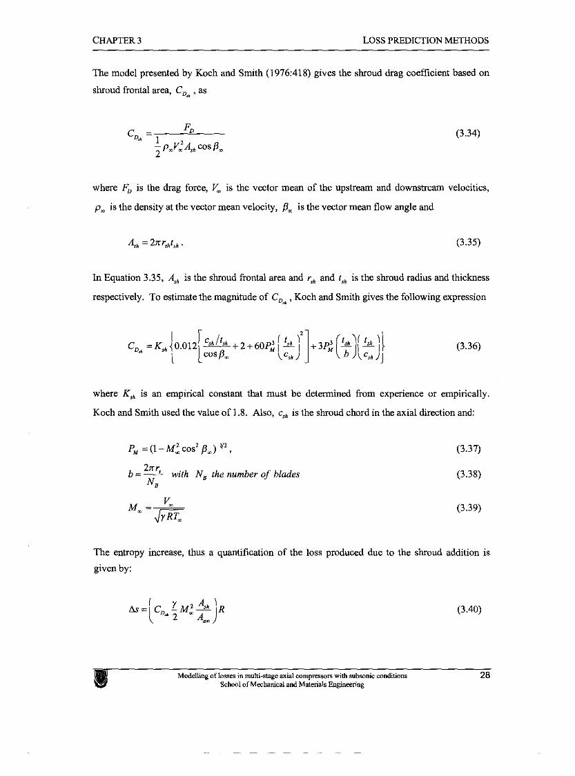
CHAPTER 3 LOSS PREDICTION METHODS
The model presented by Koch and Smith (1976:418) gives the shroud drag coefficient based on
shroud frontal area, Cud , as
where Fn is the drag force, V, is the vector mean of the upstream and downstream velocities,
p, is the density at the vector mean velocity, Dm is the vector mean flow angle and
A,, = 2zr,,t,, . (3.35)
In Equation 3.35, Ash is the shroud frontal area and r, and t,, is the shroud radius and thickness
respectively. To estimate the magnitude of CDZA , Koch and Smith gives the following expression
where K,, is an empirical constant that must be determined from experience or empirically.
Koch and Smith used the value of 1.8. Also, c,, is the shroud chord in the axial direction and:
P, = (1 - M: cos' ,
2zr, b=- with N, the number of blades
NB
The entropy increase, thus a quantification of the loss produced due to the shroud addition is
given by:
Modelling of losses in multi-stage axial compressom with subsonic conditions 28 School of Mechanical and Materials Engineering
CHAPTER 3 LOSS PREDICTION METHODS
3.5 Other losses
In Chapter 2, it was seen that only the mechanisms producing a steep velocity gradient are usually
taken into account when it comes to predicting the losses.
There are, however, numerous other mechanisms of loss, which are mostly small, but can become
significant in special cases (Denton, 1993:647). Denton advises further reading of Chapter 8 of
literature published by Glassman in 1973 for more details about these other loss mechanisms.
The most important of these are briefly discussed in the following sections.
3.5.1 Losses due to unsteady flow
Wakes, vortices and separations often mix out in the downstream blade row. This leads to mixing
in an unsteady environment and is a lot different from that which is modelled or observed in
cascade tests.
For wakes, the -mixing loss is usually relatively small and normally takes place close to the
trailing edge. Therefore, the added loss of this effect is mostly insignificant. A flow separation
can be thought of as a large wake, but in this case the added mixing loss can be large and might
have a noticeable affect on the entropy generation. The magnitude of such a process is, however,
difficult to quantify.
The vortex from one blade row will be convected though the downstream blade row in much the
same manner as a wake, but with different effects on the loss generation. If a vortex is stretched
longitudinally, from moving through the downstream blade row, it can be shown that its
secondary kinetic energy varies as the square of its length. When viscous effects then dissipate
this increased kinetic energy, it will increase the loss. Again the magnitude of such an increase is
not known, but it could have important implications in certain cases.
Other means in which unsteady flow can affect entropy generation are through dissipation of the
spanwise vorticity shed from a trailing edge as a result of changes in blade circulation, the
presence of unsteady velocity profiles due to wake passage and unsteady boundary layer
transition (Denton, 1993:648).
It is assumed that the aforementioned losses are usually small enough to justify their elimination
in loss modelling. Nevertheless, it is important that the reader is aware that such losses do
contribute to the total loss and might, in special cases, be larger in magnitude than anticipated.
Modelling af losses in multi-stage axial compressam with subsonic conditions School of Mecba~cal and Materials Engineering
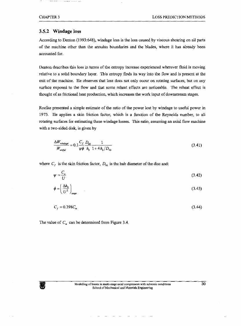
CHAPTER 3 LOSS PREDICTION METHODS
3.5.2 Windage loss
According to Denton (1993:648), windage loss is the loss caused by viscous shearing on all parts
of the machine other than the annulus boundaries and the blades, where it has already been
accounted for.
Denton describes this loss in terms of the entropy increase experienced wherever fluid is moving
relative to a solid boundary layer. This entropy finds its way into the flow and is present at the
exit of the machine. He observes that loss does not only occur on rotating surfaces, but on any
surface exposed to the flow and that some reheat effects are noticeable. The reheat effect is
thought of as frictional heat production, which increases the work input of downstream stages.
Roelke presented a simple estimate of the ratio of the power lost by windage to useful power in
1973. He applies a skin friction factor, which is a function of the Reynolds number, to all
rotating surfaces for estimating these windage losses. This ratio, assuming an axial flow machine
with a two-sided disk, is given by
where Cf is the skin friction factor, D,, is the huh diameter of the disc and:
The value of C, can be determined fkom Figure 3.4.
Modelling of losses in multi-stage axial compresson with subsonic conditions School of Mechanical and Materials Engineering
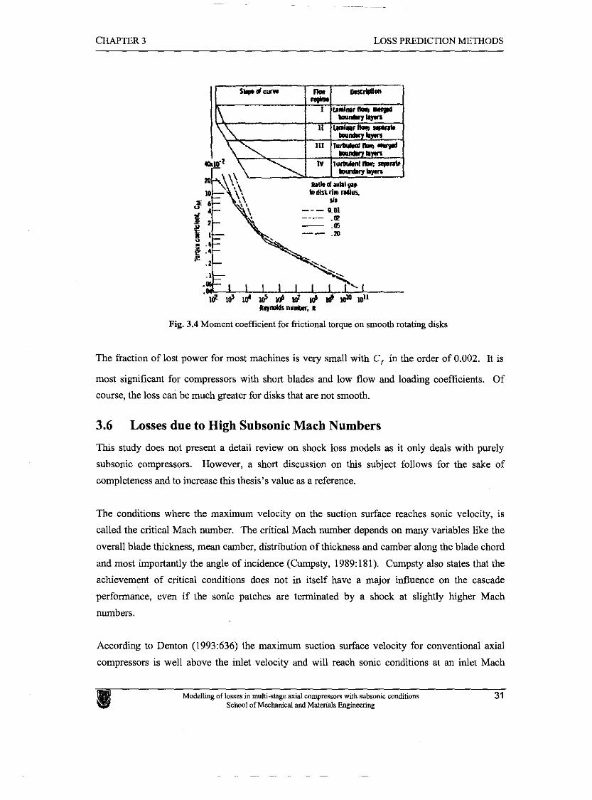
CHAPTER 3 LOSS PREDICTION METHODS
Fig. 3.4 Moment coefficient for fictional torque on smooth rotating disks
The fraction of lost power for most machines is very small with C , in the order of 0.002. It is
most significant for compressors with short blades and low flow and loading coefficients. Of
course, the loss can he much greater for disks that are not smooth.
3.6 Losses due to High Subsonic Mach Numbers
This study does not present a detail review on shock loss models as it only deals with purely
subsonic compressors. However, a short discussion on this subject follows for the sake of
completeness and to increase this thesis's value as a reference.
The conditions where the maximum velocity on the suction surface reaches sonic velocity, is
called the critical Mach number. The critical Mach number depends on many variables like the
overall blade thickness, mean camber, distribution of thickness and camber along the blade chord
and most importantly the angle of incidence (Cumpsty, 1989:181). Cumpsty also states that the
achievement of critical conditions does not in itself have a major influence on the cascade
performance, even if the sonic patches are terminated by a shock at slightly higher Mach
numbers.
According to Denton (1993:636) the maximum suction surface velocity for conventional axial
compressors is well above the inlet velocity and will reach sonic conditions at an inlet Mach
Modelhg of losses in multi-stage axial compresson with subsonic conditions 31 School of Mechanical and Materials Engineering
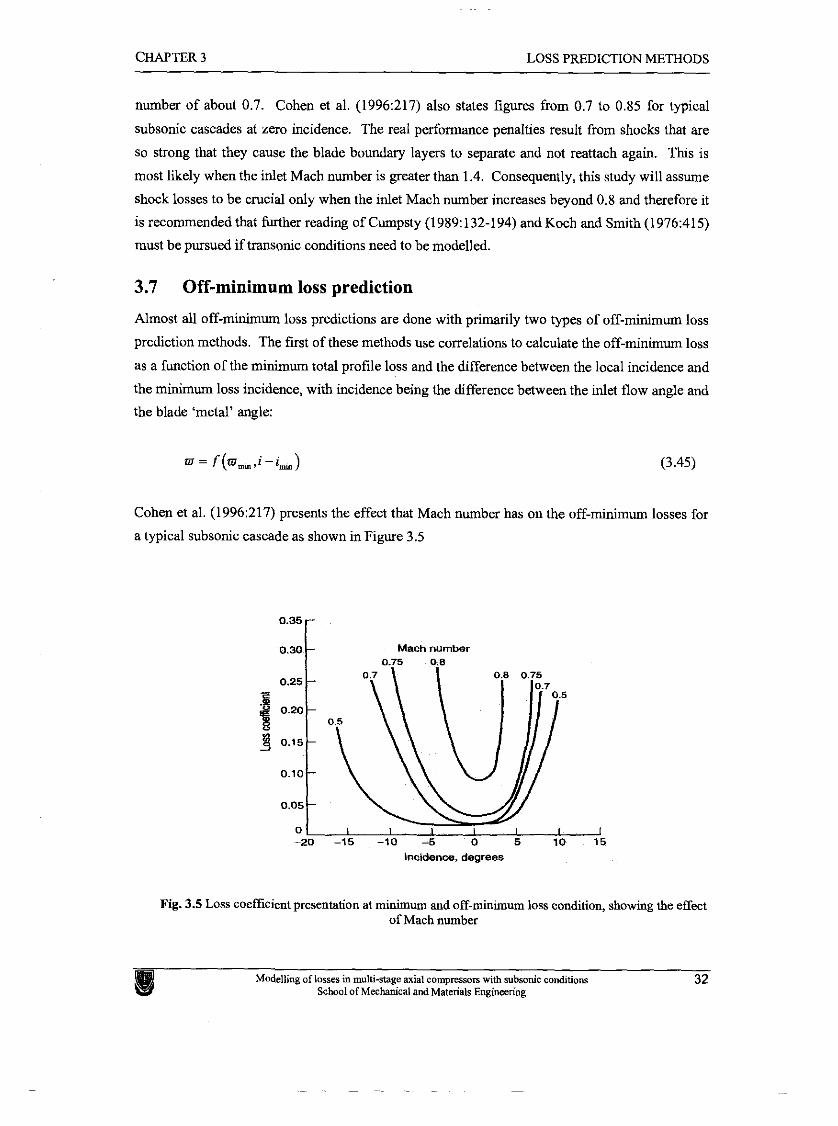
CHAPTER 3 LOSS PREDICTION METHODS
number of about 0.7. Cohen et al. (1996:217) also states figures from 0.7 to 0.85 for typical
subsonic cascades at zero incidence. The real performance penalties result from shocks that are
so strong that they cause the blade boundary layers to separate and not reattach again. This is
most likely when the inlet Mach number is greater than 1.4. Consequently, this study will assume
shock losses to be crucial only when the inlet Mach number increases beyond 0.8 and therefore it
is recommended that further r ead i i of Cumpsty (1989:132-194) and Koch and Smith (1976:415)
must be pursued if transonic conditions need to be modelled.
3.7 Off-minimum loss prediction
Almost all off-minimum loss predictions are done with primarily two types of off-minimum loss
prediction methods. The first of these methods use correlations to calculate the off-minimum loss
as a function of the minimum total profile loss and the difference between the local incidence and
the minimum loss incidence, with incidence being the difference between the inlet flow angle and
the blade 'metal' angle:
Cohen et al. (1996:217) presents the effect that Mach number has on the off-minimum losses for
a typical subsonic cascade as shown in Figure 3.5
0.30 Mach number
Incidence, degrees
Fig. 3.5 Loss coefficient presentation at minimum and off-minimum loss condition, showing the effect of Mach number
CHAPTER 3 LOSS PREDICTION METHODS
Casey (1987:276) uses a correlation given by Jansen and Moffatt in 1967 which correlates a
graph similar to Figure 3.5. This correlation is given as
where K is an off-minimum loss factor related to incidence and operating range. Chapter 4 gives
a more detailed discussion on predicting the operating range, Sp . The off-minimum loss factor
can be calculated as follows:
The second method is very similar to the prediction of the minimum profile loss by
Lieblein (1959), but the diffusion ratio, D, is corrected away from minimum loss incidence.
This value is then used in the calculation of the off-minimum momentum thickness to chord ratio.
Lieblein (1959) suggested a correlation for the off-minimum loss equivalent diffusion ratio by
using his minimum loss correlation, but applying a shift to account for the incidence angle.
cosp, l 1 1 2 + k ( i - i ) 1.43 r0.61-(tan& -tanpl) I D -- cos2 PI cosp, u 1
In the above equation k = 0.01 17 and k = 0.007 for the NACA 65-(Alo) blades and C.4 circular
arc blades respectively (Dixon, 1998:74). Starke (1980:7) suggested a value of 0.013 for their
experimental setup which consisted of 9C7132, 5C50 blades with a circular camber line. Wilson
and Korakianitis accept k = 0.01 17 as a satisfactory approximation for all blade shapes. The
momentum thickness to chord ratio can now again be calculated by the correlations, Equations
3.2. used for the minimum loss case.
3.8 Summary and conclusions
The main groupings for predicting minimum total loss in this chapter were: Blade profile losses,
endwall losses including literature on tip leakage and secondary losses, part span shroud losses,
other losses and losses due to high subsonic mach numbers.
Modelling of losses in multismge axial compressom with subsonic conditions 33 School of Mechanical and Materials Engineering
CHAPTER 3 LOSS PREDICTION METHODS
For the blade profile losses, most authors use a technique developed by Lieblein using a diffusion
factor. Koch and Smith's correlations seem to be the most complete, accounting for
compressibility, Reynolds number and streamtube contraction effects. This is also the only
model available that takes blade passage blockage into account. The loss from different profile
sections is very nearly equal at low to moderate subsonic Mach numbers. If necessary, the
correlations by Lieblein can be used for simplification purposes.
The literature on endwall losses consists of many different groupings of components. The model
of Koch and Smith appears to be the most complete and comprehensive as it does not distinguish
between loss components and models the endwall loss as a function of tip clearance and annulus
boundary layer parameters. It is further advantageous due to the fact that it gives a value for
endwall blockage resulting from the boundary layer and additional correlations are not needed to
calculate this quantity for performance prediction. Unfortunately, it requires a great amount of
iteration during performance prediction, and correlations from other authors can be used where
less complexity is desired.
Part span shroud losses should be included when applicable. Losses due to unsteady flow are
usually negligible, but can become important in special circumstances. There is, however, no
present way of predicting their magnitude. Windage loss is small in most cases, except if large
solid areas other than the annulus or blades are present in the flow path and especially if these
surfaces are not smooth.
Off-minimum loss predictions are done with primarily two types of prediction methods. The first
method calculates the off-minimum loss as a function of the minimum total profile loss and the
difference between the local incidence and the minimum loss incidence. The second method
corrects the diffusion ratio away from minimum loss incidence. This value is then used in the
calculation of the off-minimum momentum thickness to chord ratio that is used in calculating the
off-minimum loss.
It would seem rather pointless to do parametrical studies of the influence of loss parameter
changes based purely on the loss models, because these effects can almost be seen directly from
the correlations from which the models were constructed. The study of these models can
therefore not be viewed in isolation from the concepts involved in axial compressor performance
and its prediction. Chapter 4 presents the concepts involved in performance prediction.
Modelling of losses in multi-stage axial compresson with subsonic conditions 34 School of Mechanical and Materials Engineering
Chapter 4
PEPIF0 CE PREDICTION
The study of the models that predict subsonic axial compressor losses cannot be viewed in
isolation from the concepts involved in axial compressor performance prediction. This chapter
therefore attempts to provide the reader with a framework into which the loss models can be
integrated through presenting the theory required for a meanline compressor analysis.
Madelling of losses in multi-stage axial compresson with subsonic conditions School of Mechanical and Materials Engineering
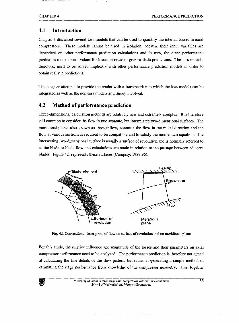
CHAPTER 4 PERFORMANCE PREDICTION
4.1 Introduction
Chapter 3 discussed several loss models that can be used to quantify the internal losses in axial
compressors. These models cannot be used in isolation, because their input variables are
dependent on other performance prediction calculations and in tum, the other performance
prediction models need values for losses in order to give realistic predictions. The loss models,
therefore, need to be solved implicitly with other performance prediction models in order to
obtain realistic predictions.
This chapter attempts to provide the reader with a framework into which the loss models can be
integrated as well as the non-loss models and theory involved
4.2 Method of performance prediction
Three-dimensional calculation methods are relatively new and extremely complex. It is therefore
still common to consider the flow in two separate, but interrelated two-dimensional surfaces. The
meridional plane, also known as throughflow, connects the flow in the radial direction and the
flow at various sections is required to be compatible and to satisfy the momentum equation. The
intersecting two-dimensional surface is usually a surface of revolution and is normally referred to
as the blade-to-blade flow and calculations are made in relation to the passage between adjacent
blades. Figure 4.1 represents these surfaces (Cumpsty, 1989:96).
Casing
Streamline .fi Meridional
plane
Fig. 4.1 Conventional description of flow on surface of revolution and on meridional plane
For this study, the relative influence and magnitude of the losses and their parameters on axial
compressor performance need to be analyzed. The performance prediction is therefore not aimed
at calculating the fine details of the flow pattern, but rather at generating a simple method of
estimating the stage performance from knowledge of the compressor geometry. This, together
Madelling of losses in multi-stage axial compreswrs with subsonic conditions 35 School of Mechanical and Materials Engineering
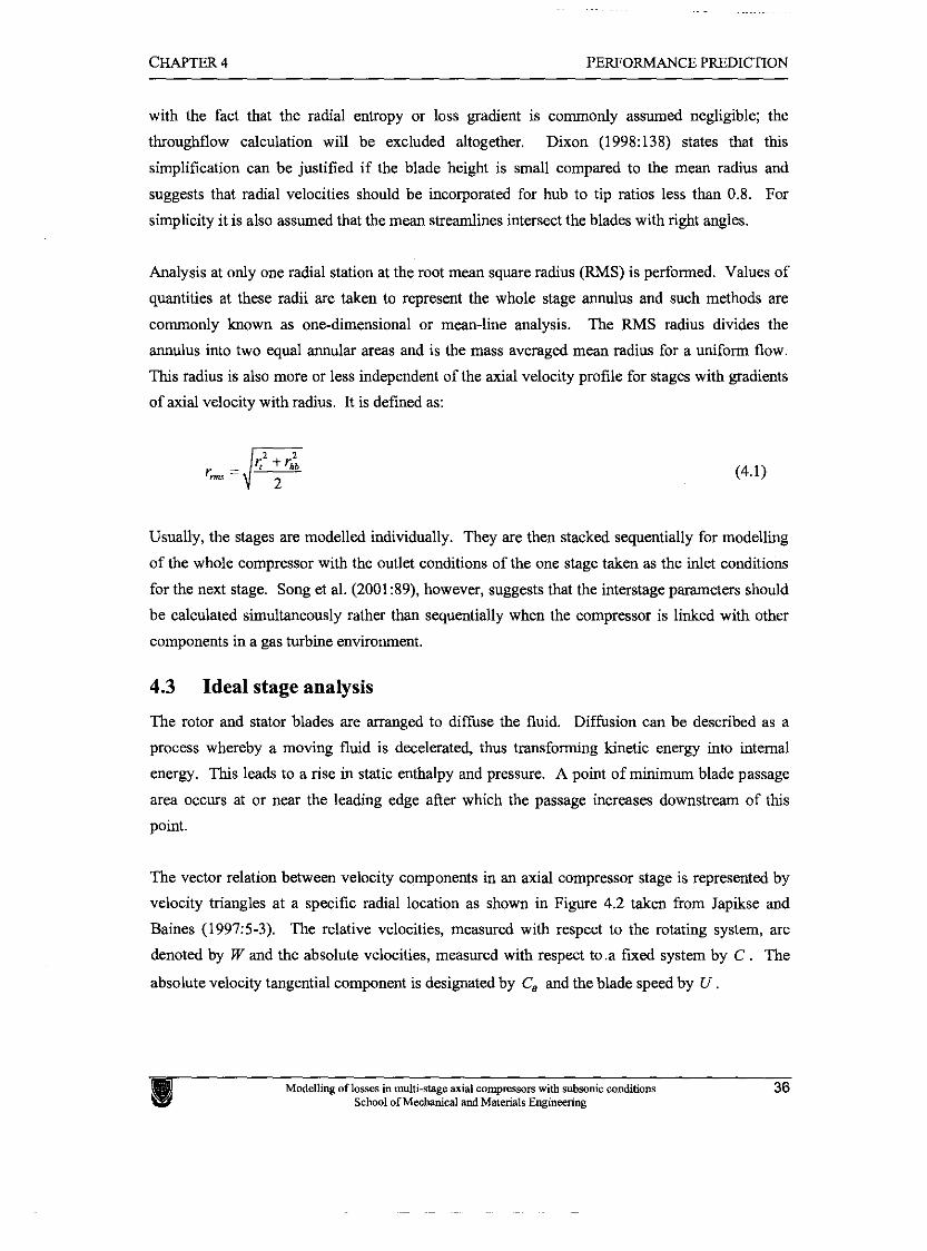
CHAPTER 4 PERFORMANCE PREDICTION
with the fact that the radial entropy or loss gradient is commonly assumed negligible; the
throughflow calculation will be excluded altogether. Dixon (1998:138) states that this
simplification can be justified if the blade height is small compared to the mean radius and
suggests that radial velocities should be incorporated for hub to tip ratios less than 0.8. For
simplicity it is also assumed that the mean streamlines intersect the blades with right angles.
Analysis at only one radial station at the root mean square radius (RMS) is performed. Values of
quantities at these radii are taken to represent the whole stage annulus and such methods are
commonly known as one-dimensional or mean-line analysis. The RMS radius divides the
annulus into two equal annular areas and is the mass averaged mean radius for a uniform flow.
This radius is also more or less independent of the axial velocity profile for stages with gradients
of axial velocity with radius. It is defined as:
Usually, the stages are modelled individually. They are then stacked sequentially for modelling
of the whole compressor with the outlet conditions of the one stage taken as the inlet conditions
for the next stage. Song et al. (2001:89), however, suggests that the interstage parameters should
be calculated simultaneously rather than sequentially when the compressor is linked with other
components in a gas turbine environment.
4.3 Ideal stage analysis
The rotor and stator blades are arranged to diffuse the fluid. Diffusion can be described as a
process whereby a moving fluid is decelerated, thus transforming kinetic energy into internal
energy. This leads to a rise in static enthalpy and pressure. A point of minimum blade passage
area occurs at or near the leading edge after which the passage increases downstream of this
point.
The vector relation between velocity components in an axial compressor stage is represented by
velocity triangles at a specific radial location as shown in Figure 4.2 taken fiom Japikse and
Baines (1997:5-3). The relative velocities, measured with respect to the rotating system, are
denoted by Wand the absolute velocities, measured with respect to.a fixed system by C . The
absolute velocity tangential component is designated by C, and the blade speed by U .
Modelling of losses in multi-stage axial compressors with subsonic conditions 36 School of Mechanical and Matenals Engineering
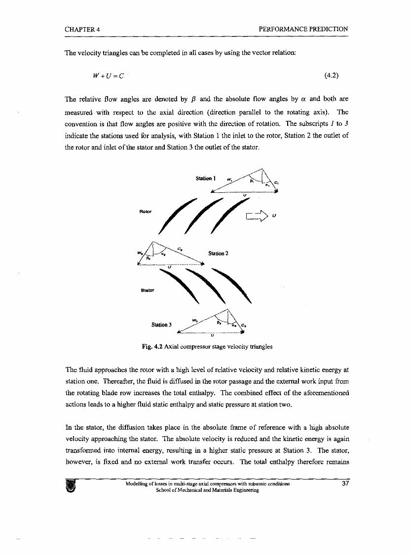
CHAPTER 4 PERFORMANCE PREDICTION
The velocity triangles can be completed in all cases by using the vector relation:
The relative flow angles are denoted by P and the absolute flow angles by a and both are
measured with respect to the axial direction (direction parallel to the rotating axis). The
convention is that flow angles are positive with the direction of rotation. The subscripts 1 to 3
indicate the stations used for analysis, with Station 1 the inlet to the rotor, Station 2 the outlet of
the rotor and inlet of the stator and Station 3 the outlet of the stator.
Fig. 4.2 Axial compressor stage velocity triangles
The fluid approaches the rotor with a high level of relative velocity and relative kinetic energy at
station one. Thereafter, the fluid is diffused in the rotor passage and the external work input from
the rotating blade row increases the total enthalpy. The combined effect of the aforementioned
actions leads to a higher fluid static enthalpy and static pressure at station two.
In the stator, the diffusion takes place in the absolute frame of reference with a high absolute
velocity approaching the stator. The absolute velocity is reduced and the kinetic energy is again
transformed into internal energy, resulting in a higher static pressure at Station 3. The stator,
however, is fixed and no external work transfer occurs. The total enthalpy therefore remains
Modelling of losses in multi-sfage axial compresson with subsonic canditions School of Mechanical and Materials Engineering
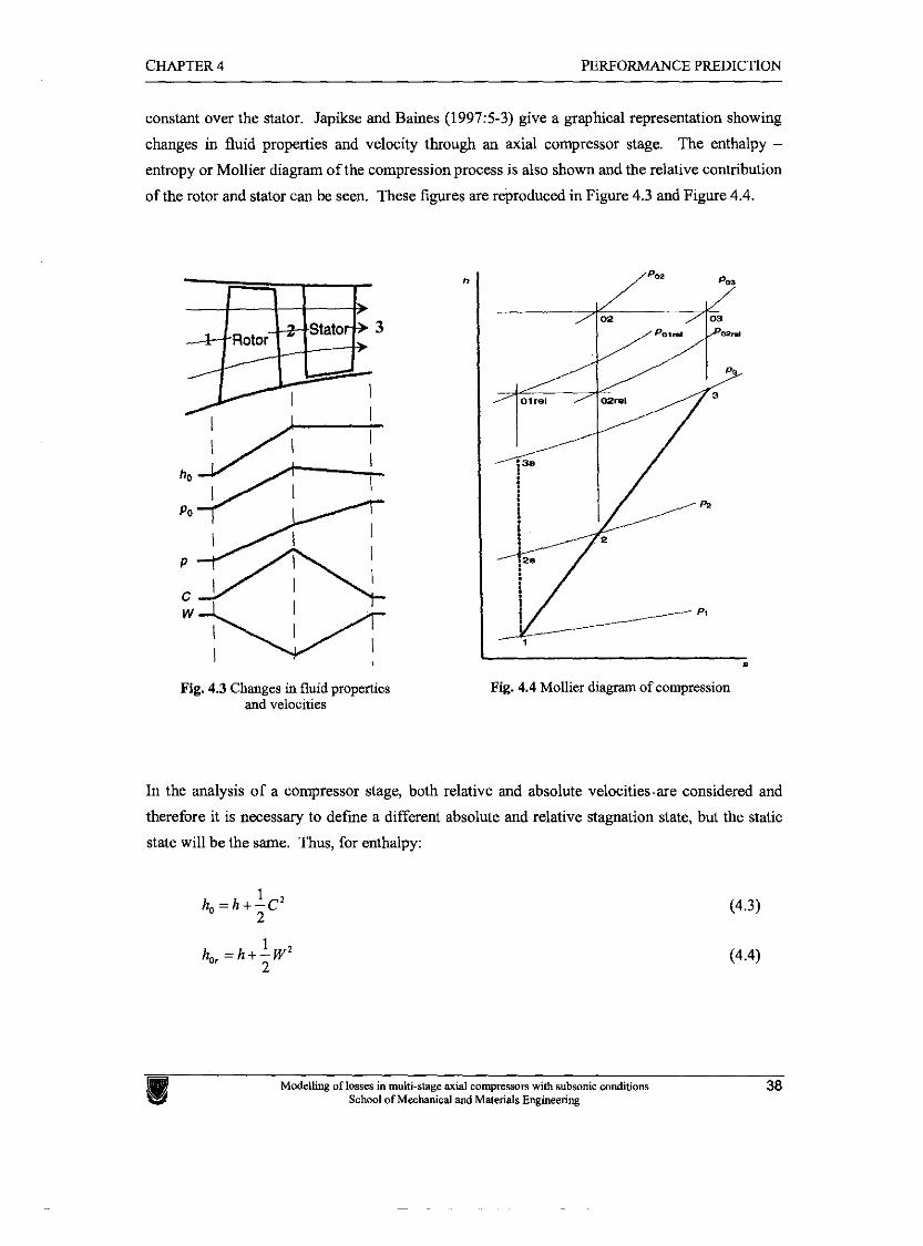
CHAPTER 4 PERFORMANCE PREDICTION
constant over the stator. Japikse and Baines (1997:5-3) give a graphical representation showing
changes in fluid properties and velocity through an axial compressor stage. The enthalpy -
entropy or Mollier diagram of the compression process is also shown and the relative contribution
of the rotor and stator can be seen. These figures are reproduced in Figure 4.3 and Figure 4.4.
Rotor
Fig. 4.3 Changes in fluid properties and velocities
L *
Fig. 4.4 Mollier diagram of compression
In the analysis of a compressor stage, both relative and absolute velocitiesme considered and
therefore it is necessary to define a different absolute and relative stagnation state, but the static
state will be the same. Thus, for enthalpy:
1 h,, =h+-W'
2
Modelling of losses in multi-stage axial compresson with subsonic conditions School of Mechanical and Materials Engineering
CHAPTER 4 PERFORMANCE PREDICTION
The subscript h, denotes the stagnation enthalpy in the absolute fiame and h,, the stagnation
enthalpy in the relative frarne. The same principle applies to stagnation temperatures in the
absolute and relative frarne. In an isentropic (no losses) compression process for a semi-perfect
or ideal gas in the absolute and relative frarne:
The Euler turbomachinery equation stems directly h m the energy and momentum equations
applied to a blade row. For adiabatic, steady flow through a rotor it follows that the work input
per unit mass flow rate is given as the change in total enthalpy between any two points 1 and 2:
When Equation 4.6 is applied along a streamline, thus a fluid element is only influenced by the
blade-to-blade pressure gradient; an invariant thermodynamic property called rothalpy can be
deduced as shown in Cumpsty (1989, 6). In rotating blade rows, rothalpy has properties
analogues to stagnation enthalpy in stationary passages. Rothalpy is conserved along a streamline
through a rotor and is defmed by:
Equation 4.7 can be written for a perfect gas to give the relative total temperature increase by:
It therfore follows that if, no change in radius occurs, T,,, =T,,, throughout the rotor. In the
stator, the work input is zero and the total enthalpy is conserved, h,, = h,, , thus assuming a
perfect gas, To3 = To2. The conservation of rothalpy in a rotor and total enthalpy in a stator is true
even in the presence of friction, loss and radius change.
CHAPTER 4 PERFORMANCE PREDICTION
For an inviscid and isentropic process, i.e. an ideal stage, the total pressure based on rothalpy or,
if no change in radius occurs, the relative total pressure is constant in the rotor and the absolute
total pressure is constant in the stator. The total pressure based on rothalpy might be defined as:
The aforementioned equations provide the basis for analysis of an ideal stage. In a real stage, the
compression is not isentropic and usually an increase in entropy leads to a decrease in the
respective total pressure. This is often used as a basis for assessing the loss of an axial
compressor stage or element and is included through the use of non-dimensional loss coefficients.
Other phenomena, for which estimates should be included in order to obtain a realistic mean line
analysis, are blockage at the annulus walls, minimum loss incidence, deviation and estimates for
the onset of stall and choke. With the magnitude of these quantities known, the ideal stage
analysis can be adapted to represent a real stage and the efficiency and other performance
parameters can be computed.
Values for these phenomena are, however, not amenable to confident mathematical models and
normally come from correlations constructed from experimental data. This data usually comes
from two-dimensional cascades, tested under controlled conditions.
4.4 Real stage parameters
This section discusses the estimation of the performance prediction parameters that are based on
correlations obtained from test data and need to be included in order to obtain a realistic meanline
analysis of a stage or are needed by some loss models. The parameters that need to be discussed
here are: Loss coefficients, blockage at the annulus walls, minimum loss incidence, deviation and
estimates for the onset of stall and choke.
4.4.1 Loss coefficients
Loss coefficients are introduced in Chapter 3 and are the dimensionless quantities used to express
the loss obtained by some loss models. An in depth discussion and comparison of the different
loss coefficients used for axial compressor blade rows are given by Brown (1972). The form of
loss coefficient that is most common for compressors and diffusers is the pressure loss
coefficient. It describes the drop in available total pressure, in the respective b e , in terms of
CHAPTER 4 PERFORMANCE PREDICTION
the inlet kinetic energy approaching the component. In adiabatic flow, a connection exists
between entropy increase and stagnation pressure decrease.
For a rotor the compressible loss coefficient is defined in terms of the relative frame as:
For a stator, in the absolute frame, the pressure loss coefficient is given by:
4.4.2 Blockage
Frictional shear forces of the flow on the blades or annulus walls cause low momentum fluid to
accumulate and form boundary layers. This leads to a reduction in effective flow area and an
increase in axial velocity. The blockage is perhaps the most critical quantity in high-speed
compressor design, but its creation is not well understood nor is its magnitude accurately
predictable (Cumpsty, 1989:311). The endwall blockage in axial compressors has been the
subject of several investigations over a period of many years. Horlock (2000:218-224) gives a
detailed comparison of the available methods and the attributes of each. The work of Smith and
Khalid et al. are discussed in detail in this paper and it is concluded that Smith's method would be
the most appropriate for determining the absolute stage blockage through a multi-stage
compressor.
For the purpose of this study the effect and magnitude of the endwall blockage will be included
through the use of an annulus blockage factor ( ABF ). This factor, which is a function of the
endwall boundary layer displacement thickness, is calculated as:
The value of the ABF is restricted to 0.83 if the value deduced from the model is greater
CHAPTER 4 PERFORMANCE PREDICTION
Values for the endwall boundary layer thickness are calculated in the Koch and Smith endwall
loss model, or when other endwall loss models are used, assumed a constant value provided by
the user. Estimates for this parameter can be obtained while using the Koch and Smith endwall
loss model. Taking into account the uncertainty involved in predicting the blockage and its
dependence on tip clearance and stage pressure rise, this method provides the best possible
solution without including additional correlations and is, in any case, based on the same data used
by Smith.
Endwall blockage leads to a reduction in the effective annulus flow area, which in turn leads to an
increase in the free stream axial velocity due to the conservation of mass, where
rn = ( ~ A v ) ~ , = ( p ~ ~ ) n _ . The effective flow area is related to the geometrical flow area
according to:
The ABF grows gradually through the compressor in a multi-stage environment. As stated
before, however, the ABF is limited to 0.83 so that the boundary layer increases in the first few
stages and then assumes a constant value in later stages where the limit is exceeded. The
boundary layer growth is simulated by inputting the exit boundary layer from a previous stage or
inlet guide vanes as an inlet boundary layer to the next stage or some form of inlet ABF reduction
throughout the stages.
4.4.3 Minimum loss incidence
Lieblein introduced the concept of minimum loss incidence in 1956. It is the incidence at which a
cascade will experience an absolute minimum loss. Many authors assume this value to be zero,
but as was seen in Chapter 3, it serves as the reference value for predicting the off-minimum loss
coefficients. and needs to be calculated for more accurate results.
The correlation assumes an equation of the form
where i, is the minimum incidence angle for a blade with zero camber and n is the slope of the
variation in incidence with camber (Lieblein, 1960:578).
Modelling of lasses in multi-stage axial compresson with subsonic conditions 42 School of Mechanical and Materials Engineering
CHAPTER 4 PERFORMANCE PREDICTION
The value of n can be found from Figure B.l.l from Appendix B.1. i, can, in turn, be calculated
from:
In Equation 4.15, (i,),, is the minimum loss incidence for a NACA-65 cascade of zero camber
and 10 percent thickness to chord ratio. Values for (i,,),, can be found from Figure B.1.2 for a
range of inlet air angles. Further, K, and Kt are correction factors for different shape
distributions and thickness to chord ratios as for the (i,),, correlation respectively. K, can be
obtained from Figure B.1.3 and K, is assumed 1.1 for C-series blades and 0.7 for DCA blades,
with NACA-65 having a value of one (Japikse and Baines, 1997:5-1 8).
Finally a correction of -1 degree should be applied to the predicted minimum loss incidence
according to Casey (1987:275). This correction allows for operation at constant stagger angle
whereas the measurements of Lieblein were carried out at a constant air angle.
4.4.4 Deviation
Deviation can be described as the difference in the outlet flow angle and the blade angle at the
trailing edge of the blade. Predictions of this value are based on empirical correlations as
described in the following sections.
The correlation that is still used most often, but with modifications and adaptations by various
authors is known as Carter's rule. Another common, but more complete and accurate, correlation
is the one provided by Lieblein (1960) and is calculated somewhat similar to his correlation for
the minimum-loss incidence. This correlation is used rather than Carter's rule due to its direct
connection with the definition for minimum-loss incidence.
The deviation at minimum loss incidence is given by
with m the slope factor of the deviation angle variation with camber at a solidity of unity.
Values for m can be obtained from Figure B.2.1. b is the solidity exponent variable with air
CHAPTER 4 PERFORMANCE PREDICTION
inlet angle and can be found from Figure B.2.2. 6, is the reference minimum-loss deviation
angle at zero camber and can be represented as:
Similar to the minimum loss incidence, (So),, is the basic variation for the NACA-65 blade
profile with a ten percent thickness distribution. Figure B.2.3 gives values for (6,),, . K, is a
correction for blade shapes with other thickness distributions than the blades used to obtain the
(6,),, correlation and Kt is the correction necessary for blades with a maximum thickness other
than 10 percent (Lieblein, 1960:580). Values for K, are assumed the same as for the minimum-
loss incidence and K, can be obtained from Figure B.2.4.
For off-minimum loss deviation, a correlation that is a function of minimum-loss deviation and
incidence is used:
In Equation 4.18, represents the slope of the deviation angle variation at the minimum-
loss incidence angle and can be found from Figure B.2.5.
Lieblein's correlation only gives a correct estimate for axial velocity density ratios of one,
however, there is no satisfactory correlation available for predicting the deviation for other axial
velocity density ratios. Usually, an addition of one or two degrees to the result is employed to
account for this (Cumpsty, 1989:171). This addition will, however, not be implemented in this
study due to further lack of support for this statement.
4.4.5 Stall and choke
The stalling incidence of a blade row is usually determined from cascade data, while the choking
incidence is a function of the cascade throat area and the inlet Mach number. From Chapter 3, if
using loss as a measure, a factor of two times the minimum profile loss for stalling and three
times the minimum profile loss for choking (see Figure 3.5) is a common measure for preliminary
estimates of the corresponding incidences (Miller, 1987:249-250). Alternatively, some authors
CHAPTER 4 PERFORMANCE PREDICTION
use an off-minimum loss correlation that employs an operating range parameter. The operating
range is defined as the range of inlet flow angle within which the loss coefficient is less than
twice the minimum loss value and can be calculated from the following correlation
where SP, is the operating range of the NACA-65 series cascades at low Mach number and KM
is a correction for the effect of Mach number. Analysis of NACA data by Hugentobler in 1986
has led to the following correlation for the operating range at low Mach number for
30° S P, 5 70":
The correction for Mach number is taken into account as proposed by Hoheisel in 1969 (Casey,
1987:275):
KM =1 for Mach number < 0.2
KM =lo- ~.s(M-0.2)" for Mach number > 0.2
Casey (1987:277) assumes that stall and choke will occur in terms of incidence at the root mean
square radius when:
The aforementioned criterion provides crude estimates for predicting when a blade row will stall
or choke. These estimates, however, provide no information on when the stage as a whole stalls
or chokes or the maximum static pressure rise that can be obtained in a stage at the stall point.
This value needs to he calculated in order to correctly predict the endwall losses as given by Koch
and Smith. Casey (1987:277) assumed very roughly the stage to he choked when no pressure rise
is being produced.
De Haller recognized in 1955 that the endwall boundary layers l i t the pressure rise achievable
by any cascade of compressor blades. His work, however, provides only a very prelimimy
Modelling of losses in multi-stage axial compressors with subsonic conditions 45 School of Mechanical and Materials Engineering
CHAPTER 4 PERFORMANCE PREDICTION
guideline and cannot really be used with confidence in this study. Koch (1981) found the
maximum static pressure rise coefficient to correlate well with a standard two-dimensional
diffuser performance when plotted against a passage width to length ratio and this seems to
provide a better estimate for predicting the stall point of a stage. According to Koch (1981:646),
"It does, however, give the peak pressure rise capability of an individual stage operating in a
multi-stage environment, and used in conjunction with a stage stacking off-design performance
prediction method, it can indicate when the limiting conditions that de-stabilize the system and
lead to surge will occur within a multi-stage compressor."
The geometry parameter used by Koch is the meanline arc length of the cambered airfoil, divided
L by the cascade trailing edge staggered spacing, -. The stage average value of the length to
g
width ratio is calculated by using the blade row inlet dynamic head of rotor and stator as the
weighting factor. The static pressure rise coefficient is based on the mean effective dynamic head
at inlet to the rotor and stator. The effective inlet kinetic energy takes into account the ability of
compressor blades with high stagger angles to re-energize low momentum boundary layer fluid
leaving an upstream blade row as this fluid impinges on the following blade row in the other
frame of reference (Casey, 1987:277).
Casey (1987:277) modified the correlation by Koch to provide an even better fit to the diffuser
data and this is given in Figure B.3.1, also showing the De Haller diffusion limit and the fit used
by Koch. The maximum value of the effective static pressure rise coefficient is calculated as
where CPD is the maximum static pressure rise coefficient from the diffuser data, K , is a
Reynolds number correction factor form Figure B.3.2, K, a correction for tip clearance effects
given by Figure B.3.3 and KAs a correction for axial spacing between the blade rows from
Figure B.3.4.
For a stage, Casey assumes the stage to choke when the stage produces no pressure rise and for
simplicity this is also accepted in this study.
CHAPTER 4 PERFORMANCE PREDICTION
4.5 Loss and efficiency
The definition of entropy allows for the easy summation of entropy gains or losses. For a perfect
where the temperatures and pressures can either have total or static values, as long as it is
consistent, and the equation can be used for rotors (relative frame) and stators (absolute frame).
Therefore, in a component, the total entropy increase is equal to the sum of all the entropy
increases due to the various losses. For a stage:
The entropy increase due to all the losses through an axial compressor can then similarly be found
from:
i
As cov,,,, = xAsss,, , i = Number of stages (4.26) I
The loss of efficiency of a stage or compressor is directly proportional to the increase in specific
entropy and also to its exit temperature (Denton, 1993:624). Efficiency is the ratio of work into
the ideal compressor or stage to actual work at a given pressure ratio and mass flow rate. In an
ideal compressor or stage, which is adiabatic and reversible, no entropy change due to losses
occurs and the process is therefore considered isentropic. The corresponding definition of
efficiency is isentropic efficiency, with the work input equal to the rise in stagnation enthalpy:
This definition is also known as the total-to-total isentropic efficiency. Other variations include
static-to-static or total-to-static and represents respective values of enthalpy used.
Modelling of losses in multi-stage axial compressors with subsonic conditions 47 School of Mechanical and Materials Engineering
CHAPTER 4 PERFORMANCE PREDICTION
On a Mollier diagram (Figure 4.4), the local slope of the pressure lines are given by the local
value of the respective temperature. If the assumption is made that these pressure lines have a
constant slope, the efficiency definition can be given in terms of the entropy increase:
4.6 Summary and conclusions
This chapter presents the performance prediction theory for a meanline analysis at the RMS
radius. The rotor and stator blades are arranged to diffuse the fluid by decelerating it, thus
transforming kinetic energy into internal energy. This leads to a rise in static enthalpy and
pressure. Through an ideal rotor, rothalpy and total pressure based on rothalpy are conserved and
through an ideal stator, total enthalpy and total pressure are conserved. Furthermore, the losses
manifest itself as entropy increases in the fluid and equivalently reduce the respective outlet total
pressure. Losses are usually expressed with the use of diensionless loss coefficients, with the
pressure loss coefficient the most commonly used as can be seen in Chapter 3.
Together with estimates for the losses, estimates for annulus blockage, minimum loss incidence,
deviation and the onset of stall and choke also need to be obtained in order to include real fluid
effects found in compressors. These quantities are found from correlations obtained from cascade
or compressor data. In this study, the correlations from Lieblein are used for the minimum loss
and deviation predictions and the correlation provided by Koch will be used for obtaining
estimates for the stalling stage pressure rise. For the annulus blockage factor, values will be
obtained from the endwall loss model from Koch and Smith and detail regarding the
implementation thereof is given in Chapter 5.
It was seen that values for entropy increases due to the different losses can be obtained for each
blade row. The sum of all the entropy gains can then be used to estimate the efficiency of single-
stage or multi-stage compressors as well as individual stages of multi-stage compressors.
In this stage of the study, enough information is available to generate a preliminary multi-stage
performance prediction code. Chapter 5 consequently presents the reader with the methodology
employed for implementing the theory and correlations obtained from the literature and given in
Chapters 3 and 4.
IMPLEMENTATION
Chapter 5 presents the methodology employed in this study for the generation of a pe~ormance
prediction code, with general applicability to subsonic multi-stage compressors with different
geometries and working fluids, which allows the interchanging of loss models. It utilizes the
theory and models described in Chapters 3 and 4.
Modelling of losses in multi-stage axial compresson with subsonic conditions School o f Mechanical and Materials Engineering
CHAPTER 5 IMPLEMENTATION
5.1 Introduction
Chapters 3 and 4 presented the reader with the available literature regarding loss models and the
basic theory for performance prediction. Some models were identified as the most suitable to use
in this study and these were described in more detail.
This chapter will focus on the methodology employed to generate a performance prediction code
from these chapter's, with general applicability to subsonic multi-stage compressors with different
geometries and working fluids, which allows the interchanging of loss models. It is further
necessary for this code to have the capability to he used for parametric studies, reflecting the
influence of input variable changes on particularly the loss magnitudes and this relation to other
performance variables.
5.2 Methodology
From the previous chapters, it was seen that an implicit approach is necessary and it was decided
to use a software package called Engineering Equation Solver (EES) Academic Version 6.867-3D
(F-Chart Software, 2003). The basic function provided by EES is the solution of a set of
algebraic equations, hut it has the advantage of automatically identifying and grouping equations
that must be solved simultaneously.
The EES code can consist of several 'sub-sections' or 'sub-equation groups' employing modules,
procedures and functions. Some of the advantages of using a modular approach are that it makes
it easy to switch between different loss models and also aids in applying the same equations in
both the relative and absolute frames by just calling them with the respective variable inputs.
Future users can easily modify or replace certain 'parts' of the code almost independently, as long
as the inputs and outputs of the calling argument are satisfied. Modules can be considered to be
stand-alone EES programs that can be called from the main EES program or from other modules
lower in the equation window. When EES calls a module, it adds the equations in the module
into the main equation set, as opposed to conventional procedures and functions, which are solved
separate and sequentially, but supports logical control statements like IF-ELSE.
A recommended algorithm to generate the code is presented in Appendix C.l and was developed
in such a way that easy implementation in lower-level programming languages would be possible
in future studies. Unfortunately, it was found that EES becomes unstable when trying to solve
too large equation sets, especially when employing modules due to the increase in sensitivity to
the guess values used. Consequently, for this study, each stage of a multi-stage compressor was
Modelling of losses in multi-stage axial compressors with subsonic conditions 49 School of Mechanical d Materials Engineering
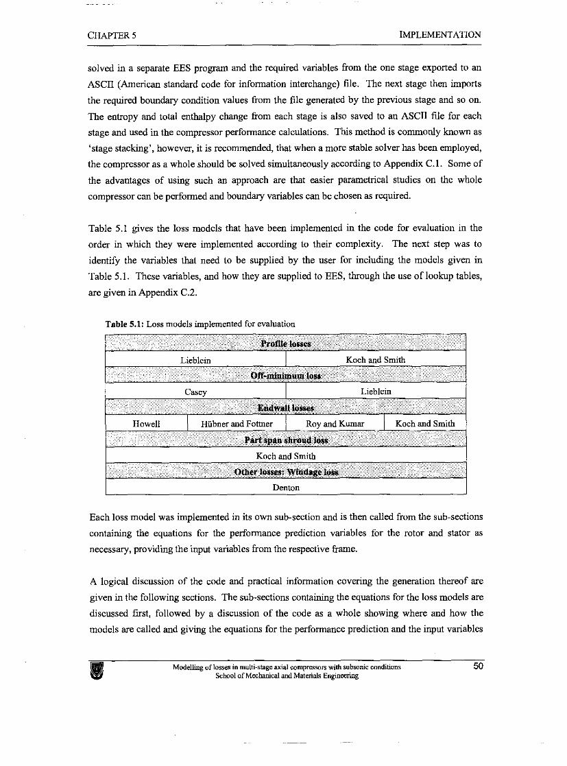
CHAPTER 5 IMPLEMENTATION
solved in a separate EES program and the required variables from the one stage exported to an
ASCII (American standard code for information interchange) file. The next stage then imports
the required boundary condition values kom the file generated by the previous stage and so on.
The entropy and total enthalpy change from each stage is also saved to an ASCII file for each
stage and used in the compressor performance calculations. This method is commonly known as
'stage stacking', however, it is recommended, that when a more stable solver has been employed,
the compressor as a whole should be solved simultaneously according to Appendix C.1. Some of
the advantages of using such an approach are that easier parametrical studies on the whole
compressor can be performed and boundary variables can be chosen as required.
Table 5.1 gives the loss models that have been implemented in the code for evaluation in the
order in which they were implemented according to their complexity. The next step was to
identify the variables that need to be supplied by the user for including the models given in
Table 5.1. These variables, and how they are supplied to EES, through the use of lookup tables,
are given in Appendix C.2.
Table 5.1: Loss models implemented for evaluation
1 Howell 1 HiibnerandFottner 1 Rov andKumar 1 Koch and Smith 1 i I. .-..-..-A .-
Part span shroud loss
I Koch and Smith I 7
i Other 10~x8: Windage loss
I Denton I
Each loss model was implemented in its own sub-section and is then called from the sub-sections
containing the equations for the performance prediction variables for the rotor and stator as
necessary, providing the input variables from the respective frame.
A logical discussion of the code and practical information covering the generation thereof are
given in the following sections. The sub-sections containing the equations for the loss models are
discussed fust, followed by a discussion of the code as a whole showing where and how the
models are called and giving the equations for the performance prediction and the input variables
Modelling of losses in multi-stage axial compresson with subsonic conditions 50 School of Mechanical and Materials Engineering
CHAPTER 5 IMPLEMENTATION
to the loss models. The complete EES source code is given in Appendix C.6, with the formatted
equation sets for the loss models and performance prediction given in Appendix C.3 and
Appendix C.4 respectively. The code is essentially generated for the NACA-65 blade profile
family, but can be easily adapted to include the other profile families commonly used in subsonic
axial compressors.
5.3 The loss models
In this section, a discussion on the implementation of the loss models is presented. The formatted
equation sets from the code for the loss models are given in Appendix C.3. The equation
numbers from Chapter 3 is also shown and the input variables and outputs from each model can
clearly be seen from the sub-section declaration, with the output variables shown to the right of
the colon.
5.3.1 Profile loss model implementation
Section C.3.1 shows the formatted equations for the Lieblein profile loss model. The correlations
of Casey for the momentum thickness to chord ratio have been implemented for evaluation. Two
equations for calculating the pressure loss coefficient have been included, with the one assuming
the form factor to be one and excluded the tenns containing it. The one not used is commented
out when running the code. To satisfy the requirements of the calling argument to this module, it
is necessary for this sub-section to return a value for blade blockage and a constant value of zero
has been used as this model was not indented to be used with a blockage value.
Section C.3.2 shows the formatted equations for the Koch and Smith profile loss model.
Corrections for conditions other than nominal are made to the momentum thickness to chord ratio
as well as the boundary layer form factor. Unfortunately, the correction factors are given in the
literature in a graphical format as given in Appendix A.2 and curve fits had to be performed in
order to obtain equations that could be implemented in the code.
The curve fit equations for the correction factors are contained in separate sub-sections that return
the values for the correction factors to the profile loss sub-section. Linear interpolation was
necessary in some cases and a sub-section to facilitate this function was also generated. Koch
and Smith limit the applicability of their model to equivalent diffusion ratios below 1.7 and a
warning mechanism was included in one of the correction factor sub-sections to wam the user
when this is not the case. These correction factor sub-sections and the sub-section to do linear
interpolation between the desired values are given after the profile loss sub-section in
Section (2.3.2.
CHAPTER 5 IMPLEMENTATION
5.3.2 Off-minimum loss model implementation
The formatted equations for the sub-section containing the equations for the off-minimum loss
model of Casey are shown in Section C.3.3 and those of Lieblein in Section C.3.4. A value of
0.01 17 was used for the constant in Equation 3.48.
5.3.3 Endwall loss model implementation
The formatted equations for the implementation of the Howell, Hiibner and Fottner and Roy and
Kumar endwall loss models are given in Section C.3.5, C.3.6 and C.3.7 respectively. The sub-
section for the Roy and Kumar model also employs a function for calculating the leakage jet
velocity. This function is showed below the sub-section containing the Roy and Kumar endwall
loss equations in Section C.3.7.
The Koch and Smith endwall loss model, presented in Section 3.3.2, gives predictions for the
endwall loss of a complete stage. However, in order to enable the evaluation of the endwall loss
in single bladerows and to see the contribution of each bladerow to the total endwall loss, the
model needs to be converted to be applicable to single bladerows. It also makes the comparison
between the different loss models simpler, because the other models are component-based.
Unfortunately, the Koch and Smith endwall loss model requires predictions of parameters like the
stalling static pressure rise coefficient from the correlation by Koch and the stage static pressure
rise coeff~cient. The implicit nature of the code can now be clearly seen from the fact that these
values are calculated for the whole stage while being input values to the rotor and stator modules.
It is further necessary for the stage freestream efficiency to he inputted to the Koch and Smith
endwall loss model sub-section. Consequently, the Koch and Smith endwall loss sub-section is
called &om the stage sub-section, with the inputs for the stage stalling static rise coefficient, stage
static pressure rise coeff~cient and the stage freestream total-to-total effkiency as input
parameters. In turn, the entropy generation due to the endwall loss from each hladerow and the
endwall boundary layer displacement thickness are returned and given as input parameters when
calling the rotor and stator sub-sections. The methodology for adapting the Koch and Smith
model to be used in such a manner are explained below.
From Appendix A.4 it was seen that the endwall parameters for a stage was correlated against the
static pressure rise coefficient divided by the maximum static pressure rise coefficient of the
The correlations were again only available in
graphical format (Appendix A.4), but curve fittings were done and these equations and how they
are used are presented in the formatted equations shown in Section C.3.8. A warning procedure,
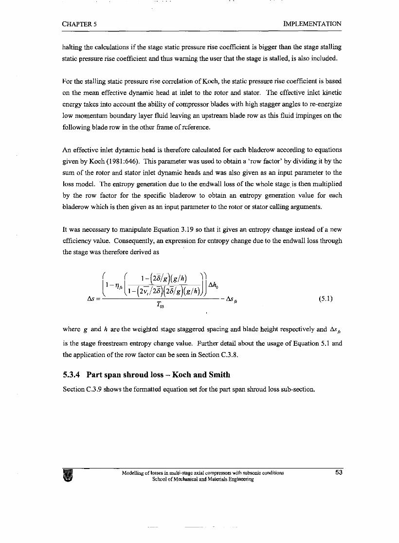
CHAPTER 5 IMPLEMENTATION
halting the calculations if the stage static pressure rise coefficient is bigger than the stage stalling
static pressure rise coefficient and thus warning the user that the stage is stalled, is also included.
For the stalling static pressure rise correlation of Koch, the static pressure rise coefficient is based
on the mean effective dy&c head at inlet to the rotor and stator. The effective inlet kinetic
energy takes into account the ability of compressor blades with high stagger angles to re-energize
low momentum boundary layer fluid leaving an upstream blade row as this fluid impinges on the
following blade row in the other frame of reference.
An effective inlet dynamic head is therefore calculated for each bladerow according to equations
given by Koch (1981:646). This parameter was used to obtain a 'row factor' by dividing it by the
sum of the rotor and stator inlet dynamic heads and was also given as an input parameter to the
loss model. The entropy generation due to the endwall loss of the whole stage is then multiplied
by the row factor for the specific bladerow to obtain an entropy generation value for each
bladerow which is then given as an input parameter to the rotor or stator calling arguments.
It was necessary to manipulate Equation 3.19 so that it gives an entropy change instead of a new
efficiency value. Consequently, an expression for entropy change due to the endwall loss through
the stage was therefore derived as
where g and h are the weighted stage staggered spacing and blade height respectively and As,
is the stage freestream entropy change value. Further detail about the usage of Equation 5.1 and
the application of the row factor can be seen in Section C.3.8.
5.3.4 Part span shroud loss - Koch and Smith
Section C.3.9 shows the formatted equation set for the part span shroud loss sub-section.
Modelling of loss= in multi-stage axial compressom with mbsonic conditions 53 School of Mechanical and Materials Engineering
CHAPTER 5 IMPLEMENTATION
5.3.5 Windage loss - Denton
The windage loss is given as a fraction of lost power to useful power in the literature. For the
purpose of implementing it in the code, it has to return either a presswe loss coefficient or an
entropy increase. The windage loss does attribute to an efficiency decrease. An entropy change
must, therefore, be returned h m this sub-section as shown in Section C.3.10. It is known that
the work input to a stage per unit mass is equal to the change of total enthalpy through the stage.
The windage loss sub-section is only applied to the rotor and if it is accepted that As = :, the
entropy change due to windage loss can be written as:
The loss models have now been presented in their specific sub-sections. However, these sub-
sections do not function on their own and realistic input variables have to be supplied. This is
done, by generating performance prediction sub-sections from which these loss models can be
called. The following sections present the generation of the performance prediction code.
5.4 The performance prediction code
5.4.1 The compressor code
A multi-stage axial compressor consists of a number of stages. Ideally, as proposed in
Appendix C.l, a single code should represent such a compressor and a sub-section that contains
the necessary equations for each stage is called according to the number of stages. As stated
previously, however, EES becomes unstable with too large equation sets and each stage has to be
solved in a separate EES program. The outputs are then written to an ASCII file for use as inputs
to the next stage and for the calculation of efficiency and other performance parameters for the
stage as a whole. For this study, the compressor code is therefore defined as an EES program that
reads the necessary variables from the ASCII files that were generated sequentially from stage
one for each stage. The ASCII files imported as lookup tables are then used to calculate
performance parameters like compressor total-to-total adiabatic efficiency, total-to-total pressure
ratio and total-to-total temperature ratio. Section C.4.1 shows the formatted equations used in the
compressor code.
CHAPTER 5 IMPLEMENTATION
5.4.2 Stage
Each stage consists of a rotor and a stator and the stage code calls the sub-codes for the rotor and
the stator. Values for the stage stalling static pressure rise coefficient, the static pressure rise
coefficient, the freestream efficiency and the row factor for each bladerow are also calculated
here. These values are used as inputs when calling the Koch and Smith endwall loss model and
values for the endwall loss entropy generation and the endwall boundary layer displacement
thickness are supplied when calling the rotor and stator sub-codes. When using another endwall
loss model in the rotor or stator sub-code, the entropy generation value from the Koch and Smith
model is not used, but the boundary layer displacement thickness parameter is still used for
calculating the endwall blockage. Section C.4.2 shows the formatted equations for a stage. In
this case, the total-to-total adiabatic efficiency is a function of the sum of the entropy increases
and the sum of the stagnation enthalpy increases of the rotor and the stator.
5.4.3 Rotor and Stator sub-sections
The Rotor and Stator sub-sections contain equations for calculating the required rotor and stator
variables respectively. Equation sets that are applicable to both the rotor and stator, contained in
different sub-sections, are called when needed. These include the equations for minimum loss
incidence, deviation, stalling static pressure rise coefficient, operating range, a test to determine
whether the cascade is stalled, and the different losses. In the case of the losses, there can be
switch between the different models simply by calling the appropriate sub-section and
commenting the other calling arguments or assignments in the code.
The author found it vety difficult to give the code a sequential structure for increased readability,
due to the implicit nature of the code and the fact that several sub-sections are called. Some
effort has been made. However, it must again be emphasized that the equations are not solved
sequentially in the sub-sections and that the equation order or form has no real importance in EES
and solves as long as the number of equations and variables are equal. Section C.4.3 shows the
equations and variables used in the Rotor sub-section and Section C.4.4 for the stator. Extensive
commentary has been included and a detailed discussion is therefore not given here. The
following points should however be noted.
The fluid property calculations were done using built-in EES functions that return the required
value with static pressure and temperature given as arguments. C, and C, were assumed
constant throughout the bladerows, but different values for p , p and a was calculated at the
inlet and outlet of each bladerow.
Modelling of losses in multi-stage axial compressors with subsonic conditions 55 School of Mechanical and Materials Engineering
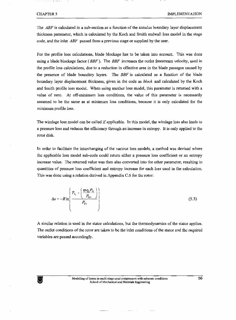
CHAPTER 5 IMPLEMENTATION
The ABF is calculated in a sub-section as a function of the annulus boundary layer displacement
thickness parameter, which is calculated by the Koch and Smith endwall loss model in the stage
code, and the inlet ABF passed from a previous stage or supplied by the user.
For the profile loss calculations, blade blockage has to be taken into account. This was done
using a blade blockage factor (BBF) . The BBF increases the outlet freestream velocity, used in
the profile loss calculations, due to a reduction in effective area in the blade passages caused by
the presence of blade boundary layers. The BBF is calculated as a function of the blade
boundary layer displacement thickness, given in the code as block and calculated by the Koch
and Smith profile loss model. When usiig another loss model, this parameter is returned with a
value of zero. At off-minimum loss conditions, the value of this parameter is necessarily
assumed to be the same as at minimum loss conditions, because it is only calculated for the
minimum profile loss.
The windage loss model can be called if applicable. In this model, the windage loss also leads to
a pressure loss and reduces the efficiency through an increase in entropy. It is only applied to the
rotor disk.
In order to facilitate the interchanging of the various loss models, a method was devised where
the applicable loss model sub-code could return either a pressure loss coefficient or an entropy
increase value. The returned value was then also converted into the other parameter, resulting in
quantities of pressure loss coefficient and entropy increase for each loss used in the calculation.
This was done using a relation derived in Appendix C.6 for the rotor:
A similar relation is used in the stator calculations, but the thermodynamics of the stator applies.
The outlet conditions of the rotor are taken to be the inlet conditions of the stator and the required
variables are passed accordingly.
Modelling of losses in multi-stage axial campresson with subsonic conditions 56 School of Mechanical and Materials Engineering
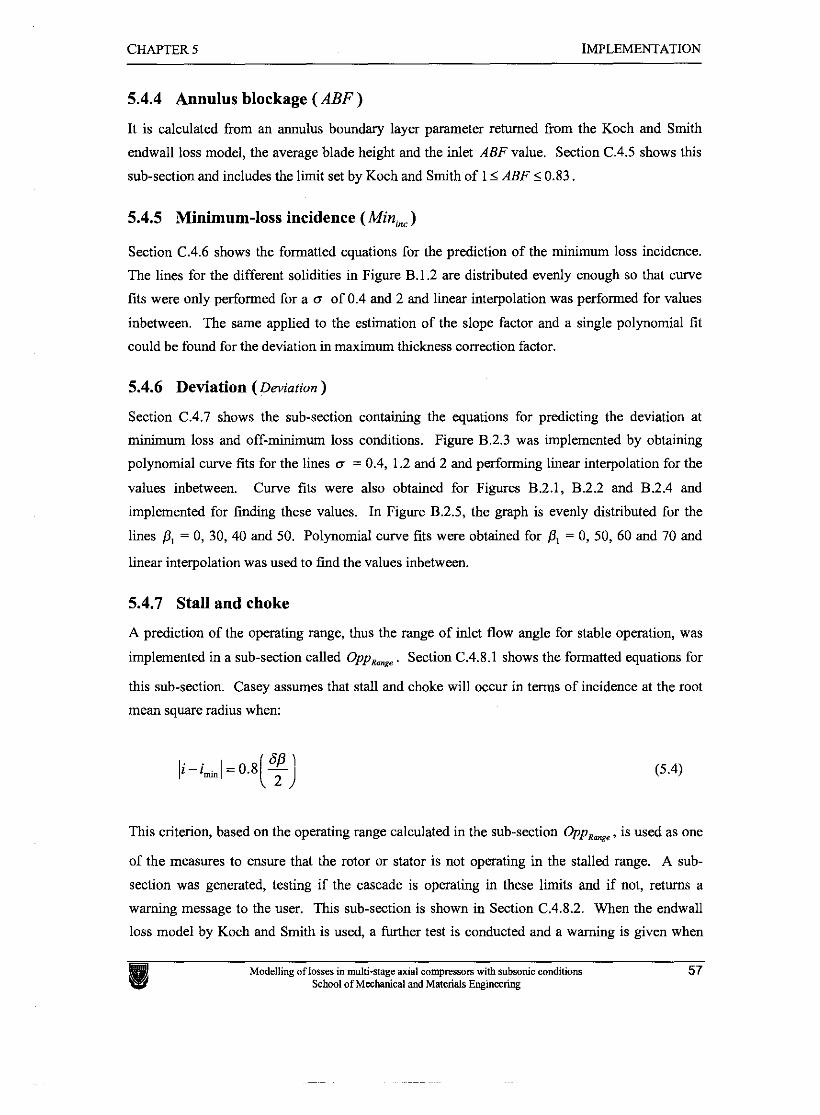
CHAPTER 5 IMPLEMENTATION
5.4.4 Annulus blockage ( ABF )
It is calculated from an annulus boundary layer parameter returned ftom the Koch and Smith
endwall loss model, the average blade height and the inlet ABF value. Section C.4.5 shows this
sub-section and includes the limit set by Koch and Smith of 1 < ABF 5 0.83.
5.4.5 Minimum-loss incidence (Min,, )
Section C.4.6 shows the formatted equations for the prediction of the minimum loss incidence.
The lines for the different solidities in Figure B.1.2 are distributed evenly enough so that curve
fits were only performed for a a of 0.4 and 2 and linear interpolation was performed for values
inbetween. The same applied to the estimation of the slope factor and a single polynomial fit
could be found for the deviation in maximum thickness correction factor.
5.4.6 Deviation (Deviation)
Section C.4.7 shows the suh-section containing the equations for predicting the deviation at
minimum loss and off-minimum loss conditions. Figure B.2.3 was implemented by obtaining
polynomial curve fits for the lines a = 0.4, 1.2 and 2 and performing linear interpolation for the
values inbetween. Curve fits were also obtained for Figures B.2.1, B.2.2 and B.2.4 and
implemented for finding these values. In Figure B.2.5, the graph is evenly distributed for the
lines p, = 0, 30, 40 and 50. Polynomial curve fits were obtained for P, = 0, 50, 60 and 70 and
linear interpolation was used to find the values inbetween.
5.4.7 Stall and choke
A prediction of the operating range, thus the range of inlet flow angle for stable operation, was
implemented in a sub-section called Opp,,, . Section C.4.8.1 shows the formatted equations for
this sub-section. Casey assumes that stall and choke will occur in terms of incidence at the root
mean square radius when:
This criterion, based on the operating range calculated in the sub-section OppRmge, is used as one
of the measures to ensure that the rotor or stator is not operating in the stalled range. A sub-
section was generated, testing if the cascade is operating in these limits and if not, returns a
warning message to the user. This suh-section is shown in Section C.4.8.2. When the endwall
loss model by Koch and Smith is used, a further test is conducted and a warning is given when
Modelling of losses in multi-stage axial compresson with subsonic conditions 57 School of Mechanical and Materials Engineering
CHAPTER 5 IMPLEMENTATTON
the static pressure rise increases beyond the predicted stalling static pressure rise coefficient as
seen in Section 5.4.3.
The prediction of the maximum static pressure rise coefficient, thus the value at stall according to
Koch and modified by Casey were implemented in the sub-section called Stall,,, . Curve fits
were again performed on the correlation figures as given in Appendix B.3 for implementation
purposes. The curve fit for the Reynolds number correction factor was facilitated with the aid of
three straight lines as can he seen from the formatted equations for this sub-section given in
Section C.4.8.3.
As stated in Chapter 4, this study makes the same assumption as Casey for choking and this is
assumed to happen when the stage produces no pressure rise. No additional correlations were
therefore implemented for predicting choke.
5.5' Summary and Conclusions
This chapter presented the methodology and generation of a performance prediction code, with
general applicability to subsonic multi-stage compressors with different geometries and working
fluids, which allows the interchanging of loss models. A software package called EES was used
for implementation. A modular approach was followed and different sub-sections were used to
structure the code, implement logical operations in EES and limit programming time by calling
common suh-sections from the relative and absolute frame respectively.
The correlations were mainly given in the literature in a graphical format and were implemented
by obtaining curve fits containing the specific variables. The loss models were implemented as
given in the literature, with the exception of the Koch and Smith endwall loss model that was
transformed from a stage based approach to a component-based model. The performance
prediction was implemented using a separate EES program for each stage that calls suh-sections
for the rotor and stator, which in turns uses the loss models from the respective h e . The stage
programs are run sequentially from the first stage to the last through exporting outputs from each
stage to an ASCII file so that the following stage can import applicable input variables from the
previous stage. An EES program was then generated that utilizes the output ASCII files to
calculate the multi-stage compressor performance variables. A method was devised where loss
models could return either an entropy increase value or a pressure loss coefficient.
Blockage was implemented with the aid of blockage factors. An annulus blockage factor ( ABF )
is used to reduce the geometrical annulus area to an effective annulus area due to the presence of
Modelling of losses in multi-stage axial compresson with subsonic conditions 58 School of Mechanical and Materials Enginee~g
CHAPTER 5 IMPLEMENTATION
an endwall boundary layer. This factor is a function of the endwall boundary displacement
thickness calculated by the endwall loss model of Koch and Smith and an inlet annulus boundary
layer parameter which can be supplied by the user or obtained fiom the output blockage value of
the previous stage. For the blade blockage due to the blade boundary layers, a blade boundary
layer factor (BBF) is used that increases the velocity used for the profile loss models. This
factor is a function of the blade boundary layer displacement thickness, which value is zero for
the Lieblein profile loss model and calculated by the Koch and Smith profile loss model.
For the prediction of stall, this code uses the endwall loss model fiom Koch and Smith to test if
the static pressure rise is larger than the stalling static pressure rise coefficient as predicted by
Koch. Another test, that was implemented, is the correlation and stall criterion given by Casey.
Choke was assumed to occur when the stage has no pressure rise.
The generated code must be verified and the methodology validated before it can be used for
obtaining interesting conclusions. Chapter 6 verifies the code against a commercial software
package called NREC and evaluates the different loss models according to their simplicity and
accuracy.
Modelling of losses in multi-stage axial campresson with subsonic conditions 59 School of Mechanical and Materials Engineering
VERIF1CA"XTON AND EVALUATION
Chapter 6 verijies the code, developed in Chapter 5, against a commercial sofhvare package
called NREC and evaluates the dzferent loss models according to their simpliciry and accuracy.
A loss model combination is chosen according to the results and the performance prediction from
this code is then compared to predictions from NREC. This is first done for a stage and then for
a multi-stage compressor.
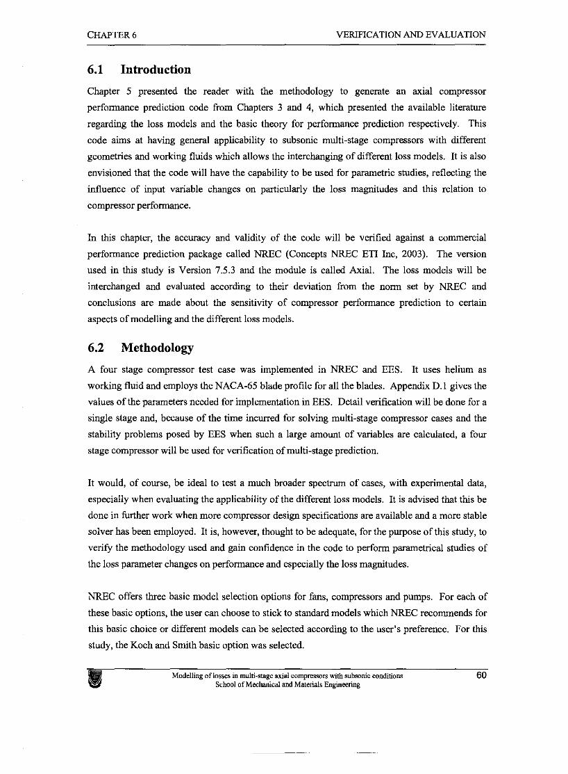
CHAPTER 6 VERIFICATION AND EVALUATION
6.1 Introduction
Chapter 5 presented the reader with the methodology to generate an axial compressor
performance prediction code from Chapters 3 and 4, which presented the available literature
regarding the loss models and the basic theory for performance prediction respectively. This
code aims at having general applicability to subsonic multi-stage compressors with different
geometries and working fluids which allows the interchanging of different loss models. It is also
envisioned that the code will have the capability to be used for parametric studies, reflecting the
influence of input variable changes on particularly the loss magnitudes and this relation to
compressor performance.
In this chapter, the accwacy and validity of the code will be verified against a commercial
performance prediction package called NREC (Concepts NREC ETI Inc, 2003). The version
used in this study is Version 7.5.3 and the module is called Axial. The loss models will be
interchanged and evaluated according to their deviation from the norm set by NREC and
conclusions are made about the sensitivity of compressor performance prediction to certain
aspects of modelling and the different loss models.
6.2 Methodology
A four stage compressor test case was implemented in NREC and EES. It uses helium as
working fluid and employs the NACA-65 blade profile for all the blades. Appendix D.l gives the
values of the parameters needed for implementation in EES. Detail verification will be done for a
single stage and, because of the time incurred for solving multi-stage compressor cases and the
stability problems posed by EES when such a large amount of variables are calculated, a four
stage compressor will be used for verification of multi-stage prediction.
It would, of course, be ideal to test a much broader spectrum of cases, with experimental data,
especially when evaluating the applicability of the different loss models. It is advised that this be
done in further work when more compressor design specifications are available and a more stable
solver has been employed. It is, however, thought to be adequate, for the purpose of this study, to
verify the methodology used and gain confidence in the code to perform parametrical studies of
the loss parameter changes on performance and especially the loss magnitudes.
NREC offers three basic model selection options for fans, compressors and pumps. For each of
these basic options, the user can choose to stick to standard models which NREC recommends for
this basic choice or different models can be selected according to the user's preference. For this
study, the Koch and Smith basic option was selected.
Modelling of losses in multi-stage axial compressors with subsonic conditions 60 School of Mechanical and Materials Engineering
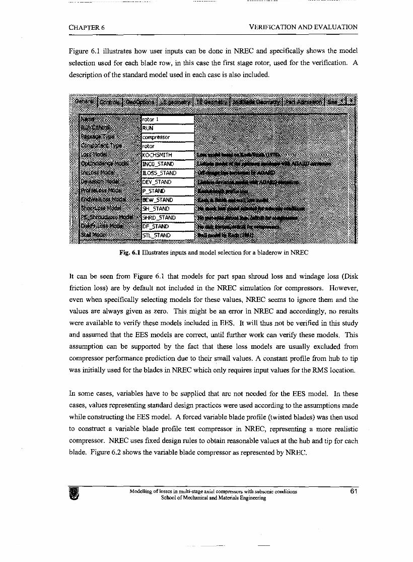
CHAPTER 6 VERIFICATION AND EVALUATION
Figure 6.1 illustrates how user inputs can be done in NREC and specifically shows the model
selection used for each blade row, in this case the first stage rotor, used for the verification. A
description of the standard model used in each case is also included.
Fig. 6.1 Illustrates inputs and model selection for a bladerow in NREC
It can be seen from Figure 6.1 that models for part span shroud loss and windage loss (Disk
friction loss) are by default not included in the NREC simulation for compressors. However,
even when specifically selecting models for these values, NREC seems to ignore them and the
values are always given as zero. This might be an error in NREC and accordimgly, no results
were available to verify these models included in EES. It will thus not be verified in this study
and assumed that the EES models are correct, until further work can verify these models. This
assumption can be supported by the fact that these loss models are usually excluded from
compressor performance prediction due to their small values. A constant profile from hub to tip
was initially used for the blades in NREC which only requires input values for the RMS location.
In some cases, variables have to be supplied that are not needed for the EES model. In these
cases, values representing standard design practices were used according to the assumptions made
while constructing the EES model. A forced variable blade profile (twisted blades) was then used
to construct a variable blade profile test compressor in NREC, representing a more realistic
compressor. NREC uses fixed design rules to obtain reasonable values at the hub and tip for each
blade. Figure 6.2 shows the variable blade compressor as represented by NREC.
Madelling of losses in multi-stage axial compressors with subsonic conditions 61 School of Mechical and Mataials Engineering
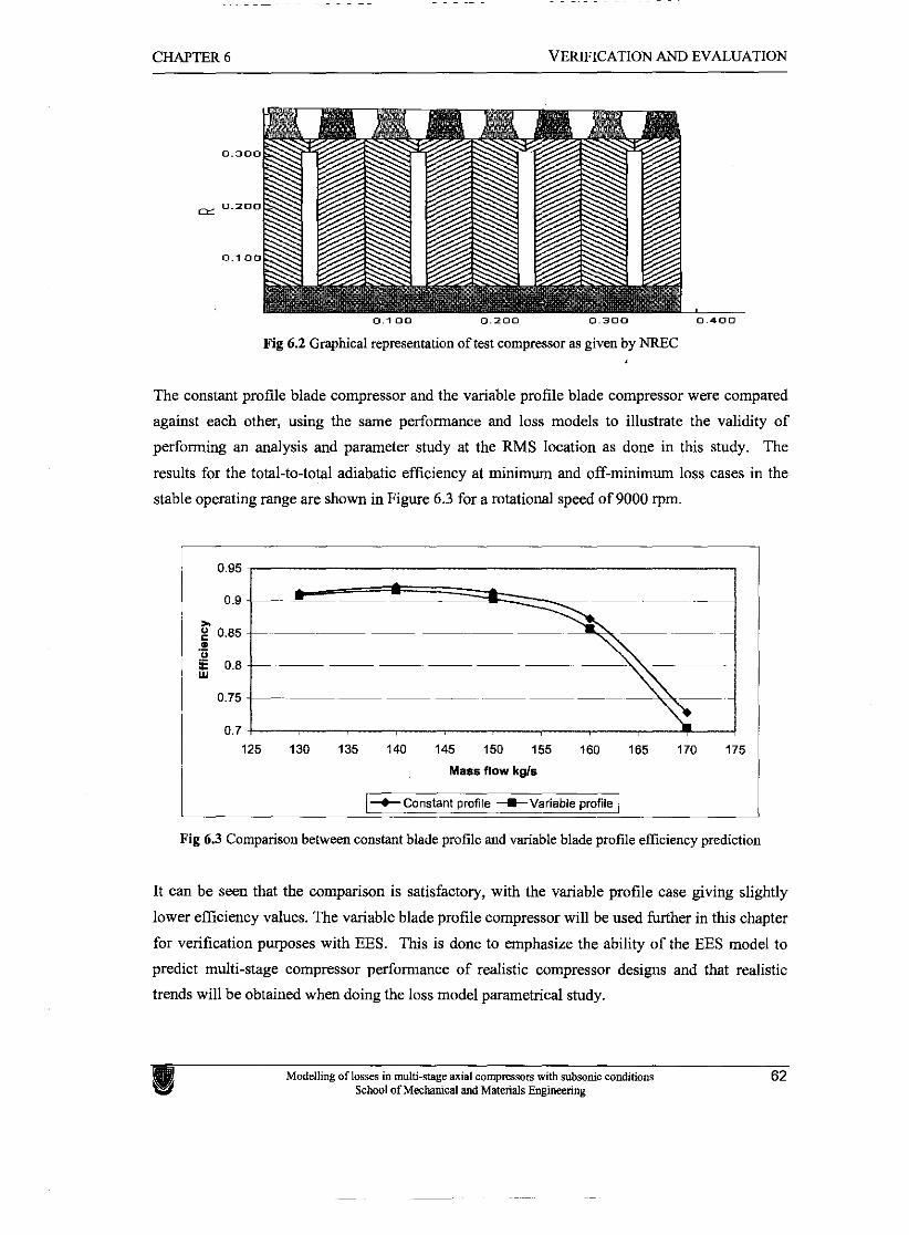
CHAPTER 6 VERIFICATION AND EVALUATION
Fig 6.2 Graphical representation of test compressor as given by NREC
The constant profile blade compressor and the variable profile blade compressor were compared
against each other, using the same performance and loss models to illustrate the validity of
performing an analysis and parameter study at the RMS location as done in this study. The
results for the total-to-total adiabatic efficiency at minimum and off-minimum loss cases in the
stable operating range are shown in Figure 6.3 for a rotational speed of 9000 rpm.
,, g 0.85 . - - - ----~.-----
-~ -
0.75.- I
0.7 -r
125 130 135 140 145 150 155 160 165 170 175
Mass flow k g k
+Constant profile +Variable profile
Fig 6.3 Comparison between constant blade profile and variable blade profile efficiency prediction
It can be seen that the comparison is satisfactory, with the variable profile case giving slightly
lower efficiency values. The variable blade profile compressor will be used further in this chapter
for verification purposes with EES. This is done to emphasize the ability of the EES model to
predict multi-stage compressor performance of realistic compressor designs and that realistic
trends will be obtained when doing the loss model parametrical study.
Modelling of losses in multi-stage axial compresson with subsonic conditions 62 School of Mechanical and Materials Engineering
CHAPTER 6 VERIFICATION AND EVALUATION
The next section presents a detailed verification of the first stage of the compressor as presented
above. This verification will display the EES model's ability to predict the performance of a
stage, without the influence of inlet blockage, which will be observed at other stages in a multi-
stage compressor. A section showing the comparison of the multi-stage compressor data between
the two codes then follows.
6.3 Single stage verification and loss model evaluation
The first stage of the test compressor was used for this purpose. The NREC model and EES code
was adapted to calculate only the first stage parameters.
6.3.1 Verification of non-loss theory and correlations
In verifying the velocity triangles and non-loss (ideal stage) parameters, the losses and deviation
were initially excluded from the simulations. Great discrepancies were observed when
comparing the predictions of the fluid properties from NREC and EES. It was found that the
values of the fluid properties, for example, specific heat capacity and density are especially
critical in the performance prediction, but that EES calculates different values than the NREC
code.
After inspection of the method in which NREC and EES calculates the fluid properties, it was
found that NREC uses input files from which constants and coefficients for the equation of state
are read. The NREC default file gave helium's specific heat capacity at constant pressure, C, , a
constant value of 7899.2 Jtkg-K, while EES gives a value of 5190 Jkg-K at the pressure and
temperature concerned. After careful consideration, it was decided to adapt the NREC input file
to the values, ranges and reference quantities used by EES for successful comparison between the
two packages.
EES uses the fundamental equation of state given by Rainer Tiller-Roth in Fundamental
Equations of State published in 1998 and ancillary equations are provided by R.D. McCarty and
V.D. Arp in "A New Wide Range Equation of State for Helium" published in 1990.
The range of applicability of the thermodynamic properties is fiom the triple point temperature
2.1768 K to 1500 K at pressures up to 100 MPa. It was further found that the density predicted
by EES and NREC still differ by a constant value of 0.18 kg/m3 at all the evaluation points
through the stage and over the entire mass flow range considered. The percentage difference over
the entire range, calculated by Equation 6.1, is less than 3%. There are numerous reasons why
this might be, but it was deemed to be outside the scope of this study to continue the investigation
Modelling of losses in multi-stage axial compresson with subsonic conditions 63 School of Mechanical and Materials Engineering
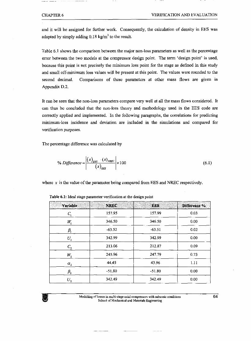
CHAPTER 6 VERIFICATION AND EVALUATION
and it will be assigned for further work. Consequently, the calculation of density in EES was
adapted by simply adding 0.18 kg/m3 to the result.
Table 6.1 shows the comparison between the major non-loss parameters as well as the percentage
error between the two models at the compressor design point. The term 'design point' is used,
because this point is not precisely the minimum loss point for the stage as defined in this study
and small off-minimum loss values will be present at this point. The values were rounded to the
second decimal. Comparisons of these parameters at other mass flows are given in
Appendix D.2.
It can be seen that the non-loss parameters compare very well at all the mass flows considered. It
can thus be concluded that the non-loss theory and methodology used in the EES code are
correctly applied and implemented. In the following paragraphs, the correlations for predicting
minimum-loss incidence and deviation are included in the simulations and compared for
verification purposes.
The percentage difference was calculated by
% Difference = 1 1. where x is the value of the parameter being compared h m EES and NREC respectively.
Table 6.1: Ideal stage parameter verification at the design point
Variable NREC EES ..
Difference . -7 %
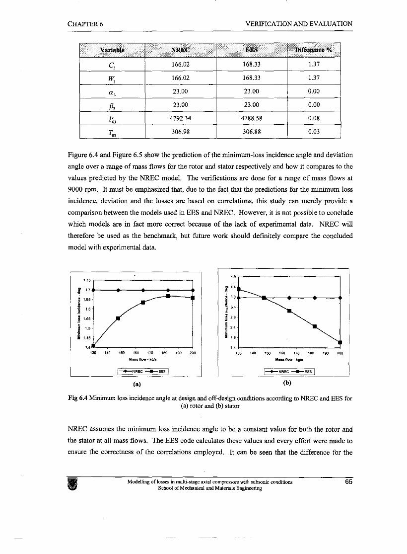
CHAPTER 6 VERIFICATION AND EVALUATION
Figure 6.4 and Figure 6.5 show the prediction of the minimum-loss incidence angle and deviation
angle over a range of mass flows for the rotor and stator respectively and how it compares to the
values predicted by the NREC model. The verifications are done for a range of mass flows at
9000 rpm. It must be emphasized that, due to the fact that the predictions for the minimum loss
incidence, deviation and the losses are based on correlations, this study can merely provide a
comparison between the models used in EES and NREC. However, it is not possible to conclude
which models are in fact more correct because of the lack of experimental data. NREC will
therefore be used as the benchmark, but future work should defmitely compare the concluded
model with experimental data.
Variable
130 140 150 160 170 160 190 200
Y... flow- L#.
+NREC +EES
(b)
EES NREC
Fig 6.4 Minimum loss incidence angle at design and off-design conditions according to MlEC and EES for (a) rotor and (b) stator
Difference %
NREC assumes the minimum loss incidence angle to be a constant value for both the rotor and
the stator at all mass flows. The EES code calculates these values and every effort were made to
ensure the correctness of the correlations employed. It can be seen that the difference for the
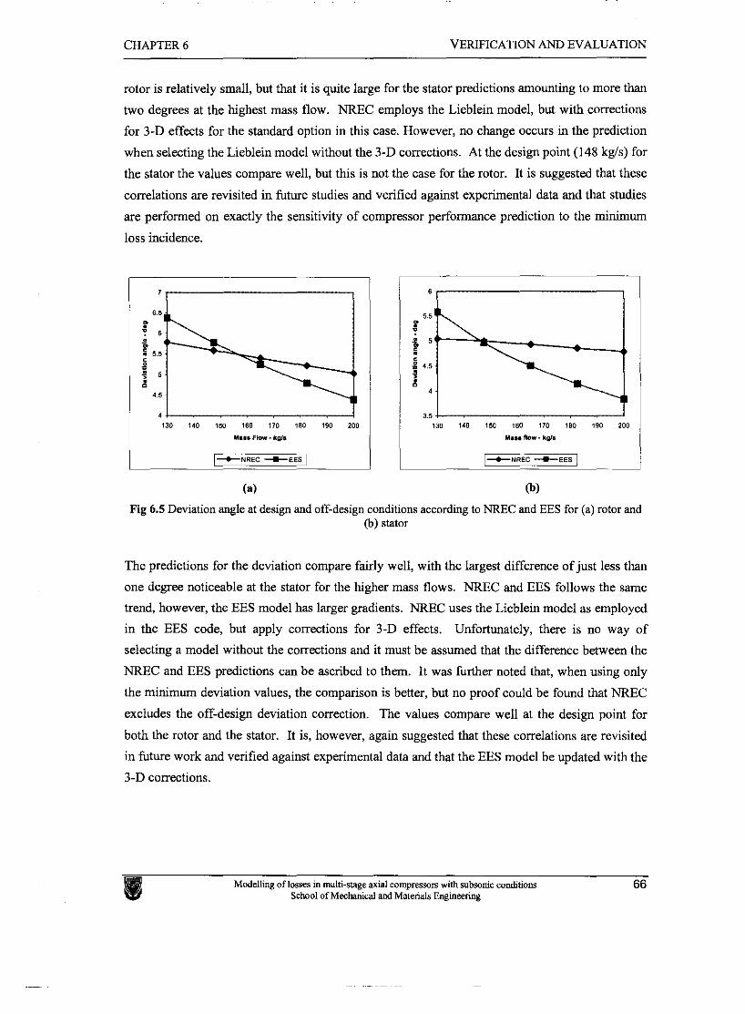
CHAPTER 6 VERIFICATION AND EVALUATION
rotor is relatively small, but that it is quite large for the stator predictions amounting to more than
two degrees at the highest mass flow. NREC employs the Lieblein model, but with corrections
for 3-D effects for the standard option in this case. However, no change occurs in the prediction
when selecting the Lieblein model without the 3-D corrections. At the design point (148 kgls) for
the stator the values compare well, but this is not the case for the rotor. It is suggested that these
correlations are revisited in future studies and verified against experimental data and that studies
are performed on exactly the sensitivity of compressor performance prediction to the minimum
loss incidence.
Fig 6.5 Deviation angle at design and off-design conditions according to NREC and EES for (a) rotor and (b) stator
The predictions for the deviation compare fairly well, with the largest difference of just less than
one degree noticeable at the stator for the higher mass flows. NREC and EES follows the same
trend, however, the EES model has larger gradients. NREC uses the Lieblein model as employed
in the EES code, but apply corrections for 3-D effects. Unfortunately, there is no way of
selecting a model without the corrections and it must be assumed that the difference between the
NREC and EES predictions can be ascribed to them. It was further noted that, when using only
the minimum deviation values, the comparison is better, but no proof could be found that NREC
excludes the off-design deviation correction. The values compare well at the design point for
both the rotor and the stator. It is, however, again suggested that these correlations are revisited
in future work and verified against experimental data and that the EES model be updated with the
3-D corrections.
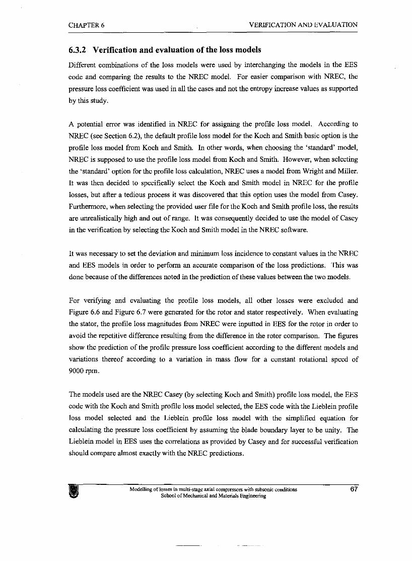
CHAPTER 6 VERIFICATION AND EVALUATION
6.3.2 Verification and evaluation of the loss models
Different combinations of the loss models were used by interchanging the models in the EES
code and comparing the results to the NREC model. For easier comparison with NREC, the
pressure loss coefficient was used in all the cases and not the entropy increase values as supported
by this study.
A potential error was identified in NREC for assigning the profile loss model. According to
NREC (see Section 6.2), the default profile loss model for the Koch and Smith basic option is the
profile loss model from Koch and Smith. In other words, when choosing the 'standard' model,
NREC is supposed to use the profile loss model kom Koch and Smith. However, when selecting
the 'standard' option for the profile loss calculation, NREC uses a model fiom Wright and Miller.
It was then decided to specifically select the Koch and Smith model in NREC for the profile
losses, but after a tedious process it was discovered that this option uses the model from Casey.
Furthermore, when selecting the provided user file for the Koch and Smith profile loss, the results
are unrealistically high and out of range. It was consequently decided to use the model of Casey
in the verification by selecting the Koch and Smith model in the NREC software.
It was necessary to set the deviation and minimum loss incidence to constant values in the NREC
and EES models in order to perform an accurate comparison of the loss predictions. This was
done because of the differences noted in the prediction of these values between the two models.
For verifying and evaluating the profile loss models, all other losses were excluded and
Figure 6.6 and Figure 6.7 were generated for the rotor and stator respectively. When evaluating
the stator, the profile loss magnitudes fiom NREC were inputted in EES for the rotor in order to
avoid the repetitive difference resulting fiom the difference in the rotor comparison. The figures
show the prediction of the profile pressure loss coefficient according to the different models and
variations thereof according to a variation in mass flow for a constant rotational speed of
9000 rpm.
The models used are the NREC Casey (by selecting Koch and Smith) profile loss model, the EES
code with the Koch and Smith profile loss model selected, the EES code with the Lieblein profile
loss model selected and the Lieblein profile loss model with the simplified equation for
calculating the pressure loss coefficient by assuming the blade boundary layer to be unity. The
Lieblein model in EES uses the correlations as provided by Casey and for successful verification
should compare almost exactly with the NREC predictions.
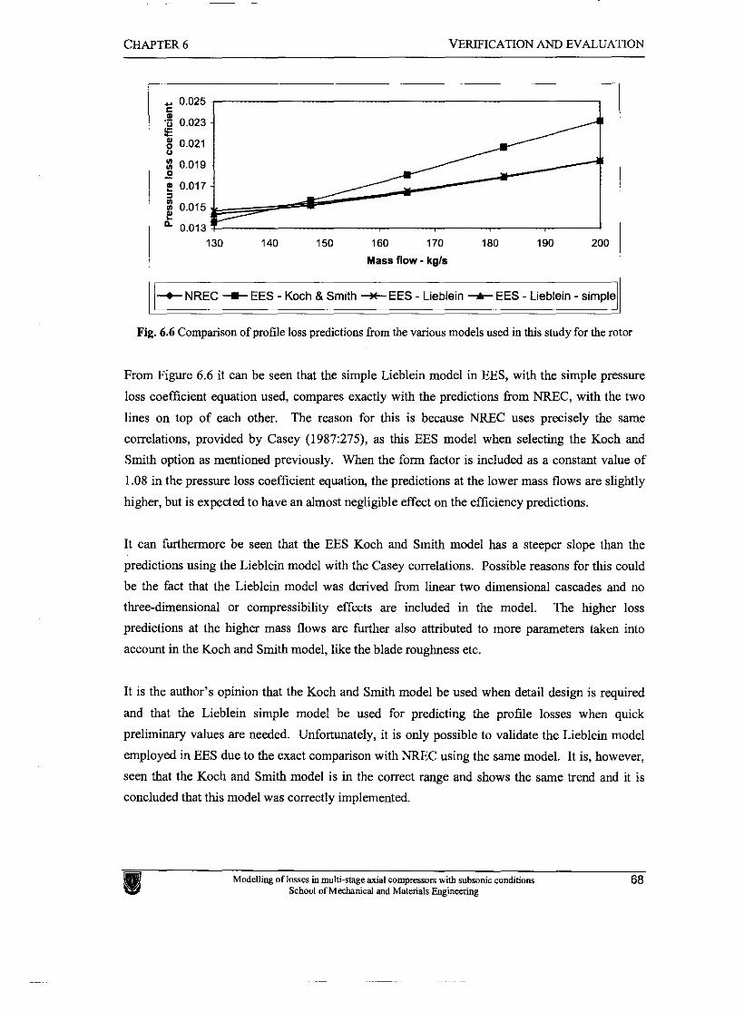
CHAPTER 6 VERIFICATION AND EVALUATION
130 140 150 160 170 180 190 200
Mass flow - kg18
t NREC t EES - Koch B Smith + EES - Lieblein -A- EES - Lieblein - simple -
Fig. 6.6 Comparison of profile loss predictions from the various models used in this study for the rotor
From Figure 6.6 it can be seen that the simple Lieblein model in EES, with the simple pressure
loss coefficient equation used, compares exactly with the predictions 6om NREC, with the two
lines on top of each other. The reason for this is because NREC uses precisely the same
correlations, provided by Casey (1987:275), as this EES model when selecting the Koch and
Smith option as mentioned previously. When the form factor is included as a constant value of
1.08 in the pressure loss coefficient equation, the predictions at the lower mass flows are slightly
higher, but is expected to have an almost negligible effect on the efficiency predictions.
It can furthermore be seen that the EES Koch and Smith model has a steeper slope than the
predictions using the Lieblein model with the Casey correlations. Possible reasons for this could
be the fact that the Lieblein model was derived 6om linear two dimensional cascades and no
three-dimensional or compressibility effects are included in the model. The higher loss
predictions at the higher mass flows are fiuther also attributed to more parameters taken into
account in the Koch and Smith model, like the blade roughness etc.
It is the author's opinion that the Koch and Smith model be used when detail design is required
and that the Lieblein simple model be used for predicting the profile losses when quick
preliminary values are needed. Unfortunately, it is only possible to validate the Lieblein model
employed in EES due to the exact comparison with NREC using the same model. It is, however,
seen that the Koch and Smith model is in the correct range and shows the same trend and it is
concluded that this model was correctly implemented.
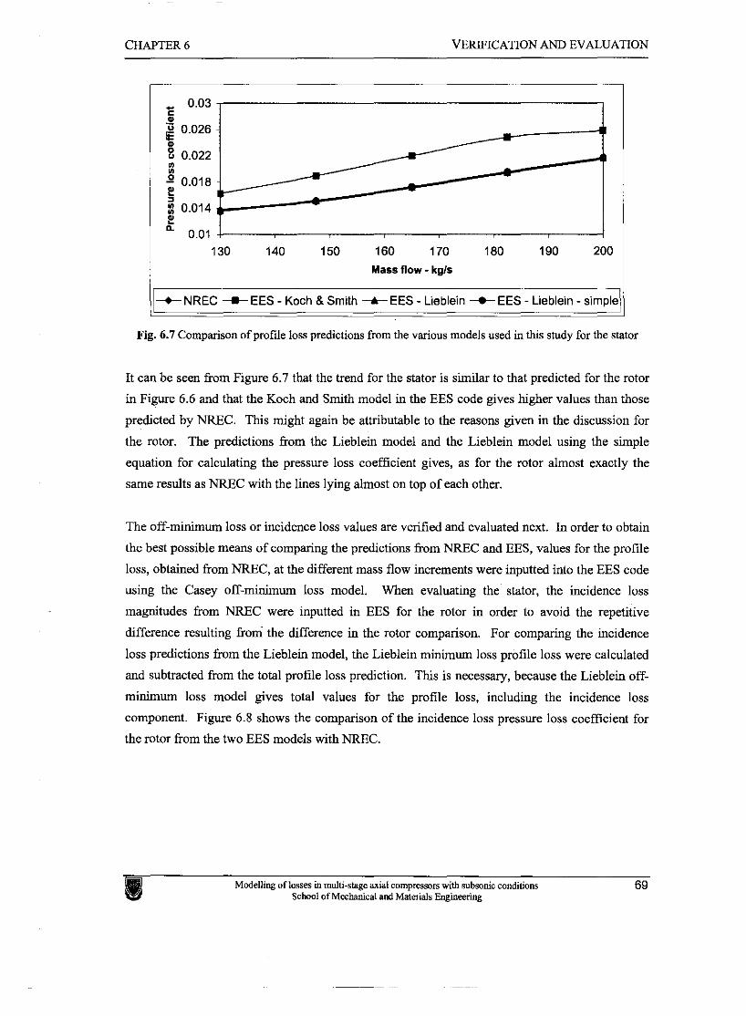
-~
CHAPTER 6 VERIFICATION AND EVALUATION
0.03 - c a
130 140 150 160 170 1 80 190 200
Mass flow - kgls
t NREC t EES - Koch 8 Smith --t- EES - Lieblein -0- EES - Lieblein - simple
Fig. 6.7 Comparison of profile loss predictions from the various models used in this study for the stator
It can be seen from Figure 6.7 that the trend for the stator is similar to that predicted for the rotor
in Figure 6.6 and that the Koch and Smith model in the EES code gives higher values than those
predicted by NREC. This might again be attributable to the reasons given in the discussion for
the rotor. The predictions from the Lieblein model and the Lieblein model using the simple
equation for calculating the pressure loss coefficient gives, as for the rotor almost exactly the
same results as NREC with the lines lying almost on top of each other.
The off-minimum loss or incidence loss values are verified and evaluated next. In order to obtain
the best possible means of comparing the predictions from NREC and EES, values for the profile
loss, obtained from NREC, at the different mass flow increments were inputted into the EES code
using the Casey off-minimum loss model. When evaluating the stator, the incidence loss
magnitudes from NREC were inputted in EES for the rotor in order to avoid the repetitive
difference resulting froni the difference in the rotor comparison. For comparing the incidence
loss predictions from the Lieblein model, the Lieblein minimum loss profile loss were calculated
and subtracted from the total profile loss prediction. This is necessary, because the Lieblein off-
minimum loss model gives total values for the profile loss, including the incidence loss
component. Figure 6.8 shows the comparison of the incidence loss pressure loss coefficient for
the rotor from the two EES models with NREC.
- - -
VERIFICATION AND EVALUATION
130 140 150 160 170 180 190 200
Mass flow - kgls
It NREC t EES - Casey t EES - Lieblein I Fig. 6.8 Comparison of incidence loss predictions from the various models for the rotor
Good agreement exists between the NREC model and the Casey and Lieblein models used in the
EES code in the region of the minimum loss point. However, a reasonable difference is noticeable
at points far removed.
The Lieblein model predicts a more 'open' parabola than both the other models tested, especially
for higher mass flows. The comparison between the Lieblein model and Casey model is good at
negative incidence only. Reasons for this difference can be attributed to the two-dimensionality
and incompressible nature of the cascades used for generating the correlation as well as the high
degrees of laminar flow that existed on the cascades. The model uses the pressure loss coefficient
equation that includes the boundary layer form factor parameter. It was found that using the
simple equation leads to even lower values for the negative incidence region.
It is suggested that this model could be considered for calculations in the region of the minimum-
loss point during the preliminary design phase due to its simplicity and the fact that it calculates
the total profile loss at minimum and slight off-minimum loss conditions relatively accurately.
The Casey model must be used where more accuracy at the off-minimum loss conditions are
desired. It is advised that further study be performed, or that verification with experimental data
be performed, before making any conclusions about which model (NREC or EES-Casey) is the
best to use for this specific test case. Figure 6.9 shows the comparison for the stator.
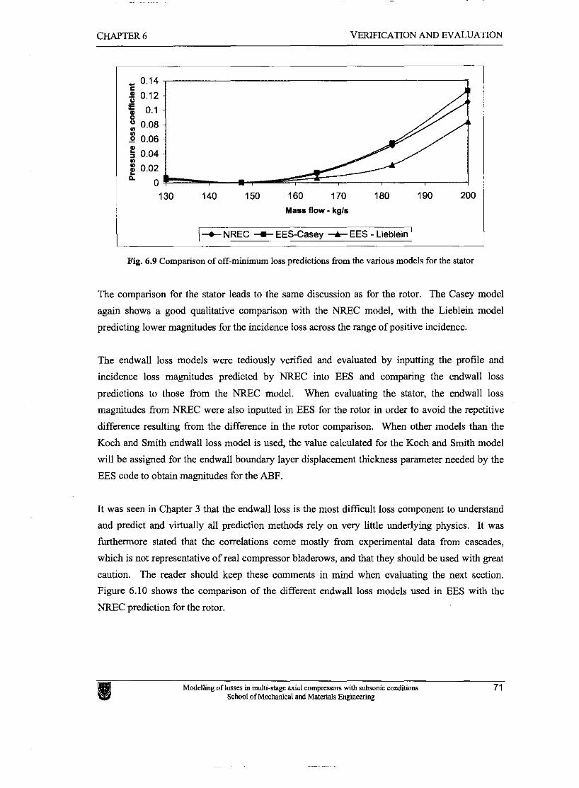
VERIFICATION AND EVALUATION
130 140 150 160 170 180 190 200 Mass flow - kgls
- I-+ NREC t EES-Casey -A- EES - Lieblein 1 Fig. 6.9 Comparison of off-minimum loss predictions Gom the various models for the stator
The comparison for the stator leads to the same discussion as for the rotor. The Casey model
again shows a good qualitative comparison with the NREC model, with the Lieblein model
predicting lower magnitudes for the incidence loss across the range of positive incidence.
The endwall loss models were tediously verified and evaluated by inputting the profile and
incidence loss magnitudes predicted by NREC into EES and comparing the endwall loss
predictions to those from the NREC model. When evaluating the stator, the endwall loss
magnitudes from NREC were also inputted in EES for the rotor in order to avoid the repetitive
difference resulting from the difference in the rotor comparison. When other models than the
Koch and Smith endwall loss model is used, the value calculated for the Koch and Smith model
will be assigned for the endwall bounda~y layer displacement thickness parameter needed by the
EES code to obtain magnitudes for the ABF.
It was seen in Chapter 3 that the endwall loss is the most difficult loss component to understand
and predict and virtually all prediction methods rely on very little underlying physics. It was
furthermore stated that the correlations come mostly from experimental data from cascades,
which is not representative of real compressor bladerows, and that they should be used with great
caution. The reader should keep these comments in mind when evaluating the next section.
Figure 6.10 shows the comparison of the different endwall loss models used in EES with the
NREC prediction for the rotor.
Modelling of losses in multi-stage axial compressors with subsonic conditions 71 School of Mechanical and Materials Engineering
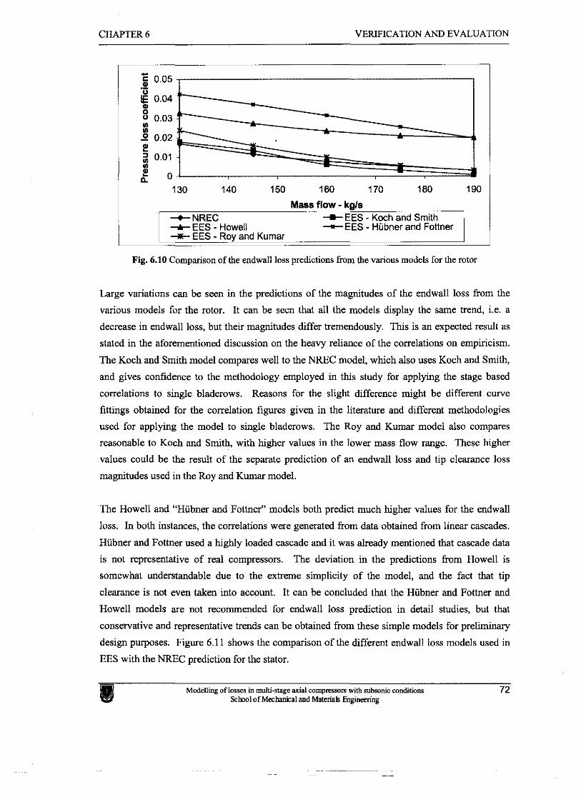
~-
CHAPTER 6
-
VERIFICATION AND EVALUATION
Mass flow - kgls t NREC t EES - Koch and Smith -A- EES - Howell + EES - Hubner and Fottner -+- EES - Roy and Kumar
Fig. 6.10 Comparison of the endwall loss predictions from the various models for the rotor
Large variations can be seen in the predictions of the magnitudes of the endwall loss from the
various models for the rotor. It can be seen that all the models display the same trend, i.e. a
decrease in endwall loss, but their magnitudes differ tremendously. This is an expected result as
stated in the aforementioned discussion on the heavy reliance of the correlations on empiricism.
The Koch and Smith model compares well to the NREC model, which also uses Koch and Smith,
and gives confidence to the methodology employed in this study for applying the stage based
correlations to single bladerows. Reasons for the slight difference might be different curve
fittings obtained for the correlation figures given in the literature and different methodologies
used for applying the model to single hladerows. The Roy and Kumar model also compares
reasonable to Koch and Smith, with higher values in the lower mass flow range. These higher
values could be the result of the separate prediction of an endwall loss and tip clearance loss
magnitudes used in the Roy and Kumar model.
The Howell and "Hiibner and Fottner" models both predict much higher values for the endwall
loss. In both instances, the correlations were generated from data obtained from linear cascades.
Hubner and Fottner used a highly loaded cascade and it was already mentioned that cascade data
is not representative of real compressors. The deviation in the predictions from Howell is
somewhat understandable due to the extreme simplicity of the model, and the fact that tip
clearance is not even taken into account. It can be concluded that the Hubner and Fottner and
Howell models are not recommended for endwall loss prediction in detail studies, but that
conservative and representative trends can be obtained from these simple models for preliminary
design purposes. Figure 6.1 1 shows the comparison of the different endwall loss models used in
EES with the NREC prediction for the stator.
Modelling of losses in multi-stage axial campresson with subsonic conditions 72 School of Mechanical and Materials Engineering
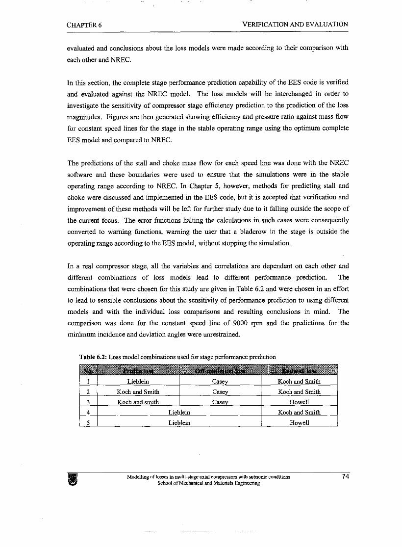
CHAPTER 6 VERIFICATION AND EVALUATION
evaluated and conclusions about the loss models were made according to their comparison with
each other and NREC.
In this section, the complete stage performance prediction capability of the EES code is verified
and evaluated against the NREC model. The loss models will be interchanged in order to
investigate the sensitivity of compressor stage efficiency prediction to the prediction of the loss
magnitudes. Figures are then generated showing efficiency and pressure ratio against mass flow
for constant speed lines for the stage in the stable operating range using the optimum complete
EES model and compared to NREC.
The predictions of the stall and choke mass flow for each speed line was done with the NREC
software and these boundaries were used to ensure that the simulations were in the stable
operating range according to NREC. In Chapter 5, however, methods for predicting stall and
choke were discussed and implemented in the EES code, hut it is accepted that verification and
improvement of these methods will be left for further study due to it falling outside the scope of
the current focus. The error functions halting the calculations in such cases were consequently
converted to warning functions, warning the user that a bladerow in the stage is outside the
operating range according to the EES model, without stopping the simulation.
In a real compressor stage, all the variables and correlations are dependent on each other and
different combinations of loss models lead to different performance prediction. The
combinations that were chosen for this study are given in Table 6.2 and were chosen in an effort
to lead to sensible conclusions about the sensitivity of performance prediction to nsing different
models and with the individual loss comparisons and resulting conclusions in mind. The
comparison was done for the constant speed line of 9000 rpm and the predictions for the
minimum incidence and deviation angles were unrestrained.
Table 6.2: Loss model combinations used for stage performance prediction
Modelling of losses in multi-stage axial compressom with subsonic conditions 74 School of Mechanical and Materials Engineering
1
2
3
4
5
Lieblein
Koch and Smith
Koch and smith
Casey
Casey
Casey
Koch and Smith
Koch and Smith
Howell
Liehlein
Liehlein
Koch and Smith
Howell
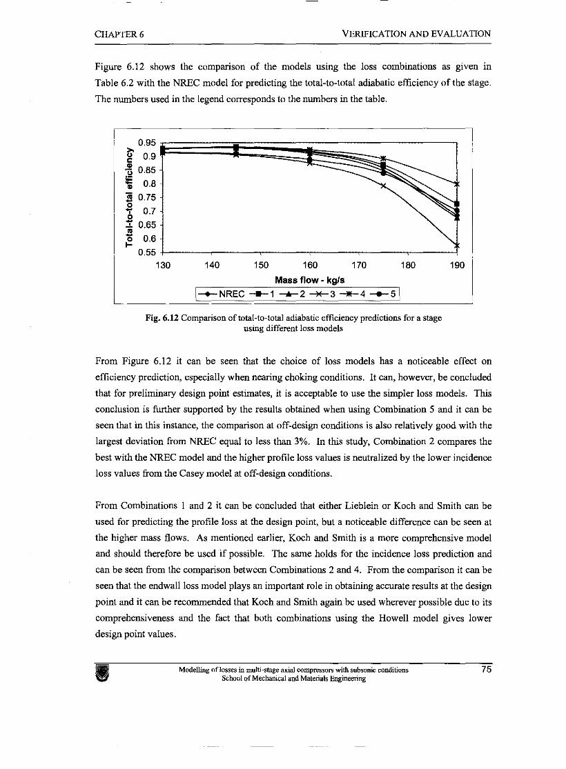
CHAPTER 6 VERIFICATION AND EVALUATION
Figure 6.12 shows the comparison of the models using the loss combinations as given in
Table 6.2 with the NREC model for predicting the total-to-total adiabatic efficiency of the stage.
The numbers used in the legend corresponds to the numbers in the table.
130 140 150 160 170 180 190
Mass flow - kgls ~ ~ N R E C t i t 2 x 3 +4 t 5 (
Fig. 6.12 Comparison of total-to-total adiabatic efficiency predictions for a stage using different loss models
From Figure 6.12 it can be seen that the choice of loss models has a noticeable effect on
efficiency prediction, especially when nearing choking conditions. It can, however, be concluded
that for preliminary design point estimates, it is acceptable to use the simpler loss models. This
conclusion is further supported by the results obtained when using Combination 5 and it can be
seen that in this instance, the comparison at off-design conditions is also relatively good with the
largest deviation from NREC equal to less than 3%. In this study, Combination 2 compares the
best with the NREC model and the higher profile loss values is neutralized by the lower incidence
loss values from the Casey model at off-design conditions.
From Combinations 1 and 2 it can be concluded that either Lieblein or Koch and Smith can be
used for predicting the profile loss at the design point, but a noticeable difference can be seen at
the higher mass flows. As mentioned earlier, Koch and Smith is a more comprehensive model
and should therefore be used if possible. The same holds for the incidence loss prediction and
can be seen from the comparison between Combinations 2 and 4. From the comparison it can be
seen that the endwall loss model plays an important role in obtaining accurate results at the design
point and it can be recommended that Koch and Smith again be used wherever possible due to its
comprehensiveness and the fact that both combinations using the Howell model gives lower
design point values.
Modelling of losses in multi-s@e axial compressors with subsonic conditions 75 School of Mechanical and Materials Ewineering
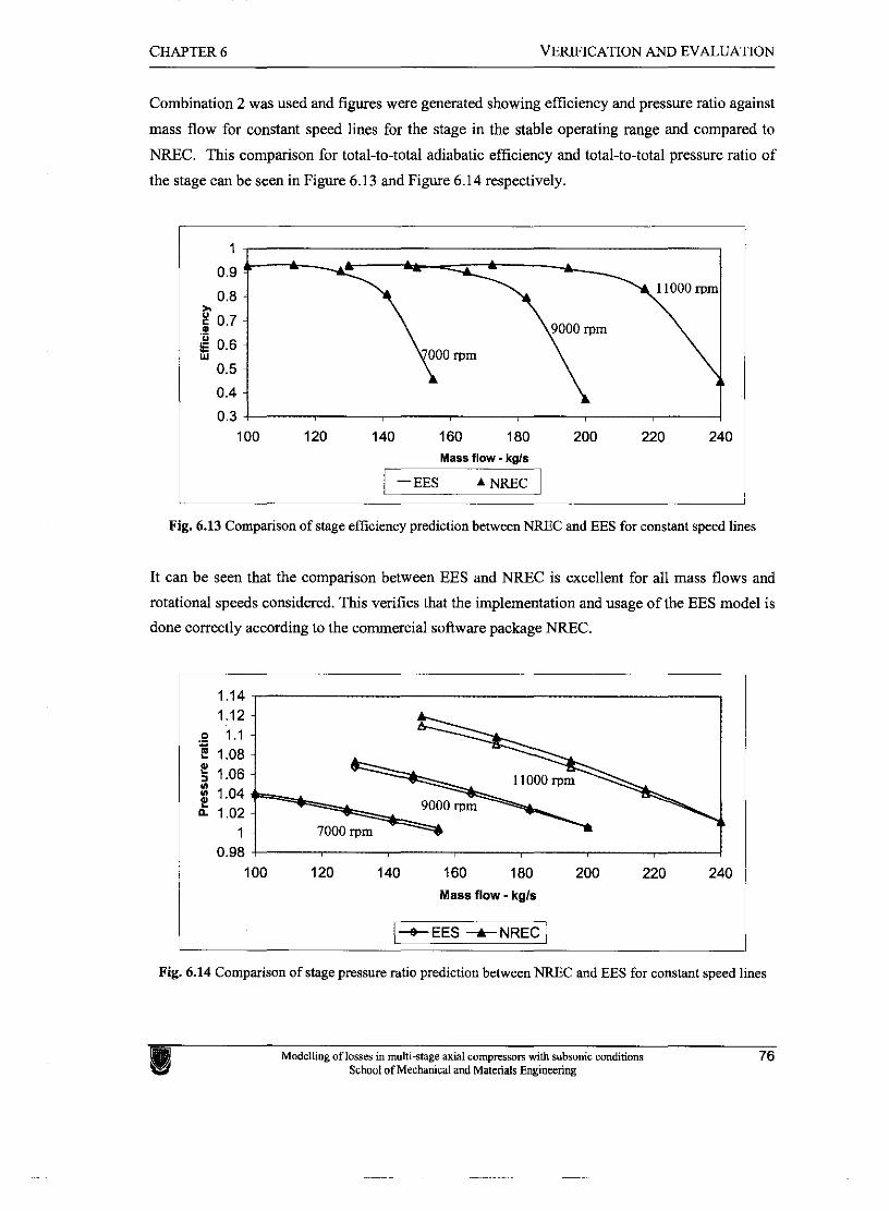
CHAPTER 6 VERIFICATION AND EVALUATION
Combination 2 was used and figures were generated showing efficiency and pressure ratio against
mass flow for constant speed lines for the stage in the stable operating range and compared to
NREC. This comparison for total-to-total adiabatic efficiency and total-to-total pressure ratio of
the stage can be seen in Figure 6.13 and Figure 6.14 respectively.
Fig. 6.13 Comparison of stage eficiency prediction between NREC and EES for constant speed lines
1 - 0.9
0.8 - * E 0.7 - .- $ 0.6 - W 0.5 -
0.4 -
0.3 7
It can be seen that the comparison between EES and NREC is excellent for all mass flows and
rotational speeds considered. This verifies that the implementation and usage of the EES model is
!' -
done correctly according to the commercial software package NREC.
100 120 140 160 180 200 220 240 Mass flow - kgls
100 120 140 160 180 200 220 240
Mass flow - kgls
Fig. 6.14 Comparison of stage pressure ratio prediction between NREC and EES for constant speed lines
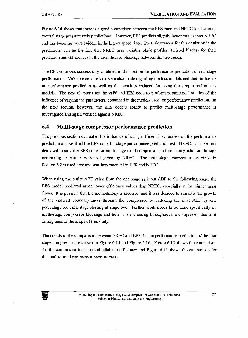
CHAPTER 6 VERIFICATION AND EVALUATION
Figure 6.14 shows that there is a good comparison between the EES code and NREC for the total-
to-total stage pressure ratio predictions. However, EES predicts slightly lower values than NREC
and this becomes more evident in the higher speed lines. Possible reasons for this deviation in the
predictions can be the fact that NREC uses variable blade profiles (twisted blades) for their
prediction and differences in the definition of blockage between the two codes.
The EES code was successfully validated in this section for performance prediction of real stage
performance. Valuable conclusions were also made regarding the loss models and their influence
on performance prediction as well as the penalties induced for using the simple preliminary
models. The next chapter uses the validated EES code to perform parametrical studies of the
influence of varying the parameters, contained in the models used, on performance prediction. In
the next section, however, the EES code's ability to predict multi-stage performance is
investigated and again verified against NREC.
6.4 Multi-stage compressor performance prediction
The previous section evaluated the influence of using different loss models on the performance
prediction and verified the EES code for stage performance prediction with NREC. This section
deals with using the EES code for multi-stage axial compressor performance prediction through
comparing its results with that given by NREC. The four stage compressor described in
Section 6.2 is used here and was implemented in EES and NREC.
When using the outlet ABF value kom the one stage as input ABF to the following stage, the
EES model predicted much lower efficiency values than NREC, especially at the higher mass
flows. It is possible that the methodology is incorrect and it was decided to simulate the growth
of the endwall boundary layer through the compressor by reducing the inlet ABF by one
percentage for each stage starting at stage two. Further work needs to be done specifically on
multi-stage compressor blockage and how it is increasing throughout the compressor due to it
falling outside the scope of this study.
The results of the comparison between NREC and EES for the performance prediction of the four
stage compressor are shown in Figure 6.15 and Figure 6.16. Figure 6.15 shows the comparison
for the compressor total-to-total adiabatic efficiency and Figure 6.16 shows the comparison for
the total-to-total compressor pressure ratio.
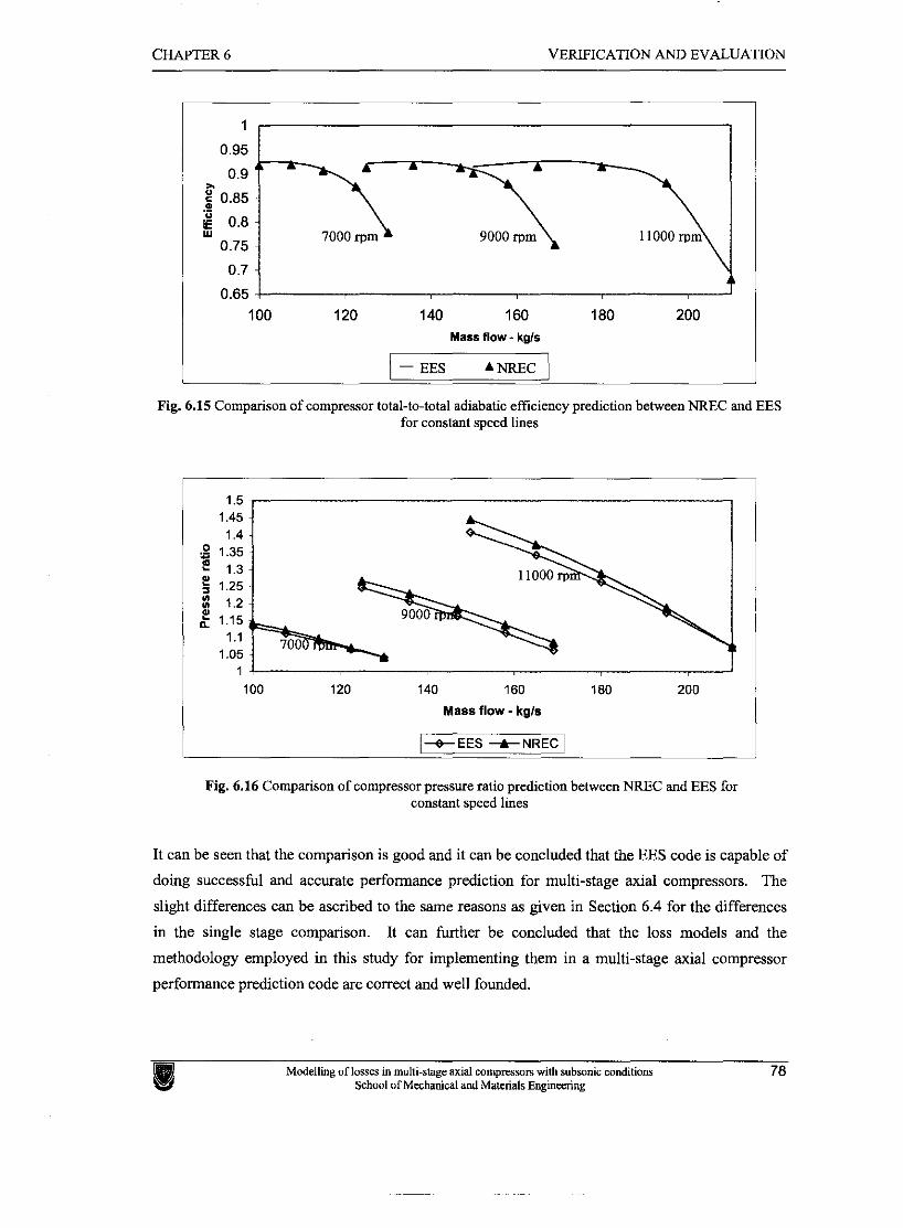
CHAPTER 6 VERIFICATION AND EVALUATION
Y
0.75 7000 rpm 9000 rpm
0.65 -1 100 120 140 160 180 200
Mass flow - kgls
- EES ANREC
Fig. 6.15 Comparison of compressor total-to-total adiabatic efficiency prediction between NREC and EES for constant speed lines
1.5 1.45 1.4
g 1.35 1.3
1.25 B 1.2 IY
1.15 1.1
1.05 1 100 120 140 160 180 200
Mass flow - kgls
Fig. 6.16 Comparison of compressor pressure ratio prediction between NREC and EES for constant speed lines
It can be seen that the comparison is good and it can be concluded that the EES code is capable of
doing successful and accurate performance prediction for multi-stage axial compressors. The
slight differences can be ascribed to the same reasons as given in Section 6.4 for the differences
in the single stage comparison. It can further be concluded that the loss models and the
methodology employed in this study for implementing them in a multi-stage axial compressor
performance prediction code are correct and well founded.
Modelling of losses in multi-stage axial compressors with subsonic conditions 78 School af Mechanical and Materials Engineering

CHAPTER 6 VERIFICATION AND EVALUATION
6.5 Summary and conclusions
In this chapter, the accuracy and validity of the engineering code generated for axial compressor
performance prediction was verified against a commercial performance prediction package called
NREC. The loss models were interchanged and evaluated according to their deviation from the
norm set by NREC and conclusions were made about the sensitivity of compressor performance
prediction to certain aspects of modelling and the different loss models. Furthermore, the ability
of the EES code to predict stage and multi-stage compressor performance was verified.
It was seen that the non-loss parameters compare very well at different mass flows and it was thus
concluded that the non-loss theory and methodology used in the EES code were correctly applied
and implemented. NREC assumes the minimum loss incidence angle to be a constant value for
both the rotor and the stator at all mass flows. The EES code calculates these values and it was
seen that differences in the stator predictions amounts to more than two degrees at the highest
mass flow. The predictions for the deviation compare fairly well, with the largest difference of
just less than one degree noticeable at the stator for the higher mass flows. It was accepted that
the difference between the NREC and EES predictions can be ascribed to the changes made by
NREC to the model for incorporating 3-D effects. It was further noted that, when using only the
minimum deviation values, the comparison is better, but no proof could be found that NREC
excludes the off-design deviation correction. It was, however, suggested that the minimum loss
incidence and deviation correlations should be revisited in future work and verified against
experimental data.
For the profile losses, it was suggested that the Koch and Smith model be used when detail design
is required and that the Lieblein simple model be used when quick preliminary values are needed.
Good qualitative comparison was obtained between the NREC model and the Casey and Lieblein
models for the incidence loss predictions in the region of the minimum loss point, although a
reasonable difference was noticeable at points far removed. It was suggested that the Lieblein
model could be considered for calculations in the region of the minimum-loss point during the
preliminary design phase due to its simplicity and the fact that it calculates the total profile loss at
minimum and slight off-minimum loss conditions relatively accurately. The Casey model must
be used where more accuracy at the off-minimum loss conditions are desired. It was advised that
further study should be performed, or that verification with experimental data be performed,
before making any conclusions about which model (NREC or EES-Casey) is the best to use for
this specific test case.
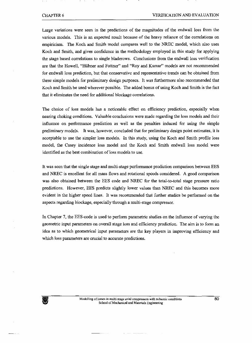
CHAPTER 6 VERIFICATION AND EVALUATION
Large variations were seen in the predictions of the magnitudes of the endwall loss from the
various models. This is an expected result because of the heavy reliance of the correlations on
empiricism. The Koch and Smith model compares well to the NREC model, which also uses
Koch and Smith, and gives confidence in the methodology employed in this study for applying
the stage based correlations to single bladerows. Conclusions from the endwall loss verification
are that the Howell, "Hiibner and Fottner" and "Roy and Kumar" models are not recommended
for endwall loss prediction, but that conservative and representative trends can be obtained from
these simple models for preliminary design purposes. It was furthermore also recommended that
Koch and Smith be used wherever possible. The added bonus of using Koch and Smith is the fact
that it eliminates the need for additional blockage correlations.
The choice of loss models has a noticeable effect on efficiency prediction, especially when
nearing choking conditions. Valuable conclusions were made regarding the loss models and their
influence on performance prediction as well as the penalties induced for using the simple
preliminary models. It was, however, concluded that for preliminary design point estimates, it is
acceptable to use the simpler loss models. In this study, using the Koch and Smith profile loss
model, the Casey incidence loss model and the Koch and Smith endwall loss model were
identified as the best combiiation of loss models to use.
It was seen that the single stage and multi-stage performance prediction comparison between EES
and NREC is excellent for all mass flows and rotational speeds considered. A good comparison
was also obtained between the EES code and NREC for the total-to-total stage pressure ratio
predictions. However, EES predicts slightly lower values than NREC and this becomes more
evident in the higher speed lines. It was recommended that further studies be performed on the
aspects regarding blockage, especially through a multi-stage compressor.
In Chapter 7, the EES-code is used to perform parametric studies on the influence of varying the
geometric input parameters on overall stage loss and efficiency prediction. The aim is to form an
idea as to which geometrical input parameters are the key players in improving efficiency and
which loss parameters are crucial to accurate predictions.
Modelling of losses in multi-stage axial compmsors with subsonic conditions 80 School of Mechanical and Materials Engineering
In this chapter the EES-code is used to perform parametric studies on the influence of vatying the
geometric input parameters on overall stage loss and efficiency prediction. The aim is to form an
idea as to which geometrical input parameters are the key players in improving efficiency and
which loss parameters are crucial to accuratepredictions.
Mcxlcllmg of lasscs in mull>-stage utsl cornpwwn wlth subconic ;undlla,n\ 5;htwl uf M w h m r a l and Malcnals Englnaring
CHAPTER 7 PARAMETRIC STUDIES
7.1 Introduction
Chapter 3 presented the reader with the models obtained from the open literature for predicting
the losses through an axial compressor. It was, however, found that it would be advantageous to
include the models in a performance prediction code, because of their extreme dependence on
each other and some of the other variables included in performance prediction and due to the
implicit nature of the calculations. Chapter 4 then presented the concepts and theory needed for
generating a basic mean line performance prediction code for including the loss models.
Chapter 5 discussed the implementation of the models and theory in a software package called
EES and in Chapter 6 the accuracy and validity of the generated code was verified against a
commercial performance prediction package.
This chapter aims at illustrating the capability of the code, generated in this study, for performing
parametric studies. These studies can be used to aid in understanding compressor design and
performance or for basic optimization problems. This is done, staying with the focus of this
study, by showing the results from several parametric studies where some of the loss parameters
were varied in the EES code and also by presenting an illustrative parametric study for optimizing
the rotor inlet blade angle.
7.2 Methodology
It was seen in Chapter 5 that the performance prediction for a multi-stage compressor comprised
of sequentially obtaining predictions for the individual stages by using the outlet conditions of the
one stage as the inputs for the next. It was also seen that each stage uses the same set of
equations for obtaining the predictions. It was, therefore, decided that it would be sufficient for
this study to do the parametric studies for a single stage only for illustrating the application of the
code for design or optimization purposes. Further study can, of course, use the code more
extensively to determine, for instance, the influence of varying some geometric parameter in the
third stage rotor to overall compressor performance etc.
The stage used is again the first stage of the four stage compressor used in Chapter 5 with its
initial input values given in Appendix D.1. Koch and Smith's profile and endwall loss models
and the incidence loss model of Casey was used due to the confidence given to their validity by
the comparisons to NREC in Chapter 6 and the fact that this combination includes the most input
parameters in the loss models. Furthermore, the part span shroud loss model was included for the
rotor and the stator and the windage loss model from Denton for the rotor.
CHAPTER 7 PARAMETRIC STLJDIES
Some of the parameters given in Appendix C.2 for the stage geometrical inputs and used as inpnt
values for the loss models are parametrically varied and the influence on efficiency prediction is
investigated. This is done by keeping all the inpnt parameters constant with the values given in
Appendix D.l, except one parameter which is varied. The first set of parametric studies
investigates the influence of the loss parameters on stage total-to-total adiabatic eff~ciency. These
parameters were chosen on the grounds that they are input parameters only to the loss models, or
other relevant correlations, and would have no effect on a simulation excluding the losses or
deviation.
Next, an illustrative parametric case study is presented which investigates the effect of a major
variable change (the rotor inlet blade angle), on the loss magnitudes to illustrate their dependence
on the performance prediction variables and each other. The effect of this loss change on stage
efficiency and pressure ratio are also shown. The EES code was adapted to include the
predictions for stall and choke as discussed in Chapter 4 and Chapter 5 and aided in determining
the range for the parametric studies. Further restrictions for the range between which the
variables are varied are obtained ffom the correlation figure boundaries. The following sections
presents the results as obtained from the parametric studies with the EES code.
7.3 The influence of some loss parameters on stage efficiency
7.3.1 The effect of axial spacing on stage efficiency
The axial spacing between the blade rows were varied between 0.1 and 20 mm. The effect of this
parameter is included in the stage performance prediction through the correction factor
implemented in the Koch stalling static pressure rise coefficient model and the Koch and Smith
endwall loss model. These correction figures are shown in Figure B.3.4 and Figure A.4.2
respectively. Figure 7.1 shows how this influenced the stage efficiency for this compressor stage.
From Figure 7.1 it can be seen that the efficiency decreases with an increase in axial spacing
between the hladerows. The slope also decreases with an increase in axial spacing, showing that
its effect is most dramatic in the range close to zero spacing.
Modelling of losses in multi-stage axial compresson with subsonic wnditians 82 School of Mechanical and Materials Engineering
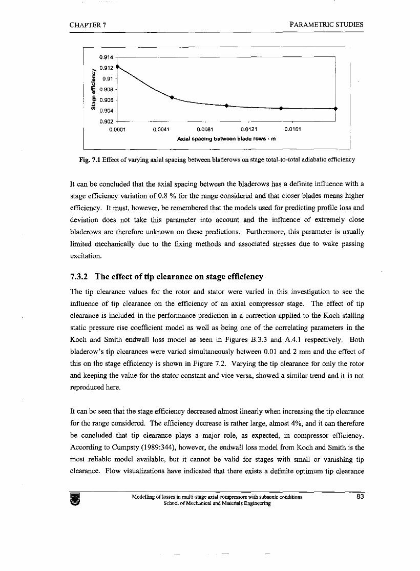
CHAPTER 7 PARAMETRIC STUDLES
, 0.912 1
0.91 - - U 5 0.908 -
$ 0.906 - ' 0.904 - A
A - v O
0.902 S 8
0.0001 0.0041 0.0081 0.0121 0.0161
Axial spacing between blade rows - m
Fig. 7.1 Effect of varying axial spacing between bladerows on stage total-to-total adiabatic efficiency
It can be concluded that the axial spacing between the bladerows has a definite influence with a
stage efficiency variation of 0.8 % for the range considered and that closer blades means higher
efficiency. It must, however, be remembered that the models used for predicting profile loss and
deviation does not take this parameter into account and the influence of extremely close
bladerows are therefore unknown on these predictions. Furthermore, this parameter is usually
limited mechanically due to the fixing methods and associated stresses due to wake passing
excitation.
7.3.2 The effect of tip clearance on stage efficiency
The tip clearance values for the rotor and stator were varied in this investigation to see the
influence of tip clearance on the efficiency of an axial compressor stage. The effect of tip
clearance is included in the performance prediction in a correction applied to the Koch stalling
static pressure rise coefficient model as well as being one of the correlating parameters in the
Koch and Smith endwall loss model as seen in Figures B.3.3 and A.4.1 respectively. Both
bladerow's tip clearances were varied simultaneously between 0.01 and 2 mm and the effect of
this on the stage efficiency is shown in Figure 7.2. Varying the tip clearance for only the rotor
and keeping the value for the stator constant and vice versa, showed a similar trend and it is not
reproduced here.
It can be seen that the stage efficiency decreased almost linearly when increasing the tip clearance
for the range considered. The efficiency decrease is rather large, almost 4%, and it can therefore
be concluded that tip clearance plays a major role, as expected, in compressor efficiency.
According to Cumpsty (1989:344), however, the endwall loss model from Koch and Smith is the
most reliable model available, but it cannot he valid for stages with small or vanishing tip
clearance. Flow visualizations have indicated that there exists a definite optimum tip clearance
Modelling of losses in multi-stage axial compresson with subsonic conditions 83 School of Mechanical and Materials Engineering
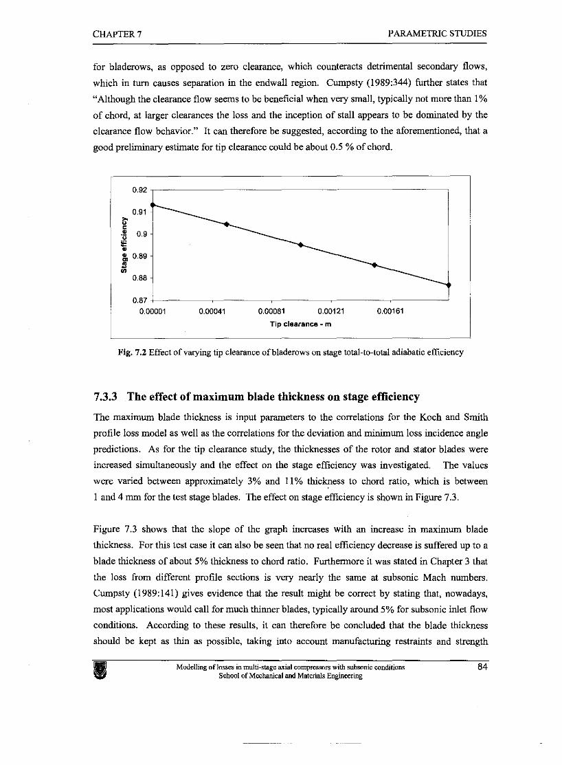
CHAPTER 7 PARAMETRIC STUDIES
for bladerows, as opposed to zero clearance, which counteracts detrimental secondary flows,
which in turn causes separation in the endwall region. Cumpsty (1989:344) further states that
"Although the clearance flow seems to be beneficial when very small, typically not more than 1%
of chord, at larger clearances the loss and the inception of stall appears to be dominated by the
clearance flow behavior." It can therefore be suggested, according to the aforementioned, that a
good preliminary estimate for tip clearance could be about 0.5 % of chord.
0.87 1 0.00001 0.00041 0.00081 0.00121 0.00161
Tip clearance - rn
Fig. 7.2 Effect of varying tip clearance of bladerows on stage total-to-total adiabatic efficiency
7.3.3 The effect of maximum blade thickness on stage efficiency
The maximum blade thickness is input parameters to the correlations for the Koch and Smith
profile loss model as well as the correlations for the deviation and minimum loss incidence angle
predictions. As for the tip clearance study, the thicknesses of the rotor and stator blades were
increased simultaneously and the effect on the stage efficiency was investigated. The values
were varied between approximately 3% and 11% thickness to chord ratio, which is between
1 and 4 mm for the test stage blades. The effect on stage eff~ciency is shown in Figure 7.3.
Figure 7.3 shows that the slope of the graph increases with an increase in maximum blade
thickness. For this test case it can also be seen that no real efficiency decrease is suffered up to a
blade thickness of about 5% thickness to chord ratio. Furthermore it was stated in Chapter 3 that
the loss from different profile sections is very nearly the same at subsonic Mach numbers.
Cumpsty (1989:141) gives evidence that the result might be correct by stating that, nowadays,
most applications would call for much thinner blades, typically around 5% for subsonic inlet flow
conditions. According to these results, it can therefore be concluded that the blade thickness
should be kept as thin as possible, taking into account manufacturing restraints and strength
Modelling of lasses in multi-stage axial compresson with subsonic conditions 84 School of Mechanical and Materials Engineering
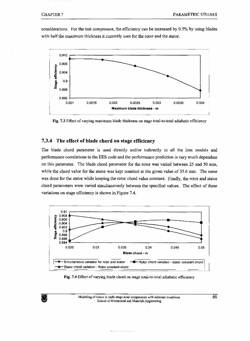
- -~
CHAPTER 7 PARAMETRIC STUDIES
considerations. For the test compressor, the efficiency can be increased by 0.5% by using blades
with half the maximum thickness it currently uses for the rotor and the stator.
Maximum blade thickness - m
Fig. 7.3 Effect of viuying maximum blade thickness on stage total-to-total adiabatic efficiency
7.3.4 The effect of blade chord on stage efficiency
The blade chord parameter is used directly andlor indirectly in all the loss models and
performance correlations in the EES code and the performance prediction is very much dependant
on this parameter. The blade chord parameter for the rotor was varied between 25 and 50 mm,
while the chord value for the stator was kept constant at the given value of 35.6 mm. The same
was done for the stator while keeping the rotor chord value constant. Finally, the rotor and stator
chord parameters were varied simultaneously between the specified values. The effect of these
variations on stage efficiency is shown in Figure 7.4.
i
I Blade chord - m
t Simultaneous variation for rotor and stator t Rotor chord variation - stator constant chord +Stator chord variation - Rotor constant chord
Fig. 7.4 Effect of varying blade chord on stage total-to-total adiabatic efficiency
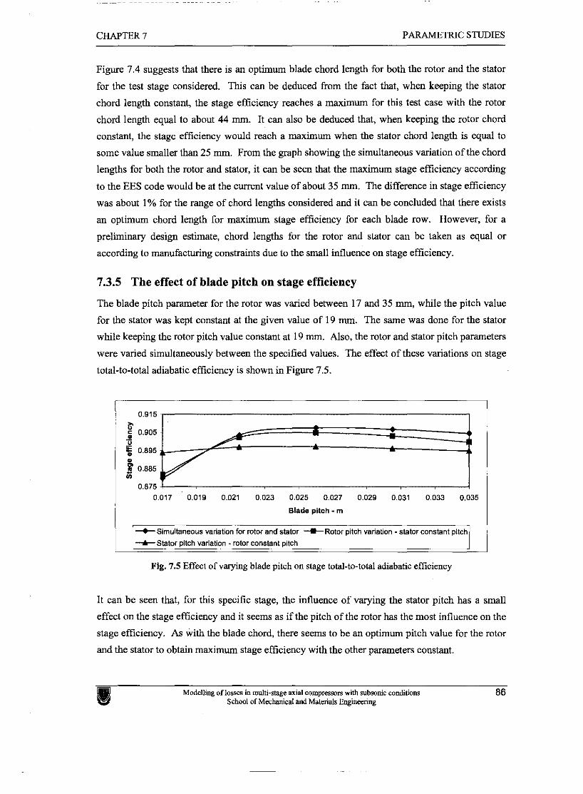
CHAPTER 7 PARAMETRIC STUDIES
Figure 7.4 suggests that there is an optimum blade chord length for both the rotor and the stator
for the test stage considered. This can be deduced from the fact that, when keeping the stator
chord length constant, the stage efficiency reaches a maximum for this test case with the rotor
chord length equal to about 44 mm. It can also be deduced that, when keeping the rotor chord
constant, the stage efficiency would reach a maximum when the stator chord length is equal to
some value smaller than 25 mm. From the graph showing the simultaneous variation of the chord
lengths for both the rotor and stator, it can be seen that the maximum stage efficiency according
to the EES code would be at the current value of about 35 mm. The difference in stage efficiency
was about 1% for the range of chord lengths considered and it can be concluded that there exists
an optimum chord length for maximum stage efficiency for each blade row. However, for a
preliminary design estimate, chord lengths for the rotor and stator can be taken as equal or
according to manufacturing constraints due to the small influence on stage efficiency.
7.3.5 The effect of blade pitch on stage efficiency
The blade pitch parameter for the rotor was varied between 17 and 35 mm, while the pitch value
for the stator was kept constant at the given value of 19 mm. The same was done for the stator
while keeping the rotor pitch value constant at 19 mm. Also, the rotor and stator pitch parameters
were varied simultaneously between the specified values. The effect of these variations on stage
total-to-total adiabatic efficiency is shown in Figure 7.5.
n o r s
0.875 4 4 0.017 0.019 0.021 0.023 0.025 0.027 0.029 0.031 0.033 0.035
Blade pitch - m
It Simultaneous variation for rotor andstator t Rotor pitch variation - stator constant pitch1
+Stator pitch variation - rotor constant pitch
Fig. 7.5 Effect of v;uying blade pitch on stage total-to-total adiabatic efficiency
It can be seen that, for this specific stage, the influence of varying the stator pitch has a small
effect on the stage efficiency and it seems as if the pitch of the rotor has the most influence on the
stage efficiency. As with the blade chord, there seems to be an optimum pitch value for the rotor
and the stator to obtain maximum stage efficiency with the other parameters constant.
Modelling o f losses in multi-stage axial compresson with subsonic conditions 86 School of Mechanical and Materials Engineering
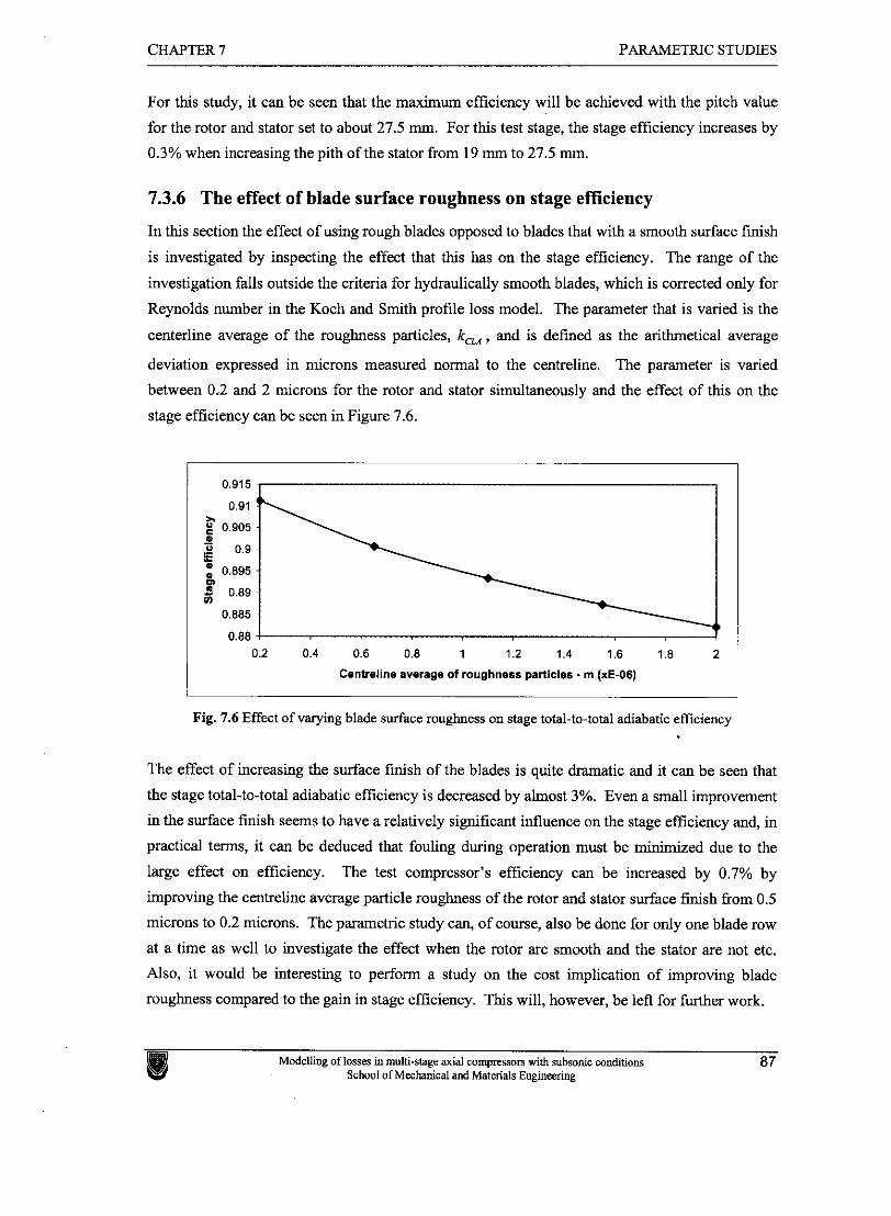
CHAPTER 7 PARAMETRIC STUDIES
For this study, it can be seen that the maximum efficiency will be achieved with the pitch value
for the rotor and stator set to about 27.5 mm. For this test stage, the stage efficiency increases by
0.3% when increasing the pith of the stator from 19 mm to 27.5 mm.
7.3.6 The effect of blade surface roughness on stage efficiency
In this section the effect of using rough blades opposed to blades that with a smooth surface finish
is investigated by inspecting the effect that this has on the stage efficiency. The range of the
investigation falls outside the criteria for hydraulically smooth blades, which is corrected only for
Reynolds number in the Koch and Smith profile loss model. The parameter that is varied is the
centerline average of the roughness particles, k , , and is defined as the arithmetical average
deviation expressed in microns measured normal to the centreline. The parameter is varied
between 0.2 and 2 microns for the rotor and stator simultanwusly and the effect of this on the
stage efficiency can be seen in Figure 7.6.
I Centreline average of roughness particles - m (xE-06)
Fig. 7.6 Effect of varying blade surface roughness on stage total-to-total adiabatic efficiency
The effect of increasing the surface finish of the blades is quite dramatic and it can be seen that
the stage total-to-total adiabatic efficiency is decreased by almost 3%. Even a small improvement
in the surface finish seems to have a relatively significant influence on the stage efficiency and, in
practical terms, it can be deduced that fouling during operation must be minimized due to the
large effect on efficiency. The test compressor's efficiency can be increased by 0.7% by
improving the centreline average particle roughness of the rotor and stator surface finish from 0.5
microns to 0.2 microns. The parametric study can, of course, also be done for only one blade row
at a time as well to investigate the effect when the rotor are smooth and the stator are not etc.
Also, it would be interesting to perform a study on the cost implication of improving blade
roughness compared to the gain in stage efficiency. This will, however, be left for further work.
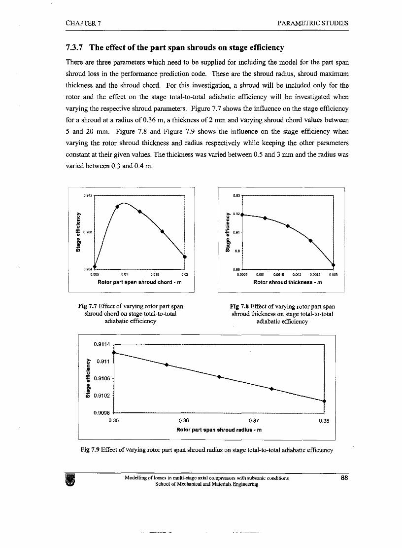
CHAPTER 7 PARAMETRIC STUDIES
7.3.7 The effect of the part span shrouds on stage efficiency
There are three parameters which need to be supplied for including the model for the part span
shroud loss in the performance prediction code. These are the shroud radius, shroud maximum
thickness and the shroud chord. For this investigation, a shroud will be included only for the
rotor and the effect on the stage total-to-total adiabatic eff~ciency will be investigated when
varying the respective shroud parameters. Figure 7.7 shows the influence on the stage efficiency
for a shroud at a radius of 0.36 m, a thickness of 2 mm and varying shroud chord values between
5 and 20 mm. Figure 7.8 and Figure 7.9 shows the influence on the stage efficiency when
varying the rotor shroud thickness and radius respectively while keeping the other parameters
constant at their given values. The thickness was varied between 0.5 and 3 rnm and the radius was
varied between 0.3 and 0.4 m.
Rotor part span shroud chord - m O m 0 5 OW? OOOlS OW2 O m 2 5 0003
Rotor shroud thickness - m
Fig 7.7 Effect of varying rotor part span shroud chord on stage total-to-total
adiabatic eff~ciency
Fig 7.8 Effect of varying rotor part span shroud thickness on stage total-to-total
adiabatic efficiency
0.9114 -
<
$ 0.911 C 0 .- g 0.9,06 H Z 0.9102
0.9098 T
0.35 0.36 0.37 0.38
Rotor part span shroud radius - m
Fig 7.9 Effect of varying rotor part span shroud radius on stage total-to-total adiabatic efficiency

CHAPTER 7 PARAMETRIC STUDIES
Figure 7.7 shows that there is an optimum chord value for the part span shroud, with the other
parameters at their constant values, resulting in maximum stage efficiency. Furthermore, it can
be seen from Figure 7.8 that the efficiency decreases with an increasing slope with an increase in
shroud thickness, leading to the conclusion that the shroud should he kept as thin as possible.
Also, from Figure 7.9, it is seen that when the part span shroud is moved fiom the hub towards
the tip, the efficiency decreases by a small percentage, however, it is uncertain if this correlation
takes the boundary layers and the interaction that would occur with them into account.
Consequently, it is advised that this correlation should only be used when the part span shroud is
placed well away from the endwalls until further study has confirmed the results. This parametric
study can similarly be performed for the stator in order to access the influence of a part span
shroud and its parameter magnitudes on the stage efficiency. The next section investigates the
effect of major variable changes like, for instance, the blade angles on the loss magnitudes to
illustrate their dependence on the performance prediction variables and each other. The effect of
this loss change on stage efficiency and pressure ratio will also be shown.
7.4 Illustrative parametric case study
A case study is presented in this section for illustrating the capability of the EES code to perform
such studies and to try and show the dependence of the loss models on the performance variables
and each other. The effect of changing the rotor blade inlet angle on the different loss
components, total loss, stage efficiency and pressure ratio will be investigated in an effort to
obtain an optimum rotor blade inlet angle value for maximum stage efficiency. The rotor inlet
blade angle was varied and the effect on the entropy change values for the different loss
components for the rotor and the total entropy change through the rotor was investigated. The
effect for the different loss components are shown in Figure 7.10.
Rotor inlet blade metal angle - m
t Profile loss t lnc~dence loss t ~ n d i a l l loss
+Part span shroud loss +Windage loss
Fig. 7.10 The effect of varying the rotor inlet blade angle on the magnifudes of the loss components
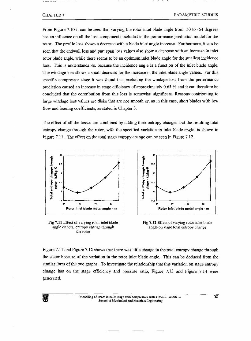
CHAPTER 7 PARAMETRIC STUDIES
From Figure 7.10 it can be seen that varying the rotor inlet blade angle from -50 to -64 degrees
has an influence on all the loss components included in the performance prediction model for the
rotor. The profile loss shows a decrease with a blade inlet angle increase. Furthermore, it can be
seen that the endwall loss and part span loss values also show a decrease with an increase in inlet
rotor blade angle, while there seems to be an optimum inlet blade angle for the smallest incidence
loss. This is understandable, because the incidence angle is a function of the inlet blade angle.
The windage loss shows a small decrease for the increase in the inlet blade angle values. For this
specific compressor stage it was found that excluding the windage loss from the performance
prediction caused an increase in stage efficiency of approximately 0.65 % and it can therefore be
concluded that the contribution from this loss is somewhat significant. Reasons contributing to
large windage loss values are disks that are not smooth or, as in this case, short blades with low
flow and loading coefficients, as stated in Chapter 3.
The effect of all the losses are combined by adding their entropy changes and the resulting total
entropy change through the rotor, with the specified variation in inlet blade angle, is shown in
Figure 7.1 1. The effect on the total stage entropy change can be seen in Figure 7.12.
dl 80 -54 52
Rotor inlet blade metal angle - m
Fig 7.11 Effect of varying rotor inlet blade angle on total entropy change through
the rotor
-W 44 -56 -52
Rotor inlet blade metal angle - m
Fig 7.12 Effect of varying rotor inlet blade angle on stage total entropy change
Figure 7.1 1 and Figure 7.12 shows that there was little change in the total entropy change through
the stator because of the variation in the rotor inlet blade angle. This can be deduced from the
similar form of the two graphs. To investigate the relationship that this variation on stage entropy
change has on the stage efficiency and pressure ratio, Figure 7.13 and Figure 7.14 were
generated.
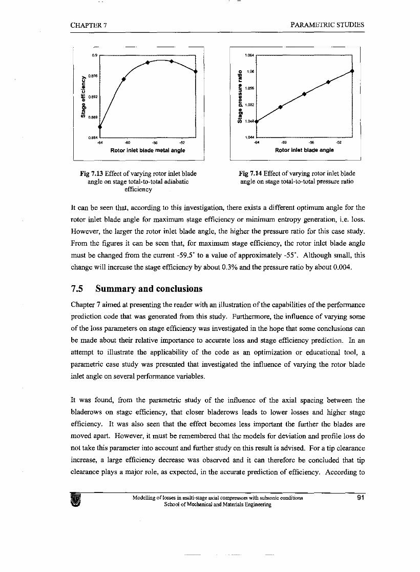
CHAPTER 7 PARAMETRIC STUDIES
64 -60 -56 -52
Rotor inlet blade metal angle
Fig 7.13 Effect of varying rotor inlet blade angle on stage total-to-total adiabatic
efficiency
-M -60 -5 -52
Rotor inlet blade angle
Fig 7.14 Effect of varying rotor inlet blade angle on stage total-to-total pressure ratio
It can be seen that, according to this investigation, there exists a different optimum angle for the
rotor inlet blade angle for maximum stage efficiency or minimum entropy generation, i.e. loss.
However, the larger the rotor inlet blade angle, the higher the pressure ratio for this case study.
From the figures it can be seen that, for maximum stage efficiency, the rotor inlet blade angle
must be changed from the cwent -59.5' to a value of approximately -55'. Although small, this
change will increase the stage efficiency by about 0.3% and the pressure ratio by about 0.004.
7.5 Summary and conclusions
Chapter 7 aimed at presenting the reader with an illustration of the capabilities of the performance
prediction code that was generated kom this study. Furthermore, the intluence of varying some
of the loss parameters on stage efficiency was investigated in the hope that some conclusions can
be made about their relative importance to accurate loss and stage efficiency prediction. In an
attempt to illustrate the applicability of the code as an optimization or educational tool, a
parametric case study was presented that investigated the intluence of varying the rotor blade
inlet angle on several performance variables.
It was found, from the parametric study of the influence of the axial spacing between the
bladerows on stage efficiency, that closer bladerows leads to lower losses and higher stage
efficiency. It was also seen that the effect becomes less important the further the blades are
moved apart. However, it must be remembered that the models for deviation and profile loss do
not take this parameter into account and further study on this result is advised. For a tip clearance
increase, a large efficiency decrease was observed and it can therefore be concluded that tip
clearance plays a major role, as expected, in the accurate prediction of efficiency. According to
CHAPTER 7 PARAMETRIC STUDIES
Cumpsty (1989:344), however, the endwall loss model from Koch and Smith cannot be valid for
stages with small or vanishing tip clearance and he further states that "Although the clearance
flow seems to be beneficial when very small, typically not more than 1% of chord, at larger
clearances the loss and the inception of stall appears to be dominated by the clearance flow
behaviour." From the blade thickness investigation, it was concluded that the blade thickness
should be kept as thin as possible, taking into account manufacturing restraints and strength
considerations. It was also seen that 5% thickness to chord ratio is a good preliminary thickness
estimate for modem subsonic compressor blades. Furthermore, it was found that there exists
optimum chord and pitch values for the rotor and stator to obtain maximum stage efficiency, but
the pitch of the rotor has the most influence. The effect of blade surface roughness also seems to
be quite dramatic, and it was found that in this case, even a small improvement in the blade
surface f ~ s h could improve the stage efficiency noticeably.
For the parametric studies concerning the part span shrouds, it was found that, as for the
compressor blades, there exists an optimum shroud chord for maximum efficiency. It was also
seen that the shroud should be as thin as possible and rather positioned closer to the hub than the
tip.
An illustrative parametric case study was also presented. For this case study, it was investigated
which value of the rotor inlet blade angle would give the highest stage efficiency with all the
other parameters constant. It was found that there existed an optimum value for this parameter
and the capability of using the code for basic optimization purposes was therefore successfully
demonstrated.
The following chapter gives a brief summary and a condensed conclusion of the study on the
modelling of losses in multi-stage axial compressors with subsonic conditions. It also gives
recommendations for further research based on the knowledge gained as to the shortcomings of
this study.
hapter 8
CONCLUSION
Chapter 8 concludes this study by giving a short summary of the preceding chapters, conclusions
that can be made from the results obtained and recommendations for &re research.
Modelling of loss= in multi-stage axial compressorr with subsonic conditions School of Mechanical and Materials Engineering
CHAPTER 8 CONCLUSION
8.1 Summary
In Chapter 1, the background leading to the study as well as a short overview of the main
concepts contained in the study was given. Further aspects that received attention were the
primary restrictions, the expected contributions and outline of the study. Chapter 2 described the
mechanisms mainly responsible for the losses and gave more detail about the mechanisms that are
commonly used in loss modelling.
Chapter 3 presented the reader with a comprehensive, but summarized literature survey regarding
loss prediction methods for subsonic axial compressors. It was found that the loss mechanisms
are interactive and complex by nature and methods of predicting them rely greatly on empirical
correlations. Also, the open literature is rather diffused and the main groupings used in this
chapter were: Blade profile losses, endwall losses including literature on tip leakage and
secondary losses, part span shroud losses, other losses, losses due to high subsonic mach numbers
and off-minimum losses.
Chapter 4 attempted to provide the reader with a framework into which the loss models can be
integrated through presenting the theory required for a meanline compressor analysis. This
chapter included discussions on methods of predicting minimum loss incidence, deviation, stall
and choke as well as methods of estimating blade and annulus blockage. Chapter 5 presented the
methodology employed for the generation of a performance prediction code, with general
applicability to subsonic multi-stage compressors with different geometries and working fluids,
which allows the interchanging of loss models. This utilized the models described in Chapters 3
and 4.
In Chapter 6 the code, developed in Chapter 5, was verified against a commercial software
package called NREC and the different loss models were evaluated according to their simplicity,
ease of implementation and accuracy. Finally, in Chapter 7, the validated EES-code was used to
perform parametric studies on the influence of varying the geometric input parameters on overall
stage loss and efficiency prediction. The aim is to form an idea as to which geometrical input
parameters are the key players in improving efficiency and which loss parameters are crucial to
accurate predictions. This was done to illustrate the ability of the code for performing such
studies to be used as an aid in understanding compressor design and performance and for basic
optimization problems.
Madelling of lasses in multi-stage axial compresson with subsonic conditions 93 School of Mechaoical and Materials Engimeming
CHAPTER 8 CONCLUSION
8.2 Conclusion
In Chapter 1 it was stated that this study aims to contribute by improving subsonic multi-stage
axial compressor expertise through investigating, and serving as a reference on, the internal loss
mechanisms, the methods of predicting their magnitudes, their implementation and their use. It
was further stated that the possibility of developing performance prediction software, with
general applicability to subsonic multi-stage compressors with different geometries and working
fluids, would he investigated.
The aforementioned were addressed by frstly providing the reader with a description of the loss
mechanisms and the most influential of these were described in more detail. The next step was to
present a comprehensive literature survey that improves this thesis's value as a reference on the
available methods of quantifying the loss mechanisms. It was seen that it would be advantageous
not to view the loss models in isolation from the concepts involved in axial compressor
performance prediction. Therefore, this study also presents the theory for axial compressor ideal
stage analysis as well as methods of predicting the other basic real fluid effects that are necessary
for basic performance prediction. A software package called Engineering Equation Solver (EES)
was used to implement the performance prediction theory and models. This code has the
capability for the considered loss models to be interchanged and evaluated against each other or
predictions from other performance prediction software. Verification was done by comparing the
results from the EES-code with those of a commercial software package called NREC at different
levels of complexity. This verification showed that the methodology used for implementing the
loss models was employed correctly and that the basic performance prediction theory was correct.
It is recommended that more test cases be considered for complete verification of the correlations
and that, if possible, experimental data should also be used. However, this is not considered part
of the scope of this study and will be left for future work.
The EES code was subsequently applied and it was found that the models given by Koch and
Smith for the minimum profile loss, endwall loss and part span shroud loss (when applicable)
with the model by Casey for the incidence loss and Denton's windage loss model was the most
comprehensive combination of the loss models considered. For preliminary estimates near the
design point, it was seen that the Lieblein model can be used for calculating the total profile loss,
i.e. including the incidence loss. Also, any endwall loss models can he used, due to the large
amount of uncertainty involved. Unfortunately, when using another endwall model than the one
given by Koch and Smith, additional estimates for annulus blockage have to be included.
Furthermore, parametric studies were performed to investigate the influence of some of the loss
Modelling of losses in multi-stage axial campressom with subsonic conditions 94 School of Mechanical and Matends Engineering
CHAPTER 8 CONCLUSION
parameters on stage efficiency and it was also illustrated how the EES-code can be used as an aid
in understanding compressor design and performance and for basic optimization problems.
8.3 Recommendations for further research
The secondary outcome of this study resulted in a preliminary meanline performance prediction
code. However, the code needs to be verified in more detail and some further research needs to
be done before the code can be considered ready to be used with confidence. The following
recommendations can be made regarding further work with the idea of improving the preliminary
code:
0
0
0
.
. .
The EES-code should be reproduced in a lower-level programming language for
increased stability and the equation sets for a whole compressor can then be solved
simultaneously, rather than one stage at a time. This approach can be very advantageous
when including the code in network analysis software.
Further research should be conducted regarding the prediction of stall and choke and the
models should be upgraded to reflect the state of the art for meanline methods.
Further research should also be conducted on the aspect of annulus blockage and the
prediction thereof. Especially, the blockage and how it is passed in simulations from one
stage to the next, i.e. how it "grows" through the compressor, should be investigated and
correctly implemented.
A much broader spectrum of test cases, preferably experimental data, should be used for
verification of the correlations used in the code as to derive correlations that would be the
most suitable to the most cases and can be accepted as default correlations for all cases.
More research should be done on methods of predicting the endwall loss due to the large
variation seen in this study from the different correlations. Unfortunately, it was noted
that great uncertainty surrounds this loss and ways to predict it.
The code can be improved by including correlations for transonic and supersonic flows.
It can also be considered to include simulations at other radial stations as the meanline.
Finally, the conceptualism that internal loss manifests as an entropy increase through the
compressor was accepted in this study and it is recommended that future loss modelling
be done with this in mind. Denton (1993) did groundbreaking work in this regard and he
rightfully suggests that every effort should be focused on understanding exactly how the
loss mechanisms work rather than to blindly use the available correlations. It is,
therefore, emphasized here that future studies on loss models should try and decrease the
dependence on empirical data. The ultimate goal would be to generate models that are
totally based on physical laws and are expressed in terms of the entropy increase it
generates.
REFERENCES
BOTHA, B W, 2002. Advanced turbomachines. School of Mechanical and Materials
Engineering. Potchefstroom University for Christian Higher Education, Course: MEG 841
BROWN, L E, 1972. Axial flow compressor and turbine loss coefficients: A comparison of
several parameters. Transactions of the ASME. Journal of Engineering for Power, 72-GT-18.
CASEY, M V, 1987. A mean Line prediction method for estimating the performance
characteristic of an axial compressor stage. Turbomachinery - Eficiency prediction and
improvement, I. Mech. E., Paper C264187
CETIN, M; UCER, A S; HIRSCH, Ch; SEROVY, G K, 1989. An off-design loss and deviation
prediction study for transonic axial compressors. Transactions of the ASME. Presented at the
Gas Turbine and Aeroengine Congress and Exposition, Toronto.
COHEN, H; ROGERS, G F C; SARAVANAMUTTOO, H I H, 1996. Gas turbine theory.
Pearson Education Limited, Longman Group Limited, ISBN 0-582-23632-0.
CONCEPTS NREC ETI Inc, 2003. Concepts NREC - Axial. Web: http:llwww.nrec.com. Date
of access: September 2003.
CUMPSTY, N A, 1989. Compressor aerodynamics. 1'' ed, Longman ScientiJic & Technical,
ISBN 0-582-01364-X
De RUYCK, J; HIRSCH, C, 1980. Investigations of an axial compressor end-wall boundary
layer prediction method. Transactions of the ASME. Journal of Engineering for Power, 80-
GT-53.
DENTON, J D, October 1993. Loss mechanisms in turbomachines. Transactions of the
ASME. Journal of Turbomochinery, 115:621-656
DIXON, S L, 1989. Fluid mechanics and thermodynamics of turbomachinery. dth ed,
Buttenuorth-Heinemann. ISBN 0-7506-7059-2
F-CHART SOFTWARE, 2003. EES - Engineering Equation Solver. Web:
http://www.fchart.com. Date of access: September 2003.
Modelling of losses in multi-stage axial compressom with subsonic conditions 96 School of Mechanical and Materials Engineering
REFERENCES
HORLOCK, J H, 2000. The determination of end-wall blockage in axial compressors: A
comparison between various approaches. Transactions of the ASME. Journal of
Turbomachinery, 122:218-224
HOWELL, A R, 1945. Design of axial compressors. Proceedings of the Institute $Mechanical
Engineers, 153.
~ N E R , J; FOTIT'JER, L, 1996. Influence of tip clearance, aspect ratio, blade loading, and
inlet boundary layer on secondary losses in compressor cascades. Transactions of the ASME.
96-GT-505
JAPIKSE, D; BAINES, N C, 1997. Introduction to turbomachinery. 2* ed, Concepts ETI,
Inc. Oxford Universify Press, ISBN 0-933283-10-5.
KOCH, C C, October 1981. Stalling pressure rise capability of axial flow compressor stages.
Transactions of the ASME. Journal of Engineering for Power, 103:645-655.
KOCH, C C; SMITH Jr., L H, July 1976. Loss sources and magnitudes in axial-flow
compressors. Transactions of the ASME. Journal ofEngineering for Power, 41 1- 424 p.
KONIG, W M; HENNECKE, D K; FO'ITNER, L, January 1996. Improved blade profile loss
and deviation angle models for advanced transonic bladings. Transactions of the ASME.
Journal of Turbomachinery, 1 1731-87 p.
LIEBLEIN, S, September 1959. Loss and stall analysis of compressor cascades. Transactions
of the ASME. Journal ofBasic Engineering, 387-400 p.
LIEBLEIN, S, September 1960. Incidence and deviation angle correlations for compressor
cascades. Transactions of the ASME. Journal of Basic Engineering, 575-587 p.
M-TECH INDUSTRIAL (Pty) Ltd., 2003. Flownex. Web: http://www.mtechindustrial.com.
Date of access: ~ e ~ t e m b e r 2003.
MILLER, D C, 1987. Off-design prediction of compressor blade losses. Turbomachinery -
Efficiency prediction and improvement, I. Mech. E., Paper C279187
Modelling of lasses in multi-stage axial compressors with subsonic conditions 97 School of Mechanical and Materials Engineering
REFERENCES
ROY, B; KUMAR, S, September 1999. Reduced order loss modelling with tip clearance,
aspect ratio and blockage effects for axial flow compressor. International Society for Air
Breathing Engines and American Institute ofAeronautics & Astronautics. ISABE 99-71 90
SHAMES, I H, 1992. Mechanics of fluids. Yd ed, McGraw Hill, Inc., ISBN 0-07-1 12815-8
SONG, T W; KIM, T S; KIM, J H; RO, S T, 2001. Performance prediction of axial flow
compressors using stage characteristics and simultaneous calculation of interstage
parameters. Proceedings of the Institution of Mechanical Engineers. Journal of Power and
Energy, 215(A):89-98
STARKE, J, 1980. The effect of the axial velocity density ratio on the aerodynamic
coefficients of compressor cascades. Transactions of the ASME. Presented at the Gas Turbine
Conference & Products show, New Orleans.
SWAN, W C, July 1961. A practical method of predicting transonic compressor
performance. Transactions of the ASME. Journal ofEngineering for Power, 322-330 p.
WILSON, D G; KORAKIANITIS, T, 1998. The design of high-efficiency turbomachinery
and gas turbines. 2& ed, Prentice-Hall, Inc., ISBN 0-13-3 12000-7
Modelling of losses in multi-stage axial compressors with subsonic conditions 98 School of Mechanical and Materials Engineering
Appendix A
ADDITIONAL LOSS MODEL INFO TION
DENTON'S BLADE PROFILE LOSS MODEL ............................................................... 99
KOCH AND SMITH BLADE PROFILE LOSS CORRELATIONS ............................... 101
DENTON'S ENDWALL LOSS MODEL ................................................................... 104
KOCH AND SMITH ENDWALL LOSS CORRELATIONS ......................................... 106
Modelling of lasses in multi-stage axial compresson with subsonic conditions School of Mechanical and Materials Engineering
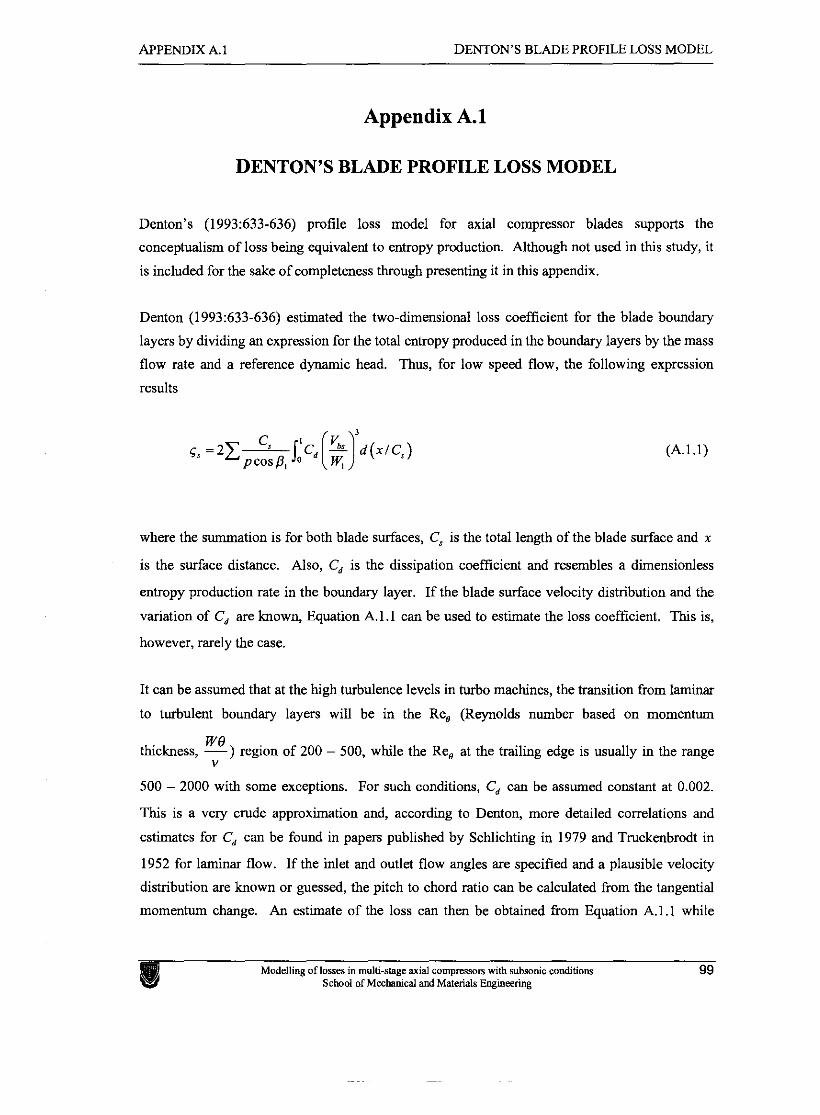
APPENDIX A. 1 DENTON'S BLADE PROFILE LOSS MODEL
Appendix A.l
DENTON'S BLADE PROFILE LOSS MODEL
Denton's (1993:633-636) profile loss model for axial compressor blades supports the
conceptualism of loss being equivalent to entropy production. Although not used in this study, it
is included for the sake of completeness through presenting it in this appendix.
Denton (1993:633-636) estimated the two-dimensional loss coefficient for the blade boundary
layers by dividing an expression for the total entropy produced in the boundary layers by the mass
flow rate and a reference dynamic head. Thus, for low speed flow, the following expression
results
where the summation is for both blade surfaces, C, is the total length of the blade surface and x
is the surface distance. Also, Cd is the dissipation coefficient and resembles a dimensionless
entropy production rate in the boundary layer. If the blade surface velocity distribution and the
variation of Cd are known, Equation A.l.l can be used to estimate the loss coefficient. This is,
however, rarely the case.
It can be assumed that at the high turbulence levels in turbo machines, the transition from laminar
to turbulent boundary layers will be in the Re, (Reynolds number based on momentum
we thickness, -) region of 200 - 500, while the Re, at the trailing edge is usually in the range
v
500 - 2000 with some exceptions. For such conditions, Cd can be assumed constant at 0.002.
This is a very crude approximation and, according to Denton, more detailed correlations and
estimates for C, can be found in papers published by Schlichting in 1979 and Tmckenbrodt in
1952 for laminar flow. If the inlet and outlet flow angles are specified and a plausible velocity
distribution are known or guessed, the pitch to chord ratio can be calculated from the tangential
momentum change. An estimate of the loss can then be obtained from Equation A.l.l while
Modelling of losses in multi-sfage axial compresson with subsonic conditions 99 School of Mechanical and Materials Engineering
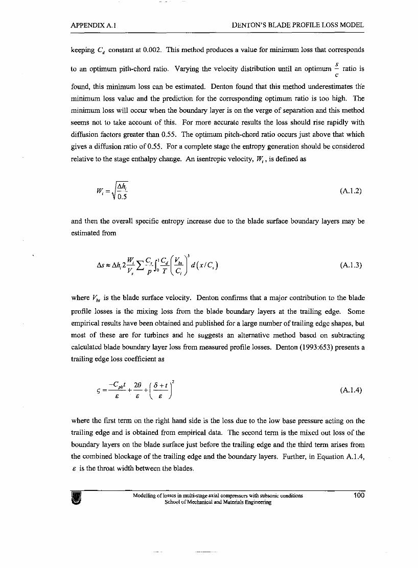
APPENDIX A. 1 DENTON'S BLADE PROFILE LOSS MODEL
keeping C, constant at 0.002. This method produces a value for minimum loss that corresponds
S to an optimum pith-chord ratio. Varying the velocity distribution until an optimum - ratio is
C
found, this minimum loss can be estimated. Denton found that this method underestimates tiie
minimum loss value and the prediction for the corresponding optimum ratio is too high. The
minimum loss will occur when the boundary layer is on the verge of separation and this method
seems not to take account of this. For more accurate results the loss should rise rapidly with
diffusion factors greater than 0.55. The optimum pitch-chord ratio occurs just above that which
gives a diffusion ratio of 0.55. For a complete stage the entropy generation should be considered
relative to the stage enthalpy change. An isentropic velocity, W] , is defined as
(A. 1.2)
and then the overall specific entropy increase due to the blade surface boundary layers may be
estimated from
(A. 1.3)
where &, is the blade surface velocity. Denton confirms that a major contribution to the blade
profile losses is the mixing loss from the blade boundary layers at the trailing edge. Some
empirical results have been obtained and published for a large number of trailing edge shapes, but
most of these are for turbines and he suggests an alternative method based on subtracting
calculated blade boundary layer loss fiom measured profile losses. Denton (1993:653) presents a
trailing edge loss coefficient as
(A. 1.4)
where the first term on the right hand side is the loss due to the low base pressure acting on the
trailing edge and is obtained from empirical data. The second term is the mixed out loss of the
boundary layers on the blade surface just before the trailing edge and the third term arises from
the combined blockage of the trailing edge and the boundary layers. Further, in Equation A.1.4,
E is the throat width between the blades.
Modelling of losses in multi-stage axial compresson with subsonic conditions 100 School of Mechanical and Materials Engineering
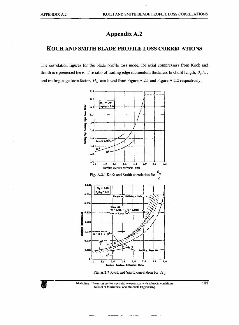
APPENDIX A.2 KOCH AND SMITH BLADE PROFILE LOSS CORRELATIONS
Appendix A.2
KOCH AND SMITH BLADE PROFILE LOSS CORRELATIONS
The correlation figures for the blade profile loss model for axial compressors from Koch and
Smith are presented here. The ratio of trailing edge momentum thickness to chord length, B,< I c ,
and trailing edge form factor, H, can found from Figure A.2.1 and Figure A.2.2 respectively.
sudlon sum M w m ~ d h
0, Pig. k 2 . 1 Koch and Smith correlation for - C
sudim Sun- DInsmd.~ n b
Fig. A.2.2 Koch and Smith correlation for IY,~
Modelling of losses in multi-stage axial compressors with subsonic conditions 101 School of Mechanical and Materials Engineering
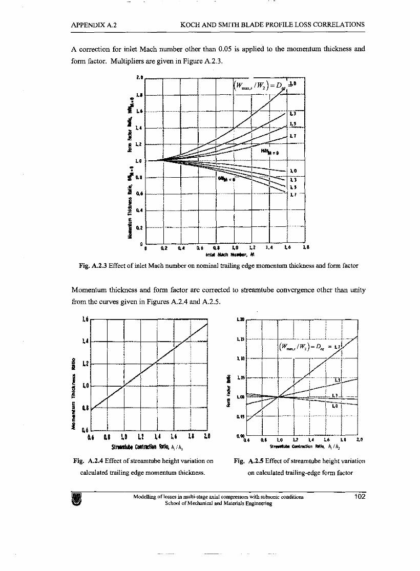
APPENDIX A.2 KOCH AND SMITH BLADE PROFILE LOSS CORRELATIONS
A correction for inlet Mach number other than 0.05 is applied to the momentum thickness and
form factor. Multipliers are given in Figure A.2.3.
Fig. A.2.3 Effect of inlet Mach number on nominal trailing edge momentum thickness and form factor
Momentum thickness and form factor are corrected to streamtube convergence other than unity
from the curves given in Figures A.2.4 and A.2.5.
St- &lb&ll Ibtk h, lhx
Fig. A.2.4 Effect of streamtube height variation on
calculated trailing edge momentum thickness.
Pig. A.2.5 Effect of streamtube height variation
on calculated trailiig-edge form factor
Modelling of losses in multi-stage axial compressom with subsonic conditions 102 School of Mechanical and Materials Enginerring
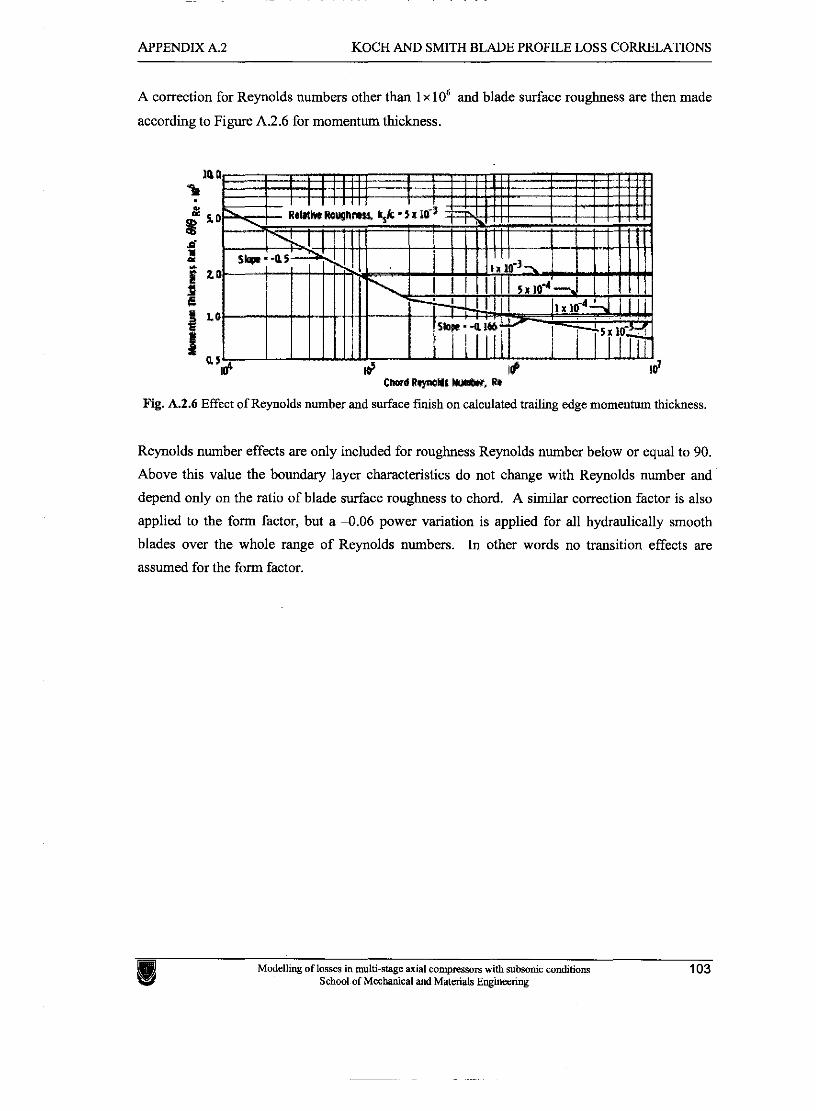
APPENDIX A.2 KOCH AND SMITH BLADE PROFILE LOSS CORRELATIONS
A correction for Reynolds numbers other than 1 x lo6 and blade surface roughness are then made
according to Figure A.2.6 for momentum thickness.
Fig.
Reynolds number effects are only included for roughness Reynolds number below or equal to 90.
Above this value the boundary layer characteristics do not change with Reynolds number and
depend only on the ratio of blade surface roughness to chord. A similar correction factor is also
applied to the form factor, but a 4 . 0 6 power variation is applied for all hydraulically smooth
blades over the whole range of Reynolds numbers. In other words no transition effects are
assumed for the f o m factor.
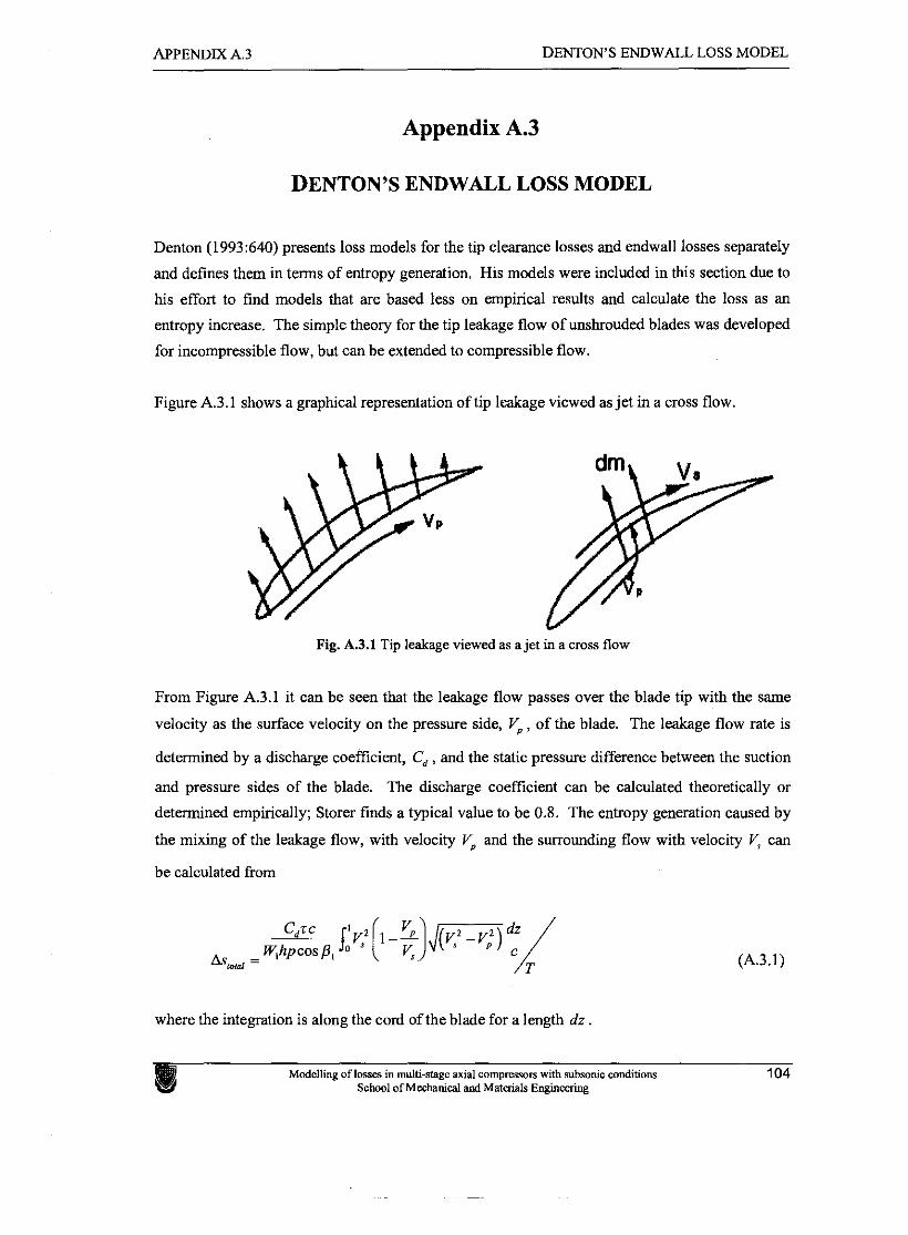
APPENDIX A.3 DENTON'S ENDWALL LOSS MODEL
Appendix A.3
DENTON'S ENDWALL LOSS MODEL
Denton (1993:640) presents loss models for the tip clearance losses and endwall losses separately
and defines them in terms of entropy generation. His models were included in this section due to
his effort to find models that are based less on empirical results and calculate the loss as an
entropy increase. The simple theory for the tip leakage flow of unshrouded blades was developed
for incompressible flow, but can be extended to compressible flow.
Figure A.3.1 shows a graphical representation of tip leakage viewed as jet in a cross flow.
Fig. A.3.1 Tip leakage viewed as a jet in a cross flow
From Figure A.3.1 it can be seen that the leakage flow passes over the blade tip with the same
velocity as the surface velocity on the pressure side, Vp , of the blade. The leakage flow rate is
determined by a discharge coefficient, C, , and the static pressure difference between the suction
and pressure sides of the blade. The discharge coefficient can be calculated theoretically or
determined empirically; Storer finds a typical value to be 0.8. The entropy generation caused by
the mixing of the leakage flow, with velocity Vp and the surrounding flow with velocity V, can
be calculated from
where the integration is along the cord of the blade for a length dz .
Madelling of losses in multi-stage axial compressors with subsonic conditions 104 School of Mechanical and Mat& Engineering
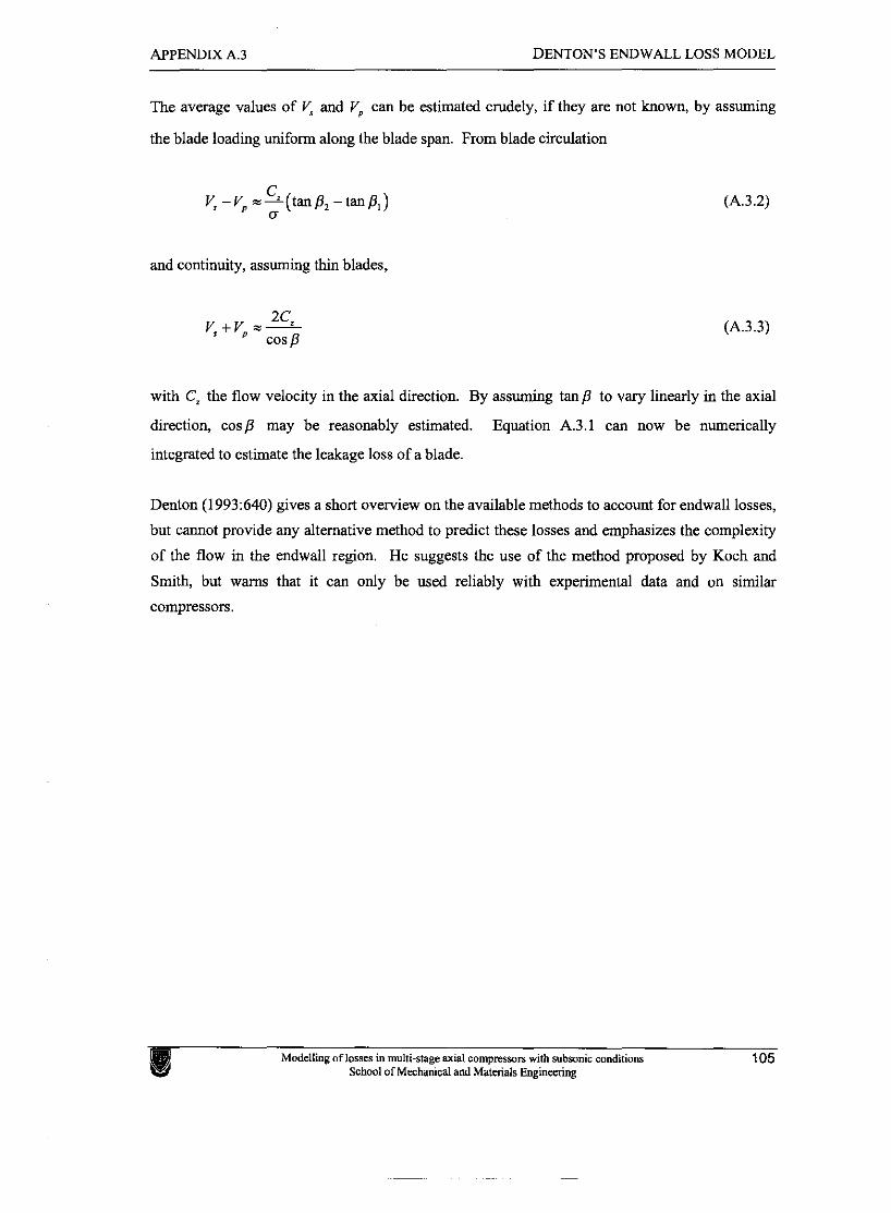
APPENDIX A.3 DENTON'S ENDWALL LOSS MODEL
The average values of V, and V, can be estimated crudely, if they are not known, by assuming
the blade loading uniform along the blade span. From blade circulation
and continuity, assuming thin blades,
with Cz the flow velocity in the axial direction. By assuming tanp to vary linearly in the axial
direction, cosp may be reasonably estimated. Equation A.3.1 can now be numerically
integrated to estimate the leakage loss of a blade.
Denton (1993:640) gives a short overview on the available methods to account for endwall losses,
but cannot provide any alternative method to predict these losses and emphasizes the complexity
of the flow in the endwall region. He suggests the use of the method proposed by Koch and
Smith, but warns that it can only be used reliably with experimental data and on similar
compressors.
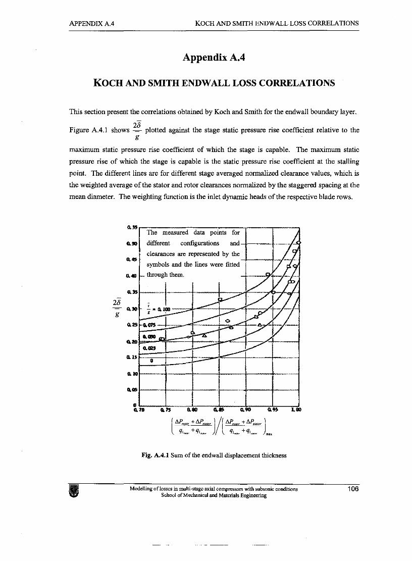
APPENDIX A.4 KOCH AND SMITH ENDWALL LOSS CORRELATIONS
Appendix A.4
KOCH AND SMITH ENDWALL LOSS CORRELATIONS
This section present the correlations obtained by Koch and Smith for the endwall boundary layer. -
26 Figure A.4.1 shows - plotted against the stage static pressure rise coefficient relative to the
g
maximum static pressure rise coefficient of which the stage is capable. The maximum static
pressure rise of which the stage is capable is the static pressure rise coefficient at the stalling
point. The different lines are for different stage averaged normalized clearance values, which is
the weighted average of the stator and rotor clearances normalized by the staggered spacing at the
mean diameter. The weighting function is the inlet dynamic heads of the respective blade rows.
clearances are represented by the
symbols and the lines were fitted
am an no as a n an r m
Fig. A.4.1 Sum of the endwall displacement thichess
Modelling of losses in multi-stage axial campresson with subsonic conditions 106 School of Mechanical and Materials Engineering
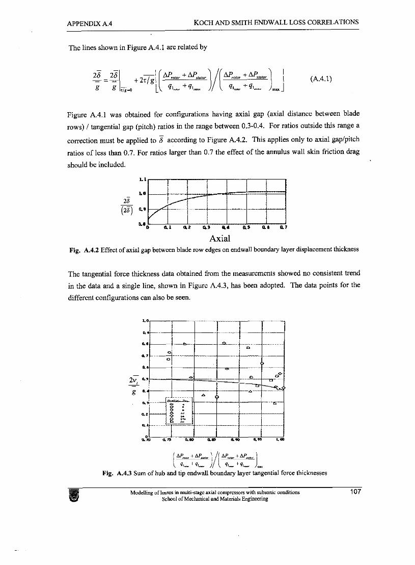
APPENDIX A.4 KOCH AND SMITH ENDWALL LOSS CORRELATIONS
The lines shown in Figure A.4.1 are related by
Figure A.4.1 was obtained for configurations having axial gap (axial distance between blade
rows) I tangential gap (pitch) ratios in the range between 0.3-0.4. For ratios outside this range a
correction must be applied to 6 according to Figure A.4.2. This applies only to axial gaplpitch
ratios of less than 0.7. For ratios larger than 0.7 the effect of the annulus wall skin friction drag
should be included.
Axial Pig. A.4.2 Effect of axial gap between blade row edges on endwall boundary layer displacement thickness
The tangential force thickness data obtained from the measurements showed no consistent trend
in the data and a single line, shown in Figure A.4.3, has been adopted. The data points for the
different configurations can also be seen.
Fig. A.43 Sum of hub and tip endwall boundary layer tangential force thicknesses
Modelling of losses in multi-stage axial compresson with subsonic conditions 107 School of Mechanical and Materials Engineering
Appendix B
DITIQNAL PERFQ CE PREDICTION
INFOWTION
........................................ B.l MINIMUM LOSS INCIDENCE CORRELATION FIGURES 108
B.2 DEVIATION CORRELATION FIGURES ...................................................................... 109
B.3 KOCH'S STALLING PRESSURE RISE CORRELATION FIGURES .......................... 111
Modelling of losses in multi-stage axial campressom with subsonic conditions School of Mechanical and Materials rnngineering
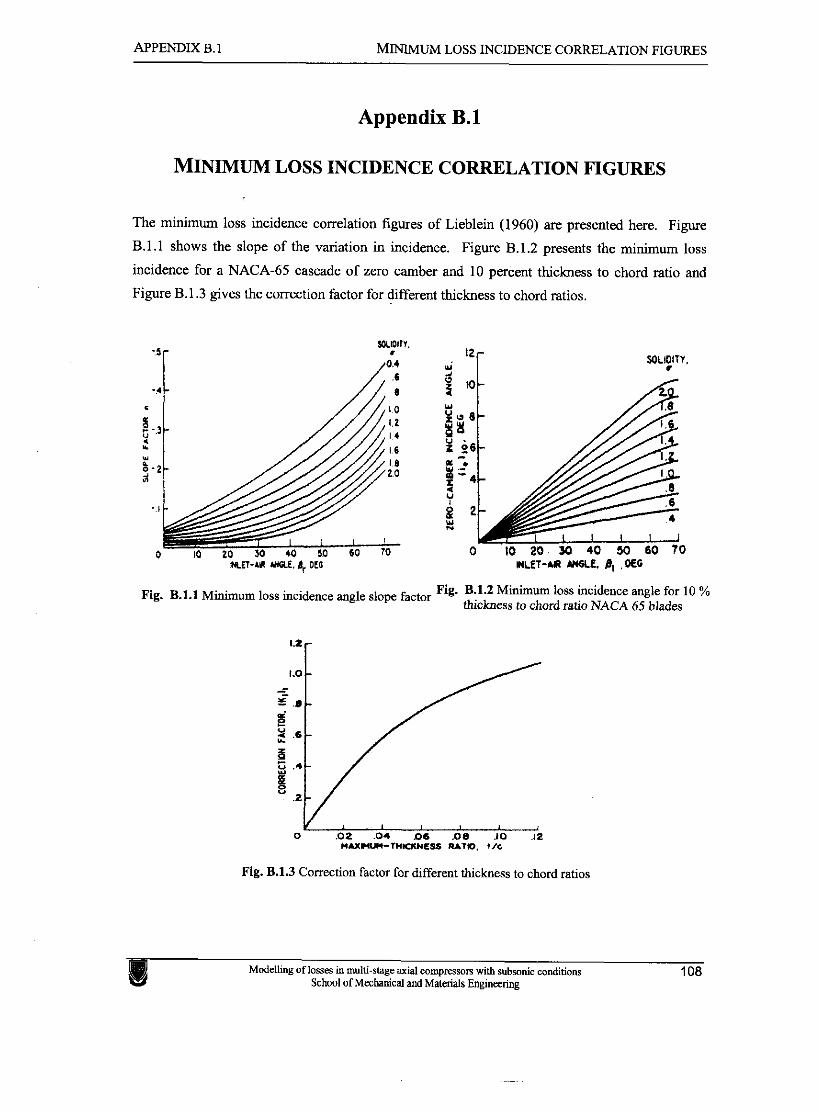
APPENDIX B. 1 MINIMUM LOSS INCIDENCE CORRELATION FIGURES
Appendix B.l
MINIMUM LOSS INCIDENCE CORRELATION FIGURES
The minimum loss incidence correlation figures of Lieblein (1960) are presented here. Figure
B.l.l shows the slope of the variation in incidence. Figure B.1.2 presents the minimum loss
incidence for a NACA-65 cascade of zero camber and 10 percent thickness to chord ratio and
Figure B.1.3 gives the correction factor for different thickness to chord ratios.
Fig. B.l.l Minimum loss incidence angle slope factor Fig. B.1.2 Minimum loss incidence angle for 10 % thickness to chord ratio NACA 65 blades
Fig. B.1.3 Correction factor for different thickness to chord ratios
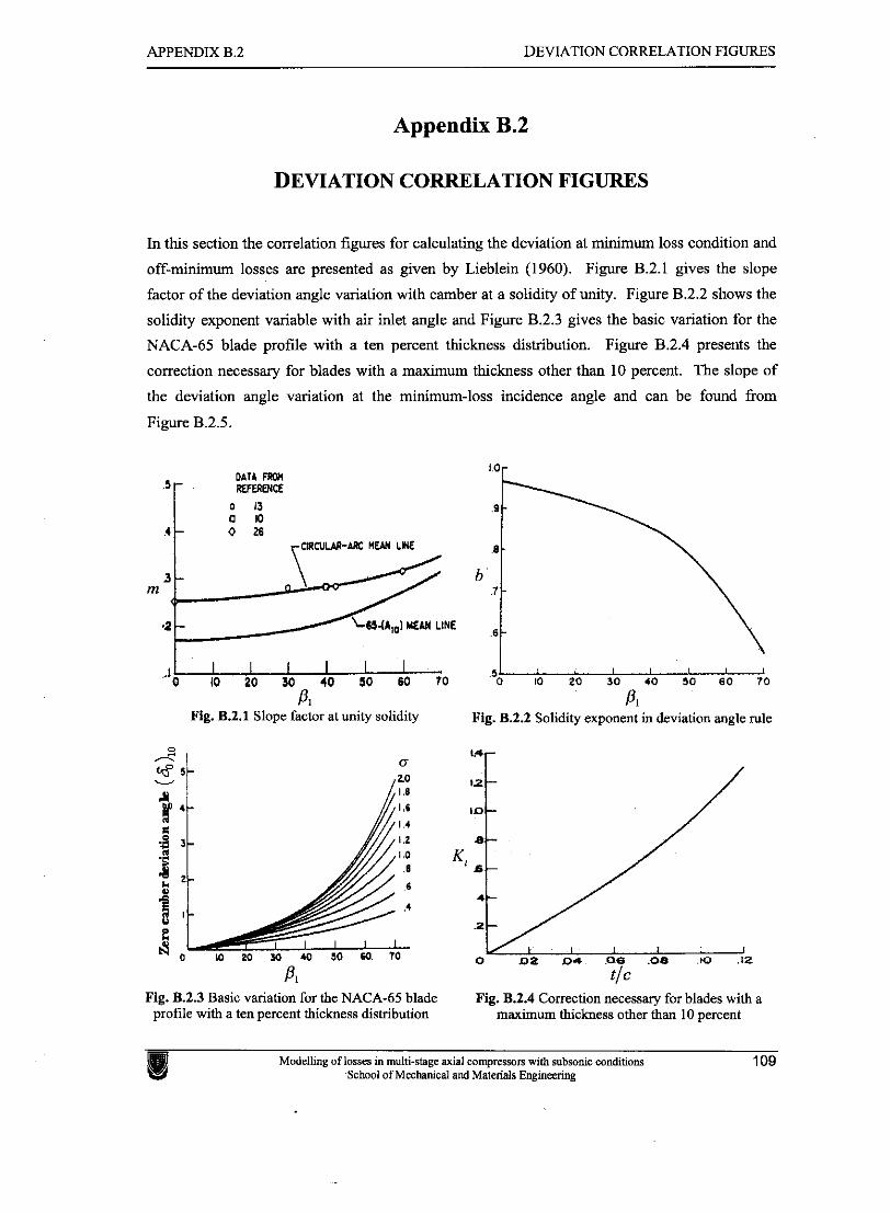
APPENDIX B.2 DEVIATION CORRELATION FIGURES
Appendix B.2
DEVIATION CORRELATION FIGURES
In this section the correlation figures for calculating the deviation at minimum loss condition and
off-minimum losses are presented as given by Lieblein (1960). Figure B.2.1 gives the slope
factor of the deviation angle variation with camber at a solidity of unity. Figure B.2.2 shows the
solidity exponent variable with air inlet angle and Figure B.2.3 gives the basic variation for the
NACA-65 blade profile with a ten percent thickness distribution. Figure B.2.4 presents the
correction necessary for blades with a maximum thickness other than 10 percent. The slope of
the deviation angle variation at the minimum-loss incidence angle and can be found from
Figure B.2.5.
P I
Fig. B.2.1 Slope factor at unity solidity
Fig. B.2.3 Basic variation for the NACA-65 blade profile with a ten percent thickness distribution
Pig. B.2.2 Solidity exponent in deviation angle rule
W Y
Fig. B.2.4 Correction necessary for blades with a maximum thickness other than 10 percent
Modelling of losses in multi-stage axial compressors with subsonic conditions School of Mechanical and Materials Enginening
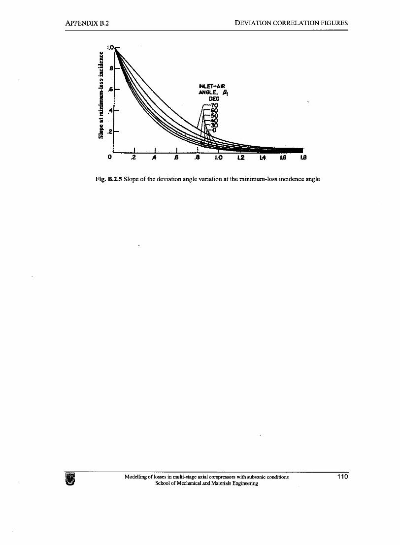
APPENDIX B.2 DEVIATION CORRELATION FIGURES
Fig. B.2.5 Slope of the deviation angle variation at the minimum-loss incidence angle
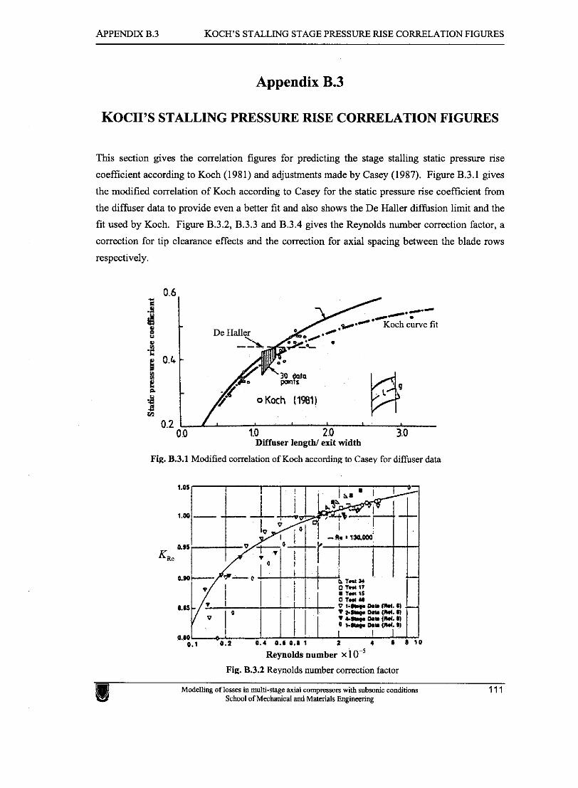
APPENDIX B.3 KOCH'S STALLING STAGE PRESSURE RISE CORRELATION FIGURES
Appendix B.3
KOCH'S STALLING PRESSURE RISE CORRELATION FIGURES
This section gives the correlation figures for predicting the stage stalling static pressure rise
coefficient according to Koch (1981) and adjustments made by Casey (1987). Figure B.3.1 gives
the modified correlation of Koch according to Casey for the static pressure rise coefficient from
the diffuser data to provide even a better fit and also shows the De Haller diffusion limit and the
fit used by Koch. Figure B.3.2, B.3.3 and B.3.4 gives the Reynolds number correction factor, a
correction for tip clearance effects and the correction for axial spacing between the blade rows
respectively.
0.2 1 0 0 1.0 2 9 3.0
Diffuser length/ exit mdth
Fig. B.3.1 Modified correlation of Koch according to Casey for diffuser data
Reynolds number x lo-* Fie;. B.3.2 Reynolds number correction factor
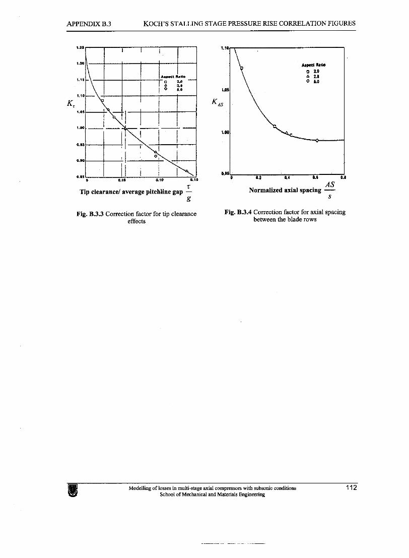
APPENDIX B.3 KOCH'S STALLING STAGE PRESSURE RISE CORRELATION FIGURES
Tip clearance/ average pitchline gap - g
Fig. B.3.3 Correction factor for tip clearance effects
awl P 0.1 0.8 a1 I
AS Normalized axial spacing -
S
Fig. B.3.4 Correction factor for axial spacing between the blade rows
Modelling of losses in multi-stage axial compresson with subsonic conditions 112 School of Mechanical and M a t e d Engineering
Appendix @
ADDITIONAL 11MPI,EMENTBTIO1\9 INFORMATION
PROGRAM ALGORITHM ................................................................................... 1 13
USER VARIABLE INPUTS ................................................................................ 1 14
LOSS MODEL FORMATTED EQUATION SETS ................................................... 1 16
PERFORMANCE PREDICTION FORMA'ITED EQUATION SETS ........................ 124
DERIVATION OF PRESSURE LOSS . ENTROPY INCREASE RELATION .......... 136
EES SOURCE CODE ....................................................................................... 137
Modelling of lasses in multi-stage axial compresson with subsonic conditions School of Mechanical and Materials Engineering
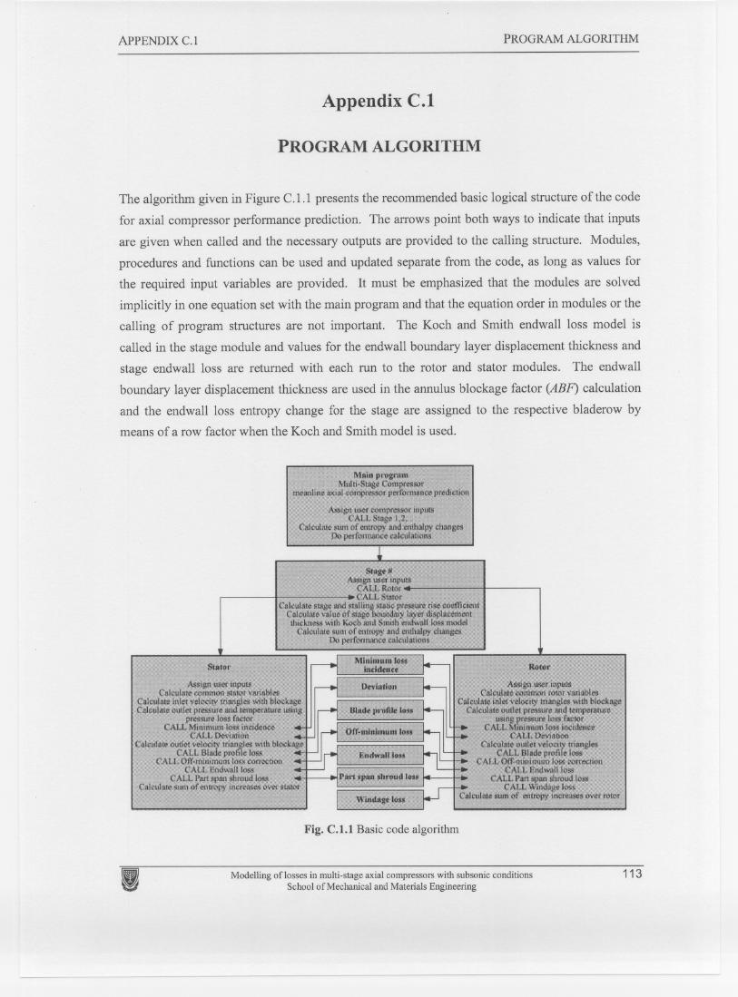
APPENDIX C.! PROGRAM ALGORITHM
Appendix C.I
PROGRAM ALGORITHM
The algorithm given in Figure C.l.l presents the recommended basic logical structure of the code
for axial compressor performance prediction. The arrows point both ways to indicate that inputs
are given when called and the necessary outputs are provided to the calling structure. Modules,
procedures and functions can be used and updated separate from the code, as long as values for
the required input variables are provided. It must be emphasized that the modules are solved
implicitly in one equation set with the main program and that the equation order in modules or the
calling of program structures are not important. The Koch and Smith endwall loss model is
called in the stage module and values for the endwall boundary layer displacement thickness and
stage endwall loss are returned with each run to the rotor and stator modules. The endwall
boundary layer displacement thickness are used in the annulus blockage factor (ABF) calculation
and the endwall loss entropy change for the stage are assigned to the respective bladerow by
means of a row factor when the Koch and Smith model is used.
Stator
Assign user inputsCaJclllato common stator vanablos
Calculate inlet velcw;hy trianalea with blcw;kageCalculate outlet pr_me and temperature tl!i1l3
prosJUte 10$5 factorCALL Minimum loss inci~nce
CALL Deviation
lea \\itll blockJl3clie loss
CALL Off-minimum loss correctionCALL &IdwaIllo.'IS
CALL ParI span shroud lossCalculate Slim of entropy iner...asos Oliff stator
It'ICanlinc
Fig. C.I.I Basic code algorithm
I Modelling oflosses in multi-stage axial compressors with subsonic conditionsSchool of Mechanical and Materials Engineering
113
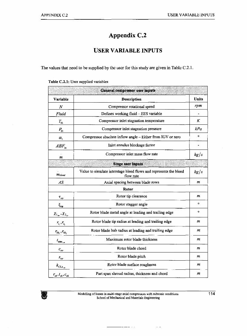
APPENDIX C.2 USER VARLABLE INPUTS
Appendix C.2
USER VARIABLE INPUTS
The values that need to be supplied by the user for this study are given in Table C.2.1.
Table C.Z.1: User supplied variables . . - .. . . . . . ... . --
General compreswr user inputs --
,,. I I
Stage urer inputs . -
Variable
N
Fluid
GI p o l
a1
ABqn
-
Description
Compressor rotational speed
Defmes working fluid - EES variable
Compressor inlet stagnation temperature
Compressor inlet stagnation pressure
Compressor absolute inflow angle - Either kom IGV or zero
Inlet annulus blockage factor
Compressor inlet mass flow rate
mbld
Units
rPm
K
kPa
0
kgls
AS
Value to simulate interstage bleed flows and represents the bleed flow rate
Rotor
Modelling of losses in multi-stage axial compresson with subsonic conditions 114 School of Mechanical and Materials Engineering
k g / ~
Axial spacing between blade rows
5 r
5, XI, 'X2,"
't, .%
' h q 3 ' h q
twr
cm
S,"
k c u ,
' t5h ' CSh
m
Rotor tip clearance
Rotor stagger angle
Rotor blade metal angle at leading and trailing edge
Rotor blade tip radius at leading and trailing edge
Rotor blade hub radius at leading and trailing edge
Maximum rotor blade thickness
Rotor blade chord
Rotor blade pitch
Rotor blade surface roughness
Part span shroud radius, thickness and chord
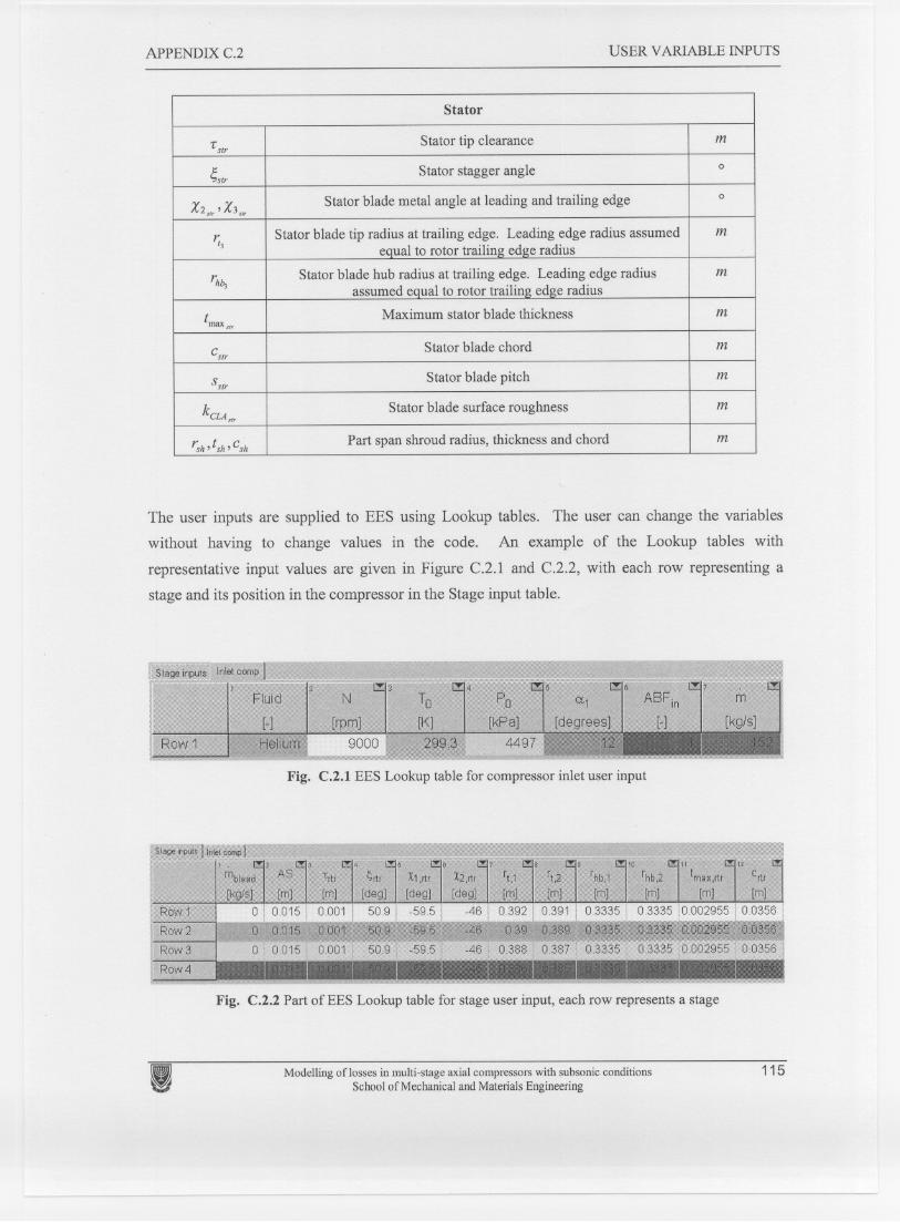
APPENDIX C.2 USER VARIABLE INPUTS
The user inputs are supplied to EES using Lookup tables. The user can change the variables
without having to change values in the code. An example of the Lookup tables with
representative input values are given in Figure C.2.! and C.2.2, with each row representing a
stage and its position in the compressor in the Stage input table.
N
[rpm]9000--- -
Fig. C.2.} EES Lookup table for compressor inlet user input
11II11IIII11II-...... -- ~ --- ~
Fig. C.2.2 Part of EES Lookup table for stage user input, each row represents a stage
I Modelling oflosses in multi-stage axial compressors with subsonic conditionsSchool of Mechanical and Materials Engineering
115
Stator
'slr Stator tip clearance m
str Stator stagger angle0
X2, ,X3",Stator blade metal angle at leading and trailing edge
0
r,J Stator blade tip radius at trailing edge. Leading edge radius assumed m
equal to rotor trailing edge radius
rh Stator blade hub radius at trailing edge. Leading edge radius m
assumed eaual to rotor trailing edge radius
tmax3trMaximum stator blade thickness m
cslrStator blade chord m
Sstr Stator blade pitch m
k Stator blade surface roughness mCLA",
r.h' ish' Csh Part span shroud radius, thickness and chord m
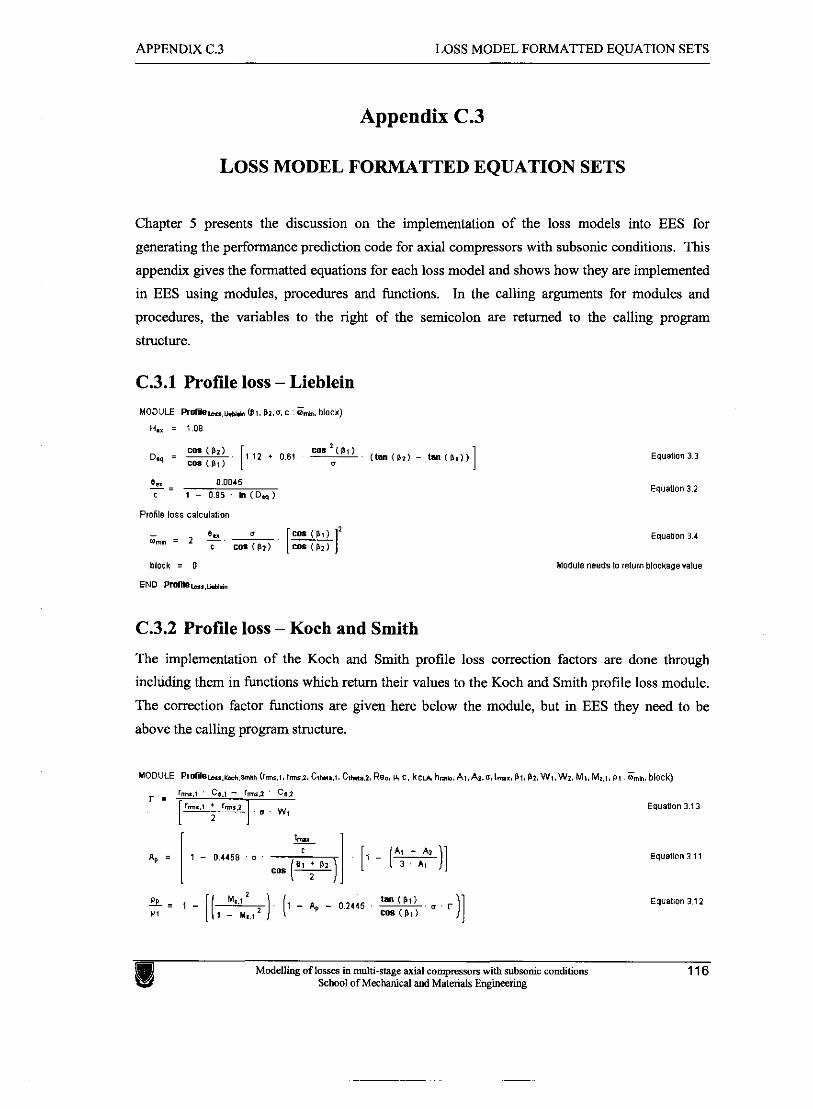
APPENDIX C.3 LOSS MODEL FORMATTED EQUATION SETS
Appendix C.3
LOSS MODEL FORMATTED EQUATION SETS
Chapter 5 presents the discussion on the implementation of the loss models into EES for
generating the performance prediction code for axial compressors with subsonic conditions. This
appendix gives the formatted equations for each loss model and shows how they are implemented
in EES using modules, procedures and functions. In the calling arguments for modules and
procedures, the variables to the right of the semicolon are returned to the calling program
structure.
C.3.1 Profde loss - Lieblein MODULE PrmIeh,,~~, @I, PI,^, c : &.block)
H . = 1.08
Profile loss caiculstion
Equation 3.3
Equation 3.2
Equsbon 3 4
Module needs to return blackagevalue
C.3.2 Profile loss - Koch and Smith
The implementation of the Koch and Smith profile loss correction factors are done through
including them in functions which return their values to the Koch and Smith profile loss module.
The correction factor functions are given here below the module, but in EES they need to be
above the calling program structure.
Equation 3 11
Equation 3 12
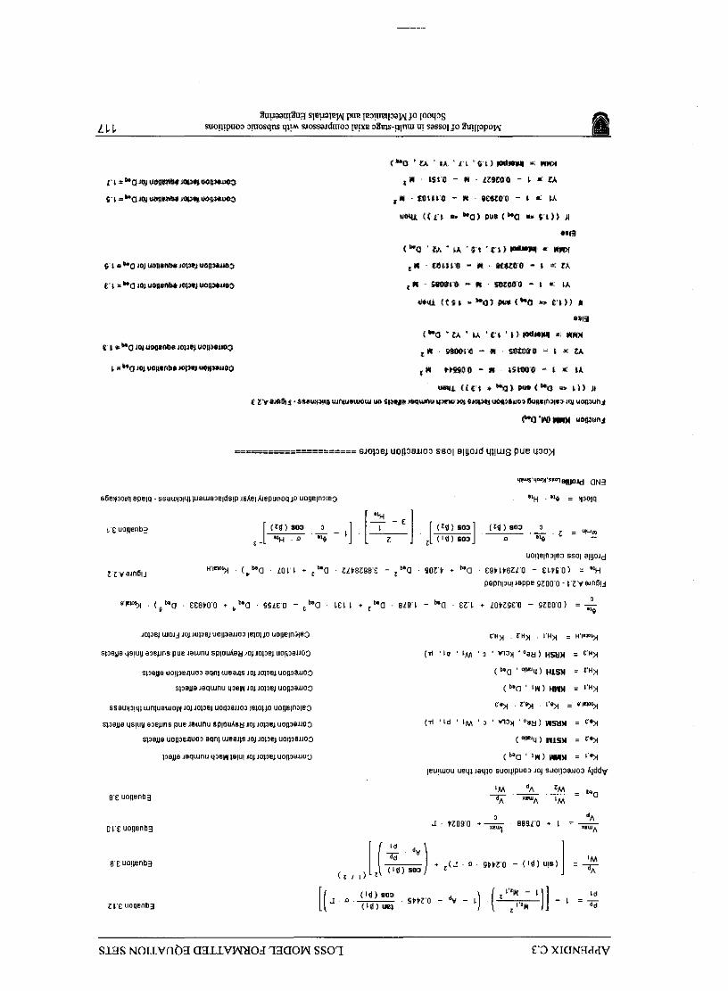
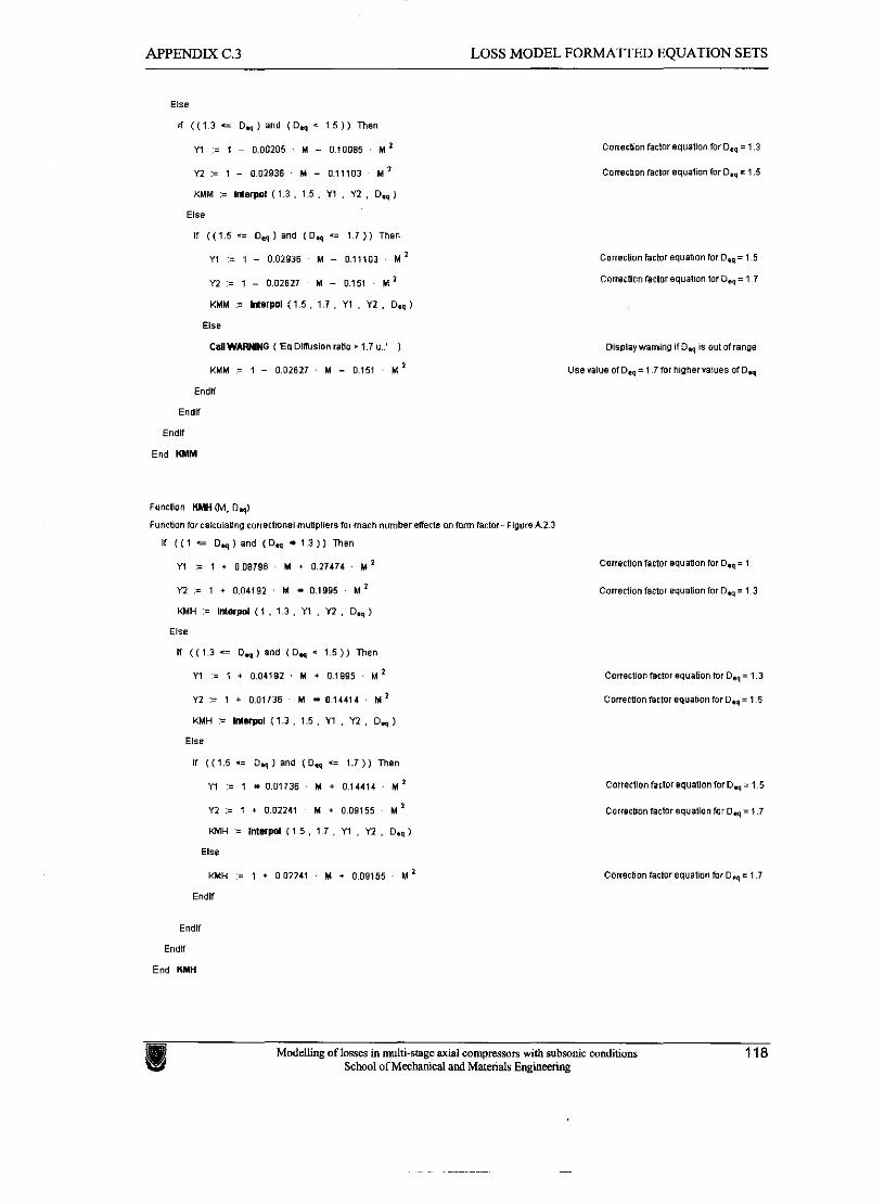
APPENDIX C.3 LOSS MODEL FORMATTED EQUATION SETS
Else
~r ( ( 1 . 3 *= D. 1 and ( Daq c 1 5 I I men
Yl = 1 - 000205 M - 0.10085 Mi
Y2 := 1 - 0.02936 M - 0.11103 M '
KMM := M e r p o l (1.3 , 1.5 . Y1 . Y2 . D, I
Else
If ( (1 .5 e o e q ) a n d (Deq c= 1 7 ) ) Thsn
Y I := 1 - 0.02836 M - 0.11103 M '
Y l := 1 - 0.02627 11 - 0.151 M
KMM := Merpo l (1.5 , 1.7 , Y1 , Y2 . D.< I
Else
C a l l W A M G ( 'Eq Dlffision ratlo r 1.7 u..' I
KHM ,= 1 - 0.02827 M - 0.151 M 1
Endn
Endlf
E"dlf
End KMM
corradonfartor equation for D., = 1.3
C~r re tnon fador equation for D..= 1.5
Conezbon factor squallon lor D., = 1 5
C ~ ~ ~ ~ l l o n f a ~ t l i r e q ~ a t l ~ n lor Dq= 1 7
D i ~ p i s y M r n i n g if Dq Is out ofrange
Use value ofD, = 1 7 for nlanervaiues ofD,,
Function KMH (M. 0,)
Funetim mr ralruistlng corrsrl'onsl rnutlpliers far mach number sffacb on form factor- Figure A 2 3
r ( ( I -= o,)and ( D ~ 1 3 ) ) men
Yl := 1 + 0.08796 M + 0.27474 M 2
Y2 = 1 + 0.04192 M O l W 5 M 2
KMH := Ir*erpd ( 1 . 1 . 3 , Y l , Y 2 . D.,)
Else
n ((1.3 r= and (D, 1 .5 ) ) men
Y l = 1 + 0.04182 . hi + D l 9 9 5 M '
Y2 := I + 0.01736 - M 014414 M '
KMH . Mwwl ( 1 . 3 , 1.5, Y1 . Y 2 , D,)
Else
r ( (1 .5 *= D, I and (D., *= 1.7 1 ) ~ h s n
Y1 := 1 0.01736 M + 0.14414 - M '
Y2 := 1 t 0.02241 M + 0.09155 M 1
KMH = lntsrpol ( 1 5 , 1 7 . Y1 , n , D., )
El59
KMH :. 1 . 002241 M + 0.09155 M a
Endn
Endlf
Endlf
End MIH
C ~ r ~ e ~ l l ~ n f a ~ t ~ r 89uat10n fOrD.*= 1
Correctcon factor equatlonfor D.,= 1 3
Come~tionfactor equation mr D.,= 1.7
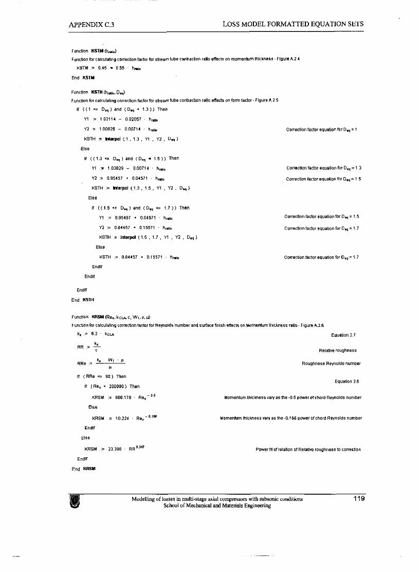
APPENDIX C.3 LOSS MODEL FORMATTED EQUATION SETS
Funrtlon KSTM (hn,J
~ u n r t l ~ n fwcalcu(abng correthonfactot tor rbesmtut le conbarllon ratio m r t s an momentum hlcknsss FIsuraA2 4
KSTM = 0 4 5 0 55 hma
End KSTH
Function KSTH (hnh, 0 3
Functmntor calculahng correction factor Dr sfrsam lube conhachon ratio effects on form fac ts - Figure A 2 5
r ( ( 1 .= D.,) and (D, < 1 . 3 ) ) Than
Y l = 1.02114 - 0.02057 h*
Y2 = 1 00829 - 0 00714 hmm
KSTH := h U p 0 l ( 1 , 1 . 3 . Y1 , Y2 , D w )
Else
11 I (1.3 -= D, 1 and ( D, i s ) ) men
Y1 = 100829 - OOOTl4 hns
n := o.ssrs7 + oo4s7 i . hmi.
KSTH := ll*erpoi ( 1 . 3 . 1.5 , Y1 , Y2 , D..)
ElSB
If ( (1 .5 rr D,) and (D., *= 1 . 7 ) ) Then
Y1 .= 0.95457 t 0.04571 - h h
Y l .= 0.84457 + 015571 . h h
KSTb = lnIerp01 ( 1 . 5 , 1 . 7 , Y1 , Y 2 , D..)
Else
KSTH .= 0.84457 + 0.15571 - h n a
Endif
Endif
E"dK
End KSTH
Conection factor equation for D., = 1
Cornction factor equation for D., = 1.3
Correction factor equation Dr D, = 1 5
comct ionfartor egust~onfor D., = 1 5
Corrsrtlon factor equatmfor D, = 1 7
k RR .= Relatlve roughness
RRe := ks ' WI ' P Roughne~s Reynolds number u
if (RRB c 9 0 ) Then
n (Re, - moo001 men
KRSM := 600.178 R.,.'~
EISB
KRSM := 10.224 RB:"'~
Endif
El68
KRSM = 23.388 R R ' ~ '
EndK
End KRSM
MOmentumthlcknessralyas h e - O 5 Dmer ofchord Reynolds number
Momenbm IhicKnessvawasthe-0166pmr ofrhard Reynolds number
Powerrn of relation of Rslative roughness to conectian
Modelling of losses in multi-stage axial compresson with subsonic conditions 119 School of Mechanical and Materials Engineering
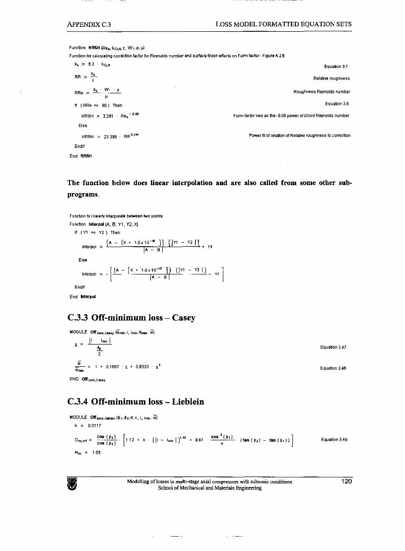
APPENDIX C.3 LOSS MODEL FORMATTED EQUATION SETS
Funcuon KRSH(Rer. k c u c , WLD. W runctionfor rakuiiling correcbonfactorror Remolds number and s u t a m f ~ l s h sflerts on Form factor- FlgursA.l.6
k, := 6 2 . k c u Equation 3.7
k RR := c Relsllw rauphners
RRe = k, W, P
v
a I RRe *= 90 I Then
KRSH = 2.281 ~e;"'
Elsa
KRSH = 23.389 RR'""
Endif
End KRSH
Roughness Remolds number
Equation 3 6
Form fartorraw asme-0 06 p m r of chord Remolds number
P w e r nl ofrslation of Relawe roughness to eonertlon
The function below does linear interpolation and are also called from some other sub-
programs.
Funrtion to iinasrlv intsmolnts betweentwo pamtr
Function Interpol LI\, 6, ~ 1 , Y2 . X )
If ( Y l >= Y2 I Then
[ A - [X + 1 . 0 ~ 1 0 ' ~ ) 1 ~ [IYI - Y l 11 Interpol = + YI
\ A - 0 1
Endlf
End Interpol
C.3.3 Off-minimum loss - Casey MODULE O l l b , ~ , m ~ . ~ 6-, i , i i , in.ha :ii)
Equation 3 47
Equation 3.46
C.3.4 Off-minimum loss - Lieblein
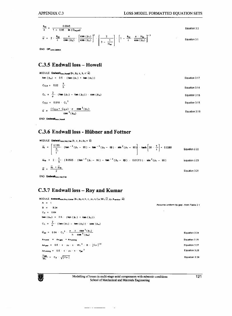
APPENDIX C.3 LOSS MODEL FORMAlTED EQUATION SETS
C.3.5 Endwall loss - Howell
Equation 3 1 7
C.3.6 Endwall loss - Hiibner and Fottner
MODULE Enaualla,,,w.rm lh, c. bv, P2. r ijl
0.165 ( t a n - ' ( @ , - 9 0 ) - t a - ' l p ~ - 9P) o i n 2 ( P ~ - 90
Equation 3.22
- OM = 2 5 (0.0505 ( t a n - ' I p l - 9 0 ) - t a n 2 ( k r - 9P) - 0.013131 r i n 1 ( p I - 9 0 )
h Equation 3.23
C.3.7 Endwall loss - Roy and Kumar MODULE E W I ~ S . I . . R ~ . - I ( P ? , P ~ , ~ I h. C . P(.X.CP.WI.U, q?,On.der:a
A = 3
B = - 0.24
C4 = 0 8 4
tan (pm) = 0 5 (tan ( 8 1 ) + Is1 ( 8 , ) )
Assume unlf~rm tle gap- mrn Table 3 1
Modelling of losses in multi-stage axial compressors with subsonic conditions 121 School of Mmhanical and Materials Engineering
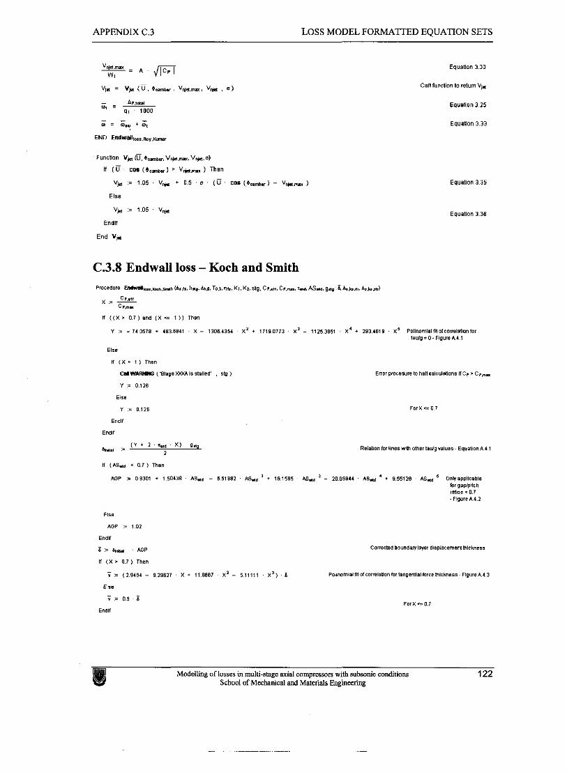
APPEM)IX C.3 LOSS MODEL FORMATTED EQUATION SETS
End Vw
C.3.8 Endwall loss - Koch and Smith
I f l f f i . + a , 0 . 7 ) Thsn
AOP .= 1 0 2
Enalr
i := 6- . MP
il ( X r 0 7 ) Then
Modelling of losses in multi-stage axial campresson with subsonic conditions 122 School of Mechanical and Materials Engineering
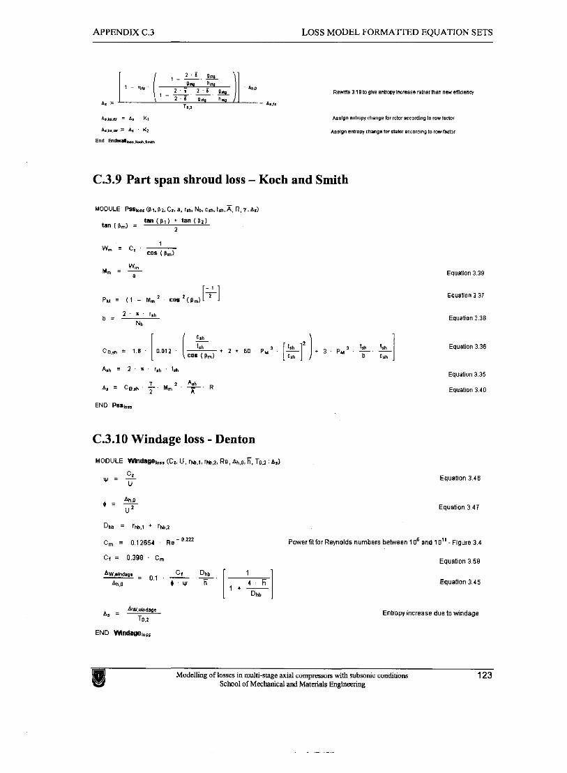
APPENDIX C.3 LOSS MODEL FORMATTED EQUATION SETS
&sign Bntropl chsngalor rotoiarrodinglo row fanor
~ r i g n entropy mmos for senr setordingto r a f a l o r
C.3.9 Part span shroud loss - Koch and Smith
C.3.10 Windage loss - Denton
MODULE Wlndaaeb,, (CZ. U, rha.9. rha.2. Re, ~ h , o . F . Tos :A,)
Equalion 3.39
Equation 3.37
Equation 3.38
Equation 3 36
Equation 3.35
Equation 3.40
Equation 3.46
Ah 0 ( = - u 2 Equation 3 47
Dhb = rhb.1 ' lhbs
C, = 012654 ~ e - O n ' Power Atlor Reynolds numbers between 10' and 10" - Flgure 3 4
Cf = 0 398 C, Equat~on 3 58
Equatlon 3.45
A, = Awmd.pc Entropyincrease due towindage To.?
END Wndage,,,,
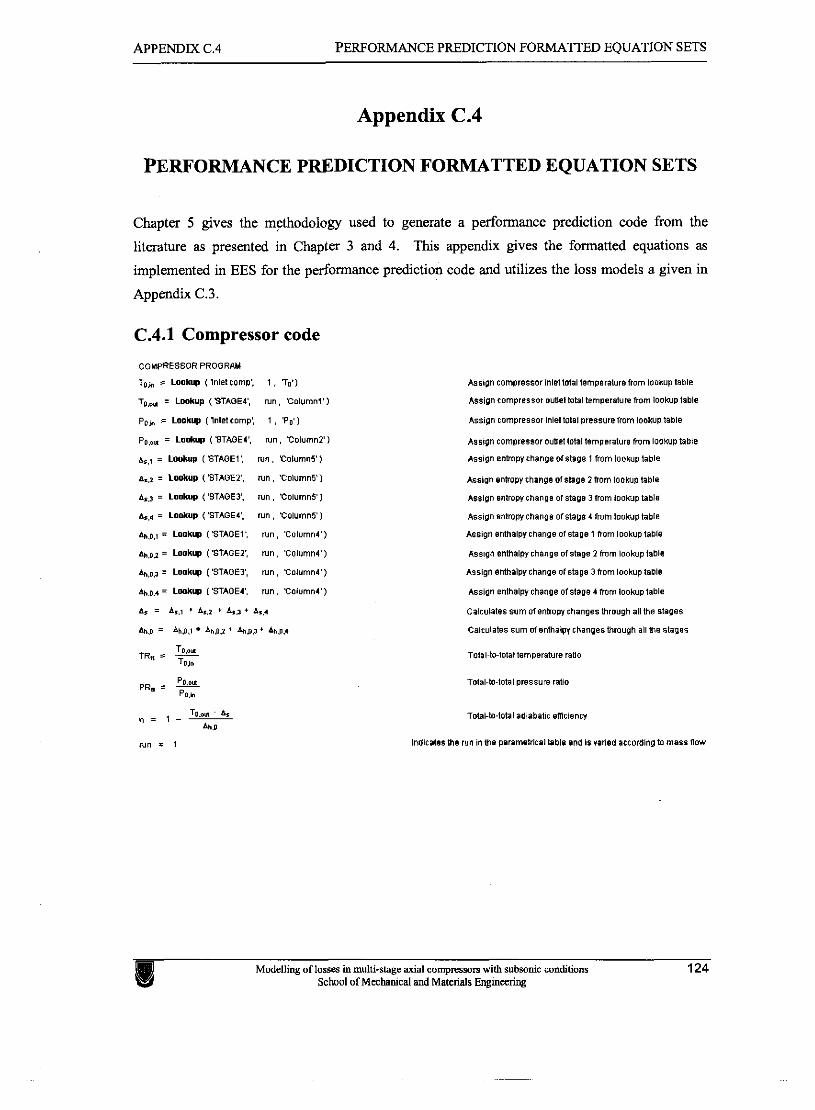
APPENDIX C.4 PERFORMANCE PREDICTION FORMATTED EQUATION SETS
Appendix C.4
PERFORMANCE PREDICTION FORMATTED EQUATION SETS
Chapter 5 gives the methodology used to generate a performance prediction code from the
literature as presented in Chapter 3 and 4. This appendix gives the formatted equations as
implemented in EES for the performance prediction code and utilizes the loss models a given in
Appendix C.3.
C.4.1 Compressor code
COWESSOR PROGRPY
T~~ F L o o m ( lnletwmp: 1 , 70'1
To,- = Lookup ( STAGE4'. run . 'Columnl')
Po, s Lookup (lnletmmp', 1 , Po ' ]
Po., = L o d w ( STAQEI', run, 'Column2 I
&,, = L&up ('STAGEY mn. Columns]
= Lmkup (STAGEZ', run, 'Columns)
AS,, = Lookup ( 3TAGE3: run. 'Columns]
A,,, = LOOXUP ( STAGEI: run, 'Columns]
Ah,o,, = Lookup (STAGE,: run, 'Columnl')
= Lookup (STAGE2: run. 'Columnl')
Ah,o, = Lookup ( 'STAGE3'. run, 'Column4')
ah.o.4 = Lmkup ('STAOEI: run. 'Column4')
A = As.? ' 4 . 2 + A s 1 + 0 . 0
Ah, = Ah9.1 4g.z ' AW.1' k9.4
TRn ' D..u Torn
pRa ' k Po.n
&s!gn Comprssmr lnlettmal temperature from lookup table
Asslgn romprersm outleltobl temperaturefmm lookuptable
A S S I ~ ~ tompre~sor lnlettotsl pressure fmm lookup table
A w g n CDmpmSSOr Outtatotal temperature from lookup table
Assign Pnbopychange ofstage 1 hom lookup table
&PW enbow change OTs$ge 2 tom lookup table
~ s s l g n entmwcnanga of stage 3fmm lookup table
As51gn entm~change ofstage 4fmm lookuptable
A661gn emhalpyrhanga ofstage 1 hom lookup table
Assign enmalmrhange of stage 2fmm lookuptable
ASSIQ~ enthalpychange afstaga 3 hom lookupta~le
A w g n enthalwchaogs of stage l m m lookuptable
CaI~~la les sum ofenhopy changes through allme stages
Calculates sum ofenthaloy changes through all the stages
~mal-to-total pressure ratio
InaiCatesme run i n n s paramehicsltable and isvaned atcoralngm mass flov
Modelling of losses in multi-stage axial compresson with subsonic conditions 124 School of Mechanical and Materials Engimring
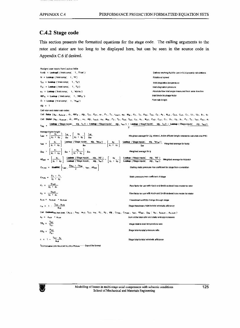
APPENDIX C.4 PERFORMANCE PREDICTION FORMATTED EQUATION SETS
C.4.2 Stage code
This section presents the formatted equations for the stage code. The calling arguments to the
rotor and stator are too long to be displayed here, but can be seen in the source code in
Appendix C.6 if desired.
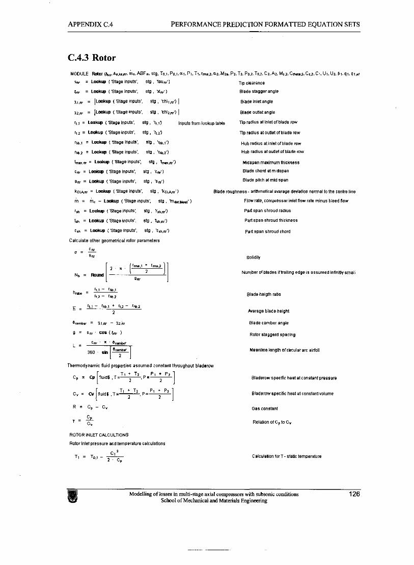
APPENDIX C.4 PERFORMANCE PREDICTION FORMATTED EQUATION SETS
C.4.3 Rotor
1-2 = Lookup (Stage inputs', stg . h.21 rm.8 = Loolw L 'Stage Inputs', $19 , b .1 '1
rm.2 = Loolwp ('Stage inputs', st9 . 'rw2')
lnmn = Lookup ( Stags inputs', st9 . I,,')
c, = L ~ U P ( ~ t a g e inputs', $10, 'c*')
sn, = Lookup (Stage Inputs', st9 , '5,')
kcmm = Lookup I Staga inputs: stp , Xcm.;)
m = m, - Lookup ( 'Stage Inputs', st9 , r n ~ ~ , ~ ' 1
r,, = L w b ('Stage inplrts', plg , 'rhm')
trh = L m u p (Stags inputs: s!g . t.h,,;)
t,h = Lookup ( 'Stage input^', $19 , 'tlh,,d)
Calculate other geometrical mtor parameters
c, o = - s",
Nb = Round I C
n p radius atoueat olblade row
Hub radius at Inlet olblade m
Hub radius atoutlet ofblade rm
Midspan mwmum mlcmess
Blade chord atmdspan
Blade pitch at mid span
Blade mughness- sdmmeticsl Pvarage dwlatlon normal tothe Centre llne
Flwrate, compressor inletflowrate minus bleed flow
Palf span shroud radlus
Palfspan shroudthirkness
Pert wan Shroud chord
Number ofblades lltralllng edge Is assumed infinlWrmati
Blade heigth aUo
Thermodynamic fluid propelfles assumed constant throughovt bladerow
T I + T I P I P I C, = CP [nUidl .T=--- I Bhd8r0wspe~f f l~ heatatronsbnt pressure
2 BIadnrwspec~c heatatconstantvolume
R = Cp - C, 088 COnSlsnt
T = SL C" Retatton ofc, to C,
ROTOR WiLETCALCULTIONS
Rotor Inlet pressure and temperature cairulatlons
CI = TI = TO,, - - CalculaUon lorT- staer tsmpsrstura 2 C.
Model l ing of losses in multi-stage axial compressors wi th subsonic conditions 126 School of Mechanical and Materials Engineering
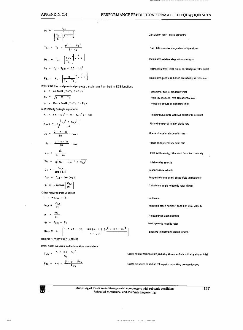
APPENDIX C.4 PERFORMANCE PREDICTION FORMATTED EOUATION SETS
Calculatlonror P - statlc pressure
Calculates relaI'm stagnation temperature
Cslculates m l a m stagnation pressure
h~ = Cp . TI),,, - 0.5 u,' R o t h a l ~ at rotor inlet equal to rothalpy at mtor ouuet
CalCUlataP preSsUre based on rothalpy at mtor inlet C, . TI
Rotor inlet thermodynamical property cllculations from buin in EES functions
PI = ~ ( f l u i d l , T = T l , P = P j ) Denslhorfluld st bladsrwinlat
a1 = d m Velocihlof sound, mls at bladeraw inlet
w = Us (nuid$ .T=TI .P=P , 1 Viscosihlofnuid at bladerow inlet
lnlet velocity triangle equations
A! = ( s . r,,? - x TW,, >I . PaF Inlet annulus area with ABF taken into account
rms.1 = Rms diameter 3 inlet ofblade row
2 Z N U I = 7' r-,,? Blade Dherlpheral speed at rmsi
1 2.5 ( C t s in (a1 + p t l ) ' + 0.5 u I P PI,." = 9,
4 . c,= I
lnlet amalrelocitv, calculatsdfrom the rontlnuih
lnlet relatheralocity
InletAbsoluterelornv
Tan#entwI component olibsoirrts lnletmloe~ty
Calculate9 angle re lamto rotor at inlet
Incidence
InIetaKlal Mach number, based on aria1 velocty
Rdable inlet Mach number
lnlet dynarnlr head to rotor
ElrectNe inlet dinam8r head for rotor
ROTOR WTLETCNCULTIONS
Rotor outlet pressure andtemperature calculations
h,+ 0 5 U12 To.?, ' OUtlEtr~iaWe I~mperatUre, romalpy at rolor ouUet= rothalpy at rotor inlet
CP
P7.2 = P,., - q! PT.I Po,,. Outlet pressure based on mthalpy inrorporating prssure losses
School of Mechanical and Materials Engineering
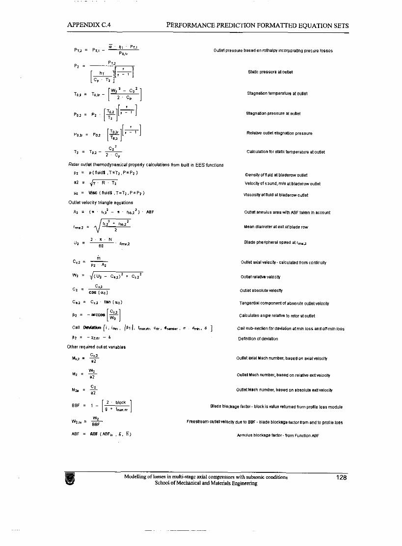
APPENDIX C.4 PERFORMANCE PREDICTION FORMATTED EQUATION SETS
TO> = TO> - [w121 ,-c72 ] stsenation temperatun at outlet
PO,, = P. , [+$+I Stagnation pressure at ouust
CI' T2 = TO,I - - Calculiltlonfor statictemperature at outlet 2 CP
Rotor oullal thsrm~dynamical propelly calculations hom bulR in EESfunctions
P? = ~ ( f l u idS , T = T 2 . P = P z ) Densib oflluid at biadwow outlet
a2 = d m - Velocn,ofsound, m ~ s at bladermamet
= Urc (fluid$ ,T=Tz.P=Pz) wscoswarnu~a at bladarow oimet
Outlet velocltg Inangle equ~tions
A? = ( n kz2 - l ihb.2') ABF Outlet annulus area with ABF taken In account
Mean dlametsr at extolblade row
2 r N Uz = , I-> Blade phenpheral speed at rm2
Outlet aaalvslocih- caiculafaa(mm continuin,
outlet absolute velorltf
Tangential component of absoiute outletvelocln,
Calculates angle relative lo rotor at outlet
Ca l subsection for denahon almin lass andolFmin loss
Definition orderlaoon
Ounet anal Mach number, based on axmlnlocln,
w2 M1 = -
82 Outlet Mach number, based on relal're entveloclly
c2 M2. = Outlnt Mach number. based on sbsolum exltvelocih
BBF ; 1 - [g2 block ] + t,m
Blade blackage fartor- blockis value returned from profile loss module
wz 2 , = Freestream outletnlorllydue to BBF- blade blockaoafartorb~m andto profile loss
ABF = ABF (ABF, , Z . 6) *nnUIUB b I 0 ~ L ~ p e fatlor- horn Function ABF
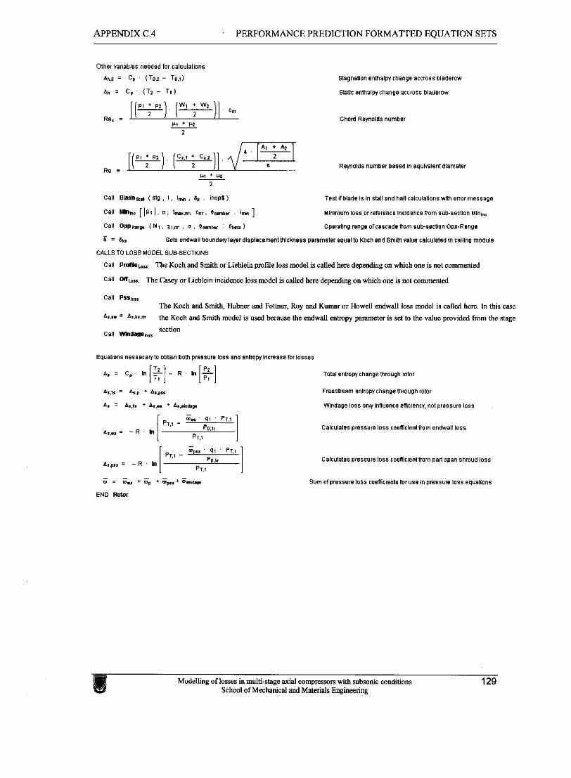
APPENDIX C.4 PERFORMANCE PREDICTION FORMATTED EQUATION SETS
Other variables needed for calculations
Ah.0 = C, . (To2 - T0.11
= C p (TI - TI)
[ ( W ! ;w2 2 cm
Re. = w, . w? -
2
Stagnation enthalwchange acemse bladerow
Statlc enmaiwchanga accross bladerow
Chord RBm01d6 number
Call BWsa* ( at9 , I , I,. . 8, . ~nopf 1 Test If blade Is In *all and hancaleulationr with enor message
call ~ i l w [ I P ! 1 . o . tnp.nr, hr. bmar : ] Mlnlmum loss or reference lncldsnra Rom subsection Mini..
Call WPR,, ( M ? . I I ~ , . D . 0-a.r : 6~ Opemtina now ~ fcasmde bom sub-secuon Opp-Range
6 = a*, Sets endwall boundarylapr dlsphcsmsnt thleknsss parameter equal to Koch and Smith villus calculated In calllng module
WS TO LOSS MODELSUBSECTIONS
Call ProNsb,, The Koch and Smith or Lieblein pmae loss model is called here depending on which one is not commented
call Mb-, The Casey or Lieblein incidence loss model is called here depending on which one is not commented
Call PPDI~,, The Koch and Smith, Hubner and Former, Roy and Kumar or Howell endwall loss model is called here. In this case
= A..h..nr the Koch and Smith model is used because the endwall entropy parameter is set to the value provided from the stage
section call wn!lw..,r
Eq~aUon5 ne58acaryto obtain both pressure loss and entropy Increase for losses
A. = Cp h [$] - R b [$] Total entropyrhangethrough rotor
Freesbeam sntrowchanpe through rotor
Wndage loss ontfinfluenre emmncy, not pressure loss
Calculates oressure 1055 roemclentfrom endwall loss
mp. 91 PT.I PT., -
A,-, = - R . b P@,* 1 Calculates pressure loss coemc~edhom panspan shroud loss
- - = ... + % *&.*G- Sum of pressure loss roemclentsfor use in pressure loss equations
END Rotor
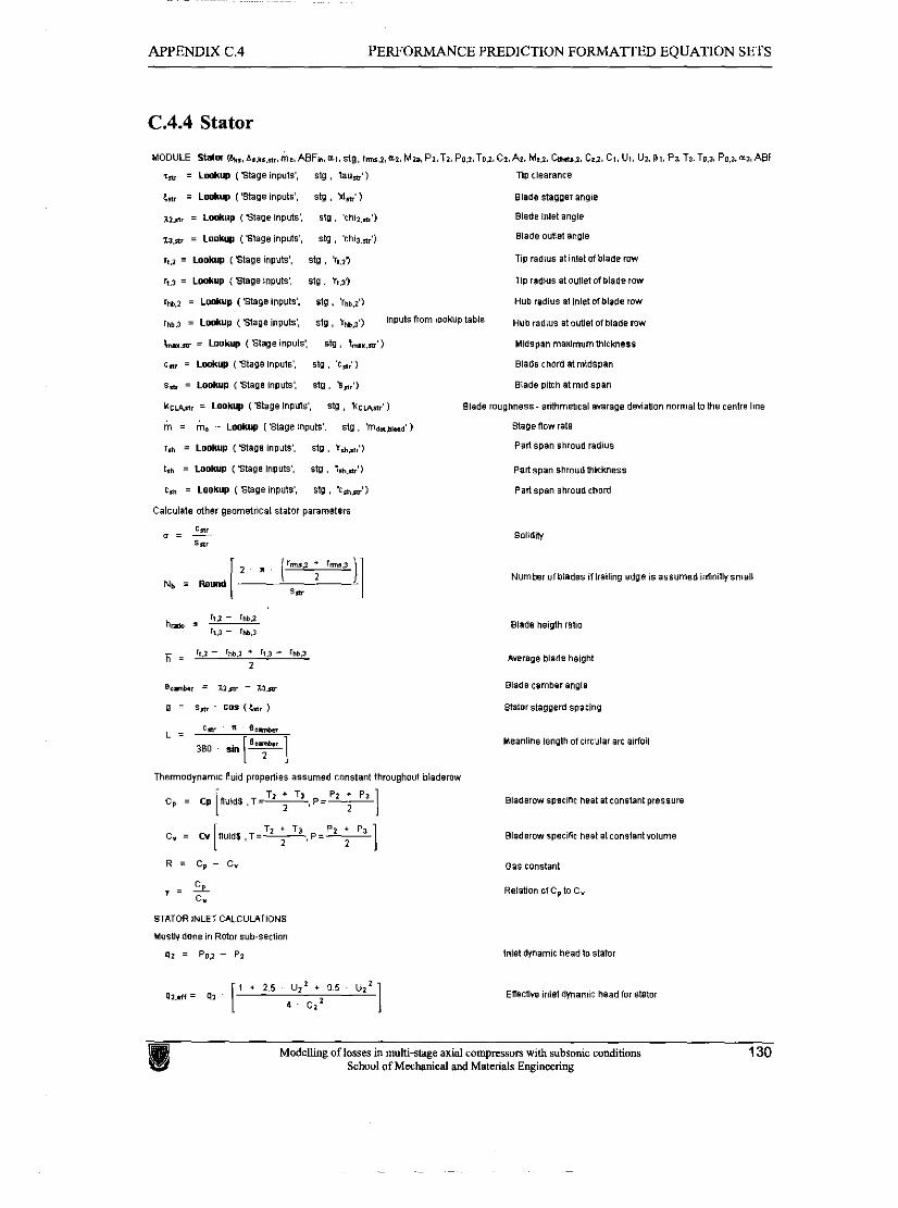
APPENDIX C.4 PERFORMANCE PREDICTION FORMATTED EQUATION SETS
C.4.4 Stator
MODULE nata (h , ,A , ,~~ ,~ , ,m~ .ABFn.a~ ,s tg , m-.2,=~. MI.,PZ,T~, PO~,TO,I,CI,A~. Mt.2. &S.L C Z . ~ . CI, UI, UI. PI. P P T ~ , T o . ~ . Po.5.wABi
r,, = Lmkup (Stage inputs', stg , l a u d ) Tip ~ lea ran~e
c,,. = Lm*lp ('Stage inputs', stq , 'dm' 1 Blade stwg01 angle
a?*, = Lmkup (Stage inputs', stg , 'ch12,,') Blade inlet angle
I ? , ~ , = Lookup (Stage inputs', stq , 'chl$,&j Biads ouaet anale
r,,? = u o k u p (Stage inputs', st9 , h . ~ l Tip radius at inlet of blade rmv
h.2 = LoolWp ('Stage inputs: stg , 'rt3? Tip radius at outletof blade row
rm.2 = LooHup ( 'Stage Inputs: st9 . 'rha.i) Hub radius a1 Inlet ofblade rmv
,ha,, = ~ookup (Stage inputs', stg , vw3,) lnp"t*n"m iookup tabla ~ u b radius at outlet ofblade row
= L O O W UP 'Stage inputs: 919, bx,,d) Midspan maromum thlrlorsss
r, = Lmkup (Stags inputs', st9 , 'id; I Blade chord at mtdrpan
o, = Lookup (Stage inputs', st9 , 3,') Blade p i t h at mld span
kc-. = Lookup ('Stage inputs', st9 , kc-.' 1 Blade roughness- srlhmetlcai avarage dmiatlon normaitothe cenhs llne
m = m, - ~ o o k y , i Stage Inputs', st9 , 'maa.ak.d' ) stam now rats
I* = Lookup (Slag8 inputs', sta , vh,.,rl) Part span shroud radlus
I,, = LOO~UP ( 3taga inputs', st9 , TShm') Part span shroudmiekness
crh = LOO~YP ( ~ t a a e inputs', stg , tsh,d) Partspan shroudchod
Calculate other gaometrlcal stator parameters
Number afbladss iftrailing edge 1s assumed mlnillysmall N. = Round
Thsrmodynamr flu~d properties assumed constant throughout blademv
STATOR INLET CALCUIATIONS
Mostbdone ~n Rotor sub.section
q, = Po3 - P2
Blade h e w ratlo
merage blads height
Blade LPmbBIPnglB
Stator staggeld sparing
Meanltne length of clrcdlar arc alfofl
Oas constant
RelationofC.to C,
lnletdmamic headto stator
Ellectirs inietdynamlr head for atator
Model l ing of lasses in multi-stage axial compresson with subsonic conditions 130 School of Mechanical and Materials Engineering
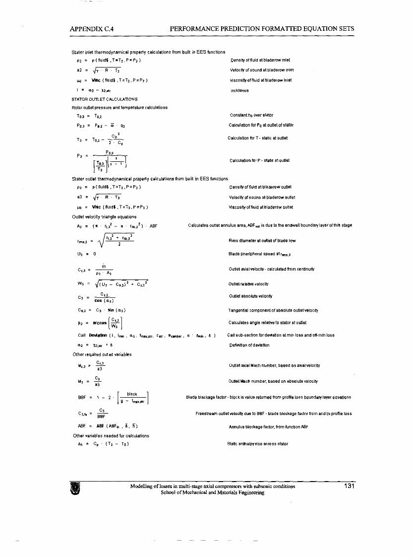
APPENDIX C.4 PERFORMANCE PREDICTION FORMATTED EQUATION SETS
Stator inlet thermodynamical property calculations from bud1 in EES functions
p2 = p(nuid$ .T=T~ ,P=PI ) Densihloffluld at bladerwlnlet
a2 = Jm veiornvofsound at bladsmnlnlet
w = W s ~ ( f l u l d $ . T = T ~ , P = P ~ ) v~scositf offluid at bladsrav Inlet
I ' a2 - war Incidence
STATOR OUTLET CALCULATIONS
Rotor Ouuet pressure and tamperahwe ralculatione
To3 = TO.? c m t m t n o over stamr
Po,$ = Po,? - w 41 Calculatlonfor Po at outlet of stator
c, ' T, = Tot - Caltulalon for T. statlc at ouUst
Calculation for P - stant at oulet
Stator outlet thermodynamical propeny calculations from built in EES functions
03 = p(flu1dS . T = h . P = p , ) Denslhloffluld at blammw ouuat
a3 = dl- velocity ol bound at bladerow outlet
= vlsc ( n m .T=T, .P=P~ 1 vmosiw ofnula at bladerow ounet
Outlet velocity triangle equations
A$ = (s r,,? - x rw12) ABF C ~ I L U I ~ ~ B B ouuetannuIus area.~BF, is due t o t h ~ enmall boundanlsyer ofthis stage
I m . 3 ' Rms Ulametar at outlet orblade rw
UI = 0 Blade pheripheral speed atr,.,a
cez = c, sin (a,) Tangenbal component of absolute outletvelorty
call oeviatlon ( i , i~ , a,. 1 ,.,,.. r., , LL.~., , o ' hh. 6 ) Call sub-sectionforde*lation atmln loss and m m i n loss
a3 = U.N ' 6 Deilnltlon of de*labon
Other required outlet rar~ables
c,,, Mz) = - Oubetaxial Mach number, based on aualvelorihl a 3
CI M, = - ouaet Mach number, based on absolutevsloclh a3
black BBF = 1 - 2 Blade b i w k a g ~ f a c t ~ t ~ blockisvalue rotumedfrorn profile loss boundlnlapr equations
C1 c3.t. ' Freestream outletvelorlhldus to BBF - blade blockage factor fmm andto proflis loss
ABF = ABF (ABFh , 6 , 6)
Other variables nssded for calculations
ah = CD (Ts - 111
MnuIus biockagefacfor, homfunrt~on ABF
Siabc enmalpy nse across stator
Modelling of losses in multi-stage axial compresson with subsonic conditions School of Mechanical and Materials Engineering
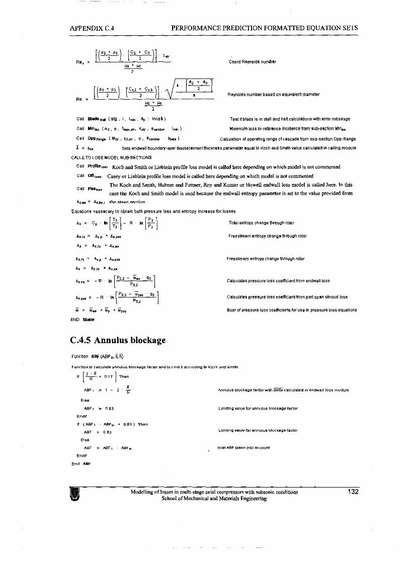
APPENDIX C.4 PERFORMANCE PREDICnON FORMAlTED EQUATION SETS
Chow Reynolds numbel
call BWW (s$ , i . lhh . ap : loop$ I Testlfblaae is in stall and halt ~alculationovlm error message
Call Minm (a?. o , t,.ar. ce,. U c m a i* I Minimum loss or reference incidence from sub-sscbon Mlni,
call OPPR~W ( ~ 2 , . ~ 2 . ~ ~ , o . 8- ha I Calrualtion ofoperatlng range orcascade from sub-section OPD-Range
E = a", sets enwall boundawlaysr dispiarsmenlmirmnssss parameter squalto Koth and Smnhvalus calculated In calling module
CRUS TO LOSS MODEL SUB-SECTiDNS
Proflleus: Koch and Smith or Lieblein pmfde loss model is called here depending on which model is not commented
call orrws, Casey or Lieblein pmfile loss model is called here depending on which model is wt commented
The Koch and Smith, Hubner and Former, Ray and Kumar or Howell endwall lass model is called here. In this call ~ss..,
case the Koch and Smith model is used because the endwall entropy parameter is set t o the value pmvided fmm
AS- = A,#. the stsop w~.tion
Equations nessacary to obtain both pressure loss and entropy increase for losses
P A, = Cp . I" [$ - R , !+B [el Total entropy change mrough rotor
AS,', = b , , ~ + & p u
A, = A,,'< A,,..
C.4.5 Annulus blockage
Llrn"l"* *a,"= '0, annulus blockage factor
IniatABF tarsn into account
Modelling of losses in multi-stage axial compresson with subsonic conditions 132 School of Mechanical and Materials Engineering
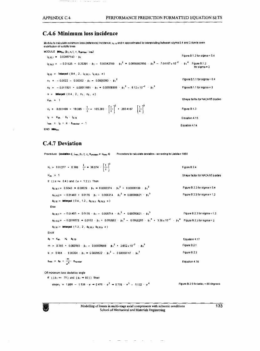
APPENDIX C.4 PERFORMANCE PREDICTION FORMATTED EQUATION SETS
C.4.6 Minimum loss incidence
~odu le to takulate minlmum ionc (re(enws1 Inadencs. $.,,o aodn approiimded by intsrvoiaflng between sigma 0.4 and 2dueto even dlsblaution of soU5Wiinas
MODULE W h o (Pl.o.1, c, Omk'imhl
I = 0.02857143 Pr Figure 8 1.2 for 519ma' 0.4
10,102 = - 0.01525 + 0.20391 B j - 0.00342769 plr 0.0000862955 8," 7 0 4 1 6 7 x 1 0 ~ - pq4 FiguraBl.2 for slpma= 2
I = Merpoi (0 .4 . 2 . i o m i io.lo.2. 01
n~ = - 0.0522 - 0.00302 . 8 , - 0.0000393 B 1 = FIgurs 8.1.1 W l Sigma= 0.4
nl = - 0.011821 + 0.00017691 8, 0.00000606 . pll - 6 . 1 2 ~ 1 0 ' 8, ' Figure 8.1 1 for sigma= 2
n = llllerpol i 0.4 , 2 , n l . nz , r r l
K,h = I Shape fartorfor NACA65 blades
C.4.7 Deviation
Procedure Devlalbn 0 , lmn, p,. I, C. em-. m 6,. 61 Pmedurelo eslculde derlltlon- arcomlngto UoMlen 1960
t Kt = 001277 r 6386 - 36074
K.h = 1
e ( l o * = 0 4 1 and ( 0 s 1 2 1 1 Then
h o $ 0 1 00043 000629 PI 00000374 P? ' + OOOOOOlO~ PI'
~ o , I o ~ : = - 001483 + 00176 PI - 0,000214 p t 2 0.00000821 - 81'
4.10 = *pol ( 0 4 , 1 2 . 60.10.1 4,,01 r r )
Else
4,,0,1= -001483 r 00176 PI - 0.000214 plf + 000000821 k t 3
60.,03:= - 0.0016575 0.0102 Pi + 0.000962 b I 2 - 0.0000255 p13 + 326x10-'
6o.10 := ntwpol (1.2 , 2 . 4 , 8 o . \ 6o.lo.r o I
Endn
4 = l(rh . 14 b.ro
rn := 0.255 + 0.000583 PI - 0.00000869 8,' + 2652x10-' 81'
b := 0964 - 000304 PI 0.0000622 . p!' - 000000147 6,'
m 6mn := h ' - 0.zmb.r
o h
Figure 82.4
Shapefactorror M c ~ 6 5 biadss
Flgure 8 2.3 for sigma = 1.2
PI' FlgUre 8.2.3f0rSlgm8= 2
EquaUon 4.17
Figure 81.1
Figure 8.2 2
Off minimum loss denallon angle
n ( ( p ! .; 70) and (PI 60)) Then
slopel = 1.006 - 1.526 - a 0.475 n 2 0276 a" 0132 .' Flgure 8.2 5for beta, = 60 degress
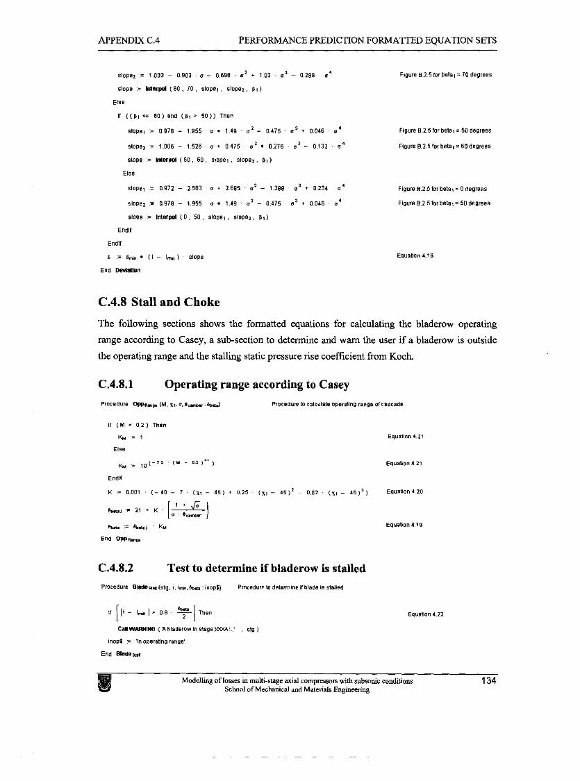
APPENDIX C.4 PERFORMANCE PREDICTION FORMATTED EQUATION SETS
slopel := 1.003 - 0.903 o - 0.696 o1 + 1 0 2 0' - 0.200 0' Figure 8.2 5 lor b s t a ~ = 70 degrees
slope = merlrol ( 6 0 . 7 0 . slope, . slope,, PI)
Else
If ( ( P I .= 6 0 ) and (PI 5 0 ) ) Than
SIOPOI := 0878 - 1.955 v 1.49 r r2 - 0.475 0' + 0.046 s 4
slope2 = 1.006 - 1528 o t 0.475 m 2 0.276 a 3 - 0.132 m'
slope = Werpol ( 5 0 , 6 0 , slopet . S l o P e ~ , PI)
Else
S I O P O ~ := 0.972 - 2.563 o + 2.605 of - 1.288 o 3 + 0.234 o'
$lope? .= 0.978 - 1.955 0 1.49 o1 - 0.475 . a' + 0.016 - o'
slops := Interpal ( 0 . 50 , slops, , slops2 . 8 , )
End11
Endlf
a := h ( I - I,. ) slope
End k.mum
F i p R 8.2.51oi betar = 50 degrees
Figure 0.2 5for beta, = 60 degrees
Figurs 0 25 for beta, = 0 degrees
Figure 8 2 5 f o r beta, = 50 degrees
C.4.8 Stall and Choke
The following sections shows the formatted equations for calculating the bladerow operating
range according to Casey, a sub-section to determine and warn the user if a bladerow is outside
the operating range and the stalling static pressure rise coefficient from Koch.
C.4.8.2 Test to determine if bladerow is stalled Pmcedurs BUclse.l (slg, I. irnh.&- : inop$) Procedureto deUrmlne lb lada is st-dbd
CarwrrunrIG ( la laderow in s l s g e m l . : , stg )
inop$ = In operaling range'
End Bladead
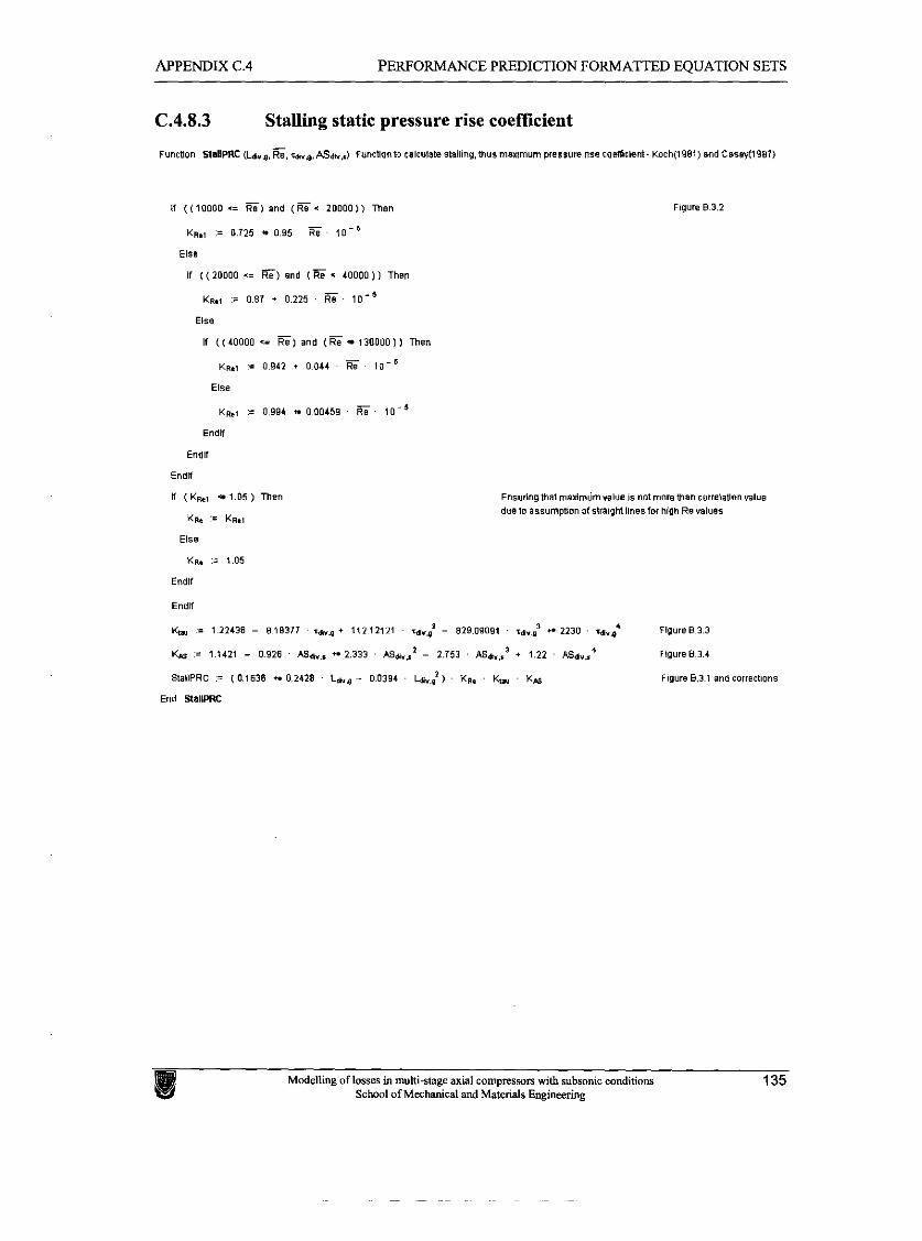
APPENDIX C.4 PERFORMANCE PREDICTION FORMATTED EQUATION SETS
C.4.8.3 Stalling static pressure rise coefficient -
Funrhon SaUPRC (Larr, Re, raro,ASa.,.l F u ~ t l o n l o calculale sblllng,tnus manmum pressure nae cochlclent- Koch(1981) and Cssal(1987)
n ( ( roooo *= K ) and (% < 100001) men
KR., = 0.725 0.95 E . 10.'
El98 -
If ( ( 20000 '= R e ) and (E . 40000 1 I Then
KR.! := 0.87 + 0.225 . ?ii l o - '
El58
W ( (40000 c- E) and (E 1 3 0 0 0 0 ) ~ Then
KR., = 0.942 + 0.041 - Ti;C
Else
KR.I .= 0.994 0.00159 10.'
Endlf
Endlf
End11
I( ( K,, 1.05 ) men
K w '= KR.I
Else
KR. .= 1.05
E"dlf
Endlf
v&, = 1 22138 - 8 18377 zag + 112 12121 - 829.09091 raw,: 2230 . wv,: Flgurs 0 3.3
IG = 1.1121 - 0.928 ASdnr 2.333 ASl.,,' - 2.753 .&Saw,.' + 1.22 AS^^^' Flgure 83.4
SbIIPRc := (0.1838 0.2428 L W , ~ - 0.0394 ~d,,:) KR. Ku, K*; Flsure 8.3.1 and corrections
End StallPFX
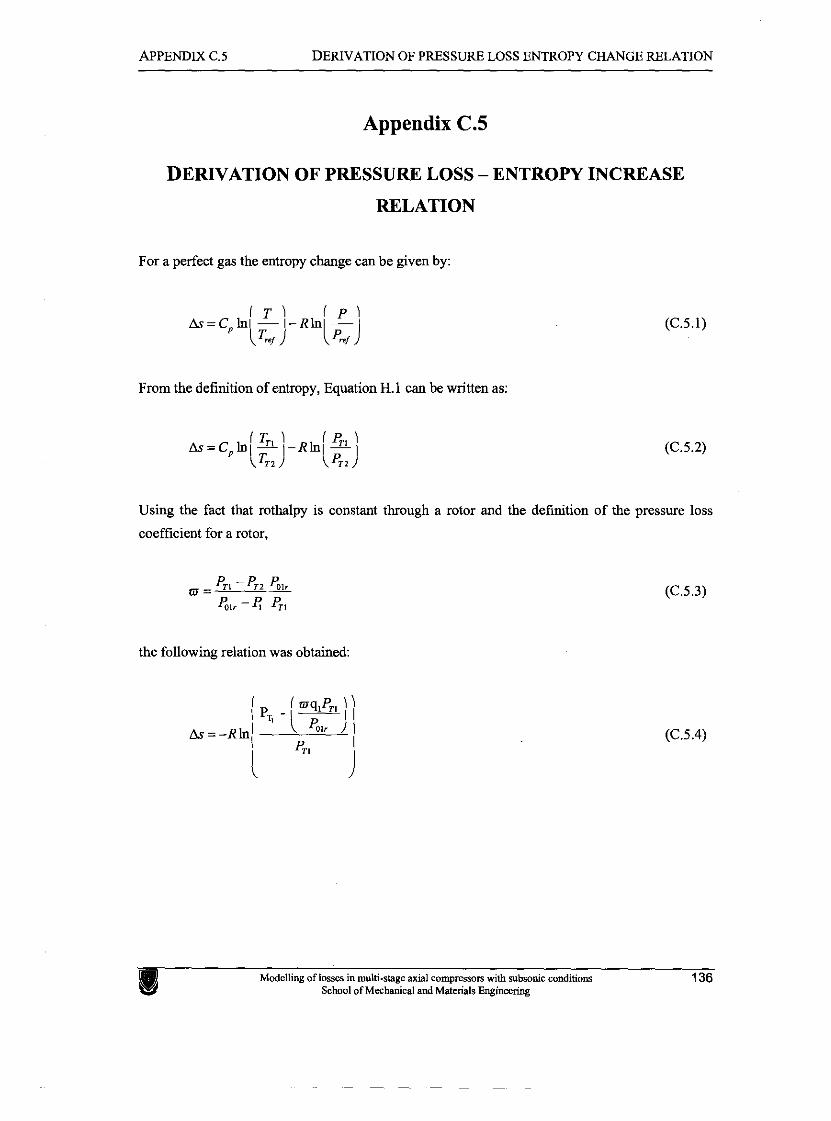
APPENDIX C.5 DERIVATION OF PRESSURE LOSS ENTROPY CHANGE RELATION
Appendix C.5
DERIVATION OF PRESSURE LOSS - ENTROPY INCREASE
RELATION
For a perfect gas the entropy change can be given by:
From the definition of entropy, Equation H.l can be written as:
Using the fact that rothalpy is constant through a rotor and the definition of the pressure loss
coefficient for a rotor.
the following relation was obtained:
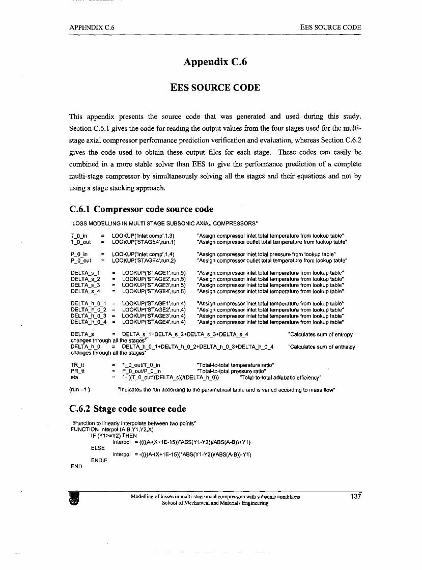
APPENDIX C.6 EES SOURCE CODE
Appendix C.6
EES SOURCE CODE
This appendix presents the source code that was generated and used during this study.
Section C.6.1 gives the code for reading the output values from the four stages used for the multi-
stage axial compressor performance prediction verification and evaluation, whereas Section C.6.2
gives the code used to obtain these output files for each stage. These codes can easily be
combined in a more stable solver than EES to give the performance prediction of a complete
multi-stage compressor by simultaneously solving all the stages and their equations and not by
using a stage stacking approach
C.6.1 Compressor code source code "LOSS MODELLING IN MULTl STAGE SUBSONIC AXIAL COMPRESSORS"
T-0-in = LOOKLP('lnle1 wmp'.l.3) "Ass gn compressor Inlet lotal temperature from ~ o o ~ u p tame' T-0-obt = LDOKJP('STAGE~',N~.~) 'Asstgn compressor o ~ t l e l total temperature from loomup taole'
P-0-in = LOOKUP('lnlet wmp'.lA) "Assign compressor inlet total pressure from lookup table" P-0-out = LOOKUP('STAGE4,run,2) "Assign compressor outlet total temperature from lookup table"
DELTA-s-I = LOOKUP('STAGEl'.run.5) "Assign wmpressor inlet total temperature from lookup table" DELTA-s-2 = LOOKUP('STAGET,mn.5) "Assign compressor inlet total temperature from lookup table" DELTA-5-3 = LOOKUP('STAGE3',run,5) "Assign wmpressor inlet total temperature from lookup table" DELTA-s-4 = LOOKUP('STAGE4.run.5) "Assign compressor inlet total temperature from lookup table"
DELTA-h-0-1 = LOOKLP('STAGEI',~CJ~.~) "Assngn compressor nlet total temperature trom look~p table' OE-TA.n-0-2 = -DOkJP('STAGEZ'.run.4) 'Ass.gn compressor inlet tom. lemperature from loom~p tab e' DELTA-h-0-3 = LOOKUP('STAGE3'.wn,4) "Assign wmpressor inlet total temperature from lookup table" DELTA-h-0-4 = LOOKUP('STAGE4'.run.4) "Assign compressor inlet total temperature from lookup table"
DELTA-s = DELTA-~-I+DELTA-s-~+DELTA-s-~+DELTA-s-~ "Calwlates sum of entropy changes through all the stages" DELTA-h-0 = DELTA-h-0-1 +DELTA_h-0-2+DELTA-hhO03+DELTAChhO-4 'Calculates sum of enthalpy changes through all the stages"
TR-tt = T-0-ouU-0-in "Total-to-total temperature ratio" PR-ll = P-0-ouVP-0-in "Total-to-total pressure ratio" eta = 1- ((T-0-our(DELTA-s))l(DELTA-h-0)) "Total-to-total adiabatic efficiency"
(run = I ) "Indicates the run according to the parametrical table and Is varied according to mass flovf
C.6.2 Stage code source code "!Function to linearly interpolate between two points" FUNCTION Interpol (A,B,YI.Y2,X)
IF (YI>=YP)THEN Interpol =((((A-(X+lE-15))'ABS(YI-Y2))/ABS(A-B))+Yl)
ELSE Interpol = -((((A-(X+lE-l5))'ABS(YI-Y2))/ABS(A-B)~Yl)
ENDIF END
Modelling of losses in multi-stage axial compressom with subsonic conditions 137 School of Mechanical and Materials Engineering
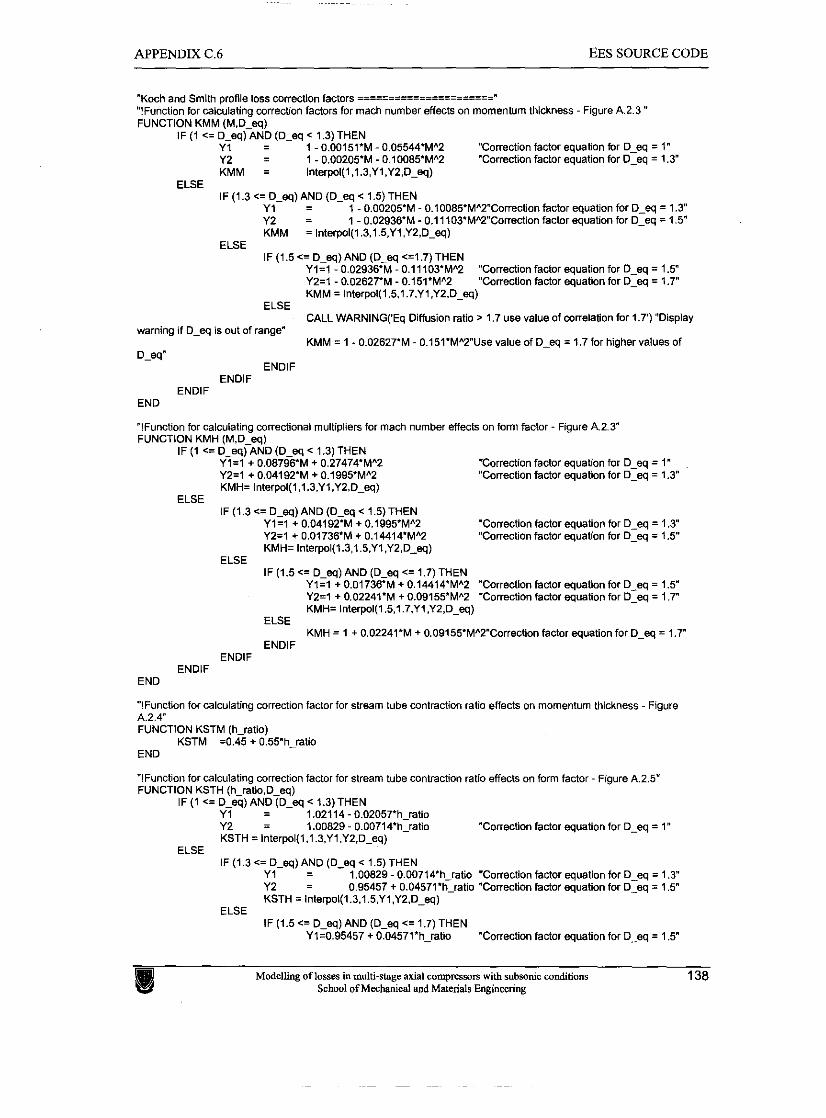
APPENDIX C.6 EES SOURCE CODE
"!Function for caiduiating correction factors for mach number effects on momentum thickness - Figure A.2.3 '' FUNCTiDN KMM (M,D-eq)
IF (1 C= D-eq) AND (D-eq < 1.3) THEN Y1 - - 1 - 0.00151'M - 0.05544'MA2 'Correction factor equation for D-eq = 1" Y2 = 1 - 0.00205'M - 0.10085'MA2 "Correction factor eauation for D ea = 1.3" - KMM = Interpoi(l.l.3.Y1,Y2.D~eq)
FI SF ---- IF (1.3 c= D-eq) AND (D-eq < 1.5)THEN
Y1 = 1 - 0.00205'M - 0.10085*MA2"Correction factor equation for D-eq = 1.3" Y2 = 1 - 0.02936'M - 0.11 103'MA2Correction factor eauation for D eq = 1.5" - KMM = Interpol(l.3,1.5,YI,Y2,D-eq)
FI SE ---- IF ( I .5 <= D-eq) AND (D-eq Cs1.7) THEN
Y l = l - 0.02936'M - 0.11 103'MA2 "Correction factor equation for D-eq = 1.5" Y2=1 - 0.02627'M - 0.151*MA2 "Correction factor equation for D-eq = 1.7 KMM = interpol(l.5.1.7.Y1,Y2,D~eq)
ELSE - -
CALL WARNING('Eq Diffusion ratio > 1.7 use value of correlation for 1.7') "Display warning if D-eq is out of range"
KMM = 1 - 0.02627'M - 0.151'MY"Use value of D-eq = 1.7 for higher values of
ENDlF ENDlF
END
*!Function for calculating correctional multipliers for mach number effects on form factor - Figure A.2.3" FUNCTiDN KMH (M.D-eq)
IF (1 <= D-eq) AND (D-eq < I .3) THEN Y1=1 + 0.08796-M + 0.27474'MA2 Correction factor equation for D-eq = 1" Y2=1 + 0.04192.M + 0.1995'MA2 "Correction factor equation for D-eq = 1.3" KMH= interpol(l,l.3.YI,Y2.D~eq)
ELSE IF (1.3 C= D-eq) AND (D-eq < 1.5)THEN
Y1=1 + 0.04192.M + 0.1995'MA2 "Correction factor equation for D-eq = 1.3" Y2=1 + 0.01736'M + 0.14414'MA2 "Correction factor equation for D-eq = 1 .5 KMH= Interpol(l.3,1.5,Y1,Y2,DDeq)
ELSE IF (1.5 C= D-eq) AND (D-aq C= 1.7) THEN
Y l = l + 0.01736'M + 0.14414'MA2 "Correction factor equation for D-eq = 1.5" Y2=1 + 0.02241'M + 0.09155'MA2 "Correction factor equation for D-eq = 1.7" KMH= interpol(1.5,1.7,Y1.Y2,D~eq)
ELSE KMH = 1 + 0.02241'M + 0.09155'MA2"Correction factor equation for D-eq = 1.7"
ENDlF ENDlF
ENDiF END
"!Function for calculating correction factor for stream tube contraction ratio effects on momentum Ulickness - Figure A.2.4' FUNCTION KSTM (h-ratio)
KSTM =0.45 + 0.55'h_ratio END
"!Function for calculating correction factor for stream tube contraction ratio effects on form factor - Figure A.2.5" FUNCTION KSTH (h-ra1io.D-eq)
IF (1 C= D-eq) AND (D-eq c 1.3)THEN Y1 - - 1.02114 - 0.02057'h-ratio Y2 = 1.00829 - 0.00714'h~rallo "Correction factor equation for D-eq = 1" KSTH = Interpol(l,l.3,YI.Y2.D-eq)
Fl SE ---- IF (1.3 c= D-eq) AND (D-eq < 1.5) THEN
Y1 = 1.00829 - 0.00714'h-ratio "Correction factor equation for D-eq = 1.3" Y2 = 0.95457 + 0.04571.h-ratio "Correction factor equation for D-eq = 1.5" KSTH = interpoi(l.3,1.5,Y1,Y2.D~eq)
ELSE IF (1.5 c= D-eq) AND (D-eq c= 1.7) THEN
Y1=0.95457 + 0.04571'h-ratio "Correction factor equation for D-eq = 1.5"
Modelling of lasses in multi-stage axial compresson with subsonic conditions 138 School of Mechanical and Materials Engineering

APPENDIX C.6 EES SOURCE CODE
Y2=0.84457 + 0.15571'h-ratio "Correction factor equation for D-eq = 1.7" KSTH = interpol(l.5.1.7.Y1.Y2.D~eq)
ELSE KSTH = 0.84457 + 0.15571.h-ratio "Correction factor equation for D-eq = 1.7"
ENDlF ENDlF
ENDlF END
"!Function for calculating correction factor for Reynolds number and surface finish effects on Momentum thickness ratio - Figure A.2.6 FUNCTION KRSM (Re-c.k-CLA,c.W_l,rho.mu)
k-s = 6.2'k-CIA "Equation 3.7" RR = k-SIC "Relative roughness" RRe = (k_s'W_l'rho)lmu "Roughness Reynolds numbe? IF (RRe <= 90) THEN "Equation 3.B"
IF (Re-c < 200000) THEN KRSM = 600.178'Re~c"+O.5) "Momentum thickness vary as the -0.5 power of
chord Reynolds number" ELSE
KRSM = 10.224'Re-cA(-0.166) "Momentum thickness vary as the -0.166 power of chord Reynolds number"
ENDlF ELSE
KRSM = 23.398'RRA(0.347) "Power fit of relation of Relative roughness to correction" ENDlF
END
"!Function for calculating correction factor for Reynolds number and surface finish effects on Form factor - Figure A.2.6" FUNCTION KRSH (Re~c.k~CLA.c.W~l.rho.mu)
k-s = 6.2-k-CLA "Equation 3.T RR = k-slc "Relative roughness" RRe = (k-s'W_l'rho)lmu "Roughness Reynolds numbe? IF (RRe <= 90) THEN "Equation 3.6"
KRSH = 2.291'Re-cA(-0.06) "Form factor vary as the -0.06 power of chord Reynolds number" ELSE
KRSH = 23.398'RRA(0.347) "Power fit of relation of Relative roughness to correction'' FNDIF
END "End of correction factor functions for Koch and Smith profile loss model ================="
"!Function to calculate annulus blockage factor and to limit it according to Koch and Smith" FUNCTION ABF(A6F-in.deita-bar,h-bar)
IF (((2*(delta-bar))lh-bar) < 0.17) THEN ABF_I=(I - Tdelta_bar/h_bar) "Annulus blockage factor with deitcbar calculated in endwall loss
module"
"Limiting value for annulus blockage factor"
IF (ABF-I'ABF-in < 0.83) THEN ABF= 0.83 "Limiting value for annulus blockage factor"
ELSE ABF= ABF-I'ABF-in "inlet ABF taken into account"
ENDlF
END
"!Module to calculate minimum loss (reference) incidence, i-0-10 and n approximated by interpolating between sigma 0.4 and 2 due to even distribution of solidity lines" MODULE Min-inc(beta-l,sigma,t,c.theta-camber:i-min)
i-0-10-1 - - 0.02857143'bela-I "Figure 8.1.2 for sigma = 0.4" i-0_10-2 - - -0.01525 + 0.20391'beta-I - 3.42769E-03'beta-lA2 + 8.62955E-05'beta_lA3 -
7.041 67E-07'beta-IA4 "Figure 6.1.2 for sigma = 2" i-0-10 - - lnterpo1(0.4.2.i~0~l0~1,i~0~10~2,sigma)
n-1 - - -0.0522- O.O0302'beta_l - 3.93E-OS"beta-lA2"Figure B.l.l for sigma = 0.4"
n-2 - - -0.011821 + 1.7691E-04'beta-I + 6.06E-06'beta-IA2 - 6.12E-07'beb-IA3
"Fioure 61.1 for sioma = 2'
"Shape factor for NACA 65 blades"
Modelling of losses in multi-stage axial compresson with subsonic conditions 139 School oiMechanical and Materials Engineering
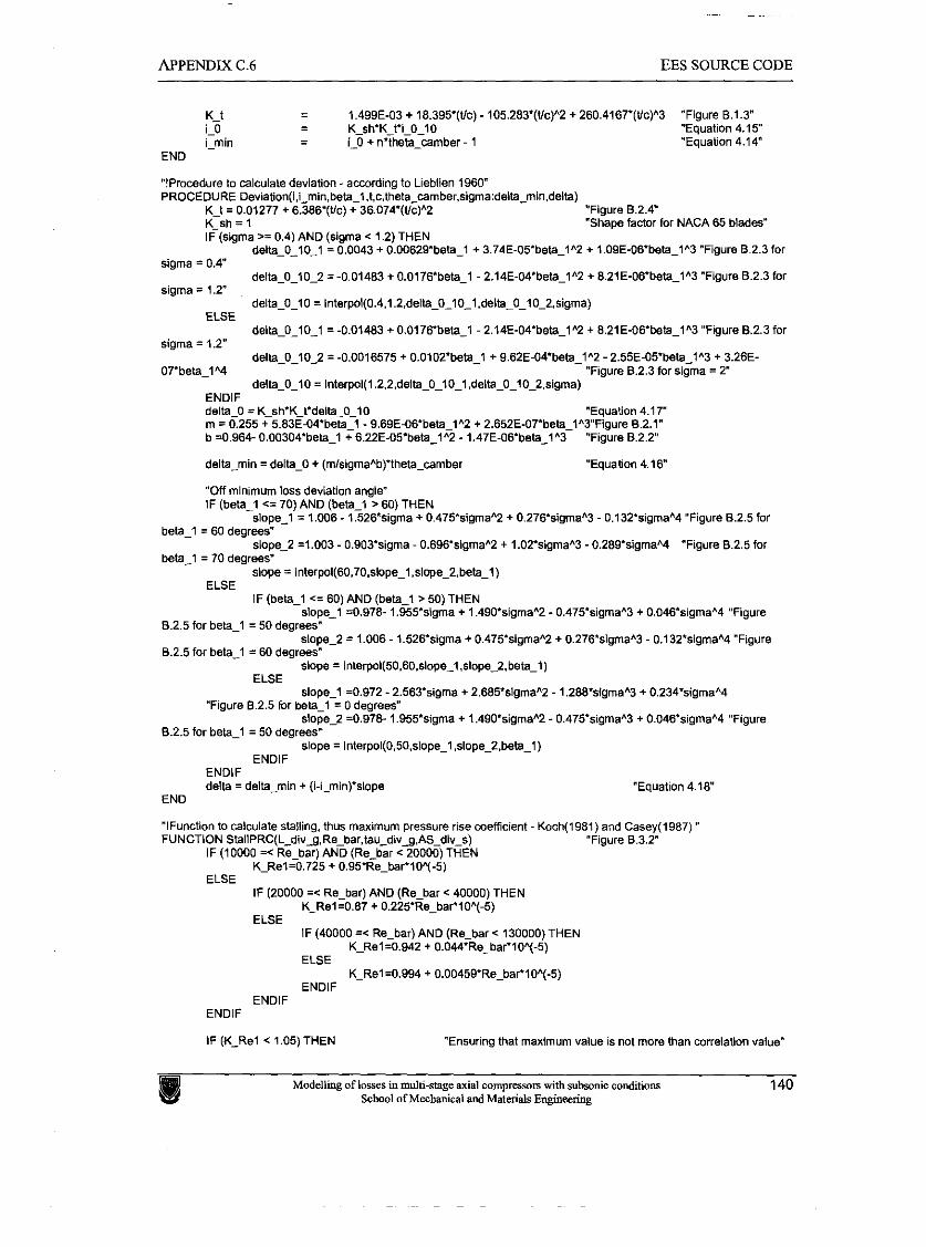
APPENDIX C.6 EES SOURCE CODE
K-t - - 1.499E-03 + 18.395"(Uc) - 105.283'(Uc)"2 + 260.4167+(U~)~3 "Figure 8.1.3"
i-0 - - K-~h^K~t'i-O-l0 "Equation 4.15" i-min - - i-0 + n'theta-camber - 1 "Equation 4.14"
END
"!Procedure to calculate deviation - according to Lieblien 1960" PROCEDURE Deviation(i,i-min,beta_l.t.c,theta-camber.sigma:delta_min,delta)
K-t = 0.01277 + 6.386'(Uc) + 36.074"(Uc)"2 "Figure 8.2.4" K-sh = I "Shape factor for NACA 65 blades' IF (sigma >= 0.4) AND (sigma < 1.2) THEN
delta-0-10-1 = 0.0043 + 0.00629'beta-1 + 3.74E-05'beta-lA2 + 1.09E-06^beta-lA3 "Figure 8.2.3 for sigma = 0.4"
delta 0 10-2 = -0.01483 + 0.0176.beta 1 - 2.14E-04'beta_lA2 + 8.21E-06'beta-lA3 "Figure 8.2.3 for - - - - -
sigma = 1.2" delta-0-10 = Inter~ol(0.4.1.2.delta~O~1O~l,delta~O~10~2,sigma)
ELSE -- ~-
delta-0-10-1 = -0.01483 + 0.0176'bela_l - 2.14E-04'beta_lA2 + 8.21E-06*beta-1"3 "Figure 8.2.3 for sigma = 1.2"
delta-0-10-2 = -0.0016575 + 0.0102'beta-1 + 9.62EO4'bela-IA2 - 2.55E-05'beta-IA3 + 3.26E- 07'beta-l"4 "Figure 8.2.3 for sigma = 2"
delta-0-10 = interpol(l.2.2,delta~0~10~1,delta~O~lO~2.sigma) FNnlF
delta-min = delta-0 + (mlsigmaAb)'theta-camber "Equation 4.16"
"Off minimum loss deviation angle" IF (beta-1 c= 70) AND (beta-1 > 60) THEN
slope-I = 1.006 - 1.526'sigma + 0.475"sigmaA2 + 0.276'sigmaA3 - 0.132'sigmaA4 "Figure 8.2.5 for beta-I = 60 degrees"
slope-2 =1.003 - 0.903'sigma - 0.696'sigmaA2 + 1.02*sigmaA3 - 0.289'sigmaA4 "Figure 8.2.5 for beta-I = 70 degrees"
slope = lnlerpo1(60,70,slope~l,slope-2,beta-1) FI SF ----
IF (beta-1 <= 60) AND (beta-I > 50) THEN slope-1 =0.978- 1.955'sigma + 1 .490*sigmaA2 - 0.475%gmaA3 + 0.046'sigmaA4 "Figure
8.2.5 for beta 1 = 50 degrees" - - slope-2 = 1.006 - 1.526.sigma + 0.475'sigmaA2 + 0.276'sigmaA3 - 0.132'sigmaA4 "Figure
8.2.5 for beta-1 = 60 degrees" slope = interpoi(50.60.siope~l.slope~2.beta_l)
FI CF ---- slope-1 =0.972 - 2.563^sigma + 2.685'sigmaA2 - 1.288^sigmaA3 + 0.234'sigmaA4
"Figure 8.2.5 for be&l = 0 degrees" slope-2 =0.97& 1.955'sigma + 1.490'sigmaA2 - 0.475'sigmaA3 + 0.046'sigmaA4 "Figure
8.2.5 for beta-1 = 50 degrees" slope = Interpoi(0.50.slope~l,slope~2.beta~l)
ENDiF ENDIF delta = delta-min + (i-i-min)'slope "Equation 4.18"
END
"fFLnc110n 10 ralcb ale slailmg, thus rnaxtrnwn pressure r.se coefic ertl - Koch(1981) a d Case)(1987, " F JNCT,Oh SlallPRC(L-d!vq.Re-oar,tata~ot~~ AS-dlv-s) "F gde 8 3 2'
IF (10000 =< Re bar) AhD (Re-oar c 20000) ThEtv ~ - ~ e l % . 7 2 5 + 0.95'<e-bar'lo'f-5)
ELSE IF (20000 =c Re-bar) AND (Re-bar < 40000) THEN
K-Re1=0.87 + 0.225'Re_bar'lO"(-5) ELSE
IF (40000 =< Re-bar) AND (Re-bar c 130000) THEN K-Rel=0.942 + 0.044^Re_barVOA(-5)
ELSE K-Rel=0.994 + 0.00459'Re-bar'lOA(-5)
ENDIF -. .. ENDiF
ENDiF
IF (K-Re1 < 1.05) THEN "Ensuring that maximum value is not more than correlation value"
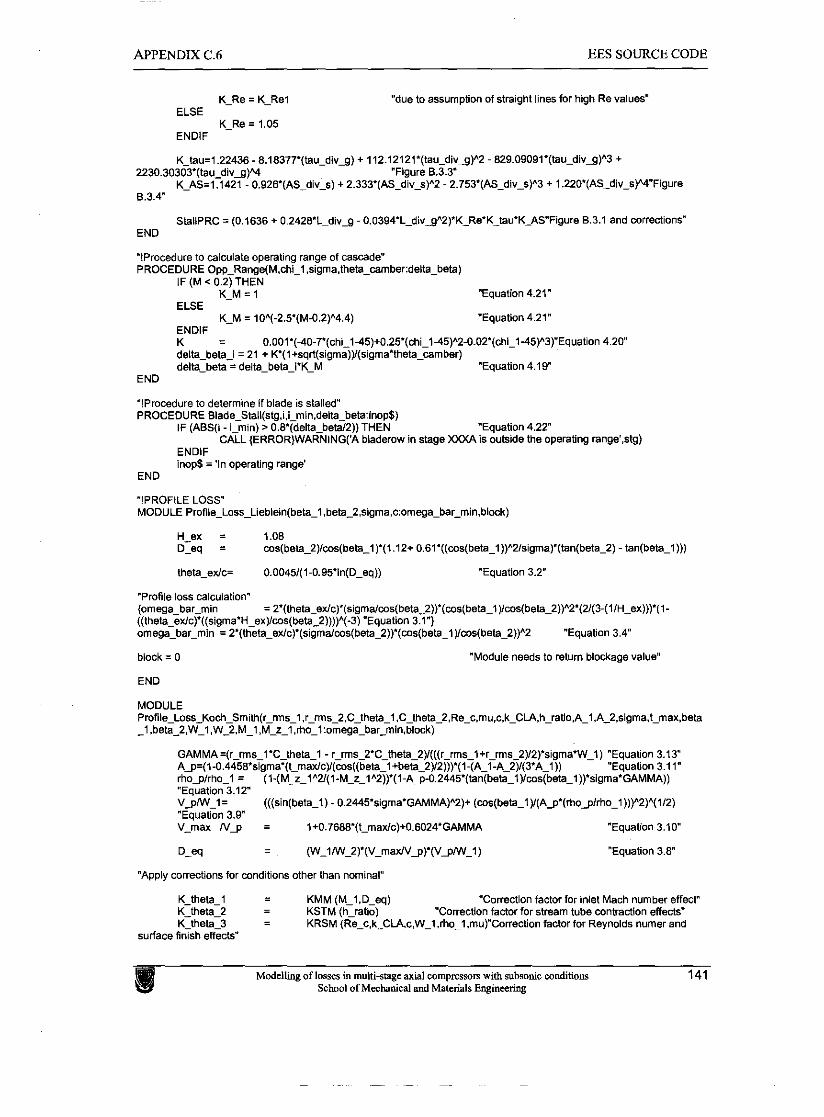
APPENDIX C.6 EES SOURCE CODE
K-Re = K-Re1 "due to assumption of straight lines for high Re values" ELSE
K-Re = 1.05 ENDiF
K-tau=1.22436 - 8.18377'(tau-divg) + 112.12121'(tau~divq)"2 - 829.09091'(tau-divg)"3 + 2230.30303*(tau-divg)"4 "Figure 8.3.3"
K-AS=1.1421 - 0.926'(AS_div-s) + 2.333'(AS-div-s)"2 - 2.753*(AS-div-s)"3 + 1.220'(AS_div-s)WFigure 8.3.4"
StallPRC = (0.1636 + 0.2428'L_divg - 0.0394.L-divqA2)'K_Re8KKtau*KKAS"Figure 8.3.1 and wrrections" END
*!Procedure to calculate operating range of cascade" PROCEDURE Opp-Range(M.chi-1 .sigma,theta-camber:delta_beta)
IF (M < 0.2) THEN K-M = 1 "Equation 4.21"
ELSE K-M = loA(-2.5'(M-0.2)"4.4) "Equation 4.21"
ENDlF K = O.OOl~(4O-7~(chi~l45)+O.25~(chi~145)A2-O.O2(chil45)A3Equation 4.20" delta-beta-i = 21 + K'(l+sqrt(sigma))/(sigma^theta-camber) delta-beta = delta-beta-i'K-M "Equation 4.19"
END
''Proceacre to determlne $1 o.ade is stal ed" PROCEDLRE Blaae.Stal,(slg ... i-mmnnaelta .betainop$)
IF (ABS(i - i-min) > O.B^(delta-beW2)) THEN "Equation 4.22 CALL (ERROR)WARNING('A bladerow in stage XXXA is outside the operating range's$)
ENDiF
''Proceacre to determlne $1 o.ade is stal ed" PROCEDLRE Blaae.Sta~,(slg ... i-m,n.aelta .betainop$)
IF (ABS(i - i-min) > 0.8'@elta-beW2)) THEN "Equation 4.22 CALL (ERRORIWARNINGI'A bladerow in stage XXXA is outside the operating range',stq)
-
inop$ ='In operating range' END
"!PROFILE LOSS" MODULE Profile-Loss-Lieblein(beta_l.beta-2.sigma.c:omega_bar-min.block)
H-ex = 1.08 D-eq = ws(beta_2)/ws(beta_1 )'(I .12+ 0.61'((~s(beta-l))~2/sigma)'(tan(beta-2) - tan(beta-1)))
theta-edc= 0.0045/(1-0.95'ln(D-eq)) 'Equation 3.2"
"Profile loss calculation" {omega-bar-min = 2'(theta-ex/c)'(s$ma/cos(beta-2)~(ws(belycos(beta-2))"2'(2/(3-(1/H~ex)))^(l- ((theta-ex/c)'((sigma^H_ex)/~os(beta_2))))~(-3) "Equation 3.1") omega-bar-min = 2'(theta-edc)'(sigma/ws(beta~2))'(ws(betal )Iws(beta-2))"2 "Equation 3.4"
block = 0 "Module needs to return blockage value"
END
MODULE Profile-Loss-Koch-Smith(r-rms-1 .r-rms-2.C-theta-I .C~theta~2,Re~c,mu,c,k~CM,h~rat io,A~l .A-2,sigma.t-max.beta - 1 ,beta-2.W-1 .W-2.M-1 ,M-2-1 .rho~l:omega~bar~min.block)
GAMMA =(r-rms-IT-theta-I - r~ms-2'C-theta-2)I(((r-rms~l+r~ms-2)/2)'sigma'W_1) "Equation 3.13" Ag=(l-O.4458'sigma'(t~madc)/(ws((beta_l+beta_2)/2)))'(1-(A~1-A~2)~(3'A~1)) "Equation 3.1 1" rhog/rho-1 = (1-(M~z~1"21(1-M~z~lA2))'(1-A~-0.2445'(tan(beta_l)Iws(beta~l))'sigma*GAMMA)) "Equation 3.12" V>MI-l= (((sin(beta-I) - 0.244Ssigma'GAMMA)"2)+ (ws(beta~l)I(Ag*(rhoglrho~l)))"2)~1/2) "Equation 3.9" V-max Ng = 1+0.7688*(t~madc)+0.60241+o.7688̂ o+o.6O24'GAMMAGAMMA "Equation 3.10"
D-eq - - (W_lNv-2Y(V-mafl~Y(V9MI-1) "Equation 3.8"
"Apply corrections for conditions other than nominal"
K-theta-I - - KMM (M-1,D-eq) "Correction factor for inlet Mach number effect" K-theta-2 - - KSTM (h-ratio) "Correction factor for stream tube contraction effects" K- theta - - KRSM (Re~c,k_CM.c.W~1.~o~l ,mu~Conection factor for Reynolds numer and
surface finish effects"
Madelling of losses in multi-stage axial compresson with subsonic conditions 141 School of Mechanical and Materials Engineering
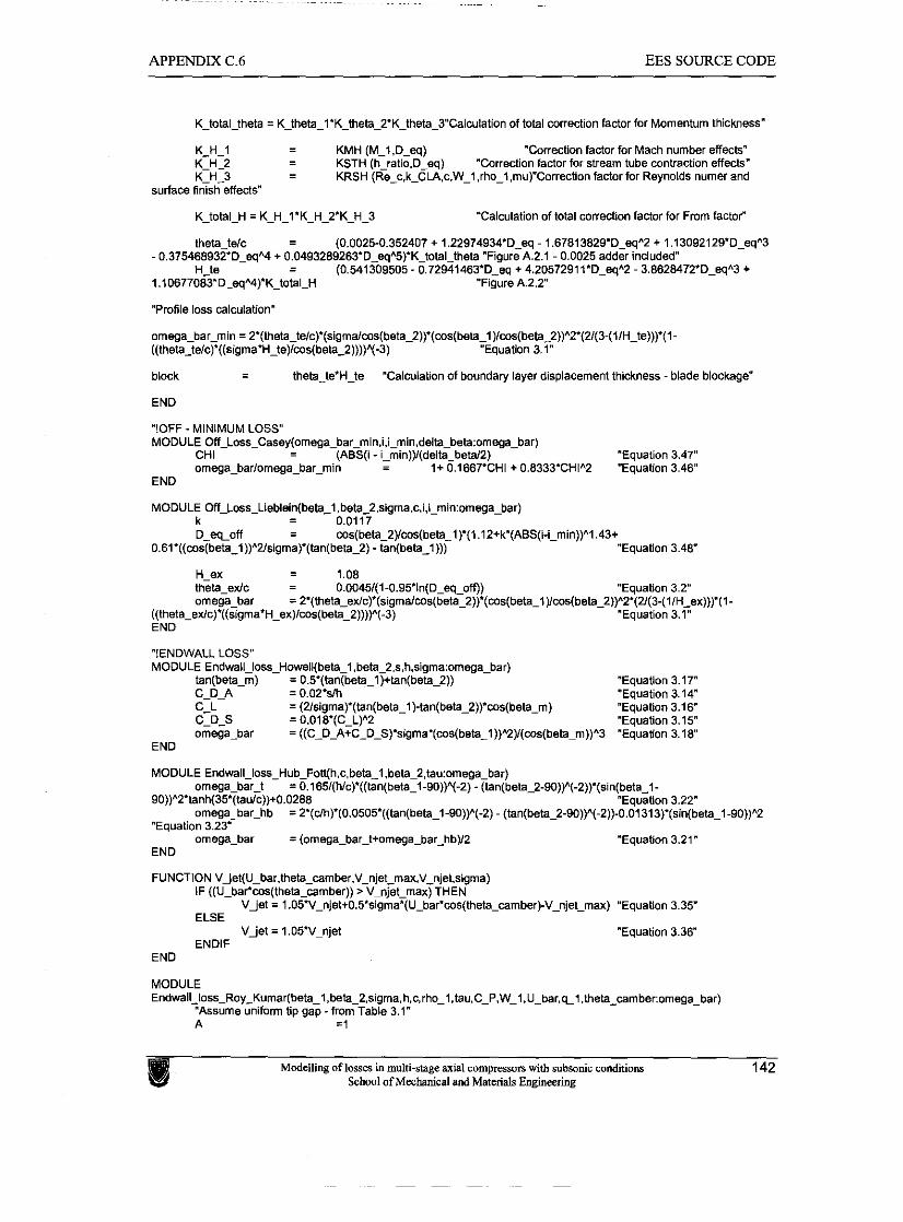
APPENDIX C.6 EES SOURCE CODE
K-total-theta = K_theta-l'K-theta_2'K-theta_3"Calculation of total correction factor for Momentum thickness"
6-h-1 - - KMH (M-1.D-W) 'Conect~on factor for Mach number effects' K-4-2 - - G T H (h-rat o.D.eq) 'Correct on factor for stream woe contract on efiecls" 6-H -3 - - KRSti ( R e ~ c , ~ ~ C ~ A , c . W ~ l . r h o ~ l . m ~ ) " C o r r e c U o n factor for Reyno,ds numer and
surface finish effects"
K-total-H = K-H-1.K-H-2'K-H-3 "Calculation of total correction factor for From factor"
tneta tdc - - (0 0025-0 352407 + 1 22974934'D-eq - 1 67813829'D_eqA2 + 1 13092t29'D_eqA3 - 0 375468932.D-eq"4 * 0 0493289263'D. eqA5)'K-total tneta 'Flg~re A 2 1 - 0 0025 adder inc ~ d e d '
h te - - (0 541309505 - 0 72941463'D ea + 4 20572911'D eqA2 - 3 8628472'D-eqA3
"Profile loss calculation"
omega-bar-min = 2'(theta~telc)'(sigma/cos(beta_2))'(cos(be1)1ms(beta~2))"2*(2/(3-(1/H~te)))'(1~ ((theta-td~)'((sigma~H~teYws(beta_2))))~-3) "Equation 3.1"
block - - theta-te'H-te "Calculation of boundaty layer displacement thickness -blade blockage"
END
"!OFF - MINIMUM LOSS" MODULE O f - L o s s _ C a s e y ( o m e g a _ b a r - m i n . i , i - m i n . d e l t a r )
CHI - - (ABS(i - i_min))/(delta-betal2) "Equation 3.47" omega-barlomega-bar-min - - I + 0.1667'CHI + 0.8333*CHIA2 "Equation 3.46"
END
MODULE Off-Loss-Lieblein(beta_l.beta-2.sigma,c.i.i-mln:omega_bar) k - - 0.0117
D - q o f f - - cos(beta_2)lcos(beta_1 )'(1.12+k'(ABS(i-i-min))'L1.43+ 0.6I'((ws(beta-l))"2/sigma)'(tan(beta_2) - tan(beta-1))) "Equation 3.48"
H-ex - - 1.08 theta-ex/c - - 0.0045/(1-0.95'ln(D~eq~off)) "Equation 3.2" omega-bar =2'(theta~ex/c)'(sigmalms(beta_2))'(cos(bel~cos(beta~2))A2'(2/(3-(1/H~ex)))'(l-
((theta-ex/~)'((sigma'H_ex)lcos(beta_2))))~(-3) "Equation 3.1" END
"!ENDWALL LOSS" MODULE Endwail-loss-Howell(beta_l.beta-2.s,h.sigma:omega_bar)
tan(beta-m) = 0.5'(tan(beta-l)+tan(beta_2)) "Equation 3.17" C-D-A = 0.02Wh "Equation 3.14" c-L = (Z/sigma)'(tan(beta-l)-tan(beta-2))'rns(beta_m) "Equation 3.18" C-D-S = 0.01 8^(C-L)"2 "Equation 3.15" omega-bar = ((C_D-A+C-D-S)'sigma~(beta_l))Y)/(rns(beta~m))"3 "Equation 3.18"
END
MODULE Endwall~loss~Hub~Fott(h,c,beta_l.beta~2,tau:omega~bar) omega-bar-t = 0.165/(hlc)'((tan(beta~l-90))Y-2) - (tan(beta-2-90))Y-Z))'(sin(beta-l-
90))A2*tanh(35*(lau/c))+0.0288 "Equation 3.22" omega-bar-hb = 2'(c/h)'(0.0505*((tan(beta_l-90))A(-2) - (tan(betx2-go))"(-2))-0.01 313)'(sin(beta_l-90))"2
"Equation 3.23" omega-bar = (omega-bar-t+omega-bar-hb)l2 "Equation 3.21"
END
FUNCTION VJet(U-bar,theta_camber,V-njet-max,V-njet,sigma) IF ((U-bar*ws(theta-camber)) > V_njet-max) THEN
VJet = 1 .057/-njet+0.5'sigma'(U_bar^cos(theta-camber)-V-njet-max) "Equation 3.35 ELSE
V j e t = I.OS'V_njet "Equation 3.36" ENDIF
END
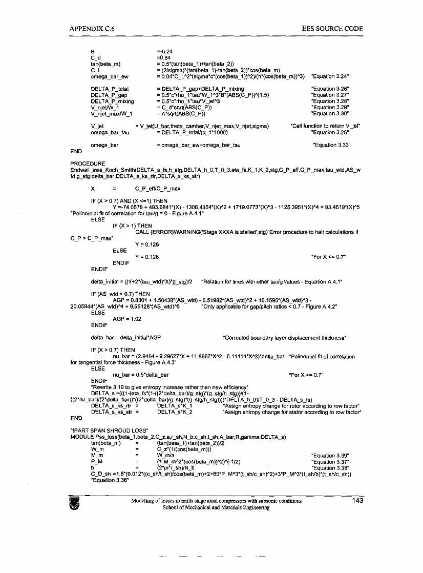
APPENDIX C.6 EES SOURCE CODE
B =-0.24 c-d =0.84 tan(beta-m) = O.S'(tan(beta-l)+tan(beta-2)) c-L = (2/sigma)"(tan(beta-1)-tan(beta-2)).ws(beta-m) omega-bar-ew = O.O4'C~LY~sigma~c'(cos(beta~l))"2)l(h'(~s(beta_m))~3) "Equation 3.24"
DELTA-P-total = DELTA-P_gap+DELTA-P-mixing "Equation 3.28" DELTA-P~ap = 0 .5~~* rho~ I~ tau~W~1~3~B~(ABS(C~P) )Y1 .S ) "Equation 3.27" DELTA-P-mixing = 0.5 'c '~o~lYau*V~etA3 "Equation 3.28" V-njetlw_I = C-d'sqri(ABS(C-P)) "Equation 3.29 V-njet-maxNV-I = A'sqrl(ABS(C-P)) "Equation 3.30"
V j e t = Vjet(U-bar,theta-camber,V~njetjmaxxVVnjet,sigma) "Call function to return V je r ' omega-bar-tau = DELTA~P~tota i l (q~l~1000) "Equation 3.25"
omega-bar = omega-bar-ew+omega-bar-tau "Equation 3.33" END
PROCEDURE Endwall~loss~Koch~Smith(DELTA~sSfs,h~stg,DELTA~h~O,T~O~3,eta~fs,K~l .K_2,stg.C~P~eff,C~P~maxxtau_wtd,AS~w td.g-stg:delta_bar.DELTA~s~ks~rtr,DELTA-s-ks-str)
IF (X > 0.7)AND (X <=I) THEN Y =-74,0578 + 493.6841'(X) - 1306.4354*(X)"2 + 1719.0773'(X)"3 - 1125.3951'(X)"4 + 93.4619'(X)"5
"Polinomiai fit of correlation for taula = 0 - Fiaure A.4.1" - - ELSE
IF (X > 1) THEN CALL (ERROR)WARNING('Stage XXXA is stalled'.stg)"Error procedure to halt calculations if
C-P > C-P-max" Y = 0.126
ELSE Y = 0.126 "For X c= 0.7"
ENDiF ENDlF
deitalnitial = ((Y+2~(tau~wtd)"X)"g~s~)/2 "Relation for lines with other taulg values - Equation A.4.1"
IF (AS-wtd < 0.7) THEN AGP = 0.8301 + 1.50438'(AS-wtd) - 6.51982'(AS-wtd)"2 + 16.1595'(AS-wtd)"3 -
20.05944*(AS_wtd)"4 + 9.55128'(AS-wld)"5 "Only applicable for gaplpilch ratios c 0.7 - Figure A.4.2' ELSE
AGP = 1.02 ENDlF
delta-bar = delta-initial'AGP "Corrected boundaly layer displacement thickness"
IF (X > 0.7) THEN nu-bar = (2.9464 - 9.29627.X + 11.8667*XA2 - 5.111 11'XA3)"deita-bar "Polinomial fit of correlation
for tangential force thickness - Figure A.4.3" ELSE
nu-bar = 0.5'delta-bar "For X <= 0.7" ENDlF "Rewrite 3.19 to give entropy increase rather than new efficiency" DELTA-s =(((l-(eta~fs*(l-((2~delta_bar)/g~stg)"(g~stgIh~stg))/(l-
( (2~nu~bar ) / (2 'de l ta_bar )~ ( (2 'de l ta_bargstg)" (gsths) ) )DELTAh_OO3 - DELTA-s-fs) DELTA-s-ks-rtr = DELTA-s*K-1 "Assign entropy change for rotor according to row factor" DELTA-s-ks-str = DELTA-s'K-2 "Assign entropy change for stator according to row factor"
END
"!PART SPAN SHROUD LOSS" MODULE P s s ~ l o s s ( b e t a ~ l . b e t a _ 2 . C ~ z . a , r ~ s h . N _ b , c ~ s h , t ~ s h , A ~ b a r . R )
tadbeta m) = Itan(beta l)+tan(beta 2)Y2 . - . w-m - - &z+l/(&(be<m))) "
M-m - - W-mla "Equation 3.39
P-M - - (I-M-m9'(w~(beta-m))~2)~(-1/2) "Equation 3.37" - b - (2'pi.r-sh)lN-b "Equation 3.38"
C-D-sh =1.8'(0.012'((c~sWt~sh)/cos(beta~m)+2+6OoP~MA33(t~~h/~~~h)A2)+33PPMA33(tt~h/b)"(ttsh/~~~h)) "EquaUon 3.36"
Modelling of losses in multi-stage axial compressom with subsonic conditions 143 School of Mechanical and Materials Engineering
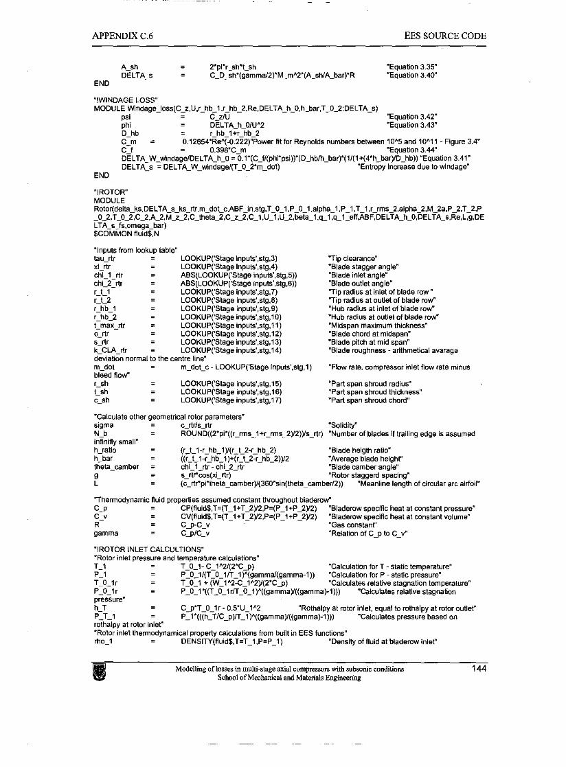
APPENDIX C.6 EES SOURCE CODE
A-sh - - 2'pi.r-sh't-sh "Equation 3.35" DELTA-s - - C-D_~h'(gammd2)'M~m~2~(A~sh/A~bar)'R "Equation 3.40"
END
"!WINDAGE LOSS MODULE Windage~ioss(C~z.U.r~hb~l,r~hb~2.Re,DELTA~h~O,h~bar,TTOO2:DELTA~s)
osi - - C zlU "Eauation 3.42" ohi - - DELTA h 0 1 ~ ~ 2 "~duation 3.43" q h b - - r-hb-I :r3bL~ C-m = 0.12654'Rey-0.222)"Power fit for Reynolds numbers between 10A5 and 10A1 1 - Figure 3.4" c-f - - 0.398'C-m "Equation 3.44" DELTA-W-windagelDELTA-h-0 = 0.1~(C~f/(phi'psi))'(D~hb/h~bar)'(1/(1+(4'h~bar)/D~hb)) "Equation 3.41" DELTA-s = DELTA-W-v,4ndage/(T-O-2*mmdot) "Entropy increase due to windage"
END
"Inputs from lookup table" tau-rtr - - LOOKUP('Stage inputs'.stg,3) xi-rtr - - LOOKUP('Stage inputs.stg.4) chi-1-rtr - - ABS(LOOKUP('Stage inputs'.stg.5)) chi-2-rtr - - ABS(LOOKUP('Stage inputs'.stg.B)) r-t-1 - - LOOKUP('Stage inputs.stg.7) - r t z - LOOKUP('Stage inputs'.stg.8) r-hb-1 - - LOOKUP('Stage inputs'.stg.9) r-hb-2 - - LOOKUP('Stage inputs'.stg,lO) t-max-rtr - - LOOKUP('Stage inputs'.stg.ll) c-rtr - - LOOKUP('Stage inputs',s$.l2) s-rtr - - LOOKUP('Stage inputs'.stg,l3) k-CLA-rtr - - LOOKUP('Stage inputs'.stg.14) deviation normal to the centre line" m-dot - - m-dot-c - LOOKUPCStage inputs',stg.l) bleed now r-sh - - LOOKUP('Stage inputs',s$,l5) t-Sh - - LOOKUP('Stage inputs'.stg,l6) c-sh - - LOOKUP('Stage inputs'.stg,l7)
'Tip clearance' "Blade stagger angle" "Blade inlet angle" "Blade outlet angle" "Tip radius at inlet of blade row" "Tip radius at outiet of blade row' "Hub radius at inlet of blade row" "Hub radius at outiet of blade row "Midspan maximum thickness" "Blade chord at midspan" "Blade pitch at mid span" "Blade roughness - arithmetical avarage
"Flow rate, compressor inlet flow rate minus
"Part span shroud radius" "Part span shmud thickness" "Part span shroud chord"
"Calculate other geometrical rotor parameters" sigma - - c-rtrls-rtr "Solidity" N-b - - ROUND((2'pi~((r-rms~l+r-rms~2)/2))/s-rtr) "Number of blades if trailing edge is assumed inflnitly small" h-ratio - - (r-t-l-r-hb-l)/(r-t-2-r-hb-2) "Blade heigth ratio" h-bar - - ((r-t-l-r-hb-l)+(r-t-2-r-hb-2))/2 "Average blade height" theta-camber = chi-1-rtr - chi-2-rtr "Blade camber angle" 9 - - s-rtrws(xi-rtr) "Rotor staggerd spacing" L - - (c-rtr*piWtheta-camber)/(360'sin(theta~Z)) "Meanline length of circular arc airfoil"
'Thermodynamic fluid properties assumed wnstant throughout bladerow" c s - - CP(fluid$,T=(T-1cT-2)12,P=(P-1+P-2)/2) "Biaderow specific heat at constant pressure"
c-v - - CV(fiuid$.T=(T-1+T-2)/2,P=(P-l+P-2)/2) "Bladerow specific heat at constant volume" R - - Cg-C-v "Gas wnstanl' gamma - - CJIC-v "Relation of C g to C-v"
"!ROTOR iNLET CALCULTIONS" "Rotor inlet pressure and temperature calculations" T-1 - -
- T-0-1- C-IA2/(2'Cg) "Calculation for T - static temperature"
p-1 - P~O~1/(T~O~1~~1)"(gammd(gamma-l)) "Calculation for P -static pressure" T-0-1 r - - T-0-1 + (W-l"2-C-IA2)/(2^Cg) "Calculates relative stagnation temperature" P-0-1 r - - P~O~I'((T~O~Ir/T_O~1~((gamma)/((gamma)-l))) "Calculates relative stagnation pressure" h-T - - Cg'~-o-lr - 0.5'~-IA2 "Rothalpy at rotor inlet, equal to rothalpy at rotor outlet" P-T-1 - - P-I'(((~-T/CJP-I )Y(gamma)l((gamma)-l))) "Caiculates pressure based on mthaipy at rotor inlet" "Rotor inlet thermodynamical property calculations from built in EES functions" rho-I - - DENSITY(fiuid$.T=T-l.P=P-1) "Density of fluid at bladerow inlet"
Modelling of losses in multi-stage axial compressan with subsonic conditions 144 School of Mechanical and Materil Engineering
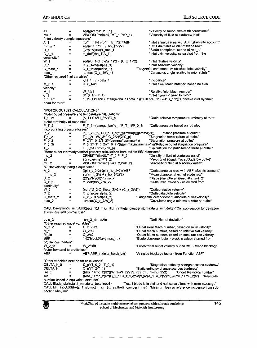
APPENDIX C.6 EES SOURCE CODE
a1 - - sqrt(gamma*R'T-1) Velocity of sound, m/s at blademw inlet" mu-1 - - VISCOSITY(~~U~~$.T=T~I ,P=P_l) "Viswsity of fluid at bladerow inler "Inlet velocity triangle equations" A-1
- - ((pi'r-1-lA2)-(pi'r-hb-lA2))'ABF "Inlet annulus area wilh ABF taken into amount" r-rms-I - - sqrt((r-1-ln2 + r-hb-lA2Y2) "Rms diameter at inlet of blade row" u-1 - - ((2*pi'NY60~r_rms_l "Blade pheripheral speed at rms-I"
c-2-1 - - m-doV(rho-I'A-1) "Inlet axial velocity, calculated from the
continuity" w-1
- - sqrt((U-1-C-theta-1)"2 + (C-z-1)"2) "Inlet relative velocity"
c-1 - - C-z-llws(alpha-I) "inlet Absolute velocity" C-theta-I - - C-z-l'tan(alpha-I) Tangential component of absolute inlet velocity" beta-I - - -arcws(C-z_INV_l) "Calculates angle relative to rotor at inlet" "Other required inlet variables" i - - -chi-1-rtr - beta-I "Incidence" M-2-1 - - C-z-llal "Inlet axial Mach number, based on axial velocitv" - --.-, M-1 - - W_l la l "Relative inlet Mach numbe? q-1 - - (P-0-lr - P-I) "Inlet dynamic head to rotor"
- q-1-eff - q~1'((1+2.5*(C~1'sin(alpha~1+beta_1))"2+0.5U12(4CA2)Effeve inlet dynamic head for rotof
"!ROTOR OUTLET CALCULATIONS "Rotor outlet pressure and temperature calculations" T-0_2r - - (h_T+ 0.5'U-2"2)lCg "Outlet relative temperature, rothalpy at rotor outlet = mthaipy at rotor inlet" P-T-2 - - P-T-1 - ( o m e g a ~ b a r ' q ~ l * P _ T ~ l ~ P ~ O ~ l r "Outlet pressure based on rothalpy inwmoratina Dressure losses" ~ ~ - . p-2 - . ~~~_21(((n_nc~)fr_2j~(gammay((~amma)-1))) "static pressure at outlet. T-0-2 - - T_0_2r - (W_2A2-C-2A2)l(2'C~) "Stagnaton temperatue at outlet" p -0-2 - . P_2'(T 0-ZK.2)~gammal(gamma-I)) "Stagnauon pressure a1 o~tlet" P-0-2 - - P-O-2'((T-O-2r~-O-2)Y(gamma)/((gamma)-l)))"Relative ouUet stagnation pressure" T-2 - - T-O-2-C-2A2/(2'Cg) "Caiculation for static temperature at outlet" "Rotor outlet thermodvnamical DroDertv calculations from built in EES functions" rho-2 - - DENSIN(&~~~,T=T-~,P=P-~) "Density of fluid at bladerow outlet" a2 - - sqrt(gamma'R'T-2) "Velocity of sound, m/s at blademw outlet" mu-2 - - VlSCOSlN(fiuid$.T=T-2,P=P-2) "Viscosity of fluid at bladerow outlet" "Outlet velocity triangle equations" A-2 - - ((pi'r-t-2A2)-(pi'r-hbb2A2))"ABF "OuUet annulus area with ABF taken in accounr' r_rmsl - - sqrt((r-t-2"2 + r-hb_ZA2)/2) "Mean diameter at exit of blade row" u-2 - - ((2'pi'N)/60)'r-rms-2 "Blade pheripheral speed at r-rmsl" c-2-2 - - m-doV(rho-2.A-2) "Outlet axial velocity -calculated from continuity" w-2
- - (sqrt((U_2-C-lheta-2)"2 + (C-2-2)"2)) "OuUet relative velocity" c-2 - - C-2-2/ws(alpha-2) "Outlet absolute velocity" C-theta-2 - - C-z_2%n(alpha_2) "Tangential component of absolute outlet velocity" beta-2 - - -arcws(C-z-2NV-2) "Calculates angle relative to rotor at outlet"
CALL Deviation(i.i~min.ABS(beta_l),t~max~rtr.c~rtr,theta~camber.sigma:deltamin,delta) "Cali sub-section for deviation at min loss and off-min loss"
beta-2 - - 4-2-r t r - delta "Definition of deviation" "Olher required outlet variables" M-2-2 - - C-z_2/a2 "OuUet axial Mach number, based on axial v e l o c i ~
M-2 - - W-2/a2 "Oullet Mach number, based on relative exit velocity" M-2a - - C-21a2 "Outlet Mach number, based on absolute exit velocity" BBF - - l-(2*block)l(g+t-max-rtr) "Blade blackage factor - block is value returned from profile loss module" W-2-fs - - W-2/BBF "Freestream outlet velocity due to BBF - blade blockage factor from and to profile loss" ABF - - ABF(ABF-in.delta_bar.h_bar) "Annulus blockage factor - from Function ABF"
"Other variables needed for caiculations" DELTA h 0 = Cg'(T-0-2 - T-0-1) "Stagnation enthalpy change accmss blademw" DELTA^^- - - Cg'(T-2-T-1) "Static enthalpy change accmss blademw" ~ e - c - - ( ( rho~l+~o~2~2' ( (W~1+W~2)/2) 'c~rtr ) l ( (mu~l+mu~2)12) "Chord Reynolds number" Re - - ( (~o_ l+rho~2) /2 ' (C~z~1+C~zZ2Y2*sqr t ( (4~(A~l+A~2) /2 ) /p i )~ ( (mu~l+mu~2~2) "Reynolds number based in equivalent diameter*' CALL Blade-stail(stg.i.i-min.delta_beta:inop$) 'Test if blade Is in stall and halt calculations with error message" CALL Min~inc(ABS(beta~l),sigma.t_max-rtr,c~rtr,lheta~camber:i~min) "Minimum loss or reference incidence from sub- section Min-inc"
Modelling of losses in multi-stage axial compressors with subsonic conditions 145 School of Mechanical and Matenals Enginening
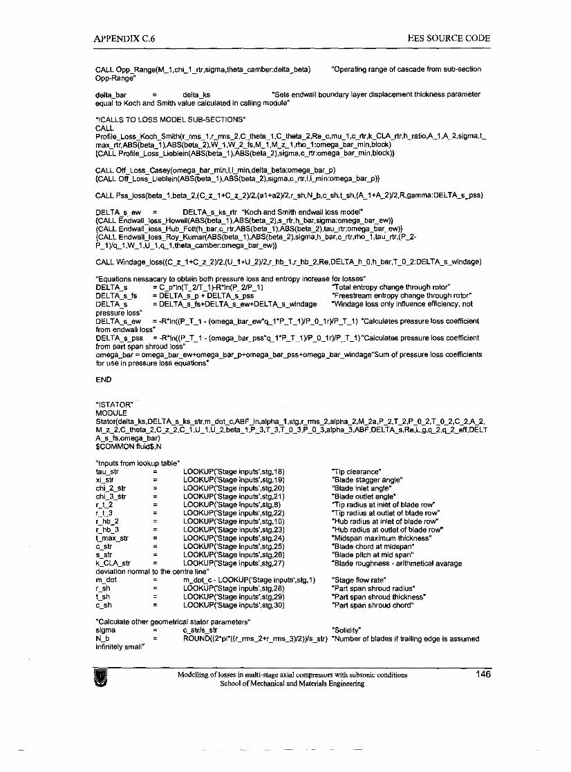
APPENDIX C.6 EES SOURCE CODE
CALL Opp-Range(M-l,chi-l-ltr,sigma.theta-camber:delta-beta) "Operating range of cascade from sub-section Opp-Range"
delta-bar - - d e l t a s "Sets endwail boundary layer displacement thickness parametel equal to Koch and Smith value calculated in calling module"
?CALLS TO LOSS MODEL SUB-SECTIONS" CALL Profile~Loss~Koch~Smith(r~rms_l,r~rms~2,C~theta~l.C~Vleta~2.Re~c.mu~l.c~rtr.k~CLA~rtr.h_ratio,A~l.A~2,sigma.t~ max-rtr,ABS(beta-l),ABS(beta-2),W-1.W-2-k.M-1 .M-2-1 .ho-1:omega-bar-min.block) (CALL Profile-Loss-Lieblein(ABS(beta_l).ABS(beta-2),sigma,c~rtr:omega_bar_min~))
CALL O~Loss-Casey(omega-bar~min,i,l-min,delta-beta:omega-barj) (CALL Off~Loss~Lieb le in (A8S(beta_ l ) ,ABS(be~2) .s igma,~~r t r , l~ i~min:0m~p) ]
CALL Pss-ioss(beta-1 .beta~2.(C~z~l+C~z~2)/2.(al+a2)/2,r~sh,N~b,c~sh,t~sh,(A~1+A~2)/2,R,gamma:DELTA~sjss)
DELTA-s-ew = DELTA-s-ks-rtr "Koch and Smith endwali loss model" (CALL Endwall~loss~Howell(ABS(beta_l).ABS(beta~2).s~~.h~bar,sigma:omega_bar~ew)) (CALL Endwall_ioss~Hub~Fon(h~bar,c~rtr.ABS(be~l).ABS(beta_2).tau~rtr:omega~bar_ew)} (CALL Endwall~loss~Roy~Kumar(A8S(beta_l).ABS(beta~2),sigma,h~bar,~~rtr,ho~l,tau~rtr.(P~2- P~1) /q~l ,W~1.U~1,q~l , theta~camber:omega~bar~ew))
CALL Windage~ioss( (C~z~l+C~z~2) /2 . (U~1+U~2) /2 . r~hb~l . r~hb~2.Re.DELTA~h~O,h~bar ,T~O~2:DELTA~s~~ndage)
"Equations nessacary to obtain both pressure ioss and entropy increase for losses" DELTA-s = Cj*ln(T-m-1)-R*ln(P_2/PP1) "Total entropy change through rotor" DELTA-s-fs = DELTA-sj + DELTA-sjss "Freestream entropy change through rotor" DELTA-s = DELTA-sp+DELTA-s-ew+DELTA-s-windage "Windage loss only influence efficiency, not pressure ioss" DELTA-s-ew = -R'in((P-T-1 - (omega-bar-ew*kl'P-T-I )/P-0-1 rYP-T-1) "Calculates pressure loss coefficient from endwaii loss" DELTA-sjss = -R'ln((P-T-1 - (omega~bargss'q_l*P~T~l)/P~O~lr)/P~T~1)"Caiculates pressure loss coefficient from part span shroud loss" omega-bar = omega-bar-ew+omega-barg+omega-barjss+omega~bar-windage"Sum of pressure ioss coefkients for use in pressure loss equations"
END
"inputs from iwkup table" tau-str - - LOOKUP('Stage inpuW.stg,l8) xi-str - - LOOKUP('Stage inpuW.stg.19) chi-2-str - - LOOKUP('Stage inpuW,stg.20) chi-3-str - - - LOOKUP('Stage inpuW.stg,21) r-t-2 - LOOKUP('Stage inpuW.stg.8) r-1-3 - - LOOKUP('Stage inpuW,stg.22) r-hb-2 - - LOOKUPCStage inpuW.stg.10) r-hb-3 - - LOOKUP('Stage inpuW.stg.23) t-max-str - - LOOKUP('Stage inpuW,stg.24) c-str - - LOOKUPCStage InpuW,stg,25) s-str - - LOOKUP('Stage inpuW,stg.26) k-CLA-str - - LOOKUP('Stage inputs',stg.27) deviation normal to the centre line" m-dot - - m-dot-c - LOOKUP('Stage inpuW.stg.1) r-sh - - LOOKUP('Stage inpuW,stg.28) t-sh - - LOOKUP('Stage inpuW,stg,29) c-s h - - LOOKUP('Stage inpuW.stg.30)
'"Tip clearance" "Biade stagger angle" "Blade inlet angle" "Blade outlet angle" "Tip radius at inlet of blade r o d "Tip radius at outlet of blade r o d "Hub radius at inlet of blade row" "Hub radius at outlet of blade row" "Midspan maximum thickness" "Blade chord at midspan" "Biade pitch at mid span" "Blade roughness -arithmetical avarage
"Stage flow rate" "Part span shroud radius" "Part span shroud thickness" 'Part span shroud chord"
"Calculate other geometrical stator parameters" sigma - - c-strls-str "Solidity"
N-b - - ROUND((2'pi'((r-rms-2+r-rms-3)/2))/s_slr) "Number of blades if trailing edge is assumed infinitely small"
Modelling of lasses in multi-stage axial compresson with subsonic conditions 146 School of Mechanical and Materials Engineering
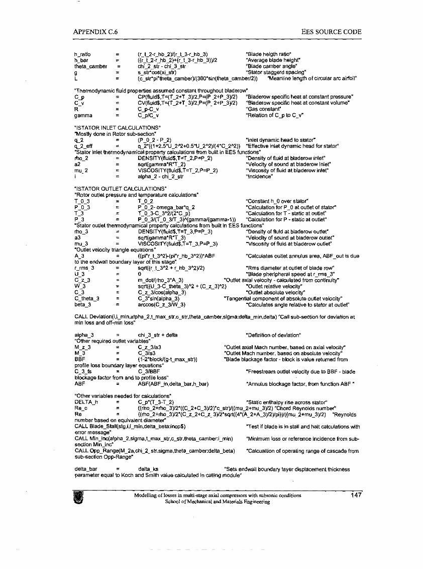
APPENDIX C.6 EES SOURCE CODE
h-ratio - - (r-t2-r-hb_2)l(r-t-3-r-hb-3) "Blade heigth ratio" h-bar - - ((r-t_2-r_hb_2)+(r-t-3-r-hb-3)y2 "Average blade heighl" theta-camber = chi-2-str - chi-3-str "Blade wmber angle" 9
- - s-st? cos(xi-str) "Stator staggerd spacing" L - - (c-str'pi*theta-camber)1(360'sin(lheta~camberI2)) "Meanline length of circular arc ailfoil"
"Thermodynamic fluid properties assumed wnstant throughout bladerow" c s - - CP(fluld$,T=(T-2+T_3)12,P=(P-2+PP3)12) "Blademw specific heat at constant pressure"
c-v - - CV(fluid$.T=(T-2+T-3)12,P=(PP2+PP3)12) "Bladerow specific heat at constant volume" R - - Cg-C-v "Gas constanr gamma - - CgIC-v "Relation of C g to C-v"
"!STATOR INLET CALCULATIONS" "MosUy done in Rotor sub-section" K 2 - - (p-0-2 - p-2) "Inlet dynamic head to stator" q-z-eff - - ~2'((l+2.5*U-2Y+0.55U-2A2)l(4~CC2n2)) "Effective Inlet dynamic head for stator" "Stator inlet thermodynamical property calculations from built in EES functions" rho-2 - - DENSlN(Ruid$,T=T-2,P=P-2) "Density of fluid at bladerow inlet" a2 - - sqrt(gamma*R'T-2) "Velocity of sound at blademw Inlet" mu-2 - - VlSCOSlTY(fluid$.T=T-2,P=P-2) "Viscosity of fluid at bladerow inlet" i = alpha-2 - chi-2-sb "Incidence"
"ISTATOR OUTLET CALCULATIONS' "Rotor outlet pressure and temperature calculations" T-0-3 - - T-0-2
P-0-3 - - P-0-2- omega-barq-2 T 3 - - T 0 3-C 3"2/12*C o)
"Constant h-0 over stator" "Calculation for P-0 at outlet of stator" "Calculation for T - static at outlet" - . ~ - . ~ ~~ ~~ ~ ~
PI 3 - - ~ ~ 0 ~ ~ ( ~ - 0 _ 3 ~ - 3 ) ~ g a m m a l ( g a m m a - l ) ) "Ca,ct.latun for P - staLc at o~ttel" "Stator odllet lhermodynam.wl properly caicblabons from brr1.1 in EES funcuons" rno-3 - - DENS.TY(RL~~S.T=T 3.P-P 3) 'Dens~Pf of f l ~ i a at bladerow odllet" a3 - - sqrt(gamma'RT-3)- "Velocity of sound at bladerow outlet" mu 3 - - VISCOSITY(fluid$.T=T 3.P=P 3) 'VswsitV of fluid at bladerow outlet" - - "outlet velocitv trianale eouations" ' . - ,
A-3 - - ((pi'r-t-3Y)-(pi'r-hb_3"2))'ABF "Calculates outlet annulus area. ABF-out is due
to the endwall boundary layer of this stage" r-rms-3 - - sqrl((r-t-3"2 + r_hb-3"2)/2) "Rms diameter at outlet of blade mw" u-3 - - 0 "Blade pheripheral speed at r-rms-3" c-2-3 - - m-doV(rh0-3'A-3) "Outlet axial velocity -calculated from continuity"
w-3 - - ~qrt((U-3-C-theta-3)~2 + (C_z-3)"2) "Outlet relative velocity" C 3 - - C z 3lwslaloha 3) "Outlet absolute velocitv"
~ - , ~ - - - ~ , -~ . - ~ . ~ . ~Itneta-3 - - ~13's n(alpna-3) '7angentla1 component of abso~lrle o~t.et ve.ocityv oeta-3 - - arccos(C_z_3M1_3) "Catmlates angle relauve to stator a1 odlet"
CALL Deviation(i. l~min.al~ha~2~t~max~str~~~strthetamber,sigma:delmin,deita) "Call sub-section for deviation at mln loss and off-mln loss"
aipha-3 - - chi-3-str + delta "Definition of deviation" "Other required outlet variables" M-2-3 - - C-z-31a3 "Outlet axial Mach number, based on axial ve1ocit)r' M-3 - - C-3la3 "Outlet Mach number, based on absolute velocity" BBF - - (1-2'blockI(~-t max stW "Blade blackaae factor - block is value returned fmm .- - - .. profile loss boundary layer equations" C-3-b z. C-YBBF blockage factor from and to profile loss" ABF - - ABF(ABF_in,delta-bar,h-bar)
- "Freestream outlet velocity due to BBF - blade
"Annulus blockage factor, from function ABF "
"Other variables needed for calculations" DELTA-h - - Cg'(T-3-T-2) "Static enthalpy rise across stato? Re-c - - ((rho-2+ho-3YZe((C-2+CC3)/2)^c_str)l((mu2+mu32) "Chord Reynolds number" Re - ((rho~2+ho~3Y2*(C~~~2+C~~~3~2*sqrt((4'()/2) "Reynolds
number based on equivalent diameter" CALL Blade-Stall(s$,i,i-min.delta_beta:inop$) "Test If blade is in stall and halt calculations with error message" CALL Min~inc(alpha-2,sigma,t-max~str,c-str,thetacamber:imin) "Minimum loss or reference lncidence from sub- section Mln inc" CALL 0pp--~nge(~-2a.chi-2-str.sigma,lheta~camber:delta-beta) '"Calcualtion of operating range of cascade from sub-section Opp-Range"
delta-bar - - delta-ks "Sets endwall boundary layer displacement thickness parameter equal to Koch and Smith vaiue calculated In calling module"
Modelling of lasses in multi-stage axial compresson with subsonic conditions 147 School of Mechanical and Materials Engineering
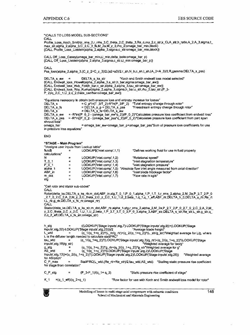
APPENDIX C.6 EES SOURCE CODE
"!CALLS TO LOSS MODEL SUB-SECTIONS"
CALL O f f - L o s s - C a s e y ( o m e g a - b a r - m l n , i , i _ m i n , d e l t ) (CALL O f f - L o s s - L i e b l e i n ( a l p h a - 2 , a l p h a - 3 , s i g m a ~
CALL ~ s s ~ l o s s ( a l p h a ~ 2 , a l ~ h a ~ 3 , ( ~ ~ ~ ~ 2 + ~ ~ z ~ 3 ) 1 2 , ( a 2 + a 3 2 , r s h , ~ b , c s h , t s h , ( A 2 + A _ 3 2 R . g a m m a : D E L T A ~ s j s s )
DELTA-s-ew = DELTA-s-k-str "Koch and Smith endwall loss model selected" (CALL Endwali~loss~Howell(alpha~2,alpha~3,s~str,h~bar,sigma:omega~bar~ew)) (CALL E n d w a l l - l o s s - H u b - F o t t ( h - b a r , c - s t r , a l p h a _ (CALL Endwaii~loss~Roy~Kumar(alpha~2,aipha~3,sigma,h~bar,c~s~,fio~2,tau~str,(P~3- P_2)/q-2.C-l .U_2.q-2,Vleta-carnber:omega_))
"Equations nessacary la obtain both pressure ioss and entropy increase for losses" DELTA-s = Cj'in(T3TT-2)-R'ln(P-3IP-2) "Total entropy change through rotor" DELTA s fs = DELTA-sj + DELTA-sjss "Freestream entropy change through rotor" DELTAS- = DELTA s &+DELTA s ew DE-TA~S .ew = -Ram((P. 0-2 - (cimiga. oar_eb?q: 2))/~-0_2).~alcdlates pressxe loss coeffic ent from endwa I oss. DELTA-59% = -R' n((P-0-2 - (omega_bargss'q_2IjIP-O-Z)'Ca1cu~a~es pressue loss weficlent horn part span shroud loss" omega-bar = omega~bar~ew+omega~barj+~rnega~barjss"Sum of pressure loss coefficients for use in pressure loss equations"
END
"STAGE - Main Program" "!Assigns user inputs from Lookup table" fluid$ - - LOOKUP$('lniet wmp'.l.l) "Defmes working fluid for use in fluid property calculations" N - - LOOKUP('iniet wmp',l.2) "Rotational speed" T-0-1 - - LOOKUP('lnlet wmp',l,3) "Inlet stagnation temperature"
p-0-1 - - LOOKUP('lnle1 cornp'.l.4) "Inlet stagnation pressure"
alpha-1 - - LOOKUP('inie1 wmp'.l.5) "Absolute flow inlet angle measured from axial direction" ABF-in - - LOOKUP('lnlet wmp',l,6) "Inlet blade blockage factor m-dot - - LOOKUP('lnle1 comp'.l,7) "Flow rate in kgls"
stg - - 1
"Call rotor and stator sub-codes" CALL Rotor(dei ta~ks.DELTA~s~k~rtr ,m~dot,ABFFinns~,T~0~1.P~0~1 ,alpha-I .P-1 .T-1,r-rms-2.alpha-2.M-2a,PP2,TT2,PP0 -2,T-0-2.C-2.A-2,M~z-2,C~theta_2,C-z-2,Cl .U-1 .U-2,beta-I ,q_l ,el-eff.ABF-rtr,DELTA-hhO,DELTADsSrtr,Re-rl r.L-rtr.g_rtr.DELTAr.L_rtr.g_rtr.DELTA_s_rs_rtr.omega_rtr)s~fs~rtr,omega_rtr) CALL
h-stg - - ((LOOKUP(Slage inputs',slg,7).LOOKUP('Stage inputs',stg.Q))+(LOOKUP('Stage inputs'.slg,22>LOOKUP('Stage inputs'.stg.23)))/2 "Average blade height" L-wtd - - (q-l/(q-1 +q-2))'(L-rtrlg_rtr)+(Q2/(q_l +q-2))'(L_strlg-str)Weighted average for Ug, where L IS the diffuser length needed to calculate staliPRC" tau-wtd - - (eIl(q_l+q_2))'(LOOKUP('Stage inputs'.s$,3~g-rtr)+(q~2l(q-l+q-2))^(LOOKUP('Stage inputs'.slg,l8yg_str) "Weighted average for taolg" g-stg - - (q-ll(q-1 +q_2))^g-rtr+(q_21(qZl+q_2))^g-strweighted average for g" - AS-wtd - (q-ll(q_l+q_2))^(LOOKUP('Stage lnputs',stg.2)/LOOKUP('Stage lnputs',stg.l3))+(e21(q_l+q~2))'(LOOKUP('Stage inputs'.s$,2)ILOOKUP('Stage inputs'.stg.26)) "Weighted average for ASIpitch" C-P-max - - StaiiPRC(L-wtd,(Re-rtr+Re-~tr)12~tau-wtd,AS-wtd) "Stalling static pressure rise coefficient for stage from correlation"
c-p-stg - - (P_~-P-~Y(L~+ ~ 2 ) "Static pressure rise coefficient of stage"
K-1 =(q-l-eff)l(q-2+~l) "Row factor for use with Koch and SmiVl endwall loss model for roto?
Modellirg of lasses in multi-stage axial campresson with subsonic conditions 148 School of Mechanical and Mataiais Engineering
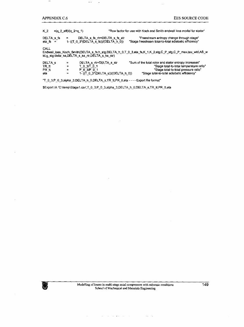
APPENDIX C.6 EES SOURCE CODE
K-2 = (%2-eM/ (~2+~1 ) "ROW factor for use with Koch and Smith endwall loss model for stato?
0ELTA.s-fs = DELTA_S.~_~~+DELTA.S-1s-str 'Freestream entropy cnange tnrodgn stage' eta-& = 1- ((T_~_~'(DELTA-~-IS)) /(DELTA-~~O]) 'Stage freestream totan-lo4ota1 adabatic effic.ency'
DELTA-s - - DELTA-s-rtr+DELTA-s-str "Sum of the total rotor and stator entropy increases" TR-tt - - T-0_3TT-0_1 "Stage total-to-total temperature ratio" PR-lt - - P_0-3/P_O-l "Stage total-to-total pressure ratio" eta - - 1- ((T-0-3'(DELTA-s))/(DELTA-h-0)) "Stage total-to-total adiabatic efficiency"
'7-0-3.P-0-3.alpha-3,DELTA-h-0,DELTA-s,TRPRe - - --Export file format"
School of Mechanical and Materials Engineering
Appendix D
DITIONAL VERIFICATION AND EVALUATION
INFO ON
D.l TEST COMPRESSOR SPECIFICATION ............................................................... 150
D.l ADDITIONAL NON-LOSS PARAMETER VERIFICATION ....................................... 152
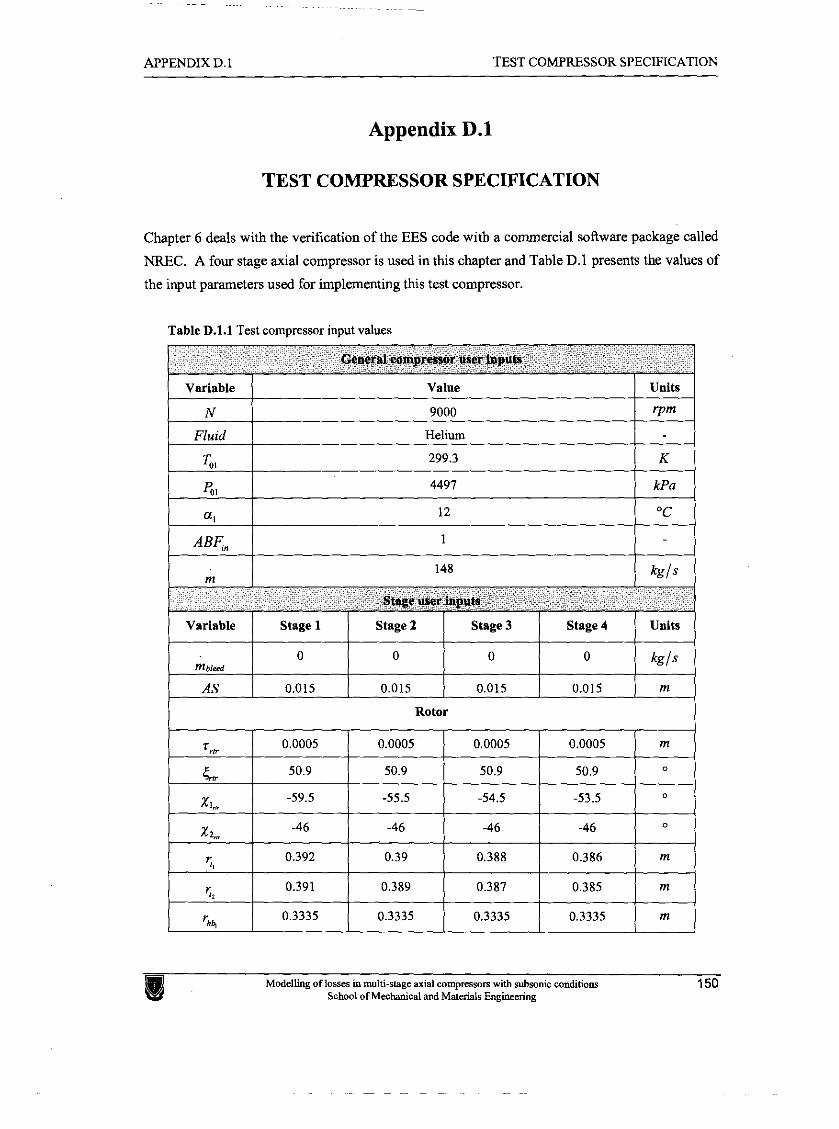
APPENDIX D. 1 TEST COMPRESSOR SPECIFICATION
Appendix D.1
TEST COMPRESSOR SPECIFICATION
Chapter 6 deals with the verification of the EES code with a commercial software package called
NREC. A four stage axial compressor is used in this chapter and Table D.l presents the values of
the input parameters used for implementing this test compressor.
Table D.l.l Test compressor input values
General cornpronor user inputs
... - - Stage user inputs
Variable
N
Fluid
t GI a1
ABF;,
M
School of Mechmical and Materials Eng~neenng
Value
9000
Helium
299.3
4497
12
1
148
Variable
r n b l d
AS
Units
'P"'
K
kPa
OC
kgls
Rotor
Stage 1
0
0.015
Stage 2
0
0.015
Stage 3
0
0.015
Stage 4
0
0.015
Units
kgls
rn
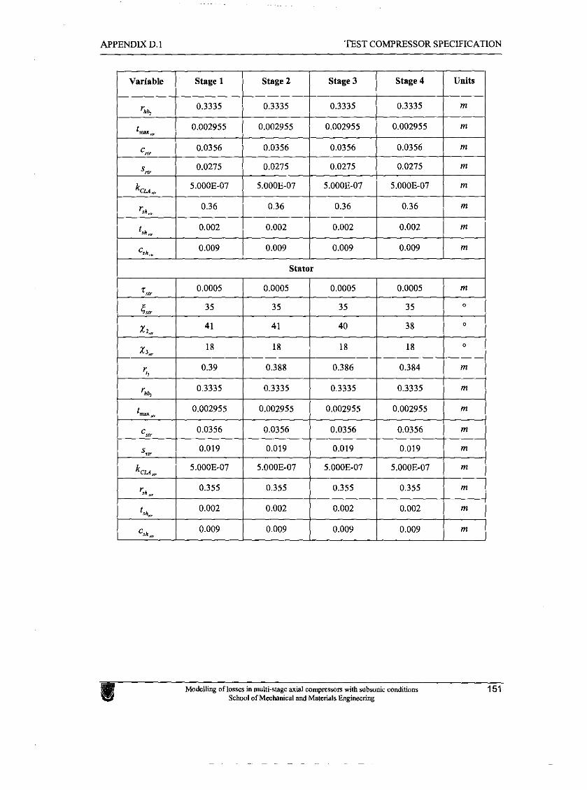
APPENDIX D. 1 TEST COMPRESSOR SPECLFICATION
Stator
Modelling of losses in multi-stage axial compressors with subsonic conditions 151 School o f Mechanical and Materials Engineering
Stage 4 Variable Units Stage 2 Stage 1 Stage 3
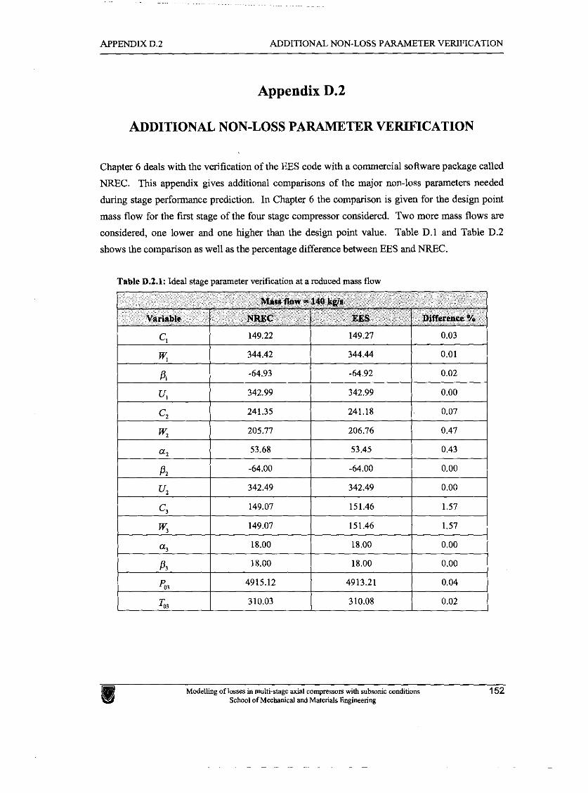
APPENDIX D.2 ADDITIONAL NON-LOSS PARAMETER VERIFICATION
Appendix D.2
ADDITIONAL NON-LOSS PARAMETER VERIFICATION
Chapter 6 deals with the verification of the EES code with a commercial software package called
NREC. This appendix gives additional comparisons of the major non-loss parameters needed
during stage performance prediction. In Chapter 6 the comparison is given for the design point
mass flow for the first stage of the four stage compressor considered. Two more mass flows are
considered, one lower and one higher than the design point value. Table D.l and Table D.2
shows the comparison as well as the percentage difference between EES and NREC.
Table D.Z.1: Ideal stage parameter verification at a reduced mass flow
Modelling of losses in multi-stage axial compressom with subsonic conditions 152 School of Mechanical and Materials Engineering
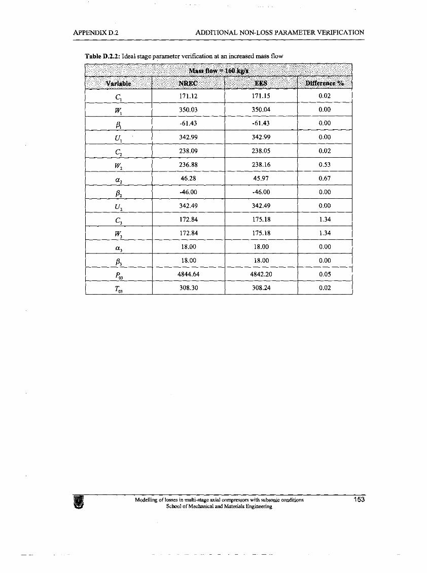
APPENDIX D.2 ADDITIONAL NON-LOSS PARAMETER VERIFICATION
Table D.2.2: Ideal stage parameter verification at an increased mass flow
1 T.. 1 308.30 I 308.24 1 0.02
Modelling of losses in multi-stage axial compressors with subsonic conditions 153 School of Mechanical and Materials Engineering