Embed Size (px)
Citation preview
Modelling of Timber-Concrete Composite Structures
Subjected to Short-Term Monotonic Loading
by
Cong Liu
A thesis submitted in conformity with the requirements
for the degree of Master of Applied Science
Civil Engineering
University of Toronto
© Copyright by Cong Liu (2016)
ii
Modelling of Timber-Concrete Composite Structures Subjected to Short-Term
Monotonic Loading
Cong Liu
Master of Applied Science
Civil and Environmental Engineering
University of Toronto
2016
Abstract
Timber-concrete composite (TCC) is an innovative and efficient construction material which
exploits the best properties of timber and concrete. The presence of shear connectors enables
the two dissimilar materials to act together as a whole, resulting in an increase in global stiffness
as well as load-carrying capacity. As this composite material is becoming increasingly more
popular in the construction industry, there is a need to develop an analysis tool which has general
applicability to timber-concrete composite systems with variations in loading schemes, specimen
configurations, materials, and types of shear connectors.
A generic 2D nonlinear finite element model is proposed in this thesis, and is verified through
extensive numerical simulations of six experiment series carried out by researchers around the
globe. Good agreement between experimentally observed behaviour and numerical simulations
were generally obtained.

iii
Acknowledgements
I would like to express my deepest gratitude to Professor Frank Vecchio for his guidance and
support over the course of my research studies. Without his boundless patience, continual
support and encouragement, I could not have achieved my goals. I would also like to thank
Professor Paul Gauvreau for his invaluable comments while reviewing my thesis.
I would like to thank my colleagues and friends Anca Jurcut, Benard Isojeh, Stamatina Chasioti,
Mark Hunter, Andac Lulec, Vahid Sadeghian, Saif Shaban, Siavash Habibi, Raymond Ma, Giorgio
Proestos, Allan Kuan, Edvard Bruun, and Dr. Min Sun for their friendship and advice throughout
the course of this project.
I would like to acknowledge the generous financial support that I received from: the Natural
Sciences and Engineering Research Council of Canada (NSERC), Read Jones Christoffersen
Consulting Engineers (RJC), the University of Toronto, and Professor Frank Vecchio.
Last but not least, I would like to thank my parents for their unconditional love, encouragement,
and patience.
iv
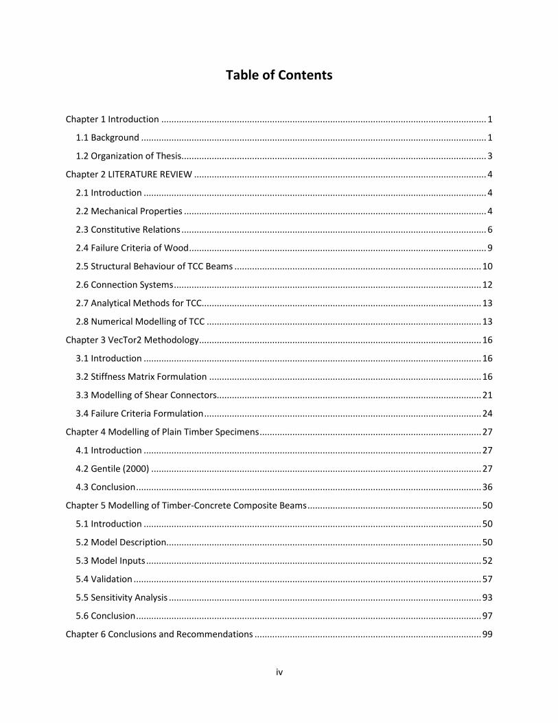
Table of Contents
Chapter 1 Introduction ................................................................................................................................. 1
1.1 Background ......................................................................................................................................... 1
1.2 Organization of Thesis ......................................................................................................................... 3
Chapter 2 LITERATURE REVIEW .................................................................................................................... 4
2.1 Introduction ........................................................................................................................................ 4
2.2 Mechanical Properties ........................................................................................................................ 4
2.3 Constitutive Relations ......................................................................................................................... 6
2.4 Failure Criteria of Wood ...................................................................................................................... 9
2.5 Structural Behaviour of TCC Beams .................................................................................................. 10
2.6 Connection Systems .......................................................................................................................... 12
2.7 Analytical Methods for TCC............................................................................................................... 13
2.8 Numerical Modelling of TCC ............................................................................................................. 13
Chapter 3 VecTor2 Methodology ................................................................................................................ 16
3.1 Introduction ...................................................................................................................................... 16
3.2 Stiffness Matrix Formulation ............................................................................................................ 16
3.3 Modelling of Shear Connectors......................................................................................................... 21
3.4 Failure Criteria Formulation .............................................................................................................. 24
Chapter 4 Modelling of Plain Timber Specimens ........................................................................................ 27
4.1 Introduction ...................................................................................................................................... 27
4.2 Gentile (2000) ................................................................................................................................... 27
4.3 Conclusion ......................................................................................................................................... 36
Chapter 5 Modelling of Timber-Concrete Composite Beams ..................................................................... 50
5.1 Introduction ...................................................................................................................................... 50
5.2 Model Description ............................................................................................................................. 50
5.3 Model Inputs ..................................................................................................................................... 52
5.4 Validation .......................................................................................................................................... 57
5.5 Sensitivity Analysis ............................................................................................................................ 93
5.6 Conclusion ......................................................................................................................................... 97
Chapter 6 Conclusions and Recommendations .......................................................................................... 99
v
6.1 Conclusions ....................................................................................................................................... 99
6.2 Recommendations .......................................................................................................................... 100
References ................................................................................................................................................ 101
Appendix Modelling Guideline ................................................................................................................ 105
vi
List of Figures
Figure 1-1 Typical forms of TCC (Frangi and Fontana, 2003) ........................................................................ 1
Figure 2-1 Typical stress-strain curves for wood (Holmberg et al.,1998) ..................................................... 6
Figure 2-2 Proposed stress-strain curves in compression (Lau, 2000) ......................................................... 8
Figure 2-3 Failure modes and failure planes (Hashin, 1980) ...................................................................... 10
Figure 2-4 Definition of composite action (Lukaszewka, 2009) .................................................................. 11
Figure 2-5 Typical load-deflection response of TCC .................................................................................... 12
Figure 2-6 Comparison of different connection systems (Dias, 2005) ....................................................... 12
Figure 2-7 FE model (van der Linden, 1999) ............................................................................................... 14
Figure 2-8 1D FE model (Fragiacomo, 2005) ............................................................................................... 15
Figure 2-9 FE model in ABAQUS (Persaud and Symons, 2006) ................................................................... 15
Figure 3-1 VecTor2 coordinate reference systems (Vecchio, 1990) ........................................................... 16
Figure 3-2 Typical stress-strain curve for wood (grain direction) ............................................................... 20
Figure 3-3 Typical stress-strain curve for wood (transverse direction) ...................................................... 21
Figure 3-4 The link element (Wong et el., 2004) ........................................................................................ 22
Figure 3-5 The contact element (Wong et el., 2004) .................................................................................. 22
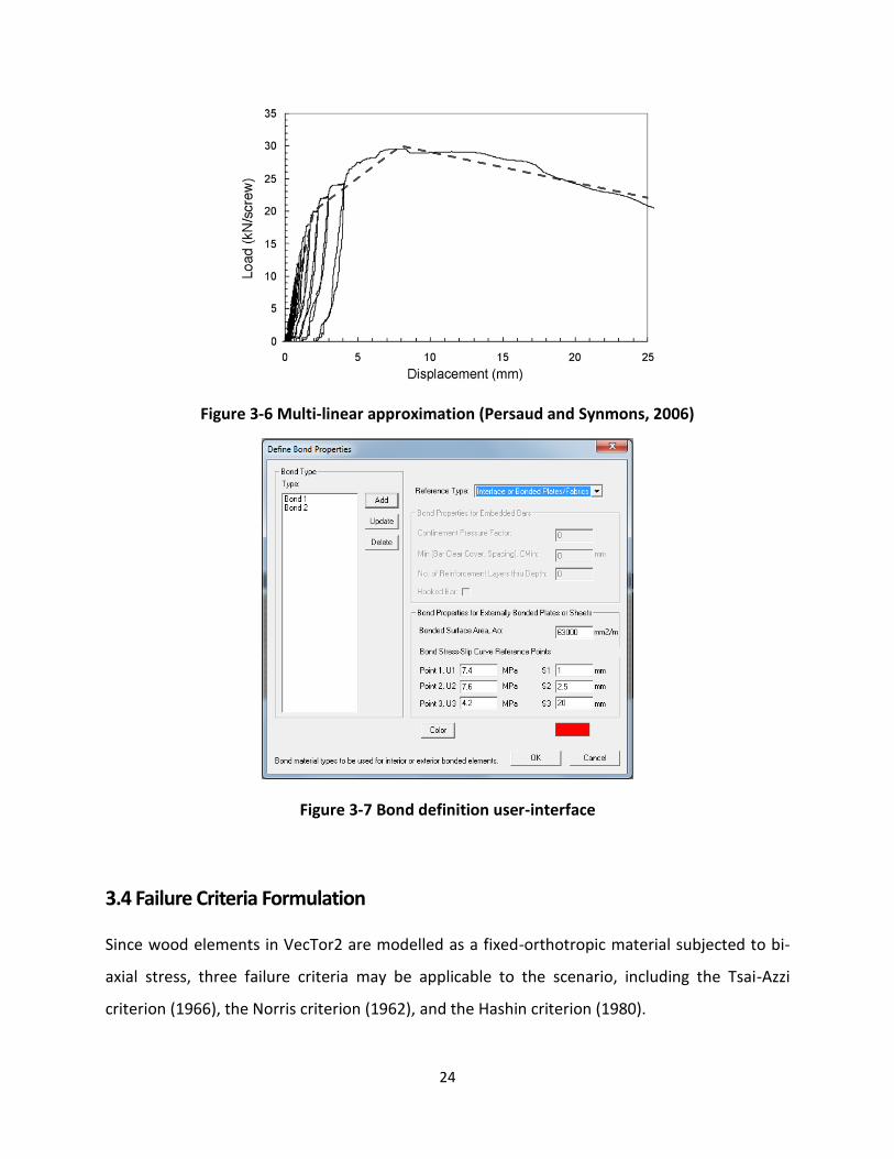
Figure 3-6 Multi-linear approximation (Persaud and Synmons, 2006) ....................................................... 24
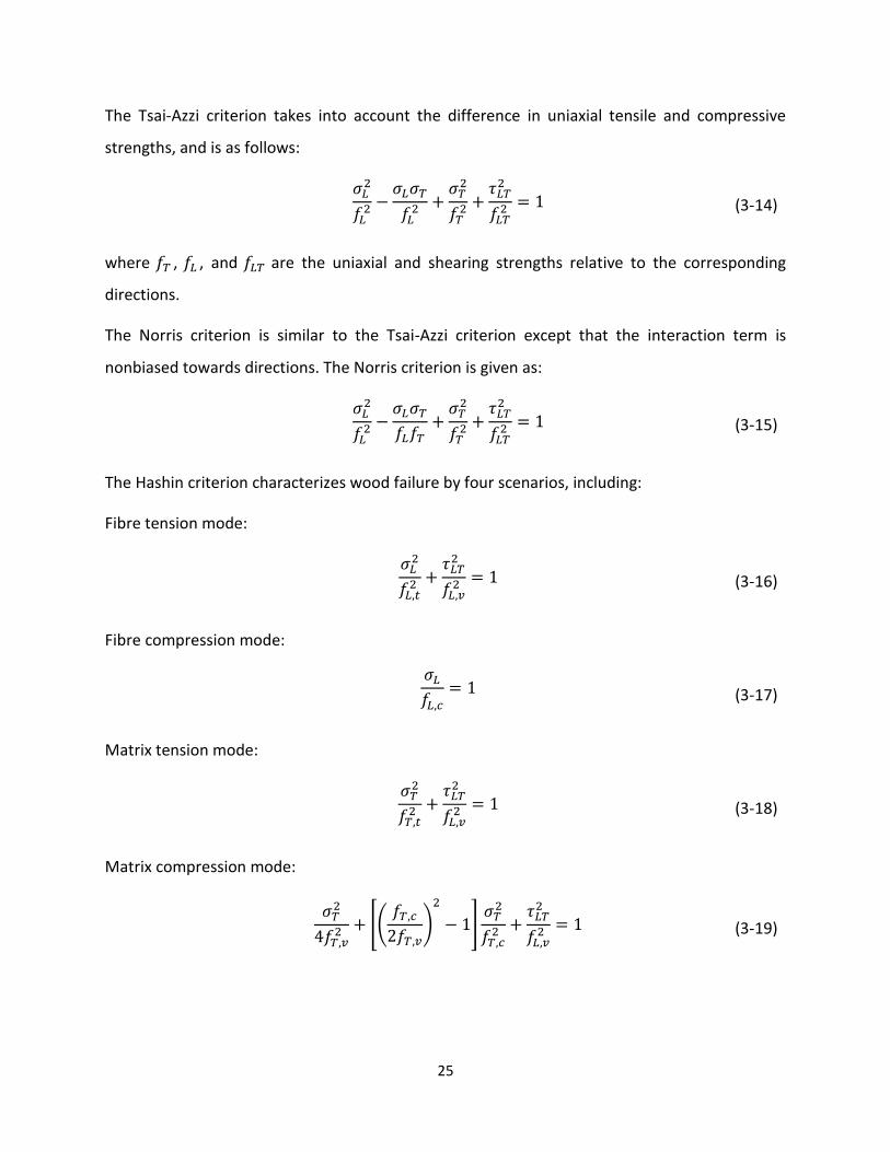
Figure 3-7 Bond definition user-interface ................................................................................................... 24
Figure 4-1 Test configuration for half-scale beams (Gentile, 2000) ........................................................... 28
Figure 4-2 Cross-sections of half-scale reinforced beams (Gentile, 2000) ................................................. 28
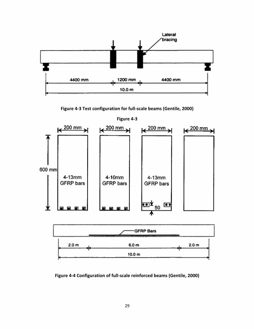
Figure 4-3 Test configuration for full-scale beams (Gentile, 2000) ............................................................ 29
Figure 4-4 Configuration of full-scale reinforced beams (Gentile, 2000) ................................................... 29
Figure 4-5 Stress-strain relationships for GFRP (Gentile, 2000) ................................................................. 30
Figure 4-6 Half-scale plain timber beams ................................................................................................... 32
Figure 4-7 Half-scale beams with GFRP reinforcement .............................................................................. 32
Figure 4-8 Full-scale beams with GFRP reinforcement at the bottom (FS1 and FS2) ................................. 32
Figure 4-9 Full-scale beam with GFRP reinforcement at the sides (FS3) .................................................... 32
Figure 4-10 Full-scale plain timber beam (FS4) ........................................................................................... 32
Figure 4-11 VecTor2 load-deflection responses ......................................................................................... 38
Figure 5-1 Sample model with smeared shear connectors ........................................................................ 51
vii
Figure 5-2 Sample model with discrete shear connectors ......................................................................... 52
Figure 5-3 Concrete definition interface ..................................................................................................... 53
Figure 5-4 Wood definition interface ......................................................................................................... 56
Figure 5-5 Contact element definition interface ........................................................................................ 57
Figure 5-6 Details of the proposed system (Persaud and Symons, 2006) .................................................. 58
Figure 5-7 Push-out test specimen (Persaud and Symons, 2006) .............................................................. 60
Figure 5-8 VecTor2 model ........................................................................................................................... 60
Figure 5-9 Load-deflection plot ................................................................................................................... 61
Figure 5-10 Load-slip plot ........................................................................................................................... 61
Figure 5-11 Deflected shape at collapse ..................................................................................................... 62
Figure 5-12 Variations of connections with and without coach screws: (a) rectangular; (b) triangular; and
(c) toothed plate connection (Yeoh, 2010) ................................................................................................. 63
Figure 5-13 Typical four-point bending test setup (dimensions in mm) (Yeoh, 2010) ............................... 63
Figure 5-14 Typical cross-sections of the bending specimens (Yeoh, 2010) .............................................. 63
Figure 5-15 FE model for specimens A1 and A2 ......................................................................................... 64
Figure 5-16 Load-slip curves (Yeoh, 2010) .................................................................................................. 65
Figure 5-17 Load-deflection plots ............................................................................................................... 67
Figure 5-18 Arrangement of Specimen F1 (Yeoh, 2010) ............................................................................. 70
Figure 5-19 Specimen details and result (Cecotti et al., 2006) ................................................................... 70
Figure 5-20 Cross sections of (a) CS1 and (b) CS3 (Deam et al., 2008) ....................................................... 72
Figure 5-21 Test setup (Deam et al., 2008) ................................................................................................. 72
Figure 5-22 Connector layout for Specimen CS3 (Deam et al., 2008) ........................................................ 73
Figure 5-23 Adopted and adjusted load-slip curve (Deam et al., 2008) ..................................................... 73
Figure 5-24 FE model for Specimen CS3 (Deam et al., 2008) ..................................................................... 74
Figure 5-25 Definition of bond between tendon and timber (Deam et al., 2008) ..................................... 74
Figure 5-26 Load-deflection plots for Specimen CS1 and CS3 .................................................................... 75
Figure 5-27 Experimental setup for Gerber Specimen ............................................................................... 77
Figure 5-28 FE model for Series 2 ............................................................................................................... 78
Figure 5-29 Load-deflection plots ............................................................................................................... 78
Figure 5-30 Close-up of sudden force drops ............................................................................................... 83
Figure 5-31 Experimental setup (van der Linden, 1999) ............................................................................. 85
Figure 5-32 Connector Types (van der Linden, 1999) ................................................................................. 85
viii
Figure 5-33 Load-deflection response ........................................................................................................ 86
Figure 5-34 Crack pattern at 14 kN per jack ............................................................................................... 90
Figure 5-35 Crack pattern at 30 kN per jack ............................................................................................... 90
Figure 5-36 Specimen cross section (Lukaszewska, 2009) .......................................................................... 90
Figure 5-37 Connector types (a) SP+N; (b) SST + S (Lukaszewska, 2009) ................................................... 91
Figure 5-38 Connector Layout (a) Top: Specimen 1 and 5 (SP + N); (b) Middle: Specimen 2 and 4 (SST + S);
(c) Bottom: Specimen 3 (SST + S) (Lukaszewska, 2009) .............................................................................. 91
Figure 5-39 Load-deflection response continued (Lukaszewska, 2009) ..................................................... 93
Figure 5-40 FE models with different mesh size ......................................................................................... 94
Figure 5-41 Comparison of predicted load-deflection responses of different mesh size .......................... 94
Figure 5-42 Load-deflection responses of Specimen CS1 with linear and nonlinear material constitutive
models ......................................................................................................................................................... 96
Figure 5-43 Load-deflection responses of Specimen S7 with linear and nonlinear material constitutive
models ......................................................................................................................................................... 96
ix
List of Tables
Table 4-1 Summary of the models .............................................................................................................. 33
Table 4-2 Summary of input parameters .................................................................................................... 33
Table 4-3 Reinforcement details ................................................................................................................. 34
Table 4-4 Summary of ultimate loads ......................................................................................................... 49
Table 5-1 Default concrete models ............................................................................................................. 53
Table 5-2 Concrete properties .................................................................................................................... 54
Table 5-3 Input Parameters ........................................................................................................................ 60
Table 5-4 Summary of the FE model ........................................................................................................... 60
Table 5-5 Summary of the Yeoh specimens ................................................................................................ 64
Table 5-6 Summary of results ..................................................................................................................... 67
Table 5-7 Characteristics of specimens ....................................................................................................... 71
Table 5-8 Specimen characteristics ............................................................................................................ 76
Table 5-9 Timber specification .................................................................................................................... 76
1
Chapter 1 Introduction
1.1 Background
Timber-concrete composite (TCC) is a construction material which was first introduced to the
construction industry in Europe, as an alternative to reinforced concrete, due to the steel
shortage after World War II. This construction technique has seen rapid development in the past
two decades and found extensive structural applications, including renovation and upgrading of
existing timber structures, new construction of mid- to low-rise buildings, and construction of
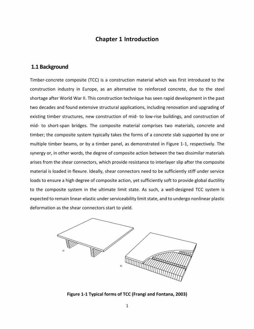
mid- to short-span bridges. The composite material comprises two materials, concrete and
timber; the composite system typically takes the forms of a concrete slab supported by one or
multiple timber beams, or by a timber panel, as demonstrated in Figure 1-1, respectively. The
synergy or, in other words, the degree of composite action between the two dissimilar materials
arises from the shear connectors, which provide resistance to interlayer slip after the composite
material is loaded in flexure. Ideally, shear connectors need to be sufficiently stiff under service
loads to ensure a high degree of composite action, yet sufficiently soft to provide global ductility
to the composite system in the ultimate limit state. As such, a well-designed TCC system is
expected to remain linear-elastic under serviceability limit state, and to undergo nonlinear plastic
deformation as the shear connectors start to yield.
Figure 1-1 Typical forms of TCC (Frangi and Fontana, 2003)
2
Although several analytical methods have been proposed to cope with the design and analysis of
TCC structures, each analytical method has its own underlying assumptions and limited scope of
application. As such, none of the methods are universally agreed upon and adopted in the
mainstream design codes. The Gamma Method, for instance, is currently adopted in Eurocode 5.
This method is suitable for linear-elastic analysis of TCC beams under serviceability limit state,
yet it neglects the plastic deformation of the shear connectors which, ultimately, results in an
overestimation of the post-yielding global stiffness. In addition, the Gamma Method was
developed based on the analytical solution of a composite beam subjected to uniformly-
distributed load; therefore, the method does not apply to situations where a TCC beam is
subjected to point loads or non-uniformly-distributed loads.
Various finite element models have been developed by several researchers (van der Linden, 1999;
Fragiacomo, 2005; Persaud and Symons, 2006). While these models can predict the load-
deflection response with reasonable accuracy, they are limited to the analysis at a global level
due to the nature of 1D FE analysis and the limitations of frame elements used in these models.
Moreover, 1D frame FE models are not applicable to complex experimental setups, such as the
prestressed specimens or the specimens built with cross-laminated timber (CLT) tested by Deam
et al (2008) and Gerber (2016), respectively.
In light of the current development of FE analysis in this field, this research programme aims to
develop a generic 2D finite element model which takes material nonlinearity and yielding of shear
connectors into account. The model will also need to be flexible and be easily adapted to deal
with the variations of TCC experimental setups.
VecTor2, originally developed at the University of Toronto for the nonlinear analysis of reinforced
or prestressed concrete structures, is a powerful 2D nonlinear finite element analysis program.
The program employs a total load, iterative secant stiffness algorithm which has been proven to
be successful in the nonlinear analysis of reinforced concrete structures. It has the potential to
analyze plain timber or TCC structures provided that appropriate material constitutive models
are implemented.
3
1.2 Organization of Thesis
This thesis presents the work undertaken to expand VecTor2’s capabilities to analyze plain timber
and timber-concrete composite structures. A brief overview of the current developments of TCC
technology, along with the research objectives of this thesis, are presented in Chapter 1.
Chapter 2 provides a literature survey that covers the key aspects related to this research project.
The topics reviewed in his chapter include the mechanical properties of wood, wood constitutive
models, failure criteria, structural behaviour of TCC, connection systems, and analytical models
of TCC, as well as numerical methods.
Chapter 3 explains the details of the stiffness matrix formulation for membrane elements and
bond-slip elements, implementation of wood constitutive models, and implementation of
existing failure criteria applicable to wood.
Chapter 4 validates the work reported in Chapter 3, through comparison of the experimental
results and the numerical results of the specimens tested by Gentile (2000). The specimens
investigated included plain timber beams and timber beams reinforced with GFRP bars, all of
which were subjected to short-term monotonic loadings.
Chapter 5 proposes a generic 2D model, and examines the model’s accuracy and general
applicability through numerical corroborations of six experiment series carried out by
researchers around the globe. The specimens investigated have variations in terms of
experimental setups, materials, and types of shear connectors.
Chapter 6 presents conclusions drawn from the numerical corroborations of this study, and
provides recommendations for future work.
4
Chapter 2 LITERATURE REVIEW
2.1 Introduction
This chapter presents a literature survey that covers the different aspects related to this research
study, including the mechanical properties and the constitutive relationships of timber, failure
criteria of wood, structural behaviour of TCC, and numerical modelling of TCC structures
subjected to short-term loadings.
Although the material in this field is very broad, the information provided in this chapter is not
intended to be exhaustive; instead, it provides an overview of the subject matter, and serves as
a stepping stone to the subsequent work of this research study.
2.2 Mechanical Properties
Contrary to concrete, wood is characterized as an anisotropic material with three axes of
symmetry; namely, longitudinal, radial, and tangential, denoted as L, R, T, respectively. The
mechanical properties along these axes are unique and independent of others.
The elastic properties of timber can be described by twelve elastic constants, including three
elastic moduli ( 𝐸𝐿 , 𝐸𝑅 , 𝐸𝑇 ), three shear moduli ( 𝐺𝑅𝑇 , 𝐺𝐿𝑇 , 𝐺𝐿𝑅 ), and six Poisson’s ratios
(𝜇𝐿𝑅 , 𝜇𝑅𝐿 , 𝜇𝐿𝑇 , 𝜇𝑇𝐿 , 𝜇𝑅𝑇 , 𝜇𝑇𝑅 The shear moduli are specific to the planes as indicated by the
subscripts, while for the Poisson’s ratios, the first letter of the subscripts refers to the direction
of applied stress and the second letter to the direction of lateral deformation. The six Poisson’s
ratio can be reduced to three according to the following relationship.
𝜇𝑖𝑗
𝐸𝑗=
𝜇𝑗𝑖
𝐸𝑖
where i ≠ j; i, j = L, R, T.
5
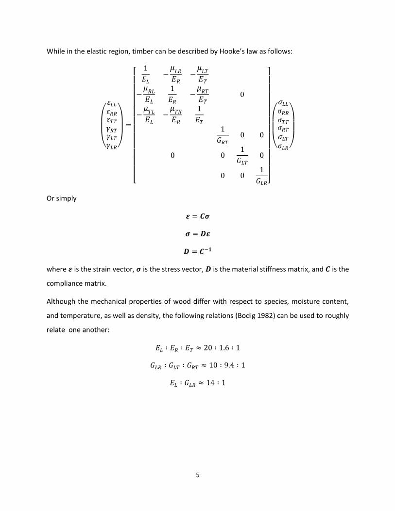
While in the elastic region, timber can be described by Hooke’s law as follows:
(
휀𝐿𝐿
휀𝑅𝑅휀𝑇𝑇
𝛾𝑅𝑇𝛾𝐿𝑇
𝛾𝐿𝑅)
=
[
1
𝐸𝐿−
𝜇𝐿𝑅
𝐸𝑅−
𝜇𝐿𝑇
𝐸𝑇
−𝜇𝑅𝐿
𝐸𝐿
1
𝐸𝑅−
𝜇𝑅𝑇
𝐸𝑇
−𝜇𝑇𝐿
𝐸𝐿−
𝜇𝑇𝑅
𝐸𝑅
1
𝐸𝑇
0
0
1
𝐺𝑅𝑇0 0
01
𝐺𝐿𝑇0
0 01
𝐺𝐿𝑅]
(
𝜎𝐿𝐿
𝜎𝑅𝑅
𝜎𝑇𝑇𝜎𝑅𝑇
𝜎𝐿𝑇
𝜎𝐿𝑅)
Or simply
𝜺 = 𝑪𝝈
𝝈 = 𝑫𝜺
𝑫 = 𝑪−𝟏
where 𝜺 is the strain vector, 𝝈 is the stress vector, 𝑫 is the material stiffness matrix, and 𝑪 is the
compliance matrix.
Although the mechanical properties of wood differ with respect to species, moisture content,
and temperature, as well as density, the following relations (Bodig 1982) can be used to roughly
relate one another:
𝐸𝐿 ∶ 𝐸𝑅 ∶ 𝐸𝑇 ≈ 20 ∶ 1.6 ∶ 1
𝐺𝐿𝑅 ∶ 𝐺𝐿𝑇 ∶ 𝐺𝑅𝑇 ≈ 10 ∶ 9.4 ∶ 1
𝐸𝐿 ∶ 𝐺𝐿𝑅 ≈ 14 ∶ 1
6
2.3 Constitutive Relations
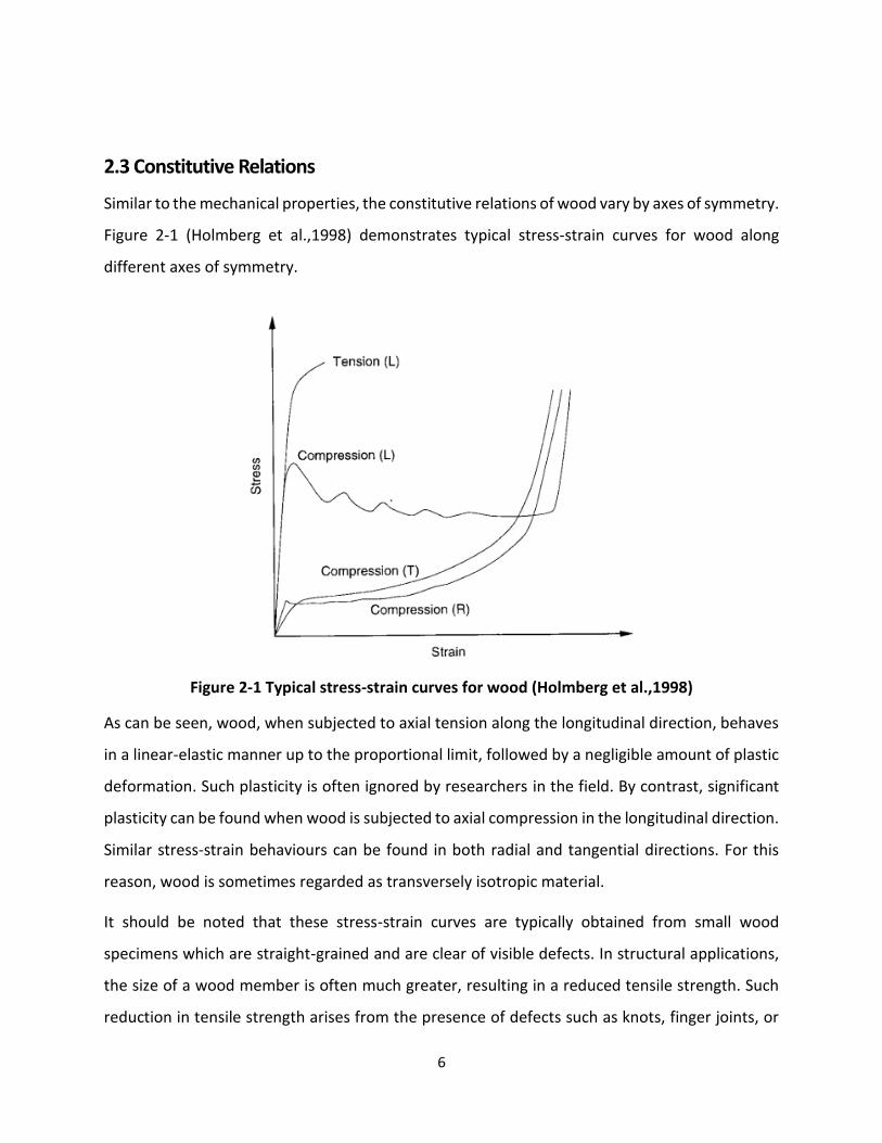
Similar to the mechanical properties, the constitutive relations of wood vary by axes of symmetry.
Figure 2-1 (Holmberg et al.,1998) demonstrates typical stress-strain curves for wood along
different axes of symmetry.
Figure 2-1 Typical stress-strain curves for wood (Holmberg et al.,1998)
As can be seen, wood, when subjected to axial tension along the longitudinal direction, behaves
in a linear-elastic manner up to the proportional limit, followed by a negligible amount of plastic
deformation. Such plasticity is often ignored by researchers in the field. By contrast, significant
plasticity can be found when wood is subjected to axial compression in the longitudinal direction.
Similar stress-strain behaviours can be found in both radial and tangential directions. For this
reason, wood is sometimes regarded as transversely isotropic material.
It should be noted that these stress-strain curves are typically obtained from small wood
specimens which are straight-grained and are clear of visible defects. In structural applications,
the size of a wood member is often much greater, resulting in a reduced tensile strength. Such
reduction in tensile strength arises from the presence of defects such as knots, finger joints, or
7
stress concentration due to grain discontinuity. Nevertheless, the stress-strain curves in
compression agree fairly well with those shown in Figure 2-1.
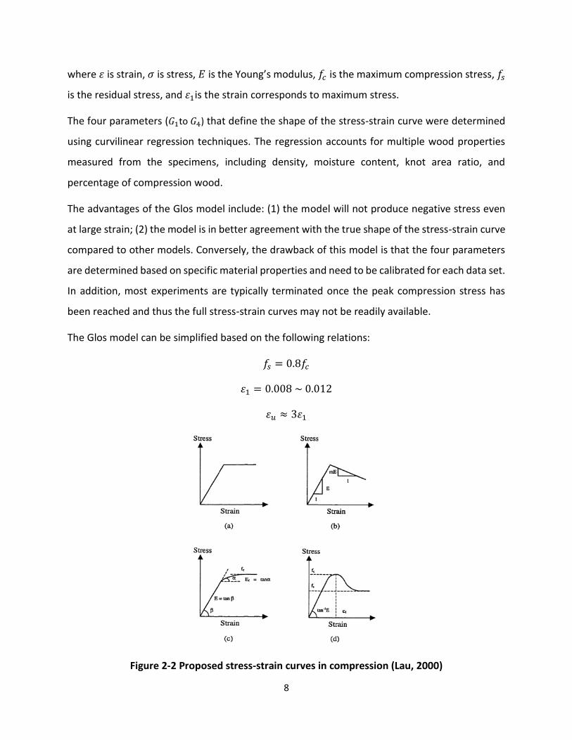
Many researchers have dealt with the nonlinear stress-strain behaviour of timber in compression.
Neely (1898) proposed a simple model which assumes an elasto-plastic stress-strain relationship
in compression with the material remaining linear-elastic in tension (Figure 2-2a). A slight
modification was suggested by Bazan (1980) (Figure 2-2b), in which the stress-strain relationship
remains linear elastic up to the proportional limit, followed by a linear decline in stress with
increasing strain. The limitation of Bazan’s model is that the model will not work for large strain
since it may produce negative stress.
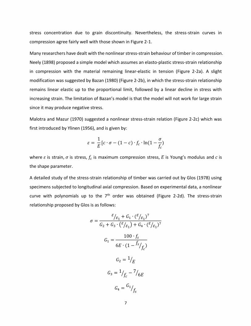
Malotra and Mazur (1970) suggested a nonlinear stress-strain relation (Figure 2-2c) which was
first introduced by Ylinen (1956), and is given by:
휀 = 1
𝐸[𝑐 ∙ 𝜎 − (1 − 𝑐) ∙ 𝑓𝑐 ∙ ln (1 −
𝜎
𝑓𝑐)
where 휀 is strain, 𝜎 is stress, 𝑓𝑐 is maximum compression stress, 𝐸 is Young’s modulus and 𝑐 is
the shape parameter.
A detailed study of the stress-strain relationship of timber was carried out by Glos (1978) using
specimens subjected to longitudinal axial compression. Based on experimental data, a nonlinear
curve with polynomials up to the 7th order was obtained (Figure 2-2d). The stress-strain
relationship proposed by Glos is as follows:
𝜎 =휀
휀1⁄ + 𝐺1 ∙ (휀 휀1⁄ )7
𝐺2 + 𝐺3 ∙ (휀 휀1⁄ ) + 𝐺4 ∙ (휀 휀1⁄ )7
𝐺1 =100 ∙ 𝑓𝑠
6𝐸 ∙ (1 −𝑓𝑠
𝑓𝑐⁄ )
𝐺2 = 1𝐸⁄
𝐺3 = 1𝑓𝑐
⁄ − 76𝐸⁄
𝐺4 =𝐺1
𝑓𝑠⁄
8
where 휀 is strain, 𝜎 is stress, 𝐸 is the Young’s modulus, 𝑓𝑐 is the maximum compression stress, 𝑓𝑠
is the residual stress, and 휀1is the strain corresponds to maximum stress.
The four parameters (𝐺1to 𝐺4) that define the shape of the stress-strain curve were determined
using curvilinear regression techniques. The regression accounts for multiple wood properties
measured from the specimens, including density, moisture content, knot area ratio, and
percentage of compression wood.
The advantages of the Glos model include: (1) the model will not produce negative stress even
at large strain; (2) the model is in better agreement with the true shape of the stress-strain curve
compared to other models. Conversely, the drawback of this model is that the four parameters
are determined based on specific material properties and need to be calibrated for each data set.
In addition, most experiments are typically terminated once the peak compression stress has
been reached and thus the full stress-strain curves may not be readily available.
The Glos model can be simplified based on the following relations:
𝑓𝑠 = 0.8𝑓𝑐
휀1 = 0.008 ~ 0.012
휀𝑢 ≈ 3휀1
Figure 2-2 Proposed stress-strain curves in compression (Lau, 2000)
9
2.4 Failure Criteria of Wood
The failure modes of wood can be extremely complex as they can be induced by one or more
mechanical stimuli. Failure of a timber beam, for instance, may be caused by rupture of the
tension fibres, delamination of fibres due to horizontal shear, buckling of the compression fibres,
or a mix of all three. This section reviews some of the failure criteria applicable to wood. These
criteria were either developed for wood, or apply to orthotropic composite material in general,
such as wood.
The Hankinson formula (1921) is the first well-known one-dimensional empirical formula
developed and it provides adequate results for compression and tension in general.
Hill (1950) proposed a failure criterion that is adapted from the von Mises criterion and has the
ability to deal with the anisotropic effects of wood. A modification to the Hill criterion was
suggested by Azzi and Tsai (1965), known as Tsai-Hill criterion. The Tsai-Hill criterion is applicable
to composite materials that have identical mechanical properties in the plane perpendicular to
the fibre orientation.
The Norris criterion (1950), originally developed for application to glued laminated timber, has
been extensively applied for modelling of strength in solid wood. Several researchers (Van der
Put 2005, Kasal and Leichti 2005; de Ruvo et al. 1980), however, have reported that it
underpredicts when biaxial loading is combined with shear.
Hoffman (1967) proposed a model that accounts for the difference between tensile strength and
compressive strength. It may be seen as an extension of the Hill criterion. This criterion has been
widely used for the analysis of brittle composite materials such as wood subjected to tension.
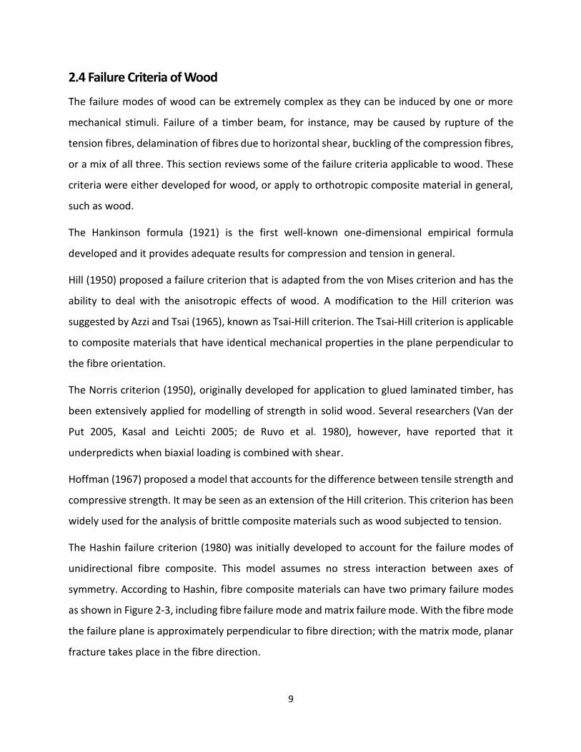
The Hashin failure criterion (1980) was initially developed to account for the failure modes of
unidirectional fibre composite. This model assumes no stress interaction between axes of
symmetry. According to Hashin, fibre composite materials can have two primary failure modes
as shown in Figure 2-3, including fibre failure mode and matrix failure mode. With the fibre mode
the failure plane is approximately perpendicular to fibre direction; with the matrix mode, planar
fracture takes place in the fibre direction.
10
Figure 2-3 Failure modes and failure planes (Hashin, 1980)
Both compression and tension can give rise to the two failure mechanisms. Therefore, there are
four failure modes, namely tensile fibre mode, compressive fibre mode, tensile matrix mode, and
compressive matrix mode. Similar to Tsai-Hill criterion, Hashin’s model is applicable to
transversely isotropic materials.
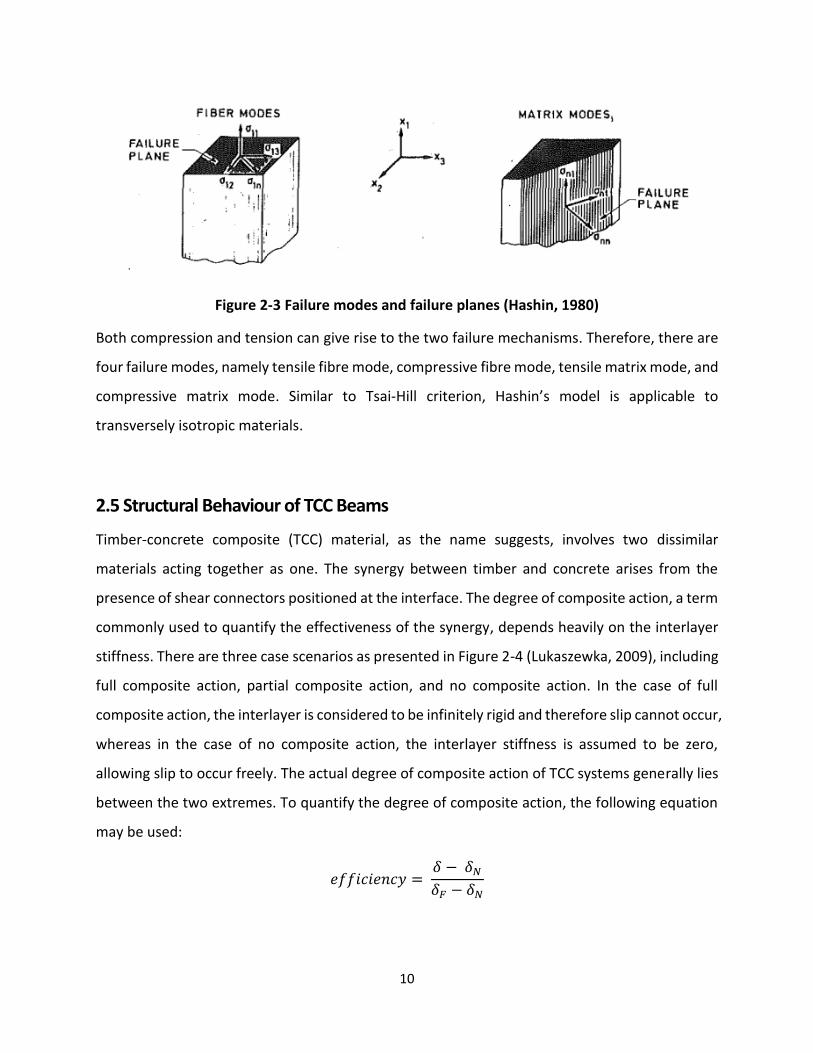
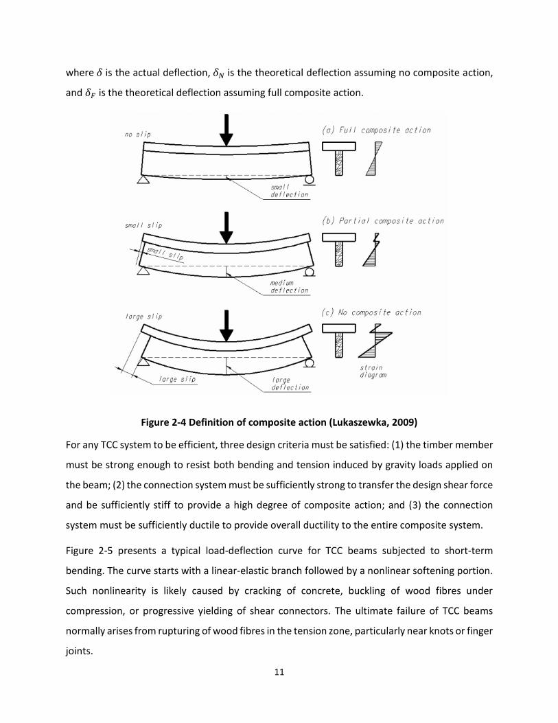
2.5 Structural Behaviour of TCC Beams
Timber-concrete composite (TCC) material, as the name suggests, involves two dissimilar
materials acting together as one. The synergy between timber and concrete arises from the
presence of shear connectors positioned at the interface. The degree of composite action, a term
commonly used to quantify the effectiveness of the synergy, depends heavily on the interlayer
stiffness. There are three case scenarios as presented in Figure 2-4 (Lukaszewka, 2009), including
full composite action, partial composite action, and no composite action. In the case of full
composite action, the interlayer is considered to be infinitely rigid and therefore slip cannot occur,
whereas in the case of no composite action, the interlayer stiffness is assumed to be zero,
allowing slip to occur freely. The actual degree of composite action of TCC systems generally lies
between the two extremes. To quantify the degree of composite action, the following equation
may be used:
𝑒𝑓𝑓𝑖𝑐𝑖𝑒𝑛𝑐𝑦 = 𝛿 − 𝛿𝑁
𝛿𝐹 − 𝛿𝑁
11
where 𝛿 is the actual deflection, 𝛿𝑁 is the theoretical deflection assuming no composite action,
and 𝛿𝐹 is the theoretical deflection assuming full composite action.
Figure 2-4 Definition of composite action (Lukaszewka, 2009)
For any TCC system to be efficient, three design criteria must be satisfied: (1) the timber member
must be strong enough to resist both bending and tension induced by gravity loads applied on
the beam; (2) the connection system must be sufficiently strong to transfer the design shear force
and be sufficiently stiff to provide a high degree of composite action; and (3) the connection
system must be sufficiently ductile to provide overall ductility to the entire composite system.
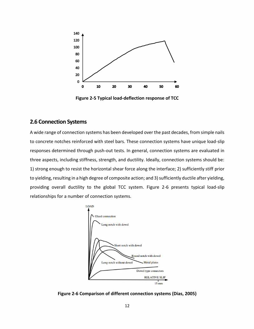
Figure 2-5 presents a typical load-deflection curve for TCC beams subjected to short-term
bending. The curve starts with a linear-elastic branch followed by a nonlinear softening portion.
Such nonlinearity is likely caused by cracking of concrete, buckling of wood fibres under
compression, or progressive yielding of shear connectors. The ultimate failure of TCC beams
normally arises from rupturing of wood fibres in the tension zone, particularly near knots or finger
joints.
12
Figure 2-5 Typical load-deflection response of TCC
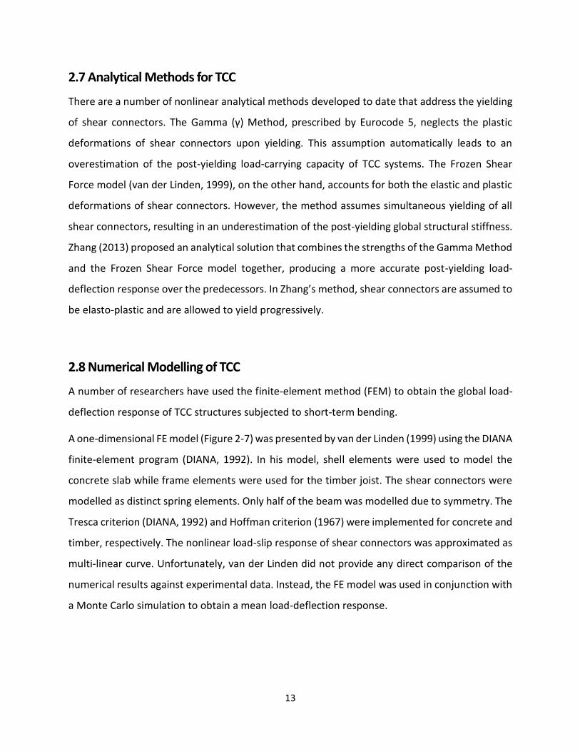
2.6 Connection Systems
A wide range of connection systems has been developed over the past decades, from simple nails
to concrete notches reinforced with steel bars. These connection systems have unique load-slip
responses determined through push-out tests. In general, connection systems are evaluated in
three aspects, including stiffness, strength, and ductility. Ideally, connection systems should be:
1) strong enough to resist the horizontal shear force along the interface; 2) sufficiently stiff prior
to yielding, resulting in a high degree of composite action; and 3) sufficiently ductile after yielding,
providing overall ductility to the global TCC system. Figure 2-6 presents typical load-slip
relationships for a number of connection systems.
Figure 2-6 Comparison of different connection systems (Dias, 2005)
13
2.7 Analytical Methods for TCC
There are a number of nonlinear analytical methods developed to date that address the yielding
of shear connectors. The Gamma (γ) Method, prescribed by Eurocode 5, neglects the plastic
deformations of shear connectors upon yielding. This assumption automatically leads to an
overestimation of the post-yielding load-carrying capacity of TCC systems. The Frozen Shear
Force model (van der Linden, 1999), on the other hand, accounts for both the elastic and plastic
deformations of shear connectors. However, the method assumes simultaneous yielding of all
shear connectors, resulting in an underestimation of the post-yielding global structural stiffness.
Zhang (2013) proposed an analytical solution that combines the strengths of the Gamma Method
and the Frozen Shear Force model together, producing a more accurate post-yielding load-
deflection response over the predecessors. In Zhang’s method, shear connectors are assumed to
be elasto-plastic and are allowed to yield progressively.
2.8 Numerical Modelling of TCC
A number of researchers have used the finite-element method (FEM) to obtain the global load-
deflection response of TCC structures subjected to short-term bending.
A one-dimensional FE model (Figure 2-7) was presented by van der Linden (1999) using the DIANA
finite-element program (DIANA, 1992). In his model, shell elements were used to model the
concrete slab while frame elements were used for the timber joist. The shear connectors were
modelled as distinct spring elements. Only half of the beam was modelled due to symmetry. The
Tresca criterion (DIANA, 1992) and Hoffman criterion (1967) were implemented for concrete and
timber, respectively. The nonlinear load-slip response of shear connectors was approximated as
multi-linear curve. Unfortunately, van der Linden did not provide any direct comparison of the
numerical results against experimental data. Instead, the FE model was used in conjunction with
a Monte Carlo simulation to obtain a mean load-deflection response.
14
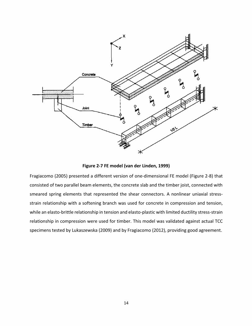
Figure 2-7 FE model (van der Linden, 1999)
Fragiacomo (2005) presented a different version of one-dimensional FE model (Figure 2-8) that
consisted of two parallel beam elements, the concrete slab and the timber joist, connected with
smeared spring elements that represented the shear connectors. A nonlinear uniaxial stress-
strain relationship with a softening branch was used for concrete in compression and tension,
while an elasto-brittle relationship in tension and elasto-plastic with limited ductility stress-strain
relationship in compression were used for timber. This model was validated against actual TCC
specimens tested by Lukaszewska (2009) and by Fragiacomo (2012), providing good agreement.
15
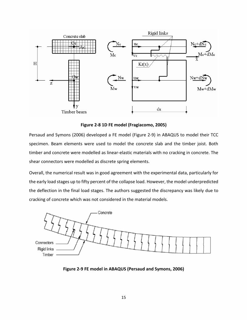
Figure 2-8 1D FE model (Fragiacomo, 2005)
Persaud and Symons (2006) developed a FE model (Figure 2-9) in ABAQUS to model their TCC
specimen. Beam elements were used to model the concrete slab and the timber joist. Both
timber and concrete were modelled as linear-elastic materials with no cracking in concrete. The
shear connectors were modelled as discrete spring elements.
Overall, the numerical result was in good agreement with the experimental data, particularly for
the early load stages up to fifty percent of the collapse load. However, the model underpredicted
the deflection in the final load stages. The authors suggested the discrepancy was likely due to
cracking of concrete which was not considered in the material models.
Figure 2-9 FE model in ABAQUS (Persaud and Symons, 2006)
16
Chapter 3 VecTor2 Methodology
3.1 Introduction
This chapter discusses the numerical modelling of timber-concrete composite (TCC) structures
using VecTor2, a two-dimensional finite element program specifically developed for the analysis
of reinforced concrete membrane structures subjected to static and dynamic loading. VecTor2
employs a total load algorithm with an iterative secant stiffness formulation, using the Modified
Compression Field Theory (MCFT) (Vecchio and Collins, 1986) and the Disturbed Stress Field
Model (DSFM) (Vecchio, 2000) as the governing behavioural models. These behavioural models
consider cracked reinforced concrete as an orthotropic material, with rotating cracks smeared
through the concrete elements. To date, VecTor2 has found extensive application in research
studies and forensic analysis of existing reinforced concrete structures. It has the potential to be
extended to analyse timber or TCC structures provided that adequate timber models and failure
criteria are implemented.
3.2 Stiffness Matrix Formulation
3.2.1 Material Stiffness Matrix Formulation
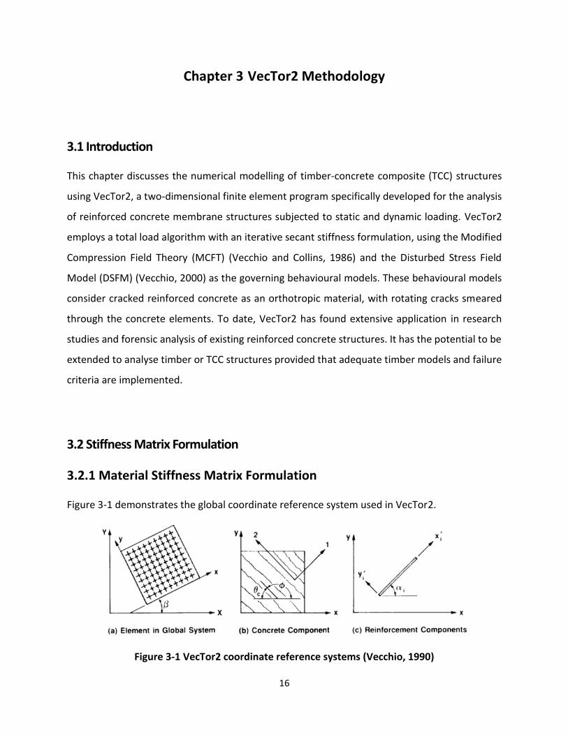
Figure 3-1 demonstrates the global coordinate reference system used in VecTor2.
Figure 3-1 VecTor2 coordinate reference systems (Vecchio, 1990)
17
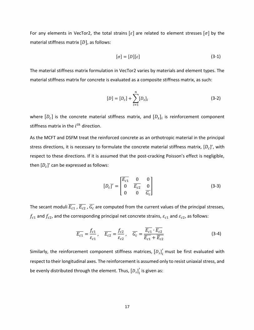
For any elements in VecTor2, the total strains [휀] are related to element stresses [𝜎] by the
material stiffness matrix [𝐷], as follows:
[𝜎] = [𝐷][휀] (3-1)
The material stiffness matrix formulation in VecTor2 varies by materials and element types. The
material stiffness matrix for concrete is evaluated as a composite stiffness matrix, as such:
[𝐷] = [𝐷𝑐] + ∑[𝐷𝑠]𝑖
𝑛
𝑖=1
(3-2)
where [𝐷𝑐] is the concrete material stiffness matrix, and [𝐷𝑠]𝑖 is reinforcement component
stiffness matrix in the 𝑖𝑡ℎ direction.
As the MCFT and DSFM treat the reinforced concrete as an orthotropic material in the principal
stress directions, it is necessary to formulate the concrete material stiffness matrix, [𝐷𝑐]’, with
respect to these directions. If it is assumed that the post-cracking Poisson’s effect is negligible,
then [𝐷𝑐]’ can be expressed as follows:
[𝐷𝑐]′ = [
𝐸𝑐1 0 0
0 𝐸𝑐2 0
0 0 𝐺𝑐
] (3-3)
The secant moduli 𝐸𝑐1 , 𝐸𝑐2
, 𝐺𝑐 are computed from the current values of the principal stresses,
𝑓𝑐1 and 𝑓𝑐2, and the corresponding principal net concrete strains, 휀𝑐1 and 휀𝑐2, as follows:
𝐸𝑐1 =
𝑓𝑐1휀𝑐1
, 𝐸𝑐2 =
𝑓𝑐2휀𝑐2
, 𝐺𝑐 =
𝐸𝑐1 ∙ 𝐸𝑐2
𝐸𝑐1 + 𝐸𝑐2
(3-4)
Similarly, the reinforcement component stiffness matrices, [𝐷𝑠]𝑖′ must be first evaluated with
respect to their longitudinal axes. The reinforcement is assumed only to resist uniaxial stress, and
be evenly distributed through the element. Thus, [𝐷𝑠]𝑖′ is given as:
18
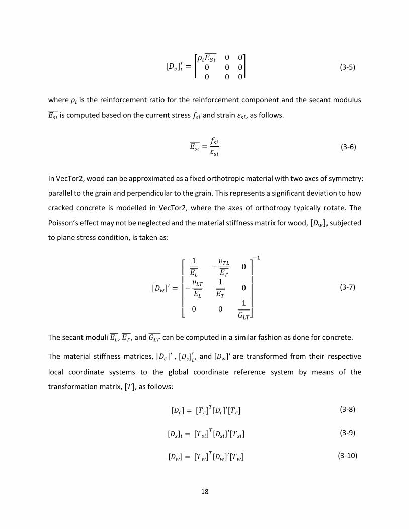
(3-5)
where 𝜌𝑖 is the reinforcement ratio for the reinforcement component and the secant modulus
𝐸𝑠𝑖 is computed based on the current stress 𝑓𝑠𝑖 and strain 휀𝑠𝑖, as follows.
(3-6)
In VecTor2, wood can be approximated as a fixed orthotropic material with two axes of symmetry:
parallel to the grain and perpendicular to the grain. This represents a significant deviation to how
cracked concrete is modelled in VecTor2, where the axes of orthotropy typically rotate. The
Poisson’s effect may not be neglected and the material stiffness matrix for wood, [𝐷𝑤], subjected
to plane stress condition, is taken as:
[𝐷𝑤]′ =
[
1
𝐸𝐿
−𝜐𝑇𝐿
𝐸𝑇
0
−𝜐𝐿𝑇
𝐸𝐿
1
𝐸𝑇
0
0 01
𝐺𝐿𝑇 ]
−1
(3-7)
The secant moduli 𝐸𝐿 , 𝐸𝑇
, and 𝐺𝐿𝑇 can be computed in a similar fashion as done for concrete.
The material stiffness matrices, [𝐷𝑐]′ , [𝐷𝑠]𝑖′ , and [𝐷𝑤]′ are transformed from their respective
local coordinate systems to the global coordinate reference system by means of the
transformation matrix, [𝑇], as follows:
[𝐷𝑐] = [𝑇𝑐]𝑇[𝐷𝑐]′[𝑇𝑐] (3-8)
[𝐷𝑠]𝑖 = [𝑇𝑠𝑖]𝑇[𝐷𝑠𝑖]′[𝑇𝑠𝑖] (3-9)
[𝐷𝑤] = [𝑇𝑤]𝑇[𝐷𝑤]′[𝑇𝑤] (3-10)
19
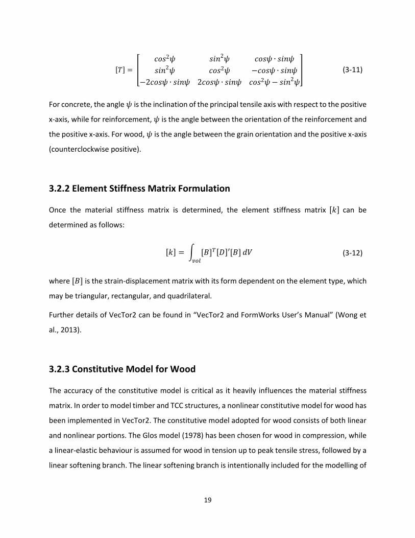
[𝑇] = [
𝑐𝑜𝑠2𝜓 𝑠𝑖𝑛2𝜓 𝑐𝑜𝑠𝜓 ∙ 𝑠𝑖𝑛𝜓
𝑠𝑖𝑛2𝜓 𝑐𝑜𝑠2𝜓 −𝑐𝑜𝑠𝜓 ∙ 𝑠𝑖𝑛𝜓
−2𝑐𝑜𝑠𝜓 ∙ 𝑠𝑖𝑛𝜓 2𝑐𝑜𝑠𝜓 ∙ 𝑠𝑖𝑛𝜓 𝑐𝑜𝑠2𝜓 − 𝑠𝑖𝑛2𝜓
] (3-11)
For concrete, the angle 𝜓 is the inclination of the principal tensile axis with respect to the positive
x-axis, while for reinforcement, 𝜓 is the angle between the orientation of the reinforcement and
the positive x-axis. For wood, 𝜓 is the angle between the grain orientation and the positive x-axis
(counterclockwise positive).
3.2.2 Element Stiffness Matrix Formulation
Once the material stiffness matrix is determined, the element stiffness matrix [𝑘] can be
determined as follows:
[𝑘] = ∫ [𝐵]𝑇[𝐷]′[𝐵] 𝑑𝑉
𝑣𝑜𝑙
(3-12)
where [𝐵] is the strain-displacement matrix with its form dependent on the element type, which
may be triangular, rectangular, and quadrilateral.
Further details of VecTor2 can be found in “VecTor2 and FormWorks User’s Manual” (Wong et
al., 2013).
3.2.3 Constitutive Model for Wood
The accuracy of the constitutive model is critical as it heavily influences the material stiffness
matrix. In order to model timber and TCC structures, a nonlinear constitutive model for wood has
been implemented in VecTor2. The constitutive model adopted for wood consists of both linear
and nonlinear portions. The Glos model (1978) has been chosen for wood in compression, while
a linear-elastic behaviour is assumed for wood in tension up to peak tensile stress, followed by a
linear softening branch. The linear softening branch is intentionally included for the modelling of
20
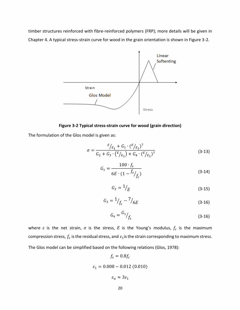
timber structures reinforced with fibre-reinforced polymers (FRP); more details will be given in
Chapter 4. A typical stress-strain curve for wood in the grain orientation is shown in Figure 3-2.
Figure 3-2 Typical stress-strain curve for wood (grain direction)
The formulation of the Glos model is given as:
𝜎 =휀
휀1⁄ + 𝐺1 ∙ (휀 휀1⁄ )7
𝐺2 + 𝐺3 ∙ (휀 휀1⁄ ) + 𝐺4 ∙ (휀 휀1⁄ )7 (3-13)
𝐺1 =
100 ∙ 𝑓𝑠
6𝐸 ∙ (1 −𝑓𝑠
𝑓𝑐⁄ )
(3-14)
𝐺2 = 1𝐸⁄ (3-15)
𝐺3 = 1𝑓𝑐
⁄ − 76𝐸⁄ (3-16)
𝐺4 =𝐺1
𝑓𝑠⁄ (3-16)
where 휀 is the net strain, 𝜎 is the stress, 𝐸 is the Young’s modulus, 𝑓𝑐 is the maximum
compression stress, 𝑓𝑠 is the residual stress, and 휀1is the strain corresponding to maximum stress.
The Glos model can be simplified based on the following relations (Glos, 1978):
𝑓𝑠 = 0.8𝑓𝑐
휀1 = 0.008 ~ 0.012 (0.010)
휀𝑢 ≈ 3휀1
21
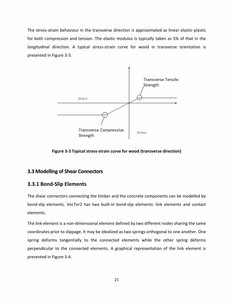
The stress-strain behaviour in the transverse direction is approximated as linear elastic-plastic
for both compression and tension. The elastic modulus is typically taken as 5% of that in the
longitudinal direction. A typical stress-strain curve for wood in transverse orientation is
presented in Figure 3-3.
Figure 3-3 Typical stress-strain curve for wood (transverse direction)
3.3 Modelling of Shear Connectors
3.3.1 Bond-Slip Elements
The shear connectors connecting the timber and the concrete components can be modelled by
bond-slip elements. VecTor2 has two built-in bond-slip elements: link elements and contact
elements.
The link element is a non-dimensional element defined by two different nodes sharing the same
coordinates prior to slippage. It may be idealized as two springs orthogonal to one another. One
spring deforms tangentially to the connected elements while the other spring deforms
perpendicular to the connected elements. A graphical representation of the link element is
presented in Figure 3-4.
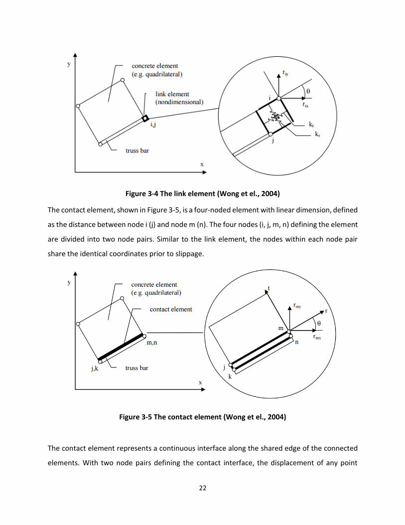
22
Figure 3-4 The link element (Wong et el., 2004)
The contact element, shown in Figure 3-5, is a four-noded element with linear dimension, defined
as the distance between node i (j) and node m (n). The four nodes (i, j, m, n) defining the element
are divided into two node pairs. Similar to the link element, the nodes within each node pair
share the identical coordinates prior to slippage.
Figure 3-5 The contact element (Wong et el., 2004)
The contact element represents a continuous interface along the shared edge of the connected
elements. With two node pairs defining the contact interface, the displacement of any point
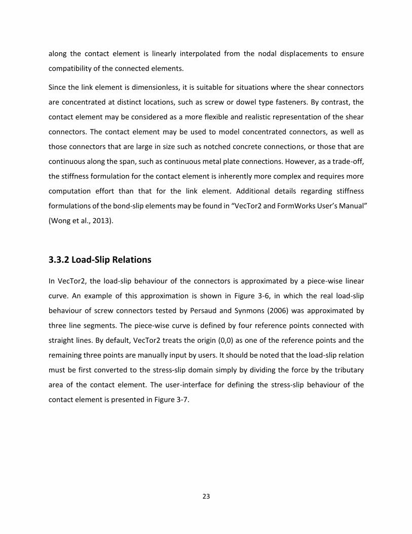
23
along the contact element is linearly interpolated from the nodal displacements to ensure
compatibility of the connected elements.
Since the link element is dimensionless, it is suitable for situations where the shear connectors
are concentrated at distinct locations, such as screw or dowel type fasteners. By contrast, the
contact element may be considered as a more flexible and realistic representation of the shear
connectors. The contact element may be used to model concentrated connectors, as well as
those connectors that are large in size such as notched concrete connections, or those that are
continuous along the span, such as continuous metal plate connections. However, as a trade-off,
the stiffness formulation for the contact element is inherently more complex and requires more
computation effort than that for the link element. Additional details regarding stiffness
formulations of the bond-slip elements may be found in “VecTor2 and FormWorks User’s Manual”
(Wong et al., 2013).
3.3.2 Load-Slip Relations
In VecTor2, the load-slip behaviour of the connectors is approximated by a piece-wise linear
curve. An example of this approximation is shown in Figure 3-6, in which the real load-slip
behaviour of screw connectors tested by Persaud and Synmons (2006) was approximated by
three line segments. The piece-wise curve is defined by four reference points connected with
straight lines. By default, VecTor2 treats the origin (0,0) as one of the reference points and the
remaining three points are manually input by users. It should be noted that the load-slip relation
must be first converted to the stress-slip domain simply by dividing the force by the tributary
area of the contact element. The user-interface for defining the stress-slip behaviour of the
contact element is presented in Figure 3-7.
24
Figure 3-6 Multi-linear approximation (Persaud and Synmons, 2006)
Figure 3-7 Bond definition user-interface
3.4 Failure Criteria Formulation
Since wood elements in VecTor2 are modelled as a fixed-orthotropic material subjected to bi-
axial stress, three failure criteria may be applicable to the scenario, including the Tsai-Azzi
criterion (1966), the Norris criterion (1962), and the Hashin criterion (1980).
25
The Tsai-Azzi criterion takes into account the difference in uniaxial tensile and compressive
strengths, and is as follows:
𝜎𝐿
2
𝑓𝐿2 −
𝜎𝐿𝜎𝑇
𝑓𝐿2 +
𝜎𝑇2
𝑓𝑇2 +
𝜏𝐿𝑇2
𝑓𝐿𝑇2 = 1 (3-14)
where 𝑓𝑇 , 𝑓𝐿 , and 𝑓𝐿𝑇 are the uniaxial and shearing strengths relative to the corresponding
directions.
The Norris criterion is similar to the Tsai-Azzi criterion except that the interaction term is
nonbiased towards directions. The Norris criterion is given as:
𝜎𝐿
2
𝑓𝐿2 −
𝜎𝐿𝜎𝑇
𝑓𝐿𝑓𝑇+
𝜎𝑇2
𝑓𝑇2 +
𝜏𝐿𝑇2
𝑓𝐿𝑇2 = 1 (3-15)
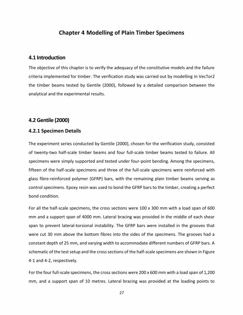
The Hashin criterion characterizes wood failure by four scenarios, including:
Fibre tension mode:
𝜎𝐿
2
𝑓𝐿,𝑡2 +
𝜏𝐿𝑇2
𝑓𝐿,𝑣2 = 1 (3-16)
Fibre compression mode:
𝜎𝐿
𝑓𝐿,𝑐 = 1 (3-17)
Matrix tension mode:
𝜎𝑇
2
𝑓𝑇,𝑡2 +
𝜏𝐿𝑇2
𝑓𝐿,𝑣2 = 1 (3-18)
Matrix compression mode:
𝜎𝑇
2
4𝑓𝑇,𝑣2 + [(
𝑓𝑇,𝑐
2𝑓𝑇,𝑣)
2
− 1]𝜎𝑇
2
𝑓𝑇,𝑐2 +
𝜏𝐿𝑇2
𝑓𝐿,𝑣2 = 1 (3-19)

26
where 𝑓𝐿,𝑡 , 𝑓𝐿,𝑐 , 𝑓𝑇,𝑡 , 𝑓𝑇,𝑐 , 𝑓𝐿,𝑣 , and 𝑓𝑇,𝑣 are, respectively, the strengths related to longitudinal
tension and compression, transverse tension and compression, and longitudinal and transverse
shear.
The Hashin criterion has been adopted into VecTor2 to account for different types of failure
modes. For flexure-critical timber beams, failures typically occur at the bottom of the beam,
where the wood fibre is essentially subjected to uniaxial tensile stress. In that scenario, both
Equation 3-18 and Equation 3-19 will be equal to zero on the left side, and the matrix failure
mode will never govern the ultimate failure. Moreover, the second term of Equation 3-16 is zero,
and therefore the Hashin criterion is reduced to uniaxial failure criterion which is the same as the
Rankine Criterion.
For shear-critical conditions, failures are more likely governed by a combination of shear stress
and axial stress, and the matrix failure modes become more prominent. However, it should also
be pointed out that the transverse tensile strength and the transverse shear strength are the less
commonly known mechanical properties of wood; their values are typically not available in the
literature.
27
Chapter 4 Modelling of Plain Timber Specimens
4.1 Introduction
The objective of this chapter is to verify the adequacy of the constitutive models and the failure
criteria implemented for timber. The verification study was carried out by modelling in VecTor2
the timber beams tested by Gentile (2000), followed by a detailed comparison between the
analytical and the experimental results.
4.2 Gentile (2000)
4.2.1 Specimen Details
The experiment series conducted by Gentile (2000), chosen for the verification study, consisted
of twenty-two half-scale timber beams and four full-scale timber beams tested to failure. All
specimens were simply supported and tested under four-point bending. Among the specimens,
fifteen of the half-scale specimens and three of the full-scale specimens were reinforced with
glass fibre-reinforced polymer (GFRP) bars, with the remaining plain timber beams serving as
control specimens. Epoxy resin was used to bond the GFRP bars to the timber, creating a perfect
bond condition.
For all the half-scale specimens, the cross sections were 100 x 300 mm with a load span of 600
mm and a support span of 4000 mm. Lateral bracing was provided in the middle of each shear
span to prevent lateral-torsional instability. The GFRP bars were installed in the grooves that
were cut 30 mm above the bottom fibres into the sides of the specimens. The grooves had a
constant depth of 25 mm, and varying width to accommodate different numbers of GFRP bars. A
schematic of the test setup and the cross sections of the half-scale specimens are shown in Figure
4-1 and 4-2, respectively.
For the four full-scale specimens, the cross sections were 200 x 600 mm with a load span of 1,200
mm, and a support span of 10 metres. Lateral bracing was provided at the loading points to

28
prevent lateral-torsional instability. Two of the beams had grooves cut into the bottom face of
the beams and one of the beams had grooves cut into the sides of the beam. The grooves had a
depth and width of 20 x 20 mm, 15 x 15 mm, and 40 x 20 mm for Beam FS-1, FS-2, and FS-3,
respectively. Due to the available lengths of the GFRP bars used, only the central 6.0 m was
reinforced. A schematic of the test setup and the configuration of the half-scale specimens are
shown in Figure 4-3 and 4-4, respectively.
Figure 4-1 Test configuration for half-scale beams (Gentile, 2000)
Figure 4-2 Cross sections of half-scale reinforced beams (Gentile, 2000)
29
Figure 4-3 Test configuration for full-scale beams (Gentile, 2000)
Figure 4-3
Figure 4-4 Configuration of full-scale reinforced beams (Gentile, 2000)
30
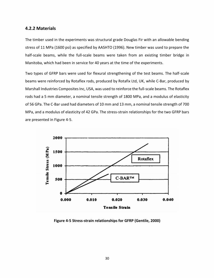
4.2.2 Materials
The timber used in the experiments was structural grade Douglas Fir with an allowable bending
stress of 11 MPa (1600 psi) as specified by AASHTO (1996). New timber was used to prepare the
half-scale beams, while the full-scale beams were taken from an existing timber bridge in
Manitoba, which had been in service for 40 years at the time of the experiments.
Two types of GFRP bars were used for flexural strengthening of the test beams. The half-scale
beams were reinforced by Rotaflex rods, produced by Rotafix Ltd, UK, while C-Bar, produced by
Marshall Industries Composites Inc, USA, was used to reinforce the full-scale beams. The Rotaflex
rods had a 5 mm diameter, a nominal tensile strength of 1800 MPa, and a modulus of elasticity
of 56 GPa. The C-Bar used had diameters of 10 mm and 13 mm, a nominal tensile strength of 700
MPa, and a modulus of elasticity of 42 GPa. The stress-strain relationships for the two GFRP bars
are presented in Figure 4-5.
Figure 4-5 Stress-strain relationships for GFRP (Gentile, 2000)
31
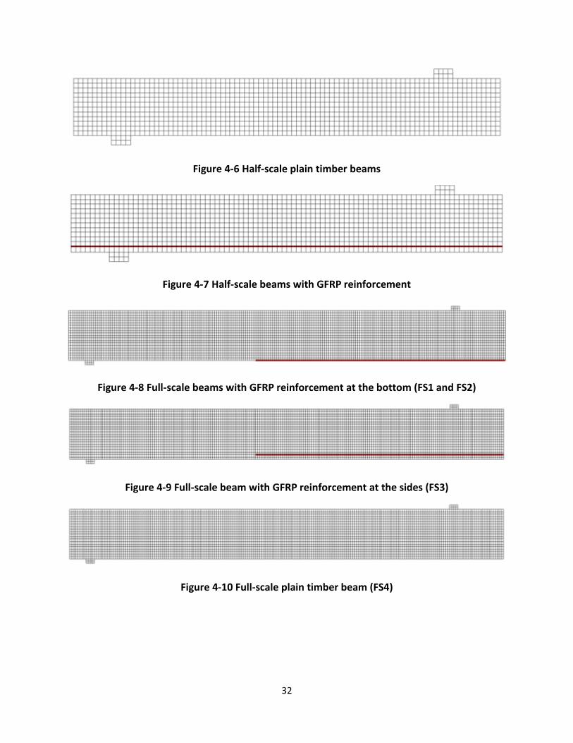
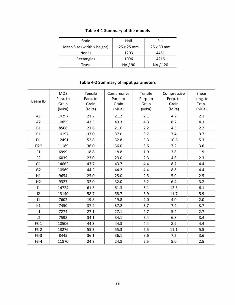
4.2.3 Modelling Details
Both the plain timber specimens and the reinforced timber specimens were modelled in VecTor2
using the auto-meshing function, with only half of the span modelled due to symmetry.
Rectangular membrane elements were used to model the timber, while truss elements were
used to model the GFRP bars. Perfect bonding was assumed between the GFRP bars and the
timber. The finite-element models created for both the half-scale beams and the full-scale beams
are presented in Figure 4-6 through Figure 4-12. A summary of the finite element models is given
in Table 4-1.
The modulus of elasticity (MOE) and the modulus of rupture (MOR) in the longitudinal direction
were reported by Gentile (2000); these values were used as the input mechanical properties of
timber. The modulus of rupture may be used as the tensile strength parallel to the grain, although
it is not a true stress because the formula by which it is calculated is valid only within the elastic
range.
It was impossible to perform FE analysis for the timber beams with only the MOE and the MOR
available, since there were other inputs required by VecTor2, namely the tensile strength
perpendicular to the grain, the compressive strength parallel to the grain, the compressive
strength perpendicular to the grain, and the shear strength. Representative values may be found
in Chapter 4 of the US Wood Handbook. However, these values were obtained from small defect-
free samples which may not be appropriate to use for full-scale structural grade timber.
To make the subsequent FE analysis possible, reasonable assumptions were made as follows: The
magnitude of the longitudinal compressive strength was taken as equal to that of the longitudinal
tensile strength. The tensile strength perpendicular to the grain and the shear strength were
assumed to be one-tenth of the tensile strength parallel to the grain, while the transverse
compressive strength was assumed to be 20% of that of the longitudinal counterpart. The full
explanation for the assumptions made here is given in Section 5.3.2 of this thesis. Lastly, the
elastic modulus perpendicular to the grain orientation was calculated as per the relations
discussed in Chapter 2 (Bodig 1982). A summary of the input parameters and the reinforcement
details is shown in Table 4-2 and Table 4-3, respectively.
32
Figure 4-6 Half-scale plain timber beams
Figure 4-7 Half-scale beams with GFRP reinforcement
Figure 4-8 Full-scale beams with GFRP reinforcement at the bottom (FS1 and FS2)
Figure 4-9 Full-scale beam with GFRP reinforcement at the sides (FS3)
Figure 4-10 Full-scale plain timber beam (FS4)
33
Table 4-1 Summary of the models
Scale Half Full
Mesh Size (width x height) 25 x 25 mm 25 x 30 mm
Nodes 1203 4451
Rectangles 1096 4216
Truss NA / 90 NA / 120
Table 4-2 Summary of input parameters
Beam ID
MOE Para. to
Grain (MPa)
Tensile Para. to
Grain (MPa)
Compressive Para. to
Grain (MPa)
Tensile Perp. to
Grain (MPa)
Compressive Perp. to
Grain (MPa)
Shear Long. to
Tran. (MPa)
A1 10257 21.2 21.2 2.1 4.2 2.1
A2 10855 43.3 43.3 4.3 8.7 4.3
B1 8568 21.6 21.6 2.2 4.3 2.2
C1 10197 37.0 37.0 3.7 7.4 3.7
D1 12491 52.8 52.8 5.3 10.6 5.3
D2* 11189 36.0 36.0 3.6 7.2 3.6
F1 6999 18.8 18.8 1.9 3.8 1.9
F2 6039 23.0 23.0 2.3 4.6 2.3
G1 14662 43.7 43.7 4.4 8.7 4.4
G2 10969 44.2 44.2 4.4 8.8 4.4
H1 9654 25.0 25.0 2.5 5.0 2.5
H2 9327 32.0 32.0 3.2 6.4 3.2
I1 14724 61.3 61.3 6.1 12.3 6.1
I2 13140 58.7 58.7 5.9 11.7 5.9
J1 7602 19.8 19.8 2.0 4.0 2.0
K1 7450 37.2 37.2 3.7 7.4 3.7
L1 7274 27.1 27.1 2.7 5.4 2.7
L2 7598 34.1 34.1 3.4 6.8 3.4
FS-1 10506 44.3 44.3 4.4 8.9 4.4
FS-2 13276 55.3 55.3 5.5 11.1 5.5
FS-3 8445 36.1 36.1 3.6 7.2 3.6
FS-4 11870 24.8 24.8 2.5 5.0 2.5
34
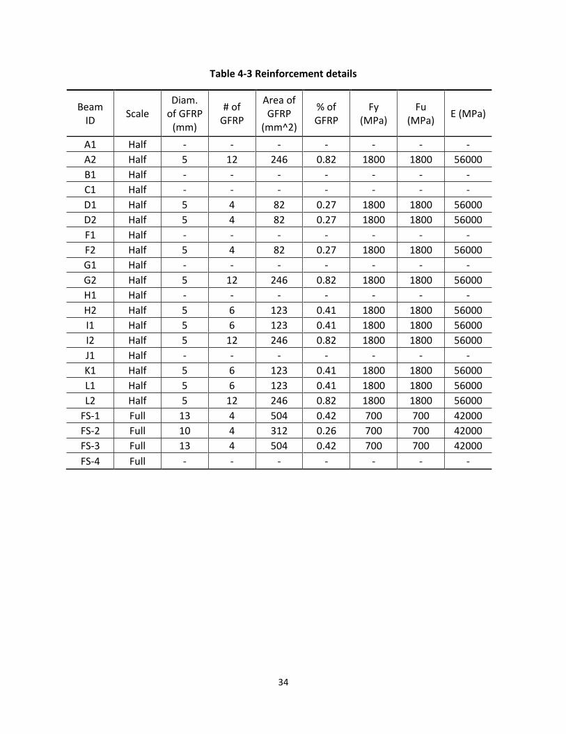
Table 4-3 Reinforcement details
Beam ID
Scale Diam.
of GFRP (mm)
# of GFRP
Area of GFRP
(mm^2)
% of GFRP
Fy (MPa)
Fu (MPa)
E (MPa)
A1 Half - - - - - - -
A2 Half 5 12 246 0.82 1800 1800 56000
B1 Half - - - - - - -
C1 Half - - - - - - -
D1 Half 5 4 82 0.27 1800 1800 56000
D2 Half 5 4 82 0.27 1800 1800 56000
F1 Half - - - - - - -
F2 Half 5 4 82 0.27 1800 1800 56000
G1 Half - - - - - - -
G2 Half 5 12 246 0.82 1800 1800 56000
H1 Half - - - - - - -
H2 Half 5 6 123 0.41 1800 1800 56000
I1 Half 5 6 123 0.41 1800 1800 56000
I2 Half 5 12 246 0.82 1800 1800 56000
J1 Half - - - - - - -
K1 Half 5 6 123 0.41 1800 1800 56000
L1 Half 5 6 123 0.41 1800 1800 56000
L2 Half 5 12 246 0.82 1800 1800 56000
FS-1 Full 13 4 504 0.42 700 700 42000
FS-2 Full 10 4 312 0.26 700 700 42000
FS-3 Full 13 4 504 0.42 700 700 42000
FS-4 Full - - - - - - -
35
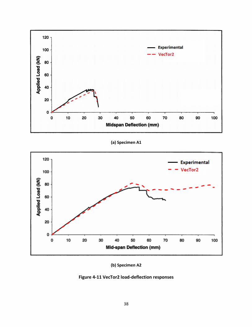
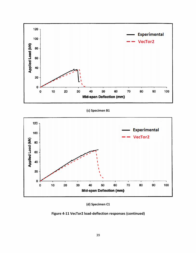
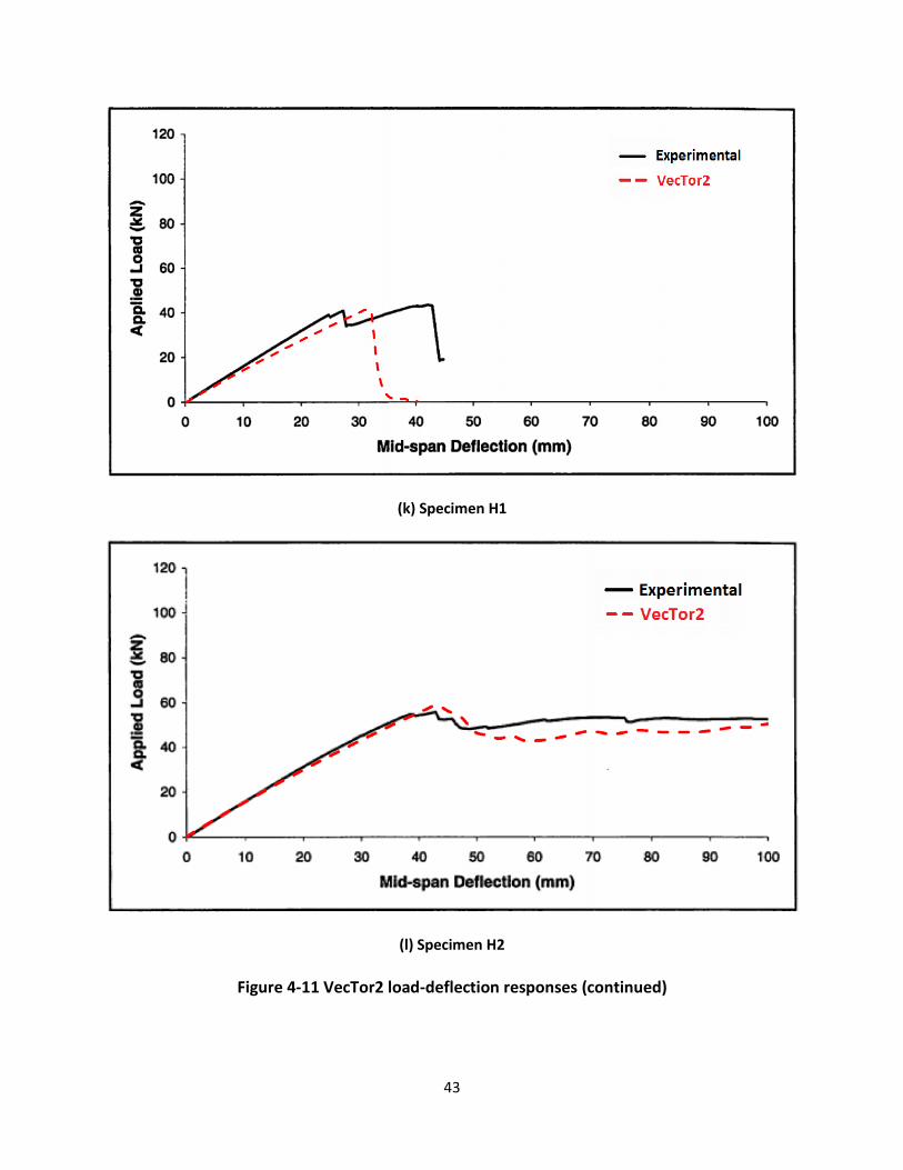
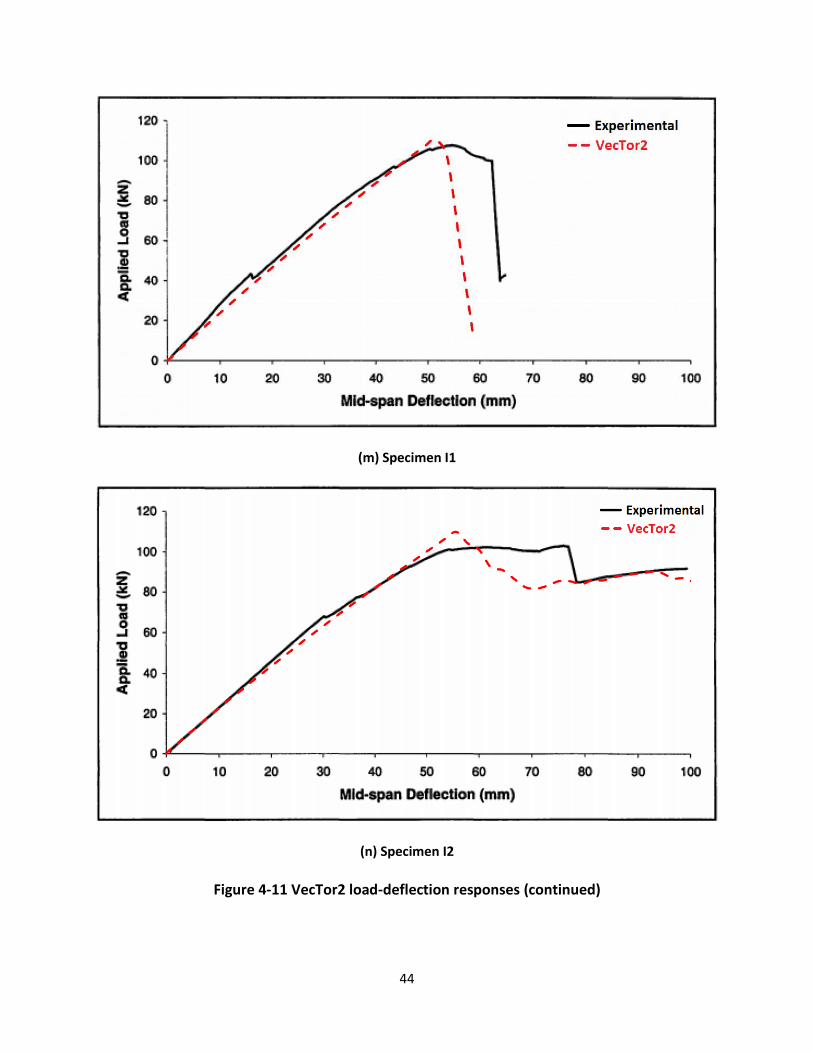
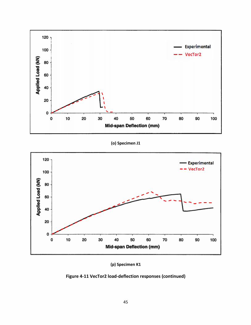
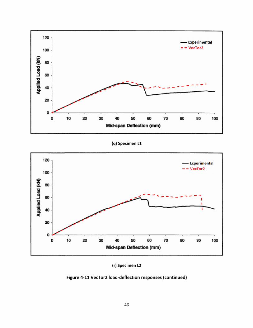
4.2.4 Modelling Results
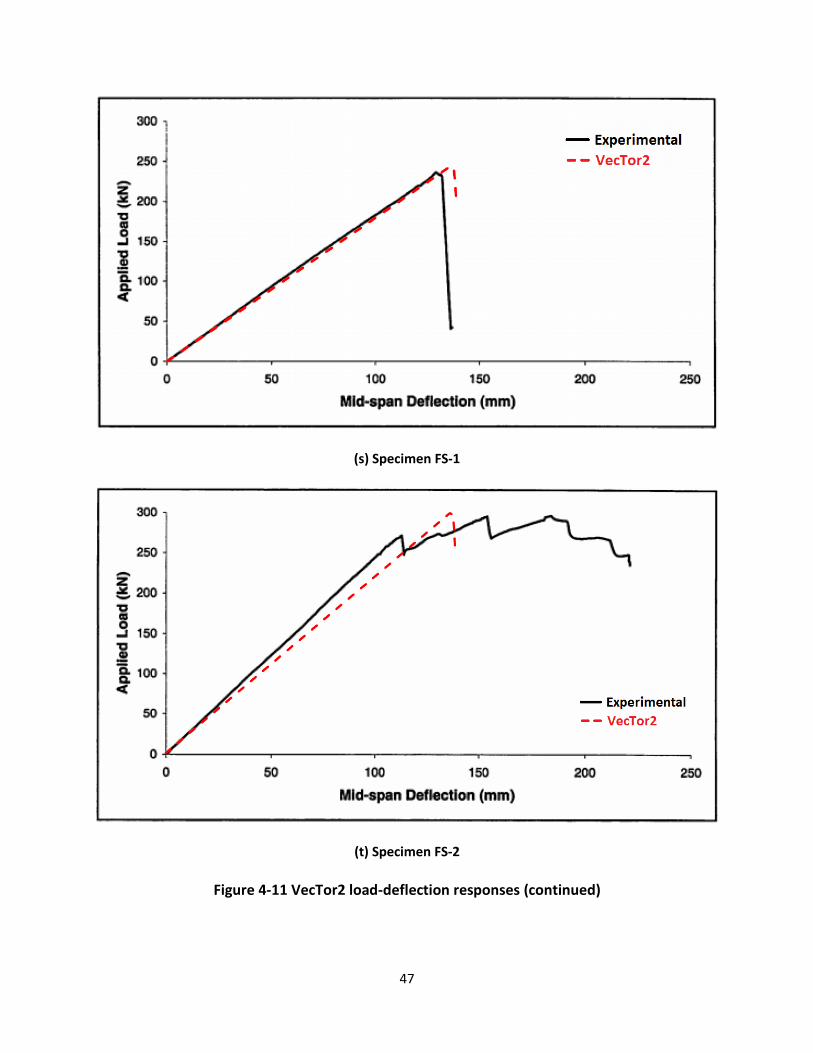
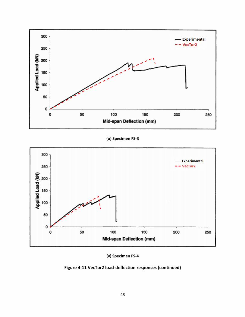
Shown in Figure 4-13 are the comparisons between the VecTor2 simulation results and the
experimental results, presented as the red dotted line and black solid line, respectively. In general,
VecTor2 was capable of predicting the pre-peak global load-deflection responses and the global
stiffness with sufficient accuracy.
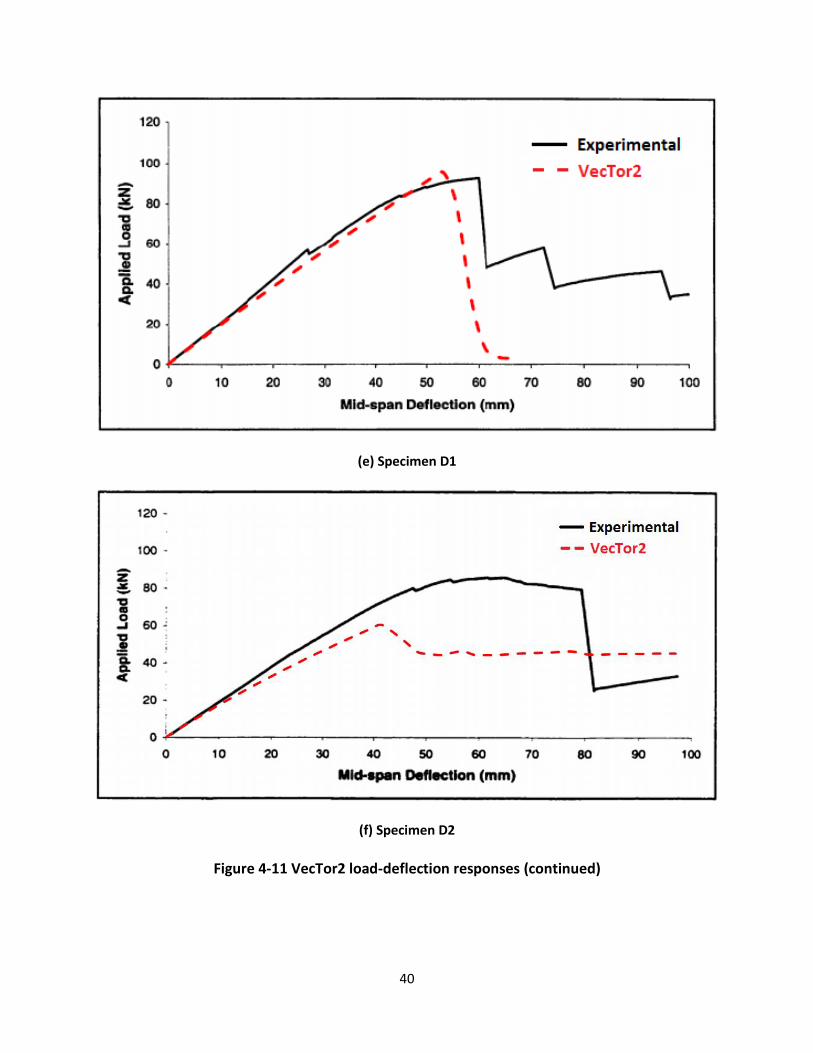
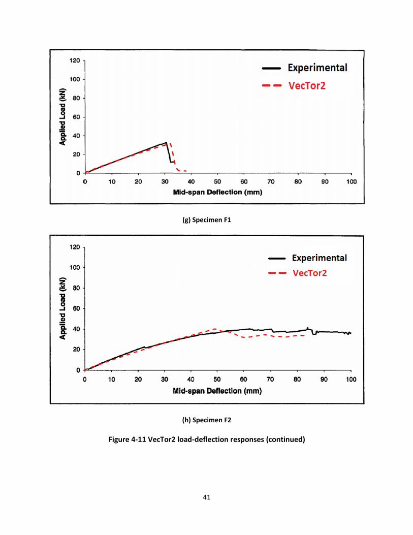
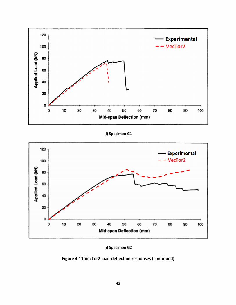
The post-peak load-deflection response of the reinforced specimens was also reasonably well
captured by VecTor2. In general, the reinforced specimens exhibited more post-peak
displacement than those without reinforcement. Specimen F2, with a modulus of elasticity (MOE)
of 6039 MPa and a modulus of rupture (MOR) of 23 MPa, exhibited a smooth and progressive
post-peak response with only 0.27% reinforcement. On the contrary, Specimen D1, while having
the same amount of reinforcement and being approximately two times stronger and stiffer than
Specimen F2, experienced a brittle failure as the applied load and the stiffness dropped rapidly
once the maximum force was reached. Specimen I2 had a reinforcement ratio of 0.82%, and
demonstrated an improved post-peak response than that of Specimen D1. Based on the above
observations, it may be concluded that the amount of post-peak response depended not only on
the reinforcement ratio, but also the quality of the timber.
Regarding the failure modes, tension failure was predicted by VecTor2 in the constant moment
region for all specimens; whereas, as per Gentile (2000), the failure modes of the specimens
included tension failure, compression failure, and flexural-shear failure which was only found in
three of the reinforced specimens. Due to the lack of information, the specimens that had
flexural-shear failures were excluded from the analysis. All plain timber beams failed in brittle
tension with no signs of crushing in compression zone, which was in agreement with the VecTor2
predictions. While all the reinforced specimens initially developed tensile cracks in the constant
moment region, half of those experienced ductile compression failure due to crushing of wood
fibre in the top face. Unfortunately, Gentile (2000) did not identify the failure modes of individual
specimen and therefore it was impossible to proceed any further with the analysis of failure
modes. Nevertheless, it was believed that VecTor2 was unable to predict the ductile compression
failures for two possible reasons as follows: 1. The true compressive strength of timber was not
36
reported in the original literature and was assumed to have the same magnitude as the tensile
strength; 2. The presence of GFRP bars hindered the propagation of tension-initiated cracks,
leading to a much more improved post-cracking tensile response of timber. Although the
currently adopted constitutive model included a simple linear softening branch in tension, the
appropriateness of it was not validated experimentally.
Although the perfect bonding assumption agreed fairly well with the experimental observations,
there were some localized debonding of GFRP bars adjacent to tensile cracks. None of the failures
were caused by debonding or delamination of the reinforcement; in the case of timber beams
externally reinforced with FRP sheets or strips, as has been reported by other researchers (Dorey
and Cheng 1996, Hernandez et al. 1997, and Bakoss et al. 1999), debonding or delamination of
the reinforcement was found to be crucial to the ultimate failures.
Table 4-4 presented the ultimate loads predicted by VecTor2, which agreed well with the
experimental measurements. The only exception was Specimen D2, in which the failure occurred
outside of the constant moment region, causing an underestimation of the modulus of elasticity
(MOE).
4.3 Conclusions
Based on the verification studies performed in this chapter, it was found that the constitutive
models adopted, and the assumptions made for the unknown mechanical properties of wood,
were appropriate in general for flexure-critical conditions. Due to the lack of information on
specimen material properties, VecTor2 was unable to capture the compression failures observed
in some of the reinforced specimens. Nevertheless, VecTor2 was able to predict the global
stiffness, the failure loads, and the initial cracks initiated by tension with sufficient accuracy.
Timber beams, when sufficiently reinforced, can have a higher tensile strength and improved
post-peak response than plain timber beams. Further research effort should be undertaken to
better understand the interaction between timber and FRP reinforcement, and to quantify the
influence of reinforcement on the post-peak tensile response of wood. There is also merit in

37
developing a more realistic constitutive model which can ultimately improve the post-peak FE
predictions.
38
(a) Specimen A1
(b) Specimen A2
Figure 4-11 VecTor2 load-deflection responses
39
(c) Specimen B1
(d) Specimen C1
Figure 4-11 VecTor2 load-deflection responses (continued)
40
(e) Specimen D1
(f) Specimen D2
Figure 4-11 VecTor2 load-deflection responses (continued)
41
(g) Specimen F1
(h) Specimen F2
Figure 4-11 VecTor2 load-deflection responses (continued)
42
(i) Specimen G1
(j) Specimen G2
Figure 4-11 VecTor2 load-deflection responses (continued)
43
(k) Specimen H1
(l) Specimen H2
Figure 4-11 VecTor2 load-deflection responses (continued)
44
(m) Specimen I1
(n) Specimen I2
Figure 4-11 VecTor2 load-deflection responses (continued)
45
(o) Specimen J1
(p) Specimen K1
Figure 4-11 VecTor2 load-deflection responses (continued)
46
(q) Specimen L1
(r) Specimen L2
Figure 4-11 VecTor2 load-deflection responses (continued)
47
(s) Specimen FS-1
(t) Specimen FS-2
Figure 4-11 VecTor2 load-deflection responses (continued)
48
(u) Specimen FS-3
(v) Specimen FS-4
Figure 4-11 VecTor2 load-deflection responses (continued)

49
Table 4-4 Summary of ultimate loads
Beam ID Pu (Exp.)
(kN) Pu (VT2)
(kN) Pu (VT2)/ Pu (Exp.)
A1 36.9 34.6 0.94
A2 75.8 82.0 1.08
B1 37.5 35.8 0.95
C1 64.7 63.0 0.97
D1 92.6 95.2 1.03
D2 85.7 60.0 0.70
F1 32.5 31.0 0.95
F2 40.0 40.0 1.00
G1 76.5 72.2 0.94
G2 77.4 85.4 1.10
H1 43.5 41.6 0.96
H2 55.9 58.4 1.04
I1 107.5 111.0 1.03
I2 103.0 90.0 0.87
J1 34.4 32.6 0.95
K1 65.1 68.2 1.05
L1 47.2 50.6 1.07
L2 59.6 69.0 1.16
FS-1 236.0 243.0 1.03
FS-2 296.0 298.6 1.01
FS-3 191.0 212.4 1.11
FS-4 132.0 126.4 0.96
Mean 1.00
Stand. Deviation 0.10
COV 9.57%
50
Chapter 5 Modelling of Timber-Concrete Composite Beams
5.1 Introduction
In Chapter 4, VecTor2’s capability of modelling the behaviour of plain timber beams was
examined. This chapter builds on the successful modelling results from Chapter 4, and is devoted
to the numerical modelling of timber-concrete composite (TCC) beams subjected to short-term
monotonic loadings. A series of experimental and numerical corroborations were performed and
the results are discussed.
The experiments selected for the verification studies are briefly described while additional details
may be found in the original literature as referenced in this thesis. In what follows, the description
of the finite element models created for the corresponding specimens are given, along with a
detailed comparison between the experimental and the numerical results.
5.2 Model Description
Despite the fact that the experiments performed by different researchers varied considerably in
terms of dimensions, load configurations, mechanical properties, materials, and the types of
shear connectors, all the finite element models created in this verification studies share the
following similarities:
1. All models consist of two basic elements: the membrane elements and the contact
elements. The membrane elements were used to model the timber and the concrete
components while the contact elements were used to represent the shear connectors.
2. Bearing plates were introduced to all the models to mitigate high local stress for the
elements directly in contact with the supports and the loading jacks. The bearing plates
were also modelled with membrane elements.
3. A number of the specimens had interlayers (e.g. particle board) between the concrete
and the timber members. Such interlayers were treated as an integral part of the
underlying timber members, and were assumed to have the same mechanical properties.
51
It is possible that this simplification can result in an overestimation of the global stiffness
as the interlayers are likely softer than the timber member. Moreover, the presence of
interlayer reduces the penetration depth of the shear connectors into the timber
members, which can cause a reduction in the stiffness and load-carrying capacity of the
shear connectors.
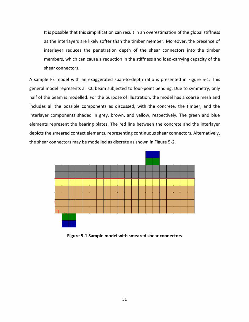
A sample FE model with an exaggerated span-to-depth ratio is presented in Figure 5-1. This
general model represents a TCC beam subjected to four-point bending. Due to symmetry, only
half of the beam is modelled. For the purpose of illustration, the model has a coarse mesh and
includes all the possible components as discussed, with the concrete, the timber, and the
interlayer components shaded in grey, brown, and yellow, respectively. The green and blue
elements represent the bearing plates. The red line between the concrete and the interlayer
depicts the smeared contact elements, representing continuous shear connectors. Alternatively,
the shear connectors may be modelled as discrete as shown in Figure 5-2.
Figure 5-1 Sample model with smeared shear connectors
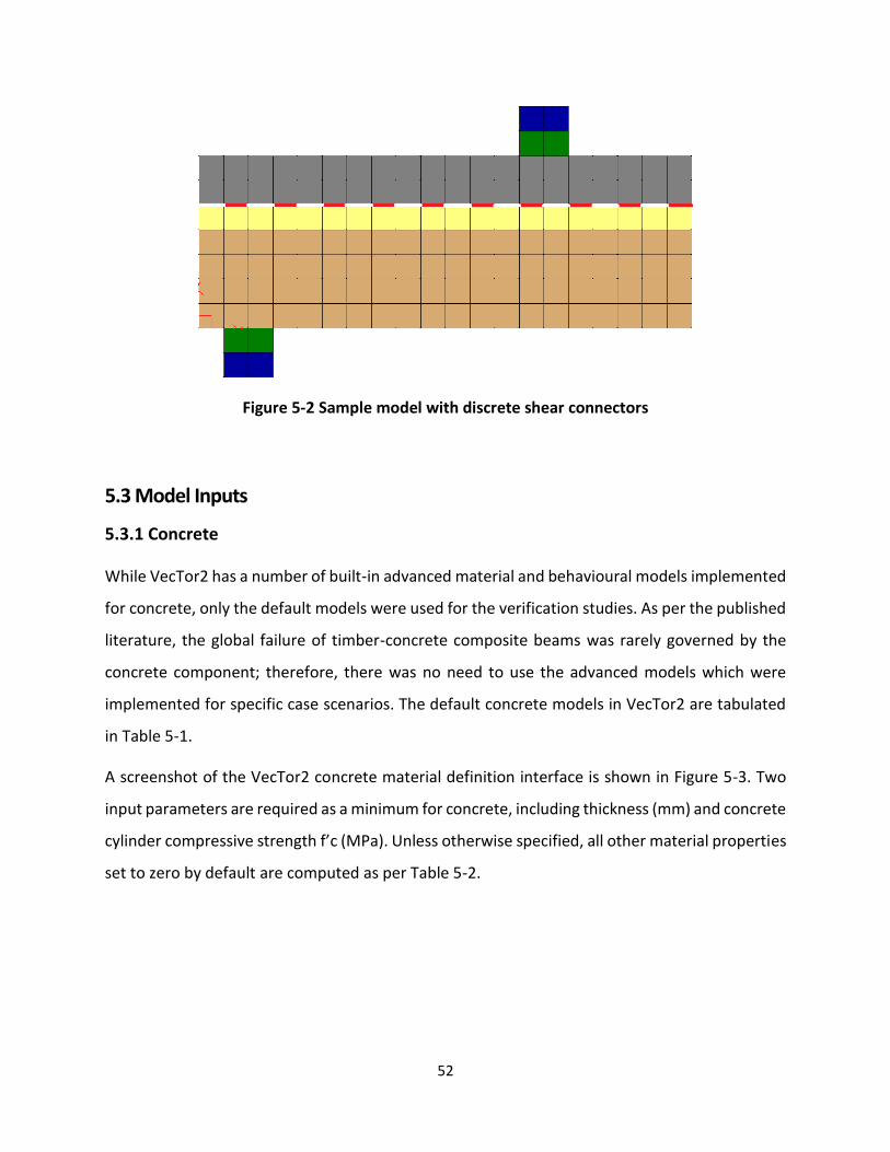
52
Figure 5-2 Sample model with discrete shear connectors
5.3 Model Inputs
5.3.1 Concrete
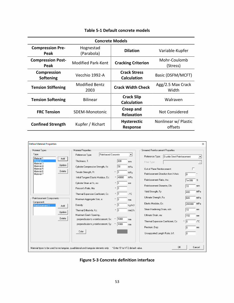
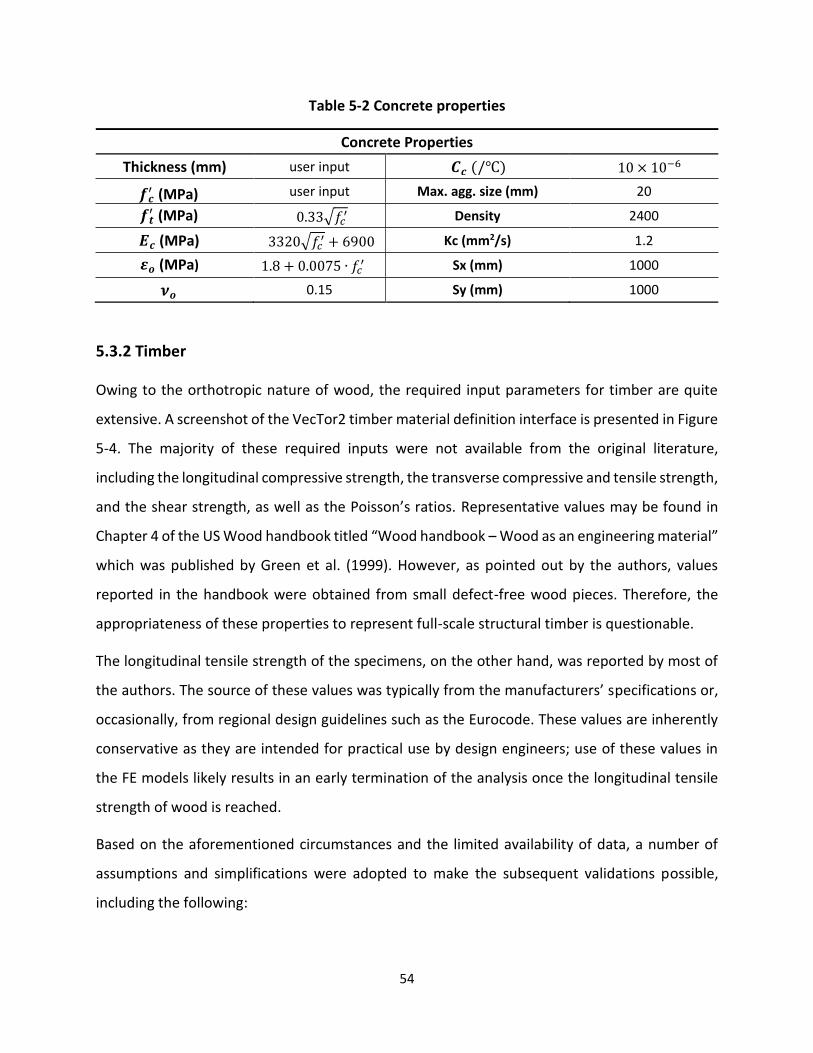
While VecTor2 has a number of built-in advanced material and behavioural models implemented
for concrete, only the default models were used for the verification studies. As per the published
literature, the global failure of timber-concrete composite beams was rarely governed by the
concrete component; therefore, there was no need to use the advanced models which were
implemented for specific case scenarios. The default concrete models in VecTor2 are tabulated
in Table 5-1.
A screenshot of the VecTor2 concrete material definition interface is shown in Figure 5-3. Two
input parameters are required as a minimum for concrete, including thickness (mm) and concrete
cylinder compressive strength f’c (MPa). Unless otherwise specified, all other material properties
set to zero by default are computed as per Table 5-2.
53
Table 5-1 Default concrete models
Concrete Models
Compression Pre-Peak
Hognestad (Parabola)
Dilation Variable-Kupfer
Compression Post-Peak
Modified Park-Kent Cracking Criterion Mohr-Coulomb
(Stress)
Compression Softening
Vecchio 1992-A Crack Stress Calculation
Basic (DSFM/MCFT)
Tension Stiffening Modified Bentz
2003 Crack Width Check
Agg/2.5 Max Crack Width
Tension Softening Bilinear Crack Slip
Calculation Walraven
FRC Tension SDEM-Monotonic Creep and Relaxation
Not Considered
Confined Strength Kupfer / Richart Hysterectic Response
Nonlinear w/ Plastic offsets
Figure 5-3 Concrete definition interface
54
Table 5-2 Concrete properties
Concrete Properties
Thickness (mm) user input
user input Max. agg. size (mm) 20
Density 2400
Kc (mm2/s) 1.2
Sx (mm) 1000
0.15 Sy (mm) 1000
5.3.2 Timber
Owing to the orthotropic nature of wood, the required input parameters for timber are quite
extensive. A screenshot of the VecTor2 timber material definition interface is presented in Figure
5-4. The majority of these required inputs were not available from the original literature,
including the longitudinal compressive strength, the transverse compressive and tensile strength,
and the shear strength, as well as the Poisson’s ratios. Representative values may be found in
Chapter 4 of the US Wood handbook titled “Wood handbook – Wood as an engineering material”
which was published by Green et al. (1999). However, as pointed out by the authors, values
reported in the handbook were obtained from small defect-free wood pieces. Therefore, the
appropriateness of these properties to represent full-scale structural timber is questionable.
The longitudinal tensile strength of the specimens, on the other hand, was reported by most of
the authors. The source of these values was typically from the manufacturers’ specifications or,
occasionally, from regional design guidelines such as the Eurocode. These values are inherently
conservative as they are intended for practical use by design engineers; use of these values in
the FE models likely results in an early termination of the analysis once the longitudinal tensile
strength of wood is reached.
Based on the aforementioned circumstances and the limited availability of data, a number of
assumptions and simplifications were adopted to make the subsequent validations possible,
including the following:
1.8 + 0.0075 ∙ 𝑓𝑐′
𝝂𝒐
𝑬𝒄 (MPa) 3320√𝑓𝑐′ + 6900
𝒇𝒄′ (MPa)
𝒇𝒕′ (MPa) 0.33√𝑓𝑐
′
𝜺𝒐 (MPa)
10 × 10−6 𝑪𝒄 (/℃)
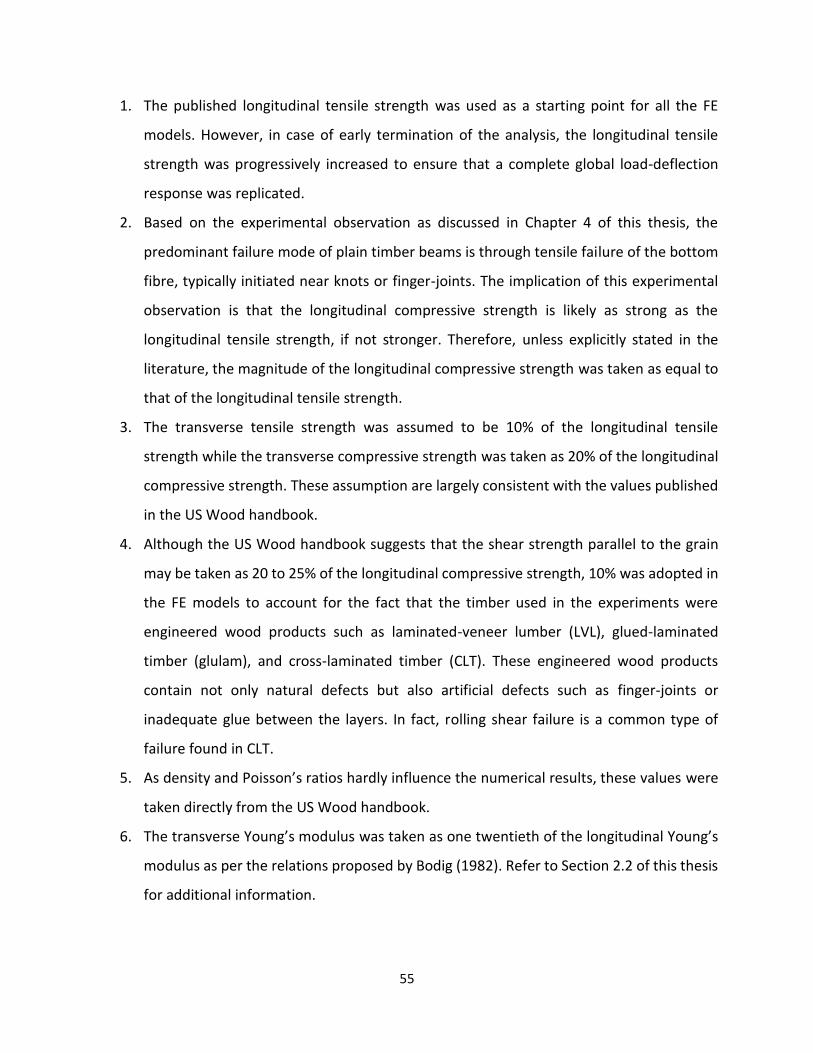
55
1. The published longitudinal tensile strength was used as a starting point for all the FE
models. However, in case of early termination of the analysis, the longitudinal tensile
strength was progressively increased to ensure that a complete global load-deflection
response was replicated.
2. Based on the experimental observation as discussed in Chapter 4 of this thesis, the
predominant failure mode of plain timber beams is through tensile failure of the bottom
fibre, typically initiated near knots or finger-joints. The implication of this experimental
observation is that the longitudinal compressive strength is likely as strong as the
longitudinal tensile strength, if not stronger. Therefore, unless explicitly stated in the
literature, the magnitude of the longitudinal compressive strength was taken as equal to
that of the longitudinal tensile strength.
3. The transverse tensile strength was assumed to be 10% of the longitudinal tensile
strength while the transverse compressive strength was taken as 20% of the longitudinal
compressive strength. These assumption are largely consistent with the values published
in the US Wood handbook.
4. Although the US Wood handbook suggests that the shear strength parallel to the grain
may be taken as 20 to 25% of the longitudinal compressive strength, 10% was adopted in
the FE models to account for the fact that the timber used in the experiments were
engineered wood products such as laminated-veneer lumber (LVL), glued-laminated
timber (glulam), and cross-laminated timber (CLT). These engineered wood products
contain not only natural defects but also artificial defects such as finger-joints or
inadequate glue between the layers. In fact, rolling shear failure is a common type of
failure found in CLT.
5. As density and Poisson’s ratios hardly influence the numerical results, these values were
taken directly from the US Wood handbook.
6. The transverse Young’s modulus was taken as one twentieth of the longitudinal Young’s
modulus as per the relations proposed by Bodig (1982). Refer to Section 2.2 of this thesis
for additional information.
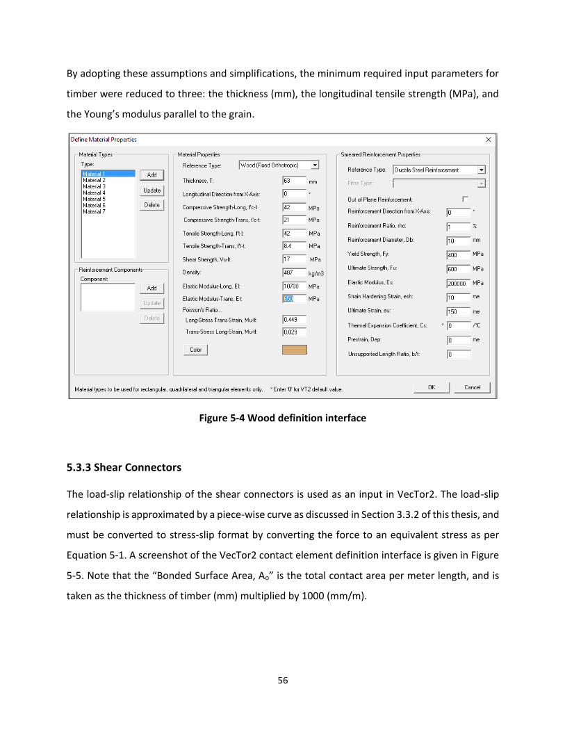
56
By adopting these assumptions and simplifications, the minimum required input parameters for
timber were reduced to three: the thickness (mm), the longitudinal tensile strength (MPa), and
the Young’s modulus parallel to the grain.
Figure 5-4 Wood definition interface
5.3.3 Shear Connectors
The load-slip relationship of the shear connectors is used as an input in VecTor2. The load-slip
relationship is approximated by a piece-wise curve as discussed in Section 3.3.2 of this thesis, and
must be converted to stress-slip format by converting the force to an equivalent stress as per
Equation 5-1. A screenshot of the VecTor2 contact element definition interface is given in Figure
5-5. Note that the “Bonded Surface Area, Ao” is the total contact area per meter length, and is
taken as the thickness of timber (mm) multiplied by 1000 (mm/m).
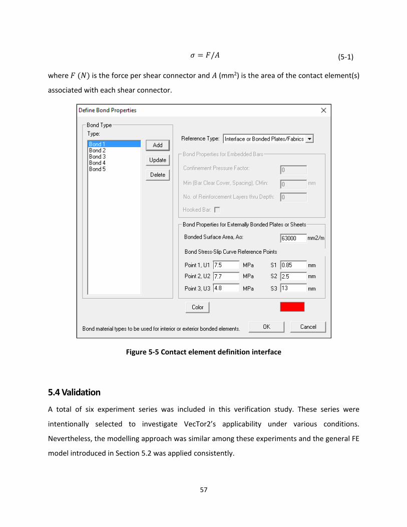
57
𝜎 = 𝐹/𝐴 (5-1)
where 𝐹 (𝑁) is the force per shear connector and 𝐴 (mm2) is the area of the contact element(s)
associated with each shear connector.
Figure 5-5 Contact element definition interface
5.4 Validation
A total of six experiment series was included in this verification study. These series were
intentionally selected to investigate VecTor2’s applicability under various conditions.
Nevertheless, the modelling approach was similar among these experiments and the general FE
model introduced in Section 5.2 was applied consistently.
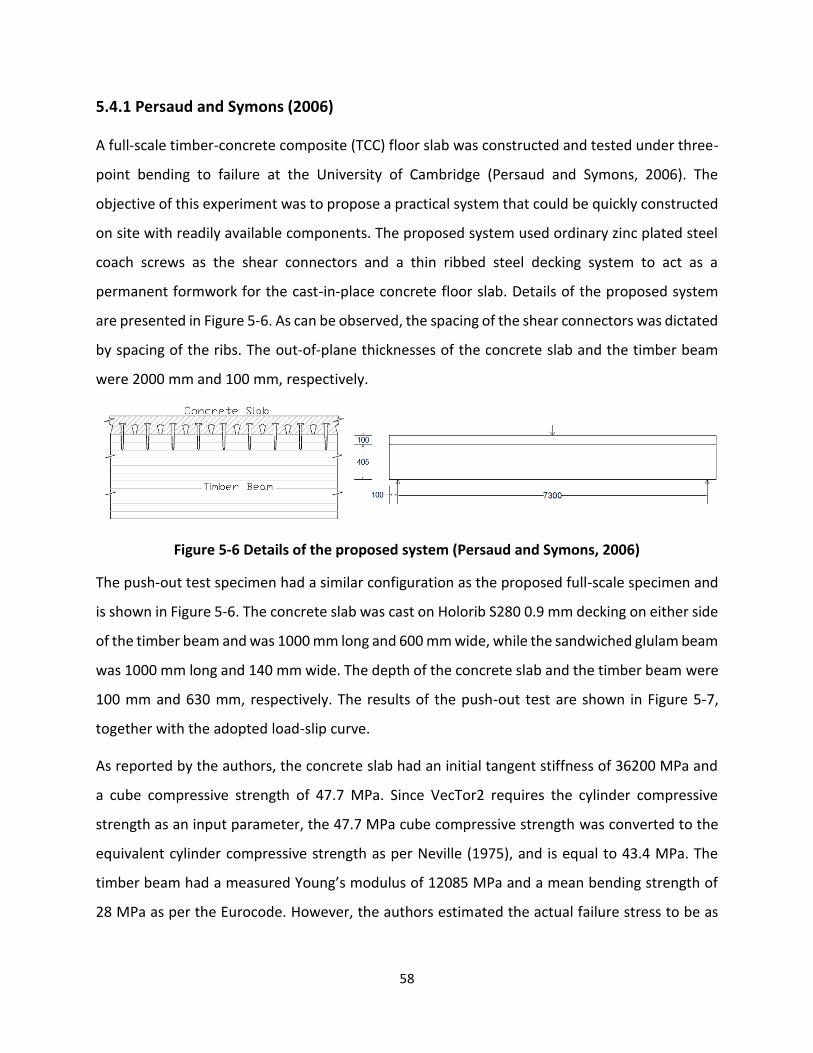
58
5.4.1 Persaud and Symons (2006)
A full-scale timber-concrete composite (TCC) floor slab was constructed and tested under three-
point bending to failure at the University of Cambridge (Persaud and Symons, 2006). The
objective of this experiment was to propose a practical system that could be quickly constructed
on site with readily available components. The proposed system used ordinary zinc plated steel
coach screws as the shear connectors and a thin ribbed steel decking system to act as a
permanent formwork for the cast-in-place concrete floor slab. Details of the proposed system
are presented in Figure 5-6. As can be observed, the spacing of the shear connectors was dictated
by spacing of the ribs. The out-of-plane thicknesses of the concrete slab and the timber beam
were 2000 mm and 100 mm, respectively.
Figure 5-6 Details of the proposed system (Persaud and Symons, 2006)
The push-out test specimen had a similar configuration as the proposed full-scale specimen and
is shown in Figure 5-6. The concrete slab was cast on Holorib S280 0.9 mm decking on either side
of the timber beam and was 1000 mm long and 600 mm wide, while the sandwiched glulam beam
was 1000 mm long and 140 mm wide. The depth of the concrete slab and the timber beam were
100 mm and 630 mm, respectively. The results of the push-out test are shown in Figure 5-7,
together with the adopted load-slip curve.
As reported by the authors, the concrete slab had an initial tangent stiffness of 36200 MPa and
a cube compressive strength of 47.7 MPa. Since VecTor2 requires the cylinder compressive
strength as an input parameter, the 47.7 MPa cube compressive strength was converted to the
equivalent cylinder compressive strength as per Neville (1975), and is equal to 43.4 MPa. The
timber beam had a measured Young’s modulus of 12085 MPa and a mean bending strength of
28 MPa as per the Eurocode. However, the authors estimated the actual failure stress to be as
59
high as 41.7 MPa. A summary of the input parameters is tabulated in Table 5-3. All other required
inputs for timber were calculated as per Section 5.3.2 of this chapter.
A TCC beam was created in VecTor2 based on the aforementioned information and the FE model
is demonstrated in Figure 5-8. Smeared contact elements were used in the model because the
spacing of the connectors in the full-scale specimen was consistent with that of the push-out test
specimens. Although the concrete slab did not have a uniform thickness over the depth due to
the decking profile, a uniform thickness was assumed in the FE model. This simplification is
reasonable because the loss of concrete area may be compensated by the steel decking. In
addition, the steel decking can act as confinement and add stiffness to the concrete slab. A
summary of the FE model is presented in Table 5-4.
Shown in Figure 5-9 is the experimental load-deflection response versus the predicted load-
deflection response; Figure 5-10 compares the predicted and the experimental load-slip curves
measured at the beam end. Notice that the dotted lines included in both plots were the analytical
result predicted by a 2D Abaqus model created by Persaud and Symons, 2006. Further details of
the Abaqus model can be found in their original paper.
Overall, the complete load-deflection response was well captured by VecTor2, better than was
done with Abaqus. A mid-span deflection of 75.6 mm and a failure load of 173.6 kN was predicted
by VecTor2 while the actual mid-span deflection and the failure load were 74.9 mm and 173 kN,
respectively. Moreover, VecTor2 predicted tension failure at mid-span, which was consistent
with the experimental observation that the final collapse of the specimen was initiated in the
region of a knot in the bottom laminates. An exaggerated deflected shape (5X magnification) of
the TCC specimen is depicted in Figure 5-11. One major discrepancy between the experimental
result and the VecTor2 prediction was that VecTor2 predicted concrete cracking near the mid
span directly under the loading jack, whereas in the experiment, no cracking was observed. Such
discrepancy may be attributed to the confining effect of the steel decking which may have
prevented the concrete slab from cracking.
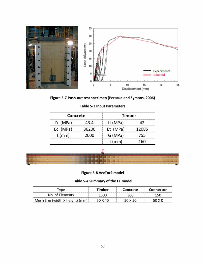
60
Figure 5-7 Push-out test specimen (Persaud and Symons, 2006)
Table 5-3 Input Parameters
Figure 5-8 VecTor2 model
Table 5-4 Summary of the FE model
f'c (MPa) 43.4 ft (MPa) 42
Ec (MPa) 36200 Et (MPa) 12085
t (mm) 2000 G (MPa) 755
t (mm) 160
Concrete Timber
Timber Concrete Connector
1500 300 150
50 X 40 50 X 50 50 X 0
Type
No. of Elements
Mesh Size (width X height) (mm)
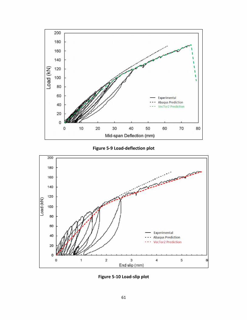
61
Figure 5-9 Load-deflection plot
Figure 5-10 Load-slip plot
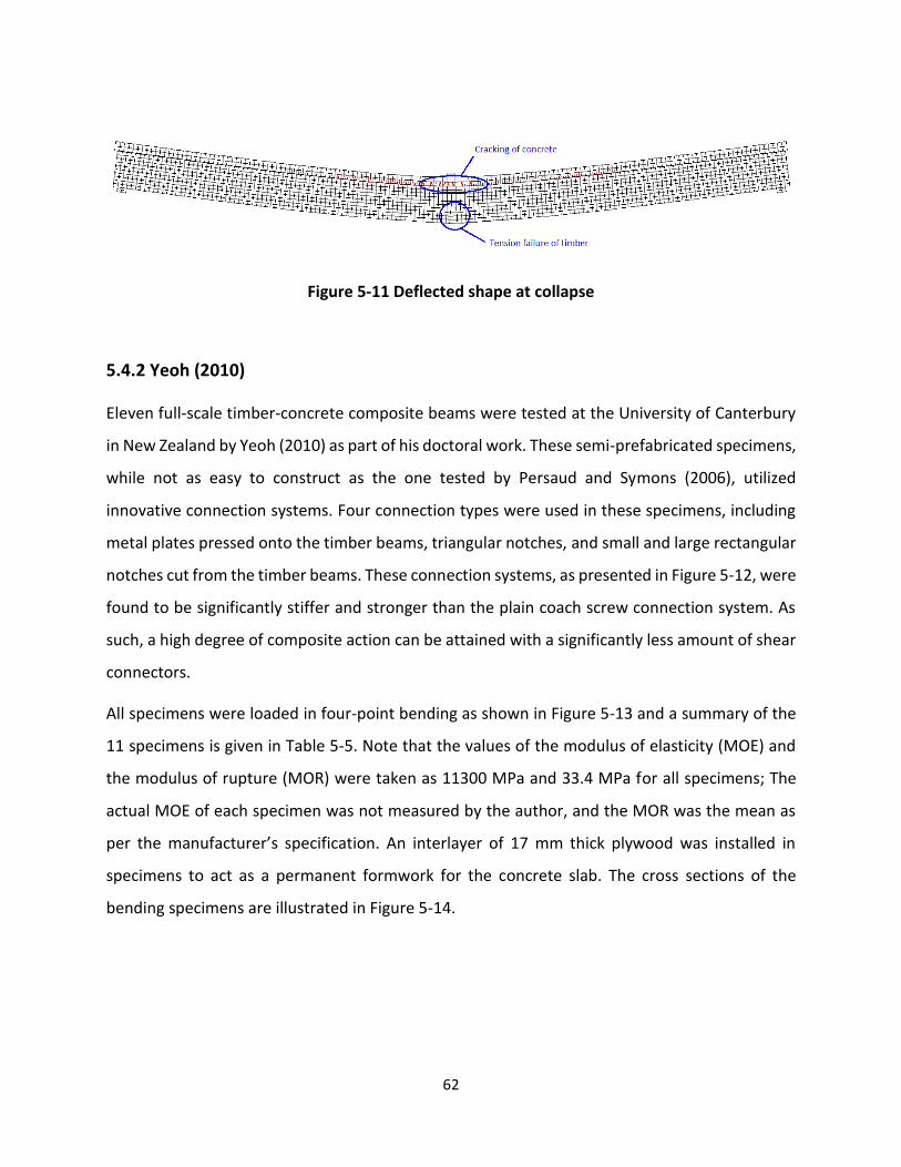
62
Figure 5-11 Deflected shape at collapse
5.4.2 Yeoh (2010)
Eleven full-scale timber-concrete composite beams were tested at the University of Canterbury
in New Zealand by Yeoh (2010) as part of his doctoral work. These semi-prefabricated specimens,
while not as easy to construct as the one tested by Persaud and Symons (2006), utilized
innovative connection systems. Four connection types were used in these specimens, including
metal plates pressed onto the timber beams, triangular notches, and small and large rectangular
notches cut from the timber beams. These connection systems, as presented in Figure 5-12, were
found to be significantly stiffer and stronger than the plain coach screw connection system. As
such, a high degree of composite action can be attained with a significantly less amount of shear
connectors.
All specimens were loaded in four-point bending as shown in Figure 5-13 and a summary of the
11 specimens is given in Table 5-5. Note that the values of the modulus of elasticity (MOE) and
the modulus of rupture (MOR) were taken as 11300 MPa and 33.4 MPa for all specimens; The
actual MOE of each specimen was not measured by the author, and the MOR was the mean as
per the manufacturer’s specification. An interlayer of 17 mm thick plywood was installed in
specimens to act as a permanent formwork for the concrete slab. The cross sections of the
bending specimens are illustrated in Figure 5-14.
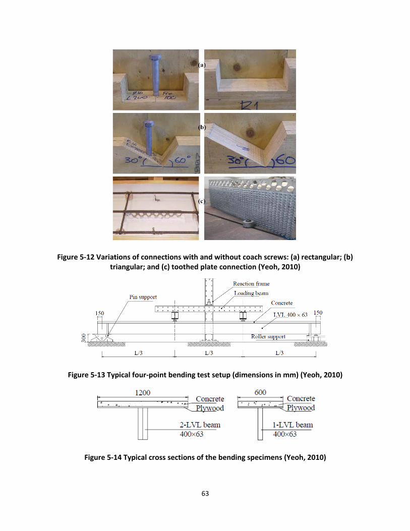
63
Figure 5-12 Variations of connections with and without coach screws: (a) rectangular; (b) triangular; and (c) toothed plate connection (Yeoh, 2010)
Figure 5-13 Typical four-point bending test setup (dimensions in mm) (Yeoh, 2010)
Figure 5-14 Typical cross sections of the bending specimens (Yeoh, 2010)
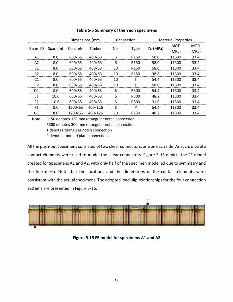
64
Table 5-5 Summary of the Yeoh specimens
All the push-out specimens consisted of two shear connectors, one on each side. As such, discrete
contact elements were used to model the shear connectors. Figure 5-15 depicts the FE model
created for Specimens A1 and A2, with only half of the specimen modelled due to symmetry and
the fine mesh. Note that the locations and the dimensions of the contact elements were
consistent with the actual specimens. The adopted load-slip relationships for the four connection
systems are presented in Figure 5-16.
Figure 5-15 FE model for specimens A1 and A2
Beam ID Span (m) Concrete Timber No. Type f'c (MPa)MOE
(MPa)
MOR
(MPa)
A1 8.0 600x65 400x63 6 R150 58.0 11300 33.4
A2 8.0 600x65 400x63 6 R150 58.0 11300 33.4
B1 8.0 600x65 400x63 10 R150 58.0 11300 33.4
B2 8.0 600x65 400x63 10 R150 38.8 11300 33.4
C1 8.0 600x65 400x63 10 T 54.4 11300 33.4
C2 8.0 600x65 400x63 10 T 58.0 11300 33.4
D1 8.0 600x65 400x63 6 R300 54.4 11300 33.4
E1 10.0 600x65 400x63 6 R300 48.2 11300 33.4
E2 10.0 600x65 400x63 6 R300 31.0 11300 33.4
F1 8.0 1200x65 400x126 8 P 54.4 11300 33.4
G1 8.0 1200x65 400x126 10 R150 48.2 11300 33.4
Note: R150 denotes 150 mm retangular notch connection
R300 denotes 300 mm retangular notch connection
T denotes triangular notch connection
P denotes toothed plate connection
Dimensions (mm) Connection Material Properties
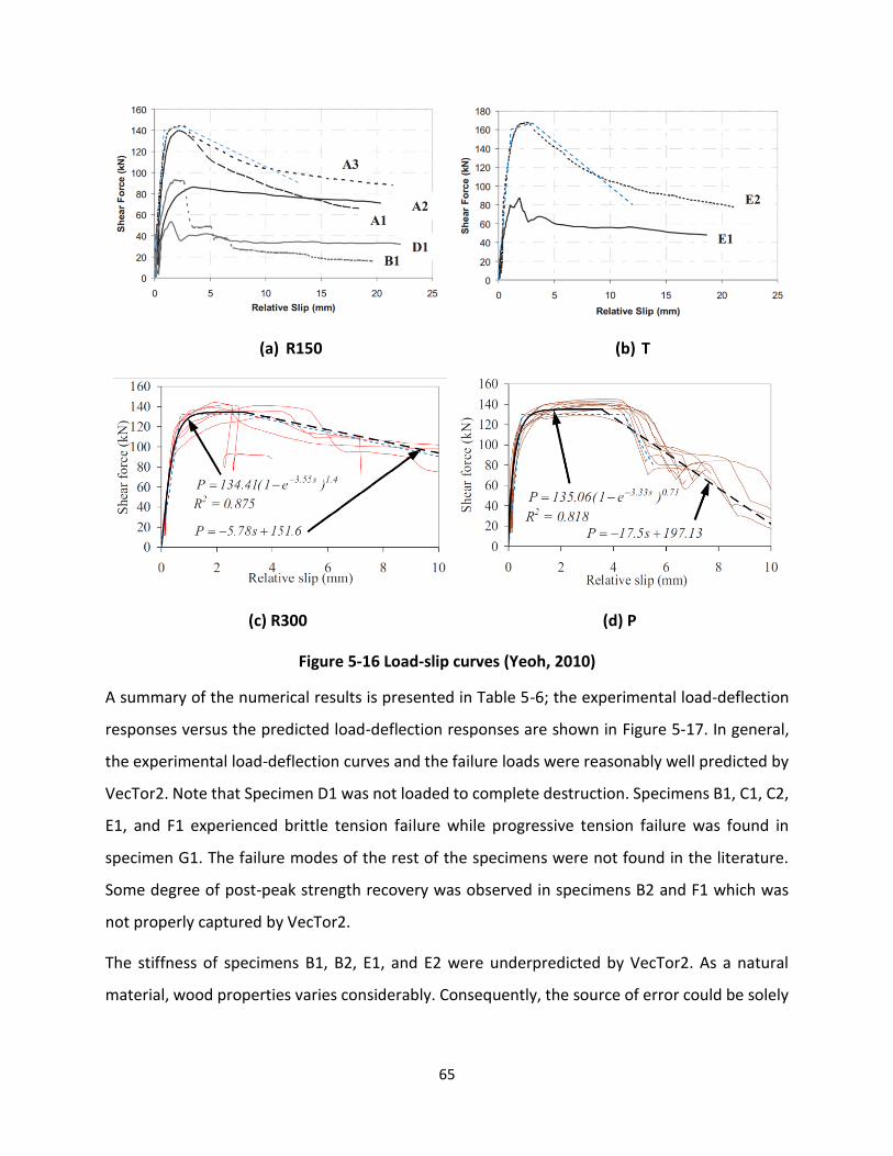
65
(a) R150 (b) T
(c) R300 (d) P
Figure 5-16 Load-slip curves (Yeoh, 2010)
A summary of the numerical results is presented in Table 5-6; the experimental load-deflection
responses versus the predicted load-deflection responses are shown in Figure 5-17. In general,
the experimental load-deflection curves and the failure loads were reasonably well predicted by
VecTor2. Note that Specimen D1 was not loaded to complete destruction. Specimens B1, C1, C2,
E1, and F1 experienced brittle tension failure while progressive tension failure was found in
specimen G1. The failure modes of the rest of the specimens were not found in the literature.
Some degree of post-peak strength recovery was observed in specimens B2 and F1 which was
not properly captured by VecTor2.
The stiffness of specimens B1, B2, E1, and E2 were underpredicted by VecTor2. As a natural
material, wood properties varies considerably. Consequently, the source of error could be solely
66
from the natural variability of modulus of elasticity of wood, which was assumed to be identical
across all specimens.
It shall be pointed out that the predicted stiffness of Specimen F1 deviated from the experimental
result at large loads. In this case, the spacing effect of the shear connectors could be ultimately
responsible for the deviation. Shown in Figure 5-18 is the arrangement of the shear connectors
of Specimen F1, and it is evident that the shear connectors were closely spaced near the support.
Ceccotti et al. (2006) tested two push-out test specimens with variable spacing and found clear
distinction between the corresponding load-slip curves. Depicted in Figure 5-19 are the specimen
details together with the experimental results as reported by Cecotti et al. (2006).
Specimen G1, contrary to the brittle tension failure predicted by VecTor2, exhibited substantial
post-peak displacement. No signs of connector failure were observed experimentally and the
unusual plateau resulted from the progressive tension failure in the timber beam.
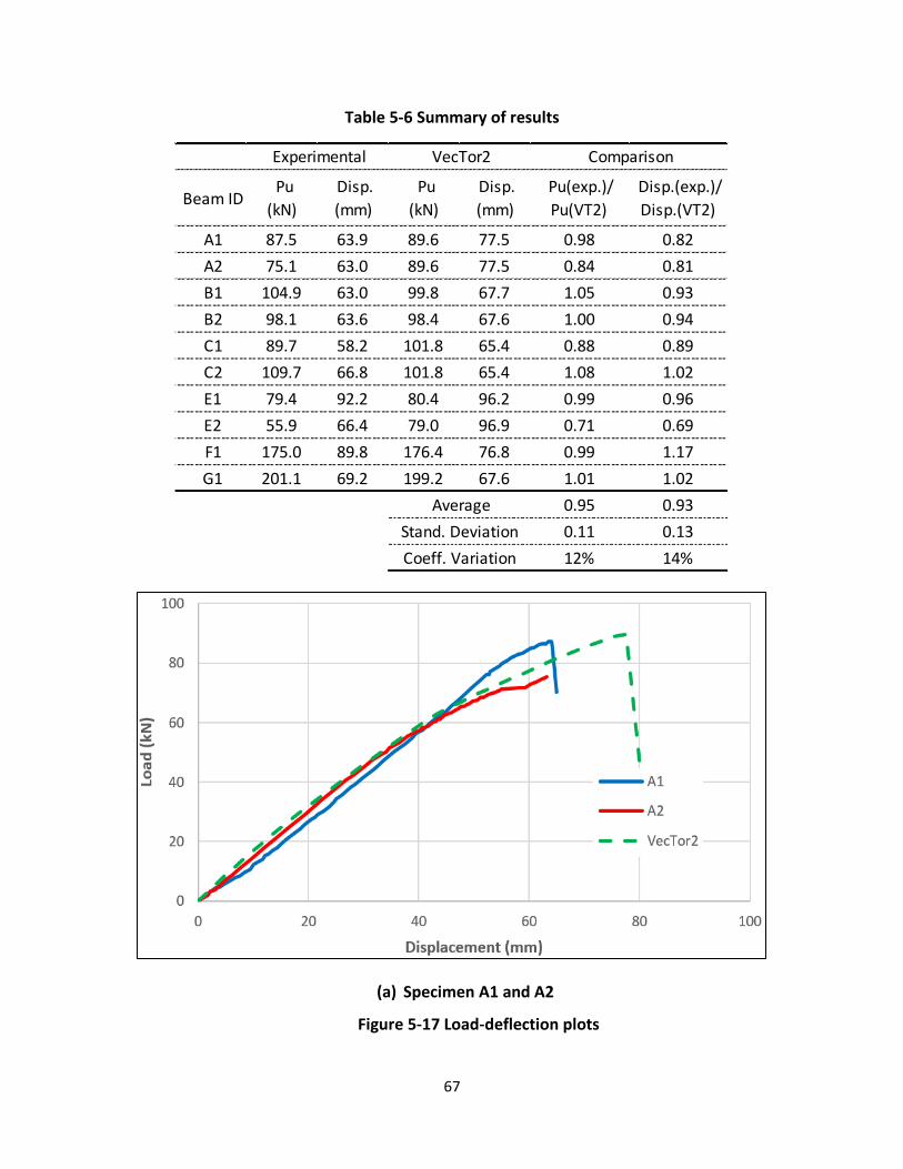
67
Table 5-6 Summary of results
(a) Specimen A1 and A2
Figure 5-17 Load-deflection plots
Beam ID Pu
(kN)
Disp.
(mm)
Pu
(kN)
Disp.
(mm)
Pu(exp.)/
Pu(VT2)
Disp.(exp.)/
Disp.(VT2)
A1 87.5 63.9 89.6 77.5 0.98 0.82
A2 75.1 63.0 89.6 77.5 0.84 0.81
B1 104.9 63.0 99.8 67.7 1.05 0.93
B2 98.1 63.6 98.4 67.6 1.00 0.94
C1 89.7 58.2 101.8 65.4 0.88 0.89
C2 109.7 66.8 101.8 65.4 1.08 1.02
E1 79.4 92.2 80.4 96.2 0.99 0.96
E2 55.9 66.4 79.0 96.9 0.71 0.69
F1 175.0 89.8 176.4 76.8 0.99 1.17
G1 201.1 69.2 199.2 67.6 1.01 1.02
0.95 0.93
0.11 0.13
12% 14%Coeff. Variation
Experimental VecTor2 Comparison
Average
Stand. Deviation

68
(b) Specimen B1 and B2
(c) Specimen C1 and C2
Figure 5-17 Load-deflection plots (continued)
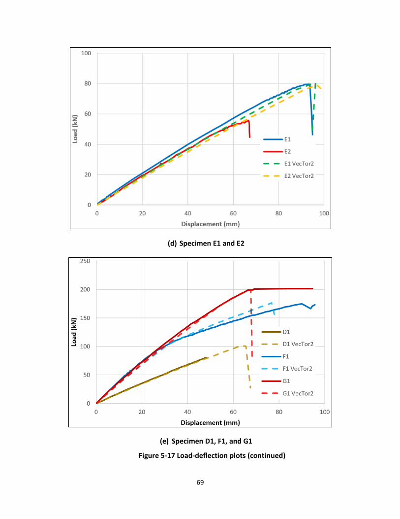
69
(d) Specimen E1 and E2
(e) Specimen D1, F1, and G1
Figure 5-17 Load-deflection plots (continued)
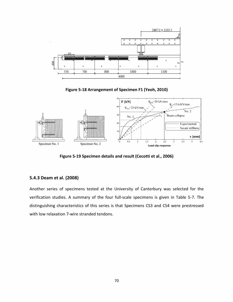
70
Figure 5-18 Arrangement of Specimen F1 (Yeoh, 2010)
Figure 5-19 Specimen details and result (Cecotti et al., 2006)
5.4.3 Deam et al. (2008)
Another series of specimens tested at the University of Canterbury was selected for the
verification studies. A summary of the four full-scale specimens is given in Table 5-7. The
distinguishing characteristics of this series is that Specimens CS3 and CS4 were prestressed
with low relaxation 7-wire stranded tendons.
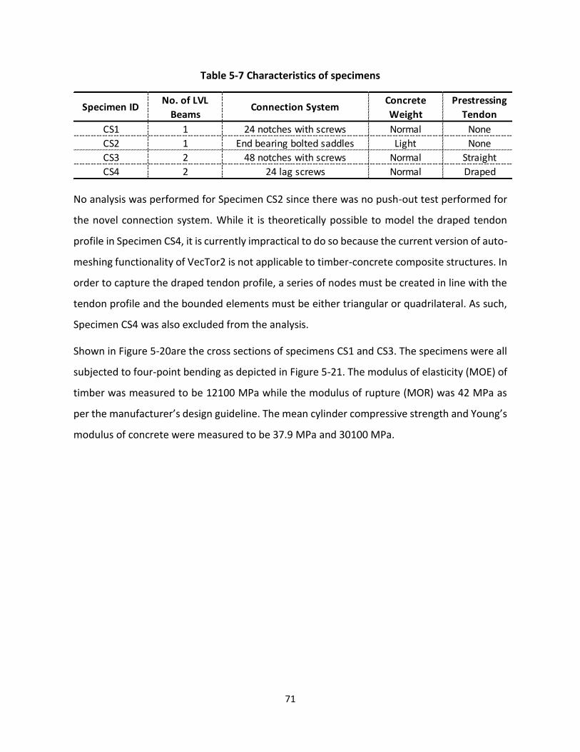
71
Table 5-7 Characteristics of specimens
No analysis was performed for Specimen CS2 since there was no push-out test performed for
the novel connection system. While it is theoretically possible to model the draped tendon
profile in Specimen CS4, it is currently impractical to do so because the current version of auto-
meshing functionality of VecTor2 is not applicable to timber-concrete composite structures. In
order to capture the draped tendon profile, a series of nodes must be created in line with the
tendon profile and the bounded elements must be either triangular or quadrilateral. As such,
Specimen CS4 was also excluded from the analysis.
Shown in Figure 5-20are the cross sections of specimens CS1 and CS3. The specimens were all
subjected to four-point bending as depicted in Figure 5-21. The modulus of elasticity (MOE) of
timber was measured to be 12100 MPa while the modulus of rupture (MOR) was 42 MPa as
per the manufacturer’s design guideline. The mean cylinder compressive strength and Young’s
modulus of concrete were measured to be 37.9 MPa and 30100 MPa.
Specimen IDNo. of LVL
BeamsConnection System
Concrete
Weight
Prestressing
Tendon
CS1 1 24 notches with screws Normal None
CS2 1 End bearing bolted saddles Light None
CS3 2 48 notches with screws Normal Straight
CS4 2 24 lag screws Normal Draped
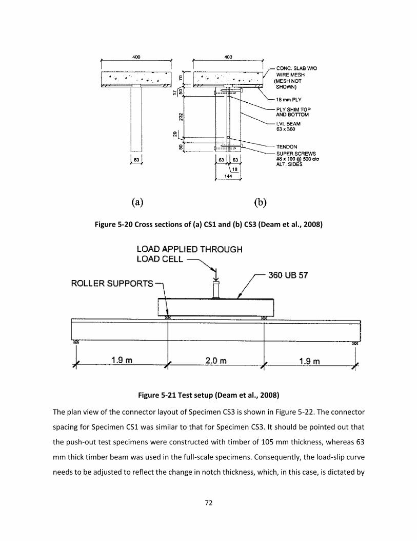
72
Figure 5-20 Cross sections of (a) CS1 and (b) CS3 (Deam et al., 2008)
Figure 5-21 Test setup (Deam et al., 2008)
The plan view of the connector layout of Specimen CS3 is shown in Figure 5-22. The connector
spacing for Specimen CS1 was similar to that for Specimen CS3. It should be pointed out that
the push-out test specimens were constructed with timber of 105 mm thickness, whereas 63
mm thick timber beam was used in the full-scale specimens. Consequently, the load-slip curve
needs to be adjusted to reflect the change in notch thickness, which, in this case, is dictated by
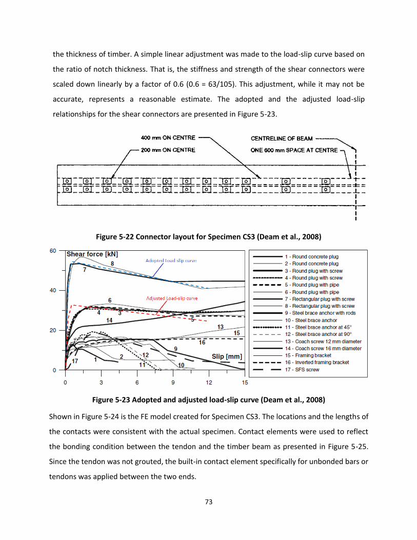
73
the thickness of timber. A simple linear adjustment was made to the load-slip curve based on
the ratio of notch thickness. That is, the stiffness and strength of the shear connectors were
scaled down linearly by a factor of 0.6 (0.6 = 63/105). This adjustment, while it may not be
accurate, represents a reasonable estimate. The adopted and the adjusted load-slip
relationships for the shear connectors are presented in Figure 5-23.
Figure 5-22 Connector layout for Specimen CS3 (Deam et al., 2008)
Figure 5-23 Adopted and adjusted load-slip curve (Deam et al., 2008)
Shown in Figure 5-24 is the FE model created for Specimen CS3. The locations and the lengths of
the contacts were consistent with the actual specimen. Contact elements were used to reflect
the bonding condition between the tendon and the timber beam as presented in Figure 5-25.
Since the tendon was not grouted, the built-in contact element specifically for unbonded bars or
tendons was applied between the two ends.

74
Figure 5-24 FE model for Specimen CS3
Figure 5-25 Definition of bond between tendon and timber
Shown in Figure 5-26 are the experimental load-deflection response versus the predicted load-
deflection responses. For Specimen CS1, yielding of the shear connectors was overpredicted
while the post-yielding stiffness was underpredicted. The accuracy of the predicted response may
have been improved if the load-slip curve corresponding to the actual notch size was available.
Nevertheless, the overall load-deflection response was captured with sufficient accuracy.
The final collapse of Specimen CS1 was caused as by rupturing of the timber beam in the constant
moment region. The corresponding tensile stress at failure load was around 60 MPa which was
about 43 % higher than the value prescribed by the manufacturer’s specification.
Specimen CS3 was not loaded to complete destruction to avoid the potential danger of tendon
failure. As can be observed, the added tendon had negligible influence on the global stiffness.
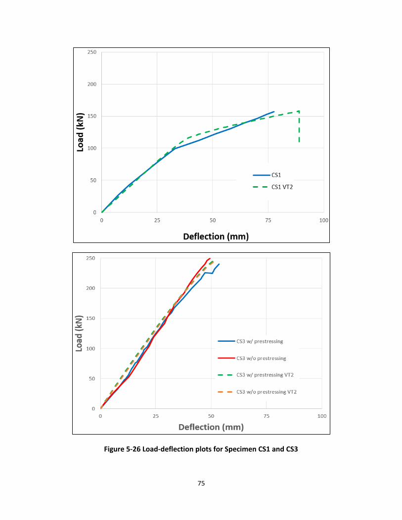
75
Figure 5-26 Load-deflection plots for Specimen CS1 and CS3

76
5.4.4 Gerber (2016)
Eighteen timber-concrete composite panels were tested at the University of British Columbia.
These panels, unlike typical TCC beams, had uniform thickness over the depth. Nevertheless, the
observed load-deflection behaviour of this series agreed fairly well with that of the TCC beams
investigated previously.
All the specimens were modelled with the same approach described in the previous three
experiment series (Section 5.4.1 through Section 5.4.3). Therefore, exhaustive modelling details
are omitted for this series. A summary of the specimen characteristics and the timber
specifications is given in Table 5-8 and Table 5-9, respectively. Additional details regarding
configuration of shear connectors and layout of shear connectors can be found in the original
literature. All specimens were loaded as per the experimental setup presented in Figure 5-27.
Table 5-8 Specimen characteristics
Table 5-9 Timber specification
Series MaterialNo.
Specimens
Specimen
Thickness
(mm)
Specimen
Length
(mm)
Depth
Concrete
(mm)
Depth
timber
(mm)
Depth
Interlayer
(mm)
S1 LSL 2 610 6096 70 89 NA
S2 LVL 2 610 6096 70 89 NA
S3 CLT 2 600 6000 70 99 NA
S4 LSL 2 610 6096 70 89 25
S5 LVL 2 610 6096 70 89 NA
S6 LSL 2 610 6096 70 89 NA
S7 LVL 2 610 6096 70 89 NA
S8 CLT 2 600 6000 70 99 NA
S9 LVL 2 610 6096 70 89 25
Material Tensile Strength
(MPa)
Young's Modulus
(MPa)
LSL 33.3 10685
LVL 37.6 13790
CLT 11.8 9500
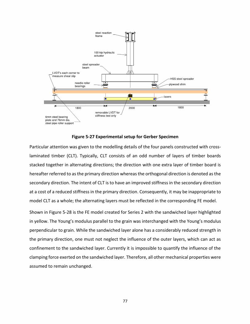
77
Figure 5-27 Experimental setup for Gerber Specimen
Particular attention was given to the modelling details of the four panels constructed with cross-
laminated timber (CLT). Typically, CLT consists of an odd number of layers of timber boards
stacked together in alternating directions; the direction with one extra layer of timber board is
hereafter referred to as the primary direction whereas the orthogonal direction is denoted as the
secondary direction. The intent of CLT is to have an improved stiffness in the secondary direction
at a cost of a reduced stiffness in the primary direction. Consequently, it may be inappropriate to
model CLT as a whole; the alternating layers must be reflected in the corresponding FE model.
Shown in Figure 5-28 is the FE model created for Series 2 with the sandwiched layer highlighted
in yellow. The Young’s modulus parallel to the grain was interchanged with the Young’s modulus
perpendicular to grain. While the sandwiched layer alone has a considerably reduced strength in
the primary direction, one must not neglect the influence of the outer layers, which can act as
confinement to the sandwiched layer. Currently it is impossible to quantify the influence of the
clamping force exerted on the sandwiched layer. Therefore, all other mechanical properties were
assumed to remain unchanged.
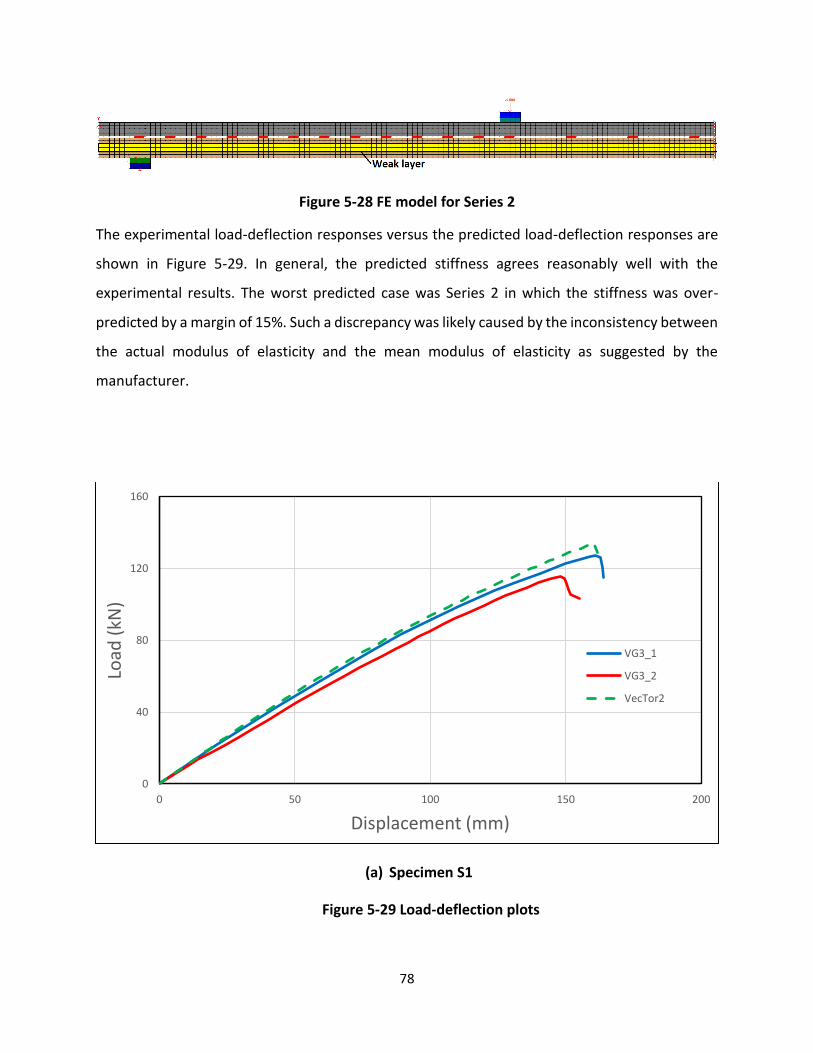
78
Figure 5-28 FE model for Series 2
The experimental load-deflection responses versus the predicted load-deflection responses are
shown in Figure 5-29. In general, the predicted stiffness agrees reasonably well with the
experimental results. The worst predicted case was Series 2 in which the stiffness was over-
predicted by a margin of 15%. Such a discrepancy was likely caused by the inconsistency between
the actual modulus of elasticity and the mean modulus of elasticity as suggested by the
manufacturer.
(a) Specimen S1
Figure 5-29 Load-deflection plots
0
40
80
120
160
0 50 100 150 200
Load
(kN
)
Displacement (mm)
VG3_1
VG3_2
VecTor2
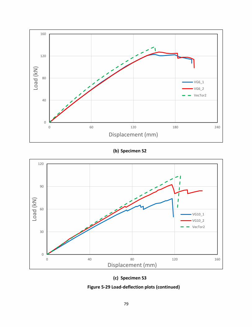
79
(b) Specimen S2
(c) Specimen S3
Figure 5-29 Load-deflection plots (continued)
0
40
80
120
160
0 60 120 180 240
Load
(kN
)
Displacement (mm)
VG6_1
VG6_2
VecTor2
0
30
60
90
120
0 40 80 120 160
Load
(kN
)
Displacement (mm)
VG10_1
VG10_2
VecTor2
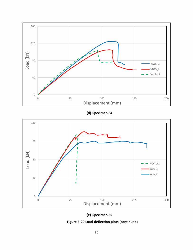
80
(d) Specimen S4
(e) Specimen S5
Figure 5-29 Load-deflection plots (continued)
0
40
80
120
160
0 50 100 150 200
Load
(kN
)
Displacement (mm)
VG15_1
VG15_2
VecTor2
0
30
60
90
120
0 75 150 225 300
Load
(kN
)
Displacement (mm)
VecTor2
AB6_1
AB6_2
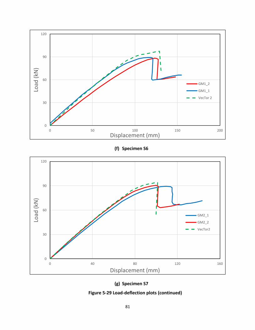
81
(f) Specimen S6
(g) Specimen S7
Figure 5-29 Load-deflection plots (continued)
0
30
60
90
120
0 50 100 150 200
Load
(kN
)
Displacement (mm)
GM1_2
GM1_1
VecTor 2
0
30
60
90
120
0 40 80 120 160
Load
(kN
)
Displacement (mm)
GM2_1
GM2_2
VecTor2
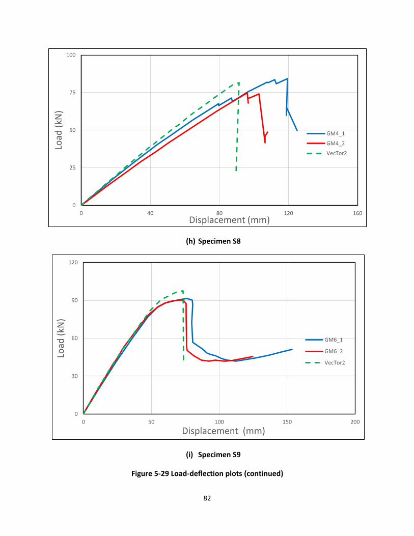
82
(h) Specimen S8
(i) Specimen S9
Figure 5-29 Load-deflection plots (continued)
0
25
50
75
100
0 40 80 120 160
Load
(kN
)
Displacement (mm)
GM4_1
GM4_2
VecTor2
0
30
60
90
120
0 50 100 150 200
Load
(kN
)
Displacement (mm)
GM6_1
GM6_2
VecTor2
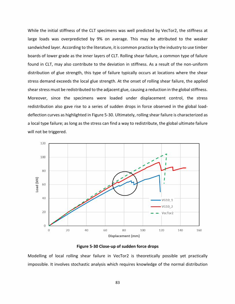
83
While the initial stiffness of the CLT specimens was well predicted by VecTor2, the stiffness at
large loads was overpredicted by 9% on average. This may be attributed to the weaker
sandwiched layer. According to the literature, it is common practice by the industry to use timber
boards of lower grade as the inner layers of CLT. Rolling shear failure, a common type of failure
found in CLT, may also contribute to the deviation in stiffness. As a result of the non-uniform
distribution of glue strength, this type of failure typically occurs at locations where the shear
stress demand exceeds the local glue strength. At the onset of rolling shear failure, the applied
shear stress must be redistributed to the adjacent glue, causing a reduction in the global stiffness.
Moreover, since the specimens were loaded under displacement control, the stress
redistribution also gave rise to a series of sudden drops in force observed in the global load-
deflection curves as highlighted in Figure 5-30. Ultimately, rolling shear failure is characterized as
a local type failure; as long as the stress can find a way to redistribute, the global ultimate failure
will not be triggered.
Figure 5-30 Close-up of sudden force drops
Modelling of local rolling shear failure in VecTor2 is theoretically possible yet practically
impossible. It involves stochastic analysis which requires knowledge of the normal distribution
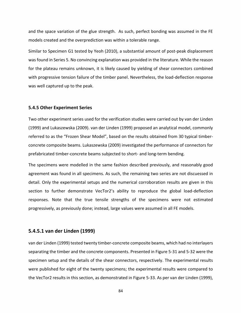
84
and the space variation of the glue strength. As such, perfect bonding was assumed in the FE
models created and the overprediction was within a tolerable range.
Similar to Specimen G1 tested by Yeoh (2010), a substantial amount of post-peak displacement
was found in Series 5. No convincing explanation was provided in the literature. While the reason
for the plateau remains unknown, it is likely caused by yielding of shear connectors combined
with progressive tension failure of the timber panel. Nevertheless, the load-deflection response
was well captured up to the peak.
5.4.5 Other Experiment Series
Two other experiment series used for the verification studies were carried out by van der Linden
(1999) and Lukaszewska (2009). van der Linden (1999) proposed an analytical model, commonly
referred to as the “Frozen Shear Model”, based on the results obtained from 30 typical timber-
concrete composite beams. Lukaszewska (2009) investigated the performance of connectors for
prefabricated timber-concrete beams subjected to short- and long-term bending.
The specimens were modelled in the same fashion described previously, and reasonably good
agreement was found in all specimens. As such, the remaining two series are not discuessed in
detail. Only the experimental setups and the numerical corroboration results are given in this
section to further demonstrate VecTor2’s ability to reproduce the global load-deflection
responses. Note that the true tensile strengths of the specimens were not estimated
progressively, as previously done; instead, large values were assumed in all FE models.
5.4.5.1 van der Linden (1999)
van der Linden (1999) tested twenty timber-concrete composite beams, which had no interlayers
separating the timber and the concrete components. Presented in Figure 5-31 and 5-32 were the
specimen setup and the details of the shear connectors, respectively. The experimental results
were published for eight of the twenty specimens; the experimental results were compared to
the VecTor2 results in this section, as demonstrated in Figure 5-33. As per van der Linden (1999),
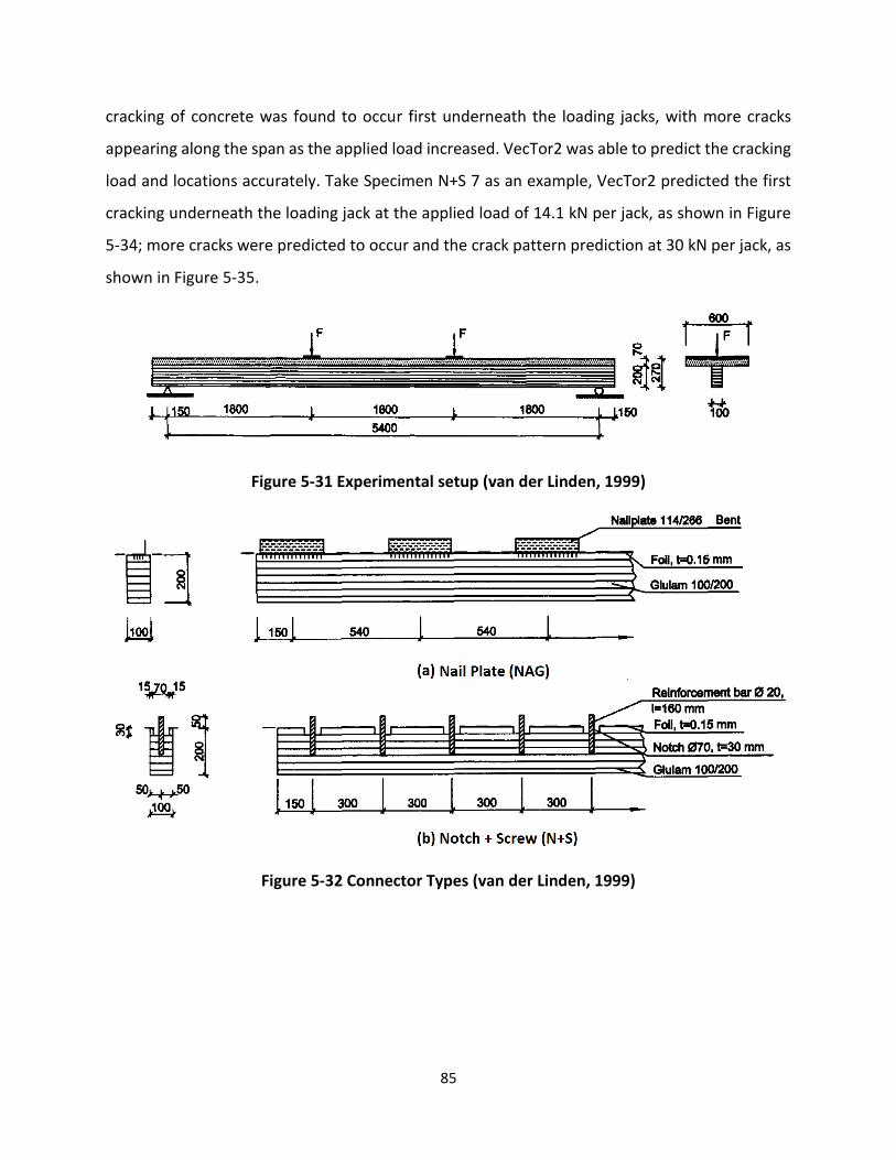
85
cracking of concrete was found to occur first underneath the loading jacks, with more cracks
appearing along the span as the applied load increased. VecTor2 was able to predict the cracking
load and locations accurately. Take Specimen N+S 7 as an example, VecTor2 predicted the first
cracking underneath the loading jack at the applied load of 14.1 kN per jack, as shown in Figure
5-34; more cracks were predicted to occur and the crack pattern prediction at 30 kN per jack, as
shown in Figure 5-35.
Figure 5-31 Experimental setup (van der Linden, 1999)
Figure 5-32 Connector Types (van der Linden, 1999)
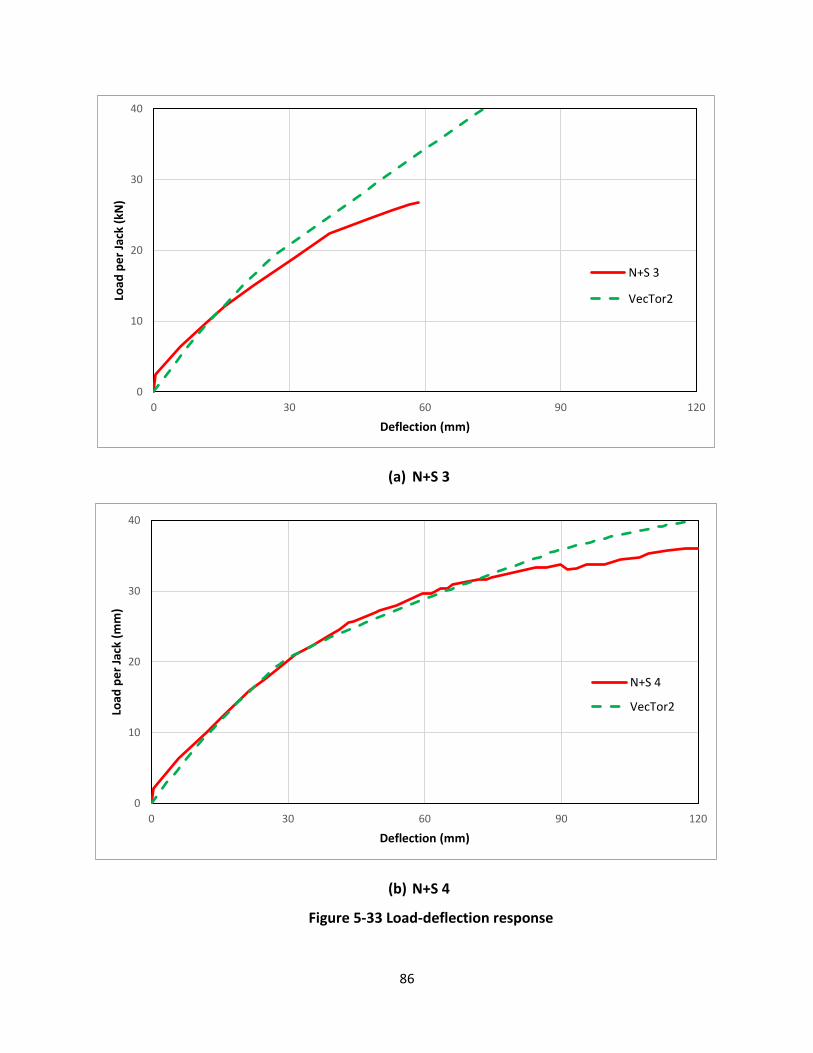
86
(a) N+S 3
(b) N+S 4
Figure 5-33 Load-deflection response
0
10
20
30
40
0 30 60 90 120
Load
pe
r Ja
ck (
kN)
Deflection (mm)
N+S 3
VecTor2
0
10
20
30
40
0 30 60 90 120
Load
pe
r Ja
ck (
mm
)
Deflection (mm)
N+S 4
VecTor2
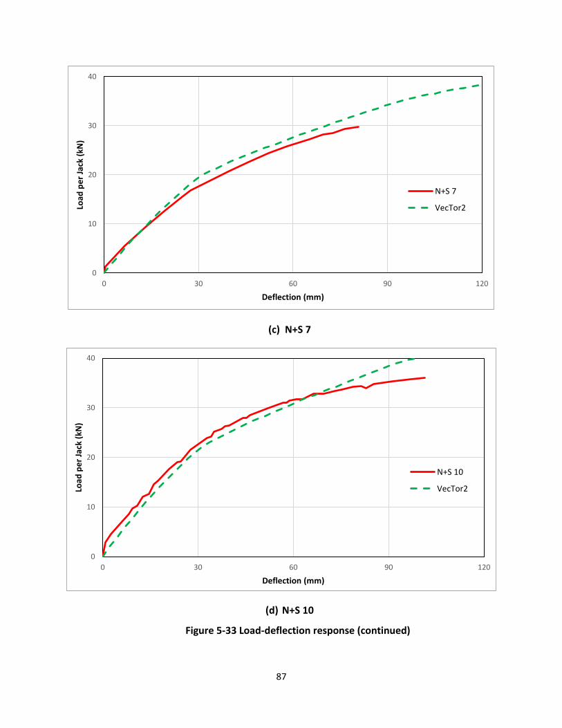
87
(c) N+S 7
(d) N+S 10
Figure 5-33 Load-deflection response (continued)
0
10
20
30
40
0 30 60 90 120
Load
pe
r Ja
ck (
kN)
Deflection (mm)
N+S 7
VecTor2
0
10
20
30
40
0 30 60 90 120
Load
pe
r Ja
ck (
kN)
Deflection (mm)
N+S 10
VecTor2
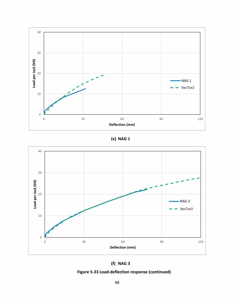
88
(e) NAG 1
(f) NAG 3
Figure 5-33 Load-deflection response (continued)
0
10
20
30
40
0 30 60 90 120
Load
pe
r Ja
ck (
kN)
Deflection (mm)
NAG 1
VecTor2
0
10
20
30
40
0 30 60 90 120
Load
pe
r Ja
ck (
kN)
Deflection (mm)
NAG 3
VecTor2
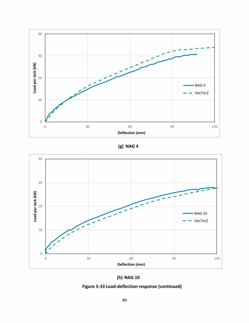
89
(g) NAG 4
(h) NAG 10
Figure 5-33 Load-deflection response (continued)
0
10
20
30
40
0 30 60 90 120
Load
pe
r Ja
ck (
kN)
Deflection (mm)
NAG 4
VecTor2
0
10
20
30
40
0 30 60 90 120
Load
pe
r Ja
ck (
kN)
Deflection (mm)
NAG 10
VecTor2
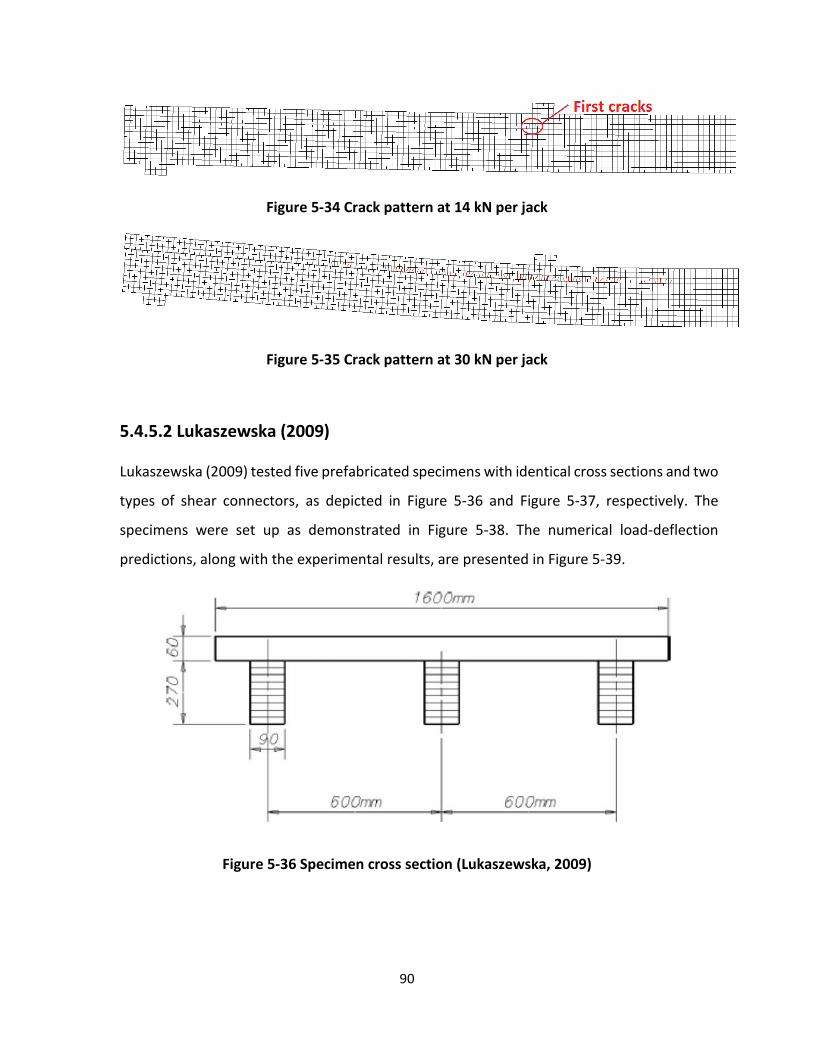
90
Figure 5-34 Crack pattern at 14 kN per jack
Figure 5-35 Crack pattern at 30 kN per jack
5.4.5.2 Lukaszewska (2009)
Lukaszewska (2009) tested five prefabricated specimens with identical cross sections and two
types of shear connectors, as depicted in Figure 5-36 and Figure 5-37, respectively. The
specimens were set up as demonstrated in Figure 5-38. The numerical load-deflection
predictions, along with the experimental results, are presented in Figure 5-39.
Figure 5-36 Specimen cross section (Lukaszewska, 2009)
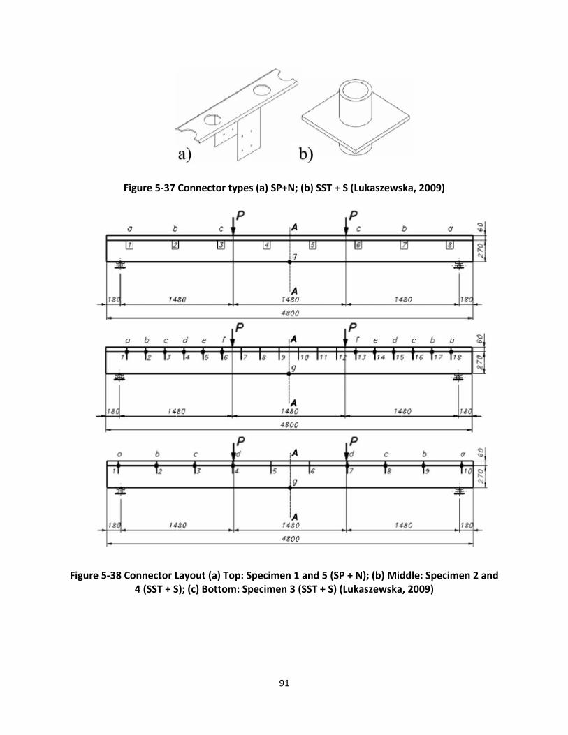
91
Figure 5-37 Connector types (a) SP+N; (b) SST + S (Lukaszewska, 2009)
Figure 5-38 Connector Layout (a) Top: Specimen 1 and 5 (SP + N); (b) Middle: Specimen 2 and 4 (SST + S); (c) Bottom: Specimen 3 (SST + S) (Lukaszewska, 2009)
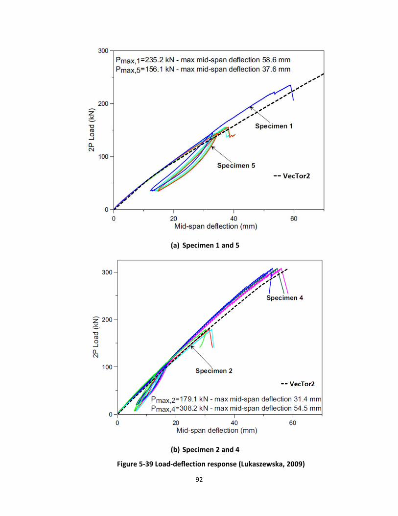
92
(a) Specimen 1 and 5
(b) Specimen 2 and 4
Figure 5-39 Load-deflection response (Lukaszewska, 2009)
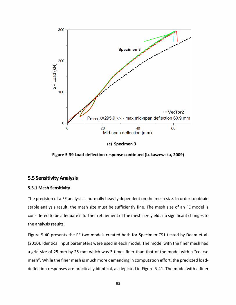
93
(c) Specimen 3
Figure 5-39 Load-deflection response continued (Lukaszewska, 2009)
5.5 Sensitivity Analysis
5.5.1 Mesh Sensitivity
The precision of a FE analysis is normally heavily dependent on the mesh size. In order to obtain
stable analysis result, the mesh size must be sufficiently fine. The mesh size of an FE model is
considered to be adequate if further refinement of the mesh size yields no significant changes to
the analysis results.
Figure 5-40 presents the FE two models created both for Specimen CS1 tested by Deam et al.
(2010). Identical input parameters were used in each model. The model with the finer mesh had
a grid size of 25 mm by 25 mm which was 3 times finer than that of the model with a “coarse
mesh”. While the finer mesh is much more demanding in computation effort, the predicted load-
deflection responses are practically identical, as depicted in Figure 5-41. The model with a finer
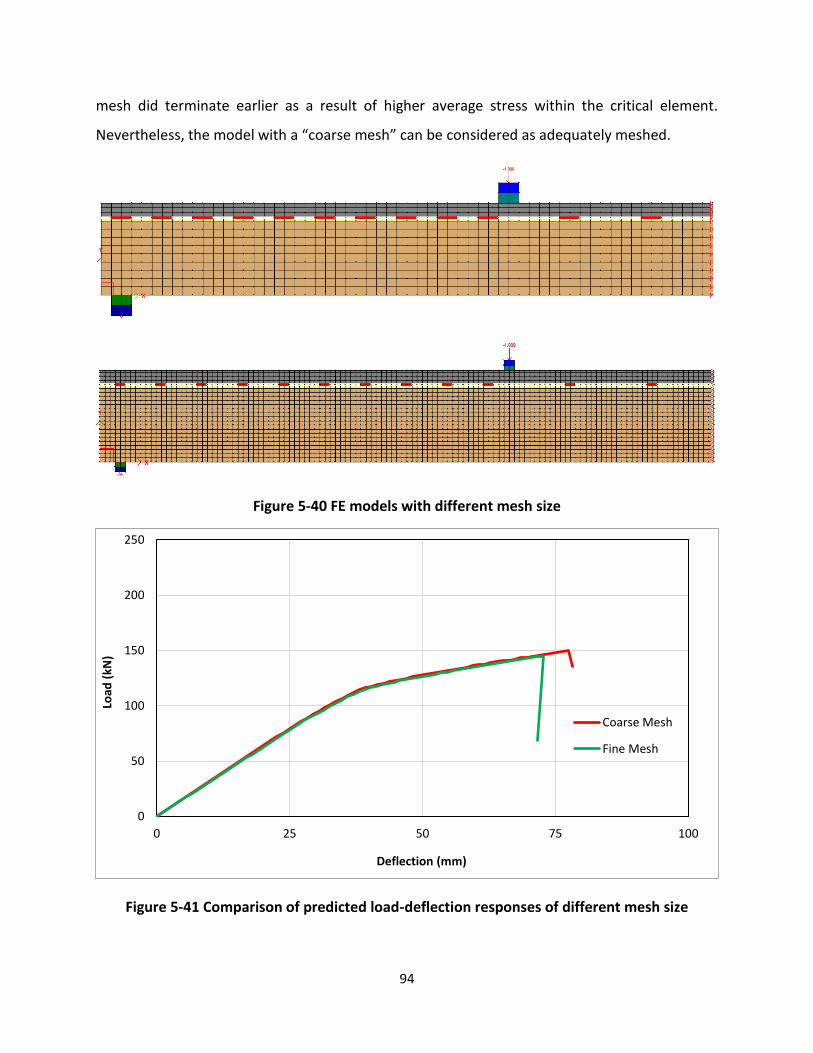
94
mesh did terminate earlier as a result of higher average stress within the critical element.
Nevertheless, the model with a “coarse mesh” can be considered as adequately meshed.
Figure 5-40 FE models with different mesh size
Figure 5-41 Comparison of predicted load-deflection responses of different mesh size
0
50
100
150
200
250
0 25 50 75 100
Load
(kN
)
Deflection (mm)
Coarse Mesh
Fine Mesh
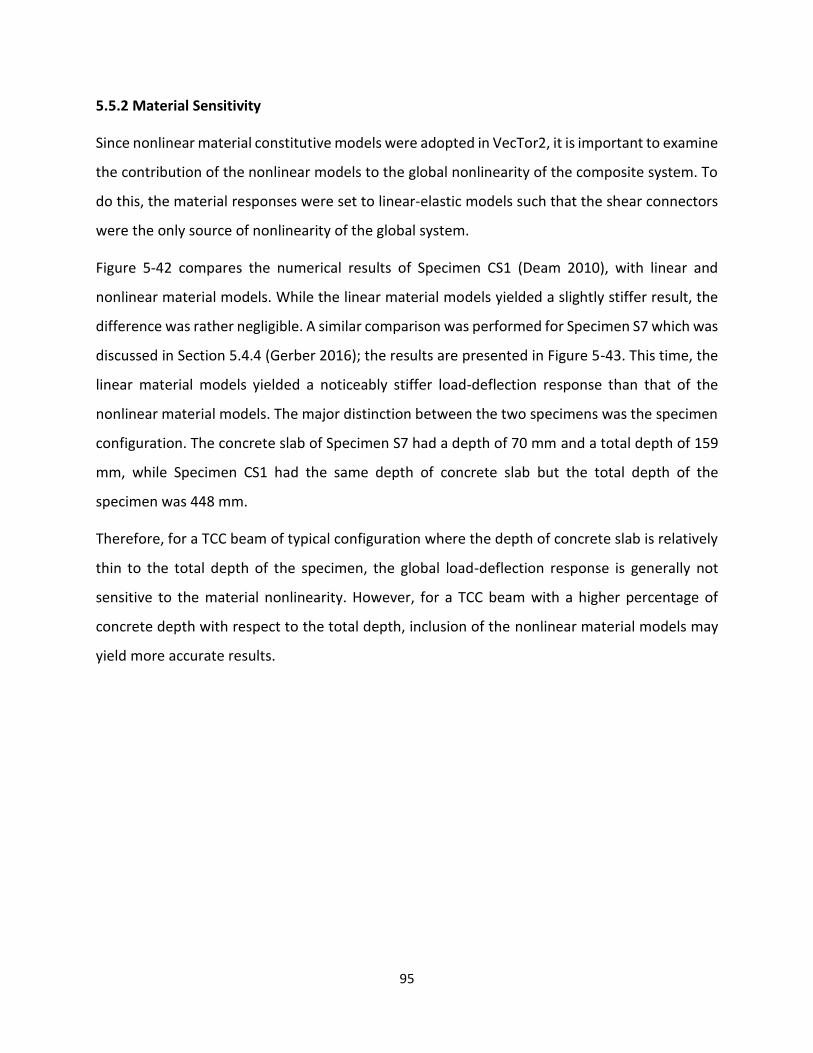
95
5.5.2 Material Sensitivity
Since nonlinear material constitutive models were adopted in VecTor2, it is important to examine
the contribution of the nonlinear models to the global nonlinearity of the composite system. To
do this, the material responses were set to linear-elastic models such that the shear connectors
were the only source of nonlinearity of the global system.
Figure 5-42 compares the numerical results of Specimen CS1 (Deam 2010), with linear and
nonlinear material models. While the linear material models yielded a slightly stiffer result, the
difference was rather negligible. A similar comparison was performed for Specimen S7 which was
discussed in Section 5.4.4 (Gerber 2016); the results are presented in Figure 5-43. This time, the
linear material models yielded a noticeably stiffer load-deflection response than that of the
nonlinear material models. The major distinction between the two specimens was the specimen
configuration. The concrete slab of Specimen S7 had a depth of 70 mm and a total depth of 159
mm, while Specimen CS1 had the same depth of concrete slab but the total depth of the
specimen was 448 mm.
Therefore, for a TCC beam of typical configuration where the depth of concrete slab is relatively
thin to the total depth of the specimen, the global load-deflection response is generally not
sensitive to the material nonlinearity. However, for a TCC beam with a higher percentage of
concrete depth with respect to the total depth, inclusion of the nonlinear material models may
yield more accurate results.
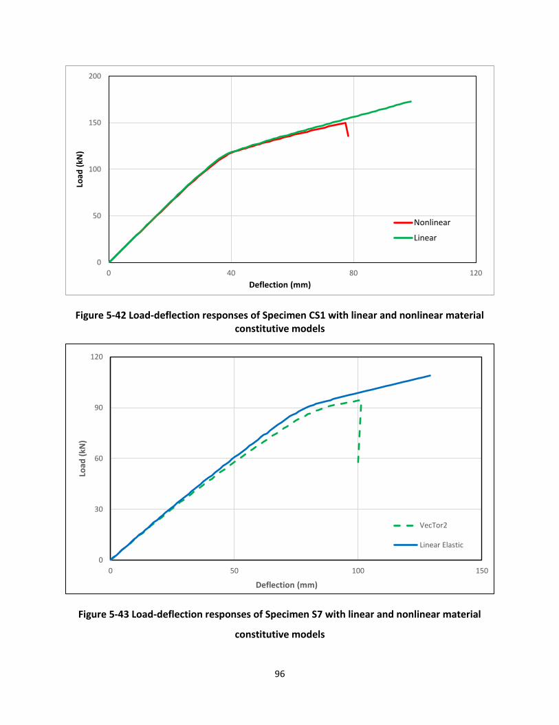
96
Figure 5-42 Load-deflection responses of Specimen CS1 with linear and nonlinear material constitutive models
Figure 5-43 Load-deflection responses of Specimen S7 with linear and nonlinear material
constitutive models
0
50
100
150
200
0 40 80 120
Load
(kN
)
Deflection (mm)
Nonlinear
Linear
0
30
60
90
120
0 50 100 150
Load
(kN
)
Deflection (mm)
VecTor2
Linear Elastic
97
5.6 Conclusions
After careful examination of VecTor2’s general applicability to various scenarios, the following
conclusions can be drawn:
The assumptions and simplifications made in Section 5.3.2 are appropriate in flexure-
critical conditions.
The total-load, secant-stiffness approach is found to be a viable approach for nonlinear
finite element modelling of plain timber, or timber composite such as timber-FRP or
timber- concrete composite.
Currently, VecTor2 is capable of analysing flexure-critical timber-concrete composite
beams subjected to short-term monotonic loadings. The load-deflection response of CLT
specimens can be predicted with reasonable accuracy using the FE model presented in
Figure 5-29.
The true tensile strength, as determined from the failure loads of the beam specimens
examined, is generally 30% to 50% higher than the mean suggested by the manufacturers.
The performance of timber-concrete composite is largely dictated by the load-slip
relationship of shear connectors. As illustrated by Yeoh (2010), the degree of composite
action can be close to 100% if the shear connectors are sufficiently stiff. What is also
observed is that the load-deflection remains fairly linear up to failure. The implication of
this observation is that high degree of composite action is achieved at a cost of reduced
global ductility.
Shear connectors may be modelled using the smeared or discrete contact elements,
depending on the connection type and the layout of shear connectors. For shear
connectors with constant spacing or shear connectors that are installed continuously
along the span such as the metal plate connectors, the smeared contact elements may be
a better option, whereas, the discrete contact element is most suitable for connectors
without uniform spacing.
Size matters. The size of shear connectors in full-scale specimens should be consistent
with that tested in the push-out test. As demonstrated in Deam et al. (2010), the accuracy
98
of the analysis is compromised when the size of shear connectors of push-out test
specimens do not match with that of the full-scale bending specimens.
The spacing effect should be taken into consideration in push-out tests. As demonstrated
in Figure 5-19, the load-slip relationship can vary considerably as a function of spacing.
Generally, the load-deflection response is well predicted by VecTor2 if the ultimate failure
is caused by either the timber beam rupturing due to high tensile stress in the wood fibre,
or by crushing of concrete. However, crushing of concrete is a less common type of failure
for TCC specimens.
Although cracking of concrete was predicted by VecTor2 for all the specimens
investigated in this thesis, it was not experimentally observed in the TCC specimens with
an interlayer acting as a permanent formwork for the concrete slab. However, van der
Linden (1999) tested twenty TCC specimens without such interlayers and found visible
cracks, which first occurred directly underneath the loading jacks. As the applied load
continued to increase, more cracks were found along the span of the specimens. This
suggests that the presence of interlayer may have confined or cushioned the bottom
concrete from cracking.
99
Chapter 6 Conclusions and Recommendations
6.1 Conclusions
The goal of this thesis was to investigate VecTor2’s potential capability to model timber-concrete
composite (TCC) structures subjected to short-term loadings. Along the process, the following
tasks were performed:
1. Implementation of appropriate wood constitutive model to describe the nonlinear
behaviour of wood.
2. Verification of the wood constitutive models by modelling plain and reinforced timber
beams subjected to short-term monotonic flexure.
3. Modelling of TCC beams subjected to short-term monotonic flexure, with variations in
test setups, specimen configurations, materials, and types of shear connectors.
With the results obtained from numerical simulations, it is confirmed that VecTor2 can model
TCC structures with sufficient accuracy. The generic FE models presented in Figure 5-1 and Figure
5-2 are found to be accurate and versatile, as they can be easily created and modified to deal
with different case scenarios.
However, the successful modelling results are limited to flexure-critical situations, where the
ultimate failure of TCC specimens is governed by brittle tension failure of timber in the bottom
face. Incomplete information on the material properties of the beam tested prevents
confirmation of the ability to model other failure modes.
Lastly, past experimental work on TCC has focused primarily on the development of shear
connectors, and the TCC performance subjected to short- and long-term monotonic loadings.
Hence, the numerical corroborations performed in this study are limited to short-term
monotonic loadings; VecTor2’s capability to perform dynamic analysis of TCC structures is
uncertain.
100
6.2 Recommendations
While a wide range of further investigation is possible, some aspects closely related to the scope
of work of this thesis are recommended for future work, as follows:
VecTor2 development:
The current pre-processor of VecTor2, FormWorks, is not able to auto-mesh a TCC beam. As such,
a step-by-step guideline is provided in Appendix B to explain the process to manually create a
TCC model in FormWorks. In order to simplify the model creation process for TCC structures,
work is required to update the FormWorks auto-meshing source code.
The post-processor, Augustus, does not read and display any results related to the bond-slip
elements. Work needs to be devoted to expand the program’s capability in this regard, and
ultimately to make the program more user-friendly for practical use.
Experimental work:
Future work must be undertaken to investigate the dynamic response of TCC. In the case of
monotonic loadings, the concrete component is of little concern as it primarily resists
compression, and the compression rarely surpasses the concrete’s compressive strength.
However, the concrete slab may become an issue under dynamic loading.
The global load-deflection response of any TCC system is heavily dependent on yielding of shear
connectors. In general, shear connectors need to be sufficiently stiff to achieve a high degree of
composite action, yet sufficiently ductile to contribute to the global ductility of a TCC system. The
use of concrete notch shear connectors investigated by Yeoh (2010) enabled a high degree of
composite action up to collapse, at the cost of reduced softening of the global load-deflection
response. From the experimental investigation conducted by Gentile (2000), as discussed in
Chapter 4, it is concluded that FRP reinforcement can be an effective measure to enhance the
post-peak response of wood in tension. Therefore, it may be worthwhile to incorporate both FRP
reinforcement and shear connectors of high stiffness within a TCC system, with each serving its
own purpose.
101
References
1. Azzi VD., Tsai SW. (1965). Anisotropic strength of composites. Exp Mech; 5–9: 283–9
2. Bakoss, S.L., Greenland, A. and Crews, K.I. (1999). Bridge deck and industrial heavy-duty
flooring system based on laminated veneer lumber beams reinforced with carbon fibre
composites. Proceedings of the 8" International Conference on Structural Faults and
Repair, London, UK, July 13- 15, 1999.
3. Bazan, I.M.M. (1980). Ultimate bending strength of timber beams (Doctoral dissertation).
Nova Scotia Tech. College. Halifax, N.S. 269p.
4. Bentz, E. (2010). Augustus: Post processor for VecTor2 (version 5.6.5). Copyright 1996-
2010 E. Bentz.
5. Bodig, J., Jayne, B. A. (1982). Mechanics of wood and wood composites. Van Nostran-
Reinhold Co, Inc., New York.
6. Ceccotti, A., Fragiacomo, M., and Giordano, S. (2006). Long-term and collapse tests on a
timber-concrete composite beam with glued-in connection. Materials and Structures,
Special Volume on Timber, in press.
7. Deam, B., Fragiacomo, M., and Gross, L. (2008). Experimental behaviour of prestressed
LVL-Concrete Composite Beams. J. Struct. Eng. 134(5): 801-809
8. Dorey, A.B. and Cheng, J.J.R. (1996). The behaviour of GFRP glued laminated timber
beams. Proceedings in Advanced Composite Materials in Bridges and Structures, ACMBS
II, M.M. El-Badry, Editor. Montreal, Quebec, Canada, pp. 787- 794.
9. de Ruvo, A., Carlsson, L., Fellers C. (1980). The biaxial strength of paper. Tappi 63(5):133–
136
10. Hemandez, R., Davalos, J.F., Sonti, S.S., Kim, Y. and Moody, R.C. (1997). Strength and
stiffness of reinforced yellow-poplar glued laminated beams. Res. Pap. FPL-RP- 554.
Madison, Wisconsin, U.S. Department. of Agriculture, Forest Service, Forest Products
Laboratory.
102
11. Fragiacomo, M. (2005). A finite element model for long-term analysis of timber-concrete
composite beams. Structural Engineering and Mechanics, 22(2), pp. 173-189.
12. Fragiacomo, M. (2012). Experimental behaviour of a full-scale timber-concrete composite
floor with mechanical connectors. Materials and Structures, 45(11): 1717-1735.
13. Frangi, A., and Fontana, M. (2003). Elasto-plastic model for timber-concrete composite
beams with ductile connection. Structural Engineering International 13 (1): 47-57.
14. Dias, A. M. P. G. (2005). Mechanical behaviour of timber-concrete joints (Doctoral
dissertation). University of Coimbra, Coimbra, Portugal.
15. Gentile, C. (2000). Flexural strengthening of timber bridge beams using FRP (MASc
dissertation). University of Manitoba.
16. Gerber, A. (2016). Timber-concrete composite connectors in flat-plate engineered wood
products (MASc dissertation). University of British Columbia.
17. Glos, P. (1978). Berichte zur Zuverlaessigkeitstheorie der Bauwerke: Zur Bestimmung des
Festigkeitsverhaltens von Brettschichtholz bei Druckbeanspruchung aus Werkstoff-und
Einwirkungskenngroessen. (Reliability theory for timber structures: determination of
compression strength behaviour of glulam components from interaction of material
properties). Heft 34/1978. Laboratorium fuer den Konstruktiven Ingenieurbau.
Technische Universitaet Muenchen. 335p.
18. Hankinson, R.L. (1921). Investigation of crushing strength of spruce at varying angles of
grain. Air Service Information Circular No. 259, U.S. Air Service.
19. Hashin, Z. (1980). Failure criteria for unidirectional fiber composites. Journal of Applied
Mechanics, 47:329-33.
20. Hoffman O. (1967). The brittle strength of orthotropic materials. J. Compos. Mater. 200-
6. 2-1.
21. Holmberg, S., Persson, K., and Petersson, H. (1998). Nonlinear mechanical behaviour and
analysis of wood and fibre materials. Computers and Structures 72. 459-480.
22. Jones RM. (1975). Mechanics of composite materials. first ed. Tokyo: McGraw Hill
Kogakusha.
103
23. Kasal, B., Leichti, RJ. (2005). State of the art in multiaxial phenomenological failure criteria
for wood members. Prog Struct Mat Eng 7:3–13
24. Lau, W. (2000). Strength model and finite element analysis of wood beam-columns in
truss applications (Doctoral dissertation). University of British Columbia.
25. Lukaszewska, E. (2009). Development of prefabricated timber-concrete composite floors
(Doctoral dissertation). Luleå tekniska universitet.
26. Malhotra, S.K. and Mazur, S.J. (1970). Buckling strength of solid timber columns. Trans
Eng. Inst. of Canada, Published in the Eng. J. I3(A-4): I-VII.
27. Neely, S. T. (1898). Relation of compression-endwise to breaking load of beam. Progress
in Timber Physics. USDA Division of Forest Circular No. 18: 13- 17.
28. Norris C.B. (1950). Strength of orthotropic materials subjected to combined stress. Report
No. 18126, US. Department of Agriculture, Forest Products Laboratory, Madison, WI.
29. Persaud, R., Symons, D. (2006). Design and testing of a composite timber and concrete
floor system. The Structural Engineer, 21, pp. 22-30.
30. van der Put TACM. (2005). The tensor polynomial failure criterion for wood. Delft Wood
Science Foundation, Delft.
31. Vecchio, F., and Collins, M. (1986). The modified compression field theory for reinforced
concrete elements subjected to shear. ACI Journal, 83(2), March-April 1986, pp. 219- 231.
32. Vecchio, F. (1990). Reinforced concrete membrane element formulation. ASCE Journal of
Structural Engineering, Vol. 116, No. 3, pp.730-750
33. Vecchio, F. (2000). Disturbed stress field model for reinforced concrete: formulation.
ASCE Journal of Structural Engineering, 126(9), September 2000, pp. 1071-1077.
34. Wong, P., Trommels, H., Vecchio, F. (2013). VecTor2 and FormWorks Manual.
35. Yeoh, D. (2010). Behaviour and design of timber-concrete composite floor system
(Doctoral dissertation). University of Canterbury.
36. Ylinen, A. (1956). A method of determining the buckling stress and the required cross-
sectional area for centrally loaded straight columns in elastic and inelastic range. IABSA
Publications. I6:529-549.

104
37. Zhang, C., Gauvreau, P. (2015). Timber-concrete composite systems with ductile
connections. Journal of Structural Engineering, 141(7).
105
Appendix Modelling Guideline
This section serves as a step-by-step guideline which aims to explain the VecTor2 modelling
process for timber-concrete composite beams subjected to short-term monotonic loadings. All
models are created with the program FormWorks (Wong et al., 2013), a pre-processor developed
specifically for VecTor2. The current auto-meshing functionality of FormWorks is not compatible
with timber-concrete composite structures; as such, all models must be manually created using
the built-in manual-meshing function. A newer version of the auto-meshing function is currently
under development, which will not only automate the model generation process, but also
improve the overall computation efficiency.
Step 1 Defining Regions
The process to manually create a timber-concrete composite beam model in FormWorks can be
tedious and time-consuming; patterns should always be exploited to simplify the process
substantially. In order to utilize such patterns, a TCC model should be first broken down into
multiples regions. Nodes and elements can then be added in batches following the specific
patterns associated with each region as defined.
The model created for Specimen CS1 tested by Deam et al. (2008) is used as a comprehensive
example. More details regarding the experimental setup can be found in Section 5.4.3 of this
thesis. Shown in Figure 1 is an example of how regions were defined for Specimen CS1. In this
case, the regions were defined entirely based on the original experimental setup, with each
region representing a particular material type (i.e. Region 2 representing the timber beam and
Region 3 representing the shear connectors). This example represents a simple yet feasible
approach that finds a balance between the computation demand, and simplicity in model
creation. All other specimens used for the validation studies in Chapter 5 were created following
the same procedure.
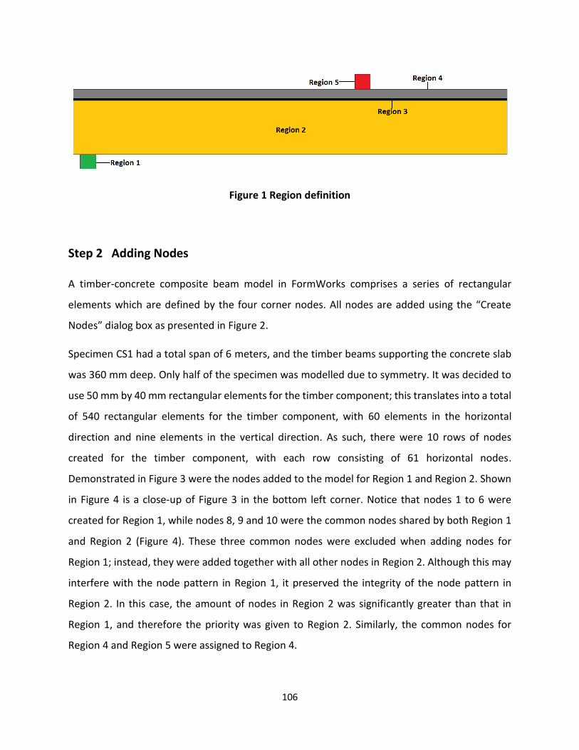
106
Figure 1 Region definition
Step 2 Adding Nodes
A timber-concrete composite beam model in FormWorks comprises a series of rectangular
elements which are defined by the four corner nodes. All nodes are added using the “Create
Nodes” dialog box as presented in Figure 2.
Specimen CS1 had a total span of 6 meters, and the timber beams supporting the concrete slab
was 360 mm deep. Only half of the specimen was modelled due to symmetry. It was decided to
use 50 mm by 40 mm rectangular elements for the timber component; this translates into a total
of 540 rectangular elements for the timber component, with 60 elements in the horizontal
direction and nine elements in the vertical direction. As such, there were 10 rows of nodes
created for the timber component, with each row consisting of 61 horizontal nodes.
Demonstrated in Figure 3 were the nodes added to the model for Region 1 and Region 2. Shown
in Figure 4 is a close-up of Figure 3 in the bottom left corner. Notice that nodes 1 to 6 were
created for Region 1, while nodes 8, 9 and 10 were the common nodes shared by both Region 1
and Region 2 (Figure 4). These three common nodes were excluded when adding nodes for
Region 1; instead, they were added together with all other nodes in Region 2. Although this may
interfere with the node pattern in Region 1, it preserved the integrity of the node pattern in
Region 2. In this case, the amount of nodes in Region 2 was significantly greater than that in
Region 1, and therefore the priority was given to Region 2. Similarly, the common nodes for
Region 4 and Region 5 were assigned to Region 4.
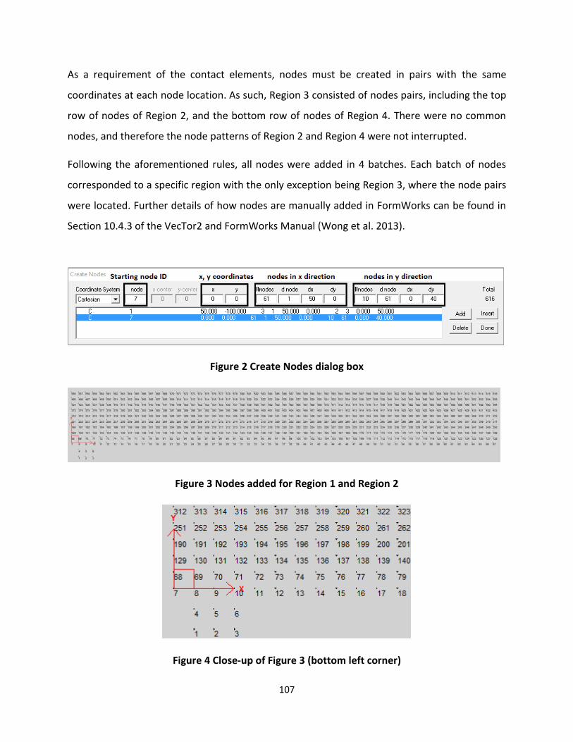
107
As a requirement of the contact elements, nodes must be created in pairs with the same
coordinates at each node location. As such, Region 3 consisted of nodes pairs, including the top
row of nodes of Region 2, and the bottom row of nodes of Region 4. There were no common
nodes, and therefore the node patterns of Region 2 and Region 4 were not interrupted.
Following the aforementioned rules, all nodes were added in 4 batches. Each batch of nodes
corresponded to a specific region with the only exception being Region 3, where the node pairs
were located. Further details of how nodes are manually added in FormWorks can be found in
Section 10.4.3 of the VecTor2 and FormWorks Manual (Wong et al. 2013).
Figure 2 Create Nodes dialog box
Figure 3 Nodes added for Region 1 and Region 2
Figure 4 Close-up of Figure 3 (bottom left corner)
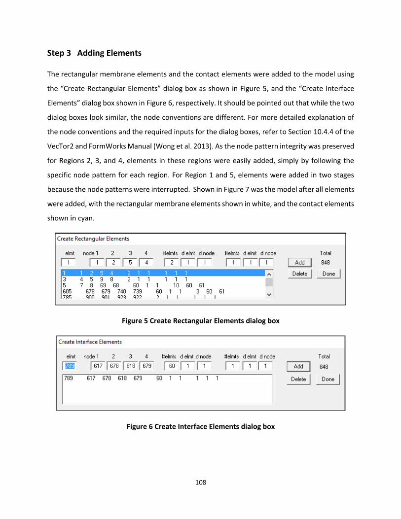
108
Step 3 Adding Elements
The rectangular membrane elements and the contact elements were added to the model using
the “Create Rectangular Elements” dialog box as shown in Figure 5, and the “Create Interface
Elements” dialog box shown in Figure 6, respectively. It should be pointed out that while the two
dialog boxes look similar, the node conventions are different. For more detailed explanation of
the node conventions and the required inputs for the dialog boxes, refer to Section 10.4.4 of the
VecTor2 and FormWorks Manual (Wong et al. 2013). As the node pattern integrity was preserved
for Regions 2, 3, and 4, elements in these regions were easily added, simply by following the
specific node pattern for each region. For Region 1 and 5, elements were added in two stages
because the node patterns were interrupted. Shown in Figure 7 was the model after all elements
were added, with the rectangular membrane elements shown in white, and the contact elements
shown in cyan.
Figure 5 Create Rectangular Elements dialog box
Figure 6 Create Interface Elements dialog box
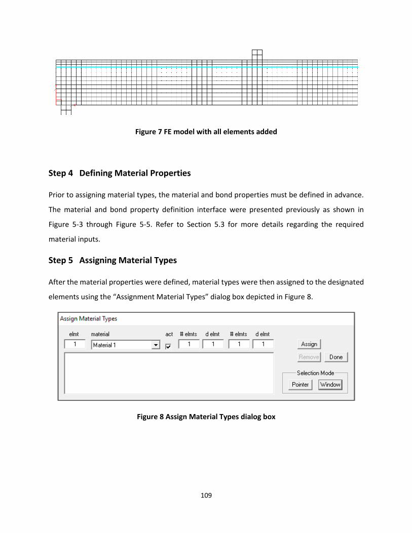
109
Figure 7 FE model with all elements added
Step 4 Defining Material Properties
Prior to assigning material types, the material and bond properties must be defined in advance.
The material and bond property definition interface were presented previously as shown in
Figure 5-3 through Figure 5-5. Refer to Section 5.3 for more details regarding the required
material inputs.
Step 5 Assigning Material Types
After the material properties were defined, material types were then assigned to the designated
elements using the “Assignment Material Types” dialog box depicted in Figure 8.
Figure 8 Assign Material Types dialog box
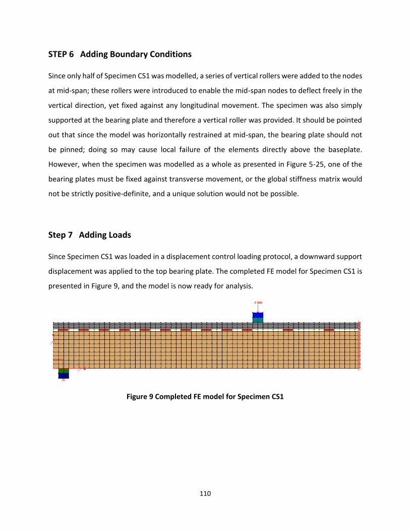
110
STEP 6 Adding Boundary Conditions
Since only half of Specimen CS1 was modelled, a series of vertical rollers were added to the nodes
at mid-span; these rollers were introduced to enable the mid-span nodes to deflect freely in the
vertical direction, yet fixed against any longitudinal movement. The specimen was also simply
supported at the bearing plate and therefore a vertical roller was provided. It should be pointed
out that since the model was horizontally restrained at mid-span, the bearing plate should not
be pinned; doing so may cause local failure of the elements directly above the baseplate.
However, when the specimen was modelled as a whole as presented in Figure 5-25, one of the
bearing plates must be fixed against transverse movement, or the global stiffness matrix would
not be strictly positive-definite, and a unique solution would not be possible.
Step 7 Adding Loads
Since Specimen CS1 was loaded in a displacement control loading protocol, a downward support
displacement was applied to the top bearing plate. The completed FE model for Specimen CS1 is
presented in Figure 9, and the model is now ready for analysis.
Figure 9 Completed FE model for Specimen CS1
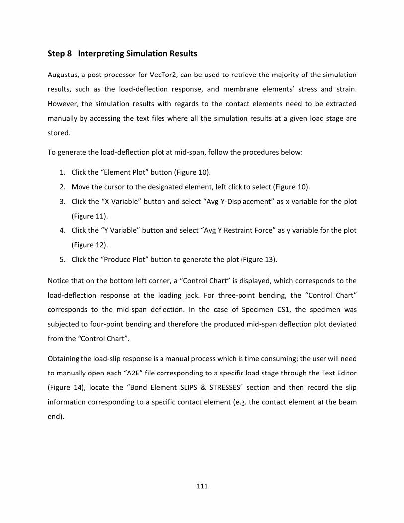
111
Step 8 Interpreting Simulation Results
Augustus, a post-processor for VecTor2, can be used to retrieve the majority of the simulation
results, such as the load-deflection response, and membrane elements’ stress and strain.
However, the simulation results with regards to the contact elements need to be extracted
manually by accessing the text files where all the simulation results at a given load stage are
stored.
To generate the load-deflection plot at mid-span, follow the procedures below:
1. Click the “Element Plot” button (Figure 10).
2. Move the cursor to the designated element, left click to select (Figure 10).
3. Click the “X Variable” button and select “Avg Y-Displacement” as x variable for the plot
(Figure 11).
4. Click the “Y Variable” button and select “Avg Y Restraint Force” as y variable for the plot
(Figure 12).
5. Click the “Produce Plot” button to generate the plot (Figure 13).
Notice that on the bottom left corner, a “Control Chart” is displayed, which corresponds to the
load-deflection response at the loading jack. For three-point bending, the “Control Chart”
corresponds to the mid-span deflection. In the case of Specimen CS1, the specimen was
subjected to four-point bending and therefore the produced mid-span deflection plot deviated
from the “Control Chart”.
Obtaining the load-slip response is a manual process which is time consuming; the user will need
to manually open each “A2E” file corresponding to a specific load stage through the Text Editor
(Figure 14), locate the “Bond Element SLIPS & STRESSES” section and then record the slip
information corresponding to a specific contact element (e.g. the contact element at the beam
end).
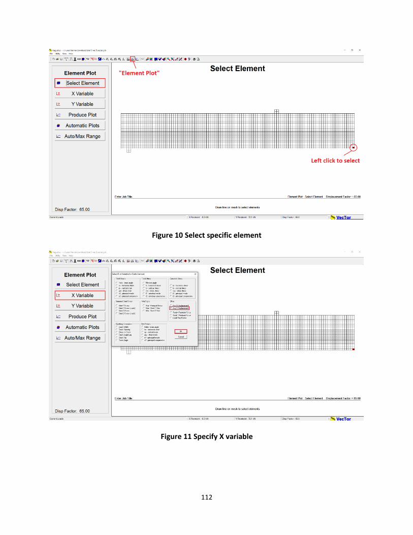
112
Figure 10 Select specific element
Figure 11 Specify X variable
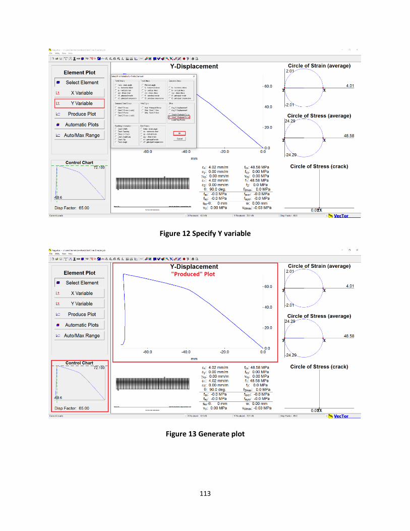
113
Figure 12 Specify Y variable
Figure 13 Generate plot
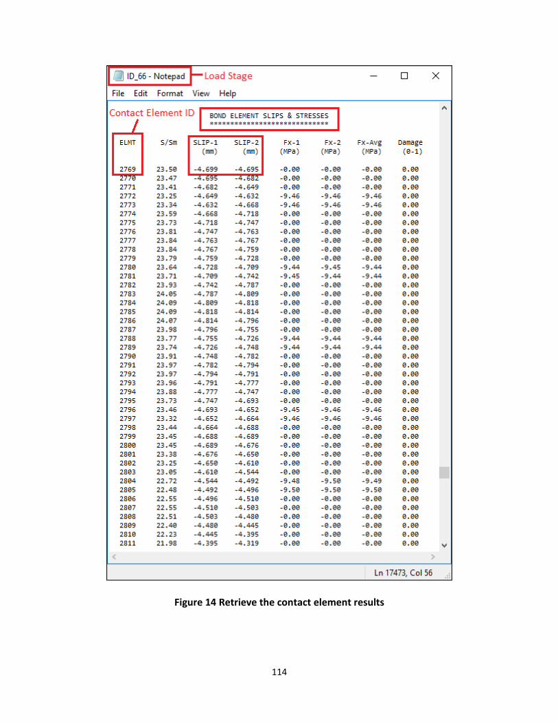
114
Figure 14 Retrieve the contact element results