Modelling the investment casting process: a novel approach

Modelling the investment casting process: a novel approach for view factor calculations and defect prediction

G. K. Upadhya, S. Das, U. Chandra and A. J. Paul

Concurrent Technologies Corporation, Johnstown, PA, USA

A rigorous simulation of the investment casting process (including view factor calculations) is tedious and time consuming. During the initial simulation stage, one needs to analyze quickly a large number of process designs to select the most promising ones for more rigorous analysis. Toward this end, a new model was developedfor the solidification heat transfer analysis of investment castings. The model is based on an approach that considers the geometric as well as the solidification parameters that dominate the heat transfer and the sequence of solidification and takes into account the radiation heat losses from the mold surface. A new and ejicient scheme is developedfor the calculation of view factor distribution on the mold surface, which governs the radiation loss. This scheme is generally applicable for models with Jinite difference representation. The model is capable ofpredicting the solid&ation time profile in the casting and can be usedfor quick estimation of defects like hot spots which lead to macroporosities. Although the proposed model is approximate, it makes only a modest sacrtfice in accuracy while making tremendous savings in computation time. The model has been validated by comparison with experimental results as weN as analytical solutions obtained from the literature.

Keywords: investment casting, view factor, process modelling

1. Introduction

Many critical and value-added components in aerospace and other key industries are manufactured by the investment casting process.’ The investment cast components are broadly classified into two categories: conventionally cast (CC) and directionally solidified (DS). CC components involve the use of a stationary mold and furnace, have equiaxed grains, and are generally used as structural components. DS castings often employ a mold withdrawal technique and can also be of two types; columnar grained (CG) or single crystal (SC). Often these components are made of expensive superalloys, are of complex shapes, and vary greatly in size. For example, turbine blades in modern aircraft engines are often directionally solidified in order to ensure superior creep and thermal fatigue properties. Emphasis on the production of near-net-shape components has further stimulated the growth of the investment casting industry in recent years. The projected overall tonnage of investment cast parts is expected to reach 250,000 tons by the year 2000.’ Since the investment casting process is relatively complex and expensive

Address reprint requests to Dr. A. J. Paul at Concurrent Technologies Corporation, 1450 Scalp Avenue, Johnstown, PA 15904, USA.

Received 8 June 1993; revised 13 November 1994; accepted 1 December 1994

Appl. Math. Modelling 1995, Vol. 19, June 0 1995 by Elsevier Science Inc. 655 Avenue of the Americas, New York, NY 10010

compared with other casting processes (e.g., sand, permanent mold, etc.), total reliance on the old-fashioned trial-and-error approach to selecting various process parameters is generally found to be time consuming and inadequate. In recent years computer simulation of the process has begun to complement the experience-based approach in meeting the demands of high quality investment cast parts in a cost-effective manner, which is evidenced in a number of publications.2-5

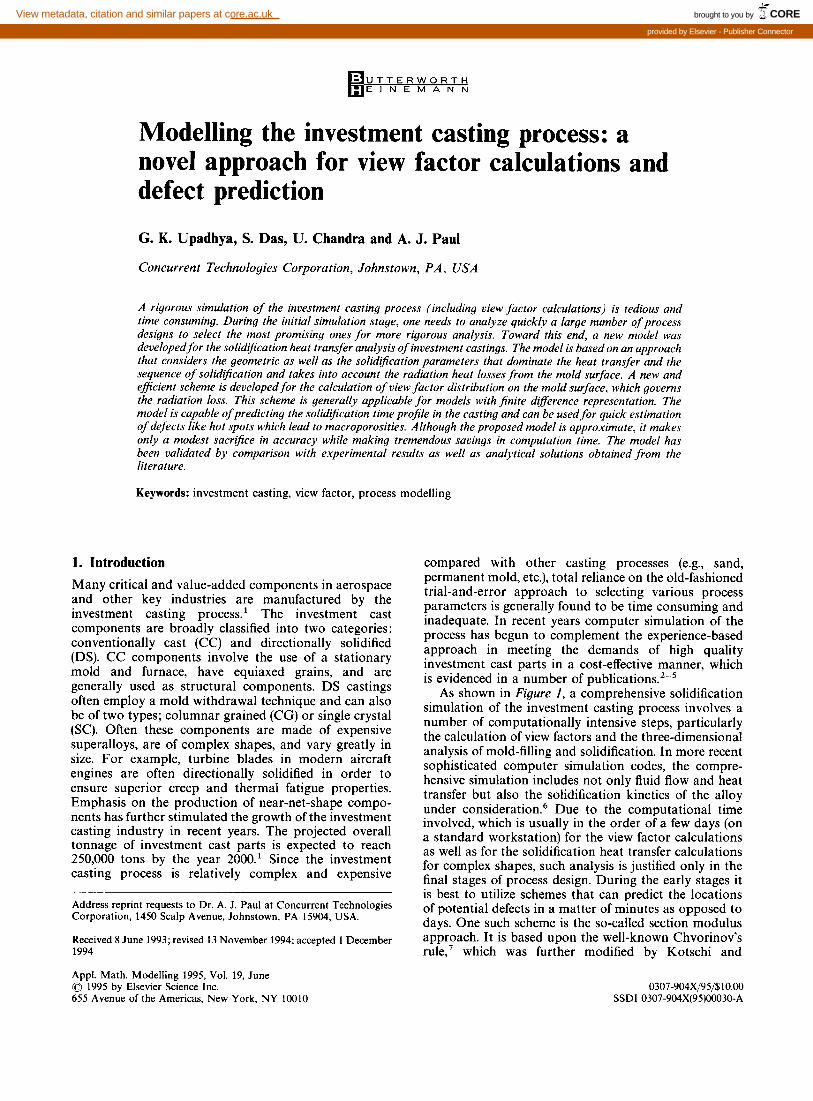
As shown in Figure 1, a comprehensive solidification simulation of the investment casting process involves a number of computationally intensive steps, particularly the calculation of view factors and the three-dimensional analysis of mold-filling and solidification. In more recent sophisticated computer simulation codes, the comprehensive simulation includes not only fluid flow and heat transfer but also the solidification kinetics of the alloy under consideration.6 Due to the computational time involved, which is usually in the order of a few days (on a standard workstation) for the view factor calculations as well as for the solidification heat transfer calculations for complex shapes, such analysis is justified only in the final stages of process design. During the early stages it is best to utilize schemes that can predict the locations of potential defects in a matter of minutes as opposed to days. One such scheme is the so-called section modulus approach. It is based upon the well-known Chvorinov’s rule, ’ which was further modified by Kotschi and

0307-904x/95/S10.00 SSDI 0307-904X(95)00030-A

brought to you by COREView metadata, citation and similar papers at core.ac.uk

provided by Elsevier - Publisher Connector

https://core.ac.uk/display/82274831?utm_source=pdf&utm_medium=banner&utm_campaign=pdf-decoration-v1

Modeling the investment casting process: G. K. Upadhya et al.

where ATsuper = superheat, Cb = specific heat, and H, = latent heat of the molten metal.

From equation (l), solidification time t is given by:

f View Facbxs Calculation I

Figure 1. A schematic diagram for complete simulation of the investment casting process

Plutshak,8 Heine et a1.,9 DeKalb et al.,” Upadhya et al.,’ 1 and others. This scheme has found tremendous application in the simulation of solidification in sand, permanent mold, and other conventional casting processes.

In this paper the scheme of Upadhya et al.” is further modified to simulate the investment casting process. It accounts for the mold as well as the heat loss by radiation at the outer surface of the mold. A new scheme for the calculation of radiation view factors (modified ray tracing scheme) is proposed which again reduces the computation time to minutes as opposed to hours or days. The results from this proposed view factor calculation scheme are compared with published analytical solutions. The combined view factor and thermal analysis model is validated by comparison with experimental results obtained from the literature. Finally, examples are provided demonstrating the applications of the model.

2. Mathematical Formulation

Consider a metal-mold system with liquid metal of any shape solidifying at temperature T,. Assume that the effective latent heat (latent heat + superheat) is the only source of heat being taken out and that all the heat is lost through the mold surface, which is at a steady temperature T,. These assumptions are reasonable, since we are interested in the solidification stage only. If the time taken to solidify the liquid pool of metal is t, the amount of heat lost in time t is given by:

Q = p VH; = hA( T, - T,)t (1)

where p, v and Hi are the density, volume, and effective heat of fusion of the metal, respectively, A is the surface area of the mold surface, h is the heat transfer coefficient at the mold surface, and To is the ambient temperature of air. The effective heat of fusion may be written as:

H; = H, + CpA7& (2)

t= PVH;

MT, - T,) (3)

Expressing the V/A ratio as the modulus parameter M, we get

t= PH; M

Ws-To) . It may be noted that equation (4) expresses solidification time as a linear function of the modulus (provided the other terms are constants), which is a significant departure from the standard Chvorinov’s rule for sand castings, which expresses solidification time as being proportional to the square of the modulus. This is mainly due to the difference in the assumption of the two models. Chvorniov’s rule is valid under the assumption of heat conduction through a semi-infinite mold thickness, which is true for most sand castings. In the model proposed here, the investment mold is assumed to be at a steady-state high temperature, losing heat by convection and radiation to the ambient.

Now modulus can be calculated at any pont in the casting using the formula6*” :

2 MC--

i$1:

(5)

‘

where N is the number of cooling directions, and d, is the distance from the mold in direction i. Using this relation, the modulus at the center of a plate section of thickness a is a/2, that for square section of side a is a/4, that for a cube section of side a is a/6, and so on. The modulus calculated by the above equation may be normalized as:

where Ma_ and M,,, are the overall average and the overall maximum modulus, respectively. The above formula can be used to compute the modulus at each cell in the finite difference representation of the casting, which gives a continuous distribution of the solidification time map in the casting. Now all that is needed for the computation of solidification time is the value of h at the mold surface.

Calculation of h

To model the investment casting process, we must be able to simulate the nature of heat loss, which is either purely radiative, or radiative as well as convective. For the general case, the heat transfer coefficient can be given by:

h = h, + h, (7)

Appl. Math. Modelling, 1995, Vol. 19, June 355


where h, and h, are the radiative and convective heat present in the model. Additional calculations are needed transfer coefficients, respectively. The radiative heat transfer coefficient is given by12:

for determining the shadowing effects for any realistic three-dimensional geometries.

h, = a&F,_,(T,2 + T;)(T, + To) (8)

where 0, E, and F,_, are the Stefan-Boltzman constant, the mold emissivity, and the viewfactor of the mold with respect to air, respectively. The convective heat transfer coefficient valid for natural convection at high temperature is given by12:

h, = c(T, - TO)“3 (9)

where c is a constant dependent on the surface geometry. For hot surfaces of plate-type, the value for c can be taken to be equal to 0.0008429 cgs units.12

It is to be noted that the value of h is calculated at the surface and the solidification time is calculated in the casting. For each point in the casting, the value of h at the closest point on the surface is taken for computing solidification time.

View factor calculation

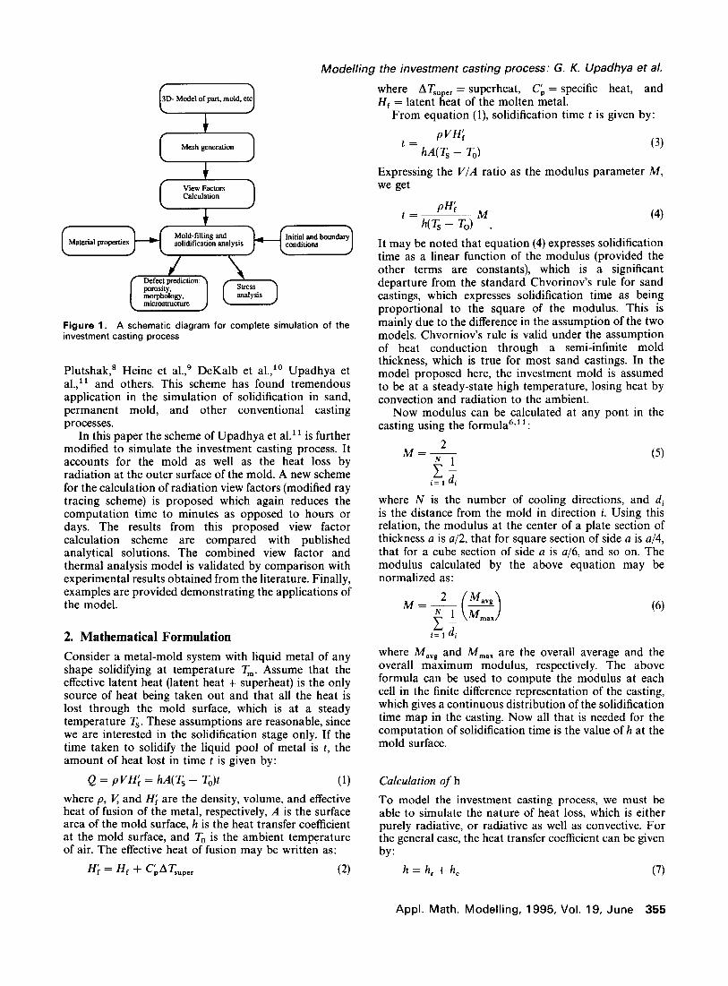
View factor is defined as the fraction of the radiation that leaves surface i in all directrions and is intercepted by surface j. Consider two surfaces dA, and dA, undergoing radiation exchange (Figure 2). The view factor for radiation exchange can be mathematically derived as1 2 :

F,_, = cos 8 cos 4

R:-2

dA,dA, (10)

where R, -2 is the distance between the two surfaces, and 0 and 4 are the angles of the two surface normals with the line joining the two surfaces.

The calculation of view factors could become very complicated when multiple surfaces are involved in the radiation process. The presence of multiple surfaces can create a partial or full obstruction in the view path between any two surfaces. Thus, the view factors will now depend not only on the two surfaces exchanging heat, but also on the shadows cast by the other surfaces

Figure 2. Illustration of radiation exchange between two surface dAl and dA2

There are several techniques to calculate the view factor. The more popular ones are briefly mentioned below, along with a new approach developed in the present investigation.

Analytical integration. The area integrals in equation (10) can be performed analytically if the areas are known. In fact tabulated values of the view factors for some simple geometries have been analytically determined and are available in the literature.13 However, such methods cannot be used for real casting geometries which have complex three dimensional shapes. Thus, one needs to look at numerical techniques available to calculate the view factors.

Numerical methods. Numerical techniques for obtaining view factors can be used in conjunction with any other numerical solution method like finite differences or finite elements. Most of these techniques rely on scanning the set of surfaces present in the model to determine whether or not they cover a particular surface. The drawback of such techniques is that they are time and space (in terms of computer memory) consuming. Efforts have been directed at minimizing these calculations by introducing realistic assumptions, by designing efficient scanning algorithms, or by using a priori information to reduce the scanning data base in some manner. The following are brief descriptions of some of the algorithms used in calculating the view factor along with shadowing effects.

Monte Carlo ray tracing. In this method,13 rays are emitted in random directions from points on surface i. Each ray is checked to see which surface it strikes. Those rays that are intercepted by the surface j are assumed to contribute to the values of Fi_ j. Random numbers are used to choose locations of the point and emitting directions. Accuracy and calculation time increases with the number of rays. The method is additive in nature and therefore the accuracy is quite good.

Projection methods. Surface i is subdivided into a number of elements, ai. Surface j is then viewed from the centroid, ci, of each of these subelements. It is assumed that the view of j from ci represents the view from any portion of the subelement a,. The viewfactor, Fij is computed from the area of subelement ai. the sum of the individual viewfactors from each subelement is Fij. The accuracy of all projection methods depends on how well the view centered at ci represents the view from each portion of a,.

Double area integration. This method, a primitive form of projection, consists of subdividing surfaces i and j into subelements ai and aj. A ray is drawn from the centroid of ai to that of aj. If the ray is not obscured, it is assumed that all of a, can see all of aj. the viewfactor is then computed by the standard view factor calculation formula (equation [lo]). This method is usually faster

356 Appl. Math. Modelling, 1995, Vol. 19, June

Modeling the invesrmenr casting process: G. K, Upadhya er al.

than other methods. However, values of Fij may not sum up to unity, but because of the speed, many more subelements cari be used. FACET, the code developed by Lawrence Livermore National Laboratory for viewfactor calculation,14 mainly uses the double area integration technique along with contour integrals.

mold. However, if one uses a code such as FACET for view factor computation, these assumptions need not be made. FACET facilitates calculation of radiation exchange between various surfaces by computing the whole view factor matrix, which has the information about view factors with respect to all other faces on the mold surface.

The proposed method. The methods outlined above for computing view factors are quite time consuming for a complex geometry involving hundreds of thousands of elements. Hence a new method was developed to compute view factors in a simple and effective manner. The method is general in nature and is applicable to both finite element and finite difference models. It should be noted that codes such as FACET are more applicable for finite element models, where the surface normals are more accurately represented, since the surface does not have the stepped nature of a finite difference model.

In the present work, a modified ray-trace method is used to calculate the view factor. The calculation is based on the definition of view factor as the fraction of energy emitted by the mold surface which goes to ambient without reaching another part of the mold surface. Thus, it is computed as the following ratio:

F,_, = Lim 2 0 N-m \‘v/

na Z-

N (finite N) (11)

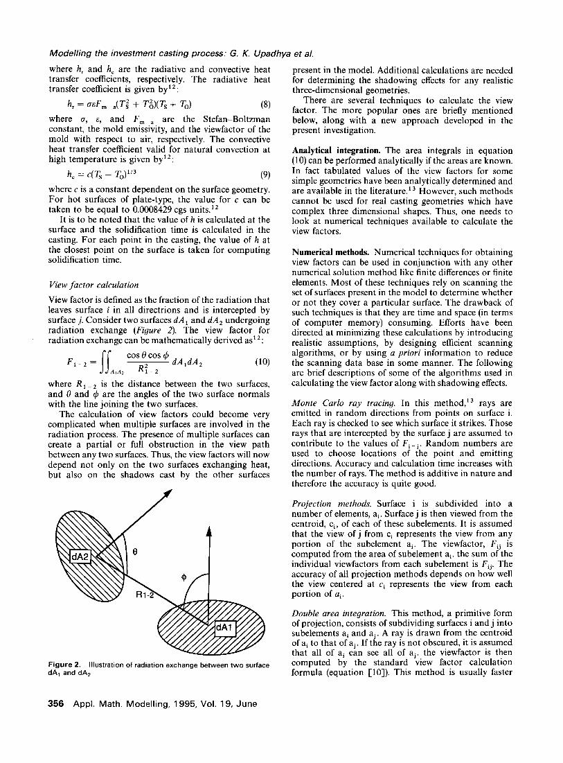
where n, is the number of rays which go into air without being intercepted by the mold surface (S), and N is the total number of rays emitted from a point (P) in all directions (see Figure 3).

There are two important assumptions in this model. First, it is assumed that the ambient temperature is constant, with a value significantly lower than the average initial temperature of the mold. Second, it is assumed that the radiant heat exchange between different regions on the mold surface is negligible in comparison with radiant losses to ambient. The mold surface behaves as a gray diffuse body. When an incident ray from a point P (see Figure 3) is intercepted by another part of the mold, the energy is absorbed by the mold without further reflection. Thus, heat loss from the surface of the mold occurs only to the surrounding air. Effects of difference in temperature between various parts of the mold surface are neglected. This assumption is reasonable for the investment casting process, since the mold preheat is very high (close to the melting temperature of the metal), and the difference in the fourth powers of temperature between the mold and the ambience is much larger when compared with the difference between two parts of the

Mold stiac

Figure 3. Schematic illustration of radiation rays from a point P on the mold surface

Thus, if a scheme can be devised to send rays in various directions, and the number going into air without mold-interception is estimated, then one can compute the view factor at any given point on the surface. This scheme is a modified form of the Monte Carlo ray tracing technique, the only difference being that the various directions in which the rays are emitted are not randomly determined. In the present method, rays are sent in all the directions from each computational point on the surface.

One simple technique of ray tracing is to send in the direction of neighbors. As shown in Figure 3, for a two-dimensional grid nine rays are sent in all directions considering the nonrepeating directions of two neighbor cells from the cell P. In a similar way, for a three-dimensional grid one ends up with 49 nonrepeating rays in all directions considering two neighbors of the computational point P. Rays are not sent below the plane of the mold surface. In a finite difference mesh (structured grid), this method of sending rays in various directions from a given cell with indices i, j, k is relatively straightforward, since the location of the nearest neighbors are directly determined by the cells i i 1, j + 1, k + 1. In an unstructured grid (which is normally the case with most finite element meshes), it is believed that the implementation of this technique is rather tedious and time consuming.

3. Computation Scheme

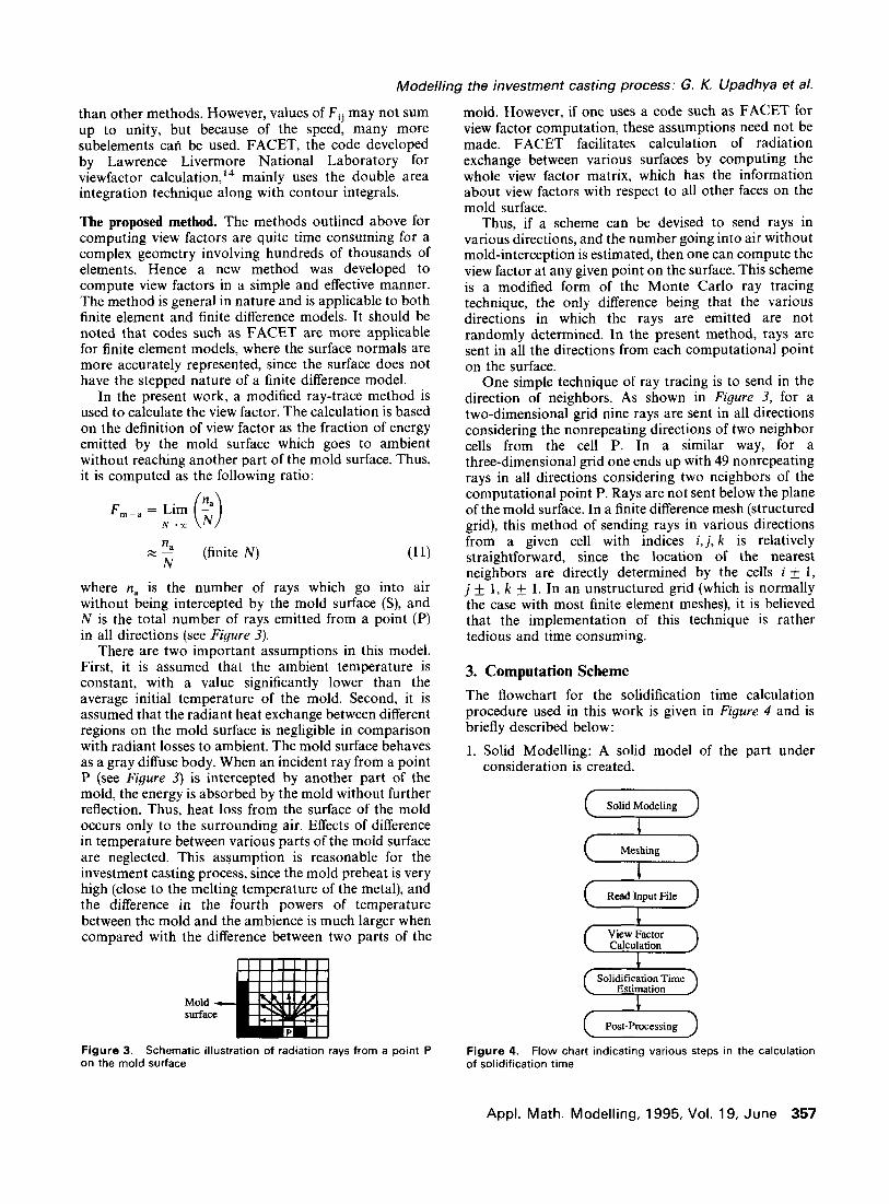
The flowchart for the solidification time calculation procedure used in this work is given in Figure 4 and is briefly described below:

1. Solid Modelling: A solid model of the part under consideration is created.

Solid Modeling

z Meshing

c

Read Input File

View Factor Calculation

z

Solidification Time Estimation

Post-Processing

Figure 4. Flow chart indicating various steps in the calculation of solidification time



2. Meshing: The part created in step 1 is subdivided into rectangular cells using a uniform grid in the x, y, and z directions. The same mesh could be used for a finite difference-based calculation of fluid flow and solidification.

3.

4.

5.

Read Input File: The solidification parameters for the part are read in this module. View Factor Calculation: From the mesh configuration, the view factor distribution at the mold surface is calculated using the approach outlined earlier. Determination of Point Modulus and Solidification Time: From the mesh information, the distance from the mold is calculated for each cell in various directions. The modulus for each cell is calculated using equation (5) and normalized using equation (6). From equation (4), the solidification time is calculated for each cell.

6. Post-processing: The results of the above calculations are viewed using the visualization and post-processing modules. If problem areas exist in the casting, such as hot spots, the gating and risering can be redesigned and calculation steps l-5 repeated until a satisfactory design is obtained.

4. Results and Validation

Any effort on modelling a process phenomenon is in- complete without adequate validation. This section cov- ers the results of validation of the model presented in this work, as well as practical applications of the model with an example.

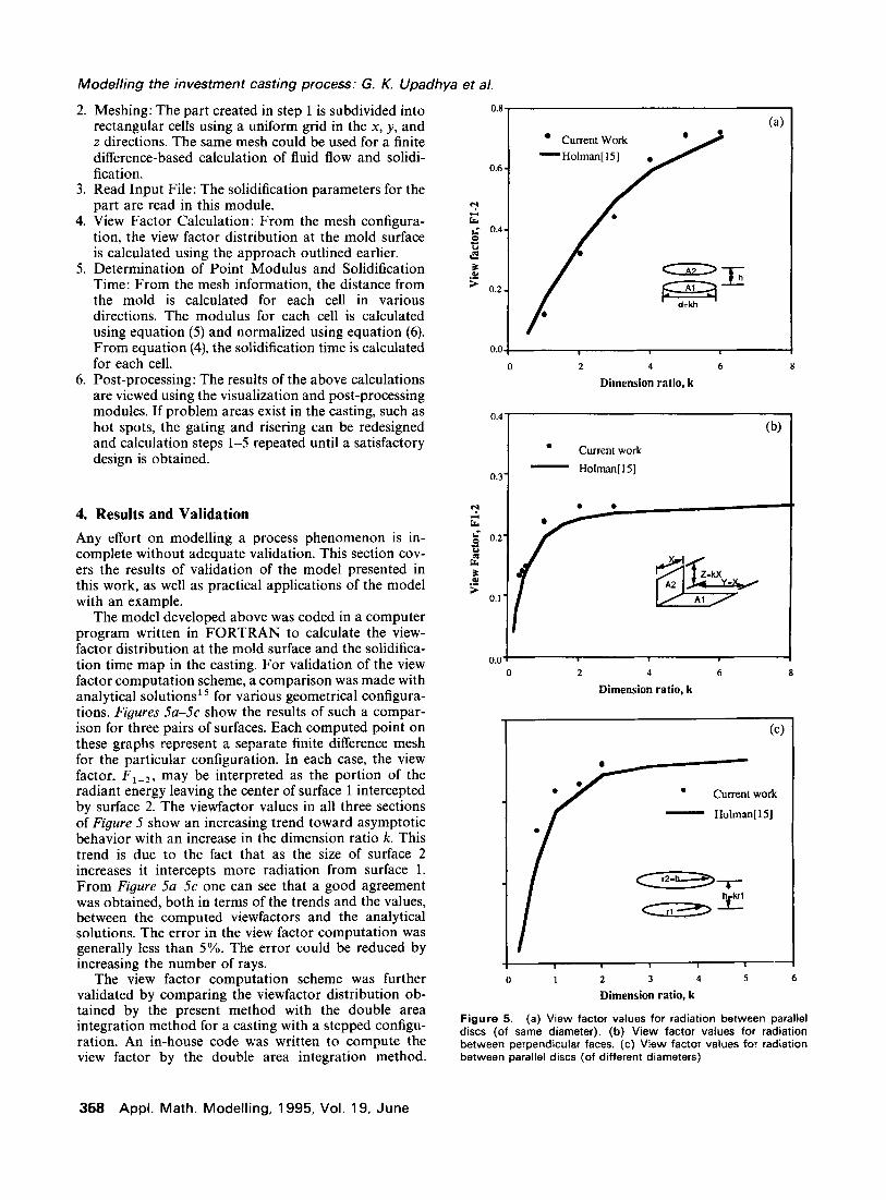
The model developed above was coded in a computer program written in FORTRAN to calculate the viewfactor distribution at the mold surface and the solidification time map in the casting. For validation of the view factor computation scheme, a comparison was made with analytical solutions ls for various geometrical configura- tions. Figures Sa-SC show the results of such a comparison for three pairs of surfaces. Each computed point on these graphs represent a separate finite difference mesh for the particular configuration. In each case, the view factor, F,_,, may be interpreted as the portion of the radiant energy leaving the center of surface 1 intercepted by surface 2. The viewfactor values in all three sections of Figure 5 show an increasing trend toward asymptotic behavior with an increase in the dimension ratio k. This trend is due to the fact that as the size of surface 2 increases it intercepts more radiation from surface 1. From Figure 5a-5c one can see that a good agreement was obtained, both in terms of the trends and the values, between the computed viewfactors and the analytical solutions. The error in the view factor computation was generally less than 5%. The error could be reduced by increasing the number of rays.

The view factor computation scheme was further validated by comparing the viewfactor distribution obtained by the present method with the double area integration method for a casting with a stepped configuration. An in-house code was written to compute the view factor by the double area integration method.


0.6

(a)

0 2 4 6

Dimension ratio, k

0.4-

(b)

l Current work

- 0.3’ Hohnan[l5]

0.0 ’

0 2 4 6 8

Dimension ratio, k

1 (cl

0 1 2 3 4 5 6

Dimension ratio, k

Figure 5. (a) View factor values for radiation between parallel discs (of same diameter). (b) View factor values for radiation between perpendicular faces. (c) View factor values for radiation between parallel discs (of different diameters)

Modelling the investment casting process: G. K. Upadhya et al.

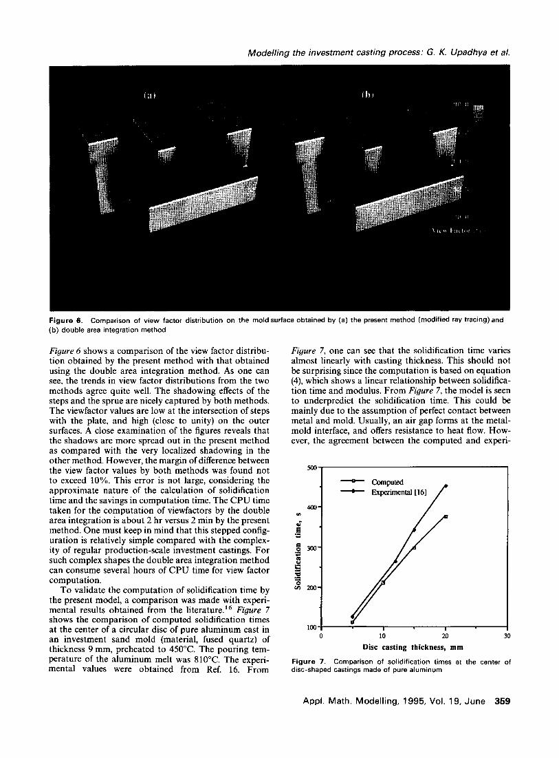
Figure 6. Comparison of view factor distribution on the mold surface obtained by (a) the present method (modified ray tracing) and (b) double area integration method

Figure 6 shows a comparison of the view factor distribution obtained by the present method with that obtained using the double area integration method. As one can see, the trends in view factor distributions from the two methods agree quite well. The shadowing effects of the steps and the sprue are nicely captured by both methods. The viewfactor values are low at the intersection of steps with the plate, and high (close to unity) on the outer surfaces. A close examination of the figures reveals that the shadows are more spread out in the present method as compared with the very localized shadowing in the other method. However, the margin of difference between the view factor values by both methods was found not to exceed 10%. This error is not large, considering the approximate nature of the calculation of solidification time and the savings in computation time. The CPU time taken for the computation of viewfactors by the double area integration is about 2 hr versus 2 min by the present method. One must keep in mind that this stepped configuration is relatively simple compared with the complex- ity of regular production-scale investment castings. For such complex shapes the double area integration method can consume several hours of CPU time for view factor computation.

To validate the computation of solidification time by the present model, a comparison was made with experimental results obtained from the literature.r6 Figure 7 shows the comparison of computed solidification times at the center of a circular disc of pure aluminum cast in an investment sand mold (material, fused quartz) of thickness 9 mm, preheated to 450°C. The pouring temperature of the aluminum melt was 810°C. The experimental values were obtained from Ref. 16. From

Figure 7, one can see that the solidification time varies almost linearly with casting thickness. This should not be surprising since the computation is based on equation (4) which shows a linear relationship between solidification time and modulus. From Figure 7, the model is seen to underpredict the solidification time. This could be mainly due to the assumption of perfect contact between metal and mold. Usually, an air gap forms at the metal- mold interface, and offers resistance to heat flow. How- ever, the agreement between the computed and experi-

so0

100 I I 0 10 20 30

Disc casting thickness, mm

Figure 7. Comparison of solidification times at the center of disc-shaped castings made of pure aluminum


Modelling the investment casting process: G. K. Upadhya et al.

2.3

0.0

Point Modulus (mm)

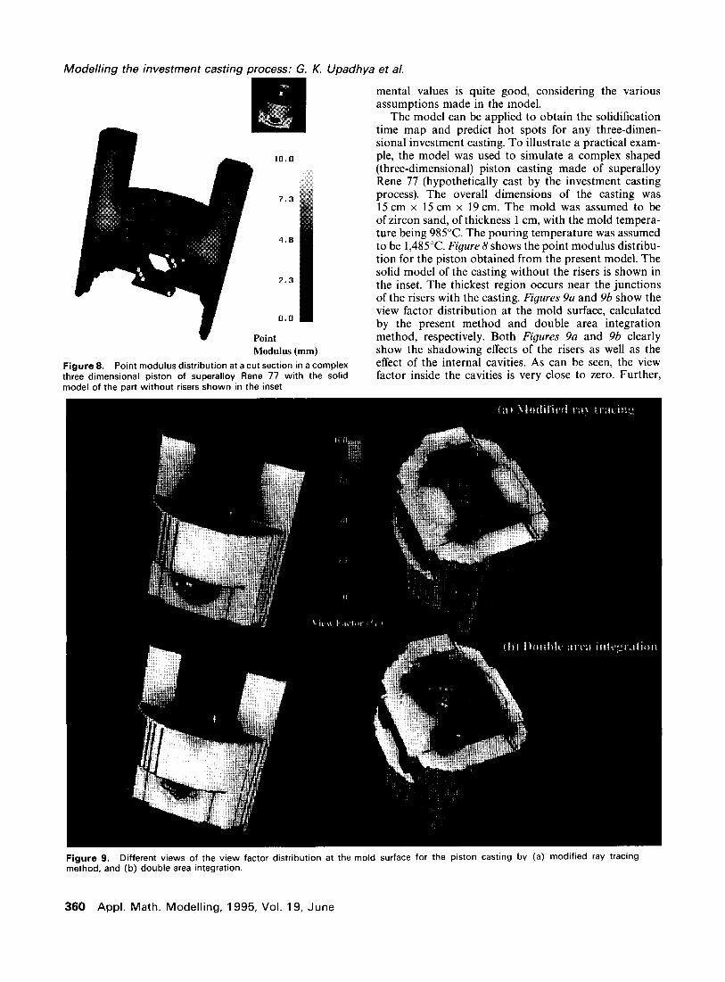
Figure 8. Point modulus distribution at a cut section in a complex three-dimensional piston of superalloy Rene 77 with the solid model of the part without risers shown in the inset

mental values is quite good, considering the various assumptions made in the model.

The model can be applied to obtain the solidification time map and predict hot spots for any three-dimensional investment casting. To illustrate a practical example, the model was used to simulate a complex shaped (three-dimensional) piston casting made of superalloy Rene 77 (hypothetically cast by the investment casting process). The overall dimensions of the casting was 15 cm x 15 cm x 19 cm. The mold was assumed to be of zircon sand, of thickness 1 cm, with the mold temperature being 985°C. The pouring temperature was assumed to be 1,485”C. Figure 8 shows the point modulus distribution for the piston obtained from the present model. The solid model of the casting without the risers is shown in the inset. The thickest region occurs near the junctions of the risers with the casting. Figures 9a and 9b show the view factor distribution at the mold surface, calculated by the present method and double area integration method, respectively. Both Figures 9a and 96 clearly show the shadowing effects of the risers as well as the effect of the internal cavities. As can be seen, the view factor inside the cavities is very close to zero. Further,

Figure 9. Different views of the view factor distribution at the mold surface for the piston casting by (a) modified ray tracing method, and (b) double area integration.


Modelling the invesrmenr casring process: G. K. Upadhya et al.

400

Solidification time, s

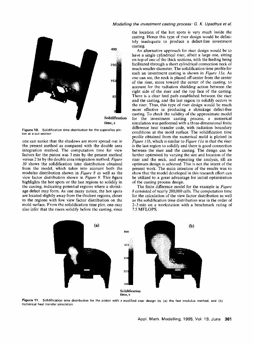
Figure 10. Solidification time distribution for the superalloy piston at a cut section

one can notice that the shadows are more spread out in the present method as compared with the double area integration method. The computation time for view factors for the piston was 3 min by the present method versus 2 hr by the double area integration method. Figure 10 shows the solidification time distribution obtained from the model, which takes into account both the modulus distribution shown in Figure 8 as well as the view factor distribution shown in Figure 9. This figure highlights the hot spots or the last regions to solidify in the casting, indicating potential regions where a shrinkage defect may form. As one many notice, the hot spots are located slightly away from the thickest regions, closer to the regions with low view factor distribution on the mold surface. From the solidification time plot, one may also infer that the risers solidify before the casting, since

the location of the hot spots is very much inside the casting. Hence this type of riser design would be defini- tely inadequate to produce a defect-free investment casting.

An alternative approach for riser design would be to have a single cylindrical riser, albeit a large one, sitting on top of one of the thick sections, with the feeding being facilitated through a short cylindrical connection neck of much smaller diameter. The solidification time profile for such an investment casting is shown in Figure Ila. As one can see, the neck is placed off-center from the center of the riser, more toward the center of the casting, to account for the radiation shielding action between the right side of the riser and the top face of the casting. There is a clear feed path established between the riser and the casting, and the last region to solidify occurs in the riser. Thus, this type of riser design would be much more effective in producing a shrinkage defect-free casting. To check the validity of the approximate model for the investment casting process, a numerical simulation was performed with a three-dimensional finite difference heat transfer code, with radiation boundary conditions at the mold surface. The solidification time profile obtained from the numerical mold is plotted in Figure 1 lb, which is similar to Figure 1 la in that the riser is the last region to solidify and there is good connection between the riser and the casting. The design can be further optimised by varying the size and location of the riser and the neck, and repeating the analysis, till an optimum design is achieved. This is not the intent of the present work. The main intention of the results was to show that the model developed in this research effort can be utilized to a great advantage for initial optimization of the casting process design.

The finite difference model for the example in Figure 8 consisted of nearly 200,000 cells. The computation time for the calculation of the view factor distribution as well as the solidification time distribution was in the order of 2-3 min on a workstation with a benchmark rating of 7.5 MFLOPS.

600

Solidification time, s

Figure 11. Solidification time distribution for the piston with a modified riser design by (a) the fast modulus method, and (b) numerical heat transfer simulation



5. Conclusions References

A simple approach is proposed for modelling the investment casting process, based on heat transfer analysis during solidification. The model considers the geometric as well as the solidification parameters that inherently dominate the heat transfer and the sequence of solidification and take into account the radiation heat loss from the mold surface to the surroundings. A new method has been developed for calculating the view factor distribution at the surface of the mold. Although the proposed method is approximate, it gives very reasonable results at a fraction of the time compared with more sophisticated methods. The view factor calculations are fed into the model for computation of the solidification time profile in the three-dimensional casting. Defects like hot spots (potential areas of macroporosities) can be predicted by use of this model in a quick efficient way and takes only minutes of computation time even for complex geometries. This range of computation time is orders of magnitude less than the computational requirements of more sophisticated finite element or finite difference models that can take hours or even days for each simulation. Thus, the model presented can be used for an initial parametric study to arrive at a reasonably good design of the casting with risers and gates, after which the design can be fed to more comprehensive models for verification. This considerably reduces the lead time required to arrive at a good casting design via process simulation.

4

5

6

I

8

9

10

11

Casting: Merals Handbook Volume 15, 9th edition. ASM International, Metals Park, Ohio, 1988 Rappaz, M. et al., eds. Modelling and Control of Casting and Welding Processes V. TMS Publications, 1991

Piwonka, T. S. et al. eds. Modelling and Control of Casting, Welding and Advanced Solidification Processes VI. TMS Publications, 1993 Yu, K. 0. et al. Solidification modeling of single-crystal investment castings. AFS Trans. 1990, 417428 Chandra, U. Benchmark problems and testing of a finite element code for solidification in investment castings. Inr. J. Num. Mefh. Eng., 1990, 30, 1301-1320 Upadhya, G. and Paul, A. J. A comprehensive casting analysis model using a geometry based technique followed by a fully coupled, 3D fluid flow, heat transfer and solidification kinetics calculations. AFS Trans. 1992; 100, 925-933 Chvorinov, N. Theory of solidification of castings. Die Giesserei 1940, 21, 1 l-224 Kotschi, R. and Plutshak, L. An easy and inexpensive technique to study solidification of castings in three dimensions. AFS Trans. 1981,89, 601-605 Heine, R. W., Uicker, J. J., and Gantenbein, D. Distance, chills and solidification macrostructure. AFS Trans. 1984,92, 135-149 Dekalb, S. W., Heine, R. W. and Uicker, J. J. Geometric modelling of progressive solidification and casting alloy macrostructure. AFS Trans. 1987, 95, 281-290 Upadhya, G., Wang, C. M. and Paul, A. J. Solidification modelling: a geometry based approach for defect prediction in castings. Light Mefals 1992, Proceedings of Light Metals Div. at 121st TMS Annual Meeting at San Diego. E. R. Cutshall, ed. 1992, 995-998

12

Acknowledgments

13

14

This work was conducted by the National Center for Excellence in Metalworking Technology, operated by Concurrent Technologies Corporation, under contract to the U.S. Navy as part of the U.S. Navy Manufacturing Technology Program.

15

16

Geiger, G. H. and Poirier, D. R. Transport Phenomena in Mefallurgy 2nd printing. Addison Wesley Publishing Co., Reading, Massachussets, 1980 Siegel, R. and Howell, J. R. Thermal Radiation Heat Transfer. Hemisphere Publishing Corp., New York, 1981 Shapiro, A. FACET-A radiation viewfactor computer code for axisymmetric 2D and 3D geometries with shadowing. Lawrence Livermore National Lab, California 1983 Holman, J. P. Hear Transfer, 5th edition McGraw-Hill, New York, 1981 Huang, H. Computer simulation of solidification in investment casting. M.S. Thesis, University of Alabama, Tuscaloosa, AL, USA, 1988


Documents

Modelling the investment casting process: a novel approach