DI

SC

US

SI

ON

P

AP

ER

S

ER

IE

S

Forschungsinstitut zur Zukunft der ArbeitInstitute for the Study of Labor

Modelling the Joint Distribution of Income and Wealth

IZA DP No. 9190

July 2015

Markus JänttiEva SierminskaPhilippe Van Kerm

Modelling the Joint Distribution of

Income and Wealth

Markus Jäntti SOFI, Stockholm University

Eva Sierminska

LISER, DIW Berlin and IZA

Philippe Van Kerm LISER

Discussion Paper No. 9190 July 2015

IZA

P.O. Box 7240 53072 Bonn

Germany

Phone: +49-228-3894-0 Fax: +49-228-3894-180

E-mail: iza@iza.org

Any opinions expressed here are those of the author(s) and not those of IZA. Research published in this series may include views on policy, but the institute itself takes no institutional policy positions. The IZA research network is committed to the IZA Guiding Principles of Research Integrity. The Institute for the Study of Labor (IZA) in Bonn is a local and virtual international research center and a place of communication between science, politics and business. IZA is an independent nonprofit organization supported by Deutsche Post Foundation. The center is associated with the University of Bonn and offers a stimulating research environment through its international network, workshops and conferences, data service, project support, research visits and doctoral program. IZA engages in (i) original and internationally competitive research in all fields of labor economics, (ii) development of policy concepts, and (iii) dissemination of research results and concepts to the interested public. IZA Discussion Papers often represent preliminary work and are circulated to encourage discussion. Citation of such a paper should account for its provisional character. A revised version may be available directly from the author.

IZA Discussion Paper No. 9190 July 2015

ABSTRACT

Modelling the Joint Distribution of Income and Wealth* This paper considers a parametric model for the joint distribution of income and wealth. The model is used to analyze income and wealth inequality in five OECD countries using comparable household-level survey data. We focus on the dependence parameter between the two variables and study whether accounting for wealth and income jointly reveals a different pattern of social inequality than the traditional ‘income only’ approach. We find that cross-country variations in the dependence parameter effectively accounts only for a small fraction of cross-country differences in a bivariate measure of inequality. The index appears primarily driven by differences in inequality in the wealth distribution. JEL Classification: C1, D31, J10 Keywords: income, wealth, inequality, copula, multivariate Gini Corresponding author: Eva Sierminska LISER (Luxembourg Institute of Socio-Economic Research) 3, avenue de la Fonte L-4364 Esch-sur-Alzette Luxembourg E-mail: eva.sierminska@liser.lu

* This research is part of the WealthPort project (Household wealth portfolios in Luxembourg in a comparative perspective) financed by the Luxembourg ‘Fonds National de la Recherche’ (contract C09/LM/04) and by core funding for CEPS/INSTEAD from the Ministry of Higher Education and Research of Luxembourg. Comments from participants to the IARIW 32nd General Conference (Boston) and to the 46th Italian Statistical Society meeting (Rome) are gratefully acknowledged.

1 Introduction

Inequality in living conditions within industrialized countries is almost always gauged on the

basis of annual household income data, the distribution of which is typically summarized in

coefficients such as the Gini index (Jenkins and Van Kerm, 2009). Far less is known about

the distribution of other measures of economic well-being, such as consumption expenditure

or wealth and asset holdings. The latter is of particular complementary interest as it captures

long-term economic resources better than income flows do and represents resources that people

are able to draw upon to face adverse shocks.

While there are obvious links between income and net wealth accumulation via savings and

borrowing constraints, the relationship between these two variables is bound to be complex

and relatively little is known about it empirically, especially outside the United States (Ken-

nickell, 2009). Income, its volatility, savings and dissavings from past income streams and

the resulting wealth portfolio allocation choices will shape the association at the household

level. The institutional environment (with regards to pensions in particular) may also exert a

key influence. We can thus expect differences in the relationship between income and wealth

across countries, as indicated by comparative work that has been conducted using data from the

Luxembourg Wealth Study (LWS) database (Sierminska et al., 2006, Jäntti et al., 2008, Sier-

minska et al., 2013, Jäntti et al., 2013).1 While wealth and income can, in particular, instances

be thought of as an alternative means of securing a standard of living, it is more likely that

they are positively associated, thereby reinforcing social inequality overall. Better knowledge

about the joint distribution of income and wealth is relevant for the design of taxation and re-

distribution policies as well as for better identification and targeting of vulnerable population

groups. This paper considers new methods in modelling and understanding this potentially

complex relationship.

Earlier work on the joint distribution of income and wealth using LWS data (Luxembourg

Wealth Study Database (LWS), 2014) used largely descriptive, non-parametric methods. In

1Reliable, internationally comparable household- or individual-level data on wealth, asset holdings and debtremain limited, with only a few exceptions. The Luxembourg Wealth Study is one of the main sources ofcross-nationally comparable data, covering both North American and European countries. The HouseholdFinance and Consumption Survey (HFCS) has recently been made available for euro-zone countries. TheSHARE (Survey of Health, Ageing and Retirement in Europe) has been collected for individuals 50 yearsand older in up to twenty countries.

1

this paper, apart from describing this relationship, we would like to extend the analysis and

ask additional counterfactual questions. For example, how would social inequality change if

the relationship between income and wealth in, say, Germany, were more like that of the United

States, but the marginal distributions were unchanged? Specifically, we want to compare over-

all inequality of income and wealth across countries and to examine if country differences are

driven by differences in the association between income and wealth, or by differences in the

marginal distributions. In our view, the most straightforward way to attain this goal is to work

with parametric methods.

The contribution of this paper is to elaborate new methods of inequality analysis in the

joint distribution of income and wealth, and to illustrate this approach using data for five

OECD countries. We develop and fit a simple yet flexible parametric model for the bivariate

distribution. The model handles the specificity of the distribution of wealth, in particular the

presence of zero and negative values. We study the joint distribution of income and wealth by

separately estimating the univariate marginal distribution models for income and for wealth,

and by estimating the parametric copula functions to capture the dependence between income

and wealth (Genest and McKay, 1986, Trivedi and Zimmer, 2007). Combining estimates for

the marginal distributions and the copula provides flexible estimates of the joint distribution of

income and wealth. This approach has the advantage of separating the problems of estimation

of marginal distributions and the dependence structure between the two variates.

Endowed with parametric estimates of the joint distribution of income and wealth for five

OECD countries, we use our model to compare the degree of dependence between the two vari-

ables in different countries. We design a straightforward counterfactual analysis to assess the

implications of variations in the dependence parameter on a bivariate version of the Gini coef-

ficient proposed by Koshevoy and Mosler (1997): we evaluate this implication by calculating

what would happen in country X if it had the dependence structure of income and wealth as in

country Y. We find that cross-country variations in the association parameter account for only

a small fraction of cross-country differences in the bivariate Gini. The index appears primarily

driven by differences in the inequality of the net worth distributions. Thus, the way people are

able to accumulate wealth matters most for the joint inequality of income and wealth and most

cross-country differences in the bivariate inequality stem from these factors.

We describe the datasets used and provide a preliminary inspection of the data in Section 2.

2

In Section 3, we present the parametric model for the joint distribution of income and wealth.

Estimation results and analysis of the bivariate Gini coefficient are presented in Section 4.

Section 5 concludes.

2 Data and preliminary inspection

We analyze and compare overall inequality in the distribution of income and wealth in five rich

countries using household survey data: a North American country—the United States—and

four European countries with varying institutional and welfare regimes: Germany, Italy, Lux-

embourg and Spain. Our choice of countries is governed by data availability and timeliness.

This group of countries also covers different ‘equity cultures’. The data for the United States

come from the 2007 Survey of Consumer Finances (SCF), for Italy the 2007 Survey of House-

hold Income and Wealth (SHIW), for Germany the 2007 wealth module of the Socio-Economic

Panel (SOEP), for Luxembourg from the 2007 wealth module of the PSELL-3/EU-SILC and

for Spain the 2008 Spanish Survey of Household Finances (EFF); see Table 1.

Table 1: Data description

Country Year Survey Type Over-sampling Unit of Analysis

Germany 2007 Socio-Economic Panel Wealth module wealthy householdItaly 2008 Survey of Household Income and Wealth Wealth survey householdLuxembourg 2007 PSELL-3/ EU-SILC Wealth module householdSpain 2008 Survey of Household Finances Wealth survey householdUnited States 2007 Suvey of Consumer Finances Wealth survey wealthy household

All datasets contain detailed information on multiple income sources and financial, non-

financial assets and debts aggregated at the household level. On the basis of this information,

we use the conceptual framework developed by the Luxembourg Wealth Study (LWS) for

creating harmonized variables of total wealth and income (Sierminska et al., 2006). The goal

of LWS is to provide users, to the extent possible, with comparable variables through ex-post

harmonization of data collected independently in separate surveys. In order to achieve this, a

thorough examination of each of the wealth and income components collected in the different

surveys has been performed to identify the most comparable aggregated data from which a

measure of household net worth—total assets minus total liabilities—is derived. Table 2 shows

the composition of our LWS measure of net worth for each of the five datasets: we are able to

obtain an aggregate measure composed of financial assets, principal residence and investment

3

real estate from which we subtract total debt, which comprises mortgages and non-housing

debt.

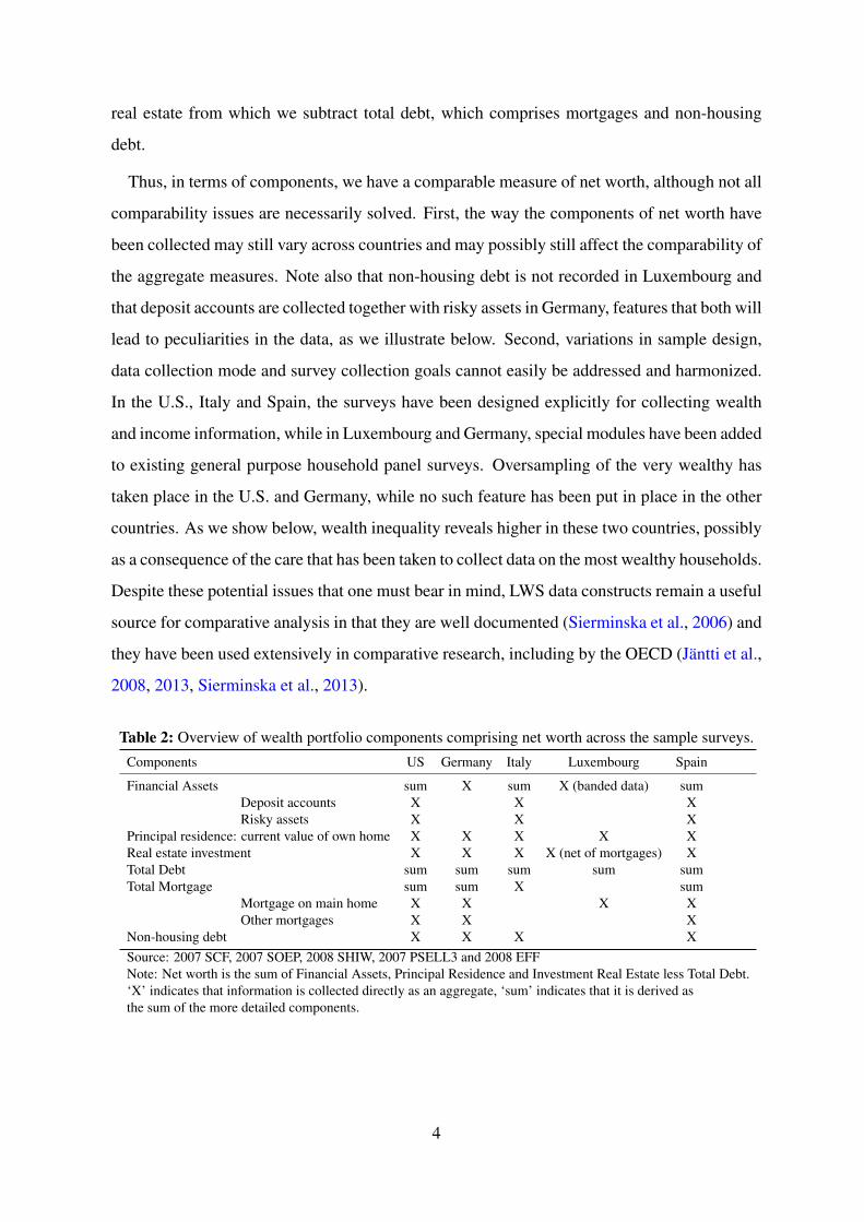
Thus, in terms of components, we have a comparable measure of net worth, although not all

comparability issues are necessarily solved. First, the way the components of net worth have

been collected may still vary across countries and may possibly still affect the comparability of

the aggregate measures. Note also that non-housing debt is not recorded in Luxembourg and

that deposit accounts are collected together with risky assets in Germany, features that both will

lead to peculiarities in the data, as we illustrate below. Second, variations in sample design,

data collection mode and survey collection goals cannot easily be addressed and harmonized.

In the U.S., Italy and Spain, the surveys have been designed explicitly for collecting wealth

and income information, while in Luxembourg and Germany, special modules have been added

to existing general purpose household panel surveys. Oversampling of the very wealthy has

taken place in the U.S. and Germany, while no such feature has been put in place in the other

countries. As we show below, wealth inequality reveals higher in these two countries, possibly

as a consequence of the care that has been taken to collect data on the most wealthy households.

Despite these potential issues that one must bear in mind, LWS data constructs remain a useful

source for comparative analysis in that they are well documented (Sierminska et al., 2006) and

they have been used extensively in comparative research, including by the OECD (Jäntti et al.,

2008, 2013, Sierminska et al., 2013).

Table 2: Overview of wealth portfolio components comprising net worth across the sample surveys.

Components US Germany Italy Luxembourg Spain

Financial Assets sum X sum X (banded data) sumDeposit accounts X X XRisky assets X X X

Principal residence: current value of own home X X X X XReal estate investment X X X X (net of mortgages) XTotal Debt sum sum sum sum sumTotal Mortgage sum sum X sum

Mortgage on main home X X X XOther mortgages X X X

Non-housing debt X X X XSource: 2007 SCF, 2007 SOEP, 2008 SHIW, 2007 PSELL3 and 2008 EFFNote: Net worth is the sum of Financial Assets, Principal Residence and Investment Real Estate less Total Debt.‘X’ indicates that information is collected directly as an aggregate, ‘sum’ indicates that it is derived asthe sum of the more detailed components.

4

Our unit of analysis is the household.2 Sample sizes range from 3,651 observations in

Luxembourg to 10,907 in Germany (Table 3). The variable total disposable household income

is created by aggregating income sources from all members and deducting taxes. This is done

for all countries except Spain, where only gross income is available.3 The variable net worth is

similarly constructed by adding up available comparable asset categories and deducting debts

from all household members, as we explained above. All values are expressed in 2009 US

dollars.4 We do not apply equivalence scales as the issue of selecting a relevant equivalence

scale for wealth is largely unsettled.5 Sample weights are used to compute all statistics and

model parameters reported in the paper.

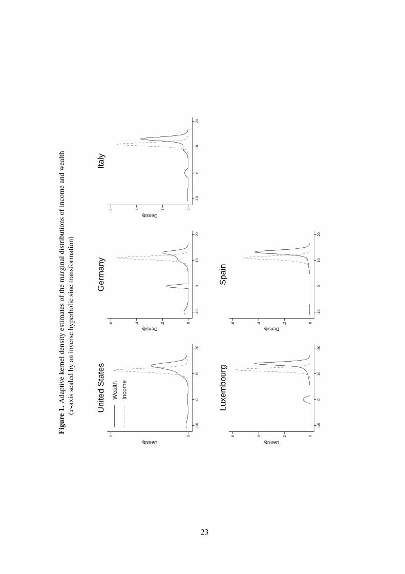
Figure 1 shows (adaptive) kernel density estimates of the marginal distributions of income

and wealth calculated from our data. To help visualize the density at small and negative values,

the x-axis is scaled by an inverse hyperbolic sine transformation. While income distributions

have broadly similar shapes in the five countries, the wealth distributions exhibit substantially

more variation across countries. The wealth distribution is typically bimodal with a first mode

at zero6 and is more stretched out over positive values, thereby exhibiting more inequality.

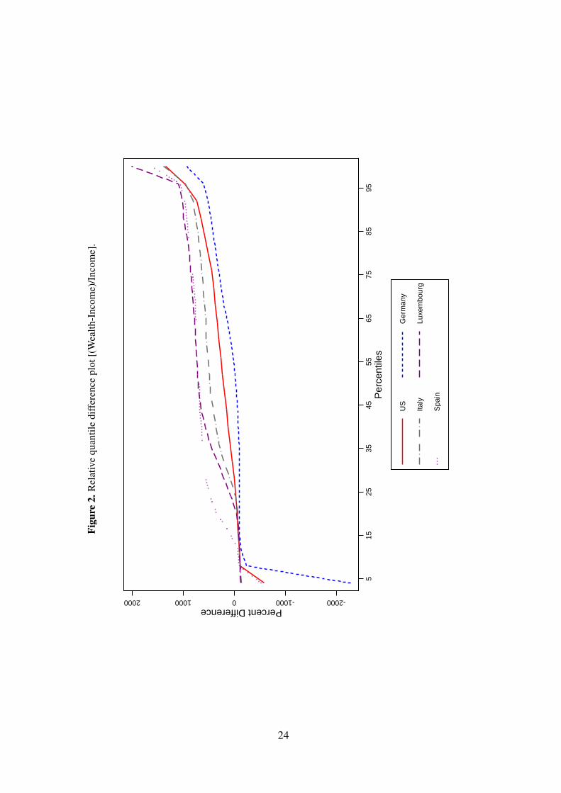
The graphical association of income and wealth is presented in Figure 2, which shows a

relative quantile-difference plot.7 At the bottom of the distribution, we find wealth quantiles to

be below the corresponding income quantiles with wide cross-country variation. The equality

between income and wealth levels occurs at the 25th percentile except for Spain (20th per-

centile) and Germany (50th percentile). Above the 25th percentile, the slope is positive and

it is followed by a steep increase for the highest percentiles. The variation of slopes indicates

that the association between income and wealth varies across countries as income accumulates

into different levels of wealth throughout the distribution.

2A household is defined as including all persons living together in the same dwelling. Sharing expenses is anadditional requirement in Italy and the United States.

3While we do not adjust for negative data on wealth, we delete observations with income less than or equal tozero as these are not considered in our income distribution model. They only represent a tiny fraction of oursamples.

4We use the national price deflators for personal consumption to express currencies in 2009 prices and thenconvert them to international dollars using PPPs for personal consumption (OECD 2011).

5See, e.g., the discussions in Bover (2010) or Jäntti et al. (2013).6Note that a spike at exactly zero tends to be smeared out over small values around zero by kernel density

estimators. See Table 3 for the share of exact zeros in each country.7A relative quantile-difference plot shows the difference between the values of a variable at each percentile of

its distribution and the corresponding values of another distribution, as a percent of the values for one of thedistributions (Kennickell, 2009).

5

When taking a detailed look at the data, we find that the fraction of negative and zero net

worth in our samples varies substantially across countries. Table 3 indicates that about 33% of

the sample in Germany has zero or negative net worth, but only about 5% in Spain, 9% in the

U.S., 11% in Italy and 12% in Luxembourg. This is driven, at least partly, by discrepancies in

data collection since the five surveys differ in the collection of assets and debts. For example,

the high share of zeros in Germany is likely related to the fact that the lowest amounts of

financial assets are disregarded; the fact that no negative net worth is recorded in Luxembourg

is likely due to the fact that only home-related debt is recorded. In any case, these values clearly

illustrate the necessity of a modelling strategy to deal with such non-positive observations.

The descriptive statistics reported in Table 3 show that the average level of wealth is much

higher than the average level of annual income. The ratio of means of wealth and income

varies substantially across countries: from about 4 in Germany to almost 10 in Luxembourg

(ratios of medians range from 0.8 in Germany to 8.1 in Luxembourg and Spain).8 Mean wealth

holdings are the largest in Luxembourg and the U.S. Median wealth holdings in Luxembourg

are particularly striking in comparison to other countries.

To gain insight into the degree of dependence between wealth and income in our countries,

Table 3 reports the proportion of observations found in the bottom and top quintile groups of

both the income and wealth distributions. If the ranks in income and wealth were perfectly

correlated, we would observe 20% of the samples in each of the groups. If, on the other hand,

there were zero correlation in ranks, we would observe about 4% of the samples in each of

the quintile group cells. A negative correlation could lead, at the extreme, to no data in these

cells. In most countries, 8 to 11 percent of the sample can be found in each of the cells. The

exception is Spain, where we find 5% of the sample in the lowest fifth of both income and

wealth and 7% in the top fifths.

There are several reasons to be interested in the association of income and wealth. For

instance, a greater positive association may suggest households are less able to rely on savings

to smooth consumption. The association also speaks to the extent that income taxation also

targets wealth holdings. (We shall return to this issue when discussing the copula estimates

below.)

8Note that unlike for the other countries for Spain we observe gross income only, thereby inflating values ofincome compared to other countries.

6

Table 3: Sample descriptives

US Germany Italy Luxembourg Spain

Observations 4,232 10,907 7,899 3,651 5,013

NW>0 0.913 0.670 0.892 0.882 0.944NW=0 0.020 0.205 0.070 0.115 0.009NW<0 0.067 0.124 0.038 0.003 0.047

MeanNet worth 572,015 136,472 284,394 578,364 339,744Income 68,542 33,101 37,368 59,424 34,348

MedianNet worth 133,900 21,739 175,976 407,088 235,330Income 40,522 27,159 30,107 50,415 29,096

Proportions in quintile groupsQI1 & QW1 9.30 11.93 10.16 9.57 5.16QI5 & QW5 11.60 8.98 11.64 8.83 7.17Note: ‘QI1 & QW1’ refers to households in both the lowest income and wealth quintile groups‘QI5 & QW5’ refers to households in both the highest income and wealth quintile groups

Table 4 shows additional summary indices of the association between income and net worth

in our samples. The Pearson correlation coefficient gives us an indication of the linear rela-

tionship between income and wealth. The others—Spearman’s ρ and Kendall’s Tau—are rank

correlation indicators closely connected to the copula dependence parameters. The latter are

often preferred to Pearson correlations for non-normal data, since they are less sensitive to out-

liers which can exert a strong influence on Pearson correlations (Croux and Dehon, 2010). We

observe the highest linear correlation between income and wealth in the U.S. (0.61) and Ger-

many (0.59) – the countries that oversampled the wealthy and probably best capture very high

wealth. Pearson correlations are low in Luxembourg (0.17) and Spain (0.17). When it comes

to rank correlations that are less sensitive to extreme data, the country ranking changes. The

highest Spearman correlation is in Italy (0.64), then in the U.S. (0.61), Luxembourg (0.46),

Germany (0.41) and Spain (0.26). A similar ranking is obtained for Kendall’s Tau. This order-

ing is different though from what comes out of the proportions of households jointly in the top

or bottom quintile groups of income and wealth reported in Table 3.

Overall the results indicate a positive dependence between income and net worth, but that

dependence is complex and may not be captured well by single summary indices. The Pearson

7

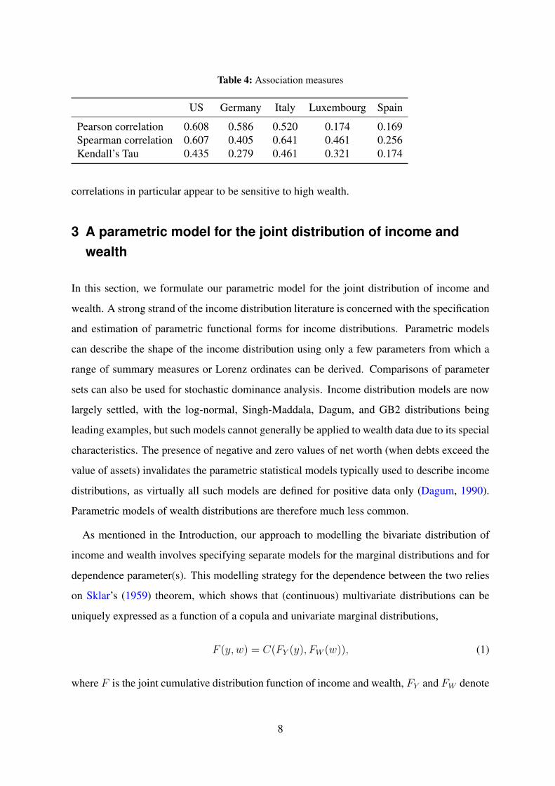
Table 4: Association measures

US Germany Italy Luxembourg Spain

Pearson correlation 0.608 0.586 0.520 0.174 0.169Spearman correlation 0.607 0.405 0.641 0.461 0.256Kendall’s Tau 0.435 0.279 0.461 0.321 0.174

correlations in particular appear to be sensitive to high wealth.

3 A parametric model for the joint distribution of income andwealth

In this section, we formulate our parametric model for the joint distribution of income and

wealth. A strong strand of the income distribution literature is concerned with the specification

and estimation of parametric functional forms for income distributions. Parametric models

can describe the shape of the income distribution using only a few parameters from which a

range of summary measures or Lorenz ordinates can be derived. Comparisons of parameter

sets can also be used for stochastic dominance analysis. Income distribution models are now

largely settled, with the log-normal, Singh-Maddala, Dagum, and GB2 distributions being

leading examples, but such models cannot generally be applied to wealth data due to its special

characteristics. The presence of negative and zero values of net worth (when debts exceed the

value of assets) invalidates the parametric statistical models typically used to describe income

distributions, as virtually all such models are defined for positive data only (Dagum, 1990).

Parametric models of wealth distributions are therefore much less common.

As mentioned in the Introduction, our approach to modelling the bivariate distribution of

income and wealth involves specifying separate models for the marginal distributions and for

dependence parameter(s). This modelling strategy for the dependence between the two relies

on Sklar’s (1959) theorem, which shows that (continuous) multivariate distributions can be

uniquely expressed as a function of a copula and univariate marginal distributions,

F (y, w) = C(FY (y), FW (w)), (1)

where F is the joint cumulative distribution function of income and wealth, FY and FW denote

8

the marginal cumulative distribution functions of income (Y ) and wealth (W ), and C is a

copula. We model F parametrically by specifying separate models for each of FY , FW and C.

We describe our specifications for each of the three components in turn.

The marginal distribution of income

Specifying a parametric model for the marginal distribution of income is unproblematic. A va-

riety of specifications are available; see, for example, McDonald (1984). We follow common

practice and rely on a Singh-Maddala specification (Singh and Maddala, 1976). The Singh-

Maddala distribution is a three-parameter model for unimodal distributions allowing varying

degrees of skewness and kurtosis and dealing with the heavy tails typical of income and earn-

ings distributions. It is used, e.g., in Brachmann et al. (1996) and Biewen and Jenkins (2005)

to model income distributions. The cumulative distribution function is

FY (y) = SM(y; a, b, q) = 1−[1 +

(y

b

)a]−q

, (2)

where b > 0 is a scale parameter, q > 0 is a shape parameter for the upper tail, a > 0

is a shape parameter affecting both tails (Kleiber and Kotz, 2003). As we show below, the

Singh-Maddala model provides a very good fit to our income data.

The marginal distribution of wealth

Specifying the marginal distribution of wealth is more difficult. Although it is customary to

analyze specific components of wealth, such as assets or debts, the literature on wealth in-

equality most often focuses on the concept of net worth, defined as the value of total assets

(financial and non-financial) minus total debts. Consequently, it is conceptually possible and

empirically relatively common to observe data with zero or negative net worth. Our paramet-

ric model must therefore be able to accommodate negative data. This rules out virtually all

specifications typically used for modeling income distributions, since these size distributions

have positive density only over the positive halfline R+.

To accommodate zero and negative data, we follow Dagum (1990) (also see Jenkins and

Jäntti, 2005) and use a finite mixture model where negative, zero and positive data are mod-

eled separately with an exponential distribution (negatives), a point-mass at zero and a Singh-

9

Maddala distribution (positives, respectively:

FW (w) =

π1 exp(θw) if w < 0

π1 + π2 if w = 0

π1 + π2 + (1− π1 − π2) SM(w;α, β, γ) if w > 0,

(3)

where π1 and π2 are the shares of negatives and zeros in the data, α, β and γ are interpreted as

above and θ > 0 is shape parameter for the negative distribution with lower values for θ > 0

leading to thicker negative tail. We depart from Dagum’s (1990) original model by using a

Singh-Maddala distribution for positive data instead of a Dagum type I distribution (the two

distributions have similar shapes).9

Copula function specification

The third ingredient of the specification of the joint distribution is the shape of the copula

C which captures the rank-order association between the two marginal distributions. In the

absence of clear guidance from earlier research regarding the most appropriate specification

for the copula in this context, we experimented with several alternative specifications: the

Plackett copula, the Clayton and rotated Clayton copulas, and a more flexible 3-parameter

specification mixing the Clayton and rotated Clayton copulas (See Trivedi and Zimmer (2007)

for a review of different copula functions and Chau (2010) on mixing copulas). The first choice

revealed most satisfactory in our application: the copula parameters for the last two models

generally could not be estimated reliably due to convergence problems and the Plackett copula

resulted in a better fit to the rank dependence of income and wealth in our datasets than the

Clayton copula.10

The specification of the Plackett copula (Plackett, 1965) is:

C(u, v; τ) =

((1 + (τ − 1)(u+ v))−

√(1 + (τ − 1)(u+ v))2)− 4uv(τ − 1)τ

)2(τ − 1) , (4)

where τ ∈ [0,∞) \ {1} is a dependence parameter. τ > 1 leads to positive dependence

9For coherence with the income distribution we use the Singh-Maddala distribution.10The Plackett copula exhibits symmetric upper-tail and lower-tail dependence whereas the Clayton copula ex-

hibits stronger lower-tail dependence. This may explain the differences in goodness of fit between these twofamiliar copula specifications.

10

and the higher τ , the higher is the dependence. Independence is obtained at τ = 1. The

Plackett copula exhibits symmetric upper-tail and lower-tail dependence. The parameter of

the Plackett copula can be related to Spearman’s rank correlation coefficient as follows: S =

((τ + 1)/(τ − 1)) − (2 log(τ)τ/(τ − 1)2), but there is no simple closed-form expression for

Kendall’s Tau in terms of the Plackett copula parameter.11 It has been used by, e.g., Bonhomme

and Robin (2009) in a model of earnings dynamics.

Estimation

Parameters of the three components FY , FW and C can be estimated separately. In this paper,

all parameters for FY and FW were first estimated by conventional maximum likelihood using

the built-in Newton-Raphson optimizer of StataTM(StataCorp, 2011).12 Maximum likelihood

estimation of the copula parameter is done in a second stage based on the sample values of

(F̂Y (yi), F̂W (wi)) with F̂Y and F̂W based on the first stage parameter estimates.

4 Estimation results

We now report results from estimating our parametric model for the joint distribution of in-

come and wealth. We first briefly report the detailed parameter estimates and assess the good-

ness of fit of the models. We then present inequality indicators derived from the model pa-

rameters, along with counterfactual constructs to quantify the role played by cross-national

differences in association parameters on differences in bivariate inequality.

Parameter estimates for the proposed model estimated for each of the five countries are re-

ported in Table 5. The top panel shows parameter estimates for the Singh-Maddala distribution

of income; the middle panel shows parameters for the mixture model of net worth, namely the

share of negative and zero data, and the four distribution parameters; the bottom panel shows

estimates of the two copula function parameters considered. Since we could not estimate re-

liably the model for negative wealth in Luxembourg given the small number of observations

reporting negative net worth—we discarded these few observations and worked with a model

11See e.g. Agresti (2010) for a discussion of Spearman’s correlation and Kendall’s Tau as measures of rankdependence.

12Example of Stata code for estimating the wealth distribution parameters is available in Jenkins and Jäntti(2005).

11

with just two components (positives and zeros) in this country.

The similarity of the income distributions across countries is reflected in the relative similar-

ity of coefficients of the Singh-Maddala distribution.13 Wealth distribution parameters, on the

other hand, vary substantially, in line with differences in the shape of the wealth distributions

across countries. For example, for data with positive wealth, the scale parameter (β) shows

large variations with much higher levels of wealth in Luxembourg. The shape parameters, in

turn, suggest relatively low inequality in Luxembourg.

In line with the rank correlation statistics reported in Table 4, our copula function parameter

estimates split our five countries into two groups: the U.S. and Italy, on the one hand, which

exhibits strong dependence between income and wealth (high copula parameters) and on the

other hand, Luxembourg, Germany and Spain, with a much smaller level of (positive) depen-

dence. Why, exactly, we find these differences is hard to tell. One possible explanation could

be differences in the patterns of home ownership and income. The interaction of institutional

differences with the full joint distribution remains a topic for future work.

The overall goodness of fit of our model can be gauged by comparing summary statistics

derived from the model parameters to the statistics computed from the raw data. Since no

closed-form expression exists for deriving the various summary measures from the model pa-

rameters, our estimation is based on Monte Carlo sampling on the basis of the models and

estimated parameters. We simulate pseudo-samples of 3000 income and wealth pairs for each

country based on the inverse sampling method: we first draw 3000 correlated pairs of uni-

formly distributed variates (u, v) where the correlation is determined by the copula parameter

(Nelsen, 2006) and we then generate the wealth and income pairs as (F−1Y (u), F−1

W (v)), that is

the u-th and v-th theoretical quantiles implied by the parameter estimates of the marginal dis-

tributions. Model-based summary statistics are finally obtained based on standard calculations

on the pseudo-samples.

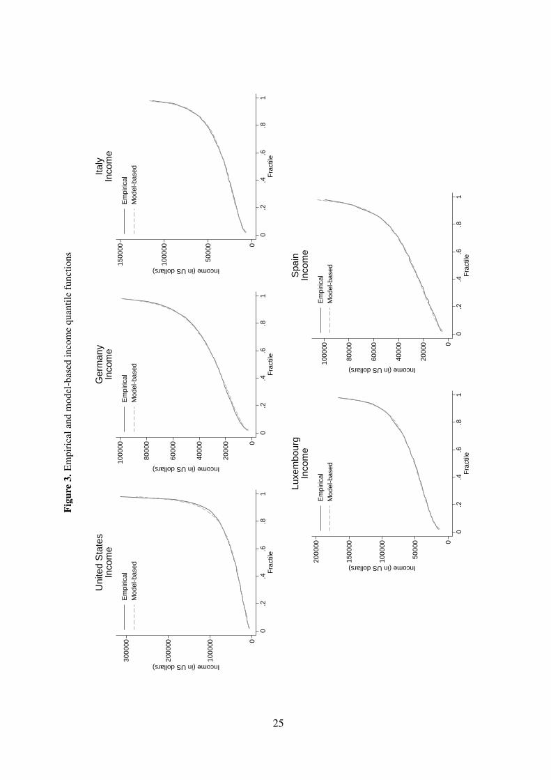
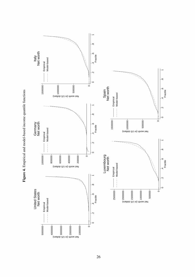
Figures 3 and 4 show observed and model-based predictions of the income quantile function

and of the wealth quantile function. Figure 5 shows observed and model-based predictions of

the copula CDF, namely the joint distribution function of household ranks in the distribution

income and wealth (the darker the color, the higher the value of the CDF, with contour lines

13The difference in parameter estimates across countries is large compared to their standard errors, suggestingthat distributions are different across countries from a statistical point of view.

12

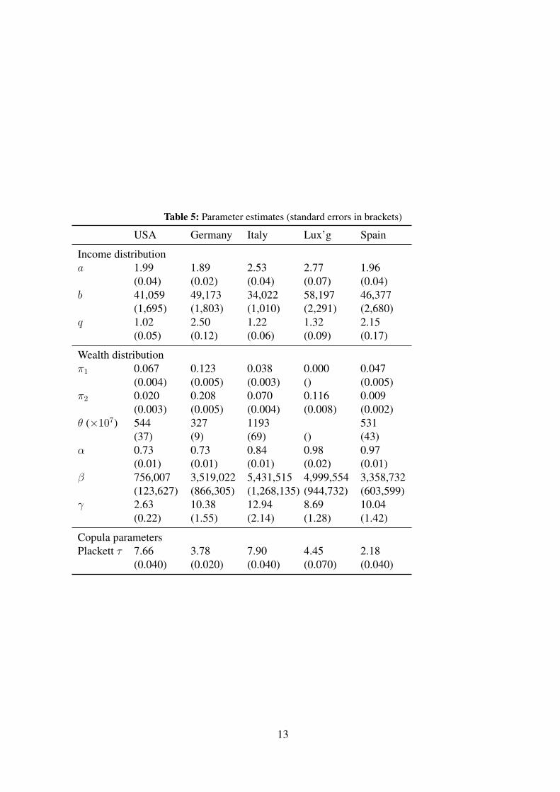
Table 5: Parameter estimates (standard errors in brackets)

USA Germany Italy Lux’g Spain

Income distributiona 1.99 1.89 2.53 2.77 1.96

(0.04) (0.02) (0.04) (0.07) (0.04)b 41,059 49,173 34,022 58,197 46,377

(1,695) (1,803) (1,010) (2,291) (2,680)q 1.02 2.50 1.22 1.32 2.15

(0.05) (0.12) (0.06) (0.09) (0.17)

Wealth distributionπ1 0.067 0.123 0.038 0.000 0.047

(0.004) (0.005) (0.003) () (0.005)π2 0.020 0.208 0.070 0.116 0.009

(0.003) (0.005) (0.004) (0.008) (0.002)θ (×107) 544 327 1193 531

(37) (9) (69) () (43)α 0.73 0.73 0.84 0.98 0.97

(0.01) (0.01) (0.01) (0.02) (0.01)β 756,007 3,519,022 5,431,515 4,999,554 3,358,732

(123,627) (866,305) (1,268,135) (944,732) (603,599)γ 2.63 10.38 12.94 8.69 10.04

(0.22) (1.55) (2.14) (1.28) (1.42)

Copula parametersPlackett τ 7.66 3.78 7.90 4.45 2.18

(0.040) (0.020) (0.040) (0.070) (0.040)

13

showing 20 isoquants for values of 0.01, 0.05, 0.10 to 0.95).

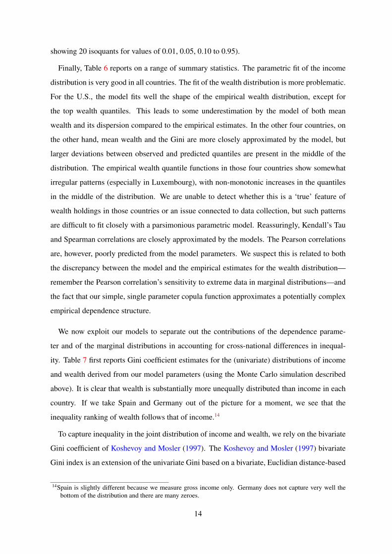
Finally, Table 6 reports on a range of summary statistics. The parametric fit of the income

distribution is very good in all countries. The fit of the wealth distribution is more problematic.

For the U.S., the model fits well the shape of the empirical wealth distribution, except for

the top wealth quantiles. This leads to some underestimation by the model of both mean

wealth and its dispersion compared to the empirical estimates. In the other four countries, on

the other hand, mean wealth and the Gini are more closely approximated by the model, but

larger deviations between observed and predicted quantiles are present in the middle of the

distribution. The empirical wealth quantile functions in those four countries show somewhat

irregular patterns (especially in Luxembourg), with non-monotonic increases in the quantiles

in the middle of the distribution. We are unable to detect whether this is a ‘true’ feature of

wealth holdings in those countries or an issue connected to data collection, but such patterns

are difficult to fit closely with a parsimonious parametric model. Reassuringly, Kendall’s Tau

and Spearman correlations are closely approximated by the models. The Pearson correlations

are, however, poorly predicted from the model parameters. We suspect this is related to both

the discrepancy between the model and the empirical estimates for the wealth distribution—

remember the Pearson correlation’s sensitivity to extreme data in marginal distributions—and

the fact that our simple, single parameter copula function approximates a potentially complex

empirical dependence structure.

We now exploit our models to separate out the contributions of the dependence parame-

ter and of the marginal distributions in accounting for cross-national differences in inequal-

ity. Table 7 first reports Gini coefficient estimates for the (univariate) distributions of income

and wealth derived from our model parameters (using the Monte Carlo simulation described

above). It is clear that wealth is substantially more unequally distributed than income in each

country. If we take Spain and Germany out of the picture for a moment, we see that the

inequality ranking of wealth follows that of income.14

To capture inequality in the joint distribution of income and wealth, we rely on the bivariate

Gini coefficient of Koshevoy and Mosler (1997). The Koshevoy and Mosler (1997) bivariate

Gini index is an extension of the univariate Gini based on a bivariate, Euclidian distance-based

14Spain is slightly different because we measure gross income only. Germany does not capture very well thebottom of the distribution and there are many zeroes.

14

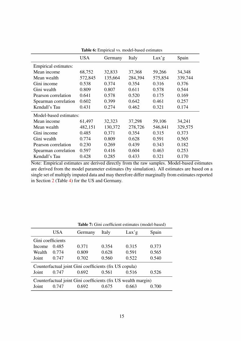
Table 6: Empirical vs. model-based estimates

USA Germany Italy Lux’g Spain

Empirical estimates:Mean income 68,752 32,833 37,368 59,266 34,348Mean wealth 572,845 135,664 284,394 575,854 339,744Gini income 0.538 0.374 0.354 0.316 0.376Gini wealth 0.809 0.807 0.611 0.578 0.544Pearson correlation 0.641 0.578 0.520 0.175 0.169Spearman correlation 0.602 0.399 0.642 0.461 0.257Kendall’s Tau 0.431 0.274 0.462 0.321 0.174

Model-based estimates:Mean income 61,497 32,323 37,298 59,106 34,241Mean wealth 482,151 130,372 278,726 546,841 329,575Gini income 0.485 0.371 0.354 0.315 0.373Gini wealth 0.774 0.809 0.628 0.591 0.565Pearson correlation 0.230 0.269 0.439 0.343 0.182Spearman correlation 0.597 0.416 0.604 0.463 0.253Kendall’s Tau 0.428 0.285 0.433 0.321 0.170

Note: Empirical estimates are derived directly from the raw samples. Model-based estimatesare derived from the model parameter estimates (by simulation). All estimates are based on asingle set of multiply imputed data and may therefore differ marginally from estimates reportedin Section 2 (Table 4) for the US and Germany.

Table 7: Gini coefficient estimates (model-based)

USA Germany Italy Lux’g Spain

Gini coefficientsIncome 0.485 0.371 0.354 0.315 0.373Wealth 0.774 0.809 0.628 0.591 0.565Joint 0.747 0.702 0.560 0.522 0.540

Counterfactual joint Gini coefficients (fix US copula)Joint 0.747 0.692 0.561 0.516 0.526

Counterfactual joint Gini coefficients (fix US wealth margin)Joint 0.747 0.692 0.675 0.663 0.700

15

extension of the Gini Mean Deviation:

G2 = 14N2

N∑i=1

N∑j=1

( yi

µy

− yj

µy

)2

+(wi

µw

− wj

µw

)2 1

2

.

Compare this with the univariate version of the Gini coefficient:

G1 = 12N2

N∑i=1

N∑j=1

∣∣∣∣∣ yi

µy

− yj

µy

∣∣∣∣∣ .G1 can be interpreted in terms of the average absolute difference (or ‘distance’) between any

two incomes drawn from a univariate distribution (normalized by the mean). The bivariate

G2 can be interpreted similarly in terms of the average Euclidian distance between any two

income-wealth pairs drawn from the joint distribution (normalized by their respective means).

The bivariate Gini is determined by the degree of inequality in the two marginal distributions

as well as by the association among the two covariates. Our focus remains on Gini coeffi-

cients because, unlike many inequality measures, they remain defined for negative and zero

net worth—an essential feature for measuring wealth inequality (Jenkins and Jäntti, 2005).15

Recall that our main objective is to assess the overall inequality of the distribution of income

and wealth. To this end, Table 7 reports estimates of the bivariate Gini. While levels of bivari-

ate inequality differ according to the specification used, the ordering of countries is preserved.

In all cases, it appears that inequality in wealth remains a key determinant of overall inequal-

ity: bivariate Ginis are close to univariate Ginis for wealth. Notice, however, that because the

association between income and wealth is not perfectly positive, the bivariate takes on a value

between the two marginal Ginis.

In order to understand the relative role of the association between income and wealth, as

captured by the copula, and the marginal distributions, Table 7 also reports two sets of coun-

terfactual estimates of the bivariate Ginis. The first set is obtained by fixing the U.S. depen-

dence parameter and applying it to all countries’ marginal distributions. The indices obtained

therefore give us the value of the bivariate Gini which would be observed in the different

countries if the association between income and wealth were as high as in the U.S. Comparing

15Arguably, more sophisticated measures of multi-dimensional inequality or poverty could be considered formore in-depth analysis (Lugo, 2005). The presence of negative net worth would however remain a criticalconstraint on the choice of relevant multidimensional inequality measures, as it is in the univariate case.

16

the counterfactual indices with the previous estimates gives us an indication of the impact of

cross-national differences in the association parameter on overall inequality differences.16

Our estimates suggest that swapping the dependence parameter would only have a small

impact on bivariate inequality. This simple mechanical exercise demonstrates that, despite the

large variations across countries in the dependence between income and wealth, these differ-

ences are of secondary importance in overall, bivariate inequality. To benchmark this effect,

the second set of counterfactuals shows what the bivariate Ginis would be if the parameters

of the marginal wealth distribution were fixed at the level of the U.S. For Germany—another

country with high wealth inequality—the impact of the swap is very small, but Spain, Luxem-

bourg and Italy would see bivariate inequality grow by about twenty percent if their distribution

of wealth were the same as in the United States (holding constant their income distribution and

their dependence parameter). The impact of cross-national differences in dependence is, by

comparison, very small.

Given that inequality of net worth is high relative to that of income, it may not be surprising

that the differences in dependence account for little in the overall inequality of income and

wealth. Indeed, a case might be made that decisions about taxation can be made largely based

on marginal distributions alone. One may also question the value of examining bivariate Gini

coefficients – differences in net worth inequality seem to dominate in those as well. However,

we still think it is useful to explore these issues; after all, it is through the analysis of inequality

of the joint distribution we discovered that net worth inequality dominates the picture.

5 Concluding remarks

Relatively little is known about the empirical relationship between income and wealth and

the overall inequality in the joint distribution of the two. In this paper, we set out to provide

a new, parametric framework for analyzing this relationship. A better understanding of this

relationship should prove useful in spheres such as the design of taxation and redistribution

policies and better identification and targeting of vulnerable population groups. A framework

16Calculations are again based on Monte Carlo sampling: to obtain counterfactual indices, a new set of pseudo-samples are drawn where the parameter of the U.S. copula functions are used to generate the correlated pairsof uniformly distributed variates and parameters of each of the countrys’ marginal distributions are used toconvert the uniform variates into income and wealth pseudo-sample values.

17

for modelling this complex relationship can therefore provide a useful tool for examining

or simulating the broader distributional implications of potential policy changes (e.g. wealth

taxation).

To achieve our goals, we consider a relatively simple parametric model for the joint dis-

tribution of income and wealth. We use this model to examine whether joint income and

wealth inequality provides us with a different pattern of social inequality than the traditional

income-only approach. Our parameter of focus is the dependence parameter between income

and wealth. We use our model to disentangle the relative contribution of cross-national differ-

ences in this dependence parameter from cross-national differences in marginal distributions

in shaping differences in overall, bivariate inequality. This is done by exploiting the simple

structure of our model to generate counterfactual distributions of interest.

The framework offered by the Sklar theorem to build a model for the bivariate distribu-

tion is attractive in this context since the marginal distributions of income and wealth have

specificities that require differentiated treatment—in particular, the presence of zero and neg-

ative net worth. It would therefore be difficult to directly identify a relevant joint distribution.

Specification of the copula function for capturing the rank-order association is a key step in

the process. We have considered several simple, tractable functions—the Plackett copula be-

ing our preferred choice—although these simple functions may not fully capture the complex

dependence between income and wealth observed in our samples.

Deriving inequality indicators from the estimated models, we find—unsurprisingly—that

Gini coefficients on income are much lower than Gini coefficients on wealth. A bivariate Gini

coefficient summarizing inequality in the joint distribution of income and wealth returns inter-

mediate values—with the highest value found in the U.S. The bivariate Gini appears largely

driven by inequality in the wealth distribution and differences across countries in the depen-

dence between income and wealth do not appear to be key drivers in international differences

in bivariate inequality, but the way people generate their wealth matters.

The variation in the positive association between income and wealth across countries, with

Italy and the U.S. standing quite apart from the rest, suggests there may be substantial variation

across countries in the ability of households to protect themselves against income shocks by

drawing on wealth. This can also be the result of safety nets if low assets is a condition of

receiving benefits, as is the case in the U.S. for example. The variation in dependence may

18

also be of interest from the perspective of taxation. The more positive the dependence, the

better income tax also targets high concentrations of wealth. This also suggest that income

taxes could be more progressive in this case. With a low dependence, the case for both income

and wealth taxation may be stronger. Low dependence can also be the result of not having

asset-based benefits, which would facilitate asset accumulation and savings for “a rainy day”

(i.e. income fluctuation). It is also possible that our results are in part accounted for by

differences in home ownership patterns across the distribution of income. Such interactions

between institutions and the joint distribution of income and wealth are important topics for

future research.

Unfortunately, although we have used some of the most comparable sources of wealth and

income data available, we can not rule out that part of the differences we find are driven by

differences in survey design and implementation. The U.S. and to some extent German data

oversample the wealthy, and although we use sample weights, if other countries simply fail to

gather wealth information from the wealthy, weights only partly solve this difference. Country-

specific institutions for wealth differ and so will the details of the survey instruments. However,

we still believe it is valuable to explore the joint distribution of income and wealth as we do

here; with time, it will become more clear what part of the differences across countries are

driven by differences in data collection and which represent genuine distributional differences.

We have taken the first steps.

References

Agresti, A. (2010), Analysis of Ordinal Categorical Data, Wiley Series in Probability and

Statistics, 2 edn, John Wiley and Sons, Inc.

Biewen, M. and Jenkins, S. P. (2005), ‘Accounting for differences in poverty between the USA,

Britain and Germany’, Empirical Economics 30(2), 331–358.

Bonhomme, S. and Robin, J.-M. (2009), ‘Assessing the equalizing force of mobility using

short panels: France, 1990–2000’, Review of Economic Studies 76(1), 63–92.

Bover, O. (2010), ‘Wealth inequality and household structure: U.S. versus Spain’, Review of

Income and Wealth 56(2), 259–290.

19

Brachmann, K., Stich, A. and Trede, M. (1996), ‘Evaluating parametric income distribution

models’, Allgemeines Statistisches Archiv 80, 285–298.

Chau, T. W. (2010), Essays on earnings mobility within and across generations using copula,

PhD thesis, University of Rochester, Dept. of Economics.

URL: http://hdl.handle.net/1802/11125

Croux, C. and Dehon, C. (2010), ‘Influence functions of the Spearman and Kendall correlation

measures’, Statistical Methods & Applications 19(4), 497–515.

Dagum, C. (1990), A model of net wealth distribution specified for negative, null and pos-

itive wealth. A case study: Italy, in C. Dagum and M. Zenga, eds, ‘Income and Wealth

Distribution, Inequality and Poverty’, Springer, Berlin and Heidelberg, pp. 42–56.

Genest, C. and McKay, J. (1986), ‘The joy of copulas: Bivariate distributions with uniform

marginals’, American Statistician 40(4), 280–3.

Jäntti, M., Sierminska, E. and Smeeding, T. (2008), The joint distribution of household income

and wealth: Evidence from the Luxembourg Wealth Study, OECD Social Employment and

Migration Working Paper 65, OECD, Directorate for Employment, Labour and Social Af-

fairs.

Jäntti, M., Sierminska, E. and Van Kerm, P. (2013), The joint distribution of income and

wealth, in J. C. Gornick and M. Jäntti, eds, ‘Income inequality. Economic Disparities and the

Middle Class in Affluent Countries’, Stanford University Press, Stanford, CA, chapter 11,

pp. 312–333.

Jenkins, S. P. and Jäntti, M. (2005), Methods for summarizing and comparing wealth distribu-

tions, ISER Working Paper 2005-05, Institute for Social and Economic Research, University

of Essex, Colchester, UK.

Jenkins, S. P. and Van Kerm, P. (2009), The measurement of economic inequality, in

W. Salverda, B. Nolan and T. M. Smeeding, eds, ‘Oxford Handbook of Economic Inequal-

ity’, Oxford University Press, chapter 3.

Kennickell, A. B. (2009), Ponds and streams: wealth and income in the U.S., 1989 to 2007,

20

Finance and Economics Discussion Series 2009-13, Board of Governors of the Federal Re-

serve System (U.S.).

Kleiber, C. and Kotz, S. (2003), Statistical size distributions in Economics and Actuarial Sci-

ences, John Wiley and Sons, Inc., New Jersey.

Koshevoy, G. A. and Mosler, K. (1997), ‘Multivariate Gini indices’, Journal of Multivariate

Analysis 60, 252–276.

Lugo, M. A. (2005), Comparing multidimensional indices of inequality: Methods and appli-

cation, ECINEQ Working Paper 14, Society for the Study of Economic Inequality.

Luxembourg Wealth Study Database (LWS) (2014), ‘http://www.lisdatacenter.

org (multiple countries; microdata last accessed in july 2014)’, Statistical micro-level

database. Luxembourg: LIS.

McDonald, J. B. (1984), ‘Some generalized functions for the size distribution of income’,

Econometrica 52(3), 647–663.

Nelsen, R. B. (2006), An introduction to copulas, 2 edn, Springer, New York.

Plackett, R. L. (1965), ‘A class of bivariate distributions’, Journal of the American Statistical

Association 60, 516–522.

Sierminska, E., Brandolini, A. and Smeeding, T. (2006), ‘The Luxembourg Wealth Study: A

cross-country comparable database for household wealth research’, Journal of Economic

Inequality 4(3), 375–383.

Sierminska, E., Smeeding, T. and Allegrezza, S. (2013), The distribution of assets and debt, in

J. C. Gornick and M. Jäntti, eds, ‘Income inequality. Economic Disparities and the Middle

Class in Affluent Countries’, Stanford University Press, Stanford, CA, chapter 10, pp. 285–

311.

Singh, S. K. and Maddala, G. S. (1976), ‘A function for size distribution of incomes’, Econo-

metrica 44(5), 963–970.

Sklar, A. (1959), ‘Fonctions de répartition à n dimensions et leurs marges’, Publications de

l’Institut de Statistique de l’Université de Paris 8, 229–231.

21

StataCorp (2011), Stata Statistical Software: Release 12, StataCorp LP, College Station.

Trivedi, P. K. and Zimmer, D. M. (2007), ‘Copula modeling: An introduction for practitioners’,

Foundations and Trends in Econometrics 1(1), 1–111.

22

Figu

re1.

Ada

ptiv

eke

rnel

dens

ityes

timat

esof

the

mar

gina

ldis

trib

utio

nsof

inco

me

and

wea

lth(x

-axi

ssc

aled

byan

inve

rse

hype

rbol

icsi

netr

ansf

orm

atio

n)

0.5

Density

-10

010

20

Wea

lth

Inco

me

Uni

ted

Sta

tes

0.2.4.6

Density

-10

010

20

Ger

man

y

0.2.4.6

Density

-10

010

20

Italy

0.2.4.6

Density

-10

010

20

Luxe

mbo

urg

0.2.4.6

Density

-10

010

20

Spa

in

23

Figu

re2.

Rel

ativ

equ

antil

edi

ffer

ence

plot

[(W

ealth

-Inc

ome)

/Inc

ome]

.

-2000-1000010002000Percent Difference

515

2535

4555

6575

8595

Per

cent

iles

US

Ger

man

y

Italy

Luxe

mbo

urg

Spa

in

24

Figu

re3.

Em

piri

cala

ndm

odel

-bas

edin

com

equ

antil

efu

nctio

ns

0

1000

00

2000

00

3000

00

Income (in US dollars)

0.2

.4.6

.81

Fra

ctile

Em

piric

alM

odel

-bas

ed

Uni

ted

Sta

tes

Inco

me

0

2000

0

4000

0

6000

0

8000

0

1000

00

Income (in US dollars)

0.2

.4.6

.81

Fra

ctile

Em

piric

alM

odel

-bas

ed

Ger

man

yIn

com

e

0

5000

0

1000

00

1500

00

Income (in US dollars)

0.2

.4.6

.81

Fra

ctile

Em

piric

alM

odel

-bas

edItaly

Inco

me

0

5000

0

1000

00

1500

00

2000

00

Income (in US dollars)

0.2

.4.6

.81

Fra

ctile

Em

piric

alM

odel

-bas

ed

Luxe

mbo

urg

Inco

me

0

2000

0

4000

0

6000

0

8000

0

1000

00

Income (in US dollars)

0.2

.4.6

.81

Fra

ctile

Em

piric

alM

odel

-bas

ed

Spa

inIn

com

e

25

Figu

re4.

Em

piri

cala

ndm

odel

-bas

edin

com

equ

antil

efu

nctio

ns

0

1000

000

2000

000

3000

000

4000

000

5000

000

Net worth (in US dollars)

0.2

.4.6

.81

Fra

ctile

Em

piric

alM

odel

-bas

ed

Uni

ted

Sta

tes

Net

wor

th

0

2000

00

4000

00

6000

00

8000

00

1000

000

Net worth (in US dollars)

0.2

.4.6

.81

Fra

ctile

Em

piric

alM

odel

-bas

ed

Ger

man

yN

et w

orth

0

5000

00

1000

000

1500

000

Net worth (in US dollars)

0.2

.4.6

.81

Fra

ctile

Em

piric

alM

odel

-bas

edItaly

Net

wor

th

0

5000

00

1000

000

1500

000

2000

000

2500

000

Net worth (in US dollars)

0.2

.4.6

.81

Fra

ctile

Em

piric

alM

odel

-bas

ed

Luxe

mbo

urg

Net

wor

th

0

5000

00

1000

000

1500

000

Net worth (in US dollars)

0.2

.4.6

.81

Fra

ctile

Em

piric

alM

odel

-bas

ed

Spa

inN

et w

orth

26

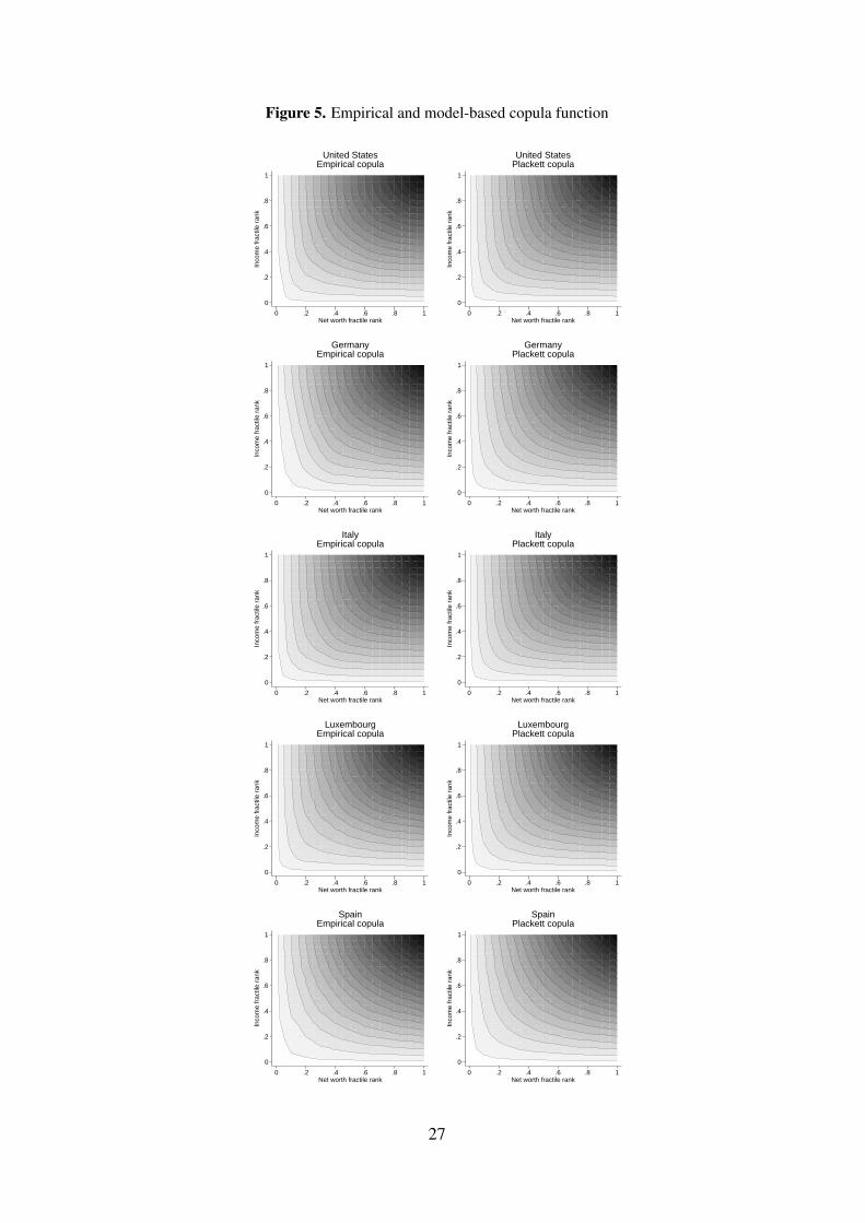
Figure 5. Empirical and model-based copula function

0

.2

.4

.6

.8

1

Inco

me

frac

tile

rank

0 .2 .4 .6 .8 1Net worth fractile rank

United StatesEmpirical copula

0

.2

.4

.6

.8

1

Inco

me

frac

tile

rank

0 .2 .4 .6 .8 1Net worth fractile rank

United StatesPlackett copula

0

.2

.4

.6

.8

1

Inco

me

frac

tile

rank

0 .2 .4 .6 .8 1Net worth fractile rank

GermanyEmpirical copula

0

.2

.4

.6

.8

1

Inco

me

frac

tile

rank

0 .2 .4 .6 .8 1Net worth fractile rank

GermanyPlackett copula

0

.2

.4

.6

.8

1

Inco

me

frac

tile

rank

0 .2 .4 .6 .8 1Net worth fractile rank

ItalyEmpirical copula

0

.2

.4

.6

.8

1

Inco

me

frac

tile

rank

0 .2 .4 .6 .8 1Net worth fractile rank

ItalyPlackett copula

0

.2

.4

.6

.8

1

Inco

me

frac

tile

rank

0 .2 .4 .6 .8 1Net worth fractile rank

LuxembourgEmpirical copula

0

.2

.4

.6

.8

1

Inco

me

frac

tile

rank

0 .2 .4 .6 .8 1Net worth fractile rank

LuxembourgPlackett copula

0

.2

.4

.6

.8

1

Inco

me

frac

tile

rank

0 .2 .4 .6 .8 1Net worth fractile rank

SpainEmpirical copula

0

.2

.4

.6

.8

1

Inco

me

frac

tile

rank

0 .2 .4 .6 .8 1Net worth fractile rank

SpainPlackett copula

27