Embed Size (px)
Citation preview
92
Review Article
MODELLING THE PROGRESS AND EFFECTS OF EUTROPHICATION IN INLAND AND COASTAL WATERS
Ali Ertürk
Cite this article as:
Ertürk, A. (2019). Modelling the progress and effects of eutrophication in inland and coastal waters. Aquatic Research, 2(2), 92-133. https://doi.org/10.3153/AR19010
Istanbul University Faculty of Aquatic Sciences, Ordu Caddesi No:8 Laleli Fatih, Istanbul-Turkey
ORCID IDs of the authors:
A.E. 0000-0002-3532-2961
Submitted: 29.03.2019
Accepted: 01.04.2019
Published online: 12.04.2019
Correspondence:
Ali ERTÜRK
E-mail: [email protected]
©Copyright 2019 by ScientificWebJournals
Available online at
http://aquatres.scientificwebjournals.com
ABSTRACT
The aim of this paper is to give a detailed overview on the predictive-model building/coding tech-niques for simulating the progress and effects of eutrophication based on differently detailed model structures. First; historical development of predictive eutrophication modelling is reviewed. Then, a generic transport model that can be coupled with any eutrophication kinetics is described. In the following sections, ecological sub models based on eutrophication kinetics and food-web are de-scribed along with the bottom-up approach based linkage of nutrient kinetics, primary production and transfer of food to higher trophic levels are demonstrated together with an example case study based on previous studies. Finally, the paper is supported by two comprehensive appendices, one that guides the interested readers how to develop a simple eutrophication modelling tool from starch and another to that summarizes an example hydrodynamic model development for forcing the flow fields in the transport model described in this paper.
Keywords: Eutrophication, Model building, Ecological modelling, Water quality
Aquatic Research 2(2), 92-133 (2019) • https://doi.org/10.3153/AR19010 E-ISSN 2618-6365
93
Aquatic Research 2(2), 92-133 (2019) • https://doi.org/10.3153/AR19010 E-ISSN 2618-6365
Introduction Mathematical models are theoretical constructs, together with assignment of numerical values to model parameters, incorpo-rating some prior observation and data from field and/or la-boratory and relating external inputs and forcing functions to system variable responses. Models can be defined as idealized formulations that represent the response of a physical system to external forcing. The cause-effect relationship between loading and concentration depends on the physical, chemical, and biological characteristics of the receiving water. In envi-ronmental science, ecological models are used to evaluate the potential impacts of external forcing factors and to understand the functioning of the system (Thomann and Mueller, 1987; Chapra, 1997; Arhonditsis and Brett, 2004). They are useful tools to get a holistic picture of ecosystems, fill in the gaps in field data or forecast the systems responses to different exter-nal forcings. Models can produce many instantaneous pictures of the ecosystem by spatially and temporally interpolation be-tween monitoring data points, allow testing of hypotheses on how the ecosystem is functioning, forecast the ecosystem be-haviour and give relatively fast answers to scientists, engi-neers and managers
Predictive Eutrophication Analysis Models
Historically, aquatic ecological modelling studies were initi-ated with simple models of nutrient cycles in fresh water eco-system in late 1960s and early 1970s, when the focus on dis-solved oxygen deficiency as the main environmental problem in aquatic ecosystems was shifted to the problems caused by excess nutrient inputs into aquatic ecosystems. The first mod-els were relatively simple consisting only of simple nutrient balances (such as the ones shown in Equation 1) with assump-tions such as completely mixed system, steady state condi-tions, representing a seasonal or annual average prevail, lim-iting nutrient being phosphorus only where total phosphorus is used as a measure of trophic status. An example of such models is given in Equation 1 and Equation 2,
(Equation 1)
where V is volume [L3], P is the total phosphorus concentra-tion [M∙L-3] QOUT is the outflow [L3∙T-1], AS is the surface area [L-2], vS is the settling velocity [L∙T-1] and W is the external sources for phosphorus [M∙T-1]. Most of the analyses were done for steady state; hence, equations such as Equation 2 were used instead of Equation 1
(Equation 2)
Another type of simple models used in those years were em-pirical models that were derived by various researchers using curve fitting techniques, such as the ones listed below (N : To-tal nitrogen [μg.l-1], P : Total phosphorus [μg·L-1], chl-A : Chlorophyll-A [μg·L-1]):
• Dillon and Rigler (1974)
(Equation 3)
• Bartsch and Gakstatter (1978)
(Equation 4)
• Rast and Lee (1978)
(Equation 5)
• Smith and Shapiro (1981)
(Equation 6)
where log and log10 are the natural and general algorithms respectively.
The trend considering the eutrophication environmental prob-lem based on as lasted until 1980’s. Therefore, extensive re-search was initiated on nutrients in aquatic ecosystems (O’Connor et al., 1968; Bloesch et al., 1977; Edmonson, 1979). Incorporation of nutrient cycles into water quality models necessitated introduction of new state variables such as Org-N, NH4
+-N, NO3--N, Org-P, PO43--P, phytoplankton
biomass, etc. and chemical/biochemical processes. In other words, more complex models than were needed. Develop-ments in the computer technology enabled scientists and engi-neers to design and develop these models. Models developed and used by Di Toro et al. (1971); Thomann et al. (1975) and Di Toro and Connolly (1980) are examples of such models. These models did not consider the aquatic ecosystem as fully mixed anymore. They were the first examples of box models and are considered as predecessors of modern nutrient dynam-ics modelling tools described in the following paragraphs.
PQPAvWdtdPV OUTSS −−=
SSOUT AvQWP+
=
( ) ( ) 136.1Plog449.1A-chllog −=
( ) ( ) 194.0Plog807.0A-chllog −=
( ) ( ) 259.0Plog76.0A-chllog −=
( ) ( ) ( )
+
−=0.334N/P0.0204
6.404logPlog55.1A-chllog 10
Aquatic Research 2(2), 92-133 (2019) • https://doi.org/10.3153/AR190010 E-ISSN 2618-6365
94
WQRRS (Water Quality for River and Reservoir Systems), is a one dimensional dynamic model which calculates the tem-poral variations of state variables in vertical dimension (z). WQRRS was developed by the United States Army Corps of Engineers (USACE), Hydraulic Engineering Centre (HEC, 1978). The model is designed to simulate nutrient dynamics in river and reservoir systems however state variables covered in the WQRRS make it also useful for ecological modelling in other aquatic ecosystems. Nutrients, phytoplankton, zoo-plankton, fish, and benthic organisms can be simulated by the model. CE-QUAL-R1 (Environmental Laboratory, 1995) is derived from this model can also simulate the sulphur cycle, iron and manganese under aerobic and anaerobic conditions.
Water Quality Analysis Simulation Program (WASP) (Di Toro et al., 1983; Ambrose et al., 1993; Wool et al., 2001) was developed by United States Environmental Protection Agency (USEPA). WASP covers transportation dynamics of advec-tion-dispersion and suspended sediment transport. The model describes six transport fields; water column, water in sediment blanks, user defined settling and resuspension velocities in water for three sediment groups, and transportation due to pre-cipitation and evaporation. WASP is a box model it is possible to generate 0, 1, 2, and 3 dimensional model networks depend-ing on the number and topology of the boxes. Several hydro-dynamic modelling software such as DYNHYD5, RIVMOD (Hosseinipour et al., 1990), SED3D (Sheng et al, 1991), and EFDC (Hamrick, 1996) can produce outputs, which can be used by WASP through external hydrodynamic linkage.
CE-QUAL-W2 (Cole and Wells, 2006) is a two-dimensional model which does both hydrodynamic and water quality sim-ulations in longitudinal and vertical dimensions (x, z). State variables constituted in the model are temperature, salinity, dissolved oxygen, CBOD, organic material composed of car-bon, nitrogen, and phosphorus (dissolved and labile, dissolved and refractory, particulate and labile, particulate and refrac-tory), ammonia nitrogen, nitrate nitrogen, phosphorus, dis-solved and particulate silica, and unlimited number of phyto-plankton, zooplankton, epiphyte and rooted aquatic macro-phyte groups.
CE-QUAL-ICM (Cerco and Cole, 1994; Cerco and Cole, 1995) is capable of simulating sediment processes in detail. However, it only includes water quality codes and to run the model output codes of CH3D hydrodynamic model, which is also developed by USACE, is necessary. Together with the
CH3D, CE-QUAL-ICM can make water quality simulations in three spatial dimensions. This model is also known as the Chesapeake Bay model. Chesapeake Bay (United States of America) was modelled intensively from 80’s up today. Many ecological modelling studies conducted for the Chesapeake Bay (Di Toro and Fitzpatrick, 1993; USACE, 2000; Schaffner, et al., 2002; Xu, 2005; Galgeos et al., 2006) con-tributed to the ecological modelling science and the literature. These models did not only consider pelagic nutrient cycles and primary production but also benthic fluxes, zooplankton and filtrating organisms.
COHERENCE (Luyten et al., 1999) is a three dimensional hy-drodynamic ecological model which was developed by the Management Unit of the Mathematical Models of the North Sea (MUMM) to use it in North Sea. ERSEM (European Re-gional Seas Ecosystem Model) (Paetsch, 2001) is developed by European Union for applications in North Sea. It is an ad-vanced model including detailed description of pelagic and benthic dynamics.
In mid 70’s another branch of ecological modelling was initi-ated. First examples of food web models that are designed to mimicking the trophic networks (Jansson, 1974; Jansson, et al., 1982; Polovina, 1984a; Polovina, 1984b) were used for re-search purposes. Unlike the most of the biogeochemical or nu-trient dynamics models, which consider the nutrient cycles and primary production more detailed, trophic network mod-els use relatively simplified approaches to consider them, or they accept them as model input rather than state variables. Trophic network models are equipped with algorithms for dealing with higher trophic levels and balancing the energy and matter in a user defined trophic network. Organisms in higher trophic levels such as fishes and macro invertebrates are good environmental indicators to track environmental health and ecological changes as adaptive response to stress, especially in estuaries and lagoons (USEPA, 2000; Vil-lanueva, et al. 2006) and therefore food network models that can simulate these organisms are valuable tools for ecological assessment of those ecosystems. These models have been ap-plied to transitional aquatic ecosystem such as coastal lagoons (Hull, et al., 2000; Gamito and Erzini, 2005; Villanueva, et al. 2006).
Coupling the nutrient dynamics and trophic network models provides the opportunity to benefit from the advantages of both frameworks. This topic was discussed by Mergey, et al.
95
Aquatic Research 2(2), 92-133 (2019) • https://doi.org/10.3153/AR19010 E-ISSN 2618-6365
(2001) and the Royal Comission on Environmental Pollution (2004). Tillmann et al. (2006) coupled CE-QUAL-ICM (Cerco and Cole, 1994) with EwE (Christensen, et al. 2005) and applied the coupled models to the Cheasepeake Bay.
Development of these models took years of study and research efforts. Appendix-A gives an insight to the reader by illustrat-ing how a simple eutrophication model could be developed from scratch.
Modelling of Transport for Inland and Coastal Waterbodies
Some aquatic ecosystems are either too large in lateral dimen-sions or too deep so that they should not be considered as com-pletely mixed. If this is the case, a model, which assumes that the ecosystem is completely mixed (such as the simple eu-trophication model discusses in the previous section) should not be applied directly. For partly mixed aquatic ecosystem, the advection-dispersion-reaction equation given below should be applied.
sinksandsourcesexternalzCCk
zCD
zCw
yCD
yCv
xCD
xCu
tC
ionsedimentat
2z2y2x
±∂∂⋅−⋅+
∂∂⋅+
∂∂⋅−
∂∂⋅+
∂∂⋅−
∂∂⋅+
∂∂⋅−=
∂∂
∑ υ
222
(Equation 7)
The terms used in Equation 7 are given below
x, y, z : Spatial coordinates [L]
u, v, w : Flow velocities in x, y, z directions respec-tively [L·T-1]
Dx, Dy, Dz : Dispersion coefficients in x, y, z directions re-spectively [L2·T-1]
C : Concentration [M·L-3]
∑ ⋅Ck : Reaction kinetics partial derivative
[M·L-3 ·T-1]
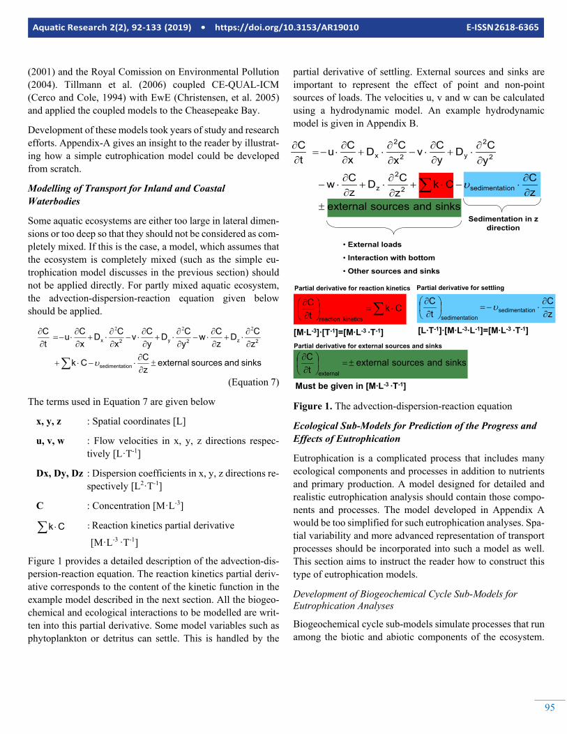
Figure 1 provides a detailed description of the advection-dis-persion-reaction equation. The reaction kinetics partial deriv-ative corresponds to the content of the kinetic function in the example model described in the next section. All the biogeo-chemical and ecological interactions to be modelled are writ-ten into this partial derivative. Some model variables such as phytoplankton or detritus can settle. This is handled by the
partial derivative of settling. External sources and sinks are important to represent the effect of point and non-point sources of loads. The velocities u, v and w can be calculated using a hydrodynamic model. An example hydrodynamic model is given in Appendix B.
Figure 1. The advection-dispersion-reaction equation
Ecological Sub-Models for Prediction of the Progress and Effects of Eutrophication
Eutrophication is a complicated process that includes many ecological components and processes in addition to nutrients and primary production. A model designed for detailed and realistic eutrophication analysis should contain those compo-nents and processes. The model developed in Appendix A would be too simplified for such eutrophication analyses. Spa-tial variability and more advanced representation of transport processes should be incorporated into such a model as well. This section aims to instruct the reader how to construct this type of eutrophication models.
Development of Biogeochemical Cycle Sub-Models for Eutrophication Analyses
Biogeochemical cycle sub-models simulate processes that run among the biotic and abiotic components of the ecosystem.
sinksandsourcesexternalzCCk
zCD
zCw
yCD
yCv
xCD
xCu
tC
ionsedimentat2
2
z
2
2
y2
2
x
±∂∂⋅−⋅+
∂∂⋅+
∂∂⋅−
∂∂⋅+
∂∂⋅−
∂∂⋅+
∂∂⋅−=
∂∂
∑ υ
Sedimentation in z direction
• External loads
• Interaction with bottom
• Other sources and sinks
∑ ⋅=
∂∂ Ck
tC
kineticsreaction
sinksandsourcesexternaltC
external±=
∂∂
zC
tC
ionsedimentationsedimentat ∂
∂⋅−=
∂∂ υ
[M∙L-3]∙[T-1]=[M∙L-3 ∙T-1] [L∙T-1]∙[M∙L-3∙L-1]=[M∙L-3 ∙T-1]
Must be given in [M∙L-3 ∙T-1]
Partial derivative for reaction kinetics Partial derivative for settling
Partial derivative for external sources and sinks
Aquatic Research 2(2), 92-133 (2019) • https://doi.org/10.3153/AR190010 E-ISSN 2618-6365
96
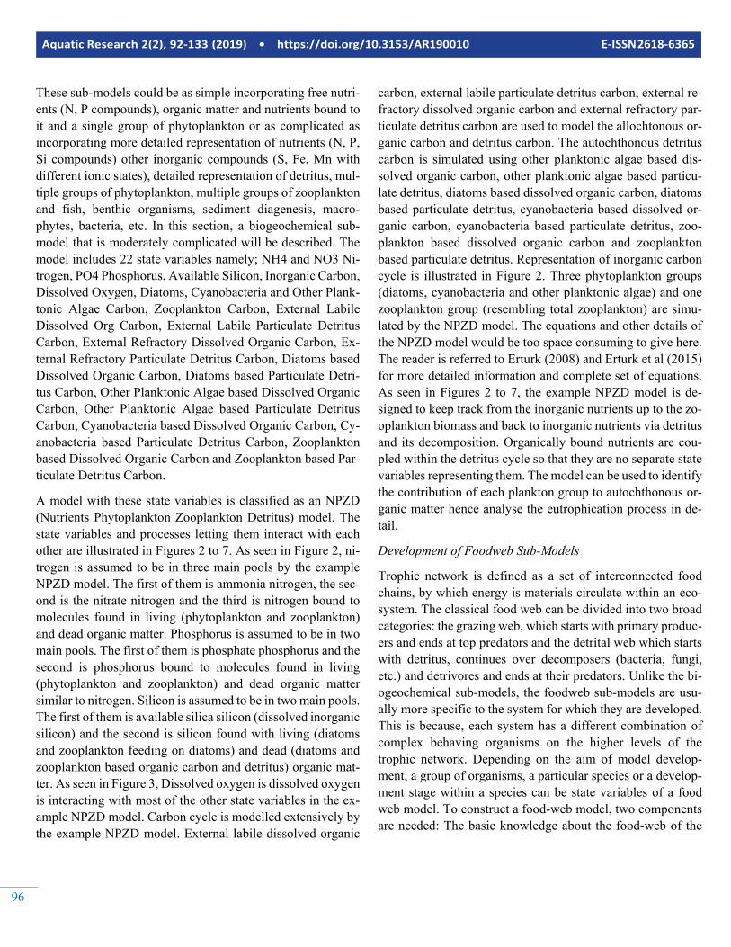
These sub-models could be as simple incorporating free nutri-ents (N, P compounds), organic matter and nutrients bound to it and a single group of phytoplankton or as complicated as incorporating more detailed representation of nutrients (N, P, Si compounds) other inorganic compounds (S, Fe, Mn with different ionic states), detailed representation of detritus, mul-tiple groups of phytoplankton, multiple groups of zooplankton and fish, benthic organisms, sediment diagenesis, macro-phytes, bacteria, etc. In this section, a biogeochemical sub-model that is moderately complicated will be described. The model includes 22 state variables namely; NH4 and NO3 Ni-trogen, PO4 Phosphorus, Available Silicon, Inorganic Carbon, Dissolved Oxygen, Diatoms, Cyanobacteria and Other Plank-tonic Algae Carbon, Zooplankton Carbon, External Labile Dissolved Org Carbon, External Labile Particulate Detritus Carbon, External Refractory Dissolved Organic Carbon, Ex-ternal Refractory Particulate Detritus Carbon, Diatoms based Dissolved Organic Carbon, Diatoms based Particulate Detri-tus Carbon, Other Planktonic Algae based Dissolved Organic Carbon, Other Planktonic Algae based Particulate Detritus Carbon, Cyanobacteria based Dissolved Organic Carbon, Cy-anobacteria based Particulate Detritus Carbon, Zooplankton based Dissolved Organic Carbon and Zooplankton based Par-ticulate Detritus Carbon.
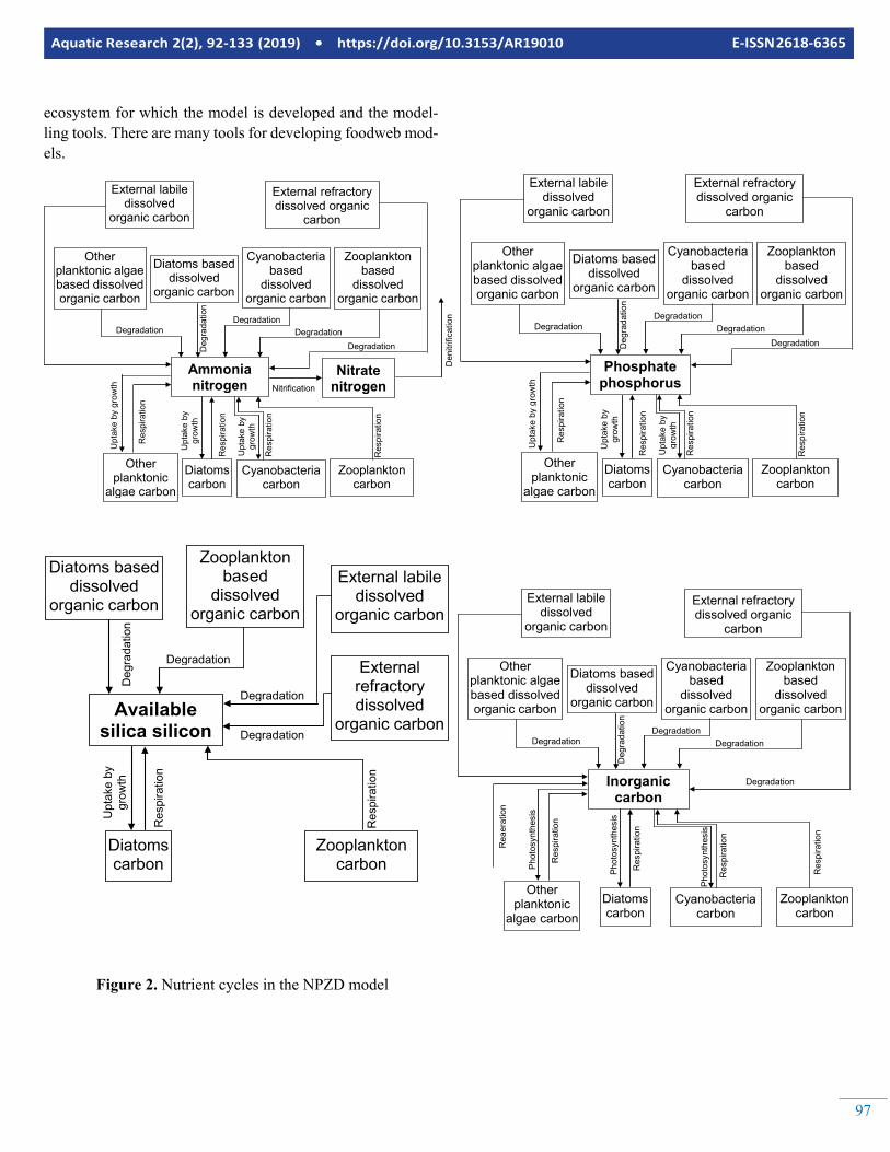
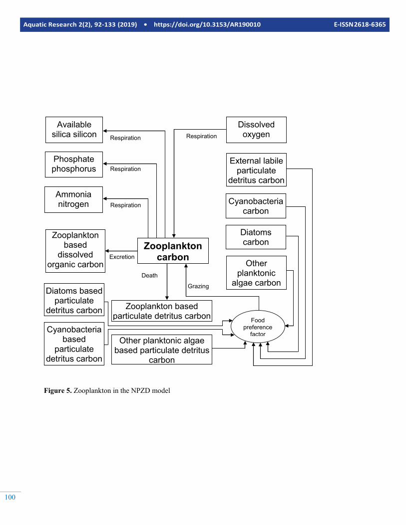
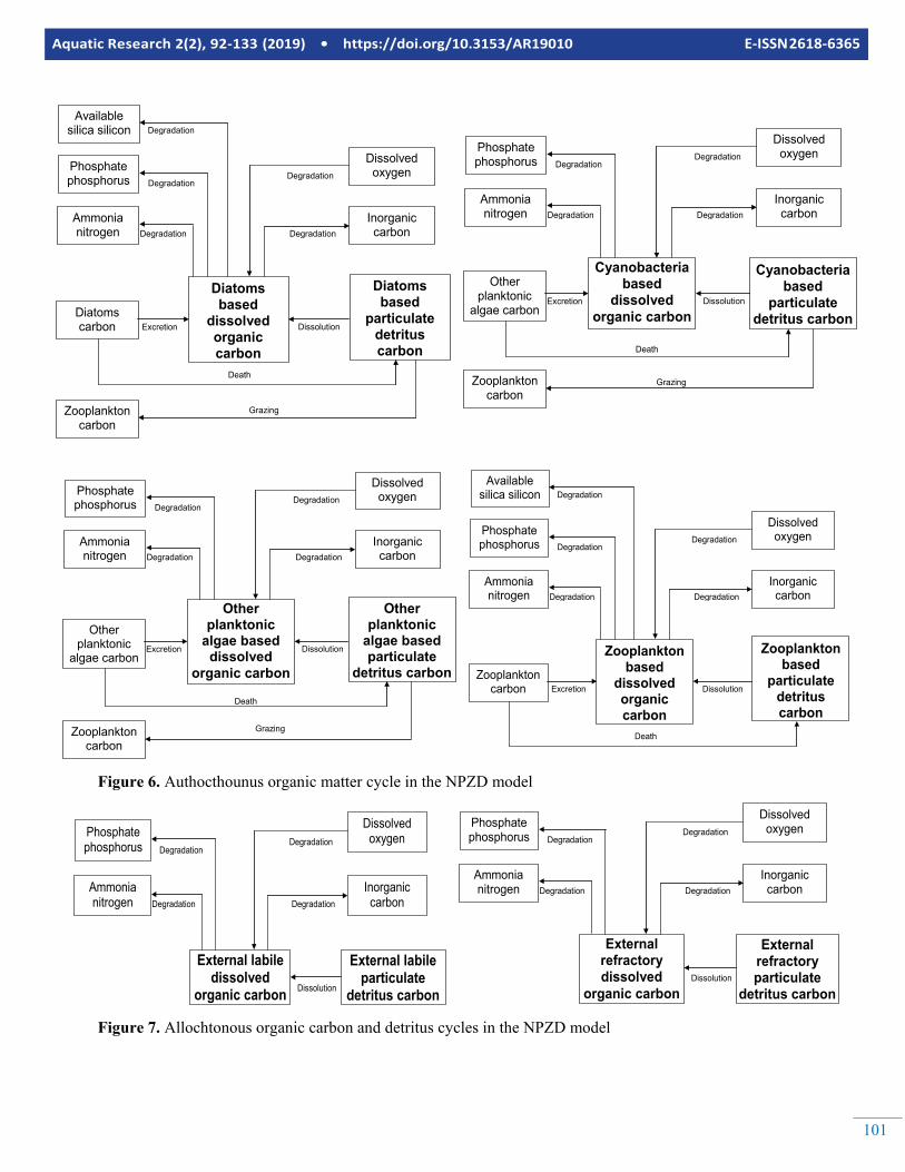
A model with these state variables is classified as an NPZD (Nutrients Phytoplankton Zooplankton Detritus) model. The state variables and processes letting them interact with each other are illustrated in Figures 2 to 7. As seen in Figure 2, ni-trogen is assumed to be in three main pools by the example NPZD model. The first of them is ammonia nitrogen, the sec-ond is the nitrate nitrogen and the third is nitrogen bound to molecules found in living (phytoplankton and zooplankton) and dead organic matter. Phosphorus is assumed to be in two main pools. The first of them is phosphate phosphorus and the second is phosphorus bound to molecules found in living (phytoplankton and zooplankton) and dead organic matter similar to nitrogen. Silicon is assumed to be in two main pools. The first of them is available silica silicon (dissolved inorganic silicon) and the second is silicon found with living (diatoms and zooplankton feeding on diatoms) and dead (diatoms and zooplankton based organic carbon and detritus) organic mat-ter. As seen in Figure 3, Dissolved oxygen is dissolved oxygen is interacting with most of the other state variables in the ex-ample NPZD model. Carbon cycle is modelled extensively by the example NPZD model. External labile dissolved organic
carbon, external labile particulate detritus carbon, external re-fractory dissolved organic carbon and external refractory par-ticulate detritus carbon are used to model the allochtonous or-ganic carbon and detritus carbon. The autochthonous detritus carbon is simulated using other planktonic algae based dis-solved organic carbon, other planktonic algae based particu-late detritus, diatoms based dissolved organic carbon, diatoms based particulate detritus, cyanobacteria based dissolved or-ganic carbon, cyanobacteria based particulate detritus, zoo-plankton based dissolved organic carbon and zooplankton based particulate detritus. Representation of inorganic carbon cycle is illustrated in Figure 2. Three phytoplankton groups (diatoms, cyanobacteria and other planktonic algae) and one zooplankton group (resembling total zooplankton) are simu-lated by the NPZD model. The equations and other details of the NPZD model would be too space consuming to give here. The reader is referred to Erturk (2008) and Erturk et al (2015) for more detailed information and complete set of equations. As seen in Figures 2 to 7, the example NPZD model is de-signed to keep track from the inorganic nutrients up to the zo-oplankton biomass and back to inorganic nutrients via detritus and its decomposition. Organically bound nutrients are cou-pled within the detritus cycle so that they are no separate state variables representing them. The model can be used to identify the contribution of each plankton group to autochthonous or-ganic matter hence analyse the eutrophication process in de-tail.
Development of Foodweb Sub-Models
Trophic network is defined as a set of interconnected food chains, by which energy is materials circulate within an eco-system. The classical food web can be divided into two broad categories: the grazing web, which starts with primary produc-ers and ends at top predators and the detrital web which starts with detritus, continues over decomposers (bacteria, fungi, etc.) and detrivores and ends at their predators. Unlike the bi-ogeochemical sub-models, the foodweb sub-models are usu-ally more specific to the system for which they are developed. This is because, each system has a different combination of complex behaving organisms on the higher levels of the trophic network. Depending on the aim of model develop-ment, a group of organisms, a particular species or a develop-ment stage within a species can be state variables of a food web model. To construct a food-web model, two components are needed: The basic knowledge about the food-web of the
97
Aquatic Research 2(2), 92-133 (2019) • https://doi.org/10.3153/AR19010 E-ISSN 2618-6365
ecosystem for which the model is developed and the model-ling tools. There are many tools for developing foodweb mod-els.
Figure 2. Nutrient cycles in the NPZD model
Ammonia nitrogen
Nitrification
Other planktonic
algae carbon
Diatoms carbon
Cyanobacteria carbon
Zooplankton carbon
Nitrate nitrogen
Res
pira
tion
Res
pira
tion
Upt
ake
by
grow
th
Upt
ake
by
grow
th
Res
pira
tion
Res
pira
tion
Upt
ake
by g
row
th
Diatoms based dissolved
organic carbon
Other planktonic algae based dissolved organic carbon
Cyanobacteria based
dissolved organic carbon
Zooplankton based
dissolved organic carbon
Degradation
Deg
rada
tion
Degradation Degradation
Den
itrifi
catio
n
External labile dissolved
organic carbon
External refractory dissolved organic
carbon
Degradation
Other planktonic
algae carbon
Phosphate phosphorus
Diatoms carbon
Cyanobacteria carbon
Zooplankton carbon
Res
pira
tion
Res
pira
tion
Upt
ake
by
grow
th
Upt
ake
by
grow
th
Res
pira
tion
Res
pira
tion
Upt
ake
by g
row
th
Diatoms based dissolved
organic carbon
Other planktonic algae based dissolved organic carbon
Cyanobacteria based
dissolved organic carbon
Zooplankton based
dissolved organic carbon
Degradation
Deg
rada
tion
Degradation Degradation
External labile dissolved
organic carbon
External refractory dissolved organic
carbon
Degradation
Available silica silicon
Diatoms carbon
Zooplankton carbon
Res
pira
tion
Upt
ake
by
grow
th
Res
pira
tion
Diatoms based dissolved
organic carbon
Zooplankton based
dissolved organic carbon
Deg
rada
tion
Degradation
External labile dissolved
organic carbon
External refractory dissolved
organic carbon
Degradation
Degradation
Inorganic carbon
Other planktonic
algae carbon Diatoms carbon
Cyanobacteria carbon
Zooplankton carbon
Phot
osyn
thes
is
Phot
osyn
thes
is
Res
pira
tion
Res
pira
tion
Res
pira
tion
Diatoms based dissolved
organic carbon
Other planktonic algae based dissolved organic carbon
Cyanobacteria based
dissolved organic carbon
Zooplankton based
dissolved organic carbon
Degradation
Deg
rada
tion
Degradation Degradation
External labile dissolved
organic carbon
External refractory dissolved organic
carbon
Degradation
Res
pira
tion
Phot
osyn
thes
is
Rea
erat
ion
Aquatic Research 2(2), 92-133 (2019) • https://doi.org/10.3153/AR190010 E-ISSN 2618-6365
98
Figure 3. Dissolved oxygen cycle
Dissolved oxygen
Nitrification
Other planktonic
algae carbon
Diatoms carbon
Cyanobacteria carbon
Zooplankton carbon
Ammonia nitrogen
Phot
osyn
thes
is
Phot
osyn
thes
is
Res
pira
tion
Res
pira
tion
Res
pira
tion
Diatoms based dissolved
organic carbon
Other planktonic algae based dissolved organic carbon
Cyanobacteria based
dissolved organic carbon
Zooplankton based
dissolved organic carbon
Degradation
Deg
rada
tion
Degradation Degradation
External labile dissolved
organic carbon
External refractory dissolved organic
carbon
Degradation
Res
pira
tion
Phot
osyn
thes
is
Rea
erat
ion
NO
3-N
upt
ake
NO
3-N
upt
ake
NO
3-N
upt
ake
Degradation
99
Aquatic Research 2(2), 92-133 (2019) • https://doi.org/10.3153/AR19010 E-ISSN 2618-6365
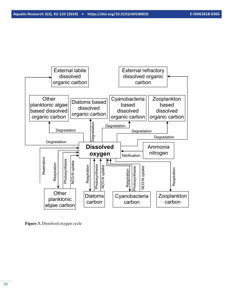
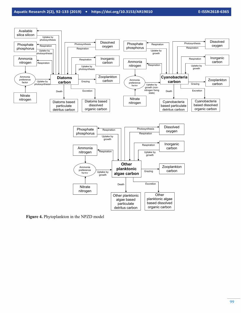
Figure 4. Phytoplankton in the NPZD model
Diatoms carbon
Zooplankton carbon Grazing
Ammonia nitrogen
Ammonia preference
factor
Phosphate phosphorus
Available silica silicon
Nitrate nitrogen
Uptake by photosynthesis
Inorganic carbon
Dissolved oxygen
Uptake by photosynthesis
Uptake by photosynthesis
Uptake by photosynthesis
Respiration
Respiration
Photosynthesis Respiration
Diatoms based particulate
detritus carbon
Death
Diatoms based dissolved
organic carbon
Excretion
Respiration
Cyanobacteria carbon
Cyanobacteria based particulate detritus carbon
Zooplankton carbon Grazing
Death
Ammonia nitrogen
Ammonia preference
factor
Phosphate phosphorus
Nitrate nitrogen
Inorganic carbon
Dissolved oxygen
Uptake by growth
Uptake by growth (non-
nitrogen fixing state)
Uptake by growth
Respiration
Respiration
Photosynthesis Respiration
Respiration
Cyanobacteria based dissolved organic carbon
Excretion
Other planktonic
algae carbon
Other planktonic algae based particulate
detritus carbon
Zooplankton carbon Grazing
Death
Ammonia nitrogen
Ammonia preference
factor
Phosphate phosphorus
Nitrate nitrogen
Inorganic carbon
Dissolved oxygen
Uptake by growth
Uptake by growth
Uptake by growth
Respiration
Respiration Photosynthesis Respiration
Respiration
Other planktonic algae based dissolved organic carbon
Excretion
Aquatic Research 2(2), 92-133 (2019) • https://doi.org/10.3153/AR190010 E-ISSN 2618-6365
100
Figure 5. Zooplankton in the NPZD model
Zooplankton carbon
Other planktonic
algae carbon Grazing
Ammonia nitrogen
Phosphate phosphorus
Available silica silicon
Diatoms carbon
Dissolved oxygen Respiration
Respiration
Zooplankton based particulate detritus carbon
Death
Zooplankton based
dissolved organic carbon
Excretion
Cyanobacteria carbon
External labile particulate
detritus carbon
Food preference
factor
Respiration
Respiration
Diatoms based particulate
detritus carbon
Cyanobacteria based
particulate detritus carbon
Other planktonic algae based particulate detritus
carbon
101
Aquatic Research 2(2), 92-133 (2019) • https://doi.org/10.3153/AR19010 E-ISSN 2618-6365
Figure 6. Authocthounus organic matter cycle in the NPZD model
Figure 7. Allochtonous organic carbon and detritus cycles in the NPZD model
Diatoms based
dissolved organic carbon
Dissolution
Ammonia nitrogen
Phosphate phosphorus
Available silica silicon
Diatoms carbon
Inorganic carbon
Dissolved oxygen
Excretion
Degradation
Degradation Degradation
Degradation
Degradation
Death
Diatoms based
particulate detritus carbon
Zooplankton carbon
Grazing
Cyanobacteria based
dissolved organic carbon
Dissolution
Ammonia nitrogen
Phosphate phosphorus
Other planktonic
algae carbon
Inorganic carbon
Dissolved oxygen
Excretion
Degradation
Degradation Degradation
Degradation
Death
Zooplankton carbon
Grazing
Cyanobacteria based
particulate detritus carbon
Other planktonic
algae based dissolved
organic carbon
Dissolution
Ammonia nitrogen
Phosphate phosphorus
Other planktonic
algae carbon
Inorganic carbon
Dissolved oxygen
Excretion
Degradation
Degradation Degradation
Degradation
Death
Zooplankton carbon
Grazing
Other planktonic
algae based particulate
detritus carbon
Zooplankton based
dissolved organic carbon
Dissolution
Ammonia nitrogen
Phosphate phosphorus
Available silica silicon
Zooplankton carbon
Inorganic carbon
Dissolved oxygen
Excretion
Degradation
Degradation Degradation
Degradation
Degradation
Death
Zooplankton based
particulate detritus carbon
External labile dissolved
organic carbon
External labile particulate
detritus carbon Dissolution
Ammonia nitrogen
Phosphate phosphorus
Inorganic carbon
Dissolved oxygen
Degradation
Degradation Degradation
Degradation
External refractory dissolved
organic carbon
External refractory particulate
detritus carbon Dissolution
Ammonia nitrogen
Phosphate phosphorus
Inorganic carbon
Dissolved oxygen
Degradation
Degradation Degradation
Degradation
Aquatic Research 2(2), 92-133 (2019) • https://doi.org/10.3153/AR190010 E-ISSN 2618-6365
102
Ecopath with Ecosim that is optimized for aqutic ecosystems will be described in this section as an example. Ecopath with Ecosim is designed for straightforward construction, parame-terization and analysis of mass-balance trophic models for various ecosystems. The core of Ecopath is derived from ECOPATH program developed by Polovnia and Ow (1983). However, Ecopath does not work under the steady state as-sumption any more. Instead, it is bases the parameterization on an assumption of mass balance of an arbitrary period (Chi-ristensen et al., 2005). This period is usually one year, but modelling an ecosystem seasonally is also possible. Ecopath allows the user to develop a generic model for any ecosystem, which can contain any number of state variables. In Ecopath terminology, a state variable is called as group or box. A box (group) in an Ecopath model can be a group of ecologically related species, a single species, or a single size/age group of given species. Since the original ECOPATH from early 1980s, Ecopath has undergone a long development process for both; the theory, ideas and as well as the software itself. The system has been optimized for direct use in fisheries assessment as well as for addressing other more general environmental ques-tions through the inclusion of the temporal dynamic model Ecosim and spatial dynamic model Ecospace. Furthermore, tools such as Ecoranger (tool for addressing uncertainty), Ecoempire (tool for calculation of empirical relationships of production over biomass ratios), Flow diagram (tool for plot-ting the defined trophic network) or Ecowrite (reporting tool) ease and enhance the model development (Christensen et al., 2005). Different versions of Ecopath with Ecosim are used for various studies with topics such as analyses of trophic interac-tions (Opiz, 1996; Okey and Pauly, 1999; Harvey et al. 2003), trophic modelling for aquatic ecosystems (Aydin et al., 2003; Mohamed et al, 2005), fisheries management and fish stock assessment (Pauly, 1998; Fayram 2005) in different aquatic ecosystems. Being applied to different aquatic ecosystems from the tropics up to Arctics, Ecopath with Ecosim is proven to be reliable. Detailed information related to methods used in,
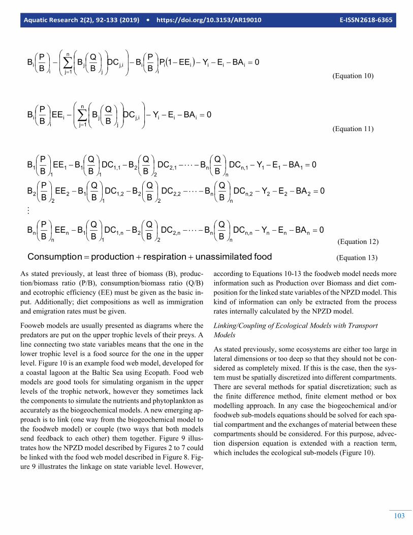
Ecopath, Ecosim and Ecospace as well as capabilities and lim-itations of these models is given by Walters et al. (1999), Wal-ters et al. (2000), Pauly et al. (2000), Christensen and Walters (2004), Kavanagah et al. (2004) and Christensen et al., (2005). Ecopath has two master equations. The first equation de-scribes the production and second equation describes the en-ergy balance for each modelled group the energy balance via consumption. The first master equation of Ecopath (Equation 8) describes how the production term for each group modelled can be split into components.
In mathematical terms, the first master equation is written as in Equation 9, where i is the index for the relevant group, Pi is the total production rate of group i, Yi is the total fishery catch rate of group i, M2i is the total predation rate for group i, Bi
the biomass of the group i, Ei the net migration rate (emigra-tion – immigration), BAi is the biomass accumulation rate for group i, while M0i = Pi (1-EEi) is the ‘other mortality’ rate for group i and EEi is the ecotrophic efficiency of group i. Equa-tion 9 can be rearranged as Equation 10 and rewritten as Equa-tion 11.
In Equation 11; j is the index for prey, P/Bi is the produc-tion/biomass ratio, Q/Bi is the consumption/biomass ratio and DCj,i is the fraction of prey j in the average diet of predator i (diet composition). A system of n linear equations (Equation 12) is obtained from Equation 12 for a trophic system with n groups.
Ecopath includes algorithms to solve this system of linear equation for one of following variables for each group: bio-mass (B), production/biomass ratio (P/B), consumption/bio-mass ratio (Q/B) or ecotrophic efficiency (EE). The energy in-put and output of all living groups must be balanced in a model. When balancing the energy for a living group addi-tional terms, which do not exist in the first master equation, are needed and with their incorporation, the second master equation of Ecopath (Equation 13) is formed.
(Equation 8)
(Equation 9)
mortality other migration net onaccumulati biomass predationby mortality catches Production
++++=
( )iiiiiiii EE1P BA E M2B Y P −++++=
103
Aquatic Research 2(2), 92-133 (2019) • https://doi.org/10.3153/AR19010 E-ISSN 2618-6365
(Equation 10)
(Equation 11)
(Equation 12)
food tedunassimila nrespiratio production nConsumptio ++= (Equation 13)
As stated previously, at least three of biomass (B), produc-tion/biomass ratio (P/B), consumption/biomass ratio (Q/B) and ecotrophic efficiency (EE) must be given as the basic in-put. Additionally; diet compositions as well as immigration and emigration rates must be given.
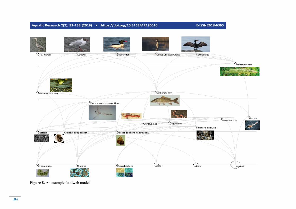
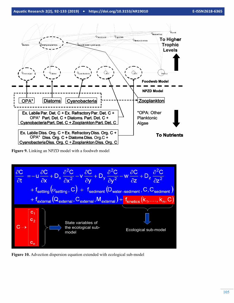
Fooweb models are usually presented as diagrams where the predators are put on the upper trophic levels of their preys. A line connecting two state variables means that the one in the lower trophic level is a food source for the one in the upper level. Figure 10 is an example food web model, developed for a coastal lagoon at the Baltic Sea using Ecopath. Food web models are good tools for simulating organism in the upper levels of the trophic network, however they sometimes lack the components to simulate the nutrients and phytoplankton as accurately as the biogeochemical models. A new emerging ap-proach is to link (one way from the biogeochemical model to the foodweb model) or couple (two ways that both models send feedback to each other) them together. Figure 9 illus-trates how the NPZD model described by Figures 2 to 7 could be linked with the food web model described in Figure 8. Fig-ure 9 illustrates the linkage on state variable level. However,
according to Equations 10-13 the foodweb model needs more information such as Production over Biomass and diet com-position for the linked state variables of the NPZD model. This kind of information can only be extracted from the process rates internally calculated by the NPZD model.
Linking/Coupling of Ecological Models with Transport Models
As stated previously, some ecosystems are either too large in lateral dimensions or too deep so that they should not be con-sidered as completely mixed. If this is the case, then the sys-tem must be spatially discretized into different compartments. There are several methods for spatial discretization; such as the finite difference method, finite element method or box modelling approach. In any case the biogeochemical and/or foodweb sub-models equations should be solved for each spa-tial compartment and the exchanges of material between these compartments should be considered. For this purpose, advec-tion dispersion equation is extended with a reaction term, which includes the ecological sub-models (Figure 10).
( ) 0BA E YEE1PBPBDC
BQB
BPB iiiii
ii
n
1jij,
jj
ii =−−−−
−
−
∑
=
0BA E YDCBQB EE
BPB iii
n
1jij,
jji
ii =−−−
−
∑
=
0BA E YDCBQBDC
BQBDC
BQB EE
BPB
0BA E YDCBQBDC
BQBDC
BQB EE
BPB
0BA E YDCBQBDC
BQBDC
BQB EE
BPB
nnnnn,n
nn2,2
2n1,1
1nn
n
222n,2n
n2,22
21,21
122
2
111n,1n
n2,12
21,11
111
1
=−−−
−⋅⋅⋅−
−
−
=−−−
−⋅⋅⋅−
−
−
=−−−
−⋅⋅⋅−
−
−
Aquatic Research 2(2), 92-133 (2019) • https://doi.org/10.3153/AR190010 E-ISSN 2618-6365
104
Figure 8. An example foodweb model
105
Aquatic Research 2(2), 92-133 (2019) • https://doi.org/10.3153/AR19010 E-ISSN 2618-6365
Figure 9. Linking an NPZD model with a foodweb model
Figure 10. Advection dispersion equation extended with ecological sub-model
Cyanobacteria Diss. Org. C + Zooplankton Diss. Org. CCyanobacteria Diss. Org. C + Zooplankton Diss. Org. C
OPA* Diatoms Cyanobacteria
Ex. Labile Par. Det. C + Ex. Refractory Par. Det. C +Part. Det. C + Diatoms. Part. Det. C +
Cyanobacteria Part. Det. C + Zooplankton Part. Det. C
Ex. Labile Diss. Org. C + Ex. Refractory Diss. Org. C +OPA* Diss. Org. C + Diatoms Diss. C +
Zooplankton
To Nutrients
To Higher Trophic Levels
*OPA: OtherPlanktonic Algae
Diatoms Cyanobacteria
Ex. Labile Par. Det. C + Ex. Refractory Par. Det. C +OPA* Part. Det. C + Diatoms. Part. Det. C +
Cyanobacteria Part. Det. C + Zooplankton Part. Det. C
Ex. Labile Diss. Org. C + Ex. Refractory Diss. Org. C +Diss. Org. C + Diatoms Diss. Org.
Zooplankton
NPZD Model
Foodweb Model
To Nutrients
To Higher Trophic Levels
State variables of the ecological sub-model Ecological sub-model
Aquatic Research 2(2), 92-133 (2019) • https://doi.org/10.3153/AR190010 E-ISSN 2618-6365
106
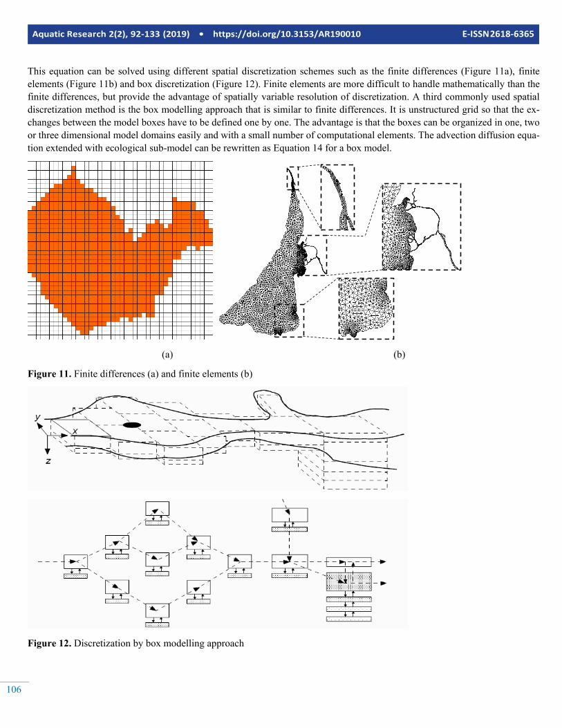
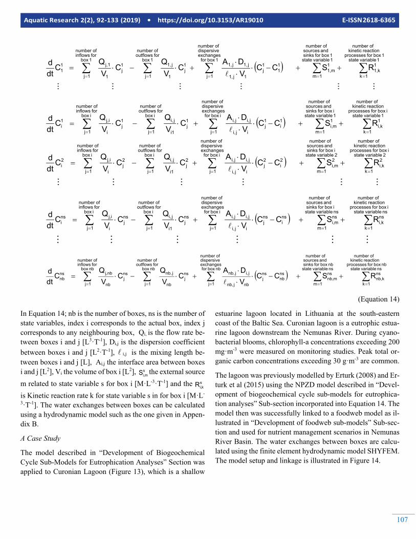
This equation can be solved using different spatial discretization schemes such as the finite differences (Figure 11a), finite elements (Figure 11b) and box discretization (Figure 12). Finite elements are more difficult to handle mathematically than the finite differences, but provide the advantage of spatially variable resolution of discretization. A third commonly used spatial discretization method is the box modelling approach that is similar to finite differences. It is unstructured grid so that the ex-changes between the model boxes have to be defined one by one. The advantage is that the boxes can be organized in one, two or three dimensional model domains easily and with a small number of computational elements. The advection diffusion equa-tion extended with ecological sub-model can be rewritten as Equation 14 for a box model.
(a) (b)
Figure 11. Finite differences (a) and finite elements (b)
Figure 12. Discretization by box modelling approach
107
Aquatic Research 2(2), 92-133 (2019) • https://doi.org/10.3153/AR19010 E-ISSN 2618-6365
( ) ∑∑∑∑∑=====
++−⋅⋅⋅
+⋅−⋅=1 variable state
1box for processes reactionkinetic
of number
1k
1k1,
1 variable state1box for sinks
and sources of number
1m
1m1,
1box for exchangesdispersive
of number
1j
11
1j
1j1,
j1,j1,1box
for outflowsof number
1j
1j
1
j1,1box for inflowsof number
1j
1j
1
j,111 RSCC
VDA
CV
QC
VQ
Cdtd
( ) ∑∑∑∑∑=====
++−⋅⋅⋅
+⋅−⋅=1 variable state
ibox for processes reactionkinetic
of number
1k
1ki,
1 variable stateibox for sinks
and sources of number
1m
1mi,
ibox for exchangesdispersive
of number
1j
1i
1j
iji,
ji,ji,ibox
for outflowsof number
1j
1j
i1
ji,ibox for inflowsof number
1j
1j
i
ij,1i RSCC
VDA
CVQ
CV
QC
dtd
( ) ∑∑∑∑∑=====
++−⋅⋅⋅
+⋅−⋅=2 variable state
ibox for processes reactionkinetic
of number
1k
2ki,
2 variable stateibox for sinks
and sources of number
1m
2mi,
ibox for exchangesdispersive
of number
1j
2i
2j
iji,
ji,ji,ibox
for outflowsof number
1j
2j
i1
ji,ibox for inflowsof number
1j
2j
i
ij,2i RSCC
VDA
CVQ
CV
QC
dtd
( ) ∑∑∑∑∑=====
++−⋅⋅⋅
+⋅−⋅=ns variable state
ibox for processes reactionkinetic
of number
1k
nski,
ns variable stateibox for sinks
and sources of number
1m
nsmi,
ibox for exchangesdispersive
of number
1j
nsi
nsj
iji,
ji,ji,ibox
for outflowsof number
1j
nsj
i1
ji,ibox for inflowsof number
1j
nsj
i
ij,nsi RSCC
VDA
CVQ
CV
QC
dtd
( ) ∑∑∑∑∑=====
++−⋅⋅
⋅+⋅−⋅=
ns variable state nbbox for processes
reactionkinetic of number
1k
nsknb,
ns variable statenbbox for sinks
and sources of number
1m
nsmnb,
nbbox for exchangesdispersive
of number
1j
nsnb
nsj
nbjnb,
ji,jnb,nbbox
for outflowsof number
1j
nsj
nb
jnb,nbbox
for inflowsof number
1j
nsj
nb
nbj,nsnb RSCC
VDA
CV
QC
VQ
Cdtd
(Equation 14)
In Equation 14; nb is the number of boxes, ns is the number of state variables, index i corresponds to the actual box, index j corresponds to any neighbouring box, Qi, is the flow rate be-tween boxes i and j [L3·T-1], Di,j is the dispersion coefficient between boxes i and j [L2·T-1], i,j is the mixing length be-tween boxes i and j [L], Ai,j the interface area between boxes i and j [L2], Vi the volume of box i [L2], s
mi,S the external source m related to state variable s for box i [M·L-3·T-1] and the s
ki,R is Kinetic reaction rate k for state variable s in for box i [M·L-
3·T-1]. The water exchanges between boxes can be calculated using a hydrodynamic model such as the one given in Appen-dix B.
A Case Study
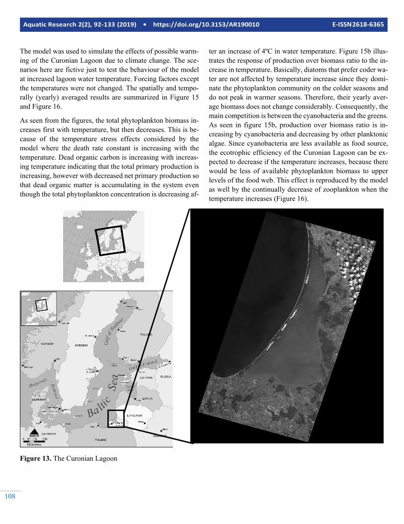
The model described in “Development of Biogeochemical Cycle Sub-Models for Eutrophication Analyses” Section was applied to Curonian Lagoon (Figure 13), which is a shallow
estuarine lagoon located in Lithuania at the south-eastern coast of the Baltic Sea. Curonian lagoon is a eutrophic estua-rine lagoon downstream the Nemunas River. During cyano-bacterial blooms, chlorophyll-a concentrations exceeding 200 mg·m-3 were measured on monitoring studies. Peak total or-ganic carbon concentrations exceeding 30 g·m-3 are common.
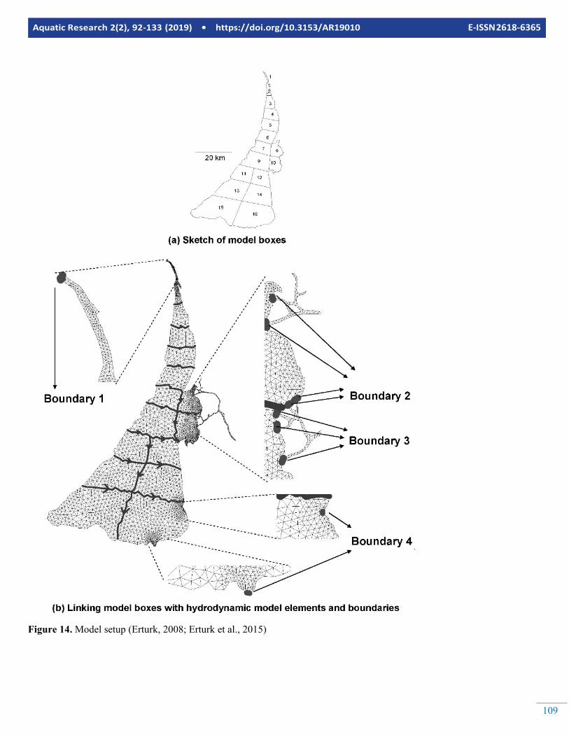
The lagoon was previously modelled by Erturk (2008) and Er-turk et al (2015) using the NPZD model described in “Devel-opment of biogeochemical cycle sub-models for eutrophica-tion analyses” Sub-section incorporated into Equation 14. The model then was successfully linked to a foodweb model as il-lustrated in “Development of foodweb sub-models” Sub-sec-tion and used for nutrient management scenarios in Nemunas River Basin. The water exchanges between boxes are calcu-lated using the finite element hydrodynamic model SHYFEM. The model setup and linkage is illustrated in Figure 14.
Aquatic Research 2(2), 92-133 (2019) • https://doi.org/10.3153/AR190010 E-ISSN 2618-6365
108
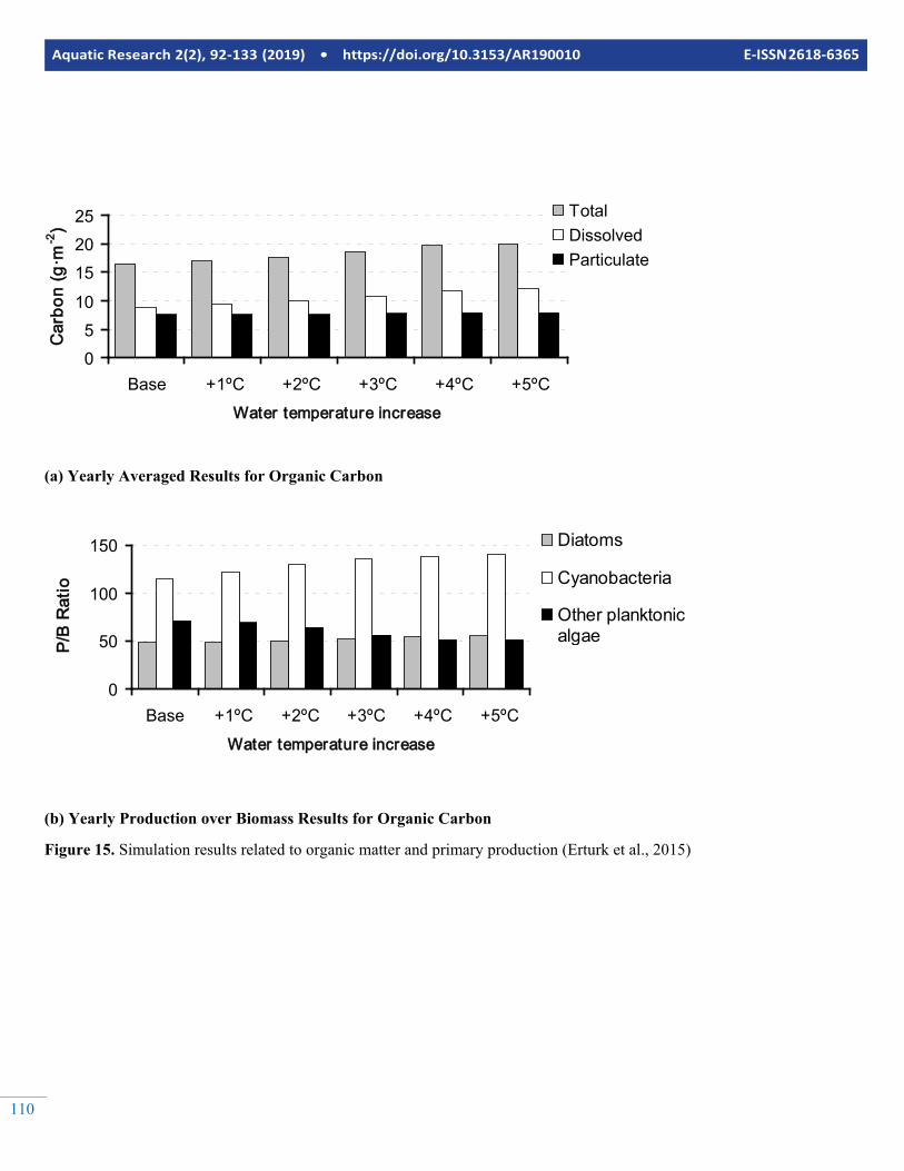
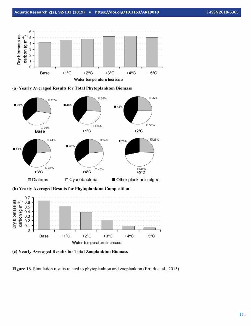
The model was used to simulate the effects of possible warm-ing of the Curonian Lagoon due to climate change. The sce-narios here are fictive just to test the behaviour of the model at increased lagoon water temperature. Forcing factors except the temperatures were not changed. The spatially and tempo-rally (yearly) averaged results are summarized in Figure 15 and Figure 16.
As seen from the figures, the total phytoplankton biomass in-creases first with temperature, but then decreases. This is be-cause of the temperature stress effects considered by the model where the death rate constant is increasing with the temperature. Dead organic carbon is increasing with increas-ing temperature indicating that the total primary production is increasing, however with decreased net primary production so that dead organic matter is accumulating in the system even though the total phytoplankton concentration is decreasing af-
ter an increase of 4ºC in water temperature. Figure 15b illus-trates the response of production over biomass ratio to the in-crease in temperature. Basically, diatoms that prefer coder wa-ter are not affected by temperature increase since they domi-nate the phytoplankton community on the colder seasons and do not peak in warmer seasons. Therefore, their yearly aver-age biomass does not change considerably. Consequently, the main competition is between the cyanobacteria and the greens. As seen in figure 15b, production over biomass ratio is in-creasing by cyanobacteria and decreasing by other planktonic algae. Since cyanobacteria are less available as food source, the ecotrophic efficiency of the Curonian Lagoon can be ex-pected to decrease if the temperature increases, because there would be less of available phytoplankton biomass to upper levels of the food web. This effect is reproduced by the model as well by the continually decrease of zooplankton when the temperature increases (Figure 16).
Figure 13. The Curonian Lagoon
109
Aquatic Research 2(2), 92-133 (2019) • https://doi.org/10.3153/AR19010 E-ISSN 2618-6365
Figure 14. Model setup (Erturk, 2008; Erturk et al., 2015)
Aquatic Research 2(2), 92-133 (2019) • https://doi.org/10.3153/AR190010 E-ISSN 2618-6365
110
(a) Yearly Averaged Results for Organic Carbon
(b) Yearly Production over Biomass Results for Organic Carbon
Figure 15. Simulation results related to organic matter and primary production (Erturk et al., 2015)
05
10
152025
Base +1ºC +2ºC +3ºC +4ºC +5ºCWater temperature increase
Car
bon
(g·m
-2)
TotalDissolvedParticulate
0
50
100
150
Base +1ºC +2ºC +3ºC +4ºC +5ºCWater temperature increase
P/B
Rat
io
Diatoms
Cyanobacteria
Other planktonicalgae
111
Aquatic Research 2(2), 92-133 (2019) • https://doi.org/10.3153/AR19010 E-ISSN 2618-6365
(a) Yearly Averaged Results for Total Phytoplankton Biomass
(b) Yearly Averaged Results for Phytoplankton Composition
(c) Yearly Averaged Results for Total Zooplankton Biomass
Figure 16. Simulation results related to phytoplankton and zooplankton (Erturk et al., 2015)
0123456
Base +1ºC +2ºC +3ºC +4ºC +5ºCWater temperature increase
Dry
bio
mas
s as
ca
rbon
(g·m
-2)
28%
36%
36%
Diatoms
Base
26%
34%
40%
+1ºC
25%
33%
42%
+2ºC
24%
35%
41%
+3ºC
Cyanobacteria
Other planktonic algea
24%
40%
36%
+4ºC
25%
47%
28%
+5ºC
00.10.20.30.40.50.60.7
Base +1ºC +2ºC +3ºC +4ºC +5ºCWater temperature increase
Dry
bio
mas
s as
ca
rbon
(g·m
-2)
Aquatic Research 2(2), 92-133 (2019) • https://doi.org/10.3153/AR190010 E-ISSN 2618-6365
112
Conclusions
Eutrophication is a complicated process and its predictive modelling may involve many tools applied in an interdiscipli-nary manner. Such a modelling effort could seem overwhelm-ing for many researchers new to the topic. This paper however shows that building such models even from scratch is really not “rocket science” and most of the aquatic scientists already have the necessary mathematical background.
Once a simple model such as the one illustrated in Appendix A, it is quite easy to extend it into more comprehensive frame-works, such as a combined ecological model linked to higher trophic compartments as described in “Ecological Sub-Mod-els for Prediction of the Progress and Effects of Eutrophica-tion” Section.
Mathematical models are not only useful to predict the pro-gress of eutrophication but they are also valuable tools for sys-tem identification. The model presented in “Development of Foodweb Sub-Models” Section is such an example, where in internals such as ecotrophic efficiency of the foodweb is esti-mated rather than the biomasses of individual trophic com-partments.
Compliance with Ethical Standard
Conflict of interests: The authors declare that for this article they have no actual, potential or perceived conflict of interests.
References Ambrose, B, Jr., Wool, T.A. Martin, J.L. (1993). The Water
Quality Analysis Simulation Program, WASP5; Part A: Model Documentation, U.S. Environmental Protection Agency, Center for Exposure Assessment Modeling, Athens, GA.,
Arhonditsis, G. B., Brett, M. T. (2004). Evaluation of the cur-
rent state of mechanistic aquatic biogeochemical model-ling. Marine Ecology Progress Series, 271, 13-26.
Aydin, K.Y., McFarlane, G.A., King, J.R., Megrey, B.A.
(2003). The BASS/MODEL Report on Trophic Models of the Subarctic Pacific Basin Ecosystems, PICES Scien-tific Report No. 25, https://www.pices.int/publica-tions/scientific_reports/Report25/default.aspx, (accessed 8.4.2019).
Bartsch, A.F., Gakstatter, J.H. (1978). Management Decision for Lake Systems on a Survey of Trophic Status, Limiting Nutrients, and Nutrient Loadings, American-Soviet Symposium on Use of Mathematical Models to Optimize Water Quality Management, 1975, U.S. Environmental Protection Agency Office of Research and Development, Environmental Research Laboratory, Gulf Breeze, FL, pp 372-394, EPA-600/9-78-024
Bloesch, J, Stadelmann, P., Bührer, H. (1977). Primary pro-
duction, mineralization and sedimentation in the euphotic zone of two swiss lakes. Limnology and Oceanography, 22(3), 511-526.
Cerco, C.F., Cole, T. (1994). Three Dimensional Eutrophica-
tion Model of Chesapeake Bay; Volume 1, Main Report, Technical Report EL 94-4, U.S. Army Corps of Engi-neers Waterways Experiment Station, Vicksburg, MS.
Cerco, C.F., Cole, T. (1995). User’s Guide to the CE-QUAL-
ICM Three Dimensional Eutrophicaiton Model, Release Version 1.0. Technical Report EL-95-15, US Army Corps of Engineers Waterways Experiment Station, Vicksburg, MS.
Chapra, S.C. (1997). Surface Water-Quality Modeling, WCB
McGraw-Hill Publisher, ISBN 0-07-024186-4 Christensen, V., Walters, C.J. (2004). Ecopath with ecosim:
methods capabilities and limitations. Ecological Model-ling, 172, 109-139.
Christensen, V., Walters, C.J., Pauly, D. (2005). Ecopath with
Ecosim: A User’s Guide, Fisheries Centre University of British Columbia Vancouver, Canada.
Cole, T.M., Wells, S.A. (2006). CE-QUAL-W2 A Two dimen-
sional, Laterally Averaged Hydrodynamic and Water Quality Model, Version 3.5, Instruction Report EL-2006-1, U.S. Army Engineering and Research Development Center, Vicksburg, MS.
Dillon, P.J., Rigler, F.H. (1974). The phosphorus-chlorophyll
relationship for lakes. Limnology and Oceanograpgy, 19, 767-773.
113
Aquatic Research 2(2), 92-133 (2019) • https://doi.org/10.3153/AR19010 E-ISSN 2618-6365
Di Toro, D.M., O’Connor, D.L., Thomann, R.V. (1971). A Dy-namic Model of the Phytoplankton Population in the Sac-ramento-San Joaquin Delta. Advances in Chemistry Se-ries 106, Nonequilibrium Systems in Natural Water Chemistry, 131.
Di Toro, D.M., Connolly, J.P. (1980). Mathematical Models
of Large Lakes, Part 2. Ontario Lake. National Environ-mental Research Center, Office of Research and Devel-opment, U.S. Environmental Protection Agency, Ecolog-ical Research Series, EPA-600/3-80-065.
Di Toro, D.M., Fitzpatrick, J.J., Thomann, R.V. (1983). Water
Quality Analysis Simulation Program (WASP) and Model Verification Program (MVP) – Documentation. Contract No 68-01-3872, Hydroscience, Inc., USA.
Di Toro, D.M., Fitzpatrick, J.J. (1993). Chesapeake Bay Sed-
iment Flux Model. Contract Report EL-93-2, Environ-mental Laboratory U.S. Army Engineer Waterways Ex-periment Station.
Edmonson, W.T. (1979). Phosphorus, nitrogen and algae in
lake washington after diversion of sewage. Science, 169, 690-691.
Environmental Laboratory, (1995). CE-QUAL-R1: A Numer-
ical One Dimensional Model of Reservoir Water Quality; User’s Manual. Instruction Report E-82-1, Rev. Ed., US Army Engineer Waterways Experiment Station, Vicks-burg MS.
Erturk, A. (2008). Modelling the Response of an Estuarine La-
goon to External Nutrient Inputs. Dissertation, Klaipeda University.
Erturk, A., Razinkovas-Baziukas, A., Zemlys, P., Umgiesser,
G. (2015). Linking carbon-nitrogen-phosphorus cycle and foodweb models of an estuarine lagoon ecosystem. Computational Science and Tecniques, 3(1), 350-412.
Fayram, A.H. (2005). Walleye Stocking in Wisconsin Lakes:
Species Interactions, Changes in Angler Effort, Optimal
Stocking Rates and Effects on Community Maturity, Dis-sertation in Biological Sciences at the University of Wis-consin, Milwaukee, USA.
Gamito, S., Erzini, K. (2005). Trophic food web and ecosys-
tem attributes of a water reservoir of the Ria Formosa (south portugal), Ecological Modelling, 181, 509-520.
Hamrick, J.M. (1996). User’s Manual for the Environmental
Fluid Dynamics Computer Code, Special Report No. 331 in Applied Marine Science and Ocean Engineering Vir-ginia Institute of Marine Science School of Marine Sci-ence, The College of William and Mary Gloucester Point, VA 23062.
Harvey, C.J., Cox, S.P., Essington, T.E., Hansson, S, Kitchell,
J.F. (2003). An ecosystem model of food web and fisher-ies interactions in the Baltic Sea. ICES Journal of Marine Science, 60, 939-950.
HEC (1978). Generalized Computer Program, Water Quality
for River-Reservoir Systems, The Hydrologic Engineer-ing Center, United States Army Corps of Engineers.
Hossenipour, E.Z., Martin J.L. (1990). The One-Dimensional
Riverline Hydrodynamic Model, RIVMOD-H Model Documentation and User’s Manual, Environmental La-boratory Office of Research and Development USEPA Athens, Georgia 30605-2700.
Hull, V., Mocenni, C., Falcucci, M., Marchettini, N. (2000).
A trophodynamic model for the lagoon of Fogliano (It-aly) with ecological dependent modifying parameters. Ecological Modelling, 134, 153-167.
Kavanagah, P., Newlands, N., Christensen, V., Pauly, D.
(2004). Automated parameter optimization for ecopath ecosystem models. Ecological Modelling, 172, 141-149.
Luyten, P.J., Jones, J.H., Proctor, R., Tabor, A., Tett, P., Wild-
Allen, K. (1999). COHERENS – A Coupled Hydrody-namical – Ecological Model for Regional and Shelf Seas: User Documentation. MUMM Report, Management Unit of the Mathematical Models of the North Sea.
Aquatic Research 2(2), 92-133 (2019) • https://doi.org/10.3153/AR190010 E-ISSN 2618-6365
114
Megrey, B.A., Taft, B.A., Peterson, W.T. (Eds.) (2001). PICES-GLOBEC International Program on Climate Change and Carrying Capacity. Report of the 2000 BASS, MODEL, MONITOR and REX Workshops, and the 2001 BASS/MODEL Workshop. PICES Sci. Rep. No. 17.
Mohamed, K.S., Zacharia, P.U., Muthiah, C., Abdurahiman,
K.P., Nayak, T.H. (2005). A Trophic Model of the Ara-bian Sea Ecosystem off Karnataka and Simulation of Fishery Yields for its Multigear Marine Fisheries. Re-search Centre of Central Marine Fisheries Research In-stitute, Karnataka, India.
O’Connor D. J., John, P. St., Di Toro, M. (1968). Water qual-
ity analyses of the Delaware River Estuary. Journal of the Sanitary Engineering Division, 94(SA6), 1225-1252.
Okey, T.A., Pauly, D.A. (1999). Mass-Balanced Model of
Trophic Flows in Prince William Sound: Decompart-mentalizing Ecosystem Knowledge. Ecosystem for Fish-eries Management, Alaska Sea Grant College Program, AL-SG-99-01, pp 621-635.
Opiz, S. (1996). Trophic Interactions in Caribbean Coral
Reefs, International Center for Living Aquatic Resources, Makati City, Philippines.
Pauly, D. (1998). Use Ecopath with Ecosim to Evaluate Strat-
egies for Sustainable Exploitation of Multi-Species Re-sources: Proceedings of a Workshop held at the Fisheries Centre of University of British Columbia, Vancouver, B.C., Canada, edited by Pauly, D., Fisheries Centre Re-search Reports, Volume 6(2), ISSN 1198-6727
Pauly, D., Christensen, V., Walters, C. (2000). Ecopath eco-
sim and ecospace as tools for evaluating ecosystem im-pacts of fisheries. ICES Journal of Marine Science, 57, 1-10.
Polovina, J.J., Ow, M.D. (1983). ECOPATH: A user’s manual
and program listings, Administrative report, H-83-23, Sothwest Fisheries Center, Honolulu Laboratory, Hono-lulu, Hawaii, USA.
Rast, W., Lee, G.F. (1978). Summary Analyses of the North American Project (US Portion) OECD Eutrophication Project: Nutrient Loading-Lake Response Relationships and Trophic State Indices, USEPA Corvallis Environ-mental Research Laboratory, Corvallis, OR, EPA-600/3-78-008.
Royal Comission on Environmental Pollution, (2004). Turn-
ing the Tide: Addressing the Impact of Fisheries on the Marine Environment, 25th Repot, Chairman: Tom Blun-dell, FMedSci.
Sheng, Y.G. Eliason, D.E., Chen, X.J., Choi, J.K. (1991). A
Three Dimensional Numerical Model of Hydrodynamics and Sediment Transport in Lakes and Estuaries: Theory, Model Development and Documentation. USEPA Ath-ens, GA, USA.
Smith, V.H., Shapiro, J. (1981). A Retroperspective Look at
the Effects of Phosphorus Removal in Lakes, in Restora-tion of Lakes and Inland Waters. USEPA, Office of Wa-ter Regulations and Standards, Washington, DC. EPA-440/5-81-010.
Thomann, R.V. Di Toro, D.M., Winfield, R.P. O’Connor,
D.O. (1975). Mathematical Modeling of Phytoplankton in Lake Ontario, 1. Model Development and Verification, National Environmental Research Center, Offıce of Re-search and Development, USEPA, Ecological Research Series, EPA-660/3-75-005.
Thomann, R.V., Mueller, J.A., (1987). Principles of Surface
Water Quality Modeling and Control, Harper Collins Publishers Inc., USA.
Tillman, D.H., Cerco, C.F., Noel, M.R. (2006). Conceptual
Processes for Linking Eutrophication and Network Mod-els. ERDC TN-SWWRP-06-9, United States Army Corps of Engineers.
USEPA, (2000). Estuarine and coastal marine waters: Bio-
assessment and biocriteria technical guidance. USEPA Report EPA-822-B00-024, Washington, DC.
115
Aquatic Research 2(2), 92-133 (2019) • https://doi.org/10.3153/AR19010 E-ISSN 2618-6365
Villanueva, M.C. Laleyeb, P., Albaret J.J., Lae, R., de Mo-raise, L. Tito, Moreaua J. (2006). Comparative analysis of trophic structure and interactions of two tropical la-goons. Ecological Modelling, 197, 461-477.
Walters, C., Pauly, D., Christensen, V. (1999). Ecospace: pre-diction of mesoscale spatial patterns in trophic relation-ships of exploited ecosystems with emphasis on the im-pact of marine protected areas. Ecosystems (1999)2, 539-554.
Walters, C., Pauly, D., Christensen, V., Kitchell, J.F. (2000). Representing density dependent consequences of life his-tory strategies in aquatic ecosystems: Ecosim II. Ecosys-tems (2000)3, pp 70-83.
Wool, T.A., Ambrose, R.B.Jr., Martin, J.L., Comer, E.A. 2001. The Water Quality Analysis Simulation Program, WASP USEPA, Centre for Exposure Assessment Model-ing, Athens, GA.
Aquatic Research 2(2), 92-133 (2019) • https://doi.org/10.3153/AR190010 E-ISSN 2618-6365
116
APPENDIX A Development and Implementation of Simplified Eutrophication Modelling Tools from Scratch
The aim of this section is to illustrate the reader how to de-velop own modelling tools that can simulate the progress of the eutrophication process on simple but complete examples. Before starting to read this section, be advised that the devel-opment of an eutrophication model from scratch is not a sim-ple process and consists of several tasks listed below:
• Development of a conceptual model• Writing the equations that form the mathematical con-
struct of the model• Development of solution schemes for the equations• Implementation of the model as a tool• Development of the supporting environment and tools
for the model
A.1. Development of a conceptual model
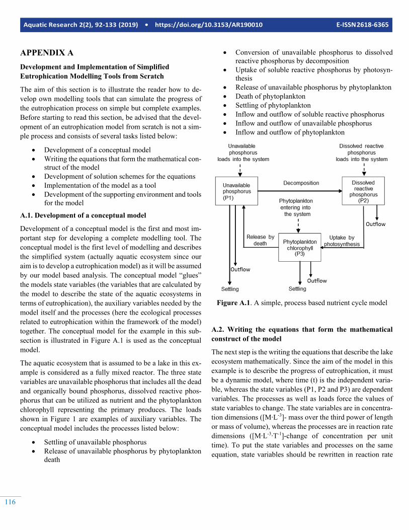
Development of a conceptual model is the first and most im-portant step for developing a complete modelling tool. The conceptual model is the first level of modelling and describes the simplified system (actually aquatic ecosystem since our aim is to develop a eutrophication model) as it will be assumed by our model based analysis. The conceptual model “glues” the models state variables (the variables that are calculated by the model to describe the state of the aquatic ecosystems in terms of eutrophication), the auxiliary variables needed by the model itself and the processes (here the ecological processes related to eutrophication within the framework of the model) together. The conceptual model for the example in this sub-section is illustrated in Figure A.1 is used as the conceptual model.
The aquatic ecosystem that is assumed to be a lake in this ex-ample is considered as a fully mixed reactor. The three state variables are unavailable phosphorus that includes all the dead and organically bound phosphorus, dissolved reactive phos-phorus that can be utilized as nutrient and the phytoplankton chlorophyll representing the primary produces. The loads shown in Figure 1 are examples of auxiliary variables. The conceptual model includes the processes listed below:
• Settling of unavailable phosphorus• Release of unavailable phosphorus by phytoplankton
death
• Conversion of unavailable phosphorus to dissolvedreactive phosphorus by decomposition
• Uptake of soluble reactive phosphorus by photosyn-thesis
• Release of unavailable phosphorus by phytoplankton• Death of phytoplankton• Settling of phytoplankton• Inflow and outflow of soluble reactive phosphorus• Inflow and outflow of unavailable phosphorus• Inflow and outflow of phytoplankton
Figure A.1. A simple, process based nutrient cycle model
A.2. Writing the equations that form the mathematicalconstruct of the model
The next step is the writing the equations that describe the lake ecosystem mathematically. Since the aim of the model in this example is to describe the progress of eutrophication, it must be a dynamic model, where time (t) is the independent varia-ble, whereas the state variables (P1, P2 and P3) are dependent variables. The processes as well as loads force the values of state variables to change. The state variables are in concentra-tion dimensions ([M∙L-3]- mass over the third power of length or mass of volume), whereas the processes are in reaction rate dimensions ([M∙L-3∙T-1]-change of concentration per unit time). To put the state variables and processes on the same equation, state variables should be rewritten in reaction rate
117
Aquatic Research 2(2), 92-133 (2019) • https://doi.org/10.3153/AR19010 E-ISSN 2618-6365
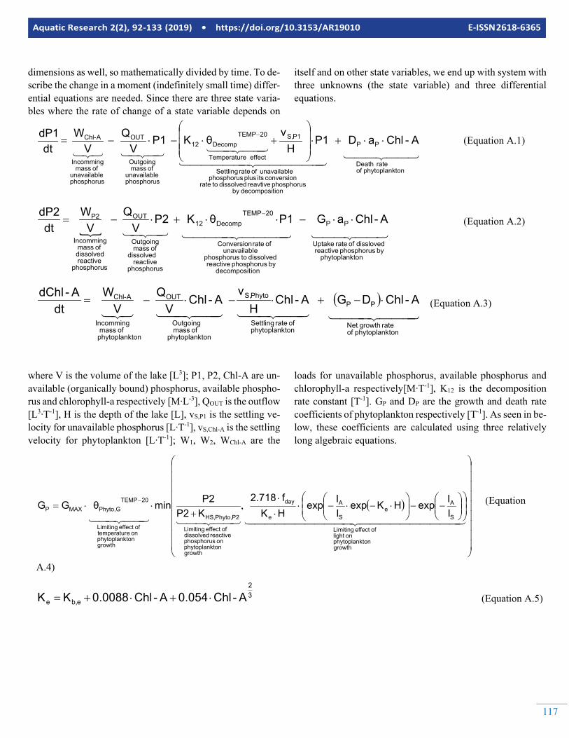
dimensions as well, so mathematically divided by time. To de-scribe the change in a moment (indefinitely small time) differ-ential equations are needed. Since there are three state varia-bles where the rate of change of a state variable depends on
itself and on other state variables, we end up with system with three unknowns (the state variable) and three differential equations.
tonphytoplank ofrate Death
PP
iondecompositby phosphorus reavtive dissolved to rate
conversion its plus phosphorus eunavailabl of rate Settling
P1S,
effect eTemperatur
20TEMPDecomp12
phosphoruseunavailabl of mass Outgoing
OUT
phosphoruseunavailabl of mass
Incomming
A-Chl A-ChlaD P1H
vθKP1
VQ
VW
dtdP1
⋅⋅+⋅
+⋅−⋅−=
− (Equation A.1)
tonphytoplank by phosphorus reactive
dissloved of rate Uptake
PP
iondecompositby phosphorus reactive
dissolved to phosphorus eunavailabl
of rateConversion
20TEMPDecomp12
phosphorusreactive
dissolved of mass Outgoing
OUT
phosphorusreactive dissolved
of mass Incomming
P2 A-ChlaG P1θKP2V
QV
Wdt
dP2⋅⋅−⋅⋅+⋅−=
− (Equation A.2)
( )
tonphytoplank ofrate growth Net
PP
tonphytoplankof rate Settling
PhytoS,
tonphytoplank of mass Outgoing
OUT
tonphytoplank of mass
Incomming
A-Chl A-ChlDG A-ChlH
vA-Chl
VQ
VW
dtA-dChl
⋅−+⋅−⋅−= (Equation A.3)
where V is the volume of the lake [L3]; P1, P2, Chl-A are un-available (organically bound) phosphorus, available phospho-rus and chlorophyll-a respectively [M∙L-3], QOUT is the outflow [L3∙T-1], H is the depth of the lake [L], vS,P1 is the settling ve-locity for unavailable phosphorus [L∙T-1], vS,Chl-A is the settling velocity for phytoplankton [L∙T-1]; W1, W2, WChl-A are the
loads for unavailable phosphorus, available phosphorus and chlorophyll-a respectively[M∙T-1], K12 is the decomposition rate constant [T-1]. GP and DP are the growth and death rate coefficients of phytoplankton respectively [T-1]. As seen in be-low, these coefficients are calculated using three relatively long algebraic equations.
( )
−−
⋅−⋅−⋅
⋅
⋅
+⋅⋅=
−
growthtonphytoplank
on lightof effect Limiting
S
Ae
S
A
e
day
growthtonphytoplank
on phosphorus reactive dissolved
of effect Limiting
P2Phyto,HS,
growthtonphytoplank
on etemperaturof effect Limiting
20TEMPGPhyto,MAXP I
IexpHKexpIIexp
HKf2.718
KP2P2minθGG , (Equation
A.4)
32
eb,e A-Chl0.054A-Chl0.0088KK ⋅+⋅+= (Equation A.5)
Aquatic Research 2(2), 92-133 (2019) • https://doi.org/10.3153/AR190010 E-ISSN 2618-6365
118
grazing nzooplanktoby tonphytoplank of
deathpredatory
ChlG
tonphytoplank of deathory non-predat
20TEMPDPhyto,RP ZaCθμD ⋅⋅+⋅=
− (Equation A.6)
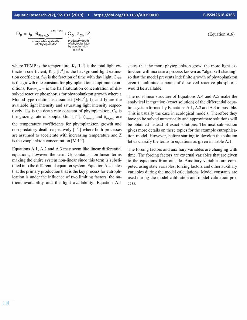
where TEMP is the temperature, Ke [L-1] is the total light ex-tinction coefficient, Kb,e [L-1] is the background light extinc-tion coefficient, fday is the fraction of time with day light, Gmax is the growth rate constant for phytoplankton at optimum con-ditions, KHS,Phyto,P2 is the half saturation concentration of dis-solved reactive phosphorus for phytoplankton growth where a Monod-type relation is assumed [M∙L-3]; IA and IS are the available light intensity and saturating light intensity respec-tively, R is the death rate constant of phytoplankton, CG is the grazing rate of zooplankton [T-1]; GPhyto,θ and DPhyto,θ are
the temperature coefficients for phytoplankton growth and non-predatory death respectively [T-1] where both processes are assumed to accelerate with increasing temperature and Z is the zooplankton concentration [M∙L-3].
Equations A.1, A.2 and A.3 may seem like linear differential equations, however the term GP contains non-linear terms making the entire system non-linear since this term is substi-tuted into the differential equation system. Equation A.4 states that the primary production that is the key process for eutroph-ication is under the influence of two limiting factors: the nu-trient availability and the light availability. Equation A.5
states that the more phytoplankton grow, the more light ex-tinction will increase a process known as “algal self shading” so that the model prevents indefinite growth of phytoplankton even if unlimited amount of dissolved reactive phosphorus would be available.
The non-linear structure of Equations A.4 and A.5 make the analytical integration (exact solution) of the differential equa-tion system formed by Equations A.1, A.2 and A.3 impossible. This is usually the case in ecological models. Therefore they have to be solved numerically and approximate solutions will be obtained instead of exact solutions. The next sub-section gives more details on these topics for the example eutrophica-tion model. However, before starting to develop the solution let us classify the terms in equations as given in Table A.1.
The forcing factors and auxiliary variables are changing with time. The forcing factors are external variables that are given to the equations from outside. Auxiliary variables are com-puted using state variables, forcing factors and other auxiliary variables during the model calculations. Model constants are used during the model calibration and model validation pro-cess.
119
Aquatic Research 2(2), 92-133 (2019) • https://doi.org/10.3153/AR19010 E-ISSN 2618-6365
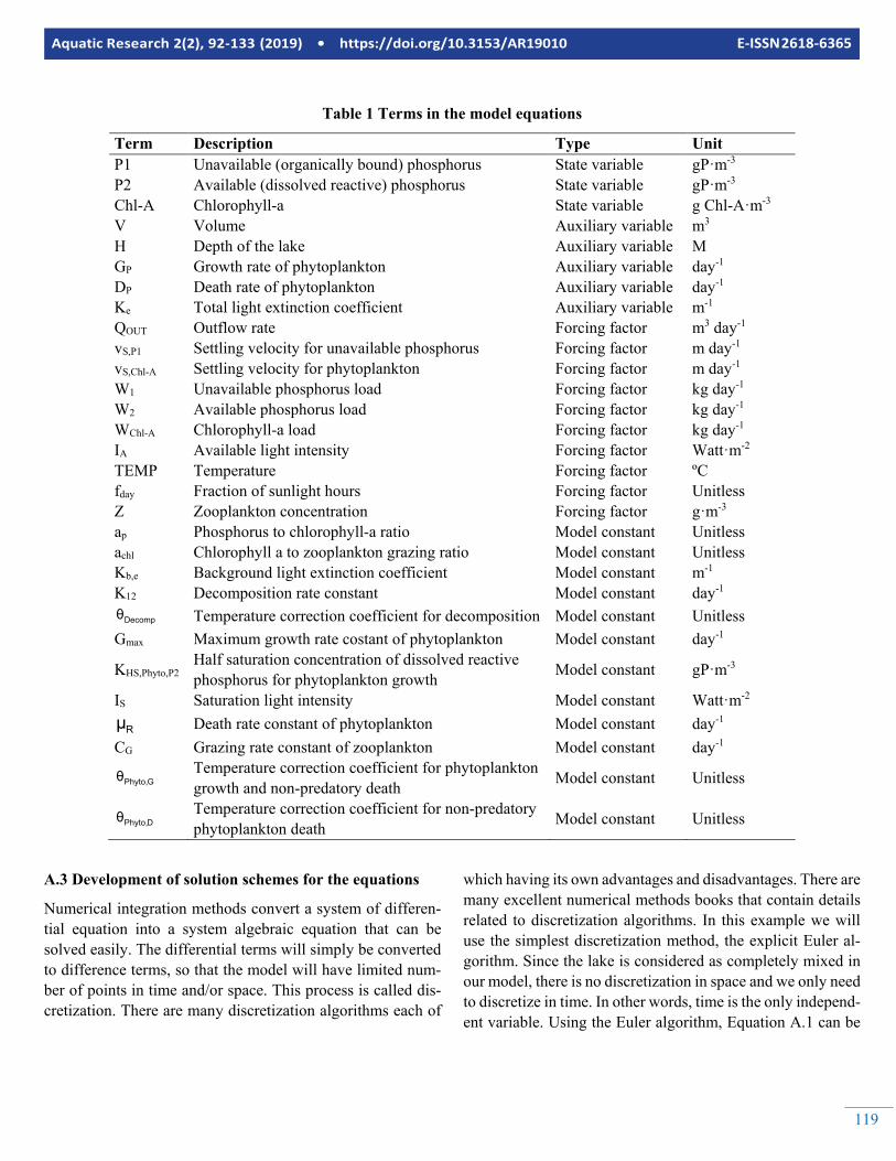
Table 1 Terms in the model equations
Term Description Type Unit P1 Unavailable (organically bound) phosphorus State variable gP·m-3 P2 Available (dissolved reactive) phosphorus State variable gP·m-3 Chl-A Chlorophyll-a State variable g Chl-A·m-3 V Volume Auxiliary variable m3 H Depth of the lake Auxiliary variable M GP Growth rate of phytoplankton Auxiliary variable day-1 DP Death rate of phytoplankton Auxiliary variable day-1 Ke Total light extinction coefficient Auxiliary variable m-1 QOUT Outflow rate Forcing factor m3 day-1 vS,P1 Settling velocity for unavailable phosphorus Forcing factor m day-1 vS,Chl-A Settling velocity for phytoplankton Forcing factor m day-1 W1 Unavailable phosphorus load Forcing factor kg day-1 W2 Available phosphorus load Forcing factor kg day-1 WChl-A Chlorophyll-a load Forcing factor kg day-1 IA Available light intensity Forcing factor Watt·m-2 TEMP Temperature Forcing factor ºC fday Fraction of sunlight hours Forcing factor Unitless Z Zooplankton concentration Forcing factor g·m-3 ap Phosphorus to chlorophyll-a ratio Model constant Unitless achl Chlorophyll a to zooplankton grazing ratio Model constant Unitless Kb,e Background light extinction coefficient Model constant m-1 K12 Decomposition rate constant Model constant day-1
Decompθ Temperature correction coefficient for decomposition Model constant Unitless Gmax Maximum growth rate costant of phytoplankton Model constant day-1
KHS,Phyto,P2 Half saturation concentration of dissolved reactive phosphorus for phytoplankton growth Model constant gP·m-3
IS Saturation light intensity Model constant Watt·m-2
Rμ Death rate constant of phytoplankton Model constant day-1 CG Grazing rate constant of zooplankton Model constant day-1
GPhyto,θ Temperature correction coefficient for phytoplankton growth and non-predatory death Model constant Unitless
DPhyto,θ Temperature correction coefficient for non-predatory phytoplankton death Model constant Unitless
A.3 Development of solution schemes for the equations
Numerical integration methods convert a system of differen-tial equation into a system algebraic equation that can be solved easily. The differential terms will simply be converted to difference terms, so that the model will have limited num-ber of points in time and/or space. This process is called dis-cretization. There are many discretization algorithms each of
which having its own advantages and disadvantages. There are many excellent numerical methods books that contain details related to discretization algorithms. In this example we will use the simplest discretization method, the explicit Euler al-gorithm. Since the lake is considered as completely mixed in our model, there is no discretization in space and we only need to discretize in time. In other words, time is the only independ-ent variable. Using the Euler algorithm, Equation A.1 can be
Aquatic Research 2(2), 92-133 (2019) • https://doi.org/10.3153/AR190010 E-ISSN 2618-6365
120
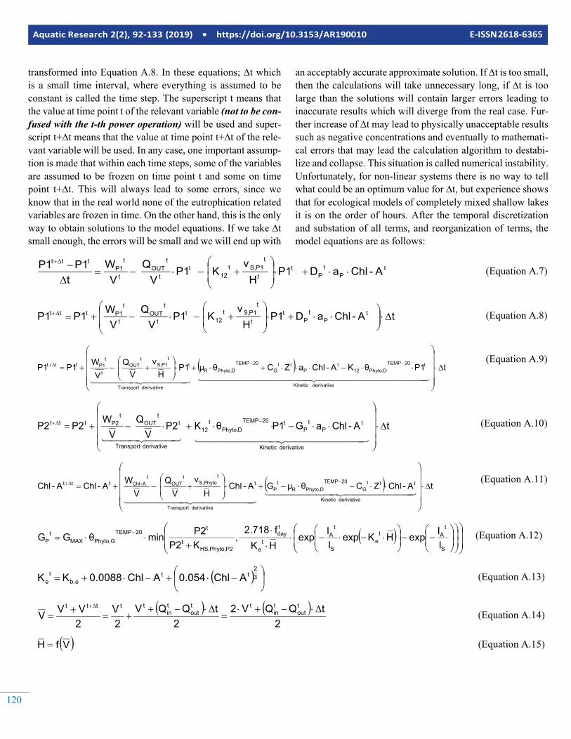
transformed into Equation A.8. In these equations; ∆t which is a small time interval, where everything is assumed to be constant is called the time step. The superscript t means that the value at time point t of the relevant variable (not to be con-fused with the t-th power operation) will be used and super-script t+∆t means that the value at time point t+∆t of the rele-vant variable will be used. In any case, one important assump-tion is made that within each time steps, some of the variables are assumed to be frozen on time point t and some on time point t+∆t. This will always lead to some errors, since we know that in the real world none of the eutrophication related variables are frozen in time. On the other hand, this is the only way to obtain solutions to the model equations. If we take ∆t small enough, the errors will be small and we will end up with
an acceptably accurate approximate solution. If ∆t is too small, then the calculations will take unnecessary long, if ∆t is too large than the solutions will contain larger errors leading to inaccurate results which will diverge from the real case. Fur-ther increase of ∆t may lead to physically unacceptable results such as negative concentrations and eventually to mathemati-cal errors that may lead the calculation algorithm to destabi-lize and collapse. This situation is called numerical instability. Unfortunately, for non-linear systems there is no way to tell what could be an optimum value for ∆t, but experience shows that for ecological models of completely mixed shallow lakes it is on the order of hours. After the temporal discretization and substation of all terms, and reorganization of terms, the model equations are as follows:
tP
tP
tt
tP1S,t
12t
t
tOUT
t
tP1
ttt
A-ChlaD P1H
vKP1
VQ
VW
tP1P1
⋅⋅+⋅
+−⋅−=
∆−∆+
(Equation A.7)
tA-ChlaDP1H
vKP1
VQ
VWP1P1 t
Pt
Pt
t
tP1S,t
12t
t
tOUT
t
tP1ttt ∆⋅
⋅⋅
+⋅
+−⋅−+=∆+ (Equation A.8)
( ) tP1θKA-ChlaZCθμP1H
vV
QV
WP1P1
derivativeKinetic
t20TEMPDPhyto,12
tP
ttG
20TEMPDPhyto,R
derivative Transport
tt
P1S,t
OUTt
tP1ttt ∆⋅
⋅⋅−⋅⋅⋅+⋅+⋅
+−+=
−−∆+
(Equation A.9)
tA-ChlaGP1θKP2V
QV
WP2P2
derivativeKinetic
tP
tP
t20TEMPDPhyto,
t12
derivative Transport
tt
OUTt
P2ttt ∆⋅
⋅⋅−⋅⋅+⋅−+=−∆+
(Equation A.10)
( ) tA-ChlZCθμGA-ChlH
vV
QV
WA-ChlA-ChlderivativeKinetic
tttG
20TEMPDPhyto,R
tP
derivative Transport
tt
PhytoS,t
OUTt
A-Chlttt ∆⋅
⋅⋅−⋅−+⋅
+−+=
−∆+
(Equation A.11)
( )
−−
⋅−⋅−⋅
⋅
⋅
+⋅⋅=
−
S
tAt
eS
tA
te
tday
P2Phyto,HS,t
t20TEMP
GPhyto,MAXt
P IIexpHKexp
IIexp
HKf2.718
KP2P2minθGG , (Equation A.12)
( )
−⋅+−⋅+= 3
2tt
eb,t
e AChl0.054AChl0.0088KK (Equation A.13)
( ) ( )2
tQQV22
tQQV2V
2VVV
tout
tin
ttout
tin
ttttt ∆⋅−+⋅=
∆⋅−++=
+=
∆+
(Equation A.14)
( )VfH = (Equation A.15)
121
Aquatic Research 2(2), 92-133 (2019) • https://doi.org/10.3153/AR19010 E-ISSN 2618-6365
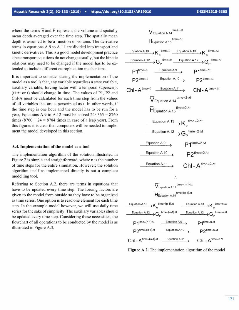
where the terms V and H represent the volume and spatially mean depth averaged over the time step. The spatially mean depth is assumed to be a function of volume. The derivative terms in equations A.9 to A.11 are divided into transport and kinetic derivatives. This is a good model development practice since transport equations do not change usually, but the kinetic relations may need to be changed if the model has to be ex-tended to include different eutrophication mechanisms.
It is important to consider during the implementation of the model as a tool is that, any variable regardless a state variable, auxiliary variable, forcing factor with a temporal superscript (t+∆t or t) should change in time. The values of P1, P2 and Chl-A must be calculated for each time step from the values of all variables that are superscripted as t. In other words, if the time step is one hour and the model has to be run for a year, Equations A.9 to A.12 must be solved 24· 365 = 8760 times (8760 + 24 = 8784 times in case of a leap year). From this figures it is clear that computers will be needed to imple-ment the model developed in this section.
A.4. Implementation of the model as a tool
The implementation algorithm of the solution illustrated in Figure 2 is simple and straightforward, where n is the number of time steps for the entire simulation. However; the solution algorithm itself as implemented directly is not a complete modelling tool.
Referring to Section A.2, there are terms in equations that have to be updated every time step. The forcing factors are given to the model from outside so they have to be organized as time series. One option is to read one element for each time step. In the example model however, we will use daily time series for the sake of simplicity. The auxiliary variables should be updated every time step. Considering these necessities, the flowchart of all operations to be conducted by the model is as illustrated in Figure A.3.
ttime A.11Equation
time
ttime A.10Equationtime
ttime A.9Equation
time
ttimeP
A.12Equation timeP
A.12Equation
ttimee
A.13Equation
timee
A.13Equation
ttime A.15Equation
ttime A.14Equation
A-Chl A-Chl
P2 P2P1 P1
GG
KK
HV
∆==
∆==
∆==
∆==
∆==
∆=
∆=
→
→
→
→ →
→ →
0
0
0
0
0
t2time A.11Equation
t2time A.10Equation
t2time A.9Equation
t2timeP
A.12Equation
t2timee
A.13Equation
t2time A.15Equation
t2time A.14Equation
A-Chl
P2 P1
G
K
HV
∆⋅=
∆⋅=
∆⋅=
∆⋅=
∆⋅=
∆⋅=
∆⋅=
→
→
→
→
→
∴ ( )
( )
( )
( )
( )
( )
( ) tntime A.11Equation
t1-ntime
tntime A.10Equationt1-ntime
tntime A.9Equation
t1-ntime
tntimeP
A.12Equation t1-ntimeP
A.12Equation
tntimee
A.13Equation
t1-ntimee
A.13Equation
t1-ntime A.15Equation
t1-ntime A.14Equation
A-Chl A-Chl
P2 P2P1 P1
G G
KK
HV
∆⋅=∆⋅=
∆⋅=∆⋅=
∆⋅=∆⋅=
∆⋅=∆⋅=
∆⋅=∆⋅=
∆⋅=
∆⋅=
→
→
→
→ →
→ →
Figure A.2. The implementation algorithm of the model
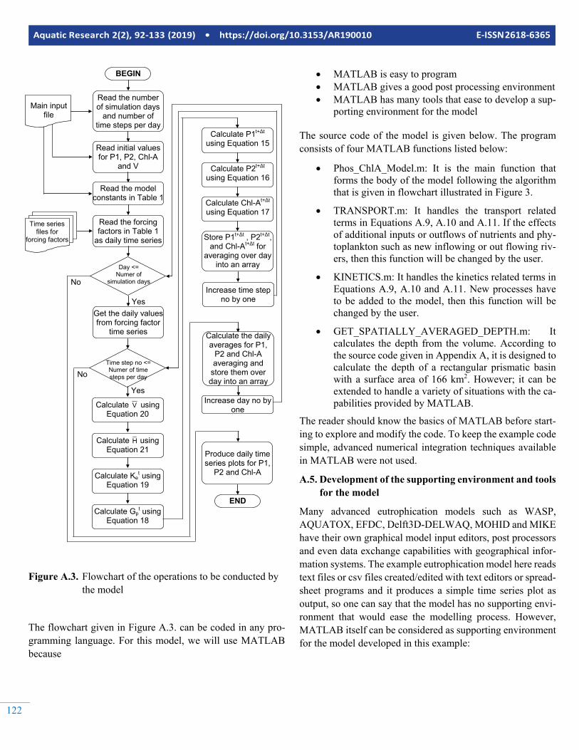
Aquatic Research 2(2), 92-133 (2019) • https://doi.org/10.3153/AR190010 E-ISSN 2618-6365
122
Figure A.3. Flowchart of the operations to be conducted by the model
The flowchart given in Figure A.3. can be coded in any pro-gramming language. For this model, we will use MATLAB because
• MATLAB is easy to program • MATLAB gives a good post processing environment • MATLAB has many tools that ease to develop a sup-
porting environment for the model
The source code of the model is given below. The program consists of four MATLAB functions listed below:
• Phos_ChlA_Model.m: It is the main function that forms the body of the model following the algorithm that is given in flowchart illustrated in Figure 3.
• TRANSPORT.m: It handles the transport related terms in Equations A.9, A.10 and A.11. If the effects of additional inputs or outflows of nutrients and phy-toplankton such as new inflowing or out flowing riv-ers, then this function will be changed by the user.
• KINETICS.m: It handles the kinetics related terms in Equations A.9, A.10 and A.11. New processes have to be added to the model, then this function will be changed by the user.
• GET_SPATIALLY_AVERAGED_DEPTH.m: It calculates the depth from the volume. According to the source code given in Appendix A, it is designed to calculate the depth of a rectangular prismatic basin with a surface area of 166 km2. However; it can be extended to handle a variety of situations with the ca-pabilities provided by MATLAB.
The reader should know the basics of MATLAB before start-ing to explore and modify the code. To keep the example code simple, advanced numerical integration techniques available in MATLAB were not used.
A.5. Development of the supporting environment and tools for the model
Many advanced eutrophication models such as WASP, AQUATOX, EFDC, Delft3D-DELWAQ, MOHID and MIKE have their own graphical model input editors, post processors and even data exchange capabilities with geographical infor-mation systems. The example eutrophication model here reads text files or csv files created/edited with text editors or spread-sheet programs and it produces a simple time series plot as output, so one can say that the model has no supporting envi-ronment that would ease the modelling process. However, MATLAB itself can be considered as supporting environment for the model developed in this example:
Read the number of simulation days
and number of time steps per day
BEGIN
Read initial values for P1, P2, Chl-A
and V
Main input file
Read the model constants in Table 1
Read the forcing factors in Table 1
as daily time series
Day <= Numer of
simulation days
Yes
Time series files for
forcing factors
Calculate V using Equation 20
Time step no <= Numer of time steps per day
Yes
Calculate H using Equation 21
Calculate Ket using
Equation 19
Calculate Gpt using
Equation 18
Calculate P1t+Δt using Equation 15
Calculate P2t+Δt using Equation 16
Calculate Chl-At+Δt using Equation 17
Store P1t+Δt , P2t+Δt, and Chl-At+Δt for
averaging over day into an array
Increase time step no by one
Calculate the daily averages for P1,
P2 and Chl-A averaging and
store them over day into an array
Get the daily values from forcing factor
time series
Increase day no by one
Produce daily time series plots for P1,
P2 and Chl-A
END
No
No
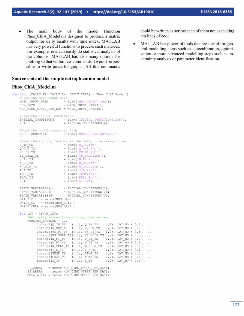
123
Aquatic Research 2(2), 92-133 (2019) • https://doi.org/10.3153/AR19010 E-ISSN 2618-6365
• The main body of the model (function Phos_ChlA_Model) is designed to produce a matrix output for daily results with time index. MATLAB has very powerful functions to process such matrices. For example, one can easily do statistical analysis of the columns. MATLAB has also many options for plotting so that within few commands it would be pos-sible to write powerful graphs. All this commands
could be written as scripts each of them not exceeding ten lines of code.
• MATLAB has powerful tools that are useful for gen-eral modelling steps such as autocalibration, optimi-zation or more advanced modelling steps such as un-certainty analysis or parameter identification.
Source code of the simple eutrophication model
Phos_ChlA_Model.m
function [DAILY_P1, DAILY_P2, DAILY_CHLA] = Phos_ChlA_Model() %Read the main input file MAIN_INPUT_DATA = load('MAIN_INPUT.inp'); NUM_DAYS = MAIN_INPUT_DATA(1); NUM_TIME_STEPS_PER_DAY = MAIN_INPUT_DATA(2); %Read the initial conditions INITIAL_CONDIITONS = load('INITIAL_CONDITIONS.inp'); V_T = INITIAL_CONDIITONS(4); %Read the model constants file MODEL_CONSTANTS = load('MODEL_CONSTANTS.inp'); %Read the forcing factors as the daily time series files Q_IN_TS = load('Q_IN.inp'); Q_OUT_TS = load('Q_OUT.inp'); VS_P1_TS = load('VS_P1.inp'); VS_CHLA_TS = load('VS_CHLA.inp'); W_P1_TS = load('W_P1.inp'); W_P2_TS = load('W_P2.inp'); W_CHLA_TS = load('W_CHLA.inp'); I_A_TS = load('I_A.inp'); TEMP_TS = load('TEMP.inp'); FDAY_TS = load('FDAY.inp'); Z_TS = load('Z.inp'); STATE_VARIABLES(1) = INITIAL_CONDIITONS(1); STATE_VARIABLES(2) = INITIAL_CONDIITONS(2); STATE_VARIABLES(3) = INITIAL_CONDIITONS(3); DAILY_P1 = zeros(NUM_DAYS); DAILY_P2 = zeros(NUM_DAYS); DAILY_CHLA = zeros(NUM_DAYS); for DAY = 1:NUM_DAYS %Get daily values from forcing time series FORCING_FACTORS = ... [interp1(Q_IN_TS (:,1), Q_IN_TS (:,2), DAY_NO + 0.5), ... interp1(Q_OUT_TS (:,1), Q_OUT_TS (:,2), DAY_NO + 0.5), ... interp1(VS_P1_TS (:,1), VS_P1_TS (:,2), DAY_NO + 0.5), ... interp1(VS_CHLA_TS(:,1), VS_CHLA_TS(:,2), DAY_NO + 0.5), ... interp1(W_P1_TS (:,1), W_P1_TS (:,2), DAY_NO + 0.5), ... interp1(W_P2_TS (:,1), W_P2_TS (:,2), DAY_NO + 0.5), ... interp1(W_CHLA_TS (:,1), W_CHLA_TS (:,2), DAY_NO + 0.5), ... interp1(I_A_TS (:,1), I_A_TS (:,2), DAY_NO + 0.5), ... interp1(TEMP_TS (:,1), TEMP_TS (:,2), DAY_NO + 0.5), ... interp1(FDAY_TS (:,1), FDAY_TS (:,2), DAY_NO + 0.5), ... interp1(Z_TS (:,1), Z_TS (:,2), DAY_NO + 0.5)]; P1_ARRAY = zeros(NUM_TIME_STEPS_PER_DAY); P2_ARRAY = zeros(NUM_TIME_STEPS_PER_DAY); CHLA_ARRAY = zeros(NUM_TIME_STEPS_PER_DAY);
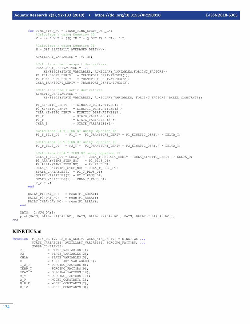
Aquatic Research 2(2), 92-133 (2019) • https://doi.org/10.3153/AR190010 E-ISSN 2618-6365
124
for TIME_STEP_NO = 1:NUM_TIME_STEPS_PER_DAY %Calculate V using Equation 20 V = (2 * V_T + ((Q_IN_T - Q_OUT_T) * DT)) / 2; %Calculate H using Equation 21 H = GET_SPATIALLY_AVERAGED_DEPTH(V); AUXILLARY_VARIABLES = [V, H]; %Calculate the transport derivatives TRANSPORT_DERIVATIVES = ... KINETICS(STATE_VARIABLES, AUXILLARY_VARIABLES,FORCING_FACTORS); P1_TRANSPORT_DERIV = TRANSPORT_DERIVATIVES(1); P2_TRANSPORT_DERIV = TRANSPORT_DERIVATIVES(2); CHLA_TRANSPORT_DERIV = TRANSPORT_DERIVATIVES(3); %Calculate the kinetic derivatives KINETIC_DERIVATIVES = ... KINETICS(STATE_VARIABLES, AUXILLARY_VARIABLES, FORCING_FACTORS, MODEL_CONSTANTS); P1_KINETIC_DERIV = KINETIC_DERIVATIVES(1); P2_KINETIC_DERIV = KINETIC_DERIVATIVES(2); CHLA_KINETIC_DERIV = KINETIC_DERIVATIVES(3); P1_T = STATE_VARIABLES(1); P2_T = STATE_VARIABLES(2); CHLA_T = STATE_VARIABLES(3); %Calculate P1_T_PLUS_DT using Equation 15 P1_T_PLUS_DT = P1_T + (P1_TRANSPORT_DERIV + P1_KINETIC_DERIV) * DELTA_T; %Calculate P2_T_PLUS_DT using Equation 16 P2_T_PLUS_DT = P2_T + (P2_TRANSPORT_DERIV + P2_KINETIC_DERIV) * DELTA_T; %Calculate CHLA_T_PLUS_DT using Equation 17 CHLA_T_PLUS_DT = CHLA_T + (CHLA_TRANSPORT_DERIV + CHLA_KINETIC_DERIV) * DELTA_T; P1_ARRAY(TIME_STEP_NO) = P1_PLUS_DT; P2_ARRAY(TIME_STEP_NO) = P2_PLUS_DT; CHLA_ARRAY(TIME_STEP_NO) = CHLA_T_PLUS_DT; STATE_VARIABLES(1) = P1_T_PLUS_DT; STATE_VARIABLES(2) = P2_T_PLUS_DT; STATE_VARIABLES(3) = CHLA_T_PLUS_DT; V_T = V; end DAILY_P1(DAY_NO) = mean(P1_ARRAY); DAILY_P2(DAY_NO) = mean(P1_ARRAY); DAILY_CHLA(DAY_NO) = mean(P1_ARRAY); end DAYS = 1:NUM_DAYS; plot(DAYS, DAILY_P1(DAY_NO), DAYS, DAILY_P2(DAY_NO), DAYS, DAILY_CHLA(DAY_NO)); end
KINETICS.m function [P1_KIN_DERIV, P2_KIN_DERIV, CHLA_KIN_DERIV] = KINETICS ... (STATE_VARIABLES, AUXILLARY_VARIABLES, FORCING_FACTORS, ... MODEL_CONSTANTS) P1 = STATE_VARIABLES(1); P2 = STATE_VARIABLES(2); CHLA = STATE_VARIABLES(3); H = AUXILLARY_VARIABLES(1); I_A_T = FORCING_FACTORS(8); TEMP_T = FORCING_FACTORS(9); FDAY_T = FORCING_FACTORS(10); Z_T = FORCING_FACTORS(11); A_P = MODEL_CONSTANTS(1); K_B_E = MODEL_CONSTANTS(2); K_12 = MODEL_CONSTANTS(3);
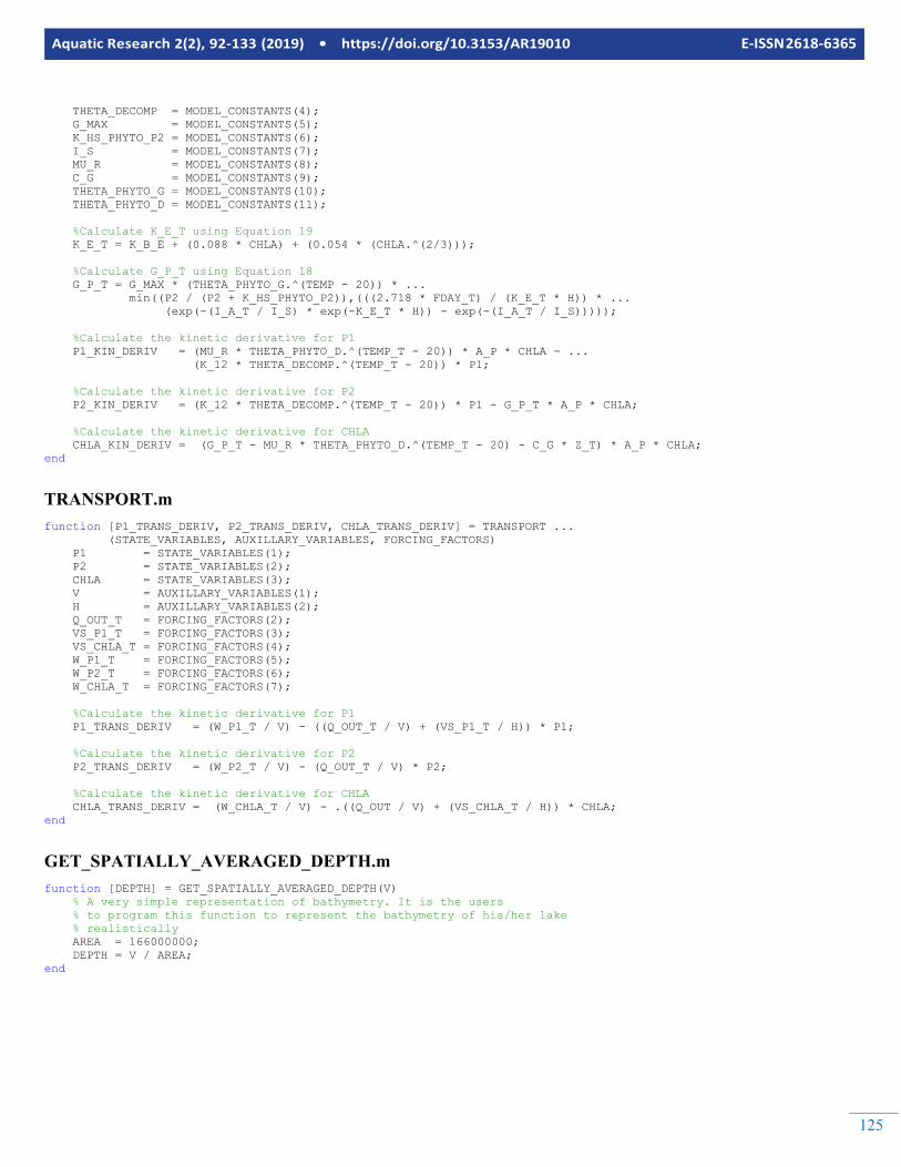
125
Aquatic Research 2(2), 92-133 (2019) • https://doi.org/10.3153/AR19010 E-ISSN 2618-6365
THETA_DECOMP = MODEL_CONSTANTS(4); G_MAX = MODEL_CONSTANTS(5); K_HS_PHYTO_P2 = MODEL_CONSTANTS(6); I_S = MODEL_CONSTANTS(7); MU_R = MODEL_CONSTANTS(8); C_G = MODEL_CONSTANTS(9); THETA_PHYTO_G = MODEL_CONSTANTS(10); THETA_PHYTO_D = MODEL_CONSTANTS(11); %Calculate K_E_T using Equation 19 K_E_T = K_B_E + (0.088 * CHLA) + (0.054 * (CHLA.^(2/3))); %Calculate G_P_T using Equation 18 G_P_T = G_MAX * (THETA_PHYTO_G.^(TEMP - 20)) * ... min((P2 / (P2 + K_HS_PHYTO_P2)),(((2.718 * FDAY_T) / (K_E_T * H)) * ... (exp(-(I_A_T / I_S) * exp(-K_E_T * H)) - exp(-(I_A_T / I_S))))); %Calculate the kinetic derivative for P1 P1_KIN_DERIV = (MU_R * THETA_PHYTO_D.^(TEMP_T - 20)) * A_P * CHLA - ... (K_12 * THETA_DECOMP.^(TEMP_T - 20)) * P1; %Calculate the kinetic derivative for P2 P2_KIN_DERIV = (K_12 * THETA_DECOMP.^(TEMP_T - 20)) * P1 - G_P_T * A_P * CHLA; %Calculate the kinetic derivative for CHLA CHLA_KIN_DERIV = (G_P_T - MU_R * THETA_PHYTO_D.^(TEMP_T - 20) - C_G * Z_T) * A_P * CHLA; end
TRANSPORT.m function [P1_TRANS_DERIV, P2_TRANS_DERIV, CHLA_TRANS_DERIV] = TRANSPORT ... (STATE_VARIABLES, AUXILLARY_VARIABLES, FORCING_FACTORS) P1 = STATE_VARIABLES(1); P2 = STATE_VARIABLES(2); CHLA = STATE_VARIABLES(3); V = AUXILLARY_VARIABLES(1); H = AUXILLARY_VARIABLES(2); Q_OUT_T = FORCING_FACTORS(2); VS_P1_T = FORCING_FACTORS(3); VS_CHLA_T = FORCING_FACTORS(4); W_P1_T = FORCING_FACTORS(5); W_P2_T = FORCING_FACTORS(6); W_CHLA_T = FORCING_FACTORS(7); %Calculate the kinetic derivative for P1 P1_TRANS_DERIV = (W_P1_T / V) - ((Q_OUT_T / V) + (VS_P1_T / H)) * P1; %Calculate the kinetic derivative for P2 P2_TRANS_DERIV = (W_P2_T / V) - (Q_OUT_T / V) * P2; %Calculate the kinetic derivative for CHLA CHLA_TRANS_DERIV = (W_CHLA_T / V) - .((Q_OUT / V) + (VS_CHLA_T / H)) * CHLA; end
GET_SPATIALLY_AVERAGED_DEPTH.m function [DEPTH] = GET_SPATIALLY_AVERAGED_DEPTH(V) % A very simple representation of bathymetry. It is the users % to program this function to represent the bathymetry of his/her lake % realistically AREA = 166000000; DEPTH = V / AREA; end
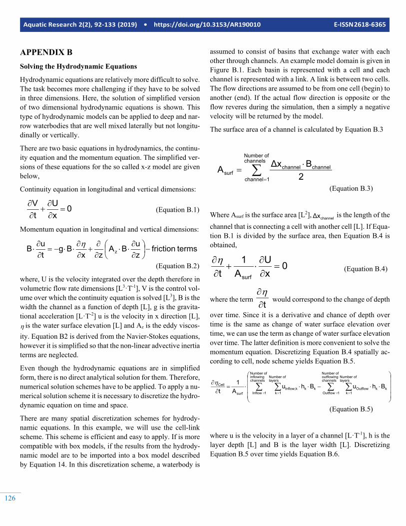
Aquatic Research 2(2), 92-133 (2019) • https://doi.org/10.3153/AR190010 E-ISSN 2618-6365
126
APPENDIX B Solving the Hydrodynamic Equations
Hydrodynamic equations are relatively more difficult to solve. The task becomes more challenging if they have to be solved in three dimensions. Here, the solution of simplified version of two dimensional hydrodynamic equations is shown. This type of hydrodynamic models can be applied to deep and nar-row waterbodies that are well mixed laterally but not longitu-dinally or vertically.
There are two basic equations in hydrodynamics, the continu-ity equation and the momentum equation. The simplified ver-sions of these equations for the so called x-z model are given below,
Continuity equation in longitudinal and vertical dimensions:
0xU
tV
=∂∂
+∂∂
(Equation B.1)
Momentum equation in longitudinal and vertical dimensions:
terms frictionzuBA
zxBg
tuB z −
∂∂⋅⋅
∂∂
+∂∂⋅⋅−=
∂∂⋅
η
(Equation B.2)
where, U is the velocity integrated over the depth therefore in volumetric flow rate dimensions [L3·T-1], V is the control vol-ume over which the continuity equation is solved [L3], B is the width the channel as a function of depth [L], g is the gravita-tional acceleration [L·T-2] u is the velocity in x direction [L], η is the water surface elevation [L] and Az is the eddy viscos-ity. Equation B2 is derived from the Navier-Stokes equations, however it is simplified so that the non-linear advective inertia terms are neglected.
Even though the hydrodynamic equations are in simplified form, there is no direct analytical solution for them. Therefore, numerical solution schemes have to be applied. To apply a nu-merical solution scheme it is necessary to discretize the hydro-dynamic equation on time and space.
There are many spatial discretization schemes for hydrody-namic equations. In this example, we will use the cell-link scheme. This scheme is efficient and easy to apply. If is more compatible with box models, if the results from the hydrody-namic model are to be imported into a box model described by Equation 14. In this discretization scheme, a waterbody is
assumed to consist of basins that exchange water with each other through channels. An example model domain is given in Figure B.1. Each basin is represented with a cell and each channel is represented with a link. A link is between two cells. The flow directions are assumed to be from one cell (begin) to another (end). If the actual flow direction is opposite or the flow reveres during the simulation, then a simply a negative velocity will be returned by the model.
The surface area of a channel is calculated by Equation B.3
∑=
⋅=
channelsof Number
1channel
channelchannelsurf 2
BΔxA
(Equation B.3)
Where Asurf is the surface area [L2], channelΔx is the length of the channel that is connecting a cell with another cell [L]. If Equa-tion B.1 is divided by the surface area, then Equation B.4 is obtained,
0xU
A1
t surf
=∂∂⋅+
∂∂η
(Equation B.4)
where the term t∂∂η
would correspond to the change of depth
over time. Since it is a derivative and chance of depth over time is the same as change of water surface elevation over time, we can use the term as change of water surface elevation over time. The latter definition is more convenient to solve the momentum equation. Discretizing Equation B.4 spatially ac-cording to cell, node scheme yields Equation B.5.
⋅⋅
−⋅⋅⋅=∂
∂ ∑ ∑∑ ∑= == =
channels outflowing
of Number
1Outflow
layersof Number
1kkkOutflow
channels inflowingof Number
1Inflow
layersof Number
1kkkkInflow,
surf
Cell BhuBhuA
1t
η
(Equation B.5)
where u is the velocity in a layer of a channel [L·T-1], h is the layer depth [L] and B is the layer width [L]. Discretizing Equation B.5 over time yields Equation B.6.
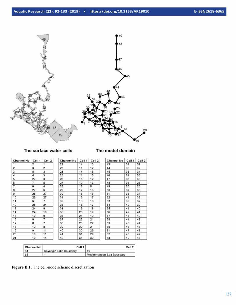
127
Aquatic Research 2(2), 92-133 (2019) • https://doi.org/10.3153/AR19010 E-ISSN 2618-6365
Figure B.1. The cell-node scheme discretization
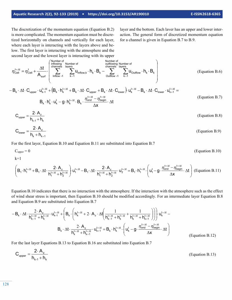
Aquatic Research 2(2), 92-133 (2019) • https://doi.org/10.3153/AR190010 E-ISSN 2618-6365
128
The discretization of the momentum equation (Equation B.2) is more complicated. The momentum equation must be discre-tized horizontally on channels and vertically for each layer, where each layer is interacting with the layers above and be-low. The first layer is interacting with the atmosphere and the second layer and the lowest layer is interacting with its upper
layer and the bottom. Each laver has an upper and lower inter-action. The general form of discretized momentum equation for a channel is given in Equation B.7 to B.9.
⋅⋅
−⋅⋅⋅∆
+= ∑ ∑∑ ∑= == =
∆+channels
outflowingof Number
1Outflow
layersof Number
1kkkOutflow
channels inflowingof Number
1Inflow
layersof Number
1kkkkInflow,
surf
tCell
ttCell BhuBhu
Atηη (Equation B.6)
( )
tx
BhguhB
uCtBuCtBCtBhBuCtBtt
begintt
endk
ttk
tk
tkk
tt1klowerk
ttklowerkupperk
ttkk
tt1-kupperk
∆⋅∆−
⋅⋅⋅−⋅⋅
=⋅⋅∆⋅−⋅⋅∆⋅+⋅∆⋅+⋅+⋅⋅∆⋅−∆+∆+
∆+
∆++
∆+∆+∆+
ηη (Equation B.7)
k1-k
zupper hh
A2C+⋅
= (Equation B.8)
1kk
zlower hh
A2C++
⋅= (Equation B.9)
For the first layer, Equation B.10 and Equation B.11 are substituted into Equation B.7
Cupper = 0 (Equation B.10)
k=1
∆⋅
∆
−⋅−⋅⋅=⋅
+⋅
⋅∆⋅−⋅
+⋅
⋅∆⋅+⋅∆+∆+
∆+∆+∆+∆+
∆+∆+∆+
∆+ tx
guhBuhh
A2tBuhh
A2tBhBtt
begintt
endt1
tt11
tt2tt
2tt
1
z1
tt1tt
2tt
1
z1
tt11
ηη(Equation B.11)
Equation B.10 indicates that there is no interaction with the atmosphere. If the interaction with the atmosphere such as the effect of wind shear stress is important, then Equation B.10 should be modified accordingly. For an intermediate layer Equation B.8 and Equation B.9 are substituted into Equation B.7
(Equation B.12)
For the last layer Equations B.13 to Equation B.16 are substituted into Equation B.7
k1-k
zupper hh
A2C+⋅
= (Equation B.13)
∆⋅
∆−
⋅−⋅⋅=⋅+⋅
⋅∆⋅
−⋅
+
++
∆⋅⋅+⋅+⋅+⋅
⋅∆⋅−
∆+∆+∆+∆+
+∆++
∆+
∆+∆++
∆+∆+∆+−
∆+∆+∆+∆+
−
tx
guhBuhh
AtB
uhhhh
tAhBuhh
AtB
ttbegin
ttendt
ktt
kktt
1ktt1k
ttk
zk
ttktt
1ktt
ktt
ktt
1kz
ttkk
tt1-ktt
ktt
1k
zk
ηη2
1122
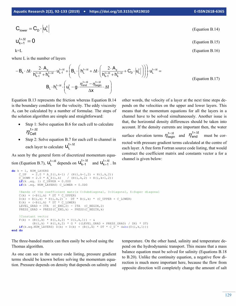
129
Aquatic Research 2(2), 92-133 (2019) • https://doi.org/10.3153/AR19010 E-ISSN 2618-6365
tLDlower uCC ⋅= (Equation B.14)
0u tt1k =∆++ (Equation B.15)
k=L (Equation B.16)
where L is the number of layers
∆⋅
∆−
⋅−⋅⋅
=⋅
⋅+
+⋅
⋅∆+⋅+⋅+⋅
⋅∆⋅−
∆+∆+∆+
∆+∆+∆+
∆+∆+∆+∆+
tx
guhB
uuChh
AthBuhh
AtB
ttbegin
ttendt
Ltt
LL
ttL
tLDtt
ktt
1-k
zttLL
tt1-Ltt
ktt
1-k
zk
ηη
22
(Equation B.17)
Equation B.13 represents the friction whereas Equation B.14 is the boundary condition for the velocity. The eddy viscosity Az can be calculated by a number of formulae. The steps of the solution algorithm are simple and straightforward:
• Step 1: Solve equation B.6 for each cell to calculate tt
Cell∆+η
• Step 2: Solve equation B.7 for each cell to channel in
each layer to calculate tt
Lu ∆+
As seen by the general form of discretized momentum equa-
tion (Equation B.7), ttLu ∆+ depends on
tt1-ku ∆+
and tt1ku ∆+
+ . In
other words, the velocity of a layer at the next time steps de-pends on the velocities on the upper and lower layers. This means that the momentum equations for all the layers in a channel have to be solved simultaneously. Another issue is that, the horizontal density differences should be taken into account. If the density currents are important then, the water
surface elevation terms ttbegin
∆+η and tt
end∆+η must be cor-
rected with pressure gradient terms calculated at the centre of each layer. A free form Fortran source code listing, that would construct the coefficient matrix and constants vector a for a channel is given below:
do k = 1, NUM_LAYERS C_UP = 2.0 * A_Z(i,k-1) / (H(i,k-1,2) + H(i,k,2)) C_DOWN = 2.0 * A_Z(i,k) / (H(i,k,2) + H(i,k+1,2)) if(k .eq. 1) C_UPPER = 0.0D0 if(k .eq. NUM_LAYERS) C_LOWER = 0.0D0 !Bands of the coefficient matrix C:Subdiagonal, D:Diagonal, E:Super diagonal C(k) = (-B(i,k) * DT * C_UPPER) D(k) = B(i,k) * H(i,k,2) + DT * B(i,k) * (C_UPPER + C_LOWER) E(k) = (-B(i,k) * DT * C_LOWER) LEVEL_GRAD = ITA (C_END,2) - ITA (C_BEGIN,2) PRESS_GRAD = PRESS(C_END,k) - PRESS(C_BEGIN,k) !Constant vector F(k) = (B(i,k) * H(i,k,2) * U(i,k,1)) - & (B(i,k) * H(i,k,2) * G * ((LEVEL_GRAD + PRESS_GRAD) / DX) * DT) if(k.eq.NUM_LAYERS) D(k) = D(k) + (B(i,k) * DT * C_D * dabs(U(i,k,1))) end do
The three-banded matrix can then easily be solved using the Thomas algorithm.
As one can see in the source code listing, pressure gradient terms should be known before solving the momentum equa-tion. Pressure depends on density that depends on salinity and
temperature. On the other hand, salinity and temperature de-pend on the hydrodynamic transport. This means that a mass balance equation must be solved for salinity (Equations B.18 to B.20). Unlike the continuity equation, a negative flow di-rection is much more important here, because the flow from opposite direction will completely change the amount of salt
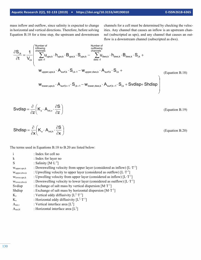
Aquatic Research 2(2), 92-133 (2019) • https://doi.org/10.3153/AR190010 E-ISSN 2618-6365
130
mass inflow and outflow, since salinity is expected to change in horizontal and vertical directions. Therefore, before solving Equation B.18 for a time step, the upstream and downstream
channels for a cell must be determined by checking the veloc-ities. Any channel that causes an inflow is an upstream chan-nel (subscripted as ups), and any channel that causes an out-flow is a downstream channel (subscripted as dws).
++⋅⋅−⋅⋅
+⋅⋅−⋅⋅
+⋅⋅⋅−⋅⋅⋅=∂∂
+++
==∑∑
ShdispSvdispSAwSAw
SAwSAw
SBhuSBhuV1
tS
ki,1ksurf,kdws,lower,1ki,1ksurf,kups,lower,
ki,ksurf,kdws,upper,1-ki,ksurf,kups,upper,
channels outflowing
of Number
1 dwski,kdws,kdws,kdws,
channels inflowingof Number
1 upskups,kups,kups,kups,
ki,
ki,
(Equation B.18)
∂∂⋅⋅
∂∂
=zSAK
zSvdisp vint,z (Equation B.19)
∂∂⋅⋅
∂∂
=xSAK
xShdisp hint,x (Equation B.20)
The terms used in Equations B.18 to B.20 are listed below:
i : Index for cell no k : Index for layer no S : Salinity [M·L-3] wupper,ups,k : Downwelling velocity from upper layer (considered as inflow) [L·T-1] wupper,dws,k : Upwelling velocity to upper layer (considered as outflow) [L·T-1] wlower,ups,k : Upwelling velocity from upper layer (considered as inflow) [L·T-1] wlower,dws,k : Downwelling velocity to lower layer (considered as outflow) [L·T-1] Svdisp : Exchange of salt mass by vertical dispersion [M·T-1] Shdisp : Exchange of salt mass by horizontal dispersion [M·T-1] Kz : Vertical eddy diffusivity [L2·T-1] Kx : Horizontal eddy diffusivity [L2·T-1] Aint,v : Vertical interface area [L2] Aint,H : Horizontal interface area [L2]
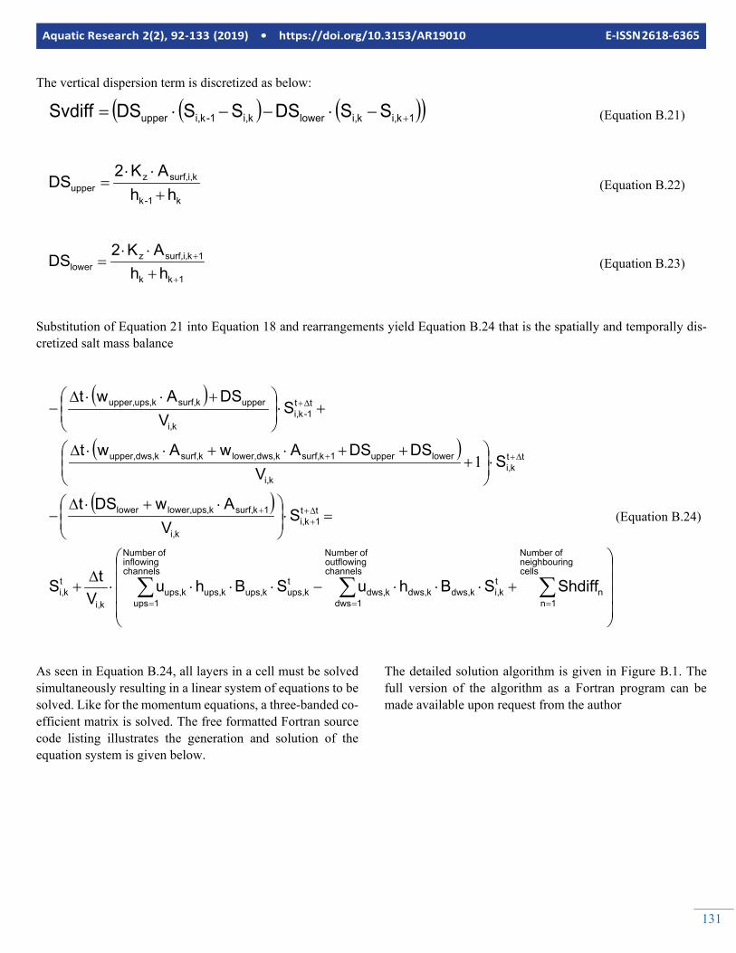
131
Aquatic Research 2(2), 92-133 (2019) • https://doi.org/10.3153/AR19010 E-ISSN 2618-6365
The vertical dispersion term is discretized as below:
( ) ( )( )1ki,ki,lowerki,1-ki,upper SSDSSSDSSvdiff +−⋅−−⋅= (Equation B.21)
k1-k
ki,surf,zupper hh
AK2DS
+⋅⋅
= (Equation B.22)
1kk
1ki,surf,zlower hh
AK2DS
+
+
+⋅⋅
= (Equation B.23)
Substitution of Equation 21 into Equation 18 and rearrangements yield Equation B.24 that is the spatially and temporally dis-cretized salt mass balance
( )
( )
( )
+⋅⋅⋅−⋅⋅⋅⋅∆
+
=⋅
⋅+⋅∆−
⋅
+
++⋅+⋅⋅∆
+⋅
+⋅⋅∆−
∑∑∑===
∆++
+
∆++
∆+
cells ngneighbouri
of Number
1nn
channels outflowing
of Number
1dws
tki,kdws,kdws,kdws,
channels inflowingof Number
1ups
tkups,kups,kups,kups,
ki,
tki,
tt1ki,
ki,
1ksurf,kups,lower,lower
ttki,
ki,
lowerupper1ksurf,kdws,lower,ksurf,kdws,upper,
tt1-ki,
ki,
upperksurf,kups,upper,
ShdiffSBhuSBhuV
tS
SV
AwDSt
SV
DSDSAwAwt
SV
DSAwt
1
(Equation B.24)
As seen in Equation B.24, all layers in a cell must be solved simultaneously resulting in a linear system of equations to be solved. Like for the momentum equations, a three-banded co-efficient matrix is solved. The free formatted Fortran source code listing illustrates the generation and solution of the equation system is given below.
The detailed solution algorithm is given in Figure B.1. The full version of the algorithm as a Fortran program can be made available upon request from the author
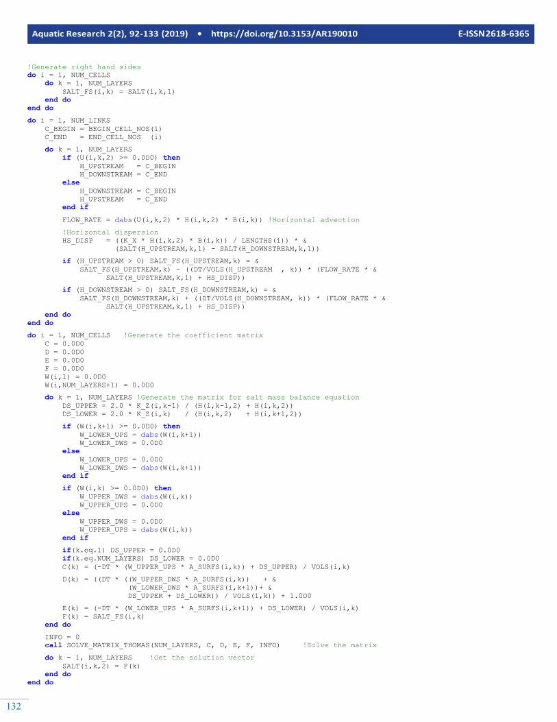
Aquatic Research 2(2), 92-133 (2019) • https://doi.org/10.3153/AR190010 E-ISSN 2618-6365
132
!Generate right hand sides do i = 1, NUM_CELLS do k = 1, NUM_LAYERS SALT_FS(i,k) = SALT(i,k,1) end do end do
do i = 1, NUM_LINKS C_BEGIN = BEGIN_CELL_NOS(i) C_END = END_CELL_NOS (i)
do k = 1, NUM_LAYERS if (U(i,k,2) >= 0.0D0) then H_UPSTREAM = C_BEGIN H_DOWNSTREAM = C_END else H_DOWNSTREAM = C_BEGIN H_UPSTREAM = C_END end if
FLOW_RATE = dabs(U(i,k,2) * H(i,k,2) * B(i,k)) !Horizontal advection
!Horizontal dispersion HS_DISP = ((K_X * H(i,k,2) * B(i,k)) / LENGTHS(i)) * & (SALT(H_UPSTREAM,k,1) - SALT(H_DOWNSTREAM,k,1))
if (H_UPSTREAM > 0) SALT_FS(H_UPSTREAM,k) = & SALT_FS(H_UPSTREAM,k) - ((DT/VOLS(H_UPSTREAM , k)) * (FLOW_RATE * & SALT(H_UPSTREAM,k,1) + HS_DISP))
if (H_DOWNSTREAM > 0) SALT_FS(H_DOWNSTREAM,k) = & SALT_FS(H_DOWNSTREAM,k) + ((DT/VOLS(H_DOWNSTREAM, k)) * (FLOW_RATE * & SALT(H_UPSTREAM,k,1) + HS_DISP)) end do end do
do i = 1, NUM_CELLS !Generate the coefficient matrix C = 0.0D0 D = 0.0D0 E = 0.0D0 F = 0.0D0 W(i,1) = 0.0D0 W(i,NUM_LAYERS+1) = 0.0D0
do k = 1, NUM_LAYERS !Generate the matrix for salt mass balance equation DS_UPPER = 2.0 * K_Z(i,k-1) / (H(i,k-1,2) + H(i,k,2)) DS_LOWER = 2.0 * K_Z(i,k) / (H(i,k,2) + H(i,k+1,2))
if (W(i,k+1) >= 0.0D0) then W_LOWER_UPS = dabs(W(i,k+1)) W_LOWER_DWS = 0.0D0 else W_LOWER_UPS = 0.0D0 W_LOWER_DWS = dabs(W(i,k+1)) end if
if (W(i,k) >= 0.0D0) then W_UPPER_DWS = dabs(W(i,k)) W_UPPER_UPS = 0.0D0 else W_UPPER_DWS = 0.0D0 W_UPPER_UPS = dabs(W(i,k)) end if
if(k.eq.1) DS_UPPER = 0.0D0 if(k.eq.NUM_LAYERS) DS_LOWER = 0.0D0 C(k) = (-DT * (W_UPPER_UPS * A_SURFS(i,k)) + DS_UPPER) / VOLS(i,k)
D(k) = ((DT * ((W_UPPER_DWS * A_SURFS(i,k)) + & (W_LOWER_DWS * A_SURFS(i,k+1))+ & DS_UPPER + DS_LOWER)) / VOLS(i,k)) + 1.0D0
E(k) = (-DT * (W_LOWER_UPS * A_SURFS(i,k+1)) + DS_LOWER) / VOLS(i,k) F(k) = SALT_FS(i,k) end do
INFO = 0 call SOLVE_MATRIX_THOMAS(NUM_LAYERS, C, D, E, F, INFO) !Solve the matrix
do k = 1, NUM_LAYERS !Get the solution vector SALT(i,k,2) = F(k) end do end do
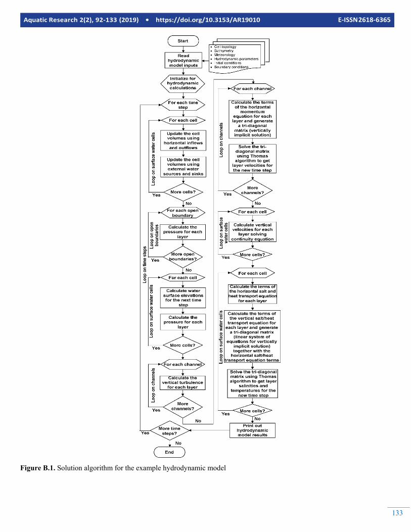
133
Aquatic Research 2(2), 92-133 (2019) • https://doi.org/10.3153/AR19010 E-ISSN 2618-6365
Figure B.1. Solution algorithm for the example hydrodynamic model