Embed Size (px)
Citation preview
“In the name of God, the merciful, the compassionate”
Modelling tidal processes in the Persian Gulf - With a view on Renewable Energy -
Dissertation with the aim of achieving a doctoral degree at
The Faculty of Mathematics, Informatics and Natural Sciences
Institute of Oceanography
University of Hamburg
Submitted by
Hossein Mashayekh Poul
2016 in Hamburg

Day of oral defense: 27.05.2016
The following evaluators recommend the admission of the dissertation:
Prof. Dr. Jan Backhaus
PD. Dr. Thomas Pohlmann
“And it is He who has released [simultaneously] the two seas, one fresh and sweet and one salty and bitter, and He placed between them a barrier and prohibiting partition.” Allah, years: 609-632, Al-Forghan 53, Quran
Abstract The main semidiurnal (M2 and S2) and diurnal (K1 and O1) tidal constituents were
simulated in the Persian Gulf (denoted PG). The topography of the PG was discretized on a
spherical grid with a resolution of 30 seconds in both latitude and longitude. It included
coastal areas prone to flooding. The model permitted flooding of drying banks up to 5 meters
above mean sea level. At the open boundary, it was forced by 13 harmonic constituents
extracted from a global tidal model. The Model results agreed well with tide gauge
observations. Co-tidal charts and flow extremes were presented for each tidal constituent. The
co-tidal charts showed two amphidromic points for semidiurnal and one for diurnal tidal
constituents. Maximum tidal amplitudes were obtained in the north-western part of the PG,
where coastal flooding prevails in wide areas. Strong tidal currents occurred in the PG but
their locations are driven by different, dominant tidal constituents. Maximum velocities were
found in shallow regions. Particularly high amplitudes of elevations and high velocities of
currents were found in the canal between Qeshm Island and the mainland. Tidal rectification
around Qeshm Island influenced hydrodynamics across the PG, as far as the coast of Saudi
Arabia and the northern part of the PG. The results provided a good estimate of the annual
kinetic energy output for the PG on the Iranian side, for the entrance of Musa estuary and
Qeshm canal.
Geological studies in the PG have revealed the existence of sub-seabed salt-domes.
Suitable, high-pass filtering of the PG seabed topography revealed the signature of these
domes on the seabed, i.e. numerous hills and valleys with amplitudes of several tens of
meters and radii from a few up to tens of kilometers. It was suspected that the 'shark skin' of
the PG seabed may affect the tidal residual flow. The interaction of tidal dynamics and these
obstacles was investigated in a non-linear hydrodynamic numerical tidal model of the PG.
First, the model was used to characterize flow patterns of residual currents generated by a
tidal wave passing over symmetric, elongated and tilted obstacles. Thereafter, it was applied
to the entire PG. The model was forced at its open boundary by the four dominant tidal
constituents residing in the PG. Each tidal constituent was separately simulated. Tidal
residual currents in the PG, as depicted by Lagrangian trajectories, revealed a stationary,
eddy-rich flow. Each eddy can be matched with a topographic obstacle. This confirmed that
the tidal residual flow field is strongly influenced by the nonlinear interaction of the tidal
wave with the bottom relief which, in turn, is deformed by salt-domes beneath the seabed.
Different areas of maximum residual current velocities were identified for each type of tidal
constituent. Two main cyclonic gyres and several adjacent gyres rotating in opposite
directions and a strong coastal current in the northern PG were identified.
The non-linear hydrodynamic numerical tidal model was applied to investigate the tidal
resonance in the PG. The model was used to characterize the amplified response of the basin
to different forcing periods. It was forced by waves with the same amplitude but different
periods ranging from 3.5 to 35.5 h with increments of 0.5 hours at its open boundary to the
Oman Sea. Each wave was simulated separately. The results revealed that, in three areas,
tidal elevations were significantly larger than the forcing amplitude, indicating resonance.
These areas were the northern PG (maximum Amplification Factor (AF) = 1.61), the Strait of
Hormuz (maximum AF = 3.00), and the southern PG (maximum AF = 1.33). The
amplification factor (AF) is the ratio of local amplitudes vs. forcing amplitude. Diurnal tides
were resonant in both the northern and southern PG. Semidiurnal constituents were amplified
in the northern Gulf as well as in the Strait of Hormuz. A simulated sea level rise due to
climate change of 1 meter increased the AF off the Arabian coast for semidiurnal tides from
0.72 to 1.21. In the Qeshm Canal in the Strait of Hormuz, AF increased from 1.36 to 1.57 for
semidiurnal and from 0.73 to 1.1 for diurnal tides. The results provide a good estimate of the
annual potential energy output for the PG on the Iranian side, for the Musa estuary and
Qeshm canal.
The tidal barotropic residual circulation in the Musa estuary was described by applying a
non-linear, 3-d hydrodynamic numerical model. The main point was to consider the effect of
evaporation on density-driven circulation and interactions with tidal currents. The Musa
estuary is located in the north-west of the PG. The climate in this region is arid, resulting in
an excess of evaporation over precipitation. There is no river runoff in this estuary. The
results suggested that the structure of the residual circulation and stratification depended on
the evaporation rate and, of course, the difference in tidal amplitude, i.e. neap and spring tide.
As a result of evaporation, the residual circulation was vertically stratified, with a dense,
saline, near-bottom flow toward the PG and relatively fresh inflow at the surface. But, in
scenarios using tides, residual circulation occurred in the opposite direction. The results
revealed a high salinity outflow and a lower salinity inflow but a stable salinity across the
whole region. There was a horizontal gradient in tidally-averaged salinity with the salinity
increasing towards the head of the Musa estuary, which is a salt producing, coastal system.
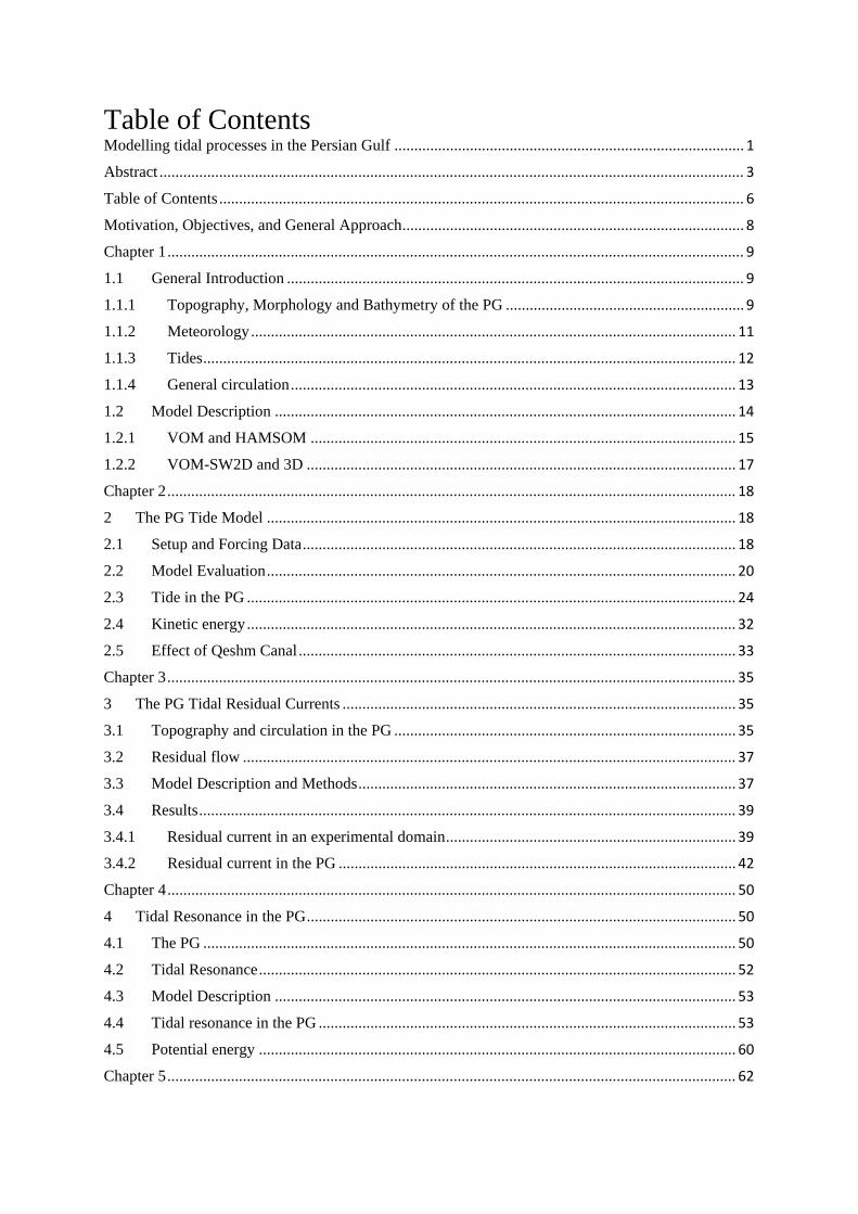
Table of Contents Modelling tidal processes in the Persian Gulf ........................................................................................ 1
Abstract ................................................................................................................................................... 3
Table of Contents .................................................................................................................................... 6
Motivation, Objectives, and General Approach ...................................................................................... 8
Chapter 1 ................................................................................................................................................. 9
1.1 General Introduction ................................................................................................................... 9
1.1.1 Topography, Morphology and Bathymetry of the PG ............................................................ 9
1.1.2 Meteorology .......................................................................................................................... 11
1.1.3 Tides ...................................................................................................................................... 12
1.1.4 General circulation ................................................................................................................ 13
1.2 Model Description .................................................................................................................... 14
1.2.1 VOM and HAMSOM ........................................................................................................... 15
1.2.2 VOM-SW2D and 3D ............................................................................................................ 17
Chapter 2 ............................................................................................................................................... 18
2 The PG Tide Model ...................................................................................................................... 18
2.1 Setup and Forcing Data ............................................................................................................. 18
2.2 Model Evaluation ...................................................................................................................... 20
2.3 Tide in the PG ........................................................................................................................... 24
2.4 Kinetic energy ........................................................................................................................... 32
2.5 Effect of Qeshm Canal .............................................................................................................. 33
Chapter 3 ............................................................................................................................................... 35
3 The PG Tidal Residual Currents ................................................................................................... 35
3.1 Topography and circulation in the PG ...................................................................................... 35
3.2 Residual flow ............................................................................................................................ 37
3.3 Model Description and Methods ............................................................................................... 37
3.4 Results ....................................................................................................................................... 39
3.4.1 Residual current in an experimental domain ......................................................................... 39
3.4.2 Residual current in the PG .................................................................................................... 42
Chapter 4 ............................................................................................................................................... 50
4 Tidal Resonance in the PG ............................................................................................................ 50
4.1 The PG ...................................................................................................................................... 50
4.2 Tidal Resonance ........................................................................................................................ 52
4.3 Model Description .................................................................................................................... 53
4.4 Tidal resonance in the PG ......................................................................................................... 53
4.5 Potential energy ........................................................................................................................ 60
Chapter 5 ............................................................................................................................................... 62
5 High evaporation and inverse estuary of the PG ........................................................................... 62
5.1 Musa estuary ............................................................................................................................. 62
5.2 Model Description and Methods ............................................................................................... 63
5.3 Results ....................................................................................................................................... 67
5.3.1 Experimental domain ............................................................................................................ 67
5.3.2 Musa estuary ......................................................................................................................... 70
Chapter 6 ............................................................................................................................................... 78
6 Summary and Conclusions............................................................................................................ 78
Acknowledgement ................................................................................................................................ 81
Declaration ............................................................................................................................................ 82
Bibliography ......................................................................................................................................... 83
Appendix ............................................................................................................................................... 90
1 Theoretical Aspects of 2D primitive equation models .................................................................. 90
1.1 Influence of the Spatial Discretization on Wave Propagation .................................................. 90
1.2 Spatial Discretisation for the ‘Primitive’ Equations ................................................................. 91
1.3 Numerical Wave Dispersion in Arakawa C-Grid ..................................................................... 92
1.4 Dispersion Relations of Arakawa C-Grids ................................................................................ 92
2 Rotational Primitive Equation Models; explicit, implicit ............................................................. 93
2.1 Explicit Scheme for the Storm Surge Model in the Arakawa C-grid ........................................ 94
2.2 The implicit Storm Surge Model .............................................................................................. 95
2.3 Horizontal Momentum Diffusion ............................................................................................ 100
2.4 Boundary Conditions for the Laplacian; Slip-conditions ........................................................ 100
2.5 Coriolis Rotation; the Problem with spatial averaging in the C-grid ...................................... 102
2.6 The Lagrangian upstream Advection Scheme, LAS: .............................................................. 104
2.7 Non-linear advective Terms in the Equations of motion ........................................................ 105
2.8 Stability of the rotational nonlinear 2D C-grid model ............................................................ 106
3 Implicit Channel Model with ‘Movable’ Boundary .................................................................... 106
3.1 Flooding towards the west ...................................................................................................... 108
3.2 Flooding towards the east ....................................................................................................... 109
List of Figures ..................................................................................................................................... 110
List of Tables ...................................................................................................................................... 114
List of publications ............................................................................................................................. 115
Motivation, Objectives, and General Approach The dynamics of tidal basins include a wide range of features with different spatial and
temporal scales. Numerical simulation of the Persian Gulf (PG) and its estuaries become an
interesting area of research. The simulations are performed by the development of
sophisticated ocean model suitable for this region of complex circulation. Such research is
important because many basic questions regarding physical processes in the PG remained
unanswered; e.g. tidal resonance and tidal residual currents and effects of evaporation on the
shallow tidal flat in the northern estuary of the PG, Musa estuary. Moreover, as tidal waves
move an enormous volume of water twice a day, for semidiurnal constituents, they provide a
great amount of renewable energy.
A numerical model is able to simulate tidal processes, with having the precise
geometrical features of the flow domain. Potential errors in numerical models result from
incomplete geometries, including simplification of coastal and bed irregularities as well as
ignoring small islands, particularly along the coastal zone. These deficiencies are important
especially in the study of residual currents. The present simulation, with the highest resolving
grid used for tidal predictions in the PG compared to various studies, can describe tidal
residual currents realistically and produces more accurate results for the other tidal processes
by considering more geometrical complexities.
The main purpose of this study is to improve the understanding of important features of
tidal dynamics and thermodynamics; with a view of tidal renewable energy. The thesis is
organized as follows: Chapter 1 presents an overview of Topography, Bathymetry and
Morphology, Meteorology, Tides and General circulation of the PG. Theory and Methods are
also described in this chapter together with a general description of VOM. The model
evaluation is described in chapter 2 and comparisons demonstrate the agreement of the model
data with available measurements. Furthermore, results of the tidal simulation by VOM-
SW2D is presented in this chapter from two published papers of this study, description
(Mashayekh Poul et al., 2016) and energy of tide (Mashayekh Poul et al., 2014) in the PG.
Analyses of the model results including Tidal Residual Current (paper in revision in JGR) are
discussed in chapter 3. Tidal Resonance in the PG is explained in chapter 4 and investigation
of the inverse estuary in the northern PG in chapter 5. Finally, Chapter 6 summaries the main
findings and presents an outlook for future studies and developments.
General Introduction
Chapter 1
1.1 General Introduction
Understanding tidal dynamics is important for coastal safety, navigation, ecology and
nowadays for Renewable Energy. The tide in semi-enclosed basins is the result of co-
oscillation with a larger sea, where basin geometry and topography play an important role.
The region of interest that is analysed in this study is the PG. For a better understanding, a
short description of the physical properties of the PG is given in the following sections.
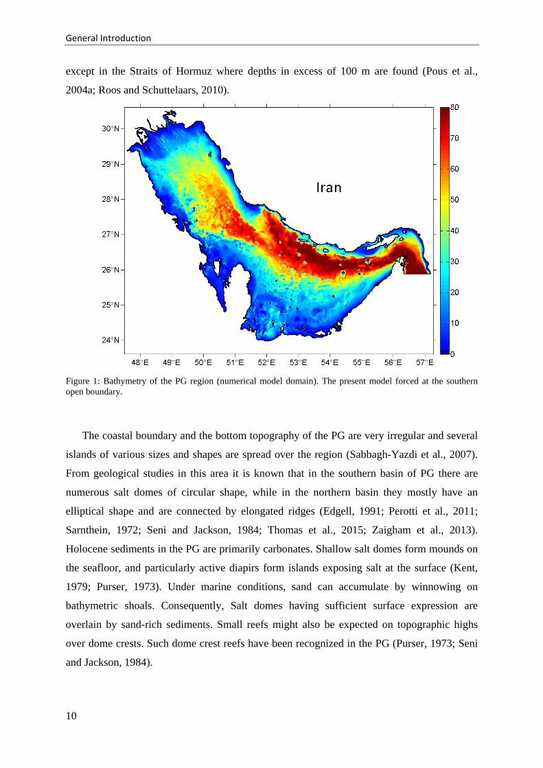
1.1.1 Topography, Morphology and Bathymetry of the PG
The PG, sometimes incorrectly called the Arabian Gulf, is a shallow semi-enclosed
marginal sea located between Iran and the Arabian Peninsula (Figure 1). It is connected with
the Indian Ocean through the Strait of Hormuz. The length of the PG is about 1000 km in
Northwest to Southeast orientation; the width varies from a maximum of 338 km to a
minimum of 56 km in the strait. The coastal orography bordering the PG exhibits distinct
contrast: while the Iranian coast is mountainous, the Arabian coast is mostly desert except
around the Strait (Yao, 2008).
The bottom topography of the PG is dominated by soft sediments at the sea floor. It is
generally deeper near the Iranian coast and is deepest near the opening of the Strait of
Hormuz. The average depth of the topography has reported 35-36m (Badri and Wilders,
2012; Moeini et al., 2010; Ranaee et al., 2011; Reynolds, 1993; Thoppil and Hogan, 2010a).
This basin is a relatively shallow zone near the closed end, extended all the way along the
southern part of the basin, roughly connected to one deeper part, with a clearly asymmetric
cross-sectional depth profile of the center part. Maximum depth in the deeper part is 80 m,
9
General Introduction
except in the Straits of Hormuz where depths in excess of 100 m are found (Pous et al.,
2004a; Roos and Schuttelaars, 2010).
Figure 1: Bathymetry of the PG region (numerical model domain). The present model forced at the southern open boundary.
The coastal boundary and the bottom topography of the PG are very irregular and several
islands of various sizes and shapes are spread over the region (Sabbagh-Yazdi et al., 2007).
From geological studies in this area it is known that in the southern basin of PG there are
numerous salt domes of circular shape, while in the northern basin they mostly have an
elliptical shape and are connected by elongated ridges (Edgell, 1991; Perotti et al., 2011;
Sarnthein, 1972; Seni and Jackson, 1984; Thomas et al., 2015; Zaigham et al., 2013).
Holocene sediments in the PG are primarily carbonates. Shallow salt domes form mounds on
the seafloor, and particularly active diapirs form islands exposing salt at the surface (Kent,
1979; Purser, 1973). Under marine conditions, sand can accumulate by winnowing on
bathymetric shoals. Consequently, Salt domes having sufficient surface expression are
overlain by sand-rich sediments. Small reefs might also be expected on topographic highs
over dome crests. Such dome crest reefs have been recognized in the PG (Purser, 1973; Seni
and Jackson, 1984).
10
General Introduction
Purser 1973 subdivided bathymetric Highs in the PG which have been grouped into three
classes: outer (basin center), intermediate and inner (coastal).
1. The central parts of the basin, where water depths generally exceed 50 m, are
characterized by numerous highs with marked vertical relief. Many of them are
salt diapirs and they have a structural origin. The latter is generally symmetric in
outline and range from islands to submerged shoals. All have one feature in
common; they are surrounded by relatively deep water.
2. The sloping sea floor is characterized by a great variety of marine highs and
depressions. They vary in diameter from several hundred meters to more than 50
km. Many emerge as islands due to salt diapirism in the Southeastern parts of the
PG. Others are low sand cays whose origins are essentially sedimentary. A limited
number are emergent pre-Holocene mesas. All have one feature in common: they
are surrounded by relatively shallow water varying in depth from 36m on the
outer parts of the homocline to less than 9m near the coast.
3. Highs situated close to the mainland shoreline may considerably affect coastal
sedimentation. They constitute low islands and shoals surrounded by complex
patterns of reefs and sand bars. Most highs have a pre-Holocene core of
"miliolite" limestone around which sediments are accreting.
1.1.2 Meteorology
The PG lies in the subtropical region where most of the Earth's deserts are to be found
and where the boundary of the tropical circulations and the synoptic weather systems of mid-
latitudes are located. The seasonal shifting of the two weather systems leads to strong
seasonal variability in near-surface meteorological conditions. The surface air temperature at
the northern PG, for instance, changes from 15◦C in winter to 34◦C in summer (Reynolds,
1993; Yao, 2008). The region is arid leading to considerable evaporation, greatly exceeding
precipitation and river discharge (Al-Subhi, 2010; Pous et al., 2004b).
The most well-known, and notorious, weather phenomenon in the PG is the Shamal. This
surface wind in the PG navigated by the mountains along the Iranian coast is predominantly
northwesterly throughout the year, i.e. along the axis of the PG (Reynolds, 1993). The
characteristics of the two seasons Shamals are markedly different (Perrone, 1979). During
winter, mainly between November and February, the wind is slightly stronger than that
during the summer, between June and September (Blain, 1998, n.d.). The summer Shamal is
continuous. It is associated with the relative strengths of the Indian and Arabian thermal lows.
11
General Introduction
The winter Shamal has a shorter duration compares to summer Shamal. It is associated with
frontal passages of the synoptic weather systems, bringing cold air over the PG from higher
latitudes. It is accompanied by such adverse weather conditions as thunderstorms, turbulence,
low visibilities, and high seas (Perrone, 1979; Reynolds, 1993). The cold and dry air
originating from the northwest during winter leads to extreme evaporation which results in
high salinity and density of the PG water (Blain, 1998, n.d.; Thoppil and Hogan, 2010a).
There are two types of winter Shamal with respect to duration, those which last 24–36 h and
those which last for a longer period of 3–5 days (Thoppil and Hogan, 2010a). Shamal wind
generated storm surges, coupled with tidal effects can lead to significant changes in the sea
level of several meters (El-Sabh and Murty, 1989).
The different diurnal heating and cooling cycles over the PG and the surrounding land
induce a strong breeze along the entire coastline, especially along the Arabian coast. One
effect of these winds is to drive surface pollutants to the beach much faster than they would
move otherwise (Reynolds, 1993).
1.1.3 Tides
Tides are an important and permanent driving force in the PG. The safe navigation of
ships through shallow water ports, estuaries and harbor engineering projects requires
knowledge of the time and height of the tides as well as the speed and direction of the tidal
currents. Also, depending on the species and water depth in this region fish may concentrate
during ebb or flood tidal currents. Finally, extracting energy from the tidal waves is important
because of its significant advantage.
During the last decade, a number of models have been applied for studies of tidal
dynamics in the PG (Bosch van Drakestein, 2014; Ganj, 2013; Gorji-Bandpy et al., 2013;
Pous et al., 2013; Sabbagh-Yazdi et al., 2007). In general, tides in the PG are complex. The
dominant tidal pattern changes from being primarily semidiurnal to diurnal (Reynolds, 1993).
The leading tidal constituents in this area are M2, K1, S2, O1, N2, P1, K2, and Q1; from
biggest to smallest. This order may change with the F-factor at other locations in the domain.
The F-factor identifies the type of tide between diurnal, semidiurnal and mixed. It is defined
as the ratio of the main diurnal over the main semidiurnal constituent’s amplitudes. For the
PG, it is K1+O1 for diurnal and M2+S2 for semidiurnal amplitudes (Najafi, 1997).
The PG has a natural period of 22.6 or 21.7 hours for tidal waves based on Japanese
method and Chrystal method (Defant, 1961), respectively. The semidiurnal and diurnal waves
generate resonant interactions in the domain. The result from these interactions is a system of
12
General Introduction
amphidromic points of Kelvin-Taylor type (Pous et al., 2013), two points for semidiurnal
constituents in the northwest and southeast ends and a single point for diurnal constituents in
the center of the PG, near Bahrain (Bosch van Drakestein, 2014; Hyder et al., 2013; Ranaee
et al., 2012; Reynolds, 1993).
1.1.4 General circulation
The circulation in the PG is driven by five types of forcing phenomena: wind-stress,
surface buoyancy fluxes, freshwater runoff, water exchange through the Strait of Hormuz and
tides (Thoppil and Hogan, 2010a). Observations of the water properties and circulation in the
PG are limited in temporal and spatial coverage (Yao, 2008). There are only a few published
basin-wide measurements:
1. Summer cruise by the German ship Meteor in 1948 (Emery, 1956).
2. Wintertime expedition of the Atlantis from Woods Hole Oceanographic Institution
in 1976 (Brewer and Dyrssen, 1985).
3. The Mt. Mitchell expedition (Reynolds, 1993) on surveys in February and June
1992.
4. Compiling the available hydrographic data to describe the aspects of the seasonal
variability (from January to August) of the water properties in the PG (Swift and
Bower, 2003).
5. Conducting measurements of the water exchange in the Strait, consisting of a
mooring site in the deep channel in Strait and four seasonal transects across the
Strait (Johns et al., 2003).
These measurements provide a long-term observation of the exchange process in the
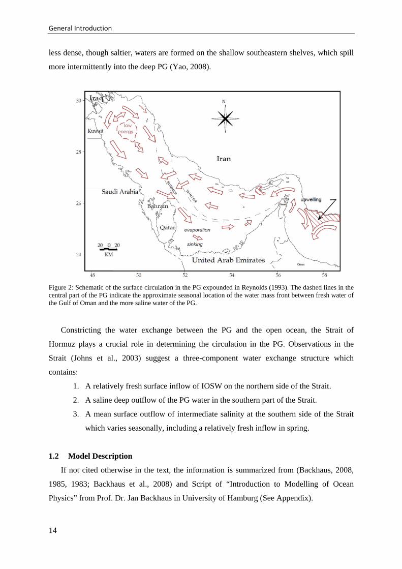
Strait. The Indian Ocean Surface Water (denoted IOSW) entering the PG through the
northern part of the Strait is swerved along the Iranian coast and appears to form a basin-wide
cyclonic circulation in the southern PG (Brewer and Dyrssen, 1985; Emery, 1956; Reynolds,
1993; Swift and Bower, 2003). Meanwhile, the relatively low salinity IOSW experiences a
salinity increase and is converted into high salinity waters in the northern gulf and in the
shallow southern gulf. A salinity front extending from the Strait separates the modified IOSW
from the salty water in the PG. The intruding IOSW shows distinct seasonal variability,
spreading much farther into the northern and southern gulf in early summer than in winter
(Figure 2). There are two down-wind coastal currents on both the Arabian and Iranian coasts
in the northern gulf. The densest waters are formed in the northern gulf during winter and
propagate southward toward the Strait throughout the year (Swift and Bower, 2003). Slightly
13
General Introduction
less dense, though saltier, waters are formed on the shallow southeastern shelves, which spill
more intermittently into the deep PG (Yao, 2008).
Figure 2: Schematic of the surface circulation in the PG expounded in Reynolds (1993). The dashed lines in the central part of the PG indicate the approximate seasonal location of the water mass front between fresh water of the Gulf of Oman and the more saline water of the PG.
Constricting the water exchange between the PG and the open ocean, the Strait of
Hormuz plays a crucial role in determining the circulation in the PG. Observations in the
Strait (Johns et al., 2003) suggest a three-component water exchange structure which
contains:
1. A relatively fresh surface inflow of IOSW on the northern side of the Strait.
2. A saline deep outflow of the PG water in the southern part of the Strait.
3. A mean surface outflow of intermediate salinity at the southern side of the Strait
which varies seasonally, including a relatively fresh inflow in spring.
1.2 Model Description
If not cited otherwise in the text, the information is summarized from (Backhaus, 2008,
1985, 1983; Backhaus et al., 2008) and Script of “Introduction to Modelling of Ocean
Physics” from Prof. Dr. Jan Backhaus in University of Hamburg (See Appendix).
14
General Introduction
1.2.1 VOM and HAMSOM
Topography is probably the most noticeable disturbance in ocean dynamics and yet still
under-represented in ocean models. The ‘quality’ of ocean models is often measured by their
horizontal resolution, rarely by their vertical. Some ocean regions would require higher
resolution than others. Thus, it seems plausible and reasonable to place resolution where it is
needed. This formed the start point for the development of vector- ocean-model (VOM),
which utilizes a static vertical adaptive grid in z-coordinates to improve the approximation of
both topography and flow by an increased vertical resolution at topographic boundaries.
VOM emerged from HAMSOM (HAMburg Shelf-Ocean Model), a three-dimensional semi-
implicit non-linear primitive equation model with a free surface (Backhaus, 2008, 1985,
1983).
Grids are organized in one dimensional vector containing only wet cells and being
defined on z-coordinate. This explains the first part of the model’s name (Vector). The grid
generator operates separately from a routine that produces the vector indexing and other grid
data needed by the model. Thus, the generation of grids for a given topography can be done
in isolation from model specific issues. VOM is defined in a C-grid (Arakawa and Lamb,
1977) because it is most commonly and most successfully used for shelf ocean modelling
(Backhaus, 1983). The adaptive grid generator delivers grids that can be implemented in any
horizontal Arakawa-grid. An index-vector for the sea surface, i.e. for the 2D model domain is
obtained by scanning the topography matrix while counting wet cells only, and storing their
counts in the vector. The last vector element is a dummy that represents all dry cells that were
discarded. For the approximation of closed boundaries in VOM, a pre-processing routine
converts grid-data into an indexing and into wet/dry masks that comply with a C-grid. The
vector-pointer that addresses the eight elements around a center-cell would deliver the (one)
dummy-index for all dry neighbor cells. Velocity components with this index would be zero.
In addition to dummy cells, individual wet/dry masks for scalars and vector-components are
derived from the gridding data. They assure a correct treatment of properties and flow vectors
at closed boundaries in any complex topography. This is exemplified by the implementation
of an adjustable slip condition for coastal parallel flow in a C-grid at a meridional coast.
VOM inherited large and well-approved parts of the numerical scheme of HAMSOM
(HAMburg Shelf Ocean Model) (Backhaus, 1985, 1983). HAMSOM served in regional seas
studies, in support of environmental, ecological and fisheries studies for both shelf and ocean,
and in regional climate investigations (Backhaus, 1996; Backhaus et al., 2008; Hainbucher
15
General Introduction
and Backhaus, 1999; Harms et al., 2000; Huang et al., 1999; Janssen et al., 2001; Schrum and
Backhaus, 1999; Stronach et al., 1993).
The numerical scheme of VOM has two important backbones inherited from HAMSOM
(Backhaus, 1983). One is the implicit solution of the heat conduction equation in the vertical,
here extended to also include advection. In view of the variety of vertical grid sizes in
adaptive grids in VOM_sw3d, this is a necessary pre-requisite for numerical stability. The
other is the implicit solution of the free surface problem, which allows avoiding time
splitting. That is, internal and external dynamics are always coupled. Time splitting, when
considering a shelf-ocean exchange, for instance, could cause a problem for relevant time
scales of deep and shallow regions may differ. VOM being designed to encompass oceans
and coastal seas with a locally isotropic vertical resolution therefore deliberately avoids a
time splitting (Backhaus et al., 2008).
Implicit schemes in VOM follow the classical approach (1) of Crank and Nicholson
(1947) but are applied in a slightly different form with the intention to increase the scheme’s
accuracy by predicting temporal changes of properties rather than properties.
𝝓𝝓𝒏𝒏+𝟏𝟏 − 𝝓𝝓𝒏𝒏 = ∆𝒕𝒕 �𝜶𝜶𝜶𝜶(𝝓𝝓𝒏𝒏+𝟏𝟏) + (𝟏𝟏 − 𝜶𝜶)𝜶𝜶(𝝓𝝓𝒏𝒏)� (1)
Here 𝜶𝜶 is the Crank–Nicholsen (CN) ‘implicitness’ pointer [0, 1], and n denotes the time-
level. L is a spatial difference operator applied to the property to be predicted 𝝓𝝓. ∆t is the
time step. The definition of: 𝝓𝝓𝒏𝒏+𝟏𝟏 = 𝝓𝝓𝒏𝒏 + ∆𝝓𝝓𝒏𝒏+𝟏𝟏 is used, where ∆𝝓𝝓𝒏𝒏+𝟏𝟏 is the temporal
change of 𝝓𝝓 within one time step. This allows implementing ∆𝝓𝝓𝒏𝒏+𝟏𝟏 as the prognostic
property of the implicit scheme. Replacing 𝝓𝝓𝒏𝒏+𝟏𝟏 in (1) by the above definition we arrive at
the implicit scheme (2) utilised in VOM for predicting temporal changes of properties
∆𝝓𝝓𝒏𝒏+𝟏𝟏 = ∆𝒕𝒕 �𝜶𝜶𝜶𝜶(𝝓𝝓𝒏𝒏+𝟏𝟏) + 𝜶𝜶(𝝓𝝓𝒏𝒏)�
In Crank and Nicholson (1947) a pointer α=0.5 was used, which ensures a neutrally stable
scheme void of amplitude damping. Apparently, with α=0, the scheme would degenerate to
an explicit one.
The procedure for solving a time step in VOM relies on the philosophy that all
components are solved individually and independently and that their sum yields the final
result. A ‘component’ could be one or more terms in the governing equations. The heat
conduction equation, for instance, is treated as one component, and each component has its
own subroutine. Therefore, the code of VOM is strictly modular.
16
General Introduction
1.2.2 VOM-SW2D and 3D
The Vector Ocean Model Shallow Water 2d (VOM-SW2d) is a two dimensional semi-
implicit nonlinear model which is developed at the institute of oceanography at the university
of Hamburg. It emanates from HAMSOM (Alvarez Fanjul et al., 1997; Backhaus, 1985) and
VOM. The model has new advection schemes implemented and allows for flooding and
drying of individual grid cells.
VOM-SW2d (Backhaus, 2008; Backhaus et al., 2008) has a two-dimensional numerical
scheme in a horizontal plane approximates the vertically integrated primitive shallow water
equations in a rotational framework. These also called ‘storm-surge’ models are central
components of three-dimensional ocean models for they deliver the spatial and temporal
evolution of the free surface, and thus an integral part of the pressure field. It is two-
dimensional primitive equation model by including rotation, diffusion, advection of
momentum, and passive tracers to mark the flow. The model is capable to operate in an
arbitrary topography with islands etc. Rotation is approximated in the presence of an irregular
coastline. The same applies for the approximation of lateral momentum diffusion controlled
by a slip boundary condition. More details in each case of this study have explained in the
chapters.
VOM_sw2d is a model in vector-notation (VOM: Vector-Ocean-Model); sw2d stands for
2D in shallow water. That is, the computational domain is mapped onto a one-dimensional
‘wet-only’ vector leaving out all cells covered by land, yet including any cells that potentially
may be wetted. The model incorporates a wetting algorithm (Backhaus, 1976) which in the
past has been optimized for many applications. It allows simulating wetting and drying of
low-lying coastal areas. Non-linearity in the model stems from the equation of continuity
(momentum in divergence), seabed friction, and the non-linear advective terms which
numerically are approximated by a Lagrangian Upstream Scheme. For parallelization, the
VOM-vector is chopped into N partitions, where N is the number of available computational
nodes. Each node runs with a performance close to 100% because the vector only contains
wet cells.
17
The Persian Gulf Tide Model
Chapter 2 The results of this chapter have been already published in (Mashayekh Poul et al., 2016)
and (Mashayekh Poul et al., 2014).
2 The PG Tide Model
The main semidiurnal (M2 and S2) and diurnal (K1 and O1) tidal constituents are
simulated in the PG. The topography is discretized on a spherical grid with a resolution of 30
seconds in both latitude and longitude. It includes coastal areas prone to flooding. The model
permits flooding of drying banks up to 5 meters above mean sea level. At the open boundary,
it is forced by 13 harmonic constituents extracted from a global tidal model. The Model
results are in good agreement with tide gauge observations. Co-tidal charts and flow extremes
are presented for each tidal constituent. The co-tidal charts show two amphidromic points for
semidiurnal and one for diurnal tidal constituents. Maximum amplitudes of sea level are
obtained for the north-western part of the PG, where coastal flooding prevails in wide areas.
Strong tidal currents occur in different parts of the PG for each type of constituents.
Maximum velocities are found in shallow regions. Particularly high amplitudes of elevations
and high speed currents are founded in the canal between Qeshm Island and the mainland.
Rectification of tides around Qeshm Island affects the propagation of tides in the PG as far as
the coast of Saudi Arabia and the northern part of the PG.
2.1 Setup and Forcing Data
The accuracy of regional tide models is often limited by bottom topography errors in
particular in shallow regions (Quaresma and Pichon, 2013). The model topography for the
PG, used in this study, has a horizontal resolution of 30 seconds (i.e. half a nautical mile)
with a lateral open boundary on the east side of the domain. The data are provided by the
18
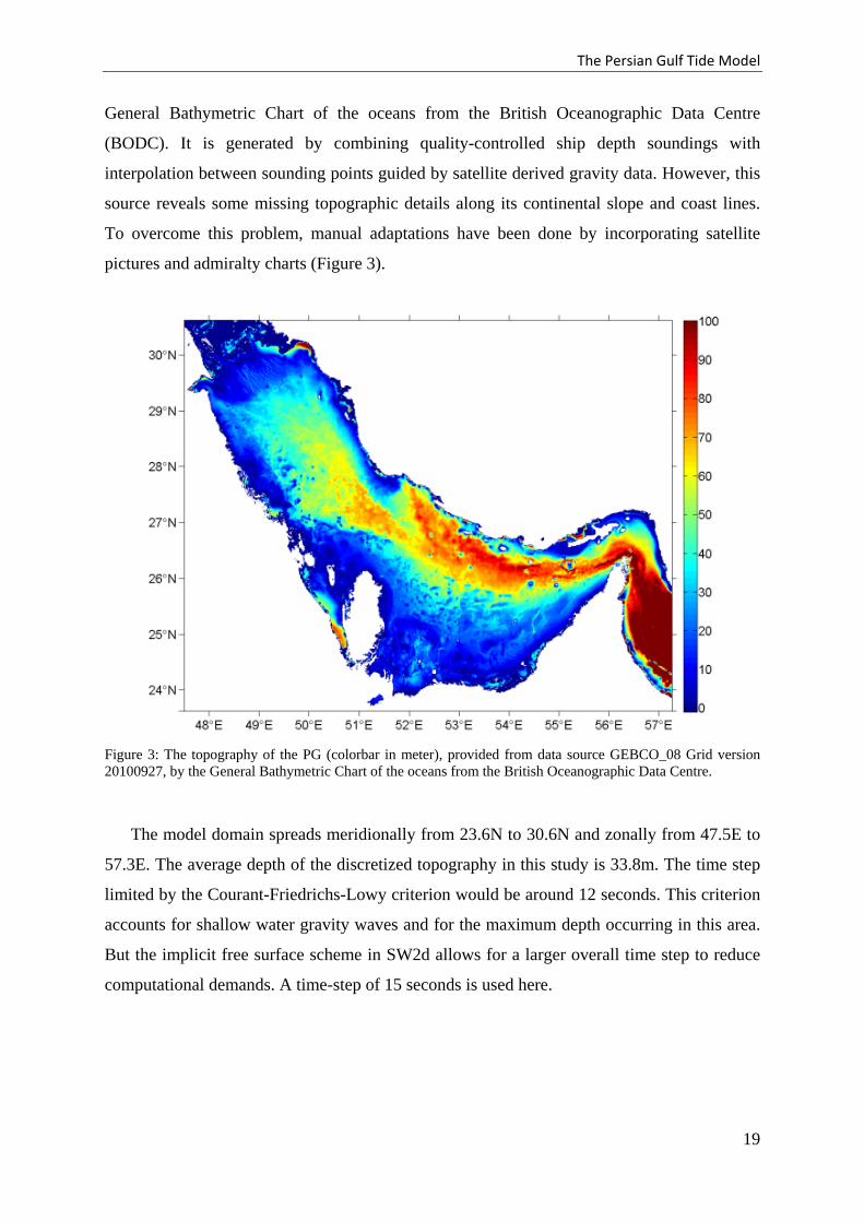
The Persian Gulf Tide Model
General Bathymetric Chart of the oceans from the British Oceanographic Data Centre
(BODC). It is generated by combining quality-controlled ship depth soundings with
interpolation between sounding points guided by satellite derived gravity data. However, this
source reveals some missing topographic details along its continental slope and coast lines.
To overcome this problem, manual adaptations have been done by incorporating satellite
pictures and admiralty charts (Figure 3).
Figure 3: The topography of the PG (colorbar in meter), provided from data source GEBCO_08 Grid version 20100927, by the General Bathymetric Chart of the oceans from the British Oceanographic Data Centre.
The model domain spreads meridionally from 23.6N to 30.6N and zonally from 47.5E to
57.3E. The average depth of the discretized topography in this study is 33.8m. The time step
limited by the Courant-Friedrichs-Lowy criterion would be around 12 seconds. This criterion
accounts for shallow water gravity waves and for the maximum depth occurring in this area.
But the implicit free surface scheme in SW2d allows for a larger overall time step to reduce
computational demands. A time-step of 15 seconds is used here.
19
The Persian Gulf Tide Model
The quadratic function of the barotropic current formulated for the bottom stress is
parameterized by a bottom friction coefficient of 1.1e-3. For momentum diffusion, horizontal
diffusion coefficients are calculated using Smagorinsky's Algorithm for each time-step from
the velocity field.
13 principal constituents, including semidiurnal and diurnal tides, are extracted using the
OSU Tidal Inversion Software (Egbert and Erofeeva, 2002) to be assembled and forced at the
lateral open boundary. These harmonic constants are essential to reproduce the regional
propagation of tidal waves, allowing non-linear harmonic interactions (Quaresma and Pichon,
2013). To account for realistic tidal elevations at the open boundary, the time-dependent
astronomical variable of V0+V was added to the surface elevation for phase correction.
The Model initialized from first of January 2011 and it simulated 12 consecutive months.
Tidal harmonic constants were extracted using Tidal Analysis Toolbox (Pawlowicz et al.,
2002) from the simulated surface elevation time series. The Tidal Analysis Toolbox uses
harmonic analysis to estimate tidal constituents and their uncertainties in scalar and vector
time series. Furthermore, tidal harmonic constants were extracted for 25 stations in the PG to
validate the model results.
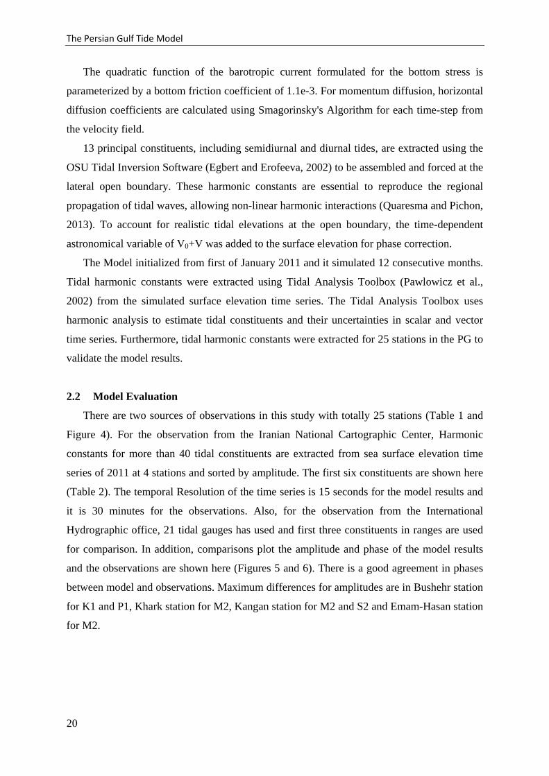
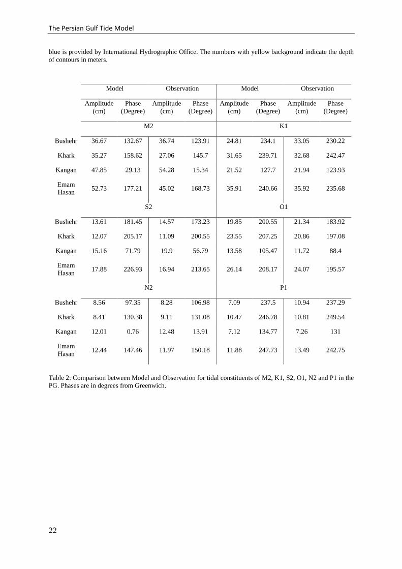
2.2 Model Evaluation
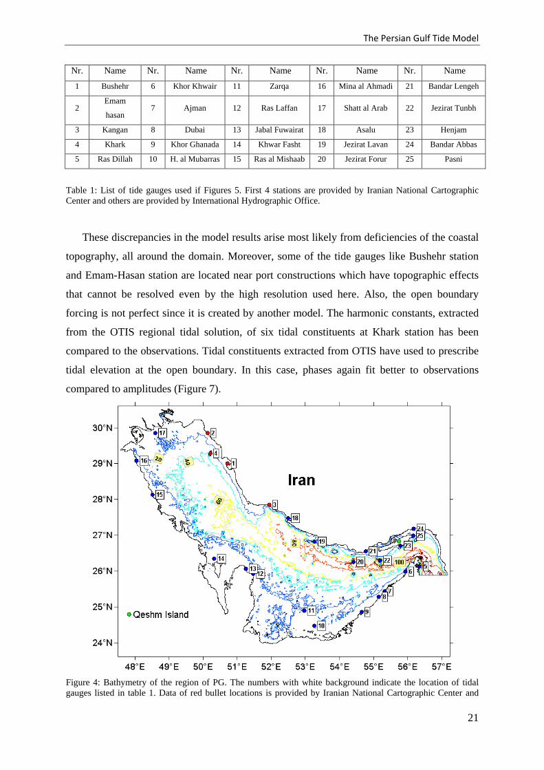
There are two sources of observations in this study with totally 25 stations (Table 1 and
Figure 4). For the observation from the Iranian National Cartographic Center, Harmonic
constants for more than 40 tidal constituents are extracted from sea surface elevation time
series of 2011 at 4 stations and sorted by amplitude. The first six constituents are shown here
(Table 2). The temporal Resolution of the time series is 15 seconds for the model results and
it is 30 minutes for the observations. Also, for the observation from the International
Hydrographic office, 21 tidal gauges has used and first three constituents in ranges are used
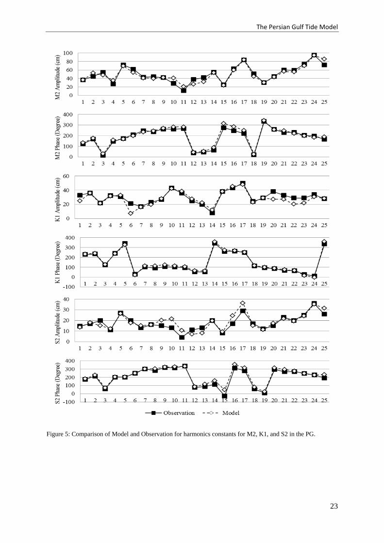
for comparison. In addition, comparisons plot the amplitude and phase of the model results
and the observations are shown here (Figures 5 and 6). There is a good agreement in phases
between model and observations. Maximum differences for amplitudes are in Bushehr station
for K1 and P1, Khark station for M2, Kangan station for M2 and S2 and Emam-Hasan station
for M2.
20
The Persian Gulf Tide Model
Nr. Name Nr. Name Nr. Name Nr. Name Nr. Name
1 Bushehr 6 Khor Khwair 11 Zarqa 16 Mina al Ahmadi 21 Bandar Lengeh
2 Emam
hasan 7 Ajman 12 Ras Laffan 17 Shatt al Arab 22 Jezirat Tunbh
3 Kangan 8 Dubai 13 Jabal Fuwairat 18 Asalu 23 Henjam
4 Khark 9 Khor Ghanada 14 Khwar Fasht 19 Jezirat Lavan 24 Bandar Abbas
5 Ras Dillah 10 H. al Mubarras 15 Ras al Mishaab 20 Jezirat Forur 25 Pasni
Table 1: List of tide gauges used if Figures 5. First 4 stations are provided by Iranian National Cartographic Center and others are provided by International Hydrographic Office.
These discrepancies in the model results arise most likely from deficiencies of the coastal
topography, all around the domain. Moreover, some of the tide gauges like Bushehr station
and Emam-Hasan station are located near port constructions which have topographic effects
that cannot be resolved even by the high resolution used here. Also, the open boundary
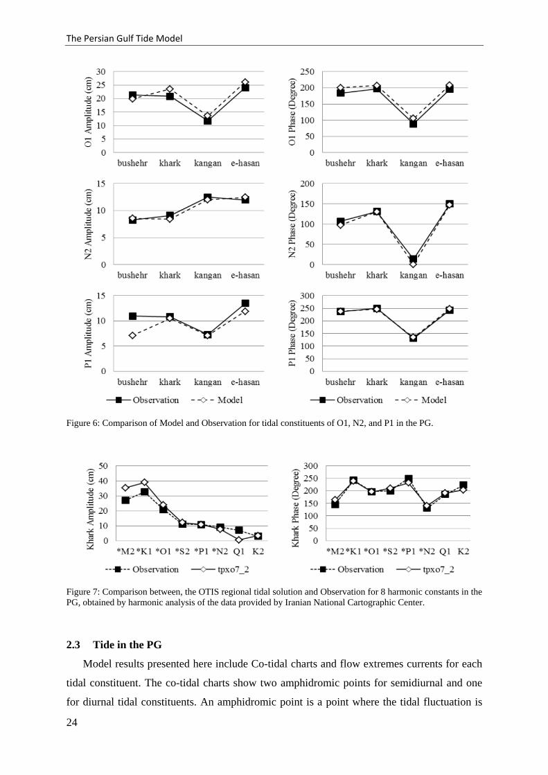
forcing is not perfect since it is created by another model. The harmonic constants, extracted
from the OTIS regional tidal solution, of six tidal constituents at Khark station has been
compared to the observations. Tidal constituents extracted from OTIS have used to prescribe
tidal elevation at the open boundary. In this case, phases again fit better to observations
compared to amplitudes (Figure 7).
Figure 4: Bathymetry of the region of PG. The numbers with white background indicate the location of tidal gauges listed in table 1. Data of red bullet locations is provided by Iranian National Cartographic Center and
21
The Persian Gulf Tide Model
blue is provided by International Hydrographic Office. The numbers with yellow background indicate the depth of contours in meters.
Model Observation Model Observation
Amplitude (cm)
Phase (Degree)
Amplitude (cm)
Phase (Degree)
Amplitude (cm)
Phase (Degree)
Amplitude (cm)
Phase (Degree)
M2 K1
Bushehr 36.67 132.67 36.74 123.91 24.81 234.1 33.05 230.22
Khark 35.27 158.62 27.06 145.7 31.65 239.71 32.68 242.47
Kangan 47.85 29.13 54.28 15.34 21.52 127.7 21.94 123.93
Emam Hasan 52.73 177.21 45.02 168.73 35.91 240.66 35.92 235.68
S2 O1
Bushehr 13.61 181.45 14.57 173.23 19.85 200.55 21.34 183.92
Khark 12.07 205.17 11.09 200.55 23.55 207.25 20.86 197.08
Kangan 15.16 71.79 19.9 56.79 13.58 105.47 11.72 88.4
Emam Hasan 17.88 226.93 16.94 213.65 26.14 208.17 24.07 195.57
N2 P1
Bushehr 8.56 97.35 8.28 106.98 7.09 237.5 10.94 237.29
Khark 8.41 130.38 9.11 131.08 10.47 246.78 10.81 249.54
Kangan 12.01 0.76 12.48 13.91 7.12 134.77 7.26 131
Emam Hasan 12.44 147.46 11.97 150.18 11.88 247.73 13.49 242.75
Table 2: Comparison between Model and Observation for tidal constituents of M2, K1, S2, O1, N2 and P1 in the PG. Phases are in degrees from Greenwich.
22
The Persian Gulf Tide Model
Figure 5: Comparison of Model and Observation for harmonics constants for M2, K1, and S2 in the PG.
23
The Persian Gulf Tide Model
Figure 6: Comparison of Model and Observation for tidal constituents of O1, N2, and P1 in the PG.
Figure 7: Comparison between, the OTIS regional tidal solution and Observation for 8 harmonic constants in the PG, obtained by harmonic analysis of the data provided by Iranian National Cartographic Center.
2.3 Tide in the PG
Model results presented here include Co-tidal charts and flow extremes currents for each
tidal constituent. The co-tidal charts show two amphidromic points for semidiurnal and one
for diurnal tidal constituents. An amphidromic point is a point where the tidal fluctuation is
24
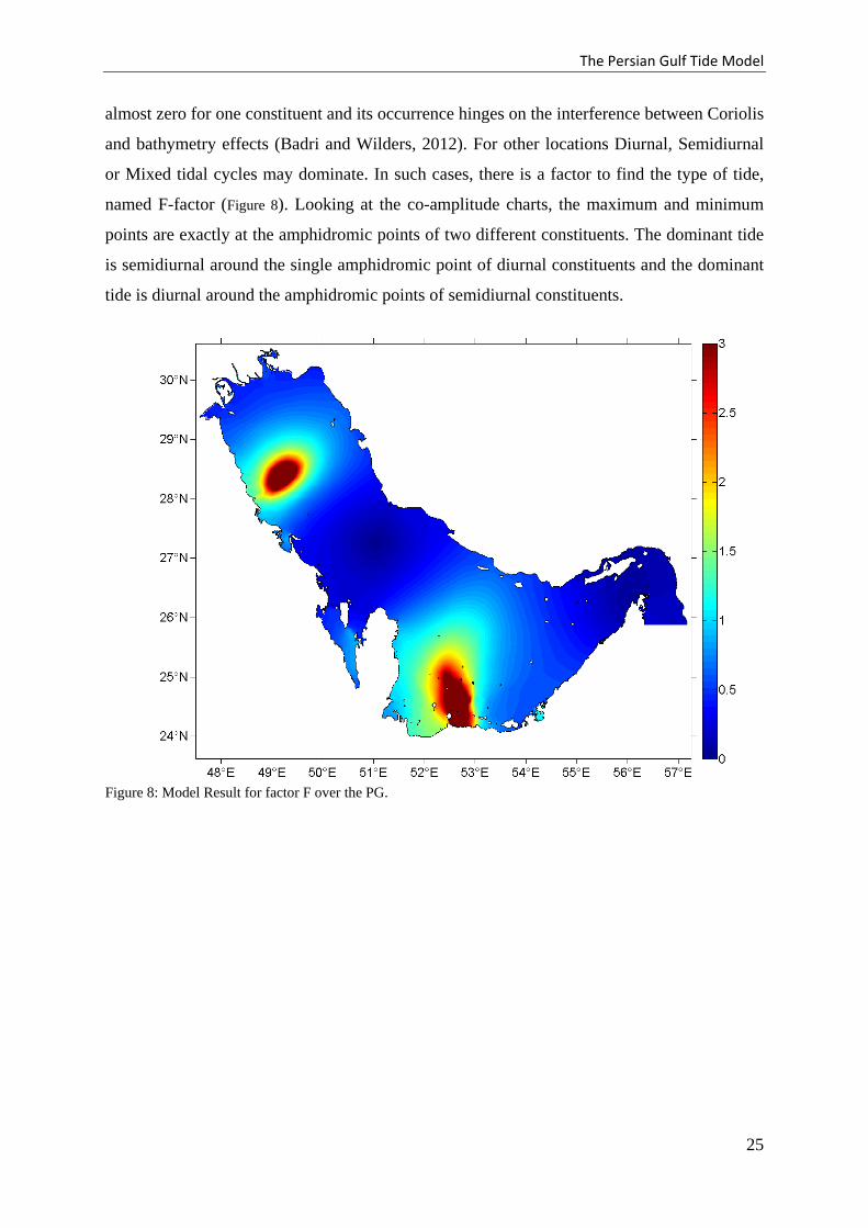
The Persian Gulf Tide Model
almost zero for one constituent and its occurrence hinges on the interference between Coriolis
and bathymetry effects (Badri and Wilders, 2012). For other locations Diurnal, Semidiurnal
or Mixed tidal cycles may dominate. In such cases, there is a factor to find the type of tide,
named F-factor (Figure 8). Looking at the co-amplitude charts, the maximum and minimum
points are exactly at the amphidromic points of two different constituents. The dominant tide
is semidiurnal around the single amphidromic point of diurnal constituents and the dominant
tide is diurnal around the amphidromic points of semidiurnal constituents.
Figure 8: Model Result for factor F over the PG.
25
The Persian Gulf Tide Model
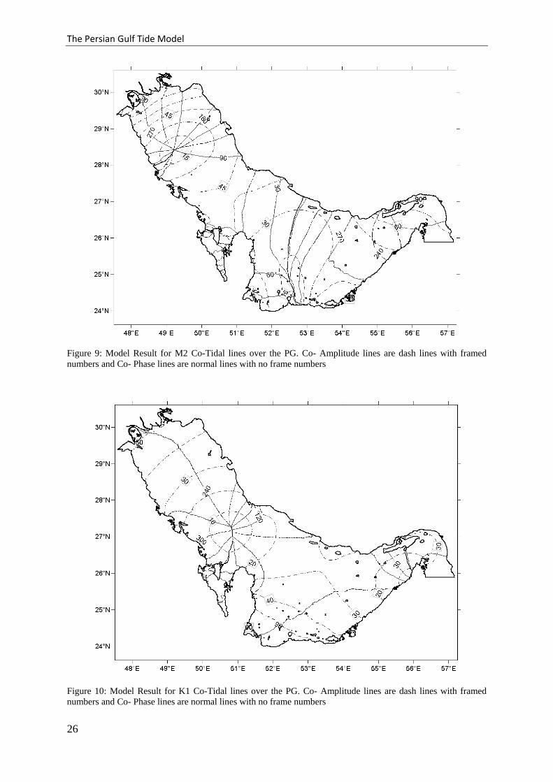
Figure 9: Model Result for M2 Co-Tidal lines over the PG. Co- Amplitude lines are dash lines with framed numbers and Co- Phase lines are normal lines with no frame numbers
Figure 10: Model Result for K1 Co-Tidal lines over the PG. Co- Amplitude lines are dash lines with framed numbers and Co- Phase lines are normal lines with no frame numbers
26
The Persian Gulf Tide Model
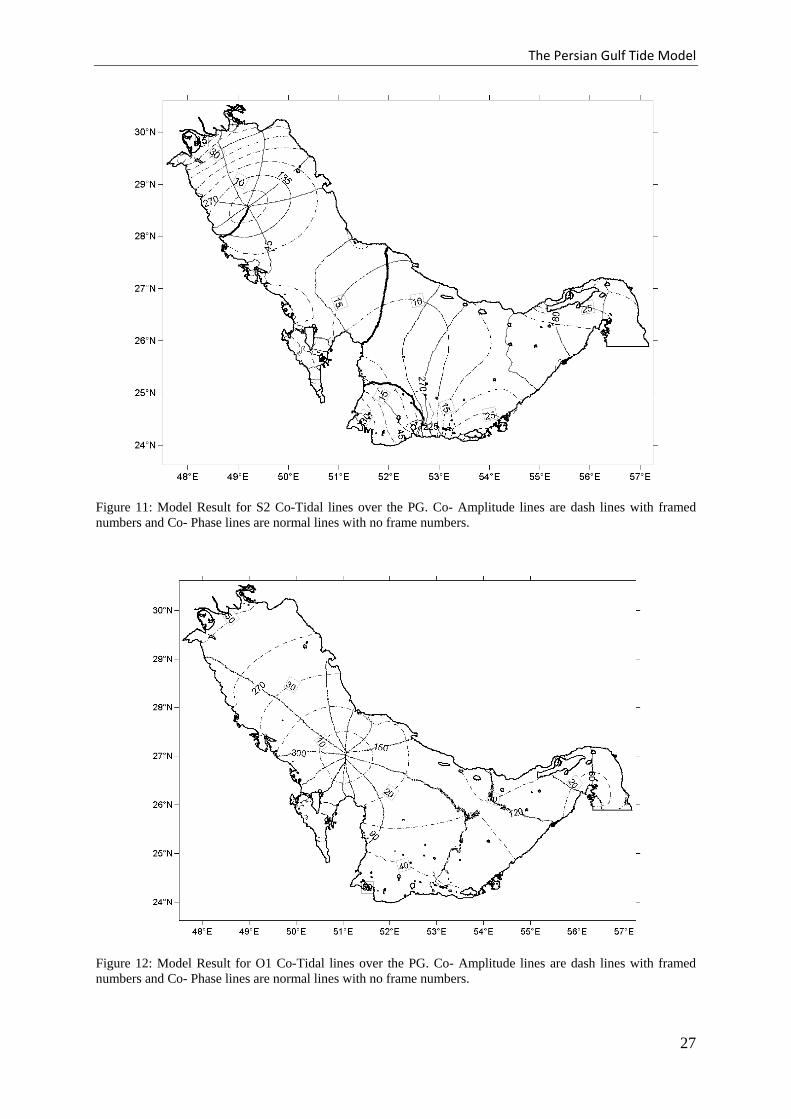
Figure 11: Model Result for S2 Co-Tidal lines over the PG. Co- Amplitude lines are dash lines with framed numbers and Co- Phase lines are normal lines with no frame numbers.
Figure 12: Model Result for O1 Co-Tidal lines over the PG. Co- Amplitude lines are dash lines with framed numbers and Co- Phase lines are normal lines with no frame numbers.
27
The Persian Gulf Tide Model
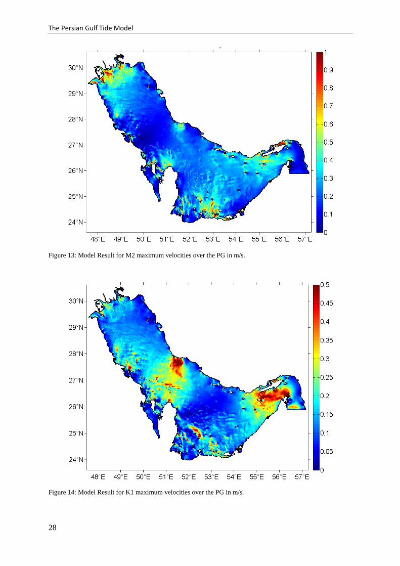
Figure 13: Model Result for M2 maximum velocities over the PG in m/s.
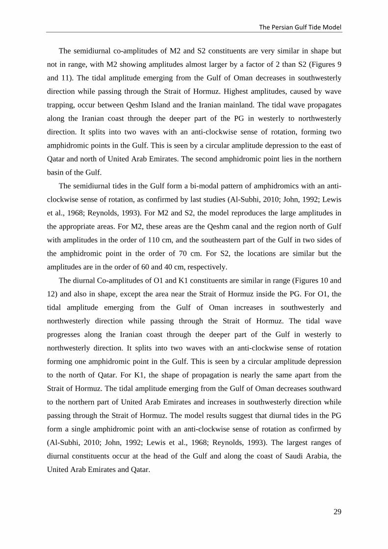
Figure 14: Model Result for K1 maximum velocities over the PG in m/s.
28
The Persian Gulf Tide Model
The semidiurnal co-amplitudes of M2 and S2 constituents are very similar in shape but
not in range, with M2 showing amplitudes almost larger by a factor of 2 than S2 (Figures 9
and 11). The tidal amplitude emerging from the Gulf of Oman decreases in southwesterly
direction while passing through the Strait of Hormuz. Highest amplitudes, caused by wave
trapping, occur between Qeshm Island and the Iranian mainland. The tidal wave propagates
along the Iranian coast through the deeper part of the PG in westerly to northwesterly
direction. It splits into two waves with an anti-clockwise sense of rotation, forming two
amphidromic points in the Gulf. This is seen by a circular amplitude depression to the east of
Qatar and north of United Arab Emirates. The second amphidromic point lies in the northern
basin of the Gulf.
The semidiurnal tides in the Gulf form a bi-modal pattern of amphidromics with an anti-
clockwise sense of rotation, as confirmed by last studies (Al-Subhi, 2010; John, 1992; Lewis
et al., 1968; Reynolds, 1993). For M2 and S2, the model reproduces the large amplitudes in
the appropriate areas. For M2, these areas are the Qeshm canal and the region north of Gulf
with amplitudes in the order of 110 cm, and the southeastern part of the Gulf in two sides of
the amphidromic point in the order of 70 cm. For S2, the locations are similar but the
amplitudes are in the order of 60 and 40 cm, respectively.
The diurnal Co-amplitudes of O1 and K1 constituents are similar in range (Figures 10 and
12) and also in shape, except the area near the Strait of Hormuz inside the PG. For O1, the
tidal amplitude emerging from the Gulf of Oman increases in southwesterly and
northwesterly direction while passing through the Strait of Hormuz. The tidal wave
progresses along the Iranian coast through the deeper part of the Gulf in westerly to
northwesterly direction. It splits into two waves with an anti-clockwise sense of rotation
forming one amphidromic point in the Gulf. This is seen by a circular amplitude depression
to the north of Qatar. For K1, the shape of propagation is nearly the same apart from the
Strait of Hormuz. The tidal amplitude emerging from the Gulf of Oman decreases southward
to the northern part of United Arab Emirates and increases in southwesterly direction while
passing through the Strait of Hormuz. The model results suggest that diurnal tides in the PG
form a single amphidromic point with an anti-clockwise sense of rotation as confirmed by
(Al-Subhi, 2010; John, 1992; Lewis et al., 1968; Reynolds, 1993). The largest ranges of
diurnal constituents occur at the head of the Gulf and along the coast of Saudi Arabia, the
United Arab Emirates and Qatar.
29
The Persian Gulf Tide Model
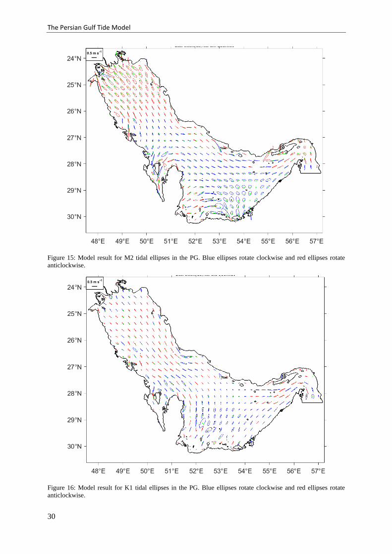
Figure 15: Model result for M2 tidal ellipses in the PG. Blue ellipses rotate clockwise and red ellipses rotate anticlockwise.
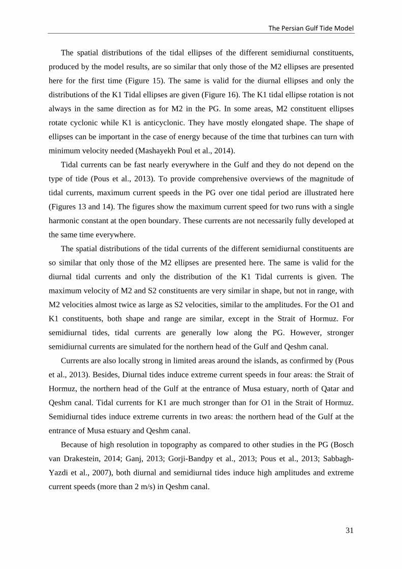
Figure 16: Model result for K1 tidal ellipses in the PG. Blue ellipses rotate clockwise and red ellipses rotate anticlockwise.
30
The Persian Gulf Tide Model
The spatial distributions of the tidal ellipses of the different semidiurnal constituents,
produced by the model results, are so similar that only those of the M2 ellipses are presented
here for the first time (Figure 15). The same is valid for the diurnal ellipses and only the
distributions of the K1 Tidal ellipses are given (Figure 16). The K1 tidal ellipse rotation is not
always in the same direction as for M2 in the PG. In some areas, M2 constituent ellipses
rotate cyclonic while K1 is anticyclonic. They have mostly elongated shape. The shape of
ellipses can be important in the case of energy because of the time that turbines can turn with
minimum velocity needed (Mashayekh Poul et al., 2014).
Tidal currents can be fast nearly everywhere in the Gulf and they do not depend on the
type of tide (Pous et al., 2013). To provide comprehensive overviews of the magnitude of
tidal currents, maximum current speeds in the PG over one tidal period are illustrated here
(Figures 13 and 14). The figures show the maximum current speed for two runs with a single
harmonic constant at the open boundary. These currents are not necessarily fully developed at
the same time everywhere.
The spatial distributions of the tidal currents of the different semidiurnal constituents are
so similar that only those of the M2 ellipses are presented here. The same is valid for the
diurnal tidal currents and only the distribution of the K1 Tidal currents is given. The
maximum velocity of M2 and S2 constituents are very similar in shape, but not in range, with
M2 velocities almost twice as large as S2 velocities, similar to the amplitudes. For the O1 and
K1 constituents, both shape and range are similar, except in the Strait of Hormuz. For
semidiurnal tides, tidal currents are generally low along the PG. However, stronger
semidiurnal currents are simulated for the northern head of the Gulf and Qeshm canal.
Currents are also locally strong in limited areas around the islands, as confirmed by (Pous
et al., 2013). Besides, Diurnal tides induce extreme current speeds in four areas: the Strait of
Hormuz, the northern head of the Gulf at the entrance of Musa estuary, north of Qatar and
Qeshm canal. Tidal currents for K1 are much stronger than for O1 in the Strait of Hormuz.
Semidiurnal tides induce extreme currents in two areas: the northern head of the Gulf at the
entrance of Musa estuary and Qeshm canal.
Because of high resolution in topography as compared to other studies in the PG (Bosch
van Drakestein, 2014; Ganj, 2013; Gorji-Bandpy et al., 2013; Pous et al., 2013; Sabbagh-
Yazdi et al., 2007), both diurnal and semidiurnal tides induce high amplitudes and extreme
current speeds (more than 2 m/s) in Qeshm canal.
31
The Persian Gulf Tide Model
2.4 Kinetic energy
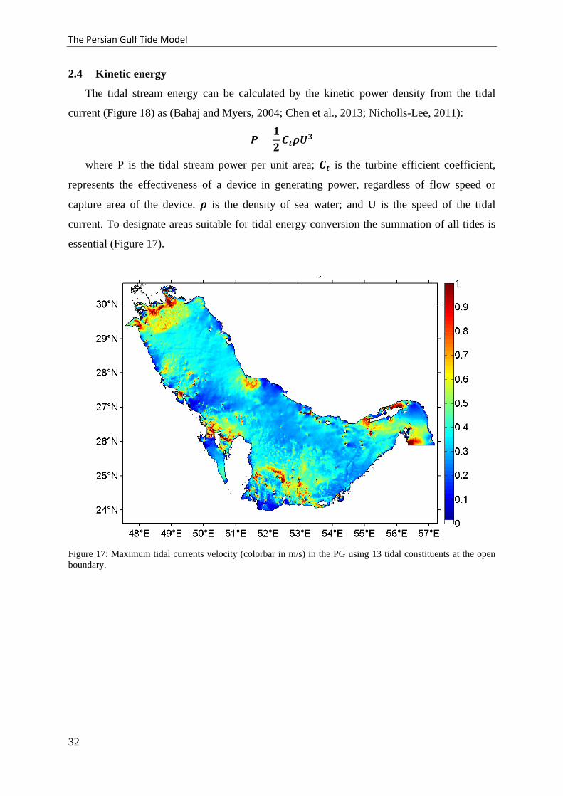
The tidal stream energy can be calculated by the kinetic power density from the tidal
current (Figure 18) as (Bahaj and Myers, 2004; Chen et al., 2013; Nicholls-Lee, 2011):
𝑷𝑷 =𝟏𝟏𝟐𝟐
𝑪𝑪𝒕𝒕𝝆𝝆𝑼𝑼𝟑𝟑
where P is the tidal stream power per unit area; 𝑪𝑪𝒕𝒕 is the turbine efficient coefficient, represents the effectiveness of a device in generating power, regardless of flow speed or
capture area of the device. 𝝆𝝆 is the density of sea water; and U is the speed of the tidal
current. To designate areas suitable for tidal energy conversion the summation of all tides is
essential (Figure 17).
Figure 17: Maximum tidal currents velocity (colorbar in m/s) in the PG using 13 tidal constituents at the open boundary.
32
The Persian Gulf Tide Model
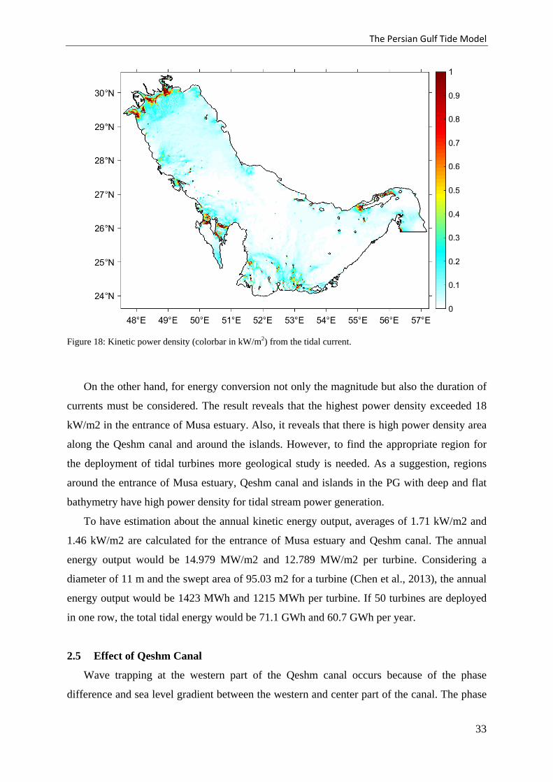
Figure 18: Kinetic power density (colorbar in kW/m2) from the tidal current.
On the other hand, for energy conversion not only the magnitude but also the duration of
currents must be considered. The result reveals that the highest power density exceeded 18
kW/m2 in the entrance of Musa estuary. Also, it reveals that there is high power density area
along the Qeshm canal and around the islands. However, to find the appropriate region for
the deployment of tidal turbines more geological study is needed. As a suggestion, regions
around the entrance of Musa estuary, Qeshm canal and islands in the PG with deep and flat
bathymetry have high power density for tidal stream power generation.
To have estimation about the annual kinetic energy output, averages of 1.71 kW/m2 and
1.46 kW/m2 are calculated for the entrance of Musa estuary and Qeshm canal. The annual
energy output would be 14.979 MW/m2 and 12.789 MW/m2 per turbine. Considering a
diameter of 11 m and the swept area of 95.03 m2 for a turbine (Chen et al., 2013), the annual
energy output would be 1423 MWh and 1215 MWh per turbine. If 50 turbines are deployed
in one row, the total tidal energy would be 71.1 GWh and 60.7 GWh per year.
2.5 Effect of Qeshm Canal
Wave trapping at the western part of the Qeshm canal occurs because of the phase
difference and sea level gradient between the western and center part of the canal. The phase
33
The Persian Gulf Tide Model
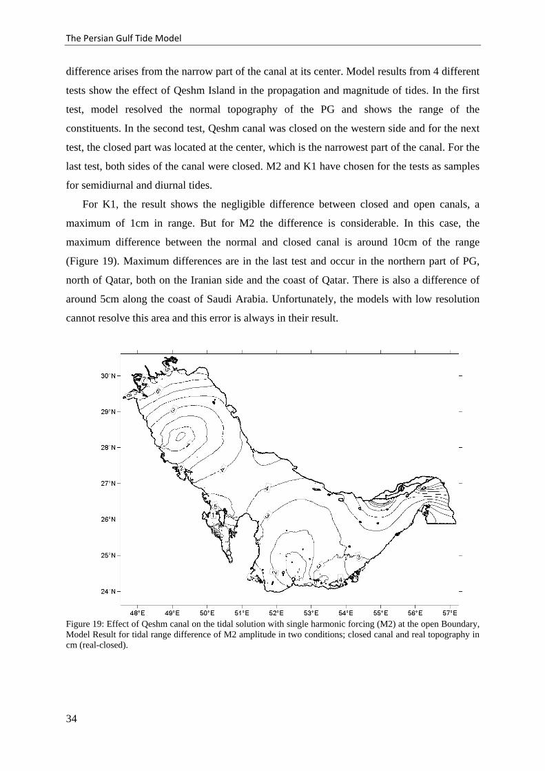
difference arises from the narrow part of the canal at its center. Model results from 4 different
tests show the effect of Qeshm Island in the propagation and magnitude of tides. In the first
test, model resolved the normal topography of the PG and shows the range of the
constituents. In the second test, Qeshm canal was closed on the western side and for the next
test, the closed part was located at the center, which is the narrowest part of the canal. For the
last test, both sides of the canal were closed. M2 and K1 have chosen for the tests as samples
for semidiurnal and diurnal tides.
For K1, the result shows the negligible difference between closed and open canals, a
maximum of 1cm in range. But for M2 the difference is considerable. In this case, the
maximum difference between the normal and closed canal is around 10cm of the range
(Figure 19). Maximum differences are in the last test and occur in the northern part of PG,
north of Qatar, both on the Iranian side and the coast of Qatar. There is also a difference of
around 5cm along the coast of Saudi Arabia. Unfortunately, the models with low resolution
cannot resolve this area and this error is always in their result.
Figure 19: Effect of Qeshm canal on the tidal solution with single harmonic forcing (M2) at the open Boundary, Model Result for tidal range difference of M2 amplitude in two conditions; closed canal and real topography in cm (real-closed).
34
Tidal Residual Currents in The Persian Gulf
Chapter 3 The results of this chapter are presented in a paper in revision in JGR.
3 The PG Tidal Residual Currents
3.1 Topography and circulation in the PG
As described in the first chapter, the PG is a shallow semi-enclosed marginal sea between
Iran in the north and the Arabian Peninsula in the south. It is connected with the Gulf of
Oman and the Indian Ocean through the Strait of Hormuz. The length of the PG is about 1000
km in Northwest to Southeast orientation; the width varies from a maximum of 338 km to a
minimum of 56 km in the Strait of Hormuz, as reported in other studies in this area (Chao et
al., 1992; Chu et al., 2008; Moeini et al., 2010; Reynolds, 1993; Yao, 2008). As the PG is
located between the Arabian Plate and the Iranian (Eurasian) Plate, topography features in the
northern and southern PG are different. The coastal topography bordering the PG shows
distinct contrast; while the Iranian coast is mountainous, the Arabian coast is mostly a desert
plain except close to the Strait of Hormuz.
The topography of the PG is dominated by soft sediments. It is generally deeper near the
Iranian coast and is deepest near the opening of the Strait of Hormuz. The average depth of
the topography is about 35-36m (Badri and Wilders, 2012; Moeini et al., 2010; Ranaee et al.,
2011; Reynolds, 1993; Thoppil and Hogan, 2010a). This basin has a relatively shallow zone
near the closed end of it, extending all the way along the southern part of the basin, roughly
connected to one deeper part, with a clearly asymmetric cross-sectional depth profile of the
main part. The maximum depth in the deeper part is 80 m while in the Straits of Hormuz
depths can exceed 100 m (Pous et al., 2004a; Roos and Schuttelaars, 2010).
As described in section 1.1.1, the coastal boundary and the bottom topography of the PG
are very irregular and several islands of various sizes and shapes are spread over the region
(Sabbagh-Yazdi et al., 2007). From geological studies in this area (Edgell, 1991; Perotti et al.,
35
Tidal Residual Currents in The Persian Gulf
2011; Sarnthein, 1972; Seni and Jackson, 1984; Thomas et al., 2015; Zaigham et al., 2013), in
the southern basin of the PG there are numerous salt domes with circular shape, while in the
Northern Basin they mostly have an elliptical shape and are connected by elongated ridges.
Holocene sediments in the PG are primarily carbonates. Shallow domes form mounds on the
seafloor, and particularly active diapirs form islands exposing salt at the surface (Kent, 1979;
Purser, 1973). Under marine conditions, sand can accumulate by winnowing on bathymetric
shoals. Consequently, Salt domes having sufficient surface expression are overlain by sand-
rich sediments. Small reefs might also be expected on topographic highs over dome crests.
Such dome crest reefs have been recognized in the PG (Purser, 1973; Seni and Jackson,
1984).
Purser in 1973 subdivided bathymetric highs in the PG. Based on his approach
bathymetric highs in the PG have been grouped into three classes based on their setting:
outer, intermediate and inner.
1. The central parts of the basin are characterized by numerous highs with marked
vertical relief.
2. The sloping sea floor is characterized by a great variety of highs and depressions.
3. Highs situated close to the mainland shoreline may considerably affect coastal
sedimentation.
In most continental shelf seas, such as the PG, the highest current speeds are associated
with the barotropic tides. In general, tides in the PG are complex. The dominant tidal pattern
changes from primarily semidiurnal to diurnal (Mashayekh Poul et al., 2016; Pous et al.,
2013; Reynolds, 1993). Barotropic tidal currents are described in detail in other studies
(Mashayekh Poul et al., 2016; Pous et al., 2013). Tidal current speeds for M2 are in the range
of 0.3 m/s to 1.0 m/s with maximum of 2.5 m/s in Qeshm Canal and for S2, O1 and K1 tidal
current speeds are in the range of 0.2 m/s to 0.5 m/s (Mashayekh Poul et al., 2016).
In spring and summer, the wind stress generates south- eastern surface currents of the
magnitude of about 0.05 m/s along the Saudi and Iranian coast. In addition, both the wind
stress and heat fluxes cause the southward currents with speeds of 0.05–0.1 m/s from the
Hormuz Strait and main basin of Gulf toward the UAE coast and Bahrain–Qatar shelf. In
winter and autumn, the cooling effect of the thermohaline fluxes leads to a removal of the
thermal stratification and density contrast between the surface and bottom waters. As a result,
the vertical stability of water column weakens significantly and the baroclinic eddies with
diameters of about 40–70 km and speeds of about 0.08– 0.15 m/s form in some parts of the
36
Tidal Residual Currents in The Persian Gulf
Gulf. In addition, the wind stress leads to shear instability and produce eddies with diameters
of 30–120 km and speeds 0.04–0.15 m/s in most parts of the PG (Hosseinibalam et al., 2011).
Previous studies reported that the tidal residual flow influence on the overall circulation
in the PG is minimal (less than 0.02 m/s) (Pous et al., 2013), except in a few localized areas
(e.g., the Iranian coast and the Strait of Hormuz) where the tidal residuals are large enough to
enhance the dominant density-driven flow (Thoppil and Hogan, 2010b). There are many
other studies on wind and density driven circulation (Chao et al., 1992; Ezam et al., 2010;
Hosseinibalam et al., 2011; Pous et al., 2015; Reynolds, 1993; Swift and Bower, 2003;
Thoppil and Hogan, 2010a, 2010b); this chapter reviews only tidal residual currents.
3.2 Residual flow
Tidal Residual currents can be induced by mean sea-level slopes or nonlinearities of the
dynamics of tidal flow. In tidal dynamics, nonlinear interactions of tidal flow with the bottom
topography are represented by the advection terms of the momentum equations. These
interactions are more important in areas where the tidal excursion is comparable to the scale
of bathymetric features and around shallow points and capes (Lavín and Marinone, 2003).
Numerical models are suitable to investigate the generation of shallow water currents and
tidal residual flows as they can resolve the nonlinear processes (Davies and Jones, 1996;
Dworak and Gómez-Valdés, 2003; Le Provost and Fornerino, 1985; Westerink et al., 1989).
Also, shallow water tides can create residual currents due to the asymmetry between the
flooding and ebbing phases. This process determines the flow structure over shallow regions,
especially along coastlines and sloping topographies. In nature, tidal residual currents are
usually one or two orders of magnitude weaker than the tidal current velocities (Robinson,
1981).
One way to drive the residual flow is separating the oscillatory and the mean part of the
current, which is common practice in wave-driven current modelling. The models which
simulate nonlinear tidal dynamics usually describe the depth-averaged velocity as a function
of time. Integration over the tidal cycle yields the residual current, in which the mass flux as
well as tidal and bed shear stress effects are included (Bakker and de Vriend, 1995).
3.3 Model Description and Methods
In this study, a two dimensional model (VOM_sw2d) is used to investigate the interaction
between tidal wave and experimental symmetric, elongated and tilted obstacles, i.e. hills and
valleys to illustrate flow pattern of residual currents passing through them. Then, the model
37
Tidal Residual Currents in The Persian Gulf
was applied to explore tide induced residual currents in PG with high resolution real
topography. The topography data are provided from data source GEBCO_08 Grid version
20100927, by the General Bathymetric Chart of the oceans from the British Oceanographic
Data Centre [IOC, IHO and BODC, 2003]. The structure of the residual circulation in the PG
is obtained by averaging the simulated horizontal momentum components, which includes the
nonlinearity of interaction between tidal wave and topography, over H (Babu et al., 2005;
Quirós et al., 1992; Yuxiang, 1988). H is the actual water depth: 𝐇𝐇 = 𝐃𝐃𝐃𝐃𝐃𝐃𝐃𝐃𝐃𝐃 + 𝛇𝛇 where 𝛇𝛇 is
sea surface elevation.
𝒖𝒖𝒓𝒓𝒓𝒓𝒓𝒓 = ∑ 𝑼𝑼𝑵𝑵𝟏𝟏
∑ 𝑯𝑯𝑵𝑵𝟏𝟏
, with a number of time steps 𝑵𝑵 = 𝑻𝑻/𝒅𝒅𝒕𝒕
Where 𝒖𝒖𝒓𝒓𝒓𝒓𝒓𝒓 is residual velocity, U is momentum, T is the period of the tidal constituent
and the time increment is dt. In the calculation T is 5 tidal periods to fit dt into the averaging
period. The calculation is done after 20 periods of spin up to reach the stationarity of tidal
wave propagation in the domain. This calculation is done for each tidal constituent
separately.
The model domain spreads meridionally from 23.6N to 30.6N and zonally from 47.5E to
57.3E. It has a horizontal resolution of 30 seconds (i.e. half a nautical mile) with a lateral
open boundary at the eastern end, representing the connection to the Indian Ocean. Each tidal
constituent was applied separately in the forcing at the open boundary to the Oman Sea.
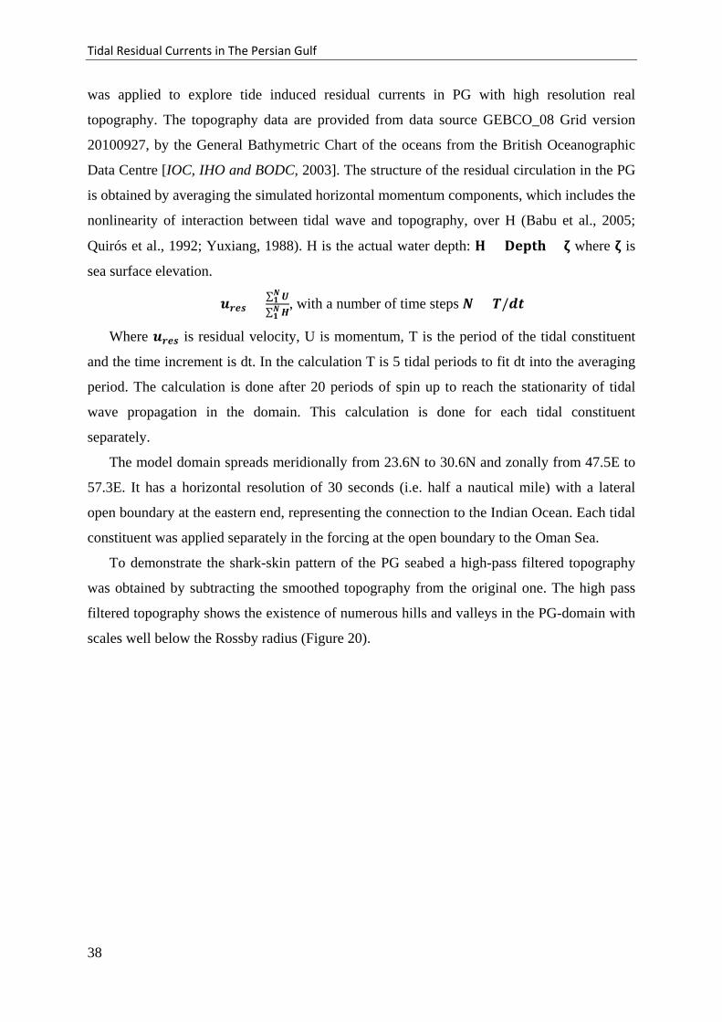
To demonstrate the shark-skin pattern of the PG seabed a high-pass filtered topography
was obtained by subtracting the smoothed topography from the original one. The high pass
filtered topography shows the existence of numerous hills and valleys in the PG-domain with
scales well below the Rossby radius (Figure 20).
38
Tidal Residual Currents in The Persian Gulf
Figure 20: High-pass filtered topography of the PG in meters (colorbar). Box 1 indicates the area zoomed in Figure 28.
3.4 Results
3.4.1 Residual current in an experimental domain
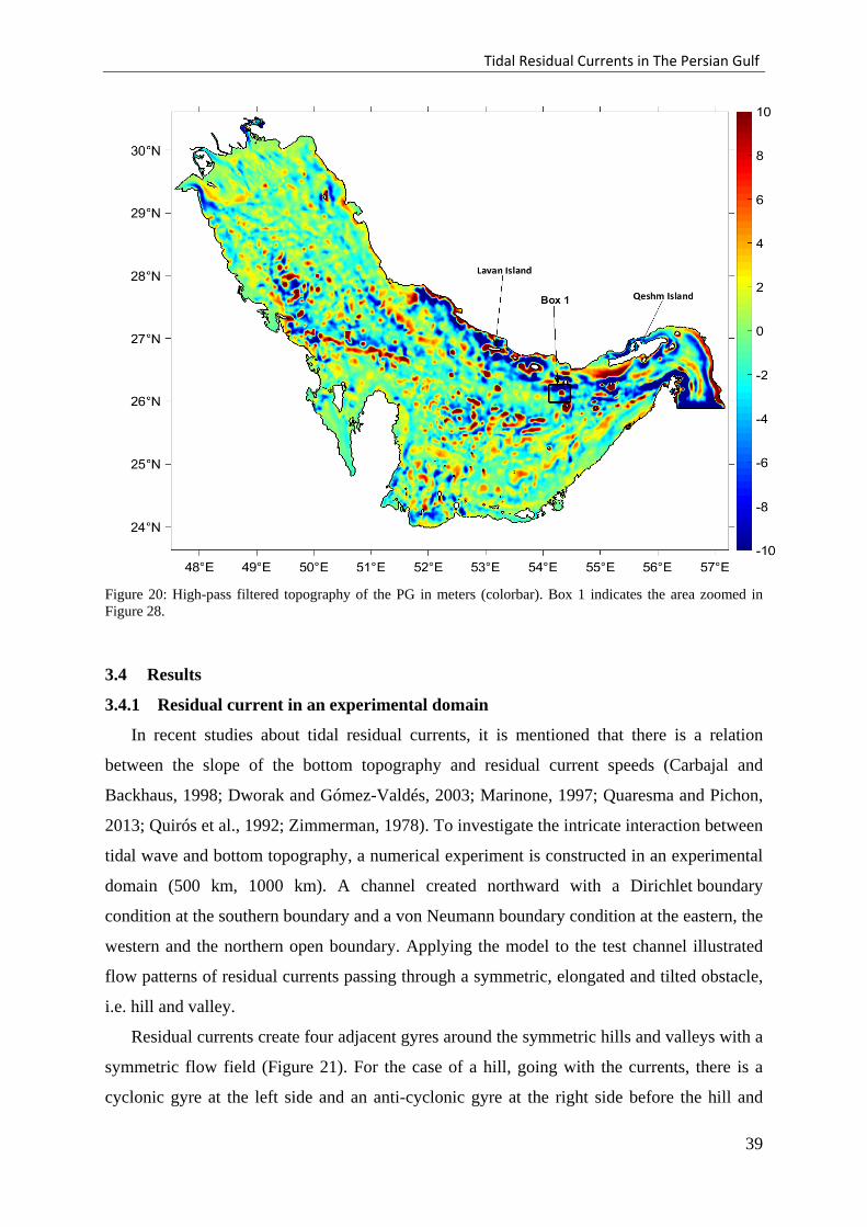
In recent studies about tidal residual currents, it is mentioned that there is a relation
between the slope of the bottom topography and residual current speeds (Carbajal and
Backhaus, 1998; Dworak and Gómez-Valdés, 2003; Marinone, 1997; Quaresma and Pichon,
2013; Quirós et al., 1992; Zimmerman, 1978). To investigate the intricate interaction between
tidal wave and bottom topography, a numerical experiment is constructed in an experimental
domain (500 km, 1000 km). A channel created northward with a Dirichlet boundary
condition at the southern boundary and a von Neumann boundary condition at the eastern, the
western and the northern open boundary. Applying the model to the test channel illustrated
flow patterns of residual currents passing through a symmetric, elongated and tilted obstacle,
i.e. hill and valley.
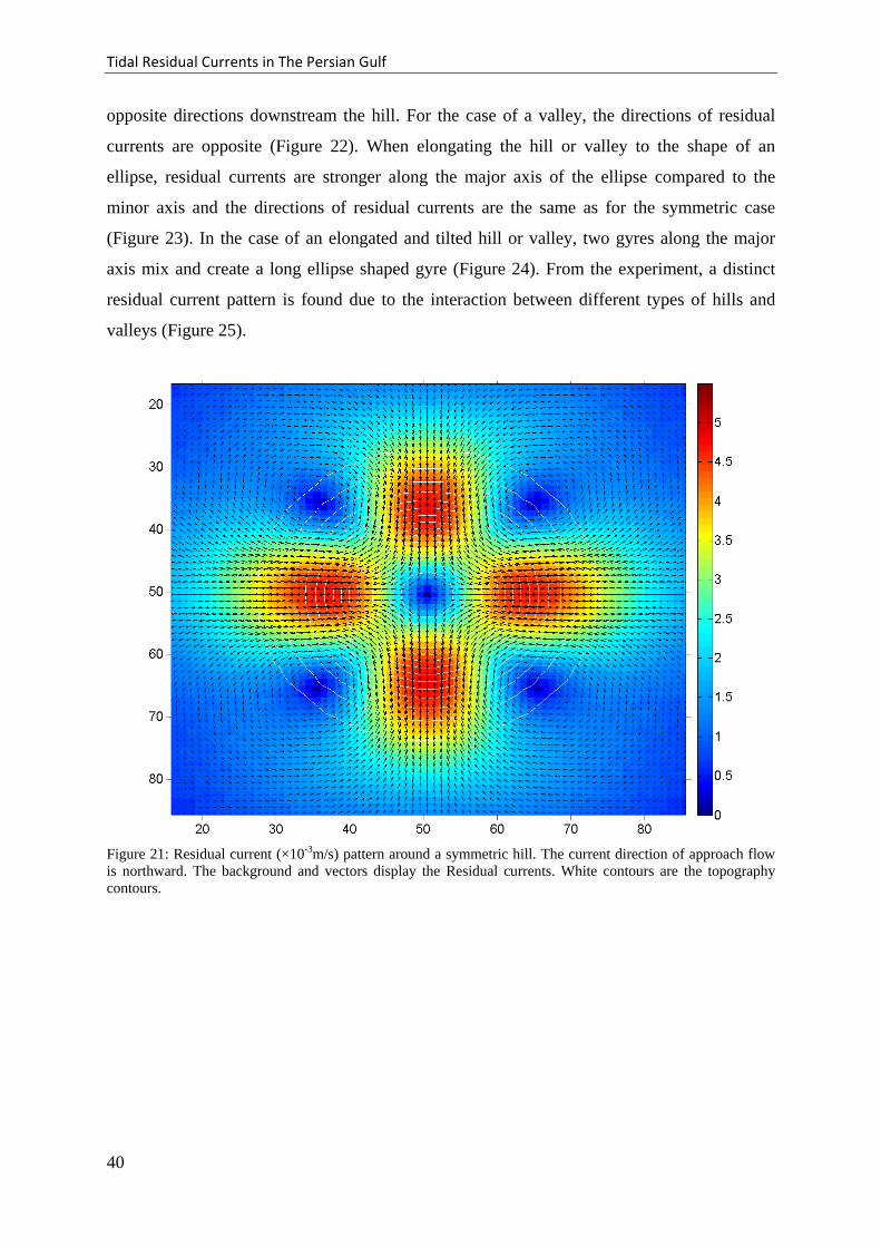
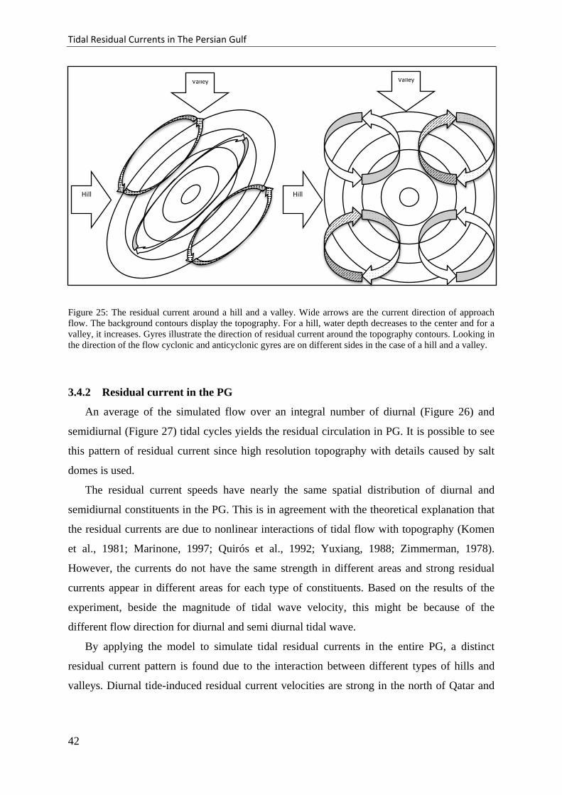
Residual currents create four adjacent gyres around the symmetric hills and valleys with a
symmetric flow field (Figure 21). For the case of a hill, going with the currents, there is a
cyclonic gyre at the left side and an anti-cyclonic gyre at the right side before the hill and
39
Tidal Residual Currents in The Persian Gulf
opposite directions downstream the hill. For the case of a valley, the directions of residual
currents are opposite (Figure 22). When elongating the hill or valley to the shape of an
ellipse, residual currents are stronger along the major axis of the ellipse compared to the
minor axis and the directions of residual currents are the same as for the symmetric case
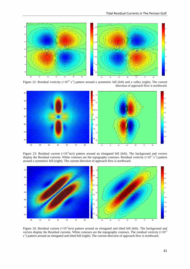
(Figure 23). In the case of an elongated and tilted hill or valley, two gyres along the major
axis mix and create a long ellipse shaped gyre (Figure 24). From the experiment, a distinct
residual current pattern is found due to the interaction between different types of hills and
valleys (Figure 25).
Figure 21: Residual current (×10-3m/s) pattern around a symmetric hill. The current direction of approach flow is northward. The background and vectors display the Residual currents. White contours are the topography contours.
40
Tidal Residual Currents in The Persian Gulf
Figure 22: Residual vorticity (×10-6 s-1) pattern around a symmetric hill (left) and a valley (right). The current
direction of approach flow is northward.
Figure 23: Residual current (×10-3m/s) pattern around an elongated hill (left). The background and vectors display the Residual currents. White contours are the topography contours. Residual vorticity (×10-5 s-1) pattern around a symmetric hill (right). The current direction of approach flow is northward.
Figure 24: Residual current (×10-3m/s) pattern around an elongated and tilted hill (left). The background and vectors display the Residual currents. White contours are the topography contours. The residual vorticity (×10-5 s-1) pattern around an elongated and tilted hill (right). The current direction of approach flow is northward.
41
Tidal Residual Currents in The Persian Gulf
Figure 25: The residual current around a hill and a valley. Wide arrows are the current direction of approach flow. The background contours display the topography. For a hill, water depth decreases to the center and for a valley, it increases. Gyres illustrate the direction of residual current around the topography contours. Looking in the direction of the flow cyclonic and anticyclonic gyres are on different sides in the case of a hill and a valley.
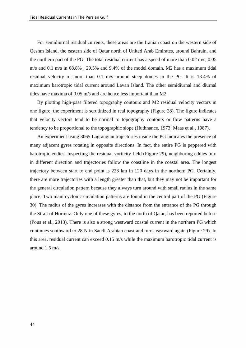
3.4.2 Residual current in the PG
An average of the simulated flow over an integral number of diurnal (Figure 26) and
semidiurnal (Figure 27) tidal cycles yields the residual circulation in PG. It is possible to see
this pattern of residual current since high resolution topography with details caused by salt
domes is used.
The residual current speeds have nearly the same spatial distribution of diurnal and
semidiurnal constituents in the PG. This is in agreement with the theoretical explanation that
the residual currents are due to nonlinear interactions of tidal flow with topography (Komen
et al., 1981; Marinone, 1997; Quirós et al., 1992; Yuxiang, 1988; Zimmerman, 1978).
However, the currents do not have the same strength in different areas and strong residual
currents appear in different areas for each type of constituents. Based on the results of the
experiment, beside the magnitude of tidal wave velocity, this might be because of the
different flow direction for diurnal and semi diurnal tidal wave.
By applying the model to simulate tidal residual currents in the entire PG, a distinct
residual current pattern is found due to the interaction between different types of hills and
valleys. Diurnal tide-induced residual current velocities are strong in the north of Qatar and
Valley
Hill
Valley
Hill
42
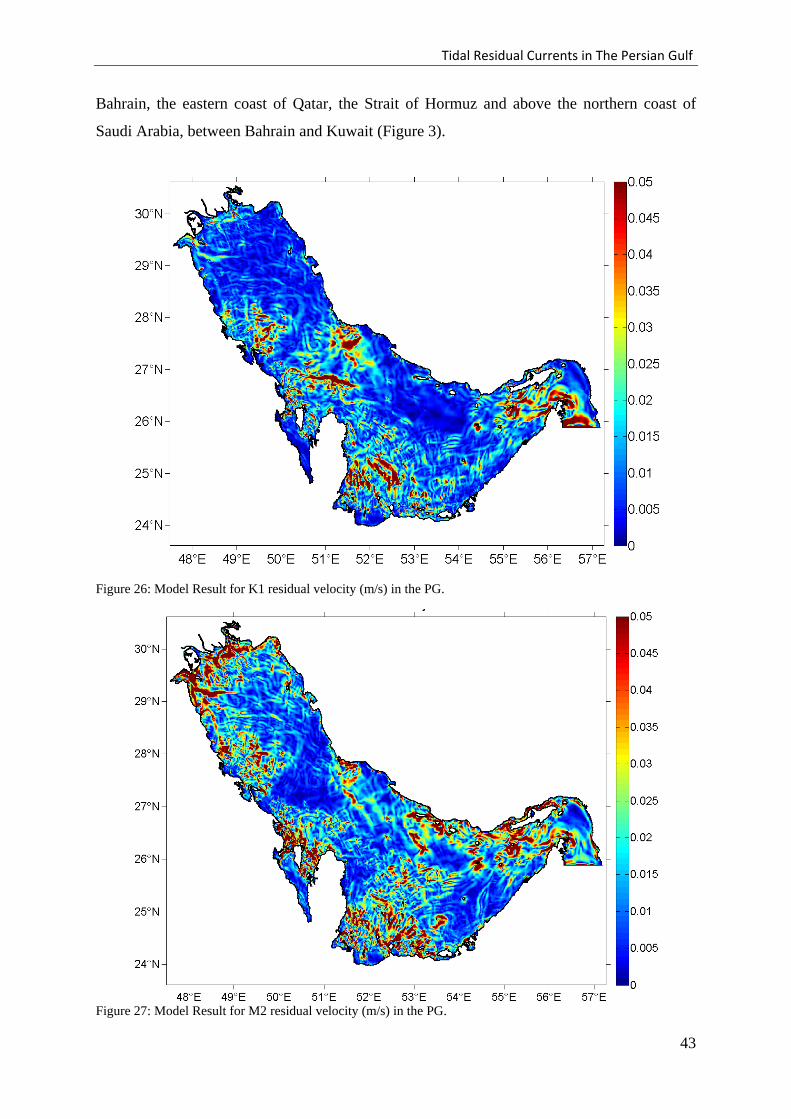
Tidal Residual Currents in The Persian Gulf
Bahrain, the eastern coast of Qatar, the Strait of Hormuz and above the northern coast of
Saudi Arabia, between Bahrain and Kuwait (Figure 3).
Figure 26: Model Result for K1 residual velocity (m/s) in the PG.
Figure 27: Model Result for M2 residual velocity (m/s) in the PG.
43
Tidal Residual Currents in The Persian Gulf
For semidiurnal residual currents, these areas are the Iranian coast on the western side of
Qeshm Island, the eastern side of Qatar north of United Arab Emirates, around Bahrain, and
the northern part of the PG. The total residual current has a speed of more than 0.02 m/s, 0.05
m/s and 0.1 m/s in 68.8% , 29.5% and 9.4% of the model domain. M2 has a maximum tidal
residual velocity of more than 0.1 m/s around steep domes in the PG. It is 13.4% of
maximum barotropic tidal current around Lavan Island. The other semidiurnal and diurnal
tides have maxima of 0.05 m/s and are hence less important than M2.
By plotting high-pass filtered topography contours and M2 residual velocity vectors in
one figure, the experiment is scrutinized in real topography (Figure 28). The figure indicates
that velocity vectors tend to be normal to topography contours or flow patterns have a
tendency to be proportional to the topographic slope (Huthnance, 1973; Maas et al., 1987).
An experiment using 3065 Lagrangian trajectories inside the PG indicates the presence of
many adjacent gyres rotating in opposite directions. In fact, the entire PG is peppered with
barotropic eddies. Inspecting the residual vorticity field (Figure 29), neighboring eddies turn
in different direction and trajectories follow the coastline in the coastal area. The longest
trajectory between start to end point is 223 km in 120 days in the northern PG. Certainly,
there are more trajectories with a length greater than that, but they may not be important for
the general circulation pattern because they always turn around with small radius in the same
place. Two main cyclonic circulation patterns are found in the central part of the PG (Figure
30). The radius of the gyres increases with the distance from the entrance of the PG through
the Strait of Hormuz. Only one of these gyres, to the north of Qatar, has been reported before
(Pous et al., 2013). There is also a strong westward coastal current in the northern PG which
continues southward to 28 N in Saudi Arabian coast and turns eastward again (Figure 29). In
this area, residual current can exceed 0.15 m/s while the maximum barotropic tidal current is
around 1.5 m/s.
44
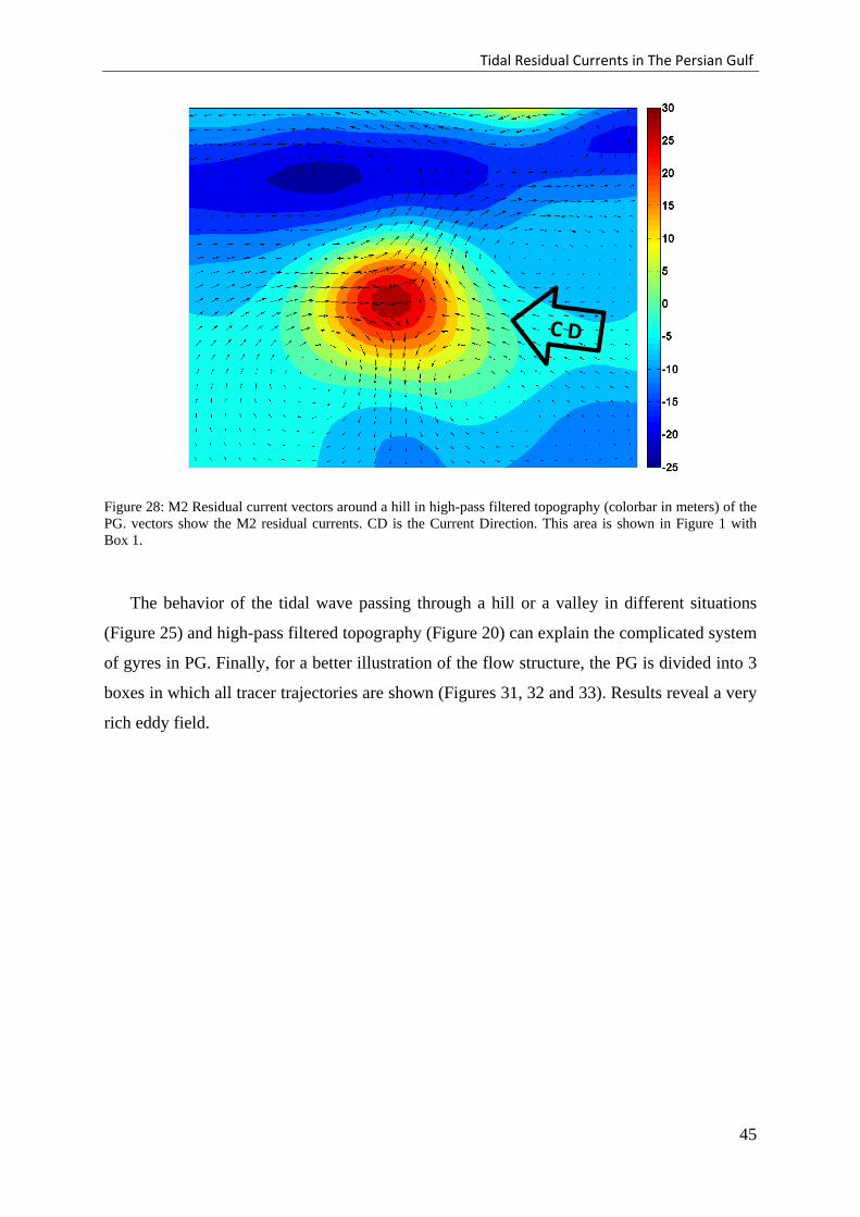
Tidal Residual Currents in The Persian Gulf
Figure 28: M2 Residual current vectors around a hill in high-pass filtered topography (colorbar in meters) of the PG. vectors show the M2 residual currents. CD is the Current Direction. This area is shown in Figure 1 with Box 1.
The behavior of the tidal wave passing through a hill or a valley in different situations
(Figure 25) and high-pass filtered topography (Figure 20) can explain the complicated system
of gyres in PG. Finally, for a better illustration of the flow structure, the PG is divided into 3
boxes in which all tracer trajectories are shown (Figures 31, 32 and 33). Results reveal a very
rich eddy field.
45
Tidal Residual Currents in The Persian Gulf
Figure 29: Lagrangian trajectories (black lines) in residual vorticity (colorbar × 10-5 s-1), running with residual velocities of M2+S2+K1+O1 for 120 days.
Figure 30: Lagrangian trajectories (black lines) in residual vorticity (colorbar × 10-5 s-1), running with residual velocities of M2+S2+K1+O1 for 120 days. Green lines show 2 main gyres in the PG. The red box in guide map shows the position of zoomed figure in the PG.
46
Tidal Residual Currents in The Persian Gulf
Figure 31: Box 1 of trajectories running with residual velocities of M2+S2+K1+O1 for 120 days. Gray marks are the start points.
47
Tidal Residual Currents in The Persian Gulf
Figure 32: Box 2 of trajectories running with residual velocities of M2+S2+K1+O1 for 120 days. Gray marks are the start points.
48
Tidal Residual Currents in The Persian Gulf
Figure 33: Box 3 of trajectories running with residual velocities of M2+S2+K1+O1 for 120 days. Gray marks are the start points.
49
Tidal Resonance in The Persian Gulf
Chapter 4
4 Tidal Resonance in the PG
I investigated resonance in the PG by applying a non-linear hydrodynamic numerical tidal
model to the PG. The model was used to characterize the amplified response of the basin to
different forcing periods. It was forced with one and the same amplitude at its open boundary
to the Oman Sea by waves with periods ranging from 3.5 h to 35.5 h with increments of 0.5
hours. Each wave was simulated separately. The results reveal that in three areas tidal
elevations are significantly larger than the forcing amplitude indicating resonance. These are
the northern PG (maximum Amplification Factor (AF) = 1.61), the Strait of Hormuz
(maximum AF = 3.00), and the southern PG (maximum AF = 1.33). The amplification factor
(AF) is defined by the ratio of local amplitudes vs. forcing amplitude. Diurnal tides are
resonant in both northern and southern PG. Semidiurnal constituents are amplified in the
northern Gulf as well as in the Strait of Hormuz. A simulated sea level rise due to climate
change of 1 meter increased the AF off the Arabian coast for semidiurnal tides from 0.72 to
1.21. In the Qeshm Canal in the Strait of Hormuz, AF increased from 1.36 to 1.57 for
semidiurnal and from 0.73 to 1.1 for diurnal tides.
4.1 The PG
The PG is a shallow semi-enclosed marginal sea between Iran and the Arabian Peninsula.
It is connected with the Gulf of Oman and the Indian Ocean through the Strait of Hormuz.
The length of the PG is about 1000 km in Northwest to Southeast orientation; the width
varies from a minimum of 56 km in the Strait of Hormuz to a maximum of 338 km. The
coastal topography bordering the PG shows distinct contrast; while the Iranian coast is
mountainous, the Arabian coast is mostly a desert plain except close to the Strait of Hormuz.
50
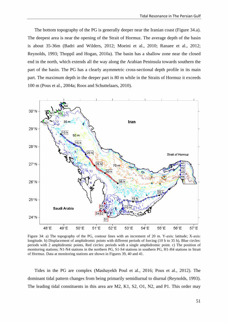
Tidal Resonance in The Persian Gulf
The bottom topography of the PG is generally deeper near the Iranian coast (Figure 34.a).
The deepest area is near the opening of the Strait of Hormuz. The average depth of the basin
is about 35-36m (Badri and Wilders, 2012; Moeini et al., 2010; Ranaee et al., 2012;
Reynolds, 1993; Thoppil and Hogan, 2010a). The basin has a shallow zone near the closed
end in the north, which extends all the way along the Arabian Peninsula towards southern the
part of the basin. The PG has a clearly asymmetric cross-sectional depth profile in its main
part. The maximum depth in the deeper part is 80 m while in the Straits of Hormuz it exceeds
100 m (Pous et al., 2004a; Roos and Schuttelaars, 2010).
Figure 34: a) The topography of the PG, contour lines with an increment of 20 m. Y-axis: latitude; X-axis: longitude. b) Displacement of amphidromic points with different periods of forcing (10 h to 35 h), Blue circles: periods with 2 amphidromic points, Red circles: periods with a single amphidromic point. c) The position of monitoring stations; N1-N4 stations in the northern PG, S1-S4 stations in southern PG, H1-H4 stations in Strait of Hormuz. Data at monitoring stations are shown in Figures 39, 40 and 41.
Tides in the PG are complex (Mashayekh Poul et al., 2016; Pous et al., 2012). The
dominant tidal pattern changes from being primarily semidiurnal to diurnal (Reynolds, 1993).
The leading tidal constituents in this area are M2, K1, S2, O1, N2, and P1. This order may
51
Tidal Resonance in The Persian Gulf
change with the F-factor at other locations in the domain. The F-factor shows the type of tide
between diurnal, semidiurnal, and mixed. It is defined as the ratio of the main diurnal over
the main semidiurnal constituent’s amplitudes. In the PG, it is K1+O1 for diurnal and M2+S2
for semidiurnal tides (Najafi, 1997).
The PG has a natural period of 22.6 or 21.7 hours for tidal waves based on the Japanese
and Chrystal method (Defant, 1961). Semidiurnal and diurnal waves interact in the basin and
form a system of amphidromic points of Kelvin-Taylor type (Pous et al., 2013). There are
two points for semidiurnal constituents in the northwest and southeast, and a single point for
diurnal constituents in the center of the Gulf, near Bahrain (Bosch van Drakestein, 2014;
Hyder et al., 2013; Ranaee et al., 2012; Reynolds, 1993).
4.2 Tidal Resonance
There are a number of coastal regions on earth the Eigen-oscillations of which being in
resonance with the tide. The resonance is the amplified response of a basin to periodic forcing
(Carbajal and Backhaus, 1998) close to its eigen-period. Resonant amplification is the ratio
between the wave height at a location within the basin and that at the open boundary
(Carbajal and Backhaus, 1998; Liang et al., 2014). The response of a basin to tidal forcing
depends on the properties of offshore tides and the influence of friction (Sutherland et al.,
2005). The most important parameters are the geometry of a basin, i.e. length, depth,
dissipation, and amplitude of forcing (Backhaus, 2015; Skiba et al., 2013). In fact, resonance
occurs when a forcing excites a natural mode of a system (Le Souëf and Allen, 2014).
Tidal waves behave similar to the long waves, and their wavelength exceeds the depth of
water in which they exist. The wavelength for the tidal waves is given by 𝐋𝐋 = 𝟐𝟐𝟐𝟐�𝐠𝐠𝐇𝐇 𝛚𝛚⁄ ,
where g is acceleration due to gravity (ms-2), H is the depth of water (m) and 𝛚𝛚 is the angular
frequency of the tidal component (radians s-1). Resonance in a tidal basin is most striking if
the quarter wave-length criterion applies (Defant, 1961; Godin, 1993; Proudman, 1953) . That
is, if the length of the basin is about a quarter wavelength of the forcing oscillation. The
resonance amplification of the tides at PG occurs due to the dimensions of the PG.
Blain (1998) reported resonant amplification of the semidiurnal and diurnal tides in the
northern PG. Hyder et al. (2013) showed that the dimensions of the Gulf result in the resonant
amplification of both the diurnal and semidiurnal tides. Roos and Schuttelaars (2010) stated
that the PG has a tidal resonance associated with the topography near the basin’s closed end.
52
Tidal Resonance in The Persian Gulf
A number of studies have argued that coastal regions around the globe are in resonance
with semidiurnal or diurnal tidal forcing (Arbic et al., 2007; Backhaus, 2015; Garrett, 1972;
Sutherland et al., 2005). Apart from cases with confirmed full and spectacular resonances,
there may be other regions with only weak or latent resonance. The latter, however, remained
largely understudied. The term ‘latent resonance’ should be understood as a not fully
developed resonance i.e. juvenile resonance (Backhaus, 2015). In coastal regions, resonant or
latent resonant responses add to the complexity of the tidal pattern and tend to intensify
nonlinear effects (Andersen et al., 2006). However, knowing how close a system is to
resonance provides an indication of the sensitivity of the local tidal regime to gradual changes
in mean sea level and to changes in geometry caused by human activities (Sutherland et al.,
2005). Using a numerical model, the frequency- dependent response of a coastal region can
be determined.
4.3 Model Description
The characteristics of tidal resonance were investigated by using the vector ocean model
shallow water (VOM-SW2d), a non-linear hydrodynamic tidal model, and applied it to the
PG (Mashayekh Poul et al., 2016). The model domain spreads meridionally from 23.6 N to
30.6 N and zonally from 47.5 E to 57.3 E. It has a horizontal resolution of 30 seconds (i.e.
half a nautical mile) with a lateral open boundary at the eastern end, representing the
connection to the Indian Ocean. In this chapter, the resonance characteristic of the PG is
presented based on the non-linear shallow water equations for periods ranging from 3.5 h to
35.5 h.
4.4 Tidal resonance in the PG
To investigate the resonance characteristics of the PG, a numerical experiment is
ascertained with 33 runs with different periods. The amplitude of the wave at the open
boundary was maintained at 1 m, but the period of oscillation was varied. The periods of
forcing ranged from 3.5 to 35.5 hours with a resolution of 30 minutes. For the 12.5 hours
period (Figure 35), which is close to M2 tide, the shape of the tidal AF was similar to the
tidal range of the M2 from recent studies (John, 1992; Reynolds, 1993). Two amphidromic
points are found in the positions reported before (John, 1992; Mashayekh Poul et al., 2016;
Pous et al., 2013; Reynolds, 1993). For the 24 hour period (Figure 36), which is close to K1
tide, the shape of the tidal AF and position of the single amphidromic point is in agreement
53
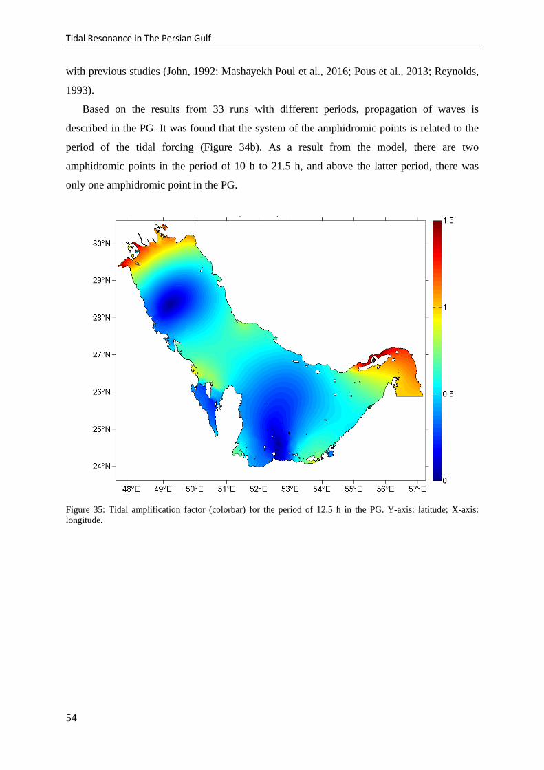
Tidal Resonance in The Persian Gulf
with previous studies (John, 1992; Mashayekh Poul et al., 2016; Pous et al., 2013; Reynolds,
1993).
Based on the results from 33 runs with different periods, propagation of waves is
described in the PG. It was found that the system of the amphidromic points is related to the
period of the tidal forcing (Figure 34b). As a result from the model, there are two
amphidromic points in the period of 10 h to 21.5 h, and above the latter period, there was
only one amphidromic point in the PG.
Figure 35: Tidal amplification factor (colorbar) for the period of 12.5 h in the PG. Y-axis: latitude; X-axis: longitude.
54
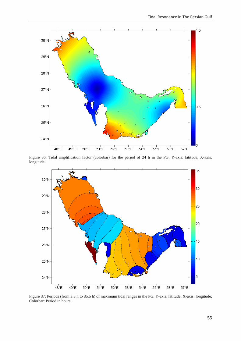
Tidal Resonance in The Persian Gulf
Figure 36: Tidal amplification factor (colorbar) for the period of 24 h in the PG. Y-axis: latitude; X-axis: longitude.
Figure 37: Periods (from 3.5 h to 35.5 h) of maximum tidal ranges in the PG. Y-axis: latitude; X-axis: longitude; Colorbar: Period in hours.
55
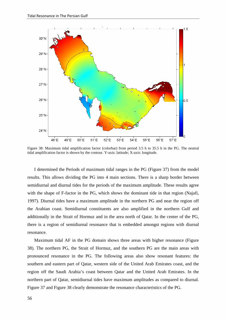
Tidal Resonance in The Persian Gulf
Figure 38: Maximum tidal amplification factor (colorbar) from period 3.5 h to 35.5 h in the PG. The neutral tidal amplification factor is shown by the contour. Y-axis: latitude; X-axis: longitude.
I determined the Periods of maximum tidal ranges in the PG (Figure 37) from the model
results. This allows dividing the PG into 4 main sections. There is a sharp border between
semidiurnal and diurnal tides for the periods of the maximum amplitude. These results agree
with the shape of F-factor in the PG, which shows the dominant tide in that region (Najafi,
1997). Diurnal tides have a maximum amplitude in the northern PG and near the region off
the Arabian coast. Semidiurnal constituents are also amplified in the northern Gulf and
additionally in the Strait of Hormuz and in the area north of Qatar. In the center of the PG,
there is a region of semidiurnal resonance that is embedded amongst regions with diurnal
resonance.
Maximum tidal AF in the PG domain shows three areas with higher resonance (Figure
38). The northern PG, the Strait of Hormuz, and the southern PG are the main areas with
pronounced resonance in the PG. The following areas also show resonant features: the
southern and eastern part of Qatar, western side of the United Arab Emirates coast, and the
region off the Saudi Arabia’s coast between Qatar and the United Arab Emirates. In the
northern part of Qatar, semidiurnal tides have maximum amplitudes as compared to diurnal.
Figure 37 and Figure 38 clearly demonstrate the resonance characteristics of the PG.
56
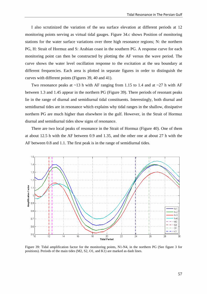
Tidal Resonance in The Persian Gulf
I also scrutinized the variation of the sea surface elevation at different periods at 12
monitoring points serving as virtual tidal gauges. Figure 34.c shows Position of monitoring
stations for the water surface variations over three high resonance regions; N: the northern
PG, H: Strait of Hormuz and S: Arabian coast in the southern PG. A response curve for each
monitoring point can then be constructed by plotting the AF versus the wave period. The
curve shows the water level oscillation response to the excitation at the sea boundary at
different frequencies. Each area is plotted in separate figures in order to distinguish the
curves with different points (Figures 39, 40 and 41).
Two resonance peaks at ~13 h with AF ranging from 1.15 to 1.4 and at ~27 h with AF
between 1.3 and 1.45 appear in the northern PG (Figure 39). There periods of resonant peaks
lie in the range of diurnal and semidiurnal tidal constituents. Interestingly, both diurnal and
semidiurnal tides are in resonance which explains why tidal ranges in the shallow, dissipative
northern PG are much higher than elsewhere in the gulf. However, in the Strait of Hormuz
diurnal and semidiurnal tides show signs of resonance.
There are two local peaks of resonance in the Strait of Hormuz (Figure 40). One of them
at about 12.5 h with the AF between 0.9 and 1.35, and the other one at about 27 h with the
AF between 0.8 and 1.1. The first peak is in the range of semidiurnal tides.
Figure 39: Tidal amplification factor for the monitoring points, N1-N4, in the northern PG (See figure 3 for positions). Periods of the main tides (M2, S2, O1, and K1) are marked as dash lines.
57
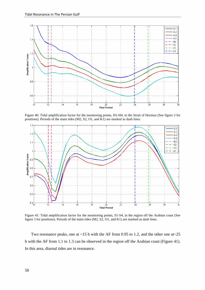
Tidal Resonance in The Persian Gulf
Figure 40: Tidal amplification factor for the monitoring points, H1-H4, in the Strait of Hormuz (See figure 3 for positions). Periods of the main tides (M2, S2, O1, and K1) are marked as dash lines.
Figure 41: Tidal amplification factor for the monitoring points, S1-S4, in the region off the Arabian coast (See figure 3 for positions). Periods of the main tides (M2, S2, O1, and K1) are marked as dash lines.
Two resonance peaks, one at ~15 h with the AF from 0.95 to 1.2, and the other one at~25
h with the AF from 1.1 to 1.3 can be observed in the region off the Arabian coast (Figure 41).
In this area, diurnal tides are in resonance.
58
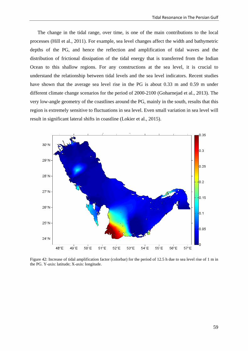
Tidal Resonance in The Persian Gulf
The change in the tidal range, over time, is one of the main contributions to the local
processes (Hill et al., 2011). For example, sea level changes affect the width and bathymetric
depths of the PG, and hence the reflection and amplification of tidal waves and the
distribution of frictional dissipation of the tidal energy that is transferred from the Indian
Ocean to this shallow regions. For any constructions at the sea level, it is crucial to
understand the relationship between tidal levels and the sea level indicators. Recent studies
have shown that the average sea level rise in the PG is about 0.33 m and 0.59 m under
different climate change scenarios for the period of 2000-2100 (Goharnejad et al., 2013). The
very low-angle geometry of the coastlines around the PG, mainly in the south, results that this
region is extremely sensitive to fluctuations in sea level. Even small variation in sea level will
result in significant lateral shifts in coastline (Lokier et al., 2015).
Figure 42: Increase of tidal amplification factor (colorbar) for the period of 12.5 h due to sea level rise of 1 m in the PG. Y-axis: latitude; X-axis: longitude.
59
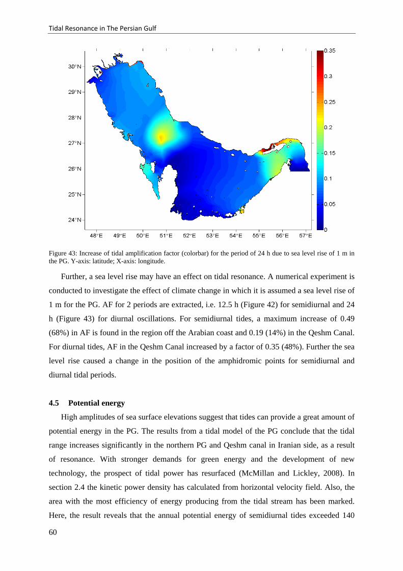
Tidal Resonance in The Persian Gulf
Figure 43: Increase of tidal amplification factor (colorbar) for the period of 24 h due to sea level rise of 1 m in the PG. Y-axis: latitude; X-axis: longitude.
Further, a sea level rise may have an effect on tidal resonance. A numerical experiment is
conducted to investigate the effect of climate change in which it is assumed a sea level rise of
1 m for the PG. AF for 2 periods are extracted, i.e. 12.5 h (Figure 42) for semidiurnal and 24
h (Figure 43) for diurnal oscillations. For semidiurnal tides, a maximum increase of 0.49
(68%) in AF is found in the region off the Arabian coast and 0.19 (14%) in the Qeshm Canal.
For diurnal tides, AF in the Qeshm Canal increased by a factor of 0.35 (48%). Further the sea
level rise caused a change in the position of the amphidromic points for semidiurnal and
diurnal tidal periods.
4.5 Potential energy
High amplitudes of sea surface elevations suggest that tides can provide a great amount of
potential energy in the PG. The results from a tidal model of the PG conclude that the tidal
range increases significantly in the northern PG and Qeshm canal in Iranian side, as a result
of resonance. With stronger demands for green energy and the development of new
technology, the prospect of tidal power has resurfaced (McMillan and Lickley, 2008). In
section 2.4 the kinetic power density has calculated from horizontal velocity field. Also, the
area with the most efficiency of energy producing from the tidal stream has been marked.
Here, the result reveals that the annual potential energy of semidiurnal tides exceeded 140
60
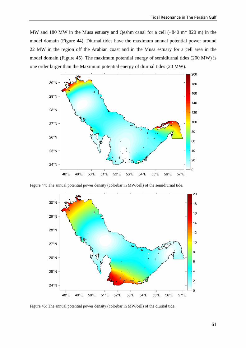
Tidal Resonance in The Persian Gulf
MW and 180 MW in the Musa estuary and Qeshm canal for a cell (~840 m* 820 m) in the
model domain (Figure 44). Diurnal tides have the maximum annual potential power around
22 MW in the region off the Arabian coast and in the Musa estuary for a cell area in the
model domain (Figure 45). The maximum potential energy of semidiurnal tides (200 MW) is
one order larger than the Maximum potential energy of diurnal tides (20 MW).
Figure 44: The annual potential power density (colorbar in MW/cell) of the semidiurnal tide.
Figure 45: The annual potential power density (colorbar in MW/cell) of the diurnal tide.
61
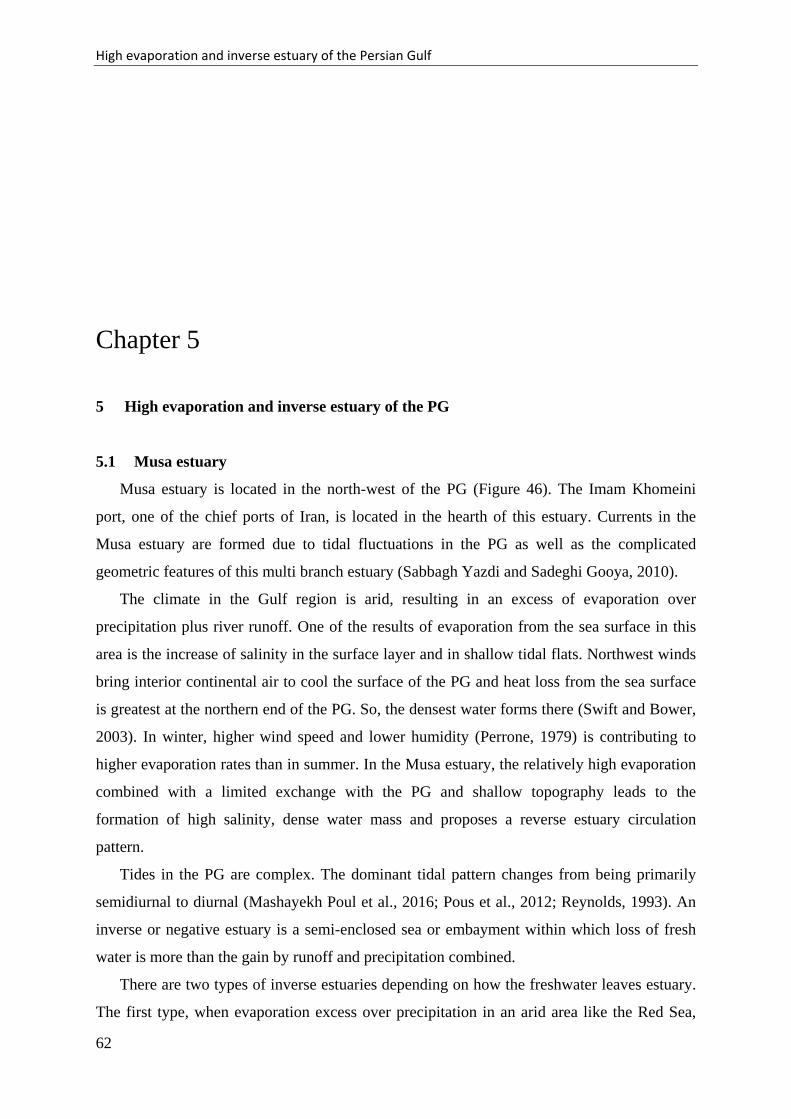
High evaporation and inverse estuary of the Persian Gulf
Chapter 5
5 High evaporation and inverse estuary of the PG
5.1 Musa estuary
Musa estuary is located in the north-west of the PG (Figure 46). The Imam Khomeini
port, one of the chief ports of Iran, is located in the hearth of this estuary. Currents in the
Musa estuary are formed due to tidal fluctuations in the PG as well as the complicated
geometric features of this multi branch estuary (Sabbagh Yazdi and Sadeghi Gooya, 2010).
The climate in the Gulf region is arid, resulting in an excess of evaporation over
precipitation plus river runoff. One of the results of evaporation from the sea surface in this
area is the increase of salinity in the surface layer and in shallow tidal flats. Northwest winds
bring interior continental air to cool the surface of the PG and heat loss from the sea surface
is greatest at the northern end of the PG. So, the densest water forms there (Swift and Bower,
2003). In winter, higher wind speed and lower humidity (Perrone, 1979) is contributing to
higher evaporation rates than in summer. In the Musa estuary, the relatively high evaporation
combined with a limited exchange with the PG and shallow topography leads to the
formation of high salinity, dense water mass and proposes a reverse estuary circulation
pattern.
Tides in the PG are complex. The dominant tidal pattern changes from being primarily
semidiurnal to diurnal (Mashayekh Poul et al., 2016; Pous et al., 2012; Reynolds, 1993). An
inverse or negative estuary is a semi-enclosed sea or embayment within which loss of fresh
water is more than the gain by runoff and precipitation combined.
There are two types of inverse estuaries depending on how the freshwater leaves estuary.
The first type, when evaporation excess over precipitation in an arid area like the Red Sea,
62
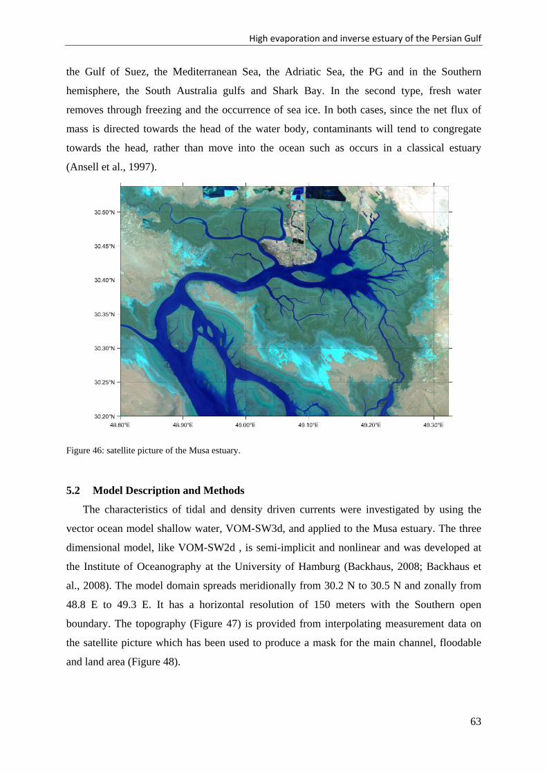
High evaporation and inverse estuary of the Persian Gulf
the Gulf of Suez, the Mediterranean Sea, the Adriatic Sea, the PG and in the Southern
hemisphere, the South Australia gulfs and Shark Bay. In the second type, fresh water
removes through freezing and the occurrence of sea ice. In both cases, since the net flux of
mass is directed towards the head of the water body, contaminants will tend to congregate
towards the head, rather than move into the ocean such as occurs in a classical estuary
(Ansell et al., 1997).
Figure 46: satellite picture of the Musa estuary.
5.2 Model Description and Methods
The characteristics of tidal and density driven currents were investigated by using the
vector ocean model shallow water, VOM-SW3d, and applied to the Musa estuary. The three
dimensional model, like VOM-SW2d , is semi-implicit and nonlinear and was developed at
the Institute of Oceanography at the University of Hamburg (Backhaus, 2008; Backhaus et
al., 2008). The model domain spreads meridionally from 30.2 N to 30.5 N and zonally from
48.8 E to 49.3 E. It has a horizontal resolution of 150 meters with the Southern open
boundary. The topography (Figure 47) is provided from interpolating measurement data on
the satellite picture which has been used to produce a mask for the main channel, floodable
and land area (Figure 48).
63
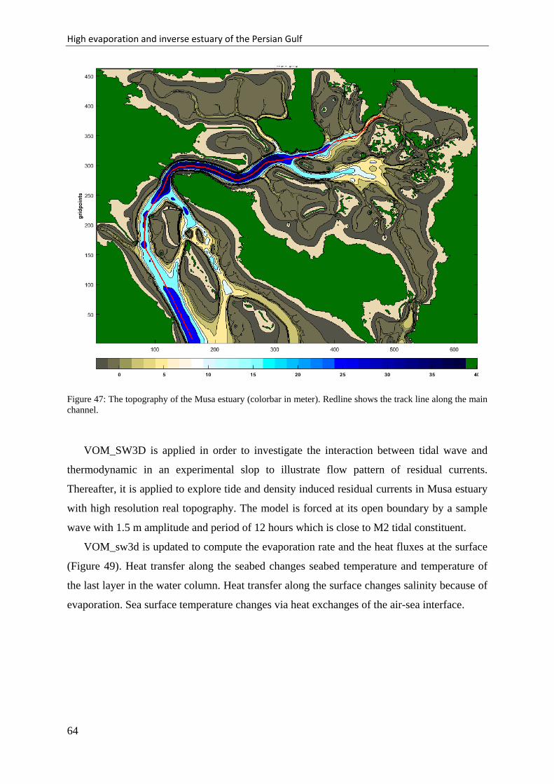
High evaporation and inverse estuary of the Persian Gulf
Figure 47: The topography of the Musa estuary (colorbar in meter). Redline shows the track line along the main channel.
VOM_SW3D is applied in order to investigate the interaction between tidal wave and
thermodynamic in an experimental slop to illustrate flow pattern of residual currents.
Thereafter, it is applied to explore tide and density induced residual currents in Musa estuary
with high resolution real topography. The model is forced at its open boundary by a sample
wave with 1.5 m amplitude and period of 12 hours which is close to M2 tidal constituent.
VOM_sw3d is updated to compute the evaporation rate and the heat fluxes at the surface
(Figure 49). Heat transfer along the seabed changes seabed temperature and temperature of
the last layer in the water column. Heat transfer along the surface changes salinity because of
evaporation. Sea surface temperature changes via heat exchanges of the air-sea interface.
64
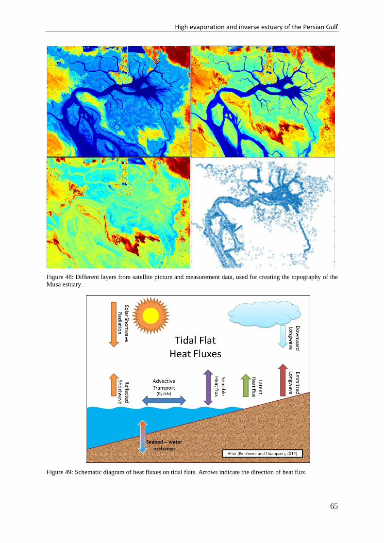
High evaporation and inverse estuary of the Persian Gulf
Figure 48: Different layers from satellite picture and measurement data, used for creating the topography of the Musa estuary.
Figure 49: Schematic diagram of heat fluxes on tidal flats. Arrows indicate the direction of heat flux.
65
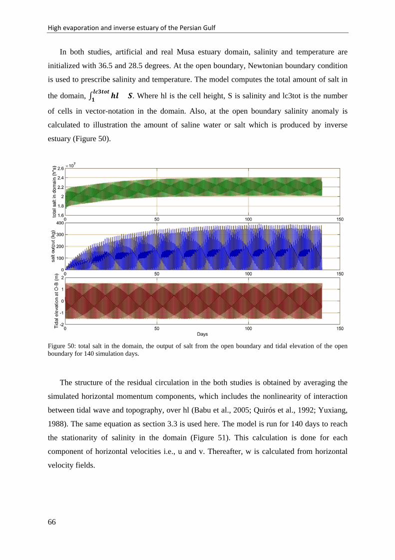
High evaporation and inverse estuary of the Persian Gulf
In both studies, artificial and real Musa estuary domain, salinity and temperature are
initialized with 36.5 and 28.5 degrees. At the open boundary, Newtonian boundary condition
is used to prescribe salinity and temperature. The model computes the total amount of salt in
the domain, ∫ 𝒉𝒉𝒉𝒉 × 𝑺𝑺𝒉𝒉𝒍𝒍𝟑𝟑𝒕𝒕𝒍𝒍𝒕𝒕𝟏𝟏 . Where hl is the cell height, S is salinity and lc3tot is the number
of cells in vector-notation in the domain. Also, at the open boundary salinity anomaly is
calculated to illustration the amount of saline water or salt which is produced by inverse
estuary (Figure 50).
Figure 50: total salt in the domain, the output of salt from the open boundary and tidal elevation of the open boundary for 140 simulation days.
The structure of the residual circulation in the both studies is obtained by averaging the
simulated horizontal momentum components, which includes the nonlinearity of interaction
between tidal wave and topography, over hl (Babu et al., 2005; Quirós et al., 1992; Yuxiang,
1988). The same equation as section 3.3 is used here. The model is run for 140 days to reach
the stationarity of salinity in the domain (Figure 51). This calculation is done for each
component of horizontal velocities i.e., u and v. Thereafter, w is calculated from horizontal
velocity fields.
66
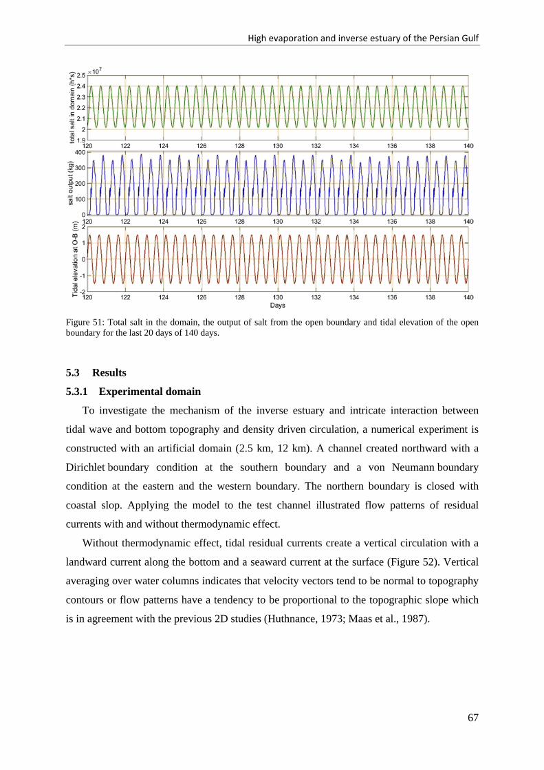
High evaporation and inverse estuary of the Persian Gulf
Figure 51: Total salt in the domain, the output of salt from the open boundary and tidal elevation of the open boundary for the last 20 days of 140 days.
5.3 Results
5.3.1 Experimental domain
To investigate the mechanism of the inverse estuary and intricate interaction between
tidal wave and bottom topography and density driven circulation, a numerical experiment is
constructed with an artificial domain (2.5 km, 12 km). A channel created northward with a
Dirichlet boundary condition at the southern boundary and a von Neumann boundary
condition at the eastern and the western boundary. The northern boundary is closed with
coastal slop. Applying the model to the test channel illustrated flow patterns of residual
currents with and without thermodynamic effect.
Without thermodynamic effect, tidal residual currents create a vertical circulation with a
landward current along the bottom and a seaward current at the surface (Figure 52). Vertical
averaging over water columns indicates that velocity vectors tend to be normal to topography
contours or flow patterns have a tendency to be proportional to the topographic slope which
is in agreement with the previous 2D studies (Huthnance, 1973; Maas et al., 1987).
67
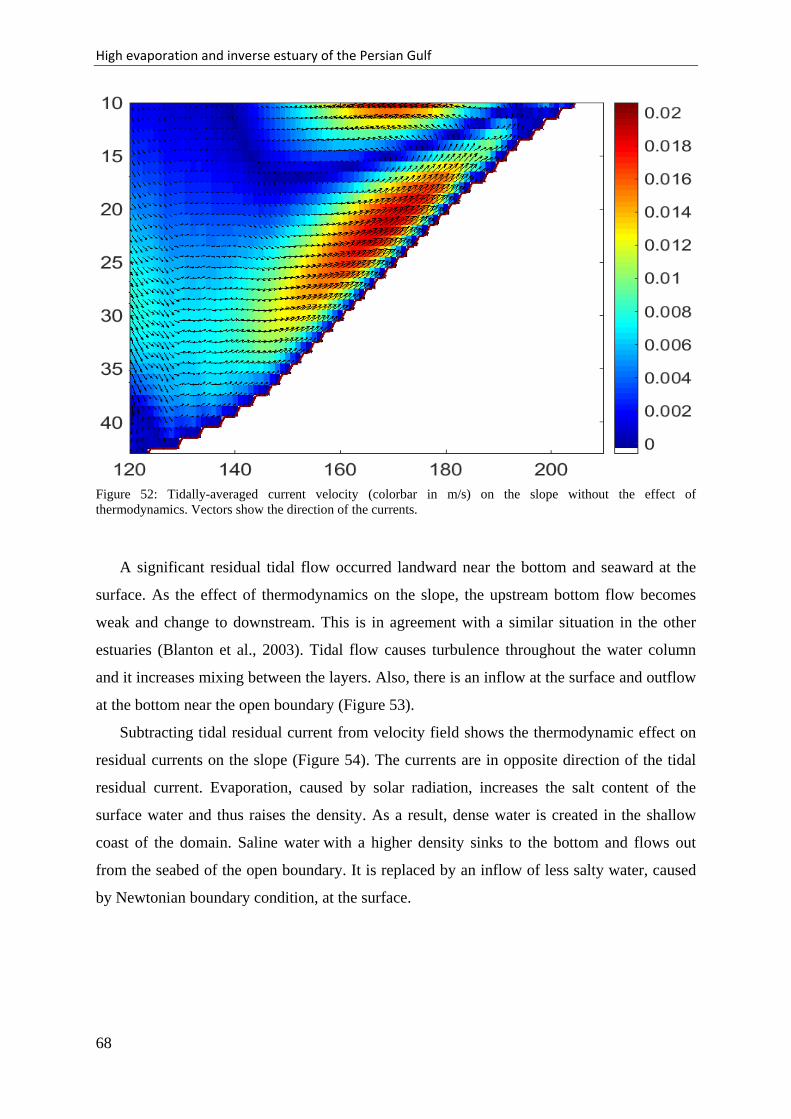
High evaporation and inverse estuary of the Persian Gulf
Figure 52: Tidally-averaged current velocity (colorbar in m/s) on the slope without the effect of thermodynamics. Vectors show the direction of the currents.
A significant residual tidal flow occurred landward near the bottom and seaward at the
surface. As the effect of thermodynamics on the slope, the upstream bottom flow becomes
weak and change to downstream. This is in agreement with a similar situation in the other
estuaries (Blanton et al., 2003). Tidal flow causes turbulence throughout the water column
and it increases mixing between the layers. Also, there is an inflow at the surface and outflow
at the bottom near the open boundary (Figure 53).
Subtracting tidal residual current from velocity field shows the thermodynamic effect on
residual currents on the slope (Figure 54). The currents are in opposite direction of the tidal
residual current. Evaporation, caused by solar radiation, increases the salt content of the
surface water and thus raises the density. As a result, dense water is created in the shallow
coast of the domain. Saline water with a higher density sinks to the bottom and flows out
from the seabed of the open boundary. It is replaced by an inflow of less salty water, caused
by Newtonian boundary condition, at the surface.
68
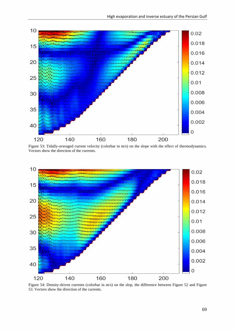
High evaporation and inverse estuary of the Persian Gulf
Figure 53: Tidally-averaged current velocity (colorbar in m/s) on the slope with the effect of thermodynamics. Vectors show the direction of the currents.
Figure 54: Density-driven currents (colorbar in m/s) on the slop, the difference between Figure 52 and Figure 53. Vectors show the direction of the currents.
69

High evaporation and inverse estuary of the Persian Gulf
5.3.2 Musa estuary
After 120 days the model has reached the steady state in thermodynamics and in
dynamics, as well. 3 tidal phases are shown each 4 hours later (Figures 55, 56 and 57). Upper
left (UL) part of each figure shows the surface layer salinity and it varies from 36.5 at the
open boundary to 60 in the shallow areas in the domain, which is the maximum limit for
salinity in the model. In the tidal flat and shallow area because of the low water exchange
salinity can reach to the maximum limit of the model. The lower left (LL) part of figures
shows the zonal section (Z093) of salinity field close to the open boundary, which is marked
with a white line in vertical grid-point, number 93, in UL. In this section, salinity varies
between 36.5 and 40 during a tidal cycle in the main channel. The second channel in this
section shows less variation in salinity, i.e. from 36.5 to 38.5. Going more inside to estuary,
upper right part of the figures shows the meridional section (M163) in the deepest part of the
domain. This is also marked with a white line in UL in horizontal grid-point, number 163, in
UL. Here salinity changes from 39.8 to 41.4. The second meridional section (M316) is
located in the center of the estuary, next to the port of Imam Khomeini. In this section,
salinity varies between 41.5 and 44 during a tidal cycle. As the effect of evaporation and
water exchange, salinity increases from the open boundary to the last section.
Figure 55: Model results for salinity (colorbar) after 120 days and 1 hour, UL: Surface layer. UR: Section M163. LL: Section Z093. LR: Section M316. Sections are marked with three lines in UL.
70
High evaporation and inverse estuary of the Persian Gulf
Figure 56: Model results for salinity (colorbar) after 120 days and 5 hours, UL: Surface layer. UR: Section M163. LL: Section Z093. LR: Section M316. Sections are marked with three lines in UL.
Figure 57: Model results for salinity (colorbar) after 120 days and 9 hours, UL: Surface layer. UR: Section M163. LL: Section Z093. LR: Section M316. Sections are marked with three lines in UL.
71
High evaporation and inverse estuary of the Persian Gulf
In all sections, the salinity contours are consistent with the contours of the normal
component of current velocity.
Figure 58: Model results after 120 days and 12 hours for section Z093 in Musa estuary. Left: salinity (colorbar). Right: V-component of current velocity (colorbar in m/s). The section is marked in Figure 55.
Figure 59: Model results after 120 days and 18 hours for section Z093 in Musa estuary. Left: salinity (colorbar). Right: V-component of current velocity (colorbar in m/s). The section is marked in Figure 55.
72

High evaporation and inverse estuary of the Persian Gulf
Figure 60: Model results after 120 days and 12 hours for section M163 in Musa estuary. Left: salinity (colorbar). Right: U-component of current velocity (colorbar in m/s). The section is marked in Figure 55.
Figure 61: Model results after 120 days and 12 hours for section M163 in Musa estuary. Left: salinity (colorbar). Right: U-component of current velocity (colorbar in m/s). The section is marked in Figure 55.
73
High evaporation and inverse estuary of the Persian Gulf
Figure 62: Model results after 120 days and 12 hours for section M316 in Musa estuary. Left: salinity (colorbar). Right: U-component of current velocity (colorbar in m/s). The section is marked in Figure 55.
Figure 63: Model results after 120 days and 12 hours for section M316 in Musa estuary. Left: salinity (colorbar). Right: U-component of current velocity (colorbar in m/s). The section is marked in Figure 55.
74
High evaporation and inverse estuary of the Persian Gulf
Each section shows two tidal phases with 6 hours difference (Figures 58 to 63). In section
Z093 current velocity varies between -2.0 to 2.3 m/s in two directions during one tidal cycle
in the main channel. In section M163 maximum velocities are -1.9 and 2.3 m/s and in section
M316 they velocity changes from -1.8 to 1.4 m/s.
An average of the simulated flow over one tidal cycle yields the residual circulation in the
Musa estuary. Same as in the artificial domain the tidal flow effects the mixing between the
layers. As a result, saline water transfers from the lower layers to the upper layers and some
low salinity water from the surface towards the bottom. Generally, tidally-averaged salinity
results in a horizontal salinity gradient with the salinity increasing towards the head of the
Musa estuary. The averages for salinity and two horizontal components of currents along the
track of the main channel are shown here (Figures 64, 65 and 66). Each part of tidally-
averaged current velocity normal to the direction of the track (Figure 66) can be matched
with a branch position in the topography.
Figure 64: Tidally-averaged salinity, (colorbar) along the track in the Musa estuary.
Figure 65: Tidally-averaged current velocity (colorbar in m/s), in the direction of the track in the Musa estuary.
75
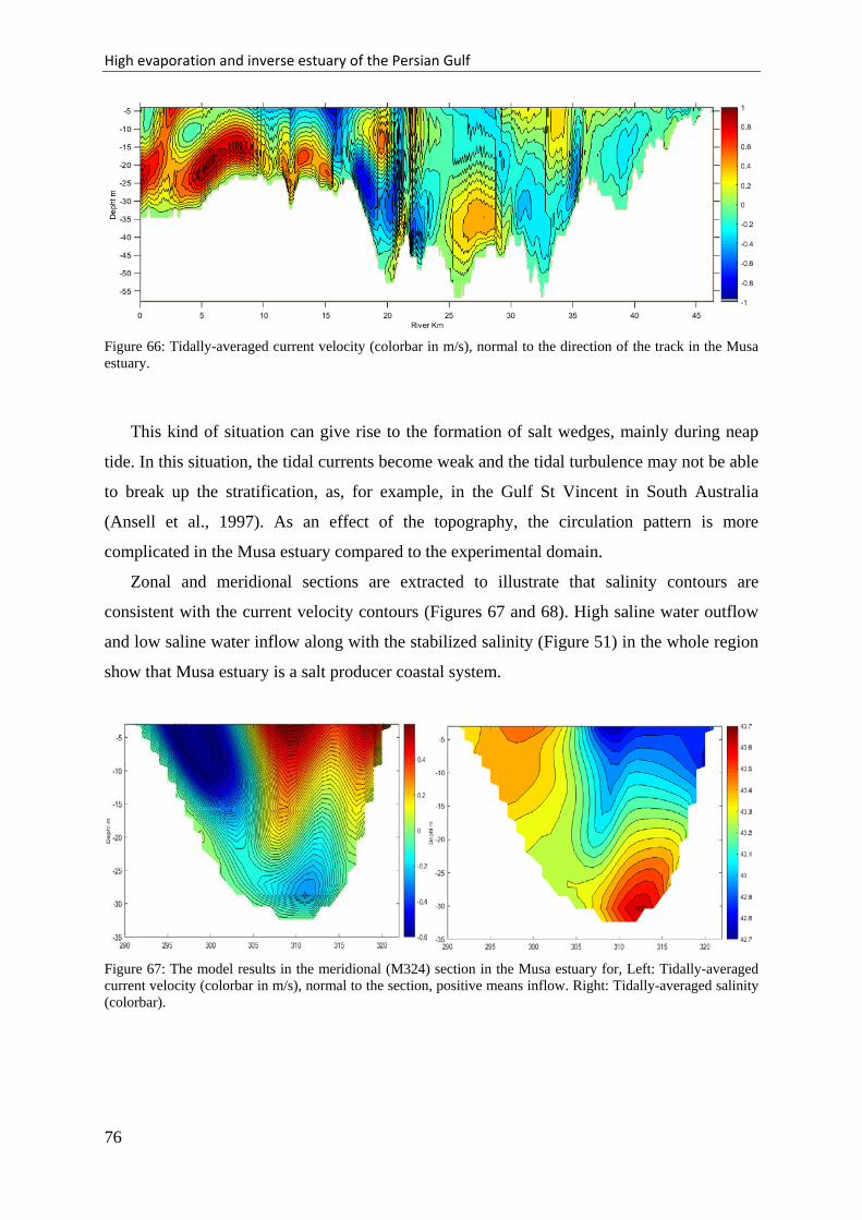
High evaporation and inverse estuary of the Persian Gulf
Figure 66: Tidally-averaged current velocity (colorbar in m/s), normal to the direction of the track in the Musa estuary.
This kind of situation can give rise to the formation of salt wedges, mainly during neap
tide. In this situation, the tidal currents become weak and the tidal turbulence may not be able
to break up the stratification, as, for example, in the Gulf St Vincent in South Australia
(Ansell et al., 1997). As an effect of the topography, the circulation pattern is more
complicated in the Musa estuary compared to the experimental domain.
Zonal and meridional sections are extracted to illustrate that salinity contours are
consistent with the current velocity contours (Figures 67 and 68). High saline water outflow
and low saline water inflow along with the stabilized salinity (Figure 51) in the whole region
show that Musa estuary is a salt producer coastal system.
Figure 67: The model results in the meridional (M324) section in the Musa estuary for, Left: Tidally-averaged current velocity (colorbar in m/s), normal to the section, positive means inflow. Right: Tidally-averaged salinity (colorbar).
76
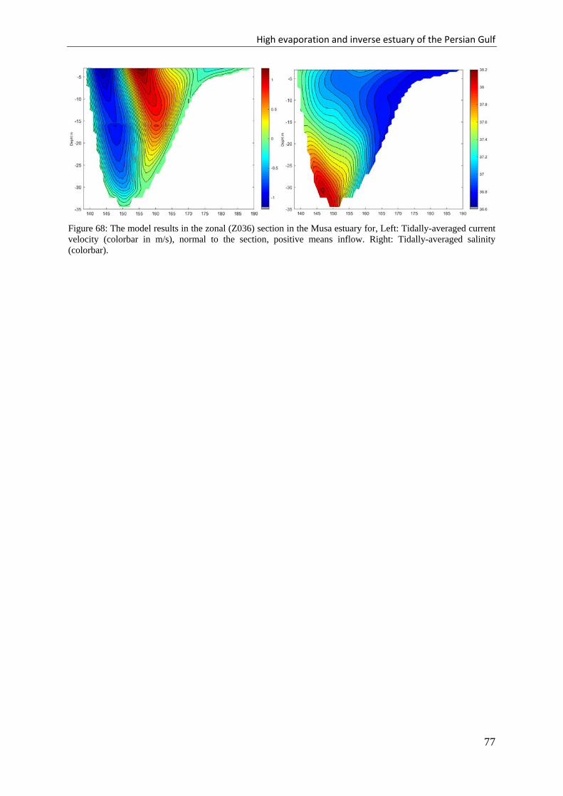
High evaporation and inverse estuary of the Persian Gulf
Figure 68: The model results in the zonal (Z036) section in the Musa estuary for, Left: Tidally-averaged current velocity (colorbar in m/s), normal to the section, positive means inflow. Right: Tidally-averaged salinity (colorbar).
77
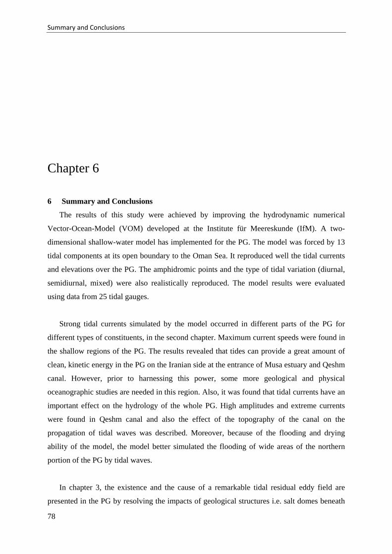
Summary and Conclusions
Chapter 6
6 Summary and Conclusions
The results of this study were achieved by improving the hydrodynamic numerical
Vector-Ocean-Model (VOM) developed at the Institute für Meereskunde (IfM). A two-
dimensional shallow-water model has implemented for the PG. The model was forced by 13
tidal components at its open boundary to the Oman Sea. It reproduced well the tidal currents
and elevations over the PG. The amphidromic points and the type of tidal variation (diurnal,
semidiurnal, mixed) were also realistically reproduced. The model results were evaluated
using data from 25 tidal gauges.
Strong tidal currents simulated by the model occurred in different parts of the PG for
different types of constituents, in the second chapter. Maximum current speeds were found in
the shallow regions of the PG. The results revealed that tides can provide a great amount of
clean, kinetic energy in the PG on the Iranian side at the entrance of Musa estuary and Qeshm
canal. However, prior to harnessing this power, some more geological and physical
oceanographic studies are needed in this region. Also, it was found that tidal currents have an
important effect on the hydrology of the whole PG. High amplitudes and extreme currents
were found in Qeshm canal and also the effect of the topography of the canal on the
propagation of tidal waves was described. Moreover, because of the flooding and drying
ability of the model, the model better simulated the flooding of wide areas of the northern
portion of the PG by tidal waves.
In chapter 3, the existence and the cause of a remarkable tidal residual eddy field are
presented in the PG by resolving the impacts of geological structures i.e. salt domes beneath
78
Summary and Conclusions
the seabed, on the dynamics of the water column. It is very likely the richest barotropic eddy
field ever observed in a marginal sea. The spatial structure of simulated residual currents was
strongly influenced by nonlinear interactions of the tidal flow with the relief of the seabed.
The latter resembling a shark-skin. That is, sub-seabed salt domes leave their signature in the
tidal residual flow. In the high-pass filtered digital topography, more than 200 obstacles were
observed which may have been caused by underlying salt domes. Only 60 salt domes have
been charted so far by field work in oil exploration (Zaigham et al., 2013). Thus, the high-
pass topography may provide further guidance for a future offshore exploration of mineral
oil. Residual currents depicted by Lagrangian trajectories indicated the presence of strong
coastal currents in the northern PG. There residuals of the M2 tide may exceed 0.15 m/s
while tidal currents in that area were around 1.5 m/s. Spatial scales of the barotropic tidal
residual eddies are in the order of 10 Km. The internal Rossby Radius of Deformation, a
measure of the scales of baroclinic eddies in the PG, was of the same order. This agreement
in scales suggests that barotropic and baroclinic eddies interact. This awaits future
investigation.
In chapter 4, the model predicted resonance for both diurnal and semidiurnal constituents.
Results reveal a system of amphidromic points of Kelvin-Taylor type with two points for
semidiurnal constituents and a single point for diurnal constituents which agrees well with
previous studies (Bosch van Drakestein, 2014; Hyder et al., 2013; Mashayekh Poul et al.,
2016; Pous et al., 2013; Ranaee et al., 2012; Reynolds, 1993). The model results unveiled the
following main features of tidal resonance in the PG:
A. Diurnal tides were resonant in the northern PG and in the region off the Arabian coast.
B. Semidiurnal tides were amplified in the northern Gulf and in the Strait of Hormuz.
C. A simulated sea level rise increased AF in the region off the Arabian coast for
semidiurnal and in the Qeshm Canal for both tides.
D. The amphidromic points were displaced in position in the PG when different periods
of forcing were used.
E. The results revealed that tides can provide a great amount of potential energy in the
Iranian side of the PG, at the Musa estuary and Qeshm canal.
F. Semidiurnal tides provide more energy (10 times) compare to diurnal tides in the PG.
Finally, in chapter 5, the mechanism of tidal barotropic residual circulation in the Musa
estuary was described by applying an updated version of VOM-SW3D with an additional
79
Summary and Conclusions
thermodynamic module into the Musa estuary. The main objective was to understand the
effect of evaporation on density-driven circulation and its interactions with tidal currents. As
a result of evaporation in this arid region, salinity increased in the surface layer and in
shallow tidal flats. Dense near-bottom water flowed toward the PG and was replaced by an
inflow of relatively fresh water at the surface. But, residual tidal currents flowed in the
opposite direction. Variation in meteorological parameters and tidal amplitude controls the
general circulation. The results revealed high salinity outflow and low salinity inflow along
with the stabilized salinity in the whole region. A horizontal gradient in tidally-averaged
salinity was found with the salinity increasing towards the head of the Musa estuary. The
results suggest that the Musa estuary is a salt producing, coastal system.
80

Acknowledgement Thanks God, the almighty, for giving me strength, tolerance, patience and good luck that
helped me to complete this work.
I would like to thank my supervisor, Professor Jan Backhaus. His interest in the field of
numerical modeling, innovative ideas, valuable suggestions and sense of determination
helped me during my PhD.
I am extremely grateful to Udo Huebner for all his help. Throughout my entire time at
Hamburg, Jan and Udo have provided me with a great deal of support. I am very grateful to
both of them.
I would like to thank my thesis committee members for all of their guidance through this
process, especially, Dr. Thomas Pohlmann and Dr. Ali Dehghani.
I was lucky to have a great group of friends. In particular, thanks Dr. Moritz Mathis; his
discussions and feedbacks have been invaluable.
The ministry of science, research and technology of Iran funded this research.
81

Acknowledgement
Declaration
I hereby declare, on oath, that I have written the present dissertation by my own and have not used other than the acknowledged resources and aids.
Hamburg, 30.03.2016
Hossein Mashayekh Poul
82
Bibliography
Bibliography Al-Subhi, A., 2010. Tide and Sea Level Characteristics at Juaymah, West Coast of the
Arabian Gulf. J. King Abdulaziz Univ. Sci. 21, 133–149.
Alvarez Fanjul, E., Gómez, B.P., Sánchez-Arévalo, I.R., 1997. A description of the tides in the Eastern North Atlantic. Prog. Oceanogr. 40, 217–244.
Andersen, O.B., Egbert, G.D., Erofeeva, S.Y., Ray, R.D., 2006. Mapping nonlinear shallow-water tides: a look at the past and future. Ocean Dyn. 56, 416–429.
Ansell, A.., Gibson, R.., Barnes, M., 1997. Oceanography and marine biology. An annual review. J. Mar. Biol. Assoc. United Kingdom 35, 653. doi:10.1017/S0025315400041795
Arakawa, A., 1972. Design of the UCLA general circulation model. Numerical Simulation of Weather and Climate.
Arakawa, A., Lamb, V.R., 1977. Computational Design of the Basic Dynamical Processes of the UCLA General Circulation Models of the Atmosphere, Methods in Computational Physics: Advances in Research and Applications, Methods in Computational Physics: Advances in Research and Applications. Elsevier.
Arakawa, A., Schubert, W.H., 1974. Interaction of a Cumulus Cloud Ensemble with the Large-Scale Environment, Part I. J. Atmos. Sci. 31, 674–701.
Arbic, B.K., St-Laurent, P., Sutherland, G., Garrett, C., 2007. On the resonance and influence of the tides in Ungava Bay and Hudson Strait. Geophys. Res. Lett. 34, L17606. doi:10.1029/2007GL030845
Babu, M.T., Vethamony, P., Desa, E., 2005. Modelling tide-driven currents and residual eddies in the Gulf of Kachchh and their seasonal variability. Ecol. Modell. 184, 299–312.
Backhaus, J., 1976. Zur Hydrodynamik im Flachwassergebiet. Ein numerisches Modell. Dtsch. Hydrogr. Zeitschrift 29, 222–238. doi:10.1007/BF02226256
Backhaus, J.O., 2015. Latent resonance in tidal rivers, with applications to River Elbe. J. Mar. Syst. 151, 71–78.
Backhaus, J.O., 2008. Improved representation of topographic effects by a vertical adaptive grid in vector-ocean-model (VOM). Part I: Generation of adaptive grids. Ocean Model. 22, 114–127.
Backhaus, J.O., 1996. Climate-sensitivity of European marginal seas, derived from the interpretation of modelling studies. J. Mar. Syst. 7, 361–382.
Backhaus, J.O., 1985. A three-dimensional model for the simulation of shelf sea dynamics. Dtsch. Hydrogr. Zeitschrift 38, 165–187.
Backhaus, J.O., 1983. A semi-implicit scheme for the shallow water equations for application to shelf sea modelling. Cont. Shelf Res. 2, 243–254.
83
Bibliography
Backhaus, J.O., Harms, I., Hübner, U., 2008. Improved representation of topographic effects by a vertical adaptive grid in Vector-Ocean-Model (VOM). Part II: Simulations in unstructured adaptive grids. Ocean Model. 22, 128–145.
Badri, M.A., Wilders, P., 2012. Flow estimation for the Persian Gulf using a kelvin wave expansion. Indian J. Geo-Marine Sci. 41, 249–258.
Bahaj, A.S., Myers, L., 2004. Analytical estimates of the energy yield potential from the Alderney Race (Channel Islands) using marine current energy converters. Renew. Energy 29, 1931–1945.
Bakker, W.T., de Vriend, H.J., 1995. Resonance and morphological stability of tidal basins. Mar. Geol. 126, 5–18.
Blain, C.A., 1998. Barotropic Tidal and Residual Circulation in the Arabian Gulf. Proc. 6th Int. Conf. Estuar. Coast. Model. 166–180.
Blain, C.A., n.d. Modeling Three-Dimensional, Thermohaline-Driven Circulation in the Arabian Gulf, in: Estuarine and Coastal Modeling (1999). ASCE, pp. 74–93.
Blanton, J.O., Seim, H., Alexander, C., Amft, J., Kineke, G., 2003. Transport of salt and suspended sediments in a curving channel of a coastal plain estuary: Satilla River, GA. Estuar. Coast. Shelf Sci. 57, 993–1006. doi:10.1016/S0272-7714(03)00005-2
Bosch van Drakestein, F.G., 2014. Modeling of tides and spreading of saline water in the Arabian Gulf and in the coastal area of Abu Dhabi with a flexible mesh model.
Brewer, P.G., Dyrssen, D., 1985. Chemical oceanography of the Persian Gulf. Prog. Oceanogr. 14, 41–55.
Carbajal, N., Backhaus, J.O., 1998. Simulation of tides, residual flow and energy budget in the Gulf of California. Oceanol. Acta 21, 429–446.
Chao, S.-Y., Kao, T.W., Al-Hajri, K.R., 1992. A Numerical Investigation of Circulation in the Arabian Gulf. J. Geophys. Res. 97, 11219–11236. doi:10.1029/92jc00841
Chen, W., Liu, W., Hsu, M., 2013. Modeling Evaluation of Tidal Stream Energy and the Impacts of Energy Extraction on Hydrodynamics in the Taiwan Strait 2191–2203. doi:10.3390/en6042191
Chu, P.C., Williams, C.L., Clem, T., Haeger, S.D., Ward, M., 2008. Environmental impact on chemical/oil spill in the Persian Gulf. Environ. Probl. Coast. Reg. VII I, 149–159. doi:10.2495/CENV080141
Davies, A.M., Jones, J.E., 1996. Sensitivity of Tidal Bed Stress Distributions, Near-Bed Currents, Overtides, and Tidal Residuals to Frictional Effects in the Eastern Irish Sea. J. Phys. Oceanogr. 26, 2553–2575.
Defant, A., 1961. Physical oceanography. Pergamon Press, New York.
Dworak, J.A., Gómez-Valdés, J., 2003. Tide-induced residual current in a coastal lagoon of the Gulf of California. Estuar. Coast. Shelf Sci. 57, 99–109.
84
Bibliography
Edgell, H., 1991. Proterozoic salt basins of the Persian Gulf area and their role in hydrocarbon generation. Precambrian Res. 54, 1–14.
Egbert, G.D., Erofeeva, S.Y., 2002. Efficient Inverse Modeling of Barotropic Ocean Tides. J. Atmos. Ocean. Technol. 19, 183–204.
El-Sabh, M.I., Murty, T.S., 1989. Storm surges in the Arabian Gulf. Nat. Hazards 1, 371–385.
Emery, K.O., 1956. Sediments and Water of Persian Gulf. Am. Assoc. Pet. Geol. Bull. 40, 2354–2383.
Ezam, M., Bidokhti, a. a., Javid, a. H., 2010. Numerical simulations of spreading of the Persian Gulf outflow into the Oman Sea. Ocean Sci. 6, 887–900.
Ganj, M., 2013. Simulation of Tidal Currents in the Persian Gulf. Int. J. Emerg. Trends Eng. Dev. 5, 31–38.
Garrett, C., 1972. Tidal Resonance in the Bay of Fundy and Gulf of Maine. Nature 238, 441–443. doi:10.1038/238441a0
Godin, G., 1993. On tidal resonance. Cont. Shelf Res. 13, 89–107.
Goharnejad, H., Shamsai, A., Hosseini, S.A., 2013. Vulnerability assessment of southern coastal areas of Iran to sea level rise: evaluation of climate change impact. Oceanologia 55, 611–637.
Gorji-Bandpy, M., Azimi, M., Jouya, M., 2013. Tidal Energy and Main Resources In the Persian Gulf. Distrib. Gener. Altern. Energy J. 28, 61–77.
Hainbucher, D., Backhaus, J.O., 1999. Circulation of the eastern North Atlantic and north-west European continental shelf - a hydrodynamic modelling study. Fish. Oceanogr. 8, 1–12.
Harms, I.H., Heath, M.R., Bryant, A.D., Backhaus, J.O., Hainbucher, D.A., 2000. Modelling the Northeast Atlantic circulation: implications for the spring invasion of shelf regions by Calanus finmarchicus. ICES J. Mar. Sci. 57, 1694–1707.
Hill, D.F., Griffiths, S.D., Peltier, W.R., Horton, B.P., Törnqvist, T.E., 2011. High-resolution numerical modeling of tides in the western Atlantic, Gulf of Mexico, and Caribbean Sea during the Holocene. J. Geophys. Res. Ocean. 116, 1–16.
Hosseinibalam, F., Hassanzadeh, S., Rezaei-Latifi, a., 2011. Three-dimensional numerical modeling of thermohaline and wind-driven circulations in the Persian Gulf. Appl. Math. Model. 35, 5884–5902. doi:10.1016/j.apm.2011.05.040
Huang, D., Su, J., Backhaus, J.O., 1999. Modelling the seasonal thermal stratification and baroclinic circulation in the Bohai Sea. Cont. Shelf Res. 19, 1485–1505.
Huthnance, J.M., 1973. Tidal current asymmetries over the Norfolk Sandbanks. Estuar. Coast. Mar. Sci. 1, 89–99.
Hyder, P., While, J., Arnold, A., O Dea, E., Furner, R., Siddorn, J., Martin, M., Sykes, P.,
85
Bibliography
2013. Evaluating a new NEMO-based Persian/Arabian Gulf tidal operational model. J. Oper. Oceanogr. 6, 3–16.
Janssen, F., Schrum, C., Hübner, U., Backhaus, J.O., 2001. Uncertainty analysis of a decadal simulation with a regional ocean model for the North Sea and Baltic Sea. Clim. Res. 18, 55–62.
John, V.C., 1992. Harmonic tidal current constituents of the western Arabian Gulf from moored current measurements. Coast. Eng. 17, 145–151.
Johns, W.E., Yao, F., Olson, D.B., Josey, S.A., Grist, J.P., Smeed, D.A., 2003. Observations of seasonal exchange through the Straits of Hormuz and the inferred heat and freshwater budgets of the Persian Gulf. J. Geophys. Res.
Kent, P.E., 1979. THE EMERGENT HORMUZ SALT PLUGS OF SOUTHERN IRAN. J. Pet. Geol. 2, 117–144. doi:10.1111/j.1747-5457.1979.tb00698.x
Komen, G.J., Riepma, H.W., Bilt, D., 1981. The generation of residual vorticity by the combined action of wind and bottom topography in a shallow sea. Oceanol. acta 4, 267–278.
Lavín, M.F., Marinone, S.G., 2003. An overview of the physical oceanography of the Gulf of California. Nonlinear Process. Geophys. Fluid Dyn.
Le Provost, C., Fornerino, M., 1985. Tidal Spectroscopy of the English Channel with a Numerical Model. J. Phys. Oceanogr. 15, 1009–1031.
Le Souëf, K.E., Allen, S.E., 2014. Physical modeling of tidal resonance in a submarine canyon. J. Geophys. Res. Ocean. 119, 1324–1343.
Lewis, J.K., Vayda, G.A., Hsu, Y.L., 1968. a Coupled Regional Tide Model. US Pat. 3,371,052.
Liang, D., Xia, J., Falconer, R. a., Zhang, J., 2014. Study on Tidal Resonance in Severn Estuary and Bristol Channel. Coast. Eng. J. 56, 1450002.
Lokier, S.W., Bateman, M.D., Larkin, N.R., Rye, P., Stewart, J.R., 2015. Late Quaternary sea-level changes of the Persian Gulf. Quat. Res. 84, 69–81.
Maas, L.R.M., Zimmerman, J.T.F., Temme, N.M., 1987. On the Exact Shape of the Horizntal Profile of a Topographically Rectified Tidal Flow. Geophys. Astrophys. Fluid Dyn. 38, 105–129.
Marinone, S.G., 1997. Tidal residual currents in the Gulf of California: Is the M2 tidal constituent sufficient to induce them? J. Geophys. Res. 102, 8611–8623.
Mashayekh Poul, H., Backhaus, J., Huebner, U., 2016. A description of the tides and effect of Qeshm canal on that in the Persian Gulf using two-dimensional numerical model. Arab. J. Geosci. 9, 148. doi:10.1007/s12517-015-2259-8
Mashayekh Poul, H., Backhaus, J.O., Huebner, U., 2014. Estimate the area with most efficiency for producing energy from tide in the Persian Gulf, in: The 11th International
86
Bibliography
Conference on Coasts, Ports and Marine Structures. Tehran, Iran.
McMillan, J., Lickley, M., 2008. The Potential of Tidal Power from the Bay of Fundy. SIAM Undergrad. Res. Online 1, 20–37.
Moeini, M.H., Etemad-Shahidi, A., Chegini, V., 2010. Wave modeling and extreme value analysis off the northern coast of the Persian Gulf. Appl. Ocean Res. 32, 209–218.
Najafi, H.S., 1997. Modelling tides in the Persian Gulf using dynamic nesting. University of Adelaide.
Nicholls-Lee, R.F., 2011. Adaptive Composite Blades for Horizontal Axis Tidal Turbines. University of Southampton.
Pawlowicz, R., Beardsley, B., Lentz, S., 2002. Classical tidal harmonic analysis including error estimates in MATLAB using T_TIDE. Comput. Geosci. 28, 929–937.
Perotti, C.R., Carruba, S., Rinaldi, M., Bertozzi, G., Feltre, L., Rahimi, M., 2011. New Frontiers in Tectonic Research - At the midst of Plate Convergence. InTech.
Perrone, T.J., 1979. Winter Shamal in the Persian Gulf.
Pous, S., Carton, X., Lazure, P., 2013. A Process Study of the Wind-Induced Circulation in the Persian Gulf. Open J. Mar. Sci. 03, 1–11. doi:10.4236/ojms.2013.31001
Pous, S., Carton, X., Lazure, P., 2012. A Process Study of the Tidal Circulation in the Persian Gulf. Open J. Mar. Sci. 02, 131–140. doi:10.4236/ojms.2012.24016
Pous, S., Lazure, P., Carton, X., 2015. A model of the general circulation in the Persian Gulf and in the Strait of Hormuz: Intraseasonal to interannual variability. Cont. Shelf Res. 94, 55–70. doi:10.1016/j.csr.2014.12.008
Pous, S.P., Carton, X., Lazure, P., 2004a. Hydrology and circulation in the Strait of Hormuz and the Gulf of Oman-Results from the GOGP99 Experiment: 2. Gulf of Oman. J. Geophys. Res. C Ocean. 109, 1–15.
Pous, S.P., Carton, X., Lazure, P., 2004b. Hydrology and circulation in the Strait of Hormuz and the Gulf of Oman — Results from the GOGP99 Experiment : 1 . Strait of Hormuz Hydrology and circulation in the Strait of Hormuz and the Gulf of Oman ; results from the GOGP99 Experiment . Part I . Strai. J. Geophys. Res. 109.
Proudman, J., 1953. Dynamical Oceanography. Methuen & Co.
Purser, B.H., 1973. Sedimentation around bathymetric highs in the southern Persian Gulf. Persian Gulf 157–177.
Quaresma, L.S., Pichon, A., 2013. Modelling the barotropic tide along the West-Iberian margin. J. Mar. Syst. 109-110, S3–S25.
Quirós, G., Badan-Dangon, A., Ripa, P., 1992. M2 currents and residual flow in the Gulf of California. Netherlands J. Sea Res. 28, 251–259.
Ranaee, E., Mosaddad, S.M., Akbari, M., 2012. Seasonal Influences of Boundary Conditions
87
Bibliography
in Coastal Water Quality Variations ( Case Study : Northern Zone of Persian Gulf ) Faculty of Physical Oceanography , Young Researchers Club ,. World Appl. Sci. J. 19, 894–903.
Ranaee, E., Mosaddad, S.M., Akbari, M., 2011. Seasonal Influences of Boundary Conditions in Coastal Water Quality Variations. World Appl. Sci. J. 13.
Reynolds, M., 1993. Physical oceanography of the Gulf, Strait of Hormuz, and the Gulf of Oman—Results from the Mt Mitchell expedition. Mar. Pollut. Bull. 27, 35–59.
Robinson, I.S., 1981. Tidal vorticity and residual circulation. Deep Sea Res. Part A. Oceanogr. Res. Pap. 28, 195–212.
Roos, P.C., Schuttelaars, H.M., 2010. Influence of topography on tide propagation and amplification in semi-enclosed basins. Ocean Dyn. 61, 21–38.
Sabbagh Yazdi, S.R., Sadeghi Gooya, A., 2010. Modeling Khowr-e Musa Multi-Branch Estuary Currents due to the Persian Gulf Tides Using NASIR Depth Average Flow Solver. J. Persian Gulf 1, 45–50.
Sabbagh-Yazdi, S.-R., Zounemat-Kermani, M., Kermani, A., 2007. Solution of depth-averaged tidal currents in Persian Gulf on unstructured overlapping finite volumes. Int. J. Numer. Methods Fluids 55, 81–101.
Sarnthein, M., 1972. Sediments and history of the Postglacial transgression in the Persian Gulf and northwest Gulf of Oman. Mar. Geol. 12, 245–266.
Schrum, C., Backhaus, J.O., 1999. Sensitivity of atmosphere-ocean heat exchange and heat content in the North Sea and the Baltic Sea. Tellus A 51, 526–549.
Seni, S.J., Jackson, M.P.A., 1984. SEDIMENTARY RECORD OF CRETACEOUS AND TERTIARY SALT MOVEMENT , EAST TEXAS BASIN ; Times , Rates , and Volumes of Salt Flow and Their Implications for Nuclear Waste Isolation and Petroleum Exploration.
Skiba, A.W., Zeng, L., Arbic, B.K., Müller, M., Godwin, W.J., 2013. On the Resonance and Shelf/Open-Ocean Coupling of the Global Diurnal Tides. J. Phys. Oceanogr. 43, 1301–1324.
Stronach, J.A., Backhaus, J.O., Murty, T.S., 1993. An update on the numerical simulation of oceanographic processes in the waters between Vancouver Island and the mainland: the GF8 model. Oceanogr. Mar. Biol. An Annu. Rev. 31, 1–86.
Sutherland, G., Garrett, C., Foreman, M., 2005. Tidal Resonance in Juan de Fuca Strait and the Strait of Georgia. J. Phys. Oceanogr. 35, 1279–1286.
Swift, S.A., Bower, A.S., 2003. Formation and circulation of dense water in the Persian/Arabian Gulf. J. Geophys. Res. 108, 3004.
Thomas, R.J., Ellison, R. a., Goodenough, K.M., Roberts, N.M.W., Allen, P. a., 2015. Salt domes of the UAE and Oman: Probing eastern Arabia. Precambrian Res. 256, 1–16.
88
Bibliography
Thoppil, P.G., Hogan, P.J., 2010a. Persian Gulf response to a wintertime shamal wind event. Deep Sea Res. Part I 57, 946–955.
Thoppil, P.G., Hogan, P.J., 2010b. A Modeling Study of Circulation and Eddies in the Persian Gulf. J. Phys. Oceanogr. 40, 2122–2134. doi:10.1175/2010JPO4227.1
Westerink, J.J., Stolzenbach, K.D., Connor, J.J., 1989. General Spectral Computations of the Nonlinear Shallow Water Tidal Interactions within the Bight of Abaco. J. Phys. Oceanogr. 19, 1348–1371.
Yao, F., 2008. Water Mass Formation and Circulation in the Persian Gulf , and Water Exchange with the Indian Ocean The Hydrogaphy and Circula-. Univ. Miami. university of Miami.
Yuxiang, T., 1988. Numerical modelling of the tide-induced residual current in the East China Sea. Prog. Oceanogr. 21, 417–429.
Zaigham, N.A., Aburizaiza, O.S., Nayyer, Z.A., Mahar, G.A., Siddique, A., 2013. Salt-Tectonics Plays Major Role in Contributing High Seawater Salinity in Arabian / persian Gulf : A Constant Constrain on Seawater Desalination. Int. J. Water Resour. Arid Environ. 2, 187–194.
Zimmerman, J.T.F., 1978. Hydrodynamics of Estuaries and Fjords, Proceedings of the 9th International Liege Colloquium on Ocean Hydrodynamics, Elsevier Oceanography Series, Elsevier Oceanography Series. Elsevier.
89
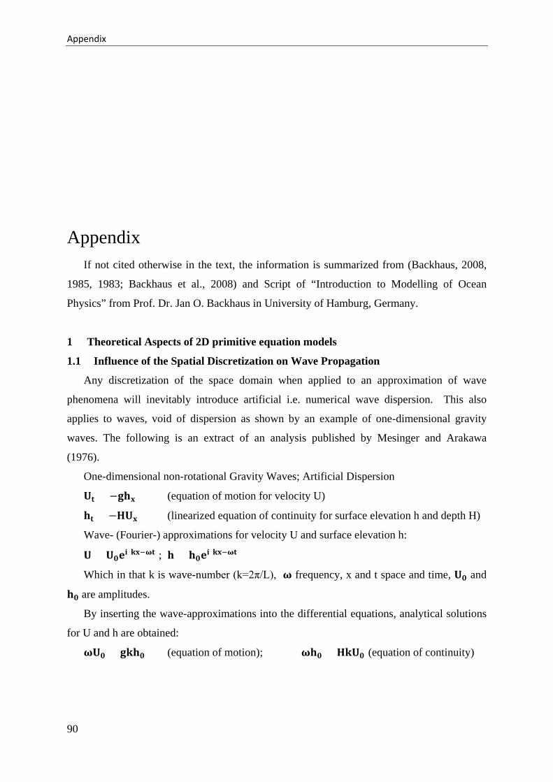
Appendix
Appendix If not cited otherwise in the text, the information is summarized from (Backhaus, 2008,
1985, 1983; Backhaus et al., 2008) and Script of “Introduction to Modelling of Ocean
Physics” from Prof. Dr. Jan O. Backhaus in University of Hamburg, Germany.
1 Theoretical Aspects of 2D primitive equation models
1.1 Influence of the Spatial Discretization on Wave Propagation
Any discretization of the space domain when applied to an approximation of wave
phenomena will inevitably introduce artificial i.e. numerical wave dispersion. This also
applies to waves, void of dispersion as shown by an example of one-dimensional gravity
waves. The following is an extract of an analysis published by Mesinger and Arakawa
(1976).
One-dimensional non-rotational Gravity Waves; Artificial Dispersion
𝐔𝐔𝐃𝐃 = −𝐠𝐠𝐃𝐃𝐱𝐱 (equation of motion for velocity U)
𝐃𝐃𝐃𝐃 = −𝐇𝐇𝐔𝐔𝐱𝐱 (linearized equation of continuity for surface elevation h and depth H)
Wave- (Fourier-) approximations for velocity U and surface elevation h:
𝐔𝐔 = 𝐔𝐔𝟎𝟎𝐃𝐃𝐢𝐢(𝐤𝐤𝐱𝐱−𝛚𝛚𝐃𝐃); 𝐃𝐃 = 𝐃𝐃𝟎𝟎𝐃𝐃𝐢𝐢(𝐤𝐤𝐱𝐱−𝛚𝛚𝐃𝐃)
Which in that k is wave-number (k=2π/L), 𝛚𝛚 frequency, x and t space and time, 𝐔𝐔𝟎𝟎 and
𝐃𝐃𝟎𝟎 are amplitudes.
By inserting the wave-approximations into the differential equations, analytical solutions
for U and h are obtained:
𝛚𝛚𝐔𝐔𝟎𝟎 = 𝐠𝐠𝐤𝐤𝐃𝐃𝟎𝟎 (equation of motion); 𝛚𝛚𝐃𝐃𝟎𝟎 = 𝐇𝐇𝐤𝐤𝐔𝐔𝟎𝟎 (equation of continuity)
90
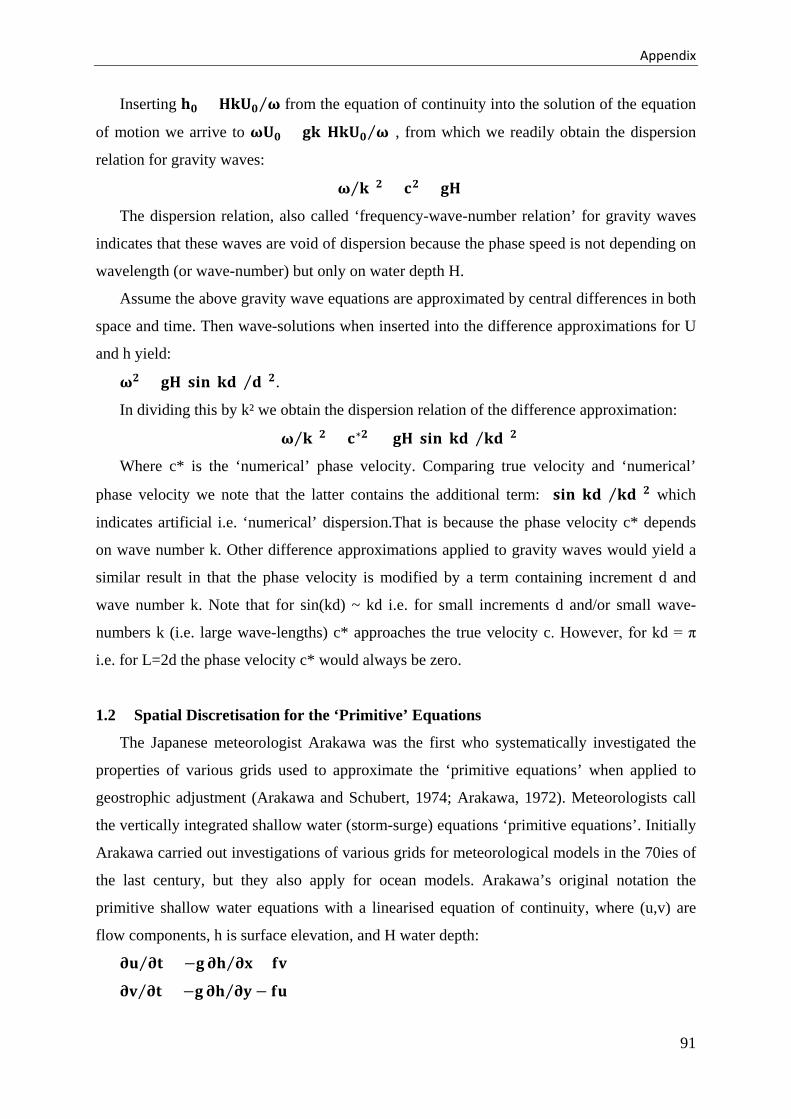
Appendix
Inserting 𝐃𝐃𝟎𝟎 = 𝐇𝐇𝐤𝐤𝐔𝐔𝟎𝟎 𝛚𝛚⁄ from the equation of continuity into the solution of the equation
of motion we arrive to 𝛚𝛚𝐔𝐔𝟎𝟎 = 𝐠𝐠𝐤𝐤(𝐇𝐇𝐤𝐤𝐔𝐔𝟎𝟎 𝛚𝛚⁄ ), from which we readily obtain the dispersion
relation for gravity waves:
(𝛚𝛚 𝐤𝐤⁄ )𝟐𝟐 = 𝐜𝐜𝟐𝟐 = 𝐠𝐠𝐇𝐇
The dispersion relation, also called ‘frequency-wave-number relation’ for gravity waves
indicates that these waves are void of dispersion because the phase speed is not depending on
wavelength (or wave-number) but only on water depth H.
Assume the above gravity wave equations are approximated by central differences in both
space and time. Then wave-solutions when inserted into the difference approximations for U
and h yield:
𝛚𝛚𝟐𝟐 = 𝐠𝐠𝐇𝐇(𝐬𝐬𝐢𝐢𝐬𝐬(𝐤𝐤𝐤𝐤) 𝐤𝐤⁄ )𝟐𝟐.
In dividing this by k² we obtain the dispersion relation of the difference approximation:
(𝛚𝛚 𝐤𝐤⁄ )𝟐𝟐 = 𝐜𝐜∗𝟐𝟐 = 𝐠𝐠𝐇𝐇(𝐬𝐬𝐢𝐢𝐬𝐬(𝐤𝐤𝐤𝐤) 𝐤𝐤𝐤𝐤⁄ )𝟐𝟐
Where c* is the ‘numerical’ phase velocity. Comparing true velocity and ‘numerical’
phase velocity we note that the latter contains the additional term: (𝐬𝐬𝐢𝐢𝐬𝐬(𝐤𝐤𝐤𝐤) 𝐤𝐤𝐤𝐤⁄ )𝟐𝟐 which
indicates artificial i.e. ‘numerical’ dispersion.That is because the phase velocity c* depends
on wave number k. Other difference approximations applied to gravity waves would yield a
similar result in that the phase velocity is modified by a term containing increment d and
wave number k. Note that for sin(kd) ~ kd i.e. for small increments d and/or small wave-
numbers k (i.e. large wave-lengths) c* approaches the true velocity c. However, for kd = π
i.e. for L=2d the phase velocity c* would always be zero.
1.2 Spatial Discretisation for the ‘Primitive’ Equations
The Japanese meteorologist Arakawa was the first who systematically investigated the
properties of various grids used to approximate the ‘primitive equations’ when applied to
geostrophic adjustment (Arakawa and Schubert, 1974; Arakawa, 1972). Meteorologists call
the vertically integrated shallow water (storm-surge) equations ‘primitive equations’. Initially
Arakawa carried out investigations of various grids for meteorological models in the 70ies of
the last century, but they also apply for ocean models. Arakawa’s original notation the
primitive shallow water equations with a linearised equation of continuity, where (u,v) are
flow components, h is surface elevation, and H water depth:
𝛛𝛛𝛛𝛛 𝛛𝛛𝐃𝐃⁄ = −𝐠𝐠 𝛛𝛛𝐃𝐃 𝛛𝛛𝐱𝐱⁄ + 𝐟𝐟𝐟𝐟
𝛛𝛛𝐟𝐟 𝛛𝛛𝐃𝐃⁄ = −𝐠𝐠 𝛛𝛛𝐃𝐃 𝛛𝛛𝛛𝛛⁄ − 𝐟𝐟𝛛𝛛
91
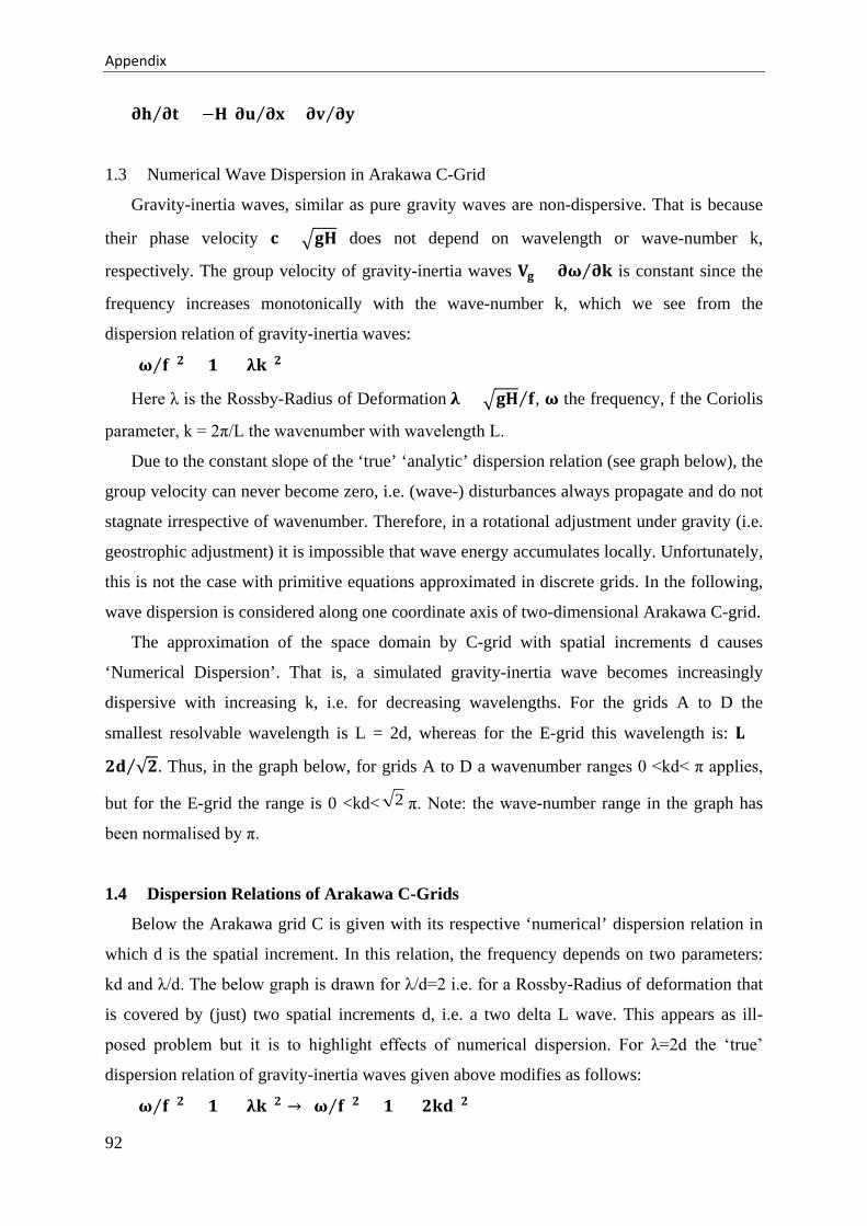
Appendix
𝛛𝛛𝐃𝐃 𝛛𝛛𝐃𝐃⁄ = −𝐇𝐇(𝛛𝛛𝛛𝛛 𝛛𝛛𝐱𝐱⁄ + 𝛛𝛛𝐟𝐟 𝛛𝛛𝛛𝛛⁄ )
1.3 Numerical Wave Dispersion in Arakawa C-Grid
Gravity-inertia waves, similar as pure gravity waves are non-dispersive. That is because
their phase velocity 𝐜𝐜 = �𝐠𝐠𝐇𝐇 does not depend on wavelength or wave-number k,
respectively. The group velocity of gravity-inertia waves 𝐕𝐕𝐠𝐠 = 𝛛𝛛𝛚𝛚 𝛛𝛛𝐤𝐤⁄ is constant since the
frequency increases monotonically with the wave-number k, which we see from the
dispersion relation of gravity-inertia waves:
(𝛚𝛚 𝐟𝐟⁄ )𝟐𝟐 = 𝟏𝟏 + (𝛌𝛌𝐤𝐤)𝟐𝟐
Here λ is the Rossby-Radius of Deformation 𝛌𝛌 = �𝐠𝐠𝐇𝐇 𝐟𝐟⁄ , 𝛚𝛚 the frequency, f the Coriolis
parameter, k = 2π/L the wavenumber with wavelength L.
Due to the constant slope of the ‘true’ ‘analytic’ dispersion relation (see graph below), the
group velocity can never become zero, i.e. (wave-) disturbances always propagate and do not
stagnate irrespective of wavenumber. Therefore, in a rotational adjustment under gravity (i.e.
geostrophic adjustment) it is impossible that wave energy accumulates locally. Unfortunately,
this is not the case with primitive equations approximated in discrete grids. In the following,
wave dispersion is considered along one coordinate axis of two-dimensional Arakawa C-grid.
The approximation of the space domain by C-grid with spatial increments d causes
‘Numerical Dispersion’. That is, a simulated gravity-inertia wave becomes increasingly
dispersive with increasing k, i.e. for decreasing wavelengths. For the grids A to D the
smallest resolvable wavelength is L = 2d, whereas for the E-grid this wavelength is: 𝐋𝐋 =
𝟐𝟐𝐤𝐤 √𝟐𝟐⁄ . Thus, in the graph below, for grids A to D a wavenumber ranges 0 <kd< π applies,
but for the E-grid the range is 0 <kd< 2 π. Note: the wave-number range in the graph has
been normalised by π.
1.4 Dispersion Relations of Arakawa C-Grids
Below the Arakawa grid C is given with its respective ‘numerical’ dispersion relation in
which d is the spatial increment. In this relation, the frequency depends on two parameters:
kd and λ/d. The below graph is drawn for λ/d=2 i.e. for a Rossby-Radius of deformation that
is covered by (just) two spatial increments d, i.e. a two delta L wave. This appears as ill-
posed problem but it is to highlight effects of numerical dispersion. For λ=2d the ‘true’
dispersion relation of gravity-inertia waves given above modifies as follows:
(𝛚𝛚 𝐟𝐟⁄ )𝟐𝟐 = 𝟏𝟏 + (𝛌𝛌𝐤𝐤)𝟐𝟐 → (𝛚𝛚 𝐟𝐟⁄ )𝟐𝟐 = 𝟏𝟏 + (𝟐𝟐𝐤𝐤𝐤𝐤)𝟐𝟐
92
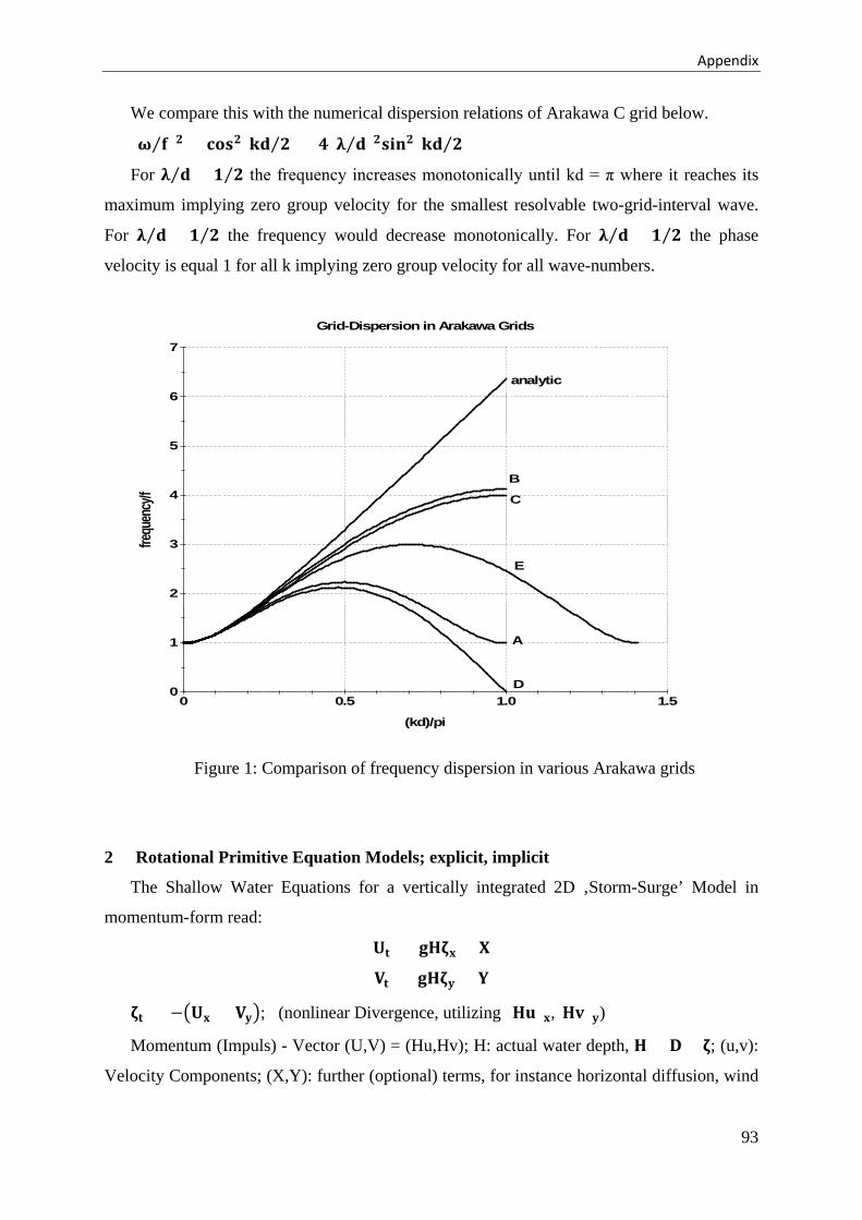
Appendix
We compare this with the numerical dispersion relations of Arakawa C grid below.
(𝛚𝛚 𝐟𝐟⁄ )𝟐𝟐 = 𝐜𝐜𝐜𝐜𝐬𝐬𝟐𝟐(𝐤𝐤𝐤𝐤 𝟐𝟐⁄ ) + 𝟒𝟒(𝛌𝛌 𝐤𝐤⁄ )𝟐𝟐𝐬𝐬𝐢𝐢𝐬𝐬𝟐𝟐(𝐤𝐤𝐤𝐤 𝟐𝟐⁄ )
For 𝛌𝛌 𝐤𝐤⁄ > 𝟏𝟏 𝟐𝟐⁄ the frequency increases monotonically until kd = π where it reaches its
maximum implying zero group velocity for the smallest resolvable two-grid-interval wave.
For 𝛌𝛌 𝐤𝐤⁄ < 𝟏𝟏 𝟐𝟐⁄ the frequency would decrease monotonically. For 𝛌𝛌 𝐤𝐤⁄ = 𝟏𝟏 𝟐𝟐⁄ the phase
velocity is equal 1 for all k implying zero group velocity for all wave-numbers.
Figure 1: Comparison of frequency dispersion in various Arakawa grids
2 Rotational Primitive Equation Models; explicit, implicit
The Shallow Water Equations for a vertically integrated 2D ‚Storm-Surge’ Model in
momentum-form read:
𝐔𝐔𝐃𝐃 + 𝐠𝐠𝐇𝐇𝛇𝛇𝐱𝐱 = 𝐗𝐗
𝐕𝐕𝐃𝐃 + 𝐠𝐠𝐇𝐇𝛇𝛇𝛛𝛛 = 𝐘𝐘
𝛇𝛇𝐃𝐃 = −�𝐔𝐔𝐱𝐱 + 𝐕𝐕𝛛𝛛�; (nonlinear Divergence, utilizing (𝐇𝐇𝛛𝛛)𝐱𝐱,(𝐇𝐇𝐟𝐟)𝛛𝛛)
Momentum (Impuls) - Vector (U,V) = (Hu,Hv); H: actual water depth, 𝐇𝐇 = 𝐃𝐃 + 𝛇𝛇; (u,v):
Velocity Components; (X,Y): further (optional) terms, for instance horizontal diffusion, wind
0
1
2
3
4
5
6
7
0 0.5 1.0 1.5
analytic
C
B
D
A
E
(kd)/pi
frequ
ency
/f
Grid-Dispersion in Arakawa Grids
93

Appendix
stress and seabed friction, nonlinear momentum advection, or Coriolis terms. The Shallow
Water Equations are a coupled system of three partial differential equations. Their explicit
approximation requires fulfilling the‚ ‘Courant-Friedrich-Lewy’ (CFL) stability-criterion:
𝚫𝚫𝐃𝐃 ≤ ∆𝐋𝐋 �𝟐𝟐𝐬𝐬−𝟏𝟏𝐠𝐠𝐇𝐇⁄
The phase velocity in the denominator contains a power (n-1) which indicates the
Dimension n of the problem (n=2 for 2D). g is earth acceleration. The CFL-criterion implies
that the propagation of free surface waves may not be larger than the numerical Phase-Speed
𝐂𝐂𝐬𝐬 = ∆𝐋𝐋 ∆𝐃𝐃⁄ . In other words, wave disturbances may propagate at maximum one spatial
increment ∆𝐋𝐋 per time step ∆𝐃𝐃. For deep Ocean regions, the CFL-criterion in particular may
constitute a very stringent limitation of the time-step. An implicit scheme may then be quite
helpful for it is independent of the CFL-criterion. However, below we at first introduce the
explicit scheme for it is a component of the implicit one. For the approximation of the space
domain of the 2D model (Figure 1) we utilise the Arakawa-C grid.
Legend: Indexing (i,j) and compass-rose indexing of variables in the ‚staggered’ Arakawa C-Grid;
locations of prognostic variables: o : v; x : u; + : 𝜁𝜁. In the staggered C-grid the indexing comprises a grid
point triple (+, x, o) under one and the same index (i,j) = C. The i-index counts in positive direction of the east
x-axis whereas j counts positive along the y-axis. (xi; y j)
2.1 Explicit Scheme for the Storm Surge Model in the Arakawa C-grid
It is only possible to solve the coupled system of equation of continuity and motion
explicitly if we separate the prognostic variables by half a time-step. Thus updating the
equation of continuity needs a velocity divergence at time-level n. This yields a new surface
+
+
+
+
+
+
+
+
+
×
×
×
×
×
×
×
×
×
o
o
o
o
o
o
o
o
o
i-1,j+1
i-1,j
i-1,j-1
i,j+1
i,j
i,j-1
i+1,j+1
i+1,j
i+1,j-1
NW
W
SW
N
C
S
NE
E
SE
94
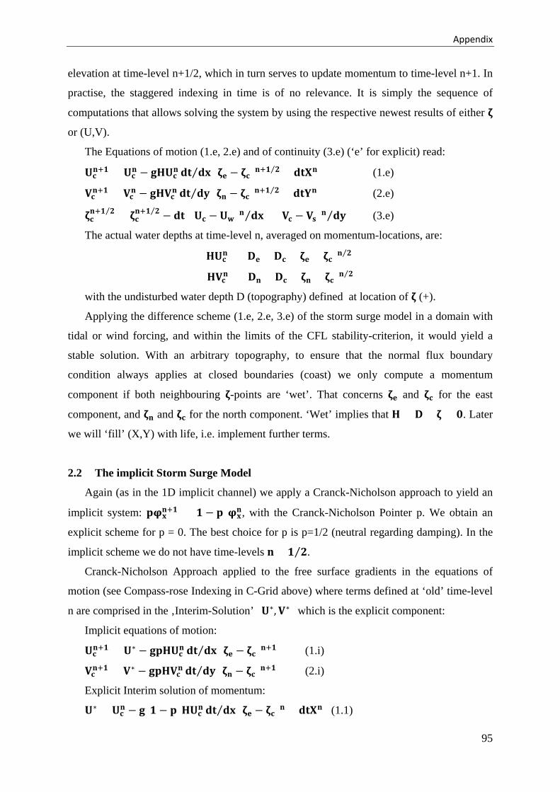
Appendix
elevation at time-level n+1/2, which in turn serves to update momentum to time-level n+1. In
practise, the staggered indexing in time is of no relevance. It is simply the sequence of
computations that allows solving the system by using the respective newest results of either 𝛇𝛇
or (U,V).
The Equations of motion (1.e, 2.e) and of continuity (3.e) (‘e’ for explicit) read:
𝐔𝐔𝐜𝐜𝐬𝐬+𝟏𝟏 = 𝐔𝐔𝐜𝐜
𝐬𝐬 − 𝐠𝐠𝐇𝐇𝐔𝐔𝐜𝐜𝐬𝐬 𝐤𝐤𝐃𝐃 𝐤𝐤𝐱𝐱⁄ (𝛇𝛇𝐃𝐃 − 𝛇𝛇𝐜𝐜)𝐬𝐬+𝟏𝟏 𝟐𝟐⁄ + 𝐤𝐤𝐃𝐃𝐗𝐗𝐬𝐬 (1.e)
𝐕𝐕𝐜𝐜𝐬𝐬+𝟏𝟏 = 𝐕𝐕𝐜𝐜
𝐬𝐬 − 𝐠𝐠𝐇𝐇𝐕𝐕𝐜𝐜𝐬𝐬 𝐤𝐤𝐃𝐃 𝐤𝐤𝛛𝛛⁄ (𝛇𝛇𝐬𝐬 − 𝛇𝛇𝐜𝐜)𝐬𝐬+𝟏𝟏 𝟐𝟐⁄ + 𝐤𝐤𝐃𝐃𝐘𝐘𝐬𝐬 (2.e)
𝛇𝛇𝐜𝐜𝐬𝐬+𝟏𝟏 𝟐𝟐⁄ = 𝛇𝛇𝐜𝐜
𝐬𝐬+𝟏𝟏 𝟐𝟐⁄ − 𝐤𝐤𝐃𝐃((𝐔𝐔𝐜𝐜 − 𝐔𝐔𝐰𝐰)𝐬𝐬 𝐤𝐤𝐱𝐱⁄ + (𝐕𝐕𝐜𝐜 − 𝐕𝐕𝐬𝐬)𝐬𝐬 𝐤𝐤𝛛𝛛⁄ ) (3.e)
The actual water depths at time-level n, averaged on momentum-locations, are:
𝐇𝐇𝐔𝐔𝐜𝐜𝐬𝐬 = (𝐃𝐃𝐃𝐃 + 𝐃𝐃𝐜𝐜 + 𝛇𝛇𝐃𝐃 + 𝛇𝛇𝐜𝐜)𝐬𝐬 𝟐𝟐⁄
𝐇𝐇𝐕𝐕𝐜𝐜𝐬𝐬 = (𝐃𝐃𝐬𝐬 + 𝐃𝐃𝐜𝐜 + 𝛇𝛇𝐬𝐬 + 𝛇𝛇𝐜𝐜)𝐬𝐬 𝟐𝟐⁄
with the undisturbed water depth D (topography) defined at location of 𝛇𝛇 (+).
Applying the difference scheme (1.e, 2.e, 3.e) of the storm surge model in a domain with
tidal or wind forcing, and within the limits of the CFL stability-criterion, it would yield a
stable solution. With an arbitrary topography, to ensure that the normal flux boundary
condition always applies at closed boundaries (coast) we only compute a momentum
component if both neighbouring 𝛇𝛇-points are ‘wet’. That concerns 𝛇𝛇𝐃𝐃 and 𝛇𝛇𝐜𝐜 for the east
component, and 𝛇𝛇𝐬𝐬 and 𝛇𝛇𝐜𝐜 for the north component. ‘Wet’ implies that 𝐇𝐇 = 𝐃𝐃 + 𝛇𝛇 > 𝟎𝟎. Later
we will ‘fill’ (X,Y) with life, i.e. implement further terms.
2.2 The implicit Storm Surge Model
Again (as in the 1D implicit channel) we apply a Cranck-Nicholson approach to yield an
implicit system: 𝐃𝐃𝛗𝛗𝐱𝐱𝐬𝐬+𝟏𝟏 + (𝟏𝟏 − 𝐃𝐃)𝛗𝛗𝐱𝐱
𝐬𝐬, with the Cranck-Nicholson Pointer p. We obtain an
explicit scheme for p = 0. The best choice for p is p=1/2 (neutral regarding damping). In the
implicit scheme we do not have time-levels 𝐬𝐬 + 𝟏𝟏 𝟐𝟐⁄ .
Cranck-Nicholson Approach applied to the free surface gradients in the equations of
motion (see Compass-rose Indexing in C-Grid above) where terms defined at ‘old’ time-level
n are comprised in the ‚Interim-Solution’ (𝐔𝐔∗, 𝐕𝐕∗) which is the explicit component:
Implicit equations of motion:
𝐔𝐔𝐜𝐜𝐬𝐬+𝟏𝟏 = 𝐔𝐔∗ − 𝐠𝐠𝐃𝐃𝐇𝐇𝐔𝐔𝐜𝐜
𝐬𝐬 𝐤𝐤𝐃𝐃 𝐤𝐤𝐱𝐱⁄ (𝛇𝛇𝐃𝐃 − 𝛇𝛇𝐜𝐜)𝐬𝐬+𝟏𝟏 (1.i)
𝐕𝐕𝐜𝐜𝐬𝐬+𝟏𝟏 = 𝐕𝐕∗ − 𝐠𝐠𝐃𝐃𝐇𝐇𝐕𝐕𝐜𝐜
𝐬𝐬 𝐤𝐤𝐃𝐃 𝐤𝐤𝛛𝛛⁄ (𝛇𝛇𝐬𝐬 − 𝛇𝛇𝐜𝐜)𝐬𝐬+𝟏𝟏 (2.i)
Explicit Interim solution of momentum:
𝐔𝐔∗ = 𝐔𝐔𝐜𝐜𝐬𝐬 − 𝐠𝐠(𝟏𝟏 − 𝐃𝐃)𝐇𝐇𝐔𝐔𝐜𝐜
𝐬𝐬 𝐤𝐤𝐃𝐃 𝐤𝐤𝐱𝐱⁄ (𝛇𝛇𝐃𝐃 − 𝛇𝛇𝐜𝐜)𝐬𝐬 + 𝐤𝐤𝐃𝐃𝐗𝐗𝐬𝐬 (1.1)
95
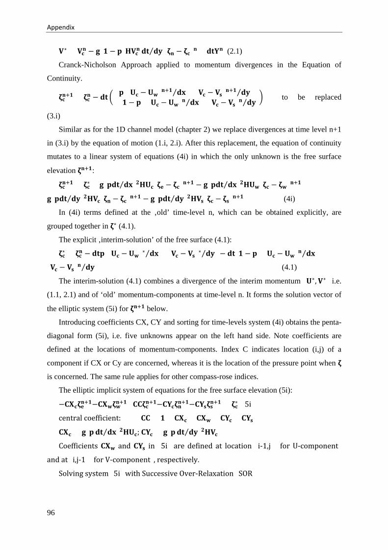
Appendix
𝐕𝐕∗ = 𝐕𝐕𝐜𝐜𝐬𝐬 − 𝐠𝐠(𝟏𝟏 − 𝐃𝐃)𝐇𝐇𝐕𝐕𝐜𝐜
𝐬𝐬 𝐤𝐤𝐃𝐃 𝐤𝐤𝛛𝛛⁄ (𝛇𝛇𝐬𝐬 − 𝛇𝛇𝐜𝐜)𝐬𝐬 + 𝐤𝐤𝐃𝐃𝐘𝐘𝐬𝐬 (2.1)
Cranck-Nicholson Approach applied to momentum divergences in the Equation of
Continuity.
𝛇𝛇𝐜𝐜𝐬𝐬+𝟏𝟏 = 𝛇𝛇𝐜𝐜
𝐬𝐬 − 𝐤𝐤𝐃𝐃 � 𝐃𝐃((𝐔𝐔𝐜𝐜 − 𝐔𝐔𝐰𝐰)𝐬𝐬+𝟏𝟏 𝐤𝐤𝐱𝐱⁄ + (𝐕𝐕𝐜𝐜 − 𝐕𝐕𝐬𝐬)𝐬𝐬+𝟏𝟏 𝐤𝐤𝛛𝛛⁄ )+(𝟏𝟏 − 𝐃𝐃)((𝐔𝐔𝐜𝐜 − 𝐔𝐔𝐰𝐰)𝐬𝐬 𝐤𝐤𝐱𝐱⁄ + (𝐕𝐕𝐜𝐜 − 𝐕𝐕𝐬𝐬)𝐬𝐬 𝐤𝐤𝛛𝛛⁄ )� to be replaced
(3.i)
Similar as for the 1D channel model (chapter 2) we replace divergences at time level n+1
in (3.i) by the equation of motion (1.i, 2.i). After this replacement, the equation of continuity
mutates to a linear system of equations (4i) in which the only unknown is the free surface
elevation 𝛇𝛇𝐬𝐬+𝟏𝟏:
𝛇𝛇𝐜𝐜𝐬𝐬+𝟏𝟏 = 𝛇𝛇𝐜𝐜
∗ + 𝐠𝐠(𝐃𝐃𝐤𝐤𝐃𝐃 𝐤𝐤𝐱𝐱⁄ )𝟐𝟐𝐇𝐇𝐔𝐔𝐜𝐜(𝛇𝛇𝐃𝐃 − 𝛇𝛇𝐜𝐜)𝐬𝐬+𝟏𝟏 − 𝐠𝐠(𝐃𝐃𝐤𝐤𝐃𝐃 𝐤𝐤𝐱𝐱⁄ )𝟐𝟐𝐇𝐇𝐔𝐔𝐰𝐰(𝛇𝛇𝐜𝐜 − 𝛇𝛇𝐰𝐰)𝐬𝐬+𝟏𝟏 +
𝐠𝐠(𝐃𝐃𝐤𝐤𝐃𝐃 𝐤𝐤𝛛𝛛⁄ )𝟐𝟐𝐇𝐇𝐕𝐕𝐜𝐜(𝛇𝛇𝐬𝐬 − 𝛇𝛇𝐜𝐜)𝐬𝐬+𝟏𝟏 − 𝐠𝐠(𝐃𝐃𝐤𝐤𝐃𝐃 𝐤𝐤𝛛𝛛⁄ )𝟐𝟐𝐇𝐇𝐕𝐕𝐬𝐬(𝛇𝛇𝐜𝐜 − 𝛇𝛇𝐬𝐬)𝐬𝐬+𝟏𝟏 (4i)
In (4i) terms defined at the ‚old’ time-level n, which can be obtained explicitly, are
grouped together in 𝛇𝛇∗ (4.1).
The explicit ‚interim-solution’ of the free surface (4.1):
𝛇𝛇𝐜𝐜∗ = 𝛇𝛇𝐜𝐜
𝐬𝐬 − 𝐤𝐤𝐃𝐃𝐃𝐃((𝐔𝐔𝐜𝐜 − 𝐔𝐔𝐰𝐰)∗ 𝐤𝐤𝐱𝐱⁄ + (𝐕𝐕𝐜𝐜 − 𝐕𝐕𝐬𝐬)∗ 𝐤𝐤𝛛𝛛⁄ ) − 𝐤𝐤𝐃𝐃(𝟏𝟏 − 𝐃𝐃)((𝐔𝐔𝐜𝐜 − 𝐔𝐔𝐰𝐰)𝐬𝐬 𝐤𝐤𝐱𝐱⁄ +
(𝐕𝐕𝐜𝐜 − 𝐕𝐕𝐬𝐬)𝐬𝐬 𝐤𝐤𝛛𝛛⁄ ) (4.1)
The interim-solution (4.1) combines a divergence of the interim momentum (𝐔𝐔∗, 𝐕𝐕∗) i.e.
(1.1, 2.1) and of ‘old’ momentum-components at time-level n. It forms the solution vector of
the elliptic system (5i) for 𝛇𝛇𝐬𝐬+𝟏𝟏 below.
Introducing coefficients CX, CY and sorting for time-levels system (4i) obtains the penta-
diagonal form (5i), i.e. five unknowns appear on the left hand side. Note coefficients are
defined at the locations of momentum-components. Index C indicates location (i,j) of a
component if CX or Cy are concerned, whereas it is the location of the pressure point when 𝛇𝛇
is concerned. The same rule applies for other compass-rose indices.
The elliptic implicit system of equations for the free surface elevation (5i):
−𝐂𝐂𝐗𝐗𝐜𝐜𝛇𝛇𝐃𝐃𝐬𝐬+𝟏𝟏−𝐂𝐂𝐗𝐗𝐰𝐰𝛇𝛇𝐰𝐰
𝐬𝐬+𝟏𝟏+𝐂𝐂𝐂𝐂𝛇𝛇𝐜𝐜𝐬𝐬+𝟏𝟏−𝐂𝐂𝐘𝐘𝐜𝐜𝛇𝛇𝐬𝐬
𝐬𝐬+𝟏𝟏−𝐂𝐂𝐘𝐘𝐬𝐬𝛇𝛇𝐬𝐬𝐬𝐬+𝟏𝟏 = 𝛇𝛇𝐜𝐜
∗ (5i)
central coefficient: 𝐂𝐂𝐂𝐂 = 𝟏𝟏 + 𝐂𝐂𝐗𝐗𝐜𝐜 + 𝐂𝐂𝐗𝐗𝐰𝐰 + 𝐂𝐂𝐘𝐘𝐜𝐜 + 𝐂𝐂𝐘𝐘𝐬𝐬
𝐂𝐂𝐗𝐗𝐜𝐜 = 𝐠𝐠(𝐃𝐃 𝐤𝐤𝐃𝐃 𝐤𝐤𝐱𝐱⁄ )𝟐𝟐𝐇𝐇𝐔𝐔𝐜𝐜; 𝐂𝐂𝐘𝐘𝐜𝐜 = 𝐠𝐠(𝐃𝐃 𝐤𝐤𝐃𝐃 𝐤𝐤𝛛𝛛⁄ )𝟐𝟐𝐇𝐇𝐕𝐕𝐜𝐜
Coefficients 𝐂𝐂𝐗𝐗𝐰𝐰 and 𝐂𝐂𝐘𝐘𝐬𝐬 in (5i) are defined at location (i-1,j) (for U-component)
and at (i,j-1) (for V-component), respectively.
Solving system (5i) with Successive Over-Relaxation (SOR)
96
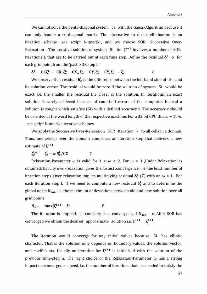
Appendix
We cannot solve the penta-diagonal system (5i) with the Gauss-Algorithm because it
can only handle a tri-diagonal matrix. The alternative to direct elimination is an
iteration scheme (see script Numerik), and we choose SOR (Successive Over-
Relaxation). The iterative solution of system (5i) for 𝛇𝛇𝐬𝐬+𝟏𝟏 involves a number of SOR-
iterations L that are to be carried out at each time step. Define the residual 𝛅𝛅𝐜𝐜𝐋𝐋 (6) for
each grid point from the ‘past’ SOR step L:
𝛅𝛅𝐜𝐜𝐋𝐋 = 𝐂𝐂𝐂𝐂𝛇𝛇𝐜𝐜
𝐋𝐋 − (𝐂𝐂𝐗𝐗𝐜𝐜𝛇𝛇𝐃𝐃𝐋𝐋 + 𝐂𝐂𝐗𝐗𝐰𝐰𝛇𝛇𝐰𝐰
𝐋𝐋 + 𝐂𝐂𝐘𝐘𝐜𝐜𝛇𝛇𝐬𝐬𝐋𝐋 + 𝐂𝐂𝐘𝐘𝐬𝐬𝛇𝛇𝐬𝐬
𝐋𝐋) − 𝛇𝛇𝐜𝐜∗ (6)
We observe that residual 𝛅𝛅𝐜𝐜𝐋𝐋 is the difference between the left hand side of (5i) and
its solution vector. The residual would be zero if the solution of system (5i) would be
exact, i.e. the smaller the residual the closer is the solution. In iterations, an exact
solution is rarely achieved because of round-off errors of the computer. Instead a
solution is sought which satisfies (5i) with a defined accuracy ε. The accuracy ε should
be oriented at the word length of the respective machine. For a 32 bit CPU this is ~ 10-6.
(see script Numerik: iterative schemes)
We apply the Successive Over-Relaxation (SOR) Iteration (7) to all cells in a domain.
Thus, one sweep over the domain comprises an iteration step that delivers a new
estimate of 𝛇𝛇𝐋𝐋+𝟏𝟏.
𝛇𝛇𝐜𝐜𝐋𝐋+𝟏𝟏 = 𝛇𝛇𝐜𝐜
𝐋𝐋 − 𝛚𝛚𝛅𝛅𝐜𝐜𝐋𝐋 𝐂𝐂𝐂𝐂⁄ (7)
Relaxation-Parameter ω is valid for 1 < ω < 2. For ω < 1 ‚Under-Relaxation’ is
obtained. Usually over-relaxation gives the fastest ‚convergence’, i.e. the least number of
iteration steps. Over-relaxation implies multiplying residual 𝛅𝛅𝐜𝐜𝐋𝐋 (7) with an ω > 1. For
each iteration step L+1 we need to compute a new residual 𝛅𝛅𝐜𝐜𝐋𝐋 and to determine the
global norm 𝐍𝐍𝐬𝐬𝐜𝐜𝐬𝐬, i.e. the maximum of deviations between old and new solution over all
grid points:
𝐍𝐍𝐬𝐬𝐜𝐜𝐬𝐬 = 𝐦𝐦𝐦𝐦𝐱𝐱�𝛇𝛇𝐋𝐋+𝟏𝟏 − 𝛇𝛇𝐋𝐋� (8)
The iteration is stopped, i.e. considered as convergent, if 𝐍𝐍𝐬𝐬𝐜𝐜𝐬𝐬 < 𝛆𝛆. After SOR has
converged we obtain the desired (approximate) solution i.e. 𝛇𝛇𝐬𝐬+𝟏𝟏 = 𝛇𝛇𝐋𝐋+𝟏𝟏.
The iteration would converge for any initial values because (5i) has elliptic
character. That is the solution only depends on boundary values, the solution vector,
and coefficients. Usually an iteration for 𝛇𝛇𝐋𝐋=𝟏𝟏 is initialised with the solution of the
previous time-step n. The right choice of the Relaxation-Parameter ω has a strong
impact on convergence-speed, i.e. the number of iterations that are needed to satisfy the
97
Appendix
norm 𝐍𝐍𝐬𝐬𝐜𝐜𝐬𝐬; apparently, the fewer iterations the better. In oceanographic applications
with complex topography, we recommend to determine Parameter ω empirically.
The introduction of Chessboard-SOR will further increase convergence speed (see
script Numerik): divide the iteration matrix into ‘white’ and ‘black’ cells as in a
chessboard. Solving SOR (7) first for all black cells yields that all of the white cells
solved subsequently will use already updated data from the black ones. This simple
‘kunstgriff’ allows significantly improving convergence-speed.
In oceanographic applications with arbitrary topography the normal condition, i.e.
the no-flux condition at closed boundaries has to be satisfied. This boundary condition
enters system (5i) via coefficients CX, CY (see chapter 2). Momentum-components
situated at a closed boundary must be zero because one of the two neighbouring cells is
dry. The same applies for the coefficients since they are defined at the location of the
respective component. Note that coefficients are time-dependent for they contain the
free surface elevation in the actual water depth HU, HV and, optionally, the friction
functions SX, SY (see below).
Obtaining the solution for (𝐔𝐔, 𝐕𝐕)𝐬𝐬+𝟏𝟏
Having solved system (5i) with the help of SOR-iteration (7) the free surface
elevation 𝛇𝛇𝐬𝐬+𝟏𝟏 is known for all grid points in the domain. This allows solving (𝐔𝐔, 𝐕𝐕)𝐬𝐬+𝟏𝟏
from (1.i) and (2.i) by applying the free surface gradients at time-level n+1 to interim
solutions.
𝐔𝐔𝐜𝐜𝐬𝐬+𝟏𝟏 = 𝐔𝐔∗ − 𝐠𝐠𝐃𝐃𝐇𝐇𝐔𝐔𝐜𝐜
𝐬𝐬 𝐤𝐤𝐃𝐃 𝐤𝐤𝐱𝐱⁄ (𝛇𝛇𝐃𝐃 − 𝛇𝛇𝐜𝐜)𝐬𝐬+𝟏𝟏 (1.i)
𝐕𝐕𝐜𝐜𝐬𝐬+𝟏𝟏 = 𝐕𝐕∗ − 𝐠𝐠𝐃𝐃𝐇𝐇𝐕𝐕𝐜𝐜
𝐬𝐬 𝐤𝐤𝐃𝐃 𝐤𝐤𝛛𝛛⁄ (𝛇𝛇𝐬𝐬 − 𝛇𝛇𝐜𝐜)𝐬𝐬+𝟏𝟏 (2.i)
--- Subtract surface gradients ---
This finalises the operations needed to solve one time-step in the 2D model. Note
that with the exception of factor (1-p) the computation of interim-vector (𝐔𝐔, 𝐕𝐕)∗ from
(1.1) and (2.1) is identical to the explicit approximation (1.e, 2.e). Thus, as for the 1D
channel, the explicit scheme forms a central part of the implicit one.
Sequence of Operations for one time step
Prior to SOR-Iteration:
Compute interim-solution 𝐔𝐔∗, 𝐕𝐕∗ (2.1, 2.2) and coefficients CX,CY,CC
Compute interim-solution 𝛇𝛇∗ (4.1) from flow divergence
SOR Iteration: sweep over all cells in domain:
Compute residual 𝛅𝛅𝐜𝐜𝐋𝐋 (6) from coefficients and previous 𝛇𝛇
98
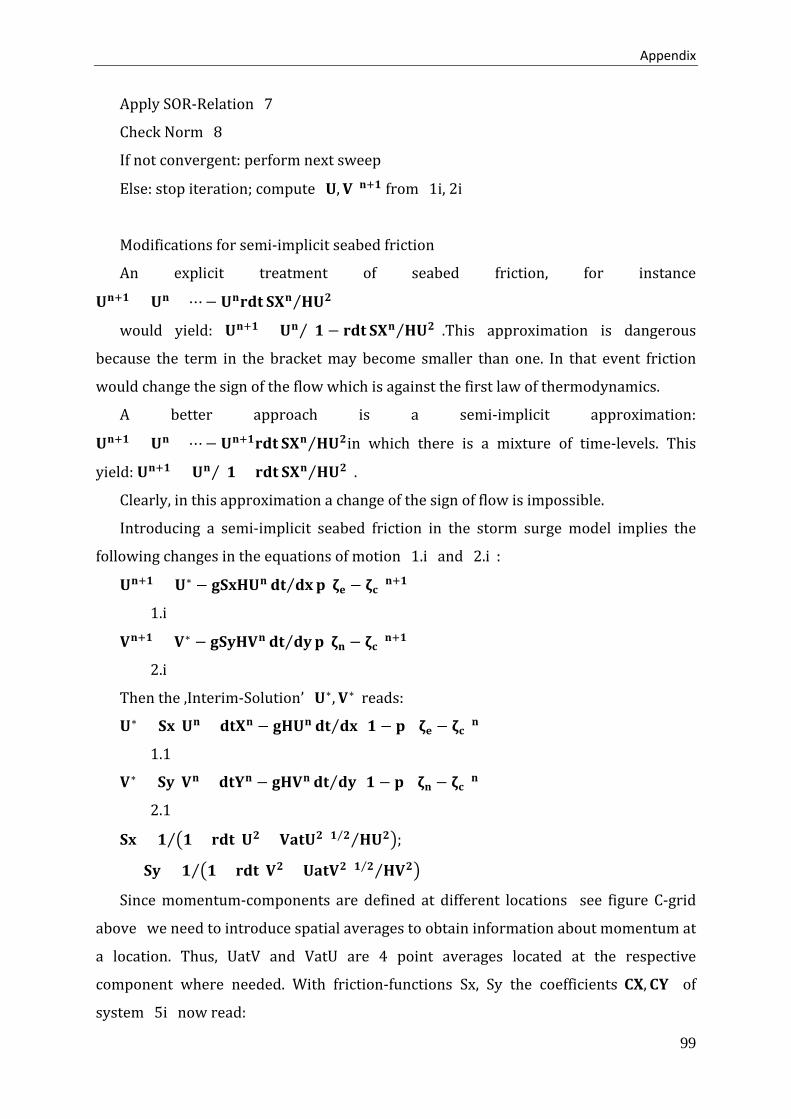
Appendix
Apply SOR-Relation (7)
Check Norm (8)
If not convergent: perform next sweep
Else: stop iteration; compute (𝐔𝐔, 𝐕𝐕)𝐬𝐬+𝟏𝟏 from (1i, 2i)
Modifications for semi-implicit seabed friction
An explicit treatment of seabed friction, for instance
𝐔𝐔𝐬𝐬+𝟏𝟏 = 𝐔𝐔𝐬𝐬 + ⋯ − 𝐔𝐔𝐬𝐬𝐬𝐬𝐤𝐤𝐃𝐃 𝐒𝐒𝐗𝐗𝐬𝐬 𝐇𝐇𝐔𝐔𝟐𝟐⁄
would yield: 𝐔𝐔𝐬𝐬+𝟏𝟏 = 𝐔𝐔𝐬𝐬 (𝟏𝟏 − 𝐬𝐬𝐤𝐤𝐃𝐃 𝐒𝐒𝐗𝐗𝐬𝐬 𝐇𝐇𝐔𝐔𝟐𝟐⁄ )⁄ .This approximation is dangerous
because the term in the bracket may become smaller than one. In that event friction
would change the sign of the flow which is against the first law of thermodynamics.
A better approach is a semi-implicit approximation:
𝐔𝐔𝐬𝐬+𝟏𝟏 = 𝐔𝐔𝐬𝐬 + ⋯ − 𝐔𝐔𝐬𝐬+𝟏𝟏𝐬𝐬𝐤𝐤𝐃𝐃 𝐒𝐒𝐗𝐗𝐬𝐬 𝐇𝐇𝐔𝐔𝟐𝟐⁄ in which there is a mixture of time-levels. This
yield: 𝐔𝐔𝐬𝐬+𝟏𝟏 = 𝐔𝐔𝐬𝐬 (𝟏𝟏 + 𝐬𝐬𝐤𝐤𝐃𝐃 𝐒𝐒𝐗𝐗𝐬𝐬 𝐇𝐇𝐔𝐔𝟐𝟐⁄ )⁄ .
Clearly, in this approximation a change of the sign of flow is impossible.
Introducing a semi-implicit seabed friction in the storm surge model implies the
following changes in the equations of motion (1.i) and (2.i):
𝐔𝐔𝐬𝐬+𝟏𝟏 = 𝐔𝐔∗ − 𝐠𝐠𝐒𝐒𝐱𝐱𝐇𝐇𝐔𝐔𝐬𝐬 𝐤𝐤𝐃𝐃 𝐤𝐤𝐱𝐱⁄ 𝐃𝐃(𝛇𝛇𝐃𝐃 − 𝛇𝛇𝐜𝐜)𝐬𝐬+𝟏𝟏
(1.i)
𝐕𝐕𝐬𝐬+𝟏𝟏 = 𝐕𝐕∗ − 𝐠𝐠𝐒𝐒𝛛𝛛𝐇𝐇𝐕𝐕𝐬𝐬 𝐤𝐤𝐃𝐃 𝐤𝐤𝛛𝛛⁄ 𝐃𝐃(𝛇𝛇𝐬𝐬 − 𝛇𝛇𝐜𝐜)𝐬𝐬+𝟏𝟏
(2.i)
Then the ‚Interim-Solution’ (𝐔𝐔∗, 𝐕𝐕∗)reads:
𝐔𝐔∗ = 𝐒𝐒𝐱𝐱(𝐔𝐔𝐬𝐬 + 𝐤𝐤𝐃𝐃𝐗𝐗𝐬𝐬 − 𝐠𝐠𝐇𝐇𝐔𝐔𝐬𝐬 𝐤𝐤𝐃𝐃 𝐤𝐤𝐱𝐱⁄ (𝟏𝟏 − 𝐃𝐃)(𝛇𝛇𝐃𝐃 − 𝛇𝛇𝐜𝐜)𝐬𝐬)
(1.1)
𝐕𝐕∗ = 𝐒𝐒𝛛𝛛(𝐕𝐕𝐬𝐬 + 𝐤𝐤𝐃𝐃𝐘𝐘𝐬𝐬 − 𝐠𝐠𝐇𝐇𝐕𝐕𝐬𝐬 𝐤𝐤𝐃𝐃 𝐤𝐤𝛛𝛛⁄ (𝟏𝟏 − 𝐃𝐃)(𝛇𝛇𝐬𝐬 − 𝛇𝛇𝐜𝐜)𝐬𝐬)
(2.1)
𝐒𝐒𝐱𝐱 = 𝟏𝟏 �𝟏𝟏 + 𝐬𝐬𝐤𝐤𝐃𝐃(𝐔𝐔𝟐𝟐 + 𝐕𝐕𝐦𝐦𝐃𝐃𝐔𝐔𝟐𝟐)𝟏𝟏 𝟐𝟐⁄ 𝐇𝐇𝐔𝐔𝟐𝟐⁄ �⁄ ;
𝐒𝐒𝛛𝛛 = 𝟏𝟏 �𝟏𝟏 + 𝐬𝐬𝐤𝐤𝐃𝐃(𝐕𝐕𝟐𝟐 + 𝐔𝐔𝐦𝐦𝐃𝐃𝐕𝐕𝟐𝟐)𝟏𝟏 𝟐𝟐⁄ 𝐇𝐇𝐕𝐕𝟐𝟐⁄ �⁄
Since momentum-components are defined at different locations (see figure C-grid
above) we need to introduce spatial averages to obtain information about momentum at
a location. Thus, UatV and VatU are 4 point averages located at the respective
component where needed. With friction-functions Sx, Sy the coefficients(𝐂𝐂𝐗𝐗, 𝐂𝐂𝐘𝐘) of
system (5i) now read:
99
Appendix
𝐂𝐂𝐗𝐗𝐜𝐜 = 𝐠𝐠𝐒𝐒𝐱𝐱𝐜𝐜(𝐃𝐃 𝐤𝐤𝐃𝐃 𝐤𝐤𝐱𝐱⁄ )𝟐𝟐𝐇𝐇𝐔𝐔𝐜𝐜; 𝐂𝐂𝐘𝐘𝐜𝐜 = 𝐠𝐠𝐒𝐒𝛛𝛛𝐜𝐜(𝐃𝐃 𝐤𝐤𝐃𝐃 𝐤𝐤𝛛𝛛⁄ )𝟐𝟐𝐇𝐇𝐕𝐕𝐜𝐜
2.3 Horizontal Momentum Diffusion
Assume that the equations of motion (1) and (2) contain a horizontal diffusion term
on their right hand side as approximated by the classical Laplacian in Compass-Rose
notation for (U,V) (assuming an equidistant grid with dx=dy=dl):
𝐀𝐀𝐃𝐃�𝐔𝐔𝐱𝐱𝐱𝐱 + 𝐔𝐔𝛛𝛛𝛛𝛛� in (1); approximation: 𝐀𝐀𝐃𝐃 (𝐔𝐔𝐄𝐄 + 𝐔𝐔𝐖𝐖 + 𝐔𝐔𝐍𝐍 + 𝐔𝐔𝐒𝐒 − 𝟒𝟒𝐔𝐔𝐂𝐂) 𝐤𝐤𝐝𝐝𝟐𝟐⁄
𝐀𝐀𝐃𝐃�𝐕𝐕𝐱𝐱𝐱𝐱 + 𝐕𝐕𝛛𝛛𝛛𝛛� in (2); approximation:
𝐀𝐀𝐃𝐃 (𝐕𝐕𝐄𝐄 + 𝐕𝐕𝐖𝐖 + 𝐕𝐕𝐍𝐍 + 𝐕𝐕𝐒𝐒 − 𝟒𝟒𝐕𝐕𝐂𝐂) 𝐤𝐤𝐝𝐝𝟐𝟐⁄
We see that the difference stencil of the Laplacian ‘grabs’ at grid-points along main
axes that are one increment apart from C, including the centre point C. What happens in
an arbitrary topography if this Laplacian is in operation? It would eventually grab dry
cells and draw in zero momentum...
2.4 Boundary Conditions for the Laplacian; Slip-conditions
The Laplacian simulates diffusion caused by lateral shear of the flow. It depends on
lateral boundary conditions at coasts. We have to discern between 2 boundary
conditions: a) the normal condition i.e. no flux across a closed boundary, and b) the ‘no-
slip at a wall’ condition, i.e. wall-parallel flow being zero at the wall (integral part of
boundary layer theory).
Consider case a. (normal condition) in the C-grid:
In this example both Uw and Uc are wet, and Ue is dry i.e. =0 because it is situated at
a closed boundary. These casesare consistent with the normal condition; they may enter
the Laplacian without causing problems. The situation is different for coastal-normal
derivatives of coastal parallel flow:
Consider case b. (no-slip condition) in the C-grid
𝑈𝑈𝑊𝑊 𝑈𝑈𝐶𝐶 𝑈𝑈𝐸𝐸 = 0,(no-flux)
× × ×
𝑤𝑤𝑤𝑤𝑤𝑤𝑤𝑤
𝑤𝑤𝑤𝑤𝑤𝑤 𝑤𝑤𝑤𝑤𝑤𝑤 𝑑𝑑𝑑𝑑𝑑𝑑
100
Appendix
Amongst other cells the Laplacian Operator (𝐔𝐔𝐄𝐄 + 𝐔𝐔𝐖𝐖 + 𝐔𝐔𝐍𝐍 + 𝐔𝐔𝐒𝐒 − 𝟒𝟒𝐔𝐔𝐂𝐂) 𝐤𝐤𝐝𝐝𝟐𝟐⁄ for
𝐔𝐔𝐂𝐂grabs 𝐔𝐔𝐍𝐍, which is dry in this example. Between 𝐔𝐔𝐍𝐍and 𝐔𝐔𝐂𝐂 is the wall at which the
north-component V is zero, and at which U must be zero as well. To highlight that the
Laplacian contains a differential of coastal parallel horizontal momentum shear we re-
write its meridional derivatives of shear as: (𝛕𝛕𝐍𝐍 − 𝛕𝛕𝐒𝐒) 𝐤𝐤𝐝𝐝⁄ in which, according to
Newton’s friction law 𝛕𝛕𝐍𝐍 = 𝐀𝐀𝐃𝐃 (𝐔𝐔𝐍𝐍 − 𝐔𝐔𝐂𝐂) 𝐤𝐤𝐝𝐝⁄ and 𝛕𝛕𝐒𝐒 = 𝐀𝐀𝐃𝐃 (𝐔𝐔𝐒𝐒 − 𝐔𝐔𝐂𝐂) 𝐤𝐤𝐝𝐝⁄ .
The example concerns the shear term 𝛕𝛕𝐍𝐍because it addresses a dry cell. Momentum
component 𝐔𝐔𝐍𝐍 in the above sketch must be zero for it lies on dry land, which implies
𝛕𝛕𝐍𝐍 = −𝐀𝐀𝐃𝐃𝐔𝐔𝐂𝐂 𝐤𝐤𝐝𝐝⁄ .
To fulfil the condition of a vanishing wall-parallel flow, i.e. ‘no-slip’ in the discrete
grid 𝐔𝐔𝐍𝐍 must be equal −𝐔𝐔𝐂𝐂. Then their spatial average would exactly be zero at the wall.
With components being equal yet having opposite sign 𝛕𝛕𝐍𝐍 = −𝟐𝟐𝐀𝐀𝐃𝐃𝐔𝐔𝐂𝐂 𝐤𝐤𝐝𝐝⁄ , which
complies with the ‘no-slip’ condition. Thus, vanishing wall-parallel flow implies maximal
shear at the wall. A vanishing shear, i.e. 𝛕𝛕𝐍𝐍 = 𝟎𝟎 at the wall requires that 𝐔𝐔𝐍𝐍is equal 𝐔𝐔𝐂𝐂.
This would be a ‘full-slip’, elsewhere also called ‘free-slip’ condition.
Conservation of mass requires that all momentum cells on dry land are zero. It is not
advisable to relax this condition. However, the control of lateral shear, i.e. slip in the
Laplacian requires a modification of momentum-components. Thus, we have to devise
an algorithm, which automatically implements a slip-condition whenever coastal
parallel shear is present, and which still allows conserving mass. For this purpose we
define wet/dry integer ‘masks’ for both momentum-components which are one if wet,
otherwise zero. The masks allow discerning, i.e. switching between computations with
the classical Laplacian in open water, i.e. away from a coast, and cases where coastal-
parallel shear occurs.
𝑈𝑈𝑁𝑁
𝑈𝑈𝐶𝐶
𝑈𝑈𝑆𝑆
𝑑𝑑𝑑𝑑𝑑𝑑
𝑤𝑤𝑤𝑤𝑤𝑤
𝑤𝑤𝑤𝑤𝑤𝑤
𝑉𝑉 = 0
×
×
×
𝑤𝑤𝑤𝑤𝑤𝑤𝑤𝑤
101
Appendix
2.5 Coriolis Rotation; the Problem with spatial averaging in the C-grid
The inclusion of Coriolis rotation terms in the C-grid is a tedious task because
momentum-components are not on the same location contrary to B- or E-grids. The
approximation of rotation at a U-component for instance requires a spatial average of
four surrounding V-components for the rotation matrix. This is the one disadvantage of
the C-grid. That is, because in an arbitrary topography not all V-neighbours might be
wet. In the worst case, i.e. when all four surrounding V-components are dry an
application of the rotation matrix would induce unwanted damping.
An example for such a case is a topography that locally degenerates to a one-
dimensional channel; for instance between an island and the mainland:
Implementing rotation in open water, away from a coast implies that Un is replaced
by the rotated U-component Urot in the approximation of the equation of motion:
𝐔𝐔𝐬𝐬+𝟏𝟏 = 𝐔𝐔𝐬𝐬 +further terms ==>𝐔𝐔𝐬𝐬+𝟏𝟏 = 𝐔𝐔𝐬𝐬𝐜𝐜𝐃𝐃 + further terms
Utilising spatial averages the rotated vector-components read:
𝐔𝐔𝐬𝐬𝐜𝐜𝐃𝐃 = 𝛂𝛂𝐔𝐔 + 𝛃𝛃𝐕𝐕𝐦𝐦𝐃𝐃𝐔𝐔;𝐕𝐕𝐬𝐬𝐜𝐜𝐃𝐃 = 𝛂𝛂𝐕𝐕 + 𝛃𝛃𝐔𝐔𝐦𝐦𝐃𝐃𝐕𝐕
Now for the worst case with spatial average 𝐕𝐕𝐦𝐦𝐃𝐃𝐔𝐔being zero 𝐔𝐔𝐬𝐬𝐜𝐜𝐃𝐃 = 𝛂𝛂𝐔𝐔, which will
decrease U for α is less than one. Thus, rotation has become dissipation. In this event,
the bilateral energy-transfer amongst components does not work because one is always
zero. Only Conclusion: abandon rotation for this case to avoid damping.
The respective four neighbour-components for spatial averages (𝐔𝐔𝐦𝐦𝐃𝐃𝐕𝐕, 𝐕𝐕𝐦𝐦𝐃𝐃𝐔𝐔) are:
𝐕𝐕𝐦𝐦𝐃𝐃𝐔𝐔: 𝐕𝐕(𝐢𝐢, 𝐣𝐣) + 𝐕𝐕(𝐢𝐢 + 𝟏𝟏, 𝐣𝐣) + 𝐕𝐕(𝐢𝐢, 𝐣𝐣 − 𝟏𝟏) + 𝐕𝐕(𝐢𝐢 + 𝟏𝟏, 𝐣𝐣 − 𝟏𝟏);
𝐔𝐔𝐦𝐦𝐃𝐃𝐕𝐕: 𝐔𝐔(𝐢𝐢, 𝐣𝐣) + 𝐔𝐔(𝐢𝐢, 𝐣𝐣 + 𝟏𝟏) + 𝐔𝐔(𝐢𝐢 − 𝟏𝟏, 𝐣𝐣) + 𝐔𝐔(𝐢𝐢 − 𝟏𝟏, 𝐣𝐣 + 𝟏𝟏);
Note inverse symmetry in the indexing. In an arbitrary topography, any one of the
four cells might be dry and usage of averages irrespective of dry cells may under-
estimate averages. For instance if only two cells are wet and one divides by four. Thus,
×
×
×
𝑑𝑑𝑑𝑑𝑑𝑑
𝑤𝑤𝑤𝑤𝑤𝑤
𝑑𝑑𝑑𝑑𝑑𝑑
𝑉𝑉 = 0
𝑉𝑉 = 0
×
×
×
𝑤𝑤𝑤𝑤𝑤𝑤𝑤𝑤
𝑤𝑤𝑤𝑤𝑤𝑤𝑤𝑤
102
Appendix
not only we have to decide whether rotation is possible but also to determine how many
wet cells enter the average. We require that at least two wet cells be present in the
average, otherwise rotation is abandoned.
Since the topography does not change in time, a counting of the number of wet cells
for averages is done once, prior to the time-loop.
2D Tracer Advection in the C-grid
Once the model has produced new values of the velocity-vector (u,v) derived from
momentum (𝐔𝐔, 𝐕𝐕) at time level n+1 a new distribution of tracers can be computed, here
exemplified for a tracer S. Neither sources nor sinks are assumed.
𝐤𝐤𝐒𝐒 𝐤𝐤𝐃𝐃⁄ = 𝛛𝛛𝐒𝐒 𝛛𝛛𝐃𝐃⁄ + 𝛛𝛛 𝛛𝛛𝐒𝐒 𝛛𝛛𝐃𝐃⁄ + 𝐟𝐟 𝛛𝛛𝐒𝐒 𝛛𝛛𝛛𝛛⁄ = 𝟎𝟎. (1)
Upstream advection-code (2) approximate (1):
𝐒𝐒𝐬𝐬+𝟏𝟏(𝐢𝐢, 𝐣𝐣) =
𝐒𝐒𝐬𝐬(𝐢𝐢, 𝐣𝐣) − ∆𝐃𝐃 𝛛𝛛𝐖𝐖𝐬𝐬+𝟏𝟏 𝐤𝐤𝐱𝐱�𝐒𝐒(𝐢𝐢, 𝐣𝐣) − 𝐒𝐒(𝐢𝐢 − 𝟏𝟏, 𝐣𝐣)�𝐬𝐬� − ∆𝐃𝐃 𝛛𝛛𝐄𝐄
𝐬𝐬+𝟏𝟏 𝐤𝐤𝐱𝐱�𝐒𝐒(𝐢𝐢 + 𝟏𝟏, 𝐣𝐣) − 𝐒𝐒(𝐢𝐢, 𝐣𝐣)�𝐬𝐬� −
∆𝐃𝐃 𝐟𝐟𝐒𝐒𝐬𝐬+𝟏𝟏 𝐤𝐤𝐱𝐱�𝐒𝐒(𝐢𝐢, 𝐣𝐣) − 𝐒𝐒(𝐢𝐢, 𝐣𝐣 − 𝟏𝟏)�𝐬𝐬� − ∆𝐃𝐃 𝐟𝐟𝐍𝐍
𝐬𝐬+𝟏𝟏 𝐤𝐤𝐱𝐱�𝐒𝐒(𝐢𝐢, 𝐣𝐣 + 𝟏𝟏) − 𝐒𝐒(𝐢𝐢, 𝐣𝐣)�𝐬𝐬� (2)
In the advection scheme (2) we use upstream ‘velocity-switches’ as given below.
𝛛𝛛𝐖𝐖𝐬𝐬+𝟏𝟏 = �𝐦𝐦𝐚𝐚𝐬𝐬�𝛛𝛛(𝐢𝐢 − 𝟏𝟏, 𝐣𝐣)� + 𝛛𝛛(𝐢𝐢 − 𝟏𝟏, 𝐣𝐣)�
𝐬𝐬+𝟏𝟏𝟐𝟐� ; 𝛛𝛛𝐄𝐄
𝐬𝐬+𝟏𝟏 = �𝐦𝐦𝐚𝐚𝐬𝐬�𝛛𝛛(𝐢𝐢, 𝐣𝐣)� − 𝛛𝛛(𝐢𝐢, 𝐣𝐣)�𝐬𝐬+𝟏𝟏
𝟐𝟐�
𝐟𝐟𝐒𝐒𝐬𝐬+𝟏𝟏 = �𝐦𝐦𝐚𝐚𝐬𝐬�𝐟𝐟(𝐢𝐢, 𝐣𝐣 − 𝟏𝟏)� + 𝐟𝐟(𝐢𝐢, 𝐣𝐣 − 𝟏𝟏)�
𝐬𝐬+𝟏𝟏𝟐𝟐� ; 𝐟𝐟𝐍𝐍
𝐬𝐬+𝟏𝟏 = �𝐦𝐦𝐚𝐚𝐬𝐬�𝐟𝐟(𝐢𝐢, 𝐣𝐣)� − 𝐟𝐟(𝐢𝐢, 𝐣𝐣)�𝐬𝐬+𝟏𝟏
𝟐𝟐�
Zonal arrangement of grid points in the staggered grid for tracer S:
note: uE has index (i,j) due to staggered grid
By defining non-dimensional coefficients:
𝐂𝐂𝐄𝐄 = ∆𝐃𝐃 𝛛𝛛𝐄𝐄 𝐤𝐤𝐱𝐱⁄ ;𝐂𝐂𝐖𝐖 = ∆𝐃𝐃 𝛛𝛛𝐖𝐖 𝐤𝐤𝐱𝐱⁄ , and 𝐂𝐂𝐍𝐍 = ∆𝐃𝐃 𝐟𝐟𝐍𝐍 𝐤𝐤𝛛𝛛⁄ ;𝐂𝐂𝐒𝐒 = ∆𝐃𝐃 𝐟𝐟𝐒𝐒 𝐤𝐤𝛛𝛛⁄ ,
We can write the advection scheme (2) in the compact explicit form (3) where
always two of the four coefficients are zero:
𝐒𝐒𝐂𝐂𝐬𝐬+𝟏𝟏 = 𝐒𝐒𝐂𝐂
𝐬𝐬(𝟏𝟏 − 𝐂𝐂𝐖𝐖 + 𝐂𝐂𝐄𝐄 − 𝐂𝐂𝐒𝐒 + 𝐂𝐂𝐍𝐍) + 𝐂𝐂𝐖𝐖𝐒𝐒𝐖𝐖𝐬𝐬 − 𝐂𝐂𝐄𝐄𝐒𝐒𝐄𝐄
𝐬𝐬 + 𝐂𝐂𝐒𝐒𝐒𝐒𝐒𝐒𝐖𝐖𝐬𝐬 − 𝐂𝐂𝐍𝐍𝐒𝐒𝐍𝐍
𝐬𝐬 (3)
Note: the compass rose indexing always assumes that C indicates the location at
which a property is computed. The neighbourhood is indexed with reference to C.
Boundary conditions: at closed lateral boundaries, an advective flux of matter is
prohibited. Thus, boundary conditions for advective horizontal fluxes are simply given
𝑆𝑆(𝑖𝑖 − 1, 𝑗𝑗) 𝑆𝑆(𝑖𝑖, 𝑗𝑗) 𝑆𝑆(𝑖𝑖 + 1, 𝑗𝑗)
+ × + × +
𝑈𝑈𝑤𝑤 𝑈𝑈𝐸𝐸
103
Appendix
by the fact that velocities are zero at closed boundaries. We can always check the
correctness of the code in a closed domain: S must be conserved. That is, the sum over
all S in wet cells must remain the same, i.e. 𝐤𝐤𝐒𝐒 𝐤𝐤𝐃𝐃 ⁄ = 𝟎𝟎.
Remark: We can interpret operator (3) as a weighted spatial average of the tracer
property S. The operator only works along coordinate axes. Therefore, it is also called:
‘Component Upstream’. Advection with a flow along grid diagonals or in curved flow is
under-represented by the simple Component Upstream scheme, and induces strong
lateral diffusion. To overcome this disadvantage we introduce an additional cell at the
grid diagonal to improve upstream interpolation. Then it would only utilise three cells
in a triangle.
Modifying component upstream to triangular upstream with the intention to obtain
a better estimate of the advected property causes a numerical approximation that is
non-consistent. With spatial and time-increments approaching zero the scheme would
not converge to the original partial differential equation. Thus, the below example for an
improved advection scheme suffers from non-consistency. We call it ‘Lagrangian
Advection Scheme’ (LAS). However, even though LAS is non-consistent it produces
much better results and is as conservative as component upstream. The same finding
applies for the rotation matrix, which again, is non-consistent.
2.6 The Lagrangian upstream Advection Scheme, LAS:
The idea of LAS is to interpolate a property that lies upstream which, when advected
with the flow during one time-step will end up at (i,j) where its value replaces tracer
S(i,j). Below is an example of a routine that computes weights for interpolation in an
upstream triangle. It uses non-dimensional excursions (cx,cy), i.e. the upstream location
of the tracer:
𝐜𝐜𝐱𝐱 = |𝛛𝛛�| 𝐤𝐤𝐃𝐃 𝐤𝐤𝐱𝐱⁄ with 𝛛𝛛� = (𝛛𝛛𝐄𝐄 + 𝛛𝛛𝐖𝐖) 𝟐𝟐⁄
𝐜𝐜𝛛𝛛 = |𝐟𝐟�| 𝐤𝐤𝐃𝐃 𝐤𝐤𝛛𝛛⁄ with 𝐟𝐟� = (𝐟𝐟𝐍𝐍 + 𝐟𝐟𝐒𝐒) 𝟐𝟐⁄
(𝛛𝛛�, 𝐟𝐟�) are velocities centred on the tracer grid point at (i,j). Increments (idel, jdel),
with deviations +/-1 define the respective quadrant out of four around (i,j) = LOCL in
which interpolation will take place. Thus, with (idel, jdel) = (-1,-1) it would be the
southwest quadrant. The minus signs in formulae for (idel,jdel) address the upstream
quadrant:
104
Appendix
𝐢𝐢𝐤𝐤𝐃𝐃𝐝𝐝 = −𝐬𝐬𝐢𝐢𝐠𝐠𝐬𝐬(𝟏𝟏. , 𝛛𝛛�); j𝐤𝐤𝐃𝐃𝐝𝐝 = −𝐬𝐬𝐢𝐢𝐠𝐠𝐬𝐬(𝟏𝟏. , 𝐟𝐟�)
The four quadrants around LOCL:
+ DGNL + JDEL + DGNL
+ IDEL + LOCL + IDEL
+ DGNL + JDEL + DGNL
Routine ‘trint’ decides about the sub-triangle within a chosen quadrant. It produces
four weights for triangular interpolation, where one of which will be zero, either 𝐰𝐰𝐈𝐈𝐃𝐃𝐄𝐄𝐋𝐋
or 𝐰𝐰𝐉𝐉𝐃𝐃𝐄𝐄𝐋𝐋, depending on the ratio cx versus cy. With the four weights 𝐰𝐰𝐋𝐋𝐋𝐋𝐂𝐂𝐋𝐋, 𝐰𝐰𝐈𝐈𝐃𝐃𝐄𝐄𝐋𝐋, 𝐰𝐰𝐉𝐉𝐃𝐃𝐄𝐄𝐋𝐋,
𝐰𝐰𝐃𝐃𝐃𝐃𝐍𝐍𝐋𝐋 produced by trint we can write our advection problem as a weighted spatial
interpolation in which the sum of all weights is one:
𝐒𝐒(𝐢𝐢, 𝐣𝐣)𝐬𝐬+𝟏𝟏 = 𝐰𝐰𝐋𝐋𝐋𝐋𝐂𝐂𝐋𝐋𝐒𝐒(𝐢𝐢, 𝐣𝐣)𝐬𝐬 + 𝐰𝐰𝐈𝐈𝐃𝐃𝐄𝐄𝐋𝐋𝐒𝐒(𝐢𝐢 + 𝐈𝐈𝐃𝐃𝐄𝐄𝐋𝐋, 𝐣𝐣)𝐬𝐬 + 𝐰𝐰𝐉𝐉𝐃𝐃𝐄𝐄𝐋𝐋𝐒𝐒(𝐢𝐢, 𝐣𝐣 + 𝐉𝐉𝐃𝐃𝐄𝐄𝐋𝐋)𝐬𝐬 +
𝐰𝐰𝐃𝐃𝐃𝐃𝐍𝐍𝐋𝐋𝐒𝐒(𝐢𝐢 + 𝐈𝐈𝐃𝐃𝐄𝐄𝐋𝐋, 𝐣𝐣 + 𝐉𝐉𝐃𝐃𝐄𝐄𝐋𝐋)𝐬𝐬
(4)
The interpolated upstream property 𝐒𝐒(𝐢𝐢, 𝐣𝐣)𝐬𝐬+𝟏𝟏 obtained from (4) replaces the tracer
S at location (i,j). This simulates Lagrangian advection. Note the result of this advection-
algorithm directly delivers the desired new tracer value. That is because only one
process, i.e. advection governs the prognostic equation. In the equations of motion
however, there is generally more than just one term contributing to a solution at time-
level n+1. Thus, as we will see below for momentum advection, the result of LAS is then
converted to a temporal change ∆S:
∆𝐒𝐒(𝐢𝐢, 𝐣𝐣)𝐬𝐬+𝟏𝟏 = 𝐒𝐒(𝐢𝐢, 𝐣𝐣)𝐬𝐬+𝟏𝟏 − 𝐒𝐒(𝐢𝐢, 𝐣𝐣)𝐬𝐬
2.7 Non-linear advective Terms in the Equations of motion
Above we have seen the straightforward implementation of the triangular
Lagrangian Advection scheme (LAS) for a scalar tracer. Including non-linear (advective)
terms for momentum advection 𝐔𝐔𝐃𝐃 = 𝛛𝛛𝐔𝐔𝐱𝐱 + 𝐟𝐟𝐔𝐔𝛛𝛛; 𝐕𝐕𝐃𝐃 = 𝛛𝛛𝐕𝐕𝐱𝐱 + 𝐟𝐟𝐕𝐕𝛛𝛛 in the equations of
motion implies applying LAS to both momentum-components. We need estimates of
spatially averaged advection velocities (𝛛𝛛�, 𝐟𝐟�) similar as for the tracer. As seen for the
scalar tracer LAS delivers the new tracer value at location (i,j) caused by advection.
However, in our equations of motion there are a number of terms not just one. Their
addition to 𝐔𝐔𝐬𝐬 or 𝐔𝐔𝐬𝐬𝐜𝐜𝐃𝐃, respectively yields the final result at time-level n+1. All of these
terms deliver temporal changes, which we add to a component at time-level n to yield
the result at n+1. We obtain a temporal advective change ∆𝐔𝐔𝐦𝐦𝐤𝐤𝐟𝐟 by subtracting 𝐔𝐔𝐬𝐬 from
105
Appendix
𝐔𝐔𝐦𝐦𝐤𝐤𝐟𝐟 delivered by LAS: ∆𝐔𝐔𝐦𝐦𝐤𝐤𝐟𝐟 = 𝐔𝐔𝐦𝐦𝐤𝐤𝐟𝐟 − 𝐔𝐔𝐬𝐬. In the below coding we, therefore subtract
unity from the center-coefficient 𝐰𝐰𝐋𝐋𝐋𝐋𝐂𝐂𝐋𝐋 for 𝐔𝐔𝐬𝐬 which delivers ∆𝐔𝐔𝐦𝐦𝐤𝐤𝐟𝐟, i.e. ‘momadv_u’.
2.8 Stability of the rotational nonlinear 2D C-grid model
Three stability criteria apply to the numerical scheme of our explicit model, and all
three my not be violated to obtain a stable simulation. Re-iterating stability criteria:
• The CFL-criterion for the free surface: ∆𝑤𝑤 ≤ ∆𝐿𝐿 �2𝑛𝑛−1𝑔𝑔𝑔𝑔⁄
• The criterion for the heat conduction (diffusion) equation: ∆𝜶𝜶𝟐𝟐 > 𝟐𝟐𝒏𝒏𝑨𝑨𝒉𝒉∆𝒕𝒕
• The Courant-Number for tracer/momentum advection: 𝑐𝑐∆𝑤𝑤 ∆𝐿𝐿⁄ ≤ 1
Advection velocity 𝐜𝐜 = 𝐦𝐦𝐦𝐦𝐱𝐱(|𝛛𝛛|, |𝐟𝐟|), n=2 (for 2D model), 𝐇𝐇 = 𝐦𝐦𝐦𝐦𝐱𝐱(𝐃𝐃 + 𝛇𝛇) in
domain, and ΔL = min(dx,dy), Ah turbulent horizontal exchange coefficient (m²/s).
3 Implicit Channel Model with ‘Movable’ Boundary
The technique to simulate a ‘movable boundary’ was originally developed for
simulations of tidal dynamics in the Wadden Sea where large areas of the sea floor are
exposed during ebb tide. With the incoming flood, banks and mud flats are inundated
due to flooding i.e. the land/water interface moves with time and space. In a numerical
model, this can only be achieved by introducing a ‘movable boundary’. For two-
dimensional cases, models with a movable boundary may simulate inundation that is
caused by a tsunami wave. They have also successfully been used to simulate bottom
arrested gravity plumes i.e. subsea avalanches of dense seawater or sediment-enriched
water in a rotational framework. Here we demonstrate and explain the technique of the
‘movable boundary’ in a one-dimensional problem. It allows extending the model to a
two-dimensional one.
106
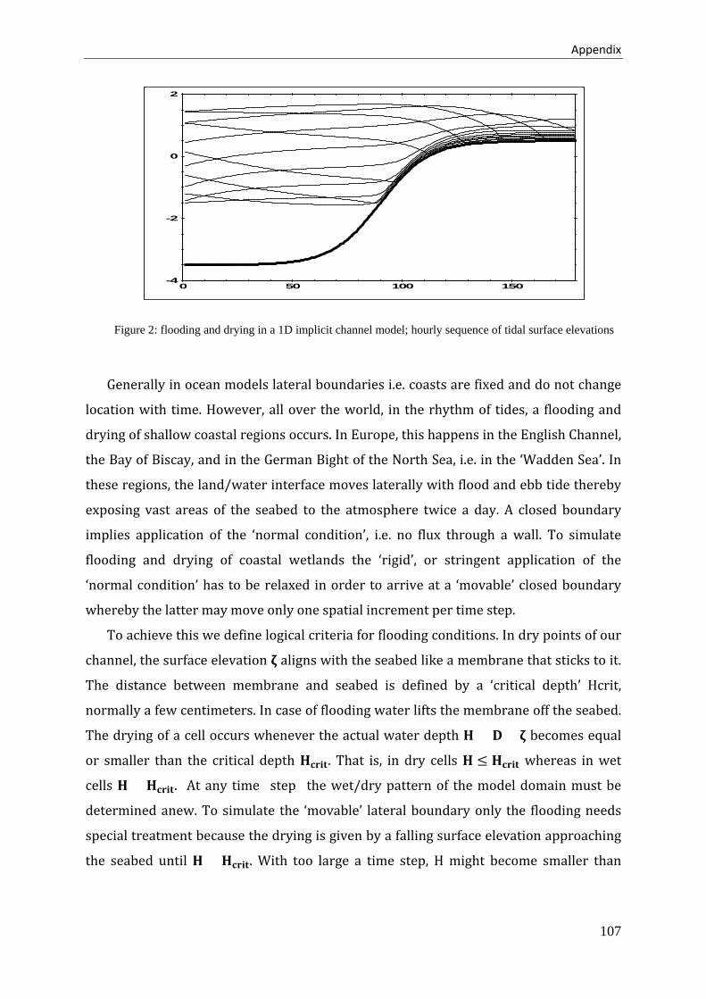
Appendix
Figure 2: flooding and drying in a 1D implicit channel model; hourly sequence of tidal surface elevations
Generally in ocean models lateral boundaries i.e. coasts are fixed and do not change
location with time. However, all over the world, in the rhythm of tides, a flooding and
drying of shallow coastal regions occurs. In Europe, this happens in the English Channel,
the Bay of Biscay, and in the German Bight of the North Sea, i.e. in the ‘Wadden Sea’. In
these regions, the land/water interface moves laterally with flood and ebb tide thereby
exposing vast areas of the seabed to the atmosphere twice a day. A closed boundary
implies application of the ‘normal condition’, i.e. no flux through a wall. To simulate
flooding and drying of coastal wetlands the ‘rigid’, or stringent application of the
‘normal condition’ has to be relaxed in order to arrive at a ‘movable’ closed boundary
whereby the latter may move only one spatial increment per time step.
To achieve this we define logical criteria for flooding conditions. In dry points of our
channel, the surface elevation 𝛇𝛇 aligns with the seabed like a membrane that sticks to it.
The distance between membrane and seabed is defined by a ‘critical depth’ Hcrit,
normally a few centimeters. In case of flooding water lifts the membrane off the seabed.
The drying of a cell occurs whenever the actual water depth 𝐇𝐇 = 𝐃𝐃 + 𝛇𝛇 becomes equal
or smaller than the critical depth 𝐇𝐇𝐜𝐜𝐬𝐬𝐢𝐢𝐃𝐃. That is, in dry cells 𝐇𝐇 ≤ 𝐇𝐇𝐜𝐜𝐬𝐬𝐢𝐢𝐃𝐃 whereas in wet
cells 𝐇𝐇 > 𝐇𝐇𝐜𝐜𝐬𝐬𝐢𝐢𝐃𝐃. At any time (step) the wet/dry pattern of the model domain must be
determined anew. To simulate the ‘movable’ lateral boundary only the flooding needs
special treatment because the drying is given by a falling surface elevation approaching
the seabed until 𝐇𝐇 < 𝐇𝐇𝐜𝐜𝐬𝐬𝐢𝐢𝐃𝐃. With too large a time step, H might become smaller than
-4
-2
0
2
0 50 100 150
107
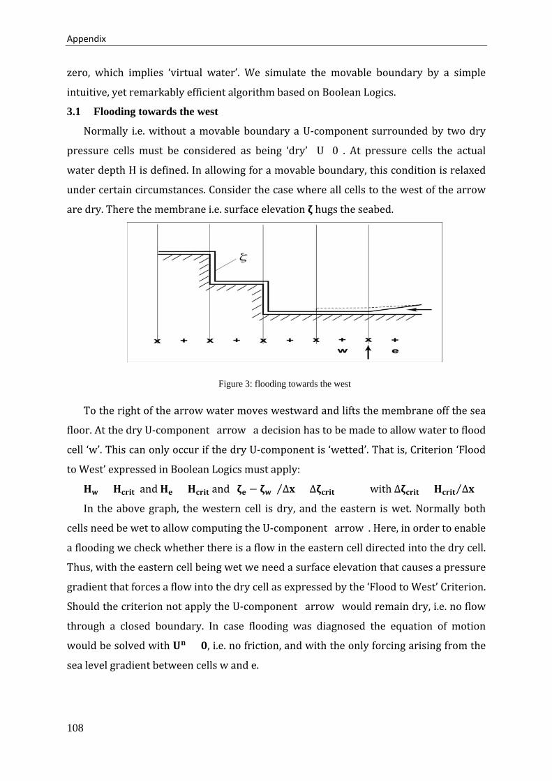
Appendix
zero, which implies ‘virtual water’. We simulate the movable boundary by a simple
intuitive, yet remarkably efficient algorithm based on Boolean Logics.
3.1 Flooding towards the west
Normally i.e. without a movable boundary a U-component surrounded by two dry
pressure cells must be considered as being ‘dry’ (U=0). At pressure cells the actual
water depth H is defined. In allowing for a movable boundary, this condition is relaxed
under certain circumstances. Consider the case where all cells to the west of the arrow
are dry. There the membrane i.e. surface elevation 𝛇𝛇 hugs the seabed.
Figure 3: flooding towards the west
To the right of the arrow water moves westward and lifts the membrane off the sea
floor. At the dry U-component (arrow) a decision has to be made to allow water to flood
cell ‘w’. This can only occur if the dry U-component is ‘wetted’. That is, Criterion ‘Flood
to West’ expressed in Boolean Logics must apply:
𝐇𝐇𝐰𝐰 < 𝐇𝐇𝐜𝐜𝐬𝐬𝐢𝐢𝐃𝐃 and 𝐇𝐇𝐃𝐃 > 𝐇𝐇𝐜𝐜𝐬𝐬𝐢𝐢𝐃𝐃 and (𝛇𝛇𝐃𝐃 − 𝛇𝛇𝐰𝐰) ∆𝐱𝐱⁄ > ∆𝛇𝛇𝐜𝐜𝐬𝐬𝐢𝐢𝐃𝐃 with ∆𝛇𝛇𝐜𝐜𝐬𝐬𝐢𝐢𝐃𝐃 = 𝐇𝐇𝐜𝐜𝐬𝐬𝐢𝐢𝐃𝐃 ∆𝐱𝐱⁄
In the above graph, the western cell is dry, and the eastern is wet. Normally both
cells need be wet to allow computing the U-component (arrow). Here, in order to enable
a flooding we check whether there is a flow in the eastern cell directed into the dry cell.
Thus, with the eastern cell being wet we need a surface elevation that causes a pressure
gradient that forces a flow into the dry cell as expressed by the ‘Flood to West’ Criterion.
Should the criterion not apply the U-component (arrow) would remain dry, i.e. no flow
through a closed boundary. In case flooding was diagnosed the equation of motion
would be solved with 𝐔𝐔𝐬𝐬 = 𝟎𝟎, i.e. no friction, and with the only forcing arising from the
sea level gradient between cells w and e.
108

Appendix
3.2 Flooding towards the east
To allow for a flooding towards the east the following situation must apply: eastern
cell is dry, western is wet and the slope of the surface elevation must be negative for
forcing a flow into the eastern cell. Thus, the ‘Flood to East’ Criterion reads:
𝐇𝐇𝐃𝐃 < 𝐇𝐇𝐜𝐜𝐬𝐬𝐢𝐢𝐃𝐃 and 𝐇𝐇𝐰𝐰 > 𝐇𝐇𝐜𝐜𝐬𝐬𝐢𝐢𝐃𝐃 and (𝛇𝛇𝐃𝐃 − 𝛇𝛇𝐰𝐰) ∆𝐱𝐱⁄ < −∆𝛇𝛇𝐜𝐜𝐬𝐬𝐢𝐢𝐃𝐃
109
List of Figures and Tables
List of Figures Figure 1: Bathymetry of the PG region (numerical model domain). The present model forced at the
southern open boundary. 10
Figure 2: Schematic of the surface circulation in the PG expounded in Reynolds (1993). The dashed
lines in the central part of the PG indicate the approximate seasonal location of the water mass front
between fresh water of the Gulf of Oman and the more saline water of the PG. 14
Figure 3: The topography of the PG (colorbar in meter), provided from data source GEBCO_08 Grid
version 20100927, by the General Bathymetric Chart of the oceans from the British Oceanographic
Data Centre. 19
Figure 4: Bathymetry of the region of PG. The numbers with white background indicate the location
of tidal gauges listed in table 1. Data of red bullet locations is provided by Iranian National
Cartographic Center and blue is provided by International Hydrographic Office. The numbers with
yellow background indicate the depth of contours in meters. 21
Figure 5: Comparison of Model and Observation for harmonics constants for M2, K1, and S2 in the
PG. 23
Figure 6: Comparison of Model and Observation for tidal constituents of O1, N2, and P1 in the PG. 24
Figure 7: Comparison between, the OTIS regional tidal solution and Observation for 8 harmonic
constants in the PG, obtained by harmonic analysis of the data provided by Iranian National
Cartographic Center. 24
Figure 8: Model Result for factor F over the PG. 25
Figure 9: Model Result for M2 Co-Tidal lines over the PG. Co- Amplitude lines are dash lines with
framed numbers and Co- Phase lines are normal lines with no frame numbers 26
Figure 10: Model Result for K1 Co-Tidal lines over the PG. Co- Amplitude lines are dash lines with
framed numbers and Co- Phase lines are normal lines with no frame numbers 26
Figure 11: Model Result for S2 Co-Tidal lines over the PG. Co- Amplitude lines are dash lines with
framed numbers and Co- Phase lines are normal lines with no frame numbers. 27
Figure 12: Model Result for O1 Co-Tidal lines over the PG. Co- Amplitude lines are dash lines with
framed numbers and Co- Phase lines are normal lines with no frame numbers. 27
Figure 13: Model Result for M2 maximum velocities over the PG in m/s. 28
Figure 14: Model Result for K1 maximum velocities over the PG in m/s. 28
Figure 15: Model result for M2 tidal ellipses in the PG. Blue ellipses rotate clockwise and red ellipses
rotate anticlockwise. 30
Figure 16: Model result for K1 tidal ellipses in the PG. Blue ellipses rotate clockwise and red ellipses
rotate anticlockwise. 30
110
List of Figures and Tables
Figure 17: Maximum tidal currents velocity (colorbar in m/s) in the PG using 13 tidal constituents at
the open boundary. 32
Figure 18: Kinetic power density (colorbar in kW/m2) from the tidal current. 33
Figure 19: Effect of Qeshm canal on the tidal solution with single harmonic forcing (M2) at the open
Boundary, Model Result for tidal range difference of M2 amplitude in two conditions; closed canal
and real topography in cm (real-closed). 34
Figure 20: High-pass filtered topography of the PG in meters (colorbar). Box 1 indicates the area
zoomed in Figure 28. 39
Figure 21: Residual current (×10-3m/s) pattern around a symmetric hill. The current direction of
approach flow is northward. The background and vectors display the Residual currents. White
contours are the topography contours. 40
Figure 22: Residual vorticity (×10-6 s-1) pattern around a symmetric hill (left) and a valley (right). The
current direction of approach flow is northward. 41
Figure 23: Residual current (×10-3m/s) pattern around an elongated hill (left). The background and
vectors display the Residual currents. White contours are the topography contours. Residual vorticity
(×10-5 s-1) pattern around a symmetric hill (right). The current direction of approach flow is
northward. 41
Figure 24: Residual current (×10-3m/s) pattern around an elongated and tilted hill (left). The
background and vectors display the Residual currents. White contours are the topography contours.
The residual vorticity (×10-5 s-1) pattern around an elongated and tilted hill (right). The current
direction of approach flow is northward. 41
Figure 25: The residual current around a hill and a valley. Wide arrows are the current direction of
approach flow. The background contours display the topography. For a hill, water depth decreases to
the center and for a valley, it increases. Gyres illustrate the direction of residual current around the
topography contours. Looking in the direction of the flow cyclonic and anticyclonic gyres are on
different sides in the case of a hill and a valley. 42
Figure 26: Model Result for K1 residual velocity (m/s) in the PG. 43
Figure 27: Model Result for M2 residual velocity (m/s) in the PG. 43
Figure 28: M2 Residual current vectors around a hill in high-pass filtered topography (colorbar in
meters) of the PG. vectors show the M2 residual currents. CD is the Current Direction. This area is
shown in Figure 1 with Box 1. 45
Figure 29: Lagrangian trajectories (black lines) in residual vorticity (colorbar × 10-5 s-1), running with
residual velocities of M2+S2+K1+O1 for 120 days. 46
Figure 30: Lagrangian trajectories (black lines) in residual vorticity (colorbar × 10-5 s-1), running with
residual velocities of M2+S2+K1+O1 for 120 days. Green lines show 2 main gyres in the PG. The red
box in guide map shows the position of zoomed figure in the PG. 46
111
List of Figures and Tables
Figure 31: Box 1 of trajectories running with residual velocities of M2+S2+K1+O1 for 120 days.
Gray marks are the start points. 47
Figure 32: Box 2 of trajectories running with residual velocities of M2+S2+K1+O1 for 120 days.
Gray marks are the start points. 48
Figure 33: Box 3 of trajectories running with residual velocities of M2+S2+K1+O1 for 120 days.
Gray marks are the start points. 49
Figure 34: a) The topography of the PG, contour lines with an increment of 20 m. Y-axis: latitude; X-
axis: longitude. b) Displacement of amphidromic points with different periods of forcing (10 h to 35
h), Blue circles: periods with 2 amphidromic points, Red circles: periods with a single amphidromic
point. c) The position of monitoring stations; N1-N4 stations in the northern PG, S1-S4 stations in
southern PG, H1-H4 stations in Strait of Hormuz. Data at monitoring stations are shown in Figures
39, 40 and 41. 51
Figure 35: Tidal amplification factor (colorbar) for the period of 12.5 h in the PG. Y-axis: latitude; X-
axis: longitude. 54
Figure 36: Tidal amplification factor (colorbar) for the period of 24 h in the PG. Y-axis: latitude; X-
axis: longitude. 55
Figure 37: Periods (from 3.5 h to 35.5 h) of maximum tidal ranges in the PG. Y-axis: latitude; X-axis:
longitude; Colorbar: Period in hours. 55
Figure 38: Maximum tidal amplification factor (colorbar) from period 3.5 h to 35.5 h in the PG. The
neutral tidal amplification factor is shown by the contour. Y-axis: latitude; X-axis: longitude. 56
Figure 39: Tidal amplification factor for the monitoring points, N1-N4, in the northern PG (See figure
3 for positions). Periods of the main tides (M2, S2, O1, and K1) are marked as dash lines. 57
Figure 40: Tidal amplification factor for the monitoring points, H1-H4, in the Strait of Hormuz (See
figure 3 for positions). Periods of the main tides (M2, S2, O1, and K1) are marked as dash lines. 58
Figure 41: Tidal amplification factor for the monitoring points, S1-S4, in the region off the Arabian
coast (See figure 3 for positions). Periods of the main tides (M2, S2, O1, and K1) are marked as dash
lines. 58
Figure 42: Increase of tidal amplification factor (colorbar) for the period of 12.5 h due to sea level rise
of 1 m in the PG. Y-axis: latitude; X-axis: longitude. 59
Figure 43: Increase of tidal amplification factor (colorbar) for the period of 24 h due to sea level rise
of 1 m in the PG. Y-axis: latitude; X-axis: longitude. 60
Figure 44: The annual potential power density (colorbar in MW/cell) of the semidiurnal tide. 61
Figure 45: The annual potential power density (colorbar in MW/cell) of the diurnal tide. 61
Figure 46: satellite picture of the Musa estuary. 63
Figure 47: The topography of the Musa estuary (colorbar in meter). Redline shows the track line along
the main channel. 64
112
List of Figures and Tables
Figure 48: Different layers from satellite picture and measurement data, used for creating the
topography of the Musa estuary. 65
Figure 49: Schematic diagram of heat fluxes on tidal flats. Arrows indicate the direction of heat flux.
65
Figure 50: total salt in the domain, the output of salt from the open boundary and tidal elevation of the
open boundary for 140 simulation days. 66
Figure 51: Total salt in the domain, the output of salt from the open boundary and tidal elevation of
the open boundary for the last 20 days of 140 days. 67
Figure 52: Tidally-averaged current velocity (colorbar in m/s) on the slope without the effect of
thermodynamics. Vectors show the direction of the currents. 68
Figure 53: Tidally-averaged current velocity (colorbar in m/s) on the slope with the effect of
thermodynamics. Vectors show the direction of the currents. 69
Figure 54: Density-driven currents (colorbar in m/s) on the slop, the difference between Figure 52 and
Figure 53. Vectors show the direction of the currents. 69
Figure 55: Model results for salinity (colorbar) after 120 days and 1 hour, UL: Surface layer. UR:
Section M163. LL: Section Z093. LR: Section M316. Sections are marked with three lines in UL. 70
Figure 56: Model results for salinity (colorbar) after 120 days and 5 hours, UL: Surface layer. UR:
Section M163. LL: Section Z093. LR: Section M316. Sections are marked with three lines in UL. 71
Figure 57: Model results for salinity (colorbar) after 120 days and 9 hours, UL: Surface layer. UR:
Section M163. LL: Section Z093. LR: Section M316. Sections are marked with three lines in UL. 71
Figure 58: Model results after 120 days and 12 hours for section Z093 in Musa estuary. Left: salinity
(colorbar). Right: V-component of current velocity (colorbar in m/s). The section is marked in Figure
55. 72
Figure 59: Model results after 120 days and 18 hours for section Z093 in Musa estuary. Left: salinity
(colorbar). Right: V-component of current velocity (colorbar in m/s). The section is marked in Figure
55. 72
Figure 60: Model results after 120 days and 12 hours for section M163 in Musa estuary. Left: salinity
(colorbar). Right: U-component of current velocity (colorbar in m/s). The section is marked in Figure
55. 73
Figure 61: Model results after 120 days and 12 hours for section M163 in Musa estuary. Left: salinity
(colorbar). Right: U-component of current velocity (colorbar in m/s). The section is marked in Figure
55. 73
Figure 62: Model results after 120 days and 12 hours for section M316 in Musa estuary. Left: salinity
(colorbar). Right: U-component of current velocity (colorbar in m/s). The section is marked in Figure
55. 74
113
List of Figures and Tables
Figure 63: Model results after 120 days and 12 hours for section M316 in Musa estuary. Left: salinity
(colorbar). Right: U-component of current velocity (colorbar in m/s). The section is marked in Figure
55. 74
Figure 64: Tidally-averaged salinity, (colorbar) along the track in the Musa estuary. 75
Figure 65: Tidally-averaged current velocity (colorbar in m/s), in the direction of the track in the
Musa estuary. 75
Figure 66: Tidally-averaged current velocity (colorbar in m/s), normal to the direction of the track in
the Musa estuary. 76
Figure 67: The model results in the meridional (M324) section in the Musa estuary for, Left: Tidally-
averaged current velocity (colorbar in m/s), normal to the section, positive means inflow. Right:
Tidally-averaged salinity (colorbar). 76
Figure 68: The model results in the zonal (Z036) section in the Musa estuary for, Left: Tidally-
averaged current velocity (colorbar in m/s), normal to the section, positive means inflow. Right:
Tidally-averaged salinity (colorbar). 77
List of Tables Table 1: List of tide gauges used if Figures 5. First 4 stations are provided by Iranian National
Cartographic Center and others are provided by International Hydrographic Office. 21
Table 2: Comparison between Model and Observation for tidal constituents of M2, K1, S2, O1, N2
and P1 in the PG. Phases are in degrees from Greenwich. 22
114
List of publications
Mashayekh Poul, H., Backhaus, J.O., Huebner, U., 2014. Estimate the area with most
efficiency for producing energy from tide in the Persian Gulf, in: The 11th International
Conference on Coasts, Ports and Marine Structures.
Mashayekh Poul, H., Backhaus, J., Huebner, U., 2016. A description of the tides and effect of
Qeshm canal on that in the Persian Gulf using two-dimensional numerical model.
Arabian Journal of Geoscience, 9, 148. doi:10.1007/s12517-015-2259-8
Mashayekh Poul H., Backhaus J., Dehghani, A., Huebner, U., 2016. Effect of subseabed salt
domes on Tidal Residual currents in the Persian Gulf. Journal of Geophysical Research
Ocean 121:3372–3380. doi: 10.1002/2015JC011421
115