Modelling, Transport and Assessment of Aquatic Toxic

Article

Modelling, Transport and Assessment of AquaticToxic Metals in Coastal Ecosystems

Franklin Torres-Bejarano 1,† ID , Hermilo Ramírez-León 2,†*,Clemente Rodríguez-Cuevas 3,† ID ,Israel Enrique Herrera-Díaz 4,† ID , Jorge J. Hernández-Gómez 5,† ID , Hector Barrios-Piña 6,† ID , andCarlos Couder-Castañeda5,†* ID

1 Departamento de Ingeniería Ambiental, Universidad de Córdoba, Montería, Colombia2 PIMAS Proyectos de Ingeniería y Medio Ambiente S.C., Ciudad de México, México3 Facultad de Ingeniería, Universidad Autónoma de San Luis Potosí, San Luis Potosí, México4 Departmento de Ingeniería Agroindustrial, Universidad de Guanajuato, Campus Celaya-Salvatierra, Celaya,

Guanajuato, Mexico5 Centro de Desarrollo Aeroespacial, Instituto Politécnico Nacional, Ciudad de México, México6 Escuela de Ingeniería y Ciencias, Tecnológico de Monterrey Campus Guadalajara 45138 Zapopan, Jalisco,

Mexico* Correspondence: [email protected]; Tel.: +52-55-5729-6000 ext 64665† These authors contributed equally to this work.

Abstract: This paper describes the development of a two-dimensional water quality model thatsolves hydrodynamic equations tied to transport equations with reactions mechanisms inherent in theprocesses. This enable us to perform an accurate assessment of the pollution in a coastal ecosystem.The model was developed with data drawn from the ecosystem found in Mexico’s southeast state ofTabasco. The coastal ecosystem consists of the interaction of El Yucateco lagoon with the Chicozapoteand Tonalá rivers, that connect the lagoon with the Gulf of Mexico. We present the results of pollutantstransport simulation in the coastal ecosystem, focusing on toxic parameters for two hydrodynamicscenarios: wet and dry seasons. As it of interest in the zone, we study the transport of four metals:Cadmium, Chromium, Nickel and Lead. In order to address our objectives we solved numerically aself-posed mathematical problem,which is based on the measured data. The performed simulationsshow to characterise metal transport within the acceptable range of accuracy and in accordancewith the measured data. The performed simulations show to characterise metals transport with anacceptable accuracy, agreeing well with measured data in total concentrations in four control pointsalong the water body. Although for the accurate implementation of the hydrodynamic-based waterquality model herein presented, boundary (geometry, tides, wind, etc.) and initial (concentrationsmeasurements) conditions are required, it poses as an excellent option when the distribution ofsolutes with high accuracy is required, easing environmental, economic and social management ofcoastal ecosystems.

Keywords: Pollutant transport modelling; metals transport modelling, free surface water bodies,toxics-reaction equation

PACS: 92.40.Qk; 91.50.Ga; 92.20.Ny;

1. Introduction

The concern for water environmental pollution by heavy metals has recently increased due to thenegative effects it might have in human beings [1,2]. Some heavy metals as Cadmium (Cd), Chromium(Cr) and Lead (Pb) may transform into persistent metallic compounds with high toxicity [3]. Due totheir damaging effects on the ecological environment and in human health, it is necessary to studyheavy metal contamination in aquatic ecosystems [4].

Metals are naturally present in small concentrations or traces in earth’s crust; many of them areessential for the growth and development of plants, animals and human beings. The geo-available

Preprints (www.preprints.org) | NOT PEER-REVIEWED | Posted: 2 April 2018 doi:10.20944/preprints201804.0024.v1

© 2018 by the author(s). Distributed under a Creative Commons CC BY license.

https://orcid.org/0000-0003-3144-7289

https://orcid.org/0000-0003-4213-4552

https://orcid.org/0000-0002-2117-7548

https://orcid.org/0000-0002-5012-6619

https://orcid.org/0000-0001-6997-3415

https://orcid.org/0000-0001-8826-3750

http://dx.doi.org/10.20944/preprints201804.0024.v1

http://creativecommons.org/licenses/by/4.0/

2 of 25

origin of these metals occurs from the mother rock to the soils after being released by weathering. Incontrast, the presence of high concentrations of metals is an indicator of anthropogenic activities, suchas hazardous wastes derived from industrial activities, mining, agriculture, etc. Nowadays, interest inthe pollution of rivers by metals has increased, because rivers serve a medium for transport of dissolvedand particulate matter from continents to the ocean. For this reason, heavy metal concentrations inwaters have been analysed worldwide [5].

In coastal waters, heavy metals are distributed through the water column and the bottomsediments. This occurs during the mixing of fresh and marine water, which causes flocculationand sedimentation of organic matter, nutrients and trace elements from rivers. Actually, dissolvedmetals come into the particulate phase due to flocculation process during estuarine mixing. Thus,heavy metals get bound to these elements and precipitate to the bottom. Flocculation plays a key role inthe dynamics of estuarine and coastal environments, controlling the transport of fine-grained cohesivesediments and particulate contaminants throughout these systems [6–8] (usually characterised bymuddy bottoms [9]). Nevertheless, it should be pointed out that during natural estuarine mixing,flocculation process may not occur; actually, salinity plays an important role in the process, dependingon the reaction mechanism of a particular metal. For instance, flocculation starts at 10% of salinityduring estuarine mixing for Cd [10,11]. Moreover, other metals are known for their nutrient-likebehaviour. Thus, flocculation process constitutes an arduous task to model [12], which is not the aimof this work.

For the above reasons, strategies and tools to mitigate the pollution of heavy metals are required[13]. A huge number of mathematical models that intend to predict the transport of heavy metals inflows exist, as for example the statistical models based on exponential functions (analytic models),which allow the achievement of a simulation in a relatively uncomplicated way. This is the case ofthe use of sigmoid functions to determine metal concentrations in rivers that can yield to averageconcentrations in a section [14]. Despite the fact that the power of CPU processors is now much betterthan decades ago, simulations continue to be carried out through analytic models which allows to usea minimum of experimental measurements [15].

Most common methods to evaluate heavy metals pollution in water bodies are based on qualityindexes, which generally use correlation or fuzzy methods for their estimation [2,16,17]; these worksmodel pollutant distribution in the area under study, through GIS system modules, which applyinterpolation methods. Nevertheless, the obtained spatial distribution through a hydrodynamicsmodule along with transport equation and considering reaction mechanisms, produces much moreaccurate results [18] (although it requires a greater effort to be implemented).

Water quality models (WQM) have increased in number and have improved in recent years,focusing on the study of the water quality as well as pollutant transport in shallow water ecosystems.The behaviour and transport of toxic substances, such as metals and/or hydrocarbons, has been deeplystudied on shallow aquatic systems during this century [19,20]. In this case, the complexity of estuarinecoastal systems must be understood in order to clearly pose the solution of the equations representingwater hydrodynamics (mass conservation and momentum equations) as well as mass transport ofpollutants (advection - diffusion - reaction equation), considering even the highly nonlinear interactionstypical of these regions. Thomann and Mueller, Thomann, Lun et al., Ji et al., Shimazu et al., Bhavsaret al. show different approaches of the toxic substances behaviour problem in water columns, as wellas their interaction with sediments and air, including mathematical models and solution methods.

The most popular numerical WQM are AQUATOX, Branched Lagrangian Transport Model(BLTM), One Dimensional Riverine Hydrodynamic, Water Quality Model (EPD-RIV1), QUAL2Kw,Water Quality Analysis Simulation Program (WASP), Water Quality for River-Reservoir Systems(WQRRS), ROMS-ICS [27] and MIKE Ecolab/ABM. Nevertheless, most of them are based on solvingmass balance/advective diffusion equation, but oriented to nutrients (as DO, BOD, PH4, Phosphorus)or pathogens (like coliforms). Such models do not contemplate metals transport [28]. A reviewregarding computational models of water quality can be found in [29], where it is pointed out that



3 of 25

WTM are of great importance for environmental management; nevertheless, they still constitute anopen research field. Although there are available WQM as discussed above, it is common to findmodels developed by particular researchers that include effects or processes specific to their case ofstudy, such as the MINEQL [30], which has been used to model the concentrations of metals in riverssince the decade of 1980.

Despite the existing WQM, the aim of this work is to develop a water quality module, which canbe coupled to a hydrodynamic numerical model, applicable to the study of hydrodynamics and waterquality in coastal ecosystems. The hydrodynamic model adopted in this work is self-developmentfor research purposes, and has been previously used in different research applications, including: thehydrodynamic-hydrological modelling in flood zones [31], the modelling of flows through vegetation[32], the modelling of the thermal discharges [33,34] and the modelling of fresh water plumes inriver-sea interaction [35]. On the other side, in order to accurately simulate turbulent viscosity, weimplemented the turbulence model discussed in detail in [36].

The water quality module herein developed takes into account many parameters, includingthe advection-diffusion-reaction mechanism. The required parameters cannot be found in a specificexisting WQM. These parameters were adopted from [37,38]. Four heavy metals, Cd, Cr, Pb and Ni,were selected for the water quality module because they are required by local institutions as wellas because they have strong toxicity to humans [39]. According to our previous knowledge, we didnot find an ad hoc module for the transport of these metals, so we developed one that contemplatesthe greatest possible number of parameters in the reaction mechanisms. This module can be appliedas any WQM (ROMS-ICS, WASP o MIKE), with the advantage that the reaction mechanisms canbe modified by calibrating each of the parameters through the equations. The case of study is theecosystem composed by El Yucateco lagoon, the Chicozapote river and the Tonalá river discharge, whichhas suffered a serious deterioration due to pollution originated by oil industry activities.

This paper begins by a detailed presentation of the coastal ecosystem we considered in Section 2.It will then go to exposition of the methodology herein applied, including the measurement protocol,the design of the hydrodynamic and water quality modules as well as the numerical strategies fortheir solution (Section 3). Thereafter, in Section 4 we present the application of this WQM to the case ofstudy, as well as the detailed results of the simulations for the transport of heavy metals, along withtwo metrics that allow to assess the accuracy of the WQM herein developed with respect to measureddata. Finally, in Section 5 we present the conclusions of this study as well as some final interestingremarks.

2. Case of study

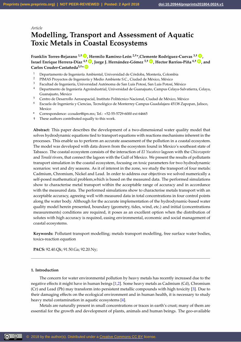
The coastal ecosystem we studied is located at the east of Tabasco State, in the southeast of Mexico.The lagoon is located between LAT 18o 10’ and 18o 12’ N, and between LONG 94o 02’ and 94o 00’ W(Fig. 1). El Yucateco lagoon interacts with Chicozapote and Tonalá rivers, before discharging to the Gulfof Mexico. Nowadays, the lagoon is one of the most important water bodies of the region.

The predominant climate in the region is warm and humid, with abundant rainfall during summer.Its annual thermal regime oscillates between 25.8oC and 27.8 oC; the highest average temperature occursin May with 29.4 oC while the minimum is registered in January with 23.1 oC. September/october isthe most rainy month with an average precipitation of 400 mm while in June the minimum incidencewith an average value of 43.3 mm.

For El Yucateco lagoon, the main hydrodynamic driven forces are winds and tides. The tide andChicozapote river permanently renew and refresh water in the lagoon.

For dry season, current flows head predominantly to north during mornings, while mainly tonortheast in afternoon hours; in both cases, current flows out of the lagoon with velocities greater than20 cm/s. For rainy season, current is variable with different directions along the system, heading tonortheast in the south part of the lagoon and to the north close to the mouth and to the connection



4 of 25

Figure 1. Location of study zone and control points in the coastal ecosystem. The centre of lagoon islocated at W 94o 01’ 12” N 18o 11’ 6”.

with Chicozapote river. Typical flow velocities about 10 cm/s are observed, which favour the formationof vortices within the lagoon.

In this zone of the Gulf of Mexico, tide presents a mixed type with diurnal influence, whoseoscillations are not greater than 30 - 60 cm. The surge is moderate in E-W direction, with a maximumheight of 2 m in normal meteorological conditions.

Main activities in the zone are agriculture, cattle farming, fishing and industry. In the last 20 years,important changes in hydrology and water quality have occurred, changing the productivity andreducing the number of endemic species. These changes have had social, economical and commercialimpacts for native population. This area is currently under industrial development, where two kindsof activities stand out: oil (extraction and production) and livestock farming, which together accountfor almost 90% of the productive sectors of Tabasco State [40]. More environmental information aboutthis ecosystem is available in [41].

Furthermore, Oil field Cinco Presidentes was established in 1963 in the vicinity of this region, beingEl Yucateco lagoon the closest water body to the oil facility. Later, a network of artificial channels(approx. 33 Km) was built by PEMEX Oil Company during such decade, with an area of about 130 ha.These channels drain a considerable volume of fresh water to the lagoon product of the drainage of thefloodplains (marshes) that surround the area.

3. Methodology

The WQM herein developed consists essentially of two parts: an hydrodynamic module and awater quality module. The later one being in charge of transporting heavy metals through the waterbody by using the hydrodynamic module results. Later, in Sections 3.2 and 3.3 these modules are



5 of 25

appropriately defined. In what follows, the protocol regarding measurement and data analysis ispresented.

3.1. Water quality measurement protocol

In measurement campaigns, water and sediment samples were collected following the guidelinesof the Standard Methods for the Examination of Water & Wastewaters methodology [42].

For heavy metals in water, 500 ml of sample were taken at each point using a Van Dorn watersampler. The samples were filtered (0.45 µm) and acidified (HNO3 at pH = 2.0), stored in amber glassbottles and refrigerated at 4.0 C for transportation [42]. For heavy metals in sediments, samples of100 g were collected from the surface layer (max. 5 cm) with an Ekman dredger. These samples werestored in sterile polyethylene bags and kept at 4.0 C for transport. All the samples were collected byduplicate to determine the precision of tests and sample handling. The chemical analyses of heavymetals in water and sediments was performed using atomic absorption spectrophotometry, with aspectrometer ICE 3500 AAS Thermo Fisher Scientifc.

According to previous in situ studies [41], several metals were initially sampled. Those whoseparameters exceeded water and/or sediment quality criteria [43,44] were selected for diagnosis: Cd,Cr, Pb and Ni.

Measured data and their chemical analyses of these parameters served to specify boundary andinitial conditions to the numerical model herein developed. They also aided to validate the model forthe study region.

3.2. Hydrodynamic module

The hydrodynamic module is based on the governing equations for shallow waters with constantdensity and free surface, which can be derived from the Reynolds-averaged Navier-Stokes equations[36]. These equations are:

∂U∂t

+ U∂U∂x

+ V∂U∂y

= −ρgρ0

∂η

∂x− 1

ρ0

∂Patm

∂x+ νTH

(∂2U∂x2 +

∂2V∂y2

), (1)

∂V∂t

+ U∂V∂x

+ V∂V∂y

= −ρgρ0

∂η

∂y− 1

ρ0

∂Patm

∂y+ νTH

(∂2U∂x2 +

∂2V∂y2

), (2)

where U and V are the mean components of velocity field in the x and y directions respectively (m/s);g is the acceleration due to gravity (m/s2); ρ is the water density (kg/m3); ρ0 is the water referencedensity (kg/m3); η is the free surface elevation (m); Patm is the atmospheric pressure (Pa); and νTH isthe horizontal eddy viscosity (m2/s).

The equation to calculate the free surface elevation is obtained by integrating the continuityequation over the water depth, which by applying a kinematic condition at the free surface, is given by

∂η

∂t= − ∂

∂x

(∫ η

−hUdz

)− ∂

∂y

(∫ η

−hVdz

), (3)

where h(x, y) is the water depth (m).As mentioned above, in order to achieve a more realistic hydrodynamics, mechanical dispersion

phenomenon is also considered through the introduction of a model of turbulence. Due to the natureof the water body herein treated, the ml-05 mixing-length model is introduced [36], which contributesto the horizontal eddy viscosity as:



6 of 25

νTH =

√√√√l4h

[2(

∂U∂x

)2+ 2

(∂V∂y

)2+

(∂V∂x

+∂U∂y

)2]

(4)

where lh is horizontal mixing length.

3.3. Water Quality Module

The water quality module can be deem as consisting of a part which is in charge of transportingthe substance plus a second one which takes into account the reaction mechanism to which the toxicantis subject. For the transport phase, the Advection-Diffusion-Reaction equation is solved:

∂C∂t︸︷︷︸

Rate of change

+U∂C∂x

+ V∂C∂y︸︷︷︸

Net rate of flow(convection)

=∂

∂x

(Ex

∂C∂x

)+

∂

∂y

(Ey

∂C∂y

)︸︷︷︸

Rate of change due to diffusion

+ ΓC︸︷︷︸Rate of change

due to reaction sources

(5)

where C is the concentration of a substance (mg/L), Ex and Ey are the horizontal dispersion coefficients(m2/s) [36]; and Γc is the substance reaction term (mg/L).

The water quality module is initialised considering no reaction (ΓC(t = 0) = 0), and assumingstationary sediment, constant kinetic coefficients and suspended solid’s uniformly distributed inspace over the river reach. Once the initial concentration distribution C is calculated through Eq. 5,it is re-estimated through a model of reaction of toxic substances. Thomann and Salas presents acomplete model which considers diffusive exchange, decomposition processes, volatilisation, settlingand re-suspension (important processes in a coastal aquatical ecosystem), which is governed by thefollowing ordinary differential equation,

ΓC =dCdt

=K f

h(

fd2 C2/ϕ2 − fd1 C1)− Kd1 fd1 C1 +

KLh

(cg

He− fd1 C1

)− vs

hfp1C1 +

vu

hfp2C2 (6)

where 1 and 2 represent the water column and sediment respectively, C1 is the concentration of thetoxic substance (mg/L) (estimated using the transport equation), C2 is the concentration of the toxicantin sediments (mg/L), K f is the diffusive exchange (m/d), h is the River depth (m), fd is the dissolvedfraction (1), fp is the particulate fraction (1), Kd1 is the degradation rate of the dissolved toxic substance(d−1), KL is the overall volatilisation transfer rate (m/d), cg is the vapour phase concentration (mg/L),He is Henry’s constant, vs is the settling velocity (m/d), vu is the re-suspended velocity (m/d) and ϕ2

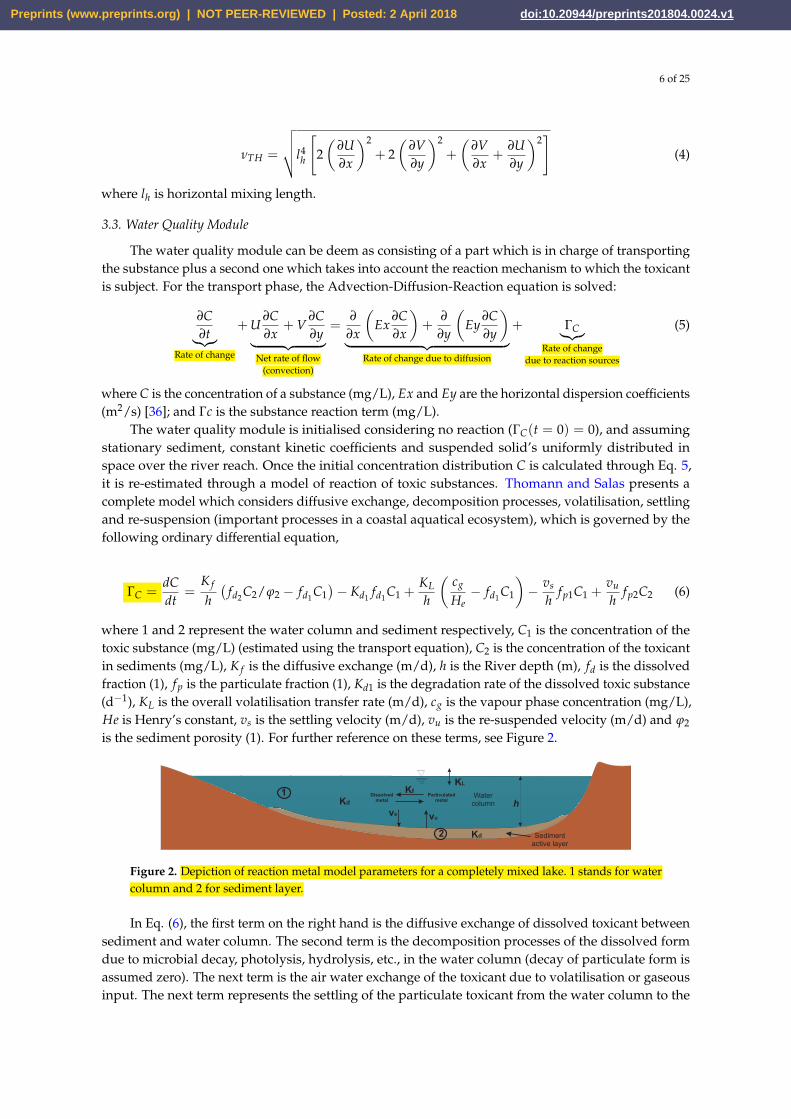
is the sediment porosity (1). For further reference on these terms, see Figure 2.

Kd2 Sedimentactive layer

Kd

1 Watercolumn

KL

h

vu

Particulated

metal

Dissolved

metal

Kf

vs

Figure 2. Depiction of reaction metal model parameters for a completely mixed lake. 1 stands for watercolumn and 2 for sediment layer.

In Eq. (6), the first term on the right hand is the diffusive exchange of dissolved toxicant betweensediment and water column. The second term is the decomposition processes of the dissolved formdue to microbial decay, photolysis, hydrolysis, etc., in the water column (decay of particulate form isassumed zero). The next term is the air water exchange of the toxicant due to volatilisation or gaseousinput. The next term represents the settling of the particulate toxicant from the water column to the



7 of 25

sediment and the last term is re-suspension into the water column of the particulate toxicant from thesediment.

A description of the processes underlying the parameters in Eq. (6) is detailed in what follows.For the decay of the dissolved substances, the most important mechanisms in the degradation

rate of the dissolved toxic substance (Kd1) are represented by the equation:

Kd1 = Kp + KH + KB (7)

where Kp is the photolysis rate (d−1), KH is the hydrolysis rate (d−1) and KB is the microbialdegradation rate (d−1).

The overall exchange rate (KL) estimates the importance of losses due to volatilisation. Accordingwith [46], the application of the two film theory yields to an overall volatilisation transfer parametergiven by,

1KL

=1kl

+1

kg He(8)

where kl is the liquid film coefficient (m/d) and kg is the gas film coefficient (m/d). As seen from Eq.(8), KL depends on chemical properties as well as on characteristics of the water body such as watervelocity (affecting kl) and wind velocity over water surface (affecting both kl and kg).

Henry’s (He) constant, present in Eqs. (6) and (8), takes into account the water-atmosphereinteraction, and it represents a partitioning of the toxicant between water and atmospheric phases. Itsdimensionless form is given by

He =cg

cw(9)

where cw the water solubility (mg/L).The sediment diffusion rate K f reflects the fact that gradients can occur between interstitial

sediments and the adjacent water column. Di Toro et al. has summarised some data respect to thiscoefficient in the following expression,

K f = 19ϕ2(MW)−2/3 (10)

where MW is the Molecular weight (g/mol) and ϕ2 the sediment porosity.To determine both settling and re-suspended velocities, a particle characterisation in the region

under study is required. In this work, such characterisation was made with sediment samples takenfrom field campaigns, where organic matter, particle sizes, porosity, humidity, etc. were quantified. Incoastal ecosystems, a good approximation to the settling velocity vs is given by Hawley, who providesthe following empirical relation,

vs = 0.2571(d)1.138 (11)

where d is the particle diameter (m).For the re-suspended velocity vu, Thomann and Di Toro have proposed the next equation:

vu = vd

(vs

vn− 1)

(12)

where vd is the net rate loss of solids (m/d) and vn is the settling net rate of the water solids (m/d).In estuarine and coastal environments, usually characterised by muddy bottoms, flocculation

plays a key role [9]; nevertheless, the water body under study have low circulation because there is notimportant water interchange with Chicozapote River. Being this a quasi-static water body with verysmall velocities, the sediment transport in the muddy environment at the bottom of the lagoon can beactually neglected.



8 of 25

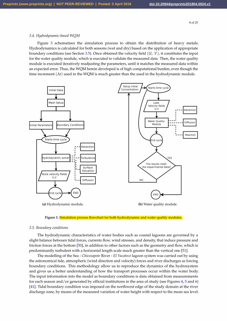
3.4. Hydrodynamic-based WQM

Figure 3 schematises the simulation process to obtain the distribution of heavy metals.Hydrodynamics is calculated for both seasons (wet and dry) based on the application of appropriateboundary conditions (see Section 3.5). Once obtained the velocity field (U, V), it constitutes the inputfor the water quality module, which is executed to validate the measured data. Then, the water qualitymodule is executed iteratively readjusting the parameters, until it matches the measured data withinan expected error. Thus, the WQM herein developed is of high computational burden, even though thetime increment (∆t) used in the WQM is much greater than the used in the hydrodynamic module.

(a) Hydrodynamic module. (b) Water quality module.

Figure 3. Simulation process flowchart for both hydrodynamic and water quality modules.

3.5. Boundary conditions

The hydrodynamic characteristics of water bodies such as coastal lagoons are governed by aslight balance between tidal forces, currents flow, wind stresses, and density, that induce pressure andfriction forces at the bottom [50], in addition to other factors such as the geometry and flow, which ispredominantly turbulent with a horizontal length scale much greater than the vertical one [51].

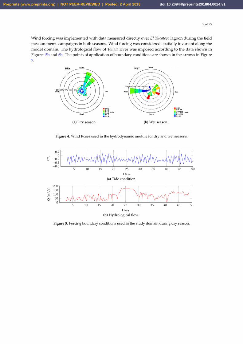
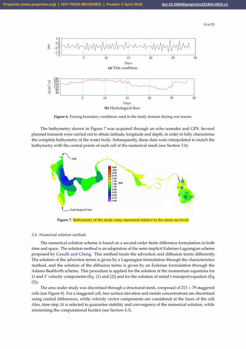
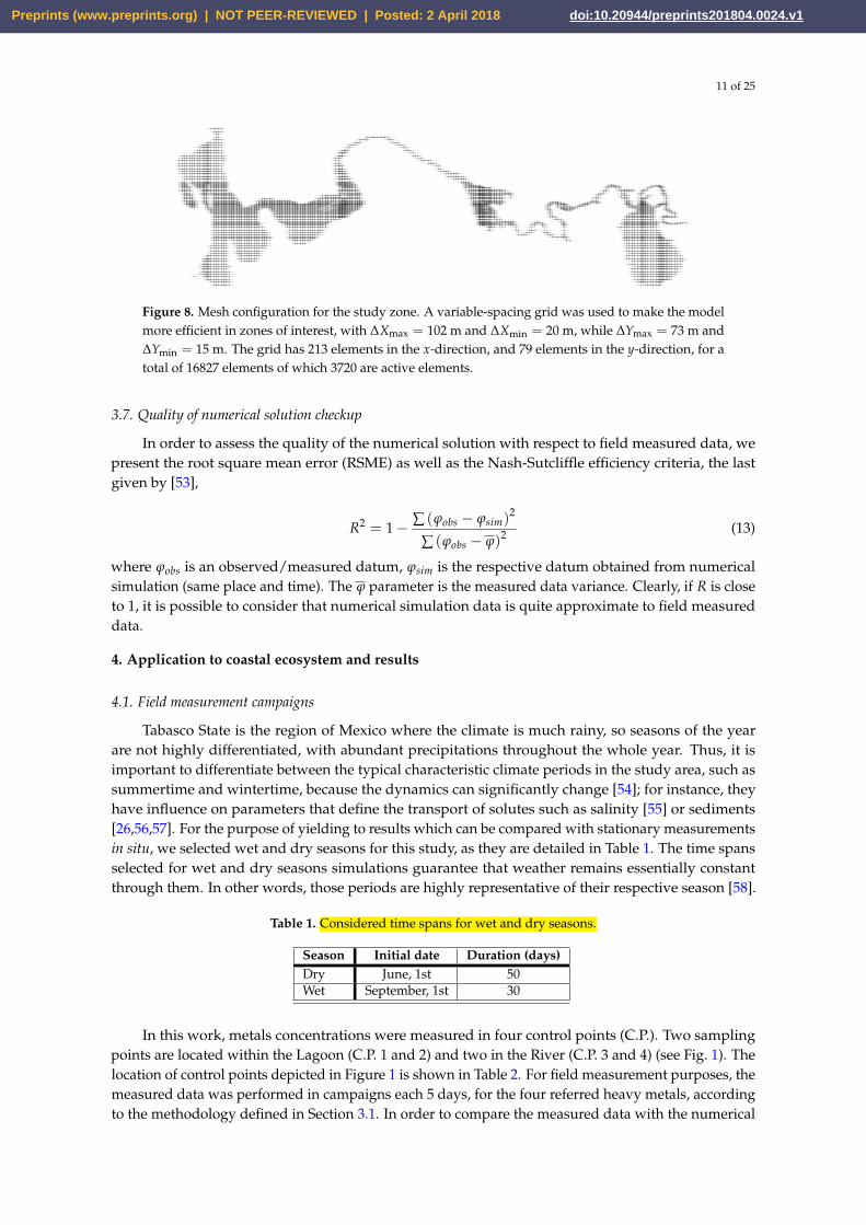
The modelling of the Sea - Chicozapote River - El Yucateco lagoon system was carried out by usingthe astronomical tide, atmospheric (wind direction and velocity) forces and river discharges as forcingboundary conditions. This methodology allow us to reproduce the dynamics of the hydrosystemand gives us a better understanding of how the transport processes occur within the water body.The input information into the model as boundary conditions is data obtained from measurementsfor each season and/or generated by official institutions in the area of study (see Figures 4, 5 and 6)[41]. Tidal boundary condition was imposed on the northwest edge of the study domain at the riverdischarge zone, by means of the measured variation of water height with respect to the mean sea level.



9 of 25

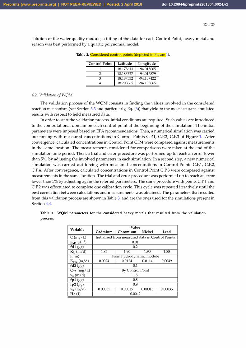
Wind forcing was implemented with data measured directly over El Yucateco lagoon during the fieldmeasurements campaigns in both seasons. Wind forcing was considered spatially invariant along themodel domain. The hydrological flow of Tonalá river was imposed according to the data shown inFigures 5b and 6b. The points of application of boundary conditions are shown in the arrows in Figure7.

>=7.56-7.5

South

EastWest

North

4.5-63-4.51.5-30-1.5

0%5%10%15%20%25%

DRY

(m/s)

(a) Dry season.

30% 25%

West East

20% 15% 10% 5%

0%

>=4.93.98-4.93.06-3.982.14-3.061.22-2.14.3-1.22

North

South

WET

(m/s)

(b) Wet season.

Figure 4. Wind Roses used in the hydrodynamic module for dry and wet seasons.

5 10 15 20 25 30 35 40 45 50−0.6−0.4−0.2

00.2

Days

(m)

(a) Tide condition.

5 10 15 20 25 30 35 40 45 500

50100150200

Days

Q(m

3 /s)

(b) Hydrological flow.

Figure 5. Forcing boundary conditions used in the study domain during dry season.



10 of 25

5 10 15 20 25 30−2

−1.5−1

−0.50

0.51

1.5

Days

(m)

(a) Tide condition.

5 10 15 20 25 30

4080

120160200240

Days

Q(m

3 /s)

(b) Hydrological flow.

Figure 6. Forcing boundary conditions used in the study domain during wet season.

The bathymetry shown in Figure 7 was acquired through an echo sounder and GPS. Severalplanned transects were carried out to obtain latitude, longitude and depth, in order to fully characterisethe complete bathymetry of the water body. Subsequently, these data were interpolated to match thebathymetry with the central points of each cell of the numerical mesh (see Section 3.6).

0.00

-.025

-0.50

-0.75

-1.00

-1.25

-1.50

-1.75

-2.00

-2.25

-2.50

-2.75

-3.00

(m)

hydrological �ow

tide

Figure 7. Bathymetry of the study zone, measured relative to the mean sea level.

3.6. Numerical solution methods

The numerical solution scheme is based on a second-order finite difference formulation in bothtime and space. The solution method is an adaptation of the semi-implicit Eulerian-Lagrangian schemeproposed by Casulli and Cheng. This method treats the advection and diffusion terms differently.The solution of the advection terms is given by a Lagrangian formulation through the characteristicsmethod, and the solution of the diffusion terms is given by an Eulerian formulation through theAdams-Bashforth scheme. This procedure is applied for the solution of the momentum equations forU and V velocity components (Eq. (1) and (2)) and for the solution of metal’s transport equation (Eq.(5)).

The area under study was discretised through a structured mesh, composed of 213 × 79 staggeredcells (see Figure 8). For a staggered cell, free surface elevation and metals concentrations are discretisedusing central differences, while velocity vector components are considered at the faces of the cell.Also, time step ∆t is selected to guarantee stability and convergence of the numerical solution, whileminimising the computational burden (see Section 4.3).



11 of 25

Figure 8. Mesh configuration for the study zone. A variable-spacing grid was used to make the modelmore efficient in zones of interest, with ∆Xmax = 102 m and ∆Xmin = 20 m, while ∆Ymax = 73 m and∆Ymin = 15 m. The grid has 213 elements in the x-direction, and 79 elements in the y-direction, for atotal of 16827 elements of which 3720 are active elements.

3.7. Quality of numerical solution checkup

In order to assess the quality of the numerical solution with respect to field measured data, wepresent the root square mean error (RSME) as well as the Nash-Sutcliffle efficiency criteria, the lastgiven by [53],

R2 = 1 − ∑ (ϕobs − ϕsim)2

∑ (ϕobs − ϕ)2 (13)

where ϕobs is an observed/measured datum, ϕsim is the respective datum obtained from numericalsimulation (same place and time). The ϕ parameter is the measured data variance. Clearly, if R is closeto 1, it is possible to consider that numerical simulation data is quite approximate to field measureddata.

4. Application to coastal ecosystem and results

4.1. Field measurement campaigns

Tabasco State is the region of Mexico where the climate is much rainy, so seasons of the yearare not highly differentiated, with abundant precipitations throughout the whole year. Thus, it isimportant to differentiate between the typical characteristic climate periods in the study area, such assummertime and wintertime, because the dynamics can significantly change [54]; for instance, theyhave influence on parameters that define the transport of solutes such as salinity [55] or sediments[26,56,57]. For the purpose of yielding to results which can be compared with stationary measurementsin situ, we selected wet and dry seasons for this study, as they are detailed in Table 1. The time spansselected for wet and dry seasons simulations guarantee that weather remains essentially constantthrough them. In other words, those periods are highly representative of their respective season [58].

Table 1. Considered time spans for wet and dry seasons.

Season Initial date Duration (days)Dry June, 1st 50Wet September, 1st 30

In this work, metals concentrations were measured in four control points (C.P.). Two samplingpoints are located within the Lagoon (C.P. 1 and 2) and two in the River (C.P. 3 and 4) (see Fig. 1). Thelocation of control points depicted in Figure 1 is shown in Table 2. For field measurement purposes, themeasured data was performed in campaigns each 5 days, for the four referred heavy metals, accordingto the methodology defined in Section 3.1. In order to compare the measured data with the numerical



12 of 25

solution of the water quality module, a fitting of the data for each Control Point, heavy metal andseason was best performed by a quartic polynomial model.

Table 2. Considered control points (depicted in Figure 1).

Control Point Latitude Longitude1 18.178613 -94.0156052 18.186727 -94.0178793 18.187532 -94.1074224 18.203065 -94.133665

4.2. Validation of WQM

The validation process of the WQM consists in finding the values involved in the consideredreaction mechanism (see Section 3.3 and particularly, Eq. (6)) that yield to the most accurate simulatedresults with respect to field measured data.

In order to start the validation process, initial conditions are required. Such values are introducedto the computational domain on each control point at the beginning of the simulation. The initialparameters were imposed based on EPA recommendations. Then, a numerical simulation was carriedout forcing with measured concentrations in Control Points C.P.1, C.P.2, C.P.3 of Figure 1. Afterconvergence, calculated concentrations in Control Point C.P.4 were compared against measurementsin the same location. The measurements considered for comparisons were taken at the end of thesimulation time period. Then, a trial and error procedure was performed up to reach an error lowerthan 5%, by adjusting the involved parameters in each simulation. In a second step, a new numericalsimulation was carried out forcing with measured concentrations in Control Points C.P.1, C.P.2,C.P.4. After convergence, calculated concentrations in Control Point C.P.3 were compared againstmeasurements in the same location. The trial and error procedure was performed up to reach an errorlower than 5% by adjusting again the referred parameters. The same procedure with points C.P.1 andC.P.2 was effectuated to complete one calibration cycle. This cycle was repeated iteratively until thebest correlation between calculations and measurements was obtained. The parameters that resultedfrom this validation process are shown in Table 3, and are the ones used for the simulations present inSection 4.4.

Table 3. WQM parameters for the considered heavy metals that resulted from the validationprocess.

Variable ValueCadmium Chromium Nickel Lead

C (mg/L) Initialised from measured data in Control PointsKd1 (d−1) 0.01fd1 (µg) 0.2KL (m/d) 1.85 1.90 1.90 1.85h (m) From hydrodynamic moduleKf12 (m/d) 0.0074 0.0124 0.0114 0.0049fd2 (µg) 0.1CT2 (mg/L) By Control Pointvs (m/d) 1.5fp1 (µg) 0.8fp2 (µg) 0.9vu (m/d) 0.00035 0.00015 0.00015 0.00035He (1) 0.0042



13 of 25

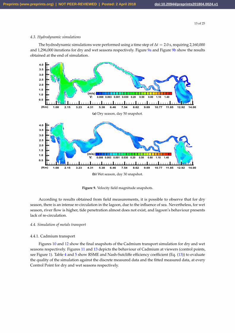
4.3. Hydrodynamic simulations

The hydrodynamic simulations were performed using a time step of ∆t = 2.0 s, requiring 2,160,000and 1,296,000 iterations for dry and wet seasons respectively. Figure 9a and Figure 9b show the resultsobtained at the end of simulation.

V: 1.401.100.800.500.200.0300.008 0.003 0.001

(m/s)

1.08 2.15 3.23 4.31(Km) 5.38 6.46 7.54 8.62 9.69 10.77 11.85 12.92 14.00

0.5

1.0

1.5

2.0

2.5

3.0

3.5

4.0

(a) Dry season, day 50 snapshot.

V: 1.401.100.800.500.200.0300.008 0.003 0.001

(m/s)

1.08 2.15 3.23 4.31(Km) 5.38 6.46 7.54 8.62 9.69 10.77 11.85 12.92 14.00

0.5

1.0

1.5

2.0

2.5

3.0

3.5

4.0

(b) Wet season, day 30 snapshot.

Figure 9. Velocity field magnitude snapshots.

According to results obtained from field measurements, it is possible to observe that for dryseason, there is an intense re-circulation in the lagoon, due to the influence of sea. Nevertheless, for wetseason, river flow is higher, tide penetration almost does not exist, and lagoon’s behaviour presentslack of re-circulation.

4.4. Simulation of metals transport

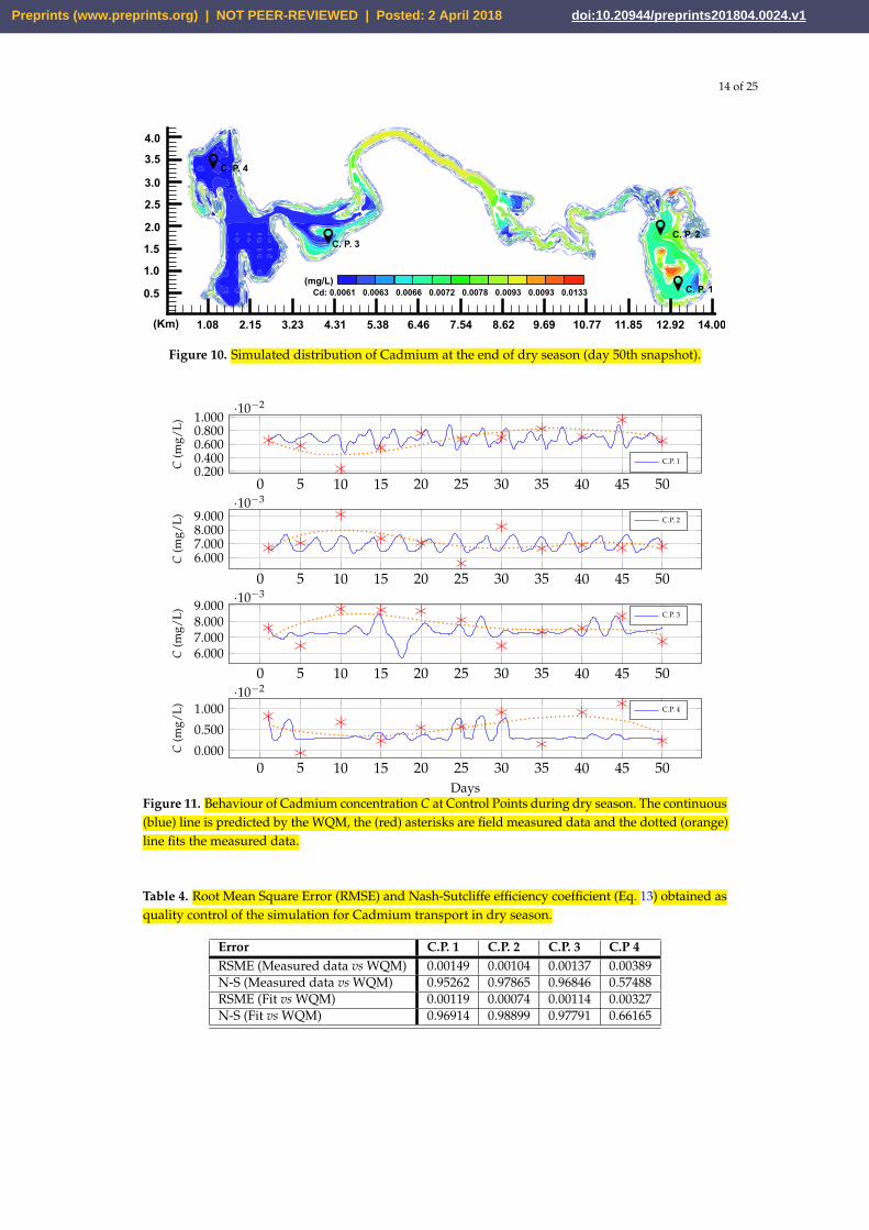
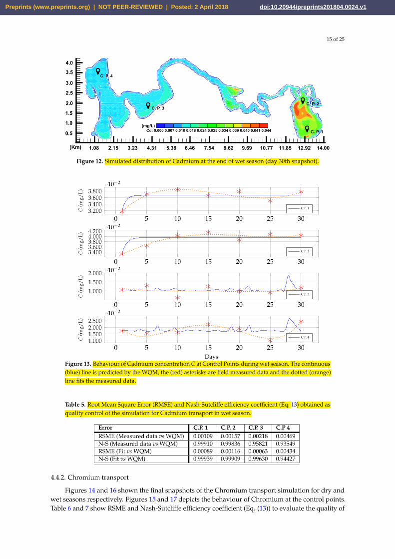
4.4.1. Cadmium transport

Figures 10 and 12 show the final snapshots of the Cadmium transport simulation for dry and wetseasons respectively. Figures 11 and 13 depicts the behaviour of Cadmium at viewers (control points,see Figure 1). Table 4 and 5 show RSME and Nash-Sutcliffe efficiency coefficient (Eq. (13)) to evaluatethe quality of the simulation against the discrete measured data and the fitted measured data, at everyControl Point for dry and wet seasons respectively.



14 of 25

Cd: 0.0061 0.0063 0.0066 0.0072 0.0078 0.0093 0.0093 0.0133 C. P. 1

C. P. 2C. P. 3

C. P. 4

(mg/L)

1.08 2.15 3.23 4.31(Km) 5.38 6.46 7.54 8.62 9.69 10.77 11.85 12.92 14.00

0.5

1.0

1.5

2.0

2.5

3.0

3.5

4.0

Figure 10. Simulated distribution of Cadmium at the end of dry season (day 50th snapshot).

0 5 10 15 20 25 30 35 40 45 500.2000.4000.6000.8001.000

·10−2

C(m

g/L)

C.P. 1

0 5 10 15 20 25 30 35 40 45 506.0007.0008.0009.000

·10−3

C(m

g/L) C.P. 2

0 5 10 15 20 25 30 35 40 45 506.0007.0008.0009.000

·10−3

C(m

g/L) C.P. 3

0 5 10 15 20 25 30 35 40 45 500.000

0.500

1.000·10−2

Days

C(m

g/L) C.P. 4

Figure 11. Behaviour of Cadmium concentration C at Control Points during dry season. The continuous(blue) line is predicted by the WQM, the (red) asterisks are field measured data and the dotted (orange)line fits the measured data.

Table 4. Root Mean Square Error (RMSE) and Nash-Sutcliffe efficiency coefficient (Eq. 13) obtained asquality control of the simulation for Cadmium transport in dry season.

Error C.P. 1 C.P. 2 C.P. 3 C.P 4RSME (Measured data vs WQM) 0.00149 0.00104 0.00137 0.00389N-S (Measured data vs WQM) 0.95262 0.97865 0.96846 0.57488RSME (Fit vs WQM) 0.00119 0.00074 0.00114 0.00327N-S (Fit vs WQM) 0.96914 0.98899 0.97791 0.66165



15 of 25

Cd: 0.000 0.007 0.010 0.018 0.024 0.025 0.034 0.039 0.040 0.041 0.044

(Km)

0.5

1.0

1.5

2.0

2.5

3.0

3.5

4.0

1.08 2.15 3.23 4.31 5.38 6.46 7.54 8.62 9.69 10.77 11.85 12.92 14.00

(mg/L)

C. P. 4

C. P. 3C. P. 2

C. P. 1

Figure 12. Simulated distribution of Cadmium at the end of wet season (day 30th snapshot).

0 5 10 15 20 25 303.2003.4003.6003.800

·10−2

C(m

g/L)

C.P. 1

0 5 10 15 20 25 303.4003.6003.8004.0004.200

·10−2

C(m

g/L)

C.P. 2

0 5 10 15 20 25 30

1.0001.5002.000 ·10−2

C(m

g/L)

C.P. 3

0 5 10 15 20 25 301.0001.5002.0002.500

·10−2

Days

C(m

g/L)

C.P. 4

Figure 13. Behaviour of Cadmium concentration C at Control Points during wet season. The continuous(blue) line is predicted by the WQM, the (red) asterisks are field measured data and the dotted (orange)line fits the measured data.

Table 5. Root Mean Square Error (RMSE) and Nash-Sutcliffe efficiency coefficient (Eq. 13) obtained asquality control of the simulation for Cadmium transport in wet season.


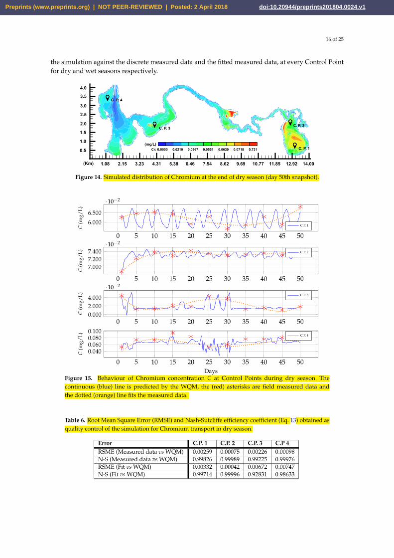
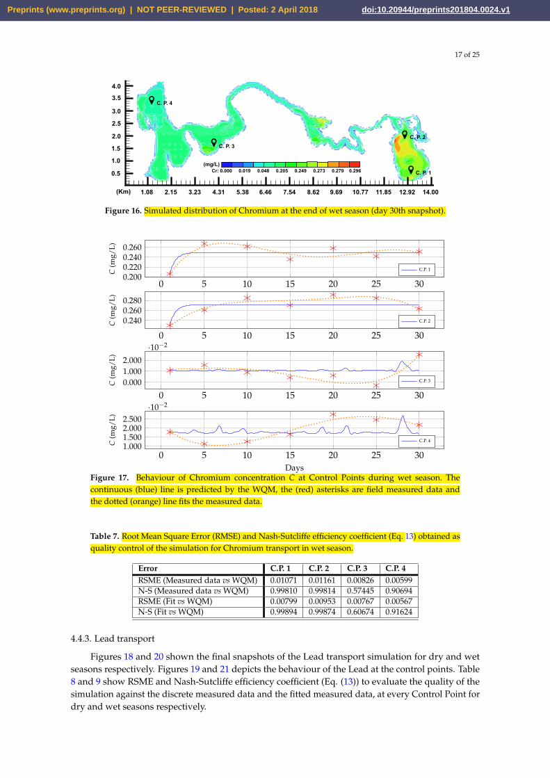
4.4.2. Chromium transport

Figures 14 and 16 shown the final snapshots of the Chromium transport simulation for dry andwet seasons respectively. Figures 15 and 17 depicts the behaviour of Chromium at the control points.Table 6 and 7 show RSME and Nash-Sutcliffe efficiency coefficient (Eq. (13)) to evaluate the quality of



16 of 25

the simulation against the discrete measured data and the fitted measured data, at every Control Pointfor dry and wet seasons respectively.

Cr: 0.0000 0.0210 0.0367 0.0551 0.0639 0.0718 0.731

1.08 2.15 3.23 4.31(Km) 5.38 6.46 7.54 8.62 9.69 10.77 11.85 12.92 14.00

0.5

1.0

1.5

2.0

2.5

3.0

3.5

4.0

(mg/L)C. P. 1

C. P. 2C. P. 3

C. P. 4

Figure 14. Simulated distribution of Chromium at the end of dry season (day 50th snapshot).

0 5 10 15 20 25 30 35 40 45 50

6.000

6.500

·10−2

C(m

g/L)

C.P. 1

0 5 10 15 20 25 30 35 40 45 50

7.0007.2007.400

·10−2

C(m

g/L) C.P. 2

0 5 10 15 20 25 30 35 40 45 500.0002.0004.000

·10−2

C(m

g/L) C.P. 3

0 5 10 15 20 25 30 35 40 45 50

0.0400.0600.0800.100

Days

C(m

g/L) C.P. 4

Figure 15. Behaviour of Chromium concentration C at Control Points during dry season. Thecontinuous (blue) line is predicted by the WQM, the (red) asterisks are field measured data andthe dotted (orange) line fits the measured data.

Table 6. Root Mean Square Error (RMSE) and Nash-Sutcliffe efficiency coefficient (Eq. 13) obtained asquality control of the simulation for Chromium transport in dry season.




17 of 25

Cr: 0.000 0.019 0.048 0.205 0.249 0.273 0.279 0.296

1.08 2.15 3.23 4.31(Km) 5.38 6.46 7.54 8.62 9.69 10.77 11.85 12.92 14.00

0.5

1.0

1.5

2.0

2.5

3.0

3.5

4.0

(mg/L)

C. P. 1

C. P. 2

C. P. 3

C. P. 4

Figure 16. Simulated distribution of Chromium at the end of wet season (day 30th snapshot).

0 5 10 15 20 25 300.2000.2200.2400.260

C(m

g/L)

C.P. 1

0 5 10 15 20 25 30

0.2400.2600.280

C(m

g/L)

C.P. 2

0 5 10 15 20 25 300.0001.0002.000

·10−2

C(m

g/L)

C.P. 3

0 5 10 15 20 25 301.0001.5002.0002.500

·10−2

Days

C(m

g/L)

C.P. 4

Figure 17. Behaviour of Chromium concentration C at Control Points during wet season. Thecontinuous (blue) line is predicted by the WQM, the (red) asterisks are field measured data andthe dotted (orange) line fits the measured data.

Table 7. Root Mean Square Error (RMSE) and Nash-Sutcliffe efficiency coefficient (Eq. 13) obtained asquality control of the simulation for Chromium transport in wet season.

Error C.P. 1 C.P. 2 C.P. 3 C.P. 4RSME (Measured data vs WQM) 0.01071 0.01161 0.00826 0.00599N-S (Measured data vs WQM) 0.99810 0.99814 0.57445 0.90694RSME (Fit vs WQM) 0.00799 0.00953 0.00767 0.00567N-S (Fit vs WQM) 0.99894 0.99874 0.60674 0.91624

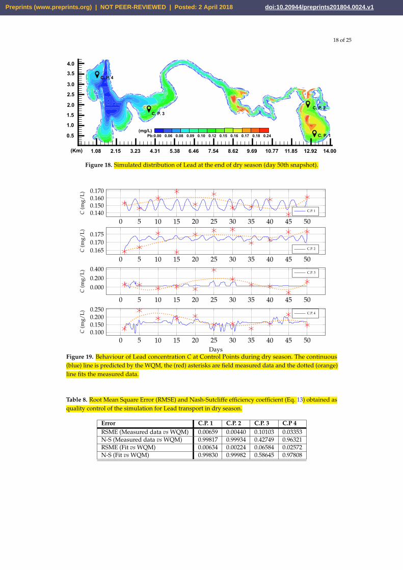
4.4.3. Lead transport

Figures 18 and 20 shown the final snapshots of the Lead transport simulation for dry and wetseasons respectively. Figures 19 and 21 depicts the behaviour of the Lead at the control points. Table8 and 9 show RSME and Nash-Sutcliffe efficiency coefficient (Eq. (13)) to evaluate the quality of thesimulation against the discrete measured data and the fitted measured data, at every Control Point fordry and wet seasons respectively.



18 of 25

Pb:0.00 0.06 0.08 0.09 0.10 0.12 0.15 0.16 0.17 0.18 0.24

1.08 2.15 3.23 4.31(Km) 5.38 6.46 7.54 8.62 9.69 10.77 11.85 12.92 14.00

0.5

1.0

1.5

2.0

2.5

3.0

3.5

4.0

(mg/L)C. P. 1

C. P. 2

C. P. 3

C. P. 4

Figure 18. Simulated distribution of Lead at the end of dry season (day 50th snapshot).

0 5 10 15 20 25 30 35 40 45 500.1400.1500.1600.170

C(m

g/L)

C.P. 1

0 5 10 15 20 25 30 35 40 45 500.1650.1700.175

C(m

g/L)

C.P. 2

0 5 10 15 20 25 30 35 40 45 50

0.0000.2000.400

C(m

g/L) C.P. 3

0 5 10 15 20 25 30 35 40 45 500.1000.1500.2000.250

Days

C(m

g/L) C.P. 4

Figure 19. Behaviour of Lead concentration C at Control Points during dry season. The continuous(blue) line is predicted by the WQM, the (red) asterisks are field measured data and the dotted (orange)line fits the measured data.

Table 8. Root Mean Square Error (RMSE) and Nash-Sutcliffe efficiency coefficient (Eq. 13) obtained asquality control of the simulation for Lead transport in dry season.




19 of 25

Pb: 0.07 0.11 0.12 0.13 0.15 0.19 0.23 0.25 0.26

1.08 2.15 3.23 4.31(Km) 5.38 6.46 7.54 8.62 9.69 10.77 11.85 12.92 14.00

0.5

1.0

1.5

2.0

2.5

3.0

3.5

4.0

(mg/L)

C. P. 1

C. P. 2

C. P. 3

C. P. 4

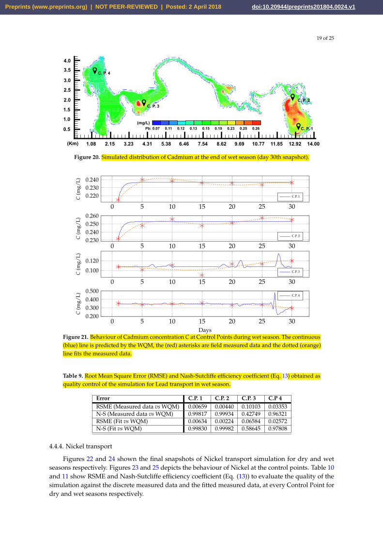
Figure 20. Simulated distribution of Cadmium at the end of wet season (day 30th snapshot).

0 5 10 15 20 25 30

0.2200.2300.240

C(m

g/L)

C.P. 1

0 5 10 15 20 25 300.2300.2400.2500.260

C(m

g/L)

C.P. 2

0 5 10 15 20 25 30

0.100

0.120

C(m

g/L)

C.P. 3

0 5 10 15 20 25 300.2000.3000.4000.500

Days

C(m

g/L) C.P. 4

Figure 21. Behaviour of Cadmium concentration C at Control Points during wet season. The continuous(blue) line is predicted by the WQM, the (red) asterisks are field measured data and the dotted (orange)line fits the measured data.

Table 9. Root Mean Square Error (RMSE) and Nash-Sutcliffe efficiency coefficient (Eq. 13) obtained asquality control of the simulation for Lead transport in wet season.


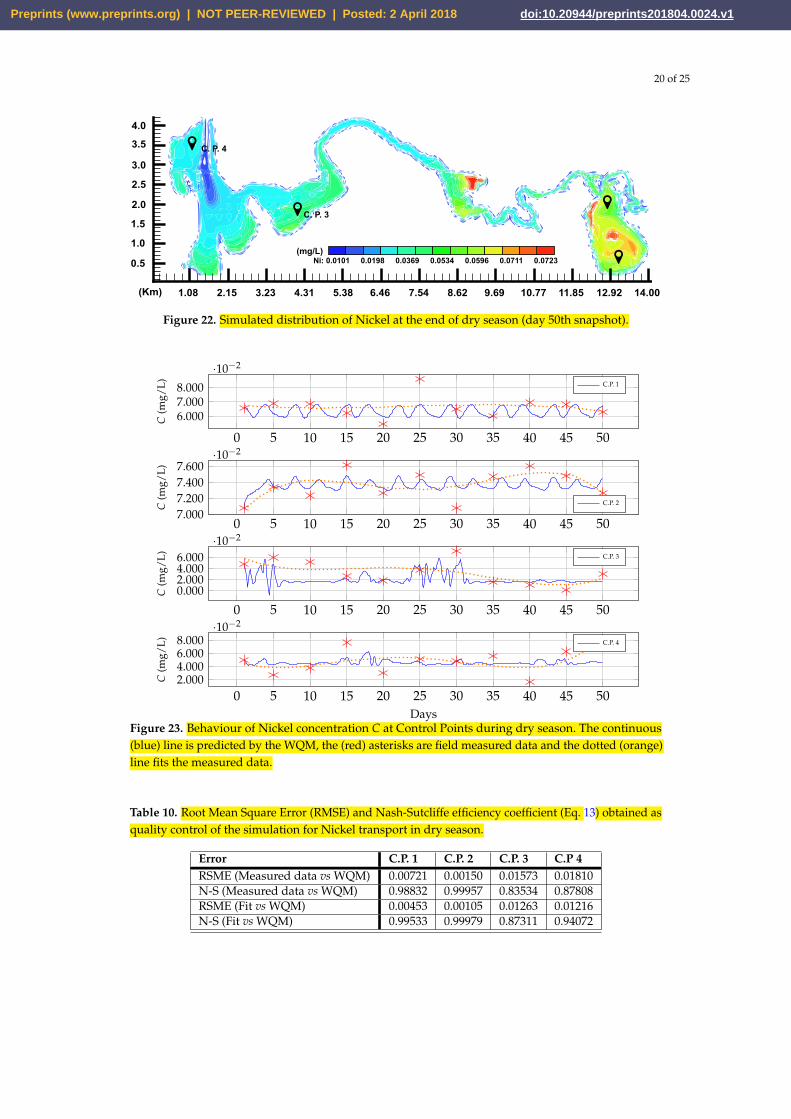
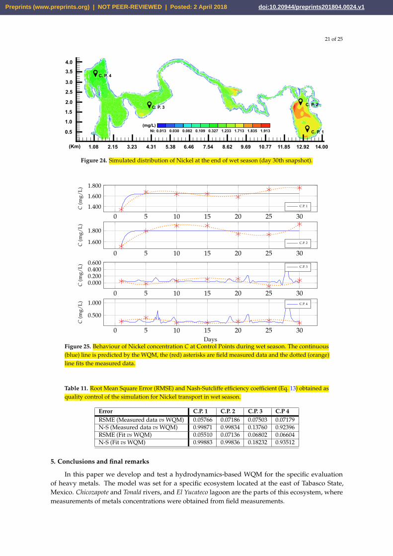
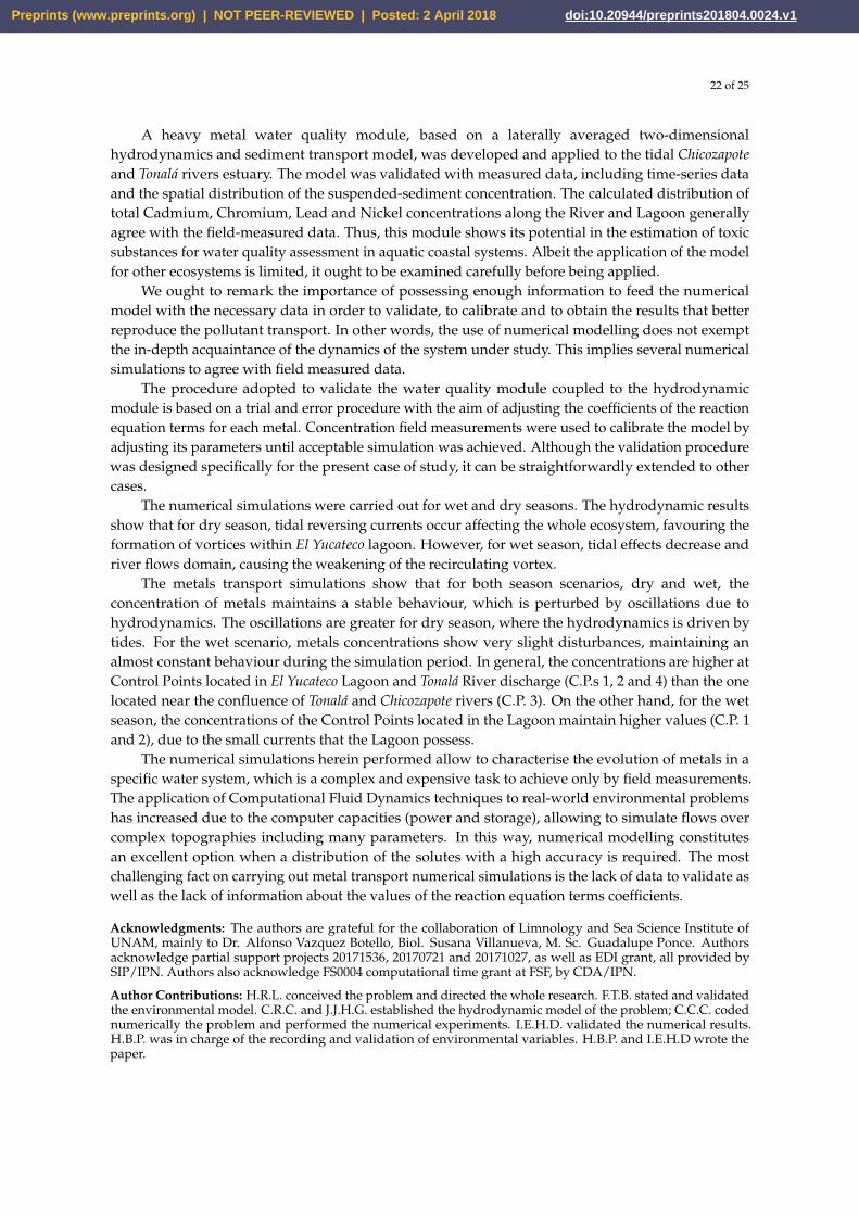
4.4.4. Nickel transport

Figures 22 and 24 shown the final snapshots of Nickel transport simulation for dry and wetseasons respectively. Figures 23 and 25 depicts the behaviour of Nickel at the control points. Table 10and 11 show RSME and Nash-Sutcliffe efficiency coefficient (Eq. (13)) to evaluate the quality of thesimulation against the discrete measured data and the fitted measured data, at every Control Point fordry and wet seasons respectively.



20 of 25

Ni: 0.0101 0.0198 0.0369 0.0534 0.0596 0.0711 0.0723

1.08 2.15 3.23 4.31(Km) 5.38 6.46 7.54 8.62 9.69 10.77 11.85 12.92 14.00

0.5

1.0

1.5

2.0

2.5

3.0

3.5

4.0

(mg/L)

C. P. 4

C. P. 3

Figure 22. Simulated distribution of Nickel at the end of dry season (day 50th snapshot).

0 5 10 15 20 25 30 35 40 45 50

6.0007.0008.000

·10−2

C(m

g/L) C.P. 1

0 5 10 15 20 25 30 35 40 45 507.0007.2007.4007.600

·10−2

C(m

g/L)

C.P. 2

0 5 10 15 20 25 30 35 40 45 500.0002.0004.0006.000

·10−2

C(m

g/L) C.P. 3

0 5 10 15 20 25 30 35 40 45 502.0004.0006.0008.000

·10−2

Days

C(m

g/L) C.P. 4

Figure 23. Behaviour of Nickel concentration C at Control Points during dry season. The continuous(blue) line is predicted by the WQM, the (red) asterisks are field measured data and the dotted (orange)line fits the measured data.

Table 10. Root Mean Square Error (RMSE) and Nash-Sutcliffe efficiency coefficient (Eq. 13) obtained asquality control of the simulation for Nickel transport in dry season.




21 of 25

Ni: 0.013 0.030 0.082 0.109 0.327 1.233 1.713 1.835 1.913

1.08 2.15 3.23 4.31(Km) 5.38 6.46 7.54 8.62 9.69 10.77 11.85 12.92 14.00

0.5

1.0

1.5

2.0

2.5

3.0

3.5

4.0

(mg/L)

C. P. 1

C. P. 2C. P. 3

C. P. 4

Figure 24. Simulated distribution of Nickel at the end of wet season (day 30th snapshot).

0 5 10 15 20 25 301.400

1.600

1.800

C(m

g/L)

C.P. 1

0 5 10 15 20 25 30

1.600

1.800

C(m

g/L)

C.P. 2

0 5 10 15 20 25 30

0.0000.2000.4000.600

C(m

g/L) C.P. 3

0 5 10 15 20 25 30

0.500

1.000

Days

C(m

g/L) C.P. 4

Figure 25. Behaviour of Nickel concentration C at Control Points during wet season. The continuous(blue) line is predicted by the WQM, the (red) asterisks are field measured data and the dotted (orange)line fits the measured data.

Table 11. Root Mean Square Error (RMSE) and Nash-Sutcliffe efficiency coefficient (Eq. 13) obtained asquality control of the simulation for Nickel transport in wet season.


5. Conclusions and final remarks

In this paper we develop and test a hydrodynamics-based WQM for the specific evaluationof heavy metals. The model was set for a specific ecosystem located at the east of Tabasco State,Mexico. Chicozapote and Tonalá rivers, and El Yucateco lagoon are the parts of this ecosystem, wheremeasurements of metals concentrations were obtained from field measurements.



22 of 25

A heavy metal water quality module, based on a laterally averaged two-dimensionalhydrodynamics and sediment transport model, was developed and applied to the tidal Chicozapoteand Tonalá rivers estuary. The model was validated with measured data, including time-series dataand the spatial distribution of the suspended-sediment concentration. The calculated distribution oftotal Cadmium, Chromium, Lead and Nickel concentrations along the River and Lagoon generallyagree with the field-measured data. Thus, this module shows its potential in the estimation of toxicsubstances for water quality assessment in aquatic coastal systems. Albeit the application of the modelfor other ecosystems is limited, it ought to be examined carefully before being applied.

We ought to remark the importance of possessing enough information to feed the numericalmodel with the necessary data in order to validate, to calibrate and to obtain the results that betterreproduce the pollutant transport. In other words, the use of numerical modelling does not exemptthe in-depth acquaintance of the dynamics of the system under study. This implies several numericalsimulations to agree with field measured data.

The procedure adopted to validate the water quality module coupled to the hydrodynamicmodule is based on a trial and error procedure with the aim of adjusting the coefficients of the reactionequation terms for each metal. Concentration field measurements were used to calibrate the model byadjusting its parameters until acceptable simulation was achieved. Although the validation procedurewas designed specifically for the present case of study, it can be straightforwardly extended to othercases.

The numerical simulations were carried out for wet and dry seasons. The hydrodynamic resultsshow that for dry season, tidal reversing currents occur affecting the whole ecosystem, favouring theformation of vortices within El Yucateco lagoon. However, for wet season, tidal effects decrease andriver flows domain, causing the weakening of the recirculating vortex.

The metals transport simulations show that for both season scenarios, dry and wet, theconcentration of metals maintains a stable behaviour, which is perturbed by oscillations due tohydrodynamics. The oscillations are greater for dry season, where the hydrodynamics is driven bytides. For the wet scenario, metals concentrations show very slight disturbances, maintaining analmost constant behaviour during the simulation period. In general, the concentrations are higher atControl Points located in El Yucateco Lagoon and Tonalá River discharge (C.P.s 1, 2 and 4) than the onelocated near the confluence of Tonalá and Chicozapote rivers (C.P. 3). On the other hand, for the wetseason, the concentrations of the Control Points located in the Lagoon maintain higher values (C.P. 1and 2), due to the small currents that the Lagoon possess.

The numerical simulations herein performed allow to characterise the evolution of metals in aspecific water system, which is a complex and expensive task to achieve only by field measurements.The application of Computational Fluid Dynamics techniques to real-world environmental problemshas increased due to the computer capacities (power and storage), allowing to simulate flows overcomplex topographies including many parameters. In this way, numerical modelling constitutesan excellent option when a distribution of the solutes with a high accuracy is required. The mostchallenging fact on carrying out metal transport numerical simulations is the lack of data to validate aswell as the lack of information about the values of the reaction equation terms coefficients.

Acknowledgments: The authors are grateful for the collaboration of Limnology and Sea Science Institute ofUNAM, mainly to Dr. Alfonso Vazquez Botello, Biol. Susana Villanueva, M. Sc. Guadalupe Ponce. Authorsacknowledge partial support projects 20171536, 20170721 and 20171027, as well as EDI grant, all provided bySIP/IPN. Authors also acknowledge FS0004 computational time grant at FSF, by CDA/IPN.

Author Contributions: H.R.L. conceived the problem and directed the whole research. F.T.B. stated and validatedthe environmental model. C.R.C. and J.J.H.G. established the hydrodynamic model of the problem; C.C.C. codednumerically the problem and performed the numerical experiments. I.E.H.D. validated the numerical results.H.B.P. was in charge of the recording and validation of environmental variables. H.B.P. and I.E.H.D wrote thepaper.



23 of 25

Conflicts of Interest: The authors declare no conflict of interest. The founding sponsors had no role in the designof the study; in the collection, analyses, or interpretation of data; in the writing of the manuscript, and in thedecision to publish the results.

References

1. Kavcar, P.; Sofuoglu, A.; Sofuoglu, S.C. A health risk assessment for exposure to trace metals via drinkingwater ingestion pathway. International Journal of Hygiene and Environmental Health 2009, 212, 216 – 227.

2. Mahato, M.K.; Singh, P.K.; Tiwari, A.K.; Singh, A.K. Risk Assessment Due to Intake of Metals inGroundwater of East Bokaro Coalfield, Jharkhand, India. Exposure and Health 2016, 8, 265–275.

3. Cao, S.; Duan, X.; Zhao, X.; Chen, Y.; Wang, B.; Sun, C.; Zheng, B.; Wei, F. Health risks of children’scumulative and aggregative exposure to metals and metalloids in a typical urban environment in China.Chemosphere 2016, 147, 404 – 411.

4. Zhang, L.; Qin, Y.w.; Ma, Y.q.; Zhao, Y.m.; Shi, Y. [Spatial distribution and pollution assessment of heavymetals in the tidal reach and its adjacent sea estuary of Daliaohe area, China ]. Huan jing ke xue= Huanjingkexue 2014, 35, 3336—3345.

5. Klavins, M.; Briede, A.; Rodinov, V.; Kokorite, I.; Parele, E.; Klavina, I. Heavy metals in rivers of Latvia.Science of The Total Environment 2000, 262, 175 – 183.

6. Manning, A.; Langston, W.; Jonas, P. A review of sediment dynamics in the Severn Estuary: influence offlocculation. Marine Pollution Bulletin 2010, 61, 37–51.

7. Erikson, L.; Wright, S.; Elias, E.; Hanes, D.; Schoellhamer, D.; Largier, J. The use of modeling and suspendedsediment concentration measurements for quantifying net suspended sediment transport through a largetidally dominated inlet. Marine Geology 2013, 345, 96–112.

8. Caruso, B. Simulation of metals total maximum daily loads and remediation in a mining-impacted stream.Journal of Environmental Engineering 2005, 131, 777–789.

9. Winterwerp, J. On the flocculation and settling velocity of estuarine mud. Continental shelf research 2002,22, 1339–1360.

10. Sholkovitz, E.R. The flocculation of dissolved Fe, Mn, Al, Cu, Ni, Co and Cd during estuarine mixing.Earth and Planetary Science Letters 1978, 41, 77 – 86.

11. Helali, M.; Oueslati, W.; Zaaboub, N.; Added, A.; Aleya, L. Chemical speciation of Fe, Mn, Pb, Zn, Cd,Cu, Co, Ni and Cr in the suspended particulate matter off the Mejerda River Delta (Gulf of Tunis, Tunisia).Journal of African Earth Sciences 2016, 118, 35–44.

12. Karbassi, A.; Nadjafpour, S. Flocculation of dissolved Pb, Cu, Zn and Mn during estuarine mixing of riverwater with the Caspian Sea. Environmental Pollution 1996, 93, 257 – 260.

13. James, I. Modelling pollution dispersion, the ecosystem and water quality in coastal waters: A review.Environmental Modelling and Software 2002, 17, 363–385.

14. Sun, J.; Wang, Z.; Li, R.; Ma, D.; Liu, B. Simulation of metal contents through correlated optimal monitoringmetals of Dagu river sediments. Procedia Environmental Sciences 2011, 8, 161–165.

15. Pintilie, S.; Branza, L.; Betianu, C.; Pavel, L.V.; Ungureanu, F.; Gavrilescu, M. MODELLING ANDSIMULATION OF HEAVY METALS TRANSPORT IN WATER AND SEDIMENTS. EnvironmentalEngineering & Management Journal (EEMJ) 2007, 6.

16. Nguyen, T.T.H.; Zhang, W.; Li, Z.; Li, J.; Ge, C.; Liu, J.; Bai, X.; Feng, H.; Yu, L. Assessment of heavy metalpollution in Red River surface sediments, Vietnam. Marine Pollution Bulletin 2016, 113, 513 – 519.

17. Zhang, Y.; Chu, C.; Li, T.; Xu, S.; Liu, L.; Ju, M. A water quality management strategy for regionallyprotected water through health risk assessment and spatial distribution of heavy metal pollution in 3marine reserves. Science of The Total Environment 2017, 599, 721 – 731.

18. Blessing, N.; Benedict, S. Computing principles in formulating water quality informatics and indexingmethods: An ample review. Journal of Computational and Theoretical Nanoscience 2017, 14, 1671–1681.

19. Chau, K. Selection and calibration of numerical modeling in flow and water quality. EnvironmentalModeling and Assessment 2004, 9, 169–178.

20. Canham, C.D.W.; Cole, J.; Lauenroth, W.K. Models in ecosystem science; Princeton University Press, 2003.21. Thomann, R.V.; Mueller, J.A. Principles of surface water quality modeling and control; Harper & Row, Publishers,

1987.



24 of 25

22. Thomann, R.V. The future “golden age” of predictive models for surface water quality and ecosystemmanagement. Journal of environmental engineering 1998, 124, 94–103.

23. Lun, R.; Lee, K.; De Marco, L.; Nalewajko, C.; Mackay, D. A model of the fate of polycyclic aromatichydrocarbons in the Saguenay Fjord, Canada. Environmental toxicology and chemistry 1998, 17, 333–341.

24. Ji, Z.G.; Hamrick, J.H.; Pagenkopf, J. Sediment and metals modeling in shallow river. Journal ofEnvironmental Engineering 2002, 128, 105–119.

25. Shimazu, H.; Ohnishi, E.; Ozaki, N.; Fukushima, T.; Nakasugi, O. A model for predicting sediment-waterpartition of toxic chemicals in aquatic environments. Water science and technology 2002, 46, 437–442.

26. Bhavsar, S.P.; Diamond, M.L.; Evans, L.J.; Gandhi, N.; Nilsen, J.; Antunes, P. Development of a coupledmetal speciation-fate model for surface aquatic systems. Environmental toxicology and chemistry 2004,23, 1376–1385.

27. Kim, C.; Lim, H.; Cerco, C. Three-dimensional water quality modelling for tidal lake and coastal waterswith ROMS-ICM. Journal of Coastal Research 2011, p. 1068.

28. Sharma, D.; Kansal, A. Assessment of river quality models: a review. Reviews in Environmental Science andBio/Technology 2013, 12, 285–311.

29. Wang, Q.; Li, S.; Jia, P.; Qi, C.; Ding, F. A review of surface water quality models. The Scientific World Journal2013, 2013.

30. Chapman, B.M. Numerical simulation of the transport and speciation of nonconservative chemicalreactants in rivers. Water Resources Research 1982, 18, 155–167.

31. Herrera-Díaz, I.; Rodríguez-Cuevas, C.; Couder-Castañeda, C.; Gasca-Tirado, J. Numericalhydrodynamic-hydrological modeling in flood zones containing infrastructure [Modelación numéricahidrodinámico-hidrológica en zonas de inundación con presencia de infraestructura]. Tecnologia y Cienciasdel Agua 2015, 6, 139–152.

32. Barrios-Piña, H.; Ramírez-León, H.; Rodríguez-Cuevas, C.; Couder-Castañeda, C. Multilayer numericalmodeling of flows through vegetation using a mixing-length turbulence model. Water (Switzerland) 2014,6, 2084–2103.

33. Ramírez-León, H.; Couder-Castañeda, C.; Herrera-Díaz, I.; Barrios-Piña, H. Numerical modeling of thethermal discharge of the Laguna Verde power station [Modelación numérica de la descarga térmica de laCentral Nucleoeléctrica Laguna Verde]. Revista Internacional de Metodos Numericos para Calculo y Diseno enIngenieria 2013, 29, 114–121.

34. Ramírez-León, H.; Barrios-Piña, H.; Torres-Bejarano, F.; Cuevas-Otero, A.; Rodríguez-Cuevas, C. Numericalmodelling of the laguna verde nuclear power station thermal plume discharge to the sea. Communicationsin Computer and Information Science 2016, 595, 495–507.

35. León, H.; Piña, H.; Cuevas, C.; Castañeda, C. Baroclinic mathematical modeling of fresh water plumes inthe interaction river-sea. International Journal of Numerical Analysis and Modeling 2005, 2, 1–14.

36. Rodriguez-Cuevas, C.; Couder-Castañeda, C.; Flores-Mendez, E.; Herrera-Díaz, I.; Cisneros-Almazan, R.Modelling shallow water wakes using a hybrid turbulence model. Journal of Applied Mathematics 2014,2014.

37. Ambrose Jr, R.B.; Wool, T.A.; Barnwell Jr, T.O. Development of Water Quality Modelingin the United States.Environmental Engineering Research 2009, 14, 200–210.

38. Kannel, P.R.; Kanel, S.R.; Lee, S.; Lee, Y.S.; Gan, T.Y. A review of public domain water quality models forsimulating dissolved oxygen in rivers and streams. Environmental Modeling & Assessment 2011, 16, 183–204.

39. Campbell, P.G.; Gailer, J. Effects of non-essential metal releases on the environment and human health. InMetal Sustainability: Global Challenges, Consequences, and Prospects; John Wiley & Sons, 2016; Vol. 221.

40. Yáñez-Arancibia, A.; Day, J.W. The Gulf of Mexico: towards an integration of coastal management withlarge marine ecosystem management. Ocean & Coastal Management 2004, 47, 537–563.

41. Botello, A.V. Monitoreo ambiental integral de los impactos de la actividad petrolera en la laguna ElYucateco, Tabasco, México. Segundo Informe técnico. Technical report, ICMyL, UNAM, 2004.

42. Eaton, A.; Franson, M.; Association, A.P.H.; Association, A.W.W.; Federation, W.E. Standard Methods forthe Examination of Water & Wastewater; Standard Methods for the Examination of Water and Wastewater,American Public Health Association, 2005.

43. Cámara de Diputados del H. Congreso de la Unión. DOF (Diario Oficial de la Federación), 2005. FederalRights Law of Mexico.



25 of 25

44. Canadian Council of Ministers of the Environment. Canadian Sediment Quality Guidelines for theProtection of Aquatic Life. In Canadian Environmental Quality Guidelines; Number 1299, Canadian Councilof Ministers of the Environment, 2002.

45. Thomann, R.; Salas, H. Modelos del destino de sustancias tóxicas. In Manual de evaluación y manejo desustancias tóxicas en aguas superficiales; CEPIS-OMS, 1988.

46. Mackay, D. Environmental and laboratory rates of volatilization of toxic chemicals from water. HazardAssessment of Chemicals: Current Developments 1981, 1.

47. Di Toro, D.M.; O’Connor, D.J.; Thomann, R.V.; St John, J.P. Analysis of fate of chemicals in receiving waters,Phase 1. In Analysis of fate of chemicals in receiving waters, phase 1; HydroQual, Inc, 1981.

48. Hawley, N. Settling velocity distribution of natural aggregates. Journal of Geophysical Research: Oceans 1982,87, 9489–9498.

49. Thomann, R.V.; Di Toro, D.M. Physico-chemical model of toxic substances in the Great Lakes. Journal ofGreat Lakes Research 1983, 9, 474–496.

50. Imberger, J.; dl Silvio, G. Mixing processes in a shallow lagoon. In Coastal Engineering 1992; 1993; pp.1867–1868.

51. Tsanis, I.; Wu, J.; Shen, H.; Valeo, C. Environmental hydraulics: hydrodynamic and pollutant transport models oflakes and coastal waters; Vol. 56, Elsevier, 2007.

52. Casulli, V.; Cheng, R.T. Semi-implicit finite difference methods for three dimentional shallow water flow.Int. J. for Numer. Methods in Fluids. 1992, 15, 629–648.

53. Horritt, M. Parameterisation, validation and uncertainty analysis of CFD models of fluvial and floodhydraulics in the natural environment. Computational fluid dynamics: applications in environmental hydraulics2005, pp. 193–213.

54. Brocchini, M.; Calantoni, J.; Postacchini, M.; Sheremet, A.; Staples, T.; Smith, J.; Reed, A.H.; Braithwaite,E.F.; Lorenzoni, C.; Russo, A.; others. Comparison between the wintertime and summertime dynamics ofthe Misa River estuary. Marine Geology 2017, 385, 27–40.

55. Dong, L.; Su, J.; Wong, L.A.; Cao, Z.; Chen, J.C. Seasonal variation and dynamics of the Pearl River plume.Continental Shelf Research 2004, 24, 1761–1777.

56. Herrera-Díaz, I.; Torres-Bejarano, F.; Moreno-Martínez, J.; Rodriguez-Cuevas, C.; Couder-Castañeda, C.Light Particle Tracking Model for Simulating Bed Sediment Transport Load in River Areas. MathematicalProblems in Engineering 2017, 2017.

57. Van Maren, D.; Hoekstra, P. Seasonal variation of hydrodynamics and sediment dynamics in a shallowsubtropical estuary: the Ba Lat River, Vietnam. Estuarine, Coastal and Shelf Science 2004, 60, 529–540.

58. Yáñez-Arancibia, A.; Day, J.W. Environmental sub-regions in the Gulf of Mexico coastal zone: the ecosystemapproach as an integrated management tool. Ocean & Coastal Management 2004, 47, 727–757.



Documents

Modelling, Transport and Assessment of Aquatic Toxic