Embed Size (px)
Citation preview

Biogeosciences, 6, 1539–1561, 2009www.biogeosciences.net/6/1539/2009/© Author(s) 2009. This work is distributed underthe Creative Commons Attribution 3.0 License.
Biogeosciences
pH modelling in aquatic systems with time-variable acid-basedissociation constants applied to the turbid, tidal Scheldt estuary
A. F. Hofmann1, J. J. Middelburg1,3, K. Soetaert1, and F. J. R. Meysman2
1Netherlands Institute of Ecology (NIOO-KNAW), Centre for Estuarine and Marine Ecology, P.O. Box 140, 4400 ACYerseke, The Netherlands2Laboratory of Analytical and Environmental Chemistry, Earth System Sciences research unit, Vrije Universiteit Brussel(VUB), Pleinlaan 2, 1050 Brussel, Belgium3Faculty of Geosciences, Utrecht University, P.O. Box 80021, 3508 TA Utrecht, The Netherlands
Received: 16 October 2008 – Published in Biogeosciences Discuss.: 7 January 2009Revised: 22 July 2009 – Accepted: 5 August 2009 – Published: 7 August 2009
Abstract. A new pH modelling approach is presented thatexplicitly quantifies the influence of biogeochemical pro-cesses on proton cycling and pH in an aquatic ecosystem, andwhich accounts for time variable acid-base dissociation con-stants. As a case study, the method is applied to investigateproton cycling and long-term pH trends in the Scheldt estu-ary (SW Netherlands, N Belgium). This analysis identifiesthe dominant biogeochemical processes involved in protoncycling in this heterotrophic, turbid estuary. Furthermore, in-formation on the factors controlling the longitudinal pH pro-file along the estuary as well as long-term pH changes areobtained. Proton production by nitrification is identified asthe principal biological process governing the pH. Its acid-ifying effect is mainly counteracted by proton consumptiondue to CO2 degassing. Overall, CO2 degassing generates thelargest proton turnover in the whole estuary on a yearly basis.The main driver of long-term changes in the mean estuarinepH over the period 2001 to 2004 is the decreasing freshwa-ter flow, which influences the pH directly via a decreasingsupply of dissolved inorganic carbon and alkalinity, and alsoindirectly, via decreasing ammonia loadings and lower nitri-fication rates.
1 Introduction
pH is often considered a master variable for the chemicalstate of aquatic ecosystems, since almost any process af-fects pH either directly or indirectly (e.g.Stumm and Mor-
Correspondence to:A. F. Hofmann([email protected])
gan, 1996; Morel and Hering, 1993). But as a result of thiscomplex interplay of different processes, we only have lim-ited understanding of the factors controlling the pH of nat-ural waters (the water column of rivers, lakes, and oceans,as well as the pore water of sediments). Given the ongoingacidification of the surface ocean (e.g.Orr et al., 2005) andcoastal seas (e.g.Blackford and Gilbert, 2007), and the largeimpact that future pH changes may have on biogeochemicalprocesses and organisms (e.g.Gazeau et al., 2007; Guinotteand Fabry, 2008), it is desirable to obtain a better quantitativeunderstanding of factors that regulate pH in natural aquaticsystems. This requires modelling tools, which basically sat-isfy two criteria: (1) models should be able to accurately pre-dict the time evolution of pH under certain biogeochemicalscenarios, and (2) models should be able to assess the con-tribution of individual biogeochemical processes in observedpH changes.
The first aspect has received quite some attention overthe last two decades. A number of modelling approacheshave been presented that allow to predict the time evolutionof pH in aquatic ecosystems (e.g.Boudreau and Canfield,1988; Regnier et al., 1997; Vanderborght et al., 2002; Hof-mann et al., 2008b). The second aspect, however, has re-ceived far less attention. Improving and extending previouswork byJourabchi et al.(2005) andSoetaert et al.(2007), wehave recently presented an extension of the conventional pHmodelling approach, developing a procedure that allows toquantify how different biogeochemical processes contributeto the overall proton cycling in an aquatic ecosystem (Hof-mann et al., 2008a). This method basically splits the totalrate of change of protons into individual contributions of theprocesses that are driving the pH change (details are given
Published by Copernicus Publications on behalf of the European Geosciences Union.

1540 A. F. Hofmann et al.: pH modelling with time variable acid-base constants
Fig. 1. The Scheldt estuary. Gray dots represent positions in the river where longitudinal profiles of influences of processes on pH, presentedin the Results section, show interesting features.
below). However, our original presentation contained an im-portant restriction: acid-base dissociation constants were as-sumed to remain constant in time. Although this assumptionis reasonable in some aquatic systems, it is not valid in en-vironments that experience substantial temporal changes intemperature and salinity.
One such environment where temporal variability in salin-ity and temperature may strongly affect pH are estuaries.Estuarine systems are characterized by pronounced salin-ity gradients, marked seasonality, a large exchange of CO2with the atmosphere, and intensive biogeochemical process-ing (Soetaert et al., 2006; Regnier et al., 1997; Vanderborghtet al., 2002). This makes them suitable (though demanding)testbeds for pH modelling methods. Hence, this study hastwo main objectives: (1) the extension of the pH modellingapproach presented byHofmann et al.(2008a) such that itcan be applied to systems where the dissociation constantsare variable over time, and (2) the validation of this approachfor an estuarine system (the Scheldt estuary). We will com-pare calculated pH values with available data, quantify theproton production or consumption due to different processes(advective-dispersive transport, CO2 air-water exchange, pri-mary production, nitrification etc.), and investigate the fac-tors that are responsible for the observed trend in the meanestuarine pH over the years 2001 to 2004.
2 Materials and methods
2.1 The Scheldt estuary
The turbid, tidal Scheldt estuary forms the end part of theScheldt river (Fig.1), which is about 350 km long in to-tal and drains a basin of 21 500 km2 in the northwest ofFrance, the northern part of Belgium and the southwest of theNetherlands (Soetaert et al., 2006). The model domain hereincludes the final stretch of river, located between the up-stream boundary at Rupelmonde (river km 0) and the down-stream boundary at Vlissingen (river km 104). Water move-ment in the Scheldt estuary is dominated by large tidal dis-placements. The volume of water that enters during floodtide at the downstream boundary of the estuary is 200 timeslarger than the freshwater discharge integrated over a wholetidal cycle at the upstream boundary (Vanderborght et al.,2007). Yearly averaged, the freshwater discharge is around100 m3 s−1 (Heip, 1988). The cross sectional area of the es-tuarine channel shows a regular trumpet-like shape, grad-ually widening from around 4000 m2 upstream to around75 000 m2 downstream (Soetaert et al., 2006). The meanwater depth varies irregularly between values of 6 m and14 m with the deepest areas located towards the downstreamboundary (Soetaert and Herman, 1995). The estuary has atotal tidally averaged volume of 3.62 km3 and a total tidallyaveraged surface area of 338 km2 (Soetaert et al., 2006;Soetaert and Herman, 1995).
Biogeosciences, 6, 1539–1561, 2009 www.biogeosciences.net/6/1539/2009/
A. F. Hofmann et al.: pH modelling with time variable acid-base constants 1541
Table 1. Biogeochemical processes included in the model formulation. Process rates:ROx=oxic mineralisation,RDen=denitrification,RNit=nitrification,RPP=primary production.γ denotes the C/N ratio of organic matter:γ =4 for the reactive organic matter fraction,γ =12for the refractory fraction.pN denotes the fraction of NH+4 in the total DIN uptake of primary production.
ROx : (CH2O)γ (NH3)+γ O2 → NH3+γ CO2+γ H2ORDen: (CH2O)γ (NH3)+0.8γ NO−
3 + 0.8γ H+→ NH3+γ CO2+0.4γ N2 ↑ +1.4γ H2O
RNit : NH3+2 O2 → NO−
3 +H2O+H+
RPP : pNNH+
4 + (1 − pN) NO−
3 + γ CO2 + (1 + γ − pN) H2O → (CH2O)γ (NH3) + (2 + γ − 2pN) O2 + (2pN − 1) H+
2.2 Biogeochemical model formulation
Hofmann et al.(2008b) provided a detailed model assess-ment of the carbon and nitrogen cycling in the Scheldt es-tuary. Their model and results provide a solid basis andare used as a starting point. The one-dimensional reactivetransport model here incorporates the same biogeochemi-cal reaction set, and uses the same forcings and kinetic de-scriptions of process rates as inHofmann et al.(2008b).The biogeochemical reaction set accounts for oxic mineral-isation, denitrification, nitrification, and primary productionwith stoichiometries as given in Table1 (for details seeHof-mann et al., 2008b). Furthermore, the model includes twophysical transport processes: the exchange of carbon diox-ide and oxygen across the air-water interface and advective-dispersive transport of dissolved constituents. The modeltracks the concentration of twelve chemical species in to-tal. Organic matter is split into a reactive (FastOM) and arefractory (SlowOM) fraction, thus leading to two separaterates for oxic mineralisation and denitrification. The result-ing mass balance equations for all state variables are given inTable2. More detailed information on the model formulationcan be found inHofmann et al.(2008b).
We deliberately did not change the design and parameter-ization of the model presented inHofmann et al.(2008b) toshow that the pH modelling procedure presented here canbe implemented as an extension to existing biogeochemicalmodels. The only, but important, difference between the twomodel implementations is the pH calculation procedure (asexplained below).
Seven acid-base equilibria are accounted for in the pH cal-culations (Table3). The respective dissociation constants(K∗’s) are calculated as functions of salinity (S), tempera-ture (T ) and hydrostatic pressure (P ). Salinity and tempera-ture may vary over time, while the mean estuarine depth, andso the hydrostatic pressure, remains constant over time. The(S,T ,P ) relations that have been reported for the dissociationconstants in the literature differ in their associated pH scale(Dickson, 1984). Before being used in the model calcula-tions, all dissociation constants are systematically convertedto the free pH scale.
2.3 Data set and model parameterization
Data on state variables, model parameters and process rateswere collected from various sources and spanned the fouryear period 2001–2004. Monthly values of the dischargeat the upstream boundary were obtained from the Ministryof the Flemish Community (MVG). Percental flow increasesalong the estuary were obtained from the SAWES model (vanGils et al., 1993; Holland, 1991) and are used to calculate thelateral input along the estuary as percentages of the upstreamflow. These percentages have been assumed constant in time.The average water depthsD of the 13 boxes in the Scheldtmodel MOSES fromSoetaert and Herman(1995) were in-terpolated to the 100 model boxes used here. The cross sec-tional area along the estuary was specified as a continuousfunction of the distance along the estuary (river kilometres)as given inSoetaert et al.(2006).
Data for [∑
NH+
4 ], [NO−
3 ], [O2], organic matter, pH(on the NBS scale), temperature and salinity were ob-tained for 16 stations between the upstream boundary atRupelmonde (Belgium) and the downstream boundary atBreskens/Vlissingen (The Netherlands) by monthly cruisesof the RV “Luctor” from the Netherlands Institute of Ecol-ogy (NIOO).
The model requires suitable boundary values for each statevariable at the upstream and downstream boundary. For [O2],[∑
NH+
4 ], [NO−
3 ], [OM], temperature and salinity, data col-lected at the monitoring station close to Breskens were takenas downstream boundary conditions. Similar data collectedat the monitoring station close to Rupelmonde were usedas upstream boundary conditions. The boundary values for[∑
HSO−
4 ], [∑
HF] and[∑
B(OH)3] were estimated fromsalinity at the boundaries assuming standard seawater pro-portions.
One problem was that suitable boundary value data wereavailable for pH, but not for dissolved inorganic carbon([∑
CO2]) or total alkalinity ([TA]). However, [TA] datawere obtained for the year 2003 for various stations withinthe estuary from Frederic Gazeau (personal communicationandGazeau et al., 2005). We used these [TA] data togetherwith the pH boundary data in an inverse way to calibratethe [
∑CO2] boundary conditions for the year 2003. Start-
ing from an initial guess for the [∑
CO2] boundary val-ues, model predicted [TA] values were compared with the
www.biogeosciences.net/6/1539/2009/ Biogeosciences, 6, 1539–1561, 2009

1542 A. F. Hofmann et al.: pH modelling with time variable acid-base constants
Table 2. Mass balance equations for the state variables in the model.ROx FastOMandROx SlowOMare the reaction rates of oxic mineralisationfor the reactive and refractory organic matter fraction respectively. Similarly,RDen FastOM, RDen SlowOM, RNit , andRPP are the rates ofdenitrification, nitrification and primary production.EC andTr C express the air-water exchange and advective-dispersive transport rates ofthe respective chemical species. [TA] denotes total alkalinity.
d[FastOM]
dt= Tr FastOM−ROxFastOM−RDenFastOM+RPP
d[SlowOM]
dt= Tr SlowOM−ROxSlowOM−RDenSlowOM
d[DOC]
dt= Tr DOC
d[O2]
dt= Tr O2+EO2 − ROxCarb− 2RNit+(2−2pN) RPP+RPPCarb
d[NO−
3 ]
dt= Tr NO−
3− 0.8RDenCarb+RNit − (1 − pN) RPP
d[S]
dt= Tr S
d[∑
CO2]
dt= Tr∑CO2
+ECO2 + ROxCarb+ RDenCarb− RPPCarb
d[∑
NH+
4 ]
dt= Tr∑NH+
4+ ROx + RDen − RNit − pN RPP
d[∑
HSO−
4 ]
dt= Tr∑HSO−
4
d[∑
B(OH)3]
dt= Tr∑B(OH)3
d[∑
HF]
dt= Tr∑HF
d[TA]
dt= Tr TA + ROx + 0.8RDenCarb+ RDen − 2 RNit − (2pN−1) RPP
Table 3. Left: acid-base equilibria in the model. Right: definition of dissociation constants (stoichiometric equilibrium constants). Valuesare calculated from temperature, salinity and pressure based on literature expressions (K∗
HSO−
4: Dickson(1990b); K∗
HF: Dickson and Riley
(1979); K∗CO2
andK∗
HCO−
3: Roy et al.(1993), with extension for whole salinity range as given inMillero (1995); K∗
W: Millero (1995);
K∗B(OH)3
: Dickson(1990a); K∗
NH+
4: Millero (1995)). All stoichiometric equilibrium constants were converted to the free proton scale, and
pressure corrected according toMillero (1995) using the mean estuarine depth for each model box. Subsequently, they are converted tovolumetric units using the temperature and salinity dependent formulation for seawater density according toMillero and Poisson(1981).
CO2 + H2O H++HCO−
3 K∗CO2
=[H+
][HCO−
3 ]
[CO2]
HCO−
3 H++CO2−
3 K∗
HCO−
3=
[H+][CO2−
3 ]
[HCO−
3 ]
H2O H++OH− K∗W
= [H+][OH−
]
B(OH)3 + H2O H++B(OH)−4 K∗B(OH)3
=[H+
][B(OH)−4 ]
[B(OH)3]
NH+
4 H++NH3 K∗
NH+
4= [H+
][NH3]
[NH+
4 ]
HSO−
4 H++SO2−
4 K∗
HSO−
4=
[H+][SO2−
4 ]
[HSO−
4 ]
HF H++F− K∗HF = [H+
][F−]
[HF]
Biogeosciences, 6, 1539–1561, 2009 www.biogeosciences.net/6/1539/2009/

A. F. Hofmann et al.: pH modelling with time variable acid-base constants 1543
available [TA] data, and subsequently, the [∑
CO2] valueswere adjusted to provide the best fit. These [
∑CO2] values
calibrated for the year 2003 were subsequently used for allother years. To be consistent with pH boundary conditionsavailable for all modelled years, [TA] boundary conditionswere not directly calibrated from available 2003 [TA] mea-surements within the estuary, but calculated from calibrated[∑
CO2] values and available pH boundary conditions ac-cording to the total alkalinity definition used in our model(see below).
2.4 pH modelling approaches
In a recent review paper on pH modelling, we showed thatthere are two main approaches to calculate pH in a reactivetransport model of an aquatic ecosystem (Hofmann et al.,2008a). These two methods can be referred to as implicitand explicit. The implicit method is the conventional pHmodelling approach. This paper advances a new (extended)version of the explicit approach. To verify their consistency,we implemented both approaches side-by-side.
2.4.1 The implicit pH modelling approach
The implicit approach is the traditional method, whichgoes back to the work ofBen-Yaakov (1970) and Cul-berson(1980), and also forms the standard approach in-cluded in textbooks on aquatic geochemistry (Millero, 2006;Sarmiento and Gruber, 2006). The more recent treatments ofthe pH modelling problem byLuff et al. (2001) andFollowset al.(2006) are also based on this implicit method. Further-more, within the context of estuarine modelling, the implicitapproach has been used byRegnier et al.(1997) andVander-borght et al.(2002), and we also implemented it in our pre-vious paper on the biogeochemistry of the Scheldt estuary(Hofmann et al., 2008b). The implicit approach is termed”implicit” because it essentially takes a detour via alkalin-ity to arrive at pH. In other words, one first expresses howbiogeochemical processes affect the alkalinity mass balance(last equation in Table2), and subsequently, at every timestep, one calculates the pH from alkalinity and other totalquantities (i.e. total carbonate, total borate, etc.). The lat-ter step comes down to the solution of a non-linear equationsystem governed by the mass action laws of the acid-base re-actions (as given in Table3). Because of this two-step proce-dure, there is no direct link between biogeochemical processrates and the actual proton production or consumption theseprocesses generate. As discussed extensively inHofmannet al. (2008a), this is a clear drawback of the implicit ap-proach, since it does not allow the modeller to quantify howimportant an individual process really is in the total protonbalance of the system.
2.4.2 The explicit pH modelling approach
Extending and improving the work ofJourabchi et al.(2005)andSoetaert et al.(2007), we recently presented a new ap-proach to pH calculations in reactive transport models (Hof-mann et al., 2008a). This method, calledexplicit here, al-lows us to describe the pH evolution over time (just like theimplicit method), but in addition, it derives the contributionof separate biogeochemical processes to the overall rate ofchange of the proton concentration. First, we briefly reviewthe main features of the explicit pH method as it was pre-sented in (Hofmann et al., 2008a), where it was assumedthat dissociation constants remain constant in time. Subse-quently, we discuss how the method can be generalized totime-variable dissociation constants, which is the novel as-pect here.
The central idea of the explicit pH modelling method isthat the total rate of change of the proton concentration canbe written as
d[H+]
dt=
∑i
d[H+]
dt i(1)
where d[H+]
dt iexpresses the contribution ofi-th process
(e.g. nitrification, CO2 degassing, etc.). This partitioning ofthe total rate of change of the proton concentration into sepa-rate contributions by different processes thus quantifies howimportant a given process is in the overall production andconsumption of protons.
The definition of total alkalinity [TA] (Dickson, 1981) thatis associated with the acid-base reaction set (Table3) in ourbiogeochemical model is
[TA] =[HCO−
3 ]+2[CO2−
3 ]+[B(OH)−4 ]+[OH−] + [NH3]
−[H+]−[HSO−
4 ]−[HF]
(2)
If one assumes that the acid-base reactions are in equilibrium,then each of the dissociated species on the right hand side canbe expressed as a function of the proton concentration[H+
],the concentrations of the total quantities[Xj ] from
X=
{∑CO2,
∑NH+
4 ,∑
HSO−
4 ,∑
B(OH)3,∑
HF}(3)
and some associated dissociation constantsK∗
i .
K∗=
{K∗
CO2, K∗
HCO−
3, K∗
B(OH)3, K∗
W , K∗
NH+
4, K∗
HSO−
4, K∗
HF
}(4)
As a consequence, total alkalinity can be written as
[TA] = f ([H+], [Xj ], K
∗
i ) (5)
www.biogeosciences.net/6/1539/2009/ Biogeosciences, 6, 1539–1561, 2009

1544 A. F. Hofmann et al.: pH modelling with time variable acid-base constants
Table 4. Process specific terms in Eqs. (8) and (14). Process rates:Tr = advective-dispersive transport,ECO2 = CO2 degassing,ROx =oxic mineralisation,RNit = nitrification,RPP= primary production. Short notations:K∗(T ) = changes in dissociation constants via changesin temperature,K∗(S) = changes in dissociation constants via changes in salinity,K∗([
∑HSO−
4 ]) = changes in dissociation constants via
changes in[∑
HSO−
4 ], K∗([∑
HF]) = changes in dissociation constants via changes in[∑
HF].
d[H+]
dt Tr =(Tr TA −
(∑j
(Tr Xj
∂[TA]
∂[Xj ]
) ))/∂[TA]
∂[H+](15)
d[H+]
dt ECO2=
(−
(ECO2
∂[TA]
∂[∑
CO2]
))/∂[TA]
∂[H+](16)
d[H+]
dt ROx=
(ROx −
(ROxCarb
∂[TA]
∂[∑
CO2]+ ROx
∂[TA]
∂[∑
NH+
4 ]
))/∂[TA]
∂[H+](17)
d[H+]
dt RDen=
(0.8RDenCarb+ RDen −
(RDenCarb
∂[TA]
∂[∑
CO2]+ RDen
∂[TA]
∂[∑
NH+
4 ]
))/∂[TA]
∂[H+](18)
d[H+]
dt RNit=
(− 2RNit −
(− RNit
∂[TA]
∂[∑
NH+
4 ]
))/∂[TA]
∂[H+](19)
d[H+]
dt RPP=
(−
(2pN − 1
)RPP −
(− RPPCarb
∂[TA]
∂[∑
CO2]− pNRPP
∂[TA]
∂[∑
NH+
4 ]
))/∂[TA]
∂[H+](20)
d[H+]
dt K∗(T )=
(−
(dTdt
∑i
(∂K∗
i∂T
∂[TA]
∂K∗i
) ))/∂[TA]
∂[H+](21)
d[H+]
dt K∗(S)=
(−
(dSdt
∑i
(∂K∗
i∂S
∂[TA]
∂K∗i
) ))/∂[TA]
∂[H+](22)
d[H+]
dt K∗([∑
HSO−
4 ])=
(−
(d[∑
HSO−
4 ]
dt
∑i
(∂K∗
i
∂[∑
HSO−
4 ]
∂[TA]
∂K∗i
) ))/∂[TA]
∂[H+](23)
d[H+]
dt K∗([∑
HF])=
(−
(d[∑
HF]
dt
∑i
(∂K∗
i
∂[∑
HF]
∂[TA]
∂K∗i
) ))/∂[TA]
∂[H+](24)
If one assumes that the dissociation constantsK∗
i do notdepend on time, the time derivative of the total alkalinity canbe specified as
d[TA]
dt=
∂[TA]
∂[H+]
d[H+]
dt+
∑j
∂[TA]
∂[Xj ]
d[Xj ]
dt(6)
This expression can be directly rearranged so that it providesan expression for the total rate of change of protons
d[H+]
dt=
(d[TA]
dt−
∑j
∂[TA]
∂[Xj ]
d[Xj ]
dt
)/∂[TA]
∂[H+](7)
By plugging the expressions ford[TA]
dtand
d[Xj ]
dtgiven in Ta-
ble (2) into Eq. (7) and regrouping terms, we arrive at
d[H+]
dt=
d[H+]
dt Tr+
d[H+]
dt ECO2
+d[H+
]
dt ROx
+
d[H+]
dt RDen
+d[H+
]
dt RNit
+d[H+
]
dt RPP
(8)
where the terms on the right hand side are given in Table4(Eqs. 15 to 20). This expression matches our sought-afterexpression Eq. (1). If the acid-base dissociation constantscan be assumed constant over time, this expression allows usto individually quantify the contributions of oxic minerali-sation, denitrification, nitrification, primary production, air-water exchange and advective-dispersive transport to the rateof change of the proton concentration. Note that the acid-base dissociation constants should only be independent of
time (accordingly, a stationary spatial gradient in these con-stants does not pose a problem). In the following section, weintroduce the novel aspect of this publication: we describehow to apply the explicit pH modelling approach to a systemwith time variable acid-base dissociation constants.
2.4.3 The explicit pH modelling approach with timevariable dissociation constants
For a number of problems in aquatic biogeochemistry, theassumption of time-invariant acid-base dissociation con-stants is not tenable. Estuaries form a prime example ofthis. Because salinity and temperature show a marked sea-sonal dependence, the acid-base dissociation constants willalso change over time. When accounting for this time-dependency, one should account for the direct effect of tem-peratureT , salinityS and pressureP on the dissociation con-stants
K∗
i = fi(T , S, P ) (9)
By assuming a constant pressure, one can removeP from thelist of variables, as we will do here. However, some temper-ature and salinity dependencies of dissociation constants areonly available on other pH scales (without loss of generalitythe seawater pH scale (K∗,SWS)) and not on the free pH scale(K∗,free) as used here. These dissociation constants can beconverted to the free pH scale using the relation (Dickson,
Biogeosciences, 6, 1539–1561, 2009 www.biogeosciences.net/6/1539/2009/

A. F. Hofmann et al.: pH modelling with time variable acid-base constants 1545
1984; Zeebe and Wolf-Gladrow, 2001)
K∗,freei =K
∗,SWSi
/1+[∑
HSO−
4 ]
K∗,freeHSO−
4
+[∑
HF]
K∗,freeHF
(10)
This implies that, in general, the dissociation constants arealso functions of[
∑HSO−
4 ] and[∑
HF]
K∗
i = fi(T , S, [∑
HSO−
4 ], [∑
HF]) (11)
Note that if one assumes that[∑
HSO−
4 ] and [∑
HF] aresimply proportional to S,[
∑HSO−
4 ] and [∑
HF] need notto be treated as independent variables. However, to pre-serve the generic nature of the presented method, we treatS, [
∑HSO−
4 ], and[∑
HF] as independent variables in thederivations below. Accordingly, if one assumes thatT , S,[∑
HSO−
4 ], and[∑
HF] are dependent on time, and so thedissociation constantsK∗
i become dependent on time, thetime derivative of total alkalinity (Eq.5) now provides themore elaborate expression
d[TA]
dt=
∂[TA]
∂[H+]
d[H+]
dt+
∑j
(∂[TA]
∂[Xj ]
d[Xj ]
dt
)+
∑i
(∂[TA]
∂K∗
i
∂K∗
i
∂T
)dT
dt+
∑i
(∂[TA]
∂K∗
i
∂K∗
i
∂S
)dS
dt+
∑i
([TA]
∂K∗
i
∂K∗
i
∂[∑
HSO−
4 ]
)d[∑
HSO−
4 ]
dt+
∑i
([TA]
∂K∗
i
∂K∗
i
∂[∑
HF]
)d[∑
HF]
dt
(12)
AppendixA details how the partial derivatives in this expres-sion can be explicitly calculated as a function of the protonconcentration, the total quantitiesXj and the dissociationconstantsK∗
i . Again, Eq. (12) can be directly transformedinto following expression for the total rate of change of pro-tons
d[H+]
dt=
(d[TA]
dt−
( ∑j
∂[TA]
∂[Xj ]
d[Xj ]
dt+∑
i
(∂[TA]
∂K∗i
∂K∗i
∂T
)dTdt
+∑i
(∂[TA]
∂K∗i
∂K∗i
∂S
)dSdt
+∑i
(∂[TA]
∂K∗i
∂K∗i
∂[∑
HSO−
4 ]
)d[∑
HSO−
4 ]
dt+∑
i
(∂[TA]
∂K∗i
∂K∗i
∂[∑
HF]
)d[∑
HF]
dt
))/∂[TA]
∂[H+]
(13)
In a similar way as above, one can plug the expressions ford[TA]
dt, and
d[Xj ]
dtas given in Table2 into Eq. (13) and rear-
range the terms so that terms associated with a given processare grouped together. This leads tod[H+
]
dt=
d[H+]
dt Tr +d[H+
]
dt ECO2+
d[H+]
dt ROx+
d[H+]
dt RDen+
d[H+]
dt RNit+
d[H+]
dt RPP+
d[H+]
dt K∗(T )+
d[H+]
dt K∗(S)+
d[H+]
dt K∗([∑
HSO−
4 ])+
d[H+]
dt K∗([∑
HF])
(14)
with process specific terms as given in Table4. In addition tothe processes already featuring in Eq. (8), there are now ad-ditional contributions related to the effect of changing tem-perature and salinity (Eqs. 21 and 22), as well as two termslinked to pH scale conversion (Eqs. 23 and 24).
2.5 Model implementation
The biogeochemical reactive transport model and the pH cal-culation procedures were implemented in FORTRAN withinthe ecological modelling framework FEMME (Soetaert et al.,2002). The model code is an extension of the code discussedin (Hofmann et al., 2008b). As noted above, the implicit pHcalculation routine was already present in this code and hasbeen retained. Here, the code was extended with the explicitpH modelling method as described in Sect.2.4.3. Accord-ingly, the model code implements two different pH calcula-tion procedures, which independently predict the pH evolu-tion of the estuary, thus allowing for a consistency check be-tween these two methods. The model code can be obtainedfrom the corresponding author or from the FEMME website:http://www.nioo.knaw.nl/projects/femme/. Post processingof the model results and visualization of the model outputwas done using the programming languageR (R Develop-ment Core Team, 2005).
2.6 Model simulations
2.6.1 Baseline simulation, calibration, generation ofoutput
The baseline simulation is the model solution that best fits thedata. It is used as the starting point for the subsequent sen-sitivity analysis. To arrive at the baseline simulation, a timedependent simulation over a four year period was performedspanning the years from 2001 to 2004. Boundary condi-tions (values for [TA],S, [
∑NH+
4 ], [OM], [O2], [NO−
3 ],[∑
HSO−
4 ], [∑
B(OH)3], and[∑
HF], temperature, and thefreshwater flow) were imposed onto the model with monthlyresolution, using the data as described in Sect.2.2. The initialconditions for this time dependent simulation were obtainedby a steady state model run, where all boundary conditionswere fixed at January 2001 values. The state variable[H+
]
(for the explicit pH modelling approach) has been initializedwith an implicitly calculated initial pH. The model was nu-merically integrated over time with an Euler scheme using atime-step of 0.00781 days. To be comparable to NIOO mon-itoring pH data (measured on the NBS pH scale), the simu-lated pH values (calculated on the free pH scale) were con-verted to the NBS scale using the Davies equation (cf. dis-cussion of the use of the Davies equation inHofmann et al.,2008b).
A sequential calibration-validation procedure was em-ployed using field data for total ammonium, nitrate + ni-trite, oxygen, organic matter, salinity, pH, total alkalinity and
www.biogeosciences.net/6/1539/2009/ Biogeosciences, 6, 1539–1561, 2009
1546 A. F. Hofmann et al.: pH modelling with time variable acid-base constants
0 20 40 60 80 100
7.5
7.6
7.7
7.8
7.9
8.0
8.1
0 20 40 60 80 100 0 20 40 60 80 100 0 20 40 60 80 100
PSfra
grep
lacem
ents
river km
pH
(NB
Ssc
ale)
2001 2002 2003 2004
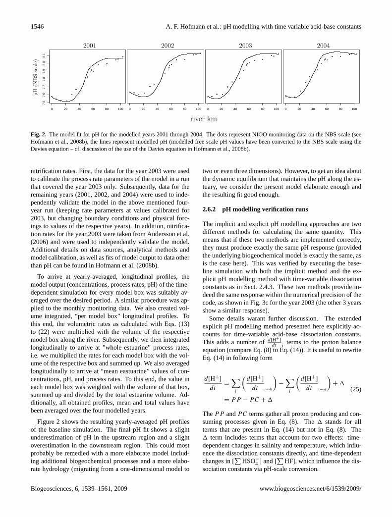
Fig. 2. The model fit for pH for the modelled years 2001 through 2004. The dots represent NIOO monitoring data on the NBS scale (seeHofmann et al., 2008b), the lines represent modelled pH (modelled free scale pH values have been converted to the NBS scale using theDavies equation – cf. discussion of the use of the Davies equation inHofmann et al., 2008b).
nitrification rates. First, the data for the year 2003 were usedto calibrate the process rate parameters of the model in a runthat covered the year 2003 only. Subsequently, data for theremaining years (2001, 2002, and 2004) were used to inde-pendently validate the model in the above mentioned four-year run (keeping rate parameters at values calibrated for2003, but changing boundary conditions and physical forc-ings to values of the respective years). In addition, nitrifica-tion rates for the year 2003 were taken fromAndersson et al.(2006) and were used to independently validate the model.Additional details on data sources, analytical methods andmodel calibration, as well as fits of model output to data otherthan pH can be found inHofmann et al.(2008b).
To arrive at yearly-averaged, longitudinal profiles, themodel output (concentrations, process rates, pH) of the time-dependent simulation for every model box was suitably av-eraged over the desired period. A similar procedure was ap-plied to the monthly monitoring data. We also created vol-ume integrated, “per model box” longitudinal profiles. Tothis end, the volumetric rates as calculated with Eqs. (13)to (22) were multiplied with the volume of the respectivemodel box along the river. Subsequently, we then integratedlongitudinally to arrive at ”whole estuarine” process rates,i.e. we multiplied the rates for each model box with the vol-ume of the respective box and summed up. We also averagedlongitudinally to arrive at “mean eastuarine” values of con-centrations, pH, and process rates. To this end, the value ineach model box was weighted with the volume of that box,summed up and divided by the total estuarine volume. Ad-ditionally, all obtained profiles, mean and total values havebeen averaged over the four modelled years.
Figure2 shows the resulting yearly-averaged pH profilesof the baseline simulation. The final pH fit shows a slightunderestimation of pH in the upstream region and a slightoverestimation in the downstream region. This could mostprobably be remedied with a more elaborate model includ-ing additional biogeochemical processes and a more elabo-rate hydrology (migrating from a one-dimensional model to
two or even three dimensions). However, to get an idea aboutthe dynamic equilibrium that maintains the pH along the es-tuary, we consider the present model elaborate enough andthe resulting fit good enough.
2.6.2 pH modelling verification runs
The implicit and explicit pH modelling approaches are twodifferent methods for calculating the same quantity. Thismeans that if these two methods are implemented correctly,they must produce exactly the same pH response (providedthe underlying biogeochemical model is exactly the same, asis the case here). This was verified by executing the base-line simulation with both the implicit method and the ex-plicit pH modelling method with time-variable dissociationconstants as in Sect.2.4.3. These two methods provide in-deed the same response within the numerical precision of thecode, as shown in Fig.3c for the year 2003 (the other 3 yearsshow a similar response).
Some details warant further discussion. The extendedexplicit pH modelling method presented here explicitly ac-counts for time-variable acid-base dissociation constants.This adds a number ofd[H+
]
dt iterms to the proton balance
equation (compare Eq. (8) to Eq. (14)). It is useful to rewriteEq. (14) in following form
d[H+]
dt=
∑i
(d[H+
]
dt prodi
)−
∑i
(d[H+
]
dt consi
)+ 1
= PP − PC + 1
(25)
ThePP andPC terms gather all proton producing and con-suming processes given in Eq. (8). The 1 stands for allterms that are present in Eq. (14) but not in Eq. (8). The1 term includes terms that account for two effects: time-dependent changes in salinity and temperature, which influ-ence the dissociation constants directly, and time-dependentchanges in[
∑HSO−
4 ] and[∑
HF], which influence the dis-sociation constants via pH-scale conversion.
Biogeosciences, 6, 1539–1561, 2009 www.biogeosciences.net/6/1539/2009/

A. F. Hofmann et al.: pH modelling with time variable acid-base constants 1547
0 20 40 60 80 100
7.6
7.8
8.0
8.2
8.4
0 20 40 60 80 100 0 20 40 60 80 100
PSfra
grep
lacem
ents
river km
pH
(NB
Ssc
ale)
A B C
Fig. 3. Verification of the explicit pH modelling method using model runs for the year 2003. The black dots represent NIOO monitoringdata (seeHofmann et al., 2008b), the black lines represent modelled pH calculated with the implicit approach and the blue lines representmodelled pH calculated with the explicit approach (modelled free scale pH values have been converted to the NBS scale using the Daviesequation (cf. discussion of the use of the Davies equation inHofmann et al., 2008b)). (a): omitting all K∗ related terms from Eq. (14); (b):considering the terms describing the variations in the dissociation constants due to changes inS andT but without the pH scale conversionrelated terms;(c): considering all terms as described in Sect. (2.4.3).
As shown below, the proton productionPP and the protonconsumptionPC are very large compared to the net rate ofchange of protonsd[H+
]
dt, and as a result,PP andPC almost
balance each other. Additionally, the1 term is also smallcompared toPP andPC. Accordingly, one is tempted toomit 1 from Eq. (14). Yet, we found that such an omis-sion introduces substantial deviations as shown in Figs.3a,b. Omitting all terms in1 from Eq. (14), yields pH profilesthat are substantially different from the correctly calculatedones (Fig.3a). Including the terms that account for the di-rect effect of temperature and salinity (but not including thepH scale effect) yields a better result (Fig.3b). However, asmall deviation is still present. Additionally including thepH scale conversion related terms makes the response of theexplicit method identical to the the implicit one, as required(Fig. 3c).
To explain why the neglect of very small terms in1 (sosmall that they irrelevant when comparingPP andPC andthe contributions of individual processes therein) can haverelatively large consequences, one must realize thatPP andPC are very large compared to the net rate of change ofprotonsd[H+
]
dt. Accordingly, a small disturbance of this bal-
ance (like ignoring1) can have a huge impact ond[H+]
dt, and
hence, on the model predicted pH value. This explains thedeviations in Fig.3. In conclusion, the explicit pH modellingmethod is powerful, but one needs to ensure that it is consis-tently implemented and no terms are omitted.
0 5 10 15 20 25
3000
3500
4000
4500
3000
3500
4000
4500
7.6
7.8
8.0
8.2
PSfra
grep
lacem
ents
pH
(NB
S)
[ ∑C
O2 ]
[TA
]
S
µm
ol/k
g-so
ln
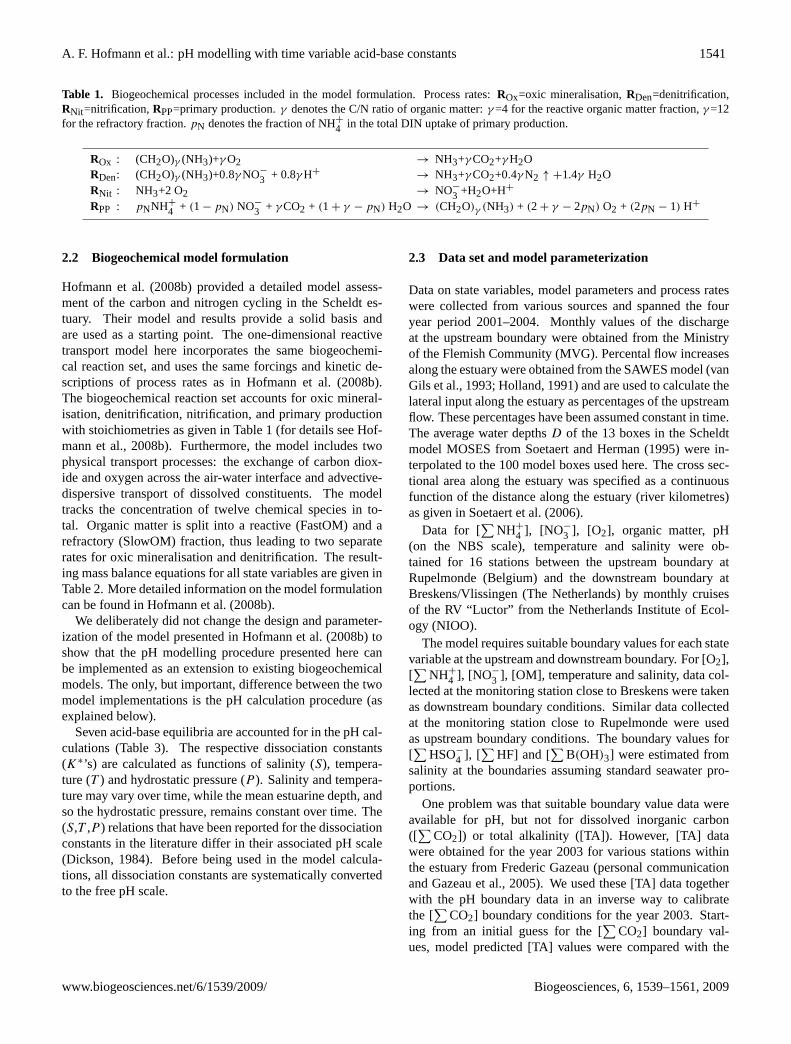
Fig. 4. Basic model simulation with no salinity dependence of theacid-base constants (values were calculated atT =15◦C andS=15),no gas exchange, and no biogeochemistry.[
∑CO2], [TA] and pH
(NBS) are plotted along the estuary as a function of salinity. ThepH from upstream to downstream increases as a result of a de-crease in the ratio between[
∑CO2] and [TA]. End-members for
[∑
CO2], [TA], andS are the upstream and downstream values for2001 in the baseline model run. Due to the simplicity of the re-maining model formulation the calculations are performed using anR script (R Development Core Team, 2005) and the acid-base mod-elling packageAquaEnv (Hofmann et al., submitted) instead of thefull FORTRAN implementation of the model.
2.6.3 Sensitivity analysis
To obtain an idea about what factors (estuarine mixing,salinity gradient, air-water gas exchange, and biologicalprocesses) control the longitudinal pH profile in the estu-ary, we performed a number of exploratory model simula-tions. Starting from a very basic scenario, processes were
www.biogeosciences.net/6/1539/2009/ Biogeosciences, 6, 1539–1561, 2009

1548 A. F. Hofmann et al.: pH modelling with time variable acid-base constants
0 5 10 15 20 25
7.4
7.6
7.8
8.0
8.2
0 5 10 15 20 25
7.4
7.6
7.8
8.0
8.2
0 5 10 15 20 25
7.4
7.6
7.8
8.0
8.2
0 5 10 15 20 25
7.4
7.6
7.8
8.0
8.2
0 5 10 15 20 25
7.4
7.6
7.8
8.0
8.2
PSfra
grep
lacem
ents
pH
(NB
S)
pH
(NB
S)
pH
(NB
S)
pH
(NB
S)
pH
(NB
S)
SSSSS
closed system, no biology
open system, no biology
closed system, biology
full biogeochemical model
Fig. 5. pH profiles along the Scheldt estuary salinity gradient. Theblue line represents the pH calculated with a closed system modelwithout biology (comparable toMook and Koene, 1975); the redline represents the pH calculated with an open system model with-out biology (comparable toWhitfield and Turner(1986) but withrealistic kinetic CO2 air-water exchange instead of a fully equili-brated system); the magenta line represents a closed system modelwith biology; the black line represents the pH calculated with thefull biogeochemical model as presented inHofmann et al.(2008b).All models are based on 2001 parameter values. The black circlesare the observed pH data for 2001.
sequentially activated to arrive at more biogeochemicallycomplex scenarios. The basic scenario simply served to in-vestigate the effect of estuarine mixing on the pH profile. Tothis end, we purposely neglected gas exchange (CO2 and O2)and biological processes, and assumed no dependence of thestoichiometric constants on salinity (values were calculatedat T =15◦C andS=15). Accordingly, in this basic scenario,the pH profile along the estuary is solely determined by con-servative mixing of [TA] and[
∑CO2], driven by the differ-
ence in upstream and downstream boundary values (Fig.4).Starting from this basic scenario, we conducted four addi-
tional simulations where groups of processes where sequen-tially activated. In a first scenario, gas exchange and biologi-cal processes where still neglected (“closed system, no biol-ogy”), but the salinity dependence of the stoichiometric con-stants was now explicitly accounted for. In two subsequentsimulations, either gas exchange was additionally activated(“open system, no biology”) or biological processes wereincluded (“closed system, biology”). In a fourth and finalsimulation, all processes were activated thus leading to thebaseline simulation as discussed above (“full biogeochemi-cal model”). To be comparable to the work ofMook andKoene(1975), the resulting pH profiles are plotted againstthe salinity gradient in the estuary (Fig.5).
2.6.4 Factors governing changes in the mean estuarinepH from 2001 to 2004
Hofmann et al.(2008b) reported an upward trend in the meanestuarine pH over the years 2001 to 2004, but did not investi-gate the underlying causes of this trend. Potential factors are
a different temperature forcing, changes in freshwater input(modifying the salinity gradient and the concentrations of allchemical species in the estuary), or temporal variations in thechemical composition of the water at the boundaries. Table5shows the inter-annual variations of these factors as well asvariations in values of important state variables volume av-eraged over the whole estuary. We carried out a sensitivityanalysis to find out which particular factors could explain theobserved four-year pH trend.
Because the temperature follows a predictable seasonal cy-cle, inter-annual changes in the temperature forcing are neg-ligible. Model runs with all parameters fixed at the 2001values, but with the actual time-variable temperature forcingfrom 2001 to 2004, show no discernably different pH profile.This leaves to investigate the effect of changing freshwaterinput and changing boundary concentrations. We suspectedthat the biogeochemistry of a particular compound was pre-dominantly influenced by changes in its total “load”, i.e., thetotal input at the upstream boundary. For example, the am-monia load is simply defined as the freshwater dischargeQ
times the upper boundary concentration[∑
NH+
4 ]up. In oursensitivity analysis, we were particularly interested whichloading changes (i.e. of which chemical variable) were re-sponsible for the observed inter-annual pH changes.
In the baseline simulation described above, boundary con-ditions and freshwater discharge vary simultaneously overtime, forced by the monthly monitoring data. To disentanglethe effects of freshwater discharge and boundary changes onthe total loading, we executed 14 simulations in which thefreshwater discharge or the boundary concentration values(upstream and downstream) were independently varied. Inthese simulations, all other state variables remained at 2001values. Table6 lists the groups of state variables for whichthe loading has changed, either by changing the freshwaterflow (left column) or the boundary conditions (right column).Each time the resulting pH change of the four year periodwas expressed as a fraction of the pH change arrived at inthe baseline scenario to quantify the importance of the givenparameter change in explaining the four-year pH trend.
3 Results
3.1 Factors controlling the pH profile along the estuary
We performed a number of exploratory simulations to inves-tigate the major controls on the longitudinal pH profile in theScheldt estuary, which is also characteristic for other estu-aries. A first striking aspect is that the pH increases fromthe upstream freshwater boundary to the downstream marineboundary. A “skeleton” simulation (with no gas exchange,no biogeochemistry and no dependence of acid-base con-stants on salinity) shows that this pH increase is simply theresult of conservative mixing of [TA] and[
∑CO2], as the
ratio [∑
CO2]/[TA] decreases (Fig.4).
Biogeosciences, 6, 1539–1561, 2009 www.biogeosciences.net/6/1539/2009/

A. F. Hofmann et al.: pH modelling with time variable acid-base constants 1549
Table 5. Model forcings (upper part of the table) and a selection of mean estuarine model values resulting from the baseline simulation(lower part of the table). The subscript “up” denotes upstream boundary condition , the subscript “down” denotes downstream boundarycondition. The boundary conditions for[TA] are calculated from boundary values for[
∑CO2] in combination with pHup and pHdown
(which are otherwise not used as boundary conditions). Concentrations are given in mmol m−3, the flow at the upstream boundaryQ isgiven in m3 s−1. The pH output from the model simulations is converted to the NBS scale to be comparable with the data.
2001 2002 2003 2004
freshwater flow (Q) 190 184 112 95pHup (NBS) 7.574 7.638 7.586 7.591pHdown (NBS) 8.069 8.124 8.117 8.114[∑
CO2]up 4700 4700 4700 4700[∑
CO2]down 2600 2600 2600 2600[TA]up 4441 4493 4470 4473[TA]down 2702 2728 2726 2733Sup 0.6 0.6 0.9 1.0Sdown 26.5 27.7 28.3 30.2[∑
NH+
4 ]up 110 105 118 72[∑
NH+
4 ]down 8 4 6 4[FastOM])up + [SlowOM])up 41 49 54 55[FastOM])down+ [SlowOM])down 10 10 7 9[O2]up 94 76 71 65[O2]down 293 272 280 268
pH (NBS) 8.010 8.053 8.069 8.095[∑
CO2] 2872 2881 2818 2795[TA] 2918 2951 2902 2898[∑
NH+
4 ] 10.4 9.1 9.5 6.8
Table 6. Model scenarios to investigate the trend in the mean estuarine pH over the years 2001 to 2004. Changes in the total “loading” forparticular chemicals either due to changes in the freshwater discharge (left column) or due to changes in the boundary concentrations (rightcolumn). The entries indicate the variables for which the loading has changed, while all other loadings have been fixed at 2001 values. Notethat in all these scenarios, [TA] boundary conditions are calculated consistently from pH boundary forcing values.
loading change via discharge loading change via boundary concentrations
a) all state variables h) all state variablesb) [
∑CO2], [TA] i) [TA] (pH)
c) S j) S
d) [∑
NH+
4 ] k) [∑
NH+
4 ]
e) [FastOM], [SlowOM] l) [FastOM], [SlowOM]
f) [O2] m) [O2]
g) [NO−
3 ], [∑
HSO−
4 ], [∑
B(OH)3], [∑
HF] n) [NO−
3 ], [∑
HSO−
4 ], [∑
B(OH)3], [∑
HF]
On top of the overall increase in pH, the observed pH pro-file shows a changing curvature with a distinct pH minimumat low salinities. Via a sensitivity analysis, we examined howstrongly different groups of processes (salinity dependenceof acid-base constants, gas exchange, biology) influence theshape of the longitudinal pH profile. Figure5 shows thatthe simulation, which considers a closed system (no CO2and O2 exchange with the atmosphere) and no biologicalprocesses, exhibits a distinct pH minimum at low salinities(blue line). However this simulated pH minimum is locatedat higher salinities (more downstream) than the observed pH
minimum. Enabling gas exchange, while keeping biologicalprocesses inactivated, results in a concave pH profile withhigh pH values and no minimum (red line). Conversely, ac-tivating biological processes in a closed system results in aconvex pH profile with a minimum but with pH values far be-low observations (magenta line). Finally, a full model simu-lation with all biological processes and gas exchange toggledon (black line) shows a profile with changing curvature andthe distinct pH minimum at low salinities. This full modelfits the observed data best, although some discrepancies re-main (a more sharply recovering pH minimum in the data
www.biogeosciences.net/6/1539/2009/ Biogeosciences, 6, 1539–1561, 2009
1550 A. F. Hofmann et al.: pH modelling with time variable acid-base constants
at low salinities, the data pH profile shows less curvature athigh salinities).
3.2 Proton production and consumption along theestuary
The prime advantage of the explicit pH modelling method isthat it calculates the proton production/consumption rates as-sociated with each individual reactive transport process. Fig-ure6a shows the contributions of individual processes to thenet rate of change of protons as calculated with Eqs. (13) to(22). Longitudinal profiles of proton production or consump-tion rates (per unit of solution volume) were extracted fromthe baseline simulation, averaged over the four year period(for every model box), and plotted cumulatively. Table7lists resulting values at selected positions (model boxes) inthe river where the pH profiles in Fig.6 show interesting fea-tures (these locations are also indicated in Fig.1).
In a first step, we can look at the overall proton cycling,i.e., the total proton production (PP ) and total proton con-sumption (PC) along the estuary. A first observation is thatthePP andPC terms are always four to five orders of mag-nitude larger than the actual rate of change of protons (whichis in the 10−5 mmol m−3 range). This implies that protonproduction and consumption are nearly balanced, and thatthe internal cycling of protons far outweighs the net protonchange over time. A second aspect is that the proton pro-duction rates, which are linked to changes in the dissociationconstants, are about three orders of magnitude smaller thanthose of other processes. Therefore, they are not presented inFigs.6 and7. Yet, as noted above, incorporation of these in-fluences is necessary for a consistent implementation of theexplicit pH approach (i.e. to model absolute pH values cor-rectly).
As shown in Fig.6a, the proton production and consump-tion per unit volume shows a marked decrease in the upperhalf of the estuary (between river km 0 and 60), after whichthe decrease proceeds more gradually. Over the whole es-tuary,PP andPC decrease by a factor of 20, from around1.3 mmol m−3 yr−1 to 0.06 mmol m−3 yr−1. This decrease inproton turn-over generates the trumpet-like shape in Fig.6a,and can be attributed to a similar decreasing trend in the bio-geochemical activity per volume of solution (as discussed be-low).
Along the estuary, the magnitude of the individual con-tributions d[H+
]
dt igenerally follows the decreasing trend in
the total proton production/consumption. The exceptions areprimary production, whose proton consumption remains rel-atively constant, and advective-dispersive transport, whichshows a noticeable profile (further discussed below). How-ever, there are some marked changes in the relative impor-tance of processes in the overall proton cycling. Nitrifica-ton and oxic mineralisation produce protons; CO2 degassing,primary production, and denitrification consume protons.The dominant proton producer at the upstream boundary is
nitrification (77%), yet its relative importance drops to 11%downstream. In parallel, the relative importance of oxicmineralisation as a proton producer increases from 23% up-stream to 64% at the downstream boundary. In terms ofproton consumption, the most important process is CO2 de-gassing. Its relative importance increases from 50% at theupstream boundary to 92% at km 32 and then decreases againto 65% at the downstream boundary. Compared to CO2 de-gassing, the proton consumption by primary production issmall. The relative importance of primary production as aproton consumer increases from 4% at the upstream bound-ary to 38% at km 67 and decreases again to 33% at the down-stream boundary. The proton consumption due to denitrifica-tion is not important in the Scheldt estuary (around 1% alongthe estuary).
The role of advective-dispersive transport in proton trans-port is markedly different from that of the biogeochemical re-actions. Advective-dispersive transport counteracts the dom-inant proton consuming or producing processes. As a resultof that, it switches sign. Around river km 32, it switchesfrom proton consumption (importing protons into a modelbox) to proton production (exporting protons from a modelbox). Moreover, its rate does not change monotonically. Pro-ton production due to advective-dispersive transport showsa maximum around river km 48 and a secondary maximumaround river km 67. At the upstream boundary advective-dispersive transport accounts for 44% of the proton con-sumption, while downstream it accounts for about 25% ofthe proton production.
Figure 6b shows the longitudinal profile of the volume-integrated proton production and consumption rates (ex-pressed “per model-box”). Table8 lists selected values alongthe estuary. The cross section area increases from around4000 m2 upstream to around 76 000 m2 downstream, whilethe mean estuarine depth remains approximately constantaround 10 m. As a result, there is a much larger estuar-ine volume in the downstream model boxes than in the up-stream model boxes. This volume increase per box com-pensates for the decrease in the rates per unit volume. Asa consequence, the volume-integrated proton production orconsumption rates in Fig.6b remain similar along the estu-ary. The mid-region of the estuary (between kms 30 and 60)emerges as the most important region for volume integratedproton cycling. In this area the proton budget is dominatedby the physical transport processes: CO2 air-water exchangeand advective-dispersive transport. The volume-integratedproton production/consumption of oxic mineralisation, pri-mary production and CO2 degassing is clearly larger down-stream than upstream. In contrast, the volume-integrated pro-ton production of nitrification is larger upstream than down-stream.
Biogeosciences, 6, 1539–1561, 2009 www.biogeosciences.net/6/1539/2009/

A. F. Hofmann et al.: pH modelling with time variable acid-base constants 1551
Table 7. Contributions of various biogeochemical processes to the proton cycling per unit of solution volume; values in mmol H+ m−3 y−1;percentages are of total production (positive quantities) or consumption (negative quantities), respectively.
km 0 km 32 km 48 km 60 km 67 km 104∑prod 1.33 10−0 5.99 10−1 4.56 10−1 1.03 10−1 1.27 10−1 5.47 10−2∑cons −1.34 10−0
−6.05 10−1−4.64 10−1
−1.08 10−1−1.31 10−1
−5.99 10−2
d[H+]
dt Tr −5.93 10−1 (44%) −4.37 10−3 (1%) 2.42 10−1 (53%) 1.91 10−2 (19%) 6.27 10−2 (49%) 1.39 10−2 (25%)d[H+
]
dt ECO2−6.64 10−1 (50%) −5.59 10−1 (92%) −3.60 10−1 (78%) −8.34 10−2 (77%) −8.16 10−2 (62%) −3.90 10−2 (65%)
d[H+]
dt ROx3.09 10−1 (23%) 1.40 10−1 (23%) 8.98 10−2 (20%) 4.93 10−2 (48%) 4.28 10−2 (34%) 3.48 10−2 (64%)
d[H+]
dt RDen−2.45 10−2 ( 2%) −3.26 10−3 (1%) −5.56 10−4 (0%) −1.20 10−4 ( 0%) −7.14 10−5 (0%) −3.17 10−5 (0%)
d[H+]
dt RNit1.02 10−0 (77%) 4.53 10−1 (76%) 1.20 10−1 (26%) 3.19 10−2 (31%) 1.96 10−2 (15%) 5.88 10−3 (11%)
d[H+]
dt RPP−5.65 10−2 ( 4%) −3.73 10−2 (6%) −1.03 10−1 (22%) −2.43 10−2 (22%) −4.94 10−2 (38%) −1.96 10−2 (33%)
d[H+]
dt K∗(T )1.70 10−4 ( 0%) 2.95 10−3 (0%) 2.27 10−3 (0%) 1.38 10−3 (1%) 9.71 10−4 (1%) −7.27 10−4 (1%)
d[H+]
dt K∗(S)6.22 10−4 ( 0%) 3.67 10−3 (1%) 2.16 10−3 (0%) 1.35 10−3 (1%) 1.07 10−3 (1%) −5.24 10−4 (1%)
d[H+]
dt K∗([∑
HSO−
4 ])−1.84 10−4 ( 0%) −1.02 10−3 (0%) −6.80 10−4 (0%) −3.66 10−4 (0%) −2.87 10−4 (0%) 8.62 10−5 (0%)
d[H+]
dt K∗([∑
HF])−5.78 10−8 ( 0%) −2.79 10−8 (0%) 4.52 10−9 (0%) −9.92 10−9 (0%) −1.31 10−8 (0%) −7.25 10−9 (0%)
Table 8. Volume integrated proton budget; proton production/consumption rates in kmol H+ y−1 per model box.
km 0 km 32 km 48 km 60 km 67 km 104∑prod 5.54 10−0 4.08 10−0 10.70 10−0 4.52 10−0 7.08 10−0 4.34 10−0∑cons −5.57 10−0
−4.12 10−0− 10.90 10−0
−4.74 10−0−7.32 10−0
−4.74 10−0
d[H+]
dt Tr −2.47 10−0−2.97 10−2 5.70 10−0 8.36 10−1 3.50 10−0 1.10 10−0
d[H+]
dt ECO2−2.76 10−0
−3.81 10−0−8.48 10−0
−3.66 10−0−4.55 10−0
−3.09 10−0
d[H+]
dt ROx1.29 10−0 9.51 10−1 2.11 10−0 2.16 10−0 2.39 10−0 2.76 10−0
d[H+]
dt RDen−1.02 10−1
−2.22 10−2−1.31 10−2
−5.24 10−3−3.98 10−3
−2.51 10−3
d[H+]
dt RNit4.25 10−0 3.08 10−0 2.81 10−0 1.40 10−0 1.09 10−0 4.66 10−1
d[H+]
dt RPP−2.35 10−1
−2.54 10−1−2.42 10−0
−1.07 10−0−2.75 10−0
−1.55 10−0
d[H+]
dt K∗(T )7.09 10−4 2.01 10−2 5.34 10−2 6.03 10−2 5.41 10−2
−5.76 10−2
d[H+]
dt K∗(S)2.59 10−3 2.50 10−2 5.09 10−2 5.93 10−2 5.97 10−2
−4.15 10−2
d[H+]
dt K∗([∑
HSO−
4 ])−7.65 10−4
−6.94 10−3−1.60 10−2
−1.61 10−2−1.60 10−2 6.83 10−3
d[H+]
dt K∗([∑
HF])−2.41 10−7
−1.90 10−7 1.06 10−7−4.35 10−7
−7.30 10−7−5.75 10−7
3.3 Whole estuarine proton budget
Figure 7 shows a proton budget integrated over the wholemodel area and averaged over the four modelled years. It canbe seen that CO2 degassing and primary production are theprocesses that net consume protons in the estuary (disregard-ing the minor contribution of denitrification). Nitrificationis the main proton producer, followed by oxic mineralisa-tion and advective-dispersive transport. Note that the protonbudget does not add up to zero, but a small negative valueremains (−20 kmol[H+
] estuary−1 y−1). This indicates thatthe estuary as a whole, averaged over a year, is not com-
pletely in steady state. This is consistent with the upwardstrend in the mean estuarine pH, which is observed in the dataand in the model simulations.
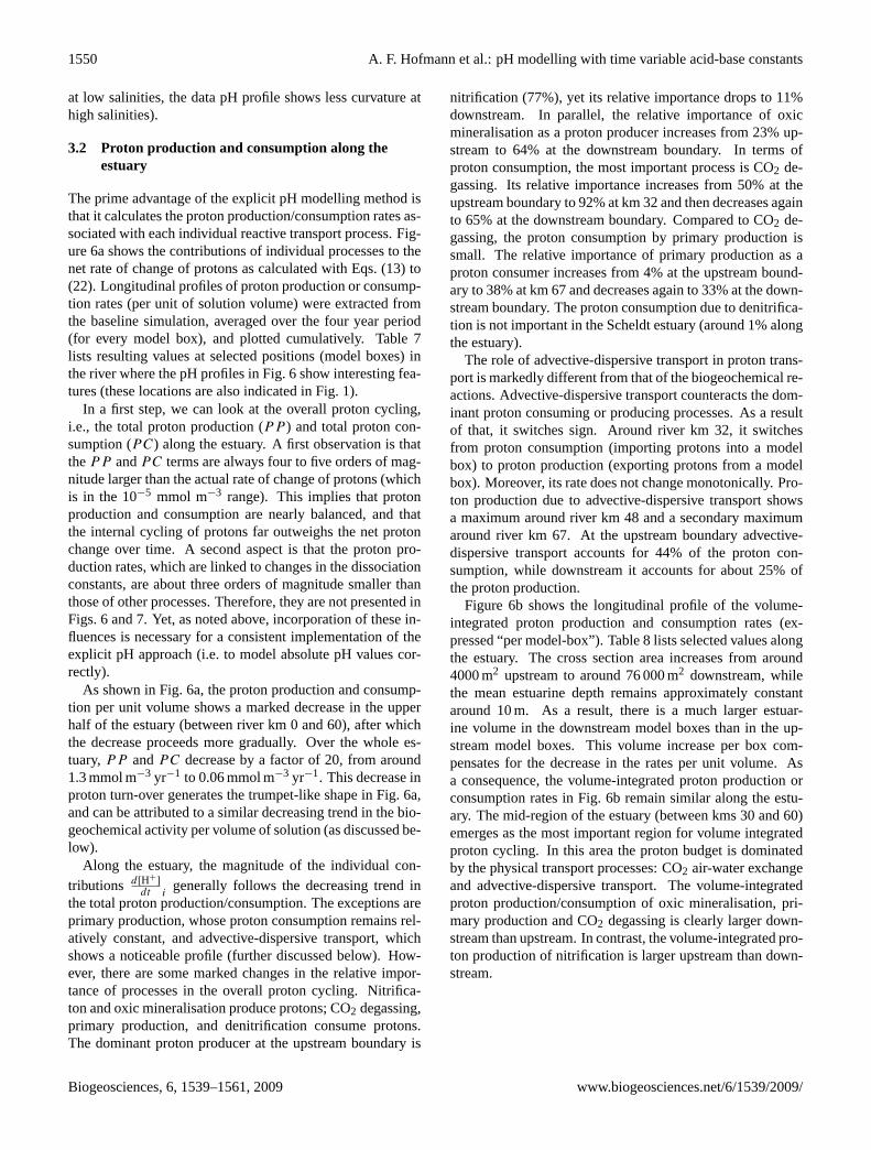
As shown in Fig.6a, the relative importance of processesin the overall proton cycling changes along the estuary. Tocapture this in a proton balance, the estuary was divided intothree zones; the upstream region between river km 0 and 30which exhibits a pH below ca. 7.6 (cf. Fig.2), the midstreamregion between river km 30 and 60 where the pH exhibitsa marked gradient, and the downstream region from riverkm 60 onwards where the pH remains approximately con-stant around 8.0. Separate proton balances were calculated
www.biogeosciences.net/6/1539/2009/ Biogeosciences, 6, 1539–1561, 2009

1552 A. F. Hofmann et al.: pH modelling with time variable acid-base constants
0 20 40 60 80 100
−1.5
−1.0
−0.5
0.0
0.5
1.0
1.5
PSfra
grep
lacem
ents
river km
mm
olH
+m−
3y−
1
Tr
ECO2
ROx
RDen
RNit
RPP
a)
0 20 40 60 80 100
−15
−10
−50
510
PSfra
grep
lacem
ents
river km
kmol
H+
mod
el-b
ox−
1y−
1
Tr
ECO2
ROx
RDen
RNit
RPP
b)
Fig. 6. The influences of kinetically modelled processes on thepH – volumetricallya) and volume integratedb), averaged overthe four modelled years. Note that the process abbreviationsgiven in the legend represent the contribution of the respective
process tod[H+]
dt, e.g., Tr signifies d[H+
]
dt Tr . Process abbrevi-ations: Tr =advective-dispersive transport,ECO2=CO2 degassing,ROx=oxic mineralisation,RNit=nitrification,RPP=primary produc-tion, K∗(T )=changes in dissociation constants via changes in tem-perature,K∗(S)=changes in dissociation constants via changesin salinity, K∗([
∑HSO−
4 ])=changes in dissociation constants via
changes in[∑
HSO−
4 ], K∗([∑
HF])=changes in dissociation con-stants via changes in[
∑HF].
for each zone (Fig.8). Because the decrease in the processrates from upstream to downstream is compensated by an in-crease in estuarine volume, the total proton production is ofthe same order of magnitude in the three zones. However,there are marked changes in the relative importance of pro-cesses.
Upstream, the proton production due to nitrification, andto a lesser extent oxic mineralisation, are counteracted byCO2 degassing and advective-dispersive transport. In themidstream section, the contribution of aerobic respirationand advective-dispersive transport (which has now becomea proton producer) are of similar magnitude as that of nitri-fication. In this midstream part, CO2 degassing is also themajor proton consuming process. In the downstream partof the estuary, nitrification is even less important, and thenet proton production by oxic mineralisation as well as the
−600
−400
−200
020
0
123
−394
178
−2.13
202
−127
PSfra
grep
lacem
ents
km
olH
+es
tuary−
1y−
1
Tr ECO2ROx RDen RNit RPP
Fig. 7. Whole estuarine proton budget, averaged over the four mod-elled years. The error bars represent the standard deviations result-ing from averaging over the four years. The process abbreviations inthe legend denote the contribution of the respective biogeochemical
process e.g.,Tr refers tod[H+]
dt Tr .
net consumption of protons by primary production gain moreimportance.
3.4 Factors responsible for the trend in the meanestuarine pH from 2001 to 2004
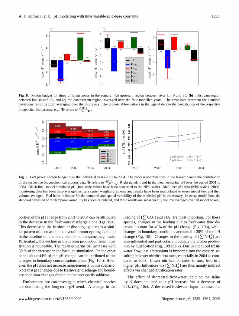
Figure9 shows the trend in the mean estuarine pH over thefour year period. Both the trend as derived from the data aswell as the trend simulated by the model are shown. The pHchanged by about 0.085 from 8.010 to 8.095 in the model,which is backed by a similar pH increase of 0.095 in thedata. There is a small offset between model and data. This isbecause the model slightly underestimates the pH in the up-stream region with low estuarine volume and overestimatesthe pH in the downstream region with high estuarine volume.Because of volume averaging, the latter dominates the meanestuarine pH.
As a first step to investigate the underlying causes of thistrend, we have plotted the volume integrated proton pro-duction/consumption for the individual years 2001 to 2004alongside each other (the values displayed in Figs. 4, 5 and6 were time averages over the whole four-year period). Thisshows that the overall proton turn-over decreased over thefour-year period. The contributions of CO2 degassing andnitrification steadily declined from 2001 to 2004 (with thedecline being more pronounced for CO2 degassing). Thecontribution from oxic mineralisation showed no clear trend,while the contribution of transport declined from 2001 to2003 and then slightly increased again from 2003 to 2004.
As a second step, we investigated the factors responsiblefor the observed pH trend by simulating the various modelscenarios in Table6. Figure10 shows the results of thesedifferent model scenarios. As discussed above, the loadingchanges of compounds can be caused by either changes inthe freshwater discharge or changes in boundary concentra-tions. We examined these two effects separately. A large
Biogeosciences, 6, 1539–1561, 2009 www.biogeosciences.net/6/1539/2009/
A. F. Hofmann et al.: pH modelling with time variable acid-base constants 1553
−100
−50
050
100
−28 −85
26
−2
92
−4
−250
−200
−150
−100
−50
050
100
70
−163
47
0
77
−37
−200
−100
010
0
81
−146
104
0
33
−86
PSfra
grep
lacem
ents
kmol
H+
estu
ary−
1y−
1
kmol
H+
estu
ary−
1y−
1
kmol
H+
estu
ary−
1y−
1
Tr
ECO2
ROx
RDen
RNit
RPP
a) b) c)
Fig. 8. Proton budget for three different zones in the estuary:(a) upstream region between river km 0 and 30,(b) midstream regionbetween km 30 and 60, and(c) the downstream region, averaged over the four modelled years. The error bars represent the standarddeviations resulting from averaging over the four years. The process abbreviations in the legend denote the contribution of the respective
biogeochemical process e.g.,Tr refers tod[H+]
dt Tr .
−0.3
−0.2
−0.1
0.0
0.1
0.2
0.0720.062
0.054 0.0320.0540.054 0.044 0.043
−0.039
−0.036−0.035
−0.03
−0.15 −0.11 −0.091 −0.067
0.063 0.031 0.021 0.024
7.85
7.90
7.95
8.00
8.05
8.10
8.15
7.85
7.90
7.95
8.00
8.05
8.10
8.15
PSfra
grep
lacem
ents
mm
olH
+m−
3y−
1
Tr
ECO2
ROx
RD
en
RNit
RPP
pH
(NB
Ssc
ale)
pH
(NB
Ssc
ale)
20012001 20022002 20032003 20042004
∆ pH model:
∆ pH data:
0.085 / (4 y)
0.095 / (4 y)
Fig. 9. Left panel: Proton budget over the individual years 2001 to 2004. The process abbreviations in the legend denote the contribution
of the respective biogeochemical process e.g.,Tr refers tod[H+]
dt Tr . Right panel: trend in the mean estuarine pH over the period 2001 to2004. Black line: model simulated pH (free scale values have been converted to the NBS scale). Blue line: pH data (NBS scale). NIOOmonitoring data has been time-averaged using a center weighting scheme and results have been interpolated to every model box and thenvolume averaged. Red bars: indicator for the temporal and spatial variability of the modelled pH in the estuary. In every model box, thestandard deviation of the temporal variability has been calculated, and these results are subsequently volume averaged over all model boxes.)
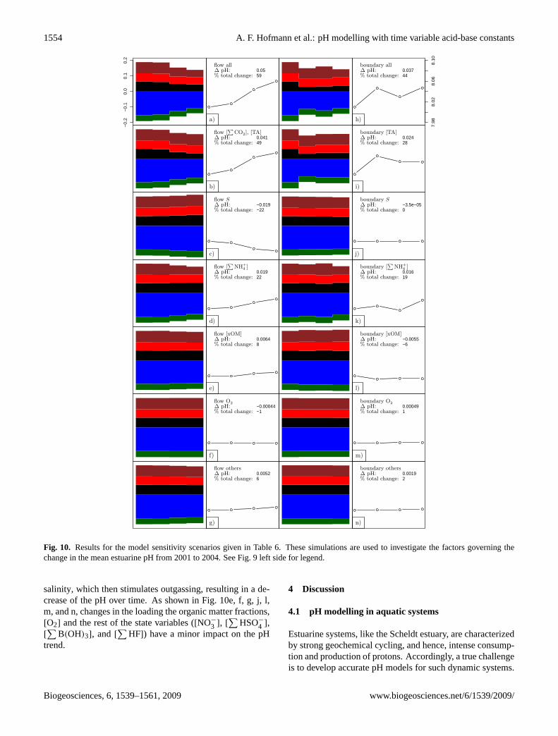
portion of the pH change from 2001 to 2004 can be attributedto the decrease in the freshwater discharge alone (Fig.10a).This decrease in the freshwater discharge generates a simi-lar pattern of decrease in the overall proton cycling as foundin the baseline simulation, albeit not on the same magnitude.Particularly, the decline in the proton production from nitri-fication is noticeable. The mean estuarine pH increases with59 % of the increase in the baseline simulation. On the otherhand, about 44% of the pH change can be attributed to thechanges in boundary concentrations alone (Fig.10h). How-ever, the pH does not increase monotonously in this scenario.Note that pH changes due to freshwater discharge and bound-ary condition changes should not be necessarily additive.
Furthermore, we can investigate which chemical speciesare dominating the long-term pH trend. A change in the
loading of[∑
CO2] and[TA] are most important. For thesespecies, changes in the loading due to freshwater flow de-crease account for 49% of the pH change (Fig.10b), whilechanges in boundary conditions account for 28% of the pHchange (Fig.10i). Changes in the loading of[
∑NH+
4 ] arealso influential and particularly modulate the proton produc-tion by nitrification (Fig.10d and k). Due to a reduced fresh-water flow, less ammonium is imported into the estuary, re-sulting in lower nitrification rates, especially in 2004 as com-pared to 2003. Lower nitrification rates, in turn, lead to ahigher pH. Influences via[
∑NH+
4 ] are thus mainly indirecteffects via changed nitrification rates.
The effect of decreased freshwater input on the salin-ity S does not lead to a pH increase but a decrease of22% (Fig.10c). A decreased freshwater input increases the
www.biogeosciences.net/6/1539/2009/ Biogeosciences, 6, 1539–1561, 2009
1554 A. F. Hofmann et al.: pH modelling with time variable acid-base constants
−0
.2−
0.1
0.0
0.1
0.2
2001 2002 2003 2004
pH
(N
BS
sca
le)
0.0559
2001 2002 2003 2004
pH
(N
BS
sca
le)
7.9
88
.02
8.0
68
.10
0.03744
2001 2002 2003 2004
pH
(N
BS
sca
le)
0.04149
2001 2002 2003 2004
pH
(N
BS
sca
le)
0.02428
2001 2002 2003 2004
pH
(N
BS
sca
le)
−0.019−22
2001 2002 2003 2004
pH
(N
BS
sca
le)
−3.5e−050
2001 2002 2003 2004
pH
(N
BS
sca
le)
0.01922
2001 2002 2003 2004
pH
(N
BS
sca
le)
0.01619
2001 2002 2003 2004
pH
(N
BS
sca
le)
0.00648
2001 2002 2003 2004
pH
(N
BS
sca
le)
−0.0055−6
2001 2002 2003 2004
pH
(N
BS
sca
le)
−0.00044−1
2001 2002 2003 2004
pH
(N
BS
sca
le)
0.000491
pH
(N
BS
sca
le)
0.00526
pH
(N
BS
sca
le)
0.00192
PSfrag replacements
flow all
flow [∑
CO2], [TA]
flow S
flow [∑
NH+
4 ]
flow [xOM]
flow O2
flow others
boundary all
boundary [TA]
boundary S
boundary [∑
NH+4 ]
boundary [xOM]
boundary O2
boundary others∆ pH:∆ pH:
∆ pH:∆ pH:
∆ pH:∆ pH:
∆ pH:∆ pH:
∆ pH:∆ pH:
∆ pH:∆ pH:
∆ pH:∆ pH:
% total change:% total change:
% total change:% total change:
% total change:% total change:
% total change:% total change:
% total change:% total change:
% total change:% total change:
% total change:% total change:
a)
b)
c)
d)
e)
f)
g)
h)
i)
j)
k)
l)
m)
n)
Fig. 10. Results for the model sensitivity scenarios given in Table6. These simulations are used to investigate the factors governing thechange in the mean estuarine pH from 2001 to 2004. See Fig.9 left side for legend.
salinity, which then stimulates outgassing, resulting in a de-crease of the pH over time. As shown in Fig.10e, f, g, j, l,m, and n, changes in the loading the organic matter fractions,[O2] and the rest of the state variables ([NO−
3 ], [∑
HSO−
4 ],[∑
B(OH)3], and[∑
HF]) have a minor impact on the pHtrend.
4 Discussion
4.1 pH modelling in aquatic systems
Estuarine systems, like the Scheldt estuary, are characterizedby strong geochemical cycling, and hence, intense consump-tion and production of protons. Accordingly, a true challengeis to develop accurate pH models for such dynamic systems.
Biogeosciences, 6, 1539–1561, 2009 www.biogeosciences.net/6/1539/2009/

A. F. Hofmann et al.: pH modelling with time variable acid-base constants 1555
In the past, a number of reactive transport models have beendeveloped that accurately reproduce the longitudinal pH pro-file of the Scheldt estuary (Regnier et al., 1997; Vanderborghtet al., 2002; Hofmann et al., 2008b). However, these modelsimplemented the implicit pH modelling approach, and so,they were not able to quantify the contribution of specificbiogeochemical processes to the overall proton cycling.
One (crude) way to investigate the importance of a singleprocess in the overall proton cycling, is to switch this processoff, and examine the effect on pH. However, because pro-cesses interact, switching off a given process will influencethe rates of the other processes, and hence, this could com-plicate the interpretation. Preferably, one wants a methodthat quantifies the contribution of individual processes con-currently and without changing the rates of biogeochemicalprocesses.
The explicit approach to pH modelling allows just that.This explicit approach was originally pioneered byJourabchiet al. (2005) andSoetaert et al.(2007), though these treat-ments were partially incomplete. The approach proposedin Jourabchi et al.(2005) is only applicable to steady stateconditions, and it also treats the effect of advective-diffusivetransport on proton cycling incompletely (the proton trans-port term is omitted). Similarly,Soetaert et al.(2007) in-troduced a method to quantify the influence of processes onpH, one process at a time, but this approach did also not ac-count for advective-dispersive transport (which is importantfor proton cycling as we show here).
Recently,Hofmann et al.(2008a) have reviewed the con-struction of pH models, and advanced an explicit pH mod-elling approach that allows to quantify the contribution ofall processes (that is physical transport and biogeochemicalreactions) on the proton cycling within an aquatic system.This approach describes the pH evolution explicitly usingan expression for the rate of change of the proton concen-tration over time. However, the approach advanced inHof-mann et al.(2008a) assumed that dissociation constants re-mained constant over time. In previous modelling studies ofthe Scheldt estuary (e.g.Vanderborght et al., 2002; Hofmannet al., 2008b), it was shown that the dissociation constantsmust be calculated as functions of the time-variable salin-ity and temperature in order to obtain reasonable fit to thepH data. In response to this, we have here extended the ex-plicit method so that the dissociation constants can changeover time. Note that both the method given inHofmann et al.(2008a) and the generic treatment presented here are appli-cable to both water column and sediment pore water ecosys-tems.
4.2 pH profile along the estuary
In the Scheldt estuary, pH increases from upstream to down-stream. In Fig.4 we show that this is an effect of a decreasing[∑
CO2] / [TA] ratio from upstream to downstream, whichitself is an effect of conservative mixing of[
∑CO2] and
[TA] with riverine and marine end-members. However, thepH increase induced by this conservative mixing exhibits nodistinct minimum at low salinities and no change in curva-ture. The distinct shape of the pH increase observed in theScheldt estuary and other estuaries, exhibits a clear minimumat low salinities and has a distinct quasi sigmoidal shape.Accordingly, the pH profile along the estuary must be de-termined by other factors.
Over the past few decades a discussion has taken placeabout what these controlling factors could be.Mook andKoene(1975) suggested that the characteristic pH profile inestuaries with high inorganic carbon loadings from upstream(like the Scheldt estuary) only results from acid-base equili-bration following the mixing of fresh water and seawater, dueto the salinity dependency of the dissociation constants of thecarbonate system. The conceptual model ofMook and Koene(1975) is very simple, it only accounts for conservative mix-ing of [
∑CO2] and [TA] and salinity dependent acid-base
equilibration. Accordingly, it ignores CO2 exchange withthe atmosphere as well as biological processes (e.g. aero-bic respiration, primary production, nitrification) that mayaffect [TA] and[
∑CO2]. The blue line in Fig.5 represents
the model ofMook and Koene(1975). It confirms that in aclosed system with no biology a pH minimum at low salin-ities is created by the salinity dependency of acid-base dis-sociation constants (as the pH profile in the case with salin-ity independent dissociation constants does not show a min-imum – Fig.4). However, this does not exclude that otherprocesses could be important in shaping the pH profile alongthe estuary.
Although the model ofMook and Koene(1975) providedreasonable agreement with measurements in the ChesapeakeBay (Wong, 1979), and is still used to predict estuarinepH profiles (Spiteri et al., 2008), it is thought to be arather crude approximation of reality.Whitfield and Turner(1986) showed that CO2 exchange with the atmosphere re-sults in significantly different pH profiles. Differences upto 0.7 pH units were found at low salinities for systems thatare fully equilibrated with the atmosphere. Enabling gas ex-change while keeping biological processes inactivated in ourmodel results in a concave pH profile with high pH valuesand no minimum (red line in Fig.5). As also argued byWhitfield and Turner(1986), this pH profile strongly deviatesfrom the one that considers no gas exchange, but it severelyoverestimates observed pH values. This shows that neglect-ing gas exchange introduces an error into the pH calculationsin the Scheldt estuary. Moreover, the effect of gas exchangeon pH profile is stronger than the salinity dependency effectof the acid-base dissociation constants.
As mentioned above, estuaries are zones of intense bio-logical activity, so neglecting biological processes in pH cal-culations seems unjustified. The strong effect of biology(or equally biogeochemistry) is shown by the magenta linein Fig. 5). This simulation produces a convex pH profilewith a clear pH minimum at low salinities, which strongly
www.biogeosciences.net/6/1539/2009/ Biogeosciences, 6, 1539–1561, 2009

1556 A. F. Hofmann et al.: pH modelling with time variable acid-base constants
underestimates observed pH values. Finally, a full modelsimulation with all biological processes and gas exchangetoggled on (black line in Fig.5) again shows a distinct pHminimum at low salinities, but the resulting pH profile fol-lows much more closely the observed data. This shows thatthe conceptual models which ignore gas exchange or biology,oversimplify the pH dynamics in an estuarine system. Ef-fectively, the conceptual model ofMook and Koene(1975)predicts a pH minimum at low salinities similar to the oneobserved in the data, but for incorrect reasons.
In summary, one can conclude that the overall pH increasein estuaries similar to the Scheldt estuary (high
∑CO2 load-
ings) results from a decreasing[∑
CO2]/[TA] ratio betweenthe riverine and marine end-members. The characteristic sig-moidal shape of the pH increase results from an interplaybetween CO2 outgassing and biological activity. Overall,biological activity has a clearly acidifying effect. Nitrifica-tion seems to be the main cause for the distinct dip in pH val-ues at low salinities. The salinity dependency of acid-basedissociation systems only has a minor effect on the charac-teristic pH profile in estuaries.
Note that a quantitative mathematical link between spatialpH gradients along the estuary and process rates at differentpoints of the estuary will be the subject of another publica-tion.
4.3 Proton production and consumption along theestuary
The pH profile in the Scheldt estuary (Fig.2) is the result of abalance between proton production and proton consumptionprocesses. Proton productionPP and the proton consump-tion PC (expressed per volume unit of solution – Eq.25) arevery large compared to the net proton production rate. Ac-cordingly, the magnitude of eitherPP or PC can be usedas a measure for the intensity of proton cycling. This pro-ton cycling intensity decreases by a factor of 20 along theestuary, going from around 1.3 mmol of protons m−3 yr−1
at the upstream boundary to 0.06 mmol of protons m−3 yr−1
downstream. The turnover time of protons can be definedas the local proton concentration divided by the proton cy-cling intensity. Using pH values of 7.55 upstream and 8.05downstream, we find that the turnover time of the proton poolis 8 days upstream and 54 days downstream. This decreasein the intensity of proton cycling matches the decrease inthe cycling intensity of total ammonium, dissolved inorganiccarbon, oxygen, and nitrate as calculated inHofmann et al.(2008b). This shows that high proton turnover is associatedwith high rates in biogeochemical processes, thus stressingthe importance of such processes in the pH dynamics of es-tuaries. Moreover, the rates of proton production and con-sumption presented here (Fig.6) are approximately the mir-ror images of the rates of oxygen production and consump-tion presented inHofmann et al.(2008b). This suggests a
tight connection between redox balance and proton cycling,which should be explored in future investigations.
Although the link between high biogeochemical rates andhigh proton turnover holds for all processes combined, itdoes not always apply to individual processes. The prime ex-ample is denitrification, which shows a negligible contribu-tion to the overall proton cycling. Still, based on the baselinesimulation, denitrification can be shown to be an importantprocess in the overall cycling of
∑NH+
4 and∑
CO2 (Hof-mann et al., 2008b). Judging from the stoichiometry (Ta-ble 1), denitrification substantially consumes protons. Basedon this, one would expect denitrification to be important inthe proton cycling. The reason why this logic fails is thatone has ignored acid-base equilibration: denitrification alsoproduces CO2, a proton source. The protons subsequentlyreleased due to dissociation of produced CO2 almost balancethe direct proton consumption of denitrification. This illus-trates the value of the explicit pH modelling approach: it isable to exactly quantify the contribution of a given process toproton cycling (properly accounting for the effects of acid-base equilibration).
Nitrification and oxic mineralisation are the important pro-ton producers, and CO2 degassing, and to a lesser extent pri-mary production, are the important proton consuming pro-cesses. This is fully consistent with previous modelling stud-ies on the Scheldt estuary (i.e.,Regnier et al., 1997). Further-more, these results are coherent withAbril and Frankignoulle(2001), who focussed on alkalinity variations and identifiedthe nitrogen cycle and the process nitrification as importantfactor governing the acid-base regime of the Scheldt estuary.In addition to confirming this, the explicit pH modelling ap-proach presented here allows to precisely calculate the con-tribution of nitrification (and other processes) in the overallproton cycling along the estuarine gradient.
The contributions of changes in the dissociation constantsin the overall proton cycling are several orders of magnitudesmaller than the influences of kinetic processes (Tables7 and8). Therefore, when describing the factors that govern thegross proton cycling intensity (PP , PC), these factors canbe neglected. However, to model pH values in a system ac-curately, i.e. more accurate than 0.1 pH units, they should beincluded in the calculations. This is especially important formodelling the proton concentration explicitly over a longerperiod of time, since deviations ind[H+
]
dtare likely to accu-
mulate.
4.4 Proton cycling and CO2 degassing
Estuaries are important sites of CO2 degassing. Within thecontext of climate change and greenhouse gas budgets, it isimportant to understand the control on the rate of CO2 de-gassing. The baseline simulation estimates a total CO2 effluxof 3.3 Gmol yr−1 over the Scheldt estuary (averaged over the2001–2004 year period, seeHofmann et al., 2008b, for de-tails). A complex interplay between different factors controls
Biogeosciences, 6, 1539–1561, 2009 www.biogeosciences.net/6/1539/2009/

A. F. Hofmann et al.: pH modelling with time variable acid-base constants 1557
this rate of CO2 degassing. We performed simulations to ex-amine the influence of the biogeochemical processes on CO2degassing. To this end, we toggled off all biological pro-cesses in the baseline simulation. In this scenario, the CO2efflux rates are reduced by approximately half over the wholeestuary. While this shows that biological processes induce alarge amount of CO2 degassing, it also indicates that there issubstantial CO2 degassing driven by non-biological mecha-nisms. Most importantly, the incoming water is significantlyoversaturated in CO2 (around 300%, seeHofmann et al.,2008b), which induces degassing during transport along theestuary.
Among the biological processes,Frankignoulle et al.(1996), Abril et al. (2000), andVanderborght et al.(2002)identified nitrification and oxic mineralisation as the impor-tant processes increasing CO2 degassing in the Scheldt, andargued that these processes are interconnected via acid-basechemistry. Our analysis confirms this, but provides addi-tional quantitative information: e.g. the proton production bynitrification is made explicit along the estuary, showing thatits importance gradually decreases downstream (see Figs.7and8).
Mechanistically, the control of acid base chemistry onCO2 outgassing is complex: the kinetic rate of CO2 out-gassing is pH dependent, so processes that produce protonsand lower the pH stimulate CO2 outgassing. Conversely, pro-cesses that consume protons prevent CO2 outgassing. Forexample, nitrification produces protons and stimulates CO2outgassing. However, some processes have mixed effects. Asmentioned above, denitrification explicitly consumes protons(an effect that diminishes CO2 outgassing) but also producesCO2. The latter effect increases CO2 outgassing directly byincreasing[
∑CO2] and CO2 oversaturation, and indirectly
via the protons produced by CO2 dissociation. This com-plexity warrants further research. The tools provided in thispublication allow for a further investigation of the control ofacid base chemistry on CO2 outgassing.
4.5 Advective dispersive transport and proton cycling
The contribution of advective-dispersive transport to the rateof change of proton concentration changes sign around riverkm 32. Advective-dispersive transport is a proton consumerupstream and a proton producer downstream. This is dueto the fact that the amount of protons produced by nitrifi-cation and oxic mineralisation in the upstream region of theestuary cannot be sufficiently compensated by proton con-sumption through CO2 degassing. This causes a net down-stream transport of protons, or equally, a net export of pro-tons by advective-dispersive transport in the upstream modelboxes. Downstream of river km 32, nitrification and oxicmineralisation reach lower levels. As a result, their protonproduction is now overcompensated by proton consumptionby CO2 degassing, which results in a net import of protonsin the model boxes there. This import of protons declines
towards the downstream boundary of the model. A thoroughinvestigation of the role of advective-dispersive transport forthe pH in the estuary, however, is beyond the scope of thispublication.
4.6 Factors responsible for the change in the meanestuarine pH from 2001 to 2004
Interannual changes in freshwater flow and boundary con-centrations (i.e. changes in the loading of chemical species)are the driving forces for changes in the whole estuarinemean pH over the years 2001 to 2004. The observed increasein mean estuarine pH from 2001 to 2004 can be attributed toa decrease in the freshwater flowQ, which is consistent withHofmann et al.(2008b). Changes in the boundary concentra-tion values further re-enforce this trend.
Changes in freshwater flow and boundary conditions influ-ence the estuarine pH “directly” via influences on[
∑CO2]
and[TA]. By this, we mean that a reduced freshwater flowimports less
∑CO2, a proton source, into the estuary, re-
sulting in a higher pH. However, there is also an “indirect”influence via[
∑NH+
4 ] and the nitrification rates in the estu-ary. This “indirect” pathway is about half as important as the“direct” influences via[
∑CO2] and[TA].
5 Conclusions
In this publication, a novel method to quantify the influencesof kinetically modelled processes on the pH of a system withtime variable acid-base dissociation constants was presentedand verified against the conventional pH modelling approach.The presented method is generic and can be applied to anyaquatic system, including the pore water of sediments. As acase study, the presented approach was applied to assess pro-ton cycling in the Scheldt estuary. We showed that the pHincrease along the Scheldt estuary is a result of a decreas-ing
∑CO2/[TA] ratio due to mixing of riverine and marine
end-member water masses. The distinct sigmoidal shape ofthe pH increase is the result of an interplay between CO2 de-gassing and biology. The salinity dependency of acid-basedissociation constants only plays a minor role. Nitrificationhas been identified as the dominant biological process affect-ing pH and proton cycling in the Scheldt estuary.
The proton cycling intensity in the estuary significantlydrops from upstream to downstream, which mirrors the de-crease in cycling intensity for total ammonium, dissolved in-organic nitrogen, oxygen, and nitrate. This confirms the im-portance of biological processes in the pH chemistry in es-tuarine systems. The importance of different processes fortotal proton cycling changes along the estuary: upstream ni-trification can be identified as most important, while mid-stream and downstream CO2 degassing is dominant. In thewhole estuary, nitrification and oxic mineralisation are themost important proton producers, while CO2 degassing, and
www.biogeosciences.net/6/1539/2009/ Biogeosciences, 6, 1539–1561, 2009

1558 A. F. Hofmann et al.: pH modelling with time variable acid-base constants
to a lesser extent primary production, are the most importantproton consuming processes. Advective-dispersive transportplays a special role as it changes its sign: it is a proton pro-ducer upstream and a proton consumer downstream. A clearinverse correlation between oxygen and proton turnover wasfound, consistent with theoretical considerations of redoxchemistry in oxic waters.
The main driver of changes in the mean estuarine pH overthe period from 2001 to 2004 is a changing freshwater flow.The pH is influenced “directly” via a changed loading of[∑
CO2] and[TA] and also – to a significant amount – “in-directly” via [
∑NH+
4 ] and changing nitrification rates in theestuary.
Appendix A
Partial derivatives
A1 Partial derivatives of [TA] with respect to equilib-rium invariants
For the work presented here, the partial derivatives of[TA]
with respect to the equilibrium invariants (i.e. the terms∂[TA]
∂[Xj ]) have been calculated analytically:
∂[TA]
∂[∑
CO2]=
[H+]K∗
1+2K∗
1K∗
2
[H+]2+[H+]K∗
1+K∗
1K∗
2(A1)
∂[TA]
∂[∑
B(OH)3]=
K∗
B(OH)3
[H+]+K∗
B(OH)3
(A2)
∂[TA]
∂[∑
NH+
4 ]=
K∗
NH+
4
[H+]+K∗
NH+
4
(A3)
∂[TA]
∂[∑
HSO−
4 ]= −
[H+]
[H+]+K∗
HSO−
4
(A4)
∂[TA]
∂[∑
HF]= −
[H+]
[H+]+K∗
F(A5)
∂[TA]
∂[H+]=
∂[HCO−
3 ]
∂[H+]+2
∂[CO2−
3 ]
∂[H+]+
∂[B(OH)−4 ]
∂[H+]+
∂[OH−]
∂[H+]+
∂[NH3]
∂[H+]−
∂[H+]
∂[H+]−
∂[HSO−
4 ]
∂[H+]−
∂[HF]
∂[H+]
(A6)
∂[HCO−
3 ]
∂[H+]=
(K∗
1
[H+]K∗
1+K∗
1K∗
2+[H+]2−
[H+]K∗
1
(2[H+
]+K∗
1
)([H+]K∗
1+K∗
1K∗
2+[H+]2)2)[
∑CO2]
(A7)
∂[CO2−
3 ]
∂[H+]= −
K∗
1K∗
2
(2[H+
]+K∗
1
)([H+]K∗
1+K∗
1K∗
2+[H+]2)2 [
∑CO2] (A8)
∂[B(OH)−4 ]
∂[H+]= −
K∗
B(OH)3
([H+]+K∗
B(OH)3)2
[
∑B(OH)3] (A9)
∂[OH−]
∂[H+]= −
K∗
W
[H+]2(A10)
∂[NH3]
∂[H+]= −
K∗
NH+
4
([H+]+K∗
NH+
4)2
[
∑NH+
4 ] (A11)
∂[H+]
∂[H+]= 1 (A12)
∂[HSO−
4 ]
∂[H+]=
(1
[H+]+K∗
HSO−
4
−
K∗
HSO−
4
([H+]+K∗
HSO−
4)2
)[
∑HSO−
4 ]
(A13)
∂[HF]
∂[H+]=
(1
[H+]+K∗
HF−
K∗
HF
([H+]+K∗
HF)2
)[
∑HF] (A14)
Note that this list is system specific, e.g. since H2SO4 dis-sociation is not considered an acid-base reaction in our sys-tem, HSO−
4 is considered a monoprotic acid.Note also that Eq. (12) contains partial derivatives of [TA]
and K∗
i with respect to one of their variables. This en-tails that all other variables of these quantities, as definedby Eqs. (5) and (11) are kept constant. That means, e.g. inthe term ∂[TA]
∂[∑
HSO−
4 ]the dissociation constants are considered
constants, although they are also functions of[∑
HSO−
4 ].Likewise, in ∂[TA]
∂K∗i
, [∑
HSO−
4 ] is considered constant, while
for∂K∗
i
∂[∑
HSO−
4 ]it is the variable. Note further that we model
Biogeosciences, 6, 1539–1561, 2009 www.biogeosciences.net/6/1539/2009/
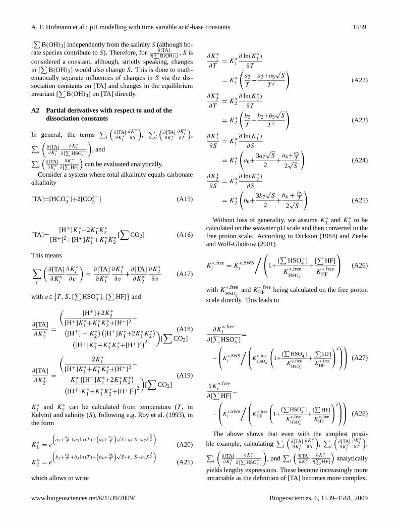
A. F. Hofmann et al.: pH modelling with time variable acid-base constants 1559
[∑
B(OH)3] independently from the salinityS (although bo-rate species contribute toS). Therefore, for ∂[TA]
∂[∑
B(OH)3], S is
considered a constant, although, strictly speaking, changesin [
∑B(OH)3] would also changeS. This is done to math-
ematically separate influences of changes inS via the dis-sociation constants on [TA] and changes in the equilibriuminvariant[
∑B(OH)3] on [TA] directly.
A2 Partial derivatives with respect to and of thedissociation constants
In general, the terms∑
i
(∂[TA]
∂K∗i
∂K∗i
∂S
),∑
i
(∂[TA]
∂K∗i
∂K∗i
∂T
),∑
i
(∂[TA]
∂K∗i
∂K∗i
∂[∑
HSO−
4 ]
), and∑
i
(∂[TA]
∂K∗i
∂K∗i
∂[∑
HF]
)can be evaluated analytically.
Consider a system where total alkalinity equals carbonatealkalinity
[TA]=[HCO−
3 ]+2[CO2−
3 ] (A15)
[TA]=[H+
]K∗
1+2K∗
1K∗
2
[H+]2+[H+]K∗
1+K∗
1K∗
2[
∑CO2] (A16)
This means∑i
(∂[TA]
∂K∗
i
∂K∗
i
∂v
)=
∂[TA]
∂K∗
1
∂K∗
1
∂v+
∂[TA]
∂K∗
2
∂K∗
2
∂v(A17)
with v∈{T , S, [
∑HSO−
4 ], [∑
HF]}
and
∂[TA]
∂K∗
1=
([H+
]+2K∗
2
[H+]K∗
1+K∗
1K∗
2+[H+]2−(
[H+] + K∗
2
) ([H+
]K∗
1+2K∗
1K∗
2
)([H+]K∗
1+K∗
1K∗
2+[H+]2)2 )
[
∑CO2]
(A18)
∂[TA]
∂K∗
2=
(2K∗
1
[H+]K∗
1+K∗
1K∗
2+[H+]2−
K∗
1
([H+
]K∗
1+2K∗
1K∗
2
)([H+]K∗
1+K∗
1K∗
2+[H+]2)2)[
∑CO2]
(A19)
K∗
1 and K∗
2 can be calculated from temperature (T , inKelvin) and salinity (S), following e.g.Roy et al.(1993), inthe form
K∗
1 = e
(a1+
a2T
+a3 ln (T )+(a4+
a5T
)√S+a6 S+a7S
32
)(A20)
K∗
2 = e
(b1+
b2T
+b3 ln (T )+(b4+
b5T
)√S+b6 S+b7S
32
)(A21)
which allows to write
∂K∗
1
∂T= K∗
1∂ ln(K∗
1)
∂T
= K∗
1
(a3
T−
a2+a5√
S
T 2
)(A22)
∂K∗
2
∂T= K∗
2∂ ln(K∗
2)
∂T
= K∗
2
(b3
T−
b2+b5√
S
T 2
)(A23)
∂K∗
1
∂S= K∗
1∂ ln(K∗
1)
∂S
= K∗
1
(a6+
3a7√
S
2+
a4+a5T
2√
S
)(A24)
∂K∗
2
∂S= K∗
2∂ ln(K∗
2)
∂S
= K∗
2
(b6+
3b7√
S
2+
b4 +b5T
2√
S
)(A25)
Without loss of generality, we assumeK∗
1 andK∗
2 to becalculated on the seawater pH scale and then converted to thefree proton scale. According toDickson(1984) andZeebeand Wolf-Gladrow(2001)
K∗,freei = K
∗,SWSi
/1+[∑
HSO−
4 ]
K∗,freeHSO−
4
+[∑
HF]
K∗,freeHF
(A26)
with K∗,freeHSO−
4andK
∗,freeHF being calculated on the free proton
scale directly. This leads to
∂K∗,freei
∂[∑
HSO−
4 ]=
−
K∗,SWSi
/K∗,freeHSO−
4
1+[∑
HSO−
4 ]
K∗,freeHSO−
4
+[∑
HF]
K∗,freeHF
2 (A27)
∂K∗,freei
∂[∑
HF]=
−
K∗,SWSi
/K∗,freeHF
1+[∑
HSO−
4 ]
K∗,freeHSO−
4
+[∑
HF]
K∗,freeHF
2 (A28)
The above shows that even with the simplest possi-
ble example, calculating∑
i
(∂[TA]
∂K∗i
∂K∗i
∂S
),∑
i
(∂[TA]
∂K∗i
∂K∗i
∂T
),∑
i
(∂[TA]
∂K∗i
∂K∗i
∂[∑
HSO−
4 ]
), and
∑i
(∂[TA]
∂K∗i
∂K∗i
∂[∑
HF]
)analytically
yields lengthy expressions. These become increasingly moreintractable as the definition of [TA] becomes more complex.
www.biogeosciences.net/6/1539/2009/ Biogeosciences, 6, 1539–1561, 2009

1560 A. F. Hofmann et al.: pH modelling with time variable acid-base constants
Therefore, we decided to calculate these terms numeri-cally by calculating [TA] twice with small disturbances ofthe independent variable
∑i
(∂[TA]
∂K∗
i
∂K∗
i
∂S
)=
([TA]([H+
], X, K∗(S+εS, T , [∑
HSO−
4 ], [∑
HF]))−
[TA]([H+], X, K∗(S−εS, T , [
∑HSO−
4 ], [∑
HF]))
)/2εS
(A29)
∑i
(∂[TA]
∂K∗
i
∂K∗
i
∂T
)=
([TA]([H+
], X, K∗(S, T +εT , [∑
HSO−
4 ], [∑
HF]))−
[TA]([H+], X, K∗(S, T −εT , [
∑HSO−
4 ], [∑
HF])
)/2εT
(A30)
∑i
(∂[TA]
∂K∗
i
∂K∗
i
∂[∑
HSO−
4 ]
)=
([TA]([H+
], X, K∗(S, T , [∑
HSO−
4 ]+ε[∑
HSO−
4 ], [∑
HF]))−
[TA]([H+], X, K∗(S, T , [
∑HSO−
4 ] − ε[∑
HSO−
4 ], [∑
HF]))
)/2εS
(A31)
∑i
(∂[TA]
∂K∗
i
∂K∗
i
∂[∑
HF]
)=
([TA]([H+
], X, K∗(S, T , [∑
HSO−
4 ], [∑
HF] + ε[∑
HF]))−
[TA]([H+], X, K∗(S, T , [
∑HSO−
4 ], [∑
HF] − ε[∑
HF]))
)/2εT
(A32)
with εv=0.1v ∀ v∈{T , S, [
∑HSO−
4 ], [∑
HF]}. Note that
[∑
HSO−
4 ] and[∑
HF] are only disturbed for calculating thedissociation constants and kept at their normal values whenthey serve as equilibrium invariants (total quantities) for cal-culating [HSO−
4 ] and [HF].
Acknowledgements.We thank four anonymous reviewers andPierre Regnier for constrcutive criticism that substantially im-proved the quality of this paper. This research was supported by theEU (Carbo-Ocean, 511 176-2) and the Netherlands Organisationfor Scientific Research (833.02.2002). This is publication number4599 of the Netherlands Institute of Ecology (NIOO-KNAW),Centre for Estuarine and Marine Ecology, P.O. Box 140, 4400 ACYerseke, The Netherlands.
Edited by: A. Borges
References
Abril, G. and Frankignoulle, M.: Nitrogen-alkalinity interactions inthe highly polluted Scheldt basin (Belgium), Water Research, 35,844–850, 2001.
Abril, G., Etcheber, H., Borges, A. V., and Frankignoulle, M.: Ex-cess atmospheric carbon dioxide transported by rivers into theScheldt estuary, Comptes Rendus De L Academie Des SciencesSerie Ii Fascicule a-Sciences De La Terre Et Des Planetes, 330,761–768, 2000.
Andersson, M. G. I., Brion, N., and Middelburg, J. J.: Comparisonof nitrifier activity versus growth in the Scheldt estuary – a turbid,tidal estuary in northern Europe, Aquat. Microb. Ecol., 42, 149–158, 2006.
Ben-Yaakov, S.: A Method for Calculating the in Situ pH of Sea-water, Limnol. Oceanogr., 15, 326–328, 1970.
Ben-Yaakov, S.: Ph Buffering of Pore Water of Recent Anoxic Ma-rine Sediments, Limnol. Oceanogr., 18, 86–94, 1973.
Blackford, J. C. and Gilbert, F. J.: pH variability and CO2 inducedacidification in the North Sea, J. Marine Syst., 64, 229–241,2007.
Boudreau, B. P. and Canfield, D. E.: A Provisional DiageneticModel for Ph in Anoxic Porewaters – Application to the FoamSite, J. Mar. Res., 46, 429–455, 1988.
Culberson, C. H.: Calculation of the Insitu Ph of Seawater, Lim-nol. Oceanogr., 25, 150–152, 1980.
Dickson, A. G. and Riley, J. P.: Estimation of Acid Dissociation-Constants in Seawater Media from Potentiometric Titrations withStrong Base .1. Ionic Product of Water – Kw, Mar. Chem., 7, 89–99, 1979.
Dickson, A. G.: An Exact Definition of Total Alkalinity anda Procedure for the Estimation of Alkalinity and Total Inor-ganic Carbon from Titration Data, Deep-Sea Research Part a-Oceanographic Research Papers, 28, 609–623, 1981.
Dickson, A. G.: Ph Scales and Proton-Transfer Reactions in SalineMedia Such as Sea-Water, Geochim. Cosmochim. Ac., 48,2299–2308, 1984.
Dickson, A. G.: Thermodynamics of the Dissociation of Boric-Acid in Synthetic Seawater from 273.15 K to 318.15 K, Deep-Sea Res., 37, 755–766, 1990a.
Dickson, A. G.: Standard Potential of the Reaction – AgCl(S)+1/2H2(G)=Ag(S)+HCl(Aq) and the Standard Acidity Constant ofthe Ion HSO−4 in Synthetic Sea-Water from 273.5 K to 318.15 K,J. Chem. Thermodyn., 22, 113–127, 1990b.
Follows, M. J., Ito, T., and Dutkiewicz, S.: On the solution of thecarbonate chemistry system in ocean biogeochemistry models,Ocean Model., 12, 290–301, 2006.
Frankignoulle, M., Bourge, I., and Wollast, R.: AtmosphericCO2Fluxes in a Highly Polluted Estuary (the Scheldt), Limnologyand Oceanography, 41, 365–369, 1996.
Gazeau, F., Gattuso, J. P., Middelburg, J. J., Brion, N., Schiette-catte, L. S., Frankignoulle, M., and Borges, A. V.: Planktonic andwhole system metabolism in a nutrient-rich estuary (the Scheldtestuary), Estuaries, 28, 868–883, 2005.
Gazeau, F., Quiblier, C., Jansen, J. M., Gattuso, J. P., Middelburg,J. J., and Heip, C. H. R.: Impact of elevated CO2 on shellfishcalcification, Geophys. Res. Lett., 34, 2007.
Guinotte, J. M. and Fabry, V. J.: Ocean acidification and its potentialeffects on marine ecosystems, Year in Ecology and ConservationBiology 2008, 2008.
Biogeosciences, 6, 1539–1561, 2009 www.biogeosciences.net/6/1539/2009/

A. F. Hofmann et al.: pH modelling with time variable acid-base constants 1561
Heip, C.: Biota and Abiotic Environment in the Westerschelde Es-tuary, Hydrobiological Bulletin, 22, 31–34, 1988.
Hofmann, A. F., Meysman, F. J. R., Soetaert, K., and Middelburg,J. J.: A step-by-step procedure for pH model construction inaquatic systems, Biogeosciences, 5, 227–251, 2008a.
Hofmann, A. F., Soetaert, K., and Middelburg, J. J.: Present nitro-gen and carbon dynamics in the Scheldt estuary using a novel1-D model, Biogeosciences, 5, 981–1006, 2008b.
Hofmann, A. F., Soetaert, K., Middelburg, J. J., and Meysman,F. J. R.: AquaEnv - an Aquatic acid-base modelling Environ-ment in R, submitted to Aquatic Geochemistry.
Holland, A.: The waste loads on the Scheldt estuary (1980–1988),Tidal Waters Division, Middelburg, The Netherlands, 1991.
Jourabchi, P., Van Cappellen, P., and Regnier, P.: Quantitative in-terpretation of pH distributions in aquatic sediments: A reaction-transport modeling approach, Am. J. Sci., 305, 919–956, 2005.
Luff, R., Haeckel, M., and Wallmann, K.: Robust and fast FOR-TRAN and MATLAB (R) libraries to calculate pH distributionsin marine systems, Comput. Geosci., 27, 157–169, 2001.
Millero, F. J. and Poisson, A.: International One-Atmosphere Equa-tion of State of Seawater, Deep-Sea Res., 28, 625–629, 1981.
Millero, F. J.: Thermodynamics of the Carbon-Dioxide System inthe Oceans, Geochim. Cosmochim. Ac., 59, 661–677, 1995.
Millero, F. J.: Chemical Oceanography, CRC / Taylor & Francis,3rd edn., 2006.
Mook, W. G. and Koene, B. K. S.: Chemistry of Dissolved In-organic Carbon in Estuarine and Coastal Brackish Waters, Es-tuar. Coast. Mar. Sci., 3, 325–336, 1975.
Morel, F. M. and Hering, J. G.: Principles and Applications ofAquatic Chemistry, John Wiley & sons, 1993.
MVG: Ministerie van de Vlaamse Gemeenschap – Afdeling Mari-tieme toegang.
Orr, J. C., Fabry, V. J., Aumont, O., Bopp, L., Doney, S. C., Feely,R. A., Gnanadesikan, A., Gruber, N., Ishida, A., Joos, F., Key,R. M., Lindsay, K., Maier-Reimer, E., Matear, R., Monfray, P.,Mouchet, A., Najjar, R. G., Plattner, G. K., Rodgers, K. B.,Sabine, C. L., Sarmiento, J. L., Schlitzer, R., Slater, R. D., Tot-terdell, I. J., Weirig, M. F., Yamanaka, Y., and Yool, A.: Anthro-pogenic ocean acidification over the twenty-first century and itsimpact on calcifying organisms, Nature, 437, 681–686, 2005.
R Development Core Team: R: A language and environment forstatistical computing, R Foundation for Statistical Computing,Vienna, Austria, available at:http://www.R-project.org, ISBN 3-900051-07-0, 2005.
Regnier, P., Wollast, R., and Steefel, C. I.: Long-term fluxes of reac-tive species in macrotidal estuaries: Estimates from a fully tran-sient, multicomponent reaction-transport model, Mar. Chem., 58,127–145, 1997.
Roy, R. N., Roy, L. N., Vogel, K. M., PorterMoore, C., Pearson,T., Good, C. E., Millero, F. J., and Campbell, D. M.: The dis-sociation constants of carbonic acid in seawater at salinities 5 to45 and temperatures O to 45 degrees C (see also erratum: Mar.Chem., 52, 183, 1996), Mar. Chem., 44, 249–267, 1993.
Sarmiento, J. L. and Gruber, N.: Ocean Biogeochemical Dynamics,Princeton University Press, Princeton, 2006.
Soetaert, K. and Herman, P. M. J.: Estimating Estuarine Resi-dence Times in the Westerschelde (the Netherlands) Using a BoxModel with Fixed Dispersion Coefficients, Hydrobiologia, 311,215–224, 1995.
Soetaert, K., deClippele, V., and Herman, P.: FEMME, a flexi-ble environment for mathematically modelling the environment,Ecol. Model., 151, 177–193, 2002.
Soetaert, K., Middelburg, J. J., Heip, C., Meire, P., Van Damme, S.,and Maris, T.: Long-term change in dissolved inorganic nutrientsin the heterotropic Scheldt estuary (Belgium, The Netherlands),Limnol. Oceanogr., 51, 409–423, 2006.
Soetaert, K., Hofmann, A. F., Middelburg, J. J., Meysman, F. J., andGreenwood, J.: The effect of biogeochemical processes on pH,Mar. Chem., 105, 30–51, 2007.
Spiteri, C., Van Cappellen, P., and Regnier, P.: Surface complexa-tion effects on phosphate adsorption to ferric iron oxyhydroxidesalong pH and salinity gradients in estuaries and coastal aquifers,Geochim. Cosmochim. Ac., 72, 3431–3445, 2008.
Stumm, W. and Morgan, J. J.: Aquatic Chemistry: Chemical Equi-libria and Rates in natural Waters, Wiley Interscience, New York,1996.
van Gils, J. A. G., Ouboter, M. R. L., and De Roij, N. M.: Modellingof Water and Sediment Quality in the Scheldt Estuary, Nether-lands J. Aquat. Ecol., 27, 257–265, 1993.
Vanderborght, J. P., Wollast, R., Loijens, M., and Regnier, P.: Ap-plication of a transport-reaction model to the estimation of bio-gas fluxes in the Scheldt estuary, Biogeochemistry, 59, 207–237,2002.
Vanderborght, J.-P., Folmer, I. M., Aguilera, D. R., Uhrenholdt,T., and Regnier, P.: Reactive-transport modelling of C, N, andO2 in a river-estuarine-coastal zone system: Application to theScheldt estuary, Marine Chemistry Special issue: Dedicatedto the memory of Professor Roland Wollast, 106, 92–110,available at: http://www.sciencedirect.com/science/article/B6VC2-4KM4719-1/2/6943e718e77392f85420f63fa86bcbc6,2007.
Whitfield, M. and Turner, D. R.: The Carbon-Dioxide System inEstuaries-an Inorganic Perspective, Science of the Total Envi-ronment, 49, 235–255, 1986.
Wong, G. T. F.: Alkalinity and pH in the Southern Chesapeake Bayand the James River Estuary, Limnology and Oceanography, 24,970–977, 1979.
Zeebe, R. E. and Wolf-Gladrow, D.: CO2 in Seawater: Equilibrium,Kinetics, Isotopes, no. 65 in Elsevier Oceanography Series, El-sevier, 1st edn., 2001.
www.biogeosciences.net/6/1539/2009/ Biogeosciences, 6, 1539–1561, 2009