Embed Size (px)
Citation preview
M O D E R NQ U A N T U MMECHANICSS E C O N D E D I T I O N

Modern Quantum MechanicsSecond Edition
Modern Quantum Mechanics is a classical graduate level textbook, covering the main quantum mechan-ics concepts in a clear, organized and engaging manner. The author, J. J. Sakurai, was a renownedtheorist in particle theory. The Second Edition, revised by Jim Napolitano, introduces topics thatextend the text’s usefulness into the 21st century such as advanced mathematical techniques associ-ated with quantum mechanical calculations, while at the same time retaining classic developmentssuch as neutron interferometer experiments, Feynman path integrals, correlation measurements, andBell’s inequality. A solution manual for instructors using this textbook can be downloaded fromwww.cambirdge.org/napolitano under the resources tab.
The late J.J. Sakurai, noted theorist in particle physics, was born in Tokyo, Japan in 1933. He receivedhis B.A. from Harvard University in 1955 and his PhD from Cornell University in 1958. He wasappointed as an assistant professor at the University of Chicago, where he worked until he becamea professor at the University of California, Los Angeles in 1970. Sakurai died in 1982 while he wasvisiting a professor at CERN in Geneva, Switzerland.
Jim Napolitano earned an undergraduate Physics degree at Rensselaer Polytechnic Institute in 1977,and a PhD in Physics from Stanford University in 1982. Since that time, he has conducted research inexperimental nuclear and particle physics, with an emphasis on studying fundamental interactions andsymmetries. He joined the faculty at Rensselaer in 1992 after working as a member of the scientific staffat two different national laboratories. Since 2014 he has been Professor of Physics at Temple University.He is author and co-author of over 150 scientific papers in refereed journals. Professor Napolitanomaintains a keen interest in science education in general, and in particular physics education at both theundergraduate and graduate levels. He has taught both graduate and upper-level undergraduate coursesin Quantum Mechanics, as well as an advanced graduate course in Quantum Field Theory.

Modern QuantumMechanics
Second Edition
J. J. SakuraiDeceased
Jim NapolitanoTemple University, Philadelphia
University Printing House, Cambridge CB2 8BS, United Kingdom
One Liberty Plaza, 20th Floor, New York, NY 10006, USA
477 Williamstown Road, Port Melbourne, VIC 3207, Australia
4843/24, 2nd Floor, Ansari Road, Daryaganj, Delhi – 110002, India
79 Anson Road, #06–04/06, Singapore 079906
Cambridge University Press is part of the University of Cambridge.
It furthers the University’s mission by disseminating knowledge in the pursuit ofeducation, learning, and research at the highest international levels of excellence.
www.cambridge.orgInformation on this title: www.cambridge.org/9781108422413DOI: 10.1017/9781108499996
c© Cambridge University Press 2017
This publication is in copyright. Subject to statutory exceptionand to the provisions of relevant collective licensing agreements,no reproduction of any part may take place without the writtenpermission of Cambridge University Press.
This book was previously published by Pearson Education, Inc. 1994, 2011
Reissued by Cambridge University Press 2017
Printed in the United Kingdom by TJ International Ltd. Padstow Cornwall
A catalogue record for this publication is available from the British Library.
Additional resources for this publication available at: www.cambridge.org/napolitano
ISBN 978-1-108-42241-3 Hardback
Cambridge University Press has no responsibility for the persistence or accuracy ofURLs for external or third-party internet websites referred to in this publicationand does not guarantee that any content on such websites is, or will remain,accurate or appropriate.
Contents
Foreword to the First Edition ix
Preface to the Revised Edition xi
Preface to the Second Edition xiii
In Memoriam xvii
1 Fundamental Concepts 11.1 The Stern-Gerlach Experiment 11.2 Kets, Bras, and Operators 101.3 Base Kets and Matrix Representations 171.4 Measurements, Observables, and the Uncertainty Relations 231.5 Change of Basis 351.6 Position, Momentum, and Translation 401.7 Wave Functions in Position and Momentum Space 50
2 Quantum Dynamics 662.1 Time-Evolution and the Schrödinger Equation 662.2 The Schrödinger Versus the Heisenberg Picture 802.3 Simple Harmonic Oscillator 892.4 Schrödinger’s Wave Equation 972.5 Elementary Solutions to Schrödinger’s Wave Equation 1032.6 Propagators and Feynman Path Integrals 1162.7 Potentials and Gauge Transformations 129
3 Theory of Angular Momentum 1573.1 Rotations and Angular-Momentum Commutation Relations 1573.2 Spin 1
2 Systems and Finite Rotations 1633.3 SO(3), SU(2), and Euler Rotations 172
v
vi Contents
3.4 Density Operators and Pure Versus Mixed Ensembles 1783.5 Eigenvalues and Eigenstates of Angular Momentum 1913.6 Orbital Angular Momentum 1993.7 Schrödinger’s Equation for Central Potentials 2073.8 Addition of Angular Momenta 2173.9 Schwinger’s Oscillator Model of Angular Momentum 2323.10 Spin Correlation Measurements and Bell’s Inequality 2383.11 Tensor Operators 246
4 Symmetry in Quantum Mechanics 2624.1 Symmetries, Conservation Laws, and Degeneracies 2624.2 Discrete Symmetries, Parity, or Space Inversion 2694.3 Lattice Translation as a Discrete Symmetry 2804.4 The Time-Reversal Discrete Symmetry 284
5 Approximation Methods 3035.1 Time-Independent Perturbation Theory: Nondegenerate Case 3035.2 Time-Independent Perturbation Theory: The Degenerate Case 3165.3 Hydrogen-Like Atoms: Fine Structure and the Zeeman Effect 3215.4 Variational Methods 3325.5 Time-Dependent Potentials: The Interaction Picture 3365.6 Hamiltonians with Extreme Time Dependence 3455.7 Time-Dependent Perturbation Theory 3555.8 Applications to Interactions with the Classical Radiation Field 3655.9 Energy Shift and Decay Width 371
6 Scattering Theory 3866.1 Scattering as a Time-Dependent Perturbation 3866.2 The Scattering Amplitude 3916.3 The Born Approximation 3996.4 Phase Shifts and Partial Waves 4046.5 Eikonal Approximation 4176.6 Low-Energy Scattering and Bound States 4236.7 Resonance Scattering 4306.8 Symmetry Considerations in Scattering 4336.9 Inelastic Electron-Atom Scattering 436
7 Identical Particles 4467.1 Permutation Symmetry 4467.2 Symmetrization Postulate 450
Contents vii
7.3 Two-Electron System 4527.4 The Helium Atom 4557.5 Multiparticle States 4597.6 Quantization of the Electromagnetic Field 472
8 Relativistic Quantum Mechanics 4868.1 Paths to Relativistic Quantum Mechanics 4868.2 The Dirac Equation 4948.3 Symmetries of the Dirac Equation 5018.4 Solving with a Central Potential 5068.5 Relativistic Quantum Field Theory 514
A Electromagnetic Units 519A.1 Coulomb’s Law, Charge, and Current 519A.2 Converting Between Systems 520
B Brief Summary of Elementary Solutions to Schrödinger’sWave Equation 523B.1 Free Particles (V = 0) 523B.2 Piecewise Constant Potentials in One Dimension 524B.3 Transmission-Reflection Problems 525B.4 Simple Harmonic Oscillator 526B.5 The Central Force Problem [Spherically Symmetrical Potential
V = V (r)] 527B.6 Hydrogen Atom 531
C Proof of the Angular-Momentum Addition Rule Given byEquation (3.8.38) 533
Bibliography 535
Index 537

Foreword to the First Edition
J. J. Sakurai was always a very welcome guest here at CERN, for he was one ofthose rare theorists to whom the experimental facts are even more interesting thanthe theoretical game itself. Nevertheless, he delighted in theoretical physics andin its teaching, a subject on which he held strong opinions. He thought that muchtheoretical physics teaching was both too narrow and too remote from application:“. . .we see a number of sophisticated, yet uneducated, theoreticians who are con-versant in the LSZ formalism of the Heisenberg field operators, but do not knowwhy an excited atom radiates, or are ignorant of the quantum theoretic derivationof Rayleigh’s law that accounts for the blueness of the sky.” And he insisted thatthe student must be able to use what has been taught: “The reader who has readthe book but cannot do the exercises has learned nothing.”
He put these principles to work in his fine book Advanced Quantum Mechanics(1967) and in Invariance Principles and Elementary Particles (1964), both ofwhich have been very much used in the CERN library. This new book, ModernQuantum Mechanics, should be used even more, by a larger and less specializedgroup. The book combines breadth of interest with a thorough practicality. Itsreaders will find here what they need to know, with a sustained and successfuleffort to make it intelligible.
J. J. Sakurai’s sudden death on November 1, 1982 left this book unfinished.Reinhold Bertlmann and I helped Mrs. Sakurai sort out her husband’s papers atCERN. Among them we found a rough, handwritten version of most of the bookand a large collection of exercises. Though only three chapters had been com-pletely finished, it was clear that the bulk of the creative work had been done. Itwas also clear that much work remained to fill in gaps, polish the writing, and putthe manuscript in order.
That the book is now finished is due to the determination of Noriko Sakuraiand the dedication of San Fu Tuan. Upon her husband’s death, Mrs. Sakurai re-solved immediately that his last effort should not go to waste. With great courageand dignity she became the driving force behind the project, overcoming all ob-stacles and setting the high standards to be maintained. San Fu Tuan willinglygave his time and energy to the editing and completion of Sakurai’s work. Per-haps only others close to the hectic field of high-energy theoretical physics canfully appreciate the sacrifice involved.
For me personally, J. J. had long been far more than just a particularly dis-tinguished colleague. It saddens me that we will never again laugh together atphysics and physicists and life in general, and that he will not see the success ofhis last work. But I am happy that it has been brought to fruition.
John S. BellCERN, Geneva
ix

Preface to the Revised Edition
Since 1989 the editor has enthusiastically pursued a revised edition of ModernQuantum Mechanics by his late great friend J. J. Sakurai, in order to extend thistext’s usefulness into the twenty-first century. Much consultation took place withthe panel of Sakurai friends who helped with the original edition, but in particularwith Professor Yasuo Hara of Tsukuba University and Professor Akio Sakurai ofKyoto Sangyo University in Japan.
This book is intended for the first-year graduate student who has studied quan-tum mechanics at the junior or senior level. It does not provide an introductionto quantum mechanics for the beginner. The reader should have had some expe-rience in solving time-dependent and time-independent wave equations. A famil-iarity with the time evolution of the Gaussian wave packet in a force-free region isassumed, as is the ability to solve one-dimensional transmission-reflection prob-lems. Some of the general properties of the energy eigenfunctions and the energyeigenvalues should also be known to the student who uses this text.
The major motivation for this project is to revise the main text. There are threeimportant additions and/or changes to the revised edition, which otherwise pre-serves the original version unchanged. These include a reworking of certain por-tions of Section 5.2 on time-independent perturbation theory for the degeneratecase, by Professor Kenneth Johnson of M.I.T., taking into account a subtle pointthat has not been properly treated by a number of texts on quantum mechanicsin this country. Professor Roger Newton of Indiana University contributed refine-ments on lifetime broadening in Stark effect and additional explanations of phaseshifts at resonances, the optical theorem, and the non-normalizable state. Theseappear as “remarks by the editor” or “editor’s note” in the revised edition. Pro-fessor Thomas Fulton of the Johns Hopkins University reworked his Coulombscattering contribution (Section 7.13); it now appears as a shorter text portionemphasizing the physics, with the mathematical details relegated to Appendix C.
Though not a major part of the text, some additions were deemed necessary totake into account developments in quantum mechanics that have become promi-nent since November 1, 1982. To this end, two supplements are included at theend of the text. Supplement I is on adiabatic change and geometrical phase (pop-ularized by M. V. Berry since 1983) and is actually an English translation of thesupplement on this subject written by Professor Akio Sakurai for the Japanese ver-sion of Modern Quantum Mechanics (copyright c© Yoshioka-Shoten Publishingof Kyoto). Supplement II on nonexponential decays was written by my colleaguehere, Professor Xerxes Tata, and read over by Professor E. C. G. Sudarshan ofthe University of Texas at Austin. Although nonexponential decays have a long
xi
xii Preface to the Revised Edition
history theoretically, experimental work on transition rates that tests such decaysindirectly was done only in 1990. Introduction of additional material is of course asubjective decision on the part of the editor; readers can judge its appropriatenessfor themselves. Thanks to Professor Akio Sakurai, the revised edition has beendiligently searched to correct misprint errors of the first ten printings of the origi-nal edition. My colleague Professor Sandip Pakvasa provided me overall guidanceand encouragement throughout this process of revision.
In addition to the acknowledgments above, my former students Li Ping, ShiXiaohong, and Yasunaga Suzuki provided the sounding board for ideas on therevised edition when taking may graduate quantum mechanics course at the Uni-versity of Hawaii during the spring of 1992. Suzuki provided the initial translationfrom Japanese of Supplement I as a course term paper. Dr. Andy Acker providedme with computer graphics assistance. The Department of Physics and Astron-omy, and particularly the High Energy Physics Group of the University of Hawaiiat Manoa, again provided both the facilities and a conducive atmosphere for me tocarry out my editorial task. Finally I wish to express my gratitude to physics (andsponsoring) senior editor Stuart Johnson and his editorial assistant Jennifer Dug-gan as well as senior production coordinator Amy Willcutt, of Addison-Wesleyfor their encouragement and optimism that the revised edition would indeedmaterialize.
San Fu TuanHonolulu, Hawaii
Preface to the Second Edition
Quantum mechanics fascinates me. It describes a wide variety of phenomenabased on very few assumptions. It starts with a framework so unlike the differ-ential equations of classical physics, yet it contains classical physics within it. Itprovides quantitative predictions for many physical situations, and these predic-tions agree with experiments. In short, quantum mechanics is the ultimate basis,today, by which we understand the physical world.
Thus, I was very pleased to be asked to write the next revised edition of ModernQuantum Mechanics, by J. J. Sakurai. I had taught this material out of this bookfor a few years and found myself very in tune with its presentation. Like manyother instructors, however, I found some aspects of the book lacking and thereforeintroduced material from other books and from my own background and research.My hybrid class notes form the basis for the changes in this new edition.
Of course, my original proposal was more ambitious than could be realized,and it still took much longer than I would have liked. So many excellent sugges-tions found their way to me through a number of reviewers, and I wish I had beenable to incorporate all of them. I am pleased with the result, however, and I havetried hard to maintain the spirit of Sakurai’s original manuscript.
Chapter 1 is essentially unchanged. Some of the figures were updated, andreference is made to Chapter 8, where the relativistic origin of the Dirac magneticmoment is laid out.
Material was added to Chapter 2. This includes a new section on elementarysolutions including the free particle in three dimensions; the simple harmonicoscillator in the Schrödinger equation using generating functions; and the linearpotential as a way of introducing Airy functions. The linear potential solution isused to feed into the discussion of the WKB approximation, and the eigenvaluesare compared to an experiment measuring “bouncing neutrons.” Also includedis a brief discussion of neutrino oscillations as a demonstration of quantum-mechanical interference.
Chapter 3 now includes solutions to Schrödinger’s equation for central poten-tials. The general radial equation is presented and is applied to the free particlein three dimensions with application to the infinite spherical well. We solve theisotropic harmonic oscillator and discuss its application to the “nuclear poten-tial well.” We also carry through the solution using the Coulomb potential with adiscussion on degeneracy. Advanced mathematical techniques are emphasized.
A subsection that has been added to Chapter 4 discusses the symmetry, knownclassically in terms of the Lenz vector, inherent in the Coulomb problem. This
xiii
xiv Preface to the Second Edition
provides an introduction to SO(4) as an extension of an earlier discussion in Chap-ter 3 on continuous symmetries.
There are two additions to Chapter 5. First, there is a new introduction toSection 5.3 that applies perturbation theory to the hydrogen atom in the context ofrelativistic corrections to the kinetic energy. This, along with some modificationsto the material on spin-orbit interactions, is helpful for comparisons when theDirac equation is applied to the hydrogen atom at the end of the book.
Second, a new section on Hamiltonians with “extreme” time dependences hasbeen added. This includes a brief discussion of the sudden approximation and alonger discussion of the adiabatic approximation. The adiabatic approximation isthen developed into a discussion of Berry’s Phase, including a specific example(with experimental verification) in the spin 1
2 system. Some material from the firstsupplement for the previous addition has found its way into this section.
The end of the book contains the most significant revisions, including reversedordering of the chapters on Scattering and Identical Particles. This is partly be-cause of a strong feeling on my part (and on the part of several reviewers) that thematerial on scattering needed particular attention. Also, at the suggestion of re-viewers, the reader is brought closer to the subject of quantum field theory, both asan extension of the material on identical particles to include second quantization,and with a new chapter on relativistic quantum mechanics.
Thus, Chapter 6, which now covers scattering in quantum mechanics, has anearly completely rewritten introduction. A time-dependent treatment is used todevelop the subject. Furthermore, the sections on the scattering amplitude andBorn approximation are rewritten to follow this new flow. This includes incor-porating what had been a short section on the optical theorem into the treatmentof the scattering amplitude, before moving on to the Born approximation. Theremaining sections have been edited, combined, and reworked, with some mate-rial removed, in an effort to keep what I, and the reviewers, felt were the mostimportant pieces of physics from the last edition.
Chapter 7 has two new sections that contain a significant expansion of theexisting material on identical particles. (The section on Young tableaux has beenremoved.) Multiparticle states are developed using second quantization, and twoapplications are given in some detail. One is the problem of an electron gas in thepresence of a positively charged uniform background. The other is the canonicalquantization of the electromagnetic field.
The treatment of multiparticle quantum states is just one path toward the de-velopment of quantum field theory. The other path involves incorporating specialrelativity into quantum mechanics, and this is the subject of Chapter 8. The sub-ject is introduced, and the Klein-Gordon equation is taken about as far as I believeis reasonable. The Dirac equation is treated in some detail, in more or less stan-dard fashion. Finally, the Coulomb problem is solved for the Dirac equation, andsome comments are offered on the transition to a relativistic quantum field theory.
The Appendices are reorganzied. A new appendix on electromagnetic units isaimed at the typical student who uses SI units as an undergraduate but is facedwith Gaussian units in graduate school.
Preface to the Second Edition xv
I am an experimental physicist, and I try to incorporate relevant experimentalresults in my teaching. Some of these have found their way into this edition, mostoften in terms of figures taken mainly from modern publications.
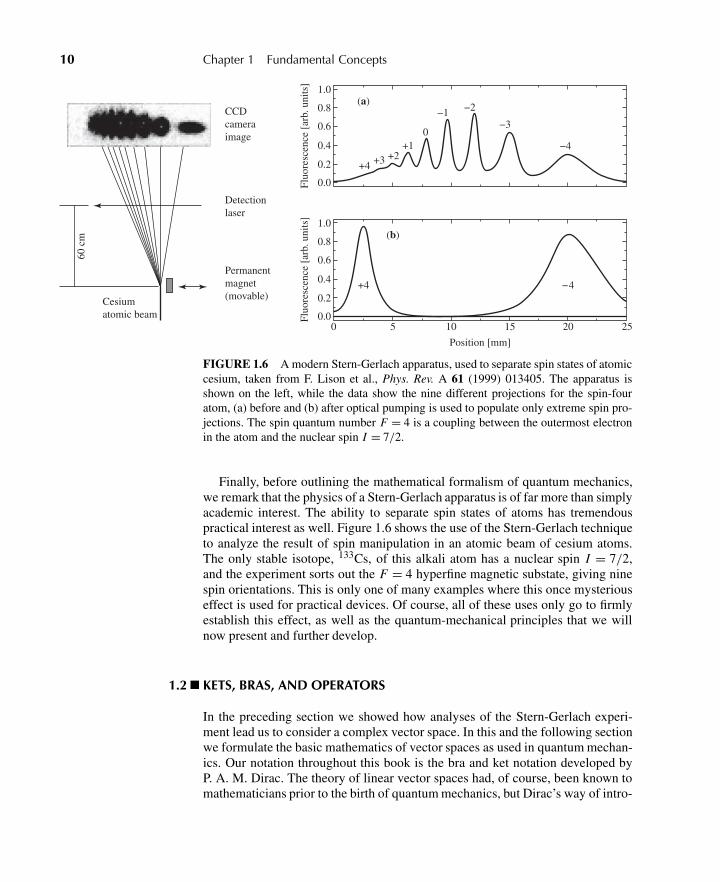
• Figure 1.6 demonstrates the use of a Stern-Gerlach apparatus to analyze thepolarization states of a beam of cesium atoms.
• Spin rotation in terms of the high-precision measurement of g − 2 for themuon is shown in Figure 2.1.
• Neutrino oscillations as observed by the KamLAND collaboration areshown in Figure 2.2.
• A lovely experiment demonstrating the quantum energy levels of “bounc-ing neutrons,” Figure 2.4, is included to emphasize agreement between theexact and WKB eigenvalues for the linear potential.
• Figure 2.10 showing gravitational phase shift appeared in the previous edi-tion.
• I included Figure 3.6, an old standard, to emphasize that the central-potential problems are very much applicable to the real world.
• Although many measurements of parity violation have been carried out inthe five decades since its discovery, Wu’s original measurement, Figure 4.6,remains one of the clearest demonstrations.
• Berry’s Phase for spin 12 measured with ultra-cold neutrons, is demonstrated
in Figure 5.6.
• Figure 6.6 is a clear example of how one uses scattering data to interpretproperties of the target.
• Sometimes, carefully executed experiments point to some problem in thepredictions, and Figure 7.2 shows what happens when exchange symmetryis not included.
• Quantization of the electromagnetic field is demonstrated by data on theCasimir effect (Figure 7.9) and in the observation of squeezed light (Fig-ure 7.10).
• Finally, some classic demonstrations of the need for relativistic quantummechanics are shown. Carl Anderson’s original discovery of the positron isshown in Figure 8.1. Modern information on details of the energy levels ofthe hydrogen atom is included in Figure 8.2.
In addition, I have included a number of references to experimental work relevantto the discussion topic at hand.
My thanks go out to so many people who have helped me with this project. Col-leagues in physics include John Cummings, Stuart Freedman, Joel Giedt, DavidHertzog, Barry Holstein, Bob Jaffe, Joe Levinger, Alan Litke, Kam-Biu Luk, Bob
xvi Preface to the Second Edition
McKeown, Harry Nelson, Joe Paki, Murray Peshkin, Olivier Pfister, Mike Snow,John Townsend, San Fu Tuan, David Van Baak, Dirk Walecka, Tony Zee, and alsothe reviewers who saw the various drafts of the manuscript. At Addison-Wesley,I have been guided through this process by Adam Black, Katie Conley, AshleyEklund, Deb Greco, Dyan Menezes, and Jim Smith. I am also indebted to JohnRogosich and Carol Sawyer from Techsetters, Inc., for their technical expertiseand advice. My apologies to those whose names have slipped my mind as I writethis acknowledgment.
In the end, it is my sincere hope that this new edition is true to Sakurai’soriginal vision and has not been weakened significantly by my interloping.
Jim NapolitanoTroy, New York
In Memoriam
Jun John Sakurai was born in 1933 in Tokyo and came to the United States asa high school student in 1949. He studied at Harvard and at Cornell, where hereceived his Ph.D. in 1958. He was then appointed assistant professor of physicsat the University of Chicago and became a full professor in 1964. He stayed atChicago until 1970 when he moved to the University of California at Los Ange-les, where he remained until his death. During his lifetime he wrote 119 articleson theoretical physics of elementary particles as well as several books and mono-graphs on both quantum and particle theory.
The discipline of theoretical physics has as its principal aim the formulation oftheoretical descriptions of the physical world that are at once concise and compre-hensive. Because nature is subtle and complex, the pursuit of theoretical physicsrequires bold and enthusiastic ventures to the frontiers of newly discovered phe-nomena. This is an area in which Sakurai reigned supreme, with his uncannyphysical insight and intuition and also his ability to explain these phenomena tothe unsophisticated in illuminating physical terms. One has but to read his verylucid textbooks on Invariance Principles and Elementary Particles and AdvancedQuantum Mechanics, or his reviews and summer school lectures, to appreciatethis. Without exaggeration I could say that much of what I did understand in par-ticle physics came from these and from his articles and private tutoring.
When Sakurai was still a graduate student, he proposed what is now known asthe V-A theory of weak interactions, independently of (and simultaneously with)Richard Feynman, Murray Gell-Mann, Robert Marshak, and George Sudarshan.In 1960 he published in Annals of Physics a prophetic paper, probably his singlemost important one. It was concerned with the first serious attempt to constructa theory of strong interactions based on Abelian and non-Abelian (Yang-Mills)gauge invariance. This seminal work induced theorists to attempt an understand-ing of the mechanisms of mass generation for gauge (vector) fields, now recog-nized as the Higgs mechanism. Above all it stimulated the search for a realisticunification of forces under the gauge principle, since crowned with success inthe celebrated Glashow-Weinberg-Salam unification of weak and electromagneticforces. On the phenomenological side, Sakurai pursued and vigorously advocatedthe vector mesons dominance model of hadron dynamics. He was the first to dis-cuss the mixing of ω and φ meson states. Indeed, he made numerous importantcontributions to particle physics phenomenology in a much more general sense,as his heart was always close to experimental activities.
I knew Jun John for more than 25 years, and I had the greatest admiration notonly for his immense powers as a theoretical physicist but also for the warmth
xvii
xviii In Memoriam
and generosity of his spirit. Though a graduate student himself at Cornell during1957–1958, he took time from his own pioneering research in K-nucleon disper-sion relations to help me (via extensive correspondence) with my Ph.D. thesis onthe same subject at Berkeley. Both Sandip Pakvasa and I were privileged to beassociated with one of his last papers on weak couplings of heavy quarks, whichdisplayed once more his infectious and intuitive style of doing physics. It is ofcourse gratifying to us in retrospect that Jun John counted this paper among thescore of his published works that he particularly enjoyed.
The physics community suffered a great loss at Jun John Sakurai’s death. Thepersonal sense of loss is a severe one for me. Hence I am profoundly thankfulfor the opportunity to edit and complete his manuscript on Modern QuantumMechanics for publication. In my faith no greater gift can be given me than anopportunity to show my respect and love for Jun John through meaningful service.
San Fu Tuan
C H A P T E R
1 Fundamental Concepts
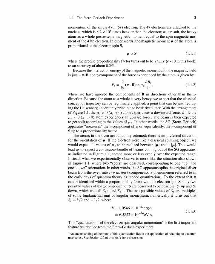
The revolutionary change in our understanding of microscopic phenomena thattook place during the first 27 years of the twentieth century is unprecedented inthe history of natural sciences. Not only did we witness severe limitations in thevalidity of classical physics, but we found the alternative theory that replaced theclassical physical theories to be far broader in scope and far richer in its range ofapplicability.
The most traditional way to begin a study of quantum mechanics is to followthe historical developments—Planck’s radiation law, the Einstein-Debye theory ofspecific heats, the Bohr atom, de Broglie’s matter waves, and so forth—togetherwith careful analyses of some key experiments such as the Compton effect, theFranck-Hertz experiment, and the Davisson-Germer-Thompson experiment. Inthat way we may come to appreciate how the physicists in the first quarter of thetwentieth century were forced to abandon, little by little, the cherished conceptsof classical physics and how, despite earlier false starts and wrong turns, the greatmasters—Heisenberg, Schrödinger, and Dirac, among others—finally succeededin formulating quantum mechanics as we know it today.
However, we do not follow the historical approach in this book. Instead, westart with an example that illustrates, perhaps more than any other example, theinadequacy of classical concepts in a fundamental way. We hope that, exposingreaders to a “shock treatment” at the onset will result in their becoming attunedto what we might call the “quantum-mechanical way of thinking” at a very earlystage.
This different approach is not merely an academic exercise. Our knowledgeof the physical world comes from making assumptions about nature, formulatingthese assumptions into postulates, deriving predictions from those postulates, andtesting such predictions against experiment. If experiment does not agree withthe prediction, then, presumably, the original assumptions were incorrect. Ourapproach emphasizes the fundamental assumptions we make about nature, uponwhich we have come to base all of our physical laws, and which aim to accom-modate profoundly quantum-mechanical observations at the outset.
1.1 THE STERN-GERLACH EXPERIMENT
The example we concentrate on in this section is the Stern-Gerlach experiment,originally conceived by O. Stern in 1921 and carried out in Frankfurt by him in
1
2 Chapter 1 Fundamental Concepts
S
N
Inhomogeneousmagnetic field
Furnace
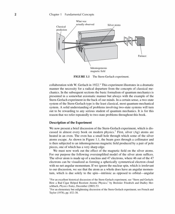
What wasactually observed Silver atoms
Classicalprediction
FIGURE 1.1 The Stern-Gerlach experiment.
collaboration with W. Gerlach in 1922.∗ This experiment illustrates in a dramaticmanner the necessity for a radical departure from the concepts of classical me-chanics. In the subsequent sections the basic formalism of quantum mechanics ispresented in a somewhat axiomatic manner but always with the example of theStern-Gerlach experiment in the back of our minds. In a certain sense, a two-statesystem of the Stern-Gerlach type is the least classical, most quantum-mechanicalsystem. A solid understanding of problems involving two-state systems will turnout to be rewarding to any serious student of quantum mechanics. It is for thisreason that we refer repeatedly to two-state problems throughout this book.
Description of the Experiment
We now present a brief discussion of the Stern-Gerlach experiment, which is dis-cussed in almost every book on modern physics.† First, silver (Ag) atoms areheated in an oven. The oven has a small hole through which some of the silveratoms escape. As shown in Figure 1.1, the beam goes through a collimator andis then subjected to an inhomogeneous magnetic field produced by a pair of polepieces, one of which has a very sharp edge.
We must now work out the effect of the magnetic field on the silver atoms.For our purpose the following oversimplified model of the silver atom suffices.The silver atom is made up of a nucleus and 47 electrons, where 46 out of the 47electrons can be visualized as forming a spherically symmetrical electron cloudwith no net angular momentum. If we ignore the nuclear spin, which is irrelevantto our discussion, we see that the atom as a whole does have an angular momen-tum, which is due solely to the spin—intrinsic as opposed to orbital—angular
∗For an excellent historical discussion of the Stern-Gerlach experiment, see “Stern and Gerlach:How a Bad Cigar Helped Reorient Atomic Physics,” by Bretislav Friedrich and Dudley Her-schbach, Physics Today, December (2003) 53.†For an elementary but enlightening discussion of the Stern-Gerlach experiment, see French andTaylor (1978), pp. 432–38.
1.1 The Stern-Gerlach Experiment 3
momentum of the single 47th (5s) electron. The 47 electrons are attached to thenucleus, which is ∼2 ×10⁵ times heavier than the electron; as a result, the heavyatom as a whole possesses a magnetic moment equal to the spin magnetic mo-ment of the 47th electron. In other words, the magnetic moment μ of the atom isproportional to the electron spin S,
μ ∝ S, (1.1.1)
where the precise proportionality factor turns out to be e/mec (e< 0 in this book)to an accuracy of about 0.2%.
Because the interaction energy of the magnetic moment with the magnetic fieldis just −μ·B, the z-component of the force experienced by the atom is given by
Fz = ∂
∂z(μ · B) � μz
∂Bz
∂z, (1.1.2)
where we have ignored the components of B in directions other than the z-direction. Because the atom as a whole is very heavy, we expect that the classicalconcept of trajectory can be legitimately applied, a point that can be justified us-ing the Heisenberg uncertainty principle to be derived later. With the arrangementof Figure 1.1, the μz > 0 (Sz < 0) atom experiences a downward force, while theμz < 0 (Sz > 0) atom experiences an upward force. The beam is then expectedto get split according to the values of μz . In other words, the SG (Stern-Gerlach)apparatus “measures” the z-component of μ or, equivalently, the z-component ofS up to a proportionality factor.
The atoms in the oven are randomly oriented; there is no preferred directionfor the orientation of μ. If the electron were like a classical spinning object, wewould expect all values of μz to be realized between |μ| and −|μ|. This wouldlead us to expect a continuous bundle of beams coming out of the SG apparatus,as indicated in Figure 1.1, spread more or less evenly over the expected range.Instead, what we experimentally observe is more like the situation also shownin Figure 1.1, where two “spots” are observed, corresponding to one “up” andone “down” orientation. In other words, the SG apparatus splits the original silverbeam from the oven into two distinct components, a phenomenon referred to inthe early days of quantum theory as “space quantization.” To the extent that μ
can be identified within a proportionality factor with the electron spin S, only twopossible values of the z-component of S are observed to be possible: Sz up and Szdown, which we call Sz+ and Sz−. The two possible values of Sz are multiplesof some fundamental unit of angular momentum; numerically it turns out thatSz = h/2 and −h/2, where
h = 1.0546 ×10⁻²⁷erg-s
= 6.5822 ×10⁻¹⁶eV-s.(1.1.3)
This “quantization” of the electron spin angular momentum∗ is the first importantfeature we deduce from the Stern-Gerlach experiment.∗An understanding of the roots of this quantization lies in the application of relativity to quantummechanics. See Section 8.2 of this book for a discussion.
4 Chapter 1 Fundamental Concepts
(a) (b)
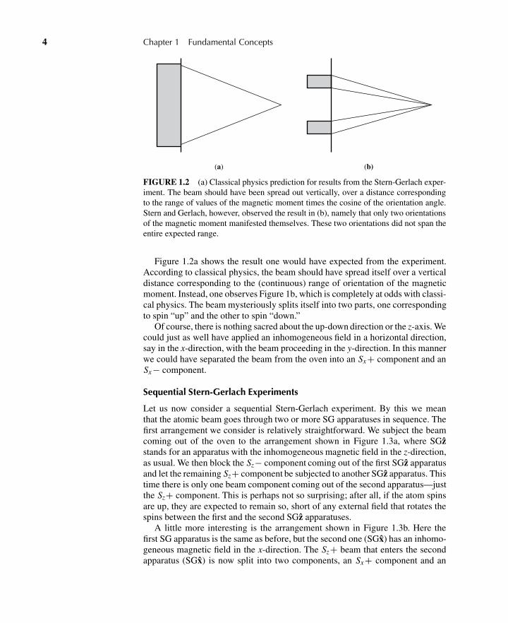
FIGURE 1.2 (a) Classical physics prediction for results from the Stern-Gerlach exper-iment. The beam should have been spread out vertically, over a distance correspondingto the range of values of the magnetic moment times the cosine of the orientation angle.Stern and Gerlach, however, observed the result in (b), namely that only two orientationsof the magnetic moment manifested themselves. These two orientations did not span theentire expected range.
Figure 1.2a shows the result one would have expected from the experiment.According to classical physics, the beam should have spread itself over a verticaldistance corresponding to the (continuous) range of orientation of the magneticmoment. Instead, one observes Figure 1b, which is completely at odds with classi-cal physics. The beam mysteriously splits itself into two parts, one correspondingto spin “up” and the other to spin “down.”
Of course, there is nothing sacred about the up-down direction or the z-axis. Wecould just as well have applied an inhomogeneous field in a horizontal direction,say in the x-direction, with the beam proceeding in the y-direction. In this mannerwe could have separated the beam from the oven into an Sx+ component and anSx− component.
Sequential Stern-Gerlach Experiments
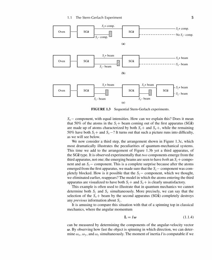
Let us now consider a sequential Stern-Gerlach experiment. By this we meanthat the atomic beam goes through two or more SG apparatuses in sequence. Thefirst arrangement we consider is relatively straightforward. We subject the beamcoming out of the oven to the arrangement shown in Figure 1.3a, where SGzstands for an apparatus with the inhomogeneous magnetic field in the z-direction,as usual. We then block the Sz− component coming out of the first SGz apparatusand let the remaining Sz+ component be subjected to another SGz apparatus. Thistime there is only one beam component coming out of the second apparatus—justthe Sz+ component. This is perhaps not so surprising; after all, if the atom spinsare up, they are expected to remain so, short of any external field that rotates thespins between the first and the second SGz apparatuses.
A little more interesting is the arrangement shown in Figure 1.3b. Here thefirst SG apparatus is the same as before, but the second one (SGx) has an inhomo-geneous magnetic field in the x-direction. The Sz+ beam that enters the secondapparatus (SGx) is now split into two components, an Sx+ component and an
1.1 The Stern-Gerlach Experiment 5
Oven SGz SGz
Sz+ comp.Sz+ comp.
No Sz– comp.Sz– comp.
Oven SGz SGx
Sz+ beamSx+ beam
Sx– beamSz– beam
Oven SGz SGx SGz
Sz+ beamSz+ beam
Sz– beam
Sz– beam
Sx+ beam
Sx– beam
(a)
(b)
(c)
FIGURE 1.3 Sequential Stern-Gerlach experiments.
Sx− component, with equal intensities. How can we explain this? Does it meanthat 50% of the atoms in the Sz+ beam coming out of the first apparatus (SGz)are made up of atoms characterized by both Sz+ and Sx+, while the remaining50% have both Sz+ and Sx−? It turns out that such a picture runs into difficulty,as we will see below.
We now consider a third step, the arrangement shown in Figure 1.3c, whichmost dramatically illustrates the peculiarities of quantum-mechanical systems.This time we add to the arrangement of Figure 1.3b yet a third apparatus, ofthe SGz type. It is observed experimentally that two components emerge from thethird apparatus, not one; the emerging beams are seen to have both an Sz+ compo-nent and an Sz− component. This is a complete surprise because after the atomsemerged from the first apparatus, we made sure that the Sz− component was com-pletely blocked. How is it possible that the Sz− component, which we thought,we eliminated earlier, reappears? The model in which the atoms entering the thirdapparatus are visualized to have both Sz+ and Sx+ is clearly unsatisfactory.
This example is often used to illustrate that in quantum mechanics we cannotdetermine both Sz and Sx simultaneously. More precisely, we can say that theselection of the Sx+ beam by the second apparatus (SGx) completely destroysany previous information about Sz .
It is amusing to compare this situation with that of a spinning top in classicalmechanics, where the angular momentum
L = Iω (1.1.4)
can be measured by determining the components of the angular-velocity vectorω. By observing how fast the object is spinning in which direction, we can deter-mine ωx , ωy , and ωz simultaneously. The moment of inertia I is computable if we
6 Chapter 1 Fundamental Concepts
know the mass density and the geometric shape of the spinning top, so there is nodifficulty in specifying both Lz and Lx in this classical situation.
It is to be clearly understood that the limitation we have encountered in deter-mining Sz and Sx is not due to the incompetence of the experimentalist. We cannotmake the Sz− component out of the third apparatus in Figure 1.3c disappear byimproving the experimental techniques. The peculiarities of quantum mechanicsare imposed upon us by the experiment itself. The limitation is, in fact, inherentin microscopic phenomena.
Analogy with Polarization of Light
Because this situation looks so novel, some analogy with a familiar classical situ-ation may be helpful here. To this end we now digress to consider the polarizationof light waves. This analogy will help us develop a mathematical framework forformulating the postulates of quantum mechanics.
Consider a monochromatic light wave propagating in the z-direction. Alinearly polarized (or plane polarized) light with a polarization vector in thex-direction, which we call for short an x-polarized light, has a space-time–dependent electric field oscillating in the x-direction
E = E0x cos(kz −ωt). (1.1.5)
Likewise, we may consider a y-polarized light, also propagating in the z-direction,
E = E0y cos(kz −ωt). (1.1.6)
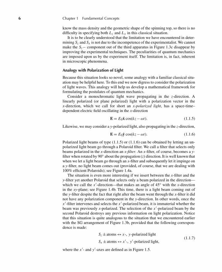
Polarized light beams of type (1.1.5) or (1.1.6) can be obtained by letting an un-polarized light beam go through a Polaroid filter. We call a filter that selects onlybeams polarized in the x-direction an x-filter. An x-filter, of course, becomes a y-filter when rotated by 90◦ about the propagation (z) direction. It is well known thatwhen we let a light beam go through an x-filter and subsequently let it impinge ona y-filter, no light beam comes out (provided, of course, that we are dealing with100% efficient Polaroids); see Figure 1.4a.
The situation is even more interesting if we insert between the x-filter and they-filter yet another Polaroid that selects only a beam polarized in the direction—which we call the x ′-direction—that makes an angle of 45◦ with the x-directionin the xy-plane; see Figure 1.4b. This time, there is a light beam coming out ofthe y-filter despite the fact that right after the beam went through the x-filter it didnot have any polarization component in the y-direction. In other words, once thex ′-filter intervenes and selects the x ′-polarized beam, it is immaterial whether thebeam was previously x-polarized. The selection of the x ′-polarized beam by thesecond Polaroid destroys any previous information on light polarization. Noticethat this situation is quite analogous to the situation that we encountered earlierwith the SG arrangement of Figure 1.3b, provided that the following correspon-dence is made:
Sz ± atoms ↔ x-, y-polarized light
Sx ± atoms ↔ x ′-, y′-polarized light,(1.1.7)
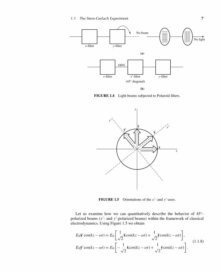
where the x ′- and y ′-axes are defined as in Figure 1.5.
1.1 The Stern-Gerlach Experiment 7
x-filter y-filter
x-filter x′-filter y-filter
No beam
(45° diagonal)
100%
(a)
(b)
No light
FIGURE 1.4 Light beams subjected to Polaroid filters.
y′
x′y
x
y′x′
y
x
FIGURE 1.5 Orientations of the x ′- and y ′-axes.
Let us examine how we can quantitatively describe the behavior of 45◦-polarized beams (x ′- and y ′-polarized beams) within the framework of classicalelectrodynamics. Using Figure 1.5 we obtain
E0x′ cos(kz −ωt) = E0
[1√2
xcos(kz −ωt) + 1√2
ycos(kz −ωt)
],
E0y′ cos(kz −ωt) = E0
[− 1√
2xcos(kz −ωt) + 1√
2ycos(kz −ωt)
].
(1.1.8)
8 Chapter 1 Fundamental Concepts
In the triple-filter arrangement of Figure 1.4b, the beam coming out of the firstPolaroid is an x-polarized beam, which can be regarded as a linear combinationof an x ′-polarized beam and a y′-polarized beam. The second Polaroid selectsthe x ′-polarized beam, which can in turn be regarded as a linear combination ofan x-polarized and a y-polarized beam. And finally, the third Polaroid selects they-polarized component.
Applying correspondence (1.1.7) from the sequential Stern-Gerlach experi-ment of Figure 1.3c to the triple-filter experiment of Figure 1.4b suggests that wemight be able to represent the spin state of a silver atom by some kind of vectorin a new kind of two-dimensional vector space, an abstract vector space not to beconfused with the usual two-dimensional (xy) space. Just as x and y in (1.1.8) arethe base vectors used to decompose the polarization vector x′ of the x′-polarizedlight, it is reasonable to represent the Sx+ state by a vector, which we call a ket inthe Dirac notation to be developed fully in the next section. We denote this vectorby |Sx ;+〉 and write it as a linear combination of two base vectors, |Sz ;+〉 and|Sz ;−〉, which correspond to the Sz+ and the Sz− states, respectively. So we mayconjecture
|Sx ;+〉 ?= 1√2|Sz ;+〉+ 1√
2|Sz ;−〉 (1.1.9a)
|Sx ;−〉 ?= − 1√2|Sz ;+〉+ 1√
2|Sz ;−〉 (1.1.9b)
in analogy with (1.1.8). Later we will show how to obtain these expressions usingthe general formalism of quantum mechanics.
Thus the unblocked component coming out of the second (SGx) apparatus ofFigure 1.3c is to be regarded as a superposition of Sz+ and Sz− in the sense of(1.1.9a). It is for this reason that two components emerge from the third (SGz)apparatus.
The next question of immediate concern is, How are we going to representthe Sy± states? Symmetry arguments suggest that if we observe an Sz± beamgoing in the x-direction and subject it to an SGy apparatus, the resulting situationwill be very similar to the case where an Sz± beam going in the y-direction issubjected to an SGx apparatus. The kets for Sy± should then be regarded as alinear combination of |Sz ;±〉, but it appears from (1.1.9) that we have alreadyused up the available possibilities in writing |Sx ;±〉. How can our vector spaceformalism distinguish Sy± states from Sx± states?
An analogy with polarized light again rescues us here. This time we considera circularly polarized beam of light, which can be obtained by letting a linearlypolarized light pass through a quarter-wave plate. When we pass such a circu-larly polarized light through an x-filter or a y-filter, we again obtain either anx-polarized beam or a y-polarized beam of equal intensity. Yet everybody knowsthat the circularly polarized light is totally different from the 45◦-linearly polar-ized (x ′-polarized or y′-polarized) light.
Mathematically, how do we represent a circularly polarized light? A right cir-cularly polarized light is nothing more than a linear combination of an x-polarized
1.1 The Stern-Gerlach Experiment 9
light and a y-polarized light, where the oscillation of the electric field for the y-polarized component is 90◦ out of phase with that of the x-polarized component:∗
E = E0
[1√2
xcos(kz −ωt) + 1√2
ycos(
kz −ωt + π2
)]. (1.1.10)
It is more elegant to use complex notation by introducing ε as follows:
Re(ε) = E/E0. (1.1.11)
For a right circularly polarized light, we can then write
ε =[
1√2
xei(kz−ωt ) + i√2
yei(kz−ωt )]
, (1.1.12)
where we have used i = eiπ/2.We can make the following analogy with the spin states of silver atoms:
Sy + atom ↔ right circularly polarized beam,
Sy − atom ↔ left circularly polarized beam.(1.1.13)
Applying this analogy to (1.1.12), we see that if we are allowed to make thecoefficients preceding base kets complex, there is no difficulty in accommodatingthe Sy± atoms in our vector space formalism:
|Sy ;±〉 ?= 1√2|Sz ;+〉± i√
2|Sz ;−〉, (1.1.14)
which are obviously different from (1.1.9). We thus see that the two-dimensionalvector space needed to describe the spin states of silver atoms must be a complexvector space; an arbitrary vector in the vector space is written as a linear combi-nation of the base vectors |Sz ;±〉 with, in general, complex coefficients. The factthat the necessity of complex numbers is already apparent in such an elementaryexample is rather remarkable.
The reader must have noted by this time that we have deliberately avoidedtalking about photons. In other words, we have completely ignored the quantumaspect of light; nowhere did we mention the polarization states of individual pho-tons. The analogy we worked out is between kets in an abstract vector space thatdescribes the spin states of individual atoms with the polarization vectors of theclassical electromagnetic field. Actually, we could have made the analogy evenmore vivid by introducing the photon concept and talking about the probabilityof finding a circularly polarized photon in a linearly polarized state, and so forth;however, that is not needed here. Without doing so, we have already accomplishedthe main goal of this section: to introduce the idea that quantum-mechanical statesare to be represented by vectors in an abstract complex vector space.†
∗Unfortunately, there is no unanimity in the definition of right versus left circularly polarizedlight in the literature.†The reader who is interested in grasping the basic concepts of quantum mechanics through acareful study of photon polarization may find Chapter 1 of Baym (1969) extremely illuminating.
10 Chapter 1 Fundamental Concepts
0.0
0.2
0.4
0.6
0.8
1.0
+4
+4 −4
+3 +2+1
0
−1 −2
−3
−4
Fluo
resc
ence
[ar
b. u
nits
]0.0
0.2
0.4
0.6
0.8
1.0
Fluo
resc
ence
[ar
b. u
nits
]
0 5 10 15 20 25
Position [mm]
60 c
m
Cesiumatomic beam
Permanentmagnet(movable)
Detectionlaser
CCDcameraimage
(b)
(a)
FIGURE 1.6 A modern Stern-Gerlach apparatus, used to separate spin states of atomiccesium, taken from F. Lison et al., Phys. Rev. A 61 (1999) 013405. The apparatus isshown on the left, while the data show the nine different projections for the spin-fouratom, (a) before and (b) after optical pumping is used to populate only extreme spin pro-jections. The spin quantum number F = 4 is a coupling between the outermost electronin the atom and the nuclear spin I = 7/2.
Finally, before outlining the mathematical formalism of quantum mechanics,we remark that the physics of a Stern-Gerlach apparatus is of far more than simplyacademic interest. The ability to separate spin states of atoms has tremendouspractical interest as well. Figure 1.6 shows the use of the Stern-Gerlach techniqueto analyze the result of spin manipulation in an atomic beam of cesium atoms.The only stable isotope, 133Cs, of this alkali atom has a nuclear spin I = 7/2,and the experiment sorts out the F = 4 hyperfine magnetic substate, giving ninespin orientations. This is only one of many examples where this once mysteriouseffect is used for practical devices. Of course, all of these uses only go to firmlyestablish this effect, as well as the quantum-mechanical principles that we willnow present and further develop.
1.2 KETS, BRAS, AND OPERATORS
In the preceding section we showed how analyses of the Stern-Gerlach experi-ment lead us to consider a complex vector space. In this and the following sectionwe formulate the basic mathematics of vector spaces as used in quantum mechan-ics. Our notation throughout this book is the bra and ket notation developed byP. A. M. Dirac. The theory of linear vector spaces had, of course, been known tomathematicians prior to the birth of quantum mechanics, but Dirac’s way of intro-
1.2 Kets, Bras, and Operators 11
ducing vector spaces has many advantages, especially from the physicist’s pointof view.
Ket Space
We consider a complex vector space whose dimensionality is specified accordingto the nature of a physical system under consideration. In Stern-Gerlach–typeexperiments where the only quantum-mechanical degree of freedom is the spinof an atom, the dimensionality is determined by the number of alternative pathsthe atoms can follow when subjected to a SG apparatus; in the case of the silveratoms of the previous section, the dimensionality is just two, corresponding to thetwo possible values Sz can assume.∗ Later, in Section 1.6, we consider the caseof continuous spectra—for example, the position (coordinate) or momentum of aparticle—where the number of alternatives is nondenumerably infinite, in whichcase the vector space in question is known as a Hilbert space after D. Hilbert,who studied vector spaces in infinite dimensions.
In quantum mechanics a physical state—for example, a silver atom with adefinite spin orientation—is represented by a state vector in a complex vectorspace. Following Dirac, we call such a vector a ket and denote it by |α〉. Thisstate ket is postulated to contain complete information about the physical state;everything we are allowed to ask about the state is contained in the ket. Two ketscan be added:
|α〉+ |β〉 = |γ 〉. (1.2.1)
The sum |γ 〉 is just another ket. If we multiply |α〉 by a complex number c, theresulting product c|α〉 is another ket. The number c can stand on the left or on theright of a ket; it makes no difference:
c|α〉 = |α〉c. (1.2.2)
In the particular case where c is zero, the resulting ket is said to be a null ket.One of the physics postulates is that |α〉 and c|α〉, with c �= 0, represent the
same physical state. In other words, only the “direction” in vector space is ofsignificance. Mathematicians may prefer to say that we are here dealing with raysrather than vectors.
An observable, such as momentum and spin components, can be representedby an operator, such as A, in the vector space in question. Quite generally, anoperator acts on a ket from the left,
A · (|α〉) = A|α〉, (1.2.3)
which is yet another ket. There will be more on multiplication operations later.
∗For many physical systems the dimension of the state space is denumerably infinite. Althoughwe will usually indicate a finite number of dimensions, N, of the ket space, the results also holdfor denumerably infinite dimensions.
12 Chapter 1 Fundamental Concepts
In general, A|α〉 is not a constant times |α〉. However, there are particular ketsof importance, known as eigenkets of operator A, denoted by
|a′〉, |a′′〉, |a′′′〉, . . . (1.2.4)
with the property
A|a′〉 = a′|a′〉, A|a′′〉 = a′′|a′′〉, . . . (1.2.5)
where a′,a′′, . . . are just numbers. Notice that applying A to an eigenket just re-produces the same ket apart from a multiplicative number. The set of numbers{a′,a′′,a′′′, . . .}, more compactly denoted by {a′}, is called the set of eigenval-ues of operator A. When it becomes necessary to order eigenvalues in a specificmanner, {a(1),a(2),a(3), . . .} may be used in place of {a′,a′′,a′′′, . . .}.
The physical state corresponding to an eigenket is called an eigenstate. Inthe simplest case of spin 1
2 systems, the eigenvalue-eigenket relation (1.2.5) isexpressed as
Sz |Sz ;+〉 = h
2|Sz ;+〉, Sz |Sz ;−〉 = − h
2|Sz ;−〉, (1.2.6)
where |Sz ;±〉 are eigenkets of operator Sz with eigenvalues ±h/2. Here we couldhave used just |h/2〉 for |Sz ;+〉 in conformity with the notation |a′〉, where aneigenket is labeled by its eigenvalue, but the notation |Sz ;±〉, already used in theprevious section, is more convenient here because we also consider eigenkets ofSx :
Sx |Sx ;±〉 = ± h
2|Sx ;±〉. (1.2.7)
We remarked earlier that the dimensionality of the vector space is determinedby the number of alternatives in Stern-Gerlach–type experiments. More formally,we are concerned with an N-dimensional vector space spanned by the N eigenketsof observable A. Any arbitrary ket |α〉 can be written as
|α〉 =∑
a′ca′ |a′〉, (1.2.8)
with a′,a′′, . . . up to a(N), where ca′ is a complex coefficient. The question of theuniqueness of such an expansion will be postponed until we prove the orthogo-nality of eigenkets.
Bra Space and Inner Products
The vector space we have been dealing with is a ket space. We now introduce thenotion of a bra space, a vector space “dual to” the ket space. We postulate thatcorresponding to every ket |α〉 there exists a bra, denoted by 〈α|, in this dual, orbra, space. The bra space is spanned by eigenbras {〈a′|}, which correspond to the
1.2 Kets, Bras, and Operators 13
eigenkets {|a′〉}. There is a one-to-one correspondence between a ket space and abra space:
|α〉DC↔〈α||a′〉, |a′′〉, . . .DC↔〈a′|, 〈a′′|, . . .
|α〉+ |β〉DC↔〈α|+ 〈β|,(1.2.9)
where DC stands for dual correspondence. Roughly speaking, we can regard thebra space as some kind of mirror image of the ket space.
The bra dual to c|α〉 is postulated to be c∗〈α|, not c〈α|, which is a very impor-tant point. More generally, we have
cα|α〉+ cβ |β〉DC↔c∗α〈α|+ c∗
β〈β|. (1.2.10)
We now define the inner product of a bra and a ket.∗ The product is writtenas a bra standing on the left and a ket standing on the right; for example,
〈β|α〉 = (〈β|) · (|α〉)bra(c)ket
. (1.2.11)
This product is, in general, a complex number. Notice that in forming an innerproduct, we always take one vector from the bra space and one vector from theket space.
We postulate two fundamental properties of inner products. First,
〈β|α〉 = 〈α|β〉∗. (1.2.12)
In other words, 〈β|α〉 and 〈α|β〉 are complex conjugates of each other. Noticethat even though the inner product is, in some sense, analogous to the familiarscalar product a ·b, 〈β|α〉 must be clearly distinguished from 〈α|β〉; the analogousdistinction is not needed in real vector space because a ·b is equal to b ·a. Using(1.2.12) we can immediately deduce that 〈α|α〉 must be a real number. To provethis just let 〈β| → 〈α|.
The second postulate on inner products is
〈α|α〉 ≥ 0, (1.2.13)
where the equality sign holds only if |α〉 is a null ket. This is sometimes knownas the postulate of positive definite metric. From a physicist’s point of view, thispostulate is essential for the probabilistic interpretation of quantum mechanics, aswill become apparent later.†
∗In the literature an inner product is often referred to as a scalar product because it is analogous toa ·b in Euclidean space; in this book, however, we reserve the term scalar for a quantity invariantunder rotations in the usual three-dimensional space.†Attempts to abandon this postulate led to physical theories with “indefinite metric.” We shall notbe concerned with such theories in this book.
14 Chapter 1 Fundamental Concepts
Two kets |α〉 and |β〉 are said to be orthogonal if
〈α|β〉 = 0, (1.2.14)
even though in the definition of the inner product, the bra 〈α| appears. The or-thogonality relation (1.2.14) also implies, via (1.2.12),
〈β|α〉 = 0. (1.2.15)
Given a ket that is not a null ket, we can form a normalized ket |α〉, where
|α〉 =(
1√〈α|α〉)
|α〉, (1.2.16)
with the property
〈α|α〉 = 1. (1.2.17)
Quite generally,√〈α|α〉 is known as the norm of |α〉, analogous to the magnitude
of vector√
a ·a = |a| in Euclidean vector space. Because |α〉 and c|α〉 representthe same physical state, we might as well require that the kets we use for physicalstates be normalized in the sense of (1.2.17).∗
Operators
As we noted earlier, observables such as momentum and spin components are tobe represented by operators that can act on kets. We can consider a more generalclass of operators that act on kets; they will be denoted by X, Y, and so forth, whileA, B, and so on will be used for a restrictive class of operators that correspond toobservables.
An operator acts on a ket from the left side,
X · (|α〉) = X |α〉, (1.2.18)
and the resulting product is another ket. Operators X and Y are said to be equal,
X = Y , (1.2.19)
if
X |α〉 = Y |α〉 (1.2.20)
for an arbitrary ket in the ket space in question. Operator X is said to be the nulloperator if, for any arbitrary ket |α〉, we have
X |α〉 = 0. (1.2.21)
∗For eigenkets of observables with continuous spectra, different normalization conventions willbe used; see Section 1.6.
1.2 Kets, Bras, and Operators 15
Operators can be added; addition operations are commutative and associative:
X + Y = Y + X , (1.2.21a)
X + (Y + Z ) = (X + Y ) + Z . (1.2.21b)
With the single exception of the time-reversal operator to be considered in Chapter4, the operators that appear in this book are all linear; that is,
X (cα|α〉+ cβ |β〉) = cαX |α〉+ cβX |β〉. (1.2.22)
An operator X always acts on a bra from the right side
(〈α|) · X = 〈α|X , (1.2.23)
and the resulting product is another bra. The ket X |α〉 and the bra 〈α|X are, ingeneral, not dual to each other. We define the symbol X† as
X |α〉DC↔〈α|X†. (1.2.24)
The operator X† is called the Hermitian adjoint, or simply the adjoint, of X. Anoperator X is said to be Hermitian if
X = X†. (1.2.25)
Multiplication
Operators X and Y can be multiplied. Multiplication operations are, in general,noncommutative; that is,
XY �= Y X . (1.2.26)
Multiplication operations are, however, associative:
X (Y Z ) = (XY )Z = XY Z . (1.2.27)
We also have
X (Y |α〉) = (XY )|α〉 = XY |α〉, (〈β|X )Y = 〈β|(XY ) = 〈β|XY . (1.2.28)
Notice that
(XY )† = Y † X† (1.2.29)
because
XY |α〉 = X (Y |α〉)DC↔(〈α|Y †)X† = 〈α|Y † X†. (1.2.30)
So far, we have considered the following products: 〈β|α〉, X |α〉, 〈α|X , and XY.Are there other products we are allowed to form? Let us multiply |β〉 and 〈α|, inthat order. The resulting product
(|β〉) · (〈α|) = |β〉〈α| (1.2.31)
16 Chapter 1 Fundamental Concepts
is known as the outer product of |β〉 and 〈α|. We will emphasize in a momentthat |β〉〈α| is to be regarded as an operator; hence it is fundamentally differentfrom the inner product 〈β|α〉, which is just a number.
There are also “illegal products.” We have already mentioned that an operatormust stand on the left of a ket or on the right of a bra. In other words, |α〉Xand X〈α| are examples of illegal products. They are neither kets, nor bras, noroperators; they are simply nonsensical. Products such as |α〉|β〉 and 〈α|〈β| arealso illegal when |α〉 and |β〉 (〈α| and 〈β|) are ket (bra) vectors belonging to thesame ket (bra) space.∗
The Associative Axiom
As is clear from (1.2.27), multiplication operations among operators are associa-tive. Actually the associative property is postulated to hold quite generally as longas we are dealing with “legal” multiplications among kets, bras, and operators.Dirac calls this important postulate the associative axiom of multiplication.
To illustrate the power of this axiom, let us first consider an outer productacting on a ket:
(|β〉〈α|) · |γ 〉. (1.2.32)
Because of the associative axiom, we can regard this equally well as
|β〉 · (〈α|γ 〉), (1.2.33)
where 〈α|γ 〉 is just a number. Thus the outer product acting on a ket is just anotherket; in other words, |β〉〈α| can be regarded as an operator. Because (1.2.32) and(1.2.33) are equal, we may as well omit the dots and let |β〉〈α|γ 〉 stand for theoperator |β〉〈α| acting on |γ 〉 or, equivalently, the number 〈α|γ 〉 multiplying |β〉.(On the other hand, if (1.2.33) is written as (〈α|γ 〉) · |β〉, we cannot afford to omitthe dot and brackets because the resulting expression would look illegal.) Noticethat the operator |β〉〈α| rotates |γ 〉 into the direction of |β〉. It is easy to see that if
X = |β〉〈α|, (1.2.34)
then
X† = |α〉〈β|, (1.2.35)
which is left as an exercise.In a second important illustration of the associative axiom, we note that
(〈β|)bra
· (X |α〉)ket
= (〈β|X )bra
· (|α〉)ket
. (1.2.36)
∗Later in the book we will encounter products like |α〉|β〉, which are more appropriately writtenas |α〉⊗ |β〉, but in such cases |α〉 and |β〉 always refer to kets from different vector spaces. Forinstance, the first ket belongs to the vector space for electron spin, the second ket to the vectorspace for electron orbital angular momentum; or the first ket lies in the vector space of particle 1,the second ket in the vector space of particle 2, and so forth.
1.3 Base Kets and Matrix Representations 17
Because the two sides are equal, we might as well use the more compact notation
〈β|X |α〉 (1.2.37)
to stand for either side of (1.2.36). Recall now that 〈α|X† is the bra that is dual toX |α〉, so
〈β|X |α〉 = 〈β| · (X |α〉)= {(〈α|X†) · |β〉}∗= 〈α|X†|β〉∗,
(1.2.38)
where, in addition to the associative axiom, we used the fundamental property ofthe inner product (1.2.12). For a Hermitian X we have
〈β|X |α〉 = 〈α|X |β〉∗. (1.2.39)
1.3 BASE KETS AND MATRIX REPRESENTATIONS
Eigenkets of an Observable
Let us consider the eigenkets and eigenvalues of a Hermitian operator A. We usethe symbol A, reserved earlier for an observable, because in quantum mechanicsHermitian operators of interest quite often turn out to be the operators representingsome physical observables.
We begin by stating an important theorem.
Theorem 1.1. The eigenvalues of a Hermitian operator A are real; the eigenketsof A corresponding to different eigenvalues are orthogonal.
Proof. First, recall that
A|a′〉 = a′|a′〉. (1.3.1)
Because A is Hermitian, we also have
〈a′′|A = a′′∗〈a′′|, (1.3.2)
where a′,a′′, . . . are eigenvalues of A. If we multiply both sides of (1.3.1) by 〈a′′|on the left, multiply both sides of (1.3.2) by |a′〉 on the right, and subtract, weobtain
(a′ − a′′∗)〈a′′|a′〉 = 0. (1.3.3)
Now a′ and a′′ can be taken to be either the same or different. Let us first choosethem to be the same; we then deduce the reality condition (the first half of thetheorem)
a′ = a′∗, (1.3.4)
18 Chapter 1 Fundamental Concepts
where we have used the fact that |a′〉 is not a null ket. Let us now assume a′ and a′′to be different. Because of the just-proved reality condition, the difference a′−a′′∗that appears in (1.3.3) is equal to a′ − a′′, which cannot vanish, by assumption.The inner product 〈a′′|a′〉 must then vanish:
〈a′′|a′〉 = 0, (a′ �= a′′), (1.3.5)
which proves the orthogonality property (the second half of the theorem).
We expect on physical grounds that an observable has real eigenvalues, a pointthat will become clearer in the next section, where measurements in quantummechanics will be discussed. The theorem just proved guarantees the reality ofeigenvalues whenever the operator is Hermitian. That is why we talk about Her-mitian observables in quantum mechanics.
It is conventional to normalize |a′〉 so that the {|a′〉} form a orthonormal set:
〈a′′|a′〉 = δa′′a′ . (1.3.6)
We may logically ask, Is this set of eigenkets complete? Because we started ourdiscussion by asserting that the whole ket space is spanned by the eigenkets of A,the eigenkets of A must form a complete set by construction of our ket space.∗
Eigenkets as Base Kets
We have seen that the normalized eigenkets of A form a complete orthonormalset. An arbitrary ket in the ket space can be expanded in terms of the eigenketsof A. In other words, the eigenkets of A are to be used as base kets in much thesame way as a set of mutually orthogonal unit vectors is used as base vectors inEuclidean space.
Given an arbitrary ket |α〉 in the ket space spanned by the eigenkets of A, letus attempt to expand it as follows:
|α〉 =∑
a′ca′ |a′〉. (1.3.7)
Multiplying 〈a′′| on the left and using the orthonormality property (1.3.6), we canimmediately find the expansion coefficient,
ca′ = 〈a′|α〉. (1.3.8)
In other words, we have
|α〉 =∑
a′|a′〉〈a′|α〉, (1.3.9)
∗The astute reader, already familiar with wave mechanics, may point out that the completeness ofeigenfunctions we use can be proved by applying the Sturm-Liouville theory to the Schrödingerwave equation. But to “derive” the Schrödinger wave equation from our fundamental postulates,the completeness of the position eigenkets must be assumed.
1.3 Base Kets and Matrix Representations 19
which is analogous to an expansion of a vector V in (real) Euclidean space:
V =∑
i
ei (ei ·V), (1.3.10)
where {ei } form an orthogonal set of unit vectors. We now recall that the asso-ciative axiom of multiplication: |a′〉〈a′|α〉 can be regarded either as the number〈a′|α〉 multiplying |a′〉 or, equivalently, as the operator |a′〉〈a′| acting on |α〉. Be-cause |α〉 in (1.3.9) is an arbitrary ket, we must have∑
a′|a′〉〈a′| = 1, (1.3.11)
where the 1 on the right-hand side is to be understood as the identity operator.Equation (1.3.11) is known as the completeness relation or closure.
It is difficult to overestimate the usefulness of (1.3.11). Given a chain of kets,operators, or bras multiplied in legal orders, we can insert, in any place at ourconvenience, the identity operator written in form (1.3.11). Consider, for example,〈α|α〉; by inserting the identity operator between 〈α| and |α〉, we obtain
〈α|α〉 = 〈α| ·(∑
a′|a′〉〈a′|
)· |α〉
=∑
a′|〈a′|α〉|2.
(1.3.12)
This, incidentally, shows that if |α〉 is normalized, then the expansion coefficientsin (1.3.7) must satisfy ∑
a′|ca′ |2 =
∑a′
|〈a′|α〉|2 = 1. (1.3.13)
Let us now look at |a′〉〈a′| that appears in (1.3.11). Because this is an outerproduct, it must be an operator. Let it operate on |α〉:
(|a′〉〈a′|) · |α〉 = |a′〉〈a′|α〉 = ca′ |a′〉. (1.3.14)
We see that |a′〉〈a′| selects that portion of the ket |α〉 parallel to |a′〉, so |a′〉〈a′| isknown as the projection operator along the base ket |a′〉 and is denoted bya′ :
a′ ≡ |a′〉〈a′|. (1.3.15)
The completeness relation (1.3.11) can now be written as∑a′a′ = 1. (1.3.16)
20 Chapter 1 Fundamental Concepts
Matrix Representations
Having specified the base kets, we now show how to represent an operator, say X,by a square matrix. First, using (1.3.11) twice, we write the operator X as
X =∑a′′
∑a′
|a′′〉〈a′′|X |a′〉〈a′|. (1.3.17)
There are altogether N2 numbers of form 〈a′′|X |a′〉, where N is the dimensional-ity of the ket space. We may arrange them into an N × N square matrix such thatthe column and row indices appear as follows:
〈a′′|row
X |a′〉column
. (1.3.18)
Explicitly we may write the matrix as
X.=
⎛⎜⎜⎝〈a(1)|X |a(1)〉 〈a(1)|X |a(2)〉 · · ·〈a(2)|X |a(1)〉 〈a(2)|X |a(2)〉 · · ·
......
. . .
⎞⎟⎟⎠ , (1.3.19)
where the symbol.= stands for “is represented by.”∗
Using (1.2.38), we can write
〈a′′|X |a′〉 = 〈a′|X†|a′′〉∗. (1.3.20)
At last, the Hermitian adjoint operation, originally defined by (1.2.24), has beenrelated to the (perhaps more familiar) concept of complex conjugate transposed.If an operator B is Hermitian, we have
〈a′′|B|a′〉 = 〈a′|B|a′′〉∗. (1.3.21)
The way we arranged 〈a′′|X |a′〉 into a square matrix is in conformity with theusual rule of matrix multiplication. To see this, just note that the matrix represen-tation of the operator relation
Z = XY (1.3.22)
reads
〈a′′|Z |a′〉 = 〈a′′|XY |a′〉=∑a′′′
〈a′′|X |a′′′〉〈a′′′|Y |a′〉. (1.3.23)
Again, all we have done is to insert the identity operator, written in form (1.3.11),between X and Y!∗We do not use the equality sign here because the particular form of a matrix representationdepends on the particular choice of base kets used. The operator is different from a representationof the operator just as the actor is different from a poster of the actor.
1.3 Base Kets and Matrix Representations 21
Let us now examine how the ket relation
|γ 〉 = X |α〉 (1.3.24)
can be represented using our base kets. The expansion coefficients of |γ 〉 can beobtained by multiplying 〈a′| on the left:
〈a′|γ 〉 = 〈a′|X |α〉=∑a′′
〈a′|X |a′′〉〈a′′|α〉. (1.3.25)
But this can be seen as an application of the rule for multiplying a square matrixwith a column matrix, once the expansion coefficients of |α〉 and |γ 〉 arrangethemselves to form column matrices as follows:
|α〉 .=
⎛⎜⎜⎜⎝〈a(1)|α〉〈a(2)|α〉〈a(3)|α〉
...
⎞⎟⎟⎟⎠ , |γ 〉 .=
⎛⎜⎜⎜⎝〈a(1)|γ 〉〈a(2)|γ 〉〈a(3)|γ 〉
...
⎞⎟⎟⎟⎠ . (1.3.26)
Likewise, given
〈γ | = 〈α|X , (1.3.27)
we can regard
〈γ |a′〉 =∑a′′
〈α|a′′〉〈a′′|X |a′〉. (1.3.28)
So a bra is represented by a row matrix as follows:
〈γ | .= (〈γ |a(1)〉, 〈γ |a(2)〉, 〈γ |a(3)〉, . . .)= (〈a(1)|γ 〉∗, 〈a(2)|γ 〉∗, 〈a(3)|γ 〉∗, . . .).
(1.3.29)
Note the appearance of complex conjugation when the elements of the columnmatrix are written as in (1.3.29). The inner product 〈β|α〉 can be written as theproduct of the row matrix representing 〈β| with the column matrix representing|α〉:
〈β|α〉 =∑
a′〈β|a′〉〈a′|α〉
= (〈a(1)|β〉∗, 〈a(2)|β〉∗, . . .)
⎛⎜⎜⎝〈a(1)|α〉〈a(2)|α〉
...
⎞⎟⎟⎠ (1.3.30)
If we multiply the row matrix representing 〈α| with the column matrix represent-ing |β〉, then we obtain just the complex conjugate of the preceding expression,
22 Chapter 1 Fundamental Concepts
which is consistent with the fundamental property of the inner product (1.2.12).Finally, the matrix representation of the outer product |β〉〈α| is easily seen to be
|β〉〈α| .=
⎛⎜⎜⎝〈a(1)|β〉〈a(1)|α〉∗ 〈a(1)|β〉〈a(2)|α〉∗ . . .
〈a(2)|β〉〈a(1)|α〉∗ 〈a(2)|β〉〈a(2)|α〉∗ . . ....
.... . .
⎞⎟⎟⎠ . (1.3.31)
The matrix representation of an observable A becomes particularly simple ifthe eigenkets of A themselves are used as the base kets. First, we have
A =∑a′′
∑a′
|a′′〉〈a′′|A|a′〉〈a′|. (1.3.32)
But the square matrix 〈a′′|A|a′〉 is obviously diagonal,
〈a′′|A|a′〉 = 〈a′|A|a′〉δa′a′′ = a′δa′a′′ , (1.3.33)
so
A =∑
a′a′|a′〉〈a′|
=∑
a′a′a′ .
(1.3.34)
Spin 12 Systems
It is here instructive to consider the special case of spin 12 systems. The base kets
used are |Sz ;±〉, which we denote, for brevity, as |±〉. The simplest operator inthe ket space spanned by |±〉 is the identity operator, which, according to (1.3.11),can be written as
1 = |+〉〈+|+ |−〉〈−|. (1.3.35)
According to (1.3.34), we must be able to write Sz as
Sz = (h/2)[(|+〉〈+|) − (|−〉〈−|)]. (1.3.36)
The eigenket-eigenvalue relation
Sz |±〉 = ±(h/2)|±〉 (1.3.37)
immediately follows from the orthonormality property of |±〉.It is also instructive to look at two other operators,
S+ ≡ h|+〉〈−|, S− ≡ h|−〉〈+|, (1.3.38)
which are both seen to be non-Hermitian. The operator S+, acting on the spin-down ket |−〉, turns |−〉 into the spin-up ket |+〉 multiplied by h. On the other
1.4 Measurements, Observables, and the Uncertainty Relations 23
hand, the spin-up ket |+〉, when acted upon by S+, becomes a null ket. So thephysical interpretation of S+ is that it raises the spin component by one unit of h; ifthe spin component cannot be raised any further, we automatically get a null state.Likewise, S− can be interpreted as an operator that lowers the spin component byone unit of h. Later we will show that S± can be written as Sx ± i Sy .
In constructing the matrix representations of the angular momentum operators,it is customary to label the column (row) indices in descending order of angularmomentum components; that is, the first entry corresponds to the maximum an-gular momentum component, the second to the next highest, and so forth. In ourparticular case of spin 1
2 systems, we have
|+〉 .=(
10
), |−〉 .=
(01
), (1.3.39a)
Sz.= h
2
(1 00 −1
), S+
.= h
(0 10 0
), S−
.= h
(0 01 0
). (1.3.39b)
We will come back to these explicit expressions when we discuss the Pauli two-component formalism in Chapter 3.
1.4 MEASUREMENTS, OBSERVABLES, AND THE UNCERTAINTY RELATIONS
Measurements
Having developed the mathematics of ket spaces, we are now in a position todiscuss the quantum theory of measurement processes. This is not a particularlyeasy subject for beginners, so we first turn to the words of the great master, P. A.M. Dirac, for guidance (Dirac 1958, p. 36): “A measurement always causes thesystem to jump into an eigenstate of the dynamical variable that is being mea-sured.” What does all this mean? We interpret Dirac’s words as follows: Beforea measurement of observable A is made, the system is assumed to be representedby some linear combination
|α〉 =∑
a′ca′ |a′〉 =
∑a′
|a′〉〈a′|α〉. (1.4.1)
When the measurement is performed, the system is “thrown into” one of theeigenstates, say |a′〉, of observable A. In other words,
|α〉 Ameasurement−−−−−−−→|a′〉. (1.4.2)
For example, a silver atom with an arbitrary spin orientation will change intoeither |Sz ;+〉 or |Sz ;−〉 when subjected to a SG apparatus of type SGz. Thus ameasurement usually changes the state. The only exception is when the state isalready in one of the eigenstates of the observable being measured, in which case
|a′〉 Ameasurement−−−−−−−→|a′〉 (1.4.3)
24 Chapter 1 Fundamental Concepts
with certainty, as will be discussed further. When the measurement causes |α〉to change into |a′〉, it is said that A is measured to be a′. It is in this sense thatthe result of a measurement yields one of the eigenvalues of the observable beingmeasured.
Given (1.4.1), which is the state ket of a physical system before the measure-ment, we do not know in advance into which of the various |a′〉’s the system willbe thrown as the result of the measurement. We do postulate, however, that theprobability for jumping into some particular |a′〉 is given by
Probability for a′ = |〈a′|α〉|2, (1.4.4)
provided that |α〉 is normalized.Although we have been talking about a single physical system, to determine
probability (1.4.4) empirically, we must consider a great number of measurementsperformed on an ensemble—that is, a collection—of identically prepared physicalsystems, all characterized by the same ket |α〉. Such an ensemble is known asa pure ensemble. (We will say more about ensembles in Chapter 3.) A beamof silver atoms that survive the first SGz apparatus of Figure 1.3 with the Sz−component blocked is an example of a pure ensemble because every memberatom of the ensemble is characterized by |Sz ;+〉.
The probabilistic interpretation (1.4.4) for the squared inner product |〈a′|α〉|2is one of the fundamental postulates of quantum mechanics, so it cannot beproved. Let us note, however, that it makes good sense in extreme cases. Supposethe state ket is |a′〉 itself even before a measurement is made; then according to(1.4.4), the probability for getting a′—or, more precisely, for being thrown into|a′〉—as the result of the measurement is predicted to be 1, which is just whatwe expect. By measuring A once again, we, of course, get |a′〉 only; quite gener-ally, repeated measurements of the same observable in succession yield the sameresult.∗ If, on the other hand, we are interested in the probability for the systeminitially characterized by |a′〉 to be thrown into some other eigenket |a′′〉 witha′′ �= a′, then (1.4.4) gives zero because of the orthogonality between |a′〉 and|a′′〉. From the point of view of measurement theory, orthogonal kets correspondto mutually exclusive alternatives; for example, if a spin 1
2 system is in |Sz ;+〉, itis not in |Sz ;−〉 with certainty.
Quite generally, the probability for anything must be nonnegative. Further-more, the probabilities for the various alternative possibilities must add up tounity. Both of these expectations are met by our probability postulate (1.4.4).
We define the expectation value of A taken with respect to state |α〉 as
〈A〉 ≡ 〈α|A|α〉. (1.4.5)
To make sure that we are referring to state |α〉, the notation 〈A〉α is sometimesused. Equation (1.4.5) is a definition; however, it agrees with our intuitive notion
∗Here successive measurements must be carried out immediately afterward. This point will be-come clear when we discuss the time evolution of a state ket in Chapter 2.
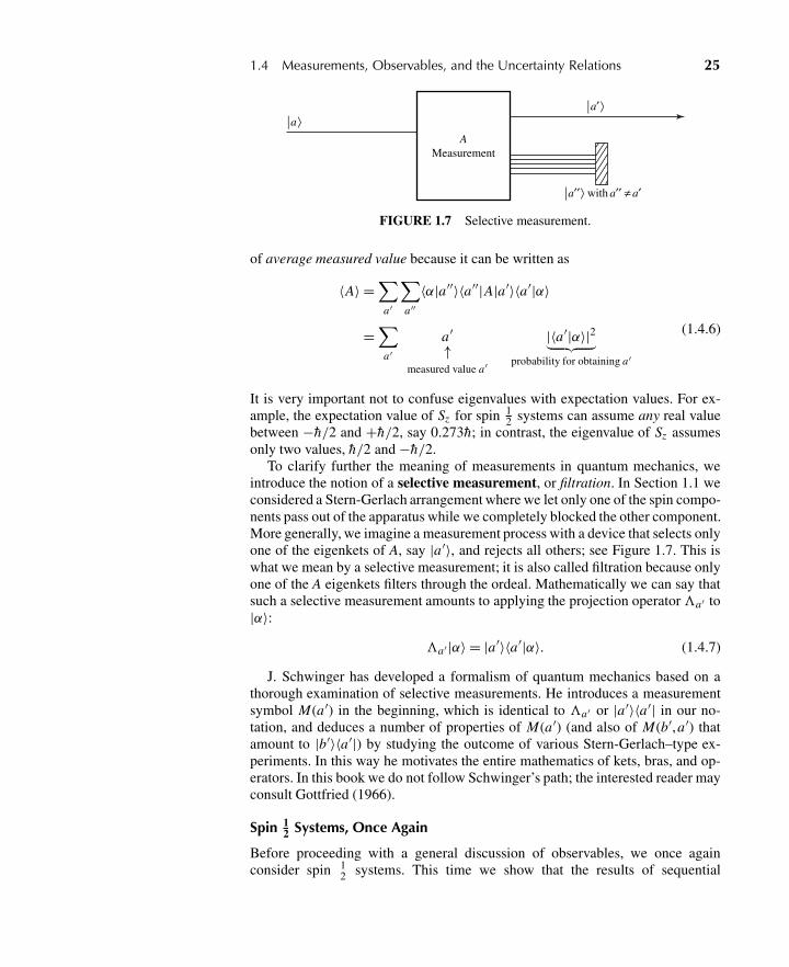
1.4 Measurements, Observables, and the Uncertainty Relations 25
AMeasurement
⏐a′′⟩ with a′′ ≠ a′
⏐a ⟩⏐a′ ⟩
FIGURE 1.7 Selective measurement.
of average measured value because it can be written as
〈A〉 =∑
a′
∑a′′
〈α|a′′〉〈a′′|A|a′〉〈a′|α〉
=∑
a′a′↑
measured value a′
|〈a′|α〉|2︸ ︷︷ ︸probability for obtaining a′
(1.4.6)
It is very important not to confuse eigenvalues with expectation values. For ex-ample, the expectation value of Sz for spin 1
2 systems can assume any real valuebetween −h/2 and +h/2, say 0.273h; in contrast, the eigenvalue of Sz assumesonly two values, h/2 and −h/2.
To clarify further the meaning of measurements in quantum mechanics, weintroduce the notion of a selective measurement, or filtration. In Section 1.1 weconsidered a Stern-Gerlach arrangement where we let only one of the spin compo-nents pass out of the apparatus while we completely blocked the other component.More generally, we imagine a measurement process with a device that selects onlyone of the eigenkets of A, say |a′〉, and rejects all others; see Figure 1.7. This iswhat we mean by a selective measurement; it is also called filtration because onlyone of the A eigenkets filters through the ordeal. Mathematically we can say thatsuch a selective measurement amounts to applying the projection operatora′ to|α〉:
a′ |α〉 = |a′〉〈a′|α〉. (1.4.7)
J. Schwinger has developed a formalism of quantum mechanics based on athorough examination of selective measurements. He introduces a measurementsymbol M(a′) in the beginning, which is identical to a′ or |a′〉〈a′| in our no-tation, and deduces a number of properties of M(a′) (and also of M(b′,a′) thatamount to |b′〉〈a′|) by studying the outcome of various Stern-Gerlach–type ex-periments. In this way he motivates the entire mathematics of kets, bras, and op-erators. In this book we do not follow Schwinger’s path; the interested reader mayconsult Gottfried (1966).
Spin 12 Systems, Once Again
Before proceeding with a general discussion of observables, we once againconsider spin 1
2 systems. This time we show that the results of sequential
26 Chapter 1 Fundamental Concepts
Stern-Gerlach experiments, when combined with the postulates of quantum me-chanics discussed so far, are sufficient to determine not only the Sx ,y eigenkets,|Sx ;±〉 and |Sy ;±〉, but also the operators Sx and Sy themselves.
First, we recall that when the Sx+ beam is subjected to an apparatus of typeSGz, the beam splits into two components with equal intensities. This means thatthe probability for the Sx+ state to be thrown into |Sz ;±〉, simply denoted as |±〉,is 1
2 each; hence,
|〈+|Sx ;+〉| = |〈−|Sx ;+〉| = 1√2
. (1.4.8)
We can therefore construct the Sx+ ket as follows:
|Sx ;+〉 = 1√2|+〉+ 1√
2eiδ1 |−〉, (1.4.9)
with δ1 real. In writing (1.4.9) we have used the fact that the overall phase (com-mon to both |+〉 and |−〉) of a state ket is immaterial; the coefficient of |+〉 canbe chosen to be real and positive by convention. The Sx− ket must be orthogo-nal to the Sx+ ket because the Sx+ alternative and Sx− alternative are mutuallyexclusive. This orthogonality requirement leads to
|Sx ;−〉 = 1√2|+〉− 1√
2eiδ1 |−〉, (1.4.10)
where we have, again, chosen the coefficient of |+〉 to be real and positive byconvention. We can now construct the operator Sx using (1.3.34) as follows:
Sx = h
2[(|Sx ;+〉〈Sx ;+|) − (|Sx ;−〉〈Sx ;−|)]
= h
2[e−iδ1 (|+〉〈−|) + eiδ1 (|−〉〈+|)].
(1.4.11)
Notice that the Sx we have constructed is Hermitian, just as it must be. A similarargument with Sx replaced by Sy leads to
|Sy ;±〉 = 1√2|+〉± 1√
2eiδ2 |−〉, (1.4.12)
Sy = h
2[e−iδ2 (|+〉〈−|) + eiδ2(|−〉〈+|)]. (1.4.13)
Is there any way of determining δ1 and δ2? Actually there is one piece of infor-mation we have not yet used. Suppose we have a beam of spin 1
2 atoms moving inthe z-direction. We can consider a sequential Stern-Gerlach experiment with SGxfollowed by SGy. The results of such an experiment are completely analogous tothe earlier case leading to (1.4.8):
|〈Sy ;±|Sx ;+〉| = |〈Sy ;±|Sx ;−〉| = 1√2
, (1.4.14)
1.4 Measurements, Observables, and the Uncertainty Relations 27
which is not surprising in view of the invariance of physical systems under rota-tions. Inserting (1.4.10) and (1.4.12) into (1.4.14), we obtain
1
2|1 ± ei(δ1−δ2)| = 1√
2, (1.4.15)
which is satisfied only if
δ2 − δ1 = π
2or − π
2. (1.4.16)
We thus see that the matrix elements of Sx and Sy cannot all be real. If the Sxmatrix elements are real, the Sy matrix elements must be purely imaginary (andvice versa). Just from this extremely simple example, the introduction of complexnumbers is seen to be an essential feature in quantum mechanics. It is convenientto take the Sx matrix elements to be real∗ and set δ1 = 0; if we were to chooseδ1 = π , the positive x-axis would be oriented in the opposite direction. The secondphase angle δ2 must then be −π/2 or π/2. The fact that there is still an ambiguityof this kind is not surprising. We have not yet specified whether the coordinatesystem we are using is right-handed or left-handed; given the x- and z-axes, thereis still a twofold ambiguity in the choice of the positive y-axis. Later we willdiscuss angular momentum as a generator of rotations using the right-handed co-ordinate system; it can then be shown that δ2 = π/2 is the correct choice.
To summarize, we have
|Sx ;±〉 = 1√2|+〉± 1√
2|−〉, (1.4.17a)
|Sy ;±〉 = 1√2|+〉± i√
2|−〉, (1.4.17b)
and
Sx = h
2[(|+〉〈−|) + (|−〉〈+|)], (1.4.18a)
Sy = h
2[−i (|+〉〈−|) + i (|−〉〈+|)]. (1.4.18b)
The Sx± and Sy± eigenkets given here are seen to be in agreement with our ear-lier guesses (1.1.9) and (1.1.14) based on an analogy with linearly and circularlypolarized light. (Note, in this comparison, that only the relative phase betweenthe |+〉 and 〈−| components is of physical significance.) Furthermore, the non-Hermitian S± operators defined by (1.3.38) can now be written as
S± = Sx ± i Sy . (1.4.19)
∗This can always be done by adjusting arbitrary phase factors in the definition of |+〉 and |−〉.This point will become clearer in Chapter 3, where the behavior of |±〉 under rotations will bediscussed.
28 Chapter 1 Fundamental Concepts
The operators Sx and Sy , together with Sz given earlier, can be readily shownto satisfy the commutation relations
[Si , Sj ] = iεi j k hSk (1.4.20)
and the anticommutation relations
{Si , Sj } = 1
2h2δi j , (1.4.21)
where the commutator [ , ] and the anticommutator { , } are defined by
[A, B] ≡ AB − B A, (1.4.22a)
{A, B} ≡ AB + B A. (1.4.22b)
(We make use of the totally antisymmetric symbol εi j k , which has the value +1for ε123 and any cyclic permutation of indices; −1 for ε213 and any cyclic per-mutation of indices; and 0 when any two indices are the same.) The commutationrelations in (1.4.20) will be recognized as the simplest realization of the angular-momentum commutation relations, whose significance will be discussed in detailin Chapter 3. In contrast, the anticommutation relations in (1.4.21) turn out to bea special property of spin 1
2 systems.We can also define the operator S ·S, or S2 for short, as follows:
S2 ≡ S2x + S2
y + S2z . (1.4.23)
Because of (1.4.21), this operator turns out to be just a constant multiple of theidentity operator
S2 =(
3
4
)h2. (1.4.24)
We obviously have
[S2, Si ] = 0. (1.4.25)
As will be shown in Chapter 3, for spins higher than 12 ,S2 is no longer a multiple
of the identity operator; however, (1.4.25) still holds.
Compatible Observables
Returning now to the general formalism, we will discuss compatible versus in-compatible observables. Observables A and B are defined to be compatible whenthe corresponding operators commute,
[A, B] = 0, (1.4.26)
and to be incompatible when
[A, B] �= 0. (1.4.27)
1.4 Measurements, Observables, and the Uncertainty Relations 29
For example, S2 and Sz are compatible observables, whereas Sx and Sz are in-compatible observables.
Let us first consider the case of compatible observables A and B. As usual, weassume that the ket space is spanned by the eigenkets of A. We may also regard thesame ket space as being spanned by the eigenkets of B. We now ask, How are theA eigenkets related to the B eigenkets when A and B are compatible observables?
Before answering this question we must touch upon a very important pointwe have bypassed earlier—the concept of degeneracy. Suppose there are two (ormore) linearly independent eigenkets of A having the same eigenvalue; then theeigenvalues of the two eigenkets are said to be degenerate. In such a case the no-tation |a′〉 that labels the eigenket by its eigenvalue alone does not give a completedescription; furthermore, we may recall that our earlier theorem on the orthogo-nality of different eigenkets was proved under the assumption of no degeneracy.Even worse, the whole concept that the ket space is spanned by {|a′〉} appears torun into difficulty when the dimensionality of the ket space is larger than the num-ber of distinct eigenvalues of A. Fortunately, in practical applications in quantummechanics, it is usually the case that in such a situation the eigenvalues of someother commuting observable, say B, can be used to label the degenerate eigenkets.
Now we are ready to state an important theorem.
Theorem 1.2. Suppose that A and B are compatible observables, and the eigen-values of A are nondegenerate. Then the matrix elements 〈a′′|B|a′〉 are all diag-onal. (Recall here that the matrix elements of A are already diagonal if {|a′〉} areused as the base kets.)
Proof. The proof of this important theorem is extremely simple. Using the defi-nition (1.4.26) of compatible observables, we observe that
〈a′′|[A, B]|a′〉 = (a′′ − a′)〈a′′|B|a′〉 = 0. (1.4.28)
Therefore, 〈a′′|B|a′〉 must vanish unless a′ = a′′, which proves our assertion.
We can write the matrix elements of B as
〈a′′|B|a′〉 = δa′a′′ 〈a′|B|a′〉. (1.4.29)
So both A and B can be represented by diagonal matrices with the same set ofbase kets. Using (1.3.17) and (1.4.29), we can write B as
B =∑a′′
|a′′〉〈a′′|B|a′′〉〈a′′|. (1.4.30)
Suppose that this operator acts on an eigenket of A:
B|a′〉 =∑a′′
|a′′〉〈a′′|B|a′′〉〈a′′|a′〉 = (〈a′|B|a′〉)|a′〉. (1.4.31)
30 Chapter 1 Fundamental Concepts
But this is nothing other than the eigenvalue equation for the operator B witheigenvalue
b′ ≡ 〈a′|B|a′〉. (1.4.32)
The ket |a′〉 is therefore a simultaneous eigenket of A and B. Just to be impartialto both operators, we may use |a′,b′〉 to characterize this simultaneous eigenket.
We have seen that compatible observables have simultaneous eigenkets. Eventhough the proof given is for the case where the A eigenkets are nondegenerate,the statement holds even if there is an n-fold degeneracy. That is,
A|a′(i)〉 = a′|a′(i)〉 for i = 1, 2, . . . , n, (1.4.33)
where |a′(i)〉 are n mutually orthonormal eigenkets of A, all with the same eigen-value a′. To see this, all we need to do is construct appropriate linear combinationsof |a′(i)〉 that diagonalize the B operator by following the diagonalization proce-dure to be discussed in Section 1.5.
A simultaneous eigenket of A and B, denoted by |a′,b′〉, has the property
A|a′,b′〉 = a′|a′,b′〉, (1.4.34a)
B|a′,b′〉 = b′|a′,b′〉. (1.4.34b)
When there is no degeneracy, this notation is somewhat superfluous because it isclear from (1.4.32) that if we specify a′, we necessarily know the b′ that appears in|a′,b′〉. The notation |a′,b′〉 is much more powerful when there are degeneracies.A simple example may be used to illustrate this point.
Even though a complete discussion of orbital angular momentum will not ap-pear in this book until Chapter 3, the reader may be aware from his or her earliertraining in elementary wave mechanics that the eigenvalues of L2 (orbital angu-lar momentum squared) and Lz (the z-component of orbital angular momentum)are h2l(l + 1) and ml h, respectively, with l an integer and ml = −l, −l + 1, . . . ,+l. To characterize an orbital angular-momentum state completely, it is neces-sary to specify both l and ml . For example, if we just say l = 1, the ml value canstill be 0, +1, or −1; if we just say ml = 1, l can be 1, 2, 3, 4, and so on. Onlyby specifying both l and ml do we succeed in uniquely characterizing the orbitalangular-momentum state in question. Quite often a collective index K ′ is used tostand for (a′,b′), so that
|K ′〉 = |a′,b′〉. (1.4.35)
We can obviously generalize our considerations to a situation where there areseveral (more than two) mutually compatible observables, namely,
[A, B] = [B ,C] = [A,C] = ·· · = 0. (1.4.36)
Assume that we have found a maximal set of commuting observables; that is,we cannot add any more observables to our list without violating (1.4.36). Theeigenvalues of individual operators A, B , C , . . . may have degeneracies, but if we
1.4 Measurements, Observables, and the Uncertainty Relations 31
specify a combination (a′,b′,c′, . . .), then the corresponding simultaneous eigen-ket of A, B ,C , . . . is uniquely specified. We can again use a collective index K ′ tostand for (a′,b′,c′, . . .). The orthonormality relation for
|K ′〉 = |a′,b′,c′, . . .〉 (1.4.37)
reads
〈K ′′|K ′〉 = δK ′K ′′ = δaa′δbb′δcc′ · · · , (1.4.38)
and the completeness relation, or closure, can be written as∑K ′
|K ′〉〈K ′| =∑
a′
∑b′
∑c′
· · · |a′,b′,c′, . . .〉〈a′,b′,c′, . . . | = 1. (1.4.39)
We now consider measurements of A and B when they are compatible observ-ables. Suppose we measure A first and obtain result a′. Subsequently, we maymeasure B and get result b′. Finally we measure A again. It follows from our mea-surement formalism that the third measurement always gives a′ with certainty;that is, the second (B) measurement does not destroy the previous informationobtained in the first (A) measurement. This is rather obvious when the eigenval-ues of A are nondegenerate:
|α〉 Ameasurement−−−−−−−→|a′,b′〉 B measurement−−−−−−−→|a′,b′〉 Ameasurement−−−−−−−→|a′,b′〉. (1.4.40)
When there is degeneracy, the argument goes as follows: After the first (A)measurement, which yields a′, the system is thrown into some linear combination
n∑i
c(i)a′ |a′,b(i)〉, (1.4.41)
where n is the degree of degeneracy and the kets |a′,b(i)〉 all have the same eigen-value a′ as far as operator A is concerned. The second (B) measurement may selectjust one of the terms in the linear combination (1.4.41)—say, |a′,b( j )〉—but thethird (A) measurement applied to it still yields a′. Whether or not there is degener-acy, A measurements and B measurements do not interfere. The term compatibleis indeed deemed appropriate.
Incompatible Observables
We now turn to incompatible observables, which are more nontrivial. The firstpoint to be emphasized is that incompatible observables do not have a completeset of simultaneous eigenkets. To show this, let us assume the converse to be true.There would then exist a set of simultaneous eigenkets with property (1.4.34a)and (1.4.34b). Clearly,
AB|a′,b′〉 = Ab′|a′,b′〉 = a′b′|a′,b′〉. (1.4.42)
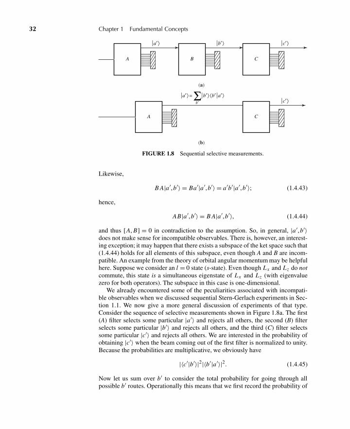
32 Chapter 1 Fundamental Concepts
A
⏐a′ ⟩
⏐a′ ⟩ = Σ⏐b′ ⟩ ⟨b′⏐a′ ⟩
A
B
⏐b′ ⟩
C
⏐c′ ⟩
⏐c′ ⟩
C
b′
(a)
(b)
FIGURE 1.8 Sequential selective measurements.
Likewise,
B A|a′,b′〉 = Ba′|a′,b′〉 = a′b′|a′,b′〉; (1.4.43)
hence,
AB|a′,b′〉 = B A|a′,b′〉, (1.4.44)
and thus [A, B] = 0 in contradiction to the assumption. So, in general, |a′,b′〉does not make sense for incompatible observables. There is, however, an interest-ing exception; it may happen that there exists a subspace of the ket space such that(1.4.44) holds for all elements of this subspace, even though A and B are incom-patible. An example from the theory of orbital angular momentum may be helpfulhere. Suppose we consider an l = 0 state (s-state). Even though Lx and Lz do notcommute, this state is a simultaneous eigenstate of Lx and Lz (with eigenvaluezero for both operators). The subspace in this case is one-dimensional.
We already encountered some of the peculiarities associated with incompati-ble observables when we discussed sequential Stern-Gerlach experiments in Sec-tion 1.1. We now give a more general discussion of experiments of that type.Consider the sequence of selective measurements shown in Figure 1.8a. The first(A) filter selects some particular |a′〉 and rejects all others, the second (B) filterselects some particular |b′〉 and rejects all others, and the third (C) filter selectssome particular |c′〉 and rejects all others. We are interested in the probability ofobtaining |c′〉 when the beam coming out of the first filter is normalized to unity.Because the probabilities are multiplicative, we obviously have
|〈c′|b′〉|2|〈b′|a′〉|2. (1.4.45)
Now let us sum over b′ to consider the total probability for going through allpossible b′ routes. Operationally this means that we first record the probability of
1.4 Measurements, Observables, and the Uncertainty Relations 33
obtaining c′ with all but the first b′ route blocked; then we repeat the procedurewith all but the second b′ blocked, and so on; then we sum the probabilities at theend and obtain∑
b′|〈c′|b′〉|2|〈b′|a′〉|2 =
∑b′
〈c′|b′〉〈b′|a′〉〈a′|b′〉〈b′|c′〉. (1.4.46)
We now compare this with a different arrangement, where the B filter is absent(or not operative); see Figure 1.8b. Clearly, the probability is just |〈c′|a′〉|2, whichcan also be written as follows:
|〈c′|a′〉|2 =∣∣∣∑
b′〈c′|b′〉〈b′|a′〉
∣∣∣2 =∑
b′
∑b′′
〈c′|b′〉〈b′|a′〉〈a′|b′′〉〈b′′|c′〉. (1.4.47)
Notice that expressions (1.4.46) and (1.4.47) are different! This is remarkablebecause in both cases the pure |a′〉 beam coming out of the first (A) filter can beregarded as being made up of the B eigenkets
|a′〉 =∑
b′|b′〉〈b′|a′〉, (1.4.48)
where the sum is over all possible values of b′. The crucial point to be noted is thatthe result coming out of the C filter depends on whether or not B measurementshave actually been carried out. In the first case, we experimentally ascertain whichof the B eigenvalues are actually realized; in the second case, we merely imagine|a′〉 to be built up of the various |b′〉’s in the sense of (1.4.48). Put in another way,actually recording the probabilities of going through the various b′ routes makesall the difference even though we sum over b′ afterwards. Here lies the heart ofquantum mechanics.
Under what conditions do the two expressions become equal? It is left as an ex-ercise for the reader to show that for this to happen, in the absence of degeneracy,it is sufficient that
[A, B] = 0 or [B ,C] = 0. (1.4.49)
In other words, the peculiarity we have illustrated is characteristic of incompatibleobservables.
The Uncertainty Relation
The last topic to be discussed in this section is the uncertainty relation. Given anobservable A, we define an operator
�A ≡ A −〈A〉, (1.4.50)
where the expectation value is to be taken for a certain physical state under consid-eration. The expectation value of (�A)2 is known as the dispersion of A. Becausewe have
〈(�A)2〉 = 〈(A2 − 2A〈A〉+ 〈A〉2)〉 = 〈A2〉− 〈A〉2, (1.4.51)
34 Chapter 1 Fundamental Concepts
the last line of (1.4.51) may be taken as an alternative definition of dispersion.Sometimes the terms variance and mean square deviation are used for the samequantity. Clearly, the dispersion vanishes when the state in question is an eigen-state of A. Roughly speaking, the dispersion of an observable characterizes “fuzzi-ness.” For example, for the Sz+ state of a spin 1
2 system, the dispersion of Sx canbe computed to be
〈S2x 〉− 〈Sx 〉2 = h2/4. (1.4.52)
In contrast the dispersion 〈(�Sz)2〉 obviously vanishes for the Sz+ state. So, forthe Sz+ state, Sz is “sharp”—a vanishing dispersion for Sz—whereas Sx is fuzzy.
We now state the uncertainty relation, which is the generalization of the well-known x-p uncertainty relation to be discussed in Section 1.6. Let A and B beobservables. Then, for any state, we must have the following inequality:
〈(�A)2〉〈(�B)2〉 ≥ 1
4|〈[A, B]〉|2. (1.4.53)
To prove this we first state three lemmas.
Lemma 1.1. The Schwarz inequality
〈α|α〉〈β|β〉 ≥ |〈α|β〉|2, (1.4.54)
which is analogous to
|a|2|b|2 ≥ |a ·b|2 (1.4.55)
in real Euclidian space.
Proof. First note that
(〈α|+λ∗〈β|) · (|α〉+λ|β〉) ≥ 0, (1.4.56)
where λ can be any complex number. This inequality must hold when λ is setequal to −〈β|α〉〈β|β〉:
〈α|α〉〈β|β〉− |〈α|β〉)|2 ≥ 0, (1.4.57)
which is the same as (1.4.54).
Lemma 1.2. The expectation value of a Hermitian operator is purely real.
Proof. The proof is trivial—just use (1.3.21).
Lemma 1.3. The expectation value of an anti-Hermitian operator, defined byC = −C†, is purely imaginary.
1.5 Change of Basis 35
Proof. The proof is trivial.
Armed with these lemmas, we are in a position to prove the uncertainty relation(1.4.53). Using Lemma 1 with
|α〉 =�A|〉,|β〉 =�B|〉, (1.4.58)
where the blank ket | 〉 emphasizes the fact that our consideration may be appliedto any ket, we obtain
〈(�A)2〉〈(�B)2) ≥ |〈�A�B〉|2, (1.4.59)
where the Hermiticity of �A and �B has been used. To evaluate the right-handside of (1.4.59), we note
�A�B = 1
2[�A,�B] + 1
2{�A,�B}, (1.4.60)
where the commutator [�A,�B], which is equal to [A, B], is clearly anti-Hermitian
([A, B])† = (AB − B A)† = B A − AB = − [A, B] . (1.4.61)
In contrast, the anticommutator {�A,�B} is obviously Hermitian, so
〈�A�B〉 = 1
2〈[A, B]〉
purely imaginary+ 1
2〈{�A,�B}〉
purely real, (1.4.62)
where Lemmas 2 and 3 have been used. The right-hand side of (1.4.59) now be-comes
|〈�A�B〉|2 = 1
4|〈[A, B]〉|2 + 1
4|〈{�A�B}〉|2. (1.4.63)
The proof of (1.4.53) is now complete because the omission of the second (theanticommutator) term of (1.4.63) can only make the inequality relation stronger.∗
Applications of the uncertainty relation to spin 12 systems will be left as exer-
cises. We come back to this topic when we discuss the fundamental x-p commu-tation relation in Section 1.6.
1.5 CHANGE OF BASIS
Transformation Operator
Suppose we have two incompatible observables A and B. The ket space in questioncan be viewed as being spanned either by the set {|a′〉} or by the set {|b′〉}. For
∗In the literature most authors use�A for our√
〈(�A)2〉, so the uncertainty relation is written as�A�B ≥ 1
2 |〈[A, B]〉|. In this book, however, �A and�B are to be understood as operators [see(1.4.50)], not numbers.
36 Chapter 1 Fundamental Concepts
example, for spin 12 systems |Sx±〉 may be used as our base kets; alternatively,
|Sz±〉 may be used as our base kets. The two different sets of base kets, of course,span the same ket space. We are interested in finding out how the two descriptionsare related. Changing the set of base kets is referred to as a change of basis ora change of representation. The basis in which the base eigenkets are given by{|a′〉} is called the A representation or, sometimes, the A diagonal representationbecause the square matrix corresponding to A is diagonal in this basis.
Our fundamental task is to construct a transformation operator that connectsthe old orthonormal set {|a′〉} and the new orthonormal set {|b′〉}. To this end, wefirst show the following.
Theorem 1.3. Given two sets of base kets, both satisfying orthonormality andcompleteness, there exists a unitary operator U such that
|b(1)〉 = U |a(1)〉, |b(2)〉 = U |a(2)〉, . . . , |b(N)〉 = U |a(N)〉. (1.5.1)
By a unitary operator we mean an operator fulfilling the conditions
U†U = 1 (1.5.2)
and
UU† = 1. (1.5.3)
Proof. We prove this theorem by explicit construction. We assert that the operator
U =∑
k
|b(k)〉〈a(k)| (1.5.4)
will do the job, and we apply this U to |a(l)〉. Clearly,
U |a(l)〉 = |b(l)〉 (1.5.5)
is guaranteed by the orthonormality of {|a′〉}. Furthermore, U is unitary:
U†U =∑
k
∑l
|a(l)〉〈b(l)|b(k)〉〈a(k)| =∑
k
|a(k)〉〈a(k)| = 1, (1.5.6)
where we have used the orthonormality of {|b′〉} and the completeness of {|a′〉}.We obtain relation (1.5.3) in an analogous manner.
Transformation Matrix
It is instructive to study the matrix representation of the U operator in the old{|a′〉} basis. We have
〈a(k)|U |a(l)〉 = 〈a(k)|b(l)〉, (1.5.7)
1.5 Change of Basis 37
which is obvious from (1.5.5). In other words, the matrix elements of the U op-erator are built up of the inner products of old basis bras and new basis kets. Werecall that the rotation matrix in three dimensions that changes one set of unit ba-sis vectors (x, y, z) into another set (x′, y′, z′) can be written as (Goldstein (2002),pp. 134–144, for example)
R =⎛⎝ x · x′ x · y′ x · z′
y · x′ y · y′ y · z′z · x′ z · y′ z · z′
⎞⎠ . (1.5.8)
The square matrix made up of 〈a(k)|U |a(l)〉 is referred to as the transformationmatrix from the {|a′〉} basis to the {|b′〉} basis.
Given an arbitrary ket |α〉 whose expansion coefficients 〈a′|α〉 are known inthe old basis,
|α〉 =∑
a′|a′〉〈a′|α〉, (1.5.9)
how can we obtain 〈b′|α〉, the expansion coefficients in the new basis? The answeris very simple: Just multiply (1.5.9) (with a′ replaced by a(l) to avoid confusion)by 〈b(k)|:
〈b(k)|α〉 =∑
l
〈b(k)|a(l)〉〈a(l)|α〉 =∑
l
〈a(k)|U†|a(l)〉〈a(l)|α〉. (1.5.10)
In matrix notation, (1.5.10) states that the column matrix for |α〉 in the new basiscan be obtained just by applying the square matrix U† to the column matrix in theold basis:
(New) = (U†)(old). (1.5.11)
The relationships between the old matrix elements and the new matrix elementsare also easy to obtain:
〈b(k)|X |b(l)〉 =∑
m
∑n
〈b(k)|a(m)〉〈a(m)|X |a(n)〉〈a(n)|b(l)〉
=∑
m
∑n
〈a(k)|U†|a(m)〉〈a(m)|X |a(n)〉〈a(n)|U |a(l)〉.(1.5.12)
This is simply the well-known formula for a similarity transformation in matrixalgebra,
X ′ = U† XU . (1.5.13)
The trace of an operator X is defined as the sum of diagonal elements:
tr(X ) =∑
a′〈a′|X |a′〉. (1.5.14)
38 Chapter 1 Fundamental Concepts
Even though a particular set of base kets is used in the definition, tr(X) turns outto be independent of representation, as shown:∑
a′〈a′|X |a′〉 =
∑a′
∑b′
∑b′′
〈a′|b′〉〈b′|X |b′′〉〈b′′|a′〉
=∑
b′
∑b′′
〈b′′|b′〉〈b′|X |b′′〉
=∑
b′〈b′|X |b′〉.
(1.5.15)
We can also prove
tr(XY ) = tr(Y X ), (1.5.16a)
tr(U† XU ) = tr(X ), (1.5.16b)
tr(|a′〉〈a′′|) = δa′ a′′ , (1.5.16c)
tr(|b′〉〈a′|) = 〈a′|b′〉. (1.5.16d)
Diagonalization
So far we have not discussed how to find the eigenvalues and eigenkets of an op-erator B whose matrix elements in the old {|a′〉} basis are assumed to be known.This problem turns out to be equivalent to that of finding the unitary matrix thatdiagonalizes B. Even though the reader may already be familiar with the diago-nalization procedure in matrix algebra, it is worth working out this problem usingthe Dirac bra-ket notation.
We are interested in obtaining the eigenvalue b′ and the eigenket |b′〉 with theproperty
B|b′〉 = b′|b′〉. (1.5.17)
First, we rewrite this as ∑a′
〈a′′|B|a′〉〈a′|b′〉 = b′〈a′′|b′〉. (1.5.18)
When |b′〉 in (1.5.17) stands for the lth eigenket of operator B, we can write(1.5.18) in matrix notation as follows:⎛⎜⎝ B11 B12 B13 . . .
B21 B22 B23 . . ....
......
. . .
⎞⎟⎠⎛⎜⎜⎝
C (l)1
C (l)2...
⎞⎟⎟⎠= b(l)
⎛⎜⎜⎝C (l)
1
C (l)2...
⎞⎟⎟⎠ , (1.5.19)
with
Bi j = 〈a(i)|B|a( j )〉 (1.5.20a)
1.5 Change of Basis 39
and
C (l)k = 〈a(k)|b(l)〉, (1.5.20b)
where i, j, k run up to N, the dimensionality of the ket space. As we know fromlinear algebra, nontrivial solutions for C (l)
k are possible only if the characteristicequation
det(B −λ1) = 0 (1.5.21)
is satisfied. This is an Nth-order algebraic equation for λ, and the N roots obtainedare to be identified with the various b(l)’s we are trying to determine. Knowingb(l), we can solve for the corresponding C (l)
k ’s up to an overall constant to bedetermined from the normalization condition. Comparing (1.5.20b) with (1.5.7),we see that the C (l)
k ’s are just the elements of the unitary matrix involved in thechange of basis {|a′〉} → {|b′〉}.
For this procedure the Hermiticity of B is important. For example, considerS+ defined by (1.3.38) or (1.4.19). This operator is obviously non-Hermitian. Thecorresponding matrix, which reads in the Sz basis as
S+.= h
(0 10 0
), (1.5.22)
cannot be diagonalized by any unitary matrix. In Chapter 2 we will encountereigenkets of a non-Hermitian operator in connection with a coherent state of asimple harmonic oscillator. Such eigenkets, however, are known not to form acomplete orthonormal set, and the formalism we have developed in this sectioncannot be immediately applied.
Unitary Equivalent Observables
We conclude this section by discussing a remarkable theorem on the unitary trans-form of an observable.
Theorem 1.4. Consider again two sets of orthonormal basis {|a′〉} and {|b′〉}connected by the U operator (1.5.4). Knowing U , we may construct a unitarytransform of A, UAU−1; then A and UAU−1 are said to be unitary equivalentobservables. The eigenvalue equation for A,
A|a(l)〉 = a(l)|a(l)〉, (1.5.23)
clearly implies that
UAU−1U |a(l)〉 = a(l)U |a(l)〉. (1.5.24)
But this can be rewritten as
(UAU−1)|b(l)〉 = a(l)|b(l)〉. (1.5.25)
40 Chapter 1 Fundamental Concepts
This deceptively simple result is quite profound. It tells us that the |b′〉’s areeigenkets of UAU−1 with exactly the same eigenvalues as the A eigenvalues. Inother words, unitary equivalent observables have identical spectra.
The eigenket |b(l)〉, by definition, satisfies the relationship
B|b(l)〉 = b(l)|b(l)〉. (1.5.26)
Comparing (1.5.25) and (1.5.26), we infer that B and UAU−1 are simultaneouslydiagonalizable. A natural question is, Is UAU−1 the same as B itself? The answerquite often is yes in cases of physical interest. Take, for example, Sx and Sz . Theyare related by a unitary operator, which, as we will discuss in Chapter 3, is actuallythe rotation operator around the y-axis by angle π/2. In this case Sx itself is theunitary transform of Sz . Because we know that Sx and Sz exhibit the same setof eigenvalues—namely, +h/2 and −h/2—we see that our theorem holds in thisparticular example.
1.6 POSITION, MOMENTUM, AND TRANSLATION
Continuous Spectra
The observables considered so far have all been assumed to exhibit discrete eigen-value spectra. In quantum mechanics, however, there are observables with con-tinuous eigenvalues. Take, for instance, pz , the z-component of momentum. Inquantum mechanics this is again represented by a Hermitian operator. In contrastto Sz , however, the eigenvalues of pz (in appropriate units) can assume any realvalue between −∞ and ∞.
The rigorous mathematics of a vector space spanned by eigenkets that exhibita continuous spectrum is rather treacherous. The dimensionality of such a spaceis obviously infinite. Fortunately, many of the results we worked out for a finite-dimensional vector space with discrete eigenvalues can immediately be gener-alized. In places where straightforward generalizations do not hold, we indicatedanger signals.
We start with the analogue of eigenvalue equation (1.2.5), which, in thecontinuous-spectrum case, is written as
ξ |ξ ′〉 = ξ ′|ξ ′〉, (1.6.1)
where ξ is an operator and ξ ′ is simply a number. The ket |ξ ′〉 is, in other words,an eigenket of operator ξ with eigenvalue ξ ′, just as |a′〉 is an eigenket of operatorA with eigenvalue a′.
In pursuing this analogy we replace the Kronecker symbol by Dirac’s δ-function—a discrete sum over the eigenvalues {a′} by an integral over the contin-uous variable ξ ′—so
〈a′|a′′〉 = δa′ a′′ → 〈ξ ′|ξ ′′〉 = δ(ξ ′ − ξ ′′), (1.6.2a)∑a′
|a′〉〈a′| = 1 →∫
dξ ′|ξ ′〉〈ξ ′| = 1, (1.6.2b)
1.6 Position, Momentum, and Translation 41
|α〉 =∑
a′|a′〉〈a′|α〉 → |α〉 =
∫dξ ′|ξ ′〉〈ξ ′|α〉, (1.6.2c)
∑a′
|〈a′|α〉|2 = 1 →∫
dξ ′|〈ξ ′|α〉|2 = 1, (1.6.2d)
〈β|α〉 =∑
a′〈β|a′〉〈a′|α〉 → 〈β|α〉 =
∫dξ ′〈β|ξ ′〉〈ξ ′|α〉, (1.6.2e)
〈a′′|A|a′〉 = a′δa′ a′′ → 〈ξ ′′|ξ |ξ ′〉 = ξ ′δ(ξ ′′ − ξ ′). (1.6.2f)
Notice in particular how the completeness relation (1.6.2b) is used to obtain(1.6.2c) and (1.6.2e).
Position Eigenkets and Position Measurements
In Section 1.4 we emphasized that a measurement in quantum mechanics is es-sentially a filtering process. To extend this idea to measurements of observablesexhibiting continuous spectra, it is best to work with a specific example. To thisend we consider the position (or coordinate) operator in one dimension.
The eigenkets |x ′〉 of the position operator x satisfying
x |x ′〉 = x ′|x ′〉 (1.6.3)
are postulated to form a complete set. Here x ′ is just a number with the dimensionof length 0.23 cm, for example, whereas x is an operator. The state ket for anarbitrary physical state can be expanded in terms of {|x ′〉}:
|α〉 =∫ ∞
−∞dx ′|x ′〉〈x ′|α〉. (1.6.4)
We now consider a highly idealized selective measurement of the position ob-servable. Suppose we place a very tiny detector that clicks only when the particleis precisely at x ′ and nowhere else. Immediately after the detector clicks, we cansay that the state in question is represented by |x ′〉. In other words, when the de-tector clicks, |α〉 abruptly “jumps into” |x ′〉 in much the same way as an arbitraryspin state jumps into the Sz+ (or Sz−) state when subjected to an SG apparatusof the Sz type.
In practice, the best the detector can do is to locate the particle within a narrowinterval around x ′. A realistic detector clicks when a particle is observed to be lo-cated within some narrow range (x ′ −�/2, x ′ +�/2). When a count is registeredin such a detector, the state ket changes abruptly as follows:
|α〉 =∫ ∞
−∞dx ′′|x ′′〉〈x ′′|α〉 measurement−−−−−−−→
∫ x ′+�/2
x ′−�/2dx ′′|x ′′〉〈x ′′|α〉. (1.6.5)
Assuming that 〈x ′′|α〉 does not change appreciably within the narrow interval, theprobability for the detector to click is given by
|〈x ′|α〉|2dx ′, (1.6.6)
42 Chapter 1 Fundamental Concepts
where we have written dx ′ for�. This is analogous to |〈a′|α〉|2 for the probabilityfor |α〉 to be thrown into |a′〉 when A is measured. The probability of recordingthe particle somewhere between −∞ and ∞ is given by∫ ∞
−∞dx ′|〈x ′|α〉|2, (1.6.7)
which is normalized to unity if |α〉 is normalized:
〈α|α〉 = 1 ⇒∫ ∞
−∞dx ′〈α|x ′〉〈x ′|α〉 = 1. (1.6.8)
The reader familiar with wave mechanics may have recognized by this timethat 〈x ′|α〉 is the wave function for the physical state represented by |α〉. Wewill say more about this identification of the expansion coefficient with the x-representation of the wave function in Section 1.7.
The notion of a position eigenket can be extended to three dimensions. It isassumed in nonrelativistic quantum mechanics that the position eigenkets |x′〉 arecomplete. The state ket for a particle with internal degrees of freedom, such asspin, ignored can therefore be expanded in terms of {|x′〉} as follows:
|α〉 =∫
d3x ′|x′〉〈x′|α〉, (1.6.9)
where x′ stands for x ′, y ′, and z′; in other words, |x′〉 is a simultaneous eigenketof the observables x, y, and z in the sense of Section 1.4:
|x′〉 ≡ |x ′, y′, z′〉, (1.6.10a)
x |x′〉 = x ′|x′〉, y|x′〉 = y ′|x′〉, z|x′〉 = z′|x′〉, (1.6.10b)
To be able to consider such a simultaneous eigenket at all, we are implicitly as-suming that the three components of the position vector can be measured simul-taneously to arbitrary degrees of accuracy; hence, we must have
[xi , x j ] = 0, (1.6.11)
where x1, x2, and x3 stand for x, y, and z, respectively.
Translation
We now introduce the very important concept of translation, or spatial displace-ment. Suppose we start with a state that is well localized around x′. Let us con-sider an operation that changes this state into another well-localized state, thistime around x′ + dx′, with everything else (for example, the spin direction) un-changed. Such an operation is defined to be an infinitesimal translation by dx′,and the operator that does the job is denoted by J(dx′):
J(dx′)|x′〉 = |x′ + dx′〉, (1.6.12)
1.6 Position, Momentum, and Translation 43
where a possible arbitrary phase factor is set to unity by convention. Notice thatthe right-hand side of (1.6.12) is again a position eigenket, but this time witheigenvalue x′ + dx′. Obviously |x′〉 is not an eigenket of the infinitesimal transla-tion operator.
By expanding an arbitrary state ket |α〉 in terms of the position eigenkets, wecan examine the effect of infinitesimal translation on |α〉:
|α〉 → J(dx′)|α〉 = J(dx′)∫
d3x ′|x′〉〈x′|α〉 =∫
d3x ′|x′ + dx′〉〈x′|α〉. (1.6.13)
We also write the right-hand side of (1.6.13) as∫d3x ′|x′ + dx′〉〈x′|α〉 =
∫d3x ′|x′〉〈x′ − dx′|α〉 (1.6.14)
because the integration is over all space and x′ is just an integration variable.This shows that the wave function of the translated state J(dx′)|α〉 is obtained bysubstituting x′ − dx′ for x′ in 〈x′|α〉.
There is an equivalent approach to translation that is often treated in the lit-erature. Instead of considering an infinitesimal translation of the physical systemitself, we consider a change in the coordinate system being used such that theorigin is shifted in the opposite direction, −dx′. Physically, in this alternativeapproach we are asking how the same state ket would look to another observerwhose coordinate system is shifted by −dx′. In this book we try not to use thisapproach. Obviously it is important that we do not mix the two approaches!
We now list the properties of the infinitesimal translation operator J(−dx′).The first property we demand is the unitarity property imposed by probabilityconservation. It is reasonable to require that if the ket |α〉 is normalized to unity,the translated ket J(dx′)|α〉 also be normalized to unity, so
〈α|α〉 = 〈α|J†(dx′)J(dx′)|α〉. (1.6.15)
This condition is guaranteed by demanding that the infinitesimal translation beunitary:
J†(dx′)J(dx′) = 1. (1.6.16)
Quite generally, the norm of a ket is preserved under unitary transformations.For the second property, suppose we consider two successive infinitesimaltranslations—first by dx′ and subsequently by dx′′, where dx′ and dx′′ neednot be in the same direction. We expect the net result to be just a single translationoperation by the vector sum dx′ + dx′′, so we demand that
J(dx′′)J(dx′) = J(dx′ + dx′′). (1.6.17)
For the third property, suppose we consider a translation in the opposite direction;we expect the opposite-direction translation to be the same as the inverse of theoriginal translation:
J(−dx′) = J−1(dx′). (1.6.18)
44 Chapter 1 Fundamental Concepts
For the fourth property, we demand that as dx′ → 0, the translation operationreduce to the identity operation
limdx′→0
J(dx′) = 1 (1.6.19)
and that the difference between J(dx′) and the identity operator be of first orderin dx′.
We now demonstrate that if we take the infinitesimal translation operator to be
J(dx′) = 1 − iK ·dx′, (1.6.20)
where the components of K, Kx , K y , and Kz , are Hermitian operators, thenall the properties listed are satisfied. The first property, the unitarity of J(dx′), ischecked as follows:
J†(dx′)J(dx′) = (1 + iK† · dx′)(1 − iK ·dx′)= 1 − i (K − K†) · dx′ + 0[(dx′)2]
� 1,
(1.6.21)
where terms of second order in dx′ have been ignored for an infinitesimal trans-lation. The second property (1.6.17) can also be proved as follows:
J(dx′′)J(dx′) = (1 − iK ·dx′′)(1 − iK ·dx′)� 1 − iK · (dx′ + dx′′)= J(dx′ + dx′′).
(1.6.22)
The third and fourth properties are obviously satisfied by (1.6.20).Accepting (1.6.20) to be the correct form for J(dx′), we are in a position to de-
rive an extremely fundamental relation between the K operator and the x operator.First, note that
xJ(dx′)|x′〉 = x|x′ + dx′〉 = (x′ + dx′)|x′ + dx′〉 (1.6.23a)
and
J(dx′)x|x′〉 = x′J(dx′)|x′〉 = x′|x′ + dx′〉; (1.6.23b)
hence, [x,J(dx′)
] |x′〉 = dx′|x′ + dx′〉 � dx′|x′〉, (1.6.24)
where the error made in approximating the last step of (1.6.24) is of second or-der in dx′. Now |x′〉 can be any position eigenket, and the position eigenkets areknown to form a complete set. We must therefore have an operator identity[
x,J(dx′)]= dx′, (1.6.25)
or
−ixK · dx′ + iK · dx′x = dx′, (1.6.26)
1.6 Position, Momentum, and Translation 45
where, on the right-hand sides of (1.6.25) and (1.6.26), dx′ is understood to be thenumber dx′ multiplied by the identity operator in the ket space spanned by |x′〉.By choosing dx′ in the direction of x j and forming the scalar product with xi , weobtain
[xi , K j ] = iδi j , (1.6.27)
where again δi j is understood to be multiplied by the identity operator.
Momentum as a Generator of Translation
Equation (1.6.27) is the fundamental commutation relation between the positionoperators x, y, z and the K operators Kx , K y , Kz . Remember that so far, the Koperator is defined in terms of the infinitesimal translation operator by (1.6.20).What is the physical significance we can attach to K?
J. Schwinger, lecturing on quantum mechanics, once remarked, “. . . for fun-damental properties we will borrow only names from classical physics.” In thepresent case we would like to borrow from classical mechanics the notion thatmomentum is the generator of an infinitesimal translation. An infinitesimal trans-lation in classical mechanics can be regarded as a canonical transformation,
xnew ≡ X = x + dx, pnew ≡ P = p, (1.6.28)
obtainable from the generating function (Goldstein 2002, pp. 386 and 403)
F(x,P) = x · P + p · dx, (1.6.29)
where p and P refer to the corresponding momenta.This equation has a striking similarity to the infinitesimal translation operator
(1.6.20) in quantum mechanics, particularly if we recall that x ·P in (1.6.29) is thegenerating function for the identity transformation (X = x,P = p). We are there-fore led to speculate that the operator K is in some sense related to the momentumoperator in quantum mechanics.
Can the K operator be identified with the momentum operator itself? Unfortu-nately, the dimension is all wrong; the K operator has the dimension of 1/lengthbecause K · dx′ must be dimensionless. But it appears legitimate to set
K = puniversal constant with the dimension of action
. (1.6.30)
From the fundamental postulates of quantum mechanics there is no way to deter-mine the actual numerical value of the universal constant. Rather, this constant isneeded here because, historically, classical physics was developed before quan-tum mechanics using units convenient for describing macroscopic quantities—thecircumference of the earth, the mass of 1 cc of water, the duration of a mean solarday, and so forth. Had microscopic physics been formulated before macroscopicphysics, the physicists would have almost certainly chosen the basic units in sucha way that the universal constant appearing in (1.6.30) would be unity.
46 Chapter 1 Fundamental Concepts
An analogy from electrostatics may be helpful here. The interaction energybetween two particles of charge e separated at a distance r is proportional to e2/r ;in unrationalized Gaussian units, the proportionality factor is just 1, but in ratio-nalized mks units, which may be more convenient for electrical engineers, theproportionality factor is 1/4πε0. (See Appendix A.)
The universal constant that appears in (1.6.30) turns out to be the same as theconstant h that appears in L. de Broglie’s relation, written in 1924,
2π
λ= p
h, (1.6.31)
where λ is the wavelength of a “particle wave.” In other words, the K operator isthe quantum-mechanical operator that corresponds to the wave number—that is,2π times the reciprocal wavelength, usually denoted by k. With this identification,the infinitesimal translation operator J(dx′) reads
J(dx′) = 1 − ip ·dx′/h, (1.6.32)
where p is the momentum operator. The commutation relation (1.6.27) now be-comes
[xi , p j ] = i hδi j . (1.6.33)
The commutation relations (1.6.33) imply, for example, that x and px (but notx and py) are incompatible observables. It is therefore impossible to find simulta-neous eigenkets of x and px . The general formalism of Section 1.4 can be appliedhere to obtain the position-momentum uncertainty relation of W. Heisenberg:
〈(�x)2〉〈(�px)2〉 ≥ h2/4. (1.6.34)
Some applications of (1.6.34) will appear in Section 1.7.So far we have concerned ourselves with infinitesimal translations. A finite
translation—that is, a spatial displacement by a finite amount—can be obtainedby successively compounding infinitesimal translations. Let us consider a finitetranslation in the x-direction by an amount�x ′:
J(�x ′x)|x′〉 = |x′ +�x ′x〉. (1.6.35)
By compounding N infinitesimal translations, each of which is characterized by aspatial displacement�x ′/N in the x-direction, and letting N → ∞, we obtain
J(�x ′x) = limN→∞
(1 − i px�x ′
N h
)N
= exp
(− i px�x ′
h
).
(1.6.36)
Here exp(−i px�x ′/h) is understood to be a function of the operator px ; gener-ally, for any operator X we have
exp(X ) ≡ 1 + X + X2
2!+·· · . (1.6.37)
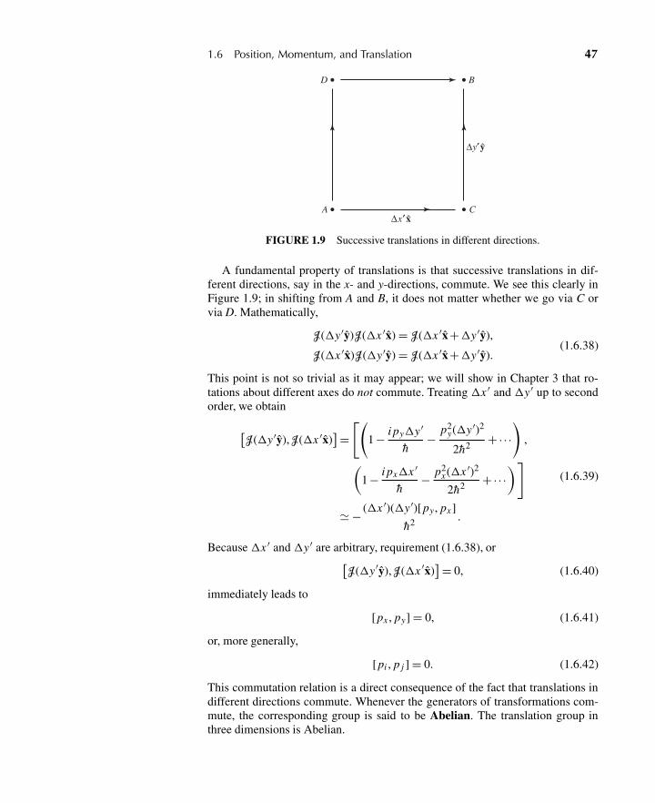
1.6 Position, Momentum, and Translation 47
A C
D B
Δy′ y
Δx′ x
FIGURE 1.9 Successive translations in different directions.
A fundamental property of translations is that successive translations in dif-ferent directions, say in the x- and y-directions, commute. We see this clearly inFigure 1.9; in shifting from A and B, it does not matter whether we go via C orvia D. Mathematically,
J(�y′y)J(�x ′x) = J(�x ′x+�y′y),
J(�x ′x)J(�y ′y) = J(�x ′x+�y′y).(1.6.38)
This point is not so trivial as it may appear; we will show in Chapter 3 that ro-tations about different axes do not commute. Treating �x ′ and �y ′ up to secondorder, we obtain
[J(�y′y),J(�x ′x)
]=[(
1 − i py�y ′
h− p2
y(�y ′)2
2h2 +·· ·)
,
(1 − i px�x ′
h− p2
x(�x ′)2
2h2 +·· ·)]
� − (�x ′)(�y′)[py, px]
h2 .
(1.6.39)
Because �x ′ and �y ′ are arbitrary, requirement (1.6.38), or[J(�y ′y),J(�x ′x)
]= 0, (1.6.40)
immediately leads to
[px , py] = 0, (1.6.41)
or, more generally,
[pi , p j ] = 0. (1.6.42)
This commutation relation is a direct consequence of the fact that translations indifferent directions commute. Whenever the generators of transformations com-mute, the corresponding group is said to be Abelian. The translation group inthree dimensions is Abelian.
48 Chapter 1 Fundamental Concepts
Equation (1.6.42) implies that px , py , and pz are mutually compatible ob-servables. We can therefore conceive of a simultaneous eigenket of px , py, pz ,namely,
|p′〉 ≡ |p′x , p′
y, p′z〉, (1.6.43a)
px |p′〉 = p′x |p′〉, py|p′〉 = p′
y|p′〉, pz|p′〉 = p′z|p′〉. (1.6.43b)
It is instructive to work out the effect of J(dx′) on such a momentum eigenket:
J(dx′)|p′〉 =(
1 − ip · dx′
h
)|p′〉 =
(1 − ip′ · dx′
h
)|p′〉. (1.6.44)
We see that the momentum eigenket remains the same even though it suffers aslight phase change, so, unlike |x′〉, |p′〉 is an eigenket of J(dx′), which we antic-ipated because [
p,J(dx′)]= 0. (1.6.45)
Notice, however, that the eigenvalue of J(dx′) is complex; we do not expect a realeigenvalue here because J(dx′), though unitary, is not Hermitian.
The Canonical Commutation Relations
We summarize the commutator relations we inferred by studying the propertiesof translation:
[xi , x j ] = 0, [ pi , p j ] = 0, [xi , p j ] = i hδi j . (1.6.46)
These relations form the cornerstone of quantum mechanics; in his book, P. A.M. Dirac calls them the “fundamental quantum conditions.” More often they areknown as the canonical commutation relations or the fundamental commuta-tion relations.
Historically it was W. Heisenberg who, in 1925, showed that the combinationrule for atomic transition lines known at that time could best be understood if oneassociated arrays of numbers obeying certain multiplication rules with these fre-quencies. Immediately afterward, M. Born and P. Jordan pointed out that Heisen-berg’s multiplication rules are essentially those of matrix algebra, and a theorybased on the matrix analogues of (1.6.46) was developed; it is now known asmatrix mechanics.∗
Also in 1925, P. A. M. Dirac observed that the various quantum-mechanicalrelations can be obtained from the corresponding classical relations just by re-placing classical Poisson brackets by commutators, as follows:
[ , ]classical → [ , ]
i h, (1.6.47)
∗Appropriately, pq −qp = h/2π i is inscribed on the gravestone of M. Born in Göttingen.
1.6 Position, Momentum, and Translation 49
where we may recall that the classical Poisson brackets are defined for functionsof q’s and p’s as
[A(q , p), B(q , p)
]classical ≡
∑s
(∂A
∂qs
∂B
∂ps− ∂A
∂ps
∂B
∂qs
). (1.6.48)
For example, in classical mechanics, we have
[xi , p j ]classical = δi j , (1.6.49)
which in quantum mechanics turns into (1.6.33).Dirac’s rule (1.6.47) is plausible because the classical Poisson brackets and
quantum-mechanical commutators satisfy similar algebraic properties. In particu-lar, the following relations can be proved regardless of whether [ , ] is understoodas a classical Poisson bracket or as a quantum-mechanical commutator:
[A, A] = 0 (1.6.50a)
[A, B] = − [B , A] (1.6.50b)
[A,c] = 0 (c is just a number) (1.6.50c)
[A + B ,C] = [A,C]+ [B ,C] (1.6.50d)
[A, BC] = [A, B]C + B [A,C] (1.6.50e)
[A, [B ,C]] + [B , [C , A]]+ [C , [A, B]] = 0, (1.6.50f)
where the last relation is known as the Jacobi identity.∗ However, there are im-portant differences. First, the dimension of the classical Poisson bracket differsfrom that of the quantum-mechanical commutator because of the differentiationswith respect to q and p appearing in (1.6.48). Second, the Poisson bracket of realfunctions of q’s and p’s is purely real, whereas the commutator of two Hermitianoperators is anti-Hermitian (see Lemma 3 of Section 1.4). To take care of thesedifferences, the factor i h is inserted in (1.6.47).
We have deliberately avoided exploiting Dirac’s analogy in obtaining thecanonical commutation relations. Our approach to the commutation relations isbased solely on (1) the properties of translations and (2) the identification ofthe generator of translation with the momentum operator modulo, a universalconstant with the dimension of action. We believe that this approach is morepowerful because it can be generalized to situations where observables have noclassical analogues. For example, the spin-angular-momentum components weencountered in Section 1.4 have nothing to do with the p’s and q’s of classicalmechanics; yet, as we will show in Chapter 3, the spin-angular-momentum com-mutation relations can be derived using the properties of rotations, just as wederived the canonical commutation relations using the properties of translations.
∗It is amusing that the Jacobi identity in quantum mechanics is much easier to prove than itsclassical analogue.
50 Chapter 1 Fundamental Concepts
1.7 WAVE FUNCTIONS IN POSITION AND MOMENTUM SPACE
Position-Space Wave Function
In this section we present a systematic study of the properties of wave functionsin both position and momentum space. For simplicity let us return to the one-dimensional case. The base kets used are the position kets satisfying
x |x ′〉 = x ′|x ′〉, (1.7.1)
normalized in such a way that the orthogonality condition reads
〈x ′′|x ′〉 = δ(x ′′ − x ′). (1.7.2)
We have already remarked that the ket representing a physical state can be ex-panded in terms of |x ′〉,
|α〉 =∫
dx ′|x ′〉〈x ′|α〉, (1.7.3)
and that the expansion coefficient 〈x ′|α〉 is interpreted in such a way that
|〈x ′|α〉|2 dx ′ (1.7.4)
is the probability for the particle to be found in a narrow interval dx ′ around x ′. Inour formalism the inner product 〈x ′|α〉 is what is usually referred to as the wavefunction ψα(x ′) for state |α〉:
〈x ′|α〉 = ψα(x ′). (1.7.5)
In elementary wave mechanics the probabilistic interpretations for the expan-sion coefficient ca′ (= 〈a′|α〉) and for the wave function ψα(x ′) (= 〈x ′|α〉) areoften presented as separate postulates. One of the major advantages of our for-malism, which was originated by Dirac, is that the two kinds of probabilistic in-terpretations are unified; ψα(x ′) is an expansion coefficient [see (1.7.3)] in muchthe same way as ca′ is. By following in the footsteps of Dirac, we come to appre-ciate the unity of quantum mechanics.
Consider the inner product 〈β|α〉. Using the completeness of |x ′〉, we have
〈β|α〉 =∫
dx ′〈β|x ′〉〈x ′|α〉
=∫
dx ′ψ∗β (x ′)ψα(x ′),
(1.7.6)
so 〈β|α〉 characterizes the overlap between the two wave functions. Note that weare not defining 〈β|α〉 as the overlap integral; the identification of 〈β|α〉 with theoverlap integral follows from our completeness postulate for |x ′〉. The more gen-eral interpretation of 〈β|α〉, independent of representations, is that it representsthe probability amplitude for state |α〉 to be found in state |β〉.
1.7 Wave Functions in Position and Momentum Space 51
This time let us interpret the expansion
|α〉 =∑
a′|a′〉〈a′|α〉 (1.7.7)
using the language of wave functions. We just multiply both sides of (1.7.7) bythe position eigenbra 〈x ′| on the left. Thus
〈x ′|α〉 =∑
a′〈x ′|a′〉〈a′|α〉. (1.7.8)
In the usual notation of wave mechanics, this is recognized as
ψα(x ′) =∑
a′ca′ua′(x ′),
where we have introduced an eigenfunction of operator A with eigenvalue a′:
ua′(x ′) = 〈x ′|a′〉. (1.7.9)
Let us now examine how 〈β|A|α〉 can be written using the wave functions for|α〉 and |β〉. Clearly, we have
〈β|A|α〉 =∫
dx ′∫
dx ′′〈β|x ′〉〈x ′|A|x ′′〉〈x ′′|α〉
=∫
dx ′∫
dx ′′ψ∗β (x ′)〈x ′|A|x ′′〉ψα(x ′′).
(1.7.10)
Therefore, to be able to evaluate 〈β|A|α〉, we must know the matrix element〈x ′|A|x ′′〉, which is, in general, a function of the two variables x ′ and x ′′.
An enormous simplification takes place if observable A is a function of theposition operator x. In particular, consider
A = x2, (1.7.11)
which actually appears in the Hamiltonian for the simple harmonic oscillatorproblem to be discussed in Chapter 2. We have
〈x ′|x2|x ′′〉 = (〈x ′|) · (x ′′2|x ′′〉) = x ′2δ(x ′ − x ′′), (1.7.12)
where we have used (1.7.1) and (1.7.2). The double integral (1.7.10) is now re-duced to a single integral:
〈β|x2|α〉 =∫
dx ′〈β|x ′〉x ′2〈x ′|α〉
=∫
dx ′ψ∗β (x ′)x ′2ψα(x ′).
(1.7.13)
52 Chapter 1 Fundamental Concepts
In general,
〈β| f (x)|α〉 =∫
dx ′ψ∗β (x ′) f (x ′)ψα(x ′). (1.7.14)
Note that the f (x) on the left-hand side of (1.7.14) is an operator, whereas thef (x ′) on the right-hand side is not an operator.
Momentum Operator in the Position Basis
We now examine how the momentum operator may look in the x-basis—that is, inthe representation where the position eigenkets are used as base kets. Our startingpoint is the definition of momentum as the generator of infinitesimal translations:(
1 − i p�x ′
h
)|α〉 =
∫dx ′J(�x ′)|x ′〉〈x ′|α〉
=∫
dx ′|x ′ +�x ′〉〈x ′|α〉
=∫
dx ′|x ′〉〈x ′ −�x ′|α〉
=∫
dx ′|x ′〉(
〈x ′|α〉−�x ′ ∂∂x ′ 〈x ′|α〉
).
(1.7.15)
Comparison of both sides yields
p|α〉 =∫
dx ′|x ′〉(
−i h∂
∂x ′ 〈x ′|α〉)
(1.7.16)
or
〈x ′|p|α〉 = −i h∂
∂x ′ 〈x ′|α〉, (1.7.17)
where we have used the orthogonality property (1.7.2). For the matrix element pin the x-representation, we obtain
〈x ′|p|x ′′〉 = −i h∂
∂x ′ δ(x′ − x ′′). (1.7.18)
From (1.7.16) we get a very important identity:
〈β|p|α〉 =∫
dx ′〈β|x ′〉(
−i h∂
∂x ′ 〈x ′|α〉)
=∫
dx ′ψ∗β (x ′)
(−i h
∂
∂x ′
)ψα(x ′).
(1.7.19)
In our formalism, (1.7.19) is not a postulate; rather, it has been derived usingthe basic properties of momentum. By repeatedly applying (1.7.17), we can also
1.7 Wave Functions in Position and Momentum Space 53
obtain
〈x ′|pn|α〉 = (−i h)n ∂n
∂x ′n 〈x ′|α〉, (1.7.20)
〈β|pn|α〉 =∫
dx ′ψ∗β (x ′)(−i h)n ∂
n
∂x ′nψα(x ′). (1.7.21)
Momentum-Space Wave Function
So far we have worked exclusively in the x-basis. But there is actually a completesymmetry between x and p (apart from occasional minus signs) that we can inferfrom the canonical commutation relations. Let us now work in the p-basis—thatis, in the momentum representation.
For simplicity we continue working in one-space. The base eigenkets in thep-basis specify
p|p′〉 = p′|p′〉 (1.7.22)
and
〈p′|p′′〉 = δ( p′ − p′′). (1.7.23)
The momentum eigenkets {|p′〉} span the ket space in much the same way as theposition eigenkets {|x ′〉}. An arbitrary state ket |α〉 can therefore be expanded asfollows:
|α〉 =∫
dp′|p′〉〈p′|α〉. (1.7.24)
We can give a probabilistic interpretation for the expansion coefficient 〈p′|α〉; theprobability that a measurement of p gives eigenvalue p′ within a narrow intervaldp′ is |〈p′|α〉|2dp′. It is customary to call 〈p′|α〉 the momentum-space wavefunction; the notation φα(p′) is often used:
〈p′|α〉 = φα(p′). (1.7.25)
If |α〉 is normalized, we obtain∫dp′〈α|p′〉〈p′|α〉 =
∫dp′|φα(p′)|2 = 1. (1.7.26)
Let us now establish the connection between the x-representation and the p-representation. We recall that in the case of the discrete spectra, the change of ba-sis from the old set {|a′〉} to the new set {|b′〉} is characterized by the transforma-tion matrix (1.5.7). Likewise, we expect that the desired information is containedin 〈x ′|p′〉, which is a function of x ′ and p′, usually called the transformationfunction from the x-representation to the p-representation. To derive the explicitform of 〈x ′|p′〉, first recall (1.7.17); letting |α〉 be the momentum eigenket |p′〉,we obtain
〈x ′|p|p′〉 = −i h∂
∂x ′ 〈x ′|p′〉 (1.7.27)
54 Chapter 1 Fundamental Concepts
or
p′〈x ′|p′〉 = −i h∂
∂x ′ 〈x ′|p′〉. (1.7.28)
The solution to this differential equation for 〈x ′|p′〉 is
〈x ′|p′〉 = N exp
(i p′x ′
h
), (1.7.29)
where N is the normalization constant to be determined in a moment. Even thoughthe transformation function 〈x ′|p′〉 is a function of two variables, x ′ and p′, wecan temporarily regard it as a function of x ′ with p′ fixed. It can then be viewedas the probability amplitude for the momentum eigenstate specified by p′ to befound at position x ′; in other words, it is just the wave function for the momentumeigenstate |p′〉, often referred to as the momentum eigenfunction (still in the x-space). So (1.7.29) simply says that the wave function of a momentum eigenstateis a plane wave. It is amusing that we have obtained this plane-wave solutionwithout solving the Schrödinger equation (which we have not yet written down).
To get the normalization constant N, let us first consider
〈x ′|x ′′〉 =∫
dp′〈x ′|p′〉〈p′|x ′′〉. (1.7.30)
The left-hand side is just δ(x ′ − x ′′); the right-hand side can be evaluated usingthe explicit form of 〈x ′|p′〉:
δ(x ′ − x ′′) = |N |2∫
dp′ exp
[i p′(x ′ − x ′′)
h
]= 2π h|N |2δ(x ′ − x ′′).
(1.7.31)
Choosing N to be purely real and positive by convention, we finally have
〈x ′|p′〉 = 1√2π h
exp
(i p′x ′
h
). (1.7.32)
We can now demonstrate how the position-space wave function is related tothe momentum-space wave function. All we have to do is rewrite
〈x ′|α〉 =∫
dp′〈x ′|p′〉〈p′|α〉 (1.7.33a)
and
〈p′|α〉 =∫
dx ′〈p′|x ′〉〈x ′|α〉 (1.7.33b)
as
ψα(x ′) =[
1√2π h
]∫dp′ exp
(i p′x ′
h
)φα(p′) (1.7.34a)
1.7 Wave Functions in Position and Momentum Space 55
and
φα(p′) =[
1√2π h
]∫dx ′ exp
(−i p′x ′
h
)ψα(x ′). (1.7.34b)
The pair of equations is just what one expects from Fourier’s inversion theo-rem. Apparently the mathematics we have developed somehow “knows” Fourier’swork on integral transforms.
Gaussian Wave Packets
It is instructive to look at a physical example to illustrate our basic formalism.We consider what is known as a Gaussian wave packet, whose x-space wavefunction is given by
〈x ′|α〉 =[
1
π1/4√
d
]exp
[ikx ′ − x ′2
2d2
]. (1.7.35)
This is a plane wave with wave number k modulated by a Gaussian profile cen-tered on the origin. The probability of observing the particle vanishes very rapidlyfor |x ′|> d; more quantitatively, the probability density |〈x ′|α〉|2 has a Gaussianshape with width d.
We now compute the expectation values of x, x2, p, and p2. The expectationvalue of x is clearly zero by symmetry:
〈x〉 =∫ ∞
−∞dx ′〈α|x ′〉x ′〈x ′|α〉 =
∫ ∞
−∞dx ′|〈x ′|α〉|2x ′ = 0. (1.7.36)
For x2 we obtain
〈x2〉 =∫ ∞
−∞dx ′x ′2|〈x ′|α〉|2
=(
1√πd
)∫ ∞
−∞dx ′ x ′2 exp
[−x ′2
d2
]= d2
2,
(1.7.37)
which leads to
〈(�x)2〉 = 〈x2〉− 〈x〉2 = d2
2(1.7.38)
for the dispersion of the position operator. The expectation values of p and p2 canalso be computed as follows:
〈p〉 = hk (1.7.39a)
〈p2〉 = h2
2d2+ h2k2, (1.7.39b)
56 Chapter 1 Fundamental Concepts
which is left as an exercise. The momentum dispersion is therefore given by
〈(�p)2〉 = 〈p2〉− 〈p〉2 = h2
2d2. (1.7.40)
Armed with (1.7.38) and (1.7.40), we can check the Heisenberg uncertainty rela-tion (1.6.34); in this case the uncertainty product is given by
〈(�x)2〉〈(�p)2〉 = h2
4, (1.7.41)
independent of d, so for a Gaussian wave packet we actually have an equalityrelation rather than the more general inequality relation (1.6.34). For this reasona Gaussian wave packet is often called a minimum uncertainty wave packet.
We now go to momentum space. By a straightforward integration—just com-pleting the square in the exponent—we obtain
〈p′|α〉 =(
1√2π h
)(1
π1/4√
d
)∫ ∞
−∞dx ′ exp
(−i p′x ′
h+ ikx ′ − x ′2
2d2
)
=√
d
h√π
exp
[−(p′ − hk)2d2
2h2
].
(1.7.42)
This momentum-space wave function provides an alternative method for obtain-ing 〈p〉 and 〈p2〉, which is also left as an exercise.
The probability of finding the particle with momentum p′ is Gaussian (in mo-mentum space) centered on hk, just as the probability of finding the particle at x ′is Gaussian (in position space) centered on zero. Furthermore, the widths of thetwo Gaussians are inversely proportional to each other, which is just another wayof expressing the constancy of the uncertainty product 〈(�x)2〉〈�p)2〉 explicitlycomputed in (1.7.41). The wider the spread in the p-space, the narrower the spreadin the x-space, and vice versa.
As an extreme example, suppose we let d → ∞. The position-space wavefunction (1.7.35) then becomes a plane wave extending over all space; the prob-ability of finding the particle is just constant, independent of x ′. In contrast, themomentum-space wave function is δ-function-like and is sharply peaked at hk. Inthe opposite extreme, by letting d → 0, we obtain a position-space wave functionlocalized like the δ-function, but the momentum-space wave function (1.7.42) isjust constant, independent of p′.
We have seen that an extremely well localized (in the x-space) state is to beregarded as a superposition of momentum eigenstates with all possible values ofmomenta. Even those momentum eigenstates whose momenta are comparable toor exceed mc must be included in the superposition. However, at such high valuesof momentum, a description based on nonrelativistic quantum mechanics is bound
1.7 Wave Functions in Position and Momentum Space 57
to break down.∗ Despite this limitation, our formalism, based on the existence ofthe position eigenket |x ′〉, has a wide domain of applicability.
Generalization to Three Dimensions
So far in this section we have worked exclusively in one-space for simplicity,but everything we have done can be generalized to three-space, if the necessarychanges are made. The base kets to be used can be taken as either the positioneigenkets satisfying
x|x′〉 = x′|x′〉 (1.7.43)
or the momentum eigenkets satisfying
p|p′〉 = p′|p′〉. (1.7.44)
They obey the normalization conditions
〈x|x′′〉 = δ3(x′ − x′′) (1.7.45a)
and
〈p|p′′〉 = δ3(p′ − p′′), (1.7.45b)
where δ3 stands for the three-dimensional δ-function
δ3(x′ − x′′) = δ(x ′ − x ′′)δ(y′ − y ′′)δ(z′ − z′′). (1.7.46)
The completeness relations read∫d3x ′|x′〉〈x′| = 1 (1.7.47a)
and ∫d3 p′|p′〉〈p′| = 1, (1.7.47b)
which can be used to expand an arbitrary state ket:
|α〉 =∫
d3x ′|x′〉〈x′|α〉, (1.7.48a)
|α〉 =∫
d3 p′|p′〉〈p′|α〉. (1.7.48b)
The expansion coefficients 〈x′|α〉 and 〈p′|α〉 are identified with the wave functionsψα(x′) and φα(p′) in position and momentum space, respectively.
∗It turns out that the concept of a localized state in relativistic quantum mechanics is far moreintricate because of the possibility of “negative energy states,” or pair creation. See Chapter 8 ofthis book.
58 Chapter 1 Fundamental Concepts
The momentum operator, when taken between |β〉 and |α〉, becomes
〈β|p|α〉 =∫
d3x ′ψ∗β (x′)(−i h∇′)ψα(x′). (1.7.49)
The transformation function analogous to (1.7.32) is
〈x′|p′〉 =[
1
(2π h)3/2
]exp
(ip′ · x′
h
), (1.7.50)
so that
ψα(x′) =[
1
(2π h)3/2
]∫d3 p′ exp
(ip′ · x′
h
)φα(p′) (1.7.51a)
and
φα(p′) =[
1
(2π h)3/2
]∫d3x ′ exp
(−ip′ · x′
h
)ψα(x′). (1.7.51b)
It is interesting to check the dimension of the wave functions. In one-dimensional problems the normalization requirement (1.6.8) implies that |〈x ′|α〉|2has the dimension of inverse length, so the wave function itself must have the di-mension of (length)−1/2. In contrast, the wave function in three-dimensionalproblems must have the dimension of (length)−3/2 because |〈x′|α〉|2 integratedover all spatial volume must be unity (dimensionless).
Problems
1.1 Prove
[AB,C D] = −AC{D, B}+ A{C , B}D − C{D, A}B +{C , A}DB.
1.2 Suppose a 2× 2 matrix X (not necessarily Hermitian or unitary) is written as
X = a0 +σ · a,
where a0 and a1,2,3 are numbers.
(a) How are a0 and ak (k = 1,2,3) related to tr(X) and tr(σk X)?
(b) Obtain a0 and ak in terms of the matrix elements Xi j .
1.3 Show that the determinant of a 2× 2 matrix σ · a is invariant under
σ · a → σ · a′ ≡ exp
(iσ · nφ
2
)σ · aexp
(−iσ · nφ2
).
Find a′k in terms of ak when n is in the positive z-direction, and interpret your result.
Problems 59
1.4 Using the rules of bra-ket algebra, prove or evaluate the following:(a) tr(XY ) = tr(Y X), where X and Y are operators.(b) (XY )† = Y † X†, where X and Y are operators.(c) exp[i f (A)] =? in ket-bra form, where A is a Hermitian operator whose eigen-
values are known.(d)
∑a′ ψ∗
a′(x′)ψa′ (x′′), where ψa′(x′) = 〈x′|a′〉.1.5 (a) Consider two kets |α〉 and |β〉. Suppose 〈a′|α〉,〈a′′ |α〉, . . . and 〈a′|β〉,
〈a′′|β〉, . . . are all known, where |a′〉, |a′′〉, . . . form a complete set of basekets. Find the matrix representation of the operator |α〉〈β| in that basis.
(b) We now consider a spin 12 system and let |α〉 and |β〉 be |sz = h/2〉 and
|sx = h/2〉, respectively. Write down explicitly the square matrix that corre-sponds to |α〉〈β| in the usual (sz diagonal) basis.
1.6 Suppose |i 〉 and | j〉 are eigenkets of some Hermitian operator A. Under what con-dition can we conclude that |i 〉+ | j〉 is also an eigenket of A? Justify your answer.
1.7 Consider a ket space spanned by the eigenkets {|a′〉} of a Hermitian operator A.There is no degeneracy.(a) Prove that ∏
a′(A − a′)
is the null operator.(b) Explain the significance of ∏
a′′ �= a′
(A − a′′)(a′ − a′′)
.
(c) Illustrate (a) and (b) using A set equal to Sz of a spin 12 system.
1.8 Using the orthonormality of |+〉 and |−〉, prove
[Si , S j ] = iεi j k hSk , {Si , S j } =(
h2
2
)δi j ,
where
Sx = h
2(|+〉〈−|+ |−〉〈+|), Sy = i h
2(−|+〉〈−|+ |−〉〈+|),
Sz = h
2(|+〉〈+|− |−〉〈−|).
1.9 Construct |S ·n;+〉 such that
S ·n|S ·n;+〉 =(
h
2
)|S ·n;+〉,
where n is characterized by the angles shown in the accompanying figure. Expressyour answer as a linear combination of |+〉 and |−〉. [Note: The answer is
cos
(β
2
)|+〉+ sin
(β
2
)eiα |−〉.
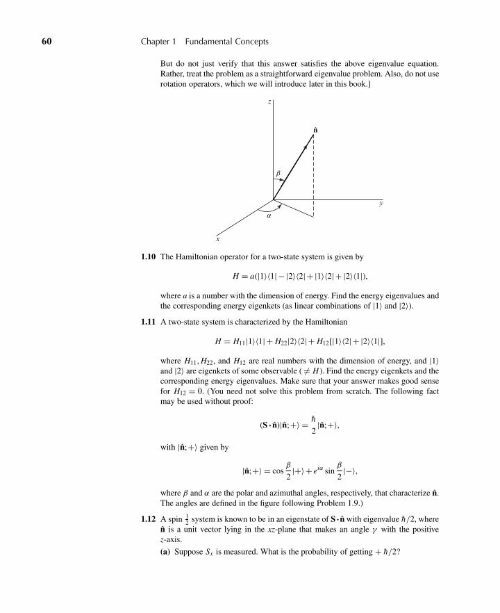
60 Chapter 1 Fundamental Concepts
But do not just verify that this answer satisfies the above eigenvalue equation.Rather, treat the problem as a straightforward eigenvalue problem. Also, do not userotation operators, which we will introduce later in this book.]
y
x
z
β
α
n
1.10 The Hamiltonian operator for a two-state system is given by
H = a(|1〉〈1|− |2〉〈2|+ |1〉〈2|+ |2〉〈1|),where a is a number with the dimension of energy. Find the energy eigenvalues andthe corresponding energy eigenkets (as linear combinations of |1〉 and |2〉).
1.11 A two-state system is characterized by the Hamiltonian
H = H11|1〉〈1|+ H22|2〉〈2|+ H12[|1〉〈2|+ |2〉〈1|],where H11, H22, and H12 are real numbers with the dimension of energy, and |1〉and |2〉 are eigenkets of some observable ( �= H ). Find the energy eigenkets and thecorresponding energy eigenvalues. Make sure that your answer makes good sensefor H12 = 0. (You need not solve this problem from scratch. The following factmay be used without proof:
(S · n)|n;+〉 = h
2|n;+〉,
with |n;+〉 given by
|n;+〉 = cosβ
2|+〉+ eiα sin
β
2|−〉,
where β and α are the polar and azimuthal angles, respectively, that characterize n.The angles are defined in the figure following Problem 1.9.)
1.12 A spin 12 system is known to be in an eigenstate of S ·n with eigenvalue h/2, where
n is a unit vector lying in the xz-plane that makes an angle γ with the positivez-axis.
(a) Suppose Sx is measured. What is the probability of getting + h/2?
Problems 61
(b) Evaluate the dispersion in Sx—that is,
〈(Sx −〈Sx〉)2〉.(For your own peace of mind, check your answers for the special cases γ = 0,π/2, and π .)
1.13 A beam of spin 12 atoms goes through a series of Stern-Gerlach–type measurements
as follows:(a) The first measurement accepts sz = h/2 atoms and rejects sz = −h/2 atoms.
(b) The second measurement accepts sn = h/2 atoms and rejects sn = −h/2 atoms,where sn is the eigenvalue of the operator S · n, with n making an angle β inthe xz-plane with respect to the z-axis.
(c) The third measurement accepts sz = −h/2 atoms and rejects sz = h/2 atoms.
What is the intensity of the final sz = −h/2 beam when the sz = h/2 beam surviv-ing the first measurement is normalized to unity? How must we orient the secondmeasuring apparatus if we are to maximize the intensity of the final sz = −h/2beam?
1.14 A certain observable in quantum mechanics has a 3 × 3 matrix representation asfollows:
1√2
⎛⎝ 0 1 01 0 10 1 0
⎞⎠ .
(a) Find the normalized eigenvectors of this observable and the correspondingeigenvalues. Is there any degeneracy?
(b) Give a physical example where all this is relevant.
1.15 Let A and B be observables. Suppose the simultaneous eigenkets of A and B{|a′,b′〉} form a complete orthonormal set of base kets. Can we always concludethat
[A, B] = 0?
If your answer is yes, prove the assertion. If your answer is no, give a counterex-ample.
1.16 Two Hermitian operators anticommute:
{A, B} = AB + B A = 0.
Is it possible to have a simultaneous (that is, common) eigenket of A and B? Proveor illustrate your assertion.
1.17 Two observables A1 and A2, which do not involve time explicitly, are known notto commute,
[A1, A2] �= 0,
yet we also know that A1 and A2 both commute with the Hamiltonian:
[A1, H ] = 0, [A2, H ] = 0.
62 Chapter 1 Fundamental Concepts
Prove that the energy eigenstates are, in general, degenerate. Are there exceptions?As an example, you may think of the central-force problem H = p2/2m + V (r ),with A1 → L z , A2 → L x .
1.18 (a) The simplest way to derive the Schwarz inequality goes as follows. First, ob-serve
(〈α|+λ∗〈β|) · (|α〉+λ|β〉) ≥ 0
for any complex number λ; then choose λ in such a way that the precedinginequality reduces to the Schwarz inequality.
(b) Show that the equality sign in the generalized uncertainty relation holds if thestate in question satisfies
�A|α〉 = λ�B|α〉with λ purely imaginary.
(c) Explicit calculations using the usual rules of wave mechanics show that thewave function for a Gaussian wave packet given by
〈x ′|α〉 = (2πd2)−1/4 exp
[i 〈p〉x ′
h− (x ′ − 〈x〉)2
4d2
]satisfies the minimum uncertainty relation√
〈(�x)2〉√
〈(�p)2〉 = h
2.
Prove that the requirement
〈x ′|�x |α〉 = (imaginary number)〈x ′|�p|α〉is indeed satisfied for such a Gaussian wave packet, in agreement with (b).
1.19 (a) Compute
〈(�Sx )2〉 ≡ 〈Sx2 〉− 〈Sx〉2,
where the expectation value is taken for the Sz+ state. Using your result, checkthe generalized uncertainty relation
〈(�A)2〉〈(�B)2〉 ≥ 1
4|〈[A, B]〉|2,
with A → Sx , B → Sy .
(b) Check the uncertainty relation with A → Sx , B → Sy for the Sx+ state.
1.20 Find the linear combination of |+〉 and |−〉 kets that maximizes the uncertaintyproduct
〈(�Sx )2〉〈(�Sy)2〉.Verify explicitly that for the linear combination you found, the uncertainty relationfor Sx and Sy is not violated.
Problems 63
1.21 Evaluate the x-p uncertainty product 〈(�x)2〉〈(�p)2〉 for a one-dimensional particleconfined between two rigid walls,
V ={
0 for 0< x < a,∞ otherwise.
Do this for both the ground and excited states.
1.22 Estimate the rough order of magnitude of the length of time that an ice pick can bebalanced on its point if the only limitation is that set by the Heisenberg uncertaintyprinciple. Assume that the point is sharp and that the point and the surface onwhich it rests are hard. You may make approximations that do not alter the generalorder of magnitude of the result. Assume reasonable values for the dimensions andweight of the ice pick. Obtain an approximate numerical result and express it inseconds.
1.23 Consider a three-dimensional ket space. If a certain set of orthonormal kets—say,|1〉, |2〉, and |3〉—are used as the base kets, the operators A and B are representedby
A.=⎛⎝ a 0 0
0 −a 00 0 −a
⎞⎠ , B.=⎛⎝ b 0 0
0 0 −ib0 ib 0
⎞⎠with a and b both real.
(a) Obviously A exhibits a degenerate spectrum. Does B also exhibit a degeneratespectrum?
(b) Show that A and B commute.
(c) Find a new set of orthonormal kets that are simultaneous eigenkets of both Aand B. Specify the eigenvalues of A and B for each of the three eigenkets. Doesyour specification of eigenvalues completely characterize each eigenket?
1.24 (a) Prove that (1/√
2)(1+ iσx ) acting on a two-component spinor can be regardedas the matrix representation of the rotation operator about the x-axis by angle−π/2. (The minus sign signifies that the rotation is clockwise.)
(b) Construct the matrix representation of Sz when the eigenkets of Sy are used asbase vectors.
1.25 Some authors define an operator to be real when every member of its matrix el-ements 〈b′|A|b′′〉 is real in some representation ({|b′〉} basis in this case). Is thisconcept representation independent? That is, do the matrix elements remain realeven if some basis other than {|b′〉} is used? Check your assertion using familiaroperators such as Sy and Sz (see Problem 1.24) or x and px .
1.26 Construct the transformation matrix that connects the Sz diagonal basis to the Sx
diagonal basis. Show that your result is consistent with the general relation
U =∑
r
|b(r)〉〈a(r)|.
1.27 (a) Suppose that f (A) is a function of a Hermitian operator A with the propertyA|a′〉 = a′|a′〉. Evaluate 〈b′′| f (A)|b′〉 when the transformation matrix from thea′ basis to the b′ basis is known.
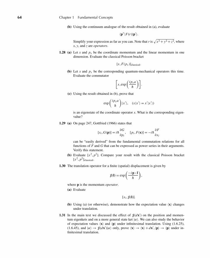
64 Chapter 1 Fundamental Concepts
(b) Using the continuum analogue of the result obtained in (a), evaluate
〈p′′ |F(r )|p′〉.Simplify your expression as far as you can. Note that r is
√x2 + y2 + z2, where
x, y, and z are operators.
1.28 (a) Let x and px be the coordinate momentum and the linear momentum in onedimension. Evaluate the classical Poisson bracket
[x , F(px )]classical.
(b) Let x and px be the corresponding quantum-mechanical operators this time.Evaluate the commutator [
x ,exp
(i px a
h
)].
(c) Using the result obtained in (b), prove that
exp
(i pxa
h
)|x ′〉, (x |x ′〉 = x ′|x ′〉)
is an eigenstate of the coordinate operator x. What is the corresponding eigen-value?
1.29 (a) On page 247, Gottfried (1966) states that
[xi ,G(p)] = i h∂G
∂pi, [pi , F(x)] = −i h
∂F
∂xi
can be “easily derived” from the fundamental commutation relations for allfunctions of F and G that can be expressed as power series in their arguments.Verify this statement.
(b) Evaluate [x2, p2]. Compare your result with the classical Poisson bracket[x2, p2]classical.
1.30 The translation operator for a finite (spatial) displacement is given by
J(l) = exp
(−ip · lh
),
where p is the momentum operator.
(a) Evaluate
[xi ,J(l)].
(b) Using (a) (or otherwise), demonstrate how the expectation value 〈x〉 changesunder translation.
1.31 In the main text we discussed the effect of J(dx′) on the position and momen-tum eigenkets and on a more general state ket |α〉. We can also study the behaviorof expectation values 〈x〉 and 〈p〉 under infinitesimal translation. Using (1.6.25),(1.6.45), and |α〉 → J(dx′)|α〉 only, prove 〈x〉 → 〈x〉 + dx′,〈p〉 → 〈p〉 under in-finitesimal translation.
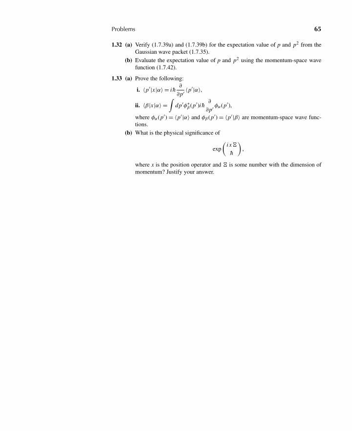
Problems 65
1.32 (a) Verify (1.7.39a) and (1.7.39b) for the expectation value of p and p2 from theGaussian wave packet (1.7.35).
(b) Evaluate the expectation value of p and p2 using the momentum-space wavefunction (1.7.42).
1.33 (a) Prove the following:
i. 〈p′|x |α〉 = i h∂
∂p′ 〈p′|α〉,
ii. 〈β|x |α〉 =∫
dp′φ∗β (p′)i h
∂
∂p′ φα(p′),
where φα(p′) = 〈p′|α〉 and φβ (p′) = 〈p′|β〉 are momentum-space wave func-tions.
(b) What is the physical significance of
exp
(i x�
h
),
where x is the position operator and � is some number with the dimension ofmomentum? Justify your answer.
C H A P T E R
2 Quantum Dynamics
So far we have not discussed how physical systems change with time. This chap-ter is devoted exclusively to the dynamic development of state kets and/or ob-servables. In other words, we are concerned here with the quantum mechanicalanalogue of Newton’s (or Lagrange’s or Hamilton’s) equations of motion.
2.1 TIME-EVOLUTION AND THE SCHRÖDINGER EQUATION
The first important point we should keep in mind is that time is just a parameterin quantum mechanics, not an operator. In particular, time is not an observablein the language of the previous chapter. It is nonsensical to talk about the timeoperator in the same sense as we talk about the position operator. Ironically, in thehistorical development of wave mechanics both L. de Broglie and E. Schrödingerwere guided by a kind of covariant analogy between energy and time on the onehand and momentum and position (spatial coordinate) on the other. Yet whenwe now look at quantum mechanics in its finished form, there is no trace of asymmetrical treatment between time and space. The relativistic quantum theoryof fields does treat the time and space coordinates on the same footing, but it doesso only at the expense of demoting position from the status of being an observableto that of being just a parameter.
Time-Evolution Operator
Our basic concern in this section is, How does a state ket change with time?Suppose we have a physical system whose state ket at t0 is represented by |α〉. Atlater times, we do not, in general, expect the system to remain in the same state|α〉. Let us denote the ket corresponding to the state at some later time by
|α, t0; t〉, (t > t0), (2.1.1)
where we have written α, t0 to remind ourselves that the system used to be in state|α〉 at some earlier reference time t0. Because time is assumed to be a continuousparameter, we expect
limt→t0
|α, t0; t〉 = |α〉, (2.1.2)
and we may as well use a shorthand notation,
|α, t0; t0〉 = |α, t0〉, (2.1.3)
66
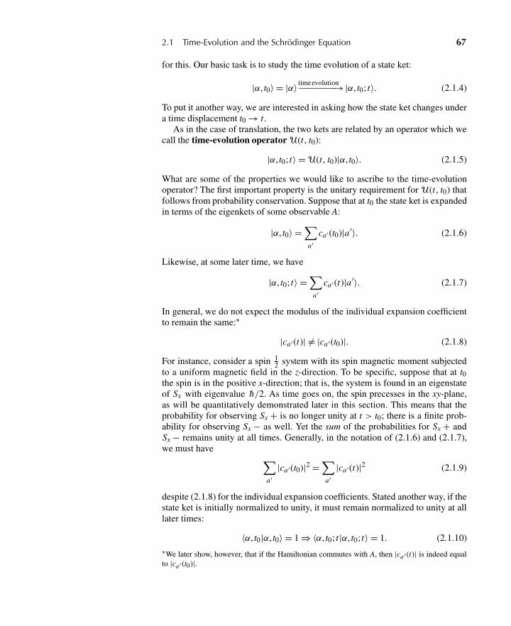
2.1 Time-Evolution and the Schrödinger Equation 67
for this. Our basic task is to study the time evolution of a state ket:
|α, t0〉 = |α〉 timeevolution−−−−−−−→|α, t0; t〉. (2.1.4)
To put it another way, we are interested in asking how the state ket changes undera time displacement t0 → t .
As in the case of translation, the two kets are related by an operator which wecall the time-evolution operator U(t , t0):
|α, t0; t〉 = U(t , t0)|α, t0〉. (2.1.5)
What are some of the properties we would like to ascribe to the time-evolutionoperator? The first important property is the unitary requirement for U(t , t0) thatfollows from probability conservation. Suppose that at t0 the state ket is expandedin terms of the eigenkets of some observable A:
|α, t0〉 =∑
a′ca′(t0)|a′〉. (2.1.6)
Likewise, at some later time, we have
|α, t0; t〉 =∑
a′ca′(t)|a′〉. (2.1.7)
In general, we do not expect the modulus of the individual expansion coefficientto remain the same:∗
|ca′(t)| �= |ca′(t0)|. (2.1.8)
For instance, consider a spin 12 system with its spin magnetic moment subjected
to a uniform magnetic field in the z-direction. To be specific, suppose that at t0the spin is in the positive x-direction; that is, the system is found in an eigenstateof Sx with eigenvalue h/2. As time goes on, the spin precesses in the xy-plane,as will be quantitatively demonstrated later in this section. This means that theprobability for observing Sx + is no longer unity at t > t0; there is a finite prob-ability for observing Sx − as well. Yet the sum of the probabilities for Sx + andSx − remains unity at all times. Generally, in the notation of (2.1.6) and (2.1.7),we must have ∑
a′|ca′(t0)|2 =
∑a′
|ca′(t)|2 (2.1.9)
despite (2.1.8) for the individual expansion coefficients. Stated another way, if thestate ket is initially normalized to unity, it must remain normalized to unity at alllater times:
〈α, t0|α, t0〉 = 1 ⇒ 〈α, t0; t|α, t0; t〉 = 1. (2.1.10)∗We later show, however, that if the Hamiltonian commutes with A, then |ca′ (t)| is indeed equalto |ca′ (t0)|.
68 Chapter 2 Quantum Dynamics
As in the translation case, this property is guaranteed if the time-evolution opera-tor is taken to be unitary. For this reason we take unitarity,
U†(t , t0)U(t , t0) = 1, (2.1.11)
to be one of the fundamental properties of the U operator. It is no coincidencethat many authors regard unitarity as synonymous with probability conservation.
Another feature we require of the U operator is the composition property:
U(t2, t0) = U(t2, t1)U(t1, t0), (t2 > t1 > t0). (2.1.12)
This equation says that if we are interested in obtaining time evolution from t0 tot2, then we can obtain the same result by considering time evolution first from t0to t1 and then from t1 to t2—a reasonable requirement. Note that we read (2.1.12)from right to left!
It also turns out to be advantageous to consider an infinitesimal time-evolutionoperator U(t0 + dt , t0):
|α, t0; t0 + dt〉 = U(t0 + dt , t0)|α, t0〉. (2.1.13)
Because of continuity [see (2.1.2)], the infinitesimal time-evolution operator mustreduce to the identity operator as dt goes to zero,
limd t→0
U(t0 + dt , t0) = 1, (2.1.14)
and, as in the translation case, we expect the difference between U(t0 +dt , t0) and1 to be of first order in dt.
We assert that all these requirements are satisfied by
U(t0 + dt , t0) = 1 − i�dt , (2.1.15)
where � is a Hermitian operator,∗
�† =�. (2.1.16)
With (2.1.15) the infinitesimal time-displacement operator satisfies the composi-tion property
U(t0 + dt1 + dt2, t0) = U(t0 + dt1 + dt2, t0 + dt1)U(t0 + dt1, t0); (2.1.17)
it differs from the identity operator by a term of order dt. The unitarity propertycan also be checked as follows:
U†(t0 + dt , t0)U(t0 + dt , t0) = (1 + i�†dt)(1 − i�dt) � 1, (2.1.18)
to the extent that terms of order (dt)2 or higher can be ignored.The operator � has the dimension of frequency or inverse time. Is there any
familiar observable with the dimension of frequency? We recall that in the old
∗If the � operator depends on time explicitly, then it must be evaluated at t0.
2.1 Time-Evolution and the Schrödinger Equation 69
quantum theory, angular frequency ω is postulated to be related to energy by thePlanck-Einstein relation
E = hω. (2.1.19)
Let us now borrow from classical mechanics the idea that the Hamiltonian is thegenerator of time evolution (Goldstein 2002, pp. 401–2). It is then natural to relate� to the Hamiltonian operator H:
�= H
h. (2.1.20)
To sum up, the infinitesimal time-evolution operator is written as
U(t0 + dt , t0) = 1 − i H dt
h, (2.1.21)
where H, the Hamiltonian operator, is assumed to be Hermitian. The reader mayask whether the h introduced here is the same as the h that appears in the ex-pression for the translation operator (1.6.32). This question can be answered bycomparing the quantum-mechanical equation of motion we derive later with theclassical equation of motion. It turns out that unless the two h’s are taken to bethe same, we are unable to obtain a relation like
dxdt
= pm
(2.1.22)
as the classical limit of the corresponding quantum-mechanical relation.
The Schrödinger Equation
We are now in a position to derive the fundamental differential equation for thetime-evolution operator U(t , t0). We exploit the composition property of the time-evolution operator by letting t1 → t , t2 → t + dt in (2.1.12):
U(t + dt , t0) = U(t + dt , t)U(t , t0) =(
1 − i H dt
h
)U(t , t0), (2.1.23)
where the time difference t − t0 need not be infinitesimal. We have
U(t + dt , t0) −U(t , t0) = −i
(H
h
)dtU(t , t0), (2.1.24)
which can be written in differential equation form:
i h∂
∂ tU(t , t0) = HU(t , t0). (2.1.25)
This is the Schrödinger equation for the time-evolution operator. Everythingthat has to do with time development follows from this fundamental equation.
70 Chapter 2 Quantum Dynamics
Equation (2.1.25) immediately leads to the Schrödinger equation for a stateket. Multiplying both sides of (2.1.25) by |α, t0〉 on the right, we obtain
i h∂
∂ tU(t , t0)|α, t0〉 = HU(t , t0)|α, t0〉. (2.1.26)
But |α, t0〉 does not depend on t, so this is the same as
i h∂
∂ t|α, t0; t〉 = H |α, t0; t〉, (2.1.27)
where (2.1.5) has been used.If we are given U(t , t0) and, in addition, know how U(t , t0) acts on the initial
state ket |α, t0〉, it is not necessary to bother with the Schrödinger equation for thestate ket (2.1.27). All we have to do is apply U(t , t0) to |α, t0〉; in this manner wecan obtain a state ket at any t. Our first task is therefore to derive formal solutionsto the Schrödinger equation for the time-evolution operator (2.1.25). There arethree cases to be treated separately:
Case 1. The Hamiltonian operator is independent of time. By this we meanthat even when the parameter t is changed, the H operator remains unchanged.The Hamiltonian for a spin-magnetic moment interacting with a time-independentmagnetic field is an example of this. The solution to (2.1.25) in such a case is givenby
U(t , t0) = exp
[−i H (t − t0)
h
]. (2.1.28)
To prove this, let us expand the exponential as follows:
exp
[−i H (t − t0)
h
]= 1 + −i H (t − t0)
h+[
(−i )2
2
][H (t − t0)
h
]2
+·· · . (2.1.29)
Because the time derivative of this expansion is given by
∂
∂ texp
[−i H (t − t0)
h
]= −i H
h+[
(−i )2
2
]2
(H
h
)2
(t − t0) +·· · , (2.1.30)
expression (2.1.28) obviously satisfies differential equation (2.1.25). The bound-ary condition is also satisfied because as t → t0, (2.1.28) reduces to the identityoperator. An alternative way to obtain (2.1.28) is to compound successively in-finitesimal time-evolution operators just as we did to obtain (1.6.36) for finitetranslation:
limN→∞
[1 − (i H/h)(t − t0)
N
]N
= exp
[−i H (t − t0)
h
]. (2.1.31)
Case 2. The Hamiltonian operator H is time-dependent but the H’s at differenttimes commute. As an example, let us consider the spin-magnetic moment sub-jected to a magnetic field whose strength varies with time but whose direction is
2.1 Time-Evolution and the Schrödinger Equation 71
always unchanged. The formal solution to (2.1.25) in this case is
U(t , t0) = exp
[−(
i
h
)∫ t
t0dt ′ H (t ′)
]. (2.1.32)
This can be proved in a similar way. We simply replace H (t − t0) in (2.1.29) and(2.1.30) by
∫ tt0
dt ′ H (t ′).Case 3. The H’s at different times do not commute. Continuing with the ex-
ample involving spin-magnetic moment, we suppose, this time, that the magneticfield direction also changes with time: at t = t1 in the x-direction, at t = t2 in they-direction, and so forth. Because Sx and Sy do not commute, H (t1) and H (t2),which go like S ·B, do not commute either. The formal solution in such a situationis given by
U(t , t0) = 1 +∞∑
n=1
(−i
h
)n ∫ t
t0dt1
∫ t1
t0dt2 · · ·
∫ tn−1
t0dtn H (t1)H (t2) · · · H (tn),
(2.1.33)
which is sometimes known as the Dyson series, after F. J. Dyson, who developeda perturbation expansion of this form in quantum field theory. We do not prove(2.1.33) now because the proof is very similar to the one presented in Chapter 5for the time-evolution operator in the interaction picture.
In elementary applications, only case 1 is of practical interest. In the remainingpart of this chapter we assume that the H operator is time-independent. We willencounter time-dependent Hamiltonians in Chapter 5.
Energy Eigenkets
To be able to evaluate the effect of the time-evolution operator (2.1.28) on a gen-eral initial ket |α〉, we must first know how it acts on the base kets used in expand-ing |α〉. This is particularly straightforward if the base kets used are eigenkets ofA such that
[A, H ] = 0; (2.1.34)
then the eigenkets of A are also eigenkets of H, called energy eigenkets, whoseeigenvalues are denoted by Ea′:
H |a′〉 = Ea′ |a′〉. (2.1.35)
We can now expand the time-evolution operator in terms of |a′〉〈a′|. Taking t0 = 0for simplicity, we obtain
exp
(−i H t
h
)=∑
a′
∑a′′
|a′′〉〈a′′|exp
(−i H t
h
)|a′〉〈a′|
=∑
a′|a′〉exp
(−i Ea′t
h
)〈a′|. (2.1.36)
72 Chapter 2 Quantum Dynamics
The time-evolution operator written in this form enables us to solve any initial-value problem once the expansion of the initial ket in terms of {|a′〉} is known. Asan example, suppose that the initial ket expansion reads
|α, t0 = 0〉 =∑
a′|a′〉〈a′|α〉 =
∑a′
ca′ |a′〉. (2.1.37)
We then have
|α, t0 = 0; t〉 = exp
(−i H t
h
)|α, t0 = 0〉 =
∑a′
|a′〉〈a′|α〉exp
(−i Ea′t
h
).
(2.1.38)In other words, the expansion coefficient changes with time as
ca′(t = 0) → ca′(t) = ca′(t = 0)exp
(−i Ea′t
h
)(2.1.39)
with its modulus unchanged. Notice that the relative phases among various com-ponents do vary with time because the oscillation frequencies are different.
A special case of interest is where the initial state happens to be one of {|a′〉}itself. We have
|α, t0 = 0〉 = |a′〉 (2.1.40)
initially, and at a later time
|a, t0 = 0; t〉 = |a′〉exp
(−i Ea′t
h
), (2.1.41)
so if the system is initially a simultaneous eigenstate of A and H, it remains so atall times. The most that can happen is the phase modulation, exp(−i Ea′t/h). Itis in this sense that an observable compatible with H [see (2.1.34)] is a constantof the motion. We will encounter this connection once again in a different formwhen we discuss the Heisenberg equation of motion.
In the foregoing discussion the basic task in quantum dynamics is reduced tofinding an observable that commutes with H and evaluating its eigenvalues. Oncethat is done, we expand the initial ket in terms of the eigenkets of that observ-able and just apply the time-evolution operator. This last step amounts merely tochanging the phase of each expansion coefficient, as indicated by (2.1.39).
Even though we worked out the case where there is just one observable A thatcommutes with H, our considerations can easily be generalized when there areseveral mutually compatible observables all also commuting with H:
[A, B] = [B ,C] = [A,C] = ·· · = 0,
[A, H ] = [B , H ] = [C , H ] = ·· · = 0. (2.1.42)
Using the collective index notation of Section 1.4 [see (1.4.37)], we have
exp
(−i H t
h
)=∑K ′
|K ′〉exp
(−i EK ′ t
h
)〈K ′|, (2.1.43)
2.1 Time-Evolution and the Schrödinger Equation 73
where EK ′ is uniquely specified once a′,b′,c′, . . . are specified. It is therefore offundamental importance to find a complete set of mutually compatible observ-ables that also commute with H. Once such a set is found, we express the initialket as a superposition of the simultaneous eigenkets of A, B, C, . . . and H. The finalstep is just to apply the time-evolution operator, written as (2.1.43). In this mannerwe can solve the most general initial-value problem with a time-independent H.
Time Dependence of Expectation Values
It is instructive to study how the expectation value of an observable changes as afunction of time. Suppose that at t = 0 the initial state is one of the eigenstatesof an observable A that commutes with H, as in (2.1.40). We now look at theexpectation value of some other observable B, which need not commute with A orwith H. Because at a later time we have
|a′, t0 = 0; t〉 = U(t ,0)|a′〉 (2.1.44)
for the state ket, 〈B〉 is given by
〈B〉 = (〈a′|U†(t ,0)) · B · (U(t ,0)|a′〉)
= 〈a′|exp
(i Ea′t
h
)B exp
(−i Ea′t
h
)|a′〉
= 〈a′|B|a′〉, (2.1.45)
which is independent of t. So the expectation value of an observable taken withrespect to an energy eigenstate does not change with time. For this reason anenergy eigenstate is often referred to as a stationary state.
The situation is more interesting when the expectation value is taken with re-spect to a superposition of energy eigenstates, or a nonstationary state. Supposethat initially we have
|α, t0 = 0〉 =∑
a′ca′ |a′〉. (2.1.46)
We easily compute the expectation value of B to be
〈B〉 =[∑
a′c∗
a′ 〈a′|exp
(i Ea′t
h
)]· B ·
[∑a′′
ca′′ exp
(−i Ea′′t
h
)|a′′〉
]
=∑
a′
∑a′′
c∗a′ca′′ 〈a′|B|a′′〉exp
[−i (Ea′′ − Ea′)t
h
]. (2.1.47)
So this time the expectation value consists of oscillating terms whose angularfrequencies are determined by N. Bohr’s frequency condition
ωa′′a′ = (Ea′′ − Ea′)
h. (2.1.48)
74 Chapter 2 Quantum Dynamics
Spin Precession
It is appropriate to treat an example here. We consider an extremely simple systemthat, however, illustrates the basic formalism we have developed.
We start with a Hamiltonian of a spin 12 system with magnetic moment
eh/2mec subjected to an external magnetic field B:
H = −(
e
mec
)S ·B (2.1.49)
(e < 0 for the electron). Furthermore, we take B to be a static, uniform magneticfield in the z-direction. We can then write H as
H = −(
eB
mec
)Sz . (2.1.50)
Because Sz and H differ just by a multiplicative constant, they obviously com-mute. The Sz eigenstates are also energy eigenstates, and the corresponding en-ergy eigenvalues are
E± = ∓ eh B
2mec, for Sz ± . (2.1.51)
It is convenient to define ω in such a way that the difference in the two energyeigenvalues is hω:
ω ≡ |e|Bmec
. (2.1.52)
We can then rewrite the H operator simply as
H = ωSz . (2.1.53)
All the information on time development is contained in the time-evolutionoperator
U(t ,0) = exp
(−iωSz t
h
). (2.1.54)
We apply this to the initial state. The base kets we must use in expanding the initialket are obviously the Sz eigenkets, |+〉 and |−〉, which are also energy eigenkets.Suppose that at t = 0 the system is characterized by
|α〉 = c+|+〉+ c−|−〉. (2.1.55)
Upon applying (2.1.54), we see that the state ket at some later time is
|α, t0 = 0; t〉 = c+ exp
(−iωt
2
)|+〉+ c− exp
(+iωt
2
)|−〉, (2.1.56)
2.1 Time-Evolution and the Schrödinger Equation 75
where we have used
H |±〉 =(±hω
2
)|±〉. (2.1.57)
Specifically, let us suppose that the initial ket |α〉 represents the spin-up (or,more precisely, Sz+) state |+〉, which means that
c+ = 1, c− = 0. (2.1.58)
At a later time, (2.1.56) tells us that it is still in the spin-up state, which is nosurprise because this is a stationary state.
Next, let us suppose that initially the system is in the Sx+ state. Comparing(1.4.17a) with (2.1.55), we see that
c+ = c− = 1√2
. (2.1.59)
It is straightforward to work out the probabilities for the system to be found in theSx± state at some later time t:
|〈Sx ±|α, t0 = 0; t〉|2 =∣∣∣∣[( 1√
2
)〈+|±
(1√2
)〈−|
]·[(
1√2
)exp
(−iωt
2
)|+〉
+(
1√2
)exp
(+iωt
2
)|−〉
]∣∣∣∣2=∣∣∣∣12 exp
(−iωt
2
)± 1
2exp
(+iωt
2
)∣∣∣∣2= cos2 ωt
2for Sx+, and (2.1.60a)
= sin2 ωt
2for Sx− (2.1.60b)
Even though the spin is initially in the positive x-direction, the magnetic field inthe z-direction causes it to rotate; as a result, we obtain a finite probability forfinding Sx− at some later time. The sum of the two probabilities is seen to beunity at all times, in agreement with the unitarity property of the time-evolutionoperator.
Using (1.4.6), we can write the expectation value of Sx as
〈Sx 〉 =(
h
2
)cos2
(ωt
2
)+(−h
2
)sin2
(ωt
2
)=(
h
2
)cosωt , (2.1.61)
so this quantity oscillates with an angular frequency corresponding to the differ-ence of the two energy eigenvalues divided by h, in agreement with our general
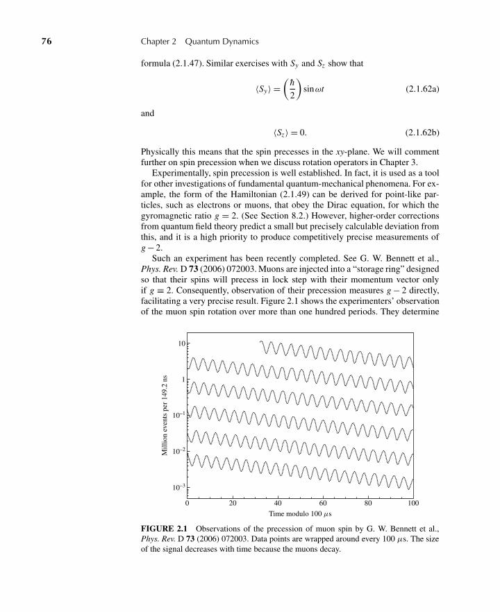
76 Chapter 2 Quantum Dynamics
formula (2.1.47). Similar exercises with Sy and Sz show that
〈Sy〉 =(
h
2
)sinωt (2.1.62a)
and
〈Sz〉 = 0. (2.1.62b)
Physically this means that the spin precesses in the xy-plane. We will commentfurther on spin precession when we discuss rotation operators in Chapter 3.
Experimentally, spin precession is well established. In fact, it is used as a toolfor other investigations of fundamental quantum-mechanical phenomena. For ex-ample, the form of the Hamiltonian (2.1.49) can be derived for point-like par-ticles, such as electrons or muons, that obey the Dirac equation, for which thegyromagnetic ratio g = 2. (See Section 8.2.) However, higher-order correctionsfrom quantum field theory predict a small but precisely calculable deviation fromthis, and it is a high priority to produce competitively precise measurements ofg − 2.
Such an experiment has been recently completed. See G. W. Bennett et al.,Phys. Rev. D 73 (2006) 072003. Muons are injected into a “storage ring” designedso that their spins will precess in lock step with their momentum vector onlyif g ≡ 2. Consequently, observation of their precession measures g − 2 directly,facilitating a very precise result. Figure 2.1 shows the experimenters’ observationof the muon spin rotation over more than one hundred periods. They determine
Mill
ion
even
ts p
er 1
49.2
ns
10–3
10–2
10–1
1
10
200 40 60 80 100
Time modulo 100 μs
FIGURE 2.1 Observations of the precession of muon spin by G. W. Bennett et al.,Phys. Rev. D 73 (2006) 072003. Data points are wrapped around every 100 μs. The sizeof the signal decreases with time because the muons decay.
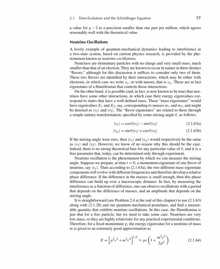
2.1 Time-Evolution and the Schrödinger Equation 77
a value for g − 2 to a precision smaller than one part per million, which agreesreasonably well with the theoretical value.
Neutrino Oscillations
A lovely example of quantum-mechanical dynamics leading to interference ina two-state system, based on current physics research, is provided by the phe-nomenon known as neutrino oscillations.
Neutrinos are elementary particles with no charge and very small mass, muchsmaller than that of an electron. They are known to occur in nature in three distinct“flavors,” although for this discussion it suffices to consider only two of them.These two flavors are identified by their interactions, which may be either withelectrons, in which case we write νe, or with muons, that is νμ. These are in facteigenstates of a Hamiltonian that controls those interactions.
On the other hand, it is possible (and, in fact, is now known to be true) that neu-trinos have some other interactions, in which case their energy eigenvalues cor-respond to states that have a well-defined mass. These “mass eigenstates” wouldhave eigenvalues E1 and E2, say, corresponding to masses m1 and m2, and mightbe denoted as |ν1〉 and |ν2〉. The “flavor eigenstates” are related to these througha simple unitary transformation, specified by some mixing angle θ , as follows:
|νe〉 = cosθ |ν1〉− sinθ |ν2〉 (2.1.63a)
|νμ〉 = sinθ |ν1〉+ cosθ |ν2〉 (2.1.63b)
If the mixing angle were zero, then |νe〉 and |νμ〉 would respectively be the sameas |ν1〉 and |ν2〉. However, we know of no reason why this should be the case.Indeed, there is no strong theoretical bias for any particular value of θ , and it is afree parameter that, today, can be determined only through experiment.
Neutrino oscillation is the phenomenon by which we can measure the mixingangle. Suppose we prepare, at time t = 0, a momentum eigenstate of one flavor ofneutrino, say |νe〉. Then according to (2.1.63a), the two different mass eigenstatecomponents will evolve with different frequencies and therefore develop a relativephase difference. If the difference in the masses is small enough, then this phasedifference can build up over a macroscopic distance. In fact, by measuring theinterference as a function of difference, one can observe oscillations with a periodthat depends on the difference of masses, and an amplitude that depends on themixing angle.
It is straightforward (see Problem 2.4 at the end of this chapter) to use (2.1.63)along with (2.1.28) and our quantum-mechanical postulates, and find a measur-able quantity that exhibits neutrino oscillations. In this case, the Hamiltonian isjust that for a free particle, but we need to take some care. Neutrinos are verylow mass, so they are highly relativistic for any practical experimental conditions.Therefore, for a fixed momentum p, the energy eigenvalue for a neutrino of massm is given to an extremely good approximation as
E =[
p2c2 + m2c4]1/2 ≈ pc
(1 + m2c2
2 p2
). (2.1.64)
78 Chapter 2 Quantum Dynamics
1.0
0.8
0.6
0.4
0.2
0
Surv
ival
pro
babi
lity
20 30 40 50 60 70 80 90 100
L0/Eve (km/MeV)
Data - BG - Geo veExpectation based on osci. parametersdetermined by KamLAND
FIGURE 2.2 Neutrino oscillations as observed by the KamLAND experiment, takenfrom S. Abe et al., Phys. Rev. Lett. 100 (2008) 221803. The oscillations as a function ofL/E demonstrate interference between different mass eigenstates of neutrinos.
If we next allow our state |νe〉 to evolve, and then at some later time t ask what isthe probability that it still appears as a |νe〉 (as opposed to a |νμ〉), we find
P(νe → νe) = 1 − sin2 2θ sin2(�m2c4 L
4E hc
), (2.1.65)
where �m2 ≡ m21 − m2
2, L = ct is the flight distance of the neutrino, and E = pcis the nominal neutrino energy.
The oscillations predicted by (2.1.65) have been dramatically observed by theKamLAND experiment. See Figure 2.2. Neutrinos from a series of nuclear re-actors are detected at a distance of ∼ 150 km, and the rate is compared to thatexpected from reactor power and properties. The curve is not a perfect sine wavebecause the reactors are not all at the same distance from the detector.
Correlation Amplitude and the Energy-Time Uncertainty Relation
We conclude this section by asking how state kets at different times are correlatedwith each other. Suppose the initial state ket at t = 0 of a physical system is givenby |α〉. With time it changes into |α, t0 = 0; t〉, which we obtain by applying thetime-evolution operator. We are concerned with the extent to which the state ketat a later time t is similar to the state ket at t = 0; we therefore construct the innerproduct between the two state kets at different times:
C(t) ≡ 〈α|α, t0 = 0; t〉= 〈α|U(t ,0)|α〉, (2.1.66)
2.1 Time-Evolution and the Schrödinger Equation 79
which is known as the correlation amplitude. The modulus of C(t) providesa quantitative measure of the “resemblance” between the state kets at differenttimes.
As an extreme example, consider the very special case where the initial ket |α〉is an eigenket of H; we then have
C(t) = 〈a′|a′, t0 = 0; t〉 = exp
(−i Ea′t
h
), (2.1.67)
so the modulus of the correlation amplitude is unity at all times—which is notsurprising for a stationary state. In the more general situation where the initial ketis represented by a superposition of {|a′〉}, as in (2.1.37), we have
C(t) =(∑
a′c∗
a′ 〈a′|)[∑
a′′ca′′ exp
(−i Ea′′ t
h
)|a′′〉
]
=∑
a′|ca′ |2 exp
(−i Ea′t
h
). (2.1.68)
As we sum over many terms with oscillating time dependence of different fre-quencies, a strong cancellation is possible for moderately large values of t. Weexpect the correlation amplitude that starts with unity at t = 0 to decrease in mag-nitude with time.
To estimate (2.1.68) in a more concrete manner, let us suppose that the stateket can be regarded as a superposition of so many energy eigenkets with simi-lar energies that we can regard them as exhibiting essentially a quasi-continuousspectrum. It is then legitimate to replace the sum by the integral∑
a′→
∫d Eρ(E), ca′ → g(E)
∣∣∣∣E�Ea′
, (2.1.69)
where ρ(E) characterizes the density of energy eigenstates. Expression (2.1.68)now becomes
C(t) =∫
d E |g(E)|2ρ(E)exp
(−i E t
h
), (2.1.70)
subject to the normalization condition∫d E |g(E)|2ρ(E) = 1. (2.1.71)
In a realistic physical situation, |g(E)|2ρ(E) may be peaked around E = E0 withwidth �E . Writing (2.1.70) as
C(t) = exp
(−i E0t
h
)∫d E |g(E)|2ρ(E)exp
[−i (E − E0)t
h
], (2.1.72)
we see that as t becomes large, the integrand oscillates very rapidly unless theenergy interval |E − E0| is small compared with h/t . If the interval for which
80 Chapter 2 Quantum Dynamics
|E − E0| � h/t holds is much narrower than�E—the width of |g(E)|2ρ(E)—weget essentially no contribution to C(t) because of strong cancellations. The char-acteristic time at which the modulus of the correlation amplitude starts becomingappreciably different from 1 is given by
t � h
�E. (2.1.73)
Even though this equation is obtained for a superposition state with a quasi-continuous energy spectrum, it also makes sense for a two-level system; in thespin-precession problem considered earlier, the state ket, which is initially |Sx+〉,starts losing its identity after ∼ 1/ω = h/(E+ − E−), as is evident from (2.1.60).
To summarize, as a result of time evolution the state ket of a physical sys-tem ceases to retain its original form after a time interval of order h/�E . In theliterature this point is often said to illustrate the time-energy uncertainty relation
�t�E � h. (2.1.74)
However, this time-energy uncertainty relation is of a very different nature fromthe uncertainty relation between two incompatible observables discussed in Sec-tion 1.4. In Chapter 5 we will come back to (2.1.74) in connection with time-dependent perturbation theory.
2.2 THE SCHRÖDINGER VERSUS THE HEISENBERG PICTURE
Unitary Operators
In the previous section we introduced the concept of time development by consid-ering the time-evolution operator that affects state kets; this approach to quantumdynamics is known as the Schrödinger picture. There is another formulation ofquantum dynamics where observables, rather than state kets, vary with time; thissecond approach is known as the Heisenberg picture. Before discussing the dif-ferences between the two approaches in detail, we digress to make some generalcomments on unitary operators.
Unitary operators are used for many different purposes in quantum mechan-ics. In this book we introduced (Section 1.5) an operator satisfying the unitarityproperty. In that section we were concerned with the question of how the basekets in one representation are related to those in some other representations. Thestate kets themselves are assumed not to change as we switch to a different set ofbase kets, even though the numerical values of the expansion coefficients for |α〉are, of course, different in different representations. Subsequently we introducedtwo unitary operators that actually change the state kets, the translation operatorof Section 1.6 and the time-evolution operator of Section 2.1. We have
|α〉 → U |α〉, (2.2.1)
where U may stand for T (dx) or U(t , t0). Here U |α〉 is the state ket correspondingto a physical system that actually has undergone translation or time evolution.
2.2 The Schrödinger Versus the Heisenberg Picture 81
It is important to keep in mind that under a unitary transformation that changesthe state kets, the inner product of a state bra and a state ket remains unchanged:
〈β|α〉 → 〈β|U †U |α〉 = 〈β|α〉. (2.2.2)
Using the fact that these transformations affect the state kets but not operators, wecan infer how 〈β|X |α〉 must change:
〈β|X |α〉 → (〈β|U †) · X · (U |α〉) = 〈β|U † XU |α〉. (2.2.3)
We now make a very simple mathematical observation that follows from the as-sociative axiom of multiplication:
(〈β|U†) · X · (U |α〉) = 〈β| · (U †XU ) · |α〉. (2.2.4)
Is there any physics in this observation? This mathematical identity suggests twoapproaches to unitary transformations:
Approach 1:|α〉 → U |α〉, with operators unchanged. (2.2.5a)
Approach 2:X → U † XU , with state kets unchanged. (2.2.5b)
In classical physics we do not introduce state kets, yet we talk about translation,time evolution, and the like. This is possible because these operations actuallychange quantities such as x and L, which are observables of classical mechanics.We therefore conjecture that a closer connection with classical physics may beestablished if we follow approach 2.
A simple example may be helpful here. We go back to the infinitesimal transla-tion operator T (dx′). The formalism presented in Section 1.6 is based on approach1; T (dx′) affects the state kets, not the position operator:
|α〉 →(
1 − ip · dx′
h
)|α〉,
x → x.(2.2.6)
In contrast, if we follow approach 2, we obtain
|α〉 → |α〉,
x →(
1 + ip · dx′
h
)x(
1 − ip · dx′
h
)= x +
(i
h
)[p · dx′,x
]= x + dx′. (2.2.7)
We leave it as an exercise for the reader to show that both approaches lead to thesame result for the expectation value of x:
〈x〉 → 〈x〉+ 〈dx′〉. (2.2.8)
82 Chapter 2 Quantum Dynamics
State Kets and Observables in the Schrödinger and the Heisenberg Pictures
We now return to the time-evolution operator U(t , t0). In the previous sectionwe examined how state kets evolve with time. This means that we were followingapproach 1, which is known as the Schrödinger picture when it is applied to timeevolution. Alternatively, we may follow approach 2, known as the Heisenbergpicture when applied to time evolution.
In the Schrödinger picture the operators corresponding to observables such asx, py , and Sz are fixed in time, while state kets vary with time, as indicated in theprevious section. In contrast, in the Heisenberg picture the operators correspond-ing to observables vary with time; the state kets are fixed—frozen, so to speak—atwhat they were at t0. It is convenient to set t0 in U(t , t0) to zero for simplicity andwork with U(t), which is defined by
U(t , t0 = 0) ≡ U(t) = exp
(−i H t
h
). (2.2.9)
Motivated by (2.2.5b) of approach 2, we define the Heisenberg picture observableby
A(H )(t) ≡ U†(t)A(S)U(t), (2.2.10)
where the superscripts H and S stand for Heisenberg and Schrödinger, re-spectively. At t = 0, the Heisenberg picture observable and the correspondingSchrödinger picture observable coincide:
A(H )(0) = A(S). (2.2.11)
The state kets also coincide between the two pictures at t = 0; at later t theHeisenberg-picture state ket is frozen at what it was at t = 0:
|α, t0 = 0; t〉H = |α, t0 = 0〉, (2.2.12)
independent of t. This is in dramatic contrast with the Schrödinger-picture stateket,
|α, t0 = 0; t〉S = U(t)|α, t0 = 0〉. (2.2.13)
The expectation value 〈A〉 is obviously the same in both pictures:
S〈α, t0 = 0; t|A(S)|α, t0 = 0; t〉S = 〈α, t0 = 0|U† A(S)U|α, t0 = 0〉= H 〈α, t0 = 0; t|A(H )(t)|α, t0 = 0; t〉H . (2.2.14)
The Heisenberg Equation of Motion
We now derive the fundamental equation of motion in the Heisenberg picture.Assuming that A(S) does not depend explicitly on time, which is the case in most
2.2 The Schrödinger Versus the Heisenberg Picture 83
physical situations of interest, we obtain [by differentiating (2.2.10)]
d A(H )
dt= ∂U†
∂ tA(S)U+U† A(S) ∂U
∂ t
= − 1
i hU† HUU† A(S)U+ 1
i hU† A(S)UU† HU
= 1
i h[A(H ),U† HU], (2.2.15)
where we have used [see (2.1.25)]
∂U
∂ t= 1
i hHU, (2.2.16a)
∂U†
∂ t= − 1
i hU† H . (2.2.16b)
Because H was originally introduced in the Schrödinger picture, we may betempted to define
H (H ) = U† HU (2.2.17)
in accordance with (2.2.10). But in elementary applications where U is given by(2.2.9), U and H obviously commute; as a result,
U† HU = H , (2.2.18)
so it is all right to write (2.2.15) as
d A(H )
dt= 1
i h
[A(H ), H
]. (2.2.19)
This equation is known as the Heisenberg equation of motion. Notice that wehave derived it using the properties of the time-evolution operator and the definingequation for A(H ).
It is instructive to compare (2.2.19) with the classical equation of motion inPoisson bracket form. In classical physics, for a function A of q’s and p’s thatdoes not involve time explicitly, we have (Goldstein 2002, pp. 396–97)
d A
dt= [A, H ]classical . (2.2.20)
Again, we see that Dirac’s quantization rule (1.6.47) leads to the correct equationin quantum mechanics. Indeed, historically (2.2.19) was first written by P. A. M.Dirac, who—with his characteristic modesty—called it the Heisenberg equationof motion. It is worth noting, however, that (2.2.19) makes sense whether or notA(H ) has a classical analogue. For example, the spin operator in the Heisenbergpicture satisfies
d S(H )i
dt= 1
i h
[S(H )
i , H]
, (2.2.21)
84 Chapter 2 Quantum Dynamics
which can be used to discuss spin precession, but this equation has no classicalcounterpart because Sz cannot be written as a function of q’s and p’s. Rather thaninsisting on Dirac’s rule, (1.6.47), we may argue that for quantities possessingclassical counterparts, the correct classical equation can be obtained from the cor-responding quantum-mechanical equation via the ansatz,
[ , ]
i h→ [ , ]classical . (2.2.22)
Classical mechanics can be derived from quantum mechanics, but the opposite isnot true.∗
Free Particles; Ehrenfest’s Theorem
Whether we work in the Schrödinger picture or in the Heisenberg picture, to beable to use the equations of motion we must first learn how to construct the appro-priate Hamiltonian operator. For a physical system with classical analogues, weassume the Hamiltonian to be of the same form as in classical physics; we merelyreplace the classical xi ’s and pi ’s by the corresponding operators in quantum me-chanics. With this assumption we can reproduce the correct classical equations inthe classical limit. Whenever an ambiguity arises because of noncommuting ob-servables, we attempt to resolve it by requiring H to be Hermitian; for instance, wewrite the quantum-mechanical analogue of the classical product xp as 1
2 (x p+ px).When the physical system in question has no classical analogues, we can onlyguess the structure of the Hamiltonian operator. We try various forms until we getthe Hamiltonian that leads to results agreeing with empirical observation.
In practical applications it is often necessary to evaluate the commutator of xi(or pi ) with functions of x j and p j . To this end the following formulas are useful:
[xi , F(p)
]= i h∂F
∂pi(2.2.23a)
and [pi , G(x)
]= −i h∂G
∂xi, (2.2.23b)
where F and G are functions that can be expanded in powers of p j ’s and x j ’s,respectively. We can easily prove both formulas by repeatedly applying (1.6.50e).
We are now in a position to apply the Heisenberg equation of motion to a freeparticle of mass m. The Hamiltonian is taken to be of the same form as in classicalmechanics:
H = p2
2m=(
p2x + p2
y + p2z
)2m
. (2.2.24)
∗In this book we follow the following order: the Schrödinger picture → the Heisenberg picture→ classical. For an enlightening treatment of the same subject in the opposite order, classical →the Heisenberg picture → the Schrödinger picture, see Finkelstein (1973), pp. 68–70 and 109.
2.2 The Schrödinger Versus the Heisenberg Picture 85
We look at the observables pi and xi , which are understood to be the momen-tum and the position operator in the Heisenberg picture even though we omit thesuperscript (H). Because pi commutes with any function of p j ’s, we have
dpi
dt= 1
i h
[pi , H
]= 0. (2.2.25)
Thus for a free particle, the momentum operator is a constant of the motion, whichmeans that pi (t) is the same as pi (0) at all times. Quite generally, it is evident fromthe Heisenberg equation of motion (2.2.19) that whenever A(H ) commutes withthe Hamiltonian, A(H ) is a constant of the motion. Next,
dxi
dt= 1
i h
[xi , H
]= 1
i h
1
2mi h∂
∂pi
⎛⎝ 3∑j=1
p2j
⎞⎠= pi
m= pi (0)
m, (2.2.26)
where we have taken advantage of (2.2.23a), so we have the solution
xi (t) = xi (0) +(
pi (0)
m
)t , (2.2.27)
which is reminiscent of the classical trajectory equation for a uniform rectilinearmotion. It is important to note that even though we have[
xi (0), x j (0)]= 0 (2.2.28)
at equal times, the commutator of the xi ’s at different times does not vanish;specifically,
[xi (t), xi (0)
]=[
pi (0)t
m, xi (0)
]= −i ht
m. (2.2.29)
Applying the uncertainty relation (1.4.53) to this commutator, we obtain
〈(�xi )2〉t 〈(�xi )2〉t=0 ≥ h2t2
4m2. (2.2.30)
Among other things, this relation implies that even if the particle is well localizedat t = 0, its position becomes more and more uncertain with time, a conclusionthat can also be obtained by studying the time-evolution behavior of free-particlewave packets in wave mechanics.
We now add a potential V(x) to our earlier free-particle Hamiltonian:
H = p2
2m+ V (x). (2.2.31)
86 Chapter 2 Quantum Dynamics
Here V(x) is to be understood as a function of the x-, y-, and z-operators. Using(2.2.23b) this time, we obtain
dpi
dt= 1
i h
[pi , V (x)
]= − ∂
∂xiV (x). (2.2.32)
On the other hand, we see that
dxi
dt= pi
m(2.2.33)
still holds because xi commutes with the newly added term V(x). We can use theHeisenberg equation of motion once again to deduce
d2xi
dt2 = 1
i h
[dxi
dt, H
]= 1
i h
[ pi
m, H
]= 1
m
dpi
dt. (2.2.34)
Combining this with (2.2.32), we finally obtain in vectorial form
md2xdt2
= −∇V (x). (2.2.35)
This is the quantum-mechanical analogue of Newton’s second law. By taking theexpectation values of both sides with respect to a Heisenberg state ket that doesnot move with time, we obtain
md2
dt2 〈x〉 = d〈p〉dt
= −〈∇V (x)〉. (2.2.36)
This is known as the Ehrenfest theorem after P. Ehrenfest, who derived it in1927 using the formalism of wave mechanics. When the theorem is written inthis expectation form, its validity is independent of whether we are using theHeisenberg or the Schrödinger picture; after all, the expectation values are thesame in the two pictures. In contrast, the operator form (2.2.35) is meaningfulonly if we understand x and p to be Heisenberg-picture operators.
We note that in (2.2.36) the h’s have completely disappeared. It is thereforenot surprising that the center of a wave packet moves like a classical particlesubjected to V(x).
Base Kets and Transition Amplitudes
So far we have avoided asking how the base kets evolve with time. A commonmisconception is that as time goes on, all kets move in the Schrödinger pictureand are stationary in the Heisenberg picture. This is not the case, as we will makeclear shortly. The important point is to distinguish the behavior of state kets fromthat of base kets.
2.2 The Schrödinger Versus the Heisenberg Picture 87
We started our discussion of ket spaces in Section 1.2 by remarking that theeigenkets of observables are to be used as base kets. What happens to the definingeigenvalue equation
A|a′〉 = a′|a′〉 (2.2.37)
with time? In the Schrödinger picture, A does not change, so the base kets, ob-tained as the solutions to this eigenvalue equation at t = 0, for instance, must re-main unchanged. Unlike state kets, the base kets do not change in the Schrödingerpicture.
The whole situation is very different in the Heisenberg picture, where theeigenvalue equation we must study is for the time-dependent operator
A(H )(t) = U† A(0)U. (2.2.38)
From (2.2.37) evaluated at t = 0, when the two pictures coincide, we deduce
U† A(0)UU†|a′〉 = a′U†|a′〉, (2.2.39)
which implies an eigenvalue equation for A(H ):
A(H )(U†|a′〉) = a′(U†|a′〉). (2.2.40)
If we continue to maintain the view that the eigenkets of observables form thebase kets, then {U†|a′〉} must be used as the base kets in the Heisenberg picture.As time goes on, the Heisenberg-picture base kets, denoted by |a′, t〉H , move asfollows:
|a′, t〉H = U†|a′〉. (2.2.41)
Because of the appearance of U† rather than U in (2.2.41), the Heisenberg-picturebase kets are seen to rotate oppositely when compared with the Schrödinger-picture state kets; specifically, |a′, t〉H satisfies the “wrong-sign Schrödinger equa-tion”
i h∂
∂ t|a′, t〉H = −H |a′, t〉H . (2.2.42)
As for the eigenvalues themselves, we see from (2.2.40) that they are un-changed with time. This is consistent with the theorem on unitary equivalent ob-servables discussed in Section 1.5. Notice also the following expansion for A(H )(t)in terms of the base kets and bras of the Heisenberg picture:
A(H )(t) =∑
a′|a′, t〉H a′
H 〈a′, t| (2.2.43)
=∑
a′U†|a′〉a′〈a′|U
= U† A(S)U,
88 Chapter 2 Quantum Dynamics
which shows that everything is quite consistent, provided that the Heisenberg basekets change as in (2.2.41).
We see that the expansion coefficients of a state ket in terms of base kets arethe same in both pictures:
ca′(t) = 〈a′|︸︷︷︸base bra
· (U|α, t0 = 0〉)︸ ︷︷ ︸state ket
(the Schrödinger picture) (2.2.44a)
ca′(t) = (〈a′|U)︸ ︷︷ ︸base bra
· |α, t0 = 0〉︸ ︷︷ ︸state ket
(the Heisenberg picture). (2.2.44b)
Pictorially, we may say that the cosine of the angle between the state ket and thebase ket is the same whether we rotate the state ket counterclockwise or the baseket clockwise. These considerations apply equally well to base kets that exhibit acontinuous spectrum; in particular, the wave function 〈x′|α〉 can be regarded eitheras (1) the inner product of the stationary position eigenbra with the moving stateket (the Schrödinger picture) or as (2) the inner product of the moving positioneigenbra with the stationary state ket (the Heisenberg picture). We will discussthe time dependence of the wave function in Section 2.4, where we will derive thecelebrated wave equation of Schrödinger.
To illustrate further the equivalence between the two pictures, we study transi-tion amplitudes, which will play a fundamental role in Section 2.6. Suppose thereis a physical system prepared at t = 0 to be in an eigenstate of observable A witheigenvalue a′. At some later time t we may ask, What is the probability amplitude,known as the transition amplitude, for the system to be found in an eigenstateof observable B with eigenvalue b′? Here A and B can be the same or different. Inthe Schrödinger picture the state ket at t is given by U|a′〉, whereas the base kets|a′〉 and |b′〉 do not vary with time; so we have
〈b′|︸︷︷︸base bra
· (U|a′〉)︸ ︷︷ ︸state ket
(2.2.45)
for this transition amplitude. In contrast, in the Heisenberg picture the state ketis stationary—that is, it remains as |a′〉 at all times—but the base kets evolveoppositely. So the transition amplitude is
(〈b′|U)︸ ︷︷ ︸base bra
· |a′〉︸︷︷︸state ket
. (2.2.46)
Obviously (2.2.45) and (2.2.46) are the same. They can both be written as
〈b′|U(t ,0)|a′〉. (2.2.47)
In some loose sense, this is the transition amplitude for “going” from state |a′〉 tostate |b′〉.
To conclude this section, let us summarize the differences between theSchrödinger picture and the Heisenberg picture. Table 2.1 provides such a sum-mary.
2.3 Simple Harmonic Oscillator 89
TABLE 2.1 The Schrödinger Picture versus the Heisenberg Picture
Schrödinger picture Heisenberg pictureState ket Moving: (2.1.5), (2.1.27) StationaryObservable Stationary Moving: (2.2.10), (2.2.19)Base ket Stationary Moving oppositely: (2.2.41), (2.2.42)
2.3 SIMPLE HARMONIC OSCILLATOR
The simple harmonic oscillator is one of the most important problems in quantummechanics. It not only illustrates many of the basic concepts and methods of quan-tum mechanics but also has much practical value. Essentially any potential wellcan be approximated by a simple harmonic oscillator, so it describes phenomenafrom molecular vibrations to nuclear structure. Moreover, because the Hamilto-nian is basically the sum of squares of two canonically conjugate variables, it isalso an important starting point for much of quantum field theory.
Energy Eigenkets and Energy Eigenvalues
We begin our discussion with Dirac’s elegant operator method, which is based onthe earlier work of M. Born and N. Wiener, to obtain the energy eigenkets andenergy eigenvalues of the simple harmonic oscillator. The basic Hamiltonian is
H = p2
2m+ mω2x2
2, (2.3.1)
where ω is the angular frequency of the classical oscillator related to the springconstant k in Hooke’s law via ω = √
k/m. The operators x and p are, of course,Hermitian. It is convenient to define two non-Hermitian operators,
a =√
mω
2h
(x + i p
mω
), a† =
√mω
2h
(x − i p
mω
), (2.3.2)
which are known as the annihilation operator and the creation operator, re-spectively, for reasons that will become evident shortly. Using the canonical com-mutation relations, we readily obtain[
a,a†]
=(
1
2h
)(−i [x , p] + i [p, x]) = 1. (2.3.3)
We also define the number operator
N = a†a, (2.3.4)
which is obviously Hermitian. It is straightforward to show that
a†a =(
mω
2h
)(x2 + p2
m2ω2
)+(
i
2h
)[x , p]
= H
hω− 1
2,
(2.3.5)
90 Chapter 2 Quantum Dynamics
so we have an important relation between the number operator and the Hamilto-nian operator:
H = hω(
N + 12
). (2.3.6)
Because H is just a linear function of N, N can be diagonalized simultaneouslywith H. We denote an energy eigenket of N by its eigenvalue n, so
N |n〉 = n|n〉. (2.3.7)
We will later show that n must be a nonnegative integer. Because of (2.3.6) wealso have
H |n〉 =(
n + 12
)hω|n〉, (2.3.8)
which means that the energy eigenvalues are given by
En =(
n + 12
)hω. (2.3.9)
To appreciate the physical significance of a, a†, and N, let us first note that
[N ,a] = [a†a,a] = a†[a,a] + [a†,a]a = −a, (2.3.10)
where we have used (2.3.3). Likewise, we can derive
[N ,a†] = a†. (2.3.11)
As a result, we have
Na†|n〉 = ([N ,a†] + a†N)|n〉 = (n + 1)a†|n〉 (2.3.12a)
and
Na|n〉 = ([N ,a] + a N)|n〉 = (n − 1)a|n〉. (2.3.12b)
These relations imply that a†|n〉(a|n〉) is also an eigenket of N with eigenvalue in-creased (decreased) by one. Because the increase (decrease) of n by one amountsto the creation (annihilation) of one quantum unit of energy hω, the term creationoperator (annihilation operator) for a† (a) is deemed appropriate.
Equation (2.3.12b) implies that a|n〉 and |n − 1〉 are the same up to a multi-plicative constant. We write
a|n〉 = c|n − 1〉, (2.3.13)
where c is a numerical constant to be determined from the requirement that both|n〉 and |n − 1〉 be normalized. First, note that
〈n|a†a|n〉 = |c|2. (2.3.14)
2.3 Simple Harmonic Oscillator 91
We can evaluate the left-hand side of (2.3.14) by noting that a†a is just the numberoperator, so
n = |c|2. (2.3.15)
Taking c to be real and positive by convention, we finally obtain
a|n〉 = √n|n − 1〉. (2.3.16)
Similarly, it is easy to show that
a†|n〉 = √n + 1|n + 1〉. (2.3.17)
Suppose that we keep on applying the annihilation operator a to both sides of(2.3.16):
a2|n〉 = √n(n − 1)|n − 2〉,
a3|n〉 = √n(n − 1)(n − 2)|n − 3〉,
...
(2.3.18)
We can obtain numerical operator eigenkets with smaller and smaller n until thesequence terminates, which is bound to happen whenever we start with a positiveinteger n. One may argue that if we start with a noninteger n, the sequence willnot terminate, leading to eigenkets with a negative value of n. But we also havethe positivity requirement for the norm of a|n〉:
n = 〈n|N |n〉 = (〈n|a†) · (a|n〉) ≥ 0, (2.3.19)
which implies that n can never be negative! So we conclude that the sequence mustterminate with n = 0 and that the allowed values of n are nonnegative integers.
Because the smallest possible value of n is zero, the ground state of the har-monic oscillator has
E0 = 1
2hω. (2.3.20)
We can now successively apply the creation operator a† to the ground state |0〉.Using (2.3.17), we obtain
|1〉 = a†|0〉,
|2〉 =(
a†
√2
)|1〉 =
[(a†)2
√2
]|0〉,
|3〉 =(
a†
√3
)|2〉 =
[(a†)3
√3!
]|0〉,
...
|n〉 =[
(a†)n
√n!
]|0〉.
(2.3.21)
92 Chapter 2 Quantum Dynamics
In this way we have succeeded in constructing simultaneous eigenkets of Nand H with energy eigenvalues
En =(
n + 12
)hω (n = 0,1,2,3, . . .). (2.3.22)
From (2.3.16), (2.3.17), and the orthonormality requirement for {|n〉}, we ob-tain the matrix elements
〈n′|a|n〉 = √nδn′,n−1, 〈n′|a†|n〉 = √
n + 1δn′,n+1. (2.3.23)
Using these together with
x =√
h
2mω(a + a†), p = i
√mhω
2(−a + a†), (2.3.24)
we derive the matrix elements of the x and p operators:
〈n′|x |n〉 =√
h
2mω(√
nδn′,n−1 +√n + 1δn′,n+1), (2.3.25a)
〈n′|p|n〉 = i
√mhω
2(−√
nδn′,n−1 +√n + 1δn′,n+1). (2.3.25b)
Notice that neither x nor p is diagonal in the N-representation we are using. Thisis not surprising because x and p, like a and a†, do not commute with N.
The operator method can also be used to obtain the energy eigenfunctions inposition space. Let us start with the ground state defined by
a|0〉 = 0, (2.3.26)
which, in the x-representation, reads
〈x ′|a|0〉 =√
mω
2h〈x ′|
(x + i p
mω
)|0〉 = 0. (2.3.27)
Recalling (1.7.17), we can regard this as a differential equation for the ground-state wave function 〈x ′|0〉: (
x ′ + x20
d
dx ′
)〈x ′|0〉 = 0, (2.3.28)
where we have introduced
x0 ≡√
h
mω, (2.3.29)
which sets the length scale of the oscillator. We see that the normalized solutionto (2.3.28) is
〈x ′|0〉 =(
1
π1/4√x0
)exp
[−1
2
(x ′
x0
)2]
. (2.3.30)
2.3 Simple Harmonic Oscillator 93
We can also obtain the energy eigenfunctions for excited states by evaluating
〈x ′|1〉 = 〈x ′|a†|0〉 =(
1√2x0
)(x ′ − x2
0d
dx ′
)〈x ′|0〉,
〈x ′|2〉 =(
1√2
)〈x ′|(a†)2|0〉 =
(1√2!
)(1√2x0
)2(x ′ − x2
0d
dx ′
)2
〈x ′|0〉, . . . ,(2.3.31)
In general, we obtain
〈x ′|n〉 =(
1
π1/4√
2nn!
)(1
xn+1/20
)(x ′ − x2
0d
dx ′
)n
exp
[−1
2
(x ′
x0
)2]
. (2.3.32)
It is instructive to look at the expectation values of x2 and p2 for the groundstate. First, note that
x2 =(
h
2mω
)(a2 + a†2 + a†a + aa†). (2.3.33)
When we take the expectation value of x2, only the last term in (2.3.33) yields anonvanishing contribution:
〈x2〉 = h
2mω= x2
0
2. (2.3.34)
Likewise,
〈p2〉 = hmω
2. (2.3.35)
It follows that the expectation values of the kinetic and the potential energies are,respectively,⟨
p2
2m
⟩= hω
4= 〈H 〉
2and
⟨mω2x2
2
⟩= hω
4= 〈H 〉
2, (2.3.36)
as expected from the virial theorem. From (2.3.25a) and (2.3.25b), it follows that
〈x〉 = 〈p〉 = 0, (2.3.37)
which also holds for the excited states. We therefore have
〈(�x)2〉 = 〈x2〉 = h
2mωand 〈(�p)2〉 = 〈p2〉 = hmω
2, (2.3.38)
and we see that the uncertainty relation is satisfied in the minimum uncertaintyproduct form:
〈(�x)2〉〈(�p)2〉 = h2
4. (2.3.39)
94 Chapter 2 Quantum Dynamics
This is not surprising because the ground-state wave function has a Gaussianshape. In contrast, the uncertainty products for the excited states are larger:
〈(�x)2〉〈(�p)2〉 =(
n + 1
2
)2
h2, (2.3.40)
as the reader may easily verify.
Time Development of the Oscillator
So far we have not discussed the time evolution of oscillator state kets or of ob-servables such as x and p. Everything we have done is supposed to hold at someinstant of time, say at t = 0; the operators x, p, a, and a† are to be regarded eitheras Schrödinger-picture operators (at all t) or as Heisenberg-picture operators att = 0. In the remaining part of this section, we work exclusively in the Heisen-berg picture, which means that x, p, a, and a† are all time-dependent even thoughwe do not explicitly write x (H )(t), and so forth.
The Heisenberg equations of motion for p and x are, from (2.2.32) and (2.2.33),
dp
dt= −mω2x (2.3.41a)
and
dx
dt= p
m. (2.3.41b)
This pair of coupled differential equations is equivalent to two uncoupled differ-ential equations for a and a†, namely,
da
dt=√
mω
2h
( p
m− iωx
)= −i ωa (2.3.42a)
and
da†
dt= i ωa†, (2.3.42b)
whose solutions are
a(t) = a(0)exp(−iωt) and a†(t) = a†(0)exp(iωt). (2.3.43)
Incidentally, these relations explicitly show that N and H are time-independentoperators even in the Heisenberg picture, as they must be. In terms of x and p, wecan rewrite (2.3.43) as
x(t) + i p(t)
mω= x(0)exp(−i ω t) + i
[p(0)
mω
]exp(−i ω t),
x(t) − i p(t)
mω= x(0)exp(i ω t) − i
[p(0)
mω
]exp(i ω t).
(2.3.44)
2.3 Simple Harmonic Oscillator 95
Equating the Hermitian and anti-Hermitian parts of both sides separately, we de-duce
x(t) = x(0)cosωt +[
p(0)
mω
]sinω t (2.3.45a)
and
p(t) = −mωx(0)sinωt + p(0)cosωt . (2.3.45b)
These look the same as the classical equations of motion. We see that the x and poperators “oscillate” just like their classical analogues.
For pedagogical reasons, we now present an alternative derivation of (2.3.45a).Instead of solving the Heisenberg equation of motion, we attempt to evaluate
x(t) = exp
(i H t
h
)x(0)exp
(−i H t
h
). (2.3.46)
To this end we record a very useful formula:
exp(i Gλ)A exp(−i Gλ) = A + iλ [G, A] +(
i2λ2
2!
)[G, [G, A]]
+·· ·+(
i nλn
n!
)[G, [G, [G, . . . [G, A]]] . . .] + ·· · ,
(2.3.47)
where G is a Hermitian operator and λ is a real parameter. We leave the proofof this formula, which is known as the Baker-Hausdorff lemma, as an exercise.Applying this formula to (2.3.46), we obtain
exp
(i H t
h
)x(0)exp
(−i H t
h
)= x(0) +
(i t
h
)[H , x(0)]+
(i2t2
2!h2
)[H , [H , x(0)]]+·· · .
(2.3.48)
Each term on the right-hand side can be reduced to either x or p by repeatedlyusing
[H , x(0)] = −i h p(0)
m(2.3.49a)
and [H , p(0)
]= i hmω2x(0). (2.3.49b)
96 Chapter 2 Quantum Dynamics
Thus
exp
(i H t
h
)x(0)exp
(−i H t
h
)= x(0) +
[p(0)
m
]t −
(1
2!
)t2ω2x(0)
−(
1
3!
)t3ω2 p(0)
m+ ·· ·
= x(0)cosωt +[
p(0)
mω
]sinωt ,
(2.3.50)
in agreement with (2.3.45a).From (2.3.45a) and (2.3.45b), one may be tempted to conclude that 〈x〉 and 〈p〉
always oscillate with angular frequency ω. However, this inference is not correct.Take any energy eigenstate characterized by a definite value of n; the expectationvalue 〈n|x(t)|n〉 vanishes because the operators x(0) and p(0) change n by ±1,and |n〉 and |n ± 1〉 are orthogonal. This point is also obvious from our earlierconclusion (see Section 2.1) that the expectation value of an observable takenwith respect to a stationary state does not vary with time. To observe oscillationsreminiscent of the classical oscillator, we must look at a superposition of energyeigenstates such as
|α〉 = c0|0〉 + c1|1〉. (2.3.51)
The expectation value of x(t) taken with respect to (2.3.51) does oscillate, as thereader may readily verify.
We have seen that an energy eigenstate does not behave like the classicaloscillator—in the sense of oscillating expectation values for x and p—no matterhow large n may be. We may logically ask, How can we construct a superpositionof energy eigenstates that most closely imitates the classical oscillator? In wave-function language, we want a wave packet that bounces back and forth withoutspreading in shape. It turns out that a coherent state defined by the eigenvalueequation for the non-Hermitian annihilation operator a,
a|λ〉 = λ|λ〉, (2.3.52)
with, in general, a complex eigenvalue λ does the desired job. The coherent statehas many other remarkable properties:
1. When it is expressed as a superposition of energy (or N) eigenstates,
|λ〉 =∞∑
n =0
f (n)|n〉, (2.3.53)
the distribution of | f (n)|2 with respect to n is of the Poisson type aboutsome mean value n:
| f (n)|2 =(
nn
n!
)exp(−n). (2.3.54)
2.4 Schrödinger’s Wave Equation 97
2. It can be obtained by translating the oscillator ground state by some finitedistance.
3. It satisfies the minimum uncertainty product relation at all times.
A systematic study of coherent states, pioneered by R. Glauber, is very rewarding;the reader is urged to work out Problem 2.19 on this subject at the end of thischapter.∗
2.4 SCHRÖDINGER’S WAVE EQUATION
The Time-Dependent Wave Equation
We now turn to the Schrödinger picture and examine the time evolution of |α, t0; t〉in the x-representation. In other words, our task is to study the behavior of thewave function
ψ(x′, t) = 〈x′|α, t0; t〉 (2.4.1)
as a function of time, where |α, t0; t〉 is a state ket in the Schrödinger picture attime t, and 〈x′| is a time-independent position eigenbra with eigenvalue x′. TheHamiltonian operator is taken to be
H = p2
2m+ V (x). (2.4.2)
The potential V(x) is a Hermitian operator; it is also local in the sense that in thex-representation we have
〈x′′|V (x)|x′〉 = V (x′)δ3(x′ − x′′), (2.4.3)
where V (x′) is a real function of x′. Later in this book we will consider more-complicated Hamiltonians—a time-dependent potential V (x, t); a nonlocal butseparable potential where the right-hand side of (2.4.3) is replaced by v1(x′′)v2(x′);a momentum-dependent interaction of the form p ·A + A ·p, where A is the vectorpotential in electrodynamics, and so on.
We now derive Schrödinger’s time-dependent wave equation. We first write theSchrödinger equation for a state ket (2.1.27) in the x-representation:
i h∂
∂ t〈x′|α, t0; t〉 = 〈x′|H |α, t0; t〉, (2.4.4)
where we have used the fact that the position eigenbras in the Schrödinger picturedo not change with time. Using (1.7.20), we can write the kinetic-energy contri-bution to the right-hand side of (2.4.4) as⟨
x′∣∣∣∣ p2
2m
∣∣∣∣α, t0; t
⟩= −
(h2
2m
)∇′2〈x′|α, t0; t〉. (2.4.5)
∗For applications to laser physics, see Sargent, Scully, and Lamb (1974) and Loudon (2000). Seealso the discussion on squeezed light at the end of Section 7.6 of this book.
98 Chapter 2 Quantum Dynamics
As for V(x), we simply use
〈x′|V (x) = 〈x′|V (x′), (2.4.6)
where V (x′) is no longer an operator. Combining everything, we deduce
i h∂
∂ t〈x′|α, t0; t〉 = −
(h2
2m
)∇′2〈x′|α, t0; t〉+ V (x′)〈x′|α, t0; t〉, (2.4.7)
which we recognize to be the celebrated time-dependent wave equation of E.Schrödinger, usually written as
i h∂
∂ tψ(x′, t) = −
(h2
2m
)∇′2ψ(x′, t) + V (x′)ψ(x′, t). (2.4.8)
The quantum mechanics based on wave equation (2.4.8) is known as wave me-chanics. This equation is, in fact, the starting point of many textbooks on quantummechanics. In our formalism, however, this is just the Schrödinger equation for astate ket written explicitly in the x-basis when the Hamiltonian operator is takento be (2.4.2).
The Time-Independent Wave Equation
We now derive the partial differential equation satisfied by energy eigenfunctions.We showed in Section 2.1 that the time dependence of a stationary state is givenby exp(−i Ea′t/h). This enables us to write its wave function as
〈x′|a′, t0; t〉 = 〈x′|a′〉exp
(−i Ea′t
h
), (2.4.9)
where it is understood that initially the system is prepared in a simultaneous eigen-state of A and H with eigenvalues a′ and Ea′ , respectively. Let us now substitute(2.4.9) into the time-dependent Schrödinger equation (2.4.7). We are then led to
−(
h2
2m
)∇′2〈x′|a′〉+ V (x′)〈x′|a′〉 = Ea′〈x′|a′〉. (2.4.10)
This partial differential equation is satisfied by the energy eigenfunction 〈x′|a′〉with energy eigenvalue Ea′ . Actually, in wave mechanics where the Hamiltonianoperator is given as a function of x and p, as in (2.4.2), it is not necessary to referexplicitly to observable A that commutes with H, because we can always choose Ato be that function of the observables x and p that coincides with H itself. We maytherefore omit reference to a′ and simply write (2.4.10) as the partial differentialequation to be satisfied by the energy eigenfunction uE (x′):
−(
h2
2m
)∇′2uE (x′) + V (x′)uE (x′) = EuE (x′). (2.4.11)
2.4 Schrödinger’s Wave Equation 99
This is the time-independent wave equation of E. Schrödinger—announced inthe first of four monumental papers, all written in the first half of 1926—that laidthe foundations of wave mechanics. In the same paper he immediately applied(2.4.11) to derive the energy spectrum of the hydrogen atom.
To solve (2.4.11) some boundary condition has to be imposed. Suppose weseek a solution to (2.4.11) with
E < lim|x′|→∞
V (x′), (2.4.12)
where the inequality relation is to hold for |x′| → ∞ in any direction. The appro-priate boundary condition to be used in this case is
uE (x′) → 0 as |x′| → ∞. (2.4.13)
Physically this means that the particle is bound or confined within a finite regionof space. We know from the theory of partial differential equations that (2.4.11)subject to boundary condition (2.4.13) allows nontrivial solutions only for a dis-crete set of values of E. It is in this sense that the time-independent Schrödingerequation (2.4.11) yields the quantization of energy levels.∗ Once the partial dif-ferential equation (2.4.11) is written, the problem of finding the energy levels ofmicroscopic physical systems is as straightforward as that of finding the char-acteristic frequencies of vibrating strings or membranes. In both cases we solveboundary-value problems in mathematical physics.
A short digression on the history of quantum mechanics is in order here. Thefact that exactly soluble eigenvalue problems in the theory of partial differentialequations can also be treated using matrix methods was already known to math-ematicians in the first quarter of the twentieth century. Furthermore, theoreticalphysicists like M. Born frequently consulted great mathematicians of the day—D. Hilbert and H. Weyl, in particular. Yet when matrix mechanics was born inthe summer of 1925, it did not immediately occur to the theoretical physicistsor the mathematicians to reformulate it using the language of partial differentialequations. Six months after Heisenberg’s pioneering paper, wave mechanics wasproposed by Schrödinger. However, a close inspection of his papers shows thathe was not at all influenced by the earlier works of Heisenberg, Born, and Jordan.Instead, the train of reasoning that led Schrödinger to formulate wave mechanicshas its roots in W. R. Hamilton’s analogy between optics and mechanics, on whichwe will comment later, and in the particle-wave hypothesis of L. de Broglie. Oncewave mechanics was formulated, many people, including Schrödinger himself,showed the equivalence between wave mechanics and matrix mechanics.
It is assumed that the reader of this book has some experience in solving thetime-dependent and time-independent wave equations. He or she should be fa-miliar with the time evolution of a Gaussian wave packet in a force-free region;should be able to solve one-dimensional transmission-reflection problems involv-ing a rectangular potential barrier, and the like; should have seen derived some
∗Schrödinger’s paper that announced (2.4.11) is appropriately entitled Quantisierung als Eigen-wertproblem (Quantization as an Eigenvalue Problem).
100 Chapter 2 Quantum Dynamics
simple solutions of the time-independent wave equation—a particle in a box, aparticle in a square well, the simple harmonic oscillator, the hydrogen atom, andso on; and should also be familiar with some general properties of the energyeigenfunctions and energy eigenvalues, such as (1) the fact that the energy levelsexhibit a discrete or continuous spectrum depending on whether or not (2.4.12)is satisfied and (2) the property that the energy eigenfunction in one dimension issinusoidal or damped depending on whether E − V (x′) is positive or negative.
In this book, we do not thoroughly cover these more elementary topics and so-lutions. Some of these (for example, the harmonic oscillator and hydrogen atom)are pursued, but at a mathematical level somewhat higher than what is usuallyseen in undergraduate courses. In any case, a brief summary of elementary solu-tions to Schrödinger’s equations is presented in Appendix B.
Interpretations of the Wave Function
We now turn to discussions of the physical interpretations of the wave function.In Section 1.7 we commented on the probabilistic interpretation of |ψ|2 that fol-lows from the fact that 〈x′|α, t0; t〉 is to be regarded as an expansion coefficient of|α, t0; t〉 in terms of the position eigenkets {|x′〉}. The quantity ρ(x′, t) defined by
ρ(x′, t) = |ψ(x′, t)|2 = |〈x′|α, t0; t〉|2 (2.4.14)
is therefore regarded as the probability density in wave mechanics. Specifically,when we use a detector that ascertains the presence of the particle within a smallvolume element d3x ′ around x′, the probability of recording a positive result attime t is given by ρ(x′, t)d3x ′.
In the remainder of this section we use x for x′ because the position operatorwill not appear. Using Schrödinger’s time-dependent wave equation, it is straight-forward to derive the continuity equation
∂ρ
∂ t+∇· j = 0, (2.4.15)
where ρ(x, t) stands for |ψ|2 as before, and j(x, t), known as the probability flux,is given by
j(x, t) = −(
i h
2m
)[ψ∗∇ψ− (∇ψ∗)ψ
]=(
h
m
)Im(ψ∗∇ψ).
(2.4.16)
The reality of the potential V (or the Hermiticity of the V operator) has playeda crucial role in our obtaining this result. Conversely, a complex potential canphenomenologically account for the disappearance of a particle; such a potentialis often used for nuclear reactions where incident particles get absorbed by nuclei.
2.4 Schrödinger’s Wave Equation 101
We may intuitively expect that the probability flux j is related to momentum.This is indeed the case for j integrated over all space. From (2.4.16) we obtain∫
d3xj(x, t) = 〈p〉t
m, (2.4.17)
where 〈p〉t is the expectation value of the momentum operator at time t.Equation (2.4.15) is reminiscent of the continuity equation in fluid dynamics
that characterizes a hydrodynamic flow of a fluid in a source-free, sink-free region.Indeed, historically Schrödinger was first led to interpret |ψ|2 as the actual matterdensity, or e|ψ|2 as the actual electric charge density. If we adopt such a view, weare led to face some bizarre consequences.
A typical argument for a position measurement might go as follows. An atomicelectron is to be regarded as a continuous distribution of matter filling up a finiteregion of space around the nucleus; yet, when a measurement is made to makesure that the electron is at some particular point, this continuous distribution ofmatter suddenly shrinks to a point-like particle with no spatial extension. Themore satisfactory statistical interpretation of |ψ|2 as the probability density wasfirst given by M. Born.
To understand the physical significance of the wave function, let us write it as
ψ(x, t) =√ρ(x, t)exp
[i S(x, t)
h
], (2.4.18)
with S real and ρ > 0, which can always be done for any complex function of x andt. The meaning of ρ has already been given. What is the physical interpretation ofS? Noting
ψ∗∇ψ = √ρ∇(
√ρ) +
(i
h
)ρ∇S, (2.4.19)
we can write the probability flux as [see (2.4.16)]
j = ρ∇S
m. (2.4.20)
We now see that there is more to the wave function than the fact that |ψ|2 is theprobability density; the gradient of the phase S contains a vital piece of infor-mation. From (2.4.20) we see that the spatial variation of the phase of the wavefunction characterizes the probability flux; the stronger the phase variation, themore intense the flux. The direction of j at some point x is seen to be normal tothe surface of a constant phase that goes through that point. In the particularlysimple example of a plane wave (a momentum eigenfunction),
ψ(x, t) ∝ exp
(ip · x
h− i E t
h
), (2.4.21)
where p stands for the eigenvalue of the momentum operator. All this is evidentbecause
∇S = p. (2.4.22)
102 Chapter 2 Quantum Dynamics
More generally, it is tempting to regard ∇S/m as some kind of “velocity,”
“v” = ∇S
m, (2.4.23)
and to write the continuity equation (2.4.15) as
∂ρ
∂ t+∇· (ρ “v”) = 0, (2.4.24)
just as in fluid dynamics. However, we would like to caution the reader againsttoo literal an interpretation of j as ρ times the velocity defined at every point inspace, because a simultaneous precision measurement of position and velocitywould necessarily violate the uncertainty principle.
The Classical Limit
We now discuss the classical limit of wave mechanics. First, we substitute ψwritten in form (2.4.18) into both sides of the time-dependent wave equation.Straightforward differentiations lead to
−(
h2
2m
)
×[∇2√ρ+
(2i
h
)(∇√
ρ) · (∇S) −(
1
h2
)√ρ|∇S|2 +
(i
h
)√ρ∇2S
]+√
ρV
= i h
[∂√ρ
∂ t+(
i
h
)√ρ∂S
∂ t
].
(2.4.25)
So far everything has been exact. Let us suppose now that h can, in some sense, beregarded as a small quantity. The precise physical meaning of this approximation,to which we will come back later, is not evident now, but let us assume
h|∇ 2S| � |∇S|2, (2.4.26)
and so forth. We can then collect terms in (2.4.25) that do not explicitly contain hto obtain a nonlinear partial differential equation for S:
1
2m|∇S(x, t)|2 + V (x) + ∂S(x, t)
∂ t= 0. (2.4.27)
We recognize this to be the Hamilton-Jacobi equation in classical mechanics,first written in 1836, where S(x, t) stands for Hamilton’s principal function. So, notsurprisingly, in the h → 0 limit, classical mechanics is contained in Schrödinger’swave mechanics. We have a semiclassical interpretation of the phase of the wavefunction: h times the phase is equal to Hamilton’s principal function, providedthat h can be regarded as a small quantity.
2.5 Elementary Solutions to Schrödinger’s Wave Equation 103
Let us now look at a stationary state with time dependence exp(−i E t/h). Thistime dependence is anticipated from the fact that for a classical system with aconstant Hamiltonian, Hamilton’s principal function S is separable:
S(x , t) = W (x) − E t , (2.4.28)
where W(x) is called Hamilton’s characteristic function (Goldstein 2002,pp. 440–44). As time goes on, a surface of a constant S advances in much the sameway as a surface of a constant phase in wave optics—a “wave front”—advances.The momentum in the classical Hamilton-Jacobi theory is given by
Pclass = ∇S = ∇W , (2.4.29)
which is consistent with our earlier identification of ∇S/m with some kind ofvelocity. In classical mechanics the velocity vector is tangential to the particletrajectory, and as a result we can trace the trajectory by following continuously thedirection of the velocity vector. The particle trajectory is like a ray in geometricoptics because the ∇S that traces the trajectory is normal to the wave front definedby a constant S. In this sense, geometrical optics is to wave optics what classicalmechanics is to wave mechanics.
One might wonder, in hindsight, why this optical-mechanical analogy was notfully exploited in the nineteenth century. The reason is that there was no moti-vation for regarding Hamilton’s principal function as the phase of some travelingwave; the wave nature of a material particle did not become apparent until the1920s. Besides, the basic unit of action h, which must enter into (2.4.18) for di-mensional reasons, was missing in the physics of the nineteenth century.
2.5 ELEMENTARY SOLUTIONS TO SCHRÖDINGER’SWAVE EQUATION
It is both instructive and useful to look at some relatively elementary solutionsto (2.4.11) for particular choices of the potential-energy function V (x). In thissection we choose some examples that illustrate contemporary physics and/or willbe useful in later chapters of this textbook.
Free Particle in Three Dimensions
The case V (x) = 0 has fundamental significance. We will consider the solutionto Schrödinger’s equation here in three dimensions using Cartesian coordinates.The solution in spherical coordinates will be left until our treatment of angularmomentum is presented in the next chapter. Equation (2.4.11) becomes
∇2uE (x) = −2m E
h2uE (x). (2.5.1)
Define a vector k where
k2 = k2x + k2
y + k2z ≡ 2m E
h2= p2
h2, (2.5.2)
104 Chapter 2 Quantum Dynamics
that is, p = hk. Differential equation (2.5.1) is easily solved using the techniqueknown as “separation of variables.” Writing
uE (x) = ux (x)uy(y)uz(z), (2.5.3)
we arrive at[1
ux
d2ux
dx2 + k2x
]+[
1
uy
d2uy
dy2 + k2y
]+[
1
uz
d2uz
dz2 + k2z
]= 0 (2.5.4)
This leads to individual plane-wave solutions uw(w) = cweikww for w = x , y, z.Note that one gets the same energy E for values ±kw.
Collecting these solutions and combining the normalization constants, we ob-tain
uE (x) = cx cyczeikx x+iky y+ikz z = Ceik·x. (2.5.5)
The normalization constant C presents the usual difficulties, which are generallyhandled by using a δ-function normalization condition. It is convenient in manycases, however, to use a “big box” normalization, where all space is containedwithin a cube of side length L. We impose periodic boundary conditions on thebox and thereby obtain a finite normalization constant C . For any real calculation,we simply let the size L → ∞ at the end of the calculation.
Imposing the condition ux (x + L) = ux (x), we have kx L = 2πnx , where nx isan integer. That is,
kx = 2π
Lnx , ky = 2π
Lny , kz = 2π
Lnz , (2.5.6)
and the normalization criterion becomes
1 =∫ L
0dx
∫ L
0dy∫ L
0dz u∗
E (x)uE (x) = L3|C|2, (2.5.7)
in which case C = 1/L3/2 and
uE (x) = 1
L3/2 eik·x. (2.5.8)
The energy eigenvalue is
E = p2
2m= h2k2
2m= h2
2m
(2π
L
)2(n2
x + n2y + n2
z
). (2.5.9)
The sixfold degeneracy we mentioned earlier corresponds to the six combinationsof (±nx ,±ny ,±nz), but the degeneracy can actually be much larger since, insome cases, there are various combinations of nx , ny , and nz that can give thesame E . In fact, in the (realistic) limit where L is very large, there can be a large
2.5 Elementary Solutions to Schrödinger’s Wave Equation 105
number of states N that have an energy between E and E + d E . This “densityof states” d N/d E is an important quantity for calculations of processes that in-clude free particles. See, for example, the discussion of the photoelectric effect inSection 5.8.
To calculate the density of states, imagine a spherical shell in k space withradius |k| = 2π |n|/L and thickness d|k| = 2πd|n|/L. All states within thisshell have energy E = h2k2/2m. The number of states d N within this shell is4πn2d|n|. Therefore,
d N
d E= 4πn2d|n|
h2|k|d|k|/m= 4π
h2m
(L
2π
)2
|k| L
2π
= m3/2 E1/2L3
√2π2h3
. (2.5.10)
In a typical “real” calculation, the density of states will be multiplied by someprobability that involves u∗
E (x)uE (x). In this case, the factors of L3 will cancelexplicitly, so the limit L → ∞ is trivial. This “big box” normalization also yieldsthe correct answer for the probability flux. Rewriting (2.4.21) with this normal-ization, we have
ψ(x, t) = 1
L3/2 exp
(ip ·x
h− i E t
h
), (2.5.11)
in which case we find
j(x, t) = h
mIm(ψ∗∇ψ) = hk
m
1
L3 = vρ, (2.5.12)
where ρ = 1/L3 is indeed the probability density.
The Simple Harmonic Oscillator
In Section 2.3 we saw an elegant solution for the case V (x) = mω2x2/2 thatyielded the energy eigenvalues, eigenstates, and wave functions. Here, we demon-strate a different approach that solves the differential equation
− h2
2m
d2
dx2 uE (x) + 1
2mω2x2uE (x) = EuE (x). (2.5.13)
Our approach will introduce the concept of generating functions, a generally use-ful technique that arises in many treatments of differential eigenvalue problems.
First, transform (2.5.13) using the dimensionless position y ≡ x/x0, wherex0 ≡ √
h/mω. Also introduce a dimensionless energy variable ε ≡ 2E/hω. Thedifferential equation we need to solve therefore becomes
d2
dy2 u(y) + (ε− y2)u(y) = 0. (2.5.14)
For y → ±∞, the solution must tend to zero; otherwise the wave functionwill not be normalizable and hence unphysical. The differential equation
106 Chapter 2 Quantum Dynamics
w′′(y) − y2w(y) = 0 has solutions w(y) ∝ exp(±y2/2), so we have to choose theminus sign. We then “remove” the asymptotic behavior of the wave function bywriting
u(y) = h(y)e−y2/2, (2.5.15)
where the function h(y) satisfies the differential equation
d2h
dy2− 2y
dh
dy+ (ε− 1)h(y) = 0. (2.5.16)
To this point, we have followed the traditional solution of the simple harmonicoscillator as found in many textbooks. Typically, one would now look for a se-ries solution for h(y) and discover that a normalizable solution is possible onlyif the series terminates. (In fact, we use this approach for the three-dimensionalisotropic harmonic oscillator in this book. See Section 3.7.) One forces this ter-mination by imposing the condition that ε− 1 be an even, nonnegative integer2n, n = 0,1,2, . . . . The solutions are then written using the resulting polynomialshn(y). Of course, ε− 1 = 2n is equivalent to E = (
n + 12
)hω, the quantization
relation (2.3.22).Let us take a different approach. Consider the “Hermite polynomials” Hn(x)
defined by the “generating function” g(x , t) through
g(x , t) ≡ e−t2+2t x (2.5.17a)
≡∞∑
n=0
Hn(x)tn
n!. (2.5.17b)
Some properties of the Hn(x) are immediately obvious. For example, H0(x) = 1.Also, because
g(0, t) = e−t2 =∞∑
n=0
(−1)n
n!t2n , (2.5.18)
it is clear that Hn(0) = 0 if n is odd, since this series involves only even powersof t . On the other hand, if we restrict ourselves to even values of n, we have
g(0, t) = e−t2 =∞∑
n=0
(−1)(n/2)
(n/2)!tn =
∞∑n=0
(−1)(n/2)
(n/2)!
n!
n!tn (2.5.19)
and so Hn(0) = (−1)n/2n!/(n/2)!. Also, since g(−x , t) reverses the sign only onterms with odd powers of t , Hn(−x) = (−1)n Hn(x).
We can take derivatives of g(x , t) to build the Hermite polynomials using re-cursion relations between them and their derivatives. The trick is that we candifferentiate the analytic form of the generating function (2.5.17a) or the series
2.5 Elementary Solutions to Schrödinger’s Wave Equation 107
form (2.5.17b) and then compare results. For example, if we take the derivativeusing (2.5.17a), then
∂g
∂x= 2tg(x , t) =
∞∑n=0
2Hn(x)tn+1
n!=
∞∑n=0
2(n + 1)Hn(x)tn+1
(n + 1)!, (2.5.20)
where we insert the series definition of the generating function after taking thederivative. On the other hand, we can take the derivative of (2.5.17b) directly, inwhich case
∂g
∂x=
∞∑n=0
H ′n(x)
tn
n!. (2.5.21)
Comparing (2.5.20) and (2.5.21) shows that
H ′n(x) = 2nHn−1(x). (2.5.22)
This is enough information for us build the Hermite polynomials:
H0(x) = 1
so H ′1(x) = 2, therefore H1(x) = 2x
so H ′2(x) = 8x , therefore H2(x) = 4x2 − 2
so H ′3(x) = 24x2 − 12, therefore H3(x) = 8x3 − 12x
...
So far, this is just a curious mathematical exercise. To see why it is relevant tothe simple harmonic oscillator, consider the derivative of the generating functionwith respect to t . If we start with (2.5.17a), then
∂g
∂ t= −2tg(x , t) + 2xg(x , t)
= −∞∑
n=0
2Hn(x)tn+1
n!+
∞∑n=0
2x Hn(x)tn
n!
= −∞∑
n=0
2nHn−1(x)tn
n!+
∞∑n=0
2x Hn(x)tn
n!. (2.5.23)
Or, if we differentiate (2.5.17b), then we have
∂g
∂ t=
∞∑n=0
nHn(x)tn−1
n!=
∞∑n=0
Hn+1(x)tn
n!. (2.5.24)
Comparing (2.5.23) and (2.5.24) gives us the recursion relation
Hn+1(x) = 2x Hn(x) − 2nHn−1(x), (2.5.25)
108 Chapter 2 Quantum Dynamics
which we combine with (2.5.22) to find
H ′′n (x) = 2n ·2(n − 1)Hn−2(x)
= 2n[2x Hn−1(x) − Hn(x)
]= 2x H ′
n(x) − 2nHn(x). (2.5.26)
In other words, the Hermite polynomials satisfy the differential equation
H ′′n (x) − 2x H ′
n(x) + 2nHn(x) = 0, (2.5.27)
where n is a nonnegative integer. This, however, is the same as the Schrödingerequation written as (2.5.16) since ε− 1 = 2n. That is, the wave functions for thesimple harmonic oscillator are given by
un(x) = cn Hn
(x
√mω
h
)e−mωx2/2h (2.5.28)
up to some normalization constant cn . This constant can be determined from theorthogonality relationship∫ ∞
−∞Hn(x)Hm(x)e−x2 = π1/22nn!δnm , (2.5.29)
which is easily proved using the generating function. See Problem 2.21 at the endof this chapter.
Generating functions have a usefulness that far outreaches our limited appli-cation here. Among other things, many of the orthogonal polynomials that arisefrom solving the Schrödinger equation for different potentials can be derived fromgenerating functions. See, for example, Problem 3.22 in Chapter 3. The interestedreader is encouraged to pursue this further from any one of the many excellenttexts on mathematical physics.
The Linear Potential
Perhaps the first potential-energy function, with bound states, to come to mind isthe linear potential, namely
V (x) = k|x |, (2.5.30)
where k is an arbitrary positive constant. Given a total energy E , this potentialhas a classical turning point at a value x = a, where E = ka. This point will beimportant for understanding the quantum behavior of a particle of mass m boundby this potential.
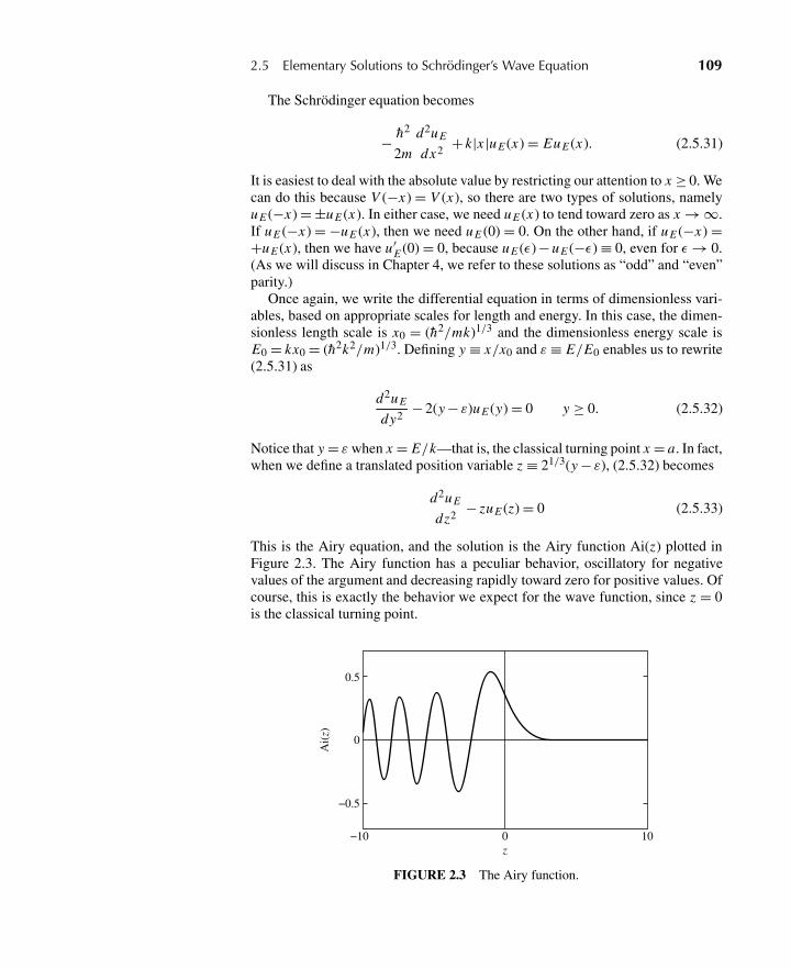
2.5 Elementary Solutions to Schrödinger’s Wave Equation 109
The Schrödinger equation becomes
− h2
2m
d2uE
dx2 + k|x |uE (x) = EuE (x). (2.5.31)
It is easiest to deal with the absolute value by restricting our attention to x ≥ 0. Wecan do this because V (−x) = V (x), so there are two types of solutions, namelyuE (−x) = ±uE (x). In either case, we need uE (x) to tend toward zero as x → ∞.If uE (−x) = −uE (x), then we need uE (0) = 0. On the other hand, if uE (−x) =+uE (x), then we have u′
E (0) = 0, because uE (ε) − uE (−ε) ≡ 0, even for ε → 0.(As we will discuss in Chapter 4, we refer to these solutions as “odd” and “even”parity.)
Once again, we write the differential equation in terms of dimensionless vari-ables, based on appropriate scales for length and energy. In this case, the dimen-sionless length scale is x0 = (h2/mk)1/3 and the dimensionless energy scale isE0 = kx0 = (h2k2/m)1/3. Defining y ≡ x/x0 and ε ≡ E/E0 enables us to rewrite(2.5.31) as
d2uE
dy2− 2(y − ε)uE (y) = 0 y ≥ 0. (2.5.32)
Notice that y = ε when x = E/k—that is, the classical turning point x = a. In fact,when we define a translated position variable z ≡ 21/3(y − ε), (2.5.32) becomes
d2uE
dz2 − zuE (z) = 0 (2.5.33)
This is the Airy equation, and the solution is the Airy function Ai(z) plotted inFigure 2.3. The Airy function has a peculiar behavior, oscillatory for negativevalues of the argument and decreasing rapidly toward zero for positive values. Ofcourse, this is exactly the behavior we expect for the wave function, since z = 0is the classical turning point.
−10 0 10z
0
0.5
−0.5
Ai(
z)
FIGURE 2.3 The Airy function.
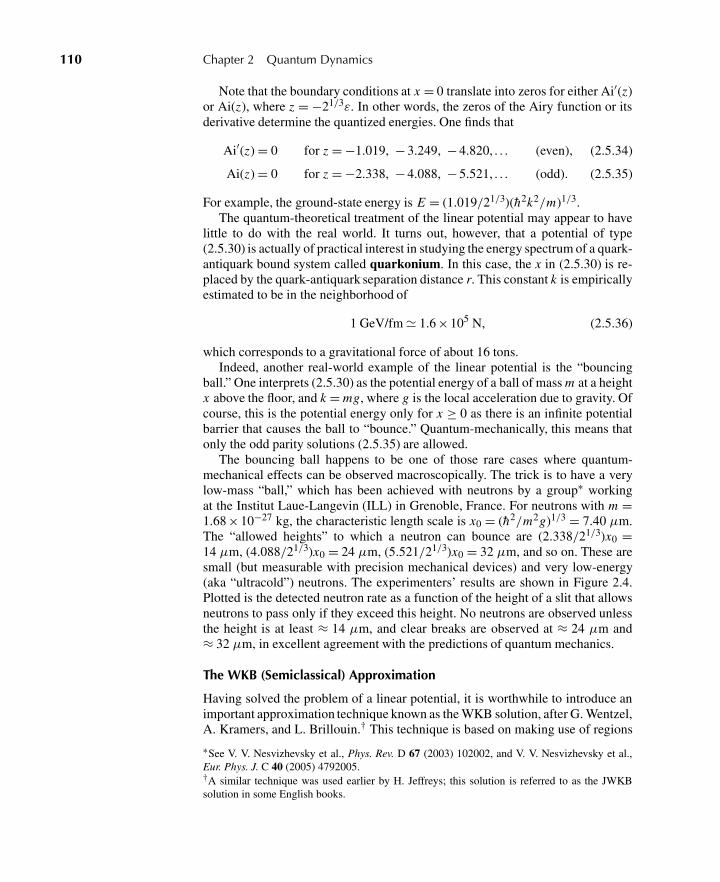
110 Chapter 2 Quantum Dynamics
Note that the boundary conditions at x = 0 translate into zeros for either Ai′(z)or Ai(z), where z = −21/3ε. In other words, the zeros of the Airy function or itsderivative determine the quantized energies. One finds that
Ai′(z) = 0 for z = −1.019, − 3.249, − 4.820, . . . (even), (2.5.34)
Ai(z) = 0 for z = −2.338, − 4.088, − 5.521, . . . (odd). (2.5.35)
For example, the ground-state energy is E = (1.019/21/3)(h2k2/m)1/3.The quantum-theoretical treatment of the linear potential may appear to have
little to do with the real world. It turns out, however, that a potential of type(2.5.30) is actually of practical interest in studying the energy spectrum of a quark-antiquark bound system called quarkonium. In this case, the x in (2.5.30) is re-placed by the quark-antiquark separation distance r. This constant k is empiricallyestimated to be in the neighborhood of
1 GeV/fm � 1.6 ×10⁵ N, (2.5.36)
which corresponds to a gravitational force of about 16 tons.Indeed, another real-world example of the linear potential is the “bouncing
ball.” One interprets (2.5.30) as the potential energy of a ball of mass m at a heightx above the floor, and k = mg, where g is the local acceleration due to gravity. Ofcourse, this is the potential energy only for x ≥ 0 as there is an infinite potentialbarrier that causes the ball to “bounce.” Quantum-mechanically, this means thatonly the odd parity solutions (2.5.35) are allowed.
The bouncing ball happens to be one of those rare cases where quantum-mechanical effects can be observed macroscopically. The trick is to have a verylow-mass “ball,” which has been achieved with neutrons by a group∗ workingat the Institut Laue-Langevin (ILL) in Grenoble, France. For neutrons with m =1.68 ×10⁻²⁷ kg, the characteristic length scale is x0 = (h2/m2g)1/3 = 7.40 μm.The “allowed heights” to which a neutron can bounce are (2.338/21/3)x0 =14 μm, (4.088/21/3)x0 = 24 μm, (5.521/21/3)x0 = 32 μm, and so on. These aresmall (but measurable with precision mechanical devices) and very low-energy(aka “ultracold”) neutrons. The experimenters’ results are shown in Figure 2.4.Plotted is the detected neutron rate as a function of the height of a slit that allowsneutrons to pass only if they exceed this height. No neutrons are observed unlessthe height is at least ≈ 14 μm, and clear breaks are observed at ≈ 24 μm and≈ 32 μm, in excellent agreement with the predictions of quantum mechanics.
The WKB (Semiclassical) Approximation
Having solved the problem of a linear potential, it is worthwhile to introduce animportant approximation technique known as the WKB solution, after G. Wentzel,A. Kramers, and L. Brillouin.† This technique is based on making use of regions
∗See V. V. Nesvizhevsky et al., Phys. Rev. D 67 (2003) 102002, and V. V. Nesvizhevsky et al.,Eur. Phys. J. C 40 (2005) 4792005.†A similar technique was used earlier by H. Jeffreys; this solution is referred to as the JWKBsolution in some English books.
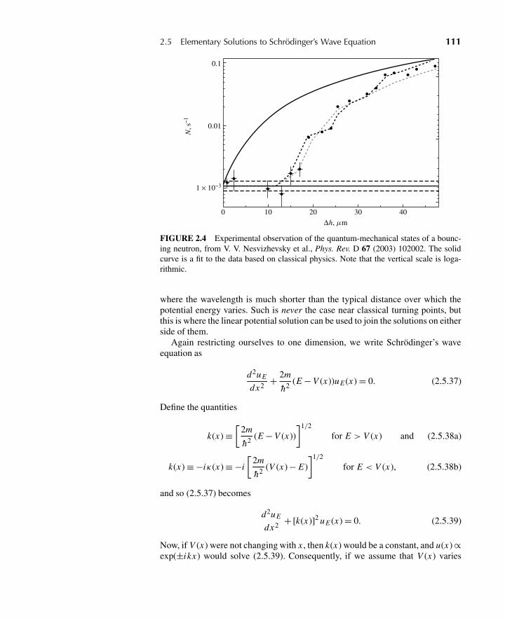
2.5 Elementary Solutions to Schrödinger’s Wave Equation 111
N, s
−1
0.1
0.01
1 × 10⁻³
0 10 20 30 40
Δh, μm
FIGURE 2.4 Experimental observation of the quantum-mechanical states of a bounc-ing neutron, from V. V. Nesvizhevsky et al., Phys. Rev. D 67 (2003) 102002. The solidcurve is a fit to the data based on classical physics. Note that the vertical scale is loga-rithmic.
where the wavelength is much shorter than the typical distance over which thepotential energy varies. Such is never the case near classical turning points, butthis is where the linear potential solution can be used to join the solutions on eitherside of them.
Again restricting ourselves to one dimension, we write Schrödinger’s waveequation as
d2uE
dx2+ 2m
h2(E − V (x))uE (x) = 0. (2.5.37)
Define the quantities
k(x) ≡[
2m
h2 (E − V (x))
]1/2
for E > V (x) and (2.5.38a)
k(x) ≡ −iκ(x) ≡ −i
[2m
h2 (V (x) − E)
]1/2
for E < V (x), (2.5.38b)
and so (2.5.37) becomes
d2uE
dx2 + [k(x)]2 uE (x) = 0. (2.5.39)
Now, if V (x) were not changing with x , then k(x) would be a constant, and u(x) ∝exp(±ikx) would solve (2.5.39). Consequently, if we assume that V (x) varies
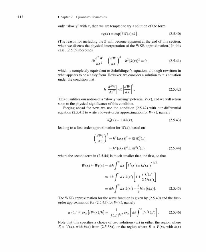
112 Chapter 2 Quantum Dynamics
only “slowly” with x , then we are tempted to try a solution of the form
uE (x) ≡ exp[i W (x)/h
]. (2.5.40)
(The reason for including the h will become apparent at the end of this section,when we discuss the physical interpretation of the WKB approximation.) In thiscase, (2.5.39) becomes
i hd2W
dx2 −(
dW
dx
)2
+ h2 [k(x)]2 = 0, (2.5.41)
which is completely equivalent to Schrödinger’s equation, although rewritten inwhat appears to be a nasty form. However, we consider a solution to this equationunder the condition that
h
∣∣∣∣d2W
dx2
∣∣∣∣� ∣∣∣∣dW
dx
∣∣∣∣2 . (2.5.42)
This quantifies our notion of a “slowly varying” potential V (x), and we will returnsoon to the physical significance of this condition.
Forging ahead for now, we use the condition (2.5.42) with our differentialequation (2.5.41) to write a lowest-order approximation for W (x), namely
W ′0(x) = ±hk(x), (2.5.43)
leading to a first-order approximation for W (x), based on(dW1
dx
)2
= h2 [k(x)]2 + i hW ′′0 (x)
= h2 [k(x)]2 ± i h2k ′(x), (2.5.44)
where the second term in (2.5.44) is much smaller than the first, so that
W (x) ≈ W1(x) = ±h∫ x
dx ′ [k2(x ′) ± ik ′(x ′)]1/2
≈ ±h∫ x
dx ′k(x ′)[
1 ± i
2
k ′(x ′)k2(x ′)
]= ±h
∫ x
dx ′k(x ′) + i
2h ln [k(x)] . (2.5.45)
The WKB approximation for the wave function is given by (2.5.40) and the first-order approximation for (2.5.45) for W (x), namely
uE (x) ≈ exp[i W (x)/h
]= 1
[k(x)]1/2 exp
[±i
∫ x
dx ′k(x ′)]
. (2.5.46)
Note that this specifies a choice of two solutions (±) in either the region whereE > V (x), with k(x) from (2.5.38a), or the region where E < V (x), with k(x)
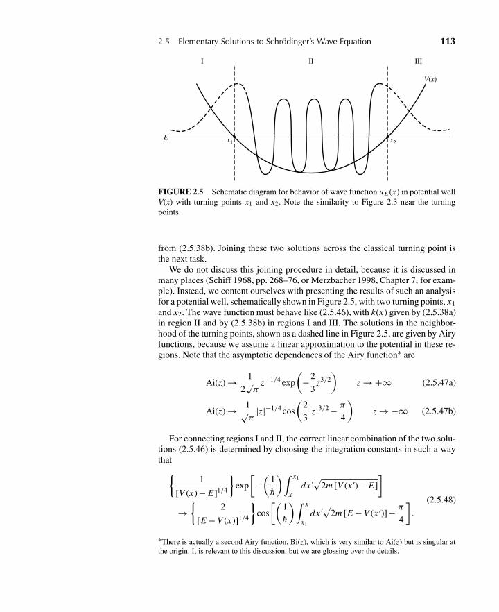
2.5 Elementary Solutions to Schrödinger’s Wave Equation 113
I II III
V(x)
x1 x2E
FIGURE 2.5 Schematic diagram for behavior of wave function uE (x) in potential wellV(x) with turning points x1 and x2. Note the similarity to Figure 2.3 near the turningpoints.
from (2.5.38b). Joining these two solutions across the classical turning point isthe next task.
We do not discuss this joining procedure in detail, because it is discussed inmany places (Schiff 1968, pp. 268–76, or Merzbacher 1998, Chapter 7, for exam-ple). Instead, we content ourselves with presenting the results of such an analysisfor a potential well, schematically shown in Figure 2.5, with two turning points, x1and x2. The wave function must behave like (2.5.46), with k(x) given by (2.5.38a)in region II and by (2.5.38b) in regions I and III. The solutions in the neighbor-hood of the turning points, shown as a dashed line in Figure 2.5, are given by Airyfunctions, because we assume a linear approximation to the potential in these re-gions. Note that the asymptotic dependences of the Airy function∗ are
Ai(z) → 1
2√π
z−1/4 exp
(−2
3z3/2
)z → +∞ (2.5.47a)
Ai(z) → 1√π
|z|−1/4 cos
(2
3|z|3/2 − π
4
)z → −∞ (2.5.47b)
For connecting regions I and II, the correct linear combination of the two solu-tions (2.5.46) is determined by choosing the integration constants in such a waythat{
1
[V (x) − E]1/4
}exp
[−(
1
h
)∫ x1
xdx ′√2m [V (x ′) − E]
]→
{2
[E − V (x)]1/4
}cos
[(1
h
)∫ x
x1
dx ′√2m [E − V (x ′)]− π4
].
(2.5.48)
∗There is actually a second Airy function, Bi(z), which is very similar to Ai(z) but is singular atthe origin. It is relevant to this discussion, but we are glossing over the details.
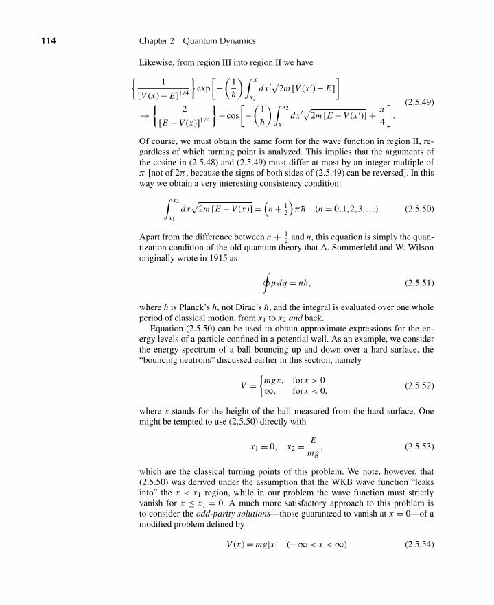
114 Chapter 2 Quantum Dynamics
Likewise, from region III into region II we have{1
[V (x) − E]1/4
}exp
[−(
1
h
)∫ x
x2
dx ′√2m [V (x ′) − E]
]→
{2
[E − V (x)]1/4
}− cos
[−(
1
h
)∫ x2
xdx ′√2m [E − V (x ′)] + π
4
].
(2.5.49)
Of course, we must obtain the same form for the wave function in region II, re-gardless of which turning point is analyzed. This implies that the arguments ofthe cosine in (2.5.48) and (2.5.49) must differ at most by an integer multiple ofπ [not of 2π , because the signs of both sides of (2.5.49) can be reversed]. In thisway we obtain a very interesting consistency condition:∫ x2
x1
dx√
2m [E − V (x)] =(
n + 12
)π h (n = 0,1,2,3, . . .). (2.5.50)
Apart from the difference between n + 12 and n, this equation is simply the quan-
tization condition of the old quantum theory that A. Sommerfeld and W. Wilsonoriginally wrote in 1915 as ∮
p dq = nh, (2.5.51)
where h is Planck’s h, not Dirac’s h, and the integral is evaluated over one wholeperiod of classical motion, from x1 to x2 and back.
Equation (2.5.50) can be used to obtain approximate expressions for the en-ergy levels of a particle confined in a potential well. As an example, we considerthe energy spectrum of a ball bouncing up and down over a hard surface, the“bouncing neutrons” discussed earlier in this section, namely
V ={
mgx , for x > 0∞, for x < 0,
(2.5.52)
where x stands for the height of the ball measured from the hard surface. Onemight be tempted to use (2.5.50) directly with
x1 = 0, x2 = E
mg, (2.5.53)
which are the classical turning points of this problem. We note, however, that(2.5.50) was derived under the assumption that the WKB wave function “leaksinto” the x < x1 region, while in our problem the wave function must strictlyvanish for x ≤ x1 = 0. A much more satisfactory approach to this problem isto consider the odd-parity solutions—those guaranteed to vanish at x = 0—of amodified problem defined by
V (x) = mg|x | (−∞< x <∞) (2.5.54)
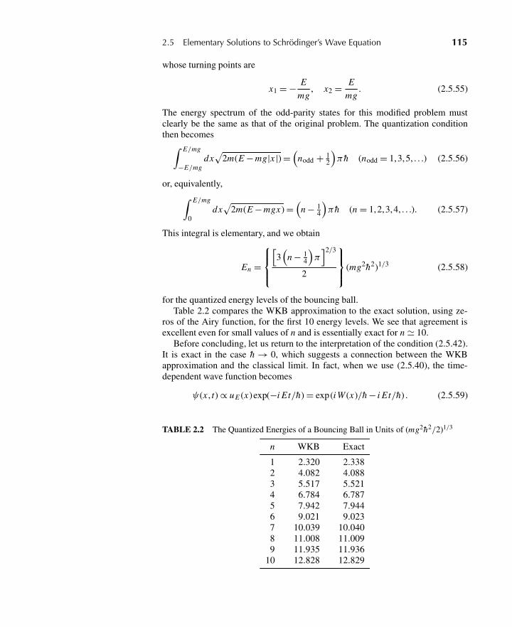
2.5 Elementary Solutions to Schrödinger’s Wave Equation 115
whose turning points are
x1 = − E
mg, x2 = E
mg. (2.5.55)
The energy spectrum of the odd-parity states for this modified problem mustclearly be the same as that of the original problem. The quantization conditionthen becomes∫ E/mg
−E/mgdx√
2m(E − mg|x |) =(
nodd + 12
)π h (nodd = 1,3,5, . . .) (2.5.56)
or, equivalently,∫ E/mg
0dx√
2m(E − mgx) =(
n − 14
)π h (n = 1,2,3,4, . . .). (2.5.57)
This integral is elementary, and we obtain
En =
⎧⎪⎨⎪⎩[3(
n − 14
)π]2/3
2
⎫⎪⎬⎪⎭ (mg2h2)1/3 (2.5.58)
for the quantized energy levels of the bouncing ball.Table 2.2 compares the WKB approximation to the exact solution, using ze-
ros of the Airy function, for the first 10 energy levels. We see that agreement isexcellent even for small values of n and is essentially exact for n � 10.
Before concluding, let us return to the interpretation of the condition (2.5.42).It is exact in the case h → 0, which suggests a connection between the WKBapproximation and the classical limit. In fact, when we use (2.5.40), the time-dependent wave function becomes
ψ(x , t) ∝ uE (x)exp(−i E t/h) = exp(i W (x)/h − i E t/h) . (2.5.59)
TABLE 2.2 The Quantized Energies of a Bouncing Ball in Units of (mg2h2/2)1/3
n WKB Exact
1 2.320 2.3382 4.082 4.0883 5.517 5.5214 6.784 6.7875 7.942 7.9446 9.021 9.0237 10.039 10.0408 11.008 11.0099 11.935 11.936
10 12.828 12.829
116 Chapter 2 Quantum Dynamics
Comparing this to (2.4.18) and (2.4.28), we see that W (x) corresponds directlyto Hamilton’s characteristic function. Indeed, condition (2.5.42) is the same as(2.4.26), the condition for reaching the classical limit. For these reasons, the WKBapproximation is frequently referred to as a “semiclassical” approximation.
We also note that condition (2.5.42) is equivalent to |k′(x)| � |k2(x)|. In termsof the de Broglie wavelength divided by 2π , this condition amounts to
λ= h√2m [E − V (x)]
� 2[E − V (x)]
|dV/dx | . (2.5.60)
In other words, λ must be small compared with the characteristic distance overwhich the potential varies appreciably. Roughly speaking, the potential must beessentially constant over many wavelengths. Thus we see that the semiclassicalpicture is reliable in the short-wavelength limit.
2.6 PROPAGATORS AND FEYNMAN PATH INTEGRALS
Propagators in Wave Mechanics
In Section 2.1 we showed how the most general time-evolution problem with atime-independent Hamiltonian can be solved once we expand the initial ket interms of the eigenkets of an observable that commutes with H. Let us translatethis statement into the language of wave mechanics. We start with
|α, t0; t〉 = exp
[−i H (t − t0)
h
]|α, t0〉
=∑
a′|a′〉〈a′|α, t0〉exp
[−i Ea′(t − t0)
h
].
(2.6.1)
Multiplying both sides by 〈x′| on the left, we have
〈x′|α, t0; t〉 =∑
a′〈x′|a′〉〈a′|α, t0〉exp
[−i Ea′(t − t0)
h
], (2.6.2)
which is of the form
ψ(x′, t) =∑
a′ca′(t0)ua′(x′)exp
[−i Ea′(t − t0)
h
], (2.6.3)
with
ua′(x′) = 〈x′|a′〉 (2.6.4)
standing for the eigenfunction of operator A with eigenvalue a′. Note also that
〈a′|α, t0〉 =∫
d3x ′〈a′|x′〉〈x′|α, t0〉, (2.6.5)
2.6 Propagators and Feynman Path Integrals 117
which we recognize as the usual rule in wave mechanics for getting the expansioncoefficients of the initial state:
ca′(t0) =∫
d3x ′u∗a′ (x′)ψ(x′, t0). (2.6.6)
All this should be straightforward and familiar. Now (2.6.2) together with(2.6.5) can also be visualized as some kind of integral operator acting on theinitial wave function to yield the final wave function:
ψ(x′′, t) =∫
d3x ′K (x′′, t ;x′, t0)ψ(x′, t0). (2.6.7)
Here the kernel of the integral operator, known as the propagator in wave me-chanics, is given by
K (x′′, t ;x′, t0) =∑
a′〈x′′|a′〉〈a′|x′〉exp
[−i Ea′(t − t0)
h
]. (2.6.8)
In any given problem the propagator depends only on the potential and is inde-pendent of the initial wave function. It can be constructed once the energy eigen-functions and their eigenvalues are given.
Clearly, the time evolution of the wave function is completely predicted ifK (x′′, t ;x′, t0) is known and ψ(x′, t0) is given initially. In this sense Schrödinger’swave mechanics is a perfectly causal theory. The time development of a wavefunction subjected to some potential is as “deterministic” as anything else in clas-sical mechanics provided that the system is left undisturbed. The only peculiarfeature, if any, is that when a measurement intervenes, the wave function changesabruptly, in an uncontrollable way, into one of the eigenfunctions of the observ-able being measured.
There are two properties of the propagator worth recording here. First, fort > t0, K (x′′, t ;x′, t0) satisfies Schrödinger’s time-dependent wave equation inthe variables x′′ and t, with x′ and t0 fixed. This is evident from (2.6.8) be-cause 〈x′′|a′〉exp[−i Ea′(t − t0)/h], being the wave function corresponding toU(t , t0)|a′〉, satisfies the wave equation. Second,
limt→t0
K (x′′, t ;x′, t0) = δ3(x′′ − x′), (2.6.9)
which is also obvious; as t → t0, because of the completeness of {|a′〉}, sum(2.6.8) just reduces to 〈x′′|x′〉.
Because of these two properties, the propagator (2.6.8), regarded as a functionof x′′, is simply the wave function at t of a particle that was localized preciselyat x′ at some earlier time t0. Indeed, this interpretation follows, perhaps moreelegantly, from noting that (2.6.8) can also be written as
K (x′′, t ;x′, t0) = 〈x′′|exp
[−i H (t − t0)
h
]|x′〉, (2.6.10)
118 Chapter 2 Quantum Dynamics
where the time-evolution operator acting on |x′〉 is just the state ket at t of a systemthat was localized precisely at x′ at time t0 (< t). If we wish to solve a moregeneral problem where the initial wave function extends over a finite region ofspace, all we have to do is multiply ψ(x′, t0) by the propagator K (x′′, t ;x′, t0) andintegrate over all space (that is, over x′). In this manner we can add the variouscontributions from different positions (x′). This situation is analogous to one inelectrostatics; if we wish to find the electrostatic potential due to a general chargedistribution ρ(x′), we first solve the point-charge problem, multiply the point-charge solution by the charge distribution, and integrate:
φ(x) =∫
d3x ′ ρ(x′)|x − x′| . (2.6.11)
The reader familiar with the theory of the Green’s functions must have recog-nized by this time that the propagator is simply the Green’s function for the time-dependent wave equation satisfying[
−(
h2
2m
)∇′′2 + V (x′′) − i h
∂
∂ t
]K (x′′, t ;x′, t0) = −i hδ3(x′′ − x′)δ(t − t0)
(2.6.12)with the boundary condition
K (x′′, t ;x′, t0) = 0, for t < t0. (2.6.13)
The delta function δ(t − t0) is needed on the right-hand side of (2.6.12) because Kvaries discontinuously at t = t0.
The particular form of the propagator is, of course, dependent on the particularpotential to which the particle is subjected. Consider, as an example, a free particlein one dimension. The obvious observable that commutes with H is momentum;|p′〉 is a simultaneous eigenket of the operators p and H:
p|p′〉 = p′|p′〉 H |p′〉 =(
p′2
2m
)|p′〉. (2.6.14)
The momentum eigenfunction is just the transformation function of Section 1.7[see (1.7.32)] which is of the plane-wave form. Combining everything, we have
K (x ′′, t ; x ′, t0) =(
1
2π h
)∫ ∞
−∞dp′ exp
[i p(x ′′ − x ′)
h− i p′2(t − t0)
2mh
]. (2.6.15)
The integral can be evaluated by completing the square in the exponent. Here wesimply record the result:
K (x ′′, t ; x ′, t0) =√
m
2π i h(t − t0)exp
[im(x ′′ − x ′)2
2h(t − t0)
]. (2.6.16)
This expression may be used, for example, to study how a Gaussian wave packetspreads out as a function of time.
2.6 Propagators and Feynman Path Integrals 119
For the simple harmonic oscillator, where the wave function of an energyeigenstate is given by
un(x)exp
(−i Ent
h
)=(
1
2n/2√
n!
)(mω
π h
)1/4
exp
(−mωx2
2h
)×Hn
(√mω
hx
)exp
[−iω
(n + 1
2
)t
], (2.6.17)
the propagator is given by
K (x ′′, t ; x ′, t0) =√
mω
2π i h sin[ω(t − t0)]exp
[{imω
2h sin[ω(t − t0)]
}×{x ′′2 + x ′2)cos[ω(t − t0)] − 2x ′′x ′}
]. (2.6.18)
One way to prove this is to use(1√
1 − ζ 2
)exp
[−(ξ2 + η2 − 2ξηζ )
(1 − ζ 2)
]= exp
[−(ξ2 +η2)]∑
n=0
(ζ n
2nn!
)Hn(ξ )Hn(η),
(2.6.19)
which is found in books on special functions (Morse and Feshbach 1953, p. 786).It can also be obtained using the a, a† operator method (Saxon 1968, pp. 144–45) or, alternatively, the path-integral method to be described later. Notice that(2.6.18) is a periodic function of t with angular frequency ω, the classical oscil-lator frequency. This means, among other things, that a particle initially localizedprecisely at x ′ will return to its original position with certainty at 2π/ω (4π/ω,and so forth) later.
Certain space and time integrals derivable from K (x′′, t ;x′, t0) are of consider-able interest. Without loss of generality, we set t0 = 0 in the following. The firstintegral we consider is obtained by setting x′′ = x′ and integrating over all space.We have
G(t) ≡∫
d3x ′K (x′, t;x′,0)
=∫
d3x ′∑a′
|〈x′|a′〉|2 exp
(−i Ea′t
h
)
=∑
a′exp
(−i Ea′t
h
).
(2.6.20)
This result is anticipated; recalling (2.6.10), we observe that setting x′ = x′′ andintegrating are equivalent to taking the trace of the time-evolution operator inthe x-representation. But the trace is independent of representations; it can be
120 Chapter 2 Quantum Dynamics
evaluated more readily using the {|a′〉} basis where the time-evolution operatoris diagonal, which immediately leads to the last line of (2.6.20). Now we seethat (2.6.20) is just the “sum over states,” reminiscent of the partition functionin statistical mechanics. In fact, if we analytically continue in the t-variable andmake t purely imaginary, with β defined by
β = i t
h(2.6.21)
real and positive, we can identify (2.6.20) with the partition function itself:
Z =∑
a′exp(−βEa′). (2.6.22)
For this reason some of the techniques encountered in studying propagators inquantum mechanics are also useful in statistical mechanics.
Next, let us consider the Laplace-Fourier transform of G(t):
G(E) ≡ −i∫ ∞
0dtG(t)exp(i E t/h)/h
= −i∫ ∞
0dt∑
a′exp(−i Ea′t/h)exp(i E t/h)/h.
(2.6.23)
The integrand here oscillates indefinitely. But we can make the integral meaning-ful by letting E acquire a small positive imaginary part:
E → E + iε. (2.6.24)
We then obtain, in the limit ε→ 0,
G(E) =∑
a′
1
E − Ea′. (2.6.25)
Observe now that the complete energy spectrum is exhibited as simple poles ofG(E) in the complex E-plane. If we wish to know the energy spectrum of a phys-ical system, it is sufficient to study the analytic properties of G(E).
Propagator as a Transition Amplitude
To gain further insight into the physical meaning of the propagator, we wish torelate it to the concept of transition amplitudes introduced in Section 2.2. But first,recall that the wave function, which is the inner product of the fixed position bra〈x′| with the moving state ket |α, t0; t〉, can also be regarded as the inner product ofthe Heisenberg-picture position bra 〈x′, t|, which moves “oppositely” with time,with the Heisenberg-picture state ket |α, t0〉, which is fixed in time. Likewise, the
2.6 Propagators and Feynman Path Integrals 121
propagator can also be written as
K (x′′, t ;x′, t0) =∑
a′〈x′′|a′〉〈a′|x′〉exp
[−i Ea′(t − t0)
h
]=∑
a′〈x′′|exp
(−i H t
h
)|a′〉〈a′|exp
(i H t0
h
)|x′〉
= 〈x′′, t|x′, t0〉,
(2.6.26)
where |x′, t0〉 and 〈x′′, t| are to be understood as an eigenket and an eigenbra ofthe position operator in the Heisenberg picture. In Section 2.1 we showed that〈b′, t|a′〉, in the Heisenberg-picture notation, is the probability amplitude for asystem originally prepared to be an eigenstate of A with eigenvalue a′ at someinitial time t0 = 0 to be found at a later time t in an eigenstate of B with eigenvalueb′, and we called it the transition amplitude for going from state |a′〉 to state |b′〉.Because there is nothing special about the choice of t0—only the time differencet − t0 is relevant—we can identify 〈x′′, t|x′, t0〉 as the probability amplitude for theparticle prepared at t0 with position eigenvalue x′ to be found at a later time t atx′′. Roughly speaking, 〈x′′, t|x′, t0〉 is the amplitude for the particle to go from aspace-time point (x′, t0) to another space-time point (x′′, t), so the term transitionamplitude for this expression is quite appropriate. This interpretation is, of course,in complete accord with the interpretation we gave earlier for K (x′′, t ;x′, t0).
Yet another way to interpret 〈x′′, t|x′, t0〉 is as follows. As we emphasizedearlier, |x′, t0〉 is the position eigenket at t0 with the eigenvalue x′ in the Heisen-berg picture. Because at any given time the Heisenberg-picture eigenkets of anobservable can be chosen as base kets, we can regard 〈x′′, t|x′, t0〉 as the transfor-mation function that connects the two sets of base kets at different times. So in theHeisenberg picture, time evolution can be viewed as a unitary transformation, inthe sense of changing bases, that connects one set of base kets formed by {|x′, t0〉}to another formed by {|x′′, t〉}. This is reminiscent of classical physics, in whichthe time development of a classical dynamic variable such as x(t) is viewed asa canonical (or contact) transformation generated by the classical Hamiltonian(Goldstein 2002, pp. 401–2).
It turns out to be convenient to use a notation that treats the space and timecoordinates more symmetrically. To this end we write 〈x′′, t ′′|x′, t ′〉 in place of〈x′′, t|x′, t0〉. Because at any given time the position kets in the Heisenberg pictureform a complete set, it is legitimate to insert the identity operator written as∫
d3x ′′|x′′, t ′′〉〈x′′, t ′′| = 1 (2.6.27)
at any place we desire. For example, consider the time evolution from t ′ to t ′′′; bydividing the time interval (t ′, t ′′′) into two parts, (t ′, t ′′) and (t ′′, t ′′′), we have
〈x′′′, t ′′′|x′, t ′〉 =∫
d3x ′′〈x′′′, t ′′′|x′′, t ′′〉〈x′′, t ′′|x′, t ′〉,(t ′′′ > t ′′ > t ′). (2.6.28)
122 Chapter 2 Quantum Dynamics
We call this the composition property of the transition amplitude.∗ Clearly, wecan divide the time interval into as many smaller subintervals as we wish. Wehave
〈x′′′′, t ′′′′|x′, t ′〉 =∫
d3x ′′′∫
d3x ′′〈x′′′′, t ′′′′|x′′′, t ′′′〉〈x′′′, t ′′′|x′′, t ′′〉
×〈x′′, t ′′|x′, t ′〉, (t ′′′′ > t ′′′ > t ′′ > t ′), (2.6.29)
and so on. If we somehow guess the form of 〈x′′, t ′′|x′, t ′〉 for an infinitesimal timeinterval (between t ′ and t ′′ = t ′ + dt), we should be able to obtain the amplitude〈x′′, t ′′|x′, t ′〉 for a finite time interval by compounding the appropriate transitionamplitudes for infinitesimal time intervals in a manner analogous to (2.6.29). Thiskind of reasoning leads to an independent formulation of quantum mechanics thatR. P. Feynman published in 1948, to which we now turn our attention.
Path Integrals as the Sum Over Paths
Without loss of generality we restrict ourselves to one-dimensional problems.Also, we avoid awkward expressions like
x ′′′′ · · ·N times
x ′′′
by using notation such as xN . With this notation we consider the transition am-plitude for a particle going from the initial space-time point (x1, t1) to the finalspace-time point (xN , tN ). The entire time interval between t1 and tN is dividedinto N − 1 equal parts:
t j − t j−1 =�t = (tN − t1)
(N − 1). (2.6.30)
Exploiting the composition property, we obtain
〈xN , tN |x1, t1〉 =∫
dxN−1
∫dxN−2 · · ·
∫dx2〈xN , tN |xN−1, tN−1〉
×〈xN−1, tN−1|xN−2, tN−2〉 · · · 〈x2, t2|x1, t1〉. (2.6.31)
To visualize this pictorially, we consider a space-time plane, as shown in Fig-ure 2.6. The initial and final space-time points are fixed to be (x1, t1) and (xN , tN ),respectively. For each time segment, say between tn−1 and tn , we are instructed toconsider the transition amplitude to go from (xn−1, tn−1) to (xn, tn); we then inte-grate over x2, x3, . . . , xN−1. This means that we must sum over all possible pathsin the space-time plane with the end points fixed.
Before proceeding further, it is profitable to review here how paths appear inclassical mechanics. Suppose we have a particle subjected to a force field deriv-
∗The analogue of (2.6.28) in probability theory is known as the Chapman-Kolmogoroff equation,and in diffusion theory as the Smoluchowsky equation.
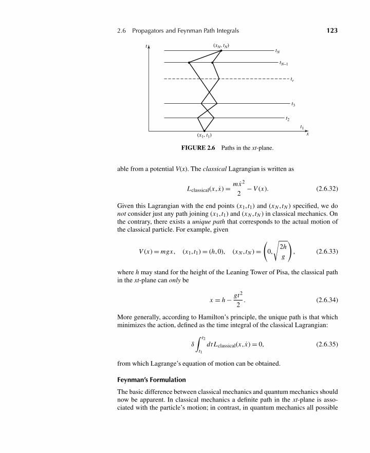
2.6 Propagators and Feynman Path Integrals 123
(xN, tN)
(x1, t1)
tN
tN−1
t3
t2t1
x
tr
t
FIGURE 2.6 Paths in the xt-plane.
able from a potential V(x). The classical Lagrangian is written as
Lclassical(x , x) = mx2
2− V (x). (2.6.32)
Given this Lagrangian with the end points (x1, t1) and (xN , tN ) specified, we donot consider just any path joining (x1, t1) and (xN , tN ) in classical mechanics. Onthe contrary, there exists a unique path that corresponds to the actual motion ofthe classical particle. For example, given
V (x) = mgx , (x1, t1) = (h,0), (xN , tN ) =(
0,
√2h
g
), (2.6.33)
where h may stand for the height of the Leaning Tower of Pisa, the classical pathin the xt-plane can only be
x = h − gt2
2. (2.6.34)
More generally, according to Hamilton’s principle, the unique path is that whichminimizes the action, defined as the time integral of the classical Lagrangian:
δ
∫ t2
t1dt Lclassical(x , x) = 0, (2.6.35)
from which Lagrange’s equation of motion can be obtained.
Feynman’s Formulation
The basic difference between classical mechanics and quantum mechanics shouldnow be apparent. In classical mechanics a definite path in the xt-plane is asso-ciated with the particle’s motion; in contrast, in quantum mechanics all possible
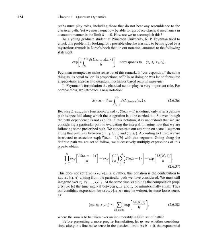
124 Chapter 2 Quantum Dynamics
paths must play roles, including those that do not bear any resemblance to theclassical path. Yet we must somehow be able to reproduce classical mechanics ina smooth manner in the limit h → 0. How are we to accomplish this?
As a young graduate student at Princeton University, R. P. Feynman tried toattack this problem. In looking for a possible clue, he was said to be intrigued by amysterious remark in Dirac’s book that, in our notation, amounts to the followingstatement:
exp
[i∫ t2
t1
dt Lclassical(x , x)
h
]corresponds to 〈x2, t2|x1, t1〉.
Feynman attempted to make sense out of this remark. Is “corresponds to” the samething as “is equal to” or “is proportional to”? In so doing he was led to formulatea space-time approach to quantum mechanics based on path integrals.
In Feynman’s formulation the classical action plays a very important role. Forcompactness, we introduce a new notation:
S(n,n − 1) ≡∫ tn
tn−1
dt Lclassical(x , x). (2.6.36)
Because Lclassical is a function of x and x , S(n,n−1) is defined only after a definitepath is specified along which the integration is to be carried out. So even thoughthe path dependence is not explicit in this notation, it is understood that we areconsidering a particular path in evaluating the integral. Imagine now that we arefollowing some prescribed path. We concentrate our attention on a small segmentalong that path, say between (xn−1, tn−1) and (xn , tn). According to Dirac, we areinstructed to associate exp[i S(n,n − 1)/h] with that segment. Going along thedefinite path we are set to follow, we successively multiply expressions of thistype to obtain
N∏n=2
exp
[i S(n,n − 1)
h
]= exp
[(i
h
) N∑n=2
S(n,n − 1)
]= exp
[i S(N ,1)
h
].
(2.6.37)
This does not yet give 〈xN , tN |x1, t1〉; rather, this equation is the contribution to〈xN , tN |x1, t1〉 arising from the particular path we have considered. We must stillintegrate over x2, x3, . . . , xN−1. At the same time, exploiting the composition prop-erty, we let the time interval between tn−1 and tn be infinitesimally small. Thusour candidate expression for 〈xN , tN |x1, t1〉 may be written, in some loose sense,as
〈xN , tN |x1, t1〉 ∼∑
all paths
exp
[i S(N ,1)
h
], (2.6.38)
where the sum is to be taken over an innumerably infinite set of paths!Before presenting a more precise formulation, let us see whether considera-
tions along this line make sense in the classical limit. As h → 0, the exponential
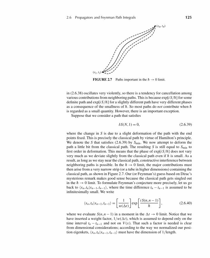
2.6 Propagators and Feynman Path Integrals 125
(xN, tN)
(x1, t1)
FIGURE 2.7 Paths important in the h → 0 limit.
in (2.6.38) oscillates very violently, so there is a tendency for cancellation amongvarious contributions from neighboring paths. This is because exp[i S/h] for somedefinite path and exp[i S/h] for a slightly different path have very different phasesas a consequence of the smallness of h. So most paths do not contribute when his regarded as a small quantity. However, there is an important exception.
Suppose that we consider a path that satisfies
δS(N ,1) = 0, (2.6.39)
where the change in S is due to a slight deformation of the path with the endpoints fixed. This is precisely the classical path by virtue of Hamilton’s principle.We denote the S that satisfies (2.6.39) by Smin. We now attempt to deform thepath a little bit from the classical path. The resulting S is still equal to Smin tofirst order in deformation. This means that the phase of exp[i S/h] does not varyvery much as we deviate slightly from the classical path even if h is small. As aresult, as long as we stay near the classical path, constructive interference betweenneighboring paths is possible. In the h → 0 limit, the major contributions mustthen arise from a very narrow strip (or a tube in higher dimensions) containing theclassical path, as shown in Figure 2.7. Our (or Feynman’s) guess based on Dirac’smysterious remark makes good sense because the classical path gets singled outin the h → 0 limit. To formulate Feynman’s conjecture more precisely, let us goback to 〈xn , tn|xn−1, tn−1〉, where the time difference tn − tn−1 is assumed to beinfinitesimally small. We write
〈xn , tn|xn−1, tn−1〉 =[
1
w(�t)
]exp
[i S(n,n − 1)
h
], (2.6.40)
where we evaluate S(n,n − 1) in a moment in the �t → 0 limit. Notice that wehave inserted a weight factor, 1/w(�t), which is assumed to depend only on thetime interval tn − tn−1 and not on V (x). That such a factor is needed is clearfrom dimensional considerations; according to the way we normalized our posi-tion eigenkets, 〈xn , tn |xn−1, tn−1〉 must have the dimension of 1/length.
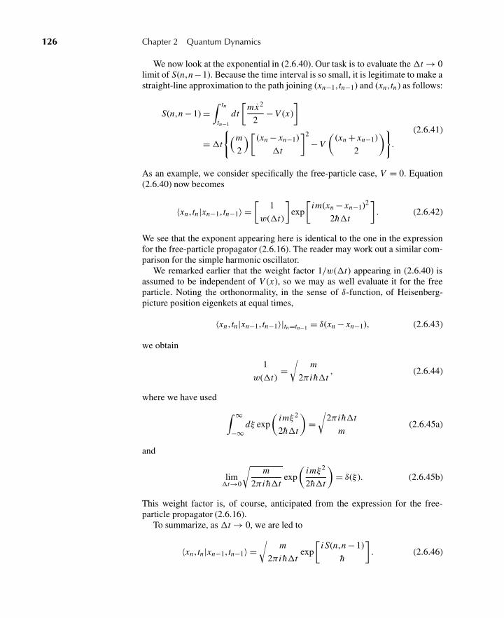
126 Chapter 2 Quantum Dynamics
We now look at the exponential in (2.6.40). Our task is to evaluate the�t → 0limit of S(n,n −1). Because the time interval is so small, it is legitimate to make astraight-line approximation to the path joining (xn−1, tn−1) and (xn, tn) as follows:
S(n,n − 1) =∫ tn
tn−1
dt
[mx2
2− V (x)
]
=�t
{(m
2
)[ (xn − xn−1)
�t
]2
− V
((xn + xn−1)
2
)}.
(2.6.41)
As an example, we consider specifically the free-particle case, V = 0. Equation(2.6.40) now becomes
〈xn , tn|xn−1, tn−1〉 =[
1
w(�t)
]exp
[im(xn − xn−1)2
2h�t
]. (2.6.42)
We see that the exponent appearing here is identical to the one in the expressionfor the free-particle propagator (2.6.16). The reader may work out a similar com-parison for the simple harmonic oscillator.
We remarked earlier that the weight factor 1/w(�t) appearing in (2.6.40) isassumed to be independent of V (x), so we may as well evaluate it for the freeparticle. Noting the orthonormality, in the sense of δ-function, of Heisenberg-picture position eigenkets at equal times,
〈xn , tn|xn−1, tn−1〉|tn=tn−1 = δ(xn − xn−1), (2.6.43)
we obtain
1
w(�t)=√
m
2π i h�t, (2.6.44)
where we have used ∫ ∞
−∞dξ exp
(imξ2
2h�t
)=√
2π i h�t
m(2.6.45a)
and
lim�t→0
√m
2π i h�texp
(imξ2
2h�t
)= δ(ξ ). (2.6.45b)
This weight factor is, of course, anticipated from the expression for the free-particle propagator (2.6.16).
To summarize, as �t → 0, we are led to
〈xn , tn|xn−1, tn−1〉 =√
m
2π i h�texp
[i S(n,n − 1)
h
]. (2.6.46)
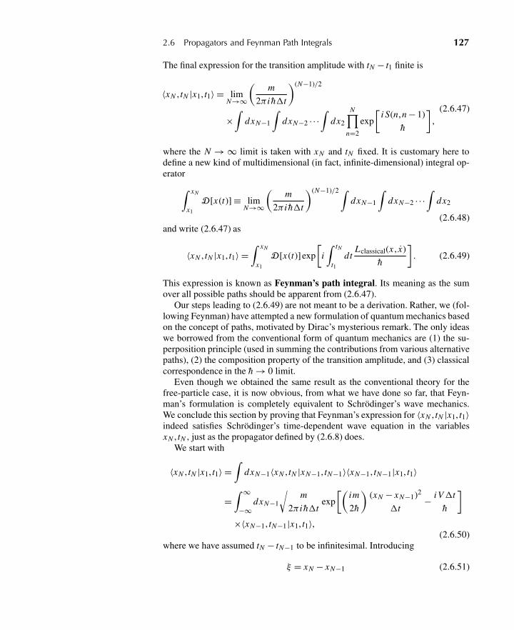
2.6 Propagators and Feynman Path Integrals 127
The final expression for the transition amplitude with tN − t1 finite is
〈xN , tN |x1, t1〉 = limN→∞
(m
2π i h�t
)(N−1)/2
×∫
dxN−1
∫dxN−2 · · ·
∫dx2
N∏n=2
exp
[i S(n,n − 1)
h
],
(2.6.47)
where the N → ∞ limit is taken with xN and tN fixed. It is customary here todefine a new kind of multidimensional (in fact, infinite-dimensional) integral op-erator∫ xN
x1
D[x(t)] ≡ limN→∞
(m
2π i h�t
)(N−1)/2 ∫dxN−1
∫dxN−2 · · ·
∫dx2
(2.6.48)and write (2.6.47) as
〈xN , tN |x1, t1〉 =∫ xN
x1
D[x(t)]exp
[i∫ tN
t1dt
Lclassical(x , x)
h
]. (2.6.49)
This expression is known as Feynman’s path integral. Its meaning as the sumover all possible paths should be apparent from (2.6.47).
Our steps leading to (2.6.49) are not meant to be a derivation. Rather, we (fol-lowing Feynman) have attempted a new formulation of quantum mechanics basedon the concept of paths, motivated by Dirac’s mysterious remark. The only ideaswe borrowed from the conventional form of quantum mechanics are (1) the su-perposition principle (used in summing the contributions from various alternativepaths), (2) the composition property of the transition amplitude, and (3) classicalcorrespondence in the h → 0 limit.
Even though we obtained the same result as the conventional theory for thefree-particle case, it is now obvious, from what we have done so far, that Feyn-man’s formulation is completely equivalent to Schrödinger’s wave mechanics.We conclude this section by proving that Feynman’s expression for 〈xN , tN |x1, t1〉indeed satisfies Schrödinger’s time-dependent wave equation in the variablesxN , tN , just as the propagator defined by (2.6.8) does.
We start with
〈xN , tN |x1, t1〉 =∫
dxN−1〈xN , tN |xN−1, tN−1〉〈xN−1, tN−1|x1, t1〉
=∫ ∞
−∞dxN−1
√m
2π i h�texp
[(im
2h
)(xN − xN−1)2
�t− i V�t
h
]×〈xN−1, tN−1|x1, t1〉,
(2.6.50)where we have assumed tN − tN−1 to be infinitesimal. Introducing
ξ = xN − xN−1 (2.6.51)
128 Chapter 2 Quantum Dynamics
and letting xN → x and tN → t +�t , we obtain
〈x , t +�t|x1, t1〉 =√
m
2π i h�t
∫ (∞)
−∞dξ exp
(imξ2
2h�t− i V�t
h
)〈x − ξ , t|x1, t1〉.
(2.6.52)
As is evident from (2.6.45b), in the limit �t → 0, the major contribution to thisintegral comes from the ξ � 0 region. It is therefore legitimate to expand 〈x −ξ , t|x1, t1〉 in powers of ξ . We also expand 〈x , t +�t|x1, t1〉 and exp(−i V�t/h) inpowers of �t , so
〈x , t|x1, t1〉+�t∂
∂ t〈x , t|x1, t1〉
=√
m
2π i h�t
∫ ∞
−∞dξ exp
(imξ2
2h�t
)(1 − i V�t
h+·· ·
)×[〈x , t|x1, t1〉+
(ξ2
2
)∂2
∂x2〈x , t|x1, t1〉+ · · ·
],
(2.6.53)
where we have dropped a term linear in ξ because it vanishes when integratedwith respect to ξ . The 〈x , t|x1, t1〉 term on the left-hand side just matches theleading term on the right-hand side because of (2.6.45a). Collecting terms that arefirst-order in �t , we obtain
�t∂
∂ t〈x , t|x1, t1〉 =
(√m
2π i h�t
)(√
2π)
(i h�t
m
)3/2 1
2
∂2
∂x2 〈x , t|x1, t1〉
−(
i
h
)�tV 〈x , t|x1, t1〉,
(2.6.54)
where we have used∫ ∞
−∞dξξ2 exp
(imξ2
2h�t
)= √
2π
(i h�t
m
)3/2
, (2.6.55)
obtained by differentiating (2.6.45a) with respect to �t . In this manner we seethat 〈x , t|x1, t1〉 satisfies Schrödinger’s time-dependent wave equation:
i h∂
∂ t〈x , t|x1, t1〉 = −
(h2
2m
)∂2
∂x2 〈x , t|x1, t1〉+ V 〈x , t|x1, t1〉. (2.6.56)
Thus we can conclude that 〈x , t|x1, t1〉 constructed according to Feynman’s pre-scription is the same as the propagator in Schrödinger’s wave mechanics.
Feynman’s space-time approach based on path integrals is not too convenientfor attacking practical problems in nonrelativistic quantum mechanics. Even forthe simple harmonic oscillator, it is rather cumbersome to evaluate explicitly the
2.7 Potentials and Gauge Transformations 129
relevant path integral.∗ However, his approach is extremely gratifying from a con-ceptual point of view. By imposing a certain set of sensible requirements on aphysical theory, we are inevitably led to a formalism equivalent to the usual for-mulation of quantum mechanics. It makes us wonder whether it is at all possibleto construct a sensible alternative theory that is equally successful in accountingfor microscopic phenomena.
Methods based on path integrals have been found to be very powerful in otherbranches of modern physics, such as quantum field theory and statistical mechan-ics. In this book the path-integral method will appear again when we discuss theAharonov-Bohm effect.†
2.7 POTENTIALS AND GAUGE TRANSFORMATIONS
Constant Potentials
In classical mechanics it is well known that the zero point of the potential energyis of no physical significance. The time development of dynamic variables such asx(t) and L(t) is independent of whether we use V (x) or V (x)+V0 with V0 constantboth in space and time. The force that appears in Newton’s second law dependsonly on the gradient of the potential; an additive constant is clearly irrelevant.What is the analogous situation in quantum mechanics?
We look at the time evolution of a Schrödinger-picture state ket subject to somepotential. Let |α, t0; t〉 be a state ket in the presence of V (x), and let ˜|α, t0; t〉 bethe corresponding state ket appropriate for
V (x) = V (x) + V0. (2.7.1)
To be precise, let’s agree that the initial conditions are such that both kets coincidewith |α〉 at t = t0. If they represent the same physical situation, this can alwaysbe done by a suitable choice of the phase. Recalling that the state ket at t can beobtained by applying the time-evolution operator U(t , t0) to the state ket at t0, weobtain
| ˜α, t0; t〉 = exp
[−i
(p2
2m+ V (x) + V0
)(t − t0)
h
]|α〉
(2.7.2)
= exp
[−i V0(t − t0)
h
]|α, t0; t〉.
In other words, the ket computed under the influence of V has a time dependencedifferent only by a phase factor exp[−i V0(t − t0)/h]. For stationary states, thismeans that if the time dependence computed with V (x) is exp[−i E(t − t0)/h],
∗The reader is challenged to solve the simple harmonic oscillator problem using the Feynmanpath-integral method in Problem 2.34 of this chapter.†The reader who is interested in the fundamentals and applications of path integrals may consultFeynman and Hibbs (1965) and also Zee (2010).
130 Chapter 2 Quantum Dynamics
then the corresponding time dependence computed with V (x)+V0 is exp[−i (E +V0)(t − t0)/h]. In other words, the use of V in place of V just amounts to thefollowing change:
E → E + V0, (2.7.3)
which the reader probably guessed immediately. Observable effects such as thetime evolution of expectation values of 〈x〉 and 〈S〉 always depend on energy dif-ferences [see (2.1.47)]; the Bohr frequencies that characterize the sinusoidal timedependence of expectation values are the same whether we use V (x) or V (x)+V0.In general, there can be no difference in the expectation values of observables ifevery state ket in the world is multiplied by a common factor exp[−i V0(t − t0)/h].
Trivial as it may seem, we see here the first example of a class of transfor-mations known as gauge transformations. The change in our convention for thezero-point energy of the potential
V (x) → V (x) + V0 (2.7.4)
must be accompanied by a change in the state ket
|α, t0; t〉 → exp
[−i V0(t − t0)
h
]|α, t0; t〉. (2.7.5)
Of course, this change implies the following change in the wave function:
ψ(x′, t) → exp
[−i V0(t − t0)
h
]ψ(x′, t). (2.7.6)
Next we consider V0 that is spatially uniform but dependent on time. We theneasily see that the analogue of (2.7.5) is
|α, t0; t〉 → exp
[−i
∫ t
t0dt ′ V0(t ′)
h
]|α, t0; t〉. (2.7.7)
Physically, the use of V (x) + V0(t) in place of V (x) simply means that we arechoosing a new zero point of the energy scale at each instant of time.
Even though the choice of the absolute scale of the potential is arbitrary, poten-tial differences are of nontrivial physical significance and, in fact, can be detectedin a very striking way. To illustrate this point, let us consider the arrangementshown in Figure 2.8. A beam of charged particles is split into two parts, each ofwhich enters a metallic cage. If we so desire, we can maintain a finite potential dif-ference between the two cages by turning on a switch, as shown. A particle in thebeam can be visualized as a wave packet whose dimension is much smaller thanthe dimension of the cage. Suppose we switch on the potential difference onlyafter the wave packets enter the cages and switch it off before the wave packetsleave the cages. The particle in the cage experiences no force because inside thecage the potential is spatially uniform; hence no electric field is present. Now letus recombine the two beam components in such a way that they meet in the inter-ference region of Figure 2.8. Because of the existence of the potential, each beam
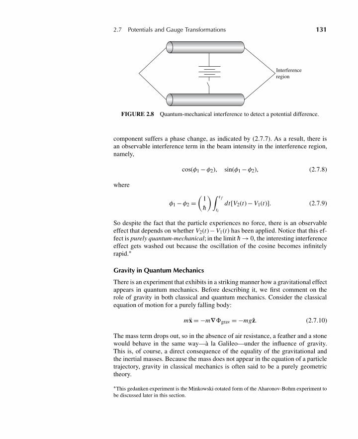
2.7 Potentials and Gauge Transformations 131
Interferenceregion
FIGURE 2.8 Quantum-mechanical interference to detect a potential difference.
component suffers a phase change, as indicated by (2.7.7). As a result, there isan observable interference term in the beam intensity in the interference region,namely,
cos(φ1 −φ2), sin(φ1 −φ2), (2.7.8)
where
φ1 −φ2 =(
1
h
)∫ t f
tidt[V2(t) − V1(t)]. (2.7.9)
So despite the fact that the particle experiences no force, there is an observableeffect that depends on whether V2(t)− V1(t) has been applied. Notice that this ef-fect is purely quantum-mechanical; in the limit h → 0, the interesting interferenceeffect gets washed out because the oscillation of the cosine becomes infinitelyrapid.∗
Gravity in Quantum Mechanics
There is an experiment that exhibits in a striking manner how a gravitational effectappears in quantum mechanics. Before describing it, we first comment on therole of gravity in both classical and quantum mechanics. Consider the classicalequation of motion for a purely falling body:
mx = −m∇�grav = −mgz. (2.7.10)
The mass term drops out, so in the absence of air resistance, a feather and a stonewould behave in the same way—à la Galileo—under the influence of gravity.This is, of course, a direct consequence of the equality of the gravitational andthe inertial masses. Because the mass does not appear in the equation of a particletrajectory, gravity in classical mechanics is often said to be a purely geometrictheory.
∗This gedanken experiment is the Minkowski-rotated form of the Aharonov-Bohm experiment tobe discussed later in this section.
132 Chapter 2 Quantum Dynamics
The situation is rather different in quantum mechanics. In the wave-mechanicalformulation, the analogue of (2.7.10) is[
−(
h2
2m
)∇2 + m�grav
]ψ = i h
∂ψ
∂ t. (2.7.11)
The mass no longer cancels; instead it appears in the combination h/m, so in aproblem where h appears, m is also expected to appear. We can see this point alsousing the Feynman path-integral formulation of a falling body based on
〈xn , tn|xn−1, tn−1〉 =√
m
2π i h�texp
⎡⎣i∫ tn
tn−1
dt
(12 mx2 − mgz
)h
⎤⎦,
(tn − tn−1 =�t → 0).
(2.7.12)
Here again we see that m appears in the combination m/h. This is in sharp contrastwith Hamilton’s classical approach based on
δ
∫ t2
t1dt
(mx2
2− mgz
)= 0, (2.7.13)
where m can be eliminated in the very beginning.Starting with the Schrödinger equation (2.7.11), we may derive the Ehrenfest
theorem
d2
dt2〈x〉 = −gz. (2.7.14)
However, h does not appear here, nor does m. To see a nontrivial quantum-mechanical effect of gravity, we must study effects in which h appears explicitly—and consequently where we expect the mass to appear—in contrast with purelygravitational phenomena in classical mechanics.
Until 1975, there had been no direct experiment that established the presenceof the m�grav term in (2.7.11). To be sure, a free fall of an elementary particlehad been observed, but the classical equation of motion—or the Ehrenfest theo-rem (2.7.14), where h does not appear—sufficed to account for this. The famous“weight of photon” experiment of V. Pound and collaborators did not test gravityin the quantum domain either, because they measured a frequency shift where hdoes not explicitly appear.
On the microscopic scale, gravitational forces are too weak to be readily ob-servable. To appreciate the difficulty involved in seeing gravity in bound-stateproblems, let us consider the ground state of an electron and a neutron boundby gravitational forces. This is the gravitational analogue of the hydrogen atom,where an electron and a proton are bound by Coulomb forces. At the same dis-tance, the gravitational force between the electron and the neutron is weaker thanthe Coulomb force between the electron and the proton by a factor of ∼ 2×1039.
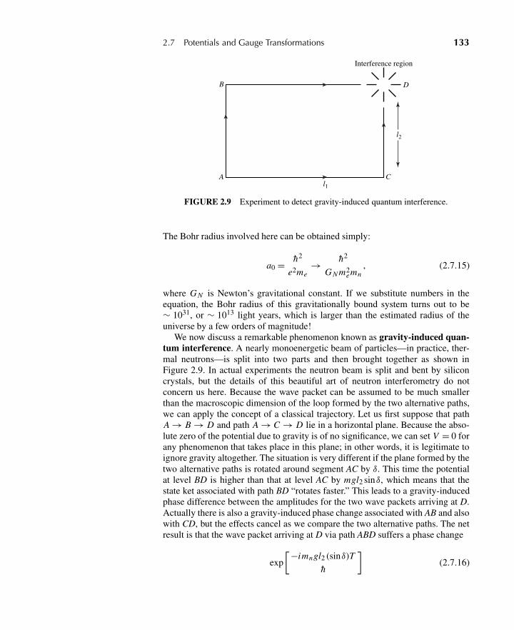
2.7 Potentials and Gauge Transformations 133
l2
l1A
B
C
D
Interference region
FIGURE 2.9 Experiment to detect gravity-induced quantum interference.
The Bohr radius involved here can be obtained simply:
a0 = h2
e2me→ h2
GN m2emn
, (2.7.15)
where GN is Newton’s gravitational constant. If we substitute numbers in theequation, the Bohr radius of this gravitationally bound system turns out to be∼ 1031, or ∼ 1013 light years, which is larger than the estimated radius of theuniverse by a few orders of magnitude!
We now discuss a remarkable phenomenon known as gravity-induced quan-tum interference. A nearly monoenergetic beam of particles—in practice, ther-mal neutrons—is split into two parts and then brought together as shown inFigure 2.9. In actual experiments the neutron beam is split and bent by siliconcrystals, but the details of this beautiful art of neutron interferometry do notconcern us here. Because the wave packet can be assumed to be much smallerthan the macroscopic dimension of the loop formed by the two alternative paths,we can apply the concept of a classical trajectory. Let us first suppose that pathA → B → D and path A → C → D lie in a horizontal plane. Because the abso-lute zero of the potential due to gravity is of no significance, we can set V = 0 forany phenomenon that takes place in this plane; in other words, it is legitimate toignore gravity altogether. The situation is very different if the plane formed by thetwo alternative paths is rotated around segment AC by δ. This time the potentialat level BD is higher than that at level AC by mgl2 sinδ, which means that thestate ket associated with path BD “rotates faster.” This leads to a gravity-inducedphase difference between the amplitudes for the two wave packets arriving at D.Actually there is also a gravity-induced phase change associated with AB and alsowith CD, but the effects cancel as we compare the two alternative paths. The netresult is that the wave packet arriving at D via path ABD suffers a phase change
exp
[−imngl2 (sinδ)T
h
](2.7.16)
134 Chapter 2 Quantum Dynamics
relative to that of the wave packet arriving at D via path ACD, where T is the timespent for the wave packet to go from B to D (or from A to C) and mn , the neutronmass. We can control this phase difference by rotating the plane of Figure 2.9; δcan change from 0 to π/2, or from 0 to −π/2. Expressing the time spent T, orl1/νwavepacket, in terms of λ, the de Broglie wavelength of the neutron, we obtainthe following expression for the phase difference:
φAB D −φAC D = − (m2ngl1l2λsin δ)
h2. (2.7.17)
In this manner we predict an observable interference effect that depends on angleδ, which is reminiscent of fringes in Michelson-type interferometers in optics.
An alternative, more wave-mechanical way to understand (2.7.17) follows. Be-cause we are concerned with a time-independent potential, the sum of the kineticenergy and the potential energy is constant:
p2
2m+ mgz = E . (2.7.18)
The difference in height between level BD and level AC implies a slight differencein p, or λ. As a result, there is an accumulation of phase differences due to theλ difference. It is left as an exercise to show that this wave-mechanical approachalso leads to result (2.7.17).
What is interesting about expression (2.7.17) is that its magnitude is neithertoo small nor too large; it is just right for this interesting effect to be detectedwith thermal neutrons traveling through paths of “table-top” dimensions. Forλ = 1.42 Å (comparable to interatomic spacing in silicon) and l1l2 = 10 cm2, weobtain 55.6 for m2
n gl1l2λ/h2. As we rotate the loop plane gradually by 90◦, wepredict the intensity in the interference region to exhibit a series of maxima andminima; quantitatively we should see 55.6/2π � 9 oscillations. It is extraordi-nary that such an effect has indeed been observed experimentally; see Figure 2.10,which is from a 1975 experiment of R. Colella, A. Overhauser, and S. A. Werner.The phase shift due to gravity is seen to be verified to well within 1%.
We emphasize that this effect is purely quantum-mechanical because as h → 0,the interference pattern gets washed out. The gravitational potential has beenshown to enter into the Schrödinger equation just as expected. This experimentalso shows that gravity is not purely geometric at the quantum level because theeffect depends on (m/h)2.∗
Gauge Transformations in Electromagnetism
Let us now turn to potentials that appear in electromagnetism. We consider anelectric and a magnetic field derivable from the time-independent scalar and vec-
∗However, this does not imply that the equivalence principle is unimportant in understandingan effect of this sort. If the gravitational mass (mgrav) and inertial mass (minert) were unequal,(m/h)2 would have to be replaced by mgravminert/h2. The fact that we could correctly predict theinterference pattern without making a distinction between mgrav and minert shows some supportfor the equivalence principle at the quantum level.
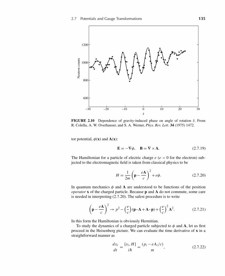
2.7 Potentials and Gauge Transformations 135
1200
1000
800
600
3020100
δ
−10−20−30
Neu
tron
cou
nts
FIGURE 2.10 Dependence of gravity-induced phase on angle of rotation δ. FromR. Colella, A. W. Overhauser, and S. A. Werner, Phys. Rev. Lett. 34 (1975) 1472.
tor potential, φ(x) and A(x):
E = −∇φ, B = ∇ ×A. (2.7.19)
The Hamiltonian for a particle of electric charge e (e < 0 for the electron) sub-jected to the electromagnetic field is taken from classical physics to be
H = 1
2m
(p− eA
c
)2
+ eφ. (2.7.20)
In quantum mechanics φ and A are understood to be functions of the positionoperator x of the charged particle. Because p and A do not commute, some careis needed in interpreting (2.7.20). The safest procedure is to write(
p− eAc
)2
→ p2 −(e
c
)(p · A+ A · p) +
(e
c
)2A2. (2.7.21)
In this form the Hamiltonian is obviously Hermitian.To study the dynamics of a charged particle subjected to φ and A, let us first
proceed in the Heisenberg picture. We can evaluate the time derivative of x in astraightforward manner as
dxi
dt= [xi , H ]
i h= (pi − eAi/c)
m, (2.7.22)
136 Chapter 2 Quantum Dynamics
which shows that the operator p, defined in this book to be the generator of trans-lation, is not the same as m d x/dt . Quite often p is called canonical momentum,as distinguished from kinematical (or mechanical) momentum, denoted by�:
�≡ mdxdt
= p− eAc
. (2.7.23)
Even though we have
[pi , p j ] = 0 (2.7.24)
for canonical momentum, the analogous commutator does not vanish for mechan-ical momentum. Instead we have
[�i ,� j ] =(
i he
c
)εi j k Bk , (2.7.25)
as the reader may easily verify. Rewriting the Hamiltonian as
H = �2
2m+ eφ (2.7.26)
and using the fundamental commutation relation, we can derive the quantum-mechanical version of the Lorentz force, namely,
md2xdt2 = d�
dt= e
[E+ 1
2c
(dxdt
×B− B× dxdt
)]. (2.7.27)
This then is Ehrenfest’s theorem, written in the Heisenberg picture, for thecharged particle in the presence of E and B.
We now study Schrödinger’s wave equation with φ and A. Our first task is tosandwich H between 〈x′| and |α, t0; t〉. The only term with which we have to becareful is
〈x′|[
p− eA(x)
c
]2
|α, t0; t〉
=[−i h∇′ − eA(x′)
c
]〈x′|
[p− eA(x)
c
]|α, t0; t〉
=[−i h∇′ − eA(x′)
c
]·[−i h∇′ − eA(x′)
c
]〈x′|α, t0; t〉.
(2.7.28)
It is important to emphasize that the first ∇′ in the last line can differentiate both〈x′|α, t0; t〉 and A(x′). Combining everything, we have
1
2m
[−i h∇′ − eA(x′)
c
]·[−i h∇′ − eA(x′)
c
]〈x′|α, t0; t〉
+ eφ(x′)〈x′|α, t0; t〉 = i h∂
∂ t〈x′|α, t0; t〉.
(2.7.29)
2.7 Potentials and Gauge Transformations 137
From this expression we readily obtain the continuity equation
∂ρ
∂ t+∇′· j = 0, (2.7.30)
where ρ is |ψ|2 as before, with 〈x′|α, t0; t〉 written as ψ , but for the probabilityflux j we have
j =(
h
m
)Im(ψ∗∇′ψ) −
( e
mc
)A|ψ|2, (2.7.31)
which is just what we expect from the substitution
∇′ → ∇′ −(
ie
hc
)A. (2.7.32)
Writing the wave function of√ρ exp(i S/h) [see (2.4.18)], we obtain an alterna-
tive form for j, namely,
j =( ρ
m
)(∇S − eA
c
), (2.7.33)
which is to be compared with (2.4.20). We will find this form to be convenientin discussing superconductivity, flux quantization, and so on. We also note thatthe space integral of j is the expectation value of kinematical momentum (notcanonical momentum) apart from 1/m:∫
d3x ′j = 〈p− eA/c〉m
= 〈�〉/m. (2.7.34)
We are now in a position to discuss the subject of gauge transformations inelectromagnetism. First, consider
φ→ φ+λ, A → A, (2.7.35)
with λ constant—that is, independent of x and t. Both E and B obviously remainunchanged. This transformation just amounts to a change in the zero point of theenergy scale, a possibility treated in the beginning of this section; we just replaceV by eφ. We have already discussed the accompanying change needed for thestate ket [see (2.7.5)], so we do not dwell on this transformation any further.
Much more interesting is the transformation
φ→ φ, A → A+∇, (2.7.36)
where is a function of x. The static electromagnetic fields E and B are un-changed under (2.7.36). Both (2.7.35) and (2.7.36) are special cases of
φ→ φ− 1
c
∂
∂ t, A → A+∇, (2.7.37)
138 Chapter 2 Quantum Dynamics
which leave E and B, given by
E = −∇φ− 1
c
∂A∂ t
, B = ∇ ×A, (2.7.38)
unchanged, but in the following we do not consider time-dependent fields andpotentials. In the remaining part of this section the term gauge transformationrefers to (2.7.36).
In classical physics, observable effects such as the trajectory of a charged par-ticle are independent of the gauge used—that is, of the particular choice of wehappen to adopt. Consider a charged particle in a uniform magnetic field in thez-direction
B = B z. (2.7.39)
This magnetic field may be derived from
Ax = −By
2, Ay = Bx
2, Az = 0 (2.7.40)
or also from
Ax = −By, Ay = 0, Az = 0. (2.7.41)
The second form is obtained from the first by
A → A−∇(
Bxy
2
), (2.7.42)
which is indeed of the form of (2.7.36). Regardless of which A we may use,the trajectory of the charged particle with a given set of initial conditions is thesame; it is just a helix—a uniform circular motion when projected in the xy-plane,superposed with a uniform rectilinear motion in the z-direction. Yet if we look atpx and py, the results are very different. For one thing, px is a constant of themotion when (2.7.41) is used but not when (2.7.40) is used.
Recall Hamilton’s equations of motion:
dpx
dt= −∂H
∂x,
dpy
dt= −∂H
∂y, . . . . (2.7.43)
In general, the canonical momentum p is not a gauge-invariant quantity; its nu-merical value depends on the particular gauge used, even when we are referring tothe same physical situation. In contrast, the kinematic momentum�, or mdx/dt ,that traces the trajectory of the particle is a gauge-invariant quantity, as one mayexplicitly verify. Because p and mdx/dt are related via (2.7.23), p must changeto compensate for the change in A given by (2.7.42).
We now return to quantum mechanics. We believe that it is reasonable to de-mand that the expectation values in quantum mechanics behave in a manner sim-ilar to the corresponding classical quantities under gauge transformations, so 〈x〉
2.7 Potentials and Gauge Transformations 139
and 〈�〉 are not to change under gauge transformations, whereas 〈p〉 is expectedto change.
Let us denote by |α〉 the state ket in the presence of A; the state ket for thesame physical situation when
A = A+∇ (2.7.44)
is used in place of A is denoted by |α〉. Here , as well as A, is a function of theposition operator x. Our basic requirements are
〈α|x|α〉 = 〈α|x|α〉 (2.7.45a)
and
〈α|(
p− eAc
)|α〉 = 〈α|
(p− eA
c
)|α〉. (2.7.45b)
In addition, we require, as usual, the norm of the state ket to be preserved:
〈α|α〉 = 〈α|α〉. (2.7.46)
We must construct an operator G that relates |α〉 to |α〉:|α〉 = G|α〉. (2.7.47)
Invariance properties (2.7.45a) and (2.7.45b) are guaranteed if
G†xG = x (2.7.48a)
and
G†(
p− eAc
− e∇c
)G = p− eA
c. (2.7.48b)
We assert that
G = exp
[ie(x)
hc
](2.7.49)
will do the job. First, G is unitary, so (2.7.46) is all right. Second, (2.7.48a) isobviously satisfied because x commutes with any function of x. As for (2.7.48b),just note that
exp
(−ie
hc
)pexp
(ie
hc
)= exp
(−ie
hc
)[p, exp
(ie
hc
)]+ p
= −exp
(−ie
hc
)i h∇
[exp
(ie
hc
)]+ p
= p+ e∇c
,
(2.7.50)
where we have used (2.2.23b).
140 Chapter 2 Quantum Dynamics
The invariance of quantum mechanics under gauge transformations can alsobe demonstrated by looking directly at the Schrödinger equation. Let |α, t0; t〉 bea solution to the Schrödinger equation in the presence of A:[
(p− eA/c)2
2m+ eφ
]|α, t0; t〉 = i h
∂
∂ t|α, t0; t〉. (2.7.51)
The corresponding solution in the presence of A must satisfy[(p− eA/c − e∇/c)2
2m+ eφ
]| ˜α, t0; t〉 = i h
∂
∂ t| ˜α, t0; t〉. (2.7.52)
We see that if the new ket is taken to be
| ˜α, t0; t〉 = exp
(ie
hc
)|α, t0; t〉 (2.7.53)
in accordance with (2.7.49), then the new Schrödinger equation (2.7.52) will besatisfied; all we have to note is that
exp
(−ie
hc
)(p− eA
c− e∇
c
)2
exp
(ie
hc
)=(
p− eAc
)2
, (2.7.54)
which follows from applying (2.7.50) twice.Equation (2.7.53) also implies that the corresponding wave equations are re-
lated via
ψ(x′, t) = exp
[ie(x′)
hc
]ψ(x′, t), (2.7.55)
where ∇(x′) is now a real function of the position vector eigenvalue x′. This can,of course, be verified also by directly substituting (2.7.55) into Schrödinger’swave equation with A replaced by A + ∇. In terms of ρ and S, we see thatρ is unchanged but S is modified as follows:
S → S + e
c. (2.7.56)
This is highly satisfactory because we see that the probability flux given by(2.7.33) is then gauge invariant.
To summarize, when vector potentials in different gauges are used for the samephysical situation, the corresponding state kets (or wave functions) must neces-sarily be different. However, only a simple change is needed; we can go from agauge specified by A to another specified by A+∇ by merely multiplying theold ket (the old wave function) by exp[ie(x)/hc] (exp[ie(x′)/hc]). The canon-ical momentum, defined as the generator of translation, is manifestly gauge de-pendent in the sense that its expectation value depends on the particular gaugechosen, whereas the kinematic momentum and the probability flux are gaugeinvariant.
2.7 Potentials and Gauge Transformations 141
The reader may wonder why invariance under (2.7.49) is called gauge invari-ance. This word is the translation of the German Eichinvarianz, where Eich means“gauge.” (There is a historical anecdote that goes with the origin of this term. Readon.)
Consider some function of position at x: F(x). At a neighboring point we ob-viously have
F(x + dx) � F(x) + (∇F) · dx. (2.7.57)
But suppose we apply a scale change as we go from x to x + dx as follows:
1|atx → [1 +�(x) ·dx]|at x+dx. (2.7.58)
We must then rescale F(x) as follows:
F(x + dx)|rescaled � F(x) + [(∇ +�)F] · dx. (2.7.59)
instead of (2.7.57). The combination ∇+� is similar to the gauge-invariant com-bination
∇ −(
ie
hc
)A (2.7.60)
encountered in (2.7.32) except for the absence of i. Historically, H. Weyl unsuc-cessfully attempted to construct a geometric theory of electromagnetism based onEichinvarianz by identifying the scale function �(x) in (2.7.58) and (2.7.59) withthe vector potential A itself. With the birth of quantum mechanics, V. Fock and F.London realized the importance of the gauge-invariant combination (2.7.60), andthey recalled Weyl’s earlier work by comparing � with i times A. We are stuckwith the term gauge invariance even though the quantum-mechanical analogue of(2.7.58),
1
∣∣∣∣at x →[
1 −(
ie
hc
)A ·dx
]∣∣∣∣at x+dx
, (2.7.61)
would actually correspond to “phase change” rather than to “scale change.”
The Aharonov-Bohm Effect
The use of vector potential in quantum mechanics has many far-reaching conse-quences, some of which we are now ready to discuss. We start with a relativelyinnocuous-looking problem.
Consider a hollow cylindrical shell, as shown in Figure 2.11a. We assume thata particle of charge e can be completely confined to the interior of the shell withrigid walls. The wave function is required to vanish on the inner (ρ= ρa) and outer(ρ = ρb) walls, as well as at the top and bottom. It is a straightforward boundary-value problem in mathematical physics to obtain the energy eigenvalues.
Let us now consider a modified arrangement where the cylindrical shell en-closes a uniform magnetic field, as shown in Figure 2.11b. Specifically, you may
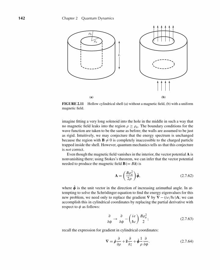
142 Chapter 2 Quantum Dynamics
ρb
ρa
L
(a) (b)
FIGURE 2.11 Hollow cylindrical shell (a) without a magnetic field, (b) with a uniformmagnetic field.
imagine fitting a very long solenoid into the hole in the middle in such a way thatno magnetic field leaks into the region ρ ≥ ρa . The boundary conditions for thewave function are taken to be the same as before; the walls are assumed to be justas rigid. Intuitively, we may conjecture that the energy spectrum is unchangedbecause the region with B �= 0 is completely inaccessible to the charged particletrapped inside the shell. However, quantum mechanics tells us that this conjectureis not correct.
Even though the magnetic field vanishes in the interior, the vector potential A isnonvanishing there; using Stokes’s theorem, we can infer that the vector potentialneeded to produce the magnetic field B (= B z) is
A =(
Bρ2a
2ρ
)φ, (2.7.62)
where φ is the unit vector in the direction of increasing azimuthal angle. In at-tempting to solve the Schrödinger equation to find the energy eigenvalues for thisnew problem, we need only to replace the gradient ∇ by ∇ − (ie/hc)A; we canaccomplish this in cylindrical coordinates by replacing the partial derivative withrespect to φ as follows:
∂
∂φ→ ∂
∂φ−(
ie
hc
)Bρ2
a
2; (2.7.63)
recall the expression for gradient in cylindrical coordinates:
∇ = ρ∂
∂ρ+ z
∂
∂z+ φ
1
ρ
∂
∂φ. (2.7.64)
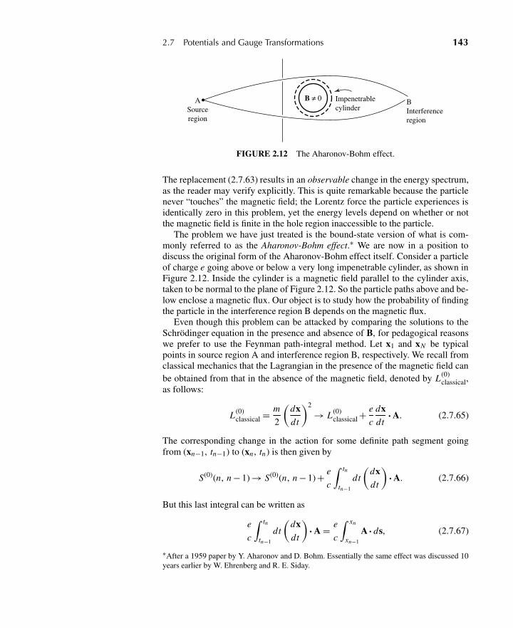
2.7 Potentials and Gauge Transformations 143
Impenetrablecylinder
B ≠ 0ASourceregion
BInterferenceregion
FIGURE 2.12 The Aharonov-Bohm effect.
The replacement (2.7.63) results in an observable change in the energy spectrum,as the reader may verify explicitly. This is quite remarkable because the particlenever “touches” the magnetic field; the Lorentz force the particle experiences isidentically zero in this problem, yet the energy levels depend on whether or notthe magnetic field is finite in the hole region inaccessible to the particle.
The problem we have just treated is the bound-state version of what is com-monly referred to as the Aharonov-Bohm effect.∗ We are now in a position todiscuss the original form of the Aharonov-Bohm effect itself. Consider a particleof charge e going above or below a very long impenetrable cylinder, as shown inFigure 2.12. Inside the cylinder is a magnetic field parallel to the cylinder axis,taken to be normal to the plane of Figure 2.12. So the particle paths above and be-low enclose a magnetic flux. Our object is to study how the probability of findingthe particle in the interference region B depends on the magnetic flux.
Even though this problem can be attacked by comparing the solutions to theSchrödinger equation in the presence and absence of B, for pedagogical reasonswe prefer to use the Feynman path-integral method. Let x1 and xN be typicalpoints in source region A and interference region B, respectively. We recall fromclassical mechanics that the Lagrangian in the presence of the magnetic field canbe obtained from that in the absence of the magnetic field, denoted by L(0)
classical,as follows:
L(0)classical =
m
2
(dxdt
)2
→ L(0)classical +
e
c
dxdt
· A. (2.7.65)
The corresponding change in the action for some definite path segment goingfrom (xn−1, tn−1) to (xn , tn) is then given by
S(0)(n, n − 1) → S(0)(n, n − 1) + e
c
∫ tn
tn−1
dt
(dxdt
)· A. (2.7.66)
But this last integral can be written as
e
c
∫ tn
tn−1
dt
(dxdt
)· A = e
c
∫ xn
xn−1
A · ds, (2.7.67)
∗After a 1959 paper by Y. Aharonov and D. Bohm. Essentially the same effect was discussed 10years earlier by W. Ehrenberg and R. E. Siday.
144 Chapter 2 Quantum Dynamics
where ds is the differential line element along the path segment, so when weconsider the entire contribution from x1 to xN , we have the following change:∏
exp
[i S(0)(n, n − 1)
h
]→
{∏exp
[i S(0)(n, n − 1)
h
]}exp
(ie
hc
∫ xN
x1
A · ds)
.
(2.7.68)
All this is for a particular path, such as going above the cylinder. We must still sumover all possible paths, which may appear to be a formidable task. Fortunately,we know from the theory of electromagnetism that the line integral
∫A · ds is
independent of paths; that is, it is dependent only on the end points, as long asthe loop formed by a pair of different paths does not enclose a magnetic flux.As a result, the contributions due to A �= 0 to all paths going above the cylinderare given by a common phase factor; similarly, the contributions from all pathsgoing below the cylinder are multiplied by another common phase factor. In thepath-integral notation we have, for the entire transition amplitude,∫
aboveD[x(t)]exp
[i S(0)(N ,1)
h
]+∫
belowD[x(t)]exp
[i S(0)(N ,1)
h
]
→∫
aboveD[x(t)]exp
[i S(0)(N ,1)
h
]{exp
[(ie
hc
)∫ xN
x1
A · ds]
above
}
+∫
belowD[x(t)]exp
[i S(0)(N ,1)
h
]{exp
[(ie
hc
)∫ xN
x1
A · ds]
below
}.
(2.7.69)
The probability for finding the particle in the interference region B depends onthe modulus squared of the entire transition amplitude and hence on the phasedifference between the contribution from the paths going above and below. Thephase difference due to the presence of B is just[(
e
hc
)∫ xN
x1
A · ds]
above
−[(
e
hc
)∫ xN
x1
A · ds]
below
=(
e
hc
)∮A · ds
=(
e
hc
)�B ,
(2.7.70)
where �B stands for the magnetic flux inside the impenetrable cylinder. Thismeans that as we change the magnetic field strength, there is a sinusoidal compo-nent in the probability for observing the particle in region B with a period givenby a fundamental unit of magnetic flux, namely,
2π hc
|e| = 4.135 ×10⁻⁷ gauss-cm2. (2.7.71)
We emphasize that the interference effect discussed here is purely quantum-mechanical. Classically, the motion of a charged particle is determined solely by
2.7 Potentials and Gauge Transformations 145
Newton’s second law supplemented by the force law of Lorentz. Here, as in theprevious bound-state problem, the particle can never enter the region in whichB is finite; the Lorentz force is identically zero in all regions where the particlewave function is finite. Yet there is a striking interference pattern that depends onthe presence or absence of a magnetic field inside the impenetrable cylinder. Thispoint has led some people to conclude that in quantum mechanics it is A ratherthan B that is fundamental. It is to be noted, however, that the observable effectsin both examples depend only on �B , which is directly expressible in terms ofB. Experiments to verify the Aharonov-Bohm effect have been performed usinga thin magnetized iron filament called a whisker.∗
Magnetic Monopole
We conclude this section with one of the most remarkable predictions of quantumphysics, which has yet to be verified experimentally. An astute student of clas-sical electrodynamics may be struck by the fact that there is a strong symmetrybetween E and B, yet a magnetic charge—commonly referred to as a magneticmonopole—analogous to electric charge is peculiarly absent in Maxwell’s equa-tions. The source of a magnetic field observed in nature is either a moving electriccharge or a static magnetic dipole, never a static magnetic charge. Instead of
∇· B = 4πρM (2.7.72)
analogous to
∇· E = 4πρ, (2.7.73)
∇· B actually vanishes in the usual way of writing Maxwell’s equations. Quantummechanics does not predict that a magnetic monopole must exist. However, itunambiguously requires that if a magnetic monopole is ever found in nature, themagnitude of magnetic charge must be quantized in terms of e, h, and c, as wenow demonstrate.
Suppose there is a point magnetic monopole, situated at the origin, of strengtheM analogous to a point electric charge. The static magnetic field is then given by
B =(eM
r2
)r. (2.7.74)
At first sight it may appear that the magnetic field (2.7.74) can be derived from
A =[
eM (1 − cosθ )
r sinθ
]φ. (2.7.75)
Recall the expression for curl in spherical coordinates:
∇ ×A = r[
1
r sinθ
∂
∂θ(Aφ sinθ ) − ∂Aθ
∂φ
]+ θ 1
r
[1
sinθ
∂Ar
∂φ− ∂
∂r(r Aφ)
]+ φ
1
r
[∂
∂r(r Aθ ) − ∂Ar
∂θ
].
(2.7.76)
∗One such recent experiment is that of A. Tonomura et al., Phys. Rev. Lett. 48 (1982) 1443.
146 Chapter 2 Quantum Dynamics
But vector potential (2.7.75) has one difficulty—it is singular on the negative z-axis (θ = π). In fact, it turns out to be impossible to construct a singularity-freepotential valid everywhere for this problem. To see this we first note “Gauss’slaw” ∫
closed surfaceB · dσ = 4πeM (2.7.77)
for any surface boundary enclosing the origin at which the magnetic monopole islocated. On the other hand, if A were nonsingular, we would have
∇·(∇ ×A) = 0 (2.7.78)
everywhere; hence,∫closed surface
B · dσ =∫
volume inside∇·(∇ ×A)d3x = 0, (2.7.79)
in contradiction with (2.7.77).However, one might argue that because the vector potential is just a device
for obtaining B, we need not insist on having a single expression for A valideverywhere. Suppose we construct a pair of potentials,
A(I) =[
eM (1 − cos θ )
r sin θ
]φ, (θ < π − ε) (2.7.80a)
A(II) = −[
eM (1 + cos θ )
r sin θ
]φ, (θ > ε), (2.7.80b)
such that the potential A(I) can be used everywhere except inside the cone de-fined by θ = π − ε around the negative z-axis; likewise, the potential A(II) canbe used everywhere except inside the cone θ = ε around the positive z-axis; seeFigure 2.13. Together they lead to the correct expression for B everywhere.∗
Consider now what happens in the overlap region ε < θ < π − ε, where wemay use either A(I) or A(II). Because the two potentials lead to the same magneticfield, they must be related to each other by a gauge transformation. To find appropriate for this problem, we first note that
A(II) − A(I) = −(
2eM
r sin θ
)φ. (2.7.81)
Recalling the expression for gradient in spherical coordinates,
∇= r∂
∂r+ θ
1
r
∂
∂θ+ φ
1
r sin θ
∂
∂φ, (2.7.82)
∗An alternative approach to this problem uses A(I) everywhere, but taking special care of thestring of singularities, known as a Dirac string, along the negative z-axis.
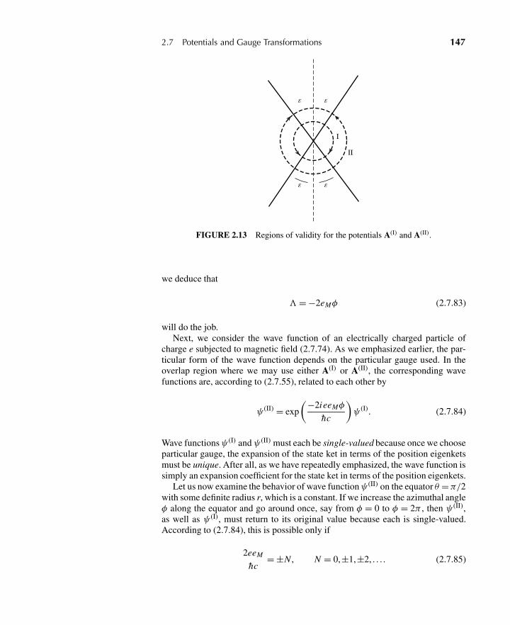
2.7 Potentials and Gauge Transformations 147
ε ε
I
II
ε ε
FIGURE 2.13 Regions of validity for the potentials A(I) and A(II).
we deduce that
= −2eMφ (2.7.83)
will do the job.Next, we consider the wave function of an electrically charged particle of
charge e subjected to magnetic field (2.7.74). As we emphasized earlier, the par-ticular form of the wave function depends on the particular gauge used. In theoverlap region where we may use either A(I) or A(II), the corresponding wavefunctions are, according to (2.7.55), related to each other by
ψ (II) = exp
(−2ieeMφ
hc
)ψ (I). (2.7.84)
Wave functionsψ (I) andψ (II) must each be single-valued because once we chooseparticular gauge, the expansion of the state ket in terms of the position eigenketsmust be unique. After all, as we have repeatedly emphasized, the wave function issimply an expansion coefficient for the state ket in terms of the position eigenkets.
Let us now examine the behavior of wave functionψ(II) on the equator θ =π/2with some definite radius r, which is a constant. If we increase the azimuthal angleφ along the equator and go around once, say from φ = 0 to φ = 2π , then ψ (II),as well as ψ (I), must return to its original value because each is single-valued.According to (2.7.84), this is possible only if
2eeM
hc= ±N , N = 0,±1,±2, . . . . (2.7.85)
148 Chapter 2 Quantum Dynamics
So we arrive at a very far-reaching conclusion: The magnetic charges must bequantized in units of
hc
2|e| �(
137
2
)|e|. (2.7.86)
The smallest magnetic charge possible is hc/2|e|, where e is the electroniccharge. It is amusing that once a magnetic monopole is assumed to exist, wecan use (2.7.85) backward, so to speak, to explain why the electric charges arequantized—for example, why the proton charge cannot be 0.999972 times |e|.∗
We repeat once again that quantum mechanics does not require magneticmonopoles to exist. However, it unambiguously predicts that a magnetic charge,if it is ever found in nature, must be quantized in units of hc/2|e|. The quanti-zation of magnetic charges in quantum mechanics was first shown in 1931 byP. A. M. Dirac. The derivation given here is due to T. T. Wu and C. N. Yang. Adifferent solution, which connects the Dirac quantization condition to the quan-tization of angular momentum, is discussed by H. J. Lipkin, W. I. Weisberger,and M. Peshkin in Annals of Physics 53 (1969) 203. Finally, we will revisit thissubject again in Section 5.6 when we discuss Berry’s Phase in conjunction withthe adiabatic approximation.
Problems
2.1 Consider the spin-precession problem discussed in the text. It can also be solved inthe Heisenberg picture. Using the Hamiltonian
H = −(
eB
mc
)Sz = ωSz,
write the Heisenberg equations of motion for the time-dependent operators Sx (t),Sy(t), and Sz(t). Solve them to obtain Sx,y,z as functions of time.
2.2 Look again at the Hamiltonian of Chapter 1, Problem 1.11. Suppose the typist madean error and wrote H as
H = H11|1〉〈1|+ H22|2〉〈2|+ H12|1〉〈2|.What principle is now violated? Illustrate your point explicitly by attempting tosolve the most general time-dependent problem using an illegal Hamiltonian ofthis kind. (You may assume H11 = H22 = 0 for simplicity.)
2.3 An electron is subject to a uniform, time-independent magnetic field of strength Bin the positive z-direction. At t = 0 the electron is known to be in an eigenstate ofS·n with eigenvalue h/2, where n is a unit vector, lying in the xz-plane, that makesan angle β with the z-axis.
∗Empirically, the equality in magnitude between the electron charge and the proton charge isestablished to an accuracy of four parts in 1019.
Problems 149
(a) Obtain the probability for finding the electron in the sx = h/2 state as a functionof time.
(b) Find the expectation value of Sx as a function of time.
(c) For your own peace of mind, show that your answers make good sense in theextreme cases (i) β → 0 and (ii) β → π/2.
2.4 Derive the neutrino oscillation probability (2.1.65) and use it, along with the datain Figure 2.2, to estimate the values of�m2c4 (in units of eV2) and θ .
2.5 Let x(t) be the coordinate operator for a free particle in one dimension in theHeisenberg picture. Evaluate
[x(t), x(0)].
2.6 Consider a particle in one dimension whose Hamiltonian is given by
H = p2
2m+ V (x).
By calculating [[H , x], x], prove
∑a′
|〈a′′ |x |a′〉|2(Ea′ − Ea′′) = h2
2m,
where |a′〉 is an energy eigenket with eigenvalue Ea′ .
2.7 Consider a particle in three dimensions whose Hamiltonian is given by
H = p2
2m+ V (x).
By calculating [x · p, H ], obtain
d
dt〈x ·p〉 =
⟨p2
m
⟩−〈x ·∇V 〉.
In order for us to identify the preceding relation with the quantum-mechanical ana-logue of the virial theorem, it is essential that the left-hand side vanish. Under whatcondition would this happen?
2.8 Consider a free-particle wave packet in one dimension. At t = 0 it satisfies theminimum uncertainty relation
〈(�x)2〉〈(�p)2〉 = h2
4(t = 0).
In addition, we know
〈x〉 = 〈p〉 = 0 (t = 0).
Using the Heisenberg picture, obtain 〈(�x)2〉t as a function of t(t ≥ 0) when〈(�x)2〉t=0 is given. (Hint: Take advantage of the property of the minimum un-certainty wave packet you worked out in Chapter 1, Problem 1.18.)
150 Chapter 2 Quantum Dynamics
2.9 Let |a′〉 and |a′′〉 be eigenstates of a Hermitian operator A with eigenvalues a′ anda′′, respectively (a′ �= a′′). The Hamiltonian operator is given by
H = |a′〉δ〈a′′|+ |a′′〉δ〈a′|,where δ is just a real number.
(a) Clearly, |a′〉 and |a′′〉 are not eigenstates of the Hamiltonian. Write down theeigenstates of the Hamiltonian. What are their energy eigenvalues?
(b) Suppose the system is known to be in state |a′〉 at t = 0. Write down the statevector in the Schrödinger picture for t > 0.
(c) What is the probability for finding the system in |a′′〉 for t > 0 if the system isknown to be in state |a′〉 at t = 0?
(d) Can you think of a physical situation corresponding to this problem?
2.10 A box containing a particle is divided into a right and a left compartment by athin partition. If the particle is known to be on the right (left) side with certainty,the state is represented by the position eigenket |R〉(|L〉), where we have neglectedspatial variations within each half of the box. The most general state vector canthen be written as
|α〉 = |R〉〈R|α〉+ |L〉〈L|α〉,where 〈R|α〉 and 〈L|α〉 can be regarded as “wave functions.” The particle can tun-nel through the partition; this tunneling effect is characterized by the Hamiltonian
H =�(|L〉〈R|+ |R〉〈L|),where � is a real number with the dimension of energy.
(a) Find the normalized energy eigenkets. What are the corresponding energyeigenvalues?
(b) In the Schrödinger picture the base kets |R〉 and |L〉 are fixed, and the statevector moves with time. Suppose the system is represented by |α〉 as givenabove at t = 0. Find the state vector |α, t0 = 0; t〉 for t > 0 by applying theappropriate time-evolution operator to |α〉.
(c) Suppose that at t = 0 the particle is on the right side with certainty. What is theprobability for observing the particle on the left side as a function of time?
(d) Write down the coupled Schrödinger equations for the wave functions 〈R|α, t0 =0; t〉 and 〈L|α, t0 = 0; t〉. Show that the solutions to the coupled Schrödingerequations are just what you expect from (b).
(e) Suppose the printer made an error and wrote H as
H =�|L〉〈R|.By explicitly solving the most general time-evolution problem with this Hamil-tonian, show that probability conservation is violated.
2.11 Using the one-dimensional simple harmonic oscillator as an example, illustrate thedifference between the Heisenberg picture and the Schrödinger picture. Discuss inparticular how (a) the dynamic variables x and p and (b) the most general statevector evolve with time in each of the two pictures.
Problems 151
2.12 Consider a particle subject to a one-dimensional simple harmonic oscillator poten-tial. Suppose that at t = 0 the state vector is given by
exp
(−i pa
h
)|0〉,
where p is the momentum operator and a is some number with dimension of length.Using the Heisenberg picture, evaluate the expectation value 〈x〉 for t ≥ 0.
2.13 (a) Write down the wave function (in coordinate space) for the state specified inProblem 2.12 at t = 0. You may use
〈x ′|0〉 = π−1/4x−1/20 exp
[−1
2
(x ′
x0
)2]
,
(x0 ≡
(h
mω
)1/2)
.
(b) Obtain a simple expression for the probability that the state is found in theground state at t = 0. Does this probability change for t > 0?
2.14 Consider a one-dimensional simple harmonic oscillator.
(a) Using
aa†
}=√
mω
2h
(x ± i p
mω
),
a|n〉a†|n〉
}={√
n|n − 1〉√n + 1|n + 1〉,
evaluate 〈m|x |n〉, 〈m|p|n〉, 〈m|{x , p}|n〉, 〈m|x2|n〉, and 〈m|p2|n〉.(b) Check that the virial theorem holds for the expectation values of the kinetic
energy and the potential energy taken with respect to an energy eigenstate.
2.15 (a) Using
〈x ′|p′〉 = (2π h)−1/2eip′ x′/h (one dimension),
prove
〈p′|x |α〉 = i h∂
∂p′ 〈p′|α〉.
(b) Consider a one-dimensional simple harmonic oscillator. Starting with theSchrödinger equation for the state vector, derive the Schrödinger equationfor the momentum-space wave function. (Make sure to distinguish the oper-ator p from the eigenvalue p′.) Can you guess the energy eigenfunctions inmomentum space?
2.16 Consider a function, known as the correlation function, defined by
C(t) = 〈x(t)x(0)〉,
where x(t) is the position operator in the Heisenberg picture. Evaluate the correla-tion function explicitly for the ground state of a one-dimensional simple harmonicoscillator.
152 Chapter 2 Quantum Dynamics
2.17 Consider again a one-dimensional simple harmonic oscillator. Do the followingalgebraically—that is, without using wave functions.
(a) Construct a linear combination of |0〉 and |1〉 such that 〈x〉 is as large as possi-ble.
(b) Suppose the oscillator is in the state constructed in (a) at t = 0. What is the statevector for t > 0 in the Schrödinger picture? Evaluate the expectation value 〈x〉as a function of time for t > 0, using (i) the Schrödinger picture and (ii) theHeisenberg picture.
(c) Evaluate 〈(�x)2〉 as a function of time using either picture.
2.18 Show that for the one-dimensional simple harmonic oscillator,
〈0|eikx |0〉 = exp[−k2〈0|x2|0〉/2],
where x is the position operator.
2.19 A coherent state of a one-dimensional simple harmonic oscillator is defined to bean eigenstate of the (non-Hermitian) annihilation operator a:
a|λ〉 = λ|λ〉,where λ is, in general, a complex number.
(a) Prove that
|λ〉 = e−|λ|2/2eλa† |0〉is a normalized coherent state.
(b) Prove the minimum uncertainty relation for such a state.
(c) Write |λ〉 as
|λ〉 =∞∑
n=0
f (n)|n〉.
Show that the distribution of | f (n)|2 with respect to n is of the Poisson form.Find the most probable value of n, and hence of E.
(d) Show that a coherent state can also be obtained by applying the translation(finite-displacement) operator e−ipl/h (where p is the momentum operator andl is the displacement distance) to the ground state. (See also Gottfried 1966,262–64.)
2.20 Let
J± = ha†±a∓, Jz = h
2(a†
+a+ − a†−a−), N = a†
+a+ + a†−a−,
where a± and a†± are the annihilation and creation operators of two independent
simple harmonic oscillators satisfying the usual simple harmonic oscillator com-mutation relations. Prove
[Jz , J±] = ±h J±, [J2, Jz] = 0, J2 =(
h2
2
)N
[(N
2
)+ 1
].
Problems 153
2.21 Derive the normalization constant cn in (2.5.28) by deriving the orthogonality rela-tionship (2.5.29) using generating functions. Start by working out the integral
I =∫ ∞
−∞g(x , t)g(x ,s)e−x2
dx ,
and then consider the integral again with the generating functions in terms of serieswith Hermite polynomials.
2.22 Consider a particle of mass m subject to a one-dimensional potential of the follow-ing form:
V ={1
2kx2 for x > 0
∞ for x < 0.
(a) What is the ground-state energy?
(b) What is the expectation value 〈x2〉 for the ground state?
2.23 A particle in one dimension is trapped between two rigid walls:
V (x) ={
0, for 0< x < L∞, for x < 0, x > L .
At t = 0 it is known to be exactly at x = L/2 with certainty. What are the relativeprobabilities for the particle to be found in various energy eigenstates? Write downthe wave function for t ≥ 0. (You need not worry about absolute normalization,convergence, and other mathematical subtleties.)
2.24 Consider a particle in one dimension bound to a fixed center by a δ-function poten-tial of the form
V (x) = −ν0δ(x), (ν0 real and positive).
Find the wave function and the binding energy of the ground state. Are there excitedbound states?
2.25 A particle of mass m in one dimension is bound to a fixed center by an attractiveδ-function potential:
V (x) = −λδ(x), (λ > 0).
At t = 0, the potential is suddenly switched off (that is, V = 0 for t > 0). Find thewave function for t > 0. (Be quantitative! But you need not attempt to evaluate anintegral that may appear.)
2.26 A particle in one dimension (−∞< x <∞) is subjected to a constant force deriv-able from
V = λx , (λ > 0).
(a) Is the energy spectrum continuous or discrete? Write down an approximateexpression for the energy eigenfunction specified by E. Also sketch it crudely.
154 Chapter 2 Quantum Dynamics
(b) Discuss briefly what changes are needed if V is replaced by
V = λ|x |.
2.27 Derive an expression for the density of free-particle states in two dimensions, nor-malized with periodic boundary conditions inside a box of side length L . Youranswer should be written as a function of k (or E) times dEdφ, where φ is the polarangle that characterizes the momentum direction in two dimensions.
2.28 Consider an electron confined to the interior of a hollow cylindrical shell whoseaxis coincides with the z-axis. The wave function is required to vanish on the innerand outer walls, ρ = ρa and ρb, and also at the top and bottom, z = 0 and L.
(a) Find the energy eigenfunctions. (Do not bother with normalization.) Show thatthe energy eigenvalues are given by
Elmn =(
h2
2me
)[k2
mn +(
lπ
L
)2]
(l = 1,2,3, . . . , m = 0,1,2, . . .),
where kmn is the nth root of the transcendental equation
Jm(kmnρb)Nm (kmnρa)− Nm (kmnρb)Jm(kmnρa) = 0.
(b) Repeat the same problem when there is a uniform magnetic field B = B z for0 < ρ < ρa . Note that the energy eigenvalues are influenced by the magneticfield even though the electron never “touches” the magnetic field.
(c) Compare, in particular, the ground state of the B = 0 problem with that ofthe B �= 0 problem. Show that if we require the ground-state energy to beunchanged in the presence of B, we obtain “flux quantization”
πρ2a B = 2πN hc
e, (N = 0,±1,±2, . . .).
2.29 Consider a particle moving in one dimension under the influence of a potentialV (x). Suppose its wave function can be written as exp[i S(x , t)/h]. Prove that S(x , t)satisfies the classical Hamilton-Jacobi equation to the extent that h can be regardedas small in some sense. Show how one may obtain the correct wave function fora plane wave by starting with the solution of the classical Hamilton-Jacobi equa-tion with V (x) set equal to zero. Why do we get the exact wave function in thisparticular case?
2.30 Using spherical coordinates, obtain an expression for j for the ground and excitedstates of the hydrogen atom. Show, in particular, that for ml �= 0 states, there is acirculating flux in the sense that j is in the direction of increasing or decreasing φ,depending on whether ml is positive or negative.
2.31 Derive (2.6.16) and obtain the three-dimensional generalization of (2.6.16).
2.32 Define the partition function as
Z =∫
d3x ′ K (x′, t ;x′ ,0)|β=it/h ,
Problems 155
as in (2.6.20)–(2.6.22). Show that the ground-state energy is obtained by taking
− 1
Z
∂Z
∂β, (β → ∞).
Illustrate this for a particle in a one-dimensional box.
2.33 The propagator in momentum space analogous to (2.6.26) is given by 〈p′′, t |p′, t0〉.Derive an explicit expression for 〈p′′, t |p′, t0〉 for the free-particle case.
2.34 (a) Write down an expression for the classical action for a simple harmonic oscil-lator for a finite time interval.
(b) Construct 〈xn , tn |xn−1, tn−1〉 for a simple harmonic oscillator using Feynman’sprescription for tn − tn−1 = �t small. Keeping only terms up to order (�t)2,show that it is in complete agreement with the t − t0 → 0 limit of the propagatorgiven by (2.6.26).
2.35 State the Schwinger action principle (see Finkelstein 1973, p. 155). Obtain thesolution for 〈x2t2|x1t1〉 by integrating the Schwinger principle and compare it withthe corresponding Feynman expression for 〈x2t2|x1t1〉. Describe the classical limitsof these two expressions.
2.36 Show that the wave-mechanical approach to the gravity-induced problem discussedin Section 2.7 also leads to phase-difference expression (2.7.17).
2.37 (a) Verify (2.7.25) and (2.7.27).
(b) Verify continuity equation (2.7.30) with j given by (2.7.31).
2.38 Consider the Hamiltonian of a spinless particle of charge e. In the presence of astatic magnetic field, the interaction terms can be generated by
poperator → poperator − eAc
,
where A is the appropriate vector potential. Suppose, for simplicity, that the mag-netic field B is uniform in the positive z-direction. Prove that the above prescriptionindeed leads to the correct expression for the interaction of the orbital magneticmoment (e/2mc)L with the magnetic field B. Show that there is also an extra termproportional to B2(x2 + y2), and comment briefly on its physical significance.
2.39 An electron moves in the presence of a uniform magnetic field in the z-direction(B = B z).
(a) Evaluate
[�x ,�y],
where
�x ≡ px − e Ax
c, �y ≡ py − e Ay
c.
(b) By comparing the Hamiltonian and the commutation relation obtained in(a) with those of the one-dimensional oscillator problem, show how we can
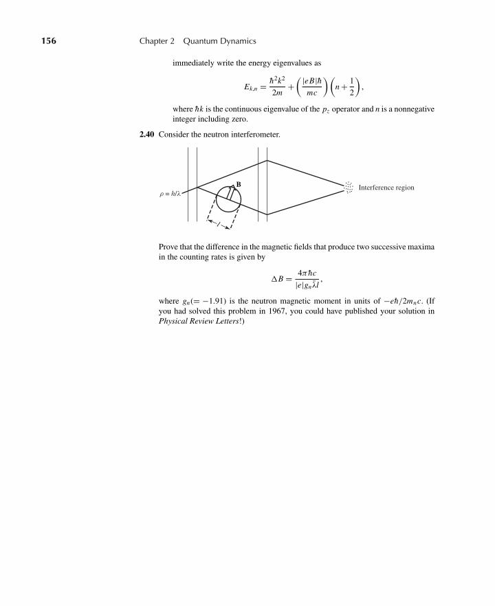
156 Chapter 2 Quantum Dynamics
immediately write the energy eigenvalues as
Ek,n = h2k2
2m+( |eB|h
mc
)(n + 1
2
),
where hk is the continuous eigenvalue of the pz operator and n is a nonnegativeinteger including zero.
2.40 Consider the neutron interferometer.
ρ = h/λB Interference region
l
Prove that the difference in the magnetic fields that produce two successive maximain the counting rates is given by
�B = 4π hc
|e|gnλl,
where gn(= −1.91) is the neutron magnetic moment in units of −eh/2mnc. (Ifyou had solved this problem in 1967, you could have published your solution inPhysical Review Letters!)
C H A P T E R
3 Theory of Angular Momentum
This chapter is concerned with a systematic treatment of angular momentumand related topics. The importance of angular momentum in modern physics canhardly be overemphasized. A thorough understanding of angular momentum is es-sential in molecular, atomic, and nuclear spectroscopy; angular-momentum con-siderations play an important role in scattering and collision problems, as well asin bound-state problems. Furthermore, angular-momentum concepts have impor-tant generalizations—isospin in nuclear physics, SU(3), SU(2)⊗U(1) in particlephysics, and so forth.
3.1 ROTATIONS AND ANGULAR-MOMENTUM COMMUTATIONRELATIONS
Finite versus Infinitesimal Rotations
We recall from elementary physics that rotations about the same axis commute,whereas rotations about different axes do not. For instance, a 30◦ rotation aboutthe z-axis followed by a 60◦ rotation about the same z-axis is obviously equivalentto a 60◦ rotation followed by a 30◦ rotation, both about the same axis. However, letus consider a 90◦ rotation about the z-axis, denoted by Rz(π/2), followed by a 90◦rotation about the x-axis, denoted by Rx (π/2); compare this with a 90◦ rotationabout the x-axis followed by a 90◦ rotation about the z-axis. The net results aredifferent, as we can see from Figure 3.1.
Our first basic task is to work out quantitatively the manner in which rotationsabout different axes fail to commute. To this end, we first recall how to representrotations in three dimensions by 3×3 real, orthogonal matrices. Consider a vectorV with components Vx , Vy , and Vz . When we rotate, the three components becomesome other set of numbers, V ′
x , V ′y , and V ′
z . The old and new components arerelated via a 3 ×3 orthogonal matrix R:⎛⎜⎝V ′
x
V ′y
V ′z
⎞⎟⎠=⎛⎝R
⎞⎠⎛⎜⎝Vx
Vy
Vz
⎞⎟⎠ , (3.1.1a)
RRT = RT R = 1, (3.1.1b)
157
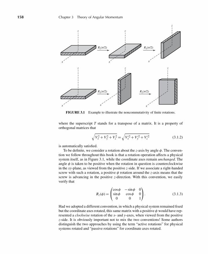
158 Chapter 3 Theory of Angular Momentum
x
z
x
z
x
z
Rz(π/2)
x
z
Rx(π/2)
x
z
x
z
Rz(π/2)
Rx(π/2)
FIGURE 3.1 Example to illustrate the noncommutativity of finite rotations.
where the superscript T stands for a transpose of a matrix. It is a property oforthogonal matrices that√
V 2x + V 2
y + V 2z =
√V ′2
x + V ′2y + V ′2
z (3.1.2)
is automatically satisfied.To be definite, we consider a rotation about the z-axis by angle φ. The conven-
tion we follow throughout this book is that a rotation operation affects a physicalsystem itself, as in Figure 3.1, while the coordinate axes remain unchanged. Theangle φ is taken to be positive when the rotation in question is counterclockwisein the xy-plane, as viewed from the positive z-side. If we associate a right-handedscrew with such a rotation, a positive φ rotation around the z-axis means that thescrew is advancing in the positive z-direction. With this convention, we easilyverify that
Rz(φ) =⎛⎝cosφ −sinφ 0
sinφ cosφ 00 0 1
⎞⎠ . (3.1.3)
Had we adopted a different convention, in which a physical system remained fixedbut the coordinate axes rotated, this same matrix with a positive φ would have rep-resented a clockwise rotation of the x- and y-axes, when viewed from the positivez-side. It is obviously important not to mix the two conventions! Some authorsdistinguish the two approaches by using the term “active rotations” for physicalsystems rotated and “passive rotations” for coordinate axes rotated.
3.1 Rotations and Angular-Momentum Commutation Relations 159
We are particularly interested in an infinitesimal form of Rz :
Rz(ε) =
⎛⎜⎜⎜⎜⎝1 − ε
2
2−ε 0
ε 1 − ε2
20
0 0 1
⎞⎟⎟⎟⎟⎠ , (3.1.4)
where terms of order ε3 and higher are ignored. Likewise, we have
Rx (ε) =
⎛⎜⎜⎜⎝1 0 0
0 1 − ε2
2−ε
0 ε 1 − ε2
2
⎞⎟⎟⎟⎠ (3.1.5a)
and
Ry(ε) =
⎛⎜⎜⎜⎜⎝1 − ε
2
20 ε
0 1 0
−ε 0 1 − ε2
2
⎞⎟⎟⎟⎟⎠ , (3.1.5b)
which may be read from (3.1.4) by cyclic permutations of x, y, z—that is, x → y,y → z, z → x . Compare now the effect of a y-axis rotation followed by an x-axisrotation with that of an x-axis rotation followed by a y-axis rotation. Elementarymatrix manipulations lead to
Rx (ε)Ry(ε) =
⎛⎜⎜⎜⎜⎝1 − ε
2
20 ε
ε2 1 − ε2
2−ε
−ε ε 1 − ε2
⎞⎟⎟⎟⎟⎠ (3.1.6a)
and
Ry(ε)Rx (ε) =
⎛⎜⎜⎜⎜⎝1 − ε
2
2ε2 ε
0 1 − ε2
2−ε
−ε ε 1 − ε2
⎞⎟⎟⎟⎟⎠ . (3.1.6b)
From (3.1.6a) and (3.1.6b) we have the first important result: Infinitesimal ro-tations about different axes do commute if terms of order ε2 and higher are ig-nored.∗ The second and even more important result concerns the manner in which∗There is a familiar example of this in elementary mechanics. The angular-velocity vector ω
that characterizes an infinitesimal change in rotation angle during an infinitesimal time intervalfollows the usual rule of vector addition, including commutativity of vector addition. However,we cannot ascribe a vectorial property to a finite angular change.
160 Chapter 3 Theory of Angular Momentum
rotations about different axes fail to commute when terms of order ε2 are kept:
Rx (ε)Ry(ε) − Ry(ε)Rx (ε) =⎛⎝ 0 −ε2 0ε2 0 00 0 0
⎞⎠= Rz(ε2) − 1,
(3.1.7)
where all terms of order higher than ε2 have been ignored throughout this deriva-tion. We also have
1 = Rany(0), (3.1.8)
where any stands for any rotation axis. Thus the final result can be written as
Rx (ε)Ry(ε) − Ry(ε)Rx (ε) = Rz(ε2) − Rany(0). (3.1.9)
This is an example of the commutation relations between rotation operationsabout different axes, which we will use later in deducing the angular-momentumcommutation relations in quantum mechanics.
Infinitesimal Rotations in Quantum Mechanics
So far we have not used quantum-mechanical concepts. The matrix R is just a3 ×3 orthogonal matrix acting on a vector V written in column matrix form. Wemust now understand how to characterize rotations in quantum mechanics.
Because rotations affect physical systems, the state ket corresponding to a ro-tated system is expected to look different from the state ket corresponding to theoriginal unrotated system. Given a rotation operation R, characterized by a 3 ×3orthogonal matrix R, we associate an operator D(R) in the appropriate ket spacesuch that
|α〉R = D(R)|α〉, (3.1.10)
where |α〉R and |α〉 stand for the kets of the rotated and original system, respec-tively.∗ Note that the 3 × 3 orthogonal matrix R acts on a column matrix madeup of the three components of a classical vector, while the operator D(R) actson state vectors in ket space. The matrix representation of D(R), which we willstudy in great detail in the subsequent sections, depends on the dimensionality Nof the particular ket space in question. For N = 2, which is appropriate for de-scribing a spin 1
2 system with no other degrees of freedom, D(R) is representedby a 2 × 2 matrix; for a spin 1 system, the appropriate representation is a 3 × 3unitary matrix, and so on.
To construct the rotation operator D(R), it is again fruitful to examine firstits properties under an infinitesimal rotation. We can almost guess how we mustproceed by analogy. In both translations and time evolution, which we studied in
∗The symbol D stems from the German word Drehung, meaning “rotation.”
3.1 Rotations and Angular-Momentum Commutation Relations 161
Sections 1.6 and 2.1, respectively, the appropriate infinitesimal operators could bewritten as
Uε = 1 − i Gε (3.1.11)
with a Hermitian operator G. Specifically,
G → px
h, ε→ dx ′ (3.1.12)
for an infinitesimal translation by a displacement dx ′ in the x-direction, and
G → H
h, ε→ dt (3.1.13)
for an infinitesimal time evolution with time displacement dt. We know from clas-sical mechanics that angular momentum is the generator of rotation in much thesame way as momentum and Hamiltonian are the generators of translation andtime evolution, respectively. We therefore define the angular-momentum operatorJk in such a way that the operator for an infinitesimal rotation around the kth axisby angle dφ can be obtained by letting
G → Jk
h, ε→ dφ (3.1.14)
in (3.1.11). With Jk taken to be Hermitian, the infinitesimal-rotation operator isguaranteed to be unitary and reduces to the identity operator in the limit dφ→ 0.More generally, we have
D(n,dφ) = 1 − i
(J · n
h
)dφ (3.1.15)
for a rotation about the direction characterized by a unit vector n by an infinitesi-mal angle dφ.
We stress that in this book we do not define the angular-momentum operator tobe x×p. This is important because spin angular momentum, to which our generalformalism also applies, has nothing to do with xi and p j . Put in another way, inclassical mechanics one can prove that the angular momentum defined to be x×pis the generator of a rotation; in contrast, in quantum mechanics we define J suchthat the operator for an infinitesimal rotation takes from (3.1.15).
A finite rotation can be obtained by compounding successively infinitesimalrotations about the same axis. For instance, if we are interested in a finite rotationabout the z-axis by angle φ, we consider
Dz(φ) = LimN→∞
[1 − i
(Jz
h
)(φ
N
)]N
= exp
(−i Jzφ
h
)= 1 − i Jzφ
h− J 2
z φ2
2h2+·· · .
(3.1.16)
162 Chapter 3 Theory of Angular Momentum
In order to obtain the angular-momentum commutation relations, we need onemore concept. As we remarked earlier, for every rotation R represented by a 3×3orthogonal matrix R, there exists a rotation operator D(R) in the appropriate ketspace. We further postulate that D(R) has the same group properties as R:
Identity: R ·1 = R ⇒ D(R) ·1 = D(R) (3.1.17a)
Closure: R1 R2 = R3 ⇒ D(R1)D(R2) = D(R3) (3.1.17b)
Inverses: RR−1 = 1 ⇒ D(R)D−1(R) = 1
R−1 R = 1 ⇒ D−1(R)D(R) = 1(3.1.17c)
Associativity : R1(R2 R3) = (R1 R2)R3 = R1 R2 R3
⇒ D(R1)[D(R2)D(R3)]
= [D(R1)D(R2)]D(R3)
= D(R1)D(R2)D(R3).
(3.1.17d)
Let us now return to the fundamental commutation relations for rotation op-erations (3.1.9) written in terms of the R matrices. Its rotation operator analoguewould read(
1 − i Jxε
h− J 2
x ε2
2h2
)(1 − i Jyε
h− J 2
y ε2
2h2
)
−(
1 − i Jyε
h− J 2
y ε2
2h2
)(1 − i Jxε
h− J 2
x ε2
2h2
)= 1 − i Jzε
2
h− 1.
(3.1.18)
Terms of order ε automatically drop out. Equating terms of order ε2 on both sidesof (3.1.18), we obtain
[Jx , Jy] = i h Jz . (3.1.19)
Repeating this kind of argument with rotations about other axes, we obtain
[Ji , Jj ] = i hεi j k Jk , (3.1.20)
known as the fundamental commutation relations of angular momentum.In general, when the generators of infinitesimal transformations do not com-
mute, the corresponding group of operations is said to be non-Abelian. Becauseof (3.1.20), the rotation group in three dimensions is non-Abelian. In contrast, thetranslation group in three dimensions is Abelian because pi and p j commute evenwith i �= j .
We emphasize that in obtaining the commutation relations (3.1.20), we haveused the following two concepts:
1. Jk is the generator of rotation about the kth axis.2. Rotations about different axes fail to commute.
3.2 Spin 12 Systems and Finite Rotations 163
It is no exaggeration to say that commutation relations (3.1.20) summarize in acompact manner all the basic properties of rotations in three dimensions.
3.2 SPIN 12 SYSTEMS AND FINITE ROTATIONS
Rotation Operator for Spin 12
The lowest number, N, of dimensions in which the angular-momentum commu-tation relations (3.1.20) are realized is N = 2. The reader has already checked, inProblem 1.8 of Chapter 1, that the operators defined by
Sx =(
h
2
){(|+〉〈−|) + (|−〉〈+|)} ,
Sy =(
i h
2
){−(|+〉〈−|) + (|−〉〈+|)} ,
Sz =(
h
2
){(|+〉〈+|) − (|−〉〈−|)}
(3.2.1)
satisfy commutation relations (3.1.20) with Jk replaced by Sk . It is not a pri-ori obvious that nature takes advantage of the lowest-dimensional realization of(3.1.20), but numerous experiments—from atomic spectroscopy to nuclear mag-netic resonance—suffice to convince us that this is in fact the case.
Consider a rotation by a finite angle φ about the z-axis. If the ket of a spin 12
system before rotation is given by |α〉, the ket after rotation is given by
|α〉R = Dz(φ)|α〉 (3.2.2)
with
Dz (φ) = exp
(−i Szφ
h
). (3.2.3)
To see that this operator really rotates the physical system, let us look at its effecton 〈Sx 〉. Under rotation this expectation value changes as follows:
〈Sx 〉 → R〈α|Sx |α〉R = 〈α|D†z (φ)SxDz(φ)|α〉. (3.2.4)
We must therefore compute
exp
(i Szφ
h
)Sx exp
(−i Szφ
h
). (3.2.5)
For pedagogical reasons we evaluate this in two different ways.
164 Chapter 3 Theory of Angular Momentum
Derivation 1: Here we use the specific form of Sx given by (3.2.1). We thenobtain, for (3.2.5),(
h
2
)exp
(i Szφ
h
){(|+〉〈−|) + (|−〉〈+|)}exp
(−i Szφ
h
)=(
h
2
)(eiφ/2|+〉〈−|eiφ/2 + e−iφ/2|−〉〈+|e−iφ/2)
= h
2[{(|+〉〈−|) + (|−〉〈+|)}cosφ+ i{(|+〉〈−|) − (|−〉〈+|)}sinφ]
= Sx cosφ− Sy sinφ.
(3.2.6)
Derivation 2: Alternatively, we may use formula (2.3.47) to evaluate (3.2.5):
exp
(i Szφ
h
)Sx exp
(−i Szφ
h
)= Sx +
(iφ
h
)[Sz , Sx ]︸ ︷︷ ︸
ihSy
+(
1
2!
)(iφ
h
)2
[Sz , [Sz , Sx ]]︸ ︷︷ ︸ihSy︸ ︷︷ ︸
h2 Sx
+(
1
3!
)(iφ
h
)3
[Sz , [Sz , [Sz , [Sz , Sx ]]]]︸ ︷︷ ︸h2 Sx︸ ︷︷ ︸
ih3 Sy
+·· ·
= Sx
[1 − φ
2
2!+·· ·
]− Sy
[φ− φ
3
3!+·· ·
]= Sx cosφ− Sy sinφ.
(3.2.7)
Notice that in derivation 2 we used only the commutation relations for Si , so thismethod can be generalized to rotations of systems with angular momentum higherthan 1
2 .For spin 1
2 , both methods give
〈Sx 〉 → R〈α|Sx |α〉R = 〈Sx 〉cosφ−〈Sy〉sinφ, (3.2.8)
where the expectation value without subscripts is understood to be taken withrespect to the (old) unrotated system. Similarly,
〈Sy〉 → 〈Sy〉cosφ+〈Sx〉sinφ. (3.2.9)
As for the expectation value of Sz , there is no change because Sz commutes withDz(φ):
〈Sz〉 → 〈Sz〉. (3.2.10)
Relations (3.2.8), (3.2.9), and (3.2.10) are quite reasonable. They show that ro-tation operator (3.2.3), when applied to the state ket, does rotate the expectationvalue of S around the z-axis by angle φ. In other words, the expectation value of
3.2 Spin 12 Systems and Finite Rotations 165
the spin operator behaves as though it were a classical vector under rotation:
〈Sk〉 →∑
l
Rkl 〈Sl 〉, (3.2.11)
where Rkl are the elements of the 3 × 3 orthogonal matrix R that specifies therotation in question. It should be clear from our derivation 2 that this property isnot restricted to the spin operator of spin 1
2 systems. In general, we have
〈Jk〉 →∑
l
Rkl 〈Jl〉 (3.2.12)
under rotation, where Jk are the generators of rotations satisfying the angular-momentum commutation relations (3.1.20). Later we will show that relations ofthis kind can be further generalized to any vector operator.
So far everything has been as expected. But now, be prepared for a surprise!We examine the effect of rotation operator (3.2.3) on a general ket,
|α〉 = |+〉〈+|α〉+ |−〉〈−|α〉, (3.2.13)
a little more closely. We see that
exp
(−i Szφ
h
)|α〉 = e−iφ/2|+〉〈+|α〉+ eiφ/2|−〉〈−|α〉. (3.2.14)
The appearance of the half-angle φ/2 here has an extremely interesting conse-quence.
Let us consider a rotation by 2π . We then have
|α〉Rz (2π) → −|α〉. (3.2.15)
So the ket for the 360◦ rotated state differs from the original ket by a minus sign.We would need a 720◦ (φ = 4π) rotation to get back to the same ket with a plussign. Notice that this minus sign disappears for the expectation value of S, becauseS is sandwiched by |α〉 and 〈α|, both of which change sign. Will this minus signever be observable? We will give the answer to this interesting question after wediscuss spin precession once again.
Spin Precession Revisited
We now treat the problem of spin precession, already discussed in Section 2.1,from a new point of view. We recall that the basic Hamiltonian of the problem isgiven by
H = −(
e
mec
)S · B = ωSz , (3.2.16)
where
ω ≡ |e|Bmec
. (3.2.17)
166 Chapter 3 Theory of Angular Momentum
The time-evolution operator based on this Hamiltonian is given by
U(t ,0) = exp
(−i H t
h
)= exp
(−i Szωt
h
). (3.2.18)
Comparing this equation with (3.2.3), we see that the time-evolution operator hereis precisely the same as the rotation operator in (3.2.3) with φ set equal to ωt. Inthis manner we see immediately why this Hamiltonian causes spin precession.Paraphrasing (3.2.8), (3.2.9), and (3.2.10), we obtain
〈Sx 〉t = 〈Sx 〉t=0 cosωt −〈Sy〉t=0 sinωt , (3.2.19a)
〈Sy〉t = 〈Sy〉t=0 cosωt +〈Sx 〉t=0 sinωt , (3.2.19b)
〈Sz〉t = 〈Sz〉t=0. (3.2.19c)
After t = 2π/ω, the spin returns to its original direction.This set of equations can be used to discuss the spin precession of a muon,
an electron-like particle that is, however, 210 times as heavy. The muon magneticmoment can be determined from other experiments—for example, the hyperfinesplitting in muonium, a bound state of a positive muon and an electron—to beeh/2mμc, just as expected from Dirac’s relativistic theory of spin 1
2 particles.(We will here neglect very small corrections that arise from quantum field theoryeffects). Knowing the magnetic moment, we can predict the angular frequencyof precession. So (3.2.19) can be, and in fact has been, checked experimentally.(See Figure 2.1.) In practice, as the external magnetic field causes spin precession,the spin direction is analyzed by taking advantage of the fact that electrons frommuon decay tend to be emitted preferentially in the direction opposite to the muonspin.
Let us now look at the time evolution of the state ket itself. Assuming that theinitial (t = 0) ket is given by (3.2.13), we obtain, after time t,
|α, t0 = 0; t〉 = e−iωt/2|+〉〈+|α〉+ e+iωt/2|−〉〈−|α〉. (3.2.20)
Expression (3.2.20) acquires a minus sign at t = 2π/ω, and we must wait untilt = 4π/ω to get back to the original state ket with the same sign. To sum up, theperiod for the state ket is twice as long as the period for spin precession:
τprecession = 2π
ω, (3.2.21a)
τstateket = 4π
ω. (3.2.21b)
Neutron Interferometry Experiment to Study 2π Rotations
We now describe an experiment performed to detect the minus sign in (3.2.15).Quite clearly, if every state ket in the universe is multiplied by a minus sign, therewill be no observable effect. The only way to detect the predicted minus signis to make a comparison between an unrotated state and a rotated state. As in
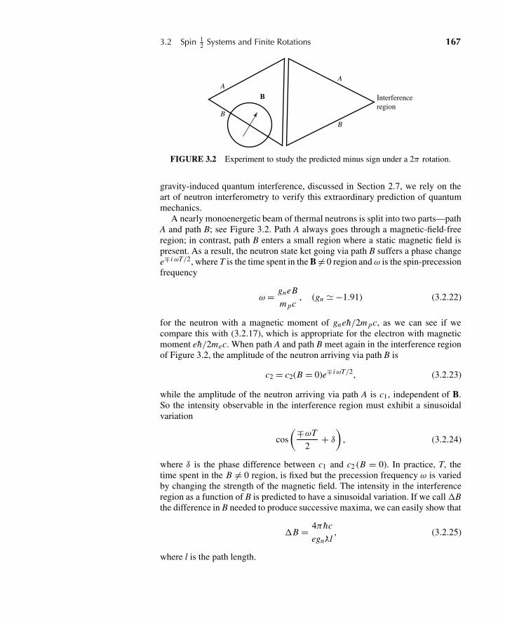
3.2 Spin 12 Systems and Finite Rotations 167
A
B
A
B
B Interferenceregion
FIGURE 3.2 Experiment to study the predicted minus sign under a 2π rotation.
gravity-induced quantum interference, discussed in Section 2.7, we rely on theart of neutron interferometry to verify this extraordinary prediction of quantummechanics.
A nearly monoenergetic beam of thermal neutrons is split into two parts—pathA and path B; see Figure 3.2. Path A always goes through a magnetic-field-freeregion; in contrast, path B enters a small region where a static magnetic field ispresent. As a result, the neutron state ket going via path B suffers a phase changee∓ i ωT/2, where T is the time spent in the B �= 0 region andω is the spin-precessionfrequency
ω = gneB
m pc, (gn � −1.91) (3.2.22)
for the neutron with a magnetic moment of gneh/2m pc, as we can see if wecompare this with (3.2.17), which is appropriate for the electron with magneticmoment eh/2mec. When path A and path B meet again in the interference regionof Figure 3.2, the amplitude of the neutron arriving via path B is
c2 = c2(B = 0)e∓ iωT/2, (3.2.23)
while the amplitude of the neutron arriving via path A is c1, independent of B.So the intensity observable in the interference region must exhibit a sinusoidalvariation
cos
(∓ωT
2+ δ
), (3.2.24)
where δ is the phase difference between c1 and c2 (B = 0). In practice, T, thetime spent in the B �= 0 region, is fixed but the precession frequency ω is variedby changing the strength of the magnetic field. The intensity in the interferenceregion as a function of B is predicted to have a sinusoidal variation. If we call�Bthe difference in B needed to produce successive maxima, we can easily show that
�B = 4π hc
egnλl, (3.2.25)
where l is the path length.
168 Chapter 3 Theory of Angular Momentum
In deriving this formula we used the fact that a 4π rotation is needed for thestate ket to return to the original ket with the same sign, as required by our formal-ism. If, on the other hand, our description of spin 1
2 systems were incorrect andthe ket were to return to its original ket with the same sign under a 2π rotation,the predicted value for �B would be just one-half of (3.2.25).
Two different groups have conclusively demonstrated experimentally that pre-diction (3.2.25) is correct to an accuracy of a fraction of a percent.∗ This is an-other triumph of quantum mechanics. The nontrivial prediction (3.2.15) has beenexperimentally established in a direct manner.
Pauli Two-Component Formalism
Manipulations with the state kets of spin 12 systems can be conveniently carried
out using the two-component spinor formalism introduced by W. Pauli in 1926.In Section 1.3 we learned how a ket (bra) can be represented by a column (row)matrix; all we have to do is arrange the expansion coefficients in terms of a certainspecified set of base kets into a column (row) matrix. In the spin 1
2 case we have
|+〉=(
10
)≡ χ+ |−〉=
(01
)≡ χ−
〈+|= (1,0) = χ†+ 〈−|= (0,1) = χ†
−(3.2.26)
for the base kets and bras and
|α〉 = |+〉〈+|α〉+ |−〉〈−|α〉=(〈+|α〉
〈−|α〉)
(3.2.27a)
and
〈α| = 〈α|+〉〈+|+ 〈α|−〉〈−|= (〈α|+〉, 〈α|−〉) (3.2.27b)
for an arbitrary state ket and the corresponding state bra. Column matrix (3.2.27a)is referred to as a two-component spinor and is written as
χ =(〈+|α〉
〈−|α〉)
≡(
c+c−
)= c+χ+ + c−χ−, (3.2.28)
where c+ and c− are, in general, complex numbers. For χ† we have
χ† = (〈α|+〉, 〈α|−〉) = (c∗+,c∗−
). (3.2.29)
The matrix elements 〈±|Sk |+〉 and 〈±|Sk |−〉, apart from h/2, are to be setequal to those of 2 ×2 matrices σk , known as the Pauli matrices. We identify
〈±|Sk |+〉 ≡(
h
2
)(σk)±,+, 〈±|Sk |−〉 ≡
(h
2
)(σk)±,−. (3.2.30)
∗H. Rauch et al., Phys. Lett. 54A (1975) 425; S. A. Werner et al., Phys. Rev. Lett. 35 (1975) 1053.
3.2 Spin 12 Systems and Finite Rotations 169
We can now write the expectation value 〈Sk〉 in terms of χ and σk :
〈Sk〉 = 〈α|Sk |α〉 =∑
a′=+,−
∑a′′=+,−
〈α|a′〉〈a′|Sk |a′′〉〈a′′|α〉
=(
h
2
)χ†σkχ , (3.2.31)
where the usual rule of matrix multiplication is used in the last line. Explicitly, wesee from (3.2.1), together with (3.2.30), that
σ1 =(
0 11 0
), σ2 =
(0 −ii 0
), σ3 =
(1 00 −1
), (3.2.32)
where the subscripts 1, 2, and 3 refer to x , y, and z, respectively.We record some properties of the Pauli matrices. First,
σ 2i = 1 (3.2.33a)
σiσ j +σ jσi = 0, for i �= j , (3.2.33b)
where the right-hand side of (3.2.33a) is to be understood as the 2 × 2 identitymatrix. These two relations are, of course, equivalent to the anticommutation re-lations
{σi ,σ j } = 2δi j . (3.2.34)
We also have the commutation relations
[σi ,σ j ] = 2iεi j kσk , (3.2.35)
which we see to be the explicit 2×2 matrix realizations of the angular-momentumcommutation relations (3.1.20). Combining (3.2.34) and (3.2.35), we can obtain
σ1σ2 = −σ2σ1 = iσ3 . . . . (3.2.36)
Notice also that
σ†i = σi , (3.2.37a)
det(σi ) = −1, (3.2.37b)
Tr(σi ) = 0. (3.2.37c)
We now consider σ ·a, where a is a vector in three dimensions. This is actuallyto be understood as a 2 ×2 matrix. Thus
σ · a ≡∑
k
akσk
=( +a3 a1 − ia2
a1 + ia2 −a3
). (3.2.38)
170 Chapter 3 Theory of Angular Momentum
There is also a very important identity,
(σ · a) (σ · b) = a · b+ iσ · (a ×b). (3.2.39)
To prove this all we need are the anticommutation and commutation relations,(3.2.34) and (3.2.35), respectively:∑
j
σ j a j
∑k
σkbk =∑
j
∑k
(1
2{σ j ,σk}+ 1
2[σ j ,σk]
)a j bk
=∑
j
∑k
(δ j k + iε j klσl
)a j bk
= a·b+ iσ · (a ×b). (3.2.40)
If the components of a are real, we have
(σ · a)2 = |a|2, (3.2.41)
where |a| is the magnitude of the vector a.
Rotations in the Two-Component Formalism
Let us now study the 2×2 matrix representation of the rotation operator D(n,φ).We have
exp
(−iS · nφh
)= exp
(−iσ · nφ2
). (3.2.42)
Using
(σ · n)n ={
1 for n even,σ · n for n odd,
(3.2.43)
which follows from (3.2.41), we can write
exp
(−iσ · nφ2
)=[
1 − (σ · n)2
2!
(φ
2
)2
+ (σ · n)4
4!
(φ
2
)4
−·· ·]
− i
[(σ · n)
φ
2− (σ · n)3
3!
(φ
2
)3
+·· ·]
= 1cos
(φ
2
)− iσ · nsin
(φ
2
). (3.2.44)
Explicitly, in 2 ×2 form we have
exp
(−iσ · nφ2
)=
⎛⎜⎜⎝ cos
(φ
2
)− inz sin
(φ
2
) (−inx − ny)
sin
(φ
2
)(−inx + ny
)sin
(φ
2
)cos
(φ
2
)+ inz sin
(φ
2
)⎞⎟⎟⎠ .
(3.2.45)
3.2 Spin 12 Systems and Finite Rotations 171
Just as the operator exp(−iS · nφ/h) acts on a state ket |α〉, the 2 × 2 matrixexp(−iσ · nφ/2) acts on a two-component spinor χ . Under rotations we changeχ as follows:
χ → exp
(−iσ · nφ2
)χ . (3.2.46)
On the other hand, the σk’s themselves are to remain unchanged under rotations.So strictly speaking, despite its appearance, σ is not to be regarded as a vector;rather, it is χ†σχ that obeys the transformation property of a vector:
χ†σkχ →∑
l
Rklχ†σlχ . (3.2.47)
An explicit proof of this may be given using
exp
(iσ3φ
2
)σ1 exp
(−iσ3φ
2
)= σ1 cosφ−σ2 sinφ (3.2.48)
and so on, which is the 2 ×2 matrix analogue of (3.2.6).In discussing a 2π rotation using the ket formalism, we have seen that a spin
12 ket |α〉 goes into −|α〉. The 2 × 2 analogue of this statement is
exp
(−iσ · nφ2
)∣∣∣∣φ=2π
= −1, for any n, (3.2.49)
which is evident from (3.2.44).As an instructive application of rotation matrix (3.2.45), let us see how we can
construct an eigenspinor of σ · n with eigenvalue +1, where n is a unit vector insome specified direction. Our object is to construct χ satisfying
σ · nχ = χ . (3.2.50)
In other words, we look for the two-component column matrix representation of|S · n;+〉 defined by
S · n|S · n;+〉 =(
h
2
)|S · n;+〉. (3.2.51)
Actually this can be solved as a straightforward eigenvalue problem (see Prob-lem 1.9 in Chapter 1), but here we present an alternative method based on rotationmatrix (3.2.45).
Let the polar and the azimuthal angles that characterize n be β and α, respec-tively. We start with
( 10
), the two-component spinor that represents the spin-up
state. Given this, we first rotate about the y-axis by angle β; we subsequently ro-tate by angle α about the z-axis. We see that the desired spin state is then ob-tained; see Figure 3.3. In the Pauli spinor language, this sequence of operations
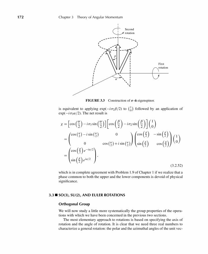
172 Chapter 3 Theory of Angular Momentum
β
α
Secondrotation
Firstrotation
FIGURE 3.3 Construction of σ ·n eigenspinor.
is equivalent to applying exp(−iσ2β/2) to( 1
0
)followed by an application of
exp(−iσ3α/2). The net result is
χ =[cos
(α2
)− iσ3 sin
(α2
)][cos
(β
2
)− iσ2 sin
(β
2
)](1
0
)
=⎛⎝cos
(α2
)− i sin(α2
)0
0 cos(α2
)+ i sin(α2
)⎞⎠⎛⎜⎝cos
(β2
)−sin
(β2
)sin
(β2
)cos
(β2
)⎞⎟⎠(1
0
)
=⎛⎜⎝cos
(β2
)e−iα/2
sin(β2
)eiα/2
⎞⎟⎠ ,
(3.2.52)
which is in complete agreement with Problem 1.9 of Chapter 1 if we realize that aphase common to both the upper and the lower components is devoid of physicalsignificance.
3.3 SO(3), SU(2), AND EULER ROTATIONS
Orthogonal Group
We will now study a little more systematically the group properties of the opera-tions with which we have been concerned in the previous two sections.
The most elementary approach to rotations is based on specifying the axis ofrotation and the angle of rotation. It is clear that we need three real numbers tocharacterize a general rotation: the polar and the azimuthal angles of the unit vec-
3.3 SO(3), SU(2), and Euler Rotations 173
tor n taken in the direction of the rotation axis and the rotation angle φ itself.Equivalently, the same rotation can be specified by the three Cartesian compo-nents of the vector nφ. However, these ways of characterizing rotation are not soconvenient from the point of view of studying the group properties of rotations.For one thing, unless φ is infinitesimal or n is always in the same direction, wecannot add vectors of the form nφ to characterize a succession of rotations. It ismuch easier to work with a 3 × 3 orthogonal matrix R because the effect of suc-cessive rotations can be obtained just by multiplying the appropriate orthogonalmatrices.
How many independent parameters are there in a 3 × 3 orthogonal matrix? Areal 3 × 3 matrix has 9 entries, but we have the orthogonality constraint
RRT = 1. (3.3.1)
This corresponds to 6 independent equations because the product RRT , being thesame as RT R, is a symmetrical matrix with 6 independent entries. As a result,there are 3 (that is, 9–6) independent numbers in R, the same number we previ-ously obtained by a more elementary method.
The set of all multiplication operations with orthogonal matrices forms agroup. By this we mean that the following four requirements are satisfied.
1. The product of any two orthogonal matrices is another orthogonal matrix,which is satisfied because
(R1 R2)(R1 R2)T = R1 R2 RT2 RT
1 = 1. (3.3.2)
2. The associative law holds:
R1(R2 R3) = (R1 R2)R3. (3.3.3)
3. The identity matrix 1—physically corresponding to no rotation—definedby
R1 = 1R = R (3.3.4)
is a member of the class of all orthogonal matrices.4. The inverse matrix R−1—physically corresponding to rotation in the oppo-
site sense—defined by
RR−1 = R−1 R = 1 (3.3.5)
is also a member.
This group has the name SO(3), where S stands for special, O stands for orthog-onal, and 3 stands for three dimensions. Note that only rotational operations areconsidered here, so we have SO(3) rather than O(3) (which can include the inver-sion operation to be discussed later in Chapter 4).
174 Chapter 3 Theory of Angular Momentum
Unitary Unimodular Group
In the previous section we learned yet another way to characterize an arbitraryrotation—that is, to look at the 2 × 2 matrix (3.2.45) that acts on the two-component spinor χ . Clearly, (3.2.45) is unitary. As a result, for the c+ and c−,defined in (3.2.28),
|c+|2 +|c−|2 = 1 (3.3.6)
is left invariant. Furthermore, matrix (3.2.45) is unimodular; that is, its determi-nant is 1, as will be shown explicitly below.
We can write the most general unitary unimodular matrix as
U (a,b) =(
a b−b∗ a∗
), (3.3.7)
where a and b are complex numbers satisfying the unimodular condition
|a|2 +|b|2 = 1. (3.3.8)
We can easily establish the unitary property of (3.3.7) as follows:
U (a,b)†U (a,b) =(
a∗ −bb∗ a
)(a b−b∗ a∗
)= 1, (3.3.9)
We can readily see that the 2 × 2 matrix (3.2.45) that characterizes a rotationof a spin 1
2 system can be written as U (a,b). Comparing (3.2.45) with (3.3.7), weidentify
Re(a) = cos
(φ
2
), Im(a) = −nzsin
(φ
2
),
Re(b) = −nysin
(φ
2
), Im(b) = −nx sin
(φ
2
),
(3.3.10)
from which the unimodular property of (3.3.8) is immediate. Conversely, it is clearthat the most general unitary unimodular matrix of form (3.3.7) can be interpretedas representing a rotation.
The two complex numbers a and b are known as Cayley-Klein parameters.Historically, the connection between a unitary unimodular matrix and a rotationwas known long before the birth of quantum mechanics. In fact, the Cayley-Kleinparameters were used to characterize complicated motions of gyroscopes in rigid-body kinematics.
Without appealing to the interpretations of unitary unimodular matrices interms of rotations, we can directly check the group properties of multiplicationoperations with unitary unimodular matrices. Note in particular that
U (a1,b1)U (a2,b2) = U (a1a2 − b1b∗2,a1b2 + a∗
2b1), (3.3.11)
where the unimodular condition for the product matrix is
|a1a2 − b1b∗2 |2 +|a1b2 + a∗
2b1|2 = 1. (3.3.12)
3.3 SO(3), SU(2), and Euler Rotations 175
For the inverse of U we have
U−1(a,b) = U (a∗,−b). (3.3.13)
This group is known as SU(2), where S stands for special, U for unitary, and 2for dimensionality 2. In contrast, the group defined by multiplication operationswith general 2×2 unitary matrices (not necessarily constrained to be unimodular)is known as U(2). The most general unitary matrix in two dimensions has fourindependent parameters and can be written as eiγ (with γ real) times a unitaryunimodular matrix:
U = eiγ(
a b−b∗ a∗
), |a|2 +|b|2 = 1, γ ∗ = γ . (3.3.14)
SU(2) is called a subgroup of U(2).Because we can characterize rotations using both the SO(3) language and the
SU(2) language, we may be tempted to conclude that the groups SO(3) and SU(2)are isomorphic—that is, that there is a one-to-one correspondence between anelement of SO(3) and an element of SU(2). This inference is not correct. Considera rotation by 2π and another one by 4π . In the SO(3) language the matricesrepresenting a 2π rotation and a 4π rotation are both 3 × 3 identity matrices;however, in the SU(2) language the corresponding matrices are −1 times the 2×2identity matrix and the identity matrix itself, respectively. More generally, U(a, b)and U (−a,−b) both correspond to a single 3 × 3 matrix in the SO(3) language.The correspondence therefore is two-to-one; for a given R, the corresponding U isdouble-valued. One can say, however, that the two groups are locally isomorphic.
Euler Rotations
From classical mechanics the reader may be familiar with the fact that an arbi-trary rotation of a rigid body can be accomplished in three steps known as Eulerrotations. The Euler rotation language, specified by three Euler angles, providesyet another way to characterize the most general rotation in three dimensions.
The three steps of Euler rotations are as follows. First, rotate the rigid bodycounterclockwise (as seen from the positive z-side) about the z-axis by angle α.Imagine now that there is a body y-axis embedded, so to speak, in the rigid bodysuch that before the z-axis rotation is carried out, the body y-axis coincides withthe usual y-axis, referred to as the space-fixed y-axis. Obviously, after the rotationabout the z-axis, the body y-axis no longer coincides with the space-fixed y-axis;let us call the former the y ′-axis. To see how all this may appear for a thin disk,refer to Figure 3.4a. We now perform a second rotation, this time about the y ′-axis by angle β. As a result, the body z-axis no longer points in the space-fixedz-axis direction. We call the body-fixed z-axis after the second rotation the z′-axis;see Figure 3.4b. The third and final rotation is about the z′-axis by angle γ . Thebody y-axis now becomes the y ′′-axis of Figure 3.4c. In terms of 3×3 orthogonalmatrices, the product of the three operations can be written as
R(α,β,γ ) ≡ Rz′ (γ )Ry′(β)Rz(α). (3.3.15)
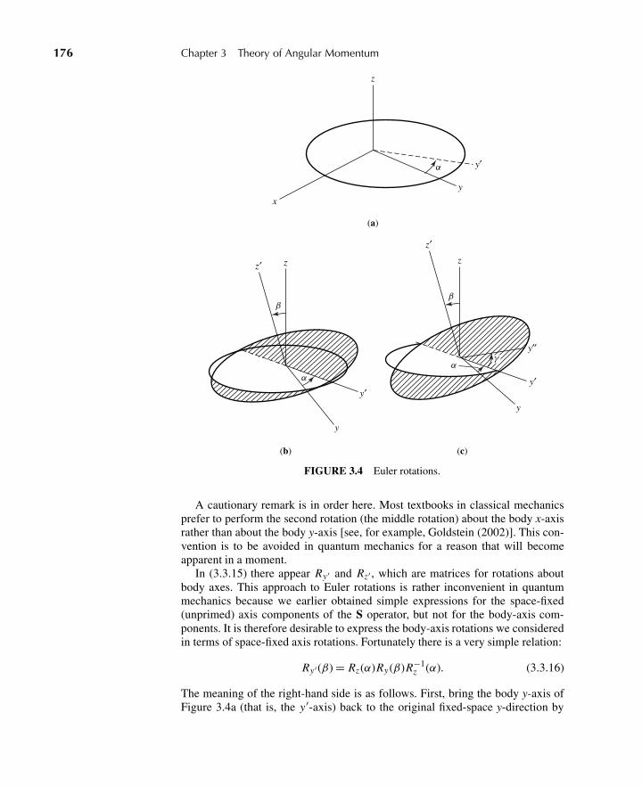
176 Chapter 3 Theory of Angular Momentum
α
α
α
ββ
z
x
z zz′
z′
y′y′
y′′
y
y
y
y′
(a)
(b) (c)
γ
FIGURE 3.4 Euler rotations.
A cautionary remark is in order here. Most textbooks in classical mechanicsprefer to perform the second rotation (the middle rotation) about the body x-axisrather than about the body y-axis [see, for example, Goldstein (2002)]. This con-vention is to be avoided in quantum mechanics for a reason that will becomeapparent in a moment.
In (3.3.15) there appear Ry′ and Rz′ , which are matrices for rotations aboutbody axes. This approach to Euler rotations is rather inconvenient in quantummechanics because we earlier obtained simple expressions for the space-fixed(unprimed) axis components of the S operator, but not for the body-axis com-ponents. It is therefore desirable to express the body-axis rotations we consideredin terms of space-fixed axis rotations. Fortunately there is a very simple relation:
Ry′(β) = Rz(α)Ry(β)R−1z (α). (3.3.16)
The meaning of the right-hand side is as follows. First, bring the body y-axis ofFigure 3.4a (that is, the y ′-axis) back to the original fixed-space y-direction by
3.3 SO(3), SU(2), and Euler Rotations 177
rotating clockwise (as seen from the positive z-side) about the z-axis by angleα; then rotate about the y-axis by angle β. Finally, return the body y-axis to thedirection of the y′-axis by rotating about the fixed-space z-axis (not about the z′-axis!) by angle α. Equation (3.3.16) tells us that the net effect of these rotations isa single rotation about the y ′-axis by angle β.
To prove this assertion, let us look more closely at the effect of both sidesof (3.3.16) on the circular disc of Figure 3.4a. Clearly, the orientation of thebody y-axis is unchanged in both cases—namely, in the y′-direction. Further-more, the orientation of the final body z-axis is the same whether we apply Ry′ (β)or Rz (α)Ry(β)R−1
z (α). In both cases the final body z-axis makes a polar angle βwith the fixed z-axis (the same as the initial z-axis), and its azimuthal angle, asmeasured in the fixed-coordinate system, is just α. In other words, the final bodyz-axis is the same as the z ′-axis of Figure 3.4b. Similarly, we can prove
Rz′(γ ) = Ry′(β)Rz(γ )R−1y′ (β). (3.3.17)
Using (3.3.16) and (3.3.17), we can now rewrite (3.3.15). We obtain
Rz′ (γ )Ry′(β)Rz(α) = Ry′(β)Rz(γ )R−1y′ (β)Ry′(β)Rz(α)
= Rz(α)Ry(β)R−1z (α)Rz(γ )Rz(α)
= Rz(α)Ry(β)Rz(γ ),
(3.3.18)
where in the final step we used the fact that Rz(γ ) and Rz(α) commute. To sum-marize,
R(α,β,γ ) = Rz(α)Ry(β)Rz(γ ), (3.3.19)
where all three matrices on the right-hand side refer to fixed-axis rotations.Now let us apply this set of operations to spin 1
2 systems in quantum mechan-ics. Corresponding to the product of orthogonal matrices in (3.3.19), there existsa product of rotation operators in the ket space of the spin 1
2 system under consid-eration:
D(α,β,γ ) = Dz(α)Dy(β)Dz(γ ). (3.3.20)
The 2 ×2 matrix representation of this product is
exp
(−iσ3α
2
)exp
(−iσ2β
2
)exp
(−iσ3γ
2
)
=(
e−iα/2 0
0 eiα/2
)(cos(β/2) −sin(β/2)
sin(β/2) cos(β/2)
)(e−iγ /2 0
0 eiγ /2
)
=(
e−i(α+γ )/2 cos(β/2) −e−i(α−γ )/2 sin(β/2)
ei(α−γ )/2 sin(β/2) ei(α+γ )/2 cos(β/2)
), (3.3.21)
where (3.2.44) was used. This matrix is clearly of the unitary unimodular form.Conversely, the most general 2×2 unitary unimodular matrix can be written inthis Euler angle form.
178 Chapter 3 Theory of Angular Momentum
Notice that the matrix elements of the second (middle) rotation exp(−iσyφ/2)are purely real. This would not have been the case had we chosen to rotate aboutthe x-axis rather than the y-axis, as done in most textbooks in classical mechanics.In quantum mechanics it pays to stick to our convention because we prefer the ma-trix elements of the second rotation, which is the only rotation matrix containingoff-diagonal elements, to be purely real.∗
The 2×2 matrix in (3.3.21) is called the j = 12 irreducible representation of the
rotation operator D(α,β,γ ). Its matrix elements are denoted by D(1/2)m′m (α,β,γ ).
In terms of the angular-momentum operators, we have
D(1/2)m′m (α,β,γ ) =
⟨j = 1
2,m ′
∣∣∣∣exp
(−i Jzα
h
)×exp
(−i Jyβ
h
)exp
(−i Jzγ
h
)∣∣∣∣ j = 1
2,m
⟩.
(3.3.22)
In Section 3.5 we will extensively study higher j-analogues of (3.3.21).
3.4 DENSITY OPERATORS AND PURE VERSUS MIXED ENSEMBLES
Polarized Versus Unpolarized Beams
The formalism of quantum mechanics developed so far makes statistical pre-dictions on an ensemble—that is, a collection—of identically prepared physicalsystems. More precisely, in such an ensemble all members are supposed to becharacterized by the same state ket |α〉. A good example of this is a beam of sil-ver atoms coming out of an SG filtering apparatus. Every atom in the beam hasits spin pointing in the same direction—namely, the direction determined by theinhomogeneity of the magnetic field of the filtering apparatus. We have not yetdiscussed how to describe quantum-mechanically an ensemble of physical sys-tems for which some, say 60%, are characterized by |α〉, and the remaining 40%are characterized by some other ket |β〉.
To illustrate vividly the incompleteness of the formalism developed so far, letus consider silver atoms coming directly out of a hot oven, yet to be subjected toa filtering apparatus of the Stern-Gerlach type. On symmetry grounds we expectthat such atoms have random spin orientations; in other words, there should be nopreferred direction associated with such an ensemble of atoms. According to theformalism developed so far, the most general state ket of a spin 1
2 system is givenby
|α〉 = c+|+〉+ c−|−〉. (3.4.1)
Is this equation capable of describing a collection of atoms with random spinorientations? The answer is clearly no; (3.4.1) characterizes a state ket whose
∗This, of course, depends on our convention that the matrix elements of Sy (or, more generally,Jy) are taken to be purely imaginary.
3.4 Density Operators and Pure Versus Mixed Ensembles 179
spin is pointing in some definite direction, namely, in the direction of n, whosepolar and azimuthal angles, β and α, respectively, are obtained by solving
c+c−
= cos(β/2)
eiα sin(β/2); (3.4.2)
see (3.2.52).To cope with a situation of this kind we introduce the concept of fractional
population, or probability weight. An ensemble of silver atoms with completelyrandom spin orientation can be viewed as a collection of silver atoms in which50% of the members of the ensemble are characterized by |+〉 and the remaining50% by |−〉. We specify such an ensemble by assigning
w+ = 0.5, w− = 0.5, (3.4.3)
where w+ and w− are the fractional population for spin-up and -down, respec-tively. Because there is no preferred direction for such a beam, it is reasonable toexpect that this same ensemble can be regarded equally well as a 50-50 mixture of|Sx ;+〉 and |Sx ;−〉. The mathematical formalism needed to accomplish this willappear shortly.
It is very important to note that we are simply introducing two real numbersw+ and w−. There is no information on the relative phase between the spin-upand the spin-down kets. Quite often we refer to such a situation as an incoher-ent mixture of spin-up and spin-down states. What we are doing here is to beclearly distinguished from what we did with a coherent linear superposition—forexample, (
1√2
)|+〉+
(1√2
)|−〉, (3.4.4)
where the phase relation between |+〉 and |−〉 contains vital information on thespin orientation in the xy-plane, in this case in the positive x-direction. In general,we should not confuse w+ and w− with |c+|2 and |c−|2. The probability conceptassociated with w+ and w− is much closer to that encountered in classical proba-bility theory. The situation encountered in dealing with silver atoms directly fromthe hot oven may be compared with that of a graduating class in which 50% of thegraduating seniors are male, the remaining 50% female. When we pick a studentat random, the probability that the particular student is male (or female) is 0.5.Whoever heard of a student referred to as a coherent linear superposition of maleand female with a particular phase relation?
The beam of silver atoms coming directly out of the oven is an example of acompletely random ensemble; the beam is said to be unpolarized because thereis no preferred direction for spin orientation. In contrast, the beam that has gonethrough a selective Stern-Gerlach–type measurement is an example of a pure en-semble; the beam is said to be polarized because all members of the ensembleare characterized by a single common ket that describes a state with spin point-ing in some definite direction. To appreciate the difference between a completelyrandom ensemble and a pure ensemble, let us consider a rotatable SG apparatus
180 Chapter 3 Theory of Angular Momentum
where we can vary the direction of the inhomogeneous B just by rotating the appa-ratus. When a completely unpolarized beam directly out of the oven is subjectedto such an apparatus, we always obtain two emerging beams of equal intensity,no matter what the orientation of the apparatus may be. In contrast, if a polarizedbeam is subjected to such an apparatus, the relative intensities of the two emergingbeams vary as the apparatus is rotated. For some particular orientation, the ratioof the intensities actually becomes 1 to 0. In fact, the formalism we developed inChapter 1 tells us that the relative intensities are simply cos2(β/2) and sin2(β/2),where β is the angle between the spin direction of the atoms and the direction ofthe inhomogeneous magnetic field in the SG apparatus.
A complete random ensemble and a pure ensemble can be regarded as theextremes of what is known as a mixed ensemble. In a mixed ensemble a certainfraction—for example, 70%—of the members are characterized by a state ket|α〉, the remaining 30% by |β〉. In such a case the beam is said to be partiallypolarized. Here |α〉 and |β〉 need not even be orthogonal; we can, for example,have 70% with spin in the positive x-direction and 30% with spin in the negativez-direction.∗
Ensemble Averages and the Density Operator
We now present the density operator formalism, pioneered by J. von Neumann in1927, that quantitatively describes physical situations with mixed as well as pureensembles. Our general discussion here is not restricted to spin 1
2 systems, but forillustrative purposes we return repeatedly to spin 1
2 systems.A pure ensemble is by definition a collection of physical systems such that ev-
ery member is characterized by the same ket |α〉. In contrast, in a mixed ensemble,a fraction of the members with relative populationw1 are characterized by |α(1)〉;some other fraction with relative population w2, by |α(2)〉; and so on. Roughlyspeaking, a mixed ensemble can be viewed as a mixture of pure ensembles, justas the name suggests. The fractional populations are constrained to satisfy thenormalization condition ∑
i
wi = 1. (3.4.5)
As we mentioned previously, |α(1)〉 and |α(2)〉 need not be orthogonal. Further-more, the number of terms in the i sum of (3.4.5) need not coincide with thedimensionality N of the ket space; it can easily exceed N. For example, for spin 1
2systems with N = 2, we may consider 40% with spin in the positive z-direction,30% with spin in the positive x-direction, and the remaining 30% with spin in thenegative y-direction.
Suppose we make a measurement on a mixed ensemble of some observableA. We may ask what is the average measured value of A when a large number ofmeasurements are carried out. The answer is given by the ensemble average of
∗In the literature, what we call pure and mixed ensembles are often referred to as pure and mixedstates. In this book, however, we use state to mean a physical system described by a definite stateket |α〉.
3.4 Density Operators and Pure Versus Mixed Ensembles 181
A, which is defined by
[A] ≡∑
i
wi 〈α(i)|A|α(i)〉
=∑
i
∑a′wi |〈a′|α(i)〉|2a′,
(3.4.6)
where |a′〉 is an eigenket of A. Recall that 〈α(i)|A|α(i)〉 is the usual quantum-mechanical expectation value of A taken with respect to state |α(i)〉. Equation(3.4.6) tells us that these expectation values must further be weighted by thecorresponding fractional populationswi . Notice how probabilistic concepts entertwice: first in |〈a′|α(i)〉|2 for the quantum-mechanical probability for state |α(i)〉to be found in an A eigenstate |a′〉, second in the probability factor wi for findingin the ensemble a quantum-mechanical state characterized by |α(i)〉.∗
We can now rewrite ensemble average (3.4.6) using a more general basis,{|b′〉}:
[A] =∑
i
wi
∑b′
∑b′′
〈α(i)|b′〉〈b′|A|b′′〉〈b′′|α(i)〉
=∑
b′
∑b′′
(∑i
wi 〈b′′|α(i)〉〈α(i)|b′〉)
〈b′|A|b′′〉.(3.4.7)
The number of terms in the sum of the b′ (b′′) is just the dimensionality of the ketspace, whereas the number of terms in the sum of the i depends on how the mixedensemble is viewed as a mixture of pure ensembles. Notice that in this form, thebasic property of the ensemble that does not depend on the particular observableA is factored out. This motivates us to define the density operator ρ as follows:
ρ ≡∑
i
wi |α(i)〉〈α(i)|. (3.4.8)
The elements of the corresponding density matrix have the following form:
〈b′′|ρ|b′〉 =∑
i
wi 〈b′′|α(i)〉〈α(i)|b′〉. (3.4.9)
The density operator contains all the physically significant information we canpossibly obtain about the ensemble in question. Returning to (3.4.7), we see thatthe ensemble average can be written as
[A] =∑
b′
∑b′′
〈b′′|ρ|b′〉〈b′|A|b′′〉= tr(ρA).
(3.4.10)
∗Quite often in the literature, the ensemble average is also called the expectation value. How-ever, in this book, the term expectation value is reserved for the average measured value whenmeasurements are carried out on a pure ensemble.
182 Chapter 3 Theory of Angular Momentum
Because the trace is independent of representations, tr(ρA) can be evaluated usingany convenient basis. As a result, (3.4.10) is an extremely powerful relation.
There are two properties of the density operator worth recording. First, the den-sity operator is Hermitian, as is evident from (3.4.8). Second, the density operatorsatisfies the normalization condition
tr(ρ) =∑
i
∑b′wi 〈b′|α(i)〉〈α(i)|b′〉
=∑
i
wi 〈α(i)|α(i)〉
= 1.
(3.4.11)
Because of the Hermiticity and the normalization condition, for spin 12 systems
with dimensionality 2 the density operator, or the corresponding density matrix, ischaracterized by three independent real parameters. Four real numbers character-ize a 2×2 Hermitian matrix. However, only three are independent because of thenormalization condition. The three numbers needed are [Sx ], [Sy], and [Sz]; thereader may verify that knowledge of these three ensemble averages is sufficientto reconstruct the density operator. The manner in which a mixed ensemble isformed can be rather involved. We may mix pure ensembles characterized by allkinds of |α(i)〉’s with appropriatewi ’s; yet for spin 1
2 systems, three real numberscompletely characterize the ensemble in question. This strongly suggests that amixed ensemble can be decomposed into pure ensembles in many different ways.A problem to illustrate this point appears at the end of this chapter.
A pure ensemble is specified by wi = 1 for some |α(i)〉—with i = n, forinstance—and wi = 0 for all other conceivable state kets, so the correspondingdensity operator is written as
ρ = |α(n)〉〈α(n)| (3.4.12)
with no summation. Clearly, the density operator for a pure ensemble is idempo-tent; that is,
ρ2 = ρ (3.4.13)
or, equivalently,
ρ(ρ− 1) = 0. (3.4.14)
Thus, for a pure ensemble only, we have
tr(ρ2) = 1 (3.4.15)
in addition to (3.4.11). The eigenvalues of the density operator for a pure ensem-ble are zero or one, as can be seen by inserting a complete set of base kets thatdiagonalize the Hermitian operator ρ between ρ and (ρ− 1) of (3.4.14). When
3.4 Density Operators and Pure Versus Mixed Ensembles 183
diagonalized, the density matrix for a pure ensemble must therefore look like
ρ.=
⎛⎜⎜⎜⎜⎜⎜⎜⎜⎜⎜⎜⎜⎜⎜⎜⎜⎝
0 00
. . .0
10
00
. . .
0 0
⎞⎟⎟⎟⎟⎟⎟⎟⎟⎟⎟⎟⎟⎟⎟⎟⎟⎠(diagonal form) (3.4.16)
It can be shown that tr(ρ2) is maximal when the ensemble is pure; for a mixedensemble, tr(ρ2) is a positive number less than 1.
Given a density operator, let us see how we can construct the correspondingdensity matrix in some specified basis. To this end we first recall that
|α〉〈α| =∑
b′
∑b′′
|b′〉〈b′|α〉〈α|b′′〉〈b′′|. (3.4.17)
This shows that we can form the square matrix corresponding to |α(i)〉〈α(i)| bycombining, in the sense of outer product, the column matrix formed by 〈b′|α(i)〉with the row matrix formed by 〈α(i)|b′′〉, which, of course, is equal to 〈b′′|α(i)〉∗.The final step is to sum such square matrices with weighting factors wi , as indi-cated in (3.4.8). The final form agrees with (3.4.9), as expected.
It is instructive to study several examples, all referring to spin 12 systems.
Example 3.1. A completely polarized beam with Sz+:
ρ = |+〉〈+| .=(
10
)(1,0)
=(
1 00 0
) (3.4.18)
Example 3.2. A completely polarized beam with Sx±:
ρ = |Sx ;±〉〈Sx ;±| =(
1√2
)(|+〉± |−〉)
(1√2
)(〈+|± 〈−|)
.=( 1
2 ± 12
± 12
12
) (3.4.19)
The ensembles of Examples 3.1 and 3.2 are both pure.
184 Chapter 3 Theory of Angular Momentum
Example 3.3. An unpolarized beam. This can be regarded as an incoherent mix-ture of a spin-up ensemble and a spin-down ensemble with equal weights (50%each):
ρ = ( 12 )|+〉〈+|+ ( 1
2)|−〉〈−|
.=(
12 0
0 12
),
(3.4.20)
which is just the identity matrix divided by 2. As we remarked earlier, the sameensemble can also be regarded as an incoherent mixture of an Sx+ ensemble andan Sx− ensemble with equal weights. It is gratifying that our formalism automat-ically satisfies the expectation( 1
2 0
0 12
)= 1
2
( 12
12
12
12
)+ 1
2
( 12 − 1
2
− 12
12
), (3.4.21)
where we see from Example 3.2 that the two terms on the right-hand side are thedensity matrices for pure ensemble with Sx+ and Sx−. Because ρ in this case isjust the identity operator divided by 2 (the dimensionality), we have
tr(ρSx ) = tr(ρSy) = tr(ρSz) = 0, (3.4.22)
where we used the fact that Sk is traceless. Thus, for the ensemble average of S,we have
[S] = 0. (3.4.23)
This is reasonable because there should be no preferred spin direction in a com-pletely random ensemble of spin 1
2 systems.
Example 3.4. As an example of a partially polarized beam, let us consider a75-25 mixture of two pure ensembles, one with Sz+ and the other with Sx+:
w(Sz+) = 0.75, w(Sx+) = 0.25. (3.4.24)
The corresponding ρ can be represented by
ρ.=3
4
(1 0
0 0
)+ 1
4
( 12
12
12
12
)
=(7
818
18
18
),
(3.4.25)
from which follows
[Sx ] = h
8, [Sy] = 0, [Sz] = 3h
8. (3.4.26)
3.4 Density Operators and Pure Versus Mixed Ensembles 185
We leave as an exercise for the reader the task of showing that this ensemble canbe decomposed in ways other than (3.4.24).
Time Evolution of Ensembles
How does the density operator ρ change as a function of time? Let us supposethat at some time t0 the density operator is given by
ρ(t0) =∑
i
wi |α(i)〉〈α(i)|. (3.4.27)
If the ensemble is to be left undisturbed, we cannot change the fractional popula-tion wi . So the change in ρ is governed solely by the time evolution of state ket|α(i)〉:
|α(i)〉 at t0 → |α(i), t0; t〉. (3.4.28)
From the fact that |α(i), t0; t〉 satisfies the Schrödinger equation, we obtain
i h∂ρ
∂ t=∑
i
wi (H |α(i), t0; t〉〈α(i) , t0; t|− |α(i), t0; t〉〈α(i) , t0; t|H )
= −[ρ, H ].
(3.4.29)
This looks like the Heisenberg equation of motion except that the sign is wrong!This is not disturbing because ρ is not a dynamic observable in the Heisenbergpicture. On the contrary, ρ is built up of Schrödinger-picture state kets and statebras that evolve in time according to the Schrödinger equation.
It is amusing that (3.4.29) can be regarded as the quantum-mechanical ana-logue of Liouville’s theorem in classical statistical mechanics,
∂ρclassical
∂ t= −[ρclassical, H ]classical, (3.4.30)
where ρclassical stands for the density of representative points in phase space.∗Thus the name density operator for the ρ appearing in (3.4.29) is indeed ap-propriate. The classical analogue of (3.4.10) for the ensemble average of someobservable A is given by
Aaverage =∫ρclassical A(q , p)d�q,p∫ρclassicald�q,p
, (3.4.31)
where d�q,p stands for a volume element in phase space.
∗Remember, a pure classical state is one represented by a single moving point in phase space(q1, . . . ,q f , p1, . . . , p f ) at each instant of time. A classical statistical state, on the other hand,is described by our nonnegative density function ρclassical(q1, . . . ,q f , p1, . . . , p f , t) such that theprobability that a system is found in the interval dq1, . . . ,dp f at time t is ρclassicaldq1, . . . ,dp f .
186 Chapter 3 Theory of Angular Momentum
Continuum Generalizations
So far we have considered density operators in ket space where the base kets arelabeled by the discrete-eigenvalues of some observable. The concept of densitymatrix can be generalized to cases where the base kets used are labeled by con-tinuous eigenvalues. In particular, let us consider the ket space spanned by theposition eigenkets |x′〉. The analogue of (3.4.10) is given by
[A] =∫
d3x ′∫
d3x ′′〈x′′|ρ|x′〉〈x′|A|x′′〉. (3.4.32)
The density matrix here is actually a function of x′ and x′′, namely,
〈x′′|ρ|x′〉 = 〈x′′|(∑
i
wi |α(i)〉〈α(i)|)
|x′〉
=∑
i
wiψi (x′′)ψ∗i (x′),
(3.4.33)
where ψi is the wave function corresponding to the state ket |α(i)〉. Notice thatthe diagonal element (that is, x′ = x′′) of this is just the weighted sum of theprobability densities. Once again, the term density matrix is indeed appropriate.
In continuum cases, too, it is important to keep in mind that the same mixedensemble can be decomposed in different ways into pure ensembles. For instance,it is possible to regard a “realistic” beam of particles either as a mixture of plane-wave states (monoenergetic free-particle states) or as a mixture of wave-packetstates.
Quantum Statistical Mechanics
We conclude this section with a brief discussion on the connection between thedensity operator formalism and statistical mechanics. Let us first record someproperties of completely random and of pure ensembles. The density matrix of acompletely random ensemble looks like
ρ.= 1
N
⎛⎜⎜⎜⎜⎜⎜⎜⎜⎜⎝
1 01
1. . .
11
0 1
⎞⎟⎟⎟⎟⎟⎟⎟⎟⎟⎠(3.4.34)
in any representation [compare Example 3.3 with (3.4.20)]. This follows from thefact that all states corresponding to the base kets with respect to which the den-sity matrix is written are equally populated. In contrast, in the basis where ρ isdiagonalized, we have (3.4.16) for the matrix representation of the density oper-ator for a pure ensemble. The two diagonal matrices (3.4.34) and (3.4.16), both
3.4 Density Operators and Pure Versus Mixed Ensembles 187
satisfying the normalization requirement (3.4.11), cannot look more different. Itwould be desirable if we could somehow construct a quantity that characterizesthis dramatic difference.
Thus we define a quantity called σ by
σ = −tr(ρ lnρ). (3.4.35)
The logarithm of the operator ρ may appear rather formidable, but the meaningof (3.4.35) is quite unambiguous if we use the basis in which ρ is diagonal:
σ = −∑
k
ρ(diag)kk lnρ(diag)
kk . (3.4.36)
Because each element ρ(diag)kk is a real number between 0 and 1, σ is necessarily
positive semidefinite. For a completely random ensemble (3.4.34), we have
σ = −N∑
k=1
1
Nln
(1
N
)= ln N . (3.4.37)
In contrast, for a pure ensemble (3.4.16), we have
σ = 0 (3.4.38)
where we have used
ρ(diag)kk = 0 or lnρ(diag)
kk = 0 (3.4.39)
for each term in (3.4.36).We now argue that physically, σ can be regarded as a quantitative measure of
disorder. A pure ensemble is an ensemble with a maximum amount of order be-cause all members are characterized by the same quantum-mechanical state ket;it may be likened to marching soldiers in a well-regimented army. According to(3.4.38), σ vanishes for such an ensemble. At the other extreme, a completely ran-dom ensemble, in which all quantum-mechanical states are equally likely, may belikened to drunken soldiers wandering around in random directions. According to(3.4.37), σ is large; indeed, we will show later that ln N is the maximum possiblevalue for σ subject to the normalization condition∑
k
ρkk = 1. (3.4.40)
In thermodynamics we learn that a quantity called entropy measures disorder. Itturns out that our σ is related to the entropy per constituent member, denoted byS, of the ensemble via
S = k σ , (3.4.41)
188 Chapter 3 Theory of Angular Momentum
where k is a universal constant identifiable with the Boltzmann constant. Infact, (3.4.41) may be taken as the definition of entropy in quantum statisticalmechanics.
We now show how the density operator ρ can be obtained for an ensemblein thermal equilibrium. The basic assumption we make is that nature tends tomaximize σ subject to the constraint that the ensemble average of the Hamiltonianhas a certain prescribed value. To justify this assumption would involve us in adelicate discussion of how equilibrium is established as a result of interactionswith the environment, which is beyond the scope of this book. In any case, oncethermal equilibrium is established, we expect
∂ρ
∂ t= 0. (3.4.42)
Because of (3.4.29), this means that ρ and H can be simultaneously diagonalized.So the kets used in writing (3.4.36) may be taken to be energy eigenkets. Withthis choice, ρkk stands for the fractional population for an energy eigenstate withenergy eigenvalue Ek .
Let us maximize σ by requiring that
δσ = 0. (3.4.43)
However, we must take into account the constraint that the ensemble average ofH has a certain prescribed value. In the language of statistical mechanics, [H] isidentified with the internal energy per constituent, denoted by U:
[H ] = tr(ρH ) = U . (3.4.44)
In addition, we should not forget the normalization constraint (3.4.40). So ourbasic task is to require (3.4.43) subject to the constraints
δ[H ] =∑
k
δρkk Ek = 0 (3.4.45a)
and
δ(trρ) =∑
k
δρkk = 0. (3.4.45b)
We can most readily accomplish this by using Lagrange multipliers. We obtain∑k
δρkk[(lnρkk + 1) +βEk +γ ] = 0, (3.4.46)
which for an arbitrary variation is possible only if
ρkk = exp(−βEk −γ − 1). (3.4.47)
3.4 Density Operators and Pure Versus Mixed Ensembles 189
The constant γ can be eliminated using the normalization condition (3.4.40), andour final result is
ρkk = exp(−βEk)N∑l
exp(−βEl)
, (3.4.48)
which directly gives the fractional population for an energy eigenstate with eigen-value Ek . It is to be understood throughout that the sum is over distinct energyeigenstates; if there is degeneracy, we must sum over states with the same energyeigenvalue.
The density matrix element (3.4.48) is appropriate for what is known in sta-tistical mechanics as a canonical ensemble. Had we attempted to maximize σwithout the internal-energy constraint (3.4.45a), we would have obtained instead
ρkk = 1
N, (independent ofk), (3.4.49)
which is the density matrix element appropriate for a completely random ensem-ble. Comparing (3.4.48) with (3.4.49), we infer that a completely random ensem-ble can be regarded as the β → 0 limit (physically the high-temperature limit) ofa canonical ensemble.
We recognize the denominator of (3.4.48) as the partition function
Z =N∑k
exp(−βEk) (3.4.50)
in statistical mechanics. It can also be written as
Z = tr(e−βH ). (3.4.51)
Knowing ρkk given in the energy basis, we can write the density operator as
ρ = e−βH
Z. (3.4.52)
This is the most basic equation from which everything follows. We can immedi-ately evaluate the ensemble average of any observable A:
[A] = tr(e−βH A)
Z
=
⎡⎢⎣ N∑k
〈A〉k exp(−βEk)
⎤⎥⎦N∑k
exp(−βEk)
.
(3.4.53)
190 Chapter 3 Theory of Angular Momentum
In particular, for the internal energy per constituent we obtain
U =
⎡⎢⎣ N∑k
Ek exp(−βEk)
⎤⎥⎦N∑k
exp(−βEk)
= − ∂
∂β(ln Z ),
(3.4.54)
a formula well known to every student of statistical mechanics.The parameter β is related to the temperature T as follows:
β = 1
kT, (3.4.55)
where k is the Boltzmann constant. It is instructive to convince ourselves of thisidentification by comparing the ensemble average [H] of simple harmonic oscil-lators with the kT expected for the internal energy in the classical limit, whichis left as an exercise. We have already commented that in the high-temperaturelimit, a canonical ensemble becomes a completely random ensemble in which allenergy eigenstates are equally populated. In the opposite low-temperature limit(β → ∞), (3.4.48) tells us that a canonical ensemble becomes a pure ensemblewhere only the ground state is populated.
As a simple illustrative example, consider a canonical ensemble made up ofspin 1
2 systems, each with a magnetic moment eh/2mec subjected to a uniformmagnetic field in the z-direction. The Hamiltonian relevant to this problem hasalready been given [see (3.2.16)]. Because H and Sz commute, the density matrixfor this canonical ensemble is diagonal in the Sz basis. Thus
ρ.=
(e−βhω/2 0
0 eβhω/2
)Z
, (3.4.56)
where the partition function is just
Z = e−βhω/2 + eβhω/2. (3.4.57)
From this we compute
[Sx ] = [Sy] = 0, [Sz] = −(
h
2
)tanh
(βhω
2
). (3.4.58)
The ensemble average of the magnetic-moment component is just e/mec times[Sz]. The paramagnetic susceptibility χ may be computed from(
e
mec
)[Sz] = χB . (3.4.59)
3.5 Eigenvalues and Eigenstates of Angular Momentum 191
In this way we arrive at Brillouin’s formula for χ :
χ =( |e|h
2mecB
)tanh
(βhω
2
). (3.4.60)
3.5 EIGENVALUES AND EIGENSTATES OF ANGULAR MOMENTUM
Up to now our discussion of angular momentum has been confined exclusivelyto spin 1
2 systems with dimensionality N = 2. In this and subsequent sections,we study more-general angular-momentum states. To this end we first work outthe eigenvalues and eigenkets of J2 and Jz and derive the expressions for matrixelements of angular-momentum operators, first presented in a 1926 paper by M.Born, W. Heisenberg, and P. Jordan.
Commutation Relations and the Ladder Operators
Everything we will do follows from the angular-momentum commutation rela-tions (3.1.20), where we may recall that Ji is defined as the generator of infinites-imal rotation. The first important property we derive from the basic commutationrelations is the existence of a new operator J2, defined by
J2 ≡ Jx Jx + Jy Jy + Jz Jz , (3.5.1)
that commutes with every one of Jk :
[J2, Jk] = 0, (k = 1,2,3). (3.5.2)
To prove this, let us look at the k = 3 case:
[Jx Jx + Jy Jy + Jz Jz , Jz] = Jx [Jx , Jz] + [Jx , Jz]Jx + Jy[Jy , Jz] + [Jy, Jz]Jy
= Jx (−i h Jy) + (−i h Jy)Jx + Jy(i h Jx ) + (i h Jx )Jy
= 0.(3.5.3)
The proofs for the cases where k = 1 and 2 follow by cyclic permutation (1 →2 → 3 → 1) of the indices. Because Jx , Jy , and Jz do not commute with eachother, we can choose only one of them to be the observable to be diagonalizedsimultaneously with J2. By convention we choose Jz for this purpose.
We now look for the simultaneous eigenkets of J2 and Jz . We denote the eigen-values of J2 and Jz by a and b, respectively:
J2|a,b〉 = a|a,b〉 (3.5.4a)
Jz |a,b〉 = a|a,b〉. (3.5.4b)
To determine the allowed values for a and b, it is convenient to work with thenon-Hermitian operators
J± ≡ Jx ± i Jy, (3.5.5)
192 Chapter 3 Theory of Angular Momentum
which are called the ladder operators, rather than with Jx and Jy . They satisfythe commutation relations
[J+, J−] = 2h Jz (3.5.6a)
and
[Jz , J±] = ±h J±, (3.5.6b)
which can easily be obtained from (3.1.20). Note also that
[J2, J±] = 0, (3.5.7)
which is an obvious consequence of (3.5.2).What is the physical meaning of J±? To answer this, we examine how Jz acts
on J±|a,b〉:Jz(J±|a,b〉) = ([Jz , J±] + J±Jz)|a,b〉
= (b ± h)(J±|a,b〉), (3.5.8)
where we have used (3.5.6b). In other words, if we apply J+(J−) to a Jz eigenket,the resulting ket is still a Jz eigenket except that its eigenvalue is now increased(decreased) by one unit of h. So now we see why J±, which step one step up(down) on the “ladder” of Jz eigenvalues, are known as the ladder operators.
We now digress to recall that the commutation relations in (3.5.6b) are remi-niscent of some commutation relations we encountered in the earlier chapters. Indiscussing the translation operator T (l), we had
[xi ,T (l)] = liT (l), (3.5.9)
and in discussing the simple harmonic oscillator, we had
[N ,a†] = a†, [N ,a] = −a. (3.5.10)
We see that both (3.5.9) and (3.5.10) have a structure similar to (3.5.6b). Thephysical interpretation of the translation operator is that it changes the eigenvalueof the position operator x by l in much the same way as the ladder operator J+changes the eigenvalue of Jz by one unit of h. Likewise, the oscillator creationoperator a† increases the eigenvalue of the number operator N by unity.
Even though J± changes the eigenvalue of Jz by one unit of h, it does notchange the eigenvalue of J2:
J2(J±|a,b〉) = J±J2|a,b〉= a(J±|a,b〉), (3.5.11)
where we have used (3.5.7). To summarize, J±|a,b〉 are simultaneous eigenketsof J2 and Jz with eigenvalues a and b ± h. We may write
J±|a,b〉 = c±|a,b ± h〉, (3.5.12)
where the proportionality constant c± will be determined later from the normal-ization requirement of the angular-momentum eigenkets.
3.5 Eigenvalues and Eigenstates of Angular Momentum 193
Eigenvalues of J2 and Jz
We now have the machinery needed to construct angular-momentum eigenketsand to study their eigenvalue spectrum. Suppose we apply J+ successively, say ntimes, to a simultaneous eigenket of J2 and Jz . We then obtain another eigenketof J2 and Jz with the Jz eigenvalue increased by nh, while its J2 eigenvalue isunchanged. However, this process cannot go on indefinitely. It turns out that thereexists an upper limit to b (the Jz eigenvalue) for a given a (the J2 eigenvalue):
a ≥ b2. (3.5.13)
To prove this assertion we first note that
J2 − J 2z = 1
2 (J+ J− + J− J+)
= 12 (J+ J †
+ + J †+ J+).
(3.5.14)
Now J+ J †+ and J †
+ J+ must have nonnegative expectation values because
J †+|a,b〉DC↔〈a,b|J+, J+|a,b〉DC↔〈a,b|J †
+; (3.5.15)
thus
〈a,b|(J2 − J 2z )|a,b〉 ≥ 0, (3.5.16)
which, in turn, implies (3.5.13). It therefore follows that there must be a bmax suchthat
J+|a,bmax〉 = 0. (3.5.17)
Stated another way, the eigenvalue of b cannot be increased beyond bmax. Now(3.5.17) also implies
J− J+|a,bmax〉 = 0. (3.5.18)
But
J− J+ = J 2x + J 2
y − i (Jy Jx − Jx Jy)
= J2 − J 2z − h Jz .
(3.5.19)
So
(J2 − J 2z − h Jz)|a,bmax〉 = 0. (3.5.20)
Because |a,bmax〉 itself is not a null ket, this relationship is possible only if
a − b2max − bmaxh = 0 (3.5.21)
or
a = bmax(bmax + h). (3.5.22)
194 Chapter 3 Theory of Angular Momentum
In a similar manner, we argue from (3.5.13) that there must also exist a bminsuch that
J−|a,bmin〉 = 0. (3.5.23)
By writing J+ J− as
J+ J− = J2 − J 2z + h Jz (3.5.24)
in analogy with (3.5.19), we conclude that
a = bmin(bmin − h). (3.5.25)
By comparing (3.5.22) with (3.5.25), we infer that
bmax = −bmin, (3.5.26)
with bmax positive, and that the allowed values of b lie within
−bmax ≤ b ≤ bmax. (3.5.27)
Clearly, we must be able to reach |a,bmax〉 by applying J+ successively to |a,bmin〉a finite number of times. We must therefore have
bmax = bmin + nh, (3.5.28)
where n is some integer. As a result, we get
bmax = nh
2. (3.5.29)
It is more conventional to work with j, defined to be bmax/h, instead of with bmax,so that
j = n
2. (3.5.30)
The maximum value of the Jz eigenvalue is j h, where j is either an integer or ahalf-integer. Equation (3.5.22) implies that the eigenvalue of J2 is given by
a = h2 j ( j + 1). (3.5.31)
Let us also define m such that
b ≡ mh. (3.5.32)
If j is an integer, all m values are integers; if j is a half-integer, all m values arehalf-integers. The allowed m-values for a given j are
m = − j , j + 1, . . . , j − 1, j︸ ︷︷ ︸2 j+1 states
. (3.5.33)

3.5 Eigenvalues and Eigenstates of Angular Momentum 195
Instead of |a,b〉, it is more convenient to denote a simultaneous eigenket of J2
and Jz by | j ,m〉. The basic eigenvalue equations now read
J2| j ,m〉 = j ( j + 1)h2| j ,m〉 (3.5.34a)
and
Jz | j ,m〉 = mh| j ,m〉, (3.5.34b)
with j either an integer or a half-integer and m given by (3.5.33). It is very impor-tant to recall here that we have used only the commutation relations (3.1.20) to ob-tain these results. The quantization of angular momentum, manifested in (3.5.34),is a direct consequence of the angular-momentum commutation relations, which,in turn, follow from the properties of rotations, together with the definition of Jkas the generator of rotation.
Matrix Elements of Angular-Momentum Operators
Let us work out the matrix elements of the various angular-momentum operators.Assuming | j ,m〉 to be normalized, we obviously have, from (3.5.34),
〈 j ′,m′|J2| j ,m〉 = j ( j + 1)h2δ j ′ jδm′m (3.5.35a)
and
〈 j ′,m′|Jz| j ,m〉 = mhδ j ′ jδm′m . (3.5.35b)
To obtain the matrix elements of J±, we first consider
〈 j ,m|J †+ J+| j ,m〉 = 〈 j ,m|(J2 − J 2
z − h Jz)| j ,m〉= h2[ j ( j + 1) − m2 − m].
(3.5.36)
Now J+| j ,m〉 must be the same as | j ,m + 1〉 (normalized) up to a multiplicativeconstant [see (3.5.12)]. Thus
J+| j ,m〉 = c+jm| j ,m + 1〉. (3.5.37)
Comparison with (3.5.36) leads to
|c+jm|2 = h2[ j ( j + 1) − m(m + 1)]
= h2( j − m)( j + m + 1).(3.5.38)
Thus we have determined c+jm up to an arbitrary phase factor. It is customary to
choose c+jm to be real and positive, so
J+| j ,m〉 =√( j − m)( j + m + 1)h| j ,m + 1〉. (3.5.39)
Similarly, we can derive
J−| j ,m〉 =√( j + m)( j − m + 1)h| j ,m − 1〉. (3.5.40)
196 Chapter 3 Theory of Angular Momentum
Finally, we determine the matrix elements of J± to be
〈 j ′,m′|J±| j ,m〉 =√( j ∓ m)( j ± m + 1)hδ j ′ j δm′,m±1. (3.5.41)
Representations of the Rotation Operator
Having obtained the matrix elements of Jz and J±, we are now in a position tostudy the matrix elements of the rotation operator D(R). If a rotation R is specifiedby n and φ, we can define its matrix elements by
D( j )m′m(R) = 〈 j ,m ′|exp
(−iJ · nφh
)| j ,m〉. (3.5.42)
These matrix elements are sometimes called Wigner functions after E. P. Wigner,who made pioneering contributions to the group-theoretical properties of rotationsin quantum mechanics. Notice here that the same j-value appears in the ket and braof (3.5.42); we need not consider matrix elements of D(R) between states withdifferent j-values because they all vanish trivially. This is because D(R)| j ,m〉 isstill an eigenket of J2 with the same eigenvalue j ( j + 1)h2:
J2D(R)| j ,m〉 = D(R)J2| j ,m〉= j ( j + 1)h2[D(R)| j ,m〉], (3.5.43)
which follows directly from the fact that J2 commutes with Jk (hence with anyfunction of Jk). Simply stated, rotations cannot change the j-value, which is aneminently sensible result.
Often in the literature, the (2 j + 1) × (2 j + 1) matrix formed by D( j )m′m(R) is
referred to as the (2 j + 1)-dimensional irreducible representation of the rotationoperator D(R). This means that the matrix that corresponds to an arbitrary rota-tion operator in ket space not necessarily characterized by a single j-value can,with a suitable choice of basis, be brought to block-diagonal form:
(3.5.44)
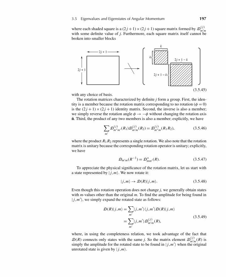
3.5 Eigenvalues and Eigenstates of Angular Momentum 197
where each shaded square is a (2 j +1)× (2 j +1) square matrix formed by D( j )m′m
with some definite value of j. Furthermore, each square matrix itself cannot bebroken into smaller blocks
2j + 1
2j + 1
2j + 1 − k
2j + 1 − k
k
k
(3.5.45)with any choice of basis.
The rotation matrices characterized by definite j form a group. First, the iden-tity is a member because the rotation matrix corresponding to no rotation (φ = 0)is the (2 j + 1) × (2 j + 1) identity matrix. Second, the inverse is also a member;we simply reverse the rotation angle φ→ −φ without changing the rotation axisn. Third, the product of any two members is also a member; explicitly, we have∑
m′D
( j )m′′m′ (R1)D ( j )
m′m(R2) = D( j )m′′m(R1 R2), (3.5.46)
where the product R1 R2 represents a single rotation. We also note that the rotationmatrix is unitary because the corresponding rotation operator is unitary; explicitly,we have
Dm′m(R−1) = D∗mm′ (R). (3.5.47)
To appreciate the physical significance of the rotation matrix, let us start witha state represented by | j ,m〉. We now rotate it:
| j ,m〉 → D(R)| j ,m〉. (3.5.48)
Even though this rotation operation does not change j, we generally obtain stateswith m-values other than the original m. To find the amplitude for being found in| j ,m ′〉, we simply expand the rotated state as follows:
D(R)| j ,m〉 =∑m′
| j ,m′〉〈 j ,m′|D(R)| j ,m〉
=∑m′
| j ,m′〉D ( j )m′m (R),
(3.5.49)
where, in using the completeness relation, we took advantage of the fact thatD(R) connects only states with the same j. So the matrix element D
( j )m′m (R) is
simply the amplitude for the rotated state to be found in | j ,m′〉 when the originalunrotated state is given by | j ,m〉.
198 Chapter 3 Theory of Angular Momentum
In Section 3.3 we saw how Euler angles may be used to characterize the mostgeneral rotation. We now consider the matrix realization of (3.3.20) for an arbi-trary j (not necessarily 1
2 ):
D( j )m′m (α,β,γ ) = 〈 j ,m ′|exp
(−i Jzα
h
)exp
(−i Jyβ
h
)exp
(−i Jzγ
h
)| j ,m〉
= e−i(m′α+mγ )〈 j ,m ′|exp
(−i Jyβ
h
)| j ,m〉.
(3.5.50)
Notice that the only nontrivial part is the middle rotation about the y-axis, whichmixes different m-values. It is convenient to define a new matrix d ( j )(β) as
d ( j )m′m (β) ≡ 〈 j ,m ′|exp
(−i Jyβ
h
)| j ,m〉. (3.5.51)
Finally, let us turn to some examples. The j = 12 case has already been worked
out in Section 3.3. See the middle matrix of (3.3.21),
d1/2 =
⎛⎜⎜⎝cos
(β
2
)−sin
(β
2
)sin
(β
2
)cos
(β
2
)⎞⎟⎟⎠ . (3.5.52)
The next simplest case is j = 1, which we consider in some detail. Clearly, wemust first obtain the 3 ×3 matrix representation of Jy . Because
Jy = (J+ − J−)
2i(3.5.53)
from the defining equation (3.5.5) for J±, we can use (3.5.41) to obtain
m = 1 m = 0 m = −1
J ( j=1)y =
(h
2
) ⎛⎜⎝ 0 −√2i 0√
2i 0 −√2i
0√
2i 0
⎞⎟⎠ m′ = 1m′ = 0.m′ = −1
(3.5.54)
Our next task is to work out the Taylor expansion of exp(−i Jyβ/h). Unlike the
case j = 12 , [J ( j=1)
y ]2 is independent of 1 and J ( j=1)y . However, it is easy to work
out: (J ( j=1)
y
h
)3
= J ( j=1)y
h. (3.5.55)
Consequently, for j = 1 only, it is legitimate to replace
exp
(−i Jyβ
h
)→ 1 −
(Jy
h
)2
(1 − cosβ) − i
(Jy
h
)sinβ, (3.5.56)
3.6 Orbital Angular Momentum 199
as the reader may verify in detail. Explicitly, we have
d (1)(β) =
⎛⎜⎜⎜⎜⎝(
12
)(1 + cosβ) −
(1√2
)sinβ
(12
)(1 − cosβ)(
1√2
)sinβ cosβ −
(1√2
)sinβ(
12
)(1 − cosβ)
(1√2
)sinβ
(12
)(1 + cosβ)
⎞⎟⎟⎟⎟⎠ . (3.5.57)
Clearly, this method becomes time-consuming for large j. Other, much easiermethods are possible, but we will not pursue them in this book.
3.6 ORBITAL ANGULAR MOMENTUM
We introduced the concept of angular momentum by defining it to be the gen-erator of an infinitesimal rotation. There is another way to approach the subjectof angular momentum when spin-angular momentum is zero or can be ignored.The angular momentum J for a single particle is then the same as orbital angularmomentum, which is defined as
L = x ×p. (3.6.1)
In this section we explore the connection between the two approaches.
Orbital Angular Momentum as Rotation Generator
We first note that the orbital angular-momentum operator defined as (3.6.1) satis-fies the angular-momentum commutation relations[
L i , L j]= iεi j k hLk (3.6.2)
by virtue of the commutation relations among the components of x and p. Thiscan easily be proved as follows:
[Lx , L y] = [ypz − zpy, zpx − x pz]= [ypz, zpx ] + [zpy, x pz]= ypx[pz , z] + pyx[z, pz]= i h(x py − ypx)= i hLz...
(3.6.3)
Next we let
1 − i
(δφ
h
)Lz = 1 − i
(δφ
h
)(x py − ypx) (3.6.4)
act on an arbitrary position eigenket |x ′, y′, z′〉 to examine whether it can be inter-preted as the infinitesimal rotation operator about the z-axis by angle δφ. Using
200 Chapter 3 Theory of Angular Momentum
the fact that momentum is the generator of translation, we obtain [see (1.6.32)][1 − i
(δφ
h
)Lz
]|x ′, y′, z′〉 =
[1 − i
(py
h
)(δφx ′) + i
(px
h
)(δφy ′)
]|x ′, y′, z′〉
= |x ′ − y ′δφ, y ′ + x ′δφ, z′〉.(3.6.5)
This is precisely what we expect if Lz generates an infinitesimal rotation about thez-axis. So we have demonstrated that if p generates translation, then L generatesrotation.
Suppose the wave function for an arbitrary physical state of a spinless par-ticle is given by 〈x ′, y′, z′|α〉. After an infinitesimal rotation about the z-axis isperformed, the wave function for the rotated state is
〈x ′, y′, z′|[
1 − i
(δφ
h
)Lz
]|α〉 = 〈x ′ + y ′δφ, y ′ − x ′δφ, z′|α〉. (3.6.6)
It is actually more transparent to change the coordinate basis:
〈x ′, y′, z′|α〉 → 〈r ,θ ,φ|α〉. (3.6.7)
For the rotated state we have, according to (3.6.6),
〈r ,θ ,φ|[
1 − i
(δφ
h
)Lz
]|α〉 = 〈r ,θ ,φ− δφ|α〉
= 〈r ,θ ,φ|α〉− δφ ∂∂φ
〈r ,θ ,φ|α〉.(3.6.8)
Because 〈r ,θ ,φ| is an arbitrary position eigenket, we can identify
〈x′|Lz |α〉 = −i h∂
∂φ〈x′|α〉, (3.6.9)
which is a well-known result from wave mechanics. Even though this relation canalso be obtained just as easily using the position representation of the momentumoperator, the derivation given here emphasizes the role of Lz as the generator ofrotation.
We next consider a rotation about the x-axis by angle δφx . In analogy with(3.6.6), we have
〈x ′, y′, z′|[
1 − i
(δφx
h
)Lx
]|α〉 = 〈x ′, y′ + z′δφx , z′ − y ′δφx |α〉. (3.6.10)
By expressing x ′, y ′, and z′ in spherical coordinates, we can show that
〈x′|Lx |α〉 = −i h
(−sinφ
∂
∂θ− cotθ cosφ
∂
∂φ
)〈x′|α〉. (3.6.11)
Likewise,
〈x′|L y|α〉 = −i h
(cosφ
∂
∂θ− cotθ sinφ
∂
∂φ
)〈x′|α〉. (3.6.12)
3.6 Orbital Angular Momentum 201
Using (3.6.11) and (3.6.12), for the ladder operator L± defined as in (3.5.5), wehave
〈x′|L±|α〉 = −i he±iφ(
±i∂
∂θ− cotθ
∂
∂φ
)〈x′|α〉. (3.6.13)
Finally, it is possible to write 〈x′|L2|α〉 using
L2 = L2z +
(1
2
)(L+L− + L−L+), (3.6.14)
(3.6.9), and (3.6.13), as follows:
〈x′|L2|α〉 = −h2[
1
sin2 θ
∂2
∂φ2 + 1
sinθ
∂
∂θ
(sinθ
∂
∂θ
)]〈x′|α〉. (3.6.15)
Apart from 1/r2, we recognize the differential operator that appears here to bejust the angular part of the Laplacian in spherical coordinates.
It is instructive to establish this connection between the L2 operator and theangular part of the Laplacian in another way by looking directly at the kinetic-energy operator. We first record an important operator identity,
L2 = x2p2 − (x ·p)2 + i hx ·p, (3.6.16)
where x2 is understood to be the operator x ·x, just as p2 stands for the operatorp ·p. The proof of this is straightforward:
L2 =∑
i j lmk
εi j k xi p jεlmk xl pm
=∑i j lm
(δilδ jm − δimδ j l)xi p j xl pm
=∑i j lm
[δilδ jmxi (xl p j − i hδ j l)pm − δimδ j lxi p j (pm xl + i hδlm )
]= x2p2 − i hx ·p−
∑i j lm
δimδ j l[xi pm(xl p j − i hδ j l) + i hδlm xi p j ]
= x2p2 − (x ·p)2 + i hx ·p.
(3.6.17)
Before taking the preceding expression between 〈x′| and |α〉, first note that
〈x′|x ·p|α〉 = x′· (−i h∇′〈x′|α〉)= −i hr
∂
∂r〈x′|α〉. (3.6.18)
Likewise,
〈x′|(x ·p)2|α〉 = −h2r∂
∂r
(r∂
∂r〈x′|α〉
)= −h2
(r2 ∂
2
∂r2 〈x′|α〉+ r∂
∂r〈x′|α〉
).
(3.6.19)
202 Chapter 3 Theory of Angular Momentum
Thus
〈x′|L2|α〉 = r2〈x′|p2|α〉+ h2(
r2 ∂2
∂r2 〈x′|α〉+ 2r∂
∂r〈x′|α〉
). (3.6.20)
In terms of the kinetic energy p2/2m, we have
1
2m〈x′|p2|α〉 = −
(h2
2m
)∇′2〈x′|α〉
= −(
h2
2m
)(∂2
∂r2 〈x′|α〉+ 2
r
∂
∂r〈x′|α〉− 1
h2r2〈x′|L2|α〉
).
(3.6.21)
The first two terms in the last line are just the radial part of the Laplacian actingon 〈x′|α〉. The last term must then be the angular part of the Laplacian acting on〈x′|α〉, in complete agreement with (3.6.15).
Spherical Harmonics
Consider a spinless particle subjected to a spherical symmetrical potential. Thewave equation is known to be separable in spherical coordinates, and the energyeigenfunctions can be written as
〈x′|n, l,m〉 = Rnl (r )Y ml (θ ,φ), (3.6.22)
where the position vector x′ is specified by the spherical coordinates r, θ , andφ, and n stands for some quantum number other than l and m—for example, theradial quantum number for bound-state problems or the energy for a free-particlespherical wave. As will be made clearer in Section 3.11, this form can be regardedas a direct consequence of the rotational invariance of the problem. When theHamiltonian is spherically symmetrical, H commutes with Lz and L2, and theenergy eigenkets are expected to be eigenkets of L2 and Lz also. Because Lk withk = 1,2,3 satisfy the angular-momentum commutation relations, the eigenvaluesof L2 and Lz are expected to be l(l + 1)h2, and mh = [−lh, (−l + 1)h, . . . , (l −1)h, lh].
Because the angular dependence is common to all problems with sphericalsymmetry, we can isolate it and consider
〈n|l,m〉 = Y ml (θ ,φ) = Y m
l (n), (3.6.23)
where we have defined a direction eigenket |n〉 . From this point of view, Y ml (θ ,φ)
is the amplitude for a state characterized by l, m to be found in the direction nspecified by θ and φ.
Suppose we have relations involving orbital angular-momentum eigenkets. Wecan immediately write the corresponding relations involving the spherical har-monics. For example, take the eigenvalue equation
Lz |l,m〉 = mh|l,m〉. (3.6.24)
3.6 Orbital Angular Momentum 203
Multiplying 〈n| on the left and using (3.6.9), we obtain
−i h∂
∂φ〈n|l,m〉 = mh〈n|l,m〉. (3.6.25)
We recognize this equation to be
−i h∂
∂φY m
l (θ ,φ) = mhY ml (θ ,φ), (3.6.26)
which implies that the φ-dependence Y ml (θ ,φ) must behave like eimφ . Likewise,
corresponding to
L2|l,m〉 = l(l + 1)h2|l,m〉, (3.6.27)
we have [see (3.6.15)][1
sinθ
∂
∂θ
(sinθ
∂
∂θ
)+ 1
sin2 θ
∂2
∂φ2+ l(l + 1)
]Y m
l = 0, (3.6.28)
which is simply the partial differential equation satisfied by Y ml itself. The orthog-
onality relation
〈l ′,m′|l,m〉 = δll′δmm′ (3.6.29)
leads to ∫ 2π
0dφ
∫ 1
−1d(cosθ )Y m′∗
l′ (θ ,φ)Y ml (θ ,φ) = δll′δmm′ , (3.6.30)
where we have used the completeness relation for the direction eigenkets,∫d�n|n〉〈n| = 1. (3.6.31)
To obtain the Y ml themselves, we may start with the m = l case. We have
L+|l, l〉 = 0, (3.6.32)
which, because of (3.6.13), leads to
−i heiφ[
i∂
∂θ− cotθ
∂
∂φ
]〈n|l, l〉 = 0. (3.6.33)
Remembering that the φ-dependence must behave like eilφ , we can easily showthat this partial differential equation is satisfied by
〈n|l, l〉 = Y ll (θ ,φ) = cle
ilφ sinl θ , (3.6.34)
204 Chapter 3 Theory of Angular Momentum
where cl is the normalization constant determined from (3.6.30) to be∗
cl =[
(−1)l
2l l!
]√[(2l + 1)(2l)!]
4π. (3.6.35)
Starting with (3.6.34) we can use
〈n|l,m − 1〉 = 〈n|L−|l,m〉√(l + m)(l − m + 1)h
= 1√(l + m)(l − m + 1)
e−iφ(
− ∂
∂θ+ i cotθ
∂
∂φ
)〈n|l,m〉
(3.6.36)
successively to obtain all Y ml with l fixed. Because this is done in many textbooks
on elementary quantum mechanics, (for example, Townsend 2000), we will notwork out the details here. The result for m ≥ 0 is
Y ml (θ ,φ) = (−1)l
2ll!
√(2l + 1)
4π
(l + m)!
(l − m)!eimφ 1
sinm θ
d l−m
d(cosθ )l−m(sinθ )2l , (3.6.37)
and we define Y −ml by
Y −ml (θ ,φ) = (−1)m[Y m
l (θ ,φ)]∗. (3.6.38)
Regardless of whether m is positive or negative, the θ -dependent part of Y ml (θ ,φ)
is [sinθ ]|m| times a polynomial in cosθ with a highest power of l −|m|. For m = 0,we obtain
Y 0l (θ ,φ) =
√2 l + 1
4πPl (cos θ ). (3.6.39)
From the point of view of the angular-momentum commutation relations alone,it might not appear obvious why l cannot be a half-integer. It turns out that severalarguments can be advanced against half-integer l-values. First, for half-integer l,and hence for half-integer m, the wave function would acquire a minus sign,
eim(2π) = −1, (3.6.40)
under a 2π rotation. As a result, the wave function would not be single-valued; wepointed out in Section 2.4 that the wave function must be single-valued becauseof the requirement that the expansion of a state ket in terms of position eigenketsbe unique. We can prove that if L, defined to be x × p, is to be identified as thegenerator of rotation, then the wave function must acquire a plus sign under a 2π
∗Normalization condition (3.6.30), of course, does not determine the phase of cl . The factor (−1)l
is inserted so that when we use the L− operator successively to reach the state m = 0, we obtainY 0
l with the same sign as the Legendre polynomial Pl (cosθ ) whose phase is fixed by Pl (1) = 1[see (3.6.39)].
3.6 Orbital Angular Momentum 205
rotation. This follows from the fact that the wave function for a 2π-rotated stateis the original wave function itself with no sign change:
〈x′|exp
(−i Lz2π
h
)|α〉 = 〈x ′ cos2π + y ′ sin2π , y′ cos2π − x ′ sin2π , z′|α〉
= 〈x′|α〉,(3.6.41)
where we have used the finite-angle version of (3.6.6). Next, let us supposeY m
l (θ ,φ) with a half-integer l were possible. To be specific, we choose the sim-plest case, l = m = 1
2 . According to (3.6.34) we would have
Y 1/21/2 (θ ,φ) = c1/2eiφ/2
√sin θ . (3.6.42)
From the property of L− [see (3.6.36)] we would then obtain
Y −1/21/2 (θ ,φ) = e−iφ
(− ∂
∂ θ+ i cotθ
∂
∂ φ
)(c1/2eiφ/2
√sinθ
)= −c1/2e−iφ/2 cotθ
√sinθ .
(3.6.43)
This expression is not permissible because it is singular at θ = 0, π . What isworse, from the partial differential equation⟨
n|L−|1
2,−1
2
⟩= −i he−iφ
(−i∂
∂ θ− cot θ
∂
∂ φ
)⟨n|1
2,−1
2
⟩= 0
(3.6.44)
we directly obtain
Y −1/21/2 = c′
1/2e−iφ/2√
sinθ , (3.6.45)
in sharp contradiction with (3.6.43). Finally, we know from the Sturm-Liouvilletheory of differential equations that the solutions of (3.6.28) with l integer forma complete set. An arbitrary function of θ and φ can be expanded in terms of Y m
lwith integer l and m only. For all these reasons it is futile to contemplate orbitalangular momentum with half-integer l-values.
Spherical Harmonics as Rotation Matrices
We conclude this section on orbital angular momentum by discussing the spheri-cal harmonics from the point of view of the rotation matrices introduced in thelast section. We can readily establish the desired connection between the twoapproaches by constructing the most general direction eigenket |n〉 by apply-ing appropriate rotation operators to |z〉, the direction eigenket in the positivez-direction. We wish to find D(R) such that
|n〉 = D(R)|z〉. (3.6.46)
206 Chapter 3 Theory of Angular Momentum
We can rely on the technique used in constructing the eigenspinor of σ · n inSection 3.2. We first rotate about the y-axis by angle θ , then around the z-axis byangle φ; see Figure 3.3 with β → θ , α → φ. In the notation of Euler angles, wehave
D(R) = D(α = φ,β = θ ,γ = 0). (3.6.47)
Writing (3.6.46) as
|n〉 =∑
l
∑m
D(R)|l,m〉〈l,m|z〉. (3.6.48)
we see that |n〉, when expanded in terms of |l,m〉, contains all possible l-values.However, when this equation is multiplied by 〈l,m ′| on the left, only one term inthe l-sum contributes, namely,
〈l,m ′|n〉 =∑
m
D (l)m′m(α = φ,β = θ ,γ = 0)〈l,m|z〉. (3.6.49)
Now 〈l,m|z〉 is just a number; in fact, it is precisely Y m∗l (θ ,φ) evaluated at θ = 0
with φ undetermined. At θ = 0, Y ml is known to vanish for m �= 0, which can
also be seen directly from the fact that |z〉 is an eigenket of Lz (which equalsx py − ypx) with eigenvalue zero. So we can write
〈l,m|z〉 = Y m∗l (θ = 0,φ undetermined)δm 0
=√
(2 l + 1)
4πPl (cos θ )
∣∣∣∣∣cos θ=1
δm 0
=√
(2 l + 1)
4πδm 0.
(3.6.50)
Returning to (3.6.49), we have
Y m′∗l (θ ,φ) =
√(2 l + 1)
4πD (l)
m′0(α = φ,β = θ ,γ = 0) (3.6.51)
or
D (l)m 0(α,β,γ = 0) =
√4π
(2 l + 1)Y m∗
l (θ ,φ)
∣∣∣∣∣θ=β,φ=α
(3.6.52)
Notice the m = 0 case, which is of particular importance:
d (l)00 (β)
∣∣∣β=θ = Pl (cos θ ). (3.6.53)
3.7 Schrödinger’s Equation for Central Potentials 207
3.7 SCHRÖDINGER’S EQUATION FOR CENTRAL POTENTIALS
Problems described by Hamiltonians of the form
H = p2
2m+ V (r ) r2 = x2 (3.7.1)
are the basis for very many situations in the physical world. The fundamentalimportance of this Hamiltonian lies in the fact that it is spherically symmetri-cal. Classically, we expect orbital angular momentum to be conserved in such asystem. This is also true quantum-mechanically, because it is easy to show that
[L,p2] = [L,x2] = 0 (3.7.2)
and therefore
[L, H ] = [L2, H ] = 0 (3.7.3)
if H is given by (3.7.1). We refer to such problems as central-potential or central-force problems. Even if the Hamiltonian isn’t strictly of this form, it is often thecase that this is a good starting point when we consider approximation schemesthat build on “small” corrections to central-potential problems.
In this section we will discuss some general properties of eigenfunctions gen-erated by (3.7.1) and a few representative central-potential problems. For moredetail, the reader is referred to any number of excellent texts that explore suchproblems in greater depth.
The Radial Equation
Equation (3.7.3) makes it clear that we should search for energy eigenstates |α〉 =|Elm〉 where
H |Elm〉 = E |Elm〉, (3.7.4)
L2|Elm〉 = l(l + 1)h2|Elm〉, (3.7.5)
Lz |Elm〉 = mh|Elm〉. (3.7.6)
It is easiest to work in the coordinate representation and solve the appropriatedifferential equation for eigenfunctions in terms of a radial function REl (r ) andspherical harmonics, as shown in (3.6.22). Combining (3.7.1), (3.7.4), and (3.7.5)with (3.6.21) and (3.6.22), we arrive at the radial equation∗[
− h2
2mr2
d
dr
(r2 d
dr
)+ l(l + 1)h2
2mr2+ V (r )
]REl (r ) = E REl (r ). (3.7.7)
∗We apologize for using m to represent both “mass” and the quantum number for angular mo-mentum. However, in this section, it should be clear from the context which is which.
208 Chapter 3 Theory of Angular Momentum
Depending on the specific form of V (r ), we may work with this equation or somevariant of it to identify the radial part REl (r ) of the eigenfunction and/or the en-ergy eigenvalues E .
In fact, we can immediately gain some insight into the effects of angular mo-mentum on the eigenfunctions by making the substitution
REl (r ) = uEl (r )
r, (3.7.8)
which reduces (3.7.7) to
− h2
2m
d2uEl
dr2+[
l(l + 1)h2
2mr2+ V (r )
]uEl (r ) = EuEl (r ). (3.7.9)
Coupling this with the fact that the spherical harmonics are separately normalized,so that the overall normalization condition becomes
1 =∫
r2dr R∗El (r )REl (r ) =
∫dr u∗
El (r )uEl (r ), (3.7.10)
we see that uEl (r ) can be interpreted as a wave function in one dimension for aparticle moving in an “effective potential”
Veff(r ) = V (r ) + l(l + 1)h2
2mr2. (3.7.11)
Equation (3.7.11) demonstrates the existence of an “angular-momentum barrier”if l �= 0, as shown in Figure 3.5. Quantum-mechanically, this means that the am-plitude (and therefore the probability) is small for locating the particle near theorigin, except for s-states. As we will see later on, this fact has important physicalconsequences in atoms, for example.
We can be more quantitative about this interpretation. Let us assume that thepotential-energy function V (r ) is not so singular so that limr→0 r2V (r ) = 0. Then,for small values of r , (3.7.9) becomes
d2uEl
dr2= l(l + 1)
r2uEl (r ) (r → 0), (3.7.12)
which has the general solution u(r ) = Ar l+1 + Br−l . It is tempting to set B = 0out of hand, because 1/r l produces severe singularities as r → 0, especially forlarge l. However, there are better reasons for setting B = 0, reasons that are rootedin the foundations of quantum mechanics.
Consider the probability flux given by (2.4.16). This is a vector quantity whoseradial component is
jr = r · j = h
mIm
(ψ∗ ∂∂rψ
)= h
mREl (r )
d
drREl (r ). (3.7.13)
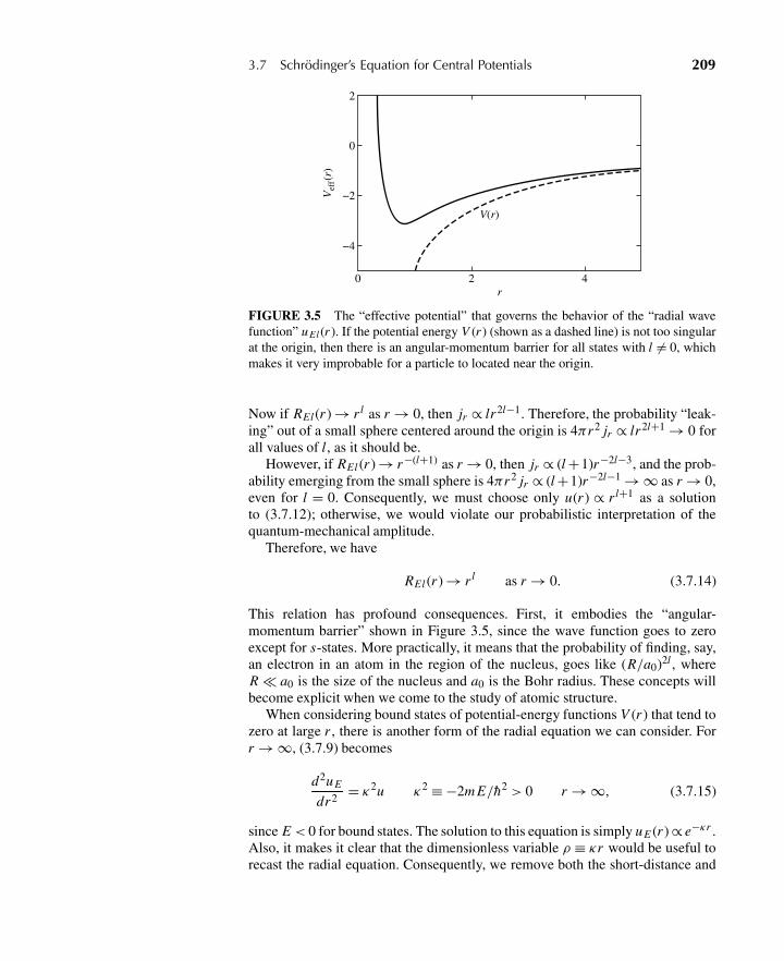
3.7 Schrödinger’s Equation for Central Potentials 209
V(r)
r
Vef
f(r)
−4
−2
0
2
0 2 4
FIGURE 3.5 The “effective potential” that governs the behavior of the “radial wavefunction” uEl (r ). If the potential energy V (r ) (shown as a dashed line) is not too singularat the origin, then there is an angular-momentum barrier for all states with l �= 0, whichmakes it very improbable for a particle to located near the origin.
Now if REl (r ) → r l as r → 0, then jr ∝ lr2l−1. Therefore, the probability “leak-ing” out of a small sphere centered around the origin is 4πr2 jr ∝ lr2l+1 → 0 forall values of l, as it should be.
However, if REl (r ) → r−(l+1) as r → 0, then jr ∝ (l +1)r−2l−3, and the prob-ability emerging from the small sphere is 4πr2 jr ∝ (l +1)r−2l−1 → ∞ as r → 0,even for l = 0. Consequently, we must choose only u(r ) ∝ r l+1 as a solutionto (3.7.12); otherwise, we would violate our probabilistic interpretation of thequantum-mechanical amplitude.
Therefore, we have
REl (r ) → r l as r → 0. (3.7.14)
This relation has profound consequences. First, it embodies the “angular-momentum barrier” shown in Figure 3.5, since the wave function goes to zeroexcept for s-states. More practically, it means that the probability of finding, say,an electron in an atom in the region of the nucleus, goes like (R/a0)2l , whereR � a0 is the size of the nucleus and a0 is the Bohr radius. These concepts willbecome explicit when we come to the study of atomic structure.
When considering bound states of potential-energy functions V (r ) that tend tozero at large r , there is another form of the radial equation we can consider. Forr → ∞, (3.7.9) becomes
d2uE
dr2 = κ2u κ2 ≡ −2m E/h2 > 0 r → ∞, (3.7.15)
since E < 0 for bound states. The solution to this equation is simply uE (r ) ∝ e−κr .Also, it makes it clear that the dimensionless variable ρ ≡ κr would be useful torecast the radial equation. Consequently, we remove both the short-distance and
210 Chapter 3 Theory of Angular Momentum
the long-distance behavior of the wave function and write
uEl (ρ) = ρl+1e−ρw(ρ), (3.7.16)
where the function w(ρ) is “well behaved” and satisfies
d2w
dρ2+ 2
(l + 1
ρ− 1
)dw
dρ+[
V
E− 2(l + 1)
ρ
]w = 0. (3.7.17)
(The manipulations that lead to this equation are left to the reader.) One thenattacks the solution w(ρ) of (3.7.17) for the particular function V (r = ρ/κ).
The Free Particle and the Infinite Spherical Well
In Section 2.5 we saw the solution to the free-particle problem in three dimen-sions, using Cartesian coordinates. We can of course approach the same problemby exploiting spherical symmetry and angular momentum. Starting from (3.7.7),we write
E ≡ h2k2
2mand ρ ≡ kr (3.7.18)
and arrive at the modified radial equation
d2 R
dρ2+ 2
ρ
d R
dρ+[
1 − l(l + 1)
ρ2
]R = 0. (3.7.19)
This is a well-known differential equation whose solutions are called sphericalBessel functions jl(ρ) and nl (ρ), where
jl(ρ) = (−ρ)l[
1
ρ
d
dρ
]l ( sinρ
ρ
), (3.7.20a)
nl (ρ) = −(−ρ)l[
1
ρ
d
dρ
]l (cosρ
ρ
). (3.7.20b)
It is easy to show that as ρ → 0, jl(ρ) → ρl and nl (ρ) → ρ−l−1. Hence, jl(ρ)corresponds to (3.7.14) and these are the only solutions we consider here.∗ It isalso useful to point out that the spherical Bessel functions are defined over theentire complex plane, and it can be shown that
jl(z) = 1
2i l
∫ 1
−1ds eizs Pl (s). (3.7.21)
∗In a treatment of “hard sphere scattering” problems, the origin is explicitly excluded, and thesolutions nl (ρ) are also kept. The relative phase between the two solutions for a given l is calledthe phase shift.
3.7 Schrödinger’s Equation for Central Potentials 211
The first few spherical Bessel functions are
j0(ρ) = sinρ
ρ, (3.7.22)
j1(ρ) = sinρ
ρ2 − cosρ
ρ, (3.7.23)
j2(ρ) =[
3
ρ3− 1
ρ
]sinρ− 3cosρ
ρ2. (3.7.24)
This result can be immediately applied to the case of a particle confined toan infinite spherical well, i.e., a potential-energy function V (r ) = 0 within r < a,but with the wave function constrained to be zero at r = a. For any given valueof l, this leads to the “quantization condition” jl(ka) = 0; that is, ka equals theset of zeros of the spherical Bessel function. For l = 0 these are obviously ka =π ,2π ,3π , . . . . For other values of l, computer programs are readily available thatcan compute the zeros. We find that
El=0 = h2
2ma2
[π2, (2π)2, (3π)2, . . .
], (3.7.25)
El=1 = h2
2ma2
[4.492,7.732,10.902, . . .
], (3.7.26)
El=2 = h2
2ma2
[5.842,8.962,12.252, . . .
]. (3.7.27)
It should be noted that this series of energy levels shows no degeneracies in l.Indeed, such degenerate energy levels are impossible, except for any accidentalequality between zeros of spherical Bessel functions of different orders.
The Isotropic Harmonic Oscillator
Energy eigenvalues for the Hamiltonian
H = p2
2m+ 1
2mω2r2 (3.7.28)
are straightforward to determine. Introducing dimensionless energy λ and radialcoordinate ρ through
E = 1
2hωλ and r =
[h
mω
]1/2
ρ, (3.7.29)
we transform (3.7.9) into
d2u
dρ2 − l(l + 1)
ρ2 u(ρ) + (λ−ρ2)u(ρ) = 0. (3.7.30)
212 Chapter 3 Theory of Angular Momentum
It is again worthwhile to explicitly remove the behavior for large (and small) ρ,although we cannot use (3.7.16) because V (r ) does not tend to zero for large r .Instead, we write
u(ρ) = ρl+1e−ρ2/2 f (ρ). (3.7.31)
This yields the following differential equation for the function f (ρ):
ρd2 f
dρ2 + 2[(l + 1) −ρ2]d f
dρ+ [λ− (2l + 3)]ρ f (ρ) = 0. (3.7.32)
We solve (3.7.32) by writing f (ρ) as an infinite series, namely
f (ρ) =∞∑
n=0
anρn . (3.7.33)
We insert this into the differential equation and set each term to zero by powersof ρ. The only surviving term in ρ0 is 2(l + 1)a1, so
a1 = 0 (3.7.34)
The terms proportional to ρ1 allow us to relate a2 to a0, which in turn can be setthrough the normalization condition. Continuing, (3.7.32) becomes
∞∑n=2
{(n + 2)(n + 1)an+2 + 2(l + 1)(n + 2)an+2 − 2nan + [λ− (2l + 3]an}ρn+1 = 0,
(3.7.35)which leads, finally, to the recursion relation
an+2 = 2n + 2l + 3 −λ(n + 2)(n + 2l + 3)
an . (3.7.36)
Immediately we see that f (ρ) involves only even powers of ρ, since (3.7.34) and(3.7.36) imply that an = 0 for odd n. Also, as n → ∞, we have
an+2
an→ 2
n= 1
q, (3.7.37)
where q = n/2 includes both odd and even integers. Therefore, for large valuesof ρ, (3.7.33) becomes
f (ρ) → constant×∑
q
1
q!
(ρ2)q ∝ eρ
2. (3.7.38)
In other words, u(ρ) from (3.7.31) would grow exponentially for large ρ (andwould therefore be unable to meet the normalization condition) unless the seriesterminates. Therefore,
2n + 2l + 3 −λ= 0 (3.7.39)
3.7 Schrödinger’s Equation for Central Potentials 213
for some even value of n = 2q , and the energy eigenvalues are
Eql =(
2q + l + 3
2
)hω ≡
(N + 3
2
)hω (3.7.40)
for q = 0,1,2, . . . and l = 0,1,2 . . . , and N ≡ 2q + l. One frequently refers to Nas the “principal” quantum number. It can be shown that q counts the number ofnodes in the radial function.
Quite unlike the square well, the three-dimensional isotropic harmonic oscil-lator has degenerate energy eigenvalues in the l quantum number. There are threestates (all l = 1) for N = 1. For N = 2 there are five states with l = 2, plus onestate with q = 1 and l = 0, giving a total of six. Notice that for even (odd) valuesof N , only even (odd) values of l are allowed. Therefore, the parity of the wavefunction is even or odd with the value of N .
These wave functions are popular basis states for calculations of various nat-ural phenomena, when the potential-energy function is a “well” of some finitesize. One of the greatest successes of such an approach is the nuclear shell model,where individual protons and neutrons are pictured as moving independently ina potential-energy function generated by the cumulative effect of all nucleons inthe nucleus. Figure 3.6 compares the energy levels observed in nuclei with thoseobtained for the isotropic harmonic oscillator and for the infinite spherical well.
It is natural to label the eigenstates of the Hamiltonian (3.7.28) as |qlm〉 or|Nlm〉. However, this Hamiltonian may also be written as
H = Hx + Hy + Hz, (3.7.41)
where Hi = a†i ai + 1
2 is an independent one-dimensional harmonic oscillator indirection i = x , y, z. In this way, we would label the eigenstates |nx ,ny ,nz〉, andthe energy eigenvalues are
E =(
nx + 1
2+ nx + 1
2+ nx + 1
2
)hω
=(
N + 3
2
)hω, (3.7.42)
where, now, N = nx + ny + nz . It is simple to show numerically that for the firstfew energy levels, the degeneracy is the same regardless of which basis is used. Itis an interesting exercise to show this in general—and also to derive the unitarytransformation matrix 〈nx ,ny ,nz |qlm〉 that changes from one basis to the other.(See Problem 3.21 at the end of this chapter.)
The Coulomb Potential
Perhaps the most important potential-energy function in physics is
V (x) = − Ze2
r, (3.7.43)
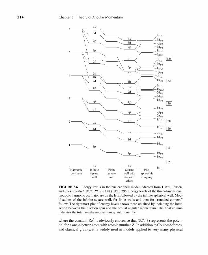
214 Chapter 3 Theory of Angular Momentum
4s
3d
2g
3p
1i2f
3s1h2d
1g
2p
1f
2s
1d
1p
1s
1p
1s
1d
2s
1f
2p
1g
2d
3s
1h
2f
3p
1i
2g3d4s
4s1/2
3d3/22g7/23d5/21i11/22g9/2
2f5/23p1/2
1i13/23p3/2
2f7/2
1h9/2
3s1/21h11/22d3/22d5/21g7/2
1g9/2
2p1/22p3/21f5/2
1f7/2
2s1/21d3/2
1d5/2
1p1/21p3/2
1s1/2
6
5
4
3
2
1
0Harmonicoscillator
Infinitesquarewell
Finitesquarewell
Squarewell withroundededges
Plusspin-orbitcoupling
126
82
50
28
20
8
2
FIGURE 3.6 Energy levels in the nuclear shell model, adapted from Haxel, Jensen,and Suess, Zeitschrift für Physik 128 (1950) 295. Energy levels of the three-dimensionalisotropic harmonic oscillator are on the left, followed by the infinite spherical well. Mod-ifications of the infinite square well, for finite walls and then for “rounded corners,”follow. The rightmost plot of energy levels shows those obtained by including the inter-action between the nucleon spin and the orbital angular momentum. The final columnindicates the total angular-momentum quantum number.
where the constant Ze2 is obviously chosen so that (3.7.43) represents the poten-tial for a one-electron atom with atomic number Z . In addition to Coulomb forces,and classical gravity, it is widely used in models applied to very many physical
3.7 Schrödinger’s Equation for Central Potentials 215
systems.∗ We consider here the radial equation based on such a function and theresulting energy eigenvalues.
The 1/r potential satisfies all the requirements that led us to (3.7.17). We there-fore search for solutions of the form (3.7.16) by determining the function w(ρ).Making the definition
ρ0 =[
2m
−E
]1/2 Ze2
h=[
2mc2
−E
]1/2
Zα, (3.7.44)
where α ≡ e2/hc ≈ 1/137 is the fine structure constant, (3.7.17) becomes
ρd2w
dρ2+ 2(l + 1 −ρ)
dw
dρ+ [ρ0 − 2(l + 1)]w(ρ) = 0. (3.7.45)
We could of course proceed to solve (3.7.45) using a series approach and derivea recursion relation for the coefficients, just as we did with (3.7.32). However, itturns out that the solution is in fact already well known.
Equation (3.7.45) can be written as Kummer’s Equation:
xd2 F
dx2 + (c − x)d F
dx− a F = 0, (3.7.46)
where
x = 2ρ,
c = 2(l + 1),
and 2a = 2(l + 1) −ρ0. (3.7.47)
The solution to (3.7.46) is called the Confluent Hypergeometric Function, whichis written as the series
F(a;c; x) = 1 + a
c
x
1!+ a(a + 1)
c(c + 1)
x2
2!+·· · , (3.7.48)
and so
w(ρ) = F(
l + 1 − ρ0
2; 2(l + 1) ; 2ρ
). (3.7.49)
Note that for large ρ, we have
w(ρ) ≈∑
Large N
a(a + 1) · · ·c(c + 1) · · ·
(2ρ)N
N!
≈∑
Large N
(N/2)N
N N
(2ρ)N
N!≈
∑Large N
(ρ)N
N!≈ eρ .
∗Indeed, 1/r potential energy functions result from any quantum field theory in three spatialdimensions with massless intermediate exchange particles. See Chapter I.6 in Zee (2010).
216 Chapter 3 Theory of Angular Momentum
Therefore, once again, (3.7.16) gives a radial wave function that would grow with-out bound unless the series (3.7.48) terminated. So, for some integer N , we musthave a + N = 0 that leads to
ρ0 = 2(N + l + 1), (3.7.50)
where N = 0,1,2 . . .
and l = 0,1,2, . . . .
It is customary (and, as we shall soon see, instructive) to define the principalquantum number n as
n ≡ N + l + 1 = 1,2,3, . . . , (3.7.51)
where l = 0,1, . . . ,n − 1.
We point out that it is possible to solve the radial equation for the Coulomb prob-lem using the generating-function techniques described in Section 2.5. See Prob-lem 3.22 at the end of this chapter.
Energy eigenvalues arise by combining (3.7.44) and (3.7.50) in terms of theprincipal quantum number; that is,
ρ0 =[
2mc2
−E
]1/2
Zα = 2n, (3.7.52)
which leads to
E = −1
2mc2 Z2α2
n2 = −13.6 eVZ2
n2 , (3.7.53)
where the numerical result is for a one-electron atom—that is, mc2 = 511 keV.Equation (3.7.53) is of course the familiar Balmer formula.
It is time to make various points. First, there is a stark disagreement betweenthe energy-level properties predicted by modern quantum mechanics, and those ofthe old Bohr model of the atom. The Bohr model had a one-to-one correspondencebetween angular-momentum eigenvalues l and principal quantum number n; infact, the ground state corresponded to n = l = 1. We see instead that only l = 0is allowed for n = 1 and that different values of l are allowed for higher energylevels.
Second, a natural length scale a0 has emerged. Since ρ = κr , where κ =√−2m E/h2 [see (3.7.15)], we have
1
κ= h
mcα
n
Z≡ a0
n
Z, (3.7.54)
where
a0 = h
mcα= h2
me2(3.7.55)
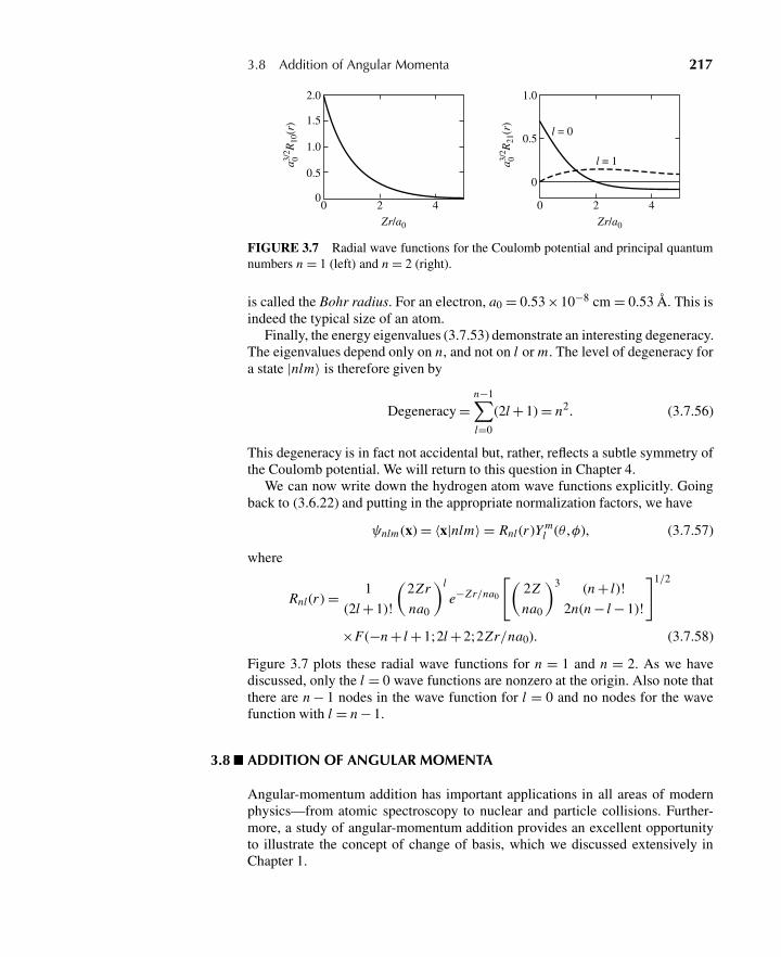
3.8 Addition of Angular Momenta 217
2.0
1.5
1.0
0.5
00 2 4
0.5
1.0
0
0 2 4
a3/2 R
10(r
)0 a3/
2 R21
(r)
0
Zr/a0 Zr/a0
l = 0
l = 1
FIGURE 3.7 Radial wave functions for the Coulomb potential and principal quantumnumbers n = 1 (left) and n = 2 (right).
is called the Bohr radius. For an electron, a0 = 0.53×10⁻⁸ cm = 0.53 Å. This isindeed the typical size of an atom.
Finally, the energy eigenvalues (3.7.53) demonstrate an interesting degeneracy.The eigenvalues depend only on n, and not on l or m. The level of degeneracy fora state |nlm〉 is therefore given by
Degeneracy =n−1∑l=0
(2l + 1) = n2. (3.7.56)
This degeneracy is in fact not accidental but, rather, reflects a subtle symmetry ofthe Coulomb potential. We will return to this question in Chapter 4.
We can now write down the hydrogen atom wave functions explicitly. Goingback to (3.6.22) and putting in the appropriate normalization factors, we have
ψnlm (x) = 〈x|nlm〉 = Rnl (r )Y ml (θ ,φ), (3.7.57)
where
Rnl (r ) = 1
(2l + 1)!
(2Zr
na0
)l
e−Zr/na0
[(2Z
na0
)3 (n + l)!
2n(n − l − 1)!
]1/2
×F(−n + l + 1;2l + 2;2Zr/na0). (3.7.58)
Figure 3.7 plots these radial wave functions for n = 1 and n = 2. As we havediscussed, only the l = 0 wave functions are nonzero at the origin. Also note thatthere are n − 1 nodes in the wave function for l = 0 and no nodes for the wavefunction with l = n − 1.
3.8 ADDITION OF ANGULAR MOMENTA
Angular-momentum addition has important applications in all areas of modernphysics—from atomic spectroscopy to nuclear and particle collisions. Further-more, a study of angular-momentum addition provides an excellent opportunityto illustrate the concept of change of basis, which we discussed extensively inChapter 1.
218 Chapter 3 Theory of Angular Momentum
Simple Examples of Angular-Momentum Addition
Before studying a formal theory of angular-momentum addition, it is worth look-ing at two simple examples with which the reader may be familiar: (1) how to addorbital angular momentum and spin-angular momentum and (2) how to add thespin-angular momenta of two spin 1
2 particles.Previously we studied both spin 1
2 systems with all quantum-mechanical de-grees of freedom other than spin—such as position and momentum—ignored andquantum-mechanical particles with the space degrees of freedom (such as posi-tion and momentum) taken into account but the internal degrees of freedom (suchas spin) ignored. A realistic description of a particle with spin must of coursetake into account both the space degree of freedom and the internal degrees offreedom. The base ket for a spin 1
2 particle may be visualized to be in the direct-product space of the infinite-dimensional ket space spanned by the position eigen-kets {|x′〉} and the two-dimensional spin space spanned by |+〉 and |−〉. Explicitly,we have for the base ket
|x′,±〉 = |x′〉⊗ |±〉, (3.8.1)
where any operator in the space spanned by {|x′〉} commutes with any operator inthe two-dimensional space spanned by |±〉.
The rotation operator still takes the form exp(−iJ · nφ/h) but J, the generatorof rotations, is now made up of two parts, namely
J = L+ S. (3.8.2)
It is actually more obvious to write (3.8.2) as
J = L⊗1 + 1 ⊗S, (3.8.3)
where the 1 in L⊗1 stands for the identity operator in the spin space, and the 1 in1⊗S stands for the identity operator in the infinite-dimensional ket space spannedby the position eigenkets. Because L and S commute, we can write
D(R) = D (orb)(R) ⊗D (spin)(R) = exp
(−iL · nφh
)⊗ exp
(−iS · nφh
). (3.8.4)
The wave function for a particle with spin is written as
〈x′,±|α〉 = ψ±(x′). (3.8.5)
The two components ψ± are often arranged in column matrix form as follows:(ψ+(x′)ψ−(x′)
), (3.8.6)
where |ψ±(x′)|2 stands for the probability density for the particle to be found at x′with spin up and down, respectively. Instead of |x′〉 as the base kets for the spacepart, we may use |n, l,m〉, which are eigenkets of L2 and Lz with eigenvalues
3.8 Addition of Angular Momenta 219
h2l(l + 1) and ml h, respectively. For the spin part, |±〉 are eigenkets of S2 andSz with eigenvalues 3h2/4 and ±h/2, respectively. However, as we will showlater, we can also use base kets that are eigenkets of J2, Jz , L2, and S2. In otherwords, we can expand a state ket of a particle with spin in terms of simultaneouseigenkets of L2, S2, Lz , and Sz or in terms of simultaneous eigenkets of J2, Jz ,L2, and S2. We will study in detail how the two descriptions are related.
As a second example, we study two spin 12 particles—say two electrons—
with the orbital degree of freedom suppressed. The total spin operator is usuallywritten as
S = S1 + S2, (3.8.7)
but again it is to be understood as
S1 ⊗1 + 1 ⊗S2, (3.8.8)
where the 1 in the first (second) term stands for the identity operator in the spinspace of electron 2 (1). We, of course, have[
S1x , S2y]= 0 (3.8.9)
and so forth. Within the space of electron 1(2), we have the usual commutationrelations [
S1x , S1y] = i hS1z ,
[S2x , S2y
] = i hS2z , . . . . (3.8.10)
As a direct consequence of (3.8.9) and (3.8.10), we have[Sx , Sy
]= i hSz (3.8.11)
and so on for the total spin operator.The eigenvalues of the various spin operators are denoted as follows:
S2 = (S1 + S2)2 : s(s + 1)h2
Sz = S1z + S2z : mhS1z : m1hS2z : m2h
(3.8.12)
Again, we can expand the ket corresponding to an arbitrary spin state of twoelectrons in terms of either the eigenkets of S2 and Sz or the eigenkets of S1z andS2z . The two possibilities are as follows:
1. The {m1,m2} representation based on the eigenkets of S1z and S2z :
|++〉, |+−〉, |−+〉, and |−−〉, (3.8.13)
where |+−〉 stands for m1 = 12 ,m2 = − 1
2 , and so forth.
220 Chapter 3 Theory of Angular Momentum
2. The {s,m} representation (or the triplet-singlet representation) based on theeigenkets of S2 and Sz :
|s = 1,m = ±1,0〉, |s = 0,m = 0〉, (3.8.14)
where s = 1 (s = 0) is referred to as a spin triplet (spin singlet).
Notice that in each set there are four base kets. The relationship between thetwo sets of base kets is as follows:
|s = 1,m = 1〉 = |++〉, (3.8.15a)
|s = 1,m = 0〉 =(
1√2
)(|+−〉+ |−+〉), (3.8.15b)
|s = 1,m = −1〉 = |−−〉, (3.8.15c)
|s = 0,m = 0〉 =(
1√2
)(|+−〉− |−+〉). (3.8.15d)
The right-hand side of (3.8.15a) tells us that we have both electrons with spin up;this situation can correspond only to s = 1, m = 1. We can obtain (3.8.15b) from(3.8.15a) by applying the ladder operator
S− ≡ S1− + S2−= (S1x − i S1y) + (S2x − i S2y)
(3.8.16)
to both sides of (3.8.15a). In doing so we must remember that an electron 1 oper-ator like S1− affects just the first entry of |++〉, and so on. We can write
S−|s = 1,m = 1〉 = (S1− + S2−)|++〉 (3.8.17)
as
√(1 + 1)(1 − 1 + 1)|s = 1,m = 0〉 =
√(12 + 1
2
)(12 − 1
2 + 1)
×|−+〉
+√(
12 + 1
2
)(12 − 1
2 + 1)|+−〉,
(3.8.18)
which immediately leads to (3.8.15b). Likewise, we can obtain |s = 1, m = −1〉by applying (3.8.16) once again to (3.8.15b). Finally, we can obtain (3.8.15d) byrequiring it to be orthogonal to the other three kets, in particular to (3.8.15b).
The coefficients that appear on the right-hand side of (3.8.15) are the simplestexample of Clebsch-Gordan coefficients, which we will discuss further at a latertime. They are simply the elements of the transformation matrix that connects the{m1,m2} basis to the {s,m} basis. It is instructive to derive these coefficients inanother way. Suppose we write the 4 ×4 matrix corresponding to
S2 = S21 + S2
2 + 2S1 · S2
= S21 + S2
2 + 2S1z S2z + S1+S2− + S1−S2+(3.8.19)
3.8 Addition of Angular Momenta 221
using the (m1,m2) basis. The square matrix is obviously not diagonal because anoperator like S1+ connects |−+〉 with |++〉. The unitary matrix that diagonalizesthis matrix carries the |m1,m2〉 base kets into the |s,m〉 base kets. The elements ofthis unitary matrix are precisely the Clebsch-Gordan coefficients for this problem.The reader is encouraged to work out all this in detail.
Formal Theory of Angular-Momentum Addition
Having gained some physical insight by considering simple examples, we arenow in a position to study more systematically the formal theory of angular-momentum addition. Consider two angular-momentum operators J1 and J2 in dif-ferent subspaces. The components of J1(J2) satisfy the usual angular-momentumcommutation relations: [
J1i , J1 j]= i hεi j k J1k (3.8.20a)
and [J2i , J2 j
]= i hεi j k J2k . (3.8.20b)
However, we have
[J1k , J2l] = 0 (3.8.21)
between any pair of operators from different subspaces.The infinitesimal rotation operator that affects both subspace 1 and subspace 2
is written as(1 − iJ1 · nδφ
h
)⊗(
1 − iJ2 · nδφh
)= 1 − i (J1 ⊗1 + 1 ⊗J2) · nδφ
h. (3.8.22)
We define the total angular momentum by
J ≡ J1 ⊗1 + 1 ⊗J2, (3.8.23)
which is more commonly written as
J = J1 + J2. (3.8.24)
The finite-angle version of (3.8.22) is
D1(R) ⊗D2(R) = exp
(−iJ1 · nφh
)⊗ exp
(−iJ2 · nφh
). (3.8.25)
Notice the appearance of the same axis of rotation and the same angle of rotation.It is very important to note that the total J satisfies the angular-momentum
commutation relations [Ji , Jj
]= i hεi j k Jk (3.8.26)
222 Chapter 3 Theory of Angular Momentum
as a direct consequence of (3.8.20) and (3.8.21). In other words, J is an angularmomentum in the sense of Section 3.1. Physically this is reasonable because Jis the generator for the entire system. Everything we learned in Section 3.5—forexample, the eigenvalue spectrum of J2 and Jz and the matrix elements of theladder operators—also holds for the total J.
As for the choice of base kets, we have two options.Option A: Simultaneous eigenkets of J2
1, J22, J1z , and J2z . We denote these by
| j1 j2;m1m2〉. Obviously the four operators commute with each other. The defin-ing equations are
J21| j1 j2;m1m2〉 = j1( j1 + 1)h2| j1 j2;m1m2〉, (3.8.27a)
J1z | j1 j2;m1m2〉 = m1h| j1 j2;m1m2〉, (3.8.27b)
J22| j1 j2;m1m2〉 = j2( j2 + 1)h2| j1 j2;m1m2〉, (3.8.27c)
J2z | j1 j2;m1m2〉 = m2h| j1 j2;m1m2〉. (3.8.27d)
Option B: Simultaneous eigenkets of J2, J21, J2
2, and Jz . First, note that this setof operators mutually commute. In particular, we have[
J2,J21
]= 0, (3.8.28)
which can readily be seen by writing J2 as
J2 = J21 + J2
2 + 2J1z J2z + J1+ J2− + J1− J2+. (3.8.29)
We use | j1, j2; jm〉 to denote the base kets of option B:
J21| j1 j2; jm〉 = j1( j1 + 1)h2| j1 j2; jm〉, (3.8.30a)
J22| j1 j2; jm〉 = j2( j2 + 1)h2| j1 j2; jm〉, (3.8.30b)
J2| j1 j2; jm〉 = j ( j + 1)h2| j1 j2; jm〉, (3.8.30c)
Jz| j1 j2; jm〉 = mh| j1 j2; jm〉. (3.8.30d)
Quite often j1, j2 are understood, and the base kets are written simply as | j ,m〉.It is very important to note that even though[
J2, Jz]= 0, (3.8.31)
we have [J2, J1z
] �= 0,[J2, J2z
] �= 0, (3.8.32)
as the reader may easily verify using (3.8.29). This means that we cannot add J2
to the set of operators of option A. Likewise, we cannot add J1z and/or J2z to theset of operators of option B. We have two possible sets of base kets correspondingto the two maximal sets of mutually compatible observables we have constructed.

3.8 Addition of Angular Momenta 223
Let us consider the unitary transformation in the sense of Section 1.5 that con-nects the two bases:
| j1 j2; jm〉 =∑m1
∑m2
| j1 j2;m1m2〉〈 j1 j2;m1m2| j1 j2; jm〉, (3.8.33)
where we have used ∑m1
∑m2
| j1 j2;m1m2〉〈 j1 j2;m1m2| = 1 (3.8.34)
and where the right-hand side is the identity operator in the ket space of givenj1 and j2. The elements of this transformation matrix 〈 j1 j2;m1m2| j1 j2; jm〉 areClebsch-Gordan coefficients.
There are many important properties of Clebsch-Gordan coefficients that weare now ready to study. First, the coefficients vanish unless
m = m1 + m2. (3.8.35)
To prove this, first note that
(Jz − J1z − J2z)| j1 j2; jm〉 = 0. (3.8.36)
Multiplying 〈 j1 j2;m1m2| on the left, we obtain
(m − m1 − m2)〈 j1 j2;m1m2| j1 j2; jm〉 = 0, (3.8.37)
which proves our assertion. Admire the power of the Dirac notation! It really paysto write the Clebsch-Gordan coefficients in Dirac’s bracket form, as we have done.
Second, the coefficients vanish unless
| j1 − j2| ≤ j ≤ j1 + j2. (3.8.38)
This property may appear obvious from the vector model of angular-momentumaddition, where we visualize J to be the vectorial sum of J1 and J2. However, itis worth checking this point by showing that if (3.8.38) holds, then the dimen-sionality of the space spanned by {| j1 j2;m1m2〉} is the same as that of the spacespanned by {| j1 j2; jm〉}. For the (m1,m2) way of counting, we obtain
N = (2 j1 + 1)(2 j2 + 1) (3.8.39)
because for given j1 there are 2 j1 + 1 possible values of m1; a similar statementis true for the other angular-momentum j2. As for the ( j ,m) way of counting, wenote that for each j, there are 2 j + 1 states, and according to (3.8.38), j itself runsfrom j1 − j2 to j1 + j2, where we have assumed, without loss of generality, thatj1 ≥ j2. We therefore obtain
N =j1+ j2∑
j= j1− j2
(2 j + 1)
= 12
[{2( j1 − j2) + 1}+ {2( j1+ j2) + 1}](2 j2 + 1)
= (2 j1 + 1)(2 j2 + 1).
(3.8.40)
224 Chapter 3 Theory of Angular Momentum
Because both ways of counting give the same N-value, we see that (3.8.38) isquite consistent.*
The Clebsch-Gordan coefficients form a unitary matrix. Furthermore, the ma-trix elements are taken to be real by convention. An immediate consequenceof this is that the inverse coefficient 〈 j1 j2; jm| j1 j2;m1m2〉 is the same as〈 j1 j2;m1m2| j1 j2; jm〉 itself. A real unitary matrix is orthogonal, so we havethe orthogonality condition∑
j
∑m
〈 j1 j2;m1m2| j1 j2; jm〉〈 j1 j2;m′1m′
2| j1 j2; jm〉 = δm1m′1δm2m′
2, (3.8.41)
which is obvious from the orthonormality of {| j1 j2;m1m2〉} together with thereality of the Clebsch-Gordan coefficients. Likewise, we also have∑
m1
∑m2
〈 j1 j2;m1m2| j1 j2; jm〉〈 j1 j2;m1m2| j1 j2; j ′m′〉 = δ j j ′δmm′ . (3.8.42)
As a special case of this, we may set j ′ = j ,m ′ = m = m1 + m2. We then obtain∑m1
∑m2
|〈 j1 j2;m1m2| j1 j2; jm〉|2 = 1, (3.8.43)
which is just the normalization condition for | j1 j2; jm〉.Some authors use somewhat different notations for the Clebsch-Gordan coeffi-
cients. Instead of 〈 j1 j2;m1m2| j1 j2; jm〉 we sometimes see 〈 j1m1 j2m2| j1 j2 jm〉,C( j1 j2 j ;m1m2m), C j1 j2 ( jm;m1m2), and so on. They can also be written in termsof Wigner’s 3- j symbol, which is occasionally found in the literature:
〈 j1 j2;m1m2| j1 j2; jm〉 = (−1) j1− j2+m√
2 j + 1
(j1 j2 j
m1 m2 −m
). (3.8.44)
Recursion Relations for the Clebsch-Gordan Coefficients
With j1, j2, and j fixed, the coefficients with different m1 and m2 are related toeach other by recursion relations. We start with
J±| j1 j2; jm〉 = ( j1± + j2±)∑m1
∑m2
| j1 j2;m1m2〉〈 j1 j2;m1m2| j1 j2; jm〉.(3.8.45)
Using (3.5.39) and (3.5.40), we obtain (with m1 → m′1,m2 → m′
2)√
( j ∓ m)( j ± m + 1)| j1 j2; j ,m ± 1〉=∑m′
1
∑m′
2
(√( j1 ∓ m′
1)( j1 ± m′1 + 1) | j1 j2;m′
1 ± 1,m ′2〉
+√
( j2 ∓ m′2)( j2 ± m′
2 + 1)| j1 j2;m′1,m′
2 ± 1〉)
×〈 j1 j2;m′1m′
2| j1 j2; jm〉.
(3.8.46)
∗A complete proof of (3.8.38) is given in Gottfried (1966), p. 215, and also in Appendix C of thisbook.
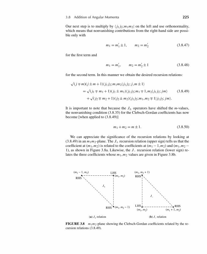
3.8 Addition of Angular Momenta 225
Our next step is to multiply by 〈 j1 j2;m1m2| on the left and use orthonormality,which means that nonvanishing contributions from the right-hand side are possi-ble only with
m1 = m′1 ± 1, m2 = m′
2 (3.8.47)
for the first term and
m1 = m′1, m2 = m′
2 ± 1 (3.8.48)
for the second term. In this manner we obtain the desired recursion relations:
√( j ∓ m)( j ± m + 1)〈 j1 j2;m1m2| j1 j2; j ,m ± 1〉
= √( j1 ∓ m1 + 1)( j1 ± m1)〈 j1 j2;m1 ∓ 1,m2| j1 j2; jm〉
+√( j2 ∓ m2 + 1)( j2 ± m2)〈 j1 j2;m1,m2 ∓ 1| j1 j2; jm〉.
(3.8.49)
It is important to note that because the J± operators have shifted the m-values,the nonvanishing condition (3.8.35) for the Clebsch-Gordan coefficients has nowbecome [when applied to (3.8.49)]
m1 + m2 = m ± 1. (3.8.50)
We can appreciate the significance of the recursion relations by looking at(3.8.49) in an m1m2-plane. The J+ recursion relation (upper sign) tells us that thecoefficient at (m1,m2) is related to the coefficients at (m1 − 1,m2) and (m1,m2 −1), as shown in Figure 3.8a. Likewise, the J− recursion relation (lower sign) re-lates the three coefficients whose m1,m2 values are given in Figure 3.8b.
(m1 − 1, m2)
(m1, m2 − 1)(m1 + 1, m2)
(m1, m2 + 1)(m1, m2)
(m1, m2)
RHS
LHS
RHSLHS RHS
RHS
J+
J−
(a) J+ relation (b) J− relation
FIGURE 3.8 m1m2-plane showing the Clebsch-Gordan coefficients related by the re-cursion relations (3.8.49).
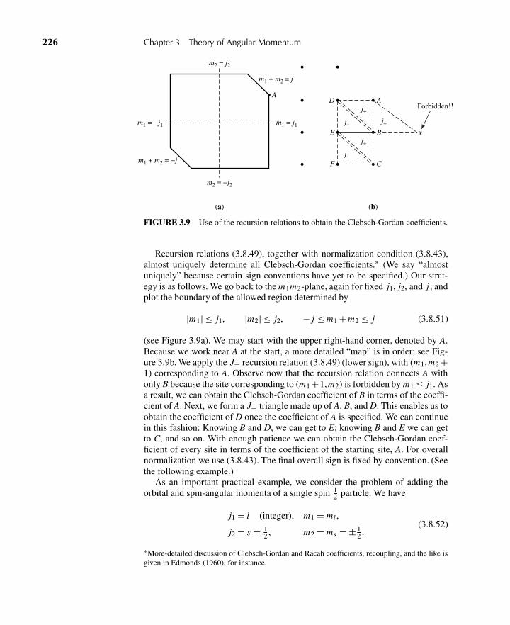
226 Chapter 3 Theory of Angular Momentum
m1 + m2 = −j
m1 = −j1 m1 = j1
m1 + m2 = j
AD
E
F
A
B x
C
m2 = j2
m2 = −j2
(a) (b)
Forbidden!!j+
j−
j+
j−
j−
FIGURE 3.9 Use of the recursion relations to obtain the Clebsch-Gordan coefficients.
Recursion relations (3.8.49), together with normalization condition (3.8.43),almost uniquely determine all Clebsch-Gordan coefficients.∗ (We say “almostuniquely” because certain sign conventions have yet to be specified.) Our strat-egy is as follows. We go back to the m1m2-plane, again for fixed j1, j2, and j , andplot the boundary of the allowed region determined by
|m1| ≤ j1, |m2| ≤ j2, − j ≤ m1 + m2 ≤ j (3.8.51)
(see Figure 3.9a). We may start with the upper right-hand corner, denoted by A.Because we work near A at the start, a more detailed “map” is in order; see Fig-ure 3.9b. We apply the J− recursion relation (3.8.49) (lower sign), with (m1,m2 +1) corresponding to A. Observe now that the recursion relation connects A withonly B because the site corresponding to (m1 +1,m2) is forbidden by m1 ≤ j1. Asa result, we can obtain the Clebsch-Gordan coefficient of B in terms of the coeffi-cient of A. Next, we form a J+ triangle made up of A, B, and D. This enables us toobtain the coefficient of D once the coefficient of A is specified. We can continuein this fashion: Knowing B and D, we can get to E; knowing B and E we can getto C, and so on. With enough patience we can obtain the Clebsch-Gordan coef-ficient of every site in terms of the coefficient of the starting site, A. For overallnormalization we use (3.8.43). The final overall sign is fixed by convention. (Seethe following example.)
As an important practical example, we consider the problem of adding theorbital and spin-angular momenta of a single spin 1
2 particle. We have
j1 = l (integer), m1 = ml ,
j2 = s = 12 , m2 = ms = ± 1
2 .(3.8.52)
∗More-detailed discussion of Clebsch-Gordan and Racah coefficients, recoupling, and the like isgiven in Edmonds (1960), for instance.
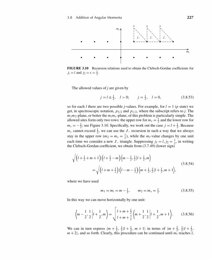
3.8 Addition of Angular Momenta 227
xms
ml
j−
x
j−
x
j−
FIGURE 3.10 Recursion relations used to obtain the Clebsch-Gordan coefficients forji = l and j2 = s = 1
2 .
The allowed values of j are given by
j = l ± 12 , l > 0; j = 1
2 , l = 0, (3.8.53)
so for each l there are two possible j-values. For example, for l = 1 (p state) weget, in spectroscopic notation, p3/2 and p1/2, where the subscript refers to j. Them1m2-plane, or better the mlms-plane, of this problem is particularly simple. Theallowed sites form only two rows: the upper row for ms = 1
2 and the lower row forms = − 1
2 ; see Figure 3.10. Specifically, we work out the case j = l + 12 . Because
ms cannot exceed 12 , we can use the J− recursion in such a way that we always
stay in the upper row (m2 = ms = 12 ), while the ml-value changes by one unit
each time we consider a new J− triangle. Suppressing j1 = l, j2 = 12 , in writing
the Clebsch-Gordan coefficient, we obtain from (3.7.49) (lower sign)√(l + 1
2 + m + 1)(
l + 12 − m
)⟨m − 1
2 , 12
∣∣l + 12 ,m
⟩=√(
l + m + 12
)(l − m − 1
2
)⟨m + 1
2 , 12
∣∣l + 12 ,m + 1
⟩,
(3.8.54)
where we have used
m1 = ml = m − 12 , m2 = ms = 1
2 . (3.8.55)
In this way we can move horizontally by one unit:
⟨m − 1
2,1
2
∣∣∣∣l + 1
2,m
⟩=√√√√ l + m + 1
2
l + m + 32
⟨m + 1
2,1
2
∣∣∣∣l + 1
2,m + 1
⟩. (3.8.56)
We can in turn express 〈m + 12 , 1
2 |l + 12 , m + 1〉 in terms of 〈m + 3
2 , 12 |l + 1
2 ,m + 2〉, and so forth. Clearly, this procedure can be continued until ml reaches l,
228 Chapter 3 Theory of Angular Momentum
the maximum possible value:
⟨m − 1
2,1
2
∣∣∣∣l + 1
2,m
⟩=√√√√ l + m + 1
2
l + m + 32
√√√√ l + m + 32
l + m + 52
⟨m + 3
2,1
2
∣∣∣∣l + 1
2,m + 2
⟩
=√√√√ l + m + 1
2
l + m + 32
√√√√ l + m + 32
l + m + 52
√√√√ l + m + 52
l + m + 72
×⟨m + 5
2,1
2
∣∣∣∣l + 1
2,m + 3
⟩...
=√
l + m + 12
2l + 1
⟨l,
1
2
∣∣∣∣l + 1
2, l + 1
2
⟩. (3.8.57)
Consider the angular-momentum configuration in which ml and ms are bothmaximal—that is, l and 1
2 , respectively. The total m = ml + ms is l + 12 , which is
possible only for j = l + 12 and not for j = l − 1
2 . So |ml = l,ms = 12 〉 must be
equal to | j = l + 12 ,m = l + 1
2 〉, up to a phase factor. We take this phase factor tobe real and positive by convention. With this choice we have⟨
l,1
2
∣∣∣∣l + 1
2, l + 1
2
⟩= 1. (3.8.58)
Returning to (3.8.57), we finally obtain
⟨m − 1
2,1
2
∣∣∣∣l + 1
2,m
⟩=√
l + m + 12
2l + 1. (3.8.59)
But this is only about one-fourth of the story. We must still determine the valueof the question marks that appear in the following:∣∣∣∣∣∣ j = l + 1
2,m
⟩=√
l + m + 12
2l + 1
∣∣∣∣∣∣ ml = m − 1
2,ms = 1
2
⟩
+?
∣∣∣∣ml = m + 1
2,ms = −1
2
⟩,∣∣∣∣ j = l − 1
2,m
⟩=?
∣∣∣∣ml = m − 1
2,ms = 1
2
⟩+? |ml = m + 1
2,ms = −1
2
⟩.
(3.8.60)
3.8 Addition of Angular Momenta 229
We note that the transformation matrix with fixed m from the (ml ,ms ) basis to the( j ,m) basis is, because of orthogonality, expected to have the form(
cosα sinα−sinα cosα
). (3.8.61)
Comparison with (3.8.60) shows that cosα is (3.8.59) itself, so we can readilydetermine sinα up to a sign ambiguity:
sin2α = 1 −(
l + m + 12
)(2l + 1)
=(
l − m + 12
)(2l + 1)
. (3.8.62)
We claim that 〈ml = m + 12 ,ms = − 1
2 | j = l + 12 ,m〉 must be positive because
all j = l + 12 states are reachable by applying the J_ operator successively to | j =
l + 12 ,m = l + 1
2 〉, and the matrix elements of J_ are always positive by convention.So the 2 ×2 transformation matrix (3.8.61) can be only⎛⎜⎜⎜⎜⎜⎝
√l + m + 1
2
2l + 1
√l − m + 1
2
2l + 1
−√
l − m + 12
2l + 1
√l + m + 1
2
2l + 1
⎞⎟⎟⎟⎟⎟⎠ . (3.8.63)
We define spin-angular functions in two-component form as follows:
Yj=l±1/2,ml = ±
√l ± m + 1
2
2l + 1Y m−1/2
l (θ ,φ)χ+
+√
l ± m + 12
2l + 1Y m+1/2
l (θ ,φ)χ−
= 1√2l + 1
⎛⎜⎝ ±√
l ± m + 12 Y m−1/2
l (θ ,φ)√l ∓ m + 1
2 Y m+1/2l (θ ,φ)
⎞⎟⎠ . (3.8.64)
They are, by construction, simultaneous eigenfunctions of L2, S2, J2, and Jz .They are also eigenfunctions of L · S, but L · S, being just
L · S =(
1
2
)(J2 − L2 − S2
), (3.8.65)
is not independent. Indeed, its eigenvalue can easily be computed as follows:
(h2
2
)[j ( j + 1) − l(l + 1) − 3
4
]=
⎧⎪⎪⎪⎨⎪⎪⎪⎩lh2
2for j = l + 1
2 ,
− (l + 1)h2
2for j = l − 1
2 .
(3.8.66)
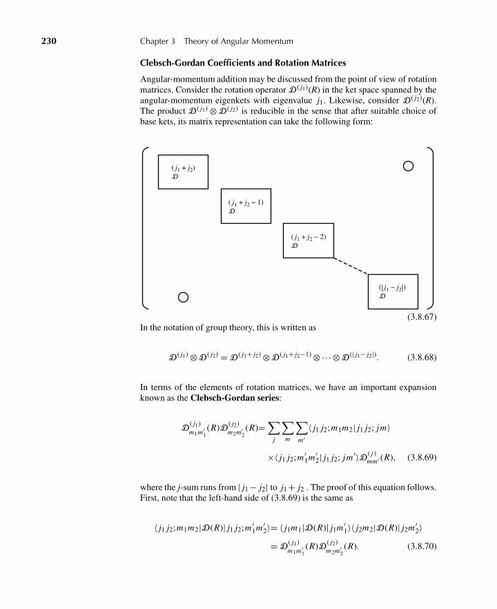
230 Chapter 3 Theory of Angular Momentum
Clebsch-Gordan Coefficients and Rotation Matrices
Angular-momentum addition may be discussed from the point of view of rotationmatrices. Consider the rotation operator D ( j1)(R) in the ket space spanned by theangular-momentum eigenkets with eigenvalue j1. Likewise, consider D ( j2)(R).The product D ( j1) ⊗D ( j2) is reducible in the sense that after suitable choice ofbase kets, its matrix representation can take the following form:
( j1 + j2)D
( j1 + j2 − 1)D
( j1 + j2 − 2)D
(| j1 − j2|)D
(3.8.67)In the notation of group theory, this is written as
D ( j1) ⊗D ( j2) = D ( j1+ j2) ⊗D ( j1+ j2−1) ⊗·· ·⊗D (| j1− j2|). (3.8.68)
In terms of the elements of rotation matrices, we have an important expansionknown as the Clebsch-Gordan series:
D( j1)m1m′
1(R)D ( j2)
m2m′2(R)=
∑j
∑m
∑m′
〈 j1 j2;m1m2| j1 j2; jm〉
×〈 j1 j2;m′1m′
2| j1 j2; jm′〉D ( j )mm′ (R), (3.8.69)
where the j-sum runs from | j1 − j2| to j1 + j2 . The proof of this equation follows.First, note that the left-hand side of (3.8.69) is the same as
〈 j1 j2;m1m2|D(R)| j1 j2;m′1m′
2〉= 〈 j1m1|D(R)| j1m′1〉〈 j2m2|D(R)| j2m′
2〉= D
( j1)m1m′
1(R)D ( j2)
m2m′2(R). (3.8.70)
3.8 Addition of Angular Momenta 231
But the same matrix element is also computable by inserting a complete set ofstates in the ( j ,m) basis. Thus
〈 j1 j2;m1m2|D(R)| j1 j2;m′1m′
2〉
=∑
j
∑m
∑j ′
∑m′
〈 j1 j2;m1m2| j1 j2; jm〉〈 j1 j2; jm|D(R)| j1 j2; j ′m′〉
× 〈 j1 j2; j ′m′| j1 j2;m′1m′
2〉
=∑
j
∑m
∑j ′
∑m′
〈 j1 j2;m1m2| j1 j2; jm〉D ( j )mm′ (R)δ j j ′
× 〈 j1 j2;m′1m′
2| j1 j2; j ′m′〉, (3.8.71)
which is just the right-hand side of (3.8.69).As an interesting application of (3.8.69), we derive an important formula for an
integral involving three spherical harmonics. First, recall the connection betweenD (l)
m0 and Y m∗l given by (3.6.52). Letting j1 → l1, j2 → l2,m′
1 → 0,m′2 → 0 (hence
m′ → 0) in (3.8.69), we obtain, after complex conjugation,
Y m1l1
(θ ,φ)Y m2l2
(θ ,φ) =√
(2l1 + 1)(2l2 + 1)
4π
∑l′
∑m′
〈l1l2;m1m2|l1l2;l ′m′〉
×〈l1l2;00|l1l2;l ′0〉√
4π
2l ′ + 1Y m′
l′ (θ ,φ). (3.8.72)
We multiply both sides by Y m∗l (θ ,φ) and integrate over solid angles. The sum-
mations drop out because of the orthogonality of spherical harmonics, and we areleft with ∫
d�Y m∗l (θ ,φ)Y m1
l1(θ ,φ)Y m2
l2(θ ,φ) (3.8.73)
=√
(2l1 + 1)(2l2 + 1)
4π(2l + 1)〈l1l2;00|l1l2;l0〉〈l1l2;m1m2|l1l2;lm〉.
The square root factor times the first Clebsch-Gordan coefficient is independent oforientations—that is, of m1 and m2. The second Clebsch-Gordan coefficient is theone appropriate for adding l1 and l2 to obtain total l . Equation (3.8.73) turns out tobe a special case of the Wigner-Eckart theorem to be derived in Section 3.11. Thisformula is extremely useful in evaluating multipole matrix elements in atomic andnuclear spectroscopy.
232 Chapter 3 Theory of Angular Momentum
3.9 SCHWINGER’S OSCILLATOR MODEL OF ANGULAR MOMENTUM
Angular Momentum and Uncoupled Oscillators
There exists a very interesting connection between the algebra of angular momen-tum and the algebra of two independent (that is, uncoupled) oscillators, which wasworked out in J. Schwinger’s notes. See Biedenharn and Van Dam (1965), p. 229.Let us consider two simple harmonic oscillators, which we call the plus type andthe minus type . We have the annihilation and creation operators, denoted by a+and a†
+ for the plus-type oscillator; likewise, we have a− and a†− for the minus-
type oscillators. We also define the number operators N+ and N− as follows:
N+ ≡ a†+a+, N− ≡ a†
−a−. (3.9.1)
We assume that the usual commutation relations among a, a†, and N hold foroscillators of the same type (see Section 2.3).
[a+,a†+] = 1, [a−,a†
−] = 1, (3.9.2a)
[N+,a+] = −a+, [N−,a−] = −a−, (3.9.2b)
[N+,a†+] = a†
+, [N−,a†−] = a†
−. (3.9.2c)
However, we assume that any pair of operators between different oscillators com-mute:
[a+,a†−] = [a−,a†
+] = 0 (3.9.3)
and so forth. So it is in this sense that we say the two oscillators are uncoupled.Because N+ and N− commute by virtue of (3.9.3), we can build up simulta-
neous eigenkets of N+ and N− with eigenvalues n+ and n−, respectively. So wehave the following eigenvalue equations for N±:
N+|n+,n−〉 = n+|n+,n−〉, N−|n+,n−〉 = n−|n+,n−〉. (3.9.4)
In complete analogy with (2.3.16) and (2.3.17), the creation and annihilation op-erators, a†
± and a±, act on |n+,n−〉 as follows:
a†+|n+,n−〉 =√
n+ + 1|n+ + 1,n−〉, a†−|n+,n−〉 =√
n− + 1|n+,n− + 1〉,(3.9.5a)
a+|n+,n−〉 = √n+|n+ − 1,n−〉, a−|n+,n−〉 = √
n−|n+,n− − 1〉. (3.9.5b)
We can obtain the most general eigenkets of N+ and N− by applying a†+ and a†
−successively to the vacuum ket defined by
a+|0,0〉 = 0, a−|0,0〉 = 0. (3.9.6)
3.9 Schwinger’s Oscillator Model of Angular Momentum 233
In this way we obtain
|n+,n−〉 = (a†+)
n+(a†
−)n−
√n+!
√n−!
|0,0〉. (3.9.7)
Next, we define
J+ ≡ ha†+a−, J− ≡ ha†
−a+, (3.9.8a)
and
Jz ≡(
h
2
)(a†
+a+ − a†−a−
)=(
h
2
)(N+ − N−) . (3.9.8b)
We can readily prove that these operators satisfy the angular-momentum commu-tation relations of the usual form[
Jz , J±]= ±h J±, (3.9.9a)
[J+, J−
]= 2h Jz . (3.9.9b)
For example, we prove (3.9.9) as follows:
h2[a†+a−,a†
−a+]= h2a†+a−a†
−a+ − h2a†−a+a†
+a−
= h2a†+(a†
−a− + 1)a+ − h2a†−(a†
+a+ + 1)a−
= h2(a†+a+ − a†
−a−) = 2h Jz . (3.9.10)
Defining the total N to be
N ≡ N+ + N− = a†+a+ + a†
−a−, (3.9.11)
we can also prove
J2≡ J 2z +
(1
2
)(J+ J− + J− J+)
=(
h2
2
)N
(N
2+ 1
), (3.9.12)
which is left as an exercise.What are the physical interpretations of all this? We associate spin up (m = 1
2 )with one quantum unit of the plus-type oscillator and spin down (m = − 1
2 ) withone quantum unit of the minus-type oscillator. If you like, you may imagine onespin 1
2 “particle” with spin up (down) with each quantum unit of the plus- (minus-)type oscillator. The eigenvalues n+ and n− are just the number of spins up and
234 Chapter 3 Theory of Angular Momentum
spins down, respectively. The meaning of J+ is that it destroys one unit of spindown with the z-component of spin-angular momentum −h/2 and creates oneunit of spin up with the z-component of spin-angular momentum +h/2; the z-component of angular momentum is therefore increased by h. Likewise J− de-stroys one unit of spin up and creates one unit of spin down; the z-component ofangular momentum is therefore decreased by h. As for the Jz operator, it simplycounts h/2 times the difference of n+ and n−, just the z-component of the totalangular momentum. With (3.9.5) at our disposal, we can easily examine how J±and Jz act on |n+,n−〉 as follows:
J+|n+,n−〉 = ha†+a−|n+,n−〉 =√
n−(n+ + 1)h|n+ + 1,n− − 1〉, (3.9.13a)
J−|n+,n−〉 = ha†−a+|n+,n−〉 =√
n+(n− + 1)h|n+ − 1,n− + 1〉, (3.9.13b)
Jz |n+,n−〉 =(
h
2
)(N+ − N−)|n+,n−〉 =
(1
2
)(n+,−n−)h|n+,n−〉.
(3.9.13c)
Notice that in all these operations, the sum n+ + n−, which corresponds to thetotal number of spin 1
2 particles, remains unchanged.Observe now that (3.9.13a), (3.9.13b), and (3.9.13c) reduce to the familiar ex-
pressions for the J± and Jz operators we derived in Section 3.5, provided that wesubstitute
n+ → j + m, n− → j − m. (3.9.14)
The square root factors in (3.9.13a) and (3.9.13b) change to√
n−(n+ + 1) → √( j − m)( j + m + 1),√
n+(n− + 1) → √( j + m)( j − m + 1),
(3.9.15)
which are exactly the square root factors appearing in (3.5.39) and (3.5.41).Notice also that the eigenvalue of the J2 operator defined by (3.9.12) changes
as follows: (h2
2
)(n+ + n−)
[(n+ + n−)
2+ 1
]→ h2 j ( j + 1). (3.9.16)
All this may not be too surprising because we have already proved that theJ± and J2 operators we constructed out of the oscillator operators satisfy theusual angular-momentum commutation relations. But it is instructive to see in anexplicit manner the connection between the oscillator matrix elements and theangular-momentum matrix elements. In any case, it is now natural to use
j ≡ (n+ + n−)
2, m ≡ (n+ − n−)
2(3.9.17)
in place of n+ and n− to characterize simultaneous eigenkets of J2 and Jz . Ac-cording to (3.9.13a) the action of J+ changes n+ into n+ +1 and n− into n− −1,
3.9 Schwinger’s Oscillator Model of Angular Momentum 235
which means that j is unchanged and m goes into m +1. Likewise, we see that theJ− operator that changes n+ into n+ −1 and n− into n+ −1 lowers m by one unitwithout changing j . We can now write as (3.9.7) for the most general N+, N−eigenket
| j ,m〉 = (a†+)
j+m(a†
−)j−m
√( j + m)!( j − m)!
|0〉, (3.9.18)
where we have used |0〉 for the vacuum ket, earlier denoted by |0,0〉.A special case of (3.9.18) is of interest. Let us set m = j , which physically
means that the eigenvalue of Jz is as large as possible for a given j . We have
| j , j〉 = (a†+)2 j
√(2 j )!
|0〉. (3.9.19)
We can imagine this state to be built up of 2j spin 12 particles with their spins all
pointing in the positive z-direction.In general, we note that a complicated object of high j can be visualized as
being made up of primitive spin 12 particles, j + m of them with spin up and the
remaining j − m of them with spin down. This picture is extremely convenienteven though we obviously cannot always regard an object of angular momentum jliterally as a composite system of spin 1
2 particles. All we are saying is that as faras the transformation properties under rotations are concerned, we can visualizeany object of angular momentum j as a composite system of 2j spin 1
2 particlesformed in the manner indicated by (3.9.18).
From the point of view of angular-momentum addition developed in the pre-vious section, we can add the spins of 2j spin 1
2 particles to obtain states withangular momentum j, j −1, j −2, . . . . As a simple example, we can add the spin-angular momenta of two spin 1
2 particles to obtain a total angular momentum ofzero as well as one. In Schwinger’s oscillator scheme, however, we obtain onlystates with angular momentum j when we start with 2j spin 1
2 particles. In thelanguage of permutation symmetry to be developed in Chapter 7, only totallysymmetrical states are constructed by this method. The primitive spin 1
2 particlesappearing here are actually bosons! This method is quite adequate if our purposeis to examine the properties under rotations of states characterized by j and mwithout asking how such states are built up initially.
The reader who is familiar with isospin in nuclear and particle physics maynote that what we are doing here provides a new insight into the isospin (or iso-topic spin) formalism. The operator J+ that destroys one unit of the minus typeand creates one unit of the plus type is completely analogous to the isospin lad-der operator T+ (sometimes denoted by I+) that annihilates a neutron (isospindown) and creates a proton (isospin up), thus raising the z-component of isospinby one unit. In contrast, Jz is analogous to Tz , which simply counts the differencebetween the number of protons and the number of neutrons in nuclei.
236 Chapter 3 Theory of Angular Momentum
Explicit Formula for Rotation Matrices
Schwinger’s scheme can be used to derive, in a very simple way, a closed formulafor rotation matrices that E. P. Wigner first obtained using a similar (but not iden-tical) method. We apply the rotation operator D(R ) to | j ,m〉, written as (3.9.18).In the Euler angle notation, the only nontrivial rotation is the second one aboutthe y-axis, so we direct our attention to
D(R) = D(α,β,γ )|α=γ=0 = exp
(−i Jyβ
h
). (3.9.20)
We have
D(R)| j ,m〉 = [D(R)a†+D−1(R)]
j+m[D(R)a†
−D−1(R)]j−m
√( j + m)!( j − m)!
D(R)|0〉. (3.9.21)
Now, D(R ) acting on |0〉 just reproduces |0〉 because, by virtue of (3.9.6), onlythe leading term, 1, in the expansion of exponential (3.9.20) contributes. So
D(R)a†±D−1(R) = exp
(−i Jyβ
h
)a†±exp
(i Jyβ
h
). (3.9.22)
Thus we may use formula (2.3.47). Letting
G → −Jy
h, λ→ β (3.9.23)
in (2.3.47), we realize that we must look at various commutators, namely[−Jy
h,a†
+]
=(
1
2i
)[a†
−a+,a†+] =
(1
2i
)a†−,
[−Jy
h,
[−Jy
h,a†
+]]
=[
−Jy
h,a†−
2i
]=(
1
4
)a†
+,
(3.9.24)
and so forth. Clearly, we always obtain either a†+ or a†
−. Collecting terms, we get
D(R)a†+D−1(R) = a†
+ cos
(β
2
)+ a†
− sin
(β
2
). (3.9.25)
Likewise,
D(R)a†−D−1(R) = a†
− cos
(β
2
)− a†
+ sin
(β
2
). (3.9.26)
Actually this result is not surprising. After all, the basic spin-up state is supposedto transform as
a†+|0〉 → cos
(β
2
)a†
+|0〉+ sin
(β
2
)a†−|0〉 (3.9.27)
3.9 Schwinger’s Oscillator Model of Angular Momentum 237
under a rotation about the y-axis. Substituting (3.9.25) and (3.9.26) into (3.9.21)and recalling the binomial theorem
(x + y)N =∑
k
N!x N−k yk
(N − k)!k!, (3.9.28)
we obtain
D(α = 0,β,γ = 0| j ,m〉 =∑
k
∑l
( j + m)!( j − m)!
( j + m − k)!k!( j − m − l)!l!
× [a†+ cos(β/2)] j+m−k[a†
− sin(β/2)]k
√( j + m)!( j − m)!
× [−a†+ sin(β/2)] j−m−l[a†
− cos(β/2)]l|0〉.(3.9.29)
We may compare (3.9.29) with
D(α = 0,β,γ = 0)| j ,m〉 =∑m′
| j ,m′〉d ( j )m′m(β)
=∑m′
d ( j )m′m(β)
(a†+) j+m′
(a†−) j−m′√
( j + m′)!( j − m ′)!|0〉.
(3.9.30)
We can obtain an explicit form for d ( j )m′m(β) by equating the coefficients of powers
of a†+ in (3.9.29) and (3.9.30). Specifically, we want to compare a†
+ raised to
j + m′ in (3.9.30) with a†+ raised to 2 j − k − l, so we identify
l = j − k − m ′. (3.9.31)
We are seeking dm′m (β) with m ′ fixed. The k-sum and the l-sum in (3.9.29) arenot independent of each other; we eliminate l in favor of k by taking advantage of(3.9.31). As for the powers of a†
−, we note that a†− raised to j −m′ in (3.9.30) au-
tomatically matches with a†− raised to k + l in (3.9.29) when (3.9.31) is imposed.
The last step is to identify the exponents of cos(β/2), sin(β/2), and (−1), whichare, respectively,
j + m − k + l = 2 j − 2k + m − m ′, (3.9.32a)
k + j − m − l = 2k − m + m′, (3.9.32b)
j − m − l = k − m + m ′, (3.9.32c)
238 Chapter 3 Theory of Angular Momentum
where we have used (3.9.31) to eliminate l. In this way we obtain Wigner’s for-mula for d ( j )
m′m(β):
d ( j )m′m(β) =
∑k
(−1)k−m+m′√
( j + m)!( j − m)!( j + m′)!( j − m′)!( j + m − k)!k!( j − k − m ′)!(k − m + m′)!
×(
cosβ
2
)2 j−2k+m−m′ (sinβ
2
)2k−m+m′
, (3.9.33)
where we take the sum over k whenever none of the arguments of factorials in thedenominator are negative.
3.10 SPIN CORRELATION MEASUREMENTS AND BELL’S INEQUALITY
Correlations in Spin-Singlet States
The simplest example of angular-momentum addition we encountered in Sec-tion 3.8 was concerned with a composite system made up of spin 1
2 particles. Inthis section we use such a system to illustrate one of the most astonishing conse-quences of quantum mechanics.
Consider a two-electron system in a spin-singlet state—that is, with a total spinof zero. We have already seen that the state ket can be written as [see (3.8.15d)]
|spin singlet〉 =(
1√2
)(|z+; z−〉− |z−; z+〉), (3.10.1)
where we have explicitly indicated the quantization direction. Recall that |z+; z−〉means that electron 1 is in the spin-up state and electron 2 is in the spin-downstate. The same is true for |z−; z+〉.
Suppose we make a measurement on the spin component of one of the elec-trons. Clearly, there is a 50-50 chance of getting either up or down because thecomposite system may be in |z+; z−〉 or |z−; z+〉 with equal probabilities. But ifone of the components is shown to be in the spin-up state, the other is necessarilyin the spin-down state, and vice versa. When the spin component of electron 1 isshown to be up, the measurement apparatus has selected the first term, |z+; z−〉of (3.10.1); a subsequent measurement of the spin component of electron 2 mustascertain that the state ket of the composite system is given by |z+; z−〉.
It is remarkable that this kind of correlation can persist even if the two parti-cles are well separated and have ceased to interact, provided that as they fly apart,there is no change in their spin states. This is certainly the case for a J = 0 sys-tem disintegrating spontaneously into two spin 1
2 particles with no relative orbitalangular momentum, because angular-momentum conservation must hold in thedisintegration process. One example of this is a rare decay of the η meson (mass549 MeV/c2) into a muon pair
η→ μ+ +μ−, (3.10.2)
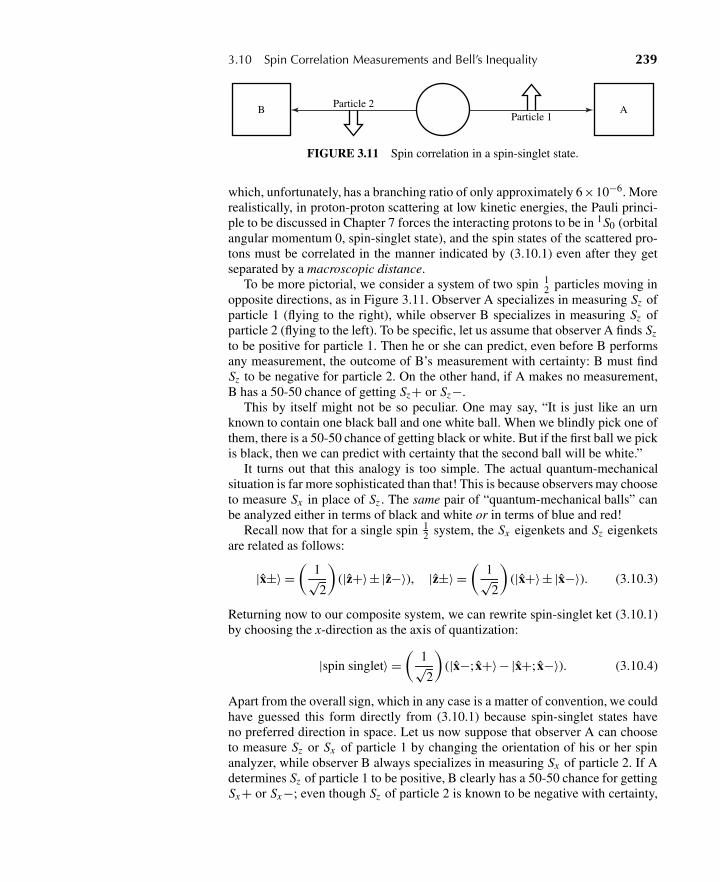
3.10 Spin Correlation Measurements and Bell’s Inequality 239
B AParticle 2
Particle 1
FIGURE 3.11 Spin correlation in a spin-singlet state.
which, unfortunately, has a branching ratio of only approximately 6×10⁻⁶. Morerealistically, in proton-proton scattering at low kinetic energies, the Pauli princi-ple to be discussed in Chapter 7 forces the interacting protons to be in 1S0 (orbitalangular momentum 0, spin-singlet state), and the spin states of the scattered pro-tons must be correlated in the manner indicated by (3.10.1) even after they getseparated by a macroscopic distance.
To be more pictorial, we consider a system of two spin 12 particles moving in
opposite directions, as in Figure 3.11. Observer A specializes in measuring Sz ofparticle 1 (flying to the right), while observer B specializes in measuring Sz ofparticle 2 (flying to the left). To be specific, let us assume that observer A finds Szto be positive for particle 1. Then he or she can predict, even before B performsany measurement, the outcome of B’s measurement with certainty: B must findSz to be negative for particle 2. On the other hand, if A makes no measurement,B has a 50-50 chance of getting Sz+ or Sz−.
This by itself might not be so peculiar. One may say, “It is just like an urnknown to contain one black ball and one white ball. When we blindly pick one ofthem, there is a 50-50 chance of getting black or white. But if the first ball we pickis black, then we can predict with certainty that the second ball will be white.”
It turns out that this analogy is too simple. The actual quantum-mechanicalsituation is far more sophisticated than that! This is because observers may chooseto measure Sx in place of Sz . The same pair of “quantum-mechanical balls” canbe analyzed either in terms of black and white or in terms of blue and red!
Recall now that for a single spin 12 system, the Sx eigenkets and Sz eigenkets
are related as follows:
|x±〉 =(
1√2
)(|z+〉± |z−〉), |z±〉 =
(1√2
)(|x+〉± |x−〉). (3.10.3)
Returning now to our composite system, we can rewrite spin-singlet ket (3.10.1)by choosing the x-direction as the axis of quantization:
|spin singlet〉 =(
1√2
)(|x−; x+〉− |x+; x−〉). (3.10.4)
Apart from the overall sign, which in any case is a matter of convention, we couldhave guessed this form directly from (3.10.1) because spin-singlet states haveno preferred direction in space. Let us now suppose that observer A can chooseto measure Sz or Sx of particle 1 by changing the orientation of his or her spinanalyzer, while observer B always specializes in measuring Sx of particle 2. If Adetermines Sz of particle 1 to be positive, B clearly has a 50-50 chance for gettingSx+ or Sx−; even though Sz of particle 2 is known to be negative with certainty,
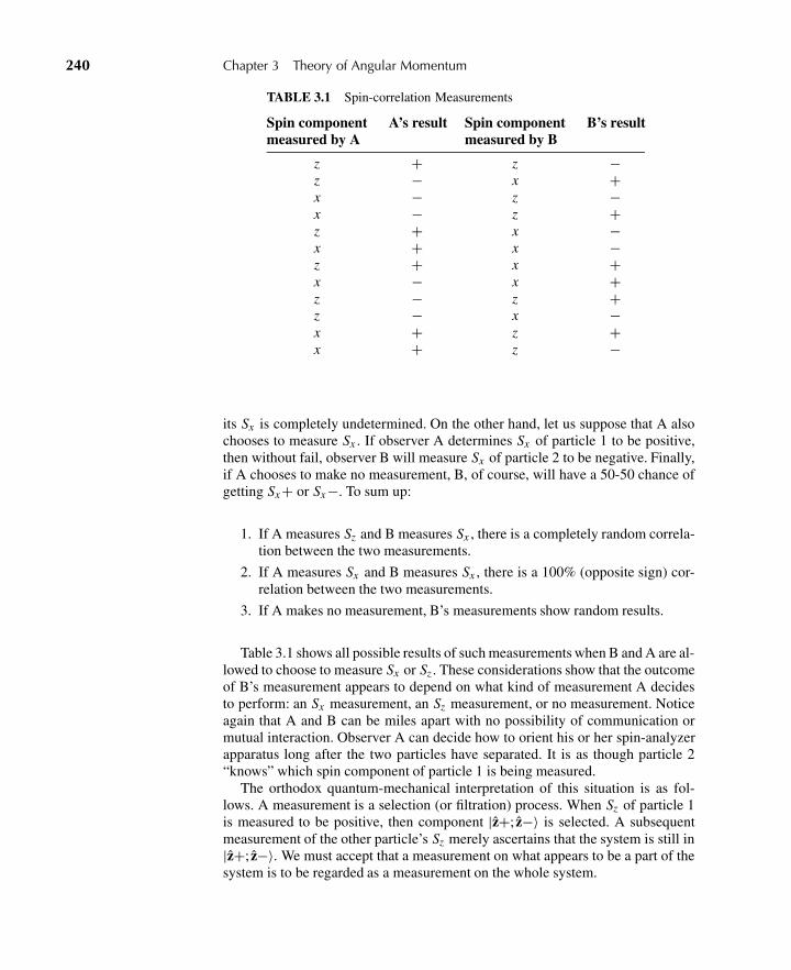
240 Chapter 3 Theory of Angular Momentum
TABLE 3.1 Spin-correlation Measurements
Spin componentmeasured by A
A’s result Spin componentmeasured by B
B’s result
z + z −z − x +x − z −x − z +z + x −x + x −z + x +x − x +z − z +z − x −x + z +x + z −
its Sx is completely undetermined. On the other hand, let us suppose that A alsochooses to measure Sx . If observer A determines Sx of particle 1 to be positive,then without fail, observer B will measure Sx of particle 2 to be negative. Finally,if A chooses to make no measurement, B, of course, will have a 50-50 chance ofgetting Sx+ or Sx−. To sum up:
1. If A measures Sz and B measures Sx , there is a completely random correla-tion between the two measurements.
2. If A measures Sx and B measures Sx , there is a 100% (opposite sign) cor-relation between the two measurements.
3. If A makes no measurement, B’s measurements show random results.
Table 3.1 shows all possible results of such measurements when B and A are al-lowed to choose to measure Sx or Sz . These considerations show that the outcomeof B’s measurement appears to depend on what kind of measurement A decidesto perform: an Sx measurement, an Sz measurement, or no measurement. Noticeagain that A and B can be miles apart with no possibility of communication ormutual interaction. Observer A can decide how to orient his or her spin-analyzerapparatus long after the two particles have separated. It is as though particle 2“knows” which spin component of particle 1 is being measured.
The orthodox quantum-mechanical interpretation of this situation is as fol-lows. A measurement is a selection (or filtration) process. When Sz of particle 1is measured to be positive, then component |z+; z−〉 is selected. A subsequentmeasurement of the other particle’s Sz merely ascertains that the system is still in|z+; z−〉. We must accept that a measurement on what appears to be a part of thesystem is to be regarded as a measurement on the whole system.
3.10 Spin Correlation Measurements and Bell’s Inequality 241
Einstein’s Locality Principle and Bell’s Inequality
Many physicists have felt uncomfortable with the preceding orthodox interpreta-tion of spin-correlation measurements. Their feelings are typified in the followingfrequently quoted remarks by A. Einstein, which we call Einstein’s locality prin-ciple: “But on one supposition we should, in my opinion, absolutely hold fast: Thereal factual situation of the system S2 is independent of what is done with the sys-tem S1, which is spatially separated from the former.” Because this problem wasfirst discussed in a 1935 paper of A. Einstein, B. Podolsky, and N. Rosen, it issometimes known as the Einstein-Podolsky-Rosen paradox.∗
Some have argued that the difficulties encountered here are inherent in theprobabilistic interpretations of quantum mechanics and that the dynamic behaviorat the microscopic level appears probabilistic only because some yet unknownparameters—so-called hidden variables—have not been specified. It is not ourpurpose here to discuss various alternatives to quantum mechanics based onhidden-variable or other considerations. Rather, let us ask, Do such theories makepredictions different from those of quantum mechanics? Until 1964, it could bethought that the alternative theories could be concocted in such a way that theywould give no predictions, other than the usual quantum-mechanical predictions,that could be verified experimentally. The whole debate would have belonged tothe realm of metaphysics rather than physics. It was then pointed out by J. S.Bell that the alternative theories based on Einstein’s locality principle actuallypredict a testable inequality relation among the observables of spin-correlationexperiments that disagrees with the predictions of quantum mechanics.
We derive Bell’s inequality within the framework of a simple model, conceivedby E. P. Wigner, that incorporates the essential features of the various alternativetheories. Proponents of this model agree that it is impossible to determine Sx andSz simultaneously. However, when we have a large number of spin 1
2 particles, weassign a certain fraction of them to have the following property:
If Sz is measured, we obtain a plus sign with certainty.
If Sx is measured, we obtain a minus sign with certainty.
A particle satisfying this property is said to belong to type (z+, x−). Notice thatwe are not asserting that we can simultaneously measure Sz and Sx to be + and−, respectively. When we measure Sz , we do not measure Sx , and vice versa.We are assigning definite values of spin components in more than one directionwith the understanding that only one or the other of the components can actuallybe measured. Even though this approach is fundamentally different from that ofquantum mechanics, the quantum-mechanical predictions for Sz and Sx measure-ments performed on the spin-up (Sz+) state are reproduced, provided that thereare as many particles belonging to type (z+, x+) as to type (z+, x−).
Let us now examine how this model can account for the results of spin-correlation measurements made on composite spin-singlet systems. Clearly, for a
∗To be historically accurate, the original Einstein-Podolsky-Rosen paper dealt with measure-ments of x and p. The use of composite spin 1
2 systems to illustrate the Einstein-Podolsky-Rosenparadox started with D. Bohm.
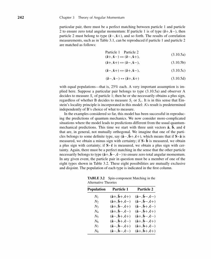
242 Chapter 3 Theory of Angular Momentum
particular pair, there must be a perfect matching between particle 1 and particle2 to ensure zero total angular momentum: If particle 1 is of type (z+, x−), thenparticle 2 must belong to type (z−, x+), and so forth. The results of correlationmeasurements, such as in Table 3.1, can be reproduced if particle 1 and particle 2are matched as follows:
Particle 1 Particle 2(z+, x−) ↔ (z−, x+), (3.10.5a)
(z+, x+) ↔ (z−, x−), (3.10.5b)
(z−, x+) ↔ (z+, x−), (3.10.5c)
(z−, x−) ↔ (z+, x+) (3.10.5d)
with equal populations—that is, 25% each. A very important assumption is im-plied here. Suppose a particular pair belongs to type (3.10.5a) and observer Adecides to measure Sz of particle 1; then he or she necessarily obtains a plus sign,regardless of whether B decides to measure Sz or Sx . It is in this sense that Ein-stein’s locality principle is incorporated in this model: A’s result is predeterminedindependently of B’s choice of what to measure.
In the examples considered so far, this model has been successful in reproduc-ing the predictions of quantum mechanics. We now consider more-complicatedsituations where the model leads to predictions different from the usual quantum-mechanical predictions. This time we start with three unit vectors a, b, and cthat are, in general, not mutually orthogonal. We imagine that one of the parti-cles belongs to some definite type, say (a−, b+, c+), which means that if S · a ismeasured, we obtain a minus sign with certainty; if S · b is measured, we obtaina plus sign with certainty; if S · c is measured, we obtain a plus sign with cer-tainty. Again, there must be a perfect matching in the sense that the other particlenecessarily belongs to type (a+, b−, c−) to ensure zero total angular momentum.In any given event, the particle pair in question must be a member of one of theeight types shown in Table 3.2. These eight possibilities are mutually exclusiveand disjoint. The population of each type is indicated in the first column.
TABLE 3.2 Spin-component Matching in theAlternative Theories
Population Particle 1 Particle 2
N1 (a+, b+, c+) (a−, b−, c−)N2 (a+, b+, c−) (a−, b−, c+)N3 (a+, b−, c+) (a−, b+, c−)N4 (a+, b−, c−) (a−, b+, c+)N5 (a−, b+, c+) (a+, b−, c−)N6 (a−, b+, c−) (a+, b−, c+)N7 (a−, b−, c+) (a+, b+, c−)N8 (a−, b−, c−) (a+, b+, c+)
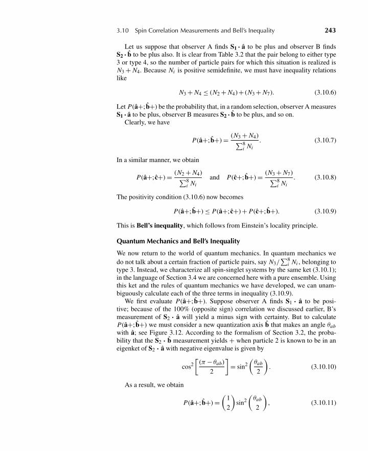
3.10 Spin Correlation Measurements and Bell’s Inequality 243
Let us suppose that observer A finds S1 · a to be plus and observer B findsS2 · b to be plus also. It is clear from Table 3.2 that the pair belong to either type3 or type 4, so the number of particle pairs for which this situation is realized isN3 + N4. Because Ni is positive semidefinite, we must have inequality relationslike
N3 + N4 ≤ (N2 + N4) + (N3 + N7). (3.10.6)
Let P(a+; b+) be the probability that, in a random selection, observer A measuresS1 · a to be plus, observer B measures S2 · b to be plus, and so on.
Clearly, we have
P(a+; b+) = (N3 + N4)∑8i Ni
. (3.10.7)
In a similar manner, we obtain
P(a+; c+) = (N2 + N4)∑8i Ni
and P(c+; b+) = (N3 + N7)∑8i Ni
. (3.10.8)
The positivity condition (3.10.6) now becomes
P(a+; b+) ≤ P(a+; c+) + P(c+; b+). (3.10.9)
This is Bell’s inequality, which follows from Einstein’s locality principle.
Quantum Mechanics and Bell’s Inequality
We now return to the world of quantum mechanics. In quantum mechanics wedo not talk about a certain fraction of particle pairs, say N3/
∑8i Ni , belonging to
type 3. Instead, we characterize all spin-singlet systems by the same ket (3.10.1);in the language of Section 3.4 we are concerned here with a pure ensemble. Usingthis ket and the rules of quantum mechanics we have developed, we can unam-biguously calculate each of the three terms in inequality (3.10.9).
We first evaluate P(a+; b+). Suppose observer A finds S1 · a to be posi-tive; because of the 100% (opposite sign) correlation we discussed earlier, B’smeasurement of S2 · a will yield a minus sign with certainty. But to calculateP(a+; b+) we must consider a new quantization axis b that makes an angle θabwith a; see Figure 3.12. According to the formalism of Section 3.2, the proba-bility that the S2 · b measurement yields + when particle 2 is known to be in aneigenket of S2 · a with negative eigenvalue is given by
cos2[
(π − θab)
2
]= sin2
(θab
2
). (3.10.10)
As a result, we obtain
P(a+; b+) =(
1
2
)sin2
(θab
2
), (3.10.11)
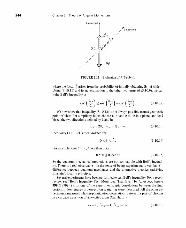
244 Chapter 3 Theory of Angular Momentum
a-direction
b-direction
⟨S2⟩
⟨S1⟩
θab
FIGURE 3.12 Evaluation of P(a+; b+).
where the factor 12 arises from the probability of initially obtaining S1 · a with +.
Using (3.10.11) and its generalization to the other two terms of (3.10.9), we canwrite Bell’s inequality as
sin2(θab
2
)≤ sin2
(θac
2
)+ sin2
(θcb
2
). (3.10.12)
We now show that inequality (3.10.12) is not always possible from a geometricpoint of view. For simplicity let us choose a, b, and c to lie in a plane, and let cbisect the two directions defined by a and b:
θab = 2θ , θac = θcb = θ . (3.10.13)
Inequality (3.10.12) is then violated for
0< θ <π
2. (3.10.14)
For example, take θ = π/4; we then obtain
0.500 ≤ 0.292 ?? (3.10.15)
So the quantum-mechanical predictions are not compatible with Bell’s inequal-ity. There is a real observable—in the sense of being experimentally verifiable—difference between quantum mechanics and the alternative theories satisfyingEinstein’s locality principle.
Several experiments have been performed to test Bell’s inequality. For a recentreview, see “Bell’s Inequality Test: More Ideal Than Ever” by A. Aspect, Nature398 (1999) 189. In one of the experiments, spin correlations between the finalprotons in low-energy proton-proton scattering were measured. All the other ex-periments measured photon-polarization correlations between a pair of photonsin a cascade transition of an excited atom (Ca, Hg, . . .),
( j = 0)γ→( j = 1)
γ→( j = 0), (3.10.16)
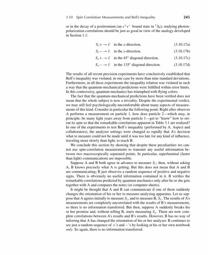
3.10 Spin Correlation Measurements and Bell’s Inequality 245
or in the decay of a positronium (an e+e− bound state in 1S0); studying photon-polarization correlations should be just as good in view of the analogy developedin Section 1.1:
Sz+ → ε in the x-direction, (3.10.17a)
Sz− → ε in the y-direction, (3.10.17b)
Sx+ → ε in the 45◦ diagonal direction, (3.10.17c)
Sx− → ε in the 135◦ diagonal direction. (3.10.17d)
The results of all recent precision experiments have conclusively established thatBell’s inequality was violated, in one case by more than nine standard deviations.Furthermore, in all these experiments the inequality relation was violated in sucha way that the quantum-mechanical predictions were fulfilled within error limits.In this controversy, quantum mechanics has triumphed with flying colors.
The fact that the quantum-mechanical predictions have been verified does notmean that the whole subject is now a triviality. Despite the experimental verdict,we may still feel psychologically uncomfortable about many aspects of measure-ments of this kind. Consider in particular the following point: Right after observerA performs a measurement on particle 1, how does particle 2—which may, inprinciple, be many light years away from particle 1—get to “know” how to ori-ent its spin so that the remarkable correlations apparent in Table 3.1 are realized?In one of the experiments to test Bell’s inequality (performed by A. Aspect andcollaborators), the analyzer settings were changed so rapidly that A’s decisionwhat to measure could not be made until it was too late for any kind of influence,traveling more slowly than light, to reach B.
We conclude this section by showing that despite these peculiarities we can-not use spin-correlation measurements to transmit any useful information be-tween two macroscopically separated points. In particular, superluminal (fasterthan light) communications are impossible.
Suppose A and B both agree in advance to measure Sz ; then, without askingA, B knows precisely what A is getting. But this does not mean that A and Bare communicating; B just observes a random sequence of positive and negativesigns. There is obviously no useful information contained in it. B verifies theremarkable correlations predicted by quantum mechanics only after he or she getstogether with A and compares the notes (or computer sheets).
It might be thought that A and B can communicate if one of them suddenlychanges the orientation of his or her to measure analyzing apparatus. Let us sup-pose that A agrees initially to measure Sz , and to measure B, Sx . The results of A’smeasurements are completely uncorrelated with the results of B’s measurements,so there is no information transferred. But then, suppose A suddenly breaks hisor her promise and, without telling B, starts measuring Sx . There are now com-plete correlations between A’s results and B’s results. However, B has no way ofinferring that A has changed the orientation of his or her analyzer. B continues tosee just a random sequence of +’s and −’s by looking at his or her own notebookonly. So again, there is no information transferred.
246 Chapter 3 Theory of Angular Momentum
3.11 TENSOR OPERATORS
Vector Operator
We have been using notations such as x, p, S, and L, but as yet we have notsystematically discussed their rotational properties. They are vector operators,but what are their properties under rotations? In this section we give a precisequantum-mechanical definition of vector operators based on their commutationrelations with the angular-momentum operator. We then generalize to tensor op-erators with more-complicated transformation properties and derive an importanttheorem on the matrix elements of vector and tensor operators.
We all know that a vector in classical physics is a quantity with three com-ponents that transforms by definition like Vi → � j Ri j V j under a rotation. It isreasonable to demand that the expectation value of a vector operator V in quan-tum mechanics be transformed like a classical vector under rotation. Specifically,as the state ket is changed under rotation according to
|α〉 → D(R)|α〉, (3.11.1)
the expectation value of V is assumed to change as follows:
〈α|Vi |α〉 → 〈α|D†(R)ViD(R)|α〉 =∑
j
Ri j 〈α|Vj |α〉. (3.11.2)
This must be true for an arbitrary ket |α〉. Therefore,
D†(R)ViD(R) =∑
j
Ri j V j (3.11.3)
must hold as an operator equation, where Rij is the 3×3 matrix that correspondsto rotation R.
Let us now consider a specific case, an infinitesimal rotation. When the rotationis infinitesimal, we have
D(R) = 1 − iεJ · nh
. (3.11.4)
We can now write (3.11.3) as
Vt + ε
i h[Vi ,J · n] =
∑j
Ri j (n;ε)Vj . (3.11.5)
In particular, for n along the z-axis, we have
R(z;ε) =⎛⎝ 1 −ε 0ε 1 00 0 1
⎞⎠ , (3.11.6)
3.11 Tensor Operators 247
so
i = 1: Vx + ε
i h[Vx , Jz] = Vx − εVy (3.11.7a)
i = 2: Vy + ε
i h[Vy , Jz] = εVx + Vy (3.11.7b)
i = 3: Vz + ε
i h[Vz , Jz] = Vz . (3.11.7c)
This means that V must satisfy the commutation relations
[Vi , Jj ] = iεi j k hVk . (3.11.8)
Clearly, the behavior of V under a finite rotation is completely determined bythe preceding commutation relations; we just apply the by-now-familiar formula(2.3.47) to
exp
(i J jφ
h
)Vi exp
(−i J jφ
h
). (3.11.9)
We simply need to calculate
[J j , [Jj , [· · · [Jj , Vi ] · · · ]]]. (3.11.10)
Multiple commutators keep on giving back to us Vi or Vk (k �= i , j ), as in spin case(3.2.7).
We can use (3.11.8) as the defining property of a vector operator. Notice thatthe angular-momentum commutation relations are a special case of (3.11.8) inwhich we let Vi → Ji , Vk → Jk . Other special cases are [y, Lz] = i hx , [x , Lz] =−i hy, [px , Lz] = −i h py , and [py, Lz] = i h px ; these can be proved explicitly.
Cartesian Tensors versus Irreducible Tensors
In classical physics it is customary to define a tensor Ti j k... by generalizing Vi →� j Ri j V j as follows:
Ti j k··· →∑
i ′
∑j ′
∑k′
· · · Rii ′ R j j ′ · · ·Ti ′ j ′k′ ··· (3.11.11)
under a rotation specified by the 3×3 orthogonal matrix R. The number of indicesis called the rank of a tensor. Such a tensor is known as a Cartesian tensor.
The simplest example of a Cartesian tensor of rank 2 is a dyadic formed outof two vectors U and V. One simply takes a Cartesian component of U and aCartesian component of V and puts them together:
Ti j ≡ Ui Vj . (3.11.12)
Notice that we have nine components altogether. They obviously transform like(3.11.11) under rotation.
248 Chapter 3 Theory of Angular Momentum
The trouble with a Cartesian tensor like (3.11.12) is that it is reducible—thatis, it can be decomposed into objects that transform differently under rotations.Specifically, for the dyadic in (3.11.12) we have
Ui Vj = U ·V3δi j + (Ui Vj −U j Vi )
2+(
Ui Vj +U j Vi
2− U ·V
3δi j
). (3.11.13)
The first term on the right-hand side, U ·V, is a scalar product invariant underrotation. The second is an antisymmetric tensor that can be written as a vectorproduct εi j k (U×V)k . There are altogether 3 independent components. The lastis a 3 × 3 symmetrical traceless tensor with 5 (= 6 − 1, where 1 comes from thetraceless condition) independent components. The number of independent com-ponents checks:
3 ×3 = 1 + 3 + 5. (3.11.14)
We note that the numbers appearing on the right-hand side of (3.11.14) are pre-cisely the multiplicities of objects with angular momentum l = 0, l = 1, and l = 2,respectively. This suggests that the dyadic has been decomposed into tensors thatcan transform like spherical harmonics with l = 0, 1, and 2. In fact, (3.11.13) isthe simplest nontrivial example to illustrate the reduction of a Cartesian tensorinto irreducible spherical tensors.
Before presenting the precise definition of a spherical tensor, we first give anexample of a spherical tensor of rank k. Suppose we take a spherical harmonicY m
l (θ ,φ). We have already seen that it can be written as Y ml (n), where the orien-
tation of n is characterized by θ and φ. We now replace n by some vector V. Theresult is that we have a spherical tensor of rank k (in place of l) with magneticquantum number q (in place of m), namely
T (k)q = Y m=q
l=k (V). (3.11.15)
Specifically, in the case k = 1, we take spherical harmonics with l = 1 and replace(z/r ) = (n)z by Vz , and so on.
Y 01 =
√3
4πcosθ =
√3
4π
z
r→ T (1)
0 =√
3
4πVz ,
Y ±11 = ∓
√3
4π
x ± iy√2r
→ T (1)±1 =
√3
4π
(∓ Vx ± i Vy√
2
).
(3.11.16)
Obviously, this can be generalized for higher k; for example,
Y ±22 =
√15
32π
(x ± iy)2
r2→ T (2)
±2 =√
15
32π(Vx ± i Vy)2. (3.11.17)
T (k)q are irreducible, just as Y (m)
l are. For this reason, working with spherical ten-sors is more satisfactory than working with Cartesian tensors.
3.11 Tensor Operators 249
To see the transformation of spherical tensors constructed in this manner, letus first review how Y m
l transform under rotations. First, we have, for the directioneigenket,
|n〉 → D(R)|n〉 ≡ |n′〉, (3.11.18)
which defines the rotated eigenket |n′〉 . We wish to examine how Y ml (n′) =
〈n′|l,m〉 would look in terms of Y ml (n). We can easily see this by starting with
D(R−1)|l,m〉 =∑m′
|l,m ′〉D (l)m′m (R−1) (3.11.19)
and contracting with 〈n| on the left, using (3.11.18):
Y ml (n′) =
∑m′
Y m′l (n)D (l)
m′m(R−1). (3.11.20)
If there is an operator that acts like Y ml (V), it is then reasonable to expect
D†(R)Y ml (V)D(R) =
∑m′
Y m′l (V)D (l)∗
mm′ (R), (3.11.21)
where we have used the unitarity of the rotation operator to rewrite D (l)m′m(R−1).
All this work is just to motivate the definition of a spherical tensor. We nowconsider spherical tensors in quantum mechanics. Motivated by (3.11.21) we de-fine a spherical-tensor operator of rank k with (2k + 1) components as
D†(R)T (k)q D(R) =
k∑q ′=−k
D (k)∗qq ′ T (k)
q ′ (3.11.22a)
or, equivalently,
D(R)T (k)q D†(R) =
k∑q ′=−k
D (k)q ′q (R)T (k)
q ′ . (3.11.22b)
This definition holds regardless of whether T (k)q can be written as Y m=q
l=k (V); forexample, (Ux + iUy)(Vx + i Vy) is the q = +2 component of a spherical tensor ofrank 2 even though, unlike (Vx + i Vy)2, it cannot be written as Y q
k (V).A more convenient definition of a spherical tensor is obtained by considering
the infinitesimal form of (3.11.22b), namely(1 + iJ · nε
h
)T (k)
q
(1 − iJ · nε
h
)=
k∑q ′=−k
T (k)q ′ 〈kq ′|
(1 + iJ · nε
h
)|kq〉(3.11.23)
or [J · n, T (k)
q
]=∑
q ′T (k)
q ′ 〈kq ′|J · n|kq〉. (3.11.24)
250 Chapter 3 Theory of Angular Momentum
By taking n in the z- and the (x± i y) directions and using the nonvanishing matrixelements of Jz and J± [see (3.5.35b) and (3.5.41)], we obtain[
Jz , T (k)q
]= hqT (k)q (3.11.25a)
and [J±, T (k)
q
]= h√
(k ∓ q)(k ± q + 1)T (k)q±1. (3.11.25b)
These commutation relations can be considered as a definition of spherical tensorsin place of (3.11.22).
Product of Tensors
We have made much use of the language of Cartesian tensors. Indeed, we haveused them to construct scalars, vectors, antisymmetric tensors, and traceless sym-metric tensors. For example, see (3.11.13). Of course, spherical-tensor languagecan also be used (Baym 1969, Chapter 17); for example,
T (0)0 = −U ·V
3= (U+1V−1 +U−1V+1 −U0V0)
3,
T (1)q = (U×V)q
i√
2,
T (2)±2 = U±1V±1,
T (2)±1 = U±1V0 +U0V±1√
2,
T (2)0 = U+1V−1 + 2U0V0 +U−1V+1√
6,
(3.11.26)
where Uq (Vq) is the qth component of a spherical tensor of rank 1, correspond-ing to vector U(V). The preceding transformation properties can be checked bycomparing with Y m
l and remembering that U+1 = −(Ux + iUy)/√
2,U−1 = (Ux −iUy)/
√2,U0 = Uz . A similar check can be made for V±1,0. For instance,
Y 02 =
√5
16π
3z2 − r2
r2,
where 3z2 − r2 can be written as
2z2 + 2
[− (x + iy)√
2
(x − iy)√2
];
hence, Y 02 is just a special case of T (2)
0 for U = V = r.A more systematic way of forming tensor products goes as follows. We start
by stating a theorem:
3.11 Tensor Operators 251
Theorem 3.1. Let X (k1)q1 and Z (k2)
q2 be irreducible spherical tensors of rank k1 andk2, respectively. Then
T (k)q =
∑q1
∑q2
〈k1k2;q1q2|k1k2;kq〉X (k1)q1
Z (k2)q2
(3.11.27)
is a spherical (irreducible) tensor of rank k.
Proof. We must show that under rotation, T (k)q must transform according to
(3.11.22).
D†(R)T (k)q D(R) =
∑q1
∑q2
〈k1k2;q1q2|k1k2;kq〉
×D†(R)X (k1)q1 D(R)D†(R)Z (k2)
q2 D(R)
=∑q1
∑q2
∑q ′
1
∑q ′
2
〈k1k2;q1q2|k1k2;kq〉
× X (k1 )q ′
1D (k1)
q ′1q1
(R−1)Z (k2)q ′
2D (k2)
q ′2q2
(R−1)
=∑k′′
∑q1
∑q2
∑q ′
1
∑q ′
2
∑q ′′
∑q ′
〈k1k2;q1q2|k1k2;kq〉
×〈k1k2;q ′1q ′
2|k1k2;k ′′q ′〉×〈k1k2;q1q2|k1k2;k ′′q ′′〉D (k′′ )
q ′q ′′ (R−1)X (k1)q ′
1Z (k2)
q ′2
,
where we have used the Clebsch-Gordan series formula (3.8.69). The precedingexpression becomes
=∑k′′
∑q ′
1
∑q ′
2
∑q ′′
∑q ′δkk′′δqq ′′ 〈k1k2;q ′
1q ′2|k1k2;k ′′q ′〉D (k′′ )
q ′q ′′ (R−1)X (k1)q ′
1Z (k2)
q ′2
,
where we have used the orthogonality of Clebsch-Gordan coefficients (3.8.42).Finally, this expression reduces to
=∑
q ′
⎛⎝∑q ′
1
∑q ′
2
〈k1k2;q ′1q ′
2|k1k2;kq ′〉X (k1)q ′
1Z (k2)
q ′2
⎞⎠D (k)q ′q (R−1)
=∑
q ′T (k)
q ′ D (k)q ′q (R−1) =
∑q ′
D (k)∗qq ′ (R)T (k)
q ′ .
The foregoing shows how we can construct tensor operators of higher or lowerranks by multiplying two tensor operators. Furthermore, the manner in whichwe construct tensor products out of two tensors is completely analogous to themanner in which we construct an angular-momentum eigenstate by adding twoangular momenta; exactly the same Clebsch-Gordan coefficients appear if we letk1,2 → j1,2,q1,2 → m1,2.
252 Chapter 3 Theory of Angular Momentum
Matrix Elements of Tensor Operators; the Wigner-Eckart Theorem
In considering the interactions of an electromagnetic field with atoms and nuclei,it is often necessary to evaluate matrix elements of tensor operators with respectto angular-momentum eigenstates. Examples of this will be given in Chapter 5.In general, it is a formidable dynamic task to calculate such matrix elements.However, there are certain properties of these matrix elements that follow purelyfrom kinematic or geometric considerations, which we now discuss.
First, there is a very simple m-selection rule:
〈α′, j ′m′|T (k)q |α, jm〉 = 0, unlessm′ = q + m. (3.11.28)
Proof. Using (3.11.25a), we have
〈α′, j ′m′|([
Jz , T (k)q
]− hqT (k)
q
)|α, jm〉 = [
(m ′ − m)h − hq]
×〈α′, j ′m′|T (k)q |α, jm〉 = 0,
so
〈α′, j ′m′|T (k)q |α, jm〉 = 0, unlessm′ = q + m.
Another way to see this is to note the transformation property of T (κ)q |α, jm〉
under rotation, namely
DT (k)q |α, jm〉 = DT (k)
q D†D|α, jm〉. (3.11.29)
If we now let D stand for a rotation operator around the z-axis, we get [see(3.11.22b) and (3.1.16)]
D(z,φ)T (k)q |α, jm〉 = e−iqφe−imφT (k)
q |α, jm〉, (3.11.30)
which is orthogonal to |α′, j ′m′〉 unless q + m = m′.We are going to prove one of the most important theorems in quantum me-
chanics, the Wigner-Eckart theorem.
Theorem 3.2.The Wigner-Eckart Theorem. The matrix elements of tensor operators withrespect to angular-momentum eigenstates satisfy
〈α′, j ′m′|T (k)q |α, jm〉 = 〈 jk;mq| jk; j ′m′〉 〈α
′ j ′||T (k)||α j〉√2 j + 1
, (3.11.31)
where the double-bar matrix element is independent of m and m′, and q .
3.11 Tensor Operators 253
Before we present a proof of this theorem, let us look at its significance. First,we see that the matrix element is written as the product of two factors. The firstfactor is a Clebsch-Gordan coefficient for adding j and k to get j ′. It dependsonly on the geometry—that is, on the way the system is oriented with respect tothe z-axis. There is no reference whatsoever to the particular nature of the tensoroperator. The second factor does depend on the dynamics; for instance, α maystand for the radial quantum number, and its evaluation may involve, for example,evaluation of radial integrals. On the other hand, it is completely independent ofthe magnetic quantum numbers m, m′, and q, which specify the orientation of thephysical system. To evaluate 〈α′, j ′m′|T (k)
q |α, jm〉 with various combinations ofm, m ′, and q ′ it is sufficient to know just one of them; all others can be related ge-ometrically because they are proportional to Clebsch-Gordan coefficients, whichare known. The common proportionality factor is 〈α′ j ′||T (k)||α j〉, which makesno reference whatsoever to the geometric features.
The selection rules for the tensor operator matrix element can be immediatelyread off from the selection rules for adding angular momentum. Indeed, from therequirement that the Clebsch-Gordan coefficient be nonvanishing, we immedi-ately obtain the m-selection rule (3.11.28) derived before and also the triangularrelation
| j − k| ≤ j ′ ≤ j + k. (3.11.32)
Now we prove the theorem.
Proof. Using (3.11.25b) we have
〈α′, j ′m′|[J±, T (k)q ]|α, jm〉 = h
√(k ∓ q)(k ± q + 1)< α′, j ′m′|T (k)
q±1|α, jm〉,(3.11.33)
or using (3.5.39) and (3.5.40) we have√( j ′ ± m′)( j ′ ∓ m′ + 1)〈α′, j ′,m′ ∓ 1|T (k)
q |α, jm〉= √
( j ∓ m)( j ± m + 1)〈α′, j ′m′|T (k)q |α, j ,m ± 1〉
+√(k ∓ q)(k ± q + 1)〈α′, j ′m′|T (k)
q±1|α, jm〉.(3.11.34)
Compare this with the recursion relation for the Clebsch-Gordan coefficient(3.8.49). Note the striking similarity if we substitute j ′ → j , m′ → m, j → j1,m → m1, k → j2, and q → m2. Both recursion relations are of the form∑
j ai j x j = 0; that is, they are first-order linear homogeneous equations withthe same coefficients ai j . Whenever we have∑
j
ai j x j = 0,∑
j
ai j y j = 0, (3.11.35)
we cannot solve for the x j (or y j ) individually, but we can solve for the ratios, so
x j
xk= y j
ykor x j = cy j , (3.11.36)
254 Chapter 3 Theory of Angular Momentum
where c is a universal proportionality factor. Noting that 〈 j1 j2;m1,m2 ±1| j1 j2; jm〉corresponds to 〈α′, j ′m′|T (k)
q±1|α, jm〉 in the Clebsch-Gordan recursion relation(3.8.49), we see that
〈α′, j ′m′|T (k)q±1|α, jm〉 = (universal proportionality constant independent
of m, q , and m′)〈 jk;m q ± 1| jk; j ′m′〉, (3.11.37)
which proves the theorem.
Let us now look at two simple examples of the Wigner-Eckart theorem.
Example 3.5. Tensor of rank 0—that is, scalar T (0)0 = S. The matrix element of
a scalar operator satisfies
〈α′, j ′m′|S|α, jm〉 = δ j j ′δmm′〈α′ j ′||S||α j〉√
2 j + 1(3.11.38)
because S acting on |α, jm〉 is like adding an angular momentum of zero. Thusthe scalar operator cannot change j ,m-values.
Example 3.6. Vector operator that in the spherical tensor language is a rank 1tensor. The spherical component of V can be written as Vq=±1,0, so we have theselection rule
�m ≡ m′ − m = ±1,0 � j ≡ j ′ − j ={ ±1
0 . (3.11.39)
In addition, the 0 → 0 transition is forbidden. This selection rule is of fundamentalimportance in the theory of radiation; it is the dipole selection rule obtained in thelong-wavelength limit of emitted photons.
For j = j ′ the Wigner-Eckart theorem—when applied to the vector operator—takes a particularly simple form, often known as the projection theorem for ob-vious reasons.
Theorem 3.3.The Projection Theorem.
〈α′, jm′|Vq |α, jm〉 = 〈α′, jm|J ·V|α, jm〉h2 j ( j + 1)
〈 jm ′|Jq | jm〉, (3.11.40)
where, analogous to our discussion after (3.11.26), we choose
J±1 = ∓ 1√2
(Jx ± i Jy) = ∓ 1√2
J±, J0 = Jz . (3.11.41)
Problems 255
Proof. Noting (3.11.26), we have
〈α′, jm|J ·V|α, jm〉 = 〈α′, jm|(J0V0 − J+1V−1 − J−1V+1)|α, jm〉= mh〈α′, jm|V0|α, jm〉+ h√
2
√( j + m)( j − m + 1)
×〈α′, jm − 1|V−1|α, jm〉− h√
2
√( j − m)( j + m + 1)〈α′, jm + 1|V+1|α, jm〉
= c jm〈α′ j ||V||α j〉(3.11.42)
by the Wigner-Eckart theorem (3.11.31), where c jm is independent of α, α′, andV, and the matrix elements of V0,±1 are all proportional to the double-bar matrixelement (sometimes also called the reduced matrix element). Furthermore, c jmis independent of m because J ·V is a scalar operator, so we may as well write itas c j . Because c j does not depend on V, (3.11.42) holds even if we let V → J andα′ → α; that is,
〈α, jm|J2|α, jm〉 = c j 〈α j ||J||α j〉. (3.11.43)
Returning to the Wigner-Eckart theorem applied to Vq and Jq , we have
〈α′, jm′|Vq |α, jm〉〈α, jm′|Jq |α, jm〉 = 〈α′ j ||V||α j〉
〈α j ||J||α j〉 . (3.11.44)
But we can write 〈α′, jm|J ·V|α, jm〉/〈α, jm|J2|α, jm〉 for the right-hand side of(3.11.44) by (3.11.42) and (3.11.43). Moreover, the left-hand side of (3.11.43) isjust j ( j + 1)h2. So
〈α′, jm′|Vq |α, jm〉 = 〈α′, jm|J ·V|α, jm〉h2 j ( j + 1)
〈 jm ′|Jq | jm〉, (3.11.45)
which proves the projection theorem.
We will give applications of the theorem in subsequent sections.
Problems
3.1 Find the eigenvalues and eigenvectors of σ y =(
0 −ii 0
). Suppose an electron
is in the spin state
(α
β
). If sy is measured, what is the probability of the result
h/2?
3.2 Find, by explicit construction using Pauli matrices, the eigenvalues for the Hamil-tonian
H = −2μ
hS·B
for a spin 12 particle in the presence of a magnetic field B = Bx x+ Byy+ Bzz.
256 Chapter 3 Theory of Angular Momentum
3.3 Consider the 2× 2 matrix defined by
U = a0 + iσ · aa0 − iσ · a
,
where a0 is a real number and a is a three-dimensional vector with real components.(a) Prove that U is unitary and unimodular.(b) In general, a 2 × 2 unitary unimodular matrix represents a rotation in three
dimensions. Find the axis and angle of rotation appropriate for U in terms ofa0, a1, a2, and a3.
3.4 The spin-dependent Hamiltonian of an electron-positron system in the presence ofa uniform magnetic field in the z-direction can be written as
H = AS(e−) · S(e+) +(
eB
mc
)(S(e−)
z − S(e+)z
).
Suppose the spin function of the system is given by χ (e−)+ χ
(e+)− .
(a) Is this an eigenfunction of H in the limit A → 0,eB/mc �= 0? If it is, what isthe energy eigenvalue? If it is not, what is the expectation value of H?
(b) Solve the same problem when eB/mc → 0, A �= 0.
3.5 Consider a spin 1 particle. Evaluate the matrix elements of
Sz(Sz + h)(Sz − h) and Sx(Sx + h)(Sx − h).
3.6 Let the Hamiltonian of a rigid body be
H = 1
2
(K 2
1
I1+ K 2
2
I2+ K 2
3
I3
),
where K is the angular momentum in the body frame. From this expression obtainthe Heisenberg equation of motion for K, and then find Euler’s equation of motionin the correspondence limit.
3.7 Let U = eiG3αeiG2βeiG3γ , where (α,β,γ ) are the Eulerian angles. In order that Urepresent a rotation (α,β,γ ), what are the commutation rules that must be satisfiedby the Gk? Relate G to the angular-momentum operators.
3.8 What is the meaning of the following equation?
U−1 AkU =∑
Rkl Al ,
where the three components of A are matrices. From this equation show that matrixelements 〈m|Ak |n〉 transform like vectors.
3.9 Consider a sequence of Euler rotations represented by
D (1/2)(α,β,γ ) = exp
(−iσ3α
2
)exp
(−iσ2β
2
)exp
(−iσ3γ
2
)
=⎛⎜⎝ e−i(α+γ )/2 cos
β
2−e−i(α−γ )/2 sin
β
2
ei(α−γ )/2 sinβ
2ei(α+γ )/2 cos
β
2
⎞⎟⎠ .
Problems 257
Because of the group properties of rotations, we expect that this sequence of oper-ations is equivalent to a single rotation about some axis by an angle θ . Find θ .
3.10 (a) Consider a pure ensemble of identically prepared spin 12 systems. Suppose the
expectation values 〈Sx〉 and 〈Sz〉 and the sign of 〈Sy〉 are known. Show how wemay determine the state vector. Why is it unnecessary to know the magnitudeof 〈Sy〉?
(b) Consider a mixed ensemble of spin 12 systems. Suppose the ensemble aver-
ages [Sx ], [Sy], and [Sz] are all known. Show how we may construct the 2× 2density matrix that characterizes the ensemble.
3.11 (a) Prove that the time evolution of the density operator ρ (in the Schrödingerpicture) is given by
ρ(t) = U(t , t0)ρ(t0)U†(t , t0).
(b) Suppose we have a pure ensemble at t = 0. Prove that it cannot evolve into amixed ensemble as long as the time evolution is governed by the Schrödingerequation.
3.12 Consider an ensemble of spin 1 systems. The density matrix is now a 3×3 matrix.How many independent (real) parameters are needed to characterize the densitymatrix? What must we know in addition to [Sx ], [Sy], and [Sz] to characterize theensemble completely?
3.13 An angular-momentum eigenstate | j ,m = mmax = j〉 is rotated by an infinitesimalangle ε about the y-axis. Without using the explicit form of the d( j )
m′m function,obtain an expression for the probability for the new rotated state to be found in theoriginal state up to terms of order ε2.
3.14 Show that the 3× 3 matrices Gi (i = 1, 2, 3) whose elements are given by
(Gi ) j k = −i hεi j k ,
where j and k are the row and column indices, satisfy the angular-momentum com-mutation relations. What is the physical (or geometric) significance of the trans-formation matrix that connects Gi to the more usual 3 × 3 representations of theangular-momentum operator Ji with J3 taken to be diagonal? Relate your result to
V → V+ nδφ× V
under infinitesimal rotations. (Note: This problem may be helpful in understandingthe photon spin.)
3.15 (a) Let J be angular momentum. (It may stand for orbital L, spin S, or Jtotal.) Us-ing the fact that Jx , Jy , Jz(J± ≡ Jx ± i Jy) satisfy the usual angular-momentumcommutation relations, prove
J2 = J 2z + J+J− − h Jz.
(b) Using (a) (or otherwise), derive the “famous” expression for the coefficient c−that appears in
J−ψ jm = c−ψ j ,m−1.
258 Chapter 3 Theory of Angular Momentum
3.16 Show that the orbital angular-momentum operator L commutes with both the op-erators p2 and x2; that is, prove (3.7.2).
3.17 The wave function of a particle subjected to a spherically symmetrical potentialV (r ) is given by
ψ(x) = (x + y + 3z) f (r ).
(a) Is ψ an eigenfunction of L2? If so, what is the l-value? If not, what are thepossible values of l that we may obtain when L2 is measured?
(b) What are the probabilities for the particle to be found in various ml states?
(c) Suppose it is known somehow that ψ(x) is an energy eigenfunction with eigen-value E. Indicate how we may find V (r ).
3.18 A particle in a spherically symmetrical potential is known to be in an eigenstate ofL2 and L z with eigenvalues h2l(l + 1) and mh, respectively. Prove that the expec-tation values between |lm〉 states satisfy
〈L x 〉 = 〈L y〉 = 0, 〈L2x 〉 = 〈L2
y〉 = [l(l + 1)h2 − m2h2]
2.
Interpret this result semiclassically.
3.19 Suppose a half-integer l-value, say 12 , were allowed for orbital angular momentum.
From
L+Y1/2,1/2(θ ,φ) = 0,
we may deduce, as usual,
Y1/2,1/2(θ ,φ) ∝ eiφ/2√
sinθ .
Now try to construct Y1/2,−1/2(θ ,φ) by (a) applying L− to Y1/2,1/2(θ ,φ); and (b)using L−Y1/2,−1/2(θ ,φ) = 0. Show that the two procedures lead to contradictoryresults. (This gives an argument against half-integer l-values for orbital angularmomentum.)
3.20 Consider an orbital angular-momentum eigenstate |l = 2,m = 0〉. Suppose this stateis rotated by an angle β about the y-axis. Find the probability for the new state tobe found in m = 0, ±1, and ±2. (The spherical harmonics for l = 0, 1, and 2 givenin Section B.5 in Appendix B may be useful.)
3.21 The goal of this problem is to determine degenerate eigenstates of the three-dimensional isotropic harmonic oscillator written as eigenstates of L2 and L z , interms of the Cartesian eigenstates |nxn ynz〉.(a) Show that the angular-momentum operators are given by
L i = i hεi j ka j a†k
L2 = h2[
N (N + 1)− a†k a†
k a j a j
],
where summation is implied over repeated indices, εi j k is the totally antisym-metric symbol, and N ≡ a†
j a j counts the total number of quanta.
Problems 259
(b) Use these relations to express the states |qlm〉 = |01m〉, m = 0, ±1, in termsof the three eigenstates |nx n ynz〉 that are degenerate in energy. Write down therepresentation of your answer in coordinate space, and check that the angularand radial dependences are correct.
(c) Repeat for |qlm〉 = |200〉.(d) Repeat for |qlm〉 = |02m〉, with m = 0, 1, and 2.
3.22 Follow these steps to show that solutions to Kummer’s Equation (3.7.46) can bewritten in terms of Laguerre polynomials Ln(x), which are defined according to agenerating function as
g(x , t) = e−xt/(1−t)
1− t=
∞∑n=0
Ln(x)tn
n!,
where 0< t < 1. The discussion in Section 2.5 on generating functions for Hermitepolynomials will be helpful.(a) Prove that Ln(0) = n! and L0(x) = 1.(b) Differentiate g(x , t) with respect to x , show that
L ′n(x)− nL ′
n−1(x) = −nLn−1(x),
and find the first few Laguerre polynomials.(c) Differentiate g(x , t) with respect to t and show that
Ln+1(x)− (2n + 1− x)Ln(x)+ n2Ln−1(x) = 0.
(d) Now show that Kummer’s Equation is solved by deriving
x L ′′n(x)+ (1− x)L ′
n(x)+ nLn(x) = 0,
and associate n with the principal quantum number for the hydrogen atom.
3.23 What is the physical significance of the operators
K+ ≡ a†+a†
− and K− ≡ a+a−
in Schwinger’s scheme for angular momentum? Give the nonvanishing matrix ele-ments of K±.
3.24 We are to add angular momenta j1 = 1 and j2 = 1 to form j = 2, 1, and 0 states.Using either the ladder operator method or the recursion relation, express all (nine){ j ,m} eigenkets in terms of | j1 j2;m1m2〉. Write your answer as
| j = 1,m = 1〉 = 1√2|+,0〉− 1√
2|0,+〉, . . . ,
where + and 0 stand for m1,2 = 1, 0, respectively.
3.25 (a) Evaluate
j∑m=− j
|d ( j )mm′ (β)|2m
for any j (integer or half-integer); then check your answer for j = 12 .
260 Chapter 3 Theory of Angular Momentum
(b) Prove, for any j,
j∑m=− j
m2|d ( j )m′m(β)|2 = 1
2j ( j + 1)sin2β+ m ′2 1
2(3 cos2β− 1).
[Hint: This can be proved in many ways. You may, for instance, examine therotational properties of J 2
z using the spherical (irreducible) tensor language.]
3.26 (a) Consider a system with j = 1. Explicitly write
〈 j = 1,m ′|Jy| j = 1,m〉in 3× 3 matrix form.
(b) Show that for j = 1 only, it is legitimate to replace e−i Jyβ/h by
1− i
(Jy
h
)sinβ−
(Jy
h
)2
(1− cos β).
(c) Using (b), prove
d ( j=1)(β) =
⎛⎜⎜⎜⎝( 1
2
)(1+ cos β) −
(1√2
)sin β
( 12
)(1− cos β)(
1√2
)sin β cos β −
(1√2
)sin β( 1
2
)(1− cos β)
(1√2
)sin β
( 12
)(1+ cos β)
⎞⎟⎟⎟⎠ .
3.27 Express the matrix element 〈α2β2γ2|J 23 |α1β1γ1〉 in terms of a series in
D jmn(αβγ ) = 〈αβγ | jmn〉.
3.28 Consider a system made up of two spin 12 particles. Observer A specializes in
measuring the spin components of one of the particles (s1z , s1x and so on), whileobserver B measures the spin components of the other particle. Suppose the systemis known to be in a spin-singlet state—that is, Stotal = 0.
(a) What is the probability for observer A to obtain s1z = h/2 when observer Bmakes no measurement? Solve the same problem for s1x = h/2.
(b) Observer B determines the spin of particle 2 to be in the s2z = h/2 state withcertainty. What can we then conclude about the outcome of observer A’s mea-surement (i) if A measures s1z; (ii) if A measures s1x ? Justify your answer.
3.29 Consider a spherical tensor of rank 1 (that is, a vector)
V (1)±1 = ∓ Vx ± i Vy√
2, V (1)
0 = Vz .
Using the expression for d ( j=1) given in Problem 3.26, evaluate∑q′
d (1)qq′ (β)V (1)
q′
and show that your results are just what you expect from the transformation prop-erties of Vx,y,z under rotations about the y-axis.
Problems 261
3.30 (a) Construct a spherical tensor of rank 1 out of two different vectors U = (Ux ,Uy ,
Uz) and V = (Vx , Vy , Vz). Explicitly write T (1)±1,0 in terms of Ux,y,z and Vx,y,z .
(b) Construct a spherical tensor of rank 2 out of two different vectors U and V.Write down explicitly T (2)
±2,±1,0 in terms of Ux,y,z and Vx,y,z .
3.31 Consider a spinless particle bound to a fixed center by a central force potential.
(a) Relate, as much as possible, the matrix elements
〈n′,l ′,m ′|∓ 1√2
(x ± iy)|n,l ,m〉 and 〈n′,l ′,m ′|z|n,l ,m〉
using only the Wigner-Eckart theorem. Make sure to state under what condi-tions the matrix elements are nonvanishing.
(b) Do the same problem using wave functions ψ(x) = Rnl (r )Y ml (θ ,φ).
3.32 (a) Write xy, xz, and (x2 − y2) as components of a spherical (irreducible) tensor ofrank 2.
(b) The expectation value
Q ≡ e〈α, j ,m = j |(3z2 − r 2)|α, j ,m = j〉is known as the quadrupole moment. Evaluate
e〈α, j ,m ′|(x2 − y2)|α, j ,m = j〉,where m ′ = j , j −1, j −2, . . . , in terms of Q and appropriate Clebsch-Gordancoefficients.
3.33 A spin 32 nucleus situated at the origin is subjected to an external inhomogeneous
electric field. The basic electric quadrupole interaction may by taken to be
Hint = eQ
2s(s − 1)h2
[(∂2φ
∂x2
)0
S2x +
(∂2φ
∂y2
)0
S2y +
(∂2φ
∂z2
)0
S2z
],
where φ is the electrostatic potential satisfying Laplace’s equation, and the coordi-nate axes are chosen such that(
∂2φ
∂x∂y
)0=(∂2φ
∂y∂z
)0=(∂2φ
∂x∂z
)0= 0.
Show that the interaction energy can be written as
A(3S2z − S2)+ B(S2+ + S2−),
and express A and B in terms of (∂2φ/∂x2)0 and so on. Determine the energyeigenkets (in terms of |m〉, where m = ± 3
2 , ± 12 ) and the corresponding energy
eigenvalues. Is there any degeneracy?
C H A P T E R
4 Symmetry in QuantumMechanics
Having studied the theory of rotation in detail, we are in a position to discuss,in more general terms, the connection between symmetries, degeneracies, andconservation laws. We have deliberately postponed this very important topic untilnow so that we can discuss it using the rotation symmetry of Chapter 3 as anexample.
4.1 SYMMETRIES, CONSERVATION LAWS, AND DEGENERACIES
Symmetries in Classical Physics
We begin with an elementary review of the concepts of symmetry and conser-vation law in classical physics. In the Lagrangian formulation of quantum me-chanics, we start with the Lagrangian L, which is a function of a generalizedcoordinate qi and the corresponding generalized velocity qi . If L is unchangedunder displacement,
qi → qi + δqi , (4.1.1)
then we must have
∂L
∂qi= 0. (4.1.2)
It then follows, by virtue of the Lagrange equation, d/dt(∂L/∂ qi )−∂L/∂qi = 0,that
dpi
dt= 0, (4.1.3)
where the canonical momentum is defined as
pi = ∂L
∂ qi. (4.1.4)
So if L is unchanged under displacement (4.1.1), then we have a conserved quan-tity, the canonical momentum conjugate to qi .
Likewise, in the Hamiltonian formulation based on H regarded as a function ofqi and pi , we have
dpi
dt= 0 (4.1.5)
262
4.1 Symmetries, Conservation Laws, and Degeneracies 263
whenever
∂H
∂qi= 0. (4.1.6)
So if the Hamiltonian does not explicitly depend on qi , which is another way ofsaying H has a symmetry under qi → qi + δqi , we have a conserved quantity.
Symmetry in Quantum Mechanics
In quantum mechanics we have learned to associate a unitary operator, say S,with an operation like translation or rotation. It has become customary to call Sa symmetry operator regardless of whether the physical system itself possessesthe symmetry corresponding to S. Further, we have learned that for symmetry op-erations that differ infinitesimally from the identity transformation, we can write
S = 1 − iε
hG, (4.1.7)
where G is the Hermitian generator of the symmetry operator in question. Let usnow suppose that H is invariant under S. We then have
S† HS = H . (4.1.8)
But this is equivalent to
[G, H ] = 0. (4.1.9)
By virtue of the Heisenberg equation of motion, we have
dG
dt= 0; (4.1.10)
hence, G is a constant of the motion. For instance, if H is invariant under transla-tion, then momentum is a constant of the motion; if H is invariant under rotation,then angular momentum is a constant of the motion.
It is instructive to look at the connection between (4.1.9) and conservation ofG from the point of view of an eigenket of G when G commutes with H. Supposethat at t0, the system is in an eigenstate of G. Then the ket at a later time obtainedby applying the time-evolution operator
|g′, t0; t〉 = U (t , t0)|g′〉 (4.1.11)
is also an eigenket of G with the same eigenvalue g′. In other words, once a ketis a G eigenket, it is always a G eigenket with the same eigenvalue. The proof ofthis is extremely simple once we realize that (4.1.9) and (4.1.10) also imply thatG commutes with the time-evolution operator, namely
G[U (t , t0)|g′〉] = U (t , t0)G|g′〉 = g′[U (t , t0)|g′〉]. (4.1.12)
264 Chapter 4 Symmetry in Quantum Mechanics
Degeneracies
Let us now turn to the concept of degeneracies. Even though degeneracies may bediscussed at the level of classical mechanics—for instance, in discussing closed(nonprecessing) orbits in the Kepler problem (Goldstein 2002)—this conceptplays a far more important role in quantum mechanics. Let us suppose that
[H , S] = 0 (4.1.13)
for some symmetry operator, and |n〉 is an energy eigenket with eigenvalue En .Then S|n〉 is also an energy eigenket with the same energy, because
H (S|n〉) = SH |n〉 = En(S|n〉). (4.1.14)
Suppose |n〉 and S|n〉 represent different states. Then these are two states withthe same energy—that is, they are degenerate. Quite often S is characterized bycontinuous parameters, say λ, in which case all states of the form S(λ)|n〉 havethe same energy.
We now consider rotation specifically. Suppose the Hamiltonian is rotationallyinvariant, so
[D(R), H ] = 0, (4.1.15)
which necessarily implies that
[J, H ] = 0, [J2, H ] = 0. (4.1.16)
We can then form simultaneous eigenkets of H, J2, and Jz , denoted by |n; j ,m〉.The argument just given implies that all states of the form
D(R)|n; j ,m〉 (4.1.17)
have the same energy. We saw in Chapter 3 that under rotation different m-valuesget mixed up. In general, D(R)|n; j ,m〉 is a linear combination of 2 j + 1 inde-pendent states. Explicitly,
D(R)|n; j ,m〉 =∑m′
|n; j ,m ′〉D ( j )m′m (R), (4.1.18)
and by changing the continuous parameter that characterizes the rotation operatorD(R), we can get different linear combinations of |n; j ,m′〉. If all states of formD(R)|n; j ,m〉 with arbitrary D(R) are to have the same energy, it is then essentialthat each of |n; j ,m〉 with different m must have the same energy. So the degener-acy here is (2 j +1)-fold, just equal to the number of possible m-values. This pointis also evident from the fact that all states obtained by successively applying J±,which commutes with H, to |n; jm〉 have the same energy.
As an application, consider an atomic electron whose potential is written asV (r )+VLS(r )L · S. Because r and L · S are both rotationally invariant, we expecta (2 j + 1)-fold degeneracy for each atomic level. On the other hand, suppose
4.1 Symmetries, Conservation Laws, and Degeneracies 265
there is an external electric or magnetic field, say in the z-direction. The rotationalsymmetry is now manifestly broken; as a result, the (2 j + 1)-fold degeneracy isno longer expected and states characterized by different m-values no longer havethe same energy. We will examine how this splitting arises in Chapter 5.
SO(4) Symmetry in the Coulomb Potential
A fine example of continuous symmetry in quantum mechanics is afforded by thehydrogen atom problem and the solution for the Coulomb potential. We carriedout the solution to this problem in Section 3.7, where we discovered that the en-ergy eigenvalues in (3.7.53) show the striking degeneracy summarized in (3.7.56).It would be even more striking if this degeneracy were just an accident, but in-deed, it is the result of an additional symmetry that is particular to the problem ofbound states of 1/r potentials.
The classical problem of orbits in such potentials, the Kepler problem, was ofcourse well studied long before quantum mechanics. The fact that the solutionleads to elliptical orbits that are closed means that there should be some (vec-tor) constant of the motion that maintains the orientation of the major axis of theellipse. We know that even a small deviation from a 1/r potential leads to preces-sion of this axis, so we expect that the constant of the motion we seek is in factparticular to 1/r potentials.
Classically, this new constant of the motion is
M = p×Lm
− Ze2
rr (4.1.19)
where we refer to the notation used in Section 3.7. This quantity is generallyknown as the Lenz vector or at times as the Runge-Lenz vector. Rather than be-labor the classical treatment here, we will move on to the quantum-mechanicaltreatment in terms of the symmetry responsible for this constant of the motion.
This new symmetry, which is called SO(4), is completely analogous to thesymmetry SO(3) studied in Section 3.3. That is, SO(4) is the group of rotationoperators in four spatial dimensions. Equivalently, it is the group of orthogonal4 × 4 matrices with unit determinant. Let us build up the properties of the sym-metry that leads to the Lenz vector as a constant of the motion, and then we willsee that these properties are those we expect from SO(4).
Our approach closely follows that given by Schiff (1968), pp. 235–39. We firstneed to modify (4.1.19) to construct a Hermitian operator. For two Hermitianvector operators A and B, it is easy to show that (A×B)† = −B×A. Therefore,a Hermitian version of the Lenz vector is
M = 1
2m(p×L− L×p)− Ze2
rr. (4.1.20)
It can be shown that M commutes with the Hamiltonian
H = p2
2m− Ze2
r; (4.1.21)
266 Chapter 4 Symmetry in Quantum Mechanics
that is,
[M, H ] = 0, (4.1.22)
so indeed M is a (quantum-mechanical) constant of the motion. Other useful re-lations can be proved, namely
L ·M = 0 = M ·L (4.1.23)
and M2 = 2
mH(
L2 + h2)
+ Z2e4. (4.1.24)
In order to identify the symmetry responsible for this constant of the motion, itis instructive to review the algebra of the generators of this symmetry. We alreadyknow part of this algebra: [
L i , L j]= i hεi j k Lk , (4.1.25)
which we wrote earlier as (3.6.2) in a notation where repeated indices (k in thiscase) are automatically summed over components. One can also show that[
Mi , L j]= i hεi j k Mk , (4.1.26)
which in fact establish M as a vector operator in the sense of (3.11.8). Finally, itis possible to derive [
Mi , M j]= −i hεi j k
2
mH Lk . (4.1.27)
To be sure, (4.1.25), (4.1.26), and (4.1.27) do not form a closed algebra, due tothe presence of H in (4.1.27), and that makes it difficult to identify these operatorsas generators of a continuous symmetry. However, we can consider the problemof specific bound states. In this case, the vector space is truncated only to thosethat are eigenstates of H , with eigenvalue E < 0. In that case, we replace H withE in (4.1.27), and the algebra is closed. It is instructive to replace M with thescaled vector operator
N ≡(− m
2E
)1/2M. (4.1.28)
In this case we have the closed algebra[L i , L j
]= i hεi j k Lk , (4.1.29a)[Ni , L j
]= i hεi j k Nk , (4.1.29b)[Ni , N j
]= i hεi j k Lk . (4.1.29c)
So what is the symmetry operation generated by the operators L and N in(4.1.29)? Although it is far from obvious, the answer is “rotation in four spatialdimensions.” The first clue is in the number of generators, namely six, each of thatshould correspond to rotation about some axis. Think of a rotation as an operation
4.1 Symmetries, Conservation Laws, and Degeneracies 267
that mixes two orthogonal axes. Then, the number of generators for rotations in nspatial dimensions should be the number of combinations of n things taken twoat a time, namely n(n − 1)/2. Consequently, rotations in two dimensions requireone generator—that is, Lz . Rotations in three dimensions require three generators,namely L, and four-dimensional rotations require six generators.
It is harder to see that (4.1.29) is the appropriate algebra for this kind of rota-tion, but we proceed as follows. In three spatial dimensions, the orbital angular-momentum operator (3.6.1) generates rotations. We saw this clearly in (3.6.6),where an infinitesimal z-axis rotation on a state |α〉 is represented in a rotatedversion of the |x , y, z〉 basis. This was just a consequence of the momentum op-erator being the generator of translations in space. In fact, a combination likeLz = x py − ypx indeed mixes the x-axis and y-axis, just as one would expectfrom the generator of rotations about the z-axis.
To generalize this to four spatial dimensions, we first associate (x , y, z) and(px , py , pz) with (x1, x2, x3) and (p1, p2, p3). We are led to rewrite the generatorsas L3 = L12 = x1 p2 − x2 p1, L1 = L23, and L2 = L31. If we then invent a newspatial dimension x4 and its conjugate momentum p4 (with the usual commutationrelations), we can define
L14 = x1 p4 − x4 p1 ≡ N1, (4.1.30a)
L24 = x2 p4 − x4 p2 ≡ N2, (4.1.30b)
L34 = x3 p4 − x4 p3 ≡ N3. (4.1.30c)
It is easy to show that these operators Ni obey the algebra (4.1.29). For example,
[N1, L2] = [x1 p4 − x4 p1, x3 p1 − x1 p3]
= p4[x1, p1]x3 + x4[p1, x1] p3
= i h(x3 p4 − x4 p3) = i h N3. (4.1.31)
In other words, this is the algebra of four spatial dimensions. We will return tothis notion in a moment, but for now we will press on with the degeneracies in theCoulomb potential that are implied by (4.1.14).
Defining the operators
I ≡ (L+ N)/2, (4.1.32)
K ≡ (L− N)/2, (4.1.33)
we easily can prove the following algebra:[Ii , I j
]= i hεi j k Ik , (4.1.34a)[Ki , K j
]= i hεi j k Kk , (4.1.34b)[Ii , K j
]= 0. (4.1.34c)
Therefore, these operators obey independent angular-momentum algebras. Itis also evident that [I, H ] = [K, H ] = 0. Thus, these “angular momenta” are
268 Chapter 4 Symmetry in Quantum Mechanics
conserved quantities, and we denote the eigenvalues of the operators I2 and K2
by i (i + 1)h2 and k(k + 1)h2, respectively, with i ,k = 0, 12 ,1, 3
2 , . . . .Because I2 −K2 = L ·N = 0 by (4.1.23) and (4.1.28), we must have i = k. On
the other hand, the operator
I2 + K2 = 1
2
(L2 + N2
)= 1
2
(L2 − m
2EM2
)(4.1.35)
leads, with (4.1.24), to the numerical relation
2k(k + 1)h2 = 1
2
(−h2 − m
2EZ2e4
). (4.1.36)
Solving for E, we find
E = −m Z2e4
2h2
1
(2k + 1)2. (4.1.37)
This is the same as (3.7.53) with the principal quantum number n replaced by2k + 1. We now see that the degeneracy in the Coulomb problem arises from thetwo “rotational” symmetries represented by the operators I and K. The degree ofdegeneracy, in fact, is (2i + 1)(2k + 1) = (2k + 1)2 = n2. This is exactly what wearrived at in (3.7.56), except it is now clear that the degeneracy is no accident.
It is worth noting that we have just solved for the eigenvalues of the hydrogenatom without ever resorting to solving the Schrödinger equation. Instead, we ex-ploited the inherent symmetries to arrive at the same answer. This solution wasapparently first carried out by Pauli.
In the language of the theory of continuous groups, which we started to developin Section 3.3, we see that the algebra (4.1.29) corresponds to the group SO(4).Furthermore, rewriting this algebra as (4.1.34) shows that this can also be thoughtof as two independent groups SU(2)—that is, SU(2)× SU(2). Although it is notthe purpose of this book to include an introduction to group theory, we will carrythis a little further to show how one formally carries out rotations in n spatialdimensions—that is, the group SO(n).
Generalizing the discussion in Section 3.3, consider the group of n×n orthogo-nal matrices R that carry out rotations in n dimensions. They can be parameterizedas
R = exp
⎛⎝in(n−1)/2∑
q=1
φqτ q
⎞⎠ , (4.1.38)
where the τ q are purely imaginary, antisymmetrical n × n matrices—that is,(τ q )T = −τ q—and the φq are generalized rotation angles. The antisymmetrycondition ensures that R is orthogonal. The overall factor of i implies that theimaginary matrices τ q are also Hermitian.
The τ q are obviously related to the generators of the rotation operator. In fact,it is their commutation relations that should be parroted by the commutation re-lations of these generators. Following along as in Section 3.1, we compare the
4.2 Discrete Symmetries, Parity, or Space Inversion 269
action of performing an infinitesimal rotation first about axis q and then aboutaxis p with the rotation carried out in reverse order. Then,(
1 + iφ pτ p)(1 + iφqτ q)− (1 + iφqτ q)(1 + iφ pτ p)
= −φ pφq [τ p ,τ q]= 1 −
(1 + iφ pφq
∑r
f pqr τ r
), (4.1.39)
where the last line of (4.1.39) recognizes that the result must be a second-orderrotation about the two axes with some linear combination of generators. The f pq
rare called structure constants for this group of rotations. This gives us the com-mutation relations [
τ p ,τ q]= i∑
r
f pqr τ r . (4.1.40)
To go further, one would need to determine the structure constants f pqr , and we
leave these details to textbooks devoted to group theory. It is not hard to show,however, that in three dimensions, f pq
r = εpqr as expected.
4.2 DISCRETE SYMMETRIES, PARITY, OR SPACE INVERSION
So far we have considered continuous symmetry operators—that is, operationsthat can be obtained by applying successively infinitesimal symmetry operations.Not all symmetry operations useful in quantum mechanics are necessarily of thisform. In this chapter we consider three symmetry operations that can be consid-ered to be discrete, as opposed to continuous—parity, lattice translation, and timereversal.
The first operation we consider is parity, or space inversion. The parity op-eration, as applied to transformation on the coordinate system, changes a right-handed (RH) system into a left-handed (LH) system, as shown in Figure 4.1.However, in this book we consider a transformation on state kets rather than onthe coordinate system. Given |α〉, we consider a space-inverted state, which isassumed to be obtained by applying a unitary operator π known as the parityoperator, as follows:
|α〉 → π |α〉. (4.2.1)
We require the expectation value of x taken with respect to the space-invertedstate to be opposite in sign.
〈α|π†xπ |α〉 = −〈α|x|α〉, (4.2.2)
a very reasonable requirement. This is accomplished if
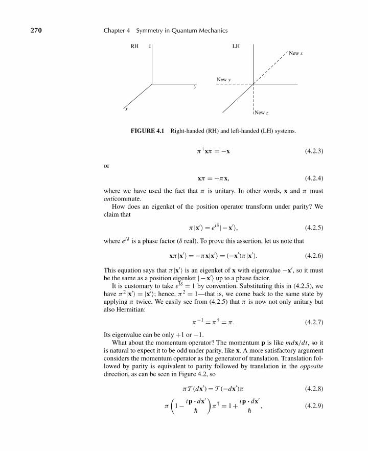
270 Chapter 4 Symmetry in Quantum Mechanics
z
y
x
New x
New z
New y
LHRH
FIGURE 4.1 Right-handed (RH) and left-handed (LH) systems.
π†xπ = −x (4.2.3)
or
xπ = −πx, (4.2.4)
where we have used the fact that π is unitary. In other words, x and π mustanticommute.
How does an eigenket of the position operator transform under parity? Weclaim that
π |x′〉 = eiδ|− x′〉, (4.2.5)
where eiδ is a phase factor (δ real). To prove this assertion, let us note that
xπ |x′〉 = −πx|x′〉 = (−x′)π |x′〉. (4.2.6)
This equation says that π |x′〉 is an eigenket of x with eigenvalue −x′, so it mustbe the same as a position eigenket |− x′〉 up to a phase factor.
It is customary to take eiδ = 1 by convention. Substituting this in (4.2.5), wehave π2|x′〉 = |x′〉; hence, π2 = 1—that is, we come back to the same state byapplying π twice. We easily see from (4.2.5) that π is now not only unitary butalso Hermitian:
π−1 = π† = π . (4.2.7)
Its eigenvalue can be only +1 or −1.What about the momentum operator? The momentum p is like mdx/dt , so it
is natural to expect it to be odd under parity, like x. A more satisfactory argumentconsiders the momentum operator as the generator of translation. Translation fol-lowed by parity is equivalent to parity followed by translation in the oppositedirection, as can be seen in Figure 4.2, so
πT (dx′) = T (−dx′)π (4.2.8)
π
(1 − ip · dx′
h
)π† = 1 + ip · dx′
h, (4.2.9)
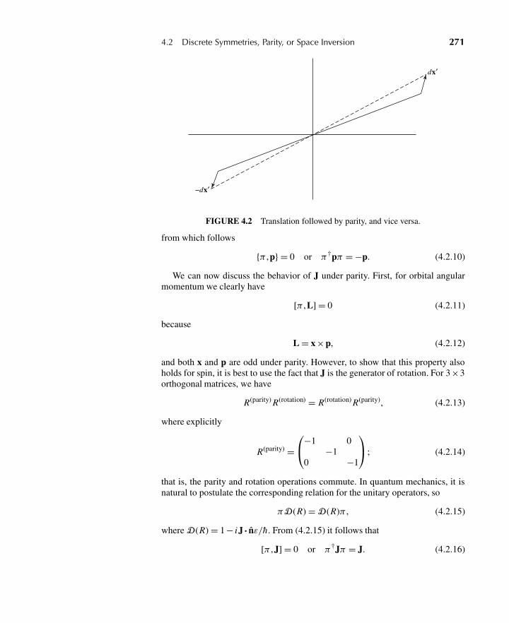
4.2 Discrete Symmetries, Parity, or Space Inversion 271
−dx′
dx′
FIGURE 4.2 Translation followed by parity, and vice versa.
from which follows
{π ,p} = 0 or π†pπ = −p. (4.2.10)
We can now discuss the behavior of J under parity. First, for orbital angularmomentum we clearly have
[π ,L] = 0 (4.2.11)
because
L = x ×p, (4.2.12)
and both x and p are odd under parity. However, to show that this property alsoholds for spin, it is best to use the fact that J is the generator of rotation. For 3×3orthogonal matrices, we have
R(parity) R(rotation) = R(rotation) R(parity), (4.2.13)
where explicitly
R(parity) =⎛⎝−1 0
−10 −1
⎞⎠ ; (4.2.14)
that is, the parity and rotation operations commute. In quantum mechanics, it isnatural to postulate the corresponding relation for the unitary operators, so
πD(R) = D(R)π , (4.2.15)
where D(R) = 1 − iJ · nε/h. From (4.2.15) it follows that
[π ,J] = 0 or π†Jπ = J. (4.2.16)
272 Chapter 4 Symmetry in Quantum Mechanics
This, together with (4.2.11), means that the spin operator S (leading to the totalangular momentum J = L+ S) also transforms in the same way as L.
Under rotations, x and J transform in the same way, so they are both vectors,or spherical tensors, of rank 1. However, x (or p) is odd under parity [see (4.2.3)and (4.2.10)], whereas J is even under parity [see (4.2.16)]. Vectors that are oddunder parity are called polar vectors, and vectors that are even under parity arecalled axial vectors, or pseudovectors.
Let us now consider operators like S · x. Under rotations they transform likeordinary scalars, such as S · L or x · p. Yet under space inversion we have
π−1S · xπ = −S · x, (4.2.17)
whereas for ordinary scalars we have
π−1L · Sπ = L · S (4.2.18)
and so on. The operator S ·x is an example of a pseudoscalar.
Wave Functions Under Parity
Let us now look at the parity property of wave functions. First, let ψ be the wavefunction of a spinless particle whose state ket is |α〉:
ψ(x′) = 〈x′|α〉. (4.2.19)
The wave function of the space-inverted state, represented by the state ket π |α〉,is
〈x′|π |α〉 = 〈−x′|α〉 = ψ(−x′). (4.2.20)
Suppose |α〉 is an eigenket of parity. We have already seen that the eigenvalueof parity must be ±1, so
π |α〉 = ±|α〉. (4.2.21)
Let us look at its corresponding wave function,
〈x′|π |α〉 = ±〈x′|α〉. (4.2.22)
But we also have
〈x′|π |α〉 = 〈−x′|α〉, (4.2.23)
so the state |α〉 is even or odd under parity, depending on whether the correspond-ing wave function satisfies
ψ(−x′) = ±ψ(x′){
evenparity,oddparity.
(4.2.24)
4.2 Discrete Symmetries, Parity, or Space Inversion 273
Not all wave functions of physical interest have definite parities in the senseof (4.2.24). Consider, for instance, the momentum eigenket. The momentum op-erator anticommutes with the parity operator, so the momentum eigenket is notexpected to be a parity eigenket. Indeed, it is easy to see that the plane wave,which is the wave function for a momentum eigenket, does not satisfy (4.2.24).
An eigenket of orbital angular momentum is expected to be a parity eigenketbecause L and π commute [see (4.2.11)]. To see how an eigenket of L2 and Lzbehaves under parity, let us examine the properties of its wave function underspace inversion,
〈x′|α, lm〉 = Rα(r )Y ml (θ ,φ). (4.2.25)
The transformation x′ → −x′ is accomplished by letting
r → r
θ → π − θ (cosθ → −cosθ )
φ→ φ+π (eimφ → (−1)meimφ ).
(4.2.26)
Using the explicit form of
Y ml = (−1)m
√(2l + 1)(l − m)!
4π(l + m)!Pm
l (cosθ )eimφ (4.2.27)
for positive m, with (3.6.38), where
P |m|l (cosθ ) = (−1)m+l
2l l!
(l +|m|)!(l −|m|)! sin−|m| θ
(d
d(cosθ )
)l−|m|sin2l θ , (4.2.28)
we can readily show that
Y ml → (−1)lY m
l (4.2.29)
as θ and φ are changed, as in (4.2.26). Therefore, we can conclude that
π |α, lm〉 = (−1)l|α, lm〉. (4.2.30)
It is actually not necessary to look at Y ml ; an easier way to obtain the same result
is to work with m = 0 and note that Lr±|l,m = 0〉(r = 0,1, . . . , l) must have thesame parity because π and (L±)r commute.
Let us now look at the parity properties of energy eigenstates. We begin bystating a very important theorem.
Theorem 4.1. Suppose
[H ,π] = 0 (4.2.31)
and |n〉 is a nondegenerate eigenket of H with eigenvalue En:
H |n〉 = En|n〉; (4.2.32)
then |n〉 is also a parity eigenket.
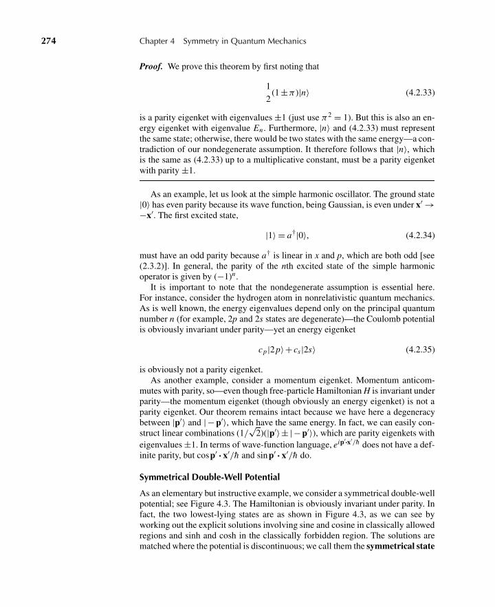
274 Chapter 4 Symmetry in Quantum Mechanics
Proof. We prove this theorem by first noting that
1
2(1 ±π)|n〉 (4.2.33)
is a parity eigenket with eigenvalues ±1 (just use π2 = 1). But this is also an en-ergy eigenket with eigenvalue En . Furthermore, |n〉 and (4.2.33) must representthe same state; otherwise, there would be two states with the same energy—a con-tradiction of our nondegenerate assumption. It therefore follows that |n〉, whichis the same as (4.2.33) up to a multiplicative constant, must be a parity eigenketwith parity ±1.
As an example, let us look at the simple harmonic oscillator. The ground state|0〉 has even parity because its wave function, being Gaussian, is even under x′ →−x′. The first excited state,
|1〉 = a†|0〉, (4.2.34)
must have an odd parity because a† is linear in x and p, which are both odd [see(2.3.2)]. In general, the parity of the nth excited state of the simple harmonicoperator is given by (−1)n.
It is important to note that the nondegenerate assumption is essential here.For instance, consider the hydrogen atom in nonrelativistic quantum mechanics.As is well known, the energy eigenvalues depend only on the principal quantumnumber n (for example, 2p and 2s states are degenerate)—the Coulomb potentialis obviously invariant under parity—yet an energy eigenket
cp|2 p〉+ cs|2s〉 (4.2.35)
is obviously not a parity eigenket.As another example, consider a momentum eigenket. Momentum anticom-
mutes with parity, so—even though free-particle Hamiltonian H is invariant underparity—the momentum eigenket (though obviously an energy eigenket) is not aparity eigenket. Our theorem remains intact because we have here a degeneracybetween |p′〉 and |− p′〉, which have the same energy. In fact, we can easily con-struct linear combinations (1/
√2)(|p′〉± |− p′〉), which are parity eigenkets with
eigenvalues ±1. In terms of wave-function language, eip′·x′/h does not have a def-inite parity, but cosp′ · x′/h and sinp′ · x′/h do.
Symmetrical Double-Well Potential
As an elementary but instructive example, we consider a symmetrical double-wellpotential; see Figure 4.3. The Hamiltonian is obviously invariant under parity. Infact, the two lowest-lying states are as shown in Figure 4.3, as we can see byworking out the explicit solutions involving sine and cosine in classically allowedregions and sinh and cosh in the classically forbidden region. The solutions arematched where the potential is discontinuous; we call them the symmetrical state
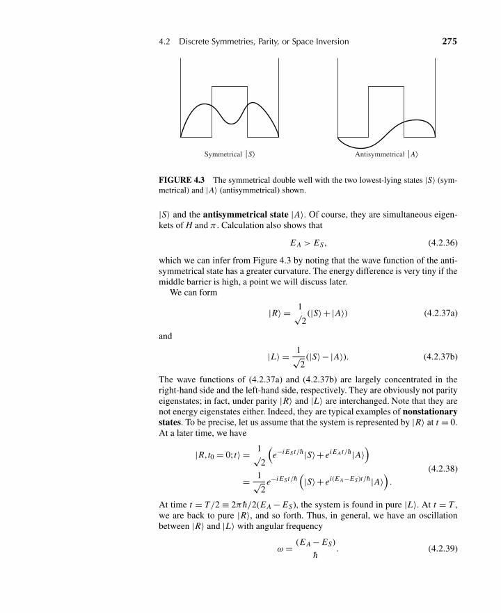
4.2 Discrete Symmetries, Parity, or Space Inversion 275
Symmetrical ⏐S⟩ Antisymmetrical ⏐A⟩
FIGURE 4.3 The symmetrical double well with the two lowest-lying states |S〉 (sym-metrical) and |A〉 (antisymmetrical) shown.
|S〉 and the antisymmetrical state |A〉. Of course, they are simultaneous eigen-kets of H and π . Calculation also shows that
E A > ES , (4.2.36)
which we can infer from Figure 4.3 by noting that the wave function of the anti-symmetrical state has a greater curvature. The energy difference is very tiny if themiddle barrier is high, a point we will discuss later.
We can form
|R〉 = 1√2
(|S〉+ |A〉) (4.2.37a)
and
|L〉 = 1√2
(|S〉− |A〉). (4.2.37b)
The wave functions of (4.2.37a) and (4.2.37b) are largely concentrated in theright-hand side and the left-hand side, respectively. They are obviously not parityeigenstates; in fact, under parity |R〉 and |L〉 are interchanged. Note that they arenot energy eigenstates either. Indeed, they are typical examples of nonstationarystates. To be precise, let us assume that the system is represented by |R〉 at t = 0.At a later time, we have
|R, t0 = 0; t〉 = 1√2
(e−i ES t/h|S〉+ ei E A t/h|A〉
)= 1√
2e−i ES t/h
(|S〉+ ei(E A−ES)t/h |A〉
).
(4.2.38)
At time t = T/2 ≡ 2π h/2(E A − ES), the system is found in pure |L〉. At t = T ,we are back to pure |R〉, and so forth. Thus, in general, we have an oscillationbetween |R〉 and |L〉 with angular frequency
ω = (E A − ES)
h. (4.2.39)
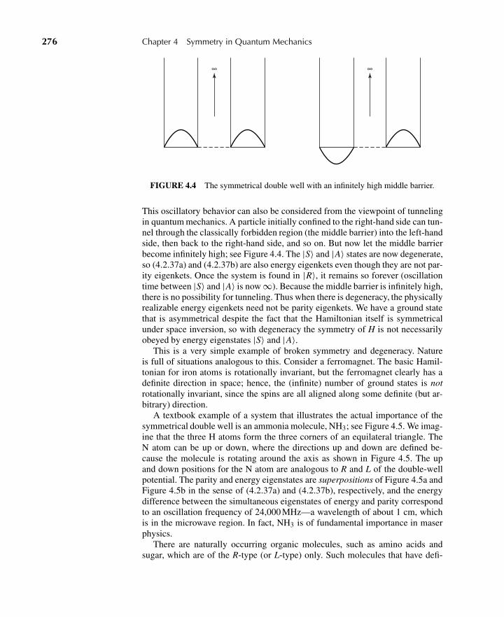
276 Chapter 4 Symmetry in Quantum Mechanics
∞ ∞
FIGURE 4.4 The symmetrical double well with an infinitely high middle barrier.
This oscillatory behavior can also be considered from the viewpoint of tunnelingin quantum mechanics. A particle initially confined to the right-hand side can tun-nel through the classically forbidden region (the middle barrier) into the left-handside, then back to the right-hand side, and so on. But now let the middle barrierbecome infinitely high; see Figure 4.4. The |S〉 and |A〉 states are now degenerate,so (4.2.37a) and (4.2.37b) are also energy eigenkets even though they are not par-ity eigenkets. Once the system is found in |R〉, it remains so forever (oscillationtime between |S〉 and |A〉 is now ∞). Because the middle barrier is infinitely high,there is no possibility for tunneling. Thus when there is degeneracy, the physicallyrealizable energy eigenkets need not be parity eigenkets. We have a ground statethat is asymmetrical despite the fact that the Hamiltonian itself is symmetricalunder space inversion, so with degeneracy the symmetry of H is not necessarilyobeyed by energy eigenstates |S〉 and |A〉.
This is a very simple example of broken symmetry and degeneracy. Natureis full of situations analogous to this. Consider a ferromagnet. The basic Hamil-tonian for iron atoms is rotationally invariant, but the ferromagnet clearly has adefinite direction in space; hence, the (infinite) number of ground states is notrotationally invariant, since the spins are all aligned along some definite (but ar-bitrary) direction.
A textbook example of a system that illustrates the actual importance of thesymmetrical double well is an ammonia molecule, NH3; see Figure 4.5. We imag-ine that the three H atoms form the three corners of an equilateral triangle. TheN atom can be up or down, where the directions up and down are defined be-cause the molecule is rotating around the axis as shown in Figure 4.5. The upand down positions for the N atom are analogous to R and L of the double-wellpotential. The parity and energy eigenstates are superpositions of Figure 4.5a andFigure 4.5b in the sense of (4.2.37a) and (4.2.37b), respectively, and the energydifference between the simultaneous eigenstates of energy and parity correspondto an oscillation frequency of 24,000 MHz—a wavelength of about 1 cm, whichis in the microwave region. In fact, NH3 is of fundamental importance in maserphysics.
There are naturally occurring organic molecules, such as amino acids andsugar, which are of the R-type (or L-type) only. Such molecules that have defi-
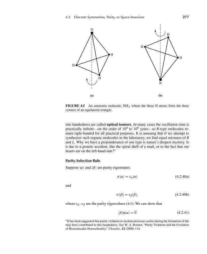
4.2 Discrete Symmetries, Parity, or Space Inversion 277
H
H
N
H
H
H
H
N
(a) (b)
FIGURE 4.5 An ammonia molecule, NH3, where the three H atoms form the threecorners of an equilateral triangle.
nite handedness are called optical isomers. In many cases the oscillation time ispractically infinite—on the order of 104 to 106 years—so R-type molecules re-main right-handed for all practical purposes. It is amusing that if we attempt tosynthesize such organic molecules in the laboratory, we find equal mixtures of Rand L. Why we have a preponderance of one type is nature’s deepest mystery. Isit due to a genetic accident, like the spiral shell of a snail, or to the fact that ourhearts are on the left-hand side?∗
Parity-Selection Rule
Suppose |α〉 and |β〉 are parity eigenstates:
π |α〉 = εα|α〉 (4.2.40a)
and
π |β〉 = εβ |β〉, (4.2.40b)
where εα , εβ are the parity eigenvalues (±1). We can show that
〈β|x|α〉 = 0 (4.2.41)
∗It has been suggested that parity violation in nuclear processes active during the formation of lifemay have contributed to this handedness. See W. A. Bonner, “Parity Violation and the Evolutionof Biomolecular Homochirality,” Chirality, 12 (2000) 114.
278 Chapter 4 Symmetry in Quantum Mechanics
unless εα = −εβ . In other words, the parity-odd operator x connects states ofopposite parity. The proof of this follows:
〈β|x|α〉 = 〈β|π−1πxπ−1π |α〉 = εαεβ(−〈β|x|α〉), (4.2.42)
which is impossible for a finite nonzero 〈β|x|α〉 unless εα and εβ are opposite insign. Perhaps the reader is familiar with this argument from∫
ψ∗βxψαdτ = 0 (4.2.43)
if ψβ and ψα have the same parity. This selection rule, first expressed by Wigner,is important in discussing radiative transitions between atomic states. As we willdiscuss in greater detail later, radiative transitions take place between states ofopposite parity as a consequence of multipole expansion formalism. This rulewas known phenomenologically from analysis of spectral lines, before the birth ofquantum mechanics, as Laporte’s rule. It was Wigner who showed that Laporte’srule is a consequence of the parity-selection rule.
If the basic Hamiltonian H is invariant under parity, nondegenerate energyeigenstates [as a corollary of (4.2.43)] cannot possess a permanent electric dipolemoment:
〈n|x|n〉 = 0. (4.2.44)
This follows trivially from (4.2.43), because with the nondegenerate assumption,energy eigenstates are also parity eigenstates [see (4.2.32) and (4.2.33)]. For adegenerate state, it is perfectly all right to have an electric dipole moment. Wewill see an example of this when we discuss the linear Stark effect in Chapter 5.
Our considerations can be generalized: Operators that are odd under parity,like p or S ·x, have nonvanishing matrix elements only between states of oppositeparity. In contrast, operators that are even under parity connect states of the sameparity.
Parity Nonconservation
The basic Hamiltonian responsible for the so-called weak interaction of elemen-tary particles is not invariant under parity. In decay processes we can have finalstates that are superpositions of opposite parity states. Observable quantities likethe angular distribution of decay products can depend on pseudoscalars such as〈S〉 · p. It is remarkable that parity conservation was believed to be a sacred prin-ciple until 1956, when Lee and Yang speculated that parity is not conserved inweak interactions and proposed crucial experiments to test the validity of parityconservation. Subsequent experiments indeed showed that observable effects dodepend on pseudoscalar quantities such as correlation between 〈S〉 and p.
To this day, one of clearest demonstrations of parity nonconservation is the ex-periment that first revealed it. This result—see Wu, Ambler, et al., Phys. Rev. 105(1957) 1413, shows a decay rate that depends on 〈S〉 · p. The decay observed is60Co →60 Ni+ e− + νe, where S is the spin of the 60Co nucleus, and the momen-tum of the emitted e− is p. A sample of spin-polarized radioactive 60Co nuclei is
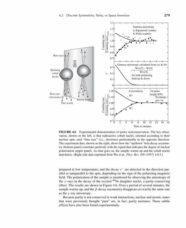
4.2 Discrete Symmetries, Parity, or Space Inversion 279
Gamma-anisotropy
Gamma-anisotropy calculated from (a) & (b)
a) Equatorial counterb) Polar counter
a)
b)
ε =εγ
W(π/2) − W(O)W(π/2)
for both polarizing field up & down
β asymmetry (At pulseheight IOV)
Exchangegas in
H
H
Cou
ntin
g ra
te⟨C
ount
ing
rate
⟩ war
m
Cou
ntin
g ra
te⟨C
ount
ing
rate
⟩ war
m
0.7
0.8
0.9
1.0
1.1
1.2
1.3
0
0.1
0.2
0.3
0.9
0.8
0.7
1.00
1.10
1.20
0 2 4 6 8 10 12 14 16 18
Time in minutes
This world
Beta rays(electrons)
Beta rays
Spinningcobaltnuclei
Mir
ror
Mirror
Mirror world
FIGURE 4.6 Experimental demonstration of parity nonconservation. The key obser-vation, shown on the left, is that radioactive cobalt nuclei, oriented according to theirnuclear spin, emit “beta rays” (i.e., electrons) preferentially in the opposite direction.The experiment data, shown on the right, shows how the “up/down” beta decay asymme-try (bottom panel) correlates perfectly with the signal that indicates the degree of nuclearpolarization (upper panel). As time goes on, the sample warms up and the cobalt nucleidepolarize. (Right side data reprinted from Wu et al., Phys. Rev. 105 (1957) 1413.)
prepared at low temperature, and the decay e− are detected in the direction par-allel or antiparallel to the spin, depending on the sign of the polarizing magneticfield. The polarization of the sample is monitored by observing the anisotropy ofthe γ -rays in the decay of the excited 60Ni daughter nuclei, a parity-conservingeffect. The results are shown in Figure 4.6. Over a period of several minutes, thesample warms up, and the β-decay asymmetry disappears at exactly the same rateas the γ -ray anisotropy.
Because parity is not conserved in weak interactions, nuclear and atomic statesthat were previously thought “pure” are, in fact, parity mixtures. These subtleeffects have also been found experimentally.
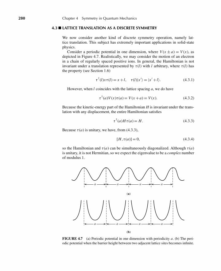
280 Chapter 4 Symmetry in Quantum Mechanics
4.3 LATTICE TRANSLATION AS A DISCRETE SYMMETRY
We now consider another kind of discrete symmetry operation, namely lat-tice translation. This subject has extremely important applications in solid-statephysics.
Consider a periodic potential in one dimension, where V (x ± a) = V (x), asdepicted in Figure 4.7. Realistically, we may consider the motion of an electronin a chain of regularly spaced positive ions. In general, the Hamiltonian is notinvariant under a translation represented by τ (l) with l arbitrary, where τ (l) hasthe property (see Section 1.6)
τ †(l)xτ (l) = x + l, τ (l)|x ′〉 = |x ′ + l〉. (4.3.1)
However, when l coincides with the lattice spacing a, we do have
τ †(a)V (x)τ (a) = V (x + a) = V (x). (4.3.2)
Because the kinetic-energy part of the Hamiltonian H is invariant under the trans-lation with any displacement, the entire Hamiltonian satisfies
τ †(a)H τ (a) = H . (4.3.3)
Because τ (a) is unitary, we have, from (4.3.3),
[H ,τ (a)] = 0, (4.3.4)
so the Hamiltonian and τ (a) can be simultaneously diagonalized. Although τ (a)is unitary, it is not Hermitian, so we expect the eigenvalue to be a complex numberof modulus 1.
a a a a
a a a a
(a)
(b)
FIGURE 4.7 (a) Periodic potential in one dimension with periodicity a. (b) The peri-odic potential when the barrier height between two adjacent lattice sites becomes infinite.
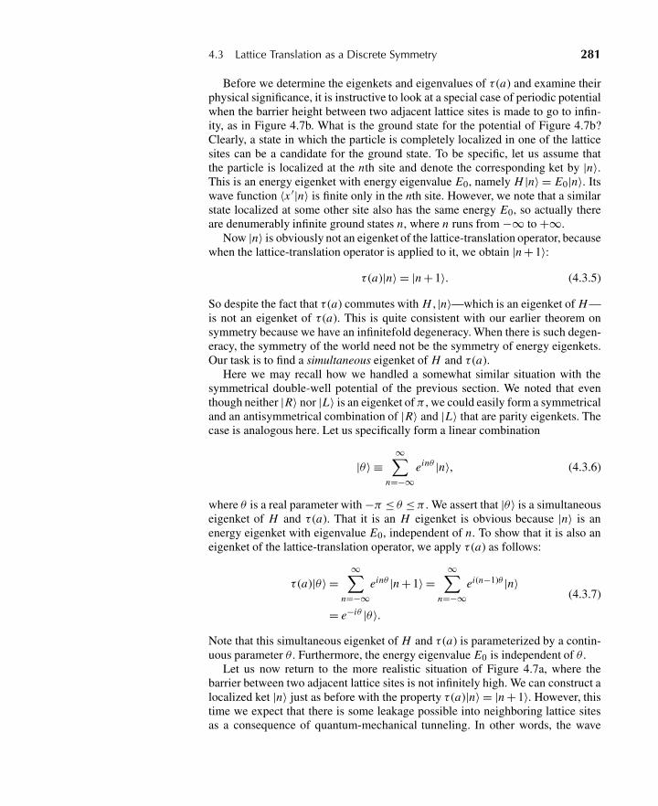
4.3 Lattice Translation as a Discrete Symmetry 281
Before we determine the eigenkets and eigenvalues of τ (a) and examine theirphysical significance, it is instructive to look at a special case of periodic potentialwhen the barrier height between two adjacent lattice sites is made to go to infin-ity, as in Figure 4.7b. What is the ground state for the potential of Figure 4.7b?Clearly, a state in which the particle is completely localized in one of the latticesites can be a candidate for the ground state. To be specific, let us assume thatthe particle is localized at the nth site and denote the corresponding ket by |n〉.This is an energy eigenket with energy eigenvalue E0, namely H |n〉 = E0|n〉. Itswave function 〈x ′|n〉 is finite only in the nth site. However, we note that a similarstate localized at some other site also has the same energy E0, so actually thereare denumerably infinite ground states n, where n runs from −∞ to +∞.
Now |n〉 is obviously not an eigenket of the lattice-translation operator, becausewhen the lattice-translation operator is applied to it, we obtain |n + 1〉:
τ (a)|n〉 = |n + 1〉. (4.3.5)
So despite the fact that τ (a) commutes with H , |n〉—which is an eigenket of H —is not an eigenket of τ (a). This is quite consistent with our earlier theorem onsymmetry because we have an infinitefold degeneracy. When there is such degen-eracy, the symmetry of the world need not be the symmetry of energy eigenkets.Our task is to find a simultaneous eigenket of H and τ (a).
Here we may recall how we handled a somewhat similar situation with thesymmetrical double-well potential of the previous section. We noted that eventhough neither |R〉 nor |L〉 is an eigenket of π , we could easily form a symmetricaland an antisymmetrical combination of |R〉 and |L〉 that are parity eigenkets. Thecase is analogous here. Let us specifically form a linear combination
|θ〉 ≡∞∑
n=−∞einθ |n〉, (4.3.6)
where θ is a real parameter with −π ≤ θ ≤ π . We assert that |θ〉 is a simultaneouseigenket of H and τ (a). That it is an H eigenket is obvious because |n〉 is anenergy eigenket with eigenvalue E0, independent of n. To show that it is also aneigenket of the lattice-translation operator, we apply τ (a) as follows:
τ (a)|θ〉 =∞∑
n=−∞einθ |n + 1〉 =
∞∑n=−∞
ei(n−1)θ |n〉
= e−iθ |θ〉.(4.3.7)
Note that this simultaneous eigenket of H and τ (a) is parameterized by a contin-uous parameter θ . Furthermore, the energy eigenvalue E0 is independent of θ .
Let us now return to the more realistic situation of Figure 4.7a, where thebarrier between two adjacent lattice sites is not infinitely high. We can construct alocalized ket |n〉 just as before with the property τ (a)|n〉 = |n + 1〉. However, thistime we expect that there is some leakage possible into neighboring lattice sitesas a consequence of quantum-mechanical tunneling. In other words, the wave
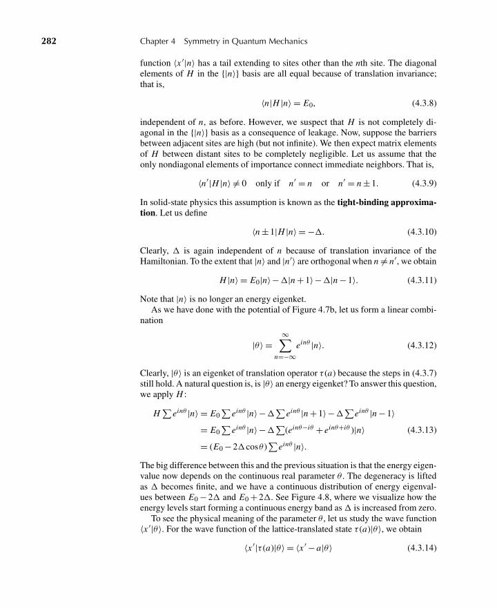
282 Chapter 4 Symmetry in Quantum Mechanics
function 〈x ′|n〉 has a tail extending to sites other than the nth site. The diagonalelements of H in the {|n〉} basis are all equal because of translation invariance;that is,
〈n|H |n〉 = E0, (4.3.8)
independent of n, as before. However, we suspect that H is not completely di-agonal in the {|n〉} basis as a consequence of leakage. Now, suppose the barriersbetween adjacent sites are high (but not infinite). We then expect matrix elementsof H between distant sites to be completely negligible. Let us assume that theonly nondiagonal elements of importance connect immediate neighbors. That is,
〈n′|H |n〉 �= 0 only if n′ = n or n′ = n ± 1. (4.3.9)
In solid-state physics this assumption is known as the tight-binding approxima-tion. Let us define
〈n ± 1|H |n〉 = −�. (4.3.10)
Clearly, � is again independent of n because of translation invariance of theHamiltonian. To the extent that |n〉 and |n′〉 are orthogonal when n �= n′, we obtain
H |n〉 = E0|n〉−�|n + 1〉−�|n − 1〉. (4.3.11)
Note that |n〉 is no longer an energy eigenket.As we have done with the potential of Figure 4.7b, let us form a linear combi-
nation
|θ〉 =∞∑
n=−∞einθ |n〉. (4.3.12)
Clearly, |θ〉 is an eigenket of translation operator τ (a) because the steps in (4.3.7)still hold. A natural question is, is |θ〉 an energy eigenket? To answer this question,we apply H :
H∑
einθ |n〉 = E0∑
einθ |n〉−�∑einθ |n + 1〉−�∑einθ |n − 1〉= E0
∑einθ |n〉−�∑(einθ−iθ + einθ+iθ )|n〉
= (E0 − 2�cosθ )∑
einθ |n〉.(4.3.13)
The big difference between this and the previous situation is that the energy eigen-value now depends on the continuous real parameter θ . The degeneracy is liftedas � becomes finite, and we have a continuous distribution of energy eigenval-ues between E0 − 2� and E0 + 2�. See Figure 4.8, where we visualize how theenergy levels start forming a continuous energy band as� is increased from zero.
To see the physical meaning of the parameter θ , let us study the wave function〈x ′|θ〉. For the wave function of the lattice-translated state τ (a)|θ〉, we obtain
〈x ′|τ (a)|θ〉 = 〈x ′ − a|θ〉 (4.3.14)
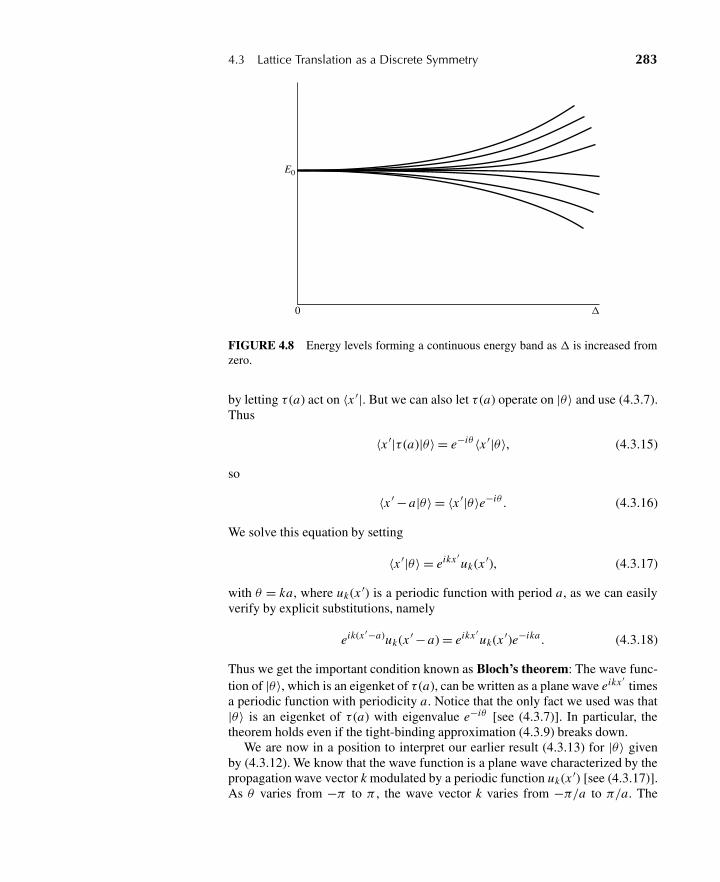
4.3 Lattice Translation as a Discrete Symmetry 283
E0
0 �
FIGURE 4.8 Energy levels forming a continuous energy band as � is increased fromzero.
by letting τ (a) act on 〈x ′|. But we can also let τ (a) operate on |θ〉 and use (4.3.7).Thus
〈x ′|τ (a)|θ〉 = e−iθ 〈x ′|θ〉, (4.3.15)
so
〈x ′ − a|θ〉 = 〈x ′|θ〉e−iθ . (4.3.16)
We solve this equation by setting
〈x ′|θ〉 = eikx ′uk(x ′), (4.3.17)
with θ = ka, where uk(x ′) is a periodic function with period a, as we can easilyverify by explicit substitutions, namely
eik(x ′−a)uk(x ′ − a) = eikx ′uk(x ′)e−ika . (4.3.18)
Thus we get the important condition known as Bloch’s theorem: The wave func-tion of |θ〉, which is an eigenket of τ (a), can be written as a plane wave eikx ′
timesa periodic function with periodicity a. Notice that the only fact we used was that|θ〉 is an eigenket of τ (a) with eigenvalue e−iθ [see (4.3.7)]. In particular, thetheorem holds even if the tight-binding approximation (4.3.9) breaks down.
We are now in a position to interpret our earlier result (4.3.13) for |θ〉 givenby (4.3.12). We know that the wave function is a plane wave characterized by thepropagation wave vector k modulated by a periodic function uk(x ′) [see (4.3.17)].As θ varies from −π to π , the wave vector k varies from −π/a to π/a. The
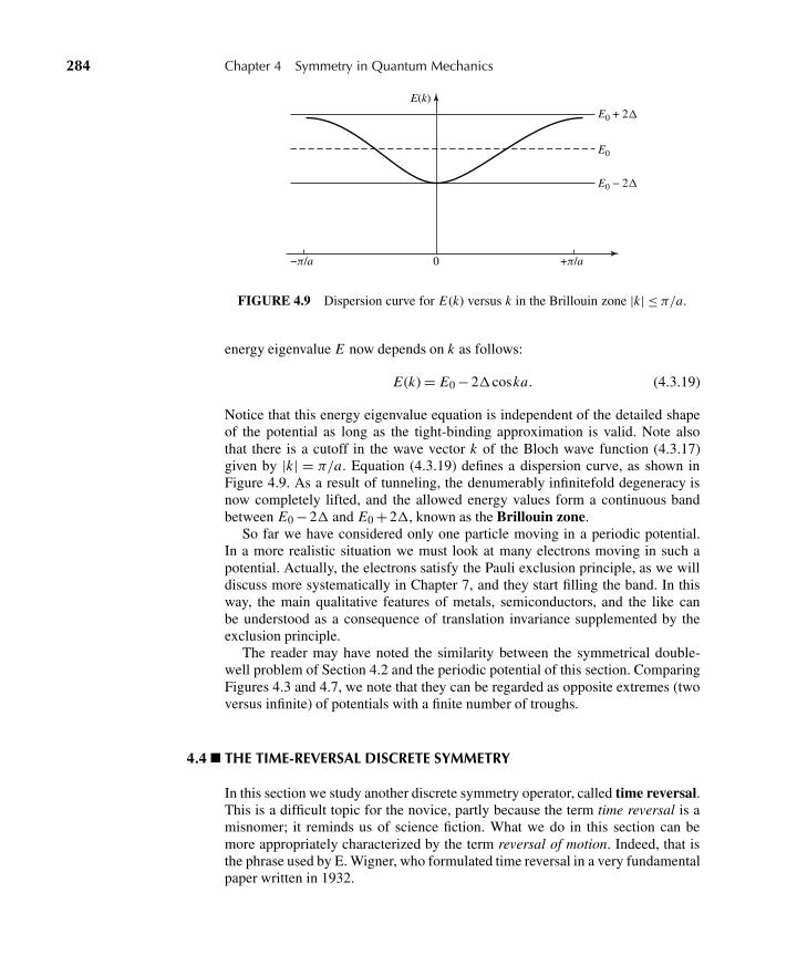
284 Chapter 4 Symmetry in Quantum Mechanics
E(k)E0 + 2�
E0
E0 − 2�
−π/a 0 +π/a
FIGURE 4.9 Dispersion curve for E(k) versus k in the Brillouin zone |k| ≤ π/a.
energy eigenvalue E now depends on k as follows:
E(k) = E0 − 2�coska. (4.3.19)
Notice that this energy eigenvalue equation is independent of the detailed shapeof the potential as long as the tight-binding approximation is valid. Note alsothat there is a cutoff in the wave vector k of the Bloch wave function (4.3.17)given by |k| = π/a. Equation (4.3.19) defines a dispersion curve, as shown inFigure 4.9. As a result of tunneling, the denumerably infinitefold degeneracy isnow completely lifted, and the allowed energy values form a continuous bandbetween E0 − 2� and E0 + 2�, known as the Brillouin zone.
So far we have considered only one particle moving in a periodic potential.In a more realistic situation we must look at many electrons moving in such apotential. Actually, the electrons satisfy the Pauli exclusion principle, as we willdiscuss more systematically in Chapter 7, and they start filling the band. In thisway, the main qualitative features of metals, semiconductors, and the like canbe understood as a consequence of translation invariance supplemented by theexclusion principle.
The reader may have noted the similarity between the symmetrical double-well problem of Section 4.2 and the periodic potential of this section. ComparingFigures 4.3 and 4.7, we note that they can be regarded as opposite extremes (twoversus infinite) of potentials with a finite number of troughs.
4.4 THE TIME-REVERSAL DISCRETE SYMMETRY
In this section we study another discrete symmetry operator, called time reversal.This is a difficult topic for the novice, partly because the term time reversal is amisnomer; it reminds us of science fiction. What we do in this section can bemore appropriately characterized by the term reversal of motion. Indeed, that isthe phrase used by E. Wigner, who formulated time reversal in a very fundamentalpaper written in 1932.
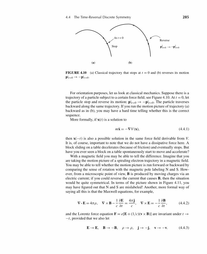
4.4 The Time-Reversal Discrete Symmetry 285
At t = 0
Stop
Reverse
(a) (b)
p⏐t=0 → −p⏐t=0
FIGURE 4.10 (a) Classical trajectory that stops at t = 0 and (b) reverses its motionp|t=0 → −p|t=0.
For orientation purposes, let us look at classical mechanics. Suppose there is atrajectory of a particle subject to a certain force field; see Figure 4.10. At t = 0, letthe particle stop and reverse its motion: p|t=0 → −p|t=0. The particle traversesbackward along the same trajectory. If you run the motion picture of trajectory (a)backward as in (b), you may have a hard time telling whether this is the correctsequence.
More formally, if x(t) is a solution to
mx = −∇V (x), (4.4.1)
then x(−t) is also a possible solution in the same force field derivable from V.It is, of course, important to note that we do not have a dissipative force here. Ablock sliding on a table decelerates (because of friction) and eventually stops. Buthave you ever seen a block on a table spontaneously start to move and accelerate?
With a magnetic field you may be able to tell the difference. Imagine that youare taking the motion picture of a spiraling electron trajectory in a magnetic field.You may be able to tell whether the motion picture is run forward or backward bycomparing the sense of rotation with the magnetic pole labeling N and S. How-ever, from a microscopic point of view, B is produced by moving charges via anelectric current; if you could reverse the current that causes B, then the situationwould be quite symmetrical. In terms of the picture shown in Figure 4.11, youmay have figured out that N and S are mislabeled! Another, more formal way ofsaying all this is that the Maxwell equations, for example,
∇· E = 4πρ, ∇ ×B− 1
c
∂E∂ t
= 4πjc
, ∇ ×E = −1
c
∂B∂ t
, (4.4.2)
and the Lorentz force equation F = e[E + (1/c)(v × B)] are invariant under t →−t , provided that we also let
E → E, B → −B, ρ → ρ, j → −j, v → −v. (4.4.3)
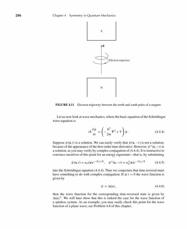
286 Chapter 4 Symmetry in Quantum Mechanics
B
S
N
Electron trajectory
FIGURE 4.11 Electron trajectory between the north and south poles of a magnet.
Let us now look at wave mechanics, where the basic equation of the Schrödingerwave equation is
i h∂ψ
∂ t=(
− h2
2m∇2 + V
)ψ . (4.4.4)
Suppose ψ(x, t) is a solution. We can easily verify that ψ(x,−t) is not a solution,because of the appearance of the first-order time derivative. However,ψ∗(x,−t) isa solution, as you may verify by complex conjugation of (4.4.4). It is instructive toconvince ourselves of this point for an energy eigenstate—that is, by substituting
ψ(x, t) = un(x)e−i En t/h , ψ∗(x,−t) = u∗n(x)e−i En t/h (4.4.5)
into the Schrödinger equation (4.4.4). Thus we conjecture that time reversal musthave something to do with complex conjugation. If at t = 0 the wave function isgiven by
ψ = 〈x|α〉, (4.4.6)
then the wave function for the corresponding time-reversed state is given by〈x|α〉∗. We will later show that this is indeed the case for the wave function ofa spinless system. As an example, you may easily check this point for the wavefunction of a plane wave; see Problem 4.8 of this chapter.
4.4 The Time-Reversal Discrete Symmetry 287
Digression on Symmetry Operations
Before we begin a systematic treatment of the time-reversal operator, some gen-eral remarks on symmetry operations are in order. Consider a symmetry operation
|α〉 → |α〉, |β〉 → |β〉. (4.4.7)
One may argue that it is natural to require the inner product 〈β|α〉 to bepreserved—that is,
〈β |α〉 = 〈β|α〉. (4.4.8)
Indeed, for symmetry operations such as rotations, translations, and even parity,this is indeed the case. If |α〉 is rotated and |β〉 is also rotated in the same manner,〈β|α〉 is unchanged. Formally, this arises from the fact that for the symmetry oper-ations considered in the previous sections, the corresponding symmetry operatoris unitary, so
〈β|α〉 → 〈β|U†U |α〉 = 〈β|α〉. (4.4.9)
However, in discussing time reversal, we see that requirement (4.4.8) turns outto be too restrictive. Instead, we merely impose the weaker requirement that
|〈β|α〉| = |〈β|α〉|. (4.4.10)
Requirement (4.4.8) obviously satisfies (4.4.10). But this is not the only way;
〈β |α〉 = 〈β|α〉∗ = 〈α|β〉 (4.4.11)
works equally well. We pursue the latter possibility in this section because, fromour earlier discussion based on the Schrödinger equation, we inferred that timereversal has something to do with complex conjugation.
Definition The transformation
|α〉 → |α〉 = θ |α〉, |β〉 → |β〉 = θ |β〉 (4.4.12)
is said to be antiunitary if
〈β|α〉 = 〈β|α〉∗, (4.4.13a)
θ (c1|α〉+ c2|β〉) = c∗1θ |α〉+ c∗
2θ |β〉. (4.4.13b)
In such a case the operator θ is an antiunitary operator. Relation (4.4.13b) alonedefines an antilinear operator.
We now claim that an antiunitary operator can be written as
θ = UK , (4.4.14)
288 Chapter 4 Symmetry in Quantum Mechanics
where U is a unitary operator and K is the complex-conjugate operator that formsthe complex conjugate of any coefficient that multiplies a ket (and stands on theright of K). Before checking (4.4.13), let us examine the property of the K oper-ator. Suppose we have a ket multiplied by a complex number c. We then have
K c|α〉 = c∗K |α〉. (4.4.15)
One may further ask, what happens if |α〉 is expanded in terms of base kets {|a′〉}?Under the action K, we have
|α〉 =∑
a′|a′〉〈a′|α〉 K→|α〉 =
∑a′
〈a′|α〉∗K |a′〉
=∑
a′〈a′|α〉∗|a′〉.
(4.4.16)
Notice that K acting on the base ket does not change the base ket. The explicitrepresentation of |a′〉 is
|a′〉 =
⎛⎜⎜⎜⎜⎜⎜⎜⎜⎜⎜⎜⎜⎝
00...010...0
⎞⎟⎟⎟⎟⎟⎟⎟⎟⎟⎟⎟⎟⎠, (4.4.17)
and there is nothing to be changed by K. The reader may wonder, for instance,whether the Sy eigenkets for a spin 1
2 system change under K. The answer is thatif the Sz eigenkets are used as base kets, we must change the Sy eigenkets becausethe Sy eigenkets (1.1.14) undergo, under the action of K,
K
(1√2|+〉± i√
2|−〉
)→ 1√
2|+〉∓ i√
2|−〉. (4.4.18)
On the other hand, if the Sy eigenkets themselves are used as the base kets, we donot change the Sy eigenkets under the action of K. Thus the effect of K changeswith the basis. As a result, the form of U in (4.4.14) also depends on the particularrepresentation (that is, on the choice of base kets) used.
Returning to θ = UK and (4.4.13), let us first check property (4.4.13b). Wehave
θ (c1|α〉+ c2|β〉) = UK (c1|α〉+ c2|β〉)= c∗
1UK |α〉+ c∗2UK |β〉
= c∗1θ |α〉+ c∗
2θ |β〉, (4.4.19)
4.4 The Time-Reversal Discrete Symmetry 289
so (4.4.13b) indeed holds. Before checking (4.4.13a), we assert that it is alwayssafer to work with the action of θ on kets only. We can figure out how the braschange just by looking at the corresponding kets. In particular, it is not necessaryto consider θ acting on bras from the right, nor is it necessary to define θ†. Wehave
|α〉 θ→|α〉 =∑
a′〈a′|α〉∗UK |a′〉
=∑
a′〈a′|α〉∗U |a′〉
=∑
a′〈α|a′〉U |a′〉. (4.4.20)
As for |β〉, we have
|β〉 =∑
a′〈a′|β〉∗U |a′〉DC↔〈β| =
∑a′
〈a′|β〉〈a′|U†
〈β|α〉 =∑a′′
∑a′
〈a′′|β〉〈a′′|U†U |a′〉〈α|a′〉
=∑
a′〈α|a′〉〈a′|β〉 = 〈α|β〉
= 〈β|α〉∗, (4.4.21)
so this checks. (Recall the notion of “dual correspondence,” or DC, from Sec-tion 1.2.)
In order for (4.4.10) to be satisfied, it is of physical interest to consider just twotypes of transformations—unitary and antiunitary. Other possibilities are relatedto either of the preceding via trivial phase changes. The proof of this assertionis actually very difficult and will not be discussed further here. See, however,Gottfried and Yan (2003), Section 7.1.
Time-Reversal Operator
We are finally in a position to present a formal theory of time reversal. Let usdenote the time-reversal operator by , to be distinguished from θ , a generalantiunitary operator. Consider
|α〉 → |α〉, (4.4.22)
where |α〉 is the time-reversed state. More appropriately, |α〉 should be calledthe motion-reversed state. If |α〉 is a momentum eigenstate |p′〉, we expect |α〉 tobe |−p′〉 up to a possible phase. Likewise, J is to be reversed under time reversal.
We now deduce the fundamental property of the time-reversal operator bylooking at the time evolution of the time-reversed state. Consider a physical sys-tem represented by a ket |α〉, say at t = 0. Then, at a slightly later time t = δt , the
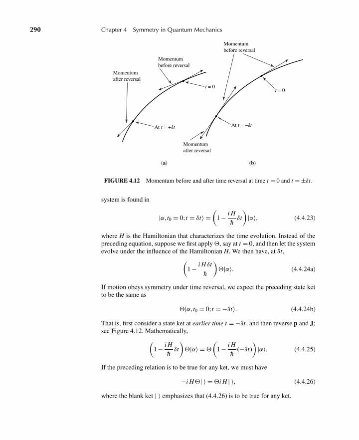
290 Chapter 4 Symmetry in Quantum Mechanics
Momentumafter reversal
Momentumafter reversal
Momentumbefore reversal
Momentumbefore reversal
At t = +δt At t = −δt
t = 0t = 0
(a) (b)
FIGURE 4.12 Momentum before and after time reversal at time t = 0 and t = ±δt .
system is found in
|α, t0 = 0; t = δt〉 =(
1 − i H
hδt
)|α〉, (4.4.23)
where H is the Hamiltonian that characterizes the time evolution. Instead of thepreceding equation, suppose we first apply , say at t = 0, and then let the systemevolve under the influence of the Hamiltonian H. We then have, at δt ,(
1 − i H δt
h
) |α〉. (4.4.24a)
If motion obeys symmetry under time reversal, we expect the preceding state ketto be the same as
|α, t0 = 0; t = −δt〉. (4.4.24b)
That is, first consider a state ket at earlier time t = −δt , and then reverse p and J;see Figure 4.12. Mathematically,(
1 − i H
hδt
) |α〉 =
(1 − i H
h(−δt)
)|α〉. (4.4.25)
If the preceding relation is to be true for any ket, we must have
−i H | 〉 = i H | 〉, (4.4.26)
where the blank ket | 〉 emphasizes that (4.4.26) is to be true for any ket.
4.4 The Time-Reversal Discrete Symmetry 291
We now argue that cannot be unitary if the motion of time reversal is tomake sense. Suppose were unitary. It would then be legitimate to cancel the i’sin (4.4.26), and we would have the operator equation
−H = H . (4.4.27)
Consider an energy eigenket |n〉 with energy eigenvalue En . The correspondingtime-reversed state would be |n〉, and we would have, because of (4.4.27),
H |n〉 = − H |n〉 = (−En) |n〉. (4.4.28)
This equation says that |n〉 is an eigenket of the Hamiltonian with energyeigenvalues −En . But this is nonsensical even in the very elementary case ofa free particle. We know that the energy spectrum of the free particle is posi-tive semidefinite—from 0 to +∞. There is no state lower than a particle at rest(momentum eigenstate with momentum eigenvalue zero); the energy spectrumranging from −∞ to 0 would be completely unacceptable. We can also see this bylooking at the structure of the free-particle Hamiltonian. We expect p to changesign but not p2; yet (4.4.27) would imply that
−1 p2
2m = −p2
2m. (4.4.29)
All these arguments strongly suggest that if time reversal is to be a usefulsymmetry at all, we are not allowed to cancel the i’s in (4.4.26); hence, hadbetter be antiunitary. In this case the right-hand side of (4.4.26) becomes
i H | 〉 = −i H | 〉 (4.4.30)
by antilinear property (4.4.13b). Now at last we can cancel the i’s in (4.4.26). Thisleads finally, via (4.4.30), to
H = H . (4.4.31)
Equation (4.4.31) expresses the fundamental property of the Hamiltonian undertime reversal. With this equation the difficulties mentioned earlier [see (4.4.27) to(4.4.29)] are absent, and we obtain physically sensible results. From now on, wewill always take to be antiunitary.
We mentioned earlier that it is best to avoid an antiunitary operator acting onbras from the right. Nevertheless, we may use
〈β| |α〉, (4.4.32)
which is to be understood always as
(〈β|) · ( |α〉) (4.4.33)
and never as
(〈β| ) · |α〉. (4.4.34)
292 Chapter 4 Symmetry in Quantum Mechanics
In fact, we do not even attempt to define 〈β| . This is one place where the Diracbra-ket notation is a little confusing. After all, that notation was invented to handlelinear operators, not antilinear operators.
With this cautionary remark, we are in a position to discuss the behavior ofoperators under time reversal. We continue to take the point of view that the operator is to act on kets
|α〉 = |α〉, |β〉 = |β〉, (4.4.35)
yet it is often convenient to talk about operators—in particular, observables—which are odd or even under time reversal. We start with an important identity:
〈β|⊗ |α〉 = 〈α| ⊗† −1|β〉, (4.4.36)
where ⊗ is a linear operator. This identity follows solely from the antiunitarynature of . To prove this let us define
|γ 〉 ≡ ⊗†|β〉. (4.4.37)
By dual correspondence we have
|γ 〉DC↔〈β|⊗ = 〈γ |. (4.4.38)
Hence,
〈β|⊗ |α〉 = 〈γ |α〉 = 〈α|γ 〉= 〈α| ⊗† |β〉 = 〈α| ⊗† −1 |β〉= 〈α| ⊗† −1|β〉,
(4.4.39)
which proves the identity. In particular, for Hermitian observables A, we get
〈β|A|α〉 = 〈α| A −1|β〉. (4.4.40)
We say that observables are even or odd under time reversal according to whetherwe have the upper or lower sign in
A −1 = ±A. (4.4.41)
Note that this equation, together with (4.4.40), gives a phase restriction on thematrix elements of A taken with respect to time-reversed states as follows:
〈β|A|α〉 = ±〈β|A|α〉∗. (4.4.42)
If |β〉 is identical to |α〉, so that we are talking about expectation values, we have
〈α|A|α〉 = ±〈α|A|α〉, (4.4.43)
where 〈α|A|α〉 is the expectation value taken with respect to the time-reversedstate.
4.4 The Time-Reversal Discrete Symmetry 293
As an example, let us look at the expectation value of p. It is reasonable toassume that the expectation value of p taken with respect to the time-reversedstate will be of opposite sign. Thus
〈α|p|α〉 = −〈α|p|α〉, (4.4.44)
so we take p to be an odd operator, namely
p −1 = −p. (4.4.45)
This implies that
p |p′〉 = − p −1 |p′〉= (−p′) |p′〉. (4.4.46)
Equation (4.4.46) agrees with our earlier assertion that |p′〉 is a momentumeigenket with eigenvalue −p′. It can be identified with |−p′〉 itself with a suitablechoice of phase. Likewise, we obtain
x −1 = x
|x′〉 = |x′〉 (up to a phase)(4.4.47)
from the (eminently reasonable) requirement
〈α|x|α〉 = 〈α|x|α〉. (4.4.48)
We can now check the invariance of the fundamental commutation relation
[xi , p j ]| 〉 = i hδi j | 〉, (4.4.49)
where the blank ket | 〉 stands for any ket. Applying to both sides of (4.4.49),we have
[xi , p j ] −1 | 〉 = i hδi j | 〉, (4.4.50)
which leads, after passing through i h, to
[xi , (−p j )] | 〉 = −i hδi j | 〉. (4.4.51)
Note that the fundamental commutation relation [xi , p j ] = i hδi j is preserved byvirtue of the fact that is antiunitary. This can be given as yet another reasonfor taking to be antiunitary; otherwise, we would be forced to abandon either(4.4.45) or (4.4.47)! Similarly, to preserve
[Ji , Jj ] = i hεi j k Jk , (4.4.52)
the angular-momentum operator must be odd under time reversal; that is,
J −1 = −J. (4.4.53)
This is consistent for a spinless system where J is just x × p. Alternatively, wecould have deduced this relation by noting that the rotational operator and thetime-reversal operator commute (note the extra i!).
294 Chapter 4 Symmetry in Quantum Mechanics
Wave Function
Suppose at some given time, say at t = 0, a spinless single-particle system is foundin a state represented by |α〉. Its wave function 〈x′|α〉 appears as the expansioncoefficient in the position representation
|α〉 =∫
d3x ′|x′〉〈x′|α〉. (4.4.54)
Applying the time-reversal operator yields
|α〉 =∫
d3x ′ |x′〉〈x′|α〉∗
=∫
d3x ′|x′〉〈x′|α〉∗,
(4.4.55)
where we have chosen the phase convention so that |x′〉 is |x′〉 itself. We thenrecover the rule
ψ (x′) → ψ∗(x′) (4.4.56)
inferred earlier by looking at the Schrödinger wave equation [see (4.4.5)]. Theangular part of the wave function is given by a spherical harmonic Y m
l . With theusual phase convention, we have
Y ml (θ ,φ) → Y m∗
l (θ ,φ) = (−1) mY −ml (θ ,φ). (4.4.57)
Now Y ml (θ ,φ) is the wave function for |l,m〉 [see (3.6.23)]; therefore, from
(4.4.56) we deduce
|l,m〉 = (−1)m|l,−m〉. (4.4.58)
If we study the probability current density (2.4.16) for a wave function of type(3.6.22) going like R(r )Y m
l , we shall conclude that for m > 0 the current flows inthe counterclockwise direction, as seen from the positive z-axis. The wave func-tion for the corresponding time-reversed state has its probability current flowing inthe opposite direction because the sign of m is reversed. All this is very reasonable.
As a nontrivial consequence of time-reversal invariance, we state an importanttheorem on the reality of the energy eigenfunction of a spinless particle.
Theorem 4.2. Suppose the Hamiltonian is invariant under time reversal and theenergy eigenket |n〉 is nondegenerate; then the corresponding energy eigenfunc-tion is real (or, more generally, a real function times a phase factor independentof x).
Proof. To prove this, first note that
H |n〉 = H |n〉 = En |n〉, (4.4.59)
4.4 The Time-Reversal Discrete Symmetry 295
so |n〉 and |n〉 have the same energy. The nondegeneracy assumption promptsus to conclude that |n〉 and |n〉 must represent the same state; otherwise, therewould be two different states with the same energy En , an obvious contradic-tion! Let us recall that the wave functions for |n〉 and |n〉 are 〈x′|n〉 and 〈x′|n〉∗,respectively. They must be the same—that is,
〈x′|n〉 = 〈x′|n〉∗ (4.4.60)
for all practical purposes—or, more precisely, they can differ at most by a phasefactor independent of x.
Thus if we have, for instance, a nondegenerate bound state, its wave functionis always real. On the other hand, in the hydrogen atom with l �= 0, m �= 0, theenergy eigenfunction characterized by definite (n, l,m) quantum numbers is com-plex because Y m
l is complex; this does not contradict the theorem because |n, l,m〉and |n, l,−m〉 are degenerate. Similarly, the wave function of a plane wave eip·x/his complex, but it is degenerate with e−ip·x/h .
We see that for a spinless system, the wave function for the time-reversed state,say at t = 0, is simply obtained by complex conjugation. In terms of ket |α〉 writtenas in (4.4.16) or in (4.4.54), the operator is the complex-conjugate operator Kitself because K and have the same effect when acting on the base ket |a′〉 (or|x′〉). We may note, however, that the situation is quite different when the ket |α〉is expanded in terms of the momentum eigenket, because must change |p′〉 into|− p′〉 as follows:
|α〉 =∫
d3 p′|− p′〉〈p′|α〉∗ =∫
d3 p′|p′〉〈−p′|α〉∗. (4.4.61)
It is apparent that the momentum-space wave function of the time-reversed stateis not just the complex conjugate of the original momentum-space wave function;rather, we must identify φ∗(−p′) as the momentum-space wave function for thetime-reversed state. This situation once again illustrates the basic point that theparticular form of depends on the particular representation used.
Time Reversal for a Spin 12 System
The situation is even more interesting for a particle with spin—spin 12 , in particu-
lar. We recall from Section 3.2 that the eigenket of S ·n with eigenvalue h/2 canbe written as
|n;+〉 = e−i Szα/he−i Syβ/h |+〉, (4.4.62)
where n is characterized by the polar and azimuthal angles β and α, respectively.Noting (4.4.53), we have
|n;+〉 = e−i Szα/he−i Syβ/h |+〉 = η|n;−〉. (4.4.63)
On the other hand, we can easily verify that
|n;−〉 = e−iαSz/he−i(π+β)Sy/h |+〉. (4.4.64)
296 Chapter 4 Symmetry in Quantum Mechanics
In general, we saw earlier that the product UK is an antiunitary operator. Compar-ing (4.4.63) and (4.4.64) with set equal to UK, and noting that K acting on thebase ket |+〉 gives just |+〉, we see that
= ηe−iπSy/h K = −iη
(2Sy
h
)K , (4.4.65)
where η stands for an arbitrary phase (a complex number of modulus unity).Another way to be convinced of (4.4.65) is to verify that if χ(n;+) is the two-component eigenspinor corresponding to |n;+〉 [in the sense that σ · nχ(n;+) =χ(n;+)], then
−iσyχ∗(n;+) (4.4.66)
(note the complex conjugation!) is the eigenspinor corresponding to |n;−〉, againup to an arbitrary phase, see Problem 4.7 of this chapter. The appearance of Syor σy can be traced to the fact that we are using the representation in which Sz isdiagonal and the nonvanishing matrix elements of Sy are purely imaginary.
Let us now note
e−iπSy/h |+〉 = +|−〉, e−iπSy/h |−〉 = −|+〉. (4.4.67)
Using (4.4.67), we are in a position to work out the effect of , written as (4.4.65),on the most general spin 1
2 ket:
(c+|+〉+ c−|−〉) = +ηc∗+|−〉−ηc∗−|+〉. (4.4.68)
Let us apply once again:
2(c+|+〉+ c−|−〉) = −|η|2c+|+〉− |η|2c−|−〉= −(c+|+〉+ c−|−〉)
(4.4.69)
or
2 = −1, (4.4.70)
(where −1 is to be understood as −1 times the identity operator) for any spinorientation. This is an extraordinary result. It is crucial to note here that our con-clusion is completely independent of the choice of phase; (4.4.70) holds no matterwhat phase convention we may use for η. In contrast, we may note that two suc-cessive applications of to a spinless state give
2 = +1, (4.4.71)
as is evident from, say, (4.4.58).More generally, we now prove
2| j half-integer〉 = −| j half-integer〉 (4.4.72a)
2| j integer〉 = +| j integer〉. (4.4.72b)
4.4 The Time-Reversal Discrete Symmetry 297
Thus the eigenvalue of 2 is given by (−1)2 j . We first note that (4.4.65) general-izes for arbitrary j to
= ηe−iπ Jy/h K . (4.4.73)
For a ket |α〉 expanded in terms of | j ,m〉 base eigenkets, we have
( ∑ | jm〉〈 jm|α〉)= (η∑e−iπ Jy/h | jm〉〈 jm|α〉∗)
= |η|2e−2iπ Jy/h∑ | jm〉〈 jm|α〉. (4.4.74)
But
e−2iπ Jy/h | jm〉 = (−1)2 j | jm〉, (4.4.75)
as is evident from the properties of angular-momentum eigenstates under rotationby 2π .
In (4.4.72b), | j integer〉 may stand for the spin state
1√2
(|+−〉± |−+〉) (4.4.76)
of a two-electron system or the orbital state |l,m〉 of a spinless particle. It isimportant only that j is an integer. Likewise, | j half-integer〉 may stand, for ex-ample, for a three-electron system in any configuration. Actually, for a systemmade up exclusively of electrons, any system with an odd (even) number ofelectrons—regardless of their spatial orientation (for example, relative orbital an-gular momentum)—is odd (even) under 2; they need not even be J2 eigenstates!
We make a parenthetical remark on the phase convention. In our earlier discus-sion based on the position representation, we saw that with the usual conventionfor spherical harmonics, it is natural to choose the arbitrary phase for |l,m〉 undertime reversal so that
|l,m〉 = (−1)m|l,−m〉. (4.4.77)
Some authors find it attractive to generalize this to obtain
| j ,m〉 = (−1)m| j ,−m〉 ( j an integer), (4.4.78)
regardless of whether j refers to l or s (for an integer spin system). We may natu-rally ask, is this compatible with (4.4.72a) for a spin 1
2 system when we visualize| j ,m〉 as being built up of “primitive” spin 1
2 objects according to Wigner andSchwinger? It is easy to see that (4.4.72a) is indeed consistent, provided that wechoose η in (4.4.73) to be +i . In fact, in general, we can take
| j ,m〉 = i2m| j ,−m〉 (4.4.79)
for any j—either a half-integer j or an integer j; see Problem 4.10 of this chap-ter. The reader should be warned, however, that this is not the only convention
298 Chapter 4 Symmetry in Quantum Mechanics
found in the literature. See, for instance, Frauenfelder and Henley (1974). Forsome physical applications, it is more convenient to use other choices; for in-stance, the phase convention that makes the J± operator matrix elements simpleis not the phase convention that makes the time-reversal operator properties sim-ple. We emphasize once again that (4.4.70) is completely independent of phaseconvention.
Having worked out the behavior of angular-momentum eigenstates under timereversal, we are in a position to study once again the expectation values of aHermitian operator. Recalling (4.4.43), we obtain, under time reversal (cancelingthe i2m factors),
〈α, j ,m|A|α, j ,m〉 = ±〈α, j ,−m|A|α, j ,−m〉. (4.4.80)
Now suppose A is a component of a spherical tensor T (k)q . Because of the Wigner-
Eckart theorem, it is sufficient to examine just the matrix element of the q = 0component. In general, T (k) (assumed to be Hermitian) is said to be even or oddunder time reversal, depending on how its q = 0 component satisfies the upper orlower sign in
T (k)q=0
−1 = ±T (k)q=0. (4.4.81)
Equation (4.4.80) for A = T (k)0 becomes
〈α, j ,m|T (k)0 |α, j ,m〉 = ±〈α, j ,−m|T (k)
0 |α, j ,−m〉. (4.4.82)
Relying on (3.6.46)–(3.6.49), we expect |α, j ,−m〉 = D(0,π ,0)|α, j ,m〉 up to aphase. We next use (3.11.22) for T (k)
0 , which leads to
D†(0,π ,0)T (k)0 D(0,π ,0) = (−1)kT (k)
0 + (q �= 0 components), (4.4.83)
where we have used D (k)00 (0,π ,0) = Pk(cosπ) = (−1)k, and the q �= 0 components
give vanishing contributions when sandwiched between 〈α, j ,m| and |α, j ,m〉.The net result is
〈α, j ,m|T (k)0 |α, j ,m〉 = ±(−1)k〈α, j ,m|T (k)
0 |α, j ,m〉. (4.4.84)
As an example, when we take k = 1, the expectation value 〈x〉 taken with respectto eigenstates of j, m vanishes. We may argue that we already know 〈x〉 = 0 fromparity inversion if the expectation value is taken with respect to parity eigenstates[see (4.2.41)]. But note that here, |α, j ,m〉 need not be parity eigenkets! For ex-ample, the | j ,m〉 for spin 1
2 particles could be cs |s1/2〉+ cp|p1/2〉.Interactions with Electric and Magnetic Fields; Kramers Degeneracy
Consider charged particles in an external electric or magnetic field. If we haveonly a static electric field interacting with the electric charge, the interaction partof the Hamiltonian is just
V (x) = eφ(x), (4.4.85)
4.4 The Time-Reversal Discrete Symmetry 299
where φ(x) is the electrostatic potential. Because φ(x) is a real function of thetime-reversal even operator x, we have
[ , H ] = 0. (4.4.86)
Unlike the parity case, (4.4.86) does not lead to an interesting conservationlaw. The reason is that
U (t , t0) �= U (t , t0) (4.4.87)
even if (4.4.86) holds, so our discussion following (4.1.9) of Section 4.1 breaksdown. As a result, there is no such thing as the “conservation of time-reversalquantum number.” As we have already mentioned, requirement (4.4.86) does,however, lead to a nontrivial phase restriction: the reality of a nondegenerate wavefunction for a spinless system [see (4.4.59) and (4.4.60)].
Another far-reaching consequence of time-reversal invariance is the Kramersdegeneracy. Suppose H and commute, and let |n〉 and |n〉 be the energyeigenket and its time-reversed state, respectively. It is evident from (4.4.86) that|n〉 and |n〉 belong to the same energy eigenvalue En(H |n〉 = H |n〉 =En |n〉). The question is, does |n〉 represent the same state as |n〉? If it does,|n〉 and |n〉 can differ at most by a phase factor. Hence,
|n〉 = eiδ|n〉. (4.4.88)
Applying again to (4.4.88), we have 2|n〉= eiδ|n〉= e−iδ |n〉= e−iδe+iδ |n〉;hence,
2|n〉 = +|n〉. (4.4.89)
But this relation is impossible for half-integer j systems, for which 2 is always−1, so we are led to conclude that |n〉 and |n〉, which have the same energy, mustcorrespond to distinct states—that is, there must be a degeneracy. This means, forinstance, that for a system composed of an odd number of electrons in an externalelectric field E, each energy level must be at least twofold degenerate no matterhow complicated E may be. Considerations along this line have interesting ap-plications to electrons in crystals, where odd-electron and even-electron systemsexhibit very different behaviors. Historically, Kramers inferred degeneracy of thiskind by looking at explicit solutions of the Schrödinger equation; subsequently,Wigner pointed out that Kramers degeneracy is a consequence of time-reversalinvariance.
Let us now turn to interactions with an external magnetic field. The Hamilto-nian H may then contain terms like
S ·B, p · A+ A · p, (B = ∇ ×A), (4.4.90)
where the magnetic field is to be regarded as external. The operators S and p areodd under time reversal; these interaction terms therefore do lead to
H �= H . (4.4.91)
300 Chapter 4 Symmetry in Quantum Mechanics
As a trivial example, for a spin 12 system the spin-up state |+〉 and its time-
reversed state |−〉 no longer have the same energy in the presence of an externalmagnetic field. In general, Kramers degeneracy in a system containing an oddnumber of electrons can be lifted by applying an external magnetic field.
Notice that when we treat B as external, we do not change B under time rever-sal; this is because the atomic electron is viewed as a closed quantum-mechanicalsystem to which we apply the time-reversal operator. This should not be con-fused with our earlier remarks concerning the invariance of the Maxwell equa-tions (4.4.2) and the Lorentz force equation under t → −t and (4.4.3). There wewere to apply time reversal to the whole world, for example, even to the currentsin the wire that produces the B field!
Problems
4.1 Calculate the three lowest energy levels, together with their degeneracies, for thefollowing systems (assume equal-mass distinguishable particles).(a) Three noninteracting spin 1
2 particles in a box of length L.
(b) Four noninteracting spin 12 particles in a box of length L.
4.2 Let Td denote the translation operator (displacement vector d); let D(n,φ) denotethe rotation operator (n and φ are the axis and angle of rotation, respectively); andlet π denote the parity operator. Which, if any, of the following pairs commute?Why?
(a) Td and Td′ (d and d′ in different directions).
(b) D(n,φ) and D(n′,φ′) (n and n′ in different directions).(c) Td and π .
(d) D(n,φ) and π .
4.3 A quantum-mechanical state ! is known to be a simultaneous eigenstate of twoHermitian operators A and B that anticommute:
AB + B A = 0.
What can you say about the eigenvalues of A and B for state !? Illustrate yourpoint using the parity operator (which can be chosen to satisfy π = π−1 = π†) andthe momentum operator.
4.4 A spin 12 particle is bound to a fixed center by a spherically symmetrical potential.
(a) Write down the spin-angular function Yj=1/2,m=1/2l=0 .
(b) Express (σ · x) Yj=1/2,m=1/2l=0 in terms of some other Y
j ,ml .
(c) Show that your result in (b) is understandable in view of the transforma-tion properties of the operator S·x under rotations and under space inversion(parity).
4.5 Because of weak (neutral-current) interactions, there is a parity-violating potentialbetween the atomic electron and the nucleus as follows:
V = λ[δ(3)(x)S·p+ S·pδ(3)(x)],
Problems 301
where S and p are the spin and momentum operators of the electron, and the nu-cleus is assumed to be situated at the origin. As a result, the ground state of an alkaliatom, usually characterized by |n,l , j ,m〉, actually contains very tiny contributionsfrom other eigenstates as follows:
|n,l , j ,m〉 → |n,l , j ,m〉+∑
n′l′ j ′m′Cn′l′ j ′m′ |n′,l ′, j ′,m ′〉.
On the basis of symmetry considerations alone, what can you say about (n′,l ′, j ′,m ′),which give rise to nonvanishing contributions? Suppose the radial wave functionsand the energy levels are all known. Indicate how you may calculate Cn′l′ j ′m′ . Dowe get further restrictions on (n′,l ′, j ′,m ′)?
4.6 Consider a symmetric rectangular double-well potential:
V =⎧⎨⎩∞ for |x |> a + b;
0 for a < |x |< a + b;V0 > 0 for |x |< a.
Assuming that V0 is very high compared to the quantized energies of low-lyingstates, obtain an approximate expression for the energy splitting between the twolowest-lying states.
4.7 (a) Let ψ(x, t) be the wave function of a spinless particle corresponding to a planewave in three dimensions. Show that ψ∗(x,−t) is the wave function for theplane wave with the momentum direction reversed.
(b) Let χ (n) be the two-component eigenspinor of σ · n with eigenvalue +1. Usingthe explicit form of χ (n) (in terms of the polar and azimuthal angles β and γthat characterize n), verify that −iσ2χ
∗(n) is the two-component eigenspinorwith the spin direction reversed.
4.8 (a) Assuming that the Hamiltonian is invariant under time reversal, prove that thewave function for a spinless nondegenerate system at any given instant of timecan always be chosen to be real.
(b) The wave function for a plane-wave state at t = 0 is given by a complex func-tion eip·x/h . Why does this not violate time-reversal invariance?
4.9 Let φ(p′) be the momentum-space wave function for state |α〉—that is, φ(p′) =〈p′|α〉. Is the momentum-space wave function for the time-reversed state θ |α〉 givenby φ(p′), by φ(−p′), by φ∗(p′), or by φ∗(−p′)? Justify your answer.
4.10 (a) What is the time-reversed state corresponding to D(R)| j ,m〉?(b) Using the properties of time reversal and rotations, prove
D( j )∗m′m(R) = (−1)m−m′
D( j )−m′ ,−m(R).
(c) Prove θ | j ,m〉 = i 2m | j ,−m〉.4.11 Suppose a spinless particle is bound to a fixed center by a potential V (x) so asym-
metrical that no energy level is degenerate. Using time-reversal invariance, prove
〈L〉 = 0
302 Chapter 4 Symmetry in Quantum Mechanics
for any energy eigenstate. (This is known as quenching of orbital angular momen-tum.) If the wave function of such a nondegenerate eigenstate is expanded as∑
l
∑m
Flm (r )Y ml (θ ,φ),
what kind of phase restrictions do we obtain on Flm (r )?
4.12 The Hamiltonian for a spin 1 system is given by
H = AS2z + B(S2
x − S2y).
Solve this problem exactly to find the normalized energy eigenstates and eigen-values. (A spin-dependent Hamiltonian of this kind actually appears in crystalphysics.) Is this Hamiltonian invariant under time reversal? How do the normal-ized eigenstates you obtained transform under time reversal?
C H A P T E R
5 Approximation Methods
Few problems in quantum mechanics—with either time-independent or time-dependent Hamiltonians—can be solved exactly. Inevitably we are forced toresort to some form of approximation. One may argue that with the advent ofhigh-speed computers, it is always possible to obtain the desired solution nu-merically to the requisite degree of accuracy; nevertheless, it remains importantto understand the basic physics of the approximate solutions, even before weembark on ambitious computer calculations. This chapter is devoted to a fairlysystematic discussion of approximate solutions to bound-state problems.
5.1 TIME-INDEPENDENT PERTURBATION THEORY:NONDEGENERATE CASE
Statement of the Problem
The approximation method we consider here is time-independent perturbationtheory—sometimes known as the Rayleigh-Schrödinger perturbation theory. Weconsider a time-independent Hamiltonian H such that it can be split into two parts,namely
H = H0 + V , (5.1.1)
where the V = 0 problem is assumed to have been solved in the sense that both theexact energy eigenkets |n(0)〉 and the exact energy eigenvalues E (0)
n are known:
H0|n(0)〉 = E (0)n |n(0)〉. (5.1.2)
We are required to find approximate eigenkets and eigenvalues for the full Hamil-tonian problem
(H0 + V )|n〉 = En|n〉, (5.1.3)
where V is known as the perturbation; it is not, in general, the full-potentialoperator. For example, suppose we consider the hydrogen atom in an externalelectric or magnetic field. The unperturbed Hamiltonian H0 is taken to be thekinetic energy p2/2m and the Coulomb potential due to the presence of the protonnucleus −e2/r . Only that part of the potential due to the interaction with theexternal E or B field is represented by the perturbation V.
303
304 Chapter 5 Approximation Methods
Instead of (5.1.3), it is customary to solve
(H0 +λV )|n〉 = En |n〉, (5.1.4)
where λ is a continuous real parameter. This parameter is introduced to keep trackof the number of times the perturbation enters. At the end of the calculation wemay set λ→ 1 to get back to the full-strength case. In other words, we assumethat the strength of the perturbation can be controlled. The parameter λ can bevisualized to vary continuously from 0 to 1, the λ = 0 case corresponding tothe unperturbed problem and λ = 1 corresponding to the full-strength problemof (5.1.3). In physical situations where this approximation method is applicable,we expect to see a smooth transition of |n0〉 into |n〉 and of E (0)
n into En as λ is“dialed” from 0 to 1.
The method rests on the expansion of the energy eigenvalues and energy eigen-kets in powers of λ. This means that we implicitly assume the analyticity of theenergy eigenvalues and eigenkets in a complex λ-plane around λ = 0. Of course,if our method is to be of practical interest, good approximations can better beobtained by taking only one or two terms in the expansion.
The Two-State Problem
Before we embark on a systematic presentation of the basic method, let us see howthe expansion in λ might indeed be valid in the exactly soluble two-state problemwe have encountered many times already. Suppose we have a Hamiltonian thatcan be written as
H = E (0)1 |1(0)〉〈1(0)|+ E (0)
2 |2(0)〉〈2(0)|+λV12|1(0)〉〈2(0)|+λV21|2(0)〉〈1(0)|,(5.1.5)
where |1(0)〉 and |2(0)〉 are the energy eigenkets for the λ = 0 problem, and weconsider the case V11 = V22 = 0. In this representation the H may be representedby the square matrix
H =⎛⎝E (0)
1 λV12
λV21 E (0)2
⎞⎠ , (5.1.6)
where we have used the basis formed by the unperturbed energy eigenkets. The Vmatrix must, of course, be Hermitian; let us solve the case when V12 and V21 arereal:
V12 = V ∗12, V21 = V ∗
21; (5.1.7)
hence, by Hermiticity,
V12 = V21. (5.1.8)
This can always be done by adjusting the phase of |2(0)〉 relative to that of |1(0)〉.The problem of obtaining the energy eigenvalues here is completely analogous to
5.1 Time-Independent Perturbation Theory: Nondegenerate Case 305
that of solving the spin-orientation problem, where the analogue of (5.1.6) is
H = a0 +σ · a =(
a0 + a3 a1a1 a0 − a3
), (5.1.9)
where we assume a = (a1,0,a3) is small and a0, a1, a3 are all real. The eigenvaluesfor this problem are known to be just
E = a0 ±√
a21 + a2
3 . (5.1.10)
By analogy, the corresponding eigenvalues for (5.1.6) are
{E1
E2
}= (E (0)
1 + E (0)2 )
2±√√√√[
(E (0)1 − E (0)
2 )2
4+λ2|V12|2
]. (5.1.11)
Let us suppose that λ|V12| is small compared with the relevant energy scale, thedifference of the energy eigenvalues of the unperturbed problem:
λ|V12| � |E (0)1 − E (0)
2 |. (5.1.12)
We can then use
√1 + ε = 1 + 1
2ε− ε
2
8+·· · (5.1.13)
to obtain the expansion of the energy eigenvalues in the presence of perturbationλ|V12|, namely
E1 = E (0)1 + λ2|V12|2
(E (0)1 − E (0)
2 )+·· ·
E2 = E (0)2 + λ2|V12|2
(E (0)2 − E (0)
1 )+·· · .
(5.1.14)
These are expressions that we can readily obtain using the general formalism tobe developed shortly. It is also possible to write down the energy eigenkets inanalogy with the spin-orientation problem.
The reader might be led to believe that a perturbation expansion always existsfor a sufficiently weak perturbation. Unfortunately, this is not necessarily the case.As an elementary example, consider a one-dimensional problem involving a par-ticle of mass m in a very weak square-well potential of depth V0 (i.e., V = −V0for −a < x < a and V = 0 for |x |> a). This problem admits one bound state ofenergy,
E = −(2ma2/h2)|λV |2, λ > 0for attraction. (5.1.15)
306 Chapter 5 Approximation Methods
We might regard the square well as a very weak perturbation to be added to thefree-particle Hamiltonian and interpret result (5.1.15) as the energy shift in theground state from zero to |λV |2. Specifically, because (5.1.15) is quadratic inV, we might be tempted to associate this as the energy shift of the ground statecomputed according to second-order perturbation theory. However, this view isfalse, because if this were the case, the system would also admit an E < 0 statefor a repulsive potential case with λ negative, which would be sheer nonsense.
Let us now examine the radius of convergence of series expansion (5.1.14). Ifwe go back to the exact expression of (5.1.11) and regard it as a function of acomplex variable λ, we see that as |λ| is increased from zero, branch points areencountered at
λ|V12| = ±i (E (0)1 − E (0)
2 )
2. (5.1.16)
The condition for the convergence of the series expansion for the λ = 1 full-strength case is
|V12|< |E (0)1 − E (0)
2 |2
. (5.1.17)
If this condition is not met, perturbation expansion (5.1.14) is meaningless.∗
Formal Development of Perturbation Expansion
We now state in more precise terms the basic problem we wish to solve. Supposewe know completely and exactly the energy eigenkets and energy eigenvalues ofthe unperturbed Hamiltonian H0—that is
H0|n(0)〉 = E (0)n |n(0)〉. (5.1.18)
The set {|n(0)〉} is complete in the sense that the closure relation 1 =∑n |n(0)〉〈n(0)|
holds. Furthermore, we assume here that the energy spectrum is nondegenerate;in the next section we will relax this assumption. We are interested in obtainingthe energy eigenvalues and eigenkets for the problem defined by (5.1.4). To beconsistent with (5.1.18), we should write (5.1.4) as
(H0 +λV )|n〉λ = E (λ)n |n〉λ (5.1.19)
to denote the fact that the energy eigenvalues E (λ)n and energy eigenkets |n〉λ are
functions of the continuous parameter λ; however, we will usually dispense withthis correct but more cumbersome notation.
As the continuous parameter λ is increased from zero, we expect the energyeigenvalue En for the nth eigenket to depart from its unperturbed value E (0)
n , sowe define the energy shift for the nth level as follows:
�n ≡ En − E (0)n . (5.1.20)
∗See the discussion on convergence following (5.1.44), under general remarks.
5.1 Time-Independent Perturbation Theory: Nondegenerate Case 307
The basic Schrödinger equation to be solved (approximately) is
(E (0)n − H0)|n〉 = (λV −�n)|n〉. (5.1.21)
We may be tempted to invert the operator E (0)n − H0; however, in general, the
inverse operator 1/(E (0)n − H0) is ill defined because it may act on |n(0)〉. Fortu-
nately, in our case (λV −�n)|n〉 has no component along |n(0)〉, as can easily beseen by multiplying both sides of (5.1.21) by 〈n(0)| on the left:
〈n(0)|(λV −�n)|n〉 = 0. (5.1.22)
Suppose we define the complementary projection operator
φn ≡ 1 −|n(0)〉〈n(0)| =∑k �=n
|k(0)〉〈k(0)|. (5.1.23)
The inverse operator 1/(E (0)n − H0) is well defined when it multiplies φn on the
right. Explicitly,
1
E (0)n − H0
φn =∑k �=n
1
E (0)n − E (0)
k
|k(0)〉〈k(0)|. (5.1.24)
Also from (5.1.22) and (5.1.23), it is evident that
(λV −�n)|n〉 = φn(λV −�n)|n〉. (5.1.25)
We may therefore be tempted to rewrite (5.1.21) as
|n〉 ?= 1
E (0)n − H0
φn(λV −�n)|n〉. (5.1.26)
However, this cannot be correct because as λ→ 0, we must have |n〉 → |n(0)〉 and�n → 0. Nevertheless, even for λ �= 0, we can always add to |n〉 a solution to thehomogeneous equation (5.1.18), namely cn|n(0)〉, so a suitable final form is
|n〉 = cn(λ)|n(0)〉+ 1
E (0)n − H0
φn(λV −�n)|n〉, (5.1.27)
where
limλ→0
cn(λ) = 1. (5.1.28)
Note that
cn(λ) = 〈n(0)|n〉. (5.1.29)
For reasons we will see later, it is convenient to depart from the usual normal-ization convention
〈n|n〉 = 1. (5.1.30)
308 Chapter 5 Approximation Methods
Rather, we set
〈n(0)|n〉 = cn(λ) = 1, (5.1.31)
even for λ �= 0. We can always do this if we are not worried about the overallnormalization, because the only effect of setting cn �= 1 is to introduce a commonmultiplicative factor. Thus, if desired, we can always normalize the ket at the veryend of the calculation. It is also customary to write
1
E (0)n − H0
φn → φn
E (0)n − H0
(5.1.32)
and similarly
1
E (0)n − H0
φn = φn1
E (0)n − H0
= φn1
E (0)n − H0
φn , (5.1.33)
so we have
|n〉 = |n(0)〉+ φn
E (0)n − H0
(λV −�n)|n〉. (5.1.34)
We also note from (5.1.22) and (5.1.31) that
�n = λ〈n(0)|V |n〉. (5.1.35)
Everything depends on the two equations in (5.1.34) and (5.1.35). Our basicstrategy is to expand |n〉 and�n in the powers of λ and then match the appropriatecoefficients. This is justified because (5.1.34) and (5.1.35) are identities that holdfor all values of λ between 0 and 1. We begin by writing
|n〉 = |n(0)〉+λ|n(1)〉+λ2|n(2)〉+ · · ·�n = λ�(1)
n +λ2�(2)n +·· · .
(5.1.36)
Substituting (5.1.36) into (5.1.35) and equating the coefficient of various powersof λ, we obtain
O(λ1) : �(1)n = 〈n(0)|V |n(0)〉
O(λ2) : �(2)n = 〈n(0)|V |n(1)〉
......
O(λN ) : �(N)n = 〈n(0)|V |n(N−1)〉,
......
(5.1.37)
so to evaluate the energy shift up to order λN , it is sufficient to know |n〉 only upto order λN−1. We now look at (5.1.34); when it is expanded using (5.1.36), we
5.1 Time-Independent Perturbation Theory: Nondegenerate Case 309
get
|n(0)〉+λ|n(1)〉+λ2|n(2)〉+ · · ·= |n(0)〉+ φn
E (0)n − H0
(λV −λ�(1)n −λ2�2
n −·· · )
× (|n(0)〉+λ|n(1)〉+ · · · ).
(5.1.38)
Equating the coefficient of powers of λ, we have
O(λ) : |n(1)〉 = φn
E (0)n − H0
V |n(0)〉, (5.1.39)
where we have used φn�(1)n |n(0)〉 = 0. Armed with |n(1)〉, it is now profitable for
us to go back to our earlier expression for �(2)n [see (5.1.37)]:
�(2)n = 〈n(0)|V φn
E (0)n − H0
V |n(0)〉. (5.1.40)
Knowing �(2)n , we can work out the λ2-term in ket equation (5.1.38) also using
(5.1.39) as follows:
O(λ2) : |n(2)〉 = φn
E (0)n − H0
Vφn
E (0)n − H0
V |n(0)〉
− φn
E (0)n − H0
〈n(0)|V |n(0)〉 φn
E (0)n − H0
V |n(0)〉.(5.1.41)
Clearly, we can continue in this fashion as long as we wish. Our operator methodis very compact; it is not necessary to write down the indices each time. Of course,to do practical calculations, we must use at the end the explicit form of φn as givenby (5.1.23).
To see how all this works, we write down the explicit expansion for the energyshift
�n ≡ En − E (0)n
= λVnn +λ2∑k �=n
|Vnk|2E (0)
n − E (0)k
+·· · ,(5.1.42)
where
Vnk ≡ 〈n(0)|V |k(0)〉 �= 〈n|V |k〉, (5.1.43)
that is, the matrix elements are taken with respect to unperturbed kets. Note thatwhen we apply the expansion to the two-state problem, we recover the earlierexpression (5.1.14). The expansion for the perturbed ket goes as follows:
310 Chapter 5 Approximation Methods
|n〉 = |n(0)〉+λ∑k �=n
|k(0)〉 Vkn
E (0)n − E (0)
k
+λ2
⎛⎝∑k �=n
∑l �=n
|k(0)〉Vkl Vln
(E (0)n − E (0)
k )(E (0)n − E (0)
l )−∑k �=n
|k(0)〉Vnn Vkn
(E (0)n − E (0)
k )2
⎞⎠+ ·· · .
(5.1.44)
Equation (5.1.44) says that the nth level is no longer proportional to the unper-turbed ket |n(0)〉 but acquires components along other unperturbed energy kets;stated another way, the perturbation V mixes various unperturbed energy eigen-kets.
A few general remarks are in order. First, to obtain the first-order energy shift, itis sufficient to evaluate the expectation value of V with respect to the unperturbedkets. Second, it is evident from the expression of the second-order energy shift(5.1.42) that two energy levels, say the ith level and the jth level, when connectedby Vij tend to repel each other; the lower one—say the ith level—tends, as a result
of mixing with the higher, jth level, to get depressed by |Vij |2/(E (0)j − E (0)
i ), whilethe energy of the jth level goes up by the same amount. This is a special case of theno-level-crossing theorem, which states that a pair of energy levels connected byperturbation do not cross as the strength of the perturbation is varied.
Suppose there is more than one pair of levels with appreciable matrix ele-ments, but the ket |n〉, whose energy we are concerned with, refers to the groundstate; then each term in (5.1.42) for the second-order energy shift is negative. Thismeans that the second-order energy shift is always negative for the ground state;the lowest state tends to get even lower as a result of mixing.
It is clear that perturbation expansions (5.1.42) and (5.1.44) will converge if|Vil/(E (0)
i − E (0)l )| is sufficiently “small.” A more specific criterion can be given
for the case in which H0 is simply the kinetic-energy operator (then this Rayleigh-Schrödinger perturbation expansion is just the Born series): At an energy E0 < 0,the Born series converges if and only if neither H0 + V nor H0 − V has boundstates of energy E ≤ E0. See Newton (1982), p. 233.
Wave-function Renormalization
We are in a position to look at the normalization of the perturbed ket. Recallingthe normalization convention we use, (5.1.31), we see that the perturbed ket |n〉is not normalized in the usual manner. We can renormalize the perturbed ket bydefining
|n〉N = Z1/2n |n〉, (5.1.45)
where Zn is simply a constant with N 〈n|n〉N = 1. Multiplying 〈n(0)| on the left,we obtain [because of (5.1.31)]
Z1/2n = 〈n0|n〉N . (5.1.46)
5.1 Time-Independent Perturbation Theory: Nondegenerate Case 311
What is the physical meaning of Zn? Because |n〉N satisfies the usual normaliza-tion requirement (5.1.30), Zn can be regarded as the probability for the perturbedenergy eigenstate to be found in the corresponding unperturbed energy eigenstate.Noting
N 〈n|n〉N = Zn〈n|n〉 = 1, (5.1.47)
we have
Z−1n = 〈n|n〉 = (〈n(0)|+λ〈n(1)|+λ2〈n(2)|+ · · ·)
× (|n(0)〉+λ|n(1)〉+λ2|n(2)〉+ · · · )= 1 +λ2〈n(1)|n(1)〉+ 0(λ3)
= 1 +λ2∑k �=n
|Vkn|2(E (0)
n − E (0)k )2
+ 0(λ3),
(5.1.48a)
so up to order λ2, we get, for the probability of the perturbed state to be found inthe corresponding unperturbed state,
Zn � 1 −λ2∑k �=n
|Vkn |2(E0
n − E0k )2
. (5.1.48b)
The second term in (5.1.48b) is to be understood as the probability for “leakage”to states other than |n(0)〉. Notice that Zn is less than 1, as expected on the basisof the probability interpretation for Z.
It is also amusing to note from (5.1.42) that to order λ2, Z is related to thederivative of En with respect to E (0)
n as follows:
Zn = ∂En
∂E (0)n
. (5.1.49)
We understand, of course, that in taking the partial derivative of En with respect toE (0)
n , we must regard the matrix elements of V as fixed quantities. Result (5.1.49)is actually quite general and not restricted to second-order perturbation theory.
Elementary Examples
To illustrate the perturbation method we have developed, let us look at two ex-amples. The first one concerns a simple harmonic oscillator whose unperturbedHamiltonian is the usual one:
H0 = p2
2m+ 1
2mω2x2. (5.1.50)
Suppose the spring constant k = mω2 is changed slightly. We may represent themodification by adding an extra potential
V = 1
2εmω2x2, (5.1.51)
312 Chapter 5 Approximation Methods
where ε is a dimensionless parameter such that ε � 1. From a certain point ofview, this is the silliest problem in the world to which to apply perturbation theory;the exact solution is immediately obtained just by changing ω as follows:
ω→ √1 + ε ω, (5.1.52)
yet this is an instructive example because it affords a comparison between theperturbation approximation and the exact approach.
We are concerned here with the new ground-state ket |0〉 in the presence of Vand the ground-state energy shift�0:
|0〉 = |0(0)〉+∑k �=0
|k(0)〉 Vk0
E (0)0 − E (0)
k
+·· · (5.1.53a)
and
�0 = V00 +∑k �=0
|Vk0|2E (0)
0 − E (0)k
+·· · . (5.1.53b)
The relevant matrix elements are (see Problem 5.5 in this chapter)
V00 =(εmω2
2
)〈0(0)|x2|0(0)〉 = εhω
4
V20 =(εmω2
2
)〈2(0)|x2|0(0)〉 = εhω
2√
2.
(5.1.54)
All other matrix elements of form Vk0 vanish. Noting that the nonvanishing energydenominators in (5.1.53a) and (5.1.53b) are −2hω, we can combine everything toobtain
|0〉 = |0(0)〉− ε
4√
2|2(0)〉+ 0(ε2) (5.1.55a)
and
�0 = E0 − E (0)0 = hω
[ε
4− ε
2
16+ 0(ε3)
]. (5.1.55b)
Notice that as a result of perturbation, the ground-state ket, when expanded interms of original unperturbed energy eigenkets {|n(0)〉}, acquires a componentalong the second excited state. The absence of a component along the first excitedstate is not surprising because our total H is invariant under parity; hence, anenergy eigenstate is expected to be a parity eigenstate.
A comparison with the exact method can easily be made for the energy shift asfollows:
hω
2→
(hω
2
)√1 + ε=
(hω
2
)[1 + ε
2− ε
2
8+·· ·
], (5.1.56)
5.1 Time-Independent Perturbation Theory: Nondegenerate Case 313
in complete agreement with (5.1.55b). As for the perturbed ket, we look at thechange in the wave function. In the absence of V, the ground-state wave function is
〈x |0(0)〉 = 1
π1/4
1√x0
e−x2/2x20 , (5.1.57)
where
x0 ≡√
h
mω. (5.1.58)
Substitution (5.1.52) leads to
x0 → x0
(1 + ε)1/4. (5.1.59)
Hence,
〈x |0(0)〉 → 1
π1/4√x0(1 + ε)1/8 exp
[−(
x2
2x20
)(1 + ε)1/2
]
� 1
π1/4
1√x0
e−x2/2x20 + ε
π1/4√x0e−x2/2x2
0
[1
8− 1
4
x2
x20
]
= 〈x |0(0)〉− ε
4√
2〈x |2(0)〉,
(5.1.60)
where we have used
〈x |2(0)〉 = 1
2√
2〈x |0(0)〉H2
(x
x0
)
= 1
2√
2
1
π1/4
1√x0
e−x2/2x20
[−2 + 4
(x
x0
)2]
,
(5.1.61)
and H2(x/x0) is a Hermite polynomial of order 2.As another illustration of nondegenerate perturbation theory, we discuss the
quadratic Stark effect. A one-electron atom—the hydrogen atom or a hydrogen-like atom with one valence electron outside the closed (spherically symmetri-cal) shell—is subjected to a uniform electric field in the positive z-direction. TheHamiltonian H is split into two parts,
H0 = p2
2m+ V0(r ) and V = −e|E|z (e < 0 for the electron). (5.1.62)
[Editor’s Note: Since the perturbation V → −∞ as z → −∞, particles bound byH0 can, of course, escape now, and all formerly bound states acquire a finite life-time. However, we can still formally use perturbation theory to calculate the shiftin the energy. (The imaginary part of this shift, which we shall ignore here, wouldgive us the lifetime of the state or the width of the corresponding resonance.)]
314 Chapter 5 Approximation Methods
It is assumed that the energy eigenkets and the energy spectrum for the unper-turbed problem (H0 only) are completely known. The electron spin turns out tobe irrelevant in this problem, and we assume that with spin degrees of freedomignored, no energy level is degenerate. This assumption does not hold for n �= 1levels of the hydrogen atoms, where V0 is the pure Coulomb potential; we willtreat such cases later. The energy shift is given by
�k = −e|E|zkk + e2|E|2∑j �=k
|zkj |2E (0)
k − E (0)j
+·· · , (5.1.63)
where we have used k rather than n to avoid confusion with the principal quantumnumber n. With no degeneracy, |k(0)〉 is expected to be a parity eigenstate; hence,
zkk = 0, (5.1.64)
as we saw in Section 4.2. Physically speaking, there can be no linear Starkeffect—that is, there is no term in the energy shift proportional to |E| becausethe atom possesses a vanishing permanent electric dipole—so the energy shift isquadratic in |E| if terms of order e3|E|3 or higher are ignored.
Let us now look at zkj , which appears in (5.1.63), where k (or j) is the collectiveindex that stands for (n, l, m) and (n′, l ′,m′). First, we recall the selection rule [see(3.11.39)]
〈n′, l ′m′|z|n, lm〉 = 0 unless
{l ′ = l ± 1m′ = m
(5.1.65)
that follows from angular momentum (the Wigner-Eckart theorem with T (1)q=0) and
parity considerations.There is another way to look at the m-selection rule. In the presence of V, the
full spherical symmetry of the Hamiltonian is destroyed by the external electricfield that selects the positive z-direction, but V (hence the total H) is still invari-ant under rotation around the z-axis; in other words, we still have a cylindricalsymmetry. Formally this is reflected by the fact that
[V , Lz] = 0. (5.1.66)
This means that Lz is still a good quantum number even in the presence of V. Asa result, the perturbation can be written as a superposition of eigenkets of Lz withthe same m, where m = 0 in our case. This statement is true for all orders—inparticular, for the first-order ket. Also, because the second-order energy shift isobtained from the first-order ket [see (5.1.40)], we can understand why only them = 0 terms contribute to the sum.
The polarizability α of an atom is defined in terms of the energy shift of theatomic state as follows:
�= −1
2α|E|2. (5.1.67)
5.1 Time-Independent Perturbation Theory: Nondegenerate Case 315
Let us consider the special case of the ground state of the hydrogen atom. Eventhough the spectrum of the hydrogen atom is degenerate for excited states, theground state (with spin ignored) is nondegenerate, so the formalism of nondegen-erate perturbation theory can be applied. The ground state |0(0)〉 is denoted in the(n, l, m) notation by (1,0,0), so
α = −2e2∞∑
k �=0
|〈k(0)|z|1,0,0〉|2[E (0)
0 − E (0)k
] , (5.1.68)
where the sum over k includes not only all bound states |n, l,m〉 (for n > 1) butalso the positive-energy continuum states of hydrogen.
There are many ways to estimate approximately or evaluate exactly the sum in(5.1.68) with various degrees of sophistication. We present here the simplest ofall the approaches. Suppose the denominator in (5.1.68) were constant. Then wecould obtain the sum by considering∑
k �=0
|〈k(0)|z|1,0,0〉|2 =∑all k
|〈k(0)|z|1,0,0〉|2
= 〈1,0,0|z2|1,0,0〉,(5.1.69)
where we have used the completeness relation in the last step. But we can easilyevaluate 〈z2〉 for the ground state as follows
〈z2〉 = 〈x2〉 = 〈y2〉 = 1
3〈r2〉, (5.1.70)
and, using the explicit form for the wave function, we obtain
〈r2〉 = a20,
where a0 stands for the Bohr radius. Unfortunately the expression for polarizabil-ity α involves the energy denominator that depends on E (0)
k , but we know that theinequality
−E (0)0 + E (0)
k ≥ −E (0)0 + E (0)
1 = e2
2a0
[1 − 1
4
](5.1.71)
holds for every energy denominator in (5.1.68). As a result, we can obtain anupper limit for the polarizability of the ground state of the hydrogen atom, namely
α <16a3
0
3� 5.3a3
0. (5.1.72)
It turns out that we can evaluate exactly the sum in (5.1.68) using a method orig-inated by A. Dalgarno and J. T. Lewis (Merzbacher 1970, p. 424, for example),which also agrees with the experimentally measured value. This gives
α = 9a30
2= 4.5a3
0. (5.1.73)
316 Chapter 5 Approximation Methods
We obtain the same result (without using perturbation theory) by solving theSchrödinger equation exactly using parabolic coordinates.
5.2 TIME-INDEPENDENT PERTURBATION THEORY:THE DEGENERATE CASE
The perturbation method we developed in the previous section fails when theunperturbed energy eigenkets are degenerate. The method of the previous sectionassumes that there is a unique and well-defined unperturbed ket of energy E (0)
n thatthe perturbed ket approaches as λ→ 0. With degeneracy present, however, anylinear combination of unperturbed kets has the same unperturbed energy; in sucha case it is not a priori obvious to what linear combination of the unperturbedkets the perturbed ket is reduced in the limit λ → 0. Here specifying just theenergy eigenvalue is not enough; some other observable is needed to completethe picture. To be more specific, with degeneracy we can take as our base ketssimultaneous eigenkets of H0 and some other observable A, and we can continuelabeling the unperturbed energy eigenket by |k(0)〉, where k now symbolizes acollective index that stands for both the energy eigenvalue and the A eigenvalue.When the perturbation operator V does not commute with A, the zeroth-ordereigenkets for H (including the perturbation) are in fact not A eigenkets.
From a more practical point of view, a blind application of formulas like(5.1.42) and (5.1.44) obviously runs into difficulty because
Vnk
E (0)n − E (0)
k
(5.2.1)
becomes singular if Vnk is nonvanishing and E (0)n and E (0)
k are equal. We mustmodify the method of the previous section to accommodate such a situation.
Whenever there is degeneracy, we are free to choose our base set of unper-turbed kets. We should, by all means, exploit this freedom. Intuitively we sus-pect that the catastrophe of vanishing denominators may be avoided by choosingour base kets in such a way that V has no off-diagonal matrix elements, such asVnk = 0 in (5.2.1). In other words, we should use the linear combinations of thedegenerate unperturbed kets that diagonalize H in the subspace spanned by thedegenerate unperturbed kets. This is indeed the correct procedure to use.
Suppose there is a g-fold degeneracy before the perturbation V is switchedon. This means that there are g different eigenkets all with the same unperturbedenergy E (0)
D . Let us denote these kets by {|m(0)〉}. In general, the perturbationremoves the degeneracy in the sense that there will be g perturbed eigenkets, allwith different energies. Let them form a set {|l〉}. As λ goes to zero, |l〉 → |l(0)〉,and various |l(0)〉 are eigenkets of H0 all with the same energy E (0)
m . However, theset |l(0)〉 need not coincide with {|m(0)〉} even though the two sets of unperturbedeigenkets span the same degenerate subspace, which we call D. We can write
|l(0)〉 =∑m∈D
〈m(0)|l(0)〉|m(0)〉,
where the sum is over the energy eigenkets in the degenerate subspace.
5.2 Time-Independent Perturbation Theory: The Degenerate Case 317
Before expanding in λ, there is a rearrangement of the Schrödinger equationthat will make it much easier to carry out the expansion. Let P0 be a projectionoperator onto the space defined by {|m(0)〉}. (Recall the discussion of projectionoperators in Section 1.3.) We define P1 = 1 − P0 to be the projection onto theremaining states. We shall then write the Schrödinger equation for the states |l〉 as
0 = (E − H0 −λV )|l〉= (E − E (0)
D −λV )P0|l〉+ (E − H0 −λV )P1|l〉.(5.2.2)
We next separate (5.2.2) into two equations by projecting from the left on (5.2.2)with P0 and P1:
(E − E (0)D −λP0V )P0|l〉−λP0V P1|l〉 = 0 (5.2.3)
−λP1V P0|l〉+ (E − H0 −λP1V )P1|l〉 = 0. (5.2.4)
We can solve (5.2.4) in the P1 subspace because P1(E − H0 − λP1V P1) is notsingular in this subspace since E is close to E (0)
D and the eigenvalues of P1 H0 P1
are all different from E (0)D . Hence we can write
P1|l〉 = P1λ
E − H0 −λP1V P1P1V P0|l〉 (5.2.5)
or, written out to order λ when |l〉 is expanded as |l〉 = |l(0)〉+λ|l(1)〉+ · · · ,
P1|l(1)〉 =∑k /∈D
|k(0)〉Vkl
E (0)D − E (0)
k
. (5.2.6)
To calculate P0|l〉, we substitute (5.2.5) into (5.2.3) to obtain(E − E (0)
D −λP0V P0 −λ2 P0V P11
E − H0 −λVP1V P0
)P0|l〉 = 0. (5.2.7)
Although there is a term of order λ2 in (5.2.7) that results from the substitution,we shall find that it produces a term of order λ in the state P0|l〉. So we obtain theequation for the energies to order λ and eigenfunctions to order zero,
(E − E (0)D −λP0V P0)(P0|l(0)〉) = 0. (5.2.8)
This is an equation in the g-dimensional degenerate subspace and clearly meansthat the eigenvectors are just the eigenvectors of the g × g matrix P0V P0 and theeigenvalues E (1) are just the roots of the secular equation
det[V − (E − E (0)D )] = 0, (5.2.9)
318 Chapter 5 Approximation Methods
where V = matrix of P0V P0 with matrix elements 〈m(0)|V |m′(0)〉. Explicitly, inmatrix form we have⎛⎜⎝V11 V12 · · ·
V21 V22 · · ·...
.... . .
⎞⎟⎠⎛⎜⎜⎝
〈1(0)|l(0)〉〈2(0)|l(0)〉
...
⎞⎟⎟⎠=�(1)l
⎛⎜⎜⎝〈1(0)|l(0)〉〈2(0)|l(0)〉
...
⎞⎟⎟⎠ . (5.2.10)
The roots determine the eigenvalues�(1)l —there are g altogether—and by substi-
tuting them into (5.2.10), we can solve for 〈m(0)|l(0)〉 for each l up to an overallnormalization constant. Thus, by solving the eigenvalue problem, we obtain inone stroke both the first-order energy shifts and the correct zeroth-order eigen-kets. Notice that the zeroth-order kets we obtain as λ→ 0 are just the linear com-binations of the various |m(0)〉’s that diagonalize the perturbation V, the diagonalelements immediately giving the first-order shift
�(1)l = 〈l(0)|V |l(0)〉. (5.2.11)
Note also that if the degenerate subspace were the whole space, we would havesolved the problem exactly in this manner. The presence of unperturbed “dis-tant” eigenkets not belonging to the degenerate subspace will show up only inhigher orders—first order and higher for the energy eigenkets and second orderand higher for the energy eigenvalues.
Expression (5.2.11) looks just like the first-order energy shift [see (5.1.37)] inthe nondegenerate case except that here we have to make sure that the base ketsused are such that V does not have nonvanishing off-diagonal matrix elements inthe subspace spanned by the degenerate unperturbed eigenkets. If the V operator isalready diagonal in the base ket representation we are using, we can immediatelywrite down the first-order shift by taking the expectation value of V, just as in thenondegenerate case.
Let us now look at (5.2.7). To be safe, we keep all terms in the g × g effectiveHamiltonian that appears in (5.2.7) to order λ2, even though we want P0|l〉 onlyto order λ. We find(
E − E (0)D −λP0V P0 −λ2 P0V P1
1
E (0)D − H0
P1V P0
)P0|l〉 = 0. (5.2.12)
For the g × g matrix P0V P0, let us call the eigenvalues vi and the eigenvectorsP0|l(0)
i 〉. The eigen energies to first order are E (1)i = E (0)
D +λvi . We assume that
the degeneracy is completely resolved so that E (1)i = E (1)
j = λ(vi − v j ) are allnonzero. We can now apply nondegenerate perturbation theory (5.1.39) to theg × g-dimensional Hamiltonian that appears in (5.2.12). The resulting correctionto the eigenvectors P0|l(0)
i 〉 is
P0|l(1)i 〉 =
∑j �=i
λP0|l(0)
j 〉v j − vi
〈l(0)j |V P1
1
E (0)D − H0
P1V |l(0)i 〉 (5.2.13)
5.2 Time-Independent Perturbation Theory: The Degenerate Case 319
or more explicitly
P0|l(1)i 〉 =
∑j �=i
λP0|l(0)
j 〉v j − vi
∑k �∈D
〈l(0)j |V |k〉 1
E (0)D − E (0)
k
〈k|V |l(0)i 〉. (5.2.14)
Thus, although the third term in the effective Hamiltonian that appears in (5.2.12)is of order λ2, it is divided by energy denominators of order λ in forming thecorrection to the eigenvector, which then gives terms of order λ in the vector. Ifwe add together (5.2.6) and (5.2.14), we get the eigenvector accurate to order λ.
As in the nondegenerate case, it is convenient to adopt the normalization con-vention 〈l(0)|l〉 = 1. We then have, from (5.2.3) and (5.2.4), λ〈l(0)|V |l〉 = �l =λ�
(1)l + λ2�
(2)l + ·· · . The λ-term just reproduces (5.2.11). As for the λ2-term,
we obtain �(2)l = 〈l(0)|V |l(1)〉 = 〈l(0)|V |P1l(1)〉 + 〈l(0)|V |P0l(1)
i 〉. Since the vec-
tors P0|l(0)j 〉 are eigenvectors of V, the correction to the vector, (5.2.14), gives no
contribution to the second-order energy shift, so we find, using (5.2.6),
�(2)l =
∑k∈D
|Vkl |2E (0)
D − E (0)k
. (5.2.15)
Our procedure works, provided that there is no degeneracy in the roots of sec-ular equation (5.2.9). Otherwise, we still have an ambiguity: To which linear con-tribution of the degenerate unperturbed kets are the perturbed kets reduced in thelimit λ→ 0? Put in another way, if our method is to work, the degeneracy shouldbe removed completely in first order. A challenge for the experts: How must weproceed if the degeneracy is not removed in first order—that is, if some of theroots of the secular equation are equal? (See Problem 5.12 of this chapter.)
Let us now summarize the basic procedure of degenerate perturbation theory:
1. Identify degenerate unperturbed eigenkets and construct the perturbationmatrix V, a g × g matrix if the degeneracy is g-fold.
2. Diagonalize the perturbation matrix by solving, as usual, the appropriatesecular equation.
3. Identify the roots of the secular equation with the first-order energy shifts;the base kets that diagonalize the V matrix are the correct zeroth-order ketsthat the perturbed kets approach in the limit λ→ 0.
4. For higher orders, use the formulas of the corresponding nondegenerateperturbation theory except in the summations, where we exclude all contri-butions from the unperturbed kets in the degenerate subspace D.
Linear Stark Effect
As an example of degenerate perturbation theory, let us study the effect of a uni-form electric field on excited states of the hydrogen atom. As is well known, inthe Schrödinger theory with a pure Coulomb potential with no spin dependence,the bound-state energy of the hydrogen atom depends only on the principal quan-tum number n. This leads to degeneracy for all but the ground state, because the
320 Chapter 5 Approximation Methods
allowed values of l for a given n satisfy
0 ≤ l < n. (5.2.16)
To be specific, for the n = 2 level, there are an l = 0 state called 2s and threel = 1(m = ±1,0) states called 2p, all with the same energy, −e2/8a0. As we applya uniform electric field in the z-direction, the appropriate perturbation operator isgiven by
V = −ez|E|, (5.2.17)
which we must now diagonalize. Before we evaluate the matrix elements in detailusing the usual (nlm) basis, let us note that the perturbation (5.2.17) has nonva-nishing matrix elements only between states of opposite parity—that is, betweenl = 1 and l = 0 in our case. Furthermore, in order for the matrix element to benonvanishing, the m-values must be the same because z behaves like a sphericaltensor of rank one with spherical component (magnetic quantum number) zero.So the only nonvanishing matrix elements are between 2s (m = 0 necessarily) and2 p with m = 0. Thus
V =
2s 2 p m = 0 2 p m = 1 2 p m = −1⎛⎜⎜⎜⎝0 〈2s|V |2 p, m = 0〉 0 0
〈2 p, m = 0|V |2s〉 0 0 0
0 0 0 0
0 0 0 0
⎞⎟⎟⎟⎠.
(5.2.18)Explicitly,
〈2s|V |2 p, m = 0〉 = 〈2 p, m = 0|V |2s〉= 3ea0|E|. (5.2.19)
It is sufficient to concentrate our attention on the upper left-hand corner of thesquare matrix. It then looks very much like the σx matrix, and we can immediatelywrite down the answer—for the energy shifts, we get
�(1)± = ±3ea0|E|, (5.2.20)
where the subscripts ± refer to the zeroth-order kets that diagonalize V:
|±〉 = 1√2
(|2s,m = 0〉± |2 p,m = 0〉). (5.2.21)
Schematically, the energy levels are as shown in Figure 5.1.Notice that the shift is linear in the applied electric field strength; hence the
term the linear Stark effect. One way we can visualize the existence of this effectis to note that the energy eigenkets (5.2.21) are not parity eigenstates and are
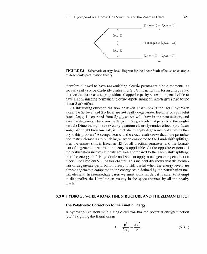
5.3 Hydrogen-Like Atoms: Fine Structure and the Zeeman Effect 321
3ea0⎪E⎪
3ea0⎪E⎪
(⎪2s, m = 0⟩ − ⎪2p, m = 0⟩)
√2
(⎪2s, m = 0⟩ + ⎪2p, m = 0⟩)
√2
No change for ⎪2p, m = ±1⟩
FIGURE 5.1 Schematic energy-level diagram for the linear Stark effect as an exampleof degenerate perturbation theory.
therefore allowed to have nonvanishing electric permanent dipole moments, aswe can easily see by explicitly evaluating 〈z〉. Quite generally, for an energy statethat we can write as a superposition of opposite parity states, it is permissible tohave a nonvanishing permanent electric dipole moment, which gives rise to thelinear Stark effect.
An interesting question can now be asked. If we look at the “real” hydrogenatom, the 2s level and 2 p level are not really degenerate. Because of spin-orbitforce, 2 p3/2 is separated from 2 p1/2, as we will show in the next section, andeven the degeneracy between the 2s1/2 and 2 p1/2 levels that persists in the single-particle Dirac theory is removed by quantum electrodynamics effects (the Lambshift). We might therefore ask, is it realistic to apply degenerate perturbation the-ory to this problem? A comparison with the exact result shows that if the perturba-tion matrix elements are much larger when compared to the Lamb shift splitting,then the energy shift is linear in |E| for all practical purposes, and the formal-ism of degenerate perturbation theory is applicable. At the opposite extreme, ifthe perturbation matrix elements are small compared to the Lamb shift splitting,then the energy shift is quadratic and we can apply nondegenerate perturbationtheory; see Problem 5.13 of this chapter. This incidentally shows that the formal-ism of degenerate perturbation theory is still useful when the energy levels arealmost degenerate compared to the energy scale defined by the perturbation ma-trix element. In intermediate cases we must work harder; it is safer to attemptto diagonalize the Hamiltonian exactly in the space spanned by all the nearbylevels.
5.3 HYDROGEN-LIKE ATOMS: FINE STRUCTURE AND THE ZEEMAN EFFECT
The Relativistic Correction to the Kinetic Energy
A hydrogen-like atom with a single electron has the potential energy function(3.7.43), giving the Hamiltonian
H0 = p2
2me− Ze2
r, (5.3.1)
322 Chapter 5 Approximation Methods
where the first term is the nonrelativistic kinetic-energy operator. However, therelativistically correct kinetic energy is
K =√
p2c2 + m2ec4 − mec2
≈ p2
2me− (p2)2
8m3ec2 . (5.3.2)
Therefore, following the notation in (5.1.1), we can treat this problem in pertur-bation theory, where H0 is given by (5.3.1) and the perturbation is
V = − (p2)2
8m3ec2 . (5.3.3)
Now in principle, this is a complicated problem because of the highly degener-ate eigenstates |nlm〉 of the hydrogen atom. However, because L commutes withp2, as we noted in (3.7.2), we also have
[L, V ] = 0. (5.3.4)
In other words, V is rotationally symmetrical and so is already diagonal in the|nlm〉 basis. Therefore, the first-order energy shifts due to V are just equal to theexpectation values in these basis states. Following (5.1.37), we write
�(1)nl = 〈nlm|V |nlm〉 = −〈nlm| (p2)2
8m3ec2 |nlm〉, (5.3.5)
where the rotational symmetry assures us that the first-order energy shifts cannotdepend on m.
In principle, (5.3.5) could be evaluated by brute force, but there is a moreelegant way. Because
(p2)2
8m3ec2 = 1
2mec2
(p2
2me
)2
= 1
2mec2
(H0 + Ze2
r
)2
, (5.3.6)
we immediately see that
�(1)nl = − 1
2mec2
[(E (0)
n
)2 + 2E (0)n 〈nlm| Ze2
r|nlm〉+ 〈nlm| (Ze2)2
r2|nlm〉
]. (5.3.7)
The problem is therefore reduced to calculating the expectation values for Ze2/rand (Ze2)2/r2. In fact, both of these expectation values can be evaluated usingsome clever tricks. We simply outline the approach here, but the interested readeris referred to Shankar (1994) or Townsend (2000) for more details.
If one imagines a hydrogen atom with a “perturbation” Vγ = γ /r , then theexpectation value in the second term of (5.3.7) is simply the first-order correctionto the energy with γ = Ze2. On the other hand, it is simple to solve this problemexactly, because it corresponds to the hydrogen atom with Ze2 → Ze2 − γ , and
5.3 Hydrogen-Like Atoms: Fine Structure and the Zeeman Effect 323
it is straightforward to find the first-order correction from the exact solution. Onefinds that
〈nlm| Ze2
r|nlm〉 = −2E (0)
n . (5.3.8)
Indeed, this is actually a statement of the virial theorem for the Coulomb potential.A similar approach can be taken for the third term in (5.3.7). In this case,
imagine a perturbation Vγ = γ /r2 that modifies the centrifugal barrier term in theeffective potential. That is, it takes l to a form that includes γ , which can again beused to write down the first-order correction. One finds that
〈nlm| (Ze2)2
r2|nlm〉 = 4n
l + 12
(E (0)
n
)2. (5.3.9)
Accordingly, using (5.3.8) and (5.3.9) along with E (0)n from (3.7.53), we
rewrite (5.3.7) as
�(1)nl = E (0)
n
[Z2α2
n2
(−3
4+ n
l + 12
)](5.3.10a)
= −1
2mec2 Z4α4
⎡⎣− 3
4n4+ 1
n3(
l + 12
)⎤⎦ . (5.3.10b)
Not unexpectedly, the relative size of the first-order correction is proportional toZ2α2, the square of the classical electron orbital velocity (in units of c).
Spin-Orbit Interaction and Fine Structure
Now let us move on to study the atomic levels of general hydrogen-like atoms—that is, atoms with one valence electron outside the closed shell. Alkali atomssuch as sodium (Na) and potassium (K) belong to this category.
The central (spin-independent) potential Vc(r ) appropriate for the valence elec-tron is no longer of the pure Coulomb form. This is because the electrostatic po-tential φ(r ) that appears in
Vc(r ) = eφ(r ) (5.3.11)
is no longer due just to the nucleus of electric charge |e|Z ; we must take intoaccount the cloud of negatively charged electrons in the inner shells. A preciseform of φ(r ) does not concern us here. We simply remark that the degeneracycharacteristics of the pure Coulomb potential are now removed in such a way thatthe higher l states lie higher for a given n. Physically, this arises from the fact thatthe higher l states are more susceptible to the repulsion due to the electron cloud.
Instead of studying the details of Vc(r ), which determines the gross structureof hydrogen-like atoms, we discuss the effect of the spin-orbit (L · S) interactionthat gives rise to fine structure. We can understand the existence of this interaction
324 Chapter 5 Approximation Methods
in a qualitative fashion as follows. Because of the central force part (5.3.11), thevalence electron experiences the electric field
E = −(
1
e
)∇Vc(r ). (5.3.12)
But whenever a moving charge is subjected to an electric field, it “feels” an effec-tive magnetic field given by
Beff = −(v
c
)×E. (5.3.13)
Because the electron has a magnetic moment μ given by
μ = eSmec
, (5.3.14)
we suspect a spin-orbit potential VL S contribution to H as follows:
HLS?=−μ ·Beff
= μ ·(v
c×E
)=(
eSmec
)·[
pmec
×(x
r
) 1
(−e)
dVc
dr
]= 1
m2ec2
1
r
dVc
dr(L · S).
(5.3.15)
When this expression is compared with the observed spin-orbit interaction, it isseen to have the correct sign, but the magnitude turns out to be too large by a factorof 2. There is a classical explanation for this that invokes spin precession (Thomasprecession after L. H. Thomas), but we shall not bother with that. See Jackson(1975), for example. We simply treat the spin-orbit interaction phenomenologi-cally and take VLS to be one-half of (5.3.15). The correct quantum-mechanicalexplanation for this discrepancy must await the Dirac (relativistic) theory of theelectron discussed in the last chapter of this book.
We are now in a position to apply perturbation theory to hydrogenic atoms us-ing VLS as the perturbation (V of Sections 5.1 and 5.2). The unperturbed Hamil-tonian H0 is taken to be
H0 = p2
2m+ Vc(r ), (5.3.16)
where the central potential Vc is no longer of the pure Coulomb form for alkaliatoms. With just H0, we have freedom in choosing the base kets:
Set 1: The eigenkets ofL2, Lz , S2, Sz .
Set 2: The eigenkets ofL2, S2, J2, Jz .(5.3.17)
5.3 Hydrogen-Like Atoms: Fine Structure and the Zeeman Effect 325
Without VLS (or HLS) either set is satisfactory in the sense that the base kets arealso energy eigenkets. With HLS added, it is far superior to use set 2 of (5.3.17)because L · S does not commute with Lz and Sz , whereas it does commute withJ2 and Jz . Remember the cardinal rule: Choose unperturbed kets that diagonalizethe perturbation. You have to be either a fool or a masochist to use the Lz , Szeigenkets [set 1 of (5.3.17)] as the base kets for this problem; if we proceeded toapply blindly the method of degenerate perturbation theory starting with set 1 asour base kets, we would be forced to diagonalize the VLS(HLS) matrix written inthe Lz , Sz representation. The results of this, after a lot of hard algebra, give usjust the J2, Jz eigenkets as the zeroth-order unperturbed kets to be used!
In degenerate perturbation theory, if the perturbation is already diagonal in therepresentation we are using, all we need to do for the first-order energy shift isto take the expectation value. The wave function in the two-component form isexplicitly written as
ψnlm = Rnl (r )Y j=l±1/2,ml , (5.3.18)
where Yj=l±1/2,ml is the spin-angular function of Section 3.8 [see (3.8.64)]. For
the first-order shift, we obtain
�nl j = 1
2m2ec2
⟨1
r
dVc
dr
⟩nl
h2
2
{l
−(l + 1)
}j = l + 1
2
j = l − 12
⟨1
r
dVc
dr
⟩nl
≡∫ ∞
0Rnl
1
r
dVc
drRnlr
2dr ,
(5.3.19)
where we have used the m-independent identity [see (3.8.66)]
∫Y†S · LYd�= 1
2
[j ( j + 1) − l(l + 1) − 3
4
]h2 = h2
2
{l
−(l + 1)
}j = l + 1
2
j = l − 12
.
(5.3.20)Equation (5.3.19) is known as Lande’s interval rule.
To be specific, consider a sodium atom. From standard atomic spectroscopynotation, the ground-state configuration is
(1s)2(2s)2(2 p)6(3s). (5.3.21)
The inner 10 electrons can be visualized to form a spherically symmetrical elec-tron cloud. We are interested in the excitation of the 11th electron from 3s to apossible higher state. The nearest possibility is excitation to 3p. Because the cen-tral potential is no longer of the pure Coulomb form, 3s and 3p are now split. Thefine structure brought about by VLS refers to even a finer split within 3p, between3 p1/2 and 3 p3/2, where the subscript refers to j. Experimentally, we observe two
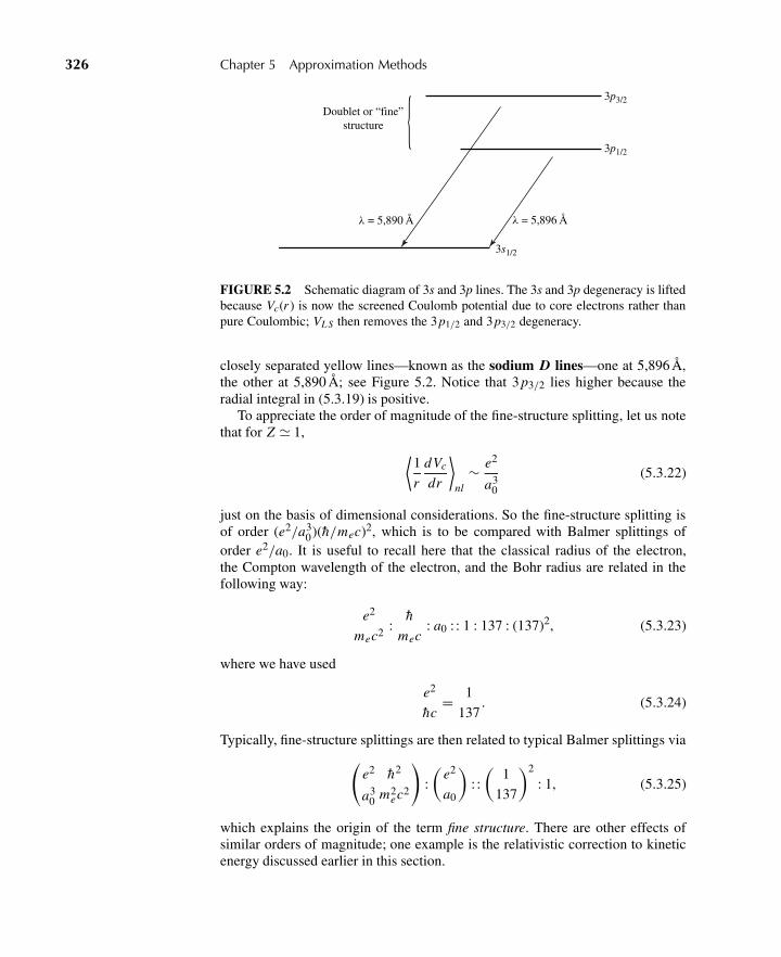
326 Chapter 5 Approximation Methods
Doublet or “fine”structure
λ = 5,890 Å λ = 5,896 Å
3s1/2
3p1/2
3p3/2
FIGURE 5.2 Schematic diagram of 3s and 3p lines. The 3s and 3p degeneracy is liftedbecause Vc(r ) is now the screened Coulomb potential due to core electrons rather thanpure Coulombic; VL S then removes the 3p1/2 and 3p3/2 degeneracy.
closely separated yellow lines—known as the sodium D lines—one at 5,896 Å,the other at 5,890 Å; see Figure 5.2. Notice that 3 p3/2 lies higher because theradial integral in (5.3.19) is positive.
To appreciate the order of magnitude of the fine-structure splitting, let us notethat for Z � 1, ⟨
1
r
dVc
dr
⟩nl
∼ e2
a30
(5.3.22)
just on the basis of dimensional considerations. So the fine-structure splitting isof order (e2/a3
0)(h/mec)2, which is to be compared with Balmer splittings oforder e2/a0. It is useful to recall here that the classical radius of the electron,the Compton wavelength of the electron, and the Bohr radius are related in thefollowing way:
e2
mec2 :h
mec: a0 : : 1 : 137 : (137)2, (5.3.23)
where we have used
e2
hc= 1
137. (5.3.24)
Typically, fine-structure splittings are then related to typical Balmer splittings via(e2
a30
h2
m2ec2
):
(e2
a0
): :
(1
137
)2
: 1, (5.3.25)
which explains the origin of the term fine structure. There are other effects ofsimilar orders of magnitude; one example is the relativistic correction to kineticenergy discussed earlier in this section.
5.3 Hydrogen-Like Atoms: Fine Structure and the Zeeman Effect 327
Before leaving this discussion, let us calculate out (5.3.19) for the case of theCoulomb potential—that is, a hydrogen atom or one-electron ion with Z protons.In this case ⟨
1
r
dVc
dr
⟩nl
=⟨
Ze2
r3
⟩nl
. (5.3.26)
We can evaluate this expectation value with the help of yet another trick. First wenote that with H0 given by (5.3.1), we have
〈nlm|[H0, A]|nlm〉 = 0 (5.3.27)
for any operator A, since H0 acting to the right or left just gives E (0)n . If we let
A = pr , the radial momentum operator, then it obviously commutes with the radialpart of the kinetic-energy term in H0. Hence, we are left with
〈nlm|[
l(l + 1)h2
2mer2 − Ze2
r, pr
]|nlm〉 = 0. (5.3.28)
Now in coordinate space, pr does not commute with functions of the coordinate rbecause of the presence of the derivative ∂/∂r . Therefore, we can explicitly carryout the commutator in (5.3.28) to arrive at
〈nlm|[− l(l + 1)h2
mer3 + Ze2
r2
]|nlm〉 = 0. (5.3.29)
Finally, then, we make use of (5.3.9) and (3.7.53) to write⟨Ze2
r3
⟩nl
= me
l(l + 1)h2
⟨(Ze2)2
r2
⟩nl
= − 2m2ec2 Z2α2
nl(l + 1)(l + 1/2)h2 E (0)n . (5.3.30)
We therefore have the spin-orbit correction to the energy eigenstates of the hydro-gen atom from (5.3.19) as
�nl j = − Z2α2
2nl(l + 1)(l + 1/2)E (0)
n
{l
−(l + 1)
}j = l + 1
2
j = l − 12
. (5.3.31)
Interestingly, this expression is nonzero for l = 0. Nevertheless, it gives the correctanswer for the energy eigenvalues of the Dirac equation, as we shall see later inthis book. The origin of this shift, attributed to something called the Darwin term,is discussed elsewhere. See, for example, Townsend (2000).
328 Chapter 5 Approximation Methods
The Zeeman Effect
We now discuss hydrogen or hydrogen-like (one-electron) atoms in a uniformmagnetic field—the Zeeman effect, sometimes called the anomalous Zeeman ef-fect with the electron spin taken into account. Recall that a uniform magnetic fieldB is derivable from a vector potential
A = 12 (B× r). (5.3.32)
For B in the positive z-direction (B = B z),
A = − 12 (Byx− Bx y) (5.3.33)
suffices, where B stands for |B|. Apart from the spin term, the interaction Hamil-tonian is generated by the substitution
p → p− eAc
. (5.3.34)
We therefore have
H = p2
2me+ Vc(r ) − e
2mec(p · A+ A ·p) + e2A2
2mec2. (5.3.35)
Because
〈x′|p ·A(x)| 〉 = −i h∇′·[A(x′)〈x′| 〉]= 〈x′|A(x) · p| 〉+ 〈x′| 〉[−i h∇′· A(x′)],
(5.3.36)
it is legitimate to replace p · A by A · p whenever
∇· A(x) = 0, (5.3.37)
which is the case for the vector potential of (5.3.33). Noting
A · p = |B|(− 12 ypx + 1
2 x py)
= 12 |B|Lz
(5.3.38)
and
A2 = 14 |B|2(x2 + y2), (5.3.39)
we obtain for (5.3.35)
H = p2
2me+ Vc(r ) − e
2mec|B|Lz + e2
8mec2 |B|2(x2 + y2). (5.3.40)
To this we may add the spin magnetic-moment interaction
−μ ·B = −e
mecS ·B = −e
mec|B|Sz . (5.3.41)
5.3 Hydrogen-Like Atoms: Fine Structure and the Zeeman Effect 329
The quadratic |B|2(x2 + y2) is unimportant for a one-electron atom; the analogousterm is important for the ground state of the helium atom where L(tot)
z and S(tot)z
both vanish. The reader may come back to this problem when he or she computesdiamagnetic susceptibilities in Problems 5.18 and 5.19 of this chapter.
To summarize, omitting the quadratic term, the total Hamiltonian is made upof the following three terms:
H0 = p2
2me+ Vc(r ) (5.3.42a)
HL S = 1
2m2ec2
1
r
dVc(r )
drL · S (5.3.42b)
HB = −e|B|2mec
(Lz + 2Sz). (5.3.42c)
Notice the factor 2 in front of Sz ; this reflects the fact that the g-factor of theelectron is 2.
Suppose HB is treated as a small perturbation. We can study the effect of HBusing the eigenkets of H0 + HLS—the J2, Jz eigenkets—as our base kets. Noting
Lz + 2Sz = Jz + Sz , (5.3.43)
we can write the first-order shift as
−e|B|2mec
〈Jz + Sz〉 j=l±1/2,m . (5.3.44)
The expectation value of Jz immediately gives mh. As for 〈Sz〉, we first recall∣∣∣∣ j = l ± 1
2,m
⟩= ±
√l ± m + 1
2
2l + 1
∣∣∣∣ml = m − 1
2, ms = 1
2
⟩
+√
l ∓ m + 12
2l + 1
∣∣∣∣ml = m + 1
2, ms = −1
2
⟩.
(5.3.45)
The expectation value of Sz can then easily be computed:
〈Sz〉 j=l±1/2,m = h
2(|c+|2 −|c−|2)
= h
2
1
(2l + 1)
[(l ± m + 1
2
)−(
l ∓ m + 1
2
)]= ± mh
(2l + 1).
(5.3.46)
In this manner we obtain Lande’s formula for the energy shift (due to the B field),
�EB = −eh B
2mecm
[1 ± 1
(2l + 1)
]. (5.3.47)
330 Chapter 5 Approximation Methods
We see that the energy shift of (5.3.47) is proportional to m. To understand thephysical explanation for this, we present another method for deriving (5.3.46). Werecall that the expectation value of Sz can also be obtained using the projectiontheorem of Section 3.11. We get [see (3.11.45)]
〈Sz〉 j=l±1/2,m = [〈S ·J〉 j=l±1/2] mh
h2 j ( j + 1)
= m〈J2 + S2 − L2〉 j=l±1/2
2h j ( j + 1)
= mh
⎡⎣(
l ± 12
)(l ± 1
2 + 1)
+ 34 − l(l + 1)
2(
l ± 12
)(l ± 1
2 + 1)
⎤⎦= ± mh
(2l + 1),
(5.3.48)
which is in complete agreement with (5.3.46).In the foregoing discussion the magnetic field is treated as a small perturbation.
We now consider the opposite extreme—the Paschen-Back limit—with a mag-netic field so intense that the effect of HB is far more important than that of HL S,which we later add as a small perturbation. With H0 + HB only, the good quantumnumbers are Lz and Sz . Even J2 is no good because spherical symmetry is com-pletely destroyed by the strong B field that selects a particular direction in space,the z-direction. We are left with cylindrical symmetry only—that is, invarianceunder rotation around the z-axis. So the Lz , Sz eigenkets |l,s = 1
2 ,ml ,ms〉 are tobe used as our base kets. The effect of the main term HB can easily be computed:
〈HB〉ml ms = −e|B|h2mec
(ml + 2ms). (5.3.49)
The 2(2l + 1) degeneracy in ml and ms that we originally had with H0 [see(5.3.42a)] is now reduced by HB to states with the same (ml) + (2ms)—namely,(ml)+ (1) and (ml +2)+ (−1). Clearly we must evaluate the expectation value ofL · S with respect to |ml ,ms〉:
〈L · S〉 = 〈Lz Sz + 12 (L+S− + L−S+)〉ml ms
= h2mlms ,(5.3.50)
where we have used
〈L±〉ml = 0, 〈S±〉ms = 0. (5.3.51)
Hence,
〈HL S〉ml ms = h2mlms
2m2ec2
⟨1
r
dVc
dr
⟩. (5.3.52)
In many elementary books there are pictorial interpretations of the weak-field result (5.3.47) and the strong-field result (5.3.49), but we do not bother
5.3 Hydrogen-Like Atoms: Fine Structure and the Zeeman Effect 331
TABLE 5.1
Dominant interaction Almost good No good Always good
Weak B HLS J2 (orL ·S) Lz , S∗z
L2,S2, Jz
Strong B HB Lz , Sz J2 (orL ·S)∗The exception is the stretched configuration—for example, p3/2 with m = ± 3
2 . Here Lz and Szare both good; this is because magnetic quantum number of Jz , m = ml +ms can be satisfied inonly one way.
with them here. We simply summarize our results in Table 5.1, where weak andstrong B fields are “calibrated” by comparing their magnitudes eh B/2mec with(1/137)2e2/a0. In this table almost good simply means good to the extent that theless dominant interaction could be ignored.
Specifically, let us look at the level scheme of a p electron l = 1( p3/2, p1/2). Inthe weak-B case, the energy shifts are linear in B, with slopes determined by
m
[1 ±
(1
2l + 1
)].
As we now increase B, mixing becomes possible between states with the samem-value—for example, p3/2 with m = ± 1
2 and p1/2 with m = ± 12 ; in this con-
nection note that the operator Lz + 2Sz that appears in HB [(5.3.42c)] is a rank 1tensor operator T (k=1)
q=0 with spherical component q = 0. In the intermediate-B re-gion, simple formulas like (5.3.47) and (5.3.49) for the expectation values are notpossible; it is really necessary to diagonalize the appropriate 2 × 2 matrix (Got-tfried and Yan 2003, Section 5.4). In the strong-B limit, the energy shifts are againproportional to |B|; as we see in (5.3.49), the slopes are determined by ml +2ms .
The Van der Waals Interaction
An important, nice application of the Rayleigh-Schrödinger perturbation theoryis to calculate the long-range interaction, or van der Waals force, between twohydrogen atoms in their ground states. It is easy to show that the energy betweenthe two atoms for large separation r is attractive and varies as r−6.
Consider the two protons of the hydrogen atoms to be fixed at a distance r(along the z-axis) with r1 the vector from the first proton to its electron and r2 thevector from the second proton to its electron; see Figure 5.3. Then the HamiltonianH can be written as
H = H0 + V
H0 = − h2
2m(∇2
1 +∇22) − e2
r1− e2
r2
V = e2
r+ e2
|r + r2 − r1| − e2
|r + r2| − e2
|r − r1| .
(5.3.53)
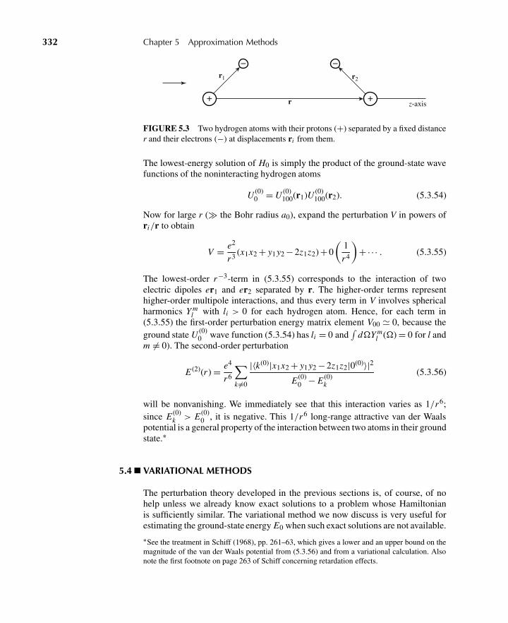
332 Chapter 5 Approximation Methods
+
− −
+z-axis
r2r1
r
FIGURE 5.3 Two hydrogen atoms with their protons (+) separated by a fixed distancer and their electrons (−) at displacements ri from them.
The lowest-energy solution of H0 is simply the product of the ground-state wavefunctions of the noninteracting hydrogen atoms
U (0)0 = U (0)
100(r1)U (0)100(r2). (5.3.54)
Now for large r (� the Bohr radius a0), expand the perturbation V in powers ofri/r to obtain
V = e2
r3 (x1x2 + y1y2 − 2z1z2) + 0
(1
r4
)+·· · . (5.3.55)
The lowest-order r−3-term in (5.3.55) corresponds to the interaction of twoelectric dipoles er1 and er2 separated by r. The higher-order terms representhigher-order multipole interactions, and thus every term in V involves sphericalharmonics Y m
l with li > 0 for each hydrogen atom. Hence, for each term in(5.3.55) the first-order perturbation energy matrix element V00 � 0, because theground state U (0)
0 wave function (5.3.54) has li = 0 and∫
d�Y ml (�) = 0 for l and
m �= 0). The second-order perturbation
E (2)(r ) = e4
r6
∑k �=0
|〈k(0)|x1x2 + y1y2 − 2z1z2|0(0)〉|2E (0)
0 − E (0)k
(5.3.56)
will be nonvanishing. We immediately see that this interaction varies as 1/r6;since E (0)
k > E (0)0 , it is negative. This 1/r6 long-range attractive van der Waals
potential is a general property of the interaction between two atoms in their groundstate.∗
5.4 VARIATIONAL METHODS
The perturbation theory developed in the previous sections is, of course, of nohelp unless we already know exact solutions to a problem whose Hamiltonianis sufficiently similar. The variational method we now discuss is very useful forestimating the ground-state energy E0 when such exact solutions are not available.
∗See the treatment in Schiff (1968), pp. 261–63, which gives a lower and an upper bound on themagnitude of the van der Waals potential from (5.3.56) and from a variational calculation. Alsonote the first footnote on page 263 of Schiff concerning retardation effects.
5.4 Variational Methods 333
We attempt to guess the ground-state energy E0 by considering a “trial ket”|0〉, which tries to imitate the true ground-state ket |0〉. To this end we first obtaina theorem of great practical importance. We define H such that
H ≡ 〈0|H |0〉〈0|0〉 , (5.4.1)
where we have accommodated the possibility that |0〉 might not be normalized.We can then prove the following.
Theorem 5.1.
H ≥ E0. (5.4.2)
This means that we can obtain an upper bound to E0 by considering various kindsof |0〉. The proof of this is very straightforward.
Proof. Even though we do not know the energy eigenket of the Hamiltonian H,we can imagine that |0〉 can be expanded as
|0〉 =∞∑
k=0
|k〉〈k|0〉, (5.4.3)
where |k〉 is an exact energy eigenket of H:
H |k〉 = Ek |k〉. (5.4.4)
Equation (5.4.2) follows when we use Ek = Ek − E0 + E0 to evaluate H in (5.4.1).We have
H =
∑k=0
|〈k|0〉|2 Ek∑k=0
|〈k|0〉|2(5.4.5a)
=
∞∑k=1
|〈k|0〉|2(Ek − E0)∑k=0
|〈k|0〉|2+ E0 (5.4.5b)
≥ E0, (5.4.5c)
where we have used the fact that Ek − E0 in the first sum of (5.4.5b) is necessarilypositive. It is also obvious from this proof that the equality sign in (5.4.2) holdsonly if |0〉 coincides exactly with |0〉—that is, if the coefficients 〈k|0〉 all vanishfor k �= 0.
334 Chapter 5 Approximation Methods
The theorem (5.4.2) is quite powerful because H provides an upper bound tothe true ground-state energy. Furthermore, a relatively poor trial ket can give afairly good energy estimate for the ground state, because if
〈k|0〉 ∼ 0(ε) fork �= 0, (5.4.6)
then from (5.4.5) we have
H − E0 ∼ 0(ε2). (5.4.7)
We see an example of this in a moment. Of course, the method does not sayanything about the discrepancy between H and E0; all we know is that H islarger than (or equal to) E0.
Another way to state the theorem is to assert that H is stationary with respectto the variation
|0〉 → |0〉+ δ|0〉; (5.4.8)
that is, δH = 0 when |0〉 coincides with |0〉. By this we mean that if |0〉+ δ|0〉 isused in place of |0〉 in (5.4.5) and we calculate H , then the error we commit inestimating the true ground-state energy involves |0〉 to order (δ|0〉)2.
The variational method per se does not tell us what kind of trial kets are tobe used to estimate the ground-state energy. Quite often we must appeal to phys-ical intuition—for example, the asymptotic behavior of wave function at largedistances. What we do in practice is to characterize trial kets by one or more pa-rameters λ1,λ2, . . . and compute H as a function of λ1,λ2, . . . . We then minimizeH by (1) setting the derivative with respect to the parameters all zero, namely
∂H
∂λ1= 0,
∂H
∂λ2= 0, . . . , (5.4.9)
(2) determining the optimum values of λ1,λ2, . . . , and (3) substituting them backinto the expression for H .
If the wave function for the trial ket already has a functional form of the exactground-state energy eigenfunction, we of course obtain the true ground-state en-ergy function by this method. For example, suppose somebody has the foresightto guess that the wave function for the ground state of the hydrogen atom must beof the form
〈x|0〉 ∝ e−r/a , (5.4.10)
where a is regarded as a parameter to be varied. We then find, upon minimizingH with (5.4.10), the correct ground-state energy −e2/2a0. Not surprisingly, theminimum is achieved when a coincides with the Bohr radius a0.
As a second example, we attempt to estimate the ground state of the infinite-well (one-dimensional box) problem defined by
V ={
0, for |x |< a∞, for |x |> a.
(5.4.11)
5.4 Variational Methods 335
The exact solutions are, of course, well known:
〈x |0〉 = 1√a
cos(πx
2a
),
E0 =(
h2
2m
)(π2
4a2
).
(5.4.12)
But suppose we did not know these. Evidently the wave function must vanishat x = ±a; furthermore, for the ground state the wave function cannot have anywiggles. The simplest analytic function that satisfies both requirements is just aparabola going through x = ±a:
〈x |0〉 = a2 − x2, (5.4.13)
where we have not bothered to normalize |0〉. Here there is no variational param-eter. We can compute H as follows:
H =
(−h2
2m
)∫ a
−a(a2 − x2)
d2
dx2 (a2 − x2)dx∫ a
−a(a2 − x2)2 dx
=(
10
π2
)(π2h2
8a2m
)� 1.0132 E0.
(5.4.14)
It is remarkable that with such a simple trial function, we can come within 1.3%of the true ground-state energy.
A much better result can be obtained if we use a more sophisticated trial func-tion. We try
〈x |0〉 = |a|λ−|x |λ, (5.4.15)
where λ is now regarded as a variational parameter. Straightforward algebra gives
H =[
(λ+ 1)(2λ+ 1)
(2λ− 1)
](h2
4ma2
), (5.4.16)
which has a minimum at
λ= (1 +√6)
2� 1.72, (5.4.17)
not far from λ= 2 (a parabola) considered earlier. This gives
Hmin =(
5 + 2√
6
π2
)E0 � 1.00298E0. (5.4.18)
336 Chapter 5 Approximation Methods
So the variational method with (5.4.15) gives the correct ground-state energywithin 0.3%—a fantastic result considering the simplicity of the trial functionused.
How well does this trial function imitate the true ground-state wave function?It is amusing that we can answer this question without explicitly evaluating theoverlap integral 〈0|0〉. Assuming that |0〉 is normalized, we have [from (5.4.1)–(5.4.4)]
Hmin =∞∑
k=0
|〈k|0〉|2 Ek
≥ |〈0|0〉|2 E0 + 9E0(1 −|〈0|0〉|2),
(5.4.19)
where 9E0 is the energy of the second excited state; the first excited state (k =1) makes no contribution by parity conservation. Solving for |〈0|0〉| and using(5.4.18), we have
|〈0|0〉|2 ≥ 9E0 − Hmin
8E0= 0.99963. (5.4.20)
Departure from unity characterizes a component of |0〉 in a direction orthogonalto |0〉. If we are talking about “angle” θ defined by
〈0|0〉 = cosθ , (5.4.21)
then (5.4.20) corresponds to
θ <∼ 1.1◦, (5.4.22)
so |0〉 and |0〉 are nearly “parallel.”One of the earliest applications of the variational method involved the ground-
state energy of the helium atom, which we will discuss in Section 7.4. We can alsouse the variational method to estimate the energies of first excited states; all weneed to do is work with a trial ket orthogonal to the ground-state wave function—either exact, if known, or an approximate one obtained by the variational method.
5.5 TIME-DEPENDENT POTENTIALS: THE INTERACTION PICTURE
Statement of the Problem
So far in this book we have been concerned with Hamiltonians that do not containtime explicitly. In nature, however, there are many quantum-mechanical systemsof importance with time dependence. In the remaining part of this chapter, weshow how to deal involving situations involving time-dependent potentials.
We consider a Hamiltonian H such that it can be split into two parts,
H = H0 + V (t), (5.5.1)
5.5 Time-Dependent Potentials: The Interaction Picture 337
where H0 does not contain time explicitly. The problem V (t) = 0 is assumed tobe solved in the sense that the energy eigenkets |n〉 and the energy eigenvalues Endefined by
H0|n〉 = En|n〉 (5.5.2)
are completely known.∗ We may be interested in situations where initially onlyone of the energy eigenstates of H0—for example, |i〉—is populated. As timegoes on, however, states other than |i〉 are populated because with V (t) �= 0, weare no longer dealing with “stationary” problems; the time-evolution operator isno longer as simple as e−i H t/h when H itself involves time. Quite generally, thetime-dependent potential V (t) can cause transitions to states other than |i〉. Thebasic question we address is, what is the probability as a function of time for thesystem to be found in |n〉, with n �= i?
More generally, we may be interested in how an arbitrary state ket changes astime goes on, where the total Hamiltonian is the sum of H0 and V (t). Supposethat at t = 0, the state ket of a physical system is given by
|α〉 =∑
n
cn(0)|n〉. (5.5.3)
We wish to find cn(t) for t > 0 such that
|α, t0 = 0; t〉 =∑
n
cn(t)e−i En t/h|n〉, (5.5.4)
where the ket on the left side stands for the state ket in the Schrödinger picture att of a physical system whose state ket at t = 0 was found to be |α〉.
The astute reader may have noticed the manner in which we have separated thetime dependence of the coefficient of |n〉 in (5.5.4). The factor e−i En t/h is presenteven if V is absent. This way of writing the time dependence makes it clear thatthe time evolution of cn(t) is due solely to the presence of V (t); cn(t) would beidentically equal to cn(0) and hence independent of t if V were zero. As we shallsee in a moment, this separation is convenient because cn(t) satisfies a relativelysimple differential equation. The probability of finding |n〉 is found by evaluating|cn(t)|2.
The Interaction Picture
Before we discuss the differential equation for cn(t), we discuss the interactionpicture. Suppose we have a physical system such that its state ket coincides with|α〉 at t = t0, where t0 is often taken to be zero. At a later time, we denote the stateket in the Schrödinger picture by |α, t0; t〉S , where the subscript S reminds us thatwe are dealing with the state ket of the Schrödinger picture.
We now define
|α, t0; t〉I = ei H0t/h|α, t0; t〉S , (5.5.5)
∗In (5.5.2) we no longer use the notation |n(0)〉, E(0)n .
338 Chapter 5 Approximation Methods
where | 〉I stands for a state ket that represents the same physical situation inthe interaction picture. At t = 0, | 〉I evidently coincides with | 〉S . For operators(representing observables) we define observables in the interaction picture as
AI ≡ ei H0t/h ASe−i H0t/h . (5.5.6)
In particular,
VI = ei H0t/h V e−i H0t/h (5.5.7)
where V without a subscript is understood to be the time-dependent potential inthe Schrödinger picture. The reader may recall here the connection between theSchrödinger picture and the Heisenberg picture:
|α〉H = e+i H t/h |α, t0 = 0; t〉S (5.5.8)
AH = ei H t/h ASe−i H t/h . (5.5.9)
The basic difference between (5.5.8) and (5.5.9) on the one hand and (5.5.6) and(5.5.7) on the other is that H rather than H0 appears in the exponential.
We now derive the fundamental differential equation that characterizes the timeevolution of a state ket in the interaction picture. Let us take the time derivative of(5.5.5) with the full H given by (5.5.1):
i h∂
∂ t|α, t0; t〉I = i h
∂
∂ t(ei H0t/h|α, t0; t〉S )
= −H0ei H0t/h|α, t0; t〉S + ei H0t/h(H0 + V )|α, t0; t〉S
= ei H0t/hV e−i H0t/hei H0t/h|α, t0; t〉S .
(5.5.10)
We thus see
i h∂
∂ t|α, t0; t〉I = VI |α, t0; t〉I , (5.5.11)
which is a Schrödinger-like equation with the total H replaced by VI . In otherwords |α, t0; t〉I would be a ket fixed in time if VI were absent. We can also showfor an observable A (that does not contain time t explicitly in the Schrödingerpicture) that
d AI
dt= 1
i h[AI , H0], (5.5.12)
which is a Heisenberg-like equation with H replaced by H0.In many respects, the interaction picture, or Dirac picture, is intermediate be-
tween the Schrödinger picture and the Heisenberg picture. This should be evidentfrom Table 5.2.
In the interaction picture we continue using |n〉 as our base kets. Thus weexpand | 〉I as follows:
|α, t0; t〉I =∑
n
cn(t)|n〉. (5.5.13)
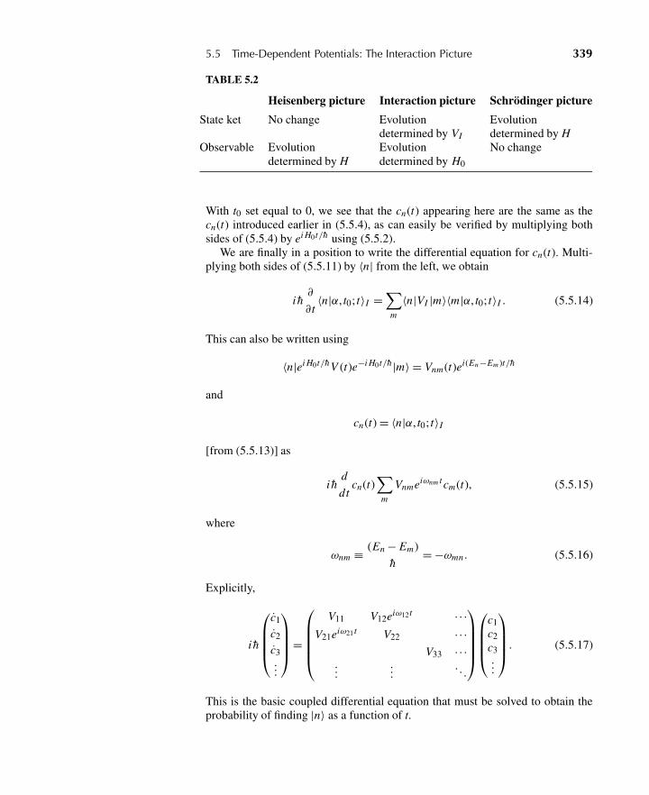
5.5 Time-Dependent Potentials: The Interaction Picture 339
TABLE 5.2
Heisenberg picture Interaction picture Schrödinger picture
State ket No change Evolution Evolutiondetermined by VI determined by H
Observable Evolution Evolution No changedetermined by H determined by H0
With t0 set equal to 0, we see that the cn(t) appearing here are the same as thecn(t) introduced earlier in (5.5.4), as can easily be verified by multiplying bothsides of (5.5.4) by ei H0t/h using (5.5.2).
We are finally in a position to write the differential equation for cn(t). Multi-plying both sides of (5.5.11) by 〈n| from the left, we obtain
i h∂
∂ t〈n|α, t0; t〉I =
∑m
〈n|VI |m〉〈m|α, t0; t〉I . (5.5.14)
This can also be written using
〈n|ei H0t/hV (t)e−i H0t/h|m〉 = Vnm(t)ei(En−Em )t/h
and
cn(t) = 〈n|α, t0; t〉I
[from (5.5.13)] as
i hd
dtcn(t)
∑m
Vnmeiωnm t cm(t), (5.5.15)
where
ωnm ≡ (En − Em)
h= −ωmn . (5.5.16)
Explicitly,
i h
⎛⎜⎜⎜⎝c1
c2
c3...
⎞⎟⎟⎟⎠=
⎛⎜⎜⎜⎜⎝V11 V12eiω12t · · ·
V21eiω21t V22 · · ·V33 · · ·
......
. . .
⎞⎟⎟⎟⎟⎠⎛⎜⎜⎜⎝
c1c2c3...
⎞⎟⎟⎟⎠ . (5.5.17)
This is the basic coupled differential equation that must be solved to obtain theprobability of finding |n〉 as a function of t.
340 Chapter 5 Approximation Methods
Time-Dependent Two-State Problems: Nuclear Magnetic Resonance,Masers, and So Forth
Exact soluble problems with time-dependent potentials are rather rare. In mostcases we have to resort to perturbation expansion to solve the coupled differentialequations (5.5.17), as we will discuss in the next section. There is, however, aproblem of enormous practical importance, which can be solved exactly—a two-state problem with a sinusoidal oscillating potential.
The problem is defined by
H0 = E1|1〉〈1|+ E2|2〉〈2| (E2 > E1)
V (t) = γ eiωt |1〉〈2|+γ e−iωt |2〉〈1|, (5.5.18)
where γ and ω are real and positive. In the language of (5.5.14) and (5.5.15), wehave
V12 = V ∗21 = γ eiωt
V11 = V22 = 0.(5.5.19)
We thus have a time-dependent potential that connects the two energy eigenstatesof H0. In other words, we can have a transition between the two states |1〉→
←|2〉.An exact solution to this problem is available. If initially—at t = 0—only the
lower level is populated so that [see (5.5.3)]
c1(0) = 1, c2(0) = 0, (5.5.20)
then the probability for being found in each of the two states is given by (Rabi’sformula, after I. I. Rabi, who is the father of molecular beam techniques)
|c2(t)|2 = γ 2/h2
γ 2/h2 + (ω−ω21)2/4sin2
{[γ 2
h2 + (ω−ω21)2
4
]1/2
t
}(5.5.21a)
|c1(t)|2 = 1 −|c2(t)|2, (5.5.21b)
where
ω21 ≡ (E2 − E1)
h, (5.5.22)
as the reader may verify by working out Problem 5.30 of this chapter.Let us now look at |c2|2 a little more closely. We see that the probability for
finding the upper-state E2 exhibits an oscillatory time dependence with angularfrequency, two times that of
�=√(
γ 2
h2
)+ (ω−ω21)2
4. (5.5.23)
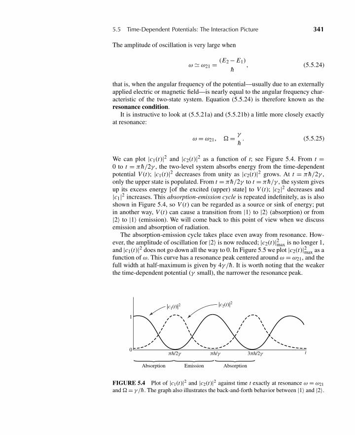
5.5 Time-Dependent Potentials: The Interaction Picture 341
The amplitude of oscillation is very large when
ω � ω21 = (E2 − E1)
h, (5.5.24)
that is, when the angular frequency of the potential—usually due to an externallyapplied electric or magnetic field—is nearly equal to the angular frequency char-acteristic of the two-state system. Equation (5.5.24) is therefore known as theresonance condition.
It is instructive to look at (5.5.21a) and (5.5.21b) a little more closely exactlyat resonance:
ω = ω21, �= γ
h. (5.5.25)
We can plot |c1(t)|2 and |c2(t)|2 as a function of t; see Figure 5.4. From t =0 to t = π h/2γ , the two-level system absorbs energy from the time-dependentpotential V (t); |c1(t)|2 decreases from unity as |c2(t)|2 grows. At t = π h/2γ ,only the upper state is populated. From t = π h/2γ to t = π h/γ , the system givesup its excess energy [of the excited (upper) state] to V (t); |c2|2 decreases and|c1|2 increases. This absorption-emission cycle is repeated indefinitely, as is alsoshown in Figure 5.4, so V (t) can be regarded as a source or sink of energy; putin another way, V (t) can cause a transition from |1〉 to |2〉 (absorption) or from|2〉 to |1〉 (emission). We will come back to this point of view when we discussemission and absorption of radiation.
The absorption-emission cycle takes place even away from resonance. How-ever, the amplitude of oscillation for |2〉 is now reduced; |c2(t)|2max is no longer 1,and |c1(t)|2 does not go down all the way to 0. In Figure 5.5 we plot |c2(t)|2max as afunction of ω. This curve has a resonance peak centered around ω = ω21, and thefull width at half-maximum is given by 4γ /h. It is worth noting that the weakerthe time-dependent potential (γ small), the narrower the resonance peak.
1
0
Absorption Emission Absorption
|c1(t)|2 |c2(t)|2
πh/2γ πh/γ 3πh/2γ t
FIGURE 5.4 Plot of |c1(t)|2 and |c2(t)|2 against time t exactly at resonance ω = ω21
and�= γ/h. The graph also illustrates the back-and-forth behavior between |1〉 and |2〉.
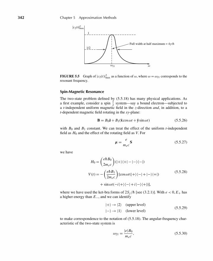
342 Chapter 5 Approximation Methods
Full width at half maximum = 4γ /h
|c2(t)|2max
1
1/2
ω21 ω
FIGURE 5.5 Graph of |c2(t)|2max as a function of ω, where ω = ω21 corresponds to theresonant frequency.
Spin-Magnetic Resonance
The two-state problem defined by (5.5.18) has many physical applications. Asa first example, consider a spin 1
2 system—say a bound electron—subjected toa t-independent uniform magnetic field in the z-direction and, in addition, to at-dependent magnetic field rotating in the xy-plane:
B = B0z + B1(xcosωt + ysinωt) (5.5.26)
with B0 and B1 constant. We can treat the effect of the uniform t-independentfield as H0 and the effect of the rotating field as V. For
μ = e
mecS (5.5.27)
we have
H0 =(
eh B0
2mec
)(|+〉〈+|− |−〉〈−|)
V (t) = −(
eh B1
2mec
)[cosωt(|+〉〈−|+ |−〉〈+|)
+ sinωt(−i |+〉〈−|+ i |−〉〈+|)],
(5.5.28)
where we have used the ket-bra forms of 2Sj/h [see (3.2.1)]. With e < 0, E+ hasa higher energy than E−, and we can identify
|+〉 → |2〉 (upper level)
|−〉 → |1〉 (lower level)(5.5.29)
to make correspondence to the notation of (5.5.18). The angular-frequency char-acteristic of the two-state system is
ω21 = |e|B0
mec, (5.5.30)
5.5 Time-Dependent Potentials: The Interaction Picture 343
which is just the spin-precession frequency for the B0 �= 0, B1 = 0 problem al-ready treated in Section 2.1. Even though the expectation values of 〈Sx ,y〉 changedue to spin precession in the counterclockwise direction (seen from the positivez-side), |c+|2 and |c−|2 remain unchanged in the absence of the rotating field. Wenow add a new feature as a result of the rotating field: |c+|2 and |c−|2 do changeas a function of time. This can be seen by identifying
−ehB1
2mec→ γ , ω→ ω (5.5.31)
to make correspondence to the notation of (5.5.18); our time-dependent inter-action (5.5.28) is precisely of form (5.5.18). The fact that |c+(t)|2 and |c−(t)|2vary in the manner indicated by Figure 5.4 for ω = ω21 and the correspondence(5.5.29), for example, implies that the spin 1
2 system undergoes a succession ofspin-flips, |+〉→
←|−〉, in addition to spin precession. Semiclassically, spin-flips ofthis kind can be interpreted as being due to the driving torque exerted by rotat-ing B.
The resonance condition is satisfied whenever the frequency of the rotatingmagnetic field coincides with the frequency of spin precession determined by thestrength of the uniform magnetic field. We see that the probability of spin-flips isparticularly large.
In practice, a rotating magnetic field may be difficult to produce experimen-tally. Fortunately, a horizontally oscillating magnetic field—for instance, in thex-direction—is just as good. To see this, we first note that such an oscillating fieldcan be decomposed into a counterclockwise component and a clockwise compo-nent as follows:
2B1xcosωt = B1(xcosωt + ysinωt) + B1(xcosωt − ysinωt). (5.5.32)
We can obtain the effect of the counterclockwise component simply by reversingthe sign of ω. Suppose the resonance condition is met for the counterclockwisecomponent
ω � ω21. (5.5.33)
Under a typical experimental condition,
B1
B0� 1, (5.5.34)
which implies, from (5.5.30) and (5.5.31), that
γ
h� ω21; (5.5.35)
As a result, whenever the resonance condition is met for the counterclockwisecomponent, the effect of the clockwise component becomes completely negligi-ble, because it amounts to ω→ −ω, and the amplitude becomes small in magni-tude as well as very rapidly oscillating.
344 Chapter 5 Approximation Methods
The resonance problem we have solved is of fundamental importance in inter-preting atomic molecular beam and nuclear magnetic resonance experiments. Byvarying the frequency of the oscillating field, it is possible to make a very precisemeasurement of magnetic moment. We have based our discussion on the solutionto differential equations (5.5.17); this problem can also be solved, perhaps moreelegantly, by introducing the rotating axis representation of Rabi, Schwinger, andVan Vleck.
Maser
As another application of the time-dependent two-state problem, let us considera maser. Specifically, we consider an ammonia molecule NH3, which—as wemay recall from Section 4.2—has two parity eigenstates |S〉 and |A〉 lying closetogether such that |A〉 is slightly higher. Let μel be the electric dipole operator ofthe molecule. From symmetry considerations we expect that μel is proportionalto x, the position operator for the N atom. The basic interaction is like −μel · E,where for a maser, E is a time-dependent electric field in a microwave cavity:
E = |E|maxzcosωt . (5.5.36)
It is legitimate to ignore the spatial variation of E because the wavelength in themicrowave region is far larger than molecular dimension. The frequency ω istuned to the energy difference between |A〉 and |S〉:
ω � (E A − ES)
h. (5.5.37)
The diagonal matrix elements of the dipole operator vanish by parity:
〈A|μel |A〉 = 〈S|μel |S〉 = 0, (5.5.38)
but the off-diagonal elements are, in general, nonvanishing:
〈S|x|A〉 = 〈A|x|S〉 �= 0. (5.5.39)
This means that there is a time-dependent potential that connects |S〉 and |A〉, andthe general two-state problem we discussed earlier is now applicable.
We are now in a position to discuss how masers work. Given a molecular beamof NH3 containing both |S〉 and |A〉, we first eliminate the |S〉-component byletting the beam go through a region of time-independent inhomogeneous elec-tric field. Such an electric field separates |S〉 from |A〉 in much the same way asthe inhomogeneous magnetic field in the Stern-Gerlach experiment separates |+〉from |−〉. A pure beam of |A〉 then enters a microwave cavity tuned to the energydifference EA − ES . The dimension of the cavity is such that the time spent bythe molecule is just (π/2)h/γ . As a result we stay in the first emission phase ofFigure 5.4; we have |A〉 in and |S〉 out. The excess energy of |A〉 is given up tothe time-dependent potential as |A〉 turns into |S〉 and the radiation (microwave)field gains energy. In this way we obtain microwave amplification by stimulatedemission of radiation, or maser.
5.6 Hamiltonians with Extreme Time Dependence 345
There are many other applications of the general time-dependent two-stateproblem, such as the atomic clock and optical pumping. In fact, it is amusingto see that as many as four Nobel Prizes in physics have been awarded to thosewho exploited time-dependent two-state systems of some form.∗
5.6 HAMILTONIANS WITH EXTREME TIME DEPENDENCE
This section is devoted to time-dependent Hamiltonians, with some “obvious”approximations in the case of very fast or very slow time dependence. A carefullook, though, points out some interesting phenomena, one of which did not cometo light until very late in the twentieth century.
Our treatment here is limited to a discussion of the basics, followed by somespecific examples. An instructive example we do not discuss is that of the squarewell with contracting or expanding walls, where the walls may move quickly orslowly. For these cases, we refer the interested reader to D. N. Pinder, Am. J. Phys58 (1990) 54, and D. W. Schlitt and C. Stutz, Am. J. Phys 38 (1970) 70.
Sudden Approximation
If a Hamiltonian changes very quickly, then the system “doesn’t have time” toadjust to the change. This leaves the system in the same state it was in before thechange and is the essence of the so-called “sudden approximation.”
Of course, even though it may have been in an eigenstate beforehand, thereis no reason to believe that this is an eigenstate of the transformed Hamiltonian.Therein lie opportunities for interesting physics. One classic example is calcu-lation of the population of electronic final states in the 3He+ ion following betadecay of the tritium atom.† See Problem 5.35 at the end of this chapter.
Let us consider a more precise statement of the sudden approximation andwork through some of the consequences. Rewrite the Schrödinger equation forthe time evolution operator (2.1.25) as
i∂
∂sU(t , t0) = H
h/TU(t , t0) = H
h�U(t , t0), (5.6.1)
where we have written time t = sT in terms of a dimensionless parameter s and atime scale T , and defined �≡ 1/T . In the sudden approximation, the time scaleT → 0, which means that h� will be much larger than the energy scale repre-sented by H . Assuming we can redefine H by adding or subtracting an arbitraryconstant, introducing some overall phase factor in the state vectors, we see that
U(t , t0) → 1 as T → 0 (5.6.2)∗Nobel Prize winners who took advantage of resonance in the two-level systems are Rabi (1944)on molecular beams and nuclear magnetic resonance; Bloch and Purcell (1952) on B field inatomic nuclei and nuclear magnetic moments; Townes, Basov, and Prochorov (1964) on masers,lasers, and quantum optics; and Kastler (1966) on optical pumping.†This has important implications for modern experiments that try to infer a nonzero neutrinomass from beta decay measurements. The Karlsruhe Tritium Neutrino Experiment (KATRIN), forexample, is in progress at the time of this writing. See J. Bonn, AIP Conf. Proc. 972 (2008) 404.
346 Chapter 5 Approximation Methods
This proves the validity of the sudden approximation. It should be appropriate ifT is small compared to 2π/ωab, where Eab = hωab is the difference between tworelevant eigenvalues of the Hamiltonian H .
Adiabatic Approximation
We tend to take the adiabatic approximation for granted. Given a Hamiltonian thatdepends on some set of parameters, we will find energy eigenvalues that dependon the values of those parameters. If the parameters vary “slowly” with time, thenthe energy eigenvalues should just follow the values one gets as the parametersthemselves change. The key is what we mean by “slowly.” Quantum-mechanicallyor otherwise, presumably we mean that the parameters change on a time scale Tthat is much larger than 2π/ωab = 2π h/Eab for some difference Eab in energyeigenvalues.
An obvious classical example is a pendulum that is transported around near thesurface of the earth. The pendulum will behave normally as you climb a mountain,with only the period slowly lengthening as the force of gravity decreases, so longas the time over which the height is changed is long compared to the pendulumperiod. If one slowly changes the electric field that permeates a hydrogen atom,the energy levels will change in pace according to the Stark effect calculation inSection 5.2.
Let us consider the mathematics of adiabatic change from a quantum-mechan-ical point of view. We follow the treatment given in Griffiths (2005) and pay par-ticular attention to the phase change as a function of time. We number the states inorder using the index n and assume no degeneracy∗ so there is no confusion withthe ordering of states crossing as time changes. Our starting point is essentially(2.1.27), but we will take t0 = 0 and suppress the initial time in our notation.
Begin with the eigenvalue equation using the notation
H (t)|n; t〉 = En(t)|n; t〉, (5.6.3)
simply noting that at any particular time t , the states and eigenvalues may change.If we now look for general solutions to the Schrödinger equation of the form
i h∂
∂ t|α; t〉 = H (t)|α; t〉, (5.6.4)
then we can write
|α; t〉 =∑
n
cn(t)eiθn(t )|n; t〉, (5.6.5)
where θn(t) ≡ − 1
h
∫ t
0En(t ′)dt ′. (5.6.6)
The separation of the expansion coefficient into the factors cn(t) and exp(iθn(t))will prove useful in a moment. Substituting (5.6.5) into (5.6.4) and using (5.6.3),
∗This is not a significant constraint. If the degeneracy is broken by H (t) after some time, we canjust “start” there. If the degeneracy is never broken by H (t), then it is irrelevant.
5.6 Hamiltonians with Extreme Time Dependence 347
we find ∑n
eiθn (t )[
cn(t)|n; t〉+ cn(t)∂
∂ t|n; t〉
]= 0. (5.6.7)
Now, taking the inner product with 〈m; t| and invoking orthonormality of theeigenstates at equal times, we arrive at a differential equation for the cn(t), namely
cm(t) = −∑
n
cn(t)ei[θn (t )−θm(t )]〈m; t|[∂
∂ t|n; t〉
]. (5.6.8)
The inner product 〈m; t|(∂/∂ t)|n; t〉 is a new feature. If H were not time-dependent, then the |n; t〉 would be stationary states, and the usual exponentialtime dependence would emerge. In order to treat this in the general case, we cango back to (5.6.3) and take the time derivative of both sides. For the case wherem �= n, we find
〈m; t|H |n; t〉 = [En(t) − Em(t)] 〈m; t|[∂
∂ t|n; t〉
]. (5.6.9)
This finally enables us to rewrite (5.6.8) as
cm(t) = −cm(t)〈m; t|[∂
∂ t|m; t〉
]−∑
n
cn(t)ei(θn−θm ) 〈m; t|H |n; t〉En − Em
, (5.6.10)
which is a formal solution to the general time-dependent problem. Equation(5.6.10) demonstrates that as time goes on, states with n �= m will mix with |m; t〉because of the time dependence of the Hamiltonian H , by virtue of the secondterm.
Now we can apply the adiabatic approximation, which amounts to neglectingthe second term in (5.6.10). Roughly, this means that
〈m; t|H |n; t〉Enm
≡ 1
τ� 〈m; t|
[∂
∂ t|m; t〉
]∼ Em
h. (5.6.11)
In other words, the time scale τ for changes in the Hamiltonian must be very largecompared to the inverse natural frequency of the state-phase factor. That is, just asfor the pendulum being carried around the earth, the Hamiltonian changes muchmore slowly than the oscillation frequency of the system. Consequently, we have
cn(t) = eiγn (t )cn(0) (5.6.12)
where γn(t) ≡ i∫ t
0〈n; t ′|
[∂
∂ t ′|n; t ′〉
]dt ′. (5.6.13)
Note that by this definition, γn(t) is real, since
0 = ∂
∂ t〈n; t|n; t〉 =
[∂
∂ t〈n; t|
]|n; t〉+ 〈n; t|
[∂
∂ t|n; t〉
](5.6.14)
348 Chapter 5 Approximation Methods
or, in other words, (〈n; t|
[∂
∂ t|n; t〉
])∗= −〈n; t|
[∂
∂ t|n; t〉
](5.6.15)
in which case the integrand in (5.6.13) is purely imaginary.Therefore, in the adiabatic approximation, if a system starts out in an eigenstate
|n〉 of H (0), then it remains in the eigenstate |n; t〉 of H (t), because ci (0) = 0unless i = n, in which case cn(0) = 1. Using (5.6.5) with (5.6.12) we have, in anobvious notation,
|α(n); t〉 = eiγn(t )eiθn (t )|n; t〉 (5.6.16)
It would appear that (5.6.16) is difficult to use, since the definition (5.6.13) as-sumes that the time dependence of the state is given, but we will find ways tomake good use of this result. In any case, it is easy to see that the result is self-consistent. We know that for the case when H is not time-dependent, we expect
|n; t〉 = e−i En t/h|n〉, (5.6.17)
and so
〈n; t|[∂
∂ t|n; t〉
]= −i
En
h, (5.6.18)
which, by (5.6.13), gives γn(t) = +Ent/h. On the other hand, (5.6.6) says thatθn(t) = −Ent/h. Thus, the two exponential factors in (5.6.16) cancel each other,and we find
|α(n); t〉 = |n; t〉 for H �= H (t), (5.6.19)
as we should expect.The addition of this new phase γn(t) is the only result of the adiabatic approx-
imation that is less than obvious. It was not considered worth pursuing for manyyears, until it was discovered that it is in fact measurable. Indeed, it turns out tobe the quantum-mechanical manifestation of very many physical phenomena thatinvolve systems that are cyclic in time.
Berry’s Phase
Excitement about the implications of (5.6.13) grew dramatically with the pub-lication of “Quantal Phase Factors Accompanying Adiabatic Changes,” byM. V. Berry, in Proceedings of the Royal Society of London, Series A 392 (1984)45. Indeed, the accumulated phase for systems that travel in a closed loop isgenerally called Berry’s Phase, although Berry himself refers to it as a “geometricphase.”
Berry’s paper is widely cited, and the interested reader will have no difficultyfinding many references. One particular paper that provides a succinct summaryand interesting implications is “The Adiabatic Theorem and Berry’s Phase,” by
5.6 Hamiltonians with Extreme Time Dependence 349
B. R. Holstein, Am. J. Phys. 57 (1989) 1079. Berry, in fact, gives a lovely his-tory of work prior to his own. See his “Anticipations of the Geometric Phase” inPhysics Today, December 1990.
Assume that the time dependence of the Hamiltonian is represented by a “vec-tor of parameters” R(t). That is, there exists some space in which the componentsof a vector R(t) specify the Hamiltonian and change as a function of time. (Inan example below, R(t) will be the magnetic field.) Therefore, we have En(t) =En(R(t)) and |n; t〉 = |n(R(t))〉, and also
〈n; t|[∂
∂ t|n; t〉
]= 〈n; t| [∇R|n; t〉] · dR
dt, (5.6.20)
where ∇R is simply a gradient operator in the space and direction of R. Thegeometric phase (5.6.13) then becomes
γn(T ) = i∫ T
0〈n; t| [∇R|n; t〉] · dR
dtdt
= i∫ R(T )
R(0)〈n; t| [∇R|n; t〉] · dR. (5.6.21)
In the case where T represents the period for one full cycle, so that R(T ) = R(0),where the vector R traces a curve C , we have
γn(C) = i∮
〈n; t| [∇R|n; t〉] · dR. (5.6.22)
With a notation that shows a bias of how we can proceed, define
An(R) ≡ i〈n; t| [∇R|n; t〉] , (5.6.23)
in which case
γn(C) =∮
CAn(R) · dR =
∫[∇R ×An(R)]· da (5.6.24)
using Stokes’ theorem, generalized∗ for the dimensionality of R. (The measureda is a small area element on some surface bounded by the closed path.) Thus,Berry’s Phase is determined by the “flux” of a generalized field
Bn(R) ≡ ∇R ×An(R) (5.6.25)
through a surface S bounded by the circuit followed by R(t) over one completecycle. One obtains the same phase γn so long as one encounters the same totalflux, regardless of the actual path followed by R(t). Note that, quite similarly
∗To be sure, generalizing Stoke’s theorem for higher dimensionality is not trivial. See a discussionof this in Berry’s original paper. In our case, however, all of our examples will involve only three-dimensional parameter vectors R.
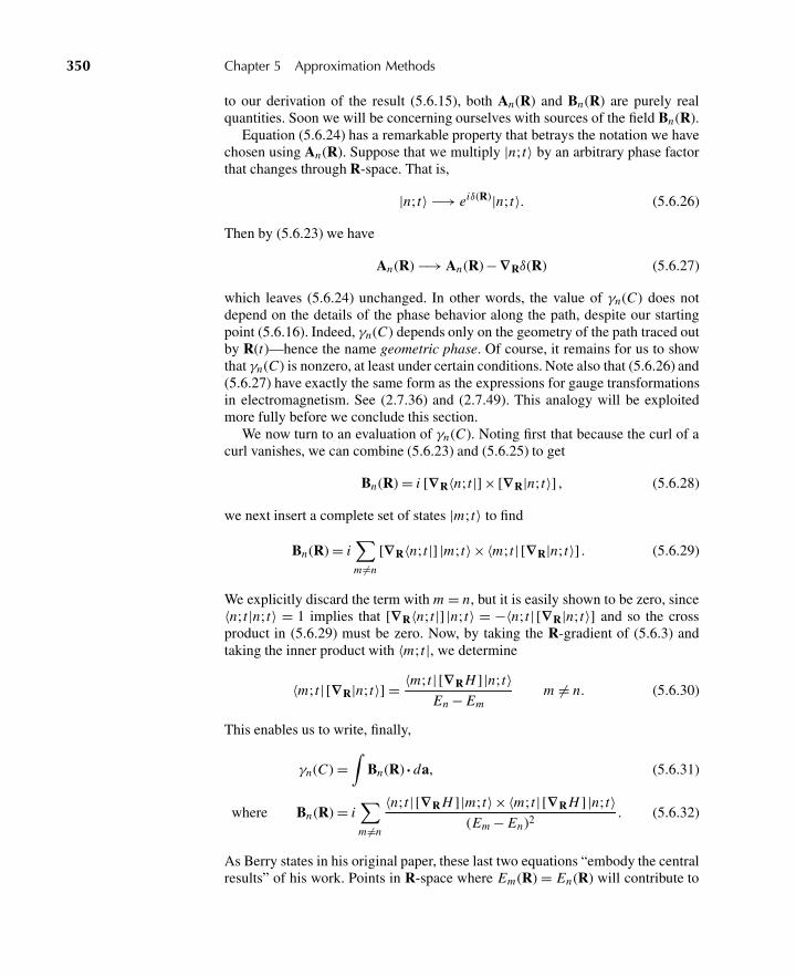
350 Chapter 5 Approximation Methods
to our derivation of the result (5.6.15), both An(R) and Bn(R) are purely realquantities. Soon we will be concerning ourselves with sources of the field Bn(R).
Equation (5.6.24) has a remarkable property that betrays the notation we havechosen using An(R). Suppose that we multiply |n; t〉 by an arbitrary phase factorthat changes through R-space. That is,
|n; t〉 −→ eiδ(R)|n; t〉. (5.6.26)
Then by (5.6.23) we have
An(R) −→ An(R) −∇Rδ(R) (5.6.27)
which leaves (5.6.24) unchanged. In other words, the value of γn(C) does notdepend on the details of the phase behavior along the path, despite our startingpoint (5.6.16). Indeed, γn(C) depends only on the geometry of the path traced outby R(t)—hence the name geometric phase. Of course, it remains for us to showthat γn(C) is nonzero, at least under certain conditions. Note also that (5.6.26) and(5.6.27) have exactly the same form as the expressions for gauge transformationsin electromagnetism. See (2.7.36) and (2.7.49). This analogy will be exploitedmore fully before we conclude this section.
We now turn to an evaluation of γn(C). Noting first that because the curl of acurl vanishes, we can combine (5.6.23) and (5.6.25) to get
Bn(R) = i [∇R〈n; t|] × [∇R|n; t〉] , (5.6.28)
we next insert a complete set of states |m; t〉 to find
Bn(R) = i∑m �=n
[∇R〈n; t|] |m; t〉×〈m; t| [∇R|n; t〉] . (5.6.29)
We explicitly discard the term with m = n, but it is easily shown to be zero, since〈n; t|n; t〉 = 1 implies that [∇R〈n; t|] |n; t〉 = −〈n; t| [∇R|n; t〉] and so the crossproduct in (5.6.29) must be zero. Now, by taking the R-gradient of (5.6.3) andtaking the inner product with 〈m; t|, we determine
〈m; t| [∇R|n; t〉] = 〈m; t| [∇R H ] |n; t〉En − Em
m �= n. (5.6.30)
This enables us to write, finally,
γn(C) =∫
Bn(R) · da, (5.6.31)
where Bn (R) = i∑m �=n
〈n; t| [∇R H ] |m; t〉×〈m; t| [∇R H ] |n; t〉(Em − En)2 . (5.6.32)
As Berry states in his original paper, these last two equations “embody the centralresults” of his work. Points in R-space where Em (R) = En(R) will contribute to
5.6 Hamiltonians with Extreme Time Dependence 351
the surface integral (5.6.31) even though the path enclosing that surface does notinclude those points.
It was realized early on that Berry’s phase could be observed using photonsmoving through a twisted optical fiber and that the geometric character of thisphase could be tested experimentally. See A. Tomita and R. Chiao, Phys. Rev.Lett. 57 (1986) 937. Indeed, this experiment can be carried out in the studentlaboratory. A description of the setup can be found in Experiments in ModernPhysics, by A. Melissinos and J. Napolitano (Academic Press 2003).
Example: Berry’s Phase for Spin 12
Let us now turn to a specific example and carry through a calculation of γn(C)from (5.6.31). We will study the phase motion for a spin 1
2 particle manipulatedslowly through a time-varying magnetic field. This particular example has in factbeen studied experimentally.
We return to (2.1.49), our familiar Hamiltonian, for a spin 12 particle in a mag-
netic field, but with some modification for a particle with arbitrary magnetic mo-ment. Since in this case, it is the magnetic field that changes slowly in time, letthe magnetic field be given by the three-dimensional vector∗ R(t). That is, R(t) isthe vector of parameters that we will change slowly. For a magnetic moment μ,our Hamiltonian is written as
H (t) = H (R(t)) = −2μ
hS ·R(t), (5.6.33)
where S is the spin 12 angular-momentum operator. Written in this way, the ex-
pectation value for the magnetic moment in the spin-up state is simply μ.Now on to the evaluation of B(R) using (5.6.32). First, it is simple enough
to show, either explicitly (see Problem 3.2 in Chapter 3) or by using rotationalsymmetry to fix R in the z-direction, that the two energy eigenvalues for (5.6.33)are
E±(t) = ∓μR(t), (5.6.34)
where R(t) is the magnitude of the magnetic-field vector, and the spin-up (down)eigenstates (with respect to the direction of R(t)) are |±; t〉. The summation in(5.6.32) consists of only one term, with denominator
(E± − E∓)2 = 4μ2 R2. (5.6.35)
It is also clear that
∇R H = −2μ
hS, (5.6.36)
leaving us with the need to evaluate the cross product
〈±; t|S|∓; t〉×〈∓; t|S|±; t〉 = 〈±; t|S|∓; t〉×〈±; t|S|∓; t〉∗ . (5.6.37)
∗In order to avoid confusion with (5.6.32), we do not use B to represent the magnetic field.
352 Chapter 5 Approximation Methods
Evaluating this matrix element would be tedious, except that we can invoke ro-tational symmetry and define the components of S relative to the direction of R.That is, |±; t〉 can be taken to be eigenstates of Sz . Thus, using (3.5.5) to write
S = 1
2(S+ + S−) x+ 1
2i(S+ − S−) y+ Sz z, (5.6.38)
we invoke (3.5.39) and (3.5.40) to find
〈±; t|S|∓; t〉 = h
2(x∓ i y) . (5.6.39)
Combining (5.6.35), (5.6.37), and (5.6.39), we have
B±(R) = ∓ 1
2R2(t)z. (5.6.40)
Of course, this result was derived by taking |±; t〉 to be eigenstates of Sz , when infact they are in the direction of R. Therefore, we actually have
B±(R) = ∓ 1
2R2(t)R. (5.6.41)
Finally, we calculate Berry’s Phase (5.6.31) to be
γ±(C) = ∓1
2
∫R · da
R2= ∓1
2�, (5.6.42)
where � is the “solid angle” subtended by the path through which the parametervector R(t) travels, relative to an origin R = 0 that is the source point for the fieldB. This emphasizes the “geometric” character of Berry’s Phase. Specifics of thepath do not matter, so long as the solid angle subtended by the path is the same.The result is also independent of the magnetic moment μ.
Soon after Berry’s prediction for this effect in spin 12 systems, two groups car-
ried out measurements using neutrons at the Institut Laue-Langevin in Grenoble,France. One of the resulting studies, T. Bitter and D. Dubbers, Phys. Rev. Lett.59 (1987) 251, used a slow (500-m/sec) neutron beam passing through a twistedmagnetic field. The second, D. J. Richardson et al., Phys. Rev. Lettt. 61 (1988)2030, made use of ultra-cold neutrons (UCN) and is more precise. UCN can bestored for long periods of time, so a cycle period T = 7.387 sec was used, ensur-ing the validity of the adiabatic theorem. Initially polarized in the z-direction, theneutrons are subjected to a rotating-magnetic-field component that is switched onat t = 0 and switched off at t = T . The magnetic-field vector traces out a circle(or ellipse, depending on adjustable parameters) in the yz-plane, depolarizing theneutrons by an amount depending on the integrated phase. Measuring the finalpolarization determines the integrated phase, and the dynamical phase (5.6.6) issubtracted out, leaving Berry’s Phase.
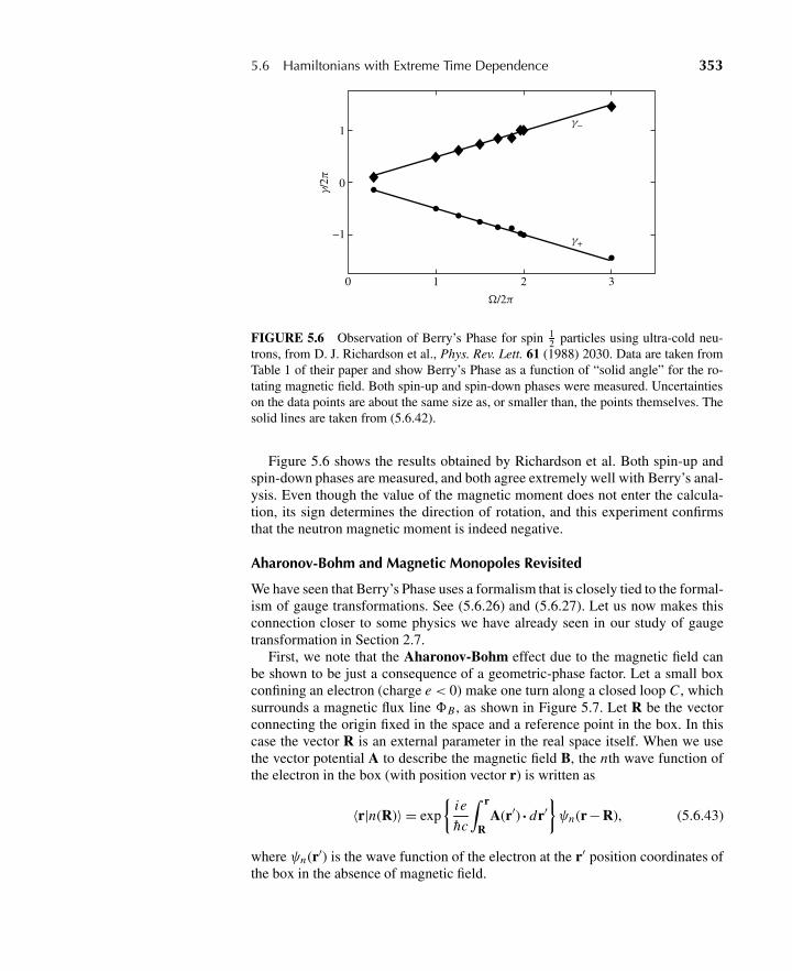
5.6 Hamiltonians with Extreme Time Dependence 353
γ−
γ+
0
−1
0
1
1 2 3
/2π
γ/2
π
FIGURE 5.6 Observation of Berry’s Phase for spin 12 particles using ultra-cold neu-
trons, from D. J. Richardson et al., Phys. Rev. Lett. 61 (1988) 2030. Data are taken fromTable 1 of their paper and show Berry’s Phase as a function of “solid angle” for the ro-tating magnetic field. Both spin-up and spin-down phases were measured. Uncertaintieson the data points are about the same size as, or smaller than, the points themselves. Thesolid lines are taken from (5.6.42).
Figure 5.6 shows the results obtained by Richardson et al. Both spin-up andspin-down phases are measured, and both agree extremely well with Berry’s anal-ysis. Even though the value of the magnetic moment does not enter the calcula-tion, its sign determines the direction of rotation, and this experiment confirmsthat the neutron magnetic moment is indeed negative.
Aharonov-Bohm and Magnetic Monopoles Revisited
We have seen that Berry’s Phase uses a formalism that is closely tied to the formal-ism of gauge transformations. See (5.6.26) and (5.6.27). Let us now makes thisconnection closer to some physics we have already seen in our study of gaugetransformation in Section 2.7.
First, we note that the Aharonov-Bohm effect due to the magnetic field canbe shown to be just a consequence of a geometric-phase factor. Let a small boxconfining an electron (charge e < 0) make one turn along a closed loop C , whichsurrounds a magnetic flux line �B , as shown in Figure 5.7. Let R be the vectorconnecting the origin fixed in the space and a reference point in the box. In thiscase the vector R is an external parameter in the real space itself. When we usethe vector potential A to describe the magnetic field B, the nth wave function ofthe electron in the box (with position vector r) is written as
〈r|n(R)〉 = exp
{ie
hc
∫ r
RA(r′) · dr′
}ψn(r − R), (5.6.43)
where ψn(r′) is the wave function of the electron at the r′ position coordinates ofthe box in the absence of magnetic field.
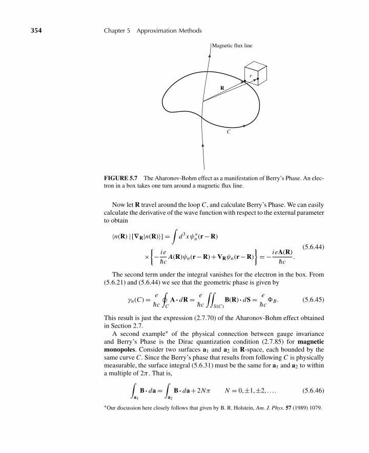
354 Chapter 5 Approximation Methods
r
R
C
Magnetic flux line
FIGURE 5.7 The Aharonov-Bohm effect as a manifestation of Berry’s Phase. An elec-tron in a box takes one turn around a magnetic flux line.
Now let R travel around the loop C , and calculate Berry’s Phase. We can easilycalculate the derivative of the wave function with respect to the external parameterto obtain
〈n(R) | [∇R|n(R)〉] =∫
d3xψ∗n (r − R)
×{− ie
hcA(R)ψn(r − R) + VRψn(r − R)
}= − ieA(R)
hc.
(5.6.44)
The second term under the integral vanishes for the electron in the box. From(5.6.21) and (5.6.44) we see that the geometric phase is given by
γn(C) = e
hc
∮C
A · dR = e
hc
∫∫S(C)
B(R) · dS = e
hc�B . (5.6.45)
This result is just the expression (2.7.70) of the Aharonov-Bohm effect obtainedin Section 2.7.
A second example∗ of the physical connection between gauge invarianceand Berry’s Phase is the Dirac quantization condition (2.7.85) for magneticmonopoles. Consider two surfaces a1 and a2 in R-space, each bounded by thesame curve C . Since the Berry’s phase that results from following C is physicallymeasurable, the surface integral (5.6.31) must be the same for a1 and a2 to withina multiple of 2π . That is,∫
a1
B · da =∫
a2
B · da + 2Nπ N = 0,±1,±2, . . . . (5.6.46)
∗Our discussion here closely follows that given by B. R. Holstein, Am. J. Phys. 57 (1989) 1079.
5.7 Time-Dependent Perturbation Theory 355
Now construct a closed surface by putting a1 “above” C and a2 below. Assumingthat we use something like the right-hand rule to consistently determine the ori-entation of da for each of the two integrals in (5.6.46), da points inward for oneof them. So we reverse the sign of da for that integral and rewrite (5.6.46) as∮
B · da = 2Nπ . (5.6.47)
Of course, inserting (5.6.41) into (5.6.47) yields ±2π , i.e. N = ±1, but that isan artifact of our choosing a spin 1
2 system for deriving (5.6.41). If we carriedthrough that example for a system with arbitrary spin, n would work out to beequal to twice the spin-projection quantum number.
Now (5.6.41) looks suspiciously like the magnetic field from a monopole withcharge 1
2 , but recall that it is in fact a Berry field. How can we relate this toan actual magnetic field for a monopole? It is actually easiest to see this whenwe express Berry’s Phase in terms of the line integral in (5.6.24) of the vectorpotential around the curve C . The gauge transformation (2.7.83) gives the formof the vector potential, and the line integral is just an integral over φ leading to afactor of 2π . We can then use this to evaluate the left side of (5.6.47), includingthe interaction with a single electric charge e to complete the phase, leading to thefactor e/hc as in (2.7.84). Thus, (5.6.47) becomes
e
hc(2eM )2π = 2Nπ
or2eeM
hc= N , (5.6.48)
which is the same result (2.7.85) that we obtained earlier in Section 2.7.
5.7 TIME-DEPENDENT PERTURBATION THEORY
Dyson Series
With the exception of a few problems like the two-level time-dependent problemof the previous section, exact solutions to the differential equation for cn(t) areusually not available. We must be content with approximate solutions to (5.5.17)obtained by perturbation expansion:
cn(t) = c(0)n + c(1)
n + c(2)n +·· · , (5.7.1)
where c(1)n ,c(2)
n , . . . signify amplitudes of first order, second order, and so on in thestrength parameter of the time-dependent potential. The iteration method used tosolve this problem is similar to what we did in time-independent perturbation the-ory. If initially only the state i is populated, we approximate cn on the right-handside of differential equation (5.5.17) by c(0)
n = δni (independent of t) and relateit to the time derivative of c(1)
n , integrate the differential equation to obtain c(1)n ,
356 Chapter 5 Approximation Methods
plug c(1)n into the right-hand side [of (5.5.17)] again to obtain the differential equa-
tion for c(2)n , and so on. This is how Dirac developed time-dependent perturbation
theory in 1927.Instead of working with cn(t), we propose to look at the time-evolution op-
erator UI (t , t0) in the interaction picture, which we will define later. We obtaina perturbation expansion for UI (t , t0), and at the very end we relate the matrixelements of UI to cn(t). If we are interested only in solving simple problems innonrelativistic quantum mechanics, all this might look superfluous; however, theoperator formalism we develop is very powerful because it can immediately beapplied to more-advanced problems, such as relativistic quantum field theory andmany-body theory.
The time-evolution operator in the interaction picture is defined by
|α, t0; t〉I = UI (t , t0)|α, t0; t0〉I . (5.7.2)
Differential equation (5.5.11) for the state ket of the interaction picture is equiva-lent to
i hd
dtUI (t , t0) = VI (t)UI (t , t0). (5.7.3)
We must solve this operator differential equation subject to the initial condition
UI (t , t0)|t=t0 = 1. (5.7.4)
First, let us note that the differential equation together with the initial condition isequivalent to the following integral equation:
UI (t , t0) = 1 − i
h
∫ t
t0VI (t ′)UI (t ′, t0)dt ′. (5.7.5)
We can obtain an approximate solution to this equation by iteration:
UI (t , t0) = 1 − i
h
∫ t
t0VI (t ′)
[1 − i
h
∫ t ′
t0VI (t ′′)UI (t ′′, t0)dt ′′
]dt ′
= 1 − i
h
∫ t
t0dt ′VI (t ′) +
(−i
h
)2 ∫ t
t0dt ′
∫ t ′
t0dt ′′VI (t ′)VI (t ′′)
+ ·· ·+(−i
h
)n ∫ t
t0dt ′
∫ t ′
t0dt ′′ · · ·
×∫ t (n−1)
t0dt (n)VI (t ′)VI (t ′′) · · ·VI (t (n))
+ ·· · .
(5.7.6)
5.7 Time-Dependent Perturbation Theory 357
This series is known as the Dyson series after Freeman J. Dyson, who appliedthis method to covariant quantum electrodynamics (QED).∗ Setting aside the dif-ficult question of convergence, we can compute UI (t , t0) to any finite order ofperturbation theory.
Transition Probability
Once UI (t , t0) is given, we can predict the time development of any state ket. Forexample, if the initial state at t = 0 is one of the energy eigenstates of H0, then toobtain the initial state ket at a later time, all we need to do is multiply by UI (t ,0):
|i , t0 = 0; t〉I = UI (t ,0)|i〉=∑
n
|n〉〈n|UI (t ,0)|i〉. (5.7.7)
In fact, 〈n|UI (t ,0)|i〉 is nothing more than what we called cn(t) earlier [see(5.5.13)]. We will say more about this later.
We earlier introduced the time-evolution operator U (t , t0) in the Schrödingerpicture (see Section 2.2). Let us now explore the connection between U (t , t0) andUI (t , t0). We note from (2.2.13) and (5.5.5) that
|α, t0; t〉I = ei H0t/h|α, t0; t〉S
= ei H0t/hU (t , t0)|α, t0; t0〉S
= ei H0t/hU (t , t0)e−i H0t0/h |α, t0; t0〉I .
(5.7.8)
So we have
UI (t , t0) = ei H0t/hU (t , t0)e−i H0t0/h . (5.7.9)
Let us now look at the matrix element of UI (t , t0) between energy eigenstates ofH0:
〈n|UI (t , t0)|i〉 = ei(En t−Ei t0)/h〈n|U (t , t0)|i〉. (5.7.10)
We recall from Section 2.2 that 〈n|U (t , t0)|i〉 is defined to be the transition ampli-tude. Hence our 〈n|UI (t , t0)|i〉 here is not quite the same as the transition ampli-tude defined earlier. However, the transition probability defined as the square ofthe modulus of 〈n|U (t , t0)|i〉 is the same as the analogous quantity in the interac-tion picture,
|〈n|UI (t , t0)|i〉|2 = |〈n|U (t , t0)|i〉|2. (5.7.11)
Parenthetically, we may remark that if the matrix elements of UI are taken be-tween initial and final states that are not energy eigenstates—for example, be-tween |a′〉 and |b′〉 (eigenkets of A and B, respectively), where [H0, A] �= 0 and/or
∗Note that in QED, the time-ordered product (t ′ > t ′′ > · · · ) is introduced, and then this pertur-bation series can be summed into an exponential form. This exponential form immediately givesU (t , t0) = U (t , t1)U (t1, t0) (Bjorken and Drell 1965, pp. 175–78).
358 Chapter 5 Approximation Methods
[H0, B] �= 0—we have, in general,
|〈b′|UI (t , t0)|a′〉| �= |〈b′|U (t , t0)|a′〉|,as the reader may easily verify. Fortunately, in problems where the interactionpicture is found to be useful, the initial and final states are usually taken to be H0eigenstates. Otherwise, all that is needed is to expand |a′〉, |b′〉, and so on in termsof the energy eigenkets of H0.
Coming back to 〈n|UI (t , t0)|i〉, we illustrate by considering a physical situa-tion where at t = t0, the system is known to be in state |i〉. The state ket in theSchrödinger picture |i , t0; t〉S is then equal to |i〉 up to a phase factor. In applyingthe interaction picture, it is convenient to choose the phase factor at t = t0 so that
|i , t0; t0〉S = e−i Ei t0/h |i〉, (5.7.12)
which means that in the interaction picture we have the simple equation
|i , t0; t0〉I = |i〉. (5.7.13)
At a later time we have
|i , t0; t〉I = UI (t , t0)|i〉. (5.7.14)
Comparing this with the expansion
|i , t0; t〉I =∑
n
cn(t)|n〉, (5.7.15)
we see that
cn(t) = 〈n|UI (t , t0)|i〉. (5.7.16)
We now go back to the perturbation expansion for UI (t , t0) [see (5.7.6)]. Wecan also expand cn(t) as in (5.7.1), where c(1)
n is first order in VI (t), c(2)n is second
order in VI (t), and so on. Comparing the expansion of both sides of (5.7.16), weobtain [using (5.5.7)]
c(0)n (t) = δni (independent of t)
c(1)n (t) = −i
h
∫ t
t0〈n|VI (t ′)|i〉dt ′
= −i
h
∫ t
t0eiωni t ′ Vni (t ′)dt ′
c(2)n (t) =
(−i
h
)2∑m
∫ t
t0dt ′
∫ t ′
t0dt ′′eiωnm t ′Vnm (t ′)eiωmi t ′′ Vmi (t ′′),
(5.7.17)
where we have used
ei(En−Ei )t/h = eiωni t . (5.7.18)
5.7 Time-Dependent Perturbation Theory 359
The transition probability for |i〉 → |n〉 with n �= i is obtained by
P(i → n) = |c(1)n (t) + c(2)
n (t) +·· · |2. (5.7.19)
Constant Perturbation
As an application of (5.7.17), let us consider a constant perturbation turned on att = 0:
V (t) ={
0, for t < 0V (independent of t), for t ≥ 0.
(5.7.20)
Even though the operator V has no explicit dependence on time, it is, in general,made up of operators like x, p, and s. Now suppose that at t = 0, we have only |i〉.With t0 taken to be zero, we obtain
c(0)n = c(0)
n (0) = δni ,
c(1)n = −i
hVni
∫ t
0eiωni t ′dt ′
= Vni
En − Ei(1 − eiωni t ),
(5.7.21)
or
|c(1)n |2 = |Vni |2
|En − Ei |2 (2 − 2cosωni t)
= 4|Vni |2|En − Ei |2 sin2
[(En − Ei )t
2h
].
(5.7.22)
The probability of finding |n〉 depends not only on |Vni |2 but also on the energydifference En − Ei , so let us try to see how (5.7.22) looks as a function of En . Inpractice, we are interested in this way of looking at (5.7.22) when there are manystates with E ∼ En so that we can talk about a continuum of final states withnearly the same energy. To this end, we define
ω ≡ En − Ei
h(5.7.23)
and plot 4sin2(ωt/2)/ω2 as a function of ω for fixed t, the time interval duringwhich the perturbation has been on; see Figure 5.8. We see that the height of themiddle peak, centered at ω = 0, is t2 and that the width is proportional to 1/t . Ast becomes large, |c(1)
n (t)|2 is appreciable only for those final states that satisfy
t ∼ 2π
|ω| = 2π h
|En − Ei | . (5.7.24)
If we call �t the time interval during which the perturbation has been turned on,a transition with appreciable probability is possible only if
�t�E ∼ h, (5.7.25)
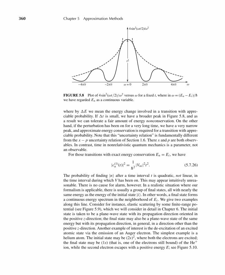
360 Chapter 5 Approximation Methods
t2
4 sin2(ωt/2)/ω2
−4π/t −2π/t ω = 0 2π/t 4π/t ω
FIGURE 5.8 Plot of 4sin2(ωt/2)/ω2 versus ω for a fixed t, where in ω = (En − Ei )/hwe have regarded En as a continuous variable.
where by �E we mean the energy change involved in a transition with appre-ciable probability. If �t is small, we have a broader peak in Figure 5.8, and asa result we can tolerate a fair amount of energy nonconservation. On the otherhand, if the perturbation has been on for a very long time, we have a very narrowpeak, and approximate energy conservation is required for a transition with appre-ciable probability. Note that this “uncertainty relation” is fundamentally differentfrom the x − p uncertainty relation of Section 1.6. There x and p are both observ-ables. In contrast, time in nonrelativistic quantum mechanics is a parameter, notan observable.
For those transitions with exact energy conservation En = Ei , we have
|c(1)n (t)|2 = 1
h2|Vni |2t2. (5.7.26)
The probability of finding |n〉 after a time interval t is quadratic, not linear, inthe time interval during which V has been on. This may appear intuitively unrea-sonable. There is no cause for alarm, however. In a realistic situation where ourformalism is applicable, there is usually a group of final states, all with nearly thesame energy as the energy of the initial state |i〉. In other words, a final state formsa continuous energy spectrum in the neighborhood of Ei . We give two examplesalong this line. Consider for instance, elastic scattering by some finite-range po-tential (see Figure 5.9), which we will consider in detail in Chapter 6. The initialstate is taken to be a plane-wave state with its propagation direction oriented inthe positive z-direction; the final state may also be a plane-wave state of the sameenergy but with its propagation direction, in general, in a direction other than thepositive z-direction. Another example of interest is the de-excitation of an excitedatomic state via the emission of an Auger electron. The simplest example is ahelium atom. The initial state may be (2s)2, where both the electrons are excited;the final state may be (1s) (that is, one of the electrons still bound) of the He+ion, while the second electron escapes with a positive energy E; see Figure 5.10.
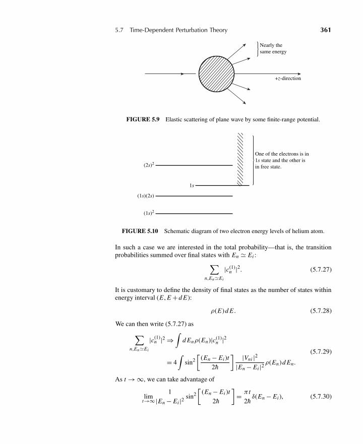
5.7 Time-Dependent Perturbation Theory 361
Nearly thesame energy
+z-direction
FIGURE 5.9 Elastic scattering of plane wave by some finite-range potential.
One of the electrons is in1s state and the other isin free state.(2s)2
(1s)(2s)
(1s)2
1s
FIGURE 5.10 Schematic diagram of two electron energy levels of helium atom.
In such a case we are interested in the total probability—that is, the transitionprobabilities summed over final states with En � Ei :∑
n,En�Ei
|c(1)n |2. (5.7.27)
It is customary to define the density of final states as the number of states withinenergy interval (E , E + d E):
ρ(E)d E . (5.7.28)
We can then write (5.7.27) as∑n,En�Ei
|c(1)n |2 ⇒
∫d Enρ(En)|c(1)
n |2
= 4∫
sin2[
(En − Ei )t
2h
] |Vni |2|En − Ei |2ρ(En)d En.
(5.7.29)
As t → ∞, we can take advantage of
limt→∞
1
|En − Ei |2 sin2[
(En − Ei )t
2h
]= π t
2hδ(En − Ei ), (5.7.30)
362 Chapter 5 Approximation Methods
which follows from
limα→∞
1
π
sin2αx
αx2= δ(x). (5.7.31)
It is now possible to take the average of |Vni |2 outside the integral sign and per-form the integration with the δ-function:
limt→∞
∫d Enρ(En)|c(1)
n (t)|2 =(
2π
h
)|Vni |2ρ(En)t
∣∣∣∣En�Ei
. (5.7.32)
Thus the total transition probability is proportional to t for large values of t, whichis quite reasonable. Notice that this linearity in t is a consequence of the fact thatthe total transition probability is proportional to the area under the peak of Figure5.8, where the height varies as t2 and the width varies as 1/t .
It is conventional to consider the transition rate—that is, the transition prob-ability per unit time. Expression (5.7.32) tells us that the total transition rate,defined by
d
dt
(∑n
|c(1)n |2
), (5.7.33)
is constant in t for large t. Calling (5.7.33) wi→[n], where [n] stands for a groupof final states with energy similar to i, we obtain
wi→[n] = 2π
h|Vni |2ρ(En)En�Ei (5.7.34)
independent of t, provided the first-order time-dependent perturbation theory isvalid. This formula is of great practical importance; it is called Fermi’s goldenrule even though the basic formalism of t-dependent perturbation theory origi-nated with Dirac. We sometimes write (5.7.34) as
wi→n =(
2π
h
)|Vni |2δ(En − Ei ), (5.7.35)
where it must be understood that this expression is integrated with∫
d Enρ(En).
We should also understand what is meant by |Vni |2. If the final states |n〉 forma quasi-continuum, the matrix elements Vni are often similar if |n〉 are similar.However, it may happen that not all energy eigenstates with the same En nec-essarily have similar matrix elements. Consider, for example, elastic scattering.The |Vni |2 that determines the scattering cross section may depend on the finalmomentum direction. In such a case, the group of final states we should con-sider must have not only approximately the same energy but also approximatelythe same momentum direction. This point becomes clearer when we discuss thephotoelectric effect.
5.7 Time-Dependent Perturbation Theory 363
Let us now look at the second-order term, still with the constant perturbationof (5.7.20). From (5.7.17) we have
c(2)n =
(−i
h
)2∑m
Vnm Vmi
∫ t
0dt ′eiωnm t ′
∫ t ′
0dt ′′eiωmi t ′′
= i
h
∑m
Vnm Vmi
Em − Ei
∫ t
0(eiωni t ′ − eiωnm t ′)dt ′.
(5.7.36)
The first term on the right-hand side has the same t dependence as c(1)n [see
(5.7.21)]. If this were the only term, we could then repeat the same argumentas before and conclude that as t → ∞, the only important contribution arisesfrom En � Ei . Indeed, when Em differs from En and Ei , the second contributiongives rise to a rapid oscillation, which does not give a contribution to the transitionprobability that grows with t.
With c(1) and c(2) together, we have
wi→[n] = 2π
h
∣∣∣∣∣Vni +∑
m
Vnm Vmi
Ei − Em
∣∣∣∣∣2
ρ(En)
∣∣∣∣∣∣En�Ei
. (5.7.37)
The formula has the following physical interpretation. We visualize that the tran-sition due to the second-order term takes place in two steps. First, |i〉 makesan energy-nonconserving transition to |m〉; subsequently, |m〉 makes an energy-nonconserving transition to |n〉, where between |n〉 and |i〉 there is overall energyconservation. Such energy-nonconserving transitions are often called virtual tran-sitions. Energy need not be conserved for those virtual transitions into (or from)virtual intermediate states. In contrast, the first-order term Vni is often said to rep-resent a direct energy-conserving “real” transition. A special treatment is neededif Vnm Vmi �= 0 with Em � Ei . The best way to treat this is to use the slow-turn-onmethod V → eηt V , which we will discuss in Section 5.9 and Problem 5.31 of thischapter. The net result is to change the energy denominator in (5.7.37) as follows:
Ei − Em → Ei − Em + iε. (5.7.38)
Harmonic Perturbation
We now consider a sinusoidally varying time-dependent potential, commonly re-ferred to as harmonic perturbation:
V (t) = Veiωt +V†e−iωt , (5.7.39)
where V may still depend on x, p, s, and so on. Actually, we encountered a time-dependent potential of this kind in Section 5.5 when we discussed t-dependenttwo-level problems.
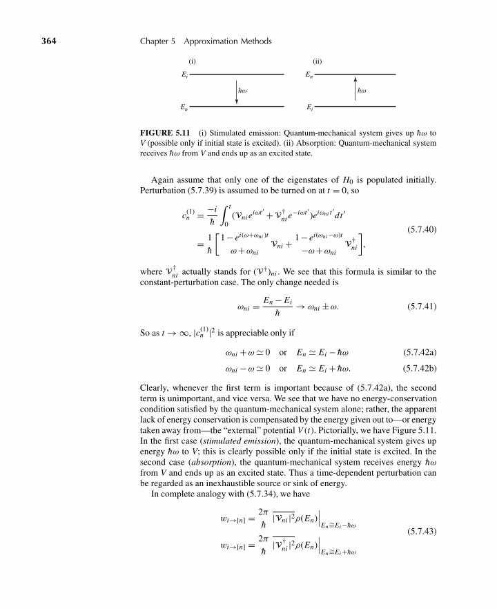
364 Chapter 5 Approximation Methods
(i) (ii)
hω hω
Ei
En
En
Ei
FIGURE 5.11 (i) Stimulated emission: Quantum-mechanical system gives up hω toV (possible only if initial state is excited). (ii) Absorption: Quantum-mechanical systemreceives hω from V and ends up as an excited state.
Again assume that only one of the eigenstates of H0 is populated initially.Perturbation (5.7.39) is assumed to be turned on at t = 0, so
c(1)n = −i
h
∫ t
0(Vni e
iωt ′ +V†ni e
−iωt ′ )eiωni t ′dt ′
= 1
h
[1 − ei(ω+ωni )t
ω+ωniVni + 1 − ei(ωni−ω)t
−ω+ωniV†
ni
],
(5.7.40)
where V†ni actually stands for (V†)ni . We see that this formula is similar to the
constant-perturbation case. The only change needed is
ωni = En − Ei
h→ ωni ±ω. (5.7.41)
So as t → ∞, |c(1)n |2 is appreciable only if
ωni +ω � 0 or En � Ei − hω (5.7.42a)
ωni −ω � 0 or En � Ei + hω. (5.7.42b)
Clearly, whenever the first term is important because of (5.7.42a), the secondterm is unimportant, and vice versa. We see that we have no energy-conservationcondition satisfied by the quantum-mechanical system alone; rather, the apparentlack of energy conservation is compensated by the energy given out to—or energytaken away from—the “external” potential V (t). Pictorially, we have Figure 5.11.In the first case (stimulated emission), the quantum-mechanical system gives upenergy hω to V; this is clearly possible only if the initial state is excited. In thesecond case (absorption), the quantum-mechanical system receives energy hωfrom V and ends up as an excited state. Thus a time-dependent perturbation canbe regarded as an inexhaustible source or sink of energy.
In complete analogy with (5.7.34), we have
wi→[n] = 2π
h|Vni |2ρ(En)
∣∣∣En∼=Ei −hω
wi→[n] = 2π
h|V†
ni |2ρ(En)∣∣∣En∼=Ei +hω
(5.7.43)
5.8 Applications to Interactions with the Classical Radiation Field 365
or, more commonly,
wi→n = 2π
h
{|Vni |2|V†
ni |2}δ(En − Ei ± hω). (5.7.44)
Note also that
|Vni |2 = |V†in |2, (5.7.45)
which is a consequence of
〈i |V†|n〉 = 〈n|V|i〉∗ (5.7.46)
(remember V†|n〉DC↔〈n|V). Combining (5.7.43) and (5.7.45), we have
emission rate for i → [n]
density of final states for[n]= absorption rate forn → [i ]
density of final states for[i ], (5.7.47)
where in the absorption case we let i stand for final states. Equation (5.7.47),which expresses symmetry between emission and absorption, is known as de-tailed balancing.
To summarize, for constant perturbation, we obtain appreciable transitionprobability for |i〉 → |n〉 only if En � Ei . In contrast, for harmonic perturba-tion, we have appreciable transition probability only if En � Ei − hω (stimulatedemission) or En � Ei + hω (absorption).
5.8 APPLICATIONS TO INTERACTIONS WITH THE CLASSICAL RADIATIONFIELD
Absorption and Stimulated Emission
We apply the formalism of time-dependent perturbation theory to the interactionsof atomic electrons with the classical radiation field. By a classical radiation fieldwe mean the electric or magnetic field derivable from a classical (as opposed to aquantized) radiation field.
The basic Hamiltonian, with |A|2 omitted, is
H = p2
2me+ eφ(x) − e
mecA · p, (5.8.1)
which is justified if
∇· A = 0. (5.8.2)
Specifically, we work with a monochromatic field of the plane wave for
A = 2A0ε cos(ω
cn ·x −ωt
), (5.8.3)
366 Chapter 5 Approximation Methods
where ε and n are the (linear) polarization and propagation directions. Equation(5.8.3) obviously satisfies (5.8.2), because ε is perpendicular to the propagationdirection n. We write
cos(ω
cn ·x −ωt
)= 1
2[ei(ω/c)n·x−iωt + e−i(ω/c)n·x+iωt ] (5.8.4)
and treat −(e/mec)A ·p as a time-dependent potential, where we express A in(5.8.3) as
A = A0ε[ei(ω/c)n·x−iωt + e−i(ω/c)n·x+iωt ]. (5.8.5)
Comparing this result with (5.7.39), we see that the e−iωt -term in
−(
e
mec
)A · p = −
(e
mec
)A0ε ·p[ei(ω/c)n·x−iωt + e−i(ω/c)n·x+iωt ] (5.8.6)
is responsible for absorption, while the e+iωt -term is responsible for stimulatedemission.
Let us now treat the absorption case in detail. We have
V†ni = − eA0
mec(ei(ω/c)(n·x)ε·p)ni (5.8.7)
and
wi→n = 2π
h
e2
m2ec2
|A0|2|〈n|ei(ω/c)(n·x)ε·p|i〉|2δ(En − Ei − hω). (5.8.8)
The meaning of the δ-function is clear. If |n〉 forms a continuum, we simply inte-grate with ρ(En). But even if |n〉 is discrete, because |n〉 cannot be a ground state(even though it is a bound-state energy level), its energy is not infinitely sharp.There may be a natural broadening due to a finite lifetime (see Section 5.9); therecan also be a mechanism for broadening due to collisions. In such cases, we regardδ(ω−ωni ) as
δ(ω−ωni ) = limγ→0
( γ2π
) 1
([ω−ωni )2 +γ 2/4]. (5.8.9)
Finally, the incident electromagnetic wave itself is not perfectly monochromatic;in fact, there is always a finite frequency width.
We derive an absorption cross section as
(Energy/unit time) absorbed by the atom (i → n)
Energy flux of the radiation field. (5.8.10)
For the energy flux (energy per area per unit time), classical electromagnetic the-ory gives us
cU = 1
2π
ω2
c|A0|2, (5.8.11)
5.8 Applications to Interactions with the Classical Radiation Field 367
where we have used
U = 1
2
(E2
max
8π+ B2
max
8π
)(5.8.12)
for energy density (energy per unit volume) with
E = −1
c
∂
∂ tA, B = ∇ ×A. (5.8.13)
Putting everything together, remembering that hω= energy absorbed by the atomfor each absorption process, we get
σ abs = hω(2π/h)(e2/m2ec2)|A0|2|〈n|ei(ω/c)(n·x)ε · p|i〉|2δ(En − Ei − hω)
(1/2π)(ω2/c)|A0|2
= 4π2h
m2eω
(e2
hc
)|〈n|ei(ω/c)(n·x)ε · p|i〉|2δ(En − Ei − hω).
(5.8.14)
Equation (5.8.14) has the correct dimension [1/(M2/T )](M2 L2/T 2)T = L2 ifwe recognize that α = e2/hc � 1/137 (dimensionless) and δ(En − Ei − hω) =(1/h)δ(ωni −ω), where δ(ωni −ω) has time dimension T.
Electric Dipole Approximation
The electric dipole approximation (E1 approximation) is based on the fact thatthe wavelength of the radiation field is far longer than the atomic dimension, sothat the series (remember ω/c = 1/λ)
ei(ω/c)n·x = 1 + iω
cn ·x +·· · (5.8.15)
can be approximated by its leading term, 1. The validity of this approximation fora light atom is explained as follows: First, the hω of the radiation field must be ofthe order of atomic level spacing, so
hω ∼ Ze2
(a0/Z )� Ze2
Ratom. (5.8.16)
This leads to
c
ω= λ∼ ch Ratom
Ze2 � 137Ratom
Z. (5.8.17)
In other words,
1
λRatom ∼ Z
137� 1 (5.8.18)
for light atoms (small Z). Because the matrix element of x is of order Ratom, thatof x2 is of order R2
atom, and so on, we see that the approximation of replacing(5.8.15) by its leading term is an excellent one.
368 Chapter 5 Approximation Methods
Now we have
〈n|ei(ω/c)(n·x)ε · p|i〉 → ε · 〈n|p|i〉. (5.8.19)
In particular, we take ε along the x-axis (and n along the z-axis). We must calcu-late 〈n|px |i〉. Using
[x , H0] = i h px
m, (5.8.20)
we have
〈n|px |i〉 = m
i h〈n|[x , H0]|i〉
= imωni 〈n|x |i〉.(5.8.21)
Because of the approximation of the dipole operator, this approximation scheme iscalled the electric dipole approximation. We may here recall [see (3.11.39)] theselection rule for the dipole matrix element. Since x is a spherical tensor of rank1 with q = ±1, we must have m′ − m = ±1, | j ′ − j | = 0,1 (no 0 → 0 transition).If ε is along the y-axis, the same selection rule applies. On the other hand, if ε isin the z-direction, q = 0; hence, m′ = m.
With the electric dipole approximation, the absorption cross section (5.8.14)now takes a simpler form upon our using (5.8.19) and (5.8.21):
σabs = 4π2αωni |〈n|x |i〉|2δ(ω−ωni ). (5.8.22)
In other words, σabs treated as a function of ω exhibits a sharp δ-function-likepeak whenever hω corresponds to the energy-level spacing at ω � (En − Ei )/h.Suppose |i〉 is the ground state; then ωni is necessarily positive. Integrating(5.8.22), we get ∫
σabs(ω)dω=∑
n
4π2αωni |〈n|x |i〉|2. (5.8.23)
In atomic physics we define oscillator strength, fni , as
fni ≡ 2mωni
h|〈n|x |i〉|2. (5.8.24)
It is then straightforward (consider [x , [x , H0]]) to establish the Thomas-Reiche-Kuhn sum rule, ∑
n
fni = 1. (5.8.25)
In terms of the integration over the absorption cross section, we have∫σabs(ω) dω = 4π2αh
2me= 2π2c
(e2
mec2
). (5.8.26)
5.8 Applications to Interactions with the Classical Radiation Field 369
Notice how h has disappeared. Indeed, this is just the oscillation sum rule alreadyknown in classical electrodynamics (Jackson 1975, for instance). Historically, thiswas one of the first examples of how “new quantum mechanics” led to the correctclassical result. This sum rule is quite remarkable because we did not specify indetail the form of the Hamiltonian.
Photoelectric Effect
We now consider the photoelectric effect—that is, the ejection of an electronwhen an atom is placed in the radiation field. The basic process is consideredto be the transition from an atomic (bound) state to a continuum state E > 0.Therefore, |i〉 is the ket for an atomic state, while |n〉 is the ket for a continuumstate, which can be taken to be a plane-wave state |k f 〉, an approximation that isvalid if the final electron is not too slow. Our earlier formula for σabs(ω) can stillbe used, except that we must now integrate δ(ωni −ω) together with the densityof final states ρ(En).
In fact, we calculated the density of states for a free particle in Section 2.5.To review, our basic task is to calculate the number of final states per unit energyinterval. As we will see in a moment, this is an example where the matrix elementdepends not only on the final state energy but also on the momentum direction.We must therefore consider a group of final states with both similar momentumdirections and similar energies.
To count the number of states, it is convenient to use the box normalizationconvention for plane-wave states. We consider a plane-wave state normalized if,when we integrate the square modulus of its wave function for a cubic box ofside L, we obtain unity. Furthermore, the state is assumed to satisfy the periodicboundary condition with periodicity of the side of the box. The wave functionmust then be of the form
〈x|k f 〉 = eik f ·x
L3/2, (5.8.27)
where the allowed values of kx must satisfy
kx = 2πnx
L, . . . , (5.8.28)
with nx a positive or negative integer. Similar restrictions hold for ky and kz .Notice that as L → ∞, kx , ky , and kz become continuous variables.
The problem of counting the number of states is reduced to that of countingthe number of dots in three-dimensional lattice space. We define n such that
n2 = n2x + n2
y + n2z . (5.8.29)
As L → ∞, it is a good approximation to treat n as a continuous variable; in factit is just the magnitude of the radial vector in the lattice space. Let us considera small-volume element such that the radial vector falls within n and n + dn andthe solid angle element d�; clearly, it is of volume n2 dn d�. The energy of the
370 Chapter 5 Approximation Methods
final-state plane wave is related to k f and hence to n; we have
E = h2k2f
2me= h2
2me
n2(2π)2
L2. (5.8.30)
Furthermore, the direction of the radial vector in the lattice space is just themomentum direction of the final state, so the number of states in the intervalbetween E and E + dE with direction into d� being k f is (remember dE =(h2k f /me)dk f ) given by∗
n2 d�dn
dEdE =
(L
2π
)3
(k2f )
dk f
dEd� dE
=(
L
2π
)3 me
h2 k f dE d�.
(5.8.31)
We can now put everything together to obtain an expression for the differentialcross section for the photoelectric effect:
dσ
d�= 4π2αh
m2eω
|〈k f |ei(ω/c)(n·x)ε · p|i〉|2 mek f L3
h2(2π)3. (5.8.32)
To be specific, let us consider the ejection of a K shell (the innermost shell)electron caused by absorption of light. The initial-state wave function is essen-tially the same as the ground-state hydrogen atom wave function, except that theBohr radius a0 is replaced by a0/Z . Thus
〈k f |ei(ω/c)(n·x)ε · p|i〉 = ε ·∫
d3xe−ik f ·x
L3/2 ei(ω/c)(n·x)
×(−i h∇)
[e−Zr/a0
(Z
a0
)3/2]
.
(5.8.33)
Integrating by parts, we can pass ∇ to the left side. Furthermore,
ε · [∇ei(ω/c)(n·x)] = 0 (5.8.34)
because ε is perpendicular to n. On the other hand, ∇ acting on e−ik f ·x bringsdown −ik f , which can be taken outside the integral. Thus, to evaluate (5.8.33),all we need to do is take the Fourier transform of the atomic wave function withrespect to
q ≡ k f −(ω
c
)n. (5.8.35)
∗This is equivalent to taking one state per cube d3xd3 p/(2π h)3 in phase space.
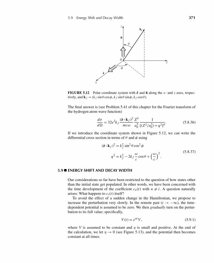
5.9 Energy Shift and Decay Width 371
φ
ε
n
θ
0
zkf
x
y
FIGURE 5.12 Polar coordinate system with ε and n along the x- and z-axes, respec-tively, and k f = (k f sinθ cosφ, k f sinθ sinφ, k f cosθ ).
The final answer is (see Problem 5.41 of this chapter for the Fourier transform ofthe hydrogen atom wave function)
dσ
d�= 32e2k f
(ε · k f )2
mcω
Z5
a50
1
[(Z2/a20) + q2]4
. (5.8.36)
If we introduce the coordinate system shown in Figure 5.12, we can write thedifferential cross section in terms of θ and φ using
(ε · k f )2 = k2f sin2 θ cos2φ
q2 = k2f − 2k f
ω
ccosθ+
(ωc
)2.
(5.8.37)
5.9 ENERGY SHIFT AND DECAY WIDTH
Our considerations so far have been restricted to the question of how states otherthan the initial state get populated. In other words, we have been concerned withthe time development of the coefficient cn(t) with n �= i . A question naturallyarises: What happens to ci (t) itself?
To avoid the effect of a sudden change in the Hamiltonian, we propose toincrease the perturbation very slowly. In the remote past (t → −∞), the time-dependent potential is assumed to be zero. We then gradually turn on the pertur-bation to its full value; specifically,
V (t) = eηt V , (5.9.1)
where V is assumed to be constant and η is small and positive. At the end ofthe calculation, we let η→ 0 (see Figure 5.13), and the potential then becomesconstant at all times.
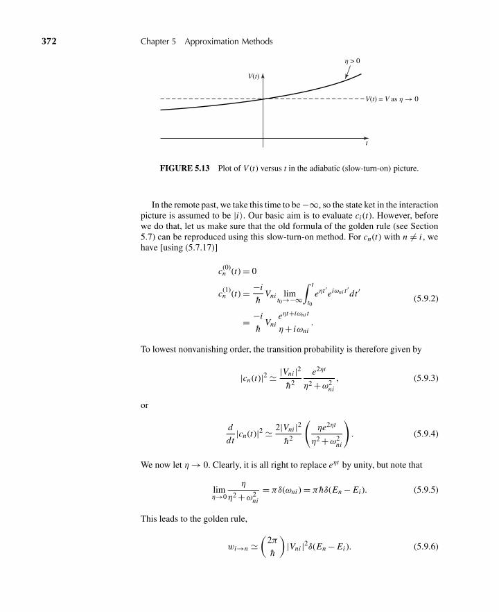
372 Chapter 5 Approximation Methods
V(t) = V as η → 0
t
V(t)
η > 0
FIGURE 5.13 Plot of V (t) versus t in the adiabatic (slow-turn-on) picture.
In the remote past, we take this time to be −∞, so the state ket in the interactionpicture is assumed to be |i〉. Our basic aim is to evaluate ci (t). However, beforewe do that, let us make sure that the old formula of the golden rule (see Section5.7) can be reproduced using this slow-turn-on method. For cn(t) with n �= i , wehave [using (5.7.17)]
c(0)n (t) = 0
c(1)n (t) = −i
hVni lim
t0→−∞
∫ t
t0eηt ′eiωni t ′dt ′
= −i
hVni
eηt+iωni t
η+ iωni.
(5.9.2)
To lowest nonvanishing order, the transition probability is therefore given by
|cn(t)|2 � |Vni |2h2
e2ηt
η2 +ω2ni
, (5.9.3)
or
d
dt|cn(t)|2 � 2|Vni |2
h2
(ηe2ηt
η2 +ω2ni
). (5.9.4)
We now let η→ 0. Clearly, it is all right to replace eηt by unity, but note that
limη→0
η
η2 +ω2ni
= πδ(ωni ) = π hδ(En − Ei ). (5.9.5)
This leads to the golden rule,
wi→n �(
2π
h
)|Vni |2δ(En − Ei ). (5.9.6)
5.9 Energy Shift and Decay Width 373
Encouraged by this result, let us calculate c(0)i , c(1)
i , and c(2)i , again using (5.7.17).
We have
c(0)i = 1
c(1)i = −i
hVii lim
t0→−∞
∫ t
t0eηt ′dt ′ = −i
hηVii e
ηt
c(2)i =
(−i
h
)2∑m
|Vmi |2 limt0→−∞
∫ t
t0dt ′eiωim t ′+ηt ′ eiωmi t ′+ηt ′
i (ωmi − iη)
=(−i
h
)2
|Vii |2 e2ηt
2η2 +(−i
h
)∑m �=i
|Vmi |2e2ηt
2η(Ei − Em + i hη).
(5.9.7)
Thus, up to second order, we have
ci (t) � 1 − i
hηVii e
ηt +(−i
h
)2
|Vii |2 e2ηt
2η2+(−i
h
)∑m �=i
|Vmi |2e2ηt
2η(Ei − Em + i hη).
(5.9.8)
Now consider the time derivative of ci [dci (t)/dt ≡ ci ], which we have from(5.9.8). Upon dividing by ci and letting η → 0 (thus replacing eηt and e2ηt byunity), we get
ci
ci�
−i
hVii +
(−i
h
)2 |Vii |2η
+(−i
h
)∑m �=i
|Vmi |2(Ei − Em + i hη)
1 − i
h
Vii
η
� −i
hVii +
(−i
h
)∑m �=i
|Vmi |2Ei − Em + i hη
.
(5.9.9)
Expansion (5.9.9) is formally correct up to second order in V. Note here thatci (t)/ci (t) is now independent of t. Equation (5.9.9) is a differential equation thatis to hold at all times. Now that we have obtained this, it is convenient to renor-malize ci so that ci (0) = 1. We now try the ansatz
ci (t) = e−i�i t/h ,ci (t)
ci (t)= −i
h�i (5.9.10)
with �i constant (in time) but not necessarily real. Clearly (5.9.10) is consistentwith (5.9.9) because the right-hand side of (5.9.10) is constant. We can see the
374 Chapter 5 Approximation Methods
physical meaning of �i by noting that e−i�i t/h|i〉 in the interaction picture im-plies e−i�i t/h−i Ei t/h|i〉 in the Schrödinger picture. In other words,
Ei → Ei +�i (5.9.11)
as a result of perturbation. That is, we have calculated the level shift using time-dependent perturbation theory. Now expand, as usual,
�i =�(1)i +�(2)
i +·· · , (5.9.12)
and compare (5.9.10) with (5.9.9); we get to first order:
�(1)i = Vii . (5.9.13)
But this is just what we expect from t-independent perturbation theory. Beforewe look at �(2)
i , recall that
limε→0
1
x + iε= Pr.
1
x− iπδ(x). (5.9.14)
Thus
Re(�(2)i ) = Pr.
∑m �=i
|Vmi |2Ei − Em
(5.9.15a)
Im(�(2)i ) = −π
∑m �=i
|Vmi |2δ(Ei − Em). (5.9.15b)
But the right-hand side of (5.9.15b) is familiar from the golden rule, so we canidentify ∑
m �=i
wi→m = 2π
h
∑m �=i
|Vmi |2δ(Ei − Em) = − 2
hIm[�(2)
i ]. (5.9.16)
Coming back to ci (t), we can write (5.9.10) as
ci (t) = e−(i/h)[Re(�i )t ]+(1/h)[Im(�i )t ]. (5.9.17)
If we define
�i
h≡ − 2
hIm(�i ), (5.9.18)
then
|ci |2 = e2Im(�i )t/h = e−�i t/h . (5.9.19)
Therefore, �i characterizes the rate at which state |i〉 disappears.
5.9 Energy Shift and Decay Width 375
It is worth checking the probability conservation up to second order in V forsmall t:
|ci |2 +∑m �=i
|cm |2 = (1 −�i t/h) +∑m �=i
wi→m t = 1, (5.9.20)
where (5.9.16) has been used. Thus the probabilities for finding the initial stateand all other states add up to 1. To put it another way, the depletion of state |i〉 iscompensated by the growth of states other than |i〉.
To summarize, the real part of the energy shift is what we usually associatewith the level shift. The imaginary part of the energy shift is, apart from −2 [see(5.9.18)], the decay width. Note also that
h
�i= τi , (5.9.21)
where τi is the mean lifetime of state |i〉 because
|ci |2 = e−t/τi . (5.9.22)
To see why �i is called width, we look at the Fourier decomposition∫f (E)e−i E t/hdE = e−i[Ei +Re(�i )]t/h−�i t/2h. (5.9.23)
Using the Fourier inversion formula, we get
| f (E)|2 ∝ 1
{E − [Ei + Re(�i )]}2 +�2i /4
. (5.9.24)
Therefore, �i has the usual meaning of full width at half maximum. Notice thatwe get the time-energy uncertainty relation from (5.9.21):
�t�E ∼ h, (5.9.25)
where we identify the uncertainty in the energy with �i and the mean lifetimewith �t .
Even though we discussed the subject of energy shift and decay width usingthe constant perturbation V obtained as the limit of (5.9.1) when η→ 0, we caneasily generalize our considerations to the harmonic perturbation case discussedin Section 5.7. All we must do is to let
En(m) − Ei → En(m) − Ei ± hω (5.9.26)
in (5.9.2), (5.9.8), and (5.9.15), and so on. The quantum-mechanical descriptionof unstable states we have developed here was originally proposed by Wigner andWeisskopf in 1930.
376 Chapter 5 Approximation Methods
Problems
5.1 A simple harmonic oscillator (in one dimension) is subjected to a perturbation
λH1 = bx ,
where b is a real constant.
(a) Calculate the energy shift of the ground state to lowest nonvanishing order.
(b) Solve this problem exactly and compare with your result obtained in (a). Youmay assume without proof that
〈un′ |x |un〉 =√
h
2mω(√
n + 1δn′ ,n+1 +√nδn′,n−1).
5.2 In nondegenerate time-independent perturbation theory, what is the probability offinding in a perturbed energy eigenstate (|k〉) the corresponding unperturbed eigen-state (|k(0)〉)? Solve this up to terms of order g2.
5.3 Consider a particle in a two-dimensional potential
V0 ={
0, for 0 ≤ x ≤ L ,0 ≤ y ≤ L∞, otherwise.
Write the energy eigenfunctions for the ground state and the first excited state. Wenow add a time-independent perturbation of the form
V1 ={λxy, for 0 ≤ x ≤ L ,0 ≤ y ≤ L0, otherwise.
Obtain the zeroth-order energy eigenfunctions and the first-order energy shifts forthe ground state and the first excited state.
5.4 Consider an isotropic harmonic oscillator in two dimensions. The Hamiltonian isgiven by
H0 = p2x
2m+ p2
y
2m+ mω2
2(x2 + y2).
(a) What are the energies of the three lowest-lying states? Is there any degeneracy?
(b) We now apply a perturbation
V = δmω2xy,
where δ is a dimensionless real number much smaller than unity. Find thezeroth-order energy eigenket and the corresponding energy to first order [thatis, the unperturbed energy obtained in (a) plus the first-order energy shift] foreach of the three lowest-lying states.
(c) Solve the H0 + V problem exactly. Compare with the perturbation results ob-tained in (b). [You may use 〈n′|x |n〉 = √
h/2mω(√
n + 1δn′,n+1 +√nδn′ ,n−1).]
5.5 Establish (5.1.54) for the one-dimensional harmonic oscillator given by (5.1.50)with an additional perturbation V = 1
2εmω2x2. Show that all other matrix elements
Vk0 vanish.
Problems 377
5.6 (From Merzbacher 1970.) A slightly anisotropic three-dimensional harmonic os-cillator has ωz ≈ ωx = ωy . A charged particle moves in the field of this oscillatorand is at the same time exposed to a uniform magnetic field in the x-direction. As-suming that the Zeeman splitting is comparable to the splitting produced by theanisotropy, but small compared to hω, calculate to first order the energies of thecomponents of the first excited state. Discuss various limiting cases.
5.7 A one-electron atom whose ground state is nondegenerate is placed in a uniformelectric field in the z-direction. Obtain an approximate expression for the inducedelectric dipole moment of the ground state by considering the expectation valueof ez with respect to the perturbed-state vector computed to first order. Show thatthe same expression can also be obtained from the energy shift � = −α|E|2/2 ofthe ground state computed to second order. (Note: α stands for the polarizability.)Ignore spin.
5.8 Evaluate the matrix elements (or expectation values) given below. If any vanishes,explain why it vanishes using simple symmetry (or other) arguments.
(a) 〈n = 2,l = 1,m = 0|x |n = 2,l = 0,m = 0〉.(b) 〈n = 2,l = 1,m = 0|pz |n = 2,l = 0,m = 0〉.[In (a) and (b), |nlm〉 stands for the energy eigenket of a nonrelativistic hydrogenatom with spin ignored.]
(c) 〈L z〉 for an electron in a central field with j = 92 , m = 7
2 , l = 4.
(d) 〈singlet,ms = 0|S(e−)z − S(e+)
z |triplet,ms = 0〉 for an s-state positronium.
(e) 〈S(1) · S(2)〉 for the ground state of a hydrogen molecule.
5.9 A p-orbital electron characterized by |n,l = 1,m = ±1,0〉 (ignore spin) is subjectedto a potential
V = λ(x2 − y2) (λ = constant).
(a) Obtain the “correct” zeroth-order energy eigenstates that diagonalize the per-turbation. You need not evaluate the energy shifts in detail, but show that theoriginal threefold degeneracy is now completely removed.
(b) Because V is invariant under time reversal and because there is no longer anydegeneracy, we expect each of the energy eigenstates obtained in (a) to gointo itself (up to a phase factor or sign) under time reversal. Check this pointexplicitly.
5.10 Consider a spinless particle in a two-dimensional infinite square well:
V ={
0, for 0 ≤ x ≤ a,0 ≤ y ≤ a∞, otherwise.
(a) What are the energy eigenvalues for the three lowest states? Is there any de-generacy?
(b) We now add a potential
V1 = λxy, 0 ≤ x ≤ a,0 ≤ y ≤ a.
Taking this as a weak perturbation, answer the following:
378 Chapter 5 Approximation Methods
(i) Is the energy shift due to the perturbation linear or quadratic in λ for each ofthe three states?
(ii) Obtain expressions for the energy shifts of the three lowest states accurate toorder λ. (You need not evaluate integrals that may appear.)
(iii) Draw an energy diagram with and without the perturbation for the three energystates. Make sure to specify which unperturbed state is connected to whichperturbed state.
5.11 The Hamiltonian matrix for a two-state system can be written as
H =(
E01 λ�
λ� E02
).
Clearly, the energy eigenfunctions for the unperturbed problems (λ = 0) are givenby
φ(0)1 =
(10
), φ
(0)2 =
(01
).
(a) Solve this problem exactly to find the energy eigenfunctions ψ1 and ψ2 and theenergy eigenvalues E1 and E2.
(b) Assuming that λ|�| � |E01 − E0
2 |, solve the same problem using time-independent perturbation theory up to first order in the energy eigenfunctionsand up to second order in the energy eigenvalues. Compare with the exactresults obtained in (a).
(c) Suppose the two unperturbed energies are “almost degenerate”; that is,
|E01 − E0
2 | � λ|�|.Show that the exact results obtained in (a) closely resemble what you wouldexpect by applying degenerate perturbation theory to this problem with E0
1 setexactly equal to E0
2 .
5.12 (This is a tricky problem because the degeneracy between the first state and thesecond state is not removed in first order. See also Gottfried 1966, p. 397, Problem1.) This problem is from Schiff 1968, p. 295, Problem 4. A system that has threeunperturbed states can be represented by the perturbed Hamiltonian matrix⎛⎝E1 0 a
0 E1 ba∗ b∗ E2
⎞⎠ ,
where E2 > E1. The quantities a and b are to be regarded as perturbations thatare of the same order and are small compared with E2 − E1. Use the second-ordernondegenerate perturbation theory to calculate the perturbed eigenvalues. (Is thisprocedure correct?) Then diagonalize the matrix to find the exact eigenvalues. Fi-nally, use the second-order degenerate perturbation theory. Compare the three re-sults obtained.
5.13 Compute the Stark effect for the 2S1/2 and 2P1/2 levels of hydrogen for a field ε suf-ficiently weak that eεa0 is small compared to the fine structure, but take the Lambshift δ (δ = 1,057 MHz) into account (that is, ignore 2P3/2 in this calculation).
Problems 379
Show that for eεa0 � δ, the energy shifts are quadratic in ε, whereas for eεa0 � δ,they are linear in ε. (The radial integral you need is 〈2s|r |2p〉 = 3
√3a0.) Briefly
discuss the consequences (if any) of time reversal for this problem. This problemis from Gottfried 1966, Problem 7-3.
5.14 Work out the Stark effect to lowest nonvanishing order for the n = 3 level of the hy-drogen atom. Ignoring the spin-orbit force and relativistic correction (Lamb shift),obtain not only the energy shifts to lowest nonvanishing order but also the corre-sponding zeroth-order eigenket.
5.15 Suppose the electron had a very small intrinsic electric dipole moment analogous tothe spin-magnetic moment (that is, μel proportional to σ ). Treating the hypothetical−μel · E interaction as a small perturbation, discuss qualitatively how the energylevels of the Na atom (Z = 11) would be altered in the absence of any externalelectromagnetic field. Are the level shifts first order or second order? Indicate ex-plicitly which states get mixed with each other. Obtain an expression for the energyshift of the lowest level that is affected by the perturbation. Assume throughout thatonly the valence electron is subjected to the hypothetical interaction.
5.16 Consider a particle bound to a fixed center by a spherically symmetrical potentialV (r ).
(a) Prove
|ψ(0)|2 =(
m
2π h2
)⟨dV
dr
⟩for all s-states, ground and excited.
(b) Check this relation for the ground state of a three-dimensional isotropic os-cillator, the hydrogen atom, and so on. (Note: This relation has actually beenfound to be useful in guessing the form of the potential between a quark andan antiquark.)
5.17 (a) Suppose the Hamiltonian of a rigid rotator in a magnetic field perpendicular tothe axis is of the form (Merzbacher 1970, Problem 17-1)
AL2 + BL z + C L y
if terms quadratic in the field are neglected. Assuming B � C , use perturbationtheory to lowest nonvanishing order to get approximate energy eigenvalues.
(b) Consider the matrix elements
〈n′l ′m ′lm
′s |(3z2 − r 2)|nlmlms〉,
〈n′l ′m ′lm
′s |xy|nlmlms〉
of a one-electron (for example, alkali) atom. Write the selection rules for �l ,�ml , and �ms . Justify your answer.
5.18 Work out the quadratic Zeeman effect for the ground-state hydrogen atom [〈x|0〉 =(1/
√πa3
0)e−r/a0 ] due to the usually neglected e2A2/2mec2-term in the Hamilto-nian taken to first order. Write the energy shift as
�= − 12χB2
380 Chapter 5 Approximation Methods
and obtain an expression for diamagnetic susceptibility, χ . The following definiteintegral may be useful: ∫ ∞
0e−αr r ndr = n!
αn+1.
5.19 (Merzbacher 1970, p. 448, Problem 11.) For the He wave function, use
ψ(x1,x2) = (Z3eff/πa3
0)exp
[−Zeff(r1 + r2)
a0
]with Zeff = 2 − 5
16 , as obtained by the variational method. The measured value ofthe diamagnetic susceptibility is 1.88× 10⁻⁶ cm3/mole.
Using the Hamiltonian for an atomic electron in a magnetic field, determine,for a state of zero angular momentum, the energy change to order B2 if the systemis in a uniform magnetic field represented by the vector potential A = 1
2 B× r.Defining the atomic diamagnetic susceptibility χ by E = − 1
2χ B2, calculateχ for a helium atom in the ground state and compare the result with the measuredvalue.
5.20 Estimate the ground-state energy of a one-dimensional simple harmonic oscillatorusing
〈x |0〉 = e−β|x|
as a trial function with β to be varied. You may use∫ ∞
0e−αx xndx = n!
αn+1.
5.21 Estimate the lowest eigenvalue (λ) of the differential equation
d2ψ
dx2+ (λ−|x |)ψ = 0, ψ → 0 for |x | → ∞
using the variational method with
ψ ={
c(α−|x |), for |x |< α0, for |x |> α (α to be varied)
as a trial function. (Caution: dψ/dx is discontinuous at x = 0.) Numerical datathat may be useful for this problem are
31/3 = 1.442, 51/3 = 1.710, 32/3 = 2.080, π2/3 = 2.145.
The exact value of the lowest eigenvalue can be shown to be 1.019.
5.22 Consider a one-dimensional simple harmonic oscillator whose classical angularfrequency is ω0. For t < 0 it is known to be in the ground state. For t > 0 there isalso a time-dependent potential
V (t) = F0x cosωt ,
where F0 is constant in both space and time. Obtain an expression for the expec-tation value 〈x〉 as a function of time using time-dependent perturbation theory
Problems 381
to lowest nonvanishing order. Is this procedure valid for ω � ω0? [You may use〈n′|x |n〉 = √
h/2mω0(√
n + 1δn′,n+1 +√nδn′,n−1).]
5.23 A one-dimensional harmonic oscillator is in its ground state for t < 0. For t ≥ 0 itis subjected to a time-dependent but spatially uniform force (not potential!) in thex-direction,
F(t) = F0e−t/τ .
(a) Using time-dependent perturbation theory to first order, obtain the probabilityof finding the oscillator in its first excited state for t > 0. Show that the t → ∞(τ finite) limit of your expression is independent of time. Is this reasonable orsurprising?
(b) Can we find higher excited states? You may use
〈n′|x |n〉 =√h/2mω(
√nδn′,n−1 +√
n + 1δn′ ,n+1).
5.24 Consider a particle bound in a simple harmonic-oscillator potential. Initially (t <0), it is in the ground state. At t = 0 a perturbation of the form
H ′(x , t) = Ax2e−t/τ
is switched on. Using time-dependent perturbation theory, calculate the probabilitythat after a sufficiently long time (t � τ ), the system will have made a transition toa given excited state. Consider all final states.
5.25 The unperturbed Hamiltonian of a two-state system is represented by
H0 =(
E01 0
0 E02
).
There is, in addition, a time-dependent perturbation
V (t) =(
0 λcosωtλcosωt 0
)(λ real).
(a) At t = 0 the system is known to be in the first state, represented by(10
).
Using time-dependent perturbation theory and assuming that E01 − E0
2 is notclose to ±hω, derive an expression for the probability that the system is foundin the second state represented by (
01
)as a function of t(t > 0).
(b) Why is this procedure not valid when E01 − E0
2 is close to ±hω?
5.26 A one-dimensional simple harmonic oscillator of angular frequencyω is acted uponby a spatially uniform but time-dependent force (not potential)
F(t) = (F0τ/ω)
(τ 2 + t2), −∞< t <∞.
382 Chapter 5 Approximation Methods
At t = −∞, the oscillator is known to be in the ground state. Using the time-dependent perturbation theory to first order, calculate the probability that the oscil-lator is found in the first excited state at t = +∞.
Challenge for experts: F(t) is so normalized that the impulse∫F(t)dt
imparted to the oscillator is always the same—that is, independent of τ ; yet forτ � 1/ω, the probability for excitation is essentially negligible. Is this reasonable?[Matrix element of x : 〈n′|x |n〉 = (h/2mω)1/2(
√nδn′,n−1 +√
n + 1δn′,n+1).]
5.27 Consider a particle in one dimension moving under the influence of some time-independent potential. The energy levels and the corresponding eigenfunctions forthis problem are assumed to be known. We now subject the particle to a travelingpulse represented by a time-dependent potential,
V (t) = Aδ(x − ct).
(a) Suppose that at t = −∞ the particle is known to be in the ground state whoseenergy eigenfunction is 〈x |i 〉 = ui (x). Obtain the probability for finding thesystem in some excited state with energy eigenfunction 〈x | f 〉 = u f (x) at t =+∞.
(b) Interpret your result in (a) physically by regarding the δ-function pulse as asuperposition of harmonic perturbations; recall
δ(x − ct) = 1
2πc
∫ ∞
−∞dωeiω[(x/c)−t].
Emphasize the role played by energy conservation, which holds even quantum-mechanically as long as the perturbation has been on for a very long time.
5.28 A hydrogen atom in its ground state [(n,l ,m) = (1,0,0)] is placed between theplates of a capacitor. A time-dependent but spatially uniform electric field (notpotential!) is applied as follows:
E ={
0, for t < 0E0e−t/τ , for t > 0.
(E0 in the positive z-direction)
Using first-order time-dependent perturbation theory, compute the probability forthe atom to be found at t � τ in each of the three 2p states: (n,l ,m) = (2,1,±1or 0).Repeat the problem for the 2s state: (n,l ,m) = (2,0,0). You need not attempt toevaluate radial integrals, but perform all other integrations (with respect to anglesand time).
5.29 Consider a composite system made up of two spin 12 objects. For t < 0, the Hamil-
tonian does not depend on spin and can be taken to be zero by suitably adjustingthe energy scale. For t > 0, the Hamiltonian is given by
H =(
4�
h2
)S1· S2.
Suppose the system is in |+−〉 for t ≤ 0. Find, as a function of time, the probabilityfor its being found in each of the following states |++〉, |+−〉, |−+〉, and |−−〉:
Problems 383
(a) By solving the problem exactly.(b) By solving the problem assuming the validity of first-order time-dependent
perturbation theory with H as a perturbation switched on at t = 0. Under whatcondition does (b) give the correct results?
5.30 Consider a two-level system with E1 < E2. There is a time-dependent potentialthat connects the two levels as follows:
V11 = V22 = 0, V12 = γ eiωt , V21 = γ e−iωt (γ real).
At t = 0, it is known that only the lower level is populated—that is, c1(0) = 1,c2(0) = 0.(a) Find |c1(t)|2 and |c2(t)|2 for t > 0 by exactly solving the coupled differential
equation
i hck =2∑
n=1
Vkn (t)eiωkn t cn , (k = 1,2).
(b) Do the same problem using time-dependent perturbation theory to lowest non-vanishing order. Compare the two approaches for small values of γ . Treat thefollowing two cases separately: (i) ω very different from ω21 and (ii) ω closeto ω21.
Answer for (a): (Rabi’s formula)
|c2(t)|2 = γ 2/h2
γ 2/h2 + (ω−ω21)2/4sin2
{[γ 2
h2 + (ω−ω21)2
4
]1/2
t
},
|c1(t)|2 = 1−|c2(t)|2.
5.31 Show that the slow-turn-on of perturbation V → V eηt (see Baym 1969, p. 257) cangenerate a contribution from the second term in (5.7.36).
5.32 (a) Consider the positronium problem you solved in Chapter 3, Problem 3.4. Inthe presence of a uniform and static magnetic field B along the z-axis, theHamiltonian is given by
H = AS1· S2 +(
eB
mec
)(S1z − S2z).
Solve this problem to obtain the energy levels of all four states using degener-ate time-independent perturbation theory (instead of diagonalizing the Hamil-tonian matrix). Regard the first and second terms in the expression for H as H0
and V, respectively. Compare your results with the exact expressions
E = −(
h2 A
4
)⎡⎣1± 2
√1+ 4
(eB
mech A
)2⎤⎦ for
{singlet m = 0
triplet m = 0
E = h2 A
4for triplet m = ±1,
where triplet (singlet) m = 0 stands for the state that becomes a pure triplet(singlet) with m = 0 as B → 0.
384 Chapter 5 Approximation Methods
(b) We now attempt to cause transitions (via stimulated emission and absorption)between the two m = 0 states by introducing an oscillating magnetic field of the“right” frequency. Should we orient the magnetic field along the z-axis or alongthe x- (or y-) axis? Justify your choice. (The original static field is assumed tobe along the z-axis throughout.)
(c) Calculate the eigenvectors to first order.
5.33 Repeat Problem 5.32, but with the atomic hydrogen Hamiltonian
H = AS1· S2 +(
eB
mec
)S1· B,
where in the hyperfine term, AS1· S2, S1 is the electron spin and S2 is the protonspin. [Note that the problem here has less symmetry than the positronium case].
5.34 Consider the spontaneous emission of a photon by an excited atom. The processis known to be an E1 transition. Suppose the magnetic quantum number of theatom decreases by one unit. What is the angular distribution of the emitted photon?Also discuss the polarization of the photon, with attention to angular-momentumconservation for the whole (atom plus photon) system.
5.35 Consider an atom made up of an electron and a singly charged (Z = 1) triton (3H).Initially the system is in its ground state (n = 1, l = 0). Suppose the system un-dergoes beta decay, in which the nuclear charge suddenly increases by one unit(realistically by emitting an electron and an antineutrino). This means that the tri-tium nucleus (called a triton) turns into a helium (Z = 2) nucleus of mass 3 (3He).
(a) Obtain the probability for the system to be found in the ground state of theresulting helium ion. The hydrogenic wave function is given by
ψn=1, l=0(x) = 1√π
(Z
a0
)3/2
e−Zr/a0 .
(b) The available energy in tritium beta decay is about 18 keV, and the size ofthe 3He atom is about 1Å. Check that the time scale T for the transformationsatisfies the criterion of validity for the sudden approximation.
5.36 Show that An(R) defined in (5.6.23) is a purely real quantity.
5.37 Consider a neutron in a magnetic field, fixed at an angle θ with respect to the z-axis,but rotating slowly in the φ-direction. That is, the tip of the magnetic field tracesout a circle on the surface of the sphere at “latitude” π− θ . Explicitly calculate theBerry potential A for the spin-up state from (5.6.23), take its curl, and determineBerry’s Phase γ+. Thus, verify (5.6.42) for this particular example of a curve C .(For hints, see “The Adiabatic Theorem and Berry’s Phase” by B. R. Holstein, Am.J. Phys. 57 (1989) 1079.)
5.38 The ground state of a hydrogen atom (n = 1, l = 0) is subjected to a time-dependentpotential as follows:
V (x, t) = V0 cos(kz −ωt).
Using time-dependent perturbation theory, obtain an expression for the transitionrate at which the electron is emitted with momentum p. Show, in particular, how
Problems 385
you may compute the angular distribution of the ejected electron (in terms of θ andφ defined with respect to the z-axis). Discuss briefly the similarities and the differ-ences between this problem and the (more realistic) photoelectric effect. (Note: Forthe initial wave function, see Problem 5.35. If you have a normalization problem,the final wave function may be taken to be
ψ f (x) =(
1
L3/2
)eip·x/h
with L very large, but you should be able to show that the observable effects areindependent of L.)
5.39 A particle of mass m constrained to move in one dimension is confined within0< x < L by an infinite-wall potential
V = ∞ for x < 0, x > L ,
V = 0 for 0 ≤ x ≤ L .
Obtain an expression for the density of states (that is, the number of states per unitenergy interval) for high energies as a function of E. (Check your dimension!)
5.40 Linearly polarized light of angular frequency ω is incident on a one-electron“atom” whose wave function can be approximated by the ground state of a three-dimensional isotropic harmonic oscillator of angular frequency ω0. Show that thedifferential cross section for the ejection of a photoelectron is given by
dσ
d�= 4αh2k3
f
m2ωω0
√π h
mω0exp
{− h
mω0
[k2
f +(ω
c
)2]}
×sin2 θ cos2φ exp
[(2hk f ω
mω0c
)cosθ
],
provided the ejected electron of momentum hk f can be regarded as being in aplane-wave state. (The coordinate system used is shown in Figure 5.12.)
5.41 Find the probability |φ(p′)|2d3 p′ of the particular momentum p′ for the ground-state hydrogen atom. (This is a nice exercise in three-dimensional Fourier trans-forms. To perform the angular integration, choose the z-axis in the direction of p.)
5.42 Obtain an expression for τ (2p → 1s) for the hydrogen atom. Verify that it is equalto 1.6× 10⁻⁹ s.

C H A P T E R
6 Scattering Theory
This chapter is devoted to the theory of scattering processes. These are processesin which a continuum initial state is transformed into a continuum final state,through the action of some potential that we will treat as a time-dependent pertur-bation. Such processes are of enormous significance. They are the primary way inwhich we learn experimentally about distributions in mass, charge, and, in gen-eral, potential energy for molecular, atomic, and subatomic systems.
6.1 SCATTERING AS A TIME-DEPENDENT PERTURBATION
We assume that the Hamiltonian can be written as
H = H0 + V (r), (6.1.1)
where H0 = p2
2m(6.1.2)
stands for the kinetic-energy operator, with eigenvalues
Ek = h2k2
2m. (6.1.3)
We denote the plane-wave eigenvectors of H0 by |k〉, and we assume that thescattering potential V (r) is independent of time.
In our treatment we recognize that an incoming particle will “see” the scatter-ing potential as a perturbation that is “turned on” only during the time that theparticle is in the vicinity of the scatterer. Therefore, we can analyze the problemin terms of time-dependent perturbation theory in the interaction picture.
To review (see Section 5.7), the state |α, t0; t0〉I evolves into the state |α, t; t0〉Iaccording to
|α, t ; t0〉I = UI (t , t0)|α, t0; t0〉I , (6.1.4)
where UI (t , t0) satisfies the equation
i h∂
∂ tUI (t , t0) = VI (t)UI (t , t0) (6.1.5)
386
6.1 Scattering as a Time-Dependent Perturbation 387
with UI (t0, t0) = 1 and VI (t) = exp(i H0t/h)V exp(−i H0t/h). The solution of thisequation can be formally written as
UI (t , t0) = 1 − i
h
∫ t
t0VI (t ′)UI (t ′, t0)dt ′. (6.1.6)
Therefore, the “transition amplitude” for an initial state |i〉 to transform into afinal state |n〉, where both are eigenstates of H0, is given by
〈n|UI (t , t0)|i〉 = δni − i
h
∑m
〈n|V |m〉∫ t
t0eiωnm t ′ 〈m|UI (t ′, t0)|i〉dt ′, (6.1.7)
where 〈n|i〉 = δni and hωnm = En − Em .To apply this formalism to scattering theory, we need to make some ad-
justments. First, there is the normalization of the initial and final states. Equa-tion (6.1.7) assumes discrete states, but our scattering states are in the continuum.We deal with this by quantizing our scattering states in a “big box”—a cube ofside L. In the coordinate representation, this gives
〈x|k〉 = 1
L3/2 eik·x, (6.1.8)
in which case 〈k′|k〉 = δkk′ , where the k take on discrete values. We will takeL → ∞ at the end of any calculation.
We also need to deal with the fact that both the intial and final states existonly asymptotically. That is, we need to work with both t → ∞ and t0 → −∞.We can take a hint from a first-order treatment of (6.1.7), in which case we set〈m|UI (t ′, t0)|i〉 = δmi inside the integral:
〈n|UI (t , t0)|i〉 = δni − i
h〈n|V |i〉
∫ t
t0eiωni t ′dt ′. (6.1.9)
In this case, as t → ∞ we saw a “transition rate” emerge as Fermi’s golden rule.So, in order to also accommodate t0 → −∞, we define a matrix T as follows:
〈n|UI (t , t0)|i〉 = δni − i
hTni
∫ t
t0eiωni t ′+εt ′dt ′, (6.1.10)
where ε > 0 and t � (1/ε). These conditions ensure that eεt′
is close to unity ast → ∞ and that the integrand goes to zero as t0 → −∞. We just need to makesure that we take the limit ε→ 0 first, before we take t → +∞.
We can now define the scattering (or S) matrix in terms of the T matrix:
Sni ≡ limt→∞
[limε→0
〈n|UI (t ,−∞)|i〉]
= δni − i
hTni
∫ ∞
−∞eiωni t ′dt ′
= δni − 2π iδ(En − Ei )Tni . (6.1.11)
Clearly, the S matrix consists of two parts. One part is that in which the final stateis the same as the initial state. The second part, governed by the T matrix, is onein which some sort of scattering occurs.
388 Chapter 6 Scattering Theory
Transition Rates and Cross Sections
Proceeding as in Section 5.7, we define the transition rate as
w(i → n) = d
dt|〈n|UI (t ,−∞)|i〉|2 , (6.1.12)
where for |i〉 �= |n〉 we have
〈n|UI (t ,−∞)|i〉 = − i
hTni
∫ t
−∞eiωni t ′+εt ′dt ′ = − i
hTni
eiωni t+εt
iωni + ε (6.1.13)
and therefore
w(i → n) = d
dt
[1
h2|Tni |2 e2εt
ω2ni + ε2
]= 1
h2|Tni |2 2ε e2εt
ω2ni + ε2
.
We need to take ε→ 0 for finite values of t , and then t → ∞. Clearly this willsend w→ 0 if ωni �= 0, so we see something like δ(ωni ) emerging, which is notunexpected given (6.1.11). In fact, because∫ ∞
−∞1
ω2 + ε2dω = π
ε(6.1.14)
for ε > 0, we have, for finite t ,
limε→0
ε e2εt
ω2ni + ε2
= πδ(ωni ) = π hδ(En − Ei ). (6.1.15)
Therefore, the transition rate is
w(i → n) = 2π
h|Tni |2 δ(En − Ei ), (6.1.16)
which is independent of time, so the limit as t → ∞ is trivial. This expressionis strikingly similar to Fermi’s golden rule (5.7.35), except that Vni has been re-placed by the more general Tni . We will see below how to determine the matrixelements Tni in general. First, however, let us continue with this discussion anduse the transition rate to express the scattering cross section.
As with Fermi’s golden rule, in order to integrate over the final-state energyEn , we need to determine the density of final states ρ(En) = �n/�En . We willdetermine the density of states for elastic scattering, where |i〉 = |k〉 and |n〉 = |k′〉and |k| = |k′| ≡ k. (Recall our discussion of the free particle in three dimensions,in Section 2.5.) For our “big box” normalization, we write
En = h2k′2
2m= h2
2m
(2π
L
)2
|n|2 so �En = h2
m
(2π
L
)2
|n|�|n|, (6.1.17)
6.1 Scattering as a Time-Dependent Perturbation 389
where n = nx i + ny j + nz k and nx ,y,z are integers. Because n = (L/2π)|k′| =(L/2π)k and L is large, we can think of |n| as nearly continuous, and the numberof states within a spherical shell of radius |n| and thickness�|n| is
�n = 4π |n|2�|n|× d�
4π, (6.1.18)
taking into account the fraction of solid angle represented by the final-state wavevector k. Therefore,
ρ(En) = �n
�En= m
h2
(L
2π
)2
|n|d�= mk
h2
(L
2π
)3
d�, (6.1.19)
and after integrating over final states, the transition rate is given by
w(i → n) = mkL3
(2π)2h3|Tni |2 d�. (6.1.20)
We use the concept of cross section to interpret the transition rate in scatteringexperiments. That is, we determine the rate at which particles are scattered into asolid angle d� from a “beam” of particles with momentum hk. The speed of theseparticles is v = hk/m, so the time it takes for a particle to cross the “big box” isL/v. Thus the flux in the particle beam is (1/L2) ÷ (L/v) = v/L3. Indeed, theprobability flux (2.4.16) for the wave function (6.1.8) becomes
j(x, t) =(
h
m
)kL3 = v
L3 . (6.1.21)
The cross section dσ is simply defined as the transition rate divided by the flux.Putting this all together, we have
dσ
d�=(
mL3
2π h2
)2
|Tni |2 . (6.1.22)
The job now before us is to relate the matrix elements Tni to the scattering poten-tial distribution V (r).
Solving for the T Matrix
We return to the definition of the T matrix. From (6.1.10) and (6.1.13) we have
〈n|UI (t ,−∞)|i〉 = δni + 1
hTni
eiωni t+εt
−ωni + iε. (6.1.23)
We can also return to (6.1.7). Writing Vnm = 〈n|V |m〉, we have
〈n|UI (t ,−∞)|i〉 = δni − i
h
∑m
Vnm
∫ t
−∞eiωnm t ′ 〈m|UI (t ′,−∞)|i〉dt ′. (6.1.24)
390 Chapter 6 Scattering Theory
Now insert (6.1.23) into the integrand of (6.1.24). This results in three terms: thefirst is δni , and the second looks just like (6.1.23) but with Tni replaced with Vni .The third term is
− i
h
1
h
∑m
VnmTmi
−ωmi + iε
∫ t
−∞eiωnm t ′+iωmi t ′+εt ′dt ′. (6.1.25)
The integral is then carried out, and sinceωnm +ωmi =ωni , the result can be takenoutside the summation. Gathering terms and comparing the result to (6.1.23), wediscover the following relation:
Tni = Vni + 1
h
∑m
VnmTmi
−ωmi + iε= Vni +
∑m
VnmTmi
Ei − Em + i hε. (6.1.26)
This is an inhomogeneous system of linear equations that can be solved for thevalues Tni , in terms of the known matrix elements Vnm . It is convenient to definea set of vectors |ψ (+)〉 in terms of components in some basis | j〉, so that
Tni =∑
j
〈n|V | j〉〈 j |ψ (+)〉 = 〈n|V |ψ (+)〉. (6.1.27)
(The choice of notation will be become apparent shortly.) Therefore, (6.1.26) be-comes
〈n|V |ψ (+)〉 = 〈n|V |i〉+∑
m
〈n|V |m〉 〈m|V |ψ (+)〉Ei − Em + i hε
. (6.1.28)
Because this must be true for all |n〉, we have an expression for the |ψ (+)〉, namely
|ψ (+)〉 = |i〉+∑
m
|m〉 〈m|V |ψ (+)〉Ei − Em + i hε
= |i〉+∑
m
1
Ei − H0 + i hε|m〉〈m|V |ψ (+)〉
or |ψ (+)〉 = |i〉+ 1
Ei − H0 + i hεV |ψ (+)〉. (6.1.29)
This is known as the Lippmann-Schwinger equation. We will discuss the physi-cal meaning of (+) in a moment by looking at 〈x|ψ (+)〉 at large distances. Clearly,the states |ψ (+)〉 have a fundamental importance, allowing us to rewrite (6.1.22)as
dσ
d�=(
mL3
2π h2
)2 ∣∣∣〈n|V |ψ (+)〉∣∣∣2 . (6.1.30)
We have introduced the matrix elements Tni simply as complex numbers, de-fined by (6.1.10). However, we can also define an operator T whose matrix ele-ments 〈n|T |i〉 = Tni by writing T |i〉 = V |ψ (+)〉. We can then operate on (6.1.29)
6.2 The Scattering Amplitude 391
from the left with V , which leads to the succinct operator equation
T = V + V1
Ei − H0 + i hεT . (6.1.31)
To the extent that the scattering potential V is “weak,” an order-by-order approx-imation scheme presents itself for the transition operator T :
T = V + V1
Ei − H0 + i hεV + V
1
Ei − H0 + i hεV
1
Ei − H0 + i hεV +·· · .
(6.1.32)We will return to this approximation scheme in Section 6.3.
Scattering from the Future to the Past
We can also picture the scattering process as evolving backward in time from aplane-wave state |i〉 in the far future to a state |n〉 in the distant past. In this case,we would write the formal solution (6.1.6) as
UI (t , t0) = 1 + i
h
∫ t0
tVI (t ′)UI (t ′, t0)dt ′, (6.1.33)
which is a form suitable for taking t0 → +∞. Our T matrix is then defined byregularizing the integral with the opposite sign exponential:
〈n|UI (t , t0)|i〉 = δni + i
hTni
∫ t0
teiωni t ′−εt ′dt ′. (6.1.34)
In this case, the T operator is defined through a different set of states |ψ (−)〉through T |i〉 = V |ψ (−)〉. We are now prepared to study practical solutions to thescattering problem and gain insight into the different scattering states |ψ (+)〉 and|ψ (−)〉.
6.2 THE SCATTERING AMPLITUDE
Let us replace hε in the Lippman-Schwinger equation with ε; this will be handy,and it presents no difficulties because the only constraints on ε are that it be pos-itive and that it be arbitrarily small. We will also continue to anticipate applica-tion to elastic scattering and use E for the initial (and final) energy. We thereforerewrite (6.1.29) as
|ψ (±)〉 = |i〉+ 1
E − H0 ± iεV |ψ (±)〉. (6.2.1)
We now confine ourselves to the position basis by multiplying 〈x| from the leftand inserting a complete set of position-basis states. Thus
〈x|ψ (±)〉 = 〈x|i〉+∫
d3x ′⟨x
∣∣∣∣ 1
E − H0 ± iε
∣∣∣∣x′⟩〈x′|V |ψ (±)〉. (6.2.2)
392 Chapter 6 Scattering Theory
This is an integral equation for scattering because the unknown ket |ψ (±)〉 ap-pears under an integral sign. To make progress, we must first evaluate the function
G±(x,x′) ≡ h2
2m
⟨x
∣∣∣∣ 1
E − H0 ± iε
∣∣∣∣x′⟩
. (6.2.3)
Because the eigenstates of H0 are most easily evaluated in the momentum basis,we proceed by inserting complete sets of states |k〉. (Recall that these are discretestates in our normalization scheme.) We then write
G±(x,x′) = h2
2m
∑k′
∑k′′
〈x|k′〉⟨k′∣∣∣∣ 1
E − H0 ± iε
∣∣∣∣k′′⟩〈k′′|x′〉. (6.2.4)
Now let H0 act on 〈k′|, use⟨k′∣∣∣∣ 1
E − (h2k′2/2m) ± iε
∣∣∣∣k′′⟩= δk′k′′
E − (h2k′2/2m) ± iε(6.2.5)
〈x|k′〉 = eik′·x
L3/2 (6.2.6)
and 〈k′′|x′〉 = e−ik′′·x′
L3/2, (6.2.7)
and put E = h2k2/2m. Equation (6.2.3) then becomes
G±(x,x′) = 1
L3
∑k′
eik′·(x−x′)
k2 − k ′2 ± iε, (6.2.8)
where we have once again redefined ε. This sum is actually easiest to do if wetake L → ∞ and convert it to an integral. Because ki = 2πni/L (i = x , y, z), theintegral measure becomes d3k ′ = (2π)3/L3 and we have
G±(x,x′) = 1
(2π)3
∫d3k ′ eik′·(x−x′)
k2 − k ′2 ± iε
= 1
(2π)2
∫ ∞
0k ′2dk ′
∫ −1
+1dμ
eik′ |x−x′|μ
k2 − k ′2 ± iε
= 1
8π2
1
i |x − x′|∫ ∞
−∞k ′dk ′
[e−ik′ |x−x′| − eik′ |x−x′|
k2 − k ′2 ± iε
], (6.2.9)
where we recognize that the integrand is even in k ′. This last integral can be doneusing complex contour integration,∗ which thereby demonstrates the importanceof ε and its sign.∗Any study of scattering theory naturally leads to circumstances that make use of complex inte-gration. This topic is covered in just about any textbook on mathematical physics—for example,Arfken and Weber (1995) or Byron and Fuller (1992).
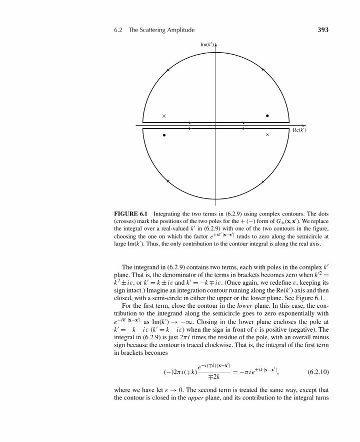
6.2 The Scattering Amplitude 393
Re(k′)
Im(k′)
FIGURE 6.1 Integrating the two terms in (6.2.9) using complex contours. The dots(crosses) mark the positions of the two poles for the + (−) form of G±(x,x′). We replacethe integral over a real-valued k′ in (6.2.9) with one of the two contours in the figure,choosing the one on which the factor e±ik′ |x−x′ | tends to zero along the semicircle atlarge Im(k′). Thus, the only contribution to the contour integral is along the real axis.
The integrand in (6.2.9) contains two terms, each with poles in the complex k′plane. That is, the denominator of the terms in brackets becomes zero when k ′2 =k2 ± iε, or k ′ = k ± iε and k ′ = −k ∓ iε. (Once again, we redefine ε, keeping itssign intact.) Imagine an integration contour running along the Re(k ′) axis and thenclosed, with a semi-circle in either the upper or the lower plane. See Figure 6.1.
For the first term, close the contour in the lower plane. In this case, the con-tribution to the integrand along the semicircle goes to zero exponentially withe−ik′ |x−x′| as Im(k ′) → −∞. Closing in the lower plane encloses the pole atk ′ = −k − iε (k ′ = k − iε) when the sign in front of ε is positive (negative). Theintegral in (6.2.9) is just 2π i times the residue of the pole, with an overall minussign because the contour is traced clockwise. That is, the integral of the first termin brackets becomes
(−)2π i (∓k)e−i(∓k) |x−x′|
∓2k= −π ie±ik |x−x′|, (6.2.10)
where we have let ε→ 0. The second term is treated the same way, except thatthe contour is closed in the upper plane, and its contribution to the integral turns
394 Chapter 6 Scattering Theory
out to be the same as the first term. We therefore get our final result, namely
G±(x,x′) = − 1
4π
e±ik|x−x′ |
|x − x′| . (6.2.11)
The reader may recognize that G ± is nothing more than Green’s function for theHelmholtz equation,
(∇2 + k2)G ± (x,x′) = δ(3)(x − x′). (6.2.12)
That is, for x �= x′, G±(x,x′) solves the eigenvalue equation H0G± = EG±.We can now rewrite (6.2.2) in a more explicit form, using (6.2.11), namely
〈x|ψ (±)〉 = 〈x|i〉− 2m
h2
∫d3x ′ e± ik |x−x′ |
4π |x − x′| 〈x′|V |ψ (±)〉. (6.2.13)
Notice that the wave function 〈x|ψ (± )〉 in the presence of the scatterer is writ-ten as the sum of the wave function for the incident wave 〈x|i〉 and a term thatrepresents the effect of scattering. As we will see explicitly later, at sufficientlylarge distances r , the spatial dependence of the second term is e± ik r/r , providedthat the potential is of finite range. This means that the positive solution (negativesolution) corresponds to the plane wave plus an outgoing (incoming) sphericalwave. This is in keeping with the origin of the sign in terms of scattering forward(backward) in time. In most physical problems we are interested in the positive so-lution because it is difficult to prepare a system satisfying the boundary conditionappropriate for the negative solution.
To see the behavior of 〈x|ψ (± )〉 more explicitly, let us consider the spe-cific case where V is a local potential—that is, a potential diagonal in the x-representation. Potentials that are functions only of the position operator x belongto this category. In precise terms, V is said to be local if it can be written as
〈x′|V |x′′〉 = V (x′)δ(3)(x′ − x′′). (6.2.14)
As a result, we obtain
〈x′|V |ψ (± )〉 =∫
d3x ′′〈x′|V |x′′〉〈x′′|ψ (± )〉 = V (x′)〈x′|ψ (± )〉. (6.2.15)
The integral equation (6.2.13) now simplifies as
〈x|ψ (± )〉 = 〈x|i〉− 2m
h2
∫d3x ′ e± ik |x−x′|
4π |x − x′| V (x′)〈x′|ψ (± )〉. (6.2.16)
Let us attempt to understand the physics contained in this equation. The vectorx is understood to be directed toward the observation point at which the wavefunction is evaluated. For a finite-range potential, the region that gives rise toa nonvanishing contribution is limited in space. In scattering processes we areinterested in studying the effect of the scatterer (that is, the finite-range potential)at a point far outside the range of the potential. This is quite relevant from a
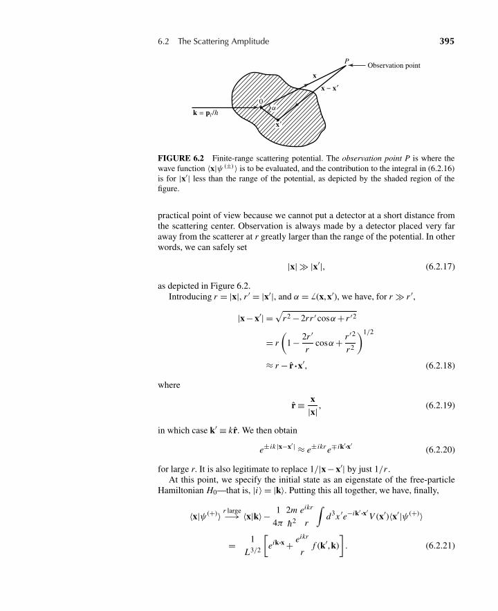
6.2 The Scattering Amplitude 395
Observation pointP
x − x′
k = pl /h
0α
x′
x
FIGURE 6.2 Finite-range scattering potential. The observation point P is where thewave function 〈x|ψ (±) 〉 is to be evaluated, and the contribution to the integral in (6.2.16)is for |x′| less than the range of the potential, as depicted by the shaded region of thefigure.
practical point of view because we cannot put a detector at a short distance fromthe scattering center. Observation is always made by a detector placed very faraway from the scatterer at r greatly larger than the range of the potential. In otherwords, we can safely set
|x| � |x′|, (6.2.17)
as depicted in Figure 6.2.Introducing r = |x|, r ′ = |x′|, and α = � (x,x′), we have, for r � r ′,
|x − x′| =√
r2 − 2rr ′ cosα+ r ′2
= r
(1 − 2r ′
rcosα+ r ′2
r2
)1/2
≈ r − r·x′, (6.2.18)
where
r ≡ x|x| , (6.2.19)
in which case k′ ≡ kr. We then obtain
e± ik |x−x′ | ≈ e± ikr e∓ ik′·x′(6.2.20)
for large r. It is also legitimate to replace 1/|x − x′| by just 1/r .At this point, we specify the initial state as an eigenstate of the free-particle
Hamiltonian H0—that is, |i〉 = |k〉. Putting this all together, we have, finally,
〈x|ψ (+)〉 r large−→ 〈x|k〉− 1
4π
2m
h2
eikr
r
∫d3x ′e−ik′·x′
V (x′)〈x′|ψ (+)〉
= 1
L3/2
[eik·x + eikr
rf (k′,k)
]. (6.2.21)
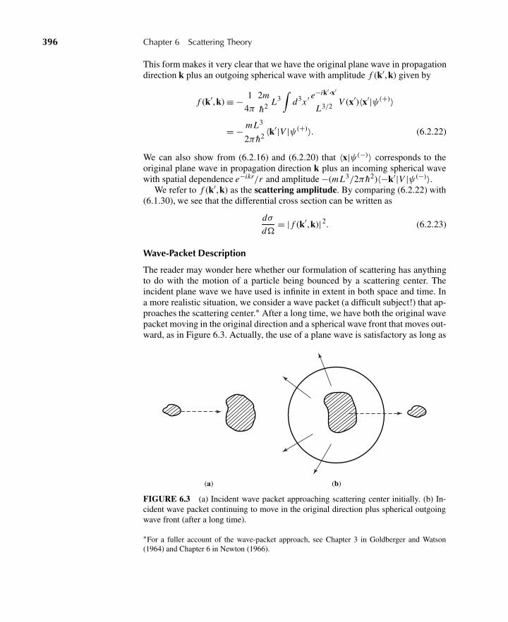
396 Chapter 6 Scattering Theory
This form makes it very clear that we have the original plane wave in propagationdirection k plus an outgoing spherical wave with amplitude f (k′,k) given by
f (k′,k) ≡ − 1
4π
2m
h2 L3∫
d3x ′ e−ik′·x′
L3/2 V (x′)〈x′|ψ (+)〉
= − mL3
2π h2 〈k′|V |ψ (+)〉. (6.2.22)
We can also show from (6.2.16) and (6.2.20) that 〈x|ψ (−)〉 corresponds to theoriginal plane wave in propagation direction k plus an incoming spherical wavewith spatial dependence e−ikr/r and amplitude −(mL3/2π h2)〈−k′|V |ψ (−)〉.
We refer to f (k′,k) as the scattering amplitude. By comparing (6.2.22) with(6.1.30), we see that the differential cross section can be written as
dσ
d�= | f (k′,k)|2. (6.2.23)
Wave-Packet Description
The reader may wonder here whether our formulation of scattering has anythingto do with the motion of a particle being bounced by a scattering center. Theincident plane wave we have used is infinite in extent in both space and time. Ina more realistic situation, we consider a wave packet (a difficult subject!) that ap-proaches the scattering center.∗ After a long time, we have both the original wavepacket moving in the original direction and a spherical wave front that moves out-ward, as in Figure 6.3. Actually, the use of a plane wave is satisfactory as long as
(a) (b)
FIGURE 6.3 (a) Incident wave packet approaching scattering center initially. (b) In-cident wave packet continuing to move in the original direction plus spherical outgoingwave front (after a long time).
∗For a fuller account of the wave-packet approach, see Chapter 3 in Goldberger and Watson(1964) and Chapter 6 in Newton (1966).
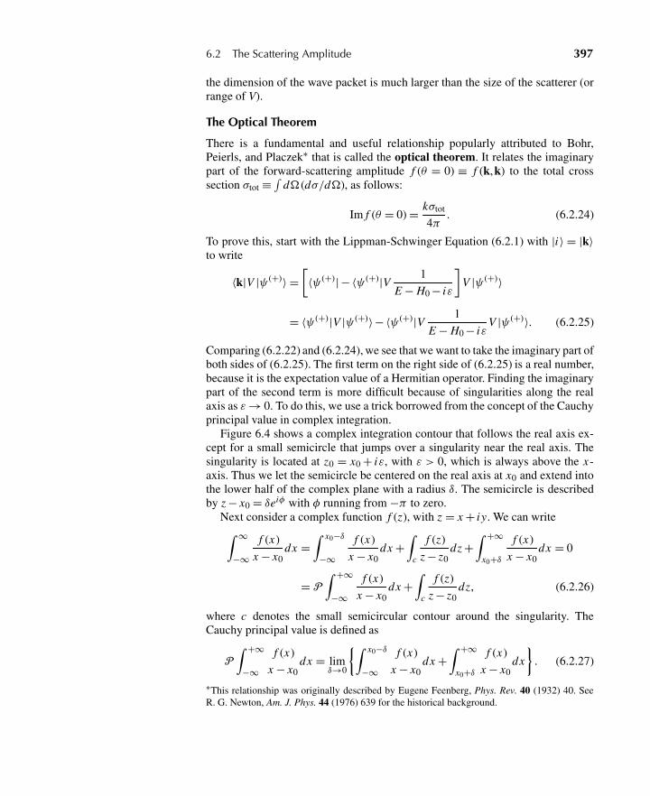
6.2 The Scattering Amplitude 397
the dimension of the wave packet is much larger than the size of the scatterer (orrange of V).
The Optical Theorem
There is a fundamental and useful relationship popularly attributed to Bohr,Peierls, and Placzek∗ that is called the optical theorem. It relates the imaginarypart of the forward-scattering amplitude f (θ = 0) ≡ f (k,k) to the total crosssection σtot ≡ ∫
d� (dσ/d�), as follows:
Im f (θ = 0) = kσtot
4π. (6.2.24)
To prove this, start with the Lippman-Schwinger Equation (6.2.1) with |i〉 = |k〉to write
〈k|V |ψ (+)〉 =[〈ψ (+)|− 〈ψ (+)|V 1
E − H0 − iε
]V |ψ (+)〉
= 〈ψ (+)|V |ψ (+)〉− 〈ψ (+)|V 1
E − H0 − iεV |ψ (+)〉. (6.2.25)
Comparing (6.2.22) and (6.2.24), we see that we want to take the imaginary part ofboth sides of (6.2.25). The first term on the right side of (6.2.25) is a real number,because it is the expectation value of a Hermitian operator. Finding the imaginarypart of the second term is more difficult because of singularities along the realaxis as ε→ 0. To do this, we use a trick borrowed from the concept of the Cauchyprincipal value in complex integration.
Figure 6.4 shows a complex integration contour that follows the real axis ex-cept for a small semicircle that jumps over a singularity near the real axis. Thesingularity is located at z0 = x0 + iε, with ε > 0, which is always above the x-axis. Thus we let the semicircle be centered on the real axis at x0 and extend intothe lower half of the complex plane with a radius δ. The semicircle is describedby z − x0 = δeiφ with φ running from −π to zero.
Next consider a complex function f (z), with z = x + iy. We can write∫ ∞
−∞f (x)
x − x0dx =
∫ x0−δ
−∞f (x)
x − x0dx +
∫c
f (z)
z − z0dz +
∫ +∞
x0+δf (x)
x − x0dx = 0
= P
∫ +∞
−∞f (x)
x − x0dx +
∫c
f (z)
z − z0dz, (6.2.26)
where c denotes the small semicircular contour around the singularity. TheCauchy principal value is defined as
P
∫ +∞
−∞f (x)
x − x0dx = lim
δ→0
{∫ x0−δ
−∞f (x)
x − x0dx +
∫ +∞
x0+δf (x)
x − x0dx
}. (6.2.27)
∗This relationship was originally described by Eugene Feenberg, Phys. Rev. 40 (1932) 40. SeeR. G. Newton, Am. J. Phys. 44 (1976) 639 for the historical background.
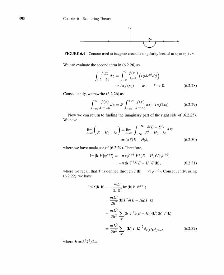
398 Chapter 6 Scattering Theory
y
x
x0
FIGURE 6.4 Contour used to integrate around a singularity located at z0 = x0 + iε.
We can evaluate the second term in (6.2.26) as∫c
f (z)
z − z0dz =
∫ 0
−πf (x0)
δeiφ
(iφδeiφdφ
)→ iπ f (x0) as δ→ 0. (6.2.28)
Consequently, we rewrite (6.2.26) as∫ ∞
−∞f (x)
x − x0dx = P
∫ +∞
−∞f (x)
x − x0dx + iπ f (x0). (6.2.29)
Now we can return to finding the imaginary part of the right side of (6.2.25).We have
limε→0
(1
E − H0 − iε
)= limε→0
∫ +∞
−∞δ(E − E ′)
E ′ − H0 − iεd E ′
= iπδ(E − H0), (6.2.30)
where we have made use of (6.2.29). Therefore,
Im〈k|V |ψ (+)〉 = −π〈ψ (+)|V δ(E − H0)V |ψ (+)〉= −π〈k|T †δ(E − H0)T |k〉, (6.2.31)
where we recall that T is defined through T |k〉 = V |ψ (+)〉. Consequently, using(6.2.22), we have
Im f (k,k) = − mL3
2π h2 Im〈k|V |ψ (+)〉
= mL3
2h2 〈k|T †δ(E − H0)T |k〉
= mL3
2h2
∑k′
〈k|T †δ(E − H0)|k′〉〈k′|T |k〉
= mL3
2h2
∑k′
∣∣〈k′|T |k〉∣∣2 δE ,h2k′2/2m , (6.2.32)
where E = h2k2/2m.
6.3 The Born Approximation 399
The optical theorem (6.2.24) now begins to appear. The factor∣∣〈k′|T |k〉∣∣2 is
proportional to the differential cross section (6.2.23). The sum, including the δfunction, is over all scattered momenta that conserve energy; in other words, itis over all directions in space. Therefore, the right-hand side of (6.2.32) is anintegral of the differential cross section over all directions and so is proportionalto the total cross section.
To carry (6.2.32) through to the end, we make use of 〈k′|T|k〉 = 〈k′|V|ψ (+)〉with (6.2.22), converting the sum to an integral as we did to go from (6.2.8) to(6.2.9). This gives
Im f (k,k) = mL3
2h2
(2π h2
mL3
)2∑k′
∣∣ f (k′,k)∣∣2 δE ,h2k′2/2m
−→ 2π2h2
m(2π)3
∫d3k ′ ∣∣ f (k′,k)
∣∣2 δ(E − h2k′2
2m
)
= h2
4πm
1
h2k/mk2∫
d�k′dσ
d�k′
= k
4πσtot, (6.2.33)
thus proving (6.2.24).Section 6.5 will provide some insights into the physical significance of the
optical theorem.
6.3 THE BORN APPROXIMATION
Our task now is to calculate the scattering amplitude f (k′,k) for some givenpotential-energy function V (x). This amounts to calculating the matrix element
〈k′|V |ψ (+)〉 = 〈k′|T |k〉. (6.3.1)
This task is not straightforward, however, since we do not have closed analyticexpressions for either 〈x′|ψ (+)〉 or T . Consequently, one typically resorts to ap-proximations at this point.
We have already alluded to a useful approximation scheme in (6.1.32). Againreplacing hε with ε, this is
T = V + V1
E − H0 + iεV + V
1
E − H0 + iεV
1
E − H0 + iεV +·· · , (6.3.2)
which is an expansion in powers of V . We will shortly examine the conditionsunder which truncations of this expansion should be valid. First, however, we willmake use of this scheme and see where it leads us.
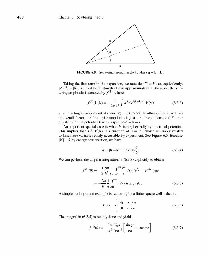
400 Chapter 6 Scattering Theory
k
k′q
θ
FIGURE 6.5 Scattering through angle θ , where q = k− k′.
Taking the first term in the expansion, we note that T = V , or, equivalently,|ψ (+)〉 = |k〉, is called the first-order Born approximation. In this case, the scat-tering amplitude is denoted by f (1), where
f (1)(k′,k) = − m
2π h2
∫d3x ′ei(k−k′)·x′
V (x′) (6.3.3)
after inserting a complete set of states |x′〉 into (6.2.22). In other words, apart froman overall factor, the first-order amplitude is just the three-dimensional Fouriertransform of the potential V with respect to q ≡ k− k′.
An important special case is when V is a spherically symmetrical potential.This implies that f (1)(k′,k) is a function of q ≡ |q|, which is simply relatedto kinematic variables easily accessible by experiment. See Figure 6.5. Because|k′| = k by energy conservation, we have
q = |k− k′| = 2k sinθ
2. (6.3.4)
We can perform the angular integration in (6.3.3) explicitly to obtain
f (1)(θ ) = −1
2
2m
h2
1
iq
∫ ∞
0
r2
rV (r )(eiqr − e−iqr )dr
= −2m
h2
1
q
∫ ∞
0r V (r )sin qr dr . (6.3.5)
A simple but important example is scattering by a finite square well—that is,
V (r ) ={
V0 r ≤ a
0 r > a.(6.3.6)
The integral in (6.3.5) is readily done and yields
f (1)(θ ) = −2m
h2
V0a3
(qa)2
[sinqa
qa− cosqa
]. (6.3.7)
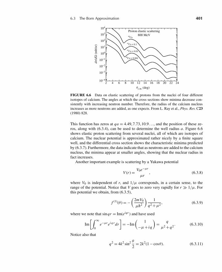
6.3 The Born Approximation 401
Proton elastic scattering800 MeV48Ca
44Ca × 0.1
42Ca × 0.01
40Ca × 0.001
10−4
10−3
10−2
10−1
100
101
102
103
104
dσ/d
(
mb/
sr)
2 4 6 8 10 12 14 16 18 20 22 24
θc.m. (deg)
FIGURE 6.6 Data on elastic scattering of protons from the nuclei of four differentisotopes of calcium. The angles at which the cross sections show minima decrease con-sistently with increasing neutron number. Therefore, the radius of the calcium nucleusincreases as more neutrons are added, as one expects. From L. Ray et al., Phys. Rev. C23(1980) 828.
This function has zeros at qa = 4.49,7.73,10.9 . . ., and the position of these ze-ros, along with (6.3.4), can be used to determine the well radius a. Figure 6.6shows elastic proton scattering from several nuclei, all of which are isotopes ofcalcium. The nuclear potential is approximated rather nicely by a finite squarewell, and the differential cross section shows the characteristic minima predictedby (6.3.7). Furthermore, the data indicate that as neutrons are added to the calciumnucleus, the minima appear at smaller angles, showing that the nuclear radius infact increases.
Another important example is scattering by a Yukawa potential
V (r ) = V0e−μr
μr, (6.3.8)
where V0 is independent of r, and 1/μ corresponds, in a certain sense, to therange of the potential. Notice that V goes to zero very rapidly for r � 1/μ. Forthis potential we obtain, from (6.3.5),
f (1)(θ ) = −(
2mV0
μh2
)1
q2 +μ2 , (6.3.9)
where we note that sinqr = Im(eiqr ) and have used
Im
[∫ ∞
0e−μr ei q r dr
]= −Im
(1
−μ+ iq
)= q
μ2 + q2. (6.3.10)
Notice also that
q2 = 4k2 sin2 θ
2= 2k2(1 − cosθ ). (6.3.11)
402 Chapter 6 Scattering Theory
Thus, in the first Born approximation, the differential cross section for scatteringby a Yukawa potential is given by
(dσ
d�
)�(
2mV0
μh2
)2 1[2k2(1 − cosθ ) +μ2
]2 . (6.3.12)
It is amusing to observe here that as μ→ 0, the Yukawa potential is reducedto the Coulomb potential, provided that the ratio V0/μ is fixed—for example, tobe ZZ′e2—in the limiting process. We see that the first Born differential crosssection obtained in this manner becomes(
dσ
d�
)� (2m)2(ZZ′e2)2
h4
1
16k4 sin4(θ/2). (6.3.13)
Even the h disappears if hk is identified as |p|, so
(dσ
d�
)= 1
16
(ZZ′e2
EK E
)21
sin4(θ/2), (6.3.14)
where EK E = |p|2/2m; this is precisely the Rutherford scattering cross sectionthat can be obtained classically.
Coming back to (6.3.5), the Born amplitude with a spherically symmetricalpotential, there are several general remarks we can make if f (k′,k) can be ap-proximated by the corresponding first Born amplitude, f (1):
1. dσ/d�, or f (θ ), is a function of q only; that is, f (θ ) depends on the energy(h2k2/2m) and θ only through the combination 2k2(1 − cosθ ).
2. f (θ ) is always real.
3. dσ/d� is independent of the sign of V.
4. For small k (q necessarily small),
f (1)(θ ) = − 1
4π
2m
h2
∫V (r )d3x ,
involving a volume integral independent of θ .
5. f (θ ) is small for large q because of rapid oscillation of the integrand.
In order to study the conditions under which the Born approximation shouldbe valid, let us return to (6.2.16), slightly rewritten as
〈x|ψ (+)〉 = 〈x|k〉− 2m
h2
∫d3x ′ eik |x−x′|
4π |x − x′|V (x′)〈x′|ψ (+)〉.
6.3 The Born Approximation 403
The approximation is that T ≈ V , which means that |ψ (+)〉 can be replaced by|k〉. Therefore, the second term on the right-hand side in this equation must bemuch smaller than the first. Let us assume that a “typical” value for the potentialenergy V (x) is V0 and that it acts within some “range” a. Writing r ′ = |x − x′|and carrying out a rough approximation on the integral, we find that our validitycondition becomes ∣∣∣∣∣2m
h2
(4π
3a3)
eikr ′
4πaV0
eik·x′
L3/2
∣∣∣∣∣�∣∣∣∣∣ eik·x
L3/2
∣∣∣∣∣ .Now for low energies (ka � 1), the exponential factors can be replaced by unity.Then, if we ignore numerical factors of order unity, the following succinct crite-rion emerges:
m|V0|a2
h2� 1. (6.3.15)
Consider the special case of the Yukawa potential in (6.3.8), in which the rangea = 1/μ. The validity criterion becomes m|V0|/h2μ2 � 1. This requirement maybe compared with the condition for the Yukawa potential to develop a bound state,which we can show to be 2m|V0|/h2μ2 ≥ 2.7, with V0 negative. In other words,if the potential is strong enough to develop a bound state, the Born approximationwill probably give a misleading result.
At high energies (ka � 1), the factors eikr ′and eik·x′
oscillate strongly overthe region of integration, so they cannot be set equal to unity. Instead, it can beshown that
2m
h2
|V0|ak
ln(ka) � 1. (6.3.16)
As k becomes larger, this inequality is more easily satisfied. Quite generally, theBorn approximation tends to get better at higher energies.
The Higher-Order Born Approximation
Now, write T to second order in V , using (6.3.2), namely
T = V + V1
E − H0 + iεV .
It is natural to continue our Born approximation approach and write
f (k′,k) ≈ f (1)(k′,k) + f (2)(k′,k),
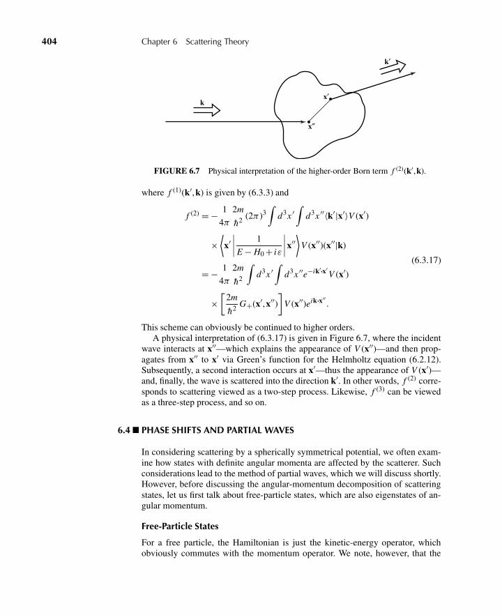
404 Chapter 6 Scattering Theory
k′
x′
x′′
k
FIGURE 6.7 Physical interpretation of the higher-order Born term f (2)(k′,k).
where f (1)(k′,k) is given by (6.3.3) and
f (2) = − 1
4π
2m
h2 (2π)3∫
d3x ′∫
d3x ′′〈k′|x′〉V (x′)
×⟨x′∣∣∣∣ 1
E − H0 + iε
∣∣∣∣x′′⟩
V (x′′)(x′′|k)
= − 1
4π
2m
h2
∫d3x ′
∫d3x ′′e−ik′·x′
V (x′)
×[
2m
h2G+(x′,x′′)
]V (x′′)eik·x′′
.
(6.3.17)
This scheme can obviously be continued to higher orders.A physical interpretation of (6.3.17) is given in Figure 6.7, where the incident
wave interacts at x′′—which explains the appearance of V (x′′)—and then prop-agates from x′′ to x′ via Green’s function for the Helmholtz equation (6.2.12).Subsequently, a second interaction occurs at x′—thus the appearance of V (x′)—and, finally, the wave is scattered into the direction k′. In other words, f (2) corre-sponds to scattering viewed as a two-step process. Likewise, f (3) can be viewedas a three-step process, and so on.
6.4 PHASE SHIFTS AND PARTIAL WAVES
In considering scattering by a spherically symmetrical potential, we often exam-ine how states with definite angular momenta are affected by the scatterer. Suchconsiderations lead to the method of partial waves, which we will discuss shortly.However, before discussing the angular-momentum decomposition of scatteringstates, let us first talk about free-particle states, which are also eigenstates of an-gular momentum.
Free-Particle States
For a free particle, the Hamiltonian is just the kinetic-energy operator, whichobviously commutes with the momentum operator. We note, however, that the
6.4 Phase Shifts and Partial Waves 405
free-particle Hamiltonian also commutes with L2 and Lz . Thus it is possible toconsider a simultaneous eigenket of H0,L2, and Lz . Ignoring spin, such a state isdenoted by |E , l,m〉 and is often called a spherical-wave state.
More generally, the most general free-particle state can be regarded as a super-position of |E , l,m〉 with various E, l, and m in much the same way as the mostgeneral free-particle state can be regarded as a superposition of |k〉 with differentk, different in both magnitude and direction. Put in another way, a free-particlestate can be analyzed using either the plane-wave basis {|k〉} or the spherical-wavebasis {|E , l,m〉}.
We now derive the transformation function 〈k|E , l,m〉 that connects the plane-wave basis with the spherical-wave basis. We can also regard this quantity asthe momentum-space wave function for the spherical wave characterized by E, l,and m. We adopt the normalization convention for the spherical-wave eigenket asfollows:
〈E ′, l ′,m′|E , l,m〉 = δll′δmm′δ(E − E ′). (6.4.1)
In analogy with the position-space wave function, we may guess the angulardependence:
〈k|E , l,m〉 = glE (k)Y ml (k), (6.4.2)
where the function glE (k) will be considered later. To prove this rigorously, weproceed as follows. First, consider the momentum eigenket |kz〉—that is, a plane-wave state whose propagation direction is along the positive z-axis. An importantproperty of this state is that it has no orbital angular-momentum component in thez-direction:
Lz |kz〉 = (x py − ypx)|kx = 0,ky = 0,kz = k〉 = 0. (6.4.3)
Actually this is plausible from classical considerations: The angular-momentumcomponent must vanish in the direction of propagation because L ·p = (x × p) ·p = 0. Because of (6.4.3)—and since 〈E ′, l ′,m′|kz〉 = 0 for m′ �= 0—we must beable to expand |kz〉 as follows:
|kz〉 =∑
l′
∫d E ′|E ′, l ′,m′ = 0〉〈E ′, l ′,m′ = 0|kz〉. (6.4.4)
Notice that there is no m′ sum; m′ is always zero. We can obtain the most generalmomentum eigenket, with the direction of k specified by θ and φ, from |kz〉 by justapplying the appropriate rotation operator as follows [see Figure 3.3 and (3.6.47)]:
|k〉 = D(α = φ,β = θ ,γ = 0)|kz〉. (6.4.5)
406 Chapter 6 Scattering Theory
Multiplying this equation by 〈E , l,m| on the left, we obtain
〈E , l,m|k〉 =∑
l′
∫d E ′〈E , l,m|D(α = φ,β = θ ,γ = 0)|E ′, l ′,m′ = 0〉
× 〈E ′, l ′,m′ = 0|kz〉=∑
l′
∫d E ′D (l′)
m0 (α = φ,β = θ ,γ = 0)
× δll′δ(E − E ′)〈E ′, l ′,m′ = 0|kz〉= D (l)
m0(α = φ,β = θ ,γ = 0)〈E , l,m = 0|kz〉.
(6.4.6)
Now 〈E , l,m = 0|kz〉 is independent of the orientation of k—that is, independent
of θ and φ—and we may as well call it√
2l+14π g∗
lE (k). So we can write, using(3.6.51),
〈k|E , l,m〉 = glE (k) Y ml (k). (6.4.7)
Let us determine glE (k). First, we note that
(H0 − E)|E , l,m〉 = 0. (6.4.8)
But we also let H0 − E operate on a momentum eigenbra 〈k| as follows:
〈k|(H0 − E) =(
h2k2
2m− E
)〈k|. (6.4.9)
Multiplying (6.4.9) with |E , l,m〉 on the right, we obtain
(h2k2
2m− E
)〈k|E , l,m〉 = 0. (6.4.10)
This means that 〈k|E , l,m〉 can be nonvanishing only if E = h2k2/2m, so we mustbe able to write glE (k) as
glE (k) = Nδ
(h2k2
2m− E
). (6.4.11)
6.4 Phase Shifts and Partial Waves 407
To determine N we go back to our normalization convention (6.4.1). We obtain
〈E ′, l ′m′|E , l,m〉 =∫
d3k ′′〈E ′, l ′,m′|k′′〉〈k′′|E , l,m〉
=∫
k ′′2dk ′′∫
d�k′′ |N |2δ(
h2k ′′2
2m− E ′
)
× δ(
h2k ′′2
2m− E
)Y m′∗
l′ (k′′)Y ml (k′′)
=∫
k′′2d E ′′
d E ′′/dk ′′
∫d�k′′ |N |2δ
(h2k ′′2
2m− E ′
)δ
(h2k ′′2
2m− E
)× Y m′∗
l′ (k′′)Y ml (k′′)
= |N |2 mk ′
h2 δ(E − E ′)δll′δmm′ ,
(6.4.12)
where we have defined E ′′ = h2k ′′2/2m to change k′′-integration into E ′′-integration. Comparing this with (6.4.1), we see that N = h/
√mk will suffice.
Therefore, we can finally write
glE (k) = h√mkδ
(h2k2
2m− E
); (6.4.13)
hence
〈k|E , l,m〉 = h√mkδ
(h2k2
2m− E
)Y m
l (k). (6.4.14)
From (6.4.14) we infer that the plane-wave state |k〉 can be expressed as a super-position of free spherical-wave states with all possible l-values; in particular,
|k〉 =∑
l
∑m
∫d E |E , l,m〉〈E , l,m|k〉
=∞∑
l=0
l∑m=−1
|E , l,m〉∣∣∣∣∣∣E=h2k2/2m
(h√mk
Y m∗l (k)
).
(6.4.15)
Because the transverse dimension of the plane wave is infinite, we expect that theplane wave must contain all possible values of impact parameter b (semiclassi-cally, the impact parameter b � lh/p). From this point of view it is no surprisethat the momentum eigenstates |k〉, when analyzed in terms of spherical-wavestates, contain all possible values of l.
We have derived the wave function for |E , l,m〉 in momentum space. Next, weconsider the corresponding wave function in position space. From wave mechan-ics, the reader should be familiar with the fact that the wave function for a free
408 Chapter 6 Scattering Theory
spherical wave is jl(kr )Y ml (r), where jl(kr ) is the spherical Bessel function of or-
der l [see (3.7.20a) and also Appendix B]. The second solution nl (kr ), although itsatisfies the appropriate differential equation, is inadmissible because it is singularat the origin. Thus we can write
〈x|E , l,m〉 = cl jl(kr )Y ml (r). (6.4.16)
To determine cl , all we have to do is compare
〈x|k〉 = eik·x
(2π)3/2 =∑
l
∑m
∫d E〈x|E , l,m〉〈E , l,m|k〉
=∑
l
∑m
∫d E cl jl(kr )Y m
l (r)h√mkδ
(E − h2k2
2m
)Y m∗
l (k)
=∑
l
(2l + 1)
4πPl (k ·r)
h√mk
cl jl(kr ),
(6.4.17)
where we have used the addition theorem
�mY ml (r)Y m∗
l (k) = [(2l + 1)/4π]Pl(k · r)
in the last step. Now 〈x|k〉 = eik·x/(2π)3/2 can also be written as
eik·x
(2π)3/2 = 1
(2π)3/2
∑l
(2l + 1)i l jl(kr )Pl(k · r), (6.4.18)
which can be proved by using the following integral representation for jl(kr ):
jl(kr ) = 1
2i l
∫ +1
−1eikr cosθ Pl (cosθ )d(cosθ ). (6.4.19)
Comparing (6.4.17) with (6.4.18), we have
cl = i l
h
√2mk
π. (6.4.20)
To summarize, we have
〈k|E , l,m〉 = h√mkδ
(E − h2k2
2m
)Y m
l (k) (6.4.21a)
〈x|E , l,m〉 = i l
h
√2mk
πjl(kr )Y m
l (r). (6.4.21b)
These expressions are extremely useful in developing the partial-wave expansion.We conclude this section by applying (6.4.21a) to a decay process. Suppose a
parent particle of spin j disintegrates into two spin-zero particles: A (spin j ) →
6.4 Phase Shifts and Partial Waves 409
B (spin 0) + C (spin 0). The basic Hamiltonian responsible for such a decay pro-cess is, in general, very complicated. However, we do know that angular momen-tum is conserved because the basic Hamiltonian must be rotationally invariant.So the momentum-space wave function for the final state must be of the form(6.4.21a), with l identified with the spin of the parent particle. This immediatelyenables us to compute the angular distribution of the decay product, because themomentum-space wave function is nothing more than the probability amplitudefor finding the decay product with relative momentum direction k.
As a concrete example from nuclear physics, let us consider the decay of anexcited nucleus, Ne20∗:
Ne20∗ → O16 + He4. (6.4.22)
Both O16 and He4 are known to be spinless particles. Suppose the magneticquantum number of the parent nucleus is ±1, relative to some direction z. Thenthe angular distribution of the decay product is proportional to |Y ±1
1 (θ ,φ)|2 =(3/8π)sin2 θ , where (θ ,φ) are the polar angles defining the relative directionk of the decay product. On the other hand, if the magnetic quantum numberis 0 for a parent nucleus with spin 1, the decay angular distribution varies as|Y 0
1 (θ ,φ)|2 = (3/4π)cos2 θ .For a general spin orientation we obtain
1∑m=−l
w(m)|Y ml=1|2. (6.4.23)
For an unpolarized nucleus the various w(m) are all equal, and we obtain anisotropic distribution; this is not surprising because there is no preferred direc-tion if the parent particle is unpolarized.
For a higher-spin object, the angular distribution of the decay is more involved;the higher the spin of the parent decaying system, the greater the complexity ofthe angular distribution of the decay products. Quite generally, through a study ofthe angular distribution of the decay products, it is possible to determine the spinof the parent nucleus.
Partial-Wave Expansion
Let us now come back to the case V �= 0. We assume that the potential is spher-ically symmetrical—that is, invariant under rotations in three dimensions. It thenfollows that the transition operator T, which is given by (6.3.2), commutes withL2 and L. In other words, T is a scalar operator.
It is now useful to use the spherical-wave basis because the Wigner-Eckarttheorem [see (3.11.38)], applied to a scalar operator, immediately gives
〈E ′, l ′,m′|T |E , l,m〉 = Tl(E)δll′δmm′ . (6.4.24)
In other words, T is diagonal both in l and in m; furthermore, the (nonvanishing)diagonal element depends on E and l but not on m. This leads to an enormoussimplification, as we will see shortly.
410 Chapter 6 Scattering Theory
Let us now look at the scattering amplitude (6.2.22):
f (k′,k) = − 1
4π
2m
h2 L3〈k′|T |k〉
−→ − 1
4π
2m
h2(2π)3
∑l
∑m
∑l′
∑m′
∫d E
∫d E ′〈k′|E ′l ′m′〉
×〈E ′l ′m′|T |Elm〉〈Elm|k〉
= − 1
4π
2m
h2 (2π)3 h2
mk
∑l
∑m
Tl(E)
∣∣∣∣∣E=h2k2/2m
Y ml (k′)Y m∗
l (k)
= −4π2
k
∑l
∑m
Tl (E)
∣∣∣∣∣E=h2k2/2m
Y ml (k′)Y m∗
l (k). (6.4.25)
To obtain the angular dependence of the scattering amplitude, let us choose thecoordinate system in such a way that k, as usual, is in the positive z-direction. Wethen have [see (3.6.50)]
Y ml (k) =
√2l + 1
4πδm0, (6.4.26)
where we have used Pl (1) = 1; hence only the terms m = 0 contribute. Taking θto be the angle between k′ and k, we can write
Y 0l (k′) =
√2l + 1
4πPl (cosθ ). (6.4.27)
It is customary here to define the partial-wave amplitude fl (k) as follows:
fl (k) ≡ −πTl(E)
k. (6.4.28)
For (6.4.25) we then have
f (k′,k) = f (θ ) =∞∑
l=0
(2l + 1) fl(k)Pl (cosθ ), (6.4.29)
where f (θ ) still depends on k (or the incident energy) even though k is suppressed.To appreciate the physical significance of fl (k), let us study the large-distance
behavior of the wave function 〈x|ψ (+)〉 given by (6.2.21). Using the expansion ofa plane wave in terms of spherical waves [(6.4.18)] and noting that (Appendix B)
jl(kr )larger−→ ei(kr−(lπ/2)) − e−i(kr−(lπ/2))
2ikr, (i l = ei(π/2)l ) (6.4.30)
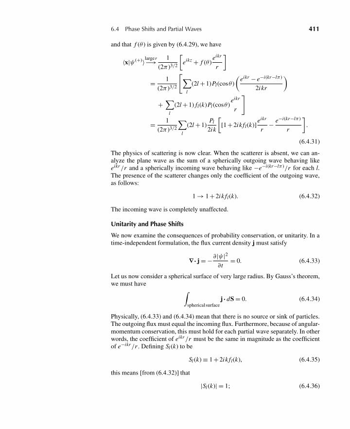
6.4 Phase Shifts and Partial Waves 411
and that f (θ ) is given by (6.4.29), we have
〈x|ψ (+)〉larger−→ 1
(2π)3/2
[eikz + f (θ )
eikr
r
]
= 1
(2π)3/2
[∑l
(2l + 1)Pl(cosθ )
(eikr − e−i(kr−lπ)
2ikr
)
+∑
l
(2l + 1) fl(k)Pl (cosθ )eikr
r
]
= 1
(2π)3/2
∑l
(2l + 1)Pl
2ik
[[1 + 2ik fl(k)]
eikr
r− e−i(kr−lπ)
r
].
(6.4.31)
The physics of scattering is now clear. When the scatterer is absent, we can an-alyze the plane wave as the sum of a spherically outgoing wave behaving likeeikr/r and a spherically incoming wave behaving like −e−i(kr−lπ)/r for each l.The presence of the scatterer changes only the coefficient of the outgoing wave,as follows:
1 → 1 + 2ik fl(k). (6.4.32)
The incoming wave is completely unaffected.
Unitarity and Phase Shifts
We now examine the consequences of probability conservation, or unitarity. In atime-independent formulation, the flux current density j must satisfy
∇· j = −∂|ψ|2∂ t
= 0. (6.4.33)
Let us now consider a spherical surface of very large radius. By Gauss’s theorem,we must have ∫
spherical surfacej · dS = 0. (6.4.34)
Physically, (6.4.33) and (6.4.34) mean that there is no source or sink of particles.The outgoing flux must equal the incoming flux. Furthermore, because of angular-momentum conservation, this must hold for each partial wave separately. In otherwords, the coefficient of eikr/r must be the same in magnitude as the coefficientof e−ikr/r . Defining Sl (k) to be
Sl (k) ≡ 1 + 2ik fl(k), (6.4.35)
this means [from (6.4.32)] that
|Sl (k)| = 1; (6.4.36)
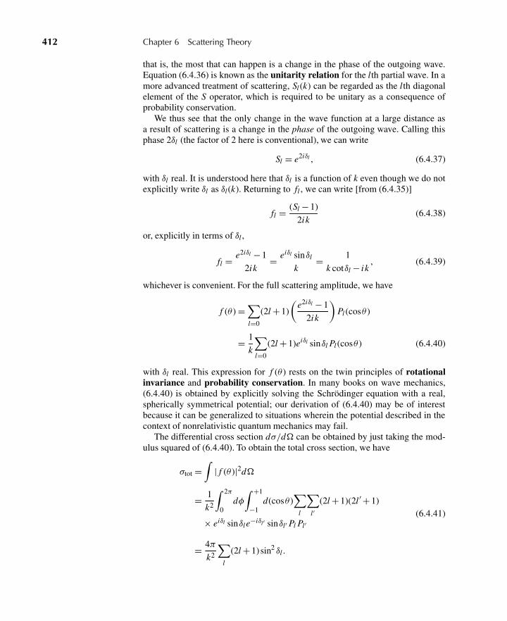
412 Chapter 6 Scattering Theory
that is, the most that can happen is a change in the phase of the outgoing wave.Equation (6.4.36) is known as the unitarity relation for the lth partial wave. In amore advanced treatment of scattering, Sl (k) can be regarded as the lth diagonalelement of the S operator, which is required to be unitary as a consequence ofprobability conservation.
We thus see that the only change in the wave function at a large distance asa result of scattering is a change in the phase of the outgoing wave. Calling thisphase 2δl (the factor of 2 here is conventional), we can write
Sl = e2iδl , (6.4.37)
with δl real. It is understood here that δl is a function of k even though we do notexplicitly write δl as δl(k). Returning to fl , we can write [from (6.4.35)]
fl = (Sl − 1)
2ik(6.4.38)
or, explicitly in terms of δl ,
fl = e2iδl − 1
2ik= eiδl sinδl
k= 1
k cotδl − ik, (6.4.39)
whichever is convenient. For the full scattering amplitude, we have
f (θ ) =∑l=0
(2l + 1)
(e2iδl − 1
2ik
)Pl (cosθ )
= 1
k
∑l=0
(2l + 1)eiδl sinδl Pl (cosθ ) (6.4.40)
with δl real. This expression for f (θ ) rests on the twin principles of rotationalinvariance and probability conservation. In many books on wave mechanics,(6.4.40) is obtained by explicitly solving the Schrödinger equation with a real,spherically symmetrical potential; our derivation of (6.4.40) may be of interestbecause it can be generalized to situations wherein the potential described in thecontext of nonrelativistic quantum mechanics may fail.
The differential cross section dσ/d� can be obtained by just taking the mod-ulus squared of (6.4.40). To obtain the total cross section, we have
σtot =∫
| f (θ )|2d�
= 1
k2
∫ 2π
0dφ∫ +1
−1d(cosθ )
∑l
∑l′
(2l + 1)(2l ′ + 1)
× eiδl sinδle−iδl′ sinδl′ Pl Pl′
= 4π
k2
∑l
(2l + 1)sin2 δl .
(6.4.41)
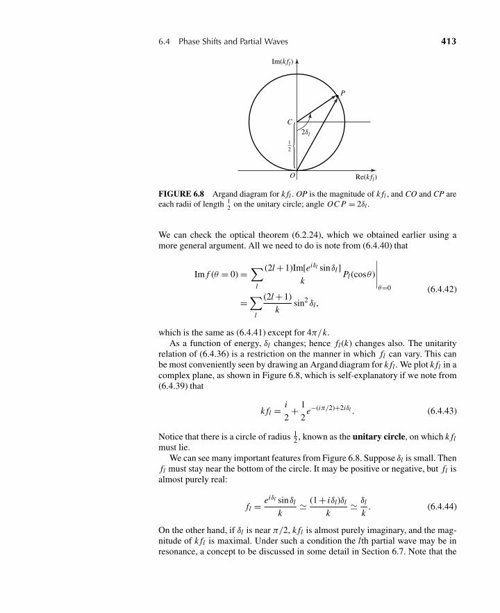
6.4 Phase Shifts and Partial Waves 413
2δl
C
O
P
Im(k fl)
Re(k fl)
12
FIGURE 6.8 Argand diagram for k fl . OP is the magnitude of k fl , and CO and CP areeach radii of length 1
2 on the unitary circle; angle OC P = 2δl .
We can check the optical theorem (6.2.24), which we obtained earlier using amore general argument. All we need to do is note from (6.4.40) that
Im f (θ = 0) =∑
l
(2l + 1)Im[eiδl sinδl ]
kPl (cosθ )
∣∣∣∣∣θ=0
=∑
l
(2l + 1)
ksin2 δl ,
(6.4.42)
which is the same as (6.4.41) except for 4π/k.As a function of energy, δl changes; hence fl (k) changes also. The unitarity
relation of (6.4.36) is a restriction on the manner in which fl can vary. This canbe most conveniently seen by drawing an Argand diagram for k fl . We plot k fl in acomplex plane, as shown in Figure 6.8, which is self-explanatory if we note from(6.4.39) that
k fl = i
2+ 1
2e−(iπ/2)+2iδl . (6.4.43)
Notice that there is a circle of radius 12 , known as the unitary circle, on which k fl
must lie.We can see many important features from Figure 6.8. Suppose δl is small. Then
fl must stay near the bottom of the circle. It may be positive or negative, but fl isalmost purely real:
fl = eiδl sinδlk
� (1 + iδl)δlk
� δl
k. (6.4.44)
On the other hand, if δl is near π/2, k fl is almost purely imaginary, and the mag-nitude of k fl is maximal. Under such a condition the lth partial wave may be inresonance, a concept to be discussed in some detail in Section 6.7. Note that the
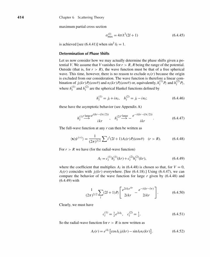
414 Chapter 6 Scattering Theory
maximum partial cross section
σ (l)max = 4πλ2(2l + 1) (6.4.45)
is achieved [see (6.4.41)] when sin2 δl = 1.
Determination of Phase Shifts
Let us now consider how we may actually determine the phase shifts given a po-tential V. We assume that V vanishes for r > R, R being the range of the potential.Outside (that is, for r > R), the wave function must be that of a free sphericalwave. This time, however, there is no reason to exclude nl (r ) because the originis excluded from our consideration. The wave function is therefore a linear com-bination of jl(kr )Pl(cosθ ) and nl (kr )Pl(cosθ ) or, equivalently, h(1)
l Pl and h(2)l Pl ,
where h(1)l and h(2)
l are the spherical Hankel functions defined by
h(1)l = jl + inl , h(2)
l = jl − inl ; (6.4.46)
these have the asymptotic behavior (see Appendix A)
h(1)l
r large−→ ei(kr−(lπ/2))
ikr, h(2)
lr large−→ − e−i(kr−(lπ/2))
ikr. (6.4.47)
The full-wave function at any r can then be written as
〈x|ψ (+)〉 = 1
(2π)3/2
∑i l (2l + 1)Al(r )Pl(cosθ ) (r > R). (6.4.48)
For r > R we have (for the radial-wave function)
Al = c(1)l h(1)
l (kr ) + c(2)l h(2)
l (kr ), (6.4.49)
where the coefficient that multiplies Al in (6.4.48) is chosen so that, for V = 0,Al(r ) coincides with jl(kr ) everywhere. [See (6.4.18).] Using (6.4.47), we cancompare the behavior of the wave function for large r given by (6.4.48) and(6.4.49) with
1
(2π)3/2
∑l
(2l + 1)Pl
[e2iδl eikr
2ikr− e−i(kr−lπ)
2ikr
]. (6.4.50)
Clearly, we must have
c(1)l = 1
2 e2iδl , c(2)l = 1
2 . (6.4.51)
So the radial-wave function for r > R is now written as
Al (r ) = eiδl[cosδl jl(kr ) − sinδlnl (kr )
]. (6.4.52)
6.4 Phase Shifts and Partial Waves 415
Using this, we can evaluate the logarithmic derivative at r = R—that is, just out-side the range of the potential—as follows:
βl ≡(
r
Al
d Al
dr
)r=R
= k R
[j ′l (k R)cosδl − n′
l (k R)sinδljl(k R)cosδl − nl (k R)sinδl
],
(6.4.53)
where j ′l (k R) stands for the derivative of jl with respect to kr evaluated at kr =
k R. Conversely, knowing the logarithmic derivative at R, we can obtain the phaseshift as follows:
tanδl = k R j ′l (k R) −βl jl(k R)
k Rn′l (k R) −βlnl (k R)
. (6.4.54)
The problem of determining the phase shift is thus reduced to that of obtaining βl .We now look at the solution to the Schrödinger equation for r < R—that is,
inside the range of the potential. For a spherically symmetrical potential, we cansolve the Schrödinger equation in three dimensions by looking at the equivalentone-dimensional equation
d2ul
dr2 +(
k2 − 2m
h2 V − l(l + 1)
r2
)ul = 0, (6.4.55)
where
ul = r Al(r ) (6.4.56)
subject to the boundary condition
ul |r=0 = 0. (6.4.57)
We integrate this one-dimensional Schrödinger equation—if necessary, numer-ically—up to r = R, starting at r = 0. In this way we obtain the logarithmicderivative at R. By continuity we must be able to match the logarithmic derivativefor the inside and outside solutions at r = R:
βl |insidesolution = βl |outsidesolution, (6.4.58)
where the left-hand side is obtained by integrating the Schrödinger equation upto r = R, and the right-hand side is expressible in terms of the phase shifts thatcharacterize the large-distance behavior of the wave function. This means that thephase shifts are obtained simply by substituting βl for the inside solution intotanδl [(6.4.54)]. For an alternative approach, it is possible to derive an integralequation for Al(r ), from which we can obtain phase shifts (see Problem 6.9 ofthis chapter).
416 Chapter 6 Scattering Theory
Hard-Sphere Scattering
Let us work out a specific example. We consider scattering by a hard, or rigid,sphere
V ={∞ for r < R
0 for r > R.(6.4.59)
In this problem we need not even evaluate βl (which is actually ∞). All we needto know is that the wave function must vanish at r = R because the sphere isimpenetrable. Therefore,
Al(r )|r=R = 0 (6.4.60)
or, from (6.4.52),
jl(k R)cosδl − nl(k R)sinδl = 0 (6.4.61)
or
tanδl = jl(k R)
nl (k R). (6.4.62)
Thus the phase shifts are now known for any l. Notice that no approximationshave been made so far.
To appreciate the physical significance of the phase shifts, let us consider thel = 0 case (S-wave scattering) specifically. Equation (6.4.62) becomes, for l = 0,
tanδ0 = sink R/k R
−cosk R/k R= − tank R, (6.4.63)
or δ0 = −k R. The radial-wave function (6.4.52) with eiδ0 omitted varies as
Al=0(r ) ∝ sinkr
krcosδ0 + coskr
krsinδ0 = 1
krsin(kr + δ0). (6.4.64)
Therefore, if we plot r Al=0(r ) as a function of distance r, we obtain a sinusoidalwave, which is shifted when compared to the free sinusoidal wave by amount R;see Figure 6.9.
Let us now study the low- and high-energy limits of tanδl . Low energy meanskR small, k R � 1. We can then use∗
jl(kr ) � (kr )l
(2l + 1)!!
nl (kr ) � − (2l − 1)!!
(kr )l+1
(6.4.65)
∗Note that (2n +1)!! ≡ (2n +1)(2n −1)(2n −3) · · ·1.
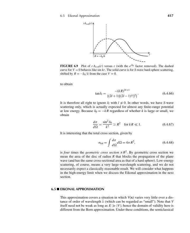
6.5 Eikonal Approximation 417
R = −δ0/k
rAl=0(r)
r
FIGURE 6.9 Plot of r Al=0(r ) versus r (with the eiδ0 factor removed). The dashedcurve for V = 0 behaves like sin kr . The solid curve is for S-wave hard-sphere scattering,shifted by R = −δ0/k from the case V = 0.
to obtain
tanδl = −(k R)2l+1
{(2l + 1)[(2l − 1)!!]2} . (6.4.66)
It is therefore all right to ignore δl with l �= 0. In other words, we have S-wavescattering only, which is actually expected for almost any finite-range potentialat low energy. Because δ0 = −k R regardless of whether k is large or small, weobtain
dσ
d�= sin2 δ0
k2� R2 for k R � 1. (6.4.67)
It is interesting that the total cross section, given by
σtot =∫
dσ
d�d�= 4πR2, (6.4.68)
is four times the geometric cross section πR2. By geometric cross section wemean the area of the disc of radius R that blocks the propagation of the planewave (and has the same cross-sectional area as that of a hard sphere). Low-energyscattering, of course, means a very large-wavelength scattering, and we do notnecessarily expect a classically reasonable result. We will consider what happensin the high-energy limit when we discuss the Eikonal approximation in the nextsection.
6.5 EIKONAL APPROXIMATION
This approximation covers a situation in which V(x) varies very little over a dis-tance of order of wavelength λ (which can be regarded as “small”). Note that Vitself need not be weak as long as E � |V |; hence the domain of validity here isdifferent from the Born approximation. Under these conditions, the semiclassical
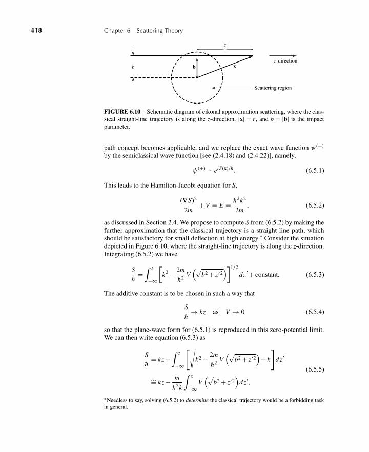
418 Chapter 6 Scattering Theory
b
z
z-direction
Scattering region
b x
FIGURE 6.10 Schematic diagram of eikonal approximation scattering, where the clas-sical straight-line trajectory is along the z-direction, |x| = r , and b = |b| is the impactparameter.
path concept becomes applicable, and we replace the exact wave function ψ(+)
by the semiclassical wave function [see (2.4.18) and (2.4.22)], namely,
ψ (+) ∼ eiS(x)/h . (6.5.1)
This leads to the Hamilton-Jacobi equation for S,
(∇S)2
2m+ V = E = h2k2
2m, (6.5.2)
as discussed in Section 2.4. We propose to compute S from (6.5.2) by making thefurther approximation that the classical trajectory is a straight-line path, whichshould be satisfactory for small deflection at high energy.∗ Consider the situationdepicted in Figure 6.10, where the straight-line trajectory is along the z-direction.Integrating (6.5.2) we have
S
h=∫ z
−∞
[k2 − 2m
h2 V(√
b2 + z′2)]1/2
dz′ + constant. (6.5.3)
The additive constant is to be chosen in such a way that
S
h→ kz as V → 0 (6.5.4)
so that the plane-wave form for (6.5.1) is reproduced in this zero-potential limit.We can then write equation (6.5.3) as
S
h= kz +
∫ z
−∞
[√k2 − 2m
h2V(√
b2 + z′2)
− k
]dz′
∼= kz − m
h2k
∫ z
−∞V(√
b2 + z′2)
dz′,
(6.5.5)
∗Needless to say, solving (6.5.2) to determine the classical trajectory would be a forbidding taskin general.
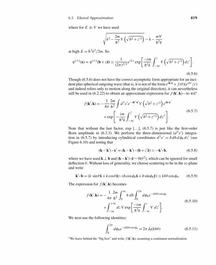
6.5 Eikonal Approximation 419
where for E � V we have used√k2 − 2m
h2V(√
b2 + z′2)
∼ k − mV
h2k
at high E = h2k2/2m. So
ψ (+)(x) = ψ (+)(b+ zz) � 1
(2π)3/2 ei k z exp
[−im
h2k
∫ z
−∞V(√
b2 + z′2)
dz′]
.
(6.5.6)
Though (6.5.6) does not have the correct asymptotic form appropriate for an inci-dent plus spherical outgoing wave (that is, it is not of the form eik·x + f (θ )(eikr/r )and indeed refers only to motion along the original direction), it can neverthelessstill be used in (6.2.22) to obtain an approximate expression for f (k′,k)—to wit∗
f (k′,k) = − 1
4π
2m
h2
∫d3x ′e−ik′·x′
V(√
b2 + z′2)
eik·x′
×exp
[− im
h2k
∫ z′
−∞V(√
b2 + z′′2)
dz′′]
.
(6.5.7)
Note that without the last factor, exp [. . .], (6.5.7) is just like the first-orderBorn amplitude in (6.3.3). We perform the three-dimensional (d3x ′) integra-tion in (6.5.7) by introducing cylindrical coordinates d3x ′ = b db dφb dz′ (seeFigure 6.10) and noting that
(k− k′) · x′ = (k− k′) · (b+ z′z) � −k′· b, (6.5.8)
where we have used k ⊥ b and (k−k′) ·z ∼ 0(θ2), which can be ignored for smalldeflection θ . Without loss of generality, we choose scattering to be in the xz-planeand write
k′· b = (k sinθ x+ k cosθ z) · (b cosφbx+ b sinφby) � kbθ cosφb. (6.5.9)
The expression for f (k′,k) becomes
f (k′,k) = − 1
4π
2m
h2
∫ ∞
0b db
∫ 2π
0dφbe−ikbθ cosφb
×∫ +∞
−∞dz V exp
[−im
h2k
∫ z
−∞V dz′
].
(6.5.10)
We next use the following identities:∫ 2π
0dφbe−ikbθ cosφb = 2π J0(kbθ ) (6.5.11)
∗We leave behind the “big box” and write f (k′,k), assuming a continuum normalization.
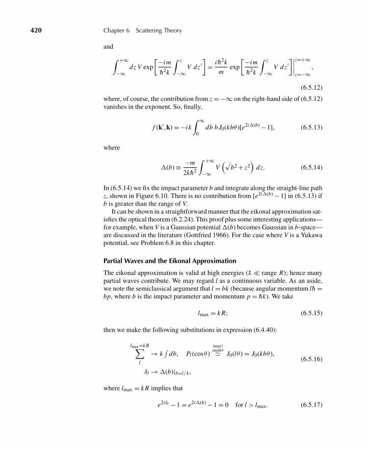
420 Chapter 6 Scattering Theory
and∫ +∞
−∞dz V exp
[−im
h2k
∫ z
−∞V dz′
]= i h2k
mexp
[−im
h2k
∫ z
−∞V dz′
]∣∣∣∣z=+∞
z=−∞,
(6.5.12)
where, of course, the contribution from z = −∞ on the right-hand side of (6.5.12)vanishes in the exponent. So, finally,
f (k′,k) = −ik∫ ∞
0db b J0(kbθ )[e2i�(b) − 1], (6.5.13)
where
�(b) ≡ −m
2kh2
∫ +∞
−∞V(√
b2 + z2)
dz. (6.5.14)
In (6.5.14) we fix the impact parameter b and integrate along the straight-line pathz, shown in Figure 6.10. There is no contribution from [e2i�(b) − 1] in (6.5.13) ifb is greater than the range of V.
It can be shown in a straightforward manner that the eikonal approximation sat-isfies the optical theorem (6.2.24). This proof plus some interesting applications—for example, when V is a Gaussian potential�(b) becomes Gaussian in b-space—are discussed in the literature (Gottfried 1966). For the case where V is a Yukawapotential, see Problem 6.8 in this chapter.
Partial Waves and the Eikonal Approximation
The eikonal approximation is valid at high energies (λ� range R); hence manypartial waves contribute. We may regard l as a continuous variable. As an aside,we note the semiclassical argument that l = bk (because angular momentum lh =bp, where b is the impact parameter and momentum p = hk). We take
lmax = k R; (6.5.15)
then we make the following substitutions in expression (6.4.40):
lmax=k R∑l
→ k∫
db, Pl (cosθ )largelsmallθ� J0(lθ ) = J0(kbθ ),
δl →�(b)|b=l/k,
(6.5.16)
where lmax = k R implies that
e2iδl − 1 = e2i�(b) − 1 = 0 for l > lmax. (6.5.17)
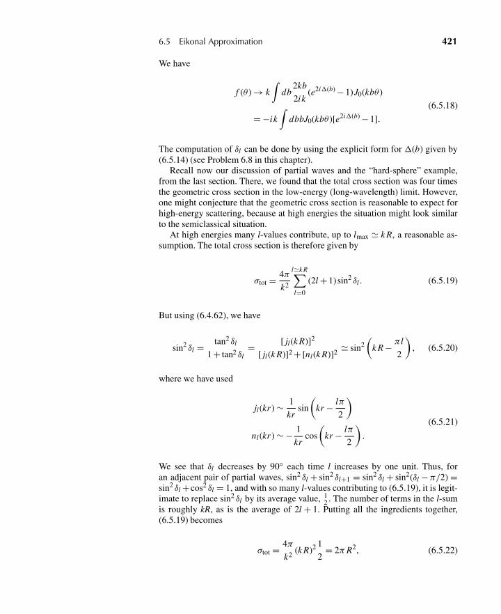
6.5 Eikonal Approximation 421
We have
f (θ ) → k∫
db2kb
2ik(e2i�(b) − 1)J0(kbθ )
= −ik∫
dbbJ0(kbθ )[e2i�(b) − 1].
(6.5.18)
The computation of δl can be done by using the explicit form for �(b) given by(6.5.14) (see Problem 6.8 in this chapter).
Recall now our discussion of partial waves and the “hard-sphere” example,from the last section. There, we found that the total cross section was four timesthe geometric cross section in the low-energy (long-wavelength) limit. However,one might conjecture that the geometric cross section is reasonable to expect forhigh-energy scattering, because at high energies the situation might look similarto the semiclassical situation.
At high energies many l-values contribute, up to lmax � k R, a reasonable as-sumption. The total cross section is therefore given by
σtot = 4π
k2
l�k R∑l=0
(2l + 1)sin2 δl . (6.5.19)
But using (6.4.62), we have
sin2 δl = tan2 δl
1 + tan2 δl= [ jl(k R)]2
[ jl(k R)]2 + [nl(k R)]2 � sin2(
k R − πl
2
), (6.5.20)
where we have used
jl(kr ) ∼ 1
krsin
(kr − lπ
2
)nl (kr ) ∼ − 1
krcos
(kr − lπ
2
).
(6.5.21)
We see that δl decreases by 90◦ each time l increases by one unit. Thus, foran adjacent pair of partial waves, sin2 δl + sin2 δl+1 = sin2 δl + sin2(δl −π/2) =sin2 δl +cos2 δl = 1, and with so many l-values contributing to (6.5.19), it is legit-imate to replace sin2 δl by its average value, 1
2 . The number of terms in the l-sumis roughly kR, as is the average of 2l + 1. Putting all the ingredients together,(6.5.19) becomes
σtot = 4π
k2(k R)2 1
2= 2πR2, (6.5.22)
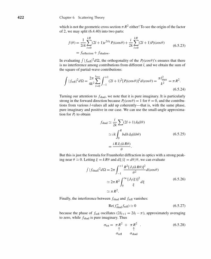
422 Chapter 6 Scattering Theory
which is not the geometric cross section πR2 either! To see the origin of the factorof 2, we may split (6.4.40) into two parts:
f (θ ) = 1
2ik
k R∑l=0
(2l + 1)e2iδl Pl (cosθ ) + i
2k
k R∑l=0
(2l + 1)Pl(cosθ )
= freflection + fshadow.
(6.5.23)
In evaluating∫ | frefl|2d�, the orthogonality of the Pl (cosθ )’s ensures that there
is no interference among contributions from different l, and we obtain the sum ofthe square of partial-wave contributions:∫
| frefl|2d�= 2π
4k2
lmax∑l=0
∫ +1
−1(2l + 1)2[Pl(cosθ )]2d(cosθ ) = πl2
max
k2 = πR2.
(6.5.24)
Turning our attention to fshad, we note that it is pure imaginary. It is particularlystrong in the forward direction because Pl (cosθ ) = 1 for θ = 0, and the contribu-tions from various l-values all add up coherently—that is, with the same phase,pure imaginary and positive in our case. We can use the small-angle approxima-tion for Pl to obtain
fshad � i
2k
∑(2l + 1)J0(lθ )
� ik∫ R
0bdb J0(kbθ )
= i R J1(k Rθ )
θ.
(6.5.25)
But this is just the formula for Fraunhofer diffraction in optics with a strong peak-ing near θ � 0. Letting ξ = k Rθ and dξ/ξ = dθ/θ , we can evaluate∫ | fshad|2d�= 2π
∫ +1
−1
R2[J1(k Rθ )]2
θ2 d(cosθ )
� 2πR2∫ ∞
0
[J1(ξ )]2
ξdξ
� πR2.
(6.5.26)
Finally, the interference between fshad and frefl vanishes:
Re( f ∗shad frefl) � 0 (6.5.27)
because the phase of frefl oscillates (2δl+1 = 2δl −π), approximately averagingto zero, while fshad is pure imaginary. Thus
σtot = πR2
↑σrefl
+ πR2
↑σshad
. (6.5.28)
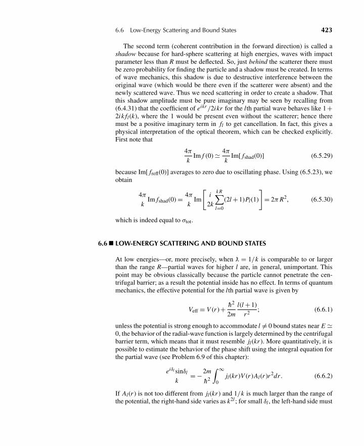
6.6 Low-Energy Scattering and Bound States 423
The second term (coherent contribution in the forward direction) is called ashadow because for hard-sphere scattering at high energies, waves with impactparameter less than R must be deflected. So, just behind the scatterer there mustbe zero probability for finding the particle and a shadow must be created. In termsof wave mechanics, this shadow is due to destructive interference between theoriginal wave (which would be there even if the scatterer were absent) and thenewly scattered wave. Thus we need scattering in order to create a shadow. Thatthis shadow amplitude must be pure imaginary may be seen by recalling from(6.4.31) that the coefficient of eikr /2ikr for the lth partial wave behaves like 1 +2ik fl(k), where the 1 would be present even without the scatterer; hence theremust be a positive imaginary term in fl to get cancellation. In fact, this gives aphysical interpretation of the optical theorem, which can be checked explicitly.First note that
4π
kIm f (0) � 4π
kIm[ fshad(0)] (6.5.29)
because Im[ frefl(0)] averages to zero due to oscillating phase. Using (6.5.23), weobtain
4π
kIm fshad(0) = 4π
kIm
[i
2k
k R∑l=0
(2l + 1)Pl(1)
]= 2πR2, (6.5.30)
which is indeed equal to σtot.
6.6 LOW-ENERGY SCATTERING AND BOUND STATES
At low energies—or, more precisely, when λ = 1/k is comparable to or largerthan the range R—partial waves for higher l are, in general, unimportant. Thispoint may be obvious classically because the particle cannot penetrate the cen-trifugal barrier; as a result the potential inside has no effect. In terms of quantummechanics, the effective potential for the lth partial wave is given by
Veff = V (r ) + h2
2m
l(l + 1)
r2 ; (6.6.1)
unless the potential is strong enough to accommodate l �= 0 bound states near E �0, the behavior of the radial-wave function is largely determined by the centrifugalbarrier term, which means that it must resemble jl(kr ). More quantitatively, it ispossible to estimate the behavior of the phase shift using the integral equation forthe partial wave (see Problem 6.9 of this chapter):
eiδl sinδlk
= −2m
h2
∫ ∞
0jl(kr )V (r )Al(r )r2dr . (6.6.2)
If Al(r ) is not too different from jl(kr ) and 1/k is much larger than the range ofthe potential, the right-hand side varies as k2l ; for small δl , the left-hand side must
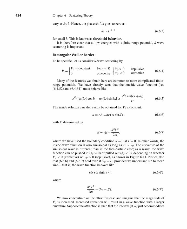
424 Chapter 6 Scattering Theory
vary as δl/k. Hence, the phase shift k goes to zero as
δl ∼ k2l+1 (6.6.3)
for small k. This is known as threshold behavior.It is therefore clear that at low energies with a finite-range potential, S-wave
scattering is important.
Rectangular Well or Barrier
To be specific, let us consider S-wave scattering by
V ={
V0 = constant for r < R
0 otherwise
{V0 > 0 repulsiveV0 < 0 attractive
(6.6.4)
Many of the features we obtain here are common to more-complicated finite-range potentials. We have already seen that the outside-wave function [see(6.4.52) and (6.4.64)] must behave like
eiδ0 [ j0(kr )cosδ0 − n0(kr )sinδ0] � eiδ0 sin(kr + δ0)
kr. (6.6.5)
The inside solution can also easily be obtained for V0 a constant:
u ≡ r Al=0(r ) ∝ sink′r , (6.6.6)
with k′ determined by
E − V0 = h2k ′2
2m, (6.6.7)
where we have used the boundary condition u = 0 at r = 0. In other words, theinside-wave function is also sinusoidal as long as E > V0. The curvature of thesinusoidal wave is different than in the free-particle case; as a result, the wavefunction can be pushed in (δ0 > 0) or pulled out (δ0 < 0), depending on whetherV0 < 0 (attractive) or V0 > 0 (repulsive), as shown in Figure 6.11. Notice alsothat (6.6.6) and (6.6.7) hold even if V0 > E , provided we understand sin to meansinh—that is, the wave function behaves like
u(r ) ∝ sinh[κr ], (6.6.6′)
where
h2κ2
2m= (V0 − E). (6.6.7′)
We now concentrate on the attractive case and imagine that the magnitude ofV0 is increased. Increased attraction will result in a wave function with a largercurvature. Suppose the attraction is such that the interval [0, R] just accommodates
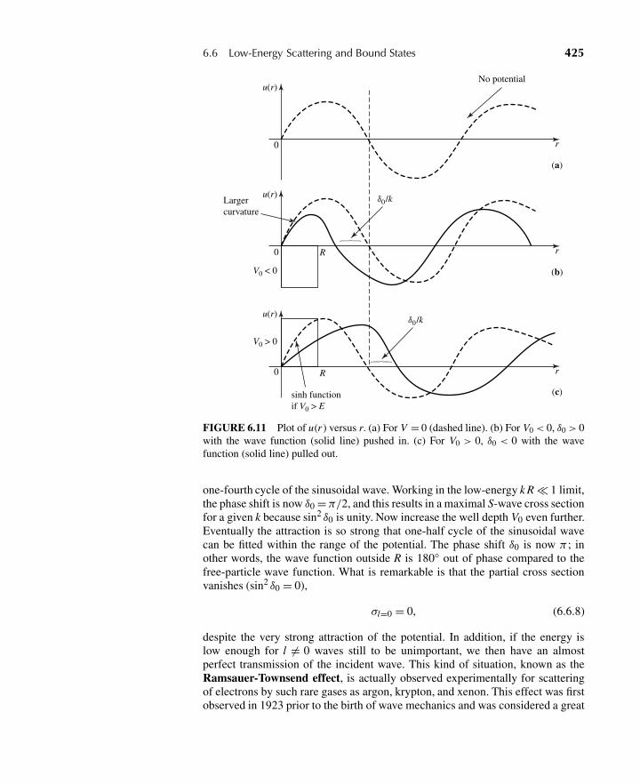
6.6 Low-Energy Scattering and Bound States 425
u(r)
u(r)
R
R
u(r)
0
0
0
Largercurvature
No potential
r
r
r
δ0/k
δ0/k
V0 < 0
V0 > 0
sinh functionif V0 > E
(a)
(c)
(b)
FIGURE 6.11 Plot of u(r ) versus r. (a) For V = 0 (dashed line). (b) For V0 < 0, δ0 > 0with the wave function (solid line) pushed in. (c) For V0 > 0, δ0 < 0 with the wavefunction (solid line) pulled out.
one-fourth cycle of the sinusoidal wave. Working in the low-energy k R � 1 limit,the phase shift is now δ0 = π/2, and this results in a maximal S-wave cross sectionfor a given k because sin2 δ0 is unity. Now increase the well depth V0 even further.Eventually the attraction is so strong that one-half cycle of the sinusoidal wavecan be fitted within the range of the potential. The phase shift δ0 is now π ; inother words, the wave function outside R is 180◦ out of phase compared to thefree-particle wave function. What is remarkable is that the partial cross sectionvanishes (sin2 δ0 = 0),
σl=0 = 0, (6.6.8)
despite the very strong attraction of the potential. In addition, if the energy islow enough for l �= 0 waves still to be unimportant, we then have an almostperfect transmission of the incident wave. This kind of situation, known as theRamsauer-Townsend effect, is actually observed experimentally for scatteringof electrons by such rare gases as argon, krypton, and xenon. This effect was firstobserved in 1923 prior to the birth of wave mechanics and was considered a great
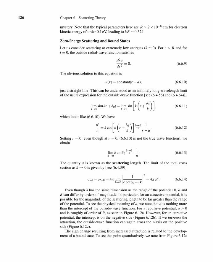
426 Chapter 6 Scattering Theory
mystery. Note that the typical parameters here are R ∼ 2 ×10⁻⁸ cm for electronkinetic energy of order 0.1 eV, leading to k R ∼ 0.324.
Zero-Energy Scattering and Bound States
Let us consider scattering at extremely low energies (k � 0). For r > R and forl = 0, the outside radial-wave function satisfies
d2u
dr2 = 0. (6.6.9)
The obvious solution to this equation is
u(r ) = constant(r − a), (6.6.10)
just a straight line! This can be understood as an infinitely long-wavelength limitof the usual expression for the outside-wave function [see (6.4.56) and (6.4.64)],
limk→0
sin(kr + δ0) = limk→0
sin
[k
(r + δ0
k
)], (6.6.11)
which looks like (6.6.10). We have
u′
u= k cot
[k
(r + δ0
k
)]k→0→ 1
r − a. (6.6.12)
Setting r = 0 [even though at r = 0, (6.6.10) is not the true wave function], weobtain
limk→0
k cotδ0k→0→ − 1
a. (6.6.13)
The quantity a is known as the scattering length. The limit of the total crosssection as k → 0 is given by [see (6.4.39)]
σtot = σl=0 = 4π limk→0
∣∣∣∣ 1
k cotδ0 − ik
∣∣∣∣2 = 4πa2. (6.6.14)
Even though a has the same dimension as the range of the potential R, a andR can differ by orders of magnitude. In particular, for an attractive potential, it ispossible for the magnitude of the scattering length to be far greater than the rangeof the potential. To see the physical meaning of a, we note that a is nothing morethan the intercept of the outside-wave function. For a repulsive potential, a > 0and is roughly of order of R, as seen in Figure 6.12a. However, for an attractivepotential, the intercept is on the negative side (Figure 6.12b). If we increase theattraction, the outside-wave function can again cross the r-axis on the positiveside (Figure 6.12c).
The sign change resulting from increased attraction is related to the develop-ment of a bound state. To see this point quantitatively, we note from Figure 6.12c
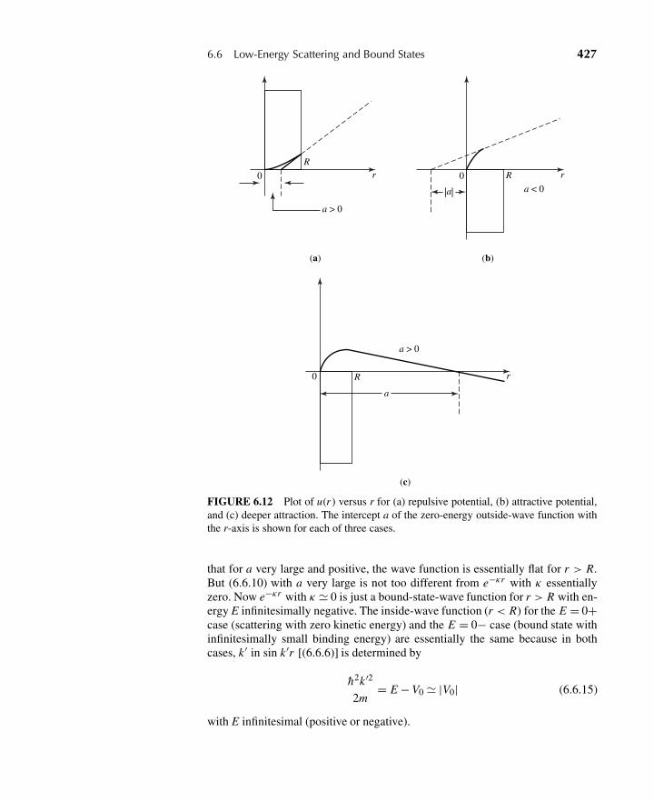
6.6 Low-Energy Scattering and Bound States 427
0
0
0
a > 0
a < 0
a > 0
R
R
R
r
r
r
|a|
a
(a)
(c)
(b)
FIGURE 6.12 Plot of u(r ) versus r for (a) repulsive potential, (b) attractive potential,and (c) deeper attraction. The intercept a of the zero-energy outside-wave function withthe r-axis is shown for each of three cases.
that for a very large and positive, the wave function is essentially flat for r > R.But (6.6.10) with a very large is not too different from e−κr with κ essentiallyzero. Now e−κr with κ � 0 is just a bound-state-wave function for r > R with en-ergy E infinitesimally negative. The inside-wave function (r < R) for the E = 0+case (scattering with zero kinetic energy) and the E = 0− case (bound state withinfinitesimally small binding energy) are essentially the same because in bothcases, k′ in sin k ′r [(6.6.6)] is determined by
h2k ′2
2m= E − V0 � |V0| (6.6.15)
with E infinitesimal (positive or negative).
428 Chapter 6 Scattering Theory
Because the inside-wave functions are the same for the two physical situa-tions (E = 0+ and E = 0−), we can equate the logarithmic derivative of thebound-state-wave function with that of the solution involving zero-kinetic-energyscattering,
−κe−κr
e−κr
∣∣∣∣r=R
=(
1
r − a
)∣∣∣∣r=R
, (6.6.16)
or, if R � a,
κ � 1
a. (6.6.17)
The binding energy satisfies
EBE = −Eboundstate = h2κ2
2m� h2
2ma2 , (6.6.18)
and we have a relation between scattering length and bound-state energy. Thisis a remarkable result. To wit, if there is a loosely bound state, we can infer itsbinding energy by performing scattering experiments near zero kinetic energy,provided a is measured to be large compared with the range R of the potential.This connection between the scattering length and the bound-state energy wasfirst pointed out by Wigner, who attempted to apply (6.6.18) to np-scattering.
Experimentally, the 3S1-state of the np-system has a bound state—that is, thedeuteron with
EBE = 2.22MeV. (6.6.19)
The scattering length is measured to be
atriplet = 5.4 ×10⁻¹³ cm, (6.6.20)
leading to the binding-energy prediction
h2
2μa2= h2
mN a2= mN c2
(h
mN ca
)2
= (938 MeV)
(2.1 ×10⁻¹⁴ cm
5.4 ×10⁻¹³ cm
)2
= 1.4 MeV,
(6.6.21)
where μ is the reduced mass approximated by mn,p/2. The agreement betweenexperiment and prediction is not too satisfactory. The discrepancy is due to thefact that the inside-wave functions are not exactly the same and that atriplet � R isnot really a good approximation for the deuteron. A better result can be obtainedby keeping the next term in the expansion of k cot δ as a function of k,
k cot δ0 = − 1
a+ 1
2r0k2, (6.6.22)
where r0 is known as the effective range (see, for example, Preston 1962, 23).
6.6 Low-Energy Scattering and Bound States 429
Bound States as Poles of Sl (k)
We conclude this section by studying the analytic properties of the amplitude Sl (k)for l = 0. Let us go back to (6.4.31) and (6.4.35), where the radial-wave functionfor l = 0 at large distance was found to be proportional to
Sl=0(k)eikr
r− e−ikr
r. (6.6.23)
Compare this with the wave function for a bound state at large distance,
e−κr
r. (6.6.24)
The existence of a bound state implies that a nontrivial solution to the Schrödingerequation with E < 0 exists only for a particular (discrete) value of κ . We mayargue that e−κr/r is like eikr/r , except that k is now purely imaginary. Apartfrom k being imaginary, the important difference between (6.6.23) and (6.6.24) isthat in the bound-state case, e−κr/r is present even without the analogue of theincident wave. Quite generally, only the ratio of the coefficient of eikr/r to that ofe−ikr/r is of physical interest, and this is given by Sl (k). In the bound-state casewe can sustain the outgoing wave (with imaginary k) even without an incidentwave. So the ratio is ∞, which means that Sl=0(k), regarded as a function of acomplex variable k, has a pole at k = iκ . Thus a bound state implies a pole (whichcan be shown to be a simple pole) on the positive imaginary axis of the complexk-plane; see Figure 6.13. For k real and positive, we have the region of physicalscattering. Here we must require [compare with (6.4.37)]
Sl=0 = e2iδ0 (6.6.25)
with δ0 real. Furthermore, as k → 0, k cot δ0 has a limiting value −1/a (6.6.13),which is finite, so δ0 must behave as follows:
δ0 → 0, ±π , . . . . (6.6.26)
Hence Sl=0 = e2iδ0 → 1 as k → 0.Now let us attempt to construct a simple function satisfying:
1.Pole at k = iκ (existence of bound state).
2. |Sl=0| = 1 for k > 0 real (unitarity).
3. Sl=0 = 1 at k = 0 (threshold behavior).
(6.6.27)
The simplest function that satisfies all three conditions of (6.6.27) is
Sl=0(k) = −k − iκ
k − iκ. (6.6.28)
[Editor’s Note: Equation (6.6.28) is chosen for simplicity rather than as a phys-ically realistic example. For reasonable potentials (not hard spheres!) the phaseshift vanishes as k → ∞.]
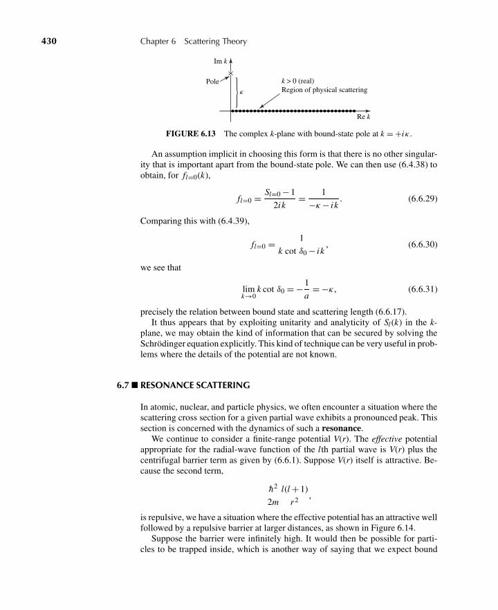
430 Chapter 6 Scattering Theory
Poleκ
k > 0 (real)Region of physical scattering
Re k
Im k
FIGURE 6.13 The complex k-plane with bound-state pole at k = +iκ .
An assumption implicit in choosing this form is that there is no other singular-ity that is important apart from the bound-state pole. We can then use (6.4.38) toobtain, for fl=0(k),
fl=0 = Sl=0 − 1
2ik= 1
−κ− ik. (6.6.29)
Comparing this with (6.4.39),
fl=0 = 1
k cot δ0 − ik, (6.6.30)
we see that
limk→0
k cot δ0 = − 1
a= −κ , (6.6.31)
precisely the relation between bound state and scattering length (6.6.17).It thus appears that by exploiting unitarity and analyticity of Sl (k) in the k-
plane, we may obtain the kind of information that can be secured by solving theSchrödinger equation explicitly. This kind of technique can be very useful in prob-lems where the details of the potential are not known.
6.7 RESONANCE SCATTERING
In atomic, nuclear, and particle physics, we often encounter a situation where thescattering cross section for a given partial wave exhibits a pronounced peak. Thissection is concerned with the dynamics of such a resonance.
We continue to consider a finite-range potential V(r). The effective potentialappropriate for the radial-wave function of the lth partial wave is V(r) plus thecentrifugal barrier term as given by (6.6.1). Suppose V(r) itself is attractive. Be-cause the second term,
h2
2m
l(l + 1)
r2 ,
is repulsive, we have a situation where the effective potential has an attractive wellfollowed by a repulsive barrier at larger distances, as shown in Figure 6.14.
Suppose the barrier were infinitely high. It would then be possible for parti-cles to be trapped inside, which is another way of saying that we expect bound
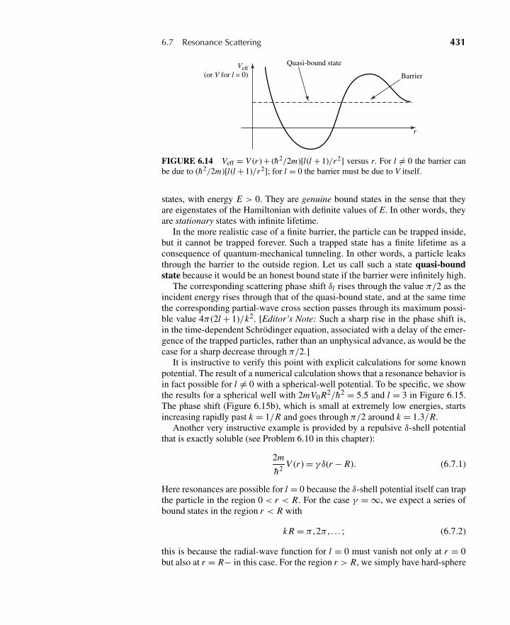
6.7 Resonance Scattering 431
Quasi-bound state
Barrier
r
Veff(or V for l = 0)
FIGURE 6.14 Veff = V (r ) + (h2/2m)[l(l + 1)/r2] versus r. For l �= 0 the barrier canbe due to (h2/2m)[l(l + 1)/r2]; for l = 0 the barrier must be due to V itself.
states, with energy E > 0. They are genuine bound states in the sense that theyare eigenstates of the Hamiltonian with definite values of E. In other words, theyare stationary states with infinite lifetime.
In the more realistic case of a finite barrier, the particle can be trapped inside,but it cannot be trapped forever. Such a trapped state has a finite lifetime as aconsequence of quantum-mechanical tunneling. In other words, a particle leaksthrough the barrier to the outside region. Let us call such a state quasi-boundstate because it would be an honest bound state if the barrier were infinitely high.
The corresponding scattering phase shift δl rises through the value π/2 as theincident energy rises through that of the quasi-bound state, and at the same timethe corresponding partial-wave cross section passes through its maximum possi-ble value 4π(2l + 1)/k2. [Editor’s Note: Such a sharp rise in the phase shift is,in the time-dependent Schrödinger equation, associated with a delay of the emer-gence of the trapped particles, rather than an unphysical advance, as would be thecase for a sharp decrease through π/2.]
It is instructive to verify this point with explicit calculations for some knownpotential. The result of a numerical calculation shows that a resonance behavior isin fact possible for l �= 0 with a spherical-well potential. To be specific, we showthe results for a spherical well with 2mV0 R2/h2 = 5.5 and l = 3 in Figure 6.15.The phase shift (Figure 6.15b), which is small at extremely low energies, startsincreasing rapidly past k = 1/R and goes through π/2 around k = 1.3/R.
Another very instructive example is provided by a repulsive δ-shell potentialthat is exactly soluble (see Problem 6.10 in this chapter):
2m
h2 V (r ) = γ δ(r − R). (6.7.1)
Here resonances are possible for l = 0 because the δ-shell potential itself can trapthe particle in the region 0 < r < R. For the case γ = ∞, we expect a series ofbound states in the region r < R with
k R = π ,2π , . . . ; (6.7.2)
this is because the radial-wave function for l = 0 must vanish not only at r = 0but also at r = R− in this case. For the region r > R, we simply have hard-sphere
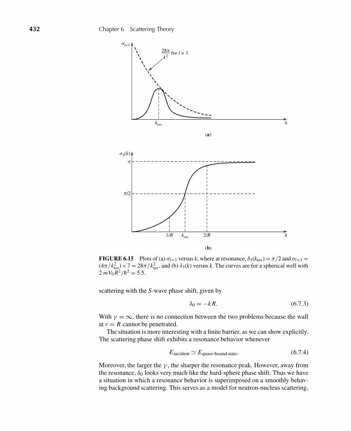
432 Chapter 6 Scattering Theory
28π
σl=3
k2for l = 3
kres
kres 2/R1/R
k
σ3(k)
k
(a)
(b)
π
π/2
FIGURE 6.15 Plots of (a) σl=3 versus k, where at resonance, δ3(kres) =π/2 and σl=3 =(4π/k2
res)×7 = 28π/k2res , and (b) δ3(k) versus k. The curves are for a spherical well with
2 mV0 R2/h2 = 5.5.
scattering with the S-wave phase shift, given by
δ0 = −k R. (6.7.3)
With γ = ∞, there is no connection between the two problems because the wallat r = R cannot be penetrated.
The situation is more interesting with a finite barrier, as we can show explicitly.The scattering phase shift exhibits a resonance behavior whenever
Eincident � Equasi-boundstate. (6.7.4)
Moreover, the larger the γ , the sharper the resonance peak. However, away fromthe resonance, δ0 looks very much like the hard-sphere phase shift. Thus we havea situation in which a resonance behavior is superimposed on a smoothly behav-ing background scattering. This serves as a model for neutron-nucleus scattering,
6.8 Symmetry Considerations in Scattering 433
where a series of sharp resonance peaks are observed on top of a smoothly varyingcross section.
Coming back to our general discussion of resonance scattering, we ask howthe scattering amplitudes vary in the vicinity of the resonance energy. If we are tohave any connection between σl being large and the quasi-bound states, δl mustgo through π/2 (or 3π/2, . . .) from below, as discussed above. In other words δlmust go through zero from above. Assuming that cotδl is smoothly varying nearthe vicinity of resonance, that is,
E � Er , (6.7.5)
we may attempt to expand δl as follows:
cot δl = cot δl |E=Er︸ ︷︷ ︸0
−c(E − Er ) + 0[(E − Er )2
]. (6.7.6)
This leads to
fl (k) = 1
k cot δl − ik= 1
k
1
[−c(E − Er ) − i ]
= − �/2
k
[(E − Er ) + i�
2
] ,(6.7.7)
where we have defined the width � by
d(cot δl)
d E
∣∣∣∣E=Er
= −c ≡ − 2
�. (6.7.8)
Notice that � is very small if cot δl varies rapidly. If a simple resonance dominatesthe lth partial-wave cross section, we obtain a one-level resonance formula (theBreit-Wigner formula):
σl = 4π
k2
(2l + 1)(�/2)2
(E − Er )2 +�2/4. (6.7.9)
So it is legitimate to regard � as the full width at half-maximum, provided theresonance is reasonably narrow so that variation in 1/k2 can be ignored.
6.8 SYMMETRY CONSIDERATIONS IN SCATTERING
Let us consider the scattering of two identical spinless charged particles via somecentral potential, such as the Coulomb potential.∗ The spatial part of the wave
∗The student unfamiliar with the elements of permutation symmetry with identical particlesshould see Chapter 7 of this textbook.
434 Chapter 6 Scattering Theory
function must now be symmetrical, so the asymptotic wave function must looklike
eik·x + e−ik·x + [ f (θ ) + f (π− θ )]eikr
r, (6.8.1)
where x = x1 − x2 is the relative position vector between the two particles 1 and2. This results in a differential cross section,
dσ
d�= | f (θ ) + f (π − θ )|2
= | f (θ )|2 +| f (π − θ )|2 + 2Re[ f (θ ) f ∗(π− θ )].
(6.8.2)
The cross section is enhanced through constructive interference at θ � π/2.In contrast, for spin 1
2− spin 12 scattering with unpolarized beam and V inde-
pendent of spin, we have the spin-singlet scattering going with space-symmetricalwave function and the spin triplet going with space-antisymmetrical wave func-tion (see Section 7.3). If the initial beam is unpolarized, we have the statisticalcontribution 1
4 for spin singlet and 34 for spin triplet; hence
dσ
d�= 1
4| f (θ ) + f (π − θ )|2 + 3
4| f (θ ) − f (π− θ )|2
= | f (θ )|2 +| f (π − θ )|2 − Re[ f (θ ) f ∗(π− θ )].
(6.8.3)
In other words, we expect destructive interference at θ � π/2. This has, in fact,been observed.
Now consider symmetries other than exchange symmetry. Suppose V and H0are both invariant under some symmetry operation. We may ask what this impliesfor the matrix element of T or for the scattering amplitude f (k′,k).
If the symmetry operator is unitary (for example, rotation and parity), every-thing is quite straightforward. Using the explicit form of T as given by (6.1.32),we see that
UH0U† = H0, U V U† = V (6.8.4)
implies that T is also invariant under U—that is,
U T U† = T . (6.8.5)
We define
|k〉 ≡ U |k〉, |k′〉 ≡ U |k′〉. (6.8.6)
Then
〈k′|T |k〉 = 〈k′|U†U T U†U |k〉= 〈k′|T |k〉. (6.8.7)
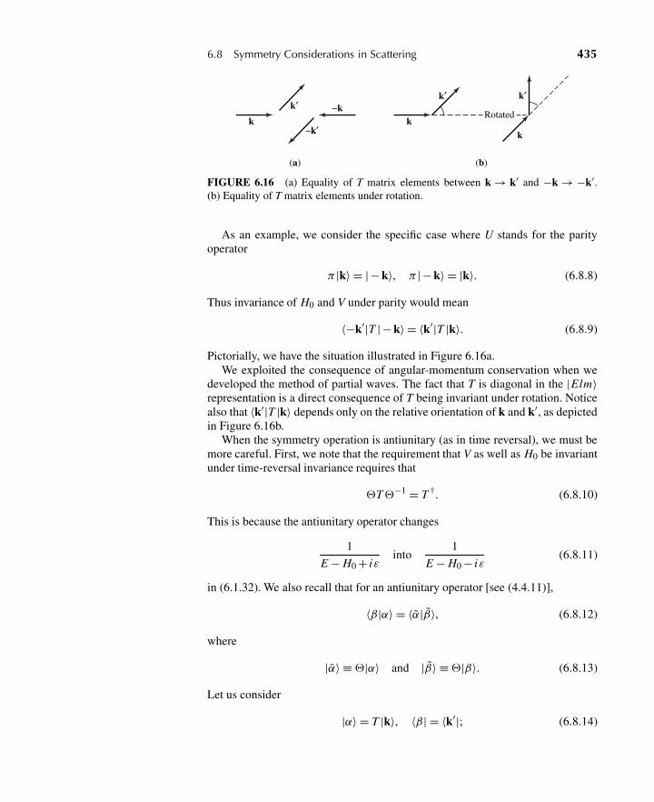
6.8 Symmetry Considerations in Scattering 435
k kk
k′k′ k′
−k′
−kRotated
(a) (b)
FIGURE 6.16 (a) Equality of T matrix elements between k → k′ and −k → −k′.(b) Equality of T matrix elements under rotation.
As an example, we consider the specific case where U stands for the parityoperator
π |k〉 = |− k〉, π |− k〉 = |k〉. (6.8.8)
Thus invariance of H0 and V under parity would mean
〈−k′|T |− k〉 = 〈k′|T |k〉. (6.8.9)
Pictorially, we have the situation illustrated in Figure 6.16a.We exploited the consequence of angular-momentum conservation when we
developed the method of partial waves. The fact that T is diagonal in the |Elm〉representation is a direct consequence of T being invariant under rotation. Noticealso that 〈k′|T |k〉 depends only on the relative orientation of k and k′, as depictedin Figure 6.16b.
When the symmetry operation is antiunitary (as in time reversal), we must bemore careful. First, we note that the requirement that V as well as H0 be invariantunder time-reversal invariance requires that
T −1 = T †. (6.8.10)
This is because the antiunitary operator changes
1
E − H0 + iεinto
1
E − H0 − iε(6.8.11)
in (6.1.32). We also recall that for an antiunitary operator [see (4.4.11)],
〈β|α〉 = 〈α|β〉, (6.8.12)
where
|α〉 ≡ |α〉 and |β〉 ≡ |β〉. (6.8.13)
Let us consider
|α〉 = T |k〉, 〈β| = 〈k′|; (6.8.14)
436 Chapter 6 Scattering Theory
then
|α〉 = T |k〉 = T −1 |k〉 = T †|− k〉|β〉 = |k〉 = |− k′〉. (6.8.15)
As a result, (6.8.12) becomes
〈k′|T |k〉 = 〈−k|T |− k′〉. (6.8.16)
Notice that the initial and final momenta are interchanged, in addition to the factthat the directions of the momenta have been reversed.
It is also interesting to combine the requirements of time reversal (6.8.16) andparity (6.8.9):
〈k′|T |k〉under = 〈−k|T |− k′〉underπ= 〈k|T |k′〉; (6.8.17)
that is, from (6.2.22) and (6.3.1) we have
f (k,k′) = f (k′,k), (6.8.18)
which results in
dσ
d�(k → k′) = dσ
d�(k′ → k). (6.8.19)
Equation (6.8.19) is known as detailed balance.It is more interesting to look at the analogue of (6.8.17) when we have spin.
Here we may characterize the initial free-particle ket by |k,ms〉, and we exploit(4.4.79) for the time-reversal portion:
〈k′,m′s |T |k,ms〉 = i−2ms+2ms′ 〈−k,−ms |T |− k′,−m′
s〉= i−2ms+2ms′ 〈k,−ms |T |k′,−m′
s〉.(6.8.20)
For unpolarized initial states, we sum over the initial spin states and divide by(2s + 1); if the final polarization is not observed, we must sum over final states.We then obtain detailed balance in the form
dσ
d�(k → k′) = dσ
d�(k′ → k), (6.8.21)
where we understand the bar on the top of dσ/d� in (6.8.21) to mean that weaverage over the initial spin states and sum over the final spin states.
6.9 INELASTIC ELECTRON-ATOM SCATTERING
Let us consider the interactions of electron beams with atoms assumed to be intheir ground states. The incident electron may get scattered elastically with finalatoms unexcited:
e− + atom (ground state) → e− + atom (ground state). (6.9.1)
6.9 Inelastic Electron-Atom Scattering 437
This is an example of elastic scattering. To the extent that the atom can be re-garded as infinitely heavy, the kinetic energy of the electron does not change. It isalso possible for the target atom to get excited:
e− + atom (ground state) → e− + atom (excited state). (6.9.2)
In this case we talk about inelastic scattering because the kinetic energy of thefinal outgoing electron is now less than that of the initial incoming electron, thedifference being used to excite the target atom.
The initial ket of the electron plus the atomic system is written as
|k,0〉, (6.9.3)
where k refers to the wave vector of the incident electron and 0 stands for theatomic ground state. Strictly speaking, (6.9.3) should be understood as the directproduct of the incident-electron ket |k〉 and the ground-state atomic ket |0〉. Thecorresponding wave function is
1
L3/2eik·xψ0(x1,x2, . . . ,xz), (6.9.4)
where we use the box normalization for the plane wave.We may be interested in a final-state electron with a definite wave vector k′.
The final-state ket and the corresponding wave function are
|k′,n〉 and1
L3/2eik′·xψn(x1, . . . ,xz), (6.9.5)
where n = 0 for elastic scattering and n �= 0 for inelastic scattering.Assuming that time-dependent perturbation theory is applicable, we can im-
mediately write the differential cross section, as in the previous section:
dσ
d�(0 → n) = 1
(hk/me L3)
2π
h|〈k′n|V |k0〉|2
(L
2π
)3(k ′me
h2
)=(
k′
k
)L6∣∣∣∣ 1
4π
2me
h2〈k′,n|V |k,0〉
∣∣∣∣2.
(6.9.6)
Everything is similar, including the cancellation of terms such as L3, with oneimportant exception: k′ ≡ |k′| is not, in general, equal to k ≡ |k| for inelasticscattering.
The next question is, what V is appropriate for this problem? The incidentelectron can interact with the nucleus, assumed to be situated at the origin; it canalso interact with each of the atomic electrons. So V is to be written as
V = − Ze2
r+∑
i
e2
|x − xi | . (6.9.7)
438 Chapter 6 Scattering Theory
Here complications may arise because of the identity of the incident electron withone of the atomic electrons; to treat this rigorously is a nontrivial task. Fortu-nately, for a relatively fast electron we can legitimately ignore the question ofidentity; this is because there is little overlap between the bound-state electronand the incident electron in momentum space. We must evaluate the matrix ele-ment 〈k′,n|V |k0〉, which, when explicitly written, is
〈k′n|V |k0〉 = 1
L3
∫d3xeiq·x〈n|− Ze2
r+∑
i
e2
|x − xi | |0〉
= 1
L3
∫d3xeiq·x
z∏i
∫d3xiψ
∗n (x1, . . . ,xz)
[− Ze2
r+∑
i
e2
|x − xi |
]×ψ0(x1, . . . ,xz)
(6.9.8)with q ≡ k− k′.
Let us see how to evaluate the matrix element of the first term, −Ze2/r , wherer actually means |x|. First we note that this is a potential between the incidentelectron and the nucleus, which is independent of the atomic electron coordinates.So it can be taken outside the integration
z∏i
∫d3xi
in (6.9.8); we simply obtain
〈n|0〉 = δn0 (6.9.9)
for the remainder. In other words, this term contributes only to the elastic-scattering case, where the target atom remains unexcited. In the elastic casewe must still integrate eiq·x/r with respect to x, which amounts to taking theFourier transform of the Coulomb potential. This can readily be done because wehave already evaluated the Fourier transform of the Yukawa potential; see (6.3.9).Hence ∫
d3xeiq·x
r= limμ→0
∫d3xeiq·x−μr
r= 4π
q2 . (6.9.10)
As for the second term in (6.9.8), we can evaluate the Fourier transform of 1/|x−xi |. We can accomplish this by shifting the coordinate variables x → x + xi :∑
i
∫d3xeiq·x
|x − xi | =∑
i
∫d3xeiq·x + xi )
|x| = 4π
q2
∑i
eiq·xi . (6.9.11)
Notice that this is just the Fourier transform of the Coulomb potential multipliedby the Fourier transform of the electron density due to the atomic electrons situ-ated at xi :
ρatom(x) =∑
i
δ(3)(x − xi). (6.9.12)
6.9 Inelastic Electron-Atom Scattering 439
We customarily define the form factor Fn(q) for excitation |0〉 to |n〉 as follows:
Z Fn(q) ≡ 〈n|∑
i
eiq·xi |0〉, (6.9.13)
which is made of coherent—in the sense of definite phase relationships—contributions from the various electrons. Notice that as q → 0, we have
1
Z〈n|∑
i
eiq·xi |0〉 → 1
for n = 0; hence the form factor approaches unity in the elastic-scattering case.For n �= 0 (inelastic scattering), Fn(q) → 0 as q → 0 by orthogonality between|n〉 and |0〉. We can then write the matrix element in (6.9.8) as∫
d3xeiq·x〈n|(
− Ze2
r+∑
i
e2
|x − xi |
)|0〉 = 4π Ze2
q2[−δn0 + Fn(q)]. (6.9.14)
We are finally in a position to write the differential cross section for inelastic(or elastic) scattering of electrons by atoms:
dσ
d�(0 → n) =
(k ′
k
)∣∣∣∣ 1
4π
2me
h2
4π Ze2
q2 [−δn0 + Fn(q)]
∣∣∣∣2= 4m2
e
h4
(Ze2)2
q4
(k ′
k
)|− δn0 + Fn(q)|2.
(6.9.15)
For inelastic scattering the δn0-term does not contribute, and it is customary towrite the differential cross section in terms of the Bohr radius,
a0 = h2
e2me, (6.9.16)
as follows:
dσ
d�(0 → n) = 4Z2a2
0
(k ′
k
)1
(qa0)4 |Fn(q)|2. (6.9.17)
Quite often dσ/dq is used in place of dσ/d�; using
q2 = |k− k′|2 = k2 + k ′2 − 2kk ′ cosθ (6.9.18)
and dq = −d(cosθ )kk′/q , we can write
dσ
dq= 2πq
kk ′dσ
d�. (6.9.19)
The inelastic cross section we have obtained can be used to discuss stop-ping power—the energy loss of a charged particle as it goes through matter.A number of people, including H. A. Bethe and F. Bloch, have discussed thequantum-mechanical derivation of stopping power from the point of view of theinelastic-scattering cross section. We are interested in the energy loss of a charged
440 Chapter 6 Scattering Theory
particle per unit length traversed by the incident charged particle. The collisionrate per unit length is Nσ , where N is the number of atoms per unit volume;at each collision process the energy lost by the charged particle is En − E0. Sod E/dx is written as
d E
dx= N
∑n
(En − E0)∫
dσ
dq(0 → n)dq
= N∑
n
(En − E0)4Z2
a20
∫ qmax
qmin
k ′
k
1
q4
2πq
kk ′ |Fn(q)|2dq
= 8πN
k2a20
∑n
(En − E0)∫ qmax
qmin
∣∣∣∣∣〈n|z∑
i=1
eiq·xi |0〉∣∣∣∣∣2
dq
q3 .
(6.9.20)
Many papers have been written on how to evaluate the sum in (6.9.20).∗ Theupshot of all this is to justify quantum-mechanically Bohr’s 1913 formula forstopping power,
dE
dx= 4πN Ze4
mev2 ln
(2mev
2
I
), (6.9.21)
where I is a semiempirical parameter related to the average excitation energy〈En − E0〉. If the charged particle has electric charge ± ze, we just replace Ze4 byz2 Ze4. It is also important to note that even if the projectile is not an electron, theme that appears in (6.9.21) is still the electron mass, not the mass of the chargedparticle. So the energy loss is dependent on the charge and the velocity of theprojectile but is independent of the mass of the projectile. This has an importantapplication to the detection of charged particles.
Quantum-mechanically, we view the energy loss of a charged particle as aseries of inelastic-scattering processes. At each interaction between the chargedparticle and an atom, we may imagine that a “measurement” of the position of thecharged particle is made. We may wonder why particle tracks in such media ascloud chambers and nuclear emulsions are nearly straight. The reason is that thedifferential cross section (6.9.17) is sharply peaked at small q; in an overwhelmingnumber of collisions, the final direction of momentum is nearly the same as thatof the incident electron due to the rapid falloff of q−4 and Fn(q) for large q.
Nuclear Form Factor
The excitation of atoms due to inelastic scattering is important for q ∼ 109 cm−1,to 1010 cm−1. If q is too large, the contributions due to F0(q) or Fn(q) dropoff very rapidly. At extremely high q, where q is now of order 1/Rnucleus ∼1012 cm−1, the structure of the nucleus becomes important. The Coulomb poten-tial due to the point nucleus must now be replaced by a Coulomb potential due to
∗For a relatively elementary discussion, see K. Gottfried (1966) and H. A. Bethe and R. W. Jackiw(1968).
6.9 Inelastic Electron-Atom Scattering 441
an extended object,
− Ze2
r→ −Ze2
∫d3x ′N(r ′)|x − x′| , (6.9.22)
where N(r ) is a nuclear charge distribution, normalized so that∫d3x ′N(r ′) = 1. (6.9.23)
The point-like nucleus can now be regarded as a special case, with
N(r ′) = δ(3)(r ′). (6.9.24)
We can evaluate the Fourier transform of the right-hand side of (6.9.22) in analogywith (6.9.10) as follows:
Ze2∫
d3x∫
d3x ′eiq·x N(r ′)|x − x′| = Ze2
∫d3x ′eiq·x′
N(r ′)∫
d3xeiq·x
r
= Ze2 4π
q2Fnucleus(q)
(6.9.25)where we have shifted the coordinates x → x + x′ in the first step and
Fnucleus ≡∫
d3xeiq·x N(r ). (6.9.26)
We thus obtain the deviation from the Rutherford formula due to the finite size ofthe nucleus,
dσ
d�=(
dσ
d�
)Rutherford
|F(q)|2, (6.9.27)
where (dσ/d�)Rutherford is the differential cross section for the electric scatteringof electrons by a point-like nucleus of charge Z |e|. For small q we have
Fnucleus(q) =∫
d3x
(1 + iq · x − 1
2q2r2(q · r)2 +·· ·
)N(r )
= 1 − 1
6q2〈r2〉nucleus +·· · .
(6.9.28)
The q · x-term vanishes because of spherical symmetry, and in the q2-term wehave used the fact that the angular average of cos2 θ (where θ is the angle betweenq and r) is just 1
3 :
1
2
∫ +1
−1d(cosθ )cos2 θ = 1
3. (6.9.29)
The quantity 〈r2〉nucleus is known as the mean square radius of the nucleus. In thisway it is possible to “measure” the size of the nucleus and also of the proton,as done by R. Hofstadter and coworkers. In the proton case the spin (magneticmoment) effect is also important.
442 Chapter 6 Scattering Theory
Problems
6.1 The Lippmann-Schwinger formalism can also be applied to a one-dimensionaltransmission-reflection problem with a finite-range potential, V (x) �= 0 for 0 <|x |< a only.
(a) Suppose we have an incident wave coming from the left: 〈x |φ〉 = eikx /√
2π .How must we handle the singular 1/(E − H0) operator if we are to have atransmitted wave only for x > a and a reflected wave and the original wave forx <−a? Is the E → E + iε prescription still correct? Obtain an expression forthe appropriate Green’s function and write an integral equation for 〈x |ψ (+)〉.
(b) Consider the special case of an attractive δ-function potential
V = −(γ h2
2m
)δ(x) (γ > 0).
Solve the integral equation to obtain the transmission and reflection ampli-tudes. Check your results with Gottfried 1966, p. 52.
(c) The one-dimensional δ-function potential with γ > 0 admits one (and only one)bound state for any value of γ . Show that the transmission and reflection am-plitudes you computed have bound-state poles at the expected positions whenk is regarded as a complex variable.
6.2 Prove
σtot � m2
π h4
∫d3x
∫d3x ′V (r )V (r ′)
sin2 k|x− x′|k2|x− x′|2
in each of the following ways.
(a) By integrating the differential cross section computed using the first-order Bornapproximation.
(b) By applying the optical theorem to the forward-scattering amplitude in thesecond-order Born approximation. [Note that f (0) is real if the first-order Bornapproximation is used.]
6.3 Estimate the radius of the 40Ca nucleus from the data in Figure 6.6 and compare tothat expected from the empirical value ≈ 1.4A1/3 fm, where A is the nuclear massnumber. Check the validity of using the first-order Born approximation for thesedata.
6.4 Consider a potential
V = 0 for r > R, V = V0 = constant for r < R,
where V0 may be positive or negative. Using the method of partial waves, show thatfor |V0| � E = h2k2/2m and kR � 1, the differential cross section is isotropic andthat the total cross section is given by
σtot =(
16π
9
)m2V 2
0 R6
h4.
Problems 443
Suppose the energy is raised slightly. Show that the angular distribution can thenbe written as
dσ
d�= A + B cosθ .
Obtain an approximate expression for B/A.
6.5 A spinless particle is scattered by a weak Yukawa potential
V = V0e−μr
μr,
where μ > 0 but V0 can be positive or negative. It was shown in the text that thefirst-order Born amplitude is given by
f (1)(θ ) = −2mV0
h2μ
1
[2k2(1− cosθ )+μ2].
(a) Using f (1)(θ ) and assuming |δl | � 1, obtain an expression for δl in terms of aLegendre function of the second kind,
Ql (ζ ) = 1
2
∫ 1
−1
Pl(ζ ′)ζ − ζ ′ dζ
′.
(b) Use the expansion formula
Ql(ζ ) = l!
1 ·3 ·5 · · · (2l + 1)
×{
1
ζ l+1+ (l + 1)(l + 2)
2(2l + 3)
1
ζ l+3
+ (l + 1)(l + 2)(l + 3)(l + 4)
2 ·4 · (2l + 3)(2l + 5)
1
ζ l+5+···
}(|ζ |> 1)
to prove each assertion.
(i) δl is negative (positive) when the potential is repulsive (attractive).
(ii) When the de Broglie wavelength is much longer than the range of thepotential, δl is proportional to k2l+1. Find the proportionality constant.
6.6 Check explicitly the x − px uncertainty relation for the ground state of a particleconfined inside a hard sphere: V = ∞ for r > a, V = 0 for r < a. (Hint: Takeadvantage of spherical symmetry.)
6.7 Consider the scattering of a particle by an impenetrable sphere
V (r ) ={
0 for r > a∞ for r < a.
(a) Derive an expression for the s-wave (l = 0) phase shift. (You need not know thedetailed properties of the spherical Bessel functions to do this simple problem!)
444 Chapter 6 Scattering Theory
(b) What is the total cross section σ [σ = ∫(dσ/d�)d�] in the extreme low-energy
limit k → 0? Compare your answer with the geometric cross section πa2. Youmay assume without proof:
dσ
d�= | f (θ )|2,
f (θ ) =(
1
k
) ∞∑l=0
(2l + 1)eiδl sinδl Pl (cosθ ).
6.8 Use δl = �(b)|b=l/k to obtain the phase shift δl for scattering at high energiesby (a) the Gaussian potential, V = V0 exp(−r2/a2), and (b) the Yukawa potential,V = V0 exp(−μr )/μr . Verify the assertion that δl goes to zero very rapidly withincreasing l (k fixed) for l � kR, where R is the “range” of the potential. [Theformula for �(b) is given in (6.5.14)].
6.9 (a) Prove
h2
2m〈x| 1
E − H0 + iε|x′〉 = −i k
∑l
∑m
Y ml (r)Y m∗
l (r′) jl(kr<)h(1)l (kr>),
where r<(r>) stands for the smaller (larger) of r and r ′.(b) For spherically symmetrical potentials, the Lippmann-Schwinger equation can
be written for spherical waves:
|Elm(+)〉 = |Elm〉+ 1
E − H0 + iεV |Elm(+)〉.
Using (a), show that this equation, written in the x-representation, leads to anequation for the radial function, Al (k; r ), as follows:
Al (k;r ) = jl(kr )− 2mik
h2
×∫ ∞
0jl(kr<)h(1)
l (kr>)V (r ′)Al (k;r ′)r ′2dr ′.
By taking r very large, also obtain
fl(k) = eiδlsinδl
k
= −(
2m
h2
)∫ ∞
0jl(kr )Al (k;r )V (r )r2dr .
6.10 Consider scattering by a repulsive δ-shell potential:(2m
h2
)V (r ) = γ δ(r − R), (γ > 0).
(a) Set up an equation that determines the s-wave phase shift δ0 as a function ofk (E = h2k2/2m).
(b) Assume now that γ is very large,
γ � 1
R,k.
Problems 445
Show that if tan kR is not close to zero, the s-wave phase shift resembles thehard-sphere result discussed in the text. Show also that for tan kR close to (butnot exactly equal to) zero, resonance behavior is possible; that is, cotδ0 goesthrough zero from the positive side as k increases. Determine approximatelythe positions of the resonances keeping terms of order 1/γ ; compare themwith the bound-state energies for a particle confined inside a spherical wall ofthe same radius,
V = 0, r < R; V = ∞, r > R.
Also obtain an approximate expression for the resonance width � defined by
� = −2
[d(cot δ0)/d E]|E=Er
,
and notice, in particular, that the resonances become extremely sharp as γ be-comes large. (Note: For a different, more sophisticated approach to this prob-lem, see Gottfried 1966, pp. 131–41, who discusses the analytic properties ofthe Dl-function defined by Al = jl/Dl .)
6.11 A spinless particle is scattered by a time-dependent potential
V(r, t) = V (r)cosωt .
Show that if the potential is treated to first order in the transition amplitude, theenergy of the scattered particle is increased or decreased by hω. Obtain dσ/d�.Discuss qualitatively what happens if the higher-order terms are taken into account.
6.12 Show that the differential cross section for the elastic scattering of a fast electronby the ground state of the hydrogen atom is given by
dσ
d�=(
4m2e4
h4q4
){1− 16[
4+ (qa0)2]2
}2
.
(Ignore the effect of identity.)
6.13 Let the energy of a particle moving in a central field be E(J1 J2 J3), where(J1, J2, J3) are the three action variables. How does the functional form of Especialize for the Coulomb potential? Using the recipe of the action-angle method,compare the degeneracy of the central-field problem to that of the Coulomb prob-lem, and relate it to the vector A.
If the Hamiltonian is
H = p2
2μ+ V (r )+ F(A2),
how are these statements changed?Describe the corresponding degeneracies of the central-field and Coulomb
problems in quantum theory in terms of the usual quantum numbers (n, l, m) andalso in terms of the quantum numbers (k, m, n). Here the second set, (k, m, n), labelsthe wave functions Dk
mn(αβγ ).How are the wave functions D k
mn(αβγ ) related to Laguerre times sphericalharmonics?
C H A P T E R
7 Identical Particles
This chapter is devoted to a discussion of some striking quantum-mechanical ef-fects arising from the identity of particles. First we present a suitable formalismand the way that nature deals with what appears to be an arbitrary choice. We thenconsider some applications to atoms more complex than hydrogen or hydrogen-like atoms. Moving on, we develop a formalism for dealing with systems of manyidentical particles, one of the ways to approach quantum field theory. Finally, asone example of a many-particle quantum-mechanical system, we outline one ap-proach to quantizing the electromagnetic field.
7.1 PERMUTATION SYMMETRY
In classical physics it is possible to keep track of individual particles even thoughthey may look alike. When we have particle 1 and particle 2 considered as asystem, we can, in principle, follow the trajectory of 1 and that of 2 separately ateach instant of time. For bookkeeping purposes, you may color one of them blueand the other red and then examine how the red particle moves and how the blueparticle moves as time passes.
In quantum mechanics, however, identical particles are truly indistinguishable.This is because we cannot specify more than a complete set of commuting ob-servables for each of the particles; in particular, we cannot label the particle bycoloring it blue. Nor can we follow the trajectory because that would entail aposition measurement at each instant of time, which necessarily disturbs the sys-tem; in particular, the two situations (a) and (b) shown in Figure 7.1 cannot bedistinguished—not even in principle.
For simplicity, consider just two particles. Suppose one of the particles, whichwe call particle 1, is characterized by |k′〉, where k ′ is a collective index for acomplete set of observables. Likewise, we call the ket of the remaining particle|k′′〉. The state ket for the two particles can be written in product form,
|k ′〉|k ′′〉, (7.1.1)
where it is understood that the first ket refers to particle 1 and the second ket toparticle 2. We can also consider
|k ′′〉|k ′〉, (7.1.2)
where particle 1 is characterized by |k ′′〉 and particle 2 by |k ′〉. Even though thetwo particles are indistinguishable, it is worth noting that mathematically, (7.1.1)
446
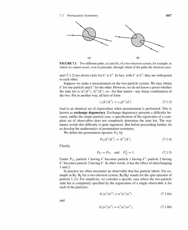
7.1 Permutation Symmetry 447
(a) (b)
FIGURE 7.1 Two different paths, (a) and (b), of a two-electron system, for example, inwhich we cannot assert, even in principle, through which of the paths the electrons pass.
and (7.1.2) are distinct kets for k ′ �= k ′′. In fact, with k′ �= k ′′, they are orthogonalto each other.
Suppose we make a measurement on the two-particle system. We may obtaink ′ for one particle and k ′′ for the other. However, we do not know a priori whetherthe state ket is |k ′〉|k ′′〉, |k ′′〉|k ′〉, or—for that matter—any linear combination ofthe two. Put in another way, all kets of form
c1|k ′〉|k ′′〉 + c2|k ′′〉|k ′〉 (7.1.3)
lead to an identical set of eigenvalues when measurement is performed. This isknown as exchange degeneracy. Exchange degeneracy presents a difficulty be-cause, unlike the single-particle case, a specification of the eigenvalue of a com-plete set of observables does not completely determine the state ket. The waynature avoids this difficulty is quite ingenious. But before proceeding further, letus develop the mathematics of permutation symmetry.
We define the permutation operator P12 by
P12|k ′〉|k ′′〉 = |k ′′〉|k ′〉. (7.1.4)
Clearly,
P21 = P12 and P 212 = 1. (7.1.5)
Under P12, particle 1 having k ′ becomes particle 1 having k ′′; particle 2 havingk′′ becomes particle 2 having k ′. In other words, it has the effect of interchanging1 and 2.
In practice we often encounter an observable that has particle labels. For ex-ample in S1 · S2 for a two-electron system, S1 (S2) stands for the spin operator ofparticle 1 (2). For simplicity, we consider a specific case where the two-particlestate ket is completely specified by the eigenvalues of a single observable A foreach of the particles:
A1|a′〉|a′′〉 = a′|a′〉|a′′〉 (7.1.6a)
and
A2|a′〉|a′′〉 = a′′|a′〉|a′′〉, (7.1.6b)
448 Chapter 7 Identical Particles
where the subscripts on A denote the particle labels, and A1 and A2 are thus theobservables A for particles 1 and 2, respectively. Applying P12 to both sides of(7.1.6a), and inserting 1 = P−1
12 P12, we have
P12 A1 P−112 P12|a′〉|a′′〉 = a′ P12|a′〉|a′′〉
P12 A1 P−112 |a′′〉|a′〉 = a′|a′′〉|a′〉. (7.1.7)
This is consistent with (7.1.6b) only if
P12 A1 P−112 = A2. (7.1.8)
It follows that P12 must change the particle labels of observables.Let us now consider the Hamiltonian of a system of two identical particles. The
observables, such as momentum and position operators, must necessarily appearsymmetrically in the Hamiltonian—for example,
H = p21
2m+ p2
2
2m+ Vpair (|x1 − x2|)+ Vext(x1) + Vext(x2). (7.1.9)
Here we have separated the mutual interaction between the two particles fromtheir interaction with some other external potential. Clearly, we have
P12 H P−112 = H (7.1.10)
for H made up of observables for two identical particles. Because P12 commuteswith H, we can say that P12 is a constant of the motion. The eigenvalues of P12that are allowed are +1 and −1 because of (7.1.5). It therefore follows that if thetwo-particle state ket is symmetrical (antisymmetrical) to start with, it remains soat all times.
If we insist on eigenkets of P12, two particular linear combinations are se-lected:
|k ′k ′′〉+ ≡ 1√2
(|k ′〉|k ′′〉 + |k ′′〉|k ′〉) (7.1.11a)
and
|k ′k ′′〉− ≡ 1√2
(|k ′〉|k ′′〉 − |k ′′〉|k ′〉) . (7.1.11b)
We can define the symmetrizer and antisymmetrizer as follows:
S12 ≡ 12 (1 + P12), A12 ≡ 1
2 (1 − P12). (7.1.12)
We can extend this formalism to include states with more than two identical par-ticles. From (7.1.12), if we apply S12(A12) to an arbitrary linear combination of
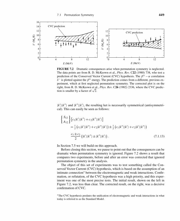
7.1 Permutation Symmetry 449
CVC prediction
0
2
4
6
8
10
12
14
16
δ− (
Mn/E
)
0 4 8 12
E (MeV)
CVC prediction
0 4 8 12
E (MeV)
δ− (
Mn/E
)
0
2
4
6
8
10
12
FIGURE 7.2 Dramatic consequences arise when permutation symmetry is neglected.The data points are from R. D. McKeown et al., Phys. Rev. C22 (1980) 738, who test aprediction of the Conserved Vector Current (CVC) hypothesis. The β± −α correlationδ− is plotted against the β± energy. The prediction comes from a different, previous ex-periment, which at first neglected permutation symmetry. The corrected plot is on theright, from R. D. McKeown et al., Phys. Rev. C26 (1982) 2336, where the CVC predic-tion is smaller by a factor of
√2.
|k ′〉|k ′′〉 and |k ′′〉|k ′〉, the resulting ket is necessarily symmetrical (antisymmetri-cal). This can easily be seen as follows:{
S12
A12
}[c1|k ′〉|k ′′〉+ c2|k ′′〉|k ′〉]
= 12
(c1|k ′〉|k ′′〉+ c2|k ′′〉|k ′〉)± 1
2
(c1|k ′′〉|k ′〉+ c2|k ′〉|k ′′〉)
c1 ± c2
2
(|k ′〉|k ′′〉± |k ′′〉|k ′〉) . (7.1.13)
In Section 7.5 we will build on this approach.Before closing this section, we pause to point out that the consequences can be
dramatic when permutation symmetry is ignored. Figure 7.2 shows a result thatcompares two experiments, before and after an error was corrected that ignoredpermutation symmetry in the analysis.
The object of this set of experiments was to test something called the Con-served Vector Current (CVC) hypothesis, which is based on the assumption of anintimate connection∗ between the electromagnetic and weak interactions. Confir-mation, or refutation, of the CVC hypothesis was a high priority, and this exper-iment was one of the most precise tests. The initial result, shown on the left inFigure 7.2, was less than clear. The corrected result, on the right, was a decisiveconfirmation of CVC.
∗The CVC hypothesis predates the unification of electromagnetic and weak interactions in whattoday is referred to as the Standard Model.
450 Chapter 7 Identical Particles
The data points in Figure 7.2, which are identical for the left- and right-handplots, are from a measurement of the beta decays of 8Li and 8B, each of whichled to a final state with two (identical) α particles, through an excited state of 8Be.That is,
8Li → 8Be∗ + e− + νe (7.1.14a)
and 8B → 8Be∗ + e+ + νe followed by (7.1.14b)8Be∗ → α+α. (7.1.14c)
The experiment determines δ−, the correlation in direction between the e±- andα-directions for the two beta decays, as a function of e± energy. The result of thismeasurement is published as R. D. McKeown et al., Phys. Rev. C22 (1980) 738.
The hatched area shows the CVC prediction derived from an earlier experi-ment, published as T. J. Bowles and G. T. Garvey, Phys. Rev. C18 (1978) 1447.This work measured the reaction
α+α→ 8Be∗ followed by (7.1.15a)8Be∗ → 8Be +γ . (7.1.15b)
This process is rather the inverse of that in (7.1.14) and proceeds through an elec-tromagnetic interaction instead of the weak interaction. Deriving the CVC predic-tion from this result requires that the αα wave function be symmetrized, but thiswas neglected at first, for the plot shown on the left of Figure 7.2. Some time later,this error was corrected for the missing factor of
√2, and the plot on the right was
published, showing much better agreement between prediction and measurement.
7.2 SYMMETRIZATION POSTULATE
So far we have not discussed whether nature takes advantage of totally symmetri-cal or totally antisymmetrical states. It turns out∗ that systems containing N iden-tical particles are either totally symmetrical under the interchange of any pair,in which case the particles are said to satisfy Bose-Einstein (B-E) statistics andhence are known as bosons, or totally antisymmetrical, in which case the particlesare said to satisfy Fermi-Dirac (F-D) statistics and hence are known as fermions.Thus
Pij |N identical bosons〉 = +|N identical bosons〉 (7.2.1a)
Pij |N identical fermions〉 = −|N identical fermions〉, (7.2.1b)
∗To be sure, there is an important subtlety that relies on our living in three-dimensional space. Itis possible to have objects, called anyons, that have a continuum of statistical properties spanningthe range between fermions and bosons, if they are constrained to two spatial dimensions. Theliterature on this subject is fascinating but scattered. The reader is referred to two early papers:F. Wilczek, “Quantum Mechanics of Fractional-Spin Particles,” Phys. Rev. Lett. 49 (1982) 957and M. V. N. Murthy, J. Law, M. Brack, and R. K. Bhaduri, “Quantum Spectrum of Three Anyonsin an Oscillator Potential,” Phys. Rev. Lett. 67 (1991) 817.
7.2 Symmetrization Postulate 451
where Pij is the permutation operator that interchanges the ith and the jth parti-cles, with i and j arbitrary. It is an empirical fact that a mixed symmetry does notoccur.
Even more remarkable is that there is a connection between the spin of a par-ticle and the statistics obeyed by it:
Half-integer-spin particles are fermions; (7.2.2a)
Integer-spin particles are bosons. (7.2.2b)
Here particles can be composite; for example, a 3He nucleus is a fermion just asthe e− or the proton is; a 4He nucleus is a boson just as the π meson or the Z0
gauge boson is.This spin-statistics connection is, as far as we know, an exact law of nature
with no known exceptions. In the framework of nonrelativistic quantum mechan-ics, this principle must be accepted as an empirical postulate. In the relativisticquantum theory, however, it can be proved that half-integer-spin particles cannotbe bosons and integer-spin particles cannot be fermions.
An immediate consequence of the electron being a fermion is that the electronmust satisfy the Pauli exclusion principle, which states that no two electronscan occupy the same state. This follows because a state like |k ′〉|k ′〉 is necessarilysymmetrical, which is not possible for a fermion. As is well known, the Pauliexclusion principle is the cornerstone of atomic and molecular physics, as well asthe whole of chemistry. To illustrate the dramatic differences between fermionsand bosons, let us consider two particles, each of which can occupy only twostates, characterized by k ′ and k ′′. For a system of two fermions, we have nochoice; there is only one possibility:
1√2
(|k ′〉|k ′′〉− |k ′′〉|k ′〉) . (7.2.3)
For bosons there are three states possible:
|k ′〉|k ′〉, |k ′′〉|k ′′〉, 1√2
(|k′〉|k ′′〉+ |k ′′〉|k ′〉) . (7.2.4)
In contrast, for “classical” particles satisfying Maxwell-Boltzmann (M-B) statis-tics with no restriction on symmetry, we have altogether four independent states:
|k ′〉|k ′′〉, |k ′′〉|k ′〉, |k ′〉|k ′〉, |k ′′〉|k ′′〉. (7.2.5)
We see that in the fermion case, it is impossible for both particles to occupy thesame state. In the boson case, for two out of the three allowed kets, both particlesoccupy the same state. In the classical (M-B) statistics case, both particles occupythe same state for two out of the four allowed kets. In this sense fermions are theleast sociable; they avoid each other to make sure that they are not in the samestate; in contrast, bosons are the most sociable, they really love to be in the samestate, even more so than classical particles obeying M-B statistics.
452 Chapter 7 Identical Particles
The difference between fermions and bosons shows up most dramatically atlow temperatures; a system made up of bosons, such as liquid 4He, exhibits a ten-dency for all particles to get down to the same ground state at extremely low tem-peratures.∗ This is known as Bose-Einstein condensation, a feature not sharedby a system made up of fermions.
7.3 TWO-ELECTRON SYSTEM
Let us now consider specifically a two-electron system. The eigenvalue of thepermutation operator is necessarily −1. Suppose the base kets we use may bespecified by x1, x2, ms1, and ms2, where ms1 and ms2 stand for the spin-magneticquantum numbers of electron 1 and electron 2, respectively.
We can express the wave function for a two-electron system as a linear combi-nation of the state ket with eigenbras of x1, x2, ms1, and ms2 as follows:
ψ =∑ms1
∑ms2
C (ms1,ms2) 〈x1,ms1;x2,ms2|α〉. (7.3.1)
If the Hamiltonian commutes with S2tot,[
S2tot, H
]= 0, (7.3.2)
then the energy eigenfunction is expected to be an eigenfunction of S2tot, and if ψ
is written as
ψ = φ(x1,x2)χ , (7.3.3)
then the spin function χ is expected to be one of the following:
χ(ms1,ms2) =
⎧⎪⎪⎪⎪⎪⎨⎪⎪⎪⎪⎪⎩
χ++1√2(χ+− +χ−+)
χ−−
⎫⎪⎪⎬⎪⎪⎭ triplet (symmetrical)
1√2(χ+− −χ−+) singlet (antisymmetrical),
(7.3.4)
where χ+− corresponds to χ(ms1 = 12 ,ms2 = − 1
2 ). Notice that the triplet spinfunctions are all symmetrical; this is reasonable because the ladder operator S1−+S2− commutes with P12, and the |+〉|+〉 state is even under P12.
We note
〈x1,ms1;x2,ms2|P12|α〉 = 〈x2,ms2;x1,ms1|α〉. (7.3.5)
∗The visual behavior of liquid helium, as it is cooled past the critical temperature, is striking.Various video examples can be seen at http://www.youtube.com/, including a classic physicsdemonstration movie, “Liquid Helium II: The Superfluid,” by A. Leitner, from 1963. See also thesite http://alfredleitner.com/.
7.3 Two-Electron System 453
Fermi-Dirac statistics thus requires
〈x1,ms1;x2,ms2|α〉 = −〈x2,ms2;x1,ms1|α〉. (7.3.6)
Clearly, P12 can be written as
P12 = P (space)12 P (spin)
12 (7.3.7)
where P (space)12 just interchanges the position coordinate, while P (spin)
12 just inter-
changes the spin states. It is amusing that we can express P (spin)12 as
P (spin)12 = 1
2
(1 + 4
h2 S1 · S2
), (7.3.8)
which follows because
S1 · S2 =
⎧⎪⎪⎪⎨⎪⎪⎪⎩h2
4(triplet)
−3h2
4(singlet).
(7.3.9)
It follows from (7.3.3) that letting
|α〉 → P12|α〉 (7.3.10)
amounts to
φ(x1,x2) → φ(x2,x1), χ(ms1,ms2) → χ(ms2,ms1). (7.3.11)
This together with (7.3.6) implies that if the space part of the wave function issymmetrical (antisymmetrical), the spin part must be antisymmetrical (symmetri-cal). As a result, the spin triplet state has to be combined with an antisymmetricalspace function, and the spin singlet state has to be combined with a symmetricalspace function.
The space part of the wave function φ(x1,x2) provides the usual probabilisticinterpretation. The probability for finding electron 1 in a volume element d3x1centered around x1 and electron 2 in a volume element d3x2 is
|φ(x1,x2)|2d3x1d3x2. (7.3.12)
To see the meaning of this more closely, let us consider the specific case where themutual interaction between the two electrons [for example, Vpair(|x1−x2|),S1· S2]can be ignored. If there is no spin dependence, the wave equation for the energyeigenfunction ψ [see (7.1.9)],[
−h2
2m∇2
1 − h2
2m∇2
2 + Vext(x1) + Vext(x2)
]ψ = Eψ , (7.3.13)
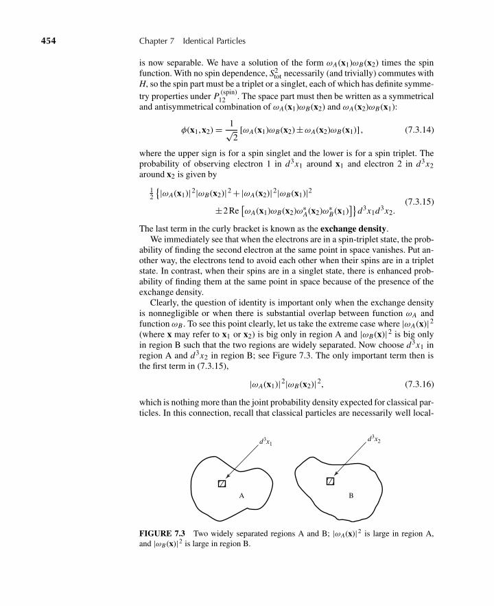
454 Chapter 7 Identical Particles
is now separable. We have a solution of the form ωA(x1)ωB(x2) times the spinfunction. With no spin dependence, S2
tot necessarily (and trivially) commutes withH, so the spin part must be a triplet or a singlet, each of which has definite symme-try properties under P (spin)
12 . The space part must then be written as a symmetricaland antisymmetrical combination of ωA(x1)ωB(x2) and ωA(x2)ωB (x1):
φ(x1,x2) = 1√2
[ωA(x1)ωB(x2) ±ωA(x2)ωB (x1)] , (7.3.14)
where the upper sign is for a spin singlet and the lower is for a spin triplet. Theprobability of observing electron 1 in d3x1 around x1 and electron 2 in d3x2around x2 is given by
12
{|ωA(x1)|2|ωB(x2)|2 +|ωA(x2)|2|ωB(x1)|2±2Re
[ωA(x1)ωB(x2)ω∗
A(x2)ω∗B (x1)
]}d3x1d3x2.
(7.3.15)
The last term in the curly bracket is known as the exchange density.We immediately see that when the electrons are in a spin-triplet state, the prob-
ability of finding the second electron at the same point in space vanishes. Put an-other way, the electrons tend to avoid each other when their spins are in a tripletstate. In contrast, when their spins are in a singlet state, there is enhanced prob-ability of finding them at the same point in space because of the presence of theexchange density.
Clearly, the question of identity is important only when the exchange densityis nonnegligible or when there is substantial overlap between function ωA andfunction ωB . To see this point clearly, let us take the extreme case where |ωA(x)|2
(where x may refer to x1 or x2) is big only in region A and |ωB (x)|2 is big onlyin region B such that the two regions are widely separated. Now choose d3x1 inregion A and d3x2 in region B; see Figure 7.3. The only important term then isthe first term in (7.3.15),
|ωA(x1)|2|ωB (x2)|2, (7.3.16)
which is nothing more than the joint probability density expected for classical par-ticles. In this connection, recall that classical particles are necessarily well local-
A B
d3x1d3x2
FIGURE 7.3 Two widely separated regions A and B; |ωA(x)|2 is large in region A,and |ωB (x)|2 is large in region B.
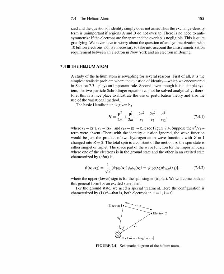
7.4 The Helium Atom 455
ized and the question of identity simply does not arise. Thus the exchange-densityterm is unimportant if regions A and B do not overlap. There is no need to anti-symmetrize if the electrons are far apart and the overlap is negligible. This is quitegratifying. We never have to worry about the question of antisymmetrization with10 billion electrons, nor is it necessary to take into account the antisymmetrizationrequirement between an electron in New York and an electron in Beijing.
7.4 THE HELIUM ATOM
A study of the helium atom is rewarding for several reasons. First of all, it is thesimplest realistic problem where the question of identity—which we encounteredin Section 7.3—plays an important role. Second, even though it is a simple sys-tem, the two-particle Schrödinger equation cannot be solved analytically; there-fore, this is a nice place to illustrate the use of perturbation theory and also theuse of the variational method.
The basic Hamiltonian is given by
H = p21
2m+ p2
2
2m− 2e2
r1− 2e2
r2+ e2
r12, (7.4.1)
where r1 ≡ |x1|, r2 ≡ |x2|, and r12 ≡ |x1 −x2|; see Figure 7.4. Suppose the e2/r12-term were absent. Then, with the identity question ignored, the wave functionwould be just the product of two hydrogen atom wave functions with Z = 1changed into Z = 2. The total spin is a constant of the motion, so the spin state iseither singlet or triplet. The space part of the wave function for the important casewhere one of the electrons is in the ground state and the other in an excited statecharacterized by (nlm) is
φ(x1,x2) = 1√2
[ψ100(x1)ψnlm (x2) ± ψ100(x2)ψnlm (x1)] , (7.4.2)
where the upper (lower) sign is for the spin singlet (triplet). We will come back tothis general form for an excited state later.
For the ground state, we need a special treatment. Here the configuration ischaracterized by (1s)2—that is, both electrons in n = 1, l = 0.
x1
x2γ
Electron 1
Electron 2
r12
Nucleus of charge + 2⏐e⏐
FIGURE 7.4 Schematic diagram of the helium atom.
456 Chapter 7 Identical Particles
The space function must then necessarily be symmetrical, and only the spinsinglet function is allowed. So we have
ψ100(x1)ψ100(x2)χsinglet = Z3
πa30
e−Z (r1 +r2)/a0χ (7.4.3)
with Z = 2. Not surprisingly, this “unperturbed” wave function gives
E = 2 ×4
(− e2
2a0
)= −108.8 eV (7.4.4)
for the ground-state energy, which is about 30% larger than the experimentalvalue.
This is just the starting point of our investigation because in obtaining theabove form (7.4.3), we have completely ignored the last term in (7.4.1) that de-scribes the interaction between the two electrons. One way to approach the prob-lem of obtaining a better energy value is to apply first-order perturbation theoryusing (7.4.3) as the unperturbed wave function and e2/r12 as the perturbation. Weobtain
�(1s)2 =⟨
e2
r12
⟩(1s)2
=∫∫
Z6
π2a60
e−2Z (r1 +r2)/a0e2
r12d3x1d3x2. (7.4.5)
To carry out the indicated integration, we first note
1
r12= 1√
r21 + r2
2 − 2r1r2 cosγ=
∞∑l =0
r l<
r l +1>
Pl (cosγ ), (7.4.6)
where r> (r<) is the larger (smaller) of r1 and r2, and γ is the angle betweenx1 and x2. The angular integration is easily performed by expressing Pl (cosγ )in terms of Y m
l (θ1,φ1) and Y ml (θ2,φ2), using the addition theorem of spherical
harmonics. (See, for example, Section 12.8 of Arfken and Weber 1995.) We have
Pl (cosγ ) = 4π
2 l + 1
l∑m =−1
Y m∗l (θ1,φ1)Y m
l (θ2,φ2). (7.4.7)
The angular integration is now trivial:∫Y m
l (θi ,φi ) d�i = 1√4π
(4π)δl 0δm 0. (7.4.8)
The radial integration is elementary (but involves tedious algebra!); it leads to∫ ∞
0
[∫ r1
0
1
r1e−(2Z/a0)(r1 +r2)r2
2 dr2 +∫ ∞
r1
1
r2e−(2Z/a0)(r1 +r2 )r2
2 dr2
]r2
1 dr1
= 5
128
a50
Z5 .
(7.4.9)
7.4 The Helium Atom 457
Combining everything, we have (for Z = 2)
�(1s)2 =(
Z6e2
π2a60
)4π(
√4π)2
(5
128
)(a5
0
Z5
)=(
5
2
)(e2
2a0
). (7.4.10)
Adding this energy shift to (7.4.4), we have
Ecal =(
−8 + 5
2
)(e2
2a0
)� −74.8eV. (7.4.11)
Compare this with the experimental value,
Eexp = −78.8eV. (7.4.12)
This is not bad, but we can do better! We propose to use the variational methodwith Z, which we call Zeff, as a variational parameter. The physical reason for thischoice is that the effective Z seen by one of the electrons is smaller than 2 becausethe positive charge of 2 units at the origin (see Figure 7.4) is “screened” by thenegatively charged cloud of the other electron; in other words, the other electrontends to neutralize the positive charge due to the helium nucleus at the center. Forthe normalized trial function we use
〈x1,x2|0〉 =(
Z3eff
πa30
)e−Zeff(r1 +r2)/a0 . (7.4.13)
From this we obtain
H =⟨
0
∣∣∣∣∣ p21
2m+ p2
2
2m
∣∣∣∣∣ 0⟩
−⟨0
∣∣∣∣ Ze2
r1+ Ze2
r2
∣∣∣∣ 0⟩+ ⟨0
∣∣∣∣ e2
r12
∣∣∣∣ 0⟩
=(
2Z2
eff
2− 2Z Zeff + 5
8Zeff
)(e2
a0
).
(7.4.14)
We easily see that the minimization of H is at
Zeff = 2 − 516 = 1.6875. (7.4.15)
This is smaller than 2, as anticipated. Using this value for Zeff we get
Ecal = −77.5eV, (7.4.16)
which is already very close, considering the crudeness of the trial wave function.Historically, this achievement was considered to be one of the earliest signs that
Schrödinger’s wave mechanics was on the right track. We cannot get this kind ofnumber by the purely algebraic (operator) method. The helium calculation wasfirst done by A. Unsöld in 1927.∗
∗A. Unsöld, Ann. Phys. 82 (1927) 355.
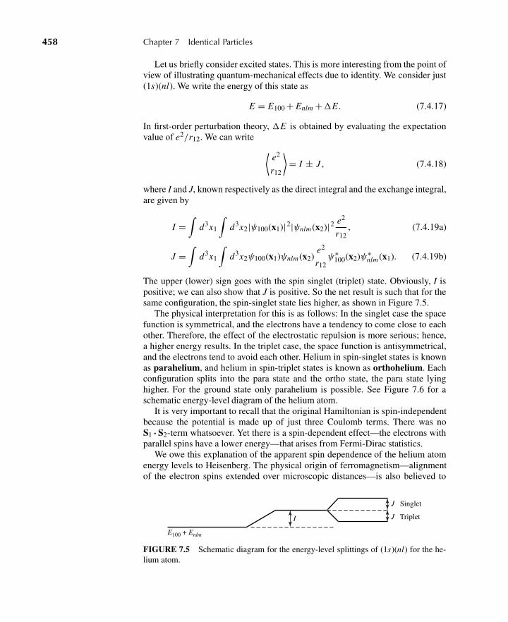
458 Chapter 7 Identical Particles
Let us briefly consider excited states. This is more interesting from the point ofview of illustrating quantum-mechanical effects due to identity. We consider just(1s)(nl). We write the energy of this state as
E = E100 + Enlm +�E . (7.4.17)
In first-order perturbation theory, �E is obtained by evaluating the expectationvalue of e2/r12. We can write ⟨
e2
r12
⟩= I ± J , (7.4.18)
where I and J, known respectively as the direct integral and the exchange integral,are given by
I =∫
d3x1
∫d3x2|ψ100(x1)|2|ψnlm (x2)|2 e2
r12, (7.4.19a)
J =∫
d3x1
∫d3x2ψ100(x1)ψnlm (x2)
e2
r12ψ∗
100(x2)ψ∗nlm (x1). (7.4.19b)
The upper (lower) sign goes with the spin singlet (triplet) state. Obviously, I ispositive; we can also show that J is positive. So the net result is such that for thesame configuration, the spin-singlet state lies higher, as shown in Figure 7.5.
The physical interpretation for this is as follows: In the singlet case the spacefunction is symmetrical, and the electrons have a tendency to come close to eachother. Therefore, the effect of the electrostatic repulsion is more serious; hence,a higher energy results. In the triplet case, the space function is antisymmetrical,and the electrons tend to avoid each other. Helium in spin-singlet states is knownas parahelium, and helium in spin-triplet states is known as orthohelium. Eachconfiguration splits into the para state and the ortho state, the para state lyinghigher. For the ground state only parahelium is possible. See Figure 7.6 for aschematic energy-level diagram of the helium atom.
It is very important to recall that the original Hamiltonian is spin-independentbecause the potential is made up of just three Coulomb terms. There was noS1 · S2-term whatsoever. Yet there is a spin-dependent effect—the electrons withparallel spins have a lower energy—that arises from Fermi-Dirac statistics.
We owe this explanation of the apparent spin dependence of the helium atomenergy levels to Heisenberg. The physical origin of ferromagnetism—alignmentof the electron spins extended over microscopic distances—is also believed to
E100 + Enlm
I
J Singlet
J Triplet
FIGURE 7.5 Schematic diagram for the energy-level splittings of (1s)(nl) for the he-lium atom.
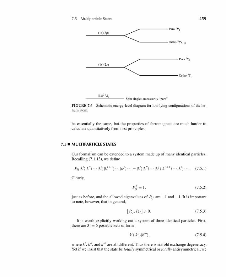
7.5 Multiparticle States 459
(1s)(2p)
(1s)(2s)
(1s)2 1S0
Para 1P1
Para 1S0
Ortho 3P2,1,0
Ortho 3S1
Spin singlet, necessarily “para”
FIGURE 7.6 Schematic energy-level diagram for low-lying configurations of the he-lium atom.
be essentially the same, but the properties of ferromagnets are much harder tocalculate quantitatively from first principles.
7.5 MULTIPARTICLE STATES
Our formalism can be extended to a system made up of many identical particles.Recalling (7.1.13), we define
Pij |k ′〉|k ′′〉 · · · |ki 〉|ki +1〉 · · · |k j 〉 · · · = |k ′〉|k ′′〉 · · · |k j 〉|ki +1〉 · · · |ki 〉 · · · . (7.5.1)
Clearly,
P2i j = 1, (7.5.2)
just as before, and the allowed eigenvalues of Pij are +1 and −1. It is importantto note, however, that in general, [
Pij , Pkl] �= 0. (7.5.3)
It is worth explicitly working out a system of three identical particles. First,there are 3! = 6 possible kets of form
|k ′〉|k ′′〉|k ′′′〉, (7.5.4)
where k ′, k ′′, and k′′′ are all different. Thus there is sixfold exchange degeneracy.Yet if we insist that the state be totally symmetrical or totally antisymmetrical, we
460 Chapter 7 Identical Particles
can form only one linear combination each. Explicitly, we have
|k ′k ′′k ′′′〉± ≡ 1√6
{|k′〉|k ′′〉|k ′′′〉± |k ′′〉|k ′〉|k ′′′〉
+|k ′′〉|k ′′′〉|k ′〉± |k ′′′〉|k ′′〉|k ′〉+ |k ′′′〉|k ′〉|k ′′〉± |k ′〉|k ′′′〉|k ′′〉} . (7.5.5)
These are both simultaneous eigenkets of P12, P23, and P13. We remarked thatthere are altogether six independent state kets. It therefore follows that there arefour independent kets that are neither totally symmetrical nor totally antisymmet-rical. We could also introduce the operator P123 by defining
P123(|k′〉|k ′′〉|k ′′′〉) = |k ′′〉|k ′′′〉|k ′〉. (7.5.6)
Note that P123 = P12 P13 because
P12 P13(|k′〉|k ′′〉|k ′′′〉)= P12
(|k ′′′〉|k ′′〉|k ′〉)= |k ′′〉|k ′′′〉|k ′〉. (7.5.7)
In writing (7.5.5) we assumed that k′, k ′′, and k ′′′ are all different. If two of thethree indices coincide, it is impossible to have a totally antisymmetrical state. Thetotally symmetrical state is given by
|k ′k ′k ′′〉+ = 1√3
(|k′〉|k ′〉|k ′′〉+ |k ′〉|k ′′〉|k ′〉+ |k ′′〉|k ′〉|k ′〉) , (7.5.8)
where the normalization factor is understood to be√
2!/3!. For more generalcases, we have a normalization factor√
N1!N2! · Nn!
N!, (7.5.9)
where N is the total number of particles and Ni is the number of times |k(i)〉occurs.
Second Quantization
A different approach to keeping track of multiparticle states, which in fact beginsto lay a foundation for quantum field theory, reexamines the way in which wedefine the state vector. This approach is known as∗ second quantization.
Define a mutliparticle state vector as
|n1,n2, . . . ,ni , . . .〉, (7.5.10)
∗The term second quantization was apparently coined in the early days of trying to extend quan-tum mechanics into field theory. The idea was that wave functions were to be turned into oper-ators, which in turn were subject to their own canonical quantization rules. Hence, quantizationwas enforced a “second” time. See, for example, Section III.12.1 in Heitler (1954).
7.5 Multiparticle States 461
where the ni specify the number of particles with eigenvalue ki for some operator.Although we take it as a perfectly valid nomenclature for a state vector, it is amember of a new kind of vector space, called “Fock space,” in which we need tobuild in the necessary permutation symmetry.
A word of caution is in order. Our Fock space (or “occupation number”) no-tation for state vectors itself makes an important assumption, namely that thereindeed exists a basis of noninteracting states. Interactions between particles canin fact, in principle, affect their very nature. Whether or not, starting on this as-sumption, we can make a self-consistent theory that itself accurately describes na-ture can only be tested by experiment. See the discussions in Landau (1996) andMerzbacher (1998). We will set this question aside, however, and move ahead atfull steam.
Let us now build a framework for a theory of many-particle systems usingstates in Fock space. We begin this task by recognizing two special cases of statesin Fock space. The first of these is
|0,0, . . . ,0, . . .〉 ≡ |0〉, (7.5.11)
for which there are no particles in any single-particle states. This state is calledthe “vacuum” and is, as usual, normalized to unity. The second special case is
|0,0, . . . ,ni = 1, . . .〉 ≡ |ki 〉, (7.5.12)
which is the state in which there is exactly one particle in the state with eigenvalueki . Of course, this is just the single-particle state that has dominated our discussionof quantum mechanics, prior to this chapter.
Now we need to learn how to build multiparticle states and then make surethat this building process respects permutation symmetry. In an obvious nod tothe creation and annihilation operators that we first encountered in Section 2.3,we define a “field operator” a†
i that increases by one the number of particles inthe state with eigenvalue ki —that is
a†i |n1,n2, . . . ,ni , . . .〉 ∝ |n1,n2, . . . ,ni + 1, . . .〉, (7.5.13)
where a normalization criterion will be used later to determine the proportionalityconstant. We postulate that the action of the particle creation operator a†
i on thevacuum is to create a properly normalized single-particle state, namely
a†i |0〉 = |ki 〉. (7.5.14)
This leads us to write
1 = 〈ki |ki〉 = [〈0|ai ][a†
i |0〉]
= 〈0|[aia
†i |0〉
]= 〈0|ai |ki 〉, (7.5.15)
which implies that
ai |ki 〉 = |0〉 (7.5.16)
462 Chapter 7 Identical Particles
so that ai acts as a particle annihilation operator. We conclude with the followingpostulates for the particle annihilation operator:
ai |n1,n2, . . . ,ni , . . .〉 ∝ |n1,n2, . . . ,ni − 1, . . .〉 (7.5.17)
ai |0〉 = 0 (7.5.18)
ai |k j 〉 = 0 if i �= j , (7.5.19)
where an economy of notation lets us combine (7.5.16) and (7.5.19) into
ai |k j 〉 = δi j |0〉. (7.5.20)
These are enough postulates to fully define the field operators ai , short of actuallyincorporating permutation symmetry.
The act of permuting two particles, one for the other, is most easily seen byputting the “first” particle in state |ki〉 and then the “second” particle in state |k j 〉,and comparing to what happens when we reverse the order in which these statesare populated. That is, we expect that, for a two-particle state,
a†i a†
j |0〉 = ±a†j a
†i |0〉, (7.5.21)
where the + (−) sign is for bosons (fermions). Applying this same logic to particleexchange in multiparticle states, we are led to
a†i a†
j − a†j a
†i = [a†
i ,a†j ] = 0 Bosons (7.5.22a)
a†i a†
j + a†j a
†i = {a†
i ,a†j } = 0 Fermions (7.5.22b)
where we make use of the “anticommutator” {A, B} ≡ AB + B A. Simply takingthe adjoint of these equations tells us that
[ai ,a j ] = 0 Bosons (7.5.23a)
{ai ,a j } = 0 Fermions (7.5.23b)
Note that the Pauli exclusion principle is automatically built into our formalism,since (7.5.22b) implies that a†
i a†i = 0 for some single-particle state |ki 〉.
Now what about the commutation rules for ai and a†j ? We would like to define
a “number operator” Ni = a†i ai that would count the number of particles in the
single-particle state |ki 〉. Our experience from Section 2.3 shows that this wouldbe possible if we had [ai ,a
†i ] = 1. In fact, a self-consistent picture of both bosons
and fermions can be built in just this way, by replacing commutators with anti-commutators. The complete algebra is summarized in Table 7.1. For both bosonsand fermions, we can define the operator
N =∑
i
a†i ai , (7.5.24)
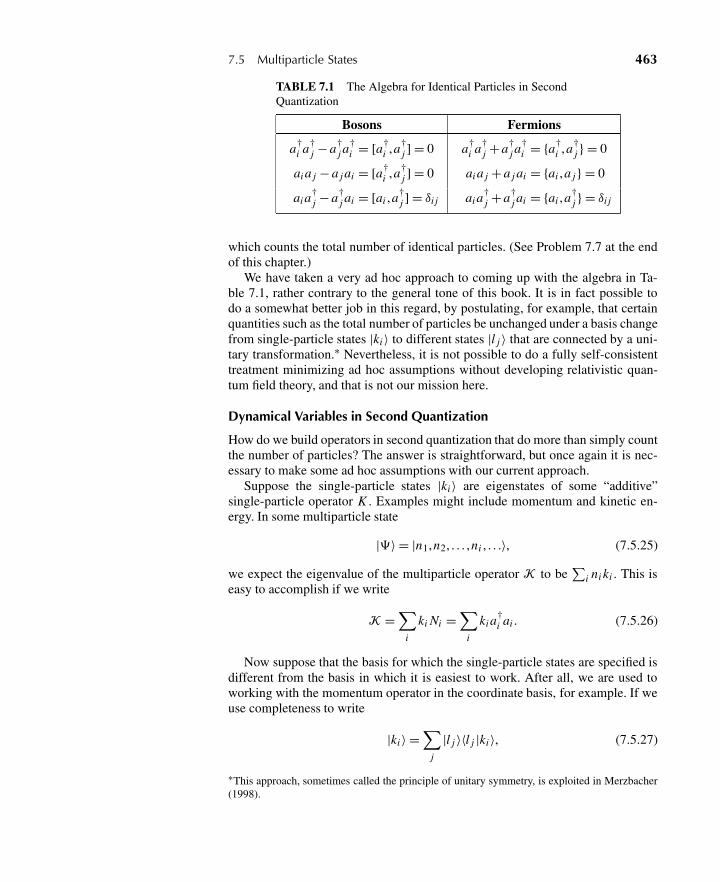
7.5 Multiparticle States 463
TABLE 7.1 The Algebra for Identical Particles in SecondQuantization
Bosons Fermions
a†i a†
j − a†j a
†i = [a†
i ,a†j ] = 0 a†
i a†j + a†
j a†i = {a†
i ,a†j } = 0
ai a j − a j ai = [a†i ,a†
j ] = 0 ai a j + a j ai = {ai ,a j } = 0
ai a†j − a†
j ai = [ai ,a†j ] = δi j ai a
†j + a†
j ai = {ai ,a†j } = δi j
which counts the total number of identical particles. (See Problem 7.7 at the endof this chapter.)
We have taken a very ad hoc approach to coming up with the algebra in Ta-ble 7.1, rather contrary to the general tone of this book. It is in fact possible todo a somewhat better job in this regard, by postulating, for example, that certainquantities such as the total number of particles be unchanged under a basis changefrom single-particle states |ki 〉 to different states |l j 〉 that are connected by a uni-tary transformation.∗ Nevertheless, it is not possible to do a fully self-consistenttreatment minimizing ad hoc assumptions without developing relativistic quan-tum field theory, and that is not our mission here.
Dynamical Variables in Second Quantization
How do we build operators in second quantization that do more than simply countthe number of particles? The answer is straightforward, but once again it is nec-essary to make some ad hoc assumptions with our current approach.
Suppose the single-particle states |ki〉 are eigenstates of some “additive”single-particle operator K . Examples might include momentum and kinetic en-ergy. In some multiparticle state
|!〉 = |n1,n2, . . . ,ni , . . .〉, (7.5.25)
we expect the eigenvalue of the multiparticle operator K to be∑
i ni ki . This iseasy to accomplish if we write
K =∑
i
ki Ni =∑
i
ki a†i ai . (7.5.26)
Now suppose that the basis for which the single-particle states are specified isdifferent from the basis in which it is easiest to work. After all, we are used toworking with the momentum operator in the coordinate basis, for example. If weuse completeness to write
|ki 〉 =∑
j
|l j 〉〈l j |ki 〉, (7.5.27)
∗This approach, sometimes called the principle of unitary symmetry, is exploited in Merzbacher(1998).
464 Chapter 7 Identical Particles
then it makes sense to postulate that
a†i =
∑j
b†j 〈l j |ki 〉, (7.5.28a)
which implies that
ai =∑
j
〈ki |l j 〉b j , (7.5.28b)
where the operators b†j and b j create and annihilate particles in the single-particle
states |l j 〉. With these assignments, acting on the vacuum state (7.5.11) with(7.5.28a) yields (7.5.27).
Equations 7.5.28 give us what we need to change the basis for our dynamicalsingle-particle operator. We have
K =∑
i
ki
∑mn
b†m〈lm |ki 〉〈ki |ln〉bn
=∑mn
b†mbn
∑i
〈lm |ki 〉ki 〈ki |ln〉
=∑mn
b†mbn〈lm |
[K∑
i
|ki 〉〈ki |]
|ln〉
or K =∑mn
b†mbn〈lm |K |ln〉. (7.5.29)
This general form is suitable for writing down a second-quantized version of anyadditive single-particle operator. Examples include not only momentum and ki-netic energy but also any “external” potential-energy function that acts individ-ually on each of the particles. All that matters is that the particles do not inter-act with each other. In the case of bosons, essentially all the particles may findthemselves in the lowest energy level of such a potential well, so long as thetemperature is low enough. (Experimentally, this phenomenon is referred to as aBose-Einstein condensate.)
Fermions would behave differently, however. The Pauli exclusion principlewill force the particles to populate increasingly higher energy levels in the well.For a system with a very large number of fermions, the total energy of the groundstate could be enormous. The highest populated energy level (known as the “Fermienergy”) might easily be much larger than the thermal energy ∼ kT . A classic ex-ample is a white dwarf star, a very dense object consisting basically of carbonatoms. The electrons in a white dwarf are, to a good approximation, bound in apotential well. The Fermi level is very high, much larger than the thermal energyfor a temperature of tens of millions of kelvins.
Many-particle systems, however, present a new situation, namely the inevitablepossibility that the particles actually interact among themselves. Once again, we
7.5 Multiparticle States 465
postulate an additive operator—that is, one in which the individual two-particleinteractions add up independently. Let the symmetrical real matrix Vij specifythe two-particle eigenvalue for an interaction between particles in single-particlestates |ki 〉 and |k j 〉. Then the second-quantized version of this operator becomes
V = 1
2
∑i �= j
Vi j Ni N j + 1
2
∑i
Vii Ni (Ni − 1). (7.5.30)
The first term sums up all of the two-particle interactions, where the factor of 1/2is necessary because this form double-counts pairs. The second term accounts forall “self-interactions” for particles in the same state; there are n(n − 1)/2 waysto take n things two at a time. The requirement that Vij be real ensures that V isHermitian.
The part of the self-energy term in (7.5.30) containing N2i exactly represents
the parts of the sum in the first term removed by specifying i �= j . Therefore, wecan combine this more neatly as
V = 1
2
∑i j
Vi j(Ni N j − Niδi j
)= 1
2
∑i j
Vi j�i j , (7.5.31)
where �i j ≡ Ni N j − Niδi j is called the pair distribution operator. Furthermore,we use Table 7.1 to write
�i j = a†i ai a
†j a j − a†
i aiδi j
= a†i
(δi j ± a†
j ai
)a j − a†
i aiδi j
= ±a†i a†
j ai a j
or �i j = (±)(±)a†i a†
j a j ai , (7.5.32)
where we used (7.5.23) to reverse the order of the last two factors. This allows usto rewrite (7.5.30) as
V = 1
2
∑i j
Vi j a†i a†
j a j ai . (7.5.33)
This sequence of creation and annihilation operators—first one particle is annihi-lated, then another, and then they are created in reverse order—is called “normalordering.” Note that we see explicitly from (7.5.22b) or (7.5.23b) that there is nocontribution from diagonal elements of V for fermions.
We can use (7.5.28) to rewrite (7.5.33) in a different basis. We have
V = 1
2
∑mnpq
〈mn|V |pq〉b†mb†
nbqbp, (7.5.34)
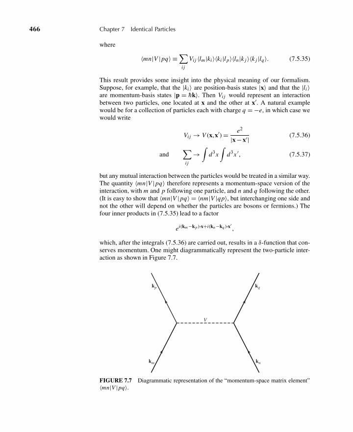
466 Chapter 7 Identical Particles
where
〈mn|V |pq〉 ≡∑
i j
Vi j 〈lm |ki〉〈ki |l p〉〈ln |k j 〉〈k j |lq〉. (7.5.35)
This result provides some insight into the physical meaning of our formalism.Suppose, for example, that the |ki〉 are position-basis states |x〉 and that the |li 〉are momentum-basis states |p = hk〉. Then Vij would represent an interactionbetween two particles, one located at x and the other at x′. A natural examplewould be for a collection of particles each with charge q = −e, in which case wewould write
Vij → V (x,x′) = e2
|x − x′| (7.5.36)
and∑
i j
→∫
d3x∫
d3x ′, (7.5.37)
but any mutual interaction between the particles would be treated in a similar way.The quantity 〈mn|V |pq〉 therefore represents a momentum-space version of theinteraction, with m and p following one particle, and n and q following the other.(It is easy to show that 〈mn|V |pq〉 = 〈nm|V |qp〉, but interchanging one side andnot the other will depend on whether the particles are bosons or fermions.) Thefour inner products in (7.5.35) lead to a factor
ei(km−kp)·x+i(kn−kq )·x′,
which, after the integrals (7.5.36) are carried out, results in a δ-function that con-serves momentum. One might diagrammatically represent the two-particle inter-action as shown in Figure 7.7.
V
kp kq
km kn
FIGURE 7.7 Diagrammatic representation of the “momentum-space matrix element”〈mn|V |pq〉.
7.5 Multiparticle States 467
Clearly we are on our way to developing a nonrelativistic version of quantumfield theory. As a specific example, we will treat the quantum-mechanical versionof the noninteracting electromagnetic field shortly. However, we will not pushthe general case beyond this point, as it goes beyond the scope of this book andis treated well in any one of several other books. See, for example, Merzbacher(1998), Landau (1996), and Fetter and Walecka (2003a).
Example: The Degenerate Electron Gas
An excellent example of the principles discussed in this section is the degenerateelectron gas. This is a collection of electrons, interacting with each other throughtheir mutual Coulomb repulsion, bound in some positively charged backgroundmedium. Physical examples include a high-temperature plasma, and even, to someapproximation, bulk metals.
This problem is treated thoroughly in Chapter 1, Section 3 of Fetter andWalecka (2003a). We present the problem and outline its solution here, but theinterested reader is referred to the original reference to fill in the details.
Our task is to find the eigenvalues of the Hamiltonian
H = Hel + Hb + Hel−b (7.5.38)
for a system of N electrons. The electrons interact among themselves accordingto
Hel =∑
i
p2i
2m+ 1
2e2∑
i
∑j �=i
e−μ|xi−x j |
|xi − x j | , (7.5.39)
where we employ a “screened” Coulomb potential but will let μ→ 0 before wefinish the calculation. The energy of the positive background is
Hb = 1
2e2∫
d3x ′∫
d3x ′′ρ(x′)ρ(x′′)e−μ|x′−x′′|
|x′ − x′′| , (7.5.40)
where ρ(x) is the number density of background particle sites. We will assume auniform background, with ρ(x) = N/V for a system of volume V = L3. Then,translating to a variable x ≡ x′ − x′′, (7.5.40) becomes
Hb = 1
2e2(
N
V
)2 ∫d3x ′
∫d3x
e−μ|x|
|x| = 1
2e2 N2
V
4π
μ2 . (7.5.41)
Thus Hb contributes simply an additive constant to the energy. The fact that thisconstant grows without bound as μ→ 0 will not be a problem, as we shall seeshortly. The interaction of the electrons with the constant background is
Hel−b = −e2∑
i
∫d3xρ(x)
e−μ|x−xi |
|x − xi |
= −e2 N
V
∑i
∫d3x
e−μ|x−xi |
|x − xi | = −e2 N2
V
4π
μ2 . (7.5.42)
468 Chapter 7 Identical Particles
Therefore, (7.5.38) becomes
H = −1
2e2 N2
V
4π
μ2+∑
i
p2i
2m+ 1
2e2∑
i
∑j �=i
e−μ|xi−x j |
|xi − x j | . (7.5.43)
The first term in this equation is just a number. The second is a one-body operatorthat we will express simply in terms of operators in second quantization in mo-mentum space. The third term is a two-body operator that will involve a bit morework to write in second quantization.
Writing the kinetic-energy term in (7.5.43) is just a matter of rewriting (7.5.29)for K being the momentum operator p and the |ln〉 being momentum-basis states.Single-particle states are denoted by i = {k,λ}, where λ = ± indicates electronspin. We know that
〈k′λ′|p|kλ〉 = hkδkk′δλλ′ , (7.5.44)
so we have ∑i
p2i
2m⇒ K =
∑kλ
h2k2
2ma†
kλakλ. (7.5.45)
Now we write the potential-energy term in (7.5.43) in second quantization,using (7.5.34) and (7.5.35). Note (7.5.36) and (7.5.37). We have
V = 1
2
∑k1λ1
∑k2λ2
∑k3λ3
∑k4λ4
〈k1λ1k2λ2|V |k3λ3k4λ4〉a†k1λ1
a†k2λ2
ak4λ4ak3λ3 , (7.5.46)
where
〈k1λ1k2λ2|V |k4λ4k3λ3〉 =∫
d3x ′∫
d3x ′′V (x′,x′′)〈k1λ1|x′〉〈x′|k3λ3〉〈k2λ2|x′′〉〈x′′|k4λ4〉
= e2
V 2
∫d3x ′
∫d3x ′′ e−μ|x′−x′′|
|x′ − x′′| e−ik1·x′χ
†λ1
eik3·x′χλ3e−ik2·x′′
χ†λ2
eik4·x′′χλ4
= e2
V 2
∫d3x
∫d3y
e−μy
ye−ik1·x′
δλ1λ3eik3·x′e−ik2·x′′
δλ2λ4eik4·x′′
= e2
V 2δλ1λ4δλ2λ3
∫d3xe−i(k1+k2−k3−k4)·x
∫d3y
e−μy
ye−i(k1−k3)·y
= e2
Vδλ1λ4δλ2λ3δk1+k2,k3+k4
∫d3y
e−μy
ye−i(k1−k3)·y (7.5.47)
using a change of variables x = x′′ and y = x′ −x′′. Finally, we define the momen-tum transfer q ≡ k1 − k3 and find
〈k1λ1k2λ2|V |k3λ3k4λ4〉 = e2
Vδλ1λ4δλ2λ3δk1+k2,k3+k4
4π
q2 +μ2 . (7.5.48)
7.5 Multiparticle States 469
The Kronecker deltas in the spin just ensure that that no spins are flipped bythis interaction, which we expect since the interaction is spin-independent. TheKronecker delta in the wave number ensures that momentum is conserved. Thus(7.5.46) becomes
V = e2
2V
∑k1λ1
∑k2λ2
∑k3
∑k4
δk1+k2,k3+k4
4π
q2 +μ2a†
k1λ1a†
k2λ2ak4λ2ak3λ1 (7.5.49)
after reducing the summations using the spin-conserving Kronecker deltas.An important feature of (7.5.49) becomes apparent if we first redefine k3 ≡ k
and k4 ≡ p. Then the terms of (7.5.49) for which q = 0 become
e2
2V
∑kp
∑λ1λ2
4π
μ2 a†kλ1
a†pλ2
apλ2akλ1 = e2
2V
4π
μ2
∑kλ1
∑pλ2
a†kλ1
akλ1
(a†
pλ2apλ2 − δkpδλ1λ2
)
= e2
2V
4π
μ2(N2 − N), (7.5.50)
where we have made use of the fermion anticommutation relations and the defini-tion of the number operator. The first term in this relation just cancels the first termof (7.5.43). The second term represents an energy −2πe2/μ2V per particle, butthis will vanish in the limit where V = L3 → ∞ while always keeping μ� 1/L.Thus the terms with q = 0 do not contribute, and they cancel the rapidly diverg-ing terms in the Hamiltonian. Indeed, this finally allows us to set the screeningparameter μ= 0 and write the second-quantized Hamiltonian as
H = H0 + H1, (7.5.51a)
where H0 =∑kλ
h2k2
2ma†
kλakλ (7.5.51b)
and H1 = e2
2V
∑kpq
′∑λ1λ2
4π
q2 a†k+q,λ1
a†p−q,λ2
apλ2akλ1 , (7.5.51c)
where the notation�′ indicates that terms with q = 0 are to be omitted. Note thatin the limit we’ve taken, a finite density n = N/V is implicitly assumed.
Finding the eigenvalues of (7.5.51) is a difficult problem, although solutionsare possible. Our approach will be to find the ground-state energy by treating thesecond term as a perturbation on the first. Although reasonable arguments can bemade why this should be a good approximation (see Fetter and Walecka), thosearguments hold only in a particular range of densities. Fortunately, that range ofdensities is relevant to physical systems such as metals, so our approach indeedhas practical interest.
This is a good time to introduce some scaling variables. The density is deter-mined by the interatomic spacing r0, that is,
n = N
V= 4π
3r3
0 , (7.5.52)
470 Chapter 7 Identical Particles
and a natural scale for r0 is the Bohr radius (3.7.55), that is, a0 = h2/me2. Wedefine a dimensionless distance scale rs = r0/a0. Our calculation of the ground-state energy will be as a function of rs .
As an introduction to calculating the expectation value E (0) of the operator H0for the ground state, we discuss the concept of Fermi energy. (Recall the discus-sion on page 464.) Because of the Pauli exclusion principle, electrons will fill theavailable energy levels up to some maximum wavenumber kF . We can relate kFto the total number of electrons by adding up all of the states with k ≤ kF :
N =∑kλ
θ (k − kF )
→ V
(2π)3
∑λ
∫d3k θ (kF − k) = V
3π2 k3F , (7.5.53)
where θ (x) = 0 for x > 0 and unity otherwise. This implies that
kF =(
3π2 N
V
)1/3
=(
9π
4
)1/3 1
r0, (7.5.54)
which shows that kF is about the same size as the inverse interparticle spacing.Now use the same approach to calculate the unperturbed energy E (0). Denoting
the ground state as |F〉, we have
E (0) = 〈F |H0|F〉 = h2
2m
∑kλ
k2θ (k − kF )
→ h2
2m
V
(2π)3
∑λ
∫d3k k2θ (kF − k) = e2
2a0N
3
5
(9π
4
)2/3 1
r2s
. (7.5.55)
Note that e2/2a0 ≈ 13.6 eV, the ground-state energy of the hydrogen atom.The first-order correction to the ground-state energy is
E (1) = 〈F |H1|F〉
= e2
2V
∑kpq
′ ∑λ1λ2
4π
q2〈F |a†
k+q,λ1a†
p−q,λ2apλ2akλ1|F〉. (7.5.56)
The summation is easy to reduce since |F〉 is a collection of single-particle stateswith occupation numbers either zero or one. The only way for the matrix elementin (7.5.56) to be nonzero is if the annihilation and creation operators pair up ap-propriately. Because q �= 0 in the sum, the only way to pair up the operators is by
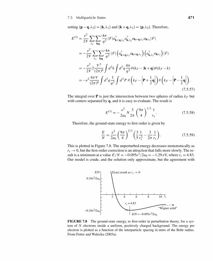
7.5 Multiparticle States 471
setting {p− q,λ2} = {k,λ1} and {k+ q,λ1} = {p,λ2}. Therefore,
E (1) = e2
2V
∑λ1
∑kq
′ 4π
q2 〈F |a†k+q,λ1
a†k,λ1
ak+q,λ1akλ1 |F〉
= − e2
2V
∑λ1
∑kq
′ 4πq2 〈F |
(a†
k+q,λ1ak+q,λ1
)(a†
k,λ1akλ1
)|F〉
= − e2
2V2
V 2
(2π)6
∫d3k
∫d3q
4π
q2 θ (kF −|k+ q|)θ (kF − k)
= −e2 4πV
(2π)6
∫d3q
1
q2
∫d3 P θ
(kF −
∣∣∣∣P + 1
2q
∣∣∣∣)θ (kF −∣∣∣∣P − 1
2q
∣∣∣∣) .
(7.5.57)
The integral over P is just the intersection between two spheres of radius kF butwith centers separated by q, and it is easy to evaluate. The result is
E (1) = − e2
2a0N
3
2π
(9π
4
)1/3 1
rs. (7.5.58)
Therefore, the ground-state energy to first order is given by
E
N= e2
2a0
(9π
4
)2/3(3
5
1
r2s
− 3
2π
1
rs
). (7.5.59)
This is plotted in Figure 7.8. The unperturbed energy decreases monotonically asrs → 0, but the first-order correction is an attraction that falls more slowly. The re-sult is a minimum at a value E/N = −0.095e2/2a0 = −1.29 eV, where rs = 4.83.Our model is crude, and the solution only approximate, but the agreement with
Exact result as rs → 0
0.10e2/2a0
−0.10e2/2a0
2 4 6 8 10 rs
rs = 4.83
E/N = −0.095e2/2a0
“Wigner solid”
E/N
FIGURE 7.8 The ground-state energy, to first-order in perturbation theory, for a sys-tem of N electrons inside a uniform, positively charged background. The energy perelectron is plotted as a function of the interparticle spacing in units of the Bohr radius.From Fetter and Walecka (2003a).
472 Chapter 7 Identical Particles
experiment is surprisingly good. For sodium metal, one finds E/N = −1.13 eV,where rs = 3.96.
7.6 QUANTIZATION OF THE ELECTROMAGNETIC FIELD
Maxwell’s equations form a complete classical description of noninteracting elec-tric and magnetic fields in free space. It is tricky to apply quantum mechanics tothat description, but it can be done in a number of ways. In this section, we willonce again take a “follow our nose” approach to the problem, based on the many-particle formalism developed in this chapter. The particles, of course, are photons,whose creation and annihilation operators obey Bose-Einstein commutation rela-tions.
We start with a brief summary of Maxwell’s equations, to establish our no-tation, and their solution in terms of electromagnetic waves. Then we derive theenergy and associate it with the eigenvalues of a Hamiltonian constructed usingbosonic creation and annihilation operators.
Including interactions with electromagnetic fields, through the inclusion ofspin 1
2 charged electrons, is the subject of quantum electrodynamics. We do notpursue this subject in this book. (See Section 5.8 for a discussion of a more adhoc way to apply electromagnetic-field interactions to atomic systems.) However,there is a fascinating quantum-mechanical effect observable with free electromag-netic fields, the Casimir effect, and we conclude this section with a description ofthe calculation and the experimental data.
Our treatment here more or less follows Chapter 4 in Loudon (2000), al-though the approach has become rather standard. See, for example, Chapter 23in Merzbacher (1998).
Maxwell’s Equations in Free Space
In the absence of any charges or currents, Maxwell’s equations (in Gaussian units;see Appendix A) take the form
∇· E = 0 (7.6.1a)
∇· B = 0 (7.6.1b)
∇ ×E+ 1
c
∂B∂ t
= 0 (7.6.1c)
∇ ×B− 1
c
∂E∂ t
= 0. (7.6.1d)
Following standard procedure, we postulate a vector potential A(x, t) such that
B = ∇ ×A, (7.6.2)
which means that (7.6.1b) is immediately satisfied. If we impose the further con-dition
∇· A = 0 (7.6.3)
7.6 Quantization of the Electromagnetic Field 473
(which is known as “choosing the Coulomb gauge”), then
E = −1
c
∂A∂ t
(7.6.4)
means that (7.6.1a) and (7.6.1c) are also satisfied. Therefore, determining A(x, t)is equivalent to determining E(x, t) and B(x, t). A solution for A(x, t) is evident,though, by observing that (7.6.1d) leads directly to
∇2A− 1
c2
∂2A∂ t2
= 0. (7.6.5)
That is, A(x, t) satisfies the wave equation, with wave speed c, just as we mighthave guessed.
The set of solutions to (7.6.5) are naturally written as
A(x, t) = A(k)e±ik·xe±iωt , (7.6.6)
where ω = ωk ≡ |k|c = kc for the solution to be valid. The Coulomb gauge con-dition (7.6.3) implies that ±ik ·A(x, t) = 0, or
k ·A(k) = 0. (7.6.7)
In other words, A(x, t) is perpendicular to the propagation direction k. For thisreason, the Coulomb gauge is frequently referred to as the “transverse gauge.”This allows us to write the general solution to (7.6.5) as
A(x, t) =∑k,λ
ekλAk,λ(x, t), (7.6.8)
where ekλ are two unit vectors (corresponding to two values for λ) perpendicularto k, and where
Ak,λ(x, t) = Ak,λe−i(ωk t−k·x) + A∗
k,λe+i(ωk t−k·x). (7.6.9)
Note that in (7.6.9) the quantities written Ak,λ on the right side of the equation arenumerical coefficients, not functions of either position or time. Note also that kand −k represent different terms in the sum. We write the superposition (7.6.8) asa sum, not an integral, because we envision quantizing the electromagnetic fieldinside a “big box” whose dimensions may eventually be taken to grow withoutbound.
We use the form (7.6.9) to ensure that Ak,λ(x, t) is real. When we quantize theelectromagnetic field, Ak,λ(x, t) will become a Hermitan operator. The coefficientsA∗
k,λ and Ak,λ will become creation and annihilation operators.As we shall see later, it is useful to take the unit vectors ekλ as directions of
circular polarization as opposed to linear. That is, if e(1)k and e(2)
k are the linearunit vectors perpendicular to k, then
ek± = ∓ 1√2
(e(1)
k ± i e(2)k
), (7.6.10)
474 Chapter 7 Identical Particles
where λ = ± denotes the polarization state. With these definitions, it is easy toshow that
e∗kλ· e±kλ′ = ±δλλ′ (7.6.11a)
and e∗kλ× e±kλ′ = ±iλδλλ′k, (7.6.11b)
where k is a unit vector in the direction of k. The electric field E(x, t) can nowbe written down from (7.6.4). The magnetic field B(x, t) can be written downsimilarly, using (7.6.2).
The energy E in the electromagnetic field is given by integrating the energydensity over all space:
E = 1
8π
∫V
[|E(x, t)|2 +|B(x, t)|2
]d3x , (7.6.12)
where, as discussed earlier, “all space” is a finite volume V = L3 with periodicboundary conditions. In other words, we are working inside an electromagneticcavity with conducting walls. This means that
k = (kx ,ky ,kz) = 2π
L(nx ,ny ,nz), (7.6.13)
where nx , ny , and nz are integers.Consider first the term dependent on the electric field in (7.6.12). Using (7.6.4)
with (7.6.8) and (7.6.9), we have
E = i
c
∑k,λ
ωk
[Ak,λe
−i(ωk t−k·x) − A∗k,λe
+i(ωk t−k·x)]
ekλ (7.6.14a)
and
E∗ = − i
c
∑k′,λ′ωk′
[A∗
k′,λ′e+i(ωk′ t−k′·x) − Ak′,λ′e−i(ωk′ t−k′·x)]
e∗k′λ′ . (7.6.14b)
Since we have already suggested that the A∗k,λ and Ak,λ will become creation and
annihilation operators, we need to take care and keep their order intact.This all leads to an awkward expression for |E|2 = E∗· E—a summation over
k, λ, k′, and λ′, with four terms inside the summation. However, an importantsimplification follows from the integral over the spatial volume. Each term insidethe sum packs all of its position dependence into an exponential so that the volumeintegral is of the form ∫
Vei(k∓k′)·xd3x = V δk,±k′ . (7.6.15)
7.6 Quantization of the Electromagnetic Field 475
Combining this with (7.6.11a), one finds∫V
|E(x, t)|2 d3x =∑k,λ
ω2k
c2 V[A∗
k,λAk,λ+ Ak,λA∗k,λ
+ A∗k,λA∗
−k,λe2iωk t + Ak,λA−k,λe−2iωk t]. (7.6.16)
Starting with (7.6.2), the calculation for |B|2 = B∗ · B is very similar. The curlbrings in factors like k × ekλ instead of the ωk/c in the calculation involvingthe electric field, but since k2 = ω2
k/c2, the result is nearly identical. The key
difference, though, is that under the change k → −k, terms like k × ekλ do notchange sign. This means that the terms analogous to the third and fourth termsin (7.6.16) appear the same way but with opposite signs. Therefore, they cancelwhen we are evaluating (7.6.12). The result is
E = 1
4πV∑k,λ
ω2k
c2
[A∗
k,λAk,λ+ Ak,λA∗k,λ
]. (7.6.17)
Photons and Energy Quantization
Our goal now is to associate (7.6.17) with the eigenvalues of a Hamiltonian op-erator. We will do this by hypothesizing that the quantized electromagnetic fieldis made up of a collection of identical particles called photons. An operator a†
λ(k)creates a photon with polarization λ and momentum hk, and aλ(k) annihilates thisphoton. The energy of a photon is hωk = hck, so we will build our Hamiltonianoperator according to (7.5.26) and write
H =∑k,λ
hωka†λ(k)aλ(k). (7.6.18)
We do not need to consider terms like (7.5.33) since, by our starting assumption,we are building a noninteracting electromagnetic field.
We are now faced with an important question. Are photons bosons or fermions?That is, what is the “spin” of the photon? We need to know whether it is integeror half-integer, in order to know which algebra is followed by the creation andannihilation operators. A fully relativistic treatment of the photon field demon-strates that the photon has spin 1 and is therefore a boson, but do we have enoughpreparation at this point to see that this should be the case?
Yes, we do. We know from Chapter 3 that rotation through an angle φ about(say) the z-axis is carried out by the operator exp(−i Jzφ/h). The possible eigen-values m of Jz show up explicitly if we rotate a state that happens to be an eigen-state of Jz , introducing a phase factor exp(−imφ). [This is what gives rise to the“famous” minus sign when a spin 1
2 state is rotated through 2π . Recall (3.2.15).]So, consider what happens if we rotate about the photon direction k through an
angle φ for a right- or left-handed circularly polarized electromagnetic wave? Thepolarization directions are the unit vectors ek± given by (7.6.10). The rotation is
476 Chapter 7 Identical Particles
equivalent to the transformation
e(1)k → e(1)′
k = cosφe(1)k − sinφe(2)
k (7.6.19a)
e(2)k → e(2)′
k = sinφe(1)k + cosφe(2)
k , (7.6.19b)
which means that the rotation introduces a phase change exp(∓iφ) to the ek±. Ap-parently, right- and left-handed circularly polarized photons correspond to eigen-values ±1h of Jz . The photon seems to have spin 1.
Consequently, we proceed under the assumption that photons are bosons.Rewriting (7.6.18) slightly as
H =∑k,λ
1
2hωk
[a†λ(k)aλ(k) + a†
λ(k)aλ(k)]
=∑k,λ
1
2hωk
[a†λ(k)aλ(k) + aλ(k)a†
λ(k) + 1]
, (7.6.20)
we recover the classical energy (7.6.17) with the definition of the operator
Ak,λ = (4π hc2)1/2 1√V
1√2ωk
aλ(k) (7.6.21)
and with the realization that the “extra term” in (7.6.20) means that all energies inthe photon field are measured relative to a “zero-point” energy
E0 = 1
2
∑k,λ
hωk =∑
k
hωk . (7.6.22)
This is the energy in the electromagnetic field when there are zero photonspresent; it is sometimes called the vacuum energy. It is an infinite number, butnevertheless a constant. More importantly, it has observable consequences.
The Casimir Effect
The vacuum energy of the electromagnetic field has a number of physical conse-quences, but probably the most dramatic is its ability to exert a macroscopic forcebetween conducting surfaces. This is called the Casimir effect, and it has beenprecisely measured and compared to calculations. Fine accounts by S. Lamore-aux have been published, including a popular article in Physics Today, February2007, and a more technical review in Reports on Progress in Physics, 68 (2005)201. See also “Fluctuating About Zero, Taking Nothing’s Measure,” by M. For-tun, in Zeroing In on the Year 2000: The Final Edition (George E. Marcus, editor,University of Chicago Press, 2000).
Casimir’s calculation relies only on the assumption of the vacuum energy(7.6.22). We reproduce it here, following Lamoreaux’s technical review article.∗∗We note that Lamoreaux’s derivation closely follows that of Itzykson and Zuber (1980), Sec-tion 3-2-4. See also Holstein (1992) for a somewhat different approach, and attendant discussion,with a particularly physical perspective.
7.6 Quantization of the Electromagnetic Field 477
Two large, parallel, conducting plates are separated by a distance d . Define a co-ordinate system where the (x , y)-plane is parallel to the surface of the conductingplates, so z measures the distance perpendicularly away from one surface. Thisallows us to write down a potential-energy function
U (d) = E0(d) − E0(∞), (7.6.23)
which gives the difference in the vacuum energy for plates with a finite and aninfinite separation. Combining (7.6.22) with (7.6.13) (and combining positive andnegative integer values), we have
E0(d) = h∑
kx ,ky ,n
ωk = hc∑
kx ,ky ,n
√k2
x + k2y +
(nπ
d
)2. (7.6.24)
[This equation actually is missing a “lost” factor of 1/2 on the n = 0 term. This isbecause only one polarization state should be counted in (7.6.22) for n = 0, sincethere is only one purely transverse mode when kz = 0. We will recover this factorbelow.] Now assume square plates with x and y lengths L � d . Since L is large,we can replace the summations over kx and ky with integrals and write
E0(d) = hc
(L
π
)2 ∫ ∞
0dkx
∫ ∞
0dky
∑n
√k2
x + k2y +
(nπ
d
)2. (7.6.25)
For the limit d → ∞ we can also replace the sum over n with an integral. Thisgives us all the necessary ingredients to evaluate (7.6.23).
Unfortunately, however, (7.6.23) is the difference between two infinite num-bers. It is plausible that the difference is finite, since for any particular value of d ,terms with large enough n will give the same result for different values of d . Thatis, both terms in (7.6.23) should tend toward infinity in the same way, and theseparts will cancel when we take the difference.
This suggests that we can handle the infinities by multiplying the integrandin (7.6.25) by a function f (k), where f (k) → 1 for k → 0 and f (k) → 0 fork → ∞. This function “cuts off” the integrand before it gets too large but does soin the same way to both terms in (7.6.23) so that the contributions from large k still
cancel.∗ It is also helpful to introduce the polar coordinate ρ =√
k2x + k2
y, in which
case dkxdky = 2πρdρ. Note that the integration limits in (7.6.25) correspond to
∗We can think of many physical reasons why there should be a cutoff at very high frequencies.In general, we expect the main contributions to come from values of k ∼ 1/d, but there are morespecific examples, such as the response of electrons in metals to very high-energy photons. Itremains an interesting problem, in any case, to see whether the eventual result can be derivedeven if there is no cutoff frequency.
478 Chapter 7 Identical Particles
1/4 of the (kx ,ky)-plane. Then (7.6.23) becomes
U (d) = 2π hc
(L
π
)2 1
4
∫ ∞
0ρdρ
[∑n
f
(√ρ2 +
(nπ
d
)2)√
ρ2 +(nπ
d
)2(7.6.26)
− d
π
∫ ∞
0dkz f
(√ρ2 + k2
z
)√ρ2 + k2
z
]. (7.6.27)
Now define a function F(κ) as
F(κ) =∫ ∞
0dx f
(πd
√x +κ2
)√x +κ2 (7.6.28a)
=∫ ∞
κ
2y2 f(π
dy)
dy. (7.6.28b)
Putting ρ2 = (π/d)2x and kz = (π/d)κ allows us to write the potential energymore succinctly, reclaiming the lost factor of 2, as
U (d) = π2hc
4d3L2
[1
2F(0) +
∞∑n=1
F(n) −∫ ∞
0F(κ)dκ
](7.6.29)
We are therefore left with evaluating the difference between an integral and a sum,both of which are reasonable approximations of each other. Indeed, if a functionF(x), defined over range 0 ≤ x ≤ N , is evaluated at integer points x = i , then theapproximation scheme known as the trapezoidal rule says that
∫ N
0F(x)dx ≈ F(0) + F(N)
2+
N∑i=1
F(i ). (7.6.30)
In our case, N → ∞ with F(N) → 0, thanks to the cutoff function f (k), and ourjob is to find the difference between the left- and right-hand sides of (7.6.30).
Fortunately, there is a theorem that evaluates this difference. It is called theEuler-Maclaurin summation formula and can be written as
F(0)
2+
∞∑i=1
F(i ) −∫ ∞
0F(x)dx = − 1
12F ′(0) + 1
720F ′′′(0) +·· · . (7.6.31)
The derivatives can be calculated using (7.6.28b). Because F(x) → 0 as x → ∞,we have
F ′(y) = −2y2 f(π
dy)
, (7.6.32)
which gives F ′(0) = 0. If we make one further, but natural, assumption about thecutoff function f (k), namely that all of its derivatives go to zero as k → 0, then
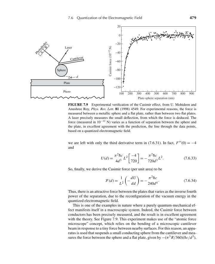
7.6 Quantization of the Electromagnetic Field 479
Plate
Sphere
Piezo
A
B
Phot
odio
des
Laser
Cantilever
d
100 200 300 400 500 600 700 800 900
Plate-sphere separation (nm)
−120
−100
−80
−60
−40
−20
0
20
Cas
imir
for
ce (
10−
12 N
)
FIGURE 7.9 Experimental verification of the Casimir effect, from U. Mohideen andAnushree Roy, Phys. Rev. Lett. 81 (1998) 4549. For experimental reasons, the force ismeasured between a metallic sphere and a flat plate, rather than between two flat plates.A laser precisely measures the small deflection, from which the force is deduced. Theforce (measured in 10−12 N) varies as a function of separation between the sphere andthe plate, in excellent agreement with the prediction, the line through the data points,based on a quantized electromagnetic field.
we are left with only the third derivative term in (7.6.31). In fact, F ′′′(0) = −4and
U (d) = π2hc
4d3 L2[−4
720
]= − π
2hc
720d3 L2. (7.6.33)
So, finally, we derive the Casimir force (per unit area) to be
F (d) = 1
L2
(−dU
dd
)= − π
2hc
240d4. (7.6.34)
Thus, there is an attractive force between the plates that varies as the inverse fourthpower of the separation, due to the reconfiguration of the vacuum energy in thequantized electromagnetic field.
This is one of the examples in nature where a purely quantum-mechanical ef-fect manifests itself in a macroscopic system. Indeed, the Casimir force betweenconductors has been precisely measured, and the result is in excellent agreementwith the theory. See Figure 7.9. This experiment makes use of the “atomic forcemicroscope” concept, which relies on the bending of a microscopic cantileverbeam in response to a tiny force between nearby surfaces. For this reason, an appa-ratus is used that suspends a small conducting sphere from the cantilever and mea-sures the force between the sphere and a flat plate, given by −(π3 R/360)(hc/d3),
480 Chapter 7 Identical Particles
where R is the sphere radius. The force deflects the cantilever, and this motion isdetected using a laser that reflects from the sphere surface. The measured forceas a function of the distance d is shown in the figure as data points, which arecompared with the theoretical prediction.
The Casimir effect has also been observed experimentally with parallel con-ducting surfaces. See, for example, G. Bressi et al., Phys. Rev. Lett. 88 (2002)041804.
If the Casimir effect is due to the presence of electromagnetic fields, and thesefields interact only with charges, then why does the electric charge e not appearanywhere in (7.6.34)? The answer lies in our starting point for the calculation,where we assumed the boundary conditions for conducting plates. These arisefrom the relative mobility of the electrons in the metal, with which the electro-magnetic field interacts. In fact, we made use of a cutoff frequency whose physicalbasis can lie in the penetrability of electromagnetic radiation at short wavelengths.Indeed, if this penetrability existed for all wavelengths, there would be no Casimireffect.
The Casimir effect has seen renewed interest in recent years, not only for itspotential application in nano-mechanical devices, but also for its calculation andinterpretation∗ using fundamental quantum field theoretical principles. In a for-mulation in terms of path integrals, the Casimir energy can be written downin terms of the free field propagator with appropriate boundary conditions. Theboundary conditions are simply defined by the objects under consideration. Theresult is an elegant expression for the Casimir energy in terms of the T -matrixscattering amplitudes for the free field from the objects, and transformation ma-trices that express each object’s geometry in a natural way with respect to theother. This approach lends itself to a number of insights. First, it allows one tocalculate the Casimir energy for any field that can be expressed in terms of thisconstrained propagator, such as scalar or fermion fields. It is also clearly amenableto any number of geometries, far beyond simple parallel plates.
Concluding Remarks
Before leaving this chapter, we should point out that our treatment in this sec-tion only hints at the many applications of quantizing the electromagnetic field.Now that we have expression (7.6.21) (and its adjoint), which is an operator thatdestroys (or creates) photons of specific wavelength and polarization, we can in-corporate it in any number of ways.
For example, we have already seen in (2.7.23) how we can add the electro-magnetic field into the conjugate momentum. This is built into the Hamiltonianin (2.7.26). Using the quantized version for A, we have an ad hoc Hamiltonianoperator that can create or destroy photons. Terms, then, proportional to A · p canbe treated as time-dependent perturbations. Thus we can let a photon be absorbed
∗There is quite a lot of recent literature. I recommend that the interested reader start with T. Emigand R. L. Jaffe, J. Phys. A 41 (2008); T. Emig, N. Graham, R. L. Jaffe, and M. Kardar, Phys. Rev.Lett. 99 (2007) 170403; and R. L. Jaffe, Phys. Rev. D 72 (2005) 021301.
7.6 Quantization of the Electromagnetic Field 481
by an atom (the photoelectric effect) or let an excited state of an atom decay spon-taneously and emit a photon.
These applications, of course, can be brought to bear just as well in systemscovered by nuclear physics or condensed-matter physics. These topics are coveredin a wide variety of books, some on quantum mechanics in general, but many thatcover specific research areas.
One particularly fascinating direction, which in fact involves noninteractingelectromagnetic fields, is quantum optics. This is a field that has come of agein the past few decades, spurred on partly by advances in laser technology anda growing interest in quantum computing and quantum information. A reflectiveview of the field is given in Roy Glauber’s Nobel Prize lecture, published in Re-views of Modern Physics 78 (2006) 1267. In the remainder of this section, we givea very brief overview of this large subject.
A hint to the richness of quantum optics is immediately apparent. By virtue of(7.6.21), the electric-field vector (7.6.14a) becomes an operator that creates anddestroys photons. The expectation value of this operator vanishes in any state |!〉with a definite number of photons—that is,
|!〉 = | . . . ,nkλ, . . .〉. (7.6.35)
This is simple to see, since (7.6.14a) changes the number of photons nkλ, in whichcase 〈!|E|!〉 becomes the inner product between orthogonal states. Thereforeany physical state needs to be a superposition of states with different numbers ofphotons. A wide variety of physical states with different properties can in princi-ple be realized, if one can manipulate this superposition. It is the ability to carryout this manipulation that has given birth to quantum optics. Problem 2.19 ofChapter 2 suggests one possible manipulation leading to something known as acoherent state. Coherent states are eigenstates of the annihilation operator a andtherefore serve as eigenstates of positive or negative frequency parts of E.
Let us explore one such type of manipulation of single-mode electric-field op-erators, following Chapter 5 of Loudon (2000). For a given direction of linearpolarization, the electric field is given by
E(χ) = E+(χ) + E−(χ) = 1
2ae−iχ + 1
2a†eiχ , (7.6.36)
where χ ≡ ωt − kz −π/2. (We absorb a factor of −(8π hωk/V )1/2 into the def-inition of the electric field.) The phase angle χ can be adjusted experimentally.Furthermore, fields with different phase angles generally do not commute. From(2.3.3) it is easily shown that
[E(χ1), E(χ2)] = − i
2sin(χ1 −χ2). (7.6.37)
The uncertainty relation (1.4.53) therefore implies that
�E(χ1)�E(χ2) ≥ 1
4|sin(χ1 −χ2)|, (7.6.38)
482 Chapter 7 Identical Particles
where the electric-field variance (�E(χ))2 is defined in the usual way as
(�E(χ))2 =⟨(E(χ))2
⟩−〈E(χ)〉2
=⟨(E(χ))2
⟩(7.6.39)
since 〈E(χ)〉 = 0 for a state with a single mode. A state |ζ 〉 for which
0 ≤ (�E(χ))2 <1
4(7.6.40)
is said to be quadrature squeezed. It is possible to write |ζ 〉 as the action of aunitary operator on the vacuum:
|ζ 〉 = exp
(1
2ζ ∗a2 − 1
2ζ (a†)2
), (7.6.41)
where ζ = siθ is called the squeeze parameter. In this state, the electric-fieldvariance is
(�E(χ))2 = 1
4
{e2s sin2
(χ − 1
2θ
)+ e−2s cos2
(χ− 1
2θ
)}. (7.6.42)
Thus one can achieve for �E(χ) a minimum
�Emin = 1
2e−s for χ = θ
2+ mπ , (7.6.43)
where m is an integer, and a maximum
�Emax = 1
2es for χ = θ
2+(
m + 1
2
)π . (7.6.44)
The resulting uncertainty relation is
�Emin�Emax = 1
4, (7.6.45)
which satisfies (7.6.38) as an equality.The observation of squeezed light is challenging, but such measurements have
been carried out. See Figure 7.10. The squeezed states are prepared using an opti-cal technique known as parametric down conversion, which allows different mag-nitudes of ζ to be selected. Each point is the result of sweeping over the phase χand measuring the noise spectrum of the electric field.
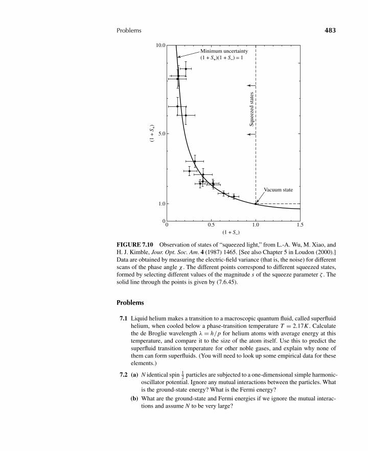
Problems 483
Vacuum state
Sque
ezed
sta
tes
Minimum uncertainty(1 + S+)(1 + S−) = 1
10.0
5.0
1.0
0
(1 +
S+)
0 0.5 1.0 1.5(1 + S−)
FIGURE 7.10 Observation of states of “squeezed light,” from L.-A. Wu, M. Xiao, andH. J. Kimble, Jour. Opt. Soc. Am. 4 (1987) 1465. [See also Chapter 5 in Loudon (2000).]Data are obtained by measuring the electric-field variance (that is, the noise) for differentscans of the phase angle χ . The different points correspond to different squeezed states,formed by selecting different values of the magnitude s of the squeeze parameter ζ . Thesolid line through the points is given by (7.6.45).
Problems
7.1 Liquid helium makes a transition to a macroscopic quantum fluid, called superfluidhelium, when cooled below a phase-transition temperature T = 2.17K . Calculatethe de Broglie wavelength λ = h/p for helium atoms with average energy at thistemperature, and compare it to the size of the atom itself. Use this to predict thesuperfluid transition temperature for other noble gases, and explain why none ofthem can form superfluids. (You will need to look up some empirical data for theseelements.)
7.2 (a) N identical spin 12 particles are subjected to a one-dimensional simple harmonic-
oscillator potential. Ignore any mutual interactions between the particles. Whatis the ground-state energy? What is the Fermi energy?
(b) What are the ground-state and Fermi energies if we ignore the mutual interac-tions and assume N to be very large?
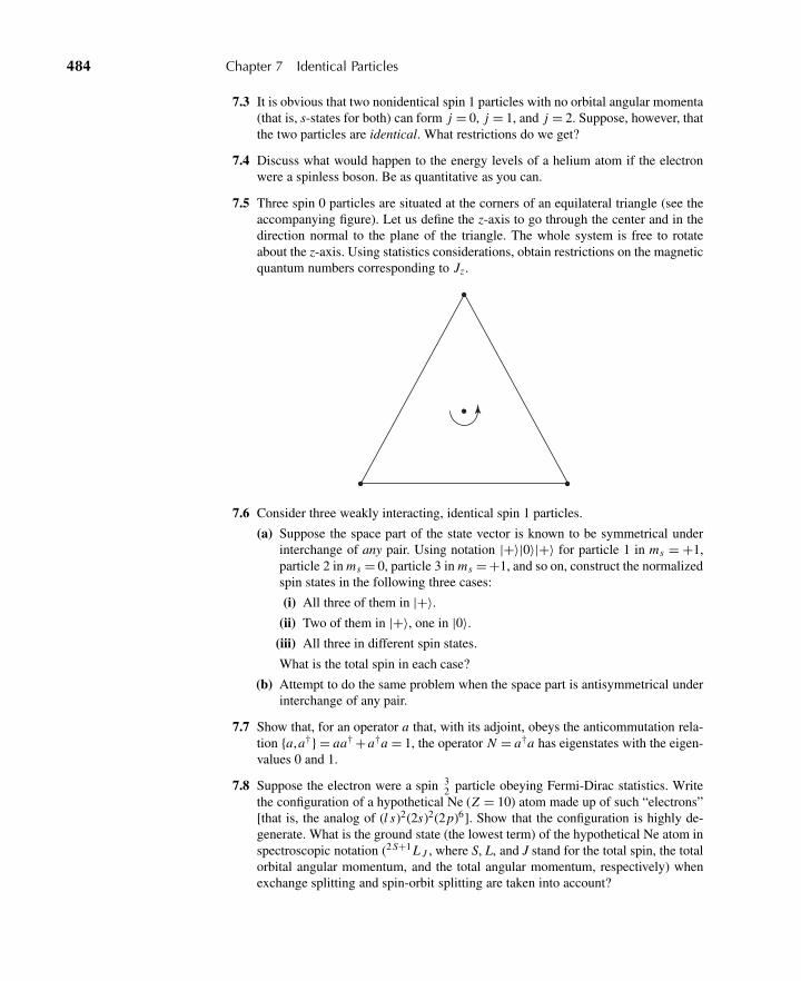
484 Chapter 7 Identical Particles
7.3 It is obvious that two nonidentical spin 1 particles with no orbital angular momenta(that is, s-states for both) can form j = 0, j = 1, and j = 2. Suppose, however, thatthe two particles are identical. What restrictions do we get?
7.4 Discuss what would happen to the energy levels of a helium atom if the electronwere a spinless boson. Be as quantitative as you can.
7.5 Three spin 0 particles are situated at the corners of an equilateral triangle (see theaccompanying figure). Let us define the z-axis to go through the center and in thedirection normal to the plane of the triangle. The whole system is free to rotateabout the z-axis. Using statistics considerations, obtain restrictions on the magneticquantum numbers corresponding to Jz .
7.6 Consider three weakly interacting, identical spin 1 particles.
(a) Suppose the space part of the state vector is known to be symmetrical underinterchange of any pair. Using notation |+〉|0〉|+〉 for particle 1 in ms = +1,particle 2 in ms = 0, particle 3 in ms = +1, and so on, construct the normalizedspin states in the following three cases:
(i) All three of them in |+〉.(ii) Two of them in |+〉, one in |0〉.
(iii) All three in different spin states.
What is the total spin in each case?
(b) Attempt to do the same problem when the space part is antisymmetrical underinterchange of any pair.
7.7 Show that, for an operator a that, with its adjoint, obeys the anticommutation rela-tion {a,a†} = aa† +a†a = 1, the operator N = a†a has eigenstates with the eigen-values 0 and 1.
7.8 Suppose the electron were a spin 32 particle obeying Fermi-Dirac statistics. Write
the configuration of a hypothetical Ne (Z = 10) atom made up of such “electrons”[that is, the analog of (l s)2(2s)2(2p)6]. Show that the configuration is highly de-generate. What is the ground state (the lowest term) of the hypothetical Ne atom inspectroscopic notation (2 S+1 L J , where S, L, and J stand for the total spin, the totalorbital angular momentum, and the total angular momentum, respectively) whenexchange splitting and spin-orbit splitting are taken into account?
Problems 485
7.9 Two identical spin 12 fermions move in one dimension under the influence of the
infinite-wall potential V = ∞ for x < 0, x > L , and V = 0 for 0 ≤ x ≤ L .
(a) Write the ground-state wave function and the ground-state energy when thetwo particles are constrained to a triplet spin state (ortho state).
(b) Repeat (a) when they are in a singlet spin state (para state).
(c) Let us now suppose that the two particles interact mutually via a very short-range attractive potential that can be approximated by
V = −λδ(x1 − x2) (λ > 0).
Assuming that perturbation theory is valid even with such a singular potential,discuss semiquantitatively what happens to the energy levels obtained in (a)and (b).
7.10 Prove the relations (7.6.11), and then carry through the calculation to derive(7.6.17).
C H A P T E R
8 Relativistic Quantum Mechanics
This final chapter provides a succinct look at how one constructs single-particlewave equations that are consistent with special relativity.
To be sure, this effort is ultimately doomed to failure. Special relativity makesit possible to create particles out of energy, but much of our development of quan-tum mechanics was based on the conservation of probability, so we can’t expectto be entirely successful. The right way to attack this problem is by starting withthe postulates of quantum mechanics and building a many-body theory of fieldsthat is relativistically consistent. Nevertheless, at energies low compared to themasses involved, we can expect single-particle quantum mechanics to be a verygood approximation to nature. Furthermore, this is a natural way to develop thenomenclature and mathematics of a relativistic field theory.
We will start with the general problem of forming a relativistic wave equationfor a free particle. This leads more or less intuitively to the Klein-Gordon equa-tion, which we will discuss in some detail. Along the way, we introduce and con-tinue to use the concepts of natural units and of relativistically covariant notation.Then, we will go through Dirac’s approach to finding a relativistic wave equationthat is linear in space-time derivatives, not quadratic. A study of the symmetriesof the Dirac equation is presented. The chapter concludes with the solution of theone-electron atom problem and its comparison with data.
This material is of course covered by many other authors. One nice reference,written when relativistic field theory was emerging out of decades of relativisticquantum mechanics, is “Elementary Relativistic Wave Mechanics of Spin 0 andSpin 1
2 Particles,” by Herman Feshbach and Felix Villars, Rev. Mod. Phys. 30(1958) 24.
8.1 PATHS TO RELATIVISTIC QUANTUM MECHANICS
The early part of the twentieth century saw the more or less simultaneous devel-opments of both relativity and quantum theory. Therefore, it is not surprising tolearn that early attempts to develop wave mechanics produced relativistic waveequations.∗ Although we now understand the many pitfalls that confounded theseearly pioneers, it took many decades to sort things out.
We begin by focussing on the Hamiltonian operator, the (Hermitian) generatorof time translations that led us to the Schrödinger equation (2.1.25) for the time
∗See Volume I, Section 1.1 of Weinberg (1995).
486
8.1 Paths to Relativistic Quantum Mechanics 487
evolution of a state. That is, a state |ψ(t)〉 evolves in time according to the equation
i h∂
∂ t|ψ(t)〉 = H |ψ(t)〉. (8.1.1)
We interpret the eigenvalues of the Hamiltonian, of course, as the allowed energiesof the system. This is where we can start to incorporate special relativity.
Natural Units
This is a good time to graduate to the use of so-called natural units—that is, unitsin which h = c = 1. Most people react to this with bewilderment when they firstsee it, but it is in fact very simple and useful.
We first consider the consequences of setting c = 1. Then, we measure time(= distance/c) in length units, such as meters or centimeters. (If you really needto know the value of time in seconds, just divide by c = 3×1010 cm/sec.) Velocitybecomes a dimensionless number, which we typically denote by β.
Setting c = 1 means that we also measure both momentum and mass in unitsof energy, such as eV or MeV. Frequently, one puts in the c explicitly and writesmomentum units as MeV/c and mass as MeV/c2. Most physicists know that theelectron mass, for example, is 0.511 MeV/c2, but very few know this value inkilograms without doing the conversion arithmetic! Just don’t be surprised ifsomeone tells you that the mass is 0.511 MeV and leaves off the c2.
Now consider what happens when we set h = 1 as well. This ties together unitsfor length and units for energy. For example, the canonical commutation relationfor the momentum and position operators says that their product has the sameunits as h. Therefore, we would measure position in units of MeV−1, or someother inverse energy unit.
Remember that you can always put back the h’s and c’s in the right places ifyou need to return to the old way of doing things. It is not uncommon to do this ifyou are trying to evaluate the result of some experiment, for example. It is handyto keep in mind that, to a very good approximation, hc = 200 MeV·fm for doingthese conversions.
As a final note, we point out that in a textbook on statistical mechanics, onewould also “naturally” set Boltzmann’s constant k = 1. That is, temperature wouldbe measured in units of energy as well.
The Energy of a Free Relativistic Particle
Consider the energy of a free particle with momentum p = |p| and mass m,namely
E p = +√
p2 + m2. (8.1.2)
We need to come up with a Hamiltonian that yields this energy eigenvalue fora state |p〉 with momentum eigenvalue p. It is the square root, however, whichplagued early efforts to come up with a relativistic wave equation, and which wemust figure out how to deal with here.
488 Chapter 8 Relativistic Quantum Mechanics
We have faced transcendental functions of operators before, such as U (t) =exp(−i H t), interpreting them in terms of their Taylor expansions. We could takethe same approach here, and write
H =√
p2 + m2 = m
[1 + p2
m2
]1/2
= m + p2
2m− p4
8m3+ p6
16m5+·· · . (8.1.3)
In fact, this would be a viable way to proceed, but it has some serious short-comings. For one, it would make it impossible to formulate a “covariant” waveequation. That is, if we formed a coordinate-space (or momentum-space) repre-sentation of a state vector |ψ〉, the resulting wave equation would have one timederivative and an infinite series of increasing spatial derivatives from the momen-tum operator. There would be no way to put time and space on an “equal footing.”
This consideration actually leads to a more important problem. Let’s go aheadand try to build this wave equation. From (8.1.1) we have
i∂
∂ t〈x|ψ(t)〉 =
∫d3 p〈x|p〉〈p|H |ψ(t)〉
=∫
d3x ′∫
d3 p〈x|p〉〈p|x′〉〈x′|E p|ψ(t)〉
=∫
d3x ′∫
d3 peip ·(x−x′)
(2π)3〈x′|E p|ψ(t)〉, (8.1.4)
and (8.1.3) means that 〈x′|E p|ψ(t)〉 becomes an infinite series of ever higher-order derivatives; see (1.7.20). This renders this wave equation nonlocal since itmust reach farther and farther away from the region near x′ in order to evaluate thetime derivative. Eventually, causality will be violated for any spatially localizedwave function 〈x|ψ(t)〉. The loss of covariance costs us a great deal indeed.
We abandon this approach and work with the square of the Hamiltonian, in-stead of with the Hamiltonian itself. This removes the problem of the square root,and all of its attendant problems, but it will introduce a different problem. Therewill be solutions to the wave equation with negative energies; these solutions arenecessary to form a complete set of basis states, but they have no obvious physi-cal meaning. Nevertheless, this approach is more useful than the one we are nowleaving.
The Klein-Gordon Equation
Start with (8.1.1) and take the time derivative once more. That is,
− ∂2
∂ t2|ψ(t)〉 = i
∂
∂ tH |ψ(t)〉 = H 2|ψ(t)〉. (8.1.5)
8.1 Paths to Relativistic Quantum Mechanics 489
We can now write down a simple wave equation for !(x, t) ≡ 〈x|ψ(t)〉. TakingH 2 = p2 + m2 and using 〈x|p2|ψ(t)〉 = −∇2!(x, t), we obtain[
∂2
∂ t2−∇2 + m2
]!(x, t) = 0. (8.1.6)
Equation (8.1.6) is known as the Klein-Gordon equation. This looks very muchlike a classical wave equation, except for the m2 term. Putting back our h’s andc’s, we see that this term introduces a length scale h/mc, called the Comptonwavelength.
The Klein-Gordon equation has nearly all the desirable qualities of a rela-tivistic wave equation. First, it is relativistically covariant. You can see that, be-cause a Lorentz transformation leaves the square of the space-time interval ds2 =dt2 − dx2 invariant. Therefore, the combination of derivatives in (8.1.6) is thesame if we change frames from (x, t) to (x′, t ′). In other words,!(x′, t ′) solves thesame equation as !(x, t).
Relativistic covariance is easier to see if one uses relativistic covariant nota-tion. We will use a notation that has become standard. That is, Greek indices run0,1,2,3 and Latin indices run 1,2,3. If an index is ever repeated in an expression,summation over that index is implied. A contravariant four-vector aμ ≡ (a0,a)has a dual covariant vector aμ = ημνaν , where η00 = +1, η11 = η22 = η33 = −1,and all other elements are zero. Thus aμ = (a0,−a). Inner products of four vec-tors can be taken only between a contravariant vector and a covariant vector; for
example, aμbμ = a0b0 − a ·b. In particular, aμaμ = (a0)2 − a2.
A key point of Lorentz transformations is that inner products of four vectors areinvariant. That is, aμbμ will have the same value in any reference frame. This isthe reason why covariant notation is very useful for demonstrating the covarianceof a particular expression.
The space-time position four-vector is xμ = (t ,x). This gives the four-gradient
∂
∂xμ=(∂
∂ t,∇)
≡ ∂μ, (8.1.7)
which is a covariant vector operator, despite the positive sign in front of the space-like part. Now, the covariance of (8.1.6) is absolutely clear. The Klein-Gordonequation becomes [
∂μ∂μ+ m2
]!(x, t) = 0. (8.1.8)
Sometimes, an even further economy of notation is achieved by writing ∂2 ≡∂μ∂
μ.Another desirable property of the Klein-Gordon equation is that it has solutions
that are in fact what we expect for a free, relativistic particle of mass m. Weexpect the time dependence to be like exp(−i E t), where E is an eigenvalue of theHamiltonian. We also expect the spatial dependence to be that of a plane wave;that is, exp(+ip ·x) for momentum p. In other words, our solution should be
!(x, t) = Ne−i(E t−p·x) = Ne−ipμ xμ , (8.1.9)
490 Chapter 8 Relativistic Quantum Mechanics
where pμ = (E ,p). Indeed, (8.1.9) solves (8.1.8) so long as
−pμ pμ+ m2 = −E2 + p2 + m2 = 0, (8.1.10)
or E2 = E2p . Thus the energy eigenvalues E = +E p are included, as they should
be. On the other hand, the negative energy eigenvalues E = −E p are also in-cluded. This was a serious stumbling block in the historical development of rel-ativistic quantum mechanics, but we will take up a practical explanation of itshortly.
Schrödinger’s nonrelativistic wave equation has a very important property—namely, it implies that probability is conserved. The probability density ρ(x, t) =ψ∗ψ (2.4.14) is a positive definite quantity, and the probability flux (2.4.16) obeysa continuity equation (2.4.15), which proves that the probability density can beinfluenced only by the flux into or out of a particular region.
One would like to identify analogous expressions using the Klein-Gordonequation, so that the wave function!(x, t) can be similarly interpreted. The formof the continuity equation strongly suggests that we construct a four-vector cur-rent jμ with the property ∂μ jμ = 0, with the probability density ρ ≡ j0. In fact,if we follow (2.4.16) to write
jμ = i
2m
[!∗∂μ!− (
∂μ!)∗!]
, (8.1.11)
then it is easy to show that ∂μ jμ = 0. Therefore, we calculate a density
ρ(x, t) = j0(x, t) = i
2m
[!∗ ∂!
∂ t−(∂!
∂ t
)∗!
]. (8.1.12)
Although this density is conserved, it is not positive definite! This was a tremen-dous problem in the development of relativistic quantum mechanics, because itrendered the standard probabilistic interpretation of the wave function impossi-ble. Eventually a consistent physical interpretation was found. Before discussingthis interpretation, though, we need to consider the effect of electromagnetic in-teractions within the context of our relativistic framework.
The explicitly covariant nature of the Klein-Gordon equation makes it straight-forward to add electromagnetic interactions into the Hamiltonian. See Section 2.7,especially (2.7.23) and (2.7.26). As before, we assume that the particle has anelectric charge e < 0. In a classical Hamiltonian, one simply makes the substitu-tions∗ E → E − e� and p → p − eA, where � is the “scalar” electric potential
∗It is worthwhile to take a moment and review the origin of these substitutions. A LagrangianL is constructed that yields the Lorentz force law, F = e
[E +v× B/c
]. For a coordinate xi , the
canonical momentum is pi ≡ ∂L/∂ xi = mxi + eAi . Hence, the kinetic energy uses the “kine-matic momentum” mxi = pi − eAi . For more details, see Taylor (2005), Section 7.9. Extensionto relativistic kinematics is relatively straightforward. The four-momentum pμ is replaced bypμ−eAμ; see Jackson (1998), Section 12.1A. When working in coordinate space, the quantum-mechanical operator for the (covariant vector) pμ = (E ,−p) is i∂μ = (i∂t , i∇). Therefore, toincorporate electromagnetism, we replace i∂μ with i∂μ− eAμ = i(∂μ+ ieAμ) ≡ i Dμ .
8.1 Paths to Relativistic Quantum Mechanics 491
and A is the vector potential. In covariant form, this becomes
pμ → pμ− eAμ, (8.1.13)
where Aμ = (�,A), so Aμ = (�,−A). This all amounts to rewriting (8.1.8) as[DμDμ+ m2
]!(x, t) = 0, (8.1.14)
where Dμ ≡ ∂μ+ ieAμ. We refer to Dμ as the covariant derivative.Unlike the nonrelativistic Schrödinger wave equation, the Klein-Gordon equa-
tion is second order in time derivatives, not first. That implies that one must notonly specify !(x, t)|t=0 for its solution, but also ∂!(x, t)/∂ t|t=0. Consequently,more information is necessary than we might have originally expected based onour experience from nonrelativistic quantum mechanics. In fact, this additional“degree of freedom” shows up as the sign of the charge of the particle. This isclear when we note that if !(x, t) solves (8.1.14), then !∗(x, t) solves the sameequation, but with e → −e.
More explicitly, we can reduce the second-order Klein-Gordon equation totwo first-order equations and then interpret the result in terms of the sign of theelectric charge. Using a rather obvious notation in which DμDμ = D2
t − D2, wecan easily write (8.1.14) as two equations, each first order in time, defining twonew functions
φ(x, t) = 1
2
[!(x, t) + i
mDt!(x, t)
](8.1.15a)
χ(x, t) = 1
2
[!(x, t) − i
mDt!(x, t)
](8.1.15b)
so that instead of specifying !(x, t)|t=0 and ∂!(x, t)/∂ t|t=0, we can specifyφ(x, t)|t=0 and χ(x, t)|t=0. Furthermore, φ(x, t) and χ(x, t) satisfy the coupledequations
i Dtφ = − 1
2mD2(φ+χ) + mφ (8.1.16a)
i Dtχ = + 1
2mD2(φ+χ) − mχ , (8.1.16b)
which bear a striking resemblance to the nonrelativistic Schrödinger equation. Wecan demonstrate this resemblance even more keenly be defining a two-componentobjectϒ(x, t) in terms of the two functions φ(x, t) and χ(x, t), and using the Paulimatrices (3.2.32). That is, for the functions φ(x, t) and χ(x, t) that satisfy (8.1.16),we define a column vector function
ϒ(x, t) ≡[φ(x, t)χ(x, t)
]. (8.1.17)
We now write the Klein-Gordon equation as
i Dtϒ =[− 1
2mD2(τ3 + iτ2) + mτ3
]ϒ . (8.1.18)
492 Chapter 8 Relativistic Quantum Mechanics
(Note that we use τ rather than σ to denote the Pauli matrices, to avoid any con-fusion with the concept of spin.) Equation (8.1.18) is completely equivalent toour formulation in (8.1.14), but it is a first-order differential equation in time. Wehave “hidden” the additional degree of freedom in the two-component nature ofϒ(x, t).
Now let us return to the question of probability current density. Now thatwe have rewritten the Klein-Gordon equation using the covariant derivative as(8.1.14), the correct form of the conserved current is
jμ = i
2m
[!∗Dμ!− (
Dμ!)∗!]
. (8.1.19)
The “probability” density (8.1.12) therefore becomes
ρ = j0 = i
2m
[!∗Dt!− (Dt!)∗!
]= φ∗φ−χ∗χ =ϒ†τ3ϒ . (8.1.20)
This is easy to see by using (8.1.15) to write !(x, t) and Dt! in terms of φ(x, t)and χ(x, t).
We are therefore led to interpret ρ as a probability charge density, where φ(x, t)is the wave function of a positive particle, and χ(x, t) is the wave function of anegative particle. That is, the Klein-Gordon equation has buried in it simultaneousdegrees of freedom for a particle of a certain charge and a particle that behavesidentically but with the opposite charge. Before going so far as to refer to these as“particle” and “antiparticle,” we should go back and consider the interpretation ofthe negative-energy solutions.
An Interpretation of Negative Energies
First consider free particles, in which case Dμ = ∂μ, and for which ϒ(x, t) ∝exp
[−i (E t − p · x)]. Inserting this into (8.1.18) yields the eigenvalues E = ±E p
as it, of course, should. We find, for the eigenfunctions,
ϒ(x, t) = 1
2(m E p)1/2
(E p + mm − E p
)e−i E p t+ip·x for E = +E p (8.1.21a)
and ϒ(x, t) = 1
2(m E p)1/2
(m − E pE p + m
)e+i E p t+ip·x for E = −E p , (8.1.21b)
with a normalization that leads to a charge density ρ = ±1 for E = ±E p . Thatis, we impose the condition that a free particle with negative charge is to be as-sociated with a particle that has negative total energy. Also, for a particle at rest,E p = m and the positive-energy solution (8.1.21a) has only an upper compo-nent (that is, χ(x, t) = 0), while the negative-energy solution (8.1.21b), has only alower component (that is, φ(x, t) = 0). This continues for the nonrelativistic casewhere p � E p and the positive-energy solution is dominated by φ(x, t) and thenegative-energy solution by χ(x, t).
8.1 Paths to Relativistic Quantum Mechanics 493
More insight into the meaning of negative energies comes from consideringthe probability current density j. Making use of (3.2.34), (3.2.35), and (8.1.18),we have
∂tρ = ∂t (ϒ†τ3ϒ) =
(∂tϒ
†)τ3ϒ +ϒ†τ3 (∂tϒ)
= 1
2im
[(∇2ϒ†
)(1 + τ1)ϒ−ϒ†(1 + τ1)
(∇2ϒ
)]= −∇· j,
where j = 1
2im
[ϒ†(1 + τ1) (∇ϒ) −
(∇ϒ†
)(1 + τ1)ϒ
]. (8.1.22)
In the case of a free particle, for either positive or negative energies, this reducesto
j = pmϒ†(1 + τ1)ϒ = p
E p. (8.1.23)
Now this would appear to be quite peculiar. With a normalization that imposespositive and negative charges on positive- and negative-energy solutions, respec-tively, we end up with a charge current density that is the same regardless ofthe sign of the charge and energy. One way to “fix” this would be to recognizethat the sign of the momentum vector p in (8.1.21b) is “wrong” since we wantthe exponent to have the form i pμxμ in order to be relativistically invariant. Wemight reverse the sign of p, therefore, for negative-energy solutions, in which case(8.1.23) would carry the “correct” sign to account for the charge of the particle.Another way of “fixing” this problem would be to say that the negative-energyparticles are moving “backwards in time.” This not only reverses the sign of p butalso lets the energy be positive in the exponent of (8.1.21b)! We have made somecontact with the popular lore of particles and antiparticles.
If we like, we can formally associate the positive-energy solution !E>0(x, t)to the Klein-Gordon equation with that for a “particle” and associate the complexconjugate of the negative energy solution!∗
E<0(x, t) with an “antiparticle.” In thiscase, (8.1.14) yields the two equations[
(∂μ− ieAμ)(∂μ− ieAμ) + m2]!particle(x, t) = 0 (8.1.24a)[
(∂μ+ ieAμ)(∂μ+ ieAμ) + m2]!antiparticle(x, t) = 0. (8.1.24b)
This makes it clear how to split the solutions to the Klein-Gordon equation intotwo pieces that correspond individually to particles with charge ±e.
———————–
This is a good time to step back from the Klein-Gordon equation. By followingour nose, we have been able to come up with a relativistic wave equation withfree-particle solutions that can be interpreted, if we try hard enough, in terms of
494 Chapter 8 Relativistic Quantum Mechanics
particles and antiparticles with charges of opposite sign. These two entities appearas the separate degrees of freedom in our two-component wave function ϒ(x, t).It is even possible to go much further and solve the Klein-Gordon for an atomicsystem, and the results compare well with experiment so long as the orbitingcharged particle has no spin. (See Problem 8.7 at the end of this chapter.)
Indeed, the lack of any spin degree of freedom gave the wrong answer forthe fine structure in the hydrogen atom and doomed the Klein-Gordon equationto be left on the sidelines in the development of relativistic quantum mechanics.This, and the fact that nobody had yet seen any evidence for antiparticles, meantthat there were too many things that needed to be cooked up to explain all theidiosyncrasies of the negative-energy solutions. It took Dirac and his leap of faithto create a wave equation linear in space and time derivatives to point us in a morefruitful direction.
8.2 THE DIRAC EQUATION
Many of the difficulties with interpreting the results from the Klein-Gordon equa-tion stem from the fact that it is a second-order differential equation in time. Thesedifficulties include a nonpositive definite probability density, and additional de-grees of freedom, although both can be identified to some extent with particlesand their oppositely charged antiparticles. Nevertheless, Dirac looked for a wayto write a wave equation that is first order in time. Along the way, he discoveredthe need for j = 1/2 angular momentum states in nature. This also lent itself to aparticularly useful interpretation of the negative-energy states.
The linear differential equation we seek can be written as
(iγ μ∂μ− m)!(x, t) = 0, (8.2.1)
where the γ μ have yet to be determined. (Of course, the constant m is also yetto be determined, but it will turn out to be the mass.) We must still insist that thecorrect energy eigenvalues (8.1.10) are obtained for a free particle (8.1.9), as does(8.1.8). We can turn (8.2.1) into (8.1.8) simply by operating on it with −iγ ν∂ν−mto get
(γ ν∂νγμ∂μ+ m2)!(x, t) = 0 (8.2.2)
and then imposing the condition that γ νγ μ∂ν∂μ = ∂μ∂μ = ημν∂ν∂μ. This condi-tion can be written succinctly, by reversing dummy indices to symmetrize:
1
2
(γ μγ ν +γ νγ μ)≡ 1
2
{γ μ,γ ν
}= ημν . (8.2.3)
Thus the four quantities γ μ, μ = 0,1,2,3, are not simply complex numbers butrather entities that obey something called a Clifford algebra. Clearly this algebra
8.2 The Dirac Equation 495
implies that (γ 0)2 = 1 (8.2.4a)(
γ i)2 = −1 i = 1, 2, 3 (8.2.4b)
and γ μγ ν = −γ νγ μ if μ �= ν. (8.2.4c)
Note that the anticommutation property of the γ μ means that each of these matri-ces are traceless.
Now substitute the free-particle solution (8.1.9) into (8.2.1) to find
γ μ pμ− m = 0, (8.2.5)
from which we can recover the free-particle energy eigenvalues E . Writing (8.2.5)out in terms of time-like and space-like parts, and then multiplying through by γ 0,we obtain
E = γ 0γ · p+γ 0m. (8.2.6)
This leads to the Dirac Hamiltonian, written in a traditional form. Making thedefinitions
αi ≡ γ 0γ i and β ≡ γ 0, (8.2.7)
we arrive at
H = α · p+βm. (8.2.8)
Note that if we add electromagnetism by making the substitution (8.1.13) into(8.2.5), and then setting A = 0 and A0 =�, we have
H = α · p+βm + e�, (8.2.9)
which controls the motion of a charged particle in an electrostatic potential �.We will make use of this when we solve the relativistic one-electron atom inSection 8.4.
Which form of the Dirac equation we use, (8.1.1) with (8.2.8) or (8.2.9), orthe covariant form (8.2.1) perhaps with the substituion (8.1.13), depends on thespecific problem at hand. For example, sometimes it is easier to use (8.2.8) whensolving problems involving dynamics and the Dirac equation, whereas it is easierto discuss symmetries of the Dirac equation in covariant forms using γ μ.
The algebra (8.2.4) can be realized with square matrices, so long as they areat least 4 × 4. We know that 2 × 2 matrices are not large enough, for example,because the Pauli matrices σ form a complete set along with the identify matrix.However {σk ,1} = 2σk , so this set is not large enough to realize the Clifford al-gebra. Therefore, !(x, t) in (8.2.1) would be a four-dimensional column vector.In order to keep a convention consistent with our matrix representation of states
496 Chapter 8 Relativistic Quantum Mechanics
and operators, we insist that α and β be Hermitian matrices. Note that this impliesthat γ 0 is Hermitian, whereas γ is anti-Hermitian.
We choose to make use of the 2 × 2 Pauli spin matrices σ (3.2.32), and wewrite
α =[
0 σ
σ 0
]and β =
[1 00 −1
]. (8.2.10)
That is, we write these 4 ×4 matrices as 2 ×2 matrices of 2 ×2 matrices.
The Conserved Current
The Dirac equation immediately solves the problem of the positive-definite natureof the probability density. Defining!† in the usual way—namely, as the complexconjugate of the row vector corresponding to the column vector!—we can showthat the quantity ρ =!†! is in fact interpretable as a probability density. First, asthe sum of the squared magnitudes of all four components of!(x, t), it is positivedefinite.
Historically, the ability of the Dirac equation to provide a positive-definiteprobability current was one of the main reasons it was adopted as the correctdirection for relativistic quantum mechanics. An examination of its free-particlesolutions led to an attractive interpretation of negative energies—and, in fact, tothe discovery of the positron.
Second, it satisfies the continuity equation
∂ρ
∂ t+∇· j = 0 (8.2.11)
for j = !†α! . (This is simple to prove. Just use the Schrödinger equation andits adjoint. See Problem 8.10 at the end of this chapter.) This means that ρ canchange only on the basis of a flow into or out of the immediate region of interestand is therefore a conserved quantity.
Instead of !†, one usually uses ! ≡ !†β = !†γ 0 in forming the proba-bility density and current. In this case, ρ = !†! = !†γ 0γ 0! = !γ 0! andj =!†γ 0γ 0α! = !γ 0α! . Because γ 0α = γ by (8.2.7), we have
∂
∂ t
(!γ 0!
)+∇·(!γ!
)= ∂μ jμ = 0, (8.2.12)
where
jμ =!γμ! (8.2.13)
is a four-vector current. Rewriting (8.2.1) in terms of four-momentum as
(γ μ pμ− m)!(x, t) = 0, (8.2.14)
and also taking the adjoint of this equation and using (8.2.4) to insert a factorof γ 0,
!(x, t)(γ μ pμ− m) = 0, (8.2.15)
8.2 The Dirac Equation 497
we come to an insightful interpretation of the conserved current for a free particle.We write
jμ = 1
2
{[!γμ
]!+! [γ μ!]}
= 1
2m
{[!γμ
]γ ν pν!+!γ ν pν
[γ μ!
]}= 1
2m![γ μγ ν+γ νγ μ] pν!
= pμ
m!! . (8.2.16)
Thus, writing the usual Lorentz contraction factor as γ yields
j0 = E
m!! = γ
[!†
up!up −!†down!down
](8.2.17)
and
j = pm!! = γ v
[!†
up!up −!†down!down
]. (8.2.18)
The factor of γ is expected because of the Lorentz contraction of the volumeelement d3x in the direction of motion. (See Holstein 1992 for an extended dis-cussion.) The meaning of the relative negative sign of the upper and lower com-ponents becomes clearer after we study the specific solutions for the free particle.
Free-Particle Solutions
We are now in a position to study solutions of the Dirac equation and their symme-try properties. Already we notice, however, that the wave function!(x, t) has fourcomponents, whereas the Klein-Gordon wave function ϒ(x, t) has two. We willsee that the additional degree of freedom in the Dirac equation is the same quan-tity we called “spin 1
2 ” at the very beginning of this book. The four-componentobject!(x, t) is called a spinor.
We get immediate insight into the nature of the solutions of the Dirac equationjust by considering free particles at rest (p = 0). In this case the Dirac equation issimply i∂t! = βm! . Given the diagonal form of β (8.2.10), we see that there arefour independent solutions for !(x, t). These are
!1 = e−imt
⎡⎢⎢⎣1000
⎤⎥⎥⎦ !2 = e−imt
⎡⎢⎢⎣0100
⎤⎥⎥⎦ !3 = e+imt
⎡⎢⎢⎣0010
⎤⎥⎥⎦ !4 = e+imt
⎡⎢⎢⎣0001
⎤⎥⎥⎦ .
(8.2.19)
Just as in the case of the Klein-Gordon equation, the lower half of the wave func-tion corresponds to negative energy, and we will need to deal with the interpreta-tion of these equations later. Both the upper and lower halves of the Dirac wave
498 Chapter 8 Relativistic Quantum Mechanics
function, however, have one component that it is tempting to call “spin up” andanother we would call “spin down.” This interpretation is in fact correct, but weneed to be somewhat more ambitious before we can state this with confidence.
Let us go on and consider free-particle solutions with nonzero momentum p =pz—that is, a particle moving freely in the z-direction. In this case, we want tosolve the eigenvalue problem H! = E! for H = αz p +βm, which is no longerdiagonal in spinor space. The eigenvalue equation becomes⎡⎢⎣ m 0 p 0
0 m 0 −pp 0 −m 00 −p 0 −m
⎤⎥⎦⎡⎢⎣ u1
u2u3u4
⎤⎥⎦= E
⎡⎢⎣ u1u2u3u4
⎤⎥⎦ . (8.2.20)
Notice that the equations for u1 and u3 are coupled together, as are the equationsfor components u2 and u4, but these components are otherwise independent ofeach other. This makes it simple to find the eigenvalues and eigenfunctions. De-tails are left as an exercise. (See Problem 8.11 at the end of this chapter.) Fromthe two equations coupling u1 and u3, we find E = ±E p . We find the same forthe two equations coupling u2 and u4. Once again, we find the expected “correct”positive-energy eigenvalue and also the “spurious” negative-energy solution. Inthe case of the Dirac equation, however, a relatively palatable interpretation isforthcoming, as we shall see shortly.
First, however, let us return to the question of spin. Continue to construct thefree-particle spinors. For E = +E p we can set either u1 = 1 (and u2 = u4 =0), in which case u3 = +p/(E p + m), or u2 = 1 (and u1 = u3 = 0), in whichcase u4 = −p/(E p + m). In both cases, as for the Klein-Gordon equation, theupper components dominate in the nonrelativistic case. Similarly, for E = −E pthe nonzero components are either u3 = 1 and u1 = −p/(E p + m) or u4 = 1 andu2 = p/(E p + m), and the lower components dominate nonrelativistically.
Now consider the behavior of the operator �· p = �z , where � is the 4 × 4matrix
� ≡[
σ 00 σ
]. (8.2.21)
We expect this operator to project out components of spin in the direction ofmomentum. Indeed, it is simple to see that the spin operator S = h
2 � projects outpositive (negative) helicity for the positive-energy solution with u1 �= 0 (u2 �= 0).We find the analogous results for the negative-energy solutions. In other words,the free-particle solutions do indeed behave appropriately according to the spin-up/down assignment that we have conjectured.
Putting this together, we write the positive-energy solutions as
u(+)R (p) =
⎡⎢⎢⎢⎣10p
E p+m
0
⎤⎥⎥⎥⎦ u(+)L (p) =
⎡⎢⎢⎢⎣010
−pE p+m
⎤⎥⎥⎥⎦ for E = +E p,
(8.2.22a)
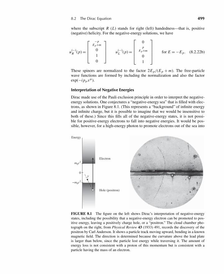
8.2 The Dirac Equation 499
where the subscript R (L) stands for right (left) handedness—that is, positive(negative) helicity. For the negative-energy solutions, we have
u(−)R (p) =
⎡⎢⎢⎢⎣−p
E p+m
010
⎤⎥⎥⎥⎦ u(−)L (p) =
⎡⎢⎢⎢⎢⎣0p
E p+m
01
⎤⎥⎥⎥⎥⎦ for E = −E p . (8.2.22b)
These spinors are normalized to the factor 2E p/(E p + m). The free-particlewave functions are formed by including the normalization and also the factorexp(−i pμxμ).
Interpretation of Negative Energies
Dirac made use of the Pauli exclusion principle in order to interpret the negative-energy solutions. One conjectures a “negative-energy sea” that is filled with elec-trons, as shown in Figure 8.1. (This represents a “background” of infinite energyand infinite charge, but it is possible to imagine that we would be insensitive toboth of these.) Since this fills all of the negative-energy states, it is not possi-ble for positive-energy electrons to fall into negative energies. It would be pos-sible, however, for a high-energy photon to promote electrons out of the sea into
Electron
Hole (positron)
Energy
0γ
m0c2
−m0c2
FIGURE 8.1 The figure on the left shows Dirac’s interpretation of negative-energystates, including the possibility that a negative-energy electron can be promoted to pos-itive energy, leaving a positively charge hole, or a “positron.” The cloud chamber pho-tograph on the right, from Physical Review 43 (1933) 491, records the discovery of thepositron by Carl Anderson. It shows a particle track moving upward, bending in a knownmagnetic field. The direction is determined because the curvature above the lead plateis larger than below, since the particle lost energy while traversing it. The amount ofenergy loss is not consistent with a proton of this momentum but is consistent with aparticle having the mass of an electron.
500 Chapter 8 Relativistic Quantum Mechanics
positive energies, where it would be observable. The “hole” left in the sea wouldalso be observable, as an object with all the properties of an electron, but withpositive charge.
Figure 8.1 also shows the original discovery of the positron, by Carl Andersonin 1933. After this discovery, the Dirac equation became the standard treatmentof relativistic quantum mechanics, explaining the spin 1
2 electron and (as we willsee) its electromagnetic interactions.
Electromagnetic Interactions
We introduce electromagnetic interactions in the Dirac equation in the same waythat we did for the Klein-Gordon equation—that is; through
p ≡ p− eA (8.2.23)
and the Dirac equation becomes, in 2 ×2 matrix form,[m σ · p
σ · p −m
][uv
]= E
[uv
], where ! =
[uv
]. (8.2.24)
At nonrelativistic (positive) energies E = K + m, the kinetic energy K � m andthe lower equation becomes
σ · pu = (E + m)v ≈ 2mv, (8.2.25)
which enables us to write the upper equation as
(σ · p) (σ · p)
2mu =
[p2
2m+ iσ
2m· (p× p)
]u = K u, (8.2.26)
where we have used (3.2.39). Now in the coordinate representation,
p× pu = (i∇ + eA)× (i∇u + eAu)
= ie [∇ × (Au) + A×∇u]
= ie(∇ ×A)u = ieBu, (8.2.27)
where B is the magnetic field associated with the vector potential A. Therefore,(8.2.26) becomes [
p2
2m−μ · B
]u = K u, (8.2.28)
where
μ = ge
2mS (8.2.29)
with
S = h
2σ (8.2.30)
and
g = 2. (8.2.31)
8.3 Symmetries of the Dirac Equation 501
In other words, the Dirac equation in the presence of an electromagnetic fieldreduces nonrelativistically to (8.2.28), which is just the time-independentSchrödinger equation (with energy eigenvalue K ) for a particle with magneticmoment μ in the presence of an external magnetic field. The magnetic moment isderived from the spin operator with a gyromagnetic ratio g = 2.
This brings us full circle. We began this book by discussing the behavior ofparticles with magnetic moments in the presence of inhomogeneous magneticfields, where it appeared that they behaved as though they had spin projectionsquantized in one of two states. We now see that this stems from a considerationof relativity and quantum mechanics, for particles that obey the Dirac equation.
8.3 SYMMETRIES OF THE DIRAC EQUATION
Let us now examine some symmetries inherent in the Dirac equation. We willconsider situations where a spin 1
2 particle sits in some external potential—that is,solutions to the equation
i∂
∂ t!(x, t) = H!(x, t) = E!(x, t), (8.3.1)
where
H = α · p+βm + V (x) (8.3.2)
for some potential-energy function V (x). This form, of course, ruins our ability towrite a covariant equation, but that is a necessary penalty if we want to talk aboutpotential energy. We note, though, that in the case of electromagnetic interactions,we can end up with exactly this form from the covariant equation if we choose aframe in which the vector potential A = 0.
Angular Momentum
Our discussion of rotational invariance for wave mechanics in three dimensionscentered on the fact that the orbital-angular-momentum operator L = x ×p com-muted with Hamiltonians with “central potentials.” This in turn hinges on the factthat L commutes with p2, and so with the kinetic-energy operator, and also x2.[See (3.7.2).]
Let us now consider the commutator [H ,L] first for the free Dirac Hamiltonian(8.2.8). It is obvious that [β,L] = 0, so we need to consider the commutator
[α · p, L i ] = [α# p#,εi j k x j pk]
= εi j kα#[p#, x j ]pk
= −iεi j kα j pk �= 0. (8.3.3)
(Recall our convention of summing over repeated indices.) In other words, theorbital-angular-momentum operator does not commute with the Dirac Hamilto-nian! Therefore, L will not be a conserved quantity for spin 1
2 particles that areeither free or bound in central potentials.
502 Chapter 8 Relativistic Quantum Mechanics
Consider, however, the spin operator (8.2.21) and its commutator with theHamiltonian. It is simple to show that β�i = �iβ. It is also easy to use (3.2.35)to show that [αi ,� j ] = 2iεi j kαk . Hence we need to evaluate
[α · p,� j ] = [αi ,� j ]pi = 2iεi j kαk pi . (8.3.4)
Thus we see (putting h back in momentarily) that even though neither L nor �
commutes with the free Dirac Hamiltonian, the combined vector operator
J ≡ L+ h
2� = L+ S (8.3.5)
does commute. That is, the Dirac Hamiltonian conserves total angular momen-tum, but not orbital momentum or spin-angular momentum separately.
Parity
In the case where V (x) = V (|x|), we expect solutions to be parity symmetrical.That is, we should have !(−x) = ±!(x). It does not appear that this is the case,however, since if x → −x, then p → −p in (8.3.2) and the Hamiltonian changesform. However, this simple look does not take into account the parity transforma-tion on spinors.
Indeed, the parity transformation operator π , discussed in Section 4.2, con-cerns only coordinate reflection. That is, π is a unitary (and also Hermitian)operator with the properties
π†xπ = −x (8.3.6a)
π†pπ = −p. (8.3.6b)
(See Equations (4.2.3) and (4.2.10).) The full parity operator, let us call it P ,needs to be augmented with a unitary operator UP , which is a 4 × 4 matrix inspinor space, and which renders the Hamiltonian (8.3.2) invariant under a paritytransformation. That is,
P ≡ πUP , (8.3.7)
where the matrix UP must have the properties
UPαU†P = −α (8.3.8a)
and UPβU†P = β (8.3.8b)
as well as U2P = 1. (8.3.8c)
Obviously UP = β = β† is consistent with these requirements. Consequently,a parity transformation on a Dirac Hamiltonian consists of taking x → −x andmultiplying on both the left and the right by β. The transformation of a spinor!(x) yields β!(−x).
8.3 Symmetries of the Dirac Equation 503
Therefore, in cases where V (x) = V (|x|), we expect to find eigenstates of theDirac Hamiltonian that are simultaneously eigenstates of parity, J2 and Jz . Luck-ily, we have already constructed angular and spinor parts of these eigenfunctions.These are the two-component spin-angular functions Y
j=l±1/2,ml (θ ,φ) defined
in (3.8.64). We will make use of these as we proceed to solve the Dirac equationfor a particular potential-energy function of this form in Section 8.4.
Charge Conjugation
We saw in (8.1.24) that for the Klein-Gordon equation, we could split the positive-and negative-energy solutions into “particle” and “antiparticle” solutions on thebasis of the association
!particle(x, t) ≡!E>0(x, t) (8.3.9a)
!antiparticle(x, t) ≡!∗E<0(x, t). (8.3.9b)
Let us work toward a similar association for the Dirac equation and then explorea symmetry operation that connects the two solutions.
For our purposes, an antiparticle is an object whose wave function behavesjust as that for a particle, but with opposite electric charge. So let’s return to thecovariant form (8.2.1) of the Dirac equation and add an electromagnetic fieldaccording to our usual prescription (8.1.13). We have(
iγ μ∂μ− eγ μAμ− m)!(x, t) = 0. (8.3.10)
We seek an equation where e → −e and which relates the new wave functionto !(x, t). The key is that the operator in (8.3.10) has three terms, only two ofwhich contain γ μ, and only one of those two contains i . So we take the complexconjugate of this equation to find[−i
(γ μ)∗∂μ− e
(γ μ
)∗Aμ− m
]!∗(x, t) = 0, (8.3.11)
and the relative sign between the first two terms is reversed. If we can now identifya matrix C such that
C(γ μ)∗
C−1 = −γ μ, (8.3.12)
we just insert 1 = C−1C before the wave function in (8.3.11) and multiply on theleft by C . The result is[
iγ μ∂μ+ eγ μAμ− m]C!∗(x, t) = 0. (8.3.13)
Therefore, the wave function C!∗(x, t) satisfies the “positron” equation (8.3.13),and !(x, t) satisfies the “electron” equation (8.3.10).
We need to identify the matrix C . From (8.2.7) and (8.2.10) we see that γ 0,γ 1, and γ 3 are real matrices, but
(γ 2)∗ = −γ 2. This makes it possible to realize
(8.3.12) with
C = iγ 2. (8.3.14)
504 Chapter 8 Relativistic Quantum Mechanics
Therefore, the “positron wave” function corresponding to !(x, t) is iγ 2!∗(x, t).It is more convenient, in turns out, to write this wave function in terms of ! =!†γ 0 = (!∗)T γ 0. (The superscript T indicates “transpose”.) This means that the“positron” wave function can be written as
C!∗(x, t) = iγ 2(!γ 0
)T = UC(!)T
, (8.3.15)
where
UC ≡ iγ 2γ 0. (8.3.16)
Therefore, the charge conugation operator is C, where
C!(x, t) = UC(!)T
. (8.3.17)
Note that the change in the space-time part of the free-particle wave function!(x, t) ∝ exp(−i pμxμ) due to C is to, effectively, take x → −x and t → −t .
Time Reversal
Let us now apply the ideas of Section 4.4 to the Dirac equation. First, a briefreview. This discussion hinged on the definition (4.4.14) of an antiunitary operatorθ :
θ = U K , (8.3.18)
where U is a unitary operator and K is an operator that takes the complex conju-gate of any complex numbers that follow it. Clearly, K does not affect the kets tothe right, and K 2 = 1.
Based on this, we defined an antiunitary operator that takes an arbitrary state|α〉 to a time-reversed (or, more properly, a motion-reversed) state |α〉; that is,
|α〉 = |α〉. (8.3.19)
We imposed two reasonable requirements on , namely (4.4.45) and (4.4.47);that is,
p −1 = −p (8.3.20a)
x −1 = x (8.3.20b)
and so J −1 = −J. (8.3.20c)
For Hamiltonians that commute with , we made the important observation(4.4.59) that an energy eigenstate |n〉 has the same energy eigenvalue as its time-reversed counterpart state |n〉. We further learned that acting twice on a spin12 state yields 2 = −1, since the two-component spinor form of (4.4.65) showsthat
= −iσy K . (8.3.21)
8.3 Symmetries of the Dirac Equation 505
In other words, U = −iσy in (8.3.18). Indeed, in this case
2 = −iσy K (−iσy K ) = σyσ∗y K 2 = −1. (8.3.22)
We will see something similar when we apply time reversal to the Dirac equation,which we now take up.
Returning to the Schrödinger equation (8.1.1) with the Dirac Hamiltonian(8.2.7), but using the γ matrices instead of α and β, we have
i∂t!(x, t) =[−iγ 0γ ·∇ +γ 0m
]!(x, t). (8.3.23)
We write our time-reversal operator, following the scheme earlier in this section,as T instead of , where
T = UT K (8.3.24)
and UT is a unitary matrix that we need to identify. As before, insert T −1T beforethe wave function on the left and right sides, and multiply through from the leftby T . The left side of (8.3.23) becomes
T (i∂t )T−1T !(x, t) = UT K (i∂t )K U−1
T UT!∗(x, t)
= −i∂tUT!∗(x, t) = i∂−t
[UT!
∗(x, t)], (8.3.25)
reversing the sign of t in the derivative, which is what we need. In order for[UT!
∗(x, t)]
to satisfy the time-reversed form of (8.3.23), we must insist that
T(
iγ 0γ)T −1 = iγ 0γ (8.3.26a)
and T(γ 0)T −1 = γ 0. (8.3.26b)
These are easily converted to a more convenient form so that we can identify UT .First, do T −1 on the left and T on the right. Next do K on the left and right.Finally, insert UT U−1
T in between the γ matrices in (8.3.26a), and then use theresult from (8.3.26b). Both results then become
U−1T (γ )UT = − (γ )∗ (8.3.27a)
and U−1T
(γ 0)
UT =(γ 0)∗
. (8.3.27b)
We now specialize to our choice (8.2.10), with (8.2.7), for the γ matrices. Onlyγ 2 is imaginary in this representation. Therefore, if we want to build UT out ofγ matrices, then (8.3.27) says that we need a combination that does not changethe sign when commuted with γ 0 and γ 2 but does change sign with γ 1 and γ 3.Rather obviously, this is accomplished by
UT = γ 1γ 3 (8.3.28)
up to some arbitrary phase factor. Indeed, this works out to be equivalent to theresult U = iσy in (8.3.21). See Problem 8.13 at the end of this chapter.
506 Chapter 8 Relativistic Quantum Mechanics
CPT
We conclude with a brief look of the operator combination CPT . Its action ona Dirac wave function !(x, t) is straightforward to work out, given the abovediscussion. That is,
CPT !(x, t) = iγ 2 [PT !(x, t)]∗
= iγ 2γ 0 [T !(−x, t)]∗
= iγ 2γ 0γ 1γ 3!(−x, t) = iγ 0γ 1γ 2γ 3!(−x, t). (8.3.29)
This combination of γ matrices is well known; in fact, it is given a special name.We define
γ 5 ≡ iγ 0γ 1γ 2γ 3. (8.3.30)
In our basis (8.2.10), again writing 4 ×4 matrices as 2 ×2 matrices of 2 ×2 ma-trices, we find that
γ 5 =[
0 11 0
]. (8.3.31)
That is, γ 5 (and therefore also CPT ) reverses the up and down two-componentspinors in the Dirac wave function. The net effect of CPT on a free-particleelectron wave function is in fact to convert it into the “positron” wave function.See Problem 8.14 at the end of this chapter.
This is a “tip of the iceberg” observation of a profound concept in relativisticquantum field theory. The notion of CPT invariance is equivalent to a total sym-metry between matter and antimatter, so long as one integrates over all potentialfinal states. For example, it predicts that the mass of any particle must equal themass of the corresponding antiparticle.
Indeed, one can show, although it is far from straightforward, that any Lorentz-invariant quantum field theory is invariant under CPT . The implications are far-reaching, particularly in this day and age when string theories offer the possibilitythat Lorentz-invariance is broken at distances approaching the Planck mass. Thereader is referred to any one of a number of advanced textbooks—and also to thecurrent literature—for more details.
8.4 SOLVING WITH A CENTRAL POTENTIAL
Our goal is to solve the eigenvalue problem
H!(x) = E!(x), (8.4.1)
where H = α · p+βm + V (r ), (8.4.2)
8.4 Solving with a Central Potential 507
and we write the four-component wave function !(x) in terms of two two-component wave functionsψ1(x) and ψ2(x) as
!(x) =[ψ1(x)ψ2(x)
]. (8.4.3)
Based on the symmetries of the Dirac equation that we have already discussed,we expect !(x) to be an eigenfunction of parity, J2 and Jz .
Parity conservation implies that β!(−x) = ±!(x). Given the form (8.2.10) ofβ, this implies that [
ψ1(−x)−ψ2(−x)
]= ±
[ψ1(x)ψ2(x)
]. (8.4.4)
This leaves us with two choices:
ψ1(−x) = +ψ1(x) and ψ2(−x) = −ψ2(x) (8.4.5a)
or ψ1(−x) = −ψ1(x) and ψ2(−x) = +ψ2(x). (8.4.5b)
These conditions are neatly realized by the spinor functions Yjml (θ ,φ) defined in
(3.8.64), where l = j ± (1/2). For a given value of j , one possible value of l iseven and the other is odd. Since the parity of any particular Y m
l is just (−1)l , weare presented with two natural choices for the angular and spinor dependences forthe conditions (8.4.5). We write
!(x) =!A(x) ≡⎡⎣ u A(r )Y jm
j−1/2(θ ,φ)
−ivA(r )Y jmj+1/2(θ ,φ)
⎤⎦ , (8.4.6a)
which is an even (odd) parity solution if j − 1/2 is even (odd), or
!(x) =!B(x) ≡⎡⎣ u B (r )Y jm
j+1/2(θ ,φ)
−ivB(r )Y jmj−1/2(θ ,φ)
⎤⎦ , (8.4.6b)
which is an odd (even) parity solution if j − 1/2 is even (odd). (The factor of −ion the lower spinors is included for later convenience.) Note that although both!A(x) and !B(x) have definite parity and quantum numbers j and m, they mixvalues of l. Orbital angular momentum is no longer a good quantum number whenwe consider central potentials in the Dirac equation.
We are now ready to turn (8.4.1) into a differential equation in r for the func-tions u A(B)(r ) and vA(B)(r ). First, rewrite the Dirac equation as two coupled equa-tions for the spinors ψ1(x) and ψ2(x). Thus
[E − m − V (r )]ψ1(x) − (σ · p)ψ2(x) = 0 (8.4.7a)
[E + m − V (r )]ψ2(x) − (σ · p)ψ1(x) = 0. (8.4.7b)
508 Chapter 8 Relativistic Quantum Mechanics
Now make use of (3.2.39) and (3.2.41) to write
σ · p = 1
r2(σ · x)(σ ·x)(σ · p)
= 1
r2(σ · x)[x ·p+ iσ · (x ×p]
= (σ · r)
[r · p+ iσ · L
r
]. (8.4.8)
Working in coordinate space, we have
r · p → r · (−i∇) = −i∂
∂r, (8.4.9)
which will act on the radial part of the wave function only. We also know that
σ · L = 2S · L = J2 − L2 − S2, (8.4.10)
so we can write
(σ · L)Y jml =
[j ( j + 1) − l(l + 1) − 3
4
]Y
jml
≡ κ( j , l)Y jml , (8.4.11)
where
κ = − j − 3
2= −(λ+ 1) for l = j + 1
2(8.4.12a)
and κ = j − 1
2= +(λ− 1) for l = j − 1
2, (8.4.12b)
where
λ≡ j + 1
2. (8.4.13)
It is trickier to calculate the effect of the matrix factor
σ · r =[
cosθ e−iφ sinθ
eiφ sinθ −cosθ
](8.4.14)
on the spinor wave functions. In principle, we can carry out the multiplication onthe Y
jml as defined in (3.8.64) and then use the definition (3.6.37) to evaluate the
result. There is an easier way, however.We expect σ · r to behave as a (pseudo)-scalar under rotations, so if we evaluate
its effect at one particular r, then it should behave this way for all r. Choose
8.4 Solving with a Central Potential 509
r = z—that is, θ = 0. Since the θ -dependent part of any Y ml (θ ,φ) contains a factor
[sinθ ]|m|, we use (3.6.39) to write
Y ml (θ = 0,φ) =
√2l + 1
4πδm0 , (8.4.15)
in which case
Yj=l±1/2,ml (θ = 0,φ) = 1√
2l + 1
[ ±√l ± m + 1/2 Y m−1/2
l (0,φ)√
l ∓ m + 1/2 Y m+1/2l (0,φ)
]
= 1√4π
[ ±√l ± m + 1/2 δm,1/2√
l ∓ m + 1/2 δm,−1/2
]
or Yj ,ml= j∓1/2(θ = 0,φ) =
√j + 1/2
4π
[ ±δm,1/2
δm,−1/2
]. (8.4.16)
Therefore,
(σ · z)Y j ,ml= j∓1/2(θ = 0,φ) = −
√j + 1/2
4π
[ ∓δm,1/2
δm,−1/2
]= −Y
j ,ml= j±1/2(θ = 0,φ),
(8.4.17)
and so, because we have argued that this result is independent of θ and φ, we have
(σ · r)Y j ,ml= j±1/2(θ ,φ) = −Y
j ,ml= j∓1/2(θ ,φ), (8.4.18)
where we have used the fact that (σ · r)2 = 1. In other words, for a given j andm, Y
j ,ml= j±1/2, (θ ,φ) is an eigenstate of σ · r with eigenvalue −1 (a consequence of
the pseudo-scalar nature of the operator) and changes l to the other allowed value,which naturally has opposite parity.
Now we return to the coupled equations (8.4.7) with solutions in the form(8.4.6). We have two choices for ψ1(x) and ψ1(x), namely “Choice A”
ψ1(x) = u A(r )Y jmj−1/2(θ ,φ) and ψ2(x) = −ivA(r )Y jm
j+1/2(θ ,φ) (8.4.19)
or “Choice B”
ψ1(x) = u B(r )Y jmj+1/2(θ ,φ) and ψ2(x) = −ivB(r )Y jm
j−1/2(θ ,φ). (8.4.20)
Note that for whichever of these two choices we pick, the effect of the factor(σ · r), which is part of (σ ·p) in (8.4.7), is to exchange l = j ±1/2 for l = j ∓1/2in the angular spinor Y
jml —that is, to switch the angular spinor factor of the
second term in each of (8.4.7) so that it is the same as the first term. In otherwords, the angular factors drop out, and we are left with just the radial equations.
510 Chapter 8 Relativistic Quantum Mechanics
Putting this all together, finally, (8.4.7) becomes for “Choice A”
[E − m − V (r )]u A(r ) −[
d
dr+ λ+ 1
r
]vA(r ) = 0 (8.4.21a)
[E + m − V (r )]vA(r ) −[
d
dr− λ− 1
r
]u A(r ) = 0 (8.4.21b)
and for “Choice B”
[E − m − V (r )]u B (r ) −[
d
dr− λ− 1
r
]vB (r ) = 0 (8.4.22a)
[E + m − V (r )]vB (r ) −[
d
dr+ λ+ 1
r
]u B(r ) = 0. (8.4.22b)
However, formally, equations (8.4.21) become (8.4.22) with the exchange λ↔−λ. Therefore, we can focus on the solution to (8.4.21) and drop the subscript A.
Equations (8.4.21) are coupled, first-order ordinary differential equations tobe solved for the u(r ) and v(r ), subject to certain boundary conditions (such asnormalizability) that will yield eigenvalues E . This solution can at least be carriedout numerically, which is practical in many situations. We conclude this chapter,however, with one case that can be solved analytically.
The One-Electron Atom
We can now consider atoms with one electron, with the potential-energy function
V (r ) = − Ze2
r. (8.4.23)
We expect that the “fine structure” of the hydrogen atom, which we studied us-ing perturbation theory in Section 5.3, should emerge naturally with our solutionusing the Dirac equation.
Start by writing (8.4.21) in terms of scaled variables, that is,
ε ≡ E
m(8.4.24)
and x ≡ mr , (8.4.25)
and recall that we write α ≡ e2(/hc) ≈ 1/137. This gives[ε− 1 + Zα
x
]u(x) −
[d
dx+ λ+ 1
x
]v(x) = 0 (8.4.26a)[
ε+ 1 + Zα
x
]v(x) +
[d
dx− λ− 1
x
]u(x) = 0. (8.4.26b)
8.4 Solving with a Central Potential 511
Next consider the behavior of the solutions as x → ∞. Equation (8.4.26a)becomes
(ε− 1)u − dv
dx= 0 (8.4.27)
and so (8.4.26b) implies that
(ε+ 1)v+ du
dx= (ε+ 1)v+ 1
ε− 1
d2v
dx2 = 0, (8.4.28)
which leads to
d2v
dx2 = (1 − ε2)v. (8.4.29)
Note that, classically, bound states require that the kinetic energy E −m −V (r ) =0 at some distance r , and V (r )< 0 everywhere, so E −m < 0 and ε = E/m < 1.Therefore, 1 − ε2 is guaranteed to be positive, and (8.4.29) implies that
v(x) = exp[−(1 − ε2)1/2x
]for x → ∞, (8.4.30)
where we require that v(x) be normalizable as x → ∞ but ignore the normaliza-tion constant for now. Similarly, (8.4.27) then implies that
u(x) = exp[−(1 − ε2)1/2x
]for x → ∞ (8.4.31)
as well.Now write u(x) and v(x) as power series with their own expansion coefficients,
and look for relationships consistent with the differential equations. Using
u(x) = e−(1−ε2)1/2x xγ∞∑
i=0
ai xi (8.4.32)
and v(x) = e−(1−ε2)1/2x xγ∞∑
i=0
bi xi , (8.4.33)
we tacitly assume that we can find series solutions making use of the same overallpower γ for both u(x) and v(x). Indeed, inserting these expressions into (8.4.26)and first considering terms proportional to xγ−1, we find, after a little rearrange-ment,
(Zα)a0 − (γ +λ+ 1)b0 = 0 (8.4.34a)
(γ −λ+ 1)a0 + (Zα)b0 = 0. (8.4.34b)
Our approach will soon yield recursion relations for the coefficients ai and bi .This means that we need to avoid a0 = 0 and b0 = 0, and the only way to do thisis to require that the determinant of (8.4.34) vanish. That is,
(Zα)2 + (γ + 1 +λ)(γ + 1 −λ) = 0 (8.4.35)
512 Chapter 8 Relativistic Quantum Mechanics
or, solving for γ ,
γ = −1 ±[λ2 − (Zα)2
]1/2. (8.4.36)
Notice first λ= j +1/2 is of order unity, so that things will break down if Zα∼ 1.In the strong Coulomb fields for Z ≈ 137, spontaneous e+e− production wouldoccur, and the single-particle nature of the Dirac equation cannot be expected toprevail. Indeed, we have Zα � 1 in cases of interest here. This also means thatthe expression within the brackets in (8.4.36) is of order unity. For the − sign, thisgives γ ∼ −2, which would be too singular at the origin. As a result, we choosethe + sign and have
γ = −1 +[(
j + 1
2
)2
− (Zα)2
]1/2
. (8.4.37)
Note that for j = 1/2 we still have a singularity at the origin, since γ < 0, but thissingularity is very weak and is integrable over space.
Starting with a value for a0 that is determined by normalization, and b0 =a0(Zα)/(γ + λ+ 1), we can find the remaining ai and bi by going back to theresult of inserting (8.4.32) and (8.4.33) into (8.4.26). Collecting powers of xγ andhigher, we find
(1 − ε)ai−1 − Zαai − (1 − ε2)1/2bi−1 + (λ+ 1 +γ + i )bi = 0 (8.4.38a)
(1 + ε)bi−1 + Zαbi − (1 − ε2)1/2ai−1 − (λ− 1 −γ − i )ai = 0. (8.4.38b)
Multiply (8.4.38a) by (1 + ε)1/2 and (8.4.38b) by (1 − ε)1/2 and then add them.This leads to a relationship between the coefficients ai and bi , namely
bi
ai= Zα(1 + ε)1/2 + (λ− 1 −γ − i )(1 − ε)1/2
Zα(1 − ε)1/2 + (λ+ 1 +γ + i )(1 + ε)1/2. (8.4.39)
This relation shows that for large values of x , where terms with large i domi-nate, ai and bi are proportional to each other. Furthermore, (8.4.38) also impliesthat ai/ai−1 ∼ 1/ i for large i. (See Problem 8.15 at the end of this chapter.) Inother words, the series (8.4.32) and (8.4.33) will grow exponentially, and not benormalizable, unless we force the series to terminate.
If we then assume that ai = bi = 0 for i = n′ + 1, then
(1 − ε)an′ − (1 − ε2)1/2bn′ = 0 (8.4.40a)
(1 + ε)bn′ − (1 − ε2)1/2an′ = 0. (8.4.40b)
Either of these leads to the same condition on the ratio of these terminating coef-ficients, namely
bn′
an′=[
1 − ε1 + ε
]1/2
. (8.4.41)
8.4 Solving with a Central Potential 513
Combining (8.4.39) and (8.4.40), we have
(1 +γ + n′)(1 − ε2)1/2 = Zαε, (8.4.42)
which, finally, can be solved for ε. Putting c back in, we determine the energyeigenvalues
E = mc2[1 + (Zα)2[√
( j+1/2)2−(Zα)2+n′]2
]1/2. (8.4.43)
We emphasize that for any given quantum number n′, the energy eigenvalues de-pend on the total angular momentum j . That is, for example, the energy will bethe same for j = 1
2 , regardless of whether it comes from coupling l = 0 or l = 1with spin 1
2 .To lowest order in Zα, (8.4.43) becomes
E = mc2 − 1
2
mc2(Zα)2
n2 , (8.4.44)
where n ≡ j + 1/2 + n′. Comparison to (3.7.53) shows that this is simply thefamiliar Balmer formula, with the addition of rest mass energy, with n being theprincipal quantum number. Including higher orders of Zα leads to the well-knownexpressions for the relativistic correction to kinetic energy (5.3.10) and the spin-orbit interaction (5.3.31).
Figure 8.2 shows the energy levels of the hydrogen atom and the experimentsthat made these measurements. A number of ingenious techniques, including two-photon absorption for connecting “forbidden” transitions, were devised in order toobtain these results. The so-called “fine structure” is clear—that is, the relativisticeffects that lead to splitting between the S and P levels for the n = 2 states, andbetween the S, P , and D levels for the n = 3 states. Problem 8.16 at the end ofthis chapter shows that the full relativistic energy levels give the same splittingsas obtained using perturbation theory.
There is, of course, a profound discrepancy between the energy levels in Fig-ure 8.2 and the result (8.4.43) we derived for the energy eigenvalues. Accordingto (8.4.43), the energy can depend only on n and j . However, we see that there isa small splitting between, for example, the 2P1/2 and 2S1/2 states. This splitting,which is called the Lamb shift after its discoverer, played a central role in makingclear the importance of relativistic quantum field theory in atomic structure. SeeHolstein (1992) for a discussion of the history of the Lamb shift, as well as bothformal and “physically intuitive” derivations of its size.
Problem 8.17 at the end of this chapter compares energy levels predicted by(8.4.43) to available high-precision data.
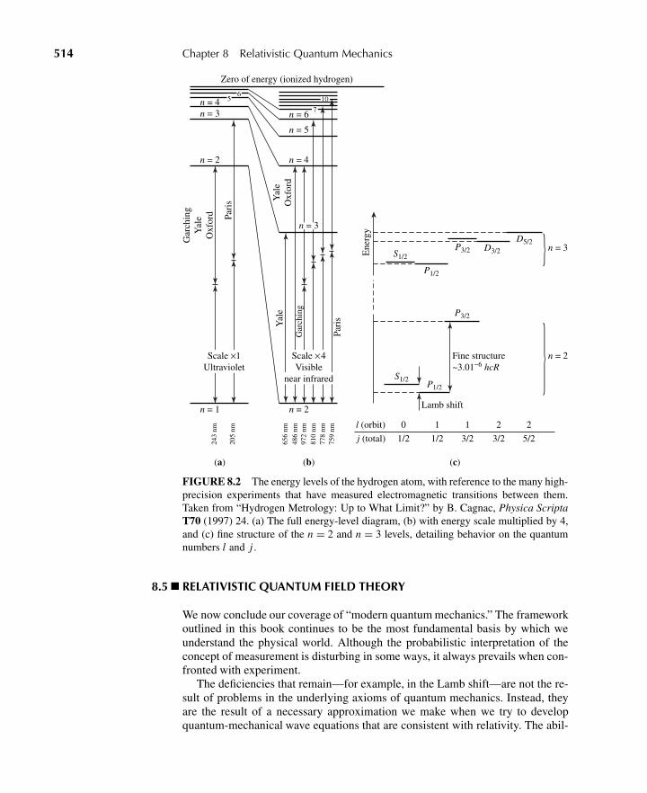
514 Chapter 8 Relativistic Quantum Mechanics
S1/2
P1/2
P3/2
S1/2P1/2
P3/2 D3/2
D5/2n = 3
n = 2
n = 2
Ene
rgy
Fine structure~3.01−6 hcR
Lamb shift
l (orbit) 0 1 1 2 2
j (total) 1/2 1/2 3/2 3/2 5/2
n = 1
n = 2
n = 3n = 4
Scale ×4Visible
near infrared
Gar
chin
g
Yal
eY
ale
Oxf
ord
Gar
chin
gY
ale
Oxf
ord Pa
ris
Pari
s
n = 3
n = 4
n = 5
n = 6
656
nm
243
nm
205
nm
486
nm97
2 nm
810
nm77
8 nm
759
nm
56
7
10
Scale ×1Ultraviolet
Zero of energy (ionized hydrogen)
(a) (b) (c)
FIGURE 8.2 The energy levels of the hydrogen atom, with reference to the many high-precision experiments that have measured electromagnetic transitions between them.Taken from “Hydrogen Metrology: Up to What Limit?” by B. Cagnac, Physica ScriptaT70 (1997) 24. (a) The full energy-level diagram, (b) with energy scale multiplied by 4,and (c) fine structure of the n = 2 and n = 3 levels, detailing behavior on the quantumnumbers l and j .
8.5 RELATIVISTIC QUANTUM FIELD THEORY
We now conclude our coverage of “modern quantum mechanics.” The frameworkoutlined in this book continues to be the most fundamental basis by which weunderstand the physical world. Although the probabilistic interpretation of theconcept of measurement is disturbing in some ways, it always prevails when con-fronted with experiment.
The deficiencies that remain—for example, in the Lamb shift—are not the re-sult of problems in the underlying axioms of quantum mechanics. Instead, theyare the result of a necessary approximation we make when we try to developquantum-mechanical wave equations that are consistent with relativity. The abil-
Problems 515
ity to create and destroy particles is inconsistent with our “single-particle” ap-proach to writing down dynamics in quantum mechanics. Instead, we would needto reexamine the Hamiltonian formalism, on which much of this book is based, inorder to address these issues.
Quantum field theory is the correct framework for addressing relativistic quan-tum mechanics and mutli-particle quantum mechanics in general. There are essen-tially two ways to approach quantum field theory, neither of which is developedhere. We mention them only for the reader interested in going on to the next steps.
One approach is through the method of “second quantization,” wherein oper-ators are introduced that create and destroy particles. These operators commutewith each other if they have integer spin, and they anticommute for half-integerspin. Work needs to be done in order to build in relativistic covariance, but it isrelatively straightforward. It is also, however, not necessary if the problem doesn’twarrant it. This is the case, for example, in a vast number of fascinating problemsin condensed-matter physics.
Second quantization is discussed in Section 7.5 of this book. For other ex-amples, see Quantum Mechanics, 3rd ed., by Eugen Merzbacher, and QuantumTheory of Many-Particle Systems, by Alexander L. Fetter and John Dirk Walecka.
The second approach is through the path-integral approach to quantum me-chanics, famously pioneered by Richard Feynman in his Ph.D. thesis. Thisconceptually appealing formalism is straightforward to extend from particlequantum mechanics to quantum fields. However, it is not straightforward to usethis formalism for calculation of typical problems until one makes the connectionto the “canonical” formalism that eventually becomes second quantization. Nev-ertheless, it is a worthwhile subject for students who would like to have a betterunderstanding of the principles that lead to the quantum many-body problem.
Path integrals are not the basis for many books on quantum field theory, butthey are beautifully exploited in Quantum Field Theory in a Nutshell by AnthonyZee.
Problems
8.1 These exercises are to give you some practice with natural units.
(a) Express the proton mass m p = 1.67262158× 1027 kg in units of GeV.
(b) Assume a particle with negligible mass is confined to a box the size of theproton, around 1 fm = 10−15 m. Use the uncertainty principle estimate theenergy of the confined particle. You might be interested to know that the mass,in natural units, of the pion, the lightest strongly interacting particle, is mπ =135 MeV.
(c) String theory concerns the physics at a scale that combines gravity, relativity,and quantum mechanics. Use dimensional analysis to find the “Planck mass”MP , which is formed from G , h, and c, and express the result in GeV.
8.2 Show that a matrix ημν with the same elements as the metric tensor ημν used inthis chapter has the property that ημληλν = δμν , the identity matrix. Thus, show thatthe natural relationship ημν = ημληνσ ηλσ in fact holds with this definition. Showalso that aμbμ = aμbμ for two four-vectors aμ and bμ.
516 Chapter 8 Relativistic Quantum Mechanics
8.3 Show that (8.1.11) is in fact a conserved current when !(x, t) satisfies the Klein-Gordon equation.
8.4 Show that (8.1.14) follows from (8.1.8).
8.5 Derive (8.1.16a), (8.1.16b), and (8.1.18).
8.6 Show that the free-particle energy eigenvalues of (8.1.18) are E = ±E p and thatthe eigenfunctions are indeed given by (8.1.21), subject to the normalization thatϒ†τ3ϒ = ±1 for E = ±E p .
8.7 This problem is taken from Quantum Mechanics II: A Second Course in QuantumTheory, 2nd ed., by Rubin H. Landau (1996). A spinless electron is bound by theCoulomb potential V (r ) = −Ze2/r in a stationary state of total energy E ≤ m.You can incorporate this interaction into the Klein-Gordon equation by using thecovariant derivative with V = −e� and A = 0. Work with the upper component ofthe wave function.(a) Assume that the radial and angular parts of the equation separate and that the
wave function can be written as e−i E t [ul (kr )/r ]Ylm (θ ,φ). Show that the radialequation becomes
d2u
dρ2+[
2E Zα
γρ− 1
4− l(l + 1)− (Zα)2
ρ2
]ul (ρ) = 0,
where α = e2, γ 2 = 4(m2 − E2), and ρ = kr .(b) Assume that this equation has a solution of the usual form of a power series
times the ρ → ∞ and ρ→ 0 solutions, that is,
ul (ρ) = ρk(1+ c1ρ+ c2ρ2 +··· )e−ρ/2,
and show that
k = k± = 1
2±√(
l + 1
2
)2
− (Zα)2
and that only for k+ is the expectation value of the kinetic energy finite andthat this solution has a nonrelativistic limit that agrees with the solution foundfor the Schrödinger equation.
(c) Determine the recurrence relation among the ci ’s for this to be a solution of theKlein-Gordon equation, and show that unless the power series terminates, thewill function will have an incorrect asymptotic form.
(d) In the case where the series terminates, show that the energy eigenvalue for thek+ solution is
E = m(1+ (Zα)2
[n − l − 1
2 +√(
l + 12
)2 − (Zα)2
]−2)1/2
,
where n is the principal quantum number.(e) Expand E in powers of (Zα)2 and show that the first-order term yields the
Bohr formula. Connect the higher-order terms with relativistic corrections, anddiscuss the degree to which the degeneracy in l is removed.
Problems 517
Jenkins and Kunselman, in Phys. Rev. Lett. 17 (1966) 1148, report measurementsof a large number of transition energies for π− atoms in large-Z nuclei. Comparesome of these to the calculated energies, and discuss the accuracy of the prediction.(For example, consider the 3d → 2p transition in 59Co, which emits a photon withenergy 384.6± 1.0 keV.) You will probably need either to use a computer to carryout the energy differences with high enough precision, or else expand to higherpowers of (Zα)2.
8.8 Prove that the traces of the γ μ, α, and β are all zero.
8.9 (a) Derive the matrices γ μ from (8.2.10) and show that they satisfy the Cliffordalgebra (8.2.4).
(b) Show that
γ 0 =(
I 00 −I
)= I ⊗ τ3
and γ i =(
0 σ i
−σ i 0
)= σ i ⊗ iτ2,
where I is the 2× 2 identity matrix, and σ i and τi are the Pauli matrices. (The⊗ notation is a formal way to write our 4×4 matrices as 2×2 matrices of 2×2matrices.)
8.10 Prove the continuity equation (8.2.11) for the Dirac equation.
8.11 Find the eigenvalues for the free-particle Dirac equation (8.2.20).
8.12 Insert one of the four solutions u(±)R,L (p) from (8.2.22) into the four-vector proba-
bility current (8.2.13) and interpret the result.
8.13 Make use of Problem 8.9 to show that UT as defined by (8.3.28) is just σ 2 ⊗ I , upto a phase factor.
8.14 Write down the positive-helicity, positive-energy free-particle Dirac spinor wavefunction !(x, t).
(a) Construct the spinors P!, C!, T !.
(b) Construct the spinor CPT ! and interpret it using the discussion of negative-energy solutions to the Dirac equation.
8.15 Show that (8.4.38) imply that u(x) and v(x) grow like exponentials if the series(8.4.32) and (8.4.33) do not terminate.
8.16 Expand the energy eigenvalues given by (8.4.43) in powers of Zα, and show thatthe result is equivalent to including the relativistic correction to kinetic energy(5.3.10) and the spin-orbit interaction (5.3.31) to the nonrelativistic energy eigen-values for the one-electron atom (8.4.44).
8.17 The National Institute of Standards and Technology (NIST) maintains a web sitewith up-to-date high-precision data on the atomic energy levels of hydrogen anddeuterium:
http://physics.nist.gov/PhysRefData/HDEL/data.html
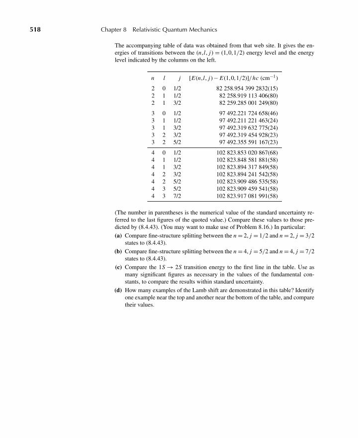
518 Chapter 8 Relativistic Quantum Mechanics
The accompanying table of data was obtained from that web site. It gives the en-ergies of transitions between the (n,l , j ) = (1,0,1/2) energy level and the energylevel indicated by the columns on the left.
n l j [E(n,l , j )− E(1,0,1/2)]/hc (cm−1)
2 0 1/2 82 258.954 399 2832(15)2 1 1/2 82 258.919 113 406(80)2 1 3/2 82 259.285 001 249(80)
3 0 1/2 97 492.221 724 658(46)3 1 1/2 97 492.211 221 463(24)3 1 3/2 97 492.319 632 775(24)3 2 3/2 97 492.319 454 928(23)3 2 5/2 97 492.355 591 167(23)
4 0 1/2 102 823.853 020 867(68)4 1 1/2 102 823.848 581 881(58)4 1 3/2 102 823.894 317 849(58)4 2 3/2 102 823.894 241 542(58)4 2 5/2 102 823.909 486 535(58)4 3 5/2 102 823.909 459 541(58)4 3 7/2 102 823.917 081 991(58)
(The number in parentheses is the numerical value of the standard uncertainty re-ferred to the last figures of the quoted value.) Compare these values to those pre-dicted by (8.4.43). (You may want to make use of Problem 8.16.) In particular:
(a) Compare fine-structure splitting between the n = 2, j = 1/2 and n = 2, j = 3/2states to (8.4.43).
(b) Compare fine-structure splitting between the n = 4, j = 5/2 and n = 4, j = 7/2states to (8.4.43).
(c) Compare the 1S → 2S transition energy to the first line in the table. Use asmany significant figures as necessary in the values of the fundamental con-stants, to compare the results within standard uncertainty.
(d) How many examples of the Lamb shift are demonstrated in this table? Identifyone example near the top and another near the bottom of the table, and comparetheir values.
A P P E N D I X
A Electromagnetic Units
Two divergent systems of units established themselves over the course of thetwentieth century. One system, known as SI (from the French le Système inter-national d’unités), is rooted in the laboratory. It gained favor in the engineer-ing community and forms the basis for most undergraduate curricula. The othersystem, called Gaussian, is aesthetically cleaner and is much favored in the the-oretical physics community. We use Gaussian units in this book, as do mostgraduate-level physics texts.
The SI system is also known as MKSA (for meter, kilogram, second, ampere),and the Gaussian is called CGS (for centimeter, gram, second) units. For problemsin mechanics, the difference is trivial, amounting only to some powers of 10.Difficulty arises, however, when incorporating electromagnetism, where charge,for example, actually has different dimensions for the two sets of units.
This appendix attempts to contrast the two systems of units with respect toelectromagnetism. Some formulas are given that should make it easy for thereader to follow the discussions in this and other graduate-level books.
A.1 COULOMB’S LAW, CHARGE, AND CURRENT
Coulomb’s law is the empirical observation that two charges Q1 and Q2 attract orrepel each other with a force FQ that is proportional to the product of the chargesand inversely proportional to the square of the distance r between them. It is mostnatural to write this as
FQ = Q1 Q2
r2 Gaussian. (A.1.1)
This is in fact the starting point for defining Gaussian units. The units of chargeare called statcoulombs, and the force between two charges of one statcoulombeach separated by one centimeter is one dyne.
It is easy to see why such a delightfully simple formulation caught on in thephysics community. Unfortunately, though, it is difficult to realize experimentally.It is much easier to set up a current source in the laboratory—perhaps with a bat-tery driving a circuit with an adjustable resistance. Furthermore, magnetic forcesbetween long wires are straightforward to measure. Therefore, the SI system isborne out of the definition of the ampere:
One ampere is that steady current which, when present in each oftwo long parallel conductors, separated by a distance d of one meter,
519
520 Appendix A Electromagnetic Units
results in a force per meter of length FI /L between them numericallyequal to 2 ×10⁻⁷ N/m.
The simple force formula for the SI system, analogous to Coulomb’s law for theGaussian system, is
FI
L= μ0
2π
I1 I2
dSI (A.1.2)
for currents I1 and I2 (measured in amperes) in each of two wires. Although(A.1.2) doesn’t carry a popularized name, it is as fundamental to the SI system ofunits as Coulomb’s law (A.1.1) is to the Gaussian system.
Based on the definition of the ampere, we must have
μ0 ≡ 4π×10−7 N/A2. (A.1.3)
Factors of 4π frequently appear in formulations of electromagnetism because oneis always bound to integrate over the unit sphere. It is a matter of taste—andnow convention—whether to take them out in the beginning or carry them aroundthrough the calculation.
If one defines a unit of charge called the coulomb as the charge passingthrough a wire carrying a current of one ampere during a time of one second, thenCoulomb’s law becomes
FQ = 1
4πε0
Q1 Q2
r2SI. (A.1.4)
With this definition of the proportionality constant, one eventually shows that thespeed of electromagnetic waves in free space is
c = 1√ε0μ0
. (A.1.5)
In our current standard units, the speed of light c is a defined quantity. Hence, ε0is also defined to be an exact value.
A relation like (A.1.5) is of course no surprise. Electric and magnetic fieldsare related to each other through Lorentz transformations, so the proportionalityconstants ε0 and μ0 should be related through c. In Gaussian units, there are noanalogues of ε0 or μ0, but c appears explicitly instead.
A.2 CONVERTING BETWEEN SYSTEMS
Electromagnetism can be developed by starting with (A.1.1) or (A.1.4) and incor-porating special relativity. For example, one first writes down Gauss’s law as
∇· E = ρ(x)/ε0 SI (A.2.1a)
or ∇· E = 4πρ(x) Gaussian (A.2.1b)
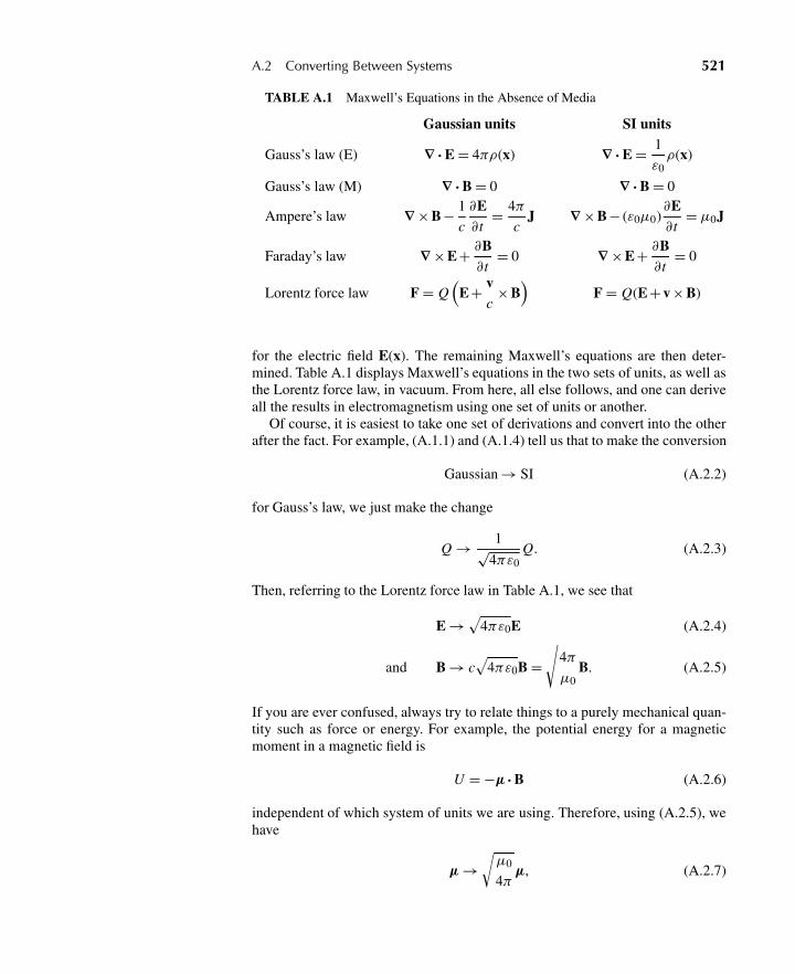
A.2 Converting Between Systems 521
TABLE A.1 Maxwell’s Equations in the Absence of Media
Gaussian units SI units
Gauss’s law (E) ∇· E = 4πρ(x) ∇· E = 1
ε0ρ(x)
Gauss’s law (M) ∇· B = 0 ∇· B = 0
Ampere’s law ∇ ×B− 1
c
∂E∂ t
= 4π
cJ ∇ ×B− (ε0μ0)
∂E∂ t
= μ0J
Faraday’s law ∇ ×E+ ∂B∂ t
= 0 ∇ ×E+ ∂B∂ t
= 0
Lorentz force law F = Q(
E+ vc
×B)
F = Q(E+ v ×B)
for the electric field E(x). The remaining Maxwell’s equations are then deter-mined. Table A.1 displays Maxwell’s equations in the two sets of units, as well asthe Lorentz force law, in vacuum. From here, all else follows, and one can deriveall the results in electromagnetism using one set of units or another.
Of course, it is easiest to take one set of derivations and convert into the otherafter the fact. For example, (A.1.1) and (A.1.4) tell us that to make the conversion
Gaussian → SI (A.2.2)
for Gauss’s law, we just make the change
Q → 1√4πε0
Q. (A.2.3)
Then, referring to the Lorentz force law in Table A.1, we see that
E →√4πε0E (A.2.4)
and B → c√
4πε0B =√
4π
μ0B. (A.2.5)
If you are ever confused, always try to relate things to a purely mechanical quan-tity such as force or energy. For example, the potential energy for a magneticmoment in a magnetic field is
U = −μ · B (A.2.6)
independent of which system of units we are using. Therefore, using (A.2.5), wehave
μ →√μ0
4πμ, (A.2.7)
522 Appendix A Electromagnetic Units
and so, referring to the starting point of this book, the magnetic moment of acirculating charge Q with angular momentum L is
μ = Q
2mcL Gaussian
→√μ0
4πμ = Q√
4πε0
1
2mcL (A.2.8)
or μ = Q
2mL SI. (A.2.9)
It is also useful to keep in mind that quantities such as Q2 have dimensions ofenergy × length in Gaussian units. This is generally enough so that you neverhave to worry about what a “statcoulomb” really is.
A P P E N D I X
BBrief Summary of Elementary
Solutions to Schrödinger’s WaveEquation
Here we summarize the simple solutions to Schrödinger’s wave equation for avariety of solvable potential problems.
B.1 FREE PARTICLES (V = 0)
The plane-wave, or momentum, eigenfunction is
ψk(x, t) = 1
(2π)3/2 eik·x−iωt , (B.1.1)
where
k = ph
, ω = E
h= p2
2mh= hk2
2m, (B.1.2)
and our normalization is ∫ψ∗
k′ψkd3x = δ(3)(k− k′). (B.1.3)
The superposition of plane waves leads to the wave-packet description. In theone-dimensional case,
ψ(x , t) = 1√2π
∫ ∞
−∞dk A(k) ei(kx−ωt )
(ω = hk2
2m
). (B.1.4)
For |A(k)| sharply peaked near k � k0, the wave packet moves with a group ve-locity
υg �(
dω
dk
)k0
= hk0
m. (B.1.5)
The time evolution of a minimum wave packet can be described by
ψ(x , t) =[
(�x)20
2π3
]1/4∫ ∞
−∞e−(�x)2
0(k−k0)2+ikx−iω(k)t dk, ω (k) = hk2
2m,
(B.1.6)
523
524 Appendix B Brief Summary of Elementary Solutions to Schrödinger’s Wave Equation
where
|ψ(x , t)|2 =⎧⎨⎩ 1
2π(�x)20
[1 + (h2t2/4m2)(�x)−4
0
]⎫⎬⎭
1/2
× exp
⎧⎨⎩− (x − hk0t/m)2
2(�x)20
[1 + (h2t2/4m2)(�x)−4
0
]⎫⎬⎭.
(B.1.7)
So the width of the wave packet expands as
(�x)0 at t = 0 → (�x)0
[1 + h2t2
4m2(�x)−4
0
]1/2
at t > 0. (B.1.8)
B.2 PIECEWISE CONSTANT POTENTIALS IN ONE DIMENSION
The basic solutions are
E > V = V0 : ψE (x) = c+eikx + c−e−ikx , k =√
2m(E − V0)
h2 . (B.2.1)
E < V = V0 (classically forbidden region):
ψE (x) = c+eκx + c−e−κx , κ =√
2m(V0 − E)
h2 (B.2.2)
(c± must be set equal to 0 if x = ± ∞ is included in the domain under discussion).
Rigid-Wall Potential (One-dimensional Box)
Here
V ={
0 for 0< x < L,∞ otherwise.
(B.2.3)
The wave functions and energy eigenstates are
ψE (x) =√
2
Lsin
(nπx
L
), n = 1,2,3 . . . ,
E = h2n2π2
2mL2 .
(B.2.4)
B.3 Transmission-Reflection Problems 525
Square-Well Potential
The potential V is
V ={
0 for |x |> a−V0 for |x |< a (V0 > 0).
(B.2.5)
The bound-state (E < 0) solutions are
ψE ∼
⎧⎪⎨⎪⎩e−κ|x | for |x |> a,
cos kx (evenparity)
sin kx (oddparity)
}for |x |< a,
(B.2.6)
where
k =√
2m(−|E |+ V0)
h2, κ =
√2m|E |
h2. (B.2.7)
The allowed discrete values of energy E = −h2κ2/2m are to be determined bysolving
ka tan ka = κa (evenparity)
ka cot ka = −κa (oddparity).(B.2.8)
Note also that κ and k are related by
2mV0a2
h2 = (k2 +κ2)a2. (B.2.9)
B.3 TRANSMISSION-REFLECTION PROBLEMS
In this discussion we define the transmission coefficient T to be the ratio of the fluxof the transmitted wave to that of the incident wave. We consider the followingsimple examples.
Square Well (V = 0 for |x |> a, V = −V0 for |x |< a.)
T = 1{1 + [
(k ′2 − k2)2/4k2k ′2]sin2 2k ′a}
= 1{1 + [
V 20 /4E(E + V0)
]sin2 (2a
√2m(E + V0)/h2)} ,
(B.3.1)
where
k =√
2m E
h2, k ′ =
√2m(E + V0)
h2. (B.3.2)
526 Appendix B Brief Summary of Elementary Solutions to Schrödinger’s Wave Equation
Note that resonances occur whenever
2a
√2m(E + V0)
h2= nπ , n = 1,2,3, . . . . (B.3.3)
Potential Barrier (V = 0 for |x |> a, V = V0 > 0 for |x |< a.)
Case 1: E < V0.
T = 1{1 + [
(k2 +κ2)2/4k2κ2]
sinh2 2κa}
= 1{1 + [
V 20 /4E(V0 − E)
]sinh2 (2a
√2m(V0 − E)/h2)} .
(B.3.4)
Case 2: E > V0. This case is the same as the square-well case with V0 replacedby −V0.
Potential Step (V = 0 for x < 0, V = V0 for x > 0, and E > V0.)
T = 4kk′
(k + k ′)2= 4
√(E − V0)E(√
E +√E − V0
)2(B.3.5)
with
k =√
2m E
h2, k ′ =
√2m(E − V0)
h2. (B.3.6)
More General Potential Barrier {V (x)> E for a < x < b, V (x)< E outsiderange [a,b].}The approximate JWKB solution for T is
T � exp
{−2
∫ b
adx
√2m[V (x) − E]
h2
}, (B.3.7)
where a and b are the classical turning points.∗
B.4 SIMPLE HARMONIC OSCILLATOR
Here the potential is
V (x) = mω2x2
2, (B.4.1)
∗JWKB stands for Jeffreys-Wentzel-Kramers-Brillouin.
B.5 The Central Force Problem [Spherically Symmetrical PotentialV = V (r)] 527
and we introduce a dimensionless variable
ξ =√
mω
hx . (B.4.2)
The energy eigenfunctions are
ψE = (2nn!)−1/2(
mω
π h
)1/4
e−ξ2/2 Hn(ξ ) (B.4.3)
and the energy levels are
E = hω
(n + 1
2
), n = 0,1,2, . . . . (B.4.4)
The Hermite polynomials have the following properties:
Hn(ξ ) = (−1)neξ2 ∂n
∂ξne−ξ2
∫ ∞
−∞Hn′ (ξ ) Hn (ξ ) e−ξ2
dξ = π1/22n!δnn′
d2
dξ2 Hn − 2ξd Hn
dξ+ 2nHn = 0
H0(ξ ) = 1, H1(ξ ) = 2ξ (B.4.5)
H2(ξ ) = 4ξ2 − 2, H3 (ξ ) = 8ξ3 − 12ξ
H4(ξ ) = 16ξ4 − 48ξ2 + 12.
B.5 THE CENTRAL FORCE PROBLEM [SPHERICALLY SYMMETRICALPOTENTIAL V = V(r)]
Here the basic differential equation is
− h2
2m
[1
r2
∂
∂r
(r2 ∂ψE
∂r
)+ 1
r2 sinθ
∂
∂θ
(sinθ
∂ψE
∂θ
)+ 1
r2 sin2 θ
∂2ψE
∂φ2
]+ V (r )ψE = EψE ,
(B.5.1)where our spherically symmetrical potential V(r) satisfies
limr→0
r2V (r ) → 0. (B.5.2)
The method of separation of variables,
!E (x) = R(x)Y ml (θ ,φ), (B.5.3)
528 Appendix B Brief Summary of Elementary Solutions to Schrödinger’s Wave Equation
leads to the angular equation
−[
1
sinθ
∂
∂θ
(sinθ
∂
∂θ
)+ 1
sin2 θ
∂2
∂φ2
]Y m
l = l(l + 1)Y ml , (B.5.4)
where the spherical harmonics
Y ml (θ ,φ), l = 0,1,2, . . . , m = −l,−l + 1, . . . ,+l (B.5.5)
satisfy
−i∂
∂φY m
l = mY ml , (B.5.6)
and Y ml (θ ,φ) have the following properties:
Y ml (θ ,φ) = (−1)m
√2l + 1
4π
(l − m)!
(l + m)!Pm
l (cosθ ) eimφ for m ≥ 0
Y ml (θ ,φ) = (−1)|m|Y |m|∗
l (θ ,φ) for m < 0
Pml (cosθ ) = (1 − cos2 θ )m/2 dm
d(cosθ )mPl (cosθ ) for m ≥ 0
Pl (cosθ ) = (−1)l
2ll!
d l(1 − cos2 θ )l
d(cosθ )l
Y 00 = 1√
4π, Y 0
1 =√
3
4πcosθ (B.5.7)
Y ±11 = ∓
√3
8π(sinθ )e±iφ
Y 02 =
√5
16π(3cos2 θ − 1)
Y ±12 = ∓
√15
8π(sinθ cosθ )e±iφ
Y ±22 =
√15
32π(sin2 θ )e±2iφ
∫Y m′∗
l′ (θ ,φ)Y ml (θ ,φ)d�= δll′δmm′
[∫d�=
∫ 2π
0dφ
∫ +1
−1d(cosθ )
].
For the radial piece of (A.5.3), let us define
uE (r ) = r R(r ). (B.5.8)
B.5 The Central Force Problem [Spherically Symmetrical PotentialV = V (r)] 529
Then the radial equation is reduced to an equivalent one-dimensional problem,namely
− h2
2m
d2uE
dr2 +[
V (r ) + l(l + 1)h2
2mr2
]uE = EuE
subject to the boundary condition
uE (r )|r=0 = 0. (B.5.9)
For the case of free particles [V (r ) = 0] in our spherical coordinates:
R(r ) = c1 jl(ρ) + c2nl (ρ) (c2 = 0 of the origin is included.), (B.5.10)
where ρ is a dimensionless variable
ρ ≡ kr , k =√
2m E
h2 . (B.5.11)
We need to list the commonly used properties of the Bessel functions andspherical Bessel and Hankel functions. The spherical Bessel functions are
jl(ρ) =(π
2ρ
)1/2
Jl+1/2(ρ)
nl (ρ) = (−1)l+1(π
2ρ
)1/2
J−l−1/2(ρ)
j0(ρ) = sin ρ
ρ, n0(ρ) = −cos ρ
ρ
j1(ρ) = sin ρ
ρ2− cos ρ
ρ, n1(ρ) = −cos ρ
ρ2− sin ρ
ρ(B.5.12)
j2(ρ) =(
3
ρ3 − 1
ρ
)sin ρ− 3
ρ2 cos ρ
n2(ρ) = −(
3
ρ3− 1
ρ
)cos ρ− 3
ρ2sin ρ.
For ρ→ 0, the leading terms are
jl(ρ) −→ρ→0
ρl
(2l + 1)!!, nl (ρ) −→
ρ→0− (2l − 1)!!
ρl+1 , (B.5.13)
where
(2l + 1)!! ≡ (2l + 1)(2l − 1) · · ·5 ·3 ·1. (B.5.14)
530 Appendix B Brief Summary of Elementary Solutions to Schrödinger’s Wave Equation
In the large ρ-asymptotic limit, we have
jl(ρ) −→ρ→∞
1
ρcos
[ρ− (l + 1)π
2
],
nl (ρ) −→ρ→∞
1
ρsin
[ρ− (l + 1)π
2
].
(B.5.15)
Because of constraints (A.5.8) and (A.5.9), R(r) must be finite at r = 0; hence,from (A.5.10) and (A.5.13) we see that the nl (ρ)-term must be deleted becauseof its singular behavior as ρ → 0. Thus R(r ) = cl jl(ρ) [or, in the notation ofChapter 6, Section 6.4, Al(r ) = R(r ) = cl jl(ρ)]. For a three-dimensional square-well potential, V = −V0 for r < R (with V0 > 0), the desired solution is
R(r ) = Al (r ) = constant jl(αr ), (B.5.16)
where
α =[
2m(V0 −|E |)h2
]1/2
, r < R. (B.5.17)
As discussed in (7.6.30), the exterior solution for r > R, where V = 0, can bewritten as a linear combination of spherical Hankel functions. These are definedas follows:
h(1)l (ρ) = jl(ρ) + inl(ρ)
h(1)∗l (ρ) = h(2)
l (ρ) = jl(ρ) − inl(ρ),(B.5.18)
which, from (A.5.15), have the asymptotic forms for ρ → ∞ as follows:
h(1)l (ρ) −→
ρ→∞1
ρei[ρ−(l+1)π/2]
h(1)∗l (ρ) = h(2)
l (ρ) −→ρ→∞
1
ρe−i[ρ−(l+1)π/2].
(B.5.19)
If we are interested in the bound-state energy levels of the three-dimensionalsquare-well potential, where V (r ) = 0, r > R, we have
ul(r ) = r Al (r ) = constant e−κr f
(1
κr
)κ =
(2m|E |
h2
)1/2
.
(B.5.20)
To the extent that the asymptotic expansions, of which (A.5.19) give the lead-ing terms, do not contain terms with exponent of opposite sign to that given, wehave—for r > R—the desired solution from (A.5.20):
Al(r ) = constant h(1)l (iκr ) = constant [ jl (iκr ) + inl (iκr )], (B.5.21)
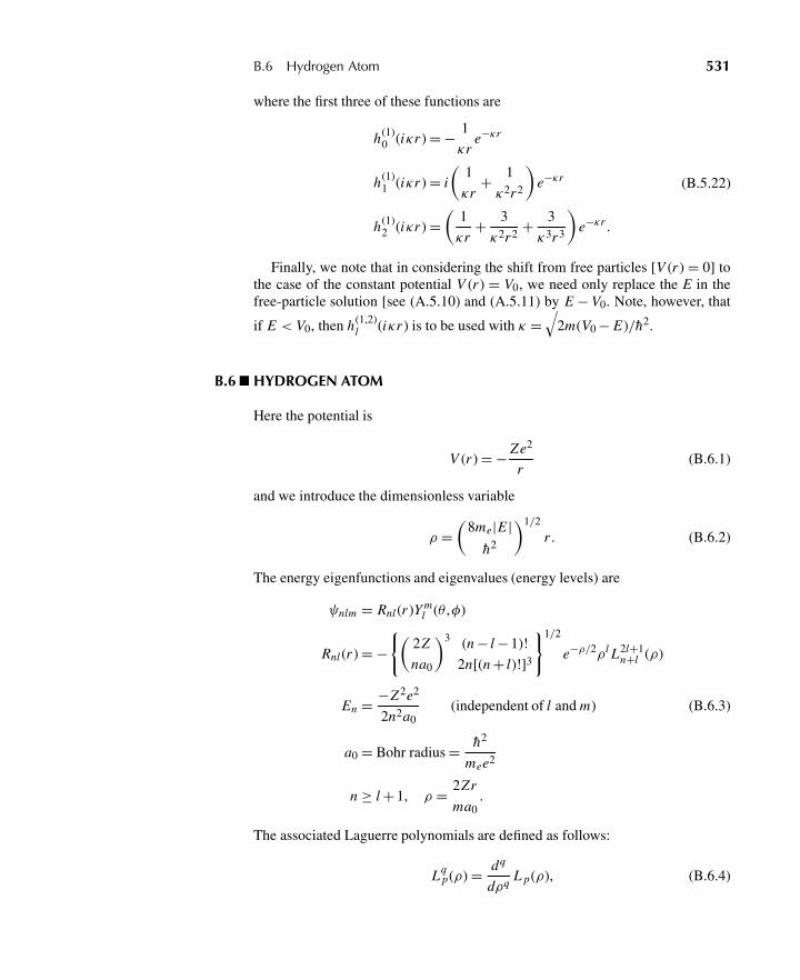
B.6 Hydrogen Atom 531
where the first three of these functions are
h(1)0 (iκr ) = − 1
κre−κr
h(1)1 (iκr ) = i
(1
κr+ 1
κ2r2
)e−κr
h(1)2 (iκr ) =
(1
κr+ 3
κ2r2 + 3
κ3r3
)e−κr .
(B.5.22)
Finally, we note that in considering the shift from free particles [V (r ) = 0] tothe case of the constant potential V (r ) = V0, we need only replace the E in thefree-particle solution [see (A.5.10) and (A.5.11) by E − V0. Note, however, that
if E < V0, then h(1,2)l (iκr ) is to be used with κ =
√2m(V0 − E)/h2.
B.6 HYDROGEN ATOM
Here the potential is
V (r ) = − Ze2
r(B.6.1)
and we introduce the dimensionless variable
ρ =(
8me|E |h2
)1/2
r . (B.6.2)
The energy eigenfunctions and eigenvalues (energy levels) are
ψnlm = Rnl (r )Y ml (θ ,φ)
Rnl (r ) = −{(
2Z
na0
)3 (n − l − 1)!
2n[(n + l)!]3
}1/2
e−ρ/2ρl L2l+1n+l (ρ)
En = −Z2e2
2n2a0(independent of l and m) (B.6.3)
a0 = Bohr radius = h2
mee2
n ≥ l + 1, ρ = 2Zr
ma0.
The associated Laguerre polynomials are defined as follows:
Lqp(ρ) = dq
dρqL p(ρ), (B.6.4)
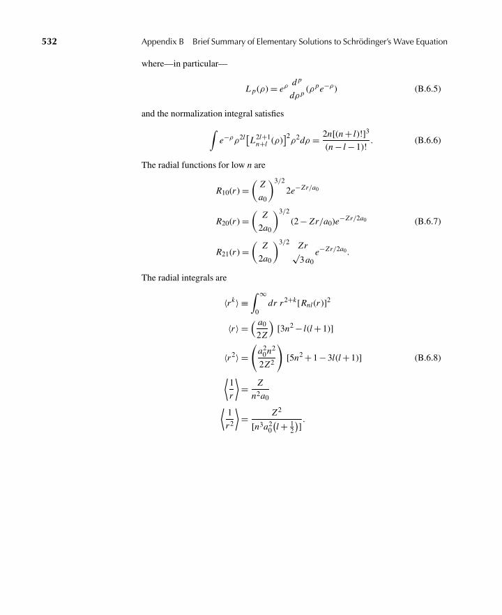
532 Appendix B Brief Summary of Elementary Solutions to Schrödinger’s Wave Equation
where—in particular—
L p(ρ) = eρd p
dρ p(ρ pe−ρ) (B.6.5)
and the normalization integral satisfies∫e−ρρ2l[L2l+1
n+l (ρ)]2ρ2dρ = 2n[(n + l)!]3
(n − l − 1)!. (B.6.6)
The radial functions for low n are
R10(r ) =(
Z
a0
)3/2
2e−Zr/a0
R20(r ) =(
Z
2a0
)3/2
(2 − Zr/a0)e−Zr/2a0 (B.6.7)
R21(r ) =(
Z
2a0
)3/2 Zr√3a0
e−Zr/2a0.
The radial integrals are
〈rk〉 ≡∫ ∞
0dr r2+k[Rnl (r )]2
〈r〉 =( a0
2Z
)[3n2 − l(l + 1)]
〈r2〉 =(
a20n2
2Z2
)[5n2 + 1 − 3l(l + 1)] (B.6.8)
⟨1
r
⟩= Z
n2a0⟨1
r2
⟩= Z2
[n3a20
(l + 1
2
)].
A P P E N D I X
CProof of the Angular-MomentumAddition Rule Given by Equation
(3.8.38)
It will be instructive to discuss the angular-momentum addition rule from thequantum-mechanical point of view. Let us, for the moment, label our angularmomenta such that j1>= j2. This we can always do. From Equation (3.8.35), the
maximum value of m, mmax, is
mmax = mmax1 + mmax
2 = j1 + j2. (C.1.1)
There is only one ket that corresponds to the eigenvalue mmax, whether the de-scription is in terms of | j1 j2; m1m2〉 or | j1 j2; jm〉. In other words, choosing thephase factor to be 1, we have
| j1 j2; j1 j2〉 = | j1 j2; j1 + j2, j1 + j2〉. (C.1.2)
In the | j1 j2; m1m2〉 basis, there are two kets that correspond to the m eigenvaluemmax − 1, namely, one ket with m1 = mmax
1 − 1 and m2 = mmax2 and one ket with
m1 = mmax1 and m2 = mmax
2 − 1. There is thus a twofold degeneracy in this basis;therefore, there must be a twofold degeneracy in the | j1 j2; jm〉 basis as well.From where could this come? Clearly, mmax − 1 is a possible m-value for j =j1+ j2. It is also a possible m-value for j = j1+ j2−1—in fact, it is the maximumm-value for this j. So j1, j2 can add to j’s of j1 + j2 and j1 + j2 − 1.
We can continue in this way, but it is clear that the degeneracy cannot increaseindefinitely. Indeed, for mmin = − j1 − j2, there is once again a single ket. Themaximum degeneracy is (2 j2 +1)-fold, as is apparent from Table C.1, which wasconstructed for two special examples: for j1 = 2, j2 = 1 and for j1 = 2, j2 = 1
2 .This (2 j2 + 1)-fold degeneracy must be associated with the 2 j2 + 1 states j:
j1 + j2, j1 + j2 − 1, . . . , j1 − j2. (C.1.3)
If we lift the restriction j1>= j2, we obtain (3.8.38).
533
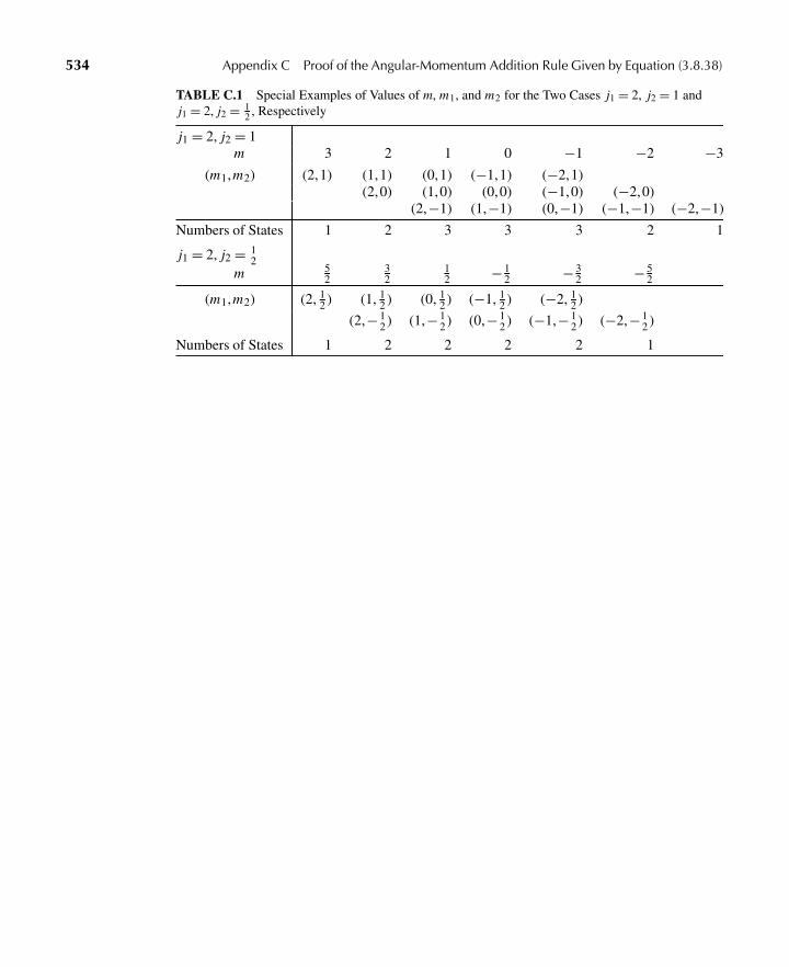
534 Appendix C Proof of the Angular-Momentum Addition Rule Given by Equation (3.8.38)
TABLE C.1 Special Examples of Values of m, m1, and m2 for the Two Cases j1 = 2, j2 = 1 andj1 = 2, j2 = 1
2 , Respectively
j1 = 2, j2 = 1m 3 2 1 0 −1 −2 −3
(m1,m2) (2,1) (1,1) (0,1) (−1,1) (−2,1)(2,0) (1,0) (0,0) (−1,0) (−2,0)
(2,−1) (1,−1) (0,−1) (−1,−1) (−2,−1)
Numbers of States 1 2 3 3 3 2 1
j1 = 2, j2 = 12
m 52
32
12 − 1
2 − 32 − 5
2
(m1,m2) (2, 12 ) (1, 1
2 ) (0, 12 ) (−1, 1
2 ) (−2, 12 )
(2,− 12 ) (1,− 1
2) (0,− 12 ) (−1,− 1
2) (−2,− 12 )
Numbers of States 1 2 2 2 2 1
Bibliography
NEW REFERENCES FOR THE SECOND EDITION
Arfken, G. B. and H. J. Weber. Mathematical Methods for Physicists, 4th ed., New York:Academic Press, 1995.
Byron, F. W. and R. W. Fuller. Mathematics of Classical and Quantum Physics, Mineola,NY: Dover, 1992.
Fetter, A. L. and J. D. Walecka. Quantum Theory of Many-Particle Systems, Mineola,NY: Dover, 2003a.
Fetter, A. L. and J. D. Walecka. Theoretical Mechanics of Particles and Continua, Mine-ola, NY: Dover, 2003b.
Goldstein, H., C. Poole, and J. Safko. Classical Mechanics, 3rd. ed., Reading, MA:Addison-Wesley, 2002.
Gottfried, K. and T.-M. Yan. Quantum Mechanics: Fundamentals, 2nd ed., New York:Springer-Verlag, 2003.
Griffiths, D. J. Introduction to Quantum Mechanics, 2nd ed., Upper Saddle River, NJ:Pearson, 2005.
Heitler, W. The Quantum Theory of Radiation, 3rd ed., Oxford (1954).
Holstein, B. R. Topics in Advanced Quantum Mechanics, Reading, MA: Addison-Wesley, 1992.
Itzykson, C. and J.-B. Zuber, Quantum Field Theory, New York: McGraw-Hill, 1980.
Jackson, J. D. Classical Electrodynamics, 3rd ed., New York: Wiley, 1998.
Landau, R. H. Quantum Mechanics II: A Second Course in Quantum Theory, New York:Wiley, 1996.
Loudon, R. The Quantum Theory of Light, 3rd ed., London: Oxford Science Publications,2000.
Merzbacher, E. Quantum Mechanics, 3rd ed., New York: Wiley, 1998.
Shankar, R. Principles of Quantum Mechanics, 2nd ed., New York: Plenum, 1994.
Taylor, J. R. Classical Mechanics, Herndon, VA: University Science Books, 2005.
Townsend, J. S. A Modern Approach to Quantum Mechanics, Herndon, VA: UniversityScience Books, 2000.
Weinberg, S. The Quantum Theory of Fields, New York: Cambridge University Press,1995.
Zee, A. Quantum Field Theory in a Nutshell, 2nd ed., Princeton, NJ: Princeton UniversityPress, 2010.
535
536 Bibliography
REFERENCE LIST FROM PRIOR EDITIONS
Baym, G. Lectures on Quantum Mechanics, New York: W. A. Benjamin, 1969.
Bethe, H. A. and R. W. Jackiw. Intermediate Quantum Mechanics, 2nd ed., New York:W. A. Benjamin, 1968.
Biedenharn, L. C. and H. Van Dam, editors. Quantum Theory of Angular Momentum,New York: Academic Press, 1965.
Dirac, P. A. M. Quantum Mechanics, 4th ed., London: Oxford University Press, 1958.
Edmonds, A. R. Angular Momentum in Quantum Mechanics, Princeton, NJ: PrincetonUniversity Press, 1960.
Feynman, R. P. and A. R. Hibbs. Quantum Mechanics and Path Integrals, New York:McGraw-Hill, 1965.
Finkelstein, R. J. Nonrelativistic Mechanics, Reading, MA: W. A. Benjamin, 1973.
Frauenfelder, H. and E. M. Henley. Subatomic Physics, Englewood Cliffs, NJ: Prentice-Hall, 1974.
French, A. P. and E. F. Taylor. An Introduction to Quantum Physics, New York: W. W.Norton, 1978.
Goldberger, M. L. and K. M. Watson. Collision Theory, New York: Wiley, 1964.
Gottfried, K. Quantum Mechanics, vol. I, New York: W. A. Benjamin, 1966.
Jackson, J. D. Classical Electrodynamics, 2nd ed., New York: Wiley, 1975.
Merzbacher, E. Quantum Mechanics, 2nd ed., New York: Wiley, 1970.
Morse, P. M. and H. Feshbach. Methods of Theoretical Physics (2 vols.), New York:McGraw-Hill, 1953.
Newton, R. G. Scattering Theory of Waves and Particles, 2nd ed., New York: McGraw-Hill, 1982.
Preston, M. Physics of the Nucleus, Reading, MA: Addison-Wesley, 1962.
Sargent III, M., M. O. Scully, and W. E. Lamb, Jr. Laser Physics, Reading, MA: Addison-Wesley, 1974.
Saxon, D. S. Elementary Quantum Mechanics. San Francisco: Holden-Day, 1968.
Schiff, L. Quantum Mechanics, 3rd. ed., New York: McGraw-Hill, 1968.
Index
AAbelian, definition of, 47Absorption, in classical
radiation fields, 365–367Absorption-emission cycle,
341–342Adiabatic approximation,
346–348Aharonov-Bohm effect,
141–145, 353–355Airy function, 109–110,
113–115Alkali atoms, 323–326Ambler, E., 278Ampere (unit), 519Ampere’s law, 521Amplitude(s)
Born, 400, 419, 443, 523and bound states, 429–430correlation, 78–80partial-wave, 410scattering, see Scattering
amplitudetransition, 86–89, 120–122,
387Anderson, Carl, 500Angular integration, in helium
atom, 456Angular momentum, 157–255
and angular-velocity vector,5–6
commutation relations for,157–163
density operator andensembles for, 178–191
Dirac equation for, 501–502orbital, see Orbital angular
momentum
rotations and commutationrelations in, 157–172
and Schrödinger’s equationfor central potentials,207–217
Schwinger’s oscillator modelof, 232–238
of silver atoms, 23and SO(3)/SU(2)/Euler
rotations, 172–178spin correlation
measurements and Bell’sinequality for, 238–245
tensor operator for, 246–255and uncoupled oscillators,
232–235Angular-momentum addition,
217–231Clebsch-Gordan coefficients
for, 223–231examples of, 218–221formal theory of, 221–224and rotation matrices,
230–231rule for, 533–534
Angular-momentum barriers,208, 209
Angular-momentumcommutation relations
and eigenvalues/eigenstates,191–192
and ladder operator, 192and rotations, 157–1632 × 2 matrix realizations, 169
Angular-momentum eigenkets,193–194
Angular-momentum eigenvaluesand eigenstates
and commutationrelations/ladder operator,191–192
constructing, 193–195and matrix elements of
angular-momentumoperator, 195–196
and rotation operator,196–199
and time reversal, 298and Wigner-Eckart theorem
and, 252–253Angular-momentum operator,
161, 195–196, 258Angular velocity vector, angular
momentum and, 5–6Annihilation operator, 89–91,
97, 152, 232–233, 465Anomalous Zeeman effect, 328Anticommutation relations, 28,
469Antilinear operator, 287,
291–292Antiparticles, in Klein-Gordon
equation, 493, 494, 503Antisymmetrical states, 275Antiunitary operator, 287, 291,
296, 434–436, 504–505Anyons, 450nApproximation methods,
303–375for classical radiation field,
365–371for degenerate energy
eigenkets, 316–321for energy shifts and decay
widths, 371–375for hydrogen-like atoms,
321–336
537
538 Index
for nondegenerate energyeigenkets, 303–316
for time-dependentHamiltonians, 345–355
time-dependent perturbationtheory, 355–365
for time-dependent potentials,336–345
time-independentperturbation theory,303–321
variational, 332–336Argand diagram, 413Argon, Ramsauer-Townsend
effect and, 425–426Associative axiom of
multiplication, 16–17Atom(s), See also specific types
Bohr, 1one-electron, 510–514polarizability of, 297
Atomic force microscope,479–480
Atomic spectroscopy, 163Axial vectors, 272
BBaker-Hausdorff formula, 95Balmer formula, 216, 513Balmer splittings, fine structure
splittings and, 326Base kets, 17–20
change of basis in, 35–36eigenkets as, 18–19and eigenkets of observables,
17–18in Heisenberg and
Schrödinger pictures,86–89
and spin 12 systems, 22
in spin 12 systems, 22–23
and transition amplitudes,86–89
Basischange of, 35–40position, 52–53
Baym, G., 250
Bell’s inequality, 241–245and Einstein’s locality
principle, 241–243and quantum mechanics,
243–245Bennett, G. W., 76Berry, M. V., 348Berry’s Phase
and gauge transformations,353–355
and time-dependentHamiltonians, 348–353
Bessel functionsproperties of, 529–530spherical, 210–211
Bethe, H. A., 439Biedenharn, L. C., 232Big box normalization, 104,
388–389Bitter, T., 352Bloch, F., 439Bloch’s theorem, 283Bohr, N., 73, 397, 440Bohr atom, 1Bohr model, 216Bohr radius, 217Boltzmann constant, 187, 487Born, M., 1, 48, 89, 99, 191Born amplitude, first-order, 400,
419, 443, 523Born approximation, 399–404,
442Bose-Einstein condensation,
452, 464Bose-Einstein statistics, 450Bosons, 450–452, 462–464, 476Bouncing ball example, 110Bound states, 423–431
and amplitude, 429–430and low-energy scattering,
423–430quasi-, 431and zero-energy scattering,
426–429Bowles, T. J., 450Bra, matrix representation of, 21Bra-ket algebra, 59Bra-ket notation, Dirac, 292Bra space, 12–14
Breit-Wigner Formula, 433Bressi, G., 480Brillouin, L., 110Brillouin zone, 284
CCannonical (fundamental)
commutation relations,48–49
Canonical ensembles, 189–190Canonical momentum, 136,
138, 140, 262Cartesian tensors, 247–250Casimir effect, 476–480Cauchy principal value, 397Cayley-Klein parameters, 174Central force problem,
Schrödinger waveequation and, 527–531
Central potentials, 506–514in eigenvalue problem,
506–510and Hamiltonians, 207, 211for one-electron atom,
510–514Schrödinger equation for, see
Schrödinger equation forcentral potentials
solving for, 506–514Cesium atoms, spin
manipulation of, 10CGS system of units, 519Charge, units for, 519–520Charge conjugation, 503–504,
506Chiao, R., 351Classical physics, symmetry in,
262–263Classical radiation field,
365–371absorption and stimulated
emission in, 365–367electric dipole approximation
for, 367–369photoelectric effect in,
369–371Clebsch-Gordan coefficients,
220properties of, 223–224
Index 539
recursion relations for,224–229
and rotation matrices,230–231
and tensors, 251–253Clebsch-Gordan series, 230–231Clebsch-Gordan series formula,
251Closure, 19Cobalt atoms
parity nonconservation for,278–279
transition energy of, 517Coherent state
for annihilation operator, 97in quantum optics, 481
Collective index, 30, 314Column vector function, 491Commutation relations, 28
angular-momentum,157–163, 169, 191–192
cannonical, 48–49and eigenvalues/eigenstates,
191–192in second quantization,
462–463Commutators, 48–49, 64, 85Compatible observables, 28–31Completely random ensembles,
179, 186Completeness relation, 19Complex conjugate transposed,
20Complex contour integration,
392–394, 397–398Complex numbers, quantum
mechanics and, 27Complex vector space, spin
states and, 9Compton effect, 1Compton wavelength, 489Confluent Hypergeometric
Function, 215Conservation laws, 262–263Conserved current, 492,
496–497, 516Conserved Vector Current
(CVC) hypothesis,449–450
Constant perturbation, 359–363Constant potential
and gauge transformations,129–131
in one dimension, 524–525Continuity equation, 496Continuous spectra, 40–41Continuous symmetry, 262–263,
265–269Continuum generalizations, for
density operator,185–186
Correlation amplitude,energy-time uncertaintyrelation and, 78–80
Correlation function, 151Coulomb (unit), 520Coulomb gauge, 473Coulomb potential
first-order energy shift for,327
and Schrödinger’s equationfor central potentials,213–217
screened, 467symmetry in, 265–269
Coulomb’s law, 519, 520Covariant derivative, 491Covariant Dirac equation, 494,
495Covariant vector operator, 489,
490nCovariant wave equations, 488,
489CPT operator combination, 506Creation operator, 89–91, 152,
232–233, 465Cross sections, for scattering,
388–389Current
conserved, 492, 496–497, 516CVC hypothesis, 449–450units of, 519–520
Cutoff frequency, Casimir effectand, 477, 480
CVC (Conserved VectorCurrent) hypothesis,449–450
DDalgarno, A., 315Davisson-Germer-Thompson
experiment, 1de Broglie, L., 46, 66, 99de Broglie’s matter waves, 1Decay width, energy shift and,
371–375Degeneracy, 59
of eigenvalues, 29, 217exchange, 447Kramers, 299and symmetries, 264–265
Degenerate electron gases,467–472
Degenerate energy eigenkets,316–321
Degenerate time-independentperturbation theory,316–321
Density matrix, 181of completely random
ensemble, 186and continuum
generalizations, 185–186Density of states, for free
particles, 105Density operator, 180–191
continuum generalizationsfor, 185–186
definition of, 181and ensemble averages,
180–185Hermitian, 182and pure/mixed ensembles,
178–191and quantum statistical
mechanics, 186–191time evolution of, 257and time evolution of
ensembles, 185Detailed balance, 365, 436Deuterium atom, energy levels
of, 517–518Diagonalization, 38–39, 64, 90Diamagnetic susceptibility, 380Dipole operator, 368
540 Index
Dirac, P. A. M., 1, 10–11, 23,49, 50, 83, 114,124–125, 148, 356, 362,494
Dirac bra-ket notation, 292Dirac δ function, 40Dirac equation, 494–507
for angular momentum,501–502
for central potentials, 507and charge conjugation,
503–504conserved current in,
496–497and CPT operator
combination, 506described, 494–496and electromagnetic
interactions, 500–501free-particle solutions of,
497–499and negative energies,
499–500parity of, 502–503symmetries of, 501–506time-reversal symmetry of,
504–505Dirac Hamiltonians, 495, 501Dirac notation, 8, 223Dirac picture, 338Dirac quantization condition,
354–355Direction eigenkets, 202–203Discrete symmetries, 269–300,
see also specific typesand Dirac equation, 504–505lattice translation as, 280–284parity as, 269–280properties of symmetry
operations, 287–289time-reversal discrete,
284–300Dispersion, 33–34Double-bar matrix element, 252Dual correspondence, 13Dubbers, D., 352Dyadic tensors, 247–248
Dynamical variables, in secondquantization approach,463–467
Dyson, F. J., 71, 357Dyson series, 71, 355–357
EEffective potential, 208, 209Ehrenfest, P., 86Ehrenfest’s theorem, 86, 132,
136Eichinvarianz, 141Eigenbras, 12–13Eigenfunctions, 51, 523Eigenkets
angular-momentum, 193–194and base kets, 17–19direction, 202–203and eigenbras, 12–13energy, see Energy eigenketsand Hermitian operator, 59and observables, 17–18parity, 273position, 41–42and simple harmonic
oscillator, 89–93simultaneous, 30in spin 1
2 systems, 12zeroth-order, 316
Eigenspinors, 296Eigenstates
angular-momentum, seeAngular-momentumeigenvalues andeigenstates
energy, 96, 273–274mass, 77in spin 1
2 systems, 12zeroth-order, 377
Eigenvaluesangular-momentum, see
Angular-momentumeigenvalues andeigenstates
and central potential,506–510
degeneracy of, 29, 217energy, 77–78, 89–93, 217and energy eigenkets, 71
and expectation values, 24–25and Hermitian operator, 17of hydrogen atom, 268and orbital angular
momentum squared, 30and simple harmonic
oscillator, 89–93in spin 1
2 systems, 12Eikonal approximation,
417–423described, 417–420and partial waves, 420–423
Einstein, A., 241Einstein-Debye theory, 1Einstein-Podolsky-Rosen
paradox, 241Einstein’s locality principle,
241–243Elastic scattering, 436, 445Electric dipole approximation,
367–369Electric fields, time-reversal
symmetry and, 298–300Electromagnetic fields
and Casimir effect, 480and Dirac equation, 500–501energy of, 474and momentum, 480–481polarization vectors of, 9quantization of, see
Quantization ofelectromagnetic field
Electromagnetic units, 519–522Electromagnetism, gauge
transformations in,134–141
Electron-atom scattering,inelastic, 436–441
Electron gases, degenerate,467–472
Electron spin, magnetic momentand, 2–4
Emission, in classical radiationfields, 365–367
Energy(-ies)of electromagnetic field, 474Fermi, 464, 470of free particles, 487–488kinetic, 321–323
Index 541
negative, 492–494, 499–500quantization of, 475–476transition, 517zero-point (vacuum), 476
Energy eigenketsdegenerate, 316–321nondegenerate, 303–316and simple harmonic
oscillator, 89–93and time-evolution operator,
71–73Energy eigenstates
parity properties of, 273–274superposition of, 96
Energy eigenvaluesdegeneracy of, 217of neutrinos, 77–78and simple harmonic
oscillator, 89–93Energy levels, of hydrogen and
deuterium atoms,513–514, 517–518
Energy shiftsfor Coulomb potentials, 327and decay width, 371–375
Energy-time uncertaintyrelation, correlationamplitude and, 78–80
Ensemble averagedefinition of, 180–181and density operator,
180–184Ensembles, 178–185
canonical, 189–190completely random, 179, 186mixed, 180and polarized vs. unpolarized
beams, 178–180pure, 24, 179, 180time evolution of, 185
Entropy, 187Equation of motion
Euler, 256Heisenberg, 82–84, 94, 256,
263Euclidian space, 34Euler angle notation, 236Euler-Maclaurin summation
formula, 478
Euler rotations, 175–178, 256Exchange degeneracy, 447Exchange density, 454Expectation values, 24–25,
164–165and Hermitian operator,
34–35time dependence of, 73
FFaraday’s law, 521Feenberg, Eugene, 397Fermi-Dirac statistics, 450,
484–485Fermi energy, 464, 470Fermions, 450–452, 462–465Fermi’s golden rule, 362, 387,
388Feshbach, H., 119Fetter, Alexander L., 467, 469,
515Feynman, R. P., 122, 124, 515Feynman’s formulation,
123–129Feynman’s path integral,
127–129, 143, 515Filtration, 25Fine structure, 323–327, 510,
517–518Finite-range potentials, 394–395Finite rotations, 166–172
and infinitesimal rotations,157–160
and neutron interferometry,166–168
noncommutativity of,157–158
Pauli two-componentformalism for, 168–172
rotation operator for spin 12
systems, 163–165and spin 1
2 systems, 163–172Finite square wells, 400–401Finkelstein, R. J., 155Fock, V., 136Fock space, 461Form factor, 439Fortun, M., 476Fourier decomposition, 375
Fourier inversion formula, 375Fourier transform, 438Fractional population, 179Franck-Hertz experiment, 1Frauenfelder, H., 298Free particles
and Dirac equation, 497–499energy of, 487–488in Heisenberg and
Schrödinger pictures,84–86
and infinite spherical well,210–211
scattering by, 404–409and Schrödinger wave
equation, 103–105,523–524
in three dimensions, 103–105Fundamental commutation
relations, 48–49
GGarvey, G. T., 450Gauge invariance, 141Gauge transformations
and Berry’s Phase, 353–355and constant potentials,
129–131definition of, 130and electromagnetism,
134–141Gaussian potential, 444Gaussian system of units,
519–522Gaussian wave packets, 55–57,
62, 65, 99–100, 118–119Gauss’s law, 146, 520–521Gauss’s theorem, 411Generating functions, 105–108Geometric phase, 348–353Gerlach, W., 2Glauber, Roy, 481Goldstein, H., 37, 176, 264Gottfried, K., 25, 152, 331, 378,
379Gravity, quantum mechanics
and, 131–134

542 Index
Green’s function, 118, 394, 404,442
Griffiths, D. J., 346
HHamilton, W. R., 99Hamiltonian matrix, for
two-state systems, 378Hamiltonian operator, 148–150
for simple harmonicoscillator, 89–90
time-dependent, 70–71and time-dependent wave
equation, 97, 98and time-evolution operator,
69time-independent, 70and two-state systems, 60
Hamiltonians, see alsoTime-dependentHamiltonians
and central potentials, 207,211
Dirac, 495, 501Hamilton-Jacobi theory, 102,
154, 418Hamilton’s characteristic
function, 103Hankel functions, 414, 529, 530Hard-sphere scattering, 416–423Harmonic oscillators, 211–214,
376, see also Simpleharmonic oscillator
Harmonic perturbation,363–365
Heisenberg, W., 1, 46, 48, 99,191
Heisenberg equation of motion,82–84, 94, 256, 263
Heisenberg picture, 148–150and base kets, 86–89free particles in, 84–86and Heisenberg equation of
motion, 82–84and propagators, 120–121and Schrödinger picture,
80–89state kets and observables in,
82
and time-dependentpotentials, 337–339
and time-evolution ofensembles, 185
unitary operator in, 80–81Heisenberg uncertainty
principle, 3, 56Helium, 452, 455–459, 483Helmholtz equation, 394, 404Henley, E. M., 298Hermite polynomials, 106–108,
527Hermitian adjoint, 15Hermitian operator, 63–64, 150
anticommute, 61definition of, 44and density
operator/ensembles,182–183
and Ehrenfest’s theorem, 84eigenvalues of, 17and energy eigenkets, 89expectation values of, 34–35and infinitesimal rotations,
161and simple harmonic
oscillators, 95, 97in spin 1
2 systems, 26as time-evolution operator, 69and time-reversal operator,
292, 298Hermiticity, 39, 182Higher-order Born
approximation, 403–404Hilbert, D., 11, 99Hilbert space, 11Holstein, B. R., 349Hooke’s law, 89Hydrogen atom
eigenvalues of, 268energy levels of, 513–514,
517–518and linear Stark effect,
319–321polarizability of, 315and Schrödinger wave
equation, 531–532
Hydrogen-like atoms, 321–336and fine structure, 323–326fine structure of, 510relativistic correction to
kinetic energy for,321–323
spin-orbit and fine structureof, 323–327
van der Waals interaction in,331–332
and Zeeman effect, 328–331
IIdentical particles, 446–483
and helium atoms, 455–459in multiparticle states,
459–472permutation symmetry for,
446–450and quantization of
electromagnetic field,472–483
symmetrization postulate for,450–452
in two-electron systems,452–455
Identity matrix, 515Identity operator, 19, 22, 28Incoherent mixtures, 179Incompatible observables,
28–29, 31–33Inelastic electron-atom
scattering, 436–441Inertia, moment of, computation
of, 5–6Infinitesimal rotation operator,
161, 199–200Infinitesimal rotations, 157–163
commutativity of, 159and finite rotation, 157–160and quantum mechanics,
160–163and vector operator, 246
Infinitesimal time-evolutionoperator, 68
Infinitesimal translation, 42–43Infinite spherical well, free
particles in, 210–211
Index 543
Inner products, 13Integral equation for scattering,
392–396Interaction picture, 337–339Irreducible tensors, 247–250Isomers, optical, 277Isospin, 235Isotropic harmonic oscillator,
211–214, 376
JJackson, J. D., 324, 369Jacobi identity, 49Jaffe, R. L., 480Jenkins, D. A., 517Jordan, P., 48, 99, 191
KKamLAND experiment, 78Kepler problem, 265Kets, 8, see also Base kets;
Eigenketsdefinition of, 11and electromagnetic field
polarization vectors, 9normalized, 14null, 11and operator, 14–15perturbed, normalization of,
310–311spin, 165state, 67–68, 82vacuum, 232–233
Ket space, 11–15, 63Kinematic momentum, 136,
138, 140Kinetic energy, relativistic
correction for, 321–323Klein-Gordon equation,
488–494Kramers, H. A., 110Kramers degeneracy, 299Kronecker symbol, 40, 469Krypton, Ramsauer-Townsend
effect and, 425–426Kummer’s equation, 215, 259Kunselman, R., 517
LLadder operator, angular
momentumcommutation relationsand, 191–192
Lagrange equation, 262Lagrangian, classical, 123, 143Laguerre polynomials, 259, 531Lamb shift, 321, 379, 513Lamoreaux, S., 476Landau, Rubin, 461, 467, 516Lande’s interval rule, 325–326Laplace-Fourier transform, 120Laporte’s rule, 278Lattice translation, as discrete
symmetry, 280–284Lattice translation operator,
281–282Legendre function, 443Lenz vector, 265Lewis, J. T., 315Light, polarization of, 6–10Linear potential, 108–110Linear Stark effect, 319–321Liouville’s theorem, 185Lipkin, H. J., 148Lippmann-Schwinger equation,
390–391, 442, 444Local potentials, 394London, F., 136Lorentz contraction factor, 497Lorentz force, 136, 143, 285Lorentz force law, 490n, 521Lorentz invariance, 506Lorentz transformations, 489Loudon, R., 472Low-energy scattering, 423–429
MMagnetic fields
and Aharonov-Bohm effect,353–354
and Stern-Gerlachexperiment, 2–4
and time-reversal discretesymmetry, 298–300
Magnetic flux, fundamental unitof, 144
Magnetic moment, 2–4, 501
Magnetic monopoles, 145–148,353–355
Marcus, George E., 476Masers, 344–345Mass eigenstates, 77Matrices, see specific typesMatrix elements
of angular-momentumoperator, 195–196
double bar, 252reduced, 255tensors, 252–255
Matrix mechanics, 48Matrix representations, 20–23Matter waves, de Broglie’s, 1Maxwell-Boltzmann statistics,
451Maxwell’s equations, 145, 285,
472–475, 521McKeown, R. D., 449, 450Mean square deviation, 34Measurements
position, 41–42quantum theory of, 23–25selective, 25spin-correlation, 238–245
Melissinos, A., 351Merzbacher, E., 315, 377, 379,
380, 461, 467, 472, 515Minimum uncertainty wave
packets, 56Mixed ensembles, 180MKS system of units, 519Momentum, see also Angular
momentumcanonical, 136, 138, 140, 262definition of, 52and electromagnetic field,
480–481kinematic, 136, 138, 140position-momentum
uncertainty relation, 46and translation generation,
45–48Momentum operator, 52–53, 58,
64Momentum-space wave
function, 53–55, 65, 151Morse, P. M., 119
544 Index
MotionEuler equation of, 256Heisenberg equation of,
82–84, 94, 256, 263Multiparticle states, 459–472
degenerate electron gases as,467–472
described, 459–460second quantization
approach, 460–467Multiplication, of operators,
15–17, 250–251Muons, spin precession of,
76–77, 166
NNational Institute of Standards
and Technology (NIST),517–518
Natural units, 487Negative energies
and Dirac equation, 499–500relativistic quantum
mechanics, 492–494Neutrino oscillations, 77–78Neutron interferometry, 156,
166–168Neutrons, ultra-cold, 352–353Newton, R. G., 397Newton’s second law, 86, 129,
144–145NIST (National Institute of
Standards andTechnology), 517–518
No-level crossing theorem, 310Non-Abelian, definition of, 162Nonconservation of parity,
278–279Nondegenerate
time-independentperturbation theory,303–316
Nonlocal wave equations, 488Nonstationary states, 73, 275Norm, 14Normalization
big box, 104, 388–389of perturbed kets, 310–311
Normalization constant, 108,204
Normalized kets, 14, 310–311Normal ordering, 465Nuclear form factor, inelastic
scattering and, 440–441Nuclear magnetic resonance,
163Nuclear shell model, 213, 214Null kets, 11Number operator, 462, 469
OObservables, 11, 28–33
compatible, 28–31eigenkets of, 17–18in Heisenberg and
Schrödinger pictures, 82incompatible, 28–29, 31–33,
35–36matrix representation of, 22and transformation operator,
35–36unitary equivalent, 39–40
Occupation number notation,for state vectors, 461
One-electron atoms, centralpotential for, 510–514
Operator equation, 246Operator identity, 44Operators, 11, 14–17, see also
specific typesassociative axiom of, 16–17definition of, 33, 63multiplication of, 15–17,
250–251for spin 1
2 systems, 25–28,163–165
and time reversal, 291–293trace of, 37–38and uncertainty relation,
33–35Optical isomers, 277Optical theorem, 397–399Orbital angular momentum,
199–206eigenvalues of, 30parity eigenket of, 273quenching of, 302
and rotation generation,199–202
and rotation matrices,205–206
and spherical harmonics,202–206
Orthogonal groups, 172–173,175
Orthogonalityand Clebsch-Gordan
coefficients, 224, 231definition of, 14of eigenkets, 17and inelastic scattering, 439and simple harmonic
oscillator, 108in spin 1
2 systems, 26and wave functions, 50, 52
Orthogonal matrices, 157–159,173
Orthohelium, 458, 459Orthonormality
and Clebsch-Gordancoefficients, 224
definition of, 18and degeneracy, 30of Dirac δ function, 126of eigenkets, 18–19in spin 1
2 systems, 22and unitary operator, 36, 59,
63Oscillations, neutrino, 77–78Oscillation strength, 368Oscillators, see also Simple
harmonic oscillatorisotropic harmonic, 211–214,
376Schwinger’s model of,
232–238uncoupled, 232–235
Outer products, matrixrepresentation of, 21–22
PPair distribution operator, 465Parahelium, 458, 459Parametric down conversions,
482
Index 545
Parity (space inversion),269–280
and central potentials, 507described, 269–272of Dirac equation, 502–503nonconservation of, 278–279parity-selection rule, 277–278for symmetrical double-well
potential, 274–277for wave functions, 272–274
Parity eigenkets, 273Parity operator, 269, 502, 506Parity-selection rule, 277–278Partially polarized beams, 180Partial-wave amplitude, 410Partial-wave expansion,
409–411Partial waves
and determination of phaseshifts, 414–415
and eikonal approximation,420–423
and hard-sphere scattering,416–417
partial-wave expansion,409–411
and phase shifts, 414–415and scattering, 409–416and unitarity, 411–414
Particles, in Klein-Gordonequation, 493, 494, 503
Paschen-Back limit, 330Path integrals, 122–129, 515Pauli, W., 168Pauli exclusion principle, 284,
451, 462, 470, 499Pauli matrices, 168–169,
491–492, 496Pauli two-component
formalism, 168–172Peierls, R., 397Permutation operator, 447Permutation symmetry, 446–450Perturbation, 303
constant, 359–363harmonic, 363–365
Perturbation expansion, formaldevelopment of,306–310
Perturbation theory, seeTime-dependentperturbation theory;Time-independentperturbation theory
Perturbed kets, 310–311Peshkin, M., 148Phase shifts
determination of, 414–415for free-particle states,
404–409and hard-sphere scattering,
210n, 416–417and unitarity, 411–414
Photoelectric effect, 369–371Photons, 475–476, 481–483Pinder, D. N., 345Placzek, G., 397Planck, M., 114Planck-Einstein relation,
angular frequence and,69
Planck’s radiation law, 1Podolsky, B., 241Poisson bracket, 48–49, 64, 83Polarizability, of atom, 297Polarization, of light, 6–10Polarized beams, 178–180Polaroid filters, 6–9Polar vectors, 272Position basis, 52–53Position eigenkets, 41–42Position-momentum uncertainty
relation, 46Position-space wave functions,
50–52Positive definite metric, 13Positrons, 499, 500Potassium atom, fine structure
and, 323–326Potential differences, 130Potentials, 129–134, 141–148,
see also specific typesand Aharonov-Bohm effect,
141–145and gauge transformations,
129–148and gravity, 131–134
and magnetic monopoles,145–148
and Schrödinger waveequation, 524
Preston, M., 428Principal quantum number, 213,
216Principle of unitary symmetry,
463nProbability charge density, 492Probability conservation, 412Probability current density, 493Probability density, 100,
490–492, 496Probability flux, 100, 208, 389,
490Projection operator, 19Projection theorem, 254–255Propagators, 116–122
and transition amplitude,120–122
and wave mechanics,116–120
Pseudoscalar, examples of, 272Pseudovectors, 272Pure ensembles, 24, 179, 180
QQuadratic Stark effect, 313–314Quadrature squeezed states, 482Quantization condition, 211Quantization of electromagnetic
field, 472–483and Casimir effect, 476–480and Maxwell’s equations,
472–475and photons, 475–476and quantum optics, 481–483
Quantization of energy,475–476
Quantum dynamics, 66–148potentials and gauge
transformations,129–148
propagators and pathintegrals, 116–129
Schrödinger and Heisenbergpictures, 80–89
546 Index
Schrödinger wave equation,97–116
simple harmonic oscillator,89–97
time-evolution andSchrödinger equation,66–80
Quantum electrodynamics,covariant, 357
Quantum field theory, 514–515Quantum interference,
gravity-induced,133–134
Quantum mechanicsand Bell’s inequality,
243–245and complex numbers, 27gravity in, 131–134and infinitesimal rotations,
160–163symmetry in, 263tunneling in, 276
Quantum optics, 481–483Quantum statistical mechanics,
186–191Quarkonium, 110Quenching, 302
RRabi, I. I., 340, 343Rabi’s formula, 340Radial equation, 207–210Radial integration, helium atom
and, 456Radiation field, classical, see
Classical radiation fieldRadiation law, Planck’s, 1Ramsauer-Townsend effect,
425–426Rayleigh-Schrödinger
perturbation theory, 303,331
Rectangular wells, low-energyscattering for, 424–426
Recursion relations,Clebsch-Gordancoefficients and,224–229
Reduced matrix element, 255
Relativistic quantum mechanics,486–515
central potential in, 506–514development of, 486–494and Dirac equation, 494–506and energy of free particles,
487–488kinetic energy in, 321–323and Klein-Gordon equation,
488–492natural units for, 487and negative energies,
492–494quantum field theory of,
514–515Renormalization,
wave-function, 310–311Resonance, 163, 341–344, 430Resonance scattering, 430–433Richardson, D. J., 352–353Rigid-wall potential,
Schrödinger waveequation and, 524
Rosen, N., 241Rotational invariance, 412Rotation generation, orbital
angular momentum and,199–202
Rotation matricesand Clebsch-Gordan
coefficients, 230–231and orbital angular
momentum, 205–206Schwinger’s oscillator model
for, 236–238Rotation operator, 160–162
effect on general kets, 165irreducible representation of,
178representations of, 196–199SO(4) group of, 265–267for spin 1
2 systems, 163–1652 × 2 matrix representation
of, 170–171Rotations, see also specific types
and angular momentumcommutation relations,157–163
finite vs. infinitesimal,157–163
and Pauli two-componentformalism, 170–172
structure constants for, 2692π , 166–168
Runge-Lenz vector, 265Rutherford scattering, 402
SSaxon, D. S., 119Scattering amplitude, 391–404
and Born approximation,399–404
described, 391–396and optical theorem, 397–399wave-packet description of,
396–397Scattering length, 426Scattering processes, 386–441
amplitude of, see Scatteringamplitude
and Born approximation,399–404
and eikonal approximation,417–423
elastic, 436from future to past, 391and hard-sphere, 416–423inelastic electron-atom,
436–441and Lippmann-Schwinger
equation, 390–391low-energy, rectangular
well/barrier, 424–426and low-energy, bound states,
423–430and optical theorem, 397–399and phase shifts/partial
waves, 404–417resonance, 430–433and symmetry, 433–436and time-dependent
perturbation, 386–393and T matrix, 389–391transition rates and cross
sections for, 388–389zero-energy, 426–429
Schiff, L., 113, 265
Index 547
Schlitt, D. W., 345Schrödinger equation, 346Schrödinger, E., 1, 66, 99, 101Schrödinger equation, see also
Schrödinger equation forcentral potentials;Schrödinger waveequation
and Aharonov-Bohm effect,142, 143
described, 69–71and Ehrenfest theorem, 132and Klein-Gordon equation,
490, 491and Kramers degeneracy, 299for linear potential, 109and momentum-space wave
function, 54in three dimensions, 415and time-evolution operator,
66–80, 185, 345,486–487
and time-independentperturbation, 317
for two particles, 455Schrödinger equation for central
potentials, 207–217and Coulomb potential,
213–217for free particles and infinite
spherical well, 210–211for isotropic harmonic
oscillator, 211–214and radial equation, 207–210
Schrödinger picture, 149–150base kets in, 86–89and energy shifts, 374free particles in, 84–86and Heisenberg picture,
80–89state kets and observables in,
82and time-dependent
potentials, 337–339and time-evolution of
ensembles, 185and transition probability, 357unitary operator in, 80–81
Schrödinger wave equation,94–116, 111, 136, 140,285
for central force problem,527–531
and classical limit of wavemechanics, 102–103
for constant potentials in onedimension, 524–525
for free particles, 523–524for free particles in three
dimensions, 103–105for hydrogen atoms, 531–532interpretations of, 100–102for linear potential, 108–110for simple harmonic
oscillator, 105–108,526–527
solutions to, 103–116,523–532
time-dependent, 97–98and time development, 94–97time-independent, 98–100for transmission-reflection
problems, 525–526WKB approximation of,
110–116Schrödinger wave function,
100–102, 294Schwartz inequality, 34, 62Schwinger, J., 25, 45, 232, 236,
343Schwinger action principle, 155Schwinger’s oscillator model,
232–238described, 232–235for rotation matrices,
236–238Screened Coulomb potential,
467Second quantization approach,
460–472, 515for degenerate electron gas,
467–472described, 460–463dynamical variables in,
463–467Selective measurement, 25
Semiclassical (WKB)approximation of waveequations, 110–116
Separation of variablestechnique, 104
Shankar, R., 322Silver atoms
polarized vs. unpolarizedbeams, 178–180
spin states of, 8–9and Stern-Gerlach
experiment, 2–4Similarity transformation, 37Simple harmonic oscillator,
89–97, 150–151, 192energy eigenkets and
eigenvalues of, 89–93ground state of, 91one-dimensional,
ground-state energy of,380
parity properties of, 274and perturbation, 311–313,
376and Schrödinger wave
equation, 105–108,526–527
time development of, 94–97Simultaneous eigenkets, 30Singlets, 383SI system of units, 519–522Slowly varying potentials, 112Sodium atoms, fine structure
and, 323–326Sodium D lines, 326SO(3) groups, 172–173, 175Sommerfled, A., 114SO(4) symmetry, 265–269Space inversion, see ParitySpace quantization, 3Spatial displacement, see
TranslationSpecific heats, Einstein-Debye
theory of, 1Spherical Bessel functions,
210–211Spherical harmonics
and helium atom, 456Laguerre times, 445
548 Index
and orbital angularmomentum, 202–206
orthogonality of, 231Spherical tensors, 248–250Spherical-wave states, 405Spin 1
2 particles, spin operatorfor, 219
Spin 12 systems, 22–23, 25–28,
59and anticommutation
relations, 28base kets in, 22–23Berry’s Phase for, 351–353and canonical ensembles, 190dispersion in, 34eigenvalues-eigenket
relations in, 12matrix representations in,
22–23operators for, 25–28, 163–165rotations of, 163–172and spin precession, 74–76and time-evolution operator,
67time reversal for, 295–298and 2 × 2 matrix, 174
Spin-angular functions,definition of, 229, 503
Spin correlations, spin-singletstates and, 238–240
Spin kets, 165Spin magnetic resonance,
342–344Spin operator, 165, 219Spin-orbit interaction, fine
structure and, 323–327Spinors, two-component, 168Spin precession, 74–77,
165–166, 324, 343Spin-singlet states, spin
correlations in, 238–240Spin states, 8–9Square-well potential,
Schrödinger waveequation and, 525
Squeezed states, 482, 483Squeeze parameter, 482, 483Statcoulomb (unit), 519State kets, 67–68, 82
State vectors, 11, 461Stationary states, 73Stern, O., 1–2Stern-Gerlach experiment, 1–10
description of, 1–4and light polarization, 6–10sequential, 4–6
Stimulated emission, 365–367Stoke’s theorem, 142, 349nStopping power,
inelastic-scattering and,439
String theory, 515Structure constants, 269Sturm-Liouville theory, 205Stutz, C., 345Sudden approximation for
time-dependentHamiltonians, 345–346
SU(2) groups, 174–175Superposition of energy
eigenstates, 96Symmetrical double-well
potential, 274–277Symmetrical states, 274–275Symmetrization postulate,
450–452Symmetry(-ies), 262–300
in classical physics, 262–263and conservation
laws/degeneracies,262–269
continuous, 262–263,265–269
and Coulomb potential,265–269
of Dirac equation, 501–506discrete, 269–300, 504–505,
see also specific typesfor identical particles,
446–452lattice translation as, 280–284parity as, 269–280permutation, 446–450properties of symmetry
operations, 287–289in quantum mechanics, 263and scattering, 433–436
SO(4), 265–269time-reversal discrete,
284–300Symmetry operator, 263
TTaylor expansion, 198Tensors, 246–255, see also
specific typesCartesian vs. irreducible,
247–250product of, 250–251rank of, 247–248and vector operator, 246–247
Thomas, L. H., 324Thomas precession, 324Thomas-Reiche-Kuhn sum rule,
368Threshold behavior, 424Tight-binding approximation,
282, 283Time-dependent Hamiltonians,
345–355, 386adiabatic approximation for,
346–348and Aharonov-Bohm
effect/magneticmonopoles, 353–355
and Berry’s Phase, 348–353sudden approximation for,
345–346Time-dependent perturbation
theory, 355–365for constant perturbation,
359–363Dyson series in, 355–357for harmonic perturbation,
363–365and scattering processes,
386–393transition probability in,
357–359Time-dependent potentials,
336–345interaction picture for,
337–339for masers, 344–345
Index 549
for spin-magnetic resonance,342–344
statement of problem for,336–337
for two-state problems,340–345
Time-dependent waveequations, 97–98
Time-evolution operator, 66–80,263, 356
and correlationamplitude/energy-timeuncertainty relation,78–80
described, 66–69and energy eigenkets, 71–73and ensembles, 185and expectation values, 73and Heisenberg equation of
motion, 83infinitesimal, 68and neutrino oscillations,
77–78and Schrödinger equation,
69–71and spin precession, 74–77
Time-independent perturbationtheory, 303–321
degenerate, 316–321development of expansion
for, 306–310examples of, 311–316and linear Stark effect,
319–321nondegenerate, 303–316statement of problem for,
303–304for two-state problem,
304–306and wave-function
renormalization,310–311
Time-independent waveequations, 98–100
Time reversal, 284–300described, 284–286of Dirac equation, 504–505and electric/magnetic fields,
298–300
formal theory of, 289–293and Kramers degeneracy, 299and properties of symmetry
operations, 287–289and spin 1
2 systems, 295–298for wave function, 294–295
Time reversal operator,289–295, 505–506
T matrix, 387, 389–391Tomita, A., 351Townsend, J. S., 322, 327Trace, definition of, 37–38Transformation functions,
53–54Transformation matrix, 36–38,
64Transformation operator, 35–36Transition amplitudes, 387
and base kets, 86–89composition property of, 122propagators as, 120–122
Transition energies, 517Transition probability, 357–359Transition rate, 362, 388–389Translation, 42–49
and cannonical commutationrelations, 48–49
infinitesimal, 42–43momentum as generator of,
45–48Translation operator, physical
interpretation of, 192Transmission-reflection,
Schrödinger waveequation and, 525–526
Transverse gauge, 473Trapezoidal rule, 4782π rotations, 166–1682× 2 matrix, 169–171, 174, 496Two-electron systems, 452–455Two-particle interactions,
464–467Two-state problems
and perturbation theory,304–306
time-dependent, 340–342
Two-state systemsHamiltonian matrix for, 378Hamiltonian operator for, 60Stern-Gerlach, 2
UUltra-cold neutrons (UCN),
352–353Uncertainty principle,
Heisenberg, 3, 56Uncertainty relation, 33–35,
78–80Uncoupled oscillators, 232–235Unitarity, 411–414Unitarity relation, 412Unitary circle, 413–414Unitary equivalent observables,
39–40Unitary operator, 36, 80–81, 263Unitary symmetry, principle of,
463nUnitary transform, 39Unitary unimodular matrix,
174–175Unpolarized beams, 178–180Unsöld, A., 458
VVacuum energy, 476Vacuum kets, 232–233Van Dam, H., 232Van der Waals’ interactions,
331–332Van Vleck, J. H., 343Variance, 34Variational approximation
methods, 332–336Vector operator, 246–247, 489,
490nVector potentials, 472Vectors, see also specific types
column vector function, 491complex vector space, 9CVC hypothesis, 449–450definition of, 246transformation properties of,
171Virtual transitions, 363von Neumann, J., 180
550 Index
WWalecka, John Dirk, 467, 469,
515Wave equations
covariant, 488, 489and Feynman’s path integral,
127–129nonlocal, 488Schrödinger, see Schrödinger
wave equationsemiclassical (WKB)
approximation of,110–116
and special relativity, 486time-dependent, 97–98time-independent, 99–100
Wave functions, 50–58for Gaussian wave packets,
55–57momentum-space, 53–55, 65,
151under parity, 272–274position-space, 50–52renormalization of, 310–311Schrödinger, 100–102, 294in three dimensions, 57–58and time reversal, 294–295
Wave mechanics, 98classical limit of, 102–103probability density in, 100propagators in, 116–120
Wave packetsand eigenfunctions, 523Gaussian, 55–57, 62, 65,
99–100, 118–119minimum uncertainty, 56and scattering, 396–397
Weisberger, W. I., 148Weisskopf, V., 375Wentzel, G., 110Weyl, H., 99Whiskers, Aharonov-Bohm
effect and, 145White dwarf star, 464Wiener, N., 89Wigner, E. P., 196, 236, 241,
278, 299, 375, 428Wigner-Eckart theorem,
252–255, 261, 298, 314,409
Wigner functions, 196Wigner’s 3− j symbol, 224Wigner’s formula, 238Wilson, W., 114
WKB (semiclassical)approximation of waveequations, 110–116
Wu, C. S., 278Wu, T. T., 148
XXenon, Ramsauer-Townsend
effect and, 425–426
YYang, C. N., 148Yukawa potential, 401–403,
438, 443
ZZee, Anthony, 515Zeeman effect, 328–331Zeeman splitting, 377Zero-energy scattering, bound
states and, 426–429Zero-point (vacuum) energy,
476Zeroth-order eigenkets, 316Zeroth-order energy eigenstates,
377