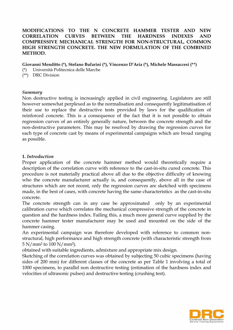
MODIFICATIONS TO THE N CONCRETE HAMMER TESTER AND NEW CORRELATION CURVES BETWEEN THE HARDNESS INDEXES AND COMPRESSIVE MECHANICAL STRENGTH FOR NON-STRUCTURAL, COMMON HIGH STRENGTH CONCRETE. THE NEW FORMULATION OF THE COMBINED METHOD. Giovanni Menditto (*), Stefano Bufarini (*), Vincenzo D’Aria (*), Michele Massaccesi (**) (*) Università Politecnica delle Marche (**) DRC Division Summary Non destructive testing is increasingly applied in civil engineering. Legislators are still however somewhat perplexed as to the normalisation and consequently legitimatisation of their use to replace the destructive tests provided by laws for the qualification of reinforced concrete. This is a consequence of the fact that it is not possible to obtain regression curves of an entirely generally nature, between the concrete strength and the non-destructive parameters. This may be resolved by drawing the regression curves for each type of concrete cast by means of experimental campaigns which are broad ranging as possible. 1. Introduction Proper application of the concrete hammer method would theoretically require a description of the correlation curve with reference to the cast-in-situ cured concrete. This procedure is not materially practical above all due to the objective difficulty of knowing who the concrete manufacturer actually is, and consequently, above all in the case of structures which are not recent, only the regression curves are sketched with specimens made, in the best of cases, with concrete having the same characteristics as the cast-in-situ concrete. The concrete strength can in any case be approximated only by an experimental calibration curve which correlates the mechanical compressive strength of the concrete in question and the hardness index. Failing this, a much more general curve supplied by the concrete hammer tester manufacturer may be used and mounted on the side of the hammer casing. An experimental campaign was therefore developed with reference to common non-structural, high performance and high strength concrete (with characteristic strength from 5 N/mm² to 100 N/mm²). obtained with suitable ingredients, admixture and appropriate mix design. Sketching of the correlation curves was obtained by subjecting 50 cubic specimens (having sides of 200 mm) for different classes of the concrete as per Table 1 involving a total of 1000 specimens, to parallel non destructive testing (estimation of the hardness index and velocities of ultrasonic pulses) and destructive testing (crushing test).

Table 1

Class Specimens Strength class (N/mm²)

Concrete class

1 50 C5 2 50 C10 3 50 C15

Non structural

4 50 C20 5 50 C25 6 50 C30 7 50 C35 8 50 C40 9 50 C45 10 50 C50 11 50 C55

Standard

12 50 C60 13 50 C65 14 50 C70 15 50 C75

High performance

16 50 C80 17 50 C85 18 50 C90 19 50 C95 20 50 C100

High strength

The different strength classes were prepared with appropriate mixes using Portland cement and an assortment of inert materials, representing typical standard Italian cements (Photo 1).

Photo 1: view of the typical specimens of a strength class

2. The concrete hammer tester The concrete hammer tester used for the tests is a modified version of a standard type N model tester (Fig. 1) modified by the Ancona Surveying Division of Eurosit s.r.l. Longitudinal section of the N-model concrete hammer tester and position at the percussion instant (Fig. 1)

1. percussion rod 2. casing 3. indicator with rod 6. ratchet 7. sliding rod 8. sliding disk 9. cap 10. brake lining 11. cover 12. pressure spring 13. hook 14. hammer 15. shock absorber spring 16. percussion spring 17. spring anchorage 18. felt washer 19. window 20. screw 21. lock nut 22. pivot 23. hook spring

In particular, a) The ratchet gear support is made of

very soft aluminium with highly finished exterior so as to guarantee excellent sliding tolerance on the casing guides.

b) A different material, namely C45-type rectified steel, was used for the hammer sliding rod and the locking system between the rod and the hammer was improved on site.

c) A different material, namely C45-type rectified steel, was used for the hammer. The drilling hammer process was modified to ensure a coaxial allowance of the one thousandth of a millimetre (+/- 0,001 mm).

d) The hammer was realised conventionally in PR80 lead steel. The surface dressing was modified, using a nitriding treatment (Nit-OX) which increases the hardness of the material (40 HRC) and the wear resistance of the surface layer. The inner part of the material acquires resilience and toughness with a greater resistance to impact. The hammer impact surface was moreover treated by induction hardening with 56/58 HRC hardness.

e) The diameter of the wire and the final shape of the percussion spring were modified to improve the junction The treatment was modified by replacing galvanising with nickel plating.

f) A different material was used for the pressure spring, changing this from C85-type steel to stainless steel so as to avoid having to treat the surface.

g) The cap was fitted with an outer thread housing a suitable locking mechanism in order to prevent the equipment from opening during transport and the piston from coming out of its housing.

h) An ergonomic plastic and rubber handgrip was fitted solidly to the back of the casing to facilitate hold and handling of the equipment and to prevent operators from touching the inner components.

i) The graduated reading scale is larger than a standard scale and has graphic modifications that permit readings with unit resolution.

j) The instrument is supplied with a black padded case holding the accessory equipment. The case not only provides better protection against jolting but is also fitted with a carrying belt.

k) The concrete hammer is supplied with a wrist belt to prevent the hammer from being dropped accidentally.

l) The concrete hammer does not have a sticker showing the curve diagram on the casing of the hammer but is supplied with a handbook showing the correlation curves.

m) The concrete hammer tester can be provided with software to process results and draw the correlation curves for particular types of concrete.

n) The instrument is supplied with silicon carbide stone, a measuring station-template, phenolphthalein and chalks for tracing the grids.

Alternatively to the mechanical instrument, the Surveying Division of Eurosit s.r.l. also manufactures an electronic concrete hammer tester with:

a) An ergonomic plastic and rubber handgrip fitted solidly to the back of the casing to

facilitate handling and to prevent operators from touching the inner components. b) A multi-line display to display useful data. The electronic card permits recording

approx. 8000 remarks, indicating the corresponding value for each, and the possibility of loading additional curves according to requirements and connecting to the service site for up-dates.

c) A magnetic reading system to avoid contact between the card and the slider d) Rechargeable lithium batteries with operational standby time of 24 hours.

The mechanical characteristics of the instrument are substantially the same as those previously described.

3. Steps of the experimental campaign The specimens used in the experimental campaign complied with the following ideal conditions required by sketching of the concrete curve: curing time: 28 days relative moisture content: constant homogeneity of the concrete quality between the surface and the deep layers carbonation of the surface layers: absent internal defects: absent

After curing (28 days): the surface of the specimen was checked to ensure that it was perfectly dry in order

to avoid any alteration of the results and then carefully cleaned using an abrasive medium-grained silicon carbide stone in order to remove flaking, grouts and roughness.

dimensions of the specimen were checked and the specimen weighed (Photo 2 - 3).

Photo 3 - Spec

Photo 2 - Dimensional check of the specimen

imen faces are checked to ensure that they are perfectly smooth

For measuring purposes, three faces of each specimen were considered, excluding in all cases, the cast-free and compressed faces. To ensure that results would not be distorted by operator discrepancies, Eurosit s.r.l. designed and constructed the ATHR (Alpha Test Hammer Robot, patent AN2002A000028, Photo 4) that (automatically) holds the cube specimens ridigly between the plates of a concrete compression machine with a stress of 1 N/mm², preventing shifting during impact. Nine hammer strokes were applied in sequence, and filmed by a special video camera and monitor at various inclinations of the device, namely at α = -90°; α = 0°, α = +90° (where α is the angle between the axis of the concrete rebound hammer and the horizontal).

Photo 4 - The ATHR (Alpha Test Hammer Robot)

following calculation of the velocity of the ultrasonic pulses (photo 5) following the crushing tests on the specimens, up to class 60 N/mm2 using a 3000 kN

concrete compression machine (Metro Com, 4000 kN model PI-MP 400 T with digital dynamometer) and from class 65 N/mm² to class 100 N/mm² using a 5000 kN concrete compression machine (Controls 5000 kN, mod C80/2 with a digital dynamometer).

Photo 5 - Evaluating the ultrasonic pulse velocity

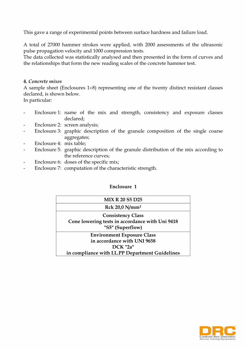
This gave a range of experimental points between surface hardness and failure load. A total of 27000 hammer strokes were applied, with 2000 assessments of the ultrasonic pulse propagation velocity and 1000 compression tests. The data collected was statistically analysed and then presented in the form of curves and the relationships that form the new reading scales of the concrete hammer test. 4. Concrete mixes A sample sheet (Enclosures 1÷8) representing one of the twenty distinct resistant classes declared, is shown below. In particular: - Enclosure 1: name of the mix and strength, consistency and exposure classes

declared; - Enclosure 2: screen analysis; - Enclosure 3: graphic description of the granule composition of the single coarse

aggregates; - Enclosure 4: mix table; - Enclosure 5: graphic description of the granule distribution of the mix according to

the reference curves; - Enclosure 6: doses of the specific mix; - Enclosure 7: computation of the characteristic strength.

Enclosure 1

MIX R 20 S5 D25 Rck 20,0 N/mm²

Consistency Class Cone lowering tests in accordance with Uni 9418

"S5" (Superflow) Environment Exposure Class in accordance with UNI 9658

DCK "2a" in compliance with LL.PP Department Guidelines

UNI 8520 part 5° UNI 8520 part 5°

Specimen type Sand Specimen type P.tto 7/15

Specimen ratio (g) 1002,0 Absorption 2,07 Specimen ratio (g) 1000,0 Absorption 0,98

Screening method wet way Screening method dry way

Testing data 28/03/2002 Testing data 28/03/2002

Wiresieves Heldback Heldback Heldback Passing Wiresieves Heldback Heldback Heldback Passing

size-modulus wire-sieve progressive progressive progressive size-modulus wire-sieve progressive progressive progressive

(M) - (mm) (g) (g) (%) (%) (M) - (mm) (g) (g) (%) (%)

46 - 31,5 0,0 0,0 0,00 100,00 46 - 31,5 0,0 0,0 0,00 100,00

45 - 25 0,0 0,0 0,00 100,00 45 - 25 0,0 0,0 0,00 100,00

44 - 20 0,0 0,0 0,00 100,00 44 - 20 0,0 0,0 0,00 100,00

43 - 16 0,0 0,0 0,00 100,00 43 - 16 35,0 35,0 3,50 96,50

42 - 12,5 0,0 0,0 0,00 100,00 42 - 12,5 133,0 168,0 16,80 83,20

41 - 10 0,0 0,0 0,00 100,00 41 - 10 0,0 168,0 16,80 83,20

40 - 8 0,0 0,0 0,00 100,00 40 - 8 484,0 652,0 65,20 34,80

39 - 6,3 23,0 23,0 2,30 97,70 39 - 6,3 168,0 820,0 82,00 18,00

37 - 4 128,0 151,0 15,07 84,93 37 - 4 118,0 938,0 93,80 6,20

34 - 2 230,0 381,0 38,02 61,98 34 - 2 23,0 961,0 96,10 3,90

31 - 1 155,0 536,0 53,49 46,51 31 - 1 0,0 961,0 96,10 3,90

28 - 0,5 81,0 617,0 61,58 38,42 28 - 0,5 0,0 961,0 96,10 3,90

25 - 0,25 119,0 736,0 73,45 26,55 25 - 0,25 0,0 961,0 96,10 3,90

22 - 0,125 253,0 989,0 98,70 1,30 22 - 0,125 0,0 961,0 96,10 3,90

20 - 0,075 0,0 989,0 98,70 1,30 20 - 0,075 16,0 977,0 97,70 2,30

fondo 13,0 1002,0 100,00 0,00 fondo 23,0 1000,0 100,00 0,00

Fineness modulus: 0-4 Fineness modulus: 2-10

Grain-range: 3,40 Grain-range: 6,40

UNI 8520 part 5° UNI 8520 part 5°

Specimen type Sandy ground Specimen type Gravel 15/30

Specimen ratio (g) 0,0 Absorption 0,00 Specimen ratio (g) 1000,0 Absorption 0,98

Screening method wet way Screening method dry way

Testing data 28/03/2002 Testing data 28/03/2002

Wiresieves Heldback Heldback Heldback Passing Wiresieves Heldback Heldback Heldback Passing

size-modulus wire-sieve progressive progressive progressive size-modulus wire-sieve progressive progressive progressive

(M) - (mm) (g) (g) (%) (%) (M) - (mm) (g) (g) (%) (%)

46 - 31,5 0,0 0,0 #DIV/0! #DIV/0! 46 - 31,5 0,0 0,0 0,00 100,00

45 - 25 0,0 0,0 #DIV/0! #DIV/0! 45 - 25 0,0 0,0 0,00 100,00

44 - 20 0,0 0,0 #DIV/0! #DIV/0! 44 - 20 317,0 317,0 31,70 68,30

43 - 16 0,0 0,0 #DIV/0! #DIV/0! 43 - 16 361,0 678,0 67,80 32,20

42 - 12,5 0,0 0,0 #DIV/0! #DIV/0! 42 - 12,5 258,0 936,0 93,60 6,40

41 - 10 0,0 0,0 #DIV/0! #DIV/0! 41 - 10 0,0 936,0 93,60 6,40

40 - 8 0,0 0,0 #DIV/0! #DIV/0! 40 - 8 58,0 994,0 99,40 0,60

39 - 6,3 0,0 0,0 #DIV/0! #DIV/0! 39 - 6,3 2,0 996,0 99,60 0,40

37 - 4 0,0 0,0 #DIV/0! #DIV/0! 37 - 4 2,0 998,0 99,80 0,20

34 - 2 0,0 0,0 #DIV/0! #DIV/0! 34 - 2 0,0 998,0 99,80 0,20

31 - 1 0,0 0,0 #DIV/0! #DIV/0! 31 - 1 0,0 998,0 99,80 0,20

28 - 0,5 0,0 0,0 #DIV/0! #DIV/0! 28 - 0,5 0,0 998,0 99,80 0,20

25 - 0,25 0,0 0,0 #DIV/0! #DIV/0! 25 - 0,25 0,0 998,0 99,80 0,20

22 - 0,125 0,0 0,0 #DIV/0! #DIV/0! 22 - 0,125 0,0 998,0 99,80 0,20

20 - 0,075 0,0 0,0 #DIV/0! #DIV/0! 20 - 0,075 0,0 998,0 99,80 0,20

fondo 0,0 0,0 #DIV/0! #DIV/0! fondo 2,0 1000,0 100,00 0,00

Enclosure 2GRAIN-SIZE DISTRIBUTION GRAIN-SIZE DISTRIBUTION

GRAIN-SIZE DISTRIBUTIONGRAIN-SIZE DISTRIBUTION

Enclosure 3: Grading curve

0,00

10,00

20,00

30,00

40,00

50,00

60,00

70,00

80,00

90,00

100,0046 - 31,545 - 2544 - 2043 - 1642 - 12,541 - 1040 - 839 - 6,337 - 434 - 231 - 128 - 0,525 - 0,2522 - 0,12520 - 0,075

Mesch-size ( mm ) - Wire sieve modulus

Hel

dbac

k (

% )

0,00

10,00

20,00

30,00

40,00

50,00

60,00

70,00

80,00

90,00

100,00

Pass

ing

( %

)

sand gravel sandy ground Lapillus

si si si siWiresieves Experimental Bolomey Fuller Cubic

100% % 49 % 0 % 24 % 27 curve curve curve Curve31,5 100,0 49,00 100,0 0,00 100,0 24,00 100,0 27,00 100,0 112,1 112,2 108,025 100,0 49,00 100,0 0,00 100,0 24,00 100,0 27,00 100,0 100,0 100,0 100,020 100,0 49,00 100,0 0,00 100,0 24,00 68,3 18,44 91,4 89,5 89,4 92,816 100,0 49,00 100,0 0,00 96,5 23,16 32,2 8,69 80,9 80,2 80,0 86,2

12,5 100,0 49,00 100,0 0,00 83,2 19,97 6,4 1,73 70,7 71,0 70,7 79,410 100,0 49,00 100,0 0,00 83,2 19,97 6,4 1,73 70,7 63,6 63,2 73,78 100,0 49,00 100,0 0,00 34,8 8,35 0,6 0,16 57,5 57,0 56,6 68,4

6,3 97,7 47,88 100,0 0,00 18,0 4,32 0,4 0,11 52,3 50,7 50,2 63,24 84,9 41,62 100,0 0,00 6,2 1,49 0,2 0,05 43,2 40,6 40,0 54,32 62,0 30,37 100,0 0,00 3,9 0,94 0,2 0,05 31,4 29,0 28,3 43,11 46,5 22,79 100,0 0,00 3,9 0,94 0,2 0,05 23,8 20,8 20,0 34,2

0,5 38,4 18,83 100,0 0,00 3,9 0,94 0,2 0,05 19,8 15,0 14,1 27,10,25 26,5 13,01 100,0 0,00 3,9 0,94 0,2 0,05 14,0 10,9 10,0 21,5

0,125 1,3 0,64 100,0 0,00 3,9 0,94 0,2 0,05 1,6 8,0 7,1 17,10,075 1,3 0,64 100,0 0,00 2,3 0,55 0,2 0,05 1,2 6,4 5,5 14,4fondo

cement= 210 kg/m3 Rck Rck 20A= 10 Res. eff. Conc. Res.conc. 42,5C= 9,1Dmax= 25H2O = 180 litres

Water cement ratio = 0,857

Enclosure 4

Sand (0-4) Sandy ground (0-6,3) Lapillus (2-10) Gravel (8-25)

Enclosure 5: Grading curve

0,0

10,0

20,0

30,0

40,0

50,0

60,0

70,0

80,0

90,0

100,0

31,525201612,51086,34210,50,250,1250,075

Mesh-size (mm)

Pass

ing

(%)

Experimental Bolomey Cubic Fuller

Mix-code Mix R 20 S5 D25 Mix 4Consistency class 20,0 N/mm²Consistency Superfluid "S5"Cement-typeMax diameter 25 mmAdmixture-type Glenium 27- Acrilico

proportion dry mass-kg volume mass absolute volume mass dry mass moisture Correction H2O moisture masses moisture masses correction H2OComponents (with single MV size) kg/l volumes - l of the mix - kg/l (with MV mixed) - kg inerts - % (Colon. AG) - l (da col. AG) - kg (da col. AK) - kg (Colon. AK) - lCement 210 3,0 70 210 210 210Water 180 1,0 180 180 54,1 125,9 -5503,2 5683,2Water cement ratio 0,857Air 25Cement+water+air 277Total litres 1000Inerts 1921,9 723 265,863 192192 1976,0 197875,6Sand 49,0 936,2 2,643 35422 94174,3 5,00 46,8 983,0 99130,8 4956,5Sandy ground 0,0 0,0 2,673 0 0,0 5,00 0,0 0,0 0,0 0,0P.tto 7/15 24,0 463,4 2,671 17350 46126,2 1,00 4,6 468,0 46592,1 465,9Gravel 15/30 27,0 522,3 2,676 19518 51891,9 0,50 2,6 524,9 52152,7 260,8Rubble 0,0 0,0 0,000 0 0,0 0,00 0,0 0,0 0,0 0,0

Admix turei proportion- % 1 2,1 2,10 2,10 2,10Silica fume proportion -% 0 0Total volume 2314,0 192584,5 2314,0 192584,5

Cement ENV 197/1 - CEM II/A-L 42,5 R - Cementir

Enclosure 6

Numer Specimen pecimen Sample mean

sample number strenght (Rn) strenght (N/mm²) (N/mm²)

C1/1 18/05/2002 19/06/2002 26,79 1,26 1,59C1/2 18/05/2002 19/06/2002 26,42 -0,89 0,80C2/1 18/05/2002 17/06/2002 25,79 0,26 0,07C2/2 18/05/2002 17/06/2002 26,26 0,74 0,54C3/1 18/05/2002 17/06/2002 25,06 -0,47 0,22C3/2 18/05/2002 17/06/2002 25,84 0,31 0,09C4/1 18/05/2002 19/06/2002 23,32 -2,21 4,89C4/2 18/05/2002 19/06/2002 24,25 -1,27 1,62C5/1 18/05/2002 19/06/2002 28,00 2,47 6,09C5/2 18/05/2002 19/06/2002 28,00 2,47 6,10C6/1 18/05/2002 17/06/2002 24,11 -1,42 2,01C6/2 18/05/2002 17/06/2002 23,55 -1,98 3,91C7/1 18/05/2002 19/06/2002 27,62 2,10 4,39C7/2 18/05/2002 17/06/2002 23,97 -1,56 2,44C7/2 18/05/2002 19/06/2002 26,79 1,26 1,58C8/1 18/05/2002 17/06/2002 29,23 3,70 13,67C8/2 18/05/2002 17/06/2002 25,81 0,28 0,08C9/1 18/05/2002 19/06/2002 28,71 3,18 10,13C9/2 18/05/2002 19/06/2002 28,16 2,63 6,93

C10/1 18/05/2002 17/06/2002 27,84 2,31 5,33C10/2 18/05/2002 17/06/2002 28,00 2,47 6,12C11/1 18/05/2002 19/06/2002 23,84 -1,68 2,84C11/2 18/05/2002 19/06/2002 23,97 -1,56 2,42C13/1 18/05/2002 17/06/2002 27,07 1,54 2,36C13/2 18/05/2002 17/06/2002 26,05 0,52 0,27C15/1 18/05/2002 19/06/2002 21,57 -3,95 15,63C15/2 18/05/2002 19/06/2002 22,51 -3,02 9,09C16/1 18/05/2002 19/06/2002 29,25 3,72 13,86C16/2 18/05/2002 19/06/2002 28,69 3,16 9,99C17/2 18/05/2002 19/06/2002 28,47 2,94 8,66C17/2 18/05/2002 19/06/2002 29,61 4,08 16,67C18/1 18/05/2002 19/06/2002 20,18 -5,34 28,55C18/2 18/05/2002 19/06/2002 19,78 -5,74 32,99C19/1 18/05/2002 19/06/2002 20,58 -4,95 24,52C19/2 18/05/2002 19/06/2002 20,43 -5,10 25,98C20/1 18/05/2002 17/06/2002 19,93 -5,59 31,28C20/2 18/05/2002 17/06/2002 19,56 -5,97 35,61C21/1 18/05/2002 19/06/2002 29,55 4,02 16,15C21/2 18/05/2002 19/06/2002 29,46 3,93 15,43C22/1 18/05/2002 17/06/2002 26,16 0,63 0,40C22/2 18/05/2002 17/06/2002 24,99 -0,54 0,29C23/1 18/05/2002 17/06/2002 28,32 2,79 7,79C23/2 18/05/2002 17/06/2002 27,11 1,58 2,51C24/1 18/05/2002 19/06/2002 20,79 -4,74 22,46C24/2 18/05/2002 19/06/2002 20,74 -4,79 22,90C25/1 18/05/2002 17/06/2002 27,60 2,07 4,30C25/2 18/05/2002 17/06/2002 27,38 1,85 3,42C26/1 18/05/2002 17/06/2002 27,30 1,77 3,13C26/2 18/05/2002 17/06/2002 27,18 1,65 2,71C27/1 18/05/2002 17/06/2002 24,82 -0,71 0,51

INSERTED Mean res. Least res. SummationSPECIMENS Rm (N/mm²) (N/mm²) (Rn - Rm)²

19,56Res. Max(N/mm²)

29,61

Mean Theoretical res. (Rm) coefficient(N/mm²) (k)

20,18

Testing data

26,61

26,03

25,45

28,01

23,79

28,00

23,83

25,80

23,81

25,88

28,58

24,90

class(N/mm²)

25,53

24,55

29,46

26,65

23,95

25

50

20,0 1,6425,53 3,00

Casting data

(s)

24,17

27,34

26,00

27,26

28,00

25,92

Mean square deviation

25,52

20,18

Declarred strenght

17

18

19

20

21

22

23

24

13

14

15

16

9

10

11

12

5

6

7

8

1

2

3

4

Enclosure 7

(Rn - Rm) (Rn - Rm)²

20,61

S

Rck test(N/mm²)

441,34

5. The Concrete Hammer Test – Regression Curves

order to estimate the compressive strength of the samples obtained, it is necessary to

R= a x Ib (1)

ith (where a, b are experimental constants)

he a, b constants were obtained through logarithms, namely linearizing, by appropriately

log R = log a + b log I = f (a,b) (2)

he difference between the actual R value and that obtained with the previous

inciple of maximum

al

Σ (logRi – log a – b logIi)² = min (3)

r

∂/∂a Σ [(logRi – log a – b logIi)²] = 0

here the values a,b are derived from the system (4).

he two equations of the system (4) are known as the normal equations of the straight line

coefficient of the estimated values:

Σ (Rci – Rvi)² S² = [ 1 − ] (0 < S² < 1) (5)

R²ci

Inhave an analytical correlation between the non destructive (hardness index I) and the destructive crushing ( R ) concrete parameters. The curve obtained in this way is called the R(I regression because R is estimated by I. The best interpolator is represented by the mean square procedure, assuming the following type of correlation w Tchanging the variables, the non-linear equation (1) into a linear equation to describe the connection between the non-destructive and destructive parameters. From (1), the following is obtained: Trelationship represents the difference of the R and I observations. These are the results of the experimental errors assigned in accordance with the Gauss law. The most reliable R and I values can be obtained with the prverisimilitude. For a series of the observations (Ri, Ji) they make this series more likely. This probability becomes greatest when the sum of the difference squares is minim(mean square principle). The problem therefore consists of making the quantity minimal: o (4) ∂/∂b Σ [(logRi – log a – b logIi)²] = 0 w Tof the square minimals. Introducing the so-called

⎯⎯⎯⎯⎯⎯⎯ Σ (Rci)²

(Σ ) – ⎯⎯⎯ n

where: he experimental estimated strength (N/mm²)

ula R = a x lb (N/mm²)

s (S2) approaches the unit, the lower the errors with (1), will be.

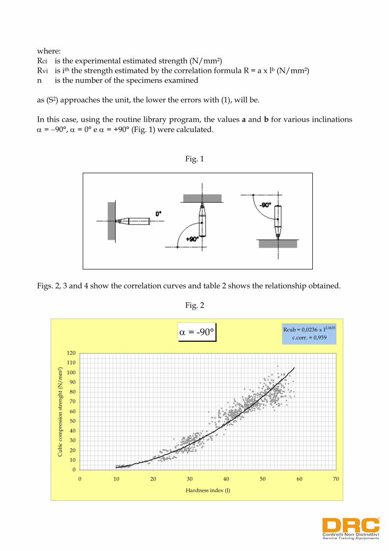
this case, using the routine library program, the values a and b for various inclinations

Fig. 1

igs. 2, 3 an

Fig. 2

Rci is tRvi is ith the strength estimated by the correlation formn is the number of the specimens examined a Inα = −90°, α = 0° e α = +90° (Fig. 1) were calculated.

F d 4 show the correlation curves and table 2 shows the relationship obtained.

α = -90° Rcub = 0,0236 x I2,0635

c.corr. = 0,959

0

10

20

30

40

50

60

70

80

90

100

110

120

0 10 20 30 40 50 60 7

Hardness index (I)

Cub

ic c

ompr

essio

n st

reng

ht (N

/mm

²)

0

Fig. 3

Fig. 4

α = 0° Rcub = 0,0034 x I2,5245

c.corr. = 0,956

0

10

20

30

40

50

60

70

80

90

100

110

120

0 10 20 30 40 50 60 70

Hardness index (I)

Cu

bic

com

pre

ssio

n st

reng

ht (N

/m

m²)

α = +90° Rcub = 0,0005 x I2,9447

70

c.corr. = 0,9484

0

10

20

30

40

50

60

70

80

90

100

110

120

0 10 20 30 40 50 60

Hardness index (Ι)

Cu

bic

com

pre

ssio

n st

reng

ht (N

/m

m²)

Table 2

α values Correlation relationship Correlation coefficient

- 90° Rcub = 0,0236 × I2,0635 0,959

0° Rcub = 0,0034 × I2,5245 0,956

+ 90° Rcub = 0,0005 × I2,9447 0,9484

6. Ultrasonic Test – The Correlation Curve

elocity of the ultrasonic pulses. esides the treatment described by Section 5, the cubic specimens were connected to the

hose acoustic

ble template for the specimen.

o 50 Hz probes, were used.

es (V) obtained with the ultrasonic test were utilised to determine the

R = c × e dV

was assumed where the constants c, d ted by applying the minimum square principle and with a procedure similar to that described in section 5.

⎯ (5000 )

The correlation curve is based on the local vBsurfaces of the ultrasonic probes in order to prevent the presence of air wimpedance would cause high damping of the signal Moreover, in order to obtain stable data of the pulse velocity, the sender and receiver probes were located in fixed positions through a suita A digital ultrasonic detector consisting of a pulse generator, an oscilloscope and twkA constant pressure was applied to the probes to improve the data stability of the time ultrasonic pulse. The data were recorded by means of the transparency procedure. The velocity valuregression curve V/R to assess the concrete strength value. A correlation of the following type

were calcula

The results are represented by fig. 5 and with the relationship

18000 Rcub = – 5 + ⎯⎯⎯

– V

and the correlation coefficient = 0,89

Fig. 5

. Combined Method . The Regression Curve

his method combines the results obtained by the concrete hammer test and the ultrasonic

the local features of the

ffect the ultrasonic pulse

of moisture and the concrete ratio hardening is

elocity pulse (V), the hardness index (I) and the

R = e × If × Vg (6)

here the constants e, f and g are again evaluated with the minimal squares principle.

0

1020

3040

5060

7080

90100

110120

130

2.000 2.500 3.000 3.500 4.000 4.500 5.000 5.500

Velocity of the ultrasonic pulses (m/sec)

Cub

ic c

ompr

essi

on s

tren

ght (

N/m

m²)

7 Tpulse test. With respect to the results of the single non-destructive methods, the combined method gives major accuracy in evaluating the concrete strength. It is well known that the concrete hammer test is affected by cortical concrete layer, while the ultra sonic pulse test is affected by the characteristics of the internal material (such as the ratio of the ingredients, the shape and the size of the aggregates, the admixture, the moisture content, the iron bars). In particular, the moisture content and the hardening time avelocity with an opposite effect to that observed for concrete hammer test. This makes the two tests complementary. With the combined method, the influencepractically annulled on the results, considerably increasing the accuracy since these parameters are difficult to assess on site. The correlation between the ultrasonic vconcrete strength ( R ) was assumed to be: w

From (6)

log R = log e + f log I + g log V = f (e,f,g) (7)

he difference between the real value R and that obtained with the relationship (6)

rors assumed to be distributed in accordance

of I and R can again be obtained with the verisimilitude principle.

is minimal (minimal

efore to reduce the quantity to a minimum.

Σ(logRi – log e – f logIi – g logVi)² = min (8)

at is

∂/∂e Σ[(logRi – log e – f logIi – g logVi)²] = 0

∂/∂f Σ[(logRi – log e – f logIi – g logVi)²] = 0 (9)

∂/∂g Σ[(logRi – log e – f logIi – g logVi)²] = 0

iving the values of e, f and g

he relationship obtained was per α = 0°

Rcub = 0,00004 × I 1,88148 × V 0,80840

(Rcub = N/mm², V = m/sec)

and the correlation coefficient = 0,97

The experimental campaign was carried out

rovisions of applicable regulations.

irectives:

NI EN 12390-1:2002

UNI 9524 FA1

Trepresents the spread of the R, V and I data. These are the results of the experimental erwith the Gauss law. More reliable values For a series (Ri, Ii, Vi) of data, they make this serious more probable. Such a probability is greatest, when the sum of the spread squares squares principle). The problem is ther th

g T

at the Research and Development Centre of

Eurosit s.r.l. – Via A. Grandi No. 40 – Ancona. Tests were carried out in compliance with the p D UUNI EN 12390-2:2002 UNI EN 12390-7:2002 UNI EN 12504-2:2001 UNI 6128 :1972 UNI 6132 :1972 UNI 9524 :1989 e

References:

. Cianfrone. F. – Facaoaru – Studio per l’introduzione in Italia del metodo non

2. dei calcestruzzi con i metodi

3. sati sull’impulso ultrasonoro e

4. tistici nell’ingegneria – Editrice Tecnico Scientifica, Pisa

5. ajani – Elementi di statistica – CEDAM, Editrice Padova 1980; on - Editoriale

7. stica e metodologia della ricerca – IIa edizione – Margiacchi –

1

distruttivo combinato, per la determinazione in loco della resistenza del calcestruzzo – LIPE L’Industria Italiana Per l’Edilizia nn. 6-7/8, 1979; Di Leo A. – Pascale G. – La stima della resistenza in situ non distruttivi – INARCOS - gennaio-febbraio, 1981; Menditto G. ed altri – I metodi non distruttivi basull’indice di rimbalzo dello sclerometro – L’industria delle costruzioni n° 159, gennaio 1985 pagg. 58÷62; Luigi Meloni – Metodi sta1972; Luigi V

6. Hugh D.Young – Statistical treatment of experimental data – MassVeschi, Milano 1993; Ballatori Enzo – StatiGaleno Editrice, Perugia 1996.