Modified Gravity

A.C. Davis, University of Cambridge

With P.Brax, C.van de Bruck, C. Burrage, D.Mota, C. Schelpe, D.Shaw

Outline

Introduction

Scalar-tensor theories

Modified gravity –f(R) theories

The Chameleon Mechanism

Tests and Constraints

Predictions

Structure Formation with f(R) theories

Fundamental physics?

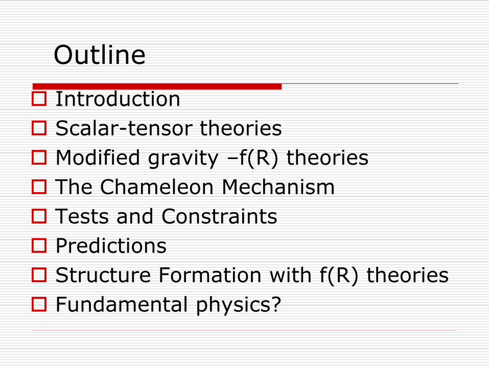
Dark Energy 73 %

Dark Matter 23 %

Atoms 4 %

Energy budget of universe

Expansion of universe accelerates rather than slowing down!

Fundamental questions raised:

What is dark energy?

Why have dark matter and dark energy roughly the same energy density?

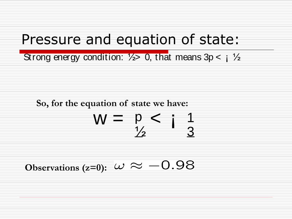
Pressure and equation of state:

So, for the equation of state we have:

w = p½

< ¡ 13

Observations (z=0):

Strong energy condit ion: ½> 0, that means 3p < ¡ ½

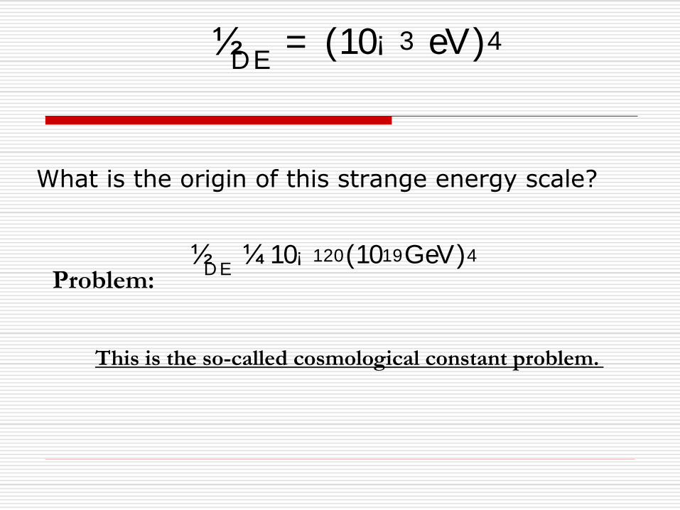
What is the origin of this strange energy scale?

Problem:

½DE

= (10¡ 3 eV)4

This is the so-called cosmological constant problem.

½D E

¼ 10¡ 120(1019GeV)4

Suitable candidates?

Cosmological constant. Plus: works perfect! Minus: badly motivated from particle physics

Scalar Fields. Can explain observations, motivated from particle physics; but many candidates strange properties, in general there is an initial condition problem in the very early universe. Coupling to matter leads to fifth forces.

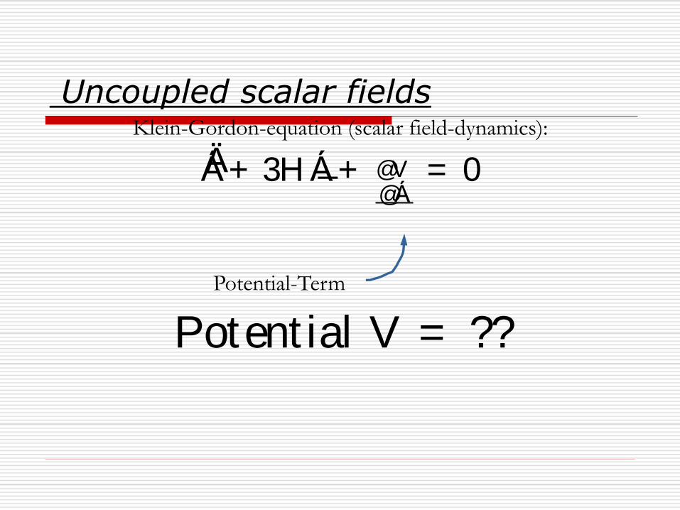
Uncoupled scalar fieldsKlein-Gordon-equation (scalar field-dynamics):

ÄÁ+ 3H _Á+ @V@Á

= 0

Potential-Term

Potent ial V = ??

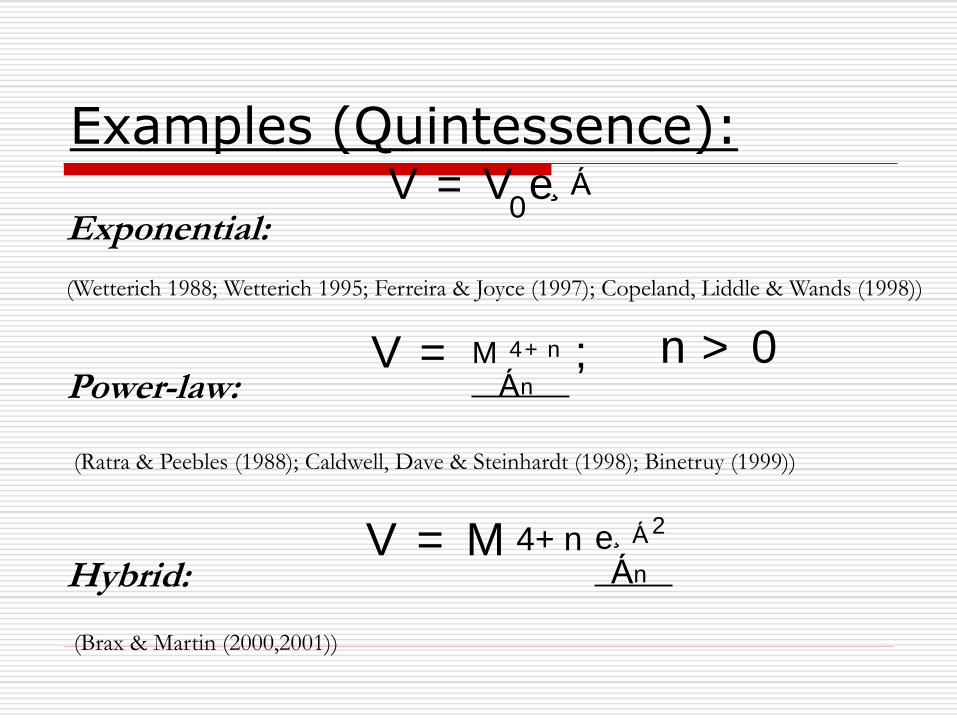
Examples (Quintessence):

Exponential:

(Wetterich 1988; Wetterich 1995; Ferreira & Joyce (1997); Copeland, Liddle & Wands (1998))

Power-law:

V = V0e Á

n > 0V = M 4+ n

Án

;

(Ratra & Peebles (1988); Caldwell, Dave & Steinhardt (1998); Binetruy (1999))

Hybrid:

(Brax & Martin (2000,2001))

V = M 4+ n e¸ Á2

Án

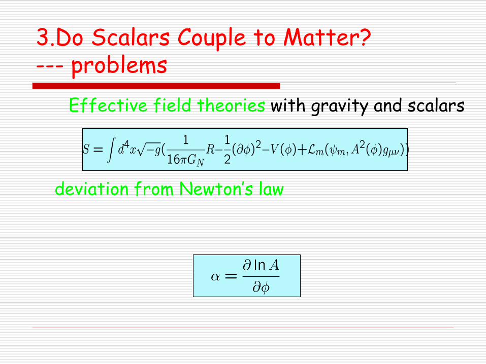
3.Do Scalars Couple to Matter?--- problems

Effective field theories with gravity and scalars

deviation from Newton’s law

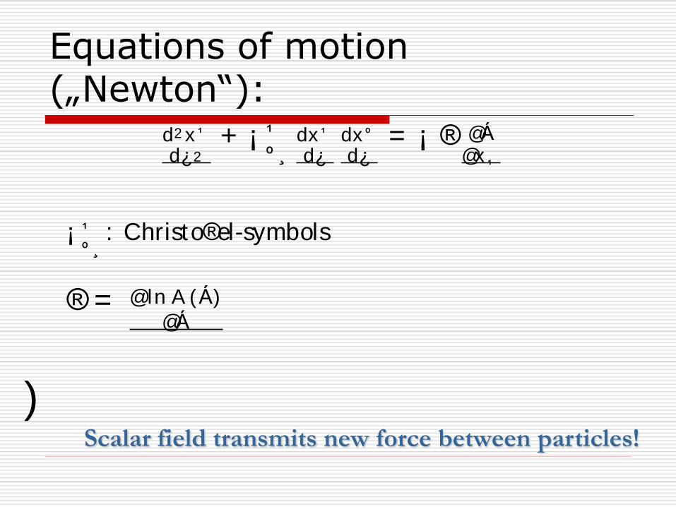
Equations of motion („Newton“):

Scalar field transmits new force between particles!

)

d2 x ¹

d¿2

+ ¡ ¹º ¸

dx ¹

d¿dx º

d¿= ¡ ® @Á

@x¹

® = @ln A (Á)

@Á

¡ ¹º ¸

: Christo®el-symbols

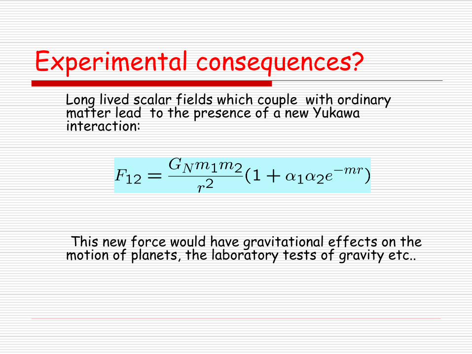
Experimental consequences?

Long lived scalar fields which couple with ordinary matter lead to the presence of a new Yukawa interaction:

This new force would have gravitational effects on the motion of planets, the laboratory tests of gravity etc..

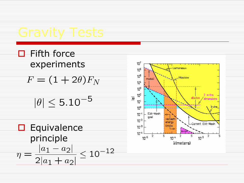
Gravity Tests

Fifth force experiments

Equivalence principle

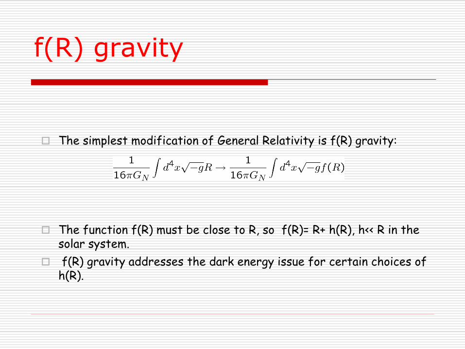
f(R) gravity

The simplest modification of General Relativity is f(R) gravity:

The function f(R) must be close to R, so f(R)= R+ h(R), h<< R in the solar system.

f(R) gravity addresses the dark energy issue for certain choices of h(R).

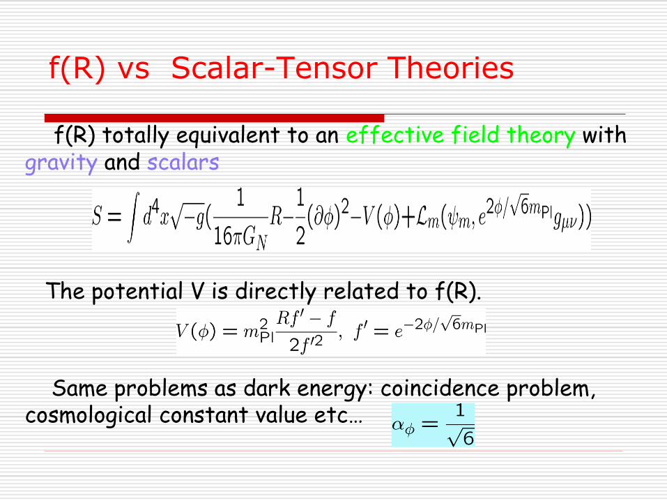
f(R) vs Scalar-Tensor Theories

f(R) totally equivalent to an effective field theory with gravity and scalars

The potential V is directly related to f(R).

Same problems as dark energy: coincidence problem, cosmological constant value etc…

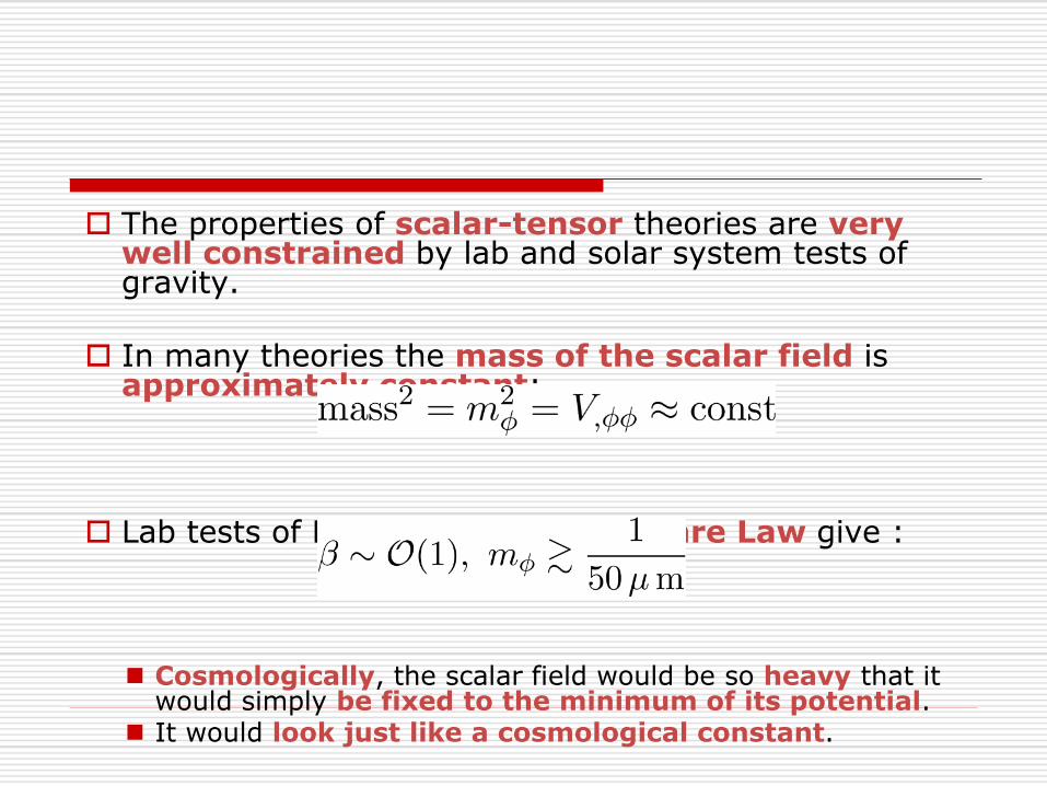
The properties of scalar-tensor theories are very well constrained by lab and solar system tests of gravity.

In many theories the mass of the scalar field is approximately constant:

Lab tests of Newton’s Inverse Square Law give :

Cosmologically, the scalar field would be so heavy that it would simply be fixed to the minimum of its potential.

It would look just like a cosmological constant.

Chameleons

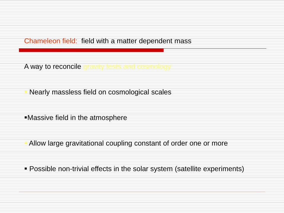
Chameleon field: field with a matter dependent mass

A way to reconcile gravity tests and cosmology:

Nearly massless field on cosmological scales

Massive field in the atmosphere

Allow large gravitational coupling constant of order one or more

Possible non-trivial effects in the solar system (satellite experiments)

Chameleons

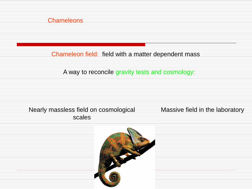
Chameleon field: field with a matter dependent mass

A way to reconcile gravity tests and cosmology:

Nearly massless field on cosmological

scales

Massive field in the laboratory

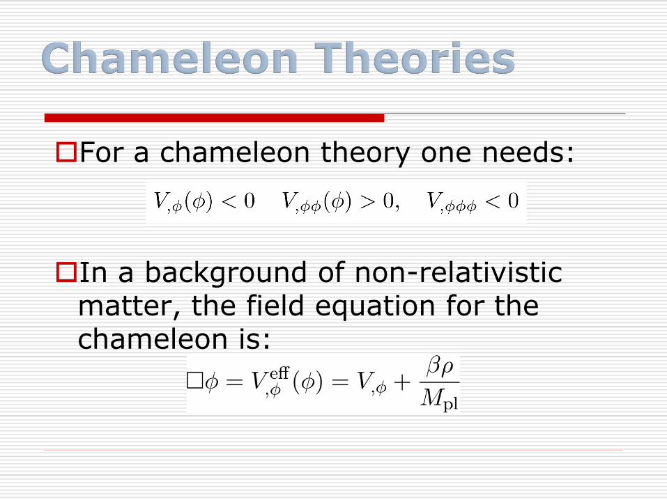
For a chameleon theory one needs:

In a background of non-relativistic matter, the field equation for the chameleon is:

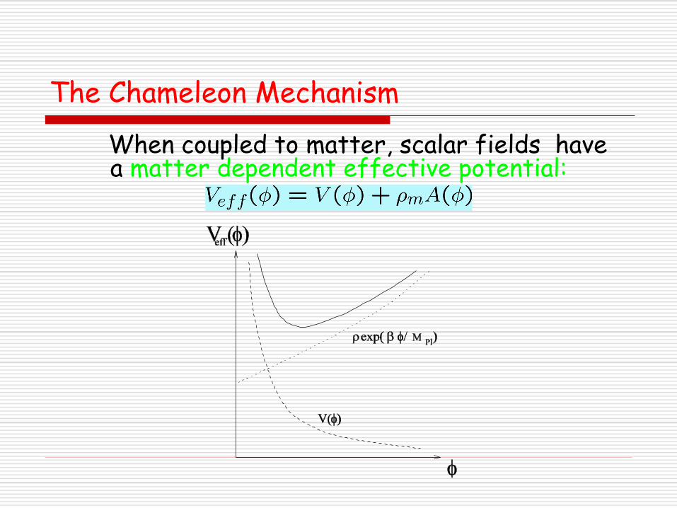
The Chameleon Mechanism

When coupled to matter, scalar fields have a matter dependent effective potential:

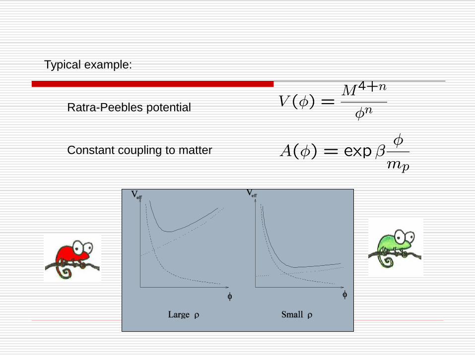
Typical example:

Ratra-Peebles potential

Constant coupling to matter

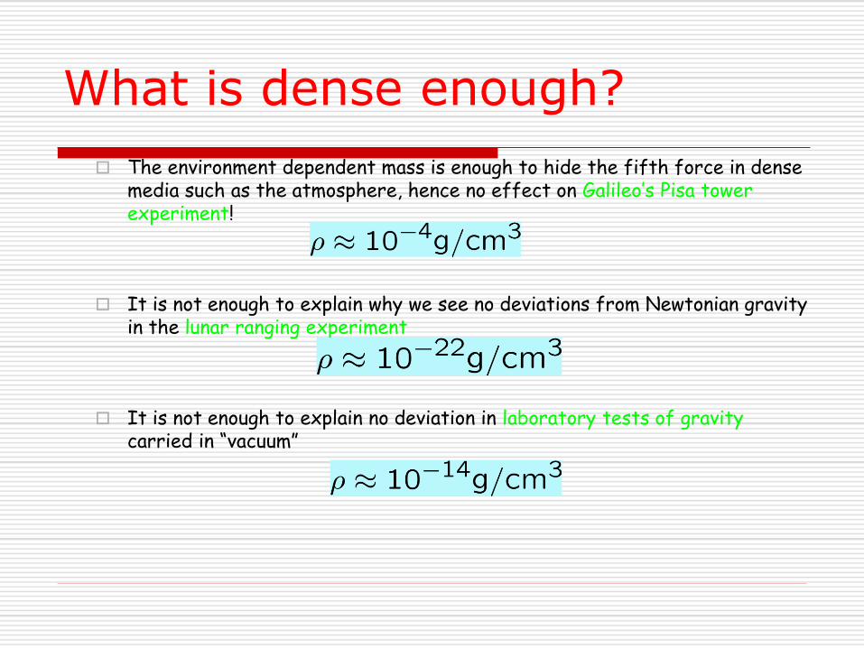
What is dense enough?

The environment dependent mass is enough to hide the fifth force in dense media such as the atmosphere, hence no effect on Galileo’s Pisa tower experiment!

It is not enough to explain why we see no deviations from Newtonian gravity in the lunar ranging experiment

It is not enough to explain no deviation in laboratory tests of gravitycarried in “vacuum”

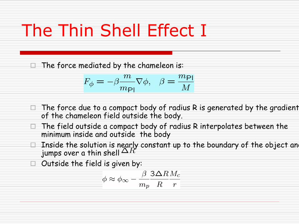
The Thin Shell Effect I

The force mediated by the chameleon is:

The force due to a compact body of radius R is generated by the gradient of the chameleon field outside the body.

The field outside a compact body of radius R interpolates between the minimum inside and outside the body

Inside the solution is nearly constant up to the boundary of the object and jumps over a thin shell

Outside the field is given by:

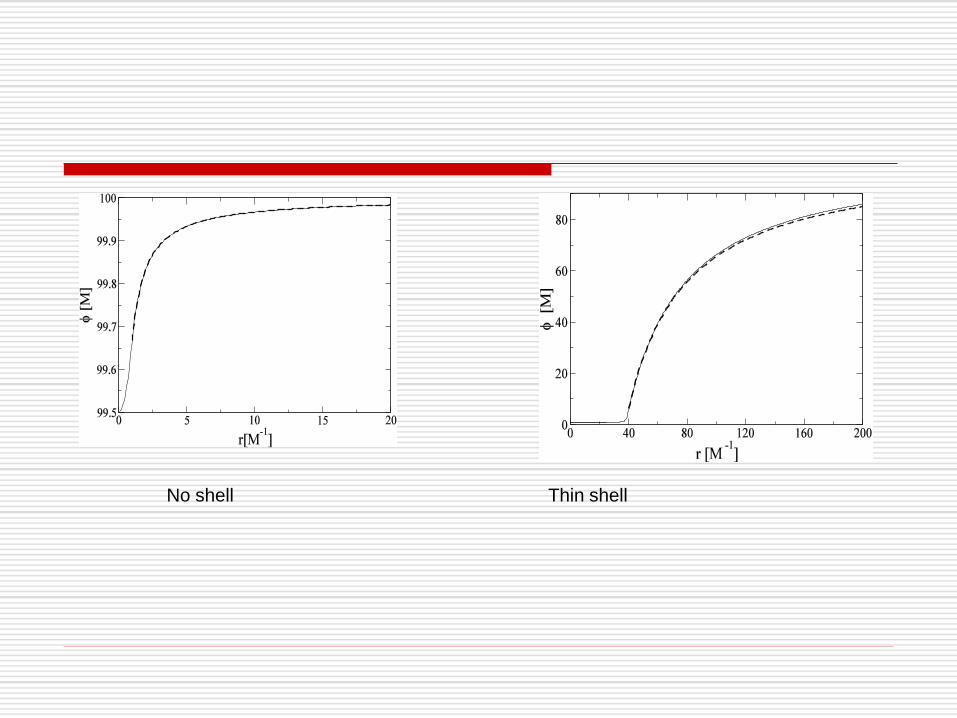
No shell Thin shell

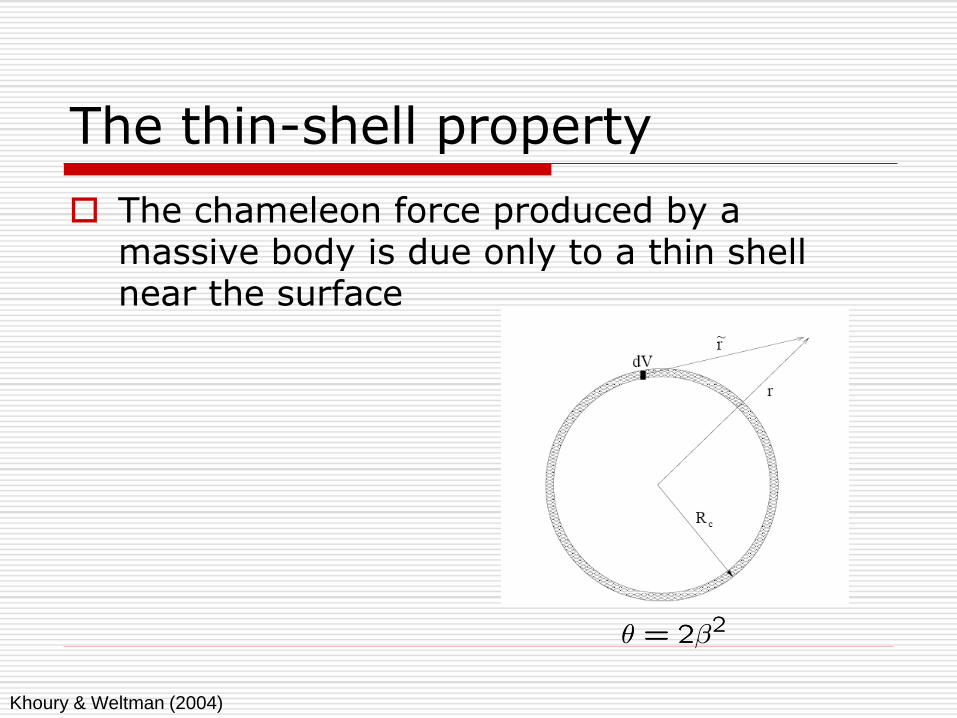
The thin-shell property

The chameleon force produced by a massive body is due only to a thin shell near the surface

Khoury & Weltman (2004)

The Thin Shell Effect II

The force on a test particle outside a spherical body is shielded:

When the shell is thin, the deviation from Newtonian gravity is small.

The size of the thin-shell is:

Small for large bodies (sun etc..) when Newton’s potential at the surface of the body is large enough.

Many authors have tried to employ a chameleon mechanism to construct f(R) gravity theories.

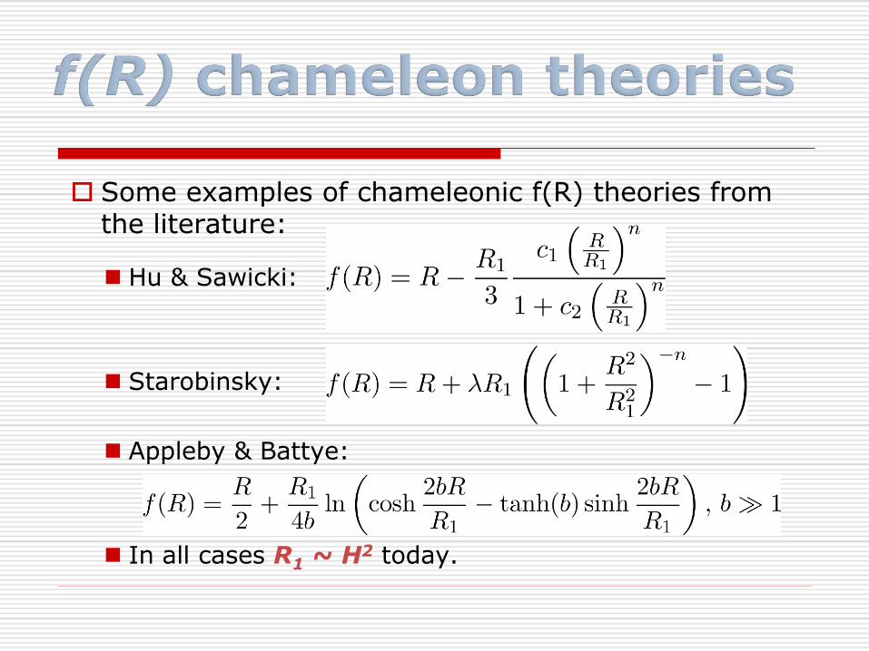
Some examples of chameleonic f(R) theories from the literature:

Hu & Sawicki:

Starobinsky:

Appleby & Battye:

In all cases R1 ~ H2 today.

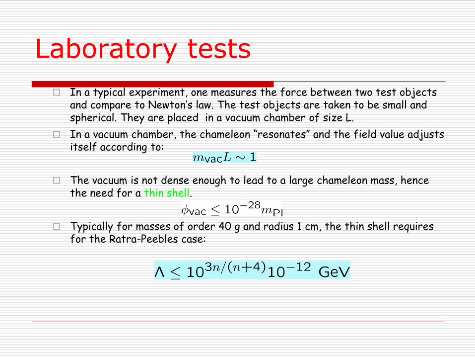
Laboratory tests

In a typical experiment, one measures the force between two test objects and compare to Newton’s law. The test objects are taken to be small and spherical. They are placed in a vacuum chamber of size L.

In a vacuum chamber, the chameleon “resonates” and the field value adjusts itself according to:

The vacuum is not dense enough to lead to a large chameleon mass, hence the need for a thin shell.

Typically for masses of order 40 g and radius 1 cm, the thin shell requires for the Ratra-Peebles case:

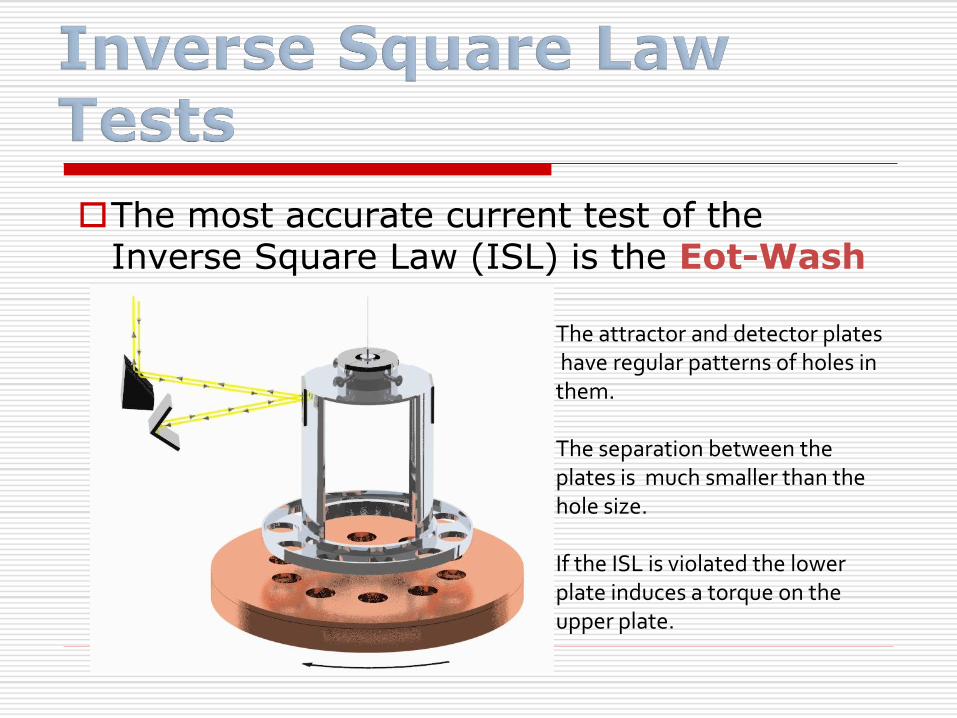
The most accurate current test of the Inverse Square Law (ISL) is the Eot-Wash experiment [2]

The attractor and detector plateshave regular patterns of holes in them.

The separation between the plates is much smaller than the hole size.

If the ISL is violated the lower plate induces a torque on the upper plate.

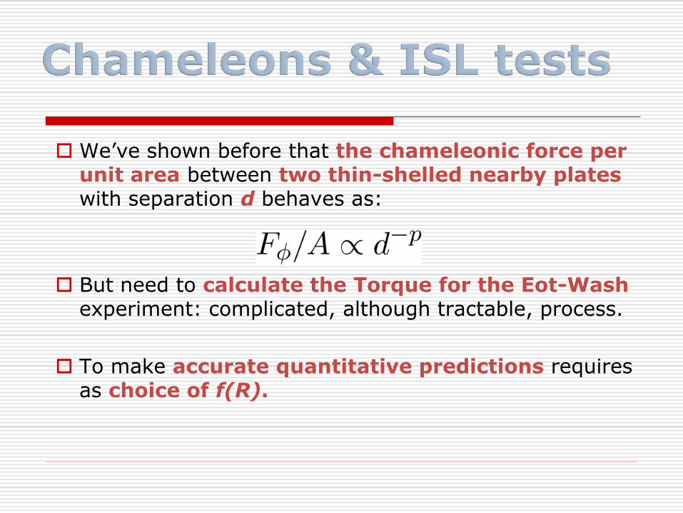
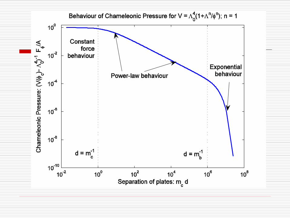
We’ve shown before that the chameleonic force per unit area between two thin-shelled nearby plates with separation d behaves as:

But need to calculate the Torque for the Eot-Wash experiment: complicated, although tractable, process.

To make accurate quantitative predictions requires as choice of f(R).

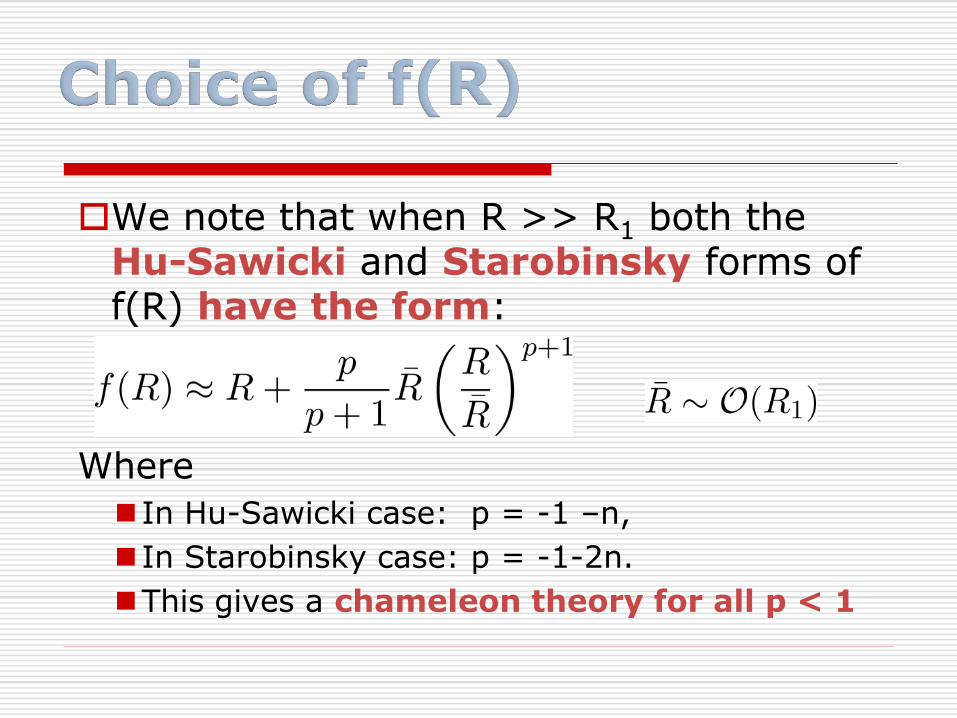
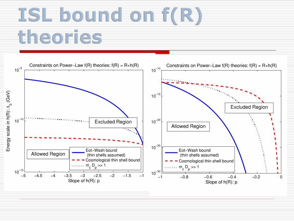
We note that when R >> R1 both the Hu-Sawicki and Starobinsky forms of f(R) have the form:

Where

In Hu-Sawicki case: p = -1 –n,

In Starobinsky case: p = -1-2n.

This gives a chameleon theory for all p < 1

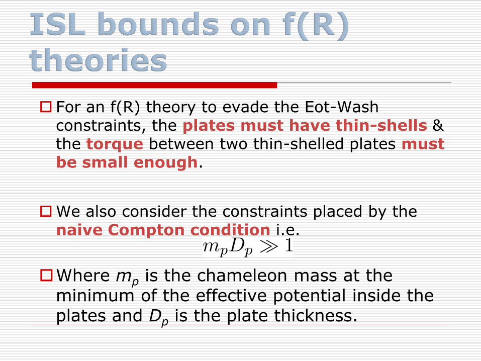
For an f(R) theory to evade the Eot-Wash constraints, the plates must have thin-shells & the torque between two thin-shelled plates must be small enough.

We also consider the constraints placed by the naive Compton condition i.e.

Where mp is the chameleon mass at the minimum of the effective potential inside the plates and Dp is the plate thickness.

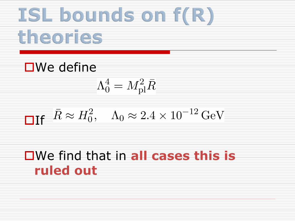
We define

If

We find that in all cases this is ruled out

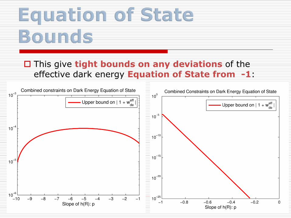
This give tight bounds on any deviations of the effective dark energy Equation of State from -1:

The Casimir Effect

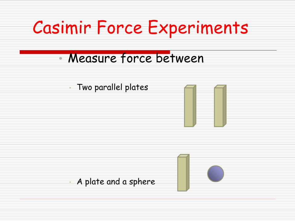
Casimir Force Experiments

• Measure force between

• Two parallel plates

• A plate and a sphere

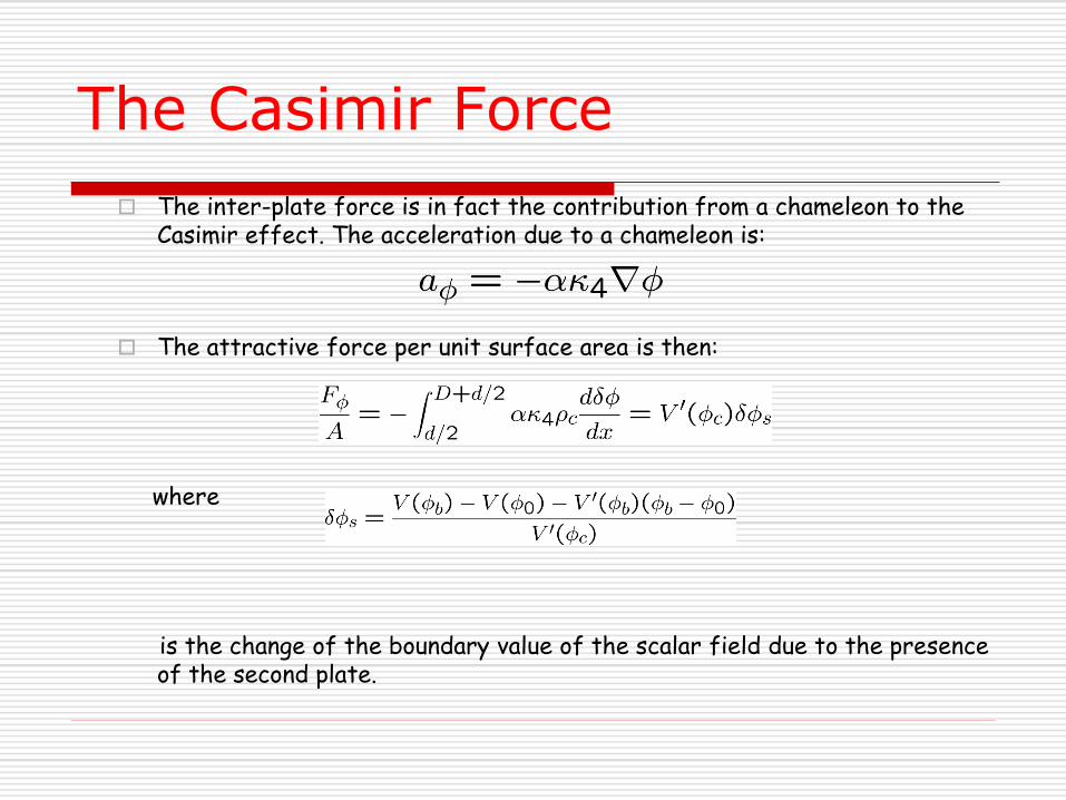
The Casimir Force

The inter-plate force is in fact the contribution from a chameleon to the Casimir effect. The acceleration due to a chameleon is:

The attractive force per unit surface area is then:

where

is the change of the boundary value of the scalar field due to the presence of the second plate.

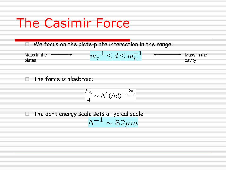
The Casimir Force

We focus on the plate-plate interaction in the range:

The force is algebraic:

The dark energy scale sets a typical scale:

Mass in the

plates

Mass in the

cavity

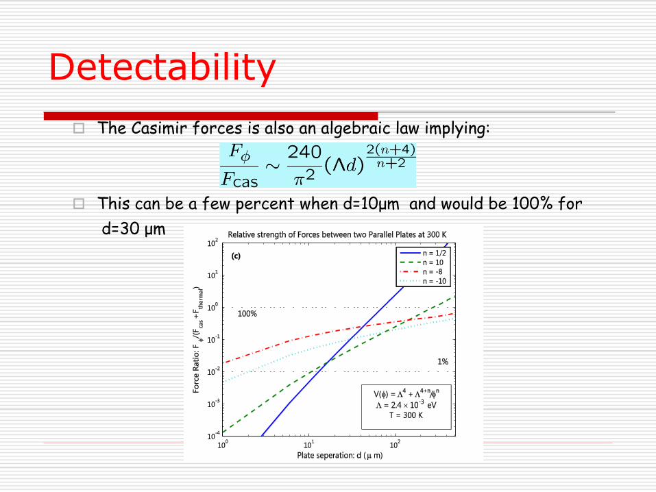
Detectability

The Casimir forces is also an algebraic law implying:

This can be a few percent when d=10μm and would be 100% for

d=30 μm

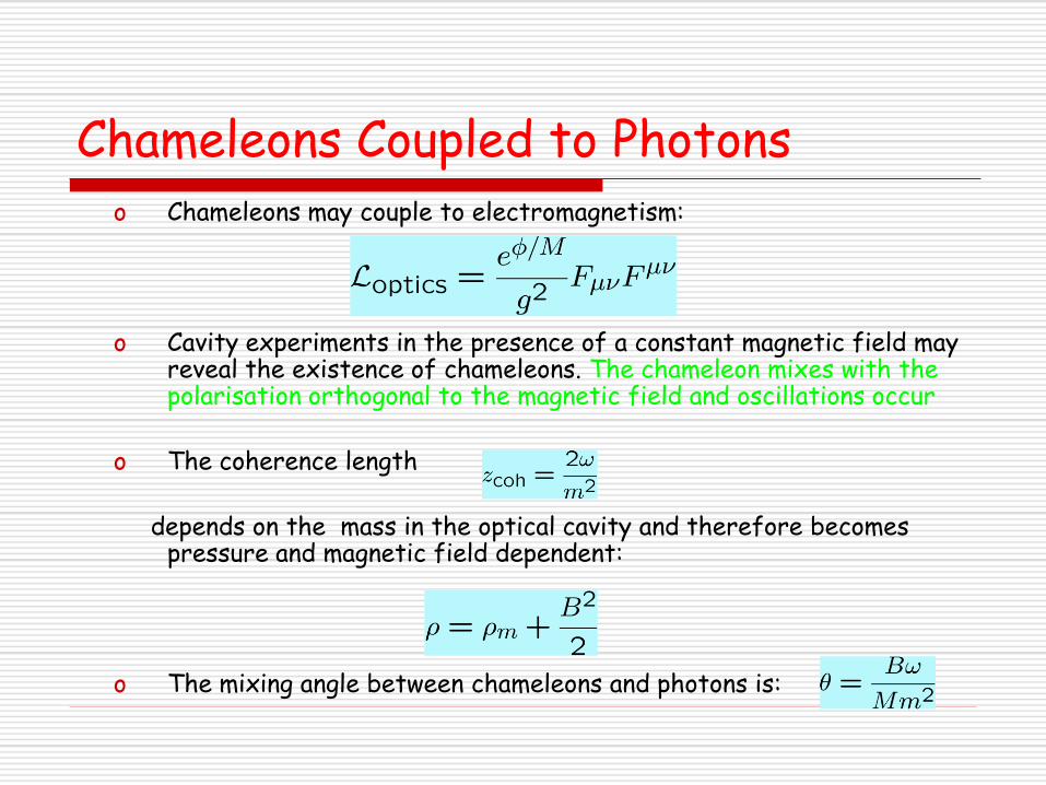
Chameleons Coupled to Photonso Chameleons may couple to electromagnetism:

o Cavity experiments in the presence of a constant magnetic field may reveal the existence of chameleons. The chameleon mixes with the polarisation orthogonal to the magnetic field and oscillations occur

o The coherence length

depends on the mass in the optical cavity and therefore becomes pressure and magnetic field dependent:

o The mixing angle between chameleons and photons is:

Astrophysical Photon-ALP Mixing

Magnetic fields known to exist in galaxies/galaxy clusters

Made up of a large number of magnetic domains

field in each domain of equal strength but randomly oriented

ALP mixing changes astrophysical observations

Non-conservation of photon number alters luminosity

Creation of polarisation in initially unpolarised light

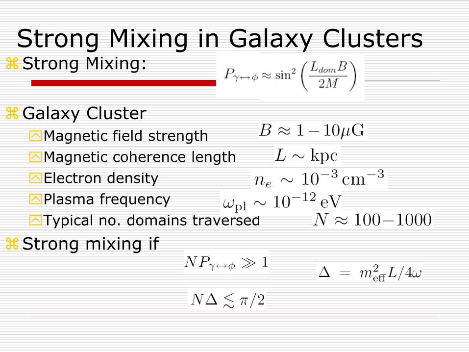
Strong Mixing:

Galaxy Cluster

Magnetic field strength

Magnetic coherence length

Electron density

Plasma frequency

Typical no. domains traversed

Strong mixing if

Strong Mixing in Galaxy Clusters

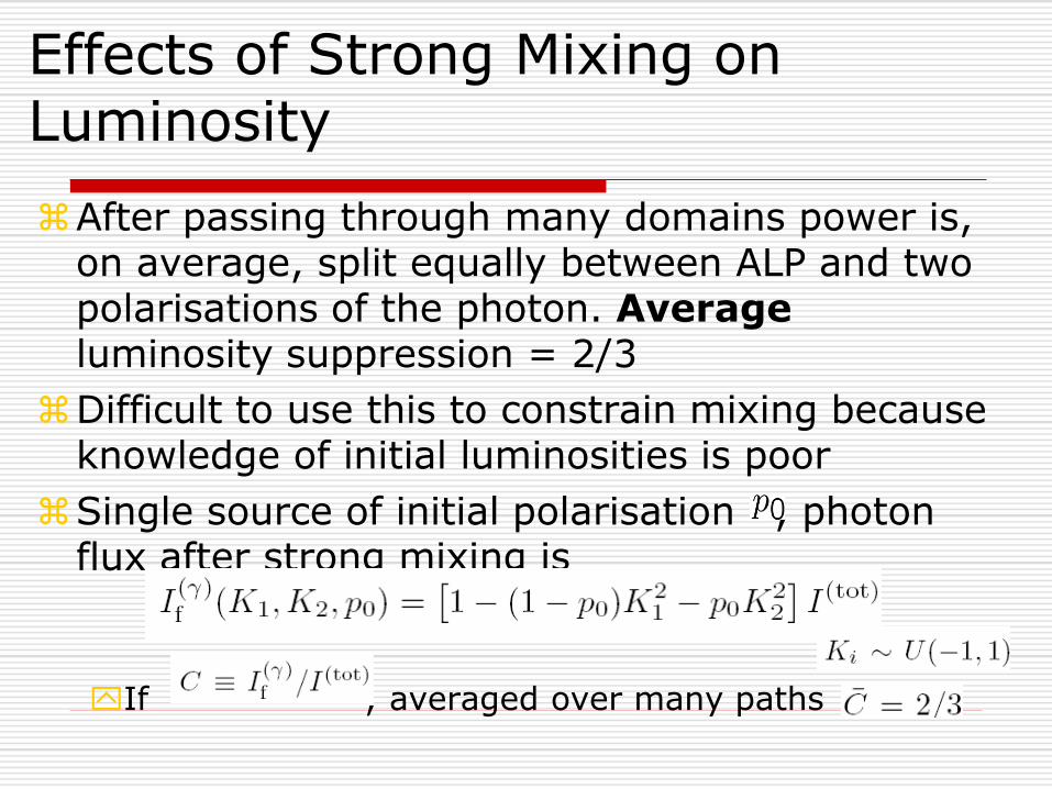
Effects of Strong Mixing on Luminosity

After passing through many domains power is, on average, split equally between ALP and two polarisations of the photon. Averageluminosity suppression = 2/3

Difficult to use this to constrain mixing because knowledge of initial luminosities is poor

Single source of initial polarisation , photon flux after strong mixing is

If ; averaged over many paths

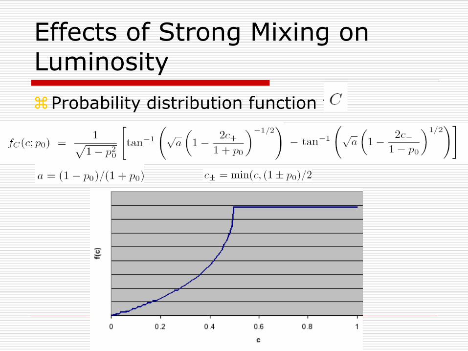
Effects of Strong Mixing on Luminosity

Probability distribution function for

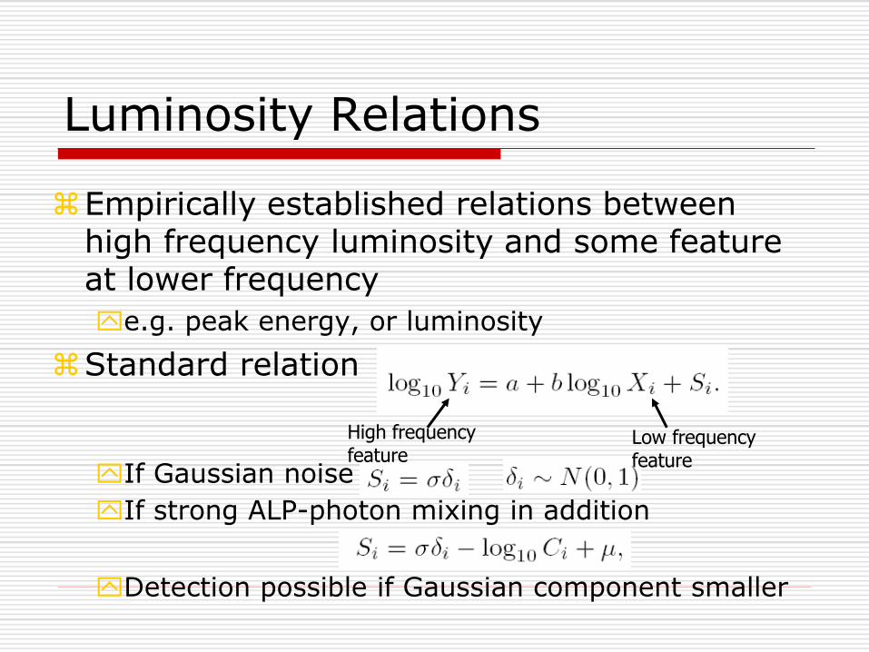
Luminosity Relations

Empirically established relations between high frequency luminosity and some feature at lower frequency

e.g. peak energy, or luminosity

Standard relation

If Gaussian noise

If strong ALP-photon mixing in addition

Detection possible if Gaussian component smaller

High frequency feature

Low frequency feature

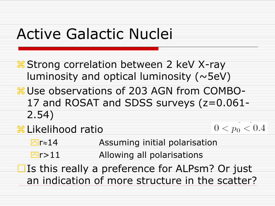
Active Galactic Nuclei

Strong correlation between 2 keV X-ray luminosity and optical luminosity (~5eV)

Use observations of 203 AGN from COMBO-17 and ROSAT and SDSS surveys (z=0.061-2.54)

Likelihood ratio

r 14 Assuming initial polarisation

r>11 Allowing all polarisations

Is this really a preference for ALPsm? Or just an indication of more structure in the scatter?

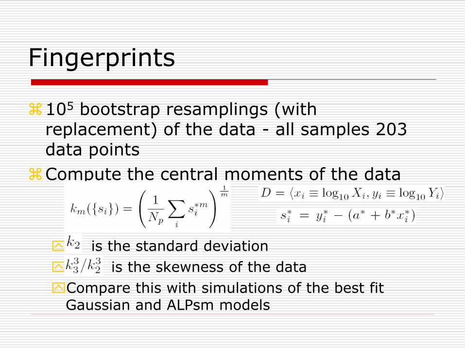
Fingerprints

105 bootstrap resamplings (with replacement) of the data - all samples 203 data points

Compute the central moments of the data

is the standard deviation

is the skewness of the data

Compare this with simulations of the best fit Gaussian and ALPsm models

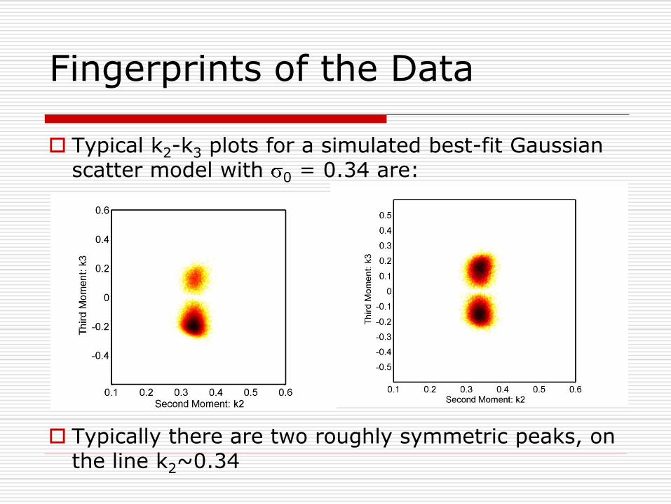
Fingerprints of the Data

Typical k2-k3 plots for a simulated best-fit Gaussian scatter model with 0 = 0.34 are:

Typically there are two roughly symmetric peaks, on the line k2~0.34

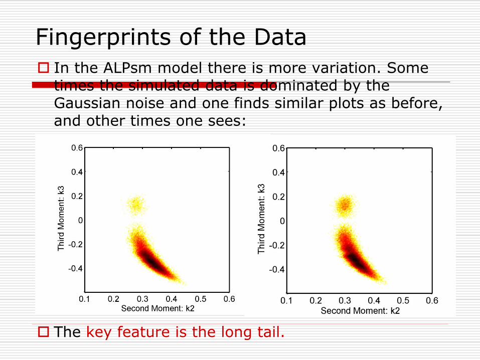
Fingerprints of the Data

In the ALPsm model there is more variation. Some times the simulated data is dominated by the Gaussian noise and one finds similar plots as before, and other times one sees:

The key feature is the long tail.

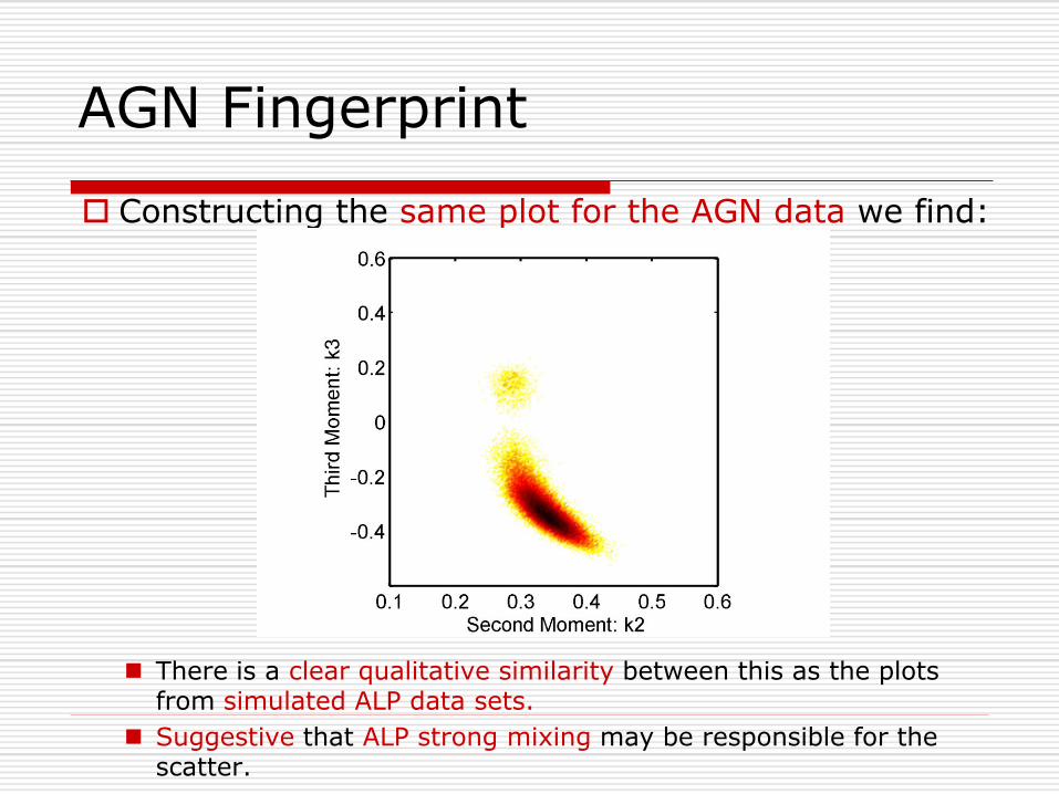
AGN Fingerprint

Constructing the same plot for the AGN data we find:

There is a clear qualitative similarity between this as the plots from simulated ALP data sets.

Suggestive that ALP strong mixing may be responsible for the scatter.

CMB – Chameleonic SZ Effect

Can we see an effect in the CMB?

When passing through galaxy clusters

the chameleon-photon conversion gives a

`chameleonic Sunyaev-Zel’dovich effect’

(Inverse Compton scattering of photons

off electrons in galaxy cluster.

Boosts CMB intensity at high frequencies and causes a decrement at low frequencies.

Observed change in intensity is

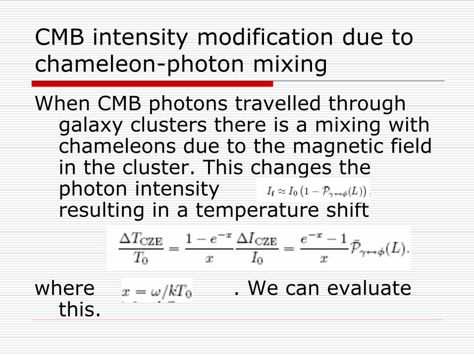
CMB intensity modification due to chameleon-photon mixing

When CMB photons travelled through galaxy clusters there is a mixing with chameleons due to the magnetic field in the cluster. This changes the photon intensity resulting in a temperature shift

where . We can evaluate this.

Large Scale Structures

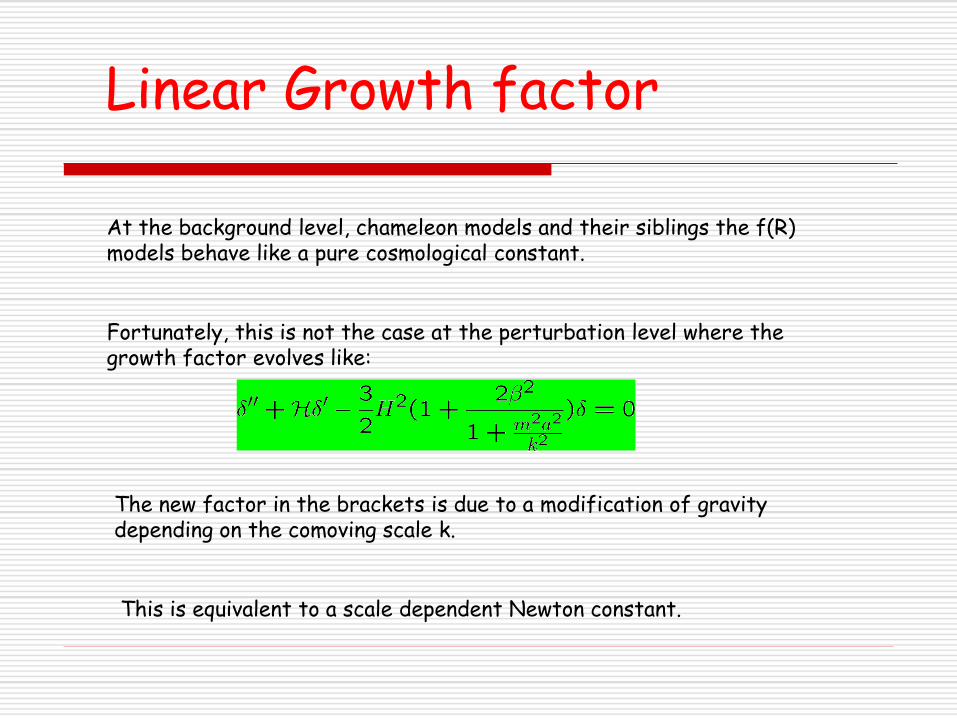
Linear Growth factor

At the background level, chameleon models and their siblings the f(R) models behave like a pure cosmological constant.

Fortunately, this is not the case at the perturbation level where the growth factor evolves like:

The new factor in the brackets is due to a modification of gravity depending on the comoving scale k.

This is equivalent to a scale dependent Newton constant.

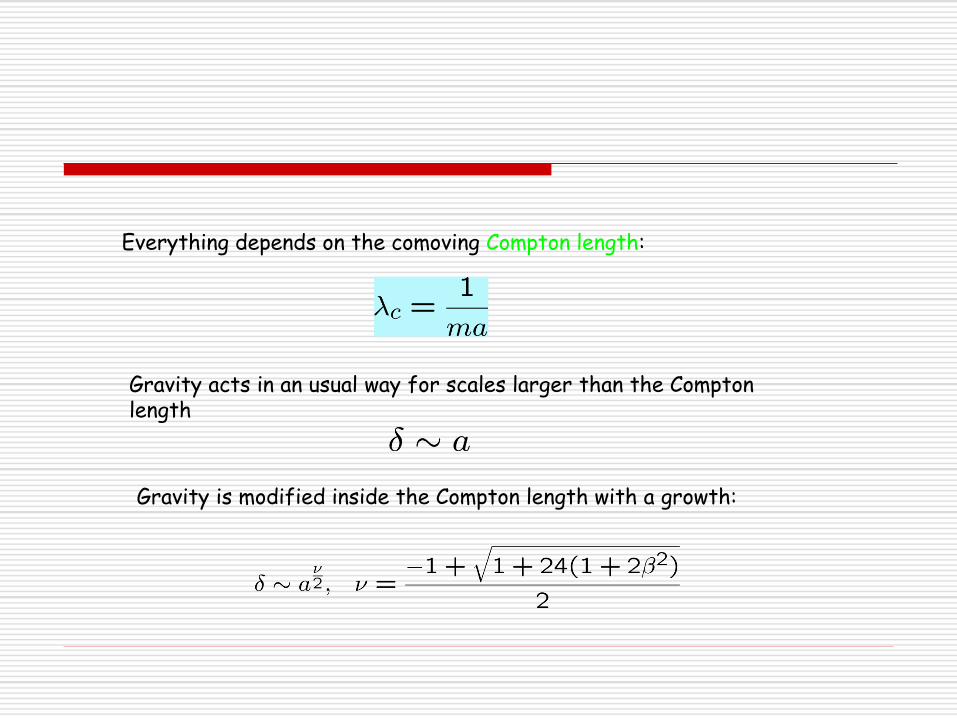
Everything depends on the comoving Compton length:

Gravity acts in an usual way for scales larger than the Compton length

Gravity is modified inside the Compton length with a growth:

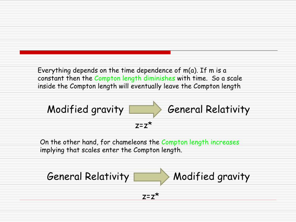
Everything depends on the time dependence of m(a). If m is a constant then the Compton length diminishes with time. So a scale inside the Compton length will eventually leave the Compton length

On the other hand, for chameleons the Compton length increases implying that scales enter the Compton length.

Modified gravity General Relativity

z=z*

General Relativity Modified gravity

z=z*

Growth index

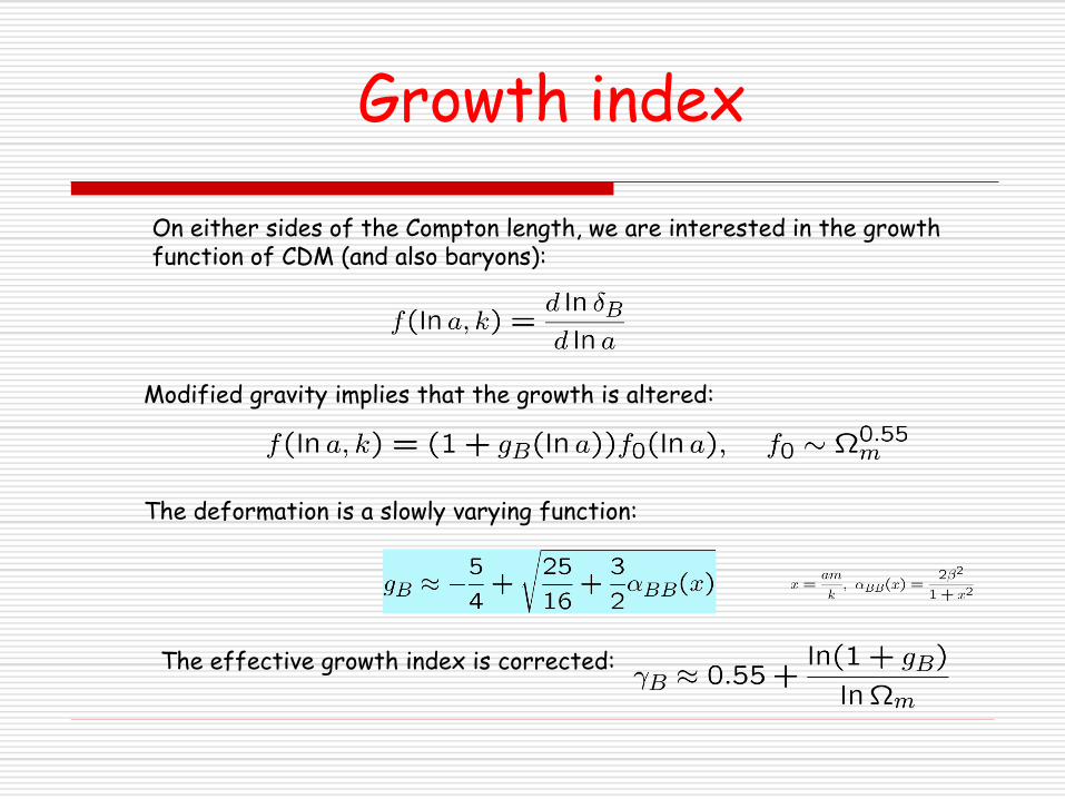
On either sides of the Compton length, we are interested in the growth function of CDM (and also baryons):

Modified gravity implies that the growth is altered:

The deformation is a slowly varying function:

The effective growth index is corrected:

CDM growth index

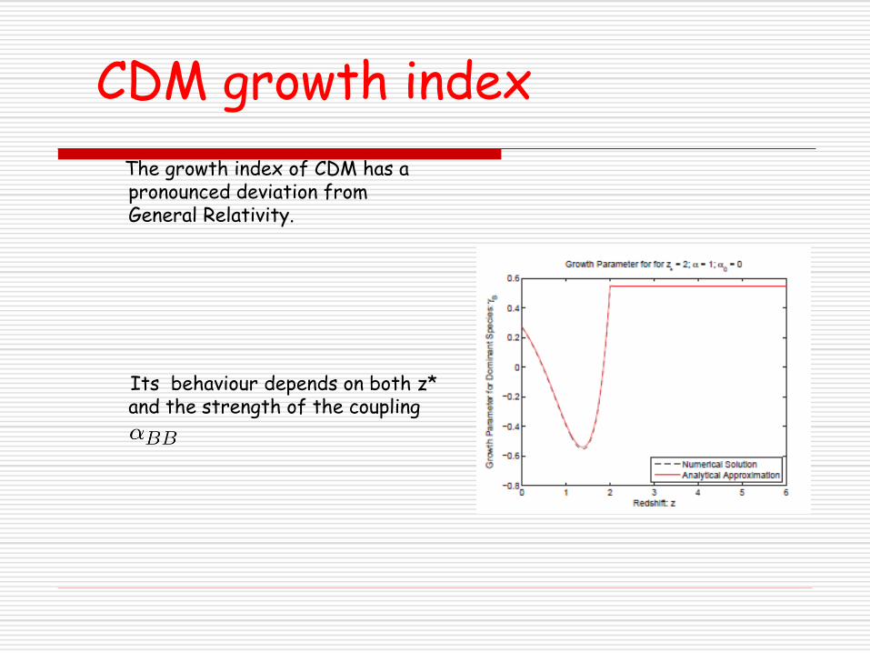
The growth index of CDM has a pronounced deviation from General Relativity.

Its behaviour depends on both z* and the strength of the coupling

Baryonic Growth index

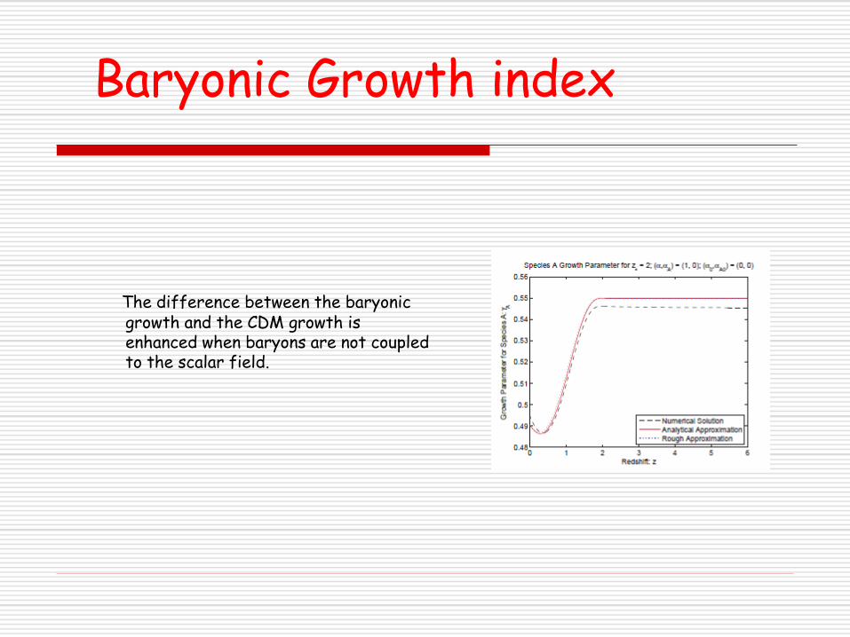
The difference between the baryonic growth and the CDM growth is enhanced when baryons are not coupled to the scalar field.

Slip Function

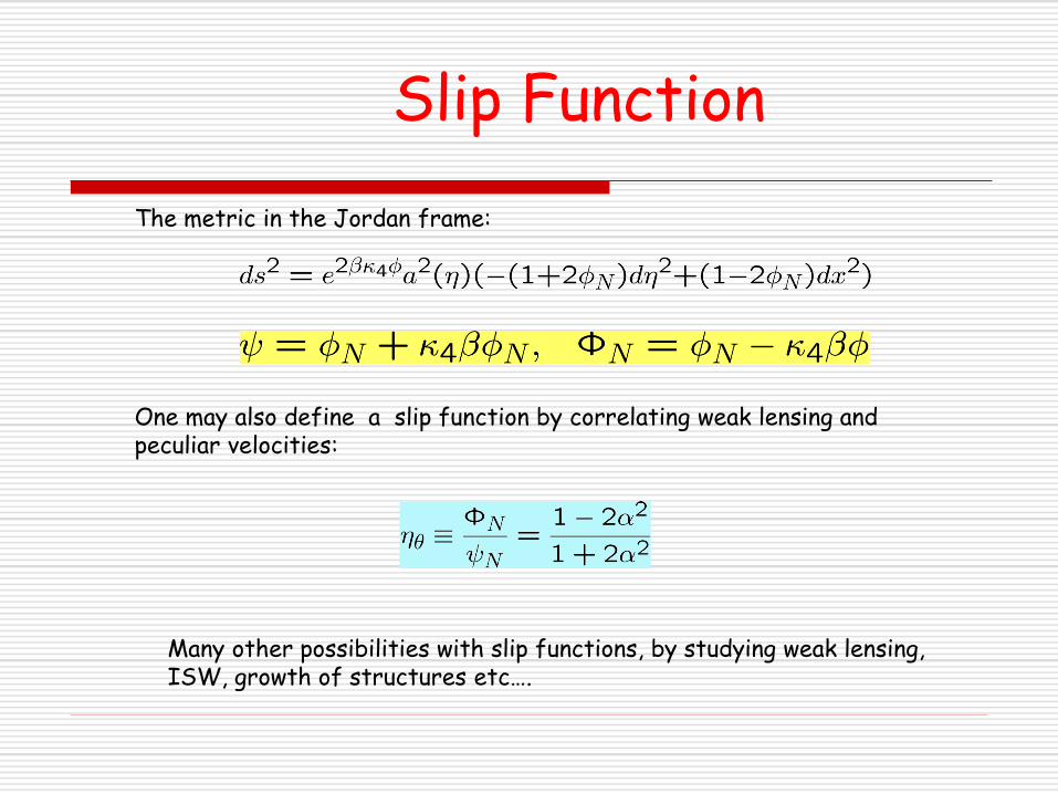
One may also define a slip function by correlating weak lensing and peculiar velocities:

Many other possibilities with slip functions, by studying weak lensing, ISW, growth of structures etc….

The metric in the Jordan frame:

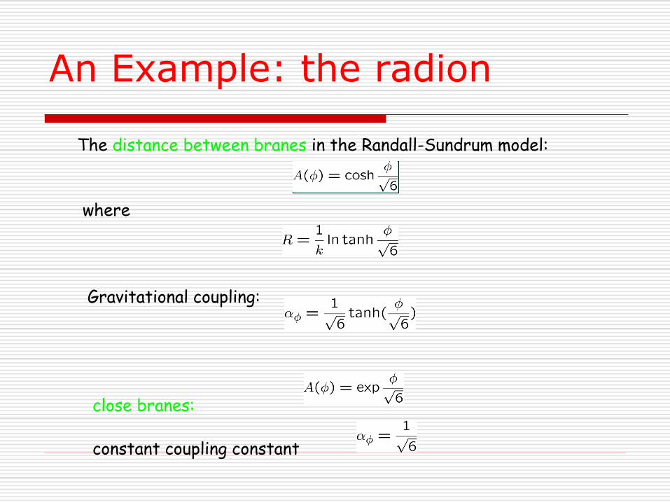
An Example: the radion

The distance between branes in the Randall-Sundrum model:

where

Gravitational coupling:

close branes:

constant coupling constant

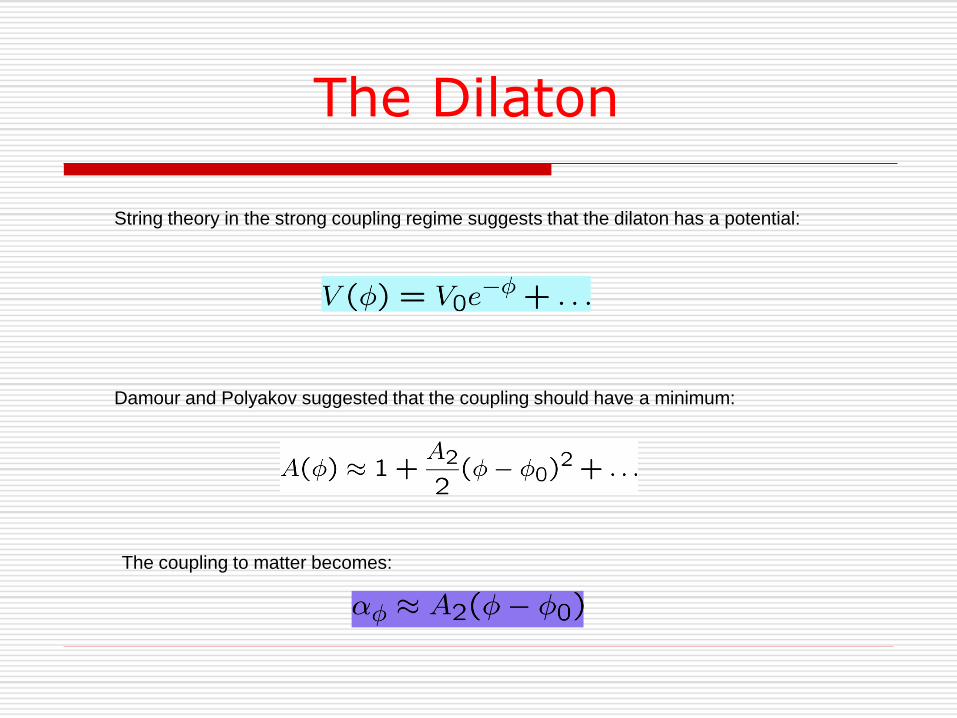
The Dilaton

String theory in the strong coupling regime suggests that the dilaton has a potential:

Damour and Polyakov suggested that the coupling should have a minimum:

The coupling to matter becomes:

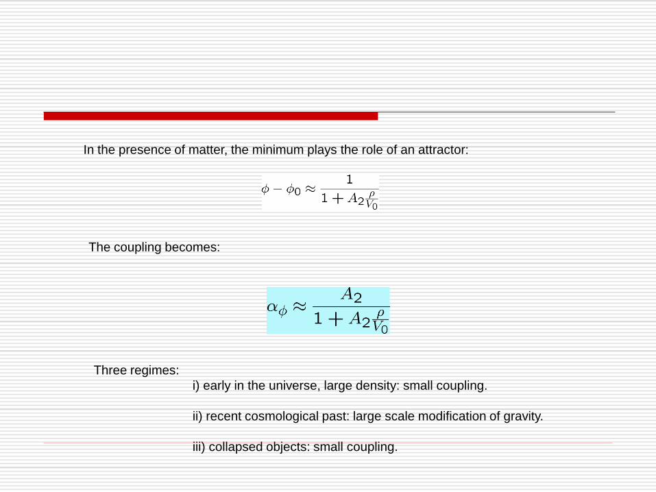
In the presence of matter, the minimum plays the role of an attractor:

The coupling becomes:

Three regimes:

i) early in the universe, large density: small coupling.

ii) recent cosmological past: large scale modification of gravity.

iii) collapsed objects: small coupling.

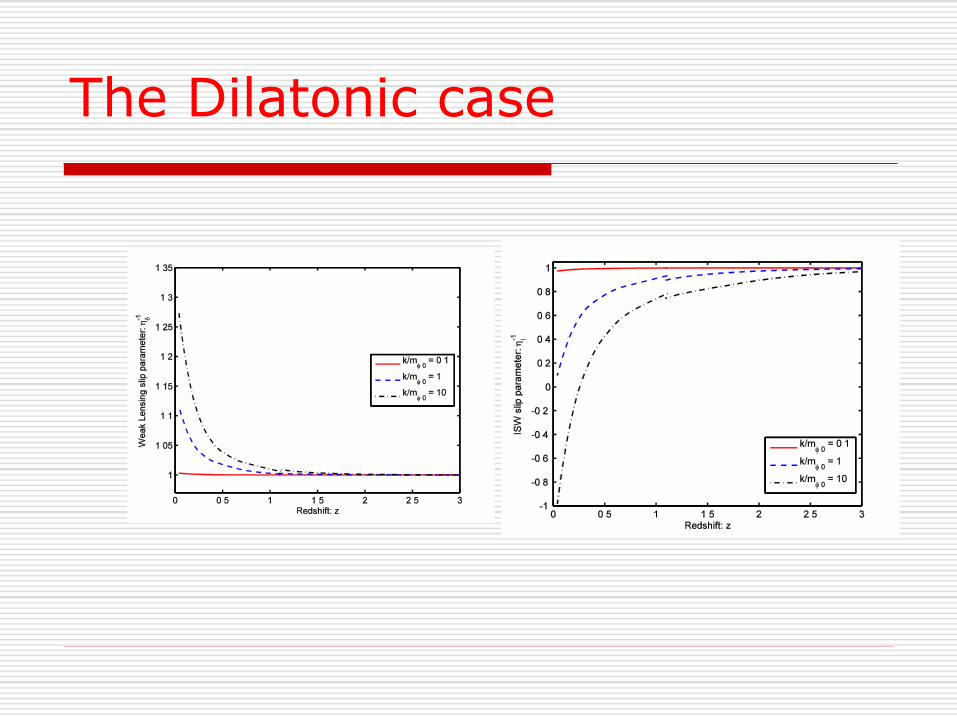
The Dilatonic case

Conclusions

Chameleon theories are intriguing and lead to new physics

The can explain the observed acceleration of the universe and lead to experimental predictions

Hints of such theories have been seen in AGNs and starlight polarisation

Experimentally viable f(R) theories are indistinguishable from a cosmological constant

Effects on large scale structure leads to exciting prospects for the future