Module 2: Representing Process and Disturbance Dynamics Using Discrete Time Transfer Functions

Module 2:Representing Process and Disturbance

Dynamics Using Discrete Time Transfer Functions

chee825 - Winter 2004 J. McLellan 2

Dynamic Models - a First Pass

• establish linkage between process dynamic representations and possible disturbance representations

• key concept - dynamic element, represented by a transfer function, driven by random shock sequence

» IID Normal - white noise


Dynamic Process Relationships

• dependence of current output on present and past values of – manipulated variable inputs– disturbance inputs

• process transfer function» “deterministic” trends between u and y

• disturbance component» relationship between (possibly stochastic) disturbance n

and y


Dynamic Models

• dependence on past values• goal - estimate models of form

• example

– how can we determine how many lagged inputs, outputs, disturbances to use?

– correlation analysis - auto/cross-correlations

y t f y t y t u t u t w t w t( ) ( ( ), ( ), , ( ), ( ), , ( ), ( ), )+ = − − −1 1 1 1L L L

y t y t w t( ) ( ) ( )+ = +1 φ


Impulse Response

• processes have inertia » no instantaneous jumps» when perturbed, require time to reach steady state

• one characterization – impulse response– pulse at time zero enters the process


Impulse Response

Process

Inp

ut

u(k

)

ou

tput

y(k

)

time

time

impulse weightsh(k), k=0,1,2,...


Impulse Response as a Weighting Pattern

Given sequence of inputs, we can predict process output

y k h j u k jj

( ) ( ) ( )= −∑=

∞

0

impulse response infinitely long if process returns to steady state asymptotically


Interpretation

Sum of impulse contributions

y k h u k h u k h u k( ) ( ) ( ) ( ) ( ) ( ) ( )= + − + − +0 1 1 2 2 K

0impact of inputmove 1 time step ago

impact of inputmove 2 time steps ago

ou

tput

y(k

)

time

(ZOH


Impulse Response Model

• impulse response is an example of non-parametric model

» practically - truncate and use finite impulse response (FIR) form

• impulse response model can be considered in– control modeling

» model predictive control (e.g., DMC)

– disturbance modeling» time series -- moving average representation


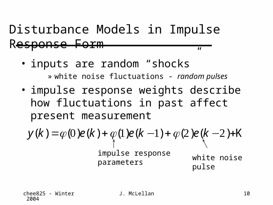
Disturbance Models in Impulse Response Form

• inputs are random “shocks”» white noise fluctuations - random pulses

• impulse response weights describe how fluctuations in past affect present measurement

y k e k e k e k( ) ( ) ( ) ( ) ( ) ( ) ( )= + − + − +φ φ φ0 1 1 2 2 K

white noisepulse

impulse responseparameters


Disturbance Models in Impulse Response Form

• also referred to as a moving average representation– moving average of present and past random shocks

entering process

y k j e k jj

( ) ( ) ( )= −∑=

∞φ0


Difference Equation Models

• recursive definition describing dependence of current output on previous inputs and outputs

• y - output; u - manipulated variable input; e - random shocks (white noise)

• example - ARMAX(1,1,1) model with time delay of 1

y t f y t y t y t p

u t u t u t m

e t e t e t q

( ) ( ( ), ( ), ( ),

( ), ( ), ( ),

( ), ( ), ( ))

+ = − −− −− −

1 111

L

L

L

y t a y t b u t e t c e t( ) ( ) ( ) ( ) ( )= − + − + + −1 0 11 1 1


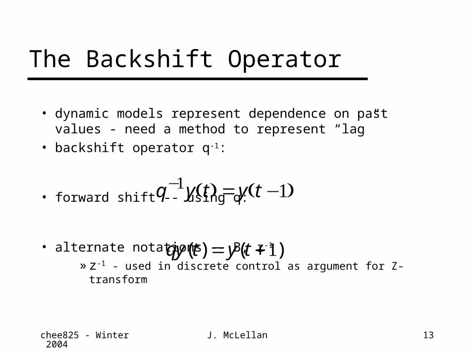
The Backshift Operator

• dynamic models represent dependence on past values - need a method to represent “lag”

• backshift operator q-1:

• forward shift -- using q:

• alternate notations -- B, z-1

» z-1 - used in discrete control as argument for Z-transform

q y t y t− = −1 1( ) ( )

qy t y t( ) ( )= +1


Transfer Function Models

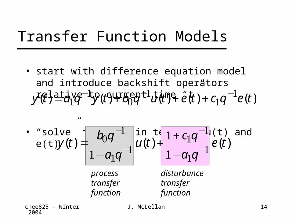
• start with difference equation model and introduce backshift operators relative to current time “t”

• “solve” for y(t) in terms of u(t) and e(t)

y t a q y t b q u t e t c q e t( ) ( ) ( ) ( ) ( )= + + +− − −1

10

11

1

y tb q

a qu t

c q

a qe t( ) ( ) ( )=

−+ +

−

−

−

−

−0

1

11

11

111

1

1processtransfer function

disturbance transfer function


Transfer Function Models

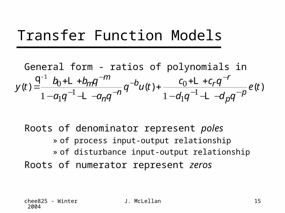
General form - ratios of polynomials in q-1

Roots of denominator represent poles» of process input-output relationship» of disturbance input-output relationship

Roots of numerator represent zeros

y tb b q

a q a qq u t

c c q

d q d qe tm

m

nn

b rr

pp

( ) ( ) ( )= + +

− − −+ + +

− − −

−

− −−

−

− −0

11

0

111 1

L

L

L

L


A Stability Test

• continuous control - poles must have negative real part in Laplace domain (complex plane)

• discrete dynamics?

Consider the sum…

if

1

11

2

0+ + + = ∑

=−

=

∞f f f

f

i

iK

f <1

Geometric Series


Stability Test

Now consider

if .

Impulse response of is {1,a,a2,…} which is

stable if

Root of denominator is q=a, or q-1=a-1

1

1

1

1 1 2 1

0

1

+ + + = ∑

=−

− − −

=

∞

−

aq aq aq

aq

i

i( ) ( )K

aq− <1 11

1 1− −aqa <1


Stability Test

Dynamic element is STABLE if» root in “q” is less than 1 in magnitude» root in “q-1” is greater than 1 in magnitude

Approach - check roots of denominator» based on argument that higher order denominator can

be factored into sum of first-order terms - Partial Fraction Expansion

» each first-order term corresponds to a elementary response - decaying or exploding


Moving Between Representations

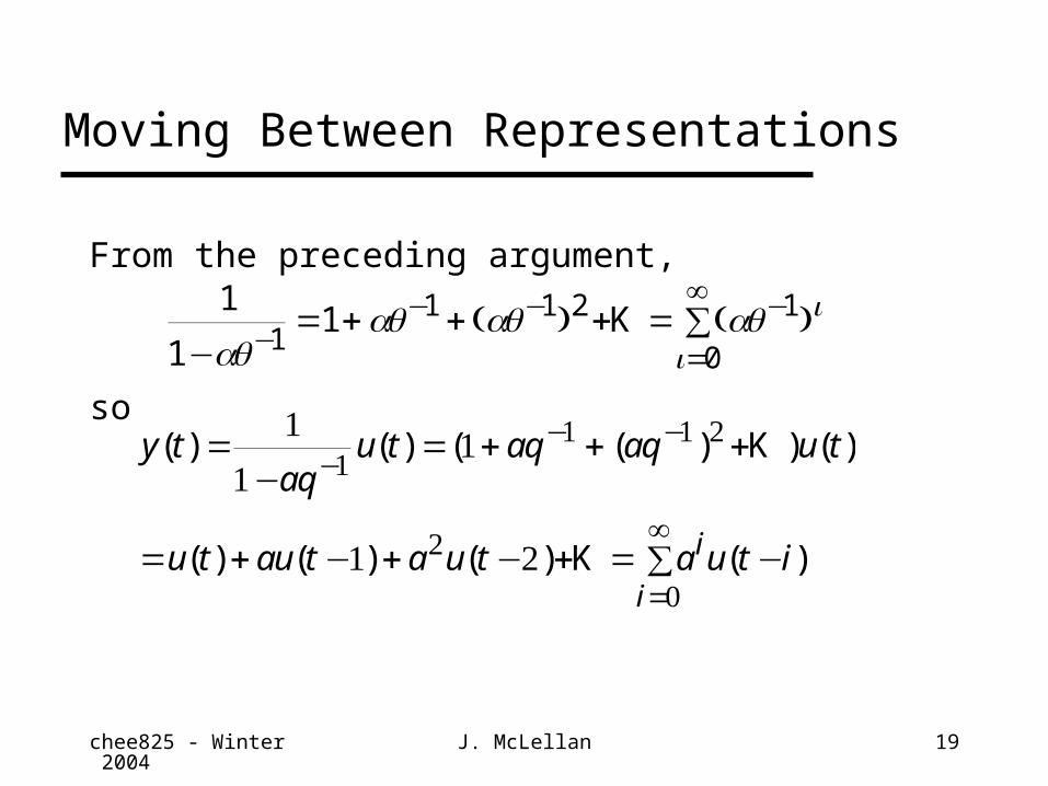
From the preceding argument,

so

1

11

11 1 2 1

0−= + + + = ∑−

− − −

=

∞

aqaq aq aq i

i( ) ( )K

y taq

u t aq aq u t

u t au t a u t a u t ii

i

( ) ( ) ( ( ) ) ( )

( ) ( ) ( ) ( )

=−

= + + +

= + − + − + = −∑

−− −

=

∞

1

11

1 2

11 1 2

2

0

K

K


Moving Between Representations

1

11

11 1 2 1

0−= + + + = ∑−

− − −

=

∞

aqaq aq aq i

i( ) ( )K

transfer function

impulse response

The transformation can be achieved by solving for theimpulse response of the discrete transfer function, or by“long division”.


Inversion

We can express transfer fn. model as impulse response model - infinite sum of past inputs.

Can we do the opposite?» express input as infinite sum of present and past

outputs? » example

asy t q u t( ) ( ) ( )= − −1 1θ

u tq

y t q y ti i

i( ) ( ) ( ) ( )=

−= ∑−

−

=

∞1

1 11

0θθ


Invertibility

Answer - this is the dual problem to stability, and is known as invertibility.

We can invert the moving average term if -- » root in “q” is less than 1 in magnitude» root in “q-1” is greater than 1 in magnitude

Invertibility corresponds to “minimum phase” in control systems, and is a “stability check” of the numerator in a transfer function.


Invertibility

One use: for some input u …

Write

as

y t q u t( ) ( ) ( )= − −1 1θ

y t u t q y t

u t y t y t

i i

i( ) ( ) ( ) ( )

( ) ( ) ( )

= −∑

= − − − − −

−

=

∞θ

θ θ

1

121 2 K

current input move

past outputs(inertia of process)


Invertibility

Importance?» particularly in estimation, where we will use this to form

residuals

y t a t a t( ) ( ) ( )= − −θ 1given model

What are the values of a(t)’s?

Reformulate

y t a t y t y t( ) ( ) ( ) ( )= − − − − −θ θ1 22 Kwhitenoise y(t)’s - measured quantities


Representing Time Delays

Using the backshift operator, a delay of “f” steps corresponds to:

Notes -- » f is at least one for sampled systems because of

sampling and “zero-order hold”» effect of current control move won’t be seen until at least

the next sampling time

q f−

Documents

Module 2: Representing Process and Disturbance Dynamics Using Discrete Time Transfer Functions