Embed Size (px)
Citation preview

INSTANCE-BASED
LEARNING
---Tejaswini H, Dept of CSE
Module 5

In contrast to learning methods that construct a general,
explicit description of the target function when training
examples are provided, instance-based learning
methods simply store the training examples.
Generalizing beyond these examples is postponed until a new
instance must be classified.
Each time a new query instance is encountered, its
relationship to the previously stored examples is examined in
order to assign a target function value for the new instance.

Instance-based learning includes nearest neighbor and locally
weighted regression methods that assume instances can be
represented as points in a Euclidean space. It also includes case-
based reasoning methods that use more complex, symbolic
representations for instances.
Instance-based methods are sometimes referred to as "lazy"
learning methods because they delay processing until a new
instance must be classified.
A key advantage of this kind of delayed, or lazy, learning is that
instead of estimating the target function once for the entire
instance space, these methods can estimate it locally and
differently for each new instance to be classified.
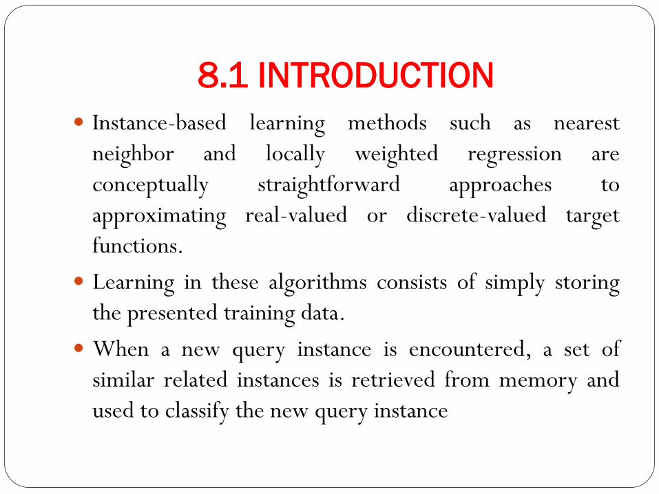
8.1 INTRODUCTION
Instance-based learning methods such as nearest
neighbor and locally weighted regression are
conceptually straightforward approaches to
approximating real-valued or discrete-valued target
functions.
Learning in these algorithms consists of simply storing
the presented training data.
When a new query instance is encountered, a set of
similar related instances is retrieved from memory and
used to classify the new query instance
One key difference between these approaches and the methods
discussed in other chapters is that instance-based approaches can
construct a different approximation to the target function for each
distinct query instance that must be classified.

disadvantages the cost of classifying new instances can be high.
This is due to the fact that nearly all computation takes place at
classification time rather than when the training examples are first
encountered.
Therefore, techniques for efficiently indexing training examples are a
significant practical issue in reducing the computation required at
query time.
they typically consider all attributes of the instances when
attempting to retrieve similar training examples from memory.
If the target concept depends on only a few of the many available
attributes, then the instances that are truly most "similar" may well
be a large distance apart.

8.2 k-NEAREST NEIGHBOR LEARNING
The most basic instance-based method is the k-NEAREST
NEIGHBOR LEARNING algorithm.
This algorithm assumes all instances correspond to points in
the n-dimensional space .
The nearest neighbors of an instance are defined in terms of
the standard Euclidean distance.

More precisely, let an arbitrary instance x be described by the
feature vector

In nearest-neighbor learning the target function may be
either discrete-valued or real-valued.
Let us first consider learning discrete-valued target
functions of the form f : V, where V is the finite set
{v1, . . . vs}.
The k-NEAREST NEIGHBOR algorithm for
approximating a discrete-valued target function is given
in Table 8.1.


As shown there, the value 𝑓 (xq) returned by this algorithm as its
estimate of f(xq) is just the most common value of f among the k
training examples nearest to xq.
If we choose k = 1, then the 1-NEAREST NEIGHBOR algorithm
assigns to 𝑓 (xq) the value f(xi) where xi is the training instance nearest
to xq
For larger values of k, the algorithm assigns the most common
value among the k nearest training examples.


Figure 8.1 illustrates the operation of the k-NEAREST
NEIGHBOR algorithm for the case where the instances are
points in a two-dimensional space and where the target
function is boolean valued.
The positive and negative training examples are shown by
"+" and "-“ respectively.
A query point xq is shown as well. Note the 1-NEAREST
NEIGHBOR algorithm classifies xq as a positive example in
this figure, whereas the 5-NEAREST NEIGHBOR algorithm
classifies it as a negative example.

Note the k-NEAREST NEIGHBOR algorithm never forms an
explicit general hypothesis 𝑓 regarding the target function f .
It simply computes the classification of each new query instance
as needed.
Nevertheless, we can still ask what the implicit general
function is, or what classifications would be assigned if we were
to hold the training examples constant and query the algorithm
with every possible instance in X.
The diagram on the right side of Figure 8.1 shows the shape of this
decision surface induced by 1-NEAREST NEIGHBOR over the
entire instance space.
The decision surface is a combination of convex polyhedra
surrounding each of the training examples.
For every training example, the polyhedron indicates the set of query
points whose classification will be completely determined by that
training example.
Query points outside the polyhedron are closer to some other
training example.
This kind of diagram is often called the Voronoi diagram of the
set of training examples.


8.2.1 Distance-Weighted NEAREST NEIGHBOR Algorithm
One obvious refinement to the k-NEAREST NEIGHBOR
Algorithm is to weight the contribution of each of the
k neighbors according to their distance to the query point
xq giving greater weight to closer neighbors.
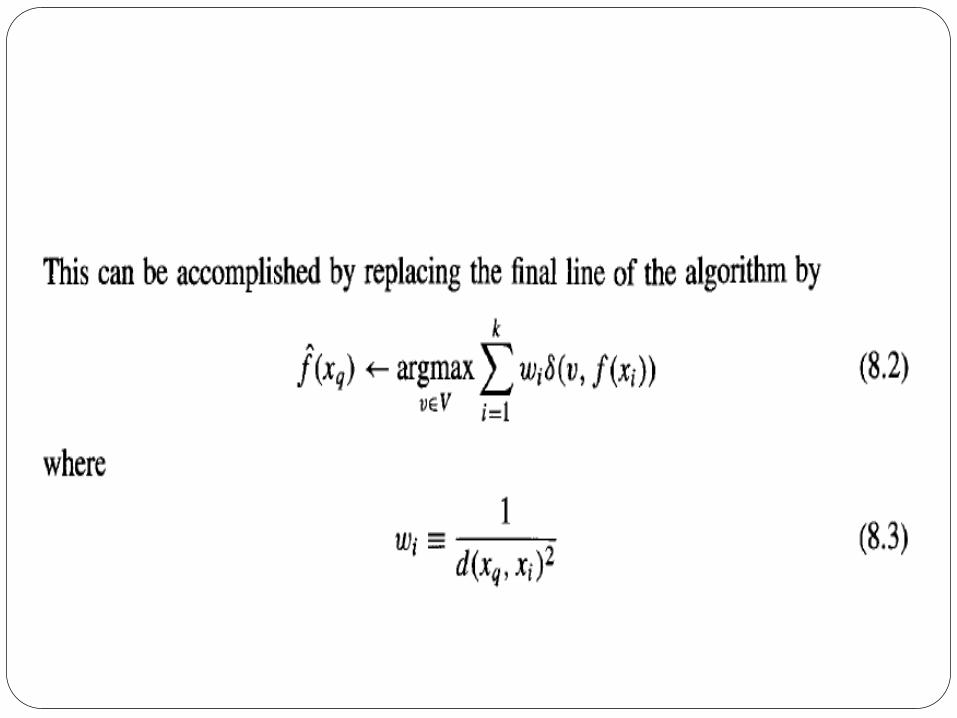
For example, in the algorithm of Table 8.1, which
approximates discrete-valued target functions, we might
weight the vote of each neighbor according to the inverse
square of its distance from xq.


Note all of the above variants of the k-NEAREST
NEIGHBOR Algorithm consider only the k nearest
neighbors to classify the query point.
Once we add distance weighting, there is really no harm
in allowing all training examples to have an influence on
the classification of the xq because very distant examples
will have very little effect on 𝑓 (xq) .

The only disadvantage of considering all examples is that our
classifier will run more slowly.
If all training examples are considered when classifying a new
query instance, we call the algorithm a global method.
If only the nearest training examples are considered, we call
it a local method.
When the rule in Equation (8.4) is applied as a global
method, using all training examples, it is known as Shepard's
method (Shepard 1968).

8.2.2 Remarks on k-NEAREST NEIGHBOR Algorithm
The distance-weighted k-NEAREST NEIGHBOR Algorithm
is a highly effective inductive inference method for many
practical problems.
It is robust to noisy training data and quite effective when it
is provided a sufficiently large set of training data.
Note that by taking the weighted average of the k neighbors
nearest to the query point, it can smooth out the impact of
isolated noisy training examples.

curse of dimensionality
One practical issue in applying k-NEAREST NEIGHBOR
Algorithms is that the distance between instances is
calculated based on all attributes of the instance (i.e., on all
axes in the Euclidean space containing the instances).
This lies in contrast to methods such as rule and decision tree
learning systems that select only a subset of the instance
attributes when forming the hypothesis.

To see the effect of this policy, consider applying k-NN to a
problem in which each instance is described by 20 attributes, but
where only 2 of these attributes are relevant to determining the
classification for the particular target function.
In this case, instances that have identical values for the 2 relevant
attributes may nevertheless be distant from one another in the 20-
dimensional instance space.
As a result, the similarity metric used by k-NN—depending on all
20 attributes-will be misleading.
The distance between neighbors will be dominated by the
large number of irrelevant attributes. This difficulty, which
arises when many irrelevant attributes are present, is
sometimes referred to as the curse of dimensionality.
Nearest-neighbor approaches are especially sensitive to this
problem.

One interesting approach to overcoming this problem is to weight
each attribute differently when calculating the distance between
two instances.
This corresponds to stretching the axes in the Euclidean space,
shortening the axes that correspond to less relevant attributes, and
lengthening the axes that correspond to more relevant attributes.
The amount by which each axis should be stretched can be
determined automatically using a cross-validation approach.

To see how, first note that we wish to stretch (multiply) the jth axis by
some factor zj, where the values z1 . . . zn are chosen to minimize the
true classification error of the learning algorithm. Second, note that
this true error can be estimated using crossvalidation.
Hence, one algorithm is to select a random subset of the available data
to use as training examples, then determine the values of z1 . . . zn that
lead to the minimum error in classifying the remaining examples.
By repeating this process multiple times the estimate for these
weighting factors can be made more accurate. This process of
stretching the axes in order to optimize the performance of k-NN
provides a mechanism for suppressing the impact of irrelevant
attributes.

An even more drastic alternative is to completely eliminate
the least relevant attributes from the instance space. This is
equivalent to setting some of the zi scaling factors to zero.
Moore and Lee (1994) discuss efficient cross-validation
methods for selecting relevant subsets of the attributes for k-
NN algorithms.
In particular, they explore methods based on leave-one-
out crossvalidation, in which the set of m training
instances is repeatedly divided into a training set of size m -
1 and test set of size 1, in all possible ways.

This leave-one out approach is easily implemented in k-NN
algorithms because no additional training effort is required each
time the training set is redefined.
Note both of the above approaches can be seen as stretching each
axis by some constant factor.
Alternatively, we could stretch each axis by a value that varies over
the instance space.
However, as we increase the number of degrees of freedom
available to the algorithm for redefining its distance metric in such
a fashion, we also increase the risk of overfitting. Therefore, the
approach of locally stretching the axes is much less common.
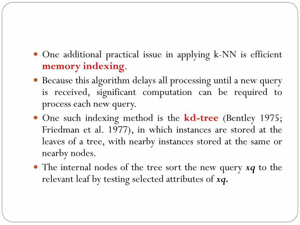
One additional practical issue in applying k-NN is efficient memory indexing.
Because this algorithm delays all processing until a new query is received, significant computation can be required to process each new query.
One such indexing method is the kd-tree (Bentley 1975; Friedman et al. 1977), in which instances are stored at the leaves of a tree, with nearby instances stored at the same or nearby nodes.
The internal nodes of the tree sort the new query xq to the relevant leaf by testing selected attributes of xq.

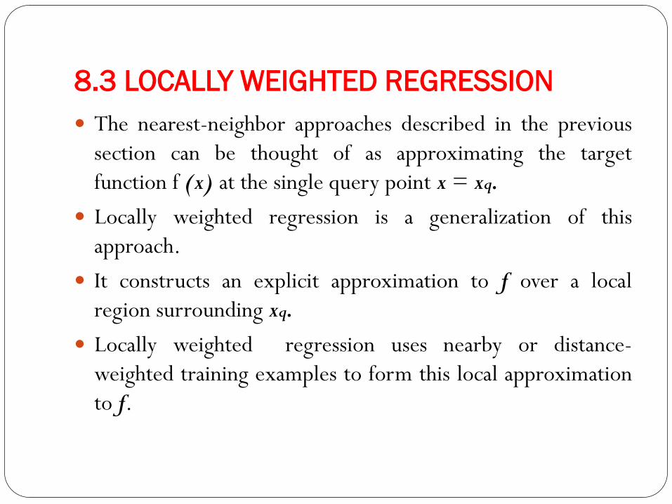
8.3 LOCALLY WEIGHTED REGRESSION
The nearest-neighbor approaches described in the previous
section can be thought of as approximating the target
function f (x) at the single query point x = xq.
Locally weighted regression is a generalization of this
approach.
It constructs an explicit approximation to f over a local
region surrounding xq.
Locally weighted regression uses nearby or distance-
weighted training examples to form this local approximation
to f.

For example, we might approximate the target function in the
neighborhood surrounding xq, using a linear function, a quadratic
function, a multilayer neural network, or some other functional
form.
The phrase "locally weighted regression" is called
local because the function is approximated based only on data near
the query point,
weighted because the contribution of each training example is
weighted by its distance from the query point, and
regression because this is the term used widely in the statistical
learning community for the problem of approximating real-valued
functions.


8.3.1 Locally Weighted Linear
Regression


Criterion two is perhaps the most esthetically pleasing
because it allows every training example to have an
impact on the classification of xq.
However, this approach requires computation that grows
linearly with the number of training examples.
Criterion three is a good approximation to criterion two
and has the advantage that computational cost is
independent of the total number of training examples;
its cost depends only on the number k of neighbors
considered.


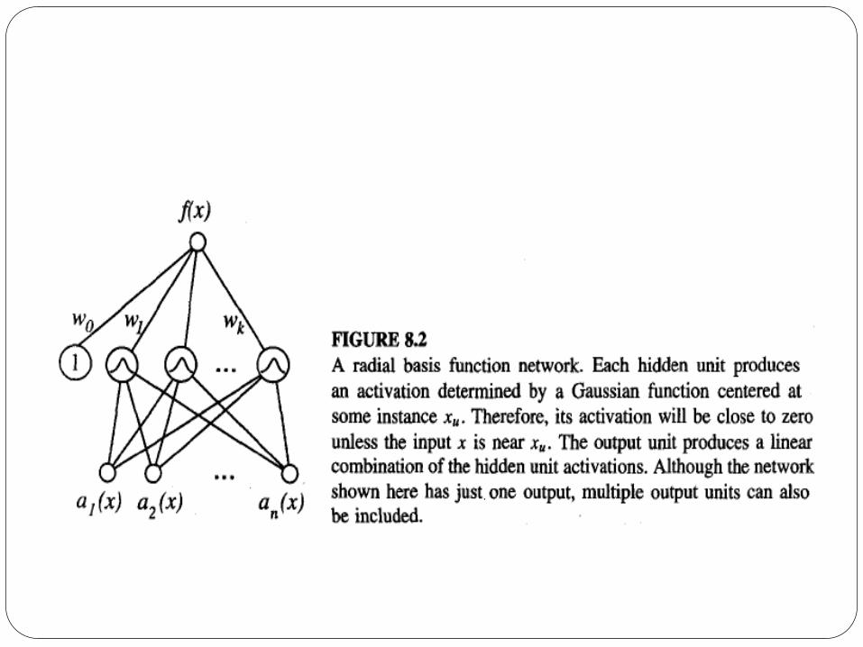
8.4 RADIAL BASIS FUNCTIONS
One approach to function approximation that is closely
related to distance-weighted regression and also to artificial
neural networks is learning with radial basis functions
In this approach, the learned hypothesis is a function of the
form
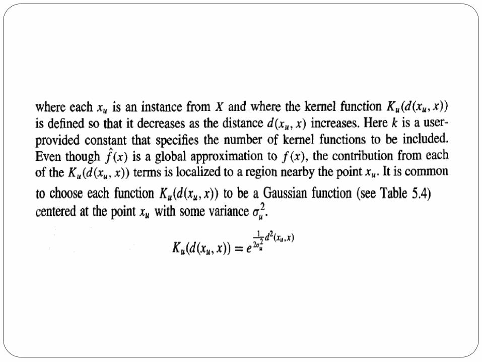
The function given by Equation (8.8) can be viewed as
describing a two-layer network where the first layer of units
computes the values of the various Ku(d(xu, x)) and where
the second layer computes a linear combination of these first-
layer unit values.
An example radial basis function (RBF) network is illustrated
in Figure 8.2.

Given a set of training examples of the target function, RBF
networks are typically trained in a two-stage process.
First, the number k of hidden units is determined and each
hidden unit u is defined by choosing the values of xu and σu2 that
define its kernel function Ku(d(xu, x)).
Second, the weights wu are trained to maximize the fit of the
network to the training data, using the global error criterion
given by Equation (8.5).
Because the kernel functions are held fixed during this
second stage, the linear weight values wu can be trained very
efficiently.

To summarize, radial basis function networks provide a global approximation to the target function, represented by a linear combination of many local kernel functions.
The value for any given kernel function is non-negligible only when the input x falls into the region defined by its particular center and width.
Thus, the network can be viewed as a smooth linear combination of many local approximations to the target function.
One key advantage to RBF networks is that they can be trained much more efficiently than feedforward networks trained with BACKPROPAGATION. This follows from the fact that the input layer and the output layer of an RBF are trained separately.

8.5 CASE-BASED REASONING
Instance-based methods such as k-NN and locally weighted
regression share three key properties.
First, they are lazy learning methods in that they defer the
decision of how to generalize beyond the training data until a
new query instance is observed.
Second, they classify new query instances by analyzing similar
instances while ignoring instances that are very different from
the query.
Third, they represent instances as real-valued points in an n-
dimensional Euclidean space.

Case-based reasoning (CBR) is a learning paradigm based on
the first two of these principles, but not the third.
In CBR, instances are typically represented using more rich
symbolic descriptions, and the methods used to retrieve
similar instances are correspondingly more elaborate.
CBR has been applied to problems such as conceptual design
of mechanical devices based on a stored library of previous
designs (Sycara et al. 1992), reasoning about new legal cases
based on previous rulings (Ashley 1990), and solving
planning and scheduling problems by reusing and combining
portions of previous solutions to similar problems (Veloso
1992).

Let us consider a prototypical example of a case-based reasoning system to ground our discussion. T
The CADET system (Sycara et al. 1992) employs casebased reasoning to assist in the conceptual design of simple mechanical devices such as water faucets.
It uses a library containing approximately 75 previous designs and design fragments to suggest conceptual designs to meet the specifications of new design problems. Each instance stored in memory (e.g., a water pipe) is represented by describing both its structure and its qualitative function.
New design problems are then presented by specifying the desired function and requesting the corresponding structure. This problem setting is illustrated in Figure 8.3.


The top half of the figure shows the description of a typical stored case called a T-junction pipe.
Its function is represented in terms of the qualitative relationships among the waterflow levels and temperatures at its inputs and outputs.
In the functional description at its right, an arrow with a "+" label indicates that the variable at the arrowhead increases with the variable at its tail.
For example, the output waterflow Q3 increases with increasing input waterflow Ql.
a "-" label indicates that the variable at the head decreases with the variable at the tail.


The bottom half of this figure depicts a new design problem described by its desired function.
This particular function describes the required behavior of one type of water faucet. Qc refers to the flow of cold water into the faucet, Qh to the input flow of hot water, and Qm to the single mixed flow out of the faucet. Similarly, Tc, Th, and Tm refer to the temperatures of the cold water, hot
water, and mixed water respectively. The variable Ct denotes the control signal for temperature that is input to
the faucet, and Cf denotes the control signal for waterflow.
Note the description of the desired function specifies that these controls Ct and Cf are to influence the water flows Qc and Qh, thereby indirectly influencing the faucet output flow Qm and temperature Tm.

Given this functional specification for the new design
problem, CADET searches its library for stored cases whose
functional descriptions match the design problem.
If an exact match is found, indicating that some stored case
implements exactly the desired function, then this case can
be returned as a suggested solution to the design problem.
If no exact match occurs, CADET may find cases that match
various subgraphs of the desired functional specification.

In Figure 8.3, for example, the T-junction function matches a
subgraph of the water faucet function graph.
More generally, CADET searches for subgraph isomorphisms
between the two function graphs, so that parts of a case can
be found to match parts of the design specification.
Furthermore, the system may elaborate the original function
specification graph in order to create functionally equivalent
graphs that may match still more cases.
It uses general knowledge about physical influences to create
these elaborated function graphs.

For example, it uses a rewrite rule that allows it to rewrite
the influence

This rewrite rule can be interpreted as stating that if B must
increase with A, then it is sufficient to find some other
quantity x such that B increases with x, and x increases with
A.
Here x is a universally quantified variable whose value is
bound when matching the function graph against the case
library.
In fact, the function graph for the faucet shown in Figure 8.3
is an elaboration of the original - functional specification
produced by applying such rewrite rules.


21-11-2019 Machine Learning-15CS73 1
Machine Learning-Module 5
Reinforcement Learning
Mr. Manoj T
Assistant Professor,
Department of CSE

21-11-2019 Machine Learning-15CS73 2
Chapter 13: Reinforcement Learning
Basics of Reinforcement Learning
• Reinforcement learning addresses the question of how an
autonomous agent that senses and acts in its environment can
learn to choose optimal actions to achieve its goals.
• This very generic problem covers tasks such as learning to
control a mobile robot, learning to optimize operations in
factories, and learning to play board games.
• Each time the agent performs an action in its environment, a
trainer may provide a reward or penalty to indicate the
desirability of the resulting state.

21-11-2019 Machine Learning-15CS73 3
• For ex : when training an agent to play a game the trainer might
provide a positive reward when the game is won, negative reward
when it is lost, and zero reward in all other states.
• The task of the agent is to learn from this indirect, delayed
reward, to choose sequences of actions that produce the greatest
cumulative reward.

21-11-2019 Machine Learning-15CS73 4
Introduction
• Consider building a learning robot. The robot, or agent, has a set
of sensors to observe the state of its environment, and a set of
actions it can perform to alter this state.
• For ex : a mobile robot may have sensors such as a camera and
sonars and actions such as “move forward” and “turn”.
• Its task is to learn a control strategy, or policy, for choosing
actions that achieve its goals.
• For ex : the robot may have a goal of docking onto its battery
charger whenever its battery level is low.
21-11-2019 Machine Learning-15CS73 5
• We assume that the goals of the agent can be defined by a reward
function that assigns a numerical value-an immediate payoff-to
each distinct action the agent may take from each distinct state.
• For ex : the goal of docking to the battery charger can be captured
by assigning a positive reward(+100) to state-action transitions
and a reward of zero to every other state-action transition.
• This reward function may be built into the robot, or known only
to an external teacher who provides the reward value for each
action performed by the robot.
• The task of the robot is to perform sequences of actions, observe
their consequences, and learn a control policy.

21-11-2019 Machine Learning-15CS73 6
• The control policy we desire is one that, from any initial state,
chooses actions that maximize the reward accumulated over time
by the agent.
• This general setting for robot learning is summarized in figure
13.1.
• It is very much apparent from the figure 13.1 that the problem of
learning a control policy to maximize cumulative reward is very
general and covers many problems beyond robot learning tasks
such as manufacturing optimization problems, sequential
scheduling problems such as choosing which taxis to send for
passengers in a large city.

21-11-2019 Machine Learning-15CS73 7
Figure 13.1: An agent interacting with its environment

21-11-2019 Machine Learning-15CS73 8
• In general, we are interested in any type of agent that must learn
to choose actions that alter the state of its environment and
where a cumulative reward function is used to define the quality
of any given action sequence.
• Within this class of problems, the actions may have deterministic
or nondeterministic outcomes. In case of a non-deterministic
outcomes, the learner lacks a domain theory that describes the
outcomes of its actions.
• One of the highly successful application of the reinforcement
learning algorithms is in game-playing problem. Tesauro (1995)
describes the TD-GAMMON program which has used
reinforcement learning to become a world-class backgammon
player.

21-11-2019 Machine Learning-15CS73 9
• The problem of learning a control policy to choose actions is similar
in some respects to the function approximation problems discussed
problems earlier.
• The target function to be learned in this case is a control policy,
𝝅: 𝑺 → 𝑨 that outputs an appropriate action a from the set A, given
the current state s from the set S.
• However, this reinforcement learning problem differs from other
function approximation tasks in several important respects.
Delayed Reward:
The task of the agent is to learn a target function 𝝅 that maps
from the current state s to the optimal action a = 𝝅(s).
In other learning methods, each training example would be a
pair of the form <s, 𝝅(s)>.

21-11-2019 Machine Learning-15CS73 10
In reinforcement learning, however, training information is
not available in this form.
Instead, the trainer provides only a sequence of immediate
reward values as the agent executes its sequence of actions.
The agent, therefore, faces the problem of temporal credit
assignment: determining which of the actions in its
sequence are to be credited with producing the eventual
rewards.
Exploration:
In reinforcement learning, the agent influences the
distribution of training examples by the action sequence it
chooses.
This raises the question of which experimentation strategy
produces most effective learning.

21-11-2019 Machine Learning-15CS73 11
The learner faces a tradeoff in choosing whether to favor
exploration of unknown states and actions (to gather new
information), or exploitation of states and actions that it has
already learned will yield high reward(to maximize its
cumulative reward).
Partially observable states:
It is convenient to assume that the agent's sensors can
perceive the entire state of the environment at each time
step, in many practical situations sensors provide only partial
information.
For ex : a robot with a forward-pointing camera cannot see
what is behind it.
In such cases, it may be necessary for the agent to consider
its previous observations together with its current sensor
data

21-11-2019 Machine Learning-15CS73 12
when choosing actions, and the best policy may be one that
chooses actions specifically to improve the observability of
the environment.
Life-long Learning:
Unlike isolated function approximation tasks, robot learning
often requires that the robot learn several related tasks
within the same environment, using the same sensors.
For ex : a mobile robot may need to learn how to dock on its
battery charger, how to navigate through narrow corridors,
and how to pick up output from laser printers.
This setting raises the possibility of using previously
obtained experience or knowledge to reduce sample
complexity when learning new tasks.
21-11-2019 Machine Learning-15CS73 13
The Learning Task
• Here we will formulate the problem of learning sequential control
strategies more precisely.
• There are many ways to do so. For ex:
We might assume the agent's actions are deterministic or that
they are nondeterministic.
We might assume that the agent can predict the next state that
will result from each action, or that it cannot.
We might assume that the agent is trained by an expert who
shows it examples of optimal action sequences, or that it must
train itself by performing actions of its own choice.

21-11-2019 Machine Learning-15CS73 14
• Let us consider the quite general formulation of the problem, based
on Markov Decision Processes(MDP).
• The formulation of the problem is given in Eqn 13.1
• In a Markov decision process (MDP) the agent can perceive a set S
of distinct states of its environment and has a set A of actions that it
can perform.
• At each discrete time step t, the agent senses the current state st,
chooses a current action at, and performs it.
Eqn 13.1

21-11-2019 Machine Learning-15CS73 15
• The environment responds by giving the agent a reward rt =r(st,at)
and by producing the succeeding state st+l = 𝜹(st,at).
• Here the functions 𝜹 and r are part of the environment and are not
necessarily known to the agent.
• In an MDP, the functions 𝜹(st,at) and r(st,at) depend only on the
current state and action, and not on earlier states or actions.
• Here we consider only the case in which S and A are finite.
Learning by agent
• The task of the agent is to learn a policy, 𝝅 : S → A, for selecting its
next action at based on the current observed state st; i.e: 𝝅(st) = at.
21-11-2019 Machine Learning-15CS73 16
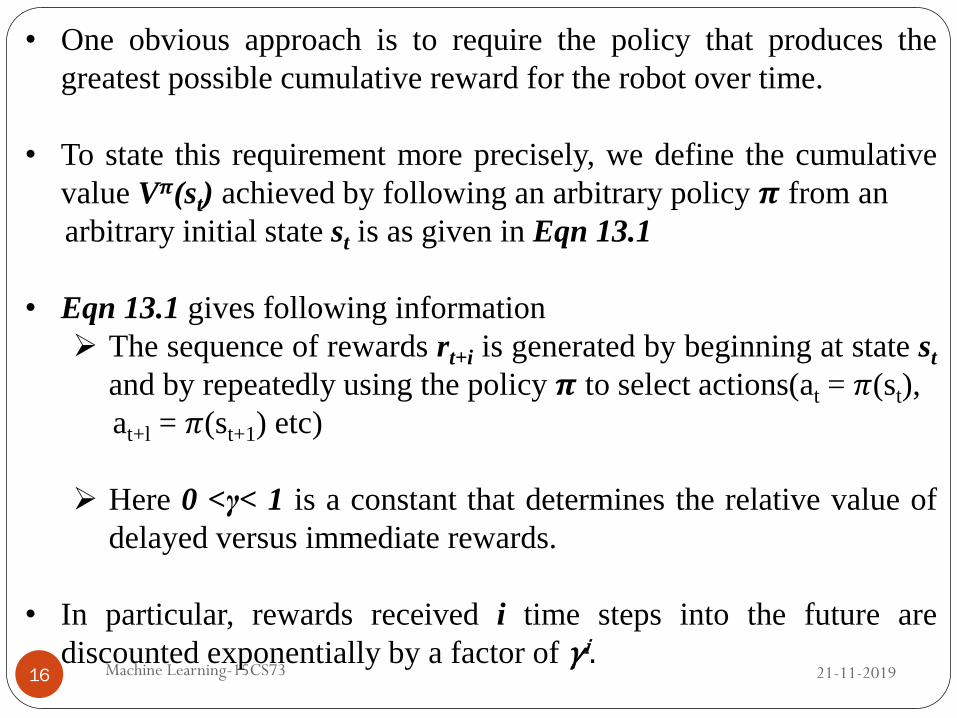
• One obvious approach is to require the policy that produces the
greatest possible cumulative reward for the robot over time.
• To state this requirement more precisely, we define the cumulative
value V𝝅(st) achieved by following an arbitrary policy 𝝅 from an
arbitrary initial state st is as given in Eqn 13.1
• Eqn 13.1 gives following information
The sequence of rewards rt+i is generated by beginning at state st
and by repeatedly using the policy 𝝅 to select actions(at = 𝜋(st),
at+l = 𝜋(st+1) etc)
Here 0 <γ< 1 is a constant that determines the relative value of
delayed versus immediate rewards.
• In particular, rewards received i time steps into the future are
discounted exponentially by a factor of γi.
21-11-2019 Machine Learning-15CS73 17
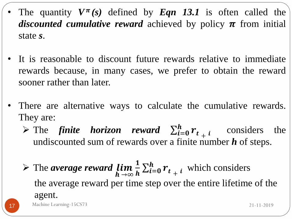
• The quantity V𝝅 (s) defined by Eqn 13.1 is often called the
discounted cumulative reward achieved by policy 𝝅 from initial
state s.
• It is reasonable to discount future rewards relative to immediate
rewards because, in many cases, we prefer to obtain the reward
sooner rather than later.
• There are alternative ways to calculate the cumulative rewards.
They are:
The finite horizon reward 𝒓𝒕 + 𝒊𝒉𝒊=𝟎 considers the
undiscounted sum of rewards over a finite number h of steps.
The average reward 𝒍𝒊𝒎𝒉 →∞
𝟏
𝒉 𝒓𝒕 + 𝒊
𝒉𝒊=𝟎 which considers
the average reward per time step over the entire lifetime of the
agent.

21-11-2019 Machine Learning-15CS73 18
• We require that the agent learn a policy 𝝅 that maximizes V𝝅(s) for
all states s.
• We will call such a policy an optimal policy and denote it by 𝝅∗
• To simplify notation, we will refer to the value function V𝝅*(s) of
such an optimal policy as V*(s).
• V*(s) gives the maximum discounted cumulative reward that the
agent can obtain starting from state s by following the optimal
policy
Eqn 13.2

21-11-2019 Machine Learning-15CS73 19
Illustration of learning task through Grid World Environment
• Consider a simple grid-world environment is depicted in the
topmost diagram of figure 13.2.
• The six grid squares in this diagram represent six possible states, or
locations, for the agent.
• Each arrow in the diagram represents a possible action the agent can
take to move from one state to another.
• The number associated with each arrow represents the immediate
reward r(s,a) the agent receives if it executes the corresponding
state-action transition.
• The immediate reward in this particular environment is defined to
be zero for all state-action transitions except for those leading into
the state labeled G

21-11-2019 Machine Learning-15CS73 20
Figure 13.2: A simple deterministic world to illustrate the basic concepts of Q-learning

21-11-2019 Machine Learning-15CS73 21
• It is convenient to think of the state G as the goal state, because the
only way the agent can receive reward, in this case, is by entering
this state.
• In this particular environment, the only action available to the agent
once it enters the state G is to remain in this state. For this reason,
we call G an absorbing state.
• Once the states, actions, and immediate rewards are defined, and
once we choose a value for the discount factor γ, we can determine
the optimal policy 𝝅* and its value function V*(s).
• In this case, let us choose γ = 0.9.
• The diagram at the right of figure 13.2 shows the values of V* for
each state. For ex : consider the bottom right state in this diagram.
21-11-2019 Machine Learning-15CS73 22
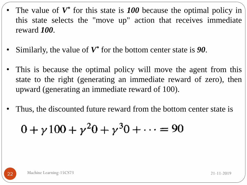
• The value of V* for this state is 100 because the optimal policy in
this state selects the "move up" action that receives immediate
reward 100.
• Similarly, the value of V* for the bottom center state is 90.
• This is because the optimal policy will move the agent from this
state to the right (generating an immediate reward of zero), then
upward (generating an immediate reward of 100).
• Thus, the discounted future reward from the bottom center state is

21-11-2019 Machine Learning-15CS73 23
Q Learning
• How can an agent learn an optimal policy 𝝅* for an arbitrary
environment?
• It is difficult to learn the function 𝝅* ∶ 𝑺 → 𝑨 directly, because the
available training data does not provide training examples of the
form <s, a> .
• Instead, the only training information available to the learner is the
sequence of immediate rewards r(si,ai) for i = 0, 1,2,3….
• One of the choice for evaluation function the agent should attempt
to learn is V*.
• The agent should prefer state sl over state s2 whenever V*(s1)
>V*(s2), because the cumulative future reward will be greater from
s1.

21-11-2019 Machine Learning-15CS73 24
• Of course the agent's policy must choose among actions, not among
states. It can use V* in certain settings to choose among actions as
well.
• The optimal action in state s is the action a that maximizes the sum
of the immediate reward r(s,a) plus the value V* of the immediate
successor state, discounted by γ.
• Thus, the agent can acquire the optimal policy by learning V*,
provided it has perfect knowledge of the immediate reward function
r and the state transition function 𝜹.
• Unfortunately, learning V* is a useful way to learn the optimal
policy only when the agent has perfect knowledge of 𝜹 and r.
Eqn 13.3

21-11-2019 Machine Learning-15CS73 25
• This requires that it be able to perfectly predict the immediate result
(i.e., the immediate reward and immediate successor) for every
possible state-action transition.
• In many practical problems, such as robot control, it is impossible
for the agent or its human programmer to predict in advance the
exact outcome of applying an arbitrary action to an arbitrary state.
• In cases where either 𝜹 or r is unknown, learning V* is unfortunately
of no use for selecting optimal actions because the agent cannot
evaluate Eqn 13.3.
• Now we should go for the evaluation function that is applicable for
more general setting.

21-11-2019 Machine Learning-15CS73 26
The Q Function
• Let us define the evaluation function Q(s,a) so that its value is the
maximum discounted cumulative reward that can be achieved
starting from state s and applying action a as the first action.
• In other words, the value of Q is the reward received immediately
upon executing action a from state s, plus the value (discounted by
γ) of following the optimal policy thereafter.
• Note that Q(s,a) is exactly the quantity that is maximized in Eqn
13.3 in order to choose the optimal action a in state s.
• Therefore, we can rewrite Eqn 13.3 in terms of Q(s,a) as
Eqn 13.4

21-11-2019 Machine Learning-15CS73 27
• This shows that if the agent learns the Q function instead of the V*
function, it will be able to select optimal actions even when it has no
knowledge of the functions r and 𝜹.
• As Eqn 13.5 makes clear, it need only consider each available
action a in its current state s and choose the action that maximizes
Q(s,a).
• Here the surprising fact is that one can choose globally optimal
action sequences by reacting repeatedly to the local values of Q for
the current state.
• This means the agent can choose the optimal action without ever
conducting a lookahead search to explicitly consider what state
results from the action.
Eqn 13.5
21-11-2019 Machine Learning-15CS73 28
• To illustrate, figure 13.2 shows the Q values for every state and
action in the simple grid world.
• Notice that the Q value for each state-action transition equals the r
value for this transition plus the V* value for the resulting state
discounted by γ.
• The optimal policy shown in the figure 13.2 corresponds to
selecting actions with maximal Q values.
21-11-2019 Machine Learning-15CS73 29
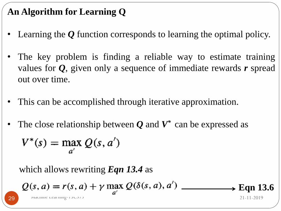
An Algorithm for Learning Q
• Learning the Q function corresponds to learning the optimal policy.
• The key problem is finding a reliable way to estimate training
values for Q, given only a sequence of immediate rewards r spread
out over time.
• This can be accomplished through iterative approximation.
• The close relationship between Q and V* can be expressed as
which allows rewriting Eqn 13.4 as
Eqn 13.6

21-11-2019 Machine Learning-15CS73 30
• This recursive definition of Q provides the basis for algorithms that
iteratively approximate Q (Watkins 1989).
• To describe the algorithm, we will use the symbol 𝑸 to refer to the
learner's estimate, or hypothesis, of the actual Q function.
• In this algorithm the learner represents its hypothesis 𝑸 by a large
table with a separate entry for each state-action pair.
• The table entry for the pair <s,a> stores the value for 𝑸 (s,a) -
learner's current hypothesis about the actual but unknown value Q(s,
a).
• The table can be initially filled with random values (though it is
easier to understand the algorithm if one assumes initial values of
zero).

21-11-2019 Machine Learning-15CS73 31
• The agent repeatedly observes its current state s, chooses some
action a, executes this action, then observes the resulting reward r =
r(s,a) and the new state s' = 𝜹(s, a).
• It then updates the table entry for 𝑸 (s,a) following each such
transition, according to the rule:
• Note this training rule uses the agent's current 𝑸 values for the new
state s' to refine its estimate of 𝑸 (s,a), for the previous state s.
• Although Eqn13.6 describes Q in terms of the functions 𝜹(s,a) and
r(s,a), the agent does not need to know these general functions to
apply the training rule of Eqn 13.7.
Eqn 13.7

21-11-2019 Machine Learning-15CS73 32
• Instead it executes the action in its environment and then observes
the resulting new state s' and reward r.
• Thus, it can be viewed as sampling these functions at the current
values of s and a.
• The Q learning algorithm for deterministic Markov decision
processes is described in the Table 13.1.
• Using this algorithm the agent's estimate 𝑸 converges in the limit to
the actual Q function, provided the system can be modeled as a
deterministic Markov decision process, the reward function r is
bounded, and actions are chosen so that every state-action pair is
visited infinitely often.

21-11-2019 Machine Learning-15CS73 33
Q learning algorithm
For each s,a initialize the table entry 𝑸 (s,a) to zero.
Observe the current state s
Do forever:
• Select an action a and execute it
• Receive immediate reward r
• Observe the new state s'
• Update the table entry for 𝑸 (s,a) as follows:
• s ⃪ s'
Table 13.1: Q Learning Algorithm, assuming deterministic rewards and actions

21-11-2019 Machine Learning-15CS73 34
An Illustrative Example
• To illustrate the operation of the Q learning algorithm, consider a
single action taken by an agent, and the corresponding refinement to
𝑸 as shown in the figure 13.3.
• In this example, the agent moves one cell to the right in its grid
world and receives an immediate reward of zero for this transition.
• It then applies the training rule of Eqn 13.7 to refine its estimate 𝑸
for the state-action transition it just executed.
• According to the training rule, the new Q estimate for this transition
is the sum of the received reward (zero) and the highest Q value
associated with the resulting state (100), discounted by γ(0.9).

21-11-2019 Machine Learning-15CS73 35
Figure 13.3:The update to 𝑄 after executing a single action

21-11-2019 Machine Learning-15CS73 36
• Each time the agent moves forward from an old state to a new one,
Q learning propagates 𝑸 estimates backward from the new state to
the old.
• At the same time, the immediate reward received by the agent for
the transition is used to augment these propagated values of 𝑸 .
• Consider applying this algorithm to the grid world and reward
function shown in figure 13.2, for which the reward is zero
everywhere, except when entering the goal state.
• Since this world contains an absorbing goal state, we will assume
that training consists of a series of episodes.
• During each episode, the agent begins at some randomly chosen
state and is allowed to execute actions until it reaches the absorbing
goal state.

21-11-2019 Machine Learning-15CS73 37
• When it does, the episode ends and the agent is transported to a new,
randomly chosen, initial state for the next episode.
• The values of 𝑸 evolve as the Q learning algorithm is applied in the
following way:
With all the 𝑸 values initialized to zero, the agent will make no
changes to any Q table entry until it happens to reach the goal
state and receive a nonzero reward.
This will result in refining the 𝑸 value for the single transition
leading into the goal state.
On the next episode, if the agent passes through this state
adjacent to the goal state, its nonzero 𝑸 value will allow
refining the value for some transition two steps from the goal,
and so on.

21-11-2019 Machine Learning-15CS73 38
Given a sufficient number of training episodes, the information
will propagate from the transitions with nonzero reward back
through the entire state-action space available to the agent,
resulting eventually in a 𝑸 table containing the Q values shown
in figure 13.2.
• The two general properties of Q learning algorithm that hold for any
deterministic MDP in which the rewards are non-negative, assuming
we initialize all 𝑸 values to zero.
i. The first property is that under these conditions the 𝑸 values
never decrease during training.
More formally, let 𝑸 n(s,a) denote the learned 𝑸 (s,a) value
after the nth iteration of the training procedure then
21-11-2019 Machine Learning-15CS73 39
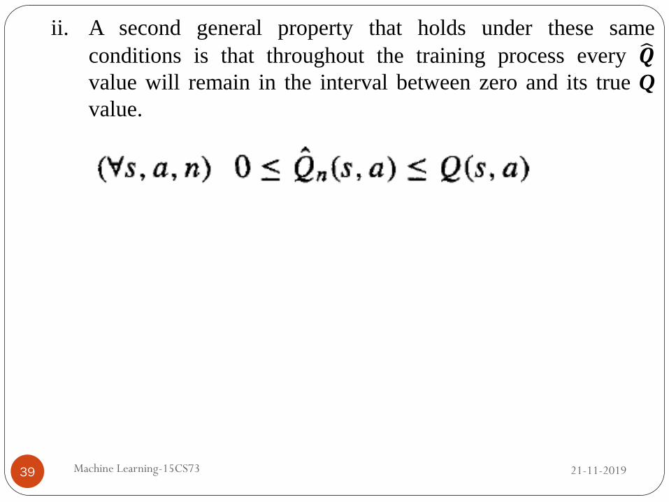
ii. A second general property that holds under these same
conditions is that throughout the training process every 𝑸
value will remain in the interval between zero and its true Q
value.
21-11-2019 Machine Learning-15CS73 40
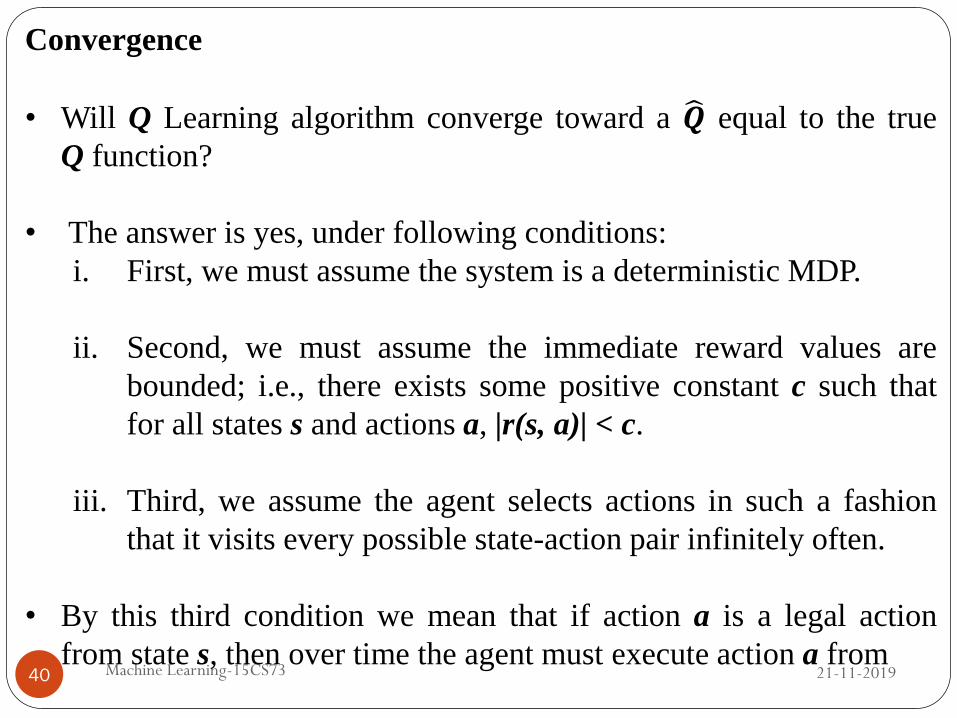
Convergence
• Will Q Learning algorithm converge toward a 𝑸 equal to the true
Q function?
• The answer is yes, under following conditions:
i. First, we must assume the system is a deterministic MDP.
ii. Second, we must assume the immediate reward values are
bounded; i.e., there exists some positive constant c such that
for all states s and actions a, |r(s, a)| < c.
iii. Third, we assume the agent selects actions in such a fashion
that it visits every possible state-action pair infinitely often.
• By this third condition we mean that if action a is a legal action
from state s, then over time the agent must execute action a from

21-11-2019 Machine Learning-15CS73 41
state s repeatedly and with nonzero frequency as the length of its
action sequence approaches infinity.
• These conditions are also restrictive in that they require the agent to
visit every distinct state-action transition infinitely often. This is a
very strong assumption in large (or continuous!) domains.
• The key idea underlying the proof of convergence is that the table
entry 𝑸 (s,a) with the largest error must have its error reduced by a
factor of γ whenever it is updated.
Theorem 13.1: Convergence of Q learning for deterministic Markov
decision processes.
• Consider a Q learning agent in a deterministic MDP with bounded
rewards (∀ s,a), |r(s, a)| ≤ c .

21-11-2019 Machine Learning-15CS73 42
• The Q learning agent uses the training rule of Eqn 13.7, initializes
its 𝑸 (s,a) table to arbitrary finite values, and uses a discount factor γ
such that 0 < γ < 1
• Let 𝑸 𝒏(s,a) denote the agent's hypothesis 𝑸 (s,a), following the nth
update. If each state-action pair is visited infinitely often, then
𝑸 𝒏(s,a) converges to Q(s,a) as n→∞, for all s,a.
Proof:
• Since each state-action transition occurs infinitely often, consider
consecutive intervals during which each state-action transition
occurs at least once.
• The proof consists of showing that the maximum error over all
entries in the Q table is reduced by at least a factor of γ during each
such interval.
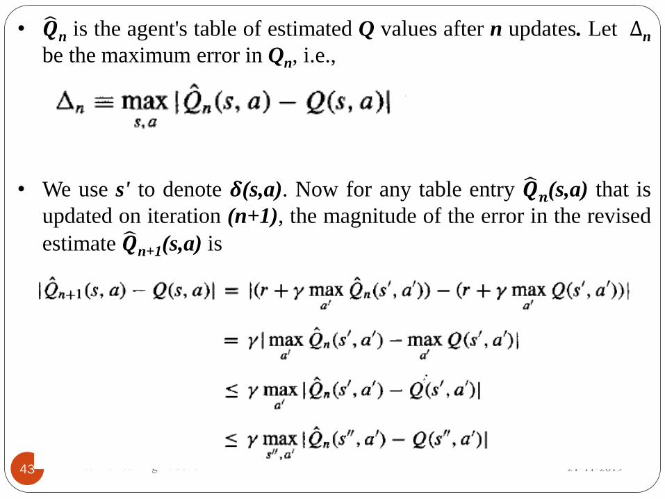
21-11-2019 Machine Learning-15CS73 43
• 𝑸 n is the agent's table of estimated Q values after n updates. Let ∆n
be the maximum error in Qn, i.e.,
• We use s' to denote 𝜹(s,a). Now for any table entry 𝑸 𝒏(s,a) that is
updated on iteration (n+1), the magnitude of the error in the revised
estimate 𝑸 n+1(s,a) is

21-11-2019 Machine Learning-15CS73 44
• Therefore,
• We use following factors while deriving the equation
For any two functions f1 and f2 the following inequality holds
We introduce a new variable s" over which the maximization is
performed.
• This is legitimate because the maximum value will be at least as
great when we allow this additional variable to vary.

21-11-2019 Machine Learning-15CS73 45
• Thus, the updated 𝑸 n+1(s,a) for any s,a is at most γ times the
maximum error in the 𝑸 n, table, An.
• The largest error in the initial table, ∆0, is bounded because values
𝑸 0(s,a) of and Q(s,a) are bounded for all s, a .
• Now after the first interval during which each s,a is visited, the
largest error in the table will be at most γ∆0 .
• After k such intervals, the error will be at most γ𝒌∆0 . Since each
state is visited infinitely often, the number of such intervals is
infinite and ∆n→ 0 as n → ∞.
• This proves the theorem.
21-11-2019 Machine Learning-15CS73 46
Experimentation Strategies
• The Q learning algorithm stated earlier does not specify how actions
are chosen by the agent.
• One obvious strategy would be for the agent in state s to select
action a that maximizes 𝑸 (s,a) thereby exploiting its current
approximation 𝑸 .
• However, with this strategy the agent runs the risk that it will
overcommit to actions that are found during early training to have
high 𝑸 values, while failing to explore other actions that have even
higher values.
• For this reason, it is common in Q learning to use a probabilistic
approach to selecting actions.

21-11-2019 Machine Learning-15CS73 47
• Actions with higher 𝑸 values are assigned higher probabilities, but
every action is assigned a nonzero probability.
• One way to assign such probabilities is
where,
P(ai/s) is the probability of selecting action ai, given that the agent
is in state s
k>0 is a constant that determines how strongly the selection favors
actions with high 𝑸 values.

21-11-2019 Machine Learning-15CS73 48
• Larger values of k will assign higher probabilities to actions with
above average 𝑸 , causing the agent to exploit what it has learned
and seek actions it believes will maximize its reward.
• In contrast, small values of k will allow higher probabilities for
other actions, leading the agent to explore actions that do not
currently have high 𝑸 values.

21-11-2019 Machine Learning-15CS73 49
Updating Sequence
• One important implication of the convergence theorem is that Q
learning need not train on optimal action sequences in order to
converge to the optimal policy.
• In fact, it can learn the Q function (and hence the optimal policy)
while training from actions chosen completely at random at each
step, as long as the resulting training sequence visits every state-
action transition infinitely often.
• This fact suggests changing the sequence of training example
transitions in order to improve training efficiency without
endangering final convergence.

21-11-2019 Machine Learning-15CS73 50
• Consider again learning in an MDP with a single absorbing goal
state. Assume as before that we train the agent with a sequence of
episodes. For each episode, the agent is placed in a random initial
state and is allowed to perform actions and to update its 𝐐 table
until it reaches the absorbing goal state.
• A new training episode is then begun by removing the agent from
the goal state and placing it at a new random initial state.
• If we begin with all 𝐐 values initialized to zero, then after the first
full episode only one entry in the agent's 𝐐 table will have been
changed: the entry corresponding to the final transition into the goal
state.
• If the agent happens to follow the same sequence of actions from
the same random initial state in its second full episode, then a
second table entry would be made nonzero, and so on.

21-11-2019 Machine Learning-15CS73 51
• If we run repeated identical episodes in this fashion, the frontier of
nonzero 𝐐 values will creep backward from the goal state at the rate
of one new state-action transition per episode.
Approaches for faster convergence
• Now consider training on these same state-action transitions, but in
reverse chronological order for each episode.
• That is, we apply the same update rule from Eqn 13.7 for each
transition considered, but perform these updates in reverse order.
• In this case, after the first full episode the agent will have updated
its 𝐐 estimate for every transition along the path it took to the goal.
• This training process will clearly converge in fewer iterations,
although it requires that the agent use more memory to store the

21-11-2019 Machine Learning-15CS73 52
entire episode before beginning the training for that episode.
• A second strategy for improving the rate of convergence is to store
past state-action transitions, along with the immediate reward that
was received, and retrain on them periodically.
• Although at first it might seem a waste of effort to retrain on the
same transition, recall that the updated 𝑸 (s,a) value is determined
by the values 𝑸 (s',a) of the successor state s' = 𝜹(s,a).
• Therefore, if subsequent training changes one of the 𝑸 (s,a) values,
then retraining on the transition <s,a> may result in an altered value
for 𝑸 (s,a).
• In general, the degree to which we wish to replay old transitions
versus obtain new ones from the environment depends on the
relative costs of these two operations in the specific problem
domain.