Embed Size (px)
Citation preview
Department of Ecosystem Science and Management Texas A&M University
Module Instructions RENR 405 Geographic Information Systems for Environmental Problem Solving
Page 2
Remarks:
Read the Learning Materials (available on the course DVD under Learning_Materials folder OR on the website under each week’s topic) before completing each module here.
Be sure to read carefully and strictly follow the instructions. Each step/module is built upon another for the most part. Do not jump from one step to another.
Save your work often as you work through the module (go to File > Save/Save As to save the current ArcMap Document).
When working on each module, be sure to save the files/outputs in the same directory (e.g. C:\gis\data). Make note of the directory or folder so that you can trace back to the files when needed.
A file name should not contain any space, be easy to remember, and cannot exceed 13 characters. You can use underscore (_) as an alternative. For example, name your file “Main_St.shp”, NOT “Main St.shp”.
GIS for Environmental Problem Solving, Module Instructions
Module 1 Page 3
Module 1: Installation of Course Materials and Introduction
Learning Objectives:
Install ArcGIS software
Upload datasets
System operability test
Learning Materials:
Before going through this module and working with ArcGIS, please review the following presentations (available on the course DVD under Learning_Materials folder OR on the website under week 1’s topic):
Keys to Success Course Introduction Framing the Problem Coordinate Systems and Projections Part I
GIS for Environmental Problem Solving, Module Instructions
Module 1 Page 4
Part I: Installation of GIS Software
*** BE SURE TO STRICTLY FOLLOW THE INSTRUCTIONS. FAILURE TO DO SO CAN RESULT IN DELAYS AND INTERRUPTIONS IN YOUR WORK IN THE COURSE. ***
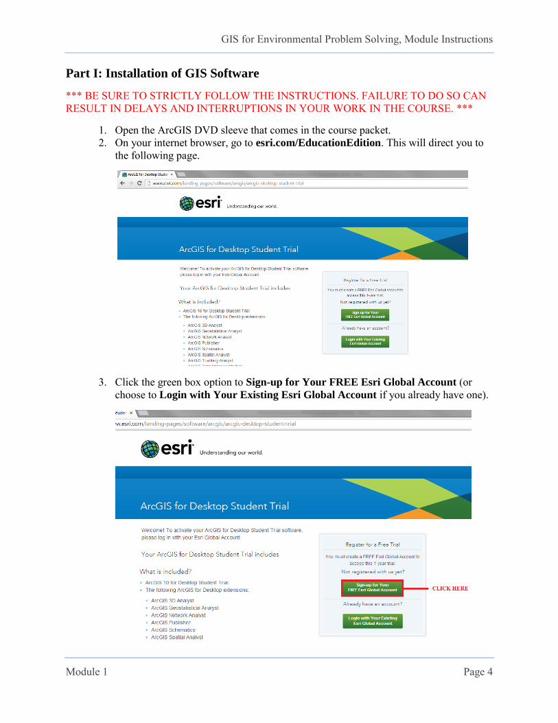
1. Open the ArcGIS DVD sleeve that comes in the course packet. 2. On your internet browser, go to esri.com/EducationEdition. This will direct you to
the following page.
3. Click the green box option to Sign-up for Your FREE Esri Global Account (or choose to Login with Your Existing Esri Global Account if you already have one).

GIS for Environmental Problem Solving, Module Instructions
Module 1 Page 5
4. Fill in your information on the next page and click Start Your Free Trial.
*** FAILURE TO LOGIN (AND ACTIVATVE THE AUTHORIZATION NUMBER IN THE NEXT STEP) WILL CAUSE DELAYS AND INTERRUPTIONS IN THE INSTALLATION AND WORKING PROCESS. ***
GIS for Environmental Problem Solving, Module Instructions
Module 1 Page 6
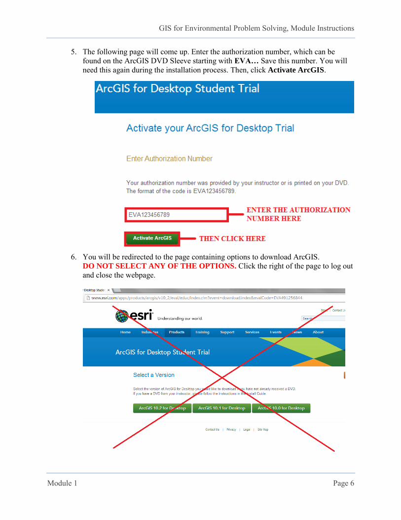
5. The following page will come up. Enter the authorization number, which can be found on the ArcGIS DVD Sleeve starting with EVA… Save this number. You will need this again during the installation process. Then, click Activate ArcGIS.
6. You will be redirected to the page containing options to download ArcGIS.
DO NOT SELECT ANY OF THE OPTIONS. Click the right of the page to log out and close the webpage.
GIS for Environmental Problem Solving, Module Instructions
Module 1 Page 7
7. Ensure that you receive an email confirmation for the activation (in the email you provided in the sign-up process). The email is usually titled “ArcGIS 10 for Desktop Student Trial” and comes from [email protected]. You should receive the email
a few minutes after activating the authorization number in step 5. *** DO NOT FOLLOW THE INSTRUCTIONS IN THE EMAIL. JUST PROCEED WITH THE STEPS BELOW. ***
8. Clear the current local hard drive (C:) of any unnecessary programs. Make sure you have at least 8 Gigabytes free space.
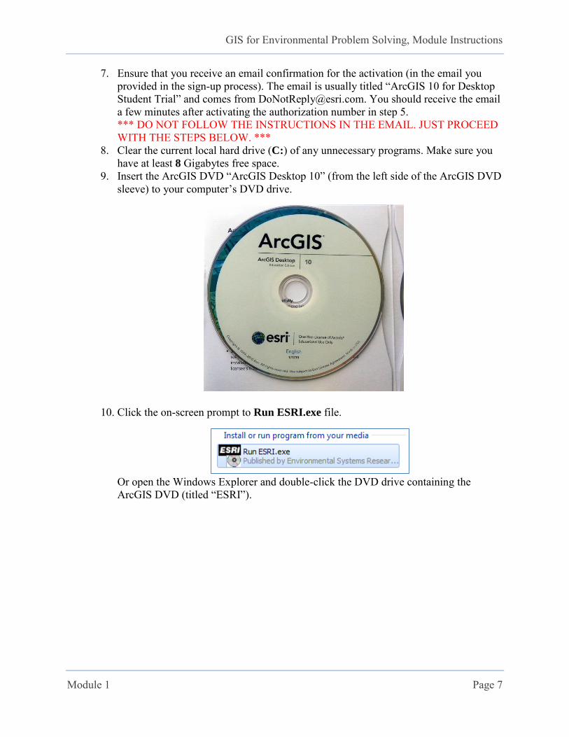
9. Insert the ArcGIS DVD “ArcGIS Desktop 10” (from the left side of the ArcGIS DVD sleeve) to your computer’s DVD drive.
10. Click the on-screen prompt to Run ESRI.exe file.
Or open the Windows Explorer and double-click the DVD drive containing the ArcGIS DVD (titled “ESRI”).
GIS for Environmental Problem Solving, Module Instructions
Module 1 Page 8
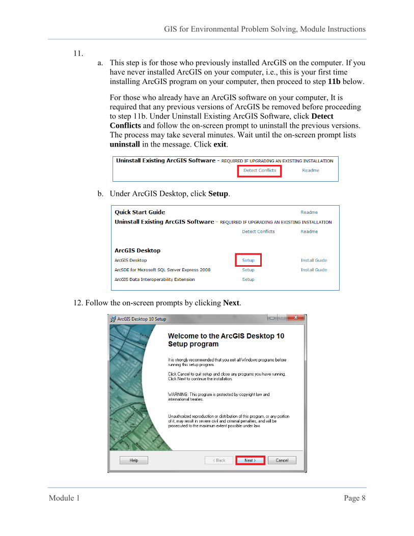
11. a. This step is for those who previously installed ArcGIS on the computer. If you
have never installed ArcGIS on your computer, i.e., this is your first time installing ArcGIS program on your computer, then proceed to step 11b below.
For those who already have an ArcGIS software on your computer, It is required that any previous versions of ArcGIS be removed before proceeding to step 11b. Under Uninstall Existing ArcGIS Software, click Detect
Conflicts and follow the on-screen prompt to uninstall the previous versions. The process may take several minutes. Wait until the on-screen prompt lists uninstall in the message. Click exit.
b. Under ArcGIS Desktop, click Setup.
12. Follow the on-screen prompts by clicking Next.

GIS for Environmental Problem Solving, Module Instructions
Module 1 Page 9
13. Select I accept the license agreement and click Next.
14. Select Complete and click Next.
*** MAKE SURE THAT THE COMPLETE OPTION IS SELECTED. OTHERWISE, YOU WILL BE MISSING SOME TOOLS/APPLICATIONS TO WORK WITH LATER ON. ***
GIS for Environmental Problem Solving, Module Instructions
Module 1 Page 10
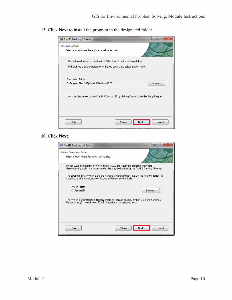
15. Click Next to install the program in the designated folder.
16. Click Next.

GIS for Environmental Problem Solving, Module Instructions
Module 1 Page 11
17. Click Next.
18. The installation process will take several minutes. Try not to work on any other programs on the computer.
GIS for Environmental Problem Solving, Module Instructions
Module 1 Page 12
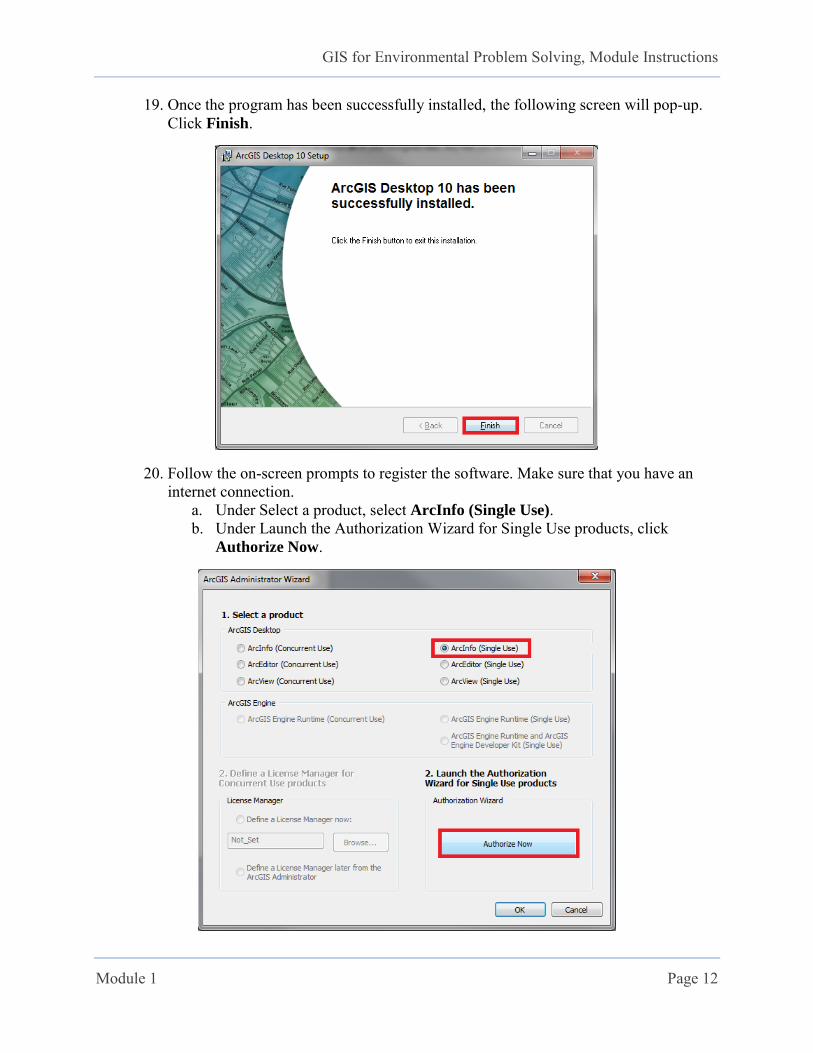
19. Once the program has been successfully installed, the following screen will pop-up. Click Finish.
20. Follow the on-screen prompts to register the software. Make sure that you have an internet connection.
a. Under Select a product, select ArcInfo (Single Use). b. Under Launch the Authorization Wizard for Single Use products, click
Authorize Now.
GIS for Environmental Problem Solving, Module Instructions
Module 1 Page 13
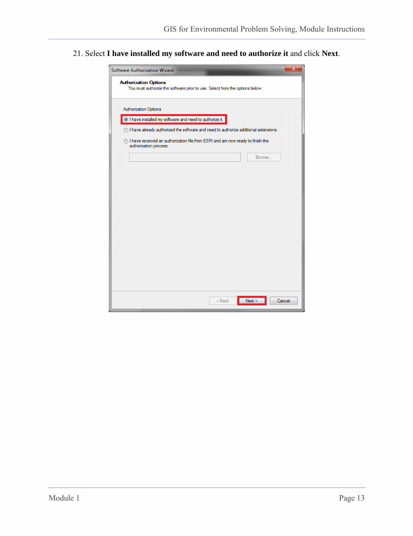
21. Select I have installed my software and need to authorize it and click Next.

GIS for Environmental Problem Solving, Module Instructions
Module 1 Page 14
22. Select Authorize with ESRI now using the Internet and click Next.
GIS for Environmental Problem Solving, Module Instructions
Module 1 Page 15
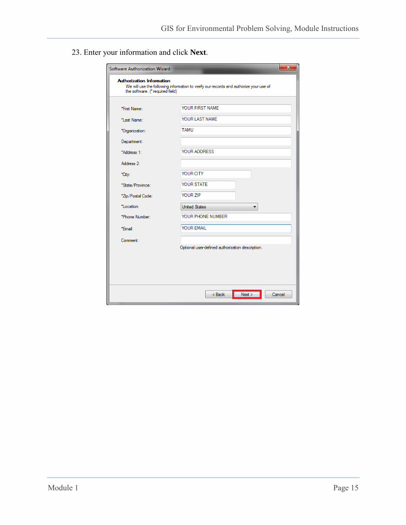
23. Enter your information and click Next.
GIS for Environmental Problem Solving, Module Instructions
Module 1 Page 16
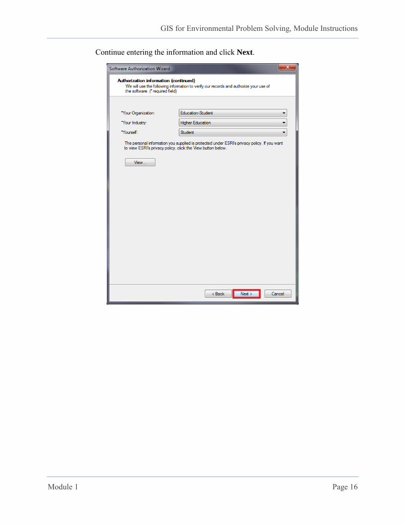
Continue entering the information and click Next.
GIS for Environmental Problem Solving, Module Instructions
Module 1 Page 17
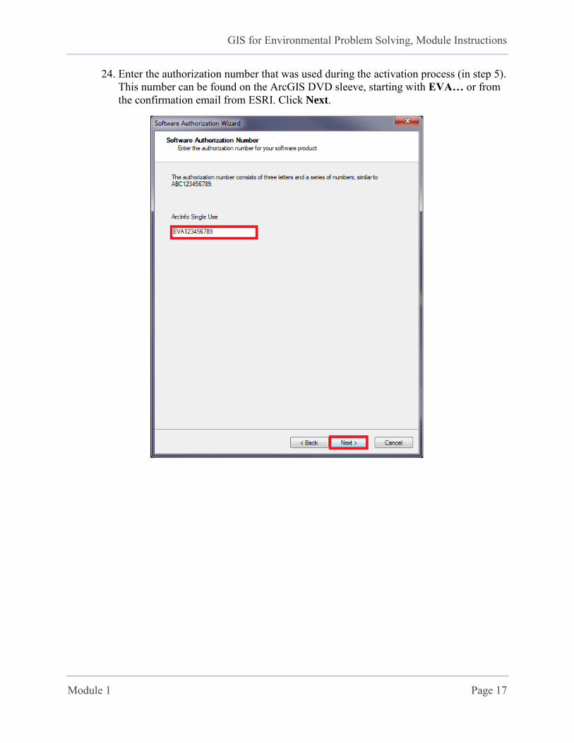
24. Enter the authorization number that was used during the activation process (in step 5). This number can be found on the ArcGIS DVD sleeve, starting with EVA… or from the confirmation email from ESRI. Click Next.

GIS for Environmental Problem Solving, Module Instructions
Module 1 Page 18
25. Select I have authorization number(s) to authorize one or more extensions and enter the same authorization number (from step 24) next to all of the extension boxes (you can copy and paste the number from one box to another). Then, click Next.
GIS for Environmental Problem Solving, Module Instructions
Module 1 Page 19
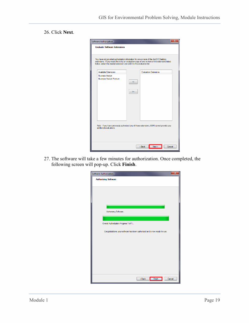
26. Click Next.
27. The software will take a few minutes for authorization. Once completed, the following screen will pop-up. Click Finish.

GIS for Environmental Problem Solving, Module Instructions
Module 1 Page 20
28. The software is now ready for use. All other materials in the DVD sleeve are not necessary for this course.
29. Now go to Start > All Programs > ArcGIS > ArcMap 10 (or type in “ArcMap” in the Search programs and files box).
Make sure that the program opens up like this:
Part II: Installation of Course Materials
1. Insert the course DVD “RENR405 GIS for Environmental Problem Solving” (provided to you in the course packet).
2. Drag and drop the folder gis onto your C drive.
*** DO NOT PLACE THE GIS FOLDER IN ANY LOCATION OTHER THAN DIRECTLY ONTO THE C DRIVE (OR IF ABSOLUTELY NECESSARY, AN ALTERNATE HARD DRIVE ON YOUR COMPUTER).
FAILURE TO PERFORM THIS STEP CAN CRITICALLY AFFECT THE PERFORMANCE IN ARCGIS FOR THE REST OF THE COURSE. ***
The instructions will use drive C as a default drive for working and saving all files onwards. If you are saving the gis folder in an alternate drive, then you need to adjust the directory when working and saving the files accordingly.
3. Now open C:\gis\Learning_Materials\week_1 and go through the materials before completing Assessment 1 on eCampus.
GIS for Environmental Problem Solving, Module Instructions
Module 2 Page 21
Module 2: Fundamentals of GIS operations
Learning Objectives:
Learn the basic operations of: o ArcCatalog
o ArcMap
o Applicable Extensions
Be able to give an example of an environmental problem
Understand the basic problem solving steps
Learning Materials:
Before going through this module and working with ArcGIS, please review the following presentations:
Develop a Conceptual Methodology
Coordinate Systems and Projections Part II
Procedure:
1. PERFORM the enclosed steps for: Setting up ArcMap for use (pages 22-25) Setting up the workspace (pages 25-28) Setting up Address Locator (pages 57-58)
2. READ the rest of the module to become familiar with each task.
*** YOU DO NOT ACTUALLY DO THESE STEPS. ONLY READ IT THROUGH! ***
GIS for Environmental Problem Solving, Module Instructions
Module 2 Page 22
Setting Up ArcMap for Use
Enabling on Extensions
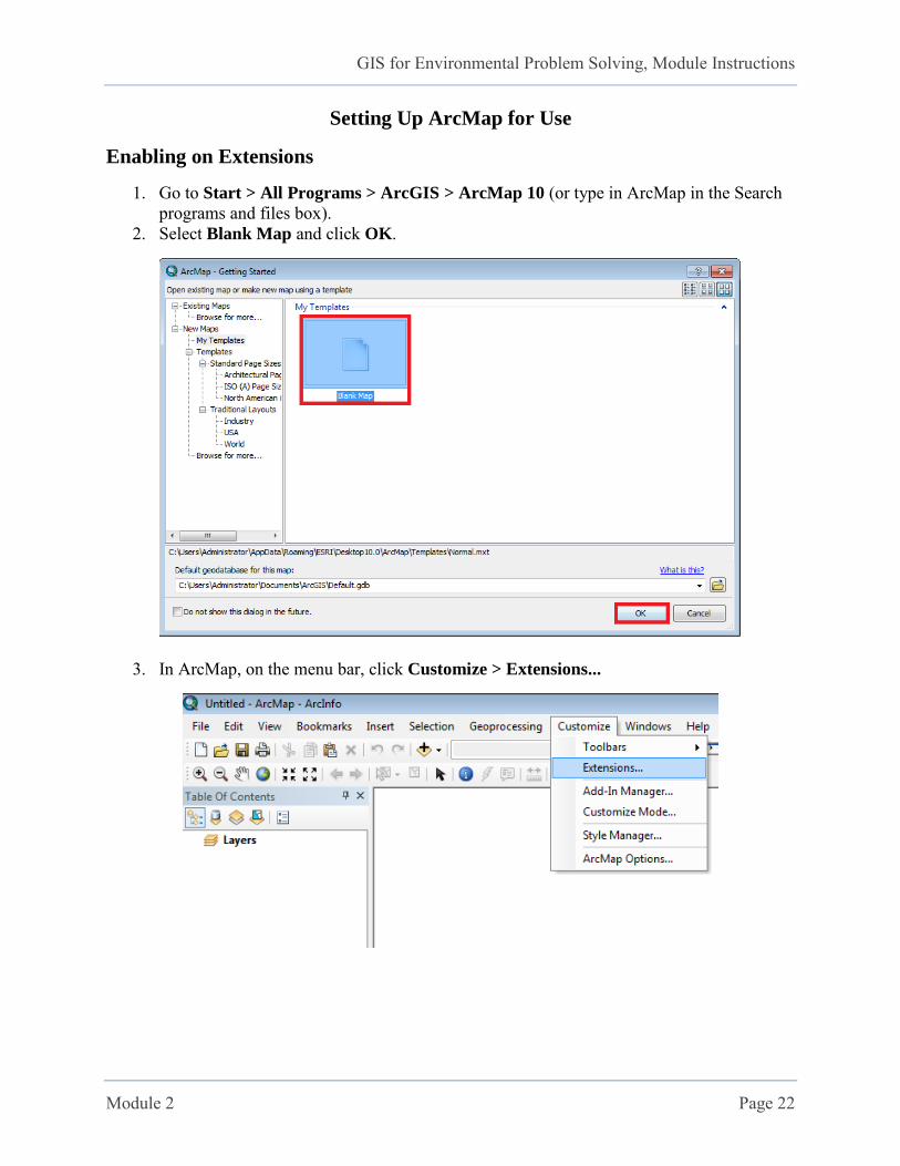
1. Go to Start > All Programs > ArcGIS > ArcMap 10 (or type in ArcMap in the Search programs and files box).
2. Select Blank Map and click OK.
3. In ArcMap, on the menu bar, click Customize > Extensions...
GIS for Environmental Problem Solving, Module Instructions
Module 2 Page 23
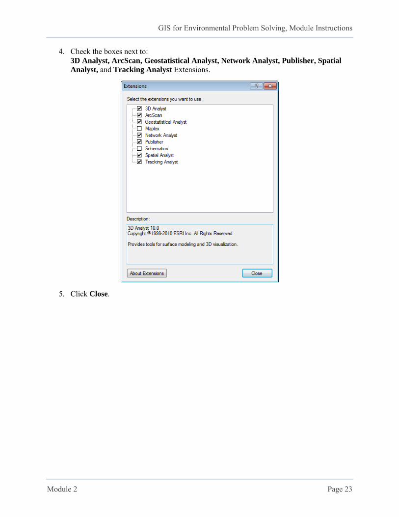
4. Check the boxes next to: 3D Analyst, ArcScan, Geostatistical Analyst, Network Analyst, Publisher, Spatial
Analyst, and Tracking Analyst Extensions.
5. Click Close.

GIS for Environmental Problem Solving, Module Instructions
Module 2 Page 24
Turning on Extensions
1. In ArcMap, right-click the gray area anywhere on the menu bar.
2. In the menu that pops up select: Editor, Geocoding, Geostatistical Analyst, Spatial Analyst, Standard, and Tools.
3. The new windows that pop up can be dragged onto the toolbar or turned on as needed. You may double-click the title bar of each pop-up window to automatically place the windows on the menu bar.
GIS for Environmental Problem Solving, Module Instructions
Module 2 Page 25
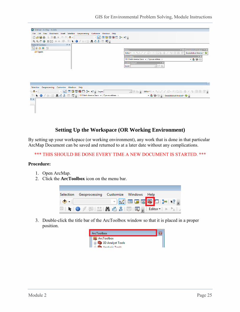
Setting Up the Workspace (OR Working Environment)
By setting up your workspace (or working environment), any work that is done in that particular ArcMap Document can be saved and returned to at a later date without any complications.
*** THIS SHOULD BE DONE EVERY TIME A NEW DOCUMENT IS STARTED. ***
Procedure:
1. Open ArcMap. 2. Click the ArcToolbox icon on the menu bar.
3. Double-click the title bar of the ArcToolbox window so that it is placed in a proper position.
GIS for Environmental Problem Solving, Module Instructions
Module 2 Page 26
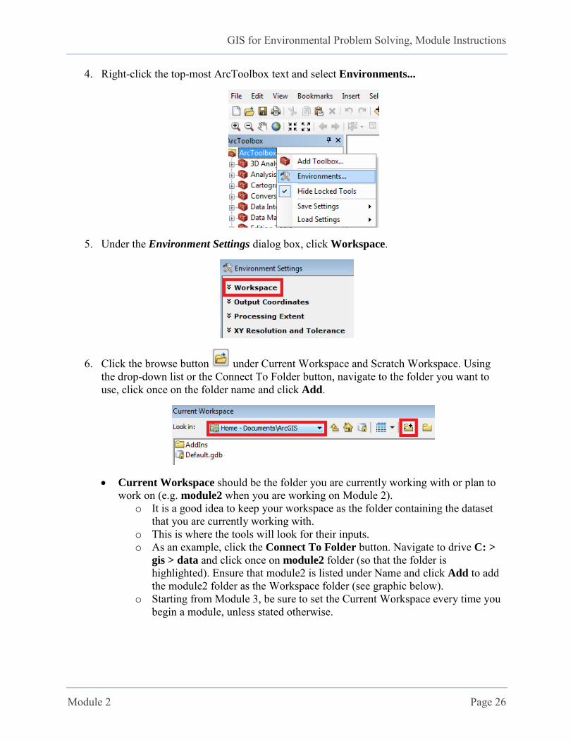
4. Right-click the top-most ArcToolbox text and select Environments...
5. Under the Environment Settings dialog box, click Workspace.
6. Click the browse button under Current Workspace and Scratch Workspace. Using the drop-down list or the Connect To Folder button, navigate to the folder you want to use, click once on the folder name and click Add.
Current Workspace should be the folder you are currently working with or plan to work on (e.g. module2 when you are working on Module 2).
o It is a good idea to keep your workspace as the folder containing the dataset that you are currently working with.
o This is where the tools will look for their inputs. o As an example, click the Connect To Folder button. Navigate to drive C: >
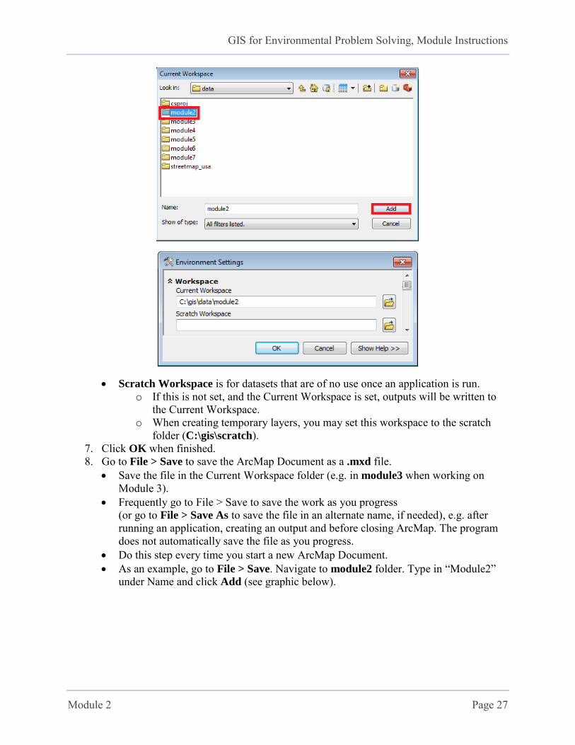
gis > data and click once on module2 folder (so that the folder is highlighted). Ensure that module2 is listed under Name and click Add to add the module2 folder as the Workspace folder (see graphic below).
o Starting from Module 3, be sure to set the Current Workspace every time you begin a module, unless stated otherwise.
GIS for Environmental Problem Solving, Module Instructions
Module 2 Page 27
Scratch Workspace is for datasets that are of no use once an application is run. o If this is not set, and the Current Workspace is set, outputs will be written to
the Current Workspace. o When creating temporary layers, you may set this workspace to the scratch
folder (C:\gis\scratch). 7. Click OK when finished. 8. Go to File > Save to save the ArcMap Document as a .mxd file.
Save the file in the Current Workspace folder (e.g. in module3 when working on Module 3).
Frequently go to File > Save to save the work as you progress (or go to File > Save As to save the file in an alternate name, if needed), e.g. after running an application, creating an output and before closing ArcMap. The program does not automatically save the file as you progress.
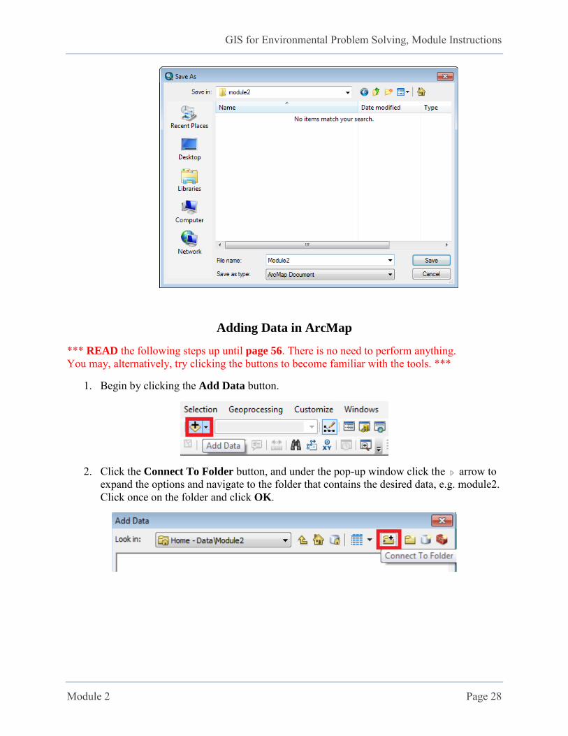
Do this step every time you start a new ArcMap Document. As an example, go to File > Save. Navigate to module2 folder. Type in “Module2”
under Name and click Add (see graphic below).
GIS for Environmental Problem Solving, Module Instructions
Module 2 Page 28
Adding Data in ArcMap
*** READ the following steps up until page 56. There is no need to perform anything. You may, alternatively, try clicking the buttons to become familiar with the tools. ***
1. Begin by clicking the Add Data button.
2. Click the Connect To Folder button, and under the pop-up window click the arrow to expand the options and navigate to the folder that contains the desired data, e.g. module2. Click once on the folder and click OK.
GIS for Environmental Problem Solving, Module Instructions
Module 2 Page 29
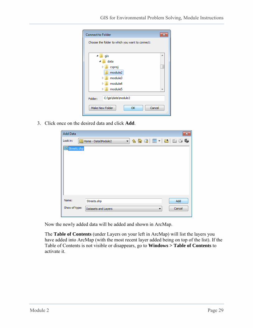
3. Click once on the desired data and click Add.
Now the newly added data will be added and shown in ArcMap.
The Table of Contents (under Layers on your left in ArcMap) will list the layers you have added into ArcMap (with the most recent layer added being on top of the list). If the Table of Contents is not visible or disappears, go to Windows > Table of Contents to activate it.
GIS for Environmental Problem Solving, Module Instructions
Module 2 Page 30
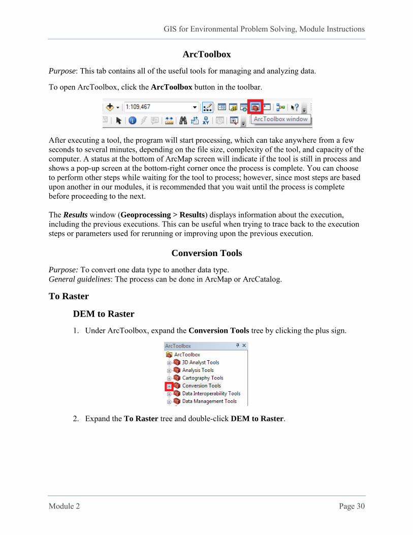
ArcToolbox
Purpose: This tab contains all of the useful tools for managing and analyzing data.
To open ArcToolbox, click the ArcToolbox button in the toolbar.
After executing a tool, the program will start processing, which can take anywhere from a few seconds to several minutes, depending on the file size, complexity of the tool, and capacity of the computer. A status at the bottom of ArcMap screen will indicate if the tool is still in process and shows a pop-up screen at the bottom-right corner once the process is complete. You can choose to perform other steps while waiting for the tool to process; however, since most steps are based upon another in our modules, it is recommended that you wait until the process is complete before proceeding to the next. The Results window (Geoprocessing > Results) displays information about the execution, including the previous executions. This can be useful when trying to trace back to the execution steps or parameters used for rerunning or improving upon the previous execution.
Conversion Tools
Purpose: To convert one data type to another data type. General guidelines: The process can be done in ArcMap or ArcCatalog.
To Raster
DEM to Raster
1. Under ArcToolbox, expand the Conversion Tools tree by clicking the plus sign.
2. Expand the To Raster tree and double-click DEM to Raster.

GIS for Environmental Problem Solving, Module Instructions
Module 2 Page 31
3. For the Input USGS DEM file parameter, select the desired DEM file by clicking the browse button. The Output raster will be automatically assigned (or can be modified accordingly).
4. Click OK.
Feature to Raster
A feature will be converted to a raster based off of a designated value. Most commonly, the value used will be one that is created by the user. This value, for most practical purposes, will be 1.
Phase I: Setting up the Feature
1. Open ArcMap. 2. Add the desired feature to the map using the Add Data button.
GIS for Environmental Problem Solving, Module Instructions
Module 2 Page 32
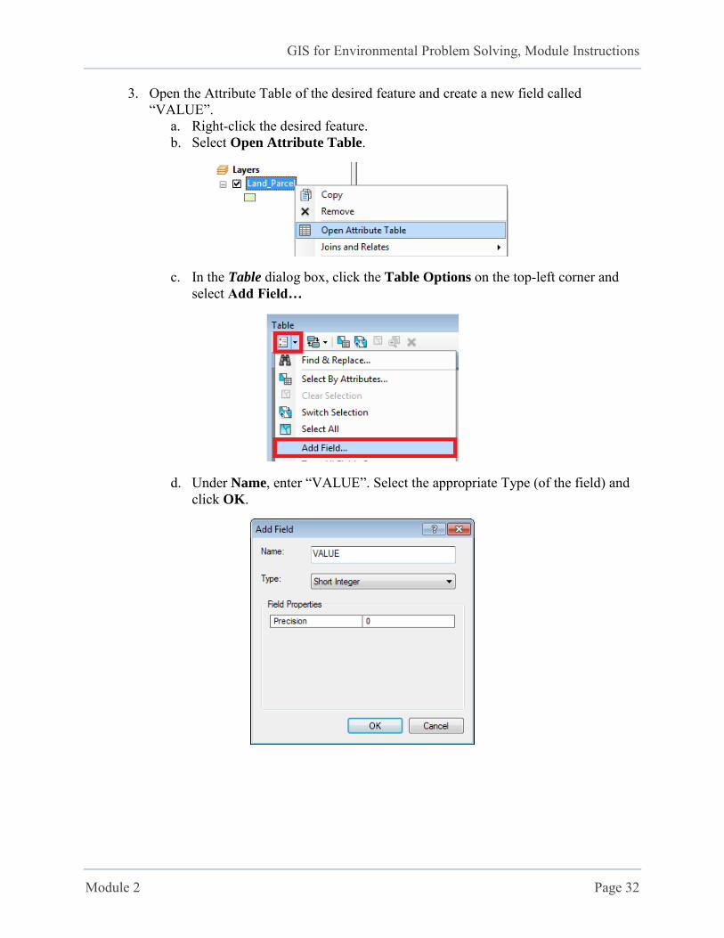
3. Open the Attribute Table of the desired feature and create a new field called “VALUE”.
a. Right-click the desired feature. b. Select Open Attribute Table.
c. In the Table dialog box, click the Table Options on the top-left corner and select Add Field…
d. Under Name, enter “VALUE”. Select the appropriate Type (of the field) and click OK.
GIS for Environmental Problem Solving, Module Instructions
Module 2 Page 33
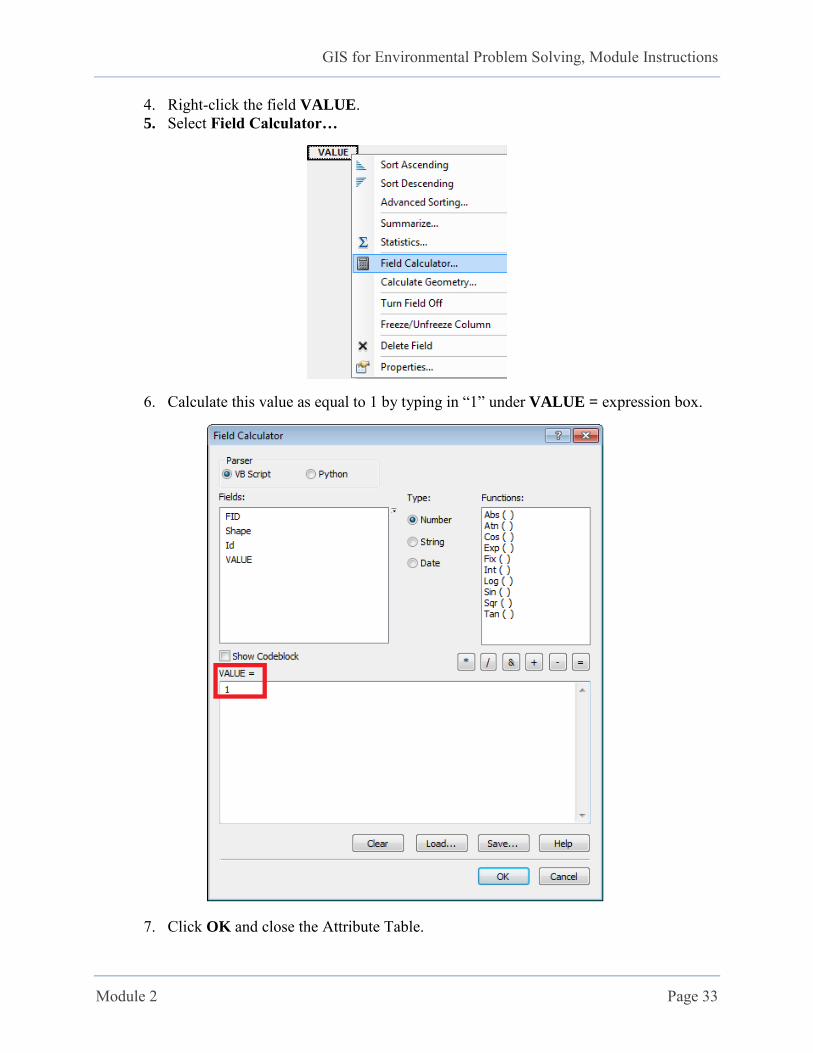
4. Right-click the field VALUE. 5. Select Field Calculator…
6. Calculate this value as equal to 1 by typing in “1” under VALUE = expression box.
7. Click OK and close the Attribute Table.
GIS for Environmental Problem Solving, Module Instructions
Module 2 Page 34
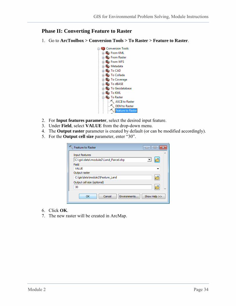
Phase II: Converting Feature to Raster
1. Go to ArcToolbox > Conversion Tools > To Raster > Feature to Raster.
2. For Input features parameter, select the desired input feature. 3. Under Field, select VALUE from the drop-down menu. 4. The Output raster parameter is created by default (or can be modified accordingly). 5. For the Output cell size parameter, enter “30”.
6. Click OK. 7. The new raster will be created in ArcMap.
GIS for Environmental Problem Solving, Module Instructions
Module 2 Page 35
Data Management Tools
Projections and Transformations
Feature
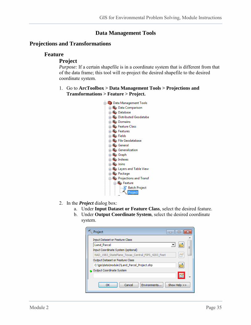
Project Purpose: If a certain shapefile is in a coordinate system that is different from that of the data frame; this tool will re-project the desired shapefile to the desired coordinate system.
1. Go to ArcToolbox > Data Management Tools > Projections and
Transformations > Feature > Project.
2. In the Project dialog box: a. Under Input Dataset or Feature Class, select the desired feature. b. Under Output Coordinate System, select the desired coordinate
system.
GIS for Environmental Problem Solving, Module Instructions
Module 2 Page 36
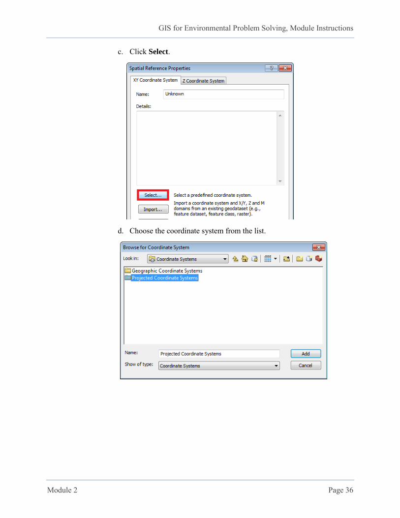
c. Click Select.
d. Choose the coordinate system from the list.
GIS for Environmental Problem Solving, Module Instructions
Module 2 Page 37
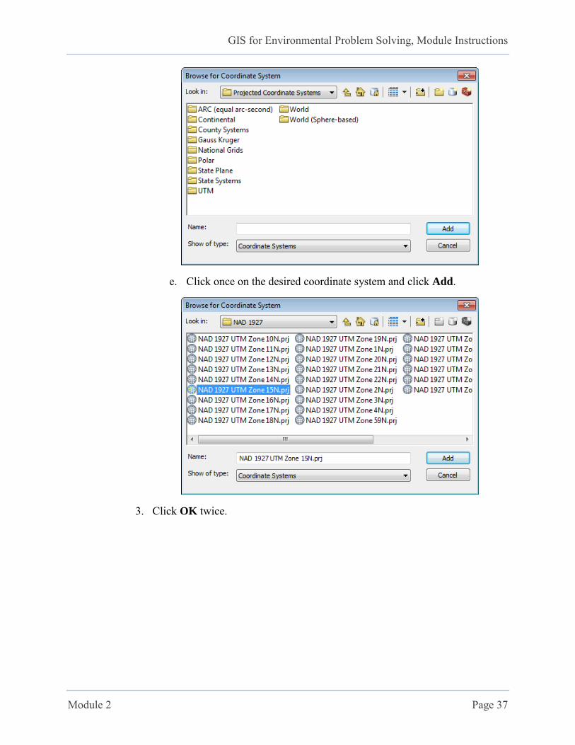
e. Click once on the desired coordinate system and click Add.
3. Click OK twice.
GIS for Environmental Problem Solving, Module Instructions
Module 2 Page 38
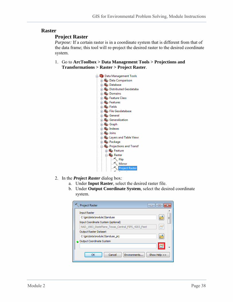
Raster
Project Raster Purpose: If a certain raster is in a coordinate system that is different from that of the data frame; this tool will re-project the desired raster to the desired coordinate system.
1. Go to ArcToolbox > Data Management Tools > Projections and
Transformations > Raster > Project Raster.
2. In the Project Raster dialog box: a. Under Input Raster, select the desired raster file. b. Under Output Coordinate System, select the desired coordinate
system.

GIS for Environmental Problem Solving, Module Instructions
Module 2 Page 39
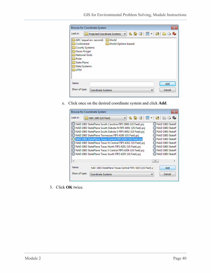
c. Click Select.
d. Choose the coordinate system from the list.
GIS for Environmental Problem Solving, Module Instructions
Module 2 Page 40
e. Click once on the desired coordinate system and click Add.
3. Click OK twice.
GIS for Environmental Problem Solving, Module Instructions
Module 2 Page 41
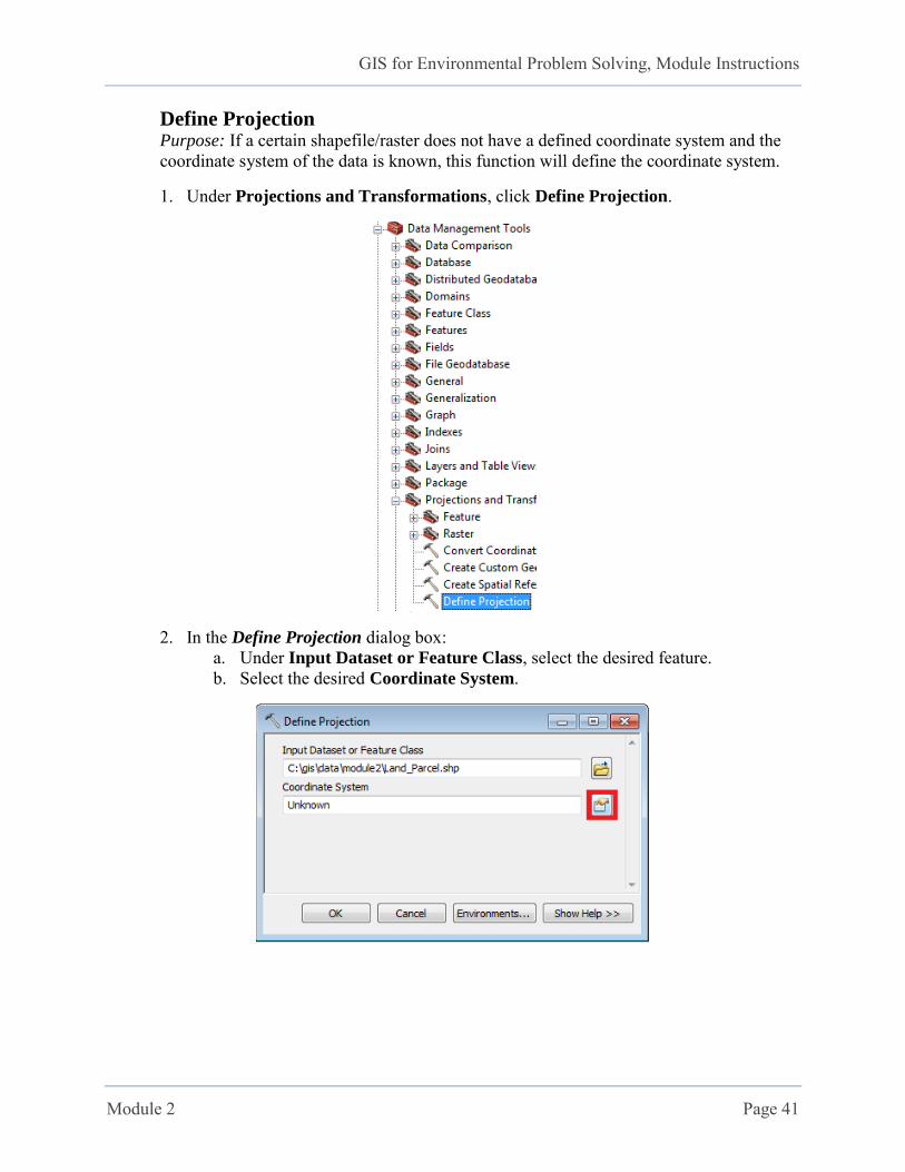
Define Projection Purpose: If a certain shapefile/raster does not have a defined coordinate system and the coordinate system of the data is known, this function will define the coordinate system.
1. Under Projections and Transformations, click Define Projection.
2. In the Define Projection dialog box: a. Under Input Dataset or Feature Class, select the desired feature. b. Select the desired Coordinate System.
GIS for Environmental Problem Solving, Module Instructions
Module 2 Page 42
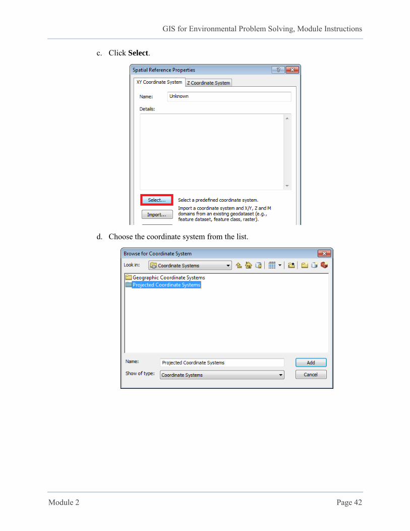
c. Click Select.
d. Choose the coordinate system from the list.
GIS for Environmental Problem Solving, Module Instructions
Module 2 Page 43
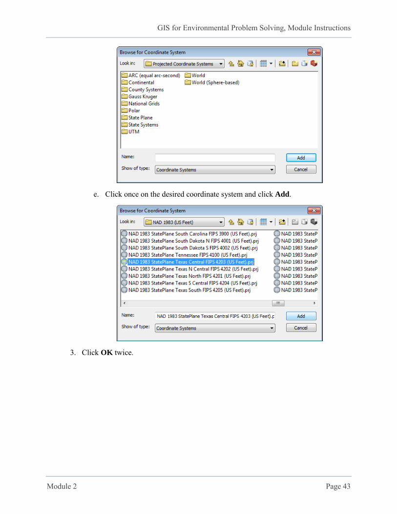
e. Click once on the desired coordinate system and click Add.
3. Click OK twice.
GIS for Environmental Problem Solving, Module Instructions
Module 2 Page 44
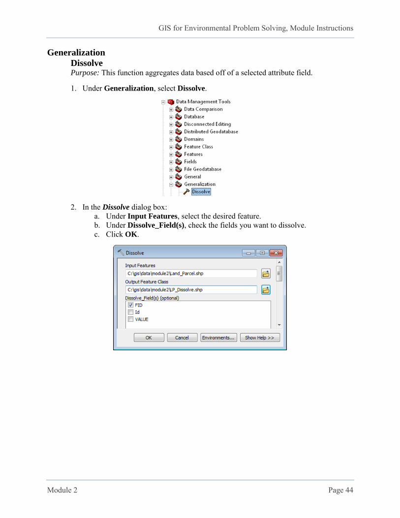
Generalization
Dissolve Purpose: This function aggregates data based off of a selected attribute field.
1. Under Generalization, select Dissolve.
2. In the Dissolve dialog box: a. Under Input Features, select the desired feature. b. Under Dissolve_Field(s), check the fields you want to dissolve. c. Click OK.
GIS for Environmental Problem Solving, Module Instructions
Module 2 Page 45
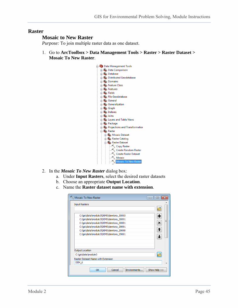
Raster
Mosaic to New Raster Purpose: To join multiple raster data as one dataset.
1. Go to ArcToolbox > Data Management Tools > Raster > Raster Dataset >
Mosaic To New Raster.
2. In the Mosaic To New Raster dialog box: a. Under Input Rasters, select the desired raster datasets b. Choose an appropriate Output Location. c. Name the Raster dataset name with extension.
GIS for Environmental Problem Solving, Module Instructions
Module 2 Page 46
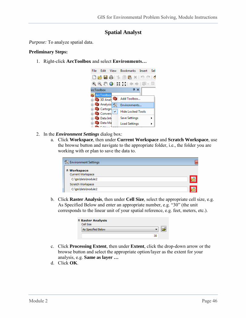
Spatial Analyst
Purpose: To analyze spatial data.
Preliminary Steps:
1. Right-click ArcToolbox and select Environments…
2. In the Environment Settings dialog box: a. Click Workspace, then under Current Workspace and Scratch Workspace, use
the browse button and navigate to the appropriate folder, i.e., the folder you are working with or plan to save the data to.
b. Click Raster Analysis, then under Cell Size, select the appropriate cell size, e.g. As Specified Below and enter an appropriate number, e.g. “30” (the unit corresponds to the linear unit of your spatial reference, e.g. feet, meters, etc.).
c. Click Processing Extent, then under Extent, click the drop-down arrow or the browse button and select the appropriate option/layer as the extent for your analysis, e.g. Same as layer …
d. Click OK.
GIS for Environmental Problem Solving, Module Instructions
Module 2 Page 47
Raster Calculator
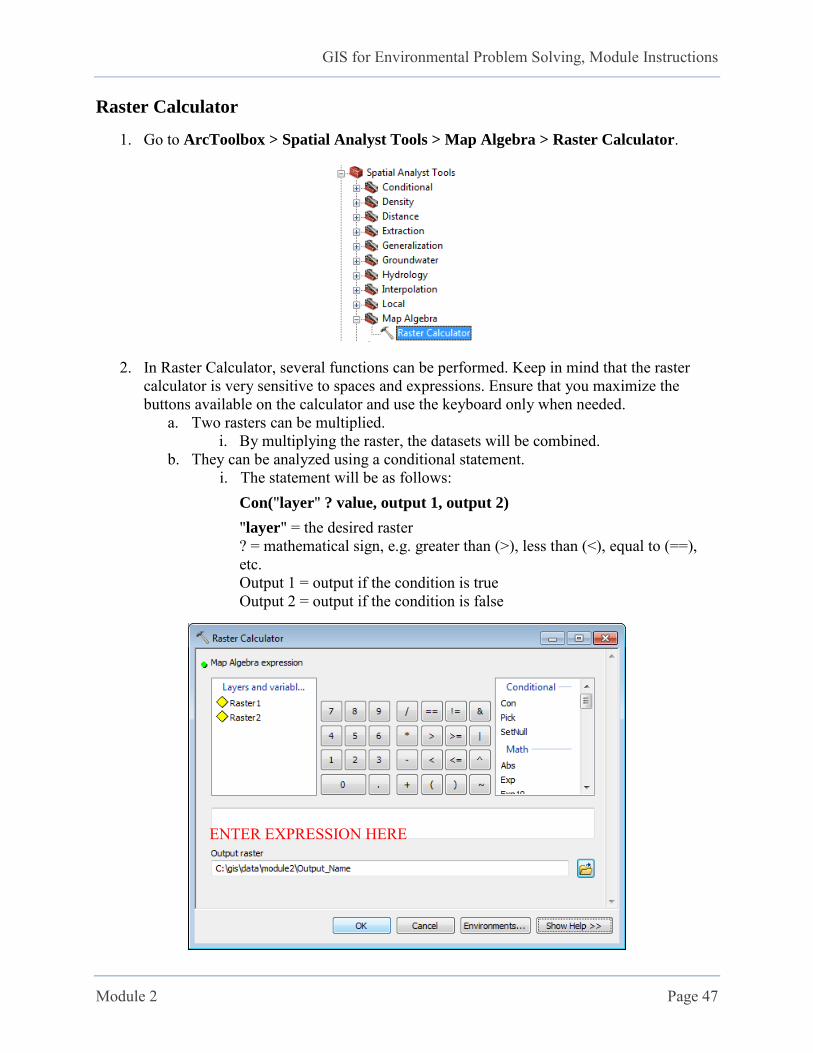
1. Go to ArcToolbox > Spatial Analyst Tools > Map Algebra > Raster Calculator.
2. In Raster Calculator, several functions can be performed. Keep in mind that the raster calculator is very sensitive to spaces and expressions. Ensure that you maximize the buttons available on the calculator and use the keyboard only when needed.
a. Two rasters can be multiplied. i. By multiplying the raster, the datasets will be combined.
b. They can be analyzed using a conditional statement. i. The statement will be as follows:
Con("layer" ? value, output 1, output 2)
"layer" = the desired raster ? = mathematical sign, e.g. greater than (>), less than (<), equal to (==), etc. Output 1 = output if the condition is true Output 2 = output if the condition is false
ENTER EXPRESSION HERE
GIS for Environmental Problem Solving, Module Instructions
Module 2 Page 48
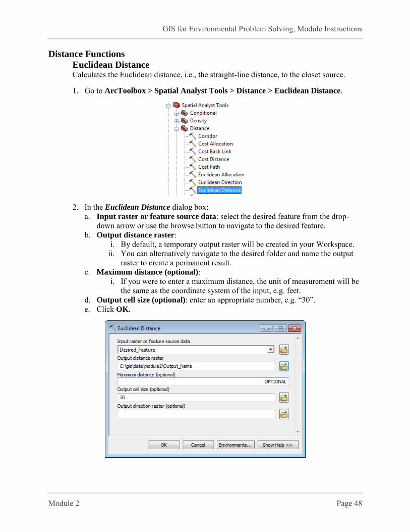
Distance Functions
Euclidean Distance Calculates the Euclidean distance, i.e., the straight-line distance, to the closet source.
1. Go to ArcToolbox > Spatial Analyst Tools > Distance > Euclidean Distance.
2. In the Euclidean Distance dialog box: a. Input raster or feature source data: select the desired feature from the drop-
down arrow or use the browse button to navigate to the desired feature. b. Output distance raster:
i. By default, a temporary output raster will be created in your Workspace. ii. You can alternatively navigate to the desired folder and name the output
raster to create a permanent result. c. Maximum distance (optional):
i. If you were to enter a maximum distance, the unit of measurement will be the same as the coordinate system of the input, e.g. feet.
d. Output cell size (optional): enter an appropriate number, e.g. “30”. e. Click OK.
GIS for Environmental Problem Solving, Module Instructions
Module 2 Page 49
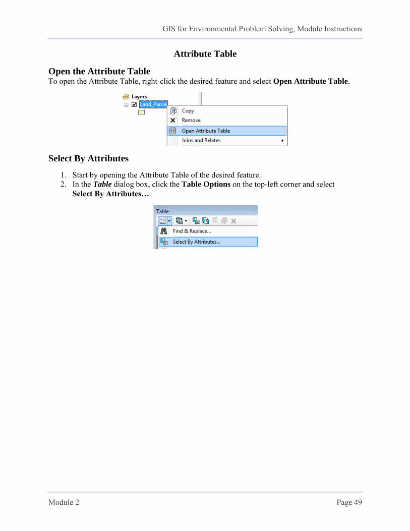
Attribute Table
Open the Attribute Table To open the Attribute Table, right-click the desired feature and select Open Attribute Table.
Select By Attributes
1. Start by opening the Attribute Table of the desired feature. 2. In the Table dialog box, click the Table Options on the top-left corner and select
Select By Attributes…
GIS for Environmental Problem Solving, Module Instructions
Module 2 Page 50
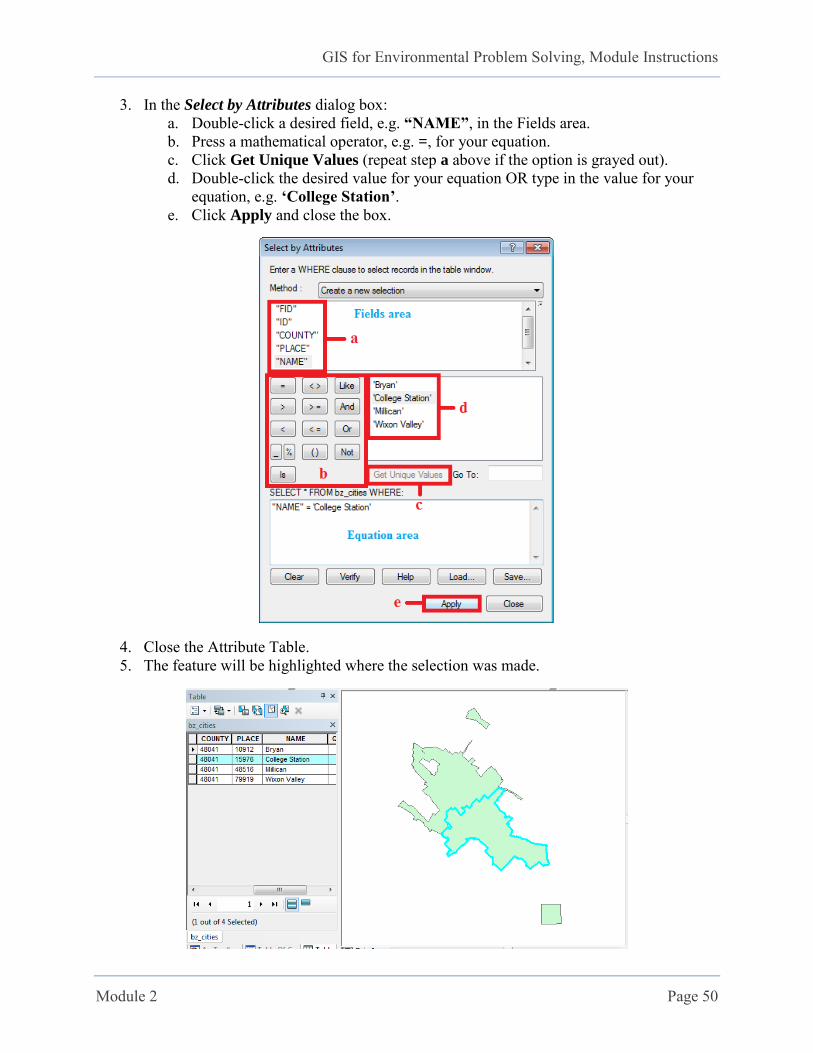
3. In the Select by Attributes dialog box: a. Double-click a desired field, e.g. “NAME”, in the Fields area. b. Press a mathematical operator, e.g. =, for your equation. c. Click Get Unique Values (repeat step a above if the option is grayed out). d. Double-click the desired value for your equation OR type in the value for your
equation, e.g. ‘College Station’. e. Click Apply and close the box.
4. Close the Attribute Table. 5. The feature will be highlighted where the selection was made.
GIS for Environmental Problem Solving, Module Instructions
Module 2 Page 51
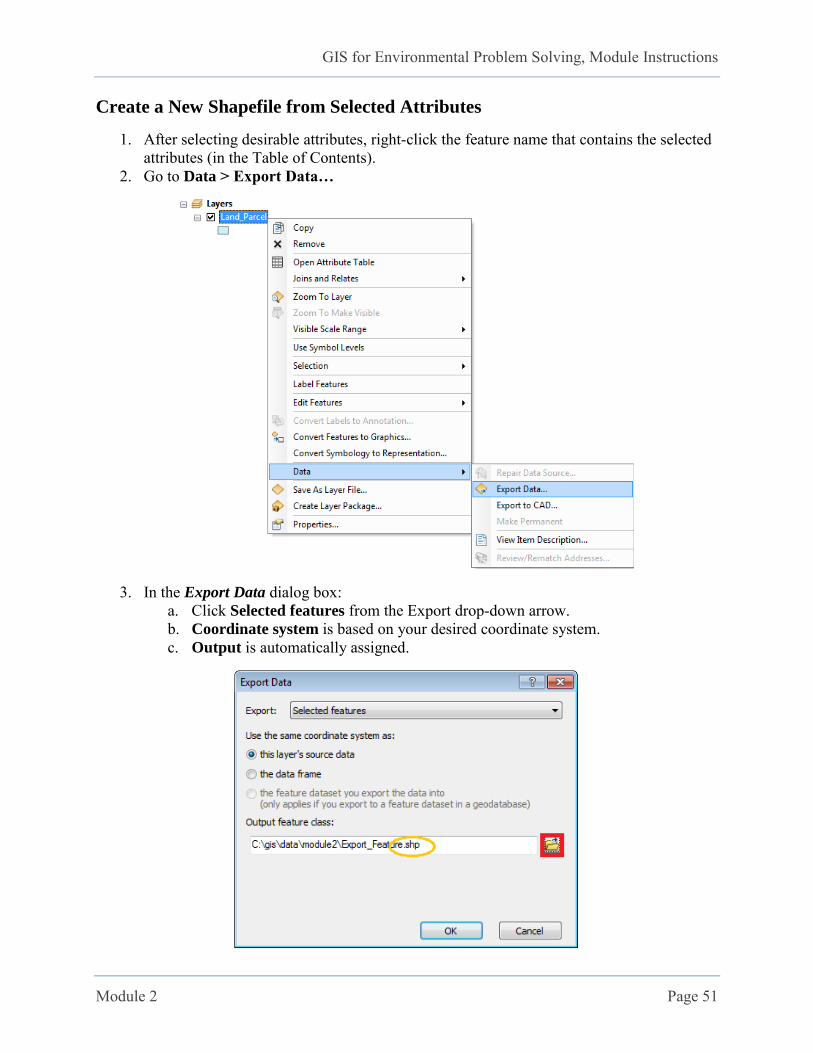
Create a New Shapefile from Selected Attributes
1. After selecting desirable attributes, right-click the feature name that contains the selected attributes (in the Table of Contents).
2. Go to Data > Export Data…
3. In the Export Data dialog box: a. Click Selected features from the Export drop-down arrow. b. Coordinate system is based on your desired coordinate system. c. Output is automatically assigned.
GIS for Environmental Problem Solving, Module Instructions
Module 2 Page 52
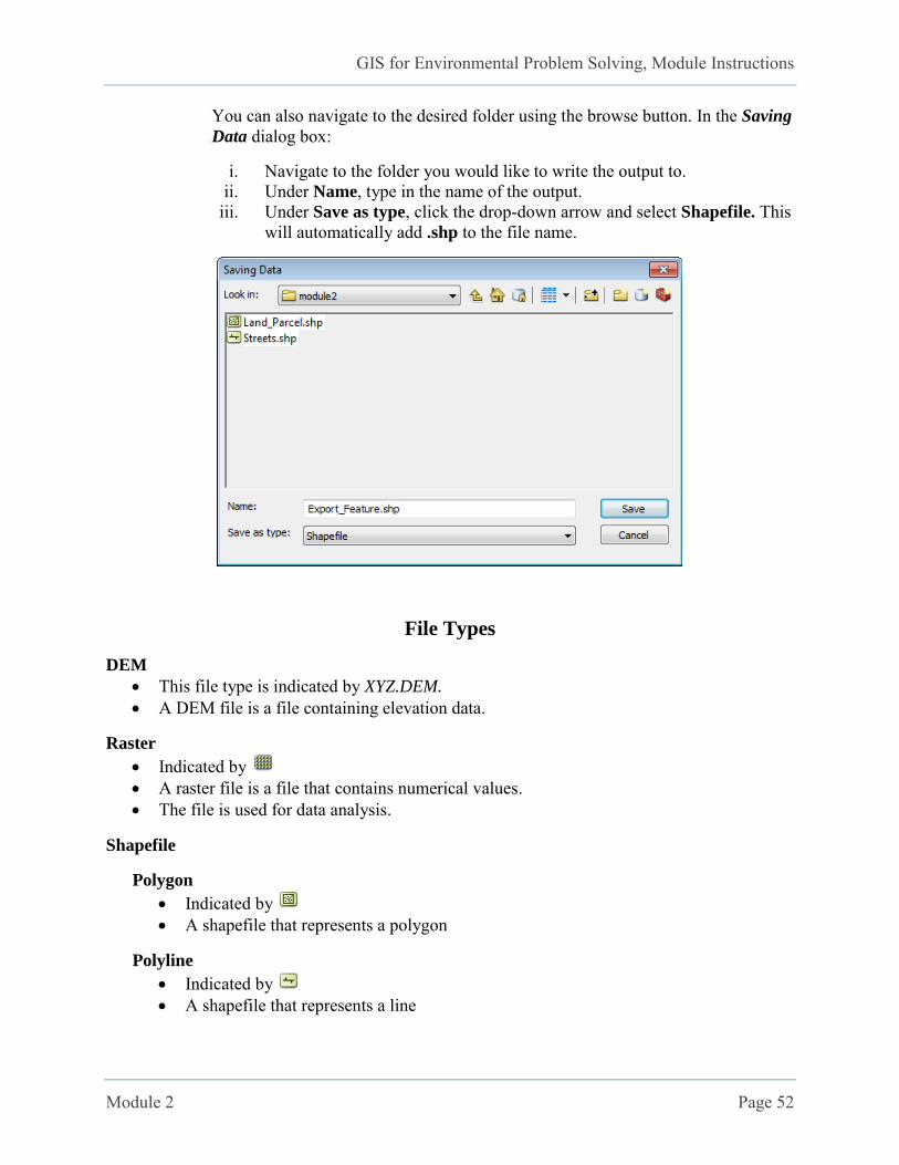
You can also navigate to the desired folder using the browse button. In the Saving
Data dialog box:
i. Navigate to the folder you would like to write the output to. ii. Under Name, type in the name of the output.
iii. Under Save as type, click the drop-down arrow and select Shapefile. This will automatically add .shp to the file name.
File Types
DEM
This file type is indicated by XYZ.DEM.
A DEM file is a file containing elevation data.
Raster
Indicated by A raster file is a file that contains numerical values. The file is used for data analysis.
Shapefile
Polygon
Indicated by A shapefile that represents a polygon
Polyline
Indicated by A shapefile that represents a line
GIS for Environmental Problem Solving, Module Instructions
Module 2 Page 53
Point
Indicated by A shapefile that represents a specific point
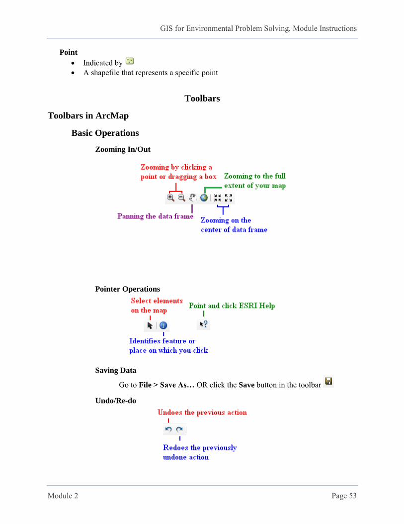
Toolbars
Toolbars in ArcMap
Basic Operations
Zooming In/Out
Pointer Operations
Saving Data
Go to File > Save As… OR click the Save button in the toolbar
Undo/Re-do
GIS for Environmental Problem Solving, Module Instructions
Module 2 Page 54
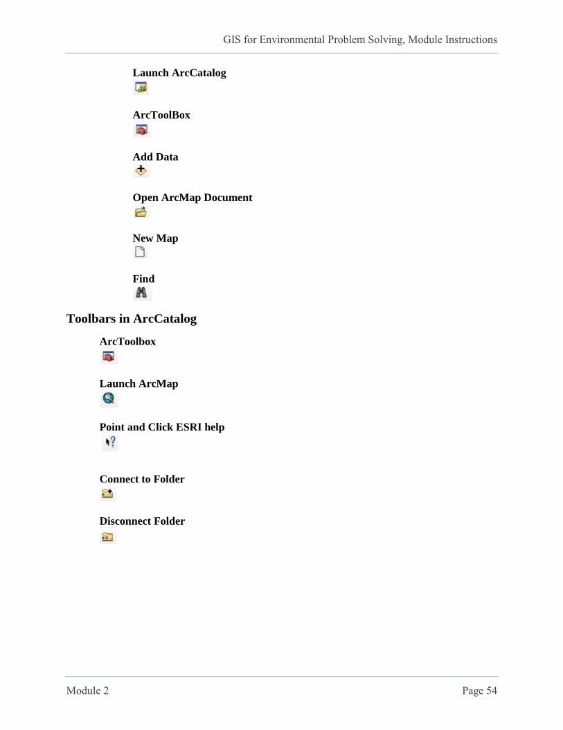
Launch ArcCatalog
ArcToolBox
Add Data
Open ArcMap Document
New Map
Find
Toolbars in ArcCatalog
ArcToolbox
Launch ArcMap
Point and Click ESRI help
Connect to Folder
Disconnect Folder
GIS for Environmental Problem Solving, Module Instructions
Module 2 Page 55
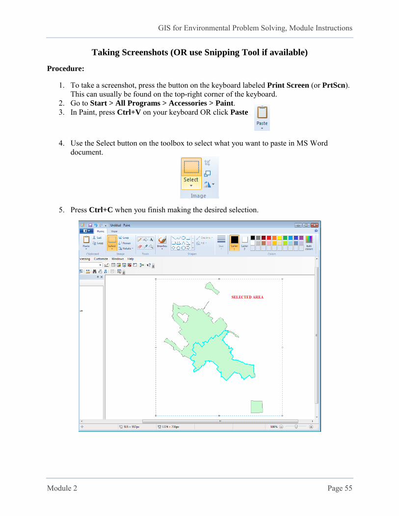
Taking Screenshots (OR use Snipping Tool if available)
Procedure:
1. To take a screenshot, press the button on the keyboard labeled Print Screen (or PrtScn). This can usually be found on the top-right corner of the keyboard.
2. Go to Start > All Programs > Accessories > Paint. 3. In Paint, press Ctrl+V on your keyboard OR click Paste
4. Use the Select button on the toolbox to select what you want to paste in MS Word document.
5. Press Ctrl+C when you finish making the desired selection.
GIS for Environmental Problem Solving, Module Instructions
Module 2 Page 56
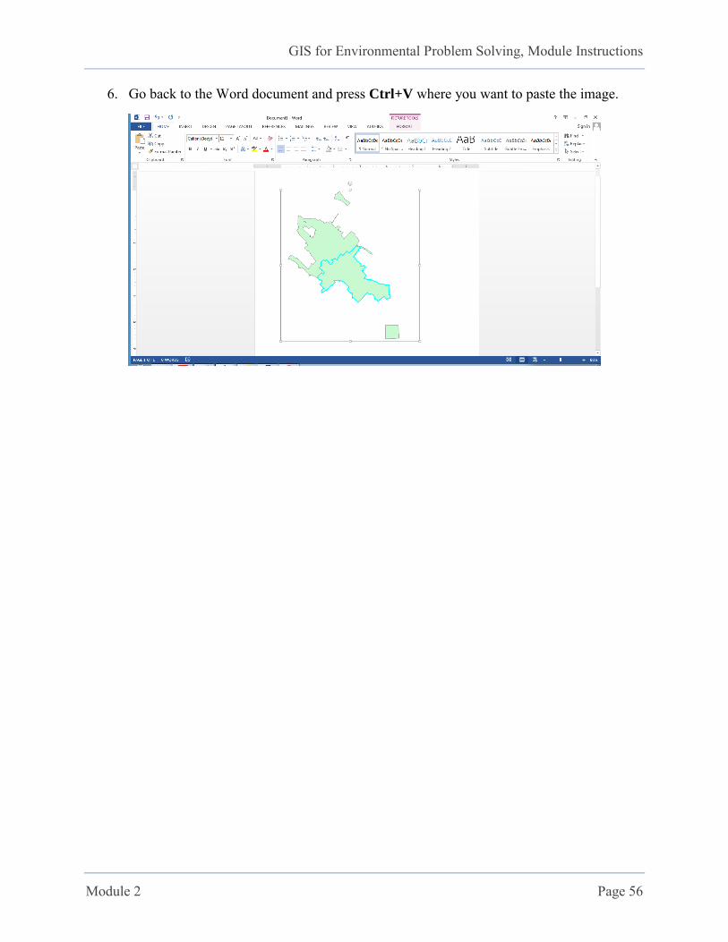
6. Go back to the Word document and press Ctrl+V where you want to paste the image.
GIS for Environmental Problem Solving, Module Instructions
Module 2 Page 57
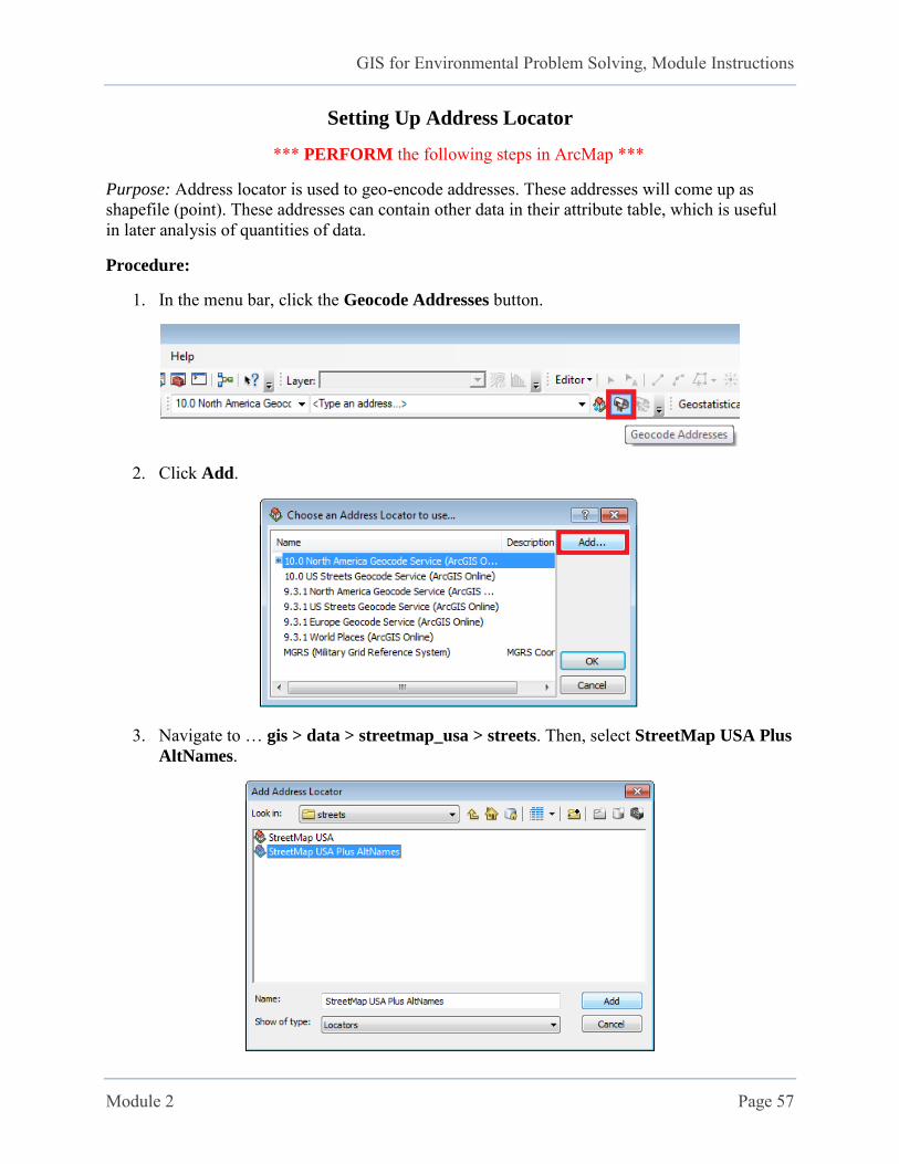
Setting Up Address Locator
*** PERFORM the following steps in ArcMap ***
Purpose: Address locator is used to geo-encode addresses. These addresses will come up as shapefile (point). These addresses can contain other data in their attribute table, which is useful in later analysis of quantities of data.
Procedure:
1. In the menu bar, click the Geocode Addresses button.
2. Click Add.
3. Navigate to … gis > data > streetmap_usa > streets. Then, select StreetMap USA Plus
AltNames.

GIS for Environmental Problem Solving, Module Instructions
Module 2 Page 58
4. Click Add. 5. Repeat steps 2-4 to add the StreetMap USA. 6. Click OK. If the Geocode Addresses dialog box pops up, click Cancel for now.
GIS for Environmental Problem Solving, Module Instructions
Module 3 Page 59
Module 3: Maneuvering of Digital Elevation Model (DEM)
Learning Objectives:
Learn to analyze, interpret, and classify elevation data Raster to vector conversion of DEM generated areas of interest Acquisition, importing and processing of Census data Overlay of shapefiles: the integrated use of Census and flood data Spatial-attribute analysis for damage assessment
Learning Materials:
Before going through this module and working with ArcGIS, please review the following presentations:
Key Words Key Processes Identify Data Needs Coordinate Systems and Projections Part III
Demonstration:
You have been given the task of analyzing Hurricane Katrina’s damage. Your job is to
assess the damages, given that the water has risen up to 0 meter. This means that everything under 0 meter in elevation is under water.
The affected area will be delineated. The total number of affected people and the total affected area will also be found.
General Problem Solving Steps:
Step 1: Frame the problem
Analysis of the scenario indicates that a hurricane has occurred in the area of New Orleans, LA. Current field measurements indicate that the water is currently at an elevation of 0 meter. The conclusion of this information is that every location below 0 meter in elevation is affected, and any location that is above this level is unaffected by the flood water. This particular area of impact needs to be delineated. Step 2: Identify data needs
The best type of data for delineating the affected area is that of elevation data, technically referred to as Digital Elevation Model (DEM). This elevation data can be divided into the affected area and the non-affected area.
GIS for Environmental Problem Solving, Module Instructions
Module 3 Page 60
Step 3: Identify decision support tools
Possible support tools for this particular situation include: Up-to-date field data (e.g. water level) An outline providing the methodology of how the data will be processed (See
Developing a Conceptual Methodology presentation from Module 2)
Step 4: Locate and assemble data
The data for this problem is available for free on the internet. http://atlas.lsu.edu/search/ (DEM, Satellite Imagery, etc.)
Step 5: Process and analyze data
Part I: Acquisition, import, and process DEMs Part II: Fill the “sink holes” Part III: Create hillshades Part IV: Reclassify DEM Part V: Convert raster of flooded area into vector Part VI: Bring in the census data Part VII: Merge the census layers Part VIII: Data analysis – finding total affected area and population Step 6: Generate information and report
GIS for Environmental Problem Solving, Module Instructions
Module 3 Page 61
Procedure
Part I: Acquisition, Import, and Process DEMs
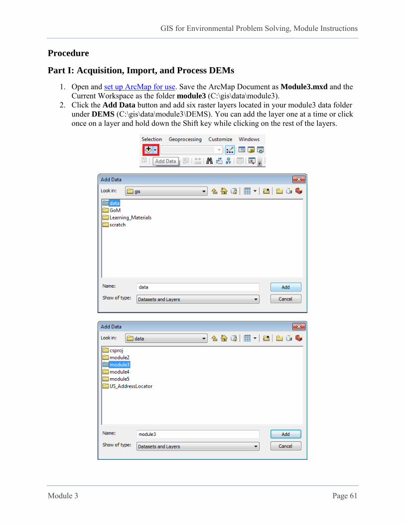
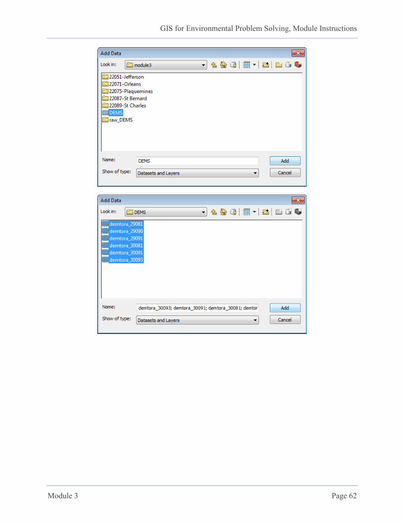
1. Open and set up ArcMap for use. Save the ArcMap Document as Module3.mxd and the Current Workspace as the folder module3 (C:\gis\data\module3).
2. Click the Add Data button and add six raster layers located in your module3 data folder under DEMS (C:\gis\data\module3\DEMS). You can add the layer one at a time or click once on a layer and hold down the Shift key while clicking on the rest of the layers.
GIS for Environmental Problem Solving, Module Instructions
Module 3 Page 62
GIS for Environmental Problem Solving, Module Instructions
Module 3 Page 63
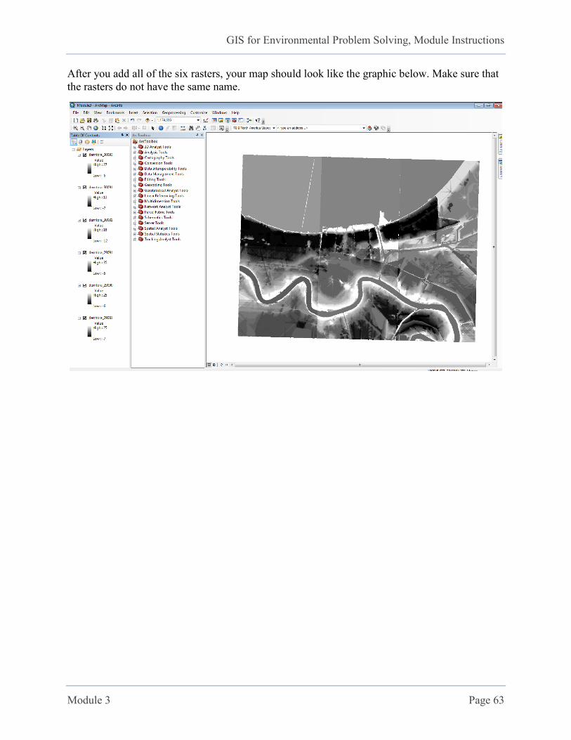
After you add all of the six rasters, your map should look like the graphic below. Make sure that the rasters do not have the same name.
GIS for Environmental Problem Solving, Module Instructions
Module 3 Page 64
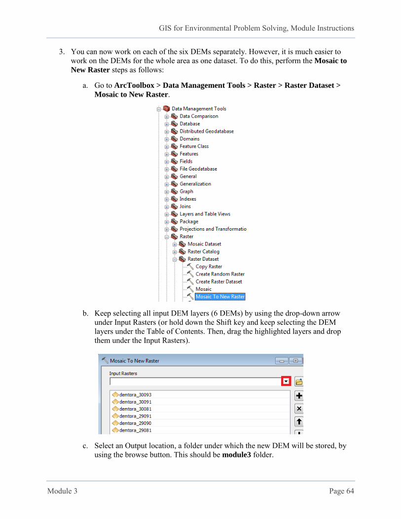
3. You can now work on each of the six DEMs separately. However, it is much easier to work on the DEMs for the whole area as one dataset. To do this, perform the Mosaic to
New Raster steps as follows:
a. Go to ArcToolbox > Data Management Tools > Raster > Raster Dataset >
Mosaic to New Raster.
b. Keep selecting all input DEM layers (6 DEMs) by using the drop-down arrow under Input Rasters (or hold down the Shift key and keep selecting the DEM layers under the Table of Contents. Then, drag the highlighted layers and drop them under the Input Rasters).
c. Select an Output location, a folder under which the new DEM will be stored, by using the browse button. This should be module3 folder.
GIS for Environmental Problem Solving, Module Instructions
Module 3 Page 65
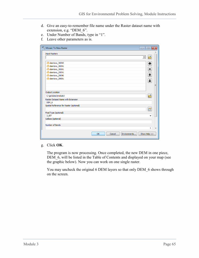
d. Give an easy-to-remember file name under the Raster dataset name with extension, e.g. “DEM_6”.
e. Under Number of Bands, type in “1”. f. Leave other parameters as is.
g. Click OK.
The program is now processing. Once completed, the new DEM in one piece, DEM_6, will be listed in the Table of Contents and displayed on your map (see the graphic below). Now you can work on one single raster.
You may uncheck the original 6 DEM layers so that only DEM_6 shows through on the screen.
GIS for Environmental Problem Solving, Module Instructions
Module 3 Page 66
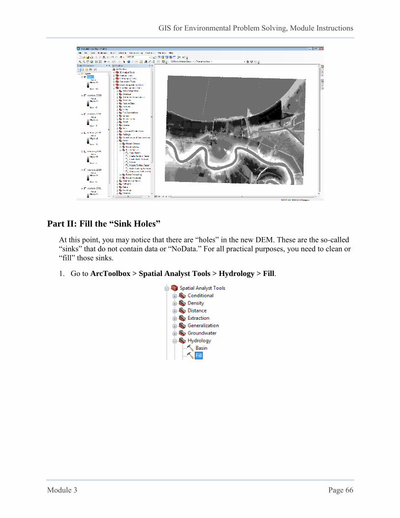
Part II: Fill the “Sink Holes”
At this point, you may notice that there are “holes” in the new DEM. These are the so-called “sinks” that do not contain data or “NoData.” For all practical purposes, you need to clean or “fill” those sinks.
1. Go to ArcToolbox > Spatial Analyst Tools > Hydrology > Fill.
GIS for Environmental Problem Solving, Module Instructions
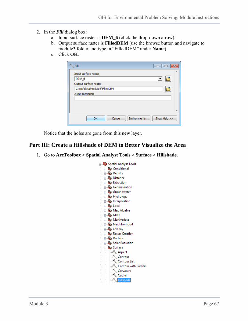
Module 3 Page 67
2. In the Fill dialog box: a. Input surface raster is DEM_6 (click the drop-down arrow). b. Output surface raster is FilledDEM (use the browse button and navigate to
module3 folder and type in “FilledDEM” under Name) c. Click OK.
Notice that the holes are gone from this new layer.
Part III: Create a Hillshade of DEM to Better Visualize the Area
1. Go to ArcToolbox > Spatial Analyst Tools > Surface > Hillshade.
GIS for Environmental Problem Solving, Module Instructions
Module 3 Page 68
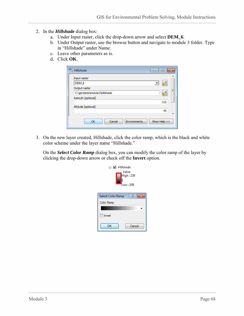
2. In the Hillshade dialog box: a. Under Input raster, click the drop-down arrow and select DEM_6. b. Under Output raster, use the browse button and navigate to module 3 folder. Type
in “Hillshade” under Name. c. Leave other parameters as is. d. Click OK.
3. On the new layer created, Hillshade, click the color ramp, which is the black and white color scheme under the layer name “Hillshade.”
On the Select Color Ramp dialog box, you can modify the color ramp of the layer by clicking the drop-down arrow or check off the Invert option.
GIS for Environmental Problem Solving, Module Instructions
Module 3 Page 69
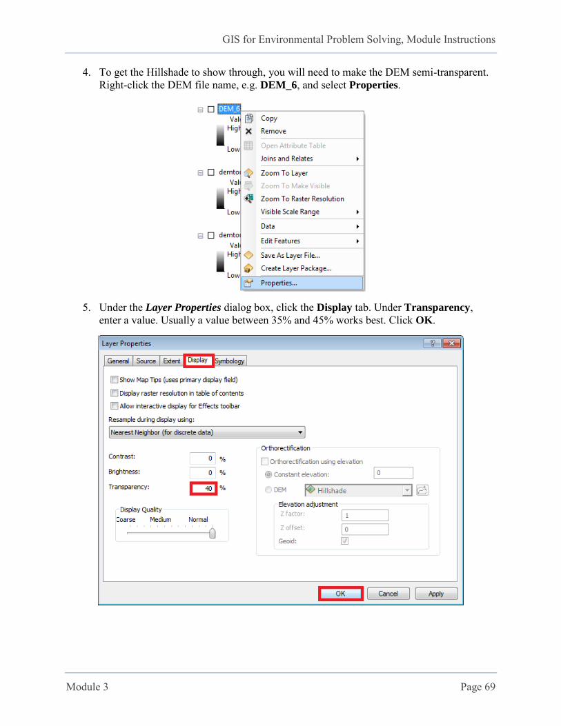
4. To get the Hillshade to show through, you will need to make the DEM semi-transparent. Right-click the DEM file name, e.g. DEM_6, and select Properties.
5. Under the Layer Properties dialog box, click the Display tab. Under Transparency, enter a value. Usually a value between 35% and 45% works best. Click OK.
GIS for Environmental Problem Solving, Module Instructions
Module 3 Page 70
Part IV: Reclassify DEM to Locate the Flooded Area
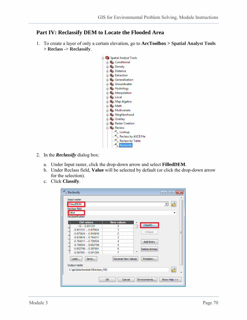
1. To create a layer of only a certain elevation, go to ArcToolbox > Spatial Analyst Tools
> Reclass -> Reclassify.
2. In the Reclassify dialog box:
a. Under Input raster, click the drop-down arrow and select FilledDEM. b. Under Reclass field, Value will be selected by default (or click the drop-down arrow
for the selection). c. Click Classify.
GIS for Environmental Problem Solving, Module Instructions
Module 3 Page 71
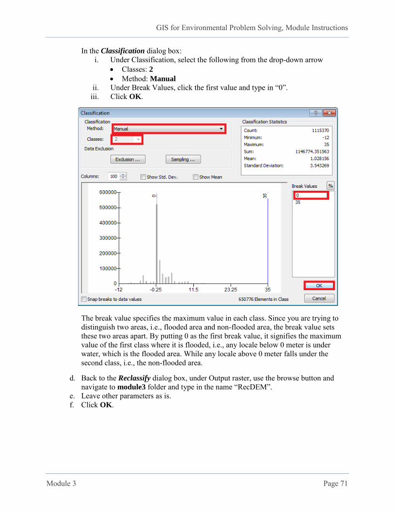
In the Classification dialog box: i. Under Classification, select the following from the drop-down arrow
Classes: 2 Method: Manual
ii. Under Break Values, click the first value and type in “0”. iii. Click OK.
The break value specifies the maximum value in each class. Since you are trying to distinguish two areas, i.e., flooded area and non-flooded area, the break value sets these two areas apart. By putting 0 as the first break value, it signifies the maximum value of the first class where it is flooded, i.e., any locale below 0 meter is under water, which is the flooded area. While any locale above 0 meter falls under the second class, i.e., the non-flooded area.
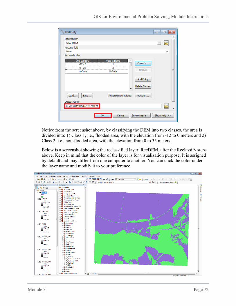
d. Back to the Reclassify dialog box, under Output raster, use the browse button and navigate to module3 folder and type in the name “RecDEM”.
e. Leave other parameters as is. f. Click OK.
GIS for Environmental Problem Solving, Module Instructions
Module 3 Page 72
Notice from the screenshot above, by classifying the DEM into two classes, the area is divided into: 1) Class 1, i.e., flooded area, with the elevation from -12 to 0 meters and 2) Class 2, i.e., non-flooded area, with the elevation from 0 to 35 meters.
Below is a screenshot showing the reclassified layer, RecDEM, after the Reclassify steps above. Keep in mind that the color of the layer is for visualization purpose. It is assigned by default and may differ from one computer to another. You can click the color under the layer name and modify it to your preference.
GIS for Environmental Problem Solving, Module Instructions
Module 3 Page 73
Part V: Convert the Raster of Flooded Area into Vector (Shapefile) for
Overlaying the Layer with Census Data
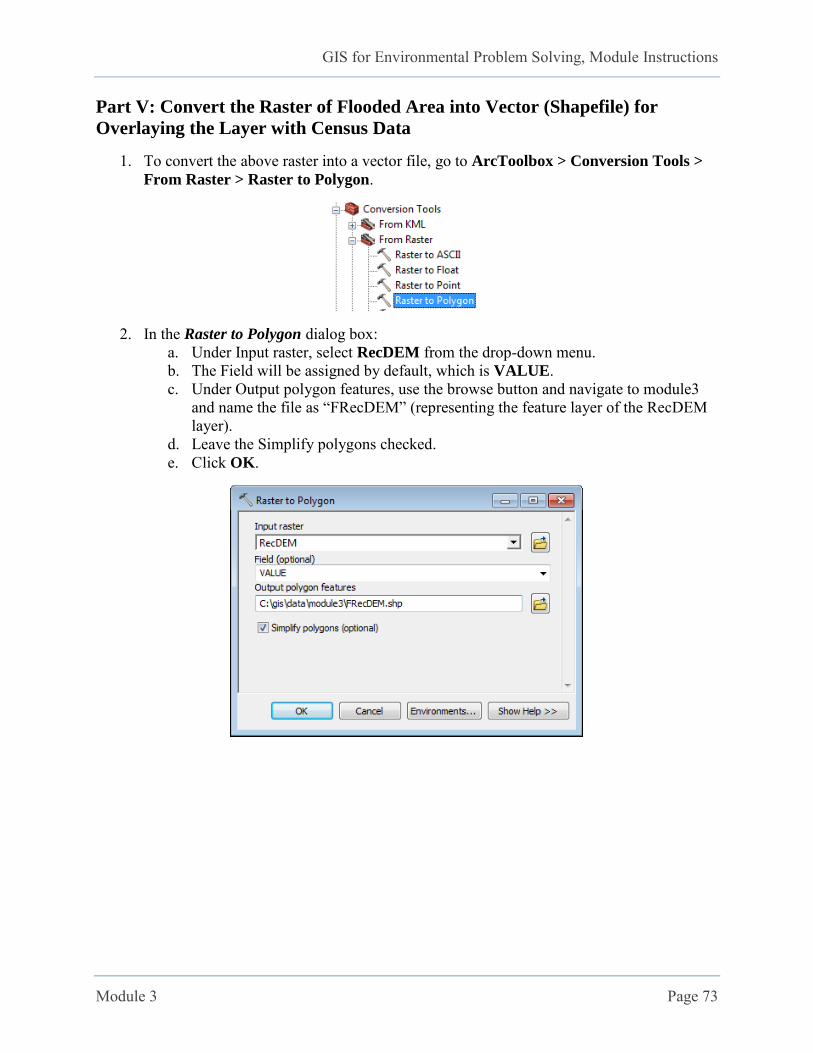
1. To convert the above raster into a vector file, go to ArcToolbox > Conversion Tools >
From Raster > Raster to Polygon.
2. In the Raster to Polygon dialog box: a. Under Input raster, select RecDEM from the drop-down menu. b. The Field will be assigned by default, which is VALUE. c. Under Output polygon features, use the browse button and navigate to module3
and name the file as “FRecDEM” (representing the feature layer of the RecDEM layer).
d. Leave the Simplify polygons checked. e. Click OK.

GIS for Environmental Problem Solving, Module Instructions
Module 3 Page 74
3. Now you will have the entire reclassified raster as a shapefile. To pull out only the certain elevation you want, click Selection on the main menu bar and choose Select By
Attributes…
4. In the Select By Attributes dialog box, a. Under Layer, make sure that the reclassified shapefile, frecdem, is selected. b. Type in “GRIDCODE” = 1 or perform the following
i. Double-click “GRIDCODE” ii. Click the equal sign =
iii. Click Get Unique Values iv. Double-click 1 v. Click OK.
The desired class, class 1, will be selected (highlighted in blue).
5. Right-click the frecdem layer and select Data > Export Data…
GIS for Environmental Problem Solving, Module Instructions
Module 3 Page 75
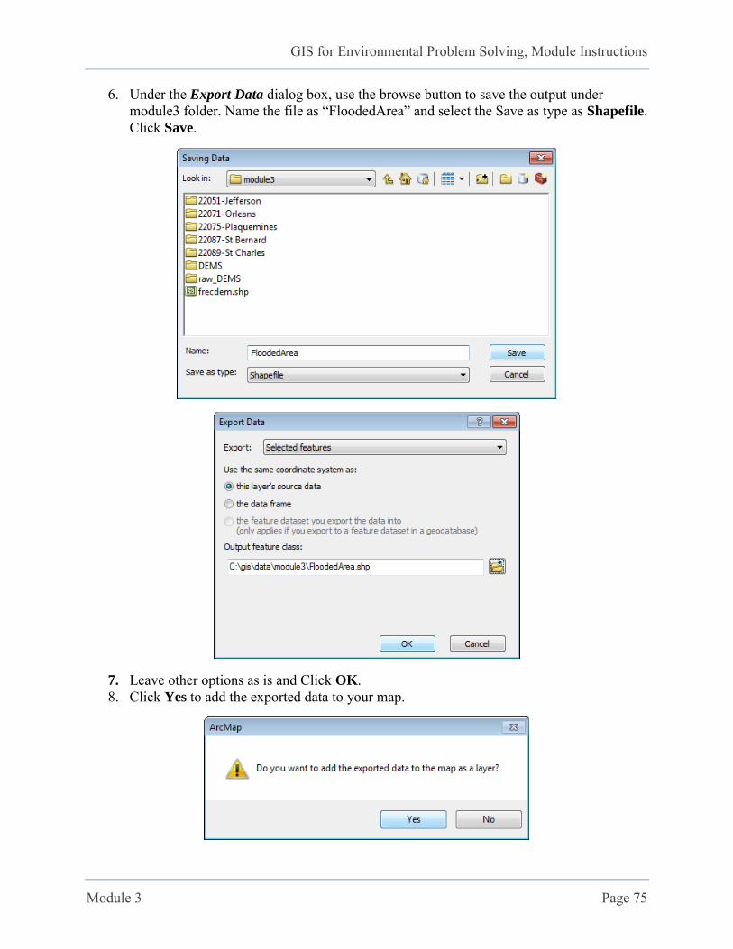
6. Under the Export Data dialog box, use the browse button to save the output under module3 folder. Name the file as “FloodedArea” and select the Save as type as Shapefile. Click Save.
7. Leave other options as is and Click OK. 8. Click Yes to add the exported data to your map.

GIS for Environmental Problem Solving, Module Instructions
Module 3 Page 76
9. Go to Selection > Clear Selected Features.
10. Uncheck other layers underneath the FloodedArea layer in the Table of Contents. This will make only the FloodedArea layer, showing where it is flooded, displayed.
11. Go to File > Save.
GIS for Environmental Problem Solving, Module Instructions
Module 3 Page 77
Part VI: Bring in the Census Data (in Tracts) from Five Parishes of New
Orleans
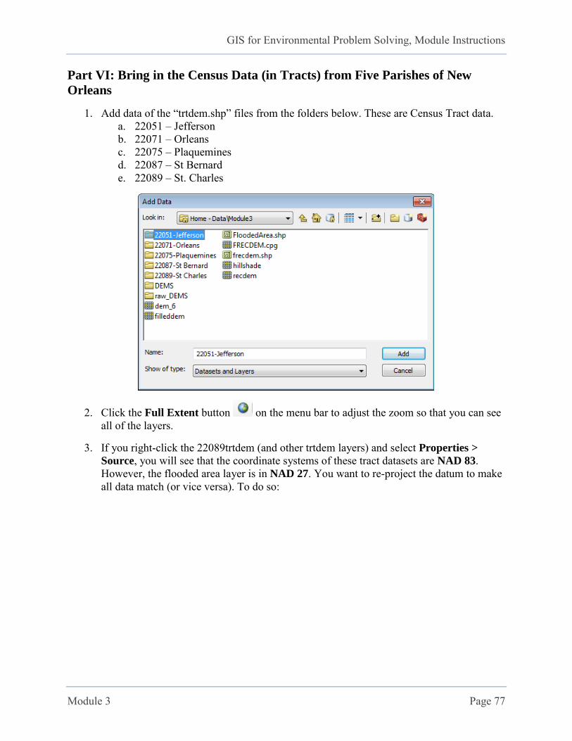
1. Add data of the “trtdem.shp” files from the folders below. These are Census Tract data. a. 22051 – Jefferson b. 22071 – Orleans c. 22075 – Plaquemines d. 22087 – St Bernard e. 22089 – St. Charles
2. Click the Full Extent button on the menu bar to adjust the zoom so that you can see all of the layers.
3. If you right-click the 22089trtdem (and other trtdem layers) and select Properties >
Source, you will see that the coordinate systems of these tract datasets are NAD 83. However, the flooded area layer is in NAD 27. You want to re-project the datum to make all data match (or vice versa). To do so:
GIS for Environmental Problem Solving, Module Instructions
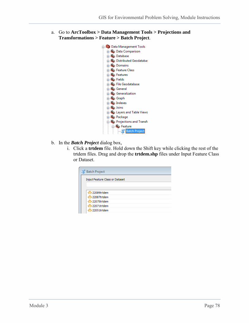
Module 3 Page 78
a. Go to ArcToolbox > Data Management Tools > Projections and
Transformations > Feature > Batch Project.
b. In the Batch Project dialog box, i. Click a trtdem file. Hold down the Shift key while clicking the rest of the
trtdem files. Drag and drop the trtdem.shp files under Input Feature Class or Dataset.

GIS for Environmental Problem Solving, Module Instructions
Module 3 Page 79
ii. Under Output Workspace, use the browse button and select module3 folder.
iii. Under Output Coordinate System, select the right button and to select a new coordinate system.
Under the Spatial Reference System dialog box,
1) Click Select to choose a coordinate system.
GIS for Environmental Problem Solving, Module Instructions
Module 3 Page 80
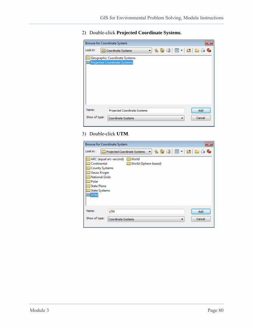
2) Double-click Projected Coordinate Systems.
3) Double-click UTM.
GIS for Environmental Problem Solving, Module Instructions
Module 3 Page 81
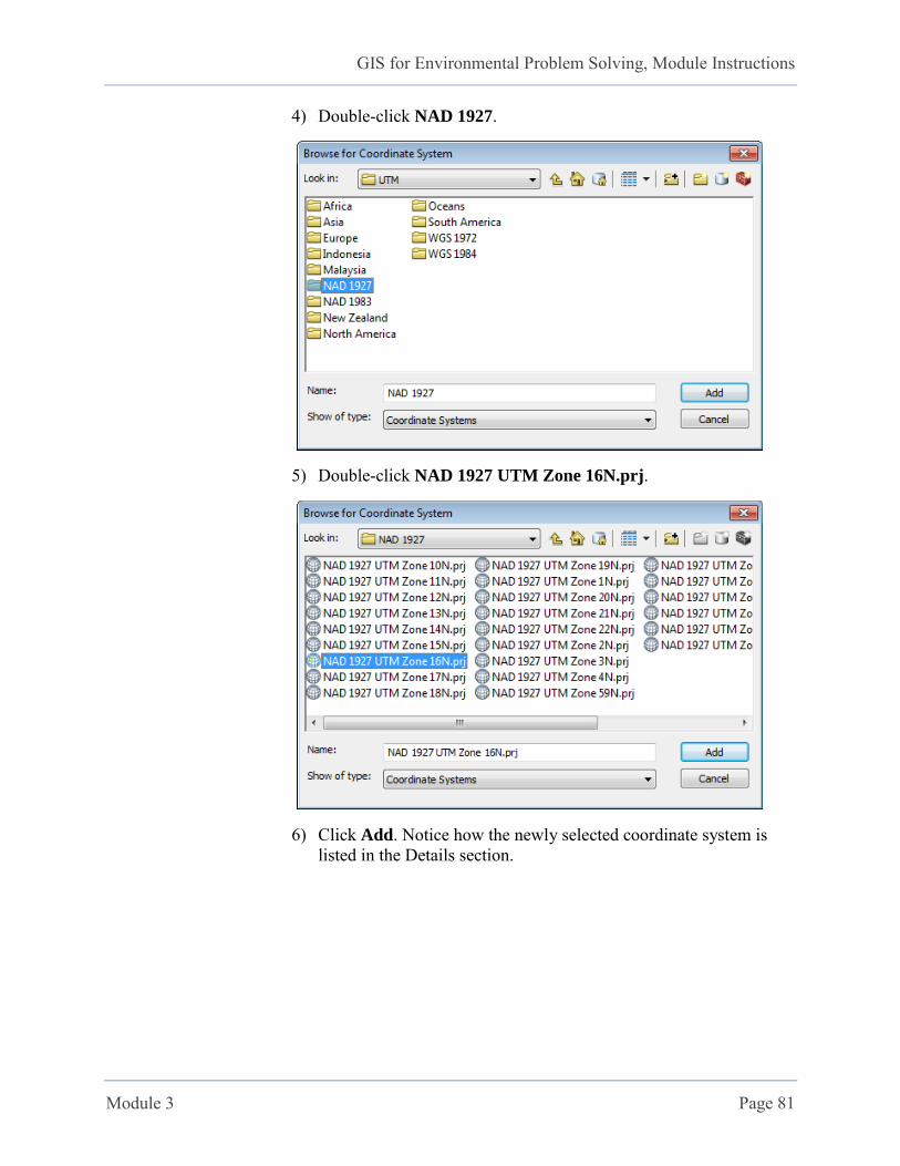
4) Double-click NAD 1927.
5) Double-click NAD 1927 UTM Zone 16N.prj.
6) Click Add. Notice how the newly selected coordinate system is listed in the Details section.
GIS for Environmental Problem Solving, Module Instructions
Module 3 Page 82
7) Click OK.
iv. Under Transformation, enter “NAD_1927_To_NAD_1983_PR_VI”.
v. Click OK.
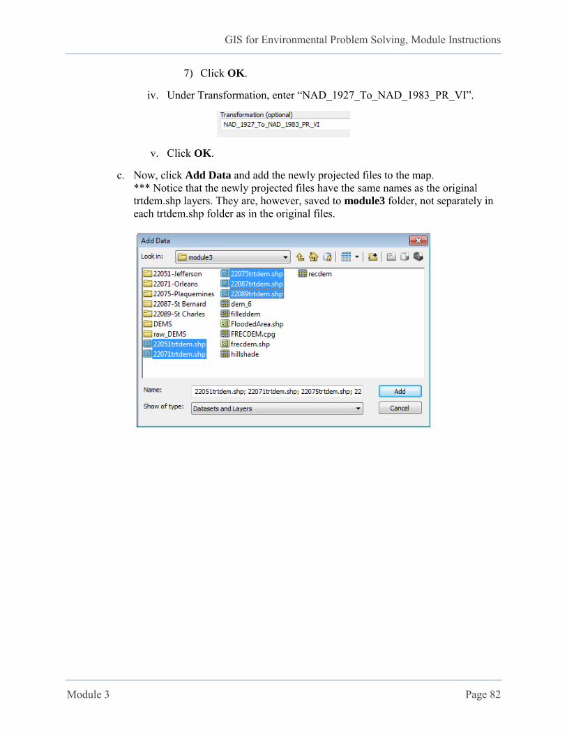
c. Now, click Add Data and add the newly projected files to the map. *** Notice that the newly projected files have the same names as the original trtdem.shp layers. They are, however, saved to module3 folder, not separately in each trtdem.shp folder as in the original files.
GIS for Environmental Problem Solving, Module Instructions
Module 3 Page 83
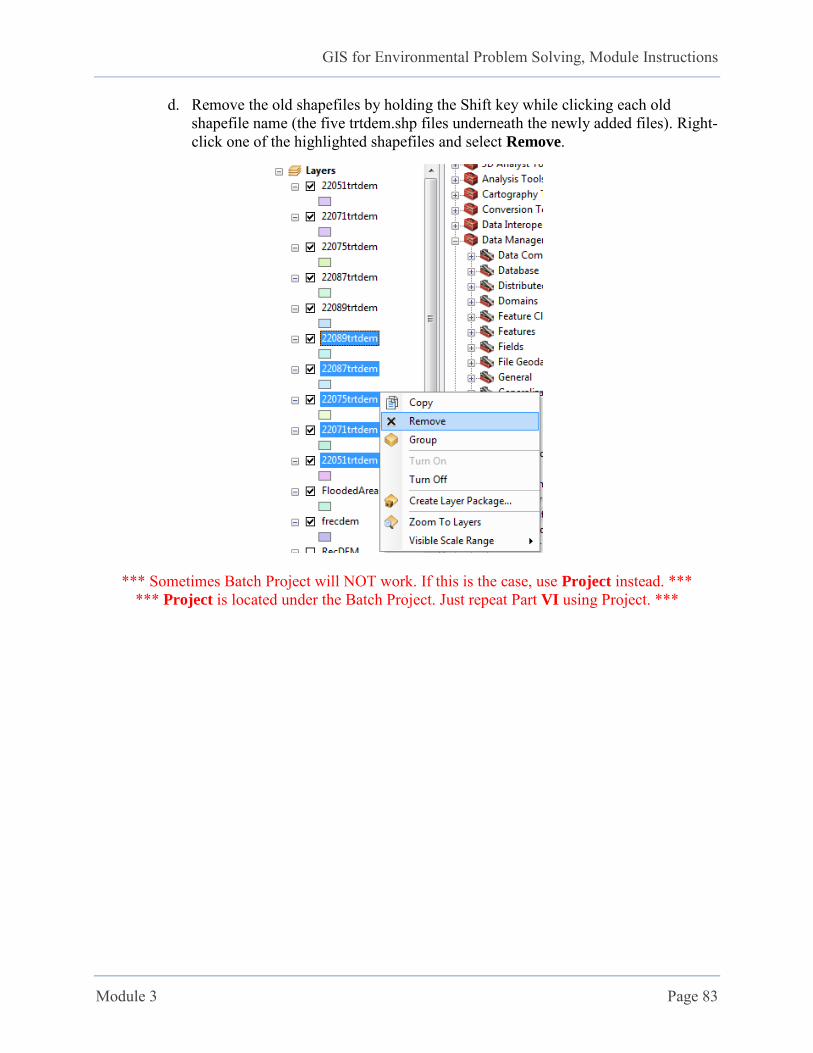
d. Remove the old shapefiles by holding the Shift key while clicking each old shapefile name (the five trtdem.shp files underneath the newly added files). Right-click one of the highlighted shapefiles and select Remove.
*** Sometimes Batch Project will NOT work. If this is the case, use Project instead. *** *** Project is located under the Batch Project. Just repeat Part VI using Project. ***
GIS for Environmental Problem Solving, Module Instructions
Module 3 Page 84
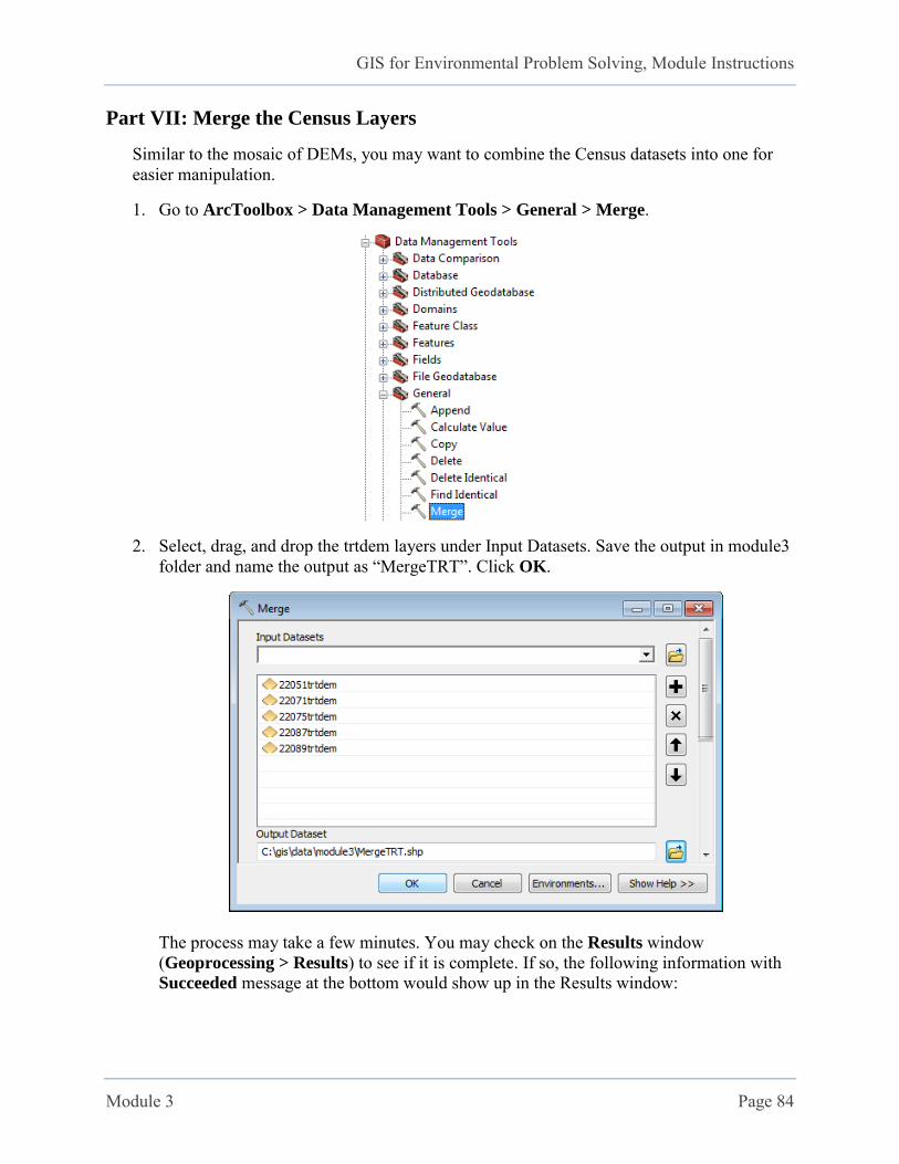
Part VII: Merge the Census Layers
Similar to the mosaic of DEMs, you may want to combine the Census datasets into one for easier manipulation.
1. Go to ArcToolbox > Data Management Tools > General > Merge.
2. Select, drag, and drop the trtdem layers under Input Datasets. Save the output in module3 folder and name the output as “MergeTRT”. Click OK.
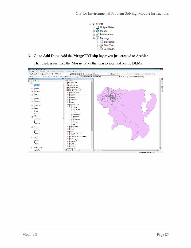
The process may take a few minutes. You may check on the Results window (Geoprocessing > Results) to see if it is complete. If so, the following information with Succeeded message at the bottom would show up in the Results window:
GIS for Environmental Problem Solving, Module Instructions
Module 3 Page 85
3. Go to Add Data. Add the MergeTRT.shp layer you just created to ArcMap.
The result is just like the Mosaic layer that was performed on the DEMs
GIS for Environmental Problem Solving, Module Instructions
Module 3 Page 86
Part VIII: Data Analysis
Part A: Total Affected Area
To begin the analysis, we will try and find the total affected area (in acres).
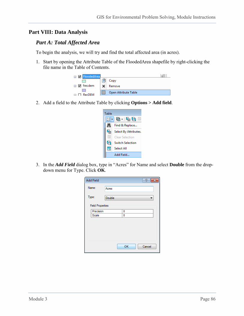
1. Start by opening the Attribute Table of the FloodedArea shapefile by right-clicking the file name in the Table of Contents.
2. Add a field to the Attribute Table by clicking Options > Add field.
3. In the Add Field dialog box, type in “Acres” for Name and select Double from the drop-down menu for Type. Click OK.

GIS for Environmental Problem Solving, Module Instructions
Module 3 Page 87
4. In the Table dialog box: a. Right-click the Acres column. b. Select Calculate Geometry…
c. Click Yes d. In the Calculate Geometry dialog box:
i. Under Property: select Area. ii. Under Coordinate System: leave it as is (NAD 1927 UTM Zone 15N).
iii. For Units: select Acres US [ac]. iv. Click OK.
The process will automatically calculate area of the layer (in acres).
5. To find the overall affected area, right-click the field Acres and select Statistics...
GIS for Environmental Problem Solving, Module Instructions
Module 3 Page 88
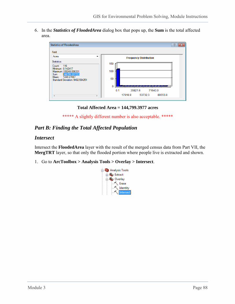
6. In the Statistics of FloodedArea dialog box that pops up, the Sum is the total affected area.
Total Affected Area = 144,799.3977 acres
***** A slightly different number is also acceptable. *****
Part B: Finding the Total Affected Population
Intersect
Intersect the FloodedArea layer with the result of the merged census data from Part VII, the MergTRT layer, so that only the flooded portion where people live is extracted and shown.
1. Go to ArcToolbox > Analysis Tools > Overlay > Intersect.

GIS for Environmental Problem Solving, Module Instructions
Module 3 Page 89
2. In the Intersect dialog box: i. Input Features: FloodedArea and MergeTRT
ii. Output Feature Class: C:\gis\data\module3\censuscut.shp iii. Click OK.
3. Refer to the document “Census Codes” in the week 1 supplemental materials folder and look up the code for total population.
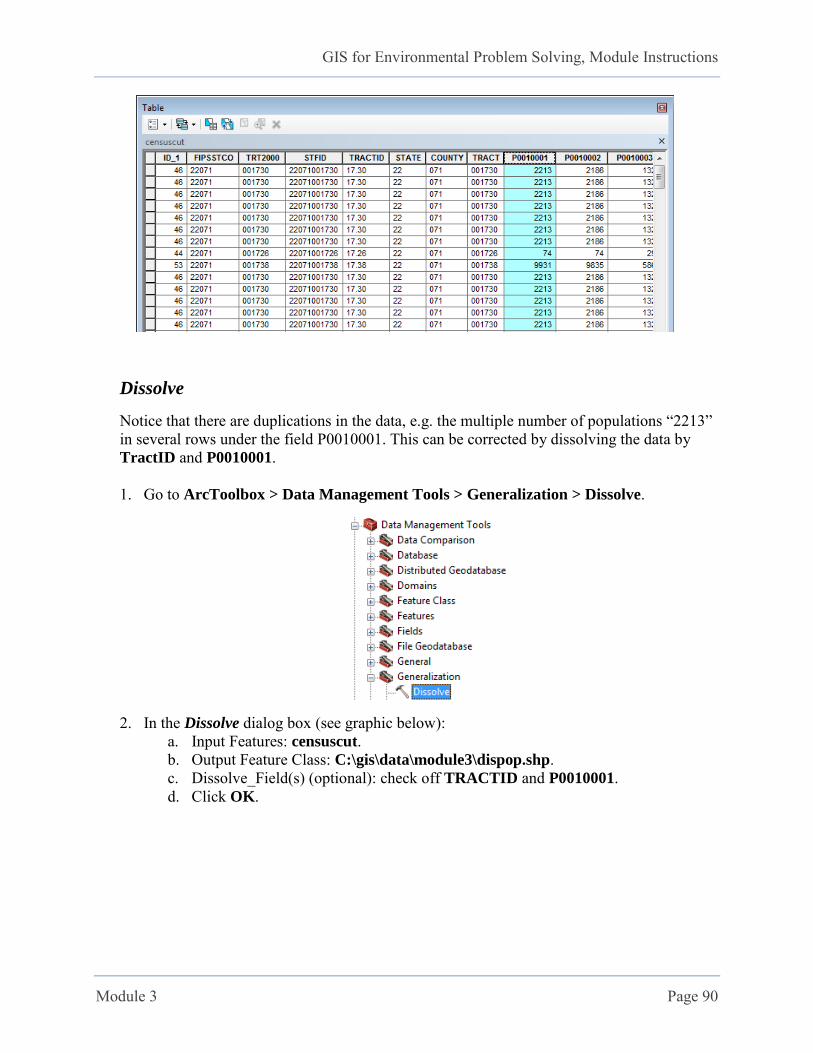
4. Open the Attribute Table of censuscut and notice that all of these codes correspond to a field in the Attribute Table. The field of interest is P0010001. Scroll the table to the right to see more fields (see the graphic below).
GIS for Environmental Problem Solving, Module Instructions
Module 3 Page 90
Dissolve
Notice that there are duplications in the data, e.g. the multiple number of populations “2213”
in several rows under the field P0010001. This can be corrected by dissolving the data by TractID and P0010001.
1. Go to ArcToolbox > Data Management Tools > Generalization > Dissolve.
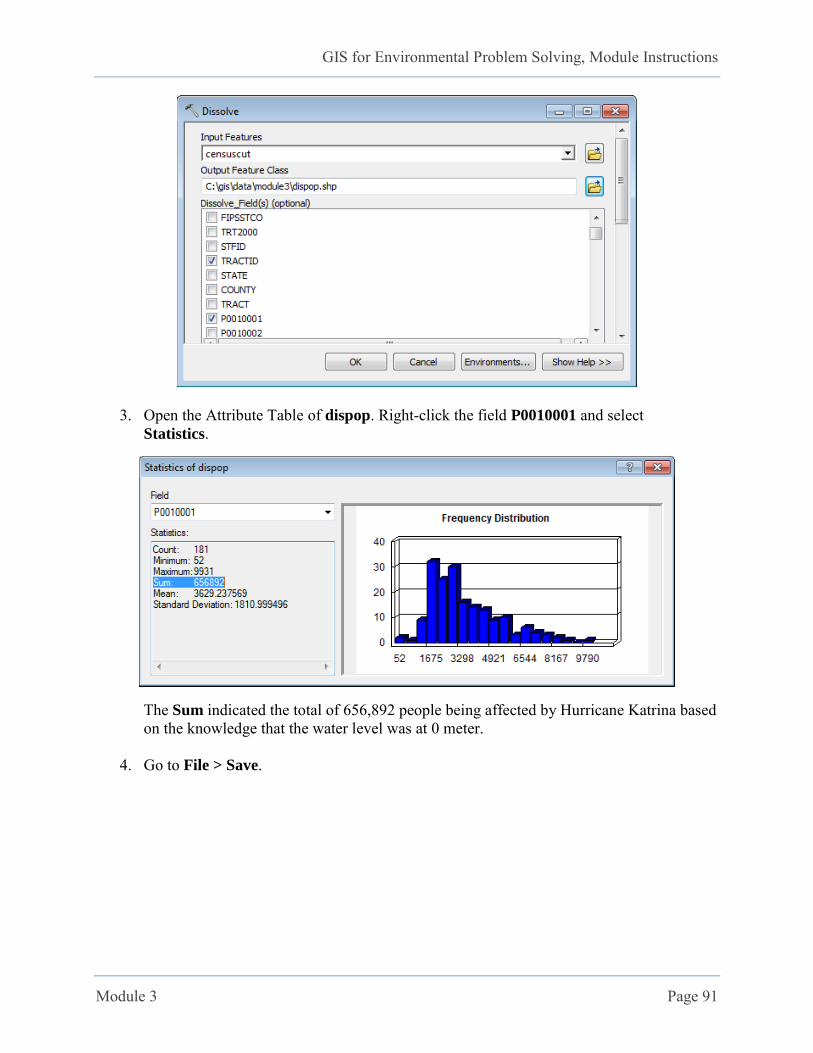
2. In the Dissolve dialog box (see graphic below): a. Input Features: censuscut. b. Output Feature Class: C:\gis\data\module3\dispop.shp. c. Dissolve_Field(s) (optional): check off TRACTID and P0010001. d. Click OK.
GIS for Environmental Problem Solving, Module Instructions
Module 3 Page 91
3. Open the Attribute Table of dispop. Right-click the field P0010001 and select Statistics.
The Sum indicated the total of 656,892 people being affected by Hurricane Katrina based on the knowledge that the water level was at 0 meter.
4. Go to File > Save.

GIS for Environmental Problem Solving, Module Instructions
Module 3 Page 92
Your Turn (You are not required to turn in this part. It is, however, a good
practice for future work in the class) Using what you read in the Learning Materials and the steps outlined in this module, solve the following problem:
New information indicates that the flood waters are rising. Their projected maximum level in the next twenty-four hours is that of 3 meters. Your job is to reassess the flooded area based on this new criterion.
GIS for Environmental Problem Solving, Module Instructions
Module 4 Page 93
Module 4: Editing Spatial Data
Learning Objectives:
Create new features
Modify features
Cut polygons
Extending the basic skills, e.g. clipping
Learning Materials:
Before working with ArcGIS, please review the following presentations:
Key Words Key Processes Identify Decision Support Tools
Demonstration:
Assume your firm is contracted to design a New Orleans re-construction housing project for the area surrounded by Agriculture St., Paris St., Abundance St., and St. Bernard St.
The preliminary assignments are:
First, you are to delineate the project area by creating a polygon that borders the four streets.
Second, you are to delineate a new road from the intersection of St. Bernard and Rosiere to Paris.
Third, by creating the new road, you are dividing the project into two sub-areas.
General Problem Solving Steps
Step 1: Frame the problem
A new development needs to be placed within Agriculture St., Paris St., Abundance St., and St. Bernard St.
Step 2: Identify data needs
An up-to-date street grid of New Orleans, LA is needed to delineate the project area.
Step 3: Identify decision support tools
Outline of exactly what the project is asking for. Step 4: Locate and assemble data
All data is also available at the following website: http://atlas.lsu.edu/ The datasets have been provided to you in the gis folder in the course DVD.

GIS for Environmental Problem Solving, Module Instructions
Module 4 Page 94
Step 5: Process and analyze data
Part I: Creating new features Part II: Adding a feature to an existing feature Part III: Modifying features Part IV: Cutting Polygons Part V: Extending your basic skills Step 6: Generate Information and report (Sample Report)
GIS for Environmental Problem Solving, Module Instructions
Module 4 Page 95
Procedure
Part I: Creating New Features
Phase I: Loading and Labeling Features
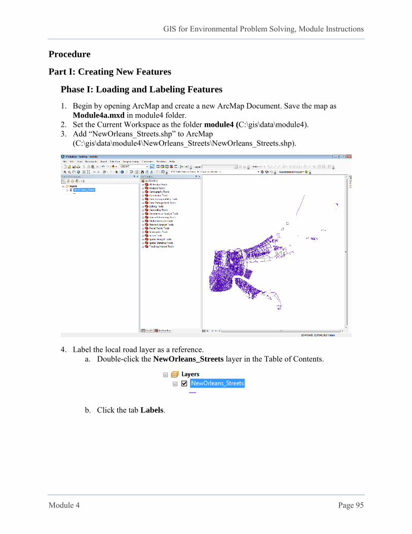
1. Begin by opening ArcMap and create a new ArcMap Document. Save the map as Module4a.mxd in module4 folder.
2. Set the Current Workspace as the folder module4 (C:\gis\data\module4). 3. Add “NewOrleans_Streets.shp” to ArcMap
(C:\gis\data\module4\NewOrleans_Streets\NewOrleans_Streets.shp).
4. Label the local road layer as a reference. a. Double-click the NewOrleans_Streets layer in the Table of Contents.
b. Click the tab Labels.
GIS for Environmental Problem Solving, Module Instructions
Module 4 Page 96
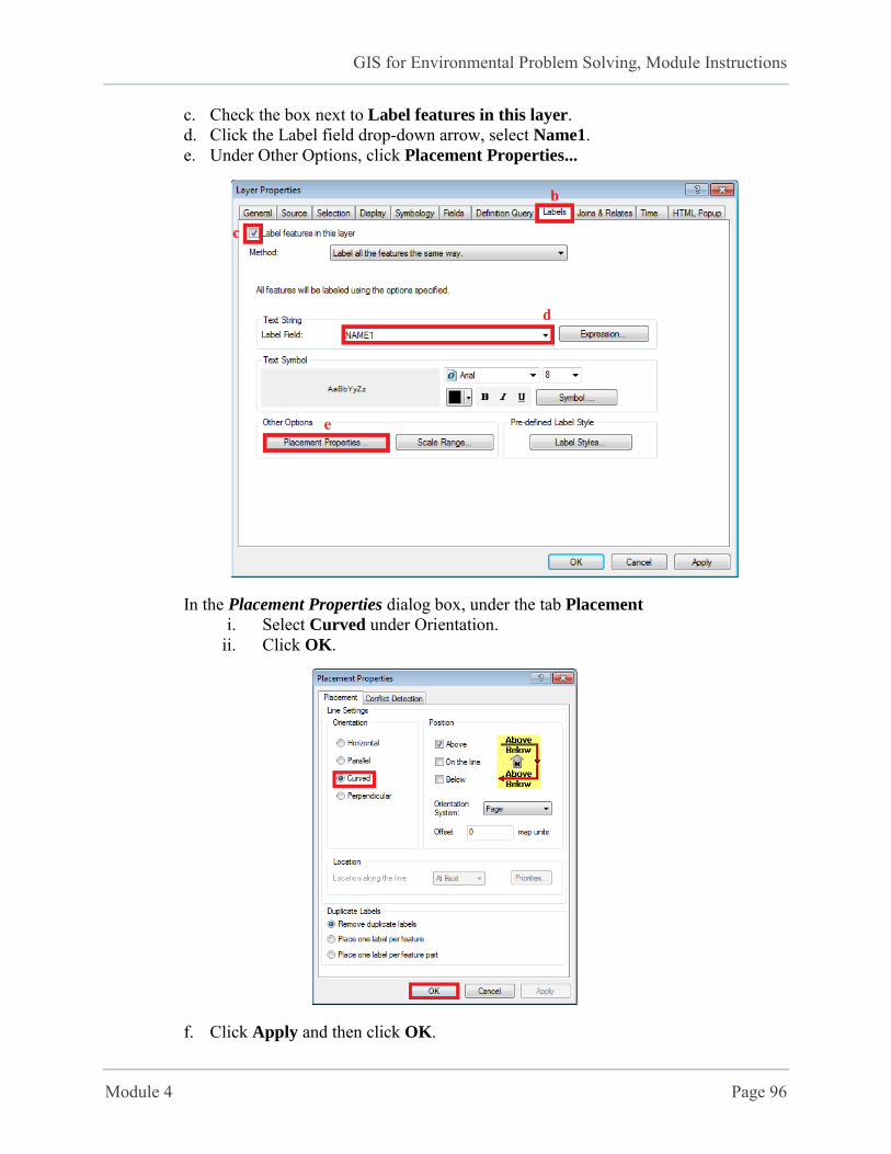
c. Check the box next to Label features in this layer. d. Click the Label field drop-down arrow, select Name1. e. Under Other Options, click Placement Properties...
In the Placement Properties dialog box, under the tab Placement
i. Select Curved under Orientation. ii. Click OK.
f. Click Apply and then click OK.

GIS for Environmental Problem Solving, Module Instructions
Module 4 Page 97
5. Right-click to open the Attribute Table of NewOrleans_Streets, 6. Click Table Options and click Select By Attributes.
a. Put in this equation: “NAME1” = ‘Agriculture’ and click Apply and Close.
7. Using the Zoom In Tool, zoom to the highlighted feature, which is the project area.
Phase II: Creating Templates for Polygon and Polyline
1. In ArcMap, open ArcCatalog from the tab on the right or click the Catalog Window
button in the toolbar.

GIS for Environmental Problem Solving, Module Instructions
Module 4 Page 98
2. Navigate to the Current Workspace, module4. Use the Connect To Folder button if needed.
3. Right-click module4 folder and go to New > Shapefile…
GIS for Environmental Problem Solving, Module Instructions
Module 4 Page 99
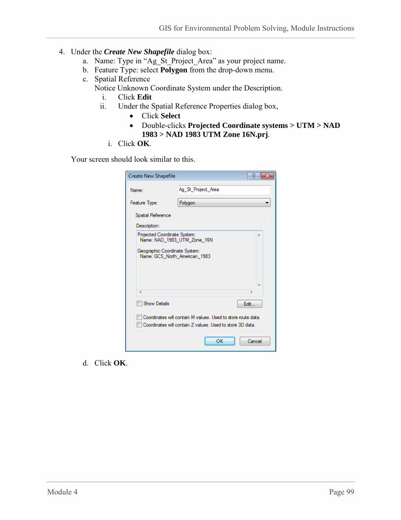
4. Under the Create New Shapefile dialog box: a. Name: Type in “Ag_St_Project_Area” as your project name. b. Feature Type: select Polygon from the drop-down menu. c. Spatial Reference
Notice Unknown Coordinate System under the Description. i. Click Edit
ii. Under the Spatial Reference Properties dialog box, Click Select Double-clicks Projected Coordinate systems > UTM > NAD
1983 > NAD 1983 UTM Zone 16N.prj. i. Click OK.
Your screen should look similar to this.
d. Click OK.
GIS for Environmental Problem Solving, Module Instructions
Module 4 Page 100
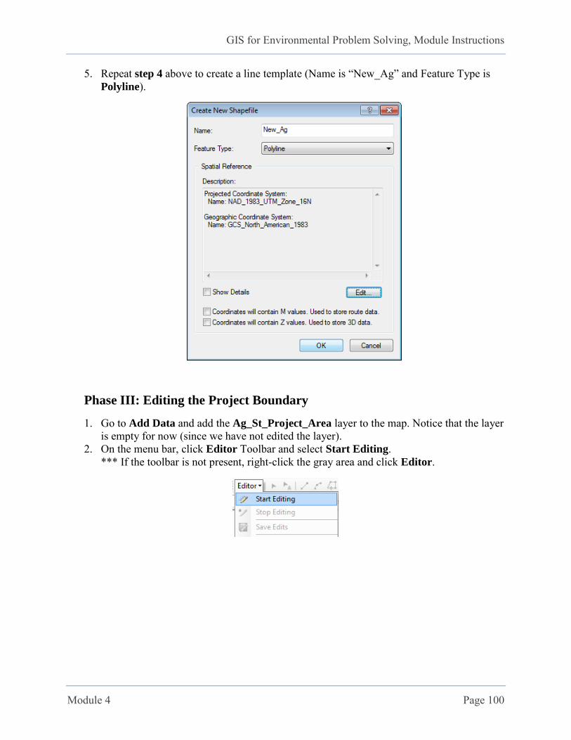
5. Repeat step 4 above to create a line template (Name is “New_Ag” and Feature Type is Polyline).
Phase III: Editing the Project Boundary
1. Go to Add Data and add the Ag_St_Project_Area layer to the map. Notice that the layer is empty for now (since we have not edited the layer).
2. On the menu bar, click Editor Toolbar and select Start Editing. *** If the toolbar is not present, right-click the gray area and click Editor.
GIS for Environmental Problem Solving, Module Instructions
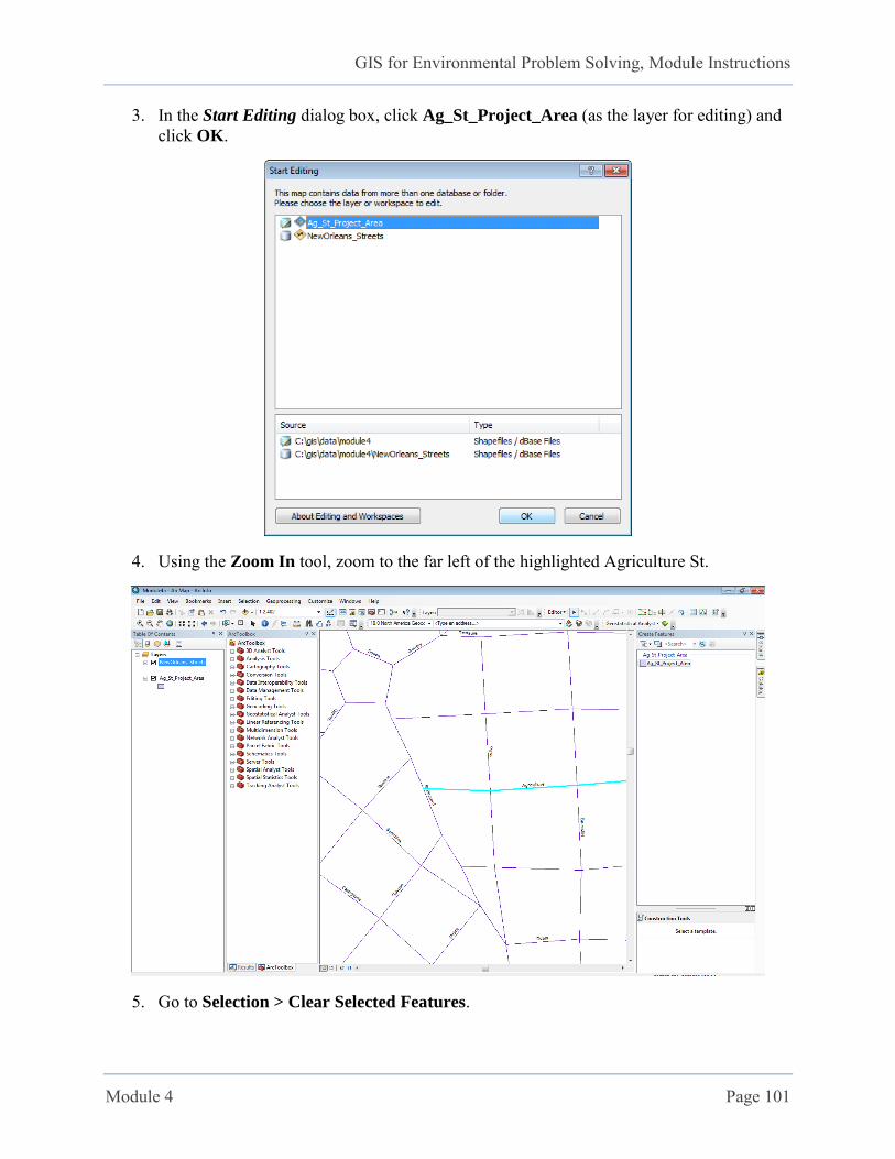
Module 4 Page 101
3. In the Start Editing dialog box, click Ag_St_Project_Area (as the layer for editing) and click OK.
4. Using the Zoom In tool, zoom to the far left of the highlighted Agriculture St.
5. Go to Selection > Clear Selected Features.
GIS for Environmental Problem Solving, Module Instructions
Module 4 Page 102
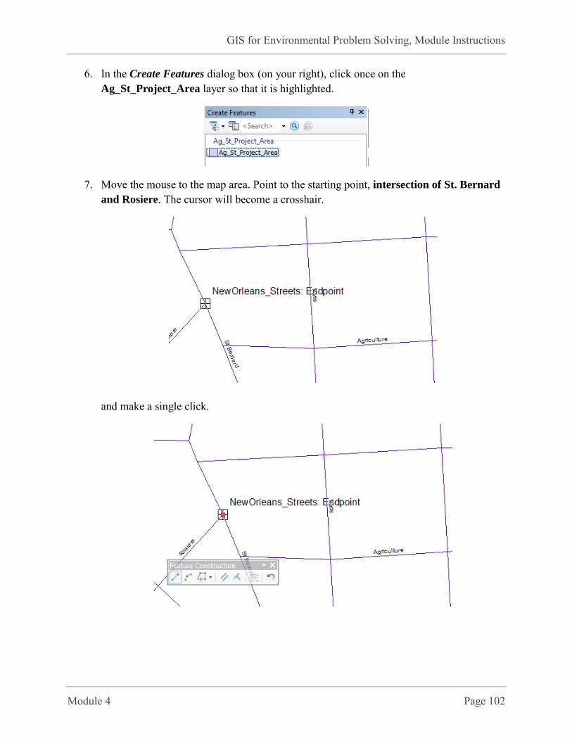
6. In the Create Features dialog box (on your right), click once on the Ag_St_Project_Area layer so that it is highlighted.
7. Move the mouse to the map area. Point to the starting point, intersection of St. Bernard
and Rosiere. The cursor will become a crosshair.
and make a single click.
GIS for Environmental Problem Solving, Module Instructions
Module 4 Page 103
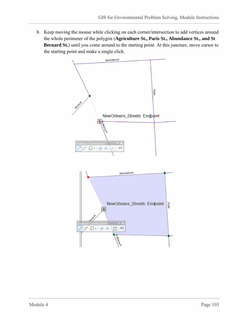
8. Keep moving the mouse while clicking on each corner/intersection to add vertices around the whole perimeter of the polygon (Agriculture St., Paris St., Abundance St., and St
Bernard St.) until you come around to the starting point. At this juncture, move cursor to the starting point and make a single click.
GIS for Environmental Problem Solving, Module Instructions
Module 4 Page 104
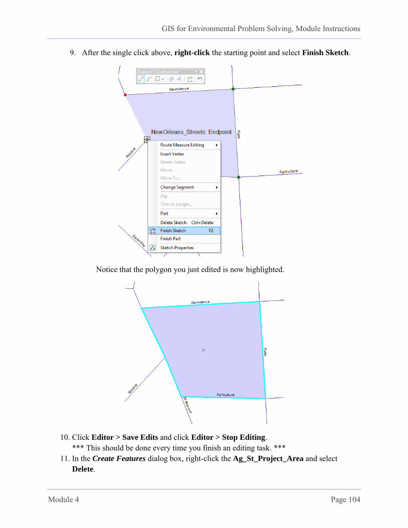
9. After the single click above, right-click the starting point and select Finish Sketch.
Notice that the polygon you just edited is now highlighted.
10. Click Editor > Save Edits and click Editor > Stop Editing. *** This should be done every time you finish an editing task. ***
11. In the Create Features dialog box, right-click the Ag_St_Project_Area and select Delete.
GIS for Environmental Problem Solving, Module Instructions
Module 4 Page 105
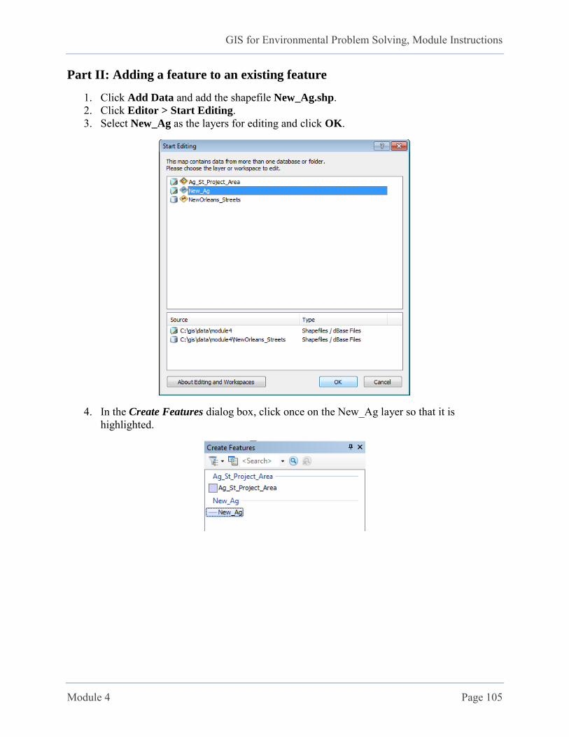
Part II: Adding a feature to an existing feature
1. Click Add Data and add the shapefile New_Ag.shp. 2. Click Editor > Start Editing. 3. Select New_Ag as the layers for editing and click OK.
4. In the Create Features dialog box, click once on the New_Ag layer so that it is highlighted.
GIS for Environmental Problem Solving, Module Instructions
Module 4 Page 106
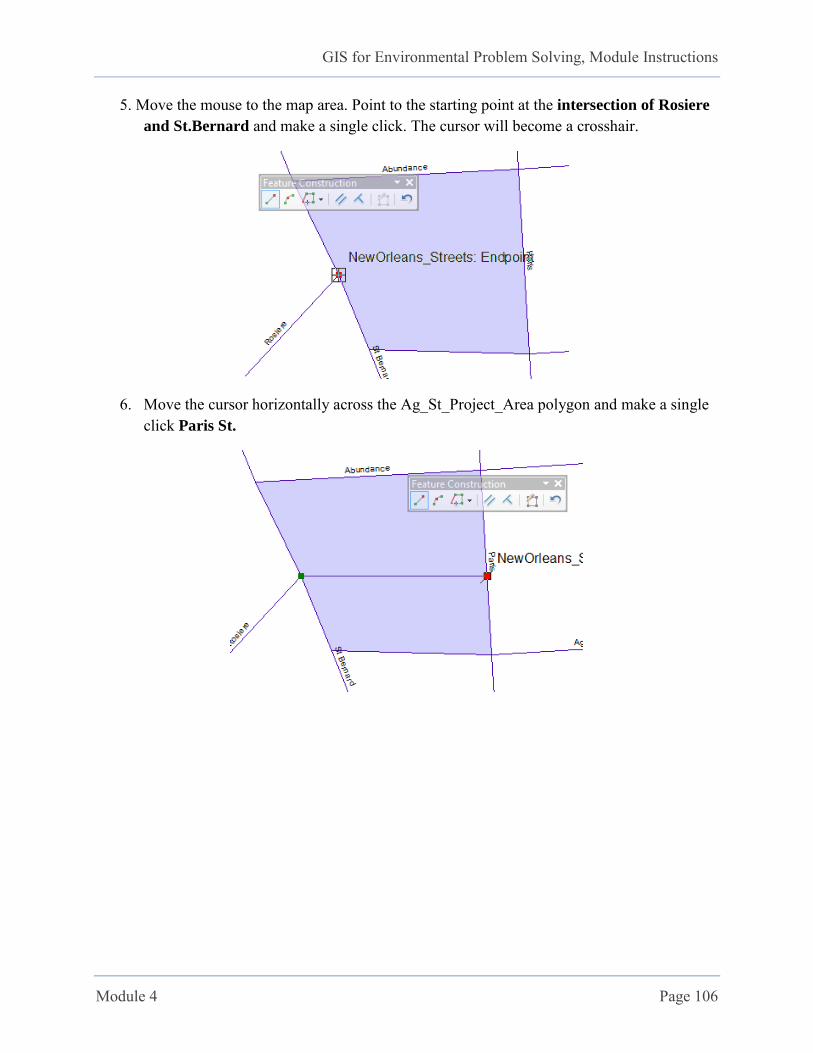
5. Move the mouse to the map area. Point to the starting point at the intersection of Rosiere
and St.Bernard and make a single click. The cursor will become a crosshair.
6. Move the cursor horizontally across the Ag_St_Project_Area polygon and make a single click Paris St.
GIS for Environmental Problem Solving, Module Instructions
Module 4 Page 107
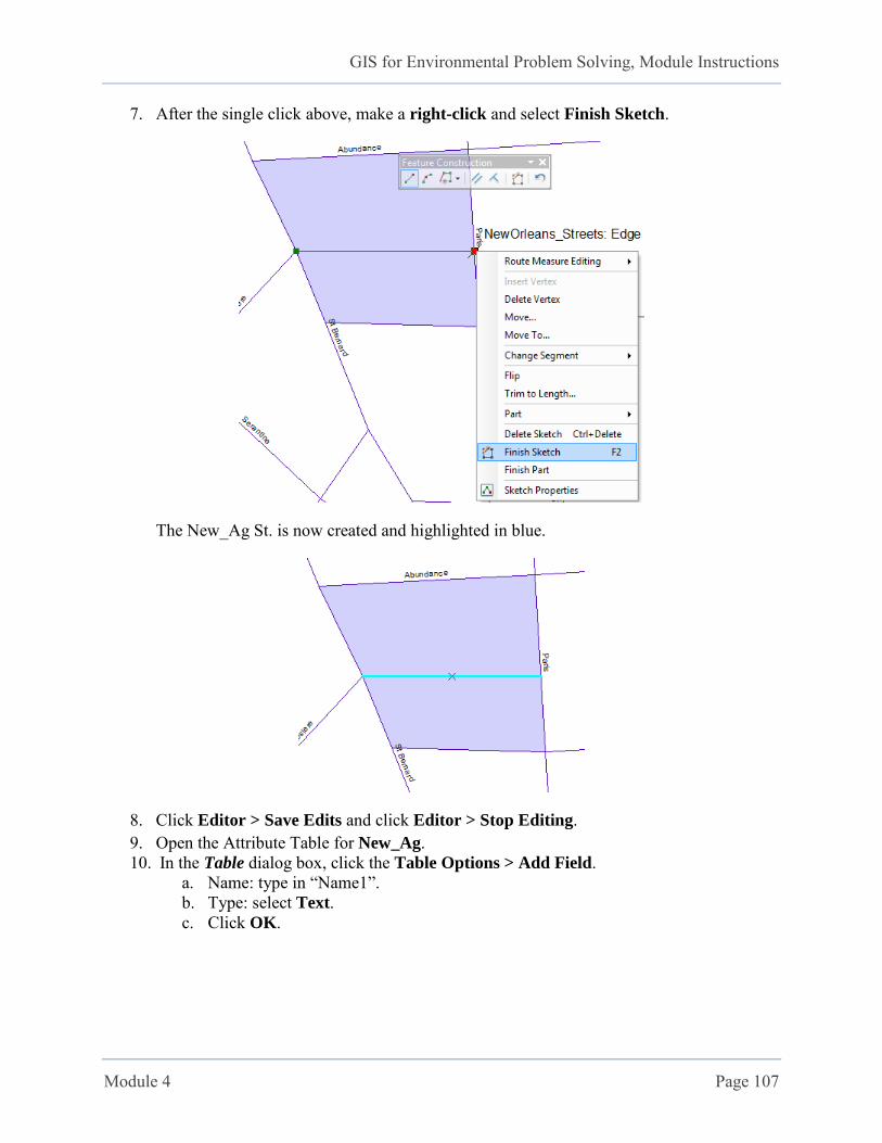
7. After the single click above, make a right-click and select Finish Sketch.
The New_Ag St. is now created and highlighted in blue.
8. Click Editor > Save Edits and click Editor > Stop Editing. 9. Open the Attribute Table for New_Ag. 10. In the Table dialog box, click the Table Options > Add Field.
a. Name: type in “Name1”. b. Type: select Text. c. Click OK.

GIS for Environmental Problem Solving, Module Instructions
Module 4 Page 108
11. Right-click the field Name1 > Field Calculator.
GIS for Environmental Problem Solving, Module Instructions
Module 4 Page 109
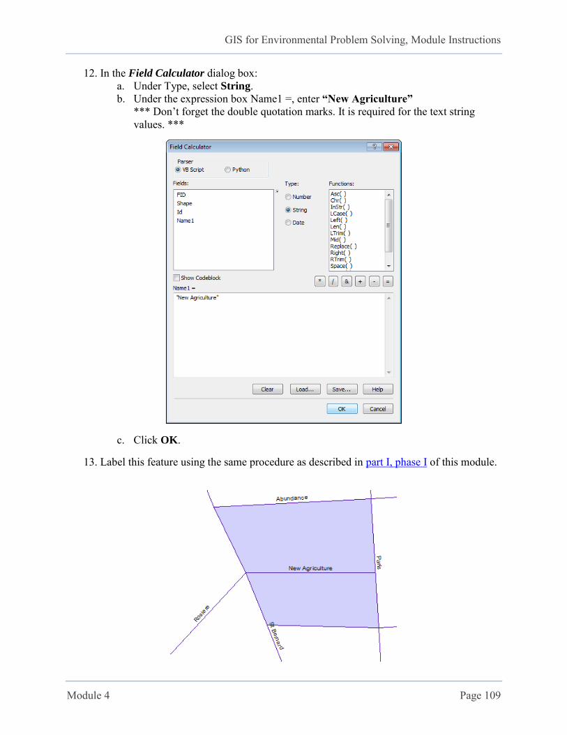
12. In the Field Calculator dialog box: a. Under Type, select String. b. Under the expression box Name1 =, enter “New Agriculture”
*** Don’t forget the double quotation marks. It is required for the text string values. ***
c. Click OK.
13. Label this feature using the same procedure as described in part I, phase I of this module.
GIS for Environmental Problem Solving, Module Instructions
Module 4 Page 110
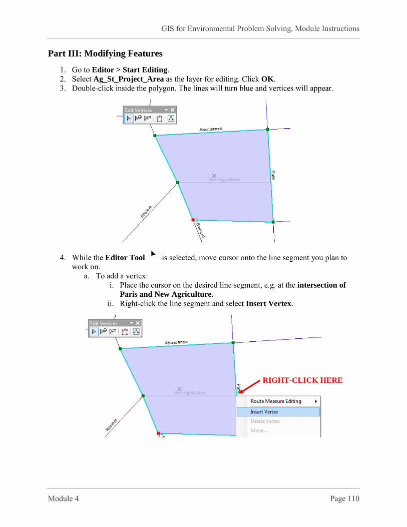
Part III: Modifying Features
1. Go to Editor > Start Editing. 2. Select Ag_St_Project_Area as the layer for editing. Click OK. 3. Double-click inside the polygon. The lines will turn blue and vertices will appear.
4. While the Editor Tool is selected, move cursor onto the line segment you plan to work on.
a. To add a vertex: i. Place the cursor on the desired line segment, e.g. at the intersection of
Paris and New Agriculture. ii. Right-click the line segment and select Insert Vertex.
RIGHT-CLICK HERE
GIS for Environmental Problem Solving, Module Instructions
Module 4 Page 111
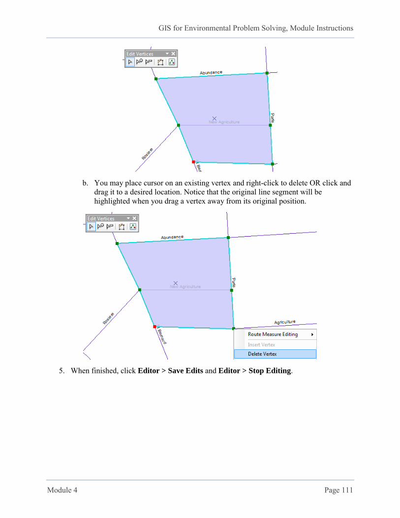
b. You may place cursor on an existing vertex and right-click to delete OR click and drag it to a desired location. Notice that the original line segment will be highlighted when you drag a vertex away from its original position.
5. When finished, click Editor > Save Edits and Editor > Stop Editing.
GIS for Environmental Problem Solving, Module Instructions
Module 4 Page 112
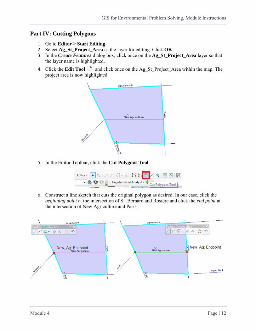
Part IV: Cutting Polygons
1. Go to Editor > Start Editing. 2. Select Ag_St_Project_Area as the layer for editing. Click OK. 3. In the Create Features dialog box, click once on the Ag_St_Project_Area layer so that
the layer name is highlighted. 4. Click the Edit Tool and click once on the Ag_St_Project_Area within the map. The
project area is now highlighted.
5. In the Editor Toolbar, click the Cut Polygons Tool.
6. Construct a line sketch that cuts the original polygon as desired. In our case, click the beginning point at the intersection of St. Bernard and Rosiere and click the end point at the intersection of New Agriculture and Paris.

GIS for Environmental Problem Solving, Module Instructions
Module 4 Page 113
7. After the single click at the end point above, right-click and select Finish Sketch.
The polygon is now split into two features.
8. Go to Editor > Save Edits and Editor > Stop Editing.
GIS for Environmental Problem Solving, Module Instructions
Module 4 Page 114
Part V: Extending Your Basic Skills
Phase I: Expanding the Project Area
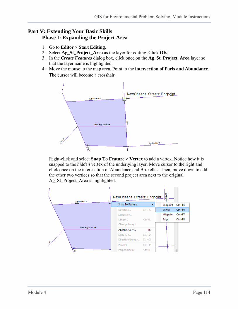
1. Go to Editor > Start Editing. 2. Select Ag_St_Project_Area as the layer for editing. Click OK. 3. In the Create Features dialog box, click once on the Ag_St_Project_Area layer so
that the layer name is highlighted. 4. Move the mouse to the map area. Point to the intersection of Paris and Abundance.
The cursor will become a crosshair.
Right-click and select Snap To Feature > Vertex to add a vertex. Notice how it is snapped to the hidden vertex of the underlying layer. Move cursor to the right and click once on the intersection of Abundance and Bruxelles. Then, move down to add the other two vertices so that the second project area next to the original Ag_St_Project_Area is highlighted.

GIS for Environmental Problem Solving, Module Instructions
Module 4 Page 115
5. Right-click the last vertex (intersection of Paris and Agriculture) and click Finish
Sketch.
6. Go to Editor > Save Edits and Editor > Stop Editing. 7. The polygon can be cut using the same procedure as above, using the Cut Polygon
Tools.

GIS for Environmental Problem Solving, Module Instructions
Module 4 Page 116
Phase II: Extending the New Agriculture Street into the Expanded
Project Area
1. Go to Editor > Start Editing. 2. Select New_Ag as the layer for editing. Click OK. 3. In the Create Features dialog box, click once on the New_Ag layer so that the layer
name is highlighted. 4. Click Editor Tool. 5. Double-click the New_Agriculture line on the map. The line will be highlighted
showing the vertices.
6. Move cursor to the vertex on Paris, where the vertex is red. Drag the sketch line to the right and click once when you reach Bruxelles. Right-click and select Finish Sketch.

GIS for Environmental Problem Solving, Module Instructions
Module 4 Page 117
7. Go to Editor > Save Edits and Editor > Stop Editing. 8. Go to File > Save.
GIS for Environmental Problem Solving, Module Instructions
Module 4 Page 118
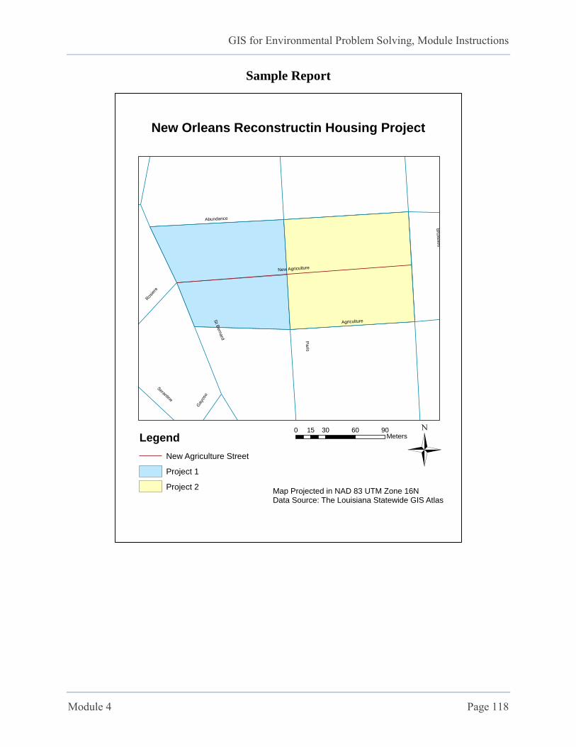
Sample Report
New AgricultureP
aris
Bru
xelle
s
Abundance
Agriculture
St B
ern
ard
Ros
iere
Desa
ix
Serantine
Gayo
so
New Orleans Reconstructin Housing Project
Legend
New Agriculture Street
Project 1
Project 2
Ü0 30 60 9015
Meters
Map Projected in NAD 83 UTM Zone 16NData Source: The Louisiana Statewide GIS AtlasCreated by STARRLab; June 1, 2010
GIS for Environmental Problem Solving, Module Instructions
Module 4 Page 119
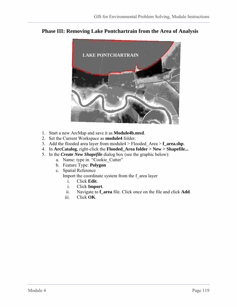
Phase III: Removing Lake Pontchartrain from the Area of Analysis
1. Start a new ArcMap and save it as Module4b.mxd. 2. Set the Current Workspace as module4 folder. 3. Add the flooded area layer from module4 > Flooded_Area > f_area.shp. 4. In ArcCatalog, right-click the Flooded_Area folder > New > Shapefile... 5. In the Create New Shapefile dialog box (see the graphic below):
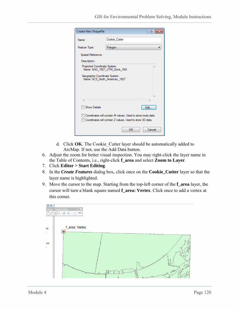
a. Name: type in “Cookie_Cutter” b. Feature Type: Polygon c. Spatial Reference
Import the coordinate system from the f_area layer i. Click Edit. i. Click Import.
ii. Navigate to f_area file. Click once on the file and click Add. iii. Click OK.
LAKE PONTCHARTRAIN
GIS for Environmental Problem Solving, Module Instructions
Module 4 Page 120
d. Click OK. The Cookie_Cutter layer should be automatically added to ArcMap. If not, use the Add Data button.
6. Adjust the zoom for better visual inspection. You may right-click the layer name in the Table of Contents, i.e., right-click f_area and select Zoom to Layer.
7. Click Editor > Start Editing. 8. In the Create Features dialog box, click once on the Cookie_Cutter layer so that the
layer name is highlighted. 9. Move the cursor to the map. Starting from the top-left corner of the f_area layer, the
cursor will turn a blank square named f_area: Vertex. Click once to add a vertex at this corner.
GIS for Environmental Problem Solving, Module Instructions
Module 4 Page 121
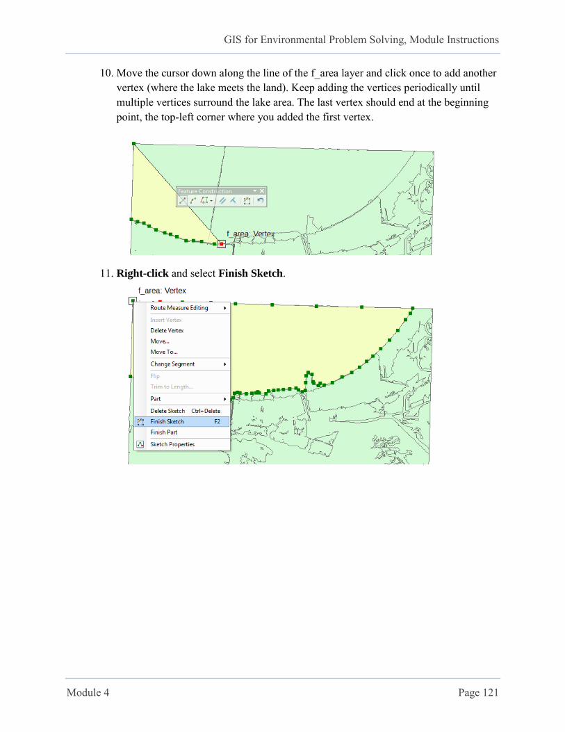
10. Move the cursor down along the line of the f_area layer and click once to add another vertex (where the lake meets the land). Keep adding the vertices periodically until multiple vertices surround the lake area. The last vertex should end at the beginning point, the top-left corner where you added the first vertex.
11. Right-click and select Finish Sketch.

GIS for Environmental Problem Solving, Module Instructions
Module 4 Page 122
Now the lake area is highlighted.
12. Click Editor > Save Edits and Editor > Stop Editing. 13. Click Editor > Start Editing. 14. In the Create Features dialog box, click once on the f_area layer so that the layer
name is highlighted. 15. Click once on the lake area you just edited. It should be highlighted in blue.
GIS for Environmental Problem Solving, Module Instructions
Module 4 Page 123
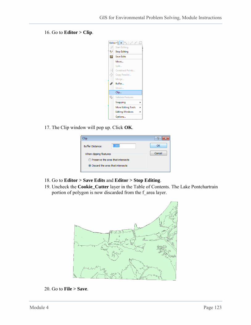
16. Go to Editor > Clip.
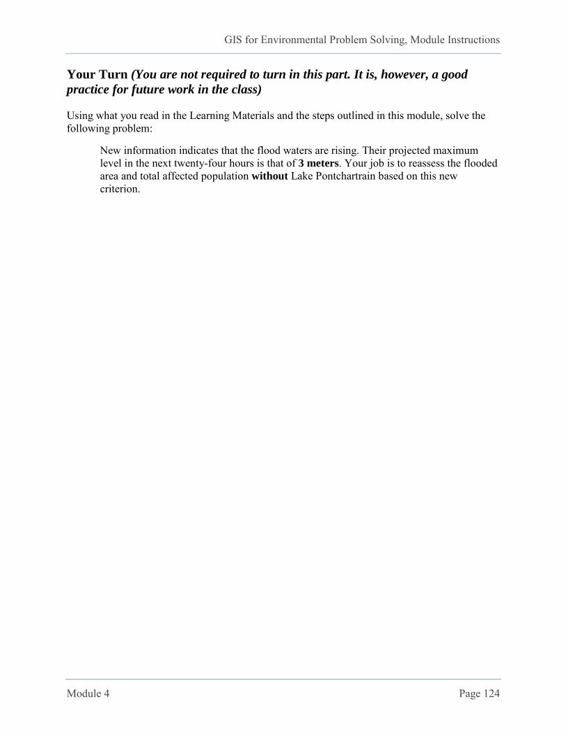
17. The Clip window will pop up. Click OK.
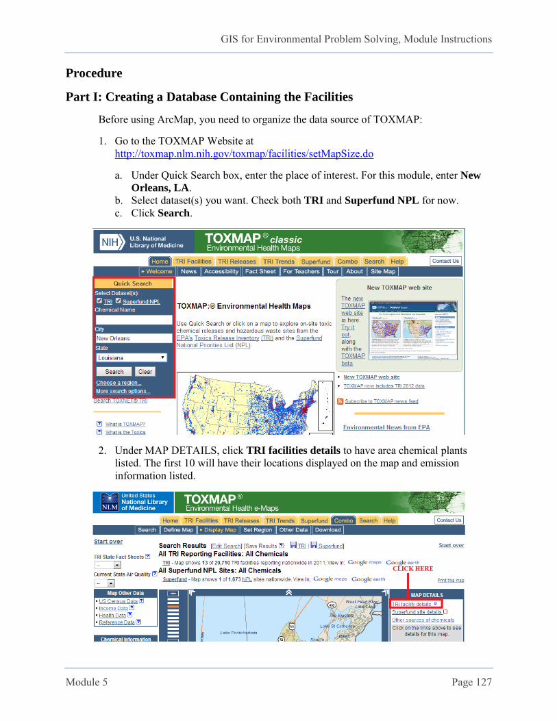
18. Go to Editor > Save Edits and Editor > Stop Editing. 19. Uncheck the Cookie_Cutter layer in the Table of Contents. The Lake Pontchartrain
portion of polygon is now discarded from the f_area layer.
20. Go to File > Save.
GIS for Environmental Problem Solving, Module Instructions
Module 4 Page 124
Your Turn (You are not required to turn in this part. It is, however, a good
practice for future work in the class) Using what you read in the Learning Materials and the steps outlined in this module, solve the following problem:
New information indicates that the flood waters are rising. Their projected maximum level in the next twenty-four hours is that of 3 meters. Your job is to reassess the flooded area and total affected population without Lake Pontchartrain based on this new criterion.

GIS for Environmental Problem Solving, Module Instructions
Module 5 Page 125
Module 5: Automate the Address Locating Process
Learning Objectives:
Basic use of Address Locator function in GIS
Automation of address locating process
Creating new GIS layer from results of address locating process
Creating attribute data in a database management system and link it to the newly created GIS layer
Learning Materials:
Before going through this module and working with ArcGIS, please review the following presentations:
Key Words Key Processes The Last Set of Problem-Solving Steps
Demonstration:
You have a list of EPA chemical sites and your job is to map them and include the main chemicals that they produce.
General Problem Solving Steps
Step 1: Frame the problem
You have a simple list of toxic facilities in the New Orleans, LA area. This list means nothing by itself because it needs to be mapped for further analysis.
Step 2: Identify data needs
An address locator is necessary to locate the specific locations of these facilities. Also a street grid of the area is useful for verifying the locations of each facility.
Step 3: Identify decision support tools
The facility chemical summary sheet information gives the ability to access the specific potential pollutants. Also a data base containing the specific pollutants may aide in determining potential hazards in the area.
Step 4: Locate and assemble data
All data is also available at these two sites:
http://toxmap.nlm.nih.gov/toxmap/facilities/setMapSize.do http://atlas.lsu.edu/search

GIS for Environmental Problem Solving, Module Instructions
Module 5 Page 126
Step 5: Process and analyze data
Part I: Creating a Database Containing the Facilities Part II: Geocoding the Facilities into a Working Map Part III: Linking the Facilities to Their Associated Chemical Data
Step 6: Generate information and report (Sample Report)
GIS for Environmental Problem Solving, Module Instructions
Module 5 Page 127
Procedure
Part I: Creating a Database Containing the Facilities
Before using ArcMap, you need to organize the data source of TOXMAP:
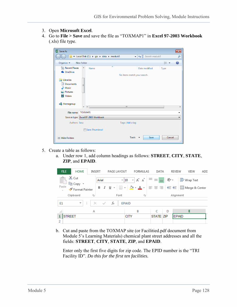
1. Go to the TOXMAP Website at http://toxmap.nlm.nih.gov/toxmap/facilities/setMapSize.do
a. Under Quick Search box, enter the place of interest. For this module, enter New
Orleans, LA. b. Select dataset(s) you want. Check both TRI and Superfund NPL for now. c. Click Search.
2. Under MAP DETAILS, click TRI facilities details to have area chemical plants listed. The first 10 will have their locations displayed on the map and emission information listed.
GIS for Environmental Problem Solving, Module Instructions
Module 5 Page 128
3. Open Microsoft Excel. 4. Go to File > Save and save the file as “TOXMAP1” in Excel 97-2003 Workbook
(.xls) file type.
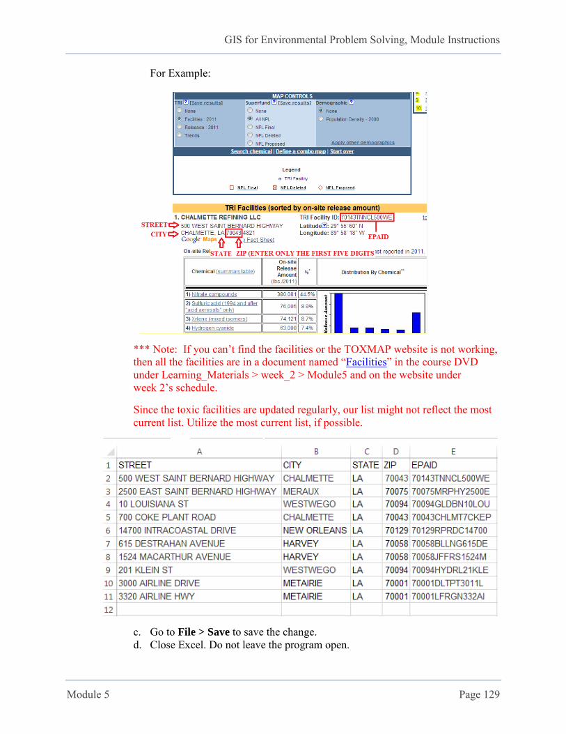
5. Create a table as follows: a. Under row 1, add column headings as follows: STREET, CITY, STATE,
ZIP, and EPAID.
b. Cut and paste from the TOXMAP site (or Facilitied.pdf document from Module 5’s Learning Materials) chemical plant street addresses and all the fields: STREET, CITY, STATE, ZIP, and EPAID.
Enter only the first five digits for zip code. The EPID number is the “TRI Facility ID”. Do this for the first ten facilities.
GIS for Environmental Problem Solving, Module Instructions
Module 5 Page 129
For Example:
*** Note: If you can’t find the facilities or the TOXMAP website is not working, then all the facilities are in a document named “Facilities” in the course DVD under Learning_Materials > week_2 > Module5 and on the website under week 2’s schedule.
Since the toxic facilities are updated regularly, our list might not reflect the most current list. Utilize the most current list, if possible.
c. Go to File > Save to save the change. d. Close Excel. Do not leave the program open.

GIS for Environmental Problem Solving, Module Instructions
Module 5 Page 130
Part II: Geocoding the Facilities into a Working Map
At this phase, you start to use ArcMap and relevant functions/tools to automate the address locating of the features of interest. In this case, the locations of the chemical facilities are registered in the TOXMAP program. You develop the database of chemical emission records of these facilities. You then use key field (EPAID) to link, i.e., join, the spatial and attribute data so that chemical emissions can be queried and displayed spatially.
1. Open ArcMap. Save the document as Module5.mxd. 2. Set the Current Workspace as module5 folder. 3. Click Add Data. Add the NewOrleansStreet.shp layer.
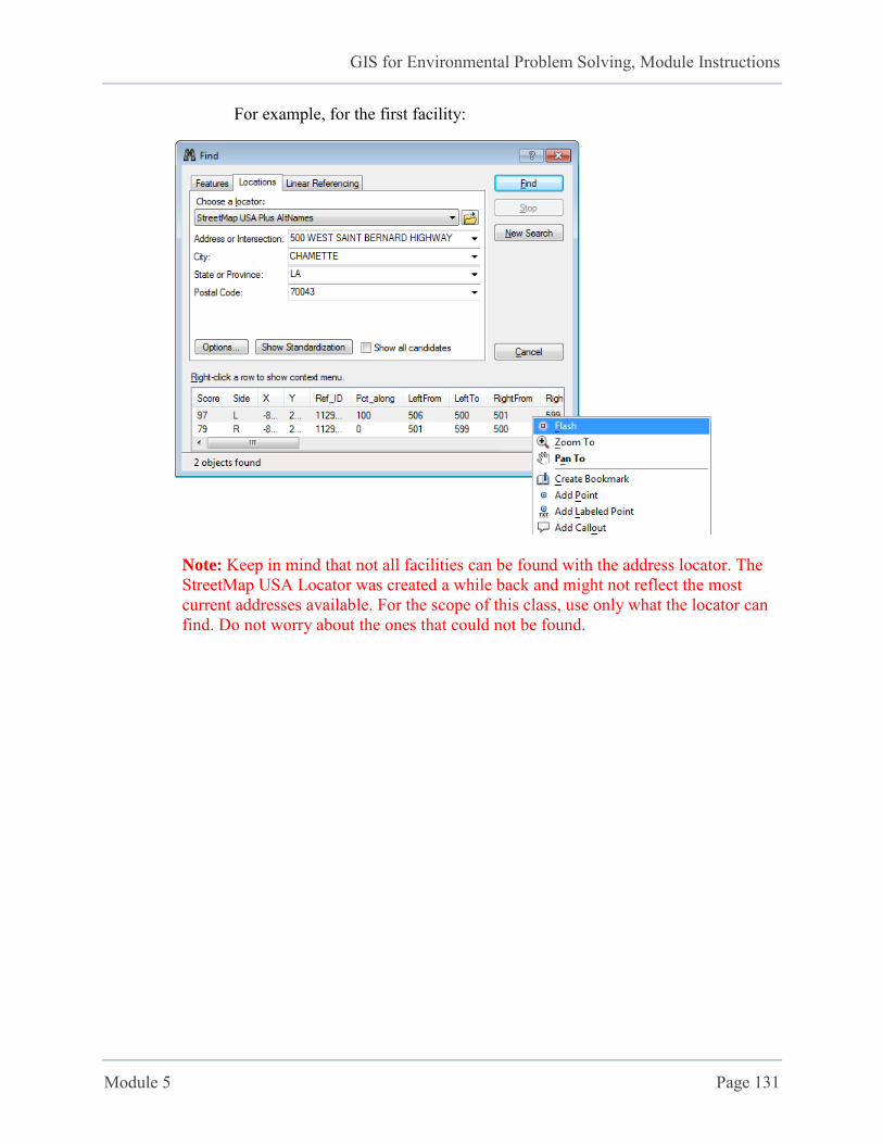
4. To verify whether the addresses listed on TOXMAP work or not, click the Find Tool on the toolbars.
5. In the Find dialog box: a. Click the Locations tab. b. Choose an address locator, e.g. StreetMap USA Plus AltNames c. Type in each address of the facilities. Then, click Find. d. Once each entry is found, right-click the item found and choose Flash.
Do not add the facilities as a point on the map as the automatic address locating process (in the subsequent steps) will help you create new geocoded shapefile.
GIS for Environmental Problem Solving, Module Instructions
Module 5 Page 131
For example, for the first facility:
Note: Keep in mind that not all facilities can be found with the address locator. The StreetMap USA Locator was created a while back and might not reflect the most current addresses available. For the scope of this class, use only what the locator can find. Do not worry about the ones that could not be found.
GIS for Environmental Problem Solving, Module Instructions
Module 5 Page 132
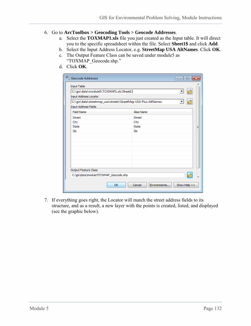
6. Go to ArcToolbox > Geocoding Tools > Geocode Addresses. a. Select the TOXMAP1.xls file you just created as the Input table. It will direct
you to the specific spreadsheet within the file. Select Sheet1$ and click Add. b. Select the Input Address Locator, e.g. StreetMap USA AltNames. Click OK. c. The Output Feature Class can be saved under module5 as
“TOXMAP_Geocode.shp.” d. Click OK.
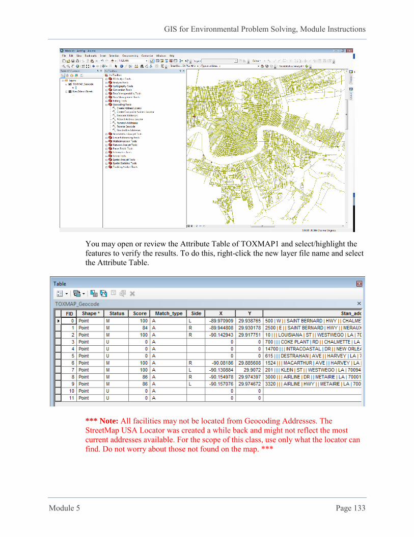
7. If everything goes right, the Locator will match the street address fields to its structure, and as a result, a new layer with the points is created, listed, and displayed (see the graphic below).
GIS for Environmental Problem Solving, Module Instructions
Module 5 Page 133
You may open or review the Attribute Table of TOXMAP1 and select/highlight the features to verify the results. To do this, right-click the new layer file name and select the Attribute Table.
*** Note: All facilities may not be located from Geocoding Addresses. The StreetMap USA Locator was created a while back and might not reflect the most current addresses available. For the scope of this class, use only what the locator can find. Do not worry about those not found on the map. ***
GIS for Environmental Problem Solving, Module Instructions
Module 5 Page 134
Getting new entries of locations of facilities:
8. As an exercise, try more of the addresses from TOXMAP listing, e.g. No. 11, No.12, and the rest of the facilities (given that the website is working). Remember to close Excel before performing the Geocode Addresses steps above.
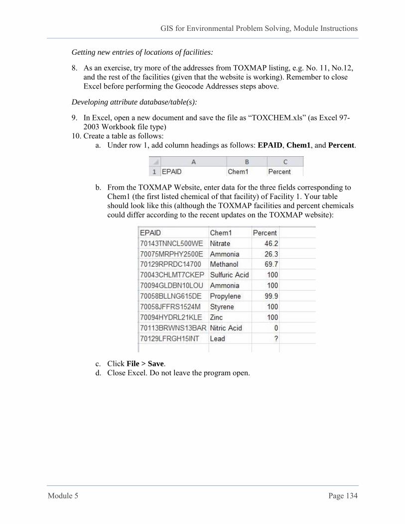
Developing attribute database/table(s):
9. In Excel, open a new document and save the file as “TOXCHEM.xls” (as Excel 97-2003 Workbook file type)
10. Create a table as follows: a. Under row 1, add column headings as follows: EPAID, Chem1, and Percent.
b. From the TOXMAP Website, enter data for the three fields corresponding to Chem1 (the first listed chemical of that facility) of Facility 1. Your table should look like this (although the TOXMAP facilities and percent chemicals could differ according to the recent updates on the TOXMAP website):
c. Click File > Save. d. Close Excel. Do not leave the program open.
GIS for Environmental Problem Solving, Module Instructions
Module 5 Page 135
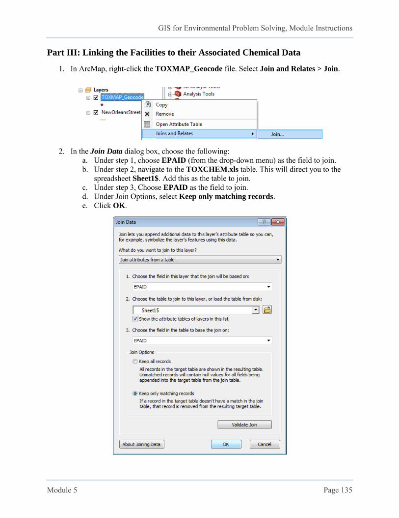
Part III: Linking the Facilities to their Associated Chemical Data
1. In ArcMap, right-click the TOXMAP_Geocode file. Select Join and Relates > Join.
2. In the Join Data dialog box, choose the following: a. Under step 1, choose EPAID (from the drop-down menu) as the field to join. b. Under step 2, navigate to the TOXCHEM.xls table. This will direct you to the
spreadsheet Sheet1$. Add this as the table to join. c. Under step 3, Choose EPAID as the field to join. d. Under Join Options, select Keep only matching records. e. Click OK.
GIS for Environmental Problem Solving, Module Instructions
Module 5 Page 136
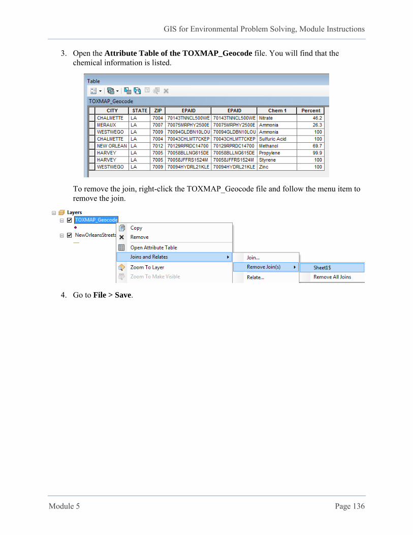
3. Open the Attribute Table of the TOXMAP_Geocode file. You will find that the chemical information is listed.
To remove the join, right-click the TOXMAP_Geocode file and follow the menu item to remove the join.
4. Go to File > Save.
GIS for Environmental Problem Solving, Module Instructions
Module 5 Page 137
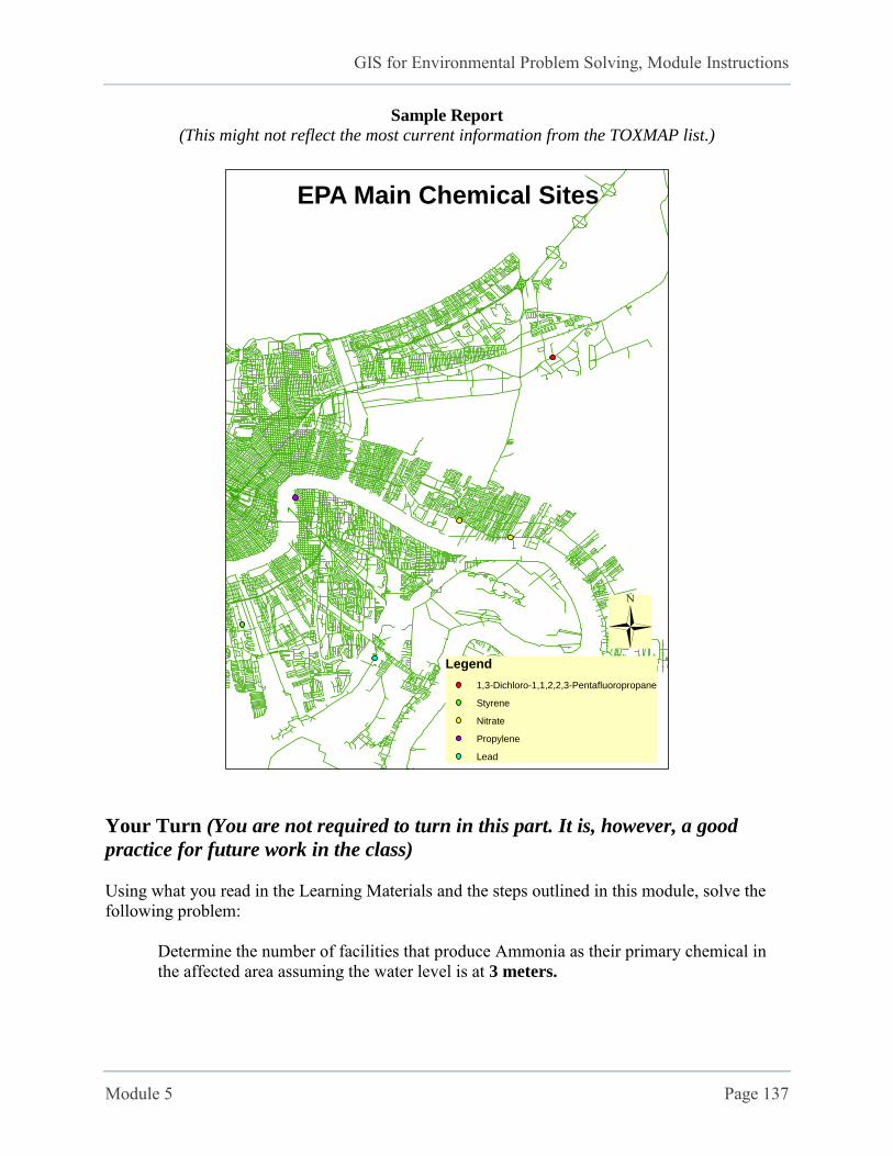
Sample Report
(This might not reflect the most current information from the TOXMAP list.)
Your Turn (You are not required to turn in this part. It is, however, a good
practice for future work in the class)
Using what you read in the Learning Materials and the steps outlined in this module, solve the following problem:
Determine the number of facilities that produce Ammonia as their primary chemical in the affected area assuming the water level is at 3 meters.
EPA Main Chemical Sites
ÜLegend
1,3-Dichloro-1,1,2,2,3-Pentafluoropropane
Styrene
Nitrate
Propylene
Lead

GIS for Environmental Problem Solving, Module Instructions
Module 6 Page 138
Module 6: Framing the Problem and Identifying Data Needs for
Quality of Life (QOL) Analysis
Learning Objectives:
Framing a problem-solving process and identifying factors and associated datasets that contribute to QOL of a city/community
Converting between vector and raster data and their integrated use for subsequent QOL analysis
Learning Materials:
Before going through this module and working with ArcGIS, please review the following presentations:
Key Words
Introduction: Quality of Life Analysis
Final Project Requirements
Sample Final Project 1
Sample Final Project 2
Sample Final Project 3

GIS for Environmental Problem Solving, Module Instructions
Module 6 Page 139
Procedure
Preliminary Steps: Identifying Factors and Datasets that Contribute to the
QOL of a City/Community
1. What defines a high quality of life: a. This depends on who the target audience is:
i. Elderly community ii. Students
iii. Working professionals iv. Married couples
2. What factors can contribute to the QOL: a. Distance to:
i. Hospitals ii. Schools
iii. Texas A&M University b. Census Data Analysis:
i. Racial mix ii. Relative income of a population
iii. Number of children per household iv. Etc...
GIS for Environmental Problem Solving, Module Instructions
Module 6 Page 140
Part I: Setting up ArcMap for the Last Set of Modules
*** All of the data for the Term Project and the rest of the modules is in the folder named “csproj” (gis > data > csproj).
*** As the final project progresses, more datasets can be individually created based on individual interpretation of QOL.
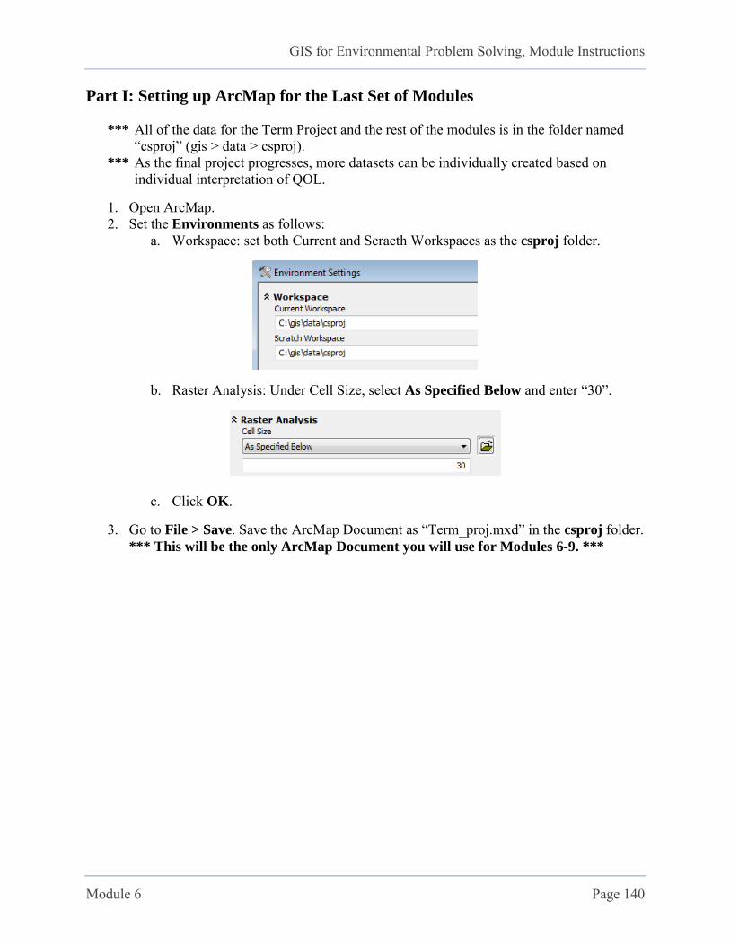
1. Open ArcMap. 2. Set the Environments as follows:
a. Workspace: set both Current and Scracth Workspaces as the csproj folder.
b. Raster Analysis: Under Cell Size, select As Specified Below and enter “30”.
c. Click OK.
3. Go to File > Save. Save the ArcMap Document as “Term_proj.mxd” in the csproj folder. *** This will be the only ArcMap Document you will use for Modules 6-9. ***
GIS for Environmental Problem Solving, Module Instructions
Module 6 Page 141
Part II: Bringing in DEMs (of College Station)
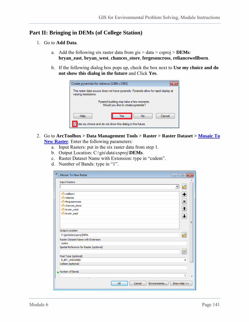
1. Go to Add Data.
a. Add the following six raster data from gis > data > csproj > DEMs: bryan_east, bryan_west, chances_store, fergesoncross, reliancewellborn.
b. If the following dialog box pops up, check the box next to Use my choice and do
not show this dialog in the future and Click Yes.
2. Go to ArcToolbox > Data Management Tools > Raster > Raster Dataset > Mosaic To
New Raster. Enter the following parameters: a. Input Rasters: put in the six raster data from step 1. b. Output Location: C:\gis\data\csproj\DEMs. c. Raster Dataset Name with Extension: type in “csdem”. d. Number of Bands: type in “1”.
GIS for Environmental Problem Solving, Module Instructions
Module 6 Page 142
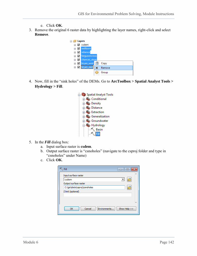
e. Click OK. 3. Remove the original 6 raster data by highlighting the layer names, right-click and select
Remove.
4. Now, fill in the “sink holes” of the DEMs. Go to ArcToolbox > Spatial Analyst Tools >
Hydrology > Fill.
5. In the Fill dialog box: a. Input surface raster is csdem. b. Output surface raster is “csnoholes” (navigate to the csproj folder and type in
“csnoholes” under Name) c. Click OK.
GIS for Environmental Problem Solving, Module Instructions
Module 6 Page 143
6. Remove all other layers except csnoholes. 7. Go to File > Save.
Part III: “Peel off” Layers from Existing Datasets for Analysis
Here, we will create a city boundary layer as a base layer for the City of College Station.
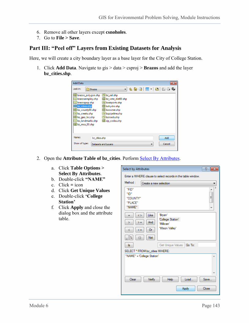
1. Click Add Data. Navigate to gis > data > csproj > Brazos and add the layer bz_cities.shp.
2. Open the Attribute Table of bz_cities. Perform Select By Attributes.
a. Click Table Options >
Select By Attributes. b. Double-click “NAME” c. Click = icon d. Click Get Unique Values e. Double-click ‘College
Station’ f. Click Apply and close the
dialog box and the attribute table.
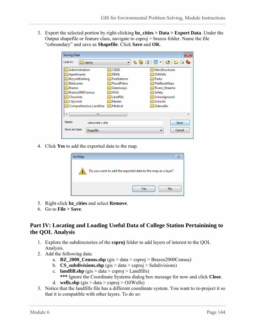
GIS for Environmental Problem Solving, Module Instructions
Module 6 Page 144
3. Export the selected portion by right-clicking bz_cities > Data > Export Data. Under the Output shapefile or feature class, navigate to csproj > brazos folder. Name the file “csboundary” and save as Shapefile. Click Save and OK.
4. Click Yes to add the exported data to the map.
5. Right-click bz_cities and select Remove. 6. Go to File > Save.
Part IV: Locating and Loading Useful Data of College Station Pertainining to
the QOL Analysis
1. Explore the subdirectories of the csproj folder to add layers of interest to the QOL Analysis.
2. Add the following data: a. BZ_2000_Census.shp (gis > data > csproj > Brazos2000Census) b. CS_subdivisions.shp (gis > data > csproj > Subdivisions) c. landfill.shp (gis > data > csproj > Landfills) *** Ignore the Coordinate Systems dialog box message for now and click Close. d. wells.shp (gis > data > csproj > OilWells)
3. Notice that the landfills file has a different coordinate system. You want to re-project it so that it is compatible with other layers. To do so:

GIS for Environmental Problem Solving, Module Instructions
Module 6 Page 145
a. Go to Data Management Tools > Projection and transformation > Feature >
Project. b. In the Projection dialog box,
i. Input Dataset or Feature Class: select landfill ii. Output Dataset or Feature Class: navigate to csproj > Landfills and name
the file “landfill_project” iii. Output Coordinate System: navigate to import a known coordinate system
from other layers, e.g. the wells layer. In the Spatial Reference Properties dialog box,
Click Import Navigate to csproj > OilWells Click once on wells.shp Click Add Click OK
iv. Click OK. The landfill_project layer is now added to the table of contents. 4. Remove the original landfill.shp to avoid confusion. 5. Go to File > Save.
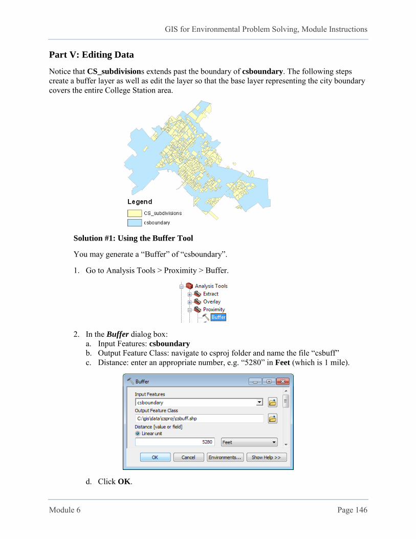
GIS for Environmental Problem Solving, Module Instructions
Module 6 Page 146
Part V: Editing Data
Notice that CS_subdivisions extends past the boundary of csboundary. The following steps create a buffer layer as well as edit the layer so that the base layer representing the city boundary covers the entire College Station area.
Solution #1: Using the Buffer Tool
You may generate a “Buffer” of “csboundary”.
1. Go to Analysis Tools > Proximity > Buffer.
2. In the Buffer dialog box: a. Input Features: csboundary b. Output Feature Class: navigate to csproj folder and name the file “csbuff” c. Distance: enter an appropriate number, e.g. “5280” in Feet (which is 1 mile).
d. Click OK.

GIS for Environmental Problem Solving, Module Instructions
Module 6 Page 147
3. The resulted polygon shapefile csbuff should cover all new subdivisions. To visually see the result, right-click the csbuff layer and select Zoom To Layer. Click and drag the csbuff layer and place the layer under the CS_subdivisions and csboundary layers.
4. Go to File > Save.
Solution #2: Using the Editing Tool (revisit module 4 for additional editing steps)
You may skip this part if you successfully completed Solution #1. Although, it is still a good practice on your editing skills.
You do not need to modify the boundary in too much detail. Try adding a few points that covers the new subdivisions outside the old city
boundary.
1. Click and drag the csboundary layer on top of the CS_subdivisions layer. 2. Go to Editor > Start Editing. 3. Select csboundary as the layer to edit. Click OK (and Continue if a warning
message pops up). 4. Click Editor Tool. 5. Click once on the csboundary layer on the map so that the layer is highlighted in
blue. 6. Hold down the Shift key. Click the CS_subdivisions portion that extends beyond
the csboundary layer, e.g. the yellow portion circled as in the left graphic below.
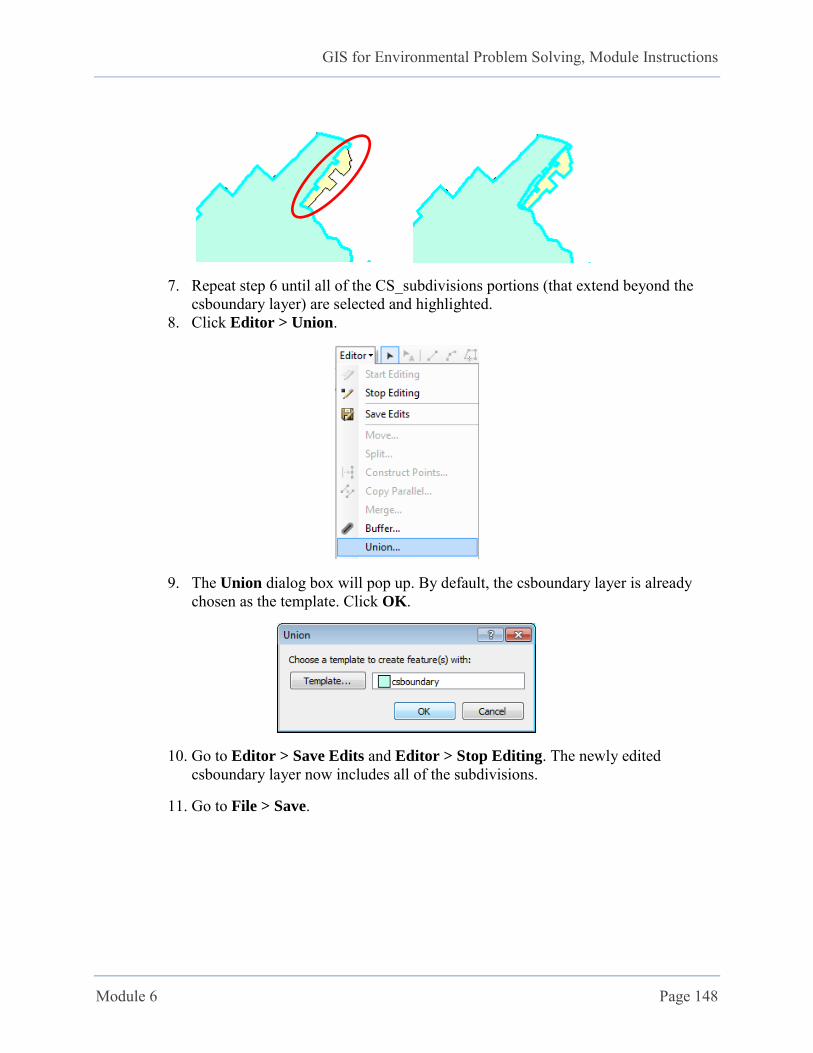
GIS for Environmental Problem Solving, Module Instructions
Module 6 Page 148
7. Repeat step 6 until all of the CS_subdivisions portions (that extend beyond the csboundary layer) are selected and highlighted.
8. Click Editor > Union.
9. The Union dialog box will pop up. By default, the csboundary layer is already chosen as the template. Click OK.
10. Go to Editor > Save Edits and Editor > Stop Editing. The newly edited csboundary layer now includes all of the subdivisions.
11. Go to File > Save.

GIS for Environmental Problem Solving, Module Instructions
Module 6 Page 149
Part VI: Learn to Convert Vector to Raster
**** e. g. csbuff ****
1. Go to ArcToolbox > Conversion Tools > To Raster > Feature to Raster. 2. In the Features to Raster dialog box:
a. Input features: select csbuff from the drop-down menu b. Field: select QOL from the drop-down menu c. Output cell size: enter “30”. d. Output raster: navigate to csproj folder and name the output “CSRaster”. e. Click OK.
3. Right-click the CSRaster layer and select Zoom To Layer to better see the entire layer. 4. Right-click ArcToolbox and select Environments… 5. In the Environment Settings dialog box:
a. Click Processing Extent. b. Under Extent, click the drop-down arrow and select Same as layer CSRaster. c. Click OK.
6. Go to File > Save.
The essences of the above steps are:
To create a project area, i.e., the City of College Station, as the “Base” raster for further computation.
To use the CSRaster to define the geographic extent for other rasters such as distance maps of QOL factors.
As the value of this reference raster (CSRaster) is set to “1”, its multiplication with other rasters will result in the inherited value of the operand raster.
GIS for Environmental Problem Solving, Module Instructions
Module 7 Page 150
Module 7: Support tools, Data Assembly, and Preliminary
Processing
Learning Objectives:
Basics of raster data manipulation
Flow directions and flow paths
Distance functions
Geo-statistical analysis
Normalizing data
Learning Materials:
Before going through this module and working with ArcGIS, please review the following presentations:
Key Processes QOL_Assessment Final Project Requirements
Sample Final Project 1
Sample Final Project 2
Sample Final Project 3
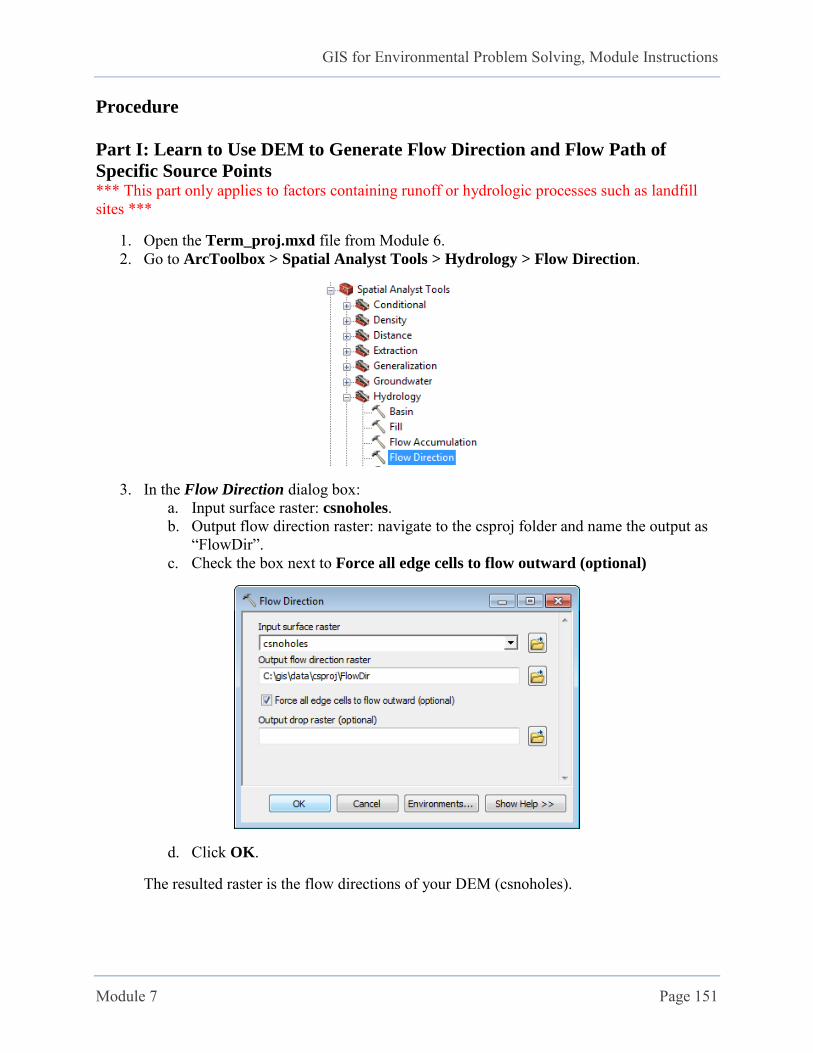
GIS for Environmental Problem Solving, Module Instructions
Module 7 Page 151
Procedure
Part I: Learn to Use DEM to Generate Flow Direction and Flow Path of
Specific Source Points *** This part only applies to factors containing runoff or hydrologic processes such as landfill sites ***
1. Open the Term_proj.mxd file from Module 6. 2. Go to ArcToolbox > Spatial Analyst Tools > Hydrology > Flow Direction.
3. In the Flow Direction dialog box: a. Input surface raster: csnoholes. b. Output flow direction raster: navigate to the csproj folder and name the output as
“FlowDir”. c. Check the box next to Force all edge cells to flow outward (optional)
d. Click OK.
The resulted raster is the flow directions of your DEM (csnoholes).
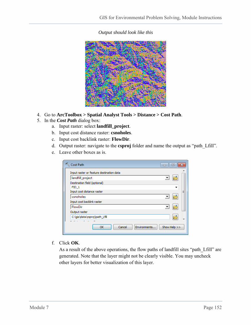
GIS for Environmental Problem Solving, Module Instructions
Module 7 Page 152
Output should look like this
4. Go to ArcToolbox > Spatial Analyst Tools > Distance > Cost Path. 5. In the Cost Path dialog box:
a. Input raster: select landfill_project. b. Input cost distance raster: csnoholes. c. Input cost backlink raster: FlowDir. d. Output raster: navigate to the csproj folder and name the output as “path_Lfill”.
e. Leave other boxes as is.
f. Click OK. As a result of the above operations, the flow paths of landfill sites “path_Lfill” are generated. Note that the layer might not be clearly visible. You may uncheck other layers for better visualization of this layer.
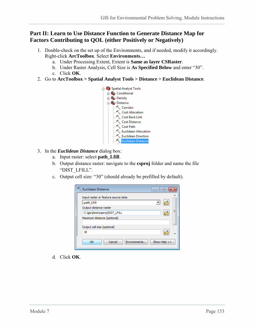
GIS for Environmental Problem Solving, Module Instructions
Module 7 Page 153
Part II: Learn to Use Distance Function to Generate Distance Map for
Factors Contributing to QOL (either Positively or Negatively)
1. Double-check on the set up of the Environments, and if needed, modify it accordingly. Right-click ArcToolbox. Select Environments…
a. Under Processing Extent, Extent is Same as layer CSRaster. b. Under Raster Analysis, Cell Size is As Specified Below and enter “30”. c. Click OK.
2. Go to ArcToolbox > Spatial Analyst Tools > Distance > Euclidean Distance.
3. In the Euclidean Distance dialog box: a. Input raster: select path_Lfill. b. Output distance raster: navigate to the csproj folder and name the file
“DIST_LFILL”. c. Output cell size: “30” (should already be prefilled by default).
d. Click OK.
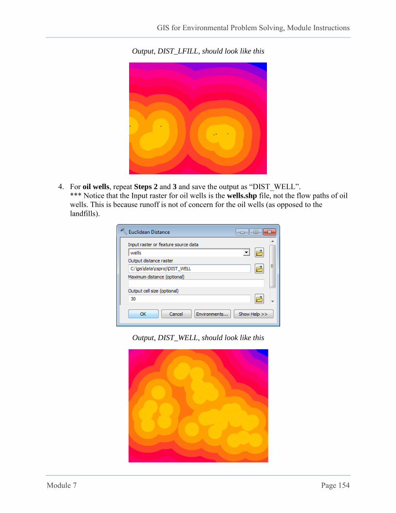
GIS for Environmental Problem Solving, Module Instructions
Module 7 Page 154
Output, DIST_LFILL, should look like this
4. For oil wells, repeat Steps 2 and 3 and save the output as “DIST_WELL”. *** Notice that the Input raster for oil wells is the wells.shp file, not the flow paths of oil wells. This is because runoff is not of concern for the oil wells (as opposed to the landfills).
Output, DIST_WELL, should look like this
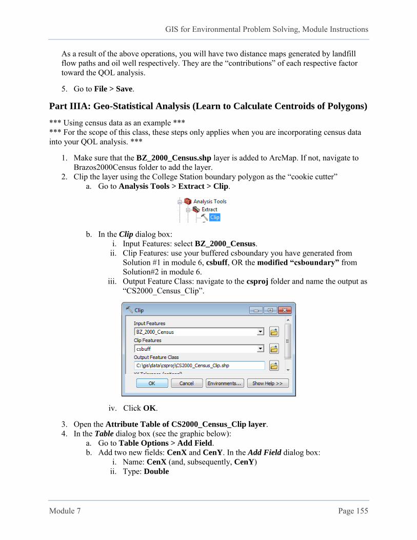
GIS for Environmental Problem Solving, Module Instructions
Module 7 Page 155
As a result of the above operations, you will have two distance maps generated by landfill flow paths and oil well respectively. They are the “contributions” of each respective factor toward the QOL analysis.
5. Go to File > Save.
Part IIIA: Geo-Statistical Analysis (Learn to Calculate Centroids of Polygons)
*** Using census data as an example *** *** For the scope of this class, these steps only applies when you are incorporating census data into your QOL analysis. ***
1. Make sure that the BZ_2000_Census.shp layer is added to ArcMap. If not, navigate to Brazos2000Census folder to add the layer.
2. Clip the layer using the College Station boundary polygon as the “cookie cutter” a. Go to Analysis Tools > Extract > Clip.
b. In the Clip dialog box: i. Input Features: select BZ_2000_Census.
ii. Clip Features: use your buffered csboundary you have generated from Solution #1 in module 6, csbuff, OR the modified “csboundary” from Solution#2 in module 6.
iii. Output Feature Class: navigate to the csproj folder and name the output as “CS2000_Census_Clip”.
iv. Click OK.
3. Open the Attribute Table of CS2000_Census_Clip layer. 4. In the Table dialog box (see the graphic below):
a. Go to Table Options > Add Field. b. Add two new fields: CenX and CenY. In the Add Field dialog box:
i. Name: CenX (and, subsequently, CenY) ii. Type: Double
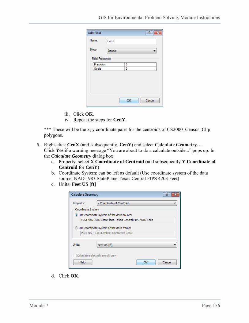
GIS for Environmental Problem Solving, Module Instructions
Module 7 Page 156
iii. Click OK. iv. Repeat the steps for CenY.
*** These will be the x, y coordinate pairs for the centroids of CS2000_Census_Clip polygons.
5. Right-click CenX (and, subsequently, CenY) and select Calculate Geometry… Click Yes if a warning message “You are about to do a calculate outside...” pops up. In
the Calculate Geometry dialog box: a. Property: select X Coordinate of Centroid (and subsequently Y Coordinate of
Centroid for CenY) b. Coordinate System: can be left as default (Use coordinate system of the data
source: NAD 1983 StatePlane Texas Central FIPS 4203 Feet) c. Units: Feet US [ft]
d. Click OK.
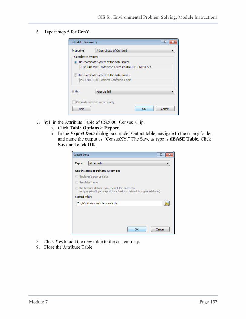
GIS for Environmental Problem Solving, Module Instructions
Module 7 Page 157
6. Repeat step 5 for CenY.
7. Still in the Attribute Table of CS2000_Census_Clip. a. Click Table Options > Export. b. In the Export Data dialog box, under Output table, navigate to the csproj folder
and name the output as “CensusXY.” The Save as type is dBASE Table. Click Save and click OK.
8. Click Yes to add the new table to the current map. 9. Close the Attribute Table.
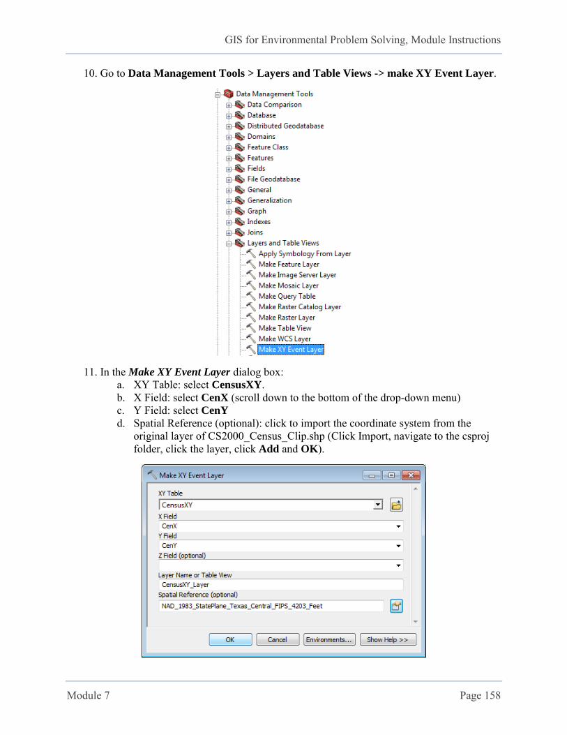
GIS for Environmental Problem Solving, Module Instructions
Module 7 Page 158
10. Go to Data Management Tools > Layers and Table Views -> make XY Event Layer.
11. In the Make XY Event Layer dialog box: a. XY Table: select CensusXY. b. X Field: select CenX (scroll down to the bottom of the drop-down menu) c. Y Field: select CenY d. Spatial Reference (optional): click to import the coordinate system from the
original layer of CS2000_Census_Clip.shp (Click Import, navigate to the csproj folder, click the layer, click Add and OK).
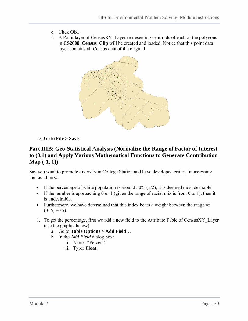
GIS for Environmental Problem Solving, Module Instructions
Module 7 Page 159
e. Click OK. f. A Point layer of CensusXY_Layer representing centroids of each of the polygons
in CS2000_Census_Clip will be created and loaded. Notice that this point data layer contains all Census data of the original.
12. Go to File > Save.
Part IIIB: Geo-Statistical Analysis (Normalize the Range of Factor of Interest
to (0,1) and Apply Various Mathematical Functions to Generate Contribution
Map (-1, 1))
Say you want to promote diversity in College Station and have developed criteria in assessing the racial mix:
If the percentage of white population is around 50% (1/2), it is deemed most desirable. If the number is approaching 0 or 1 (given the range of racial mix is from 0 to 1), then it
is undesirable. Furthermore, we have determined that this index bears a weight between the range of
(-0.5, +0.5).
1. To get the percentage, first we add a new field to the Attribute Table of CensusXY_Layer (see the graphic below).
a. Go to Table Options > Add Field… b. In the Add Field dialog box:
i. Name: “Percent” ii. Type: Float
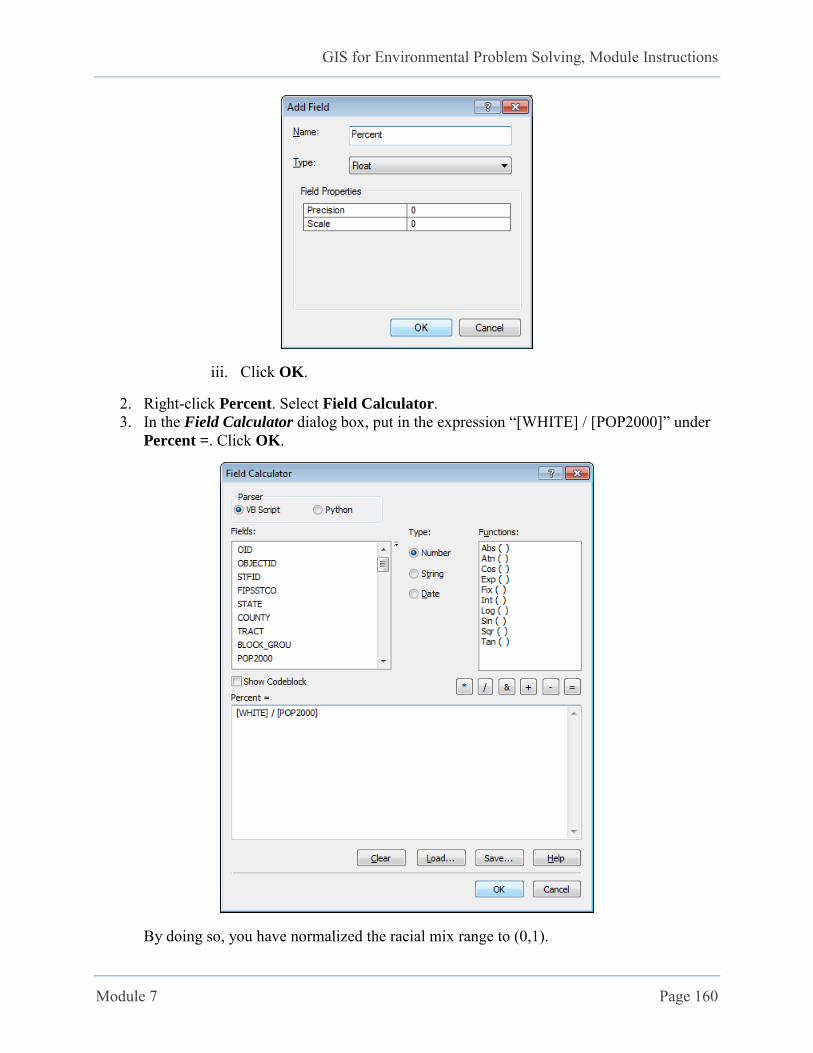
GIS for Environmental Problem Solving, Module Instructions
Module 7 Page 160
iii. Click OK.
2. Right-click Percent. Select Field Calculator. 3. In the Field Calculator dialog box, put in the expression “[WHITE] / [POP2000]” under
Percent =. Click OK.
By doing so, you have normalized the racial mix range to (0,1).

GIS for Environmental Problem Solving, Module Instructions
Module 7 Page 161
4. Next we can use a parabolic function to calculate the contribution based on Percent. Assume x is Percent. E is the expectation value of 0.5. F(x) is the contribution of Percent. Then:
𝐹(𝑥) =
{
1 −
(𝑥 − 𝐸)2
(1 − 𝐸)2, 𝐸 ≤ 𝑥 ≤ 1
1 −(𝑥 − 𝐸)2
𝐸2, 0 ≤ 𝑥 < 𝐸
5. Still in the Attribute Table of CensusXY_Layer, add another new field, N1 a. Go to Table Options > Add Field… b. In the Add Field dialog box:
i. Name: “N1” ii. Type: Float
6. Right-click N1 and select Field Calculator. 7. In the Field Calculator dialog box:
a. Check the box next to Show Codeblock. b. Under Pre-Logic Script Code, put in the following expression
Dim y If [Percent] >= 0.5 Then y=1-([Percent]-0.5)*([Percent]-0.5)/0.25 else y=1-([Percent]-0.5)*([Percent]-0.5)/0.25 end if *** Note that the above script is a generalized form. When the expectation value
is 0.5, then the script actually collapses into one equation (since E = 0.5 and 1-E = 0.5).
c. Under N1 =, enter “y”
(See the graphic below)
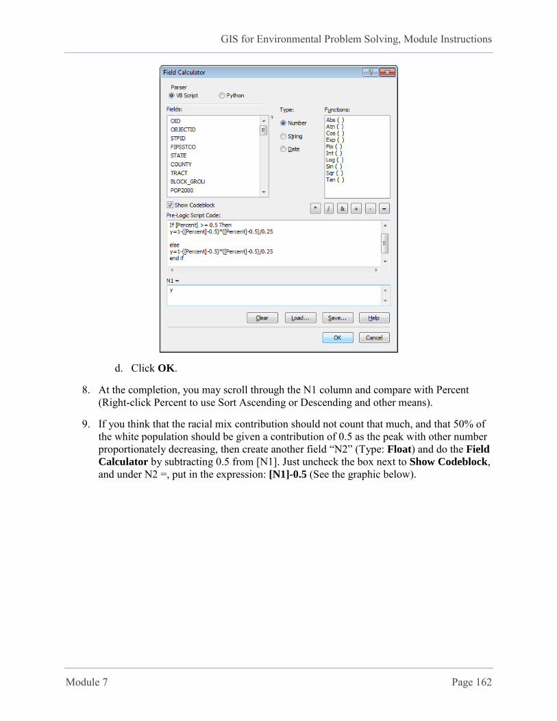
GIS for Environmental Problem Solving, Module Instructions
Module 7 Page 162
d. Click OK.
8. At the completion, you may scroll through the N1 column and compare with Percent (Right-click Percent to use Sort Ascending or Descending and other means).
9. If you think that the racial mix contribution should not count that much, and that 50% of the white population should be given a contribution of 0.5 as the peak with other number proportionately decreasing, then create another field “N2” (Type: Float) and do the Field
Calculator by subtracting 0.5 from [N1]. Just uncheck the box next to Show Codeblock, and under N2 =, put in the expression: [N1]-0.5 (See the graphic below).

GIS for Environmental Problem Solving, Module Instructions
Module 7 Page 163
10. Click OK and close the Attribute Table. 11. Go to File > Save.
Part IIIC: Geo-Statistical Analysis (Conduct Geostatisictal Analysis and
Convert the Results Back to Raster Distance Map)
*** Using the CensusXY_Layer as an example. ***
1. Click Geostatisical Analyst Toolbar. If this is not an option, then right-click the gray area in the menu bar and select
Geostatistical Analyst.
2. Choose Geostatistical Wizard.
3. In the Geostatistical Wizard dialog box: a. By default, the Inverse Distance Weighting will be chosen as the method. We
can start with this method. So, leave the selection as is.
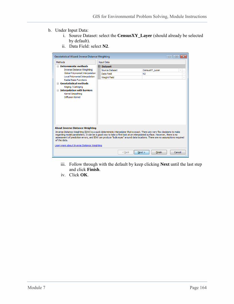
GIS for Environmental Problem Solving, Module Instructions
Module 7 Page 164
b. Under Input Data: i. Source Dataset: select the CensusXY_Layer (should already be selected
by default). ii. Data Field: select N2.
iii. Follow through with the default by keep clicking Next until the last step and click Finish.
iv. Click OK.
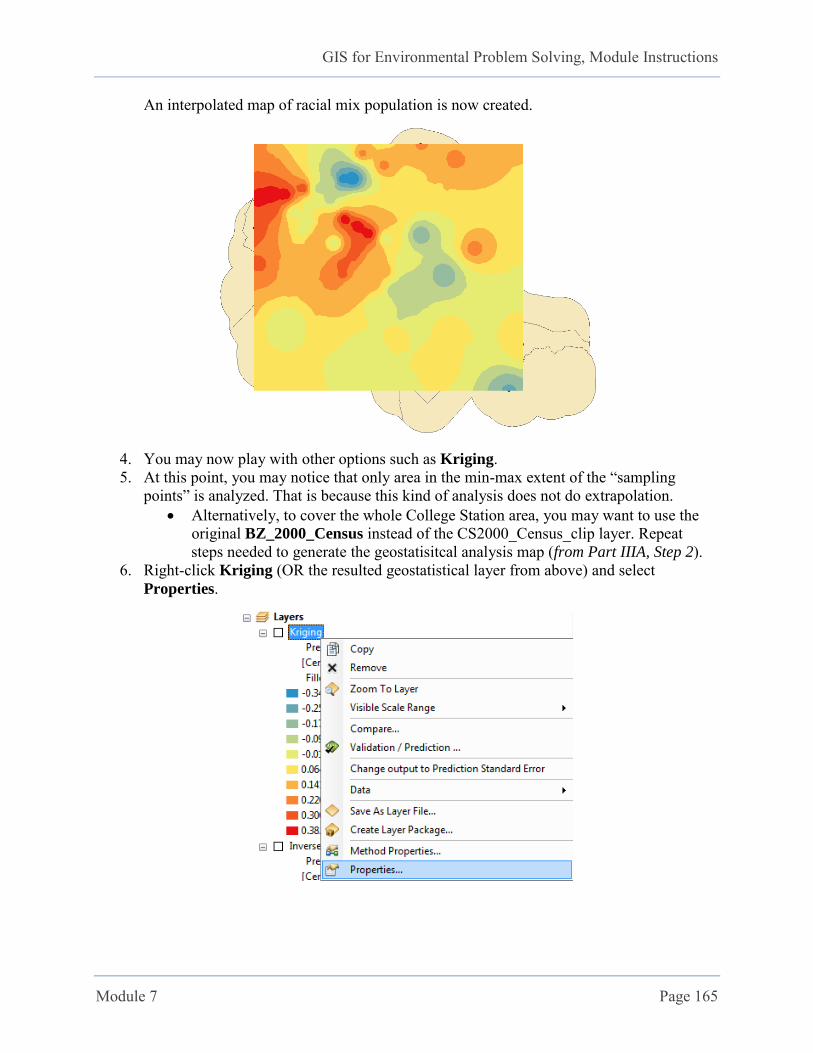
GIS for Environmental Problem Solving, Module Instructions
Module 7 Page 165
An interpolated map of racial mix population is now created.
4. You may now play with other options such as Kriging. 5. At this point, you may notice that only area in the min-max extent of the “sampling
points” is analyzed. That is because this kind of analysis does not do extrapolation. Alternatively, to cover the whole College Station area, you may want to use the
original BZ_2000_Census instead of the CS2000_Census_clip layer. Repeat steps needed to generate the geostatisitcal analysis map (from Part IIIA, Step 2).
6. Right-click Kriging (OR the resulted geostatistical layer from above) and select Properties.
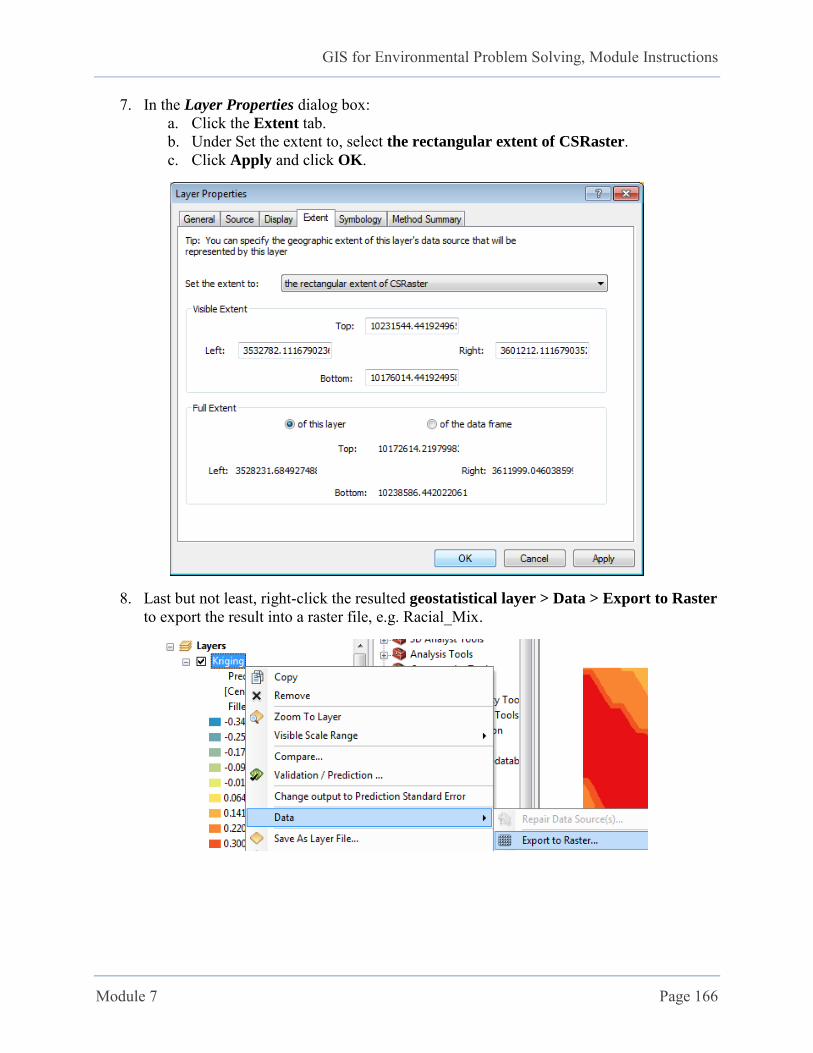
GIS for Environmental Problem Solving, Module Instructions
Module 7 Page 166
7. In the Layer Properties dialog box: a. Click the Extent tab. b. Under Set the extent to, select the rectangular extent of CSRaster. c. Click Apply and click OK.
8. Last but not least, right-click the resulted geostatistical layer > Data > Export to Raster
to export the result into a raster file, e.g. Racial_Mix.

GIS for Environmental Problem Solving, Module Instructions
Module 7 Page 167
9. In the GA Layer To Grid dialog box: a. Input geostatistical layer: select Kriging. b. Output surface raster: navigate to the csproj folder and name the file
“Racial_Mix”. c. Output cell size: enter “30”. d. Leave other parameters as is.
e. Click OK.
This raster is ready for incorporation into the Emycin algorithm for calculating the contribution of racial mix to QOL in the ensuing steps.
10. Go to File > Save.
The Racial_Mix layer (from Kriging and N2 Data Field) should look similar to this:
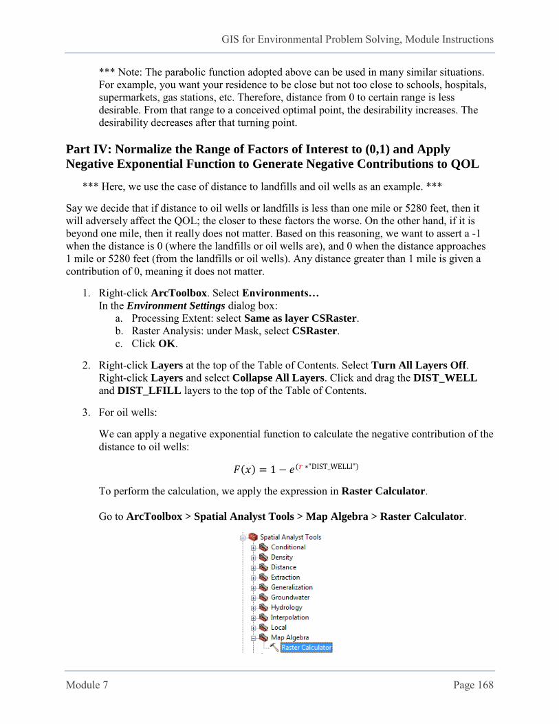
GIS for Environmental Problem Solving, Module Instructions
Module 7 Page 168
*** Note: The parabolic function adopted above can be used in many similar situations. For example, you want your residence to be close but not too close to schools, hospitals, supermarkets, gas stations, etc. Therefore, distance from 0 to certain range is less desirable. From that range to a conceived optimal point, the desirability increases. The
desirability decreases after that turning point.
Part IV: Normalize the Range of Factors of Interest to (0,1) and Apply
Negative Exponential Function to Generate Negative Contributions to QOL
*** Here, we use the case of distance to landfills and oil wells as an example. ***
Say we decide that if distance to oil wells or landfills is less than one mile or 5280 feet, then it will adversely affect the QOL; the closer to these factors the worse. On the other hand, if it is beyond one mile, then it really does not matter. Based on this reasoning, we want to assert a -1 when the distance is 0 (where the landfills or oil wells are), and 0 when the distance approaches 1 mile or 5280 feet (from the landfills or oil wells). Any distance greater than 1 mile is given a contribution of 0, meaning it does not matter.
1. Right-click ArcToolbox. Select Environments… In the Environment Settings dialog box:
a. Processing Extent: select Same as layer CSRaster. b. Raster Analysis: under Mask, select CSRaster. c. Click OK.
2. Right-click Layers at the top of the Table of Contents. Select Turn All Layers Off. Right-click Layers and select Collapse All Layers. Click and drag the DIST_WELL and DIST_LFILL layers to the top of the Table of Contents.
3. For oil wells:
We can apply a negative exponential function to calculate the negative contribution of the distance to oil wells:
𝐹(𝑥) = 1 − 𝑒(𝑟 ∗"DIST_WELLl")
To perform the calculation, we apply the expression in Raster Calculator. Go to ArcToolbox > Spatial Analyst Tools > Map Algebra > Raster Calculator.

GIS for Environmental Problem Solving, Module Instructions
Module 7 Page 169
4. In the Raster Calculator dialog box, enter the following expression using the steps below.
Con("DIST_WELL" < 5280, - Exp( - 1 * ("DIST_WELL" + 1) / 5280),0)
The raster calculator is very sensitive to spaces and expressions. Ensure that you maximize the buttons available on the calculator. Here are the steps to enter the expression:
a. Double-click Con under Conditional b. Double-click DIST_WELL under Layers and variables c. Click the < button d. Using the raster calculator buttons, click 5280 e. Click once behind the comma in the expression box so that the cursor shows up,
blinking between , and )
f. Click the button - g. Double-click Exp under Math h. Click the button - i. Click the button 1 j. Click the button * k. Click the button ( l. Double-click DIST_WELL m. Click the button + n. Click the button 1 o. Click once at the expression in between the two close brackets p. Click the button / q. Using the raster calculator buttons, click 5280 r. Click once at the end of the expression behind the close bracket s. Press , on your keyboard t. Click the button 0 u. Click the button )
*** See the graphic of how the expression should be shown below. v. Drag your mouse to select and highlight the entire expression. Right-click the
highlighted expression and select Copy. Paste and save the expression in a Word
Document. This way you have a working equation that can be modified and use with the next factor contributing to QOL, e.g. landfills.
w. Under Output raster, navigate to the csproj folder and name the output “Wells”
CLICK HERE

GIS for Environmental Problem Solving, Module Instructions
Module 7 Page 170
x. Click OK.
The above algebra sets all cells with original distance values to 0 and those within 5280 feet to (-1, 0) and creates a new normalized layer (in raster) “Wells.” In other words,
being closet to the wells will return the normalized values closet to -1, while being farther away from the wells, the normalized values start to increase and approach 0 at the farthest, i.e., 5280 feet or 1 mile in this case.
You may click the color ramp of the layer and modify it to your preference.
The Wells layer as a result of the normalization step above
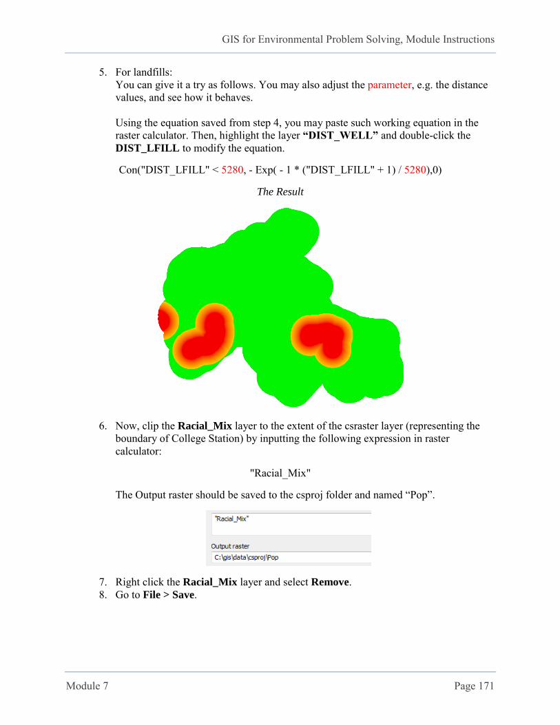
GIS for Environmental Problem Solving, Module Instructions
Module 7 Page 171
5. For landfills: You can give it a try as follows. You may also adjust the parameter, e.g. the distance values, and see how it behaves. Using the equation saved from step 4, you may paste such working equation in the raster calculator. Then, highlight the layer “DIST_WELL” and double-click the DIST_LFILL to modify the equation.
Con("DIST_LFILL" < 5280, - Exp( - 1 * ("DIST_LFILL" + 1) / 5280),0)
The Result
6. Now, clip the Racial_Mix layer to the extent of the csraster layer (representing the boundary of College Station) by inputting the following expression in raster calculator:
"Racial_Mix"
The Output raster should be saved to the csproj folder and named “Pop”.
7. Right click the Racial_Mix layer and select Remove. 8. Go to File > Save.
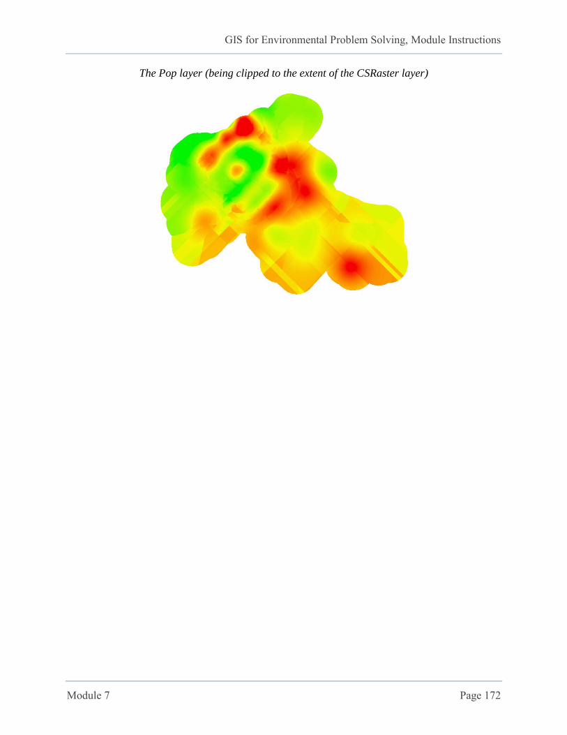
GIS for Environmental Problem Solving, Module Instructions
Module 7 Page 172
The Pop layer (being clipped to the extent of the CSRaster layer)
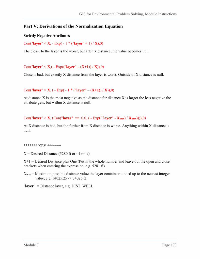
GIS for Environmental Problem Solving, Module Instructions
Module 7 Page 173
Part V: Derivations of the Normalization Equation
Strictly Negative Attributes
Con("layer" < X, - Exp( - 1 * ("layer" + 1) / X),0)
The closer to the layer is the worst, but after X distance, the value becomes null.
Con("layer" < X,( - Exp(("layer" – (X+1)) / X)),0)
Close is bad, but exactly X distance from the layer is worst. Outside of X distance is null.
Con("layer" > X, ( - Exp( - 1 * ("layer" – (X+1)) / X)),0)
At distance X is the most negative as the distance for distance X is larger the less negative the attribute gets, but within X distance is null.
Con("layer" > X, (Con("layer" == 0,0, ( - Exp(("layer" - Xmax) / Xmax)))),0)
At X distance is bad, but the further from X distance is worse. Anything within X distance is null.
******* KEY *******
X = Desired Distance (5280 ft or ~1 mile)
X+1 = Desired Distance plus One (Put in the whole number and leave out the open and close brackets when entering the expression, e.g. 5281 ft)
Xmax = Maximum possible distance value the layer contains rounded up to the nearest integer value, e.g. 34025.25 -> 34026 ft
"layer" = Distance layer, e.g. DIST_WELL
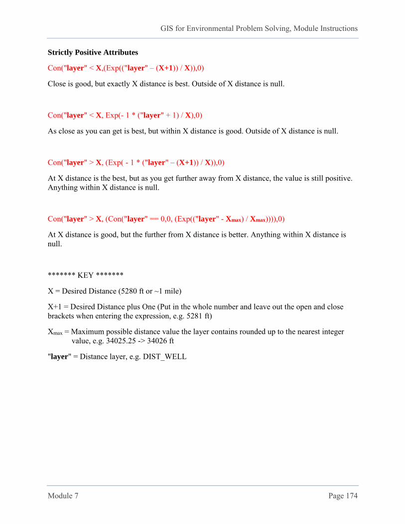
GIS for Environmental Problem Solving, Module Instructions
Module 7 Page 174
Strictly Positive Attributes
Con("layer" < X,(Exp(("layer" – (X+1)) / X)),0)
Close is good, but exactly X distance is best. Outside of X distance is null.
Con("layer" < X, Exp(- 1 * ("layer" + 1) / X),0)
As close as you can get is best, but within X distance is good. Outside of X distance is null.
Con("layer" > X, (Exp( - 1 * ("layer" – (X+1)) / X)),0)
At X distance is the best, but as you get further away from X distance, the value is still positive. Anything within X distance is null.
Con("layer" > X, (Con("layer" == 0,0, (Exp(("layer" - Xmax) / Xmax)))),0)
At X distance is good, but the further from X distance is better. Anything within X distance is null.
******* KEY *******
X = Desired Distance (5280 ft or ~1 mile)
X+1 = Desired Distance plus One (Put in the whole number and leave out the open and close brackets when entering the expression, e.g. 5281 ft)
Xmax = Maximum possible distance value the layer contains rounded up to the nearest integer value, e.g. 34025.25 -> 34026 ft
"layer" = Distance layer, e.g. DIST_WELL
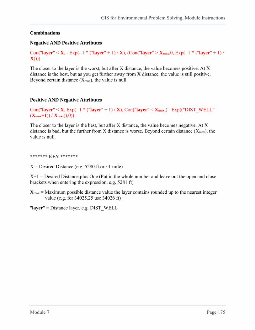
GIS for Environmental Problem Solving, Module Instructions
Module 7 Page 175
Combinations
Negative AND Positive Attributes
Con("layer" < X, - Exp(- 1 * ("layer" + 1) / X), (Con("layer" > Xmax,0, Exp(- 1 * ("layer" + 1) / X))))
The closer to the layer is the worst, but after X distance, the value becomes positive. At X distance is the best, but as you get further away from X distance, the value is still positive. Beyond certain distance (Xmax), the value is null.
Positive AND Negative Attributes
Con("layer" < X, Exp(- 1 * ("layer" + 1) / X), Con("layer" < Xmax,( - Exp(("DIST_WELL" - (Xmax+1)) / Xmax)),0))
The closer to the layer is the best, but after X distance, the value becomes negative. At X distance is bad, but the further from X distance is worse. Beyond certain distance (Xmax), the value is null.
******* KEY *******
X = Desired Distance (e.g. 5280 ft or ~1 mile)
X+1 = Desired Distance plus One (Put in the whole number and leave out the open and close brackets when entering the expression, e.g. 5281 ft)
Xmax = Maximum possible distance value the layer contains rounded up to the nearest integer value (e.g. for 34025.25 use 34026 ft)
"layer" = Distance layer, e.g. DIST_WELL
GIS for Environmental Problem Solving, Module Instructions
Module 8 Page 176
Module 8: Map Algebra and Emycin Equation Learning Objectives:
Using Map Algebra in the Raster Calculator Encoding the fuzzy logic algorithm of Emycin as Map Algebra for use in the Raster
Calculator
Learning Materials:
Before going through this module and working with ArcGIS, please review the following presentations:
Emycin in a Spatial Scale Final Project Requirements
Sample Final Project 1
Sample Final Project 2
Sample Final Project 3
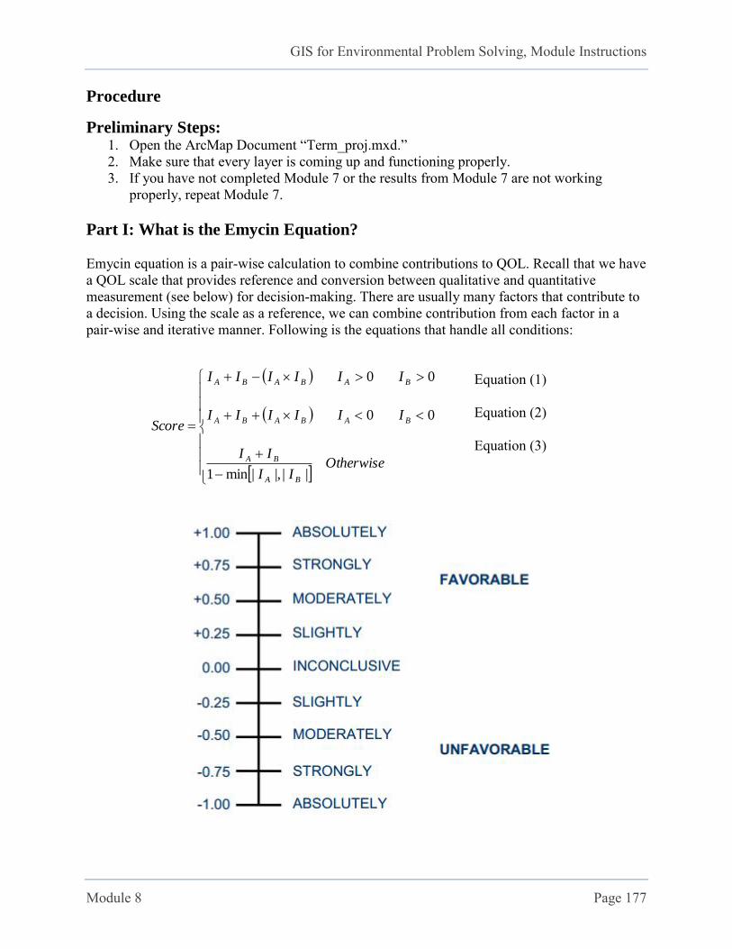
GIS for Environmental Problem Solving, Module Instructions
Module 8 Page 177
Procedure
Preliminary Steps: 1. Open the ArcMap Document “Term_proj.mxd.” 2. Make sure that every layer is coming up and functioning properly. 3. If you have not completed Module 7 or the results from Module 7 are not working
properly, repeat Module 7. Part I: What is the Emycin Equation?
Emycin equation is a pair-wise calculation to combine contributions to QOL. Recall that we have a QOL scale that provides reference and conversion between qualitative and quantitative measurement (see below) for decision-making. There are usually many factors that contribute to a decision. Using the scale as a reference, we can combine contribution from each factor in a pair-wise and iterative manner. Following is the equations that handle all conditions:
Equation (1)
Equation (2) Equation (3)
OtherwiseII
II
IIIIII
IIIIII
Score
BA
BA
BABABA
BABABA
|||,|min1
00
00

GIS for Environmental Problem Solving, Module Instructions
Module 8 Page 178
A visualization of how Emycin equation works
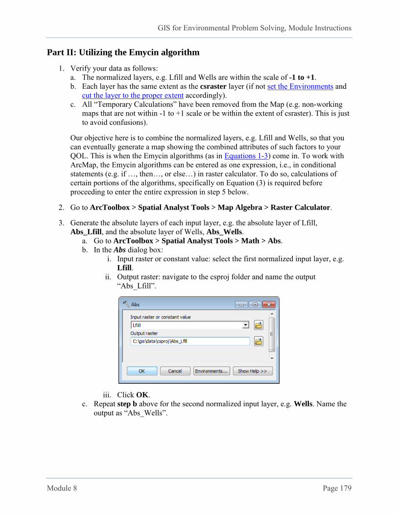
GIS for Environmental Problem Solving, Module Instructions
Module 8 Page 179
Part II: Utilizing the Emycin algorithm
1. Verify your data as follows: a. The normalized layers, e.g. Lfill and Wells are within the scale of -1 to +1. b. Each layer has the same extent as the csraster layer (if not set the Environments and
cut the layer to the proper extent accordingly). c. All “Temporary Calculations” have been removed from the Map (e.g. non-working
maps that are not within -1 to +1 scale or be within the extent of csraster). This is just to avoid confusions).
Our objective here is to combine the normalized layers, e.g. Lfill and Wells, so that you can eventually generate a map showing the combined attributes of such factors to your QOL. This is when the Emycin algorithms (as in Equations 1-3) come in. To work with ArcMap, the Emycin algorithms can be entered as one expression, i.e., in conditional statements (e.g. if …, then…, or else…) in raster calculator. To do so, calculations of
certain portions of the algorithms, specifically on Equation (3) is required before proceeding to enter the entire expression in step 5 below.
2. Go to ArcToolbox > Spatial Analyst Tools > Map Algebra > Raster Calculator.
3. Generate the absolute layers of each input layer, e.g. the absolute layer of Lfill, Abs_Lfill, and the absolute layer of Wells, Abs_Wells.
a. Go to ArcToolbox > Spatial Analyst Tools > Math > Abs. b. In the Abs dialog box:
i. Input raster or constant value: select the first normalized input layer, e.g. Lfill.
ii. Output raster: navigate to the csproj folder and name the output “Abs_Lfill”.
iii. Click OK. c. Repeat step b above for the second normalized input layer, e.g. Wells. Name the
output as “Abs_Wells”.
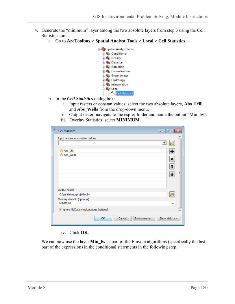
GIS for Environmental Problem Solving, Module Instructions
Module 8 Page 180
4. Generate the “minimum” layer among the two absolute layers from step 3 using the Cell Statistics tool.
a. Go to ArcToolbox > Spatial Analyst Tools > Local > Cell Statistics.
b. In the Cell Statistics dialog box:
i. Input rasters or constan values: select the two absolute layers, Abs_Lfill and Abs_Wells from the drop-down menu.
ii. Output raster: navigate to the csproj folder and name the output “Min_lw”. iii. Overlay Statistics: select MINIMUM.
iv. Click OK.
We can now use the layer Min_lw as part of the Emycin algorithms (specifically the last part of the expression) in the conditional statements in the following step.
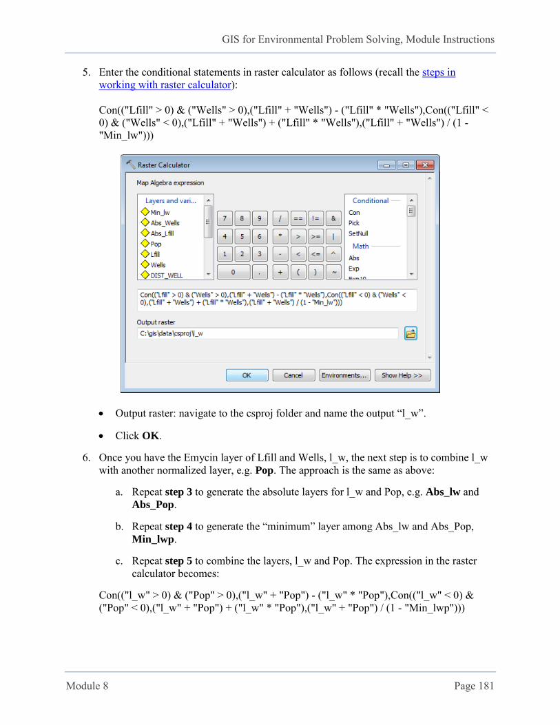
GIS for Environmental Problem Solving, Module Instructions
Module 8 Page 181
5. Enter the conditional statements in raster calculator as follows (recall the steps in working with raster calculator): Con(("Lfill" > 0) & ("Wells" > 0),("Lfill" + "Wells") - ("Lfill" * "Wells"),Con(("Lfill" < 0) & ("Wells" < 0),("Lfill" + "Wells") + ("Lfill" * "Wells"),("Lfill" + "Wells") / (1 - "Min_lw")))
Output raster: navigate to the csproj folder and name the output “l_w”.
Click OK.
6. Once you have the Emycin layer of Lfill and Wells, l_w, the next step is to combine l_w with another normalized layer, e.g. Pop. The approach is the same as above:
a. Repeat step 3 to generate the absolute layers for l_w and Pop, e.g. Abs_lw and Abs_Pop.
b. Repeat step 4 to generate the “minimum” layer among Abs_lw and Abs_Pop, Min_lwp.
c. Repeat step 5 to combine the layers, l_w and Pop. The expression in the raster calculator becomes:
Con(("l_w" > 0) & ("Pop" > 0),("l_w" + "Pop") - ("l_w" * "Pop"),Con(("l_w" < 0) & ("Pop" < 0),("l_w" + "Pop") + ("l_w" * "Pop"),("l_w" + "Pop") / (1 - "Min_lwp")))

GIS for Environmental Problem Solving, Module Instructions
Module 8 Page 182
Output raster: navigate to the csproj folder and name the output “lw_p”. Click OK.
The Emycin layer, lw_p, from the steps above
7. Notice that the expressions in steps 5 and 6 are the same. Only the input layers are different (Lfill and Wells in step 5 AND l_w and Pop in step 6). The expression simply combines the values from two normalized input layers while still maintaining the output values within the scale of -1 to +1.

GIS for Environmental Problem Solving, Module Instructions
Module 8 Page 183
In the Final Project, you may begin to assimilate your own data, i.e., other factors pertaining to QOL. Recall that you must first generate a distance layer of each factor. Then, normalize the distance layer so that the values are bounded within the scale of -1 to +1. Then, keep adding the normalized layer using Emycin algorithms (as in step 6) until all factors are combined. Make sure that once all factors are combined, your final layer still has the value within -1 to +1 scale.
GIS for Environmental Problem Solving, Module Instructions
Module 9 Page 184
Module 9: Creation of a Final Report for QOL Analysis
Learning Objectives:
Iterative process of combining indices by the use of Map Algebra/Emycin in the Raster Calculator
Manipulation of the final result, including its conversion from raster to vector Spatial overlays and queries for the depictions of locale-specific and city-wide QOL
indicators
Design of map-based documents
Integration of spatial, graphic, and attribute data into a cohesive reporting document
Learning Materials:
Before going through this module and working with ArcGIS, please review the following presentations:
Previous Learning Materials Final Project Requirements
Sample Final Project 1
Sample Final Project 2
Sample Final Project 3

GIS for Environmental Problem Solving, Module Instructions
Module 9 Page 185
Part I: Convert the QOL Raster Back to Vector for Overlay with Subdivisions
for the Location-Specific QOL Indicator
After iterations of Emycin (all of QOL factors combined), you can now convert the QOL raster back to vector for overlaying with subdivisions for the location-specific QOL indicator. The following steps illustrate only the 3 QOL factors (landfills, oil wells, and racial mix) combined. In your Final Project, these steps should be performed once you combine all QOL factors and area ready to identify the final QOL indices.
1. First, you want to multiply the QOL raster, e.g. lw_p by 1000 in Raster Calculator. Put in the following expression:
Int("lw_p" * 1000)
Output raster: navigate to the csproj folder and name the output “New_lw_p”. Click OK.
New_lw_p after being converted to the scale of -1000 to +1000
lw_p is a floating raster. This step converts the floating raster into integer. While the overall range is still bounded between -1 and +1, by multiplying the values by 1000, the new range is bounded between -1000 and +1000. Only a raster that has integer values is best represented in a vector format. This step was done to make the final result easier to visualize and analyze.
2. Convert New_lw_p into feature: a. Go to ArcToolbox > Conversion Tools > From Raster > Raster to
Polygon.
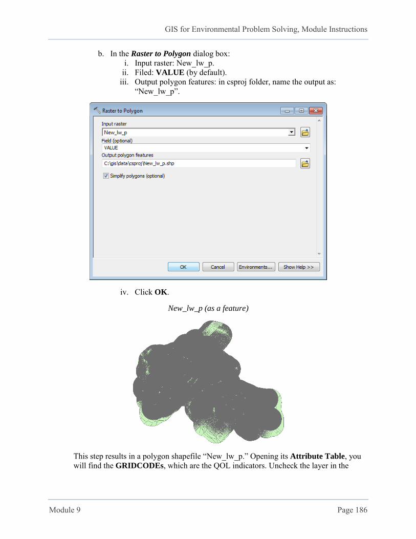
GIS for Environmental Problem Solving, Module Instructions
Module 9 Page 186
b. In the Raster to Polygon dialog box: i. Input raster: New_lw_p.
ii. Filed: VALUE (by default). iii. Output polygon features: in csproj folder, name the output as:
“New_lw_p”.
iv. Click OK.
New_lw_p (as a feature)
This step results in a polygon shapefile “New_lw_p.” Opening its Attribute Table, you will find the GRIDCODEs, which are the QOL indicators. Uncheck the layer in the
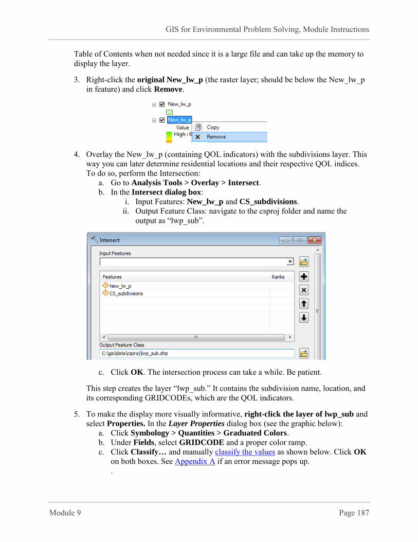
GIS for Environmental Problem Solving, Module Instructions
Module 9 Page 187
Table of Contents when not needed since it is a large file and can take up the memory to display the layer.
3. Right-click the original New_lw_p (the raster layer; should be below the New_lw_p in feature) and click Remove.
4. Overlay the New_lw_p (containing QOL indicators) with the subdivisions layer. This way you can later determine residential locations and their respective QOL indices. To do so, perform the Intersection:
a. Go to Analysis Tools > Overlay > Intersect. b. In the Intersect dialog box:
i. Input Features: New_lw_p and CS_subdivisions. ii. Output Feature Class: navigate to the csproj folder and name the
output as “lwp_sub”.
c. Click OK. The intersection process can take a while. Be patient.
This step creates the layer “lwp_sub.” It contains the subdivision name, location, and its corresponding GRIDCODEs, which are the QOL indicators.
5. To make the display more visually informative, right-click the layer of lwp_sub and select Properties. In the Layer Properties dialog box (see the graphic below):
a. Click Symbology > Quantities > Graduated Colors. b. Under Fields, select GRIDCODE and a proper color ramp. c. Click Classify… and manually classify the values as shown below. Click OK
on both boxes. See Appendix A if an error message pops up. .
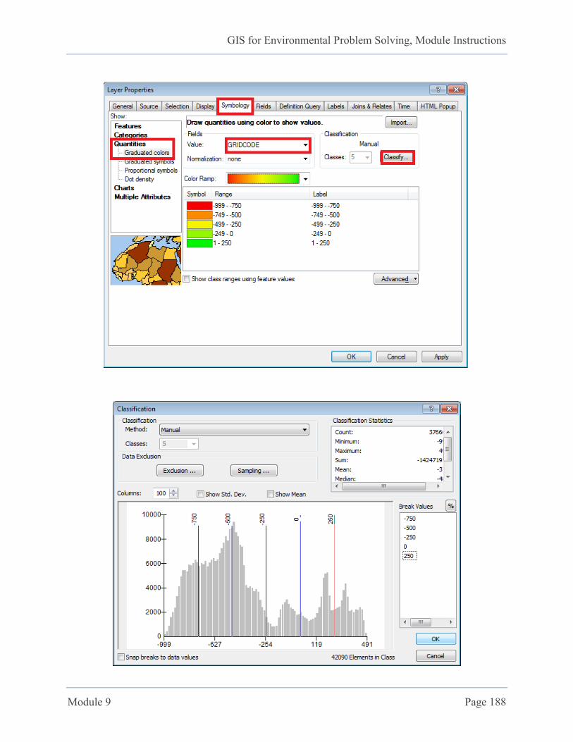
GIS for Environmental Problem Solving, Module Instructions
Module 9 Page 188
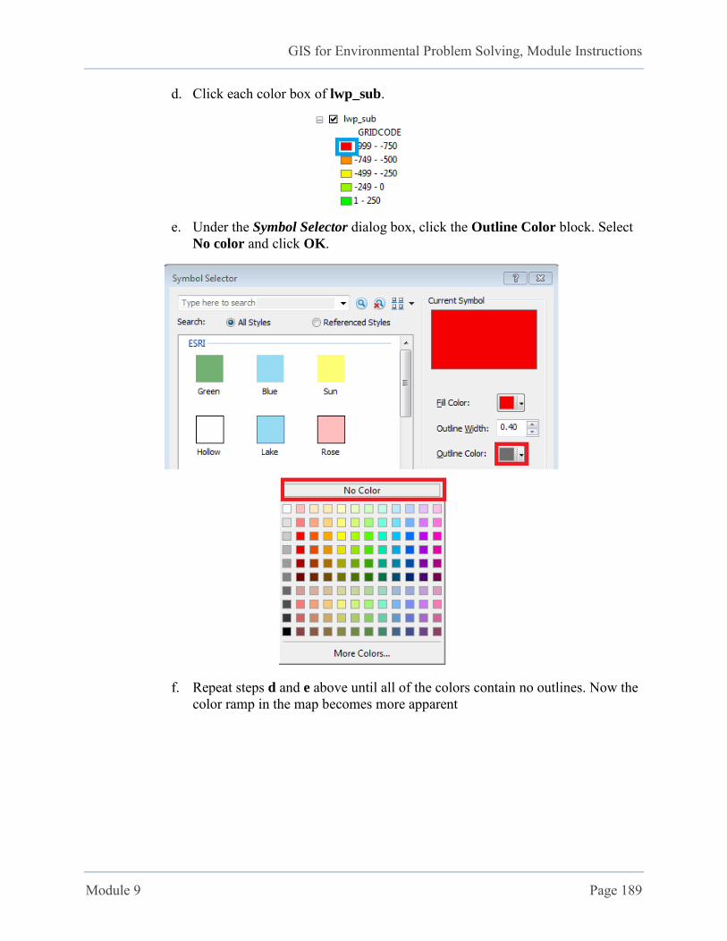
GIS for Environmental Problem Solving, Module Instructions
Module 9 Page 189
d. Click each color box of lwp_sub.
e. Under the Symbol Selector dialog box, click the Outline Color block. Select No color and click OK.
f. Repeat steps d and e above until all of the colors contain no outlines. Now the color ramp in the map becomes more apparent
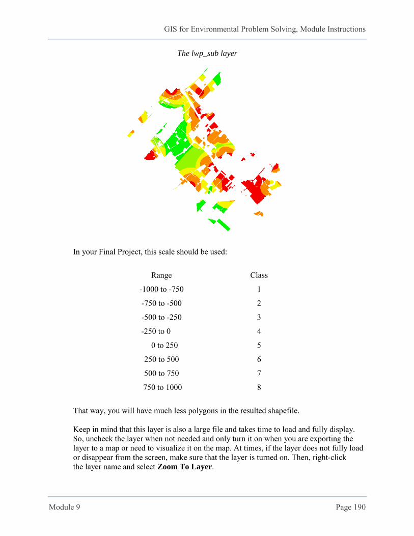
GIS for Environmental Problem Solving, Module Instructions
Module 9 Page 190
The lwp_sub layer
In your Final Project, this scale should be used:
Range
-1000 to -750
-750 to -500
-500 to -250
-250 to 0
0 to 250
250 to 500
500 to 750
750 to 1000
Class
1
2
3
4
5
6
7
8
That way, you will have much less polygons in the resulted shapefile. Keep in mind that this layer is also a large file and takes time to load and fully display.
So, uncheck the layer when not needed and only turn it on when you are exporting the layer to a map or need to visualize it on the map. At times, if the layer does not fully load or disappear from the screen, make sure that the layer is turned on. Then, right-click the layer name and select Zoom To Layer.
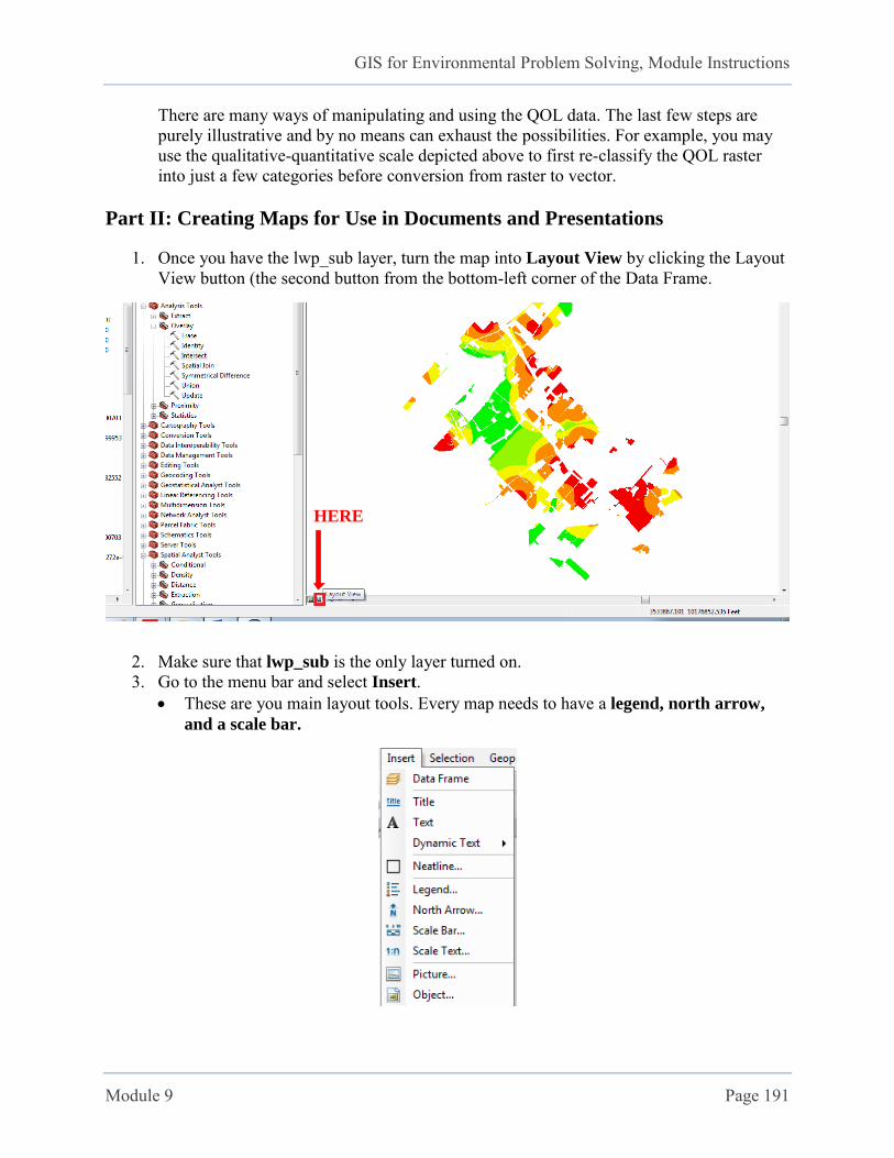
GIS for Environmental Problem Solving, Module Instructions
Module 9 Page 191
There are many ways of manipulating and using the QOL data. The last few steps are purely illustrative and by no means can exhaust the possibilities. For example, you may use the qualitative-quantitative scale depicted above to first re-classify the QOL raster into just a few categories before conversion from raster to vector.
Part II: Creating Maps for Use in Documents and Presentations
1. Once you have the lwp_sub layer, turn the map into Layout View by clicking the Layout View button (the second button from the bottom-left corner of the Data Frame.
2. Make sure that lwp_sub is the only layer turned on. 3. Go to the menu bar and select Insert.
These are you main layout tools. Every map needs to have a legend, north arrow,
and a scale bar.
HERE
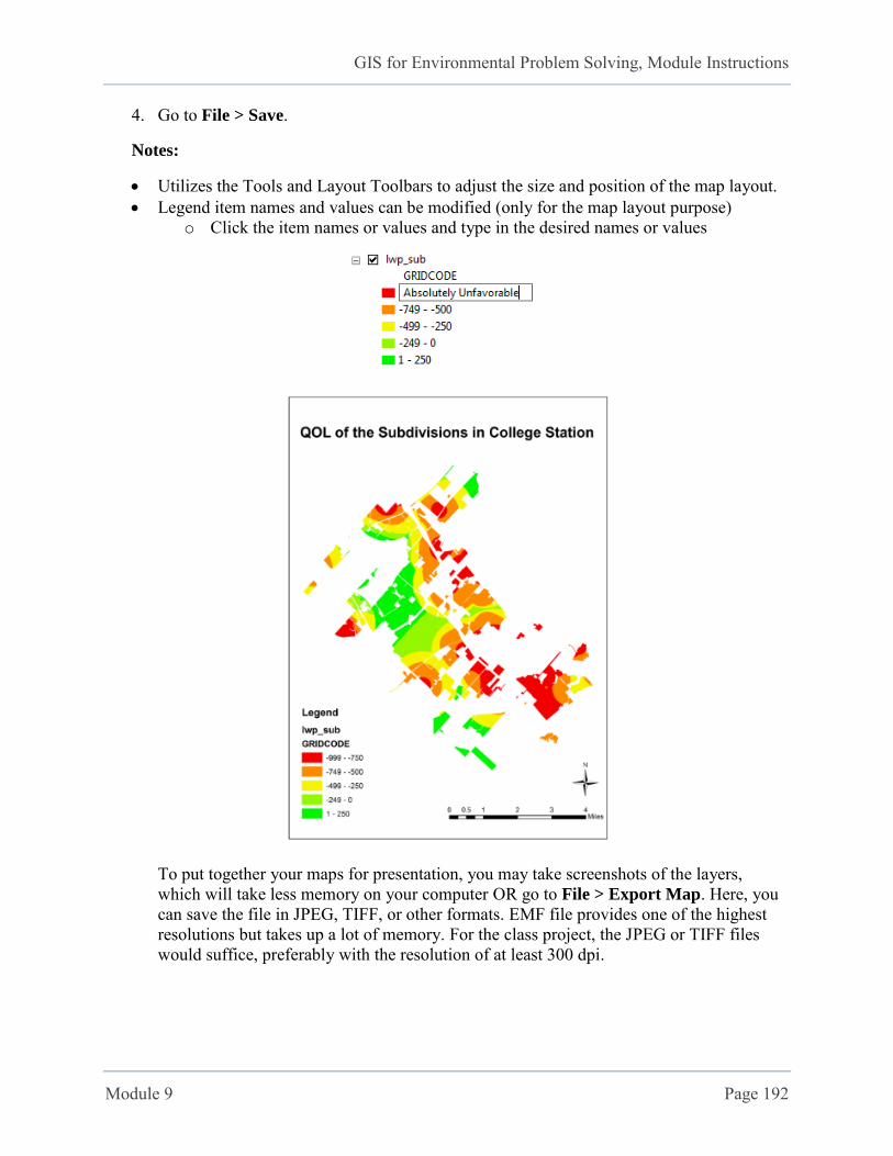
GIS for Environmental Problem Solving, Module Instructions
Module 9 Page 192
4. Go to File > Save.
Notes:
Utilizes the Tools and Layout Toolbars to adjust the size and position of the map layout. Legend item names and values can be modified (only for the map layout purpose)
o Click the item names or values and type in the desired names or values
To put together your maps for presentation, you may take screenshots of the layers, which will take less memory on your computer OR go to File > Export Map. Here, you can save the file in JPEG, TIFF, or other formats. EMF file provides one of the highest resolutions but takes up a lot of memory. For the class project, the JPEG or TIFF files would suffice, preferably with the resolution of at least 300 dpi.
GIS for Environmental Problem Solving, Module Instructions
Module 9 Page 193
Part III: Locating the Addresses and Identify QOL Indices
*** This part should be done when you are reach the final stage of the Final Project. The map layers of normalized layers, the Emycin layers, and other relevant layers from the previous parts should already be prepared and exported as JPEG, TIFF, or other formats for the presentation.***
1. To put the addresses on the map, switch the map back to Data View (the button next to the Layout View).
2. Use the Address Locator to establish a point layer of shapefile for locations of randomly selected residences. The process follows that of Module 6, Part II, Step 5.
a. Click the Find Tool on the toolbars. b. In the Find dialog box:
i. Click the Locations tab . ii. Choose a locator, e.g. StreetMap USA Plus AltNames.
iii. Type in a residential address in College Station. iv. Click Find. v. Once the tool locates the address, it will show up on the box at the bottom
(under the address you typed in). Right-click the address and choose to Add Point/Labeled Point/Callout on the map.
*** Keep in mind that the Add Point/Labeled Point/Callout options will add a permanent graphic on your map. So, try doing this (along with identifying QOL index below) as the last steps after you completed the previous parts and when you are ready to prepare the maps for presentation. ***
3. To determine a QOL index associated with an address:
a. Click the Identify Tools on the menu bar. b. In the Identify dialog box:
i. Under Identify from, select the lwp_sub layer. ii. Move your mouse over the lwp_sub map and click the selected address
(from step 2) on the map. The Identify dialog box will display information of the specific cell you click, i.e., your selected address. The value next to GRIDCODE is the QOL index of the selected address (would be within the range of -1000 to +1000).
4. Go to File > Save.
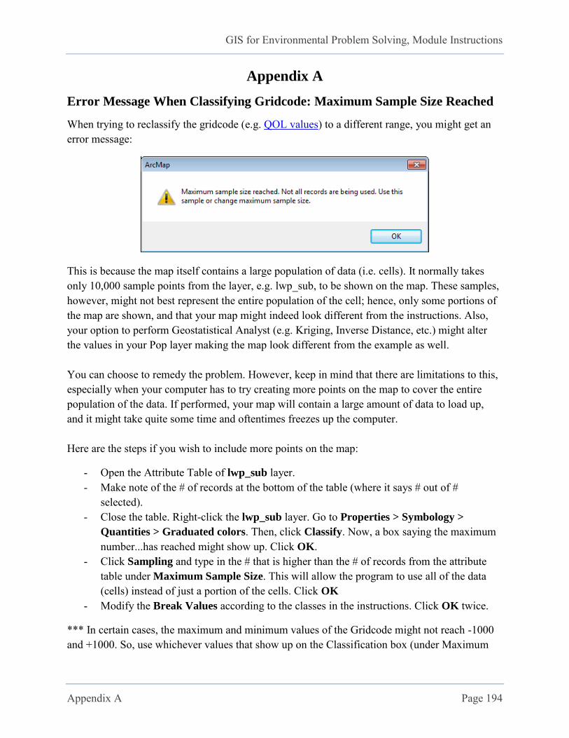
GIS for Environmental Problem Solving, Module Instructions
Appendix A Page 194
Appendix A
Error Message When Classifying Gridcode: Maximum Sample Size Reached
When trying to reclassify the gridcode (e.g. QOL values) to a different range, you might get an error message:
This is because the map itself contains a large population of data (i.e. cells). It normally takes only 10,000 sample points from the layer, e.g. lwp_sub, to be shown on the map. These samples, however, might not best represent the entire population of the cell; hence, only some portions of the map are shown, and that your map might indeed look different from the instructions. Also, your option to perform Geostatistical Analyst (e.g. Kriging, Inverse Distance, etc.) might alter the values in your Pop layer making the map look different from the example as well. You can choose to remedy the problem. However, keep in mind that there are limitations to this, especially when your computer has to try creating more points on the map to cover the entire population of the data. If performed, your map will contain a large amount of data to load up, and it might take quite some time and oftentimes freezes up the computer. Here are the steps if you wish to include more points on the map:
- Open the Attribute Table of lwp_sub layer. - Make note of the # of records at the bottom of the table (where it says # out of #
selected). - Close the table. Right-click the lwp_sub layer. Go to Properties > Symbology >
Quantities > Graduated colors. Then, click Classify. Now, a box saying the maximum number...has reached might show up. Click OK.
- Click Sampling and type in the # that is higher than the # of records from the attribute table under Maximum Sample Size. This will allow the program to use all of the data (cells) instead of just a portion of the cells. Click OK
- Modify the Break Values according to the classes in the instructions. Click OK twice.
*** In certain cases, the maximum and minimum values of the Gridcode might not reach -1000 and +1000. So, use whichever values that show up on the Classification box (under Maximum

GIS for Environmental Problem Solving, Module Instructions
Appendix A Page 195
and Minimum) for the Classification. You should end up having 8 classes with more or less maximum and minimum values according to your result. Now your map should contain and show the entire population data of lwp_sub layer. Sometimes, if the program does not load up the map correctly (due to the above limitations), try right-clicking the lwp_sub layer and select Zoom to Layer. You might even have to save, close, and open up the program again the see the newly modified map. You will also encounter this issue at the last part of the final project when you have the final aggregated layer of 8 factors contributing to QOL.