Embed Size (px)
Citation preview

MATHICSE
Mathematics Institute of Computational Science and Engineering
School of Basic Sciences - Section of Mathematics
Address:
EPFL - SB - MATHICSE (Bâtiment MA)
Station 8 - CH-1015 - Lausanne - Switzerland
http://mathicse.epfl.ch
Phone: +41 21 69 37648
Fax: +41 21 69 32545
Moment equations for
the mixed formulation of the
Hodge Laplacian with
stochastic data
F. Bonizzoni, A. Buffa, F. Nobile
MATHICSE Technical Report Nr. 31.2012
August 2012

Moment equations for the mixed formulation of the
Hodge Laplacian with stochastic data ∗
Francesca Bonizzoni],†, Annalisa Buffa‡, Fabio Nobile],†
August 21, 2012
] MOX– Modellistica e Calcolo ScientificoDipartimento di Matematica “F. Brioschi”
Politecnico di Milanovia Bonardi 9, 20133 Milano, Italy
† CSQI– MATHICSEEcole Polytechnique federale de LausanneStation 8, CH-1015 Lausanne, Switzerland
‡ Istituto di Matematica Applicata e Tecnologie Informatiche del CNRvia Ferrata 1, 27100 Pavia, Italy
[email protected], [email protected]
Keywords: stochastic PDE, Hodge-Laplace problem, moment equations, sparsetensor product approximation.
Abstract
We study the mixed formulation of the stochastic Hodge-Laplace prob-lem defined on a n-dimensional domain D (n ≥ 1), with random forcingterm. In particular, we focus on the magnetostatic problem and on theDarcy problem in the three dimensional case. We derive and analyze themoment equations, that is the deterministic equations solved by the m-thmoment (m ≥ 1) of the unique stochastic solution of the stochastic prob-lem. We find stable tensor product finite element discretizations, both fulland sparse, and provide optimal order of convergence estimates. In partic-ular, we prove the inf-sup condition for sparse tensor product finite elementspaces.
∗This work has been supported by the Italian grant FIRB-IDEAS (Project n. RBID08223Z)“Advanced numerical techniques for uncertainty quantification in engineering and life scienceproblems”.
1

1 Introduction
Many engineering applications are affected by uncertainty. This uncertaintymay be due to the incomplete knowledge on the input data or some intrinsicvariability of them. For example, if we model the two-phase flow in a porousmedium, randomness arises in the permeability tensor, due to impossibility ofa full characterization of conductivity properties of subsurface media, but alsoin the source term, typically pressure gradients or impervious boundaries. Seefor example [45, 42, 20, 21, 44, 38, 18, 7]. Similar situations appear in manyother applications, such as combustion flows, earthquake engineering, biomedicalengineering and finance. Probability theory provides an effective tool to includeuncertainty in the model. We refer to [30, 9, 1] for probability measures onBanach spaces, and to [28, 27, 36, 16] and the references therein for stochasticpartial differential equations. We notice that the SPDEs that we consider inthis work differ from those in [28, 27, 36, 16] since we are taking Lm-intregrableprocesses.
In this work we focus on the linear Hodge-Laplace problem in mixed for-mulation, with stochastic forcing term and homogeneous boundary conditions.This problem includes the magnetostatic and electrostatic equations as well asthe Darcy problem for monophase flows in saturated media.
The mathematical framework involving the Hodge-Laplace is the exteriorcalculus, a theoretical approach that, using tools from differential geometry,allows to simultaneously treat many different problems. In particular, the HodgeLaplacian dδ+δd, where δ is the formal adjoint of the exterior derivative d, mapsdifferential k-forms to differential k-forms, and unifies some important second-order differential operators, such as the Laplacian and curl − curl problemsarising in electromagnetics. For more details, see [3, 4, 14].
The solution of the mixed formulation of the stochastic Hodge-Laplace prob-lem is a couple (u, p) of random fields taking values in a suitable space of differ-ential forms. The description of these random fields requires the knowledge oftheir moments. A possible approach is to compute the moments by the Monte-Carlo method in which, after sampling the probability space, the deterministicPDE is solved for each sample and the results are combined to obtain statisticalinformation about the random field. This is a widely used technique, but itfeatures a very slow convergence rate. Improvements can be achieved by sev-eral techniques. We mention for instance the Multilevel Monte-Carlo methodappeared in recent years in literature, and applied to both stochastic ODEs andPDEs: see [24, 19, 8, 26, 13] and the references therein.
An alternative strategy is to directly calculate the moments of interest of thestochastic solution without doing any sampling. Indeed, the aim of the presentwork is to derive the moment equations, that is the deterministic equationssolved by the m-points correlation functions of the stochastic solution, showtheir well-posedness and propose a stable sparse finite element approximation.
2

The stochastic problem has the form
T
[up
]=
[f1
f2
]a.e. in D,
where T is a second order linear differential operator, D is a domain in Rn, andthe forcing terms f1(ω, x), f2(ω, x) are random fields, with x ∈ D, ω ∈ Ω andΩ indicating the set of possible outcomes. The m-th moment equation involvesthe tensor product operator T⊗m := T ⊗ · · · ⊗ T︸ ︷︷ ︸
m times
and the forcing term is given
by the m-points correlation function of the couple
[f1
f2
].
We start proving the well-posedness of the m-th moment equation. Althoughthis comes easily from a tensorial argument, we also present a direct proof of theint-sup condition for the tensor operator T⊗m. This proof generalizes to someextent to the case of non tensor product spaces and will be the key tool to showthe stability of a sparse finite element approximation.
Concerning the numerical approximation of the m-th moment equation, atensorized FE approach for the numerical approximation of the moment equa-tions is viable only for small m, as the number of degrees of freedom increasesexponentially in m. For large m one should consider instead sparse approxima-tions (see e.g. [41, 12, 34, 35, 40] and the references therein). We consider bothfull tensor product and sparse tensor product finite element approximations, andprove their stability using the tools from the finite element exterior calculus. See[2, 3, 4, 15]. In particular, the stability of a full tensor product approximation isa simple consequence of a tensor product argument. On the contrary, a tensorproduct argument does not apply if sparse tensor product approximations areconsidered and a direct proof of the inf-sup condition is needed, and will beproved in Section 6. We also provide optimal order of convergence estimatesboth for the full and the sparse approximations.
The analysis on well-posedness and stable discretization for the m-pointscorrelation problem developed in this work will be necessary to analyze morecomplex situations with randomness appearing in the operator itself instead ofsimply in the right hand side. This case can be treated for small randomnessby a perturbation approach (Taylor or Neumann expansions, see e.g. [6, 42, 20]and the references therein) and is currently under investigation.
The outline of the paper is the following: in Section 2 after recalling thedefinitions of the classical Sobolev spaces, we generalize them to the Sobolevspaces of differential forms. We then recall the main results on the mixed for-mulation of the Hodge-Laplace problem in the deterministic setting, stating thewell-posedness of the problem and translating it to the language of partial differ-ential equations using the proxy fields. In Section 3 we consider the stochasticcounterpart of the mixed Hodge Laplacian problem, and we prove the well-posedness of its weak formulation. Section 4 is dedicated to the analysis of themoment equations where we provide in particular the constructive proof of the
3

inf-sup condition for the tensor product operator T⊗m. In Section 5 we focus ontwo problems of particular interest from the point of view of applications: thestochastic magnetostatic equations and the stochastic Darcy problem. Finally,in Section 6, we provide both full and sparse finite element discretizations forthe deterministic m-th moment problem, we prove their stability and optimalorder of convergence estimates.
2 Sobolev spaces of differential forms andthe deterministic Hodge-Laplace problem
In this section we first recall the main concepts and definitions concerning the fi-nite element exterior calculus and the Sobolev spaces of differential forms, whichgeneralize the classical Sobolev spaces. We prove the inf-sup condition for themixed formulation of the Hodge-Laplace problem providing a choice of test func-tions different from the classical one proposed in [3]. This will be needed later onto prove the equivalent inf-sup condition for the m-points correlation problem.Finally, we use the proxy fields correspondences to translate the Hodge-Laplaceproblem in the three dimensional case to the language of partial differential equa-tions with the aim of showing that this general setting includes some importantproblems of practical interest. For more details we refer to [3, 4, 14].
2.1 Classical Sobolev spaces
Let D ⊂ Rn be a domain in Rn. We denote with Lm(D) the Lebesgue space ofindex m with 1 ≤ m <∞. Lm(D) is a Banach space endowed with the standardnorm
‖f‖Lm(D) :=
(∫D|f(x)|mdx
)1/m
. (1)
When p = 2 we obtain the only Hilbert space of this class, with inner productgiven by
(f, g)L2(D) :=
∫Df(x)g(x)dx, f, g ∈ L2(D).
We denote with Hs(D) the Sobolev space defined as:
Hs(D) :=f ∈ L2(D)|Dαf ∈ L2(D) for all |α| ≤ s
. (2)
Hs(D) is a Hilbert space with the natural inner product
(f, g)Hs(D) :=∑|α|≤s
〈Dαf,Dαg〉L2(D), for f, g ∈ Hs(D).
For more on the Lebesgue spaces Lm(D) and the Sobolev spaces Hs(D) see forexample [29]. As it will be useful later on, we also recall the following Sobolev
4

spaces constrained by boundary conditions on ΓD ⊂ ∂D:
H1ΓD
(D) =v ∈ L2(D) | ∇v ∈ L2(D), v|ΓD
= 0,
HΓD(curl , D) =
v ∈ (L2(D))n | curl v ∈ (L2(D))n, v × ν|ΓD
= 0,
HΓD(div , D) =
v ∈ (L2(D))n | div v ∈ L2(D), v · ν|ΓD
= 0,
where ν is the outer-pointing normal versor. These spaces are Hilbert spaceswith respect to the graph norm.
Considering now a probability space (Ω, dP), the definition of Lm generalizesimmediately. In this case we will use the notation
(Lm(Ω, dP), ‖ · ‖Lm(Ω,dP)
)to denote the Banach space of real random variables on Ω with finite m-thmoment. If m = 2,
(L2(Ω, dP), ‖ · ‖L2(Ω,dP)
)is the Hilbert space of all real
random variables on Ω with finite second moment, equipped with the usualinner product
(f(ω), g(ω))L2(Ω,dP) :=
∫Ωf(ω)g(ω)dP(ω), for f, g ∈ L2(Ω, dP).
2.2 Sobolev spaces of differential forms
In order to generalize the definitions of the Sobolev spaces Hs(D) to differentialforms, we need to briefly recall the basic objects and results of exterior algebraand exterior calculus, inspired by [3]. The natural setting is a sufficiently smoothfinite dimensional manifold D with or without boundary. For our purposes, wecan restrict ourselves to the particular case of a n-dimensional bounded domainD ⊂ Rn with boundary denoted by ∂D ⊂ Rn−1. In this way, at each pointx ∈ D the tangent space is naturally identified with Rn and we make thisassumption throughout the paper. We denote by AltkRn, 1 ≤ k ≤ n, the spaceof alternating k-linear maps on Rn. Clearly, Alt0Rn = R and AltnRn = R,and the unique element in AltnRn is a volume form voln. We recall the wedgeproduct ∧ : AltkRn × AltlRn → Altk+lRn and the inner product (·, ·)AltkRn :AltkRn×AltkRn → R for k+ l ≤ n. Starting from this inner product, the Hodgestar operator ? : AltkRn → Altn−kRn is defined: u ∧ ?w = (u,w)AltkRn voln (seee.g. [3]).
A differential k-form on D is a map u which associates to each x ∈ D anelement ux ∈ AltkRn. We denote by Λk(D) the space of all smooth differential k-forms on D. The wedge product of alternating k-forms may be applied pointwiseto define the wedge product of differential forms: (u∧w)x = ux∧wx. The exteriorderivative dk maps Λk(D) into Λk+1(D) for each k ≥ 0 and it is defined as
dkux(v1, . . . , vk+1) =k+1∑j=1
(−1)j+1∂vjux(v1, . . . , vj , . . . , vk+1), u ∈ Λk(D),
v1, . . . , vk+1 ∈ Rn, where the hat is used to indicate a suppressed argument. Theexterior derivative satisfies the key property dk+1 dk = 0, ∀ k. The coderivative
5

operator δk : Λk(D) → Λk−1(D) is the formal adjoint of the exterior derivativeand it is defined by
?δku = (−1)kdn−k ? u, u ∈ Λk(D). (3)
To lighten the notation, in the following we omit the k when no ambiguityarises. The trace operator Tr : Λk(D) → Λk(∂D) is defined as the pullback ofthe inclusion ∂D → D. We denote with vol the unique volume form in Λn(D)such that at each x ∈ D, voln is the unique form associated with AltnRn. Giventwo differential k-forms on D it is possible to define their L2-inner product asthe integral of their pointwise inner product in AltkRn:
(u,w) :=
∫D
(ux, wx)AltkRn vol =
∫Du ∧ ?w, u, w ∈ Λk(D). (4)
In the following we will denote with ‖ · ‖ the norm induced by the L2-innerproduct (·, ·). The following integration by parts formula holds:
(du, v) = (u, δv) +
∫∂D
Tr(u) ∧ Tr(?v), u ∈ Λk(D), v ∈ Λk+1(D). (5)
The completion of Λk(D) in the norm induced by the scalar product (4)defines the Hilbert space L2Λk(D). The Sobolev space of square integrable k-forms whose exterior derivative is also square integrable is given by
HΛk(D) =u ∈ L2Λk(D)| du ∈ L2Λk+1(D)
. (6)
It is a Hilbert space equipped with the inner product
(u,w)HΛk(D) := (u,w) + (du,dw) .
In analogy with HΛk(D), it is possible to define the Hilbert space
H∗Λk(D) :=u ∈ L2Λk(D)| δu ∈ L2Λk−1(D)
. (7)
Let ∂D = ΓD ∪ ΓN , ΓD ∩ΓN = ∅. As it is standard ([3]), the spaces (6) and (7)can be endowed with boundary conditions:
HΓDΛk(D) :=
u ∈ HΛk(D)| Tr(u)|ΓD
= 0. (8)
H∗ΓNΛk(D) :=
u ∈ H∗Λk(D)| Tr(?u)|ΓN
= 0.
With the spaces defined in (8) and the exterior derivative operator, we canconstruct the L2 de Rham complex:
0→ HΓDΛ0(D)
d−→ . . .d−→ HΓD
Λn(D) −→ 0. (9)
6

Since d d = 0, we haveBk ⊆ Zk, (10)
where Bk is the image of d in HΓDΛk(D) while Zk is the kernel of d inHΓD
Λk(D).
The following orthogonal decomposition of L2Λk(D), known as Hodge de-composition, holds:
L2Λk(D) = Bk ⊕B⊥k (11)
where B⊥k is the L2-complement of Bk.We define two projection operators π⊥ and π as follows:
π⊥ : Bk ⊕B⊥k → B⊥k (12)
v = dv + v⊥ 7→ v⊥
π : Bk ⊕B⊥k → B⊥k−1 (13)
v = dv + v⊥ 7→ v.
We recall a classical result in the theory of Sobolev spaces:
Lemma 2.1 (Poincare inequality) There exists a positive constant CP thatdepends only on the domain D such that
‖v‖ ≤ CP ‖dv‖ ∀v ∈ Z⊥k (14)
where Z⊥k is the orthogonal complement of Zk in HΓDΛk(D).
For the sake of simplicity, we consider only the case of geometries which aretrivial from the topological point of view. More precisely, from now on, we makethe following
Assumption 2.1 The domain D ⊂ Rn is bounded, Liptschitz and contractible.Its boundary ∂D is given by the disjoint union of two open sets ΓD and ΓN , withΓD,ΓN 6= ∅, ΓD contractible as well and with boundary sufficiently regular (atleast piecewise C1).
Under assumption 2.1, B⊥k = B∗k, where B∗k is the image of δ in H∗ΓNΛk(D).
This relation is proved in the three dimensional case in [17], and generalizes tothe n dimensional case (see e.g. [32]).
Remark 2.1 The case of non-trivial topology can likely be treated following [4],but it would make the exposition of our results much more difficult.
Remark 2.2 We assume ΓD,ΓN 6= ∅, but the two limit cases treated in [3] canbe considered with suitable modifications of our argument.
7

We end the section by introducing the following notations for two Hilbert spaceswe will use later on:
Wk :=
[L2Λk(D)L2Λk−1(D)
], Vk :=
[HΓD
Λk(D)
HΓDΛk−1(D)
], (15)
with the inner products (·, ·)Wk, (·, ·)Vk , and the norms ‖ · ‖Wk
, ‖ · ‖Vk .
2.3 Mixed formulation of the Hodge-Laplace problem
The Hodge Laplacian is the differential operator δd + dδ mapping k-forms intok-forms, and the Hodge-Laplace problem is the boundary value problem for theHodge Laplacian. Suppose we have a domain D ⊂ Rn satisfying Assumption2.1. We consider a particular case of the mixed formulation of the Hodge-Laplaceproblem with variable coefficients described in [3, 4, 14], which allows to includethe Darcy problem (see Section 2.3.1). Given a non negative coefficient α ∈ R+
and source terms
[f1
f2
]∈Wk, find
[up
]such that
δdu+ dp = f1 in Dδu− αp = f2 in D
Tr(u) = 0 on ΓDTr(p) = 0 on ΓD
Tr(?u) = 0 on ΓNTr(?du) = 0 on ΓN
(16)
We introduce T : Vk → V ′k, the linear operator of order two represented by thematrix:
T :=
[δd dδ −αId
]=
[A B∗
B −αId
], (17)
where V ′k =
[(HΓD
Λk(D))′
(HΓDΛk−1(D))′
]is the dual space of Vk defined in (15), the
operators A and B are defined as:
A : HΓDΛk(D)→ (HΓD
Λk(D))′ (18)
〈Av,w〉 := (dv,dw)
B : HΓDΛk(D)→ (HΓD
Λk−1(D))′ (19)
〈Bv, q〉 := (v,dq)
and B∗ is the adjoint of B. Moreover we introduce the linear operators F1 ∈(HΓD
Λk)′ and F2 ∈ (HΓDΛk−1)′ defined as:
F1 : HΓDΛk(D)→ R (20)
F1(v) := (f1, v)
8

F2 : HΓDΛk−1(D)→ R (21)
F2(q) := (f2, q)
The mixed formulation of the deterministic Hodge Laplacian with homogeneousessential boundary conditions on ΓD and homogeneous natural boundary con-ditions on ΓN is
Deterministic Problem:
Given
[F1
F2
]∈ V ′k, find
[up
]∈ Vk s.t.
T
[up
]=
[F1
F2
]in V ′k,
(22)
Theorem 2.1 For every α > 0, problem (22) is well-posed, so that there existsa unique solution that depends continuously on the data. In particular, thereexist positive constants C1, C
′1 that depend only on the Poincare constant CP
and on the parameter α, such that for any
[up
]∈ Vk there exists
[vq
]∈ Vk
with⟨T
[up
],
[vq
]⟩V ′k,Vk
≥ C1
∥∥∥∥[ up]∥∥∥∥2
Vk
= C1
(‖u‖2HΛk + ‖p‖2HΛk−1
), (23)∥∥∥∥[ vq
]∥∥∥∥Vk
≤ C ′1∥∥∥∥[ up
]∥∥∥∥Vk
. (24)
The same result holds with α = 0 provided that F2 corresponds to f2 ∈ δHΓDΛk(D).
The well-posedness of problem (22) is proved in [3] by showing the equivalent inf-sup condition for the bounded bilinear and symmetric form 〈T ·, ·〉 : Vk×Vk → R(23), (24) (see [5, 11]). However, we report it entirely (with a slightly differentchoice of test functions) as a preparatory step for the proofs we will proposelater on.Proof. We need to show (23) and (24). Let us start considering α > 0. For a given[up
]we use the Hodge decomposition (11):[
up
]=
[du + u⊥
dp + p⊥
], (25)
with du ∈ Bk, dp ∈ Bk−1, u⊥ ∈ B⊥k and p⊥ ∈ B⊥k−1. We choose as test functions[vq
]=
[u⊥ + dp⊥
γu − dp
], (26)
where γ is a positive parameter to be set later. Relation (26) can also be written in acompact form as [
vq
]= P
[up
], (27)
9

where
P =
[π⊥ dπ⊥
γπ −dπ
](28)
and the operators π⊥, π are defined in (12) and (13) respectively. Substituting (26)into (23), using the property d d = 0, the Hodge decomposition (11) and the Poincareinequality (14) we find⟨
T
[up
],
[vq
]⟩V ′k,Vk
= (du,dv) + (v,dp) + (u,dq)− α (p, q)
= ‖du⊥‖2 + ‖dp⊥‖2 + γ‖du‖2 + α‖dp‖2 − αγ(p⊥, u
)≥ ‖du⊥‖2 + ‖dp⊥‖2 + γ‖du‖2 + α‖dp‖2
− αγ1/2
2
(C2P ‖dp⊥‖2 + γC2
P ‖du‖2)
≥ ‖du⊥‖2 +(
1− α
2γ1/2C2
P
)‖dp⊥‖2+
γ
(1− αγ1/2C2
P
2
)‖du‖2 + α‖dp‖2.
It is possible to choose γ in order to make (23) true with C1 = C1(CP , α). The inequality(24) with C1 = C ′1(CP , α) follows from the Hodge decomposition (11) and Poincareinequality (14).
The proof in the case α = 0 is very similar. Suppose f2 ∈ δHΓDΛk(D). In order to
have a unique solution, we need to look for p ∈ B⊥k−1. Fixed u = du+u⊥ ∈ HΓDΛk(D)
we again choose the test functions as in (27): v = dp+ u⊥ ∈ HΓDΛk(D) and q = u ∈
B⊥k−1. Using the Poincare inequality (14) and the orthogonal decomposition (11) we
are able to prove the relations (23) and (24). A simple consequence of Theorem 2.1 (see [11]) is that there exists a positive
constant K = K(CP , α) such that∥∥∥∥[ up]∥∥∥∥
Vk
≤ K∥∥∥∥[ F1
F2
]∥∥∥∥V ′k
. (29)
Another way to express the result given in Theorem 2.1 is given by thefollowing
Proposition 2.1 Given T as in (17) and P as in (28), ∀[up
]∈ Vk it holds
⟨T
[up
], P
[up
]⟩V ′k,Vk
≥ C1
∥∥∥∥[ up]∥∥∥∥2
Vk
(30)
‖P‖L(Vk,Vk) ≤ C ′1. (31)
2.3.1 Translation to the language of partial differential equations
Let us consider the case D ⊂ R3, naturally identifying the space TxD with R3.Thanks to the identification of Alt0R3 and Alt3R3 with R, and of Alt1R3 and
10

HΓDΛk(D) d Tr|ΓD
u
k = 0 H1ΓD
(D) ∇ u|ΓD
k = 1 HΓD(curl , D) curl u× n|ΓD
k = 2 HΓD(div , D) div u · n|ΓD
k = 3 L2(D) 0 0
Table 1: Correspondences in terms of proxy fields between the space of differen-tial forms HΛk(D) and the classical spaces of functions and vector fields, in thecase n = 3.
Alt2R3 with R3, we can establish correspondences between the spaces of differ-ential forms and scalar or vector fields. These fields are called proxy fields. Inparticular, we can identify each 0-form and 3-form with a scalar-valued function,and each 1-form and 2-form with a vector-valued function. Table 1 summarizesthe correspondences in terms of proxy fields for the spaces of differential formsHΓD
Λk(D), the exterior derivative operators and the trace operators. Based onthe identifications in Table 1 we can reinterpret the de Rham complex (9) asfollows:
0 −→ H1ΓD
(D)∇−→ HΓD
(curl , D)curl−−−→ HΓD
(div, D)div−−→ L2(D) −→ 0 (32)
In this section we will use the symbol (·, ·) to denote the inner product in L2(D),that corresponds by proxy identifications to the inner product in L2Λk(D).
• Let us start with k = 0. In this case HΓDΛ−1(D) = 0, so p = 0. Then
u ∈ H1ΓD
(D) satisfies
(∇u,∇v) = (f1, v) ∀v ∈ H1ΓD
(D). (33)
We obtain the usual weak formulation of the Poisson equation equippedwith homogeneous Dirichlet boundary conditions on ΓD and homogeneousNeumann boundary conditions on ΓN .
• For k = 1 and α = 0, the linear operator T of order two defined in (17) isrepresented by the matrix
T =
[curl 2 ∇−div 0
]. (34)
Problem (22) is the weak formulation of the magnetostatic/electrostatic
equations (see for example [33, 10, 25]). Indeed, V1 =
[HΓD
(curl , D)H1
ΓD(D)
]and
[up
]∈ V1 satisfies
(curl u, curl v) + (∇p, v) = (f1, v)(u,∇q) = (f2, q) .
∀[vq
]∈ V1. (35)
11

• When k = 2,
T =
[−∇div curl
curl −αId
].
Problem (22) is the mixed formulation of the vectorial Poisson equation:
find
[up
]∈ V2 =
[HΓD
(div , D)HΓD
(curl , D)
]s.t.
(div u,div v) + (curl p, v) = (f1, v)(u, curl q)− α (p, q) = (f2, q)
∀[vq
]∈ V2. (36)
• Finally, for k = 3, problem (22) models the flow in porous media. We canreinterpret the linear tensor operator of order two T as
T =
[0 div−∇ −αId
], (37)
where α > 0 is linked to the inverse of the permeability. Hence, problem
(22) is the Darcy equations: find
[up
]∈ V3 =
[L2(D)
HΓD(div , D)
]s.t.
(div p, v) = (f1, v)(u,div q)− α (p, q) = 0
∀[vq
]∈ V3. (38)
3 Stochastic Sobolev spaces of differential forms andstochastic Hodge Laplacian
3.1 Stochastic Sobolev spaces of differential forms
Let v1 ∈ V1 and v2 ∈ V2, where V1, V2 are Hilbert spaces. Let v1⊗v2 : V1×V2 → Rdenote the symmetric bilinear form which acts on each couple (w1, w2) ∈ V1×V2
byv1 ⊗ v2(w1, w2) = (v1, w1)V1 (v2, w2)V2 ,
where (·, ·)V1 denotes the inner product in V1 and (·, ·)V2 the inner product in V2.Let us define an inner product (·, ·)V1⊗V2 on the set of such symmetric bilinearforms as (
v1 ⊗ v2, v′1 ⊗ v′2
)V1⊗V2 =
(v1, v
′1
)V1
(v2, v
′2
)V2, (39)
and extend it by linearity to the set
span v1 ⊗ v2 : v1 ∈ V1, v2 ∈ V2 (40)
composed of finite linear combinations of such symmetric bilinear forms.
Definition 3.1 Given V1 and V2 Hilbert spaces, the tensor product V1⊗V2 is theHilbert space defined as the completition of the set (40) under the inner product(·, ·)V1⊗V2 in (39).
12
In the following we will denote with ‖ · ‖V1⊗V2 the norm induced by the innerproduct (·, ·)V1⊗V2 . Definition 3.1 naturally generalizes to the tensor productof m Hilbert spaces, with m ≥ 2 integer. For more details on tensor productspaces and on norms on tensor product spaces see for example [37, 31] and thereferences therein.
Let (Ω,A,P) be a complete probability space and V a separable Hilbertspace. The stochastic counterpart of V is the Hilbert space given by the tensorproduct V ⊗ L2(Ω, dP), where L2(Ω, dP) is the Hilbert space defined in Section2.1. Let L2 (Ω;V ) be the Bochner space composed of functions u such that ω 7→‖u(ω)‖2V is measurable and integrable, so that ‖u‖L2(Ω;V ) :=
(∫Ω ‖u(ω)‖2V dP(ω)
)1/2is finite. We observe that there is a unique isomorphism from V ⊗ L2(Ω, dP) toL2 (Ω;V ) which maps ψ⊗µ ∈ V ⊗L2(Ω, dP) onto the function ω 7→ µ(ω)ψ ∈ V .
The definition of the Hilbert space L2 (Ω;V ) easily generalizes to the Banachspace Lm (Ω;V ) with m ≥ 1 integer. We say that a random field u : Ω → V isin the Bochner space Lm (Ω;V ) if ω 7→ ‖u(ω)‖mV is measurable and integrable,
so that ‖u‖Lm(Ω;V ) :=(∫
Ω ‖u(ω)‖mV dP(ω))1/m
is finite.In the following we focus on two stochastic Sobolev spaces of differential
forms, namely Lm (Ω;Wk) and Lm (Ω;Vk) with m ≥ 1 integer, where Wk and Vkare Sobolev spaces of differential forms defined in (15).
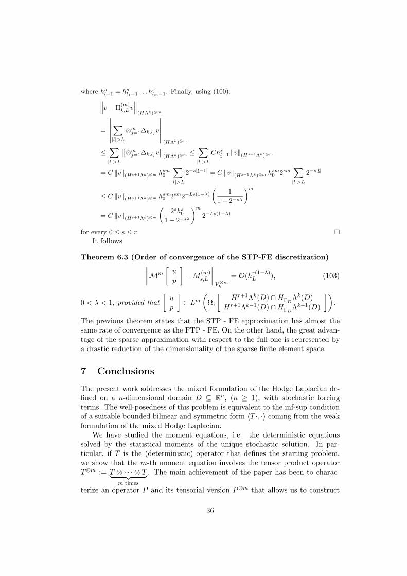
3.2 Stochastic mixed Hodge-Laplace problem
Let D be a domain in Rn satisfying assumption 2.1. Let be given
[F1
F2
]∈
Lm (Ω;V ′k), with m ≥ 1, defined as the stochastic version of (20) and (21):
F1(ω) : HΓDΛk(D)→ R
F1(ω)(v) := (f1(ω), v)
F2(ω) : HΓDΛk−1(D)→ RF2(ω)(q) := (f2(ω), q)
where
[f1
f2
]∈ Lm (Ω;Vk) is given. The stochastic counterpart of problem (22)
is:
Stochastic Problem:
Given m ≥ 1 and
[F1
F2
]∈ Lm (Ω;V ′k) , find
[up
]∈ Lm (Ω;Vk) s.t.
T
[u(ω)p(ω)
]=
[F1(ω)F2(ω)
]in V ′k, a.e. in Ω.
(41)
13

Theorem 3.1 (Well-posedness of the stochastic Hodge Laplacian) Forevery α > 0 problem (41) is well-posed, so that there exists a unique solution thatdepends continuously on the data. The same result holds with α = 0 provided
that F2 corresponds to f2 ∈ Lm(
Ω; δHΓDΛk(D)
).
Proof. Thanks to Theorem 2.1, for almost all ω ∈ Ω, problem (41) admits a unique
solution
[u(ω)p(ω)
]∈ Vk, the mapping ω 7→
[u(ω)p(ω)
]is measurable and we have:∥∥∥∥[ u(ω)
p(ω)
]∥∥∥∥Vk
≤ K∥∥∥∥[ F1(ω)
F2(ω)
]∥∥∥∥V ′k
a.e. in Ω (42)
with K = K(CP , α) independent of ω (see (29)). For any m ≥ 1,(E
[∥∥∥∥[ u(ω)p(ω)
]∥∥∥∥mVk
])1/m
≤ K
(E
[∥∥∥∥[ F1(ω)F2(ω)
]∥∥∥∥mV ′k
])1/m
.
By hypothesis
[F1
F2
]∈ Lm (Ω;V ′k), hence we conclude that
[up
]∈ Lm (Ω;Vk).
4 Deterministic problems for the statistics of u andp
We are interested in the statistical moments of the unique stochastic solution[up
]of the stochastic problem (41). We exploit the linearity of the system
T
[u(ω)p(ω)
]=
[F1(ω)F2(ω)
]to derive the moment equations, that is the determin-
istic equations solved by the statistical moments of the unique stochastic solution[up
]. At the beginning we focus on the first moment equation. Then, after
recalling the definition of the m-th statistical moment (m ≥ 2 integer) and themain concepts about the tensor product of operators defined on Hilbert spaces,we establish the well-posedness of the m-th moment problem. The main achieve-ment is the constructive proof of the inf-sup condition for the tensor productoperator T⊗m stated in Theorem 4.2. Indeed, this proof extends to the case ofsparse tensor product approximations (see Section 6.4).
4.1 Equations for the mean
Following [43, 41], we provide a way to compute the first statistical moment ofthe unique stochastic solution of the stochastic Hodge Laplace problem (41).
Given a random field v ∈ L1 (Ω;V ), where V in a Hilbert space, its firststatistical moment E [v] ∈ V is well defined, and is given by:
E [v] (x) :=
∫Ωv(ω, x)dP, x ∈ D. (43)
14

Definition (43) easily applies to the vector case (V = Vk, V = Wk).
Suppose that
[F1
F2
]∈ L1 (Ω;V ′k), so that the unique solution of the stochas-
tic problem is such that
[up
]∈ L1 (Ω;Vk). To derive the first moment equation
we simply apply the mean operator to the stochastic problem (41). We exploitthe commutativity between the operators T defined in (17) and E defined in
(43), so that E[up
]is a solution of:
Mean Problem
Given
[F1
F2
]∈ L1 (Ω;V ′k) , find Es ∈ Vk s.t.
T (Es) = E[F1
F2
]in V ′k,
(44)
where E[F1
F2
]∈ V ′k is defined as:
E[F1
F2
]([vq
]):=
(E[f1
f2
],
[vq
])Wk
∀[vq
]∈ Vk.
Theorem 2.1 states the well-posedness of problem (44), hence E[up
]is the
unique solution. We notice that problem (44) has exactly the same structure ofproblem (41) with loading terms given by the mean of the loading terms in (41).
4.2 Statistical moments of a random function
Let u ∈ Lm (Ω;V ), where V is a Hilbert space and Lm (Ω;V ) is defined as inSection 3.1. Then u⊗m := u⊗ · · · ⊗ u︸ ︷︷ ︸
m times
∈ L1(Ω, V ⊗m), where from now on V ⊗m
denotes the tensor product space V ⊗ · · · ⊗ V︸ ︷︷ ︸m times
. Hence we can give the following
definition:
Definition 4.1 Given u ∈ Lm (Ω;V ), m ≥ 2 integer, then the m-th moment ofu(ω) is defined by
Mm [u] := E [u⊗ · · · ⊗ u] =
∫Ωu(ω)⊗ · · · ⊗ u(ω)dP(ω) ∈ V ⊗m. (45)
It clearly holds ‖Mm [u] ‖V ⊗m ≤ ‖u‖mLm(Ω;V ). Definition 4.1 with m = 1 is (43).Moreover, Definition 4.1 easily generalizes to the vector case.
15

4.3 Tensor product of operators on Hilbert spaces
We will see that the deterministic equation for the m-th moment involves thetensor product of the operator T . Hence, we need to describe some aspects ofthe theory of tensor product operators on Hilbert spaces. For more details seefor example [37] and the references therein.
Suppose that T1 : V1 → V ′1 , T2 : V2 → V ′2 are continuous operators on theHilbert spaces V1 and V2 respectively. T1⊗T2 is defined on functions of the typeφ⊗ ψ, with φ ∈ V1, ψ ∈ V2 as:
(T1 ⊗ T2) (φ⊗ ψ) = T1φ⊗ T2ψ ∈ V ′1 ⊗ V ′2 .
This definition extends to V1 ⊗ V2 by linearity and density. The tensor productof two bounded operators on Hilbert space is still a bounded operator, as statedby the following
Proposition 4.1 Let T1 : V1 → V ′1, T2 : V2 → V ′2 be bounded operators onHilbert spaces V1 and V2 respectively. Then
‖T1 ⊗ T2‖L(V1⊗V2,V ′1⊗V ′2) = ‖T1‖L(V1,V ′1)‖T2‖L(V2,V ′2).
Proof. See [37]. The definition of the tensor product of two operators on Hilbert spaces and
Proposition 4.1 generalize to tensor product of any finite number of operatorsdefined on Hilbert spaces.
We detail now the vector case, since it will be useful in the next section.Let V1 = V2 = Vk, where Vk is defined in (15), and T1 = T2 = T , whereT = (T )i,j=1,2 : Vk → V ′k is the linear operator of order two defined in (17). Thetensor product operator T⊗m := T ⊗ · · · ⊗ T︸ ︷︷ ︸
m
, (m ≥ 1 integer), is the operator
of order 2m that maps tensors in V ⊗mk to tensors is (V ′k)⊗m defined as
(T⊗m)i1...i2m = Ti1i2 ⊗ · · · ⊗ Ti2m−1i2m . (46)
Given X ∈ V ⊗mk , T⊗mX is a tensor of order m in (V ′k)⊗m given by
(T⊗mX)i1...im =2∑
j1,...,jm=1
(Ti1j1 ⊗ · · · ⊗ Timjm)Xj1...jm , i1, . . . , im = 1, 2. (47)
Definition 4.2 Let T and Vk be as before and let X ∈ V ⊗mk and Y ∈ V ⊗mk . Wedefine
⟨T⊗mX,Y
⟩=
2∑i1,...,im=1
2∑j1,...,jm=1
〈Ti1,j1 · · ·Tim,jmXj1,...,jm , Yi1,...,im〉 . (48)
16

4.4 Equations for the m-th moment
Following [43], we analyze the m-th moment equation for m ≥ 2. Suppose[F1
F2
]∈ Lm (Ω;V ′k) so that
[up
]∈ Lm (Ω;Vk). To derive the deterministic
m-th moment problem we tensorize the stochastic problem (41) with itself mtimes:
T ⊗ . . .⊗ T︸ ︷︷ ︸m times
[u(ω)p(ω)
]⊗m=
[F1(ω)F2(ω)
]⊗min (V ′k)⊗m, for a.e. ω ∈ Ω.
We take the expectation on both sides and we exploit the commutativity be-
tween the operators T and E. By definition, E[up
]⊗m= Mm
[up
]. Thus,
Mm
[up
]is a solution of
m-Points Correlation Problem:
Given m ≥ 2 integer and
[F1
F2
]∈ Lm (Ω;V ′k) , find M⊗ms ∈ V ⊗mk s.t.
T⊗mM⊗ms =Mm
[F1
F2
]in (V ′k)⊗m,
(49)
where Mm
[F1
F2
]∈ (V ′k)⊗m is defined as:
Mm
[F1
F2
]([vq
]):=
(Mm
[f1
f2
],
[vq
])W⊗m
k
∀[vq
]∈ V ⊗mk .
We notice that in the right-hand side of (49) we have the m-points correlationof the loading terms of problem (41).
Remark 4.1 Note that problem (44) is a saddle-point problem, and (49) iscomposed of m ”nested” saddle-point problems. Indeed, if for example m = 2,T ⊗ T can be represented by the matrix
T ⊗ T =
δd⊗ δd δd⊗ d d⊗ δd d⊗ dδd⊗ δ δd⊗−αId d⊗ δ d⊗−αId
δ ⊗ δd δ ⊗ d −αId⊗ δd −αId⊗ dδ ⊗ δ δ ⊗−αId −αId⊗ δ −αId⊗−αId
. (50)
Theorem 4.1 (Well-posedness of the m-th problem) For every α > 0,problem (49) is well-posed, so that there exists a unique solution that dependscontinuously on the data. The same result holds with α = 0 provided that F2
corresponds to f2 ∈ Lm(
Ω; δHΓDΛk(D)
).
17

Proof. Theorem 4.1 can be proved by a simple tensor product argument, as follows.
Since problem (22) is well-posed, the inverse operator T−1 exists and is linear and
bounded. Now we take into account the tensor operator (T−1)⊗m = T−1 ⊗ . . .⊗ T−1︸ ︷︷ ︸m times
.
It is the inverse operator of T⊗m. Moreover, it is linear and bounded (Proposition 4.1).
Hence we can immediately conclude the well-posedness of problem (49).
Remark 4.2 The approach presented in the proof is not completely satisfactoryin view of a finite dimensional approximation. Indeed, when considering a finitedimensional version of the operator, Th := T |Vk,h : Vk,h → V ′k,h, where Vk,h isa finite dimensional subspace of Vk, and aiming at proving the well-posednessof the tensor operator (Th)⊗m = Th ⊗ . . .⊗ Th︸ ︷︷ ︸
m times
, this tensor product argument
applies only if the finite dimensional subspace is a tensor product space V ⊗mk,h .It will not apply straightforwardly if sparse tensor product spaces are consideredinstead.
4.4.1 Constructive proof of inf-sup condition for the tensorized prob-lem
Here we propose an alternative proof of Theorem 4.1 that consists in showingthe inf-sup condition for T⊗m. This proof will be used later on to prove thestability of a sparse tensor product finite element discretization, which is ofpractical interest for moderately large m as it reduces considerably the curse ofdimensionality with respect to a full tensor product approximation.A result equivalent to Theorem 4.1 is the following
Theorem 4.2 (Tensorial inf-sup condition) For every M⊗ms ∈ V ⊗mk , thereexist a test function M⊗mt ∈ V ⊗mk and positive constantsCm = Cm(α,CP,1, ‖T‖, ‖P‖), C ′m = C ′m(α,CP,1, ‖T‖, ‖P‖)) s.t.⟨
T⊗mM⊗ms ,M⊗mt⟩
(V ′k)⊗m,V ⊗mk≥ Cm‖M⊗ms ‖2
V ⊗mk
, (51)
‖M⊗mt ‖V ⊗mk≤ C ′m‖M⊗ms ‖V ⊗m
k, (52)
where CP,1 is introduced in (60) and P is defined in (28).
Before presenting the proof we state the tensorized versions of the Hodgedecomposition and the Poincare inequality, which are two keys ingredients inthe proof of the inf-sup condition for the deterministic problem (22).
Let us write the space V ⊗mk as
V ⊗mk = Vk ⊗ V⊗(m−1)k =
[HΓD
Λk(D)
HΓDΛk−1(D)
]⊗ V ⊗(m−1)
k =
[UmkUmk−1
](53)
18

where we defined
Umk := HΓDΛk(D)⊗ V ⊗(m−1)
k , (54)
Umk−1 := HΓDΛk−1(D)⊗ V ⊗(m−1)
k (55)
We obtain the tensorial Hodge decomposition following the idea of the one di-mensional Hodge decomposition (11). Indeed, for every integer m ≥ 2, we splitUmk (Umk−1 is analogous) as:
Tensorial Hodge Decomposition: (56)
Umk = Bmk ⊕Bm,⊥
k (57)
where
Bmk := d⊗ Id⊗(m−1) Umk−1 = Bk ⊗ V
⊗(m−1)k
Bm,⊥k := B⊥k ⊗ V
⊗(m−1)k
and Bk, B⊥k are defined in Section 2.
The tensor operators π⊥ ⊗ Id⊗(m−1) and π ⊗ Id⊗(m−1) respectively defined in(12) and (13) act on Umk (Umk−1 is analogous) as:
π⊥ ⊗ Id⊗(m−1) : Umk = Bmk ⊕Bm,⊥
k → Bm,⊥k (58)
v = d⊗ Id⊗(m−1)v + v⊥ 7→ v⊥
π ⊗ Id⊗(m−1) : Umk = Bmk ⊕Bm,⊥
k → Bm,⊥k−1 (59)
v = d⊗ Id⊗(m−1)v + v⊥ 7→ v.
The tensorial Poincare inequality is proved in the following lemma.
Lemma 4.1 (Tensorial Poincare inequality) For every integer m ≥ 2, thereexists a positive constant CP,1 such that
‖v‖(L2Λk(D))⊗m ≤ CP,1‖Id⊗ . . .⊗ d︸︷︷︸i
⊗ . . .⊗Id v‖L2Λk⊗...⊗L2Λk+1︸ ︷︷ ︸i
⊗...⊗L2Λk , (60)
∀v ∈ L2Λk ⊗ . . .⊗ (Z⊥k )︸︷︷︸i
⊗ . . .⊗ L2Λk(D), where Z⊥k is defined in Section 2.2.
Proof. We know that HΛk(D) is a Hilbert space with the inner product (u, v)HΛk and
(u, u)HΛk = ‖u‖2HΛk . Besides, we know that Z⊥k is a Hilbert space with the equivalent
inner product (du,dv) and norm ‖du‖ = (du,du). A consequence of the Open Mapping
Theorem states that given m Hilbert spaces H1, . . . ,Hm, the topology of H1⊗ . . .⊗Hm
depends only on the topology and not on the choice of the inner products of H1, . . . ,Hm.
19

If we apply this statement with Hi = Z⊥k and Hj = HΛk(D), i 6= j, we can conclude
the inequality (60). A simple consequence of the previous lemma is:
‖v‖(L2Λk(D))⊗m ≤ CP,m‖d⊗mv‖(L2Λk+1(D))⊗m ∀v ∈(Z⊥k
)⊗m, (61)
where CP,m > 0 depends only on the domain D and on m.Proof. [Proof of Theorem 4.2]
As shown before,Mm
[up
]is a solution of (49). Uniqueness of the solution of problem
(49) is related to the global inf-sup condition (51), (52) (see [5, 11]). Suppose α > 0(the case α = 0 is analogous). To lighten the notations, in the proof we use the brackets〈·, ·〉 without specifying the spaces we consider, when no ambiguity arises. We use thetensorial Hodge decomposition (57) and the tensorial Poicare inequality (Lemma 4.1).We prove (51) by induction. In Theorem 2.1 we already proved the inf-sup condition
with m = 1. Now suppose m = 2. We fix M⊗2s =
[(M⊗2
s )1:
(M⊗2s )2:
]where (M⊗2
s )1:
(respectively (M⊗2s )2:) means that in the tensor of order two M⊗2
s = (M⊗2s )ij=1,2 we fix
i = 1 (respectively i = 2) and let j vary. Using (53) and (57) with m = 2 we decompose
M⊗2s =
[d⊗ Id(Ms )1: + (M⊥s )1:
d⊗ Id(Ms )2: + (M⊥s )2:
]∈[
U2k
U2k−1
],
where
(M⊥s )1: = π⊥ ⊗ Id(M⊗2s )1: ∈ B2,⊥
k
(M⊥s )2: = π⊥ ⊗ Id(M⊗2s )2: ∈ B2,⊥
k−1
(Ms )1: = π ⊗ Id(M⊗2s )1: ∈ B2,⊥
k−1
(Ms )2: = π ⊗ Id(M⊗2s )2: ∈ B2,⊥
k−2.
We choose M⊗2t = P ⊗ PM⊗2
s , where P is defined in (28), so that:⟨T ⊗ TM⊗2
s ,M⊗2t
⟩=⟨T ⊗ TM⊗2
s , P ⊗ PM⊗2s
⟩=
2∑i,j=1
⟨Tij ⊗ T (M⊗2
s )j:, (P ⊗ PM⊗2s )i:
⟩. (62)
Let⟨Tij ⊗ T (M⊗2
s )j:, (P ⊗ PM⊗2s )i:
⟩= Iij . We will bound each term Iij for i, j = 1, 2.
Using (47) we explicit the term (P ⊗ PM⊗2s )i::
(P ⊗ PM⊗2s )i: = Pi1 ⊗ P (M⊗2
s )1: + Pi2 ⊗ P (M⊗2s )2:. (63)
Let us start from the case i = j = 1.
I11 =⟨A⊗ T (M⊗2
s )1:, (π⊥ ⊗ P (M⊗2
s )1: + dπ⊥ ⊗ P (M⊗2s )2:)
⟩. (64)
Since d d = 0,⟨A⊗ T (M⊗2
s )1:,dπ⊥ ⊗ P (M⊗2
s )2:)⟩
= 0 and A ⊗ T (d ⊗ IdMs )1: ≡ 0.Hence,
I11 =⟨A⊗ T (M⊥s )1:, Id⊗ P (M⊥s )1:
⟩=⟨d⊗ T (M⊥s )1:,d⊗ P (M⊥s )1:
⟩≥ C1‖d⊗ Id(M⊥s )1:‖2L2Λk+1⊗Vk
.
20

The last step follows from Proposition 2.1. If i = 1 and j = 2 we find
I12 =⟨B∗ ⊗ T (M⊗2
s )2:, π⊥ ⊗ P (M⊗2
s )1: + dπ⊥ ⊗ P (M⊗2s )2:
⟩. (65)
Since π⊥ ⊗ P (M⊗2s )1: ∈ B2,⊥
k ,⟨B∗ ⊗ T (M⊗2
s )2:, π⊥ ⊗ P (M⊗2
s )1:
⟩= 0. Hence,
I12 =⟨B∗ ⊗ T (M⊥s )2:,d⊗ P (M⊥s )2:
⟩=⟨d⊗ T (M⊥s )2:,d⊗ P (M⊥s )2:
⟩≥ C1‖d⊗ Id(M⊥s )2:‖2L2Λk⊗Vk
.
If i = 2 and j = 1 we find
I21 =⟨B ⊗ T (M⊗2
s )1:, γπ ⊗ P (M⊗2
s )1: − dπ ⊗ P (M⊗2s )2:
⟩. (66)
Since⟨B ⊗ T (M⊗2
s )1:,dπ ⊗ P (M⊗2
s )2:
⟩= 0, and
⟨B ⊗ T (M⊥s )1:, Id⊗ P (Ms )1:
⟩= 0,
we have:
I21 = γ 〈B ⊗ T (d⊗ Id(Ms )1:), Id⊗ P (Ms )1:〉= γ 〈d⊗ T (Ms )1:,d⊗ P (Ms )1:〉≥ γC1‖d⊗ Id(Ms )1:‖2L2Λk⊗Vk
.
If i = j = 2
I22 = −α⟨Id⊗ T (M⊗2
s )2:, γπ ⊗ P (M⊗2
s )1: − dπ ⊗ P (M⊗2s )2:
⟩= α
⟨Id⊗ T (M⊗2
s )2:,dπ ⊗ P (M⊗2
s )2:
⟩(67)
− α⟨Id⊗ T (M⊗2
s )2:, γπ ⊗ P (M⊗2
s )1:
⟩. (68)
Since⟨Id⊗ T (M⊥s )2:,dπ
⊗ P (M⊗2s )2:
⟩= 0, we find
(67) = α 〈d⊗ T (Ms )2:,d⊗ P (Ms )2:〉≥ αC1‖d⊗ Id(Ms )2:‖2L2Λk⊗Vk
.
Moreover, since⟨Id⊗ T (dπ ⊗ Id(M⊗2
s )2:), π ⊗ P (M⊗2
s )1:
⟩= 0, we find
(68) = −αγ⟨Id⊗ T (M⊥s )2:, Id⊗ P (Ms )1:
⟩≥ −α
2γ1/2
(‖Id⊗ T (M⊥s )‖2L2Λk−1⊗V ′k
+ γ‖Id⊗ P (Ms )1:‖2L2Λk⊗Vk
)≥ −α
2γ1/2
(C2P,1‖T‖2L(Vk,V ′k)‖d⊗ Id(M⊥s )2:‖2L2Λk⊗Vk
+γC2P,1‖P‖2L(Vk,Vk)‖d⊗ Id(Ms )1:‖2L2Λk+1⊗Vk
),
where we used Proposition 4.1 and Lemma 4.1. Using the lower bounds on I11, I12, I21
and I22, we can now conclude that:
(62) ≥ C1‖d⊗ Id(M⊥s )1:‖2L2Λk+1⊗Vk
+(C1 −
α
2γ1/2C2
P,1‖T‖2L(Vk,V ′k)
)‖d⊗ Id(M⊥s )2:‖2L2Λk⊗Vk
+ γ(C1 −
α
2γ1/2C2
P,1‖P‖2L(Vk,Vk)
)‖d⊗ Id(Ms )1:‖2L2Λk⊗Vk
+ αC1‖d⊗ Id(Ms )2:‖2L2Λk⊗Vk.
21

Hence, if we choose γ sufficiently small, condition (51) is satisfied for m = 2. Nowsuppose that the problem for the (m−1)-th moment is well-posed, and in particular that
the inf-sup condition is verified with the test function M⊗(m−1)t = P⊗(m−1)M
⊗(m−1)s :⟨
T⊗(m−1)M⊗(m−1)s , P⊗(m−1)M⊗(m−1)
s
⟩≥ Cm−1‖M⊗(m−1)
s ‖2V⊗(m−1)k
, (69)
where Cm−1 = Cm−1(CP,1, α, ‖T‖, ‖P‖) > 0. We want to prove (51). As before, we
fix M⊗ms =
[(M⊗ms )1:
(M⊗ms )2:
]where (M⊗ms )1: (respectively (M⊗ms )2:) means that in the
tensor of order m, M⊗ms = (M⊗ms )i1...im=1,2, we fix i1 = 1 (respectively i1 = 2) and leti2, . . . , im vary. Using (53) and (57) we decompose
M⊗ms =
[(M⊥s )1: + d⊗ Id⊗(m−1)(Ms )1:
(M⊥s )2: + d⊗ Id⊗(m−1)(Ms )2:
]∈[
UmkUmk−1
],
where now
(M⊥s )1: = π⊥ ⊗ Id⊗(m−1)(M⊗ms )1: ∈ Bm,⊥k
(M⊥s )2: = π⊥ ⊗ Id⊗(m−1)(M⊗ms )1: ∈ Bm,⊥k−1
(Ms )1: = π⊥ ⊗ Id⊗(m−1)(M⊗ms )1: ∈ Bm,⊥k−1
(Ms )2: = π⊥ ⊗ Id⊗(m−1)(M⊗ms )1: ∈ Bm,⊥k−2 .
We choose M⊗mt = P⊗mM⊗ms , so that:⟨T⊗mM⊗ms ,M⊗mt
⟩=⟨T⊗mM⊗ms , P⊗mM⊗ms
⟩=
2∑i,j=1
⟨Ti,j ⊗ Tm−1(M⊗ms )j:, (P
⊗mM⊗ms )i:⟩. (70)
Let Jij =⟨Ti,j ⊗ Tm−1(M⊗ms )j:, (P
⊗mM⊗ms )i:⟩. We follow a completely similar rea-
soning as before, and we apply (69). If i = j = 1,
J11 =⟨A⊗ T⊗(m−1)(M⊗ms )1:, (P ⊗ P⊗(m−1)M⊗ms )1:
⟩≥ Cm−1‖d⊗ Id⊗(m−1)(M⊥s )1:‖2L2Λk+1⊗V ⊗(m−1)
k
.
If i = 1 and j = 2,
J12 =⟨B∗ ⊗ T⊗(m−1)(M⊗ms )2:, (P ⊗ P⊗(m−1)M⊗ms )1:
⟩≥ Cm−1‖d⊗ Id⊗(m−1)(M⊥s )2:‖2L2Λk⊗V ⊗(m−1)
k
.
If i = 2 and j = 1,
J21 =⟨B ⊗ T⊗(m−1)(M⊗ms )1:, (P ⊗ P⊗(m−1)M⊗ms )2:
⟩≥ γCm−1‖d⊗ Id⊗(m−1)(Ms )1:‖2L2Λk⊗V ⊗(m−1)
k
.
22

If i = j = 2,
J22 = −α⟨
Id⊗ T⊗(m−1)(M⊗ms )2:, (P ⊗ P⊗(m−1)M⊗ms )2:
⟩≥ αCm−1‖d⊗ Id⊗(m−1)(Ms )2:‖2L2Λk⊗V ⊗(m−1)
k
+
− α
2γ1/2
(C2P,1‖T‖
2(m−1)L(Vk,V ′k)‖d⊗ Id⊗(m−1)(M⊥s )2:‖2L2Λk⊗V ⊗(m−1)
k
+
+γC2P,1‖P‖
2(m−1)L(Vk,Vk)‖d⊗ Id⊗(m−1)(Ms )1:‖2L2Λk⊗V ⊗(m−1)
k
).
Hence, if we choose γ sufficiently small, condition (51) is satisfied. Relation (52) follows
from the orthogonal decomposition (57) and the tensorial Poincare inequality in Lemma
4.1. Another way to express the result given in Theorem 4.2 is the following
Proposition 4.2 Given T as in (17) and P as in (28), ∀Mms it holds⟨
T⊗mM⊗ms , P⊗mM⊗ms⟩
(V ′k)⊗m,V ⊗mk≥ Cm
∥∥M⊗ms ∥∥2
V ⊗mk
.
As a simple consequence of Proposition 4.1 we have also the bound on P⊗m.
Remark 4.3 We underline that the operator P is not the classical one presentedin [3] to prove the well-posedness of the deterministic Hodge-Laplace problem.Indeed it is the minimal one such that the inf-sup condition for 〈T⊗m·, ·〉 : V ⊗mk ×V ⊗mk → R (for every finite m ≥ 1) is satisfied. With the classical operator, theinf-sup condition for m ≥ 2 is not automatically satisfied.
5 Some three-dimensional problems important in ap-plications
In Section 2.3.1 we have reinterpreted the deterministic Hodge-Laplace problemin n = 3 dimensions in terms of PDEs. Here we translate in terms of partialdifferential equations the stochastic Hodge-Laplace problem. In particular, wefocus on the two problems obtained for k = 1 and k = 3: the stochastic mag-netostatic/electrostatic equations and the stochastic Darcy equations, and weexplicitly write the systems solved by the mean and the two-points correlationof the unique stochastic solution of the stochastic problem.
5.1 The stochastic magnetostatic/electrostatic equations
Take k = 1 and α = 0. Let f1 ∈ Lm(Ω;L2Λ1(D)
), f2 ∈ Lm
(Ω;L2Λ0(D)
)be stochastic functions with, m ≥ 1 integer, representing an uncertain currentand an uncertain charge respectively. The stochastic magnetostatic/electrostaticproblem is the stochastic counterpart of problem (35). Thanks to Theorem 3.1,the stochastic magnetostatic/electrostatic problem admits a unique stochastic
23

solution that depends continuously on the data. If m ≥ 1, the first statistical
moment M1
[up
]= E
[up
]is well-defined, and is the unique solution of (see
(44)): find Es =
[Es,1Es,2
]∈ V1 such that
(curl Es,1, curl v) + (∇Es,2, v) = (E [f1] , v)(Es,1,∇q) = (E [f2] , q) .
∀[vq
]∈ V1, (71)
where the parenthesis in (71) mean the L2-inner product. In the case m ≥ 2, the
second statistical moment M2
[up
]is well-defined, and is the unique solution
of (see (49) with m = 2): find
M⊗2s ∈ V1⊗V1 =
[HΓD
(curl , D)⊗HΓD(curl , D) HΓD
(curl , D)⊗H1ΓD
(D)
H1ΓD
(D)⊗HΓD(curl , D) H1
ΓD(D)⊗H1
ΓD(D)
]such that
(curl ⊗ curl (M⊗2
s )11, curl ⊗ curl (M⊗2t )11
)+(
curl ⊗∇(M⊗2s )12, curl ⊗ Id(M⊗2
t )11
)+(
∇⊗ curl (M⊗2s )21, Id⊗ curl (M⊗2
t )11
)+(∇⊗∇(M⊗2
s )22, (M⊗2t )11
)=(
M2 [f1] , (M⊗2t )11
)−(curl ⊗ Id(M⊗2
s )11, curl ⊗∇(M⊗2t )12
)−(
∇⊗ Id(M⊗2s )12, Id⊗∇(M⊗2
t )12
)=(E [f1f2] , (M⊗2
t )12
)−(Id⊗ curl (M⊗2
s )12,∇⊗ curl (M⊗2t )21
)−(
Id⊗∇M⊗2s )21,∇⊗ Id(M⊗2
t )21
)=(E [f2f1] , (M⊗2
t )21
)((M⊗2
s )11,∇⊗∇(M⊗2t )22
)=(M2 [f2] , (M⊗2
t )22
)(72)
∀M⊗2t ∈ V1 ⊗ V1, where the parenthesis in (72) have to be intended as inner
product in (L2(D))3 ⊗ (L2(D))3.
5.2 The stochastic Darcy problem
Let k = 3, f2 ≡ 0 and f1 ∈ Lm(Ω;L2Λ3(D)
), m ≥ 1 integer, representing an
uncertain source in porous media flow. The stochastic Darcy problem is thestochastic counterpart of problem (38). Thanks to Theorem 3.1, the stochasticDarcy problem admits a unique stochastic solution that depends continuously
on the data. If m ≥ 1, the first statistical moment M1
[up
]= E
[up
]is
well-defined, and is the unique solution of (see (44)): find Es =
[Es,1Es,2
]∈ V3
24

such that (div Es,2, v) = (E [f1] , v)(Es,1,div q)− α (Es,2, q) = 0
∀[vq
]∈ V3. (73)
where the parenthesis in (73) mean the L2-inner product. In the case m ≥ 2, the
second statistical moment M2
[up
]is well-defined, and is the unique solution
of (see (49) with m = 2): find
M⊗2s ∈ V3 ⊗ V3 =
[L2(D)⊗ L2(D) L2(D)⊗HΓD
(div , D)HΓD
(div , D)⊗ L2(D) HΓD(div ;D)⊗HΓD
(div ;D)
]such that
(div ⊗ div (M⊗2
s )22, (Mt)11
)=(M2 [f1] , (Mt)11
)(div ⊗ Id(M⊗2
s )21, Id⊗ div (M⊗2t )12
)− α
(div ⊗ Id(M⊗2
s )22, (M⊗2t )12
)= 0(
Id⊗ div (M⊗2s )12, div ⊗ Id(M⊗2
t )21
)− α
(Id⊗ div (M⊗2
s )22, (M⊗2t )21
)= 0(
(M⊗2s )11, div ⊗ div (M⊗2
t )22
)− α
((M⊗2
s )12,div ⊗ Id(M⊗2t )22
)−α
((M⊗2
s )21, Id⊗ div (M⊗2t )22
)+ α2
((M⊗2
s )22, (M⊗2t )22
)= 0
(74)∀M⊗2
t ∈ V3 ⊗ V3, where the parenthesis in (72) have to be intended as innerproduct in L2(D)⊗ L2(D).
6 Finite element discretization of the moment equa-tions
In this section we aim to derive a stable discretization for the moment equations,i.e. the deterministic problems solved by the statistics of the unique stochastic
solution
[up
]. First we recall the main concepts concerning the finite element
differential forms and the existence of a stable finite element discretization forthe mean problem (44). Then we construct both a full and a sparse tensorproduct finite element discretization for the m-th problem, with m ≥ 2 integer,we prove their stability and provide optimal order of convergence estimates.
6.1 Finite element differential forms
Following [3], throughout this section we assume that the domain D ⊂ Rnsatisfying Assumption 2.1 is a polyhedral domain in Rn which is partitionedinto a finite set of n-simplices. These simplices are such that their union is theclosure of D and the intersection of any two of them, if non-empty, is a common
25

k = 0 P−r Λ0(Th) Lagrangian elements of degree ≤ rk = 1 P−r Λ1(Th) Nedelec 1-nd kind H(curl ) elements of order r − 1
k = 2 P−r Λ2(Th) Nedelec 1-nd kind H(div ) elements of order r − 1
k = 3 P−r Λ3(Th) Discontinuous elements of degree ≤ r − 1
Table 2: Proxy fields correspondences between finite element differential formsP−r Λk(Th) and the classical finite element spaces for n = 3.
sub simplex. We denote the partition with Th and the discretization parameterwith h. To discretize the moment equations we use the finite element differentialforms
P−r Λk(Th) =v ∈ HΛk(D)| v|T ∈ P−r Λk(T ) ∀ T ∈ Th
, (75)
where the space P−r Λk(T ) and the de Rham subcomplex
0 −→ P−r Λ0(Th)d−→ · · · d−→ P−r Λn(Th) −→ 0
are treated in [3, 25]. Since we are particularly interested in the n = 3 case,we resume in Table 2 the correspondences between the finite element differentialforms (75) and the classical finite element spaces of scalar and vector functions.The spaces P−r Λk(Th) are not the only choice. Indeed, in [3, 4, 25, 14] the au-thors present other finite element differential forms to discretize the deterministicHodge Laplacian.
In [4] the authors propose the construction of a projector Πk,h : HΛk(D)→P−r Λk(Th) which is a cochain map, that is it commutes with the exterior deriva-tive, and such that the following approximation property holds:
‖v −Πk,hv‖HΛk(D) ≤ Chs‖v‖Hs+1Λk(D), ∀ v ∈ Hs+1Λk(D), 0 ≤ s ≤ r, (76)
where HsΛk(D) is the space of differential k-forms with square integrable partialderivatives of order at most s, and C is independent of h. Moreover, Πk,h isbounded by a constant Cπ independent of h:
‖Πk,hv‖HΛk ≤ Cπ‖v‖HΛk ∀ v ∈ HΓDΛk(D). (77)
Since we are dealing with Dirichlet boundary conditions on ΓD, we make thefollowing
Assumption 6.1 There exists a bounded (see (77)) cochain projector, that byabuse of notation we denote still by Πk,h,
Πk,h : HΓDΛk(D)→ P−r,ΓD
Λk(Th) := P−r Λk(Th) ∩HΓDΛk(D), (78)
such that (76) is satisfied for every v ∈ Hs+1Λk(D) ∩HΓDΛk(D), 0 ≤ s ≤ r.
26

Assumption 6.1 is satisfied in the two and three dimensional case: see [39]. The ndimensional case is still a topic of current research, whereas if natural boundaryconditions are imposed on ∂D, the existence of such an operator is proved in [3],and if essential boundary conditions are imposed on ∂D, the existence of suchan operator is proved in [15].
6.2 Discrete mean problem
The problem solved by the mean of the unique stochastic solution of the stochas-tic Hodge Laplacian turns out to be the deterministic Hodge Laplacian. In [3] theauthors study the finite element formulation of the deterministic Hodge Lapla-cian with natural boundary conditions on ∂D (ΓD = ∅). In [4] all the resultsobtained in [3] for ΓD = ∅ are extended to include the case of essential boundaryconditions on ∂D (ΓN = ∅). Under Assumption 6.1, all the results in [3, 4] applyto the general case ΓD, ΓN 6= ∅.
Let(P−r,ΓD
Λk(Th), d)
be the finite element de Rham subcomplex, h the dis-
cretization parameter, and Vk,h =
[P−r,ΓD
Λk(Th)
P−r,ΓDΛk−1(Th)
]. The finite element for-
mulation of problem (44) is:
Mean Problem - FE Formulation
Given
[F1
F2
]∈ L1 (Ω;V ′k) , find Es,h ∈ Vk,h s.t.
T (Es,h) = E[F1
F2
]in V ′k,h.
(79)
In [3] the authors show the stability of (79) by proving the inf-sup condition forthe bounded bilinear and symmetric form 〈T ·, ·〉 restricted to the finite elementspaces. Moreover, using a quasi-optimal error estimate and the interpolationproperty (76), the authors deduce the following order of convergence estimate:∥∥∥∥E [ up
]− Es,h
∥∥∥∥Vk
= O(hr), for E[up
]∈[
Hr+1Λk(D) ∩HΓDΛk(D)
Hr+1Λk−1(D) ∩HΓDΛk−1(D)
],
(80)
where E[up
]and Es,h are the unique solutions of problems (44) and (79)
respectively.
6.3 Discrete m-th moment problem: full tensor product approx-imation
The full tensor product finite element formulation (FTP-FE) of problem (49) is:
27

m-Points Correlation Problem (FTP-FE):
Given m ≥ 2 integer and
[F1
F2
]∈ Lm (Ω;V ′k) , find M⊗ms,h ∈ V
⊗mk,h s.t.
T⊗mM⊗ms,h =Mm
[F1
F2
]in (V ′k,h)⊗m
(81)
Theorem 4.1 applies to problem (81), as a consequence of a tensor productstructure (see Remark 4.2). We conclude therefore the stability of the full tensorproduct finite element discretization V ⊗mk,h .
Let Mm
[up
]be the unique solution of problem (49) and M⊗ms,h be the
unique solution of problem (81). Exploiting the Galerkin orthogonality andthe stability of the discretization, we can obtain the following quasi-optimalconvergence estimate:∥∥∥∥Mm
[up
]−M⊗ms,h
∥∥∥∥V ⊗mk
≤ C infM⊗m
h ∈V ⊗mk,h
∥∥∥∥Mm
[up
]−M⊗mh
∥∥∥∥V ⊗mk
. (82)
To study the approximation properties of the space V ⊗mk,h we construct the
tensorial projection operator Π⊗mk,h as follows.
Definition 6.1 Let Πk,h : HΓDΛk(D) → P−r,ΓD
Λk(Th) be a bounded cochainprojector satisfying Assumption 6.1. Given m ≥ 2 integer, we define
Π⊗mk,h := Πk,h ⊗ . . .⊗Πk,h︸ ︷︷ ︸m times
:(HΓD
Λk(D))⊗m
→(P−r,ΓD
Λk(Th))⊗m
. (83)
Since Πk,h is bounded in HΛk-norm by Cπ, Π⊗mk,h is bounded in (HΛk)⊗m-normby (Cπ)m (Proposition 4.1). Moreover, since it is the tensor product of cochainprojectors, it is itself a cochain projector. We state the approximation propertiesof Π⊗mk,h in the following
Proposition 6.1 The projector Π⊗mk,h introduced in Definition 6.1 is such that
‖v −Π⊗mk,h v‖(HΛk)⊗m ≤ Chs‖v‖(Hs+1Λk)⊗m (84)
for all v ∈ (Hs+1Λk(D) ∩HΓDΛk(D))⊗m, 0 ≤ s ≤ r, where C is independent of
h.
28

Proof. We already know the result for m = 1 (see (76)). Let m = 2. By triangleinequality,
‖v −Π⊗2k,hv‖HΛk⊗HΛk
≤ ‖v −Πk,h ⊗ Id v‖HΛk⊗HΛk + ‖Πk,h ⊗ (Id−Πk,h) v‖HΛk⊗HΛk
≤ Chs‖v‖Hs+1Λk⊗HΛk + Cπ‖v − Id⊗Πk,hv‖HΛk⊗HΛk
≤ Chs‖v‖Hs+1Λk⊗HΛk + CCπhs‖v‖HΛk⊗Hs+1Λk
≤ Chs(1 + Cπ)‖v‖Hs+1Λk⊗Hs+1Λk ,
where we used (76). By induction on m, we conclude (84). From the approximation properties of the projector Π⊗mk,h (84), it follows
Theorem 6.1 (Order of convergence of the FTP-FE discretization)∥∥∥∥Mm
[up
]−M⊗ms,h
∥∥∥∥V ⊗mk
= O(hr), (85)
provided that
[up
]∈ Lm
(Ω;
[Hr+1Λk(D) ∩HΓD
Λk(D)
Hr+1Λk−1(D) ∩HΓDΛk−1(D)
]).
6.4 Discrete m-th moment problem: sparse tensor product ap-proximation
In Section 6.3 we proved the stability of the full tensor product finite elementdiscretization V ⊗mk,h = Vk,h ⊗ . . .⊗ Vk,h︸ ︷︷ ︸
m times
. The main problem of this approach is
that it is strongly affected by the curse of dimensionality. Indeed, if dim(Vk,h) =Nh, the space V ⊗mk,h has dimension (Nh)m which is impractical for m moderatelylarge. A reduction in the dimensionality of the problem is possible if we considera sparse tensor product finite element (STP-FE) approximation instead (see e.g.[43, 41, 12, 40, 23] and the references therein).
Let T0 be a regular mesh of the physical domain D ⊂ Rn, and Tl∞l=0 bea sequence of partitions obtained by uniform mesh refinement, that is hl =hl−1/2, where hl is the discretization parameter of Tl. We have a sequenceP−r Λk(Tl)
∞l=0
of finite dimensional subspaces of the space Vk, which are nested
and dense in Vk. Let us define the orthogonal complement of P−r Λk(Tl−1) in
P−r Λk(Tl): Sk,l = P−r Λk(Tl) \ P−r Λk(Tl−1), and set Zk,l =
[Sk,lSk−1,l
]. For every
integer m ≥ 2, we define the sparse tensor product finite element space of level
L > 0, V(m)k,L , as:
V(m)k,L :=
⊕|l|≤L
(Zk,l1 ⊗ . . .⊗ Zk,lm) , (86)
where l is a multi index in Nm0 and |l| is its length l1 + . . .+ lm. At the numericallevel it may not be needed to explicitly build a basis for Zk,l. In [22] the authors
29

propose to use a redundant basis for the space (86) and an algorithm to solvethe m-th moment problem in the sparse tensor product framework.
The sparse tensor product finite element (STP-FE) approximation of prob-lem (49) is:
m-Points Correlation Problem (STP-FE):
Given m ≥ 2 integer and
[F1
F2
]∈ Lm (Ω;Vk) , find M
(m)s,L ∈ V
(m)k,L s.t.
T⊗mM(m)s,L =Mm
[F1
F2
]in(V
(m)k,L
)′(87)
Let us fix j ∈ 1, . . . ,m. We observe that:
V(m)k,L :=
⊕|l|≤L
(Zk,l1 ⊗ . . .⊗ Zk,lm)
=⊕
∑i6=j li≤L
Zk,l1 ⊗ . . .⊗ Zk,lj−1⊗
L−∑
i6=j li⊕lj=0
Zk,lj
⊗ Zk,lj+1⊗ . . .⊗ Zk,lm
=⊕
∑i6=j li≤L
(Zk,l1 ⊗ . . .⊗ Zk,lj−1
⊗ Vk,L−∑i6=j li⊗ Zk,lj+1
⊗ . . .⊗ Zk,lm)
=⊕|l|=L
(Zk,l1 ⊗ . . .⊗ Zk,lj−1
⊗ Vk,lj ⊗ Zk,lj+1⊗ . . .⊗ Zk,lm
).
Hence, we obtain an equivalent representation of the space V(m)k,L :
V(m)k,L =
⊕|l|=L
(Zk,l1 ⊗ . . .⊗ Zk,lj−1
⊗ Vk,lj ⊗ Zk,lj+1⊗ . . .⊗ Zk,lm
)=
[U
(m)k,L,j
U(m)k−1,L,j
],
(88)where
U(m)k,L,j :=
⊕|l|=L
(Zk,l1 ⊗ . . .⊗ Zk,lj−1
⊗ P−r Λk(Tlj )⊗ Zk,lj+1⊗ . . .⊗ Zk,lm
), (89)
and U(m)k−1,L,j is defined analogously. In [3], the authors prove the discrete Hodge
decompositionP−r Λk(Tl) = Bk,l ⊕B⊥k,l, (90)
where Bk,l is the image of d in P−r Λk(Tl) and B⊥k,l is its orthogonal complement.Using (90) we can carry the tensorial Hodge decomposition (57) to the discretelevel.
30

Lemma 6.1 (Discrete Tensorial Hodge Decomposition) For every inte-
ger m ≥ 2, the space U(m)k,L,j admits the following orthogonal decomposition:
U(m)k,L,j = B
(m)k,L,j ⊕B
(m),⊥k,L,j (91)
where
B(m)k,L,j :=
⊕|l|=L
(Zk,l1 ⊗ . . .⊗ Zk,lj−1
⊗Bk,lj ⊗ Zk,lj ⊗ . . .⊗ Zk,lm)
(92)
B(m),⊥k,L,j :=
⊕|l|=L
(Zk,l1 ⊗ . . .⊗ Zk,lj−1
⊗B⊥k,lj ⊗ Zk,lj ⊗ . . .⊗ Zk,lm)
(93)
(94)
Proof. Let us suppose j = 1 w.l.o.g. We need to show that the spaces B(m)k,L,1 and
B(m),⊥k,L,1 are orthogonal. Let us take v =
∑|l|=L bk,l1 ⊗ zk,l2 ⊗ . . . ⊗ zk,lm ∈ B
(m)k,L,1 and
v =∑|p|=L bk,p1 ⊗ zk,p2 ⊗ . . .⊗ zk,pm ∈ B
(m),⊥k,L,1 , then
(v, v) =∑|l|=L
∑|p|=L
(bk,l1 , bk,p1
) m∏i=2
(zk,li , zk,pi) =∑|l|=L
∑|p|=L
(bk,l1 , bk,p1
) m∏i=2
δli,pi .
In the second equality we used that (zk,li , zk,pi) = 0 if li 6= pi. But l2 = p2, . . . , lm = pmimply l1 = p1. Since bl1 and bl1 belong to orthogonal spaces, then (v, v) = 0. By linearity,
the previous relation extents to all elements of the spaces B(m)k,L,1 and B
(m),⊥k,L,1 .
The tensor product operators Id⊗(j−1) ⊗ π⊥ ⊗ Id⊗(m−j) and Id⊗(j−1) ⊗ π ⊗Id⊗(m−j) map each element of the space U
(m)k,L,j onto the spaces U
(m)k,L,j and U
(m)k−1,L,j
respectively. Indeed, let us take j = 1 w.l.o.g and v =∑|l|=L pk,l1 ⊗ zk,l2 ⊗ . . .⊗
zk,lm ∈ U(m)k,L,1. Using (90), we split v as
v =∑|l|=L
dpk−1,l1 ⊗ zk,l2 ⊗ . . .⊗ zk,lm +∑|l|=L
p⊥k,l1 ⊗ zk,l2 ⊗ . . .⊗ zk,lm ,
where dpk−1,l1∈ Bk,l1 = dB⊥k−1,l1
, p⊥k,l1 ∈ B⊥k,l1 ,∑|l|=L dpk−1,l1
⊗ zk,l2 ⊗ . . . ⊗zk,lm ∈ B
(m)k,L,1 and
∑|l|=L p
⊥k,l1⊗ zk,l2 ⊗ . . .⊗ zk,lm ∈ B
(m),⊥k,L,1 . Then,(
π⊥ ⊗ Id⊗(m−1))v :=
∑|l|=L
(p⊥k,l1 ⊗ zk,l2 ⊗ . . .⊗ zk,lm
)∈ B
(m),⊥k,L,1 ⊂ U
(m)k,L,1(
π ⊗ Id⊗(m−1))v :=
∑|l|=L
(pk,l1 ⊗ zk,l2 ⊗ . . .⊗ zk,lm
)∈ B
(m),⊥k−1,L,1 ⊂ U
(m)k−1,L,1.
By linearity, the previous definitions extent to all elements of the spaces U(m)k,L,1.
Observe that the operators Id⊗(j−1) ⊗ dπ⊥ ⊗ Id⊗(m−j) and Id⊗(j−1) ⊗ dπ ⊗
31

Id⊗(m−j) map each element of the space U(m)k,L,j onto the spaces U
(m)k+1,L,j and
U(m)k,L,j respectively.
As a consequence, the tensor product operator
P⊗m =(P ⊗ Id⊗(m−1)
)(Id⊗ P ⊗ Id⊗(m−2)
). . .(
Id⊗(m−1) ⊗ P)
is well defined on the sparse tensor product finite element space V(m)k,L , and it
maps V(m)k,L onto V
(m)k,L .
In [3] the authors prove the discrete Poincare inequality. It directly followsthe discrete tensorial Poincare inequality.
Lemma 6.2 (Discrete Tensorial Poincare inequality) Let Th be a regularmesh on the physical domain D ⊂ Rn. For every integer m ≥ 2, there existsa positive constant CP,disc,1 that depends only on Cπ, defined in (77) and CP,1,defined in (60), and is otherwise independent of h, such that:
‖uh‖(L2Λk(D))⊗m ≤ CP,disc,1‖Id⊗ . . .⊗ d︸︷︷︸i
⊗ . . .⊗Id uh‖L2Λk⊗...⊗L2Λk+1︸ ︷︷ ︸i
⊗...⊗L2Λk ,
(95)∀ uh ∈ L2Λk ⊗ . . . ⊗ (Z⊥k,h)︸ ︷︷ ︸
i
⊗ . . . ⊗ L2Λk(D), where Zk,h is the kernel of d in
P−r,ΓDΛk(Th) and Z⊥k,h is its L2-orthogonal complement.
As simple consequence of the previous lemma and of the properties of theoperator Π⊗mk,h , we have:
‖uh‖(L2Λk(D))⊗m ≤ CP,disc,m‖d⊗muh‖(L2Λk+1(D))⊗m ∀uh ∈(Z⊥k,h
)⊗m,
where CP,disc,m depends only on CP,m (defined in (61)) and Cπ.We are now ready to state the main result of this section.
Theorem 6.2 (Stability of the STP-FE discretization) For every α ≥ 0,problem (87) is a stable discretization for the m-th moment problem (49). In
particular, for every M(m)s,L ∈ V
(m)k,L , there exist a test function M
(m)t,L ∈ V
(m)k,L and
positive constants Cm,disc, C′m,disc independent of hL, s.t.⟨
T⊗mM(m)s,L ,M
(m)t,L
⟩(V
(m)k,L
)′,V
(m)k,L
≥ Cm,disc‖M(m)s,L ‖
2V ⊗mk
, (96)
‖M (m)t,L ‖V ⊗m
k≤ C ′m,disc‖M
(m)s,L ‖V ⊗m
k. (97)
To prove the stability of problem (87), we can not use a tensor product argu-ment as we did to prove the stability of the FTP-FE discretization. We needto explicitly prove the inf-sup condition for the tensor product operator T⊗m
32

restricted to the STP-FE space V(m)k,L . As we mentioned in section 4.4.1, the
constructive proof of the inf-sup condition for T⊗m defined on V ⊗mk extends to
V(m)k,L .
Proof. Suppose α > 0 (the case α = 0 is analogous). We prove (96) for m = 2. The
general result follows by induction on m. We fix M(2)s,L =
[(M
(2)s,L)1:
(M(2)s,L)2:
]∈
[U
(2)k,L,1
U(2)k−1,L,1
],
where U(2)k,L,1 is defined by (89) with m = 2 and j = 1, and we decompose it using (91):
M(2)s,L =
[d⊗ Id(Ms,L)1: + (M⊥s,L)1:
d⊗ Id(Ms,L)2: + (M⊥s,L)2:
],
where
(M⊥s,L)1: = π⊥ ⊗ Id(M(2)s,L)1: ∈ B
(2),⊥k,L,1
(M⊥s,L)2: = π⊥ ⊗ Id(M(2)s,L)2: ∈ B
(2),⊥k−1,L,1
(Ms,L)1: = π ⊗ Id(M(2)s,L)1: ∈ B
(2),⊥k−1,L,1
(Ms,L)2: = π ⊗ Id(M(2)s,L)2: ∈ B
(2),⊥k−2,L,1.
We choose M(2)t,L = P ⊗PM (2)
s,L. By performing the same steps of the constructive proof
of the inf-sup condition (Section 4.4.1), we conclude (96). Relation (97) follows from the
orthogonal decomposition (91) and the tensorial discrete Poincare inequality in Lemma
6.2. Another way to express the result given in Theorem 6.2 is the following
Proposition 6.2 Given T as in (17) and P as in (28), ∀M (m)s,L it holds⟨
T⊗mM(m)s,L , P
⊗mM(m)s,L
⟩(V
(m)k,L
)′,V
(m)k,L
≥ Cm,disc∥∥∥M (m)
s,L
∥∥∥2
V ⊗mk
.
Let Mm
[up
]be the unique solution of problem (49) and M
(m)s,L be the
unique solution of problem (87). Exploiting the Galerkin orthogonality andthe stability of the discretization, we can obtain the following quasi-optimalconvergence estimate:∥∥∥∥Mm
[up
]−M (m)
s,L
∥∥∥∥V ⊗mk
≤ C infM
(m)t,L ∈V
(m)k,L
∥∥∥∥Mm
[up
]−M (m)
t,L
∥∥∥∥V ⊗mk
. (98)
To study the approximation properties of the space V(m)k,L we construct the
sparse tensorial projection operator Π(m)k,L as follows.
Definition 6.2 Let Πk,h : HΓDΛk(D) → P−r,ΓD
Λk(Th) be a bounded cochainprojector satisfying Assumption 6.1. Given m ≥ 2 integer, we define
Π(m)k,L :=
∑|l|≤L
⊗∆k,lj , (99)
33

where ∆k,l := Πk,hl −Πk,hl−1.
Π(m)k,L is a bounded cochain projector. To state its approximation properties, we
need the following technical lemma.
Lemma 6.3 It holds:
∑|l|>L
2−γ|l| =m−1∑i=0
(1
2γ − 1
)m−i(L+mi
)2−γL ≤
(1
1− 2−λγ
)m2−Lγ(1−λ)
(100)for every real γ > 0 and integer L > 0, with 0 < λ < 1.
Proof. To prove the equality, we observe that
∑|l|>L
2−γ|l| =
∞∑j=L+1
∑|l|=j
2−γj =
∞∑j=L+1
(j +m− 1m− 1
)2−γj .
It is sufficient to show that
∞∑j=L+1
(j +K − 1m− 1
)2−γj =
m−1∑i=0
(1
2γ − 1
)m−i(L+Ki
)2−γL. (101)
for every integer K. We prove (101) by induction on m. If m = 1,
∞∑j=L+1
(j +K − 1
0
)2−γj =
2−γ(L+1)
1− 2−γ=
1
2γ − 12−γL.
Let us assume the result true for m− 1. Then
∞∑j=L+1
(j +K − 1m− 1
)2−γj
=
∞∑j=L+1
(j +K − 1m− 1
)2γ − 1
2γ − 12−γj
=1
2γ − 1
∞∑j=L+1
(j +K − 1m− 1
)(2−γ(j−1) − 2−γj
)=
1
2γ − 1
∞∑i=L
(i+Km− 1
)2−γi −
∞∑j=L+1
(j +K − 1m− 1
)2−γj
=
1
2γ − 1
( L+Km− 1
)2−γL +
∞∑j=L+1
((j +Km− 1
)−(j +K − 1m− 1
))2−γj
=
1
2γ − 1
( L+Km− 1
)2−γL +
∞∑j=L+1
(j +K − 1m− 2
)2−γj
.
34

Applying recursively the previous equality we get:
∞∑j=L+1
(j +K − 1m− 1
)2−γj =
m−1∑i=0
(1
2γ − 1
)m−i(L+Ki
)2−γL.
Let us now show the inequality. Let 0 < λ < 1.
m−1∑i=0
(1
2γ − 1
)m−i(L+mi
)2−γL ≤
m−1∑i=0
(1
2λγ − 1
)m−i(L+mi
)2−γL
=2−γL
(2λγ − 1)m
m−1∑i=0
(2λγ − 1)i(L+mi
)≤ 2−γL
(2λγ − 1)m(2λγ)L+m
=
(1
1− 2−λγ
)m2−Lγ(1−λ).
Proposition 6.3 The projector Π(m)k,L introduced in Definition 6.2 is such that
‖v −Π(m)k,L v‖(HΛk)⊗m ≤ Chs(1−λ)
L ‖v‖(Hs+1Λk)⊗m , (102)
0 < λ < 1, for all v ∈ (Hs+1ΓD
Λk(D))⊗m, 0 ≤ s ≤ r, where C = C(m,λ, s) isindependent of hL.
Proof. Following [12], we proceed in three steps. We start considering the approxi-mation properties of ∆k,l. Using (76) we have:∥∥∥∆k,l ⊗ Id⊗(m−1)v
∥∥∥(HΛk)⊗m
=∥∥∥Πk,hl
⊗ Id⊗(m−1)v −Πk,hl−1⊗ Id⊗(m−1)v
∥∥∥(HΛk)⊗m
≤∥∥∥v −Πk,hl
⊗ Id⊗(m−1)v∥∥∥
(HΛk)⊗m+∥∥∥v −Πk,hl−1
⊗ Id⊗(m−1)v∥∥∥
(HΛk)⊗m
≤ Chsl ‖v‖Hs+1Λk⊗(HΛk)⊗(m−1) + Chsl−1 ‖v‖Hs+1Λk⊗(HΛk)⊗(m−1)
≤ Chsl−1 ‖v‖Hs+1Λk⊗(HΛk)⊗(m−1) ,
for every 0 < s < r.Now, we consider the tensor product ⊗mj=1∆k,lj . By recursion,∥∥⊗mj=1∆k,ljv
∥∥(HΛk)⊗m ≤ Chsl−1 ‖v‖(Hs+1Λk)⊗m ,
35
where hsl−1 = hsl1−1 . . . hslm−1. Finally, using (100):∥∥∥v −Π
(m)k,L v
∥∥∥(HΛk)⊗m
=
∥∥∥∥∥∥∑|l|>L
⊗mj=1∆k,ljv
∥∥∥∥∥∥(HΛk)⊗m
≤∑|l|>L
∥∥⊗mj=1∆k,ljv∥∥
(HΛk)⊗m ≤∑|l|>L
Chsl−1 ‖v‖(Hs+1Λk)⊗m
= C ‖v‖(Hs+1Λk)⊗m hsm0∑|l|>L
2−s|l−1| = C ‖v‖(Hs+1Λk)⊗m hsm0 2sm∑|l|>L
2−s|l|
≤ C ‖v‖(Hs+1Λk)⊗m hsm0 2sm2−Ls(1−λ)
(1
1− 2−sλ
)m= C ‖v‖(Hs+1Λk)⊗m
(2shs0
1− 2−sλ
)m2−Ls(1−λ)
for every 0 ≤ s ≤ r. It follows
Theorem 6.3 (Order of convergence of the STP-FE discretization)∥∥∥∥Mm
[up
]−M (m)
s,L
∥∥∥∥V ⊗mk
= O(hr(1−λ)L ), (103)
0 < λ < 1, provided that
[up
]∈ Lm
(Ω;
[Hr+1Λk(D) ∩HΓD
Λk(D)
Hr+1Λk−1(D) ∩HΓDΛk−1(D)
]).
The previous theorem states that the STP - FE approximation has almost thesame rate of convergence as the FTP - FE. On the other hand, the great advan-tage of the sparse approximation with respect to the full one is represented bya drastic reduction of the dimensionality of the sparse finite element space.
7 Conclusions
The present work addresses the mixed formulation of the Hodge Laplacian de-fined on a n-dimensional domain D ⊆ Rn, (n ≥ 1), with stochastic forcingterms. The well-posedness of this problem is equivalent to the inf-sup conditionof a suitable bounded bilinear and symmetric form 〈T ·, ·〉 coming from the weakformulation of the mixed Hodge Laplacian.
We have studied the moment equations, i.e. the deterministic equationssolved by the statistical moments of the unique stochastic solution. In par-ticular, if T is the (deterministic) operator that defines the starting problem,we show that the m-th moment equation involves the tensor product operatorT⊗m := T ⊗ · · · ⊗ T︸ ︷︷ ︸
m times
. The main achievement of the paper has been to charac-
terize an operator P and its tensorial version P⊗m that allows us to construct
36

suitable test functions to prove the inf-sup condition for the tensor problem〈T⊗m·, ·〉 both at the continuous level and at the discrete level with full or sparseFE discretizations. By this tool we have been able to show that known stableFE approximations for the deterministic problem are also stable and optimallyconvergent for the tensorial problem both in the full and sparse versions.
References
[1] R. J. Adler and J. E. Taylor, Random fields and geometry, Springer Mono-graphs in Mathematics, Springer, New York, 2007.
[2] D. N. Arnold, Differential complexes and numerical stability, Proceedingsof the International Congress of Mathematicians, Vol. I (Beijing, 2002)(Beijing), Higher Ed. Press, 2002, pp. 137–157.
[3] D. N. Arnold, R. S. Falk, and R. Winther, Finite element exterior calculus,homological techniques, and applications, Acta Numer. 15 (2006), 1–155.
[4] , Finite element exterior calculus: from Hodge theory to numericalstability, Bull. Amer. Math. Soc. (N.S.) 47 (2010), no. 2, 281–354.
[5] I. Babuska and A. K. Aziz, Survey lectures on the mathematical foundationsof the finite element method, The mathematical foundations of the finiteelement method with applications to partial differential equations (Proc.Sympos., Univ. Maryland, Baltimore, Md., 1972), Academic Press, NewYork, 1972, pp. 1–359.
[6] Ivo Babuska and Panagiotis Chatzipantelidis, On solving elliptic stochasticpartial differential equations, Comput. Methods Appl. Mech. Engrg. 191(2002), no. 37-38, 4093–4122.
[7] I. Babuska, F. Nobile, and R. Tempone, A stochastic collocation method forelliptic partial differential equations with random input data, SIAM Journalon Numerical Analysis 45 (2007), no. 3, 1005–1034.
[8] A. Barth, C. Schwab, and N. Zollinger, Multi-level Monte Carlo finite el-ement method for elliptic PDEs with stochastic coefficients, NumerischeMathematik 119 (2011), 123–161.
[9] V. I. Bogachev, Gaussian measures, Mathematical Surveys and Mono-graphs, vol. 62, American Mathematical Society, Providence, RI, 1998.
[10] A. Bossavit, Computational electromagnetism. Variational formulations,complementarity, edge elements, Electromagnetism, Academic Press Inc.,San Diego, CA, 1998.
37

[11] F. Brezzi and M. Fortin, Mixed and hybrid finite element methods, SpringerSeries in Computational Mathematics, vol. 15, Springer-Verlag, New York,1991.
[12] H-J. Bungartz and M. Griebel, Sparse grids, Acta Numer. 13 (2004), 147–269.
[13] J. Charrier, R. Scheichl, and A.L. Teckentrup, Finite element error analysisof elliptic pdes with random coefficients and its application to multilevelmonte carlo methods, BICS Preprint 2/11, University of Bath, 2011.
[14] S. H. Christiansen, H. Z. Munthe-Kaas, and B. Owren, Topics in structure-preserving discretization, Acta Numer. 20 (2011), 1–119.
[15] S. H. Christiansen and R. Winther, Smoothed projections in finite elementexterior calculus, Math. Comp. 77 (2008), no. 262, 813–829.
[16] R. Dalang, D. Khoshnevisan, C. Mueller, D. Nualart, and Y. Xiao, A mini-course on stochastic partial differential equations, Lecture Notes in Mathe-matics, vol. 1962, Springer-Verlag, Berlin, 2009.
[17] P. Fernandes and G. Gilardi, Magnetostatic and electrostatic problems in in-homogeneous anisotropic media with irregular boundary and mixed boundaryconditions, Math. Models Methods Appl. Sci. 7 (1997), no. 7, 957–991.
[18] H. J. H. Franssen, A. Alcolea, M. Riva, M. Bakr, M. van der Wiel, F. Stauf-fer, and A. Guadagnini, A comparison of seven methods for the inversemodelling of groundwater flow. Application to the characterisation of wellcatchments, Advances in Water Resources 32 (2009), no. 6, 851 – 872.
[19] M. Giles, Improved multilevel Monte Carlo convergence using the Mil-stein scheme, Monte Carlo and quasi-Monte Carlo methods 2006, Springer,Berlin, 2008, pp. 343–358.
[20] A. Guadagnini and S. P. Neuman, Nonlocal and localized analyses of condi-tional mean steady state flow in bounded, randomly nonuniform domains: 1.Theory and computational approach, Water Resour. Res. 35 (1999), no. 10,2999–3018.
[21] , Nonlocal and localized analyses of conditional mean steady stateflow in bounded, randomly nonuniform domains: 2. Computational exam-ples, Water Resour. Res. 35 (1999), no. 10, 3019–3039.
[22] H. Harbrecht, R. Schneider, and C. Schwab, Multilevel frames for sparsetensor product spaces, Numer. Math. 110 (2008), no. 2, 199–220.
[23] , Sparse second moment analysis for elliptic problems in stochasticdomains, Numerische Mathematik 109 (2008), 385–414.
38

[24] S. Heinrich, Multilevel monte carlo methods, Large-Scale Scientific Com-puting (Svetozar Margenov, Jerzy Wasniewski, and Plamen Yalamov, eds.),Lecture Notes in Computer Science, vol. 2179, Springer Berlin / Heidelberg,2001, pp. 58–67.
[25] R. Hiptmair, Finite elements in computational electromagnetism, Acta Nu-mer. 11 (2002), 237–339.
[26] H. Hoel, E. Schwerin, A. Szepessy, and R. Tempone, Adaptive multilevelmonte carlo simulation, Numerical Analysis of Multiscale Computations,Lecture Notes in Computational Science and Engineering, vol. 82, SpringerBerlin Heidelberg, 2012, pp. 217–234.
[27] H. Holden, B. Øksendal, J. Ubøe, and T. Zhang, Stochastic partial differ-ential equations: A modeling, white noise functional approach, Probabilityand its Applications, Birkhauser Boston Inc., Boston, MA, 1996.
[28] J. Kampe de Feriet, Random solutions of partial differential equations, Pro-ceedings of the Third Berkeley Symposium on Mathematical Statistics andProbability, 1954–1955, vol. III (Berkeley and Los Angeles), University ofCalifornia Press, 1956, pp. 199–208.
[29] S. Kesavan, Topics in functional analysis and applications, John Wiley &Sons Inc., New York, 1989.
[30] M. Ledoux and M. Talagrand, Probability in banach spaces, Classics inMathematics, Springer-Verlag, Berlin, 2011.
[31] W. A. Light and E. W. Cheney, Approximation theory in tensor productspaces, Lecture Notes in Mathematics, vol. 1169, Springer-Verlag, Berlin,1985.
[32] W. S. Massey, A basic course in algebraic topology, Graduate Texts in Math-ematics, vol. 127, Springer-Verlag, New York, 1991.
[33] P. Monk, Finite element methods for Maxwell’s equations, Numerical Math-ematics and Scientific Computation, Oxford University Press, New York,2003.
[34] F. Nobile, R. Tempone, and C. G. Webster, An anisotropic sparse gridstochastic collocation method for partial differential equations with randominput data, SIAM J. Numer. Anal. 46 (2008), no. 5, 2411–2442.
[35] , A sparse grid stochastic collocation method for partial differentialequations with random input data, SIAM J. Numer. Anal. 46 (2008), no. 5,2309–2345.
[36] C. Prevot and M. Rockner, A concise course on stochastic partial differentialequations, Lecture Notes in Mathematics, vol. 1905, Springer, Berlin, 2007.
39

[37] M. Reed and B. Simon, Methods of modern mathematical physics: Func-tional analysis, second ed., vol. I, Academic Press Inc., New York, 1980.
[38] M. Riva, A. Guadagnini, and M. De Simoni, Assessment of uncertaintyassociated with the estimation of well catchments by moment equations,Advances in Water Resources 29 (2006), no. 5, 676 – 691.
[39] J. Schoberl, A posteriori error estimates for Maxwell equations, Math.Comp. 77 (2008), no. 262, 633–649.
[40] C. Schwab and C. J. Gittelson, Sparse tensor discretizations of high-dimensional parametric and stochastic pdes, Acta Numerica 20 (2011), 291–467.
[41] C. Schwab and R. A. Todor, Sparse finite elements for elliptic problems withstochastic loading, Numer. Math. 95 (2003), no. 4, 707–734.
[42] D. M. Tartakovsky and S. P. Neuman, Transient flow in bounded randomlyheterogeneous domains: 1. Exact conditional moment equations and recur-sive approximations, Water Resour. Res. 34 (1998), no. 1, 1–12.
[43] T. von Petersdorff and C. Schwab, Sparse finite element methods for oper-ator equations with stochastic data, Appl. Math. 51 (2006), no. 2, 145–180.
[44] M. Ye, S. P. Neuman, A. Guadagnini, and D. M. Tartakovsky, Nonlocal andlocalized analyses of conditional mean transient flow in bounded, randomlyheterogeneous porous media, Water Resour. Res. 40 (2004), no. 5.
[45] D. Zhang, Stochastic methods for flow in porous media coping with uncer-tainties, Academic Press, 2002.
40

Recent publications :
MATHEMATICS INSTITUTE OF COMPUTATIONAL SCIENCE AND ENGINEERING Section of Mathematics
Ecole Polytechnique Fédérale CH-1015 Lausanne
18.2012 D. KRESSNER, M. PLESINGER, C. TOBLER: A preconditioned low-rank CG method for parameter-dependent Lyapunov matrix
equations 19.2012 A. MANZONI, T. LASSILA, A. QUARTERONI, G. ROZZA: A reduced-order strategy for solving inverse Bayesian shape identification
problems in physiological flows 20.2012 J. BONNEMAIN. C. MALOSSI, M. LESINIGO, S. DEPARIS, A. QUARTERONI, L. VON
SEGESSER: Numerical simulation of left ventricular assist device implantations: comparing the
ascending and the descending aorta cannulations 21.2012 A. ABDULLE, M. HUBER: Discontinuous Galerkin finite element heterogeneous multiscale method for
advection-diffusion problems with multiple scales 22.2012 R. ANDREEV, C. TOBLER: Multilevel preconditioning and low rank tensor iteration for space-time
simultaneous discretizations of parabolic PDES 23.2012 P. CHEN, A. QUARTERONI, G. ROZZA: Stochastic optimal Robin boundary control problems of advection-dominated
elliptic equations 24.2012 J. BECK, F. NOBILE, L. TAMELLINI, R. TEMPONE: Convergence of quasi-optimal stochastic Galerkin methods for a class of PDES
with random coefficients 25.2012 E. FAOU, F. NOBILE, C. VUILLOT: Sparse spectral approximations for computing polynomial functionals 26.2012 G. ROZZA, A. MANZONI, F. NEGRI: Reduction strategies for PDE-constrained optimization problems in
haemodynamics 27.2012 C. EFFENBERGER: Robust successive computation of eigenpairs for nonlinear eigenvalue problems 28.2012 C. LUBICH, T. ROHWEDDER, R. SCHNEIDER, B. VANDEREYCKEN: Dynamical approximation of hierarchical Tucker and tensor-train tensors 29.2012 A. ABDULLE, Y. BAI: Adaptive reduced basis finite element heterogeneous multiscale method 30.2012 L. KARLSSON, D. KRESSNER: Optimally packed chains of bulges in multishift QR algorithms 31.2012 F. BONIZZONI, A. BUFFA, F. NOBILE: Moment equations for the mixed formulation of the Hodge Laplacian with
stochastic data

ERRATUM: Moment equations for the mixed
formulation of the Hodge Laplacian with stochastic
data
Francesca Bonizzoni, Annalisa Buffa, Fabio Nobile
November 22, 2012
In Section 6.4 of the report “Moment equations for the mixed formulationof the Hodge Laplacian with stochastic data” we constructed the sparse tensor
product space V(m)k,L to discretize the tensor product space V ⊗m
k . The proof ofthe stability of the sparse discretization (Theorem 6.2) is based on the discretetensorial Hodge decomposition stated in Lemma 6.1. Since, in general, theoperators π⊥ and π do not map each element of the discrete one-dimensionalspace P−
r Λk(Tl) onto a discrete k-form, the result in Lemma 6.1 is not true. Asa consequence, also the proof of Theorem 6.2 is wrong.
Here we propose the correct proof of the stability of the sparse discretization(Theorem 6.2, now Theorem E.1), which requires Lemma E.1. On the otherhand, the final estimates on the order of convergence still hold (Proposition 6.3and Theorem 6.3). However, for completeness, we restate also these results (nowProposition E.1 and Theorem E.2) in a slightly improved version.
E.1 Discrete m-th moment problem: sparse tensor product ap-proximation
We briefly recall the construction of the sparse tensor product space V(m)k,L of
level L > 0 with m ≥ 2 integer (see Section 6.4, formula (86)):
V(m)k,L :=
|l|≤L
(Zk,l1 ⊗ . . .⊗ Zk,lm) , (E.1)
where Zk,l =
Sk,l
Sk−1,l
, Sk,l = P−
r Λk(Tl) \ P−r Λk(Tl−1) and
P−r Λk(Tl)
∞l=0
is
a sequence of nested and dense finite dimensional subspaces of the space Vk
(hl = hl−1/2). We also recall the sparse tensor product finite element (STP-FE)approximation of problem (49):
1

m-Points Correlation Problem (STP-FE):
Given m ≥ 2 integer and
F1
F2
∈ Lm (Ω;Vk) , find M
(m)s,L ∈ V
(m)k,L s.t.
T⊗mM(m)s,L = Mm
F1
F2
in
V
(m)k,L
(E.2)
From now on we make the following regularity assumption on the domain D,which will be needed to prove the stability of the numerical schemes we proposein this paper.
Assumption E.1 For every 0 ≤ k ≤ n, there exists 0 < s ≤ 1 such that
HΓDΛk(D) ∩H∗
ΓNΛk(D) ⊆ HsΛk(D). (E.3)
Inclusion (E.3) is verified for an s-regular domain s.t. ΓD = ∂D and ΓN = ∅. Inparticular, if ∂D is smooth, then D is 1-regular, and if D is Lipschitz, then D is1/2-regular. See [3] and the references therein. We assume the second inclusionto be verified in our more general setting where ΓN = ∅ and ΓD ∂D.
To prove the stability of (E.2) we can not use a tensor product argument aswe did to prove the stability of the FTP-FE discretization. We need to explicitlyprove the inf-sup condition for the tensor product operator T⊗m restricted to the
STP-FE space V(m)k,L . The proof of this sparse inf-sup condition rests on two key
ingredients. On one hand, we make use of the continuous inf-sup operator P⊗m
introduced in the proof of Theorem 4.2. On the other hand, we use a reasoningsimilar to the one proposed in [12] which defines and uses the so-called GAPproperty (see [12] and the references therein): we seek for its analogue in thecase of STP-FE space, which will be called in what follows STP-GAP property.The main ingredient of the STP-GAP property is the sparse tensorial projection
operator Π(m)k,L (see Definition 6.2). It is defined starting from the projector Πk,h,
for which we recall a result sharper than (76):
v −Πk,hvL2Λk ≤ Chs vHsΛk , ∀ v ∈ HsΛk, 0 ≤ s ≤ r. (E.4)
It is easy to verify that Π(m)k,L is a bounded cochain projector. Moreover,
Π(m)k,L
HΓD
Λk(D)⊗m
=
|l|≤L
(Sk,l1 ⊗ . . .⊗ Sk,lm) .
We state the STP-GAP property for m = 2, but its generalization to m ≥ 2is straightforward.
2

Lemma E.1 (STP-GAP property) For every
vh ∈ Π(2)k,L
HΓD
Λk(D)⊗HΓDΛk(D)
there exist 0 < s ≤ 1 and positive constants C(1), C(2), C(3), C(4) independentof h0 such that
dπ ⊗ dπvh −Π(2)k,L (dπ ⊗ dπvh)
HΛk⊗HΛk
≤ C(1)hs0 vhHΛk⊗HΛk , (E.5)dπ ⊗ π⊥vh −Π
(2)k,L
dπ ⊗ π⊥vh
HΛk⊗HΛk
≤ C(2)hs0 vhHΛk⊗HΛk , (E.6)π⊥ ⊗ dπvh −Π
(2)k,L
π⊥ ⊗ dπvh
HΛk⊗HΛk
≤ C(3)hs0 vhHΛk⊗HΛk , (E.7)π⊥ ⊗ π⊥vh −Π
(2)k,L
π⊥ ⊗ π⊥vh
HΛk⊗HΛk
≤ C(4)hs0 vhHΛk⊗HΛk , (E.8)
where π⊥, π are defined in (12) and (13), respectively. Note that vh is uniquelyexpressed as vh = dπ ⊗ dπvh + dπ ⊗ π⊥vh + π⊥ ⊗ dπvh + π⊥ ⊗ π⊥vh thanksto the continuous Hodge decomposition (57).
Proof. Let vh ∈ Π(2)k,L
HΓD
Λk(D)⊗HΓDΛk(D)
, so that Π
(2)k,Lvh = vh. Since Π
(2)k,L is
a cochain map, it holds:
d⊗ d vh = d⊗ dΠ(2)k,L vh = Π
(2)k,Ld⊗ d vh, (E.9)
d⊗ Id vh = d⊗ IdΠ(2)k,L vh = Π
(2)k,Ld⊗ Id vh, (E.10)
Id⊗ d vh = Id⊗ dΠ(2)k,L vh = Π
(2)k,LId⊗ d vh. (E.11)
By definition of B⊥k and Assumption 2.1, B⊥
k ⊂ HΓDΛk ∩ H∗
ΓNΛk, so that, thanks to
Assumption E.1,
Δk,lwL2Λk ≤ C hsl−1 wHsΛk ≤ C hs
l−1 wHΛk ∀w ∈ B⊥k . (E.12)
• Let us start proving inequality (E.8). To this end, we need to bound four quan-tities:
π⊥ ⊗ π⊥vh −Π(2)k,L
π⊥ ⊗ π⊥vh
L2Λk⊗L2Λk
, (E.13)dπ⊥ ⊗ π⊥vh −Π
(2)k,L
dπ⊥ ⊗ π⊥vh
L2Λk+1⊗L2Λk
, (E.14)π⊥ ⊗ dπ⊥vh −Π
(2)k,L
π⊥ ⊗ dπ⊥vh
L2Λk⊗L2Λk+1
, (E.15)dπ⊥ ⊗ dπ⊥vh −Π
(2)k,L
dπ⊥ ⊗ dπ⊥vh
L2Λk+1⊗L2Λk+1
. (E.16)
Using that vh =+∞
L=0
|l|=L Δk,l1 ⊗ Δk,l2vh, the triangular inequality and
3

(E.12),
(E.13) ≤
|l|>L
(Δk,l1 ⊗Δk,l2)π⊥ ⊗ π⊥ vh
L2Λk⊗L2Λk
=
|l|>L
Δk,l1π⊥ ⊗ Id
Id⊗Δk,l2π
⊥ vhL2Λk⊗L2Λk
≤
|l|>L
C hsl1−1
Id⊗Δk,l2π⊥ vh
HΛk⊗L2Λk
≤
|l|>L
C hsl1−1 hs
l2−1 vhHΛk⊗HΛk (E.17)
where C > 0 is independent on hl ∀l. Observing that
(d⊗ Id)π⊥ ⊗ π⊥vh
= d⊗ π⊥vh ∈ Πk,L
HΓD
Λk(D)⊗B⊥
k
so that (Δk+1,l1 ⊗ Id)d⊗ π⊥vh
= 0 if l1 > L, we can bound (E.14):
(E.14) =d⊗ π⊥vh −Π
(2)k,L
d⊗ π⊥vh
L2Λk⊗L2Λk
≤L
l1=0
+∞
l2=L−l1+1
(Δk+1,l1 ⊗Δk,l2)d⊗ π⊥ vh
L2Λk+1⊗L2Λk
≤L
l1=0
+∞
l2=L−l1+1
Δk+1,l1L(L2Λk+1,L2Λk+1)
(Id⊗Δk,l2)d⊗ π⊥ vh
L2Λk+1⊗L2Λk
≤ C
L
l1=0
+∞
l2=L−l1+1
hl2−1 d⊗ Id vhL2Λk+1⊗HΛk
≤ C(L+ 1)
+∞
l2=1
hsl2−1 vhHΛk⊗HΛk
≤ Chs0 vhHΛk⊗HΛk (E.18)
where we have used that Δk+1,l1L(L2Λk+1,L2Λk+1) is bounded by a constant
independent of hl1 . By symmetry, we can obtain that
(E.15) ≤ Chs0 vhHΛk⊗HΛk . (E.19)
Finally, using (E.9), we have
(d⊗ d)π⊥ ⊗ π⊥ vh = d⊗ d vh = d⊗ d Π
(2)k,L vh = Π
(2)k,L (d⊗ d)
π⊥ ⊗ π⊥ vh,
so that the quantity in (E.16) vanishes. Thus, putting together (E.17), (E.18),(E.19), we conclude (E.8).
• Let us prove inequality (E.7). We need to bound two quantities:π⊥ ⊗ dπ vh −Π
(2)k,L
π⊥ ⊗ dπvh
L2Λk⊗L2Λk
, (E.20)dπ⊥ ⊗ dπ vh −Π
(2)k,L
dπ⊥ ⊗ dπvh
L2Λk+1⊗L2Λk
. (E.21)
4

Since π⊥ ⊗ dπ vh = π⊥ ⊗ Id vh − π⊥ ⊗ π⊥ vh and π⊥ ⊗ Id vh ∈ B⊥k ⊗
Πk,L(HΓDΛk(D)), and using (E.8),
(E.20) ≤π⊥ ⊗ Id vh −Π
(2)k,L π⊥ ⊗ Id vh
L2Λk⊗L2Λk
+π⊥ ⊗ π⊥ vh −Π
(2)k,L π⊥ ⊗ π⊥ vh
L2Λk⊗L2Λk
≤L
l2=0
+∞
l1=L+1−l2
(Δk,l1 ⊗Δk,l2)π⊥ ⊗ Id
vh
L2Λk⊗L2Λk + C hs
0 vhHΛk⊗HΛk
≤L
l2=0
+∞
l1=L+1−l2
Δk,l2L(L2Λk,L2Λk) hsl1−1 vhHΛk⊗HΛk + C hs
0 vhHΛk⊗HΛk
≤ C hs0 vhHΛk⊗HΛk . (E.22)
Moreover, using (E.8)
(E.21) ≤dπ⊥ ⊗ Id vh −Π
(2)k,L dπ⊥ ⊗ Id vh
L2Λk+1⊗L2Λk
+dπ⊥ ⊗ π⊥ vh −Π
(2)k,L dπ⊥ ⊗ π⊥ vh
L2Λk+1⊗L2Λk
≤ C hs0 vhHΛk⊗HΛk . (E.23)
In the last inequality we exploited (E.10), which implies that dπ⊥ ⊗ Id vh =
d⊗ Id vh = d⊗ Id Π(2)k,L vh = Π
(2)k,L dπ⊥ ⊗ Id vh, so that
dπ⊥ ⊗ Id vh −Π(2)k,L dπ⊥ ⊗ Id vh
L2Λk+1⊗L2Λk
= 0.
Using (E.22) and (E.23) we conclude (E.7).
• To show (E.6), we write vh as vh = Id ⊗ dπ vh + Id ⊗ π⊥ vh and proceed as inthe proof of (E.7).
• To show (E.5) we observe that
dπ ⊗ dπvh −Π(2)k,L (dπ ⊗ dπvh)
HΛk⊗HΛk
=Id⊗ Id−Π
(2)k,L
Id⊗ Id− dπ ⊗ π⊥ − π⊥ ⊗ dπ − π⊥ ⊗ π⊥ vh
HΛk⊗HΛk
≤vh −Π
(2)k,L vh
HΛk⊗HΛk
+dπ ⊗ π⊥ vh −Π
(2)k,Ldπ
⊗ π⊥ vh
HΛk⊗HΛk
+π⊥ ⊗ dπ vh −Π
(2)k,Lπ
⊥ ⊗ dπ vh
HΛk⊗HΛk
+π⊥ ⊗ π⊥ vh −Π
(2)k,Lπ
⊥ ⊗ π⊥ vh
HΛk⊗HΛk
and we conclude (E.5) using that vh = Π(2)k,L vh, and (E.6), (E.7), (E.8).
We are now ready to prove the main result of this section
5

Theorem E.1 (Stability of the STP-FE discretization) For every α ≥ 0there exists h0 > 0 such that for all h0 ≤ h0 problem (E.2) is a stable discretiza-
tion for the m-th moment problem (49). In particular, for every M(m)s,L ∈ V
(m)k,L ,
there exists a test function M(m)t,L ∈ V
(m)k,L and positive constants Cm,disc =
Cm,disc (Cm) (Cm is introduced in (51)), C m,disc = C
m,disc
α, P ,
Π(2)k,L
s.t.T⊗mM
(m)s,L ,M
(m)t,L
V
(m)k,L
,V
(m)k,L
≥ Cm,discM (m)s,L 2
V ⊗mk
, (E.24)
M (m)t,L V ⊗m
k≤ C
m,discM(m)s,L V ⊗m
k. (E.25)
Proof. Suppose α > 0 (the case α = 0 is analogous). We fix M(m)s,L ∈ V
(m)k,L and
look for a sparse test function M(m)t,L ∈ V
(m)k,L such that (E.24) and (E.25) are satisfied.
We choose M(m)t,L = Π
(m)k,L P⊗m M
(m)s,L . Thanks to Proposition 4.1 and the boundness of
the operators P and Π(m)k,L , we immediately conclude (E.25). In the proof of (E.24), we
use brackets ·, · without specifying the spaces taken into account, when no ambiguityarises.
T⊗mM
(m)s,L ,M
(m)t,L
=
T⊗mM
(m)s,L ,Π
(m)k,L P⊗m M
(m)s,L
=T⊗mM
(m)s,L , P⊗mM
(m)s,L
−T⊗mM
(m)s,L ,
Id⊗m −Π
(m)k,L
P⊗m M
(m)s,L
.
We observe that, thanks to the continuous inf-sup condition (51),
T⊗mM
(m)s,L , P⊗mM
(m)s,L
≥ Cm
M (m)s,L
2
V ⊗mk
, (E.26)
and, from Lemma E.1,T⊗mM
(m)s,L ,
Id⊗m −Π
(m)k,L
P⊗m M
(m)s,L
≤ TmL(Vk,V k)
M (m)s,L
V ⊗mk
Id⊗m −Π
(m)k,L
P⊗m M
(m)s,L
V ⊗mk
≤ C hs0 TmL(Vk,V
k)
M (m)s,L
2
V ⊗mk
.
Therefore, for h0 sufficiently small, (E.24) follows. Another way to express the result given in Theorem E.1 is the following:
∀ M(m)s,L it holds
T⊗mM
(m)s,L , P⊗mM
(m)s,L
V
(m)k,L
,V
(m)k,L
≥ Cm,disc
M (m)s,L
2
V ⊗mk
.
Let Mm
up
be the unique solution of problem (49) and M
(m)s,L be the
unique solution of problem (E.2). Exploiting the Galerkin orthogonality and
6

the stability of the discretization, we can obtain the following quasi-optimalconvergence estimate:
Mm
up
−M
(m)s,L
V ⊗mk
≤ C infM
(m)t,L ∈V (m)
k,L
Mm
up
−M
(m)t,L
V ⊗mk
. (E.27)
To state the approximation properties of the sparse projector Π(m)k,L and, as
a consequence, of the sparse space V(m)k,L , we use Lemma 6.3 and the following
Proposition E.1 The projector Π(m)k,L introduced in Definition 6.2 is such that
v −Π(m)k,L v(L2Λk)⊗m ≤ Ch
s(1−λ)L v(HsΛk)⊗m , (E.28)
0 < λ < 1, for all v ∈ (HsΓD
Λk(D))⊗m, 0 < s ≤ r, where C = C(m,λ, s) isindependent of hL.
Proof. Following [13], we proceed in three steps. We start considering the approxi-mation properties of Δk,l. Using the triangular inequality and (E.4) we have:
Δk,l ⊗ Id⊗(m−1)v(L2Λk)⊗m
≤ Chsl−1 vHsΛk⊗(L2Λk)⊗(m−1) ,
for every 0 < s ≤ r. Now, we consider the tensor product ⊗mj=1Δk,lj . By recursion,
⊗mj=1Δk,ljv
(L2Λk)⊗m ≤ Chs
l−1 v(HsΛk)⊗m ,
where hsl−1 = hs
l1−1 . . . hslm−1. Finally, using Lemma 6.3:
v −Π(m)k,L v
(L2Λk)⊗m
=
|l|>L
⊗mj=1Δk,ljv
(L2Λk)⊗m
≤
|l|>L
⊗mj=1Δk,ljv
(L2Λk)⊗m
≤
|l|>L
Chsl−1 v(HsΛk)⊗m = C v(HsΛk)⊗m hsm
0
|l|>L
2−s|l−1|
= C v(HsΛk)⊗m hsm0 2sm
|l|>L
2−s|l|
≤ C v(HsΛk)⊗m hsm0 2sm2−Ls(1−λ)
1
1− 2−sλ
m
= C v(HsΛk)⊗m
2shs
0
1− 2−sλ
m
2−Ls(1−λ)
for every 0 < s ≤ r. It follows
Theorem E.2 (Order of convergence of the STP-FE discretization)
Mm
up
−M
(m)s,L
V ⊗mk
= O(hr(1−λ)L ), (E.29)
7

0 < λ < 1, provided that
up
∈ Lm
Ω;
HrΛk(D) ∩HΓD
Λk(D)
HrΛk−1(D) ∩HΓDΛk−1(D)
dudp
∈ Lm
Ω;
HrΛk+1(D) ∩HΓD
Λk+1(D)
HrΛk(D) ∩HΓDΛk(D)
.
References
[1] R. J. Adler and J. E. Taylor, Random fields and geometry, Springer Mono-graphs in Mathematics, Springer, New York, 2007.
[2] D. N. Arnold, Differential complexes and numerical stability, Proceedingsof the International Congress of Mathematicians, Vol. I (Beijing, 2002)(Beijing), Higher Ed. Press, 2002, pp. 137–157.
[3] D. N. Arnold, R. S. Falk, and R. Winther, Finite element exterior calculus,homological techniques, and applications, Acta Numer. 15 (2006), 1–155.
[4] , Finite element exterior calculus: from Hodge theory to numericalstability, Bull. Amer. Math. Soc. (N.S.) 47 (2010), no. 2, 281–354.
[5] I. Babuska and A. K. Aziz, Survey lectures on the mathematical foundationsof the finite element method, The mathematical foundations of the finiteelement method with applications to partial differential equations (Proc.Sympos., Univ. Maryland, Baltimore, Md., 1972), Academic Press, NewYork, 1972, pp. 1–359.
[6] Ivo Babuska and Panagiotis Chatzipantelidis, On solving elliptic stochasticpartial differential equations, Comput. Methods Appl. Mech. Engrg. 191(2002), no. 37-38, 4093–4122.
[7] I. Babuska, F. Nobile, and R. Tempone, A stochastic collocation method forelliptic partial differential equations with random input data, SIAM Journalon Numerical Analysis 45 (2007), no. 3, 1005–1034.
[8] A. Barth, C. Schwab, and N. Zollinger, Multi-level Monte Carlo finite el-ement method for elliptic PDEs with stochastic coefficients, NumerischeMathematik 119 (2011), 123–161.
[9] V. I. Bogachev, Gaussian measures, Mathematical Surveys and Mono-graphs, vol. 62, American Mathematical Society, Providence, RI, 1998.
[10] A. Bossavit, Computational electromagnetism. Variational formulations,complementarity, edge elements, Electromagnetism, Academic Press Inc.,San Diego, CA, 1998.
8

[11] F. Brezzi and M. Fortin, Mixed and hybrid finite element methods, SpringerSeries in Computational Mathematics, vol. 15, Springer-Verlag, New York,1991.
[12] A. Buffa, Remarks on the discretization of some noncoercive operator withapplications to heterogeneous Maxwell equations, SIAM J. Numer. Anal. 43(2005), no. 1, 1–18 (electronic).
[13] H-J. Bungartz and M. Griebel, Sparse grids, Acta Numer. 13 (2004), 147–269.
[14] J. Charrier, R. Scheichl, and A.L. Teckentrup, Finite element error analysisof elliptic pdes with random coefficients and its application to multilevelmonte carlo methods, BICS Preprint 2/11, University of Bath, 2011.
[15] S. H. Christiansen, H. Z. Munthe-Kaas, and B. Owren, Topics in structure-preserving discretization, Acta Numer. 20 (2011), 1–119.
[16] S. H. Christiansen and R. Winther, Smoothed projections in finite elementexterior calculus, Math. Comp. 77 (2008), no. 262, 813–829.
[17] R. Dalang, D. Khoshnevisan, C. Mueller, D. Nualart, and Y. Xiao, A mini-course on stochastic partial differential equations, Lecture Notes in Mathe-matics, vol. 1962, Springer-Verlag, Berlin, 2009.
[18] P. Fernandes and G. Gilardi, Magnetostatic and electrostatic problems in in-homogeneous anisotropic media with irregular boundary and mixed boundaryconditions, Math. Models Methods Appl. Sci. 7 (1997), no. 7, 957–991.
[19] H. J. H. Franssen, A. Alcolea, M. Riva, M. Bakr, M. van der Wiel, F. Stauf-fer, and A. Guadagnini, A comparison of seven methods for the inversemodelling of groundwater flow. Application to the characterisation of wellcatchments, Advances in Water Resources 32 (2009), no. 6, 851 – 872.
[20] M. Giles, Improved multilevel Monte Carlo convergence using the Mil-stein scheme, Monte Carlo and quasi-Monte Carlo methods 2006, Springer,Berlin, 2008, pp. 343–358.
[21] A. Guadagnini and S. P. Neuman, Nonlocal and localized analyses of condi-tional mean steady state flow in bounded, randomly nonuniform domains: 1.Theory and computational approach, Water Resour. Res. 35 (1999), no. 10,2999–3018.
[22] , Nonlocal and localized analyses of conditional mean steady stateflow in bounded, randomly nonuniform domains: 2. Computational exam-ples, Water Resour. Res. 35 (1999), no. 10, 3019–3039.
[23] H. Harbrecht, R. Schneider, and C. Schwab, Multilevel frames for sparsetensor product spaces, Numer. Math. 110 (2008), no. 2, 199–220.
9

[24] , Sparse second moment analysis for elliptic problems in stochasticdomains, Numerische Mathematik 109 (2008), 385–414.
[25] S. Heinrich, Multilevel monte carlo methods, Large-Scale Scientific Com-puting (Svetozar Margenov, Jerzy Wasniewski, and Plamen Yalamov, eds.),Lecture Notes in Computer Science, vol. 2179, Springer Berlin / Heidelberg,2001, pp. 58–67.
[26] R. Hiptmair, Finite elements in computational electromagnetism, Acta Nu-mer. 11 (2002), 237–339.
[27] H. Hoel, E. Schwerin, A. Szepessy, and R. Tempone, Adaptive multilevelmonte carlo simulation, Numerical Analysis of Multiscale Computations,Lecture Notes in Computational Science and Engineering, vol. 82, SpringerBerlin Heidelberg, 2012, pp. 217–234.
[28] H. Holden, B. Øksendal, J. Ubøe, and T. Zhang, Stochastic partial differ-ential equations: A modeling, white noise functional approach, Probabilityand its Applications, Birkhauser Boston Inc., Boston, MA, 1996.
[29] J. Kampe de Feriet, Random solutions of partial differential equations, Pro-ceedings of the Third Berkeley Symposium on Mathematical Statistics andProbability, 1954–1955, vol. III (Berkeley and Los Angeles), University ofCalifornia Press, 1956, pp. 199–208.
[30] S. Kesavan, Topics in functional analysis and applications, John Wiley &Sons Inc., New York, 1989.
[31] M. Ledoux and M. Talagrand, Probability in banach spaces, Classics inMathematics, Springer-Verlag, Berlin, 2011.
[32] W. A. Light and E. W. Cheney, Approximation theory in tensor productspaces, Lecture Notes in Mathematics, vol. 1169, Springer-Verlag, Berlin,1985.
[33] W. S. Massey, A basic course in algebraic topology, Graduate Texts in Math-ematics, vol. 127, Springer-Verlag, New York, 1991.
[34] P. Monk, Finite element methods for Maxwell’s equations, Numerical Math-ematics and Scientific Computation, Oxford University Press, New York,2003.
[35] F. Nobile, R. Tempone, and C. G. Webster, An anisotropic sparse gridstochastic collocation method for partial differential equations with randominput data, SIAM J. Numer. Anal. 46 (2008), no. 5, 2411–2442.
[36] , A sparse grid stochastic collocation method for partial differentialequations with random input data, SIAM J. Numer. Anal. 46 (2008), no. 5,2309–2345.
10

[37] C. Prevot and M. Rockner, A concise course on stochastic partial differentialequations, Lecture Notes in Mathematics, vol. 1905, Springer, Berlin, 2007.
[38] M. Reed and B. Simon, Methods of modern mathematical physics: Func-tional analysis, second ed., vol. I, Academic Press Inc., New York, 1980.
[39] M. Riva, A. Guadagnini, and M. De Simoni, Assessment of uncertaintyassociated with the estimation of well catchments by moment equations,Advances in Water Resources 29 (2006), no. 5, 676 – 691.
[40] J. Schoberl, A posteriori error estimates for Maxwell equations, Math.Comp. 77 (2008), no. 262, 633–649.
[41] C. Schwab and C. J. Gittelson, Sparse tensor discretizations of high-dimensional parametric and stochastic pdes, Acta Numerica 20 (2011), 291–467.
[42] C. Schwab and R. A. Todor, Sparse finite elements for elliptic problems withstochastic loading, Numer. Math. 95 (2003), no. 4, 707–734.
[43] D. M. Tartakovsky and S. P. Neuman, Transient flow in bounded randomlyheterogeneous domains: 1. Exact conditional moment equations and recur-sive approximations, Water Resour. Res. 34 (1998), no. 1, 1–12.
[44] T. von Petersdorff and C. Schwab, Sparse finite element methods for oper-ator equations with stochastic data, Appl. Math. 51 (2006), no. 2, 145–180.
[45] M. Ye, S. P. Neuman, A. Guadagnini, and D. M. Tartakovsky, Nonlocal andlocalized analyses of conditional mean transient flow in bounded, randomlyheterogeneous porous media, Water Resour. Res. 40 (2004), no. 5.
[46] D. Zhang, Stochastic methods for flow in porous media coping with uncer-tainties, Academic Press, 2002.
11