Money Management - OoCities · Money Management Abstract ... The Payoff table is not under the control of the speculator. The speculator either takes or rejects the bet

© 2004 - 2006 gbosmis – webpage: www.geocities.com/gbosmis (10/4/2006)

1

Money Management

Abstract The scope of this article is to compile a list of useful money management formulas and to explain the important role that money management plays in successful speculation. In General In an ideal world there lives an investor named Beta, who after years of hard work managed to accumulate enough capital, with which to invest. One of the investment choices is to put his money in an ideal stock with a known probability of payoff for each year of the investment:

• There is a 50% chance the stock would generate a positive return of 100%

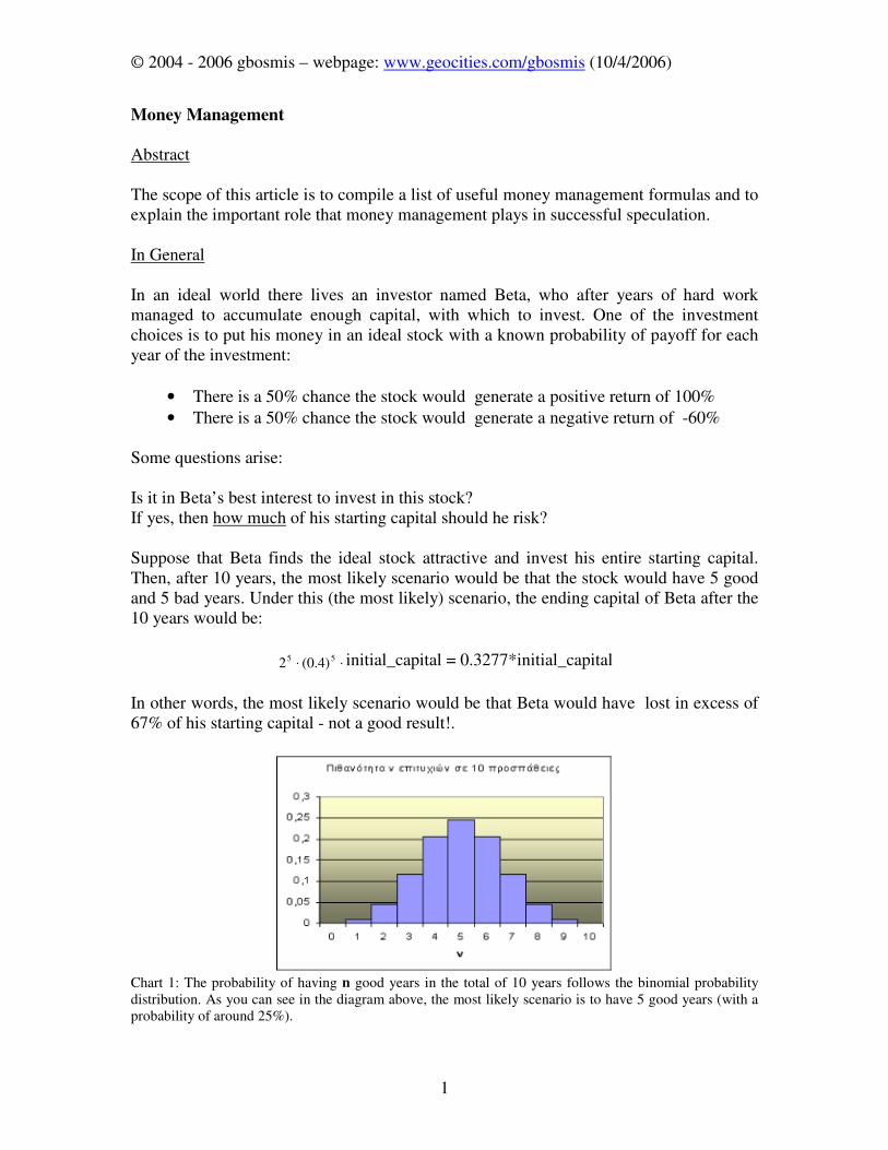
• There is a 50% chance the stock would generate a negative return of -60% Some questions arise: Is it in Beta’s best interest to invest in this stock? If yes, then how much of his starting capital should he risk? Suppose that Beta finds the ideal stock attractive and invest his entire starting capital. Then, after 10 years, the most likely scenario would be that the stock would have 5 good and 5 bad years. Under this (the most likely) scenario, the ending capital of Beta after the 10 years would be:

⋅⋅ 55 )4.0(2 initial_capital = 0.3277*initial_capital

In other words, the most likely scenario would be that Beta would have lost in excess of 67% of his starting capital - not a good result!.

Chart 1: The probability of having n good years in the total of 10 years follows the binomial probability distribution. As you can see in the diagram above, the most likely scenario is to have 5 good years (with a probability of around 25%).


2

Observe that the order that ‘good’ and ‘bad’ years appear during Beta’s investment doesn’t play a role in Beta’s final bankroll (for example; 5 good and 5 bad years always result in the same final bankroll, no matter what the order is). Is there an alternative way; a different criterion, which Beta can follow? Is there a criterion that will greatly reduce the probability of large drawdowns in Beta’s starting capital, and at the same time help him exploit the advantage that the ideal stock presents? The answer is YES. If he bets 33% of his current capital on this ideal stock at the beginning of each year. After the end of the year, if the price of the stock had a positive return, he liquidates part of his position in order to maintain a portion of 33% of his capital allocated to the stock. If the price of the stock had a negative return, he buys more (again to maintain a portion of 33% of his capital allocated to the stock). If Beta wants a safer ride, he must bet an even smaller portion of his current capital on this ideal stock. The WHY’s of the above will be answered in the pages that follow. Real world and Ideal world – A warning to the wise! The world that Beta lives in is an ideal world. In this world there is only risk. That means that the exact outcome is not known beforehand, however we know what the possible outcomes are with their corresponding probabilities. Unfortunately, in the real world, we are not talking about risk but about uncertainty. Uncertainty means that not only don’t we know what the outcome will be, but in addition, we don’t know what the possible outcomes are and their corresponding probabilities of occurrence. Uncertainty is a big drawback and must instill in us a conservativeness regarding financial decisions and capital allocation. The statistical inferences regarding possible outcomes must not be taken for granted. We must proceed with great caution and conservatism. Our total capital allocation must take into account the worst possible scenario, no matter how infrequent we might think that it appears. Expectation Expectation answers the question: ‘when do we take a bet’. The answer is simple. We take a bet only if it has a positive expectation. But what is expectation? Suppose you face the simple bet:

• Win an equal amount to the one that you bet (with probability p)

• Lose the amount you bet (with probability q = 1-p) Then Expectation is:

Expectation = p*1 + q*(-1) = p-q In the general case that we have, for every unit we bet, various payoffs

ix ( ix >0 for profit

and ix <0 for loss) with corresponding probabilities of occurrence

ip then expectation

becomes:


3

Expectation = ∑ ⋅i

ii xp

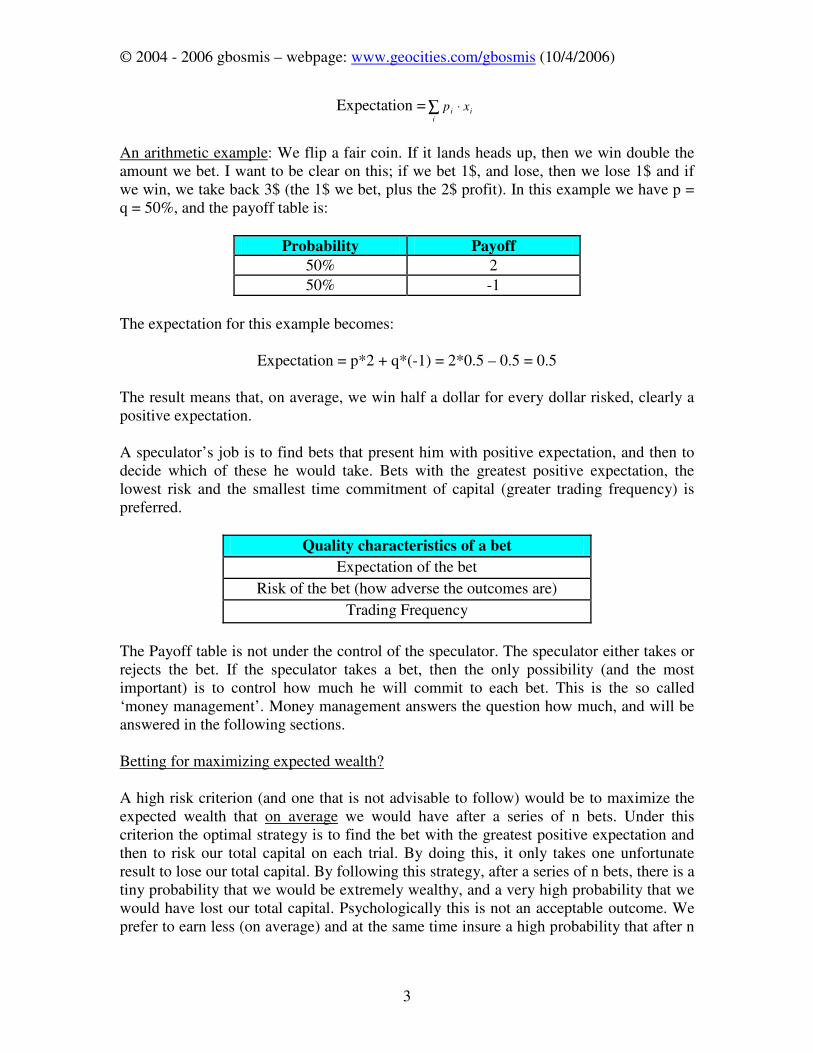
An arithmetic example: We flip a fair coin. If it lands heads up, then we win double the amount we bet. I want to be clear on this; if we bet 1$, and lose, then we lose 1$ and if we win, we take back 3$ (the 1$ we bet, plus the 2$ profit). In this example we have p = q = 50%, and the payoff table is:

Probability Payoff

50% 2

50% -1

The expectation for this example becomes:

Expectation = p*2 + q*(-1) = 2*0.5 – 0.5 = 0.5 The result means that, on average, we win half a dollar for every dollar risked, clearly a positive expectation. A speculator’s job is to find bets that present him with positive expectation, and then to decide which of these he would take. Bets with the greatest positive expectation, the lowest risk and the smallest time commitment of capital (greater trading frequency) is preferred.

Quality characteristics of a bet

Expectation of the bet

Risk of the bet (how adverse the outcomes are)

Trading Frequency

The Payoff table is not under the control of the speculator. The speculator either takes or rejects the bet. If the speculator takes a bet, then the only possibility (and the most important) is to control how much he will commit to each bet. This is the so called ‘money management’. Money management answers the question how much, and will be answered in the following sections. Betting for maximizing expected wealth? A high risk criterion (and one that is not advisable to follow) would be to maximize the expected wealth that on average we would have after a series of n bets. Under this criterion the optimal strategy is to find the bet with the greatest positive expectation and then to risk our total capital on each trial. By doing this, it only takes one unfortunate result to lose our total capital. By following this strategy, after a series of n bets, there is a tiny probability that we would be extremely wealthy, and a very high probability that we would have lost our total capital. Psychologically this is not an acceptable outcome. We prefer to earn less (on average) and at the same time insure a high probability that after n


4

trials we are ahead of our starting capital. By just maximizing expected wealth after n trials, the probability of bankruptcy is:

P(bankruptcy) = 1 – p^n where p is the probability of success. In this case, the probability of succeeding in all n bets is p^n (which is very small) but the terminal capital in this case will be enormous:

Terminal capital = starting capital * (1 + bet_gain_factor)^n

In the fair coin example of the previous section, after 10 trials the probability of bankruptcy is approximately 99.9% but there is a tiny 1 in a thousand (0.1%) probability that our terminal wealth will be 59049 times our initial wealth!!! So, by maximizing expected wealth, we become (on average) 59 times more wealthy after 10 bets. It may seem as a good result, but with the same logic, he who has one foot in the ice and one foot in the fire, he feels comfortable on average-. It’s obvious that a different logic must be followed. Betting a constant amount or a constant fraction? It’s a logical assumption that in a series of bets, with the same characteristics, one must allocate a constant fraction of your current capital on each bet. This is mainly for two reasons:

• By betting a constant fraction of our wealth, in successive bets, we attain geometric growth of our capital, while betting a constant amount in successive bets, ensure linear growth of our capital.

• By betting a constant fraction we ensure that bankruptcy is not possible, because losing bets will result in the reduction of the absolute amount we risk and wining bets will result in the increase of the amount betted. On the other hand, when we bet a constant amount, a losing streak can result in bankruptcy.

Kelly criterion Why we didn’t choose to maximized expected wealth has been answered in a previous section. The optimal criterion would be to maximize an alternative measure of wealth, the logarithm of wealth. This is the so called Kelly criterion Kelly, J. L. "A New Interpretation of Information Rate," Bell System Technical Journal, Vol. 35, pp 917-926, 1956). By doing this, we greatly reduce the probability of a small terminal wealth value. y�1st Case: Consider a bet where we win what we bet, if successful, and lose what we bet if unsuccessful. After a successful outcome our wealth will be:

)1(01 fBB +⋅=


5

where B1 is our wealth after the bet outcome B0 is our wealth before the bet outcome f is the fraction of our wealth that we risked in this bet After a failure our wealth will be:

)1(01 fBB −⋅=

We want to find the optimal criterion for determining f in a series of bets of this kind. After N successive bets we will have W wining and L losing bets. Obviously N = W + L. Our final wealth will be:

LW

N ffBB )1()1(0 −⋅+⋅=

We know from mathematics that )ln(xex = so we have:

( )

−⋅+⋅=

⋅LWN ff

NBN

B)1()1(ln

1exp

0

The exponent [ ]LWff

NfG )1()1(ln

1)( −⋅+= describes the geometric growth of our wealth

per bet. Its expected value will be:

)1ln()1ln()1ln()1ln()( fqfpfN

Lf

N

WEfg −⋅++⋅=

−⋅++⋅=

where p is the probability of a wining bet and q=1-p is the probability of a losing bet. The Kelly criterion says to maximize g. The first step is to find the first order derivative of g with regards to f:

)1()1()1()1(11)(

ff

fqp

ff

fqqfpp

f

q

f

pfg

−⋅+−−

=−⋅+

⋅−−⋅−=

−−

+=′

The optimal value of f (the one that maximizes g) is found by solving

qpffg −=⇒=′ *0)( . That’s it!!! Kelly betting fraction for this kind of bet is equal to p-

q. y��nd Case: Consider a bet with different payoffs for success and failure. If we bet 1$ and win, the winnings are a$ (we take back 1$ + a$). If we lose, we lose b$ for each dollar risked. In this case we have (following similar logic):

[ ]LWfbfa

NfG )1()1(ln

1)( ⋅−⋅⋅+=


6

)1()1()1()1(11)(

fbfa

fbaqbpa

fbfa

fqbafpbaqbpa

fb

qb

fa

pafg

⋅−⋅⋅+⋅⋅−⋅−⋅

=⋅−⋅⋅+

⋅⋅⋅−⋅⋅⋅−⋅−⋅=

⋅−⋅

−⋅+

⋅=′

ba

qbpaffg

⋅⋅−⋅

=⇒=′ *0)(

In other words; the Kelly betting fraction for this kind of bet is equal to (ap-bq)/(ab). y��rd Case: Consider a bet with many (more than two) different possible payoffs. In this case we have:

∑ ⋅+⋅=i

ii fxpfg )1ln()(

where

ix are the various payoffs (ix >0 for profit and

ix <0 for loss) with corresponding

probabilities of occurrence ip . When fxi ⋅ are small with regards to 1 then we can make

the approximation 2/)1ln( 2zzz −=+ and the pervious equation becomes:

∑ ∑ ⋅⋅⋅−⋅⋅=i i

iiii fxpfxpfg22

2

1)(

so we have:

∑ ∑ ⋅⋅−⋅=′i i

iiii fxpxpfg2

)(

∑

∑

⋅

⋅=⇒=′

iii

iii

xp

xp

ffg2

*0)(


7

Bellow is a table that summarizes the results for the previous three cases:

Bet Kind Optimal Kelly fraction

• we win what we betted if success and we lose what we betted if failure

• probability to win the bet is p, probability to lose the bet is q

qpf −=*

• we win a times what we betted and we lose b times what we betted

• probability to win the bet is p, probability to lose the bet is q

ba

qbpaf

⋅⋅−⋅

=*

• probability ip to have a payoff

ix

• fxi ⋅ small with regards to 1 ∑

∑

⋅

⋅=

iii

iii

xp

xp

f2

*

The role of risk By looking at the results in the above table, we observe that the optimal betting fraction declines when the risk of a bet rises. In other words, a bet with more adverse probable results will have a smaller optimal betting fraction from another (when the remaining characteristics of the two bets are the same). This is more obvious in the 3rd case where the denominator of the betting fraction is the variance of the payoffs of this bet (to be

exact: it is the variance plus something small because Variance = 2

2

⋅−⋅ ∑∑

iii

iii xpxp .

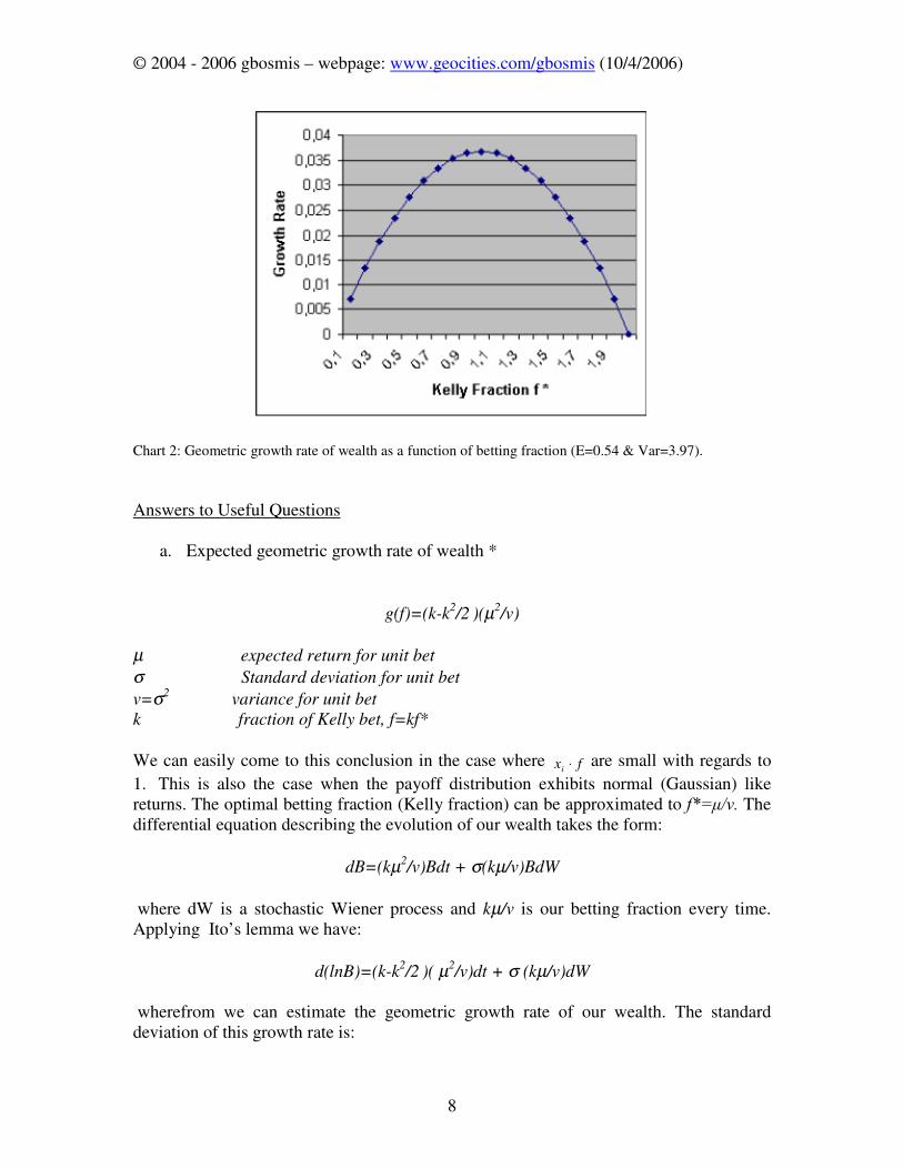
What happens in the case that we don’t bet the optimal betting fraction? Maximum geometric growth of wealth is attained when we bet the optimal fraction calculated by the Kelly criterion. In the case where we are betting less than the Kelly fraction, we ensure smaller draw downs in expense of a smaller growth rate for our wealth (we don’t take full advantage of the opportunity that we have) resulting in more time being required to achieve our goals. If we over bet, we achieve smaller growth rates and at the same time risk potential draw downs that are much larger. There is no reward for over betting! Things get much worse when over betting exceeds a certain point. In this case, the geometric growth rate becomes zero, and for even higher betting fractions becomes negative. Bankruptcy is almost certain!!


8

Chart 2: Geometric growth rate of wealth as a function of betting fraction (E=0.54 & Var=3.97). Answers to Useful Questions

a. Expected geometric growth rate of wealth *

g(f)=(k-k2/2

)(µ2

/v)

µ expected return for unit bet

σ Standard deviation for unit bet

v=σ2 variance for unit bet

k fraction of Kelly bet, f=kf* We can easily come to this conclusion in the case where fxi ⋅ are small with regards to

1. This is also the case when the payoff distribution exhibits normal (Gaussian) like returns. The optimal betting fraction (Kelly fraction) can be approximated to I ��Y��The differential equation describing the evolution of our wealth takes the form:

dB=(kµ2/v)Bdt + σ(kµ/v)BdW

where dW is a stochastic Wiener process and kµ/v is our betting fraction every time. Applying Ito’s lemma we have:

d(lnB)=(k-k2/2

)( µ2

/v)dt + σ (kµ/v)dW wherefrom we can estimate the geometric growth rate of our wealth. The standard deviation of this growth rate is:


9

6W'HY>J�I�@� �N��1 The expected time (or equivalently: expected number of trades) that is required for our wealth to reach a certain level b (multiple of our initial wealth) is:

E(T) = g

1 ln(b)

* Expected geometric growth rate of wealth is in other words the expected logarithmic growth of wealth per trade:

g = 1/n * E[Ln(Xn/Xo)] where Xn is final wealth, Xo is initial wealth and n is the number of trades. Note that E[Ln(a)] ��/Q�(>D@��

b. Drawdown Formulas Again we note that these formulas are approximations and are accurate for normal-like payoffs. If we choose a fractional Kelly betting strategy (bet a fraction k of the optimal f* Kelly fraction) and we assume that our initial wealth is equal to 1 then the probability of our wealth reaching b>1 before reaching a<1 is:

kk

k

ab

abaP

/21/21

/211),( −−

−

−−

=

The probability that we will never reach a<1 is:

P(a)=a2/k-1

For example if someone keeps betting a fraction f* (k=1) of his capital in each bet then the probability of his wealth retreating to a, is simply a. If he is betting f*/2 then this probability becomes much smaller, a^3. We present some arithmetic results in the tables that follow:


10

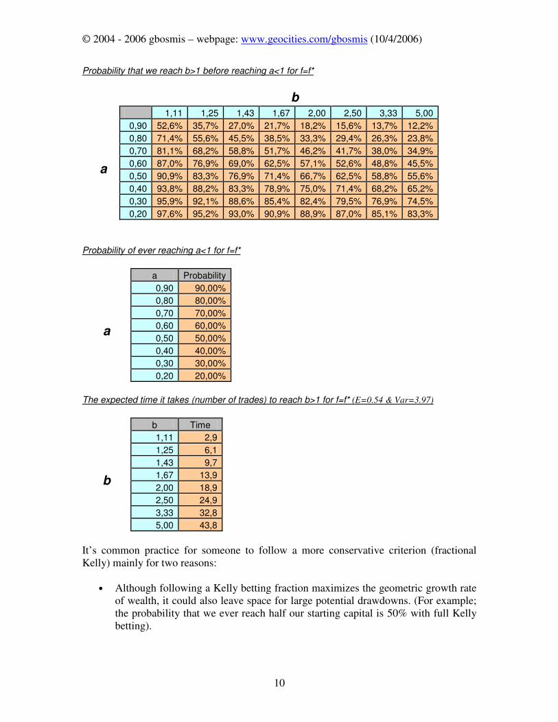
Probability that we reach b>1 before reaching a<1 for f=f*

b 1,11 1,25 1,43 1,67 2,00 2,50 3,33 5,00 0,90 52,6% 35,7% 27,0% 21,7% 18,2% 15,6% 13,7% 12,2% 0,80 71,4% 55,6% 45,5% 38,5% 33,3% 29,4% 26,3% 23,8% 0,70 81,1% 68,2% 58,8% 51,7% 46,2% 41,7% 38,0% 34,9%

0,60 87,0% 76,9% 69,0% 62,5% 57,1% 52,6% 48,8% 45,5% a

0,50 90,9% 83,3% 76,9% 71,4% 66,7% 62,5% 58,8% 55,6% 0,40 93,8% 88,2% 83,3% 78,9% 75,0% 71,4% 68,2% 65,2% 0,30 95,9% 92,1% 88,6% 85,4% 82,4% 79,5% 76,9% 74,5% 0,20 97,6% 95,2% 93,0% 90,9% 88,9% 87,0% 85,1% 83,3%

Probability of ever reaching a<1 for f=f*

a Probability 0,90 90,00% 0,80 80,00% 0,70 70,00%

0,60 60,00% a

0,50 50,00% 0,40 40,00% 0,30 30,00% 0,20 20,00%

The expected time it takes (number of trades) to reach b>1 for f=f* (E=0.54 & Var=3.97)

b Time 1,11 2,9 1,25 6,1 1,43 9,7

1,67 13,9 b

2,00 18,9 2,50 24,9 3,33 32,8 5,00 43,8

It’s common practice for someone to follow a more conservative criterion (fractional Kelly) mainly for two reasons:

• Although following a Kelly betting fraction maximizes the geometric growth rate of wealth, it could also leave space for large potential drawdowns. (For example; the probability that we ever reach half our starting capital is 50% with full Kelly betting).


11

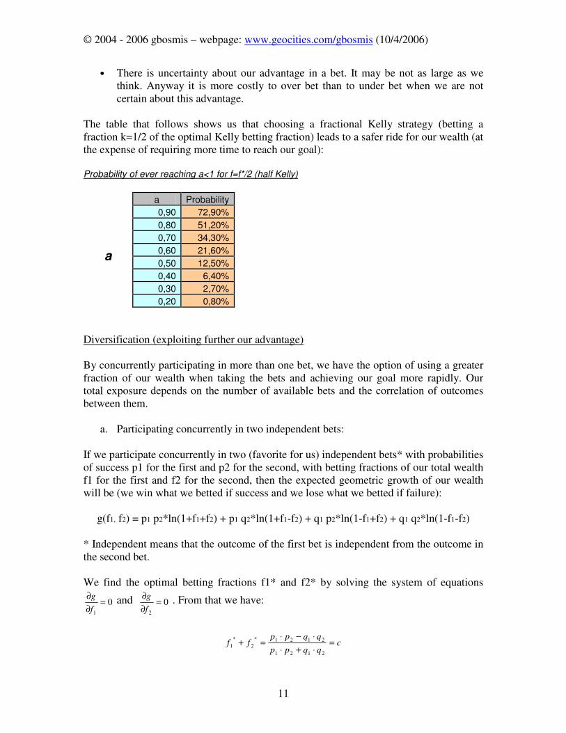
• There is uncertainty about our advantage in a bet. It may be not as large as we think. Anyway it is more costly to over bet than to under bet when we are not certain about this advantage.

The table that follows shows us that choosing a fractional Kelly strategy (betting a fraction k=1/2 of the optimal Kelly betting fraction) leads to a safer ride for our wealth (at the expense of requiring more time to reach our goal): Probability of ever reaching a<1 for f=f*/2 (half Kelly)

a Probability 0,90 72,90% 0,80 51,20% 0,70 34,30%

0,60 21,60% a

0,50 12,50% 0,40 6,40% 0,30 2,70% 0,20 0,80%

Diversification (exploiting further our advantage) By concurrently participating in more than one bet, we have the option of using a greater fraction of our wealth when taking the bets and achieving our goal more rapidly. Our total exposure depends on the number of available bets and the correlation of outcomes between them.

a. Participating concurrently in two independent bets: If we participate concurrently in two (favorite for us) independent bets* with probabilities of success p1 for the first and p2 for the second, with betting fractions of our total wealth f1 for the first and f2 for the second, then the expected geometric growth of our wealth will be (we win what we betted if success and we lose what we betted if failure):

g(f1, f2) = p1 p2*ln(1+f1+f2) + p1 q2*ln(1+f1-f2) + q1 p2*ln(1-f1+f2) + q1 q2*ln(1-f1-f2) * Independent means that the outcome of the first bet is independent from the outcome in the second bet. We find the optimal betting fractions f1* and f2* by solving the system of equations

01

=∂∂f

g and 02

=∂∂f

g . From that we have:

cqqpp

qqppff =

⋅+⋅⋅−⋅

=+2121

2121*

2

*

1


12

dqppq

pqqpff =

⋅+⋅⋅−⋅

=−2121

2121*

2

*

1

and finally f1*=(c+d)/2 , f2*=(c-d)/2. A simple arithmetic result: In the simple case where p1, p2 = p = 60% and q1, q2 = q = 40% we have c = 0.385 and d = 0 so we have: f1*= 19.2% and f2*= 19.2%. In other words, we can practically bet - double the amount we would have bet if only one of these independent bets were available (20%).

b. The Theory behind a portfolio of bets What will happen if we had many available correlated bets to choose? In this case the usage of some matrix algebra calculations will be required to determine the optimal betting fraction for each bet. In matrix notation we will have:

F* = C-1M

C the variance – covariance matrix between available bets � the column-matrix containing the expectancy of each bet F* the row-matrix containing optimal betting fraction that we must allocate in each

bet The geometric growth rate for our wealth will be:

g(f1*,…,fn

*) = ½(F*)TCF* In the general case where we have allocated a different fraction in each available bet and these fractions are described with the raw-matrix F, the formulas bellow are handy:

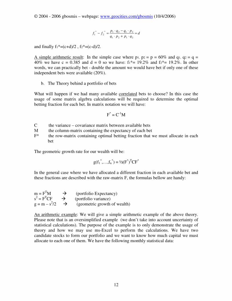
m = FTM Æ (portfolio Expectancy) s2 = FTCF Æ (portfolio variance) g = m – s2/2 Æ (geometric growth of wealth) An arithmetic example: We will give a simple arithmetic example of the above theory. Please note that is an oversimplified example (we don’t take into account uncertainty of statistical calculations). The purpose of the example is to only demonstrate the usage of theory and how we may use ms-Excel to perform the calculations. We have two candidate stocks to form our portfolio and we want to know how much capital we must allocate to each one of them. We have the following monthly statistical data:


13

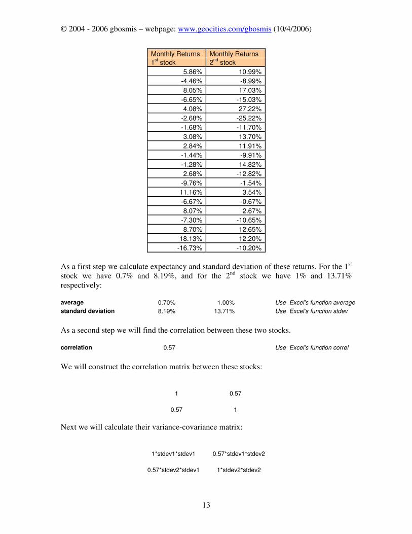
Monthly Returns Monthly Returns 1

st stock 2

nd stock

5.86% 10.99% -4.46% -8.99% 8.05% 17.03%

-6.65% -15.03% 4.08% 27.22%

-2.68% -25.22% -1.68% -11.70% 3.08% 13.70% 2.84% 11.91%

-1.44% -9.91% -1.28% 14.82% 2.68% -12.82%

-9.76% -1.54% 11.16% 3.54% -6.67% -0.67% 8.07% 2.67%

-7.30% -10.65% 8.70% 12.65%

18.13% 12.20% -16.73% -10.20%

As a first step we calculate expectancy and standard deviation of these returns. For the 1st stock we have 0.7% and 8.19%, and for the 2nd stock we have 1% and 13.71% respectively: average 0.70% 1.00% Use Excel’s function average standard deviation 8.19% 13.71% Use Excel’s function stdev

As a second step we will find the correlation between these two stocks. correlation 0.57 Use Excel’s function correl

We will construct the correlation matrix between these stocks:

1 0.57

0.57 1

Next we will calculate their variance-covariance matrix:

1*stdev1*stdev1 0.57*stdev1*stdev2

0.57*stdev2*stdev1 1*stdev2*stdev2


14

By substituting we have:

C = 1*0.0819*0.0819 0.57*0.0819*0.1371 = 0.006708 0.0064

0.57*0.1371*0.0819 1*0.1371*0.1371 0.0064 0.018796

And we will use Excel’s function minverse to find C-1

220.8330591 -75.19438144

-75.19438144 78.8055823

We will find F* by multiplying above result with the expectancy matrix:

220.8330591 -75.19438144 * 0.70% Use Excel’s function mmult

-75.19438144 78.8055823 1.00%

So finally:

F* = 0.793887599

0.261695153

The interpretation is as follow: If you have 100$, use 5$ margin and bet 79 dollars in 1st stock and 26$ n 2nd stock. The geometric growth rate of wealth will be:

0.5 * (F*)T x C x F* = 0.793887599 0.261695153 x 0.007 = 0.008174 0.01 Per

month And the expected time it takes to double our money will be:

E(T in months) = ln(2)/g = ln(2)/0.008174 = 84.8 months Imposing constraints on exposure levels It is often required that our total exposure to positions does not exceed a certain percentage of our wealth. In order to estimate the optimal allocation between available


15

bets, we must take this extra constraint into account . We achieve that by using the so called Lagrange multipliers l. With this technique we have:

F* = C-1 (M + L)

�i fi* = c

where L is the column matrix [l l ....l]� and c is the constraint regarding the total fraction of our capital that we want to bet. A simple arithmetic example: We take the simple case where m1 = 15%, m2 ��DQG�11, 12 = 100% and the two bets are independent. If we had no constraint then the best allocation will be f1

* = 15%, f2* = 20%. On the other hand, if we impose the constraint

that our total exposure will be no greater than 20% (in other words c=0.2) we will algebraically have: f1

* + f2* = (0.15 + l) + (0.2 + l) = 0.2 Æ l = -0.075. It follows that f1*

= 7.5% and f2* = 12.5%.

Good and Bad properties of the Kelly criterion (+) Asymptotically maximizes the growth rate of our wealth. (+) Asymptotically minimizes the time we need to reach a goal. (+) Maximizes median logarithmic wealth. (+) We don’t risk ruin. (+) On average we are never behind in wealth level after n=1,2,…. repetitions of the bet from anyone following a different strategy. (+) We follow an optimal ‘myopic’ policy (we only need to consider in every step what kind of bet is available). (+) If we want to achieve lower drawdown risk, at the expense of greater time to reach our goal, then all we have to do is bet fractional Kelly. That is equivalent to having a negative exponential utility function d*omegad with d<0. The relation between d and Kelly fraction k is k = 1/(1–d). (-) Equal number of wins and losses gives us lower wealth than the initial. That’s because (1+f)(1-f)*W = (1-f^2)*W ��:� (-) When the expectancy of a bet is high and the observed risk is very low, the optimal betting fraction may become unrealistically high. (-) If there is uncertainty or erroneous estimation about how high our advantage is then it may be possible that we will over bet. (-) Over betting will lead to ruin. In the fixed coin flip case, betting double Kelly will make our logarithmic growth rate of wealth zero, and betting even more will make it negative. (-) It can take a long time for a Kelly bettor to dominate an essentially different strategy. (-) It is possible to have very poor return outcome if a bad scenario is realized.


16

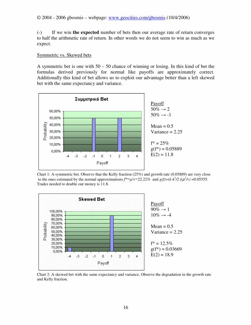
(-) If we win the expected number of bets then our average rate of return converges to half the arithmetic rate of return. In other words we do not seem to win as much as we expect. Symmetric vs. Skewed bets A symmetric bet is one with 50 – 50 chance of winning or losing. In this kind of bet the formulas derived previously for normal like payoffs are approximately correct. Additionally this kind of bet allows us to exploit our advantage better than a left skewed bet with the same expectancy and variance.

Payoff 50% :�� 50% :�-1 Mean = 0.5 Variance = 2.25 f* = 25% g(f*) = 0.05889 E(2) = 11.8

Chart 1: A symmetric bet. Observe that the Kelly fraction (25%) and growth rate (0.05889) are very close

to the ones estimated by the normal approximations I ��Y 22.22% and g(f)=(k-k2/2

)(µ2

/v) =0.05555. Trades needed to double our money is 11.8.

Payoff 90% :�� 10% :�-4 Mean = 0.5 Variance = 2.25 f* = 12.5% g(f*) = 0.03669 E(2) = 18.9

Chart 2: A skewed bet with the same expectancy and variance. Observe the degradation in the growth rate and Kelly fraction.


17

Examples of skewed bets

• Selling an out of the money option usually results in realising a small profit and a very small chance of losing a substantial amount.

• Arbitrage (the selling of a more expensive item and the buying of a less expensive and almost equivalent one). In most of the cases it will work out and we will realize a small profit , however if something unusual happens then we can lose big.

Bad properties of skewed bets

• It is not easy to estimate the statistical properties of the bet due to the rareness of bad events. Usually we are overestimating expectancy and underestimating variance.

• We need a greater statistical sample. • A very rare and so far unobserved adverse event can have significant impact on

the Kelly betting fraction. We may over bet substantially and get seduced by the steady small income we receive).

Bibliography

1. A. Papoulis – “Probability, Random Variables, and Stochastic Processes”, McGraw-Hill Inc. 2. Kelly, J. L. "A New Interpretation of Information Rate," Bell System Technical Journal, Vol. 35,

pp 917-926, 1956 3. Ed Thorp – “The Kelly criterion in blackjack, sports betting, and the stock market”, 10th

International Conference on Gambling and Risk Taking 4. Nassim Nicholas Taleb Empirica LLC and Courant Institute of Mathematical Sciences, New York

University Avital Pilpel Department of Philosophy, Columbia University - "Random Processes, Opacity, and Knowledge: The Central Problem"


18

Money Management examples (for optimal Kelly fraction betting)

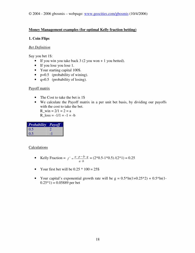
1. Coin Flips

Bet Definition Say you bet 1$:

• If you win you take back 3 (2 you won + 1 you betted).

• If you lose you lose 1.

• Your starting capital 100$.

• p=0.5 (probability of wining).

• q=0.5 (probability of losing). Payoff matrix

• The Cost to take the bet is 1$

• We calculate the Payoff matrix in a per unit bet basis, by dividing our payoffs with the cost to take the bet. R_win = 2/1 = 2 = a R_loss = -1/1 = -1 = -b

Probability Payoff

0.5 2 0.5 -1

Calculations

• Kelly Fraction = ba

qbpaf

⋅⋅−⋅

=* = (2*0.5-1*0.5) /(2*1) = 0.25

• Your first bet will be 0.25 * 100 = 25$

• Your capital’s exponential growth rate will be g = 0.5*ln(1+0.25*2) + 0.5*ln(1-0.25*1) = 0.05889 per bet


19

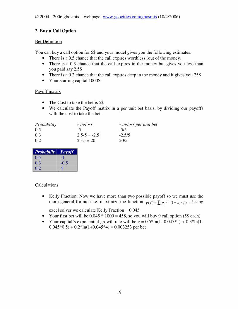
2. Buy a Call Option

Bet Definition You can buy a call option for 5$ and your model gives you the following estimates:

• There is a 0.5 chance that the call expires worthless (out of the money)

• There is a 0.3 chance that the call expires in the money but gives you less than you paid say 2.5$

• There is a 0.2 chance that the call expires deep in the money and it gives you 25$

• Your starting capital 1000$. Payoff matrix


• We calculate the Payoff matrix in a per unit bet basis, by dividing our payoffs with the cost to take the bet.

Probability win/loss win/loss per unit bet 0.5 -5 -5/5 0.3 2.5-5 = -2.5 -2.5/5 0.2 25-5 = 20 20/5

Probability Payoff

0.5 -1 0.3 -0.5 0.2 4

Calculations

• Kelly Fraction: Now we have more than two possible payoff so we must use the more general formula i.e. maximize the function ∑ ⋅+⋅=

iii fxpfg )1ln()( . Using

excel solver we calculate Kelly Fraction = 0.045

• Your first bet will be 0.045 * 1000 = 45$, so you will buy 9 call option (5$ each)

• Your capital’s exponential growth rate will be g = 0.5*ln(1- 0.045*1) + 0.3*ln(1-0.045*0.5) + 0.2*ln(1+0.045*4) = 0.003253 per bet


20

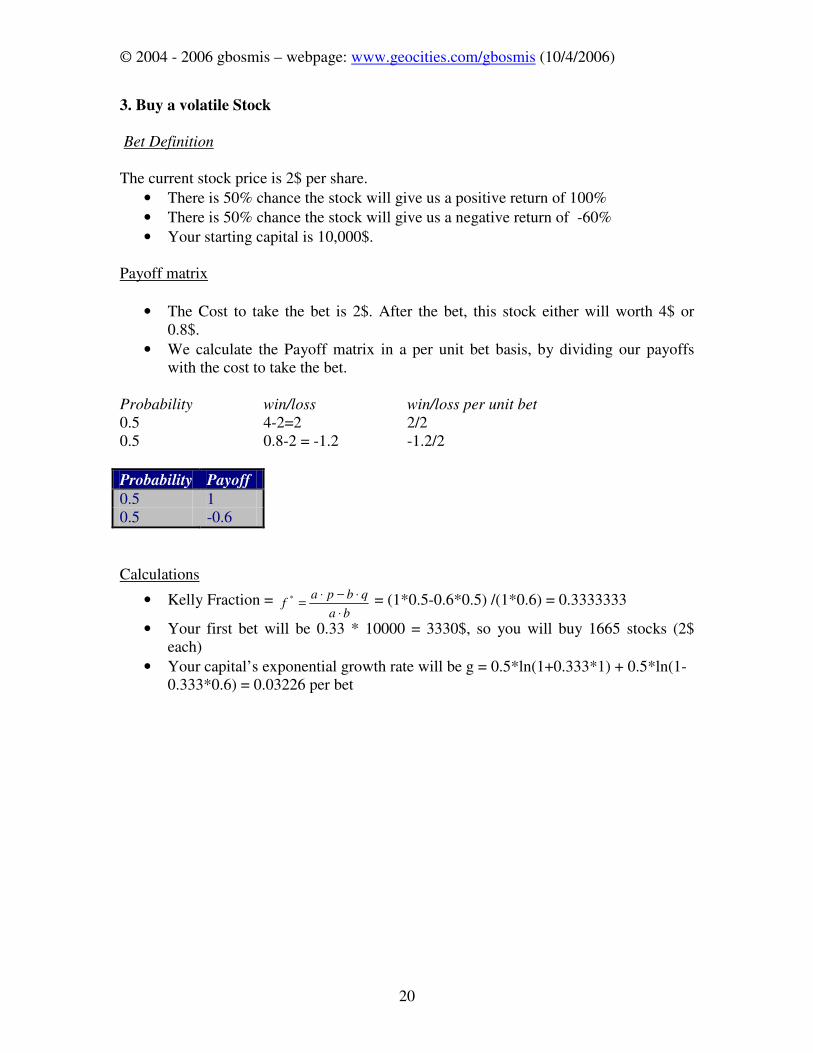
3. Buy a volatile Stock

Bet Definition The current stock price is 2$ per share.

• There is 50% chance the stock will give us a positive return of 100%

• There is 50% chance the stock will give us a negative return of -60%

• Your starting capital is 10,000$. Payoff matrix

• The Cost to take the bet is 2$. After the bet, this stock either will worth 4$ or 0.8$.


Probability win/loss win/loss per unit bet 0.5 4-2=2 2/2 0.5 0.8-2 = -1.2 -1.2/2

Probability Payoff

0.5 1 0.5 -0.6

Calculations

• Kelly Fraction = ba

qbpaf

⋅⋅−⋅

=* = (1*0.5-0.6*0.5) /(1*0.6) = 0.3333333

• Your first bet will be 0.33 * 10000 = 3330$, so you will buy 1665 stocks (2$ each)

• Your capital’s exponential growth rate will be g = 0.5*ln(1+0.333*1) + 0.5*ln(1-0.333*0.6) = 0.03226 per bet


21

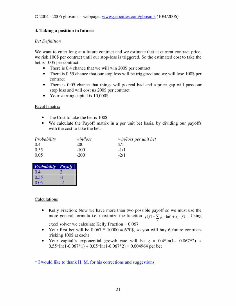
4. Taking a position in futures

Bet Definition

We want to enter long at a future contract and we estimate that at current contract price, we risk 100$ per contract until our stop-loss is triggered. So the estimated cost to take the bet is 100$ per contract.

• There is 0.4 chance that we will win 200$ per contract

• There is 0.55 chance that our stop loss will be triggered and we will lose 100$ per contract

• There is 0.05 chance that things will go real bad and a price gap will pass our stop loss and will cost us 200$ per contract

• Your starting capital is 10,000$. Payoff matrix



Probability win/loss win/loss per unit bet 0.4 200 2/1 0.55 -100 -1/1 0.05 -200 -2/1

Probability Payoff

0.4 2 0.55 -1 0.05 -2

Calculations

• Kelly Fraction: Now we have more than two possible payoff so we must use the more general formula i.e. maximize the function ∑ ⋅+⋅=

iii fxpfg )1ln()( . Using

excel solver we calculate Kelly Fraction = 0.067

• Your first bet will be 0.067 * 10000 = 670$, so you will buy 6 future contracts (risking 100$ at each)

• Your capital’s exponential growth rate will be g = 0.4*ln(1+ 0.067*2) + 0.55*ln(1-0.067*1) + 0.05*ln(1-0.067*2) = 0.004964 per bet

* I would like to thank H. M. for his corrections and suggestions.

Documents

Money Management - OoCities · Money Management Abstract ... The Payoff table is not under the control of the speculator. The speculator either takes or rejects the bet