Monitoring catalytic trickle bedreactor using operating data

Viljami Iso-Markku

School of Chemical Engineering

Thesis submitted for examination for the degree of Master ofScience in Technology.Helsinki 15.05.2021

Supervisor

Prof. Francesco Corona

Advisor

MSc. Samuli Bergman

Copyright © 2021 Viljami Iso-Markku

Aalto University, P.O. BOX 11000, 00076 AALTOwww.aalto.fi

Abstract of the master’s thesis

Author Viljami Iso-MarkkuTitle Monitoring catalytic trickle bed reactor using operating dataDegree programme Advanced Energy SolutionsMajor Industrial Energy Processes and Sustainability Code of major AAESupervisor Prof. Francesco CoronaAdvisor MSc. Samuli BergmanDate 15.05.2021 Number of pages 69 Language EnglishAbstractStatistical methods have been widely used in analyzing and monitoring complicatedchemical processes. These methods are often referred to as statistical process control(SPC). However, chemical processes are typically multivariate in nature. Multivariatestatistical process control (MSPC) methods were developed to specifically deal withthe higher dimensional process data. Multivariate methods that researchers havepreviously used for chemical processes are principal component analysis (PCA) andpartial least squares (PLS).

This thesis studies the use of multilevel simultaneous component analysis (MLSCA)to be used as an anomaly detection method for a trickle bed reactor that is usedto dearomatize hydrocarbons. The main goal of this thesis is to demonstrate howMLSCA could be used to monitor and detect anomalies from chemical reactors purelybased on the changes occurring in the temperature profiles. This is achieved bysetting up the data to represent the cross section of the reactor instead of analyzingthe time series during one catalyst life cycle.

This thesis present two MLSCA-based models that offers better visualization ofthe reactors operating conditions, which could be used for anomaly detection andidentification. The first experiment uses temperature differences from each levelagainst the feed temperature and the second experiment uses temperature differencesthat are calculated between each level instead of using raw temperature values. Theanomaly detection is performed by using classical scatter plots on the model scoresand by fitting Hotelling’s T 2 and Q statistics on the data produced by the MLSCAmodel.Keywords Multilevel simultaneous component analysis, principal component

analysis, process monitoring, anomaly detection, trickle-bed reactor

Aalto-yliopisto, PL 11000, 00076 AALTOwww.aalto.fi

Diplomityön tiivistelmä

Tekijä Viljami Iso-MarkkuTyön nimi Triklekerrosreaktorin monitorointi operointidatan perusteellaKoulutusohjelma Advanced Energy SolutionsPääaine Industrial Energy Processes and Sustainability Pääaineen koodi AAETyön valvoja Prof. Francesco CoronaTyön ohjaaja MSc. Samuli BergmanPäivämäärä 15.05.2021 Sivumäärä 69 Kieli EnglantiTiivistelmäTilastolliset menetelmät ovat olleet laajalti käytössä kemianteollisuudessa monimut-kaisten prosessien analysointiin, seurantaan ja hallintaan liittyvissä tehtävissä. Näitämenetelmiä kuvataan yleisesti termillä tilastollinen prosessinohjaus. Kemianteolli-suuden prosessit ovat luonnostaan moniulotteisia. Moniulotteisia prosesseja vartenon erikseen kehitetty monimuuttujaisia tilastollisia prosessienohjauksen menetel-miä, jotka perustuvat suurien datamäärien analysointiin, sekä muuttujien välistenvuorovaikutusten huomioonottamiseen. PCA (pääkomponenttianalyysi, PrincipalComponent Analysis) ja PLS (Projection to Latent Structures) ovat esimerkkejämonimuuttujaisista tilastollisia prosessinohjauksen mentelmistä, joita on käytettyhyödyksi kemiallisten prosessien analysoinnissa.

Tässä työssä tutkitaan kuinka MLSCA-analyysiä voidaan käyttää tunnistamaanpoikkeamia kiinteäpetisestä triklekerrosreaktorista, jota käytetään aromaattistenyhdisteiden poistamiseen hiilivedyistä. Poikkeamia pyritään tunnistamaan analysoi-malla pelkästään reaktorin lämpötilaprofiileja. Tämä saadaan aikaan järjestämällälämpötiladata kuvaamaan reaktorin poikkileikkausta sen sijaan, että mallilla analy-soitaisiin lämpötilojen aikasarjoja.

Työ sisältää kaksi koetta, joiden tarkoituksena on sekä parantaa reaktorin kun-non visualisointia että tutkia mallin poikkeamantunnistuksen hyvyyttä. Pelkkienlämpötila-arvojen sijaan, kokeissa käytetään lämpötilaeroja. Ensimmäisessä kokeessakäytetään lämpötilaeroja, jotka on laskettu reaktorin tasoista syötön lämpötilaavasten. Toisessa kokeessa lämpötilaerot on laskettu reaktorin tasojen välistä. Poik-keamantunnistuksessa käytetään klassisia pistearvojen perusteella tehtyjä pistekaa-vioita sekä laskemalla mallille Hotellingin T 2- ja Q-statistiikka arvot sekä näidenluottamusraja-arvot.Avainsanat MLSCA, pääkomponenttianalyysi, prosessien monitorointi,

poikkeamatunnistus, triklekerrosreaktori

5

PrefaceThis master’s thesis was done for NAPCON of Neste Engineering Solutions Oybetween January 2020 and January 2021.

When starting my bachelor’s degree in Bioproduct and Process engineeringand even during the master’s degree phase in Industrial Energy Processes andSustainability, it never crossed my mind that my Master’s thesis would be aboutanalyzing a chemical reactor by using multivariate statistical methods. Workingwith this thesis meant that I had to get familiarized with completely new field ofmultivariate statistics. This work has definitely been an interesting one.

I want to thank my supervisor, Professor Francesco Corona for his guidancethroughout the thesis process. I’m grateful for having a supervisor who always hadthe time to consult whether I had troubles on the experimental part or the writingpart of the thesis. Basically, thank you for helping with literally everything regardingthe thesis work.

Thank you to my advisor Samuli Bergman and the whole NAPCON team formaking this Master’s thesis possible. Thank you for keeping the worl load low forthe first half of 2020, so that I could focus working on the thesis.

Finally I want to express my gratitude also to my family and friends for theirsupport throughout the years of studying. Finally, the biggest thank you to myparents for always being there for me.

Helsinki, 20.1.2020

Viljami Iso-Markku

6

ContentsAbstract 3

Abstract (in Finnish) 4

Preface 5

Contents 6

Symbols and abbreviations 8

1 Introduction 9

2 Dearomatization in petroleum industry 112.1 Hydrodearomatization . . . . . . . . . . . . . . . . . . . . . . . . . . 112.2 Trickle-bed reactor . . . . . . . . . . . . . . . . . . . . . . . . . . . . 13

2.2.1 Hot spots . . . . . . . . . . . . . . . . . . . . . . . . . . . . . 142.2.2 Liquid maldistribution . . . . . . . . . . . . . . . . . . . . . . 14

2.3 Process Description . . . . . . . . . . . . . . . . . . . . . . . . . . . . 162.3.1 Dearomatization reactor . . . . . . . . . . . . . . . . . . . . . 18

3 Multivariate statistical process control 213.1 Preprocessing . . . . . . . . . . . . . . . . . . . . . . . . . . . . . . . 22

3.1.1 Mean centering and variance scaling . . . . . . . . . . . . . . 233.1.2 Variable selection . . . . . . . . . . . . . . . . . . . . . . . . . 243.1.3 Filtering and smoothing . . . . . . . . . . . . . . . . . . . . . 24

3.2 Latent variable methods . . . . . . . . . . . . . . . . . . . . . . . . . 253.2.1 Principal Component Analysis . . . . . . . . . . . . . . . . . . 253.2.2 Multiway Principal Component Analysis . . . . . . . . . . . . 283.2.3 Multilevel Simultaneous Component Analysis . . . . . . . . . 29

3.3 Anomaly detection . . . . . . . . . . . . . . . . . . . . . . . . . . . . 313.3.1 Hotelling’s T 2 . . . . . . . . . . . . . . . . . . . . . . . . . . . 333.3.2 Q Statistic . . . . . . . . . . . . . . . . . . . . . . . . . . . . . 33

3.4 Anomaly identification . . . . . . . . . . . . . . . . . . . . . . . . . . 343.5 The amount of principal components . . . . . . . . . . . . . . . . . . 35

3.5.1 Cumulative percentage of total variation . . . . . . . . . . . . 363.5.2 Size of variances of principal components . . . . . . . . . . . . 363.5.3 Scree graph . . . . . . . . . . . . . . . . . . . . . . . . . . . . 363.5.4 Cross-validation . . . . . . . . . . . . . . . . . . . . . . . . . . 37

4 Experimental setup 39

5 Results 455.1 Between-frame, dT vs feed temperature . . . . . . . . . . . . . . . . . 455.2 Within-frame, dT vs feed temperature . . . . . . . . . . . . . . . . . 495.3 Between-frame, dT between levels . . . . . . . . . . . . . . . . . . . . 55

7

5.4 Within-frame, dT between levels . . . . . . . . . . . . . . . . . . . . . 57

6 Disussion and conclusion 63

References 66

8

Symbols and abbreviations

SymbolsB Loading matrixE Residual matrixk Time instantKi Number of observations in each framem Global meanT Score matrixtb,i, Pb Between component scores and and loadings for frame itw,i, Pw Within component scores and and loadings for frame iT 2 Hotelling’s T2 indexT 2

α Hotelling’s T2 limitQ2 Q statistic indexQ2

α Q statistic limitRb, Rw Retained between frame components and within frame componentsW Diagonal matrix where wi,i =

√Ki

x Vector with elements xi

X Matrix with elements xij

Xunf Unfolded matrixXb Between-frame matrixXw Within-frame matrix

AbbreviationsMLSCA Multilevel Simultaneous Component AnalysisMPCA Multi-way Principal Component AnalyisMSPC Multivariate Statistical Process ControlSPM Statistical Process MonitoringPCA Principal Component AnalysisPLS Partial Least SquaresSPC Statistical Process ControlSPE Squared Prediction Error

9

1 IntroductionThe emphasis on proper process monitoring has gained increased significance in thelast few decades. Detecting and diagnosing of process disturbances and faults that cannegatively affect the quality of the process or the quality of the product is a criticalstep in operational excellence. Therefore developing more advanced process controlsystems used for process monitoring has gained an increased focus. Developing theseadvanced monitoring techniques for chemical processes is a challenging task sincemodern factories are typically equipped with numerous sensors that are simultaneouslymeasuring multiple different variables. The information recorded by the differentsensors can be overloaded by high level of noise to make control even more complicated.These huge data sets that are accompanied with high level of noise need their owntool for analyzes in order to get the most crucial information available.

Typically in heavy industry, proactive approach on eliminating any issues inthe process is a favorable operation compared to the reactive approach. Thus earlydetection of process faults is an essential tool to prevent harmful impacts on thequality or the quantity of the product that is being processed. Early fault detectioncan also prevent equipment malfunctions that can improve the life cycle of thoseequipment’s. In order to built a proper fault detection system, one is required tohave a proper understanding of the process behaviour together with the knowledge ofdifferent control or monitoring techniques. This can be for example a mathematicalmodel that captures the dynamic evaluation of the process. The model ideally hasthe type of information build in that enables the detection of faults. Based on themodel results, faults can be detected by observing deviations from the actual processconditions from the results predicted by the model. These models can be e.g. theso called first-principle models, that are based on the fundamental principles thatgovern the process evolution. Instead of using first-principle models, data-driventechniques can be used to reduce the models complexity. Data-driven models aretypically much simpler as they do not need similar level of process knowledge.

The data-driven techniques used in industrial processes are often referred to asstatistical process control (SPC). SPC methods have been accepted by the industryas a data-driven techniques due to their effectiveness and simplicity. SPC is basedon applying statistical methods to detect both the source and the time that causesdeviations in the performance of the process. The simplest way of monitoring processfaults or anomalies in an industrial process is to set operating ranges for the processvariables in question and raise an alarm if these limits are broken. The limits areoften chosen based on some chemical of physical limitations of the process that stillensures safe operations. Problems such as these can be classified under the univariatemonitoring where one wants to monitor only one variable at a time. Methods suchas schewart charts and cumulative sum charts have been well established for thesetypes of univariate monitoring problems. Univariate monitoring methods can thusbe used if the problem in question is fairly simple.

However, most chemical processes are multivariate by nature and more advancedmethods are needed to analyze the relationships between multiple variables. As mostchemical processes do have huge amount of mutually correlated variables. Multiple

extensions have been developed on the SPC framework to include dynamic andhighly correlated multivariate data. These multivariate techniques are collectivelyreferred to as multivariate statistical process control (MSPC) [1]. MSPC models canmainly be divided into two different categories, unsupervised learning and supervisedlearning. In unsupervised learning the model learns the structures of the data withoutany specified categories. An example of unsupervised learning is principal componentanalysis (PCA). Contrary to unsupervised learning, supervised learning learns afunction that maps the relationship between input and output. Partial least squares(PLS) is one example of a supervised learning model. Efficient data mining anddata based modeling thus enables the exploitation of huge data sets to be used formodelling purposes.

The goal of this thesis is to develop an anomaly detection system to be used ina dearomatization reactor. By using an efficient monitoring, the dearomatizationreactor can be controlled more accurately and anomalies that have an negative effecton the product quality can be detected earlier. The biggest benefit of an accuratelymonitored unit is the increased knowledge of reactors conditions, since safety is theprime importance of a large scale chemical unit. Thus early detection of possiblefaults that could cause severe harm for both the unit and the operators is a crucialstep towards optimal operation. Moreover, there is also an increased demand forthese processes to operate more cost-effectively. If the unit can be ran near itsoptimal state where the product quality is constantly high, the market value of theunit is increased.

The literature review presented in this thesis can be divided into two parts. Thefirst parts gives an introduction to the dearomatization process, the dearomatizationreactor that is analyzed and to the most common types of anomalies that are presentin reactors like these. The second part focuses on the unsupervised statisticalmethods that have been utilized by industry for anomaly detection proposes. Thisincludes principal component analysis (PCA), multiway principal component analysis(MPCA) and multilevel simultaneous component analysis (MLSCA). Furthermore,the classical anomaly detection and identification methods such as Hotelling’s T2and Q statistic are discussed. These concepts are presented in Sections 2 and 3. Theexperimental setup is discussed in Section 4 and the results of the modelling arepresented in Section 5. Finally, Section 6 composes results and proposes possiblenew directions for future research.

11

2 Dearomatization in petroleum industryThis chapter gives a brief description on the main unit operations and phenomenon’sthat a typical hydrocarbon dearomatization unit contains. The most consideration isput to the dearomatization reactors. A process description of the unit used for thisstudy is presented. Following that, more detailed information will be given aboutthe reactor and the several phenomena occurring in the reactor. The objective ofthe detailed description is to provide an overview of the used measurements and thetypical behaviour of the reactor.

2.1 HydrodearomatizationToday’s oil refineries have strict restrictions on their fuel qualities. For example thereare strict environmental resitrictions on sulphur and nitrogen emission. In order to re-move compounds that cause some of these emission, different hydrotreating processesare carried out in the refinery. Hydrotreating processes are thus used to obtain fuelsthat have improved quality and lower concentration on polluting compounds. In gen-eral, hydrotreating processes in refineries can be used to stabilize petroleum productsin catalytic reactors. This stabilization is obtained by saturating the unsaturatedhydrocarbons. Simultaneously to the stabilization, unpleasant elements are removedfrom the products. Elements such as sulphur, nitrogen, oxygen that are bound toaromatics are removed. Hydrotreating is thus one of the key processes in modernoil-refining. The three main types of hydrotreating process occurring in refineries arehydrodesulphurization (HDS), hydrodenitrogenation (HDN) and hydrodearomatiza-tion (HDA) [2]. This thesis is only focusing on the hydrodearomatization processwhere the main objective is to remove aromatic compounds.

Aromatic compounds are known to increase particulate and NOX emissions incombustion engines due to burning at high temperatures [3]. For this reason adearomatization unit is often present in the refineries. The purpose of the dearom-atization unit is thus to remove the aromatic compounds from the feedstock thatconsists of a mixture of hydrocarbons. Currently, standard hydrotreating technologyhas been adapted for dearomatization purposes. Standard hydrotreating is a con-tinuous catalytic process where hydrogen reacts with oil in high temperatures in atrickle-bed reactor. Despite the clear importance of dearomatization in the refiningindustry, it has not gained much attention compared to the wide literature availableon hydrodesulfurization and hydrodenitrification [4].

Catalytic hydrotreating is the most developed and commonly adapted processfor reducing the content of aromatic compounds from hydrocarbon fuels [5]. Indearomatization, the aromatic rings are hydrogenated by converting aromatics tocycloalkanes [6]. Research has shown that the aromatics found in the petroleumdistillates can be divided into four groups: 1) monoaromatics, 2) diaromatics, 3)triaromatics and 4) polyaromatics, where the prefix relates to the number of aromaticrings. Aromatic compounds with more than one ring are dearomatized ring by ringin successive steps. Poly- and triaromatics are hydrogenated first to diaromatics,diaromatics are further hydrogenated to monoaromatics and finally monoaromatics

12

are hydrogenated to cycloalkanes. The hydrogenation of the first ring is in general thefastest, and the rate of hydrogenation of the following rings tend to slow down. Thismulti-ring dearomatization occurs at lower severity compared to the dearomatizationof monoaromatics to cycloalkanes. Thus, the hydrogenation of monoaromatics is thekey step on producing low aromatic concentrated product [4]. Reaction pathways ofdearomatizating monoaromatics (benzene) and diaromatics (napthalene) is shown inFigure 1.

Figure 1: Hydrogenation of benzene and naphthalene

Aromatic hydrogenation reactions are reversible and highly exothermic, producingsignificant amount of heat. The more there are aromatic compounds present thehigher is the heat production. The heats of reaction typically range between 63-71kJ/mol H2 [4]. If the feedstock is rich in aromatic compounds, the reaction cansustain itself due of the exothermic nature. Hereafter hydrogenation refers only tothe hydrogenation of aromatic compounds (dearomatization).

Hydrogenation is typically carried out over a supported metal or metal sulfidecatalyst. In non-catalytic hydrogenation the operating temperatures are high, thus acatalyst is used to lower the activation energy in which the hydrogenation reaction canstart. The catalyst thus allows the hydrogenation of aromatic compounds to occurin lower temperatures. Main catalyst metals used in industrial hydrogenation can bedivided into two categories: precious and base metals. Metals such as: cobolt, nickel,ruthenium, rhodium, palladium and platinum have been used for hydrogenationpurposes. Platinum and nickel are the two most common precious and base metalcatalysts used for hydrogenation respectively. Platinum has better activity, but nickelhas lower price and reaction temperatures [7]. When hydrogenating feedstocks thatcontain observable amounts of catalyst poisons such as sulphur and nitrogen, nickelbased catalyst are favoured. If the feedstock is completely sulphur and nitrogenfree, precious metal catalyst can be used . The precious metal catalysts thus aremore prominent to be damaged by catalyst poisons and should only be used withextremely clean feedstock. Nickel has greater resistance to catalyst poison and it canbe used for more dirtier feeds [4].

The hydrogenation reactions occur in the active sites of the catalyst particles.However, because the feedstock is typically not purified from all of the possiblecatalyst poisons, the saturation of aromatic compounds competes with the removalof sulphur and nitrogen. Both of these elements causes the loss of activity in themetal catalysts. Nitrogen is a passivizing agent, but sulphur causes permanent loss ofcatalyst activity. This behaviour where catalyst loses its activity over time is calledcatalyst deactivation. It is a slow, unavoidable phenomena, but the severity of theconsequences can be reduced by optimatal operation [8]. Catalyst deactivation has

13

been observed to occur with all of the previously mentioned metal catalysts (Co, Ni,Ru, Rh, Pd, Pt). Catalyst deactivation can be divided into six mechanisms of catalystdecay: 1) poisoning, 2) fouling, 3) thermal degradation, 4) mechanical degradation, 5)vapor-solid or solid-solid reactions and 6) crushing. It can be seen that the main causescan be divided into three main causes: chemical, mechanical or thermal deactivation.[8]. In hydrocarbon dearomatization the most common ways to deactivate thecatalyst is by chemical poisoning by coke and sulphur. Coking is an reversibleprocess, but sulphur poisoning is irreversible thus permanently deactivating thecatalyst [9]. Sulphur adsorbs strongly on to catalyst surface, blocking the adsorptionof the reactants on to the surface [10]. Catalyst deactivation is typically compensatedby increasing the operating temperatures to account for the loss of catalyst activity.

2.2 Trickle-bed reactorHydrotreating processes are commonly operated in a fixed bed reactor. Among thevarious configurations that a fixed bed reactor can have, trickle-bed reactor is themost commonly used for three-phase reactions. The term three-phase refers to agas-liquid-solid systems. Most commercial trickle-bed reactors operate adiabaticallyat high temperatures and pressures [11]. Trickle-bed reactors are dominant choicewhen the reaction is carried out between at least two components, in which one is ingas phase and one in liquid phase over a solid catalyst.

The characteristic of a catalytic trickle-bed reactor is that a liquid phase flowsdownwards through the reactor over fixed beds of catalyst particles co-currently orcounter currently with a gas phase. The four main flow regimes often encountered intrickle-bed reactors are trickle flow, bubble flow, mist flow and pulsating flow. Theflow regimes are changing based on the occurring mass velocities. Lower flow ratestend to achieve trickle flow regimes and higher flow rates produces bubble flow andpulse flow patterns. In trickle flow, the liquid forms a thin film around the solidcatalyst particles while the gas phase fills the remaining void space [11]. Illustrationof a trickle-bed reactor together with a trickle-flow regime is shown in Figure 2.Trickle-bed reactors design is advantageous since it has no moving parts, thus themaintenance and operation costs are reduced. Conversely, trickle-bed reactors havemajor disadvantages in mass transfer and internal blockages. The concern on masstransfer becomes rather evident in hydrogenation because of the low solubility ofhydrogen. Catalyst particles can also become filled with liquid, exposing the outersurface of the catalyst directly to the gas phase if there are no flowing liquid. If thereaction rate is dependant on the liquid reactant, the wetting efficiency reduces thereaction rate and conversely if the reaction rate depends on the gas phase, the reactionrate increase since the non-wetted catalyst surface has less resistance on mass transfercompared to a situation where the catalyst surface would be covered by the liquid.Also highly viscous liquid can block the catalyst pores which can then lead to largepressure drops. These issues can potentially lead to severe liquid maldistributionand formation of hot spots. It becomes evident that uniform distribution of fluids inthe reactor is the biggest concern of trickle-bed reactors. Still, trickle-bed reactorsare the most common reactor type used in hydrogenation since the fixed, packed

14

beds are easy and cheap to operate [12].

Figure 2: Illustration of a trickle-bed reactor and a trickle flow [12].

2.2.1 Hot spots

As mentioned earlier, trickle-bed reactor are used to perform highly exothermic reac-tions such as hydrogenation of aromatic compounds. One of the major disadvantageswas the inferior capability to unload heat, caused by the low heat capacity of the gas.The liquid acts as a heat sink while the reaction takes place. Thus the formation ofhot spots becomes an issue if the heat is not sufficiently removed. Hot spot is a placein the reactor where the reactors temperature profile attains a local maximum [13].

Hot spots are an undesired phenomena since they are known to decrease theactivity of the catalyst. In addition to that, hot spots can potentially develop areaction runaway due to the formation of a positive feedback loop. In a positivefeedback loop, the increased temperature increases the rate of the reaction whichconsequently accelerate the heat production. This can continue until the mechanicalstrength of the reactor can’t hold the increased temperature and pressure. Theend result can be damaged reactors casing or even an explosion. Too high localtemperature and varying residence times also promotes undesired side reactions suchas hydrocracking [14]. For these reasons it is important to monitor when the hotspots begin to form so actions can be taken to prevent them.

Research has shown potential reasons that may cause the formation of hot spotssuch as: such as: ineffective liquid inlet distributor, incorrect packaging technique,fine catalyst particles, changing liquid properties or physical obstructions [15].

2.2.2 Liquid maldistribution

Uniform liquid maldistribution is a essential factor during the design and operationof a trickle-bed reactor. Ineffective liquid distribution can cause obstructions or

15

channels that can potentially negatively affect large portions of the catalyst bed.Both phenomenon’s can result in undesirable effects where liquid is not supplied toa section of the catalyst bed. This directly reduces the effectiveness of the reactorsince part of the catalyst bed becomes bypassed, which essentially means that inthese regions no reaction is occurring. These regions are referred to as dry zones inwhich the reactor is not fully utilized, which basically renders the catalyst in thoseregions useless. Furthermore, these dry zones have no liquid phase to remove theheat which can lead to a formation of a hot spots. It should be noted that if enoughliquid gets vaporized, the reaction can still continue in these dry zones [16].

In a catalytic trickle-bed reactor that is packed with same size catalyst particles,the void fraction between the catalyst particles are thought to be uniform. However,if the catalyst particles are distributed non-uniformly, the difference in void fractionswill cause channels where fluid is flowing at different velocities [16]. The channelsthat are formed in the catalyst bed are in the direction of the flow. This phenomena,where a fluid with high local velocity bypasses the catalyst particles without properreaction is called channeling [14]. Channeling is a common phenomena observed intrickle-bed reactors and it is a typical indicator of a poor performance of the reactor.Since the channeling fluid is bypassing most of the catalyst bed, the fluid doesn’thave enough time to be in contact with the catalyst particles. When the residencetime of the fluid changes the desired amount of product might not be formed [14].The incomplete catalyst wetting can easily propagate to other severe problems aswas explained earlier.

In general, liquid maldistribution in the reactor has a direct effect on the reactorsperformance since the gas liquid mixture would have an improper contact over thecatalyst surfaces throughout the reactor. Figure 3 represents one case of channelingin trickle-bed reactor. It is necessary to notice that the channeling does not alwaysoccur throughout the whole catalyst bed, but it can also occur in just one smallerpart in the reactor.

16

Figure 3: Representation of improper catalyst wetting forming channels in thecatalyst bed and properly wetted catalyst bed.

2.3 Process DescriptionThe dearomatization unit studied in this thesis consists of two trickle-bed reactorswith a packed bed catalyst bed, two gas separators, a distillation column, preheaterfurnace and several heat exchangers. A flow diagram and the descriptions of themain streams of the whole unit can be seen in Figure 4 and Table 1.

Figure 4: Representation of the dearomatization unit

The main aromatic concentrated feedstock is in liquid phase. Before feeding it tothe dearomatization reactor the liquid feedstock is mixed with recycle and makeup

17

Stream number Description Unit1 Feedstock (Aromatic hydrocarbons) t/h2 Dearomatized hydrocarbons t/h3 Recycle hydrogen t/h4 Gas separation product (dearomatized hydrocarbons) t/h5 Makeup hydrogen t/h6 Feed to distillation column t/h7 Recycle from gas separation t/h8 Recycle from distillation column t/h9 Final product t/h10 Distillate t/h

Table 1: The main process streams

hydrogen and the recycle stream from gas separation and distillation column. Thegas-liquid mixture is preheated by using the heat of the product stream coming outof the dearomatization reactors in the heat exchangers and in the furnace. Thisensures a reaction rate high enough for the dearomatization reaction to start. Thenthe preheated mixture is fed to the first dearomatization reactor. Most of thedearomatization is done on the first reactor when the catalyst is new. When thecatalyst gets older and more deactivated the reaction starts to occur in the secondreactor.

Once the hydrocarbon feedstock have been dearomatized, the heat of the dearoma-tized product stream is exchanged back to the feedstock by using the heat exchangers.This cools down the product stream and preheats the feedstock. After the heatexchangers the dearomatized and cooled down hydrocarbons are fed to the gas sepa-ration unit, where the gas that mostly consists of unreacted hydrogen is separatedfrom the dearomatized hydrocarbons. Hydrogen is then recycled back to the dearom-atization reactors. The liquid stream in which gas has been separated is further splitinto two streams, recycle from gas separation and feed to distillation column. Therecycle stream is fed back to the dearomatization reactors. This stream dilutes themain feedstocks aromatic compound concentration, thus acting as a cooling stream.The second stream coming from the gas separation is fed to the distillation columnto be refined to higher value products.

The distillation columns overhead stream is fed into a gas separator, where thegaseous part is removed. The remaining liquid is divided into a reflux and distillate.The distillate consists of the lightest reaction product compounds. The final productis drawn off from the bottom of the distillation column. The final product stream isalso split into two streams. One stream gets recycled back to the dearomatizationreactors. Similary to the recycle from the gas separation unit, this stream also actsas a cooling stream. The other stream proceeds to flow to the next unit downstream.The quality of the final product is monitored by using online analysers such asflash point temperature analyser and distillation curve analyser. Regular laboratoryanalyzes are also made to provide more in depth knowledge about the productspecifications.

18

Since this thesis focuses on monitoring the dearomatization reactors, we are notgoing to put any further emphasis on the gas separation and the distillation unitoperations.

2.3.1 Dearomatization reactor

The dearomatization reactor used in this study is a co-current catalytic trickle-bedreactor. The reactor is mainly monitored through the use of temperature sensorsthat are spread along the reactor. Other sensors, like pressure, are also presentin the reactor. However, since this study is about monitoring the reactor throughthe temperature profiles, we are not interested in any other sensors outside ofthe temperature sensors. The reactor used in this thesis has a setup where thetemperature sensors are positioned in three poles that go through the reactor asshown in Figure 5. Each pole have seven sensors. Each sensor have roughly thesame spacing between them. However, the sensors are not positioned at the samelevel between the three poles, instead the sensors have slightly diagonal formation.Having the three poles go through the reactor together with the sensor placementproduces a good visual on what is happening inside the reactor. The setup allowscomplete monitoring of the temperature profiles throughout the whole reactor. Inthis thesis, we make the assumption that the height difference of the sensors betweenthe poles are negligible. This way we can divide the reactor into sevens levels, whereeach level contains three temperature sensors.

Figure 5: Temperature sensor setup in the dearomatization reactor.

Monitoring the temperature profiles is an important factor for the daily operationof the unit. The temperature profiles brings valuable information about the condi-tion of the reactor. As it was explained earlier, the reaction is highly exothermicwhich causes increase in the temperature when the dearomatization reaction begins.

19

Following this temperature increase we can deduce how much reaction is currentlytaking place and also where in the reactor the reaction is occurring. It is importantto understand that in the ideal case the whole reactor is not reacting as a one bigunit. Instead the reaction is occurring at a specific level, only proceeding downwardswhen the catalyst gets deactivated on the upper parts of the reactor. In an idealcase, the active area where the reaction is occurring would proceed downwards as aunified level as shown in Figure 6. By having the temperature sensors attached tothe poles that are going through the reactor, the operators should be able to followthe increase in the level-wise temperatures to roughly estimate in which level thereaction is currently proceeding. Some data-based soft sensors can also be utilized tomonitor the overall temperature profile. As the more deactivated the reactor gets, themore the operators have to increase the feed temperature to account for the loss ofreactivity of the catalyst. Methods like weighted average bed temperature (WABT)can be used to monitor the whole reactor instead of using the level-wise approach.Thus, based on the temperature measurements and using process knowledge it shouldbe possible to determine both the active level where the reaction is occurring andthe state of the life cycle of the reactor. As in is the dearomatization reactor stillat the start of the run (SOR), middle of the run (MOR) or in the end of the run(EOR) state.

However in large scale industrial reactors, the behaviour can also be far from theexplained ideal case. Anomalies, such as catalyst deactivation, channeling, hot spotsor sensor malfunctioning all have an effect on the temperature profiles. This can leadto incorrect assumptions on the state of the reactor, causing unfavorable changesin the operation procedures. Incorrect operation then reduce the overall efficiencyof the unit. Thus correct monitoring of the reactor is important aspect not only ondetecting anomalies, but also ensuring that the reactor is operated at the optimalprocess conditions.

It can now be understood that optimal monitoring of the reactor is an importantaspect on maximizing the unit safety and profitability. If the catalyst gets deactivatedtoo quickly, the unit has to shutdown prematurely which can be expensive especiallyif other units downstream are effected by it. Conversely, if the unit still has activecatalyst left when the predetermined planned shutdown occurs, the expensive unusedactive catalyst will be thrown away, meaning that the unit could’ve potentiallybe operated at higher load. Understanding what is happening inside the reactorthrough the temperature profiles can thus provide valuable information for the peopleoperating the unit.

.

20

Figure 6: Ideal reaction behavior in the dearomatization reactor shown as the redslice. The reactors state from left to right: SOR, MOR, EOR.

21

3 Multivariate statistical process controlToday’s modern industrial plants are being heavily instrumented, constantly collectingand recording large amounts of data from multiple process variables. In normaloperation, these variables correlate due to the physical and chemical properties ofthe process. Great emphasis is being put on how to efficiently use this data e.gon process modelling, monitoring and controlling purposes. Especially in processmonitoring purposes, this data can be used for early detection and identification offaults or abnormal process conditions. Due to the correlation structure in the data,univariate control charts may not be suitable for the process monitoring purposes[17].

Multivariate statistical process control uses methods from multivariate statisti-cal analysis to analyze the relationships occurring in the data in high dimensions.Compared to univariate statistical methods that handle one variable at time, multi-variate statistical methods can deal with multiple variables simultaneously. Thesemultivariate techniques are also important tools in chemometrics, which is a field ofstudy where information is extracted from chemical system by using different datadriven methods [18]. Multivariate statistical process control includes a number ofmethods where the core is to build a model that best describes the obtained processdata. The most common ways to built the model is through the so called projectionor latent variable methods. The basic idea is that a high-dimensional space withmultiple variables is projected into lower-dimensional space, spanned by a number oflatent variables. These latent variables captures significant variation in the data. Toidentify the correct projection method, one has to find the latent variables that bestdescribe the measured variables [19]. Statistical control charts are built based on theresults obtained from the latent variable method. The main idea of MSPC-methodsis thus to extract useful information from the data and construct some form ofstatistics for monitoring purposes [1].

Multiple classical methods that can convert high-dimensional data into easilyinterpretable information are available in literature. The basis of these methods isprincipal component analysis (PCA). Being an unsupervised learning method, PCAlearns the behaviour of the data and detects any data points that deviate from theexpected behaviour. This makes the method advantageous, since it is possible thatwide-ranging data from past process faults might not always be available, whichconstraints the use of statistical classifiers for fault detection. Other significantclassical method is partial least squares (PLS). PLS is a supervised, regression basedmethod that can be interpreted as performing a PCA on a covariance matrix of twomatrices. It is useful tool when one wants to model the relationship between themodel inputs and outputs [20]. Because we are not interested in those relationshipsin this reactor monitoring problem, only PCA based methods are discussed in thissection.

By extracting the useful information through PCA, Hotelling’s T 2 and Q statistic,also known as Squared Prediction Error (SPE), charts can be built for processmonitoring purposes. The goal of the process monitoring charts is to provide amethod to observe that the operation of the process goes as planned and also

22

to detect any possible anomalous behaviour as early as possible. The main fourprocedures associated with process monitoring are: fault detection, fault identification,fault diagnosis and process recovery. However, not all of the procedures need to beimplemented for a process monitoring problem [17]. More detailed discussion will behad on the procedures later in this section.

This section begins in Section 3.1 by describing simple data pretreatment pro-cedures. In Section 3.2 three PCA based methods, ordinary principal componentanalysis, multi-way principal component analysis and multilevel simultaneous com-ponent analysis , used for process monitoring are discussed. Sections 3.3 and 3.4deals with detection and identification of anomalies.

3.1 PreprocessingOften the quality of real process data can become a problem when developing latentvariable models. Therefore it becomes a necessity to preprocess the data so that themodel does not result in invalid results. Methods that for example try to capture thelargest variation in the data might require one to clear the time series of any abnormalspikes that are e.g. due to unit shut downs in order for the model to capture the correctvariation during the training period. Production related data is typically stored astime series where uneven measurement spacing between observations becomes anissue as most of the theory of working with time series is developed for equally spaceddata [21]. Multiple different methods have been developed of transforming the datato be equally spaced, in which the most common is some form of interpolation [22].The three most common ways to reconstruct the data obtained from the processhistory systems are: 1) compressing, 2) sampling and 3) archiving. In 1) all of thelogged data values are retrieved. In 2) the user defines a sampling rate, such ashourly average, and a function retrieves values that are evenly spaced in this timespan. These values are interpolated so the maximum and minimum values could bemissed. In 3) the system returns the last logged value instead of interpolating. Inthis thesis no extra effort was put into finding the best spacing method for the data.Instead during the data acquisition the data was sampled in hourly averages in theprocess history system.

Many of the MSPC-methods assume that the data is stationary. This means thatthe mean and the variance over the time series are constant. In order to obtain thestationary data, the time series either needs to be cleaned-up, where spikes irrelevantto the process dynamics are removed or the time series needs to be de-trended. Inde-trending, a slow and gradual change in some property of the time series is removed.The most common de-trending methods are some form of a differencing the timeseries or by removing the trend through a regressor based methods. De-trendingmethods can be split into four approaches: 1) differencing (first-,second- or higherorder, 2) fitting a simple function (least squares: quadratic, exponential etc.), 3)digital filtering and 4) fitting of polynomials [22]. In this work the data was chosennot to be de-trended, since we wanted to included the dynamics that are caused bythe dearomatization reaction so no further discussion on the available methods willbe had.

23

3.1.1 Mean centering and variance scaling

After the data acquisition the raw data set is typically mean centered and sometimesscaled to unit variance before it is processed with the different multivariate analysismethods. Mean centering is performed to remove the offsets of the variables as in thedata set is re-positioned around the mean of the data set. In other words the dataset has a new mean of 0. The main four reasons to center the data are: 1) reduce therank of the model, 2) increase the models fit to the data, 3) removing specific offsetsand 4) avoiding numerical problems [23]. Centering is usually performed along thecolumns, which involves of removing the column means from each element of theN × J matrix X producing a mean centered matrix Xc.

Xc = X − 1mT (1)

where 1 is a N × 1 vector of ones, m is the 1 × J column mean vector.Variance scaling compared to mean centering does not affect the structure of the

data. However it is used to change the weights on how the model is fitted. Scalingcan be used for multiple different reason, where some of the key ones are: 1) to adjustthe different magnitudes of the variables, 2) to accommodate for the differences of thevariances of the distributions and 3) to allow modelling data with multiple differentsize subsets [23]. Scaling to unit variance is used when the variables have differentmagnitude or are in different units. It is used because units with small variationcould be completely discarded from the model as the variable with high variationwould dominate the model solution. In other words variables are scaled so that theyhave an equal influence on the model. The resulting columns are said to be ’scaledto unit variance’ as in the sum of the squared values of each column equals to 1 [24].Since mean centering does not remove the scale difference it is typical to combinemean centering and variance scaling produce a data set with 0 mean and standarddeviation of 1. This is called standardizing the data set.

Xcs = WXc (2)

where W is a J × J diagonal matrix with a scaling factor for the jth column onits jth diagonal. Typical scaling factor is the inverse of the standard deviation ofthe column wi,j = 1

σj.

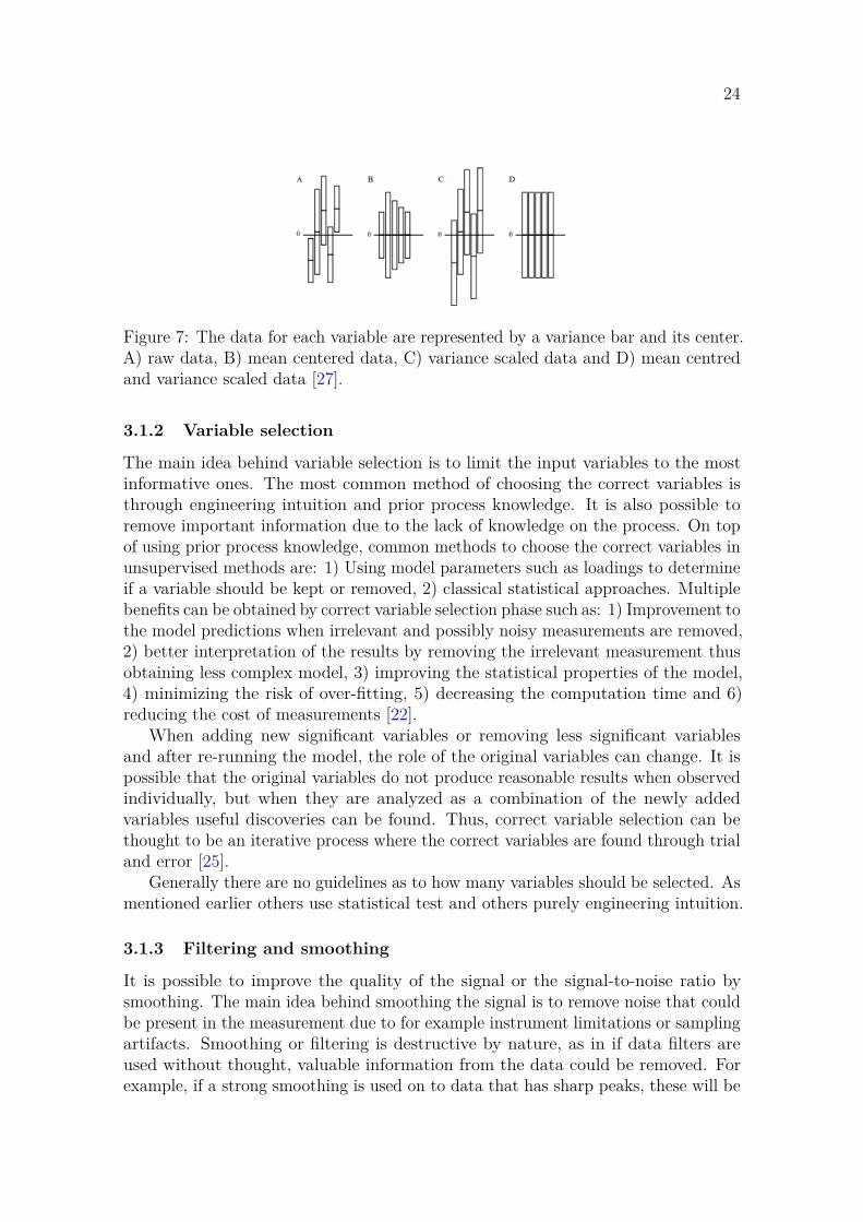
The effect of mean centering and variance scaling on a dataset is illustrated inFigure 7.

24

Figure 7: The data for each variable are represented by a variance bar and its center.A) raw data, B) mean centered data, C) variance scaled data and D) mean centredand variance scaled data [27].

3.1.2 Variable selection

The main idea behind variable selection is to limit the input variables to the mostinformative ones. The most common method of choosing the correct variables isthrough engineering intuition and prior process knowledge. It is also possible toremove important information due to the lack of knowledge on the process. On topof using prior process knowledge, common methods to choose the correct variables inunsupervised methods are: 1) Using model parameters such as loadings to determineif a variable should be kept or removed, 2) classical statistical approaches. Multiplebenefits can be obtained by correct variable selection phase such as: 1) Improvement tothe model predictions when irrelevant and possibly noisy measurements are removed,2) better interpretation of the results by removing the irrelevant measurement thusobtaining less complex model, 3) improving the statistical properties of the model,4) minimizing the risk of over-fitting, 5) decreasing the computation time and 6)reducing the cost of measurements [22].

When adding new significant variables or removing less significant variablesand after re-running the model, the role of the original variables can change. It ispossible that the original variables do not produce reasonable results when observedindividually, but when they are analyzed as a combination of the newly addedvariables useful discoveries can be found. Thus, correct variable selection can bethought to be an iterative process where the correct variables are found through trialand error [25].

Generally there are no guidelines as to how many variables should be selected. Asmentioned earlier others use statistical test and others purely engineering intuition.

3.1.3 Filtering and smoothing

It is possible to improve the quality of the signal or the signal-to-noise ratio bysmoothing. The main idea behind smoothing the signal is to remove noise that couldbe present in the measurement due to for example instrument limitations or samplingartifacts. Smoothing or filtering is destructive by nature, as in if data filters areused without thought, valuable information from the data could be removed. Forexample, if a strong smoothing is used on to data that has sharp peaks, these will be

25

smoothed out. Therefore it should always be considered if the signal needs to filteredor not. Each time series and model is different so no clear rule has been made whenthe data should be filtered so the decision is left for the modeller [22, 24].

The simplest and easiest smoothing filters are moving average and polynomialsmoothing. The moving average filter takes a window of N samples and replaces thecentral point of the window by the moving average. Then the window shifts forwardas in it excludes the last point in the window and includes the next and repeats thecalculation [26]. The degree in which the smoothing is performed can be controlledby changing the length of the moving window. If the moving window is increasedstronger smoothing is obtained. In the polynomial smoothing, a smooth polynomialis fitted into the data by using least-squares. Then a window of N samples slidesover the data at each timestep. Smoothed points are evaluated by the polynomialfunctions midpoint. Then the window shifts forward, dropping and replacing thelast and the next datapoints respectively [24].

3.2 Latent variable methods3.2.1 Principal Component Analysis

Principal component analysis (PCA) is a linear dimensionality reduction techniquethat produces a lower-dimensional representation of the original data set. PCA triesto explain the relationship between the variables of the data by using a numberof components called principal components. Principal components are linear com-binations of the original variables. Each principal component explains partly thetotal variance. The first principal component corresponds to the direction where theprojected data points have the largest variance. The second principal componentis taken orthogonal to the first principal component and it tries to maximize thevariation in that direction. Each subsequent principal components follow the sameprocedure, where new principal components are taken as orthogonal to the previousone until all of the variation is captured by the principal components. In summary,PCA decomposes the original data matrix into loadings, scores and residuals [28].An alternative way of explaining PCA is that a process subspace that contains thetrue variation of the data is being identified. The process subspace is complementedby noise subspace, which ideally only contains noise. Example of how the processsubspace and noise subspace are related to the PCA model and the model residualscan be seen in Figure 8 [19].

Let X be a N ×J matrix with N observations on J variables. In order to representthe original data in principal component subspace, an eigenvalue decomposition isperformed to the covariance matrix of X to obtain the principal components.

C = 1(N − 1)XT X = PΛP T (3)

where: C is a J ×J covariance matrix of XT X, N is the number of observations, Λis a S ×S diagonal matrix with eigenvalues λi of C on the diagonal axis in descendingorder, P is a J × J loading matrix that contains the principal components (PCs)

26

Figure 8: Decomposition of original data matrix X into process subspace and noisesubspace [19].

which are the eigenvectors of C.If the objective is to make further calculations in the principal component space,

new coordinates can then be defined by applying a linear transformation to theoriginal data matrix X:

T = XP (4)

where: T is a N ×J score matrix in which the elements of vector t are representedby its relative principal components, with t1 being the first principal component andso on. The scores are the new coordinates of the original observations in the principalcomponent subspace and their direction is defined by the loadings P . Since PCA is adimensionality reduction technique, most of the variation can typically be explainedby small number of principal components compared to the original dimensions of thematrix X, thus the dimensionality of the data is reduced. The original data matrixcan be reconstructed by retaining the wanted principal components and by usingEquation 5.

X = TP T + E (5)

where: T and P are the score and loading matrices respectively and E is theN × J residual matrix.

Principal components can also be computed by performing a singular value de-composition (SVD) to the original data matrix. Using a singular value decompositionon the original data matrix X gives:

X = UΣV T (6)

where: U is a N ×J orthogonal matrix, Σ is a J ×J diagonal matrix with singular

27

values σi on diagonal axis in descending order and V is a J × J orthogonal matrix.With this decomposition we can see that:

XT X = V ΣT UT UΣV T

XT X = V ΣT ΣV T

XT X = V Σ2V T

(7)

By comparing Equation 7 to Equation 3 it can be seen that V = P and σi =√︂(N − 1)λi. By setting U = T and by using Equations 4 and 5, the new scores and

reconstructed data matrix X can be calculated.Figure 9 shows the projection of the data from the original space to the principal

component space. It can be seen that in the original space (Figure 9a) the observationsare defined by three variables, X1, X2 and X3 In Figure 9b two principal components(PC1 and PC2) are used to represent the original space. PC1 is in the direction ofthe most variation in the observations. PC2 is orthogonal to PC1 and it representsmost of the variation left in the observations. In this example the dimensions of theoriginal data set have been successfully reduced from three variables to two principalcomponents.

(a) (b)

Figure 9: a) Observations in original three-dimensional space b) Observations in PCsubspace with two PC:s [29].

28

3.2.2 Multiway Principal Component Analysis

PCA can be used in identifying meaningful sources of intra-individual variabilityin the observed variables for a single run or batch. However chemical processestypically vary at different levels [30][31]. In a single day, multiple different batchescan be processed or in a case of continuous process multiple different runs havebeen done in the past. Since there are multiple batches or runs to be studied, onemight want to study the intra-individual differences in each batch, but also the inter-individual differences between the batches. Due to the three-way structure of thedata, ordinary PCA is not anymore applicable. Multiway-PCA is a three dimensionalextension of the ordinary PCA. The three dimension of the array represent theobservations, variables and batches (or e.g catalyst runs in the case of continuousprocess). Multiway-PCA is statistically and algorithmically similar with ordinaryPCA [32].

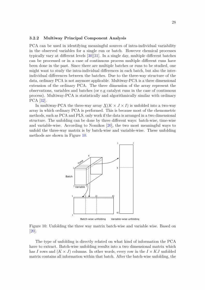
In multiway-PCA the three-way array X(K × J × I) is unfolded into a two-wayarray in which ordinary PCA is performed. This is because most of the chemometricmethods, such as PCA and PLS, only work if the data is arranged in a two dimensionalstructure. The unfolding can be done by three different ways: batch-wise, time-wiseand variable-wise. According to Nomikos [20], the two most meaningful ways tounfold the three-way matrix is by batch-wise and variable-wise. These unfoldingmethods are shown in Figure 10.

Figure 10: Unfolding the three way matrix batch-wise and variable wise. Based on[20].

The type of unfolding is directly related on what kind of information the PCAhave to extract. Batch-wise unfolding results into a two dimensional matrix whichhas I rows and (K × J) columns. In other words, every row in the I × KJ unfoldedmatrix contains all information within that batch. After the batch-wise unfolding, the

29

two dimenesional matrix is mean centered which corresponds to removing the meantrajectory of each variable. In batch-wise unfolding, PCA analyzes the variabilityamong the batches I by summarizing the information in the data with respect tovariables and their time variation [20]. Even though batch-wise unfolding is the mostcommon unfolding method for batch processes, it has its own weaknesses. Differentbatch lengths causes problems for applying the PCA algorithm. The calculatedloadings can only be used if the assumption is made that all the following batcheswill have the same length, which is rarely the case. Multiple ideas to overcome thisproblem has been proposed. These ideas include methods such as: adding anothervariables to mark the beginning and end of each batch , dynamic time warping(DTW), truncating batches to the smallest length etc [33].

Variable-wise unfolding results into two dimensional matrix that has dimension(KI × J). Now mean centering the data matrix means that the ’grand mean’ isremoved from each variable. PCA performed on the variable-wise unfolded matrixanalyzes the dynamic behaviour of each variable around the ’grand mean’ for eachvariable. Variable-wise unfolding is not typically the interest when monitoring batchprocesses [20]. This method doesn’t suffer from the same weakness of needing acomplete dataset, since the loading matrix is constructed based on the amount ofvariables which stays constant throughout the monitoring process[33]. Variable-wiseunfolding should be mostly used if the process is more or less constant. Batch-wiseunfolding has also been implemented for continuous processes, but typically the focushas only been in specific occasions such as: start-ups, shutdowns, restarts etc.

3.2.3 Multilevel Simultaneous Component Analysis

In some cases the multiway structured data can be difficult to analyze properly dueto the different runs of batches being very different. Therefore the overall data mightnot have a proper multiway structure. In cases like this, Multilevel SimultaneousComponent Analysis (MLSCA) is proposed as a better option. MLSCA was developedby Timmerman [34] explicity for multilevel structured data and it enhances greatlythe interpretation of large sets of process data compared to ordinary PCA. MLSCAfollows similar procedures as normal multiway-PCA, as in the three-way data matrixfirst needs be unfolded into two-way matrix. This is done by variable-wise unfoldingas presented in the previous section.

Consider a collection I of data matrices Xi(Ki×J) that gets variable-wise unfoldedinto two-way matrix X(N × J). The matrix X contains observations for I batchesof length Ki on J variables where the total number of observations N = ∑︁I

i=1 Ki.MLSCA decomposes the matrix X into three components: an offset term, a betweencomponent part and a within component part. An element xijk of matrix X containsan observations for batch i on variable j at time ki can be modelled as the sum ofthe three components [34].

xijki= xj⏞⏟⏟⏞

offset

+(︂xij − xj

)︂⏞ ⏟⏟ ⏞

between component

+(︂xijki

− xij

)︂⏞ ⏟⏟ ⏞

within component

, (8)

The objective of the model is approximate the original data as good as possible

30

through the three components.In MLSCA every data matrix Xi with Ki observations and J variables can be

decomposed to the following model.

Xi = 1KimT + 1Ki

tb,iPTb + Tw,iP

Tw + Ei (9)

where: 1Kiis a (Ki × 1) vector of ones, mT (J × 1) contains the offsets of the

process variables J across all measurement occasions, tb,i(Rb ×1) is the i-th row vectorof the between score matrix for Rb retained between components, P T

b (J × Rb) is thebetween loading matrix, Tw,i(Ki × Rw) is the within score matrix for Rw retainedwithin components, P T

w (J ×Rw) is the within loading matrix, and Ei(Ki ×J) containsthe residuals.

Figure 11: MLSCA algorithm

The offset term stays constant for all observations throughout the data. Thebetween component scores describes the non-dynamic deviation of each batch fromthe global mean and the within component scores describes the dynamic deviationof each element xijk from the mean of its own batch. Flow diagram of the MLSCAmethod is presented in Figure 11. The MLSCA model is fit to the data by byminimizing the sum of squared residuals, which summarizes on performing row-weighted PCA to the between component and a simultaneous component analysis(SCA) to the within component part. Constrains are imposed so that the three partscan be solved independently as explained in [34].

Between frame part can be estimated by calculating the variable-wise meanin each frame and stacking the mean vectors together obtaining a between meanmatrix Xb (I × J). The between frame model is then estimated by computing asingular value decomposition (SVD) of the row-weighted between frame mean matrixWXb = USV T , where W is a diagonal matrix having wi,i =

√Ki. The between

frame part thus corresponds on performing a row-wise weighted PCA. Row weightedPCA is thus taking into account the number of samples per run. Between framescores Tb and between frame loadings Pb and the reconstructed between mean matrix

31

can be calculated from equations 10, 11 and 12:

Tb = W −1URb (10)

Pb = VRbSRb (11)

Xb = TbPTb + Eb (12)

where URb,VRb and SRb contains the columns corresponding to the retainedbetween principal components.

Within frame model follows the idea of Simultaneous Component Analysis (SCA).Four variants of SCA is proposed in [35] called SCA-P, SCA-PF2, SCA-IND andSCA-ECP. The four variants differ from eachother with respect to the constraintsimposed on the covariances of the component scores. SCA performs PCA on locally(within each frame) mean centered data matrix Xw. Similarly to between framemodel, SVD is performed to this data matrix with the exception that no weightingis used. Within part scores, loadings and the reconstructed within mean matrix arecalculated as follows:

Tw = URw (13)

Pw = VRwSRw (14)

Xw = TwP Tw + Ew (15)

where URw,VRw and SRw contains the columns corresponding to the retainedwithin principal components.

MLSCA thus provides one set of scores and loadings for both between and withincomponent models. This allows the clear separation of the variation that occurse.g between different runs and the variation that occurs within one both for eachvariable. Both the between and within component loadings are constrained to betime and frame invariant. This ensures that all of the component scores for all runscan be equally interpreted and that the scores can be directly compared betweendifferent runs [34].

3.3 Anomaly detectionStatistical process monitoring typically involves different tasks such as: anomalydetection, anomaly identification, anomaly estimation and anomaly reconstruction.Detecting the anomalies in the process operation is the first task in statistical processmonitoring. Once a model that represents the normal behaviour of the processhas been developed, it is necessary to detect deviations from this behaviour. Thisis one of the core objectives of the anomaly detection. [36]. The different taskstypically have three common aims: 1) detect deviations between the current andthe desired process state 2) predict values for the chosen process variables and 3)

32

classify the current process state. The first task compares the original variables usedfor constructing the model to a new data set to detect if the process is operating atthe same region as the training data. The second task involves using the measuredvariables and the built model to estimate values for another variable. The last taskis used to classify the process state. [37].

Two different statistics are mainly used to estimate the statistical fit of themodel: Hotelling’s T 2 statistics and Q statistic (also known as Squared PredictionError). Hotelling’s T 2 analyzes the score matrix produced by PCA to examine thevariability of the projected data in to the new principal component subspace. Qstatistic analyzes the residual data that represents the variability of the data that isprojected into the residual subspace [38]. T 2 and Q statistic are common tools sincethey summarise the multivariate process information of multiple variables into asingle number. Depending on the situation, these two statistics are usually combinedwith PCA or PLS to produce a good quality control method that is also suitable forreal large scale processes [36].

Unusual high Q statistic indicates that the correlation structure of the data haschanged for the original process variables. The model is not anymore able to capturethis variation, meaning that the observation is far away from the principal componentsubspace which causes the Q statistic to increase. Unusually high T 2 indicates thatthe observations is far away from the origin of the principal component subspace.Due to e.g. an anomaly, a process variables value can deviate a lot from the expectedmean value. If the Q statistic value is low, but T 2 is high it can still be assumed thatthe model is valid since most of the variation is captured [36]. However, usually asituation like that can be caused by a change in the operating conditions which itselfis not necessary a fault. These different types of outliers can be seen from Figure12. Observations 1 and 4 are close to the PCA plane but far away from the regularobservation, these observations would have higher Hotelling’s T 2 values. These canbe denoted as good leverage points. Orthogonal outliers, such as observation 5 isclose to the regular observations but far away from the PCA plane. This observationwould have high Q statistic, but low T 2. Observations 2 and 3 are both far awayfrom the regular observations and from the PCA plane so they can be denoted asbad leverage points (high Q statistic and high T 2) [39].

Figure 12: PCA plane with high T 2 and Q statistic visualized [39]

33

3.3.1 Hotelling’s T 2

The Hotelling’s T 2 is a generalization of the Student’s t-statistic that is used inmultivariate hypothesis testing. In other words, Hotelling’s T 2 is a measure of thedistance within the principal component plane from an observation to its origin.Hotelling’s T 2 can be interpreted as the normalised sum of squared scores and itsvalues at time k can be calculated as [40]:

T 2 = tT λ−1t (16)

where: t are the principal component scores at time k and λ is a diagonal matrixof the inverse of the eigenvalues arranged in descending order corresponding tothe amount of the retained principal components. An upper control limit can becalculated for Hotelling’s T 2 with the assumption, that if the Hotelling’s T 2 valueexceeds, the control limit the data point can be considered as abnormal. Assumingthat the process datapoints follows multivariate normal distribution and that themean and covariance can be estimated from the data, the distribution of the datasetcan be assumed to be as [36]:

T 2α = l(N2 − 1)

N(N − l)Fl,N−l (17)

If the data set is large so that the mean and covariance can be estimated withease, the upper control limit can be determined from the chi-squared distribution[39].

T 2α =

√︂χ2

p,α (18)

where: χ2α is % quartile of the chi-square distribution and p is the degrees of

freedom.

3.3.2 Q Statistic

Q statistic, also known as Squared Prediction Error (SPE), measures how much ofthe variation in the data is not captured by the latent variables (PC:s) of the model.It is the difference between the original data point x to its projection on the lowerdimensional principal component plane. It is a practical tool to evaluate the validityof the model for each data point since it gives information about the lack of fit ofthe model for each data point [40]. Q statistic is defined as sum of squares of theresidual matrix E.

Q = eeT (19)

where: e is the ith row from the residual matrix E.The sample is considered as normal if its Q statistic is lower than its upper control

limit Qlim. When the Q statistic of a sample is outside of the upper control limit, itmeans that there is a new type of variation present and the model is not fit for thatsample. Sample like this can be denoted as an outlier, which in retrospective can

34

be a measurement error or a possible process anomaly. Jackson and Mudholkar [40]derived the following expression for the upper control limit:

Qlim = θ1

⎡⎣1 +cα

√︂2θ2h2

0

θ1+ θ2h0(h0 − 1

θ21

⎤⎦1/h0

(20)

whereθi =

m∑︂j=l+1

λij (21)

h0 = 1 − 2θ1θ3

3θ22

(22)

where cα is the standard normal deviate corresponding to the upper (1 − α)percentile, λj is the jth eigenvalue, l is the amount of principal components retained.

The control limit value can also be computed from the Wilson-Hilferty approx-imation for a chi-squared distribution. It assumes that the orthogonal distancesraised to the power of 2/3 are approximately normally distributed, with mean µ(Q 2

3 )and standard deviation σ(Q 2

3 ) [39].

Qlim = (µ + σZ.975)2/3 (23)

It should be noted that Q statistic and T 2 statistic assumes that the data isnormally distributed. This might not be the case in industrial chemical processes, sotrusting blindly the confidence limits is not advised. Note that only the confidencelimits depend on a certain distribution, not the Q and T 2 measures as such.

3.4 Anomaly identificationIn the previous section it was explained that process anomalies can be detectedby computing the two different multivariate statistics together with the score plots.The calculated statistics however do not detect which variable could be causing thisanomaly or what is wrong with the process, they just indicate that the process is notanymore operating under the assumed normal variation. For these reasons anomalyidentification can be implemented to further investigate the results obtained from thePCA based model and from the obtained Hotelling’s T2 and Q statistic. Contributionplots are typical way of visualizing the model results, revealing which variables areinfluencing the model residuals the most. Analyzing the contribution can pinpointto the variables that are causing the this behaviour. It can thus be summarised, thatthe point of contribution plots is to reveal which variable is accounting the most tothe observed anomalies. In other words, in contribution analysis the variables thataccount for the largest contribution to the anomalies are identified [19].

After an anomaly has been detected by the increased value of Q statistic or T 2, itcan be identified so that correct operation can be adjusted and so that he fault can becorrected if possible. Contribution plots are well known tool for fault identification, asthey indicate which variable have caused the observed deviation. For T 2, the variable

35

that forces the score further away from zero along the jth principal component arefound by inspecting:

T 2c = xPj (24)

where: T 2c is a vector with the contributions from each process variable at time k.

Pj is a diagonal matrix of the column vector pj and x denotes the vector of originaldata at time k.

For Q statistic, the variable contribution can be calculated easily since theQ statistic value is the squared prediction error summed over the variables, thecontribution of a variable J to the Q statistic is then:

Qc = e = x − x̃ (25)where: Qc is a vector with the contributions from each process variable at time

k. x denotes the vector of original data at time k and x̃ denotes its reconstructionusing a model with j PCs.

By plotting the Qc and T2c as a bar chart, the contributions of each variable to

the Q statistic and T2 can easily be seen. The size of the bars indicates how mucheach variable contributes to the prediction error. Example of the contribution plotscan be seen in Figure 13.

Figure 13: The contributions of each variable to the prediction error at randomsample.

3.5 The amount of principal componentsAs PCA is a dimensionality reduction technique, it is also necessary to define howto select the correct amount of principal components to retain. So far it has onlybeen said that we retain p principal components, but no discussion have beenmade on how this procedure can be performed or how we determine the amountof principal components that should be retained. Multiple different methods forchoosing the amount principal components have been proposed such as cumulativepercentage of total variation, size of variances of principal components, a scree graph,cross-validation and other recently developed methods. The first three methods arecommonly used even though their justification is sort of ’rule of thumb’ as they seem

36

to work in practice [28]. However since they are in common use, skipping them forthe case of lack of justification seems unwise. In addition to the more commonlyused methods, more justified rule based methods such as cross-validation are alsopresented. Also a newly developed methods which computes a hard threshold basedon singular values is shown.

3.5.1 Cumulative percentage of total variation

In cumulative percentage of total variation method, the amount of principal compo-nents are chosen so that the retained principal components explain a predeterminedfraction of the total variation. The variance captured by each principal commponentis calculated by using the eigenvalues defined in PCA:

tm = 100m∑︂

k=1λk/

p∑︂j=1

λk (26)

where λi is k-th largest eigenvalue after performing PCA. The cut-off value tco forcaptured variance is typically set to around 70% and 90% and the amount of principalcomponents to be retained is the smallest integer for which tm > tco. It is also typicalfor the tco value to decrease the more variables the data set have [28]. This rule isapplicable whether a covariance or a correlation matrix is used to compute PCs.

3.5.2 Size of variances of principal components

Compared to the previous rule, this rule is only valid when PCs have been computedfrom a correlation matrix. It sets a cut-off value in which if the eigenvalues corre-sponding to the principal components exceeds, the principal component is retained.The rule states that if all variables are independent, then the PCs are equal to theoriginal variables and all of them have a unit variances in the case of correlationmatrix. This means that if the principal components eigenvalue is less than 1, itcontains less information than the original variable thus it will be excluded. It isnoted that the cut-off value of 1 might retain too few PCs and a new cut-off valuebased on simulation studies is proposed to be 0.7 [28].

3.5.3 Scree graph

The scree graph is by far the most biased way of choosing the retained principalcomponent, since it involves looking at the graph and based on the curve the choiceon how many principal components should be retained is made. In a scree graph theeigenvalues λi are plotted into y-axis and index value for the eigenvalue is plotted intox-axis as shown in Figure 14. Then the idea is to inspect the graph and determinewhere an ’elbow’, a point in which prior values decrease steeply and following valuesdecrease less steeply, is located. The value of the ’elbow’ is then the amount ofprincipal components to be retained [28].

37

Figure 14: Scree graph for the correlation matrix.

3.5.4 Cross-validation

Cross-validation of multivariate data set was introduced by Wold [41]. In crossvalidation it is assumed that the most significant principal components model thedata and the less significant principal components model noise. The significance ofeach principal component can be tested by seeing how well an unknown sample ispredicted. This method validates one principal component at a time until all theprincipal component have been validated. If the first component is considered to bevalid, it gets subtracted from the full data set. The leftover residuals are then usedfor testing the validity of the next principal component. PCA model for data matrixX is computed. To validate component a, the following procedure is applied.

1. Let X(a) be the residuals after a − 1 components.

2. Calculate the sum of squares for X(f)

SSx(a) =I∑︂

i=1

J∑︂j=1

x2ij(f) (27)

3. Apply PCA on the reduced I − 1 dataset. Obtain the score matrix T andloading matrix P .

4. For sample i, calculate the scores by: T̃ i = xiPT

5. For sample i, calculate the model with a principal components by: x̃ai = t̂

a

i P

6. Repeat by removing another sample until all samples have been removed

7. Calculate the predicted residual error sum of squares (PRESS) between thepredicted and observed values:

PRESS =I∑︂

i=1

J∑︂j=1

(x̃aij − xij)2 (28)

38

Here the data set X is divided arbitrary into G groups. Then all the rowsbelonging to the first group are removed thus forming a new matrix X(1) and areduced data set X(−1). A PCA model is built on the reduced data set X(−1). Thematrix X(1) that contains the removed group is used as testing set. Then newpredicted values are calculated for X(1) (Equations 4 and 5). Then the residuals(PRESS) are computed from the predicted and actually observed values. This processis then repeated for the second group X(2) and is continued until the residuals for allof the groups have been calculated.

Finally compute the ratio R. If the value of R is < 1.0, the prediction are betterby including the group since the total error of the test set is lower than the sum ofthe residuals by fitting a model with p components.

R = PRESS

RSS(29)

39

4 Experimental setupThe objective of this thesis was to develop a process monitoring method for thedearomatization reactor that was presented in Section 2.3.1. The target for themonitoring method was investigate if we can detect anomalies, such as catalyst deac-tivation, hot spots or liquid maldistribution, purely based on the changes occurringin the temperature profiles of the reactor. Operation data was collected for thefeed temperature sensor and for the 21 temperature sensors in the reactor roughlythroughout one catalyst cycle. The sampling interval of 1 hour were used in thisstudy.

The studied reactor as shown in Section 2.3.1 Figure 5 is equipped with 21temperature sensors. These sensors are positioned in three poles, thus each pole haveseven sensors. Since the data consists of only one catalyst cycle, typical monitoringsetup where different catalyst runs would be compared against each other is notpossible to do. Instead, in order to efficiently monitor the anomalies based on thetemperature profiles, the data is setup to represent the reactor. This means thatinstead of using the temperature sensors as the variables for the component model,new variables that represent the three poles are formed and the temperature sensorsact as observations. We have now formed a 7 × 3 matrix that represents the reactorstemperature profile at time k as shown in Figure 15. This data matrix is a snapshotthat represents reactors temperature profiles at time k and it allows us to monitor thereactor based on the temperature profiles of the three poles. The reactor is dividedinto seven levels, where we assume that the temperature sensors would be placedat the same height. This will naturally cause small error, which however should benegligible. Three-way data matrix is obtained when new snapshot at time k + i isobtained and a three-way matrix is formed by concatenating the new matrix afterthe previous one. The way the total data set is structured before modeling is shownin Figure 16. The experimental set-up can be thought as a batch process instead ofa continuous process. We are not setting up the data to directly monitor the timeseries of the temperature sensors. Instead we treat every snapshot k as a new batch,that shows how the temperature profile evolves throughout the reactor.

The three-way data matrix contains both the between-snapshot and the within-snapshot variation. Between-snapshot variation reflects the overall temperaturebehaviour between the snapshots, in other words it shows how the averaged reactortemperature is proceeding as a function of time. The within-snapshot reflects thedynamic variation or how the temperature is changing along the reactor as a functionof time. In ordinary PCA, these variation are confounded. Three-way extension ofthe PCA might also not be optimal since the data is collected under different processconditions due to e.g catalyst deactivation and the snapshots can’t be considered to bereplicates of each other. For this reason multilevel simultaneous component analysisis applied. This sensor configuration allows the use of MLSCA to investigate howthe overall temperature changes in the reactor and also how the reaction proceeds ineach level at every snapshot k + i, i = 0, . . . , I by separating the data set into the twodifferent models, between-frame and within-frame, as explained in Section 3.2.3. Thebetween-frame models how the temperature is evolving between the snapshots and

40

Figure 15: Data matrix that represents the reactor at time k.

Figure 16: Three-way data matrix.

the within frame models the axial temperature temperature profile in each snapshot.We will expect the main variation in both models to be caused by the increasedreaction temperature. Noise e.g uneven temperature profiles should be captured bythe residuals.

Typically the training set would cover most of the catalyst life-cycle or it would atleast represent the process in ’normal operating conditions’. Any deviations from this’normal operations’ would then be marked as possible anomalies or faults. However,trying to find a time frame where ’normal operating conditions’ are present is difficultsince the data has non-stationary behaviour. Also if the same model would laterbe used to validate other catalyst life-cycles, the same operating conditions mightnot be applicable anymore due to e.g. changes in feed composition or changes inthe operation equipment. This would mean that years of operating data would begathered and time frames, where no anomalies were present should be hand pickedfor the training purposes. And even still, the model can become invalid if substantialchanges are made to the operating conditions or the equipment. Since the dataused in this thesis covered only one catalyst life-cycle, a different training setup wasneeded. Therefore the training set was setup to be in a time frame where no reaction

41

is yet happening. This means that in the training set the temperature profiles alongthe three poles are uniform and there are no major temperature deviations both inaxial and radial directions.

Since the data is non-stationary by default, as in the temperature sensors have’natural drifting’ due to the reaction increasing the level-wise temperatures, the ideaof the training data was to be a baseline that represent a situation in which weassume that the catalyst is either 100% active or 100% deactive. In either way thismeans that that the temperature difference over the reactor would be close to 0◦C andthe temperature profile in the reactor should be completely uniform across the threepoles. Figure 17 shows the average temperature difference over the reactor during thetraining phase. As we can see the three poles have close to 0◦C temperature increaseover the reactor and the behaviour of the three poles are uniform. The assumption isthat the training set do not represent the ’normal operating conditions’, but instead itrepresents the ’ideal temperature profiles. The ’ideal temperature profiles’ as shownin Figure 6 in Section 2.3.1 assumes that the temperature profiles are uniform dueto the reaction proceeding downwards a level at a time. When a level starts thedearomatization reaction, we assume non-ideality which means that there should betemperature deviations between the poles. Assumptions can then be made based onthe monitoring statistics and process knowledge if the reactor is behaving normallyand conclusion can be drawn on how far the deactivation has proceeded. Secondreason for using a training set like this would be that if the model would be usedon-line, it could be trained relatively easy without any prior history data. Priorhistory data could be used if it could be guaranteed that the feedstock contains thesame amount of aromatics to ensure the same operating conditions. Since the studiedreactor was the second one in the reactor series, it will only start reacting after thefirst one starts deactivating. This means that we can use roughly the first monthafter the unit start-up as a training set. The following graphs have been masked inorder to preserve the confidentiality of the actual operating conditions.

Figure 17: Temperature difference over the reactor in the three poles for the trainingset for the first 1000 hours of operation.

Time series of the averaged raw temperatures of the three poles throughout thewhole catalyst life cycle are shown in Figure 18. It was mentioned earlier, that theloss of catalyst activity is usually compensated by increasing the feed temperature,thus increasing the overall temperature of the reactor. However, as it can be seen

42

from Figure 18, it is not easy to observe if the temperature has been increased. Thisis because the feedstock aromatic concentration is fluctuating. Better visualizationis thus needed in order to detect the state of the reactor as in is the reactor inthe SOR, MOR or EOR phase. Two different approaches are tested for bettervisualization: 1) temperature differences from each level against the feed temperatureand 2) temperature differences between levels. In 1) we simply calculate the differencein temperatures from each level against the feed temperature. In 2) the temperaturedifferences are calculated level-wise, as in the first level would be the temperaturedifference between level 1 and feed and in the second level temperature differenceswould be level 2 vs level 1. This setup should achieve better visualization on thereactor conditions.

Figure 18: The operating temperatures for the three poles throughout the catalystlife cycle.

Before analyzing the data with MLSCA, minor preprocessing for the data hadto be done. While analyzing the training set of the data, it was observed that thethird level of the reactor had a clear offset in Pole 2. This offset becomes even moreevident when plotting a picture from one of the training set snapshots. The offsetcan be seen as a timeseries and also as a snapshot in Figures 19 and 20. Sincethe reaction is exothermic and the process is thought to be adiabatic, endothermicreactions are negligible. Also this behaviour starts immediately after the start-upwhen no reaction is yet happening. This leads to the conclusion that the sensor ismalfunctioning. The offset was consistent throughout the whole catalyst life cycle,so it was corrected by averaging it based on the surrounding sensors.

The training set for the MLSCA consists of the first 1000 data points and theremaining 13000 data points will be used for testing the model. The data set willfurther be preprocessed by mean centering. Scaling to unit variance will not beperformed, since all of the variables are in the same units in the same magnitude.

43

Figure 19: Timeseries of the training set temperatures for the three poles. Offset isseen on level 3.

44

Figure 20: Snapshot of the temperature values at time k for the three poles. Offsetis seen on level 3.

45

5 Results

5.1 Between-frame, dT vs feed temperatureAfter removing offsets by mean centering the data set was analyzed by MLSCA.The three between-frame principal component explains 99,0%, 0,99% and 0,01%of the between-frame variation respectively. Next, a correct amount of principalcomponents needs to be chosen for the MLSCA model. Considering that there areonly three variables present, the amount of principal components to be retained canbe easily chosen by one of the ’rule of thumb’ methods. In this case cumulativepercentage of total variation is used and one principal component is retained. Byobserving Table 2 it can be seen that the first principal component weights all polesequally and all of the values are positive. This indicates that the first principalcomponent tries to model the overall gross temperature profile. This makes sense aswe have already observed from Figure 17 that during the training period the threepoles are behaving almost uniformly. The second and third principal componentshave substantially lower weights and the values are both positive and negative. Thisindicates that the small temperature differences between the poles are being modelledby the second and third principal components. The second principal component ismodelling the temperature difference from Pole 3 against the remaining two polesand the third principal component is modelling the temperature difference from Pole2 against the two remaining poles. This small variation can also be seen from Figure17. If the behaviour of the poles would be completely uniform, no variation could beseen and the second and third principal components would not contain any weightsin them. However, since the behaviour is not completely ideal and also becausethe temperature sensors were not perfectly in the same level, the small variation ispresent in the component model. Since the training was done during a time framewhere the behaviour of the temperature profiles were close to uniform, even theslightest temperature deviations should become visible when the reactor stars thehydrogenation reaction. This variation should then become visible in the processmonitoring charts.

Table 2: Between-frame loading values for the three principal components.

1st component 2nd component 3rd component45,5 2,5 -0,942,9 0,2 1,846,7 -2,7 -0,7

Figure 21a and 21b shows the averaged temperature differences vs feed for thethree poles over the reactor and the between-frame scores as time series respectively.Firstly, it can be observed by comparing Figure 21a to Figure 18 that we have achieveda clear improvement on visualization of the state of the reactor. By calculating thetemperature differences vs the feed temperature and by setting the training period

46

temperature differences roughly to 0◦C, we can easily point out when the reactor hasstarted the hydrogenation process. First we can observe that the overall temperaturedifference vs the feed is steadily growing until the 8000th data point. During thistime frame the catalyst in the first reactor in series is slowly deactivating, causingour test reactor to slowly increase its heat production. However, at the peak valuewe can conclude that the first reactor has been completely deactivated. At the peakvalue our reactor has full control of the dearomatization process. After the peakvalue the overall temperature difference vs feed is slowly decreasing which is causedby the catalyst deactivation. If our test reactor would be the first one in series, thetemperature difference graph would only be the second half of the Figure 21a sinceit would instantly have full control of the dearomatization process.

Since the process is non stationary, the dynamic change in the temperature caneasily be observed by presenting the between-frame scores as time series. We caneasily observe the similarity of the real temperature profiles and the first principalcomponent. The first principal component curve confirms the assumption made fromthe loadings. The first principal components curve has the same profile as the realtemperature plots meaning that it tries to model the overall temperature profile overthe reactor. The assumption made for the second and third principal componentscan also be confirmed. We observe that these two component curves start to deviatefrom the 0 roughly at the same time as we can observe the temperature in the polesto start deviating from each other. It is interesting to notice that roughly around11500th data point we can observe a possible formation of a hot spot in Pole 1. Thissudden increase in temperature can be observed from the 2nd and 3rd principalcomponent curve.

Figure 22 shows the overall score plots of the MLSCA components for the between-frame part where one scatter point in the graphs represent the reactors state atsnapshot k + i. In Figure 22a and 22b the state of the reactor can be observedtogether with the temperature differences between the poles. When the data pointsare close to the origin no reaction is occurring and the temperature profiles are evenacross the three poles. In these two graphs the horizontal movement of the individualscatter points is thus directly related to the averaged temperature difference from thepoles vs feed. The vertical movement is explaining the magnitude of the temperaturedifferences between the poles. If one wants to focus only on the temperature profilebased anomalies, Figure 22c provides the most information since it plots principalcomponent 2 against principal component 3 which accounts for the residuals of themodel. If the reactor would be ideal and if the temperature difference betweenthe poles would be 0◦C, all the data points would be close to the origin. Thus,in this graph the horizontal and vertical movement is directly proportional to thetemperature differences between the three poles. As we have already discussed thatthe reactor is not ideal so minor temperature deviations will naturally occur betweenthe poles. This is the time between data points 0 to 10000, where we can observe thepoints leaving the origin. However, it is interesting to notice the possible formationof the hot spot that was mentioned earlier. We see that in all three graphs thescores are following a clear trajectory that have an elliptical shape. Suddenly ataround the 11500th data point the score points clearly change the trajectory they

47

were previously moving on. No clear clustering can be observed in the graphs, butwe can easily observe that the second and third component can clearly separate thetime point where the hot spot formed into two different regimes.

Multivariate Statistical Process Control (MSPC) charts were used in post snapshotmonitoring to test if Hotelling T 2 and Q statistic could be used in anomaly detectionpurposes. Figure 23a and 23b shows the Hotelling’s T 2 and Q statistic graphsrespectively. The red line represents the limit where values below it have behaviourclose to the training set data. It can be seen that the Hotelling’s T 2 graph is almostidentical to the first principal component as seen in Figure 21b. Since the referencepoint for the Hotelling’s T 2 calculations is in the training set, this is expected due tothe non stationary behaviour of the data. The Hotelling’s T 2 can thus be concluded tovisualize the state of the reactor rather than providing an explicit anomaly detection.

The Q statistic graph (Figure 23b) however provides more interesting information.Since the model was build by retaining only one principal component, the Q statisticis directly modeling the temperature differences between the three poles. We canobserve that the Q statistic starts to deviate from its initial value and roughly aroundthe 4000th datapoint the curve crosses the limit line. After this point the curvehas a slight upwards trend, indicating that the temperature deviation between thepoles are constantly increasing the more reaction are present. Comparing the Figure23b to Figure 21a it can be observed that Q statistic starts to increase at the sametime where the tree poles start to deviate from each other due to the reactor takingcontrol of more reaction. Small temperature deviations are expected and can be

(a) Real temperature profile along the three poles versus process time

(b) Between-frame scores

Figure 21: a) Averaged temperature difference over the three poles and b) MLSCAscores versus process time.

48

(a) PC1vsPC2 (b) PC1vsPC3 (c) PC2vsP32

Figure 22: Between-frame MLSCA component scores.

(a) Between-frame Hotelling’s T 2

(b) Between-frame Q statistic

Figure 23: a) Fault detection using T 2 -statistic. b) Fault detection using Q statistic

considered as part of normal operation since the reactor is not ideal, but the higherthe Q statistic increase the bigger is the temperature difference between the poles.The formation of a hot spot is also clearly captured by the Q statistic. Aroundthe 11500th data point we can again observe the large spike in the curve, which isoccurring exactly at the same point as we saw in the initial data.

Since the data is non-stationary and the monitoring statistics are calculated basedon the static training set, it can be concluded that these statistic do not necessarydetect anomalies or faults when the control limit is broken. It should be though moreof an anomalous behaviour or that the process conditions have changed. When theQ and Hotelling’s T2 break the control limit, the model has broken the assumptionof ideal temperature profiles that we defined during the training period. In the

49

Hotelling’s T 2 graph, we are not detecting anomalies, but we are visualizing the stateof the reactor in univariate manner. Since the Hotelling’s T 2 measures the distancebetween new observations to the mean of the training set, the rise of the statistic isnot an anomaly, it is just natural drift due to the non-stationary behaviour of the dataand since the data wasn’t detrended. The Q statistic however can be used for anomalydetection as was seen on the formation of hot spot. However, everything beforethe hot spot is not necessary an anomaly even though the graph keeps increasingas little temperature deviation between the poles should be expected. The resultsshould be handled together with process knowledge to decide how much temperaturedeviation is allowed and at which point it can be accounted as anomalous behaviour.The graphs are more of an informative way of saying that the reactor is operatingdifferently from the conditions obtained in the training set. These issues naturallyalso cause the control limit line to be used with caution. Static limit combined withnon-stationary data can easily mislead the user to draw incorrect conclusions.

5.2 Within-frame, dT vs feed temperatureThe second part of the MLSCA model contains the within-frame or the withinreactor variation. The within-frame part of the model was constructed from thesnapshot-wise mean centered data. The within-frame principal components accounts92,2%, 6,9% and 0,9% of the variation respectively. All of the three componentvalues can be seen in Table 3. Similar to the between-frame mode, the amount ofprincipal components to be retained can also be chosen by the cumulative percentageof total variation method. Again the first principal component contains over 90 % ofthe total variation, so one within-frame component is retained. The first principalcomponent weights all the variables positively, so we again make the assumptionthat it tries to model the overall temperature profile in each level. However, in thewithin-frame the most weight is put onto Pole 2 implicating the Pole 2’s dynamicvariation is greater than its adjacent poles. Considering that in the between-frameall the poles had similar weights, this imbalance suggests that when observing eachlevel individually, we have some form of deviation between the temperatures betweenthe poles. This variance stayed hidden in the between-frame part which was onlydealing with the averaged temperature difference values that were calculated overthe reactor.

Table 3: Within-frame loading values for the corrected three principal components.

1st component 2nd component 3rd component68,3 31,3 -9,9125,0 -28,8 -3,587,8 16,6 12,7

Second and third principal components are again modelling the temperaturedifferences between each pole in each level. Considering that the second principal

50

component is giving a rather large positive weight on Pole 1 and 3 and negativefor Pole 2. We can assume that the second component is partially modeling thegross temperature profile on Poles 1 and 3 and partially modeling the temperaturedifference from these poles to Pole 2. Third principal components weights are low sowe assume that it is purely modelling the temperature differences.

Figure 24 shows the frame-wise mean centered temperatures for each level. We canobserve that when the temperature in the reactors starts to increase, the second levelis running significantly cooler. Also the profile does not have a similar shape than itsadjacent poles. This behaviour where one level is constantly and marginally colderin one level than its adjacent poles could be an indication of a possible channellingphenomena. This same behaviour is also present on the third level after roughly the9500th data point. The hot spot that was mentioned earlier is now clearly shown toform on the fifth level. Compare this to the between-frame where we only had anidea that somewhere in the reactor a hot spot was forming. However, we alreadyobserve an inaccuracy for building the model. By using temperature differences fromeach level against the feed, we lose track on where the reaction is proceeding sincethe temperature increase on higher levels propagate to lower levels. This causes thesimultaneous rise in temperature that we can see around the 5000th data point. Thewithin component scores can also be plotted as a time series to observe the dynamicchange. From the scores we can observe part of the reason for the imbalanced in theloadings. The first principal component is following the Pole 2’s profile especially inthe first four levels. The second principal component is modeling the temperatureprofiles of Pole 1 and Pole 3 on the first four levels, but it is also trying to model thetemperature difference from Pole 2 to its adjacent poles. This imbalance makes theinterpretation of the graphs slighty more difficult compared to the between-framepart. The sudden temperature increase from the formation of the hot spot is seen inthe 3rd principal component. However, due to the frame-wise mean centering it ispresent in all of the levels, instead of only on the bottom three.

Instead of only inspecting the time series, the scores can also be plotted as thetypical score plots. The scatter plots of the within-frame scores from the training setis shown in Figure 25. We see that the within-frame model clearly separates eachlevel into its own clusters. Because of the strong clustering, monitoring each levelindividually should be possible.

Within frame scores throughout the whole catalyst life cycle for all of the principalcomponents is shown in Figure 27. The score plots with the first component presentmonitors the temperature deviation together with the reaction. The residual scoreplot, PC2vPC3, in Figure 27, mostly models the temperature deviation in each level.Since the residual score plot contains the the temperature differences between thepoles it is the most interesting scatter plot to observe. From the residual scatter plot itcan easily be observed if one of the levels have deviating temperature profiles betweenthe poles. When the points in the scatter plot is close to origin, no temperaturedeviation between the poles are observed. The two remaining plots in Figure 27 donot provide too useful information. This is due to the non-stationary of the dataand since the temperature differences are calculated against the feed temperaturefrom each level, the score plots are not efficient way to determine in which level the

51

Figure 24: Within-frame mean centered temperatures for each level

(a) PC1vPC2 (b) PC1vPC3 (c) PC2vPC3

Figure 25: MLSCA within-frame principal components

reaction is proceeding. This was already observed from Figure 24. It is interestingto notice that in all of the scatter plots, similar to the between frame model, thetrajectory of the scores change at the 11500th data point. If one would only observethe score plots, as assumption could be made that a possible hot spot would beoccurring in all of the levels simultaneously. Due to the non-stationary of the dataand since the temperature differences are calculated against the feed temperature

52

from each level, the score plots are not efficient way to determine in which level thereaction is proceeding.

T 2 and Q statistic values can also be computed for each level separately Figure26. Due to the non-stationary behaviour of the data, the mean of the dataset isconstantly moving. This causes the mean of Hotelling’s T 2 also to move. Comparedto between frame model where we had a static mean temperature the T 2 could beinterpreted to represent the reactors state. In the within model it is telling whenthe levels are at the same temperature as the mean temperature of the reactor.This information can’t be used for any monitoring purposes. By retaining the firstprincipal component, the Q statistic would model partially the temperature profilesof Poles 1 and 3 and also the temperature deviation between the poles in each leveland the results can be seen in Figure 26). Since the 2nd principal component triesto model the overall temperature profiles of the Pole 1 and 3 especially on the firstfour levels, we see the Q statistic to rise unreasonably high. For this reason, wecan’t confidently say that it has the same property as the between-frame model.If we would like it to model purely the temperature differences between the poles,we should retain two within-frame components. However, this would not cover thetemperature differences between Pole 1 and Pole 3 as we saw from the loadings.Based on the Q statistic, we would also assume that a hot spot could be forming atthe same time also on level one and two. When we observed the real temperatureprofiles (not mean centered) we concluded that this was not the case. The hot spotwas only forming in level five. This error is a consequence of the within-frame modelbeing mean centered at each snapshot. The formation of the hot spot increasedthe mean temperature of Pole 1 and since we are measuring how far each level isfrom the mean temperature it causes this error. For these reasons the Qstatisticbecomes highly unreliable method for detecting temperature deviations with thissetup. It becomes clear that the temperature differences vs feed setup do not producereasonable results even though the same setup behaves great in the between-framemodel.

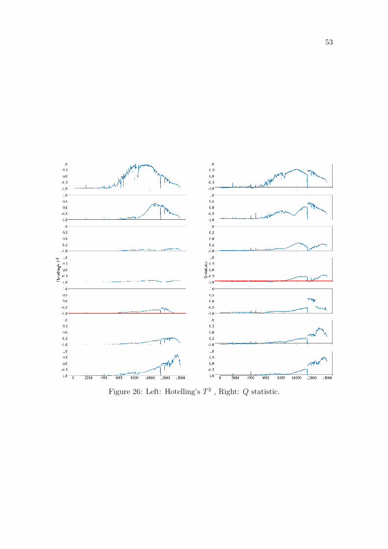
53

Figure 26: Left: Hotelling’s T 2 , Right: Q statistic.

54

Figure 27: Within-frame scores throughout the reactors life cycle.

55

5.3 Between-frame, dT between levelsThe second experimental setup was done by calculating temperature differencesbetween each level instead of using the feed temperature for each level. This setupshould provide a better interpretation on the dynamic variation, as in in which levelthe reaction is proceeding. The same mean centered data set was used before usingthe MLSCA algorithm. The obtained between-frame components explain 99%, 0,99%and 0,01% of the variation respectively. We can use the same method of cumulativepercentage of total variation to choose the amount of principal components to beretained, since we are dealing with the same three variables. Again only principalcomponent is chosen for the modelling purpose. Table 4 shows the between-frameloadings that were obtained after modelling the training set. So far the new setupis following exactly the same behaviour as our previous between-frame model. Thefirst principal component is again explaining the overall, gross temperature profile.The second principal component is explaining the temperature difference from Pole 1to Poles 2 and 3 and the third principal component is explaining the temperaturedifference from Pole 2 to Pole 1 and 3.

Table 4: Between-frame loading values for the corrected three principal components.

1st component 2nd component 3rd component7,5 -0,7 0,17,7 0,1 -0,58,1 0,5 0,3

The averaged temperature differences between levels for the three poles and thebetween-frame scores are seen in Figure 28a and Figure 28b. We can observe thatthe main profile of the temperature curves are close to what we saw in the previousbetween-frame set-up. However with the temperature differences between levels,the temperature curves do not have the exact same bell shape that we observed inthe previous model. Compared to the raw temperature values (Figure 18) we stillobtain better visualization by using the level-wise temperature differences. Since weobtained similar weighting for the loadings for this setup-up, it is no surprise thatthe first principal component curve has the same profile as the temperature profilesfrom the three poles. The second and third principal component are again modellingthe temperature differences between the poles, where the most concrete example canbe seen during the formation of the hot spot.

Figure 29 shows the score plot of the MLSCA between components. Each scatteragain represents the reactor at snapshot k + i. It is interesting that by using thisdifferent temperature difference calculation, we can see that the scatter plots aredividing the data into two clear clusters. Compare this to the temperature differencevs feed set-up, where we mostly saw a change in the trajectory of the scatter points.This is especially clear on the Figure 29c which plots the residuals of the MLSCAmodel. The first cluster contains the data before the occurrence of the hot spot

56

and the latter contains the data after the formation of the hot spot. Since thebetween-frame model is only dealing with the averaged temperature values, theoverall interpretation of the score plots is exactly the same as we had in the previousbetween-frame model. The main difference is the visualization which is caused bythe different calculation set-up.

The same MSPC charts were also for this model and can be seen in Figures 30aand 30b. Since the underlying behaviour of the model is almost identical for thebetween-frame part, the Hotelling’s T 2 and Q statistic is assumed to also behavesimilarly to the previous model. This is confirmed by looking at the Figure 30a,where the Hotelling’s T 2 graph has the same profile as the first principal component.Reasoning for this was already explained in section 5.1. The Q statistic curve alsolooks a little different compared to the one obtained in the previous model. Theinformation that it contains, however is exactly the same. Since we already confirmedthat the first principal component models the gross temperature profile, it onlymakes sense that the Q statistic models the residuals, as in the average temperaturedifferences between the poles.

Again we disregard the control limit line due to the non-stationary behaviour anduse it just as an indication to mark when the reactor has reached its initial state.

(a) Real temperature profile along the three poles versus process time

(b) Between-frame scores

Figure 28: a) Averaged temperature difference over the three poles and b) MLSCAscores versus process time.

57

(a) PC1vsPC2 (b) PC1vsPC3 (c) PC2vsPC3

Figure 29: Between-frame MLSCA component scores.

(a) Between-frame T 2 residual

(b) Between-frame Q statistic

Figure 30: a) Fault detection using T 2 -statistic. b) Fault detection using Q statistic

5.4 Within-frame, dT between levelsWithin-frame model was also reconstructed by using temperature differences betweenlevels instead of having temperature difference versus the feed temperature. Theloadings are presented in Table 5 and the principal components account for 86,7%,11,9% and 1,3% of the variation respectively. Compared to the previous within-frame model, the loadings are weighting the first principal component more equally.However, for this time the modeling is mainly done based on Pole 1 and Pole 3,instead of Pole 2 which was constantly running colder on the first three levels. Thefirst principal component is chosen to be retained for modelling purposes by usingthe cumulative percentage of total variation -method.

Figure 32 shows the frame-wise mean centered temperature and within-frame

58

Table 5: Within-frame loading values for the three principal components.

1st component 2nd component 3rd component-124,5 39,6 -16,5-102,1 -66,1 -6,3-144,6 12,6 18,7

scores for each level. By using the temperature differences between levels, the firstgraphs shows the temperature differences between level 1 vs feed. Second graphshows level 2 vs level 1 etc. It should be kept in mind that now the temperaturecurves are always related to the level that is on top of the observed level. Thismeans that even though we can see clear differences between the temperature curves,it doesn’t necessary mean that there is temperature deviation in that exact levelbetween the poles. It means that when we compare the single levels temperature toits upper level, the temperature increase or decrease is not equal. For example, if weobserve the third level more closely, the first intuition would say that on that levelthe temperatures should be deviating considerably at around the 8000th data point.However, if we look at the real temperature values on that level (Figure 31), we seethat the temperatures are roughly equal. Since the temperature increase from level 2to level 3 in Pole 2 is higher than, its adjacent poles, we observe it as a temperaturedeviation on Figure 32. Thus, one needs to always keep in mind where the referencestate for the observed temperature curves are.

Figure 31: Real temperatures on level 3.

The scatter plots for all of the levels from the training set can be seen in Figure33. Again all the levels are separated clearly to their own clusters, so monitoringeach level individual becomes possible. The whole life cycle for all of the principalcomponents is shown in Figure 35. Similar to the temperature differences vs feedtemperature, the PC1vsPC2 and PC1vsPC3 figures show the temperature deviationtogether with the reaction in each level and the PC2vsPC3 figure shows the residualsof the MLSCA model. The biggest difference in the scatter plots that have PC1present compared to the previous within-frame model is that by using the level-wisetemperature differences there is no temperature propagation to lower levels. Thismeans that following where the reaction is proceeding together with the temperature

59

Figure 32: Within-frame raw temperatures and within-frame scores for each level.

deviation becomes possible. Now the scatter points are moving along PC1 only whenthere are reaction present in that level. In the residual score plots, if the scatterpoints are close to the origin, there is no temperature deviation present. When thescatter points start to move it indicates that the temperature increase in the threepoles is not equal, which can be an indication of an anomaly. We can observe thatthe hot spot occurring at the 11500th data point is not anymore that visible on all ofthe graphs. We see that the trajectory of the data points changes massively only onthe levels 4-6, which is a clear improvement on the accuracy of the model comparedto the temperature difference vs feed one. Based on the score plots it can already bepointed out that the hot spot did occur on level 5, since a new cluster of points isformed around that time.

Hotelling’s T 2 did not improve after changing the calculation of temperaturedifferences. The moving mean still causes the same issues as was observed on theprevious within model. For this reason T 2 results will be completely disregarded.The Q statistics accuracy seemed to improve reasonably when using the level-wisetemperature differences. Similar to the residual score plot, we need to rememberthat an increase in the Q statistic is not a direct indication that on that specificlevel the poles have different temperatures. The rise of Q statistic indicates that

60

(a) PC1vsPC2 (b) PC1vsPC3 (c) PC2vsPC3

Figure 33: Within-frame MLSCA component scores.

the temperature increase between the levels is not completely uniform, which canbecome a little misleading if one forgets that the reference state is constantly moving.If we look again at the Q statistic value at the 9000th data point on the first level,we see that it barely crosses the control limit value. Compare this to the previouswithin-frame model (Figure 26) where it obtained the maximum value at the samepoint. This time the Q statistic is more accurate since it models the differences inthe temperature increase between the poles. The Q statistic is still not perfect as wecan observe it to be over its limit even after the 13000th data point. At this pointthe first level is completely deactivated, but because the hot spot was formed a littlebit earlier, the mean of Pole 1 was increased which is inaccurately modelled by thewithin components due to the frame-wise mean centering. However, this error hasdecreased substantially compared to the previous within-frame mode. Even thoughthe Q statistic seemed to improve greatly compared to the previous within-framemodel, it is still inconvenient and misleading to be used in this kind of monitoringproblem. Most of the problems are coming back to the frame-wise mean centeringprocedure. Since the poles in the reactor do not have the same temperatures on eachlevel, the combination of frame-wise mean centering and unbalanced temperatureprofiles makes the Q statistic unreliable. The second part is that we are modellingthe difference between temperature increase between the levels, instead of the actualtemperature differences between the levels. In other words, the Q statistic explainsif the temperature increased caused by the reaction has been even between the threepoles. This information can used, but it has to be accompanied together with processknowledge and deep understanding what the model is trying to represent.

61

Figure 34: Left: Q statistic, Right: Hotelling’s T 2.

62

Figure 35: Within-frame scores throughout the reactors life cycle.

63

6 Disussion and conclusionThe goal of this thesis was to develop an anomaly detection system for a trickle-bedreactor that is used for dearomatizing hydrocarbons. The aim for the work wasto investigate if MLSCA could be used to detect the formation of disadvantageousphenomenons occurring in the reactor purely based on the changes in the temperatureprofiles. The main motivation for this was to investigate if it’s possible to visualizethese phenomenons so that the information could potentially be used for dailyoperation in fault detection purposes. The multivariate statistical technique used inthis thesis was MLSCA together with the classical anomaly detection methods ofHotelling’s T 2 and Q statistic.

The literature part of the thesis presents the typical deromatization unit that ispresent in modern refineries together with the most common anomalies occurring intrickle-bed reactors. Hot spots, channeling and catalyst deactivation is discussed andtheir effects on the dearomatization reaction and the reactor are presented. Further,multivariate statistical process control methods are discussed. The main focus is onprincipal component analysis, multiway principal component analysis and multilevelsimultaneous component analysis. Principal component analysis as been previouslyimplemented to monitor temperature sensors of a nuclear reactor. However, inPCA different sources of information occurring in the data are confounded, makinganalyzing the data set difficult. Thus MLSCA were implemented for analyzing theprocess data. MLSCA is a powerful method when studying data over a large timeperiod, that is run under different process conditions, since MLSCA is able to separatethe between component and within component variation from the data. These twodifferent types of variation can then be modelled and analyzed independently, whichmakes the method advantageous compared to ordinary PCA, since it is developedpurely for multilevel structured data. Lastly methods to detect and identify anomaliestogether with methods to choose the correct amount of principal components arediscussed.

In the experimental part MLSCA was implemented to the data obtained fromthe temperature sensors in the trickle-bed reactor. Two different setups were usedto obtain better visualization. In the first method we calculate the temperaturedifferences from each level in the reactor vs the feed temperature. In the second setupwe calculate the temperature differences between each level. Since the dearomatizationreaction is exothermic, the temperature in the reactor is rising when the reactionis occurring. By calculating the temperature differences, were able to analyze thestate of the reactor easier, since we can observe the increase in temperatures. Theapproach for setting up the data is not typical in PCA based monitoring problems.Due to lacking data for multiple catalyst cycles and wanting to monitor phenomenonse.g. channeling, a normal time series could not be used. We thus want to seewhat is happening inside the reactor each time the data acquisition system logsnew temperature values for each sensor. Since the reactor was already divided intolevels in order to monitor what is happening inside the reactor, we decided to setup the data to represent the reactor in this format. This means that the original 21temperature sensors were positioned in the data matrix to represent the reactor. The

64

21 temperature sensors were thus transformed from being typical variables to beingmeasurement occasions and three new pseudovariables were formed that representsthe three poles going through the reactor. This extraordinary data set up allowedus to monitor the cross-section of the reactor or the dynamic variation occurringin the three poles throughout the reactor. Each time the data acquisition systemlogs a new temperature value, we can feed them to the model and observe how thereactors conditions have changed. The set up thus allows us to observe how thereactors conditions are changing every k time steps and it allows us to see how thetemperature profiles in the three poles are changing every k time step throughoutthe reactor.

The problems caused by the non-stationary data were understood during thework. However we wanted to keep the trend in the temperature sensors visible sinceit contains important dynamic information from the system. It was understoodthat this choice made the use of Hotelling’s T2 and Q-statistic and especially theirlimits problematic. Due to having static control limits and non-stationary data, wecan’t be fully certain that a measurement braking its control limit would be a directindication of a fault or anomaly. Another problem caused by the non-stationaritywere later observed. Since new datapoints are mean centered based on the trainingset, a sudden increase of temperature in one level in one of the poles leads to anincrease of the mean temperature of that pole. If that temperature increase is highenough, it will cause a significant inaccuracy for the monitoring statistics as was seenin the results of this thesis.

In both experimental set-up, the between-frame model did produce informativeresults. We were able to capture the main variation in the temperature profiles byusing only one principal component. The residuals of the between-frame model wereable to capture at least one type of unwanted phenomenon, which was later inspectedto be a possible formation of a hot spot. Also the visualization aspect of the state ofthe reactor was greatly improved just by using temperature differences instead ofraw temperature values. The within-frame model however was more problematic.In the temperature difference vs feed model, we weren’t able to train the modelproperly, so that the residuals would only contain the temperature deviations. Thiscaused misleading information especially on the calculation of the Q statistic. Alsothis calculation set-up had the issue of the temperature propagation to lower levels,which made it difficult to determine where the reaction is actually proceeding. Inthe level-wise temperature difference model we did get better interpretation on thereactions location, since a temperature increase would only occur when a reactionis present in that level. No propagation should be observed. This model howeversuffered from mainly modelling the temperature increase from one level to the other,which can cause a lot of uncertainty if the person interpreting the results do nothave vast knowledge of the process and the modelling method. In both within-framemodels the use of Hotelling’s T2 and Q statistic seemed to be weaker monitoringmethods than by using normal score plots.

Based on the obtained results, it was concluded that instead of using ordinaryPCA, MLSCA can be used to analyze the data obtained from chemical reactors.The lower level, within component variation is clearly separated from the higher

65

level between component variation. However, more testing with different data setupsshould be done in order to test if better results could be obtained by minimizingthe effects of the frame-wise mean centering. Future research should also focuson developing dynamic control limits for the MLSCA model, so that anomalousbehaviour could be detected without having a deep process knowledge. Or the wholeMLSCA model could be used with dynamic setup so that the model parameterswould get updated in order to produce more accurate results.

66

References[1] Ge, Z., Song, Z, Multivariate Statistical Process Control Process Monitoring

Methods and Applications, Springer-Verlag, London, 2013.

[2] Bhaskar, M., Valavarasu, G., Sairam, B., Balaraman, K.S, Balu.K. Three PhaseReactor Model to Simulate the Performance of Pilot-Plant and Industrial Trickle-Bed Reactors Sustaining Hydrotreating Reactions, Industrial & EngineeringChemistry Research, 2004, vol.43, pp. 6654-6669.

[3] Sanati, M., Harrysson, B., Faghihi, M., Gevert, B., Järås, S. Catalytic Hy-drodearomatization, Catalysis, 2002, vol. 16, pp. 1-42.

[4] Stanislau, A., Cooper, B. Aromatic Hydrogenation Catalysis: A Review,Catalysis Reviews: Science and Enginerring, 1994. vol. 36. pp. 75-123.

[5] Sharma, M., Sharma, P,. Kim, J. Solvent Extraction of aromatic componentfrom petroleum derived fuels: a perspective review. RSC Advances, 2013, vol.3, pp. 10103-10126.

[6] Louloudi, A., Papayannakos, N. Hydrogenation of benzene on La-Ni and claysupported La-Ni catalysts, Applied Catalysis A: General, 1998. vol. 175, pp.21-31.

[7] AlAsseel, A., Jackson, Hydrogenation: Catalysts and Processes, Berlin, Boston.De Guyter, Inc. 2018.

[8] Bartholomew, C. Catalyst Deactivation and Regeneration, Kirk-Othmer Ency-clopedia of Chemical Technology, 2003, vol. 5, pp. 255-322.

[9] Poels, E., Van Beek, W,. den Hoed, C. Deactivation of fixed bed nickelhydrogenation catalysts by sulfur, Fuel, 1995, vol. 74, pp. 1800-1805.

[10] Bartholomew, C. Mechanisms of catalyst deactivation, Applied Catalysis A:General, 1987, vol. 34, pp. 81-104.

[11] Al-Dahhan, M., Larachi, F., Dudukovic, M., Lauren, A. High-Pressure Trickle-Bed Reactors: A Review, Industrial & Engineering Chemistry Research, 1997,vol. 36, pp. 3292-3314.

[12] Castelan, R., Eduardo, C. Mathematical Modelling and Simulation of a Trickle-Bed Reactor for Petroleum Feedstocks Hydrotreating. PhD thesis, TechincalUniversity of Denmark, 2019.

[13] Biardi, G., Baldi, G. Three-phase catalytic reactors, Catalysis Today, 1999, vol.52, pp. 223-234.

[14] Mousazadeh, F. Hot spot formation in trickle bed reactors, PhD thesis, DeltUniversity of Technology, 2013.

67

[15] Boelhouwer, J., Piepers, H., Drinkenburg B. Advantages of Forced Non-steadyOperated Trickle-Bed Reactors, Chemical Engineering % Technology, 2002, vol.22, no. 6, pp. 647-650.

[16] Oliveros, G., Smith, J. M, Dynamic Studies of Dispersion and Channeling inFixed Beds, AlChE Journal, 1982, vol. 28, no. 5, pp. 751-759.

[17] Chiang, L., Russel, E., Braatz, R., Fault Detection and Diagnosis in IndustrialSystems, 2001, Springer-Verlag, London.

[18] Wold, S. Chemometrics; what do we mean with it, and what do we want from it?,Chemometrics and Intelligent Laboratory Systems, 1995, vol. 30, pp. 109-115.

[19] Rosen, C., A Chemometric Approach to Process Monitoring and Control WithApplications to Wastewater Treatment Operation, PhD thesis, Lund University,2001.

[20] Nomikos, P. Statistical Process Control of Batch Processes, PhD thesis, Mc-Master University, 1995.

[21] Zumbach, G., Müller, U. Operators on inhomogeneous time series, WordScientific Publishing Company, 2001, vol. 4, pp. 147-177

[22] Klimkiewich, A. Multivariate Statistical Process Optimization in the IndustrialProduction of Enzymes, PhD thesis, University of Copenhagen, 2016

[23] Bro, R., Smilde, A. Centering and scaling in component analysis, JOURNALOF CHEMOMETRICS, 2003, vol. 17, pp. 16-33.

[24] Gemperline, P, PRACTICAL GUIDE to CHEMOMETRICS, 2006. Taylor &Francis Group.

[25] Andersen, C., Bro, R. Variable selection in regression - a tutorial, Journal ofCHEMOMETRICS, 2010, vol. 24, pp- 728-737.

[26] Massart, D., Vandeginste, B., Buydens, L., Lewi, P., Smeyers-Verbeke, J.Control charts, Chapter 7 in: Handbook of Chemometrics and Qualimetrics:Part A, 1998. pp. 151-170.

[27] Rosen, C., Lennox, L. A. Monitoring wastewater treatment operation. Part I:Multivariate monitoring, Water Research, 2001, vol. 35, no. 14, pp. 3402-3410.

[28] Jolliffe, I. T. Principal Component Analysis, 2011 New York: Springer, 2 ed.

[29] Haimi, H. Data-derived soft sensors in biological wastewater treatment, PhDthesis, Aalto University, 2016.

[30] De Noord, O., Theobald, E. H. Multilevel component analysis and multilevelPLS of chemical process data, Journal of chemometrics, 2005, vol. 19, no. 5-7,pp. 301-307.

68

[31] Timmerman, M., Ceulemans, E., Lichtwarch-Aschoff, A., Vansteelandt, K.,Multilevel Simultaneous Component Analysis for Studying Intra-IndividualVariability and Inter-Individual Differences, Dynamic Process Methodology inthe Social and Developmental Sciences, vol. 291, pp- 291-318.

[32] Nomikos, P. MacGregor, J.F. Monitoring batch processes using multiwayprincipal component analysis, AlChe Journal, 1994, vol. 40, pp. 1361-1375.

[33] Garcia, S. Batch Process Analysis using MPCA/MPLS, A Comparison Study,McMaster University, Unpublished.

[34] Timmerman, M. E. Multilevel component analysis, British Journal of Mathe-matical and Statistical Psychology, 2006, vol. 59, no. 2, pp. 301-320.

[35] Timmerman, M., Kiers, H., Four simultaneous component models for the analysisof multivariate time series from more than one subject to model intraindividualand interindivudal differences, Psychometrika, 2003, vol. 63, pp. 105-121.

[36] Qin, S. J. Statistical process monitoring: basics and beyond Journal ofchemometrics, 2003, vol. 17, no. 8-9, pp. 480-502.

[37] Vermasvuori, M. Methodology for utilising prior knowledge in constructingdatabased process monitoring systems with an application to dearomatizationprocess, PhD Thesis, Helsinki University of Technology, 2008.

[38] Mujica, L., Rodellar, J., Fernandez, A., Güemez, A. Q-statistic and T2-statisticPCA-based measures for damage assessment in structures, Structural HealthMonitoring, 2010. vol. 10, pp. 539-553.

[39] Hubert, M., Rousseeuw, P. J., and Branden, K. V. ROBPCA: A New Approachto Robust Principal Component Analysis. Technometrics, 2005, vol. 47, no. 1.

[40] Jackson, J. E. and Mudholkar, G. S. Control procedures for residuals associatedwith principal component analysis, Technometrics, 1979, vol. 21, no. 3, pp.341-349.

[41] Wold, S. Cross-validatory estimation of the number of components in factor andprincipal components models, Technometrics, 1978, vol. 20, no. 4, pp. 397–405.