MONTE CARLO METHODS IN GEOPHYSICAL INVERSE PROBLEMSrses.anu.edu.au/~malcolm/papers/pdf/SamMos02.pdf · MONTE CARLO METHODS IN GEOPHYSICAL INVERSE ... Physics and Geophysics ... and

MONTE CARLO METHODS IN GEOPHYSICAL INVERSEPROBLEMS

Malcolm SambridgeResearch School of Earth SciencesInstitute of Advanced StudiesAustralian National UniversityCanberra, ACT, Australia

Klaus MosegaardNiels Bohr Institute for AstronomyPhysics and GeophysicsUniversity of CopenhagenCopenhagen, Denmark

Received 27 June 2000; revised 15 December 2001; accepted 9 September 2002; published 5 December 2002.

[1] Monte Carlo inversion techniques were first used byEarth scientists more than 30 years ago. Since that timethey have been applied to a wide range of problems,from the inversion of free oscillation data for wholeEarth seismic structure to studies at the meter-scalelengths encountered in exploration seismology. This pa-per traces the development and application of MonteCarlo methods for inverse problems in the Earth sci-ences and in particular geophysics. The major develop-ments in theory and application are traced from theearliest work of the Russian school and the pioneeringstudies in the west by Press [1968] to modern importancesampling and ensemble inference methods. The paper isdivided into two parts. The first is a literature review,and the second is a summary of Monte Carlo techniquesthat are currently popular in geophysics. These include

simulated annealing, genetic algorithms, and other im-portance sampling approaches. The objective is to act asboth an introduction for newcomers to the field and acomprehensive reference source for researchers alreadyfamiliar with Monte Carlo inversion. It is our hope thatthe paper will serve as a timely summary of an expandingand versatile methodology and also encourage applica-tions to new areas of the Earth sciences. INDEX TERMS:3260Mathematical Geophysics: Inverse theory; 1794 History of Geophysics:Instruments and techniques; 0902 Exploration Geophysics: Computa-tional methods, seismic; 7294 Seismology: Instruments and techniques;KEYWORDS:Monte Carlo nonlinear inversion numerical techniquesCitation: Sambridge, M., and K. Mosegaard, Monte Carlo Methods inGeophysical Inverse Problems, Rev. Geophys, 40(3), 1009, doi:10.1029/2000RG00089, 2002.

1. INTRODUCTION

[2] Hammersley and Handscomb [1964] define MonteCarlo methods as “the branch of experimental mathe-matics that is concerned with experiments on randomnumbers.” (A glossary is included to define some com-monly used terms. The first occurrence of each is itali-cized in text.) Today, perhaps, we would modify thisdefinition slightly to “experiments making use of randomnumbers to solve problems that are either probabilisticor deterministic in nature.” By this we mean either thesimulation of actual random processes (a probabilisticproblem) or the use of random numbers to solve prob-lems that do not involve any random process (a deter-ministic problem). The origin of modern Monte Carlomethods stem from work on the atomic bomb during theSecond World War, when they were mainly used fornumerical simulation of neutron diffusion in fissile ma-terial, that is, a probabilistic problem. Later it was real-ized that Monte Carlo methods could also be used fordeterministic problems, for example, evaluating multidi-mensional integrals. Early successes came in the fields ofoperations research: Thomson [1957] describes a Monte

Carlo simulation of the fluctuations of traffic in theBritish telephone system.

[3] In the 50 years since the modern development ofMonte Carlo methods by Ulam, von Neumann, Fermi,and Metropolis, they have been applied to a large arrayof problems in the physical, mathematical, biological,and chemical sciences (see Hammersley and Handscomb[1964] for an early but still very readable account of theirorigins and uses). Although the phrase “Monte Carlomethod” was first used by Metropolis and Ulam [1949],there are documented examples of essentially the sameprinciples being applied much earlier. Kelvin [1901] haddescribed the use of “astonishingly modern Monte Carlotechniques” (as noted by Hammersley and Handscomb[1964]) in a discussion of the Boltzmann equation. Ear-lier still, Hall [1873] recounts numerical experiments todetermine the value of � by injured officers during theAmerican Civil War. This procedure consisted of throw-ing a needle onto a board containing parallel straightlines. The statistics of number of times the needle inter-sected each line could be used to estimate �. The use-fulness of Monte Carlo type of numerical experimentswas therefore known well before the beginning of the

Copyright 2002 by the American Geophysical Union. Reviews of Geophysics, 40, 3 / September 2002

8755-1209/02/2000RG000089$15.00 1009, doi:10.1029/2000RG000089● 3-1 ●

century; however, their systematic development andwidespread use had to wait for the arrival of the elec-tronic computer.

[4] The direct simulation of probability distributionsis at the basis of all Monte Carlo methods. The earlywork of Metropolis et al. [1953] was the first to show howto sample a space according to a Gibbs-Boltzmann dis-tribution, using simple probabilistic rules. Today thedevelopment of Monte Carlo techniques and the under-lying statistical theory is a large and active area ofresearch [Flournay and Tsutakawa, 1989]. Earth scien-tists have embraced the use of Monte Carlo methods formore than 30 years. This paper traces some of thosedevelopments and, in particular, the use of Monte Carlomethods in inverse problems, where information is to beinferred from indirect data, for example, estimating thevariations of seismic wave speed at depth in the Earthfrom observations at the surface. Real geophysical ob-servations are often noisy and incomplete and alwaysimperfectly constrain the quantities of interest. MonteCarlo techniques are one of a number of approachesthat have been applied with success to geophysical in-verse problems. Over the past 15 years the range ofproblems to which they have been applied has grownsteadily. The purpose of this review paper is to summa-rize the role played by Monte Carlo methods in (mainly)geophysical inversion and also to provide a starting pointfor newcomers to the field.

[5] This paper consists of two parts. The first is aliterature review, which describes the origins and majordevelopments in the use of Monte Carlo methods forgeophysical inverse problems. It is hoped that this willgive an overview of the field to the newcomer and act asa source of references for further study. The second partof the paper is intended as more of a tutorial. Here wedescribe some of the details of how to use modernMonte Carlo methods for inversion, parameter estima-tion, optimization, uncertainty analysis, and ensembleinference. We have tried to emphasize the limitations aswell as the usefulness of Monte Carlo–based methodsand also to highlight some of the trends in currentresearch. In addition to an extensive bibliography andglossary of common terms we have also included a list ofworld wide web addresses where (at the time of writing)further material, computer code, and other informationcan be found. It is hoped that this will serve as a startingpoint for the interested reader to explore this activeinterdisciplinary research field for themselves.

2. A BRIEF HISTORY OF MONTE CARLOINVERSION IN GEOPHYSICS

2.1. Beginnings of Monte Carlo Inversion[6] In the summer of 1966 the third international

symposium on Geophysical Theory and Computers washeld at Cambridge, United Kingdom. The subsequentproceedings were published a year later as a special issue

of the Geophysical Journal of the Royal AstronomicalSociety and contain some classic papers. One of these isthe now famous article by Backus and Gilbert [1967],which, along with several others by the same authors[Backus and Gilbert, 1968, 1970], established the foun-dations of geophysical inverse theory. In this paper it wasshown that nonuniqueness was a fundamental propertyof geophysical inverse problems; that is, if any Earthmodel could be found to satisfy “gross Earth data,” thenan infinite number of them would exist. In the samepaper it was shown how this nonuniqueness could beexploited to generate unique models with special prop-erties as an aid to interpretation. In the same volume isa paper by Keilis-Borok and Yanovskaya [1967] (describ-ing earlier work in the USSR), which was the first tointroduce Monte Carlo inversion methods into geophys-ics. From that date the use of Monte Carlo inversiontechniques has become widespread in geophysics, butinterestingly enough their initial appeal was that theyoffered a way of dealing with the nonuniqueness prob-lem.

[7] At this time Monte Carlo inversion (MCI) meantgenerating discrete Earth models in a uniform randomfashion between pairs of upper and lower bounds, whichwere chosen a priori. Each generated Earth model wastested for its fit to the available data and then acceptedor rejected. The final set of accepted Earth models wereused for interpretation [Press, 1970b]. As the computa-tional power became available in the latter part of the1960s, Monte Carlo inversion became feasible for someimportant problems in seismology. The first applicationswere to the inversion of seismic body-wave travel times(compressional and shear) and 97 eigenperiods of theEarth’s free oscillations for variations in the Earth’scompressional (�), shear (�) wave velocities, and density(�) as a function of depth [Press, 1968; Wiggins, 1969;Press, 1970a, 1970b].

[8] The main appeal of MCI was that it avoided allassumptions of linearity between the observables andthe unknowns representing the Earth model upon whichmost previous techniques relied. In addition, it wasthought that a measure of uniqueness of the solutionswould be obtained by examining the degree to which thesuccessful models agreed or disagreed [Press, 1968]. Theoriginal Monte Carlo paper by Keilis-Borok andYanovskaya [1967] introduced the “hedgehog” inversion(attributed to V. Valius and later published by Valius[1968]), which sought to map out a region of acceptablemodels in parameter space. This was done by determin-istically sampling all models in the vicinity of an accept-able model, which had previously been determined byMCI. The whole process could then be repeated manytimes over. This approach was later used in the estima-tion of upper mantle Q structure from Rayleigh waveattenuation [Burton and Kennett, 1972; Burton, 1977] andin other surface-wave dispersion studies [Biswas andKnopoff, 1974].

[9] Shortly after its introduction, criticisms of Monte

3-2 ● Sambridge and Mosegaard: MONTE CARLO INVERSION 40, 3 / REVIEWS OF GEOPHYSICS

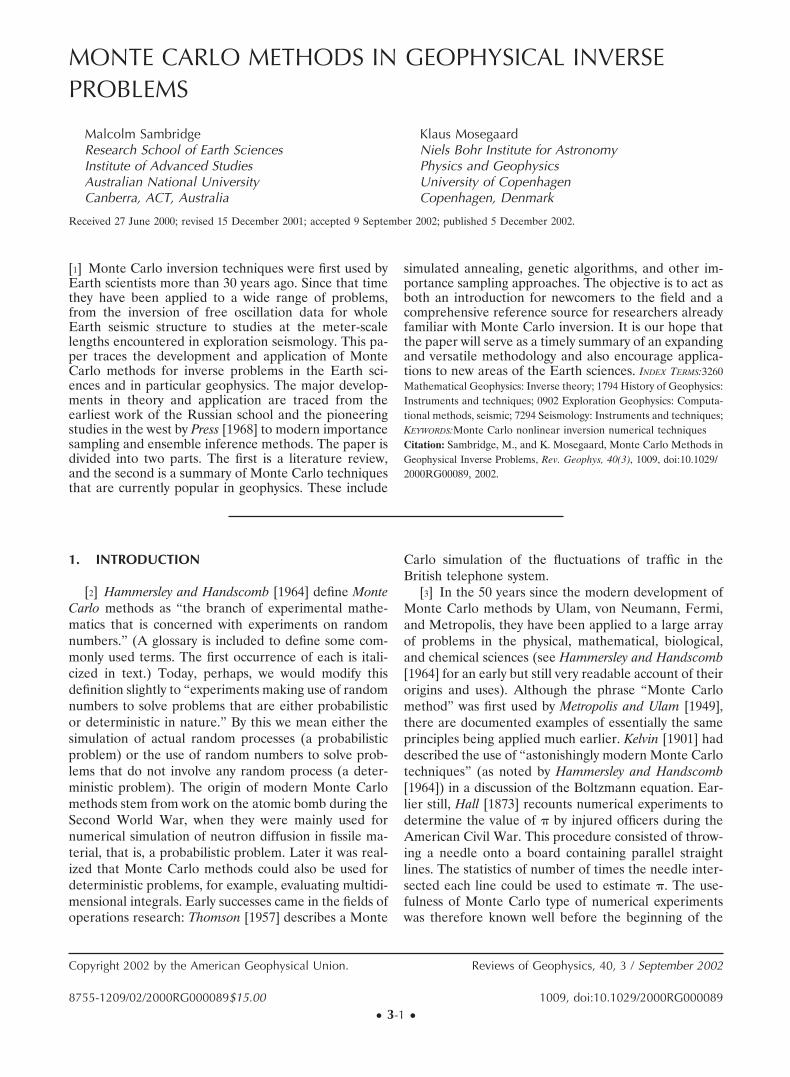
Carlo inversion followed. One problem was that it isnever known whether sufficient number of models hadbeen tested. It was always possible that acceptable mod-els may exist that bear no resemblance to the satisfactorymodels that had been obtained; hence the real Earthmay lay outside of the estimated “nonuniquenessbounds.” An uncomfortable possibility was that the ac-ceptable models might form multiple unconnected “is-lands” in parameter space (see Figure 1). An MCIapproach might miss some of these islands altogether.(In the work of Press [1968], 5 million Earth models weretested, and just 6 were found that passed all data tests.See Figures 2 and 3). In practice, this meant that sets ofupper and lower bounds estimated by MCI could not beliterally interpreted as “hard” bounds on, say, velocity ordensity as a function of depth. For this reason Press[1970b] refers to his estimated envelope of acceptableEarth models as “a guide to hypotheses rather than firmconclusions.”

[10] An approach developed by Anderssen and Senata[1971, 1972] went some way to answering these criti-cisms. They developed a statistical procedure for esti-mating the reliability of a given set of nonuniquenessbounds. Their method was subsequently applied to theinversion of seismic and density profiles by a number ofauthors [Worthington et al., 1972, 1974; Goncz andCleary, 1976].

[11] Another criticism of MCI, argued by Haddon andBullen [1969], was that the successful models generatedwere likely to contain unnecessary complexity (e.g., thetypical small-scale oscillations that had been obtained in

velocity or density depth profiles). This was because thelikelihood of generating a parametrically simple modelwas very small, and hence MCI results were biasedtoward physically unrealistic Earth models. One way thisdifficulty was addressed was by seeking families of “un-complicated” Earth models, with acceptable fit to data.Wiggins [1969] devised a parameterization for 1-D veloc-ity profiles that allowed one to impose velocity, velocitygradient with depth, and velocity curvature bounds si-multaneously. This technique has been used in a numberof areas since [e.g., Cary and Chapman, 1988; Kennett,1998]. Anderssen et al. [1972] extended the earlier workof Anderssen and Senata [1972] to include constraints onthe form of the Earth models generated by MCI. Theynoted that the resulting set of parameter bounds ob-tained by MCI would be affected by the constraintsimposed on the Earth model. For example, if the gradi-ent of a density profile were constrained tightly over a

Figure 1. Contours of a data misfit function, �(m), (shaded)in the parameter space of a nonlinear problem. The twoshaded areas represent the regions of acceptable data fit, whilethe darker elliptical lines are contours of some regularizationfunction, �(m). The diamond represents the model with thebest data fit and is distinct from the triangle, which is thedata-acceptable model with least �. The square is the modelwith minimum �, but it does not satisfy the data.

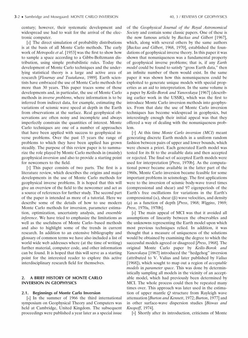
Figure 2. The flow chart of the early Monte Carlo algorithmused by Press [1968]. Note that the 1-D Earth model had tosatisfy data constraints on travel times, eigenfrequencies, andmass and moment of inertia of the Earth before passing intothe output population (see Figure 3). (From Press [1968].)

40, 3 / REVIEWS OF GEOPHYSICS Sambridge and Mosegaard: MONTE CARLO INVERSION ● 3-3

particular depth range, then this would result in rela-tively narrow bounds on the density, giving the falseimpression that the average density over the depth rangewas well determined. Clearly, care had to be used wheninterpreting MCI results obtained under smoothnessconstraints.

2.2. Monte Carlo Techniques Fall Out of Favor[12] During the 1970s, attention moved away from

Monte Carlo inversion and toward linear inverse prob-lems and the use of prior information to resolve non-uniqueness (often referred to as ill posedness in linearproblems) [Wiggins, 1972; Jackson, 1972; 1979]. Linearinversion techniques became popular and were appliedwidely (for a recent summary see Snieder and Trampert[1999]). Uniform Monte Carlo searching of parameterspaces was thought to be too inefficient and too inaccu-rate for problems involving large numbers of unknowns,for example, 50–100. (Note that in the earlier work ofPress [1968] and Wiggins [1969] it was possible to in-crease efficiency, by testing “partial models” againstsubsets of the data, and thereby reject many unaccept-able models early on. Figure 2 shows an outline ofPress’s original MCI algorithm where this is employed.)Nevertheless, uniform random search methods stillfound applications. In addition to the regional andglobal travel time studies, other applications of MCIhave included electromagnetic induction [Anderssen,1970], Rayleigh wave attenuation [Mills and Fitch, 1977;Mills and Hales, 1978], regional magnetotelluric studies[Hermance and Grillot, 1974; Jones and Hutton, 1979],estimation of mantle viscosities [Ricard et al., 1989], andestimation of plate rotation vectors [Jestin et al., 1994].

[13] An attractive feature of discrete linear inversionschemes was that estimates of resolution and model

covariance could be obtained [Franklin, 1970; Jordanand Franklin, 1971; Wiggins, 1972]. In this case, resolu-tion measures the degree by which model parameterscan be independently determined (from each other),while model covariance measures the degree by whicherrors in the data propagate into uncertainty in themodel parameters. Together they allow assessment ofconfidence bounds and trade-offs between parameters,which can be very useful in analyzing inversion results.

[14] A difficulty with linearized estimates of resolu-tion and covariance is that they are based on localderivative approximations, evaluated about the best datafitting model, and as such can become less accurate, asthe data-model relationship becomes more nonlinear.This can often lead to an underestimate of uncertaintyand hence overconfidence in results. Around the sametime as applications of discrete inverse theory werebecoming widespread, it was shown how Monte Carlosampling techniques could also be used to determineresolution estimates but without the need for invokingderivative approximations [Wiggins, 1972; Kennett andNolet, 1978].

[15] The influence of nonlinearity can vary consider-ably between problems. For example, earthquake hypo-center location using travel times of seismic phases isoften described as weakly nonlinear [see Buland, 1976](although examples exist of the failure of linearizationeven in this case [e.g., Billings et al., 1994; Lomax et al.,2000]). In contrast, the estimation of seismic velocitystructure from high-frequency seismic (body) waveforms can be highly nonlinear [see Mellman, 1980; Caryand Chapman, 1988]. In the latter case, subtle changes invelocity structure can significantly influence the detailsof the observed seismograms.

[16] Once nonlinearity is taken into account, it can be

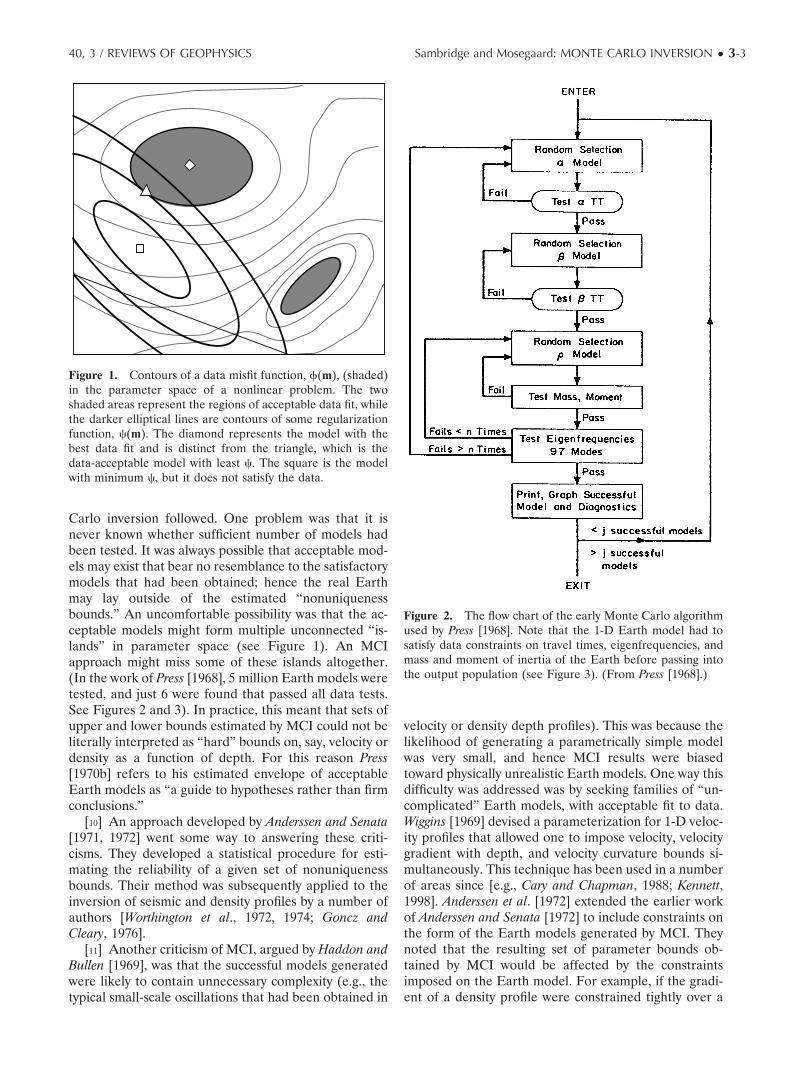
Figure 3. The six seismic and density Earth models that passed all tests shown in Figure 2 from the 5 milliongenerated (from Press [1968]).


useful to view the process of inversion in terms of opti-mization in a high-dimensional parameter space. Usu-ally, some objective function is devised that measures thediscrepancy between observables and theoretical predic-tions from a model. The precise nature of the optimiza-tion problem to be solved can vary considerably. Forexample, one might seek to minimize an objective func-tion based solely on a measure of fit to data [e.g., Caryand Chapman, 1988] or one based on a linear combina-tion of data fit and model regularization (for a discussionsee Menke [1989]). A constrained optimization problemcan be produced with the addition of (explicit) con-straints on the unknowns [e.g., Sabatier, 1977a, 1977b,1977c; Parker, 1994], or the data itself might enter onlyin these constraints, while the objective function repre-sents regularization on the model. (This is often calledextremal inversion; for examples, see Jackson [1976],Parker [1977], Constable et al. [1987] and Parker [1994]).In some cases these formulations are equivalent, and, ingeneral, the most appropriate one will depend on theparticular problem in hand and the questions beingasked of the data.

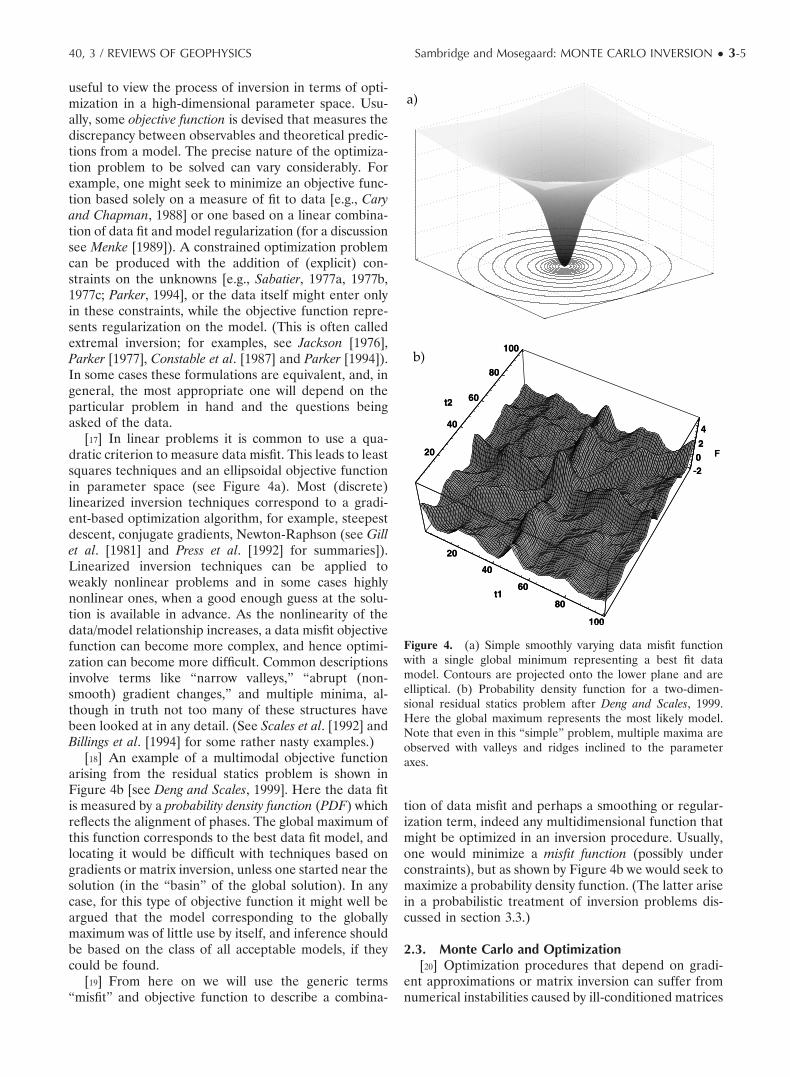
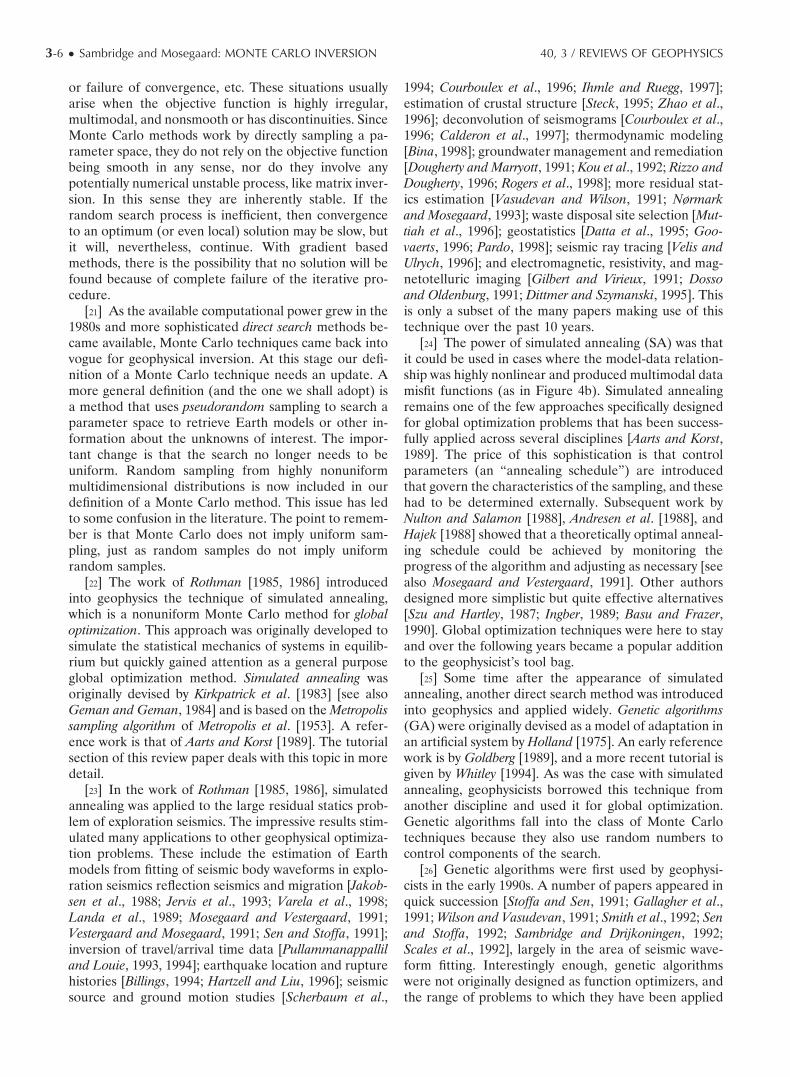
[17] In linear problems it is common to use a qua-dratic criterion to measure data misfit. This leads to leastsquares techniques and an ellipsoidal objective functionin parameter space (see Figure 4a). Most (discrete)linearized inversion techniques correspond to a gradi-ent-based optimization algorithm, for example, steepestdescent, conjugate gradients, Newton-Raphson (see Gillet al. [1981] and Press et al. [1992] for summaries]).Linearized inversion techniques can be applied toweakly nonlinear problems and in some cases highlynonlinear ones, when a good enough guess at the solu-tion is available in advance. As the nonlinearity of thedata/model relationship increases, a data misfit objectivefunction can become more complex, and hence optimi-zation can become more difficult. Common descriptionsinvolve terms like “narrow valleys,” “abrupt (non-smooth) gradient changes,” and multiple minima, al-though in truth not too many of these structures havebeen looked at in any detail. (See Scales et al. [1992] andBillings et al. [1994] for some rather nasty examples.)

[18] An example of a multimodal objective functionarising from the residual statics problem is shown inFigure 4b [see Deng and Scales, 1999]. Here the data fitis measured by a probability density function (PDF) whichreflects the alignment of phases. The global maximum ofthis function corresponds to the best data fit model, andlocating it would be difficult with techniques based ongradients or matrix inversion, unless one started near thesolution (in the “basin” of the global solution). In anycase, for this type of objective function it might well beargued that the model corresponding to the globallymaximum was of little use by itself, and inference shouldbe based on the class of all acceptable models, if theycould be found.

[19] From here on we will use the generic terms“misfit” and objective function to describe a combina-

tion of data misfit and perhaps a smoothing or regular-ization term, indeed any multidimensional function thatmight be optimized in an inversion procedure. Usually,one would minimize a misfit function (possibly underconstraints), but as shown by Figure 4b we would seek tomaximize a probability density function. (The latter arisein a probabilistic treatment of inversion problems dis-cussed in section 3.3.)

2.3. Monte Carlo and Optimization[20] Optimization procedures that depend on gradi-

ent approximations or matrix inversion can suffer fromnumerical instabilities caused by ill-conditioned matrices

Figure 4. (a) Simple smoothly varying data misfit functionwith a single global minimum representing a best fit datamodel. Contours are projected onto the lower plane and areelliptical. (b) Probability density function for a two-dimen-sional residual statics problem after Deng and Scales, 1999.Here the global maximum represents the most likely model.Note that even in this “simple” problem, multiple maxima areobserved with valleys and ridges inclined to the parameteraxes.


or failure of convergence, etc. These situations usuallyarise when the objective function is highly irregular,multimodal, and nonsmooth or has discontinuities. SinceMonte Carlo methods work by directly sampling a pa-rameter space, they do not rely on the objective functionbeing smooth in any sense, nor do they involve anypotentially numerical unstable process, like matrix inver-sion. In this sense they are inherently stable. If therandom search process is inefficient, then convergenceto an optimum (or even local) solution may be slow, butit will, nevertheless, continue. With gradient basedmethods, there is the possibility that no solution will befound because of complete failure of the iterative pro-cedure.

[21] As the available computational power grew in the1980s and more sophisticated direct search methods be-came available, Monte Carlo techniques came back intovogue for geophysical inversion. At this stage our defi-nition of a Monte Carlo technique needs an update. Amore general definition (and the one we shall adopt) isa method that uses pseudorandom sampling to search aparameter space to retrieve Earth models or other in-formation about the unknowns of interest. The impor-tant change is that the search no longer needs to beuniform. Random sampling from highly nonuniformmultidimensional distributions is now included in ourdefinition of a Monte Carlo method. This issue has ledto some confusion in the literature. The point to remem-ber is that Monte Carlo does not imply uniform sam-pling, just as random samples do not imply uniformrandom samples.

[22] The work of Rothman [1985, 1986] introducedinto geophysics the technique of simulated annealing,which is a nonuniform Monte Carlo method for globaloptimization. This approach was originally developed tosimulate the statistical mechanics of systems in equilib-rium but quickly gained attention as a general purposeglobal optimization method. Simulated annealing wasoriginally devised by Kirkpatrick et al. [1983] [see alsoGeman and Geman, 1984] and is based on the Metropolissampling algorithm of Metropolis et al. [1953]. A refer-ence work is that of Aarts and Korst [1989]. The tutorialsection of this review paper deals with this topic in moredetail.

[23] In the work of Rothman [1985, 1986], simulatedannealing was applied to the large residual statics prob-lem of exploration seismics. The impressive results stim-ulated many applications to other geophysical optimiza-tion problems. These include the estimation of Earthmodels from fitting of seismic body waveforms in explo-ration seismics reflection seismics and migration [Jakob-sen et al., 1988; Jervis et al., 1993; Varela et al., 1998;Landa et al., 1989; Mosegaard and Vestergaard, 1991;Vestergaard and Mosegaard, 1991; Sen and Stoffa, 1991];inversion of travel/arrival time data [Pullammanappalliland Louie, 1993, 1994]; earthquake location and rupturehistories [Billings, 1994; Hartzell and Liu, 1996]; seismicsource and ground motion studies [Scherbaum et al.,

1994; Courboulex et al., 1996; Ihmle and Ruegg, 1997];estimation of crustal structure [Steck, 1995; Zhao et al.,1996]; deconvolution of seismograms [Courboulex et al.,1996; Calderon et al., 1997]; thermodynamic modeling[Bina, 1998]; groundwater management and remediation[Dougherty and Marryott, 1991; Kou et al., 1992; Rizzo andDougherty, 1996; Rogers et al., 1998]; more residual stat-ics estimation [Vasudevan and Wilson, 1991; Nørmarkand Mosegaard, 1993]; waste disposal site selection [Mut-tiah et al., 1996]; geostatistics [Datta et al., 1995; Goo-vaerts, 1996; Pardo, 1998]; seismic ray tracing [Velis andUlrych, 1996]; and electromagnetic, resistivity, and mag-netotelluric imaging [Gilbert and Virieux, 1991; Dossoand Oldenburg, 1991; Dittmer and Szymanski, 1995]. Thisis only a subset of the many papers making use of thistechnique over the past 10 years.

[24] The power of simulated annealing (SA) was thatit could be used in cases where the model-data relation-ship was highly nonlinear and produced multimodal datamisfit functions (as in Figure 4b). Simulated annealingremains one of the few approaches specifically designedfor global optimization problems that has been success-fully applied across several disciplines [Aarts and Korst,1989]. The price of this sophistication is that controlparameters (an “annealing schedule”) are introducedthat govern the characteristics of the sampling, and thesehad to be determined externally. Subsequent work byNulton and Salamon [1988], Andresen et al. [1988], andHajek [1988] showed that a theoretically optimal anneal-ing schedule could be achieved by monitoring theprogress of the algorithm and adjusting as necessary [seealso Mosegaard and Vestergaard, 1991]. Other authorsdesigned more simplistic but quite effective alternatives[Szu and Hartley, 1987; Ingber, 1989; Basu and Frazer,1990]. Global optimization techniques were here to stayand over the following years became a popular additionto the geophysicist’s tool bag.

[25] Some time after the appearance of simulatedannealing, another direct search method was introducedinto geophysics and applied widely. Genetic algorithms(GA) were originally devised as a model of adaptation inan artificial system by Holland [1975]. An early referencework is by Goldberg [1989], and a more recent tutorial isgiven by Whitley [1994]. As was the case with simulatedannealing, geophysicists borrowed this technique fromanother discipline and used it for global optimization.Genetic algorithms fall into the class of Monte Carlotechniques because they also use random numbers tocontrol components of the search.

[26] Genetic algorithms were first used by geophysi-cists in the early 1990s. A number of papers appeared inquick succession [Stoffa and Sen, 1991; Gallagher et al.,1991; Wilson and Vasudevan, 1991; Smith et al., 1992; Senand Stoffa, 1992; Sambridge and Drijkoningen, 1992;Scales et al., 1992], largely in the area of seismic wave-form fitting. Interestingly enough, genetic algorithmswere not originally designed as function optimizers, andthe range of problems to which they have been applied


is quite broad. (For reviews, see Davis [1987], Goldberg[1989], and Gallagher and Sambridge [1994].) Neverthe-less, their main role in geophysics (as in many otherdisciplines) has been as a global optimization tool. Likesimulated annealing, the metaphor underlying geneticalgorithms is a natural optimization process, in this casebiological evolution. Many variants of genetic algorithmsexist (even when applied to optimization). Indeed, theyare probably best viewed as a class of methods ratherthan as a well-defined algorithm. As with simulatedannealing, some asymptotic convergence results areknown for particular versions [Davis and Principe, 1991].However, all versions involve control parameters, whichdetermine the characteristics of the direct search pro-cess, and tuning them for each problem can be non-trivial.

[27] Within a few years of their introduction, geneticalgorithms became quite popular within the Earth sci-ences and were applied in a wide range of areas. Someexamples include earthquake hypocenter location [Ken-nett and Sambridge, 1992; Sambridge and Gallagher,1993; Billings et al., 1994; Wan et al., 1997; Muramatsuand Nakanishi, 1997]; estimation of focal mechanismsand seismic source characteristics [Kobayashi and Na-kanishi, 1994; Zhou et al., 1995a; Sileny, 1998; Yu et al.,1998]; mantle viscosity estimation [King, 1995; Cadek etal., 1998; Kido et al., 1998]; groundwater monitoring andmanagement problems [McKinney and Lin, 1994; Ritzelet al., 1994; Cieniawski et al., 1995; Rogers et al., 1995;Tang and Mays, 1998]; meteorite classification [Conwayand Bland, 1998]; seismic anisotropy estimation [Horneand Macbeth, 1994; Levin and Park, 1997]; near-sourceseismic structure [Zhou et al., 1995b]; regional, crustalseismic structure and surface wave studies [Lomax andSnieder, 1994, 1995a, 1995b; Drijkoningen and White,1995; Yamanaka and Ishida, 1996; Neves et al., 1996];design of microseismic networks [Jones et al., 1994];fission track dating [Gallagher, 1995]; seismic profilingand migration [Jervis et al., 1993; Jin and Madariaga,1993; Nolte and Frazer, 1994; Horne and Macbeth, 1994;Boschetti et al., 1996; Docherty et al., 1997]; seismicreceiver functions studies [Shibutani et al., 1996]; prob-lems in geotectonics [Simpson and Priest, 1993]; magne-totelluric inversion [Everett and Schultz, 1993]; inversionof potential fields [Boschetti et al., 1997]; conditioning oflinear systems of equations [Curtis and Snieder, 1997];seismic ray tracing [Sadeghi et al., 1999]; there are manyothers. Some studies have involved devising variants ofthe basic approach and adapting them to the character-istics of individual problems [e.g., Sambridge and Gal-lagher, 1993; Koper et al., 1999].

[28] The question as to whether simulated annealingor genetic algorithms perform better for a particularproblem (i.e., more efficiently, more likely to find ac-ceptable or even optimal models, etc.) has been ad-dressed by a number of authors, both within the Earthsciences and elsewhere [see Scales et al., 1992; Ingber andRosen, 1992; Sen and Stoffa, 1995; Horne and Macbeth,

1998]. Most commonly, these studies compare perfor-mance on particular optimization problems, and fromthese it is difficult to draw general conclusions. Quiteclearly, their relative performance varies between appli-cations and also with the particular versions of eachmethod that are being compared. For a recent, veryreadable, discussion of the types of optimization prob-lem for which they are each suited, see Gershenfeld[1999].

[29] A few other global optimization techniques(again originating in other fields) have made fleetingappearances in the geophysical literature. Two notableexamples are evolutionary programming [Minster et al.,1995] and Tabu (or Taboo) search [Cvijovic and Kli-nowski, 1995; Vinther and Mosegaard, 1996; Zheng andWang, 1996]. The former is related to genetic algorithmsbut was developed quite independently [Fogel, 1962;Fogel et al., 1966]. Again, the primary motivation was notoptimization but the simulation of complex adaptivesystems (see Gell-Mann [1994] for a popular discussion).Tabu search is not strictly speaking a Monte Carlomethod since it does not make use of random numbers,but it is able to climb out of local minima in misfitfunctions [Cvijovic and Klinowski, 1995; Vinther and Mo-segaard, 1996]. Very recently, a new Monte Carlo directsearch technique known as a neighbourhood algorithm(NA) has been proposed, this time developed specifi-cally for sampling in geophysical inverse problems [Sam-bridge, 1999a]. The approach makes use of conceptsfrom the growing field of computational geometry andbares little resemblance to either genetic algorithms orsimulated annealing. It is difficult to say much aboutthese approaches with any confidence as experience withgeophysical problems is still rather limited.

2.4. Ensemble Inference Rather Than Optimization[30] The renewed interest in Monte Carlo techniques

for global optimization and exploration raised a familiarquestion, that is, how to make use of the sampling theyproduced to assess trade-offs, constraints and resolution,in multimodal nonlinear problems. Put another way,how can one use the collection of Earth models gener-ated by a Monte Carlo procedure to do more thanestimate a set of “best fitting” parameters. This was, ineffect, a return to the questions posed by the first usersof Monte Carlo; however, the response adopted by thesecond generation of practitioners was to take a Bayes-ian approach. This statistical treatment of inverse prob-lems became well known to geophysicists through thework of Tarantola and Valette [1982a, 1982b; see alsoTarantola, 1987] and had been applied extensively tolinearized problems. Monte Carlo techniques allowed anextension of the Bayesian philosophy to nonlinear prob-lems.

[31] Bayesian inference is named after Bayes [1763],who presented a method for combining prior informa-tion on a model with the information from new data. Inthis formulation of an inverse problem all information is


represented in probabilistic terms (i.e., degrees of be-lief). Bayesian inference is reasonably general in that itcan be applied to linear or nonlinear problems. (It isdealt with in more detail in the tutorial section of thispaper.) In short, it combines the prior informationknown on the model, with the observed data, and pro-duces the posterior probability density function (PDF) onthe model parameters, which is taken as the “completesolution” to the inverse problem. (Standard referencesare by Box and Tiao [1973], and useful recent books areby Smith [1991] and Gelman et al. [1995]. Summarieswithin a geophysical context are given by Duijndam[1988a, 1988b] and Mosegaard and Tarantola [1995].)The Bayesian approach is not without its criticisms. Forexample, implicit in its formulation is that one mustknow the statistical character of all error, or noise,processes in the problem, which can be very difficult insome cases, especially when the theoretical predictionsfrom a model involve approximations. In addition, it is acontroversial issue as to whether prior information canbe adequately represented probabilistically (see Scalesand Snieder [1997] and Gouveia and Scales [1998] for adiscussion). (Note that probabilistic prior information isoften called “soft” and differs from strict inequalities onthe model parameters, which are referred to as “hard”prior information [see Backus, 1988; Stark, 1992]).

[32] In a Bayesian approach the posterior PDF spansthe entire model space. The case where it is a Gaussiancan be dealt with effectively using linearized inversiontechniques [see Tarantola, 1987; Menke, 1989]. Linear-ized techniques use local curvature information on thePDF about its maximum to estimate resolution andtrade-offs. If the PDF is a Gaussian, then the localcurvature defines the complete structure of the PDF inparameter space. For highly nonlinear problems theposterior PDF can have a complex multimodal shape,arising from the nature of the data fit (likelihood func-tion) or perhaps from the inclusion of complex priorinformation. In this case, global optimization techniquesare needed to identify the maximum of the posteriorprobability density; however, as the complexity of thePDF increases, a single “most probable” model (if oneexists) has little meaning (see Figure 4b). Even if onecould be found, a linearized treatment of resolutionproblem would be of little value (essentially because thelocal information on the PDF’s curvature is not repre-sentative of the PDF as a whole). In these cases, infor-mation on the complete shape of the posterior is neededto produce Bayesian measures of uncertainty and reso-lution. It is here that Monte Carlo methods have majoradvantages over linearized (local) methods, since thesampling they produce can be used to calculate Bayesianintegrals. Within a Bayesian context then, the emphasisis less on optimization and more on sampling the mostprobable regions of parameter space as determined bythe posterior PDF, a process known as importance sam-pling. (Compare this to the early MCI work where theemphasis was on exploring the acceptable regions of

parameter space, as defined by data and prior con-straints.)

[33] Monte Carlo integration of multidimensionalprobability distributions is an active area of research incomputational statistics (for summaries see Flournay andTsutakawa [1989], Smith [1991], Smith and Roberts[1993], and Gelman et al. [1995]). Over the past 10 years,geophysicists have begun to use Markov Chain MonteCarlo (MCMC) methods, which directly simulate theposterior PDF, that is, draw random samples distributedaccording to the posterior PDF, and from these calculateBayesian estimates of constraint and resolution [seeKoren et al., 1991; Mosegaard and Tarantola, 1995; Gal-lagher et al., 1997; Gouveia and Scales, 1998]. It is notsurprising that many of these studies arise in seismologyand in particular the estimation of Earth structure fromhigh-frequency body waveforms, especially in explora-tion studies. This is an area where complex multimodaland multidimensional PDFs can result from the discrep-ancies between observed and predicted seismograms.An example is shown in Figure 4b, which comes from thework of Deng and Scales [1999].

[34] At the end of the 1990s, Monte Carlo integrationand importance sampling have become firmly estab-lished as the technique of choice for Bayesian inversionsin nonlinear problems. Debate continues over whetherthe Bayesian paradigm is appropriate in many cases (seeScales and Snieder [1997] for a discussion). However,Monte Carlo (adaptive or nonuniform) sampling of pa-rameter spaces has also remained popular in studies thatdo not invoke the Bayesian philosophy. (Many of thepapers cited above fall into this category.) In these casesthe issues of mapping out and characterizing the class ofacceptable models remain just as relevant today as whenthe original hedgehog algorithm was proposed morethan 30 years ago [Keilis-Borok and Yanovskaya, 1967;Valius, 1968]. Characterizing the properties of all accept-able models, or an obtained finite ensemble, has been acentral issue for many authors, and a variety of algo-rithms have been proposed (see Constable et al. [1987],Vasco et al. [1993], Lomax and Snieder [1994, 1995b]Douma et al. [1996], and Sambridge [1999b] for exam-ples). This is perhaps the factor that most clearly distin-guishes a study of inverse problems from that of param-eter estimation.

[35] With the growth and spread of high-performancecomputing, Monte Carlo inversion techniques are nolonger restricted to the owners of supercomputers. Astheir use becomes more widespread, we can expect thatdirect sampling of a parameter space will become rou-tine for nonlinear problems, and the need for lineariza-tion will diminish in many cases. (This is arguably al-ready the case for problems with relatively fewunknowns, e.g., earthquake hypocenter location.) Also,one might expect that larger scale problems (i.e., involv-ing many more unknowns) will increasingly be tackledusing Monte Carlo techniques, within either a Bayesianor non-Bayesian framework. For the foreseeable future


very large scale nonlinear problems, like 3-D mantleseismic tomography, are likely to remain beyond therange of Monte Carlo techniques; however, it is worthnoting that a Monte Carlo technique has already beenapplied to a 2-D borehole tomography problem (involv-ing fewer unknowns than mantle tomography, but oftenmore nonlinear) [Vasco et al., 1993]. As Monte Carlosampling is better understood and becomes more acces-sible, it seems likely that it will become an increasinglyuseful tool for nonlinear inversion. It is hoped that thispaper, and in particular the following tutorial section,will add to that awareness and encourage students andresearchers to think about it themselves.

3. MONTE CARLO METHODS: THE TECHNOLOGYOF INFORMATION

[36] In the next section we outline some of the mainMonte Carlo approaches that have been used to tacklegeophysical inverse problems. We describe some of thebasic concepts and provide a source of references forfurther reading. Some open questions are also high-lighted. At all times we assume that we have somecriterion, �, which measures the discrepancy betweenobservations and predictions and perhaps includes someother information. Its evaluation for any given model, x,constitutes a solution to the forward problem. In somecases we may be interested in optimizing this objectivefunction; in others we may be more interested in sam-pling it adequately enough to either evaluate Bayesianinformation measures (as discussed in section 3.3), orestimate properties of the data acceptable models thatfit within our chosen (usually finite dimensional) param-eter space.

[37] Several of the approaches discussed here arecommonly associated with a Bayesian approach to inver-sion. However, it is worth noting that they can also beemployed independently of a Bayesian inversion, that is,simply to perform a direct search of a parameter space.

3.1. Preliminaries

3.1.1. Linearization or Monte Carlo?[38] The first question one needs to address is

whether a Monte Carlo technique (like SA, GA, NA,etc.) or a linearized approach (based on matrix inver-sion) would be most appropriate for a particular prob-lem. The answer depends on the nature of the data-model relationship, the number of unknowns, and, to alesser extent, the computational resources available.

[39] As the data-model relationship becomes morecomplex, the misfit function (or PDF) will also increasein complexity (e.g., multimodal, etc.), and Monte Carlotechniques will be favored over linearized techniques fortwo reasons. The first is that they are more numericallystable in the optimization/parameter search stage. Thisis because they do not rely on the convergence of se-

quence of model perturbations (like a linearized ap-proach) and at the same time avoid the need for matrixinversion.

[40] The second reason for favoring Monte Carlotechniques is that they are usually more reliable inappraising the solution, that is, estimating uncertainty bymeans of model covariance and resolution matrices (seesection 3.3). This is (again) because they avoid deriva-tives and hence the numerical approximations on whichlinearized estimates of model covariance and resolutionare based [see Menke, 1989]. Linearized techniques areprone to underestimate uncertainty when nonlinearity issevere. Also, a direct search of the parameter space mayindicate significant trade-offs and even multiple classesof solution, which would not be found using lineariza-tion.

[41] Unfortunately, it is not possible to know whetherlinearized estimates of model covariance and resolutionare accurate until a fully nonlinear calculation has beenperformed. The same is true for the optimization pro-cess itself, that is, whether linearized techniques arelikely to be unstable or require heavy damping to con-verge, problems that could well be alleviated using adirect search technique.

[42] In some cases, for example, in many waveforminversion studies encountered in seismic exploration, thedata-model relationship can become so complex thatfully nonlinear direct search techniques are the onlyviable approach. At the opposite end of the scale, withdiscrete linear, or linearized, problems with relativelyfew unknowns (e.g., 10–50), it is often overlooked thatMonte Carlo techniques can be both very convenientand efficient.

[43] It is also worth pointing out that linearization isnot always possible or practical in some cases. This is thecase when the observables are not differentiable func-tions of the unknowns. An example is when the forwardproblem involves a complex calculation such as the nu-merical modeling of landscape evolution in response totectonic and erosional processes [van der Beek andBraun, 1999; Braun, 2002]. In this case the unknowns arethe rate of tectonic uplift and parameters that relate rateof surface processes to geometrical features like drain-age area and surface slope, while the observables aregeochronological constraints on exhumation rate andmorphological properties of the landscape. In theseproblems, there is no analytical relationship betweenunknowns and observables, and hence linearized tech-niques are not appropriate. However, direct search tech-niques can still be applied because they only require theability to solve the forward problem. Furthermore, all ofthe direct search algorithms presented in section 3.2 cantake advantage of parallel computation because eachforward solution can be performed independently. Itseems likely that this is an area where Monte Carlotechniques will find more applications in the future.

[44] It is important to stress that Monte Carlo tech-niques are not a panacea for geophysical inversion. They


are only applicable to discretized problems, that is, oneswhere a finite parameterization has been chosen, and aswith all discrete inversion approaches, the results willinevitably be dependent on the suitability of that choice.Also, it is clear that as the number of unknowns becomelarge (say, greater than a few hundred) then directsearch techniques become impractical because of thecomputation involved. The actual limiting dimensionwill vary considerably between applications because itdepends on the computational cost of solving the for-ward problem. However, it is also clear that as comput-ing power continues to grow, so will the range of prob-lems that can be addressed with Monte Carlotechniques.

3.1.2. Which Monte Carlo Technique?[45] The choice between the competing flavors of

Monte Carlo technique is much less clear than whetherone should be used in the first place. In general, thereappears to be no preferred method of choice in allcircumstances. In the next few sections we discuss thebasic mechanics of different classes of Monte Carloapproach and make some comparisons. Here we make afew general observations which may help in deciding onwhich Monte Carlo technique to choose.

[46] In cases where the cost of the forward modelingis not excessive and the number of unknowns is small(say �10), a simple deterministic grid search [e.g., Sam-bridge and Kennett, 1986] may be practical (see section3.2.2). This would have the attraction of being bothreliable (guaranteeing a global minimum on the chosengrid) and useful for uncertainty analysis because thesamples are uniformly distributed and hence produce anunbiased sample of the parameter space. With moderncomputing power this most simplistic of techniques canbecome surprisingly efficient for some problems. Ofcourse, grid search techniques become impractical wheneither the number of unknowns or the computationalcost of the forward problem is high, and one must turnto the more sophisticated irregular parameter spacesampling methods.

[47] It is beyond the scope of this paper to enter the(perhaps never-ending) argument between Bayesian andnon-Bayesian approaches to inversion [Scales andSnieder, 1997]. However, it should be noted that a Bayes-ian inversion is often implemented with a Markov chainMonte Carlo (MCMC) approach (section 3.2.3.1), forexample, using the Metropolis algorithm. This, in turn, isclosely related to the optimization technique simulatedannealing (section 3.2.3), and so, in general, if a Bayes-ian approach were preferred, then these would be thenatural algorithms of choice for both optimization anduncertainty estimation (see section 3.2.3.1 for a discus-sion).

[48] Several authors have argued for genetic algo-rithms (section 3.2.4) as a powerful parameter spacesearch technique (see above), although the ensemble ofparameter space samples produced by a genetic algo-

rithm does not (in general) follow any prescribed prob-ability distribution and so cannot be used directly for aquantitative uncertainty analysis (within a Bayesianframework) (see section 3.4). The neighbourhood algo-rithm (section 3.2.5), which is both a search and ap-praisal technique, offers a potential solution to thisproblem. Ultimately, the choice between Monte Carlodirect search techniques will often depend as much onissues of practical convenience, like the availability ofsuitable computer software, as the precise details of thealgorithms.

3.1.3. Generating Random Samples

3.1.3.1. Pseudorandom Deviates[49] All Monte Carlo techniques make use of random

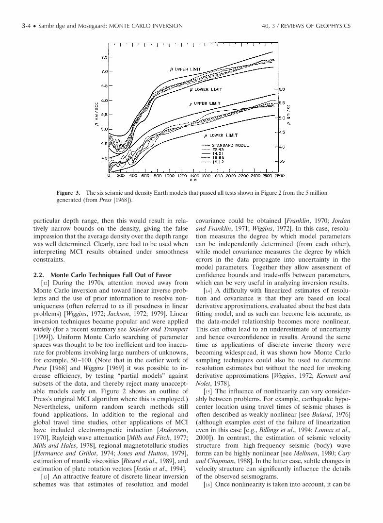
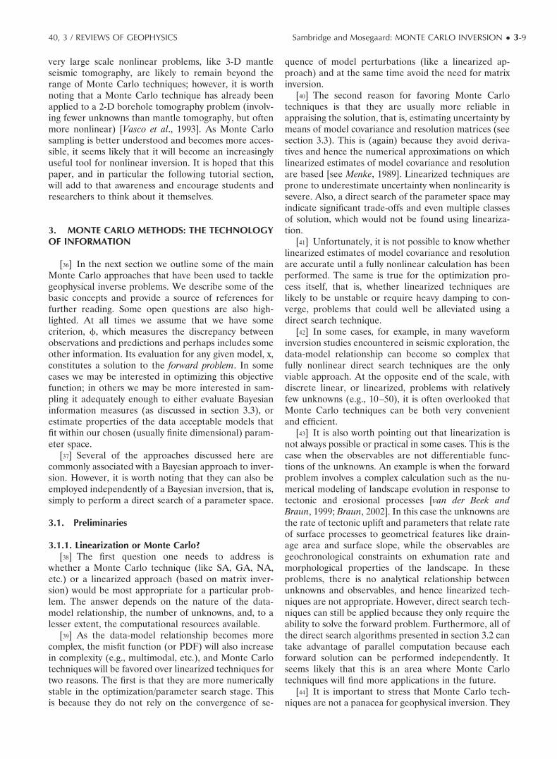
number generators of some kind. This is the case evenwhen the ultimate task is to generate multidimensionalrandom deviates distributed according to complicatedPDFs, for example, with the Metropolis-Hastings algo-rithm (see section 3.2.3.1). The common approach is togenerate pseudorandom numbers using a linear or mul-tiplicative congruent method. For a survey of theory andmethods, see Park and Miller [1988], and for descriptionsof “workhorse” techniques, see Press et al. [1992]. Figure5a shows 1000 pairs of pseudorandom numbers plottedas points in the plane.

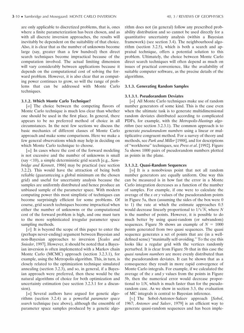
3.1.3.2. Quasi-Random Sequences[50] It is a nonobvious point that not all random

number generators are equally uniform. One way thiscan be measured is in how fast the error in a MonteCarlo integration decreases as a function of the numberof samples. For example, if one were to calculate theaverage of the x or y values of the pseudorandom pointsin Figure 5a, then (assuming the sides of the box were 0to 1) the rate at which the estimate approaches 0.5would decrease linearly proportional to 1/�N, where Nis the number of points. However, it is possible to domuch better by using quasi-random (or subrandom)sequences. Figure 5b shows an example of N 1000points generated from two quasi sequences. The quasisequence generates a set of points that are (in a well-defined sense) “maximally self-avoiding.” To the eye thislooks like a regular grid with the vertices randomlyperturbed. It is clear from Figure 5b that in this case thequasi random numbers are more evenly distributed thanthe pseudorandom deviates. It can be shown that as aconsequence they result in more rapid convergence ofMonte Carlo integrals. For example, if we calculated theaverage of the x and y values from the points in Figure5b, then the numerical error would decrease propor-tional to 1/N, which is much faster than for the pseudo-random case. As we show in section 3.3, the evaluationof MC integrals is central to Bayesian inference.

[51] The Sobol-Antonov-Saleev approach [Sobol,1967; Antonov and Saleev, 1979] is an efficient way togenerate quasi-random sequences and has been imple-


mented in a convenient form by Press et al. [1992].However, care must be taken in using quasi-randomnumbers, especially when they form the components of avector (i.e., Earth model) in a multidimensional space.In this case each component in the (quasi-random) vec-tor must be generated from an independent quasi se-quence. The main problem is that some components ofmultidimensional quasi-random vectors can have a highdegree of correlation. It is only when sufficiently manyquasi vectors are generated that the correlation disap-pears. In dimensions as low as 10, it may require manythousands of samples before the overall correlation be-

tween all components is negligible, and hence the sam-ples are usable. Morokoff and Caflisch [1994] describethese issues in detail. Quasi-random sequences are usedin the neighbourhood algorithm of Sambridge [1999a](see also section 3.2.5) and are finding increasing num-bers of applications in multidimensional numerical inte-gration [Morokoff and Caflisch, 1994].

3.2. Searching a Parameter Space With Monte CarloMethods

3.2.1. Exploration Versus Exploitation[52] A useful framework for comparing different

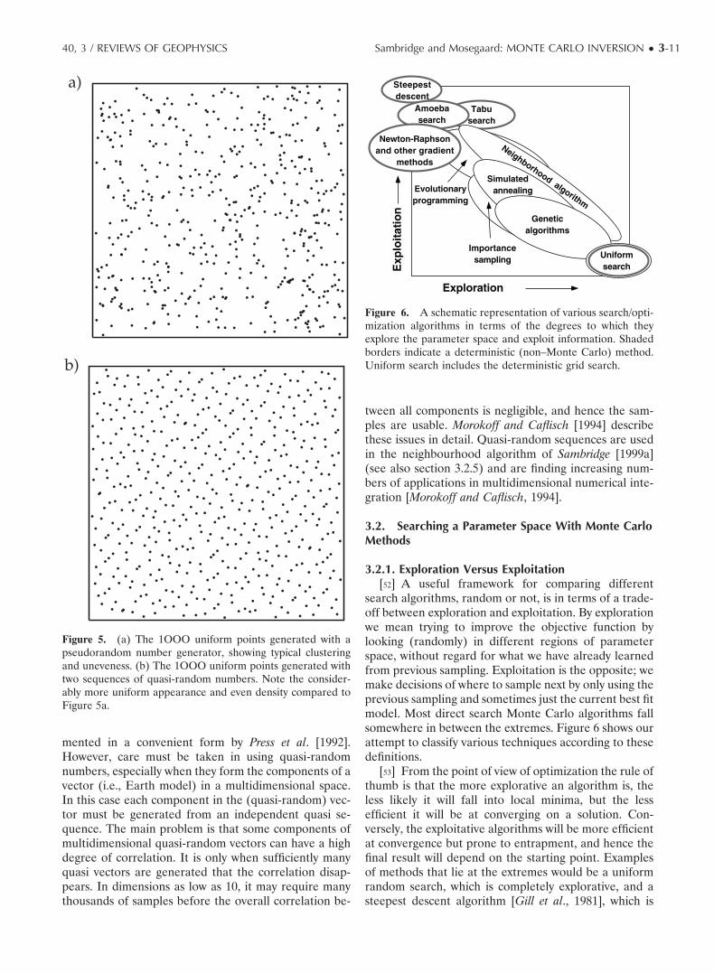
search algorithms, random or not, is in terms of a trade-off between exploration and exploitation. By explorationwe mean trying to improve the objective function bylooking (randomly) in different regions of parameterspace, without regard for what we have already learnedfrom previous sampling. Exploitation is the opposite; wemake decisions of where to sample next by only using theprevious sampling and sometimes just the current best fitmodel. Most direct search Monte Carlo algorithms fallsomewhere in between the extremes. Figure 6 shows ourattempt to classify various techniques according to thesedefinitions.

[53] From the point of view of optimization the rule ofthumb is that the more explorative an algorithm is, theless likely it will fall into local minima, but the lessefficient it will be at converging on a solution. Con-versely, the exploitative algorithms will be more efficientat convergence but prone to entrapment, and hence thefinal result will depend on the starting point. Examplesof methods that lie at the extremes would be a uniformrandom search, which is completely explorative, and asteepest descent algorithm [Gill et al., 1981], which is

a)

b)

Figure 5. (a) The 1OOO uniform points generated with apseudorandom number generator, showing typical clusteringand uneveness. (b) The 1OOO uniform points generated withtwo sequences of quasi-random numbers. Note the consider-ably more uniform appearance and even density compared toFigure 5a.

Figure 6. A schematic representation of various search/opti-mization algorithms in terms of the degrees to which theyexplore the parameter space and exploit information. Shadedborders indicate a deterministic (non–Monte Carlo) method.Uniform search includes the deterministic grid search.


purely exploitative. Clearly, the most appropriate tech-nique will depend on the nature of the problem. Forsmoothly varying near quadratic objective functions wewould prefer an exploitative approach, which allowsrapid converge, for example, a Newton-type descentmethod. For highly nonlinear problems with multipleminima/maxima in the objective function a combinationof exploration and exploitation would probably suit best.However, controlling the trade-off between the twoproperties is often quite difficult, as is deciding in ad-vance which approach is best suited to a particularproblem.

3.2.2. Uniform Sampling[54] The simplest form of randomized sampling of a

parameter space is uniform sampling. For a problemwith d distinct unknowns the ith random sample is thevector xi,

x i � �i1

d

riei , (1)

where ri is a (0,1) uniform random deviate and ei is theunit vector along the ith axis in parameter space. Foreach new sample some data fit, or other objective func-tion, �, must be evaluated, and hence forward modelingperformed. As discussed above, this was the first fullynonlinear approach used by geophysicists more than 30years ago. Note that, by definition, uniform sampling isnot biased toward any particular region of parameterspace, and there is hence no possibility of entrapment inlocal minima of �. Equally, however, it does not concen-trate sampling, and, even with modern supercomputers,it is usually inefficient once the number of unknownsbecomes greater than 10. This is the so-called “curse ofdimensionality.” For example, if we imagine the param-eter space filled by a regular multidimensional Cartesiangrid with (nk � 1) intervals per axis, then the number ofdistinct nodes (and hence models) in this grid is nk

d,which can become enormous, even in relatively smalldimensions.

[55] In practice, one always undersamples a parame-ter space. In many Monte Carlo studies the total numberof samples generated is much smaller than the numberof vertices of a single “unit cube” in a Cartesian grid,that is, 2d, and in this sense one always tends to under-sample parameter spaces in practice. For most problemsthe only viable approach is for the MC search algorithmto concentrate sampling in particular “promising” re-gions of parameter space, that is, adapt itself to theobjective function �. One area where uniform MCsearch has continued to be useful is in sampling underhard prior constraints on the unknowns. An exampleappears in the work of Wiggins [1972] [see also Cary andChapman, 1998; Kennett, 1988].

3.2.3. Simulated Annealing[56] The simulated annealing method exploits a sta-

tistical mechanical analogy to search for the global min-imum of an objective function � possessing a largenumber of secondary minima. The algorithm simulatesthe process of chemical annealing in which a meltedcrystalline material is cooled slowly through its freezingpoint, thereby approximately settling into its energyground state. By identifying the objective function withthe energy of the crystalline material and by appropriatedefinition of a temperature parameter for the simula-tions, it is possible to simulate a “cooling” of the systemto be optimized. A sufficiently slow cooling of this sys-tem will, by analogy to the chemical annealing, result inconvergence to a near-optimal configuration, character-ized by a near-minimal value of the objective function.

[57] Simulated annealing is based on the Metropolis-Hastings algorithm or the Gibbs Sampler, and we shalltherefore take a closer look at these algorithms here.Later, we shall also see why these algorithms are theworkhorses in Bayesian Monte Carlo calculations.

3.2.3.1. Markov Chain Monte Carlo:Metropolis, Hastings, and Gibbs

[58] The idea behind the Metropolis-Hastings algo-rithm and the Gibbs Sampler is the same. They are bothso-called Markov Chain Monte Carlo algorithms de-signed to generate samples of a probability distribution pover a high-dimensional space � under the special dif-ficulty that no explicit mathematical expression exists forp. Only an algorithm that allows us to calculate thevalues of p at a given point in the space is available. Thisis a typical situation in geophysics where p is a probabil-ity density derived from a misfit function � through, forexample,

p�mk � A � exp (�B��mk ) , (2)

where mk is a model and A and B are constants. Veryoften p (mk) can only be evaluated for a particular Earthmodel through a very computer-intensive calculation.

[59] Let us consider the mechanics of the Metropolis-Hastings algorithm, for simplicity, we consider a situa-tion where we wish to sample a probability distribution pin a discretized model space �. Sampling from thedistribution p means that the probability of visitingmodel m is proportional to p(m). To generate a simplealgorithm that samples p, we can make the followingassumptions:

1. The probability of visiting a point mi in modelspace, given that the algorithm currently is at point mj,depends only on mj and not on previously visited points.This is the so-called Markov property. This propertymeans the algorithm is completely described by a tran-sition probability matrix Pij whose ijth component is theconditional probability of going to point mi, given thealgorithm currently visits mj.

2. For all points mj in �, there are exactly N points mi,


including mj itself, for which Pij is nonzero. If this prop-erty holds, we say that the algorithm is regular, and theset of N accessible points constitutes what we call theneighborhood �j of mj.

3. It is possible for the algorithm to go from any pointmj to any other point mi, given enough steps. An algo-rithm satisfying this property is called irreducible.

[60] The question now is, which transition probabilitymatrix Pij leads to an algorithm that samples the targetdistribution p? The answer is that there exists infinitelymany such transition probability matrices. We willchoose one that is simple, namely, one that satisfiesmicroscopic reversibility:

Pij p�m j � Pji p�m i . (3)

It is easy to see that any choice of Pij satisfying micro-scopic reversibility will continue to sample p once it hasalready started doing so. This is a simple consequence ofthe fact that if the algorithm has probability p(mj) ofvisiting mj, then the probability that a transition from mj

to mi takes place in a given iteration is Pijp(mj). Simi-larly, the probability that a transition from mi to mj takesplace in a given iteration is Pjip(mi). Microscopic revers-ibility means that the probability of these two transitionsis the same at all times, and the fact that each pair ofpoints in � maintains mutual equilibrium in this waymeans that there is overall equilibrium sampling at thetarget distribution p. For more details see, for example,Mosegaard and Tarantola [1995] or Mosegaard and Sam-bridge [2002].

[61] In the Metropolis-Hastings algorithm the transi-tion probabilities Pij are given by

Pij �1N min �1,

p�m i

p�m j � , (4)

and hence satisfy equation (3). This is, in practice, real-ized in the following way.

[62] Assume that the current point visited by the al-gorithm is mj. We now choose (or, rather, propose) oneof its N neighbors mi with probability

Pproposal � 1/N . (5)

Finally, we accept mi only with probability

Paccept � min �1,p�m i

p�m j � . (6)

If mi is accepted, the algorithm goes to mi in this itera-tion, but if mi is rejected, the algorithm stays in mj (mj isvisited once again). It is clear that the above algorithmhas transition probabilities given by equation (4).

[63] The remaining question of how to make the al-gorithm sample p in the first place is more complicated,but fortunately it can be shown [see, e.g., Tierney 1994]that the distribution of samples produced by any algo-rithm satisfying our requirements will indeed convergetoward p when the number of iterations goes to infinity.

The problem of estimating the speed of convergence ispresently unresolved, but some practical advice on howto run this type of algorithm was found by Hastings[1970] and Mosegaard [1998].

[64] According to the mechanics of the Gibbs Samplerin a typical implementation, operating in a K-dimen-sional model space, each iteration consists of K substeps,one for each parameter. The kth substep perturbs onlythe kth parameter, and it has its own transition proba-bility matrix Pij

k . The neighborhood �jk of a point mj

consists of all points mi that differ from mj in only the kthparameter. This means, in particular, that the neighbor-hoods of two points are either identical or disjoint.

[65] Assume again that the current point visited by thealgorithm is mj. We now run K steps, and in each step,instead of proposing one of its N neighbors uniformly atrandom, we choose mi from the neighborhood �j

k ac-cording to the conditional probability distribution

p�m i�� jk �

p�m i

�mk��j

k p�mk , (7)

without any accept/reject probability (i.e., the chosen mi

is always accepted). In each step, only one parameter isperturbed (or is possibly left unchanged), so after com-pletion of one iteration (consisting of all K steps), allparameters have been perturbed.

[66] That this algorithm samples p is easy to see. Thetransition probability matrix for each step is given by

Pijk � p�m i�� j

k , (8)

which clearly satisfies microscopic reversibility, equation(3), so if mi � �j

k, then

Pijk p�m j � p(m i�� j

k p�m j

�p�m i �

mk � �jk

p�mk p�mj

p(mj)�

mk � �ik

p�mk p�mi

p�mj��ik p�mi

Pjik p�mi ,

where we have used that the neighborhoods �jk and �i

k

are identical. Since each step of an iteration satisfiesmicroscopic reversibility, so does the entire iteration,and the algorithm samples the target distribution p as-ymptotically.

[67] Whether the Metropolis-Hastings algorithm orthe Gibbs Sampler is the most efficient depends on theproblem at hand. The Gibbs Sampler takes much feweriterations before it samples p correctly, but the many


steps needed to perform an iteration may render itinefficient for problems where evaluation of p is com-puter-intensive. Rothman [1986] gives an example of theuse of a Gibbs Sampler in a case where p can beefficiently evaluated for all perturbations of a singlemodel parameter.

3.2.3.2. Simulated Annealing Algorithm[68] It is an empirical fact that the process of chemical

annealing, where a crystalline material is slowly cooledthrough its melting point, results in formation of highlyordered, low-energy crystals. The slower the cooling, themore perfect is the crystal growth, and the lower is thelattice energy. This process can be viewed as a “physicaloptimization method” in which the objective function isthe lattice energy E. The process can be simulated inlarge numerical systems by identifying the model param-eters of the system with state space variables and theobjective function of the optimization problem with theenergy E. In each step of the algorithm, thermal fluctu-ations in the system are simulated by randomly perturb-ing model parameters, and the fluctuations are con-trolled by a temperature parameter T. The simulatedannealing algorithm [Kirkpatrick et al., 1983] runs asfollows: In each step a random perturbation of themodel parameters mj of the numerical system is at-tempted. The new set of model parameters mi are ac-cepted if the value of the objective function E decreases.However, if E increases, the new parameters may beaccepted with probability

Paccept � exp ��ET � , (9)

where �E is the change in the objective function and Tis the temperature parameter. If the new model is re-jected, a new perturbation is attempted in the next move,and the above process of decision is repeated.

[69] A close inspection of the above algorithm revealsthat for constant temperature parameter T it is actuallya Metropolis-Hastings algorithm designed to sample theprobability distribution [Metropolis et al., 1953],

PB(m)

exp ��E�m

T �Z�T

, (10)

which is known in statistical physics as the Gibbs-Boltz-mann distribution. Here 1/Z(T) is a normalization con-stant. In simulated annealing, however, the temperatureparameter is gradually decreased from a high value,allowing large “thermal” fluctuations, down to zero,where only decreasing values of the objective functionare allowed. For decreasing temperature T the Gibbs-Boltzmann distribution converges toward a distributionhaving all its probability mass in the global minimum forE. In other words, as the temperature gradually ap-proaches zero, the probability that our system is close to

the global minimum for its objective function ap-proaches 1.

[70] In simulated annealing the Gibbs-Boltzmann dis-tribution can also be sampled by means of a Gibbssampler. Rothman [1986] gives an example where theresidual statics problem of reflection seismology issolved in this way.

3.2.3.3. Nulton-Salamon Annealing Schedule[71] In practice, one has to face the fact that the above

theory is only true for an infinitely slow “cooling.” Theproblem is therefore to find a way to decrease thetemperature in a finite number of steps, such that theprobability that the system is close to the global mini-mum for E after the annealing simulation is maximum.

[72] Nulton and Salamon [1988] devised a near-opti-mal annealing method that keeps the numerical systemclose to “thermal equilibrium” at all times. The actualmean value �E� of the objective function is kept at aconstant distance

v ��E� � �E�eq

�E�T (11)

from the never realized equilibrium mean value �E�eq.Here �E(T) is the standard deviation of the fluctuatingobjective function, and the distance v is known as the“thermodynamic speed.” The authors arrive at the fol-lowing differential equation for the annealing tempera-ture schedule T(t):

dTdt � �

vT

��T �C �T , (12)

where C(T) and �(T) are the heat capacity and therelaxation time of the system, respectively. Estimation ofC(T) and �(T) from statistical information about thesystem, collected during the annealing process, is de-scribed by Andresen et al. [1988]. An approximate, tem-perature-dependent transition probability matrix PE (T)for transitions between “energy levels” is formed duringthe annealing process. For each temperature the heatcapacity can be evaluated from the eigenvector of PE

(T 3 �) with eigenvalue 1, and the relaxation time canbe calculated from the second largest eigenvalue ofPE(T).

[73] In practice, the thermodynamic speed v in equa-tion (12) is adjusted such that the annealing temperatureis close to zero after a predetermined number of itera-tions, given by the computer resources available to theoptimization.

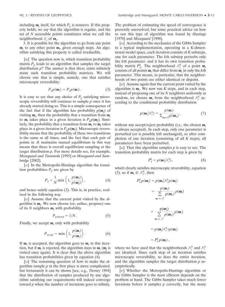
[74] Figure 7 shows an example where a reflectionseismic data set was inverted through simulated anneal-ing optimization. A common-depth-point gather fromthe data set was transformed into the � � p domain(essentially a plane-wave decomposition), and twotraces, representing ray parameters p 0.000025 s/mand p 0.000185 s/m, respectively, were inverted toobtain a horizontally stratified nine-layer model. Each


layer was characterized by a P velocity, a density, and anattenuation. Figure 7 shows the two traces, each re-peated 5 times, and the wavelet. Misfit (“energy” insimulated annealing terminology) was calculated by gen-erating full waveform acoustic � � p seismograms fromthe subsurface model and computing the L2-norm of thedifference between computed and observed (� � p trans-formed) data.

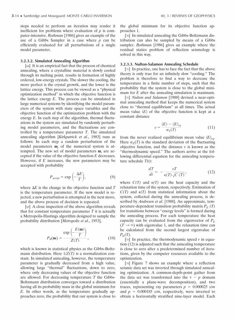
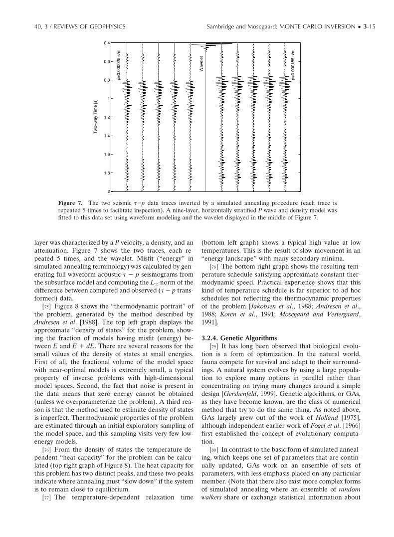
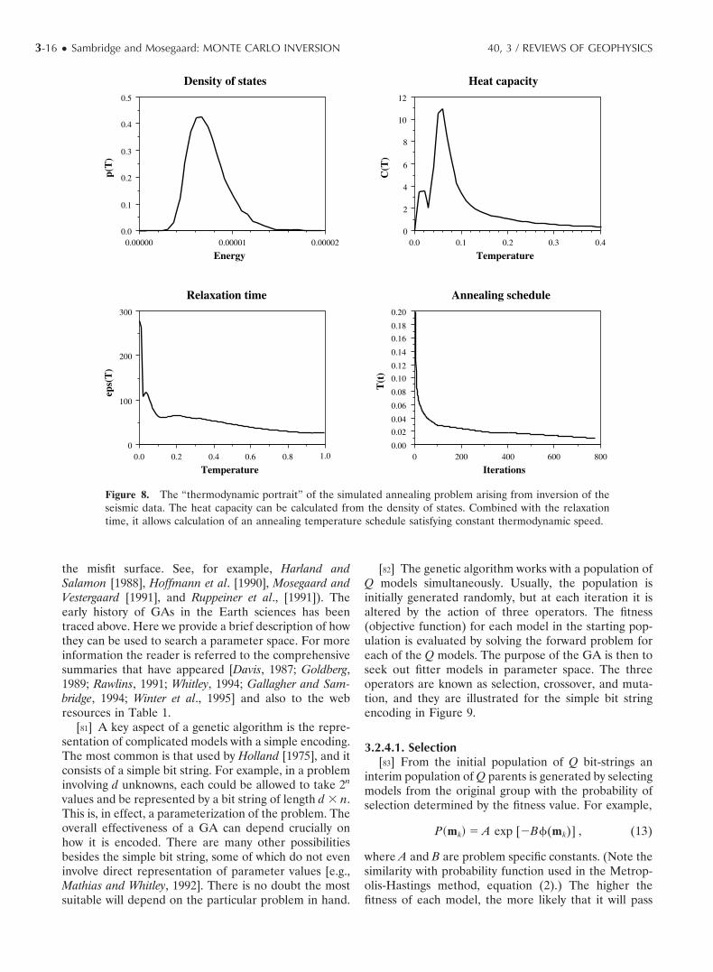
[75] Figure 8 shows the “thermodynamic portrait” ofthe problem, generated by the method described byAndresen et al. [1988]. The top left graph displays theapproximate “density of states” for the problem, show-ing the fraction of models having misfit (energy) be-tween E and E � dE. There are several reasons for thesmall values of the density of states at small energies.First of all, the fractional volume of the model spacewith near-optimal models is extremely small, a typicalproperty of inverse problems with high-dimensionalmodel spaces. Second, the fact that noise is present inthe data means that zero energy cannot be obtained(unless we overparameterize the problem). A third rea-son is that the method used to estimate density of statesis imperfect. Thermodynamic properties of the problemare estimated through an initial exploratory sampling ofthe model space, and this sampling visits very few low-energy models.

[76] From the density of states the temperature-de-pendent “heat capacity” for the problem can be calcu-lated (top right graph of Figure 8). The heat capacity forthis problem has two distinct peaks, and these two peaksindicate where annealing must “slow down” if the systemis to remain close to equilibrium.

[77] The temperature-dependent relaxation time

(bottom left graph) shows a typical high value at lowtemperatures. This is the result of slow movement in an“energy landscape” with many secondary minima.

[78] The bottom right graph shows the resulting tem-perature schedule satisfying approximate constant ther-modynamic speed. Practical experience shows that thiskind of temperature schedule is far superior to ad hocschedules not reflecting the thermodynamic propertiesof the problem [Jakobsen et al., 1988; Andresen et al.,1988; Koren et al., 1991; Mosegaard and Vestergaard,1991].

3.2.4. Genetic Algorithms[79] It has long been observed that biological evolu-

tion is a form of optimization. In the natural world,fauna compete for survival and adapt to their surround-ings. A natural system evolves by using a large popula-tion to explore many options in parallel rather thanconcentrating on trying many changes around a simpledesign [Gershenfeld, 1999]. Genetic algorithms, or GAs,as they have become known, are the class of numericalmethod that try to do the same thing. As noted above,GAs largely grew out of the work of Holland [1975],although independent earlier work of Fogel et al. [1966]first established the concept of evolutionary computa-tion.

[80] In contrast to the basic form of simulated anneal-ing, which keeps one set of parameters that are contin-ually updated, GAs work on an ensemble of sets ofparameters, with less emphasis placed on any particularmember. (Note that there also exist more complex formsof simulated annealing where an ensemble of randomwalkers share or exchange statistical information about

Figure 7. The two seismic ��p data traces inverted by a simulated annealing procedure (each trace isrepeated 5 times to facilitate inspection). A nine-layer, horizontally stratified P wave and density model wasfitted to this data set using waveform modeling and the wavelet displayed in the middle of Figure 7.


the misfit surface. See, for example, Harland andSalamon [1988], Hoffmann et al. [1990], Mosegaard andVestergaard [1991], and Ruppeiner et al., [1991]). Theearly history of GAs in the Earth sciences has beentraced above. Here we provide a brief description of howthey can be used to search a parameter space. For moreinformation the reader is referred to the comprehensivesummaries that have appeared [Davis, 1987; Goldberg,1989; Rawlins, 1991; Whitley, 1994; Gallagher and Sam-bridge, 1994; Winter et al., 1995] and also to the webresources in Table 1.

[81] A key aspect of a genetic algorithm is the repre-sentation of complicated models with a simple encoding.The most common is that used by Holland [1975], and itconsists of a simple bit string. For example, in a probleminvolving d unknowns, each could be allowed to take 2n

values and be represented by a bit string of length d � n.This is, in effect, a parameterization of the problem. Theoverall effectiveness of a GA can depend crucially onhow it is encoded. There are many other possibilitiesbesides the simple bit string, some of which do not eveninvolve direct representation of parameter values [e.g.,Mathias and Whitley, 1992]. There is no doubt the mostsuitable will depend on the particular problem in hand.

[82] The genetic algorithm works with a population ofQ models simultaneously. Usually, the population isinitially generated randomly, but at each iteration it isaltered by the action of three operators. The fitness(objective function) for each model in the starting pop-ulation is evaluated by solving the forward problem foreach of the Q models. The purpose of the GA is then toseek out fitter models in parameter space. The threeoperators are known as selection, crossover, and muta-tion, and they are illustrated for the simple bit stringencoding in Figure 9.

3.2.4.1. Selection[83] From the initial population of Q bit-strings an

interim population of Q parents is generated by selectingmodels from the original group with the probability ofselection determined by the fitness value. For example,

P�mk � A exp [�B�(mk)] , (13)

where A and B are problem specific constants. (Note thesimilarity with probability function used in the Metrop-olis-Hastings method, equation (2).) The higher thefitness of each model, the more likely that it will pass

Figure 8. The “thermodynamic portrait” of the simulated annealing problem arising from inversion of theseismic data. The heat capacity can be calculated from the density of states. Combined with the relaxationtime, it allows calculation of an annealing temperature schedule satisfying constant thermodynamic speed.


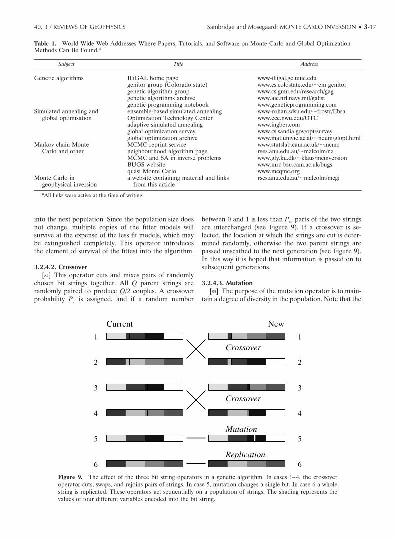
into the next population. Since the population size doesnot change, multiple copies of the fitter models willsurvive at the expense of the less fit models, which maybe extinguished completely. This operator introducesthe element of survival of the fittest into the algorithm.

3.2.4.2. Crossover[84] This operator cuts and mixes pairs of randomly

chosen bit strings together. All Q parent strings arerandomly paired to produce Q/2 couples. A crossoverprobability Pc is assigned, and if a random number

between 0 and 1 is less than Pc, parts of the two stringsare interchanged (see Figure 9). If a crossover is se-lected, the location at which the strings are cut is deter-mined randomly, otherwise the two parent strings arepassed unscathed to the next generation (see Figure 9).In this way it is hoped that information is passed on tosubsequent generations.

3.2.4.3. Mutation[85] The purpose of the mutation operator is to main-

tain a degree of diversity in the population. Note that the

Table 1. World Wide Web Addresses Where Papers, Tutorials, and Software on Monte Carlo and Global OptimizationMethods Can Be Found.a

Subject Title Address

Genetic algorithms IlliGAL home page www-illigal.ge.uiuc.edugenitor group (Colorado state) www.cs.colostate.edu/em genitorgenetic algorithm group www.cs.gmu.edu/research/gaggenetic algorithms archive www.aic.nrl.navy.mil/galistgenetic programming notebook www.geneticprogramming.com

Simulated annealing andglobal optimisation

ensemble-based simulated annealing www-rohan.sdsu.edu/frostr/EbsaOptimization Technology Center www.ece.nwu.edu/OTCadaptive simulated annealing www.ingber.comglobal optimization survey www.cs.sandia.gov/opt/surveyglobal optimization archive www.mat.univie.ac.at/neum/glopt.html

Markov chain MonteCarlo and other

MCMC reprint service www.statslab.cam.ac.uk/mcmcneighbourhood algorithm page rses.anu.edu.au/malcolm/naMCMC and SA in inverse problems www.gfy.ku.dk/klaus/mcinversionBUGS website www.mrc-bsu.cam.ac.uk/bugsquasi Monte Carlo www.mcqmc.org

Monte Carlo ingeophysical inversion

a website containing material and linksfrom this article

rses.anu.edu.au/malcolm/mcgi

aAll links were active at the time of writing.

Figure 9. The effect of the three bit string operators in a genetic algorithm. In cases 1–4, the crossoveroperator cuts, swaps, and rejoins pairs of strings. In case 5, mutation changes a single bit. In case 6 a wholestring is replicated. These operators act sequentially on a population of strings. The shading represents thevalues of four different variables encoded into the bit string.


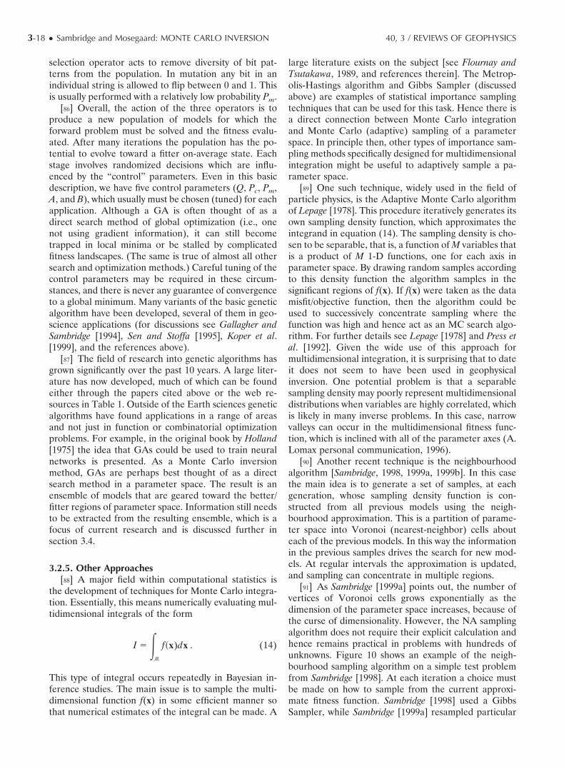
selection operator acts to remove diversity of bit pat-terns from the population. In mutation any bit in anindividual string is allowed to flip between 0 and 1. Thisis usually performed with a relatively low probability Pm.

[86] Overall, the action of the three operators is toproduce a new population of models for which theforward problem must be solved and the fitness evalu-ated. After many iterations the population has the po-tential to evolve toward a fitter on-average state. Eachstage involves randomized decisions which are influ-enced by the “control” parameters. Even in this basicdescription, we have five control parameters (Q, Pc, Pm,A, and B), which usually must be chosen (tuned) for eachapplication. Although a GA is often thought of as adirect search method of global optimization (i.e., onenot using gradient information), it can still becometrapped in local minima or be stalled by complicatedfitness landscapes. (The same is true of almost all othersearch and optimization methods.) Careful tuning of thecontrol parameters may be required in these circum-stances, and there is never any guarantee of convergenceto a global minimum. Many variants of the basic geneticalgorithm have been developed, several of them in geo-science applications (for discussions see Gallagher andSambridge [1994], Sen and Stoffa [1995], Koper et al.[1999], and the references above).

[87] The field of research into genetic algorithms hasgrown significantly over the past 10 years. A large liter-ature has now developed, much of which can be foundeither through the papers cited above or the web re-sources in Table 1. Outside of the Earth sciences geneticalgorithms have found applications in a range of areasand not just in function or combinatorial optimizationproblems. For example, in the original book by Holland[1975] the idea that GAs could be used to train neuralnetworks is presented. As a Monte Carlo inversionmethod, GAs are perhaps best thought of as a directsearch method in a parameter space. The result is anensemble of models that are geared toward the better/fitter regions of parameter space. Information still needsto be extracted from the resulting ensemble, which is afocus of current research and is discussed further insection 3.4.

3.2.5. Other Approaches[88] A major field within computational statistics is

the development of techniques for Monte Carlo integra-tion. Essentially, this means numerically evaluating mul-tidimensional integrals of the form

I � ��

f�x)dx . (14)

This type of integral occurs repeatedly in Bayesian in-ference studies. The main issue is to sample the multi-dimensional function f(x) in some efficient manner sothat numerical estimates of the integral can be made. A

large literature exists on the subject [see Flournay andTsutakawa, 1989, and references therein]. The Metrop-olis-Hastings algorithm and Gibbs Sampler (discussedabove) are examples of statistical importance samplingtechniques that can be used for this task. Hence there isa direct connection between Monte Carlo integrationand Monte Carlo (adaptive) sampling of a parameterspace. In principle then, other types of importance sam-pling methods specifically designed for multidimensionalintegration might be useful to adaptively sample a pa-rameter space.

[89] One such technique, widely used in the field ofparticle physics, is the Adaptive Monte Carlo algorithmof Lepage [1978]. This procedure iteratively generates itsown sampling density function, which approximates theintegrand in equation (14). The sampling density is cho-sen to be separable, that is, a function of M variables thatis a product of M 1-D functions, one for each axis inparameter space. By drawing random samples accordingto this density function the algorithm samples in thesignificant regions of f(x). If f(x) were taken as the datamisfit/objective function, then the algorithm could beused to successively concentrate sampling where thefunction was high and hence act as an MC search algo-rithm. For further details see Lepage [1978] and Press etal. [1992]. Given the wide use of this approach formultidimensional integration, it is surprising that to dateit does not seem to have been used in geophysicalinversion. One potential problem is that a separablesampling density may poorly represent multidimensionaldistributions when variables are highly correlated, whichis likely in many inverse problems. In this case, narrowvalleys can occur in the multidimensional fitness func-tion, which is inclined with all of the parameter axes (A.Lomax personal communication, 1996).

[90] Another recent technique is the neighbourhoodalgorithm [Sambridge, 1998, 1999a, 1999b]. In this casethe main idea is to generate a set of samples, at eachgeneration, whose sampling density function is con-structed from all previous models using the neigh-bourhood approximation. This is a partition of parame-ter space into Voronoi (nearest-neighbor) cells abouteach of the previous models. In this way the informationin the previous samples drives the search for new mod-els. At regular intervals the approximation is updated,and sampling can concentrate in multiple regions.

[91] As Sambridge [1999a] points out, the number ofvertices of Voronoi cells grows exponentially as thedimension of the parameter space increases, because ofthe curse of dimensionality. However, the NA samplingalgorithm does not require their explicit calculation andhence remains practical in problems with hundreds ofunknowns. Figure 10 shows an example of the neigh-bourhood sampling algorithm on a simple test problemfrom Sambridge [1998]. At each iteration a choice mustbe made on how to sample from the current approxi-mate fitness function. Sambridge [1998] used a GibbsSampler, while Sambridge [1999a] resampled particular


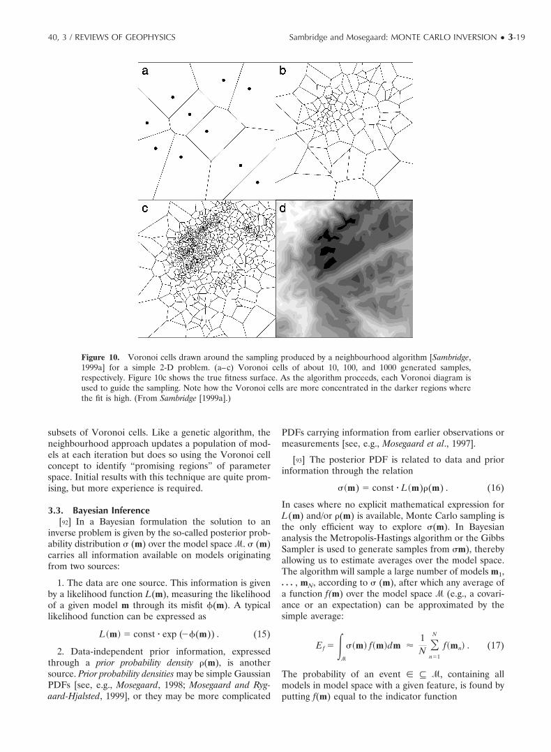
subsets of Voronoi cells. Like a genetic algorithm, theneighbourhood approach updates a population of mod-els at each iteration but does so using the Voronoi cellconcept to identify “promising regions” of parameterspace. Initial results with this technique are quite prom-ising, but more experience is required.

3.3. Bayesian Inference[92] In a Bayesian formulation the solution to an

inverse problem is given by the so-called posterior prob-ability distribution � (m) over the model space �. � (m)carries all information available on models originatingfrom two sources:

1. The data are one source. This information is givenby a likelihood function L(m), measuring the likelihoodof a given model m through its misfit �(m). A typicallikelihood function can be expressed as

L�m � const � exp (��(m)) . (15)

2. Data-independent prior information, expressedthrough a prior probability density �(m), is anothersource. Prior probability densities may be simple GaussianPDFs [see, e.g., Mosegaard, 1998; Mosegaard and Ryg-aard-Hjalsted, 1999], or they may be more complicated

PDFs carrying information from earlier observations ormeasurements [see, e.g., Mosegaard et al., 1997].

[93] The posterior PDF is related to data and priorinformation through the relation

��m) const � L�m)�(m) . (16)

In cases where no explicit mathematical expression forL(m) and/or �(m) is available, Monte Carlo sampling isthe only efficient way to explore �(m). In Bayesiananalysis the Metropolis-Hastings algorithm or the GibbsSampler is used to generate samples from �m), therebyallowing us to estimate averages over the model space.The algorithm will sample a large number of models m1,� � � , mN, according to � (m), after which any average ofa function f(m) over the model space � (e.g., a covari-ance or an expectation) can be approximated by thesimple average:

Ef � ��

��m f�m dm �1N �

n1

N

f�mn . (17)

The probability of an event � � �, containing allmodels in model space with a given feature, is found byputting f(m) equal to the indicator function

Figure 10. Voronoi cells drawn around the sampling produced by a neighbourhood algorithm [Sambridge,1999a] for a simple 2-D problem. (a–c) Voronoi cells of about 10, 100, and 1000 generated samples,respectively. Figure 10c shows the true fitness surface. As the algorithm proceeds, each Voronoi diagram isused to guide the sampling. Note how the Voronoi cells are more concentrated in the darker regions wherethe fit is high. (From Sambridge [1999a].)


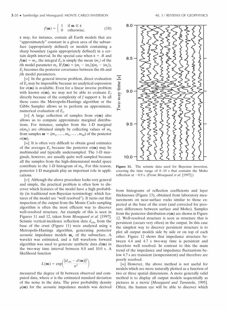
f�m � � 1 if m � ε0 otherwise. (18)

ε may, for instance, contain all Earth models that are“approximately” constant in a given area of the subsur-face (appropriately defined) or models containing asharp boundary (again appropriately defined) in a cer-tain depth interval. In the special case when ε � andf(m) mi, the integral Ef is simply the mean �mi� of theith model parameter mi. If f(m) (mi � �mi�)(mj � �mj�),Ef becomes the posterior covariance between the ith andjth model parameters.

[94] In the general inverse problem, direct evaluationof Ef may be impossible because no analytical expressionfor �(m) is available. Even for a linear inverse problemwith known �(m), we may not be able to evaluate Ef

directly because of the complexity of f support ε. In allthese cases the Metropolis-Hastings algorithm or theGibbs Sampler allows us to perform an approximate,numerical evaluation of Ef.

[95] A large collection of samples from �(m) alsoallows us to compute approximate marginal distribu-tions. For instance, samples from the 1-D marginal�(mk) are obtained simply by collecting values of mk

from samples m (m1, � � � , mk, � � � , mM) of the posterior�(m).

[96] It is often very difficult to obtain good estimatesof the averages Ef because the posterior �(m) may bemultimodal and typically undersampled. The 1-D mar-ginals, however, are usually quite well sampled becauseall the samples from the high-dimensional model spacecontribute to the 1-D histogram of mk. For this reason,posterior 1-D marginals play an important role in appli-cations.

[97] Although the above procedure looks very generaland simple, the practical problem is often how to dis-cover which features of the model have a high probabil-ity (in traditional non-Bayesian terminology: which fea-tures of the model are “well resolved”). It turns out thatinspection of the output from the Monte Carlo samplingalgorithm is often the most efficient way to discoverwell-resolved structure. An example of this is seen inFigures 11 and 12, taken from Mosegaard et al. [1997].Seismic vertical-incidence reflection data dobs from thebase of the crust (Figure 11) were analyzed using aMetropolis-Hastings algorithm, generating posterioracoustic impedance models mn of the subsurface. Awavelet was estimated, and a full waveform forwardalgorithm was used to generate synthetic data d(m) inthe two-way time interval between 8.0 and 10.0 s. Alikelihood function

L(m) exp�dobs � d�m)2

�2 �measured the degree of fit between observed and com-puted data, where � is the estimated standard deviationof the noise in the data. The prior probability density�(m) for the acoustic impedance models was derived

from histograms of reflection coefficients and layerthicknesses (Figure 13), obtained from laboratory mea-surements on near-surface rocks similar to those ex-pected at the base of the crust (and corrected for pres-sure differences between surface and Moho). Samplesfrom the posterior distribution �(m) are shown in Figure12. Well-resolved structure is seen as structure that ispersistent (occurs very often) in the output. In this casethe simplest way to discover persistent structure is toplot all output models side by side or on top of eachother. Figure 12 shows that impedance structure be-tween 4.4 and 4.7 s two-way time is persistent andtherefore well resolved. In contrast to this the maintrend of the impedance and impedance fluctuations be-low 4.7 s are transient (nonpersistent) and therefore arepoorly resolved.

[98] However, the above method is not useful formodels which are more naturally plotted as a function oftwo or three spatial dimensions. A more generally validmethod is to display all output models sequentially aspictures in a movie [Mosegaard and Tarantola, 1995].Often, the human eye will be able to discover which

Figure 11. The seismic data used for Bayesian inversion,covering the time range of 8–10 s that contains the Mohoreflection at 8.9 s. (From Mosegaard et al. [1997].)


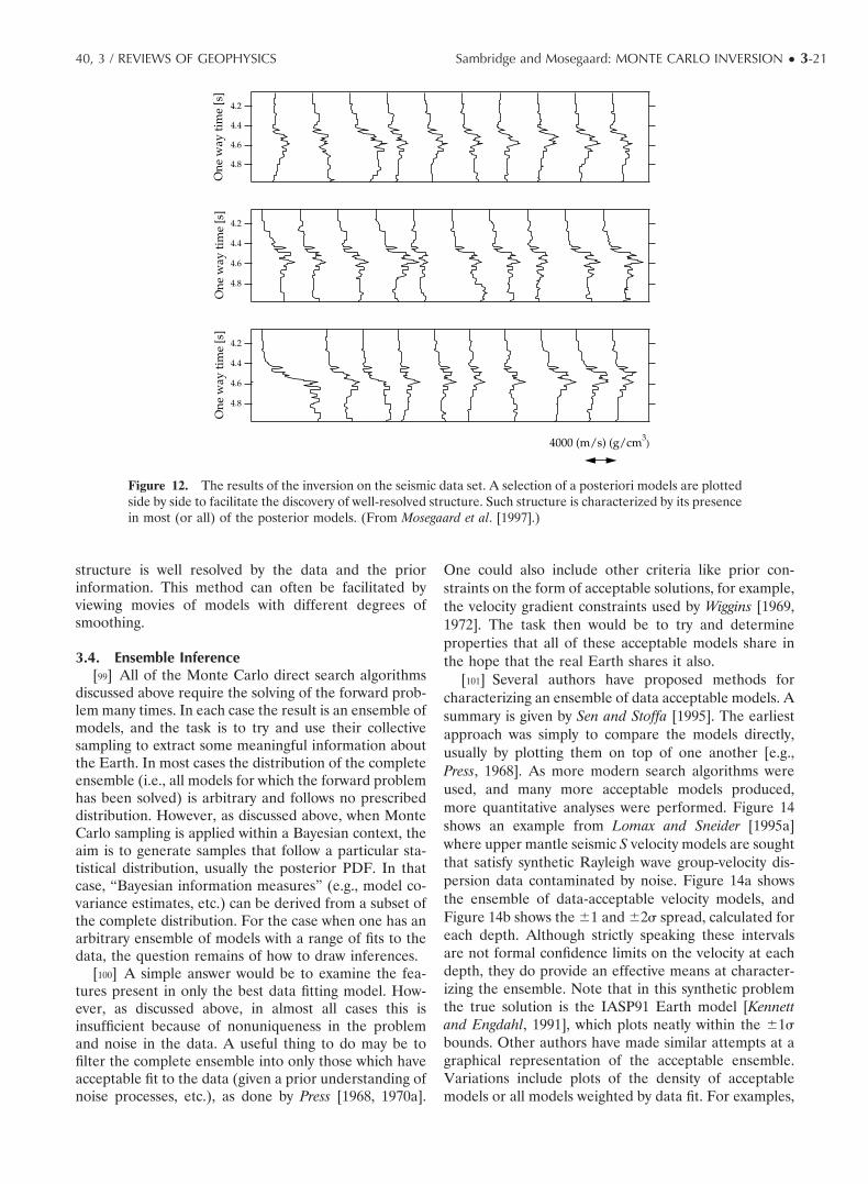
structure is well resolved by the data and the priorinformation. This method can often be facilitated byviewing movies of models with different degrees ofsmoothing.

3.4. Ensemble Inference[99] All of the Monte Carlo direct search algorithms

discussed above require the solving of the forward prob-lem many times. In each case the result is an ensemble ofmodels, and the task is to try and use their collectivesampling to extract some meaningful information aboutthe Earth. In most cases the distribution of the completeensemble (i.e., all models for which the forward problemhas been solved) is arbitrary and follows no prescribeddistribution. However, as discussed above, when MonteCarlo sampling is applied within a Bayesian context, theaim is to generate samples that follow a particular sta-tistical distribution, usually the posterior PDF. In thatcase, “Bayesian information measures” (e.g., model co-variance estimates, etc.) can be derived from a subset ofthe complete distribution. For the case when one has anarbitrary ensemble of models with a range of fits to thedata, the question remains of how to draw inferences.

[100] A simple answer would be to examine the fea-tures present in only the best data fitting model. How-ever, as discussed above, in almost all cases this isinsufficient because of nonuniqueness in the problemand noise in the data. A useful thing to do may be tofilter the complete ensemble into only those which haveacceptable fit to the data (given a prior understanding ofnoise processes, etc.), as done by Press [1968, 1970a].

One could also include other criteria like prior con-straints on the form of acceptable solutions, for example,the velocity gradient constraints used by Wiggins [1969,1972]. The task then would be to try and determineproperties that all of these acceptable models share inthe hope that the real Earth shares it also.

[101] Several authors have proposed methods forcharacterizing an ensemble of data acceptable models. Asummary is given by Sen and Stoffa [1995]. The earliestapproach was simply to compare the models directly,usually by plotting them on top of one another [e.g.,Press, 1968]. As more modern search algorithms wereused, and many more acceptable models produced,more quantitative analyses were performed. Figure 14shows an example from Lomax and Sneider [1995a]where upper mantle seismic S velocity models are soughtthat satisfy synthetic Rayleigh wave group-velocity dis-persion data contaminated by noise. Figure 14a showsthe ensemble of data-acceptable velocity models, andFigure 14b shows the �1 and �2� spread, calculated foreach depth. Although strictly speaking these intervalsare not formal confidence limits on the velocity at eachdepth, they do provide an effective means at character-izing the ensemble. Note that in this synthetic problemthe true solution is the IASP91 Earth model [Kennettand Engdahl, 1991], which plots neatly within the �1�bounds. Other authors have made similar attempts at agraphical representation of the acceptable ensemble.Variations include plots of the density of acceptablemodels or all models weighted by data fit. For examples,

Figure 12. The results of the inversion on the seismic data set. A selection of a posteriori models are plottedside by side to facilitate the discovery of well-resolved structure. Such structure is characterized by its presencein most (or all) of the posterior models. (From Mosegaard et al. [1997].)


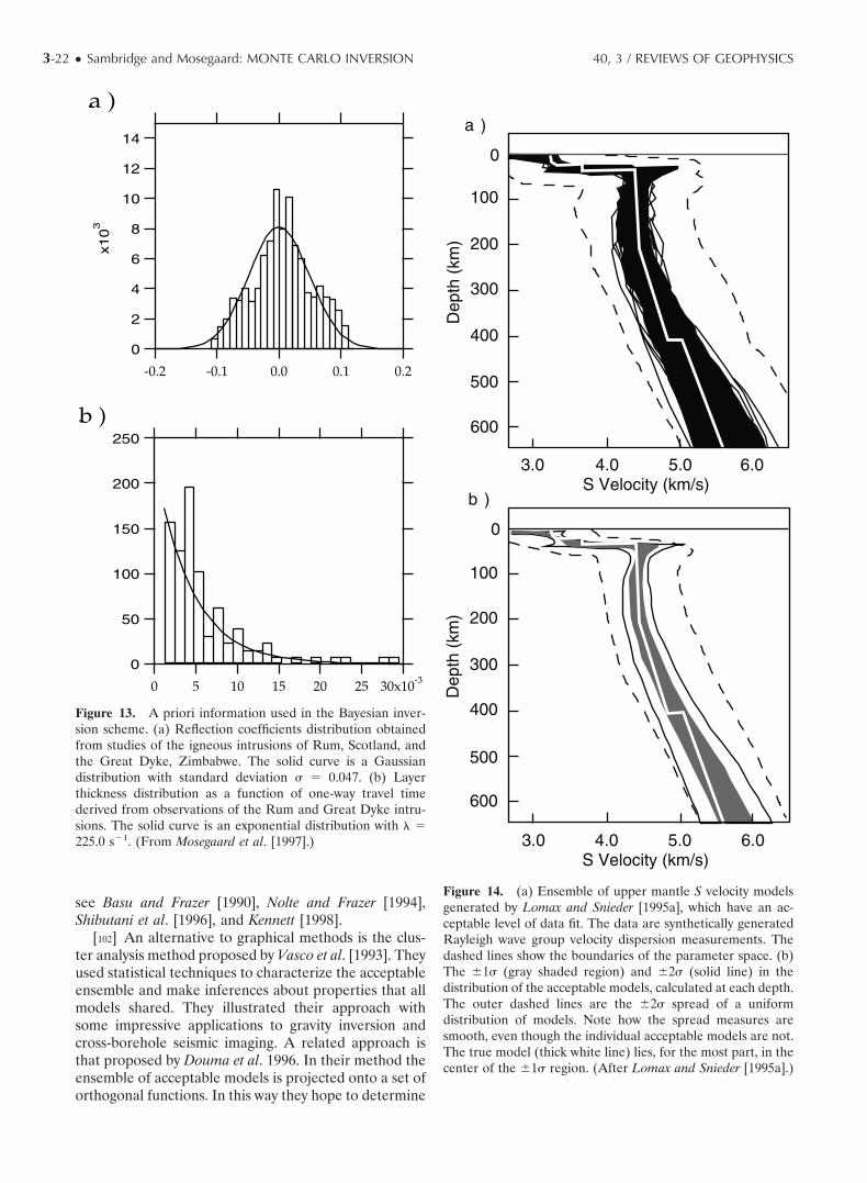
see Basu and Frazer [1990], Nolte and Frazer [1994],Shibutani et al. [1996], and Kennett [1998].

[102] An alternative to graphical methods is the clus-ter analysis method proposed by Vasco et al. [1993]. Theyused statistical techniques to characterize the acceptableensemble and make inferences about properties that allmodels shared. They illustrated their approach withsome impressive applications to gravity inversion andcross-borehole seismic imaging. A related approach isthat proposed by Douma et al. 1996. In their method theensemble of acceptable models is projected onto a set oforthogonal functions. In this way they hope to determine

Figure 14. (a) Ensemble of upper mantle S velocity modelsgenerated by Lomax and Snieder [1995a], which have an ac-ceptable level of data fit. The data are synthetically generatedRayleigh wave group velocity dispersion measurements. Thedashed lines show the boundaries of the parameter space. (b)The �1� (gray shaded region) and �2� (solid line) in thedistribution of the acceptable models, calculated at each depth.The outer dashed lines are the �2� spread of a uniformdistribution of models. Note how the spread measures aresmooth, even though the individual acceptable models are not.The true model (thick white line) lies, for the most part, in thecenter of the �1� region. (After Lomax and Snieder [1995a].)

Figure 13. A priori information used in the Bayesian inver-sion scheme. (a) Reflection coefficients distribution obtainedfrom studies of the igneous intrusions of Rum, Scotland, andthe Great Dyke, Zimbabwe. The solid curve is a Gaussiandistribution with standard deviation � 0.047. (b) Layerthickness distribution as a function of one-way travel timederived from observations of the Rum and Great Dyke intru-sions. The solid curve is an exponential distribution with � 225.0 s�1. (From Mosegaard et al. [1997].)


the well constrained information hidden in the ensem-ble. As with the method of Vasco et al. [1993] thetechnique is appropriate if the ensemble forms a singlecluster and not multiple disjointed clusters, as depictedin Figure 1. If multiple clusters exist, then they must beidentified, and the approach applied separately to each.

[103] Recently, Sambridge [1999b] has proposed anapproach to estimate Bayesian information measuresfrom an arbitrarily distributed ensemble. In this case theneighborhood approximation (mentioned above in con-nection with a search algorithm) is applied to the com-plete ensemble, that is, all models for which the forwardmodel has been solved. A standard MCMC integrationprocedure is then used to resample according to theneighborhood approximation and to produce unbiasedestimates of Bayesian integrals. The advantage of thisapproach is that it can, in principle, extract Bayesianestimates from ensembles generated by any method, forexample, a genetic algorithm. A caveat, which applies toall of these techniques, is that at best they can onlyextract what information exists in a given ensemble ofmodels. If the available ensemble does not adequatelyrepresent (or sample) the acceptable region in parame-ter space, then the result will be biased.

[104] In the past few years, geophysicists have begunto develop techniques for ensemble inference. The un-derlying idea is that basing inferences on an ensemble ofpotential solutions is more useful than considering justone (usually best fit) model. The current range of ap-proaches available are useful but by no means completeor applicable in all circumstances. It seems likely thatthis will be an area of further research in the nextdecade.

3.5. Resources on the Net[105] It may be useful to the reader to have a list of

web site addresses where more information can be foundon various topics discussed in this paper. At some sites acomputer code is also available. Table 1 shows a collec-tion that we are aware of. Many other sites can be foundby following the links on these pages.

4. CONCLUSIONS

[106] In this paper we have summarized the currentstate of the Monte Carlo methodology, as applied ingeophysics. Some open questions and directions for fu-ture research have been discussed. The Earth sciencesare a rich source of large and complicated inverse prob-lems. Often they can be posed in a way suitable forattack with MC methods. In doing so, the Earth scientistmust remember that the development of Monte Carlotechniques is a multidisciplinary effort, and it can bebeneficial to look at what has been done elsewhere. It ishoped that this paper will facilitate that process bydrawing the attention of geophysicists to relevant refer-

ence material in computational statistics and otherfields.

[107] We have highlighted the connection between thecomputational approaches commonly used for data fit-ting and model appraisal with those in the fields ofoptimization and statistical inference. Techniques suchas simulated annealing, genetic algorithms, and otherstatistical importance sampling methodologies have allstarted life elsewhere but become useful additions to thegeophysicists tool bag. One issue that was prevalent atthe outset (�30 years ago) was how to make robustinferences from an ensemble of data acceptable models.In recent times this question has come back into focus.Geophysicists are good at generating models, and evenat finding some that fit data, but quantitative and reliableinferences are needed for drawing conclusions. The sta-tistical and other approaches discussed in this paperhave begun to answer these questions in a quantitativemanner.

GLOSSARY

[108] Acceptable models: A set of Earth models (seedefinition) that are consistent with observations, takinginto account the presence of noise and errors in theobservables. Usually, the acceptable models are thosefor which the objective (or data misfit) function is lessthan, or equal to, a predetermined value.

[109] Bayesian inference: A (purely) probabilistic pro-cedure for information updating. In the typical scenarioprior information, represented by a prior probabilitydistribution, is updated by information from experimen-tal data, represented by a likelihood function. The re-sulting state of information is represented by the (nor-malized) product of the prior distribution and thelikelihood function, the so-called posterior probabilitydistribution. The terms “prior” and “posterior” refer to“before” and “after” data collection, respectively.

[110] Direct search: A parameter space search method(see definition) that does not use Frechet derivatives orgradient information of the objective function. It onlyuses evaluations of the objective function at points inparameter space.

[111] Earth model: A representation of some physicalproperties of the Earth, usually in a discrete form wherethe earth property, for example, Earth’s density varia-tion, is described by a finite number of parameters, forexample, the average density of rocks in a series of depthintervals from the surface of the Earth.

[112] Ensemble inference: The procedure whereby in-formation is extracted or conclusions are drawn from acollection of inputs, or Earth models, rather than asingle model. Genetic Algorithms, Simulated Annealing,and the Neighbourhood algorithm are all examples ofensemble inference (direct search) techniques.

[113] Forward problem: The calculation of predictionsfrom an Earth model, to be compared with the observa-


tions. The solution of the forward problem is a necessarystep in determining the fit to the data. The degree ofnonlinearity in the forward problem can be a majorcause of difficulty in finding Earth models that fit data.

[114] Genetic algorithm: A computational methodpopular for global optimization problems. This is a fullynonlinear direct search method, which means that itavoids linearization and does not use derivatives of theobjective function being optimized. The procedure isbased on an analogy with principles of evolution and“survival of the fittest.” Originally developed as a modelfor adaptive behavior in an artificial system, it has beenapplied to complex optimization problems across thephysical sciences.

[115] Global optimization: A numerical procedurewhere the values of some variables are sought that givean optimum value of some function, that is, maximum orminimum over all possibilities.

[116] Importance sampling: A Monte Carlo algorithmdesigned to sample a given function, or probability den-sity, with a sampling density proportional to that func-tion or probability density.

[117] Inverse problem: The term used to describe thesituation where inversion is applied. (See definition ofinversion).

[118] Inversion: The process by which information isobtained about a physical quantity from indirect infor-mation, for example, on Earth’s seismic structure fromthe travel times of elastic waves generated by earth-quakes.

[119] Likelihood function: A function describing theprobability that a given parameterized model is consis-tent with observed data. The likelihood function is afunction of the model and measures the fit betweenmodel predictions and observations.

[120] Markov Chain: See random walk.[121] MCI (Monte Carlo Inversion): The term used to

describe the earliest forms of uniform random parame-ter space searching, as applied to seismological problemsin the work of Press [1968, 1970a].

[122] MCMC (Markov Chain Monte Carlo): A multi-dimensional random sampling procedure where the nextsample only depends on the location of the currentsampling point.

[123] Metropolis-Hastings algorithm: A simple im-portance sampling algorithm (see definition of impor-tance sampling) based on a random walk.

[124] Misfit function: The same as objective function,except that one always minimizes a misfit function.

[125] Monte Carlo: A prefix indicating that themethod or approach makes use of repeated trials, orsampling, generated with the use of random numbers,named after the famous French city associated withcasinos.

[126] Monte Carlo integration: A numerical integra-tion procedure for functions, which is efficient in high-dimensional spaces. Instead of using functional values ina uniform grid to produce a numerical approximation of

an integral, they are evaluated at randomly selectedpoints (often generated by an importance sampling al-gorithm (see above). The integral can then be approxi-mated by an average of these values, and the chance ofmissing areas of high functional values is strongly re-duced.

[127] Objective function: A function calculated fromone or more variables which is usually the subject of anoptimization process, that is, the variables are sought,which optimize the objective function. The objectivefunction can be a measure of discrepancy with observeddata (data misfit) or a combination of data misfit andother criteria.

[128] Parameter space: An abstract multidimensionalregion describing the set of all possible values that Earthmodels can take. Each point in the parameter spacerepresents an Earth model.

[129] Parameter space search: The process of findingEarth models that have an acceptable or optimal valueof the objective function.

[130] Posterior PDF: A probability density represent-ing, in a Bayesian computation, the combination of priorinformation and data information.

[131] Prior probability density: A probability densityrepresenting, in a Bayesian computation, the informa-tion available before data is acquired (or considered).

[132] Probability density function (PDF): A statisticalterm used to describe the probability distribution asso-ciated with a random variable. For example, the well-known “bell-shaped” Gaussian distribution is a PDF of aone-dimensional normal random variable. The area un-der the curve between any two given values representsthe probability that a realization of the variable will fallbetween these values. Multidimensional PDFs are usedto describe the joint behavior of a random vector (whosecomponents are all random variables).

[133] Pseudorandom number: The result of a numer-ical procedure (a generator), which has certain statisticalproperties. For example, the histogram of many pseudo-random numbers will tend toward a uniform distribu-tion. Most computing systems provide pseudorandomnumber generators that use a linear congruent method[see Park and Miller, 1988].

[134] Quasi-random number: Sometimes called “sub-random” numbers, similar definition as for pseudoran-dom numbers. Often it is based on number theoretictechniques and usually converges much faster than pseu-dorandom numbers to a uniform distribution.

[135] Random Walk: A perturbative sequence of ran-dom changes to a point in a multidimensional space. Auniform random walk is one where the asymptotic con-vergence is to a uniform density of samples in parameterspace. See also Markov Chain Monte Carlo (MCMC).

[136] Simulated annealing: A Metropolis-Hastings al-gorithm designed to simulate certain aspects of a statis-tical mechanical system. The simulated annealing (SA)algorithm samples a Gibbs-Boltzmann distribution inthe model space, and a characteristic feature of this


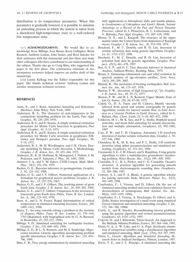
distribution is its temperature parameter. When thisparameter is gradually lowered, it is possible to simulatean annealing process in which the system is taken froma disordered high-temperature state to a well-orderedlow temperature state.

[137] ACKNOWLEDGMENTS. We would like to ac-knowledge Steve Billings, Jean Braun, Kerry Gallagher, BrianKennett, Anthony Lomax, John Scales, and Roel Snieder fortheir assistance with this manuscript and also these and manyother colleagues who have contributed to our understanding ofthe subject. Thanks also go to Craig Bina, who suggested thispaper in the first place. The constructive criticisms of twoanonymous reviewers helped improve an earlier draft of thismanuscript.

[138] Louise Kellogg was the Editor responsible for thispaper. She thanks technical reviewer Anthony Lomax andanother anonymous technical reviewer.

REFERENCES

Aarts, E., and J. Korst, Simulated Annealing and BoltzmannMachines, John Wiley, New York, 1989.

Anderssen, R. S., The character of non-uniqueness in theconductivity modelling problem for the Earth, Pure Appl.Geophys., 80, 238–259, 1970.

Anderssen, R. S., and E. Senata, A simple statistical estimationprocedure for Monte Carlo Inversion in geophysics, PureAppl. Geophys., 91, 5–13, 1971.

Anderssen, R. S., and E. Senata, A simple statistical estimationprocedure for Monte Carlo inversion in geophysics: Effi-ciency and Hempel’s paradox, Pure Appl. Geophys., 96,5–14, 1972.

Anderssen, R. S., M. H. Worthington, and J. R. Cleary, Den-sity modelling by Monte Carlo Inversion, I, Methodology,Geophys. J. R. Astron. Soc., 29, 433–444, 1972.

Andresen, B., K. H. Hoffman, K. Mosegaard, J. Nulton, J. M.Pedersen, and P. Salamon, J. Phys., 49, 1485, 1988.

Antonov, I. A., and V. M. Saleev, USSR Comput. Math. Math.Phys., 19(1), 252–256, 1979.

Backus, G. E., Bayesian inference in geomagnetism, Geophys.J., 92, 125–142, 1988.

Backus, G. E., and J. F. Gilbert, Numerical applications of aformalism for geophysical inverse problems, Geophys. J. R.Astron. Soc., 13, 247–276, 1967.

Backus, G. E., and J. F. Gilbert, The resolving power of grossEarth data, Geophys. J. R. Astron. Soc., 16, 169–205, 1968.

Backus, G. E., and J. F. Gilbert, Uniqueness in the inversion ofinaccurate gross Earth data, Philos. Trans. R. Soc. London,Ser. A., 266, 123–192, 1970.

Basu, A., and L. N. Frazer, Rapid determination of criticaltemperature in simulated annealing inversion, Science, 249,1409–1412, 1990.

Bayes, T., An essay towards solving a problem in the doctrineof chances, Philos. Trans. R. Soc. London, 53, 370–418,1763 (Reprinted, with biographical note by G. A. Barnard,in Biometrika, 45, 293–315, 1958).

Billings, S. D., Simulated annealing for earthquake location,Geophys. J. Int., 118, 680–692, 1994.

Billings, S. D., B. L. N. Kennett, and M. S. Sambridge, Hypo-centre location: Genetic algorithms incorporating problemspecific information, Geophys. J. R. Astron. Soc., 118, 693–706, 1994.

Bina, C. R., Free energy minimization by simulated annealing

with applications to lithospheric slabs and mantle plumes,in Geodynamics of Lithosphere and Earth’s Mantle; SeismicAnisotropy as a Record of the Past and Present DynamicProcesses, edited by J. Plomerova, R. C. Liebermann, andV. Babuska, Pure Appl. Geophys., 151, 605–618, 1998.

Biswas, N. N., and L. Knopoff, The structure of the uppermantle under the United States from dispersion of Rayleighwaves, Geophys. J. R. Astron. Soc., 36, 515–539, 1974.

Boschetti, F., M. C. Dentith, and R. D. List, Inversion ofseismic refraction data using genetic algorithms, Geophys-ics, 61, 1715–1727, 1996.

Boschetti, F., M. C. Dentith, and R. D. List, Inversion ofpotential field data by genetic algorithms, Geophys. Pros-pect., 45(3), 461–478, 1997.

Box, G. E. P., and G. C. Tiao, Bayesian Inference in StatisticalAnalysis, Addison-Wesley, Reading, Mass., 1973.

Braun, J., Estimating exhumation rate and relief evolution byspectral analysis of age-elevation profiles, Terra Nova,14(3), 205–209, 2002.

Buland, R., The mechanics of locating earthquakes, Bull. Seis-mol. Soc. Am., 66, 173–187, 1976.

Burton, P. W., Inversions of high frequency Q��1(f), Geophys.

J. R. Astron. Soc., 48, 29–51, 1977.Burton, P. W., and B. L. N. Kennett, Upper Mantle Zone of

low Q, Nature, 238, 84, 87–90, 1972.Cadek, O., D. A. Yuen, and H. Cizkova, Mantle viscosity

inferred from geoid and seismic tomography by geneticalgorithms; results for layered mantle flow, in Joint Inver-sion as a General Problem in Earth Sciences, edited by L.Ballani, Phys. Chem. Earth, 23, 9–10, 865–872, 1998.

Calderon, M. C., M. K. Sen, and P. L. Stoffa, Hopfield neuralnetworks, and mean field annealing for seismic deconvolu-tion and multiple attenuation, Geophysics, 62, 992–1002,1997.

Cary, P. W., and C. H. Chapman, Automatic 1-D waveforminversion of marine seismic refraction data, Geophys. J., 93,527–546, 1988.

Chunduru, R. K., M. K. Sen, and P. L. Stoffa, 2-D resistivityinversion using spline parameterization and simulated an-nealing, Geophysics, 61, 151–161, 1996.

Cieniawski, S. E., J. W. Eheart, and S. Ranjithan, Using geneticalgorithms to solve a multiobjective groundwater monitor-ing problem, Water Resour. Res., 31(2), 399–409, 1995.

Constable, S. C., R. L. Parker, and C. G. Constable, Occam’sinversion: A practical algorithm for generating smoothmodels from electromagnetic sounding data, Geophysics,52, 289–300, 1987.

Conway, A. J., and P. A. Bland, A genetic algorithm schemefor pairing meteorite finds, Meteorol. Planet. Sci., 33(3),491–499, 1998.

Courboulex, F., J. Virieux, and D. Gibert, On the use ofsimulated annealing method and cross-validation theory fordeconvolution of seismograms, Bull. Seismol. Soc. Am.,86(4), 1187–1193, 1996a.

Courboulex, F., J. Virieux, A. Deschamps, D. Gibert, and A.Zollo, Source investigation of a small event using empiricalGreen’s functions and simulated annealing, Geophys. J. Int.,125, 768–780, 1996b.

Curtis, A., and R. Snieder, Reconditioning inverse problemsusing the genetic algorithm and revised parameterization,Geophysics, 62, 1524–1532, 1997.

Cvijovic, D., and J. Klinowski, Taboo Search: An Approach tothe Multiple Minima Problem, Science, 267, 664–666, 1995.

Datta, G. A., L. W. Lake, and G. A. Pope, Stochastic simula-tion of categorical variables using a classification algorithmand simulated annealing, Math. Geol., 27(6), 763–787, 1995.

Davis, L., Genetic Algorithms and Simulated Annealing, Re-search Notes in Artificial Intelligence, Pitman, London, 1987.

Davis, T. E., and J. C. Principe, A simulated annealing like


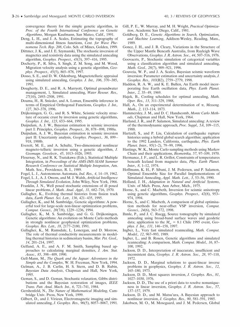
convergence theory for the simple genetic algorithm, inProc. of the Fourth International Conference on GeneticAlgorithms, Morgan Kaufmann, San Mateo, Calif., 1991.

Deng, L. H., and J. A. Scales, Estimating the topography ofmulti-dimensional fitness functions, Cent. for Wave Phe-nomena Tech. Rep. 208, Colo. Sch. of Mines, Golden, 1999.

Dittmer, J. K., and J. E. Szymanski, The stochastic inversion ofmagnetics and resistivity data using the simulated annealingalgorithm, Geophys. Prospect., 43(3), 397–416, 1995.

Docherty, P., R. Silva, S. Singh, Z. M. Song, and M. Wood,Migration velocity analysis using a genetic algorithm, Geo-phys. Prospect., 45(5), 865–878, 1997.

Dosso, S. E., and D. W. Oldenburg, Magnetotelluric appraisalusing simulated annealing, Geophys. J. Int., 106, 370–385,1991.

Dougherty, D. E., and R. A. Marryott, Optimal groundwatermanagement, 1, Simulated annealing, Water Resour. Res.,27(10), 2493–2508, 1991.

Douma, H., R. Snieder, and A. Lomax, Ensemble inference interms of Empirical Orthogonal Functions, Geophys. J. Int.,127, 363–378, 1996.

Drijkoningen, G. G., and R. S. White, Seismic velocity struc-ture of oceanic crust by inversion using genetic algorithms,Geophys. J. Int., 123, 653–664, 1995.

Duijndam, A. J. W., Bayesian estimation in seismic inversionpart I: Principles, Geophys. Prospect., 36, 878–898, 1988a.

Duijndam, A. J. W., Bayesian estimation in seismic inversionpart II: Uncertainty analysis, Geophys. Prospect., 36, 899–918, 1988b.

Everett, M. E., and A. Schultz, Two-dimensional nonlinearmagneto-telluric inversion using a genetic algorithm, J.Geomagn. Geoelectr., 45, 1013–1026, 1993.

Flournay, N., and R. K. Tsutakawa (Eds.), Statistical MultipleIntegration, in Proceedings of the AMS-IMS-SIAM SummerResearch Conference on Statistical Multiple Integration, Am.Math. Soc., Providence, R. I., 1989.

Fogel, L. J., Autonomous Automata, Ind. Res., 4, 14–19, 1962.Fogel, L. J., A. J. Owens, and M. J. Walsh, Artificial Intelligence

Through Simulated Evolution, John Wiley, New York, 1966.Franklin, J. N., Well posed stochastic extensions of ill posed

linear problems, J. Math. Anal. Appl., 31, 682–716, 1970.Gallagher, K., Evolving thermal histories from fission track

data, Earth Planet. Sci. Lett., 136, 421–435, 1995.Gallagher, K., and M. Sambridge, Genetic algorithms: A pow-

erful tool for large-scale non-linear optimization problems,Comput. Geosci., 20(7/8), 1229–1236, 1994.

Gallagher, K., M. S. Sambridge, and G. G. Drijkoningen,Genetic algorithms: An evolution on Monte Carlo methodsin strongly nonlinear geophysical optimization problems,Geophys. Res. Lett., 18, 2177–2180, 1991.

Gallagher, K., M. Ramsdale, L. Lonergan, and D. Morrow,The role of thermal conductivity measurements in model-ling thermal histories in sedimentary basins, Mar. Pet. Geol.,14, 201–214, 1997.

Gelfand, A. E., and A. F. M. Smith, Sampling based ap-proaches to calculating marginal densities, J. Am. Stat.Assoc., 85, 398–409, 1990.

Gell-Mann, M., The Quark and the Jaguar: Adventures in theSimple and the Complex, W. H. Freeman, New York, 1994.

Gelman, A., J. B. Carlin, H. S. Stern, and D. B. Rubin,Bayesian Data Analysis, Chapman and Hall, New York,1995.

Geman, S., and D. Geman, Stochastic relaxation, Gibbs distri-butions and the Bayesian restoration of images, IEEETrans. Patt. Anal. Mach. Int., 6, 721–741, 1984.

Gershenfeld, N., The Nature of Mathematical Modeling, Cam-bridge Univ. Press, New York, 1999.

Gilbert, D., and J. Virieux, Electromagnetic imaging and sim-ulated annealing, J. Geophys. Res., 96(5), 8057–8067, 1991.

Gill, P. E., W. Murray, and M. H. Wright, Practical Optimiza-tion, Academic San Diego, Calif., 1981.

Goldberg, D. E., Genetic Algorithms in Search, Optimization,and Machine Learning, Addison-Wesley, Reading, Mass.,1989.

Goncz, J. H., and J. R. Cleary, Variations in the Structure ofthe Upper Mantle Beneath Australia, from Rayleigh WaveObservations, Geophys. J. R. Astron. Soc., 44, 507–516, 1976.

Goovaerts, P., Stochastic simulation of categorical variablesusing a classification algorithm and simulated annealing,Math. Geol., 28(7), 909–921, 1996.

Gouveia, W. P., and J. A. Scales, Bayesian seismic waveforminversion: Parameter estimation and uncertainty analysis, J.Geophys. Res., 103(B2), 2759–2779, 1998.

Haddon, R. A. W., and K. E. Bullen, An Earth model incor-porating free Earth oscillation data, Phys. Earth Planet.Inter., 2, 35–49, 1969.

Hajek, B., Cooling schedules for optimal annealing, Math.Oper. Res., 13, 311–329, 1988,

Hall, A., On an experimental determination of �, Messeng.Math., 2, 113–114, 1873.

Hammersley, J. M., and D. C. Handscomb, Monte Carlo Meth-ods, Chapman and Hall, New York, 1964.

Harland, J. R., and P. Salamon, Simulated annealing: A reviewof the thermodynamic approach, Proc. Suppl., 5A, 109–115,1988.

Hartzell, S., and P. Liu, Calculation of earthquake rupturehistories using a hybrid global search algorithm; applicationto the 1992 Landers, California, earthquake, Phys. EarthPlanet. Inter., 95(1–2), 79–99, 1996.

Hastings, W. K., Monte Carlo sampling methods using MarkovChain and their applications, Biometrika, 57, 97–109, 1970.

Hermance, J. F., and L. R. Grillot, Constraints of temperaturesbeneath Iceland from magneto data, Phys. Earth Planet.Inter., 8, 1–12, 1974.

Hoffmann, K. H., P. Sibani, J. M. Pedersen, and P. Salamon,Optimal Ensemble Size for Parallel Implementations ofSimulated Annealing, Appl. Math. Lett., 3, 53–56, 1990.

Holland, J. H., Adaptation in Natural and Artificial Systems,Univ. of Mich. Press, Ann Arbor, Mich., 1975.

Horne, S., and C. Macbeth, Inversion for seismic anisotropyusing genetic algorithms, Geophys. Prospect., 42(8), 953–974, 1994.

Horne, S., and C. Macbeth, A comparison of global optimisa-tion methods for near-offset VSP inversion, Comput.Geosci., 24(6), 563–572, 1998.

Ihmle, P., and J. C. Ruegg, Source tomography by simulatedannealing using broad-band surface waves and geodeticdata; application to the Mw 8.1 Chile 1995 event, Geo-phys. J. Int., 131, 146–158, 1997.

Ingber, L., Very fast simulated reannealing, Math. Comput.Model., 12, 967–993, 1989.

Ingber, L., and B. Rosen, Genetic algorithms and simulatedreannealing: A comparison, Math. Comput. Model., 16, 87–100, 1992.

Jackson, D. D., Interpretation of inaccurate, insufficient andinconsistent data, Geophys. J. R. Astron. Soc., 28, 97–110,1972.

Jackson, D. D., Marginal solutions to quasi-linear inverseproblems in geophysics, Geophys. J. R. Astron. Soc., 12,165–180, 1973.

Jackson, D. D., Most squares inversion, J. Geophys. Res., 81,1027–1030, 1976.

Jackson, D. D., The use of a priori data to resolve nonunique-ness in linear inversion, Geophys. J. R. Astron. Soc., 57,137–157, 1979.

Jackson, D. D., and M. Matsu’ura, A Bayesian approach tononlinear inversion, J. Geophys. Res., 90, 581–591, 1985.

Jakobsen, M. O., M. Mosegaard, and J. M. Pedersen, Global


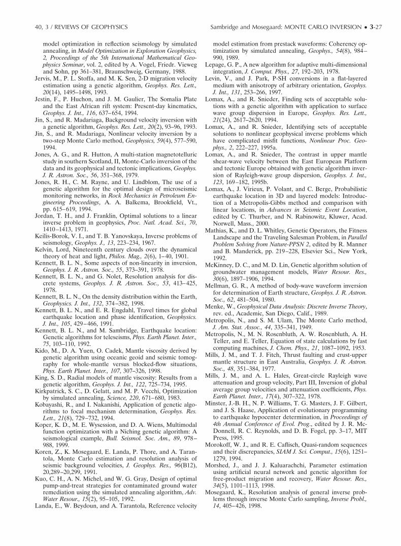
model optimization in reflection seismology by simulatedannealing, in Model Optimization in Exploration Geophysics,2, Proceedings of the 5th International Mathematical Geo-physics Seminar, vol. 2, edited by A. Vogel, Friedr. Viewegand Sohn, pp 361–381, Braunschweig, Germany, 1988.

Jervis, M., P. L. Stoffa, and M. K. Sen, 2-D migration velocityestimation using a genetic algorithm, Geophys. Res. Lett.,20(14), 1495–1498, 1993.

Jestin, F., P. Huchon, and J. M. Gaulier, The Somalia Plateand the East African rift system: Present-day kinematics,Geophys. J. Int., 116, 637–654, 1994.

Jin, S., and R. Madariaga, Background velocity inversion witha genetic algorithm, Geophys. Res. Lett., 20(2), 93–96, 1993.

Jin, S., and R. Madariaga, Nonlinear velocity inversion by atwo-step Monte Carlo method, Geophysics, 59(4), 577–590,1994.

Jones, A. G., and R. Hutton, A multi-station magnetotelluricstudy in southern Scotland, II, Monte-Carlo inversion of thedata and its geophysical and tectonic implications, Geophys.J. R. Astron. Soc., 56, 351–368, 1979.

Jones, R. H., C. M. Rayne, and U. Lindblom, The use of agenetic algorithm for the optimal design of microseismicmonitoring networks, in Rock Mechanics in Petroleum En-gineering Proceedings, A. A. Balkema, Brookfield, Vt.,pp. 615–619, 1994.

Jordan, T. H., and J. Franklin, Optimal solutions to a linearinverse problem in geophysics, Proc. Natl. Acad. Sci., 70,1410–1413, 1971.

Keilis-Borok, V. I., and T. B. Yanovskaya, Inverse problems ofseismology, Geophys. J., 13, 223–234, 1967.

Kelvin, Lord, Nineteenth century clouds over the dynamicaltheory of heat and light, Philos. Mag., 2(6), 1–40, 1901.

Kennett, B. L. N., Some aspects of non-linearity in inversion,Geophys. J. R. Astron. Soc., 55, 373–391, 1978.

Kennett, B. L. N., and G. Nolet, Resolution analysis for dis-crete systems, Geophys. J. R. Astron. Soc., 53, 413–425,1978.

Kennett, B. L. N., On the density distribution within the Earth,Geophysics. J. Int., 132, 374–382, 1998.

Kennett, B. L. N., and E. R. Engdahl, Travel times for globalearthquake location and phase identification, Geophysics.J. Int., 105, 429–466, 1991.

Kennett, B. L. N., and M. Sambridge, Earthquake location:Genetic algorithms for teleseisms, Phys. Earth Planet. Inter.,75, 103–110, 1992.

Kido, M., D. A. Yuen, O. Cadek, Mantle viscosity derived bygenetic algorithm using oceanic geoid and seismic tomog-raphy for whole-mantle versus blocked-flow situations,Phys. Earth Planet. Inter., 107, 307–326, 1998.

King, S. D., Radial models of mantle viscosity: Results from agenetic algorithm, Geophys. J. Int., 122, 725–734, 1995.

Kirkpatrick, S. C., D. Gelatt, and M. P. Vecchi, Optimizationby simulated annealing, Science, 220, 671–680, 1983.

Kobayashi, R., and I. Nakanishi, Application of genetic algo-rithms to focal mechanism determination, Geophys. Res.Lett., 21(8), 729–732, 1994.

Koper, K. D., M. E. Wysession, and D. A. Wiens, Multimodalfunction optimization with a Niching genetic algorithm: Aseismological example, Bull. Seismol. Soc. Am., 89, 978–988, 1999.

Koren, Z., K. Mosegaard, E. Landa, P. Thore, and A. Taran-tola, Monte Carlo estimation and resolution analysis ofseismic background velocities, J. Geophys. Res., 96(B12),20,289–20,299, 1991.

Kuo, C. H., A. N. Michel, and W. G. Gray, Design of optimalpump-and-treat strategies for contaminated ground waterremediation using the simulated annealing algorithm, Adv.Water Resour., 15(2), 95–105, 1992.

Landa, E., W. Beydoun, and A. Tarantola, Reference velocity

model estimation from prestack waveforms: Coherency op-timization by simulated annealing, Geophys., 54(8), 984–990, 1989.

Lepage, G. P., A new algorithm for adaptive multi-dimensionalintegration, J. Comput. Phys., 27, 192–203, 1978.

Levin, V., and J. Park, P-SH conversions in a flat-layeredmedium with anisotropy of arbitrary orientation, Geophys.J. Int., 131, 253–266, 1997.

Lomax, A., and R. Snieder, Finding sets of acceptable solu-tions with a genetic algorithm with application to surfacewave group dispersion in Europe, Geophys. Res. Lett.,21(24), 2617–2620, 1994.

Lomax, A., and R. Snieder, Identifying sets of acceptablesolutions to nonlinear geophysical inverse problems whichhave complicated misfit functions, Nonlinear Proc. Geo-phys., 2, 222–227, 1995a.

Lomax, A., and R. Snieder, The contrast in upper mantleshear-wave velocity between the East European Platformand tectonic Europe obtained with genetic algorithm inver-sion of Rayleigh-wave group dispersion, Geophys. J. Int.,123, 169–182, 1995b.

Lomax, A., J. Virieux, P. Volant, and C. Berge, Probabilisticearthquake location in 3D and layered models: Introduc-tion of a Metropolis-Gibbs method and comparison withlinear locations, in Advances in Seismic Event Location,edited by C. Thurber, and N. Rabinowitz, Kluwer, Acad.Norwell, Mass., 2000.

Mathias, K., and D. L. Whitley, Genetic Operators, the FitnessLandscape and the Traveling Salesman Problem, in ParallelProblem Solving from Nature-PPSN 2, edited by R. Mannerand B. Manderick, pp. 219–228, Elsevier Sci., New York,1992.

McKinney, D. C., and M. D. Lin, Genetic algorithm solution ofgroundwater management models, Water Resour. Res.,30(6), 1897–1906, 1994.

Mellman, G. R., A method of body-wave waveform inversionfor determination of Earth structure, Geophys. J. R. Astron.Soc., 62, 481–504, 1980.

Menke, W., Geophysical Data Analysis: Discrete Inverse Theory,rev. ed., Academic, San Diego, Calif., 1989.

Metropolis, N., and S. M. Ulam, The Monte Carlo method,J. Am. Stat. Assoc., 44, 335–341, 1949.

Metropolis, N., M. N. Rosenbluth, A. W. Rosenbluth, A. H.Teller, and E. Teller, Equation of state calculations by fastcomputing machines, J. Chem. Phys., 21, 1087–1092, 1953.

Mills, J. M., and T. J. Fitch, Thrust faulting and crust-uppermantle structure in East Australia, Geophys. J. R. Astron.Soc., 48, 351–384, 1977.

Mills, J. M., and A. L. Hales, Great-circle Rayleigh waveattenuation and group velocity, Part III, Inversion of globalaverage group velocities and attenuation coefficients, Phys.Earth Planet. Inter., 17(4), 307–322, 1978.

Minster, J.-B. H., N. P. Williams, T. G. Masters, J. F. Gilbert,and J. S. Haase, Application of evolutionary programmingto earthquake hypocenter determination, in Proceedings of4th Annual Conference of Evol. Prog., edited by J. R. Mc-Donnell, R. C. Reynolds, and D. B. Fogel, pp. 3–17, MITPress, 1995.

Morokoff, W. J., and R. E. Caflisch, Quasi-random sequencesand their discrepancies, SIAM J. Sci. Comput., 15(6), 1251–1279, 1994.

Morshed, J., and J. J. Kaluarachchi, Parameter estimationusing artificial neural network and genetic algorithm forfree-product migration and recovery, Water Resour. Res.,34(5), 1101–1113, 1998.

Mosegaard, K., Resolution analysis of general inverse prob-lems through inverse Monte Carlo sampling, Inverse Probl.,14, 405–426, 1998.


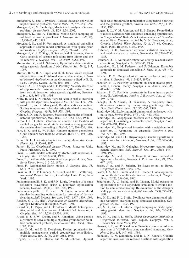
Mosegaard, K., and C. Rygaard-Hjalsted, Bayesian analysis ofimplicit inverse problems, Inverse Probl., 15, 573–583, 1999.

Mosegaard, K., M. Sambridge, Monte Carlo analysis of inverseproblems, Inverse Probl., 18, R29–R54, 2002.

Mosegaard, K., and A. Tarantola, Monte Carlo sampling ofsolutions to inverse problems, J. Geophys. Res., 100(B7),12,431–12,447, 1995.

Mosegaard, K., and P. Vestergaard, A simulated annealingapproach to seismic model optimization with sparse priorinformation, Geophys. Prospect., 39(5), 599–611, 1991.

Mosegaard, K., S. C. Singh, D. Snyder, and H. Wagner, MonteCarlo analysis of seismic reflections from Moho and theW-reflector, J. Geophys. Res., 102, 2,969–2,981, 1997.

Muramatsu, Y., and I. Nakanishi, Hypocenter determinationusing a genetic algorithm, J. Natl. Disaster Sci., 19(1), 1–7,1997.

Muttiah, R. S., B. A. Engel, and D. D. Jones, Waste disposalsite selection using GIS-based simulated annealing, in Neu-ral Network Applications in the Geosciences, edited by B. G.Lees, Comput. Geosci., 22(9), 1013–1017, 1996.

Neves, F. A., S. C. Singh, and K. F. Priestley, Velocity structureof upper-mantle transition zones beneath central Eurasiafrom seismic inversion using genetic algorithms, Geophys.J. Int., 125, 869–878, 1996.

Nolte, B., and L. N. Frazer, Vertical seismic profile inversionwith genetic algorithms, Geophys. J. Int., 117, 162–179, 1994.

Normark, E., and K. Mosegaard, Residual statics estimation:Scaling temperature schedules using simulated annealing,Geophys. Prospect., 41(5), 565–578, 1993.

Nulton, J. D., and P. Salamon, Statistical mechanics of combi-natorial optimization, Phys. Rev., A37, 1351–1356, 1988.

Pardo, I. E., Optimal selection of number and location ofrainfall gauges for areal rainfall estimation using geostatis-tics and simulated annealing, J. Hydrol., 210, 206–220, 1998.

Park, S. K., and K. W. Miller, Random number generators:Good ones are hard to find, Commun. ACM, 31, 1192–1201,1988.

Parker, R. L., Understanding inverse theory, Annu. Rev. EarthPlanet. Sci., 5, 35–64, 1977.

Parker, R. L., Geophysical Inverse Theory, Princeton Univ.Press, Princeton, N. J., 1994.

Press, F., Earth models obtained by Monte Carlo inversion, J.Geophys. Res., 73, 5223–5234, 1968.

Press, F., Earth models consistent with geophysical data, Phys.Earth Planet. Inter., 3, 3–22, 1970a.

Press, F., Regionalized Earth models, J. Geophys. Res., 75,6575–6581, 1970b.

Press, W. H., B. P. Flannery, A. T. Saul, and W. T. Vetterling,Numerical Recipes, 2nd ed., Cambridge Univ. Press, NewYork, 1992.

Pullammanappallil, S. K., and J. N. Louie, Inversion of seismicreflection traveltimes using a nonlinear optimizationscheme, Geophys., 58(11), 1607–1620, 1993.

Pullammanappallil, S. K., and J. N. Louie, A generalizedsimulated-annealing optimization for inversion of first-ar-rival times, Bull. Seismol. Soc. Am., 84(5), 1397–1409, 1994.

Rawlins, G. J. E., (Ed.), Foundations of Genetics Algorithms,Morgan Kaufmann Burlington, Mass., 1991.

Ricard, Y., C. Vigny, and C. Froidevaux, Mantle heterogene-ities, geoid, and plate motion: A Monte Carlo inversion, J.Geophys. Res., 94, 13,739–13,754, 1989.

Ritzel, B. J., J. W. Eheart, and S. Ranjithan, Using geneticalgorithms to solve a multiple objective groundwater pollu-tion containment problem, Water Resour. Res., 30(5), 1589–1603, 1994.

Rizzo, D. M., and D. E. Dougherty, Design optimization formultiple management period groundwater remediation,Water Resour. Res., 31(8), 2549–2561, 1996.

Rogers, L. L., F. U. Dowla, and V. M. Johnson, Optimal

field-scale groundwater remediation using neural networksand the genetic algorithm, Environ. Sci. Tech., 29(5), 1145–1155, 1995.

Rogers, L. L., V. M. Johnson, and R. B. Knapp, Remediationtradeoffs addressed with simulated annealing optimization,in Computational Methods in Contamination and Remedia-tion of Water Resources, edited by V. N. Burganos, et al.,Comput. Methods Water Resour., 12(1), 59–66, Comput.Mech. Publ., Billerica, Mass., 1998.

Rothman, D. H., Nonlinear inversion statistical mechanics,and residual statics corrections, Geophysics, 50, 2784–2796,1985.

Rothman, D. H., Automatic estimation of large residual staticscorrections, Geophysics, 51, 332–346, 1986.

Ruppeiner, G., J. M. Pedersen, and P. Salamon, Ensembleapproach to simulated annealing, J. Phys., 1(1), 455–470,1991.

Sabatier, P. C., On geophysical inverse problems and con-straints, J. Geophys., 43, 115–137, 1977a.

Sabatier, P. C., Positivity constraints in linear inverse prob-lems, I, General theory, Geophys. J. R. Astron. Soc., 48,415–441, 1977b.

Sabatier, P. C., Positivity constraints in linear inverse prob-lems, II, Applications, Geophys. J. R. Astron. Soc., 48, 443–459, 1977c.

Sadeghi, H., S. Suzuki, H. Takenaka, A two-point, three-dimensional seismic ray tracing using genetic algorithms,Phys. Earth Planet. Inter., 113, 355–365, 1999.

Sambridge, M., Exploring multi-dimensional landscapes with-out a map, Inverse Probl., 14(3), 427–440, 1998.

Sambridge, M., Geophysical inversion with a Neighbourhoodalgorithm, I, Searching a parameter space, Geophys. J. Int.,138, 479–494, 1999a.

Sambridge, M., Geophysical inversion with a neighbourhoodalgorithm, II, Appraising the ensemble, Geophys. J. Int.,138, 727–746, 1999b.

Sambridge, M., and G. G. Drijkoningen, Genetic algorithms inseismic waveform inversion, Geophys. J. Int., 109, 323–342,1992.

Sambridge, M., and K. Gallagher, Hypocentre location usinggenetic algorithms, Bull. Seismol. Soc. Am., 83(5), 1467–1491, 1993.

Sambridge, M., and B. L. N. Kennett, A novel method ofhypocentre location, Geophys. J. R. Astron. Soc., 87, 679–697, 1986.

Scales, J. A., and R. Snieder, To Bayes or not to Bayes,Geophysics, 62, 1045–1046, 1997.

Scales, J. A., M. L. Smith, and T. L. Fischer, Global optimiza-tion methods for multimodal inverse problems, J. Comput.Phys., 103(2), 258–268, 1992.

Scherbaum, F., C. Palme, and H. Langer, Model parameteroptimization for site-dependent simulation of ground mo-tion by simulated annealing: Re-evaluation of the AshigaraValley prediction experiment, Nat. Hazards, 10(3), 275–296,1994.

Sen, M. K., and P. L. Stoffa, Nonlinear one-dimensional seis-mic waveform inversion using simulated annealing, Geo-physics, 56, 1624–1638, 1991.

Sen, M. K., and P. L. Stoffa, Rapid sampling of model spaceusing genetic algorithms, Geophys. J. Int., 108, 281–292,1992.

Sen, M. K., and P. L. Stoffa, Global Optimization Methods inGeophysical Inversion, Adv. Explor. Geophys., vol. 4,Elsevier Sci., New York, 1995.

Sharma, S. P., and P. Kaikkonen, Two-dimensional non-linearinversion of VLF-R data using simulated annealing, Geo-phys. J. Int., 133, 649–668, 1998.

Shibutani, T., M. Sambridge, and B. L. N. Kennett, Geneticalgorithm inversion for receiver functions with application


to crust and uppermost mantle structure beneath easternAustralia, Geophys. Res. Lett., 23, 1829–1832, 1996.

Sileny, J., Earthquake source parameters and their confidenceregions by a genetic algorithm with a “memory,” Geophys.J. Int., 134, 228–242, 1998.

Simpson, A. R., and S. D. Priest, The application of geneticalgorithms to optimisation problems in geotechnics, Com-put. Geotech., 15(1), 1–19, 1993.

Smith, A. F. M., Bayesian computational methods, Philos.Trans. R. Soc. London Ser. A, 337, 369–386, 1991.

Smith, A. F. M., and G. O. Roberts, Bayesian Computation viathe Gibbs Sampler and Related Markov Chain MonteCarlo Methods, J. R. Stat. Soc, Ser. B., 55, 3–23, 1993.

Smith, M. L., J. A. Scales, and T. L. Fischer, Global search andgenetic algorithms, Leading Edge, 11, 22–26, 1992.

Snieder, R., and J. Trampert, Inverse problems in geophysics,in Wavefield Inversion, edited by A. Wirgin, pp. 119–190,Springer-Verlag, New York, 1999.

Sobol, I. M., On the distribution of points in a cube and theapproximate evaluation of integrals, USSR Comput. Math.Math. Phys., 7(4), 86–112, 1967.

Stark, P. B., Minimax confidence intervals in geomagnetism,Geophys. J. Int., 108, 329–338, 1992.

Steck, L. K., Simulated annealing inversion of teleseismicP-wave slowness and azimuth for crustal velocity structureat Long Valley Caldera, Geophys. J. Int., 22, 497–500, 1995.

Stoffa, P. L., and M. K. Sen, Nonlinear multiparameter opti-mization using genetic algorithms: Inversion of plane waveseismograms, Geophys, 56, 1794–1810, 1991.

Szu, H., and R. Hartley, Fast simulated annealing, Phys. Lett.,Ser., A. 122, 157–162, 1987.

Tang, A., and L. W. Mays, Genetic algorithms for optimaloperation of soil aquifer treatment systems, Water Resour.Manage., 12(5), 375–396, 1998.

Tanner, M. A., Tools for Statistical Inference: Methods for theExploration of Posterior Distributions and Likelihood Func-tions, 3rd ed., Springer-Verlag, New York, 1996.

Tarantola, A., Inverse Problem Theory, Elsevier Sci., New York,1987.

Tarantola, A., and B. Valette, Inverse problems quest forinformation, J. Geophys., 50, 159–170, 1982a.

Tarantola, A., and B. Valette, Generalized nonlinear inverseproblems solved using the least squares criterion, Rev. Geo-phys. Space Phys., 20(2), 219–232, 1982b.

Thomson, W. E., Analogue computers for stochastic processes,in Abbrev. Processes of the Oxford Math, Conference forSchoolteachers and Industrialists, pp. 54–57, The TimesPubl., London, 1957.

Tierney, L., Markov chains for exploring posterior distribu-tions, Ann. Stat., 22, 1701–1762, 1994.

Valius, V. P., Opredelenie seismicheskikh razrezov po sovok-upnosti nabludenii, (Determination of seismological sec-tions through ensemble control), Vichislitelnaya Seismol., 4,3–14, 1968.

van der Beek, P., and J. Braun, Control on post-mid Creta-ceous landscape evolution in the southeastern highlands ofAustralia: Insights from numerical surface process models,J. Geophys. Res., 104, 4945–4966, 1999.

Varela, C. L., P. L. Stoffa, and M. K. Sen, Background velocityestimation using non-linear optimization for reflection to-mography and migration misfit, Geophys. Prospect., 46(1),51–78, 1998.

Vasco, D. W., L. R. Johnson, and E. L. Majer, Ensembleinference in geophysical inverse problems, Geophys. J. Int.,117, 711–728, 1993.

Vasudevan, K., and W. G. Wilson, Simulated annealing staticscomputation using an order-based energy function, Geo-phys., 56(11), 1831–1839, 1991.

Velis, D. R., and T. J. Ulrych, Simulated annealing two-pointray tracing, Geophys. Res. Lett., 32(2), 201–204, 1996.

Vestergaard, P., and K. Mosegaard, Inversion of post-stackseismic data using simulated annealing, Geophys. Prospect.,39(5), 613–624, 1991.

Vinther, R., and K. Mosegaard, Seismic inversion throughTabu Search, Geophys. Prospect., 44(4), 555–570, 1996.

Wan, Y., R. Liu, and H. Li, The inversion of 3-D crustalstructure and hypocenter location in the Beijing-Tianjin-Tangshan-Zhangjiakou area by genetic algorithm, ActaSeismol. Sin., 10(6), 769–781, 1997.

Whitley, D. L., A genetic algorithm tutorial, Stat. Comput., 4,65–85, 1994.

Wiggins, R. A., Monte Carlo inversion of body wave observa-tions, J. Geophys. Res., 74, 3171–3181, 1969.

Wiggins, R. A., The general inverse problem: Implication ofsurface waves and free oscillations for Earth Structure, Rev.Geophys., 10, 251–285, 1972.

Wilson, W. G., K. Vasudevan, Application of the geneticalgorithm to residual statics estimation, Geophys. Res. Lett.,18, 2181–2184, 1991.

Winter, G., J. Periaux, M. Galan, and P. Cuesta, (Eds.), Ge-netic Algorithms in Engineering and Computer Science, JohnWiley, New York, 1995.

Worthington, M. H., J. R. Cleary, and R. S., Anderssen,Density modelling by Monte Carlo inversion, II, Compari-son of recent Earth models, Geophys. J. R. Astron. Soc., 29,445–457, 1972.

Worthington, M. H., J. R. Cleary, and R. S., Anderssen, Upperand lower mantle shear velocity modelling by Monte Carloinversion, Geophys. J. R. Astron. Soc., 36, 91–103, 1974.

Yamanaka, H., and H. Ishida, Applicaton of genetic algo-rithms to an inversion of surface-wave dispersion data, Bull.Seismol. Soc. Am., 86(2), 436–444, 1996.

Yu, T. T., J. Fernandez, and J. B. Rundle, Inverting theparameters of an earthquake-ruptured fault with a geneticalgorithm, Comput. and Geosci., 24(2), 173–182, 1998.

Zhao, L. S., M. K. Sen, P. L. Stoffa, and C. Frohlich, Appli-cation of very fast simulated annealing to the determinationof the crustal structure beneath Tibet, Geophys. J. Int., 125,355–370, 1996.

Zheng, C., P. Wang, Parameter structure identification usingtabu search and simulated annealing, Adv. Water Resour.,19(4), 215–224, 1996.

Zhou, R., F. Tajima, and P. L. Stoffa, Earthquake sourceparameter determination using genetic algorithms, Geo-phys. Res. Lett., 22(4), 517–520, 1995a.

Zhou, R., F. Tajima, and P. L. Stoffa, Application of geneticalgorithms to constrain near-source velocity structure forthe 1989 Sichuan earthquakes, Bull. Seismol. Soc. Am.,85(2), 590–605, 1995b.

K. Mosegaard, Neils Bohr Institute for Astronomy, Physics,and Geophysics, Department of Geophysics, University ofCopenhagen, Juliane Maries Vej 30, DK-2100 Copenhagen 0,Denmark. ([email protected])

M. Sambridge, Research School of Earth Sciences, Instituteof Advanced Studies, Australian National University, CanberraACT 0200, Australia. ([email protected])


Documents

MONTE CARLO METHODS IN GEOPHYSICAL INVERSE PROBLEMSrses.anu.edu.au/~malcolm/papers/pdf/SamMos02.pdf · MONTE CARLO METHODS IN GEOPHYSICAL INVERSE ... Physics and Geophysics ... and