Monte Carlo Ray Tracing - Cornell University · Monte Carlo integration • If I do this many times, what is the expected value? – when there are ﬁnitely many possibilities, outcome

© 2013 Steve Marschner • Cornell CS4620 Spring 2013 • Lecture 22

Monte Carlo Ray Tracing

CS 4620 Lecture 22

1


Basic ray tracing

• Many advanced methods build on the basic ray tracing paradigm• Basic ray tracer: one sample for everything

– one ray per pixel– one shadow ray for every point light– one reflection ray, possibly one refraction ray, per intersection

2


Basic ray traced image

[Gla

ssne

r 89

]

3


Discontinuities in basic RT

• Perfectly sharp object silhouettes in image– leads to aliasing problems (stair steps)

• Perfectly sharp shadow edges– everything looks like it’s in direct sun

• Perfectly clear mirror reflections– reflective surfaces are all highly polished

• Perfect focus at all distances– camera always has an infinitely tiny aperture

• Perfectly frozen instant in time (in animation)– motion is frozen as if by strobe light

4


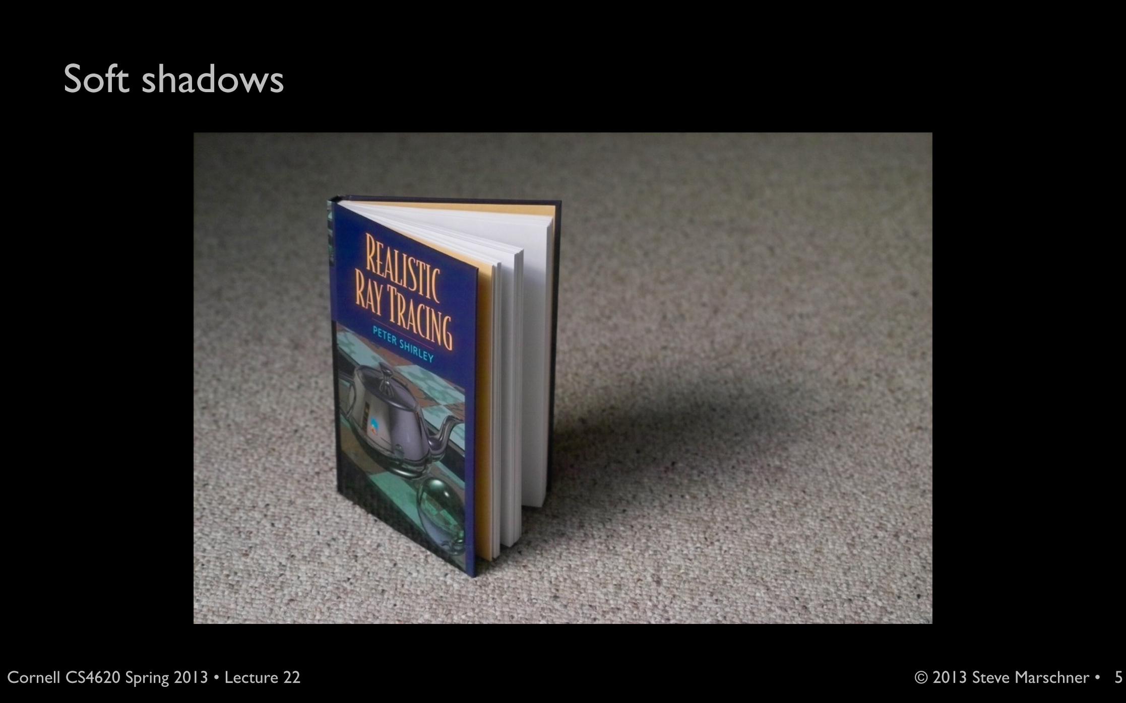
Soft shadows

5


Cause of soft shadows

point lights cast hard shadows

6


Cause of soft shadows

area lights cast soft shadows

7


Glossy reflection

[Laf

ortu

ne e

t al

. 97]

8


Cause of glossy reflection

smooth surfaces produce sharp reflections

9


Cause of glossy reflection

rough surfaces produce soft (glossy) reflections

10


Depth of field

11


Cause of focusing effects

what lenses do (roughly)

12



point aperture produces always-sharp focus

13



finite aperture produces limited depth of field

14


Motion blur

[Coo

k, P

orte

r, C

arpe

nter

198

4]

15


Cause of motion blur

16

© 2013 Steve Marschner • Cornell CS4620 Spring 2013 • Lecture 22 17Pixar—Monsters University (2013)


Creating soft shadows

• For area lights: use many shadow rays– and each shadow ray gets a different point on the light

• Choosing samples– general principle: start with uniform in square

18


Creating glossy reflections

• Jitter the reflected rays– Not exactly in mirror direction; add a random offset– Can work out math to match Phong exactly– Can do this by jittering the normal if you want

19


Depth of field

• Make eye rays start at random points on aperture– always going toward a point on the focus plane

20


Motion blur

• Caused by finite shutter times– strobing without blur

• Introduce time as a variable throughout the system– object are hit by rays according to their position at a given time

• Then generate rays with times distributed over shutter interval

21


But how, exactly?

• A key tool for getting all these effects accurately in a ray tracer is Monte Carlo integration

• Step 1: all these effects are actually integration problems• Step 2: they can be solved using Monte Carlo integration

22

I(x) =1

|t1 � t0|

Z t1

t0

L(p,d(x), t)dtI(x) = L(p,d(x), t0)


Motion blur by integration

23

instantaneous lightmeasurement

light averaged overshutter interval

x

p

d

L(x,v) =I cos ✓

r2L(x,v) =

1

|S|

Z

S

I cos ✓

r2dA


Soft shadows by integration

24

illumination from single point

illumination averaged overlight source area

(for those counting: I have hidden a cosine factor in I, don’t worry about it today)

S

x

vr

I(x) = L(p,d(x)) I(x) =1

|D|

Z

DL(p,d(x,p))dA(p)


Depth of field by integration

25

D

x

x

pp

dd

light along a single ray

light averaged overrays through aperture


Monte Carlo integration

• How to integrate a function we don’t know much about?– we can only evaluate it by tracing rays– reasoning about how light changes from one ray to the next is tricky

• Idea: evaluate at a random place and call use that sample to make an estimate of the average value (and thereby integral) of the function

26

t0 t1t

f(t)

g(t) = f(t)|t1 � t0|

Knowing only the value at tand the size of the intervalmy best estimate of the integralis:



• If I do this many times, what is the expected value?– when there are finitely many possibilities, outcome k will happen in a fraction

p(k) of trials, hence

– in our continuous case this becomes an integral

– for the estimator on the previous slide

27

E{g(t)} =

Z t1

t0

g(t)p(t)dt

E{g[k]} =X

k

g[k]p[k]

here p(t) is a probability density for outcomes around t

here p(k) is the probability of outcome k

E{g(t)} = E{f(t)|t1 � t0|} =

Z t1

t0

f(t)|t1 � t0| p(t) dt

=

Z t1

t0

f(t) dt

but p(t) =1

|t1 � t0|



• In general Monte Carlo integration works like this– choose x randomly in some domain D with some probability density p(x)– evaluate f(x) and form the estimator

– the expected value of g(x) will then be

• Get better and better approximations to that expected value by averaging together a lot of independent samples

28

g(x) =f(x)

p(x)

E{g(x)} =

Z

Df(x) dx


Monte Carlo in rendering

• Motion blur: select random t in the shutter interval

• Depth of field: select random p uniformly over the aperture D

• Area light: select source point y uniformly over the light source S

29

g(t) = L(p,d(x), t) |t1 � t0|

g(p) = L(p,d(x,p)) |D|

g(y) =I cos ✓(y)

r(y)2|S|


Monte Carlo for surface reflection

• Key integral to be evaluated is

– and a common approach is to sample with

30

p(w) / fr(v,w)

L(x,v) =

Z

H2

fr(v,w)Li(x,w)(w · n) dw


The Blue Umbrella

• Latest Pixar short• Made partly to showcase new

more photorealistic rendering– much of it based on the ideas we saw

in this lectureworth a look:http://rainycitytales332.tumblr.com

31

http://rainycitytales332.tumblr.com

http://rainycitytales332.tumblr.com

Documents

Monte Carlo Ray Tracing - Cornell University · Monte Carlo integration • If I do this many times, what is the expected value? – when there are ﬁnitely many possibilities, outcome