Monte Carlo Simulationapalczew/CFP_lecture4.pdf · Monte Carlo simulation on Z. In this context Y is called the control variate. Computational Finance – p. 25. Since adding a constant

Lecture 4

Monte Carlo Simulation

Lecture Notes

by Jan Palczewski

with additionsby Andrzej Palczewski

Computational Finance – p. 1

We know from Discrete Time Finance that one can computea fair price for an option by taking an expectation

EQ

(

e−rTX)

Therefore, it is important to have algorithms to compute theexpectation of a random variable with a given distribution.In general, we cannot do it precisely – there is only an ap-proximation on our disposal.

In previous lectures we studied methods to generate inde-pendent realizations of a random variable. We can use thisknowledge to generate a sample from a distribution of X.

Main theoretical ingredients that allow to compute approxi-mations of expectation from a sample of a given distributionare provided by the Law of Large Numbers and the CentralLimit Theorem.


Let X1, X2, . . . be a sequence of independent identically dis-tributed random variables with expected value µ and vari-

ance σ2. Define the sequence of averages

Yn =X1 +X2 + · · · +Xn

n, n = 1, 2, . . . .

(Law of Large Numbers) Yn converges to µ almost surelyas n→ ∞.

Let

Zn =(X1 − µ) + (X2 − µ) + · · · + (Xn − µ)√

n.

(Central Limit Theorem) The distribution of Zn converges

to N(0, σ2).


Assume we have a random variable X with unknown expec-tation and variance

a = EX, b2 = VarX.

We are interested in computing an approximation to a andpossibly b.

Suppose we are able to take independent samples of Xusing a pseudo-random number generator.

We know from the strong law of large number, that the aver-age of a large number of samples can give a good approxi-mation to the expected value.


Therefore, if we let X1, X2, . . . , XM denote a sample from adistribution of X, one might expect that

aM =1

M

M∑

i=1

Xi

is a good approximation to a.

To estimate variance we use the following formula (noticethat we divide by M − 1 and not by M )

b2M =

∑Mi=1(Xi − aM )2

M − 1.


Assessment of the precision

of estimation of a and b2

By the central limit theorem we know that∑M

i=1Xi behaves

approximately like a N (Ma,Mb2) distributed random vari-able.Therefore

aM − a is approximately N (0,b2

M).

In other words

aM − a ∼ b√MZ,

where Z ∼ N (0, 1).

Therefore aM converges to a with speed O(

b√M

)

.Computational Finance – p. 6

More quantitative

P

(

a− 1.96b√M

≤ aM ≤ a+1.96b√M

)

= 0.95.

This is equivalent to

P

(

aM − 1.96b√M

≤ a ≤ aM +1.96b√M

)

= 0.95.

Replacing the unknown b by the approximation bM we seethat the unknown expected value a lies in the interval

[

aM − 1.96 bM√M

,aM +1.96 bM√

M

]

approximately with probability 0.95.

The interval above is called a 95 percent confidence inter-val. Computational Finance – p. 7

Confidence intervals explained

If Z ∼ N(µ, σ2) then

P(µ− 1.96σ < Z < µ+ 1.96σ) = 0.95

because

Φ(1.96) = 0.975

To construct a confidence interval with a confidence level αdifferent from 0.95, we have to find a number A such that

φ(A) = 1− 1− α

2.

Then the α-confidence interval

P(µ− Aσ < Z < µ+ Aσ) = α.


The width of the confidence interval is a measure ofthe accuracy of our estimate.

In 95% of cases the true value lies in the confidenceinterval.

Beware! In 5% of cases it is outside the interval!

The width of the confidence interval depends on twofactors:

Number of simulations M

Variance of the variable X


[

aM − 1.96 bM√M

,aM +1.96 bM√

M

]

1. The size of the confidence interval shrinks like the in-verse square root of the number of samples. This isone of the main disadvantages of Monte Carlo method.

2. The size of the confidence interval is directly propor-tional to the standard deviation of X. This indicatesthat Monte Carlo method works the better, the smallerthe variance of X is. This leads to the idea of variancereduction, which we shall discuss later.


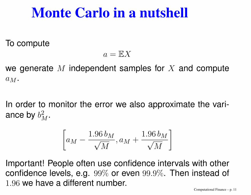
Monte Carlo in a nutshell

To compute

a = EX

we generate M independent samples for X and computeaM .

In order to monitor the error we also approximate the vari-

ance by b2M .

[

aM − 1.96 bM√M

,aM +1.96 bM√

M

]

Important! People often use confidence intervals with otherconfidence levels, e.g. 99% or even 99.9%. Then instead of1.96 we have a different number.


Monte Carlo put into action

We can now apply Monte Carlo simulation for the computa-tion of option prices.

We consider a European-style option ψ(ST ) with the payofffunction ψ depending on the terminal stock price.

We assume that under a risk-neutral measure the stockprice St at t ≥ 0 is given by

St = S0 exp

((r − 1

2σ2)t+ σWt

)

.

Here Wt is a Brownian motion.


We know that Wt ∼√tZ with Z ∼ N (0, 1).

We can therefore write the stock price at expiry T as

ST = S0 exp

((r − 1

2σ2)T + σ

√TZ

)

.

We can compute a fair price for ψ(ST ) taking the discountedexpectation

E[

e−rTψ(

S0e(r− 1

2σ2)T+σ

√TZ)]

This expectation can be computed via Monte Carlo methodwith the following algorithm


✬

✫

✩

✪

for i = 1 to Mcompute an N (0, 1) sample ξiset Si = S0 exp

((r − 1

2σ2)T + σ

√Tξi)

set Vi = e−rTψ(Si)endset aM = 1

M

∑Mi=1 Vi

The output aM provides an approximation of the optionprice. To assess the quality of our computation, we com-pute an approximation to the variance

b2M =1

M − 1

∑

i

(Vi − aM )2

to construct a confidence interval.


Confidence intervals v. sample size


Variance Reduction Techniques

Antithetic Variates

Control Variate

Importance Sampling (not discussed here)

Stratified Sampling (not discussed here)


We have seen before that the size of the confidence intervalis determined by the value of

√

Var(X)√M

,

where M is the sample size.

We would like to find a method to decrease the width ofthe confidence interval by other means than increasing thesample size M .

A simple idea is to replace X with a random variable Ywhich has the same expectation, but a lower variance.

In this case we can compute the expectation of X via MonteCarlo method using Y instead of X.

Since the variance of Y is lower than the variance of X theresults are better.


The question is how we can find such a random variable Ywith a smaller variance that X and the same expectation.

There are two main methods to find Y :

a method of antithetic variates

a method of control variates


Antithetic VariatesThe idea is as follows. Next to X consider a random variable Z

which has the same expectation and variance as X but is negative

correlated with X, i.e.

cov(X,Z) ≤ 0.

Now take as Y the random variable

Y =X + Z

2.

Obviously E(Y ) = E(X). On the other hand

Var(Y ) = cov

(X + Z

2,X + Z

2

)

=1

4

(Var(X) + 2 cov(X,Z)

︸︷︷︸

≤0

+Var(Z)︸︷︷︸

=Var(X)

)≤ 1

2Var(X).

With this we can reduce the variance by a factor of 2.Computational Finance – p. 19

On the way to find Z...

In the extreme case, if we would know that E(X) = 0, wecould just take Z = −X. Then Y = 0 would give the rightresult, even deterministically.

The equality above would then trivially hold

cov(X,−X) = −Var(X).

But in general we don’t know the expectation.

The expectation is what we want to compute, so this naiveidea is not applicable.

But it puts us on the right track!


The following Lemma is a step further to identify a suitablecandidate for Z and hence for Y .

Lemma. Let X be an arbitrary random variable and f amonotonically increasing or monotonically decreasing func-tion, then

cov(f(X), f(−X)) ≤ 0.

Let us now consider the case of a random variable which isof the form f(U), where U is a standard normal distributedrandom variable, i.e. U ∼ N (0, 1).

The standard normal distribution is symmetric, and hencealso −U ∼ N (0, 1).

It then follows obviously that f(U) ∼ f(−U).In particular they have the same expectation !


Therefore, in order to compute the expectation of X = f(U),we can take Z = f(−U) and define

Y =f(U) + f(−U)

2.

If we now assume that the map f is monotonically increas-ing, then we conclude from the previous Lemma that

cov(f(U), f(−U)

)≤ 0

and we finally obtain

E

(f(U) + f(−U)

2

)

= E(f(U)),

Var

(f(U) + f(−U)

2

)

<1

2Var(f(U)).


Implementation

✬

✫

✩

✪

for i = 1 to Mcompute an N (0, 1) sample ξiset S+

i = S0 exp((r − 1

2σ2)T + σ

√Tξi)

set S−i = S0 exp

((r − 1

2σ2)T − σ

√Tξi)

set V +i = e−rTψ(S+

i )

set V −i = e−rTψ(S−

i )

set Vi = (V +i + V −

i )/2

endset aM = 1

M

∑Mi=1 Vi

The output aM provides an approximation of the optionprice.


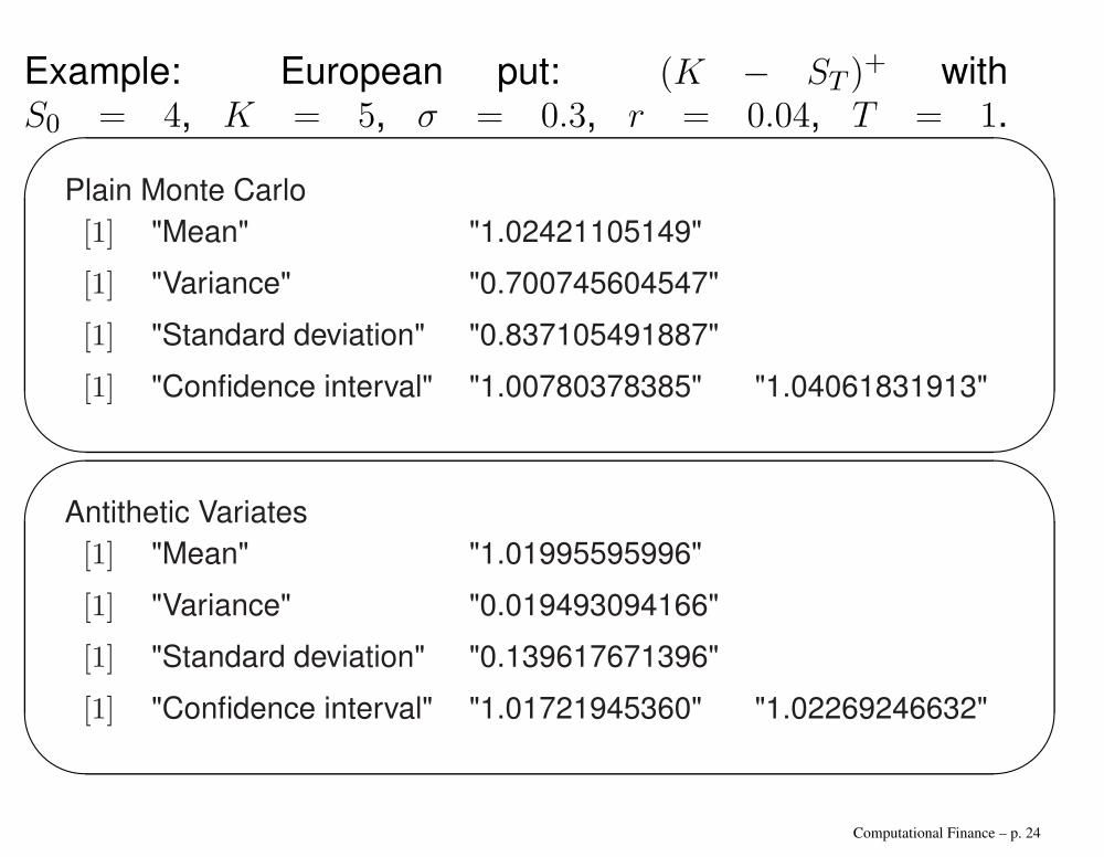
Example: European put: (K − ST )+ with

S0 = 4, K = 5, σ = 0.3, r = 0.04, T = 1.✬

✫

✩

✪

Plain Monte Carlo

[1] "Mean" "1.02421105149"

[1] "Variance" "0.700745604547"

[1] "Standard deviation" "0.837105491887"

[1] "Confidence interval" "1.00780378385" "1.04061831913"

✬

✫

✩

✪

Antithetic Variates

[1] "Mean" "1.01995595996"

[1] "Variance" "0.019493094166"

[1] "Standard deviation" "0.139617671396"

[1] "Confidence interval" "1.01721945360" "1.02269246632"


Control Variates

Given that we wish to estimate E(X), suppose that we cansomehow find another random variable Y which is close toX in some sense and has known expectation E(Y ).

Then the random variable Z defined by

Z = X + E(Y )− Y

obviously satisfies

E(Z) = E(X).

We can therefore obtain the desired value E(X) by runningMonte Carlo simulation on Z.

In this context Y is called the control variate.


Since adding a constant to a random variable does notchange its variance, we see that

Var(Z) = Var(X − Y ).

Therefore, in order to get some benefit from this approachwe would like X − Y to have a small variance.

This is what we mean by ”close in some sense” from theprevious slide.

There is in general no clear candidate for a control variate,this depends on the particular problem. Intuition is needed !


Fine-tuning the Control Variate

Given that we have a candidate Y for a control variate, wecan define for any θ ∈ R

Zθ = X + θ(E(Y )− Y ).

We still have E(Z) = E(X), so we may apply Monte Carlo toZθ in order to compute E(X).

We have

Var(Zθ) = Var(X − θY ) = Var(X)− 2θ cov(X,Y ) + θ2Var(Y )

We can consider this as a function of θ and look for theminimizer.


It is easy to see that the minimizer is given by

θmin =cov(X,Y )

Var(Y )

One can furthermore show that Var(Zθ) < Var(X) if and onlyif θ ∈ (0, 2 θmin).

In general, however, the expression cov(X,Y ) which is usedto compute θmin is not known.

The idea is to run Monte Carlo, where in a first stepcov(X,Y ) is computed via Monte Carlo method with loweraccuracy and the approximation is then used in a secondstep in order to compute E(Zθ) = E(X) by Monte Carlomethod as indicated above.


Underlying asset as control variate

If S(t) is an asset price then exp(−rt)S(t) is a martingaleand

E[exp(−rT )S(T )] = S(0).

Suppose we are pricing an option on S with discounting pay-off Y . From independent replications Si, i = 1, . . . ,M , wecan form the control variate estimator

1

M

M∑

i=1

(

Yi −(Si − erTS(0)

))

.


Hedge control variates

Because the payoff of a hedged portfolio has a lower stan-dard deviation than the payoff of an unhedged one, usinghedges can reduce the volatility of the value of the portfolio.

A delta hedge consists of holding ∆ = ∂C/∂S shares inthe underlying asset, which is rebalanced at the discretetime intervals. At time T , the hedge consists of the savingsaccount and the asset, which closely replicates the payoffof the option. This gives

C(t0)er(T−t0) −

n∑

i=0

(∂C(ti)

∂S− ∂C(ti−1)

∂S

)

Stier(T−ti) = C(T ),

where ∂C(t−1/∂S = ∂C(tn)/∂S = 0.Computational Finance – p. 30

After rearranging terms we get

C(t0)er(T−t0)+

n−1∑

i=0

∂C(ti)

∂S

(Sti+1−Stier(ti+1−ti)

)er(T−ti+1) = C(T ).

Because the term

CV =

n−1∑

i=0

∂C(ti)

∂S

(Sti+1 − Stie

r(ti+1−ti))er(T−ti+1)

is a martingale due to the known property that option priceis a value of the hedging portfolio, the mean of CV is zero.


We can use than CV as a control variate.

When we are pricing a call option on S with discounting pay-

off C(T ) = (ST − K)+, then from independent replications

SjT , CV j , j = 1, . . . ,M , we can form the control variate esti-

mator

C(t0)er(T−t0) =

1

M

M∑

j=1

(

Cj(T )− CV j)

.


Example: Average Asian option

Asian options are options where payoff depends on the av-erage price of the underlying asset during at least some partof the life of the option. The payoff from the average call is

max(Save −K, 0) = (Save −K)+

and that from the average put is

max(K − Save, 0) = (K − Save)+,

where Save is the average value of the underlying asset cal-culated over a predetermined averaging period.


Asian Options and Control Variates

The average call option traded on the market has a payoffof the form

(

1

n

n∑

i=1

Sti −K

)+

Even in the most elementary Black-Scholes model, there isno analytic expression for this price.

On the other hand, for the corresponding geometric averageAsian option

(( n∏

i=1

Sti

) 1n

−K

)+

there is an analytic formula similar to Black-Scholes formula.


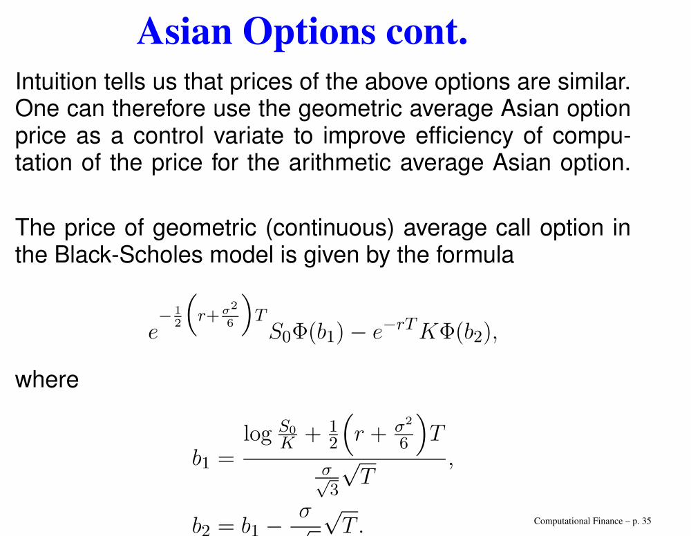
Asian Options cont.

Intuition tells us that prices of the above options are similar.One can therefore use the geometric average Asian optionprice as a control variate to improve efficiency of compu-tation of the price for the arithmetic average Asian option.

The price of geometric (continuous) average call option inthe Black-Scholes model is given by the formula

e− 1

2

(

r+σ2

6

)

TS0Φ(b1)− e−rTKΦ(b2),

where

b1 =log S0

K + 12

(

r + σ2

6

)

T

σ√3

√T

,

b2 = b1 −σ√3

√T . Computational Finance – p. 35

Algorithm

Let P be the price of the geometric average option in B-Smodel (where an analytic formula is available).For k = 1, 2, . . . ,M simulate sample paths

(S(k)t0 , S

(k)t1 , . . . , S

(k)tn ) and calculate

Ak = e−rT(1

n

n∑

i=1

S(k)ti −K

)+

, Gk = e−rT

(( n∏

i=1

S(k)ti

) 1n

−K)+

Then calculate Xk = Ak − (Gk − P ).Price is estimated by

aM =1

M

M∑

k=1

Xk

and the confidence interval ...Computational Finance – p. 36

Asian option improved

It appears that the formula for the geometric (continuous)average call option gives the price which differs by almost1% from the price obtained by MC simulations. This pricediscrepancy can be explained by the fact that in the MC sim-ulation we use discrete geometric averaging and not contin-uous. Fortunately we can also derive in the Black-Scholesmodel an analytic formula for the geometric discrete aver-age call option.


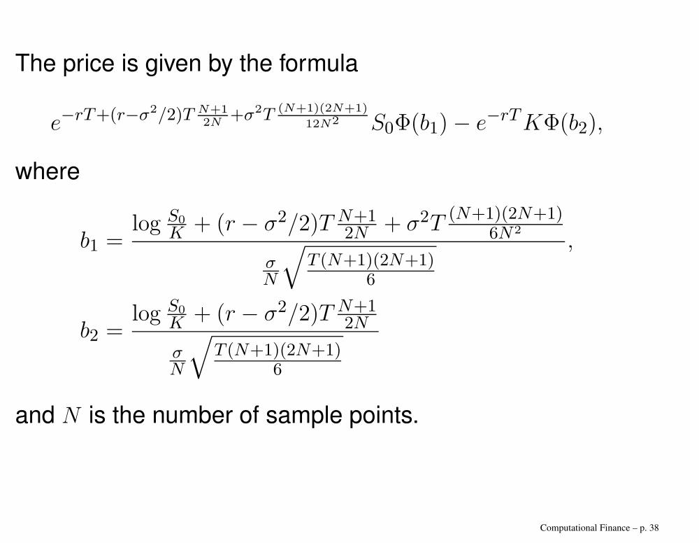
The price is given by the formula

e−rT+(r−σ2/2)T N+12N

+σ2T (N+1)(2N+1)

12N2 S0Φ(b1)− e−rTKΦ(b2),

where

b1 =log S0

K + (r − σ2/2)T N+12N + σ2T

(N+1)(2N+1)6N2

σN

√T (N+1)(2N+1)

6

,

b2 =log S0

K + (r − σ2/2)T N+12N

σN

√T (N+1)(2N+1)

6

and N is the number of sample points.


Other applications of the control variate technique:

valuation of options with "strange" payoffs,

American options,

various path-dependent options.


Random walk construction

We focus on simulating values (W (t1), . . . ,W (tn)) at a fixedset of points 0 < t1 < · · · < tn.Let Z1, . . . , Zn be independent standard normal random vari-ables.For a standard Brownian motion W (0) = 0 and subsequentvalues are generated as follows

W (ti+1) =W (ti) +√

ti+1 − tiZi+1, i = 0, . . . , n− 1.

For log-normal stock prices and equidistributed time pointsti+1 − ti = δt, for i = 0, . . . , n− 1, we have

Sti+1 = Sti exp

((r − 1

2σ2)δt+ σ

√δtξi

)

,

where ξi is a sample from N (0, 1).Computational Finance – p. 40

Computing the Greeks

Finite Differences

For fixed h > 0, we estimate ∆ = ∂ψ∂x by forward finite differ-

ences1

h

(

E[ψ(Sx+hT )

]− E

[ψ(SxT )

])

or by centered finite differences

1

2h

(

E[ψ(Sx+hT )

]− E

[ψ(Sx−hT )

])

,

where SxT denotes the value of ST under the condition S0 =x.

The both terms of these differences can be estimated byMonte Carlo methods.


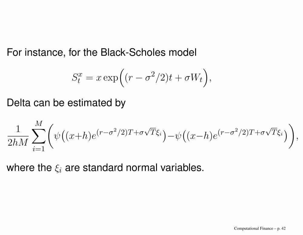
For instance, for the Black-Scholes model

Sxt = x exp(

(r − σ2/2)t+ σWt

)

,

Delta can be estimated by

1

2hM

M∑

i=1

(

ψ((x+h)e(r−σ

2/2)T+σ√Tξi)−ψ((x−h)e(r−σ2/2)T+σ

√Tξi))

,

where the ξi are standard normal variables.


General setting

Let a contingent claim have the form

Y (θ) = ψ(X1(θ), . . . , Xn(θ)

),

where θ is a parameter on which the instrument depends.The derivative with respect to θ is the Greek parameter weare interested in.The payoff of this instrument is α(θ) = E[Y (θ)].The forward and centered differences by which we calculateGreeks are

AF = h−1(α(θ+h)−α(θ)

), AC = (2h)−1

(α(θ+h)−α(θ−h)

).

In addition we have two methods of Monte Carlo simula-tions for the two values of α which appear in these differ-ences. We can simulate each value of α by an independentsequence of random numbers (this will be denoted by an ad-ditional subscript i) or use common random numbers (thiswill be denoted by a subscript ii).


Hence in fact we have four estimators: AF,i, AF,ii, AC,i and

AC,ii.

To assess the accuracy of these estimators let us considertheir bias and variance. Then we can combine these twovalues into a mean square error (MSE) which is given by

MSE(A) = Bias2(A) + Var(A).

For bias we have an approximation

Bias(A) ≈ bhβ ,

where β = 1 for forward differences and β = 2 for centereddifferences (possibly with different positive b).For variance we have

Var(A) ≈ σ2/Mhη,

where M is the number of simulations, η = 1 for commonrandom numbers and η = 2 for independent random num-bers in simulating the difference of α’s (possibly with differ-ent values of σ).


Assuming the following step size dependence on M

h ≈M−γ ,

we find optimal γ

γ = 1/(2β + η).

Then the rate of convergence for our estimators is

O(

M− β

2β+η

)

.

As follows from these approximations, it is advised to userather centered differences and common random numbers,

i.e. the estimator AC,ii, as it produces smaller error and

higher order of convergence.


Pathwise differentiation of the payoff

In cases where ψ is regular and we know how to differentiateSxT with respect to x, Delta can be computed as

∆ =∂

∂xE[ψ(SxT )] = E

[ ∂

∂xψ(SxT )

]= E

[ψ′(SxT )

∂SxT∂x

]

For instance, in the Black-Scholes model, ∂SxT

∂x = SxT

x and

∆ = E[ψ′(SxT )

SxTx

]

provided the derivative ψ′ exists.


General setting

The differentiation of the payoff as a method of calculatingGreeks is based on the following equality

α′(θ) =d

dθE[Y (θ)] = E

[dY

dθ

]

.

The interchange of differentiation and integration holds un-der the assumption that the differential quotient

h−1(Y (θ + h)− Y (θ)

)

is uniformly integrable.


The uniform integrability mentioned on the previous slideholds when

A1. X ′i(θ) exists with probability 1 for every θ ∈ Θ and i =

1, . . . , n, where Θ is a domain of θ,

A2. P(Xi(θ) ∈ Dψ) = 1 for θ ∈ Θ and i = 1, . . . , n, where Dψ

is a domain on which ψ is differentiable,

A3. ψ is Lipschitz continuous,

A4. for all assets Xi we have

|Xi(θ1)−Xi(θ2)| ≤ κi|θ1 − θ2|,

where κi is a random variable with E[κi] <∞.


Black-Scholes delta

ψ(SxT ) = e−rT (SxT −K)+

with

SxT = x exp((r − σ2/2)T + σ

√TZ)

and Z ∼ N (0, 1).

Thendψ

dx=

dψ

dSxT× dSxT

dx.

For the first derivative we clearly have

d

dSxT(SxT −K)+ =

{

0 if SxT < K,

1 if SxT > K.

This derivative fails to exists at ST = K but the event ST = Khas probability 0.


Finally

dψ

dx= e−rT

SxTx11Sx

T>K.

This is already the expression which is easy for Monte Carlosimulations.

But Gamma cannot be computed by this approach since evenfor vanilla options the payoff function in not twicely differen-tiable.


Likelihood ratio

We have to compute a derivative of E[ψ(SxT )].

Assume that we know the transition density

g(SxT ) = g(x, SxT ).

Then

E[ψ(SxT )] =

∫

ψ(SxT )g(SxT )dS

xT =

∫

ψ(S)g(x, S)dS

To calculate ∆ we get

∆ =∂

∂xE[ψ(SxT )] =

∫

ψ(S)∂

∂xg(x, S)dS =

=

∫

ψ(S)∂ log g

∂xg(x, S)dS = E

[ψ(S)

∂ log g

∂x

].


Black-Scholes gamma

When the transition function g(x, ST ) which is the probabil-ity density function is smooth, all derivatives can be easilycomputed.

For the gamma we have

Γ =∂2

∂x2E[ψ(SxT )] =

∫

ψ(S)(∂2 log g

∂x2g(x, S) +

∂ log g

∂x

∂g

∂x

)

dS =

=

∫

ψ(S)

(∂2 log g

∂x2+(∂ log g

∂x

)2)

g(x, S)dS =

=E

[

ψ(S)

(∂2 log g

∂x2+(∂ log g

∂x

)2)]

.


For the log-normal distributions, we have

g(x, ST ) =1√

2πσ2TST×

exp

(

−(log ST − log x− (r − σ2/2)T

)2

2σ2T

)

,

∂ log g(x, ST )

∂x=

logST − log x− (r − σ2/2)T

xσ2T,

∂2 log g(x, ST )

∂x2= −1 + log ST − log x− (r − σ2/2)T

x2σ2T.

Putting this all together, we have the likelihood ratio methodfor the gamma of options in the Black-Scholes model.


A very nice survey of applications of Monte Carlo to pricingof financial derivatives may be found in

Boyle, Brodie, Glasserman (1997) ”Monte Carlo methodsfor security pricing”, Journal of Economic Dynamics andControl 21.

There is also a fundamental monograph

Paul Glasserman Monte Carlo Methods in Financial Engi-neering, Springer 2004.


Documents

Monte Carlo Simulationapalczew/CFP_lecture4.pdf · Monte Carlo simulation on Z. In this context Y is called the control variate. Computational Finance – p. 25. Since adding a constant