Stanford Artificial Intelligence LaboratoryMemo AIM-280

eb , (.. M a y 1 9 7 6

Computer Science DepartmentReport No. STAN-B-76-555 . .

MONTE CARLO SIMULATION OF TOLERANCINGIN DISCRETE PARTS MANUFACTURING AND ASSEMBLY

bY

David D. Grossman

Research sponsored by

Nat ional Science Foundat ion

COMPUTER SCIENCE DEPARTMENTStanford University

Stanford Artificial Intelligence LaboratoryMemo AIM-280

May 1976

Computer Science DepartmentReport No. STAN-CS-7 6-555

MONTE CARLO SIMULATION OF TOLERANCINGIN DISCRETE PARTS MANUFACTURING AND ASSEMBLY

bY

David D. Grossman

--m. ABSTRACT

. The assembly of discrete parts is strongly affected by imprecise components, imperfect fixturesand toois, and inexact measuremets. It is often necessary to design higher precision into themanufacturing and assembly process than is functionally needed in the final product. Productionengineers must trade off between alternative ways of selecting individual tolerances in order toachieve minimum cost, while preserving product integrity. This paper describes acomprehensive Monte Carlo method for systematically anaiysing the stochastic implications oftoierancing and related forms of imprecision. The method is illustrated by four examples, one ofwhich is chosen from the field of assembly by computer controlled manipulators.

permznent address: Computer Sciences Department, IBM T. J. Watson ResearcA Center, p.0. aox218, Yorhtown Heights, New York 10398.

This research was supported by the National Science Foundation under Contract NSF APR 74-0139&A02 . The dews and cOnChsiOns COntdned in this document qre those of the author(s) andshould not be interpreted as neCeSSaYily tepYeJenting the ojkial policies, either expressed OTimplied, of Stanford University, NSF, or the V. S. Government.

INTriODUCTION

The assembly of discrete parts is a major fraction of industrial production. The role ofcomputers in this field has been limited primarily to production and inventory control,computer aided design, and programming numerically controlled machine tools. Very littleprogress has been made in applying computers “to the problem of simulating assemblyprocesses, in spite .of the fact that such simulation offers the possibility of considerablesavings over the alternative cost of building pilot production lines.

When one examines other large industrial fields one finds that computer simulation is amuch more widely used tool. There are basically two reasons, however, why this tool has notbeen extensively applied in discrete parts assembly. First, because assembly is not a scientificdiscipline, experience is formulated as a set of ad hoc principles rather than as a

mathematical theory. Although such principles may be set forth in textbooks,111 it is difficultto embody them in computer simulations. This situation is in sharp contrast, for example, tothe way differential equations can be used to model complex chemical processes. The secondreason is that assembly. environments contain an immense variety of dissimilar objects. Thisaspect of assembly is in sharp contrast, for instance, to nuclear physics simulations where allneutrons behave in the same way. .

. The only obvious unifying principle in discrete parts assembly is that in S-dimensional spaceno two *objects may intersect. This fact suggests a formulation of the simulation problem interms of set theory, an approach which is being taken in research on parts description at the.

University of Rochester.[2,3,41 Set theoretic representations are good for determining if agiven point is inside +a particular set, but performance difficulties arise on problemsinvolving pairs of ‘sets. For example, the question of whether or not a piston intersects amotor block is difficult to answer because it is likely to cause a lengthy search for a pointcontained in both sets. Compounding this difficulty is the fact that assembly involvescontinuous motion of the discrete parts, so that it is desirable to be able to solve set

e intersection problems at every instant of time. The computational algorithms would not behard to formulate, but the execution times would be extremely long, even on the fastestcomputers in the world. For this reason, simulation of the full assembly process is intractable,although simulation of special classes of assembly problems is’still a practical and achievablegoa:l.

From among the many aspects of assembly which could conceivably be modeled, this paperis concerned with the implications of tolerancing and imperfection. In the literature on thissubject, dimensional tolerancing has come to mean specifying the tolerances of parts inmechanical drawings. A national standard has been established which defines the meaningsof tolerancing symbols in drawings I51 and textbooks have been written to explain the use of

these symbols.[61 The emphasis on drawings, however, tends to obscure the underlying

reasons for being concerned with tolerances. The issue is not so much what 3.000+.005 cmmeans but rather why the designer chose to specify this tolerance in the first place.

There are three factors which enter into specifying tolerances in drawings. First, the discretepart which is described must ultimately be assembled into a product which is expected tohave some function, and the tolerance may be needed to provide this function. For instance,it is highly desirable that each chamber of a Colt revolver align accurately with tie barrel.Secondly, the part may be required to have certain tolerances in order that the assemblyprocess itself be feasible. For example, in order to-assemble an automobile engine, the holesin the gasket must align with those in the block. Also, it is often necessary to have veryaccurate parts to avoid jamming vibratory feeders. In fact, it is often necessary to designhigher precision into the assembly process than is functionally needed in the final product.Finally, tolerances may be assigned to correspond to the capabilities of the manufacturingmethod chosen., Tolerances achievable by sheet metal stamping would not be the same asthose achievable on a numerically controlled machine tool, and it would be foolish to assigntolerances in a drawing which would give unreasonably small yields.

The product designer uses his expertise in product design, assembly, and manufacturing tospecify tolerances in the drawing which are both adequate and achievable. An excellenttextbook has been published which describes the considerations ‘involved in this process.PI

, The process is complicated because the design criteria depend on the combined tolerances,rather than on the tolerances individually. Typically, the designer must trade off betweenalternative ways of selecting individual tolerances in order to achieve some resultanttolerance with minimum cost. Unfortunately, the 3-dimensional relationships involved are

. usually too tedious to allow a’rigorous mathematical treatment in all but the simplest cases.The designer therefore uses a great deal of intuition in reaching s decision. Finally he writesdown a number like 3.000*.005 cm and throws away all the information which went into thisdecision.

A recent paper from General Motors describes a system which enables product designers tospecify a set of individual parts tolerances and simulate the stochastic properties ofinteresting resultant tolerances.183 The system is based on the Monte Carlo method, asimulation technique which is well known and has’ been widely used in many other

191M applications. The existence of the GM paper shows that a need exists for simulation toolsin the field of parts tolerancing. The problem of tolerancing is sufficiently hard, and thestakes are sufficiently high, that intuition is no longer a satisfactory method for specifyingparts tolerances.

The approach taken in the GM work is to provide an interactive system in which the usercan obtain high statistics very quickly. In order to achieve execution speed, the user mustexplicitly provide all the equations which tell how the resultant tolerances depend on theindividual tolerances. The system models just the positions and orientations of a few featuresof the part, rather than the entire part shape. This system is apparently proving quite usefulto GM designers.

Aside from the GM work, the only other published papers relating to modeling partstolerances are those from the university of Rochester, where a language called PADL for

HI

representing a class of discrete parts IS being developed. [2,3,41 The hope is that PADL

descriptions can someday be used to generate programs for numerically controlled machine

tools which can make the parts.

The topic of parts representation without regard to tolerancing has been studied by Binford,

Agm, and Nevatia, [10,11,121

’

and Lieberman

and Lavin.’ 18’ *‘I

Braid El 3’ 14’ Baumgart,’ ’ 5’ 16’ Grossman,’ “I

Although none of these parts modeling schemes was designed with

tolerancing in mind, both the Baumgart and Grossman approaches offer a natural way of

adding Monte Carlo procedures to simulate tolerances. As the author of one of these papers,

my choice of which of the two systems to use for the current work was highly biased. I chose

to use my own system solely because I am much more familiar with it.

Although the balance of this paper describes a specific implementation of Monte Carlo

tolerancing within a parts representation system, many of the issues discussed are

implementation independent. The point of this paper IS not simply to give a blueprint for a

specific way of simulating tolerances but rather to show that such a system is possible, to

expose some of the design issues, and to give examples of ways in which the system might beused.

The simulation method described In this paper most closely resembles that of the GM paper,

but there are several mapr differences. Whereas the CM system computes the resultanttolerances of indivrdual parts from tolerances specified in mechanical drawings, the current

work IS much more comprehensive. It allows one to simulate the propagation of tolerances all

the way from the manufacturing process right through the assembly process. Also, while the

GM work requires that the user explicitly supply formulas for the resultant tolerances as

functions of the individual tolerances, the current work provides system routines which

automatically perform these sorts of operations numerically. This provision is particularly

useful because in many situations the relevant formulas can not be derived in closed form.

On the other hand the GM system is Interactive, runs at high speed, and yields high

. statlstrcs answers, while the current system runs in batch mode, executes much more slowly,

and therefore yields much poorer statistics.

The next section of this paper reviews the main features of my earlier publication on

representing parts by PL/I procedures and explains how this system can easily be applied to

the Monte Carlo simulation of parts tolerances. This method is then illustrated by four

specific examples, one of which is chosen from the field of assembly by computer controlled

manipulators. The reason for chosmg this example IS that this research was carried out as

part of continuing manipulator projects at the IBM T. J. Watson Research Center and the

Stanford University Artificial Intelhgence Laboratory. However, it IS important to stress that

the slmulatlon techniques described here are applicable not only m the domain of computer

controlled assembly, but also in the much wider domam of manufacturmg and assembly as

they exist in industry today, usmg conventional equipment and procedures. The paper closes

wrth a discussion of research areas appropriate for extension of the Monte Carlo tolerancing

method.

151

MONTE CARLO METHOD

Distributions -

The basic idea of any Monte Carlo calculation is. to generate an ensemble of models whichsimulates an ensemble of real entities.r91 The statistical properties of the real entities maythen be simulated by studying the corresponding properties of the models. Such simulation is

. useful when purely analytical methods cannot be found.

For the case of’ discrete parts manufacturing and assembly, the real entities consist ofthree-dimensiona! objects at a workstation. These objects include component parts and theirfeatures, tools and fixtures, measuring instruments, and automation equipment up to thelevel of complexity of transfer lines and computer controlled manipulators. For all of theseobjects, the primary attributes to be modeled are shape, position, and orientation.

In simulating statistical distributions of shape, position, and orientation attributes, it isnecessary to define the meaning of expressions of the form 3.000f.005 cm. One possibledefinition would be a normal distribution with a mean of 3.000 cm and a standard deviationof which ,005 cm is some small integral multiple. This choice would allow dimensions to falloutside the specified range, albeit infrequently. Another possibility would be to have a.

. .distribution which goes rigorously to zero outside the specified range. Inside the range, thedistribution could be uniform, or peaked at 3.000 cm, or bimodally peaked at 2.995 cm and3.005 cm. The distribution function might also be skewed if, for example, a part has beenmanufactured in a fixture which is showing signs of progressive wear.

The ANSI dimensioning and tolerancing standards do not specify what statistical

distribution is implied by expressions of the form 3.000&.005 cm. 153 This omission is actuallynecessary, because’ the shape of the distribution function depends on the manufacturingprocess, so that the choice of this shape is best left to the production engineer. In the system

- described in this paper, an arbitrary choice was made to restrict the class of alloweddistributions to be either uniform or normal. This choice was made for the sake ofconvenience and does not represent any inherent limitation in the method.

Part Ensembles

In most parts modeling systems the user describes each part in terms of numbers which areentered directly into a data structure. This data structure, therefore, represents a particularin~lancc of a part rather than an ensemble of similar parts. For the Monte Carlo simulationof tolerances, however, it is necessary that the parts modeling system provide some simplemeans of representing ensembles. What is needed, therefore, is a system in which the userdescribes parts not in terms of numbers but in terms of partzmeters that are assignednumerical values when a part is instantiated. The advantage of such a system for this MonteCarlo simulation is that a random number generator may be used to assign values to these

parameters.

The use of parameters to characterize arbitrary attributes of parts is one of the principle

features of the Procedural Geometric Modeling System (PGMS) developed earlier by this

author.” ” This modeling system was therefore used for the current study. The reader isreferred to the earlier publication for details concerning the way in which PCMS represents

3-dimensional obpfts as PL/I procedures. A brief summary of the main features of this

system are included here for the sake of completeness. Further features wilt be explained in

subsequent sections of this paper as the need arises.

In PCMS, a hypothetical part whose name 1s “widget” and which has two attributes might

be invoked by the calhng sequence

CALL SOLID(WIDGET,A,Bj;

The generic widget itself would be represented by a PLlI procedure whose entry point isnamed WIDGET. This procedure would describe how the widget is hierarchicallyconstructed out of its component subparts. These subparts might be positive SOLID’s or

negative HOLE’s For example,

WIDGET. ENTRY (A,B);CA LL SOLID(CW BOID,A ,A ,B);

CALL HOLE(CUBOID,A,A12,B- 10);

RETURN,

A library of parts procedures already exrsts which starts with the primitive POINT and

includes such objects as LINE, CUBOID, CONE, WEDGE, CYLNDR, and HEMISPH.

More compiicated objects have also been coded, up to the level of complexity of IMM, whichrepresents the IBM Research mechanical mampulator, and SUARM, which represents theStanford University arm.

In addition to parts procedures, PCMS provides routines to perform transformations in3-dimensional space. For example, if the generic widget were translated by C units along the

Y-ax is and then rotated by D degrees about the X-axis, the callmg sequence would be

CALL YTRAN(C);

CALL XROT(D);

CALL SOLID(WIDGET,A,B);

A particular instance of a widget would be invoked by assigning values to the parameters.

For example,

CALL YTRAN( 12);

CA LL XROT(30); .

CA LL SOLID( W lDCET,3.000,16.5);

An ensemble of 500 similar widgets would be represented by the calling sequence

DO I= 1 TO 500;CALL YTRA N( 12+RA ND&O. 1,+0.3));CA LL XROT( 30+GA USS(2.5));CALL SOLID(WII)CET,3.000+~AND(-.005,+.OO5),16.5+RAND(-.2,+.2));END;.

where the function RAND(X,Y) returns a random number uniformly distributed on theinterval from X to Y, and the function GAUSS(Z) returns a random number normallydistributed with.mean 0 and standard deviation 2.

S e m a n t i c s

Once an ensemble of parts has been represented, PCMS provides a way to derive propertiesfrom the representation. This process is referred to as attaching semantics to therepresentation. The f@t step is to code a semantic routine which can compute a desiredproperty, For example, the routine TOTVOL shotin below adds up the volume of allpositive and negative CUBOID’s in any object. ’

TOTVOL: PROCEDURE (NODE,X,Y,Z);DECLARE NODE. ENTRY;IF NODE=CUBOID THEN VOLUME=VOLUME+POLARITY~~X~~Y~Z;RETURN;END TOTVOL;

Next, calls to system routines BEGIN, EXEC, and END are used to attach these semantics tothe system and the part procedure of interest is executed. In the case of the ensemble of 500widgets, one could print the volume of each widget with the following code.

DO I= 1’ TO 500;VOLUME=@ ItJNITIALIZE VOLUME::</CALL BEGIN(5000); /+ALLOCATE STORAGE:::/CALL EXEC(TOTVOL); IQATTACH SEMANTICS:::/

’ CALL YTRAN( 12+RAND(-O&0.3));CALL XROT( 30+GAUSS(2.5));tiLL SOLID(WIDGET,3.000~RAND(-.OO5,+.005),16.5+RAND(-.2,+.2));CALL END; /tcDEALLOCATE STORACE,:c/PUT SKIP DATA (VOLUME); /((PRINT WIDGET VOLUME<</END;

Generalizing from this example, one can easily see how to ‘provide semantics to displayhistograms of almost any desired properties of the ensemble. What is probably not clearfrom this example is the fact that for more realistic parts, the hierarchy of subpart calls

involves so much computation that execution is usually rather slow. For instance, when the

procedure for the Stanford arm IS executed on an IBM 370/168 runnmg the VM time

sharmg system with 120 users, each instantiation takes about 6 seconds of virtual CPU time

and t minute of elapsed time. Derrving the properties of an ensemble of 500 Stanford arms

would therefore require about 8 hours of elapsed time. This number IS prohibitively long for

casual use of the system. However, 8 hours of elapsed time m slmulatmg a complex

mechanism would certainly not be excessive if the derived properties were to revea! a design

deficiency which would have taken months to correct had the hardware been built first.

Another fact which is not pJear from the example above IS that parts of typical complexrryrequire the allocation of several hundred thousand bytes of intermediate storage The

Stanford arm procedure, for rnstance, requires nearly 3OOK of storage The reason behind .

thrs need for intermediate storage relates to the detailed lmplementatlon of PCMS, a topic

WhrcR 1s djscussed in my prloi pubkatlon and which will be omitted here.

EXAMPLES

R Ivet-Hoie Bracket

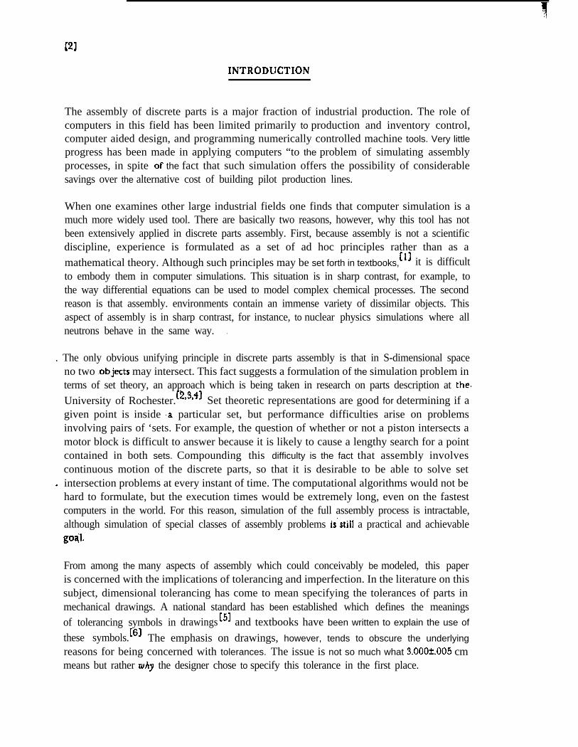
The fmt example chosen to illustrate Monte Carlo tolerancmg In PGMS is similar to rhe

wet-hole bracket used as the example rn the GM paper. A few changes were made because

the orlgrnal drawrng shows only a partrat view of the bracket in two dimensrons, while in

PGMS it is desirable to model the part completely and in three drmenslons.

The modified rivet-hole bracket may be represented by the follow-q code:

RHBRAK: ENTRY (X l,Y l.RADI,X2,Y2,RAD2~NG,THlCK,LENG,NSECT);

DECLARE RHBFRAMl34,4j FLOAT;

CALL STORE!RHBFRAME);

CALL SOLID(WEDGE,THlCK,LENG,ANG,I); /sBRACK ET4

CALL XYZTRAN(X l,Y 1‘0);

CALL HOLE(CYLNDR,THlCK,RAD 1,NSECT); IsHOLE I,:(/

C A L L RECALL(RMBFRAME);

CALL XYZTRAN(X?,Y2,0;;

CALL HOLE(CYLNDR,THICK,RAD2,NSECT); /<tHOLE 2~1

RETURN,

The call m the above code to the PGMS routine STORE IS used to save the current

coordinate frame in the local array RHBFRAME. Subsequently, the current frame is

translated from the corner of the bracket to the posmon of the fn-st hole. The current frame

IS then returned to the bracket corner by the RESTORE routme, so that It may subsequently

be translated to the posltion of the second hole.

. Figure 1: Drawing of Rivet-Hole Bracket

RHBRAK ( )WEDGE (1)

GLINE (1,l)LINE (1,l;i)

POINT (l,l,l,l)POINT (l,l,l,Z)

GLINE (1,2)LINE (1,2,1)

POINT ( 1,2,1,1)FOINT ( 1,2,1,2)

CLINE (1,3)LINE (1,3,1.) *

POINT (1,3,1,1)POINT (1,3,1,2),

--S.

. . . (a total of 9 GLINE’S)

CY LNDR (2)GLINE (2,l)

LINE (2,1,1) ’P O I N T (2,1,&l) ’POINT (2,1,1,2)

. . . (a total of 3t4NSECT GLINE’S)

CYLNDR (3).GLINE (3,l) .

ONE (3,1,1). POINT (3,1,1,1)

POINT (3,1,1,2)

c

. . . (a total of 3sNSECT GLINE’S)

Figyrc 2: Rivet-Hole Bracket Subpart Hierarchy

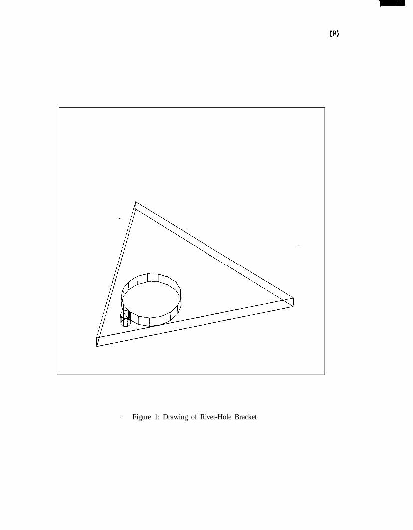
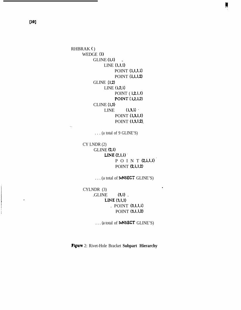
The ten parameters of this procedure represent the seven dimensions subject to tolerancing,the part thickness and length, and the number of sectors used in approximating thecylindrical holes by polyhedra. The effect of this polyhedral approximation can be seen inFigure 1 which was generated by attaching a standard graphics semantic routine to theRHBRAK procedure,

The RHBRAK procedure represents a subpart hierarchy of 40+24sNSECT nodes asindicated in Figure 2. At the top level, the RHBRAK consists of a solid WEDGE and twoCYLNDR holes. The WEDGE in turn is composed of nine GLINE’s (general lines), each ofwhich is made out of one LINE with two end POINT’s. Every level in this hierarchy can bereferred to by a unique s&address, also shown in Figure 2. For instance, the LINE along thebottom left edge of the RHBRAK has a subaddress of (1,3,1). The importance of thesesubaddresses will become clearer in the discussion which follows.

In the GM paper, the designer is concerned with the clearance between the two holes andthe clearances between the second hole’ and the edges of the part. In order to study theseresultants, the following semantic routine might be used.

--.BRAKRES: PROCEDURE (NODE,X l,Y 1,RAD l,X2,Y2,RAD2);DECLARE (RGHTEDGE,LEFTEDGE,HOLEl,HOLE2) POINTER;DECLARE NODE ENTRY;IF NODE-RHB,RAK THEN DO;

CALL DEFINE (RGHTEDGE, 1,2,1);CALL DEFINE (LEFTEDGE, 1,3,1);CALL DEFINE (HOLE 1,2);CALL DEFINE (HOLE2,3);CLEAR l=DISTOO(HOLE l,HOLE2)-RAD I-RAD2;CLEAR2=DISTOX(HOLE2,RGHTEDGE);CLEAR3=DISTOX(HOLE2,LEFTEDGE);END;

RETURN;END BRAKRES;

The DEFINE routine of PCMS is used to associate a PL/I pointer variable with anypreviously specified frame in the part hierarchy. The first argument in the call to DEFINEgibes the name of the pointer variable and the subsequent arguments give the subaddress inthe part hierarchy. Encoding these subaddresses requires that the user have a manual whichsummarizes the subpart hierarchy generated by each procedure in the part library andshows drawings of the basic volume shapes. Understanding subaddresses is currently themost tedious aspect of PGMS.,

The function DISTOO invoked in this semantic routine returns the distance from Origin toOrigin (00) of the two specified frames. The function DISTOX returns the distance fromOrigin to X-axis (OX) of the two specified frames. In order to have written this code it isnecessary to have known that every LINE runs along the X-axis of its frame, and that every

WI

CYLNDR runs along’ the positive Z-axis of its frame. Thus CLEARI, CLEAR2, andCLEA R3 are the desired clearances. It can be seen from this example that the polyhedralapproximation has absolutely no effect on the statistical properties of these clearances.

Finally, a short program may be written to attach these semantics to the system and print thethree clearances for each of 500 rivet-hole brackets.

.DO I-l TO’500;CALL BEGIN(50000);CALL EXEC(BRAKRES);CALL .SOLID(RHBRAK,1.325+GAUSS(.OO5/3),

.875+CAUSS(.005/3),

.2+RAND(-.0075,.0075),2525+GAUSS(.005/3),1.615+GAUSS(.00513),l.%RA ND{-.0075,.0075),67+RAND(-.25,+.25),

--. 0.25,8.0,1);

CALL END;PUT SKIP DATA (CLEAR l,CLEAR2,CLEAR3);END; ’

/$4X 1#4//sY lt41

/6RA D 1 t4/

/#x20/

/8Y 201/*RA D2,)//*A NC+//I;~THICK<~I/t{LENGtit//tiNSECT

Because execution time varies roughly in proportion to the total number of nodes in thesubpart hierarchy, NSECT has been set to 1 here. This simulation of 500 rivet-hole bracketstakes about 3 minutes of CPU time on an IBM 370/168.

For this example, using PGMS to model tolerances is somewhat more difficult than usingthe GM system, largely because the tedium of understanding subaddresses outweighs that of

* writing down a few trigonometric formulas. As the examples become more complicated,however, the subaddress problem remains about constant, while the trigonometry problemsb.ecome much worse. The overall balance therefore swings in favor of PGMS.

B6x M a n u f a c t u r e ’ ’

This example of Monte Carlo tolerancing is concerned with a manufacturing process inwhich 4 holes are drilled into a rectangular box. The holes are made by a gang drill withdrill bits held in four separate chucks, while the box is held in a fixture attached to the drillbed. The box is 12 cm long, 8 cm wide, and 4 cm high, and the four corner holes haveradius 3 mm and depth 2.5 cm and are nominally 1 cm from each edge.

Tolerance errors in the positions of the holes are generated because the fixture may be

translated or rotated slightly in the plane of the drill bed, and each of the four drill chucks

may be radially displaced slightly from its nominal position. To make the example somewhatmore interesting, it will be assumed that the rotational error in positioning the fixture isabout an skis which runs through a corner rather than the center of the box.

Each of the drill bits may be modeled as a cylinder which has been radially displaced byRADERR in a random direction from its desired position.

DRILBIT: ENTRY (RADERR,LENG,RAD,NSECT);CALL ZROT(RAND(O,360));CALL XTRAN(RADERR);CALL >OLID(CYLNDR,LENG,RAD,NSECT);RETURN;.

An ensemble of boxes m,anufactured by this process may then be represented as a cuboidwith holes cut out by the four drill bits.

RECTBOX: ENTRY (X,Y,Z,LENG,RAD,NSECT,

--. XERR,YERR,ANGERR,RADERR);CALL SOLID(CUBOID,X,Y,Z); /QBLOCK~~/CALL ZROT(ANCERR);CALL XYZTRAN(XERR,YERR,Z-LENG);‘CA.LL XYZTRAN( l,l,O);C A L L HOLE(DRILBIT,RADERR,LENG,RAD,NSECT); IsHOLE llr4/

CALL XTRAN(X-2);C A L L HOLE(DRILBIT,RADERR,LENG,RAD,NSECT); /##HOLE 2t4/CALL YTRAN(Y-2);C A L L HOiE(DRILBIT,RADERR,LENG,RAD,NSECT); /aHOLE 3s/ . .C A L L XTRAN(2X);CALL HOLE(DRILBIT,RADERR,LENG,RAD,NSECT); /sHOLE 4t4/

RETURN;

The next step is to code a semantic routine which can derive the coordinates of the fourholes with respect’to the coordinate system of the box.

HOLFIND: PROCEDURE (NODE);DECLARE (HOLE l,HOLE2,HOLE3,HOLE4) POINTER;DECLARE NODE ENTRY;IF NODE-RECTBOX THEN DO;

CALL DEFINE (HOLE 1,2>; CALL ORIGIN (HOLE l,POS 1);CALL DEFINE (HOLE2,3); CALL ORIGIN (HOLE2,POS2);CALL DEFINE (HOLE3,4); CALL ORIGIN (HOLE3,POS3);CALL DEFINE (HOLE4,5); CALL ORIGIN (HOLE4,POS4);END;

RETURN;END HOLFIND;

WI

I Figure 3: DoubleExposure Drawing of Rectangular Box

[I51

The PCMS routine ORIGIN returns the origin vector associated with the frame of theobject pointed to by the first argument. Finally, the locations of each of the four holes, in anensemble of 500 boxes may be printed by attaching these semantics and executing theRECTBOX.

DECLARE (POS 1(3),POS2(3),POS3($POS4(3)) FLOAT;DO I-1 TO 500;

CALL BECIN(80000);CALL EXEC(HOLFIND);CALL,SOLID(RECTBOX,12,8,4, /9x ,Y ,Z#4/

2.5,0.3,1, Iti4LENC,RAD,NSECT+IGAUSS(O.1/3), /ttXERRb#/GAUSS(O.1/3), /#dY ERRt*IRAND&2.5,2.5), /taANGERRtit/GAUSS(0.05/3)); /~RADERRI;~/

CALL END;PUT SKIP DATA (POS l,POS2,POS3,POS4);END;

Execution time is about 8 minutes on an IBM 370/168. A “double-exposure” drawingshowing overlapping views of two boxes in the ensemble appears in Figure 3. This drawing

. was generated by attaching a ’ standard graphics semantic routine and calling theRECTBOX procedure twice. The fact that graphics are produced so easily within PGMS isof considerable help in verifying that the simulation is working properly.

One aspect of this simulation which is perhaps unrealistic is that the fixture is perturbed foreach box. in the ensemble. In an actual manufacturing operation, on the other hand, thefixture would be locked in place, The statistical distribution,s obtained in the actual,manufacturing operation would therefore be narrower than those derived from thissimulation.

What has been simulate& here is an ensemble of boxes produced by Independent setups asopposed to an ensemble produced by a fixed setup. In most cases of batch production, thissimulation would be good enough for all practical purposes. One can imagine situations,however, in which the independent setup assumption is not appropriate. For instance, ifpairs of consecutive boxes were to be attached to one another, the fact that both wereproduced on the same setup might be important. For this case, the code would have to bechanged to simulate pairs of boxes instead of single boxes.

Actually, the box would probably be manufactured by trying a succession of setups until onewas found which yielded satisfactory boxes, and this setup would then be retained for theremainder of the batch. Simulating the resulting ensemble is possible within PGMS, but itentails modeling the conditions used to determine whether or not the setup is satisfactory.Modeling conditional decisions is discussed briefly in the section of this paper dealing withextensions of the Monte Carlo method.

Box and Lid Assembly

This example is concerned with attaching a lid to the box of the previous example. The lidis 12 cm by 8 cm by 0.5 cm thick and is assumed to have been manufactured in the samemanner as the box. At assembly time, a fixture is used which holds the lid rigidly in placeon top of the box in such a way that the edges line up perfectly. The issue is whether or notthe holes in the lid are aligned sufficiently well with those in the box to allow four screws to’be inserted. ,

A procedure which represents both the box and its lid is shown below.

BOXNLID: ENTRY (X,Y,ZBOX,ZLID,LENG,RAD,NSECT,XERRB,YERRB,ANGERRB,RADERRB,XERRL,YERRL,ANGERRL,RADERRL);

CALL SOLID(RECTBOX,X,Y,ZBOX,LENG,RAD,NSECT, /QBOX+/XERRB,YERRB,ANGERRBB,RADERRB);

’ CALL ZTRAN(ZBOX);CALL SQLID(RECTBOX,X,Y,ZLID,ZLID,RAD,NSECT, /GLIDQ/

XERRL,YERRL,ANGERRL,RADERRL);RETURN;

. The next step is to code a semantic routine which computes the alignment errors for each ofthe four pairs of holes.

ALIGNER: PROCEDURE (NODE);DECLARE (BOX,LID) POINTER;DECLARE NHOLE BINARY FIXED; 1

DECLARE NODE ENTRY;IF NODE-BOXNLID THEN DO;

FOR NHOLE=I TO 4 DO;CALL DEFINE (BOX, l,NHOLE+ 1,l);CALL DEFINE (LID,2,NHOLE+ 1,l);ERROR(NHOLE)-DISTOZ(BOX,LID);END;

END;RETURN; ’END ALIGNER;

The subaddresses in these DEFINE statements identify frames of corresponding CYLNDRholes in the box and lid. The function DISTOZ returns the distance from the Origin toZ-axis (02) of these two frames.

If it is assumed that the assembly process is unsuccessful whenever any of the four screwhole misalignments exceeds 2 mm, a simple procedure can be written to determine thenumber of successful assemblies in an ensemble of 500 boxes and lids.

. Figure 4: Drmwing of Unsuccessful Box and Lid Assembly

DECLARE .ERROR(4);DO I- 1 TO 500;

NSUCCESS=O;CALL BEGIN{ 120000);CALL EXEC(ALICNER);CALL SOLID(BOXNLID,12,8,4,0.5, /~~X,Y,ZBOX,ZLIDQI

2.5,0.3,1, /s:tLENG,RA b,NSECT:rlCAUSS(O.l/$ /ttXERRB,:k/GAUSS(O.l/3), /tcY ERR B::!/RA ND(-2.5,2.5), /oANGERRB<t/GA USS(O.O5/3), /~~RADERRB~:~/CAUSS(O.l/3), i~~XERRL::~/GAUSS(O.l/3), /+Y ERR Ltt/

R A ND(-2.5,2.5), &~ANGERRL::~/GAUSS(O.O5/3)); /taRA DERRL+/

CALL END;IF ERROR( 1)<.2

-.. 8c ERROR(2)<.2& ERROR(3)<.2

. & ERROR(4)<.2 .THEN NSUCCESS=NSUCCESS+ 1;

END;PUT SKIP DATA (NSUCCESS);

When this prograin is executed, it determines that 27% of the assemblies would be successful.A bout 10 minutes of CPU time are required to obtain this result using an IBM 3701168. Adrawing of one of the unsuccessful assemblies is shown in Figure 4:

Since in principle the lids are symmetric, it is also possible to generate an ensemble in whichthe lids have been randomly flipped upside down or rotated a180 degrees in the horizontal

w plane between the time of manufacture and the time of assembly. Such an ensemblesimulates the common industrial practise of throwing freshly manufactured parts into atotebin. The simulation then yields 19% successful assemblies. The reason why this percentage ismuch lower than the previous one is related to the fact that the rotational error in thefixture was assumed to be about an axis which ran through a corner of the box rather thanthrough its center. ,

Stanford Arm

The final example is taken from the field of computer controlled manipulators. Currently,two manipulator arms are being used at the Stanford University Artificial IntelligenceLaboratory to study problems in industrial automation. Figure 5 shows a drawing of one ofthese arms holding a power screwdriver and a screw. Although the arm had been modeled ’much earlier by .Baumgart, El61 this picture was obtained by using PGMS procedures instead.

Figure !!k Drawing of Stanford Arm

WI

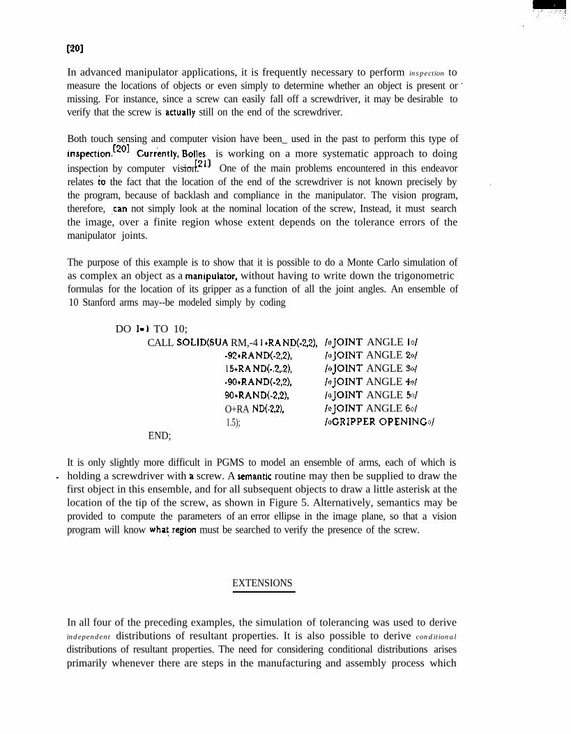
In advanced manipulator applications, it is frequently necessary to perform inspection tomeasure the locations of objects or even simply to determine whether an object is present or ’missing. For instance, since a screw can easily fall off a screwdriver, it may be desirable toverify that the screw is Qactually still on the end of the screwdriver.

Both touch sensing and computer vision have been_ used in the past to perform this type ofinspection.[2oJ Currkntly, Boll;& is working on a more systematic approach to doinginspection by computer vision. One of the main problems encountered in this endeavorrelates to the fact that the location of the end of the screwdriver is not known precisely bythe program, because of backlash and compliance in the manipulator. The vision program,therefore, ,can not simply look at the nominal location of the screw, Instead, it must searchthe image, over a finite region whose extent depends on the tolerance errors of themanipulator joints.

.

The purpose of this example is to show that it is possible to do a Monte Carlo simulation ofas complex an object as a manipulatbr, without having to write down the trigonometricformulas for the location of its gripper as a function of all the joint angles. An ensemble of10 Stanford arms may--be modeled simply by coding

DO I-l TO 10;CALL S.OLID(SUA RM,-4 I +RA NP(-2,2), /({JOINT ANGLE i+/

-92+RAND(-2,2), /::tJOINT ANGLE 2::~/I 5+RA ND{-.2,.2), /ctJOINT ANGLE 3::</-9O+RAND(-2,2), isJOINT ANGLE 4,:</gOtRAND{-2,2), /(<JOINT ANGLE 5:::/O+RA ND{-2,2), /ttJOINT ANGLE 6011.5); IQGRIPPER OPENING::</

END;

It is only slightly more difficult in PGMS to model an ensemble of arms, each of which isa holding a screwdriver with a screw. A semantic routine may then be supplied to draw the

first object in this ensemble, and for all subsequent objects to draw a little asterisk at thelocation of the tip of the screw, as shown in Figure 5. Alternatively, semantics may beprovided to compute the parameters of an error ellipse in the image plane, so that a visionprogram will know what,region must be searched to verify the presence of the screw.

EXTENSIONS

In all four of the preceding examples, the simulation of tolerancing was used to deriveindependent distributions of resultant properties. It is also possible to derive conditional

distributions of resultant properties. The need for considering conditional distributions arisesprimarily whenever there are steps in the manufacturing and assembly process which

WI

involve conditional actions. Actually, such actions are quite common in discrete partspt‘oduction, although they tend to be overlooked because these steps are usually implicitlyassumed.

For instance, one expects an assembly worker to know without being told that

IF the lid doesn’t fitTHEN throw it out and try another one

ELSE attach it

Alternatively, the worker might ignore any requirement of interchangeability and save thenonfitting lid until a matching box was found. In either case, the statistical properties of theresulting assemblies would no longer be the same. This fact is true whether or not theconditional instructions are stated explicitly.

Not all conditional actions have the si,mple form IF . . . THEN . ..ELSE. For example, theassembly process might involve sliding the lid until it is aligned with the box. This stepwould move each Ii&by a different amount, depending on the initial misalignment of thatparticular lid and box.

, In a PGMS tolerancing simulation, the addition of steps which simulate conditional actions. is a straightforward process, provided that these actions can be stated in the form of

procedures which involve spatial transformations no parse than rotations and translationsby well defined amounts. For an IF . . . THEN . . . ELSE action, one simply adds theappropriate IF . . . THEN . . . ELSE clause to the program. A problem arises, however, thatthere are conditional actions which can not be easily expressed in the form of well definedprocedures.

A common and insidious example of such actions relates to the way parts are oftenchamfered to make’ the assembly process easier. As the assembly is performed, the chamfers

e force parts into slightly different positions and alter their subsequent statistical properties.The effect of a chamfer in locating a single pin can be expressed fairly easily in the form ofa procedure, but for more than one pin the effect of chamfering becomes very difficult tostate explicitly.

*The effect of chamfers is .a specific case of a general process which may be called fitting oractommodatton. Case studies performed at the Charles Stark Draper Laboratory indicate that

in typical industrial assemblies, rbughly 15% of the steps involve accommodation. c223

Although this process is industrially important, it is very difficult to simulate except in thesimplest situations. For instance, it is well known that the way to attach a lid to a box is toput all four screws in loosely and then tighten them, rather than tightening each oneimmediately. Unfortunately, even in this case it is not known how to express the exactprocess of accommodation in the form of a well defined procedure.

However, it is possible to approximutu many accommodation processes.. For example, in the

WI

box assembly one can say that the first screw to be loosely inserted produces a translation ofthe lid such that its hole aligns with the corresponding box hole. The second screw producesa rotation of the lid which makes the vector from the first to the second lid hole align withthe corresponding box vector, followed by a translation of the lid along this vector to makethe two alignment errors equal and opposite. The third screw only produces a translationorthogonal to the previous vector, and the fourth screw has no effect. Clearly, this procedureis only. an approximation to what really happens, but the chances are that it is a goodenough approximation for most practical purposes. ,An alternative approximation would beto say that each successive screw produces a transformation of the lid to a new position such ,that the sum of the squares of of the alignment errors is minimized. In either of these cases,one can easily add to PGM$ proocedures which simulate the approximate accommodationprocess.

Another extension of Monte Carlo tolerancing would be to simulate the process of makingmeasurements with imperfect measuring tools. For example, suppose a computer visionsystem is used to locate the position of a hole in a part so that a manipulator can insert ascrew. This measurement is limited by the camera resolution, which may be on the order ofone picture element ii? the scanning array. The measurement is also limited by pan and tilterrors in aiming the camera. Projecting the camera errors from the image plane back to theactual hole in three-dimensional space will generally give an elongated region within whichthe location of the hole can not be resolved. If several features of a part are located in thismanner, the position and orientation of the part itself may be derived. All of these steps canbe simulated within PGMS.

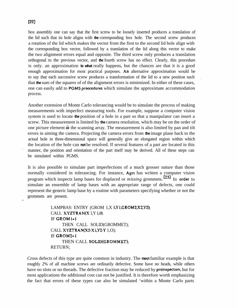
It is also possible to simulate part imperfections of a much grosser nature than thosenormally considered in tolerancing. For instance, Agin has written a computer visionprogram which inspects lamp bases for displaced or missing grommets. [231 In <order tosimulate an ensemble of lamp bases with an appropriate range of defects, one couldrepresent the generic lamp base by a routine with parameters specifying whether or not thegrommets are present.

a

LAMPBAS: ENTRY (GROM 1,X 1,Y l,GROMZ,XZ,YZ);CALL XYZTRAN(X l,Y 1,O);IF GROMl-1

THEN CALL SOLID(GROMMET);CALL XYZTRAN(XZ-X l,YZ-Y 1,O);IF GROMZ- I

THEN CALL SOLID(GROMMET);RETURN;

Cross defects of this type are quite common in industry. The most familiar example is thatroughly 2% of all machine screws are ordinarily defective. Some have no heads, while othershave no slots or no threads. The defective fraction may be reduced by preinspection, but formost applications the additional cost can not be justified. It is therefore worth emphasizingthe fact that errors of these types can also be simulated ‘within a Monte Carlo parts

tolerancing system. .

CONCLUSION

This paper has described a Monte Carlo approach to the simulation of tolerancing andother forms of imprecision in discrete’ parts manufacturing and assembly. An implementationof the method, based on the Procedural Geometric Modeling System developed earlier bythis author, is illustrated by four specific examples, one’of which was chosen from the fieldof assembly by computer controlled manipulators.

There appears tb be a pressing need for simulation techniques relating to discrete partsmanufacturing and assembly. The assembly process is strongly affected by imprecisecomponents, imperfect fixtures and tools, and inexact measurements. It is often necessary todesign higher precision into the manufacturing and assembly process than is functionallyneeded in the final product, Production costs are highly dependent on specified tolerancesand the resultant product yields.

The technique described in this paper can provide production engineers with a systematic. way of analyzing the stochastic implications of tolerancing and other forms of imprecision.

ACKNOWLEDGEMENT

This paper was partially motivated by Russell Taylor’s work on high level languages forcomputer con trolled manipulators. One of his programs determines allowed loci of

e workpieces by resolving symbolic geometric constraints. The paper was also motivated by thecomputer vision research of Bob Belles, One of his programs calculates the region of animage to be searched for a desired feature of a workpiece that has been displaced slightlyfrom its nominal position. Discussions with Taylor and Belles in the early stages of this workhave proved very valuable. Their results, incidentally, will be published soon as part of theirdoctoral dissertations.

This work was performed at the Stanford AI Lab, as part of the Computer IntegratedAssembly Systems project headed by Tom Binford. I want to thank Peter Will, manager ofthe Automation Research project at the IBM T. J. Watson Research Center, from which Iwas on sabbatical leave, for making my year at SAIL possible.

Finally, I want to acknowledge the logistical assistance of Mike Blasgen and LarryLieberman in this work.

[241

REFERENCES

[ 13 W. V. Tipping, An Introduction to Mechanical Assembly, Business Books, London,England, 1969.

c21 An Introduction to PADL, Production Automation Project Technical MemorandumTM-22, University of Rochester, December 1974.

[31 A. A. G. Requicha, N. M. Samuel, and H. B. Voelcker, Part and Assembly DescriptionLanguages - II, Production Automation Technical Memorandum TM-ZOa, University ofRochester, revised November 1974.

141 Discrete Part Manufacturing: Theory and Practice, Production Automation ProjectTechnical Report TR-l-1, University of Rochester, 1974.

[51 Dimensionhg and Tol,erancing, American National Standards Institute Report ANSIY 14.5-1973, ptiblishetl by IEEE, New York, 1973.

161 Lowell W. Foster, Geometric Dimensioning and Tolerancing: A Working Guide,Addison-Wesley Publishing Co., Reading, Massachusetts, 1970.

[71 Earlwood T. Fortini, Dimensioning For Interchangeable Manufacture, Industrial PressInc., New York, 1967.

[83 Harold W. Gugel, Monte Carlo Simulation With Interactive Graphics, GM Research: Publication GMR- 153 1, General Motors Corporation Research Laboratories, Warren,

Michigan, October ‘1974.

[91 John M. Hammersley and David C. Handscomb, Monte Carlo Methods, Wiley, New- York, 1964.

cl01 Gerald J. .Agin, Representation and Description of Curved Objects, Stanford ArtificialIntelligence Laboratory Memo AIM-173 and, Stanford University Computer Science ReportSTA N-&305, October 1972.

c 111 Gerald J. Agi’n and Thomas 0. Binford, Computer Description of Curved 06jects, ThirdInternational Joint Conference on Artificial Intelligence, Stanford, August 1973.

[I21 Ramakant Nevatia, Structured Descriptions of Complex Curved Objects for Recognitionand Visual Memory, Stanford Artificial Intelligence Laboratory Memo AIM-250 andStanford University Computer Science Report STAN-CS-464, October 1974.

1131 I. C. Braid, Designing With Volumes, Cantab Press, Cambridge, England, 1974.

1141 I, C. Braid, The Synthesis of Solids Bounded by Many Faces, Communications of theACM, Volume 18, Number 4, p. 209, April 1975.

(151 Bruce G. Baumgart, Winged Edge Polyhedron Representation, Stanford ArtificialIntelligence Laboratory Memo AIM- 179 and Stanford University Computer Science ReportSTAN-CS-320, October 1972. -.,

1161 Bruce G: Baumgart, GEOMED, Stanford Artificial Intelligence Laboratory MemoAIM-232 and Stanford University Computer Science Report STAN-CS-4 14, May 1974.

[171 David D. Grossman, Procedural Representation of Three-Dimensional Oyectj, IBMResearch Report RC-5314, T. J. Watson Research Center, Yorktown Heights, N. Y., March14, 1975; to be published in IBM Journal of Research and Development.

[18l Mark A. Lavin and Laurence I. Lieberman, A System for Modeling Three-DimensionalObjects, IBM Research Report RC-5765, T. J. Watson Research Center, Yorktown Heights,N. Y., December 17, 19f5; to be published in IBM Journal of Research and Development.

-.

cl91 Mark A. Lavin, MODFEAT: A System for Naming Polyhedral Features o fThree-Dimensional Oyects, IBM Research Report RC-5764, T. J. Watson Research Center,Yorktown Heights, N. Y., December 17, 1975.

1201 Robert Bolles and Richard ‘Paul, TAQ Use of Sensory Feedback in a ProgrammableAssembly System, Stanford Artificial Intelligence Laboratory Memo AIM-220 and StanfordUniversity Computer Science Report STAN-(X-396, October 1973.

1211 Robert C. Belles, Verification Vision Within a Programmable Assembly System: AnIntroductory Discussfan, Stanford Artificial Intelligence Laboratory Memo AIM-275 andStanford University. Computer Science Report STAN-CS-75-537, December 1975.

* 1221 J. Nevins, D. Whitney,,S. Drake, D. Killoran, M. Lynch, D. Seltzer, S. Simunovic, R. M.Spencer, P. Watson, and A. Woodin, Exploratory Resfarch in industrial Modular Assembly,Charles Stark Draper Laboratory Report R-921, Cambridge, Massachusetts, December 1,1974 to August 31, 1975. *

1231 C. Rosen, D. Nitzan, G. Agin, G. Andeen, J. Berger, J. Eckerle, G. Gleason, J. Hill, J,Kremers, B. Meyer, W. Park, and A. Sword, Exploratory Research in Advanced Automation,Stanford Research Institute Project 2591 Report 2, Menlo Park, California, August 1974.