Monte Verit / Ascona, · Sacha Varone Haute École de Gestion de Genève University of Applied Sciences Western Switzerland (HES-SO) Campus Battelle, Bâtiment F, 7 route de Drize,

A general framework for routing problems with stochasticdemands

Iliya MarkovMichel BierlaireJean-François CordeauYousef MaknoonSacha Varone

École Polytechnique Fédérale de Lausanne May 2017

STRC 17th Swiss Transport Research Conference Monte Verità / Ascona, May 17 – 19, 2017

A general framework for routing problems with stochastic demands May 2017

École Polytechnique Fédérale de Lausanne

A general framework for routing problems with stochastic demands

Iliya Markov, Michel BierlaireTransport and Mobility LaboratorySchool of Architecture, Civil and EnvironmentalEngineeringÉcole Polytechnique Fédérale de LausanneStation 18, 1015 Lausanne, Switzerlandiliya.markov,[email protected]:fax:

Jean-François CordeauCIRRELT and HEC Montréal3000 chemin de la Côte-Sainte-CatherineMontréal, Canada H3T [email protected]:fax:

Yousef MaknoonFaculty of Technology, Policy, and ManagementDelft University of TechnologyJaffalaan 5, 2628 BX Delft, The [email protected]:fax:

Sacha VaroneHaute École de Gestion de GenèveUniversity of Applied Sciences WesternSwitzerland (HES-SO)Campus Battelle, Bâtiment F, 7 route de Drize,1227 Carouge, [email protected]:fax:

May 2017

Abstract

We introduce a unified modeling and solution framework for various classes of rich vehicle and inventoryrouting problems as well as other probability-based routing problems with a time-horizon dimension.Demand is assumed to be stochastic and non-stationary, and is forecast using any forecasting model thatprovides expected demands over the planning horizon, with error terms from any empirical distribution.We discuss possible applications to various problems from the literature and practice: from health care,waste collection, and maritime inventory routing, to routing problems based on event probabilities,such as facility maintenance where the breakdown probability of a facility increases with time. Weprovide a detailed discussion on the effects of the stochastic dimension on modeling and the solutionmethodology. We develop a mixed integer non-linear model, provide examples of how it can be reducedand adapted to specific problem classes, and demonstrate that probability-based routing problems over aplanning horizon can be seen through the lens of inventory routing. The optimization methodology isheuristic, based on Adaptive Large Neighborhood Search. The case study is based on waste collectionand facility maintenance instances derived from real data. We analyze the cost benefits of open toursand the availability of better forecasting methodologies. We demonstrate that relaxing the distributionalassumptions on the error terms and calculating probabilities using simulation information has only aminor impact on computation time. Simulating the error terms on the final solution further allows us toverify the low level of occurrence of undesirable events, such as stock-outs, overflows or breakdowns,with a moderate impact on the routing cost compared to alternative realistic policies. What is more,simulating the objective of the final solution shows that it is an excellent representation of the real cost.

Keywordsunified framework, stochastic demand, forecasting, inventory policies, inventory routing, vehicle routing,

probability-based routing

i


1 Introduction

In this work, we develop a generalized framework for various classes of rich stochastic vehicle and

inventory routing problems as well as other probability-based routing problems with a time-horizon

dimension. The logistic setting includes a heterogeneous fixed fleet to service demand points from supply

points in a distribution, collection, or other context. Vehicles can perform open tours with multiple supply

point visits per tour when and as needed. One can have time windows, maximum tour durations, visit

periodicities and various other practically relevant constraints. The proposed framework can be applied to

many classical types of routing problems that appear in the literature, such as the vehicle routing problem

(VRP), the inventory routing problem (IRP), the periodic VRP, the pickup and delivery problem, routing

problems based on event probabilities, etc., subject to various operational and decision policies.

In the literature on routing problems, there are three main types of stochastic parameters: stochastic

demands, stochastic customers, and stochastic travel and service times, with the first one being the most

commonly treated (Gendreau et al., 2014, 2016). Stochastic demands are not known in advance but

only probabilistically, and we assume knowledge of the parameters defining the demand distribution.

Stochastic customers are not known in advance, but there is a probability associated with the existence of

a customer. There is little literature on this type of problem (Gendreau et al., 2016). Stochastic travel

times account for the impact on travel times of random events such as road accidents. It is important to

distinguish between stochastic travel times and time-dependent travel times, the latter being deterministic

(Gendreau et al., 2016). Stochastic service times refer to the uncertainty about the time spent servicing a

customer. In our framework, we consider stochastic demands where demand points are known in advance,

but their demands over the planning horizon are uncertain. Demands over the planning horizon can be

non-stationary and are forecast using any model that provides point forecasts, with error terms from

any empirical distribution that can be simulated. Demand uncertainty may lead to the occurrence of

undesirable events which, depending on the context, can be stock-outs, overflows, breakdowns, etc.

Various techniques for modeling uncertainty exist in the literature. Scenario sampling and stochastic

modeling based on Markov decision processes both lead to problems that suffer from the curse of

dimensionality for realistic size instances (Pillac et al., 2013). Approximate dynamic programming

(Powell, 2011) helps alleviate the problem in the latter case. The robust optimization approach produces

solutions that remain feasible under the worst case scenario for a given budget of uncertainty. This

approach is distribution-free as for each parameter it only needs a nominal value and a symmetric interval

in which the parameter can vary. It relies on specific reformulations depending on whether parameter

uncertainty appears column-wise (Soyster, 1973), row-wise (Bertsimas and Sim, 2003, 2004), or only in

the right-hand side (Minoux, 2009). Moreover, complications arise if there is inter-row dependency in

the uncertainty on the right-hand side, as is the case in our problem due to inventory tracking from one

period to another (see Delage and Iancu, 2015). Robust optimization is rarely used for routing problems

(Gendreau et al., 2016). We can give the examples of Sungur et al. (2008) and Gounaris et al. (2013) who

treat stochastic demands for the VRP and Aghezzaf (2008) and Solyalı et al. (2012) for the IRP. Chance

constrained approaches guarantee that a constraint will be satisfied with a certain probability. They

are appropriate if uncertainty appears row-wise and have been used to model route failures in vehicle

routing problems with stochastic demands (see references in Gendreau et al., 2014). Although chance

1


constraints can be linearized under certain conditions, the set of phenomena they can model is rather

limited. Moreover, both robust optimization and chance constrained approaches have a clear risk-aversion

bias shifting the treatment of uncertainty to the constraints. They also leave open the question of how to

define the budget of uncertainty or the distribution percentile for the chance.

Our first contribution is in consolidating the treatment of demand uncertainty to intuitively capture

the cost dimension of undesirable events. Often these have to be paid for. For example, in a vendor

managed inventory setting, a stock-out at a customer may result in a penalty for the supplier due to a

service level agreement. In a waste collection problem, the municipality may charge the collector for

a container overflow. Given that these costs are known upfront, the main benefit of our framework is

that there are no tunable parameters with respect to uncertainty. The cost effect of uncertainty takes

part in the objective function, thus minimizing the risk, including its cost impact in the decision process,

and weighting it with respect to the rest of the cost components. Taking a small risk may sometimes be

beneficial if it significantly reduces other cost components. It is important to note that in our framework

the undesirable events are not unrecoverable disasters. They have a monetary aspect and their occurrence

should be able to be minimized to a reasonable level. Their states are frequently revisited, unlike

what is usually the case in robust optimization. That is, in a good solution these are rare events. The

framework is not appropriate for frequently occurring undesirable events. Such should be modeled using

alternative approaches. The reason for this is that, due to the complex propagation of uncertainty in our

framework, the objective function becomes more conservative with growing probabilities of occurrence

of the undesirable events.

Our second contribution is in the computational tractability of our modeling framework. The probabilistic

information that we use in the treatment of uncertainty can largely be pre-computed, and thus allows us

to relax the distributional assumptions on the random variables. We provide a detailed discussion on the

effects of the stochastic dimension on modeling and the solution methodology. Our final contribution is

in the generality of the approach. We discuss possible applications to various problems from the literature

and practice: from health care, waste collection, and maritime inventory routing, to routing problems

based on event probabilities, such as facility maintenance where the breakdown probability of a facility

increases with time. We develop a mixed integer non-linear model, provide examples of how it can be

reduced and adapted to specific problem classes, and demonstrate that probability-based routing problems

over a planning horizon can be seen through the lens of inventory routing.

The optimization methodology is heuristic, based on Adaptive Large Neighborhood Search (ALNS)

with operators specifically designed to capture the complex logistic setting as well as the stochastic

demand element. The ALNS exhibits excellent performance on benchmark instances and instances

derived from real data. The case study is based on waste collection and facility maintenance instances

derived from real data. We analyze the cost benefits of open tours and the availability of better forecasting

methodologies. We demonstrate that relaxing the distributional assumptions on the error terms and

calculating probabilities using simulation information has only a minor impact on computation time.

Simulating the error terms on the final solution further allows us to verify the low level of occurrence of

undesirable events, such as stock-outs, overflows or breakdowns, with a moderate impact on the routing

cost compared to alternative realistic policies. What is more, simulating the objective of the final solution

shows that it is an excellent representation of the real cost.

2


The remainder of this article is organized as follows. Section 2 offers a brief review of the relevant

literature on rich routing problems and several specific application areas, such as waste collection,

health care, and maritime routing problems, with a specific focus on problems with stochastic demands.

Section 3 describes the unified framework from a conceptual point of view. It is detailed in the following

sections, with Section 4 discussing the stochastic dimension and Section 5 developing the mathematical

formulation. Section 6 provides examples of how the framework can be reduced and adapted to various

specific problem classes. Section 7 is dedicated to the solution methodology based on ALNS. Section 8

presents the numerical experiments and, finally, Section 9 concludes with an outline of future work

directions.

2 Related Literature

This section offers a literature review of various stochastic problem types that can be modeled using the

generalized framework described in Section 3, starting from rich vehicle and inventory routing problems

and going through several specific and pertinent application areas.

2.1 Rich Vehicle and Inventory Routing Problems

Rich vehicle routing problems are multi-constrained routing problems that extend the classical capacitated

VRP (Dantzig and Ramser, 1959) by including a variety of features relevant to real-world problems,

such as time windows, driver constraints, multiple depots or intermediate/satellite facilities, dynamism,

stochastic information, etc. The recent work of Lahyani et al. (2015) develops a taxonomy and a definition

of rich VRPs.

Our framework considers a routing problem with a variety of rich VRP features, in particular intermediate

facilities, a heterogeneous fixed fleet, and multiple depots with the flexibility of open tours. While the

multi-depot and open VRP have been studied for a long time, most of the literature on the VRP with

intermediate facilities has appeared recently. Bard et al. (1998a) develop a branch-and-cut algorithm

for the single-period VRP with satellite facilities which is able to solve small instances. Angelelli and

Speranza (2002a) and Angelelli and Speranza (2002b) solve a periodic VRP with intermediate facilities

applied to waste collection. Kim et al. (2006) develop a simulated annealing heuristic for the single-period

version of the problem, including features such as workload balancing and tour compactness. Crevier

et al. (2007) study a variant of the problem called the multi-depot VRP with inter-depot routes, and

solve it with a hybrid methodology relying on a set covering formulation. Muter et al. (2014) develop

a branch-and-price algorithm for the same problem. Hemmelmayr et al. (2013) propose a Variable

Neighborhood Search (VNS) method for the periodic version of this problem in a waste collection setting.

Hemmelmayr et al. (2014) extend it to include bin allocation decisions as well. A conceptually similar

problem occurs in vehicle routing problems for electric and alternative fuel vehicles where the role of

intermediate facilities is played by the charging stations (see e.g. Schneider et al., 2014, 2015, Goeke and

Schneider, 2015). The heterogeneous fixed fleet VRP was formalized in the work of Taillard (1999) and

was the subject of intensive study in the following decade, with state-of-the-art exact algorithms due to

3


Baldacci and Mingozzi (2009) and heuristic algorithms due to Penna et al. (2013) and Subramanian et al.

(2012). Regarding multiple depots and open tours, Markov et al. (2016b) show that allowing open tours

ending at a different depot than the origin depot could lead to significant cost savings.

Rich routing problems often include an uncertainty component. In dynamic routing problems, parameters

are partly unknown and gradually revealed with time. In dynamic and stochastic routing problems, we

have access to probability information of the unknown parameters. Ritzinger et al. (2016) summarize the

recent literature on dynamic and stochastic vehicle routing problems and offer a classification scheme

based on the available stochastic information. Gendreau et al. (2016) center their survey on the state

of the art of the a priori and the re-optimization paradigm for stochastic routing problems, the two

being the predominantly used paradigms by researchers. Although multi-constrained inventory routing

problems with real-world features have recently begun to appear in the literature, the term rich IRP has

not established itself as in the case of the VRP. The sections below provide a survey of various rich

vehicle and inventory routing problems. The focus is on stochastic problems from several application

areas that fit the generalized framework proposed in Section 3 below.

2.2 Health Care Routing Problems

Health care routing problems may involve all types of stochastic parameters mentioned in Section 1,

i.e stochastic demands, stochastic customers, and stochastic travel and service times. As the last two

types are out of the scope of this research, we focus our review on stochastic demand problems. We

note, however, that workload balancing and the continuity of service are two features that often appear

in the literature focused on stochastic customers and service times (see Lanzarone and Matta, 2009,

2012, Lanzarone et al., 2012, Errarhout et al., 2014, 2016). Demands for products appear in health care

routing problems that treat the pick-up and delivery of drugs, biological samples, and medical equipment.

Hemmelmayr et al. (2010) solve a stochastic blood distribution problem, which considers shortfalls and

spoilage. To balance delivery and spoilage costs, they limit the probability of spoilage to 5% by sampling

product usage during the spoilage period and taking the 5% quantile as the maximum inventory level

at the hospital. To guard against product shortage, the authors develop a two-stage stochastic program

with recourse. The setup assumes that at the beginning of each day information about the inventory of

each hospital is available. The MILP and VNS approaches of Hemmelmayr et al. (2009) are extended to

handle stochastic product usage, in both cases using external sampling to convert the two-stage stochastic

optimization problem into a deterministic one. The simulation experiments show that employing a simple

recourse policy is sufficient to provide a reliable and cost-efficient blood supply. Niakan and Rahimi

(2015) and Shi et al. (2017) study the problem of delivering drugs with uncertain demands to patient

homes. Both authors apply fuzzy programming approaches to the problem and report the value added of

incorporating uncertainty into the model.

2.3 Waste Collection Routing Problems

Johansson (2006) and Mes (2012) use simulation to confirm the benefits of migrating from static to

dynamic collection policies in Malmö, Sweden and a study area in the Netherlands, respectively, where

4


containers are equipped with level and motion sensors, respectively. Mes (2012) finds a positive added

value of investing in level sensors compared to simple motion sensors that detect when a container was

emptied. Mes et al. (2014) apply optimal learning techniques to tune the parameters related to inventory

control (deciding which containers to select) assuming accurate container level information. They find

strong benefits from parameter tuning. Nolz et al. (2011) develop a tabu search algorithm for a stochastic

inventory routing problem for the collection of infectious waste from pharmacies. Nolz et al. (2014b)

propose a scenario sampling method and an adaptive large neighborhood search algorithm for the same

problem. Nolz et al. (2014a) extend this to a bi-objective problem, trading off satisfaction of pharmacies,

local authorities and the minimization of public health risks against routing costs. They propose three

meta-heuristic approaches for this problem. Bitsch (2012) develops a VNS for an inventory routing

problem applied to the collection of recyclable waste in a Danish region. Waste level is stochastic and

containers should be emptied so that the probability of overflow is six sigmas away. Markov et al. (2016a)

describe a stochastic waste collection inventory routing problem over a finite planning horizon. Waste

containers are equipped with sensors that communicate their levels on each day. A forecasting model

produces point demand forecasts and estimates a forecasting error, which is used for calculating the

probability of container overflows and route failures. The authors propose a mixed integer non-linear

model and develop an ALNS, which exhibits excellent performance on benchmark instances. It also

performs significantly better compared to alternative policies on real instances from Geneva, Switzerland

in its ability to limit the occurrence of container overflows for the same routing cost.

2.4 Maritime Routing Problems

The maritime inventory routing problem (MIRP) or the inventory ship routing problem is the application

of the inventory routing problem to the maritime sector. Papageorgiou et al. (2014) point out three

important differences between maritime and road-based IRPs. The classical road-based IRP assumes a

central depot, which is not necessarily the case in maritime transportation. In the maritime setting, vessels

typically travel long distances round the clock. With the addition of the time consuming port operations,

the planning horizon becomes much longer. Finally, in maritime transportation vessels usually visit very

few ports in succession (two or three), unlike in road-based transportation where vehicles visit dozens of

customers.

Cheng and Duran (2004) describe a decision support system applied to crude oil transportation and

inventory management. They integrate discrete event simulation and stochastic optimal control. The

optimal control problem is formulated as a Markov decision process that incorporates travel time and

demand uncertainty. To overcome the computational burden, approximate methods based on dynamic

programming are used to determine near-optimal control policies that minimize the expected total cost.

Yu (2009) discuss a stochastic MIRP with multiple supply and demand ports, where the only stochastic

element is the demand. They formulate the problem as a stochastic program and use branch-and-price

to solve medium-sized instances. Arslan and Papageorgiou (2015) study a maritime fleet renewal and

deployment problem under demand and charter cost uncertainty, which determines the fleet size, mix,

and deployment strategy to satisfy stochastic demands over the planning horizon. The authors introduce a

multi-stage stochastic programming look-ahead model, solve it in a rolling horizon fashion, and explore

5


the impact of different scenario trees with different recourse functions.

The distribution of Liquefied Natural Gas (LNG) is an important MIRP application area. Moraes and

Faria (2016) study an LNG planning problem for an oil and gas company, which includes inventory

tracking over a planning horizon but no explicit routing. They develop a two-stage stochastic linear model

to address uncertainties related to the LNG demand and spot prices. The objective is the minimization of

expected cost, considering stock costs and the possibility of exporting the surplus gas. Halvorsen-Weare

et al. (2013) consider an LNG routing and scheduling problem with time windows, berth capacity and

inventory level constraints. They propose and test various robustness strategies with respect to travel

times and daily LNG production rates.

2.5 Discussion

What becomes evident from the literature is that we are far from having a unified approach for modeling

stochasticity and evaluating the produced solutions. Authors treat different stochastic parameters, impose

different simplifying assumptions on them, and model them using a variety of approaches, with or without

explicit recourse policies and penalties for the occurrence of undesirable events. In this work, we propose

a unified modeling and solution approach for rich vehicle and inventory routing problems. It provides a

common language for describing and modeling routing problems with stochastic demands and imposes

very few distributional assumptions. The approach distinguishes itself through several unifying features,

namely 1) the applicability to various types of rich routing problem, including VRP and IRP, 2) the

minimization of the occurrence of rare undesirable events, such as stock-outs, overflows, breakdowns

and route failures, 3) the presence of recourse policies, 4) the integration of realistic demand forecasting,

5) and the intuitive evaluation of the produced solution through simulation. Simulation is used to both

measure the frequency of occurrence of undesirable events in the final solution and to evaluate how close

it is to the real cost.

3 General Setting and Concepts

The general setting in which the framework is developed includes depots, supply points and demand

points. The problem is solved in a context, which can be distribution, collection, or other. While the term

supply point is suggestive of a distribution context, supply points can be used in any context. In particular,

they can be thought of as supplying empty space in a collection context. Vehicles execute tours that can

visit multiple supply and demand points. Demand point sequences between two supply point visits are

called trips, and a trip may belong to two different tours. Tours originate and terminate at depots. The

origin and destination depot may be different, and they may ot may not coincide geographically with the

supply points. Figure 1 illustrates an example of a tour in a distribution context. It visits a supply point

after the origin depot, performs three trips and terminates its tour at a destination depot different from the

origin depot. Trip 3 in the figure continues in the next tour until the first supply point visit. The routing

aspect of the problem is formalized in the mathematical formulation in Section 5.

The problem is solved for a single period or for a sequence of periods forming a planning horizon. In

6


Figure 1: Example of a vehicle tour in a distribution context

depot supply point demand point

trip 1trip 2 trip 3

each period, each demand point exhibits stochastic demand, which can be non-stationary. It is important

to highlight that stochasticity refers to normal operations, and not to hazard or deep uncertainty (Gendreau

et al., 2016). That is, by normal operations here we refer to the fact that the stochastic information is

readily available and straightforward to estimate. Demand is forecast using a forecasting model. In our

framework, we can use any forecasting model that provides point forecasts, i.e. expected demands for

each demand point over the planning horizon, and a distribution of the forecasting error, which can be

derived by applying the model on historical data. The distribution does not need to be theoretical. The

only requirement is that we should be able to simulate it. Therefore, an empirical distribution is also

eligible as we can sample from it. The forecasting model, with the details and assumptions behind it, is

presented in Section 4.1.

In the presence of a multi-period planning horizon, there is the need for inventory tracking at the demand

points. In a distribution context, demand reduces the inventory with time, while in a collection context

it contributes to it. Inventory is also affected by the deliveries or collections, depending on context.

Inventory updates occur at discrete points in time, in the beginning of each period, incorporating the

demands and visits of the previous period. That is, inventory at the start of period t is a function of the

inventory in period t − 1, the demand in period t − 1 and the quantity delivered to, or collected from,

the demand point in period t − 1. In addition, for a period t, the sequence of actions is 1) inventory

update, 2) delivery/collection, 3) demand realization. That is, at delivery/collection in period t, the

expected inventory does not incorporate the demand in period t. The sequence of actions is formalized in

Section 4.2, while the inventory tracking logic is defined by the constraints in Section 5.2.

Demand stochasticity may lead to the occurrence of undesirable events, which depending on the context

can be stock-outs, overflows, or other. A stock-out event occurs in a distribution context and signifies

an event in which the demand point stocked out due to higher than expected demands. An overflow

event is the counterpart in a collection context. Using the forecasting error distribution, we can calculate

the probability of each demand point being in a given state for each period in the planning horizon.

We consider two possible states, one being the undesirable event and the other being the alternative.

For certain problems the state probabilities can be exogenously determined with an event probability

function rather than computed using the output of the forecasting model. We refer to these problems as

7


probability-based routing. They are described in mode detail in Section 6.5.

Each demand point has an inventory capacity and vehicles deliver or collect according to an inventory

policy. The two policies we consider are the order-up-to (OU) level policy and the maximum level (ML).

The former delivers up to inventory capacity in a distribution context and collects the full inventory

in a collection context. Under the latter, the delivery or collection amount is part of the decisions.

Undesirable events are not only linked to demand points. Stochastic demands can also lead to route

failures, which occur if the vehicle runs out of capacity before reaching the next scheduled visit to a supply

point due to higher than expected demands. A recourse policy is used to escape from an undesirable

event. The recourse can be a high-cost emergency delivery or collection for a stock-out or an overflow,

or an emergency visit to a supply point for a route failure. Moreover, for demand points we apply a

single-period back-order limit, meaning that the recourse policy should be applied during the period

in which the undesirable event occurs. Undesirable events, states and their probabilities, and recourse

policies are described in further detail in Sections 4.2, 4.3 and 4.4, with all the elements put together in

the formulation of the objective function in Section 5.1. Inventory policies and their impact on modeling

and the solution methodology are the subject of Section 4.5.

Finally, the framework is applied in a rolling horizon fashion. That is, the problem is solved for the

planning horizon, the decisions in period t = 0 are implemented, after which the horizon is rolled over

by a period. This approach protects against myopic decisions, as considering more information over a

planning horizon, including stochastic information, helps making better informed decisions now. And, by

rolling over, we gradually include more of the future uncertainty.

4 Dealing with the Stochastic Dimension

Our framework considers stochastic demands with all other parameters being fully deterministic. Here

we discuss in detail how various aspects of demand stochasticity are defined, pre-processed, used and

generalized, as well as their impact in complicating the solution methodology. Section 4.1 outlines the

forecasting of future demands and the minimum amount of forecasting information that the framework

needs. Section 4.2 describes how the forecasts are used in deriving the demand point state probabilities

during the planning horizon. Section 4.3 demonstrate that the same probability derivations hold for a

distribution and for a collection context, thus contributing to the generality of the proposed approach.

Section 4.4 discusses the use of simulation for calculating the state probabilities when numerical methods

cannot be used. Finally, Section 4.5 outlines the challenges related to the use of an ML as opposed to an

OU inventory policy.

4.1 Forecasting

Given a set of demand points P and a planning horizon T = 0, ..., u, let ρit denote the stochastic demand

of point i in period t. We decompose ρit as:

ρit = E (ρit) + εit, (1)

8


where E (ρit) is the expected demand and εit is the stochastic error component.

Assumption 1. The stochastic error component of demand is modeled as εitiid∼ D($), where $ is a

vector of parameters defining the distribution. The distribution D($) may be any theoretical or empirical

distribution.

Justification. Starting with the second part, our modeling framework remains general, as the choice of

probability distribution D($) is not restricted. Regarding independence, it is a simplifying assumption

which is widely used in the literature (Gendreau et al., 2016). What makes it a mild assumption in our

case is that it is imposed on the error component εit, rather than directly on the demands ρit. Correlation

may be captured partially or to a good extent by the expected demands E (ρit) through the use of a

forecasting model that includes the appropriate factors. In fact, decomposing demand into a common and

an individual component, as formula (1) does, is one technique that Gendreau et al. (2016) identify as a

way to reduce the gap between theory and practice.

Definition 1. A forecasting model provides the expected demands E (ρit) ,∀i ∈ P, t ∈ T and the distribu-

tion D($) of the forecasting error component.

4.2 Demand Point States and Probabilities

Let us assume, for the sake of presentation, a problem in a distribution context, where σit = 1 denotes

that demand point i is in a state of stock-out in period t, while σit = 0 denotes otherwise. Given a set of

vehicles K , a regular delivery to a demand point is one which is executed by a vehicle k ∈ K . Contrarily,

an emergency delivery occurs when the demand point is in a state σit = 1 and when there is no vehicle

k ∈ K that visits demand point i in period t. An emergency delivery to demand point i incurs a high cost

ζi and always brings the inventory level at the demand point to its capacity ωi.

We extend the idea of the state probability trees introduced in Markov et al. (2016a). Consider a demand

point i with initial inventory Ii0 on day 0. Denote by Λi0 the inventory after delivery, which for the sake of

the example is such that demand point i is in state σi0 = 0 on day 0. If there are no regular deliveries to the

demand point over the planning horizon, its state probability tree develops as illustrated in Figure 2. We

observe that all branches starting from a state σit = 0 involve the calculation of conditional probabilities,

while those starting from a state σit = 1 involve unconditional probabilities because the inventory is

set to capacity by the emergency delivery. For our problem, we are only interested in the probability

of stock-out, i.e. of being in a state σit = 1. For period t = 0, this is either 0 or 1, depending on the

initial state, while for all other periods it is obtained by successively multiplying the branch probabilities.

Regular deliveries require starting new probability trees. For a demand point i, given a regular delivery

in period g, the stock-out probability in period g is calculated on the tree with root in the period of the

previous regular delivery, or in period 0 if there was no previous regular delivery. On the other hand, the

stock-out probability in periods g + 1 and later are calculated on the tree started in period g, with the

inventory after delivery denoted by Λig.

Definition 2. Ii0 is the initial inventory of demand point i. It is observed and known with certainty.

Definition 3. The sequence of actions in any period t is: 1) update of inventory Iit of demand point i in

period t with demand ρi(t−1), 2) regular delivery leading to inventory after delivery Λit, and 3) realization

9


Figure 2: State probability tree for a demand point without regular deliveries

σi0 =0

σi1 =0

σi1 =1

σi2 =0

σi2 =1

σi2 =0

σi2 =1

σi3 =0

σi3 =1

σi3 =0

σi3 =1

σi3 =0

σi3 =1

σi3 =0

σi3 =1

σi4 =0

σi4 =1

σi4 =0

σi4 =1

σi4 =0

σi4 =1

σi4 =0

σi4 =1

σi4 =0

σi4 =1

σi4 =0

σi4 =1

σi4 =0

σi4 =1

σi4 =0

σi4 =1

P(Λ

i0−ρ i0>

0)

P(Λi0 −ρ

i0 60)

P(Λ i0−ρ i0−

ρ i1>0

|Λ i0−ρ i0>

0)

P(Λi0−ρi0−ρi160|Λi0−ρi0>0)

P(ω i−ρ i1>

0)

P(ωi−ρi160)

P(Λi0−ρi0−ρi1−ρi2>0

|Λi0−ρi0−ρi1>0)

P(Λi0−ρi0−ρi1−ρi260|Λi0−ρi0−ρi1>0)

P(ωi−ρi2>0)

P(ωi−ρi260)

P(ωi−ρi1−ρi2>0|ωi−ρi1>0)

P(ωi−ρi1−ρi260|ωi−ρi1>0)

P(ωi−ρi2>0)

P(ωi−ρi260)

P(Λi0−ρi0−ρi1−ρi2−ρi3>0

|Λi0−ρi0−ρi1−ρi2>0)

P(Λi0−ρi0−ρi1−ρi2−ρi360|Λi0−ρi0−ρi1−ρi2>0)

P(ωi−ρi3>0)

P(ωi−ρi360)



P(ωi−ρi3>0)

P(ωi−ρi360)

P(ωi−ρi1−ρi2−ρi3>0

|ωi−ρi1−ρi2>0)

P(ωi−ρi1−ρi2−ρi360|ωi−ρi1−ρi2>0)P(ωi−ρi3>0)

P(ωi−ρi360)



P(ωi−ρi3>0)

P(ωi−ρi360)

· · ·

· · ·

· · ·

· · ·

· · ·

· · ·

· · ·

· · ·

· · ·

· · ·

· · ·

· · ·

· · ·

· · ·

· · ·

· · ·

of demand ρit. In other words, regular deliveries in period t take place before the realization of the

demand in period t.

Assumption 2. A regular delivery to demand point i in period t sets its inventory after delivery Λit

according to expectation, i.e. Λit is known with certainty.

Justification. Under an OU policy, this is always the case. Since Λit = ωi, the delivery amount up to ωi

is always non-negative. Route failures, defined in Section 5.1, capture the probability of greater than

expected delivery amounts. On the other hand, under an ML policy, the delivery amount may turn out to

be negative. In other words, at delivery the realized inventory may be higher than the chosen value of Λit.

In this case, a delivery will not be performed. Consequently, under an ML policy this assumption leads to

an over-estimation of the real cost.

Consider a tree rooted in period g ∈ T . If g = 0 and there is no regular delivery in g = 0, then the

inventory after delivery Λi0 = Ii0. Using the stochastic demand decomposition formula (1), the exhaustive

list of stock-out probabilities is given by:

• The unconditional probability of stock-out at the root node:

P(Λig − ρig 6 0

)= P

(εig > Λig − E

(ρig

)). (2)

10


• The unconditional probabilities of stock-out at emergency deliveries, a special case of (2):

P(ωi − ρig′ 6 0

)= P

(εig′ > ωi − E

(ρig′

)), ∀g′ > g. (3)

• The conditional probabilities of stock-out starting from the root node:

P

Λig −

h∑t=g

ρit 6 0

∣∣∣∣∣∣∣ Λig −

h−1∑t=g

ρit > 0

=

= P

h∑t=g

εit > Λig −

h∑t=g

E (ρit)

∣∣∣∣∣∣∣h−1∑t=g

εit < Λig −

h−1∑t=g

E (ρit)

, ∀h > g.

(4)

• The conditional probabilities of stock-out starting from emergency deliveries, a special case of (4):

P

ωi −

h∑t=g′

ρit 6 0

∣∣∣∣∣∣∣∣ ωi −

h−1∑t=g′

ρit > 0

=

= P

h∑t=g′

εit > ωi −

h∑t=g′

E (ρit)

∣∣∣∣∣∣∣∣h−1∑t=g′

εit < ωi −

h−1∑t=g′

E (ρit)

, ∀h > g′ > g.

(5)

Proposition 1. Under an OU policy in a distribution context, the stock-out probabilities for demand

point i can be pre-computed for all t ∈ T .

Proof. Consider the unconditional and conditional probabilities (2)–(5) for a tree rooted in period g.

Under an OU policy and Assumption 2, a regular delivery in period g implies Λig = ωi. Given the

distribution of the stochastic error component under Assumption 1 and the expected demands under

Definition 1, the referred to probabilities can be pre-computed. Since the planning horizon T = 0, . . . , u

is finite, the number of trees is bounded by u. Hence, all trees can be pre-computed.

Markov et al. (2016a) develop the mathematical derivations for evaluating the probabilities numerically

in the case where D($) ≡ N(0, ς2) and thus numeric integration can be used. For a general distribution

D($), the probabilities are evaluated by simulation, which is discussed in Section 4.4 below.

4.3 Equivalence of Stock-out and Overflow Probabilities

In Section 3, we mentioned that a distribution and a collection problem are logically equivalent because

collection can be thought of as the distribution of empty space. Here we present and prove the following

proposition.

Proposition 2. The calculation of the overflow probabilities in a collection context is identical to the

calculation of the stock-out probabilities in a distribution context.

Proof. Redefine Λig as the inventory after collection of demand point i in period g. The unconditional

probability of overflow of demand point i with a regular collection in period g is expressed as:

P(Λig + ρig > ωi

)= P

(εig > ωi − Λig − E

(ρig

)), (6)

11


the last expression being logically equivalent to expression (2), up to the value of the right-hand side. The

conditional probability of overflow of demand point i with a regular collection in period g is expressed as:

P

Λig +

h∑t=g

ρit > ωi

∣∣∣∣∣∣∣ Λig +

h−1∑t=g

ρit < ωi

=

P

h∑t=g

εit > ωi − Λig −

h∑t=g

E(ρit)

∣∣∣∣∣∣∣h−1∑t=g

εit < ωi − Λig −

h−1∑t=g

E(ρit)

, ∀h > g,

(7)

the last expression being logically equivalent to expression (4), up to the value of the right-hand side.

The equivalence with respect to the unconditional and conditional probabilities of overflow starting from

emergency collections follows as they are special cases of (6) and (7).

Corollary 1. Under an OU policy in a collection context, the overflow probabilities for demand point i

can be pre-computed for all t ∈ T .

4.4 Pre-computing the Demand Point Probabilities

The calculation of the conditional probabilities of stock-out or overflow involves the summation of

random variables. Thus, numerical evaluation is restricted to distributions D($) for which the distribution

of sums of random variables, e.g. as they appear in formulas (4) and (7), is defined. In such circumstances,

stochastic routing problems tend to use distributions that adhere to the simple convolution property,

the normal distributions being an obvious candidate (Gendreau et al., 2016). Nevertheless, in view of

Proposition 1 and Corollary 1, we can use simulation to pre-compute all unconditional and conditional

probabilities for a generalized forecasting error distribution D($).

To calculate the stock-out probabilities of any demand point i, we construct a matrix EM×|T | with M rows

and |T | columns. The number of columns represents the number of periods |T | in the planning horizon.

The number of rows M should be sufficient to ensure the satisfactory precision of the probabilities. An

element of the matrix E is defined as:

em j =

j∑g=1

εig , (8)

where εig is randomly drawn from D($). Thus, each row of the matrix E contains sums of error

realizations, where the number of summed errors corresponds to the column index. Consider a distribution

context, in which the general case of the unconditional stock-out probabilities is represented by formula

(2). Since Λig and E(ρig) are known, all we need to do in order to obtain the required probability is count

the number of rows in column 1 of the matrix E that satisfy the condition εig > Λig − E(ρig

), and divide

that number by M. The calculation of the conditional probabilities is slightly more involved. Formula (4)

can be rewritten as:

P(∑h

t=g εit > Λig −∑h

t=g E (ρit) ,∑h−1

t=g εit < Λig −∑h−1

t=g E (ρit))

P(∑h−1

t=g εit < Λig −∑h−1

t=g E (ρit)) , ∀h > g · (9)

To calculate the probability in the numerator, we count the number of rows of the matrix E for which

12


column h − g satisfies the second condition and at the same time column h − g + 1 satisfies the first

condition, and divide thus number by M. To calculate the probability in the denominator, we count the

number of rows in column h − g that satisfy the condition, and divide this number by M. The ratio gives

the required conditional probability. Using this procedure, all stock-out probabilities can be completely

pre-computed.

This approach relies on Assumption 1 of the independence of the errors among the demand points and

across time. In particular, only one matrix E needs to be constructed for all demand points. Given

formulas (2)–(5), for each demand point the number of probabilities to calculate depends polynomially

on the number of periods in the planning horizon. The complexity of calculating each probability is

linear with the number of rows M. For a realistic problem size, the time it takes to pre-compute these

probabilities is immaterial. In particular, for 250 demand points over a seven-period planning horizon, all

probabilities can be pre-computed in less than a minute using a matrix E with M = 100, 000 rows.

4.5 Maximum Level Inventory Policy

As already hinted in Section 3, the ML inventory policy is applicable to a wide array of problems.

However, under this policy the values of Λig, which are the inventories after delivery/collection of demand

point i in period g, are not known in advance and therefore the stock-out/overflow probabilities cannot

be precomputed for the planning horizon. Calculating the probabilities dynamically during runtime is

computationally inefficient, especially if that requires simulation. A compromise may be a discretized

ML policy as shown in Figure 3, which is still more general than the OU policy, and in which Λig is

chosen from a set of discrete (perhaps equally spaced) values. For all practical purposes, the emergency

deliveries/collections should still apply an OU policy, otherwise the combinatorial dimension becomes

intractable.

Proposition 3. Under a discretized ML policy, the stock-out probabilities in a distribution context and

the overflow probabilities in a collection context for demand point i can be pre-computed for all t ∈ T .

Moreover, the number of probabilities to pre-compute grows linearly with the number discrete levels.

Proof. Proposition 1 proves the case for an OU policy in a distribution context, in which the set of

probabilities (2)–(5) are calculated for Λig = ωi. For the discretized ML policy, this set of probabilities

is calculated for all Λig ∈ Li, where Li is the set of discrete levels for demand point i. For all practical

purposes, ωi ∈ Li. Thus, the OU policy is a special case of the discretized ML policy. Given a

Figure 3: Level discretization for a demand point

Discrete level 1

Discrete level 2

Discrete level 3

13


finite set Li, the stock-out probabilities in a distribution context can thus be pre-computed. Applying

Corollary 1 in the same way, it follows that the overflow probabilities in a collection context can also

be pre-computed. Finally, under Assumption 2, when a delivery or collection starts a new tree, its

probabilities are independent of those of the trees earlier or later in the planning horizon. Thus, the

number of probabilities to pre-compute in a discretized ML policy grows linearly with the cardinality of

the set Li for each demand point i.

5 Mathematical Formulation

Consider the previously introduced heterogeneous fixed fleet K and planning horizon T = 0, . . . , u. For

each vehicle k ∈ K and period t ∈ T we are given a directed graph Gkt(Nkt,Akt). The set O includes

all origin and destination depots, where O′kt ⊂ O is the set of origin depots for vehicle k in period t and

O′′kt ⊂ O is the set of destination depots for vehicle k in period t. In addition, P is the set of demand

points,D is the set of supply points,Nkt = O′kt ∪O′′kt ∪P∪D is the set of all points potentially reachable

by vehicle k in period t, andAkt = (i, j) : ∀i, j ∈ Nkt, i , j is the set of arcs connecting the latter. The

correct definition of the sets O′kt and O′′kt implies that O′′kt ∩O′k(t+1) , ∅, i.e there is at least one depot where

vehicle k can end its tour in period t and start its tour in period t + 1. The distance matrix is asymmetric,

with πi j the length of arc (i, j) ∈ Akt, for any vehicle k and period t. Vehicle k can have a specific travel

time matrix for each period t, where τi jkt is the travel time of vehicle k on arc (i, j) ∈ Akt in period t.

Point i ∈ O ∪ P ∪ D has a single time window [λi, µi], where λi and µi stand for the earliest and latest

possible start-of-service time. Service duration at point i is denoted by δi, with service durations in the

set O being zero. A cost of ξi is charged for a visit to demand point i. The inventory holding cost and the

inventory capacity at demand point i are denoted by ηi and ωi, respectively. A safety inventory limit κi

arbitrarily close to zero is applied for demand point i. A cost χi is charged for a stock-out at and a cost ζi

is charged for an emergency delivery to demand point i.

Each vehicle k is defined by a daily deployment cost ϕk, a unit-distance running cost βk, a unit-time

running cost θk, and a capacity Ωk. The maximum tour duration of vehicle k in period t is denoted by Hkt.

If Hkt = 0, vehicle k is not available in period t. The correct definition of the sets O′kt and O′′kt implies that

when Hkt = 0, ∃ o′ ∈ O′kt,∃ o′′ ∈ O′′kt s.t. πo′o′′ = 0, i.e there is at least one physical depot at which vehicle

k can stay idle in period t. A penalty Θ is applied on the difference between the minimum and maximum

vehicle workload, the latter represented by the total duration of the tours a vehicle executes over the

planning horizon. Thus, the penalty serves as an incentive to balance workload among the vehicles. The

binary flags αikt denote whether demand point i is accessible for delivery by vehicle k in period t. The

flags αikt can also be used to express continuity of service, restricting the vehicle(s) that can visit a given

demand point. There is the option of imposing periodicity on the visit schedules. The set Ci contains

the visit period combinations for demand point i, and the binary constant αrt denotes whether period t

belongs to visit period combination r ∈ Ci for any given demand point i. The set Li defines for each

demand point i its inventory levels for the discretized ML policy.

We introduce the following binary decision variables: xi jkt = 1 if vehicle k traverses arc (i, j) in period t,

0 otherwise; yikt = 1 if demand point i is visited by vehicle k in period t; zkt = 1 if vehicle k is used in

14


Table 1: Notations

Sets

T planning horizon = 0, . . . , u T + shifted planning horizon = 1, . . . , u, u + 1

O′kt set of origin points for vehicle k in period t O′′kt set of destination points for vehicle k in period t

P set of demand points D set of supply points

Nkt = O′kt ∪ O′′kt ∪ P ∪D K set of vehicles

Sk set of trips executed by vehicle k S a particular trip in Sk

NS number of visits in S St set of demand points in trip S visited in period t

Ci set of demand point visit period combinations fordemand point i

Li set of discrete levels for demand point i

Parameters

ρit stochastic demand of point i in period t (random variable)

εit stochastic error term of demand point i in period t

πi j length of arc (i, j)

τi jkt travel time of vehicle k on arc (i, j) in period t

λi, µi lower and upper time window bound at point i

δi service duration at point i

ξi visit cost to demand point i (monetary)

ηi inventory holding cost at demand point i (monetary)

ωi inventory capacity of demand point i

κi safety inventory at demand point i

χi stock-out cost at demand point i (monetary)

ζi emergency delivery cost to demand point i (monetary)

σit = 1 if demand point i is in a state of stock-out in period t, 0 otherwise

ϕk daily deployment cost of vehicle k (monetary)

βk unit-distance running cost of vehicle k (monetary)

θk unit-time running cost of vehicle k (monetary)

Ωk capacity of vehicle k

Hkt maximum tour duration for vehicle k in period t

Θ penalty on the difference between the minimum and maximum vehicle workload over the planning horizon

αikt = 1 if demand point i is accessible for delivery by vehicle k in period t, 0 otherwise

αrt = 1 if period t belongs to visit period combination r, 0 otherwise

ψ route failure cost multiplier (RFCM)

CS the average routing cost of going from S ∈ Skt to the nearest supply point and back (monetary)

Decision Variables

xi jkt = 1 if vehicle k traverses arc (i, j) in period t, 0 otherwise

yikt = 1 if point i is visited by vehicle k in period t, 0 otherwise

zkt = 1 if vehicle k is used in period t, 0 otherwise

cir = 1 if visit period combination r is assigned to demand point i, 0 otherwise

ìrt = 1 if discrete level r is chosen for demand point i in period t, 0 otherwise

qikt expected delivery quantity to demand point i by vehicle k in period t

Qikt expected cumulative quantity delivered by vehicle k when arriving at point i in period t

Iit expected inventory at demand point i at the start of period t

S ikt start-of-service time of vehicle k at point i in period t

¯bkt, bkt lower and upper bound on the tour duration of vehicle k in period t

¯B, B lower and upper bound on the workload for each vehicle

15


period t, 0 otherwise; vir = 1 if visit day combination r ∈ Ci is assigned to demand point i, 0 otherwise;

ìrt = 1 if inventory level r of the discretized ML policy is chosen for demand point i in period t, 0

otherwise. In addition, the following continuous variables are used: qikt is the expected delivery quantity

to demand point i by vehicle k in period t; Qikt is the expected quantity on vehicle k when arriving at

point i ∈ O ∪ P ∪D in period t; Iit is the expected inventory at demand point at the start of period t; S ikt

is the start-of-service time of vehicle k at point i ∈ O ∪ P ∪D in period t;¯bkt and bkt are the lower and

upper bound on the tour duration of vehicle k in period t; and¯B and B are the lower and upper bound

on the workload for each vehicle. The notations are summarized in Table 1. In Sections 5.1 and 5.2,

we develop the optimization model’s objective and constraints, respectively. Both the objective and the

constraints are presented in a distribution context, with only minor changes needed to modify them for a

collection or other context.

5.1 Objective Function

The objective function consists of six components. The Expected Inventory Holding Cost (EIHC) is the

cost due to keeping the expected inventory at the demand points:

EIHC =∑

t∈T∪T +

∑i∈P

ηiIit . (10)

The Visit Cost (VC) component applies a cost for each visit to a demand point:

VC =∑t∈T

∑k∈K

∑i∈P

ξiyikt . (11)

The Routing Cost (RC) component applies the three vehicle-related costs, namely the daily deployment

cost ϕk, the unit-distance running cost βk and the unit-time running cost θk, for each period t ∈ T and

each vehicle k ∈ K :

RC =∑t∈T

∑k∈K

ϕkzkt + βk

∑i∈Nkt

∑j∈Nkt

πi jxi jkt + θk

∑o′′∈O′′kt

S o′′kt −∑

o′∈O′kt

S o′kt

. (12)

The Workload Balancing (WB) component attempts to balance the workload over the planning horizon

equally among the vehicles. It penalizes the difference between the lowest and the highest workload and

is expressed as:

WB = Θ(B −¯B) . (13)

The Expected Stock-Out and Emergency Delivery Cost (ESOEDC) component, as its name suggests,

reflects the stock-out and emergency delivery cost and writes as:

ESOEDC =∑

t∈T∪T +

∑i∈P

P (σit=1

∣∣∣∣ Λim : m = max(0, g < t : ∃k ∈ K : yikg=1

)) χi + ζi − ζi

∑k∈K

yikt

, (14)

where the probability of being in a state of stock-out is conditional on the most recent regular delivery,

16


identified for each demand point i by the index m. For a given demand point i, the max operator returns

the period 0 if the demand point has not had any regular deliveries before period t, or the period g of the

most recent regular delivery. The inventory of point i after delivery in period m is defined as:

Λim = Iim +∑k∈K

qikm . (15)

For period t and demand point i, the ESOEDC applies the stock-out cost χi and the emergency delivery

cost ζi in case there is no regular delivery in that period, and only the stock-out cost χi in case there is a

regular delivery. Although there is no uncertainty in period t = 0, we still need to pay the stock-out cost

if the demand point is in a state of stock-out. On the other hand, the inventories at the start of the first

period after the end of the planning horizon are completely determined by the decisions taken during the

planning horizon. For this reason, the ESOEDC is computed for t ∈ T ∪T +, where T + = 1, . . . , u, u+1.

The probabilities that appear in the expression for the ESOEDC are the state probabilities from the trees

of the type shown in Figure 2.

The expected route failure cost (ERFC) captures the risk of the vehicle running out of capacity before

reaching the next scheduled visit to a supply point due to higher than expected demands. It is expressed

as:

ERFC =∑k∈K

∑S ∈Sk

NS −1∑n=1

ψCS P (nΩk < ΞS 6 (n + 1)Ωk) , (16)

where Sk is the set of supply point delimited trips executed by vehicle k, S ∈ Sk is a particular trip

in that set, NS is the number of deliveries and ΞS the quantity delivered in that trip, and CS is the

average routing cost of going from the demand points in S to the nearest supply point and back. The

set Sk is generated by inspecting the routing variables xi jkt for each vehicle k and identifying the supply

point delimited trips. The last trip executed by vehicle k for the planning horizon, even if it does not

end with a supply point, is still included in Sk. Formula (16) captures the possibility of having multiple

route failures in each trip S , with the number of route failures limited at the extreme by the number of

deliveries NS minus one. The quantity delivered in the trip S is defined as:

ΞS =∑S0∈S

∑s∈S0

(Λs0 − Is0) +∑

t∈T\0

∑St∈S

∑s∈St

Λst − Λsm +

t−1∑h=m

ρsh

,where m = max(0, g < t : ∃k′ ∈ K : ysk′g = 1) .

(17)

In the formula above, St denotes the set of demand points in trip S visited in period t. The expression

Λst − Λsm +∑t−1

h=m ρsh represents the quantity delivered to demand point s in period t > 0, and is the

difference between the point’s inventory levels after delivery in periods t and m, plus the random demands

from period m to period t − 1. This expression collapses to the OU policy for Λst = Λsm = ωs, in which

case the quantity delivered to point s is simply∑t−1

h=m ρsh. As in the ESOEDC, the index m identifies

the most recent regular delivery to point s. The parameter ψ ∈ [0, 1], which we refer to as the Route

Failure Cost Multiplier (RFCM), is used to scale up or down the degree of conservatism implied in the

ERFC.

17


The resulting objective function z is non-linear and is the sum of the six components presented above:

min z = EIHC + VC + RC + WB + ESOEDC + ERFC. (18)

The RC, ESOEDC and ERFC components are extended and adapted from Markov et al. (2016a). The

objective function is evaluated over the planning horizon, but the decisions to implement are those in

period t = 0. As a consequence, the decisions we implement in period t = 0 are forward-looking. After

they are implemented, the planning horizon is rolled over by one period and the problem is solved again.

Thus, at each rollover we include more information about the future. This rolling horizon approach was

central to inventory routing problems since the seminal works in this field (e.g. Bard et al., 1998b). On

the contrary, if we were to solve the problem period by period in isolation, this would lead to myopic

decisions, often or always postponing deliveries/collections for the future in order to minimize the routing

cost for the current period (Trudeau and Dror, 1992).

Assumption 3. The objective function and the constraints presented in Section 5.2 below ignore inventory

tracking at the supply points.

Justification. Inventory tracking at the supply points is relevant when there is restrictive capacity at the

supply points. However, in the presence of multiple supply points, uncertainty propagates in several ways

that are difficult to capture unless the objective function is evaluated by simulation at each iteration of the

solution algorithm. Examples include but are not restricted to:

• The effect of emergency deliveries/collections on the supply point inventories, where it is unclear

which supply points will be affected and by how much.

• The effect of undelivered quantity on the vehicle when reaching a supply point. This is due to lower

than expected demands of the previously visited points.

Nevertheless, in most cases the supply point inventories are easier to monitor and manage. In many

collection problems, e.g. waste collection, tracking supply point inventories is irrelevant. Thus, in terms

of practical implications, the effect of this assumption in most realistic situations is limited.

5.1.1 Calculating the Route Failure Probabilities

Proposition 4. The route failure probabilities cannot be pre-computed.

Proof. As per formula (17), the route failure probabilities depend on Λst and Λsm, whose values are not

known in advance, but depend on the decision variables qskt and qskm.

As a consequence, the route failure probabilities need to be calculated at runtime. However, the infor-

mation needed for their calculation can to a large degree be pre-processed. This approach relies on

Assumption 1 of the independence of the errors among the demand points and across time. We build

a matrix E|M|×|P|(|T |−1) in the same way as in Section 4.4, i.e. the column entries are sums of random

variables, and the column index identifies the number of summed random variables. The number of

columns is the number of demand points |P| multiplied by the number of periods in the planning horizon

minus one, i.e. (|T | − 1). We disregard the demands in the last period of the planning horizon, as given

18


the action sequence in Definition 3, their effect is realized in the first period after the end of the planning

horizon, where tours are not planned. The number of rows M should be sufficient to ensure the satisfactory

precision of the probabilities.

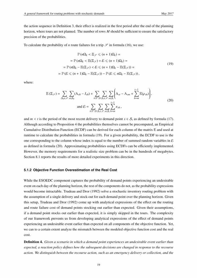
To calculate the probability of n route failures for a trip S in formula (16), we use:

P (nΩk < ΞS 6 (n + 1)Ωk) =

= P (nΩk < E(ΞS ) + E 6 (n + 1)Ωk) =

= P (nΩk − E(ΞS ) < E 6 (n + 1)Ωk − E(ΞS )) =

= P (E 6 (n + 1)Ωk − E(ΞS )) − P (E 6 nΩk − E(ΞS )) ,

(19)

where:

E (ΞS ) =∑S0∈S

∑s∈S0

(Λs0 − Is0) +∑

t∈T\0

∑St∈S

∑s∈St

Λst − Λsm +

t−1∑h=m

E(ρsh)

,and E =

∑t∈T\0

∑St∈S

∑s∈St

t−1∑h=m

εsh ,

(20)

and m < t is the period of the most recent delivery to demand point s ∈ St as defined by formula (17).

Although according to Proposition 4 the probabilities themselves cannot be precomputed, an Empirical

Cumulative Distribution Function (ECDF) can be derived for each column of the matrix E and used at

runtime to calculate the probabilities in formula (19). For a given probability, the ECDF to use is the

one corresponding to the column whose index is equal to the number of summed random variables in E

as defined in formula (20). Approximating probabilities using ECDFs can be efficiently implemented.

However, the memory requirements for a realistic size problem can be in the hundreds of megabytes.

Section 8.1 reports the results of more detailed experiments in this direction.

5.1.2 Objective Function Overestimation of the Real Cost

While the ESOEDC component captures the probability of demand points experiencing an undesirable

event on each day of the planning horizon, the rest of the components do not, as the probability expressions

would become intractable. Trudeau and Dror (1992) solve a stochastic inventory routing problem with

the assumption of a single delivery and stock-out for each demand point over the planning horizon. Given

this setup, Trudeau and Dror (1992) come up with analytical expressions of the effect on the routing

and route failure cost of demand points stocking out earlier than expected. Given their assumptions,

if a demand point stocks out earlier than expected, it is simply skipped in the tours. The complexity

of our framework prevents us from developing analytical expressions of the effect of demand points

experiencing an undesirable event earlier than expected on all components of the objective function. Yet,

we can to a certain extent analyze the mismatch between the modeled objective function cost and the real

cost.

Definition 4. Given a scenario in which a demand point experiences an undesirable event earlier than

expected, a reaction policy defines how the subsequent decisions are changed in response to the recourse

action. We distinguish between the recourse action, such as an emergency delivery or collection, and the

19


reaction policy.

Reaction policies can vary from doing nothing to completely re-optimizing the subsequent decisions.

Proposition 5. Given the un-captured effect of demand points experiencing an undesirable event earlier

than expected, in the absence of the EIHC component, the objective function 18 always overestimates the

real cost, in any context.

Proof. Take a demand point i that experiences an undesirable event, such as a stock-out or an overflow,

in period g and is not visited for regular service in period g. Considering a do-nothing reaction policy,

there will naturally be no effect on the VC, RC, WB and ESOEDC components of the objective function.

Note also that, for a given solution, the ESOEDC component already captures the probability, and hence

the expected cost, of the undesirable event for each demand point in each period of the planning horizon.

Disregarding the EIHC component, it remains to analyze the effect on the ERFC component. We identify

two basic scenarios:

1. Point i is never visited for regular service or is only visited for regular service in periods t 6 g. In

all these cases, there is no emergency service before the tours, if any, which visit point i for regular

service. Thus, the ERFC component is unaffected, hence the total cost is unaffected. The objective

function matches the real cost.

2. There is at least one visit for a regular collection from point i in periods t > g. Since the tour

visiting point i for regular service would distribute or collect less volume, the ERFC component

overestimates the real route failure cost. Therefore, the objective function overestimates the real

cost.

Naturally, given the existence of a more sophisticated reaction policy, the overestimation of the real

cost may be higher. On the other hand, the costs applied by EIHC component are not symmetric for a

distribution and a collection context. In a collection context, an emergency collection reduces inventory.

In this case, even in presence of the EIHC component, the objective function overestimates the real cost.

However, in a distribution context, an emergency delivery increases inventory and the direction of the

final effect of all components on the objective function is unclear.

The overestimation due to the do-nothing reaction policy is straightforward to evaluate using simulation

on the final solution. However, since the effect of an optimal reaction policy requires re-optimizing the

rest of the planning horizon after an undesirable event, it is impossible to have a precise evaluation for a

sufficient number of scenarios. Nevertheless, we can propose bounds depending on what components

are included in the objective function as well as other assumptions. We examine this in more detail in

Section 8.1.

5.2 Constraints

Starting from the basic routing constraints, tours have an origin and a destination depot, as ensured by

constraints (21), which also allow for simple relocation tours not visiting any demand or supply points.

Constraints (22) and (23) stipulate no return to the origin depots and no departure from the destination

20


depots. Given the possibility of open tours, we need to ensure that a vehicle’s destination depot in period t

is the same as its origin depot in period t + 1. Constraints (24) propagate this condition over the planning

horizon. Further on, constraints (25) and (26) link the visit and the routing variables, and constraints (27)

ensure that a point is visited at most once per period. Accessibility restrictions are enforced by constraints

(28). The latter can also be used to express continuity of service. Given that the problem is solved in a

rolling horizon fashion, it would not make sense to re-optimize at each rollover the vehicle(s) allowed

serve each point. On the contrary, these can be pre-defined using the binary flags αikt. Constraints (29)

ensure flow conservation.∑o′∈O′kt

∑j∈Nkt

xo′ jkt =∑i∈Nkt


xio′′kt ∀t ∈ T , k ∈ K (21)

∑i∈Nkt

xio′kt = 0 ∀t ∈ T , k ∈ K , o′ ∈ O′kt (22)∑j∈Nkt

xo′′ jkt = 0 ∀t ∈ T , k ∈ K , o′′ ∈ O′′kt (23)∑i∈Nkt

xiokt =∑

j∈Nk(t+1)

xo jk(t+1) ∀t ∈ T , k ∈ K , o ∈ O′′kt ∩ O′k(t+1) (24)

yikt =∑j∈Nkt

xi jkt ∀t ∈ T , k ∈ K , i ∈ Nkt \ O′′kt (25)

y jkt =∑i∈Nkt

xi jkt ∀t ∈ T , k ∈ K , j ∈ O′′kt (26)∑k∈K

yikt 6 1 ∀t ∈ T , i ∈ P (27)

yikt 6 αikt ∀t ∈ T , k ∈ K , i ∈ D ∪ P (28)∑i∈Nkt

xi jkt =∑i∈Nkt

x jikt ∀t ∈ T , k ∈ K , j ∈ D ∪ P (29)

The periodicity related constraints establish that a demand point i may be visited in periods r drawn from

one of several visit period combinations Ci for demand point i. Constraints (30) assign exactly one visit

period combination to each demand point, while constraints (31 allow a demand point to be visited only

in the periods corresponding to the assigned visit period combination (Cordeau et al., 1997). The set Ci

can contain visit period combinations with different frequencies, which makes the visit frequency part of

the optimization decisions.∑r∈Ci

cir = 1 ∀i ∈ P (30)∑k∈K

yikt −∑r∈Ci

αrtcir = 0 ∀t ∈ T , i ∈ P (31)

The inventory constraints at the demand points include constraints (32), which track the expected inventory

in period t as a function of the expected inventory, the quantity delivered to the point, and its expected

demand in period t − 1. Constraints (33) ensure that the expected inventory remains above the safety

level κi which can be arbitrarily close to zero, and constraints (34) force a delivery if the inventory is

below κi for point i in period t = 0. In addition, a rolling horizon enforces a one-period back-order limit.

Constraints (35)–(38) define the discrete ML policy outlined in Section 4.5. Constraints (35) stipulate

21


that if demand point is visited, then a discrete inventory level after delivery must be chosen. Constraints

(36) and (37) provide a lower and upper bound on the delivery quantity, which if the point is visited, is

equal to the difference between the chosen level and the expected inventory. The latter also imply that if

the point is visited, the chosen level will be higher than the expected inventory. Constraints (38) force the

delivery quantity to zero if the point is not visited. If the sets Li = ωi,∀i ∈ P, the discretized ML policy

reduces to the OU policy.

Iit = Ii(t−1) +∑k∈K

qik(t−1) − E(ρi(t−1)) ∀t ∈ T +, i ∈ P (32)

Iit > κi ∀t ∈ T +, i ∈ P (33)

κi − Ii0 6 κi

∑k∈K

yik0 ∀i ∈ P (34)∑k∈K

yikt −∑r∈Li

ìrt = 0 ∀t ∈ T , i ∈ P (35)

qikt >∑r∈Li

rìrt − Iit − (1 − yikt)ωi ∀t ∈ T , k ∈ K , i ∈ P (36)

qikt 6∑r∈Li

rìrt − Iit + (1 − yikt)ωi ∀t ∈ T , k ∈ K , i ∈ P (37)

qikt 6 ωiyikt ∀t ∈ T , k ∈ K , i ∈ P (38)

In the context of vehicle capacities, constraints (39) limit the cumulative quantity delivered by the vehicle

at each demand point, while constraints (40) reset it to zero at the supply points. Constraints (41) are

optional, and imposing them forces a visit to a supply point immediately after the origin depot, which

is appropriate in many applications in a distribution context. Similarly, setting the cumulative quantity

to zero at the destination depot will force a visit to a supply point just before it, which is appropriate

in many applications in a collection context. Keeping track of the cumulative quantity delivered by the

vehicle is achieved by constraints (42). Constraints (43) link the quantity delivered by the vehicle from

one period to the next.

qikt 6 Qikt 6 Ωk ∀t ∈ T , k ∈ K , i ∈ P (39)

Qikt = 0 ∀t ∈ T , k ∈ K , i ∈ D (40)

Qo′kt = Ωk ∀t ∈ T , k ∈ K , o′ ∈ O′ (41)

Qikt + q jkt 6 Q jkt + Ωk(1 − xi jkt

)∀t ∈ T , k ∈ K , i ∈ Nkt, j ∈ Nkt \ D (42)

Qo′k(t+1) > Qo′′kt ∀t ∈ T , k ∈ K , o′ ∈ O′, o′′ ∈ O′′ (43)

The next set of constraints express the intra-period temporal characteristics of the problem. Constraints

(44) calculate the start-of-service time at each point. In addition, these constraints eliminate the possibility

of subtours and ensure that a point is not visited more than once by the same vehicle. Constraints (45)

enforce the time windows. Constraints (46) bound the tour duration from above and below. Constraints

(47) enforce the maximum tour duration, and with it availabilities and vehicle use. Constraints (48) and

(49) bound the total tour duration over the planning horizon for each vehicle. The difference between¯B

22


and B is the difference between the lowest and highest vehicle workload over the planning horizon.

S ikt + δi + τi jkt 6 S jkt +(µi + δi + τi jkt

) (1 − xi jkt

)∀t ∈ T , k ∈ K , i ∈ Nkt, j ∈ Nkt (44)

λiyikt 6 S ikt 6 µiyikt ∀t ∈ T , k ∈ K , i ∈ Nkt (45)

¯bkt 6


S o′′kt −∑

o′∈O′kt

S o′kt 6 bkt ∀t ∈ T , k ∈ K (46)

bkt 6 Hktzkt, ∀t ∈ T k ∈ K (47)

¯B 6

∑t∈T

¯bkt ∀k ∈ K (48)

B >∑t∈T

bkt ∀k ∈ K (49)

Finally, lines (50)-(51) establish the variable domains.

xi jkt, yikt, zkt, cir′ , ìr′′t ∈ 0, 1 ∀t ∈ T , k ∈ K , i, j ∈ Nkt, r′ ∈ Ci, r′′ ∈ Li (50)

qikt,Qikt, Iit, S ikt, ¯bkt, bkt, ¯

B, B > 0 ∀t ∈ T , k ∈ K , i ∈ Nkt (51)

6 Application Examples

The framework developed and presented in Sections 3, 4 and 5 can be applied to problems from different

fields of routing and logistics optimization. In the sections below, we discuss in more detail a vehicle

routing problem, a health care inventory routing problem, a waste collection inventory routing problem, a

maritime inventory routing problem, and a facility maintenance problem.

6.1 The Vehicle Routing Problem

In a VRP setting, the presence of stochastic demands may lead to route failures but stock-outs/overflows

do not apply. The objective function formulation includes the two components:

min z = RC + ERFC. (52)

The generalized framework can be applied to a stochastic VRP setting in the following way. The planning

horizon T = 0, 1, 2 contains three periods and Hk0 = Hk2 = 0,∀k ∈ K , i.e. no vehicle is available in

periods t = 0 and t = 2. Moreover, Ii0 = ωi and Li = ωi,∀i ∈ P, i.e. the initial inventory of all demand

points is equal to capacity and we apply an OU inventory policy. Thus, given the action sequence of

Definition 3, the visits to the demand points will deliver the demands ρi0 realized in period 0. Since the

demand point capacity ωi does not apply per se, it should be such that ρi0 < ωi for all possible realizations

of the demand. The VRP is a single-period problem and the fact that it is solved for period t = 1 is of no

consequence. Finally, constraints (27) are replaced by (53) below to enforce a delivery to each demand

23


point in period t = 1, in order to guarantee a feasible VRP solution.∑k∈K

yik1 = 1 ∀i ∈ P (53)

The periodicity related constraints (30) and (31) are dropped as they become irrelevant for a single period.

The rest of the constraints remain the same as in Section 5.2.

6.2 The Health Care Inventory Routing Problem

The health care IRP generalizes the nurse routing and scheduling problem, in which nurses visit patient

homes to provide treatment. In this problem, P is a set of patient homes, whileD is a set of medical facil-

ities. In addition to providing treatment, nurses deliver medications with stochastic demand. Continuity

of service and workload balancing, which are the two paramount concerns in the nurse routing problem,

are supported by the framework. As is the periodic aspect, given that medical treatments usually have to

be performed with a certain frequency. Pricing can also be introduced in the setup via a negative visit

cost. The objective function is composed of the five components:

min z = VC + RC + WB + ESOEDC + ERFC. (54)

The constraints remain the same as in Section 5.2.

6.3 The Waste Collection Inventory Routing Problem

In this IRP variant, trucks collect waste from containers with stochastic demands. In the application that

we consider, P denotes a set of sensorized containers for recyclable materials, whileD denotes a set of

recycling facilities. The objective consists of the three components:

min z = RC + EOECC + ERFC, (55)

where EOECC is the Expected Overflow and Emergency Collection cost, a collection context counterpart

of the ESOEDC. The basic routing constraints (21)–(29), the inventory related (32)–(38), and the vehicle

capacity related (39)–(43) constraints also need to be recast for a collection context. In particular, a

recycling facility must be visited immediately before the destination depot. Markov et al. (2016a) use past

container level information to predict future demands, using the forecasting model of Markov et al. (2015)

which assumes a normal distribution for the stochastic error component. They use objective (55) to solve

rich IRP instances derived from real data coming from the canton of Geneva, Switzerland. The result

is a significant reduction in the occurrence of container overflows for the same routing cost compared

to alternative policies. Markov et al. (2016a) also analyze the solution properties of a rolling horizon

approach and derive empirical lower and upper bounds.

24


6.4 The Maritime Inventory Routing Problem

In this problem, a fleet of ships transports petroleum products from a setD of supply terminals to a set

P of demand terminals with limited inventory capacity. A particular feature of this application is that

emergency deliveries may be impractical due to long shipping distances. Figure 4 depicts a setup in which

the state of stock-out at a demand terminal is a final state. Once it is reached, the terminal stays in a state

of stock-out unless there is a regular delivery planned by the optimization model. The tree depicted in

Figure 4 is a special case of the one depicted in Figure 2 and therefore fits the current framework.

Maritime routing problems are often modeled on time-expanded graphs, similar to the one depicted in

Figure 5, in which each point (i, j, . . . , k) appears in each period of the planning horizon (0, 1, . . . , u). The

graph includes an artificial source s and sink e. In each period, a ship may stay at the same point or move

to another point. In other words, the problem is characterized by open and multi-period tours, which

may include idling. Our framework implicitly allows for multi-period tours, by generating an origin and

destination depot at zero distance from each demand and supply terminal. A tour can thus effectively end

at a demand or supply terminal in period t and start from it in period t + 1.

The objective is the sum of five components:

min z = EIHC + VC + RC + ESOC + ERFC, (56)

Figure 4: State probability tree for a demand terminal without regular deliveries

σi0 =0

σi1 =0

σi1 =1

σi2 =0

σi2 =1

σi2 =1

σi3 =0

σi3 =1

σi3 =1

σi3 =1

σi4 =0

σi4 =1

σi4 =1

σi4 =1

σi4 =1

P(Λi0−ρi0>

0)

P(Λi0−ρi060)

P(Λi0−ρi0−

ρi1>0

|Λi0−ρi0>

0)

P(Λi0−ρi0−ρi160|Λi0−ρi0>0)

P = 1

P(Λi0−ρi0−ρi1−ρi2>0

|Λi0−ρi0−ρi1>0)

P(Λi0−ρi0−ρi1−ρi260|Λi0−ρi0−ρi1>0)

P = 1

P = 1

P(Λi0−ρi0−ρi1−ρi2−ρi3>0

|Λi0−ρi0−ρi1−ρi2>0)

P(Λi0−ρi0−ρi1−ρi2−ρi360|Λi0−ρi0−ρi1−ρi2>0)

P = 1

P = 1

P = 1

· · ·

· · ·

· · ·

· · ·

· · ·

Figure 5: Time-expanded graph

(i, 0) (i, 1) (i, 2)· · ·

(i, u)

( j, 0) ( j, 1) ( j, 2)

· · ·

( j, u)

......

......

...

(k, 0) (k, 1) (k, 2)

· · ·

(k, u)

s e

Time

25


where ESOC is the Expected Stock-Out Cost component, which is modified from the ESOEDC component

presented in Section 5.1 by excluding the emergency delivery cost logic. The ESOC is formulated

as:

ESOC =∑

t∈T∪T +

∑i∈P

(P

(σit = 1 | Λim : m = max

(0, g < t : ∃k ∈ K : yikg = 1

))χi

). (57)

The VC component captures terminal docking fees. The constraints remain the same as in Sec-

tion 5.2.

6.5 The Facility Maintenance Problem

The facility maintenance problem is a probability-based routing problem in which a set of facilities is

visited by a set of technicians for inspection and repair. In this problem, the set P represents the facilities,

while the setD is irrelevant and can be reduced to a dummy supply point. Uncertainty with respect to

breakdowns can be considered as accumulating as would inventory. Consider facility i ∈ P in period t.

We can interpret state σit = 1 as a breakdown, and the state σit = 0 as operational. If a facility is in a

state of breakdown in period t, an emergency visit must be performed to repair it. However, there is no

expected period in which a facility will be in a state of breakdown. The probability of a breakdown is a

function of the number of periods since the most recent visit, and is illustrated in Figure 6, where pgi is

the probability of a breakdown, which depends on the number of periods g that have elapsed since the

most recent visit. The technicians are scheduled to perform inspections of the facilities over the planning

horizon. An inspection visit starts a new state probability tree as would a regular delivery/collection. The

probability function pgi can, for example, be defined as:

pgi =

arctan(ag)π/2

, (58)

where a is a tunable parameter defining the curvature of the probability function. The complete objective

is the sum of the three components:

min z = VC + RC + EERC, (59)

where EERC is the Expected Emergency Repair Cost, which is expressed as:

EERC =∑

t∈T∪T +

∑i∈P

(P

(σit = 1 | m : m = max

(0, g < t : ∃k ∈ K : yikg = 1

))ζi). (60)

The concept of route failure does not exist in the facility maintenance problem. All inventory related

constraints (32)–(38) and vehicle capacity related constraints (39)–(43) are irrelevant and can be dropped

from the model presented in Section 5.2. The new set of constraints (61) is added to force a visit to a

facility in a state of breakdown in period t = 0.∑k∈K

yik0 = 1, ∀i ∈ P : σi0 = 1 (61)

26


Figure 6: State probability tree for a facility without inspection visits

σi0 =0

σi1 =0

σi1 =1

σi2 =0

σi2 =1

σi2 =0

σi2 =1

σi3 =0

σi3 =1

σi3 =0

σi3 =1

σi3 =0

σi3 =1

σi3 =0

σi3 =1

σi4 =0

σi4 =1

σi4 =0

σi4 =1

σi4 =0

σi4 =1

σi4 =0

σi4 =1

σi4 =0

σi4 =1

σi4 =0

σi4 =1

σi4 =0

σi4 =1

σi4 =0

σi4 =1

1−

p1 i

p 1i

1 − p2i

p 2i

1 − p1i

p 1i

1 − p3i

p3i

1 − p1i

p1i

1 − p2i

p2i

1 − p1i

p1i

1 − p4i

p4i

1 − p1i

p1i

1 − p2i

p2i

1 − p1i

p1i

1 − p3i

p3i

1 − p1i

p1i

1 − p2i

p2i

1 − p1i

p1i

· · ·

· · ·

· · ·

· · ·

· · ·

· · ·

· · ·

· · ·

· · ·

· · ·

· · ·

· · ·

· · ·

· · ·

· · ·

· · ·

7 Methodology

Our generalized framework is not limited to any specific solution methodology. Various meta-heuristic

or hybrid approaches can be applied. We extend the ALNS developed by Markov et al. (2016a), which

exhibits excellent performance on VRP and IRP benchmark instances from the literature, as well as on

waste collection IRP instances derived from real data coming from the canton of Geneva, Switzerland.

Here, we discuss the additions and changes to the original algorithm in order to account for all the

features present in the generalized framework. Section 7.1 defines the solution representation used by

the algorithm, while Section 7.2 lists the additional operators designed to tackle the full set of features

present in the framework. The general description of the ALNS, as well as the parameter configuration

on which it runs are described in detail in Markov et al. (2016a).

7.1 Solution Representation

The ALNS admits infeasible intermediate solutions with all types of feasibility violations described in

Markov et al. (2016a) plus a violation of the visit period combination. Here, we redefine some of the

violations defined in Markov et al. (2016a) to reflect the generality of the framework or the distribution

context in which it is presented. Using (x)+ = max0, x, we have:

27


1. Vehicle capacity violation VΩ(s) is redefined to capture the more general concept of trips in the

framework, with trips being supply point delimited sequences, possibly spanning over multiple

periods. It is the sum of excess volume delivered in each trip and is formulated as:

VΩ(s) =∑k∈K

∑S ∈Sk

∑t∈T

∑St∈S

∑s∈St

qskt −Ωk

+

. (62)

2. Time window violation Vµ(s) is the total violation of the visited points’ upper time window bounds.

It remains unchanged.

3. Duration violation is the sum of excess tour durations. It is redefined to reflect the presence of

multiple origin and destination depots:

VH(s) =∑t∈T

∑k∈K

∑o′′∈O′′

S o′′kt −∑

o′∈O′S o′kt − H

+

. (63)

4. Demand point capacity violation is redefined for a distribution context and computes the sum of

negative demand point inventories ∀t ∈ T +, i ∈ P, or:

Vω(s) =∑t∈T +

∑i∈P

(−Iit)+. (64)

5. Backorder limit violation is redefined for a distribution context and is the sum of negative demand

point inventories in period t = 0,∀i ∈ P that are not visited in period t = 0. In mathematical terms,

this is expressed as:

V0(s) =∑i∈P

1 −∑

k∈K

yik0

(−Ii0)+

. (65)

6. Accessibility violation Vα(s) is the sum of the unaccessible point visits. It remains unchanged.

7. Visit period combination violation captures visits to demand points performed outside of the

assigned visit period combinations, as well as unperformed visits when such are required by the

assigned visit period combinations. Mathematically, it is expressed as:

Vr(s) =∑t∈T

∑i∈P

∣∣∣∣∣∣∣∣∑k∈K

yikt −∑r∈Ci

αrtcir

∣∣∣∣∣∣∣∣. (66)

With the above violations, the complete solution cost during the search is represented by:

f (s) = z(s) + LΩVΩ(s) + LµVµ + LHVH(s) + LωVω(s) + L0V0(s) + LαVα(s) + LrVr(s), (67)

where parameters LΩ through Lr penalize each type of feasibility violation.

28


7.2 Operators

To incorporate the features of the framework, we need to both develop new operators and introduce

modifications to some of the operators described in Markov et al. (2016a). We include the following

three new repair operators to the ALNS:

1. Replace a destination depot: This operator selects a random tour and replaces its destination depot

with a random destination depot o ∈ O′′kt, where t ∈ T is the period in which the tour is executed

and k ∈ K is the vehicle executing it. The algorithm then finds min t′ > t s.t. Hkt′ > 0, i.e. the next

period t′ for which vehicle k is available, and changes the origin depot of the tour that vehicle k

executes in period t′ to o.

2. Change visit period combination: This operator selects a random demand point i ∈ P and assigns

to it a random visit period combination r ∈ Ci.

3. Change inventory level after delivery: This operator selects a random tour executed in period t and

a random demand point i in this tour. It then selects a random level r ∈ Li s.t. Λit = rìrt > Iit and

assigns it to demand point i in period t.

The change visit period combination operator is applied to each demand point i ∈ P before the start

of the search in order for the visit period combination violation to be defined. Finally, the presence of

visit period combinations may render infeasible an excessive number of solutions. In order to keep this

number under control, various modifications may be applied to the destroy and repair operators described

in Markov et al. (2016a) that remove, insert and swap demand points, for example:

• demand point i ∈ P may be inserted in a tour executed in period t, only when αrt = 1, i.e. when

period t belongs to the visit period combination r assigned to demand point i,

• demand point i ∈ P may be removed from a tour executed in period t, only when αrt = 0, i.e. when

period t does not belong to the visit period combination r assigned to demand point i,

• demand points i and j ∈ P belonging to different tours may be swapped in both conditions above

hold.

More sophisticated logic may also be applied, for example inserting a demand point in all periods

belonging to the assigned visit period combination and removing it from all periods not belonging to

it.

8 Numerical Experiments

In the following, we carry out a series of experiments to investigate various features of the proposed

unified framework. The first two sets of experiments address the forecasting methodology. Section 8.1

tests the effect on computation time of using ECDFs derived from simulated errors in calculating the

route failure probabilities. Section 8.2 evaluates the impact of better forecasts, i.e. forecasts with smaller

errors, on the expected cost. It shows to what extent implementing or investing in better forecasting

29


techniques would improve the solution cost. The next two sets of experiments focus on modeling-related

questions. Section 8.3 explores the objective function overestimation of the real cost using simulation on

the final solution, and tests an intuitive upper bound. Section 8.4 studies the benefit of allowing open

tours, i.e. tours with destination depots different than their origin depots. These four sections use the

waste collection IRP instances introduced in Markov et al. (2016a). Finally, in Section 8.5 we present

a new case study based on the facility maintenance problem, a probability-based routing problem, and

develop computational experiments on instances derived from real data. The ALNS is implemented as

a single-threaded application in Java, and the probability calculations for the state probability trees are

performed in R. All tests have been run on a 3.33 GHz Intel Xeon X5680 server running a 64-bit Ubuntu

16.04.2. In all experiments below, each instance is solved 10 times using the ALNS parameter tuning as

in Markov et al. (2016a).

8.1 Using Simulation for the Route Failure Probabilities

The waste collection IRP instances introduced in Markov et al. (2016a), and used in Sections 8.1 to

8.4, includes 63 instances, each covering a week of white glass collections in the canton of Geneva,

Switzerland in 2014, 2015, or 2016. Tours are constrained to a maximum duration of four hours each, and

the time windows correspond to 8:00 a.m. to 12:00 p.m. The planning horizon is seven days long, starting

on Monday and finishing on Sunday. Each instance contains a maximum of two trucks of volume capacity

in the order of 30,000 liters and weight capacity of 10,000 to 15,000 kg, not available on Saturday and

Sunday. On average, there are 41 containers per instance, and the maximum is 53, and their volumes

range from 1000 to 3000 liters. Two dumps are located far apart in the periphery of the city of Geneva.

The trucks incur a daily deployment cost of 100 CHF, a cost of 2.95 CHF per kilometer and a cost of 40

CHF per hour. The overflow cost is set to 100 CHF. The demands for each instance are forecast using the

forecasting model presented in Markov et al. (2016a) using, for each instances, the previous 90 days of

data, and assuming a normal distribution of the error terms. The forecasting model in question is based

on a mixture of count data models. For details, the reader is referred to Markov et al. (2016a) and Markov

et al. (2015).

As discussed in Section 5.1.1, the use of a general distribution D($) requires the use of Empirical

Cumulative Distribution Functions (ECDFs) in the calculation of the route failure probabilities. Clearly,

the main risk of using ECDFs is their impact on computation time and the precision of the result they

produce. To investigate that, we use the methodology described in Section 5.1.1 and simulate the normally

distributed error component provided by the forecasting model to construct a matrix E with M = 100, 000

rows for each instance and derive ECDFs, which are then used at runtime. The ECDFs are constructed

using the EmpiricalDistribution class of the Apache Commons Math 3.6.1 release1. We test two

configurations for the ECDFs, one binning the 100,000 draws in 1000 bins and one binning them in 100

bins. Computational experiments show that the configuration with 1000 bins exhibits a squared error with

respect to the normal distribution in the order of 10−7, while for the configuration with 100 bins, it is in

the order of 10−6. Additionally, for each of these two configurations, we test two versions of the ALNS.

The first one is the “original" version, which calculates the probability of route failure at each change in

1http://commons.apache.org/proper/commons-math/javadocs/api-3.6.1/index.html

30

http://commons.apache.org/proper/commons-math/javadocs/api-3.6.1/index.html


Table 2: Impact of ECDFs on computation time

Cost (CHF) Runtime (s.) ECDF calls (millions)

ALNS version Bins ECC RFCM Best Avg Worst Best Avg Worst Best Avg Worst

Original - 100 1 662.65 666.64 672.87 870.65 906.84 936.40 - - -

Original 1000 100 1 662.82 666.97 673.43 1028.87 1096.86 1153.05 84.91 94.93 105.52

Original 100 100 1 662.29 666.61 673.40 912.54 955.96 990.57 84.11 94.54 103.84

Efficient 1000 100 1 662.63 666.74 673.35 909.06 948.77 982.68 52.95 58.90 65.00

Efficient 100 100 1 662.49 666.46 672.73 869.52 903.81 932.79 52.94 58.44 63.90

the solution. The second one is the “efficient" version, which uses the ECDFs more sparingly, calculating

the probability of route failure only when changes include inserting new points into or removing points

from a tour, but not when points in a tour are only rearranged.

Table 2 reports the results of the experiments. The experiments are performed using the objective function

(55) with an Emergency Collection Cost (ECC) of 100 CHF and a Route Failure Cost Multiplier (RFCM)

of one. We highlight that the waste collection IRP model of Markov et al. (2016a) assumes a maximum of

one route failure per depot-to-dump or dump-to-dump trip. In addition, trips do no span over consecutive

periods, as each daily tours ends with a visit to a dump just before the destination depot. In the table,

each row reports averaged values over the 63 instances. The first column identifies the version of the

ALNS used, i.e. original vs. efficient, while the second one identifies the binning configuration. A dash

signifies that the ALNS uses the analytical approximation of the normal distribution of Abramowitz

and Stegun (1972) presented in Markov et al. (2016a). This is the base version of the ALNS against

which we compare the effect of using ECDFs on the computation time. The next two columns show the

ECC and the RFCM, which are the same for all instances. The fifth, sixth and seventh column present

the best, average and worst cost over 10 runs. In a similar fashion, the eight, ninth and tenth column

report the best, average and worst computation time, and the eleventh, twelfth and thirteenth column

report the best, average and worst number of calls to the ECDFs over 10 runs. Expectedly, Table 2 shows

that the different implementations have no impact on the solution cost. However, there is a significant

impact on the computation time and the number of calls to the ECDFs. The efficient implementations

use approximately 40% fewer calls to the ECDFs, with a corresponding reduction in computation time

of 10-15% for the configuration with 1000 bins and about 5% for the configuration with 100 bins. Both

efficient implementations are faster than the original implementations. We observe also that the efficient

implementation with 100 bins has a computation time that is virtually the same as that of the base

implementation with an analytical approximation of the normal distribution. However, as mentioned

before, the binning configuration with 1000 bins has an error which is one degree of magnitude lower,

while the computation time is only about 5% higher. Thus, this configuration may be preferable. In sum,

the results show that for the 63 instances under consideration, the use of ECDFs has only a minor impact

on the computation time. Further testing is needed to confirm whether this result holds in general.

8.2 Evaluating the Impact of Better Forecasts

Given the central role of forecasting in our framework, this section studies the effect of better forecasts

on the quality of the solution. In particular, it tries to answer the question of whether it is beneficial to

31


implement, or invest in, better forecasting techniques. The experiments are performed on modifications

of 53 of the waste collection IRP instances proposed by Markov et al. (2016a). As in Section 8.1, the

demands of the original 53 instances are forecast using the forecasting model presented in Markov et al.

(2016a), which provides the expected demands E (ρit) ,∀i ∈ P, t ∈ T , and the standard deviation ς of the

errors εit, where εitiid∼N

(0, ς2

). To emulate having access to different quality of forecasts, we proceed

as follows. First, we replace the expected demands E (ρit) by the observed demands ρoit from the historical

data. Secondly, we perturb the observed demands by drawing randomly from N(0, υς2

), where the

forecasting error multiplier υ ∈ 0.00, 0.25, 0.50, 0.75, 1.00. Thus, each of the 53 original instances is

transformed into 5 instances, where the forecast quality ranges from perfect for υ = 0 to the one resulting

from the current forecasting techniques for υ = 1.

As expected, Figure 7 shows that the distribution of the expected costs exhibits growth with respect to the

forecasting error multiplier. In addition, Figure 8 suggests that the costs probably follows a trend which

is closer to exponential than to linear. To verify this, we perform a linear and an exponential fit, where the

explanatory variables are the forecasting error multiplier υ and a dummy variable for each subset of 5

instances except one. The exponential fit is based on the formula:

z(s) ∼ a + exp(b + cP), (68)

where a, b and the vector c are estimable parameters, and P is the matrix of explanatory variables. The

linear fit produces an adjusted R2 of 0.82, and has a Residual Sum of Squares (RSS) of 1,784,393. In

comparison, the exponential fit has an RSS of 1,185,938, which is lower by one third. This result gives an

indication that the solution quality improves exponentially with the improvement in the forecast quality.

Thus, implementing, or investing in, better forecasting techniques would have an important impact on the

solution of the 63 instances under consideration. Further testing is needed to confirm whether this result

holds in general.

Figure 7: Cost distribution for different forecasting error multipliers

0

500

1000

1500

0 0.25 0.5 0.75 1Forecasting error multipliers

Cos

t (C

HF

)

32


Figure 8: Linear vs. exponential fit for different forecasting error multipliers.

400

500

600

700

800

0.00 0.25 0.50 0.75 1.00Forecasting error multipliers

Ave

rage

Cos

t (C

HF

)

Legend Average Cost Exponential Fit Linear Fit

8.3 Using Simulation to Evaluate the Objective Function Overestimation of the RealCost

In Section 5.1.2, we discussed the objective function overestimation of the real cost, which is due to the

un-captured effect in most parts of the objective function of demand points experiencing an undesirable

event, such as a stock-out or an overflow, earlier than expected. The purpose of this section is to assess

the overestimation for the 63 waste collection IRP instances introduced in Markov et al. (2016a) through

simulation on the final solution. The simulation experiment is the same as the one used in Markov et al.

(2016a). That is, on the final solution produced by the ALNS, we perform 10,000 simulations, sampling

independently the error terms εit, where εitiid∼N

(0, ς2

), and applying it to the expected demand E(ρit),

for each container i ∈ P and each day t ∈ T . Then, in addition to evaluating the effect on the occurrence

of container overflows and route failures, we also assess the effect on the overestimation of the real cost

brought about by the occurrence of overflows.

Computing the overestimation due to a do-nothing reaction policy is trivial. In the absence of inventory

holding costs, which is the case for the waste collection IRP instances, the effect is only present in the

ERFC component. Naturally, the overestimation will be higher for an optimal reaction policy which, in the

occurrence of overflows, re-optimizes all subsequent decisions. However, computing the overestimation

due to an optimal reaction policy has a significant computational burden, as it requires that re-optimization

should be done during the 10,000 simulation runs for each instance. Thus, we develop the following

bound on the overestimation due to an optimal reaction policy. Take a container i that overflows in period

g and which is visited for regular collection in periods t > g. Now, take the minimum period min t > g in

which container i is visited for regular collection and imagine that the optimal policy is so good that it

can remove the cost effect of container i from all periods t > min t. In other words, 1) we remove the

container from all tours executed in periods t > min t. This produces the highest possible overestimation

of the RC and ERFC components. 2) We also equalize to zero the probability of overflow in periods

t > min t, which leads to the highest possible overestimation of the EOECC component.

Using the objective function (55), with an ECC of 100 CHF and an RFCM of one, and assuming a single

overflow per trip, the results of the simulation runs indicate that, averaged over the 63 instances, the

33


number of overflows ranges from 0.81 at the 75th percentile to 3.25 at the 99th percentile, while the

number of route failures ranges from 0.05 at the 75th percentile to 0.08 at the 99th percentile. At the

same time, the overestimation due to a do-nothing reaction policy is 0.00% for all simulation percentiles,

undoubtedly because of the marginal contribution of the ERFC component to the total cost. On the other

hand, the upper bound of the optimal reaction policy ranges from 0.02% at the 75th percentile to 1.07% at

the 99th percentile, indicating the very low level of overestimation of the real cost. At the 99th percentile,

the median overestimation is 0.65% and the maximum one is 9.08%. We also observe, not surprisingly,

a strong correlation in the order of 80% between the number of overflows and the upper bound of the

optimal reaction policy across the 63 instances.

8.4 Evaluating the Impact of Open Tours

In a deterministic VRP setting, Markov et al. (2016b) find an average improvement of 2.54% of the

best solution when allowing open tours on modifications of the Crevier et al. (2007) instances. The

improvements go up to more than 10% for some of the instances, and appear to be negatively related to

the instance size. To evaluate the effect of open tours on realistic instances, we use the 63 waste collection

IRP instances proposed by Markov et al. (2016a) by constructing four to eight depots for each vehicle,

depending on historical data, of which one is its home depot, and require that the vehicle should return

to its home depot only on Friday. Table 3 provides the results of the comparison, where each line is an

averaged result over the 63 instances. For the objective function (55) with an ECC of 100 CHF and an

RFCM of one, allowing open tours leads to an average decrease of 6.16% in the objective, with values

ranging from 0 to 12.07%. For the routing-only objective, consisting simply of the RC component, the

average decrease is 9.64%, with values ranging from 0 to 17.12%. The case study presented in Markov

et al. (2016b) includes regions where such tours are practiced. Therefore, this result demonstrates that the

findings and conclusions therein are valid, and in fact even more pronounced, for a multi-day problem.

The improvements for a multi-day problem do not seem to be related to the instance size.

8.5 Solving the Facility Maintenance Problem

The facility maintenance problem, as defined in Section 6.5, considers a set of facilities that have to be

periodically inspected in order to limit the occurrence of breakdowns. We create a set of 94 instances,

derived from the waste collection IRP instances presented in Markov et al. (2016a). The instances contain

an average of 42 facilities, with a maximum of 62. Tours are constrained to a maximum duration of

four hours each, and the time windows correspond to 8:00 a.m. to 12:00 p.m. The planning horizon is

Table 3: Comparison between closed-tour and open-tour solutions

Type ECC RFCM Best Cost (CHF) Avg Cost (CHF) Gap Avg Best (%)

Complete & Closed Tours 100 1 662.80 666.93 0.62

Complete & Open Tours 100 1 622.60 647.54 4.00

Routing-only & Closed Tours 0 0 421.99 422.48 0.12

Routing-only & Open Tours 0 0 377.59 391.87 3.73

34


seven days long, starting on Monday and finishing on Sunday. Each instance contains a maximum of

two vehicles, not available on Saturday and Sunday. The vehicles incur a daily deployment cost of 100

CHF, a cost of 2.95 CHF per kilometer and a cost of 40 CHF per hour. The emergency repair cost for

each facility is set to 100 CHF and the visit cost to 1 CHF. For the breakdown probabilities, we use the

event probability function defined by expression (58) for a = 0.025. In addition, for each facility i ∈ P in

period 0, we draw a random number between 1 and 5, inclusive, for the number of days since the most

recent visit.

To analyze the value added of the probabilistic objective function, we perform two types of experiments.

In the first type, we use the full probabilistic objective function as defined by formula (59). In the second

type, we use a deterministic objective function consisting of the VC and RC components only. In addition,

for the deterministic objective, since there is no constraint to force facility visits, we introduce a service

level expressed as the maximum allowed probability for a facility breakdown. Table 4 presents the results

of the comparison, where each line is an averaged result over the 94 instances. The first column identifies

the objective used, i.e. probabilistic vs. deterministic. The second column reports the service level in

terms of the maximum allowed probability of breakdown. For the probabilistic objective this is 1, or in

other words it is trivially satisfied. For the deterministic objective, we test the levels of 0.10, 0.05 and

0.01. The next three columns report the average Routing Cost (RC), average Visit Cost (VC), and average

Expected Emergency Repair Cost (EERC). The latter only applies to the probabilistic objective function.

The last four columns present the average number of breakdowns after 10,000 simulations of the event

probability function defined by expression (58).

From Table 4, it becomes immediately clear that the deterministic objective functions underperform

the probabilistic one. The first deterministic objective function with a service level p < 0.10 leads to a

halving of the routing and the visit cost, with a total saving of 408.07 CHF. Nevertheless, this decrease is

more than compensated by a higher number of breakdowns at all percentiles. By capturing this through

the expected emergency repair cost, the probabilistic objective integrates it in an intelligent way that leads

to a relatively moderate increase in the routing and visit cost, compared to a more significant decrease in

the realizations of breakdowns after simulations. Moreover, as in a collection context, the probabilistic

objective function (59) overestimates the real cost. Thus the real routing and visit cost for the probabilistic

objective may be lower. Improving the service level to p < 0.05 in the deterministic objective leads to a

much higher routing and visit cost, but the number of breakdowns after simulation is still higher than that

of the probabilistic objective. Improving the service level even further to p < 0.01 results in infeasible

solutions for the currently used event probability function.

Table 4: Comparison of probabilistic vs. deterministic visit policies

Avg Num Breakdowns

Objective p < Avg RC Avg VC Avg EERC 75th perc. 90th perc. 95th perc. 99th perc.

Probabilistic 1.00 716.62 78.43 1,478.84 12.92 15.04 16.36 18.91

Deterministic 0.10 352.60 34.38 – 19.98 22.65 24.21 27.30

Deterministic 0.05 909.56 87.48 – 14.66 16.82 18.18 20.76

Deterministic 0.01 infeasible

35


9 Conclusion

In this work, we introduce, analyze and formulate a generalized framework for solving various classes

of vehicle and inventory routing problems as well as other probability-based routing problems with a

time-horizon dimension. Demand is assumed to be stochastic and non-stationary and is forecast using

any forecasting model that provides expected demands over the planning horizon, with error terms from

any empirical distribution. The formulation includes many rich routing features relevant to real-world

problems, such as multiple depots, open and multi-period tours, intermediate facilities, time windows,

accessibility restrictions, visit periodicities and service choice, etc. The practical applicability of the

approach is reinforced by the fact that most probability values related to demand stochasticity can be

pre-computed. Thus, the effect on computation time is marginal, which is critical for operational problems,

such as waste collection, health care routing, and others discussed in the text. Finally, we show that some

problems where the inventory component is not present, such as facility maintenance, can still be viewed

through the prism of inventory routing, with event probabilities at the demand points, or breakdown

probabilities in this specific example, accumulating as would inventory.

We focus the numerical experiments on realistic instances of the waste collection inventory routing prob-

lem and the facility maintenance problem. We analyze the cost benefits of open tours and the availability

of better forecasting methodologies. We demonstrate that relaxing the distributional assumptions on the

forecasting error terms and calculating probabilities using empirical cumulative distribution functions

has only a minor impact on computation time. Simulating the error terms on the final solution further

allows us to verify the low level of occurrence of undesirable events and shows that the objective is an

excellent representation of the real cost. Capturing the facility breakdown probability in our framework

leads to significantly fewer realized breakdowns after simulation, while having only a moderate effect

on the routing and visit cost. There are three main directions for future work. The first one concerns

the mathematical model and the assumptions behind it. Developing a more comprehensive objective

function that captures more of the probability propagations may make it possible to relax some of the

assumptions and to allow an even richer routing setting. Secondly, developing more benchmark instances

will allow testing the framework’s full capabilities on different problem types. While there exist bench-

mark instances for many of the reviewed problems, they are largely deterministic or involve a very simple

routing structure. In order for the conclusions to be meaningful, it is critical that the instances represent

or at least are derived from real data. Finally, tests on additional instances will help improve the solution

methodology by parameter tuning and identifying missing and potentially useful new operators.

Acknowledgement

The authors would also like to thank Raphaël Lüthi and Prisca Aeby, both master student at the Transport

and Mobility Laboratory of École Polytechnique Fédérale de Lausanne, for their dedicated and high-

quality work on this problem. The authors would also like to thank Matthieu de Lapparent, a scientific

collaborator at the same laboratory, for his advice on probability and statistics related questions.

36


10 References

Abramowitz, M. and I. A. Stegun (eds.) (1972) Handbook of Mathematical Functions with Formulas,

Graphs, and Mathematical Tables, New York: Dover Publications, ISBN ISBN 978-0-486-61272-0.

Aghezzaf, E.-H. (2008) Robust distribution planning for supplier-managed inventory agreements when

demand rates and travel times are stationary, The Journal of the Operational Research Society, 59 (8)

1055–1065, ISSN 01605682.

Angelelli, E. and M. G. Speranza (2002a) The application of a vehicle routing model to a waste-collection

problem: Two case studies, The Journal of the Operational Research Society, 53 (9) 944–952, ISSN

01605682.

Angelelli, E. and M. G. Speranza (2002b) The periodic vehicle routing problem with intermediate

facilities, European Journal of Operational Research, 137 (2) 233–247, ISSN 0377-2217.

Arslan, A. N. and D. J. Papageorgiou (2015) Bulk ship fleet renewal and deployment under uncertainty:

A multi-stage stochastic programming approach. Working Paper, Department of Industrial & Systems

Engineering, University of Florida, Gainesville, FL, USA.

Baldacci, R. and A. Mingozzi (2009) A unified exact method for solving different classes of vehicle

routing problems, Mathematical Programming, 120 (2) 347–380, ISSN 0025-5610.

Bard, J. F., L. Huang, M. Dror and P. Jaillet (1998a) A branch and cut algorithm for the VRP with satellite

facilities, IIE Transactions, 30 (9) 821–834, ISSN 0740-817X.

Bard, J. F., L. Huang, P. Jaillet and M. Dror (1998b) A decomposition approach to the inventory routing

problem with satellite facilities, Transportation Science, 32 (2) 189–203.

Bertsimas, D. and M. Sim (2003) Robust discrete optimization and network flows, Mathematical Pro-

gramming, 98 (1-3) 49–71, ISSN 0025-5610.

Bertsimas, D. and M. Sim (2004) The price of robustness, Operations Research, 52 (1) 35–53.

Bitsch, B. (2012) Inventory routing with stochastic demand, Master Thesis, Aarhus School of Business

and Social Sciences, Aarhus University, Aarhus, Denmark.

Cheng, L. and M. A. Duran (2004) Logistics for world-wide crude oil transportation using discrete

event simulation and optimal control, Computers & Chemical Engineering, 28 (6–7) 897–911, ISSN

0098-1354.

Cordeau, J.-F., M. Gendreau and G. Laporte (1997) A tabu search heuristic for periodic and multi-depot

vehicle routing problems, Networks, 30 (2) 105–119, ISSN 1097-0037.

Crevier, B., J.-F. Cordeau and G. Laporte (2007) The multi-depot vehicle routing problem with inter-depot

routes, European Journal of Operational Research, 176 (2) 756–773, ISSN 0377-2217.

Dantzig, G. and R. Ramser (1959) The truck dispatching problem., Management Science, 6, 80–91.

37


Delage, E. and D. A. Iancu (2015) Robust Multistage Decision Making, chap. 2, 20–46.

Errarhout, A., S. Kharraja and C. Corbier (2016) Two-stage stochastic assignment problem in the home

health care, IFAC-PapersOnLine, 49 (12) 1152–1157, ISSN 2405-8963. 8th IFAC Conference on

Manufacturing Modelling, Management and Control MIM, Troyes, France, 28–30 June 2016.

Errarhout, A., S. Kharraja and A. Matta (2014) The uncertainty in the home health care assignment

problem, paper presented at the Proceedings of the 3rd International Conference on Operations

Research and Enterprise Systems, 453–459, ISBN 978-989-758-017-8.

Gendreau, M., O. Jabali and W. Rei (2014) Chapter 8: Stochastic vehicle routing problems, in P. Toth and

D. Vigo (eds.) Vehicle Routing: Problems, Methods, and Applications, Second Edition, SIAM.

Gendreau, M., O. Jabali and W. Rei (2016) 50th anniversary invited article–future research directions in

stochastic vehicle routing, Transportation Science, 50 (4) 1163–1173.

Goeke, D. and M. Schneider (2015) Routing a mixed fleet of electric and conventional vehicles, European

Journal of Operational Research, 245 (1) 81–99.

Gounaris, C. E., W. Wiesemann and C. A. Floudas (2013) The robust capacitated vehicle routing problem

under demand uncertainty, Operations Research, 61 (3) 677–693.

Halvorsen-Weare, E. E., K. Fagerholt and M. Rönnqvist (2013) Vessel routing and scheduling under

uncertainty in the liquefied natural gas business, Computers & Industrial Engineering, 64 (1) 290–301,

ISSN 0360-8352.

Hemmelmayr, V., K. F. Doerner, R. F. Hartl and S. Rath (2013) A heuristic solution method for node

routing based solid waste collection problems, Journal of Heuristics, 19 (2) 129–156, ISSN 1381–1231.

Hemmelmayr, V., K. F. Doerner, R. F. Hartl and M. W. Savelsbergh (2010) Vendor managed inventory

for environments with stochastic product usage, European Journal of Operational Research, 202 (3)

686–695, ISSN 0377-2217.

Hemmelmayr, V., K. F. Doerner, R. F. Hartl and M. W. P. Savelsbergh (2009) Delivery strategies for

blood products supplies, OR Spectrum, 31 (4) 707–725, ISSN 0171-6468.

Hemmelmayr, V. C., K. F. Doerner, R. F. Hartl and D. Vigo (2014) Models and algorithms for the

integrated planning of bin allocation and vehicle routing in solid waste management, Transportation

Science, 48 (1) 103–120.

Johansson, O. M. (2006) The effect of dynamic scheduling and routing in a solid waste management

system, Waste Management, 26 (8) 875–885, ISSN 0956-053X.

Kim, B. I., S. Kim and S. Sahoo (2006) Waste collection vehicle routing problem with time windows,

Computers & Operations Research, 33 (12) 3624–3642.

Lahyani, R., M. Khemakhem and F. Semet (2015) Rich vehicle routing problems: From a taxonomy to a

definition, European Journal of Operational Research, 241 (1) 1–14, ISSN 0377-2217.

38


Lanzarone, E. and A. Matta (2009) Value of perfect information in home care human resource planning

with continuity of care, paper presented at the Proceedings of the 35th conference on operational

research applied to health services (ORAHS 2009).

Lanzarone, E. and A. Matta (2012) A cost assignment policy for home care patients, Flexible Services

and Manufacturing Journal, 24 (4) 465–495, ISSN 1936-6590.

Lanzarone, E., A. Matta and E. Sahin (2012) Operations management applied to home care services:

The problem of assigning human resources to patients, IEEE Transactions on Systems, Man, and

Cybernetics - Part A: Systems and Humans, 42 (6) 1346–1363, Nov 2012, ISSN 1083-4427.

Markov, I., M. Bierlaire, J.-F. Cordeau, Y. Maknoon and Sacha (2016a) Inventory routing with non-

stationary stochastic demands, Technical Report, TRANSP-OR 160825, École Polytechnique Fédérale

de Lausanne, Switzerland.

Markov, I., M. de Lapparent, M. Bierlaire and S. Varone (2015) Modeling a waste disposal process via a

discrete mixture of count data models, paper presented at the Proceedings of the 15th Swiss Transport

Research Conference (STRC), April 17–19, 2015, Ascona, Switzerland.

Markov, I., S. Varone and M. Bierlaire (2016b) Integrating a heterogeneous fixed fleet and a flexible as-

signment of destination depots in the waste collection VRP with intermediate facilities, Transportation

Research Part B: Methodological, 84, 256–273, ISSN 0191-2615.

Mes, M. (2012) Using simulation to assess the opportunities of dynamic waste collection, in S. Bangsow

(ed.) Use Cases of Discrete Event Simulation, 277–307, Springer Berlin Heidelberg, ISBN 978-3-642-

28776-3.

Mes, M., M. Schutten and A. P. Rivera (2014) Inventory routing for dynamic waste collection, Waste

Management, 34 (9) 1564–1576, ISSN 0956-053X.

Minoux, M. (2009) Robust linear programming with right-handside uncertainty, duality and applications,

in C. A. Floudas and P. M. Pardalos (eds.) Encyclopedia of Optimization, 2nd edition, 3317–3327,

Springer.

Moraes, L. A. and L. F. Faria (2016) A stochastic programming approach to liquified natural gas planning,

Pesquisa Operacional, 36, 151–165, 04 2016, ISSN 0101-7438.

Muter, I., J.-F. Cordeau and G. Laporte (2014) A branch-and-price algorithm for the multidepot vehicle

routing problem with interdepot routes, Transportation Science, 48 (3) 425–441.

Niakan, F. and M. Rahimi (2015) A multi-objective healthcare inventory routing problem; a fuzzy

possibilistic approach, Transportation Research Part E: Logistics and Transportation Review, 80,

74–94, ISSN 1366-5545.

Nolz, P. C., N. Absi and D. Feillet (2011) Optimization of infectious medical waste collection using RFID,

in J. W. Böse, H. Hu, C. Jahn, X. Shi, R. Stahlbock and S. Voß (eds.) Computational Logistics, vol. 6971

of Lecture Notes in Computer Science, 86–100, Springer Berlin Heidelberg, ISBN 978-3-642-24263-2.

39


Nolz, P. C., N. Absi and D. Feillet (2014a) A bi-objective inventory routing problem for sustainable waste

management under uncertainty, Journal of Multi-Criteria Decision Analysis, 21 (5-6) 299–314, ISSN

1099-1360.

Nolz, P. C., N. Absi and D. Feillet (2014b) A stochastic inventory routing problem for infectious medical

waste collection, Networks, 63 (1) 82–95, ISSN 1097-0037.

Papageorgiou, D. J., G. L. Nemhauser, J. Sokol, M.-S. Cheon and A. B. Keha (2014) MIRPLib - a

library of maritime inventory routing problem instances: Survey, core model, and benchmark results,

European Journal of Operational Research, 235 (2) 350–366, ISSN 0377-2217.

Penna, P. H. V., A. Subramanian and L. S. Ochi (2013) An iterated local search heuristic for the

heterogeneous fleet vehicle routing problem, Journal of Heuristics, 19 (2) 201–232, ISSN 1381-1231.

Pillac, V., M. Gendreau, C. Guéret and A. L. Medaglia (2013) A review of dynamic vehicle routing

problems, European Journal of Operational Research, 225 (1) 1–11, ISSN 0377-2217.

Powell, W. B. (2011) Approximate Dynamic Programming: Solving the Curses of Dimensionality, Second

Edition, John Wiley & Sons.

Ritzinger, U., J. Puchinger and R. F. Hartl (2016) A survey on dynamic and stochastic vehicle routing

problems, International Journal of Production Research, 54 (1) 215–231.

Schneider, M., A. Stenger and D. Goeke (2014) The electric vehicle-routing problem with time windows

and recharging stations, Transportation Science, 48 (4) 500–520.

Schneider, M., A. Stenger and J. Hof (2015) An adaptive VNS algorithm for vehicle routing problems

with intermediate stops, OR Spectrum, 37 (2) 353–387, ISSN 0171-6468.

Shi, Y., T. Boudouh and O. Grunder (2017) A hybrid genetic algorithm for a home health care routing

problem with time window and fuzzy demand, Expert Systems with Applications, 72, 160–176, ISSN

0957-4174.

Solyalı, O., J.-F. Cordeau and G. Laporte (2012) Robust inventory routing under demand uncertainty,

Transportation Science, 46 (3) 327–340.

Soyster, A. L. (1973) Technical note–convex programming with set-inclusive constraints and applications

to inexact linear programming, Operations Research, 21 (5) 1154–1157.

Subramanian, A., P. H. V. Penna, E. Uchoa and L. S. Ochi (2012) A hybrid algorithm for the heterogeneous

fleet vehicle routing problem, European Journal of Operational Research, 221 (2) 285–295, ISSN

0377-2217.

Sungur, I., F. Ordóñez and M. Dessouky (2008) A robust optimization approach for the capacitated

vehicle routing problem with demand uncertainty, IIE Transactions, 40 (5) 509–523.

Taillard, É. D. (1999) A heuristic column generation method for the heterogeneous fleet VRP, RAIRO -

Operations Research, 33 (1) 1–14, 1 1999, ISSN 1290-3868.

40


Trudeau, P. and M. Dror (1992) Stochastic inventory routing: Route design with stockouts and route

failures, Transportation Science, 26 (3) 171–184.

Yu, Y. (2009) Stochastic ship fleet routing with inventory limits, Ph.D. Thesis, University of Edinburgh,

UK.

41

Documents

Monte Verit / Ascona, · Sacha Varone Haute École de Gestion de Genève University of Applied Sciences Western Switzerland (HES-SO) Campus Battelle, Bâtiment F, 7 route de Drize,